
Forecasting Philippine Exchange Rate Against US Dollar Using Auto-Regressive Integrated Moving Average (Arima) Model
Joemarie A. Pono, MS Sultan Kudarat State University, Department of AB Economics, EJC Montilla, Tacurong City, Sultan Kudarat, PhilippinesORCID
ID: 0000-0003-1202-6972Abstract: The ARIMA model fit for forecasting was the subject of the study on forecasting the Philippine exchange rate. Several models were used, however, ARIMA is one of the models that several researchers have used to anticipate various time series data due to its benefits. The research used the Box-Jenkins technique, including identification, estimation, diagnosis, and forecasting. By identifying the most significant model, lowest volatility, maximum likelihood estimation, and lowest AIC and BIC, the ARIMA (1,1,1) was the best model. When inflationary (deflationary) pressures occur, policymakers ideally use expansionary (contractionary) fiscal policy and contractionary (expansionary) monetary policy. Based on the findings, policymakers and concerned institutions, such as the Bangko Sentral ng Pilipinas, may use their discretion to impose dirty float in 2021-2023, which were indicated as having a continual fall in the currency rate.
Keywords: ARIMA, exchange rate, univariate time series
I. Introduction
The exchange rate measures the value of a native currency in terms of another money (NwanKwo, 2014; Gadwala & Mathur, 2001, Uruttia &Olfindo, 2015). The unstable exchange rate is one of the problems that many countries problems. Changes in the exchange rate have repercussions for further economic growth (Uruttia &Olfindo, 2015), as stated by Betts and Kehoe (2008) and Gabay (2012) in their respective research articles. Exchange rate volatility affects a country's competitiveness and debt servicing and contributes to future price fluctuations. In most cases, international transactions are completed quickly. Forecasting exchange rates is required to evaluate the foreigndenominated cash flows in international transactions. As a result, anticipating exchange rates is critical for assessing the rewards and dangers associated with the global business environment.
The persistent decline and rise in the value of the native currency concerning other currencies are known as an unstable exchange rate (exchange rate). Because of its impact on both rich and developing countries, it has received much attention in prior international finance literature. Exchange rate variations have a substantial impact on macroeconomic variables such as exports (Wang & Barrett, 2007); trade (Doyle, 2001); employment growth (Clark, Dollar, & Micco, 2004, Aterido, Hallward-Driemeier, & Pages, 2011); and economic activity (Tenreyro, 2007; Adewuyi & Akpokodje, 2013).
ARIMA explains and analyzes exchange rate behavior, applying many modeling approaches. One of the most popular uses of current univariate time series forecasting is the prediction of exchange rates (Box et al., 1994, Nyoni, 2018). A systematic approach for detecting, diagnosing, checking, and employing autoregressive (p), integrated (q), and moving average (d) time series models is known as Box – Jenkins analysis. Several academics tested the ARIMA model's usefulness in exchange rate forecasting (Tseng, Tzeng, Yu, and Yuan, 2001; Znacko, 2013; Appiah & Adetunde, 2014, Etuk, 2014; Nwankwo, 2014; Tlegenova, 2014, Ngan, 2016). Forecasting exchange rates is thus a valuable technique for policymakers and implementers to assess an economy's performance and manage future economic movements and shocks. Changes in exchange rates impact both internal and external activities, as well as the financial success of an economy as a whole. It is critical to comprehend the behavior of the foreign currency market.
Most macroeconomic indicators are influenced by exchange rate fluctuations, including exports (Wang &
Barrett, 2007 cited in Alagidede & Ibrahim, 2016); trade (Doyle, 2001; Clark, Tamirisa, & Wei, S-J. 2004 cited in Alagidede & Ibrahim, 2016); inflation (Danjuma, Shuaibu, & Sa'id, 2013 cited in Alagidede & Ibrahim, 2016); employment growth (Tenreyro, 2007, Adewuyi & Akpokodje, 2013).
In 2017, the Philippines was hit by worldwide financial crisis, resulting in a 3.7 percent increase in the country's deficit. Since the Philippines is based on the dollar, the volatility of the currency has a substantial impact on economic performance. The sharp drop in exports wreaked havoc on the manufacturing sector (Pederanga, 2009). Since the early 1970s, when the Bretton Woods adjusted fixed exchange rate system collapsed, the study of the exchange rate and its volatility has been intensively explored empirically (Crosby, 2000).
The ARIMA model is used to anticipate the Philippine exchange rate in this study. In the Philippines, studies on exchange rates have been done (Uruttia & Olfindo, 2015; Martinez-Hernandez, 2017). There have been debates concerning exchange rate swings, which have constantly been the subject of new study projects. Because of this issue with the exchange rate, the researcher will evaluate the feasibility of Box-ARIMA Jenkin's model for forecasting the Philippine exchange rate and the economy's performance. This study is significant for national lawmakers to design an adequate strategy to limit exchange rate movements and future shocks to macroeconomic fundamentals.
Ngan (2016) used the ARIMA model to anticipate the exchange rate between VND and USD for the next 12 months of 2016. He checks the ARIMA model's applicability for forecasting exchange rates in Vietnam by comparing the anticipated exchange rate to the real exchange rate. As a consequence of the findings, it was determined that the ARIMA model is suitable for projecting the exchange rate of Vietnam in the short run.
Nwankwo also forecasted the exchange rate of the Naira to the US Dollar (2014). According to the study's findings, the AR (1) order was recommended as a potential prediction model for forecasting the Naira-Dollar exchange rate. It was also concluded that depreciation of the exchange rate will make imports more expensive than before if the country is unable to reduce imports or increase the volume and value of exports. It resulted in an unfavorable balance of trade, which, in turn, will have a severe impact on the balance of payment, potentially leading to further depreciation of the domestic economy. As a result, the government should be able to limit or control inflation. Increase savings and free up additional resources for future ventures.
A study by Ayekple, Harris, Frempong, and Amevialor (2015) on forecasting the exchange rate of the Ghanaian Cedi to the US Dollar using the Autoregressive Integrated Moving Average (ARIMA) and the random walk model indicated that the two models have minor differences but similar outcomes based on the anticipated values. The expected figures show a growing exchange rate between the Ghanaian Cedi and the US Dollar for the next three years.
In Nigeria, forecasting exchange rates is a common practice. According to Nwankwo's (2014) study on projecting exchange rates, depreciation is far more expensive than before. Trade imbalances develop when imports cannot diminish and improve the country's export operations, which, in turn, might imply economic performance. Hadjixenophontos and Christodoulou-Volos (2017) look into the ARIMA model's predictive capacity and series prediction models. Forecasting the exchange rate using models is critical to determining how it behaves and influences economic growth.
Long and Smith (2008, Haseeb, Abidin, Hye, &Hartani, 2019) investigated the viability of short- and longterm monetary models of exchange rate cointegration using the Autoregressive distributed lag model approach. Sinha, Gupta, and Randev (2010) examined the state of the Indian economy prior to, during, and after the recession, using GDP, exchange rate, inflation, capital markets, and budget deficit as indicators. They also used the ARIMA model to forecast some of the critical economic variables. They discovered that GDP, foreign investments, fiscal deficit, and capital markets would rise in the 2010-11 timeframe, while the rupee-dollar exchange rate would remain stable.
The convenience of employing the Box-Jenkins methodology to handle nonstationary variables is a distinguishing feature of an ARIMA model. Aczel and Josephy (1992) discovered that ARIMA models could produce superior forecasts when identified using the bootstrap method. Compared to nonparametric and Markov switching models, Pagan and Schwert (1990) found evidence that ARIMA models performed well.
According to the above statement and theory, the real exchange rate converts one currency's value into another and gauges a country's competitiveness and possibly stability. In the long run, internal and external shocks diverge from the real exchange rate. In acute crisis scenarios, these differences can be significant. Exchange rate volatility has an impact on economic equilibrium. The continuous fluctuation of the exchange rate is an indicator of economic disequilibrium from economic stabilization.
ARIMA model can anticipate exchange rates based on different works of literature. To forecast exchange rate rates, this study will use Box-ARIMA. Jenkin's This will also put ARIMA's forecasting ability to the test. This research will be helpful to policymakers and implementers in developing appropriate policies to regulate exchange rate fluctuations and their influence on the Philippine economy. The primary goal of this research is to determine which ARIMA model is best for estimating foreign exchange rates in the Philippines.
II. Method
The major goal of this research was to find a viable ARIMA model for forecasting the Philippine exchange rate. This research was planned as a developmental or time series study. The study was carried out in the Philippines. The average quarterly exchange rate from January 1990 to September 2018 was used as the data and instrument in this investigation. The information gathered is secondary. The Philippine Statistics Authority provided this information on exchange rates (PSA). The researcher stated that the work will be reviewed by the University's Ethics and Review Committee. Box-Jenkins This study's analysis was done with ARIMA. The procedures of identification, estimate, diagnostics, and forecasting were followed to come up with the optimal model. The ethical consideration in the study's conduct is guided by the ethical standard form, with corrections made in the minutes following the panelists' judgment of plagiarism and authorship.
III. Results and Discussion
Identification
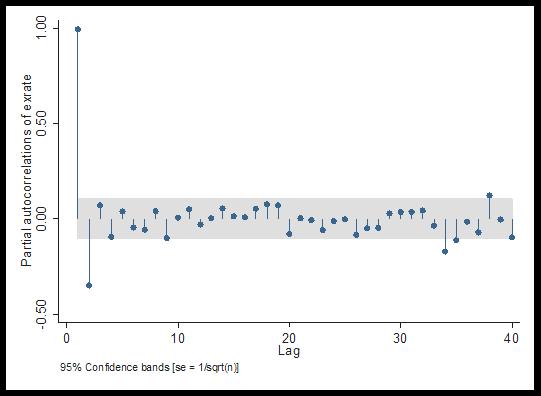
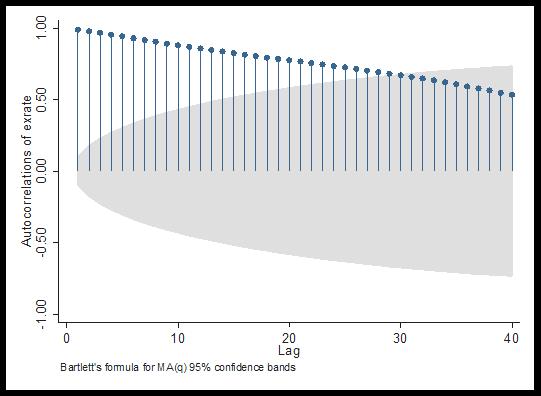
The graph also revealed that there was a significant trend and drift in the exchange rate from 1998 to 2008. In addition, the autocorrelation and partial autocorrelation functions reveal gradual decay, indicating non-stationary.
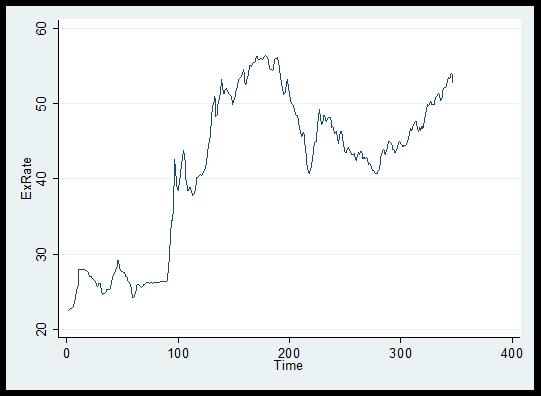
The PACF and ACF correlograms show that there are multiple spikes beyond the confidence interval, indicating the presence of drift and trend. In the figures, there was also a slow deterioration in PACF and ACF.
The Unit Root Test of Stationarity is shown in table 1. The MacKinnon approximation p-value for Z(t) is greater than 95% confidence level (0.5296 > 0.05), implying that the null hypothesis that the "exrate" has a unit root and is nonstationary is accepted.
Dickey-Fuller test for unit root Number of obs = 346 Interpolated Dickey-Fuller
MacKinnon approximate p-value for Z(t) = 0.5269
Stationarity Transformation at 1st difference
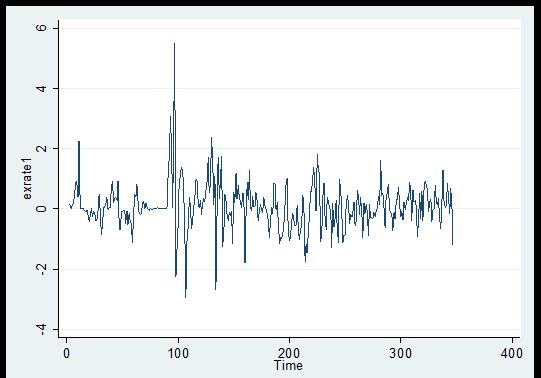
The first difference in the Philippine exchange rate is depicted in Figure 4. From February 1990 until November 2018, the first difference results were calculated. Figure 2 depicts the considerable volatility of the currency rate from 1998 to 2000. The characteristics of stationarity for the first difference of the Philippine exchange rate were then investigated in this study.
The Unit Root Test of Stationarity was shown in table 2. As shown, the MacKinnon approximation p-value for Z(t) is less than 95 percent confidence level (0.000> 0.05), implying that the null hypothesis that the "exrate" has no unit root is rejected and the series is stationary at the first difference (lag 1).
Dickey-Fuller test for unit root Number of obs = 345
Interpolated Dickey-Fuller
1% Critical 5% Critical 10% Critical
MacKinnon approximate p-value for Z(t) = 0.0000
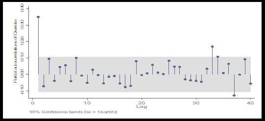
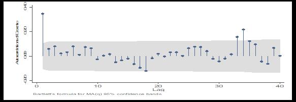
The autocorrelation function (ACF) and partial autocorrelation function (PACF) analyses for the initial difference of the Philippine exchange rate are shown in Figures 5 and 6. The partial autocorrelation function (PACF) exhibited a substantial spike on the first order, whereas the autocorrelation function (ACF) indicated a significant spike on the order of one. This means that the autoregressive portion can be represented by a moving average of order 1 and 1. As a result,
ARIMA can be used to represent the first difference in the Philippine exchange rate (1, 1, 1). Cuts off and tails off of spikes should be included in the analysis of series using the ARIMA model, implying that models ARIMA (1,1,0) and ARIMA (0,1,1) are also significant models.
The identified model is based on spikes outside the 95 percent confidence interval. There are also spikes outside of the confidence interval, as shown in the AC and ACF values. ARIMA (1,1,0), ARIMA (0,1,1), and ARIMA (0,1,2) are the correlogram-based models (1,1,1).
Estimation
The criteria of the ARIMA model were listed in the table, which included significant coefficients, volatility, likelihood statistics, BIC, and AIC. According to the results, ARIMA (1, 1, 1) is the best model for forecasting Philippine exchange rates since it has the largest significant coefficient, lowest volatility, highest likelihood statistics, and lowest AIC and BIS.
Diagnostic Checking
The findings of the correlograms at first difference, including autocorrelation and partial autocorrelation, gave an output of a statistically significant residual, which was diagnosed as totally random. The outlier also faded inside the confidence interval.