APPENDIX B—Input-Output Modeling and Economic Contribution

Input-Output Modeling and Economic Contribution

This section explains how to estimate the economic contribution of the energy and mining industries to the Utah economy using Input-Output (IO) modeling. Most of the discussions in the appendix are primarily based on Deller (2019), Henderson and Evans (2017), and Parajuli and others (2018). The structure of the discussion is following Gale and Kim (2022) closely.

Utah Input-Output Model

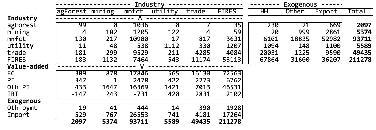
The Input-Output (IO) table in figure B1 is constructed using the 2020 IMPLAN database for Utah. Industries are highly aggregated to six sectors for illustration purposes, that is, 1) agriculture and forestry (agForest), 2) mining industry (mining), 3) manufacturing (mnfct), 4) utility (utility), 5) trade (trade) and 6) finance, insurance, real estate, education, and other services (FIRES).

A central concept of IO modeling is the interrelationship between the producing sectors of the region, the consuming sectors (e.g., households), and the rest of the world (i.e., regional imports and exports). In the IO table in figure B1, it is possible to read across the industry row to determine total commodity demand. That is, each row accounts for the sales by the industry named at its left to the industries identified across the top of the table and to the final consumers listed in the right-hand section of the row. It is composed of commodities consumed by activities in production (intermediate demand) (the box labeled A activities), household consumption, other demand (= government consumption and investment), and exports. The sum of a row is the total output or total sales of an industry. For example, sales by the mining industry are shown in row two of figure B1 as the total output worth $5,374 million. $1,205 million is sold to the mnfct (which processes it for further sale), $122 million is sold to utility industry, and $2,861 million is sold outside of Utah. Household consumption is $20 million. Within the mining industry itself, $102 million is sold.

Each column in figure B1 reports payments (purchases or other inputs) made from the industry identified at the top of the column to the entities named at the left. Below the box labeled A, payments by the industry to employees, holders of capital, and indirect business taxes are found in box labeled V, value-added. Exogenous purchases are purchases from industries outside the region and are identified as import or categorized as other payments. The sum of the entries in each column represents the total purchases by the industry.

Figure B1. Aggregate Input-Output Table for Utah, 2020 [$ million]. agForestry = agriculture, forestry, hunting and mining; Manufacture = utilities, construction and manufacturing; FIRES= wholesale and retail trade, transportation, finance, insurance, real estate, education, and other services; EC = employee compensation (wage); PI = proprietors’ income, Oth PI = other property type income; IBT = indirect business tax, taxes on production and imports; Oth pymt = Federal + State taxes or expenditure, and changes in capital and inventory additions/deletions, HH = Household consumption, Other = Government expenditure + changes in capital and inventory additions/deletions.

Since profits, losses, depreciation (capital), taxes, etc., are recorded in the table, the total purchases and payments must equal to total sales or inputs equal to outputs. So, it is called “Input Output” table. For example, the purchases and payments of the mining industry are shown in column 2 of Figure B1, $0.5 million from agForest, $217 million from mnfct, $48 million from utility, $299 million from trade, and $1132 million from FIRES. There is the payment to labor (EC: employee compensation), $878 million, proprietors’ income (PI), $1 million, and other property income, $1647 million. Utah mining industry imports from outside the state is $767 million. Notice that the total inputs, $5,374 million is the same as the total outputs identified in row 2. If the patterns of expenditures made by a sector are stated in terms of proportions, this means that the proportions of all inputs needed to produce one dollar of output in a given sector can be used to identify linear production relationships. This is accomplished by dividing the dollar value of inputs purchased from each sector by total expenditures. Or each transaction in a column is divided by the column sum. The resulting table is called the “direct requirements” table as in Figure B2.

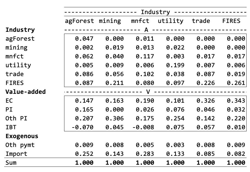
Figure B2. Direct Requirement Table. FIRES= wholesale and retail trade, transportation, finance, insurance, real estate, education, and other services; EC = employee compensation (wage); PI = proprietors’ income, Oth PI = other property type income; IBT = indirect business tax, taxes on production and imports; Oth pymt = Federal + State taxes or expenditure, and changes in capital and inventory additions/deletions, HH = Household consumption, Other = Government expenditure + changes in capital and inventory additions/deletions.

The direct requirements table can only be read down each column. Each cell represents the dollar amount of inputs required from the industry or other entity named at the left to produce one dollar’s worth of output from the sector named at the top. The upper part of the table (box A) is often referred to as the “technical coefficients.” In this example, for every dollar of sales by the mining industry, requires no output from agForest, 1.9 cents worth of additional output from itself, 4.0 cents of output from mnfct, 0.9 cents from utility, 5.6 cents from trade, and 21 cents from FIRES. 16.3 cents will be paid as the wage and 14.3 cents worth of inputs are imported for one dollar of output in the mining industry.

Economic Impact Analysis

An economic impact analysis (EIA) examines the effect of an event on the economy. The impact analysis reveals the ripple effect of new or foregone revenues from possible entry and exit of a particular firm or business within a sector or changes in exogenous final demand. The effects of the change on the other sectors can be predicted using Figure B2. For example, assume that export demand for the Utah mining industry increases by $1,000. From Figure B2, any new final demand for the mining industry will require purchases from the other sectors of the economy. The amounts shown in the second column are multiplied by the change in final demand to give the following figures: $0.09 (= 0.0009 x $1,000) from agForest, $19 (= 0.019 x $1,000) from mining, $40 (= 0.040 x $1,000) from mnfct, $9 (= 0.009 x $1,000) from utility, $56 (= 0.056 x $1,000) from trade, and $211 (= 0.211 x $1,000) from FIRES. These are called the (first round) indirect effects and, in this example, they amount to $334. The total impact on the economy is $1,334 (the initial change, $1,000 plus the total (first round) indirect effects, $334).

As Deller (2019) pointed out, the strength of IO modeling is that it does not stop at this point, but also measures the additional rounds of indirect effects of an increase in mining industry exports. In this example, mining industry increased purchases of mnfct goods by $40. To supply mining industry’s new needs from mnfct, the mnfct sector must increase its production by $40 to accomplish this. Firms in mnfct sector must purchase additional inputs from the other regional sectors to produce this $40 of output. agForest and FIRES must purchase additional inputs as well. Continuing our $1,000 increase in export demand for the Utah mining industry(i.e., after many rounds of indirect changes), the total indirect effects are $1 in agForest, $20 in mining, $54 in mnfct, $15 in utility, $76 in trade, and $322 in FIRES. The total impact will be $1,000 (initial direct effect) plus $488 (indirect effect) or $1,488.

Typically, the result of the direct and indirect effects is presented as a “total requirements table,” or the Leontief inverse table (figure B3). Each cell in Figure B3 indicates the dollar value of output from the sector named at the left that will be required in total (i.e., direct plus indirect) for a one dollar increase in final demand for the output from the sector named at the top of the column. For example, the element in the second row of the second column, 1.020, indicates the total dollar increase in output of mining industry that results from a $1 increase in final demand for mining products is $1.020 (for every dollar of direct mining output sales, there will be an additional 2.0 cents of economic activity as measured by industry sales). The element in third, fourth, fifth and sixth rows for mining sector column, 0.054, 0.015, 0.076, and 0.322 indicate that the total increase in mnfct, utility, trade and FIRES due to a dollar increase in the demand for mining industry are 5.4 cents and 1.5 cents, 7.6 cents, and 32.2, respectively.

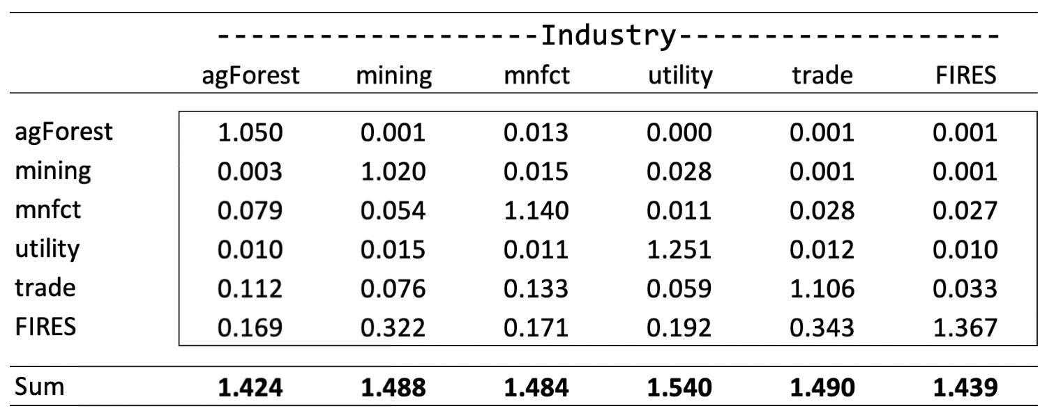
Figure B3. Total Requirements Table (Leontief Inverse Table)

Through the discussion of the total requirements table, the notion of external changes in final demand rippling throughout the economy was introduced. The total requirements table can be used to compute the total impact a change in final demand for one sector will have on the entire economy. Specifically, the sum of each column shows the total increase in regional output resulting from a $1 increase in final demand for the column heading sector. In the mining industry example, an increase of $1 in the demand will yield a total increase in regional output equal to $1.488. This number represents the initial dollar increase (direct effect) plus 48.8 cents (indirect effects). The column totals are often referred to as Type I output multipliers. If the initial change is $1,000 as in the above example, Type I effect is $1,488, which is the sum of $1000 and $488 indirect change.

The IO model and resulting (Type I) multipliers described up to this point present only part of the story. In this construction of the total requirements table and the resulting multipliers in figure B3, the production technology does not include labor (it is an open model in the terminology of IO modeling). In this case, the multiplier captures only the initial effect (initial change in final demand or the initial shock) and the impact of industry-to-industry sales. A more complete picture would include labor in the total requirements table. In the terminology of IO modeling, the model should be closed with respect to labor. If this is done, we have a different type of multiplier, specifically a Type II multiplier, which is composed of the initial and indirect effects as well as what is called the “induced effects.” The Type II multiplier is a more comprehensive measure of economic impact because it captures industry to industry transactions (indirect) as well as the impact of labor spending income in the economy (induced effect).

Notice that, to meet the new outputs described above, each sector pays its workers. For example, mining industry pays 16.3 cents per dollar of (additional) output as reported in Figure B2. The $1,000 increase in mining industry results in $1,020 changes in output, and thus mining industry pays an additional $166 (= 0.163 x $1,020) as employee compensation. Similarly, agForest, mnfct, and FIRES sectors pay additional wages due to the new outputs. In the case of mining industry, the induced

effect is calculated to be $310 per dollar of change in exogenous demand. In other words, $1,000 increase in export in mining industry results in $310 induced output changes. All told, the total economic impact (sum of direct, indirect, and induced) is $1,789 (= direct, $1,000 + indirect $488 + induced $310). The Type II multiplier is calculated as 1.798.

Economic Contribution Analysis

While economic impact and contribution analyses are two different concepts with meaningful differences in regional economic analysis, both terms are used interchangeably, yielding confusion among practitioners (Watson et al., 2007; Henderson and Evans, 2017; Parajuli et al., 2018). The economic contribution analysis, for example, captures gross change in the region’s existing economy (relative importance of an existing industry to an economy), whereas the impact analysis reveals the ripple effect of new activity (exogenous demand change) (Henderson and Evans, 2017; Parajuli and others, 2018; IMPLAN 2022a, 2022b). In other words, contribution analysis is about looking at how the current state of the sector supports other businesses in the local economy. Using the total production values to represent the sector’s final demands in an IO model will overestimate the value of the sector of interest and its associated economic contribution to other sectors of the economy (Henderson and Evans, 2017).

As discussed in Henderson and Evans (2017), Parajuli and others (2018), and IMPLAN (2022a, 2022b), economic contribution analysis (ECA) uses the IO table as in impact analysis. The difference is that ECA estimates the direct and indirect effects of the sector in situ, that is, without assuming any external change in the final demands. Since the final demand remains unchanged, the analysis focuses on calculating a value that represents the direct contribution of a sector of the economy such that the sum of the total output is preserved. The contribution of an existing sector of the economy can be calculated with an adjustment factor that preserves the output values in the transactions table and the adjustment factor is the reciprocal of the sector’s Type I multiplier. In the previous example, a Type I multiplier for the mining industry is 1.488. The direct contributions made by the mining industry are total output of the mining industry 1.448-1, which is $3,612 million = $5,374 million/1.488. It is a value which fully preserves the transaction table’s output value for mining industry.