Appendix A Literature Review

APPENDIX A

Literature Review

Current approaches to converting total column aerosol optical depth (AOD) retrieved from satellites into estimates of ground-level PM2.5 (particulate matter with an aerodynamic diameter less than or equal to 2.5 microns) concentrations have various limitations. First, retrieved total column AODs from satellites have errors associated with some issues. Such issues include excessive spatial averaging that mixes urban and rural areas and thus underestimates AOD in the more polluted urban areas (for example, Hu, Waller, Lyapustin, Wang, Al-Hamdan, and others 2014; Hu, Waller, Lyapustin, Wang, and Liu 2014; Lyapustin and others 2011); reflective surfaces, such as desert dust, that make it more difficult to separate the reflection of sunlight by aerosols from the surface reflection (for example, Sorek-Hamer and others 2015); “patchwork” surfaces in urban areas, where several different land-use types, each with different albedos, may all be present within a single satellite pixel (for example, Oo and others 2010); and the presence of undetected thin clouds, which can also create a positive bias in AOD retrievals (for example, Sun and others 2011). These limitations in satellite AOD products are consistent with some of the errors identified in using satellite observations to determine ground-level PM2.5 concentrations. For example, the high estimates in Egypt, Qatar, and Saudi Arabia are consistent with overestimates of AOD in regions with highly reflective surfaces. These problems can be mitigated by careful analysis and identification of the satellite observations and retrieval algorithms that give the most accurate and precise estimates of AOD for a given region, rather than trying to find one satellite product that works sufficiently well for all conditions around the globe. A deep understanding of the strengths and weaknesses of the different satellite AOD products is thus essential to determining which product will be most useful for a given set of geographic and meteorological conditions.

Most previous validation work on the use of satellite observations to estimate ground-level PM2.5 has been performed in developed countries with extensive, well-calibrated, long-term ground-level-monitoring (GLM) observations of PM2.5 (Type V countries, using the proposed typology in chapter 1). However, the performance of the statistical models and chemical transport models (CTMs) used to derive these relationships is not as well characterized in many low- and middle-income countries (LMICs), where GLM is infrequent or absent and few

field campaigns have been performed to make PM2.5 observations with which to train and test the models. In addition, any GLM observations that are available in LMICs may be difficult to access or may require significant effort to quality-assure the data. Being able to access these data sets and assess the quality of the measurements is thus a critical part of this project. The lack of GLM in many LMICs also introduces difficulties in trying to relate the spatially averaged AOD observations to variations in PM2.5 within a city (due to distance from roadways and other pollution sources), which suggests the need to combine satellite observations with GLM observations and data on pollution sources within a city using interpolation techniques (for example, de Hoogh and others 2016; Vienneau and others 2013).

This appendix contains a literature review that discusses the approaches used (and their strengths and limitations) in each of the three key steps in combining satellite observations with GLM measurements of PM2.5:

• The retrieval of AOD from satellite observations of reflected solar radiation (second section) • The translation of the vertically integrated AOD observation into an estimate of the ground-level PM2.5 concentration, including any bias corrections (third section) • Simultaneously interpolating these satellite-derived PM2.5 estimates and the available GLM data (fourth section).

Based on this review, recommendations are made for LMICs on how best to incorporate satellite data into their monitoring plans (fifth section). The recommendations use the following proposed typology of countries based on their levels of engagement with air-quality monitoring:

• Type I: Countries with no existing measurements and no history of routine measurements of atmospheric composition of any kind. Some anecdotal measurements or one-time sampling may have taken place. • Type II: Countries with some information on atmospheric composition available (perhaps PM10 or total suspended particulates [TSPs]) but of variable quality without rigorous quality assurance (QA) procedures. • Type III: Countries that possess reliable information but with poor spatial or temporal coverage. For example, monitoring may exist in only one city or routine monitoring may exist for a period of a year or two but is no longer being collected because of equipment malfunction or lack of repairs. • Type IV: Good, reliable AQ monitoring underway or being established. • Type V: routine, long-term AQ monitoring.

AVAILABLE AEROSOL-OPTICAL-DEPTH PRODUCTS

Monitoring the distribution and properties of atmospheric aerosols from satellites is a crucial component of establishing the radiative forcing of aerosols and their impact on climate, and it is of growing interest for regional and urban air-quality monitoring. The degree to which aerosol particles suspended in the atmosphere interact with light depends on the size and shape of the particles. Smaller particles that scatter light at visible (VIS) and shorter ultraviolet (UV) wavelengths have negligible effect at longer near-infrared (nIr) wavelengths where (in the absence of clouds) there is a relatively clear view to the surface.

These dependencies on spectral properties can be exploited through satellite observations in the VIS through nIr wavelengths to infer properties of the aerosols classified according to a limited set of models. The ability to measure aerosols is dependent on there being reasonably good contrast between the light scattered from the particles and that reflected from the surface at VIS wavelengths. For this reason, aerosol retrievals are often limited to darker surfaces (for example, ocean or vegetation). Integral to this approach is the need to infer the surface reflectance at VIS wavelengths in the absence of aerosols. This is typically achieved either by using observations from previous times (when aerosols were not present) or by relying on relationships with the signals at longer wavelengths unaffected by the aerosols. These methods tend to also work best for darker surfaces. The monitoring of aerosols based on reflected light is also restricted to daytime conditions. radiative-transfer (rT) models enable accurate simulations of reflectance at the top of the atmosphere (TOA) in the presence of aerosol layers with a variety of optical properties. By properly accounting for surface reflectance from land and ocean backgrounds, it is possible to retrieve several important aerosol properties by comparing satellite-observed TOA reflectances to those calculated from an rT model. Typically, to optimize processing time, TOA reflectances are precalculated by the rT model for several combinations of aerosols and are stored in look-up tables (LUTs) accessed by a retrieval algorithm. The rT calculations are performed for a range of aerosol optical thicknesses, so each stored reflectance value in the LUT corresponds to an aerosol optical thickness (AOT).

Because the surface type plays such an important role in aerosol retrievals, and because concentrations of aerosols often correspond to land or ocean provenance regions, somewhat different approaches are implemented over land and ocean. For land retrievals, specification of land surface reflectance is more difficult because of the greater heterogeneity of global land cover. For this reason, direct observations of land-surface reflectance are preferred over using simulated land-surface reflectances. Threshold tests are typically applied to all land pixels to ensure that only dark vegetated pixels are processed. The total TOA reflectance is the sum of the observed land surface and atmospheric contributions. The matching aerosol model is one with a TOA reflectance that produces the smallest residual with respect to observed TOA reflectances in bands sensitive to the presence of aerosols. The AOD and other properties associated with the selected model are reported.

Variations on this retrieval approach have been used to generate aerosol products from satellite observations. The World Meteorological Organization (WMO) maintains an online record of satellite technology and products related to weather, water, and climate called the Observing Systems Capability Analysis and review Tool (OSCAr)1 that is a very good reference of all past, current, and future aerosol products. The operational and science remote sensing capabilities collected there provide different levels of information about the aerosol constituents. Multispectral imaging radiometers (for example, Advanced Baseline Imager [ABI], Moderate-resolution Imaging Spectroradiometer [MODIS], and Visible Infrared Imaging radiometer Suite [VIIrS]) are capable of column AOD and aerosol particle size determinations. Multiangle radiometers (for example, Multi-angle Imaging Spectroradiometer [MISr]) and polarization imagers (for example, Multi-viewing, Multi-channel, Multi-Polarization Imaging mission [3MI] or Polarization and Directionality of the Earth’s reflectances [POLDEr])

can provide more detail on aerosol size or type information, and space-based lidars (light detection and ranging devices) (for example, Cloud-Aerosol Lidar with Orthogonal Polarization [CALIOP]) are used for aerosol and cloud profiling.

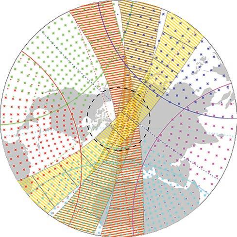
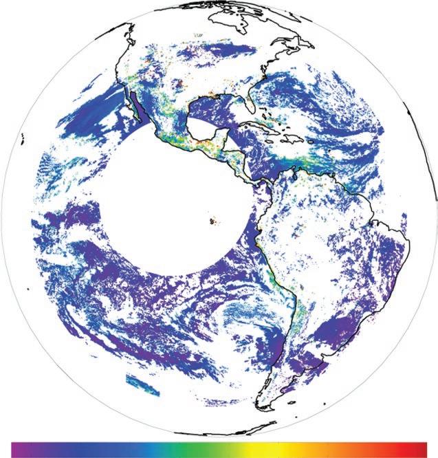
Aerosol products derived from instruments aboard polar satellites in low earth orbit (LEO) (for example, Advanced Very High resolution radiometer [AVHrr], MODIS, and VIIrS) provide global coverage roughly once per day, with spatial resolution on the order of 1 to 10 kilometers, and that depends on the orbit path. Products derived from instruments on geostationary (GEO) satellites (for example, ABI, Advanced Himawari Imager [AHI], Geostationary Operational Environmental Satellite [GOES-Imager], and Spinning Enhanced Visible and Infrared Imager [SEVIrI]) provide coverage over the full field of view (that is, Full Disk) at less than 30-minute frequency with a spatial resolution of roughly 2 to 4 kilometers, and that varies with the satellite zenith angle. As a resource for air-quality monitoring at specific locations around the world, it is necessary that remotely sensed aerosol-optical-depth products used to infer ground-level PM2.5 concentrations are available in near real-time (nrT) and that the products provide adequate coverage for regions of interest. Figure A.1 illustrates the coverage provided by LEO and GEO satellites in the northern hemisphere. A summary of the aerosol products produced by the current series of LEO and GEO satellites is provided in table A.1.

Satellite-based AOD products typically undergo a very rigorous validation process before they are officially released. This process includes extensive comparisons to ground-based AOD measurements (for example, Aerosol robotic network [AErOnET]; Holben and others 2001) as well as intercomparisons with other established AOD products and with other science missions that can provide more detailed aerosol information (for example, aerosol profiles via CALIOP). As a result, the errors are fairly well documented and are typically expressed as a bias from truth (that is, accuracy) and the scatter relative to this bias (that is, the precision), though the metrics used can vary from program to program. In addition, products are always accompanied by data quality flags that identify locations of good and degraded performance with strong recommendations to refer to these ratings when used in any application. For PM2.5 air-quality applications, these error specifications should be used to propagate uncertainties in the satellite retrievals of AOD to the estimates of ground-level PM2.5 concentrations.

The next two subsections provide an overview of satellite-based AOD retrievals from polar and geostationary platforms. One significant finding of this review is that alternative products have sometimes been developed by different organizations, but not all AOD products described in the published literature are currently made available to users. The national Oceanic and Atmospheric Administration (nOAA) MODIS products are currently the most accessible, but the long-term status of MODIS is uncertain, with the Joint Polar Satellite System (JPSS) VIIrS instrument expected to provide continuing coverage into the future. The AOD products from GEO satellites can provide greater temporal coverage of aerosol events, but currently the only reliable coverage is from the the European Organisation for the Exploitation of Meteorological Satellites (EUMETSAT) Meteosat Second Generation (MSG) satellite providing coverage of Europe and Africa. The Geostationary Operational Environmental Satellite-r

FIGURE A.1

Coverage provided by available polar and geostationary weather satellites

a. Current coverage provided by available polar and geostationary satellites b. Future coverage after planned updates of geostationary satellites

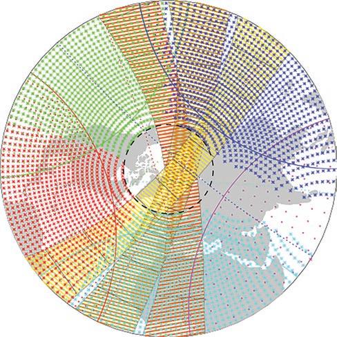
Source: World Bank. Note: The three bands in each panel illustrate three consecutive swaths from the Moderate-Resolution Imaging Spectroradiometer in sun-synchronous orbit providing once per day coverage. Green, red, turquoise, magenta, and blue points represent coverage from the geostationary satellites. The left panel shows current coverage; the right panel shows future coverage with roughly two times higher spatial resolution.

TABLE A.1 Summary of operational aerosol products

AGENCY [DEVELOPER]

EUMETSAT

[CNRS-ICARE]

EUMETSAT

[EUMETSAT]

SATELLITE [INSTRUMENT]

MSG

[SEVIRI]

Metop-A Metop-B [AVHRR, GOME-2, IASI]

ORBIT [TYPE] PRODUCT(S)

0 E SMAOL

[GEO]

9:30 dsc

9:30 dsc

[LEO] Polar Multi-Sensor Aerosol Product

HSR 5 × 40 10 × 40 kilometer swath 960 × 1920 kilometer

REFRESH [COVERAGE]

15 minutes

[Europe, Africa]

Daily [Global]

NEAR REAL-TIME AVAILABILITY

Yes

Yes

JMA

[JMA-MSC]

NASA

[NASA-GSFC]

NASA

[NASA-GSFC] Himawari-8/9

[AHI]

Terra

Aqua [MODIS]

Terra

Aqua [MODIS] 141. E

[GEO]

10:30 dsc

13:30 asc

[LEO]

10:30 dsc

13:30 asc

[LEO] AOD [East Asia, Indonesia, Australia] TBD

10 km Dark Target AOD Daily 10 km Deep Blue AOD [Global] 10 km combined AOD

3 km Dark Target AOD MAIAC AOD (1 kilometer) gridded Amazon data set Daily [Global] Yes

TBD

2000–12

continued

TABLE A.1, continued

AGENCY [DEVELOPER]

NOAA

[NASA-GSFC]

SATELLITE [INSTRUMENT]

NOAA-20

[VIIRS]

ORBIT [TYPE] PRODUCT(S) REFRESH [COVERAGE]

13:30 asc

[LEO] 10 kilometer Dark Target AOD Daily 10 kilometer Deep Blue AOD [Global] 10 kilometer Combined AOD

NEAR REAL-TIME AVAILABILITY

TBD

NASA

[JPL]

NOAA

[NOAA-NCEI]

NOAA

[NOAA-SPSD]

NOAA

[NOAA-STAR] Terra

[MISR]

NOAA-19

NOAA-15

NOAA-18

[AVHRR]

GOES-13

GOES-15

[IMAGER]

NOAA-20

[VIIRS] 10:30 dsc

[LEO]

15:20 asc

18:15 asc

19:02 asc

[LEO]

75. W

135. W

[GEO]

13:30 asc

[LEO] 3 kilometer Dark Target AOD

AOD (MIL2ASAE)

AOT

GASP-East AOD

GASP-West AOD

AOT 9 days [Global]

Daily [Global; Ocean only] Yes

Yes

1 hour

[CONUS]

Daily [Global] Yes

Yes

NOAA

[NOAA-STAR] GOES-16

GOES-17

[ABI] 75. W

137. W

[GEO] SMAOD 5, 10, or 15 minutes [North and South America] Yes

Source: World Bank. Note: In column 3, Low Earth orbits (LEOs) are all sun-synchronous and identified in terms of the daytime equator crossing time and direction (that is, ascending [asc] or descending [dsc]); Geostationary (GEO) orbits are identified by their satellite longitude. ABI = Advanced Baseline Imager; AOD = aerosol optical depth; AVHRR = Advanced Very High Resolution Radiometer; CNRS-ICARE = Centre National de la Recherché Scientific–Institut de Combustion, Réactivité et Environnement; CONUS = continental United States; EUMETSAT = European Organisation for the Exploitation of Meteorological Satellites; GASP = GOES Aerosol/Smoke Product; GOES = Geostationary Operational Environmental Satellite; GOME-2 = Global Ozone Monitoring Experiment-2; GSFC = Goddard Space Flight Center; IASI = Infrared Atmospheric Sounding Interferometer; IMAGER = GOES Imager; JMA = Japan Meteorology Agency; JPL = Jet Propulsion Laboratory; MAIAC = Multi-Angle Implementation of Atmospheric Correction; MIL2ASAE = MISR level 2 aerosol parameters; MISR = Multi-angle Imaging Spectroradiometer; MODIS = Moderate-Resolution Imaging Spectroradiometer; MSC = Meteorological Satellite Center; MSG = Meteosat Second Generation; NASA = National Aeronautics and Space Administration; NOAA = National Oceanic and Atmospheric Administration; SEVIRI = Spinning Enhanced Visible and Infrared Imager; SMAOD = suspended matter, aerosol optical depth; SMAOL = SEVIRI-MSG Aerosol Over Land; STAR = Center for Satellite Applications and Research; TBD = to be determined; VIIRS = Visible Infrared Imaging Radiometer Suite.

series (GOES-r) products over north and South America were made available in 2018. However, the availability of Japan Meteorology Agency (JMA) Himawari data with coverage over East Asia and Indonesia is uncertain, and no current geostationary satellite mission is providing AOD products in the region of India and western Asia. Furthermore, the availability of satellite coverage does not ensure that AOD products will be produced, because the retrievals are limited by environmental conditions (for example, must be cloud-free) and surface conditions (for example, must be snow-free). The third subsection looks at three urban locations to review how satellite-derived AOD coverage might be provided to support air-quality missions.

Polar-orbiting satellites

MODIS products Aerosol products derived from observations by the MODIS aboard the national Aeronautics and Space Administration’s (nASA’s) Terra and Aqua satellites are among the most widely studied products in the aerosol remote sensing

community. This pair of instruments (MODIS-Terra and MODIS-Aqua) has created a climate record extending over 15 years. Although MODIS has already exceeded its design lifetime, calibration and validation efforts continue to maintain the calibration accuracy of the instruments to ensure the integrity of the ongoing observations. Studies based on MODIS data provide some of the best examples of the application of space-based AOD to the understanding of global climate and regional air-quality conditions (see the third section below).

Two primary AOD products are produced from the MODIS observations based on the Dark Target2 and Deep Blue3 aerosol-retrieval algorithms. These two products are made readily available to users. A third research product from MODIS, Multi-Angle Implementation of Atmospheric Correction (MAIAC), has been used in many studies but is not yet processed operationally.

Dark Target: The nASA Dark Target algorithm produces AOD over ocean and other dark land (for example, vegetated) surfaces using two separate algorithms for the different regimes. The standard product for climate studies is AOD aggregated at 10-kilometer resolution (Levy and others 2013). Over land, the retrieval produces AOD at 550 nanometers, the AOD model/weight, and surface reflectance at 2,130 nanometers based on 500-meter resolution observations at 470, 650, and 2,130 nanometers and using a LUT of rT-model–computed reflectances as a function of aerosol and surface properties. Dark targets are identified as pixels where the 2,130-nanometer reflectance is between 0.01 and 0.25. For these locations, the quality flag is set based on the goodness of the fit between the observed and modeled reflectance. Targets with reflectance up to 0.4 are processed through a separate algorithm path but flagged as reduced quality. To meet the growing interest in AOD for regional studies, the product over land is now also produced at a 3-kilometer resolution (remer and others 2013). The error estimate of the 10-kilometer AOD based only on good-quality retrievals has been assessed against AErOnET measurements to be ±(0.05 + 0.15 AODAErOnET),4 whereas the error in the 3-kilometer product is ±(0.05 + 0.20 AODAErOnET). This product is available through the nASA Level-1 and Atmospheric Archive and Distribution System (LAADS) Distributed Active Archive Center (DAAC)5,6 or through the nASA WOrLDVIEW website.7

Investigations of the use of the 3-kilometer Dark Target product to provide better definition of local aerosol gradients (Munchak and others 2013) suggest that the 3-kilometer product does provide better spatial coverage (see figure A.2). However, this product tends to overestimate the aerosol loading and can be susceptible to noise problems in urban areas, likely because of inadequate characterization of surface features. For such applications, some caution is advised.

Deep Blue: The Deep Blue aerosol algorithm explicitly models surface reflectance, rather than estimating it from observations at 2,130 nanometers as in the Dark Target algorithm. This explicit modeling allows the Deep Blue algorithm to be applied to bright surfaces such as desert, semiarid, and urban regions (Hsu and others 2013). To enable retrievals over brighter surfaces, the algorithm uses the 412-nanometer or “deep blue” band on MODIS (where the surface reflectance over land is much lower than in low-frequency visible bands), thus providing better contrast with the aerosol signal. This product is computed over land at 1-kilometer resolution and aggregated to 10 kilometers. Surface reflectance is determined by one of several methods depending on the surface type, including use of a database that takes account of seasonal changes and the variability of urban landscapes based on the normalized difference vegetation index (nDVI).

FIGURE A.2

MODIS Dark Target 10-kilometer and 3-kilometer aerosol-optical-depth products retrieved for clear land and ocean fields of view and the local 5-kilometer average derived from the products, outer circle, compared to ground-based measurements, inner circle, over Baltimore, US

a. MODIS Dark Target 10-kilometer product b. MODIS Dark Target 3-kilometer product

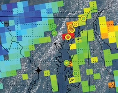
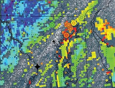
AOD at 0.55 µm

-0.05 0.05 0.15 0.25 0.35 0.45 0.55 0.65 0.75

Source: Munchak and others 2013. Note that these results used an older version of the MODIS surface reflectance scheme, and more recent versions (for example, Gupta and others 2016) show much better performance over urban areas. Note: AOD = aerosol optical depth; MODIS = Moderate-Resolution Imaging Spectroradiometer.

The (prognostic) uncertainty derived by Deep Blue is comparable to the error estimate of the Dark Target product for typical aerosol levels in the range from 0.1 to 0.5, ± 0.03 + 0.2τDB.

The combined Deep Blue and Dark Target aerosol product was developed to provide users with the alternative of a single merged MODIS product (Sayer and others 2014). It applies nDVI criteria based on a monthly composite to select either the Dark Target or Deep Blue AOD for a given 10-kilometer pixel location:

• nDVI ≤ 0.2

Use Deep Blue • nDVI ≥ 0.3 Use Dark Target • 0.2 < nDVI < 0.3 Use product with highest quality or report mean value.

As a result, Deep Blue is reported over desert regions, Dark Target is selected over permanent vegetation, and in other areas the selection of Deep Blue or Dark Target varies with the season. Comparison of the two products to AErOnET indicates that neither Deep Blue nor Dark Target consistently outperforms the other (see map A.1). Dark Target tends to have slightly smaller overall errors compared to AErOnET, but Deep Blue provides additional coverage and tends to perform better for low-AOD conditions. Both the Deep Blue and the combined product are available through the nASA LAADS DAAC or through the nASA WOrLDVIEW website.

MAIAC: The Multi-Angle Implementation of Atmospheric Correction (MAIAC) algorithm8 is an atmospheric correction algorithm designed for

MAP A.1

Fraction of good-quality attempted retrievals from Deep Blue and Dark Target algorithms showing differences in coverage over desert regions, and showing differences in coverage due to the quality checks applied in each algorithm

a. Deep Blue fraction assigned good QA

80°

Latitude 40°

0°

–40°

–80° –180° –90° 0° 90°

Longitude

Fraction of retrievals that passed QA checks (range 0–1) 180°

0 0.25 0.5 0.75 1.0

Latitude b. Dark Target / ocean fraction assigned good QA

80°

40°

0°

–40°

–80° –180° –90° 0° 90° 180°

Longitude

Source: Sayer and others 2014. Note: QA = quality assurance.

MODIS that performs simultaneous retrievals of atmospheric aerosols and bidirectional surface reflectance (Emili and others 2011; Lyapustin and others 2011). Unlike the Dark Target and Deep Blue algorithms, the MAIAC algorithm does not rely on any predetermined relationships with the shortwave information to constrain the surface retrieval but instead invokes a multiangle, multitemporal retrieval of the surface bidirectional reflectance distribution function and aerosol loading, based on assumptions that the surface reflectance does not change over a 16-day period and that AOD changes little over 25-kilometer distances. The resulting AOD product is generated on a one-kilometer sinusoidal grid. Over vegetated regions (forest, cropland, grassland, and savanna), more than 66 percent of retrievals are within the expected error ±(0.05 + 0.05t) with a correlation coefficient to AErOnET better than 0.86 (Martins and others 2017).

results over other bright backgrounds were less precise, especially for low aerosol signals where the retrieval problem is not as well constrained (for example, 55 percent of retrievals within the expected error for urban regions).

The MAIAC aerosol product is nominally distributed through the nASA LAADS DAAC9,10 but appears to be currently unavailable except for a limited data set over the Amazon basin in South America from 2000 to 2012.11,12 Online information indicates support of the product is ongoing13,14,15 with a potential extension to process VIIrS data in the works.16

VIIRS products The Visible Infrared Imaging radiometer Suite (VIIrS) sensor is a scanning radiometer on Suomi-national Polar-orbiting Partnership (Suomi-nPP) and the Joint Polar Satellite System (JPSS) satellites operated by nOAA and nASA. Over land, the nOAA VIIrS AOD product17 is generated with a LUTbased retrieval of AOD, based on five aerosol models using observed reflectance in 750-meter moderate-resolution bands at 412, 445, 488, 672, and 2,250 nanometers (Jackson and others 2013). The surface reflectance in the red (672 nanometers) and blue (488 nanometers) bands is inferred based on an empirical relationship with the shortwave infrared (2,250 nanometers) band that holds mainly for dark surfaces. The AOD is then determined from observed blue-to-red reflectance ratios by matching the observed signal to computed values for a given aerosol model. AOD retrievals are not performed for clouds, snow, fire, glint, and other bright surfaces identified, based on a shortwave infrared nDVI threshold (nDVISWIr < 0.05 with a 2,250-nanometer reflectance > 0.3). nDVISWIr > 0.2, consistent with vegetation backgrounds, is required for high-quality retrievals.

The AOD output is available as an intermediate product at 750-meter resolution and as a 6-kilometer (eight-by-eight aggregated) product, thus providing some advantage over the MODIS 3- and 10-kilometer products for analysis of the localized aerosol distribution. While studies of regional applications of VIIrS AOD products have been presented as conference papers, no comprehensive review of the product has been published. The overall performance of the VIIrS product has been validated against requirements with uncertainties similar to that of MODIS Dark Target (Huang and others 2016). However, comparisons of the 1-kilometer MAIAC AOD product to the high-resolution VIIrS product (see figure A.3) found that the VIIrS product was biased to higher AOD in urban and mountainous regions and was susceptible to errors in regions of snowmelt (Superczynski, Kondragunta, and Lyapustin 2017). The official nOAA VIIrS products are distributed through the Comprehensive Large Array-Data Stewardship System (CLASS)18 and with the most recent 90 days available via file transport protocol (FTP).19

Alternatives to the operational nOAA VIIrS AOD product are in development. For example, the nASA Dark Target algorithm was applied to VIIrS data, and results were compared with the operation nOAA algorithm and to MODIS (Levy and others 2015). The nASA Deep Blue algorithm20 also has been applied to VIIrS data. In addition, the nOAA Center for Satellite Applications and research (STAr) has published work describing an enhanced AOD algorithm capable of retrieving aerosols over brighter surfaces and comparable to the Deep Blue product (Zhang and others 2016). Finally, VIIrS products based on the MAIAC algorithm have been referenced in online presentations, but the status of such products is unclear. Once available, these alternative products

FIGURE A.3

Comparison of VIIRS 750-meter and MAIAC one-kilometer aerosoloptical-depth products during western US fires, 2013

a. VIIRS 750-meter AOD product

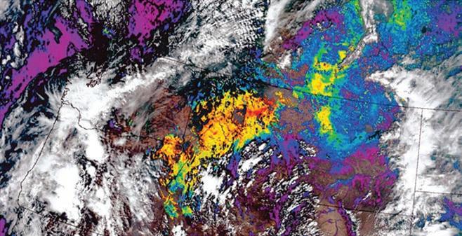
b. MAIAC one-kilometer AOD product

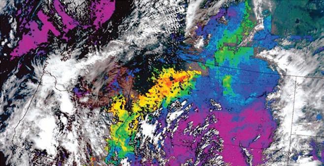
AOD

0.0 0.1 0.2 0.3 0.4 0.5 0.6 0.7 0.8 0.9 1.0

Source: Superczynski, Kondragunta, and Lyapustin 2017. Note: AOD = aerosol optical depth; MAIAC = Multi-Angle Implementation of Atmospheric Correction; VIIRS = Visible Infrared Imaging Radiometer Suite.

may provide improved coverage, in particular for urban areas, potentially increasing their utility for regional air-quality applications.

MISR products The Multi-angle Imaging Spectroradiometer (MISr) instrument uses multiangle techniques in the VIS and nIr to acquire stereoscopically resolved observations of AOD under sunlit conditions (Diner and others 1998). All 36 channels (nine cameras and four spectral bands) are used when performing aerosol retrievals over land (Martonchik and others 2004). MISr measurements (between 70.5° forward and 70.5° aft) span a wide range of scattering angles and

air mass factors providing information on aerosol microphysical properties and yielding sensitivity to optically thin aerosols. The MISr retrieval approach relies on describing the change in surface contrast with view (camera) angle over a region 17.6 kilometers by 17.6 kilometers in size, composed of 16 by 16 (256) subregions, each 1.1 kilometer by 1.1 kilometer. This subregion size is the nominal spatial resolution of MISr when observing in Global Mode, and 17.6 kilometers is the spatial resolution of MISr’s retrieved aerosol product. Aerosol retrievals are performed on only a regional and not a subregional basis, because the entire region is used to determine the surface contribution to the reflectance. In addition to having a lower horizontal resolution than the MODIS and VIIrS products, the MISr instrument has a smaller swath than MODIS (400 kilometers versus 2,330 kilometers) and thus only observes a given location once every nine days, unlike once a day for MODIS and VIIrS.

The performance of AOD retrievals from MISr is comparable to that of MODIS. Martonchik and others (2004) compared MISr AOD with AErOnET observations and found that at 17.6-kilometer spatial resolution, the estimated uncertainty is about 0.08. When the spatial resolution was degraded to 52.8 kilometers, the estimated MISr AOD uncertainty decreased to about 0.05. Khan and others (2005) found that 66 percent of the measurements agreed with AErOnET within ±(0.05 + 0.2τ). Kahn and others (2009) compared MISr with MODIS AOD and found that where coincident AOD retrievals are obtained over the ocean, the MISr-MODIS correlation coefficient is about 0.9 with a slope of 0.75; over land, the correlation coefficient is about 0.7 with a slope of 0.60. MISr AOD data are available from the Jet Propulsion Laboratory.21

AVHRR products The Advanced Very High resolution radiometer (AVHrr/3) instrument provides visible-through-Ir remote sensing observations on the LEO satellites flown by nOAA (for example, nOAA-15) and by the European Organisation for the Exploitation of Meteorological Satellites (EUMETSAT) (for example, Metop-A). However, the operational nOAA AOD product22 is produced only over oceans, though the application for AOD retrievals over land has also been investigated (Li and others 2013). The nASA Deep Blue algorithm has been applied to the nOAA data to produce an aggregated 8.8-kilometer product over land and ocean with an expected error over land of ±(0.05 + 0.25τ) (Sayer and others 2017). This application of Deep Blue uses a database of surface reflectance for retrievals over bright surfaces, but because AVHrr lacks a 412-nanometer band, the red band at 620 nanometers is used instead. Because the surface at 630 nanometers is not as dark as 412 nanometers, the sensitivity of the aerosol retrieval is limited compared to MODIS and VIIrS. AVHrr also lacks a shortwave band that is used in the MODIS/VIIrS algorithms to derive the surface reflectance for dark targets. For AVHrr, the surface is modeled as an empirical function of nDVI. However, this product was available online only through 2011.23

EUMETSAT produces an operational multisensor aerosol product based on observations from AVHrr, the Global Ozone Monitoring Experiment (GOME; a medium-resolution double UV-VIS spectrometer), and the infrared atmospheric sounding interferometer (IASI)–Fourier transform spectrometer.24,25 However, the primary input for the AOD retrieval is derived from GOME, and the resolution of the product (5 kilometers by 40 kilometers for

Metop-A or 10 kilometers by 40 kilometers for Metop-B) is dictated by this instrument.

Geostationary satellites

GOES-NOP imager products The GOES-n series geostationary satellites (GOES-nOP; for example, GOES13 East at 75° W and GOES-15 West at 135° W) operated by nOAA are able to provide Full Disk imagery of the Earth covering north and South America in a single VIS band and four Ir bands with a refresh rate of 30 minutes. For over 15 years, nOAA has supported the generation of an operational AOD product based on the GOES observations. Being limited to a single (uncalibrated) VIS band, the accuracy of this product is somewhat less than other, more advanced products, but the GOES product is still of significant value owing to its unique temporal information. The GOES Aerosol/Smoke Product (GASP)26 is derived using a surface reflectance based on a 28-day composite (converted to albedo using an rT model) and AOD retrieved using an rT-model–computed LUT and comparing observations to model reflectances in the VIS band (Knapp and others 2005). The retrieval is limited to a single continental aerosol model and restricted to regions with dark vegetation. GASP is produced at fourkilometer resolution (at nadir) with a quoted precision of ±0.13 and a correlation of R of 0.72 with AErOnET. The current product is limited to the continental United States, and products are available in binary format in nrT from the nOAA Satellite Products and Services Division website.27 This product was discontinued in 2018 from GOES-13 (East) when the GOES-16 products became operational.

SEVIRI-MSG products The SEVIrI-MSG Aerosol Over Land (SMAOL) product28 (based on observations from the Spinning Enhanced Visible and Infrared Imager [SEVIrI] on Meteosat Second Generation [MSG]) was developed by HYGEOS for the Centre national de la recherché Scientific (CnrS). SMAOL is distributed in nrT though the ICArE Data and Services Center (Bernard and others 2011; Mei and others 2012). The algorithm approach is similar to that of the GOES GASP product but with greater sensitivity. SEVIrI observations at 630, 810, and 1640 nanometers (corrected for gas absorption and molecular scattering) are used to derive AOD at 550 nanometers chosen from between five aerosol models using a LUT approach to minimize the differences at the three wavelengths. The product is generated at the three-kilometer (at nadir) resolution and produced every 15 minutes during daytime/cloud-free conditions and subject to some viewing and scattering angle restrictions. With the MSG satellite at 0° longitude, the product provides coverage of Europe and Africa. The surface reflectance used in the retrieval is based on a fit to the minimum reflectance over a 14-day period. This methodology is valid only for dark targets; therefore, desert regions (such as the Sahara, Sahel, and namib) are excluded. The product has been validated with comparisons to AErOnET and to the MODIS Dark Target AOD product and found to provide good estimates of both diurnal and daily variations in AOD (see figure A.4). Error sources include possible subpixel cloud contamination, errors in surface reflectance estimation, and possible temporal noise in model selection.

FIGURE A.4

Detection of temporal variations in aerosol optical depth with the SEVIRI-MSG aerosol over land product compared to AERONET measurements at Palaiseau, France, and to MODIS, July 14, 2006

Aerosol optical thickness (0.6 micrometers) 0.6

0.5

0.4

0.3

0.2

0.1

0

6.0 6.5 7.0 7.5 8.0 8.5 9.0 9.510.010.511.011.512.012.513.013.514.014.515.015.516.016.517.017.518.018.5 Time (UT)

Aeronet 675nm MODIS Aqua 660nm (1 pix) SEVIRI 635nm MODIS Terra 660nm (1 pix)

Source: ©Bernard and others 2011; CC BY 3.0. Note: AERONET = Aerosol Robotic Network; AOT = aerosol optical thickness; MODIS = Moderate-Resolution Imaging Spectroradiometer; MSG = Meteosat Second Generation; nm = nanometer; SEVIRI = Spinning Enhanced Visible and Infrared Imager; UT = Universal Time.

GOES-R ABI products GOES-r is the first in a series of next-generation geostationary environmental satellites covering the western hemisphere.29 It was launched as GOES-16 in november 2016. For earth remote sensing, observations are collected by the Advanced Baseline Imager (ABI), which offers much-improved spatial, temporal, and spectral information over the preceding GOES-nOP Imager series. For the past year, the ABI instrument products have undergone an intensive validation process. In December 2017, the satellite was moved to the GOES East position, with products scheduled to become operational in 2018.

The GOES-r AOD and aerosol-particle–sized products30,31 are derived from ABI reflectance measurements through physical retrievals that utilize a LUT of TOA reflectance that is precalculated using an rT model. retrievals are performed separately over land (for dark surfaces) and ocean. The baseline AOD product is generated at two-kilometer resolution (at nadir) for Full Disk and continental United States (COnUS) geographic coverage areas. The Full Disk AOD output product is generated at 15-minute intervals (see figure A.5), whereas the COnUS product is generated at five-minute intervals. The GOES-r product performance specification is a function of AOD value. For intermediate AOD loading between 0.04 and 0.8, the accuracy over land is ± 0.04 and the precision

FIGURE A.5

Full disk coverage at 550 nanometers of GOES-R SMAOD product over ocean and land

AOD

0.00 0.50 1.00 1.50 2.00

Source: World Bank. Note: AOD = aerosol optical depth; GOES = Geostationary Operational Environmental Satellite R series; SMAOD = suspended matter, aerosol optical depth.

is ± 0.25, which is similar to the equivalent polar products. Once approved, the GOES-r AOD product will be distributed through the nOAA’s Comprehensive Large Array-Data Stewardship System.32,33

Although the GOES-r program product is the official operational AOD product, alternative algorithms have been developed to also measure aerosol properties from GOES-r data. For example, the Enterprise Processing System (EPS) AOD algorithm34 is an algorithm from nOAA STAr intended to support the generation of an AOD product from GOES-r ABI and JPSS VIIrS with a common methodology.35 The status of the nOAA EPS product is uncertain at this time.

Himawari-8/9 AHI products Himawari-8/9 is a new series of geostationary weather satellites operated by the JMA. The imagery collected by Himawari-8/9 is produced by the Advanced Himawari Imager (AHI), which is very similar in design to the ABI instrument flown on GOES-16. Although the MODIS Deep Blue, GOES-r, and EPS

algorithms have been applied and tested on AHI data, these products are not currently available. The JMA advertises their own environmental products,36,37 but these are also not freely available.38,39

Case studies

In table A.2 three urban locations with poor air quality are reviewed to evaluate the available satellite AOD products and to assess the utility and limitations of these products for the regions. Each location includes a link to the nASA WOrLDVIEW website with visualizations of the Dark Target and Deep Blue aerosol products from MODIS-Terra and MODIS-Aqua.

In Delhi, India, the air quality in late fall is affected by widespread smoke from rural crop fires combined with the localized urban smog trapped in the

TABLE A.2 Case study of satellite aerosol-optical-depth applicability for three representative low- and middle-income country urban areas

LOCATION

Delhi, India

Lima, Peru

COORDINATES LAND TYPE/CLIMATE

28°36′36″N, 77°13′48″E Land type: Semivegetated, desert, urban Topography: Yamuna River basin Climate: Rain Jun to Oct

12°2′36″S, 77°1′42″W Air quality: Widespread smoke from rural crop fires mixed with urban smog Land type: Coastal desert, urban, semivegetated Topography: Andes foothills Climate: Persistent clouds/fog May to Nov Air quality: Urban (localized) smog

COVERAGE

MODIS

VIIRS

MISR

WORLDVIEWa

MODIS

VIIRS

MISR

ABI WORLDVIEWb

Ulaanbaatar, Mongolia 47°55′N, 106°55′E Land type: Grasslands (steppes) Topography: Tuul River valley Climate: Seasonal snow cover

Air quality: Desert dust, urban smog, coal/wood fires (winter) MODIS

VIIRS

MISR

AHI

WORLDVIEWc

Source: World Bank, produced with Esri ArcGIS. Note: AHI = Advanced Himawari Imager; MISR = Multi-angle Imaging Spectroradiometer; MODIS = Moderate-Resolution Imaging Spectroradiometer; VIIRS = Visible Infrared Imaging Radiometer Suite. a. https://worldview.earthdata.nasa.gov/?p=geographic&l=MODIS_Aqua_SurfaceReflectance_Bands143(hidden),MODIS_Terra_SurfaceReflectance _Bands143(hidden),MODIS_Aqua_CorrectedReflectance_TrueColor(hidden),MODIS_Terra_CorrectedReflectance_TrueColor,MODIS_Terra _NDVI_8Day(hidden),MODIS_Terra_AOD_Deep_Blue_Combined(hidden),MODIS_Terra_AOD_Deep_Blue_Land(hidden),MODIS_Terra _Aerosol(hidden),MODIS_Terra_Aerosol_Optical_Depth_3km(hidden),MODIS_Aqua_Aerosol(hidden),MODIS_Aqua_AOD_Deep_Blue _Combined(hidden),MODIS_Aqua_Aerosol_Optical_Depth_3km(hidden),MODIS_Aqua_AOD_Deep_Blue_Land(hidden),Reference_Labels,Reference _Features(hidden),Coastlines&t=2017-03-04&z=3&v=75.58614905641733,27.64425081916523,78.66232093141733,29.24825472541523&ab=off& as=2017-03-04&ae=2017-03-11&av=3&al=true. b. https://worldview.earthdata.nasa.gov/?p=geographic&l=MODIS_Aqua_SurfaceReflectance_Bands143(hidden),MODIS_Terra_SurfaceReflectance _Bands143(hidden),MODIS_Aqua_CorrectedReflectance_TrueColor(hidden),MODIS_Terra_CorrectedReflectance_TrueColor,MODIS_Terra _NDVI_8Day(hidden),MODIS_Terra_AOD_Deep_Blue_Combined(hidden),MODIS_Terra_AOD_Deep_Blue_Land(hidden),MODIS_Terra _Aerosol(hidden),MODIS_Terra_Aerosol_Optical_Depth_3km(hidden),MODIS_Aqua_Aerosol(hidden),MODIS_Aqua_AOD_Deep_Blue _Combined(hidden),MODIS_Aqua_Aerosol_Optical_Depth_3km,MODIS_Aqua_AOD_Deep_Blue_Land(hidden),Reference_Labels,Reference_Features (hidden),Coastlines&t=2017-05-25&z=3&v=-77.91445867492484,-12.577473819870836,-76.37857000304984,11.608479679245836&ab=off&as=2017-03-04&ae=2017-03-11&av=3&al=true. c. https://worldview.earthdata.nasa.gov/?p=geographic&l=MODIS_Aqua_SurfaceReflectance_Bands143(hidden),MODIS_Terra_SurfaceReflectance _Bands143(hidden),MODIS_Aqua_CorrectedReflectance_TrueColor(hidden),MODIS_Terra_CorrectedReflectance_TrueColor,MODIS_Terra _NDVI_8Day(hidden),MODIS_Terra_AOD_Deep_Blue_Combined(hidden),MODIS_Terra_AOD_Deep_Blue_Land(hidden),MODIS_Terra _Aerosol(hidden),MODIS_Terra_Aerosol_Optical_Depth_3km(hidden),MODIS_Aqua_Aerosol(hidden),MODIS_Aqua_AOD_Deep_Blue _Combined(hidden),MODIS_Aqua_Aerosol_Optical_Depth_3km(hidden),MODIS_Aqua_AOD_Deep_Blue_Land(hidden),Reference_Labels,Reference _Features(hidden),Coastlines&t=2017-04-25&z=3&v=106.0165808187288,47.38272533863788,107.5524694906038,48.35171947926288&ab=off& as=2017-03-04&ae=2017-03-11&av=3&al=true.

Yamuna river basin around the city. When conditions are clear, the MODIS Deep Blue product typically provides complete coverage across the region, but the Dark Target product is excluded from parts of the urban area where the background signal is high. Also, the coverage from the Dark Target algorithm varies with the season depending on the stage of vegetation growth in the surrounding rural area. On very bad days the smoke can be so widespread and thick that localized variations in air quality cannot be determined. During these periods, the Dark Target product is sometimes not produced at all for the region.

The pollution in Lima, Peru, is largely due to localized urban smog. Lima is located on the west coast of South America with weather patterns greatly influenced by the Humboldt Current and its location just west of the foothills of the Andes mountains. For significant portions of the year (May to november), Lima is often engulfed in fog, and during these periods the remote sensing of AOD is not possible. In addition, the background signal from the city and the surrounding desert is relatively bright, such that the coverage from the Dark Target product is minimal. The Deep Blue product does provide coverage over the urban environment but with frequent gaps due to clouds. In addition, as Lima is situated on the coast, AOD retrievals are not produced for any pixels with a mix of land and water, further reducing the coverage of the Deep Blue product for this city.

Ulaanbaatar, Mongolia, is in the Tuul river valley at the foot of the heavily forested Bogd Kahn Uul mountains and is surrounded by a steppe ecoregion where the largely grassland vegetation varies with the seasons. In winters, the entire region is covered with snow. The air-quality problems in Ulaanbaatar are highest in the winter months when use of coal and wood for heat gives rise to significant smoke emissions that couple with the local smog from cars and other sources. Because satellite-based AOD retrievals are not capable of distinguishing aerosol from the bright background of snow, neither the Dark Target nor Deep Blue products are useful under these conditions. At other times of year on clear days, the Deep Blue product does provide fairly good coverage over the region, but the coverage from the Dark Target algorithm is spotty, often limited only to the nearby vegetated mountainous areas and not providing information in the urban and steppe environments.

CONVERTING AOD TO GROUND-LEVEL PM2.5

Many studies have attempted to convert satellite AOD to ground-level PM2.5 concentration estimates using either statistical techniques (the first subsection below), approaches based on the chemical transport model (CTM) (discussed in the second subsection), or hybrid approaches that mix the two (discussed in the third subsection).

Statistical approaches

Several studies have used a purely statistical approach, where linear mixed effects models (for example, Hu, Waller, Lyapustin, Wang, Al-Hamdan, and others 2014; Sorek-Hamer and others 2015) or nonlinear generalized additive models (GAMs; Sorek-Hamer and others 2013; Strawa and others 2013) have been trained on historical GLM data to predict ground-level PM2.5 using AOD and other meteorological and geographic variables as input variables. The advantages of statistical approaches are that the statistical models can be trained for

specific areas and are easier to run than CTMs. However, unlike CTM approaches, statistical models require a substantial amount of GLM data for the model training and can be used only in the region in which they were trained.

Statistical approaches also provide an estimate of the uncertainty in their predictions. In addition, the uncertainty in AOD, planetary boundary layer (PBL) height, and other variables can be propagated to the ground-level PM2.5 estimates by running the statistical model for the high and low error bounds of the variable, and then combining that uncertainty with the estimated uncertainty of the statistical fit itself.

Linear mixed-effects models Linear mixed-effects models assume a linear relationship between the predictors and the modeled variable but allow the intercepts and slopes to vary with the day by fitting fixed (that is, constant) and random (that is, daily varying) values for those parameters, with the limitation that the random values cannot also vary with location. routines for training these models are included in the open source r statistical program.

Hu, Waller, Lyapustin, Wang, Al-Hamdan, and others (2014) used a two-stage linear mixed-effects model to estimate ground-level PM2.5 concentrations at one-kilometer resolution from MAIAC AOD data over the Southeast United States. In the first stage the predictors included MAIAC AOD, wind speed, and elevation, as well as the length of major roads, percent forest cover, and point emissions of PM2.5 within one kilometer of the site. The second stage used geographically weighted regression (GWr) to predict the residuals from the firststage model using the MAIAC AOD. GWr is an extension of least-squares regression that allows predictor coefficients to vary spatially by weighting the estimate-observation pairs according to the inverse-squared distance from individual observation sites, resulting in a spatially continuous prediction of PM2.5 over an area at one-kilometer resolution.

The GLM data used in the training had 166 monitors over a domain of 800 by 1,200 square kilometers. Hu, Waller, Lyapustin, Wang, Al-Hamdan, and others (2014) found that all of the first-stage predictors were significant at an α = 0.05 level. The first-stage model explained 64 percent of the variability with a mean error of 2.8 micrograms per cubic meter and a root-mean-square error (rMSE) of 3.9 micrograms per cubic meter. The second-stage GWr model increased the variability explained to 67 percent and reduced the mean error to 2.5 micrograms per cubic meter but had little impact on the rMSE.

Sorek-Hamer and others (2015) used a linear mixed-effects model to predict ground-level PM2.5 at 10-kilometer resolution over Israel, using MODIS Deep Blue AOD data to provide better retrievals over the desert surfaces in the area. The MODIS AOD was the only predictor variable used in the model. Over Israel, this model explained 45 percent of the variability in PM2.5 and 69 percent of the variability in PM10, with rMSE of 12.1 and 27.9 micrograms per cubic meter, respectively.

Lv and others (2016) developed a method to account for the spatial and temporal variations in PM2.5 and missing AOD observations before applying a Bayesian hierarchical mixed-effects model. This gap-filling approach uses the observed seasonal mean AOD/PM2.5 ratio at a given site and the measured PM2.5 concentration to produce an estimated AOD for the site even on days when clouds or other effects prevent AOD retrieval. Ordinary kriging (see the section “Co-kriging” in this appendix) is then applied to the retrieved and estimate AOD

values to provide a daily AOD field over the entire region. Temperature, relative humidity, and planetary boundary layer height (PBLH) were taken from nCEP forecast data, and MODIS land cover and USGS elevation data were also used as spatial predictors. The final model explained 78 percent of the variability in PM2.5 in north China and provided ground-level PM2.5 concentration fields at 12-kilometer resolution with complete spatial coverage.

Generalized additive models Generalized additive models (GAMs) are a generalization of linear regression models that are able to account for the potentially nonlinear dependence of the modeled variable on the values of the predictors. The functional dependence of each predictor is determined during the fit as a linear combination of basis functions, with a penalty applied for the number of degrees of freedom included in each functional form. routines for training GAMs are included in the open source r statistical program.

Strawa and others (2013) used a weighted GAM to predict daily PM2.5 concentrations at sites in the San Joaquin Valley in California. They found that a weighted GAM including MODIS dark-target AOD, ozone-monitoring instrument (OMI) AOD, OMI tropospheric nitrogen dioxide (nO2) columns, and a dayof-year variable explained 74 percent of the variability in PM2.5, as compared to 17 percent from a linear model.

Sorek-Hamer and others (2013) also used MODIS and OMI data to predict daily PM2.5 concentrations in the San Joaquin Valley. Their GAM used MODIS Dark Target AOD, MODIS Deep Blue AOD, OMI tropospheric nO2 columns, and a day-of-year variable. This explained 61 percent of the variability in PM2.5 with an rMSE of 13.0 micrograms per cubic meter.

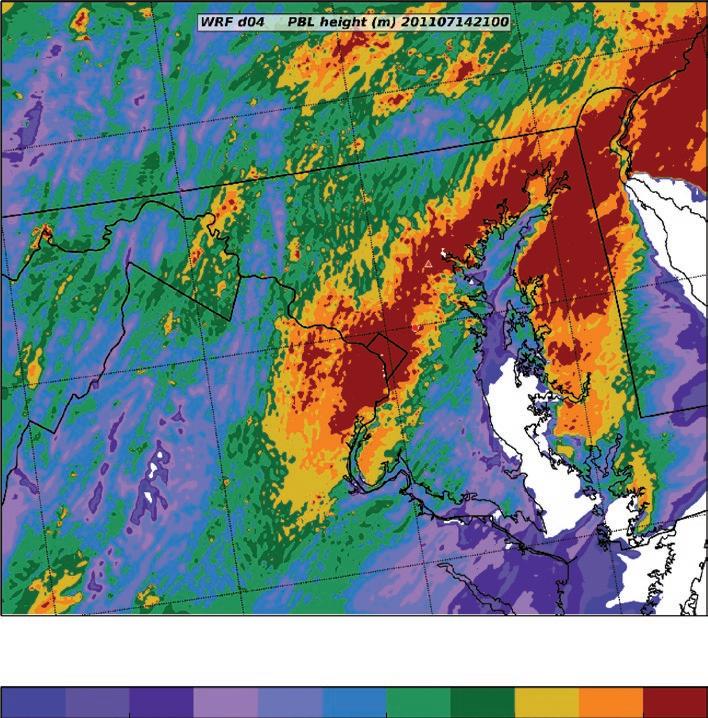
Sources of planetary boundary layer height data A key property in determining the relationship between total column AOD and ground-level PM2.5 is the height of the planetary boundary layer (PBL; for example, Alexeeff and others 2015; Chatfield and others 2017; Lee, Chatfield, and Strawa 2016), which varies significantly with time of day, geography, season, and meteorological conditions. For example, PBLH can vary on an urban scale with distance from the city center, distance from coastlines, and other factors, as shown in figure A.6. Including predicted PBLH from meteorological model simulations (especially as an AOD/PBLH ratio) has been shown to significantly increase the performance of the statistical approaches (for example, Chatfield and others 2017).

When there is a well-mixed convective PBL and the aerosols in the PBL dominate the total AOD, there should be a nearly linear relationship between groundlevel PM2.5 and the AOD/PBLH ratio, and thus for PBL variability to account for much of the variability in the relationship of AOD to PM2.5. However, for areas with very shallow PBLs, or when a smoke or dust plume is present above the PBL, the total column AOD may have no relationship to the ground-level PM2.5 at all. Thus, in those circumstances, the PBLH along with other parameters can be used to filter suspect estimates of ground-level PM2.5 concentrations.

Public sources of PBLH data include in situ radiosonde and aircraft vertical profiles, ground-based and satellite remote sensing retrievals, and numerical weather prediction model data. These sources are discussed further below.

Radiosonde and aircraft profiles: Various methods are available for calculating the PBLH from radiosonde profiles of temperature, relative humidity, and

FIGURE A.6

Planetary boundary layer height in areas surrounding Washington, DC, US, on July 14, 2011, at 21:00 UTC

78°W 77°W 76°W 75°W

40°N 75°W

40°N

79°W

39°N

39°N

38°N

79°W 39°N 78°W 77°W

Height of the planetary boundary layer (meters) 76°W

1,000 1,200 1,400 1,600 1,800 2,000

Source: World Bank, using Python software. Note: Planetary-boundary-layer (PBL) height was calculated using the Weather Research and Forecasting (WRF) model. UTC = Coordinated Universal Time.

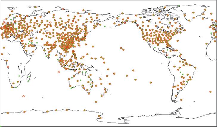
wind (for example, Seidel, Ao, and Li 2010). Though considered the gold standard for observing the vertical structure of the atmosphere, radiosondes in global operational networks are generally launched only twice daily and often not at ideal times to estimate the peak daytime PBLH. Furthermore, as shown in map A.2, the radiosonde launch locations are concentrated in higher-income countries in Europe, north America, and Southeast Asia, and there is notably poorer coverage in Africa, Central Asia, and Central and South America. Therefore, the measured profiles and PBLH may not be representative of the cities in LMICs.

The Aircraft Meteorological Data relay (AMDAr), which includes data from US aircraft from the Meteorological Data Collection and reporting System (MDCrS), is a global data set produced by commercial aircraft equipped with instruments to measure meteorological data during flights (for example, Drüe and others 2008; Fleming 1996; Zhu and others 2015). Meteorological data

MAP A.2

Radiosonde launch locations for 00:00 UTC, December 8, 2017

Latitude 90°

60°

30°

0°

–30°

–60°

–90°

0° 60° 120° 180° –120° –60° 0° Longitutde

Source: The plot was generated from an application on the Naval Research Laboratory (NRL) website: http://www .usgodae.org/cgi-bin/cvrg_con.cgi. Note: UTC = Coordinated Universal Time.

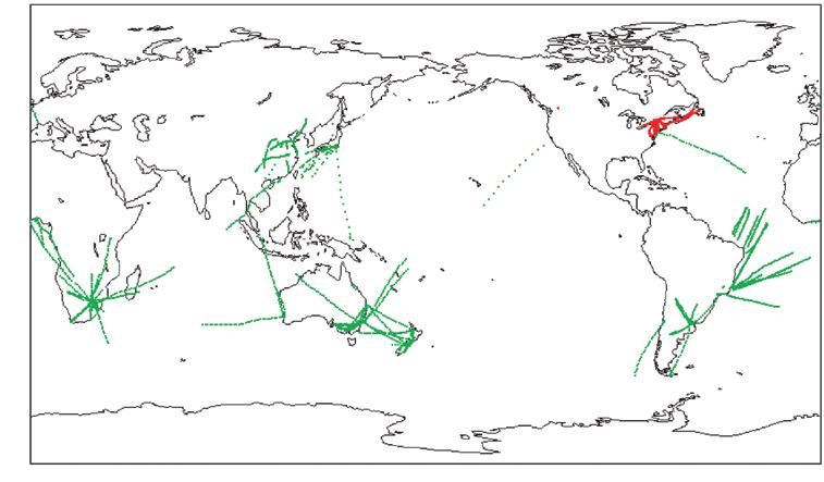
measured at different heights during takeoff and landing have been used to calculate PBLH around the globe (McGrath-Spangler and Denning 2012, 2013). The AMDAr coverage is more variable than that of radiosondes but also tends to be concentrated in the higher income regions (map A.3).

Ground-based remote sensing: Ground-based remote sensing systems, including lidar, ceilometer, sonic detection and ranging (SODAr), and Doppler wind profilers (DWPs), are capable of providing observations of the PBLH for field campaigns or as part of operational networks. Of these, currently only lidar networks routinely produce PBLH products available for public use. There are three networks contributing to WMO’s Global Atmospheric Watch (GAW) Aerosol Lidar Observations network (GALIOn)40 that provide PBLH data:

• The European Aerosol research Lidar network (EArLInET)41 consists of 28 stations distributed over Europe. • The Asian Dust and Aerosol Lidar Observation network (AD-net) includes 20 stations in Asia including Ulaanbaatar, Mongolia, and Phimai, Thailand, with nrT coverage (map A.3). • The nASA Micro-Pulse Lidar network (MPLnET) is a federated network of currently 23 active Micro-Pulse Lidar (MPL) systems located around the globe, including stations at Kanpur, India; Omkoi, Thailand; and Windpoort, namibia (map A.3). An improved PBLH retrieval algorithm has recently been incorporated into the latest version (version 3) of the operational product that is less susceptible to contamination by clouds and residual layers that can result in errors (Lewis and others 2013). retrievals of PBLH with this new algorithm have been validated with PBLH calculated from ozonesonde

MAP A.3

Aircraft observation coverage from AMDAR and MDCRS, December 8, 2017

90° a. AMDAR

60°

30°

Latitude 0°

–30°

–60°

–90°

0°

90°

60°

30°

Latitude 0°

–30° 60° 120° 180° –120° –60° 0° Longitude

b. MDCRS

–60°

–90°

0° 60° 120° 180° –120° –60° 0°

Longitude

Source: Generated from an application on the Naval Research Laboratory (NRL) website: http://www.usgodae. org/cgi-bin/cvrg_con.cgi. Note: AMDAR = Aircraft Meteorological Data Relay; MDCRS = Meteorological Data Collection and Reporting System. Red lines = Canadian AMDAR data; green lines = other AMDAR data; blue lines = MDCRS data.

soundings produced during the DISCOVEr-AQ field campaign and compared to high-resolution Weather research and Forecasting (WrF) model simulations (Hegarty and others 2018; Lewis and others 2013). The data are available in nrT (approximately one-hour processing delay).

Satellite data: Only a few studies have examined PBLH using satellite data (Martins and others 2010). radio occultation data from global positioning system (GPS) satellites have been used to determine PBLH but because of the long tangential path of the GPS signal through the atmosphere the horizontal resolution is coarse ranging from tens to hundreds of kilometers (Ao and others 2012; Guo and others 2011). PBLH retrievals from the Cloud-Aerosol Lidar with Orthogonal Polarization (CALIOP; Winker, Hunt, and McGill 2007; Winker and others 2009) onboard the Cloud-Aerosol Lidar and Infrared Pathfinder Satellite Observations (CALIPSO) satellite have been used to evaluate numerical weather prediction model reanalysis data (Jordan, Hoff, and Bacmeister 2010) during 2006. More recently, a global data set of CALIPSO PBLH retrievals was generated for June 2006 to December 2012, evaluated with PBLHs calculated with AMDAr meteorological data, and used to examine global seasonal variability in the midday PBLH (McGrath-Spangler and Denning 2012, 2013). In addition, CALIPSO PBLHs were compared favorably with radiosondes over China during 2011 to 2014 (Zhang and others 2016). The CALIPSO cloud and aerosol products used to derive the PBLHs for these studies are available through the nASA Langley Data Archive Center (DArC).42 Unfortunately, the PBLHs were produced independently for only these limited research projects and currently are not yet produced regularly for public dissemination. However, no continuous data sets of satellite-derived PBLHs are publicly available.

NWP model data: numerical weather prediction (nWP) models assimilate all types of meteorological and environmental observations to produce three-dimensional meteorological fields that are as accurate a representation of the true atmospheric state as possible at a given time. There are two types of nWP data: operational and reanalysis. Operational forecast centers run nWP models several times per day to provide numerical guidance to human weather forecasters and inputs to air-quality forecast models. Operational nWP data have the advantage of being available in near real-time, often within three to four hours of the beginning of a forecast cycle, whereas reanalysis nWP data have a latency period of several months. However, operational nWP models are continuously being updated to correct bugs and address problems in physical parameterization schemes, complicating long-term historical analysis. On the other hand, reanalysis nWP data are generated with models similar to those used in operational centers but frozen in development. When enough changes in the state of nWP modeling accumulates, a new version of the reanalysis, usually with the same starting date as the previous version, is generated with an updated model. Thus, reanalysis data are more appropriate for looking at temporal trends and are also subject to more thorough evaluations and analysis. Both types of nWP data could be used depending on the time requirements on data availability of a particular research task. The observational data described above when available will be used to complement the nWP data, particularly for situations in which the observational data provide a better representation of the local conditions than the grid-averaged nWP data.

Operational NWP: The national Centers for Environmental Prediction (nCEP) Global Forecast System (GFS) is a global model with four daily run cycles beginning at 0000, 0600, 1200, and 1800 UTC (Coordinated Universal Time). For each cycle the GFS model is run for 384 hours, and the initial analysis and forecast fields are available on global latitude-longitude grids of 0.25°, 0.5°, and 1.0° resolution in grib2 format.43 Forecast output is available at each hour for the first 180 forecast hours, every 3 hours from 180 to 240 hours, and then every 12 hours until 384 hours. The analysis and forecast fields include PBLH and temperature, horizontal winds, vertical velocity, specific and relative humidity, geopotential height, and cloud water mixing ratios at the surface and 30 pressure levels with 25 hecto Pascals (about 200 meters) spacing up to 900 hecto Pascals. The model output is available from the nOAA nCEP ftp server generally within 5 hours after the beginning of the forecast cycle.

The Canadian Meteorological Center (CMC) produces a global nWP forecast twice daily at 0000 and 1200 UTC for 240 hours called the Global Deterministic Prediction System (GDPS).44 The CMC GDPS initial analysis and forecast data are available on a 0.24° latitude-longitude grid in grib2 format.45 The data are available every 3 hours out to 140 hours and every 6 hours to 240 hours. The variables include temperature, winds, and relative humidity at the surface and 23 pressure levels. A PBLH diagnostic is not included but could be calculated from vertical model profiles; however, the vertical resolution is coarse ranging from 15 hecto Pascals (about 120 meters) from the surface to 50 hecto Pascals (more than 450 meters) above 900 hecto Pascals, and this would affect the accuracy of the PBLH calculation. The latency time between the beginning of the model cycle and model data availability is approximately 4 to 5 hours.

The JMA runs a Global Spectral Model (GSM) four times a day. The runs at 0000, 0600, and 1800 UTC are for 84 hours, and the 1200 UTC run is for 264 hours. Output data are available in grib2 format on a 0.5° latitude-longitude grid at 3-hour intervals up to 84 hours and then 6-hour intervals up to 264 hours from the WMO Global Information System Centres (GISCs) website. The PBLH diagnostic is not included in the available output fields but could be calculated from temperature, wind, and moisture variables. The data latency time and specific access procedures were not clearly documented on the GISC website. The JMA also produces a mesoscale model forecast with five-kilometer resolution for a domain centered over Japan but including eastern Mongolia. However, only graphical outputs seem to be available in the public domain.

The Fleet numerical Oceanographic Center produces a global nWP forecast with the navy Global Environmental Model (Hogan and others 2014) four times per day with a horizontal resolution of about 37 kilometers. However, the gridded output fields are not readily accessible and may be restricted to organizations within the United States.

The European Center for Medium range Weather Forecasts (ECMWF) and United Kingdom Meteorological Office (UKMET) also produce global nWP forecasts,46 but the output data are only provided for a licensing fee based on the amount and type of data being requested.

Operational models such as the nCEP GFS are continuously being updated with new physical parameterization schemes (for example, Han and Pan 2011) and new sources of observational data to be assimilated through observing system experiments and observing system simulation experiments (for example, Atlaskin and Vihma 2012). The improvements are often evaluated at the

continental to hemispheric scale using geopotential height anomaly correlations and at regional and local scales against temperature, winds, and moisture observations (for example, Cucurull and Derber 2008) but not PBLH. A Google Scholar search for evaluations of operational model PBLH outputs over land produced no results, perhaps because of the general lack of continuous PBLH observations in most locations. nevertheless, data from operational models are used in satellite algorithms; for example, the MODIS cloud height algorithm uses GFS temperature profile data (for example, Holtz and others 2008). Thus, given the general lack of observations, it seems to be a reasonable procedure to use GFS PBLHs as an estimate of the PBLH in LMICs to determine PM2.5 from column AOD measurements. Furthermore, in 2016 nOAA announced the development of a new model to replace the current GFS. The model will still be called the GFS and but will feature a new dynamic core, the Finite Volume on a Cubed Sphere (FV3), that is expected to increase the model’s accuracy and numerical efficiency.47 The new GFS model is projected to be operational in 2019 (Schneider 2016).

MERRA reanalysis: The Modern Era retrospective-analysis for research and Applications (Bosilovich 2008; MErrA) is a nASA reanalysis from 1979 to the present day produced using the Goddard Earth Observing System (GEOS) Data Assimilation System (DAS) Version 5 (GEOS-5 DAS; rienecker and others 2008). The reanalysis data are on the GEOS-5 native 576 by 361 grid with 0.625° by 0.5° resolution at the surface and include PBLH and temperature, winds, relative humidity at the surface, and either 42 pressure levels at three hourly intervals or 72 pressure levels at six-hour intervals. The 42-level product has 8 levels below 800 hecto Pascals, while the 72-level product has 12. An updated version of the reanalysis (Bosilovich and others 2015; Gelaro and others 2017; MErrA2) extends from 1980 to the present with a latency time of approximately one to two months.

MErrA PBLH data have been evaluated using PBLH retrievals from the CALIPSO satellite (Winker, Hunt, and McGill 2007; Winker and others 2009) over a western hemisphere domain from 60° S to 60° n for August and December 2006 and Africa in August 2006 (Jordan, Hoff, and Bacmeister 2010). The evaluation indicated a better MErrA-CALIPSO correlation in August in both domains (R of 0.73) than in December (R of 0.47). Over the Sahara Desert the MErrA PBLHs were clustered around 1 to 3 kilometers above ground level and generally lower than those of CALIPSO that had several clusters around 1 to 2 kilometers, 3.5 to 4.5 kilometers, and 5 to 6 kilometers above ground level.

The PBLHs from the atmospheric modeling component of GEOS-5 (Atmospheric General Circulation Model) used to derive MErrA have also been evaluated with micro-MPL retrievals at the nASA Goddard Space Flight Center (GSFC) in Maryland for the period of 2001 to 2008 (Lewis and others 2013). The model and MPL diurnal cycles agreed well but the model underestimated the maximum daily PBLH compared to the MPL retrievals by about 0.4 kilometers.

There is inherent uncertainty in any source of PBLH data. This uncertainty can be attributed to three sources: (1) the methods used to calculate it from in situ observations (for example, Hegarty and others 2018; Seidel, Ao, and Li 2010), (2) the retrieval method (for example, Lewis and others 2013; Winker, Hunt, and McGill 2007), or (3) error in the nWP model (for example Jordan, Hoff, and Bacmeister 2010; Lewis and others 2013; McGrath-Spangler

and Denning 2012, 2013). This uncertainty can be near to 50 percent (for example, Lewis and others 2013; Seidel and others 2012). The uncertainty can also be dependent on the synoptic weather conditions. Hegarty and others (2018) found poor agreement between PBLHs calculated from ozonesondes with different methods, MPL retrievals, and mesoscale model outputs on days with southerly and southwesterly flow in the Baltimore–Washington, DC, area, but good agreement between PBLHs calculated with all methods, MPL retrievals, and model data on days with northerly winds. This suggests that, whenever possible, data from both observations and models should be compared to quantify the uncertainty of the PBLH inputs to the algorithms used to determine the ground-level PM2.5 concentrations for satellite AOD retrievals.

Chemical transport model–based approaches

Several studies (for example, van Donkelaar, Martin, and Park 2006) have used CTMs to determine a time-varying relationship between ground-level PM2.5 concentrations and satellite AOD observations. This relationship is then used to scale the CTM aerosol profile to match the satellite-observed AOD, providing an improved estimate of the ground-level PM2.5 concentration than would be possible from the CTM alone. The advantages of this approach include that it can be generalized to apply to any region of the globe, can provide daily estimates of the relationship between AOD and PM2.5 (similar to mixed effects models) (see the section “Statistical approaches” in this appendix), and can account for the impact of elevated PM2.5 layers on this relationship, thereby identifying periods where the AOD is likely dominated by aerosols above the PBL and thus do not provide good data on ground-level PM2.5 concentrations. The disadvantages are that it requires the running of a CTM, which can be a complicated and labor-intensive process, and that it is highly dependent on the ability of the CTM to correctly predict aerosol vertical profiles, even when the CTM predictions of AOD are off. However, the use of publicly available CTM output (see the section “Chemical transport model–based approaches” in this appendix) could reduce the labor issues for LMICs.

Errors in AOD can be propagated through the CTM methods by repeating the process for the high and low error bounds on the AOD. However, quantifying the uncertainty in the CTM estimate of the relationship between AOD and surface concentrations is not straightforward, since this relationship is sensitive to errors in multiple aerosol components at multiple vertical levels, as well as errors in relative humidity. Thus, the method used here to account for this error is to assume a constant relative error based on post hoc validation of the CTM PM2.5 estimates (for example, ±47 percent, based on the “rest of world” results of van Donkelaar, Martin, Brauer, and Boys 2015).

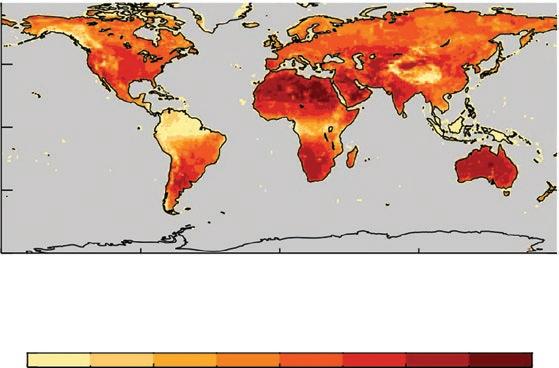
Van Donkelaar, Martin, and Park (2006) used MODIS Dark Target AOD and MISr AOD separately to predict annual mean ground-level PM2.5 concentrations over north Americausing the GEOS-Chem model (v7-02-01, 1° by 1° nested resolution over north America, driven with GEOS-3 meteorology) to predict the relationship between AOD and PM2.5. Using MISr AOD explained 34 percent of the variability, and the MISr-predicted values had a mean bias of 3.1 micrograms per cubic meter and a slope of 0.57. Using MODIS Dark Target explained 48 percent of the variability with a mean bias of 5.1 micrograms per cubic meter and a slope of 0.82.

Van Donkelaar and others (2010) used MODIS Dark Target AOD and MISr AOD together to provide long-term average (2001–06) global estimates of ground-level PM2.5 concentrations at about 10 kilometers (0.1° by 0.1°) resolution using the GEOS-Chem model (v8-01-04, 2° by 2.5° resolution, driven with GEOS-4 meteorology) to predict the relationship between AOD and PM2.5. In the present study, the MODIS and MISr data were filtered to remove observations that had an anticipated bias greater than the larger of ±0.1 or ±20 percent. remaining MODIS and MISr AOD retrievals were averaged to produce a single value for a grid cell. Over north America, the model explained 59 percent of the observed variability with a slope of 1.07 and a mean bias of −1.75 micrograms per cubic meter, both substantial improvements over the estimates of van Donkelaar, Martin, and Park (2006).

Van Donkelaar and others (2011) used MODIS Dark Target AOD and the GEOS-Chem model (v8-03-01, 2° by 2.5° resolution, driven with GEOS-5 meteorology) to estimate daily PM2.5 concentrations during a major biomass burning event around Moscow in the summer of 2010. During this event, the standard MODIS retrieval incorrectly identified some of the aerosol as cloud due to the large AOD values. relaxing the cloud screening increased MODIS coverage by 21 percent with no evidence of false aerosol detection. GLM PM2.5 data were estimated from PM10 observations for several nearby sites, because only two sites had PM2.5 observations. The satellite product explained 85 percent of the variability in these estimated PM2.5 observations with a slope of 1.06.

Geng and others (2015) used the combined MODIS Dark Target and MISr AOD product of van Donkelaar and others (2010) to determine long-term average (2006–12) PM2.5 concentrations over China at about 10 km (0.1° by 0.1°) resolution using the GEOS-Chem model (version 9-01-02, 0.5° by 0.667° nested resolution over China, driven with GEOS-5 meteorology) to predict the relationship between AOD and PM2.5. Comparison with ground-level PM2.5 concentrations observations showed the satellite-based product explained 55 percent of the variability in PM2.5 with a slope of 0.77.

Van Donkelaar and others (2015) used satellite AOD observations and the GEOS-Chem model to produce annual average PM2.5 estimates (1998–2012) over the globe. The MODIS radiance observations were used in an optimal estimation framework (van Donkelaar and others 2013) to derive PM2.5 estimates that were consistent with the GEOS-Chem aerosol scheme for 2004–10, which were then combined with the product of van Donkelaar and others (2010) for 2001–03 to produce a global, decadal average PM2.5 estimate at about 10-kilometer resolution. The work of Boys and others (2014), which used AOD from the SeaWIFS and MISr satellites and the GEOS-Chem model to estimate the temporal variation in PM2.5, was then applied to this decadal average to produce a 15-year global estimate of ground-level PM2.5. Comparisons with decadal mean GLM data over north America gave an R of 58 percent with a slope of 0.96 and a 1−σ error of −1 microgram per cubic meter + 16 percent. Over Europe, the comparison gave an R of 53 percent with a slope of 0.78 and a 1−σ error of 1 microgram per cubic meter +21 percent, whereas over the rest of the world the R was 0.66, the slope was 0.68, and the 1−σ error was −1 microgram per cubic meter + 47 percent.

Sources of AOD-PM2.5 relationships from observations Until recently, few data were available from colocated observations of AOD and ground-level PM2.5. The Surface Particulate Matter network (SPArTAn) was established to address this need (Snider and others 2015). The network includes

a global federation of ground-level monitors of hourly PM2.5, primarily in highly populated regions in proximity to existing ground-based sun photometers (for example, AErOnET sites) that measure AOD. Together, these instruments provide an empirical measure of the AOD/PM2.5 ratio that is used to relate satellite AOD retrievals to ground-level PM2.5.

The current SPArTAn network is fairly sparse, but adding an AErOnET and SPArTAn site to a given city would provide valuable data on the local variation of the AOD/PM2.5 ratio at a relatively low cost. However, in the absence of these data, this ratio can be estimated from CTM output.

Sources of aerosol profile data from CTMs For LMICs to use the CTM approach without having to run CTMs themselves, they need publicly available CTM data sets that can be used to match aerosol profiles with AOD observations. Several potential sources of these data for LMICs are discussed below.

MERRA-2 Reanalysis: The nASA MErrA-2 reanalysis (Provençal and others 2017) provides hourly average AOD at 550 nm both by total and by aerosol component, as well as the surface mass concentration for each component, at a horizontal resolution of 0.5° by 0.625°. However, aerosol vertical profiles are only provided every three hours as instantaneous (snapshot) profiles. MErrA-2 uses the nASA GEOS-5 atmospheric general circulation model (Colarco and others 2014). The aerosol component of MErrA-2 is based on the Goddard Chemistry Aerosol radiation and Transport Model (GOCArT; Chin and others 2000; Colarco and others 2010, 2014; Kim and others 2013). Funded mainly by nASA Earth Science programs, the GOCArT model was developed to simulate atmospheric aerosols (including sulfate, black carbon, organic carbon, dust, and sea salt), carbon monoxide, and sulfur gases. The reanalysis has about a twomonth latency. All of the data are freely available for download from nASA via MDISC,48 managed by the nASA Goddard Earth Sciences (GES) Data and Information Services Center (DISC).

NCEP NGAC forecasts: nEMS GFS Aerosol Component (nGAC; Lu, da Silva, and others 2016) is a global inline aerosol forecast system. The forecast model component of the nGAC is the GFS based on the nOAA Environmental Modeling System (nEMS; Black and others 2007, 2009) which, in turn, is based on the common modeling framework using Earth System Modeling Framework (ESMF). The aerosol component of the nGAC is GOCArT (Chin and others 2000; Kim and others 2013).

The initial production implementation of nGAC with global-dust-only forecast was implemented in September 2012 (Lu, da Silva, and others 2016). The current nGAC operational forecast produces 120-hour global multispecies forecasts including dust, sea salt, sulfate, and carbonaceous aerosols. The system runs twice daily within the nCEP Production Job Suite at the 0000Z cycle and 1200Z cycle. Although no satellite data assimilation is currently performed, research is underway to add the assimilation of the nOAA VIIrS AOD product to nGAC (Lu, Wei, and others 2016). Output is posted to a 1° by 1° longitude/latitude grid with a 3-hour forecast interval to 120 hours. The files (in grib2 format) include three-dimensional profiles of individual aerosol components (dust, sea salt, sulfate, organic carbon, and black carbon), temperature, and relative humidity, as well as two-dimensional fields including the model-calculated total AOD and the AOD from each aerosol component.

NCAR MOZART-4/GEOS-5 forecasts: nCAr provides output from their MOZArT-4/GEOS-5 global air-quality simulations (Emmons and others 2010) for public use, both in nrT and in a historical archive going back to 2007.49 The representation of tropospheric aerosols in MOZArT-4 is based on the work of Tie and others (2001, 2005) and includes the calculation of sulfate, black carbon, primary organic, secondary organic aerosols (SOAs), ammonium nitrate, and sea salt (Lamarque and others 2005). Because only the bulk mass is calculated, a lognormal number distribution is assumed for all aerosols to calculate the surface area (and thus AOD), using a different geometric mean radius and standard deviation for each type of aerosol (based on Chin and others 2002). Sea salt aerosols are included in the model with four size bins (0.1–0.5, 0.5–1.5, 1.5–5, and 5–10 micrometers), and emissions are calculated online (Mahowald, Lamarque, and others 2006). However, the distributions of four sizes of dust (0.05–0.5, 0.5–1.25, 1.25–2.5, and 2.5–5.0 micrometers) are set from monthly mean distributions taken from online calculations in the Community Atmosphere Model (CAM) (Mahowald, Muhs, and others 2006), and thus the model does not include prognostic dust. Hygroscopic growth of the aerosols is determined from the ambient relative humidity, with different rates for each type of aerosol (Chin and others 2002). Washout of all aerosols, except hydrophobic black carbon and organic carbon, is set to 20 percent of the washout rate of nitric acid (HnO3) (Horowitz 2006; Tie and others 2005). Comparisons of calculated AOD over the ocean to AOD retrievals from the MODIS satellite instrument indicate this is a reasonable washout rate.

The nCAr MOZArT-4/GEOS-5 aerosol profiles are provided at a horizontal resolution of 1.875° by 2.5° every six hours. However, the output files include only the bulk mass for each size bin, and so the model AOD has to be calculated from these data by the user.

UK Met Office research ensemble forecast: The UK Met Office provides an operational global forecast at 17-kilometer resolution that includes prognostic and interactive dust for a four-member hybrid ensemble. An additional aerosol forecasting global model, including carbonaceous aerosols and sulfate aerosols, is run as a research product using a copy of the operational model, with aerosol chemistry using the CLASSIC scheme (Bellouin and others 2011; Mulcahy and others 2014). However, the additional aerosols do not feed back to the dynamics. This research product is available only via the principal investigator (Malcolm Brooks, malcolm.e.brooks@metoffice.gov.uk).

ECMWF Copernicus Atmospheric Monitoring Service: The ECMWF Copernicus Atmospheric Monitoring Service (CAMS) produces twice-daily 120-hour global forecasts of total aerosols, aerosol components (dust, sea salt, biomass burning, sulfate), and AOD at about 40-kilometer spatial resolution (0.5625° by 0.5625°) at a three-hour temporal resolution. CAMS also produces the Monitoring Atmospheric Chemistry and Climate (MACC) reanalysis (Toll and others 2015) of AOD and component AOD at about 80-kilometer resolution (1.125° by 1.125°). However, both products currently require purchasing a license from ECMWF and thus may not be the correct solution for many LMICs.

CAMS currently uses a simple bin scheme (IFS-LMD [Integrated Forecast System–Laboratoire de Météorologie Dynamique]) for its near real-time forecasts and the MACC reanalysis. IFS-LMD mainly follows the aerosol treatment in the Laboratoire d’Optique Atmosphérique / LMD-Z Laboratoire de Météorologie Dynamique–Zoom (LOA/LMD-Z) model (Boucher and others 2003; reddy and others 2005). Five types of tropospheric aerosols are

considered: sea salt, dust, organic carbon, black carbon, and sulfate aerosols. Prognostic aerosols of natural origin, such as mineral dust and sea salt, are described using three size bins. Emissions of dust depend on the 10-meter wind, soil moisture, the UV-VIS component of the surface albedo, and the fraction of land covered by vegetation when the surface is snow-free. A correction to the 10-meter wind to account for gustiness is also included (Morcrette and others 2009). Sea-salt emissions are diagnosed using a source function based on work by Guelle and others (2001) and Schulz, de Leeuw, and Balkanski (2004). Sources for the other aerosol types are taken from the Speciated Particulate Emission Wizard (SPEW) and the Emission Database for Global Atmospheric research (EDGAr) annual or monthly mean climatologies (Dentener and others 2006). Emissions of organic matter, black carbon, and SO2 linked to fire emissions are obtained using the Global Fire Assimilation System based on MODIS satellite observations of fire radiative power, as described in Kaiser and others (2012).

In addition, the ECMWF forecasts assimilate MODIS AOD data at 550 nanometers in a 4D-Var framework that has been extended to include the aerosol total mixing ratio as an extra control variable (Benedetti and others 2009).

Hybrid approaches

Hybrid approaches are those in which both the output from CTMs and statistical models are used to convert satellite AOD retrievals into predictions of ground-level PM2.5. For example, van Donkelaar, Martin, Spurr, and Burnett (2015) used geographically weighted regression (GWr) to relate the errors between the GLM PM2.5 observations and their estimate of ground-level PM2.5 based on MODIS AOD observations and GEOS-Chem simulations (van Donkelaar and others 2013). They used the Matlab function glmfit, but opensource options in Python are available (for example, the pyglmnet library).

The spatial predictors used were the percentage of urban land cover (at one-kilometer resolution) and the subgrid elevation difference (that is, the difference between the mean elevation for a 0.5° by 0.67° GEOS-Chem grid box, the local elevation from high-resolution maps). In addition, the GEOS-Chem predictions for the relative contributions of nitrate, primary carbonaceous, and secondary organic aerosol to the total PM2.5 were used as additional predictors.

GWr was then used to predict the bias between monthly mean ground-level PM2.5 estimates and the satellite-derived estimate of ground-level PM2.5. This gave spatially varying, but constant with time, bias-correction estimates at a fine resolution (one kilometer) over north America. However, although the bias-correction is constant with time, the uncorrected values vary with time (daily for areas with MODIS coverage) and thus provide daily estimates of ground-level PM2.5. The bias-corrected satellite product showed a much higher correlation with surface observation and a better regression slope but had similar rMSE with respect to surface monitors as the uncorrected product.

COMBINING GLM AND SATELLITE DATA

The two most common methods that have been used to simultaneously interpolate satellite-derived PM2.5 estimates and GLM data to obtain city-scale PM2.5 estimates are co-kriging and simultaneous land-use regression (for example, Alexeeff and others 2015; de Hoogh and others 2016; Lee, Chatfield, and Strawa 2016).

Co-kriging

Like most spatial interpolation schemes, ordinary kriging uses a weighted average of neighboring samples (that is, from a spatially distributed set of groundlevel monitors of PM2.5) to predict PM2.5 concentrations across an urban area. However, in ordinary kriging the weights depend not only on the distance between the prediction location and the measured points, but also on the spatial autocorrelation in the data (Millar and others 2010). Kriging also provides error estimates for its predictions.

Co-kriging is an extension of ordinary kriging that can take advantage of additional data sets or variables, using both the correlations between the monitors and the cross-correlations between the monitor data and the additional data sets to make better predictions. In the application of interest here, the second data set would be the satellite-derived ground-level PM2.5 estimates produced using one of the methods outlined earlier in this appendix, but additional data sets, such as meteorological data, can be incorporated via co-kriging (Millar and others 2010; Pearce and others 2009; Wu, Winer, and Delfino 2006). Kriging is generally done using licensed software such as ArcGIS, but open source options (for example, the pyKrige toolkit in Python) also are available.

For LMICs, the advantage of combining satellite data with GLM data via co-kriging is that it potentially reduces the number of GLM stations required to adequately cover an urban area via ordinary kriging. Kriging is most suitable for cases where the GLM network (1) is spatially dense, (2) captures the general spatial variation of PM2.5, and (3) adequately covers the edges of the study area. Applying kriging to sparse data will either result in over-smoothed surfaces or over-fitted predictions. Using the more spatially dense satellite estimates of surface level PM2.5 in co-kriging could thus address these limitations of kriging for urban areas with sparse GLM networks.

Co-kriging has other potential advantages. It does not require any data beyond the GLM network data and the satellite-derived ground-level PM2.5 estimates. In contrast, land-use regression requires substantial additional data (see the sections “Co-kriging” and “Land-use regression” in this appendix). Furthermore, co-kriging can be applied independently at each time point, so that the temporal resolution of the maps produced can be the same as the initial GLM and satellite data, allowing for short-term average (that is, daily) predictions of PM2.5 concentrations. In fact, Alexeeff and others (2015) showed that to estimate chronic (annual) exposure to PM2.5, kriging applied to annual average data was insufficient to capture the exposure accurately, and thus kriging had to be applied to the daily data and then averaged to provide annual estimates. However, the spatial resolution of the predictions is limited by the spatial density and resolution of the input data sets, making predictions on a one-kilometer scale or finer difficult.

An example of the use of co-kriging to supplement a sparse GLM network was provided by Singh and others (2011), who demonstrated how CTM predictions of ground-level PM2.5 concentrations could be used as a secondary variable in a co-kriging interpolation of GLM data to predict PM10 concentration over northern Italy. They used 14 PM10 monitors and five-kilometer resolution CTM predictions over a 60-kilometer by 60-kilometer domain. Their co-kriging models were able to explain 88–90 percent of the variability in PM10 with an rMSE of 16 micrograms per cubic meter, which was lower than the kriging

value (20 micrograms per cubic meter). In addition, they found that the predicted maps of PM10 concentration were substantially different between kriging and co-kriging, with the co-kriging map capturing more of the expected special variation of PM10 in the domain. In addition, Singh, Venkatachalam, and Gautam (2017) used co-kriging to fill in missing MISr AOD data using observations from the MODIS instruments. However, there is no example of co-kriging with satellite-based PM2.5 products in the literature.

Land-use regression

Land-use regression (LUr) spatially links GLM network data of PM2.5 with other associated variables (such as elevation, distance from roads, population density, and land-use type) to develop finer-scale and more accurate estimates of longterm PM2.5 concentrations within an urban area than is possible with kriging (Millar and others 2010). The most predictive variables are identified through least-squares linear regression (Briggs and others 1997). Other studies (for example, Vienneau and others 2013) have incorporated data on meteorology (for example, wind direction; Arain and others 2007; ryan and others 2008) and satellite observations of aerosols, nO2, and other pollutants (for example, Lee, Chatfield, and Strawa 2016) into the regression as well. The development of predictor variables from geographic information system (GIS) files is generally performed using licensed software such as ArcGIS, but the regression can be performed using open-source software such as r.

LUr is an attractive option for estimating PM2.5 concentrations at a neighborhood scale within urban areas with sparse measurement networks, since the regression can be used to predict concentration at the scale of the land-use data in unmonitored areas. However, the method assesses only spatial variation and thus can predict only long-term average concentrations (for example, monthly or annual). In addition, the method generally requires a significant amount of GIS skill to apply and requires much more input data than co-kriging (see the section “Co-kriging” in this appendix).

Several studies have used satellite estimates of ground-level PM2.5 within LUr models. For example, Vienneau and others (2013) used MODIS-derived groundlevel PM2.5 estimates (at 10-kilometer resolution) as a predictor in a land-use regression model to estimate annual average PM10 concentrations over Europe at a resolution of 100 meters. The LUr models using the satellite data had consistently higher correlations and generally lower mean bias and mean absolute errors (MAEs) than the LUr models that did not use satellite data. The models using satellite data to predict annual average PM10 generally explained between 35 and 50 percent of the variability in PM10 (mean absolute error of 4.6 to 6.0 micrograms per cubic meter).

Lee, Chatfield, and Strawa (2016) adopted a different approach in which LUr is included in the linear mixed-effects statistical model used to relate MODIS Deep Blue AOD to ground-level PM2.5 estimates for California (see, for example, the section “Statistical approaches” in this appendix). Separate LUr models were built for each season and trained using three years of data from 142 GLM sites. The land-use predictors included distance from major highways, population density, estimated pollutant emissions from the US EPA national Emission Inventory, elevation, percentage of developed land, distance from the coast, and the air basin in which each measurement site was located. In addition, daily values for AOD, wind speed, relative humidity, temperature, and PBLH from the

weather stations nearest to the site were also used as predictors. This addition of temporally varying data with land-use data allows for predictions of daily and annual average PM2.5 at the fine spatial scales possible with land-use regression. Lee, Chatfield, and Strawa (2016) found that the model was able to explain 66 percent of the variability of PM2.5 over California (MAE of 3.7 micrograms per cubic meter, rMSE of 5.7 micrograms per cubic meter) and that the modeled relationship between AOD and PM2.5 varied significantly by day.

De Hoogh and others (2016) used the 10-kilometer resolution satellitederived estimated of ground-level PM2.5 from van Donkelaar, Martin, Spurr, and Burnett (2015) as a predictor in a land-use regression model of PM2.5 over western Europe, predicting annual average PM2.5 concentrations at a resolution of 100 meters. The model also included satellite estimates of tropospheric nO2 columns at a 10-kilometer resolution, as well as independent CTM predictions of ground-level PM2.5 and nO2 from the MACC-II EnSEMBLE model, which was the median value of seven individual regional CTMs (CHIMErE, EMEP, EUrAD, LOTOS-EUrOS, MATCH, MOCAGE, and SILAM). Additional predictors included high-resolution data on land cover, roads, and altitude. They found that the PM2.5 LUrmodels that included both the satellite and CTM estimates of ground-level PM2.5 explained about 60 percent of the spatial variation in measured (annual average) PM2.5 concentrations, substantially more than was explained by the LUr model without satellite or CTM data (33–38 percent).

Data sets for land-use regression

If an LMIC has detailed GIS data on land use, population density, roads, pollutant emissions, and other fields needed for LUr, those should be used, because they would reflect the best local knowledge regarding the conditions likely to lead to high levels of PM2.5. However, since some LMICs may not have these data freely available, high-resolution, global data sets for the predictors used in the LUr studies discussed above were identified in this review:

• Land-cover type can be determined from the 0.5-kilometer MODIS-based

Global Land Cover Climatology provided by USGS.50 This map is based on based on 10 years (2001–10) of Collection 5.1 MCD12Q1 land-cover–type data and used 17 land-cover categories. The map is generated by choosing, for each pixel, the land cover classification with the highest overall confidence from 2001 to 2010 (Broxton and others 2014). These data can also be used to calculate parameters such as the percentage of developed land within a given radius of the site. • Distance from coasts can be determined using the World Water Bodies GIS layer.51 • GIS data on population density52 and major roads53 are available through the nASA Socioeconomic Data and Applications Center (SEDAC) hosted at

Columbia University. • The SEDAC Gridded Population of the World, version 4 (GPWv4) Population

Density product (CIESIn 2016) consists of estimates of human population density, based on counts consistent with national censuses and population registers, for the years 2000, 2005, 2010, 2015, and 2020. A proportional allocation gridding algorithm, utilizing approximately 12.5 million national and subnational administrative units, is used to assign population values to 30-arc-second (about one-kilometer) grid cells.

• The SEDAC Global roads Open Access Data Set (CIESIn and ITOS 2013; grOADS) combines the best available roads data by country into a global roads data set, using the Un Spatial Data Infrastructure Transport (UnSDI-T) version 2 as a common data model. Because the data are compiled from multiple sources, the date range for road network representations ranges from the 1980s to 2010 depending on the country (most countries have no confirmed date), and spatial accuracy varies. • In addition, OpenStreetMap54 is an open source, community project that maintains data about roads, trails, railway stations, and other landmarks, all over the world. OpenStreetMap emphasizes local knowledge, and contributors use aerial imagery, GPS devices, and low-tech field maps to verify that

OpenStreetMap is accurate and up to date. The inspection of these data suggests that the data are more detailed and occasionally more accurate than the grOADS database, but the data sources are also less well documented. • Topography data can be obtained from the Global Multi-resolution Terrain

Elevation Data 2010 (GMTED2010)55 created by the USGS and the national

Geospatial-Intelligence Agency (nGA). This data set has multiple spatial resolutions, 30, 15, and 7.5 arcseconds, and is a replacement for the previous

GTOPO30 data. • Spatially resolved global air pollutant emissions at a 0.1° by 0.1° resolution (about 10 kilometers) are available for the years 2008 and 2010 from the

EDGAr-HTAP_V2 emission inventory for several pollutants (CH4, CO, SO2, nO x, nonmethane volatile organic compounds, nH 3, PM10, PM2.5, black carbon, and organic carbon).

RECOMMENDATIONS FOR LMICS

These recommendations for the use of satellite observations to supplement GLM data in LMICs (using the typology proposed in chapter 1 and reproduced at the beginning of this appendix) are based on the literature review above:

• For Type I countries, since no GLM data are available, the only possible approach to convert AOD to ground-level PM2.5 for these countries is a CTMbased approach. Bias correction of the CTM-based estimates is also not possible for these countries, because there are no data with which to characterize the model bias. Thus, the raw CTM-based estimates of ground-level PM2.5 at the native resolution of the satellite AOD product should be used, but the derived ground-level PM2.5 values should be assigned a high uncertainty that reflects not only the uncertainty in the AOD but also the estimated uncertainty in the CTM-derived AOD to PM2.5 relationship (for example, about 50 percent based on van Donkelaar, Martin, Brauer, and Boys 2015). It is likely in this case that only city-average estimates will be possible, and that the annual estimates will be more reliable than the daily estimates. • For Type II countries, the small amount of available GLM data (with variable quality) will provide at least some ability to derive a bias estimate for the raw

CTM-based estimates of ground-level PM2.5 discussed above. However, without improvement in the QA procedures in these countries, it will not be possible to be certain that the bias-corrected estimate is truly more accurate than the raw estimate, and thus both values should be reported and stored. This will allow for reprocessing of the satellite estimates when more rigorous QA

procedures are developed. Similar to Type I countries, it is likely that only city-average estimates will be possible, and that the annual estimates will be more reliable than the daily estimates. • The GLM data in Type III countries allow both statistical and biascorrected CTM-based approaches for converting AOD to PM2.5 to be considered. CTM-based approaches may still be the best approach for these countries, but statistical approaches should also be tested before making a final decision. If GLM data from several sites exist, but only for a short period, those data can be used to develop seasonally and geographically varying statistical models and/or seasonally and geographically varying bias corrections for CTM-based approaches. If only a single site exists in the urban area, a seasonally varying statistical model and/or bias correction is still possible, but both the model and the bias correction would have to be applied uniformly across the urban area. Land-use regression (LUr; see the section “Land-use regression” in this appendix) can be combined with either technique to provide a finer-scale estimate of annual average ground-level PM2.5 (at about 0.5-kilometer resolution) using the data sets described in the section “Data sets for land-use regression” in this appendix, and co-kriging (see the section “Co-kriging” in this appendix) can be used to derive daily estimates across the city. • Type IV countries will be able to take advantage of the same approaches outlined above for Type III countries. However, the more extensive measurement networks will allow for more accurate estimates of the geographical and seasonal variation in the AOD to PM2.5 relationship. Thus, at this point, purely statistical approaches may begin to outperform CTM-based estimates, especially for regions where the model’s emission inventories are out of date or otherwise inaccurate. • In Type V countries, the main use of satellite observations is to help fill in the gaps of the existing monitoring network to cover more of the country’s population. These countries also tend to have access to higher-resolution, regional

CTM simulations that are customized for their region. Thus, both statistical and CTM-based approaches can be used.

In addition, the following recommendations on data sources and other methodological concerns are made for all countries interested in using satellite data to supplement GLM data:

• All countries should use the satellite product that offers the best balance of accurate AOD and spatial resolution for their country. For example, regions near bright urban or desert surfaces should prefer the MODIS Deep Blue product (see the section “Polar-orbiting satellites” in this appendix), since this has been demonstrated to give better performance in these regions. The extension of this algorithm to VIIrS will help maintain this capability over the next two decades. However, the MAIAC algorithm or the application of the Deep Blue algorithm to geostationary observations may provide better

AOD observations in the near future. • The highest-possible spatial resolution for satellite AOD will likely be between 2 and 4 kilometers (for geostationary observations) or 1 and 10 kilometers (for polar observations). Consequently, finer predictions will be possible only for cases where GLM data exist (via LUr; see the section

“Land-use regression” in this appendix).

• Some cities may have poor satellite coverage due to clouds or snow-covered surfaces regardless of the choice of the AOD product. This will reduce the number of days for which a daily estimate is possible and will need to be accounted for in the annual averages. • If local data on PBLH are available in a city (for example, Ulaanbaatar,

Mongolia), the measured PBLH should be used in statistical approaches. • For countries without the capacity to perform their own meteorological or chemical transport modeling, the freely available global model data sets provided by organizations in the United States for estimates of PBL height (see the section “Statistical approaches” in this appendix), aerosol vertical profiles (see the section “Chemical transport model–based approaches” in this appendix), and other parameters should be used. For long-term studies, the nASA

MErrA-2 reanalysis should be used, because this will represent the best estimate of the historical atmospheric state. However, the reanalysis takes two months to produce, and thus for short-term forecasts and advisories the nCEP GFS output (including the nGAC aerosol forecasts) should be used. • In all cases, the errors from the AOD retrieval, the CTM estimate of the aerosol profiles, and the statistical models used (either directly or for bias correction) should be quantified and used to quantify the error in the derived PM2.5 estimate. • In addition, cases where the nCEP nGAC forecasts and/or the MErrA-2 reanalyses suggest that the AOD is dominated (more than 70 percent) by aerosols above the PBL height should be flagged as potentially poor-quality satellite data, and thus poor-quality ground-level PM2.5 estimates.

NOTES

1. https://www.wmo-sat.info/oscar/gapanalyses?variable=6. 2. https://darktarget.gsfc.nasa.gov/. 3. https://deepblue.gsfc.nasa.gov/. 4. This is a formula for the total error, which depends on the AErOnET AOD value. At low

AOD values, the error will be at least 0.05 whereas at high AOD values the error will be at 15 percent. 5. https://ladsweb.modaps.eosdis.nasa.gov/tools-and-services/#stage_MODIS.pl. 6. https://ladsweb.modaps.eosdis.nasa.gov/search/order/2/MOD04_L2--6,MYD04_L2 --6,MOD04_3K--6,MYD04_3K--6. 7. https://worldview.earthdata.nasa.gov. 8. https://ladsweb.modaps.eosdis.nasa.gov/missions-and-measurements/modis /MAIAC_ATBD_v1.pdf. 9. https://ladsweb.modaps.eosdis.nasa.gov/missions-and-measurements/science-domain /maiac/. 10. https://ladsweb.modaps.eosdis.nasa.gov/missions-and-measurements/products /MCD19A2/. 11. https://ladsweb.modaps.eosdis.nasa.gov/archive/allData/6/MCD19A2/. 12. https://ladsweb.modaps.eosdis.nasa.gov/archive/allData/6/MCD19A2/. 13. https://landweb.modaps.eosdis.nasa.gov/cgi-bin/QA_WWW/newPage.cgi. 14. https://landweb.modaps.eosdis.nasa.gov/cgi-bin/QA_WWW/newPage.cgi?filename =sciTestMenu_C6. 15. https://landweb.modaps.eosdis.nasa.gov/QA_WWW/forPage/C6_test_MOD19.html. 16. https://modis.gsfc.nasa.gov/sci_team/meetings/201606/presentations/land/devadiga.pdf. 17. https://www.star.nesdis.noaa.gov/smcd/emb/viirs_aerosol/index.php/. 18. https://www.avl.class.noaa.gov/saa/products/search?datatype_family=VIIrS_EDr. 19. https://www.avl.class.noaa.gov/saa/products/search?datatype_family=VIIrS_EDr.

20. https://deepblue.gsfc.nasa.gov/data. 21. https://misr.jpl.nasa.gov/getData/accessData/. 22. https://www.ncdc.noaa.gov/cdr/atmospheric/avhrr-aerosol-optical-thickness. 23. https://portal.nccs.nasa.gov/datashare/AVHrrDeepBlue/. 24. https://www.eumetsat.int/what-we-monitor/atmosphere. 25. https://www.eumetsat.int/what-we-monitor/atmosphere. 26. https://www.star.nesdis.noaa.gov/smcd/emb/aerosols/products_geo.php. 27. http://www.ssd.noaa.gov/PS/FIrE/GASP/gasp.html. 28. http://www.icare.univ-lille1.fr/projects/seviri-aerosols. 29. https://www.goes-r.gov. 30. https://www.goes-r.gov/products/baseline-aerosol-opt-depth.html. 31. https://www.goes-r.gov/downloads/users/conferencesAndEvents/2014/GOES-r_Series _Program/04-Laszlo_pres.pdf. 32. https://www.avl.class.noaa.gov/saa/products/welcome. 33. https://www.ncdc.noaa.gov/goes-r-series-satellites/goes-r-series-frequently -asked-questions. 34. https://www.star.nesdis.noaa.gov/jpss/documents/ATBD/ATBD_EPS_Aerosol _AOD_v3.0.1.pdf. 35. https://www.star.nesdis.noaa.gov/star/documents/meetings/2015JPSSAnnual /dayFive/06_Session9_Wolf_STArEnterpriseAlgorithmsPlanJPSSAnnualMeeting 082815.pdf. 36. https://www.jma.go.jp/jma/jma-eng/satellite/index.html. 37. http://www.data.jma.go.jp/mscweb/technotes/msctechrep61-6.pdf. 38. http://www.jmbsc.or.jp/en/meteo-data.html. 39. http://www.jmbsc.or.jp/en/Data/Himawari-8-JMBSC-HP(2017.02.20).pdf. 40. https://www.gaw-wdca.org/. 41. https://www.earlinet.org/index.php?id=earlinet_homepage. 42. http://www-calipso.larc.nasa.gov. 43. http://www.nco.ncep.noaa.gov/pmb/products/gfs. 44. https://weather.gc.ca. 45. https://weather.gc.ca/grib/grib2_glb_25km_e.html. 46. https://www.metoffice.gov.uk/services/data. 47. http://www.noaa.gov/media-release/noaa-to-develop-new-global-weather-model. 48. https://disc.sci.gsfc.nasa.gov/datasets?page=1&keywords=MErrA-2. 49. https://www.acom.ucar.edu/wrf-chem/mozart.shtml. 50. https://lpdaac.usgs.gov/products/mcd12q1v006/. 51. https://www.arcgis.com/home/item.html?id=e750071279bf450cbd510454a80f2e63. 52. http://sedac.ciesin.columbia.edu/data/set/gpw-v4-population-density/data-download. 53. http://sedac.ciesin.columbia.edu/data/set/groads-global-roads-open-access-v1 /data-download. 54. http://www.openstreetmap.org. 55. https://www.usgs.gov/core-science-systems/eros/coastal-changes-and-impacts /gmted2010?qt-science_support_page_related_con=0#qt-science_support_page_related _con.

REFERENCES

Alexeeff, S. E., J. Schwartz, I. Kloog, A. Chudnovsky, P. Koutrakis, and B. A. Coull. 2015.

“Consequences of Kriging and Land Use regression for PM2.5 Predictions in Epidemiologic

Analyses: Insights into Spatial Variability Using High-resolution Satellite Data.” Journal of

Exposure Science & Environmental Epidemiology 25 (2): 138–44. Ao, C. O., D. E. Waliser, S. K. Chan, J. L. Li, B. Tian, F. Xie, and A. J. Mannucci. 2012. “Planetary

Boundary Layer Heights from GPS radio Occultation refractivity and Humidity Profiles.”

Journal of Geophysical Research 117: D16117. Arain, M. A., r. Blair, n. Finkelstein, J. r. Brook, T. Sahsuvaroglu, B. Beckerman, L. Zhang, and

M. Jerrett. 2007. “The Use of Wind Fields in a Land Use regression Model to Predict Air

Pollution Concentrations for Health Exposure Studies.” Atmospheric Environment 41 (16): 3453–64.

Atlaskin, E., and T. Vihma. 2012. “Evaluation of nWP results for Wintertime nocturnal

Boundary-Layer Temperatures over Europe and Finland.” Quarterly Journal of the Royal

Meteorological Society 138: 1440–51. Bellouin, n., J. rae, J. A. Jones, C. Johnson, J. Haywood, and O. Boucher. 2011. “Aerosol Forcing in the Climate Model Intercomparison Project (CMIP5) Simulations by HadGEM2-ES and the role of Ammonium nitrate.” Journal of Geophysical Research 116: D20206. Benedetti, A., J. J. Morcrette, O. Boucher, A. Dethof, r. Engelen, M. Fisher, H. Flentje, n. Huneeus, L. Jones, J. Kaiser, S. Kinne, A. Mangold, M. razinger, A. J. Simmons, and

M. Suttie. 2009. “Aerosol Analysis and Forecast in the European Centre for Medium-range

Weather Forecasts Integrated Forecast System: 2. Data Assimilation.” Journal of Geophysical

Research: Atmospheres (1984–2012) 114: D13205. Bernard, E., C. Moulin, D. ramon, D. Jolivet, J. riedi, and J.-M. nicolas. 2011. “Description and

Validation of an AOT Product over Land at the 0.6 μm Channel of the SEVIrI Sensor

Onboard MSG.” Atmospheric Measurement Techniques 4: 2543–65. Black, T., H. M. H. Juang, and M. Iredell. 2009. “The nOAA Environmental Modeling System at nCEP.” Preprint for the American Meteorological Society, Joint Session 2A.6, “23rd

Conference on Weather Analysis and Forecasting/19th Conference on numerical Weather

Prediction,” Omaha, nE, June 1–5, 2009.

Black, T., H. M. H. Juang, W. Y. Yang, and M. Iredell. 2007. “An ESMF Framework for nCEP

Operational Models.” Paper presented at the American Meteorological Society, Joint Session

J3.1, “22nd Conference on Weather Analysis and Forecasting/18th Conference on numerical

Weather Prediction,” Park City, UT, June 25–29, 2007. Bosilovich, M. G. 2008. “nASA’s Modern Era retrospective-Analysis for research and

Applications: Integrating Earth Observations.” Earthzine (September 26, 2008). https:// earthzine.org/nasas-modern-era-retrospective-analysis/. Bosilovich, M. G., S. Akella, L. Coy, r. Cullather, C. Draper, r. Gelaro, r. Kovach, Q. Liu, A. Molod,

P. norris, K. Wargan, W. Chao, r. reichle, L. Takacs, Y. Vikhliaev, S. Bloom, A. Collow,

S. Firth, G. Labow, G. Partyka, S. Pawson, O. reale, S. D. Schubert, and M. Suarez. 2015.

“MErrA-2: Initial Evaluation of the Climate.” Technical report Series on Global Modeling and Data Assimilation no. 43. Greenbelt, MD: nASA Goddard Space Flight Center. Boucher, O., C. Moulin, S. Belviso, O. Aumont, L. Bopp, E. Cosme, r. von Kuhlmann,

M. G. Lawrence, M. Pham, M. S. reddy, J. Sciare, and C. Venkataraman. 2003. “DMS

Atmospheric Concentrations and Sulphate Aerosol Indirect radiative Forcing: A

Sensitivity Study to the DMS Source representation and Oxidation.” Atmospheric

Chemistry and Physics 3: 49–65. Boys, B. L., r. V. Martin, A. van Donkelaar, r. J. MacDonell, n. C. Hsu, M. J. Cooper, r. M. Yantosca, Z. Lu, D. G. Streets, Q. Zhang, and S. W. Wang. 2014. “Fifteen-Year Global

Time Series of Satellite-Derived Fine Particulate Matter.” Environmental Science &

Technology 48 (19): 11109–18. Briggs, D. J., S. Collins, P. Elliott, P. Fischer, S. Kingham, E. Lebret, K. Pryl, H. van reeuwijk,

K. Smallbone, and A. van Der Veen. 1997. “Mapping Urban Air Pollution Using GIS:

A regression-Based Approach.” International Journal of Geographical Information Science 11 (7): 699–718.

Broxton, P. D., X. Zeng, D. Sulla-Menashe, P. A. Troch. 2014. “A Global Land Cover Climatology

Using MODIS Data.” Journal of Applied Meteorology and Climatology 53: 1593–605. Chatfield, r., M. Sorek-Hamer, A. Lyapustin, and Y. Liu. 2017. “Daily Kilometer-Scale MODIS

Satellite Maps of PM2.5 Describe Wintertime Episodes.” Paper 263193 presented at the “Air and Waste Management Association 2017 Annual Conference and Exhibition,” Pittsburgh,

PA, June 5–9.

Chin, M., P. Ginoux, S. Kinne, O. Tores, B. n. Holben, B. n. Duncan, r. V. Martin, J. A. Logan,

A. Higurashi, and T. nakajima. 2002. “Tropospheric Aerosol Optical Thickness from the

GOCArT Model and Comparisons with Satellite and Sun Photometer Measurements.”

Journal of Atmospheric Science 59: 461–83. Chin, M., r. B. rood, S. J. Lin, J. F. Müller, and A. M. Thompson. 2000. “Atmospheric Sulfur

Cycle Simulated in the Global Model GOCArT: Model Description and Global Properties.”

Journal of Geophysical Research: Atmospheres 105 (D20): 24671–87.

CIESIn (Center for International Earth Science Information network, Columbia University). 2016. “Gridded Population of the World, Version 4 (GPWv4): Population Density.” Palisades, nY: nASA Socioeconomic Data and Applications Center (SEDAC). https://doi.org//10.7927 /H4nP22DQ. CIESIn (Center for International Earth Science Information network, Columbia University) and ITOS (Information Technology Outreach Services, University of Georgia). 2013. “Global roads Open Access Data Set, Version 1 (grOADSv1).” Palisades, nY: nASA Socioeconomic

Data and Applications Center (SEDAC). https://doi.org/10.7927/H4VD6WCT. Colarco, P., A. da Silva, M. Chin, and T. Diehl. 2010. “Online Simulations of Global Aerosol

Distributions in the nASA GEOS-4 Model and Comparisons to Satellite and Ground-Based

Aerosol Optical Depth.” Journal of Geophysical Research: Atmospheres 115: D14207. Colarco, P. r., E. P. nowottnick, C. A. randles, B. Yi, P. Yang, K. M. Kim, J. A. Smith, and

C. G. Bardeen. 2014. “Impact of radiatively Interactive Dust Aerosols in the nASA GEOS-5

Climate Model: Sensitivity to Dust Particle Shape and refractive Index.” Journal of

Geophysical Research: Atmospheres 119 (2): 753–86. Cucurull, L., and J. C. Derber. 2008. “Operational Implementation of COSMIC Observations into nCEP’s Global Data Assimilation System.” Weather and Forecasting 23: 702–11. de Hoogh, K., J. Gulliver, A. van Donkelaar, r. V. Martin, J. D. Marshall, M. J. Bechle, G. Cesaroni,

M. C. Pradas, A. Dedele, M. Eeftens, and B. Forsberg. 2016. “Development of West-European

PM2.5 and nO2 Land Use regression Models Incorporating Satellite-Derived and Chemical

Transport Modelling Data.” Environmental Research 151: 1–10. Dentener, F., S. Kinne, T. Bond, O. Boucher, J. Cofala, S. Generoso, P. Ginoux, S. Gong,

J. J. Hoelzemann, and A. Ito, and L. Marelli. 2006. “Emissions of Primary Aerosol and

Precursor Gases in the Years 2000 and 1750 Prescribed Data-Sets for AeroCom.” Atmospheric

Chemistry and Physics 6 (12): 4321–44. Diner, D. J., J. C. Beckert, T. H. reilly, C. J. Bruegge, J. E. Conel, r. A. Kahn, J. V. Martonchik,

T. P. Ackerman, r. Davies, S. A. Gerstl, and H. r. Gordon. 1998. “Multi-Angle Imaging

Spectroradiometer (MISr) Instrument Description and Experiment Overview.” IEEE

Transactions on Geoscience and Remote Sensing 36 (4): 1072–87. Drüe, C., W. Frey, A. Hoff, and T. Hauf. 2008. “Aircraft-Type Specific Errors in AMDAr Weather reports from Commercial Aircraft.” Quarterly Journal of the Royal Meteorological Society 134: 229–39.

Emili, E., A. Lyapustin, Y. Wang, C. Popp, S. Korkin, M. Zebisch, S. Wunderle, and M. Petitta. 2011. “High Spatial resolution Aerosol retrieval with MAIAC: Application to Mountain regions.” Journal of Geophysical Research 116: D23211. Emmons, L. K., S. Walters, P. G. Hess, J.-F. Lamarque, G. G. Pfister, D. Fillmore, C. Granier, A.

Guenther, D. Kinnison, T. Laepple, J. Orlando, X. Tie, G. Tyndall, C. Wiedinmyer,

S. L. Baughcum, and S. Kloster. 2010. “Description and Evaluation of the Model for Ozone and related Chemical Tracers, Version 4 (MOZArT-4).” Geoscientific Model Development 3: 43–67.

Fleming, r. J. 1996. “The Use of Commercial Aircraft as Platforms for Environmental

Measurements.” Bulletin of the American Meteorological Society 77: 2229–42. Gelaro, r., W. McCarty, M. J. Suárez, r. Todling, A. Molod, L. Takacs, C. A. randles,

A. Darmenov, M. G. Bosilovich, r. reichle, K. Wargan, L. Coy, r. Cullather, C. Draper,

S. Akella, V. Buchard, A. Conaty, A. M. da Silva, W. Gu, G.-K. Kim, r. Koster, r. Lucchesi,

D. Merkova, J. E. nielsen, G. Partyka, S. Pawson, W. Putman, M. rienecker, S. D. Schubert,

M. Sienkiewicz, and B. Zhao. 2017. “The Modern-Era retrospective Analysis for research and Applications, Version 2 (MErrA-2).” Journal of Climate 30 (14): 5419–54. Geng, G., Q. Zhang, r. V. Martin, A. van Donkelaar, H. Huo, H. Che, J. Lin, and K. He. 2015.

“Estimating Long-Term PM2.5 Concentrations in China Using Satellite-Based Aerosol Optical

Depth and a Chemical Transport Model.” Remote Sensing of Environment 166: 262–70. Guelle, W., M. Schulz, Y. Balkanski, and F. Dentener. 2001. “Influence of the Source Formulation on Modeling the Atmospheric Global Distribution of Sea Salt Aerosol.” Journal of Geophysical

Research: Atmospheres 106 (D21): 27509–24. Guo, P., Y.-H. Kuo, S. V. Sokolovskiy, and D. H. Lenschow. 2011. “Estimating Atmospheric

Boundary Layer Depth Using COSMIC radio Occultation Data. ” Journal of the Atmospheric

Sciences 68 (8): 1703–13.

Gupta, P., r. C. Levy, S. Mattoo, L. A. remer, and L. A. Munchak. 2016. “A Surface reflectance

Scheme for retrieving Aerosol Optical Depth over Urban Surfaces in MODIS Dark Target retrieval Algorithm. ” Atmospheric Measurement Techniques 9: 3293–308. Han, J., and H.-L. Pan. 2011. “revision of Convection and Vertical Diffusion Schemes in the nCEP Global Forecast System.” Weather and Forecasting 26: 520–33. Hegarty, J. D., J. Lewis, L. McGrath-Spangler, J. Henderson, A. J. Scarino, r. Adams-Selin,

M. Hicks, r. Ferrare, P. DeCola, and E. Welton. 2018. “Analysis of the Planetary Boundary

Layer Height during DISCOVEr-AQ Baltimore–Washington, DC with Lidar and Highresolution WrF Modeling.” 2018. Journal of Applied Meteorology and Climatology 57: 2679–96. Hogan, T. F., M. Liu, J. A. ridout, M. S. Peng, T. r. Whitcomb, B. C. ruston, C. A. reynolds,

S. D. Eckermann, J. r. Moskaitis, n. L. Baker, J. P. McCormack, K. C. Viner, J. G. McLay,

M. K. Flatau, L. Xu, C. Chen, and S. W. Chang. 2014. “The navy Global Environmental

Model.” Oceanography 27 (3): 116–25. Holben, B. n., D. Tanre, A. Smirnov, T. F. Eck, I. Slutsker, n. Abuhassan, W. W. newcomb,

J. S. Schafer, B. Chatenet, F. Lavenu, and Y. J. Kaufman. 2001. “An Emerging Ground-Based

Aerosol Climatology: Aerosol Optical Depth from AErOnET.” Journal of Geophysical

Research: Atmospheres 106 (D11): 12067–97. Holtz, r. E., S. A. Ackerman, F. W. nagle, r. Frey, S. Dutcher, r. E. Kuehn, M. A. Vaughan, and

B. Baum. 2008. “Moderate resolution Imaging Spectroradiometer (MODIS) Cloud Detection and Height Evaluation Using CALIOP.” Journal of Geophysical Research 113: D00A19. Horowitz, L. W. 2006. “Past, Present, and Future Concentrations of Tropospheric Ozone and

Aerosols: Methodology, Ozone Evaluation, and Sensitivity to Aerosol Wet removal.” Journal of Geophysical Research 111: D22211. Hsu, n. C., M. J. Jeong, C. Bettenhausen, A. M. Sayer, r. Hansell, C. S. Seftor, J. Huang, and

S. C. Tsay. 2013. “Enhanced Deep Blue Aerosol retrieval Algorithm: The Second Generation.”

Journal of Geophysical Research: Atmospheres 118 (16): 9296–315. Hu, X., L. A. Waller, A. Lyapustin, Y. Wang, M. Z. Al-Hamdan, W. L. Crosson, M. G. Estes,

S. M. Estes, D. A. Quattrochi, S. J. Puttaswamy, and Y. Liu. 2014. “Estimating Ground-Level

PM2.5 Concentrations in the Southeastern United States Using MAIAC AOD retrievals and a Two-Stage Model.” Remote Sensing of Environment 140: 220–32. Hu, X., L. A. Waller, A. Lyapustin, Y. Wang, and Y. Liu. 2014. “10-year Spatial and Temporal

Trends of PM2.5 Concentrations in the Southeastern US Estimated Using High-resolution

Satellite Data.” Atmospheric Chemistry and Physics 14 (12): 6301–14. Huang, J., S. Kondragunta, I. Laszlo, H. Liu, L. A. remer, H. Zhang, S. Superczynski, P. Ciren,

B. n. Holben, and M. Petrenko. 2016. “Validation and Expected Error Estimation of SuominPP VIIrS Aerosol Optical Thickness and Ångström Exponent with AErOnET.” Journal of

Geophysical Research: Atmospheres 121: 7139–60. Jackson, J. M., H. Liu, I. Laszlo, S. Kondragunta, L. A. remer, J. Huang, and H.-C. Huang. 2013.

“Suomi-nPP VIIrS Aerosol Algorithms and Data Products.” Journal of Geophysical

Research: Atmospheres 118: 12673–89. Jordan, n. S., r. M. Hoff, and J. T. Bacmeister. 2010. “Validation of Goddard Earth Observing

System-Version 5 MErrA Planetary Boundary Layer Heights Using CALIPSO.” Journal of

Geophysical Research: Atmospheres 115 (D24): D24218. Kahn, r. A., B. J. Gaitley, J. V. Martonchik, D. J. Diner, K. A. Crean, and B. Holben. 2005.

“Multiangle Imaging Spectroradiometer (MISr) Global Aerosol Optical Depth Validation

Based on 2 Years of Coincident Aerosol robotic network (AErOnET) Observations.”

Journal of Geophysical Research: Atmospheres 110: D10S04. Kahn, r. A., D. L. nelson, M. J. Garay, r. C. Levy, M. A. Bull, D. J. Diner, J. V. Martonchik,

S. r. Paradise, E. G. Hansen, and L. A. remer. 2009. “MISr Aerosol Product Attributes and

Statistical Comparisons with MODIS.” IEEE Transactions on Geoscience and Remote Sensing 47 (12): 4095–114. Kaiser, J., A. Heil, M. Andreae, A. Benedetti, n. Chubarova, L. Jones, J.-J. Morcrette, M. razinger,

M. Schultz, M. Suttie, and G. r. van der Werf. 2012. “Biomass Burning Emissions Estimated with a Global Fire Assimilation System Based on Observed Fire radiative Power.”

Biogeosciences 9 (1): 527–54.

Kim, D., M. Chin, H. Bian, Q. Tan, M. E. Brown, T. Zheng, r. You, T. Diehl, P. Ginoux, and

T. Kucsera. 2013. “The Effect of the Dynamic Surface Bareness on Dust Source Function,

Emission, and Distribution. Journal of Geophysical Research: Atmospheres 118 (2): 871–86.

Knapp, K. r., r. Frouin, S. Kondragunta, and A. Prados. 2005. “Toward Aerosol Optical Depth retrievals over Land from GOES Visible radiances: Determining Surface reflectance.”

International Journal of Remote Sensing 26 (18): 4097–116. Lamarque, J.-F., J. T. Kiehl, P. G. Hess, W. D. Collins, L. K. Emmons, P. Ginoux, C. Luo, and X. Tie. 2005. “response of a Coupled Chemistry-Climate Model to Changes in Aerosol Emissions:

Global Impact on the Hydrological Cycle and the Tropospheric Burdens of OH, Ozone and nO.” Geophysical Research Letters 32: L16809. Lee, H. J., r. B. Chatfield, and A. W. Strawa. 2016. “Enhancing the Applicability of Satellite remote Sensing for PM2.5 Estimation Using MODIS Deep Blue AOD and Land Use regression in California, United States.” Environmental Science & Technology 50 (12): 6546–55.

Levy, r. C., S. Mattoo, L. A. Munchak, L. A. remer, A. M. Sayer, F. Patadia, and n. C. Hsu. 2013.

“The Collection 6 MODIS Aerosol Products over Land and Ocean.” Atmospheric

Measurement Techniques 6: 2989–3034. Levy, r. C., L. A. Munchak, S. Mattoo, F. Patadia, L. A. remer, and r. E. Holz. 2015. “Towards a

Long-Term Global Aerosol Optical Depth record: Applying a Consistent Aerosol retrieval

Algorithm to MODIS and VIIrS-Observed reflectance.” Atmospheric Measurement

Techniques 8: 4083–110. Lewis, J. r., E. J. Welton, A. M. Molod, and E. Joseph 2013. “Improved Boundary Layer Depth retrievals from MPLnET.” Journal of Geophysical Research: Atmospheres 118: 9870–79. Li, Y., Y. Xue, G. de Leeuw, C. Li, L. Yang, T. Hou, and F. Marir. 2013. “retrieval of Aerosol Optical

Depth and Surface reflectance over Land from nOAA AVHrr Data.” Remote Sensing of

Environment 133: 1–20.

Lu, C.-H., A. da Silva, J. Wang, S. Moorthi, M. Chin, P. Colarco, Y. Tang, P. S. Bhattacharjee,

S.-P. Chen, H.-Y. Chuang, H.-M. H. Juang, J. McQueen, and M. Iredell. 2016. “The

Implementation of nEMS GFS Aerosol Component (nGAC) Version 1.0 for Global Dust

Forecasting at nOAA/nCEP.” Geoscientific Model Development 9: 1905–19. Lu, C.-H., S.-W. Wei, S. Kondragunta, Q. Zhao, J. McQueen, J. Wang, and P. Bhattacharjee. 2016. “nCEP Aerosol Data Assimilation Update: Improving nCEP Global Aerosol

Forecasts Using JPSS-nPP VIIrS Aerosol Products.” Paper presented at the “8th

International Cooperative for Aerosol Prediction.” http://icap.atmos.und.edu/ICAP8 /Day3/Lu_nCEP_ThursdayAM.pdf. Lv, B., Y. Hu, H. H. Chang, A. G. russell, and Y. Bai. 2016. “Improving the Accuracy of Daily PM2.5

Distributions Derived from the Fusion of Ground-Level Measurements with Aerosol Optical

Depth Observations, a Case Study in north China.” Environmental Science & Technology 50 (9): 4752–59. Lyapustin, A., Y. Wang, I. Laszlo, r. Kahn, S. Korkin, L. remer, r. Levy, and J. S. reid. 2011.

“Multiangle Implementation of Atmospheric Correction (MAIAC): 2. Aerosol Algorithm.”

Journal of Geophysical Research 116: D03211. Mahowald, n., J.-F. Lamarque, X. Tie, and E. Wolff. 2006. “Sea Salt Aerosol response to Climate

Change: Last Glacial Maximum, Pre-Industrial and Doubled Carbon Dioxide Climates.”

Journal of Geophysical Research 111: D05303. Mahowald, n. M., D. r. Muhs, S. Levis, P. J. rasch, M. Yoshioka, C. S. Zender, and C. Luo. 2006.

“Change in Atmospheric Mineral Aerosols in response to Climate: Last Glacial Period,

Preindustrial, Modern, and Doubled Carbon Dioxide Climates.” Journal of Geophysical

Research 111: D10202.

Martins, V. S., A. Lyapustin, L. A. S. de Carvalho, C. C. F. Barbosa, and E. M. L. M. novo. 2017.

“Validation of High-resolution MAIAC Aerosol Product over South America.” Journal of

Geophysical Research: Atmospheres 122: 7537–59. Martins, J. P. A., J. Teixeira, P. M. M. Soares, P. M. A. Miranda, B. H. Kahn, V. T. Dang, F. W. Irion,

E. J. Fetzer, and E. Fishbein. 2010. “Infrared Sounding of the Trade-Wind Boundary Layer:

AIrS and the rICO Experiment.” Geophysical Research Letters 37 (24): L24806.

Martonchik, J. V., D. J. Diner, r. Kahn, B. Gaitley, and B. n. Holben. 2004. “Comparison of MISr and AErOnET Aerosol Optical Depths over Desert Sites.” Geophysical Research Letters 31 (16): L16102. McGrath-Spangler, E. L., and A. S. Denning. 2012. “Estimates of north American Summertime

Planetary Boundary Layer Depths Derived from Space-Borne Lidar.” Journal of Geophysical

Research: Atmospheres 117: D15101. McGrath-Spangler, E. L., and A. S. Denning. 2013. “Global Seasonal Variations of Midday

Planetary Boundary Layer Depth from CALIPSO Space-Borne LIDAr.” Journal of

Geophysical Research: Atmospheres 118: 1226–33. Mei, L., Y. Xue, G. de Leeuw, T. Holzer-Popp, J. Guang, Y. Li, L. Yang, H. Xu, X. Xu, C. Li, Y. Wang,

C. Wu, T. Hou, X. He, J. Liu, J. Dong, and Z. Chen. 2012. “retrieval of Aerosol Optical Depth over Land Based on a Time Series Technique Using MSG/SEVIrI Data.” Atmospheric

Chemistry and Physics 12: 9167–85. Millar, G., T. Abel, J. Allen, P. Barn, M. noullett, J. Spagnol, and P. L. Jackson. 2010. “Evaluating

Human Exposure to Fine Particulate Matter Part II: Modeling.” Geography Compass 4 (7): 731–49.

Morcrette, J.-J., O. Boucher, L. Jones, D. Salmond, P. Bechtold, A. Beljaars, A. Benedetti, A. Bonet,

J. Kaiser, M. razinger, M. Schulz, S. Serrar, A. J. Simmons, M. Sofiev, M. Suttie, A. M.

Tompkins, and A. Untch. 2009. “Aerosol Analysis and Forecast in the European Centre for

Medium-range Weather Forecasts Integrated Forecast System: Forward Modeling.” Journal of Geophysical Research: Atmospheres (1984–2012) 114 (D6): D06206. Mulcahy, J. P., D. n. Walters, n. Bellouin, and S. F. Milton. 2014. “Impacts of Increasing the

Aerosol Complexity in the Met Office Global numerical Weather Prediction Model.”

Atmospheric Chemistry and Physics 14: 4749–78. Munchak, L. A., r. C. Levy, S. Mattoo, L. A. remer, B. n. Holben, J. S. Schafer, C. A. Hostetler, and r. A. Ferrare. 2013. “MODIS 3 km Aerosol Product: Applications over Land in an Urban /Suburban region.” Atmospheric Measurement Techniques 6: 1747–59. Oo, M. M., M. Jerg, E. Hernandez, A. Picon, B. M. Gross, F. Moshary, and S. A. Ahmed. 2010.

“Improved MODIS Aerosol retrieval Using Modified VIS/SWIr Surface Albedo ratio over

Urban Scenes.” IEEE Transactions on Geoscience and Remote Sensing 48 (3): 983–1000. Pearce, J. L., S. L. rathbun, M. Aguilar-Villalobos, and L. P. naeher. 2009. “Characterizing the

Spatiotemporal Variability of PM2.5 in Cusco, Peru Using Kriging with External Drift.

Atmospheric Environment 43 (12): 2060–69. Provençal, S., V. Buchard, A. M. da Silva, r. Leduc, n. Barrette, E. Elhacham, and S. H. Wang. 2017. “Evaluation of PM2.5 Surface Concentrations Simulated by Version 1 of nASA’s MErrA

Aerosol reanalysis over Israel and Taiwan.” Aerosol and Air Quality Research 17: 253–61. reddy, M. S., O. Boucher, n. Bellouin, M. Schulz, Y. Balkanski, J.-L. Dufresne, and M. Pham. 2005. “Estimates of Global Multicomponent Aerosol Optical Depth and Direct radiative

Perturbation in the Laboratoire de Météorologie Dynamique General Circulation Model.”

Journal of Geophysical Research: Atmospheres (1984–2012) 110 (D10): D10S16. remer, L. A., S. Mattoo, r. C. Levy, and L. A. Munchak. 2013. “MODIS 3 km Aerosol Product:

Algorithm and Global Perspective.” Atmospheric Measurement Techniques 6: 1829–44. rienecker, M. M., M. J. Suarez, r. Todling, J. Bacmeister, L. Takacs, H.-C. Liu, W. Gu,

M. Sienkiewicz, r. D. Koster, r. Gelaro, I. Stajner, and J. E. nielsen. 2008. “The GEOS-5 Data

Assimilation System—Documentation of Versions 5.0.1, 5.1.0, and 5.2.0.” NASA GSFC

Technical Report Series on Global Modeling and Data Assimilation vol. 27, nASA /TM-2007-104606. ryan, P. H., G. K. LeMasters, L. Levin, J. Burkle, P. Biswas, S. Hu, S. Grinshpun, and T. reponen. 2008. “A Land-Use regression Model for Estimating Microenvironmental Diesel Exposure

Given Multiple Addresses from Birth through Childhood.” Science of the Total Environment 404 (1): 139-47. Sayer, A. M., n. C. Hsu, J. Lee, n. Carletta, S.-H. Chen, and A. Smirnov. 2017. “Evaluation of nASA Deep Blue/SOAr Aerosol retrieval Algorithms Applied to AVHrr Measurements.”

Journal of Geophysical Research: Atmospheres 122: 9945–67.

Sayer, A. M., L. A. Munchak, n. C. Hsu, r. C. Levy, C. Bettenhausen, and M.-J. Jeong. 2014.

“MODIS Collection 6 Aerosol Products: Comparison between Aqua’s e-Deep Blue, Dark

Target, and “Merged” Data Sets, and Usage recommendations.” Journal of Geophysical

Research: Atmospheres 119: 13965–89. https://doi.org/10.1002/2014JD022453. Schneider, T. 2016. “next Generation Global Prediction System (nGGPS) Phase 2 Atmospheric

Dynamic Core Evaluation.” Presentation for UMAC, June 22, 2016. https://www.weather .gov/media/sti/nggps/Phase%202%20Dycore%20Evaluation%20Briefing%2022%20

June%202016%20UMAC%20Final%20for%20posting%2006272016.pdf. Schulz, M., G. de Leeuw, and Y. Balkanski. 2004. “Sea-Salt Aerosol Source Functions and

Emissions.” In Emissions of Atmospheric Trace Compounds, edited by C. Granier, P. Artaxo, and C. E. reeves, 333–59. Dordrecht, the netherlands: Kluwer. Seidel, D. J., C. O. Ao, and K. Li. 2010. “Estimating Climatological Planetary Boundary Layer

Heights from radiosonde Observations: Comparison of Methods and Uncertainty Analysis.”

Journal of Geophysical Research 115 (D16): D16113. Seidel, D. J., Y. Zhang, A. C. M. Beljaars, J.-C. Golaz, A. r. Jacobson, and B. Medeiros. 2012.

“Climatology of the Planetary Boundary Layer over the Continental United States and

Europe.” Journal of Geophysical Research 117: D17106. Singh, V., C. Carnevale, G. Finzi, E. Pisoni, and M. Volta. 2011. “A Cokriging Based

Approach to reconstruct Air Pollution Maps, Processing Measurement Station

Concentrations and Deterministic Model Simulations.” Environmental Modelling &

Software 26 (6): 778–86. Singh, M. K., P. Venkatachalam, and r. Gautam. 2017. “Geostatistical Methods for Filling Gaps in Level-3 Monthly-Mean Aerosol Optical Depth Data from Multi-Angle Imaging

Spectroradiometer.” Aerosol and Air Quality Research 17: 1963–74. Snider, G., C. L. Weagle, r. V. Martin, A. van Donkelaar, K. Conrad, D. Cunningham, C. Gordon,

M. Zwicker, C. Akoshile, P. Artaxo, and n. X. Anh. 2015. “SPArTAn: A Global network to

Evaluate and Enhance Satellite-Based Estimates of Ground-Level Particulate Matter for

Global Health Applications.” Atmospheric Measurement Techniques 8: 505–21. Sorek-Hamer, M., I. Kloog, P. Koutrakis, A. W. Strawa, r. Chatfield, A. Cohen, W. L. ridgway, and D. M. Broday. 2015. “Assessment of PM2.5 Concentrations over Bright Surfaces Using

MODIS Satellite Observations.” Remote Sensing of Environment 163: 180–85. Sorek-Hamer, M., A. W. Strawa, r. B. Chatfield, r. Esswein, A. Cohen, and D. M. Broday. 2013.

“Improved retrieval of PM2.5 from Satellite Data Products Using non-Linear Methods.”

Environmental Pollution 182: 417–23.

Strawa, A. W., r. B. Chatfield, M. Legg, B. Scarnato, and r. Esswein. 2013. “Improving retrievals of regional Fine Particulate Matter Concentrations from Moderate resolution Imaging

Spectroradiometer (MODIS) and Ozone Monitoring Instrument (OMI) Multisatellite

Observations.” Journal of the Air & Waste Management Association 63 (12): 1434–46. Sun, W., G. Videen, S. Kato, B. Lin, C. Lukashin, and Y. Hu. 2011. “A Study of Subvisual Clouds and Their radiation Effect with a Synergy of CErES, MODIS, CALIPSO, and AIrS Data.”

Journal of Geophysical Research: Atmospheres 116: D22207. Superczynski, S. D., S. Kondragunta, and A. I. Lyapustin. 2017. “Evaluation of the Multi-Angle

Implementation of Atmospheric Correction (MAIAC) Aerosol Algorithm through

Intercomparison with VIIrS Aerosol Products and AErOnET.” Journal of Geophysical

Research: Atmospheres 122: 3005–22. https://doi.org/10.1002/2016JD025720. Tie, X., G. Brasseur, L. Emmons, L. Horowitz, and D. Kinnision. 2001. “Effects of Aerosols on

Tropospheric Oxidants: A Global Model Study.” Journal of Geophysical Research 106: 2931–64.

Tie, X., S. Madronich, S. Walters, D. Edwards, P. Ginoux, n. Mahowald, r. Zhang, C. Luo, and

G. Brasseur. 2005. “Assessment of the Global Impact of Aerosols on Tropospheric Oxidants.”

Journal of Geophysical Research 110: D03204. Toll, V., K. reis, r. Ots, M. Kaasik, A. Männik, M. Prank, and M. Sofiev. 2015. “SILAM and MACC reanalysis Aerosol Data Used for Simulating the Aerosol Direct radiative Effect with the nWP Model HArMOnIE for Summer 2010 Wildfire Case in russia.” Atmospheric

Environment 121: 75–85.

van Donkelaar, A., r. V. Martin, M. Brauer, and B. L. Boys. 2015. “Use of Satellite Observations for Long-Term Exposure Assessment of Global Concentrations of Fine Particulate Matter.”

Environmental Health Perspectives 123 (2): 135–43. van Donkelaar, A., r. V. Martin, M. Brauer, r. Kahn, r. Levy, C. Verduzco, and P. J. Villeneuve. 2010. Global Estimates of Ambient Fine Particulate Matter Concentrations from Satellite-

Based Aerosol Optical Depth: Development and Application.” Environmental Health

Perspectives 118 (6): 847–55. van Donkelaar, A., r. V. Martin, and r. J. Park. 2006. “Estimating Ground-Level PM2.5 Using

Aerosol Optical Depth Determined from Satellite remote Sensing.” Journal of Geophysical

Research: Atmospheres 111: D21201. van Donkelaar, A., r. V. Martin, r. J. Spurr, and r. T. Burnett. 2015. “High-resolution Satellite-

Derived PM2.5 from Optimal Estimation and Geographically Weighted regression over north America.” Environmental Science & Technology 49 (17): 10482–91. van Donkelaar, A., r. V. Martin, r. J. Spurr, E. Drury, L. A. remer, r. C. Levy, and J. Wang. 2013.

“Optimal Estimation for Global Ground-Level Fine Particulate Matter Concentrations.”

Journal of Geophysical Research: Atmospheres 118 (11): 5621–36. Vienneau, D., K. de Hoogh, M. J. Bechle, r. Beelen, A. van Donkelaar, r. V. Martin, D. B. Millet,

G. Hoek, and J. D. Marshall. 2013. “Western European Land Use regression Incorporating

Satellite- and Ground-Based Measurements of nO2 and PM10.” Environmental Science &

Technology 47 (23): 13555–64. Winker, D. M., W. H. Hunt, and M. J. McGill. 2007. “Initial Performance Assessment of CALIOP.”

Geophysical Research Letters 34 (19): L19803. Winker, D. M., M. A. Vaughan, A. Omar, Y. Hu, K. A. Powell, Z. Liu, W. H. Hunt, and S. A. Young. 2009. “Overview of the CALIPSO Mission and CALIOP Data Processing Algorithms.”

Journal of Atmospheric and Oceanic Technology 26 (11): 2310–23. Wu, J., A. M. Winer, and r. J. Delfino. 2006. “Exposure Assessment of Particulate Matter Air

Pollution before, during, and after the 2003 Southern California Wildfires.” Atmospheric

Environment 40 (18): 3333–48. Zhang, H., S. Kondragunta, I. Laszlo, H. Liu, L. A. remer, J. Huang, S. Superczynski, and P. Ciren. 2016. “An Enhanced VIIrS Aerosol Optical Thickness (AOT) retrieval Algorithm over Land

Using a Global Surface reflectance ratio Database.” Journal of Geophysical Research:

Atmospheres 121: 10717–38. Zhu, Y., J. C. Derber, r. J. Purser, B. A. Ballish, and J. Whiting. 2015. “Variational Correction of

Aircraft Temperature Bias in the nCEP’s GFI Analysis System.” Monthly Weather Review 143: 3774–803.