2.2.3 CFD validation: other computational settings

Urban wind energy potential: Impact of building arrangement and height 17

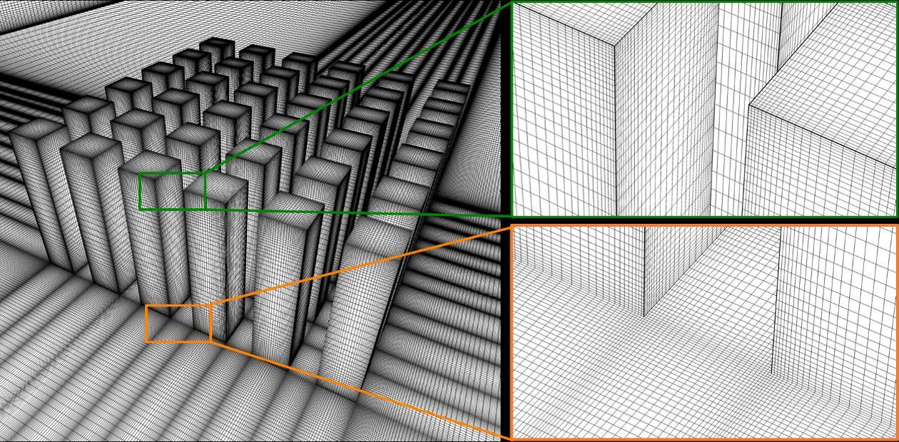
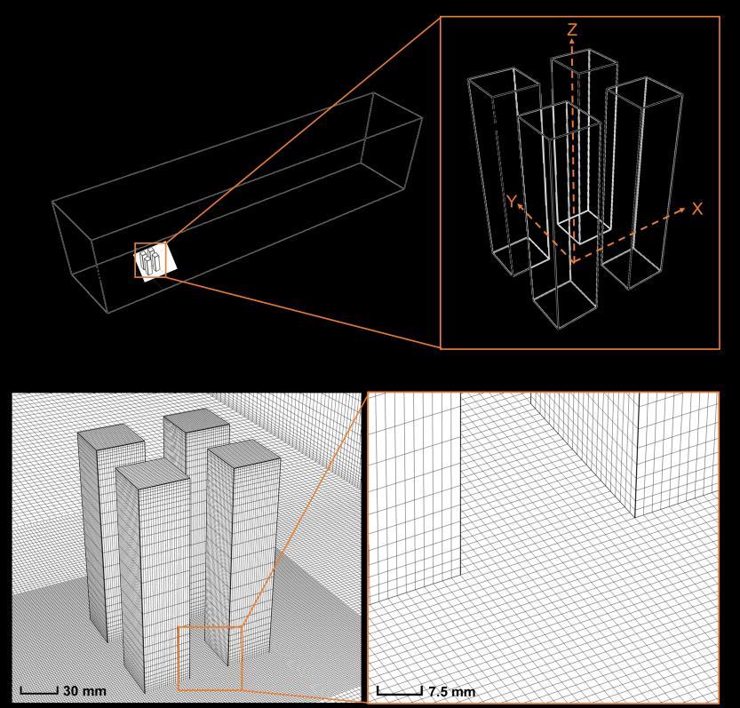
length is 3H, which is smaller than that proposed by the best practice guidelines, to limit unintended streamwise gradients in the vertical inlet profiles [87, 88]. The computational grid consists of 5,464,450 hexahedral cells, see Fig. 2.2b, with 20 cells in the passage between the buildings. The maximum and average y* values are 76 and 40, respectively. This ensures that the center points of wall-adjacent cells are located in the logarithmic layer of the boundary layer, thus the standard wall functions can be employed for the near-wall treatment. The grid resolution is based on a grid-sensitivity analysis presented in Section 2.2.4.

2.2.3 CFD validation: other computational settings

The profiles of the mean wind speed, turbulent kinetic energy and turbulence dissipation rate at the domain inlet are specified using the measured incident vertical profiles of the mean velocity and turbulence intensity, shown in Fig. 2.1b. The turbulent kinetic energy k is calculated from U(z) and TI (z) using Eq. 2.1, where a is 1.5. The turbulence dissipation rate ɛ is given by Eq. 2.2, with κ, u * ABL and z0 representing the von Karman constant (= 0.42), the ABL friction velocity (= 0.55 m/s), and the aerodynamic roughness length (= 9×10-6 m). ��(��)=��(����(��)��(��))2 (2.1)

�������� ∗ 3 ��(��+��0) (2.2)

Figure 2.2. Perspective view of (a) computational domain and (b) computational grid at surfaces of the building models and part of the ground surface (5,464,450 cells).

18 Chapter 2

The standard wall functions are employed together with roughness modification on the ground surface [89]. The values of the roughness parameters, i.e., the sand-grain roughness height ks (m) and the roughness constant Cs, are determined using their consistency relationship with the aerodynamic roughness length z0 [87], (Eq. (2.3)):

9.793��0 (2.3)

In this study, ks = 0.0007 m and Cs = 0.13 for the ground surface. The building walls have roughness ks = 0 and Cs = 0.5. Zero static gauge pressure is applied at the outlet plane. Symmetry conditions, i.e., zero normal velocity and zero normal gradients of all variables, are imposed on the top and lateral sides of the domain.

The commercial CFD software ANSYS/Fluent v19.0 is used to solve the 3D RANS equations using the Linear Pressure–Strain (LPS) Reynolds Stress Model (RSM) turbulence model for closure. The RSM is selected based on a sensitivity analysis presented in Section 2.2.5. The iterative semi-implicit method for pressure-linked equations (SIMPLE) scheme is used to couple velocity and pressure [90]. Second-order discretization schemes are used for both the convection and viscous diffusion terms of the governing equations. Convergence is assumed to be obtained when the scaled residuals level off and reach a minimumof 10−5 for continuity, 10−8 for x, y, z momentum and k, 10−6 for ɛ, and 10−7 for the six Reynolds stress tensor components.

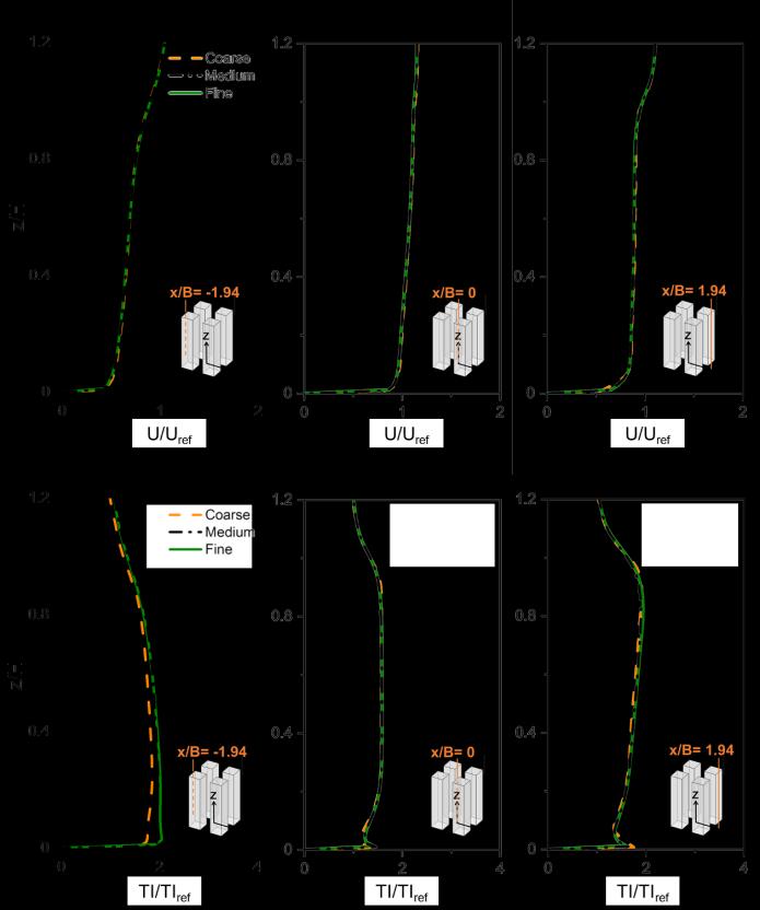
Figure 2.3. (a-c) Dimensionless mean streamwise velocity and (d-f) turbulence intensity along three lines in the vertical centerplane (y/B = 0) for coarse, medium and fine grid.