4.2 CFD validation study

Urban wind energy potential: Impacts of urban density and layout 69

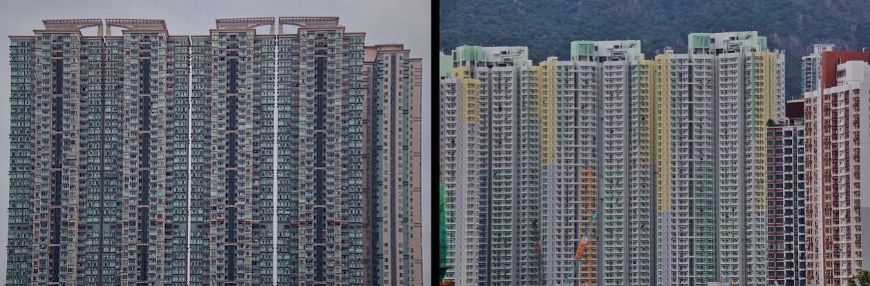
Figure 4.1. Photos of high-rise buildings in close proximity in the Kowloon City District, Hong Kong (photographed by Po-Ki Li).

This paper is systematized as follows: The predictions are compared with wind tunnel measurements for the CFD validation study, as illustrated in Section 4.2. Section 4.3 describes the CFD simulation details, consisting of all case scenarios, the computational domain, grid, settings, and grid-sensitivity analysis. In Section 4.4, the CFD simulations present the results of four impacts: (i) the urban density, (ii) the building corner shape, (iii) urban layout, and (iv) the wind direction on the evaluation of wind power potential. The limitations in the current study are discussed in Section 4.5. Section 4.6 summarizes the main conclusions obtained.

The wind tunnel experiments are performed using an open-circuit atmospheric boundary layer wind tunnel of Eindhoven University of Technology (TU/e). The cross-section of the wind tunnel is 0.5 m × 0.65 m with 13 m long. A set of floor roughness elements is located 0.65 m ahead of the test section to reproduce the atmospheric boundary layer. The test model consists of four square cuboids placed as a 2×2 building array with a straight crossing street-canyon width of 0.028 m. The dimensions of the square cuboid model are 0.031 m  0.031 m  0.14 m, resulting in a blockage ratio of 3% in the wind tunnel with a scale of 1:643. The turbulent flow instrumentation (TFI) Cobra probe is utilized to measure the 3-component flow velocities and turbulence intensities [82]. Fig. 4.2a shows the locations of monitoring points on the lateral view of 6 profiles along the vertical centerlines (y/B = 0) at 6 positions (x/B = -2.9, -1.94, -0.97, 0, 0.97 and 1.94). The dimensionless incident vertical profiles (Fig. 4.2b) of time-averaged streamwise velocity (u/uref) and total turbulence intensity (TI/TIref) are measured from the empty wind tunnel, which are readily employed in CFD validation. The values of uref and TIref are 13.4 m/s and 8% at the building height.

70 Chapter 4

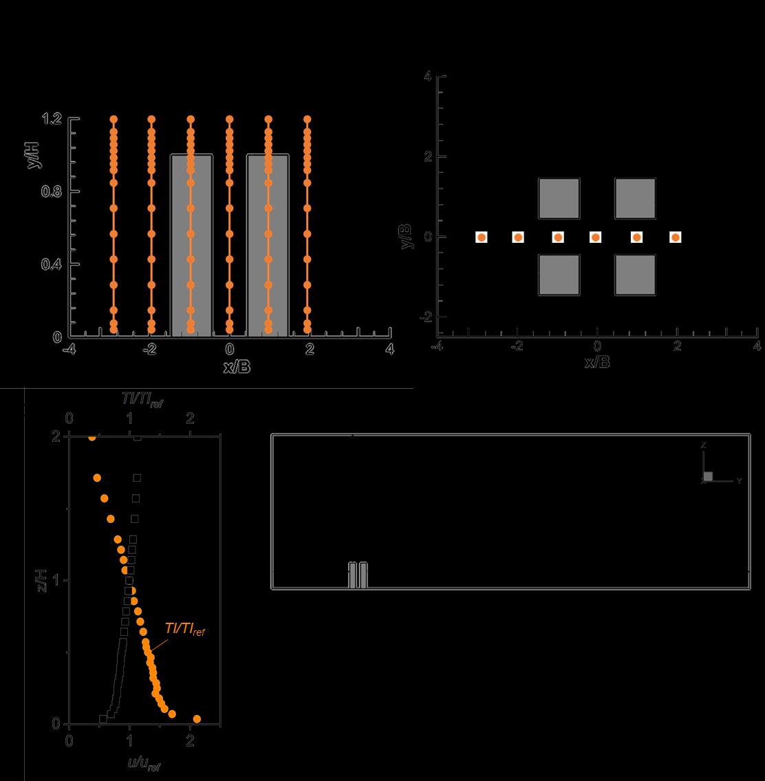
Figure 4.2. (a) Locations of monitoring points on lateral view of 6 profiles along the vertical centerlines (y/B = 0) at 6 positions (x/B = -2.9, -1.94, -0.97, 0, 0.97 and 1.94); (b) the dimensionless incident profiles; and (c) the computational domain for CFD validation.

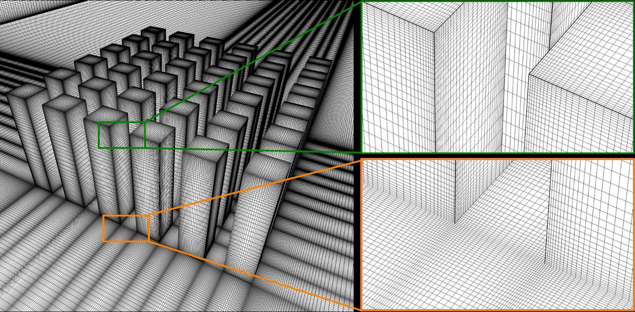
The overall computational domain for the reduced-scale CFD validation study is depicted in Fig. 4.2c, following the CFD best practice guidelines [99, 152]. The high grid resolution computational mesh is generated using hexahedral elements only, with a total number of 5,464,450 cells. No less than 20 cells are disposed along with the passage distance between the crossing street canyons. A peak stretch factor of 1.1 is adopted with the least cell volume of 2.7×109 m3 to ensure y* values within 30 and 350 for proper implementation of the standard wall function treatment. For the boundary conditions, the solid walls are arranged as the no-slip walls. The ground surfaces integrate the sand-grain roughness modification with the roughness height (ks) of 0.0007 m and the roughness constant (Cs) of 0.13. To realize the roughness in the windtunnel tests, the aerodynamic roughness length z0 is set as 9×10-6 m. The outlet boundary is specified to be 1 atm. The lateral and top boundaries are imposed as symmetry with zero normal velocity and zero normal gradients of flow variables. The grid-sensitivity analysis has checked