
Spring 2024, Volume 17
EDITOR: Ramesh Mohan
DESIGN & LAYOUT: Ramesh Mohan and Rebecca Marcus
MISSION STATEMENT: The Empirical Economics Bulletin is the undergraduate journal for the Department of Economics, Bryant University. The journal is produced in conjunction with the Bryant Economic Undergraduate Symposium. The focal point of the Symposium is on training undergraduate students in the art of writing, presenting, and publishing empirical research papers on a range of socio-economic and economic topics. The Symposium’s primary emphasis is empirical studies with policy relevance. Students are then able to publish their empirical papers in the Empirical Economics Bulletin. An objective of the Economics’ Department, Bryant University is to train students to conduct quantitative economic data analysis and to present the results in a coherent and meaningful way. This objective is met through having the Symposium and the publication of the Empirical Economics Bulletin. The first issue was in Spring 2008 and has been published annually with original work from an array of student authors.
SUBMISSION GUIDELINES: Students may submit their socio-economic and economic work here: Ramesh Mohan at rmohan@bryant.edu. Limit one submission per author. Each submission should have a title page with the title; name of author; abstract; keywords; JEL classification; author’s email. Previously published work is not accepted. The reading period is September 1 to December 1. Copyright reverts to author upon publication.
Any questions may be directed to Professor Ramesh Mohan at rmohan@bryant.edu.
© 2024 Empirical Economics Bulletin
Table of Contents
Economic Peaks, An Analysis of Financial & Real Estate Speculations in the Top 5 U.S Cities, Nicholas M. Basley .....................................................................................................................1
Beyond the Arc: Investigating the Impact of 3-Point Shots on NBA Revenue: An Empirical Analysis, Cameron Bolduc .17
The Role of Institutional Quality Factors on Inequality in Upper-Middle Income Countries in Latin America, Alexia Brandao ..................................................................................................32
Does Money Really Buy Success? Empirical Analysis of Money Spent Effect on English Premier League Team’s Performances/Success: A Panel Data Analysis, Barnaby Brandon .46
Time Series Analysis of the Impact of Climate Change on the Rocky Mountain Ski Industry, Charlotte Christo ....................................................................................................................57
The Causes All Time High Chronic Homelessness: A Panel Analysis, Robert Knight 76
SHIFTING THE ICE: Analyzing the Impact of the 2013 NHL CBA to the Competitive Balance of the League, Ryan Lacy ..........................................................................................................93
How UNSDGs are Reflected in Folklore, Jacob Mann .............................................................110
A Panel Data Analysis of the Effect of Corruption and Macroeconomic Factors on Inequality and Poverty in Latin America, Annie McDonald ............................................................................126
Hosting Mega Events Impact on GDP Growth: A Panel Data Analysis, Silas Pearce ...............143
Hitting the Books: An Empirical Analysis of the Effect of Education Expenditure on GDP per Capita and Economic Growth, Matt Simmons 157
The Causal Nexus Between Government Expenditure on Education and Individual Savings Behaviorin Argentina, Amanda Spielman 172
HDI and Standard of Living: A Panel Data Analysis of Latin America, Matthew Susich ......... 190
Capital Flows and Corruption on Southeast and East Asia’s Economic Growth: A Panel Data Analysis, TithVitou Teng .......................................................................................................205
A Cross-Section Analysis of Factors Affecting Interstate 11 Migration in the United States, Kasey Thomas 227
An Empirical Analysis of the Status of Income Inequality New England in 2022, Aidan Wilkinson ...............................................................................................................................250
Broken Asset Bubbles: The Factors affect Japan's Economy from Prosperity to Decline, Mark Yang 262
Economic Peaks, An Analysis of Financial & Real Estate Speculations in the Top 5 U.S Cities
Nicholas M. Basley
Abstract:
Economic Peaks conducts a comprehensive analysis of financial and real estate speculations in the United States, more specifically the top five cities per population in the United States. This study spans the period from 2000 to 2023, utilizing time series data to reveal economic trends and identify potential structural breaks during recession periods. By employing advanced statistical methods, the research aims to discern distinctive patterns in the housing and financial markets of each of the major cities, unveiling the presence of unsustainable price appreciation and the factors contributing to its emergence. This study seeks to offer valuable insights into the dynamics of economic fluctuations, enabling an understanding of the diverse trajectories these five cities experienced during the twenty-three year timeframe.
JEL Classification: —-
Keywords: Real Estate, Recession, NYC, PHOENIX, HOUSTON, LA, CHICAGO, Housing
Bryant University 1150 Douglas Pike, Smithfield, RI 02917
Owner- Basley Realty LLC. Phone: (860)-230-7152 Email: nbasley@bryant.edu
Empirical Economic Bulletin, Vol. 17 1
1.0 Introduction
The real estate market in the United States has undergone significant scrutiny and analysis in recent years, particularly in the aftermath of the housing market crises of the early 2000s.
Economic Peaks embarks on a comprehensive examination of financial and real estate speculations within the top five populous cities in the United States over the period spanning 2000 to 2023. Through advanced statistical methods, this research aims to uncover distinct economic trends, identify potential structural breaks during recessionary periods, and discern patterns within the housing and financial markets of each major urban center.
With a focus on the cities of New York City (NYC), Phoenix, Houston, Los Angeles (LA), and Chicago, this study aims to unveil the presence of unsustainable price appreciation and investigate the factors contributing to its emergence in these dynamic urban environments. By diving into time series data and employing rigorous analysis techniques, Economic Peaks seeks to offer valuable insights into the diverse economic trajectories experienced by these cities over the twenty-three-year period.
Beginning with an exploration of trends of structural breaks and their impact on the real estate market, this research sets the stage for understanding the evolving landscape of the housing sector. Additionally, the literature review explores the seminal research on housing bubbles, combining the findings from studies by Glaeser and Nathanson (2014), Baker (2018), Himmelberg, Mayer, and Sinai (2005), and Cheng, Raina, and Xiong (2013). This review aims to deepen the understanding of housing bubbles and inform strategies for mitigating their impact, laying a solid foundation for the analysis. Through a combination of empirical analysis and critical review of existing literature, Economic Peaks explores to contribute to the overall
Empirical Economic Bulletin, Vol. 17 2
knowledge on real estate speculation and economic fluctuations. By uncovering the underlying drivers of price appreciation and market dynamics within major U.S. cities, this research seeks to provide actionable insights for investors and stakeholders to promote sustainable growth and stability in the housing market.
The rest of the paper is organized as follows: Section 2 provides an overview of trends. Section 3 gives a brief literature review. Section 4 Outlines the Empirical Model, Data, and Estimation Methodology. Section 5 Presents/Discusses the Empirical Results. Followed by a Conclusion in Section 6.
2.0 TRENDS OF STRUCTURAL BREAKS AND IMPACTS ON THE REAL ESTATE MARKET
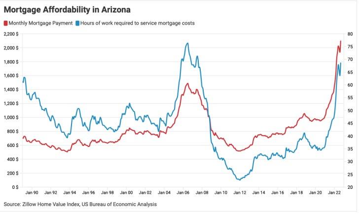
In Los Angeles, the homeless population surged to 41,290 individuals in 2020, representing a 61% increase over five years, with 70% of them remaining unsheltered. Projections indicate that the city's housing crisis will only escalate, as the population is expected to reach 4.3 million residents by 2029. To accommodate this growth, the city must facilitate the production of 456,643 housing units by 2029, a target that necessitates a fivefold increase in housing production compared to the previous decade.
The shortage of affordable housing has exacerbated the homelessness crisis, with only 83,865 housing units added between 2010 and 2019 despite a population increase of over 190,000 residents. As a result, Los Angeles has become one of the nation's most expensive cities, with 59% of renter households burdened by housing costs. This pressing issue underscores the urgent
Empirical Economic Bulletin, Vol. 17 3
need for comprehensive solutions to address housing affordability and mitigate the impact of homelessness in the city.
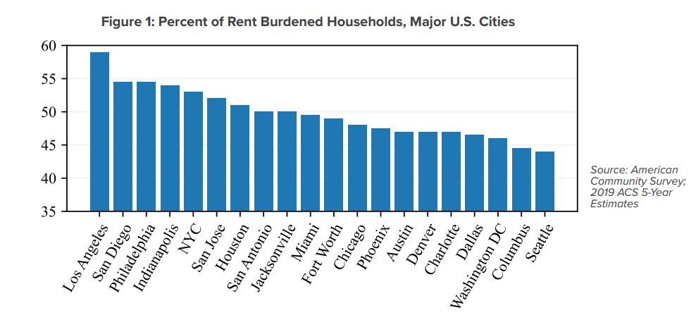
Source: U.S. Census Bureau, National Association of Realtors, and Real Estate Center at Texas A&M University
Figure 2: Total Housing Sales Texas vs. United States
Empirical Economic Bulletin, Vol. 17 4
Figure 2 depicts the Total Housing Sales trend for Texas compared to the United States over the period from 2000 to 2020, highlighting the Trend-Cycle Component. It illustrates the fluctuating patterns of housing sales in both regions, capturing the cyclical nature of the real estate market. Notably, Texas concludes the two-decade period with an impressive 80-point increase compared to the average housing sales in the United States. This significant uptrend in housing sales underscores the robustness of the Texas real estate market and its resilience amid changing economic conditions.
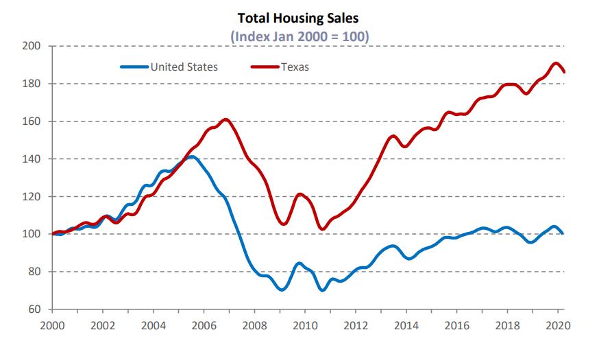
Source: Zillow Home Value Index, US Bureau of Economic Analysis
Arizona's housing market faces significant challenges, with rising interest rates leading to the highest home buying costs since 2007, requiring households to work approximately 68.72 hours per month to service mortgages, nearly double the requirements from September 2020. Despite a
Figure 3: Mortgage Affordability in Arizona
Empirical Economic Bulletin, Vol. 17 5
slight decrease in the housing supply deficit to 98,190 units in 2021, demand continues to outstrip supply, fueled by factors like brisk in-migration and increased housing demand during the pandemic. To meet demand, Arizona needs to add roughly 43,900 new housing units annually, rising to 63,580 units to close the shortfall within five years, highlighting the urgency for increased construction activity to address the housing shortage.
4: Combined Fig. 1&2 Home Price Index NY, CA, IL, and Respective Locations
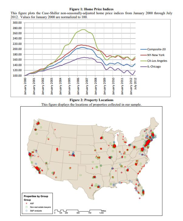
Source: NATIONAL BUREAU OF ECONOMIC RESEARCH
Figure
Empirical Economic Bulletin, Vol. 17 6
Figure 4 depicts the indices in the study and analyzes the trends in the home price index across the United States from 2000 to 2007. It examines how home prices evolved over this period, considering factors such as location-specific effects and variations in housing market dynamics. The findings highlight fluctuations in home prices across different regions and their impact on the overall housing market during this timeframe.
5:
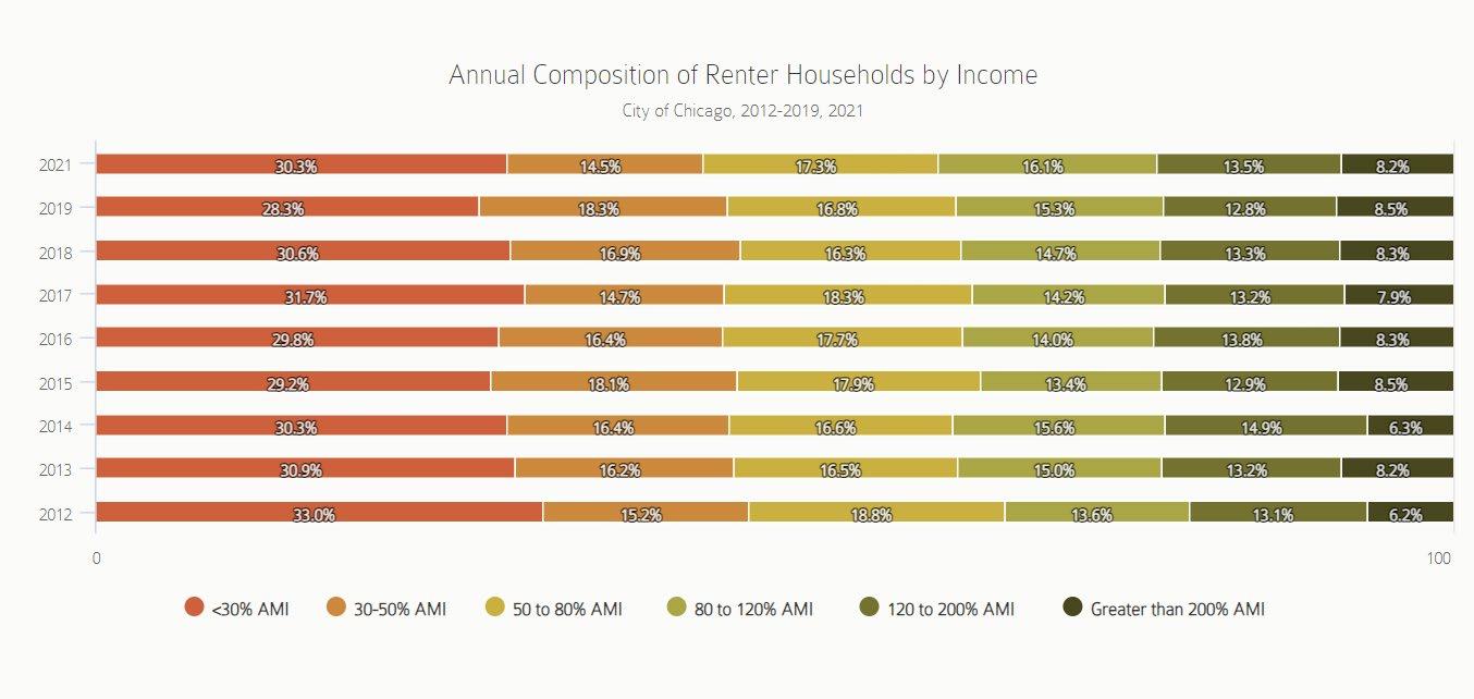
Source: Institute for Housing Studies at DePaul University
Figure 5 depicts Renter Households by Income between 2012 and 2021. Chicago saw a decline in the proportion of renters earning less than 80% of the area median income (AMI), particularly among those earning less than 30% of the AMI. However, during the pandemic from 2019 to 2021, there was a reversal in this trend, with an increase in the share of renters earning less than 30% of the AMI, likely due to economic instability. There was a decrease in the proportion of renters earning between 30% and 50% of the AMI during this period. Despite government
Figure
Annual Composition of Renter Households by Income
Empirical Economic Bulletin, Vol. 17 7
support, economic uncertainty for lower-income households remains a significant factor influencing these shifts in Chicago's rental market.
3.0 Literature Review
Housing bubbles have been a subject of considerable interest and concern in the field of economics, particularly since the Great Recession. This review aims to provide a comprehensive overview of research on housing bubbles, examining key studies that analyze their causes, consequences, and potential policy responses. This review encompasses a wide range of works focusing on housing bubbles, including seminal research by Glaeser and Nathanson (2014), Baker (2018), Himmelberg, Mayer, and Sinai (2005), and Cheng, Raina, and Xiong (2013). The objective is to synthesize findings from these studies to deepen understanding of housing bubbles and inform strategies for mitigating their impact.
A search of academic databases was conducted to identify relevant studies on housing bubbles. Inclusion criteria were based on the research and focus on analyzing housing market dynamics, while exclusion criteria were applied to ensure the exclusion of non-peer-reviewed sources and studies lacking empirical analysis. The reviewed literature provides insights into various aspects of housing bubbles, including their formation, propagation, and eventual collapse. Glaeser and Nathanson (2014) highlight the role of speculative behavior and irrational exuberance in fueling housing bubbles, while Baker (2018) examines the lasting impact of the housing bubble on the economy ten years after the Great Recession. Himmelberg, Mayer, and Sinai (2005) offer a
Empirical Economic Bulletin, Vol. 17 8
framework for assessing high house prices, distinguishing between fundamental factors and market misperceptions, while Cheng, Raina, and Xiong (2013) investigate the involvement of Wall Street in the housing bubble. Critical analysis of the reviewed literature reveals methodological challenges in identifying and measuring housing bubbles, as well as debates surrounding the effectiveness of policy interventions in addressing them. While some researchers emphasize the importance of regulatory measures to prevent excessive speculation and provide housing affordability, others caution against unintended consequences of government intervention. The review highlights the complexity of housing bubbles as phenomena shaped by a combination of economic fundamentals, market psychology, and institutional factors. Addressing housing bubbles requires a multifaceted approach that integrates macroeconomic policies, financial regulations, and urban planning strategies. Future research should focus on refining methodologies for identifying and predicting housing bubbles, as well as evaluating the effectiveness of policy interventions in preventing their recurrence. Additionally, more research is needed to understand the regional dynamics of housing bubbles and their differential impact on diverse communities.
4.0 DATA AND EMPIRICAL METHODOLOGY
4.1 Data
The present study seeks to comprehensively examine the phenomenon of structural breaks and their association with economic recessions in five prominent metropolitan areas: New York City, Los Angeles, Chicago, Houston, and Phoenix. The research endeavors to define the determinants
Empirical Economic Bulletin, Vol. 17 9
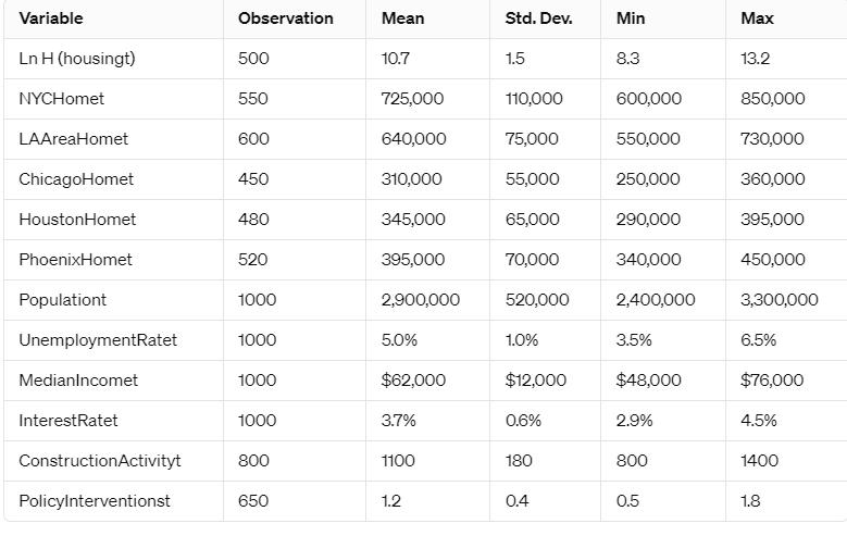
of these structural shifts within the housing markets of these cities, employing a multifaceted analytical approach.Central to the investigation, the indicators are as follows, local housing market conditions, demographic shifts, economic performance metrics including unemployment rates and median income levels, as well as external factors such as prevailing interest rates and construction activity. Through statistical analysis, the study aims to discern correlations between these variables and episodes of structural breaks in the housing markets of the cities. By digging into how these factors mix with housing market fluctuations, the study aims to uncover insights into why cities' housing markets sometimes go berserk, especially when the economy may take a plunge.
Empirical Economic Bulletin, Vol. 17 10
Table 1: Summary Statistics
4.2 Empirical Model
The analytical approach adopted in this study is set in time-series modeling, specifically tailored to housing market dynamics. Given the complexities and non-normal distributions often observed in housing market data, particularly due to the irregularity of market transactions, conventional regression techniques such as Ordinary Least Squares (OLS) may not be work in these cases. As such, a Negative Binomial Generalized Linear Model (GLM) with a logarithmic link function emerges as a more appropriate method. This modeling framework accommodates the variability inherent in housing market variables, characterized by higher standard errors relative to their means, facilitating a wider exploration of the relationships between various determinants and housing market trends across the study period.
Ln H (housingt) = αt + β0 + β1NYCHomet + β2LAAreaHomet + β3ChicagoHomet + β4HoustonHomet + β5PhoenixHomet + β6Populationt + β7UnemploymentRatet + β8MedianIncomet + β9InterestRatet + β10ConstructionActivityt + β11PolicyInterventionst +ε.
This equation models the logarithm of housing market trends (H) over time (t) as a function of various predictors. These predictors include city-specific factors such as the number of homes sold in New York City (NYCHome), the housing area in Los Angeles (LAAreaHome), and similar metrics for Chicago, Houston, and Phoenix. Population size, unemployment rates, median income levels, interest rates, construction activity, and policy interventions are all
Empirical Economic Bulletin, Vol. 17 11
considered as predictors. The equation aims to capture the relationship between these predictors and housing market dynamics, accounting for potential influences on fluctuations in housing prices and market trends over the specified time period.
5.0 EMPIRICAL RESULTS
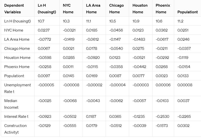
The empirical estimation results for the housing variable fluctuations are shown in Table 2. The ln housing variable shows a notable increase from 10.5 to 10.7, indicating a significant positive trend in housing market activity. NYC Home variable experiences an increase from -0.0321 to 0.0237, suggesting a shift towards higher home sales activity in New York City. Unemployment Rate t demonstrates a slight increase from -0.00008 to -0.00005, although small, it signifies a potential uptick in unemployment rates impacting the housing market.
Interest Rate t exhibits a substantial decrease from 0.1187 to -0.0923, suggesting a significant negative impact on housing market trends due to lower interest rates. LA Area Home experiences a decline from -0.0612 to -0.0772, indicating a decrease in housing area activity in Los Angeles. Median Incomet shows a reduction from -0.0043 to -0.0025, suggesting a potential decrease in median income levels affecting the housing market dynamics.
Table 2
Empirical Economic Bulletin, Vol. 17 12

6.0 Conclusion
Empirical Economic Bulletin, Vol. 17 13
This study provides valuable insights into the complex dynamics of urban housing markets in five major cities. Through the empirical analysis of various factors such as home sales, housing area, population size, unemployment rates, and interest rates, among others, significant trends and relationships have emerged. The findings indicate an interconnection between these factors and housing market dynamics, influencing trends in housing prices, sales activity, and market stability over time.
One notable finding is the diverse impact of city-specific variables on housing market trends. While variables such as home sales in New York City and housing area in Los Angeles exhibit significant effects on housing prices and market activity, the influence of factors like unemployment rates and interest rates underscores the broader economic context shaping housing dynamics. The study highlights the importance of considering both local and macroeconomic factors in understanding housing market fluctuations and structural breaks.
Overall, the study contributes to the ongoing discourse on housing market dynamics by shedding light on urban housing markets. By identifying key determinants of housing market trends and structural breaks, policymakers and investors can leverage these to inform strategic decisions aimed at creating greater resilience and stability in urban housing markets. However, further research may be conducted to explore various factors and their interactions, ensuring a comprehensive understanding of the complexities involved in housing market dynamics.
Appendix: Variable Description
Empirical Economic Bulletin, Vol. 17 14
● Ln H (housingt) represents the natural log of housing market indicators or variables of interest in the top 5 US cities over time.
●αt denotes the time-specific effect capturing any overall trend or variation common to all cities.
●β0 represents the intercept or constant term capturing the baseline level of housing market indicators.
●The variables β1NYCHomet, β2LAAreaHomet, β3ChicagoHomet, β4HoustonHomet, and β5PhoenixHomet represent the respective home-related indicators or variables for each city.
● Populationt captures the population dynamics in each city over time.
● UnemploymentRatet denotes the unemployment rate in each city over time.
● MedianIncomet represents the median income levels in each city over time.
● InterestRatet denotes the prevailing interest rates in each city over time.
● ConstructionActivityt represents the level of construction activity in each city over time.
● PolicyInterventionst captures any policy interventions or regulatory changes impacting the housing markets in each city over time.
●ε represents the error term capturing unobserved factors or random fluctuations in the housing market indicators.
BIBLIOGRAPHY
Empirical Economic Bulletin, Vol. 17 15
● Glaeser, E., & Nathanson, C. G. (2014). Housing Bubbles. Journal of Economic Perspectives, 28(1), 193-214.
● Baker, D. (2018). The Housing Bubble and the Great Recession: Ten Years Later. SSRN Electronic Journal.
● Himmelberg, C., Mayer, C., & Sinai, T. (2005). Assessing High House Prices: Bubbles, Fundamentals and Misperceptions. Journal of Economic Perspectives, 19(4), 67-92.
● Cheng, I., Raina, S., & Xiong, W. (2013). Wall Street and the Housing Bubble. The Review of Financial Studies, 26(9), 2267-2296.
● Gaines, Dr., Torres, Dr., Miller, Silva, & Griffin Carter. (2020). Texas Housing Insight
● DePaul University. (2023). 2023 State of Rental Housing in the City of Chicago
● Gabriel, & Kung. (2023). Tackling the Housing Crisis: Streamlining to Increase Housing Production in Los Angeles.
● Sense. (2022). Arizona Housing Affordability Update.
Empirical Economic Bulletin, Vol. 17 16
Beyond the Arc: Investigating the Impact of 3-Point Shots on NBA Revenue: An
Empirical Analysis
Cameron Bolduc
Abstract:
This paper investigates the impact of Stephen Curry’s revolution of the three-point shot and its impact on NBA’s revenues. The study will incorporate the five years prior to Stephen Curry’s back-to-back MVP’s and the five years after those MVP’s. The model will examine three-point makes and percentage per game, along with a player’s effective field goal percentage, as well as playoff wins and attendance in home games. The study’s results showed that in the five years after Stephen Curry changed the game and won his MVPs, the three-point shot was a big driver in a team’s revenue. These results do not align with previous paper’s work and should encourage further studies on the topic. The results in this study indicate that the play style of a player must include the three-point shot as the NBA is a business at the end of the day, and being able to shoot threes gives a team more chances of success, along with more money.
JEL Classification: L83, Z23
Keywords: 3-Point Shot, NBA Revenues
Department of Economics, Bryant University, 1150 Douglas Pike, Smithfield, RI 02917. Email: cameronbolduc0907@gmail.com.
Empirical Economic Bulletin, Vol. 17 17
1.0 INTRODUCTION
Stephen Curry changed the way that the game of basketball has been played because of his ability to shoot three-point shots better than arguably any other player in NBA history. Throughout different eras, the game of basketball has seen different players revolutionize and bring about new fans to the game because of their play style. Two easy examples of this are Michael Jordan and Allen Iverson. Jordan was a name known across the world, and his skillset was so great that he was the main driver behind the surge of NBA basketball. Prior to Jordan being drafted in 1984, the league was trending downwards, but afterwards, the TV viewership for the NBA reached levels previously unknown. Alongside that, rather than teams being disbanded as was planned prior, teams were added to the league (Reynolds, 2022). As far as Allen Iverson, his idol was none other than Michael Jordan. He led a cultural revolution in the NBA as he did not change his persona at any point to please anybody (Gordon, 2016). Not only that, but he was also a player that many shorter basketball players with professional aspirations looked up to, as despite being only six feet, he managed to win a Most Valuable Player Award (MVP).
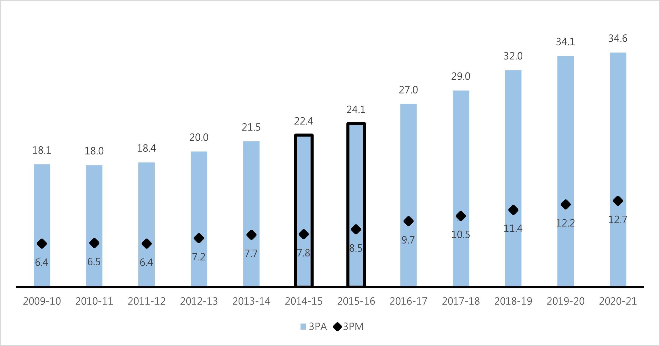
I will investigate what the impact Stephen Curry had on the NBA is by looking at the five years prior to his back-to-back MVPs, otherwise known as his first five seasons in the NBA, and the five seasons after those MVPs. This study is important because while other studies have looked at the determinants of NBA revenue, none have considered whether Stephen Curry is another example of a player that has revolutionized basketball in the way that a Michael Jordan or Allen Iverson have. I was someone who grew up during this period and played in many different basketball leagues. In doing this, I was a part of the revolution to shoot more threepointers and witnessed many of my friends or other players purchase Stephen Curry jerseys, shoes, etc. Another aspect to consider is that often in my early childhood, when someone would throw a piece of trash into the garbage, they may have yelled, “Kobe!”. As I began to grow up, I started hearing a shift from, “Kobe!”, into “Curry!”. As seen in Figure 2, since Stephen Curry was drafted in 2009, the three-point shot has become more and more utilized, aside from years pointed out where it makes sense that a decrease in three-pointers was seen.
Empirical Economic Bulletin, Vol. 17 18
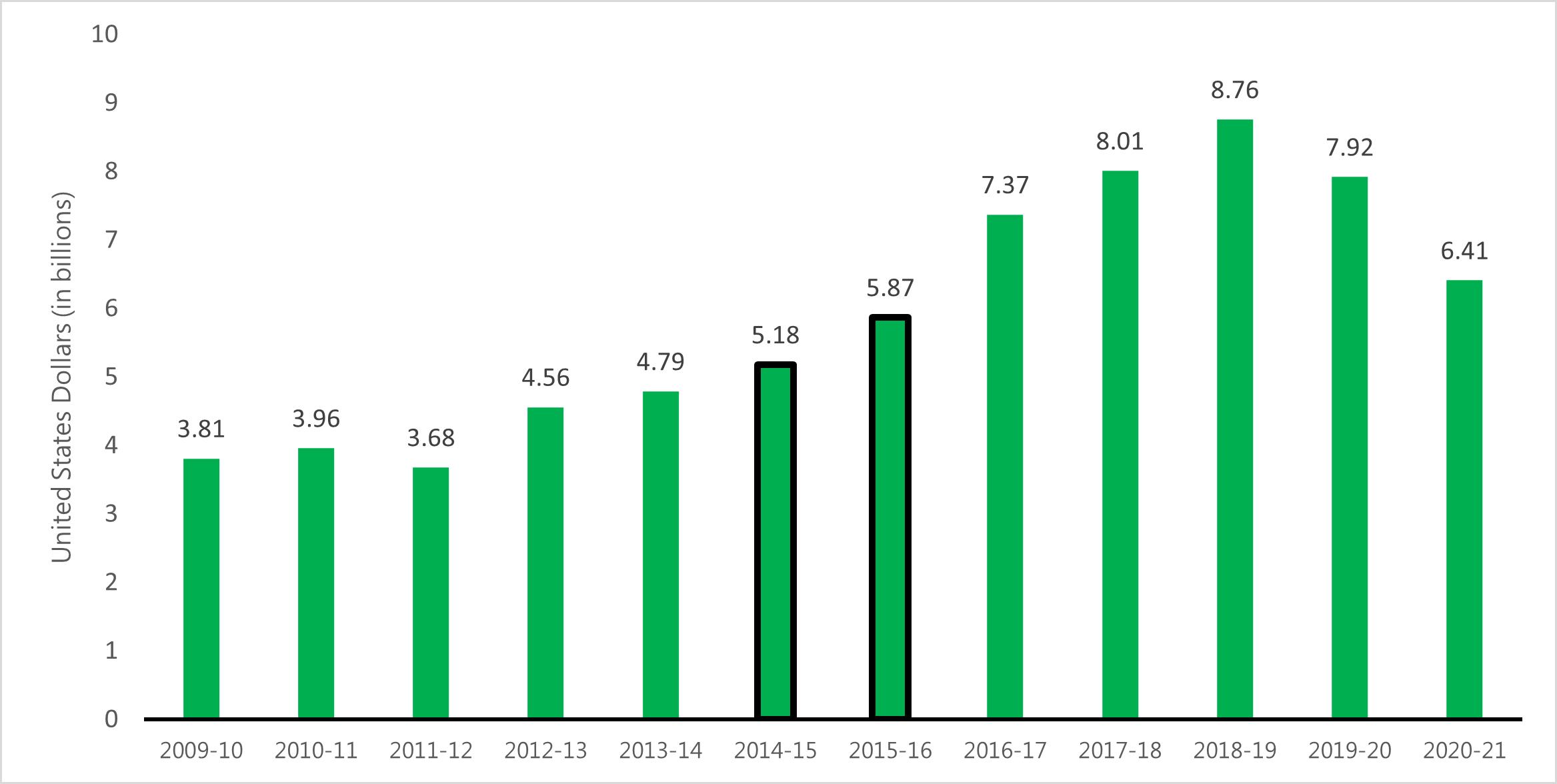
Over this same period, the NBA has seen increases in revenue (see Figure 1) in all, but the same seasons as previously mentioned. Prior studies have examined the increases in NBA revenue, but neglected to focus on the value that Stephen Curry may have brought to the NBA. Another area that shows that Curry was extremely valuable to generating revenue for the league is the fact that he is consistently near the top or at the top of NBA jersey sales. Since 2001, Stephen Curry has been the leader in jersey sales three different seasons, behind only Kobe Bryant and LeBron James who have done it six and seven times, respectively (Pimentel, 2023). Curry is also trending towards being the number one jersey seller of the 2023-24 season (Release, 2024)
The rest of the paper is organized as follows: Section 2 explores the trend surrounding the topic. Section 3 dives into the literature review of previous studies in this general topic area. The data and empirical methodology of the study are shown and explained in Section 4. The results are shown and explained in Section 5. Lastly, there is a conclusion that wraps up the paper in Section 6.
2.0 3-POINTERS AND REVENUE, 2009 THROUGH 2021
Figure 1 shows that from 2009 to 2021, excluding the shortened season (2011-12) and the season where the Covid-19 pandemic arose (2019-20) and the following season (2020-21), the NBA’s revenue increased. In 2011-12, the NBA season for each team was shortened from eighty-two games to sixty-six games (Beck, 2011). This was nearly a twenty percent decrease from the regular eighty-two game season. As for the 2019-20 season, the world was brought to a halt in March of 2020, and the season was again shortened, even after the NBA Bubble in Florida was played out. Not every team qualified for the NBA Bubble and the range of regular season games played ranged from sixty-four games to seventy-five games (2019-20 NBA Standings, 2020). With that, there were no full arenas for the last eight regular season games played for the teams invited to the bubble, nor with the playoff games. Lastly, the 2020-21 season was again shortened, and arenas were again not filled. The season was seventy-two games, ten less than a standard season and for the majority, if not the entire season, many teams were in limited capacity arenas (NBA.com Staff, 2021). The two years with black outlines are
Empirical Economic Bulletin, Vol. 17 19
the two years excluded from the study, being both of Stephen Curry’s back-to-back Most Valuable Player seasons.
Figure 1: NBA Total Revenue by Season
Source: Statista
Figure 2 depicts the yearly three-point attempts on average league wide, overlayed with the three-point makes each year meeting the same criteria. The number of three-point attempts in the NBA has increased every year since the 2010-11 season. The decrease from 2009-10 to 2010-11 was only by one tenth of an attempt per season, otherwise known as a fraction of a percent decrease. Similarly, the three-pointers made also increased in all but one season. The decrease in three-pointers made was from the 2010-11 season to the 2011-12 season, and it was again by one tenth of a shot, or a roughly one and a half percent decrease. Diving deeper into the numbers, the average percentage of these years was 35.7 percent (NBA League Averages – Per Game, 2024). Out of the twelve seasons in Figure 2, five of the seasons had three-point percentages that were less than the average (three-pointers made over three-pointers attempted). It is important to note, two of those seasons were the two seasons excluded from the study. The
Empirical Economic Bulletin, Vol. 17 20
largest negative difference however was in the 2011-12 lockout shortened season. On the flip side, the largest positive difference was in the Covid-19 shortened season of 2020-21.
Source: Basketball Reference
3.0 LITERATURE REVIEW
In the 2009 NBA draft, Stephen Curry was drafted by the Golden State Warriors. Since then, the NBA’s revenue has increased each season aside from the 2011-12, 2019-20, and 202021 seasons (National Basketball Association Total League Revenue from 2001/02 to 2022/03). All three can be deemed outliers as the former was the shortened season, and the latter two were the pandemic seasons. This is where the NBA finished its season in a bubble with no fans, and the following season saw zero to a fraction of the fans allowed in the arenas. There are many drivers behind the NBA revenue increases.
Reilly et al. (2023) attributed somewhere between $15 and $20 million lost each season because of star players missing games (load management), something that the league has worked to remove during this season (Reilly et al. 2023). Star players missing games obviously have an
Figure 2: NBA 3-Point Attempts vs 3-Point Makes
Empirical Economic Bulletin, Vol. 17 21
impact on how many viewers the game gets, as people are more likely to tune in when the best players are playing. Likewise, when fans buy tickets for games and those star players decide to sit out for load management, those fans get upset, and would be less likely to then buy another ticket. Reilly et al. determined that stars would miss games for five reasons: letting injury heal sufficiently, in the second game of back-to-back days with a game, against the bottom-feeder teams, when the game is of lesser importance for their playoff hopes, and lastly, when the game is less likely to affect revenues such as an away game (Reilly et al. 2023).
The three-point shot was brought into the league in 1979, and Harrison (2019) examined the effects of many factors, including this, on NBA revenue increases. His study’s purpose was to see how play style affects revenue in the league. As this study took place five years ago, Harrison found that the total number of three’s attempted grew nearly seven percent on average from 2012-13 to 2017-18, while revenues grew over fifteen percent on average during that same period (Harrison, 2019). It is no secret that the three-point shot has become more popular in the past decade, but some other factors that Harrison looked at were arena age, all-star votes, playoff wins, and city population (Harrison, 2019). The study concluded that the three-point shot resulted in lower revenues at a statistically significant level. This occurred while playoff wins, all-star votes, and population were not statistically significant, but all showed positive impact on revenue.
In his assessment of different sports leagues, Bradbury contested that the better a team played (the more success that team had) the more revenue that individual team made. Not only did Bradbury find this in the NBA, but he found it in every league besides, surprisingly, the NFL (Bradbury, 2019). More specifically, how a team performs in the playoffs determines a difference of about seven million dollars in revenue. Another aspect of this revenue boost is when a new stadium gets erected. With a new stadium, teams saw an increase in attendance of fans, again, except for the NFL. Something else that Bradbury looked at was teams with another team in that same market. In the NBA, this meant the Los Angeles Clippers and Lakers, the New York Knicks and New Jersey, then Brooklyn Nets. There was no negative effect on either the Lakers or Knicks, which Bradbury attributed to the fact that these teams are top revenue
Empirical Economic Bulletin, Vol. 17 22
generating teams in the NBA (Bradbury, 2019). Lastly, Bradbury’s study claimed that population increased a team’s revenue.
Right around the time Stephen Curry began his seasons of three-point barrages, Gannaway et al. (2014) explored how the pivot of the NBA into being more concerned with scoring points impacted players and their productivity. Contrary to popular belief, the study found that introducing the three-point line increases productivity for taller players as opposed to smaller players. Likewise, taller players have been at a higher demand from NBA teams. After the three-point line was created, centers saw their shot attempts increase by over three and a half percent, while both forwards and guards saw their shot attempts decrease. This is interesting because with a three-point line, it is generally the smaller players that are better at shooting than centers. The researchers pinpoint this increase to the fact that the defenses became more spread out after the invention of the three-point line, making defense closer to the basket more difficult (Gannaway et al. 2014).
4.0
DATA AND EMPIRICAL METHODOLOGY
4.1 Data
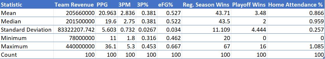
The study examines time-series data from the years 2009-2014 and 2016-2021, looking at variables that determine the revenue in the NBA. The data comes from a variety of sources. The revenues for each team come from Statista.com and the attendance figures come from ESPN.com. The remainder of the variables: points per game, three pointers made, three pointer shooting percentage, efficient field goal percentage, regular season wins, and playoff wins, were found on basketballreference.com. The summary statistics for the variables listed above can be found in Table 1.
Empirical Economic Bulletin, Vol. 17 23
Table 1: Summary Statistics
4.2 Empirical Model
The model used in this study is a modified version of the model used in Harrison’s (2019) study. The difference between Harrison’s study to this study is that it examines more of how the three-point revolution and Stephen Curry impacted the revenue among the NBA. This differs from Harrison’s study because he looked at five years including both years when Stephen Curry won MVP. While Harrison’s study was evaluating the effect of play style on NBA revenue from the 2013-2014 season to the 2017-18 season, this study assesses the impact of the three-point shot. To do that, this study compares the seasons falling between 2009 and 2014 and then 20162021. Furthermore, Harrison included more variables regarding the teams’ arenas and the cities where the arenas are located. I added the effective field goal percentage as well to the study, along with points per game.
The model used in this study is as follows:
Team Revenue = β0 + β1(PPG) + β2(3PM) + β3(3P%) + β4(eFG%) + β5(Reg. Season Wins) +β6(Playoff Wins) + β7(Home Attendance %) + ε
The dependent variable being team revenue is being studied to determine how the change in play style of the NBA impacted the revenue versus other factors. Next, the independent variables include four offensive metrics and three team-based metrics. The four offensive metrics were found by taking the top ten players from each of the season studied in terms of threepointers attempted. Upon doing that, the same player’s points per game, three-pointers made per game, three-point shooting percentage, and effective field goal percentage. The first two of those are self-explanatory as to what they are, with three-pointers being from behind the three-point line. The three-point shooting percentage is the percentage of three-pointers made of the attempts. The effective field goal percentage is an adjusted field goal percentage that considers that three-pointers are greater than two-pointers. Next, regular season wins, and playoff wins can be a direct indicator of a team’s revenue as a more successful team is likely to bring in more fans than a team that is not successful. The more successful a team is, the more tickets they will sell,
Empirical Economic Bulletin, Vol. 17 24
and those tickets may also be priced higher than a team struggling to fill its arena. Similarly, home attendance percentage is along those same lines, and can drive a team’s revenue. As not every team has the same capacity in their arena, percentage is a better indicator of how they are filling the stadium.
5.0 EMPIRICAL RESULTS
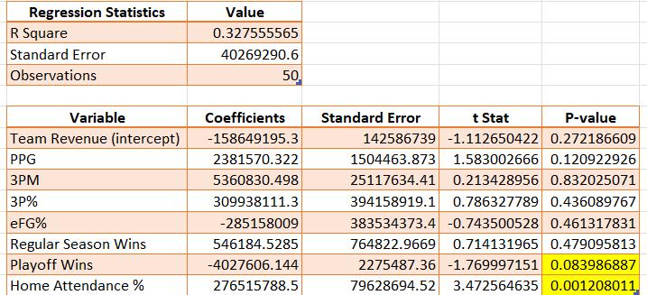
The three tables below depict the regression results for the data, and then a comparison amongst the 2009-14 and 2016-21 datasets. This comparison will demonstrate the effectiveness of Stephen Curry in changing the game via the three-point shot and how much of an effect it truly had on revenue. Table 4 accounted for the variation in revenue the best, explaining seventytwo and a half percent, while Table 2 accounted for roughly sixty-four percent. The same cannot be said for Table 3, which used the data from 2009-14, which can only account for a third of the variation in the dependent variable of team revenue. The r-square value mentioned above is highlighted in each of the three tables, as well as any variable that is significant at the one, five, or ten percent levels.
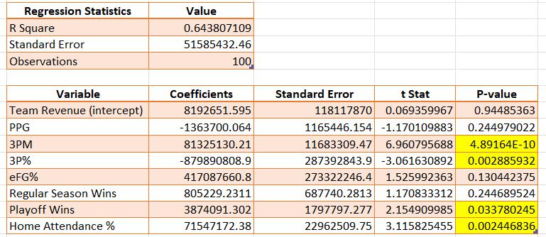
The overall empirical estimation results are presented in Table 2. This regression used the data from every year in the study to capture the effect that the three-point shot, and other variables had in total. This model showed that four variables were statistically significant in
Table 2: Regression results for years 2009-14 and 2016-21
Empirical Economic Bulletin, Vol. 17 25
being a determinant of the team’s revenue. The number of three pointers made (3PM), threepoint percentage (3P%), and home attendance percentage were all found to be statistically significant at the one percent level. A team’s number of playoff wins was also found to be statistically significant, but at the five percent level. While three pointers made were found to have a positive effect of over eighty-one million dollars, it is important and interesting to note that an increase in a player’s three-point percentage decreases a team’s revenue according to this model. Not surprisingly, the playoff wins of a team and home attendance percentage had a positive effect on a team’s revenue. The former coincides with Harrison’s 2019 findings that playoff wins have a positive impact on revenue in the NBA at a significant level. The other three variables were not statistically significant at any level.
Table 3: Regression results for 2009-14
The above regression in table 3 suggests that the model and variables I selected were not at all a great representation of the drivers of revenue in the NBA during the 2009-14 seasons. Of the three regressions, the variables were able to explain the smallest amount of variation in NBA revenue with this model, at just near thirty-three percent. Playoff wins and home attendance as a percentage of the stadium’s capacity were the only two statistically significant variables in this model. Home attendance has a massive coefficient, meaning that on average, a one percent increase in home attendance while holding other variables constant will increase revenue by roughly two-hundred and sixty million dollars. It is interesting to note that playoff wins had a
Empirical Economic Bulletin, Vol. 17 26
negative impact on revenue in this model, but it was only statistically significant at the ten percent level. This fact is what I attribute to the high coefficient for home attendance percentage, that the only other statistically significant variable (playoff wins) was negative. It is also interesting to note that the intercept was a negative number unlike the other two models.
Table 4: Regression results for 2016-21
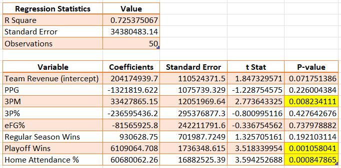
In Table 4, the model explains more of the variance in a team’s revenue than either of the models. This means that the variables I chose better explain the 2016-21 seasons as opposed to the 2009-14 seasons, as expected. This is a demonstration of how Stephen Curry impacted the game as variables related to his play style better determined revenue after his back-to-back MVPs. Unlike the 2009-14 regression, three pointers made were a large positive driver in revenue at a statistically significant level of one percent. The coefficient for 3PM means that on average, holding other variables constant, one more three-pointer made will increase a team’s revenue by over thirty-three million dollars. Something of importance is that this is a much smaller figure than the model in Table 2 suggests. However, like Table 2, which tested the data for all the years, playoff wins, and home attendance were statistically significant variables. In this case, both variables were statistically significant at the one percent level. From 2016-21, home attendance was a much larger driver than playoff wins. On average, a one percent increase in home attendance, ceteris paribus, increases revenue by over sixty-million dollars, while one playoff win, ceteris paribus, increases revenue by over six million dollars.
Empirical Economic Bulletin, Vol. 17 27
6.0 CONCLUSION
This paper examined the effect that Stephen Curry had on NBA revenue with his change around how the game of basketball was played because of his usage of the three-point shot. As it turns out, the three-point shot, and Curry did have a great effect on being a determinant of a team’s revenue in the NBA. There are, however, limitations in this study. In the first set of five years, there was a lockout meaning that the season was shortened, thus revenues went down. Similarly, in the second set of five years, after Curry won back-to-back MVPs, there was the COVID-19 pandemic which halted the entire world, never mind just the game of basketball. The effect on the NBA was that the season where the pandemic first hit was shortened and then finished without fans, in a bubble. The following season, states had differing policies on the Coronavirus, and some teams were able to fill their stands more than others, but it did not come close to pre-pandemic levels. Seeing as home attendance percentage was an independent variable in this study, the results may have been skewed.
Two key drivers of an NBA team’s revenue are playoff wins and fan attendance. It is important to consider that the three-point shot plays a large role in both playoff wins and fan attendance. Stephen Curry, the all-time leader in three-pointers made in the NBA has won four NBA championships, the first of which was in his first MVP season, the 2014-15 season. If a team is looking to generate higher revenue, a great way of winning games and getting fans to come watch is to utilize the three-point shot. This would mean that the traditional power forward and center positions must adapt to survive. This is already being shown because many of the taller players in the NBA have developed three-point shots. The players that have not adapted this feature to their skill set are often not as valued as they were prior to the Stephen Curry revolution.
Empirical Economic Bulletin, Vol. 17 28
Appendix A: Variable Description
and Data Source
Acronym Description
Team Revenue Revenue of the team in the NBA
PPG Points Per Game: the total number of a player’s points divided by number of games played
3PM 3-Pointers Made: the total number of a player’s made three-pointers divided by number of games played
3P% 3-Point Percentage: the total number of threepointers made divided by number of three-pointers attempted
eFG% Effective Field Goal Percentage: an adjusted statistical measure of a player’s field goal percentage accounting for three-pointers being worth more
Reg. Season Wins Regular Season Wins: a team’s number of wins in the regular season
Playoff Wins Playoff Wins: a team’s number of wins in the postseason tournament
Home Attendance %
Home Attendance Percentage: a calculated figure using the number of average attendees over the stadium’s capacity
Data source
Statista
Basketball Reference
Basketball Reference
Basketball Reference
Basketball Reference
Basketball Reference
Basketball Reference
Computed using ESPN data
Empirical Economic Bulletin, Vol. 17 29
BIBLIOGRAPHY
“2019-20 NBA Standings.” Basketball Reference, 2020. https://www.basketballreference.com/leagues/NBA_2020_standings.html.
Beck, Howard. “N.B.A. Reaches a Tentative Deal to Save the Season.” The New York Times, November 26, 2011. https://www.nytimes.com/2011/11/27/sports/basketball/nba-andbasketball-players-reach-deal-to-end-lockout.html.
Bradbury, John Charles. “Determinants of Revenue in Sports Leagues: An Empirical Assessment.” Economic Inquiry 57, no. 1 (September 11, 2018): 121–40. https://doi.org/10.1111/ecin.12710.
Gannaway, Grant, Craig Palsson, Joseph Price, and David Sims. “Technological Change, Relative Worker Productivity, and Firm-Level Substitution.” Journal of Sports Economics 15, no. 5 (July 15, 2014): 478–96. https://doi.org/10.1177/1527002514542740.
Gordon, Jeremy. “How Allen Iverson Changed the NBA.” The Wall Street Journal, September 9, 2016. https://www.wsj.com/articles/BL-DFB-23959.
Harrison, Jake. “The Effect of Play Style on NBA Revenues.” UC Berkeley Economics, May 10, 2019. https://www.econ.berkeley.edu/sites/default/files/Harrison_Jake_The%20Effect%20of%20 Play%20Style%20on%20NBA%20Revenues.pdf.
“National Basketball Association Total League Revenue from 2001/02 to 2022/23.” Statista, November 28, 2023. https://www.statista.com/statistics/193467/total-league-revenue-ofthe-nba-since-2005/.
“NBA League Averages - Per Game.” Basketball Reference, 2024. https://www.basketballreference.com/leagues/NBA_stats_per_game.html.
NBA.com Staff. “Where NBA Teams Stand on In-Arena Attendance.” NBA.com, May 28, 2021. https://www.nba.com/news/where-nba-teams-stand-on-in-arena-attendance.
Pimentel, Anatoly. “Top-Selling NBA Jerseys since 2001.” BetMGM, December 11, 2023. https://sports.betmgm.com/en/blog/nba/top-selling-nba-jerseys-since-2001-bm05/.
Reilly, Patrick, John L. Solow, and Peter von Allmen. “When the Stars Are Out: The Impact of Missed Games on NBA Television Audiences.” Journal of Sports Economics 24, no. 7 (June 4, 2023): 877–902. https://doi.org/10.1177/15270025231174616.
Empirical Economic Bulletin, Vol. 17 30
Release, Official. “Stephen Curry Leads Top-Selling Jerseys so Far This Season.” NBA.com, January 31, 2024. https://www.nba.com/news/top-selling-jerseys-first-half-2023-24.
Reynolds, Tim. “Stern, Talent Influx Led to NBA Transformation during 1980’s.” Fox Business, January 17, 2022. https://www.foxbusiness.com/sports/stern-talent-influx-led-to-nbatransformation-during-1980s.
Empirical Economic Bulletin, Vol. 17 31
The Role of Institutional Quality Factors on Inequality in Upper-Middle Income Countries in Latin America
Alexia Brandaoa
Abstract
This paper investigates the influence that institutional quality factors have on the power or spread of inequality across low-income countries, as opposed to high income countries. As such, an empirical study and analysis will be conducted to measure the impact of the following institutional quality factors: control of corruption, government effectiveness, political stability and absence of violence/terrorism, regulatory quality, rule of law, and voice and accountability. Specifically, cross-sectional or panel data from the World Bank will be utilized to look at upper-middle income nations in Latin America.
The factors will be simultaneously measured against the Gini Coefficient. These countries include Brazil, Argentina, the Dominican Republic and Peru from 2008 – 2022
Results from the panel data will show that a variety of institutional quality factors have significant influence over inequality factors and many variables contribute to this disparity, including Foreign Direct Investment and Global Competitiveness.
JEL Classification: I3, N4, O2, O4
Keywords: Institutional Quality Index, Foreign Direct Investment, Political Stability, Global Competitiveness, Gini Index
Bryant University, 1150 Douglas Pike, Smithfield, RI02917. Phone: (401) 536-7729
Email: abrandao@bryant.edu
Empirical Economic Bulletin, Vol. 17 32
1.0 INTRODUCTION
For a multitudinous array of reasons, lower-income nations face several disadvantages that hinder their overall development. Factors, such as limited resources, poor infrastructure, limited access to capital, health, education challenges, and so many more contribute heavily to the ever-growing constraints that are placed on the stimulation of economic growth, as well as improvement in living standards. In examining these variables, a question comes forth specifically in lower-income nations as to what is causing inequality, and if there are any ways to make change. With that being said, many nations are utilizing the Institutional Quality Index (IQI) and its indicators to reflect the strength of institutions that underpin social and economic development. By definition, this index is a composite indicator that measures the impact of aggregate and individual governance. It is composed of the World Governance Indicators and places importance on institutional control, with an emphasis on governance systems, procedures, and activities. As such, the factors that make up the index include the following: control of corruption, government effectiveness, political stability and absence of violence/terrorism, regulatory quality, rule of law, and voice and accountability. In addressing these concerns, impoverished nations can address specific weaknesses in their institutions to promote an environment of sustainable development and growth. Several studies have since uncovered that “local policies could be better targeted to reduce gaps and increase expenditure efficiency, foremost among which are anti-corruption actions… especially in regions which are lagging behind” (Ferrara & Nistico, 2019).
As such, this study will investigate the impact of the institutional quality index in a series of upper-middle income countries in Latin America, including Argentina, Brazil, the Dominican Republic, and Peru from 2008-2023. The study will aim to enhance the understanding of institutional quality factors, as well as the impact that the Gini coefficient plays within the policy implementation throughout these nations. The Gini Coefficient, which is an economic measure that analyzes the depth of inequality, is the most significant measure and variable within this study. Specifically, its value ranges from 0 to 1, with 0 representing perfect equality and 1 representing perfect inequality. In terms of economic policy, a higher Gini indicates greater inequality within a population, and vice versa. From a policy perspective, this analysis is significant toward the
Empirical Economic Bulletin, Vol. 17 33
comprehension of inequalities, as well as the make-up of policy structures. In taking a closer look at the failure of the institutional quality factors in lower income nations, this study will showcase the regional multidimensional inequalities within these six lower income nations.
This paper was guided by various research objectives that differ from other studies. First, it will investigate the possibility of interdependence between Institutional Quality Factors to the Gini Coefficient with the utilization of panel data. Secondly, it examines the influence of investment inflow and multidimensional well-being indicators on institutional quality. Lastly, this paper analyzes the difference between high-income countries (HICs) and low-income countries (LICs) in terms of inequality through an indepth comparative analysis between the two. As such, there is not a wide variety of existing literature that highlights the significance of institutional quality factors when in relation to LICs, but this paper successfully responds to many unanswered questions.
The remainder of the paper is outlined as follows: Section 2 outlines the trend of the given topic. Section 3 consists of a brief literature review. Section 4 dives into the data and empirical methodology, while section 5 reveals the empirical results of the research. Lastly, this is followed by a conclusion in section 6.
2.0 TREND
In order to measure the levels of inequality properly and effectively in relation to the institutional quality index, trends in the Gini Coefficient must be identified. As previously mentioned, the Gini index measures the extent in which distribution among individuals and households within an economy deviates from perfectly equal distribution. The utilization of the Gini index is essential in this study, as it aims to address levels of inequality across lower-income nations globally. Specifically, the index is useful in providing a standardized measure of income distribution, policy implications, and the respective countries relationship with development. Understanding this is imperative, and the coefficient successfully allows for comparisons over time across a multitudinous array of countries.
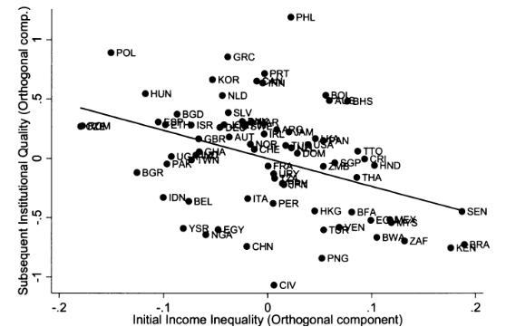
Figure 1 shows income inequality as captured by the Gini coefficient between 1981-1985 for a range of countries. This figure reinforces the correlation between income
Empirical Economic Bulletin, Vol. 17 34
inequality and institutional quality factors, as well as considering a range of economic conditions that also impact institutional quality as a whole.
Figure 1: Initial Income Inequality and Subsequent Institutional Quality
Source: The Review of Economics and Statistics
Per exploring a relationship between these two variables, it is easy to consider the impact that this will have on the following institutional quality factors: control of corruption, government effectiveness, political stability, absence of violence/terrorism, regulatory quality, rule of law, and voice and accountability. In many instances, as per depiction in Figure 1, poor institutional quality renders a higher degree of inequality. On the other hand, it is common that the opposite trend is seen within high-income nations, like the United States, China, and Singapore.
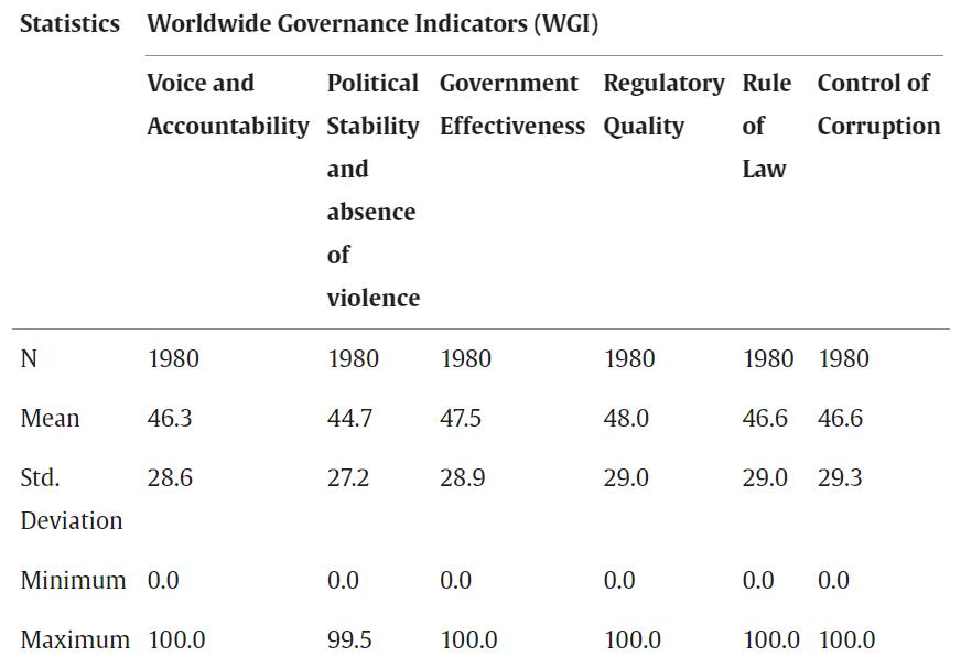
These variables can also be measured through the utilization of World Governance Indicators (WGI), which measure the quality of public governance at national and international levels. These indices are useful in understanding the different aspects of governance that have an overarching impact on governance quality, policy implications, social outcomes, and the overall growth and development of a country.
Figure 2 shows the descriptive statistics of World Governance Indicators aggregate data on a 10-year basis, which highlights the mean, standard deviation, minimum, and maximum for each indicator. In addition to this, these statistics provide a quantitative foundation for various policy implications within the latter half of this study.
Empirical Economic Bulletin, Vol. 17 35
Figure 2: Descriptive Statistics of WGI Aggregate Data (2012-2022)
Source: The Worldwide Governance Indicators
3.0 LITERATURE REVIEW
To shed light on the importance of the institutional quality index, various studies have been conducted in previous years. When examining institutional quality as a whole, a clear distinction must be made between low-income countries (LICs) and high-income countries (HICs). Simply put, this is due to the fact that the quality of institutions and their impact on economic growth varies significantly between countries. While lowincome countries are taxed with limited resources and higher levels of corruption, higherincome countries are oftentimes resource rich and have stronger structures. In a study conducted between high and middle-income countries, it is revealed that “An average MIC gains relatively more from improving its quality of legal system and property rights, whereas an average HIC benefits relatively more from each unit of improvement in its regulatory environment” (Parsa & Datta, 2023). In addition to this, researchers also dive into the difference between HICs and MICs when examining business start-ups. To understand why institutional quality plays a significant role, it is important to understand that governance, as well as size and strength of HICs, is truly a determinant of
Empirical Economic Bulletin, Vol. 17 36
entrepreneurial success. Furthermore, several policy implications in HICs outweigh those of MICs and LICs (Ben Ali, 2023).
On an international level, the same issues persist. Through looking at the Middle East and North African (MENA) regions, political regimes and governance play a significant factor that cannot be ignored when considering institutional quality. Similarly to analysis conducted in high, middle, and low-income nations, the MENA region provides insight on political stability and governance. Through a series of natural resource rents, socioeconomic status, and institutional quality factors shape the future of fiscal and monetary policies in order to reduce inequalities (Agheli, 2017). Evidence found from the Granger non-causality test uncovers unidirectional causation, meaning that “x” causes “y”, but “y” does not necessarily cause “x” to occur. This causation was, for the most part, found within MICs and LICs, where nations are impacted more so by improvements to regulatory environments. Since these nations are more commonly expected to be lackluster in terms of resources as compared to higher income nations, this trend is expected to occur.
Since the institutional quality index uncovers lots in terms of inequality, it is imperative to understand regional multidimensional factors. One case study focused on Italy uncovered that “disparities in multidimensional well-being go beyond the historical GDP divide between the Centre-North and the South of Italy… institutional quality matters in affecting regional multidimensional well-being inequalities and the effect varies heterogeneously according to the level of public expenditure, institutional dimensions, and spatial spillovers” (Ferrara & Nistico, 2019). Similar findings registered throughout Africa, where a holistic approach was utilized to look at environmental and housing factors. Once again, findings uncovered that governance and longevity of the regime / term of power have the power to exacerbate inequalities in all forms (Ongo Nkoa & Song, 2022). This is important to consider for the following: Foreign Direct Investment, Healthcare, Education, and Economic Development. In order to facilitate sustainable and effective development initiatives, these nations must be provided with the proper trajectory that will impact social, economic, and political outcomes.
A multitudinous array of research and development in relation to Foreign Direct Investment (FDI) inflows also lays within the institutional quality channel, per the
Empirical Economic Bulletin, Vol. 17 37
reasons listed above. Within reason, evidence outlines the potential role of institutional quality in terms of absorption in FDI spillovers. Due to the fact that quality of institutions is essential in the enhancement of market growth, literature shows that greater macroeconomic and financial stability indicate a positive relationship (Aziz, 2022). This can further be outlined in the understanding that institutional operations outline a certain level of attractiveness, which contributes to overall gross domestic product (GDP), as well as the Global Competitiveness Index (GCI). Within Central and Eastern Europe (CEECs), it is evident that “CEECs differ with respect to institutional quality (IQ)” (Dorozynski et al., 2020). Because sound governance is likely to attract aid, as opposed to corruption factors, it is evident that there are several forms of discrepancy in terms of institutional quality between low-income, middle-income, and high-income nations.
4.0 DATA AND EMPIRICAL METHODOLOGY
4.1 Data
The study uses panel data from 2008 to 2023. Data was obtained from the World Bank websites Worldwide Governance Indictors. As per the World Bank, it has been found that the WGI help researchers and analysts assess broad patterns in perceptions of governance across countries over time. Publicly available WGI data comes from across the world with these three criteria in mind: produced by credible organizations, provide comparable cross-country data, and are regularly updated.
4.2 Empirical Model
Following a study done by Lambert and Aronson in 1993, this study aims to look at the impact of institutional quality factors on inequality in upper-middle income countries in Latin America. Within Lambert and Aronson’s study, they observe an inequality decomposition analysis with the utilization of the Gini coefficient and Lorenz curve, but this model adds to the study by adding in the institutional quality index. The model could be written as follows:
Empirical Economic Bulletin, Vol. 17 38
Within this model, the following variables are considered: Gini Coefficient, Voice and Accountability (VA), Political Stability No Violence (PSNV), Government Effectiveness (GE), Regulatory Quality (RQ), Rule of Law (ROL), and Control of Corruption (CC).
Figure 3 below shows the Gini Index in the respective countries from 2008-2022, which provided great insight prior to the actual running of the regression analysis. This variable analysis looks at the difference in aggregate flows, as well as impact on WGI and Institutional Quality.
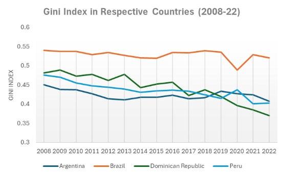
Furthermore, the study has a series of independent variables that were obtained from various sources and research conducted. As such, the observation is looking at four countries in Latin America with similar populations and economic growth, but they are all tested against the independent variable. In simple terms, the independent variable is manipulated or controlled and is hypothesized to have a causal effect on the dependent variable(s). In this instance, inequality has an impact on all of the institutional quality factors: control of corruption, government effectiveness, political stability and absence of violence/terrorism, regulatory quality, rule of law, and voice and accountability. By looking at the Gini coefficient in this case, the research will be able to show a clear distinction between each country as per the provided data set.
Figure 3: Gini Coefficient in Respective Countries (2008-2022)
Empirical Economic Bulletin, Vol. 17 39
5.0 EMPIRICAL RESULTS
The empirical results of the regression are presented below and are displayed individually in relation to each country.
Table 1: Argentina Regression Analysis
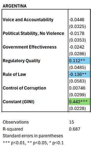
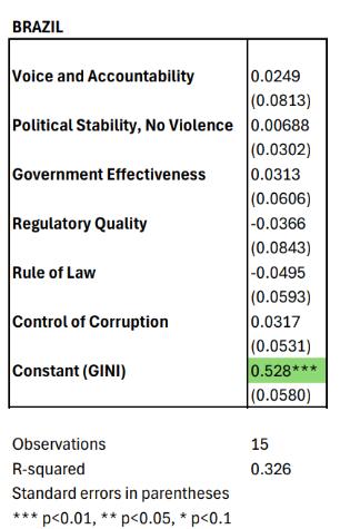
Table 2: Brazil Regression Analysis
Empirical Economic Bulletin, Vol. 17 40
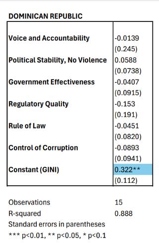
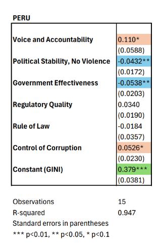 Table 3: Dominican Republic Regression Analysis
Empirical Economic Bulletin, Vol. 17 41
Table 4: Peru Regression Analysis
From these results, a few things can be stated in conclusion. First and foremost, when looking at Peru, it is evident that the Political Stability No Violence (PSNV) variable has a positive impact on income equality with a Gini of 0.379. In addition to this, Government Effectiveness (GE) in Peru essentially lowers the Gini Index, which in turn effectively lowers income inequality. Lastly, it is evident that Voice and Accountability (VA) for Peru has a positive coefficient, with its value being 0.110. With that being said, this can be interpreted in a variety of ways. For the purposes of this study, this means that even when people feel like they have a voice, there is still more income inequality within the respective country. Additionally, this implies that less fortunate people are more likely to speak up in contractionary or recessionary periods.
In addition to this, there were many significant variables found in the analysis of Argentina. First and foremost, when there is greater regulatory quality in Argentina, there is still an increase in the Gini index, which increases income inequality. In Argentina, this value came out to be 0.443. Additionally, when there is less rule of law, which equated to a value of -0.136, there is more income equality, not inequality. Based on what we can predict for the Gini Index, there is a strong likelihood that the role that the government plays in the economy and overall life in Argentina has a negative impact on income equality.
The analysis of the Dominican Republic and Brazil did not yield many results, which leads to the overall limitations of this research. First and foremost, the total number of observations was limited, especially since only four countries were considered for the study. In addition to this, there is a strong possibility that the reported data could be misreported, especially in countries that have high levels of corruption – which is evident in multiple nations across Latin America. This likely leads to the concept that the results could be insignificant due to possibilities of skewed data. Lastly, the size of governments, economies, and roles of the government likely play a factor in the inconsistency of results across the four observed countries.
5.0 CONCLUSION
In summary, this study was able to find that Argentina’s government likely has a negative impact on income inequality. This conclusion is based on the impact of regulatory quality and rule of law on the Gini Index. In addition to this, the study found
Empirical Economic Bulletin, Vol. 17 42
that overall, across various observed countries, when the government works in a way to help its citizens, it effectively lowers the Gini Index, or lowers income inequality. In addition to these findings, further research can be done to look at data on a more frequent basis and expand the topic to more countries of observation.
Empirical Economic Bulletin, Vol. 17 43
Appendix A:
Variable Name and Data Source
Acronym Description
FDI Foreign Direct Investment flows by country in millions of dollars
VA Voice & Accountability
PSNV Political Stability, No Violence
GE Government Effectiveness
RQ Regulatory Quality
ROL Rule of Law
CC Control of Corruption
GI or GC Gini Index or Gini Coefficient
Data source
US Bureau of Economic Analysis
World Governance
Indicators (World Bank)
World Governance
Indicators (World Bank)
World Governance
Indicators (World Bank)
World Governance
Indicators (World Bank)
World Governance
Indicators (World Bank)
World Governance
Indicators (World Bank)
US Bureau of Economic Analysis
Empirical Economic Bulletin, Vol. 17 44
BIBLIOGRAPHY
Agheli, L. (2017). Political Stability, Misery Index and Institutional Quality: Case Study of Middle East and North Africa. Economic Studies, 26(6), 30-46.
Aziz, O. G. (2022). FDI Inflows and Economic Growth in Arab Region: The Institutional Quality Channel. International Journal of Finance and Economics, 27(1), 1009-1024.
Ben Ali, T. (2023). How Does Institutional Quality Affect Business Start-up in High and Middle-Income Countries? An International Comparative Study. Journal of the Knowledge Economy, 14(3), 2830-2877.
Chong, A., & Gradstein, M. (2007). Inequality and Institutions. The Review of Economics and Statistics, 89(3), 454–465.
Dorozynski, T., Dobrowolska, B., & Kuna-Marszalek, A. (2020). Institutional Quality in Central and East European Countries and Its Impact on FDI Inflow. Entrepreneurial Business and Economics Review, 8(1), 91-110.
Ferrara, A. R., & Nistico, R. (2019). Does Institutional Quality Matter for Multidimensional Well-Being Inequalities? Insights from Italy. Social Indicators Research, 145(3), 1063–1105.
Ongo Nkoa, B. E., & Song, J. S. (2022). Does Institutional Quality Increase Inequalities in Africa? Journal of the Knowledge Economy, 13(3), 1896–1927.
Parsa, M., & Datta, S. (2023). Institutional Quality and Economic Growth: A Dynamic Panel Data Analysis of MICs and HICs for 2000-2020. International Economic Journal, 37(4), 675–712.
Empirical Economic Bulletin, Vol. 17 45
Does Money Really Buy Success? Empirical Analysis
of Money Spent Effect on English Premier League Team’s Performances/Success: A Panel Data Analysis
Barnaby Brandon
Abstract:
This paper investigates the empirical relationship between the wages of English Premier League teams and their success. This study incorporates information from the league regarding each team’s spending and the performance of each of these teams every year. Each team has a specific spending structure based on the magnitude of the club and ability of the players. The research will look at all teams that have stayed in the premier league for the past 10 years as some teams come in and out of the Premier League with the relegation and promotion system. The results will show whether having higher spending correlates with success or if it is purely about the ability of the team. A series of OLS regression models are estimated
JEL Classification: Z2, Z20
Keywords: Wages, English Premier League, Performance. Applied Economics, Bryant University, 1150 Douglas Pike, Smithfield, RI02917. Phone: (781) 995-7616. Email: bbrandon@bryant.edu.
Empirical Economic Bulletin, Vol. 17 46
1.0 INTRODUCTION
The influx of money into the English Premier League has led to it being revered worldwide as the most competitive domestic league in the world. Manchester City and Chelsea have both won the Champions League in the last 6 years with that competition having the best teams from Europe.
This study aims to enhance understanding of whether spending all the money that they do in the transfer market has the actual results on the pitch. For example, this past summer transfer window Chelsea spent over 600 million euros which is the most ever spent in a window and currently they are in 8th place. This study will go across the last 10 seasons and among 10 teams and will explore this relationship. The relevance of this study is that all these clubs tend to go for quantity over quality especially when they are coming up from the Championship which is the second tier in England. This will show the relationship in full, and owners can see that when approaching transfers spending all the money may not be the best.
In terms of research issues there aren’t many. To begin with a few of the clubs such as Aston Villa and Newcastle weren’t in the Premier League for 3 years and 1 year respectively. Although to have a good variety of teams and not just the top ten this had to be done, it shouldn’t be that much of an issue in the data and regressions. This is the only issue with the data that has been seen so far.
This paper was guided by 3 research objectives that differ from other studies: First it investigates the relationship between money spent and success on the pitch. This has been a hot topic in the world of soccer in recent years with Saudi, Qatari, and American owners and immediately thinking that spending money will lead to success. Second it incorporates multiple levels of teams while a lot of studies will just focus on those teams that spend the most which gives you a biased viewpoint and biased results. Lastly it also incorporates controls variables such as goal difference, and average attendance so that the results are more accurate as opposed to just comparing finishing position and money spent.
Section 2 gives a brief literature review. Section 3 outlines the empirical model. Data and estimation methodology are discussed in section 4. Finally, section 5 presents and discusses the empirical results. This is followed by a conclusion in section 6.
Empirical Economic Bulletin, Vol. 17 47
2.0 TREND
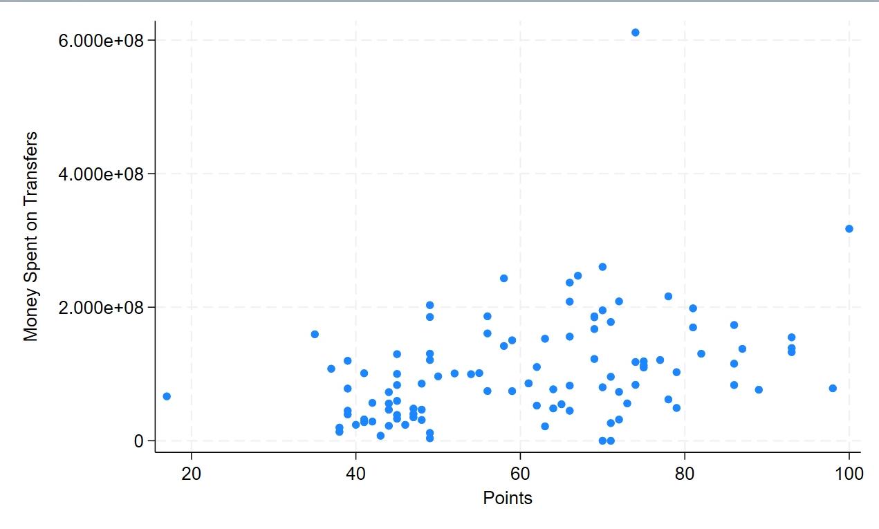
Money Spent on Transfers vs Points
Source: Transfer Markt, and Premier League
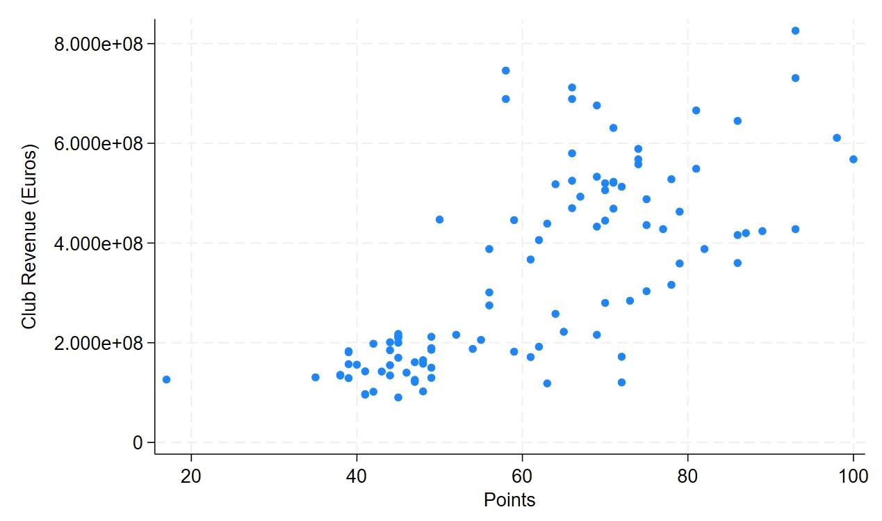
2: Club Revenue vs Points
Figure 1:
Empirical Economic Bulletin, Vol. 17 48
Figure
Source: Transfer Markt, and Premier League
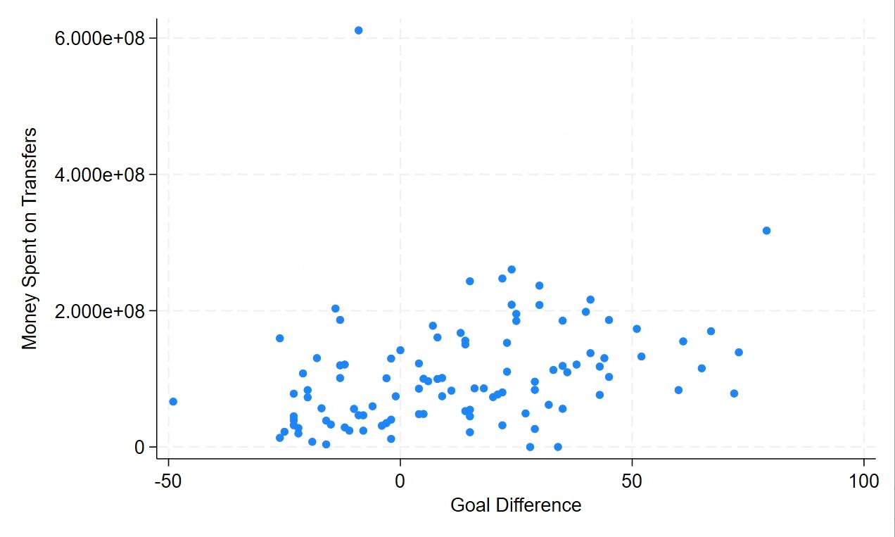
Figure 3: Money Spent on Transfers vs Goal Difference
Source: Transfer Markt, and Premier League
Empirical Economic Bulletin, Vol. 17 49
Figure 4: Average Attendance vs Points
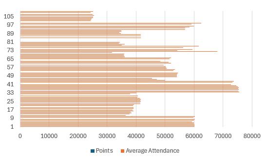
Source: Transfer Markt, and Premier League
These are preliminary trends, but they still give off good information. Beginning with Figure 1 the comparison of points and amount spent in the transfer markets is the root of this research. As you can see there is a positive relationship between the two of them but if you are to look at Figure 2 you can see that club revenue and points has an even more positive relationship. Looking at these two in comparison you would think that immediately that it is revenue that makes clubs, but it is likely the case that those with higher revenue already have quality players compared to those who have to spend more in the transfer market. Moving onto Figure 3 this graph shows the trend of the amount of money spent and goal difference. Goal difference is the difference between goals scored and goals conceded in a season. Over the teams and years analysed you can see that although many of them have spent different amounts some will have the same exact goal difference pointing again to the point that money doesn’t buy success. Lastly looking at Figure 4 this compares points and average attendance as having a big home crowd can be a massive advantage. As points begins to increase the number of points also does but not consistently which points to the fact that sometimes
Empirical Economic Bulletin, Vol. 17 50
teams have the quality that no matter where they play they can win so looking at that attendance does have an effect but possibly not as much as people would like.
3.0 LITERATURE REVIEW
There is a plethora of research that has been done on the economics of Soccer/Football with it being one of the most profitable sports in the world. To begin with, in terms of the focus of the research there are many areas within soccer that you can conduct economic research on. For example, Wei conducted a study on the effects of temperature on the performance of players, this is relevant as it is good to see if anyone is using unique variables to track performance this wasn’t the case as Wei used physical and cognitive performance as the dependent (Wei, 2022). Along the same lines as this study Ashworth researched the effects of selection bias in soccer and once again there is the possibility of unique variables or viewpoints, but it was rather basic although you can still see how the study is performed (Ashworth, Heyndels, 2007). Various recent literature has done research that links a soccer team’s wages and the production and success of the team. The commonality among this set of research is the negative relationship between wage dispersal and team performance. Domizio’s work as well as Coates research found this relationship (Domizio, 2021; Coates, 2014). Coate’s research was unique as it was one of the first bit of research done into the MLS as it is a young league while Domizio investigated the Italian first division which is far more established (Domizio, 2021; and Coates, 2014). They both found that it doesn’t matter where it is if there is a large dispersal of a club’s wages then there will be a drop in performance which points to the idea of wages creating a disjointed team and the club underperforming as a result. The studies performed by Campa, Royuela, Thrane, and Lucifora all touch upon the idea of measuring performance within soccer and seeing how they are measuring it is extremely useful as soccer is so multifaceted a good performance to someone may be terrible to someone else. Beginning with Campa he explored the transfer values of players and whether their performance matches their transfer. The way performance was measured was using variables based on position but wasn’t exactly the best way possible to measure performance (Campa, 2021). Following Campa, Royuela was looking at the success of teams not just individual success. The use of elo points is far more reliable and in terms of the options to measure success this has been the most effective I’ve seen (Royuela, 2018). For
Empirical Economic Bulletin, Vol. 17 51
Thrane and Lucifora’s research they used a vector of performance variables which is useful but when there are databases such as the elo ratings there is no need (Thrane, 2019; Lucifora, 2003).
4.0 DATA AND EMPIRICAL METHODOLOGY
4.1
Data
The study uses panel data from 2013 to 2023. Data were obtained from the Premier League website. Summary statistics for the data are provided in Table 1.
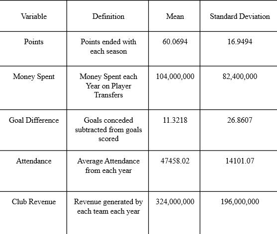
4.2 Empirical Model
The original model is from Thrane’s research into how Norwegian player pay relates to their performance. (Thrane, 2019). His model was logEi = Pβpi + Tβti + Cβci + μi with E- Earnings, P- Performance, T- Team Dummies, C- Player Characteristics
Table 1 Summary Statistics
Empirical Economic Bulletin, Vol. 17 52
The adapted model:
Success is the dependent variable and is a measure of the amount of points each team i got in year t. Money spent is the independent variable of interest with it being how much each team spent on players every year. Following this the controls are Average attendance, Revenue and Goal difference. Beginning with average attendance this is the average attendance each i team had in year t. This is an extremely important control as fans and the support they receive is extremely influential in the success of a soccer team. Following attendance, the next control is revenue. This is simply the amount of revenue i team brought in t year. This is also very important as it obviously provides them with funds to purchase players but also allows them to have state-of-the-art technology and facilities which also are crucial to success. The last control that will be used is Goal difference. This is the goal difference of i team for the t year and this is very important as well as it is easy to measure success through points as it is very straightforward but with using Goal difference it gives us a more in-depth view into i team’s ability to play. Goal difference is calculated by subtracting the number of goals conceded in i season from the number of goals scored in the same season.
�������������������������������� = ����0 + ����1 ������������������������������������������������ + ����2 ���������������������������������������������������������������������������� + ����3 ���������������������������������������������������� + ����4 ���������������������������������������������������������������� + ������������
Empirical Economic Bulletin, Vol. 17 53
5.0 EMPIRICAL RESULTS
The empirical estimation results are presented in Table 2. The empirical estimation shows the negative relationship between spending money and higher performance from the teams.
Table 2: Regression Analysis
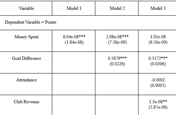
Note: *** , **, and * denotes significance at the 1%, 5%, and 10% respectively. Standard errors in parentheses
There are three models in this regression. The first of these is just our dependent variable points and money spent. This allows us to see the pure relationship between the two of them. Model 2 adds in the control variable goal difference. This was done as goal difference is the most important control variable. Lastly Model 3 was run which contains all the controls and this gives us a look at the relationship with all other factors involved. Now looking at the results of these
Empirical Economic Bulletin, Vol. 17 54
regressions. In Model 1 for every million a club spends it is expected that points will increase by 0.0804 points. For Model 2, for every million spent you would expect points to increase 0.0208. As well as the money spent being significant, the goal difference is also found to be positive and significant. Lastly, with Model 3 for every million spent you would expect points to increase 0.0101. You can see that Club revenue is significant and positive as well as goal difference. This is a good sign as it shows that these controls have a strong relationship with the dependent variable. Overall, Money spent, and points have a positive relationship and the controls chosen were significant at times.
5.0 LIMITATIONS AND FUTURE WORK
There are a few limitations to this work. Firstly, due to clubs getting relegated and promoted so frequently I couldn’t use all the teams in the Premier League and only could use teams that stayed up the whole time. As well as this more controls could have possibly been used to provide a more accurate look at the relationship. The data set was also only ten years long and not all information being publicly available, so I wasn’t able to find certain clubs’ statistics. Lastly, in future work the focus of the study could also include clubs from other countries.
6.0 CONCLUSION
In summary, the relationship between our dependent variable points and independent variable money spent is positive and significant in two of the three regressions. The results in this paper point to the fact that if you spend more money in the transfer window you would be expected to increase your point tally by around 0.010 for every million you spend. As the regression models went on the magnitude of the coefficient for money spent decreases, this was expected as you had more controls the more accurate the relationship is. As well as this, when in Model 3 the relationship was not found to be significant but then to show that controls were chosen well both, goal difference and club revenue were found to be positive and significant. In terms of policy recommendations based off of this research you can see that although the relationship is significant and positive between money spent and points, you must be calculated with your investments as blindly spending money doesn’t work as shown by Chelsea in 2022-23.
Empirical Economic Bulletin, Vol. 17 55
BIBLIOGRAPHY
Lucifora, Claudio, and Rob Simmons. “Superstar Effects in Sport.” Journal of Sports Economics , vol. 4, no. 1, Feb. 2003, pp. 35–55, https://doi.org/10.1177/1527002502239657 .
Ashworth, John, and Bruno Heyndels. “Selection Bias and Peer Effects in Team Sports.” Journal of Sports Economics 8, no. 4 (Aug. 2007): 355–377. https://doi.org/10.1177/1527002506287695 .
Campa, Domenico. “Exploring the Market of Soccer Player Registrations: An Empirical Analysis of the Difference Between Transfer Fees and Estimated Players’ Inherent Value.” Journal of Sports Economics 23, no. 4 (November 24, 2021): 379–406. https://doi.org/10.1177/15270025211059527
Wei, Xiahai, et al. "Temperature and Outdoor Productivity: Evidence from Professional Soccer Players." SSRN Electronic Journal , 2022. https://doi.org/10.2139/ssrn.4307950 .
Royuela, Vicente, and Roberto Gásquez. "On the Influence of Foreign Players on the Success of Football Clubs." Journal of Sports Economics 20, no. 5 (October 31, 2018): 718–741. https://doi.org/10.1177/1527002518807960 .
Thrane, Christer. "Performance and Actual Pay in Norwegian Soccer." Journal of Sports Economics 20, no. 8 (May 26, 2019): 1051–1065. https://doi.org/10.1177/1527002519851146 .
Di Domizio, Marco, et al. "Payroll Dispersion and Performance in Soccer: A Seasonal Perspective Analysis for Italian Serie A (2007–2021)." Contemporary Economic Policy 40, no. 3 (February 10, 2022): 513–525. https://doi.org/10.1111/coep.12566
Coates, Dennis, et al. "Superstar Salaries and Soccer Success." Journal of Sports Economics 17, no. 7 (August 3, 2016): 716–735. https://doi.org/10.1177/1527002514547297 .
Empirical Economic Bulletin, Vol. 17 56
Time Series Analysis of the Impact of Climate Change on the Rocky Mountain Ski Industry
Charlotte Christoa
Abstract:
This paper investigates the correlation between climate change and the ski industry. This study will incorporate the annual snowfall and mean temperature and annual visitations to American ski resorts. The model studied will investigate if the rising temperatures affect snow fall totals in popular ski areas as well the visitor amounts per season. This model will be used to run a multiple regression that will account for various controls including the distribution of snow fall throughout the season.
JEL Classification: Q52, Z1, L83
Keywords: Climate Change, Global Warming, Sports Industries, and Resorts
a Department of Economics, Bryant University, 1150 Douglas Pike, Smithfield, RI02917. Email: cchristo2@bryant.edu
Empirical Economic Bulletin, Vol. 17 57
1.0 INTRODUCTION
This study aims to enhance understanding the impact that climate change will have on the demand for snow sports specifically skiing. As stated below in the literature review, the number of optimal ski days are decreasing due to the increasing temperatures and decreasing snowfall. Although Earth has experienced cyclical climate variation in the past, the Earth has experienced nothing like this. The magnitude of the change and the increased rapid rate this change is happening has caused a worldwide impending crisis. Human activity has had a very big impact into this crisis; one-way humans have contributed has been increased greenhouse gas emissions. Greenhouse gasses are gases that are in the Earth’s atmosphere that trap heat. Since the Industrial Revolution, humans have significantly increased these emissions in turn significantly increasing the heat retention and surface temperatures (Why is climate change happening and what are the causes?). If these greenhouse gas emissions were remarkably reduced the average surface temperature increase could be capped at 2 degrees Celsius, however if they are not reduced, the increase could be observed at 5 degrees Celsius or more (World Bank Climate Change Knowledge Portal)
One impact of climate change is lessening snowfall. Since 1930, the total snowfall has decreased. Fifty seven percent of the weather stations across the United States has seen a decrease in snowfall. This is due to the proportion of winter precipitation being snow has been decreased (Climate change indicators: Snowfall 2020). Snowfall is very important to the ecosystems and all the organisms living in them, including humans. In some areas of The United States people are dependent on snowmelt for water supply since snowmelt contributes to seventy five percent of the water supply. Another impact of lessening snow
Empirical Economic Bulletin, Vol. 17 58
fall is winter recreation activities, such as skiing. The economic impacts of the decrease in ski activity could negatively affect the communities that rely on these activities (Climate change indicators: Snowfall 2020).
The ski industry in the Alps alone is worth approximately thirty billion dollars. This industry is in danger with fifty three percent of European ski resort in high risk of snow scarcity. As stated before, if carbon emissions do not decrease the temperature increase could be more than five degrees Celsius. “If the world were to hit 4C of heating, 98% of the resorts would be at very high risk of scarce snow cover” (Laville, 2023). As discussed in more detail below, the duration of snow cover has been decreasing as well. On average, the duration of snow cover has decreased by thirty-six days. The industry could adapt by more snowmaking. “According to the most recent study, the use of snowmaking to achieve 50% snow coverage on pistes reduces the number of European resorts at high risk of loss of snow cover to 27% at 2C and 71% at 4C” (Laville, 2023). However, snowmaking is costly in expenses, water, and energy usage. If this adaptation occurs, the water consumption could raise about five hundred and forty litres of water. The French Alps consumption could increase by nine times by the year 2100 if temperatures rise as predicted (Laville, 2023). A study from the University of Waterloo and University of Innsbruck has found that the U.S ski industry has lost more than five billion dollars over the last two decades due to climate changes caused by humans. From a policy perspective, this analysis is critical for the risk assessment of the ski industry. The ski industry is facing severe economic challenges and needs to adapt to them.
Empirical Economic Bulletin, Vol. 17 59
This paper was guided by three research objectives that differ from other studies: First the independent variable is annual ski visitation instead of the length of season, optimal snow days, or number of resorts. Second it incorporates the median household income as well as other demand side factors towards skiing. Third this study incorporates El Nino years to account for lesser snowfall in the northern Rocky Mountain Region and more in the southern.
The rest of the paper is organized as follows: Section 2 gives brief overview of trends found in the Data. Section 3 gives a brief literature review. Section 4 outlines the empirical model. Data and estimation methodology are discussed in section 4. Finally, section 5 presents and discusses the empirical results. This is followed by a conclusion in section 6
2.0 TREND OF SKI VISITATION VARIABLES
Figure 1 illustrates the notable trend of seasonal Rocky Mountain ski visitation steadily rising over time. The graph captures a compelling narrative of the burgeoning popularity of skiing in the Rocky Mountain region, showcasing a consistent upward trajectory in visitor numbers across multiple seasons.
Empirical Economic Bulletin, Vol. 17 60
Figure 1: Rocky Mountain Seasonal Ski Visitation Increases
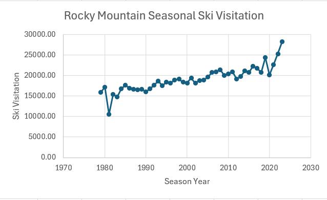
S ource: National Skier Association
Figure 2 shows the trends in the Median Household Income. Over the past few decades, America has witnessed a gradual but notable increase in median household income, reflecting the evolving economic landscape of the nation. From the late 20th century to the present day, statistical data consistently portrays a rising trend in median household income, indicating a positive trajectory for the financial well-being of American families. This upward movement underscores several factors, including advancements in technology, shifts in labor markets, and policy interventions aimed at enhancing economic opportunities. Despite occasional fluctuations influenced by economic cycles, the overarching pattern illustrates a steady improvement in the standard of living for many households across the country. This trend in rising median household income
Empirical Economic Bulletin, Vol. 17 61
speaks to the resilience and adaptability of the American economy, as well as ongoing efforts to promote prosperity and economic mobility for all citizens.
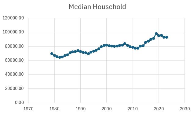
Source: Federal Reserve Economic Data (FRED)
Figure 3 shows the cumulative snow fall per season. In recent years, a concerning trend has emerged regarding the average snowfall amounts in the Rocky Mountains per season, showing a noticeable decrease over time. This decline in snowfall is particularly alarming given the region's heavy reliance on consistent snow accumulation for its tourism and recreational industries, including skiing and snowboarding.
Figure 2: Median Household Income
Empirical Economic Bulletin, Vol. 17 62
Figure 3: Snow Fall Per Season
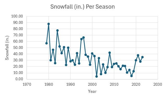
Source: University of Colorado
3.0 LITERATURE REVIEW
Human activities, particularly the combustion of fossil fuels, have triggered a relentless ascent in Earth's temperature, a trend projected to persist into the foreseeable future. As temperatures climb, the landscape of precipitation shifts, with snowfall giving way to rainfall in many regions. This transition poses a substantial threat to the ski industry, as noted by Dawson and Scott (2007), who assert that even with efforts to curb emissions, ski seasons across Vermont are poised for significant shrinkage. Projections extend to 2039, indicating a reduction in average season lengths ranging from 4 to 14 percent. Delving further into climate forecasts for the period spanning 2040 to 2069, utilizing midrange and high greenhouse gas emission scenarios, reveals a stark reality: ski resorts will grapple with heightened snowmaking demands and operational expenses alongside dwindling visitor numbers and diminished profitability.
The ramifications of scant snow and escalating temperatures extend beyond the confines of the slopes, exerting a palpable impact on visitor metrics. Ballotta et al. (2020)
Empirical Economic Bulletin, Vol. 17 63
highlight the volatility inherent in visitor numbers, particularly outside peak seasons, attributing abrupt declines to insufficient snow cover. Parthum and Christensen's (2022) findings echo this sentiment, prognosticating a 40 to 60 percent reduction in snow-related visitation under forthcoming climate scenarios. Meanwhile, Bergerhammer and Schmude (2014) offer a comprehensive analysis of optimal ski days, revealing a disheartening trend of diminishing prospects for skiing enjoyment. Across the spectrum of years surveyed, from the 2010 season to projections for the 2050s, the decline in optimal ski days ranges from 35 to 91 percent, painting a bleak picture of the industry's future.
Stieger et al. (2019) shed light on the ripple effects of dwindling snow cover, elucidating how diminished snowfall in key urban markets erodes public perception of ideal skiing conditions and dampens demand. Within the skiing community, enthusiasts known as "powder chasers" wield significant influence, their fervent pursuit of fresh snow driving peak attendance on mountains. However, as the frequency of powder days diminishes, so too does the allure for these dedicated skiers, potentially curtailing the sporadic surges in visitation that traditionally coincide with abundant snowfall. Moen and Fredman's (2007) examination of skiable days in Sweden corroborates this narrative, indicating a precipitous decline in ski-able days per season from 2070 to 2100, with an average shortfall of 96 days. Furthermore, the study illuminates a disconcerting trend wherein snowfall persists across fewer days, hastened by the hastening retreat of snow cover in a warmer climate.
In the face of these sobering projections, the ski industry finds itself at a crossroads, compelled to confront the existential threat posed by climate change. Strategies to mitigate the adverse effects of diminishing snowfall and rising temperatures necessitate a multifaceted approach, encompassing both adaptation and advocacy. Ski resorts must invest in snowmaking infrastructure and diversify their offerings to accommodate alternative activities during periods of scant snowfall. Simultaneously, industry stakeholders must galvanize efforts to advocate for policies aimed at curbing greenhouse gas emissions and mitigating the drivers of climate change.
Empirical Economic Bulletin, Vol. 17 64
Moreover, collaboration between public and private sectors is imperative to foster innovation and resilience within the ski industry. By fostering partnerships with climate research institutions, ski resorts can leverage cutting-edge data and insights to inform strategic decision-making and long-term planning. Similarly, cooperation with governmental agencies can facilitate the implementation of regulatory frameworks that incentivize sustainable practices and reduce the carbon footprint of ski resorts.
Ultimately, the fate of the ski industry hinges on its capacity to adapt to a rapidly changing climate while championing sustainability and environmental stewardship. As the specter of climate change looms large, the resilience of the ski industry will be tested like never before, demanding bold action and unwavering commitment to safeguarding the winter sports we cherish.
4.0 DATA AND EMPIRICAL METHODOLOGY
4.1 Data
The study uses annual time series data from 1978 to 2023. Data were obtained from Colorado State University, Federal Reserve Economic Data (FRED), and the National Ski Areas Association (NSAA). Summary statistics for the data are provided in Table 1.
Variable Observation Mean Std. Dev. Min Max Rocky Mountain Ski Visitation 45 19,055.556 2944.854 10,486 28,174 Average Temperature 45 23.159 2.229 18.79 27.57 Snowfall (in) 45 32.45 18.435 4.6 88 Number of Holidays on Weekends 45 1.1333 1.5165 0 4 Empirical Economic Bulletin, Vol. 17 65
Table 1 Summary Statistics
4.2 Empirical Model
Following Bollota et al. (2020) this study adapted and modified the regression model for ski visitors. This study looks at annual ski visitation instead of daily. This study also added median household income, disposable income, amount of ski resorts in operation, as well as El Nino years.
The model could be written as follow:
Ski Visitation = β0 + β1 (Average Temperature) + β2 (Snowfall) +β3 (Holidays on weekdays) + β4 (Leap year) + β5 (El Nino) +β6 (Median Household Income) +β7 (Disposable personal income) +β8 (Number of Ski Areas in Operation) + ε (1)
The dependent variable Rocky Mountain ski visitation are the recorded people that skied in the Rocky Mountain Region within the given season. This statistic includes Colorado, Utah, Montana, Wyoming, New Mexico, and Idaho.
Independent variables consist of eight variables obtained from Colorado State University and FRED. Average temperature (β1), snowfall (β2), and number of holidays on weekends (β3) are all seasonal totals. Meaning that the data is only collected during the ski season, which in this study is defined as November to March. Leap Year (β4) is a dummy variable where 1 represents it was a leap year and 0 as it was not. El Nino (β5) follows the same pattern where 1 represents an El Nino year and 0 represents a non-El Nino
Leap Year (Dummy) 45 .244 .4346 0 1 Median Household Income 45 78,061.136 8533.1396 64,440 97,970 Disposable Income 45 10224.449 3647.339 5063.142 17,138.717 Ski Resorts 45 99.5556 4.8079 95 113 El Nino (dummy) 45 .5556 .5025 0 1
Empirical Economic Bulletin, Vol. 17 66
year. Median Household income (β6) is an average of the monthly household income of that given year. The data was collected from FRED. Disposable personal income (β7) was also collected from FRED as a monthly total and converted to a annual average. Lastly Number of ski areas in operation (β8) was collected from the Lost Resorts Project and is a count of the ski areas in operation that given season.
The expected signs of each of these variables can be found in Appendix B. With a one degree increase in average temperature the impact on ski visitation is expected to be negative based on prior studies and the hypothesis of this current study. Snowfall, however, is estimated to be positive, due to the increased demands on powder days. The number of holidays on weekends is expected to negatively affect ski visitation. Weekends and holidays are typical sell out days, if the holiday is on a weekend that is one less day of that week selling out. Leap year is projected to be positive due to Leap Day being a popular ski day every four years. The number of ski resorts is projected to be negative since that is increasing the supply of ski tickets to be sold, which would lessen demand. El Nino year however would be positive. El Nino weather patterns typically result in more snowstorms meaning more powder days with increased demand. Both Disposable personal income and median household income will increase the ski visitation since people will have more money to spend on ski tickets and rentals.
5.0 EMPIRICAL RESULTS
The empirical estimation results are presented in Table 2. The empirical estimation shows the negative relationship between average temperature and Rocky Mountain Ski visitation. In the third regression it shows that a one degree Fahrenheit increase in average temperature results in approximately 253 less visitors per year.
Empirical Economic Bulletin, Vol. 17 67
Table 2: Regression results for Rocky Mountain Ski Visitation
(°F)
(210.4182)
(12.51568) # Holidays on Weekends
Year
(446.4803) Ski Resorts
Disposable Income .8271524 (.0657656) .592663*** (.1593412
Household
.1028961 (.0639556)
Note: *** , **, and * denotes significance at the 1%, 5%, and 10% respectively. Standard errors in parentheses
The statistical analysis of factors influencing ski visitation yields compelling insights into the dynamics shaping this recreational industry. At the forefront, the average temperature emerges as a pivotal variable, with its estimate demonstrating statistical significance at the 1% level. This underscores the profound impact of temperature on ski visitation patterns, with colder temperatures generally correlating with increased attendance.
Similarly, the snowfall variable returns a statistically significant positive relationship with ski visitation, reaffirming the intuitive link between abundant snow cover and
Rocky Mountain Ski
I II III CONSTANT 46242.3
19552.71 (5534.797) 14061.74
-128.7642
-222.8406**
-253.5507***
-25.46303
46.15875***
43.14028**
309.9339
197.3953
223.6058*
Leap
-282.9331
-392.1581
-333.5977
-238.5491
-61.36884
-55.45092
El
159.153
1071.788** (414.0718) 1117.881***
R2 0.2470 0.8573 0.8668 F-statistics 2.08* 31.74*** 29.29*** Number of obs. 45 45 45
Visitation
(11585.42)
(6404.773) Average Temperature
(93.142373)
(93.18251) Snowfall (in.)
(28.16322)
(13.66912)
(279.3725)
(123.592)
(122.1131)
(1029.763)
(454.4458)
(98.77067)
(45.80091)
(44.99896)
Nino
(923.9262)
(406.4708)
Median
Income
Empirical Economic Bulletin, Vol. 17 68
heightened interest in skiing activities. Disposable personal income emerges as another influential factor, with a statistically significant estimate at the 1% level. This finding aligns with expectations, as greater disposable income typically translates to increased spending on recreational pursuits such as skiing, thereby driving up ski visitation rates.
Moreover, the presence of El Niño conditions exerts a notable influence on ski visitation, as evidenced by its strong positive relationship in the regression analysis. El Niño years, characterized by elevated snowfall and lower temperatures in the Rocky Mountain region, tend to attract greater numbers of skiers seeking optimal skiing conditions.
Interestingly, the occurrence of holidays on weekends emerges as a statistically significant factor, albeit at the 10% level. This finding suggests that holidays falling on weekends coincide with heightened ski visitation, possibly due to extended leisure periods for potential skiers.
Conversely, variables such as the number of ski resorts in operation for each year, median household income, and leap years do not exhibit statistically significant relationships with ski visitation. Despite their inclusion in the model, these variables fail to exert discernible influence on skiing trends.
Overall, the regression model proves robust and statistically significant at the 1% level, as evidenced by an F statistic of 29.29. Moreover, the model's high R-squared statistic of 0.8668 indicates that it accounts for a substantial portion, specifically 86.68%, of the variability observed in ski visitation data. This suggests that the included variables collectively provide a comprehensive explanation of the factors driving ski visitation patterns, offering valuable insights for industry stakeholders and policymakers alike.
6.0 CONCLUSION
Empirical Economic Bulletin, Vol. 17 69
In conclusion, this study delves into the intricate relationship between climate change and the demand for snow sports, particularly skiing. As outlined in the literature review, the impact of climate change on skiing is multifaceted, encompassing factors such as declining snowfall, shifting precipitation patterns, and rising temperatures. While cyclical climate variations have occurred throughout Earth's history, the unprecedented magnitude and rapid rate of contemporary climate change pose an unprecedented challenge, constituting a global crisis with far-reaching implications.
Human activities, notably the combustion of fossil fuels and resultant greenhouse gas emissions, are identified as primary drivers of climate change. These emissions contribute to the retention of heat in Earth's atmosphere, exacerbating the warming trend and disrupting climatic patterns essential for snowfall and winter recreation.
The repercussions of diminished snowfall extend beyond the realms of ecology to impact various sectors of society, including winter tourism and recreation. Skiing, a cornerstone of winter tourism, faces significant economic challenges as snow cover diminishes and ski seasons shorten. The ski industry, valued at billions of dollars globally, is particularly vulnerable to climate change-induced disruptions, with a substantial portion of European ski resorts at risk of snow scarcity in the coming decades.
In response to these challenges, adaptation strategies such as increased snowmaking are proposed, albeit with associated costs and environmental impacts. Additionally, this paper highlights the critical role of empirical research in understanding
Empirical Economic Bulletin, Vol. 17 70
the complex dynamics of ski visitation. By employing a comprehensive regression model incorporating factors such as temperature, snowfall, income levels, and El Niño events, this study offers valuable insights into the determinants of ski visitation patterns in the Rocky Mountain region. The empirical findings underscore the significance of temperature, snowfall, disposable income, and El Niño conditions as key drivers of ski visitation. Despite efforts to include variables such as median household income and the number of ski resorts in operation, their lack of statistical significance suggests a nuanced interplay of factors shaping ski visitation trends.
Overall, this study contributes to a deeper understanding of the nexus between climate change and winter recreation, shedding light on the challenges faced by the ski industry and the imperative for adaptive measures. By elucidating the complex dynamics underlying ski visitation patterns, this research informs policymakers and industry stakeholders, facilitating evidence-based decision-making aimed at enhancing the resilience of the ski industry in the face of climate change.
Empirical Economic Bulletin, Vol. 17 71
Appendix A: Variable Description and Data Source
Acronym Description
Average
Temperature
The average seasonal temperature calculated from monthly averages from the months of November to March
Snowfall The total cumulative snowfall in the months of November to March
Holidays on Weekends
The number of holidays that were on the weekends throughout the season
Leap Year If the season contains a leap day
El Nino year El Niño year is the periodic warming of sea surface temperatures in the central and eastern equatorial Pacific Ocean, causing changes such as altered weather patterns and increased rainfall in some regions.
Data source
Colorado State University
Colorado State University
Calendar
Calendar
NOAA
Empirical Economic Bulletin, Vol. 17 72
Median Household Income
The Average median household income for that calendar year FRED
Disposable Household income The average disposable personal income of that year in the United States FRED
The number of ski areas that are in operation in the region during that season Lost Resorts Project
Number of Ski Areas in Operation
Appendix B- Variables and Expected Signs
Variable What it captures Expected sign
Empirical Economic Bulletin, Vol. 17 73
Average Temperature
Snowfall
Holidays on Weekends
The amount that one degree change in temperature impacts ski visitation -
The amount that one inch change of snowfall will impact ski visitation +
The amount that one additional holiday on the weekend will impact ski visitation -
Leap Year
El Nino Year
Median Household Income
Amount that one additional day in the year contributes to ski visitation +
The impact that the weather changes in an El Nino year has to ski visitation
The impact that an increase in median household income has on si visitation
Disposable Personal Income
Number of Ski Areas in Operation
Effects of Disposable income on ski visitaiton +
Supply side factor of ski visitation +
+
+
Empirical Economic Bulletin, Vol. 17 74
BIBLIOGRAPHY
References
Ballotta, L., Fusai, G., Kyriakou, I., Papapostolou, N. C., & Pouliasis, P. K. (2020). Risk management of climate impact for tourism operators: An empirical analysis on ski resorts. Tourism Management, 77, 104011.
Berghammer, A., & Schmude, J. (2014). The Christmas—Easter shift: Simulating alpine ski resorts' future development under climate change conditions using the parameter ‘optimal ski day’. Tourism Economics, 20(2), 323-336.
Dawson, J., & Scott, D. (2007). Climate change vulnerability of the Vermont ski tourism industry (USA). Annals of Leisure research, 10(3-4), 550-572.
Dawson, J., Scott, D., & McBoyle, G. (2009). Climate change analogue analysis of ski tourism in the northeastern USA. Climate Research, 39(1), 1-9.
Environmental Protection Agency. (2020, November 2). Climate change indicators: Snowfall. EPA. https://19january2021snapshot.epa.gov/climate-indicators/climate-change-indicatorssnowfall_.html
Laville, S. (2023, December 26). Ski Resorts Battle for a future as snow declines in climate crisis. The Guardian. https://www.theguardian.com/environment/2023/dec/26/ski-resortsbattle-for-a-future-as-snow-declines-in-climate-crisis
Media Relations. (2024, February 29). U.S. ski industry suffers $5b hit from climate change. Waterloo News. https://uwaterloo.ca/news/media/us-ski-industry-suffers-5b-hit-climatechange
Moen, J., & Fredman, P. (2007). Effects of climate change on alpine skiing in Sweden. Journal of sustainable tourism, 15(4), 418-437.
Parthum, B., & Christensen, P. (2022). A market for snow: Modeling winter recreation patterns under current and future climate. Journal of Environmental Economics and Management, 113, 102637.
Steiger, R., Scott, D., Abegg, B., Pons, M., & Aall, C. (2019). A critical review of climate change risk for ski tourism. Current Issues in Tourism, 22(11), 1343-1379. Why is climate change happening and what are the causes?. Why is climate change happening and what are the causes? | U.S. Geological Survey. (n.d.). https://www.usgs.gov/faqs/why-climate-change-happening-and-what-are-causes
World Bank Climate Change Knowledge Portal. Climate Change Knowledge Portal. (n.d.). https://climateknowledgeportal.worldbank.org/overview#:~:text=Climate%20change%20is %20the%20significant,change%20from%20natural%20weather%20variability
Empirical Economic Bulletin, Vol. 17 75
The Causes All Time High Chronic Homelessness: A Panel Analysis
Robert Knight
Abstract:
This paper investigates what economic indicators affect the rate of homelessness in the United States. By combining both the personal issues of the homeless people themselves along with economic structural issues in U.S. this study finds what the largest determinants of chronic homelessness. The study includes variables such as median house prices from the Case Shiller Index, the poverty rate, unemployment rate, health care expenditures per capita and demographics to find what causes a higher homeless rate. The data used to determine the conclusions will be pulled from twenty different major U.S. metropolitan cities to showcase how different economic variables can affect homeless populations. This study shows that certain demographics are far more likely to experience homelessness and that there are clear structural issues that need to be solved.
JEL Classification: I30, I32, I14
a Department of Economics, Bryant University, 1150 Douglas Pike, Smithfield, RI02917. Phone: (612) 806-2435. Email: rknight4@bryant.edu
Empirical Economic Bulletin, Vol. 17 76
1.0 INTRODUCTION
Chronic homelessness describes people who having either experienced homelessness repeatedly or for over a year due to a disabling condition. It is a problem that has continued to grow in the United States in the past five years. In 2023 a new record high was hit as over 144,000 people were chronically homeless, roughly 22% of all homeless people (National Alliance to End Homelessness). The reasons behind homeless are often complex and long lasting. The goal of this paper is to determine the root causes of chronic homelessness in the United States. By understanding the problem and its determinants we can better help those who are struggling to find housing. The importance behind helping the homeless population cannot be understated. The majority of people who struggle to find housing have high rates of mental illnesses and substance abuse disorders. Not only does this negatively impact them, but it also impacts the community they live in and our society as a whole.
This paper is different from other studies in this field in three ways First it investigates not only the personal issues of the people themselves that struggle with chronic homelessness, but it also examines the structural issues behind them that are economic based. Second it uses data from twenty cities in the Case-Shiller Index across the US. This allows us to evaluate how different cities are handling homelessness with their policies. Finally, this paper investigates data from a ten-year period. The recency of this data can help fill in major gaps in other studies that have missed major global events such as the pandemic. This paper successfully fills the limitations of previous studies.
The rest of the paper will be organized into six sections: Section 2 briefly covers the extensive literature on this topic. There have been plenty of high-quality studies on homelessness that will help us with the foundation of this issue. This is especially the case recently, as tent cities and chronic homelessness has been on the rise. Section 3 outlines the empirical model and all its components. Data and estimation methodology are discussed in section 4. Finally, section 5 presents and discusses the empirical results. This is followed by a conclusion in section 6.
Empirical Economic Bulletin, Vol. 17 77
2.0 Homeless Rates and the Availability of Low-Cost Housing
The main correlation this paper drives to prove is between homeless rates and the availability of low-cost housing. Figure 1 showcases this exact trend in ten select cities from the years 2017 to 2022. The graph clearly shows that cities that experienced the highest increase in median rent prices saw an equal reaction in their homeless population. This increase in housing prices can offset any other positive changes in the economy. For example, later in the data there is a decrease in unemployment rate and poverty rate in multiple cities, yet homeless rates continue to increase. It does not matter if people are working bringing in more money if they still cannot afford housing.
When housing prices increase, people are often forced to allocate an unsustainable portion of their income towards rent or mortgage payments, leaving little left for other necessities. Many families and individual are forced with the difficult choice of paying rent or other critical needs like food, healthcare, or education. Moreover, the unattainability of affordable housing can exacerbate issues such as overcrowding, substandard living conditions, and reliance on temporary shelters or precarious housing arrangements. These issues can lead to an endless cycle for people that is hard to overcome without external support or government assistance.
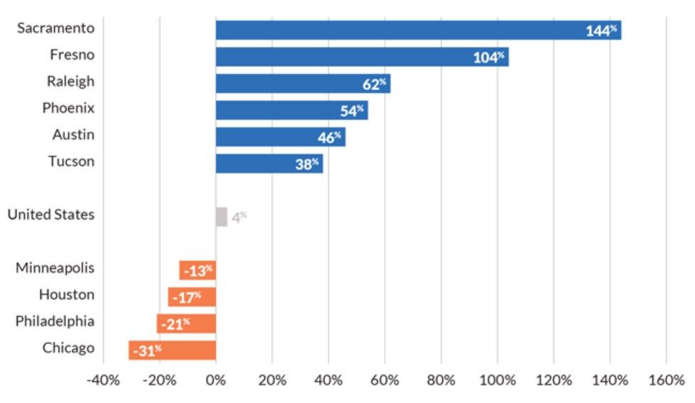
Empirical Economic Bulletin, Vol. 17 78
Figure 1: Median Rent Prices
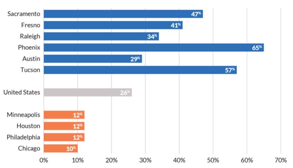
Source: Pew Charitable Trusts
3.0 LITERATURE REVIEW
There have been many economic studies conducted on the determinants behind homelessness in the United States. Most papers direct their attention towards one of two main explanations; the personal issues of the homeless people themselves or the economic structural problems behind them. The personal issues of homeless people can cover a myriad of complex problems, but the ones most focused on are mental health and substance abuse. It is well known that mental illness is a massive driver of homelessness in the U.S. In a study done by Gutwinksi et al. (2021), 76% of all homeless people suffer from a mental illness of some kind. People that suffer from extreme depression, bi-polar disorder, schizophrenia and PTSD are far more likely to experience homelessness in their lives (Substance Abuse and Mental Health Services Administration). In addition, homeless people who struggle with mental health are ten times more likely to commit suicide (National Health Care for Homeless Council).
Closely related to mental health among the homeless community is drug abuse, with one often leading to the other. McVicar et al 2013 contends that “homeless
Empirical Economic Bulletin, Vol. 17 79
individuals are more likely to be substance users and substance users are more likely to be homeless”. The Substance Abuse and Mental Health Services Administration reports that 16% of homeless people report having a substance abuse problem, the actual number most likely being much higher. Substance abuse is also one of the major leading causes of mortality in the homeless population (Baggett et al, 2013). In terms of tobacco, smoking prevalence ranged from 57% to 82% among homeless adults (Soar et al. 2020).
Opioids present an even larger issue as opioid-related overdose deaths have quadrupled since 2010 (National Alliance to End Homelessness). Unfortunately, it can be very difficult for homeless people to seek treatment and preventative care due to lack of funding and insurance. While there are some organizations that are working to give high quality health care to the homeless, such as the National Health Care for the Homeless Council, they are simply too many homeless to take care of for them to bear.
One of the largest problems with solving the personal issues of the homeless is that their roots can be hard to trace Mental disorders are often the combination of genetic disorders and past trauma, such as physical or mental assault, an abusive childhood, posttraumatic stress disorder or serious mental health issues. For example, children that experience abusive relationships with their guardians are far more likely to develop mental health issues. Collins (2013) saw a strong correlation between adverse childhood events and becoming homeless later. The more severe the stressor was for the youth the higher the likelihood of homelessness later in life. Similarly, infants who suffer from health issues can increase the likelihood of a family becoming homeless due to the high expenses (Curtis et al. 2011). Unfortunately, many of these issues are hard to solve at a societal level due to their uniqueness to the individual.
Now that we have discussed the personal issues that lead to chronic homelessness in the United States, we will discuss the structural problems that make it hard for individuals to find housing. According to Elliot and Krivo (1991), there are four major structural problems that cause homelessness; lack of low cost housing, high poverty rates, poor economic conditions, and lack of community health care facilities. Many other studies back up this concept, such as Cebula and Alexander (2020) and Heston (2023) who both found that homelessness is positively associated with the overall cost of living. The poverty rate and unemployment rate have consistently been tied to overall homeless
Empirical Economic Bulletin, Vol. 17 80
rates as well (Homelessness Policy Research Institute). When it comes to health care expenditures per capita, the United States ranks the highest among developed countries. These high costs are especially difficult on those in poverty, as 56% of all people living under the poverty line report that they struggle to pay medical bills (The Commonwealth Fund). Overall, it is far easier to both understand the economic conditions that drive homelessness and the steps that we need to take to solve them in comparison to personal issues. That is why the majority of the factors measured in this study are from the broad economic perspective.
4.0 DATA AND EMPIRICAL METHODOLOGY
4.1 Data
This study uses panel data from 2013 to 2023 from twenty different cities on the Case Shiller Index. The cities studied were Atlanta, Boston, Charlotte, Chicago, Cleveland, Dallas, Denver, Detroit, Las Vegas, Los Angeles, Miami, Minneapolis, New York, Phoenix, Portland, San Diego, San Francisco, Seattle, Tampa and Washington D.C. All data was gathered from the United States Census Bureau and the Bureau of Labor Statistics. Summary statistics are shown in Table 1.
Empirical Economic Bulletin, Vol. 17 81
Table 1 Summary Statistics
4.2 Empirical Model
Following the Elliot and Krivo (1991) this study modified their model using slightly different metrics for variables along with additional factors for the homeless population. The dependent variable in this model is the number of homeless. The independent variables are the Case Shiller Index, the poverty rate, unemployment rate,
Variable Observation Mean Std. Dev. Min Max Number of Homeless 220 10,469.94 1,208.52 870 88025 Hispanic 220 3,102.42 396.34 10 46,996 African American 220 5,411.84 813.6 203 59292 Unemployment Rate 220 0.048 0.0011 0.023 0.103 Poverty Rate 220 0.125 0.013 0.105 0.148 Case Shiller Index 220 211.47 46.42 146.82 297.46 National Health Expenditure 220 3,529.91 555.72 2,783.3 4,464.6
Empirical Economic Bulletin, Vol. 17 82
national health expenditure per capita and demographics. Our goal was to find the correlation between low cost housing in the United States and the homeless population. However, instead of evaluating that market by looking at low rent housing averages nationwide, we used the Case Shiller Index composite of twenty major cities across the U.S. and the median average house prices. This adaptation allows a far more detailed look into major metropolitan areas where the homeless rates are highest. The city differences also allow interesting perspectives of what polices best work to combat homelessness. In addition, we use the poverty rate, which is ratio of people who are living under the poverty line. The unemployment rate measures the ratio of people in the labor force that are without jobs. Instead of evaluating mental health expenditures as a determinate of homelessness, our model uses health expenditure per capita. This variable is far more encompassing of the expensive health care system instead of focusing on one issue within it. Finally, we included demographics, in particular Hispanics and African Americans, as they are unproportionately overrepresented in the homeless population in the United States.
The model could be written as follow:
These variables were chosen based off what we believed were the most significant determinates of homeless rates. Data for these variables was also readily available from reliable sources such as the U.S. Census Bureau, U.S. Bureau of Labor statistics and the Case Shiller Index.
5.0 EMPIRICAL RESULTS
The empirical estimation results are presented in Table 2. Our model is extremely accurate in predicting the impact of our independent variables on the rate of homelessness as the R-squared was .959. The constant, Hispanics and African Americans
Empirical Economic Bulletin, Vol. 17 83
were all significant variables. The constant, which is the number of homeless people when all else is zero, was positive at 15,633.23.
Table 2: Regression Results
The estimation shows a strong positive correlation with Hispanics and African Americans and homelessness. This result was expected due to their overrepresentation in the homeless population. The unemployment rate had a positive coefficient, meaning the more the unemployment rate increased so did the homeless population. An increase in the Case Shiller Index led to a great increase in the number of homeless. This result solidifies our hypothesis that high housing prices is one of the major causes of homelessness. Interestingly, the U.S. poverty rate had a negative correlation with homeless rates. This was due to a decrease nationally in the amount of people in poverty in the past ten years. Consequently, our model interpreted that as poverty having a positive effect on homelessness, which is not the case. National health expenditures per capita had a slight negative correlation with homeless rates. The variables of unemployment rate, poverty rate, Case Shiller Index and national health expenditures per capita were not statistically significant so these findings are not conclusive.
Coefficients Standard Error t Stat P-value Constant 15633.2257 7764.503976 2.013422 0.045329 Hispanics 1.706054033 0.119385325 14.29032 6.23E-33 African Americans 0.422673832 0.072803332 5.805694 2.31E-08 Unemployment Rate 34517.47282 21444.19403 1.609642 0.108957 US Poverty Rate -51411.86206 38378.90192 -1.33959 0.181807 CSI 39.62579169 31.85419807 1.243974 0.214876 NHI -4.643995203 2.910557089 -1.59557 0.112068
Empirical Economic Bulletin, Vol. 17 84
Understanding that different cities would have different economic conditions, we also separated the data into different categories. For example, New York and Los Angeles have the highest rates of homelessness and saw an increase in almost 60,000 homeless people in the last 10 years combined. Despite this increase in homelessness, both of those cities saw a decrease in unemployment during that time period excluding 2020 (see figure 2). Further exploration explains that the far higher increase in housing prices completely offset any positive changes that happened in unemployment. Despite the additional amount of people working in those cities, many of them still could not afford housing. Once again, this example drives home how important housing prices are in determining the homeless population.
2:
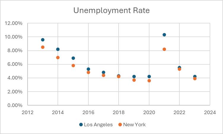
6.0 LIMITATIONS AND POLICY IMPLICATIONS
The limitations of the data in this study are relatively small. All data was gathered from the U.S. Census Bureau and U.S. Labor of Statistics, which are both reputable sources. However, the significance of the variables that were included in this study were not as high as we would have liked. Examining previous research leads us to believe that
Figure
Empirical Economic Bulletin, Vol. 17 85
there should be stronger significance between the structural issues of poverty, unemployment, the Case Shiller Index, national health expenditures per capita and homeless rates. However, the causes of homelessness can be extremely complex with a multitude of variables that are hard to track. As a result, the conclusions we draw from this data may not be as accurate as we would like them to be.
The policy implications for this study are simple yet hard to put into action. Possibly the most important is a need for policies that help lower housing prices. The housing market right now is terribly inflated due to strict zoning laws that make it hard for more houses to be built. These laws need to be repealed in order to allow more construction and at a greater density. Far too many cities continue to build sprawled out, suburban homes that end up having exceedingly high prices. Apartment buildings are not only low cost to build but also sustainable as the U.S. population continues to grow. Above all else, a decrease in price of low cost housing would help millions of Americans find shelter and make the homeless crisis much better.
Another policy recommendation that would help decrease the chronic homelessness crisis is a better safety net for those in need. This is a broad recommendation, but valid nonetheless. As our data shows, Hispanics and African Americans are overrepresented in the homeless population. The welfare programs that we have in place are weak, unorganized, and ineffective. They often have stringent work requirements in order for people to receive benefits. This can be an unrealistic demand for those who are struggling to find housing, let alone a job. To make matters worse, welfare can sometimes discourage work by giving better benefits to those without jobs. Once someone has a high enough income, benefits can abruptly stop, making the proposition of going without work more appealing.
Finally, homelessness is not only an economic problem but a humanitarian one as well. As mentioned previously in the paper, an increase in the number of chronically homeless hurts not only those individual American citizens but our society as a whole Homeless people are far more likely to have mental disorders, substance abuse, have diseases and commit crimes. Countless previous studies that turning a blind eye to this problem will only make it worse over time as those experiencing homelessness now are far more likely to experience it again.
Empirical Economic Bulletin, Vol. 17 86
7.0 CONCLUSION
In summary, this study investigates the correlation between several economic indicators and chronic homeless rates in the United States. We gathered data from twenty different cities across the U.S. using the Case Shiller Index. Our results show a strong correlation between minorities, in specific African Americans and Hispanics, and homelessness. While our data does not show significance among many of our variables, it is still a strong base for other researchers to use. More importantly, policy makers should use studies like this to pass new laws. Housing restrictions need to be reduced in order to increase the number of houses built and their density. Programs that help groups at risk of homelessness should receive more funding and care. Lastly, we should view chronic homelessness as a national emergency that can and will negatively affect us all.
Empirical Economic Bulletin, Vol. 17 87
Appendix
A: Variable Description and Data Source
Acronym Description
Homeless The total population of homeless in a city at a given time
CSI Measures the changes in the sale prices of singlefamily homes in twenty cities across the U.S.
NHE The amount of money spent on health care and related activities per capita
Poverty The ratio of people living under the poverty line at any given time
Unemployment The number of unemployed people as a percentage of the work force
Demographics The ethnic makeup of the homeless population, in this case Hispanics and African Americans
Data source
US Census Bureau
Case Shiller Index
US Bureau of Labor Statistics
US Bureau of Labor Statistics
US Bureau of Labor Statistics
US Census
Appendix B- Variables and Expected Signs
Empirical Economic Bulletin, Vol. 17 88
CSI Changes in sale prices of homes across the country
Relative capital cost (c1/c2)
Relative labor cost (w1/w2)
Unemployment
GDP times neighbor’s investment
Demographics Change in Exchange rate (∆e)
Expected
Acronym Variable Description
sign
+
NHE
+
Poverty
+
+
+ Empirical Economic Bulletin, Vol. 17 89
BIBLIOGRAPHY
About Us. Commonwealth Fund. (n.d.). https://www.commonwealthfund.org/about-us
American Psychological Association. (n.d.). Apa PsycNet. American Psychological Association. https://psycnet.apa.org/record/1991-27186-001
Author links open overlay panelJoanne Neale, Highlights•Patterns of substance use amongst people who are homeless are varied and changeable.•Men, & AbstractBackgroundPeople who are homeless and using substances frequently encounter barriers to accessing support. This paper aims to inform policy and practice by analysing changes in the tobacco. (2022, August 3). Substance use and homelessness: A longitudinal interview study conducted during COVID-19 with implications for policy and Practice. International Journal of Drug Policy. https://www.sciencedirect.com/science/article/pii/S0955395922002341
Baggett, T. P., Hwang, S. W., O’Connell, J. J., Porneala, B. C., Stringfellow, E. J., Orav, E. J., Singer, D. E., & Rigotti, N. A. (2013, February 11). Mortality among homeless adults in Boston: Shifts in causes of death over a 15-year period. JAMA internal medicine. https://www.ncbi.nlm.nih.gov/pmc/articles/PMC3713619/
By: Mark Saldua. (n.d.). Addressing social determinants of health among individuals experiencing homelessness. SAMHSA. https://www.samhsa.gov/blog/addressing-socialdeterminants-health-among-individuals-experiencinghomelessness#:~:text=21%20percent%20of%20individuals%20experiencing,having%20a %20substance%20use%20disorder.
Economic and noneconomic factors influencing ... (n.d.-a). https://onlinelibrary.wiley.com/doi/abs/10.1111/ajes.12320
Heston, T. F. (2023, October 13). The cost of living index as a primary driver of homelessness in the United States: A cross-state analysis. Cureus.
https://www.ncbi.nlm.nih.gov/pmc/articles/PMC10574586/
Empirical Economic Bulletin, Vol. 17 90
Homelessness and employment. (n.d.-b). https://socialinnovation.usc.edu/wpcontent/uploads/2020/08/Homelessness-and-Employment.pdf
HPRI. (2024, March 27). https://hpri.usc.edu/
The long-term effects of homelessness on children. (n.d.-c).
https://legislature.vermont.gov/Documents/2014/WorkGroups/Vermont Child Poverty Council/Reports and Resources/W~Homelessness~The Long-term effects of Homelessness on Children-January 2007~10-31-2013.pdf
Navigating homelessness: The effect of housing navigation centers on recidivism. Federation of American Scientists. (2023, June 12). https://fas.org/publication/navigating-homelessnessthe-effect-of-housing-navigation-centers-on-recidivism/
NE;, C. M. H. K. (n.d.). Life shocks and homelessness. Demography. https://pubmed.ncbi.nlm.nih.gov/23868747/
Richard J. Cebula & Gigi M. Alexander. (1970a, January 1). Economic and noneconomic factors influencing geographic diff. American Journal of Economics and Sociology. https://ideas.repec.org/a/bla/ajecsc/v79y2020i2p511-540.html
Richard J. Cebula & Gigi M. Alexander. (1970b, January 1). Economic and noneconomic factors influencing geographic diff. American Journal of Economics and Sociology. https://ideas.repec.org/a/bla/ajecsc/v79y2020i2p511-540.html
S;, G. S. S. K. (n.d.-a). The prevalence of mental disorders among homeless people in highincome countries: An updated systematic review and meta-regression analysis. PLoS medicine. https://pubmed.ncbi.nlm.nih.gov/34424908/
S;, G. S. S. K. (n.d.-b). The prevalence of mental disorders among homeless people in highincome countries: An updated systematic review and meta-regression analysis. PLoS medicine. https://pubmed.ncbi.nlm.nih.gov/34424908/
Empirical Economic Bulletin, Vol. 17 91
State of Homelessness: 2023 edition. National Alliance to End Homelessness. (2024, January 6). https://endhomelessness.org/homelessness-in-america/homelessness-statistics/state-ofhomelessness/#key-facts
Substance abuse and homelessness: Statistics and rehab treatment. American Addiction Centers. (2024, February 7). https://americanaddictioncenters.org/rehab-guide/homeless
Watts, G. R. (2021, November 1). Homelessness is an ethical issue in America. Journal of Ethics
| American Medical Association. https://journalofethics.ama-assn.org/article/homelessnessethical-issue-america/2021-
11#:~:text=Homelessness%20as%20a%20Health%20Hazard&text=Chronic%20conditions %2C%20such%20as%20diabetes,than%206%20times%20as%20prevalent.
Empirical Economic Bulletin, Vol. 17 92
SHIFTING THE ICE: Analyzing the Impact of the 2013
NHL CBA to the Competitive Balance of the
League
Ryan Lacya
Abstract:
This paper investigates whether the 2013 National Hockey League (NHL) Collective Bargaining Agreement (CBA), which hardened the existing salary cap, increased team revenue sharing, and instituted additional restrictions on player contracts, results in a more competitively balanced league. The study incorporates an OLS regression and Quantile regression to examine the impact of the 2013 CBA on the competitive balance of the league. The results show that the changes allow for a dispersion of talent, specifically offensive talent, and demonstrated a positive relationship between spending and points obtained by teams in the top 25% of the league. Conversely, teams that did not spend (bottom 25%) had a negative correlation.
JEL Classification: D21, L83, J53
Keywords: National Hockey League, Competitive Balance, Collective Bargaining Agreement, and Salary Cap
a Department of Economics, Bryant University, 1150 Douglas Pike, Smithfield, RI 02917. Phone: (508) 431-5198. Email: rlacy@bryant.edu
Empirical Economic Bulletin, Vol. 17 93
1.0 INTRODUCTION:
For decades, dynasties ruled professional sports in the United States. The New York Yankees ruled Major League Baseball with 27 world championships. The Celtics and Laker combined for 34 NBA championships (17 apiece), which is over 46% of all of the NBA championships. Last, but not least, the Montreal Canadians lorded over the National Hockey League winning 24 Stanley Cup titles in their franchise history. Competitive balance in sports leagues is a measure of league parity, a condition of being equal and fair in a contest, where fans of the league believe that the outcome of each contest is unpredictable, and not predetermined because of disparate talent between the teams (Alwell, 2020). According to prior research, predictability tends to reduce attendance because fans take a greater interest when the outcome of games is uncertain (Lee, 2020). As such, league commissioners strive to increase competitive balance in their leagues as it keeps players and fans consistently engaged over the course of an entire season (Alwell, 2020). This paper will analyze whether the changes implemented by the NHL in the 2013 Collective Bargaining Agreement, which has been extended through a 2022 Memorandum of Understanding through league year 2026, has resulted in a more competitively balanced NHL league.
This paper differs from other studies because it analyzes whether the changes as incorporated in the 2013 NHL Collective Bargaining Agreement, which hardened the existing salary cap, increased team revenue sharing, and instituted additional restrictions on player contracts, resulted in a more competitively balanced league. Through a regression analysis and quantile analysis with multiple variables, including team winning percentage, payroll/league average payroll, team goals for/league average goals for, team goals against/league average goals against, and playoff appearances, this paper will analyze the impact those changes had on the competitiveness of the league. There is very little empirical work in the literature concentrating on the latest changes to the NHL CBA, and its impact on the competitiveness of the league, so this paper successfully fills this void.
The rest of the paper is organized as follows: Section 2 gives a brief discussion regarding trends. Section 3 provides a literature review. Section 4 outlines the empirical mode and discusses the data and methodology used. Section 5 presents and discusses the empirical results, and section 6 features the conclusion.
Empirical Economic Bulletin, Vol. 17 94
2.0 TRENDS:
The success of a professional sports league rests on its competitive balance because a level playing field creates uncertainty in the outcome of the game, driving engagement, attendance, viewership, and fan passion. The uncertainty of outcomes in sports is commonly referred to as competitive balance because predictability tends to reduce attendance as fans take a greater interest when the outcome of games is uncertain (Lee, 2020). Competitive balance in a sports league can be described as the distribution of wins in a league; and leagues that have a more even distribution of wins among its teams are said to be more competitively balanced (Woltring, 2015), but in essence it is that uncertainty of outcome that defines an exciting sporting event between two evenly matched teams. Without fans, sports leagues do not thrive financially, and fans will not attend if they perceive a significant competitive imbalance between the two teams.
Sports history has shown this to be true, as evidenced by the declining attendance at New York Yankee games, a team in the middle of a dynastic run from 1950 to 1958. During those nine seasons, the Yankees won eight (8) American League pennants, and six (6) World Series Championship, and yet the team saw a 31% decrease in attendance. Similarly, the American League saw a decrease in attendance over the same time frame, even though attendance was up year over year in the more competitively balanced National League as shown in the Figure below.
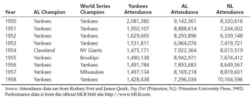
Fan perception was that the Yankees were far superior to the rest of the American League, so the outcome of the games was predetermined, and fans adjusted accordingly, which negatively impacted the Yankees’ financially.
Empirical Economic Bulletin, Vol. 17 95
Leading into the 2004-05 season, the NHL faced a crisis that affected both the financial viability and competitive balance of the league. By 2004, average salaries in the NHL had almost tripled since the 1993-94 season, however revenues had not kept pace causing substantial league wide losses, as confirmed by two different studies that analyzed the profitability of the NHL. Although each report, one by Arthur Levitt and the other by Forbes, disagreed on certain creative accounting by select owners, both reports confirmed that a majority of teams were losing money on an annual basis (Grant, 2008). Moreover, attendance was at a four-year low and five televised games of the Stanley Cup finals between the Tampa Bay Lightning and the Calgary Flames averaged a lowly 2.6 on the Nielsen scale, making the series the 19th most-watched network television program that week. Put simply, NHL hockey was losing its place among the four major sports leagues in terms of fan/viewership interest (Brinkman, 2006). Unsurprisingly, in this difficult economic environment, team owners in the non-traditional, small market, Sun Belt cities such as Nashville, Charlotte, and Atlanta, where the NHL had aggressively expanded during the 1990’s, were claiming a lack of competitive balance, in part, because the League economics, from their perspective, made it impossible for their front offices to compete for top free agents and subsequently assemble a competitive team, which directly and negatively impacted attendance and decreasing revenues (Brinkman, 2006). With the NHL losing money, the owners locked out the players prior to the 2004-05 season and became the first major professional sports league to lose an entire season due to labor strife, but the owners sought cost certainty above all else, and the 2005 Collective Bargaining Agreement (CBA) reflected it.
NHL Owners locked out the players
NHL became the first professional sports league to lose an entire season to labor dispute.
2005 NHL Collective Bargaining Agreement
Salary Cap
Adopted hard salary cap for the first time
Contracts
24% reduction in all player contracts
Revenue Sharing
Implemented Revenue Sharing
Although the NHL took several measures to ensure that teams could not cheat or circumvent the salary cap through side deals with players including the provisions of gifts, or
Empirical Economic Bulletin, Vol. 17 96
payment for endorsement deals, there were player contracts entered into between 2005 and 2012 that frustrated the intent of the hard salary cap, and necessitated additional changes to the cap, player contracts, and revenue sharing, which are evidenced in the 2013 CBA Agreement. The easiest way to circumvent the salary cap imposed via the 2005 CBA was through long-term contracts, which spread out the value of a player’s salary over an incredibly long period of time, and many of those contracts also had huge variances year to year to mitigate the impact of player’s salary on the salary cap in any particular year. As a result, there was a much shorter lockout leading into the 2012-13 season, which resulted in additional changes as summarized below. The key significant changes in the 2013 CBA include the following:
• Contract salary variance is capped at 35 percent from year to year, with the provision that the last year cannot vary more than 50 percent from the highest-salaried year.
• The "Roberto Luongo Rule," in which teams that had issued and were paying out those circumventing contracts would be punished through "recapture" penalties.
• Contract term limits, as teams could re-sign their own players to a maximum of eight years and sign free agents to a max of seven years.
• The ability to retain salary in trades, which changed the transactions market.
• Players’ share of hockey related revenue fell from 57% to a 50/50 split in revenue between players and owners.
• As it relates to the league's payroll cap, the cap was set at $60 million for the 2012-13 season though teams could spend up to $70.2 million in the transition period. The payroll floor was set at $44 million. For the 2013-14 season, the cap was set at $64.3 million while the floor remained at $44 million.
• Revenue sharing spread an additional $200 million among lower revenue generating teams, with a $60 million NHLPA-initiated growth fund included. (Riche, 2013)
Unlike after the canceled 2004-05 season, the fans returned quickly when the 2012-13 lockout ended, and by the end of the decade, revenues continued to climb, and the salary cap had gone from $64.3 million in 2013 to $81.5 million by 2019 (Brinkman, 2006). From a perspective of the financial viability of the League, the 2013 CBA appears to have dramatically helped stabilize the financial issues that led to the 2004-05 season lockout, but this paper will analyze whether it also resulted in a more competitively balanced league.
3.0 LITERATURE REVIEW:
Since many professional sports leagues utilize a salary cap, there have been studies that have analyzed the competitive balance of all four major professional sports leagues in the United States (MLB, NFL, NBA, and NHL) to determine which are more competitively balanced.
Mitchell Woltring used the Generalizability Theory to analyze levels of competitive balance in
Empirical Economic Bulletin, Vol. 17 97
each of the four major professional sports leagues in North America (MLB, NBA, NFL, and NHL) over a 10-year period from 2005-2014, utilizing win/loss data, and concluded that NFL and NHL leagues were more competitively balanced than MLB and NBA leagues (Woltring, 2015). Similarly, another study analyzed multiple professional sports leagues in United States to determine if the NBA league was the most unbalanced from a competitive standpoint (Alwell, 2020). Through computation of several different models based on winning percentage, transitional properties, championships, and league measures, the author concluded that the National Basketball Association has less levels of parity both in the short term and over the course of history than other American professional sports leagues (Alwell, 2020). Likewise, a study has analyzed the four major professional leagues to determine if pay inequalities affected team performances (Frick et al., 2003). Frick, Prinz, and Winkelmann's study used data (winning percentage and wage disparity by roster) from sixteen consecutive seasons beginning in 1988, and found that among the four major professionals sports leagues, in the NHL, a team is more successful as the pay distribution becomes more unequal over those sixteen seasons (Frick et al., 2003). The study confirmed the importance of elite, top-end talent to the team success in the NHL, "This implies that a single 'star- player' may be of paramount importance for the team's performance - which, in turn will lead to a highly skewed distribution of player salaries without negatively affecting the performance of those at the lower end of the pay hierarchy" (Frick et al., 2003).
There are also studies that have narrowly focused on the NHL and analyzed the impact on the competitive balance of the NHL as a result of a range of factors, such as the introduction of free agency, salary cap, revenue sharing, salary distribution and impact of foreign imported players. In the National Hockey League, unrestricted free agency was introduced in 1995 and a hard salary cap was introduced in 2005. A study analyzed how each affected the competitive balance of the league after being introduced into the league (Lee, 2020). For purposes of that study, competitive balance was correlated to current and prior years’ winning percentages (Lee, 2020). The author concluded that unrestricted free agency had a minimal impact on increasing the competitive balance of the league, but that the implementation of a hard salary cap in the NHL increased competitiveness (Lee, 2020).
Likewise, another study analyzed the impact of the implementation of a hard salary cap in the NHL to the competitiveness of the league and team revenues (Grossman, 2010). The data
Empirical Economic Bulletin, Vol. 17 98
supported the conclusion that team revenues, especially for teams that had smaller attendance numbers or expansion teams, benefited from the hard salary cap, but that the data was not conclusive that the salary cap had a significant impact on improving the competitive balance of the league (Grossman, 2010). Another study analyzed whether the implementation of a salary cap resulted in the redistribution of top talent, which positively impacted the competitive balance of the league (Grant, 2008). This study used an adjusted measure of team standard deviation of win percentage and concluded that the presence of top talent and median salary were found to be the primary determinants of team success, and further concluded that the implementation of a salary cap changed the competitive balance in the NHL, through a redistribution of top ranked talent (Grant, 2008).
Whereas prior studies analyzed the impact of a salary cap on the competitiveness of the NHL, another study analyzed the impact of revenue sharing on the competitive balance of the league (Brinkman, 2006). Brinkman analyzed team payroll and performance to determine if mathematically, using ordinary least squares regression, there was a link between team revenue/payroll and team performance (Brinkman, 2006). After analyzing the team point totals for each year from 1994-2004 in relation to team’s payroll, Brinkman concluded that “a team’s ability to compete on the ice had relatively little to do with how liberal they were with the pocketbook. Indeed, not even a league-high payroll nearly two times the league average could save the 2003-04 New York Rangers from winning a mere 32.9 percent of their contests that year” (Brinkman, 2006).
In examining the effect of a star player, who typically has a higher salary, on team performance, a study examined the relationship between salary distribution and team performance using four completed seasons (2000-01 to 2003-04) of the National Hockey League (Marchand et al., 2006). The authors concluded that buying a key player (superstar) or two-top talents at a high salary produces better results according to the measures of team performance, rather than a more balanced salary distribution among non-superstar (journeyman) players (Marchand et al., 2006). As this study was done prior to the implementation of the hard salary cap in the NHL, it did not consider how a hard salary cap can impact the unequal distribution of salary in relation to roster construction, which can have an impact on competitive balance.
Lastly, in analyzing the NHL from a competitive standpoint, another study did not analyze structural changes relating to how the league and teams operate, such as a salary cap or
Empirical Economic Bulletin, Vol. 17 99
revenue sharing, but focused on the players themselves. It analyzed the impact of rookies and imported players, meaning players that played in foreign leagues who then decided to join the NHL as free agents, on the competitive balance of the league (Finn et al., 2005). The authors found that the pool of rookies had no significant impact on competitive balance, but that the talent pool of imported players did have an impact on competitive balance. Since the study only analyzed data from games that pre-dated the first Collective Bargaining Agreement, which altered free agency and implemented a salary cap, there was no salary cap or limitations on foreign imported players during the data set, so whether imported players have the same impact now remains unclear (Finn et al., 2005).
Because of free agent contracts that circumvented the terms and intent of the salary cap provisions that were included in the 2005 CBA, new provisions were added and incorporated into the 2013 CBA that hardened the salary cap more, incorporated more restrictive terms in free agent player contracts, increased team revenue sharing, and made other adjustments to further try to increase parity among the teams and improve the financial health of the league. As noted in other studies, the fans returned quickly when the 2012-13 lockout ended, and by the end of the decade, revenues continued to climb, and the salary cap had gone from $64.3 million in 2013 to $81.5 million by 2019 (Brinkman, 2006). From a perspective of the financial viability of the League, the 2013 CBA appears to have helped stabilize the financial issues that led to the 200405 season lockout, but have the changes incorporated into the 2013 CBA resulted in a more competitively balanced league?
4.0 DATA AND EMPIRICAL METHODOLOGY
4.1
DATA
The study uses including team winning percentage, payroll/league average payroll, team goals for/league average goals for, team goals against/league average goals against, and playoff appearances, from the following NHL seasons: 1999-2000 to 2003-2004 (pre-2005 CBA and the implementation of the first NHL salary cap); 2005-06 to 2010-11 (2005 CBA); and 2013-14 to 2022-23 (2013 CBA). Hockey Reference provided historical data from 1999-2023 for all NHL Teams. Additionally, contract data was provided from Hockey Zone from 1999 - 2000, USA Today Database from 2000-2008 and Spotrac from 2011 – 2023. With respect to data limitations, there is a gap in the data as the 2009 and 2010 seasons did not have publicly available contract data, and the 2012, 2018, 2019 seasons were shortened due to the 2012 lockout and COVID-19
Empirical Economic Bulletin, Vol. 17 100
Pandemic. Please see Appendixes A (Descriptive Statistics), B (OLS Regression) and C (Quantile Regression) included at the end of the paper.
4.2 EMPIRICAL MODEL
Similar to Alwell (2020) the subject study evaluated the competitive balance across the NHL by comparing the teams against each other using the standard deviation of win percentage to discern impact. Likewise, this study adapted and modified the impact of revenue sharing and money spent by teams in the NHL between small and big market teams through payroll spent compared to the league average, similar to the methodology used in Brinkman (2006). The subject paper added three independent variables to the combined model as utilized by Alwell and Brinkman including: goals against per team divided by league average goals against, severity of salary cap limitations/restrictions, and playoffs.
In summary, the subject study utilizes a regression analysis and quantile analysis to determine if the 2013 CBA resulted in a more competitively balanced NHL league, factoring the following variables: team winning percentage, payroll/league average payroll, team goals for/league average goals for, team goals against/league average goals against, and team playoff appearances for the NHL seasons analyzed. The modeling formula can be expressed as follows:
ExPo = β0+β1playoffs+ β2 sevsalcap + β3goalsf + β4goalsa+ β5paylg + β6winp + ε
Independent variables consist of six variables obtained from various sources. First, winp represents the winning percentage of each team. Second, paylg is the payroll spent by team divided by the league average payroll. Third, goalsf is the goals for divided by the league average goals for. Fourth, goalsa is the goals against divided by the league average goals against. Fifth, sevsalcap is a dummy variable representing the severity of the salary cap with one assigned to years with a salary cap and zero assigned to years without a salary cap denoting the increase in talent dispersion amongst the teams. Sixth, playoffs is a dummy variable with one assigned to teams that made the playoffs and zero assigned to teams that did not make the playoffs. The dependent variable, ExPo, represents the expected points by team which is how they determine who makes the playoffs. See table below.
Empirical Economic Bulletin, Vol. 17 101
ExPo
Expected Points (Points are a combination of wins and overtime losses)
Playoffs Dummy Variable (1, if they made playoffs; 0, if they missed playoffs)
Sevsalcap Dummy Variable (1, if the league played with a salary cap; 0, if the league did not)
Goalsf Goals for per game divided by league average goals per game
Goalsa Goals allowed per game divided by league average goals allowed per game
Paylg Team salary cap spent divided by league higher limit salary cap (for the years without a salary cap the league average salary cap spent was used as the denominator)
Winp Win Percentage (%)
5.0 EMPIRICAL RESULTS
As shown in the OLS Regression, found in Appendix B, the results indicated that all control variables are statistically significant at the 95% level except playoffs. Additionally, the severity of the salary cap variable (Sevsalcap) has a negative relationship with points, which demonstrates that with a salary cap there is a dispersion of talent amongst the teams as, theoretically, teams cannot keep all of their superstars and still be cap compliant, resulting in decreased points per team. The OLS regression all shows a negative relationship between spending and points. The difference between the OLS regression and the Quantile Regression, which is shown in Appendix C, are the fluctuations in the R2 value as the OLS is more in line with the 75th quantile regression (the top 25% of teams) where those values were closer to 0.68 than the 25th and 50th quantile regression which were both below with an R2 value of 0.46 and 0.62 respectively. This cause could be due in part to certain teams from the middle or bottom 25% relocating, like the Atlanta Thrashers who relocated and became the Winnipeg Jets at the beginning of the 2011 season. The relocation of a team can impact the spending of that team on re-signing players and/or aggressively signing free agents. Additionally, the bottom 25% of teams relative to spending had increased fluctuation and volatility related to wins, in part because lower revenue teams cannot overcome signing a player to an expensive contract, who then underperforms or is injured for an extended period-of-time, without it affecting the year-to-year success.
Empirical Economic Bulletin, Vol. 17 102
Likewise, regarding the results of the Quantile regression, the largest negative relationship exists between points and salary cap spending amongst the bottom 25% of the teams, as these are the smaller to mid-market teams that have the most variance in terms of yearover-year spending and success. The Quantile regression also shows the flaw in the salary cap as the top revenue generated teams who routinely spend at the cap or go over the supposed “hardcap limit” through creative designations like Long Term Injured Reserve (LITR) are the teams primarily in big hockey markets (Boston, New York, Montreal, etc.). Teams in the bottom 25% of spending lost more, so theoretically, those teams should have had higher draft positions, since the NHL operates arranges the draft order in reverse (with the five teams with the fewest points entering a lottery for the number one selection) so those GMs had opportunities to draft young elite talent in the draft, which should impact the team’s win totals. Although each draft may not contain a generational talent (i.e., Gretzky, Bourque, or McDavid) most drafts do have impactful elite players that should have a positive impact on wins. The data demonstrated a positive correlation among teams in the top 25% of spending with wins, but additional research might be needed to analyze the effect of how General Managers (GM) are spending the money and drafting talent, and how teams used LITR designations to exceed the hard limit of the salary cap.
6.0 CONCLUSION
In a league that is competitively balanced, there should be an uncertainty of outcomes that will result in some fluctuations among teams’ winning percentages over time as some teams get better and others get worse. As such, do the changes made in the 2013 NHL CBA positively impact the league’s competitive balance? Yes. The implementation of a more nuanced salary cap and other changes balances the league and allows for a dispersion of talent, specifically the offensive talent as goals per game trended upwards during the timeframe. However, it should be noted that teams showed a willingness to spend provided the success offsets the cost of winning, as demonstrated by the positive relationship between spending and points obtained by teams in the top 25% of the league. Teams in the top 25% in spending obtained more wins. Conversely, teams that did not spend (bottom 25%) had a negative correlation. As such, lower revenue producing teams, which do not spend as much, may still not be as competitive as teams with more resources, which may explain why the NHL recently approved the sale and relocation of the Arizona Coyotes, which will be relocated to Salt Lake City, Utah, in the hopes of revitalizing the franchise.
Empirical Economic Bulletin, Vol. 17 103
Since certain teams historically struggle, additional research is needed to determine if it is because of an ineffectual scouting department and General Manager that cannot identify talented NHL players or whether the owner is more focused on receiving his share of the revenue sharing provided for under the 2013 CBA terms rather than being committed to creating a winning program, by spending on players or scouting. Also, the League responded to attempts by teams to circumvent the provisions of the 2005 CBA with the changes instituted in the 2013 CBA, but given the use of LITR designations, which have benefitted higher revenue teams and allowed certain teams to exploit the rules and exceed the hard limit of the salary cap, the NHL may need to install additional restrictions regarding LITR designations when the current CBA expires in 2026. As such, although the changes made in the 2013 NHL CBA positively impacted the league’s competitive balance, the League may still need to take additional steps in the future to help level the playing ice and ensure competitive balance for all 32 NHL teams.
Empirical Economic Bulletin, Vol. 17 104
APPENDIX A DESCRIPTIVE STATISTICS
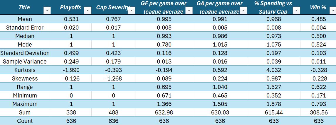
Empirical Economic Bulletin, Vol. 17 105
APPENDIX B OLS REGRESSION
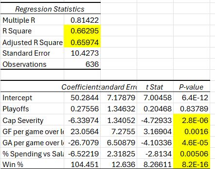
Empirical Economic Bulletin, Vol. 17 106
APPENDIX C QUANTILE REGRESSIONS
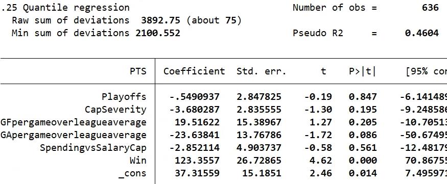
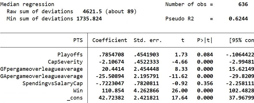
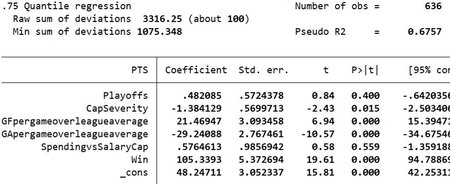
Empirical Economic Bulletin, Vol. 17 107
BIBLIOGRAPHY
Alwell, Kevin, "Analyzing Competitive Balance in Professional Sport" (2020). Honors Scholar Theses. 650. https://opencommons.uconn.edu/srhonors_theses/650
Brinkman, Taylor, “Sharing the Wealth in the “New NHL”: The Implications of Revenue Sharing for Competitive Balance, Payroll Spending, and Profits” (2006). Vanderbilt Undergraduate Research Journal, Volume 2, Number 1, 1-16.
Collective Bargaining Agreement Between NHL and NHLPA, Article 49.1k, July 22, 2005.
Collective Bargaining Agreement Between NHL and NHLPA, September 16, 2012.
Fenn, A et al., “The Influence of Structural Changes and International Players on Competitive Balance in the NHL” (2005). Atlantic Economic Journal, 33, 215-224.
Fort, Rodney; Maxcy, Joel, “Competitive Balance in Sports Leagues: An Introduction” (2003). Journal of Sports Economics, 4(2), 154-60.
Frick, B et al., “Pay Inequalities and Team Performance: Empirical Evidence from the North American Leagues” (2003). International Journal of Manpower, 24(4), 472-488.
Grant, M, “Competitive Balance in the National Hockey League after the Salary Cap” (2008). Undergraduate Thesis Colorado College Research Journal.
Grossman, Lauren, "Microeconomic Study of a Labor Union: An Econometrics Analysis of how the NHL Salary Cap has Affected the Competitive Balance of the NHL and Determinants of Team Revenue" (2010). Undergraduate Theses and Capstone Projects. 69. https://digitalshowcase.lynchburg.edu/utcp/69
Hockey-Reference. (2024). Schedule and Results 1999-2023. Retrieved from https://www.hockey-reference.com/
Hockey Zone Plus. (2024). Team Contract and Salary Data 1999-2000. Retrieved from https://hockeyzoneplus.com/
Lee, Travis, “Competitive Balance in the National Hockey League after Unrestricted Free Agency and the Salary Cap” (2020). MPRA, https://mpra.ub.uni-muenchen.de/108400/
Marchand, Joseph et al., “Salary Distribution and Performance: Evidence from the National Hockey League” (2006). Center for Policy Research, Maxwell School of Citizenship and Public Affairs, 1-25.
Memorandum of Understanding between National Hockey League and National Hockey League Players’ Association, July 10, 2010.
Riche, P. (2013, January 6) NHL Owners, Players, Score New CBA Saving the 2013 Hockey Season. Forbes. Retrieved from https://www.forbes.com/sites/prishe/2013/01/06/nhl-ownersplayers-score-new-cba-saving-the-2012-13-hockey-season/?sh=29f8f7b45385
Empirical Economic Bulletin, Vol. 17 108
Spence, R. (2008, August 31) MLB and NHL: Top and Bottom Team Salaries. Crashing the Goalie. Retrieved from https://crashingthegoalie.wordpress.com/2008/11/04/no-limits-to-mlbsalaries/
Spotrac. (2024). Team Salaries and Contract Data 2011-2023. Retrieved from https://www.spotrac.com/
Totty, Evan; Owens, Mark, “Salary Caps and Competitive Balance in Professional Sports Leagues” (2011). Journal for Economic Educators, Volume 11, No. 2.
USA Today (2024). Team Salaries and Contract Data, 2000-2008. Retrieved from https://www.usatoday.com/sports/nhl/
Woltring, M.T. (2015). Examining Competitive Balance in North American Professional Sports Using Generalizability Theory: A Comparison of the Big Four [Doctoral dissertation, Middle Tennessee State University].
Zimbalist, Andrew, “Competitive Balance in Professional Sports Leagues: An Introduction” (2002). Journal of Sports Economics, 4(2), 111-21.
Zimbalist, Andrew, “Reflections on salary shares and salary caps” (2010). Journal of Sports Economics, 11(1), 17-28.
Empirical Economic Bulletin, Vol. 17 109
How UNSDGs are Reflected in Folklore
Jacob Mann
Abstract:
This paper investigates the relationship between the United Nation’s Sustainable Development Goals in a country and the prevalence of those goals in that country’s folklore. The study incorporates folklore collected into an aspect-based sentiment analyzer to examine the prevalence of, and attitude towards various aspects of the text A combination of ConceptNet and the widely available Natural Language Toolkit is implemented to retrieve polarity scores related to key aspects of the texts. The results indicate that there are correlations between the attitude towards a theme in folklore, and the attitudes towards that theme in a country.
JEL Classification: Z11
Keywords: Literature, Machine Learning, Preference a Department of Economics, Bryant University, 1150 Douglas Pike, Smithfield, RI02917. Phone: (401) 767 0671. Email: jacobmann@hotmail.co.uk
Empirical Economic Bulletin, Vol. 17 110
INTRODUCTION
The factors that determine preference are multifaceted, yet culture plays a huge role; and little is a better reflection of culture than its folklore. Folklore: the stories and parables withing a society that prevail through time, typically through word of mouth. These stories have been passed down until collected and are therefore assumed to have survived due to a relationship to the lives of the people who tell them, in a climate of a naturally selective process of story extinction. This paper aims to explore the idea that the attitudes and culture of society is reflected in its literature, and therefore the societies preferences are also reflected.
To explore the relationship between preference and language, modern developments offer Aspect- Based Sentiment Analysis. This paper aims to use this machine learning approach to retrieve numerical values of the positive or negative sentiment towards various key aspects of society. It is in this respect that this paper differs; while sentiment analysis techniques have been used on literature before, it is new that aspect- based sentiment analysis is being used to compare to attitudes of the literature towards an aspect to the apparent attitudes of the nation of origin. These aspects are selected from a subset of the United Nations Sustainable Development Goals, a set of seventeen aims that target long term national health, for all countries.
The rest of the paper is organized as follows: Section 1 gives a brief review of the modern state of SDGs in the target countries, Section 2 offers a review of the literature that was relevant to the field or creation of this paper, Section 3 outlines the data and empirical model. Section 4 goes on to present and discuss the results, which is followed by a conclusion in section 5.
Empirical Economic Bulletin, Vol. 17 111
1.0 TREND OF MODERN SDGs
The SDGs of the UN into improve the most important aspects of social and global health within a country, by targeting specific areas of a country’s performance. These include the most important areas of life in the modern day, such as the provisions of food, water, education, and the responsible use of natural resources. For this paper a sample of 6 SDGs were chosen as the focus of the technical analysis. To compare the results of the technical analysis with their reflections in reality, the current state of each SDG must be understood in each respective country, so that a comprehensive and informed expectation can be formed of the aspect- based sentiment analysis results
The six SDGs that were the focus of the paper are respectively titled ‘no poverty’, ‘zero hunger’, ‘good health and well-being’, ‘quality education’, ‘gender equality’, and ‘clean water and sanitation’. As part of the release documentation about the SDG's, the UN also detailed world development indicators, and therefore specific variables, which reflect the progress of an SDG in a country. Order to judge the current state of the six sample SDGs in the relevant countries, six separate world development indicators were used, according to the direction of the UN. The summary of each country’s indicator is on Appendix B, and visualizations of two aspects of the data are shown in Figure 1 and Figure 2. Shown are the indicators of ‘Quality Education’ and ‘Clean Water and Sanitation’.
Empirical Economic Bulletin, Vol. 17 112
Figure 1: Educational attainment, (% of population that completed secondary education)
Educational attainment, at least completed upper secondary, population 25+, total (%)
People using safely managed drinking water services (% of population)
Data collected from World Bank, World Development Indicators
The above graphs and relevant data represent the wide differences in the countries analysed, with each SDG indicator being led by different countries, and the proficiency of each country also varying. With relation to poverty, for example, Greece, Italy, and Russia, should theoretically lead with the highest coefficients as they exhibit the strongest symptoms of poverty. This is expected to hold across the SDGs; countries with higher sympotms of modern struggle are expected to have higher scores in sentiment analysis due to the assumption that contributing factors to both will have remained constant due to the country acting as a controled system for each societal set- up. Furthermore, it would be expected that Russian and perhaps Italian
Figure 2: People using safely managed drinking water (% of population)
0 100
0 50 100 150
Empirical Economic Bulletin, Vol. 17 113
sentiment towards ‘Clean Water and Santiation’ would be more negative than other countries, and sentiment would be less positive towards ‘Quality Education’ in Italy and Greece.
2.0 LITERATURE REVIEW
The analysis of folklore is well documented in literature, the links between folklore and culture too. The idea that folklore reflects the culture it inhabits was detailed by Michalopoulos & Xue, 2021 who showed that proximity to a feature in life would increase the occurrence of that feature in Folklore. Using a model of ConceptNet for sentiment extraction, the paper showed the links between the prevalence of geographical features and their prevalence in literature, using an analysis that found the rate of a sentiment occurring, in the study ‘Folklore’. This study laid the foundation for this paper, even suggesting an ABSA approach in the conclusion. ‘Folklore’ was a study based on a dataset of folklore collected by Yuri Berezkin, a historian, who had collected the set from over 958 cultural groups globally. Furthermore, analysis conducted on the dataset by Berezkin showed the prevalence of various specific motifs in the literature, related to cultural events such as marriage. The relationship between literature and culture is the core of this study, and it successfully proves the links between the two.
The paper Automated Sentiment Analysis of Text Data with NLTK, by Jiawei Yao, 2019, details the model of NLTK, its implementation methods and performance. It begins by explaining the origins of NLTK, as a package released by Steven Bird and Edward Loper from the University of Pennsylvania. The paper then goes on to detail the steps in applying and using NLTK, as well as the way to visualize the data. Furthermore, the paper details CSV importation, something that was also massively useful. Also, the method of application of a public vector set is detailed, and
Empirical Economic Bulletin, Vol. 17 114
the advantages of this method. The paper also detailed the drawbacks of the NLTK method, which include a lack of word order importance, which decreases accuracy of this model.
Using a system in which a “vectorizer” and “classifier” were made using training, and then implemented into a model to perform sentiment analysis on tweets in Sentiment Analysis with NLP on Twitter Data, by Hasan and Maliha, 2019. The sentiment analysis performed provided higher accuracy than other models due to the specific training, and due to the specific nature of the data. Furthermore, this paper details the process of API implementation, web scraping, parsing and a bag of words model for sentiment analysis.
The United Nations Sustainable Development Goals are a collection of seventeen aims for countries to focus on in order to improve their long-term sustainability and health, created by the United Nations. First introduced in 2015 at the United Nations Sustainable Development Summit, the goals are the heart of the 2030 Agenda for Sustainable Development. These goals include a range of environmental, social, and economic aims, from gender equality to sustainable uses of land and natural resources.
ConceptNet is a group of weighted word embeddings, which connects words and phrases according to their varying weights to each other. Credited to ConceptNet 5.5: An Open
Multilingual Graph of General Knowledge by Speer et al, 2016, the vector set allows sentiment analysis models to perform more accurate analysis through the use of this more advanced vector set. The works by not only relating words that are similar in everyday for most common usage, but also by relating words to their other forms such as a verb to its infinitive or a single noun to a plural, as well as doing this across languages. This allowed the tested model to answer SAT analogy style questions with higher accuracy than any model prior. The implementation of this
Empirical Economic Bulletin, Vol. 17 115
vector set was crucial in this overall paper. Figure 3 is from the ConceptNet website and details the links in language provided by the vector set.
The Mythology Catalogue is an online resource of over 4,000 folktales gathered and published by Jon F White, from 2019 to 2022. Many come from books or other academic resources, while many come from Yuri Berezkin’s collected catalogue.

3.0 DATA AND EMPIRICAL METHODOLOGY
3.1 Data
The study uses a subset of data from Yuri Berezkin’s catalogue. Data was obtained from Mythologydatabase.com. A summary for the data is provided in Table 1, summary statistics on each country, how many lines and how many tales from each country were analyzed. Line count was pertinent, due to the nature of the model which requires tweet length, or at most sentence long, inputs to analyze. While the total number of lines analyzed was below optimal, data collection had to be done manually, which added a constraint.
Figure 3
Figure Obtained from ConceptNet Website
Empirical Economic Bulletin, Vol. 17 116
3.2 Empirical Model
Table 1 Summary Statistics
Textual data was extracted from ‘Folklore Database’ website and then put into an excel file. Use the ‘pandas’ library this data was extracted and used on a Jupiter notebook for sentiment analysis in Python. Pandas allows easy access of excel and other Microsoft files in a Python format, a library initially developed in 2008. The necessary sentence length constraint of the ABSA model, the data was Formatted into a table which could be read by pandas. To perform the aspect-based sentiment analysis, the natural language toolkit, NLTK, was implemented. The sentiment analyzer uses a VADER (Valence Aware Dictionary for Sentiment Reasoning), a process that uses lexicon and rule-based language processing to return a result of the sentiment of an aspect, based on a set of predetermined relationships between the aspects or tokens. In order to perform aspect-based sentiment analysis, ConceptNet was implemented. ConceptNet is a semantic network, which provides the links between words and phrases which allows the
Russia Germany Norway England Italy Netherlands Greece Japan Folklore 8 8 8 8 7 6 6 5 Lines 240 123 246 107 190 50 163 103
Empirical Economic Bulletin, Vol. 17 117
model to analyze the text with regard to not only the input aspects, but also the 50 most related terms, according to ConceptNet.
The method of retrieval for this was an API, which allowed the retrieval of related terms to any desired input aspects. To not exceed API retrieval limits, caching of the related terms was implemented. First the texts were tokenized, using the ‘sent-tokenize’ function. Then, sentiment was calculated using ‘SentimentIntensityAnalyzer’, which converts the sentiment score into a value from -1 to +1, with 0 representing no sentiment.
This returned the sentiment of each line of each text, which were then summed to give a value of sentiment towards an aspect. Both aspect sentiment value and aspect sentiment absolute value were used in analysis of results. In order to retrieve encompassing results that offer a truer reflection of the SDG prevalence in the folklore, 5 words were selected to represent each SDG as aspects. For ‘No Poverty’, the words selected were ‘Hunger’, ‘Starving’, ‘Underfed’, ‘Malnutrition’, ‘insecure’. The model produced aspect-based sentiment results for each line analyzed with regard to each word input as an aspect. Appendix A details each word used for each SDG. These were selected with an aim to both analyze sentiments of words relevant to the lexis of the folklore, and also that aligns with a compassion with modern SDG indicators.
4.0 EMPIRICAL RESULTS
The empirical results show varying sentiments by country and aspect, though inferences must be made on a case-by-case nature due to the limitations of the dataset. Correlations to modern data
Empirical Economic Bulletin, Vol. 17 118
are seen, however. Both the total aggregate sentiment results, and the adjusted results are shown in Tables 2 & 3. Adjusted results are obtained by dividing each sentiment by the number of lines that were analyzed for that sentiment, and then by multiplying by the average number of lines that were analyzed, 152.75. (Table 3)
Specific results show relationships between sentiments of ‘Clean Water and Sanitation’ and ‘Quality Education’ and the real progress of each country in this SDG. While it is inferred that there is a common causal element between the sentiment and modern results, analysis results showed to heavily weigh on the aspect inputs, showing a need for more data to be analyzed. This model has, however, demonstrated a model for future aspect- based sentiment analysis of folklore, with an aim to determining causality.
Another datum to be considered is the overall summation of the absolute values of sentiment. This returns a result that adds the strength of all sentiments, regardless of sentiment, to give a reflection of the strength of a sentiment in a culture. (Table 4) This can theoretically be correlated with the prevalence of an issue in a culture, and with a more encompassing data set this would be expected to be reflected. A comparison of sentiment strength to modern SDG indicators reveals only cursory correlations, but does provide a framework for future analysis.
Empirical Economic Bulletin, Vol. 17 119
Table 2: Aspect- Based Sentiment Analysis Summation Results
Table 3: Line Adjusted Aspect- Based Sentiment Results
Russia Germany Norway Netherlands England Japan Greece Italy No Poverty -2.35973 -3.87712 -0.61081 -1.98147 -0.68052 -4.23637 -1.0655 -1.2495 Zero Hunger 0.388876 -0.92755 -0.17107 0 0 1.3336710.46031 0 Good health and well being -2.35808 -1.97184 -5.39189 -0.79247 -1.97347 -1.245431.65982 0 Quality Education -0.18209 0.833233 1.371211 0 3.547369 1.464324 0 0.753419 Gender Equality -0.44488 2.379299 0 -4.95521 1.397448 00.81717 0.575787 Clean Water and Sanitation -0.9615 0.790947 1.726059 0 0 1.971513 0 0
Russia Germany Norway Netherlands England Japan Greece Italy No Poverty -3.7076 -3.122 -0.9837 -0.6486 -0.4767 -2.8566 -1.137 -1.5542 Zero Hunger 0.611 -0.7469 -0.2755 0 0 0.89930.4912 0 Good health and well being -3.705 -1.5878 -8.6835 -0.2594 -1.3824 -0.83981.7712 0 Quality Education -0.2861 0.67095 2.2083 0 2.4849 0.9874 0 0.93715 Gender Equality -0.699 1.9159 0 -1.622 0.9789 0 -0.872 0.7162 Clean Water and Sanitation -1.5107 0.6369 2.779775 0 0 1.3294 0 0 Empirical Economic Bulletin, Vol. 17 120
Table 4: Line- Adjusted Aspect Strength Results
Russia Germany Norway Netherlands England Japan Greece Italy No Poverty 3.649198 2.597743 1.861873 1.981473 0.680523 4.236366 1.800763 1.324101 Zero Hunger 0.388876 0.927553 0.171068 0 0 3.513992 0.460312 0 Good health and well being 2.79087 4.844535 6.124592 2.869867 1.973473 4.089548 1.659821 0 Quality Education 0.767887 0.833233 1.751471 0 3.547369 3.668076 0 0.91855 Gender Equality 1.552576 3.647496 0 4.95521 1.397448 0 0.817166 1.453698 Clean Water and Sanitation 0.961498 0.790947 3.099195 0 0 1.971513 0 0 Empirical Economic Bulletin, Vol. 17 121
5.0 CONCLUSION
In summary, this paper provides an outline for inferring cultural attitudes from literature. While the dataset size was less than ideal, correlations did appear, and further analysis performed with more data can aim to show significant relationships between societal attitudes and SDG outcomes in society, proving the relationship between literature and culture. This theory has a wide range of economic implications; the main internal determinant of preference is culture, thus a greater understanding of the determinants of culture provides a greater understanding of the determinants of preference, and preference is a direct economic force. Furthermore, the combination of NLTK and ConceptNet is an analysis process that is widely applicable, and generally widely effective. This paper has demonstrated a further use of these models in literature, although pre- training on a labeled dataset would have been ideal to produce more accurate results, as shown by Yao. Furthermore, the exploration for the common influential variable that dictates both modern behavior and folklore, thus by extension ancient culture, is advanced.
Empirical Economic Bulletin, Vol. 17 122
SDG
Appendix
Aspect Words
A: Aspect Input Description
No Poverty Poverty, Poor, Destitute, Beggary, Neediness
Zero Hunger Hunger, Starving, Underfed, Malnutrition, Insecure
Death, Sickness, Illness, Unhealthy, Unhealthy
Good Health and WellBeing
Quality Education Learning, Education, Cunning, Clever, Wise
Gender Equality Women, Equality, Female, Chivalry, Wife
Clean Water and Sanitation Water, Tap, Stream, Drink, Quench
Empirical Economic Bulletin, Vol. 17 123
APPENDIX B
Poverty gap at $6.85 a day (2017 PPP) (%)
Prevalence of moderate or severe food insecurity in the population (%)
Maternal mortality ratio (modeled estimate, per 100,000 live births)
Educational attainment, at least completed upper secondary, population 25+, total (%) (cumulative)
People using safe drinking water (% of population)
Russian Federation [RUS] Germany [DEU] Norway [NOR] Netherlands [NLD] United Kingdom [GBR] Japan [JPN] Greece [GRC] Italy [ITA]
1.175 0.145455 0.218182 0.146154 0.430769 0.5 1.976923 1.661538
6.942857 3.671429 4.714286 4.985714 4.914286 3.328571 11.97143 7.085714
11.66667 5.166667 2.75 5.25 8.916667 5 4.916667 6.25
88.58234 82.40696 76.94986 68.9199 81.33108 82.75804 57.55379 47.70307
14.57143 33.61378 40.87067 37.90476 27.79618 9.732402 19.83333 29.74121
Proportion of seats held by women in national parliaments (%)
75.68024 99.89836 99.17597 99.97557 99.88297 98.39477 99.14078 94.11498 Empirical Economic Bulletin, Vol. 17 124
BIBLIOGRAPHY
Jiawei Yao 2019 J. Phys.: Conf. Ser. 1187 052020
Speer, R., Chin, J., & Havasi, C. (2017, February). Conceptnet 5.5: An open multilingual graph of general knowledge. In Proceedings of the AAAI conference on artificial intelligence (Vol. 31, No. 1).
Bird, S., Klein, E., & Loper, E. (2009). Natural language processing with python. O’Reilly.
Yeung, S. M. C. (2019). UNSDGs and future quality management - Social policy for developing sustainable development mindset. Corporate Governance and Sustainability Review, 3(2), 26-33. http://doi.org/10.22495/cgsrv3i2p3
World Development Indicators, World Bank Group Archives, Washington, D.C., United States. White, J. F. (n.d.). The mythology database. https://www.mythologydatabase.com/folktales.php
Michalopoulos S, Xue MM. Folklore. Q J Econ. 2021 Jan 30;136(4):1993-2046. doi: 10.1093/qje/qjab003. PMID: 34658674; PMCID: PMC8505355.
Jiawei Yao 2019 J. Phys.: Conf. Ser. 1187 052020 DOI 10.1088/1742-6596/1187/5/052020
Steven Bird and Edward Loper. 2004. NLTK: The Natural Language Toolkit. In Proceedings of the ACL Interactive Poster and Demonstration Sessions, pages 214 217, Barcelona, Spain. Association for Computational Linguistics.
M.R. Hasan, M. Maliha and M. Arifuzzaman, "Sentiment Analysis with NLP on Twitter Data," 2019 International Conference on Computer, Communication, Chemical, Materials and Electronic Engineering (IC4ME2), Rajshahi, Bangladesh, 2019, pp. 1 4, doi: 10.1109/IC4ME247184.2019.9036670.
Empirical Economic Bulletin, Vol. 17 125
A Panel Data Analysis of the Effect of Corruption and Macroeconomic
Factors on Inequality and Poverty in Latin America
Annie McDonald a
Abstract:
This paper investigates how a country’s income inequality and poverty are affected by corruption, and other economic indicators. The study’s purpose is to find which countries harbor corruption that causes more inequality and poverty and if high or low levels of macroeconomic factors, like unemployment for example, cause an increase in inequality/poverty as well. The panel data will include 11 countries located in Latin America and it will cover a ten-year period (2012-2021). After running six regressions, the results showed there were some differences from other papers. It was found that certain countries exhibit unique challenges that contribute to their distinct levels of inequality. Therefore, there is no set rule on how to deal with inequality and poverty.
JEL Classification: D73, D63, E02, C33, O54
Keywords: Corruption, Inequality, Poverty, Institutional Quality, Macroeconomic Factors, Panel Data Analysis
a Department of Economics, Bryant University, 1150 Douglas Pike, Smithfield, RI 02917. Email: amcdonald3@bryant.edu.
Empirical Economic Bulletin, Vol. 17 126
1.0 INTRODUCTION
Latin America is one of the most unequal regions in the world. The InterAmerican Development Bank says that “The 10% highest earners make 12 times more than the poorest 10%” (Bachelet, 2024). Inequality and poverty have many different causes and can affect countries in different ways. High unemployment, low GDP, high inflation, and other macroeconomic factors can cause inequality as well as poverty to increase. In addition to these factors, corruption is something that plays a large role in creating more inequality and poverty. Corruption is a reason why inequality is so prevalent in the region of Latin America. The Miami Herald says, “Corruption is thriving across the world, but at a faster pace in Latin America. Argentina, Honduras, Nicaragua, Venezuela, Cuba, El Salvador, Guatemala, and Peru are among the countries that saw their corruption perception levels worsen last year” (Oppenheimer, 2024). It is shown by the Corruption Perceptions Index from Transparency International that corruption is worsening in Latin America, and this is leading to increased inequality and poverty in the region.
This study aims to enhance understanding of how control of corruption and other variables effect inequality, specifically in Latin America. From a policy perspective, this analysis is important because poor management of macroeconomic factors and corruption leads to an increase in inequality Countries need policies that reduce the possibility of inequality and poverty to sustain a well-functioning economy and a free society. The relevance of this study is important as it helps to further understand corruption and inequality in the world and what can be done to alleviate its affects. It will show real examples of the relationship between inequality and corruption as well which macroeconomic factors affect inequality and poverty the most.
This paper was guided by several research objectives. First, it investigates the effect of corruption and other factors on inequality and poverty in Latin America using panel data analysis. Most papers study the effect of institutional quality on inequality, but I will be focusing on just control of corruption. I want to put more emphasis on the relationship between corruption and inequality. Second, most of the papers I found look at corruption and inequality in the continents of Asia and Africa. I will be looking at this relationship in Latin America where I researched that it is the most unequal region in the
Empirical Economic Bulletin, Vol. 17 127
world. Lastly, I wanted to see how poverty is affected by corruption in addition to inequality, which is not seen as frequently as inequality in current literature.
The rest of the paper is organized as follows: Section 2 explains certain trends that were examined. Section 3 gives a brief literature review. Section 4 outlines data and the empirical model. Finally, section 5 presents and discusses the empirical results. This is followed by a discussion of limitations and policy implications in section 6 as well as a conclusion in section 7.
2.0 TRENDS
Figure 1 shows a graph of inequality and perceptions of corruption. Inequality is shown on the x-axis while perceptions of corruption are shown on the y-axis. The graph includes multiple countries around the world. We can see that Venezuela is the country with the highest perception of corruption while South Africa has the highest inequality. Also, there is a line drawn on the graph that has a positive slope. This means that there is a positive relationship between perceptions of corruption and inequality. In other words, as perceptions of corruption go up, inequality also goes up. This makes a lot of sense because countries with worse corruption tend to have more inequality.
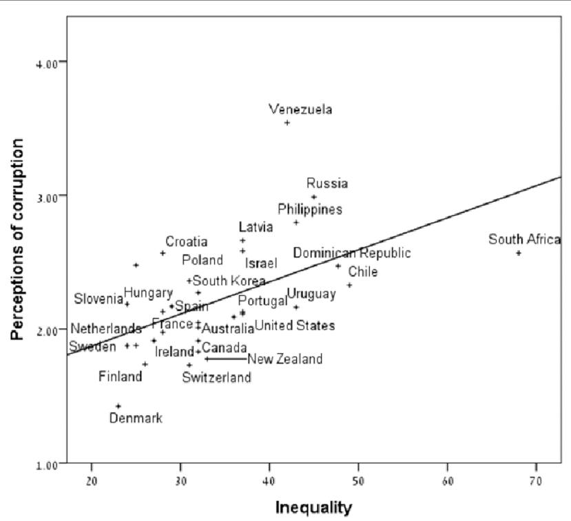
Source: Ariely & Uslander (2017)
Figure 1: Corruption and Inequality
Empirical Economic Bulletin, Vol. 17 128
Figure 2 shows the Corruption Perceptions Index of countries worldwide. The countries that are in the red have lower CPI scores, which means that they have more corruption. The countries in the yellow have higher scores and less corruption. Some of the countries that are the darkest red are Somalia, Syria, Libya, North Korea, Venezuela, Yemen, as well as a few more. These are countries with some of the worst corruption and score in the 0-9 range for CPI. We know that these countries have a lot of political instability, which fosters more inequality. The map shows that these countries with poor institutions are also the most corrupt. Some of the more yellow countries are the Scandinavian countries of Norway, Sweden, Finland, and Denmark. These are the cleanest countries, and they score in the 90-100 range for CPI. We know these countries have stable governments, which means they have less inequality, and the map shows they also have the least corruption.
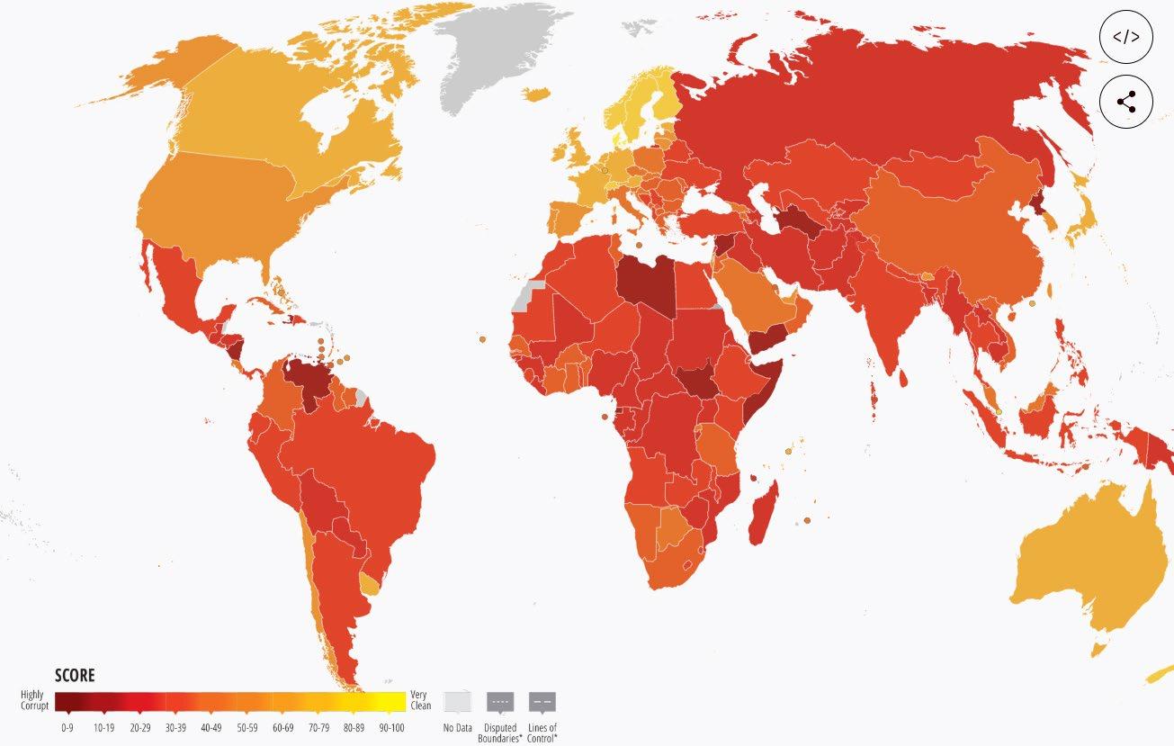
Source: Transparency International (2023)
Figure 2: Corruption and Poor Countries
Empirical Economic Bulletin, Vol. 17 129
3.0 LITERATURE REVIEW
There have been plenty of studies conducted that showed the relationship between corruption, inequality, and different macroeconomic factors. In their paper, Oueghlissi & Derbali (2021) found that democratic governments reduce corruption as well as maintaining low unemployment. They recommend that developing countries should focus on lowering the unemployment rate in order to maintain democracy and avoid corruption. Another study looked at economic determinants of corruption in developed and developing countries. In their paper, Acaravci et al. (2022) contended that economic growth and quality of governance contribute to reducing corruption. Similarly, it was found in another study that corruption negatively affected economic growth in developing countries (Spyromitros & Panagiotidis, 2022). These studies all have a similar trend in that corruption negatively impacts economic indicators like unemployment and economic growth. It was also found that the quality of institutions was a factor when looking for corrupt countries. A good institutional quality meant that a country was less likely to have corruption while a bad institutional quality meant that more corruption was likely.
While the previous papers focused more on just corruption, the next few papers will include the relationship between corruption and inequality. In their paper, Zandi et al. (2022) determine if corruption, inflation, and unemployment have an effect on income inequality in some developing countries in Asia. They found that corruption, inflation, and unemployment have a positive relationship with the GINI index, which means that these macroeconomic factors increase income inequality in these Asian countries. In a similar study, Kunawotor, Bokpin, & Barnor (2020) look at how institutional quality effects income inequality in Africa. It was found that the governance indicators of control of corruption and rule of law decreased income inequality while government effectiveness, voice and accountability, regulatory quality, and political stability did not significantly decrease inequality. In another study, the authors try to determine if corruption matters for unemployment in southern Africa. They found that the education level and income inequality are the main reasons for unemployment. But for youth unemployment, corruption is more of a problem (Adjor & Kebalo, 2018).
Empirical Economic Bulletin, Vol. 17 130
More studies performed research relating to the relationship of corruption and inequality. Afonso & Longras (2022) examined how corruption, institutional quality, and offshoring affect income inequality, comparative advantage, and economic growth. They found that countries can improve international trade, the labor market, and economic growth by reducing corruption which will increase institutional quality and offshoring. In a study by Policardo, Sanchez Carrera, & Risso (2019), they researched if there is causality between income inequality and corruption in OECD countries. It was found that the causality between corruption and income inequality is country specific, and that corruption increases income inequality, and income inequality positively affects corruption.
4.0 DATA AND EMPIRICAL METHODOLOGY
4.1 Data
The study uses panel data from 2012 to 2021. Data was obtained from the World Bank, World Development Indicators, World Governance Indicators, and Statista. The countries studied were Argentina, Bolivia, Brazil, Colombia, Costa Rica, Ecuador, Honduras, Paraguay, Peru, El Salvador, and Uruguay. Summary statistics for the data are provided in Table 1.
Empirical Economic Bulletin, Vol. 17 131
Table 1 Summary Statistics
4.2 Empirical Model
The study is based on the work of Kunawotor, Bokpin, & Barnor (2020) and is modified to show how control of corruption affects inequality in Latin America rather than all the governance indicators (voice and accountability, political stability, government effectiveness, regulatory quality, rule of law). In addition, poverty will be another dependent variable that will be used that is interchangeable with inequality. Some of the macroeconomic factors are added to the model as well, taken from the Kunawotor, Bokpin, & Barnor (2020) paper. The selection of these variables was based on available data for the countries I selected to study. The model is written below.
Variable Obs Mean Std. Dev. Min Max Inequality 110 45.85 4.44 38 53.9 Poverty 110 26.25 13.34 4.6 56.9 Unemployment 110 6.87 3.17 2.02 16.43 GDP 110 7793.59 4472.32 2064.55 19026.05 FDI 110 9.69e+09 2.01e+10 -1.13e+09 9.26e+10 Control of corruption 110 41.97 20.47 14.22 91.43 Population growth 110 1.10 0.52 -0.082 1.95 Gross capital formation 110 1.86 12.18 -25.54 53.56 Natural resource rent 110 3.47 3.12 0.54 14.53 Age dependency ratio 110 53.21 5.76 43.12 65.49 Govt expenditure 110 15.42 2.38 10.87 20.38 Trade 110 56.45 22.61 22.49 121.19
Empirical Economic Bulletin, Vol. 17 132
inequality = ����0 + ����1unemployment + ����2FDI + ����3GDP + ����4population growth + ����5control of corruption + ����6gross capital formation + ����7natural resource rent + ����8age dependency ratio + ����9govt expenditure ����10trade+ ε
Inequality is the dependent variable. It measures how fairly income is distributed in a country. The GINI coefficient is what measures inequality, where a 0 means perfect equality and 100 means perfect inequality. Other regressions will be run as well, with poverty as the dependent variable instead of inequality. Poverty data is based on the poverty headcount ratio at $6.85 a day. This data was found from the World Bank Development Indicators as well as Statista to fill in some of the gaps for the inequality data.
The independent variables are unemployment, foreign direct investment (FDI), gross domestic product (GDP), population growth, control of corruption, gross capital formation, natural resource rent, age dependency ratio, government expenditure, and trade. The data for these variables were found from the World Bank Development Indicators as well as the World Bank Governance Indicators for control of corruption data. Unemployment shows how many people do not have a job in each country for the years 2012-2021. It is measured by the percentage of the total labor force for each country. FDI measures investments made in a foreign country. It is measured by net inflows and is in current US dollars. GDP is the measure of economic activity in a country. In the data, it is measured by GDP per capita and is in current US dollars. Population growth is measured as the annual percentage growth in population in each country. Control of corruption measures perceptions of the extent to which public power is used for private gain and a capture of the state by elites and private interests Gross capital formation is the usage of physical capital in production and is measured as annual percentage growth. Natural resource rent is the reliance on natural resources in a country and is measured as a percentage of GDP. The age dependency ratio is the sum of young age population and old age population and is measured as a percentage of the working age population. Government expenditure is the general government’s final consumption expenditure as a percentage of GDP. Trade is the sum of exports and imports of goods and services measured as a percentage of GDP
Empirical Economic Bulletin, Vol. 17 133
5.0 EMPIRICAL RESULTS
The empirical estimation results are presented in Table 2 and Table 3. Three regressions were run for the two dependent variables of inequality and poverty. The first column of data shows the fixed effect regression, then the second column shows the random effect regression. The last column shows the OLS regression.
Empirical Economic Bulletin, Vol. 17 134
Table
2:
Regression results for Inequality in Latin America
Number of obs. 110 110 110
Note: ***, **, and * denotes significance at the 1%, 5%, and 10% respectively. Standard errors in parentheses
Inequality I (FE) II (RE) III (OLS) Constant 20.95*** (4.84) 51.29*** (4.08) 51.29*** (4.08) Unemployment 0.23*** (0.08) 0.47*** (0.097) 0.47*** (0.097) GDP -0.00004 (0.0001) -0.0002 (0.0001) -0.0002 (0.0001) FDI 6.29e-11** (2.74e-11) 1.30e-10*** (1.41e-11) 1.30e-10*** (1.41e-11) Control of corruption 0.014 (0.027) 0.033 (0.023) 0.033 (0.023) Pop growth 0.12 (0.64) 4.37*** (0.52) 4.37*** (0.52) Gross capital formation -0.005 (0.011) -0.02 (0.018) -0.02 (0.018) Natural resource rent -0.189** (0.077) 0.14* (0.082) 0.14* (0.082) Age dependency ratio 0.42*** (0.079) -0.266*** (0.06) -0.266*** (0.06) Govt expenditure -0.198 (0.14) -0.34*** (0.12) -0.34*** (0.12) Trade 0.066** (0.0296) 0.077*** (0.015) 0.077*** (0.015) R2 0.0204 0.8119 0.8119 F-statistics 9.06*** 42.73***
Empirical Economic Bulletin, Vol. 17 135
Table 3: Regression Results for Poverty in Latin America
Note: ***, **, and * denotes significance at the 1%, 5%, and 10% respectively. Standard errors in parentheses
Poverty I (FE) II (RE) III (OLS) Constant -29.97*** (10.43) 59.17*** (15.34) 59.17*** (15.34) Unemployment 0.77*** (0.183) 0.56 (0.37) 0.56 (0.37) GDP -0.0007** (0.0003) -0.003*** (0.0004) -0.003*** (0.0004) FDI 1.49e-10** (5.90e-11) 2.29e-10*** (5.30-11) 2.29e-10*** (5.30-11) Control of corruption 0.087 (0.059) 0.16* (0.023) 0.16* (0.023) Pop growth 0.14 (1.38) 0.19 (1.96) 0.19 (1.96) Gross capital formation 0.0996 (0.023) -0.054 (0.068) -0.054 (0.068) Natural resource rent 0.099 (0.167) -0.174 (0.31) -0.174 (0.31) Age dependency ratio 0.98*** (0.17) -0.13 (0.23) -0.13 (0.23) Govt expenditure 0.183 (0.301) -1.49*** (0.406) -1.49*** (0.406) Trade -0.067 (0.064) 0.133** (0.058) 0.133** (0.058) R2 0.0545 0.7047 0.7047 F-statistics 7.10*** 23.62*** Number
of obs. 110 110 110
Empirical Economic Bulletin, Vol. 17 136
The regression results in Table 2 show the three regressions that were run. The fixed effect regression has a very low R2 of 0.0204 meaning that the model does not account for much of the variation within the data. The random effects regression has a higher R2 of 0.8119 which means this model does account for more variability in the data. The random effects model measures the relationship between the dependent and independent variables while also accounting for unobserved heterogeneity over time.
When focusing on the random effects regression model, several significant variables were found in Table 2 with inequality as the dependent variable. These include the constant, unemployment, FDI, population growth, natural resource rent, age dependency ratio, government expenditure, and trade. The constant coefficient was shown to be positive for this regression. This means that the dependent variable of inequality is a non-zero value when all independent variables are equal to zero. The unemployment constant was also positive for the RE regression. This means that on average, as unemployment increases, inequality also increases. The FDI coefficient for this regression was positive as well, meaning that as FDI goes up, inequality goes up. This is consistent with the findings from Kunawotor, Bokpin, & Barnor (2020). The natural resource rent coefficient was positive for the random effect regression. It was significant at the 10% level. The age dependency coefficient was negative for the model. It was significant at the 1% level, and this was consistent with the findings of Kunawotor, Bokpin, & Barnor (2020). Government expenditure had a negative coefficient for the random effect model as well. This means that as government expenditure goes up, inequality goes down on average. Trade had a positive coefficient meaning that when trade goes up, inequality goes up.
In Table 3 with poverty as the dependent variable, the constant, GDP, FDI, control of corruption, government expenditure, and trade were statistically significant. The constant had a positive coefficient in the random effects regression. GDP, on the other hand, had a negative coefficient, meaning it has a negative relationship with poverty. It was significant at the 1% level. Also significant at the 1% level, FDI had a positive coefficient in the regression which means it has a positive relationship with poverty. Control of corruption and trade also had a positive relationship with poverty. Control of corruption was significant at the 10% level while trade was significant at the
Empirical Economic Bulletin, Vol. 17 137
5% level. Finally, government expenditure had a negative coefficient meaning that it has a negative relationship with poverty at the 1% significance level.
When interpreting these results in terms of relative change in the independent variable, we can see that FDI, government expenditure, and trade are the most frequent significant variables. In addition, I was surprised at first to see that some of the results I found were different than the results in the Kunawotor, Bokpin, & Barnor (2020) paper. However, it makes sense that there will be some differences because I focused on a different region than those authors did. We can see from these results that different variables affect inequality and poverty differently. There is an emphasis on the complex relationships between various macroeconomic factors, corruption, and inequality as well as poverty within Latin America. There is no constant rule that every country must follow. Certain economic factors affect countries in different ways. This helped me come to my conclusion that there is no set rule that all countries need to follow in order to help inequality and poverty. This is in line with the findings of Policardo, Sanchez Carrera, & Risso (2019). I also found that the relationship between corruption and inequality/poverty was not as significant as I thought it would be. Again, this could be because of the countries that I choose.
6.0 LIMITATIONS AND POLICY IMPLICATIONS
Some limitations that were encountered were the lack of data for countries in Latin America. Many countries did not have full datasets that could be used to accurately study. This limited the number of countries I could use. More countries would mean more data and would make the results more accurate. Also, I had to use averages to fill in some of the missing data for trade and poverty. This is another limitation to the study as it makes the results less accurate than if I could find the correct values for these missing data points.
The policy implications for this study would be to focus on the factors that contribute the most to reducing inequality and poverty based on what is needed in a certain country. As stated earlier, it was found that there is no worldwide rule that helps alleviate the effects of inequality and poverty. It is country specific based on the main issues that create inequality and poverty in that country. Keeping unemployment and
Empirical Economic Bulletin, Vol. 17 138
inflation low, increasing GDP and FDI, as well as successfully controlling corruption would all be good examples of effective ways to reduce inequality and poverty.
7.0 CONCLUSION
In summary, there are many different factors that contribute to increasing inequality and poverty. It appears that countries with better institutional qualities that control corruption more effectively tend to do better at reducing inequality and poverty. These countries are better at managing macroeconomic factors that can lead to inequality and poverty. In this study, the factors that were focused on were unemployment, GDP, FDI, population growth, control of corruption, gross capital formation, natural resource rent, age dependency ratio, government expenditure, and trade. It was found that FDI, government expenditure, and trade were the most frequent significant variables. These could be some factors to focus on to reduce inequality and poverty. However, the main finding was that certain countries have different challenges that contribute to their individual levels of inequality/poverty. There cannot be one specific way to deal with inequality and poverty. It must be on a country basis, not a worldwide basis.
Empirical Economic Bulletin, Vol. 17 139
Appendix A: Variable Description and Data Source
Variable Description
Inequality Using the Gini index, this measures how the distribution of income or consumption among individuals or households within an economy deviates from a perfectly equal distribution. A Gini index of 0 represents perfect equality, while an index of 100 implies perfect inequality.
Poverty The percentage of the population living on less than $6.85 a day at 2017 international prices.
Unemployment Measured as total unemployment as a percentage of the labor force.
GDP Gross domestic product per capita measured in US dollars.
FDI Measured as net inflows of foreign direct investment to GDP.
Control of corruption
Pop growth
Gross capital formation
Natural resource rent
Captures perceptions of the extent to which public power is exercised for private gain, including both petty and grand forms of corruption, as well as capture of the state by elites and private interests.
Measured as the annual percentage growth in population.
The extent of usage of physical capital in production and measured as gross capital formation to GDP.
The extent of reliance on natural resources in a country and it is measured as total natural resources rent as a percentage of GDP
Age dependency ratio Computed as the sum of young age population and old age population as a ratio of the working age population.
Govt expenditure Measured as general government final consumption expenditure as a percentage of GDP
Trade The sum of exports and imports of goods and services measured as a percentage of GDP
Data source
World Bank Development Indicators / Statista
World Bank Development Indicators
World Bank Development Indicators
World Bank Development Indicators
World Bank Development Indicators
World Bank Governance Indicators
World Bank Development Indicators
World Bank Development Indicators
World Bank Development Indicators
World Bank Development Indicators
World Bank Development Indicators
World Bank Development Indicators
Empirical Economic Bulletin, Vol. 17 140
Variable
Appendix B: Variables
and Expected Signs
What it captures Expected sign
Unemployment Measure of those unemployed in a country.
GDP
FDI
Control of corruption
Pop growth
GDP per capita.
Inflows of FDI within a country.
Ability of a country to control corruption.
The growth of a population in a country.
Gross capital formation Measures fixed capital acquisitions.
Natural resource rent Reliance of a country on natural resources.
Age dependency ratio
Govt expenditure
Trade
Ratio of the working age population in a country.
The amount a government spends.
Sum of imports and exports.
+
+
+
-
+
-
-
-
+
Empirical Economic Bulletin, Vol. 17 141
BIBLIOGRAPHY
Acaravci, A., Artan, S., Hayaloglu, P., & Erdogan, S. (2022). Economic and Institutional Determinants of Corruption: The Case of Developed and Developing Countries. Journal of Economics and Finance, pp. 207-231.
Adjor, D. M., & Kebalo, L. (2018). Does Corruption Matter for Unemployment in SADC countries? Review of Economic & Business Studies, pp. 65-92.
Afonso, O., & Longras, A. R. (2022). Corruption, Institutional Quality, and Offshoring: How Do They Affect Comparative Advantage, Inter-country Wage Inequality, and Economic Growth? Metroeconomica, pp. 987-1020.
Ariely, G., & Uslander, E. (2017). Corruption, Fairness, and Inequality. International Political Science Review, pp. 349-362.
Bachelet, P. A. (2024). The Complexities of Inequality in Latin America and the Caribbean. Retrieved from IDB: https://www.iadb.org/en/news/complexities-inequality-latinamerica-and-caribbean
Corruption Perceptions Index. (2023). Retrieved from Transparency International: https://www.transparency.org/en/cpi/2023.
Kunawotor, M. E., Bokpin, G. A., & Barnor, C. (2020). Drivers of income inequality in Africa: Does institutional quality matter? African Development Review, pp. 718-729.
Oppenheimer, A. (2024). Corruption is thriving in Latin America, and may keep rising. US fights back. Retrieved from Miami Herald: https://www.miamiherald.com/news/local/newscolumns-blogs/andres-oppenheimer/article285011497.html.
Oueghlissi, R., & Derbali, A. (2021). Democracy, Corruption and Unemployment: Empirical Evidence from Developing Countries. Munich Personal RePEc Archive, pp. 1-26.
Policardo, L., Sanchez Carrera, E. J., & Risso, W. A. (2019). Causality between income inequality and corruption in OECD countries. World Development Perspectives.
Spyromitros, E., & Panagiotidis, M. (2022). The impact of corruption on economic growth in developing countries and a comparative analysis of corruption measurement indicators. Cogent Economics & Finance, pp. 1-30.
Zandi, G. R., Rehan, R., Hye, Q. M., Mubeen, S., & Abbas, S. (2022). Do Corruption, Inflation and Unemployment Influence the Income Inequality of Developing Asian Countries? International Journal of Applied Economics, Finance and Accounting, pp. 118-128.
Empirical Economic Bulletin, Vol. 17 142
HOSTING
MEGA EVENTS
IMPACT ON GDP GROWTH: A Panel Data Analysis
Silas Pearce
Abstract:
This paper investigates the impact of hosting “mega events” such as the Olympics on a country’s GDP growth. The study incorporates information on the country’s factors of economic development. Spillovers will be modeled through the state of the global economy by using controls such as countries that did not host mega events. The results show that countries that host the Olympics do not see any extra GDP growth than those that did not host an event.
JEL Classification: H5, O4, Z2
Keywords: Olympics, GDP Growth, Tourism,
a Department of Economics, Bryant University, 1150 Douglas Pike, Smithfield, RI02917. Phone: (603) 660-4881. Email: spearce1@bryant.edu
Empirical Economic Bulletin, Vol. 17 143
1.0 INTRODUCTION
Having the opportunity to host mega-events such as, the Olympics, FIFA World Cup, and Formula 1 races, is a prestigious experience for host countries. Host countries spend, “$8.9 billion on average,” (Budzier, et al., 2016) which is no small expenditure. Countries are willing to spend this amount to host in hopes that the benefits that mega-events are believed to bring, such as notoriety, respect, and most importantly increased economic benefits. Do these benefits make up for the costs of these massive events?
This study aims to enhance how much is gained for a country’s economic growth through the hosting of mega-events. From a policy perspective, this analysis is important to provide spending recommendations for countries that are bidding to host these events, to make sure it is a good investment or if the money should be spent on more pressing issues. The relevance of this study comes with the US bidding to host the 2024 Olympics, hosting some games of the 2026 FIFA World Cup, and hosting the 2028 Summer Olympics.
This paper was guided by three research objectives that differ from other studies: First being the investigation will investigate multiple different Olympics and multiple different FIFA World Cups; Second; the time frame of events will be larger than previous studies have analyzed. Last, it analyzes how the economic growth in the rest of the world is compared to the host country. This will help account for any current world events that may be throwing off the results of the model and over/under estimate growth.
Empirical Economic Bulletin, Vol. 17 144
The rest of the paper is organized as follows: Section 2 highlights trends of mega-events and economic growth. Section 3 gives a brief literature review. Section 3 outlines the empirical model. Data and estimation methodology are discussed in section 4. Finally, section 5 presents and discusses the empirical results. This is followed by a conclusion in section 6.
2.0 MEGA-EVENTS AND ECONOMIC GROWTH
Figure 1 shows how much investment goes into hosting the Olympics each year for a country. It is a costly venture that takes years of investment and construction for events that last two weeks. The more recent Olympic games of the past decade have been the most expensive, with the 21’ Tokyo games being the most expensive by almost 33% more than the previous highest, Sochi ’14. Some of the extra costs for the Tokyo games were caused by COVID-19 regulations, which makes it an outlier. With such an increase in costs, this only makes it more difficult for there to be an economic gain from the events.
Empirical Economic Bulletin, Vol. 17 145
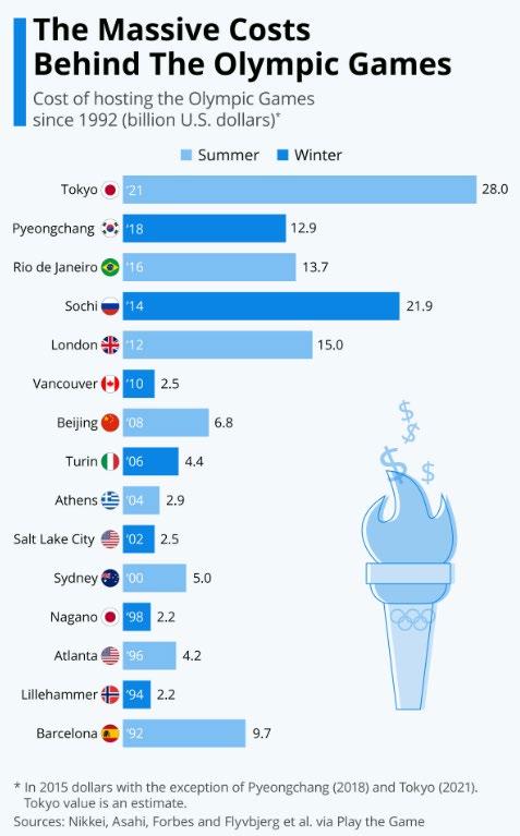
Source: Statista
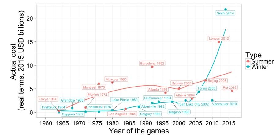
Source: (Budzier, et al., 2016)
Figure 1: Costs of Olympic Games
Figure 2: Time Series Cost of Olympics
Empirical Economic Bulletin, Vol. 17 146
3.0 LITERATURE REVIEW
Many countries have put forward bids to the International Olympic Committee to host the Olympics, but since 2008 the number of bids has only decreased every four years (Huang, et al., 2022). One factor leading to this decline in bids is the increasing costs to host mega-events, as seen in Figure 1. The other factor is the confusion on if these megaevents bring in enough of an economic benefit to pay for those high costs. Previous reports and studies show that there is no clear cut answer or consensus to the question. Some of the studies found that there is no significant effect of hosting the Olympics on GDP growth, (Whitson & Horne, 2006; Kobierecki & Pierzgalski, 2022; Ferris, et al., 2022). In a review of the costs/benefits of these events, (Whitson & Horne, 2006) looked at Japan and talked about how construction of new infrastructure that takes place for the games is generally looked at as beneficial for the country. It’s believed to add jobs make space for future events, but what they found was that in cases the arenas or stadiums don’t see enough use to stay profitable once the mega-events have come and gone.
Many found short term benefits immediately after hosting the event, (Anton, et al., 2011; Elahi, et al., 2021). These short-term benefits come in the form of job growth and tourism in the 1-2 years preceding, the year of, and the 1-2 years following the event (Elahi, et al., 2021). No studies showing any form of long-term benefits from hosting mega-events was found. One of the main problems with the literature is highlighted by Ferris et al. (2022) is that most of the studies have relatively small sample size and the studies could benefit
Empirical Economic Bulletin, Vol. 17 147
from using a larger data set. One of the factors that limits the studies are that the World Cup and Olympic Games are only hosted every 4 years which makes it difficult to collect a large data set that is comparable to some of the control countries or non-host countries (Firgo, 2021).
A couple of the studies that used empirical models to answer their questions about the costs and benefits of these events will be the focus of the literature. (Wan & Song, 2019) found that the 2012 UK Olympics were profitable, but the 2014 Brazil World Cup was not and (Firgo, 2021) found it varied between Summer and Winter Olympics, showing that it can vary on a case-by-case basis. The literature shows that there is no direct yes or no answer to the question of whether mega-events have a positive or negative impact on a country’s economy. (Kobiercki & Pierzgalski, 2022) came to a similar conclusion after finding insignificant results for the London Olympics, Canadian Olympics, South African World Cup, and the Brazilian Olympics/World Cup. They believed that although their results did not show a direct positive economic impact from these events, that does not mean that countries do not see some sort of benefit. Each host country handles their preparation for these events differently and contributes different sized investments to it, which means they will receive a different impact from it. One study took it a step further, saying that the state of a countries current development is one of the main factors that determines how hosting will imapct the countries GDP growth, “the World Cup of 2002 did not have the same effect in the dynamism of the economic activity in South Korea and Japan,” (Anton, et al., 2011).
Empirical Economic Bulletin, Vol. 17 148
4.0 DATA AND EMPIRICAL METHODOLOGY
4.1 Data
The study uses annual panel data from 1999 to 2019. Data were obtained from the World Development Indicators (WDI) The data is from countries that have hosted the Olympics and non-host countries in a similar economic state that were also potential candidates for hosting the Olympics at some point. The countries were chosen based off Kobiercki & Pierzgalski’s 2022 work. Summary statistics for the data are provided in Table 1.
Table 1 Summary Statistics
4.2 Empirical Model
Using the aspects from the studies by Wan & Song (2019) and Kobierecki & Pierzgalski (2022) the model was assembled to account for GDP growth. We added a dummy variable to compare which countries hosted the Olympics and which countries did not.
The model could be written as follow:
GDP LIFE INF EXP IND TOUR Mean 36218.69731 77.86154 3.269543 4.52567E+11 4.99E+11 2.39E+10 Standard Error 739.0460861 0.187422 0.253688 23277493244 3.83E+10 1.27E+09 Median 39691.48231 79.03293 2.292253 2.82834E+11 1.88E+11 1.72E+10 Standard Deviation 16591.54348 4.207619 5.695275 5.22578E+11 8.61E+11 2.85E+10 Sample Variance 275279315.1 17.70406 32.43616 2.73088E+23 7.41E+23 8.1E+20 Kurtosis -0.6443628 -0.19843 100.781 4.939452001 11.19027 7.971425 Skewness -0.13517057 -0.77838 8.399216 2.184614911 3.221713 2.61049 Range 83778.2573 19.32878 90.2246 2.65081E+12 5.51E+12 1.86E+11 Minimum 3206.730026 65.02756 -4.4781 4797546243 3E+09 4.28E+08 Maximum 86984.98733 84.35634 85.74649 2.65561E+12 5.51E+12 1.86E+11 Sum 18254223.44 39242.21 1647.85 2.28094E+14 2.51E+14 1.2E+13 Count 504 504 504 504 504 504
Empirical Economic Bulletin, Vol. 17 149
GDP is the annual growth domestic product per capita in 2017 international dollars. GDP is used as an endogenous variable. It demonstrates the benefits that countries stand to gain from hosting the Olympics Measuring GDP per capita is important to help gauge a better economic comparison between the countries without population size impact the results.
Independent variables consist of six variables obtained from the WDI Appendix A and B provide data source, acronyms, descriptions, expected signs, and justifications for using the variables. First, LIFE represents the country’s life expectancy at birth in total years. This helps account for the contribution that human capital makes towards a country’s GDP. Second, INF accounts for inflation in consumer prices by annual percentage. Third, EXP represents the amount of exports a country exchanges in current US dollars Exports are a big contributing factor to a country’s GDP. Fourth, IND measures the value of industry added in US dollars which includes construction. This is included to account for any value added through the arenas, hospitality services, restaurants, or anything else that is built to accommodate the events. Fifth, TOUR is a measure of international tourism expenditures in current US dollars to account for the increase in visitors that occurs during and after the events. Sixth, CONS is a measure of consumption expenditure in current US dollars to account for one of the major GDP contributors. Lastly, HOST is a dummy variable is labeled 1 if the country has hosted the Olympics within the 20 year time period and 0 if the country has not. This allows for the comparison between the host and nonhost countries to measure the impact of the Olympics.
������������ = �������� + �������� ���������������� + �������� ������������ + �������� ������������ + �������� ������������ + �������� ���������������� + �������� ���������������� + �������� ���������������� + ����⬚
Empirical Economic Bulletin, Vol. 17 150
5.0 EMPIRICAL RESULTS
The empirical estimation results are presented in Table 2.
Table 2: Regression Results
GDP per capita
CONSTANT -185220.15 (9515.77)***
LIFE 2825.05 (121.82)***
INF 177.59** (84.61)
EXP 7.417E-09 (2.708E-09)***
IND -1.218E-08 (1.773E-09)***
TOUR 4.959E-08 (4.0397E-08)
CONS 2.804E-09 (5.117E-10)***
HOST -4021.47268 (888.785)*** R2 0.698822121 F-statistics 164.41
Observations
503
Note: *** , **, and * denotes significance at the 1%, 5%, and 10% respectively. Standard errors in parentheses
The LIFE variable estimate was significant at the 1% level. The estimate indicated that LIFE was positively associated with GDP, meaning that as a countries life expectancy increases, GDP per capita increases. The model estimates that a one year increase in life expectancy will increase the country’s GDP per capita by approximately $2825.05. The INF variable was significant at the 5% level. The estimate indicated that a 1% increase in inflation will increase a country’s GDP per capita by approximately $177.59. In theory, inflation should have a negative effect on GDP per capita, so the positive correlation in the model may be due to the increase on wages that comes to combat inflation. The EXP variable was significant at the 1% level. The estimate indicated that a $1 billion increase
Empirical Economic Bulletin, Vol. 17 151
in exports increases GDP per capita by approximately $7.42. The IND variable was significant at the 1% level. The estimate indicated that a $1 billion increase in IND decreases GDP per capita by $12.18. This is as expected since construction of new stadiums and arenas can be costly. The TOUR variable was the only variable that was not significant at any level. The model estimate indicated that a $1 billion increase in tourism increases GDP per capita by $49.59. The CONS variable was significant at the 1% level. The estimate indicated that a $1 billion increase in CONS will increase a country’s GDP per capita by approximately $2.80. The HOST variable was significant at the 1% level. The estimate indicated that hosting the Olympics would result in approximately a $4021.47 decrease in GDP per capita. This result implies that hosting the Olympics has negative impacts on GDP growth.
5.0
CONCLUSION
In conclusion, hosting the Olympics have negative effects to GDP per capita. The results in this paper imply that countries looking to host the Olympics should investigate the opportunity costs to see if the funding should be dedicated to other areas. If the country has a low GDP per capita, it should not consider hosting the Olympics due to the negative affects it would have on it’s peoples welfare. If a country is to host the Olympics, it should not devote a large amount of funding to building new arenas, stadiums, or infrastructure This conclusion can be made from the negatively correlated IND variable, since construction is included. Instead, countries should take the approach that the U.S. is taking for hosting FIFA World Cup games in 2026. The U.S. is using already existing stadiums to host the games, instead of building any new arenas. As seen in Figure 1, the two most expensive Olympics were the Sochi and Tokyo Olympics, which both had new arenas constructed for the events.
Empirical Economic Bulletin, Vol. 17 152
Instead of building these fancy, new stadiums, host countries should be devoting their Olympic budget to attract tourists and market domestically produced products. Seeing that the results showed increased tourism and exports have a positive effect on GDP per capita, it would be beneficial to focus on these two areas. Possible areas host countries could look to fund would be improving infrastructure to be able to account for added tourism, such as improving public transportation or hotel services to attract visitors. Improving these areas would have lasting benefits for the country after the events, not just during.
Empirical Economic Bulletin, Vol. 17 153
Appendix A: Variable Description and Data Source
Acronym Description Data source
GDP
LIFE
INF
EXP
GDP per capita based on purchasing power parity (PPP). PPP GDP is gross domestic product converted to international dollars using purchasing power parity rates. An international dollar has the same purchasing power over GDP as the U.S. dollar has in the United States. GDP at purchaser's prices is the sum of gross value added by all resident producers in the country plus any product taxes and minus any subsidies not included in the value of the products. It is calculated without making deductions for depreciation of fabricated assets or for depletion and degradation of natural resources. Data are in constant 2017 international dollars.
Life expectancy at birth indicates the number of years a newborn infant would live if prevailing patterns of mortality at the time of its birth were to stay the same throughout its life.
Inflation as measured by the consumer price index reflects the annual percentage change in the cost to the average consumer of acquiring a basket of goods and services that may be fixed or changed at specified intervals, such as yearly. The Laspeyres formula is generally used.
Exports of goods and services represent the value of all goods and other market services provided to the rest of the world. They include the value of merchandise, freight, insurance, transport, travel, royalties, license fees, and other services, such as communication, construction, financial, information, business, personal, and government services. They exclude compensation of employees and investment income (formerly called factor services) and transfer payments. Data are in current U.S. dollars.
World Bank Group –World Development Indicators
IND
Industry (including construction) corresponds to ISIC divisions 05-43 and includes manufacturing (ISIC divisions 10-33). It comprises value added in mining, manufacturing (also reported as a separate
World Bank Group –World Development Indicators
World Bank Group –World Development Indicators
World Bank Group –World Development Indicators
World Bank Group –World Development Indicators
Empirical Economic Bulletin, Vol. 17 154
subgroup), construction, electricity, water, and gas. Value added is the net output of a sector after adding up all outputs and subtracting intermediate inputs. It is calculated without making deductions for depreciation of fabricated assets or depletion and degradation of natural resources. The origin of value added is determined by the International Standard Industrial Classification (ISIC), revision 4. Data are in current U.S. dollars.
TOUR International tourism expenditures are expenditures of international outbound visitors in other countries, including payments to foreign carriers for international transport. These expenditures may include those by residents traveling abroad as same-day visitors, except in cases where these are important enough to justify separate classification. For some countries they do not include expenditures for passenger transport items. Data are in current U.S. dollars.
CONS Final consumption expenditure (formerly total consumption) is the sum of household final consumption expenditure (private consumption) and general government final consumption expenditure (general government consumption). Data are in current U.S. dollars.
World Bank Group –World Development Indicators
World Bank Group –World Development Indicators
Empirical Economic Bulletin, Vol. 17 155
BIBLIOGRAPHY
Anton, A. J. M., Alonso, J. J. M. & Rodriguez, G. S., 2011. Mega-events impact on economic growth: Analysis of the South African World Cup. African Journal of Business Management, 5(16), pp. 69406948.
Budzier, A., Flyvbjerg, B. & Stewart, A., 2016. The Oxford Olympics Study 2016: The Cost and Cost Overrun at the Games. University of Oxford.
Elahi, A., Gholampour, S. & Askarian, F., 2021. The Effects of Sports Mega-Events on Host Communities: A Systematic Review of Studies in Three Recent Decades. Sports Business Journal, 1(1), pp. 13-30.
Ferris, S. P., Koo, S., Park, K. & Yi, D. T., 2022. The Effects of Hosting Mega Sporting Events on Local Stock Markets and Sustainable Growth. Sustainability, 15(1).
Firgo, M., 2021. The causal economic effects of Olympic Games on host regions. Regional Science and Urban Economics, Volume 88.
Huang, J., Bai, X., Zhou, G. & Zhang, M., 2022. Empirical Study on The Economic Financial Impact of the Successful Application and Hosting of the Olympic Games on the Host Countries Based on a Regression Model. ICIDC, p. 12.
Kobierecki, M. M. & Pierzgalski, M., 2022. Sports Mega-Events and Economic Growth: A Synthetic Control Approach. Journal of Sports Economics, 23(5).
Lee, C.-K. & Taylor, T., 2005. Critical Reflections on the Economic Impact Assessment of a Mega-Event: The Case of 2002 FIFA World Cup. Tourism Management, 26(4), pp. 595-603.
Varano, J., 2017. Major Sport Events: Are They Worth It?. The Conversation.
Wan, S. K. & Song, H., 2019. Economic Impact Assessment of MEga-Events in the United Kingdom and Brazil. Journal of Hospitality & Tourism Research, 43(7).
Whitson, D. & Horne, J., 2006. Underestimated Costs and Overestimated Benefits Comparing the Outcomes of Sports Mega-Events in Canada and Japan. The Sociological Review, 54(2).
Empirical Economic Bulletin, Vol. 17 156
Hitting the Books: An Empirical
Analysis of the Effect of Education Expenditure on GDP per Capita and Economic Growth
Matt Simmons
Abstract:
This paper investigates the link between education spending in Mexico and Central American countries and illegal immigration to the United States. Despite challenges like poverty and governance issues, these nations experience significant migration to the U.S., underscoring the need for deeper insights. Analyzing economic motivations and migration costs, the study emphasizes education expenditure's role in economic growth. Through empirical analysis, it highlights the importance of addressing root causes and offers policy recommendations. Overall, this research contributes to understanding the intricate relationship between education, immigration, and economic development.
JEL Classification: H52, I24, I25, J11
Keywords: Education, Mexico, Belize, Guatemala, Honduras, El Salvadore, Nicaragua, GDP, Economic Growth, Migration
Department of Economics, Bryant University, 1150 Douglas Pike, Smithfield, RI02917. Phone: (401)232-6379. Email: Msimmons1@bryant.edu
Empirical Economic Bulletin, Vol. 17 157
1.0 INTRODUCTION
In the last few years, the United States has seen a significant increase in border encounters with migrants from Mexico and other Central American countries, such as Guatemala, Honduras, El Salvador, Belize, and Nicaragua. In light of this, this paper will present an empirical study on the relationship between education spending in these countries and gross domestic product (GDP) per capita in an attempt to explain the flow of illegal immigrants to the United States. By looking at the current state of education in these countries and the factors that could be causing people to seek opportunities in the United States, this paper aims to provide a better understanding of this complex issue.
According to the Organization for Economic Co-operation and Development (OECD), Mexico has the lowest tax-to-GDP ratio in the organization, which suggests that it is possible for the country to increase tax revenues and allocate those additional resources to education. Other Central American countries face challenges such as poverty, natural disasters, and dysfunctional or corrupt governments, which may hinder their ability to invest in education. For instance, in Guatemala, a country with a history of political instability and corruption, the government's ability to invest in education has been severely limited, leading to lower educational attainment higher poverty rates as well as increasing outmigration.
The expectation of increased educational attainment for these migrants or their families could play a major part in the motivation of recent Latino arrivals in the United States. This very well could be responsible for the changing migration patterns from Latin America in recent years. Over the last 5 years, the number of illegal immigrants coming into the United States from these countries has increased sharply. This highlights the importance of understanding the specific factors driving immigration from each of these individual countries. Specifically, the ongoing political and economic instability in Nicaragua has led to a surge in the number of Nicaraguan immigrants seeking asylum in the United States, as many likely are fleeing violence and persecution in their home country.
It is important to consider the migrant's motivations when analyzing the reasons for the recent giant influx of migrants to the United States. These motivations include factors such as job opportunities, higher wages, and better living conditions. By examining these factors, we can
Empirical Economic Bulletin, Vol. 17 158
better understand why individuals decide to leave their home countries and seek a better life in the United States.
Additionally, it is crucial to consider the costs of migration, both financial and nonfinancial, when analyzing the reasons for the recent wave of immigrants. These costs include the obvious financial burden of traveling to a new country, as well as the potentially less obvious emotional and psychological costs of leaving one's home and family behind. By considering these costs, we can gain a more comprehensive understanding of the complex decision-making process that individuals go through when deciding to migrate.
Thus, this paper will investigate the impact that education spending has on the flow of illegal immigration from Mexico and other Central American countries to the United States. By exploring the various factors influencing this trend, we hope to provide a clearer picture of the complex relationship between education and immigration.
The rest of the paper is organized as follows: Section 2 discusses current trends. Section 3 gives a brief literature review. Section 4 outlines the empirical model, Data and estimation methodology. Finally, section 5 presents and discusses the empirical results. This is followed by a conclusion in section 6.
2.0 TREND
Figure 1 shows migration trends from Central America to the United States in the years 2021 through 2024. This can be influenced by various factors, including economic disparities, job opportunities, and the desire for a better quality of life. From 2021 to 2024, encounters have been frequent at the Southwest Land Border the United States shares with Mexico, with fiscal year 2021 experiencing approximately 1.7 million encounters, 2022 with more than 2.2 million encounters, and the first half of fiscal year 2023 experiencing nearly 1.1 million encounters. As of March 2024, there were 189,441 encounters, indicating a sustained high level of migration pressures. The ongoing migration and its implications on both the United States and Central American countries stresses the importance of addressing the root causes of migration and exploring comprehensive and sustainable solutions to support economic development and reduce the need for migration.
Empirical Economic Bulletin, Vol. 17 159
Figure 1: Encounters per Year by Demographic
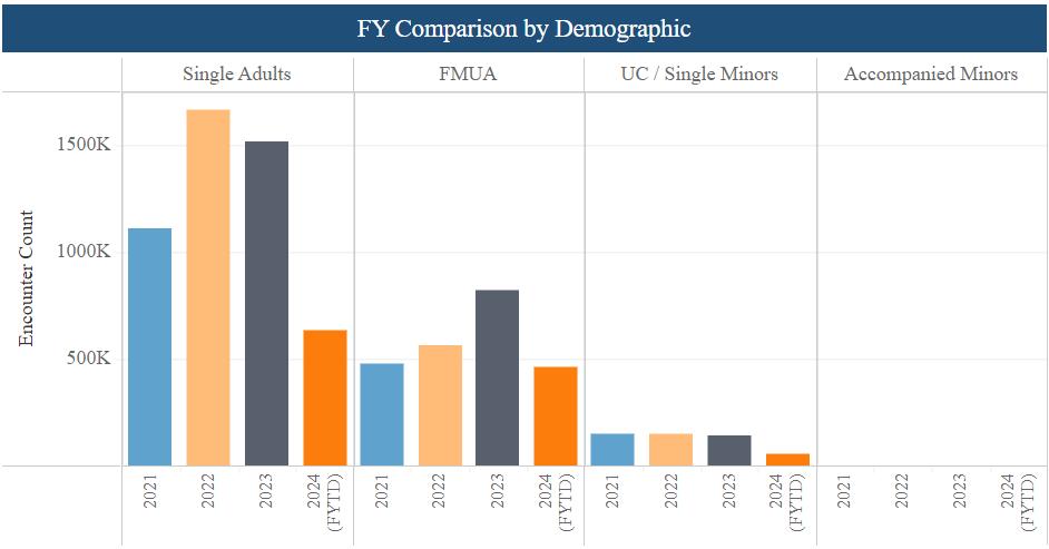
Source: United States Border Patrol and The Office of Field Operations
Figure 2 shows the inflow of remittances as a percentage of GDP for the six Central American countries, Mexico, Honduras, Guatemala, Belize, El Salvador, and Nicaragua, which have experienced notable growth over the last decade. This trend is particularly significant in Guatemala and Nicaragua, where the increase in remittances as a share of GDP has been the most substantial. This growing reliance on remittances can be attributed to various factors, including economic disparities, job opportunities, and family ties between migrants and their home countries.
Recent events and news have highlighted the importance of remittances in the region. Additionally, the political and social instability in some Central American countries has been a driving force behind the migration of people, further reinforcing the reliance on remittances as a vital source of income for families back home. This highlights the critical role of remittances in supporting the livelihoods of millions of families in Central America and underscores the need for policies and initiatives that aim to leverage these flows to foster economic development and reduce the need for migration in the first place.
Empirical Economic Bulletin, Vol. 17 160
Figure 2: Personal Remittances Received as a Percentage of GDP
Source: World Bank Database
3.0 LITERATURE REVIEW
Firstly, Deme & Mahmoud (2020) emphasize the importance of considering both the quantity and quality of education in understanding its impact on economic growth. They argue that investments in education should not only focus on increasing enrollment rates but also on enhancing cognitive skills and innovation capabilities. This perspective intersects with Velkovska & Trenovski's (2023) findings, which highlight education's role in reducing poverty and income inequality through investments in human capital development. Both studies examine the importance of holistic education policies that address not only access but also educational quality.
Contrasting this view, Li & Wye (2023) provide insights into the moderating role of financial development in the relationship between education expenditure and economic growth. They suggest that in poorer provinces, financial development amplifies the impact of education expenditure on economic growth. This perspective adds a layer of complexity to the discussion, highlighting the need to consider broader economic factors when evaluating the effectiveness of education investment. It intersects with the findings of Zhang et al. (2019), who emphasize the
0 5 10 15 20 25 30 2013 2014 2015 2016 2017 2018 2019 2020 2021 2022 Mexico Guatemala El Salvador Belize Honduras Nicaragua Empirical Economic Bulletin, Vol. 17 161
importance of addressing infrastructure constraints and enhancing financial accessibility to promote sustainable economic growth. Zhang et al. delve deeper into the role of financial development, suggesting that not only does it directly promote economic growth, but it can also indirectly enhance government expenditure in education, particularly in poorer provinces. Their study proposes policy interventions such as improving loan application procedures, addressing liquidity constraints in the financial sector, and decreasing interest rates for student loans to facilitate credit expansion and increase resources for educational financing.
Furthermore, Bawa & Pouris (2023) shed light on the significant economic contributions of public universities, emphasizing the indirect economic impact of education expenditure through research and business engagement activities. While their study does not directly examine the relationship between education expenditure and economic growth, it provides insights into the broader ecosystem within which education investment operates. This perspective intersects with Pastor et al.'s (2012) findings on the economic impact of universities on local economies, suggesting broader implications for education expenditure's role in promoting regional development. Pastor et al. delve deeper into the economic impact of universities, particularly in the context of the Valencian Public Universities (VPUs). They emphasize the diverse contributions made by higher education institutions to society, including the revitalization of the local productive fabric and the injection of demand through expenditure and investments. The study highlights the importance of universities as drivers of socio-economic development in their respective regions and emphasizes the need for comprehensive assessments of their economic impact.
Moreover, Li & Wye's (2023) findings on the role of financial development in moderating the relationship between education expenditure and economic growth suggest that policy interventions aimed at enhancing financial accessibility and infrastructure development could amplify the impact of education expenditure on economic growth. This view aligns with Zhang et al.'s (2019) emphasis on addressing infrastructure constraints and improving financial accessibility to promote sustainable economic growth. Both studies highlight the interconnectedness of education expenditure with broader economic policies and infrastructure development initiatives.
Empirical Economic Bulletin, Vol. 17 162
Additionally, the findings of Deme & Mahmoud (2020) on the importance of considering both the quantity and quality of education in understanding its impact on economic growth exemplify the need for holistic education policies that prioritize not only access but also educational quality. This perspective resonates with Velkovska & Trenovski's (2023) emphasis on investments in human capital development to reduce poverty and income inequality. Together, these studies highlight the multifaceted nature of education expenditure's impact on economic growth and the need for comprehensive policy approaches that integrate education investment with broader economic policies and infrastructure development initiatives.
In summary, these studies offer complementary perspectives on education expenditure's impact on economic growth, emphasizing the importance of considering both the quantity and quality of education, as well as broader economic factors such as financial development and infrastructure constraints. While each study provides unique insights, there are some disagreements in their emphasis on education expenditure's impact and the need for more diverse approaches that integrate education investment with broader economic policies and infrastructure development initiatives.
4.0 DATA AND EMPIRICAL METHODOLOGY
4.1
Data
The data used in this empirical research paper focuses on six Latin American countries: Mexico, Belize, Guatemala, Honduras, El Salvador, and Nicaragua, and uses the period of 2003 to 2021, utilizing a panel data set to examine the relationship between various economic indicators and their implications for economic development. The data source used was The World Bank Database, which provides comprehensive and reliable information on the variables used in the research.
The dependent variable in the study is Real GDP per capita in constant 2015 US$, which is the standard indicator used to evaluate economic growth and development as well as quality of life considerations. The independent variables utilized were the population (Pop), primary school enrollment rate (PSE), education expenditure (EduExp), and lagged 1-year GDP per capita, or (RGDP/Cap)t-1. These variables were chosen because of their impact on economic growth and
Empirical Economic Bulletin, Vol. 17 163
according to the literature they contribute to the differences in economic performance among the countries selected and to test which educational factors hold more weight in this discussion.
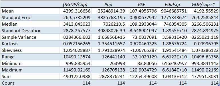
4.2 Empirical Model
Y = β0 + β1(Pop) + β2(PSE) + β3(EduExp) + β4(RGDP/Cap)t-1 + ε
In the model, the independent variable Pop was selected due to the significant impact on economic growth it has according to prior literature, as measured by the dependent variable, GDP per capita. The variables PSE and EduExp were chosen to determine the effect that they have on a country's economic performance, as well as compare them to each other. Lastly, the variable (RGDP/Cap)t-1 was selected for two reasons. The first is that it helps to account for the potential effects of past economic performance on current GDP per capita, such as momentum. The other reason is that when looking at education spending and primary school enrollment, some of the data can get clouded by outside noise, and having this control variable helps to reduce that so that this paper can look specifically at how education spending and enrollment affect the country's future economic performance.
The population variable (Pop) is essential in determining the size of the labor force and the potential market for goods and services, as well as controlling for what tends to be a large contributor to economic performance. This is essential because this paper illustrates the relationship specifically between education spending and enrollment to the economic growth of a nation. One reason for this is a growing population can contribute to economic growth by increasing the number of individuals participating in the workforce and consuming goods and
Empirical Economic Bulletin, Vol. 17 164
services, or conversely having a higher or lower population can affect the scale at which the economy operates. This relationship is supported by empirical evidence from various studies, which suggest that a larger population can lead to increased demand for goods and services, thus driving economic growth (Smith, 2019; Johnson & Williams, 2020).
Primary school enrollment (PSE) is a key indicator of the level of education in a population. This can obviously be affected by quite a few factors, such as culture, geography, access to schooling, and poverty levels. Higher primary school enrollment rates lead to better educational outcomes, which in turn leads to a more productive labor force as well as more innovation and economic growth. Research indicates that higher primary school enrollment rates are associated with long-term economic growth and development, as they improve both cognitive and non-cognitive skills within a workforce (Lee, 2017; Wilson & Brown, 2018).
Education expenditure (EduExp) is a critical factor in determining the quality of education, as well as the major focus of this paper. Higher levels of education expenditure have been proven to lead to improved educational infrastructure, teacher training and the value they add, as well as improved access to educational resources for people who may otherwise not have it. This in turn plays a crucial role in reducing circumstances such as income inequality and poverty, which in turn translates to increased economic growth. Studies have shown that education expenditure has a positive relationship with economic growth, as it enhances human capital development and fosters innovation (Green & Jones, 2018; Johnson & Williams, 2020).
Lagged 1 year GDP per capita, or (GDP/Cap)t-1 plays the important role of a control variable within the model. The inclusion of this lagged GDP per capita variable in the model helps to reduce the spillover from the potential effects of past economic performance on current GDP per capita. This can take the form of momentum or stagnation, but more importantly, isolates the increase from the year prior. This variable captures the short-term persistence of economic growth and can help to identify potential relationships between past economic conditions and current education spending and in turn, migration patterns. The inclusion of this variable is essential in seeing the true effects of education spending and primary school enrollment, which shows the role of education in economic growth, as it accounts for the influence of past economic performance on current outcomes (Smith & Johnson, 2019; Lee & Wilson, 2021).
Empirical Economic Bulletin, Vol. 17 165
In summary, the model aims to capture the relationship between education and economic growth by examining the impact of primary school enrollment and education expenditure by controlling for outside factors using the variables of population and lagged GDP per capita on economic growth. This analysis aims to provide insights into the factors that affect education's impact on economic growth and how this may be a contributing factor to the massive wave of migrants illegally entering the United States through Mexico
5.0 EMPIRICAL RESULTS
The findings of the model show both a significant and positive relationship between education expenditure and GDP per capita, indicating how pivotal of a role education spending plays in bolstering GDP per capita. This correlation shows that increased investments in education should fuel economic growth. As we know from past literature, education plays a crucial role in enhancing human capital and generating innovation, which in turn contributes to a country’s economic prosperity. This is backed up by the model, and for this reason, policymakers should really prioritize education spending as a cornerstone of economic development, recognizing its pivotal role in improving human capital and innovation.
Nevertheless, while primary school enrollment demonstrates a negative impact on short-term GDP per capita, the effect is not statistically significant. This means that although the model shows a negative coefficient, very little value should be given to that finding. Even though the model doesn’t illustrate this, the importance of focusing on education quality and access to higher levels of education to maximize the economic benefits of education spending, alongside efforts to enhance primary education access. According to past studies, the quality of education is more important than the quantity of years of schooling when looking at economic growth, which could explain this inconsistent output.
The control variable, lagged GDP per capita, is, as expected, significant and positive. Even though this may seem fairly common sense, its main function is that it helps clear away the short-term persistence of economic growth and mutes potential links between past economic conditions in this model. This approach is essential in understanding the role of education in economic growth, as it accounts for the influence of past economic performance on current outcomes so that what the model displays is a more nuanced look at the effect.
In conclusion, this study emphasizes the critical role of education expenditure in fostering economic growth. Policymakers should prioritize education investments to nurture human capital and innovation, in turn facilitating economic development. In this, it is important to listen to the literature and prioritize the quality of the education over the quantity, which is further backed by this model. By doing
Empirical Economic Bulletin, Vol. 17 166
so, a country could foster economic growth and provide better opportunities for its constituents, which would decrease the necessity of immigrating to a country with better economic outcomes.
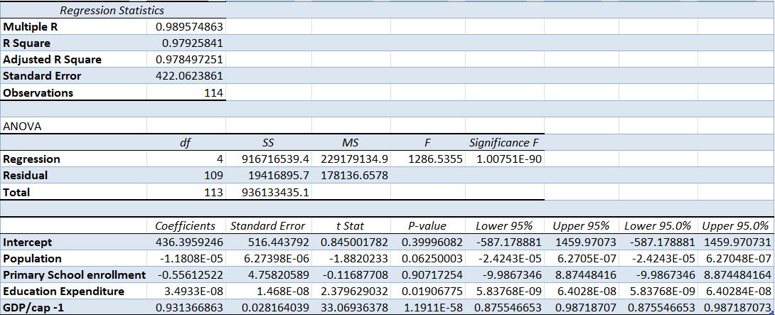
6.0 CONCLUSION
The findings of the study emphasize the critical role of education expenditure in fostering economic growth, highlighting the significant and positive relationship between the two. This correlation suggests that increased investments into the education system of a country will fuel economic growth by raising human capital and promoting innovation. Policymakers should prioritize education as a cornerstone of economic development, recognizing its pivotal role in adding to human capital and driving innovation. While the primary school enrollment variable demonstrates a negative impact on short-term GDP per capita, the effect is not statistically significant, meaning that it should not be considered relevant. This shows the importance of focusing on education quality and access to higher levels of education to take advantage of the economic benefits of education spending. However, this should be done alongside efforts to enhance primary education access, because although this model doesn’t show it, there is plenty of literature backing that
In light of these findings, policymakers should focus heavily on the quality of their country's education, and not take a parsimonious approach to education spending when discussing economic policy. This approach should focus on enhancing the quality of education, increasing access to higher levels of education, and ensuring that education spending is aligned with broader economic development goals. By doing so, these policies can foster economic
Empirical Economic Bulletin, Vol. 17 167
growth and drive economic development, which will in turn generate those profits back to the government, and more importantly, slow or even eventually stop the mass exodus from these Latin American countries that is currently happening.
Empirical Economic Bulletin, Vol. 17 168
Appendix A: Variable Description and Data Source
Acronym Description
Pop
PSE
EduExp
Foreign Direct Investment flows by country in millions of dollars
Foreign Direct Investment flows non manufacturing by country in millions of dollars
Foreign Direct Investment flows manufacturing by country in millions of dollars
Data source
(RGDP/Cap)t-1
Gross Domestic Product in millions of dollar
US Bureau of Economic Analysis
US Bureau of Economic Analysis
US Bureau of Economic Analysis
International Monetary Fund
Empirical Economic Bulletin, Vol. 17 169
Works Cited:
Alves, Pedro Jorge Holanda Figueiredo, PhD., et al. "Fiscal Decentralization and Economic Growth: Evidence from Brazilian States." Public Sector Economics 47.2 (2023): 255-80. ProQuest. Web. 29 Apr. 2024.
Central American migration: Facts, FAQs, and how to help (2023). Retrieved from https://www.worldvision.org/refugees-news-stories/central-american-migration-facts
Deme, Mamit, and Ali M. A. Mahmoud. “Effect of Quantity and Quality of Education on Per Capita Real-GDP Growth: Evidence from Low- and Middle-Income African Countries.” Applied Economics, vol. 52, no. 57, Dec. 2020, pp. 6248–64. EBSCOhost, https://doi.org/10.1080/00036846.2020.1789058.
Hanushek, Eric A., and Ludger Woessmann. "The Role of Cognitive Skills in Economic Development." Journal of Economic Literature, vol. 46, no. 3, 2008, pp. 607-68.
Hatefi, S. M., and S. A. Torabi. “A Slack Analysis Framework for Improving Composite Indicators with Applications to Human Development and Sustainable Energy Indices.” Econometric Reviews, vol. 37, no. 3, Mar. 2018, pp. 247–59. EBSCOhost, search.ebscohost.com/login.aspx?direct=true&db=ecn&AN=1721603&site=ehost-live.
Jerven, Morten, and Deborah Johnston. “Statistical Tragedy in Africa? Evaluating the Data Base for African Economic Development.” Journal of Development Studies, vol. 51, no. 2, Feb. 2015, pp. 111–15. EBSCOhost, search.ebscohost.com/login.aspx?direct=true&db=ecn&AN=1520796&site=ehost-live.
Li, Xinyao, and Chung-Khain Wye. “The Effect of Investment in Education on China’s Economic Growth: The Role of Financial Development.” Chinese Economy, vol. 56, no. 1, Jan. 2023, pp. 69–87. EBSCOhost, https://doi.org/10.1080/10971475.2022.2058182.
Luca Bortolotti, Mario Biggeri, Is the slowdown of China's economic growth affecting multidimensional well-being dynamics?, Structural Change and Economic Dynamics, Volume 63, 2022, Pages 478-489, ISSN 0954-349X, https://doi.org/10.1016/j.strueco.2022.07.003.
Empirical Economic Bulletin, Vol. 17 170
OECD (2021). Tax-to-GDP Ratio by Country. [Data set]. Retrieved from https://www.oecd.org/tax/tax-policy/tax-to-gdp-ratio.htm
Pew Research Center (2023). Changing Migration Patterns from Latin America and Spain. [Data set]. Retrieved from https://www.pewresearch.org/hispanic/2023/01/01/changingmigration-patterns-from-latin-america-and-spain/
The Guatemalan-Mexican Border: Central American Immigration to the United States: An Overview (2021). Retrieved from https://globalist.yale.edu/blog/2020/04/18/theguatemalan-mexican-border-central-american-immigration-to-the-united-states/
Tong Zhang, Xunpeng Shi, Dayong Zhang, Junji Xiao, Socio-economic development and electricity access in developing economies: A long-run model averaging approach, Energy Policy, Volume 132, 2019, Pages 223-231, ISSN 0301-4215, https://doi.org/10.1016/j.enpol.2019.05.031.
Velkovska, Ivana, and Borce Trenovski. "Economic Growth Or Social Expenditure: What is More Effective in Decreasing Poverty and Income Inequality in the European Union - a Panel VAR Approach." Public Sector Economics 47.1 (2023): 111-42. ProQuest. Web. 29 Apr. 2024.
Empirical Economic Bulletin, Vol. 17 171
The Causal Nexus Between Government Expenditure on Education and Individual Savings Behavior in Argentina
Amanda Spielmana
Abstract:
This paper investigates the possibility of interdependence between education and savings by looking at the relationship between a country’s government expenditure on education and the saving rate Public education expenditure has been studied as an explanatory variable for economic growth, but similar studies determining its impact on household savings behavior are lacking. This research looks to determine Granger Causality using the Vector Error Correction Model between this measure of the quality of education and savings rate for Argentina. The results show bidirectional causality between the savings rate and government expenditure on education, as well as unidirectional causality with government expenditure on education to inflation and savings on unemployment.
JEL Classification: E21, G41, G51, G53
Keywords: Savings Rate, Government Education Expenditure, Household Savings
a Department of Economics, Bryant University, 1150 Douglas Pike, Smithfield, RI 02917. Email: aspielman@bryant.edu
Empirical Economic Bulletin, Vol. 17 172
1.0 INTRODUCTION
Long term research has provided the perception that “savings contribute to higher investment and hence higher GDP growth in the short run” (Mohan, 2006). However, more current research has shown that economic growth actually contributes to savings (Mohan, 2006). Either way, savings rates and individual savings behavior have long been used as an economic indicator for a country’s sustainability or the lifestyle of their people. This paper aims to contribute to research on what determines these rates.
To do this, this study aims to enhance understanding of the determinants of savings with the main variable of interest being education Education will be measured in terms of quality. From a macroeconomic perspective, the study will be able to make policy suggestions for governments on how they can increase savings rates, an important economic indicator, through their own expenditure actions and prioritizations. By understanding additional determinants of personal savings, which governments can change themselves, will allow countries to have better control over their economic condition and economic outlook.
Previous studies looking at education and savings have focused on financial literacy as a measure of education or examined the impacts of learning in a micro-economics behavioural research setting. For example, Bennet (2018) examined the “effects of educational attainment on an individual’s portfolio diversity and their propensity to invest in specific financial asset classes.” While they found that individuals with higher educational attainment are more likely to invest in more diverse portfolios and in various asset classes, these findings are not as helpful at a macro level with regards to policy implications
This paper was guided by three research objectives that differ from other studies: First it investigates the possibility of causality between government expenditure on education and the savings rate. Additionally, this study will include a variety of previously studied determinants related to culture, income, and the labor market to serve as a synthesis of many previous research studies. Lastly, Granger Causality will be used to not only analyze the causal relationship between education and savings but also the causal relationships among these control variables included in the VEC model, as well.
Empirical Economic Bulletin, Vol. 17 173
The rest of the paper is organized as follows: Section 2 gives a brief literature review. Section 3 outlines the empirical model used to test for Granger Causality. Data and estimation methodology are discussed in section 4. Finally, section 5 presents and discusses the empirical results and policy implications. This is followed by a conclusion in section 6.
2.0 Tracking Socioeconomic Dynamics: Government Spending, Economic Indicators, and Savings Trends in Argentina
It is important to understand how savings behaviors have changed over time in Argentina, before understanding what might affect it. It is also important to consider it in comparison to other countries. Figure 1 shows how the savings rate in Argentina (as a % of GDP) compares to other countries classified in their region by the World Bank. Their savings rate has ranged from 14.7% to 32% and shows an overall slight downward trend. Based on GDP per capita, Argentina falls in the upper rankings of income compared to the region but stands out less when looking at how individuals use this income.
1: Gross Domestic Savings (as % of GDP) in Argentina Compared to Region
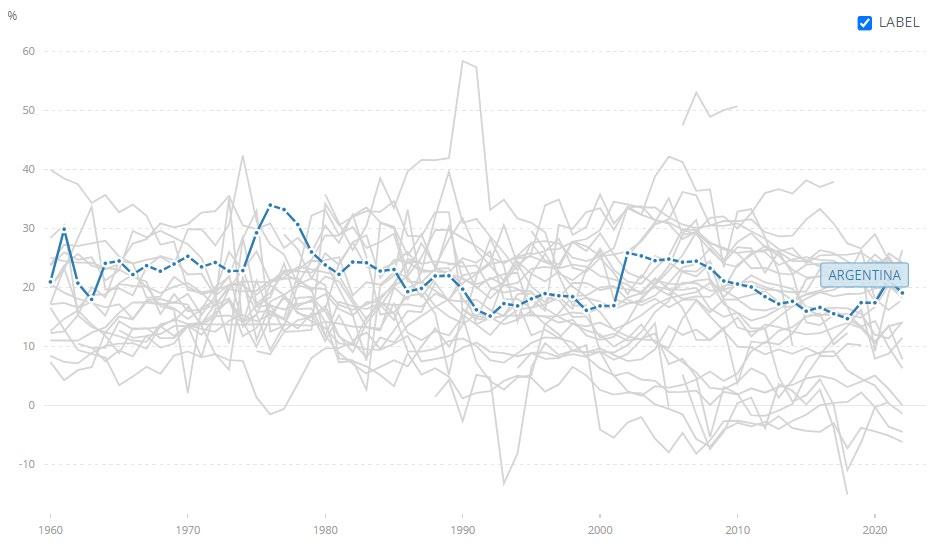
Source: World Bank Database
In order to determine why individuals’ savings rates in Argentina might not be as high as individuals’ savings rates in other countries we look at savings trends relating to a
Figure
Empirical Economic Bulletin, Vol. 17 174
variety of economic and cultural factors. Figure 2 shows government expenditure on education and savings. Contrary to what we might expect, we see that government expenditure on education, as a percentage of GDP, is actually lower when gross domestic savings (as a percentage of GDP) is higher.
and Government Expenditure on Education Government expenditure on education, total (% of GDP) [SE.XPD.TOTL.GD.ZS] Gross domestic savings (% of GDP) [NY.GDS.TOTL.ZS]
Source: World Bank Database
Figure 3 shows the trend between savings and inflation in Argentina since 1983. We see that in times when inflation reaches its peak, so does savings, and they follow similar jumps over time. Typically, we would expect that as inflation rises, the purchasing power of consumers decrease, and more of their income goes to consumption on necessities rather than saving.
Figure 2: Gross Domestic Savings and Government Expenditure on Education
0 2 4 6 8 0 10 20 30 40 Gov. Expenditure on Edu Gross Domestic Savings Savings
Empirical Economic Bulletin, Vol. 17 175
Figure 3: Gross Domestic Savings and Inflation
Savings and Inflation
Inflation, GDP deflator (annual %) [NY.GDP.DEFL.KD.ZG]
Gross domestic savings (% of GDP) [NY.GDS.TOTL.ZS]
Source: World Bank Database
Inflation, GDP Deflator, Annual Change
Lastly, Figure 4 shows the relationship between savings and unemployment. As individuals in the labor force lose their job, we expect they have less money to put towards savings. Therefore, we see that as unemployment rises, savings decreases, and the negative relationship follows the economic upswings and downswings relatively consistently.
Figure 4: Gross Domestic Savings and Unemployment
Savings and Unemployment
Unemployment, total (% of total labor force) (national estimate) [SL.UEM.TOTL.NE.ZS]
Gross domestic savings (% of GDP) [NY.GDS.TOTL.ZS]
Source: World Bank Database
-1000 0 1000 2000 3000 4000 0 10 20 30 40
Gross Domestic Savings
0 5 10 15 20 25 0 5 10 15 20 25 30 35 40 1 3 5 7 9 11 13 15 17 19 21 23 25 27 29 31 33 35 37 39 41 43 45 47 49 Unemployment (%) Gross Domestic Savings
Empirical Economic Bulletin, Vol. 17 176
3.0 LITERATURE REVIEW
Household and individual saving behaviors can be an important economic indicator for a country. Not only can it show independence and sustainability, but also trends for future economic growth and provide determinants of wealth. Ersin and Eti (2017) find that a lack of savings, even starting at a young age, “directs country economies to foreign sources…[and] increases the debt of the country.” Based on new findings related to the determinants of savings, governments have begun to investigate opportunities for policies and precautions to increase savings (Doker et al., 2016). Belekhova and Rossoshanskii (2018) explain their findings provide further support for already current political courses focused on the birth rate, promoting public health, and optimizing the financial system. However, they also note that future policies must also work to develop more effective social policies, as well.
A large portion of literature concentrated on finding the true demographic and cultural determinants of savings have been studied using middle-income countries or transition economies. According to Doker et al. (2016), for these transition economies which have “transitioned from a planned economic system to market economy, the structure of savings has changed from public funds to private savings.” Additionally, Mpaata et al. (2020) explain their findings which suggest “from the developed country context, Social Influence positively affects Savings Behavior,” which differs from developing economies who experience a “negative impact of social influence on savings behavior.” Understanding the differences in determinants based on country characteristics proves to also be a must in research going forward.
Traditional studies focus on macroeconomic variables and their relation to savings rate and find variables such as GDP per capita, female labor force participation, dependency ratio, unemployment, and urbanization to be related (Doker et al., 2016; Błoch 2023; Grigoli et al., 2018; Niculescu-Aron and Mihăescu, 2012; Iqbal et al., 2021). In studying the direct relations to income, Hashim et al. (2017) investigates the influence of CPI, GNI, and interest rates on the savings rate in Malaysia. Despite unsignificant results, the study finds a positive relationship between interest rate, CPI, and savings. However, other studies also investigate the relationship between income and savings using per capita income growth and find it to be positively significant (Edwards, 1996; Hussein and
Empirical Economic Bulletin, Vol. 17 177
Thirlwall, 1999; Grigoli et al., 2018). Edwards (1996) goes so far as to claim per capita income growth as “the most important determinant of private and public savings.” Beyond this, Edwards (1996) study finds that countries with higher political instability tend to have lower public savings and looks to identify why the savings rate in Latin America is especially low. Their study ultimately suggests this is due to the magnitudes of their determinants in Latin America, and not to be blamed by structural differences. This study will be of help to this current research in identifying the determinants of savings in Latin America, beyond the independent variables we will study.
Consumer confidence is also heavily linked to the saving activities of individuals and households, especially in higher income countries. However, Vanlaer et al. (2019) find that consumer confidence in terms of the general economic situations has a substantially smaller effect on household saving compared to confidence in individual household financial situations. Current literature also explains the strong positive relationship between savings and interest rates (Ogaki et al. 1996). It is from this that we wonder whether the level of education one receives can change the influence of consumer confidence based on individual situational awareness and awareness of the economic conditions of the country’s economy, as a whole.
Newer studies determine culture to be related to the formation of the saving (Ersin and Eti, 2017; Shoham and Malul, 2012). Variables used as a measure of culture include the level of uncertainty avoidance and the level of how collectivist a society is, both of which were found to be positively significant with savings rates (Shoham and Malul, 2012).
Despite an influx of current research which has looked to determine the impact of financial literacy and financial education on savings rate, a large literature gap still remains in understand the influence of general education, more specifically, quality of education, on savings behavior (Lusardi, 2008; Rothwell and Wu, 2017; Calderone et al., 2018). Grigoli et al. (2018) includes government spending components on education and health in their analysis but finds ambiguous results. Zwane et al. (2016) aims to include the level of education received as an explanatory variable for household savings levels by accounting for a head of household with a primary, secondary, and or tertiary education with binary variables. They find secondary and tertiary education to have a positive significant impact in all of their models, while primary is positive, but not significant. This differs from the
Empirical Economic Bulletin, Vol. 17 178
findings of Morisset and Revoredo (1995). They find the effects of primary and secondary education on savings to both be positive and significant, while university education (tertiary) is only positive for industrial countries.
We expect that individuals with more education will be more financially aware and may have greater access to financial markets and accounts. Additionally, those who are educated likely have greater discretionary income to put towards saving. Cole et al. (2014) also explains that “education increases financial market participation, measured by investment income and equities ownership, while dramatically reducing the probability that an individual declares bankruptcy, experiences a foreclosure, or is delinquent on a loan.”
A study done in Kenya after the introduction of Free Primary Education in 2003 found their experimental program to be associated with increases in the use of formal financial services, such as mobile banking; however, the study found little improvements in retirement planning and subjective well-being (Ajayi and Ross, 2017).
Past theoretical research has looked at the impacts of education level, government spending on education, and other human capital index variables as determinants or GDP (Villela and Paredes, 2022; Ziberi et al. 2022; Malangeni and Phiri 2018). Therefore, the research presented within this current paper aims to investigate these same variables, with savings rate and attainment of accounts at financial institutions.
4.0 DATA AND EMPIRICAL METHODOLOGY
4.1 Data
The study uses annual, time series data from 1982 to 2022 for Argentina. Data was obtained from the World Bank website through their World Development Indicators DataBank Summary statistics for the data are provided in Table 1.
Table 1 Summary Statistics
Variable Observation Mean Std. Dev. Min Max Poverty (POV) 33 5.724 4.792 1 24 Inflation (INF) 50 193.532 518.843 -3.561 3046.091 Empirical Economic Bulletin, Vol. 17 179
4.2 Empirical Model
This study will follow the model used by Demano and Sibera (2022), to measure the relationship between economic growth, investment, and saving using a tertiary VAR model for Granger Causality:
The model for this study which adds a fourth variable and uses savings rate as the dependent variable is written as follow:
Gov. Exp. on Edu as a % of GDP (GOVEXP) 41 3.550 1.620 1.046 5.776 Gross Domestic Savings as a % of GDP (SAV) 50 21.155 4.519 14.725 33.983 Labor force Participation (LFP) 39 57.534 3.584 50.3 61.943 Age Dependency Ratio (ADR) 50 59.937 3.381 53.779 64.517 Unemployment (UMP) 48 8.504 4.600 2 19.59
�������� = ����1 + �����1,���� ��������−���� + �����1,���� ��������−���� + ���� ����=1 �����1,���� ��������−���� + ���� ����=1 ������������ ���� ����=1 �������� = ����2 + �����2,���� ��������−���� + �����2,���� ��������−���� + ���� ����=1 �����2,���� ��������−���� + ���� ����=1 ������������ ���� ����=1 �������� = ����3 + �����3,���� ��������−���� + �����3,���� ��������−���� + ���� ����=1 �����3,���� ��������−���� + ���� ����=1 ������������ ���� ����=1
������������������������������������������������ = ����1 + �����1,���� ������������������������������������������������−���� + �����1,���� ����������������������������������������−���� + ���� ����=1 �����1,���� ����������������������������������������−���� + �����1,���� ������������������������������������−���� + ���� ����=1 ���� ����=1 ������������ ���� ����=1 ���������������������������������������� = ����2 + �����2 ���� ����������������������������������������−���� + �����2 ���� ����������������������������������������−���� + �����2 ���� ������������������������������������−���� + ���� ����=1 ���� ����=1 �����2 ���� ������������������������������������������������−���� + ���� ����=1 ������������ ���� ����=1 ���������������������������������������� = ����3 + �����3,���� ����������������������������������������−���� + �����3,���� ����������������������������������������−���� + �����3 ���� ������������������������������������−���� + ���� ����=1 ���� ����=1 �����3,���� ������������������������������������������������−���� + ���� ����=1 ������������ ���� ����=1 Empirical Economic Bulletin, Vol. 17 180
P is the maximum number of lagged observations included in the model. Given that the data used for this analysis is yearly, 2 lags will be included. ������������������������������������������������ is a measure of the gross domestic savings in Argentina as a percentage of GDP As defined by The World Bank’s data glossary, “Gross domestic savings are calculated as GDP less final consumption expenditure (total consumption)” (Glossary | DataBank, n.d.). ���������������������������������������� is a measure of Argentina’s government’s expenditure on education as a percentage of GDP. The World Bank’s data glossary writes “General government expenditure on education (current, capital, and transfers) is expressed as a percentage of GDP. It includes expenditure funded by transfers from international sources to government. General government usually refers to local, regional and central governments” (Glossary | DataBank, n.d). ���������������������������������������� is a measure of the annual % inflation using GDP deflator. As defined by The World Bank, “inflation as measured by the annual growth rate of the GDP implicit deflator shows the rate of price change in the economy as a whole. The GDP implicit deflator is the ratio of GDP in current local currency to GDP in constant local currency” (Glossary | DataBank, n.d.). Lastly, ���������������������������������������������������� shows the percentage of the Argentina labor force who currently is without a job, but is available for or seeking employment.
A Granger Causality test is used to identify a causal relationship with variables, when using time series data. “Granger causality examines whether lagged values of one variable helps to predict another variable or studies the causal relation that exists among different economic variables” (Denano & Sibera, 2022). Before determining Granger Causality, I ran an Augmented-Dickey Fuller Test to determine if a unit root is present in the model. If a unit root is present, it means the time series is non-stationary, meaning the mean and variance may not be constant over time. A Johansen Cointegration Test uses an estimation of a “vector error-correction model to obtain likelihood ratios”. “The role of the cointegration is to link between the relations among a set of integrated (no stationary) series and the long-term equilibrium. The presence of a co-integrating equation is interpreted as a long-run equilibrium relationship among the variables” (Demano and Sibera, 2022). To test for co-integration Johansen’s Trace test and Maximum Eigenvalue test are used. The
������������������������������������ = ����4 + �����4 ���� ����������������������������������������−���� + �����4 ���� ����������������������������������������−���� + �����4 ���� ������������������������������������−���� + ���� ����=1 ���� ����=1 �����4 ���� ������������������������������������������������−���� + ���� ����=1 ������������ ���� ����=1
Empirical Economic Bulletin, Vol. 17 181
Trace test has a null hypothesis that there are at most r co-integrating against the alternative that there are more than r co-integrating vectors while the Maximum Eigenvalue test has a null hypothesis that there are exactly r co-integrating vectors against the alternative that there are more than r co-integrating vectors.
5.0 EMPIRICAL RESULTS
To test for stationarity, the Augmented-Dickey Fuller test was used. Level variable statistics are smaller than the critical value in the case for savings, government expenditure on education, and unemployment, indicating the variables are not stationary. In the presence of non-stationarity, it is critical to take the first difference the variables. At the level of the data, proceeding with the Granger Causality test would lead to misspecification. By differencing the three remaining variables, the series becomes stationary.
Augmented-Dickey Fuller Test – P-Values
After gathering the results of unit roots, I next determine if co-integration exists, using the same order of integrated variables. The Johansen test is used to calculate the trace statistics and maximum eigenvalue statistics. If the trace or max-eigenvalue statistics is/are greater than the level of critical value, we reject the null hypothesis. According to my results, we have enough evidence to reject the null, indicating that co-integration and a long-run relationship exists between savings, government expenditure on education, inflation, and unemployment.
Johansen Test for Co-Integration (Trace Test)
Maximum Rank Eigen Value Trace Value 5% Critical Value 0 0.74208 53.0021 47.8561 1 0.3327 15.059 29.7971 2 0.1109 3.7346 15.4947
Variables Variable at Level Variable at First Differences Savings 0.3425 0.0000*** Gov. Exp. on Edu 0.7863 0.0000*** Inflation 0.0005*** 0.0000*** Unemployment 0.5603 0.0000*** Empirical Economic Bulletin, Vol. 17 182
Johansen Cointegration Test (Max-Eigen Test)
After completing the unit root and co-integration test, I could proceed with the Granger Causality test using the VECM. The results show unidirectional causality runs from government expenditure on education to inflation, and from savings to unemployment. Bidirectional granger causality was found between savings and government expenditure on education.
Granger Causality F statistics Probability Results
Cholesky’s impulse response function measures the dynamic response of endogenous variables to a one standard deviation shock in one of the structural shocks. This helps to identify how each variable in the model reacts to the shock over time. The graphs below show the plotted IRFs as calculated using the VAR representation of the model. We see that the response of gross domestic savings to both government expenditure
3 0.0157 0.442 3.8415
Maximum Rank Eigen Value Max-Eigen Value 5% Critical Value 0 0.7421 37.9431 27.5843 1 0.3327 11.3245 21.1316 2 0.1109 3.2825 14.2646 3 0.0157 0.442 3.8415
Savings to Gov. Exp. on Edu 3.04442 0.0642 Bidirectional Gov. Exp. on Edu to Savings 4.24891 0.0249 Causality Inflation on Gov. Exp. to Edu 1.39759 0.2645 Unidirectional Gov. Exp. on Edu to Inflation 7.43039 0.0027 Causality Unemployment to Gov. Exp. on Edu 1.21888 0.314 No Gov. Exp on Edu to Unemployment 1.33664 0.2824 Causality Inflation to Savings 1.74506 0.1869
Savings to Inflation 0.22956 0.7959
Unemployment on Savings 0.08469 0.919 Unidirectional Savings on Unemployment 5.22233 0.0098
Unemployment to Inflation 1.1464 0.3283
Inflation to Unemployment 0.38233 0.6848
No
Causality
Causality
No
Causality
Empirical Economic Bulletin, Vol. 17 183
on education and inflation is negative, but increasing. The response to government expenditure on education never becomes positive, but the response to inflation does around 5.5. The opposite trend is true for the response of savings to unemployment. This response increases, but starts positive, until around 5 when it becomes decreasing.
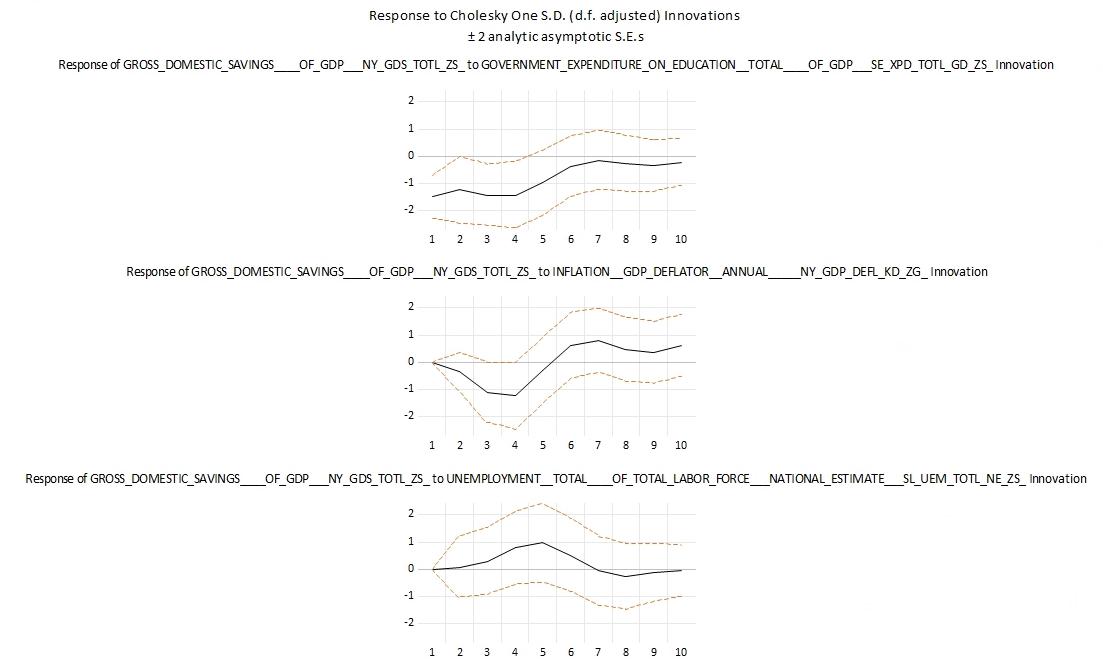
5.0 CONCLUSION
This study uses VECM and Granger Causality tests to determine the nexus between savings, government expenditure on education, inflation, and unemployment in Argentina for the period 1982-2022. The main goal of this study was to better determine how education is related to savings behaviors, while not only focusing on financial literacy. By including government expenditure on education as a measure of the quality of education within Argentina, I was able to identify bidirectional Granger Causality, meaning that government expenditure on education Granger Causes savings, and savings also Granger Causes government expenditure on education. This is an interesting relationship that should continue to be studied, and determined how the relationship is different among countries of different income levels. It is also interesting to find unidirectional causality runs from government expenditure on education to inflation, and from savings to unemployment.
Empirical Economic Bulletin, Vol. 17 184
Policy makers should keep these in mind as they attempt to better foster savings environments in their counties. As individual’s savings becomes increasingly used as a way to measure stability of a country and indicates sustainability as an economy, it is critical to understand all the components that may incentivize strong savings habits or make individual saving more feasible.
Appendix A: Variable Description and Data Source
Variable Name Description
Savings Gross domestic savings are calculated as GDP less final consumption expenditure (total consumption).
GovExpEDU General government expenditure on education (current, capital, and transfers) is expressed as a percentage of GDP. It includes expenditure funded by transfers from international sources to government. General government usually refers to local, regional and central governments.
Inflation Inflation as measured by the annual growth rate of the GDP implicit deflator shows the rate of price change in the economy as a whole. The GDP implicit deflator is the ratio of GDP in current local currency to GDP in constant local currency.
Unemploy Unemployment refers to the share of the labor force that is without work but available for and seeking employment. Definitions of labor force and unemployment differ by country.
Data source
World Bank national accounts data
UNESCO Institute for Statistics (UIS)
World Bank national accounts data
International Labour Organization
Empirical Economic Bulletin, Vol. 17 185
BIBLIOGRAPHY
Ajayi, K. F., & Ross, P. H. (2020). The Effects of Education on Financial Outcomes: Evidence from Kenya. Economic Development and Cultural Change, 69(1), 253–289.
https://doi.org/10.1086/702996
Błoch, W. (2023). What drives the savings rate in middle-income countries? Economics and Business Review, 9(4). https://doi.org/10.18559/ebr.2023.4.1072
Calderone, M., Fiala, N., Mulaj, F., Sadhu, S., & Sarr, L. (2018). Financial Education and Savings Behavior: Evidence from a Randomized Experiment among Low-Income Clients of Branchless Banking in India. Economic Development and Cultural Change, 66(4), 793–825. https://doi.org/10.1086/697413
Cole, S., Paulson, A., & Shastry, G. K. (2014). Smart Money? The Effect of Education on Financial Outcomes. The Review of Financial Studies, 27(7), 2022–2051.
Denano, T., & Sibera, S. (2022). The Causal Nexus between Economic Growth, Investment and Saving using Vector Error Correction Model in Ethiopia. Studies of Applied Economics, 40(3), Article 3. https://doi.org/10.25115/eea.v40i3.7887
Doker, A., Turkmen, A., & Emsen, Ö. (2016). What are the Demographic Determinants of Savings? An Analysis on Transition Economies (1993-2013). Procedia Economics and Finance, 39, 275–283. https://doi.org/10.1016/S2212-5671(16)30324-0
Edwards, S. (1996). Why are Latin America’s savings rates so low? An international comparative analysis. Journal of Development Economics, 51(1), 5–44. https://doi.org/10.1016/S0304-3878(96)00424-5
Empirical Economic Bulletin, Vol. 17 186
Ersin, İ., & Eti, S. (2017). Measuring the waste-conscious and saving habits of the youth in Turkey: The sample of Istanbul Medipol university. International Journal of Islamic Economics and Finance Studies, 3(3), 41–49.
Glossary | DataBank. (n.d.). The World Bank. Retrieved March 21, 2024, from https://databank.worldbank.org/metadataglossary/world-developmentindicators/series/NY.GDP.DEFL.KD.ZG
Grigoli, F., Herman, A., & Schmidt-Hebbel, K. (2018). Saving in the world. World Development, 104, 257–270. https://doi.org/10.1016/j.worlddev.2017.11.022
Hashim, D. B., Pin, F. B., & Mohd Isa, M. Y. B. (2017a). Factors Influencing Savings Rate in Malaysia. International Journal of Economics and Finance, 9(6), 52. https://doi.org/10.5539/ijef.v9n6p52
Hussein, K. A., & Thirlwall, A. P. (1999). Explaining differences in the domestic savings ratio across countries: A panel data study. Journal of Development Studies, 36(1), 31–52. https://doi.org/10.1080/00220389908422610
Iqbal, M., Rehman, H. ur, Arshed, N., & Sardar, M. S. (2021). The Macroeconomic and Demographic Determinants of Saving Behavior in Selected Countries of Asia. Journal Global Policy and Governance, 10(1), Article 1. https://doi.org/10.14666/2194-7759-10-1004
Lusardi, A. (2008). Household Saving Behavior: The Role of Financial Literacy, Information, and Financial Education Programs (Working Paper 13824). National Bureau of Economic Research. https://doi.org/10.3386/w13824
Empirical Economic Bulletin, Vol. 17 187
Malangeni, L., & Phiri, A. (2018). Education and Economic Growth in Post-apartheid South Africa: An Autoregressive Distributive Lag Approach. International Journal of Economics and Financial Issues, 8(2), Article 2.
Mpaata, E., Koske, N., & Saina, E. (2020). Social Influence And Savings Behavior: Evidence From A Developing Country Context. SEISENSE Journal of Management, 3, 56–67.
https://doi.org/10.33215/sjom.v3i4.396
Niculescu-Aron, I., & Mihăescu, C. (2012). Determinants of Household Savings in EU:What Policies for Increasing Savings? Procedia - Social and Behavioral Sciences, 58, 483–492.
https://doi.org/10.1016/j.sbspro.2012.09.1025
Ogaki, M., Ostry, J. D., & Reinhart, C. M. (1996). Saving Behavior in Low- and Middle-Income Developing Countries: A Comparison. Staff Papers (International Monetary Fund), 43(1), 38–71. https://doi.org/10.2307/3867352
Revoredo, C. L., & Morisset, J. P. (1999). Savings and Education: A Life-Cycle Model Applied to a Panel of 74 Countries (SSRN Scholarly Paper 620680).
https://papers.ssrn.com/abstract=620680
Rothwell, D. W., & Wu, S. (2024). The Impact of Financial Education Participation on Financial Knowledge and Efficacy: Evidence from the Canadian Financial Capability Survey. https://doi.org/10.31235/osf.io/mpz4v
Shoham, A., & Malul, M. (2012). The role of cultural attributes in savings rates. Cross Cultural Management: An International Journal, 19, 304–314.
https://doi.org/10.1108/13527601211247062
Empirical Economic Bulletin, Vol. 17 188
Villela, R., & Paredes, J. J. (2022). Empirical Analysis on Public Expenditure for Education, Human Capital and Economic Growth: Evidence from Honduras. Economies, 10(10), Article 10. https://doi.org/10.3390/economies10100241
Willem, V., Link to external site, this link will open in a new tab, Samantha, B., & Wim, M. (2020). Consumer Confidence and Household Saving Behaviors: A Cross-Country Empirical Analysis. Social Indicators Research, 147(2), 677–721. https://doi.org/10.1007/s11205-019-02170-4
Ziberi, B. F., Rexha, D., Ibraimi, X., & Avdiaj, B. (2022). Empirical Analysis of the Impact of Education on Economic Growth. Economies, 10(4), Article 4. https://doi.org/10.3390/economies10040089
Zwane, T., Greyling, L., & Maleka, M. (2016). The Determinants Of Household Savings In South Africa: A Panel Data Approach. International Business & Economics Research Journal (IBER), 15, 209. https://doi.org/10.19030/iber.v15i4.9758
Empirical Economic Bulletin, Vol. 17 189
HDI and Standard of Living: A Panel Data Analysis of Latin America
Matthew Susich
Abstract:
This paper investigates the correlation between the Human Development Index and other significant measures of standard of living. The study incorporates data for upper- and middle-income countries in Latin America (Mexico, Costa Rica, Columbia, Peru, Uruguay, Brazil, Paraguay, Guatemala, Jamaica, Belize, and Bolivia) surrounding standard of living, including GDP per capita, public spending on education, public spending on health, GNI per capita, unemployment, infant mortality, and inflation. The conclusions from this study are drawn from regression analysis and tests of correlation between the Human Development Index and alternative measures of standard of living.
The results show that unemployment and infant mortality are negatively correlated with HDI and statistically significant.
JEL Classification: F63, I31
Keywords: Economic Development, General Welfare, Well-Being
a Department of Economics, Bryant University, 1150 Douglas Pike, Smithfield, RI02917. Phone: (401) 232-6379. Email: msusich@bryant.edu.
Empirical Economic Bulletin, Vol. 17 190
1.0 INTRODUCTION
The Human Development Index (HDI) is one of the most widely used economic measures of human development, overall welfare, and standard of living on a global scale. It is primarily a summary statistic that measures three main dimensions: health, education, and overall standard of living. HDI is mainly used to compare standard of living across countries. It is also considered a far more accurate and precise measure of standard of living and economic development than other measures, such as gross domestic product (GDP) per capita. However, measuring standard of living can be difficult because ultimately, it is complex and is the product of a large variety of factors. So, how well does the human development index measure human development and general well-being?
This study aims to test the accuracy of HDI as a development measure by analyzing its correlation with alternative measures of health, education, and overall standard of living. The HDI is a composite measure that uses health measures (life expectancy at birth and life expectancy index), education measures (expected years of schooling, mean years of schooling, and education index), and standard of living measures (GNI per capita and GNI index) to acquire a general understanding of a country’s level of human development (Human Development Reports, 2022). Using the HDI measures of eleven upper/middle income Latin American countries over a 22-year period, this study will assess the accuracy of HDI by testing its correlation with alternative important measures of development and standard of living. Unemployment, inflation, and infant mortality are important measures of development and well-being but are not specifically captured by HDI.
Empirical Economic Bulletin, Vol. 17 191
This study is relevant because its conclusions have implications for how to assess the economic development of a country and the general welfare of its citizens properly and accurately. It will contribute to the understanding of economic and human development and how best to assess them. This study also aims to uncover the variables most strongly correlated with development and whether HDI provides a proper reflection. Furthermore, the findings and conclusions of this study have the potential to inform policy and development decisions for economic and governmental leaders in Latin America.
This paper was guided by three research objectives that differ from other studies: First it investigates the accuracy of HDI as a development measure; Second, it examines the impact of alternative development measures on HDI; Last, the study specifically examines upper/middle income Latin American countries and their development. There is very little empirical work in the literature concentrating on Latin American countries and the correlation between HDI and the aforementioned alternative variables. This paper successfully fills this void.
The rest of the paper is organized as follows: Section 2 discusses different trends surrounding HDI and its relationship to alternative variables. Section 3 gives a brief literature review. Section 4 outlines the empirical model and discusses data and estimation methodology. Finally, section 5 presents and discusses the empirical results. This is followed by a conclusion in section 6.
Empirical Economic Bulletin, Vol. 17 192
2.0 TREND
Figure 1 shows the relationship between HDI and the employment rate and unemployment rate in Central and Eastern European countries Based on this graph, the HDI value and employment rate seem to move in similar directions, while the HDI value and unemployment rate seem to move in opposite directions. This would indicate that the HDI accurately reflects development in terms of unemployment. In other words, the HDI decreases when unemployment is higher and increases when unemployment is lower.
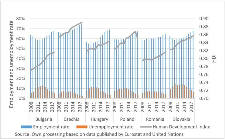
Source: (Popa, Jimon, David, & Sahlian, 2021)
Figure 2 shows two separate graphs. The graph on the left shows the worldwide trend of infant mortality over ten years (2000-2010). The graph on the right shows the worldwide trend of HDI over the same ten-year period. Based on these graphs, it is evident that these two measures are moving in opposite directions. This would indicate that the
Figure 1: Employment rate, unemployment rate, and HDI
Empirical Economic Bulletin, Vol. 17 193
steady increases in overall HDI over time has reflected the decrease in overall infant mortality over that same period. In other words, these graphs indicate that HDI does indeed reflect changes in infant mortality, even though that measure is not directly used in the calculation of HDI.
Figure 2: Trend in the Infant Mortality Rate and HDI 2000-2010
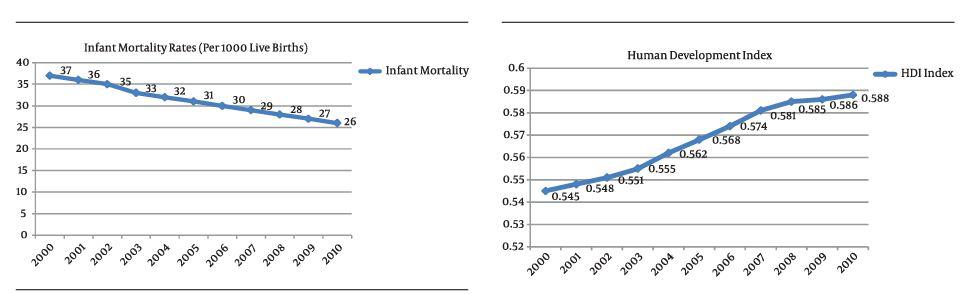
Source: (Alijanzadeh, Asefzadeh, & Zare, 2016)
Figure 3 shows the trend of HDI in 4 of the upper/middle-income countries in Latin America (Brazil, Mexico, Costa Rica, and Uruguay) compared to the world average for 1990-2021. For all 4 countries and the world average, the graph shows a slight increasing trend over time. It also shows that all the countries have had higher HDI values than the world average over the 21-year period.
Empirical Economic Bulletin, Vol. 17 194
Figure 3: Trend in HDI for Mexico, Brazil, Uruguay, and Costa Rica 1990-2021
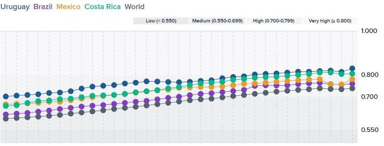
Source: (Human Development Reports, 2022)
3.0 LITERATURE REVIEW
There have been a number of studies related to the examination of the Human Development Index (HDI) as a measure of standard of living, quality of life, and overall welfare. Most of this research was focused on correlational studies between HDI and alternative measures of standard of living. A study by Elistia and Syahzuni (2018) concluded that there was a significant correlation between human development and economic growth, as measured by GDP per capita. Furthermore, a cross-country regression analysis conducted by Shah (2016) also found that there was high correlation between HDI and other welfare measures, such as GDP per capita, literacy rate, life expectancy at birth, Gini index, etc. The author of this study also contended that improvements in education, health, and income are the best means of improving overall human development (Shah, 2016). Furthermore, Alijanzadeh et al. (2016) also found a negative correlation between infant mortality and a number of welfare indicators, including HDI, GDP per capita, and life expectancy. Priambodo (2020) found that unemployment and poverty had a negative effect on HDI, while Ogbebor et al. (2020)
Empirical Economic Bulletin, Vol. 17 195
found that inflation had both a negative and significant impact on standard of living in Nigeria.
However, a study by Sinaga (2020) that investigated the impact of a variety of independent variables on poverty found that HDI had a negative but insignificant impact on poverty. Binder and Georgiadis (2011) found that the development of HDI in a particular country can be drastically different than changes in that country’s GDP. Conversely, Kula et al. (2010) found that health spending as a percentage of GDP was positively correlated with measures of happiness in a given country. This suggests that the allocation of funds as a percentage of GDP has a greater impact on standard of living than the level of GDP itself.
4.0 DATA AND EMPIRICAL METHODOLOGY
4.1 Data
The study uses annual panel data from 2001 to 2021. Data was obtained from the World Bank website World Development Indicators. Data was also obtained from the Human Development Reports website surrounding the Human Development Index. The data includes 7 independent variables for 11 Latin American countries over a 22-year period.
The summary statistics for the data can be found in Table 1.
Table 1: Summary Statistics
Variable Observations Mean Std. Dev. Min Max HDI 242 0.7176 0.0549 0.556 0.83 GDP 242 4412520 8456926 2599.186 3.25e+07 GNI 242 4201070 8068279 2534.837 3.13e+07 EDU 242 4.6925 1.4246 2.0682 8.4371 HEA 242 3.6376 1.2608 1.4673 6.5674 UNEMP 242 7.0465 3.4690 1.902 16.661 INF MORT 242 17.5984 8.4312 5 53.1 INFLAT 242 5.3827 3.6023 -7.1138 22.0228 Empirical Economic Bulletin, Vol. 17 196
4.2 Empirical Model
Following Mpofu (2013), this study adapted and modified their econometric model used to analyze the impact of different variables on HDI in South Africa. This study adds to this model by including alternative measures, such as unemployment, inflation, and infant mortality, to test their impact on HDI in 11 Latin American countries. The model could be written as follows:
ln(HDI) = β0 + β1(ln(GDP)) + β2(ln(EDU)) + β3(ln(HEA)) + β4(ln(GNI))β5(UNEMP) – β6(INF MORT) – β7(INFLAT) + ε
HDI is a country’s human development index score. It is a composite statistic that measures a country’s human development based off of its citizens’ ability to have a long and healthy life, knowledge, and a decent standard of living (Human Development Reports, 2022). HDI is one of the most widely used measures of a country’s economic and human development. In this model, HDI will act as the dependent variable in order to test each of the variables impact on it as well as to test the accuracy of HDI as a development and standard of living measure. The definition of HDI is consistent with Human Development Reports definition of HDI (Human Development Reports, 2022) .
The independent variables for this model consist of seven variables obtained from various sources. Appendix A provides descriptions, expected signs, and justifications for using the variables. First, GDP represents the gross domestic product per capita of the given country EDU represents the country’s level of general expenditure on education as a percentage of that year’s gross domestic product. Similarly, HEA represents the country’s general expenditure on health as a percentage of that year’s gross domestic product. GNI represents the country’s gross national income
Empirical Economic Bulletin, Vol. 17 197
per capita of the given country. Furthermore, UNEMP is the percentage of the country’s labor force that is unemployed for that year. INF MORT is the number of infant deaths per 1,000 live births. Finally, INFLAT represents the percentage increase or decrease in consumer prices for that year. The GDP, GNI, EDU, and HEA variables were logarithmically transformed to follow with the study that this model is based on and to see the percentage increase of HDI as a result of a 1% increase in the dependent variables from the regression. The other independent variables were not logarithmically transformed in order to test the impact of a one unit increase in the variable on HDI.
5.0 EMPIRICAL RESULTS
The empirical estimation results are presented in Table 2. The empirical estimation shows the relationship between the HDI value and the measures of standard of living included in the model for the eleven Latin American countries over the 22-year period. The regression model as a whole was found to be statistically significant and returned an r-squared value of about 0.75, indicating that the model predicts the dependent variable well.
Table 2: Regression Results for Econometric Model
Dependent Variable: Human Development Index Value
Ln (GDP Per Capita) 0.2215** (0.0916)
Ln (Education Expenditure) 0.0221** (0.0102)
Ln (Health Expenditure) 0.0526*** (0.0115)
Ln (GNI Per Capita) -0.2191** (0.0917)
Unemployment -0.0015* (0.0009)
Infant Mortality -0.0062*** (0.0004)
Inflation -0.0006 (0.0007)
Constant -0.3481*** (0.0240)
Empirical Economic Bulletin, Vol. 17 198
Prob > F 0.0000
Note: *** , **, and * denotes significance at the 1%, 5%, and 10% respectively. Standard errors in parentheses.
The GDP variable was found to be positively correlated with HDI value and statistically significant at the 5% level. This finding was expected as generally, increased GDP per capita ties into greater standard of living and financial security. The EDU variable was also found to have a positive correlation with HDI and statistically significant at 5%.
Again, this result was expected as education as a dimension is one of the three main pillars of the HDI calculation. Similarly, the HEA variable had a positive correlation as was significant at the 1% level. Health is another dimension of the HDI calculation, so this result was expected. One interesting finding was the negative correlation between the GNI variable and HDI. Since a decent standard of living is the third dimension of HDI, a positive correlation was expected. However, the significant correlation between the GDP and GNI variables could explain this unexpected result. The UNEMP variable was negatively correlated with HDI and statistically significant at 10%. This result makes sense as higher unemployment is usually correlated with a loss of income and job security, which would negatively impact standard of living and human development.
Furthermore, the INF MORT variable was also found to have a negative relationship with HDI and statistically significant at the 1% level. Again, this was expected given that a higher infant mortality typically indicates worse public health and lower human development. Finally, the INFLAT variable was found to be negatively correlated with HDI but not statistically significant. This result makes sense given that low levels of
R-Squared 0.7542 Adjusted
0.7469
R-Squared
Empirical Economic Bulletin, Vol. 17 199
inflation are typically considered sustainable and linked to economic growth. It is likely, however, that much higher rates of inflation could potentially negatively impact human development.
5.0 CONCLUSION
In summary, the Human Development Index is a reliable measure of human development and standard of living. The results indicate that the HDI measure does indeed reflect alternative measures of standard of living and overall well-being, outside of the measures that are used in its calculation. For example, this study found that HDI was negatively correlated with both unemployment and infant mortality. Although these measures are not directly used in the calculation of the HDI value, this would indicate that the HDI measure reflects changes in alternative measures of standard of living. Based on this study, the HDI value is a fairly precise and accurate measure of a given country’s standard of living and human development.
This study has several implications for policy makers seeking to improve economic and human development within these Latin American countries. First, greater government expenditure on healthcare and education is positively associated with a greater HDI value. In other words, greater investment in these areas can work to improve human development. Furthermore, devoting investment and research into specifically reducing infant mortality can help to improve human development. Additionally, the results of this study also indicate that economic policy makers should aim to reduce unemployment in order to increase quality of life for citizens. However, there are several limitations to the findings of this study. First, the data set only incorporated data from eleven Latin American countries. Future research could
Empirical Economic Bulletin, Vol. 17 200
focus on different areas of the world to test this study’s results across different geographical regions. Secondly, all of the included countries were either upper- or middle-income countries. It is possible that testing the correlation between HDI and alternative standard of living measures within lower-income countries could yield different results. Furthermore, the data set only incorporated 22 years of recent data, from 2001-2022. Using a longer or more recent data set could potentially uncover different patterns and trends in the realm of human development. Finally, the econometric model was run using only a handful of alternative standard of living measures. Future research could explore the relationship between HDI and additional human development measures, such as access to the internet, access to clean water, etc. These studies could work to further evaluate and understand the accuracy and precision of HDI as a quality of life and human development measures.
Appendix A: Variables and Expected Signs
Acronym
GDP
EDU
HEA
GNI
Variable Description
GDP per capita.
Education expenditure as a percentage of GDP.
General health expenditure as a percentage of GDP.
GNI per capita.
The number of people unemployed as a
What it captures Expected sign
The country’s total production per person.
The country’s investment into sustaining and improving its education system.
The country’s investment into sustaining and improving its healthcare system.
The country’s total national income per person.
The country’s level of financial security for its citizens.
+
+
+
+
UNEMP
_ Empirical Economic Bulletin, Vol. 17 201
percentage of the total labor force.
INF MORT
INFLAT
The total number of infant deaths per 1,000 live births.
The percentage change in the overall price level of consumer goods.
The country’s general level of public health and medical care.
The country’s overall level of price stability.
Empirical Economic Bulletin, Vol. 17 202
References
Alijanzadeh, M., Asefzadeh, S., & Zare, S. A. (2016). Correlation Between Human Development Index and Infant Mortality Rate Worldwide. Biotech Health Science
Binder, M., & Georgiadis, G. (2011). Determinants of Human Development: Capturing the Role of Institutions. Center for Economic Studies and ifo Institute.
Blancard, S., & Hoarau, J.-F. (2011). Optimizing the new formulation of the United Nations' human development index: An empirical view from data envelopment analysis. Economics Bulletin, 989-1003.
Elistia, & Syahzuni, B. (2018). The Correlation of the Human Development Index (HDI) Towards Economic Growth (GDP Per Capita) in 10 ASEAN Member Countries. Journal of Humanities and Social Studies , 40-46.
Human Development Reports. (2022). Country Insights. Retrieved from Human Development Reports: https://hdr.undp.org/data-center/specific-country-data#/countries/CHL
Khan, N. H., Ju, Y., & Hassan, S. T. (2019). Investigating the determinants of human development index in Pakistan: an empirical analysis. Environmental Science and Pollution Research.
Kula, M., Panday, P., & Mantia, K. (2010). Real GDP, Well-being, and Happiness. International Journal of Arts and Sciences, 431-443.
Mpofu, R. T. (2013). STANDARD OF LIVING, QUALITY OF LIFE AND PER CAPITA GDP: A SOUTH AFRICAN EXPERIENCE. Corporate Ownership and Control.
Ogbebor, P. I., Oguntodu, J. A., & Oyinloye, P. O. (2020). Inflation and Standard of Living in Nigeria. International Journal of Developing Country Studies, 1-19.
Popa, A. F., Jimon, S. A., David, D., & Sahlian, D. N. (2021). Influence of Fiscal Policies and Labor Market Characteristics on Sustainable Social Insurance Budgets - Empirical Evidence from Central and Eastern European Countries. Sustainability.
Priambodo, A. (2020). The Impact of Unemployment and Poverty on Economic Growth and the Human Development Index (HDI). Perwiwa International Journal of Economics & Business (PIJEB).
Shah, S. (2016). Determinants of Human Development Index: A Cross-Country Empirical Analysis. Pune: National Institute of Bank Management.
Empirical Economic Bulletin, Vol. 17 203
Sinaga, M. (2020). Analysis of Effect of GRDP (Gross Regional Domestic Product) Per Capita, Inequality Distribution Income, Unemployment and HDI (Human Development Index) on Poverty. Budapest International Research and Critics Institute Journal, 2309-2317.
Empirical Economic Bulletin, Vol. 17 204
Capital Flows and Corruption on Southeast and East
Asia’s Economic Growth: A Panel Data Analysis
TithVitou Tenga
Abstract
This paper investigates the role of capital flows both from internal and external sources on economic growth, as well as the main social obstacle factor to growth, corruption. The paper attains this by conducting panel data analysis for Southeast and East Asian countries from 2005-2022. Sources of capital flows are divided into external sources, i.e. foreign direct investment (FDI) and personal remittance, and internal sources, i.e. domestic bank credit and stock market capitalization The results show that corruption hinders economic growth and only some sources of capital have a positive impact on the economy while the effect of other sources such as FDI are not statistically significant.
JEL Classification: C33, O16, K40
Keywords: Economic growth, capital, corruption, financial markets
a Department of Mathematics and Economics, Bryant University, 1150 Douglas Pike, Smithfield, RI02917. Email: tteng@bryant.edu.
Empirical Economic Bulletin, Vol. 17 205
1.0 INTRODUCTION
This research aims to dive further and enhance our understanding of the relationship between capital flows, corruption, and economic growth. From a policy perspective, this analysis is important because it looks into factors that impede or boost economic growth and provides policymakers with the evidence needed to take steps to tackle any issues standing as obstacles to the growth of the overall economy and the standard of living. The relevance of this study is that it encompasses corruption and capital flows at the same time and drills even further into many components of capital, potentially aiding policymakers in choosing which source or component to focus on and shifting more resources toward it.
Simultaneously, the research will also look at why some capital, which is supposed to have a positive impact on economic growth, is rendered not significantly impactful.
Corruption and capital flows have been big contributors to economic growth all around the world, but they take the role of more significant players in emerging regions where higher perceived levels of corruption and gradually developing financial systems persist. Corruption itself has been debated between two theories regarding its impact on economic growth. The first theory, known as the “grease the wheel” theory, suggests that corruption allows for the circumvention of any inefficiency in the economy caused by players such as the government, hence leading to a more efficient economy. On the other hand, the “sand the wheels” theory states that corruption leads to inequality in terms of wealth and resource distribution, impeding growth, innovation, and efficiency.
Corruption in East Asia can be thought of as having a chain of reasons behind it. The multiple changes in regimes over quick succession and emanation from war led to a weak institutional framework, political patronage, and poverty which led players in the economy to exploit corruption for their personal growth while there was no procedure in place to tackle corruption. These go on to create a vicious cycle and become embedded as part of cultural factors in which everyone believes that corruption is the key to growth, at least individually. Although there are improvements in perceived corruption levels in some East Asian countries such as China, other countries especially in the southeast region still face a very high perceived level of corruption.
Empirical Economic Bulletin, Vol. 17 206
Capital flows, on the other side, have always been theorized to have a positive impact on economic growth although it does not guarantee wealth and income equality. The conclusion that many researchers aim to accomplish is the magnitude of the impact and the causality relationship. Growth in financial development contributes as a compounding factor to the effect. Multiple studies have shown that more efficient, more accessible, and more in-depth financial institutions and markets have smoothly allocated capital resources from those with excess funds but no opportunities available to those lacking funds but with opportunities in need of those funds. It is also important to note that the smoothness of capital flows can also be impacted by corruption as that capital may not be allocated efficiently and there is not enough credibility in the rule of laws to protect investors and their funds.
In East Asia, besides China, Japan and the four tiger economies, financial development as seen through the expansion of private credit or the stock market exchange are varied among the rest and still considered as developing. For instance, the five tiger cub economies have seen more financial developments than countries such as Cambodia, Myanmar, and Laos which just established the exchange after the 2010s and the market capitalization of listed domestic companies as a percentage of GDP does not even make up to 10 basis points properly.
This paper was guided by two research objectives that differ from other studies: First, it looks into the impact of corruption and capital flows on economic growth, specifically in East Asia using panel data; lastly, it investigates which source of capital is more relevant than the others by further incorporating the variable of personal remittance There is very little empirical work in the literature concentrating on East Asia as a group using panel data model.
The rest of the paper is organized as follows: Section 2 provides some evidence showcasing the relationship between corruption, capital flows, and economic growth. Section 3 gives a brief literature review of previous studies conducted on the role of corruption and capital flows on economic growth Section 4 outlines the empirical model. Data and estimation methodology are discussed in section 5. Finally, section 6 presents the discussion on the empirical results, which is subsequently followed by a conclusion in section 7.
Empirical Economic Bulletin, Vol. 17 207
2.0 TREND of Corruption and Capital to Economic Growth
Figure 1 illustrates the trend between economic growth as proxied by the natural log of real GDP and the reversed corruption perception index (CPI). From the figure, it self-explains that corruption has a negative relationship to economic growth, supporting the “sand the wheels” theory. With recent movements and progress in combating corruption among emerging countries through various ways and if anti-corruption movement produces fruition, those emerging countries at the second half of the trend may position themselves for the boost in growth later, if not sooner.
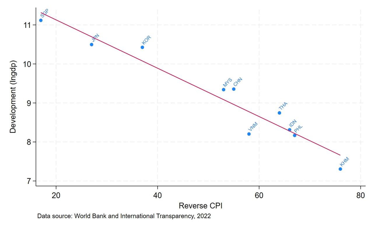
Empirical Economic Bulletin, Vol. 17 208
Figure 1: Correlation between Economic Growth and Corruption Perceived Index
Figure 2 shows the trend of another proxy of corruption, which is control of corruption from 2005 to 2022. Control of corruption measures the perception that public power is exercised for private gains. Singapore is leading the group while China has shown an increase in its control of corruption and Cambodia is at the bottom, exhibiting a decreasing trend in its control of corruption.
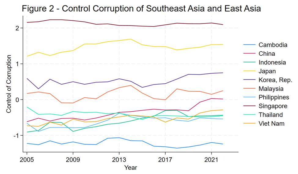
Data Source: World Bank
Figure 3 illustrates that there are fluctuations of foreign direct investment net inflows (FDI) in dollars amount from year to year (2018 to 2022) with 2021 as the year with the most FDI since it is the year when the economy around the world started to recover from the pandemic. The number and trend also vary by country. For instance, China saw a big decline in FDI between 2021 and 2022 while Singapore saw a constant number and Japan saw an increase. With the Chinese economy as well as the world’s major countries such as the U.S. and those in European countries experiencing a tightening policy to cool
Empirical Economic Bulletin, Vol. 17 209
down their economy, it can be forecasted that FDI will decrease especially among emerging countries in Southeast Asia.
3: Foreign Direct Investment Net Inflows by Year and Country
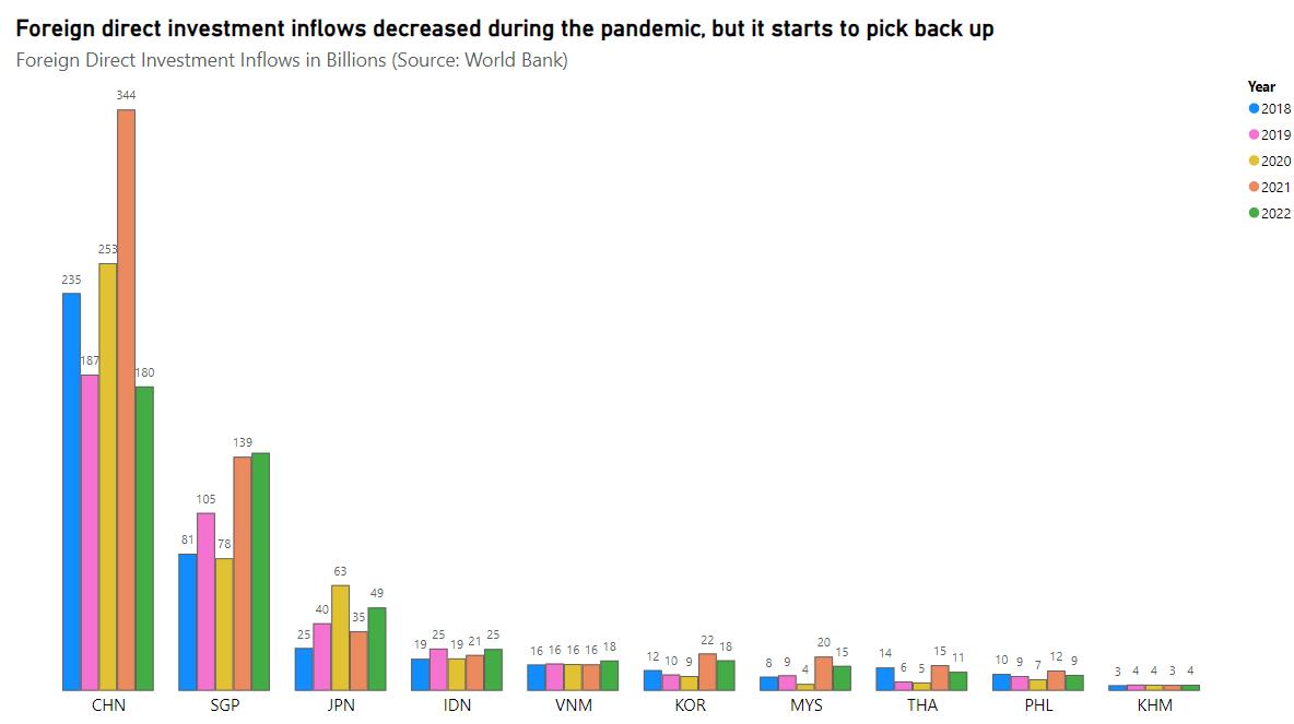
Data Source: World Bank
Figure 4 reveals the correlation between the development of financial market proxied by market capitalization of listed domestic countries as a percentage of GDP to economic growth. Market cap exhibits a positive relationship, showcasing that high growth economy tends to have a robust and much more activities in the financial market.
Figure
Empirical Economic Bulletin, Vol. 17 210
Figure 4: Correlation between Market Capitalization and Economic Growth
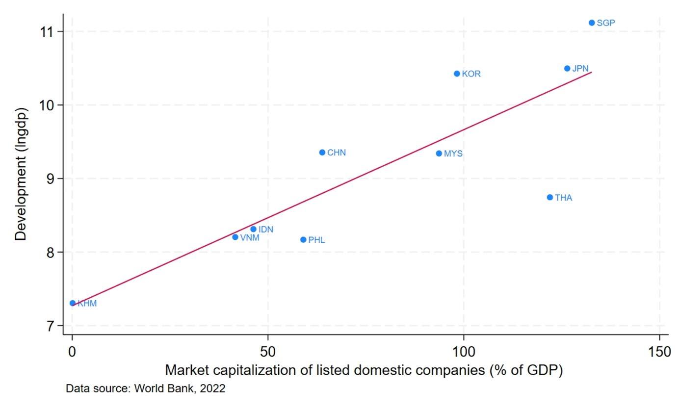
Figure 5 conveys the trend of the development of financial institutions proxied by the domestic credit to the private sector by banks as a percentage of GDP. Overall, there has been an increasing trend overall among countries in the last six years. Among the emerging countries, Cambodia has seen the largest increase, but Cambodian’s economic growth (natural log of real GDP per capita) is not growing as fast as it would be implied, which is interesting to question and look further. Additionally, as mentioned above, if the world’s largest economies experience negative growth in the upcoming one to two years, we may see an impact on this trend in terms of decreasing or increasing at a decreasing rate.
Empirical Economic Bulletin, Vol. 17 211
5: Domestic Credit to Private Sector by Banks as a percentage of GDP
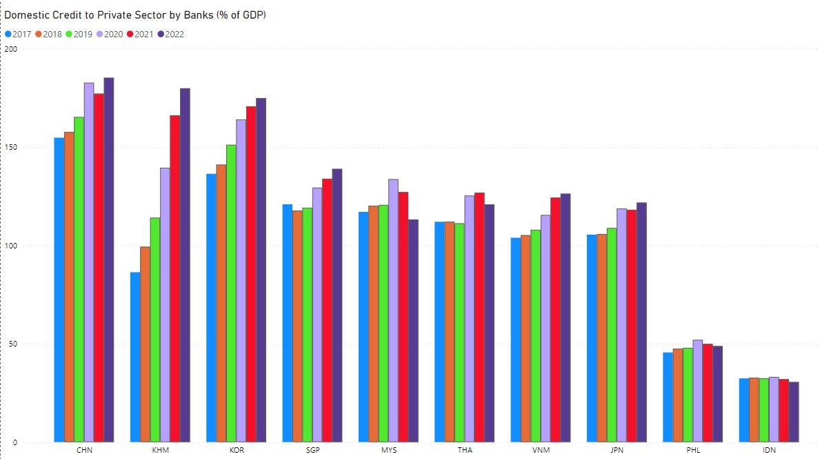
Data Source: World Bank
3.0 LITERATURE REVIEW
Numerous studies have been done to convey the relationship between capital flows as well as corruption on economic growth. Capital flows from entities with funds available to others with investment opportunities theoretically enhance everyone’s welfare and make everyone better off, leading to the growth in the economy. On the other hand, corruption impedes economic growth as it is considered a major obstacle to the smoothness of the flow in capital. According to Paulo et al (2022), corruption is worse, especially in emerging economies, where the rule of law and governance effectiveness is low and still evolving. However, there is a counterargument theory that corruption is not bad for the economy. Leff (1964) argues that corruption can promote economic growth, facilitating beneficial exchanges and allowing individuals and businesses to circumvent strict government regulations and correct preexisting government failures to generate vibrant economic activity. This theory is known as “grease the wheels”.
Figure
Empirical Economic Bulletin, Vol. 17 212
Corruption in terms of bribery, nepotism, lobbying, invades all societies, however, that is much more detrimental in countries or regions with low rule of law and complicated bureaucracy. Countries with solid institutions designed to prevent control from elites are seen to be wealthier than countries with fragile institutions dominated by elites’ desires in power, implying that corruption is worse in emerging economies, where the rule of law and governance effectiveness is low and still evolving (Paulo et al., 2022).
Grundler and Potrafke (2019) denoted that corruption is negatively associated with economic growth and real GDP per capita decreased by around 17% in the long run. Going along the line, the study by Paulo et al (2022) on the Latin American and Caribbean countries from 2000 to 2018 found that one standard deviation increase in corruption, measured by Transparency International’s reversed corruption perception index (CPI), is associated with a decrease of 12.2% in GDP per capita and 3.05% in economic growth, further supporting the “sand the wheels” theory. In the same study, Paulo et al. (2022) also denoted that corruption leads to lower investment in physical capital and foreign investment flow and that there is a bidirectional causality between lower economic development and higher corruption. There is no consensus whether corruption is an issue to economic growth. Some economists claim that corruption is an obstacle to economic growth “sands the wheels” and some argue that corruption functions as “grease in the wells” for economic growth, however, empirical evidence and study tends to show that corruption has a negative impact on economic growth.
The rule of law can protect against the diversion of resources, but in societies with corruption, that rule of law is often the primary driver and the consequences are hindrances on economic development through increased transaction costs, rent-seeking, uncertainties, inefficient investment, discouragement of innovation, misallocation of economic resources, and distortion of market regulations (Paulo et al., 2022; Grundler and Potrafke, 2019; Jin-Wei, 2000).
The impact of corruption affects the economy directly and indirectly. Study by Jin-Wei (2000) examine the indirect effects of corruption on economic growth as high levels of corruption tend to steer the mix of capital inflows towards hot money, hence making host countries more vulnerable to currency crises. Additionally, by discouraging foreign direct investment inflows and misallocating those resources for private gains,
Empirical Economic Bulletin, Vol. 17 213
corruption reduces the scope for beneficial financial development, since FDI flows have been shown to carry the most solid growth externalities. On the other hand, Abotsi (2017) denotes that 68% of the countries in Asia scored less than the tolerable level of corruption for investment as corruption has been observed to be significant in virtually all Asian countries, but, despite this, the region remains the number one global investment destination. Furthermore, countries with low control of corruption has negative impact on foreign direct investment (FDI), and countries with high control of corruption has positive impact on FDI (Abotsi, 2017).
Studies conducted by Bassanini & Scarpetta (2001) show that financial openness to international transactions such as FDI, trade, borrowing funds, aids, have exhibited positive relationship to economic growth. This relationship is then compounded in the economy whose financial market is operational and informational efficient as shown by Hondroyiannis (2004). Osani (2020) found that each government indicator and financial development indicator has a different level of magnitude from one another on the capital flows, hence economic growth. For instance, financial institutions prevail over financial markets in the dissemination of capital flows, hence have more impact on economic development (Osani, 2020). An empirical study by Shan (2020) found that swift change and reform in the financial sector and opening up the domestic financial market has brought significant growth in the economy. The study also found that there is a bidirectional causality between financial opening and economic growth (Shan, 2020). Financial development has impact on the economy through many channels and mechanisms. A well-functioning and efficient financial market and financial intermediaries provide liquidity, reduce cost, reduce risk, enhance the integrity of the market, act as a channel for transferring funds efficiently from those without investment opportunity to those with investment opportunity but without fund as well as reducing the asymmetric information. One of the channels is through the stock market. Regulated and efficient stock market provides liquidity and more investment opportunities as investors now have more trust and options rather than investing in long-duration projects (Hondroyiannis et al., 2004). Hondroyiannis et al. (2004) did the study on Greece and found that upward shock in the stock market (rise in market capitalization) is associated with the increase in total output and increases in private bank credit boosts real economic
Empirical Economic Bulletin, Vol. 17 214
activity. Countries should strive to develop sound financial markets, including the trading activities of capital markets and countries should make every effort to prevent a banking crisis or currency crisis from occurring in order to eliminate, or at least mitigate, the influence they would have on capital flows’ effect on economic growth (Shen et al., 2010).
4.0 DATA AND EMPIRICAL METHODOLOGY
4.1 Data
The study uses annual data to conduct panel data analysis from 2005 to 2022 on ten countries in Southeast and East Asia. All the data except for the CPI index and World Governance Indicators (WGI) were obtained from the World Development Indicators in the World Bank website Those data are each country’s yearly real GDP per capita, foreign direct investment net inflows, market capitalization of listed domestic companies, domestic credit to private sectors by banks, personal remittance, labor force participation rate, percentage of government expenditure on education, mortality rate under five, and fixed capital investment. All of the variables from World Bank are transformed into log-normal.
The CPI data is calculated annually and published by Transparency International, using thirteen different data sources from twelve institutions. The data collection and methodology behind this index is based on the perceptions among business executives and country experts on the public sectors’ corruptive activities such as bribery, nepotism, etc.
The CPI data from Transparency International ranges from 0 to 100, in which 0 is perceived as the most corrupted and 100 is perceived as the least corrupted. The study takes the same stance of the literature to potentially show the negative impact of corruption by modifying the data into reversed CPI in which the higher the CPI, the more corrupted the country is perceived to be. Summary statistics for the data are provided in Table 1.
Empirical Economic Bulletin, Vol. 17 215
Table 1: Descriptive Statistics
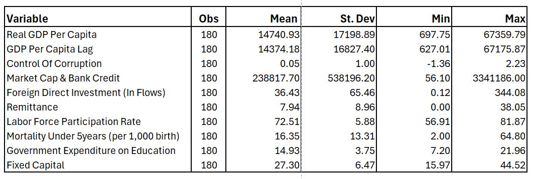
Source: World Bank and Author’s Calculation
4.2 Empirical Model
Following Paulo et al. (2020) and Hondroyiannis et al. (2004), this study adapted and combined the ideas behind the two papers together on corruption and capital flows with the addition of personal remittance
The model could be written as follows:
��������������������ℎ�������� represents the economic growth of country i at year t. Natural log of real GDP per capita is a proxy for ��������������������ℎ�������� , which data is obtained from the World Bank. It can also be considered as a representative for the improvement in standard of living a person.
Independent variables consist of four main variables. Appendix A and B provide data sources, acronyms, descriptions, expected signs, and justifications for using the variables. First, ������������������������������������������������ represents the proxy for corruption through seven proxies from Transparency International and WGI. Second, ���������������������������������������� is the proxy for development of financial markets and institutions for country i at year t . It is the log-normal of the
�������������������������������� = �������� + �������� ������������������������−���� + �������� ������������������������������������������������ + �������� ���������������������������������������� + �������� ������������������������ + �������� ������������������������ + ���������������� + �������� + �������� + ������������ (1)
Empirical Economic Bulletin, Vol. 17 216
transformation of domestic bank credit and stock market capitalization of listed domestic countries through addition. Third, ������������������������ is log-normal of foreign direct investment net inflows in country i at year t. Then, ������������������������ is the log normal of the personal remittance received which attempts to capture the capital inflows from national workers overseas. Lastly, ������������ is a vector capturing other determinants of economic growth such as mortality rate, human capital, physical capital, workforce, etc. �������� is the country-fixed effect that absorbs the heterogeneity factors between countries while �������� is the time effect that accounts period-specific shocks common to all countries.
5.0 EMPIRICAL RESULTS
The empirical estimation results are presented in Figure 6 and 7. The same empirical model is run seven times, each time with a different proxy of corruption. In each of the sub-model, it is run three times with fixed effect, random effect, and OLS. Exhibit 1 in the Appendix shows the tests and diagnostics before running the model. Using the Hausman test, fixed effect is chosen to mainly describe the result. The empirical estimation shows a negative relationship between economic growth and corruption. Capital through financial markets and institutions and personal remittance have a positive relationship with economic growth while the impact of FDI is unambiguous.
Empirical Economic Bulletin, Vol. 17 217
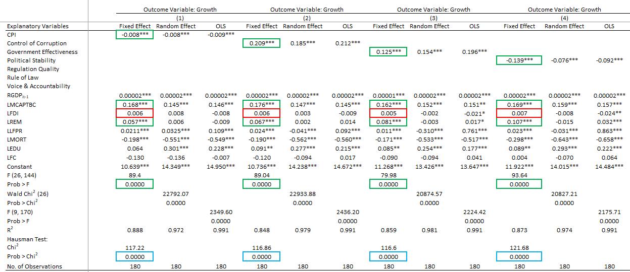
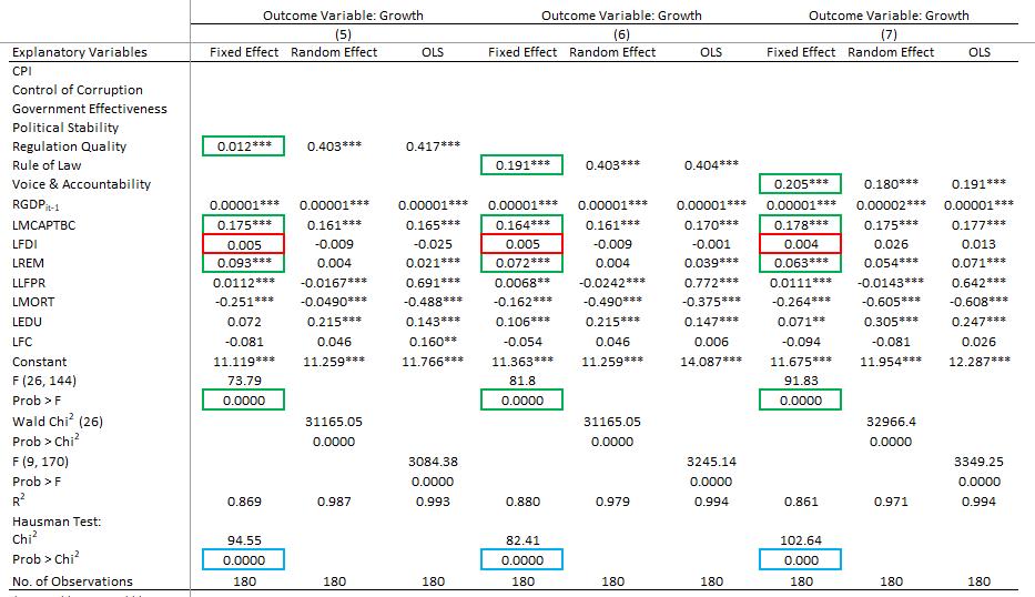
Note: *** , **, and * denotes significance at the 1%, 5%, and 10% respectively.
Figure 6: Regression Results Part 1
Figure 6: Regression Results Part 2
Empirical Economic Bulletin, Vol. 17 218
The CPI variable estimate in Model 1 was significant at the 1% level. The parameter estimate of CPI is consistent with the result of Paulo et al. (2022). The estimate indicated that CPI was negatively associated with economic growth in the Southeast and East Asia. Each proxy of corruption across all seven models is statistically significant at 1% as they consistently show that corruption impedes and is negatively associated with economic growth. This result is identical only differ in magnitude when looking at the random effect and OLS. In Model 2, as the control of corruption increases by 1%, economic growth will increase by 0.2%, holding everything else constant. Meanwhile, in Model 4, as political stability and absence of violence/terrorism, which measures the likelihood of political instability and politically-motivated violence, increases by 1%, economic growth 0.14%, holding everything else constant. Development of financial markets and institutions through its capital allocation proxied by the market capitalization of listed domestic companies and total domestic bank credit is statistically significant across all models and it indicates consistently that financial markets and institutions are positively associated with economic growth. This is also consistent with the random effect and OLS as well as with the findings of Hondroyiannis et al. (2004). Looking at the fixed effect alone, FDI is not statistically significant across all models even though it shows a positive sign. In other models of random effect and OLS, FDI is either not statistically significant or statistically significant with a negative sign. It is not consistent with the findings of Hondroyiannis et al. (2004) since this model incorporates corruption. This is expected as we hypothesize that capital with high interference from the government, especially in a highly corrupted country, is not allocated efficiently and may be exercised for private gains. On the other hand, personal remittances received by households from members working abroad is statistically significant across all models and the result shows that it consistently has a positive impact on economic growth. FDI usually needs approval from the government and it often is given to the government for distributing and investing that capital while capital through financial markets and personal remittances usually reaches corporate, businesses, households, and individuals directly or with less participation from the government. The degree of interference with those capitals from the government may make the impact of capital vary by forms, encouraging further study.
Empirical Economic Bulletin, Vol. 17 219
6.0 POLICY IMPLICATIONS
Policy implications subsequently follow after the findings. It is hard and almost impossible to do policy implications when the policymaker who has the power to do it is corrupted, and assuming it is not the case is a very big assumption. Corruption is like cockroaches: it is resilient, persistent and it spreads rapidly and it multiplies in the dark which cannot be easily observed. The more you deal with it, the more you realize there is more to come. We can try to combat with corruption like how we deal with those cockroaches. Identify the infestations: what are the sources, who are the players in it, and what are considered corruption? It then comes to sanitation, pesticide, and hygiene: remove and mitigate the sources that contribute to corruption. Then, close off entry points for corruption and implement education for corruption control and train groups of chosen people who still have the willingness to fight corruption. Combating corruption requires a collaborative effort, it is not just what the government can do, it is also what each individual can do. If corruption is reduced as it is impossible to eliminate them just like how you cannot completely eradicate cockroaches, FDI will potentially be allocated efficiently and may show positive impact on economic growth. Regarding the financial markets and institutions, it needs to be as much efficient as possible to have a higher impact on growth. Some approaches such as reducing corruption, education on the roles of capital, establishing an effective regulations to oversee the market, building trust and reducing information asymmetry will attract more participants into the market even foreign investors in terms of foreign portfolio inflows to make the market more liquid and more efficient. Tax incentives, transaction costs, and subsidies could also be considered to attract more funds. On the other hand, remittances should have a matching program to certain limits for incentivizing.
7.0 LIMITATIONS
There is no perfect model in this world nor there is a model without any limitations. It is important to distinguish between good data and great data, especially in our case. Great data are usually behind the pay-wall. Although we got our data from sources like World Bank and they adjust it, the World Bank initially gets those data reported and prepared by
Empirical Economic Bulletin, Vol. 17 220
government agencies and if that country is corrupted, the credibility of those data also decreases. There are also problems with inputs such as the use of proxy and specification and there are also other biases that is very hard to account for such as omitted variable bias. The fixed effect model does not account for time-invariant causes. More observations are helpful and useful in this and future study. With more observations, it also comes with more flexibility, enhanced precision, as well as reducing bias and increasing statistical power. More observations allow us to study each country separately across multiple periods of time and conduct a comparison as each country has different level of corruption and different development in financial markets. Grouping countries by sub-regions or by similar level of corruption is also encouraged for future study. Difference in difference could be studied on a specific country which exhibits an increasing trend in its governance and control of corruption to see how impact of each capital changes.
8.0 CONCLUSION
In summary, corruption is a very big obstacle to economic growth, eroding trust and confidence, distorting the allocation of resources, hindering investment, increasing inequality, degrading the environment, discouraging people, chipping away productivity fueling grievances and conflict, as well as the capital flows through the economy, in which the flow may be disrupted and cannot be allocated efficiently. The results in this paper imply that corruption hinders economic growth across all seven models. With the presence of corruption, only certain forms of capital are shown to have a positive impact on economic growth as those particular forms have less to no interference from the government. FDI, with the high interference from the government, has an ambiguous effect. Corruption needs to be reduced for the economy to grow more efficiently and the impact may need to study from time to time to see the difference.
Empirical Economic Bulletin, Vol. 17 221
BIBLIOGRAPHY
Abotsi, A. K. (2017). Tolerable Level of Corruption for Foreign Direct Investment in Europe and Asia. Contemporary Economics
Bank, W. (2024). World Development Indicators. Retrieved from World Bank: https://databank.worldbank.org/source/world-development-indicators
Bank, W. (2024). Worldwide Governance Indicators. Retrieved from World Bank: https://www.worldbank.org/en/publication/worldwide-governance-indicators
Bassanini, A., & Scarpetta, S. (2001). THE DRIVING FORCES OF ECONOMIC GROWTH: PANEL DATA EVIDENCE FOR OECD COUNTRIES. OECD.
Grundler, K., & Potrafke, N. (2019). Corruption and economic growth: New empirical evidence. European Journal of Political Economy
Hondroyiannis, G., Lolos, S., & Papapetrou, E. (2004). Financial markets and economic growth. Bank of Greece, Economic Research Department.
International, T. (2022). Corruption Perception Index. Retrieved from TransparencyOrg: https://www.transparency.org/en/cpi/2022
Jin Wei, S. (2000). NEGATIVE ALCHEMY? CORRUPTION AND COMPOSITION OF CAPITAL FLOWS. OECD Development Centre
Leff, N. (1964). Economic development through bureaucratic corruption. American Behavioral Scientist.
Osina, N. (2021). Global governance and gross capital flows dynamics. Review of World Economics.
Paulo, L. D., Lima, R. C., & Tigre, R. (2022). Corruption and economic growth in Latin. WILEY.
Shan, J. (2020). Financial opening and economic growth: a quantitative assessment. In R. G.Song, China: New Engine of World Growth (pp. 94-106). Canberra: ANU Press.
Shen, C., Lee, C., & Lee, C. (2010). WHAT MAKES INTERNATIONAL CAPITAL FLOWS PROMOTE ECONOMIC GROWTH? AN INTERNATIONAL CROSS COUNTRY ANALYSIS. Scottish Journal of Political Economy.
Empirical Economic Bulletin, Vol. 17 222
Appendix A: Variable Description and Data Source
Acronym Description
Growth Growth in real GDP per capita proxied by natural logarithm of real GDP per capita
Data source
World Bank
CPI Corruption perceived index Transparency International
FDI Foreign Direct Investment net inflows in current dollars World Bank
MCAPTBC Development of financial systems proxied by the transformation through addition between market capitalization of listed domestic companies and domestic credit to private sectors by banks in current dollars
World Bank
REM Personal remittance received in current dollars World Bank
LFPR Total Labor Force Participation Rate (% of total population ages 15-64) World Bank
EDU Education Expenditure in current US $ World Bank
MORT Mortality rate under 5 (per 1000 live births)
WGI Six Governance Indicators
FC Fixed capital formation as % of GDP
World Bank
World Governance Index
World Bank
Empirical Economic Bulletin, Vol. 17 223
Acronym
Appendix B- Variables and Expected Signs
Variable Description
CPI Reversed Corruption perceived index
FDI
MCAPTBC
Foreign Direct Investment net inflows in current dollars
Transformation through addition between market capitalization of listed domestic companies and domestic credit to private sectors by banks in current dollars
REM
LFPR
Personal remittance received in current dollars
What it captures Expected sign
Perceived corruption in public institutions -
Investment inflows from abroad +/-
EDU
MORT
Total Labor Force
Participation Rate (% of total population ages 1564)
Education Expenditure in current US $
Mortality rate under 5 (per 1000 live births)
Development of financial system +
Proxy for fund from household members working abroad +
Human capital and labor markets +
Human Capital +
Human Capital/Health Stock -
Empirical Economic Bulletin, Vol. 17 224
WGI Six Governance Indicators Proxy for governance and corruption +/-
FC Fixed capital formation as % of GDP Physical Capital +
Appendix C- Tests and Diagnostics
Tests Null Hypothesis
Joint-F Test
BP LM Test
H0: Years are jointly equal to zero (time fixed effects are not needed)
H0: Variances across entities is equal to zero (No significant difference across units or no panel effect => Simple OLS)
BP/LM Test
Modified Wald Test
Wooldrige Test
H0: Residuals across entities are not correlated (no cross sectional dependence)
H0: Homoskedasiticity (constant variance)
H0: No first order serial/autocorrelation
Test Statistics
F stat= 4.19; Prob> F= 0.0000 <0.05
Chibar2 = 24037.53; Prob > Chibar2 =0.0000 <0.05
Chi2 = 138.262; Pr = 0.0000 < 0.05
Chi2 = 960.41; Prob > Chi2 =0.0000 <0.05
F stat= 24.387; Prob > F 0.0008 < 0.05
Conclusion
Reject H0; Time fixed effects are needed
Reject H0; Random effects are needed
Reject H0; Panel are correlated (cross-sectional dependence)
Reject H0; Conclude Heteroskedasticity
Reject H0; Conclude Serial Correlation
Empirical Economic Bulletin, Vol. 17 225
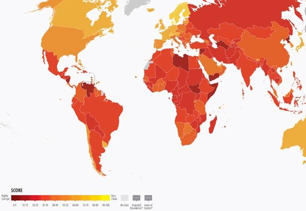
Empirical Economic Bulletin, Vol. 17 226
Appendix D- Heat Map of Corruption by Transparency International
A Cross-Section Analysis of Factors Affecting Interstate 11 Migration in the United States
Kasey Thomasa
Abstract:
This paper investigates the factors influencing interstate migration in the United States of America. This study incorporates political affiliations and income and property tax policy into an existing migration determinants model. This is done to examine the influence of policy or potential future policies on an individual’s decision-making in addition to household factors. The greatest factors influencing an individual's decision to move are the average January temperature, the income tax rate, and the number of hazardous waster sites in the state.
JEL Classification: R23, R28
Keywords: Regional Migration, Neighborhood Characteristics.
a Department of Economics, Bryant University, 1150 Douglas Pike, Smithfield, RI 02917. Email: kthomas13@bryant.edu.
Empirical Economic Bulletin, Vol. 17 227
1.0 INTRODUCTION
Interstate migration has been studied in a variety of fields because of its importance to understanding economic, social, and political dynamics of a nation. In economics, interstate migration is often studied as it relates to labor markets, regional development, demand and consumer patterns, housing markets, and fiscal policy. But migration data provides useful insights into individuals’ preferences, values, and needs. These insights are invaluable from a policy perspective as these are the what they should be built from. This study seeks to enhance the understanding of the factors influencing interstate migration in the United States. Examining economic factors like income tax and expected earnings and non-economic factors like climate and political affiliation. Determining which factors have the most sway is also important because it can help determine why people are moving to specific states over others with seemingly similar features. Studying these factors can help explain why people are moving to the places that they are moving to in order to best build solutions to rapidly growing populations or rapidly dwindling populations.
Domestic migration rates are increasing for the first time since 50s (Biermeier and Allen, 2023). There are several reasons driving domestic migration and while workrelated moves are still the highest reason, cost of living moves are up 3.7% (Biermeier and Allen, 2023). The COVID-19 pandemic reinvented the way people work and new flexibility options are giving individuals more opportunity to live and work where they want. As a result, outmigration trends from major urban areas has accelerated (Rogers et al., 2023). States like Texas, Florida, and South Carolina are experiencing major population booms as their states have lower housing costs, lower taxes, and warmer weather (Rogers et al , 2023). While states like New York, California, and Illinois are experiencing the greatest rates of outmigration, likely due to rising costs, housing, and taxes (Biermeier and Allen, 2023). All of this was only exacerbated by the pandemic closures and subsequent pent-up demand leading to a mass exodus during and postpandemic.
Empirical Economic Bulletin, Vol. 17 228
While empirical studies on factors affecting interstate migration have been conducted before. This paper differentiates from other studies in two ways. Firstly, it examines political affiliation of the state’s governors which can give an understanding to the electoral politics and policies affecting migration. Second, it cross-examines data from before and after the COVID-19 pandemic to give a better understanding of recent moving trends that have been brought on by the pandemic. Through the preliminary research conducted, there was little found on politics as a factor affecting migration from a policy perspective and there were not many studies conducted that included data postpandemic as it is still fairly recent. This paper aims fill these voids, especially given the trends surrounding interstate migration and political polarity as of late.
The rest of the paper is arranged as follows: Section 2 gives a brief analysis of current trends in domestic migration. Section 3 provides a brief literature review featuring studies related to the topic. Section 4 outlines the empirical model followed by the data and methodology. Finally, section 5 presents and discusses the empirical results. Followed by policy implications and a conclusion in section 6.
2.0 DOMESTIC MIGRATION TRENDS
Figure 1 shows net migration in the United States from 2021-2022. The United States saw a significant shift in domestic migration post-COVID. While areas in the northeast around Boston, New York, and Washington DC are the areas where outmigration was traditionally seen, Californiaand urban centers in states like Texas and Florida are experiencing significant outmigration as well. Areas with the highest net in-migration were predominantly in the southeast and the western corridor, states like Georgia, South Carolina, Arizona, and Nevada.
Empirical Economic Bulletin, Vol. 17 229
Figure 1: Net Domestic Migration by County
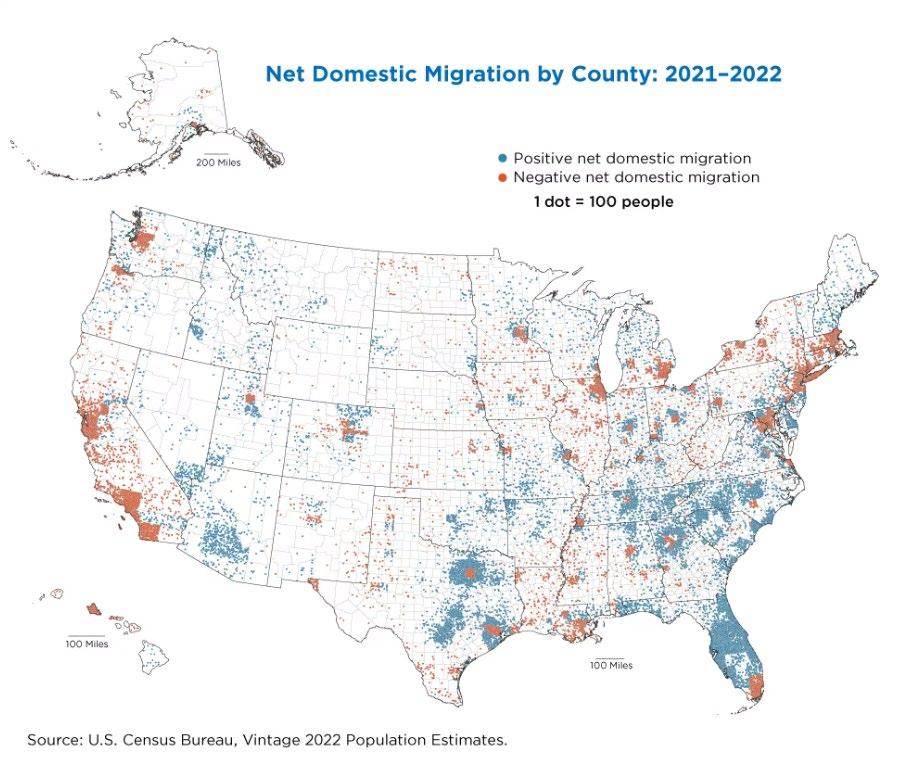
Source: United States Census Bureau
Figure 2 shows a breakdown of individual’s reasons for moving domestically in the US. Housing-related reasons were cited as the number one reason for moving in both years. The number one reason within that category being home size or location. Other was also statistically significant as a reason for moving. It had a 2% increase from 2021. Other included specifically reasons such as climate, taxes, health, and college. Taxes had the highest increase within the category at 2%.
Empirical Economic Bulletin, Vol. 17 230
Figure
2: Reasons for Moving 2021-2022
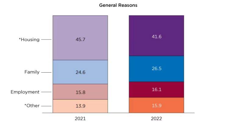
Source: United States Census Bureau
Figure 3 provides a visual to regional population growth in 2023. The South region had the most population growth at 39%. The South experienced over 10% more growth than the next highest growth region, the West. The trend south revolved around warmer weather, low cost of living, low taxes, and a robust economy. In an article by Biermeier and Allen for Forbes, South Carolina and Texas have a strong and constantly growing job market that is drawing in young people specifically. While conservative politics and low taxes are the main draw for older individuals (Biermeier and Allen, 2023).
3: United States Population Growth by Region
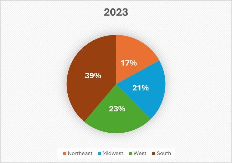
Source: United States Census Bureau (data)
Figure
Empirical Economic Bulletin, Vol. 17 231
Figure 4 shows domestic migration in 2022 stratified by race. Of those that moved to a different state in 2022, those that identified as Native Hawaiian or Pacific Islander made up the largest percentage. This is followed by those that identify as Asian at 2.9%.
Stratifying migration data is important because it can help identify which people are moving and this can help determine why people are moving. It is also important to include that the percentages are based on those that self-reported their race.
Figure 4: Domestic Migration (stratified by Race) 2022
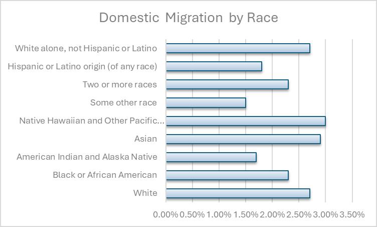
Source: United States Census Bureau
Figure 5 shows party affliation by state. This chart shows that the states that are experiecing rapid population growth are predominately home to Republican or Republican leaning voters. The states that are experiecing the most out migration, California, New York, and Illinois are predominantly Democrats or lean Democratic. While New York and California are experiencing an exodus over skyrocketing cost of living and rising taxes, Illinois is experiencing significant outmigraiton due to employment opportunities and infrastructure (Biermeier and Allen, 2023). While all factors may not be directly related to the government and their policy decision, some factors are and the trend remains the same.
Empirical Economic Bulletin, Vol. 17 232
5: Party Affliation by State
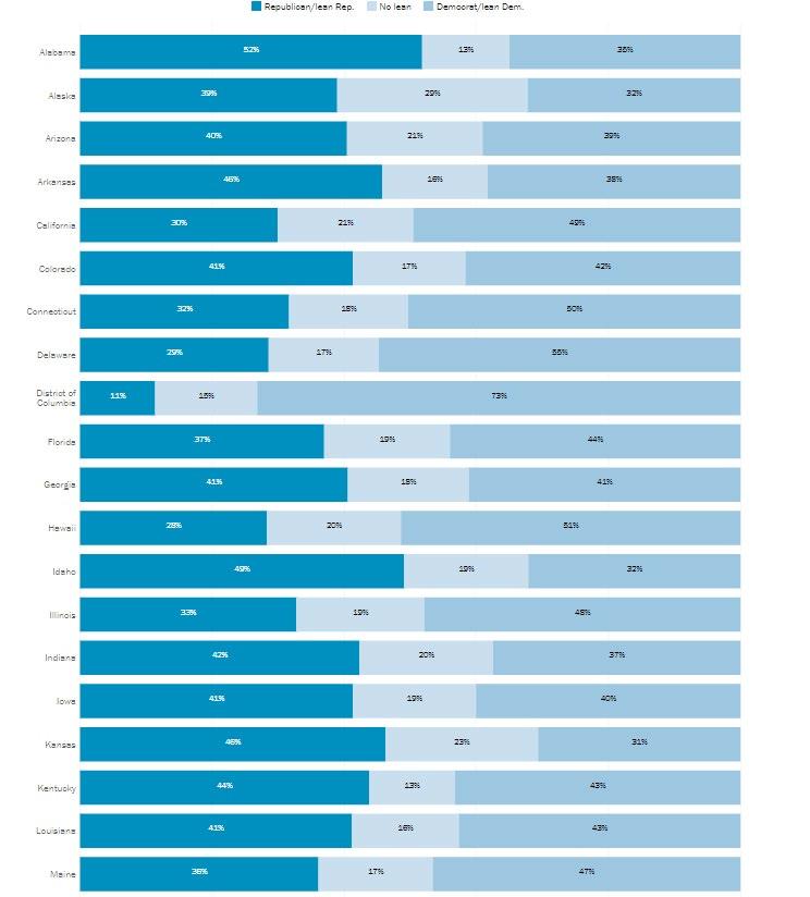
Source: Pew Research Center
(See Appendix C for the rest of chart)
Figure
Empirical Economic Bulletin, Vol. 17 233
3.0 LITERATURE REVIEW
Interstate migration in the United States has been studied from a variety of angles. The common variable investigated is expected future income as done by Cebula (2005) and Kennan and Walker (2011). Both found that expected future income had a strong effect on interstate migration decisions. Kennan and Walker’s (2011) study uniquely looked at geographic differences in mean wages which showed a positive relationship between decision making and expected future income. Cebula (2005) investigated both economic and household factors and the empirical model used is adapted from this study.
Hsieh and Wang (2022) looked into the effect of income and property tax policy in the 1980s and how that influenced domestic migration. Property tax was not found to be a factor affecting an individual’ s decision to move but income tax was a statistically significant factor. This study adds individual income tax and property tax rates from this work and adapts it to this one.
Conway and Rork (2022) examined moving van data to determine interstate migration patterns in the U.S. Examining data over a decade (2009-2019) shows a strong relationship between end of year policy changes and proposals and migration. Ihlanfedlt and Rodgers (2022) investigated property tax in the state of Florida and found that property tax had a negative relationship with moving. Similarly, Cassidy et al. (2023) looked into income tax policies and migration across states. It was found that the introduction of income tax did not change overall revenue levels in the long run due to mass outmigration to states without or very low-income tax (Cassidy et al., 2023). The migration data shows that policy changes affected the net in-migration to nearby states that had little to no income tax.
Empirical Economic Bulletin, Vol. 17 234
While these are predominantly economic factors there are several non-economic factors that influence migration across states. Cooke et al. (2022) and Mullholland and Young (2016) contended with occupational licensing as a key decision factor.
Occupational licensing as a something that bars individuals from moving was found to have no effect and thus policy changes that lead to standardization have little effect in the long run either (Cooke et al., 2022). Mullholland and Young (2016) looked at both occupational licensing as something that prevents individuals from moving but also as a factor influencing the move. In this study they also added income qualifiers to each job and subsequent license. They found that income level that the licensed job provided influenced migration to particular states more so than the licensing itself.
Gimpel and Schuknecht (2001) investigated interstate migration as a result of electoral patterns and how political leanings may influence interstate outmigration. While their findings confirmed their hypothesis there were some additional findings that were very interesting. They found that cross-state migration was more common with Democratic voters and out-migration was more common in states where the gubernational election did not conform to one individual political beliefs.
4.0 DATA AND EMPIRICAL METHODOLOGY
4.1 Data
The study uses annual data from 2012 and 2022 to perform a cross-sectional analysis. Data was obtained from various sources including the United States Census Bureau, the FBI, NOAA, FRED, and the EPA. Summary statistics for 2012 are provided in Table 1. Summary statistics for 2022 are provided in Table 2.
Table 1 Summary Statistics (2012)
Empirical Economic Bulletin, Vol. 17 235
Summary
Table 2 Summary Statistics (2022)
4.2 Empirical Model
Following the model created by Cebula (2005), the model for this paper examines average January Temperatures, expected future earnings, hazardous waste sites, and
Statistics ExpEarn PropTax IncTax Vcrime AvgJanTemp HazWaste GovAffil InMigration Mean 43499.5 0.012064 5.5621 346.43 34.542 24.08 0.4 140330.3 Standard Error 955.0372 0.000743 0.399912 17.37102 1.774180098 3.511246072 0.069985 16922.53497 Median 42591 0.0112 5.995 319.05 33.95 13 0 106786 Mode #N/A 0.0092 0 #N/A 25.1 13 0 #N/A Standard Deviation 6753.133 0.005256 2.827807 122.8317 12.54534778 24.82825908 0.494872 119660.3923 Sample Variance 45604804 2.76E-05 7.996494 15087.62 157.385751 616.442449 0.244898 14318609493 Kurtosis 0.285986 -0.63741 0.125334 -0.6963 3.013789903 3.105301255 -1.90049 3.74029316 Skewness 0.782127 0.501922 -0.61764 0.3731780.695264471 1.844590658 0.420985 1.856633829 Range 30114 0.0205 11 484.9 72.8 108 1 512717 Minimum 33441 0.0027 0 122.7 -12.8 0 0 24431 Maximum 63555 0.0232 11 607.6 60 108 1 537148 Sum 2174975 0.6032 278.105 17321.5 1727.1 1204 20 7016515 Count 50 50 50 50 50 50 50 50 Summary Statistics ExpEarn PropTax IncTax Vcrime AvgJanTemp HazWaste GovAfill InMigration Mean 63219.92 0.8418 5.3116 359.816 21.902 26.16 0.46 163328.94 Standard Error 1222.435 0.053624 0.448188 21.21697 1.769638473 3.649921442 0.0712 21039.1288 Median 61932 0.75 5.2 332.2 21.1 16.5 0 123920 Mode #N/A 0.53 0 #N/A 18.5 12 0 #N/A Standard Deviation 8643.921 0.379181 3.169167 150.0267 12.51323365 25.80884202 0.503457 148769.1065 Sample Variance 74717375 0.143778 10.04362 22508 156.5810163 666.0963265 0.253469 22132247040 Kurtosis -0.14494 -0.1757 0.14788 0.845445 1.27234934 3.086711464 -2.05657 5.77519883 Skewness 0.507124 0.745646 0.062815 0.880857 0.672486178 1.8098112 0.165522 2.188416945 Range 38191 1.49 13.3 677.2 64.9 115 1 712818 Minimum 46370 0.3 0 103.3 -2.4 0 0 26151 Maximum 84561 1.79 13.3 780.5 62.5 115 1 738969 Sum 3160996 42.09 265.58 17990.8 1095.1 1308 23 8166447 Count 50 50 50 50 50 50 50 50 Empirical Economic Bulletin, Vol. 17 236
violent crime per 100,000 people. To differentiate this study, property tax and income tax were added from Hsieh and Wang (2022) as well as governor’s political affiliation.
The model could be written as follow:

β6HazWaste+β7GovAffil + ε (1) is interstate migration categorized as those that lived in a different state as of one year ago. is used as an endogenous variable. Interstate migration is defined by the United States Census Bureau as an individual or family who had a different state of residence 1 year ago (US Census Bureau). Data used for the dependent variable comes from the Census Bureau and for this study in-migration data was used as it was more readily available than postal code requests or DMV requests.
The independent variables consist of seven variables from various sources.
Appendix A and B provide data sources, acronyms, descriptions, expected signs, and justifications for each variable. Firstly, ExpEarn represents the earnings that someone would expect to earn in the state they are moving to. Next, PropTax is the property tax in each state. IncTax is the income tax in each state. Third, VCrime represents violent crime per 100,000 people in a given state. Fourth is AvgJanTemp. This represents the average temperature in January for each state. All of the temperatures are recorded in the largest cities in each state and may not be totally representative of weather in all parts of the state. Particularly those with diverse climates. Fifth, HazWaste represents the number of hazardous waste sites located in a state. Finally, GovAffil will be a dummy variable representing the party affiliation of each state’s governors.
Empirical Economic Bulletin, Vol. 17 237
5.0 EMPIRICAL RESULTS
The empirical estimations can be found below. Table 3 is the results of the ordinary least sqares regression for 2012. This indicates a positive relationship between interstate migration and income tax rates, the average temperature in January, and the number of hazardous waste sites within a state. Table 4 is the results of the ordinary least squares regression for 2022. These results also revealed a positive relationship between interstate migration and income tax rates, the average temperature in January, and the number of hazardous waste sites. The results of the correlation matrices for both years can be found in Appendix C for governor affiliation in 2022 and expected future earnings in both 2012 and 2022. These results indicate a positive though not statistically significant relationship between these variables and interstate migration.
Table 3: Results for OLS 2012
ExpEarn 0.8309
-2.0920
PropTax 0.8524
-2910579.6122
IncTax 0.0059**
-4966.9929
Vcrime 0.8159 -106.1768
AvgJanTemp 0.0003** -1102.7488
HazWaste 4.51E-06** -543.5022
GovAffil 0.2890 -26431.1838
R-squared 0.625
F-Statistics 2.74E-07
Observations 50
2012 Interstate Migration
Intercept 0.9334 -118308.2850
Empirical Economic Bulletin, Vol. 17 238
Table 4: Results for
OLS 2022
(1.52E+05) ExpEarn 0.252 (2.033)
PropTax -0.864 (5.46E+04)
IncTax 0.004** (5151.843)
Vcrime 0.91 (106.05)
AvgJanTemp 0.00037** (1431.68)
HazWaste 5.38E-05** (732.713)
GovAffil 0.585 (3.40E+04)
Observations 50
Note: ** denotes significance at the 5%. Standard errors in parentheses.
The IncTax, AvgJanTemp, and HazWaste were statistically significant at the 5% level. Average January temperatures and hazardous waste sites was in line with the study conducted by Cebula (2005). Income tax was not statistically significant in the study conducted by Hsieh and Wang (2022). But the positive effect is consistent with their study though. Based on this study and the work conducted before, it can be concluded that income tax rates in destination is states is a factor in individual migration decisions. Cebula (2005) did find that expected future earnings were significant but this study did not. Although there was a positive correlation between expected future earnings (ExpEarn) and interstate migration in both 2012 and 2022. There was also a much stronger correlation between governor’s political affiliation and interstate migration in
2022 Interstate Migration Intercept -9.06E+04
F-Statistics
R-squared 0.615
9.567
Empirical Economic Bulletin, Vol. 17 239
2022 than 2012 although it was not statistically significant. This is in line with a study conducted by Gimpel and Schuknecht (2001) in which they found that policy and individual affiliation had an affect on migration but governor, senate, and representative affiliation did not. But the correlation being stronger in 2022 is in line with current partisan political trends in the United States.
6.0 DISCUSSION AND CONCLUSIONS
6.1
Limitations and Further Research
There are some limitations to this study predominantly in the areas of data collection and data sources. State-level data was used across all variables in order to unified results but state-level data may not be the most effective at identifying the true relationships between independent and dependent variables. Firstly, expected future earnings (ExpEarn) data was taken from the US Census Bureau’s wage data base. The Census Bureau uses mean wages as the basis for expected earnings. This may not be reflectively of the state as a whole as high income areas could skew the mean wages higher than say the median wages in the state. Take California for example, with high income areas like Silicoln Valley and Los Angeles raising the mean income earned but this is not reflective of the largely rural and agricultural economy in California which tend to be lower wage earners and does not reflect the levels of high income inequality within the state (Thorman and Payares-Montoya, 2024). County-level data, median wages, or median income may be more effective at outlining the true expected earnings of the state. Also stratifying for types of jobs may also be more effective in identifying relationships between interstate migration and expected future income. Secondly, governor affiliation was chosen as the data was readily available. While most governor’s can serve a maximum of two four-year terms. Some states like New York, have no term limits for their governors. This would mean that the tastes of individuals within a state may not be accurately represented. Also this creates a blanket and is not truly reflective of the political climate of a state as there are varying types and levels of each political party. Also in 2012, Rhode Island had a libertarian governor which was qualified as Republican for ease of use but this is not fully accurate. In further studies, it may be more effective to use the party with the highest percentage of
Empirical Economic Bulletin, Vol. 17 240
individual registered voters. This is more nuanced but it may be more accurate in reflecting the tastes of those in a state. Which in turn, may be more accurate in moving decisions. Another way this could be done would be by dividing the state by region and examining the regional voting patterns or voter registrations. This way voter patterns could be most accurately assessed.
Lastly, January temperatures were collected in one city in each state. The average temperature for the month is only reflective of that area. This means that for states that are geographically diverse, the temperature recorded may not be reflective of the state as a whole. Take New York, the temperature was recorded in Albany and at John F. Kennedy Airport over a period of 35+ years. But it is much warmer on average than Syracuse or Buffalo. This is the case for many states especially in the western United States, with colder mountain regions and low elevation desert basins. For the purposes of this research a general temperature was adequate but stratifying by region or county would be more accurate to determine the relationship between that and interstate migration.
6.2 Policy Implications
This data is important for both states with high in-migration and states with highoutmigration rates. States with increasing populations need to focus on housing, infrastructure planning, and energy sources. States that are facing high outmigration need to focus on tax policy, job opportunities, and scaling back extreme policies in favor of more centrist ones. Rapidly increasing populations put strain on the communities that are facing the largest amount of growth. Housing in the area may be limited and the limited supply raises costs significantly. States can take action to alleviate the housing burden by easing regulatory and zoning processes for developers of both single family homes and apartment complexes. This lowers the cost of the build, allowing more to be built while simultaneously lowering the cost (Minott and Selby, 2022). In the same vein, increasing populations need stronger infrastructure to handle the increased number of people living there. This does not just mean that current infrastructure needs to be improved but also that there needs to be some element of planning for anticipated capacity five to ten years from now as it is likely that the population, particularly in the South, will continue to grow. This includes street planning, expanding and preparing public schools, expanding
Empirical Economic Bulletin, Vol. 17 241
sewer and water, and other elements that are essential to the foundation of a local economy. Along with general infrastructure improvements and planning, there needs to be a push for increases to the energy production. More people mean more energy is needed. State and local governments need to prepare both traditional base load energy sources like coal, gas, and oil but also renewables. States that can be prepared with traditional sources of energy while also providing incentives for renewables like wind, hydropower, and solar. This will come from having a political environment that supports both.
States that are experiencing high levels of outmigration need to take steps that would encourage individuals to stay. Firstly, lowering taxes would encourage individuals to stay rather than moving to a more tax advantageous state. A trend that has increased as result of COVID-19. Lowering taxes has other benefits to the state outside of just making it more affordable for the people that live there. Lowering taxes raises after-tax rewards which encourages greater work effort, savings, and investment (Gale and Samwick, 2014). As well as lowering taxes to make it more affordable to live there, there needs to be policies in place that provide livable wage jobs particularly those in middle wage jobs. Middle wage jobs for non-college educated workers are shrinking, especially after the pandemic (Autor, 2022). In a survey conducted by the Census Bureau, this is one of the main reasons that people are moving (Kerns-D’Amore, 2023). A way to aid in this is to increase the state’s industrial base. Many corporations have moved out of certain states due to high taxes and regulatory challenges. States can attract companies by incentivizing them through tax and regulatory rollback. Industrial jobs can provide livable wages especially for middle income skilled workers. Finally, scaling back on controversial policies in favor of more mainstream, centrist policies may stop mass exodus from more left/left-leaning states. Take Oregon’s Measure 110, for example, it has caused many to move from the state particularly urban centers like Portland (Wilson, 2024). Measure 110 decriminalized possession in small amounts of virtually all drugs. The rationale behind this ballot measure was to encourage those struggling with addiction to seek recovery rather than punishing them (Wilson, 2024). But the citation and recommendation system is not working, especially in cities. Oregon does not have enough publicly funded rehabilitation facilities to handle the amount of people that need access to them and many
Empirical Economic Bulletin, Vol. 17 242
do not contact the hotline that would take the fine and citation away. The cycle continues. Since the measure passed overdoses increased 241%, 23% of which can be directly attributed to decriminalization, according to a study published in the Journal of Health Economics. Extreme policies have pushed many to move to more right/right-leaning states as seen in the trends section of this paper. Scaling back on these policies would encourage people to remain in the state as a result.
6.3 Conclusion
Interstate migration is increasing for the first time since the 70s. This change in trends is driven by the COVID-19 pandemic. This study found that income tax rates, January temperatures, and the number hazardous waste sites in a state were the significant contributors to the decision to move. Ones expected future earnings in the state they are moving to had positive effects but were not found to be statistically significant in either years. Governor affiliation had a positive effect in 2022 but was also not statistically significant. These results have significant policy implications for states experiences significance population changes in either direction. For rising populations, there needs to be focus on infrastructure and housing. For declining populations, there needs to be focus on affordability and mainstream policies. Changes to these policies may ease the burden of interstate migration in all states effected. This research can help give those within a state insights into the tastes, values, and preferences of the people that live there, want to live there, or want to leave. Knowing these things can aid in building policies and programs that can best serve the people in every state.
Empirical Economic Bulletin, Vol. 17 243
Appendix A: Variable Description and Data Source
Acronym Description
InMigration
ExpEarn
PropTax
IncTax
Vcrime
AvgJanTemp
HazWaste
Interstate migration in the United States, indicates individuals that had a home address in a different state one year prior.
Earnings an individual is expecting to earn in the state they are moving to, does not include tax, mean wages is basis in database.
Property tax rate in each state.
Income tax rate in each state.
Data source
US Census Bureau
US Census Bureau
Bankrate
Bankrate (2022) and FRED (2022)
Violent crime per 100,000 people per state. Federal Bureau of Investigation
Average temperature for the month of January
National Oceania and Atmospheric Association
Number of hazardous waste sites that exist within a state US Environmental Protection Agency
GovAffil The political affiliation of each state’s governor. Ballotpedia
Appendix B- Variables and Expected Signs
Acronym
ExpEarn
PropTax
IncTax
Vcrime
AvgJanTemp
HazWaste
Variable Description
Earnings one expects to earn in the state they are moving to
Property tax rate
Income tax rate
Violent crime per 100,000
Average temperatures for the month of January
Number of hazardous waste sites in a state
What it captures Expected sign
Effect of expected income on the decision to move +
Tax effects on decision to move -
Tax effects on the decision to move -
Effects of violent crime levels on decision to move -
Effects of temperature on the decision to move +/-
Health costs/benefits to moving
Empirical Economic Bulletin, Vol. 17 244
GovAffil Political affiliation of each state’s governor
Effects of politics in the decision to move +/-
Appendix C: Additional Items
Proportion of Registered Voters by State
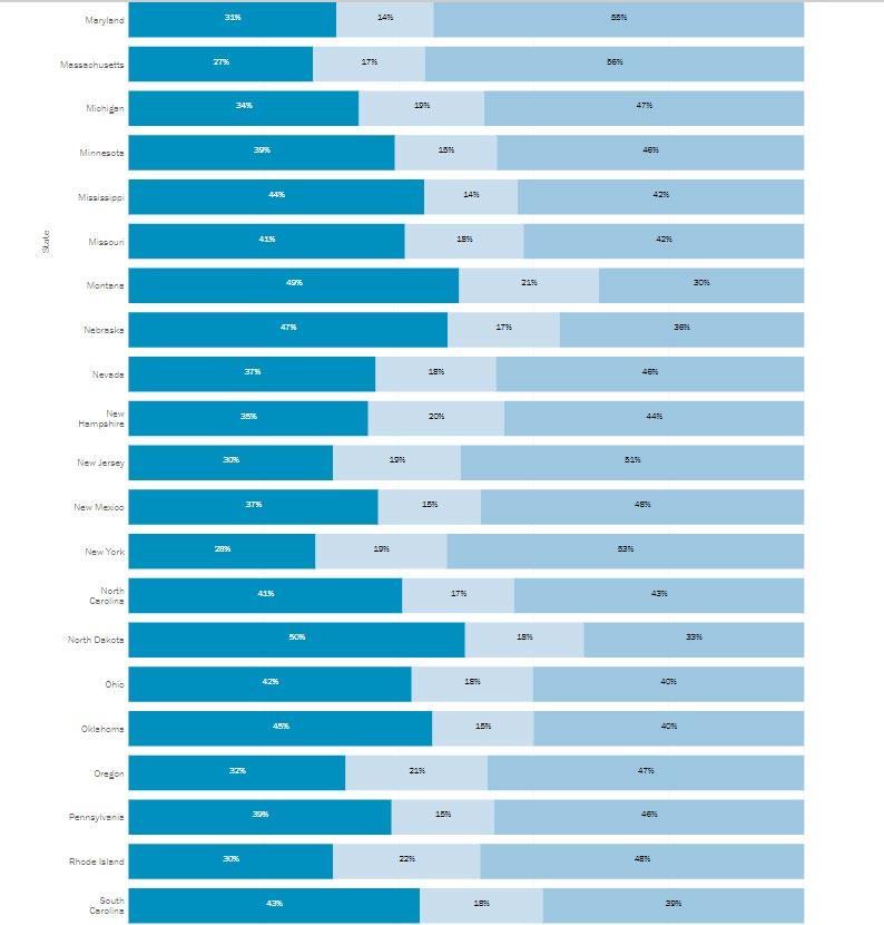
-
Empirical Economic Bulletin, Vol. 17 245
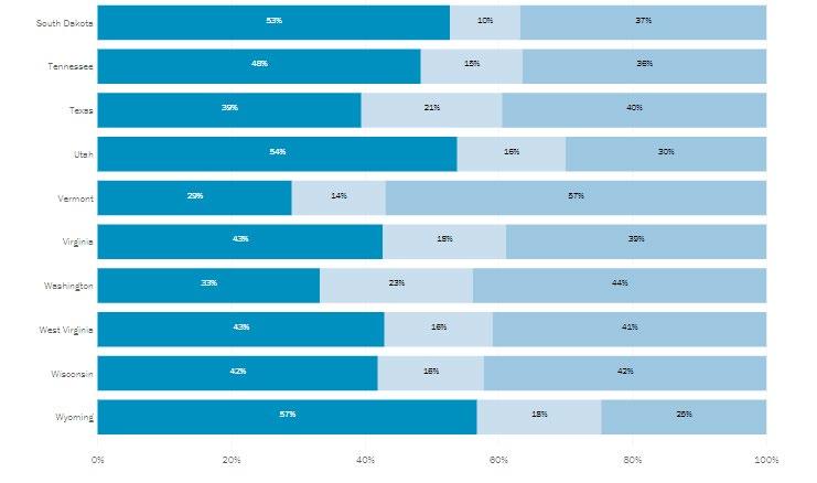
Matrices
e
2012 ExpEarn PropTax IncTax Vcrime AvgJanTemp HazWaste GovAffil InMigration ExpEarn 1 PropTax 0.456588 1 IncTax -0.08025 -0.02361 1 Vcrime -0.05175 -0.11742 -0.41954 1 AvgJanTemp -0.41027 -0.41294 0.128893 0.148857 1 HazWaste 0.237026 0.422703 0.094585 0.079266 0.072860514 1 GovAffil 0.225117 -0.08301 0.361787 -0.078560.023470743 0.072086642 1 InMigration -0.00777 0.074232 -0.17008 0.222152 0.454198529 0.605471617 0.020568 1 2022 ExpEarn PropTax IncTax Vcrime AvgJanTemp HazWaste GovAffil InMigration ExpEarn 1 PropTax 0.445566 1 IncTax 0.079093 0.162296 1 Vcrime -0.23301 -0.34281 -0.20745 1 AvgJanTemp -0.27624 -0.44095 0.104739 0.148154 1 HazWaste 0.349992 0.432565 0.246739 -0.01278 0.135938792 1 GovAffil 0.358515 0.173035 0.403845 -0.0791 0.0192877 0.358605213 1 InMigration 0.1519 0.018553 -0.15579 0.099166 0.478881726 0.568554672 0.06349 1 Empirical Economic Bulletin, Vol. 17 246
Correlation
BIBLIOGRAPHY
Autor, D. (2022, March 14). The shrinking share of middle-income jobs. Econofact. https://econofact.org/the-shrinking-share-of-middle-income-jobs
Biermeier, D., & Allen, S. (2023, September 4). 10 states people are fleeing and 10 states people are moving to. Forbes. https://www.forbes.com/home-improvement/features/states-moveto-from/
Cebula, R. (2005). Internal Migration Determinants: Recent Evidence. International Advances in Economic Research, 267–274.
Conway, K., & Rork, J. (2022). On Measuring US Interstate Migration with Moving Van Data. Population Research and Policy Review, 1431–1449.
Environmental Protection Agency. (n.d.). National Priorities List . EPA. https://www.epa.gov/superfund/national-priorities-list-npl-sites-state
Federal Bureau of Investigation. (n.d.). FBI — table 5. FBI:UCR. https://ucr.fbi.gov/crime-inthe-u.s/2012/crime-in-the-u.s.2012/tables/5tabledatadecpdf/table_5_crime_in_the_united_states_by_state_2012.xls
Federal Reserve Bank of St. Louis. (n.d.). Per Capita Personal Income By State. FRED. https://fred.stlouisfed.org/release/tables?eid=257197&rid=110
Gale, W., & Samwick, A. (2014). Effects of income tax changes on economic growth. Brookings Institute. https://www.brookings.edu/wpcontent/uploads/2016/06/09_effects_income_tax_changes_economic_growth_gale_samwi ck.pdf
Gimpel, J., & Schuknecht, J. (2001). Interstate Migration and Electoral Politics. The University of Chicago Press, 63(1), 207–231. https://www.jstor.org/stable/2691899
Gleason, P. (2023, August 4). Why migration data matters so much. Forbes. https://www.forbes.com/sites/patrickgleason/2023/07/31/why-migration-data-matters-somuch/?sh=14576fa25c81
Hsieh, M.-F., & Wang, H. (2022). Do People Move to Reduce Tax Burdens? The Tax Reform Act of 1986 as a Natural Experiment. Taiwan Economic Review , 50(1), 1–50.
Hunt, M., & Probasco, J. (2023, May 17). Property taxes by State. Bankrate. https://www.bankrate.com/real-estate/property-tax-by-state/#what-are
Empirical Economic Bulletin, Vol. 17 247
Ihlanfeldt, K., & Rogers, L. (2022). Homestead Exemptions, Heterogenous Assessment, and Property Tax Progressivity. National Tax Journal, 75(1), 7–29.
Kennan, J., & Walker, J. (2011). The Effect of Expected Income on Individual Migration Decisions. Econometrica, 79(1), 211–251. https://www.jstor.org/stable/41057441
Kerns-D’Amore, K. (2023, November 1). Change in marital status became more common reason for moving from 2021 to 2022, housing/neighborhood improvement reasons declined. Census.gov. https://www.census.gov/library/stories/2023/09/why-peoplemove.html#:~:text=As%20in%20several%20recent%20years,common%20between%2020 21%20and%202022.
Minott, O., & Selby , J. (2022, August 10). Ten actions cities can take to improve housing affordability. Bipartisan Policy Center. https://bipartisanpolicy.org/blog/10-actions-tohousing-affordability/
Mulholland, S., & Young, A. (2016). Occupational Licensing and Interstate Migration. Cato Journal, 36.
NCEI.Monitoring.Info@noaa.gov. (n.d.). Climate at a glance: Statewide . National Centers for Environmental Information (NCEI). https://www.ncei.noaa.gov/access/monitoring/climateat-a-glance/statewide/time-series/50/tavg/1/1/20122013?base_prd=true&begbaseyear=1901&endbaseyear=2000
Pew Research Center. (2015, May 12). Party affiliation by state. Pew Research Center’s Religion & Public Life Project. https://www.pewresearch.org/religious-landscapestudy/database/compare/party-affiliation/by/state/
Property tax. Ballotpedia. (n.d.). https://ballotpedia.org/Property_tax
Rogers, L., Spell, L., & Perry, M. (2023, March 30). Domestic outmigration from some urban counties slowed, smaller gains in rural counties. Census.gov. https://www.census.gov/library/stories/2023/03/domestic-migration-trends-shifted.html
State individual income tax rates and brackets for 2022. Tax Foundation. (2024, February 22). https://taxfoundation.org/data/all/state/state-income-tax-rates-2022/
State individual income tax rates, as of July 1, 2012. (n.d.). https://files.taxfoundation.org/20190311152905/state_individualincome_rates-2000-201220130219.pdf
Thorman, T., & Payares-Montoya, D. (2024, April 17). Income inequality in California. Public Policy Institute of California. https://www.ppic.org/publication/income-inequality-incalifornia/
Empirical Economic Bulletin, Vol. 17 248
United States Census Bureau. (2023, September 21). State-to-state migration flows. Census.gov. https://www.census.gov/data/tables/time-series/demo/geographic-mobility/state-to-statemigration.html
United States Census Bureau. (n.d.). Geographic Mobility by Selected Characteristics. Census Data Exploration. https://data.census.gov/table?q=migration&g=010XX00US
Wilson, C. (2024, February 7). Oregon pioneered a radical drug policy. now it’s reconsidering. NPR. https://www.npr.org/2024/02/07/1229655142/oregon-pioneered-a-radical-drugpolicy-now-its-reconsidering
Yahoo! (2012). Most and least taxing states 2012. Yahoo! Finance. https://finance.yahoo.com/news/most-and-least-taxing-states-2012.html?guccounter=2
Empirical Economic Bulletin, Vol. 17 249
An Empirical Analysis of the Status of Income Inequality New England in 2022
Aidan Wilkinson
Abstract:
This paper investigates the status of income inequality within the New England states in 2022. The empirical analysis conducted within this paper uses a similar model within Fadi Fawaz et al. for high income countries to analyze and predict the Gini coefficient within the six New England States. More specifically, the model that is tested analyzes monthly unemployment rate, the labor force participation rate, welfare spending, and the top 1% wealth distribution. The results show that Rhode Island and Maine Gini indexes could only be described by the top 1% wealth distribution and welfare spending, respectively. We also find that a large welfare spending budget yields greater income inequality in states that have a larger spending budget, more specifically Massachusetts being a prime example. Outside of New Hampshire, an increasing labor force participants effectively decreases income inequality. Finally, we found that any directional change in the unemployment rate does not have a noticeable impact on income inequality. With limitations, we found that there is inclusive evidence that certain macroeconomic indicators can affect the Gini index within the six New England states, more specifically income inequality.
JEL Classification: O15, D31, I24, I28, I12, I14
Keywords: Income, Income Inequality, Gini, Health, Education, Government Policy
a Department of Economics, Bryant University, 1150 Douglas Pike, Smithfield, RI02917. Phone: (401) 232-6379. Email: rmohan@bryant.edu.
Empirical Economic Bulletin, Vol. 17 250
1.0 INTRODUCTION
Today, the interconnectedness of the world has allowed everyone to be more aware of the crucial problems like income inequality. Income inequality is one of the more prominent problems in modern society, especially in the free market economy of the United States. One of the many models in economics that describes income inequality, more specifically economic inequality, is the Lorenz curve. The Lorenz Curve was developed by economist Max Lorenz with the intention to describe inequality in respect to wealth distribution. Another significant and popular way of measuring income inequality with the Gini coefficient. The relationship between the two variables is relatively straightforward: the Lorenz curve shows the “gap” that represents how well wealth is distributed while the Gini coefficient represents the severity of income inequality in an index. This study will analyze what macroeconomic indicators, among others, affect the Gini coefficient overall. Throughout this paper, we will analyze certain trends with our indicators that we will be analyzing between 2010 and 2022. In that 12 year span, many historical events have occurred that have likely been a huge transition period for the economy such as the aftermath of the 2008 financial crisis and the COVID19 pandemic. Additionally, this paper will be looking back at previous literature and analyzing what past research has found. Many recent papers have argued that researchers before them often “overlooked” certain indicators to which they believe would have been a massive determinant towards describing what affects the Gini coefficient, or income inequality in general. In hindsight, there are many pathways that researchers could have gone down and found credible results. Although sometimes this argument can be rather invalid considering modern events going on around the world (i.e. a pandemic) having a collateral effect on certain things in the economy. Despite that, this paper will continue research in the field of income inequality. By collecting data from the U.S. Census Bureau and the St. Louis Fred, we will be determining what macroeconomic indicators (more specifically, the labor force participation rate, per capita income, and the unemployment rate) among others such as the (TBD). Based on the analysis, we will conclude what indicators have had the most impact over the last decade.
Empirical Economic Bulletin, Vol. 17 251
2.0 TREND (OF THE GIVEN TOPIC)
Figure 1 shows how the Gini coefficient has changed over the last 12 years within Massachusetts, Rhode Island, New Hampshire, Vermont, Connecticut, and Maine. In 2012, the variation of the Gini coefficient between the six states in the region was .034 (between .465 and .431). By 2022, the range grew from .034 to .83 (between .519 and .431). For a majority of the 12 years that we collected our sample from, New Hampshire almost always had the lowest Gini coefficient, meaning the state was the most equal income wise.
Connecticut was constantly the state with the highest Gini coefficient until 2021 when Massachusetts saw a large increase in their respective Gini from 2021 to 2022.
Figure 1:

Gini Coefficient By State Since 2011
Massachusetts Rhode Island Connecticut New Hampshire Vermont Maine
Figure 2 shows welfare spending by state in the same period. Massachusetts welfare spending was the highest average spending per year with roughly $7 billion. Between 2016 and 2020, each state was relatively consistent with their spending. Connecticut had the largest dip in welfare spending between 2012 and 2016, but then proceeded to see a $2 billion increase in spending between 2021 to present. In 2016, New Hampshire, Rhode Island, and Vermont were all spending less than $1 billion in welfare spending. Finally, in terms to the labor force participation rate, the largest average labor force participation rate
0.42 0.44 0.46 0.48 0.5 0.52 Jan-11 Jan-12 Jan-13 Jan-14 Jan-15 Jan-16 Jan-17 Jan-18 Jan-19 Jan-20 Jan-21 Jan-22 Gini Index
Empirical Economic Bulletin, Vol. 17 252
was new Hampshire with 68%. The variation for averages in the LFPR was roughly 6%, showing some consistency within all states.
Figure 2:

Welfare Spending by State Since 2011
Massachusetts Rhode Island Connecticut New Hampshire Vermont Maine
3.0 LITERATURE REVIEW
Analyzing income inequality, no matter the size of the region, country, or area, has been practiced using the Gini Coefficient. The United States has been tracking the Gini coefficient since 1963, according to the St. Louis Fred. Over the last 60 years, the U.S. has seen periods of an increasing Gini coefficient. The index ranges from zero (0) to one (1) where 0 is perfect equality and 100 is perfect inequality. According to FRED, the data collected to generate an index number is “household survey” data obtained from various areas in the government. With that, previous papers have used this coefficient to highlight social inequality, more specifically, income inequality. The motivation behind previous papers have noted that past research papers “have failed” to look at the impact of income inequality across citizens, such as Newman et al. (2015). Newman et al. (2015) motivation came from the lack of research from previous papers when it comes to focusing on a smaller segment of people (i.e., residential areas) and wanted to see if economies that are more government controlled (or economies with more government intervention) have a lower
$0 $2 $4 $6 $8 Jan-11 Jan-12 Jan-13 Jan-14 Jan-15 Jan-16 Jan-17 Jan-18 Jan-19 Jan-20 Jan-21 Jan-22 USD in Billions
Empirical Economic Bulletin, Vol. 17 253
Gini than more free-market economies. The results from the paper showed that a government-controlled economy shows no differences in income inequality in comparison to the standard free-market economy. Like Newman et al. (2015), Wilkinson and Pickett (2009) were not satisfied with previous research, more specifically the research in income inequality and health. In their research, Wilkinson and Pickett (2009) wanted to see if there was a relationship between income status and social health (i.e., educational attainment, educational enrollment, mental illness, violence, obesity, drug abuse, etc.). The findings in this paper showed that the more someone were to look at lower income classes, the worse the “social health” would be, meaning that one of the examples of poor “social health” would be present. With that, there is a direct relationship between income and social health. Curran and Mahutga (2018) also look at the relationship between income and overall human health. Like Wilkinson and Pickett (2009), Curran and Mahutga (2018) also found that there is a direct relationship between income and health. In fact, Curran and Mahutga (2018) also found that health declines exponentially the further down one would go in the income bracket.
Schneiders and Hastings (2017) wanted to continue research by looking at household spending on services. Both of their findings showed that there was a direct relationship between household spending on services and income. Duncan and Murnane’s (2016) motivation comes from previous research looking at education and income inequality. This time, Duncan and Murnane (2016) analyzes the effect of certain government policies on educational attainment levels in respect to income inequality with before-and-after empirical analysis. Results showed that there was in fact very little success, if any, when it came to current government policies in place to increase all levels of education enrollment. Finally, Fawaz et al. (2012) analyzes income inequality with the Gini coefficient in high-income developing countries (referred to as HDICs) and lowincome developing countries (referred to as LDICs). He and others found that human capital and economic uncertainty were two of the largest impacts on growing income inequality. The first model shown in Fawaz et al. (2012) is the inspiration behind this empirical analysis. In the model, use the Gini coefficient (continuous variable) as their dependent variable. The independent variables in Fawaz et al. (2012) that will be used in this paper are per capita income (by country), the average unemployment rate (by country),
Empirical Economic Bulletin, Vol. 17 254
and the secondary educational attainment. In their paper, they added an additional independent variable that is per capita income squared, likely due to concern about heteroscedasticity. The variable that represents secondary educational attainment in Fawaz et al. (2012) is analyzed with a two-year lag period to hopefully make up for lack misinformation. In this empirical analysis, we will be using per capita income, unemployment, and secondary educational attainment, represented in a similar fashion like Fawaz et al. (2012). The contribution towards this area of research will be analyzing tertiary education attainment, represented in the same manner as secondary education attainment. In a scenario where the model is malfunctioned, there will likely be the addition of the effective federal funds rate as an independent variable (either as an addition or replacement towards tertiary education attainment. With the given information, this paper will continue the research from Fawaz et al (2012) and others. Additionally, the final contribution to this area of research will be adding multiple health indicators, including the number of births of women between 15 and 50 by marital status and age. More specifically, this paper will analyze trends in this field and use filtered data that will bring us to believe that it will likely influence greater income inequality. Also, our model will include disability status by age and sex year over year. Finally, this paper will also contribute to this area of research by including current data with respect to the Lorenz Curve. The Lorenz Curve is a widely known graph that represents the distribution of wealth within a population and will be used to analyze the inequality gap and actual income distribution over the years by state.
4.0 DATA AND EMPIRICAL METHODOLOGY
4.1 Data
The data for this research paper will be collected from numerous sources. First, much of the data that represents economics indicators will be from the St. Louis Fred, the U.S. Census Bureau, and the World Bank. Additionally, we will be collecting data from an independent website for tracking government spending in order to retrieve welfare spending by state, one of the variables that will be present in our logistic regression model. After the data is collected from these sources, each variable will be translated into its natural log form in order to run a logistic regression. A logistic regression will be used to
Empirical Economic Bulletin, Vol. 17 255
identify if any of the indicators used have a growth of decaying effect on the respective Gini Coefficients. The data that is collected will range from 2011 and 2022. Data from 2022 was the most recently posted data available in each of the six New England states.
4.2 Empirical Model
Following Fawaz et al. (2015), this study has adjusted their logistic regression model. In this model, we have added the following independent logistic variables by state: unemployment rate reported monthly by state, labor force participation rate by state, welfare spending by each New England state, and the Top 1% wealth share.
Ln-Ginii = β0 + β1(Ln-URState) + β2(Ln-LFPRState) + β3(Ln-Welfare SpendingState) + β4(Ln-T1% Wealth Share)+ εi
Ln-Ginii is the annual reported index for income inequality by state. The index ranges from 0 (perfect inequality) and 1 (perfect inequality) and is reported on an annual basis by year. Ln-URState is the unemployment rate reported monthly by each of the six New England States. Similarly, Ln-LFPRState is also reported monthly by state. The final two variables that are translated into their natural log form are welfare spending by state and the top 1% wealth share by state. The top 1% wealth share is the average share per month based on value of assets. Finally, welfare spending data is collected from an independent website that tracks how much each state spends on welfare per month between 2011 and 2022.
5.0 EMPIRICAL RESULTS
In our empirical results, one of the main takeaways came from the unemployment data. No matter the impact, positive or negative, the change in the unemployment rate has very little impact on income inequality between all six New England states. On the other hand, an increasing Labor Force Participation Rate decreases the Gini index to all states that the variable is significant. Another large standout is that Massachusetts is one of two states that experiences increasing inequality from welfare spending (the other state being Maine). We also analyzed the share of wealth distribution and the impact it would have on each state’s respective Gini coefficient. Based on our results, we found that an increasing
Empirical Economic Bulletin, Vol. 17 256
top 1% wealth share decreases income inequality in three states to which the variable can describe the Gini index (Massachusetts, New Hampshire, and Vermont). The only state that was negatively impacted by a growing wealth share of the top 1% was Rhode Island. Rhode Island and Maine were the two states in the region that had less than two variables in our model that could describe their respective Gini coefficients. One important note from this is that both Rhode Island and Maine had the two lowest Gini coefficient variations compared to other New England states. After finding this, we conducted additional research into the population density for each state. It was found after the fact that Rhode Island and Maine were ranked in the top five most and least condense states respectively (as of 2022).
Another crucial finding is that Vermont was the only New England state that had all four variables present in the model be significant (in addition to the intercept). Finally, New Hampshire was the only state that was negatively impacted by the growing labor force participation rate, but is also the only state that was positively impacted by less welfare spending and less share from the top 1% .
Despite the positive results that came from our empirical model, there are a few limitations that should be noted from our research. First, a relevant portion of the data comes from the U.S. Census Bureau which could likely lead to a lack of reported data or even misreported data. As previously mentioned, our data ranged from 2011 to 2022. Knowing that this data was reported on a monthly basis, perhaps the amount of observations we collected (144) was too little to come up with an accurate model. Additionally, the selected variables could have also been a reason why our results were not consistent with each state. Finally, the timeline our data was collected was through the pandemic (2020-2022) which could also result in the possibility that our data could have been skewed from this.
For those looking to advance research in this field, perhaps it would be optimal to consider other macroeconomic variables when building a new model. It would also be worth while to consider expanding the studied states (i.e., east coast, west coast, entire nation?). No matter the new approach, the opportunity to expand research in this field is growing with new availability of data.
Empirical Economic Bulletin, Vol. 17 257
5.1 CONCLUSION
Based on our findings, we can conclude that Rhode Island and Maine’s Gini index could only be described by the top 1% wealth distribution and welfare spending, respectively. In terms to the welfare spending, a larger budget in welfare spending yields a greater Gini index or yields greater income inequality. As previously mentioned, Massachusetts the largest welfare budget over the 12-year spans the data was collected and based on the results from our logistic regression model, we found that Massachusetts’ Gini index was severely impacted the most among other New England states. The final major takeaway from this research was the little impact unemployment had on the Gini index. Even in states to which the variable was significant, changing unemployment rate had very little impact on the Gini index in each state in the New England region. Continuing research in this field should consider expanding the model presented in this paper to a larger demographic sample size. With that, this area of research has considerably a lot of potential to expand and find many breakthroughs to explain the current state of income inequality not only within regions, but in larger demographic areas as well.
Empirical Economic Bulletin, Vol. 17 258
Appendix
A: Variable Description and Data Source
Acronym Description
LFPRState
URState
Welfare SpendingState
T1% Wealth Share
Data source
Monthly reported labor force participation rate by state St. Louis Fred Data
Monthly reported unemployment rate data by state St. Louis Fred Data
Monthly reported welfare spending data by state between 2011 and 2022.
Independent website for tracking government expenditures
Aggregate for individuals who reside in the top 1% (assets, income: net worth). World Bank
Empirical Economic Bulletin, Vol. 17 259
Acronym
LFPRState
Appendix B- Variables and Expected Signs
Variable Description
Monthly reported labor force participation rate by state
URState
Welfare SpendingState
T1% Wealth Share
What it captures Expected sign
St. Louis Fred Data +
Monthly reported unemployment rate data by state St. Louis Fred Data -
Monthly reported welfare spending data by state between 2011 and 2022.
Independent website for tracking government expenditures -
Aggregate for individuals who reside in the top 1% (assets, income: net worth). World Bank -
Empirical Economic Bulletin, Vol. 17 260
BIBLIOGRAPHY
Curran, M. & Mahutga, M. C., 2018. Income Inequality and Population Health: A Global Gradient?. Journal of Health and Social Behavior, 59(4), p. 18.
Duncan, G. J. & Murnane, R. J., 2016. Rising Inequality in Family Incomes and Children's Educational Outcomes. RSF: The Russell Sage Foundation Journal of the Social Sciences, 2(2), p.17.
Fawaz, F., Rahnamamoghadam, M. & Valcarcel, V., 2012. Fluctuations, Uncertanity, and Income Inequality in Developing Countries. Eastern Economic Journal, 38(4), p. 16.
Newman, B. J., Christopher, J. D. & Lown, P. L., 2015. False Consciousness or Class Awareness? Local Income Inequality, Personal Economic Position, and Belief in American Meritocracy. American Journal for Political Science, Volume 59, p. 15.
Schnieder, D. & Hastings, O. P., 2017. Income Inequality and Household Labor. Social Forces, 96(2), p. 26.
Wilkinson, R. G. & Pickett, K. E., 2009. Income Inequality and Social Dysfunction. Annual Review of Sociology, Volume 35, p. 19.
Empirical Economic Bulletin, Vol. 17 261
Broken Asset Bubbles: The Factors affect Japan's Economy from Prosperity to Decline
Mark Yang
Abstract
Japan was in the most prosperous period of the economy in the 1980s, during which the GDP growth rate of Japan was high-speed, and the economic scale of Japan was second only to the United States in the world. Japan became the second largest economy in the world. But the boom was the unsustainable illusion of a bubble economy of rising house and stock prices. In the early 1990s, the collapse of Japanese real estate and stock market prices severely affected the Japanese economy, leaving many banks and companies heavily indebted. Japan's economy fell into a decade-long stagnation known as the "lost decade." The effects of this bubble economy on Japan have persisted even to the present. This paper will study the variables affecting the Japanese economy from the aspects of macroeconomic factors and social structure factors and discuss what led to the prosperity of the Japanese economy in the period of the bubble economy and what led to the breakdown of the Japanese bubble economy and the decline that continues to this day.
JEL Classification: O11, O15,O16,O40
Keywords: Economy growth, GDP, Productivity, Aging population
a Department of Economics, Bryant University, 1150 Douglas Pike, Smithfield, RI02917. Phone: (401) 618-2145. Email: byang3@bryant.edu
Empirical Economic Bulletin, Vol. 17 262
1.0 INTRODUCTION
This paper uses the time series model to analyze the changes of Japan's GDP growth rate during the 50 years from 1973 to 2022 and the effects of various variables on Japan's economic development.
In the 1980s, Japan experienced a period of rapid economic growth, becoming the world's second largest economy after the United States. In the 1990s, however, the Japanese bubble economy, which relied on stock prices and real estate, burst, plunging the economy into a decade-long recession, the effects of which continue to this day.
This paper uses empirical analysis to study the relationship between population aging, foreign direct investment, import and export of goods and services, domestic loans, net domestic savings, gross domestic consumption, inflation rate and Japan's GDP growth rate through regression equations. Then, based on the regression results, this study will analyze which variables have a statistically significant correlation with the change in Japan's GDP. In the end, the paper will analyze the reasons that affect the development of Japanese economy or cause the recession of Japanese economy according to the existing correlation, and put forward some suggestions for the implementation of future economic policies.
2.0 TREND (OF THE GIVEN TOPIC)
Figure 1 shows Japan's GDP growth trend from 1973 to 2022. The Y-axis shows the ratio of GDP growth. As can be seen from the figure, Japan experienced a negative economic growth in 1974 and then its GDP rate increased significantly from 1975 to 1989. After 1990, the GDP growth rate declined and remained at a slow or even negative level. While the negative economic growth in 2009 was due to the global economic crisis, the negative economic growth in 2020 will be due to COVID-19.
Empirical Economic Bulletin, Vol. 17 263
Figure 1: GDP Growth
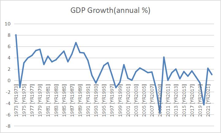
Data from database: World Development Indicators
Figure 2 shows the changes in Japan's aging population between 1973 and 2022. The Y-axis shows the percentage of Japanese over the age of 65. We can see that the aging rate of Japan's population has been on the rise for the past 50 years, which is a major reason for Japan's slow economic growth.
Empirical Economic Bulletin, Vol. 17 264
Figure 2: Population aging
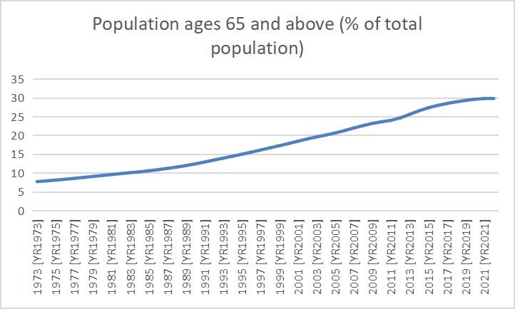
Data from database: World Development Indicators
Figure 3 shows the change in the ratio of imports and exports of goods and services to total GDP over a 50-year period. It can be seen that from 1973 to 1987, Japan's imports and exports of goods and services accounted for a larger proportion than in the 1990s. Japan's import and export also experienced a certain decline in the 1990s, which was not eased until 2000 and began to increase significantly.
Empirical Economic Bulletin, Vol. 17 265
Figure 3: Exports and imports of goods and services (% of GDP)
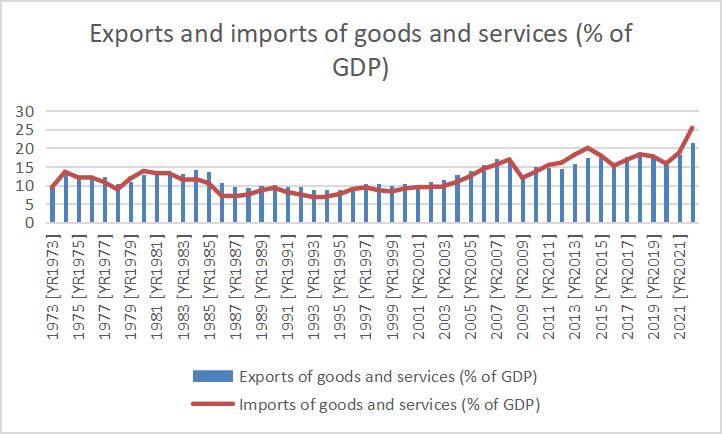
Data from database: World Development Indicators
Figure 4 shows the change in Japan's net national saving share. As can be seen from the figure, before 1990, Japan's national net savings ratio basically hovered around 35%. After 1990, the proportion of savings in Japan showed a gradual decline.
Figure 4: Exports and imports of goods and services (% of GDP)
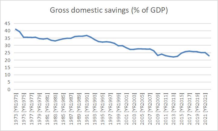
Empirical Economic Bulletin, Vol. 17 266
Data
from database: World Development
Indicators
Figure V shows the change in the share of net national consumption. As can be seen from the graph, the net national consumption share fell sharply in 1987, then roughly stabilized between 100 and 98, and increased significantly around 2010.
Figure 5: Gross national expenditure (% of GDP)
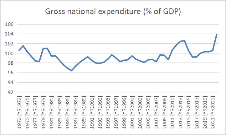
Data from database: World Development Indicators
Japan's inflation rate was very high until 1975, and even reached over 20 in 1974. Japan's inflation rate remained low after 1981 and rose again in 1991 before falling. After 1994, Japan experienced negative inflation, that is, a situation of shrinking inflation. This continued for two decades until 2014, when the first positive inflation occurred.
Empirical Economic Bulletin, Vol. 17 267
Figure 6: Inflation, GDP deflator (annual %)
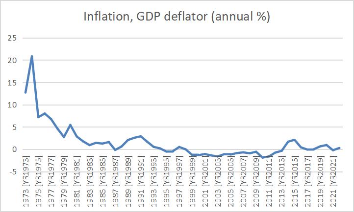
Data from database: World Development Indicators
3.0 LITERATURE REVIEW
Researchers analyze the relationship between energy quality and economic production from the energy perspective and the correlation between GDP and energy intensity. It is found that GDP is related to final energy consumption after quality correction.(Nakajima and Matsushima, 2021) This study suggests that economic inactivity caused by reduced energy access may be directly linked to lower economic growth. In addition, the researchers further suggest that the performance of the Japanese economy is closely related to the quantity and quality of energy. Energy quality is essential in Japan, which has a low energy self-sufficiency rate. (Nakajima and Matsushima,2021)
Another critical factor affecting Japan's slow growth is its aging population. The study found that the development of the Japanese economy is affected by the population of different ages.(Oliver) For example, the increase in people over 75 years old is positively related to GDP growth, while the rise of people in the 60-75 age group will lead to negative GDP growth. The researchers studied the relationship between population aging and economic development through regression analysis and data model, and the final result suggested that the government
Empirical Economic Bulletin, Vol. 17 268
should formulate comprehensive strategies to deal with the impact of population aging on the economy.
From the perspective of competitiveness, the researchers analyze the causes of Japan's economic stagnation and its difficulties. By comparing the competitiveness of Japan with that of East Asian countries, the author puts forward the view that globalization is essential to national competitiveness. The article points out that although macroeconomic policies can alleviate the plight of economic stagnation to a certain extent, they cannot improve national competitiveness.(Parc) As East Asian countries gradually surpass Japan's competitiveness, Japan faces a more profound dilemma. Therefore, only by paying more attention to globalization can Japan enhance its international competitiveness and promote economic recovery.
Another perspective is the role of foreign direct investment (FDI) in revitalizing the Japanese economy. By analyzing the FDI inflow trend when Japan suffered economic recession before and during the "lost decade," this paper highlights the influence of the FDI variable on the Japanese economy. The importance of FDI in promoting employment, output, and productivity in Japan was then highlighted. Finally, it is concluded that FDI is vital in revitalizing Japan's economic growth. The report recommends further measures to encourage foreign direct investment to revive the Japanese economy.(Bâlgăr and Drăgoi)
The article reviews the period from the peak of Japan's rapid economic development in the 1980s to the trough of Japan's economic recession in the 1990s. Various factors contributing to Japan's economic rise, such as national policies, high work ethic, high savings rate, and investment rate, are discussed. An in-depth discussion of the causes of the recession, such as over investment, tight government policies, and poor lending policies of banks, follows this. Finally, the article concludes that the government's policy mistakes led to the economic recession.(Georgescu and Glăvan)
This paper studies the relationship between patent applications and Japan's GDP growth and establishes a model in a multivariate framework. The study found a long-term relationship between patent applications, value-added manufacturing output, and annual GDP and growth. The results of the ARDL model show that patent applications have a one-way causal relationship
Empirical Economic Bulletin, Vol. 17 269
with economic growth. The study concludes that increasing patent applications will be one of the critical variables in Japan's economic development.(KHALILI)
4.0 DATA AND EMPIRICAL METHODOLOGY
4.1 Data
This study uses the time series research method to study ten variables that affect Japan's GDP growth during the 50 years from 1973 to 2022. The study uses data from World Development Indicators for Japan from 1973 to 2022, which are in line with professional standards. Since I analyzed imports and exports of goods and services together, there are actually eleven variables in this study. Table 1 provides summary statistics of the data.
Table 1 Summary Statistics
Population ages 65 and above (% of total
4.2 Empirical Model
Adapted from Japan's Deteriorating Fiscal Situation by Robert Dekle, the article analyzes the dramatic increase in Japan's debt-to-GDP ratio, the impact of an aging population on the economy, changes in government savings and investment, and future fiscal sustainability. On top
Variable Observation Mean Std.Dev Min Max
population) 50 17.41457 7.32027 7.66965 29.92456 Domestic credit to private sector (% of GDP) 50 165.27599 27.39004 119.95455 217.76089 Exports of goods and services (% of GDP) 50 12.97013 3.17994 8.81647 21.56989 Imports of goods and services (% of GDP) 50 12.27444 4.15188 6.80943 25.40159 Foreign direct investment, net inflows (% of GDP) 50 0.18967 0.29426 -0.05209 1.23960 Gross domestic savings (% of GDP) 50 30.38867 5.10204 22.00717 40.94528 Inflation, GDP deflator (annual %) 50 1.54181 3.95619 -1.88074 20.81005 Gross national expenditure (% of GDP) 50 99.32781 1.47083 96.39755 103.82710 Stocks traded, total value (% of GDP) 48 59.32331 42.26728 11.29986 143.80324 Merchandise trade (% of GDP) 50 21.72039 5.85834 13.31003 38.62790 Unemployment, total (% of total labor force) (national estimate) 50 3.17940 1.10987 1.30000 5.38600 Empirical Economic Bulletin, Vol. 17 270
of this, the text further analyzes the changes in imports and exports of goods and services, foreign direct investment, Japan's domestic inflation rate, total national consumption, stock trading, merchandise trade, and unemployment rate over a 50-year period. The model could be written as follow:
GDP Growth=β0+β1(Aging population)-β2(Exports of goods and services)+β3(Imports of goods and services)+β4(Unemployment)-β5(Inflation)+β6(Gross domestic savings)-β7(Gross national expenditure)+β8(Merchandise trade)-β9(FDI)-β10(Domestic credit)+β11(Stock trade)+ϵ
GDP is the growth rate of Japan's gross domestic product between 1973 and 2022. It measures the total value of all final goods and services produced in Japan each year for 50 years. Gross domestic product (GDP) is usually used to measure the economic condition of a country. We can evaluate Japan's domestic economic situation and economic development trend by analyzing Japan's GDP growth rate
The independent variables are composed of ten variables that affect the development of the Japanese economy between 1973 and 2022. Data for all variables are provided by World Development Indicators. The ten variables are population aging, domestic credit, imports and exports of goods and services, foreign direct investment, net domestic savings, inflation, net domestic spending, stock trading, commodity trading, and unemployment. This paper will examine whether these ten variables had an impact on the state of the Japanese economy, causing it to peak in 1980, undervalue and slump in 1990.
5.0 EMPIRICAL RESULTS
Table 2 shows the regression results of 11 variables such as population aging, domestic credit, export of goods and services, import of goods and services, foreign direct investment, net domestic savings, inflation rate, net gross national expenditure, stock transactions, commodity transactions, and unemployment rate on the rate of change of Japan's GDP in the past 50 years.
Empirical Economic Bulletin, Vol. 17 271
Table 2: Regression results for the Japan’s GDP Growth
From the regression results, it can be concluded that the ratio of population aged over 65 has a positive impact on the change of Japan's GDP, but its P-value is 0.0915, which is greater than 0.05. Therefore, although it is close to the significance boundary, it is still not statistically significant at the 5% significance level. The coefficient of domestic credit to the private sector is negative, and the p-value is 0.00157, so this variable is statistically significantly negatively correlated with the growth of the change in GDP. The P-value for exports of goods and services was 0.18064, which is not statistically significant. However, the P-value of imports of goods and services is 0.01372 and the coefficient is 1.60746. This shows that imports of goods and services have a statistically significant positive correlation with changes in Japan's GDP. The coefficient of net inflow of FDI is -2.97773, and the P value is 0.03709. This variable is significantly negatively correlated with GDP growth. The coefficient of domestic saving is 1.36197, and the P-value is 0.000403, which has a very significant positive correlation with GDP growth. The inflation coefficient is -0.61884 and the P value is 0.0000625. Therefore, the inflation rate and GDP growth also have a very significant negative correlation. The coefficient of gross national expenditure is -0.40328 with a P value of 0.00735, which has a very significant negative correlation. The P-value of the total value of stock trading is 0.51106, and the P-value of commodity trade is 0.64830. Neither of these two variables has a statistically significant
Coefficients Standard Error t Stat P-value Lower 95% Upper 95% Intercept 0 #N/A #N/A #N/A #N/A #N/A Population ages 65 and above 0.377639882 0.218715723 1.726624299 0.092149676 -0.064754425 0.820034189 Domestic credit to private sector -0.06592554 0.019399687 -3.398278507 0.00157453 -0.105165112 -0.026685969 Exports of goods and services -0.90955762 0.667233155 -1.363178093 0.180645036 -2.259164063 0.440048824 Imports of goods and services 1.607455679 0.622767557 2.581148715 0.013722795 0.347789397 2.867121961 Foreign direct investment, net inflows -2.977725162 1.379413762 -2.158688889 0.037088047 -5.767852854 -0.18759747 Gross domestic savings 1.361965277 0.35189138 3.870413867 0.000402614 0.650197778 2.073732776 Inflation, GDP deflator -0.61883626 0.137967931 -4.485363038 6.25496E-05 -0.897902742 -0.339769778 Gross national expenditure -0.403284216 0.142599055 -2.828098805 0.007355276 -0.69171803 -0.114850403 Stocks traded, total value 0.008449065 0.0127386 0.663264821 0.511062623 -0.017317185 0.034215316 Merchandise trade -0.264027921 0.57437324 -0.459680052 0.648298222 -1.425807459 0.897751617 Unemployment, total 1.21461245 0.714267618 1.700500511 0.096999279 -0.230130176 2.659355075 Empirical Economic Bulletin, Vol. 17 272
correlation. The P-value of total unemployment is 0.09, which is close to the significance boundary, but still does not have a statistically significant correlation.
Overall, among these variables, domestic credit to the private sector, imports of goods and services, net inflows of foreign direct investment, domestic savings, and the rate of inflation have a statistically significant correlation with the rate of change in GDP. The negative coefficient of domestic credit reflects that excessive credit growth can lead to a decline in Japan's GDP growth, resulting in economic instability. The positive coefficient of imports of goods and services indicates that the higher import level is conducive to the recovery of the Japanese economy. Net inflows of foreign direct investment are normally positive for GDP growth. However, the negative coefficient of FDI on Japan's GDP growth indicates that it may have a negative effect on GDP growth because of competition with domestic investment, or foreign investment is mainly concentrated in some industries that do not promote economic growth. The positive coefficient of domestic saving reflects that a higher savings rate would boost Japan's economy. Finally, the negative coefficient of the inflation rate is due to the uncertainty caused by high inflation, which reduces investment and seriously affects economic development.
However, due to the different sources of data, the accuracy of data, and the time range of data, this study also has certain limitations. The model used in the study may also have some problems such as missing variables.
For the policy implication. First, because credit growth will lead to economic slowdown, policymakers can supervise and control credit growth. Second, since imports are positively correlated with GDP growth, policies can be implemented to further reduce trade barriers and thus promote economic growth. Third, although FDI is negatively correlated with GDP growth, FDI can promote GDP growth in most cases. Japan can reverse the negative effects by adopting policies that attract more foreign investment, which can affect economic growth. Fourth, domestic savings will have a positive effect on GDP growth, and the government can encourage citizens to save more. Fifth, the inflation rate will affect investment and slow down economic development. Controlling the inflation rate is an effective measure that Japan can take.
Empirical Economic Bulletin, Vol. 17 273
5.0 CONCLUSION
This paper uses a time series model to analyze the variables that affect Japan's GDP growth rate during the 50 years from 1973 to 2022. This paper analyzes ten variables of macroeconomic and social structural factors to study the impact of the Japanese economy from the boom period of the bubble economy to the recession after the bubble burst. According to the regression results of empirical analysis, private sector domestic credit, imports of goods and services, domestic savings rate and inflation rate all have statistically significant effects on the change of Japan's GDP. Although this study analyzes Japan's economic development over a period of time, it also has certain limitations due to the limitations of data accuracy, data sources and time range. Finally, the Japanese case offers a valuable lesson about the importance of macroeconomic stability and structural reforms.
Empirical Economic Bulletin, Vol. 17 274
BIBLIOGRAPHY
Khalili, F., Lau, W., & Cheong, K. (2016). Patent application– GDP growth nexus: The case of japan. International Journal of Economic Perspectives, 10(4), 197-205. Retrieved from http://bryant.idm.oclc.org/login?url=https://www.proquest.com/scholarly-journals/patentapplication-gdp-growth-nexus-case-japan/docview/1964461250/se-2
Oliver, M. (2015). Population ageing and economic growth in japan. The International Journal of Sociology and Social Policy, 35(11), 841-863. doi:https://doi.org/10.1108/IJSSP-022015-0018
Motohashi, K., & Kanamori, T. (2008). Information technology and economic growth: A comparison between japan and korea. Seoul Journal of Economics, 21(4), 505-526. Retrieved from http://bryant.idm.oclc.org/login?url=https://www.proquest.com/scholarlyjournals/information-technology-economic-growth-comparison/docview/215570835/se-2
Shostak, A. B. (2007, Sep). Japan's approach to aging and dying. The Futurist, 41, 8. Retrieved from http://bryant.idm.oclc.org/login?url=https://www.proquest.com/magazines/japans-approachaging-dying/docview/218579395/se-2
Gunarto, T., Ciptawaty, U., Yuliawan, D., Mahyudin, A., Pratama, A. D., & Wahyudi, H. (2024). Comparison of energy consumption to economic growth in developing asian and developed asian countries. International Journal of Energy Economics and Policy, 14(1), 264271.doi:https://doi.org/10.32479/ijeep.14871
Tsukamoto, I. (1999). Appraisal practice and japan's bubble economy. The Appraisal Journal, 67(2), 195-198. Retrieved from http://bryant.idm.oclc.org/login?url=https://www.proquest.com/scholarly-journals/appraisalpractice-japans-bubble-economy/docview/199922819/se-2
Patrick, H. (2014). ABENOMICS: JAPAN'S NEW ECONOMIC POLICY PACKAGE. Economics, Management and Financial Markets, 9(4), 11-17. Retrieved from http://bryant.idm.oclc.org/login?url=https://www.proquest.com/scholarly-journals/abenomicsjapans-new-economic-policy-package/docview/1650863194/se-2
Alexander, J. W., Adams, Klein, Kumasaka, Shinozaki, F. G., Lawrence R, . . . Witt, M. A.(2009). Social capital in japan's post-bubble economy. The Journal of Asian Studies, 68(2), 577.doi:https://doi.org/10.1017/S0021911809000722
Dekle, R. (2003). JAPAN'S DETERIORATING FISCAL SITUATION: HUGE INCREASE IN DEBT-GDP RATIO JAPAN'S RECENT FISCAL POSITION RECENT GOVERNMENT SAVING RECENT PUBLIC INVESTMENT RECENT GOVERNMENT DEBT AND LIABILITIES SHARP DECLINE IN PUBLIC SAVING, ONLY MODERATE
Empirical Economic Bulletin, Vol. 17 275
INCREASE IN PUBLIC INVESTMENT UNFUNDED LIABILITIES INCREASE THE GOVERNMENT'S NET OBLIGATIONS FISCAL SUSTAINABILITY RECENT FISCAL REFORM MEASURES PROGRESS IN HEALTHCARE AND SOCIAL SECURITY REFORM WITHOUT SIGNIFICANT FISCAL REFORMS, PROSPECTS ARE GRIM CONCLUDING COMMENTS REFERENCES. CESifo Forum, 4(4), 16-20. Retrieved from http://bryant.idm.oclc.org/login?url=https://www.proquest.com/scholarly-journals/japansdeteriorating-fiscal-situation/docview/217446190/se-2
Empirical Economic Bulletin, Vol. 17 276
