21 minute read
Diagram 6: Hazard Classifications (Reference 14


4. HYDROLOGIC MODELLING
4.1. Sub-catchment Definition
Advertisement
The total catchment represented by the current DRAINS model is 9.14 km2. This area has been represented by 781 sub-catchments (Figure 10) giving an average sub-catchment size of approximately 1.17 hectares. The sub-catchment delineation ensures that where hydraulic controls exist that these are accounted for and able to be appropriately incorporated into hydraulic routing. The pit and pipe network is shown on Figure 11. The drainage system defined in the model comprises: • 1457 pipes. • 1593 inlet pits. • 487 junction pits.
4.2. Impervious Surface Area
Runoff from connected impervious surfaces such as roads, gutters, roofs, or concrete surfaces occurs significantly faster than from vegetated surfaces. This results in a faster concentration of flow within the downstream area of the catchment and increased peak flow in some situations. It is therefore necessary to estimate the proportion of the catchment area that is covered by impervious surfaces.
DRAINS categorises these surface areas as either: • Paved areas (impervious areas directly connected to the drainage system). • Supplementary areas (impervious areas not directly connected to the drainage system; instead, connected to the drainage system via the pervious areas) and • Grassed areas (pervious areas).
Within the Powells Creek catchment, the impervious value was determined using the Table 14 and the land types within each sub catchment. The proportion of pervious area and remaining impervious area was defined as: • For sub catchments with imperviousness below 25% (typically parks), the pervious area is defined as 70% of the non-impervious area and the remaining impervious area is defined as 30% of the non-impervious area. • For sub catchments with imperviousness above 25% (typically residential properties), the pervious area is defined as 30% of the non-impervious area and the remaining impervious area is define as 70% of the non-impervious area.
Table 14: Impervious Percentage per Land-use
Land-use Category Residential/Commercial property Impervious Percentage
60% Impervious
Non-bitumen road reserve
60% Impervious Vacant non hard surface land 0% Impervious Green space (such as public parks) 0% Impervious Roadway/Car parks 100% Impervious Urbanised land within Canada Bay LGA 70% Impervious Waterways 0% Impervious
4.3. Rainfall Losses
Methods for modelling the proportion of rainfall that is “lost” to infiltration are outlined in ARR2019 (Reference 5). The methods are of varying degrees of complexity, with the more complex options only suitable if sufficient data are available. The method most typically used for design flood estimation is to apply an initial and continuing loss to the rainfall. The initial loss represents the wetting of the catchment prior to runoff starting to occur and the continuing loss represents the ongoing infiltration of water into the saturated soils while rainfall continues.
Rainfall losses from a paved or impervious area are considered to consist of only an initial loss (an amount sufficient to wet the pavement and fill minor surface depressions). Losses from grassed areas are comprised of an initial loss and a continuing loss as indicated in Section 3.3.6.
4.4. Design Rainfall Data
Rainfall intensities were derived from the BoM website using ARR (Reference 5) data (Table 6). Calculation of the Probable Maximum Precipitation (PMP) was undertaken using the Generalised Short Duration Method (GSDM) according to Reference 9.
For the PMP estimate the following criteria applied: • as the catchment area is less than 1000 km2 and located in the coastal transitional area the Generalised Short Duration Method (GSDM) was adopted. • zero adjustment for elevation was assumed as the catchment topography is less than 1500 m AHD. • a moisture adjustment factor of 0.7 was adopted. • the catchment is assumed to be 100% 'smooth'.
5. HYDRAULIC MODELLING
5.1. TUFLOW
The TUFLOW modelling package includes numerical scheme for the solution of the depth averaged shallow water equations in two dimensions. The TUFLOW software has been widely used for a range of similar floodplain projects both internationally and within Australia and is capable of dynamically simulating complex overland flow regimes. The TUFLOW model build used in this study is 2020-10-AA-iSP-w64 and further details regarding TUFLOW software can be found in the User Manual (Reference 10).
The model uses a regularly spaced computational grid, with a cell size of 2 m by 2 m. This resolution was adopted as it provides an appropriate balance between providing sufficient detail for roads and overland flow paths, while still resulting in workable computational run-times. The model grid was established by sampling from a DEM generated from a triangulation of filtered ground points from the ALS dataset, discussed in Section 2.4 and shown in Figure 3.
The TUFLOW hydraulic model includes the Powells Creek catchment to Homebush Bay with the open channel in 1D and the overland areas in 2D. The total area included in the 2D model is approximately 10 km2. The extents of the TUFLOW model are shown in Figure 12.
5.2. Boundary Locations
Local runoff hydrographs were extracted from the DRAINS model for inclusion within the TUFLOW model domain. These were applied to the downstream end of the sub-catchments within the 2D domain of the hydraulic model. The inflow locations typically corresponded with inlet pits on the roadway as this is where most rainfall is directed.
The downstream boundary was located at the Parramatta River, as shown in Figure 12.
5.3. Roughness Co-efficient
The hydraulic efficiency of the flow paths within the TUFLOW model is represented in part by the hydraulic roughness or friction factor formulated as Manning’s “n” values. This factor describes the net influence of bed roughness and incorporates the effects of vegetation and other features which may affect the hydraulic performance of the flow path.
The Manning’s “n” values adopted, including flow paths (overland, pipe and in-channel), are shown in Table 15 and were based on site inspection and past experience in similar floodplain environments.
Table 15: Manning’s “n” values adopted in TUFLOW
Material Bitumen road reserve and some car parks Green space - golf course, parks, vacant lots Residential/urban area Non-bitumen road reserve Waterways Pipes Manning’s "n" Value
0.02 0.04 0.03 0.032 0.015 0.012
5.4. Hydraulic Structures
5.4.1. Buildings
Buildings and other significant features likely to act as flow obstructions were incorporated into the model network based on building footprints, defined using aerial photography. These types of features were modelled as impermeable obstructions to the floodwaters.
5.4.2. Fencing and Obstructions
Smaller localised obstructions within or bordering private property, such as fences, were not explicitly represented within the hydraulic model, due to the relative impermanence of these features. The cumulative effects of these features on flow behaviour were assumed to be addressed partially by the adopted roughness parameters.
5.4.3. Bridges
Key hydraulic structures were included in the hydraulic model, as shown in Figure 12, bridges were modelled as 1D features within the 1D channels, with the purpose of maintaining continuity within the model.
The modelling parameter values for the culverts and bridges were based on the geometrical properties of the structures, which were obtained from detailed survey, photographs taken during site inspections, and previous experience modelling similar structures.
5.5. Blockage Assumptions
Blockage of hydraulic structures can occur with the transportation of several materials by flood waters. This includes vegetation, garbage bins, building materials and cars, the latter occurred in the Newcastle area in the June 2007 floods. However, the disparity in materials that may be mobilised within a catchment can vary greatly.
Debris availability and mobility can be influenced by factors such as channel shear stress, height of floodwaters, severity of winds, storm duration and seasonal factors relating to vegetation. The channel shear stress and height of floodwaters that influence the initial dislodgment of blockage materials are also related to the AEP of the event. Storm duration is another influencing factor, with the mobilisation of blockage materials generally increasing with increasing storm duration.
The potential effects of blockage include: • decreased conveyance of flood waters through the blocked hydraulic structure or drainage system. • variation in peak flood levels. • variation in flood extent due to flows diverting into adjoining flow paths; and • overtopping of hydraulic structures.
Existing practices and guidance on the application of blockage can be found in: • ARR Revision Project 11 Blockage of Hydraulic Structures (Reference 12); and • the policies of various local authorities and infrastructure agencies.
Current modelling has been undertaken assuming no blockage of pipes, culverts and bridges greater than 225 mm in diameter. Pipes less than or equal to 225 mm in diameter were conservatively assumed to be completely blocked. On grade pits were assumed as 20% blockage and sag pits were assumed as 50% blocked. These blockage values were adopted for all events in this report unless stated otherwise.
Various scenarios have been investigated to assess the catchment’s sensitivity to blockage and the results of this are discussed in Section 9. These scenarios included blockage of all pipes, blockage of bridges/culverts over the open channel, and blockage of the drainage infrastructure.
No historical evidence of blocking of structures in the catchment is available; however, it is possible that changed activities on the floodplain may mean that there may be a higher chance of blockage today than in the past. For example, colorbond fencing is much less permeable and less likely to collapse than the more traditional paling fencing. Individual palings becoming mobile in a flood are also less likely to cause blockage than a panel of colorbond fencing. In some council areas garbage bins are known to become mobile during floods and can cause blockage. In summary, it is impossible to accurately determine whether blockage will or will not be an issue in the next flood.
5.6. Ground Truthing
Inspection of the above-ground features along the catchment’s overland flow paths was undertaken following calibration of the hydraulic model as part of the 2016 Powells Creek Revised Flood Study (Reference 2). This entailed producing design flood results and mapping the peak flood depth in detail across the catchment. This allowed identification of features (largely buildings) that blocked or partially blocked overland flow. Model schematisation of these features was then compared to the actual features on a site visit and the model was updated where any discrepancy was identified. Changes were minor and only impacted results in the vicinity of the modification.
6. MODEL CALIBRATION AND VERIFICATION
6.1. Introduction
It is important that the performance of the overall modelling system be substantiated prior to defining design flood behaviour. Typically, in urban areas such information is lacking. Issues which may prevent a thorough calibration of hydrologic and hydraulic models are: • there is only a limited amount of historical flood information available for the study area; and • rainfall records for past floods are limited and there is a lack of temporal information describing historical rainfall patterns within the catchment.
The adopted rainfall parameters for calibration of the DRAINS model are shown in Table 17. These parameters are different to those in the 2016 Powells Creek Revised Flood Study (Reference 2). They were chosen to eliminate the high storage volume at each drainage pit in TUFLOW adopted in Reference 2 to achieve a calibration.
The rainfall loss values adopted in the 2016 Powells Creek Revised Flood Study (Reference 2) for calibration and design are shown in Table 16.
Table 16: Rainfall Loss Values Adopted in the 2016 Powells Creek Revised Flood Study (Reference 2)
The rainfall loss values adopted for calibration in the present study are provided on Table 17.
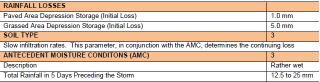
Table 17: Rainfall Loss Values Adopted in the Present Study
RAINFALL LOSSES
Paved Area Depression Storage (Initial Loss) Grassed Area Depression Storage (Initial Loss)
SOIL TYPE
Low runoff potential, high infiltration rates (consists of sand and gravel)
ANTECEDENT MOISTURE CONDITONS
Description Total Rainfall in 5 Days Preceding the Storm
6.2. Results
1.0 mm 5.0 mm
1
3
Rather wet 12.5 to 25 mm
The results of the calibration and verification process using the six historical events are shown on Figure 13 (Elva Street Gauge) and Figure 14 (across catchment) and on Table 18 (Elva Street Gauge) and Table 19 (across the catchment).
Table 18: Calibration Results - Elva Street Gauge
Date Recorded Level (m AHD) Modelled Level St Sabina Pluviometer (m AHD)
3-Feb-90 6.58 6.63
7-Feb-90 6.62 6.65
10-Feb-90 7.00 6.96
17-Feb-90 6.38 6.54
18-Mar-90 7.14 6.86
2-Jan-96 - 7.91
Difference
(m) 0.05
0.03
-0.14
0.16
-0.28
Modelled Level Elva St Pluviometer (m AHD)
6.63
6.59
6.91
Difference
(m) 0.05 -0.03
-0.09
Table 19: Calibration Results - Peak Heights
Address Location Surveyed Level 1990 February 10 (m AHD) Surveyed Level 1996 January 2 (m AHD)
Modelled Level 1990 February 10 (m AHD) Modelled Level 1996 January 2 (m AHD) Difference1990 February 10 (m AHD)
Difference1996 January 2 (m AHD)
21 Llandilo Avenue Garage Floor Level 29.90 - 29.93 - 0.03 - 21 Llandilo Avenue North-West Corner 28.80 - 28.60 - -0.20 -
8 Agnes Street
Driveway and Front Boundary - 26.71 - 26.52 - -0.19
41 Albyn Road Crest of Driveway - 22.54 - 22.48 - -0.06
41 Albyn Road
Low Point along West. Boundary - 21.64 - 21.56 - -0.08
47 Albyn Road Garage Floor Level - 21.18 - 21.16 - -0.02 37 Redmyre Road Crest of Driveway - 13.27 - 13.21 - -0.06
37 Redmyre Road
Ground Level at Garage - 12.21 - 12.23 - 0.02
35 Redymre Road Crest of Driveway - 13.26 - 13.20 - -0.06
35 Redmyre Road
45 Churchill Avenue
60 Churchill Avenue
Ground Level at Back Fence Base Steps at Front House Ground Level at Path Granny Flat - 12.13 - 12.11 - -0.02
- 10.74 - 11.06 - 0.32
- 11.49 - 11.47 - -0.02
Pharmacy adjoining Plaza Entrance, The Boulevarde
- 12.29 - 12.54 - 0.25
65 Oxford Street Carport Slab - 24.16 - 23.95 - -0.22
63 Oxford Street
SouthWest corner of house - 23.75 - 23.61 - -0.14
61 Oxford Street Garage Floor Level - 23.24 - 22.99 - -0.25
59 Oxford Street Patio Level - 23.14 - 23.04 - -0.10
Address Location
141Albert Street
135 Albert Street
Ground level along eastern fence Bottom steps rear of house
Surveyed Level 1990 February 10 (m AHD) Surveyed Level 1996 January 2 (m AHD)
Modelled Level 1990 February 10 (m AHD) Modelled Level 1996 January 2 (m AHD) Difference1990 February 10 (m AHD) Difference1996 January 2 (m AHD)
19.51 - 19.28 - -0.24 -
18.49 - Not Flooded - Not Flooded -
137 Albert Street Crest of driveway 19.24 - Not Flooded - Not Flooded -
137 Albert Street
Water reached floor level 19.01 - Not Flooded - Not Flooded -
100 Beresford Road
Driveway at entrance to house 15.91 - 15.77 - -0.14 -
102 Beresford Road
104 Beresford Road
110 Beresford Road
Ground level at back door Ground level rear house Midway along eastern fence 16.43 - 16.23 - -0.20 -
17.00 - 16.59 - -0.41 -
17.50 - 17.63 - 0.13 -
108 Beresford Road
Base steps rear house 17.49 - 17.26 - -0.23 - 53 Beresford Road Garage floor level 15.29 - 15.05 - -0.24 -
89 Rochester Street 109 Rochester Street
Floor level shop 12.84 - 12.68 - -0.16 - Base steps rear house 14.33 - 14.19 - -0.14 -
109 Rochester Street
57 Rochester Street
38-46 Burlington Road
Base steps rear house - 14.15 - 14.33 - 0.18
Ground level back yard
Ground level at rear shed - 9.92 - 10.10 - 0.18
9.71 - 9.55 - -0.16 -
48 Burlington Road
Ground Floor Level - 9.55 - 9.54 - -0.01
29 Burlington Road
Stormwater reached this level at rear of factory 9.16 - 8.88 - -0.28 -
30 The Crescent Garage Floor Level - 8.70 - 8.75 - 0.05 31 The Crescent Garage Floor Level - 8.33 - 8.24 - -0.09 79 The Crescent Floor level 8.20 - 7.02 - -1.18 - 79 The Crescent Base patio at rear - 7.75 - 7.78 - 0.03
12 Loftus Crescent
86 Underwood Road
Ground level backyard 7.87 - Local runoff - Local runoff -
Base steps front house - 4.89 - 4.65 - -0.24
82 Underwood Road
90 Underwood Road
Ground level at front house and driveway Base steps front of house 4.97 - 4.44 - -0.53 -
- 4.74 - 4.41 - -0.33
Address Location
60 Ismay Avenue
Ground level at front of house
Surveyed Level 1990 February 10 (m AHD) Surveyed Level 1996 January 2 (m AHD)
Modelled Level 1990 February 10 (m AHD) Modelled Level 1996 January 2 (m AHD) Difference1990 February 10 (m AHD) Difference1996 January 2 (m AHD)
- 3.83 - 3.80 - -0.03
55 Ismay Avenue Base front steps 4.30 4.11 3.32 4.11 -0.98 0.00 51 Ismay Avenue Base front steps 4.19 Local runoff - - Local runoff - 56 Ismay Avenue Base front steps 3.83 - 3.66 - -0.17 - 49 Ismay Avenue Base front steps - 4.16 - 4.00 - -0.16 48 Ismay Avenue Base front steps - 3.43 - 3.36 - -0.07 41 Ismay Avenue Base front steps 3.71 Local runoff - - Local runoff -
10 Mitchell Road
Ground level low side house - 14.75 - 14.75 - 0.00
6 Mitchell Road
104 Arthur Street
Ground level low side house Ground level front of house - 14.35 - 14.18 - -0.17
- 13.87 - 13.62 - -0.25
106 Arthur Street
105 Arthur Street
Ground level at boundary Ground level at house steps side house - 13.85 - 13.62 - -0.23
- 13.89 - 13.81 - -0.08
29 Arthur Street Base front steps - 13.23 - 13.22 - -0.01
29 Arthur Street
Ground level at rear fence - 12.98 - 12.70 - -0.28
6 Kessell Avenue
Ground level at fence 8.42 - 8.14 - -0.28 -
6 Kessell Avenue
Water reached floor level - 7.76 - 7.79 - 0.03
Note: Local runoff denotes when the flooding is very localised and is therefore not identified in the TUFLOW model.
6.3. Discussion of Results
6.3.1. Elva Street Gauge - Table 18 and Figure 13
Apart from 18th March 1990 and to a lesser extent 10th February 1990, there is a good match to the peak at the Elva Street gauge using the St Sabina pluviometer. The use of the Elva Street pluviometer significantly improves the match for the 10th February 1990 event compared to using the St Sabina pluviometer.
For all events, the relative timings of the water level gauge and the pluviometer are incorrect due to timing errors with the instruments. This was recognised in Reference 8 and an attempt was made to correct this by assuming that the "clocks" decrease or increase in speed linearly (this can be calculated as the on and off times are recorded and the elapsed real time can be compared to the chart time).
In general, the gauge shows a more rapid rise and fall than the model results. Thus, the model
assumes a greater volume of runoff than recorded.
Where comparisons can be made, the results from the St Sabina and Elva Street pluviometer show similar shapes of hydrographs. The timing of the two pluviometers is also similar suggesting that the error in timing is the water level gauge. The two pluviometers are only 800 m apart, but timing differences may reflect the passage of a storm across the area.
For the historical event of 10th February 1990, most of the differences between surveyed and modelled levels were within 0.2 m. However, the modelled flood level at 79 The Crescent was 1.18 m below the level recorded at the floor. The ALS at this location was 7.05 m AHD which was far lower than the recorded flood level of 8.2 m AHD.
The differences were also generally within 0.2 m for the historical event of 2nd January 1996.
In summary the results appear reasonable for these two events, but it should be noted that as both events had shallow overland depths (generally less than 0.5m) a difference of 0.2m is significant. Unfortunately, it is impossible to resurvey the locations or review whether the recorded levels are reliable. However, some confidence in the results is provided in that (certainly for 2nd January 1996) the model produces results above and below the recorded level which suggests that there is no consistent error in the modelling (e.g the peak flows are consistently too low or too high).
7. DESIGN EVENT MODELLING
7.1. Overview
There are two basic approaches to determining design flood levels, namely: • flood frequency analysis – based upon a statistical analysis of the flood events, and • rainfall and runoff routing – design rainfalls are processed by hydrologic and hydraulic computer models to produce estimates of design flood behaviour.
The flood frequency approach requires a reasonably complete homogenous record of flood levels and flows over several decades to give satisfactory results. Powells Creek is one of the two catchments in the Sydney basin that has a reasonably reliable water level record over a long period and has had velocity gaugings undertaken (required to derive a rating curve). Thus, flood frequency analysis can be undertaken. However, this approach only provides results at the gauge location and a rainfall and runoff routing approach, using DRAINS model results, is also required to derive inflow hydrographs to the TUFLOW hydraulic model, which determines design flood levels, flows and velocities in areas beyond the actual gauge location. This approach reflects current engineering best practice and is consistent with the quality and quantity of available data.
7.2. Critical Duration for Rainfall Runoff Approach
To determine the critical storm duration for various parts of the catchment, modelling of the range of design events was undertaken using temporal patterns from ARR2019 with the approach described in Section 3.3.7. The adopted critical storm durations are provided in Table 20.
Table 20: Adopted Critical Storm Duration Events
Design Rainfall Event Adopted Critical Storm Duration
0.5EY 45 minutes 20% AEP 45 minutes 10% AEP 60 minutes 5% AEP 60 minutes 2% AEP 60 minutes 1% AEP 60 minutes 0.5% AEP 60 minutes 0.2% AEP 60 minutes PMF 60 minutes
7.3. Downstream Boundary Conditions
In addition to runoff from the catchment, downstream areas can also be influenced by high water levels at the confluence of the Parramatta River and Powells Creek. Consideration must therefore also be given to accounting for the joint probability of coincident flooding from both catchment runoff and backwater effects.
A full joint probability analysis to consider the interaction of these two mechanisms is beyond the scope of the present study. It is accepted practice to estimate design flood levels in these situations using a ‘peak envelope’ approach that adopts the highest of the predicted levels from
the two mechanisms. However, the 1986 Parramatta River Flood Study (Reference 13) indicates that in this reach of the river the design water level is determined by the tide level and no design flood levels are provided. For the present study, a constant water level of was applied to the downstream boundary for each design rainfall event as shown on Table 21. The typical tidal in Homebush Bay is +0.6 m AHD to -0.4 m AHD and the maximum ocean tide in a year is 1.1 m AHD.
Table 21: Adopted Tailwater Levels for Design Events
Design Rainfall Event (AEP) Downstream Design Level (AEP)
0.5EY
0.5EY
20% 10% 5% 2% 1% 0.5% 0.2% PMF
20% 10% 5% 5% 5% 1% 1% 1%
Downstream Water Level (m AHD)
1.2 1.2 1.2 1.4 1.4 1.4 1.43 1.43 1.43
7.4. Design Results
The results from this study are presented on figures as summarised below. • Peak flood level profiles in Figure 15. • Peak flood depths and level contours in Figure 16. • Peak flood velocities in Figure 17. • Provisional hydraulic hazard in Figure 18 and • Provisional hydraulic categorisation in Figure 19.
The definition and methodology used to derive these categorisations from the results are discussed below.
7.4.1. Summary of Results
Peak flood levels, depths and velocities at key locations within the catchment are summarised in Table 22, Table 23 and Table 24 for the design events. These key locations coincide with the key locations used for the sensitivity analysis discussed in Section 9 and are shown on Figure 4.
Table 25 provides the peak flows at Homebush Bay Drive for the design events.
Table 22: Peak Flood Levels (m AHD) at Key Locations – Design Events
ID Location 1.0 EY 20% AEP 10% AEP 5% AEP 2% AEP 1% AEP 0.5% AEP 0.2% AEP PMF
H01 Pedestrian Bridge 2 1.34 1.42 1.51 1.66 1.70 1.74 1.78 1.82 2.67 H02 Pedestrian Bridge 1 1.30 1.36 1.42 1.59 1.63 1.66 1.70 1.74 2.48 H03 Front of community Centre 1.97 2.00 2.01 2.02 2.03 2.03 2.06 2.15 3.55 H04 Railway underpass 2 East side 7.41 7.44 7.46 7.47 7.49 7.50 7.52 7.53 8.56 H05 Railway underpass east side 6.08 6.23 6.34 6.41 6.55 6.63 6.72 6.84 8.36 H06 Railway underpass west Side 5.88 6.06 6.14 6.20 6.32 6.36 6.43 6.52 6.58 H07 7 Concord Avenue low point 1.55 1.72 1.79 1.88 1.93 2.00 2.06 2.14 3.55 H08 George Street low point near soccer field 2.44 2.89 2.98 3.16 3.29 3.43 3.59 3.89 4.56 H09 Powells Creek @ Argonne Street 1.83 1.84 1.85 2.00 2.09 2.16 2.23 2.32 4.10 H10 Powells Creek @ Pomeroy Bridge 2.40 2.53 2.55 2.60 2.64 2.67 2.71 3.85 H11 Powells Creek @ Allen Street 2.98 3.32 3.44 3.54 3.63 3.70 3.76 3.87 5.28 H12 Powells Creek @ Brussels Street 1.69 1.79 1.87 2.02 2.11 2.19 2.25 2.34 4.12 H13 Powells Creek @ Warsaw Street 1.79 1.85 1.93 2.07 2.17 2.25 2.31 2.40 4.17


