

An Open Energy Outlook: Decarbonization Pathways for the USA
September 2022

Introduction
There is growing consensus that the world needs to reach net-zero carbon dioxide (CO 2) emissions around the middle of this century to limit global average temperature rise to 1.5 degrees Celsius above pre-industrial levels and avoid the worst effects of anthropogenic climate change (IPCC, 2021, 2022a). Rapid and far-reaching global efforts focused on deep decarbonization will be required to achieve this target (IPCC, 2022b). The United States is the second largest primary energy consumer and CO 2 emitter, representing 17% of global primary energy supply and 13% of global emissions (EIA, 2021a and WRI, 2020). Despite rapid growth in renewable electric power, fossil fuels still represented 79% of U.S. primary energy consumption in 2021 (EIA, 2022a). U.S. mitigation efforts will be critical to the global effort to reach carbon neutrality and will require an unprecedented effort to drive the deployment of carbon-free energy technologies.
Appropriate action will necessitate fundamental changes in how we produce and consume energy and must be driven by climate-informed policy. Policymakers face the monumental challenge of crafting effective climate policy in the face of highly uncertain expectations about the future. The stakes are high because energy infrastructure is expensive and long-lived. Computer models of the energy system – referred to as energy system models – provide a way to examine future energy system evolution, test the effects of proposed policies, and explore the role of uncertainty. Model-based analysis can yield insights that inform the policymaking process. Unfortunately, many of these computer models are opaque to outsiders and are used to run a few scenarios that do not properly account for uncertainty (DeCarolis et al., 2012). Given the stakes associated with climate change, energy system researchers must do better.
This report – and the underlying modeling effort – endeavor to improve conventional model-based analysis in three ways. First, this study relies solely on the use of open-source models and data. Making both the model source code and data publicly available allows interested parties to replicate and build on the results published in this report. We use the open-source Tools for Energy Model Optimization and Analysis (Temoa) to examine decarbonization pathways across the energy system ( Temoa, 2021). Second, we employ sensitivity and uncertainty analysis to evaluate how future uncertainty may affect the results of interest and the insights we draw for policymakers. Third, this model-based analysis results from a community effort, with formal and informal contributions from various experts across many institutions. We think that large, multi-institutional efforts drawing on a wide range of expertise can dramatically improve the modeling process (DeCarolis et al., 2020).
The following section describe the specific objectives of this report. There are many critical issues to examine related to U.S. deep decarbonization; thus, this report is necessarily limited in scope. We hope to turn the Open Energy Outlook into a long-term effort, with updated modeling and analysis released annually. To do so, we are forming an industrial consortium to support this effort moving forward. Details are available on the project website. In the meantime, we invite third parties to build on our work by downloading, examining, and extending the modeling framework used in this analysis.
Objectives 2
This report summarizes a model-based analysis that addresses the following key questions:
What is the trajectory of greenhouse gas emissions under different scenarios, and to what degree do these scenarios fall short of achieving net-zero emissions by 2050?
Motivation: It is well understood that attaining net-zero CO 2 emissions will require aggressive policy action. As described below, this report includes simulations for a family of policy scenarios that cover a range of possible outcomes. Analyzing politically feasible policy scenarios compared to a prescriptive net-zero scenario helps to illustrate the ambition gap.
What are alternate, near-optimal, feasible pathways to achieve net-zero emissions by 2050?
Motivation: While a single, deterministic model run will deliver the appearance of precise results, input uncertainty can significantly affect results. The report goes beyond conventional scenario analysis, exploring a range of near-optimal deep decarbonization pathways for the U.S.
Scenarios
This report focuses on a series of policy scenarios highlighting the interplay between policy and technology to achieve deep reductions in CO 2 emissions by 2050. The scenarios described below are meant to cover a wide range of plausible outcomes that lead to varying degrees of emissions reduction.
No new policy beyond 2021 (‘No Policy’)
This scenario assumes that all existing policies as of the end of 2021 remain in their current form, and no new federal or state policies are implemented. The results indicate how projected fuel prices and technology costs will shape the energy system in the absence of climate policies. A no-policy baseline provides a valuable point of comparison to the policy scenarios. The policies included in this scenario represent the policies in place by the end of 2021: state-level Renewable Portfolio Standards (RPS), the Cross-State Air Pollution Rule (CSAPR), the California cap and trade program, and the federal Investment Tax Credit (ITC). Note that these existing policies are also included in the other scenarios described below. In this No Policy scenario, exogenous fuel prices are set based on the EIA Annual Energy Outlook (AEO) 2022 Reference case.
It is worth noting that in August of 2022, the U.S. Congress passed the Inflation Reduction Act (IRA), which allocated ~ $385 billion in funding for climate mitigation activities between 2022 and 2031. This report does not include an explicit analysis of the IRA provisions. We do, however, explore how the provisions in the IRA align with the results of the scenarios included in our modeling efforts and their associated results.
State-level action in the absence of federal policy (‘State Action’)
This scenario considers the possibility of ambitious state-level action to reduce CO 2 emissions without any new federal policy beyond what was available by the end of 2021. The scenario assumes that a collection of U.S. states will implement legislation to achieve net-zero CO 2 emissions from electricity by 2050. To select the states that would most likely pursue such a policy, we include those states with a renewable or clean energy policy and that have demonstrated a potential willingness to pursue more ambitious actions (e.g., voting history). Figure 1 shows the states with net-zero targets for power generation in this State Action scenario. This scenario is not meant to serve as a policy forecast but rather an ambitious yet plausible scenario where a subset of state governments take action to reduce emissions. The results inform the degree to which bottom-up, state-level action can reduce emissions compared to the scenarios involving federal action. In this scenario, exogenous fuel prices are set based on the EIA AEO 2022 Low Oil Price case, consistent with price impacts from reductions in petroleum demand.
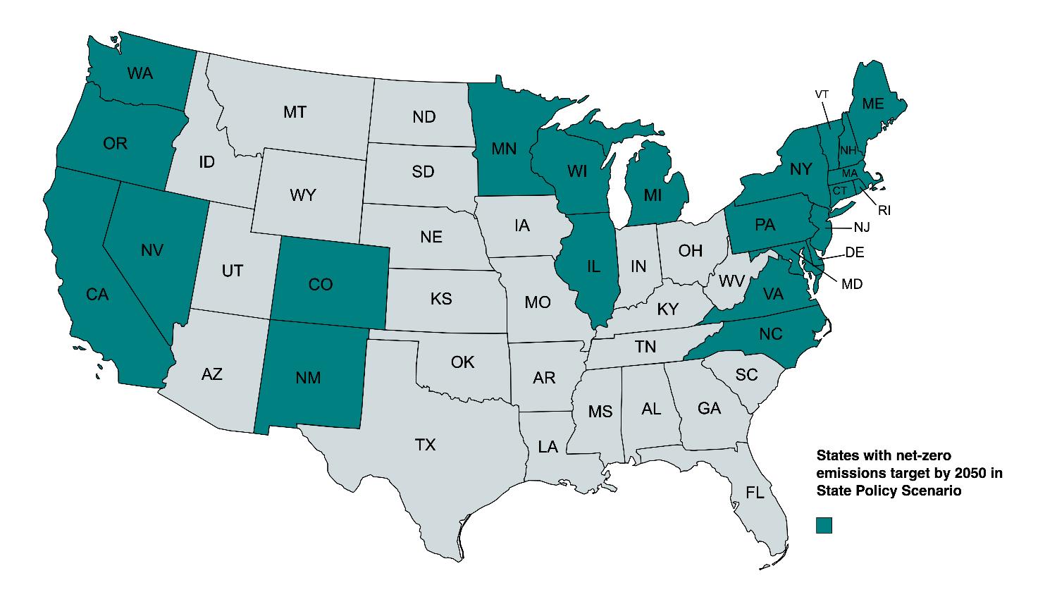
Figure 1: States with targets of net-zero CO2 emissions from the power sector in the State Action scenario.
UNFCCC COP26 commitments (‘COP26’)
This scenario includes the policy commitments in the U.S. Nationally Determined Contribution (NDC), submitted to the UNFCCC as part of the COP26 negotiations. Compared to the No Policy scenario, the results from this scenario indicate how international commitments to climate mitigation can drive reductions in greenhouse gas emissions. Compared with the Net Zero scenario, this COP26 scenario shows the ambition gap between existing international commitments and achieving net-zero emissions. In this scenario, exogenous fuel prices are set based on the EIA AEO 2022 Low Oil Price case.
Policy neutral net-zero (‘Net Zero’)
This scenario assumes that the United States will reach net-zero CO 2 emissions by 2050. A constraint caps CO 2 emissions across the energy system to achieve this objective, with linear declines beginning in the 2025 model period and reaching net-zero by 2050. The ‘net’ term indicates that the model can balance any residual CO 2 emissions with carbon dioxide removal (CDR) technologies that draw CO 2 directly out of the atmosphere, including biomass integrated gasification combined cycle with carbon capture and sequestration (BECCS) and direct air capture (DAC). The results from this scenario provide a prescriptive look at the energy system transformation to net-zero without regard to the specific policy mechanisms required to achieve it. In this scenario, exogenous fuel prices are set based on the EIA AEO 2022 Low Oil Price case.
The scenarios in the report collectively represent a full range of emissions pathways. The No Policy and Net Zero scenarios form upper and lower bounds on the emissions trajectories. The remaining scenarios - State Action and COP26 - represent varying levels of policy ambition that will produce emissions trajectories within the prescribed range.
A note on fuel prices
Fuel prices are an exogenous input to the current version of Temoa used for this analysis. Specifically, this analysis relies on fuel prices reported in the Annual Energy Outlook 2022 published by the Energy Information Administration (EIA) (EIA, 2022b). Figure 2 shows the price ranges of natural gas for power generation, gasoline, diesel, and coal used in this analysis. The No Policy scenario relies on the prices in EIA’s reference case, while the State Action, COP26, and Net Zero scenarios rely on the prices in EIA’s low oil case. These differences in the prices among the scenarios aim to capture the price elasticity of supply: as demand for fuels decreases in the State Action, COP26, and Net Zero scenarios, the price also drops. The range presented for each case represents the distribution of regional fuel prices across the U.S.
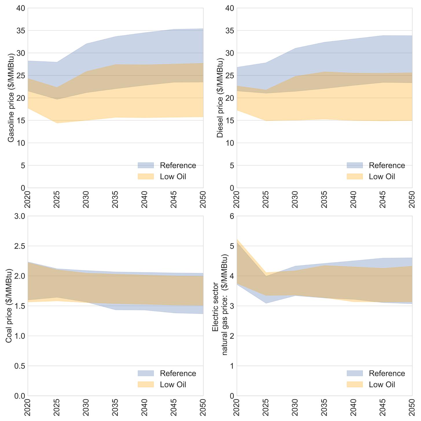
Figure 2: Fuel price assumptions based on EIA Annual Energy Outlook 2022 Reference and Low Oil Price cases. The range presented for each case represents the range in regional fuel prices.
Modeling Framework
4.1 Model structure
This project relies on Tools for Energy Model Optimization and Analysis (Temoa), an open-source energy system optimization model (ESOM). Like other ESOMs, Temoa represents the energy system as a process-based network in which technologies are linked together by flows of energy commodities. Each process is defined by an exogenously specified set of techno-economic parameters such as investment costs, operations and maintenance costs, conversion efficiencies, emission rates, and availability factors. Temoa is a linear program that minimizes the total system cost of energy supply over the user-specified time horizon, subject to both system-level and user-defined constraints. The complete algebraic formulation of Temoa is presented in Hunter et al. (2013) , with updates provided in the Temoa documentation ( Temoa, 2021). The Temoa model and input database represent distinct elements. The model has an abstract (i.e., generic) formulation that can operate on different input databases. The model source code is available in the Temoa GitHub repository ( Temoa, 2022) and is available under the GPLv2 license.
4.2
OEO energy system representation
The Open Energy Outlook (OEO) database on which Temoa operates to produce the results in this report is available in a separate OEO GitHub repository ( Venkatesh et al., 2022) and includes extensive sector-by-sector documentation in the form of Jupyter notebooks.
Regional differences in fuel supply, renewable resources, end-use demands, and existing capacities are key determinants of how the future U.S. energy system may evolve. While it would be helpful to model all 50 states (so we can capture state-level energy and climate policies), such a spatial resolution would be computationally infeasible, given the other modeling requirements. Thus, the input database for Temoa aggregates states into regions. Figure 3 shows the regions in the database based on state-level aggregations.
The modeled base year in this report is 2020, followed by five-year periods that extend to 2050. The model assumes that all years within a given 5-year time period are identical; thus, the optimal results represent an indicative year within the 5 years. To capture operational issues and balance the supply and demand of electricity at the sub-annual level, the model relies on a “representative days” approach where eight days, modeled at an hourly resolution, represent an entire year’s operations. These representative days are selected from annual datasets that include energy demands and varying renewable energy capacity factors.
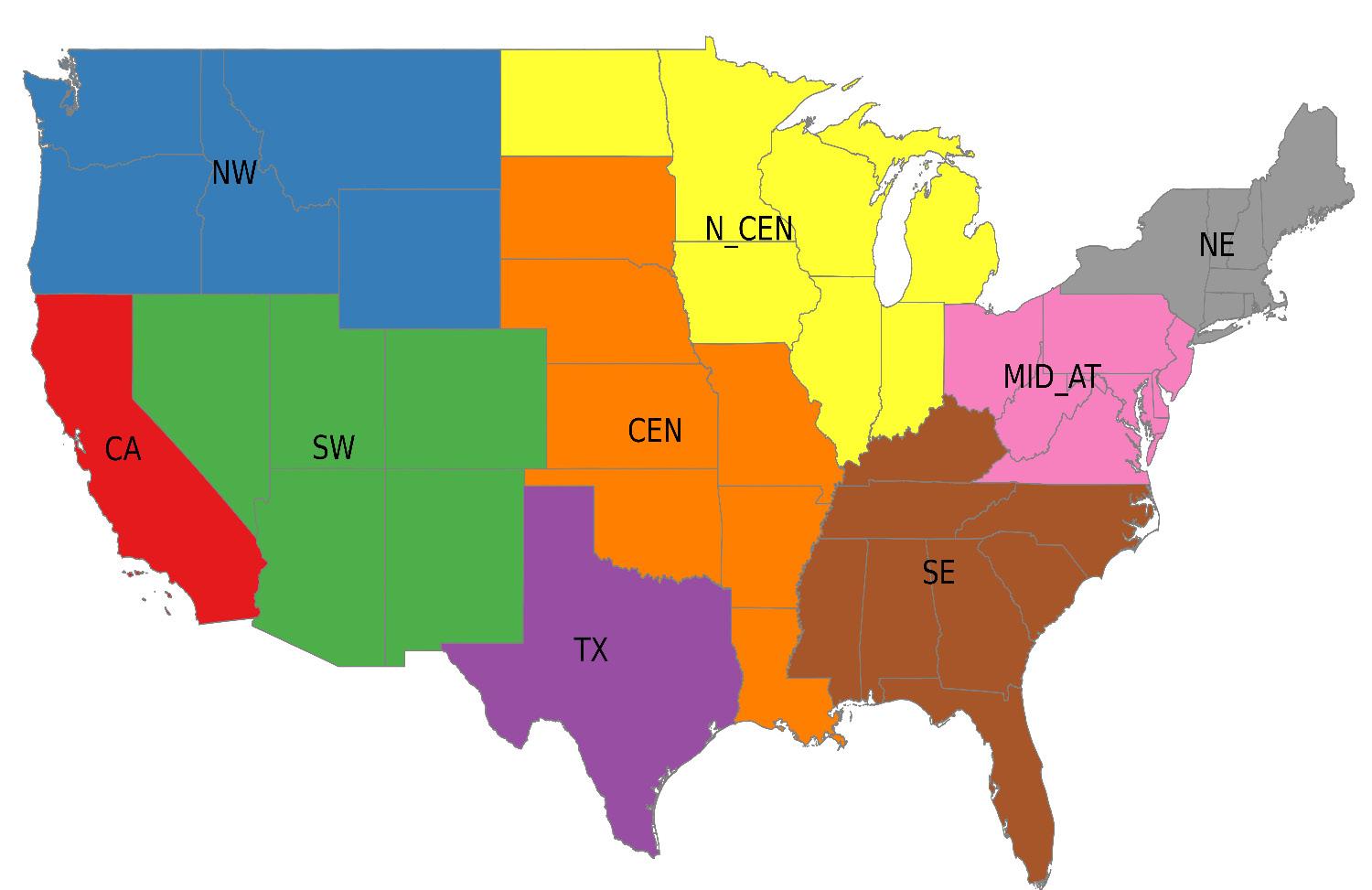
Figure 3: OEO modeled regions include CA (California), NW (Northwestern US), SW (Southwestern US), TX (Texas), N_CEN (Northcentral US), CEN (Central US), SE (Southeastern US), MID_AT (Mid-Atlantic US), NE (Northeastern US).
Temoa is often solved in perfect foresight mode, where all decision variables corresponding to installed capacity and commodity flows are optimized simultaneously across all future periods. To account for the computational complexity encountered with modeling representative days, however, the results in this report are based on a myopic approach where the model solves one time period at a time. Such a myopic approach is more realistic, providing a limited look ahead rather than the “crystal ball” associated with perfect foresight modeling.
Technologies in the Temoa database are represented by engineering-economic parameters, including capital costs, fixed and variable operations and maintenance costs, conversion efficiencies, and emissions coefficients. End-use service demands, such as light- and heavy-duty transport, buildings space heating and cooling, and industrial processes, are specified exogenously. The strength of models such as Temoa resides in their ability to capture these detailed cost and performance characteristics. While high granularity in technology representation can be an asset, unnecessary detail degrades computational performance and makes the model results harder to interpret. Across the sectors modeled in this project, we have applied transparent assumptions informed by expert judgment regarding technology representation and service demands. The descriptions in the documentation notebooks in the GitHub repository present all these assumptions in detail ( Venkatesh et al., 2022). The project Roadmap ( DeCarolis et al., 2022) guided these assumptions.
A Comparison of Different Decarbonization Pathways for the U.S. Energy System
5.1. Four scenarios show pathways to achieve 20%, 40%, 50%, and 100% net reductions in CO 2 emissions by 2050
As previously noted, this report explores four scenarios that represent alternative energy futures for the U.S.: (1) No Policy; (2) COP26; (3) State Action; and (4) Net Zero CO 2 Emissions. Figure 4 shows the resulting CO 2 emissions for each of these scenarios.
The No Policy scenario retains existing energy and emissions regulations (as of 2021) that affect the energy system optimization but do not expand, strengthen, or weaken these policies. Thus, the No Policy scenario serves as a reference case against which to compare the impacts of new CO 2 emissions constraints. As shown in Figure 4, the least-cost energy system under existing policies (as of 2021) results in a 20% decrease in annual CO 2 emissions between 2020 and 2050. The State Action scenario incorporates a linear emissions constraint for CO 2 between 2020 and 2050 for 23 states. Overall, the State Action scenario results in a reduction of 40% in annual CO 2 emissions by 2050, heterogeneously distributed throughout the United States. Due to the California cap and trade program, there are years in which the emissions decrease more than 40% compared to the No Policy scenario, which can be seen in the non-linear differences between the two scenarios in Figure 4.
The COP26 scenario reflects a 50% reduction in CO 2 emissions between 2020 and 2030 using a linear constraint, with no further emissions reductions after 2030. This constraint on emissions between is binding in every time period up to 2030, meaning that the modeled CO 2 emissions are exactly equal to the constraint. The results in this scenario demonstrate the importance of such emissions constraints to achieve reductions beyond the No Policy case. Even though the COP26 and State Action scenarios result in comparable levels of CO 2 emissions in 2050, the cumulative emissions across the entire study period are considerably different, as shown in the second panel in Figure 4. Due to the rapid reductions in emissions in the early years of the COP26 case, the cumulative emissions are 105 Gt CO 2, whereas the cumulative emissions for the State Action case are 130 Gt CO 2. This result underscores the value of early and bold reductions in emissions. The Net Zero scenario assumes a linear CO 2 emissions reduction between 2020 and 2050. This pathway results in a slower decline in emissions through 2035, relative to the COP26 case, but ultimately a deeper reduction in annual and cumulative emissions by 2050.
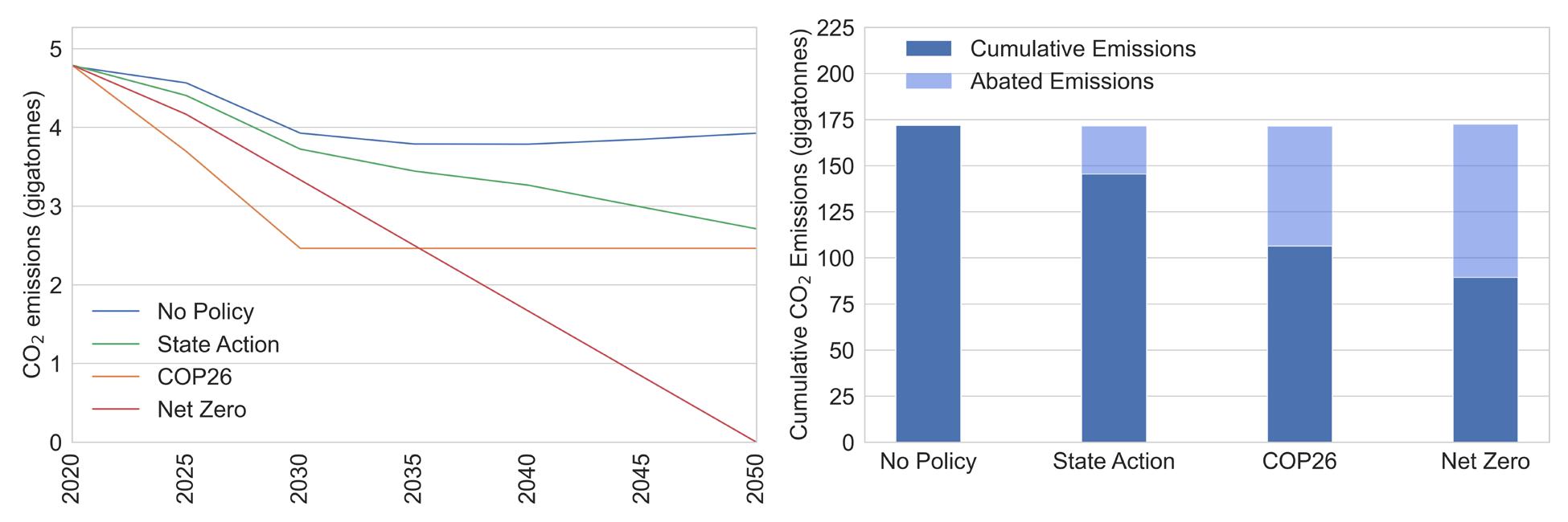
Figure 4: CO2 emissions trajectories for each scenario (left); cumulative CO2 emissions and avoided emissions between 2020 and 2050 (right).
5.2. Policies that constrain carbon result in continued growth in renewables, exceeding 50% of the energy supply in the Net Zero scenario
Figure 5 shows the trends in primary energy use that drive emissions reductions in each scenario.
Across all scenarios, there is a marked decrease in the use of petroleum and increases in the share of primary energy from both wind and solar power. Without further policy interventions, the No Policy case shows only a modest decrease in coal, a substantial decrease in petroleum consumption, considerable growth in renewables, and growth in natural gas use. In fact, by 2050, natural gas provides approximately 45% of primary energy use in the No Policy case.
State-level net-zero CO 2 targets in 23 states result in significant changes in the mix of resources in the U.S. energy system. By 2050, coal and petroleum use decreases by approximately 60% relative to 2020. Like in the No Policy scenario, natural gas use increases in the State Action scenario, reaching 30% of the energy mix in 2050. Overall, fossil fuel demand decreases by 35% in 2050 relative to 2020. The rapid growth of solar and wind power and a slight increase in nuclear energy production enable the reductions in fossil fuel use.
The COP26 scenario requires the most rapid decline in CO 2 emissions, resulting in a 50% reduction between 2020 and 2030. This steep decline occurs through the near elimination of coal use, a 55% reduction in petroleum use, and rapid expansion of biomass, wind, and solar energy. In this scenario, the cap on CO 2 emissions remains constant between 2030 and 2050, resulting in a shifting mix of primary energy sources. Petroleum use continues to decline as larger shares of the vehicle fleet electrify. Natural gas consumption expands, and, in the later years, there is a reduction in nuclear production due to retirements. While the 2050 CO 2 emissions are comparable between the State Action and COP26 cases, the pathways and the resulting energy mix in 2050 look quite different. These differences are due to the timing of the required emissions reductions (e.g., which options are more cost-effective in the year in which action is required) and the regional heterogeneities in emissions reductions in the State Action case.
The Net Zero case requires a significantly greater mitigation effort. Emission reductions occur through the total elimination of coal use and the decline, but not elimination, of natural gas and petroleum use. This scenario also includes a substantial expansion of biomass, solar, and wind energy, as well as an expansion of nuclear power in the later years. Ultimately, the Net Zero scenario relies on CDR to compensate for residual emissions from the remaining fossil fuel consumption.
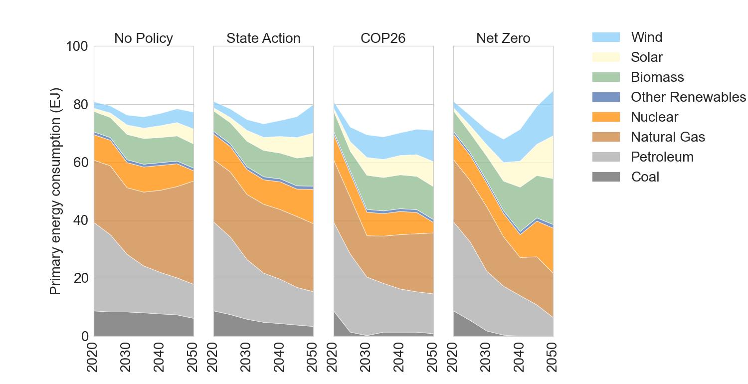
Figure 5: Primary energy consumption across all modeled scenarios.
5.3. Carbon capture and storage (CCS) is likely needed even in scenarios with more modest carbon constraints, while carbon dioxide removal (CDR) is likely needed to reach net-zero CO 2 emissions
Figure 6 shows each scenario’s CO 2 reductions attributable to carbon capture and storage (CCS) and carbon dioxide removal (CDR). In the No Policy case, there is minimal deployment of CCS and direct air capture (DAC) for geologic sequestration. The constraint representing the existing California cap-and-trade program primarily drives the use of these technologies. The COP26 scenario deploys 0.4 Gt CO 2 /year of CDR in 2030 and every year after that. The State Action scenario, which reaches comparable emissions in 2050 to the COP26 scenario but at a lower annual rate of reduction, requires far less CDR than the COP26 case. In 2050, however, there is some deployment of DAC with captured CO 2 used for fuel production (DAC to fuels). This deployment results from regional heterogeneity in emissions reductions, with some regions lacking the sequestration capability and thus producing fuels. In the Net Zero scenario, the latter years require considerable CDR. Relative to 2020 emissions, the net-zero emissions in 2050 are fully achieved by sequestering CO 2 via DAC (~25% of 2020 emissions) and CCS (~12% of 2020 emissions).
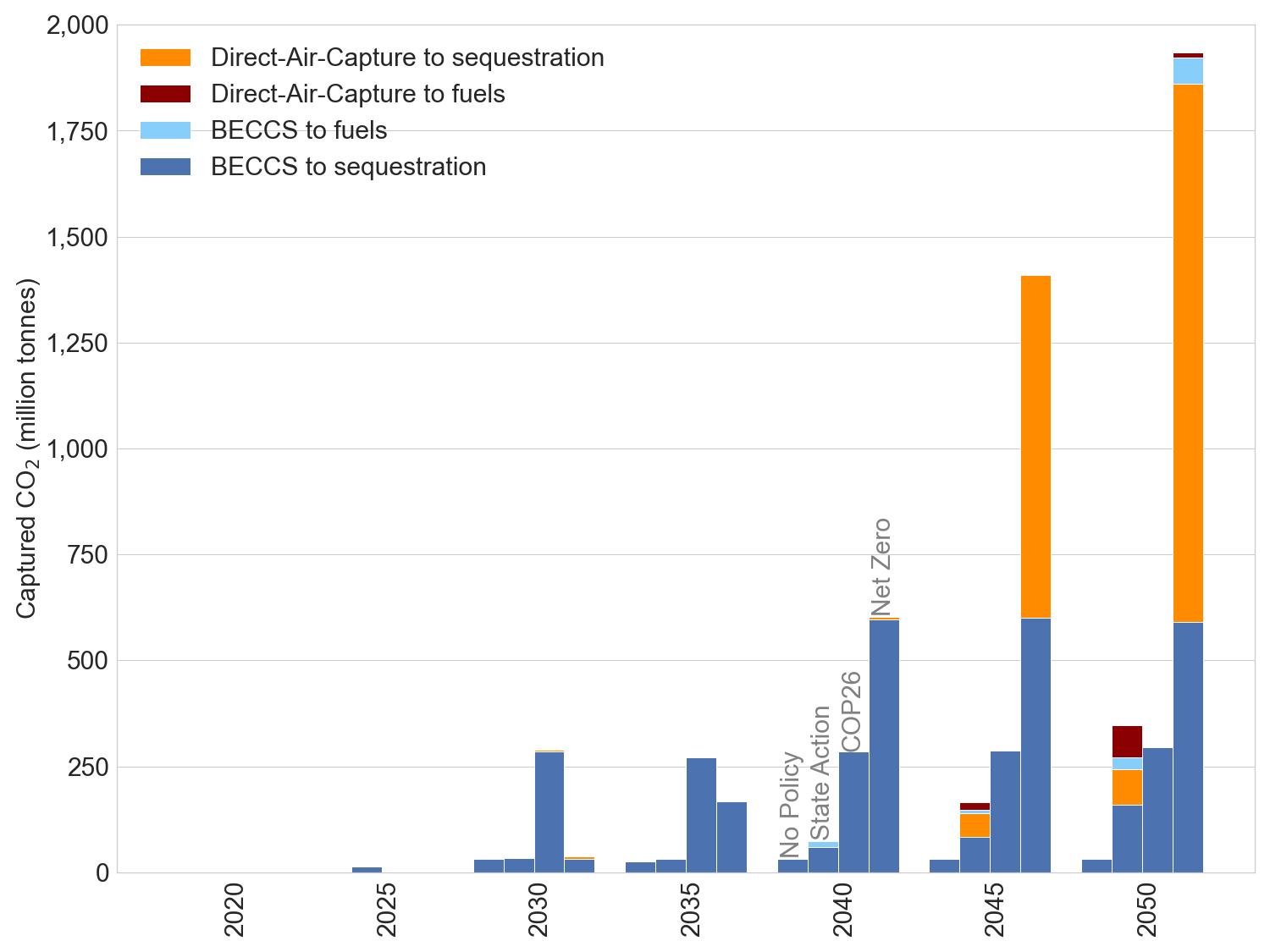
Figure 6: Captured CO 2 via BECCS and DAC use in each modeled scenario.
5.4. To meet net-zero CO 2 emissions in the energy sector by 2050, electrification of end uses will lead to considerable growth in demand for electricity. In turn, electrification will require large, rapid, and sustained investments in the power sector
The results of the simulations show that all decarbonization pathways require the expansion and decarbonization of the power sector. Figure 7 shows the electricity generating capacity by type for each of the four scenarios. In the No Policy case, there is a 30% increase in total nameplate capacity and an expansion of renewables by 2050 relative to 2020. By 2050, there are over 700 GW of solar capacity and nearly 450 GW of wind capacity in this scenario. The additions needed to achieve these capacity levels are comparable to the capacity additions observed in recent years (EIA, 2021b). In both the State Action and COP26 scenarios, renewables have even greater deployment. The Net Zero scenario results in an even more substantial expansion of the power sector to enable the electrification of other sectors, namely transportation and industry. In 2050, solar and wind capacity total 2,300 GW and 1,300 GW, respectively, in the Net Zero scenario. These capacity levels would represent a greater than 20-fold increase in solar capacity and a 10-fold increase in wind capacity (relative to 2020 values). Annual capacity additions would need to be more than three times higher than those in recent years (EIA, 2021b). Operating the grid with this level of variable renewables would also require considerable energy storage capacity (over 900 GW in 2050).
The expansion of generating capacity shown in the left-hand panel in Figure 7 is driven by an increase in generation needed. In the Net Zero scenario, the total generation in 2050 is over 10,000 TWh, more than double the electricity demand in 2020, almost double the generation in the No New Policy scenario in 2050, and ~1.8 times higher than in the COP26 scenario in 2050. The four scenarios also result in different fuel shares. Wind and solar power account for increasing shares of total generation in all scenarios, reaching 60% of electric generation in the No Policy scenario, over 75% in the State Action scenario, and nearly 90% in the State Action and Net Zero scenarios in 2050. Reliance on these renewable resources requires other resources to balance variability. In the No Policy scenario, natural gas provides balancing resources and dispatchable power, accounting for nearly 25% of generation in 2050. In this scenario, coal still contributes a small share of generation. Finally, the percentage of generation from nuclear power decreases in this No Policy scenario due to retirements by 2050.
Battery storage plays an increasingly important role in the State Action, COP26, and Net Zero scenarios starting in the 2030s, providing valuable grid balancing services. Nonetheless, in the State Action and COP26 scenarios, natural gas still accounts for a small share of generation in 2050 (6% and 3%, respectively). In the Net Zero scenario, natural gas generation phases out by 2035. The share of electricity generation from nuclear power is over 15% of total generation in 2050 in the State Action and Net Zero scenarios. While coal generation phases out in the 2030s in the COP26 and Net Zero scenarios, in the State Action scenario, very small shares of coal power remain throughout the analysis period, mainly in regions where no stringent emissions constraints are active. Biomass, hydropower, and geothermal account for small generation shares in the State Action, COP26, and Net Zero scenarios. While the Temoa database used for this analysis includes technologies that use hydrogen for power generation, such technologies are not deployed at a significant scale in any of the scenarios analyzed.
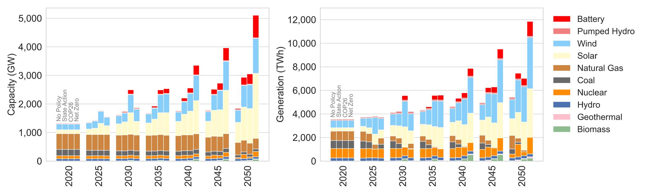
Figure 7: Power generation capacity [GW] (left) and generation [TWh] (right) by fuel type under each modeled scenario.
5.5. The industrial and transportation sectors drive growth in electricity and hydrogen demand
As noted in the previous section, electricity demand grows in all scenarios but more substantially in the State Action, COP26, and Net Zero scenarios. In addition, demand for hydrogen for non-power end uses increases. Figure 8 shows system-wide hydrogen and electricity demand in all scenarios, segmented by end use category. This figure highlights that electrification of industry and transportation are key drivers for the overall increase in electricity demand. The results also show increasing electrification of the residential and commercial sectors, albeit resulting in relatively smaller overall increases in their electricity use. Hydrogen consumption for process energy and fuels substantially increases, reaching over 3,500 PJ in 2050 relative to 2020 in the Net Zero scenario.
The left panel of Figure 9 shows direct energy use for the transportation sector by fuel type. This figure shows that direct energy demand for the transportation sector decreases in all scenarios due to efficiency improvements. Demand for electricity for electric vehicles increases even in the No Policy Scenario. In the Net Zero scenario, electricity demand for transportation would total 1,500 TWh, accounting for around 17% of electricity demand in 2050. In comparison, demand for electricity for transportation would be 850 TWh (and account for 15% of electricity demand) in 2050 in the No New Policy scenario. Interestingly, demand for electricity for transportation in the COP26 and State Action scenarios would be slightly lower than in the No New Policy scenario (less than 800 TWh). As noted in Section 3, to account for the price elasticity of supply associated with lower fossil fuel used in the scenarios with climate policies, oil prices are higher in the No Policy scenario than in the other scenarios. As a result, the difference in the total cost of ownership between electric vehicles (EV) and internal combustion engine vehicles (ICEV) is higher in the No Policy scenario than in the other scenarios. This difference in the marginal cost of EVs (compared to ICEVs) drives the higher deployment of EVs in the No Policy scenario than in the COP26 and State Action scenarios. The stringent carbon constraint drives the even higher deployment of EVs in the Net Zero scenario. Modeling improvements to better incorporate the price elasticity of supply is an ongoing effort that will be included in future OEO reports.
Hydrogen use also increases slightly in the transportation sector in all scenarios. Freight transportation drives the increased demand for hydrogen. The stringent carbon constraint also drives increased use of hydrogen for transportation in the Net Zero scenario. The use of hydrogen for transport is higher in the State Action scenario than the COP26, driven by regional net-zero CO 2 emissions targets - hydrogen fuel cell vehicles (HFCVs) are primarily deployed in those regions.
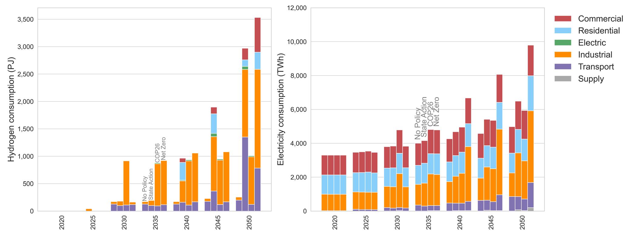
Figure 8: System-wide hydrogen (left) and electricity (right) consumption by sector in each modeled scenario.
The right panel Figure 9 shows direct energy use for the industrial sector by fuel type. Electricity is already widely used in the industrial sector, currently accounting for 13% of industrial energy consumption (EIA, 2022c). In the 2020-2024 time period, Temoa meets nearly 20% of industrial demand with electricity. The difference between the observed consumption in 2020 and the modeled consumption in 2020 is due primarily to the coarse representation of industrial technologies in Temoa’s industrial sector. The first model time period is also a slight look into the future, so the simulation results are not a direct comparison to the 2020 US energy landscape.
In the Net Zero scenario, there is a substantial growth in demand for electricity in the industrial sector throughout the analysis period. In this scenario, the industrial sector accounts for over 60% of total electricity demand in 2050, while electricity accounts for over 50% of direct energy inputs to the sector. Hydrogen use also increases slightly in the industrial sector in the State Action and Net Zero scenarios. In 2050, hydrogen accounts for up to 5% of direct energy inputs to industry in both scenarios. It is worth noting that bioenergy contributes more to industrial energy demand than hydrogen in all scenarios. Several factors drive the relatively low industrial hydrogen consumption. First, the current version of the Temoa database allows electrification of many industrial processes, which the model favors over hydrogen alternatives. Second, electrolytic hydrogen production remains capital intensive throughout the model’s time horizon. Future decreases in electrolysis costs may make electrolytic hydrogen production more favorable. The availability of carbon dioxide removal and biomass technologies also play a role; the model finds both solutions to be cheaper than electrolytic hydrogen production. Based on the simulations biomass could supply 15% of direct energy for industry in the Net Zero scenario by 2050.
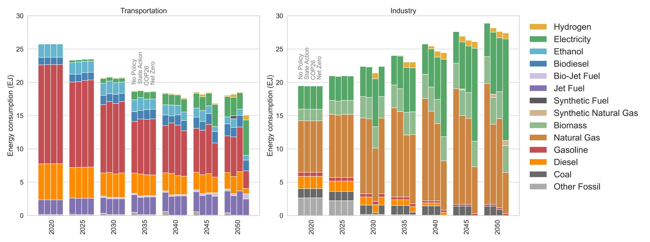
Figure 9: Energy consumption by fuel type in the transportation (left) and the industrial (right) sectors in each modeled scenario.
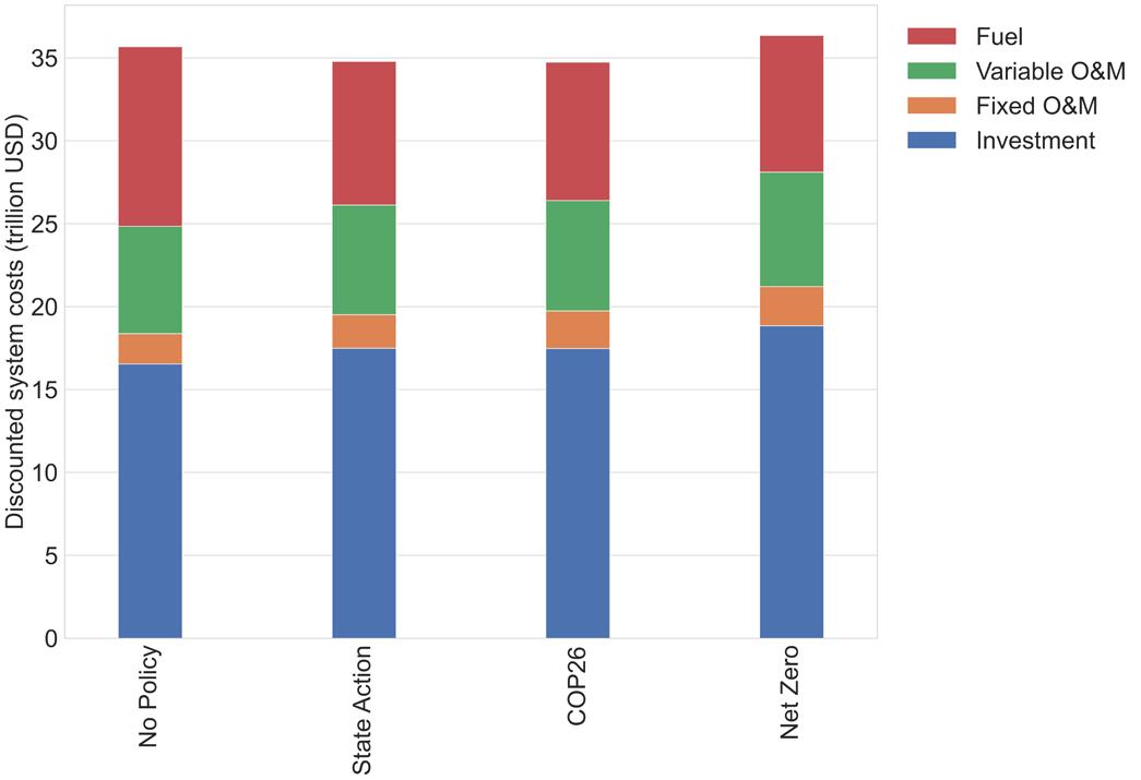
5.6. The total discounted cost of operating the energy system is comparable in the No Policy and Net Zero scenarios. Replacing capital assets that reach the end of life during the modeling period drives investment costs in all scenarios The present value of the costs of operating the energy system are $35.7, $35, $34.9, and $36.5 trillion in the No Policy, State Action, COP26, and Net Zero scenarios, respectively, as shown in Figure 10. Investment costs account for the largest share of discounted costs in all scenarios, while fuel costs account for 30%, 25%, 24%, and 22% in the No Policy, State Action, COP26, and Net Zero scenarios, respectively. Two factors drive higher fuel costs in the No Policy scenario: higher oil prices and higher fossil fuel demand. As noted in Section 3, oil prices in the climate policy scenarios are lower than in the No Policy scenario to account for the price elasticity of supply.
The investment costs in Figure 10 include the costs to replace existing energy assets as they reach their end of life and the costs of new assets needed to meet the growing demand for services and energy carriers. Indeed, Figure 11 shows that replacing assets that reach their end of life (particularly transportation assets) contributes the largest share to investment costs. Figure 11 also shows the effect of discounting on the present value of these investments. While undiscounted costs in later years are higher, their contribution to the present value is relatively small due to the multi-decadal time horizon. For example, the difference in the undiscounted investment costs between the No New Policy and Net Zero scenarios is relatively small in the 2020s, but it is $3 trillion in the 2050-2054 period.
The IPCC recently suggested that the capital needed to support global decarbonization efforts that are consistent with the 1.5-degree target is available but poorly allocated (IPCC, 2022b). The results of this analysis similarly suggest that the capital needed to meet decarbonization targets is likely available. The difference in undiscounted (nominal) investment costs between the No Policy and the Net Zero scenarios ranges between $0.01 trillion in the 2020-2024 period and $3 trillion in the 2050-2054 period. In contrast, the Congressional Budget Office estimated a nominal GDP in 2050 of $70 trillion (CBO, 2022).
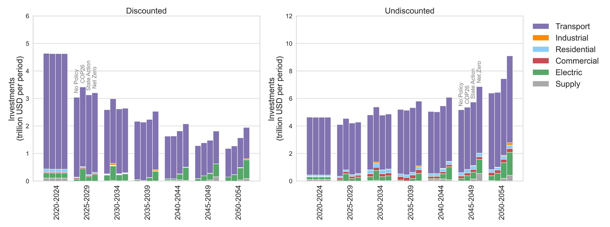
Figure 11: Discounted (left) and undiscounted (right) investment costs by economic sector under each modeled scenario.
Figure 10: Present value of system-wide costs under each modeled scenario.
Net Zero CO 2 Scenario –
A Deep Dive
6.1. In a net zero future, emissions decrease in all sectors. However, carbon dioxide removal is needed to counterbalance residual emissions in some sectors
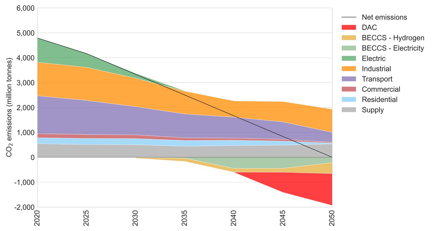
Figure 12 details the breakdown of (positive) CO 2 emissions by sector, offset by CDR from three technologies: BECCS to hydrogen, BECCS to electricity, and DAC. Nearly 2,000 million tons of CO 2 need to be offset to reach net-zero emissions in 2050, representing about 40% of the annual system-wide CO 2 emissions at the start of the time horizon (2020). The electric sector is the first to decarbonize, and the buildings sector produces minimal emissions. The transport sector continues to contribute significantly to emissions until 2050 due to remaining fossil fuel use (primarily jet fuel for aviation). Natural gas use for direct air capture drives emissions in the industrial sector. The supply sector in Figure 12 includes biomass and fossil fuel production emissions.
6.2. A net-zero CO 2 future relies on complementary solar and wind with energy storage, flexible nuclear, and strategic renewable energy curtailment
Figure 13 shows the hourly electricity load profile in 2020, 2035, and 2050 in the Net Zero scenario. Daily peak load increases fivefold between 2020 and 2050 due to end-use electrification in the transportation, buildings, and industrial sectors. To meet growing end-use electrification demand, the model overbuilds capacity to ensure sufficient renewable capacity during low wind and solar availability. As a result, the model curtails 1,400 TWh of wind and solar in 2050, equal to about 35% of total U.S. electricity consumption in 2021 (EIA, 2022d ). Flexible nuclear (25% hourly ramp rate, no turndown constraints) complements variable renewable energy technologies, ramping up and down to a lesser extent than wind and solar. Battery storage also plays a crucial role in balancing hourly load fluctuations. The batteries charge during hours where there is excess generation and some off-peak hours in 2050. The model includes representations of 4- and 8-hour storage duration batteries but primarily deploys only 4-hour batteries.
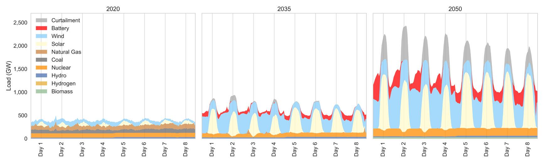
Figure 12: CO 2 emissions by sector, including carbon dioxide removal, in the Net Zero scenario.
Figure 13: Hourly electricity load profile in 2020, 2035, and 2050 in the Net Zero scenario.
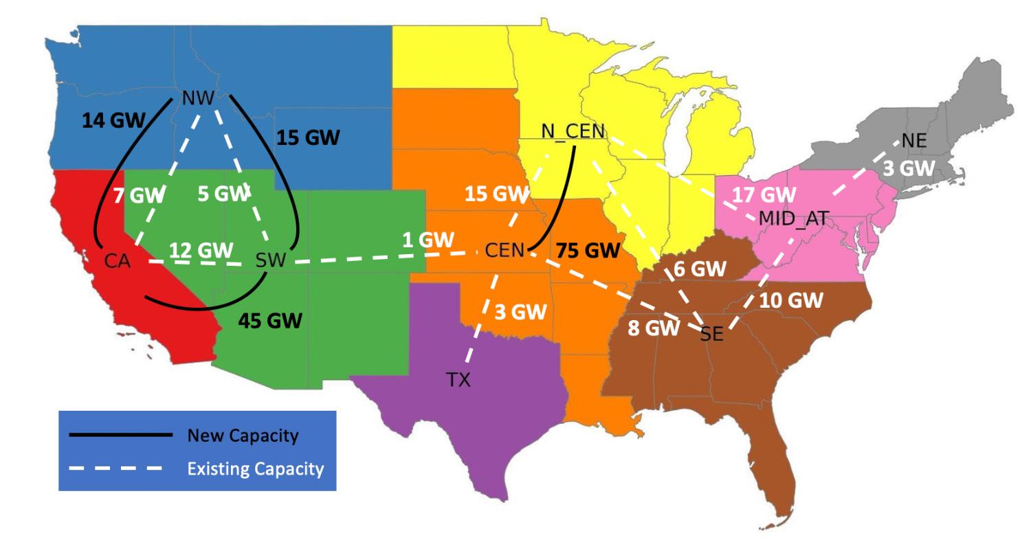
6.3. To support high electrification, the Net Zero scenario requires substantial investments in transmission capacity In order to meet the demands of a net-zero economy, the model constructs more than double the current U.S. inter-regional transmission capacity. Figure 14 shows transmission capacity additions in the net-zero scenario from 2020 to 2050. Inter-regional transmission capacity allows the model to over-build electric capacity in regions with high resource availability (then use such electricity in another region). The current version of Temoa does not explicitly model electricity transmission within a region. Intra-regional transmission is also likely to grow under deep decarbonization scenarios.
The bulk of new inter-regional transmission carries electricity between California and the Southwest and Central and North Central regions. The model constructs 45 GW and 75 GW of new transmission capacity between these regions, respectively. In the Northeast, Mid-Atlantic, Southeast, and Texas, the model doesn’t construct any new inter-regional transmission capacity. Instead, the model generates all electricity to meet regional electricity demand within these regions.
6.4. In the transportation sector, a net-zero CO 2 future capitalizes on efficiency gains in the early periods and widespread electrification in the latter years While CO 2 emissions substantially decrease in the transportation sector, the sector does not necessarily reach zero CO 2 emissions in the Net Zero scenario. While the model deploys electric and hydrogen fuel cell vehicles, fossil fuels (including gasoline, diesel, and jet fuel) also contribute to final energy consumption in every period, as shown in Figure 15.
Throughout the modeling period, energy demand for land-based transportation decreases as a result of efficiency improvement. Furthermore, between 2035 and 2050, much land-based transportation transitions from fossil fuels to electric and hydrogen fuel cell vehicles (HFCVs). By 2050, EVs or HFCVs meet 65% of light-duty vehicle (LDV) miles traveled (vmt), 100% of medium-duty and short-haul heavy-duty vehicle (HDV) vmt, and nearly 75% of long-haul heavy-duty truck vmt. About half of the transit bus fleet electrifies, while B20 (20% biodiesel, 80% diesel) or gasoline fuel most school buses in 2050. Passenger and freight rail continue to consume diesel, but about 75% of demand is met with biodiesel by 2050.
While there are some efficiency gains in shipping, such improvements are insufficient to substantially reduce emissions from this segment. Instead, some reductions in emissions occur as a result of fuel switching: in 2050, liquid hydrogen accounts for roughly a third of the energy supply for shipping. Unfortunately, neither efficiency gains nor fuel switching reduce emissions from aviation. The Temoa database currently includes synthetic fuels as an alternative aviation fuel. However, such fuels prove too expensive throughout the analysis period and fossil-based jet fuel remains the fuel of choice for airplanes. These results suggest that CDR (as characterized in the Temoa database) is more cost-effective than fully eliminating fossil fuels from the transportation sector. While the CDR technologies included in the database are not yet deployed at scale, the techno-economic parameters in the database can serve as performance targets for these technologies.
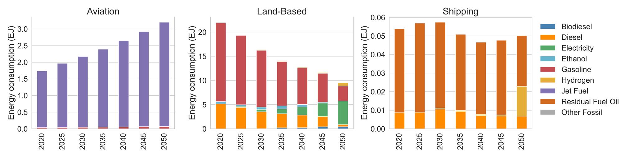
Figure 15: Transportation energy consumption by fuel type in the Net Zero scenario by transportation segment. The left panel shows aviation, the center panel shows land-based transport (including road and rail), and the right panel shows shipping.
Figure 14: Transmission capacity in the Net Zero scenario. All existing transmission capacity values are drawn from PowerGenome.
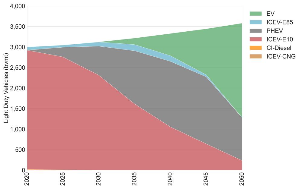
6.5. Plug-in hybrids drive early electrification in the light-duty fleet. Full battery electric vehicles take over as the dominant technology in the Net Zero scenario starting in 2045 In the LDV fleet, vehicle electrification remains modest through 2030 (Figure 16). Gasoline consumption falls, though, as the model deploys more efficient ICEVs and starts to transition to plug-in hybrid electric vehicles (PHEVs). Beginning in 2030, the model quickly transitions away from ICEVs, adopting PHEVs and EVs. PHEV deployment remains high through the end of the model’s time horizon, as these vehicles are more efficient than ICEVs but less expensive than battery EVs. The 2050 LDV fleet is 65% EVs and 30% PHEVs, with the remaining demand met by gasoline ICEVs. The model relies on some E85 in intermediate periods but phases out all E85 vehicles by 2050.
6.6. Distance requirements drive the choice of fuel/technology for heavy-duty vehicles, with shorter distances electrifying and longer distances opting for hydrogen HDVs transition away from fossil fuels much slower than the light-duty fleet. However, unlike LDV, the entire short-haul HDV fleet is zero-emission by 2050, with about three-quarters of demand met by EVs and one quarter by hydrogen vehicles. While battery electric long-haul vehicles are possible options in the model, they are not deployed. Instead, the model chooses hydrogen fuel cell long-haul trucks, which have less of a cost premium compared to EVs due to the large battery capacities required for long-distance freight uses. Long-haul trucks are one of the last sub-sectors to substantially decarbonize; the model uses diesel to meet >90% of demand until 2045, finding that it is less expensive to decarbonize other vehicles or other sectors of the economy. Due to a long-haul truck’s short lifetime (7 years), the model does not deploy decarbonized long-haul trucks until the final period, when it transitions a large fraction of the fleet. Only under net-zero constraints in 2050 does HFCV use increase, offsetting diesel consumption.
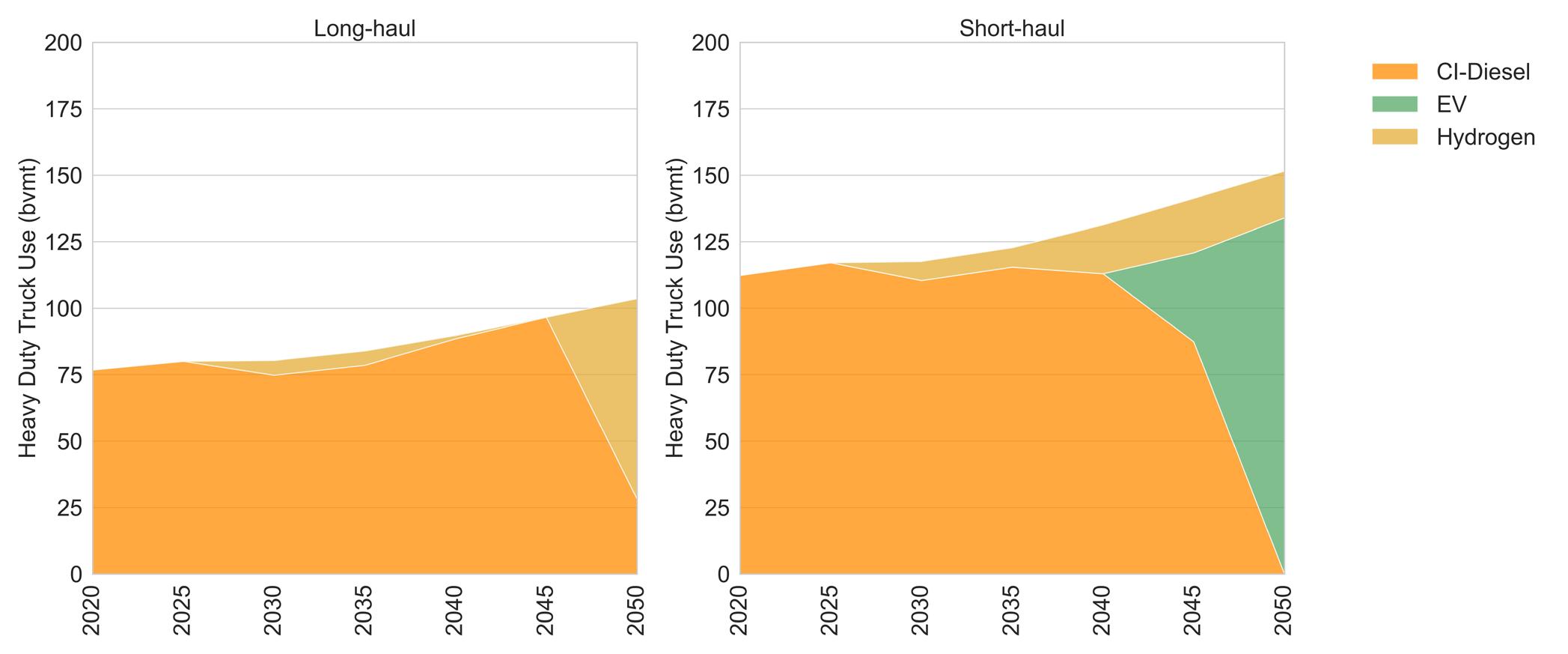
Figure 16: Light-duty vehicle deployment by vehicle type in the Net-Zero scenario.
Figure 17: Heavy-duty vehicle deployment for long-haul (left) and short-haul (right) transportation by vehicle type in the Net Zero scenario.
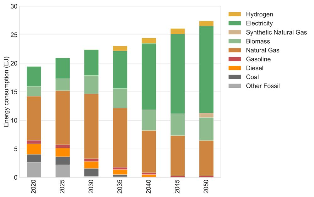
6.7. In the Net Zero scenario, a mix of energy resources (including electricity) is used to meet industrial energy demand
In the Net Zero scenario, the industrial sector consumes a significant amount of energy, including electricity, biomass, natural gas, coal, and other fossil fuels, particularly in the earlier periods. As the sector is constrained to decarbonize to meet the emissions reductions target, increasing amounts of electricity and some synthetic natural gas replace fossil fuels towards the end of the time horizon, as shown in Figure 18.
Electrification is driven by relatively mature technologies such as electric boilers, heating, ventilation and air conditioning (HVAC) systems, and machine drives. Natural gas persists in industries that require process heat at high temperatures and cogeneration of heat and electricity. Biomass grows to meet almost all energy demands in the pulp and paper sector. It is worth noting that the Temoa database doesn’t currently include a representation for some low carbon options (such as ammonia, ethylene, or methanol), which could be used for industrial energy. Also, energy fuels used as feedstock in the industrial sector are currently not considered. Future iterations of this analysis will include improvements in these areas.
6.8. Partial electrification is already possible in the most carbon-intensive industries, but accelerated innovations are needed for further decarbonization of these segments
Figure 19 shows energy use in a few critical domestic industrial sectors - cement and iron & steel. In these carbon-intensive industries, some electrification is possible. However, natural and gas continue to account for a large share of industrial energy through the analysis period. The model starts deploying some synthetic natural gas in these sectors in the last modeling period. Further decarbonization can be expected through accelerated innovations that are not currently modeled here. For example, in the cement industry, electric kilns, increasing renewable energy use (such as biomass), and CCS could reduce emissions further. Similarly, advances in the iron & steel industry may include hydrogen steelmaking, material efficiency improvements, and CCS. Ongoing work aims to represent these technologies in the Temoa database.
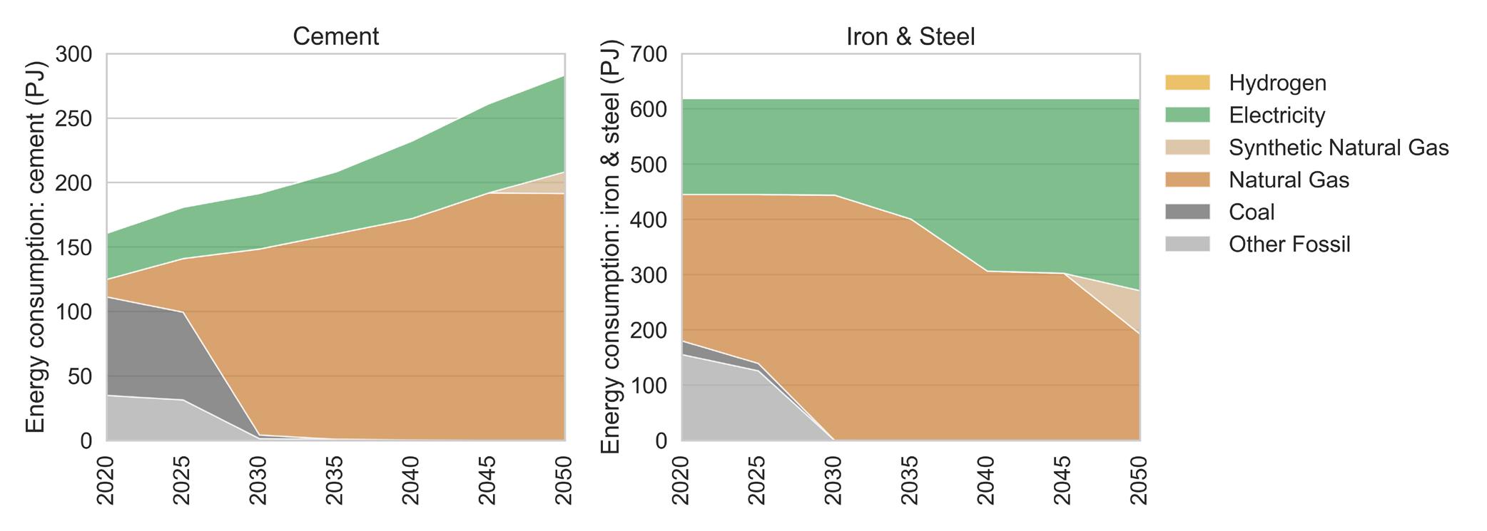
Figure 18: Annual industrial energy consumption by fuel type in the Net Zero scenario.
Figure 19: Energy consumption by fuel type for cement production (left) and iron & steel manufacturing (right) in the Net Zero scenario.
6.8. There is significant adoption of electric heat pumps and water heaters in buildings, but some natural gas use persists
Electrification drives emissions reductions in residential and commercial buildings, as shown in the top row in Figure 20. HVAC accounts for the majority of final energy demand in the buildings sector (as shown in the bottom row in Figure 20). A shift to heat pumps for space heating and electric water heaters accounts for much of the electrification in this sector. Indeed, over 80% of HVAC systems deployed in later years are heat pumps. Some synthetic natural gas use appears in 2050 to meet the net zero emissions target. CDR offsets the remaining fossil natural gas use in 2050, suggesting that it is more cost-effective than full electrification or more synthetic natural gas use in the buildings sector.
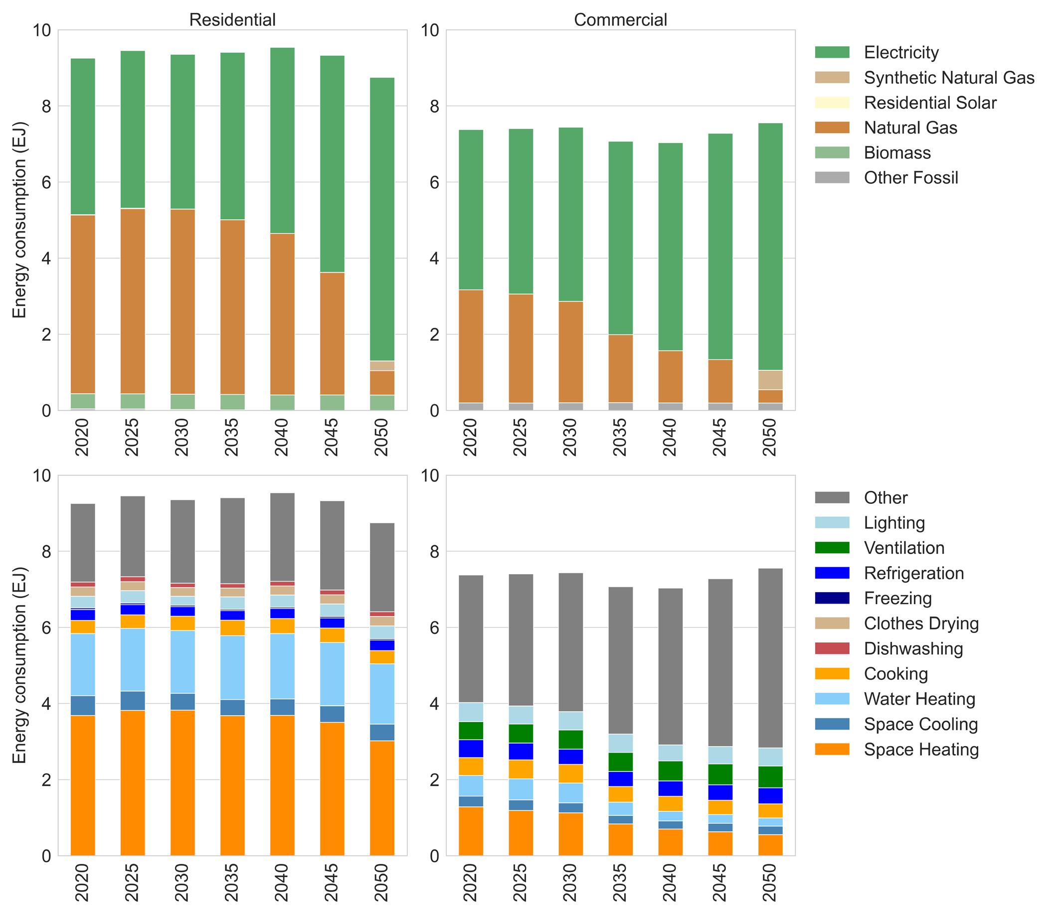
Figure 20: Energy consumption by fuel type (top) and end-use (bottom) in residential and commercial buildings in the Net Zero scenario.
6.10. Bioenergy with carbon capture and sequestration accounts for nearly all hydrogen production in the Net Zero scenario, as this technology has the added benefit of removing CO 2 from the atmosphere.
In the Net Zero scenario, hydrogen use increases throughout the period of analysis, particularly in the transportation and industrial sectors (see Figure 9). Figure 21 shows hydrogen produced by production method. The Temoa database for this analysis includes a representation of biomass, natural gas, and electric technologies for hydrogen production. Until 2045, bioenergy with carbon capture (BECCS) is the source of nearly all the hydrogen in the energy system - nearly 3,500 PJ of hydrogen. Indeed, around half the available biomass in the Net Zero scenario is used to produce hydrogen. The BECCS-to-hydrogen pathway is preferred over other hydrogen production pathways such as electrolysis or natural gas steam methane reforming. BECCS has the added benefit of capturing biogenic carbon, which can be sequestered or used, thus providing CDR. In 2050, the model deploys some electrolytic hydrogen as the model approaches the limits in biomass resource availability.
6.11. Consistent with recent IPCC reports, carbon dioxide removal with geologic storage is likely needed to achieve net-zero CO 2
Figure 12 showed the need for CDR to meet net-zero targets by 2050. While the Temoa database used for this analysis includes technologies that use captured CO 2 for synthetic fuel production, most of the captured CO 2 in the model is sequestered underground through geologic storage, as shown in Figure 22. In 2050, more than 90% of the captured CO 2 is sequestered, primarily in the Texas (TX) and central U.S. (CEN) regions. The remaining 10% of captured CO 2 in 2050 is used to produce synthetic fuels, primarily synthetic natural gas. These results suggest that the added cost of converting CO 2 to useful products is higher than using some fossil fuels, CDR, and geologic storage.
6.12. Shadow prices range from less than $100/tonne CO 2 in the early years to above $600/tonne CO 2
Figure 23 presents the shadow prices on the national CO 2 emissions constraint derived from the model solution. This shadow price represents the abatement cost of the most expensive carbon abatement technology deployed in a given period. Thus, shadow prices represent the additional cost of CO 2 removed from the energy system at each time step. As the CO 2 constraints tighten, the cost of removing each additional ton of CO 2 increases. Lower-cost technologies, particularly in the power sector, set this marginal abatement cost at $60/ tonne (present value) in 2025. By 2050, the marginal abatement cost increases tenfold, reaching roughly $600/tonne (present value). DAC, an expensive technology, sets this high marginal abatement cost in 2050. Technology and performance improvements that reduce the cost of the currently costly technologies would decrease this marginal abatement cost.
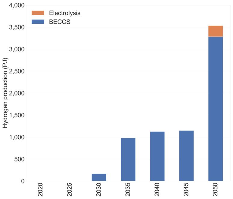
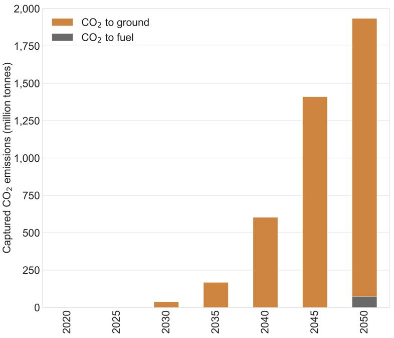
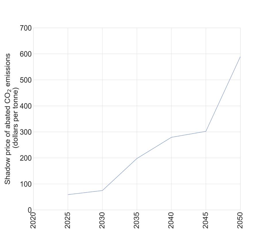
Figure 21: Hydrogen production by production method in the Net Zero scenario.
Figure 22: Captured CO2 emissions by end use in the Net Zero scenario. CO2 to ground is sequestered, while CO2 to fuel creates synthetic fuels.
Figure 23: Shadow price of abated CO2 in the Net Zero scenario.
Modeling to Generate Alternatives – An Approach for Structural Uncertainty Analysis
For energy systems modeling to inform decision-making, it must account for the role of future uncertainty. In energy modeling, there are generally two types of uncertainty to consider: parametric and structural. Parametric uncertainty refers to uncertainty in the input values assigned within the model. Structural uncertainty refers to the uncertainty in the model formulation itself. Since energy system models are highly simplified versions of reality, the structural uncertainty in modeling efforts can be significant. In addition, real-world transitions can deviate from the cost-optimal solution dictated by a single deterministic run ( Trutnevyte, 2016). If these uncertainties are unaccounted for, model results can mislead decision makers into a false sense of certainty about the suggested energy system transformation. Thus, rather than performing conventional scenario analysis with a limited num
ber of scenarios to account for uncertainty in inputs, we assess structural uncertainty in this report. Future work will focus on assessing parametric uncertainties.
Here, a method called Modeling to Generate Alternatives (MGA) is applied to the modeling framework to systematically examine technology tradeoffs in the Net Zero scenario. Berntsen & Trutnevyte, (2017) describe this approach in more detail. Briefly, a new objective function that minimizes the sum of non-zero decision variables from the initial solution is formulated. A random coefficient weights each decision variable (activity variable) in the [-1, 1] range. A slack of 1% on the total system cost is afforded to the model and introduced as a new constraint in the MGA iterations. Due to computational limits, the MGA relies on an adapted database that has fewer representative days than the database used for the deterministic analysis. Furthermore, the MGA results in this section relies on 200 simulations. Through some preliminary testing, we confirmed that the range of solutions are consistent in 200 and 400 simulations. Finally, we tested that the deterministic solution of the Net Zero scenario using the full database generally fits within the range of the solutions found in the MGA analysis with the adapted database.
The figures in this section show results from the 200 MGA iterations as a light blue band and the deterministic results from the Net Zero scenario as a dark blue curve. The figures also include the deterministic solution from the No Policy, represented by the orange curve. The histogram in the right panel of the figures represents the distribution of results from the MGA iterations in 2050 and coincides with the range defined by the light blue band in 2050.
7.1. The results of the Modeling to Generate Alternatives analysis show an extensive range of potential future capacities for solar and nuclear power
Figure 24 shows the range of solar capacity installed in the electric sector in the MGA simulations. Even in the MGA simulations that yield relatively lower solar power capacities, solar power forms an integral part of the power system accounting for at least 2,000 GW of capacity by 2050. These simulations also rely on firm sources like natural gas or nuclear capacity to maintain grid reliability. At the high end of the range of MGA simulations, installed solar capacities reach 4,000 GW. These simulations did not invest in new traditional firm resources but instead overbuilt solar capacity to account for solar’s lower relative capacity factors. A Shapiro-Wilk test indicates that the distribution of solar capacities in 2050 is approximately normal. The solar capacity from the deterministic simulation presented earlier in this report is in the top 5 percentile of capacities installed from the MGA simulations until 2040. However, in 2050, the deterministic results lie within one standard deviation of the mean capacities from the MGA runs (~2,300 GW).
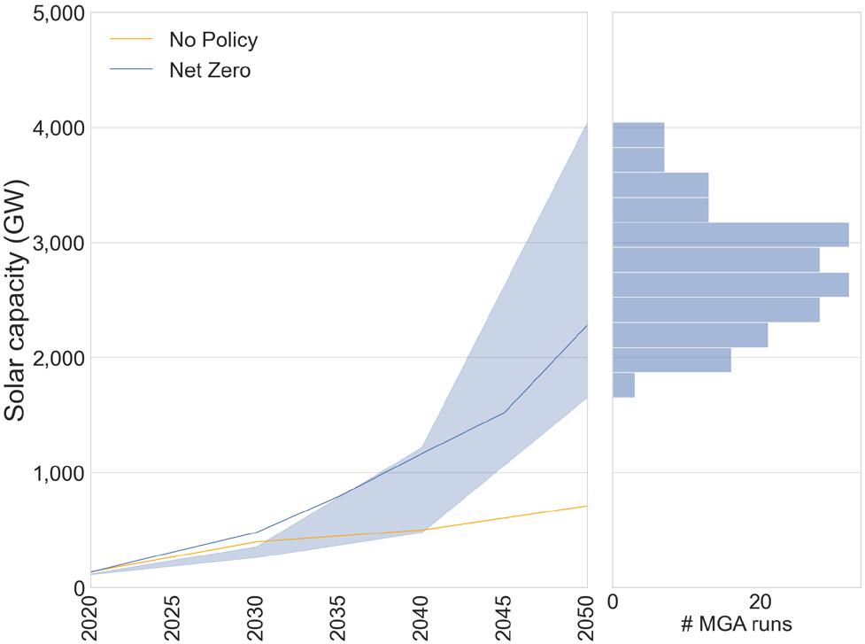
24: Modeling to generate alternatives results for solar capacity in the Net Zero scenario. The left subplot shows the range of capacities deployed. The subplot on the right displays the distribution of the MGA simulation results for 2050.
Figure
Figure 25 shows that a large range of nuclear capacities (80-550 GW) can be installed in the electric sector to meet net-zero constraints. However, the distribution of MGA solutions skews to lower nuclear capacity installations (<200 GW for 65% of simulations). These lower nuclear capacity solutions are frequently coupled with higher solar and wind capacities.
7.2. Modeling to Generate Alternative shows a large range of fossil fuel use, but most simulations suggest a substantial reduction in fossil fuel consumption
Figure 26 shows primary fossil fuel use for the MGA simulations. In the MGA simulations, coal use in 2050 in the Net Zero scenario ranges between 0 and 11 EJ. However, in almost 90% of the MGA runs, coal use is entirely absent by 2050. The histogram of MGA solutions for natural gas is unimodal at ~20 EJ by 2050, coinciding approximately with the deterministic run (~19 EJ by 2050). The remaining solutions are distributed between 1 – 65 EJ of natural gas. Petroleum use spans a range of 0.5 - 5 EJ by 2050, where about 25% of solutions resulted in less than 1 EJ of use. The remaining solutions are normally distributed with the mean approximately coinciding with the Net Zero deterministic estimate (3.7 EJ).
Almost 12% of MGA solutions resulted in higher aggregate fossil fuel use compared to the No Policy case, driven by increased natural gas use in some MGA simulations. These solutions were accompanied by lower nuclear primary energy (<15 EJ by 2050) relative to MGA solutions with lower fossil fuel use. In simulations with high fossil fuel usage, electricity use in the transportation sector ranges between 400 and 800 TWh by 2050, the latter being approximately the total electricity demand in the deterministic simulation for the No Policy scenario. Residential sector electricity use is higher in the MGA simulations than in the deterministic simulation for the No Policy scenario, but lower than the deterministic simulation for the Net Zero scenario. Emissions targets in the MGA simulations are met by extensive deployment of DAC, ranging between 1,600 – 3,600 million tonnes of CO 2 captured. Hydrogen use is also substantial in the MGA simulations spanning 20 - 40 EJ. The lower bounds of both DAC and hydrogen use from the MGA simulations are higher than the estimates from the deterministic simulation for the Net Zero scenario.
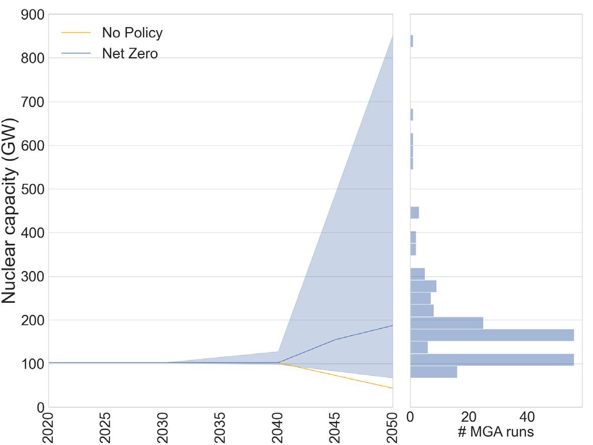
Figure 25: Modeling to generate alternatives results for nuclear capacity in the Net Zero scenario. The left subplot shows the range of capacities deployed. The subplot on the right displays the distribution of the MGA simulation results for 2050.
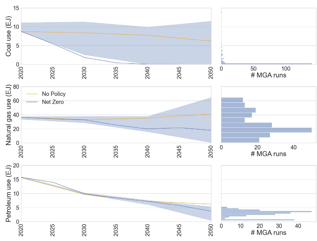
Figure 26: Modeling to generate alternatives results for coal, natural gas, and petroleum use in the Net Zero scenario. The left subplot shows the range of capacities deployed. The subplot on the right displays the distribution of the MGA simulation results for 2050.
Increase in natural gas use, primarily in the industrial sector, is responsible for the uptick in total fossil fuel observed in 2045. Increased use is observed in both the MGA (Figure 26) and the deterministic simulation for the Net Zero scenario (Figure 5). In the deterministic run, the DAC-to-sequestration pathway becomes cost competitive under the emissions constraints, which allows for increased natural gas use. In the MGA simulations synthetic fuel production from DAC is also adopted to a certain extent. Generally, the model finds natural gas combined with DAC to be a cheaper alternative to other decarbonization options.
7.3. Modeling to Generate Alternatives shows a range of solutions with high deployments of electric vehicles, hydrogen, and direct air capture
The top panel in Figure 27 shows the range of hydrogen deployment across the MGA simulations. Hydrogen is part of the energy mix in all the MGA simulations, with a minimum of 5 EJ in use by 2050. Almost 40% of the solutions favor 10 EJ or less hydrogen deployment; however, the remaining solutions are somewhat evenly distributed across a range (10 – 40 EJ). The MGA simulations also include a wide range of DAC deployment, as shown in the center panel of Figure 27. Like hydrogen, MGA simulations for the Net Zero scenario always include DAC deployment. In 2050, mitigation through DAC spans a large range (270 – 3,900 million tonnes of captured CO 2). The results of the deterministic simulation for the Net Zero scenario is approximately the mean of DAC use from the MG A runs. Solutions with lower amounts of DAC use are associated with increased electrification in all other sectors. In the residential and commercial sectors, the increase in electrification is relatively lower compared to increases in the transportation and industrial sectors. The increases in electricity use in these sectors are due to the higher penetration of EVs and increased electrification in industries like food processing and chemical manufacturing. DAC in the MGA simulations is used for a mix of both CO 2 sequestration as well as synthetic fuel production. Finally, the bottom panel in Figure 27 shows the range of electrification in the transportation sector across MGA simulations. Electrification in this sector is a key component to meeting net-zero goals across all 200 simulations, indicated by a lower bound electricity use of 750 TWh.
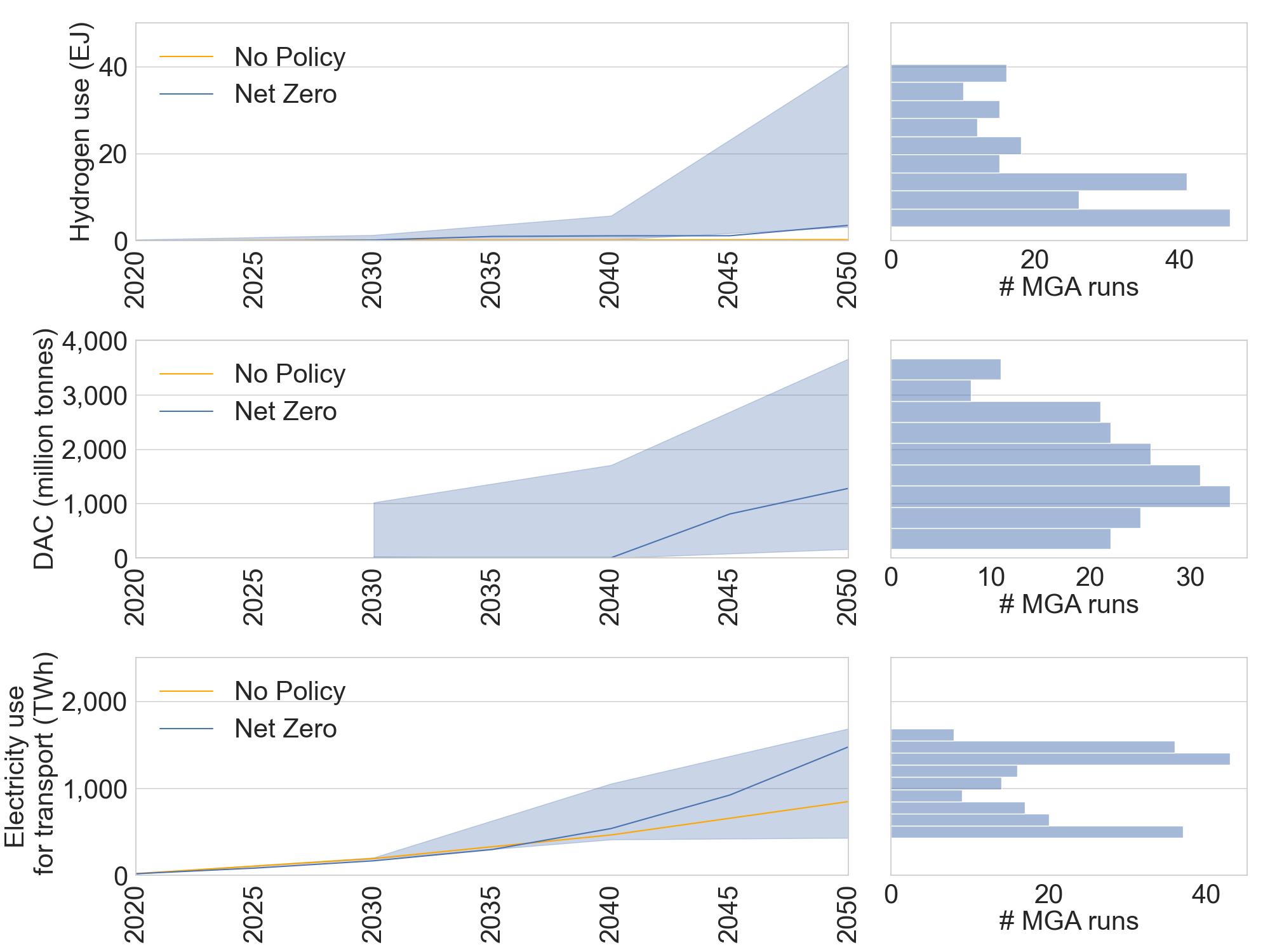
Figure 27: Modeling to generate alternatives results for hydrogen production, direct air capture deployment, and electricity use in the transportation sector of the net-zero scenario. The left subplot shows the range of hydrogen use across all MGA iterations. The subplot on the right displays the distribution of the MGA simulation results for 2050.
7.4. Modeling to Generate Alternatives allows an analysis of the tradeoffs and complementarities between technology deployments for decarbonization
One of the benefits of using MGA is the ability to evaluate how the deployment of technologies correlates, which in turn helps identify tradeoffs and synergies in technologies. Figure 28 shows a correlation plot to explore tradeoffs between critical technology deployments in 2050 in the MGA simulations for the Net Zero scenario. The correlations highlight technology pairs where the range of solutions from the higher (lower) end of one technology are consistently associated with higher (lower) deployment of the paired technology across the MGA simulations (blue squares). In cases where the higher (lower) end of a technology is consistently associated with the lower (higher) deployment of a paired technology, an anti-correlation is identified (red squares). Note that the correlations in this figure do not provide information about the magnitude of technology deployments. Positively correlated technologies could still have relatively low deployment rates.
Predictably, the results show that solar and wind generation are positively correlated. However, solar generation and deployment of battery capacity are more positively correlated than wind generation and batteries. These correlations suggest that batteries are the primary source of reliability support for solar power. While batteries also support wind integration, in MGA simulations with higher wind deployments, nuclear power provides some of the reliability support needed. Wind and nuclear are also positively correlated with EVs. By contrast, solar and batteries are practically uncorrelated with EVs. In the representative days used to capture the operations of the power system, EV charging is assumed to primarily occur during the night, when solar power is not available, wind speeds are typically higher, and some nuclear baseload is “free” from the need to meet peak loads. This assumption about EV charging behavior drives the correlations between these technologies. These results do not imply that solar and batteries wouldn’t be deployed in scenarios with high EV deployment. Indeed, such technologies are deployed in all of the MGA simulations. Instead, the results suggest that the relative contribution of wind and nuclear to power generation is slightly higher in scenarios with higher rates of vehicle electrification.
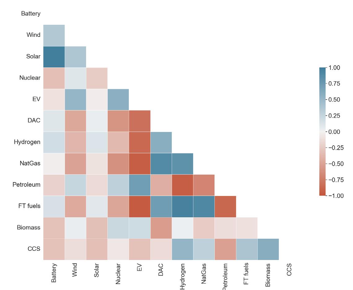
Complex interactions drive the correlations for transportation fuels shown in Figure 28. First, there is a positive correlation between DAC and hydrogen. These two technologies are negatively correlated with EV, suggesting that there is competition between vehicle electrification and DAC/Hydrogen pathways. Furthermore, the correlation between EV and petroleum is slightly positive. DAC and hydrogen enable synthetic fuel production through the Fischer-Tropsch process. These synthetic fuels can be used instead of vehicle electrification while also replacing petroleum-based fuels. In MGA simulations with extensive EV adoption, deployment rates for DAC and hydrogen technologies are relatively lower, and so is the supply of synthetic fuels. As a result, in simulations with relatively high EV adoption, petroleum fuels continue to provide energy for end-uses that cannot be electrified. As a reminder, these correlations do not provide information about the magnitude of the deployment of the technologies. So, while there is a positive correlation between EV deployment and petroleum use, demand for petroleum is substantially lower in 2050 (relative to 2020) across all MGA simulations (as shown in Figure 26).
As previously noted, hydrogen production is positively correlated with natural gas, DAC, and CCS. Hydrogen production is uncorrelated or negatively correlated with fuels used for electricity generation (wind, solar, nuclear, and batteries). These results highlight that electrolysis for hydrogen production is expensive relative to other production pathways in the model. The correlations between natural gas and hydrogen suggest a difference in the MGA simulations and the deterministic simulation for the Net Zero scenario. BECCS is the primary source of hydrogen production in the deterministic simulation of the Net Zero scenario. However, Figure 28 shows that hydrogen and biomass are largely uncorrelated across MGA simulations. By contrast, hydrogen and natural gas are positively correlated. These correlations reflect that in almost 50% of all MGA simulations, steam methane reforming of natural gas with and without CCS is used to produce at least 1,000 PJ of hydrogen by 2050. Using natural gas to produce hydrogen is only possible in the Net Zero scenario because CCS and DAC are available. As previously noted, DAC (and to a lesser extent, CCS) have not been deployed at scale. The costs and performance parameters for these technologies represented in the Temoa database could serve as a reference point for performance targets. Furthermore, future work to evaluate parametric uncertainty would improve understanding about the robustness of these results.
Figure 28: Correlation plot for Modeling to Generate Alternatives results in the Net Zero scenario.
The Inflation Reduction Act of 2022 – How does it relate to the findings of this report?
The U.S. Congress passed the Inflation Reduction Act (IRA) in August 2022 (H.R.5376: Inflation Reduction Act of 2022, 2022). This bill is the first ever to establish firm commitments to decarbonizing the U.S. energy system. While the analysis presented in this report does not include a parametrization of the policy instruments included in the IRA, the results presented in this report highlight a broad set of technologies that could be deployed to meet net zero CO 2 emissions from the U.S. energy sector by 2050. Table 1 describes the support these crucial technologies received in the IRA. To the right of each provision in Table 1, we present the range of capacities deployed in the MGA simulations under the Net Zero scenario, highlighting the strong agreement between the technologies targeted by the IRA and the technologies deployed in the modeled results.
Table 1: Provision in the Investment Reduction Act to support technologies needed in the Net Zero scenario
Technologies needed in the Net Zero scenario
Wind and solar power
Stationary battery storage
Nuclear power
Vehicle electrification
Provisions in the IRA in support of decarbonization technologies
• New advanced manufacturing production tax credit to support the domestic production of components used in solar systems and wind turbines.
• Extends the renewable electricity investment and production tax credits until 2024
• Establishes clean electricity investment and production tax credits to start in 2025
• Lifts the offshore wind moratorium and allows leasing in the U.S. territories
• New energy credit for solar and wind in low-income communities
• New advanced manufacturing production tax credit to support the domestic production of battery components, including the critical minerals needed in the batteries
• Enhanced use of the Defense Production Act of 1950 for critical mineral processing
• New nuclear power production tax credit
• New funding to increase the availability of High-Assay Low-Enriched Uranium
• Modifies the existing consumer credit for the purchase of electric vehicles
• New consumer tax credit for the purchase of used electric vehicles
• New commercial clean vehicle credit for the purchase of commercial electric vehicles
• New domestic manufacturing conversion grants to retool car manufacturing facilities for the production of electric vehicles
Range from OEO MGA solutions (in 2050)
Wind capacity: 1,200 - 1,465 GW
Solar capacity: 1,650 - 4,045 GW
Battery storage capacity: 430 - 1,480 GW
Nuclear capacity: 67 GW - 852 GW
Transportation electricity use: 430 - 1,685 TWh
Technologies needed in the Net Zero scenario
Provisions in the IRA in support of decarbonization technologies
• New clean hydrogen production tax credit that supports hydrogen produced with less than 4 kg CO 2 e/kg
Hydrogen (and derivatives)
Bio-based energy
Industrial decarbonization
• New advanced energy project credit support low-carbon industrial heat, which could be produced with hydrogen
• New commercial clean vehicle credit for the purchase of clean vehicles, which presumably includes hydrogen and derivatives
• New domestic manufacturing conversion grants to retool car manufacturing facilities for the production of hydrogen fuel cell vehicles
• New clean electricity production credit that supports BECCS
• New clean energy fuel production credit that supports fuels produced with a maximum emissions rate of ~50 kg CO 2 e/MJ
• New sustainable aviation fuel credit for which some biofuels would be eligible
• New commercial clean vehicle credit for the purchase of clean vehicles, which presumably includes some biofuels
• New funding to support advanced biofuel industries (excluding corn-based ethanol) and investments in infrastructure for blending, storing, supplying, or distributing biofuels
• New advanced industrial facilities deployment program to invest in projects that reduce emissions from energy-intensive industries (in addition to direct support for hydrogen, bioenergy, and CCS)
• Extends credit for energy efficiency home improvements
Range from OEO MGA solutions (in 2050)
Hydrogen use: 3- 40 EJ
Building electrification and efficiency improvements
Carbon capture and sequestration
• New home energy performance-based whole house rebates to support while-house energy-saving retrofits
• New high-efficiency electric home rebate program that funds building electrification, including heat pumps, heat pump water heaters, and electric stoves
• Enhanced use of Defense Production Act of 1950 for heat pumps
• Establishes clean electricity production tax credit that expands eligibility to include power generation with CCS
• New advanced energy project credit for which CCS is eligible
• Enhances the carbon capture and sequestration tax credit for carbon capture
Primary energy use from biomass: 6 - 17 EJ
Direct Air Capture
• Enhances the carbon capture and sequestration tax credit for direct air capture
N/A
N/A
CCS range: 0 - 1,790 million tonnes of capture CO 2 emissions
DAC: 163 - 3,660 million tonnes of CO 2 captured
The budget for the climate and energy provisions in the IRA totals ~$385 billion to be spent between 2022 and 2031. The additional investment and fixed costs of operating the energy system up to 2030 in the deterministic simulation of the Net Zero scenario relative to the No Policy scenario included in this report total ~$390 billion. Note that this total excludes fuel costs, as the IRA primarily appropriates funds to reduce technology costs to consumers and producers through rebates and tax credits. This comparison between the allocated budget for the IRA and the costs from the simulations presented here supports the argument that the bill serves as a “down payment” for decarbonizing the U.S. energy system. More importantly, the IRA provides support for a broad set of technologies. The MGA simulations suggest that there isn’t just one technology pathway that meets the net-zero target by 2050. Instead, different combinations of technologies could be deployed to meet this decarbonization goal. By investing in a multitude of possible technologies, the IRA ensures that one or more of the possible pathways will be possible.
References
H.R.5376: Inflation Reduction Act of 2022, (2022) (testimony of 117th Congress). https://www.congress.gov/ bill/117th-congress/house-bill/5376
Berntsen, P. B., & Trutnevyte, E. (2017). Ensuring diversity of national energy scenarios: Bottom-up energy system model with Modeling to Generate Alternatives. Energy, 126, 886–898. https://doi.org /10.1016/J.ENERGY.2017.03.043
CBO. (2022). Long Term Economic Projections for the U.S. https://www.cbo.gov/data/budget-economic-data#12
DeCarolis, J. F., Hunter, K., & Sreepathi, S. (2012). The Case for Repeatable Analysis with Energy Economy Optimization Models. https://doi.org/10.1016/j.eneco.2012.07.004
DeCarolis, J. F., Jaramillo, P., Johnson, J. X., McCollum, D. L., Trutnevyte, E., Daniels, D. C., Akın-Olçum, G., Bergerson, J., Cho, S., Choi, J. H., Craig, M. T., de Queiroz, A. R., Eshraghi, H., Galik, C. S., Gutowski, T. G., Haapala, K. R., Hodge, B. M., Hoque, S.,Jenkins, J. D., … Zhou, Y. (2020). Leveraging Open-Source Tools for Collaborative Macro-energy System Modeling Efforts. Joule, 4(12), 2523–2526. https://doi.org/10.1016/j.joule.2020.11.002
DeCarolis, J., Jaramillo, P., Eshraghi, H., Trutnevyte, E., de Queiroz, A. R., Patankar, N., Nock, D., Yeh, S., Johansson, D., McCollum, D., Lin, Z., Jenn, A., Hoque, S., Choi, J.-H., Zhou, Y., Cho, S., Bergerson, J., Siddiqui, S., MacLean, H., … Smith, A. (2022). Roadmap: Open Energy Outlook for the United States. https://github.com/TemoaProject/oeo/blob/3d22fb79e7216fc98b4eb85b3ea764f e2acd41d8/OEO_Roadmap.md (Original work published 2020)
EIA. (2021a). What is the United States’ share of world energy consumption. Frequently Asked Question (FAQ). https://www.eia.gov/tools/faqs/ EIA. (2021b). Renewables account for most new U.S. electricity generating capacity in 2021. https://www.eia. gov/todayinenergy/detail.php?id=46416
EIA. (2022a). U.S. energy facts explained. https://www.eia.gov/energyexplained/us-energy-facts/ EIA. (2022b). Annual Energy Outlook 2022. https://www.eia.gov/outlooks/aeo/ EIA. (2022c). Use of energy explained: energy use in industry. https://www.eia.gov/energyexplained/ use-of-energy/industry.php
EIA. (2022d). Monthly Energy Review. https://www.eia.gov/totalenergy/data/monthly/ Friedrich, J., Ge, M., & Pickens, A. (2020). This Interactive Chart Shows Changes in the World’s Top 10 Emitters. https://www.wri.org/insights/interactive-chart-shows-changes-worlds-top-10-emitters Hunter, K., Sreepathi, S., & Decarolis, J. F. (2013). Modeling for Insight Using Tools for Energy Model Optimization and Analysis (Temoa). Energy Economics, 40, 339–349. https://temoacloud.com/ wp-content/uploads/2019/12/Hunter_etal_2013.pdf
IPCC. (2021). Climate Change 2021: The Physical Science Basis. Contribution of Working Group I to the Sixth Assessment Report of the Intergovernmental Panel on Climate Change (V., Masson-Delmotte, P. Zhai, A. Pirani, S.L. Connors, C. Péan, S. Berger, N. Caud, Y. Chen, L. Goldfarb, M.I. Gomis, M. Huang, K. Leitzell, E. Lonnoy, J.B.R. Matthews, T.K. Maycock, T. Waterfield, O. Yelekçi, & B. Z. R. Yu, Eds.). Cambridge University Press. https://doi.org/doi:10.1017/9781009157896
IPCC. (2022a). Climate Change 2022: Impacts, Adaptation, and Vulnerability. Contribution of Working Group II to the Sixth Assessment Report of the Intergovernmental Panel on Climate Change (H.-O. Pörtner, D.C. Roberts, M. Tignor, E.S. Poloczanska, K. Mintenbeck, A. Alegría, M. Craig, S. Langsdorf, S. Löschke, v. Möller, A. Okem, & B. Rama, Eds.). Cambridge University Press. IPCC. (2022b). Climate Change 2022: Mitigation of Climate Change. Contribution of Working Group III to the Sixth Assessment Report of the Intergovernmental Panel on Climate Change (P.R. Shukla, J. Skea, R. Slade, A. Al Khourdajie, R. van Diemen, D. McCollum, M. Pathak, S. Some, P. Vyas, R. Fradera, M. Belkacemi, A. Hasija, G. Lisboa, S. Luz, & J. Malley, Eds.). Cambridge University Press. Temoa. (2021). Tools for Energy Model Optimization and Analysis (Temoa). https://temoacloud.com/ temoaproject/ Temoa. (2022). GitHub - TemoaProject/temoa: Tools for Energy Model Optimization and Analysis. https://github.com/TemoaProject/temoa
Trutnevyte, E. (2016). Does cost optimization approximate the real-world energy transition? Energy, 106, 182–193. https://doi.org/10.1016/J.ENERGY.2016.03.038
Venkatesh, A., Sinha, A., & Jordan, K. (2022). GitHub—TemoaProject/oeo: Open Energy Outlook for the United States. https://github.com/TemoaProject/oeo
About the Open Energy Outlook Initiative
The Open Energy Outlook Initiative is a collaboration between the Scott Institute for Energy Innovation at Carnegie Mellon University and North Carolina State University. The Sloan Foundation and the Scott Institute provided invaluable seed funding to support this initiative.
This report was written by:
Aranya Venkatesh, Carnegie Mellon University
Katherine Jordan, Carnegie Mellon University
Aditya Sinha, North Carolina State University
Jeremiah Johnson, North Carolina State University
Paulina Jaramillo, Carnegie Mellon University
The authors are solely responsible for the contents of this report.
Former and current students and research staff also contributed to the development of Temoa and the database used for the analysis presented in this report. The findings in this report do not represent the opinions of these researchers or the organizations where they currently work, but their contribution deserves an acknowledgement:
Hadi Eshragi, Lumina Decision Systems (formerly at North Carolina State University)
Gavin Mouat, North Carolina State University
Brandon Tucker, North Carolina State University
Rhiva Singh, Amazon Web Services (formerly at Carnegie Mellon University)
Cameron Wade, Sutubra Research
The Open Energy Outlook Initiative is supported by an advisory board of experts who provided input on modeling assumptions, data sources, and research priorities. Their insights were extremely valuable for preparing this report. Members of this advisory board include:
Gökçe Akın-Olçum, Environmental Defense Fund
Yohannes Alamerew, University of California at Santa Barbara
Joule Bergerson, University of Calgary
Soolyeon Cho, North Carolina State University
Joon-Ho Choi. University of Southern California
Michael Craig, University of Michigan
Amanda D. Smith, University of Utah
David Daniels, Chalmers University
Christopher Galik, North Carolina State University
Timothy Gutowski, Massachusetts Institute of Technology
Karl Haapala, Oregon State University
Bri-Mathias Hodge, University of Colorado at Boulder and NREL
Simi Hoque, Drexel University
Jesse Jenkins, Princeton University
Alan Jenn, University of California at Davis
Enze Jin, University of California at Santa Barbara
Daniel Johansson, Chalmers University
Noah Kaufman, Columbia University
Juha Kiviluoma, VTT Technical Research Centre of Finland
Zhenhon Lin, Oak Ridge National Laboratory
Inêz M.L. Azevedo, Stanford University
Heather MacLean, University of Toronto
Dharik Mallapragada, Massachusetts Institute of Technology
Eric Masanet, University of California at Santa Barbara
Mohammad Masnadi, University of Pittsburgh
David McCollum, Oak Ridge National Laboratory
Colin McMillan, National Renewable Energy Laboratory
Destenie Nock, Carnegie Mellon University
Neha Patankar, Binghamton University
Dalia Patiño-Echeverri, Duke University
Anderson Rodrigo de Queiroz, North Carolina State University
Costa Samaras, Carnegie Mellon University
Greg Schivley, Carbon Impact Consulting
Sauleh Siddiqui, America University (Washington, DC)
Jethro Ssengonzi, North Carolina State University
Evelina Trutnevyte, University of Geneva
Parth Vaishanv, University of Michigan
Gernot Wagner, Columbia University
Sonia Yeh, Chalmers University
Yuyu Zhou, Iowa State University
A special thank you to Joseph DeCarolis, who is the original developer of Temoa and was an original Co-PI of the Open Energy Outlook Initiative. Joe is a professor at North Carolina State University and is currently on leave as Administrator of the Energy Information Administration. The contents of this report do not represent Joe’s views and are the sole responsibility of the report authors.
If you or your organization are interested in supporting the efforts of the Open Energy Outlook Initiative, please consider becoming a member of the Open Energy Outlook Consortium. For information about becoming a consortium member and the benefits of doing so, please visit our website at www.openenergyoutlook.org