Dyna Edition 190 - Abril of 2015

DYNA Journal of the Facultad de Minas, Universidad Nacional de Colombia - Medellin Campus

DYNA 82 (190), April, 2015 - ISSN 0012-7353 Tarifa Postal Reducida No. 2014-287 4-72 La Red Postal de Colombia, Vence 31 de Dic. 2015.

FACULTAD DE MINAS

DYNA

http://dyna.medellin.unal.edu.co/

DYNA is an international journal published by the Facultad de Minas, Universidad Nacional de Colombia, Medellín Campus since 1933. DYNA publishes peer-reviewed scientific articles covering all aspects of engineering. Our objective is the dissemination of original, useful and relevant research presenting new knowledge about theoretical or practical aspects of methodologies and methods used in engineering or leading to improvements in professional practices. All conclusions presented in the articles must be based on the current state-of-the-art and supported by a rigorous analysis and a balanced appraisal. The journal publishes scientific and technological research articles, review articles and case studies.

DYNA publishes articles in the following areas: Organizational Engineering Civil Engineering Materials and Mines Engineering

Geosciences and the Environment Systems and Informatics Chemistry and Petroleum

Mechatronics Bio-engineering Other areas related to engineering

Publication Information

Indexing and Databases

DYNA (ISSN 0012-73533, printed; 2346-2183, online) is published by the Facultad de Minas, Universidad Nacional de Colombia, with a bimonthly periodicity (February, April, June, August, October, and December). Circulation License Resolution 000584 de 1976 from the Ministry of the Government.

DYNA is admitted in:

Contact information Web page: E-mail: Mail address: Facultad de Minas

http://dyna.unalmed.edu.co dyna@unal.edu.co Revista DYNA Universidad Nacional de Colombia Medellín Campus Carrera 80 No. 65-223 Bloque M9 - Of.:107 Telephone: (574) 4255068 Fax: (574) 4255343 Medellín - Colombia © Copyright 2014. Universidad Nacional de Colombia The complete or partial reproduction of texts with educational ends is permitted, granted that the source is duly cited. Unless indicated otherwise.

Notice All statements, methods, instructions and ideas are only responsibility of the authors and not necessarily represent the view of the Universidad Nacional de Colombia. The publisher does not accept responsibility for any injury and/or damage for the use of the content of this journal.

The concepts and opinions expressed in the articles are the exclusive responsibility of the authors.

The National System of Indexation and Homologation of Specialized Journals CT+I-PUBLINDEX, Category A1 Science Citation Index Expanded Journal Citation Reports - JCR Science Direct SCOPUS Chemical Abstract - CAS Scientific Electronic Library on Line - SciELO GEOREF PERIÓDICA Data Base Latindex Actualidad Iberoaméricana RedALyC - Scientific Information System Directory of Open Acces Journals - DOAJ PASCAL CAPES UN Digital Library - SINAB CAPES

Publisher’s Office Juan David Velásquez Henao, Director Mónica del Pilar Rada T., Editorial Coordinator Catalina Cardona A., Editorial Assistant Amilkar Álvarez C., Diagrammer Byron Llano V., Editorial Assistant Institutional Exchange Request DYNA may be requested as an institutional exchange through the Landsoft S.A., IT e-mail canjebib_med@unal.edu.co or to the postal address: Reduced Postal Fee Biblioteca Central “Efe Gómez” Tarifa Postal Reducida # 2014-287 4-72. La Red Postal Universidad Nacional de Colombia, Sede Medellín de Colombia, expires Dec. 31st, 2015 Calle 59A No 63-20 Teléfono: (57+4) 430 97 86 Medellín - Colombia

SEDE MEDELLÍN

DYNA

SEDE MEDELLÍN

COUNCIL OF THE FACULTAD DE MINAS

JOURNAL EDITORIAL BOARD

Dean John Willian Branch Bedoya, PhD

Editor-in-Chief Juan David Velásquez Henao, PhD Universidad Nacional de Colombia, Colombia

Vice-Dean Pedro Nel Benjumea Hernández, PhD Vice-Dean of Research and Extension Verónica Botero Fernández, PhD Director of University Services Carlos Alberto Graciano, PhD Academic Secretary Carlos Alberto Zarate Yepes, PhD Representative of the Curricular Area Directors Néstor Ricardo Rojas Reyes, PhD Representative of the Curricular Area Directors Abel de Jesús Naranjo Agudelo Representative of the Basic Units of AcademicAdministrative Management Germán L. García Monsalve, PhD Representative of the Basic Units of AcademicAdministrative Management Gladys Rocío Bernal Franco, PhD Professor Representative Jaime Ignacio Vélez Upegui, PhD Delegate of the University Council León Restrepo Mejía, PhD FACULTY EDITORIAL BOARD

Editors George Barbastathis, PhD Massachusetts Institute of Technology, USA Tim A. Osswald, PhD University of Wisconsin, USA Juan De Pablo, PhD University of Wisconsin, USA Hans Christian Öttinger, PhD Swiss Federal Institute of Technology (ETH), Switzerland Patrick D. Anderson, PhD Eindhoven University of Technology, the Netherlands Igor Emri, PhD Associate Professor, University of Ljubljana, Slovenia Dietmar Drummer, PhD Institute of Polymer Technology University ErlangenNürnberg, Germany Ting-Chung Poon, PhD Virginia Polytechnic Institute and State University, USA Pierre Boulanger, PhD University of Alberta, Canadá Jordi Payá Bernabeu, Ph.D. Instituto de Ciencia y Tecnología del Hormigón (ICITECH) Universitat Politècnica de València, España

Dean John Willian Branch Bedoya, PhD

Javier Belzunce Varela, Ph.D. Universidad de Oviedo, España

Vice-Dean of Research and Extension Verónica Botero Fernández, PhD

Luis Gonzaga Santos Sobral, PhD Centro de Tecnología Mineral - CETEM, Brasil

Members Hernán Darío Álvarez Zapata, PhD Oscar Jaime Restrepo Baena, PhD Juan David Velásquez Henao, PhD Jaime Aguirre Cardona, PhD Mónica del Pilar Rada Tobón MSc

Agustín Bueno, PhD Universidad de Alicante, España Henrique Lorenzo Cimadevila, PhD Universidad de Vigo, España Mauricio Trujillo, PhD Universidad Nacional Autónoma de México, México

Carlos Palacio, PhD Universidad de Antioquia, Colombia Jorge Garcia-Sucerquia, PhD Universidad Nacional de Colombia, Colombia Juan Pablo Hernández, PhD Universidad Nacional de Colombia, Colombia John Willian Branch Bedoya, PhD Universidad Nacional de Colombia, Colombia Enrique Posada, Msc INDISA S.A, Colombia Oscar Jaime Restrepo Baena, PhD Universidad Nacional de Colombia, Colombia Moisés Oswaldo Bustamante Rúa, PhD Universidad Nacional de Colombia, Colombia Hernán Darío Álvarez, PhD Universidad Nacional de Colombia, Colombia Jaime Aguirre Cardona, PhD Universidad Nacional de Colombia, Colombia

DYNA 82 (190), April, 2015. Medellín. ISSN 0012-7353 Printed, ISSN 2346-2183 Online

CONTENTS Editorial

Juan D. Velásquez

The importance of being chemical affinity. Part VI: The harvest

Guillermo Salas-Banuet, José Ramírez-Vieyra, Oscar Restrepo-Baena, María Noguez-Amaya & Bryan Cockrell

Review of mathematical models to describe the food salting process Julián Andrés Gómez-Salazar, Gabriela Clemente-Polo, & Neus Sanjuán-Pelliccer

Geotechnical behavior of a tropical residual soil contaminated with gasolina

Óscar Echeverri-Ramírez, Yamile Valencia-González, Daniel Eduardo Toscano-Patiño, Francisco A. Ordoñez-Muñoz, Cristina Arango-Salas & Santiago Osorio-Torres

Container stacking revenue management system: A fuzzy-based strategy for Valparaiso port

Héctor Valdés-González, Lorenzo Reyes-Bozo, Eduardo Vyhmeister, José Luis Salazar, Juan Pedro Sepúlveda & Marco Mosca-Arestizábal

The influence of the glycerin concentration on the porous structure of ferritic stainless steel obtained by anodization

Alexander Bervian, Gustavo Alberto Ludwig, Sandra Raquel Kunst, Lílian Vanessa Rossa Beltrami, Angela Beatrice Dewes Moura, Célia de Fraga Malfatti & Claudia Trindade Oliveira

Synthesis and characterization of polymers based on citric acid and glycerol: Its application in non-biodegradable polymers

Jaime Alfredo Mariano-Torres, Arturo López-Marure & Miguel Ángel Domiguez-Sánchez

Methodology for the evaluation of the residual impact on landscape due to an opencast coal mine in Laciana Valley (Spain)

María Esther Alberruche-del Campo, Julio César Arranz-González, Virginia Rodríguez-Gómez, Francisco Javier Fernández-Naranjo, Roberto Rodríguez-Pacheco & Lucas Vadillo-Fernández

Encryption using circular harmonic key

Jorge Enrique Rueda-Parada

Evaluation of the toxicity characteristics of two industrial wastes valorized by geopolymerization process

Carolina Martínez-López, Johanna M. Mejía-Arcila, Janneth Torres-Agredo & Ruby Mejía-de Gutiérrez

A hybrid genetic algorithm for ROADEF’05-like complex production problems

Mariano Frutos, Ana Carolina Olivera & Fernando Tohmé

Environmental and economic impact of the use of natural gas for generating electricity in The Amazon: A case study Wagner Ferreira Silva, Lucila M. S. Campos, Jorge L.Moya-Rodríguez & Jandecy Cabral-Leite

Classification of voltage sags according to the severity of the effects on the induction motor Adolfo Andrés Jaramillo-Matta, Luis Guasch-Pesquer & Cesar Leonardo Trujillo-Rodríguez

A methodology for analysis of cogeneration projects using oil palm biomass wastes as an energy source in the Amazon

13 23 31 38 46 53 60 70 74 82 89 96

Rosana Cavalcante de Oliveira, Rogério Diogne de Souza e Silva & Maria Emilia de Lima Tostes

105

Application architecture to efficiently manage formal and informal m-learning. A case study to motivate computer engineering students

113

José Antonio Álvarez-Bermejo, Antonio Codina-Sánchez & Luis Jesús Belmonte-Ureña

Acoustic analysis of the drainage cycle in a washing machine

Juan Lladó-Paris & Beatriz Sánchez-Tabuenca

Atmospheric corrosivity in Bogota as a very high-altitude metropolis questions international standards

John Fredy Ríos-Rojas, Diego Escobar-Ocampo, Edwin Arbey Hernández-García & Carlos Arroyave

Electricity consumption forecasting using singular spectrum analysis

Moisés Lima de Menezes, Reinaldo Castro Souza & José Francisco Moreira Pessanha

Computational simulation of a diesel generator consuming vegetable oil "in nature" and air enriched with hydrogen

Ricardo Augusto Seawright-de Campos, Manoel Fernandes Martins-Nogueira & Maria Emília de Lima-Tostes

9

121 128 138 147

A reconstruction of objets by interferometric profilometry with positioning system of labeled target periodic

Néstor Alonso Arias-Hernández, Martha Lucía Molina-Prado, & Jaime Enrique Meneses-Fonseca

153

Convergence analysis of the variables integration method applied in multiobjetive optimization in the reactive power compensation in the electric nets

160

Secundino Marrero-Ramírez, Ileana González-Palau & Aristides A. Legra-Lobaina

Lossless compression of hyperspectral images with pre-byte processing and intra-bands correlation

Assiya Sarinova, Alexander Zamyatin & Pedro Cabral

Study of land cover of Monte Forgoselo using Landsat Thematic Mapper 5 images (Galicia, NW Spain)

Xana Álvarez-Bermúdez, Enrique Valero-Gutiérrez del Olmo, Juan Picos-Martín & Luis Ortiz-Torres

Inventory planning with dynamic demand. A state of art review

Marisol Valencia-Cárdenas, Francisco Javier Díaz-Serna & Juan Carlos Correa-Morales

Structural analysis of a friction stir-welded small trailer

166 173 182

Fabio Bermúdez-Parra, Fernando Franco-Arenas & Fernando Casanova-García

192

A branch and bound hybrid algorithm with four deterministic heuristics for the resource constrained project scheduling problem (RCPSP)

198

Daniel Morillo-Torres, Luis Fernando Moreno-Velásquez & Francisco Javier Díaz-Serna

Decision making in the product portfolio: Methods adopted by Brazil’s innovative companies Daniel Jugend a, Sérgio Luis da Silva, Manoel Henrique Salgado & Juliene Navas Leoni

Determination of the topological charge of a bessel-gauss beam using the diffraction pattern through of an equilateral aperture Cristian Hernando Acevedo, Carlos Fernando Díaz & Yezid Torres-Moreno

Inspection of radiant heating floor applying non-destructive testing techniques: GPR and IRT

Susana Lagüela-López, Mercedes Solla-Carracelas, Lucía Díaz-Vilariño & Julia Armesto-González

Iron ore sintering. Part 3: Automatic and control systems

Alejandro Cores, Luis Felipe Verdeja, Serafín Ferreira, Íñigo Ruiz-Bustinza, Javier Mochón, José Ignacio Robla & Carmen González Gasca

3D Parametric design and static analysis of the first Spanish winch used to drain water from mines José Ignacio Rojas-Sola & Jesús Molino-Delgado

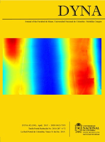
Our cover Image alluding to Article: Inspection of radiant heating floor applying non-destructive testing techniques: GPR and IRT Authors: Susana Lagüela-López, Mercedes Solla-Carracelas, Lucía Díaz-Vilariño & Julia Armesto-González

208 214 221 227 237

DYNA 82 (190), April, 2015. Medellín. ISSN 0012-7353 Printed, ISSN 2346-2183 Online

CONTENIDO Editorial

Juan D. Velásquez

La importancia de llamarse afinidad química. Parte VI: La cosech

Guillermo Salas-Banuet, José Ramírez-Vieyra, Oscar Restrepo-Baena, María Noguez-Amaya & Bryan Cockrell

Revisión de modelos matemáticos para describir el salado de alimentos Julián Andrés Gómez-Salazar, Gabriela Clemente-Polo, & Neus Sanjuán-Pelliccer

Comportamiento geotécnico de un suelo residual tropical contaminado con gasolina

Óscar Echeverri-Ramírez, Yamile Valencia-González, Daniel Eduardo Toscano-Patiño, Francisco A. Ordoñez-Muñoz, Cristina Arango-Salas & Santiago Osorio-Torres

Sistema de gestión de ingreso para el aparcamiento de contenedores: Una estrategia fuzzy para el puerto de Valparaíso

Héctor Valdés-González, Lorenzo Reyes-Bozo, Eduardo Vyhmeister, José Luis Salazar, Juan Pedro Sepúlveda & Marco Mosca-Arestizábal

Influencia de la concentración de glicerina en la estructura porosa obtenida por anodización de acero inoxidable ferrítico

Alexander Bervian, Gustavo Alberto Ludwig, Sandra Raquel Kunst, Lílian Vanessa Rossa Beltrami, Angela Beatrice Dewes Moura, Célia de Fraga Malfatti & Claudia Trindade Oliveira

Síntesis y caracterización de polímeros a base de ácido cítrico y glicerol: Su aplicación en polímeros no biodegradables

Jaime Alfredo Mariano-Torres, Arturo López-Marure & Miguel Ángel Domiguez-Sánchez

Metodología para la evaluación del impacto paisajístico residual de una mina de carbón a cielo abierto en el Valle de Laciana (España)

María Esther Alberruche-del Campo, Julio César Arranz-González, Virginia Rodríguez-Gómez, Francisco Javier Fernández-Naranjo, Roberto Rodríguez-Pacheco & Lucas Vadillo-Fernández

Encriptación usando una llave en armónicos circulares

Jorge Enrique Rueda-Parada

Evaluación de las características de toxicidad de dos residuos industriales valorizados mediante procesos de geopolimerización Carolina Martínez-López, Johanna M. Mejía-Arcila, Janneth Torres-Agredo & Ruby Mejía-de Gutiérrez

Algoritmo genético híbrido para problemas complejos de producción tipo ROADEF’05

Frutos, Ana Carolina Olivera & Fernando Tohmé

Impacto económico y ambiental del uso del gas natural en la generación de electricidad en El Amazonas: Estudio de caso

Wagner Ferreira Silva, Lucila M. S. Campos, Jorge L.Moya-Rodríguez & Jandecy Cabral-Leite

Clasificación de los huecos de tensión de acuerdo a la severidad de los efectos en el motor de inducción

9 13 23 31 38 46 53 60 70 74 82 89

Adolfo Andrés Jaramillo-Matta, Luis Guasch-Pesquer & Cesar Leonardo Trujillo-Rodríguez

96

Una metodología para el análisis de proyectos de cogeneración utilizando residuos de biomasa de palma de aceite como fuente de energía en la Amazonia

105

Rosana Cavalcante de Oliveira, Rogério Diogne de Souza e Silva & Maria Emilia de Lima Tostes

Sistema para gestionar eficientemente el aprendizaje formal e informal en m-learning. Aplicación a estudios de ingeniería José Antonio Álvarez-Bermejo, Antonio Codina-Sánchez & Luis Jesús Belmonte-Ureña

Análisis acústico del ciclo de desagüe de una lavadora

Juan Lladó-Paris & Beatriz Sánchez-Tabuenca

Corrosividad atmosférica en Bogotá como metrópolis a una gran altitud, inquietudes a normas internacionales

John Fredy Ríos-Rojas, Diego Escobar-Ocampo, Edwin Arbey Hernández-García & Carlos Arroyave

Previsión del consumo de electricidad mediante análisis espectral singular

Moisés Lima de Menezes, Reinaldo Castro Souza & José Francisco Moreira Pessanha

Simulación de un grupo generador diesel consumiendo aceite vegetal “in natura” y aire enriquecido con hidrógeno

Ricardo Augusto Seawright-de Campos, Manoel Fernandes Martins-Nogueira & Maria Emília de Lima-Tostes

Reconstrucción de objetos por perfilometría interferométrica con sistema de posicionamiento de mira periódica

113 121 128 138 147

Néstor Alonso Arias-Hernández, Martha Lucía Molina-Prado, & Jaime Enrique Meneses-Fonseca

153

Análisis de la convergencia del método de integración de variables aplicado en la optimización multiobjetivos de la

160

compensación de potencia reactiva en redes de suministro eléctrico

Secundino Marrero-Ramírez, Ileana González-Palau & Aristides A. Legra-Lobaina

Lossless compresión de imágenes hiperespectrales con tratamiento pre-byte e intra-bandas de correspondencias

Assiya Sarinova, Alexander Zamyatin & Pedro Cabral

Estudio de la cubierta vegetal del Monte Forgoselo mediante imágenes de Landsat TM 5 (Galicia, NW España) Xana Álvarez-Bermúdez, Enrique Valero-Gutiérrez del Olmo, Juan Picos-Martín & Luis Ortiz-Torres

Planeación de inventarios con demanda dinámica. Una revisión del estado del arte

Marisol Valencia-Cárdenas, Francisco Javier Díaz-Serna & Juan Carlos Correa-Morales

Análisis estructural de un pequeño remolque unido con soldadura por fricción agitación

166 173 182

Fabio Bermúdez-Parra, Fernando Franco-Arenas & Fernando Casanova-García

192

Un algoritmo híbrido de ramificación y acotamiento con cuatro heurísticas determinísticas para el problema de programación de tareas con recursos restringidos (RCPSP)

198

Daniel Morillo-Torres, Luis Fernando Moreno-Velásquez & Francisco Javier Díaz-Serna

La toma de decisiones en portafolio de productos: Métodos adoptados por las empresas innovadoras de Brasil

Daniel Jugend a, Sérgio Luis da Silva, Manoel Henrique Salgado & Juliene Navas Leoni

208

Determinación de la carga topológica de un haz bessel-gauss mediante el patrón de difracción a través de una abertura triangular equilatera

214

Cristian Hernando Acevedo, Carlos Fernando Díaz & Yezid Torres-Moreno

Inspección de suelos radiantes mediante técnicas no destructivas: GPR y IRT

Susana Lagüela-López, Mercedes Solla-Carracelas, Lucía Díaz-Vilariño & Julia Armesto-González

Sinterización de minerales de hierro. Parte 3: Sistemas automáticos y de control

Alejandro Cores, Luis Felipe Verdeja, Serafín Ferreira, Íñigo Ruiz-Bustinza, Javier Mochón, José Ignacio Robla & Carmen González Gasca

Diseño paramétrico tridimensional y análisis estático del primer malacate español utilizado para drenar agua de las minas

José Ignacio Rojas-Sola & Jesús Molino-Delgado

Nuestra carátula Imágenes alusivas al artículo: Inspección de suelos radiantes mediante técnicas no destructivas: GPR y IRT Authors: Susana Lagüela-López, Mercedes Solla-Carracelas, Lucía Díaz-Vilariño & Julia Armesto-González

221 227 237

Editorial

Una Guía Corta para Escribir Revisiones Sistemáticas de Literatura Parte 4 Esta es la última editorial de la serie dedicada al proceso de Revisión Sistemática de Literatura. En ella se aborda el proceso de documentación de la búsqueda, la selección de estudios, el análisis de los documentos seleccionados, el análisis de calidad la extracción de información y, finalmente, la síntesis de datos que corresponde a la respuesta de las preguntas de investigación a la luz de la información recopilada. Al leer estas cuatro editoriales como un todo, espero que los autores y lectores de la revista DYNA obtengan una visión global de la metodología que facilite el proceso de revisión de literatura y su posterior publicación.

1

Documentación del Proceso de Búsqueda

Una de las principales características de la revisión sistemática es que el proceso de búsqueda es repetible y sus resultados son auditables. Por ello, es requerido que se documente el proceso de búsqueda reportando la siguiente información en el documento final [1][2]:  Bases bibliográficas, libros, bibliografías y contactos usados.  Palabras clave y cadenas de búsqueda.  Periodo cubierto en la revisión.

Hay diferentes opciones disponibles al seleccionar la libraría digital dependiendo del área de conocimiento y es por ello que la selección debe realizarse con sumo cuidado; por ejemplo, en el caso de energía, electrónica y comunicaciones resulta obligatorio consultar la librería digital IEEE Xplorer; no obstante, otras selecciones comunes incluyen: ScienceDirect, SpringerLink, Wiley online library, Emerald, ACM, Kluwer, JStor e ISI Web of Science. En adición, Google Scholar, Pubmed, Ebsco, Academic Search Premier, World Scientific Net, Scopus, Compendex e Inspec también pueden ser de utilidad, dependiendo del tema particular que se este abordando.

En algunas ocasiones los investigadores restringen la búsqueda a las revistas más representativas del área, tal como en [3]; sin embargo, debe recalcarse que no deben olvidarse las bibliotecas tradicionales localizadas en universidades y centros de investigación, ya que ellas pueden contener documentos muy importantes para el proceso de revisión.

Otro aspecto fundamental en la búsqueda de documentos

es la selección adecuada de palabras clave, términos alternativos y posibles sinónimos [4], ya que de estos depende cuales documentos serán recuperados automáticamente. En algunos casos, cuando el Inglés no es la lengua materna, la selección de términos en un área nueva para el investigador puede ser especialmente difícil.

Otro aspecto importante es el dominio de la herramienta de búsqueda, y particularmente como estructurar la cadena de búsqueda para poder obtener el plural de los términos, considerar palabras cercanas, usar comodines y poder buscar frases exactas.

De acuerdo con [5], dos métricas pueden ser usadas para analizar la estrategia automática de búsqueda: la precisión, definida como el número de estudios relevantes recuperados sobre el total de estudios recuperados; y la sensibilidad, que es el número de estudios relevantes recuperados sobre el total de estudios relevantes existentes. Una estrategia óptima de búsqueda tiene usualmente una precisión entre el 20% y el 30% y una sensibilidad entre el 80% y el 99% [5].

Esto significa que para un total de cien estudios finalmente seleccionados, el investigador tuvo que revisar, al menos, entre 400 y 500 estudios recuperados automáticamente; esto significa también, que cuando la búsqueda no esta bien estructura, se deben analizar mucho más de 500 estudios para seleccionar los mismos 100 estudios.

Una de las herramientas preferidas para realizar la búsqueda es Scopus (www.scopus.com) porque incluye más de 219.000 títulos de aproximadamente 5.000 editoriales científicas, incluyendo las mayores editoriales en el mundo, tales como IEEE, Elsevier, Emerald, Springer y Wiley; adicionalmente, Scopus tiene un importante conjunto de herramientas para el análisis de literatura. Algunos consejos para crear búsquedas útiles en Scopus son los siguientes:  Se pueden usar los operadores booleanos AND, OR y AND NOT en la cadena de búsqueda.  La expresión w1 W/n w2 indica que los términos w1 y w2 no pueden estar separados por más de n términos.  La expresión w1 PRE/n w2 especifica que el término w1 precede el término w2 por no más de n términos.  El asterisco es un comodín; por ejemplo, la cadena forecast* encuentra las palabras forecasts, forecasting y forecasted.

© The author; licensee Universidad Nacional de Colombia.

DYNA 82 (190), pp. 9-12. April, 2015 Medellín. ISSN 0012-7353 Printed, ISSN 2346-2183 Online DOI: http://dx.doi.org/10.15446/dyna.v82n190.49511

Velásquez / DYNA 82 (190), pp. 9-12. April, 2015.



Sólo es necesario utilizar el singular de una palabra ya que el plural y el posesivo son automáticamente considerados.  Use las llaves (“{” y “}”) para indicar frases exactas.  Use las comillas dobles para indicar búsqueda aproximada. En este caso se puede usar el ‘*’ como comodín.

En Scopus también es posible ejecutar varias búsquedas y luego combinarlas usando los operadores lógicos OR, AND y AND NOT. Adicionalmente, Scopus presenta opciones para excluir o limitar la búsqueda por autores, años, instituciones, áreas temáticas, tipos de documento, palabras clave, afiliaciones, etc. También es posible exportar información bibliográfica a administradores de referencias. Recientemente, Elsevier incorporó el administrador bibliográfico Mendeley a ScienceDirect tal que es posible importar directamente a Mendeley documentos en formato pdf e información bibliográfica.

En el caso de la librería digital IEEE Xplorer, algunos consejos para realizar búsquedas avanzadas son los siguientes:  Se pueden usar los operadores booleanos AND, OR y NOT en la cadena de búsqueda.  Los signos de puntuación son ignorados en las cadenas de búsqueda.  Sólo es necesario utilizar el singular de una palabra ya que el plural y el posesivo son automáticamente considerados.

También se consideran automáticamente las palabras en inglés americano e inglés británico.  Las comillas dobles se usan para indicar frases exactas.  El ‘*’ es usado como comodín.

Frecuentemente, el uso de librerías digitales y bases de datos no es suficiente para localizar la literatura más relevante y se hace necesario consultar en las librerías de las universidades y centros de investigación en busca de libros, reportes de investigación, tesis de maestría, disertaciones de doctorado y cualquier otro tipo de literatura que pueda ser útil en su investigación. Se deben utilizar las referencias relevantes ya localizadas para poder extender la lista de palabras clave y refinar la cadena de búsqueda.

Cuando el reporte es escrito, es común presentar la cadena de búsqueda que fue usada en la librerías digitales con el fin de hacer la búsqueda reproducible, verificable y explícita y para poder actualizarla después [4]. Por ejemplo, en [6] se reporta el proceso de búsqueda de la siguiente forma: Our five research questions contain the following key words: “Software Engineer, Software Engineering, Motivation, De-Motivation, Productive, Characteristics, outcome, Model”. A list of synonyms was constructed for each of these words, as in the example for research question 1 which contains keywords ‘Software Engineer’ and ‘Characteristics’:

keywords((engineer* OR developer* OR professional* OR programmer* OR personnel OR people OR analyst* OR team leader* OR project manager* OR practitioner* OR maintainer* OR designer* OR coder* OR tester*) AND characteristic* OR types OR personality OR human factors OR different OR difference* OR psychology OR psychological factors OR motivator* OR prefer* OR behavio*r*) 2

Selección de los Estudios

Es el proceso de selección de los estudios que serán utilizados finalmente en la revisión. Cuando la búsqueda es ejecutada usando las cadenas de búsquedas diseñadas en el paso anterior, una gran cantidad de documentos es recuperada automáticamente, pero únicamente unos pocos documentos serán relevantes para la revisión. Una búsqueda bien diseñada permite recuperar la literatura más relevante relacionada con el área de investigación; pero también muchos documentos irrelevantes o por fuera del foco del estudio; de esta forma, es obligatorio el realizar una depuración manual de los documentos recuperados automáticamente.

De esta forma, cuando el protocolo de investigación es escrito, se deben definir dos listas en la sección donde se describe el protocolo de selección, una para los criterios de inclusión y otra para los criterios de exclusión [1][2]. La claridad es obligatoria en la definición de los criterios para que el proceso pueda ser auditado o reproducido [7]. Los documentos son comúnmente descartados mediante la lectura de sus títulos, resúmenes o conclusiones [7]; pero en caso de duda, se requiere una lectura más profunda. Es muy común que se realice la exclusión basándose en el idioma del documento o cuando los documentos son opiniones, puntos de vista o anécdotas [6]. El filtrado manual de los documentos es realizado por la aplicación de los criterios de inclusión y exclusión con el fin de poder determinar cuales serán los documentos finalmente usados en la revisión [1][2].

Cuando hay documentos traslapados en su contenido o duplicados, se debe seleccionar únicamente el más completo de ellos y el resto de documentos debe ser descartado; véase por ejemplo [8]. Los directores de tesis, compañeros, expertos y contactos son una fuente muy valiosa para determinar si se han omitido documentos importantes [7].

Otro aspecto muy importante es el uso apropiado de herramientas de software para el manejo de las referencias [9][4], tales como Zotero, Mendeley, Papers, Sente, Qiqqa, EndNote, Reference Manaer o ProCite, ya que el número final de documentos puede ser muy grande. Algunos gestores de referencias bibliográficas como Papers o Mendeley, permiten que el usuario pueda administrar los documentos, agregar notas y resaltar o subrayar textos directamente en los documentos.

10

Velásquez / DYNA 82 (190), pp. 9-12. April, 2015.

3

Análisis de los Documentos Seleccionados

En la sección de resultados de los informes de SLR, se describe el proceso de recuperación de documentos y se analizan los documentos finalmente seleccionados como un todo; en esta sección del reporte y para el caso de las revisiones sistemáticas de literatura, muchas de las preguntas de investigación comúnmente usadas en los estudios de mapeo sistemático son indirectamente respondidas; esto es, las preguntas como tal no son formuladas pero si se reporta el resultado de su análisis. En la Tabla I se describen los tipos comunes de tablas usada para analizar los documentos, así como también las columnas típicas de dichas tablas.

Para mediar la contribución de un autor, es posible calcular el puntaje S que depende del número de autores del estudio (n) y de la posición ordinal (i) del nombre del autor en la lista de autores del documento analizado, tal como se muestra en [10]:

Tabla 1.

Tablas comúnmente usadas para analizar los documentos seleccionados en revisiones sistemáticas de literatura y mapeos sistemáticos Tabla Columnas Típicas Número de documentos Librería Digital seleccionados por libreria Número Total de Documentos digital Número de Documentos Incluidos Numero de Documentos Excluidos Estudios Seleccionados

Autores Librería Digital Título Año Fuente Número de Citaciones Tipo de Documento Tipo de Estudio Tema del Estudio Objetivo del Estudio Método de Investigación [Otras columnas…]

Número de Artículos Publicados por Revista

Nombre de la Revista Numero de Artículos Porcentaje (%)

Número de Artículos Publicados por Editorial

Editorial Número de Artículos Porcentaje (%)

Tenga en cuenta que un puntaje de 1,0 es obtenido cuando el documento tiene un solo autor; se obtienen puntajes de 0,60 (primer autor) y de 0,40 (segundo autor) cuando el documento tiene dos autores, y así sucesivamente.

También se pueden usar otros indicadores bibliométricos para analizar la literatura, tal como el factor de impacto o el índice de colaboración.

La mayoría de artículos reportando resultados de SLR, indican el número de artículos recuperados automáticamente, seleccionados usando los criterios de inclusión, descartados usando los criterios de exclusión, y finalmente seleccionados usando el análisis de calidad; véase por ejemplo [11].

Artículos más Citados

Autores Año Fuente Número de Citaciones

Número de Artículos por Autor

Autor Filiación Número de Citas por Autor Numero de Artículos Puntaje S

Número de Artículos por País

País Número de Filiaciones Diferentes Número de Autores Número de Artículos Porcentaje de Artículos (%) Puntaje Total S por País

4

Número de artículos por Continente

Continente Número de Filiaciones Diferentes Número de Autores Número de Artículos Porcentaje de Artículos (%) Puntaje Total S por Continente

Número de Artículos Publicados por Año

Año Número de Artículos Porcentaje de Artículos (%) Porcentaje Acumulado (%)

1.5 ∑ 1.5

Realización del Análisis de Calidad

Los resultados del análisis de calidad de los estudios seleccionados pueden ser usados como [1][2]:  Un indicador de la calidad para determinar cómo ha progresado el campo de investigación; este es un indicador de la madurez de la investigación.  Un criterio para determinar que estudios deben ser excluídos cuando no cumplen con un nivel mínimo de calidad.  Un criterio para medir la importancia que debe tener cada estudio en la respuesta de las preguntas de investigación.  Un mecanismo para explicar la diferencia entre los resultados de estudios similares.  Un criterio para sugerir nueva investigación.

Nota: Algunas de estas tablas pueden ser presentadas alternativamente como gráficas.

El análisis de calidad es dependiente de los objetivos de la revisión seleccionada. Las Tablas 5 y 6 de la ref. [1] contienen una recopilación de preguntas usadas en el análisis de calidad de diferentes estudios.

Una forma de realizar el análisis de la calidad es considerar en que proporción cada estudio seleccionado

11

Velásquez / DYNA 82 (190), pp. 9-12. April, 2015.

permite responder las preguntas de investigación [3]; comúnmente se usa una escala nominal: Y (si), N (no) y P (parcialmente). Para obtener un puntaje final para cada estudio, se asignan valores a la escala nominal, por ejemplo, se asigna 1,0 a Y, 0,5 a P y 0,0 a N, y luego se suman los puntos asignados a cada estudio. Los resultados de la evaluación de la calidad son comúnmente presentados en forma de una tabla detallada.

5

Extracción de los Datos

La información para responder las preguntas de investigación y realizar la evaluación de la calidad es recolectada en forma de tablas o cualquier otro tipo de sistema de toma de notas [1][7]. Las tablas son diseñadas en una manera consistente con las preguntas de investigación y permiten enfatizar las similitudes y diferencias entre los estudios [1].

Cuando un gestor de referencias como Mendeley o Paper es usado, es posible resaltar texto con diferentes colores, subrayar y agregar anotaciones y comentarios en los documentos con el fin de facilitar la extracción de datos y su posterior revisión. Una selección común es usar diferentes colores para marcar las partes donde cada respuesta a una pregunta de investigación específica aparece en el documento.

6

Síntesis de los Datos

En este paso [2], las preguntas de investigación son respondidas usando la información recolectada. Cuando los estudios primarios son cuantitativos, la síntesis puede ser realizada usando técnicas estadísticas, tales como el metaanálisis; pero cuando los estudios son cualitativos, la síntesis es narrativa (descriptiva) resumiendo los principales hechos. En la síntesis descriptiva, es usual preparar tablas y gráficos que resuman la información relevante respecto a la pregunta o preguntas de investigación consideradas. Dos aproximaciones pueden ser usadas para responder estudios cualitativos [12]: centradas en los conceptos o centradas en los autores.

Referencias [1]

Kitchenham, B.A. and Charters, S., Guidelines for performing systematic literature reviews in software engineering. Technical Report EBSE-2007-01, 2007.

[2] S. Sorrell, Improving the evidence base for energy policy: The role of systematic reviews, Energy Policy, 35 (3), pp. 1858-1871, 2007. http://dx.doi.org/10.1016/j.enpol.2006.06.008 [3] Kitchenham, B., Brereton, O.P., Budgen, D., Turner, M., Bailey, J. and Linkman, S., Systematic literature reviews in software engineering – A systematic literature review, Information and Software Technology, 51 (1), pp.

7-15, 2009. http://dx.doi.org/10.1016/j.infsof.2008.09.009 [4] Bolderston, A.,Writing an Effective Literature Review, Journal of Medical Imaging and Radiation Sciences, 39 (2), pp. 86-92, 2008. http://dx.doi.org/10.1016/j.jmir.2008.04.009 [5] Zhang, H., Babar, M.A. and Tell, P., Identifying relevant studies in software engineering, Information and Software Technology, 53 (6), pp. 625-637, 2011. http://dx.doi.org/10.1016/j.infsof.2010.12.010 [6] Beecham, S., Baddoo, N., Hall, T., Robinson, H. and Sharp, H., Motivation in software engineering: A systematic literature review, Information and Software Technology, 50 (9-10), pp. 860-878, 2008. http://dx.doi.org/10.1016/j.infsof.2007.09.004 [7] Randolph, J.J., A guide to writing the dissertation literature review, Practical Assessment, Research & Evaluation, 4 (13), pp. 1-13, 2009.

[8] Khurum, M. and Gorschek, T., A systematic review of domain analysis solutions for product lines, The Journal of Systems and Software, 82 (12) pp.

1982-2003, 2009. http://dx.doi.org/10.1016/j.jss.2009.06.048 [9] Pautasso, M., Ten simple rules for writing a literature review, PLoS Computational Biology, 9 (7), pp.

1-4, 2013. http://dx.doi.org/10.1371/journal.pcbi.1003149 [10] Yuan, H. and Shen, L., Trend of the research on construction and demolition waste management, Waste Management, 31 (4), pp. 670679, 2011. http://dx.doi.org/10.1016/j.wasman.2010.10.030 [11] Hauge, Ø., Ayala, C. and Conradi, R., Adoption of open source software in software-intensive organizations – A systematic literature review, Information and Software Technology, 52 (11), pp.

1133-1154, 2010. http://dx.doi.org/10.1016/j.infsof.2010.05.008 [12] Webster, J. and Watson, R.T., Editorial. Analyzing the past to prepare for the future: Writing a literature review, MIS Quarterly, 26 (2), pp. xiii-xxiii, 2002.

Juan D. Velásquez, MSc, PhD Profesor Titular Universidad Nacional de Colombia E-mail: jdvelasq@unal.edu.co http://orcid.org/0000-0003-3043-3037

12

The importance of being chemical affinity. Part VI: The harvest Guillermo Salas-Banuet a, José Ramírez-Vieyra b, Oscar Restrepo-Baena c, María Noguez-Amaya d & Bryan Cockrell e a

Universidad Nacional Autónoma de México, salasb@unam.mx Universidad Nacional Autónoma de México, jgrv@unam.mx c Universidad Nacional de Colombia, ojestre@unal.edu.co d Universidad Nacional Autónoma de México, nogueza@unam.mx e University of California, Berkeley, bryan.cockrell@berkeley.edu b

Received: September 5th, 2014. Received in revised form: November 3th, 2014. Accepted: November 25th, 2014.

Abstract The quantitative scale of electronegativity, obtained by Linus Pauling, as a result of qualitative electron affinity background, generated multiple different and interesting proposals until today, which have proved to be the effort of ingenuity to get a universal concept of affinity, which has resulted incomplete. Thermodynamics, specifically its thermochemical branch, has offered an explanation, which has been accepted by The International Union of Pure and Applied Chemistry (IUPAC), as incomplete as the former. In both cases, it is thought that the error is in regard to affinity as a property, rather than a behavior.

Keywords: Affinity, Electronegativity, chemistry, history, thermodynamics.

La importancia de llamarse afinidad química. Parte VI: La cosecha Resumen La escala cuantitativa de electronegatividad obtenida por Linus Pauling, como resultado de aquellas antecedentes cualitativas de electroafinidad, generó múltiples propuestas diferentes e interesantes, hasta el día de hoy, lo que ha mostrado ser el esfuerzo del ingenio por conseguir un concepto universal de afinidad, que ha resultado incompleto. La termodinámica, específicamente su rama termoquímica, ha ofrecido una explicación, tampoco universal, que ha sido aceptada por la Unión Internacional de Química Pura y Aplicada (IUPAC, por sus siglas en inglés), igual de incompleta. En ambos casos, se piensa que el error está en considerar a la afinidad como una propiedad, en vez de un comportamiento.

Palabras clave: Afinidad, electronegatividad, química, historia, termodinámica.

y la termodinámica lo haría usando los conceptos de energía y entropía.

1. Introducción Si se considera cierta la afirmación de que Antoine Lavoisier es el padre de la química, entonces esta nace en 1789 cuando publica su libro Traité Élémentaire de Chimie.

Con ello, su gestación estaría en la búsqueda de una teoría congruente que explicara la afinidad química, su proceso de parto en el desarrollo de los conceptos tempranos de electricidad y calor y su primer alimento en el de estructura atómica.

Después, la química continuaría buscando explicaciones para la afinidad a través del concepto de electronegatividad desencadenando una serie de propuestas de escalas sostenidas en diversos intentos para explicar su razón lógica-

2. Antecedentes En la visión histórica occidental, la primera manera de explicar el mundo y sus transformaciones fue la hierofánica; se piensa que el concepto intuitivo de afinidad química estuvo presente en las mentes de algunos -seguramente pocos- de los hombres que -desde la Prehistoria y durante decenas de miles de años- transformaron las rocas, usando fogatas y hornos, en cerámicas y metales. Esa experiencia permitió que, al iniciarse el periodo de la Historia, se desarrollara un conocimiento práctico y óptimo, en

© The author; licensee Universidad Nacional de Colombia.

DYNA 82 (190), pp. 13-22. April, 2015 Medellín. ISSN 0012-7353 Printed, ISSN 2346-2183 Online DOI: http://dx.doi.org/10.15446/dyna.v82n190.48730

Salas-Banuet et al / DYNA 82 (190), pp. 13-22. April, 2015.

Mesopotamia (antigua Irak y el noreste de Siria), Egipto y Persia (actualmente Irán) [1]. Ese conocimiento fue tomado y repensado por los griegos, libre de influencias religiosas, entre los siglos VI y II a.C. [2]. Como resultado de este ejercicio, a finales de ese tiempo y en el ambiente de las ciencias exactas del Museo Alejandrino, nació la alquimia científica. El pensamiento griego permanecería inmutable hasta el siglo IX, cuando los musulmanes de Bagdad, Damasco y Toledo lo modificaron -dando origen a una alquimia más mágica que científica- y lo difundieron; hacia finales del siglo XIII llegaría a gran parte de Europa, donde se asimilaría y propagaría a otras partes del mundo [3]. El conocimiento práctico de los materiales fue tomado por los romanos, hasta el siglo V d. C. cuando se derrumbó su imperio. Con él quedó un vacío de poder que dejó a una Europa medieval sumida en constantes luchas, hasta que fue llenado por la dominante Iglesia Cristiana de Roma, la cual presionó a los creyentes para que se utilizara su pensamiento religioso para definir y explicar todo, incluso a la naturaleza; a partir del siglo IX, algunos de sus integrantes comenzaron a luchar por su propia independencia de pensamiento. En el siglo XII, en Europa se descubrieron, tradujeron y difundieron los textos de los pensadores griegos clásicos, con lo cual surgió el Renacimiento, en el siglo XV, y la Ilustración, a finales del siglo XVII. En este siglo, Robert Boyle le dio la espalda a algunas teorías alquímicas y estableció hipótesis químicas -usando las ideas de los griegos, las suyas propias y las de sus contemporáneos- con las que fundó los estudios sobre la afinidad química; entre estos, destacan la propuesta de tablas cualitativas de afinidad.

Es en el siglo XVIII cuando la química se consolida como una ciencia, gracias al trabajo de Antoine Lavoisier y sus varios colaboradores [4]. A partir del siglo XIX, la nueva ciencia se enriquece y evoluciona debido desarrollos intelectuales y experimentales diversos -de la propia área y de otras- como los relativos a la electricidad, el calor y el átomo, lo que permitió, en el primer tercio del siglo XX, que Linus Pauling presentara una tabla cuantitativa de electronegatividad (de afinidad), cimentada en la determinación del porcentaje del carácter iónico de los enlaces covalentes -obtenido con las energías de algunos enlaces químicos, a través de la medición de los calores de formación de varios compuestos- y una definición de la misma [5].

determinan por potenciales de ionización sucesivos), en la forma de N = n – Z, donde n es el número de electrones alrededor del núcleo en un estado de ionización dado y Z es el número atómico del núcleo. Definieron la electronegatividad de un átomo neutro en fase gaseosa: X = (-dE/dN)N = 0 donde dE es el cambio de energía que acompaña al cambio en la carga, dN. Indicaron que al usar el primer potencial de ionización y la afinidad del primer electrón, su X era equivalente a la relación de Mulliken; así, enfatizaron la la cercanía a esa relación y asentaron que las unidades de la X deberían ser de energía por electrón; por supuesto, compararon exitosamente su escala con la de Mulliken [5]. Que la X sea igual a (-dE/dN) quiere decir que después de juntarse dos átomos se obtendrá una disminución en la energía, si los electrones se transfieren al átomo, para el cual el descenso de energía total (dE) excede al incremento total en la energía del átomo del que se remueven esos electrones; ese descenso de la energía total se debe a la ganancia de una carga electrónica fraccional, dN [7]. Allen [8] subrayó que con esto se estableció a la X como un concepto de transferencia de carga.

En un trabajo que llegó a ser clásico, Robert Parr et al. [9] revisaron el concepto de X desde el punto de vista de la teoría de la densidad funcional. Esta viene de dos teoremas de Hohenberg y Kohn, los cuales establecen que la densidad electrónica (ρ) determina todas las propiedades de un átomo o una molécula en un estado neutro no degenerado y la energía de un átomo para un estado neutro degenerado. La teoría define que el potencial químico electrónico μ es igual a (∂E/∂N)ν, donde ν es una constante del potencial externo debido a las cargas nucleares establecidas (el potencial del núcleo); tanto la cantidad de E (la energía electrónica) como de N (el número de electrones) son funciones de ρ. Parr y sus compañeros comentaron que encontraron que la X era la misma para todos los orbitales naturales en un átomo o molécula en sus estados neutros (el potencial químico); precisaron el concepto de la X como el potencial químico negativo, con lo que X = - μ = (∂E/∂N)ν = ½(I + A); como la conexión con la definición de Mulliken [5] era inmediata, se le calificó de absoluta. Esto significa que cuando dos átomos A y B, con un μA diferente a μB, se unen químicamente, el sistema se equilibrará a un nuevo valor común de μ, diferente a los de A y B. Con X = -μ y la analogía existente entre μ y la energía libre de Gibbs, se implicaba una igualdad de la X para cualquier cantidad de átomos enlazados, con lo que se validó el principio igualador de Sanderson; y explican: la diferencia de electronegatividad en los estados de valencia, produce la transferencia de electrones entre los átomos de la molécula en formación, así, los electrones se distribuyen entre los orbitales para igualar el potencial químico de orbital a orbital.

Allen [8] comenta que el trabajo de Parr et al. fue citado en más de 300 artículos, en algunos de los cuales se cita también a Sanderson. Bartolotti [10] subraya que con el trabajo de Parr se conectó a X con la mecánica cuántica y que μ fue introducido en la teoría de la densidad funcional como un multiplicador de Lagrange, para asegurar que el número de partículas sería conservado al minimizarse la energía. En otro comentario, Ralph Pearson [11] hace notar que μ es una cantidad que caracteriza a cualquier sistema químico, átomo, radical, ión o molécula; que es constante en cualquier parte del sistema; que mide la tendencia de los electrones a escapar del sistema; y que,

3. Explicaciones químicas para la afinidad Con la propuesta de Linus Pauling, se inicia la presentación de una multiplicidad de escalas, conceptos y definiciones de electronegatividad, X, que intentan explicar la afinidad de elementos y compuestos. En la primera mitad del siglo XX se dieron las primeras [5].

3.1. La afinidad química en la 2ª mitad del siglo XX. Raymond Iczkowski y John Margrave [6] usaron la energía atómica -tomada como las energías de los iones positivo y negativo relativas a los átomos neutros- expresada en una serie de potencias en N (cuyos coeficientes se 14

Salas-Banuet et al / DYNA 82 (190), pp. 13-22. April, 2015.

Afirma que esta interpretación no destruye para nada la idea coloquial de la X como "atraer" o el "poder de jalar" electrones, ya que si la energía promedio de los electrones en el átomo A es más baja que la energía promedio de los electrones en el átomo B, entonces el átomo A atraerá los electrones del átomo B, cuando A y B se unan.

Más tarde [13], Lelan Allen estableció que la X es una propiedad íntima de la Tabla Periódica y una definición para ella: la energía promedio de un electrón, de los de la capa de valencia, para átomos libres en su estado basal, indicando que las energías del electrón pueden ser determinadas directamente con los datos espectroscópicos, de ahí el nombre para su electronegatividad, y que esta descripción llevaba a una definición mejorada de la X de grupo (o de sustituyentes), así como a la extensión y refinamiento en el uso de las perturbaciones de la X en la teoría orbital molecular cualitativa y semicuantitativa y al entendimiento del orden de las reglas de la X orbital híbrida, tales como que sp > sp2 > sp3. Estableció la Xespec como (mεp + nεs)/(m + n), para elementos representativos, en donde εp y εs son las energías de ionización s y p; m y n son el número de electrones de p y s. Afirmó que los valores de la Xespec se ajustan (comparando gráficas) bastante a los de las ampliamente aceptadas escalas de Pauling [14] y de Allred y Rochow [15], lo que, para él, es de primera importancia.

Precisa que la Xespec permite racionalizar dos aspectos: 1) la separación diagonal de la Tabla Periódica entre metales y no metales -estableciendo a los elementos B, Si, Ge, As, Sb, Te, Bi y Po como los metaloides- y 2) la formación de moléculas a partir de los gases nobles. Para él, estos gases son el punto primordial de la Tabla Periódica porque sus Xs presentan dos caras: tienen altos valores, con lo que muestran su capacidad para retener a sus electrones, pero ningún valor para atraer a otros. Afirma que la X es la energía de activación para el enlace y que: 1. con la diferencia de las electronegatividades espectroscópicas, ΔXespec, entre dos átomos diferentes, es posible sistematizar las propiedades de un amplio grupo de materiales conocidos: sólidos iónicos, moléculas covalentes, metales, minerales, polímeros inorgánicos y orgánicos, semiconductores, etc. e identificar el carácter iónico (la polaridad del enlace) de esos átomos; y 2. la X de los metales de transición no puede ser determinada de manera simple debido a la naturaleza de las distribuciones radiales del orbital d y que esto se nota en el poco uso que de ella hacen los químicos de esos metales. Comparó su escala con las de Allred y Rochow, Boyd y Edgecombe, Mulliken y Pauling: XP = 1.75 x 103 Xespec (Kj/mol) o XP = 0.69Xespec (eV).

El mayor valor de Xespec la presenta el Ne = 4.783, seguido por los elementos: F = 4.193, He = 4.16, O = 3.61 y Ar = 3.242. Su método tiene la ventaja de poder estimar las electronegatividades de elementos que no pueden ser obtenidas por otros medios, como la del Francio, al que Allen asigna un valor de 0.67.

como es una propiedad sólo de sistemas al equilibrio, lo es de estados neutros. Señala que la electronegatividad de Pauling (XP) -y las otras electronegatividades similares- difiere bastante de la absoluta de Parr, ya que, para esta última, es una propiedad de un átomo libre en el estado neutro y no de uno en su estado de valencia excitado, adecuado para tomar parte en una molécula. Indica que la aplicación de la escala de Pauling es útil para estimar las polaridades de los enlaces y, en algún grado, las resistencias de los enlaces entre átomos diferentes; mientras que la absoluta es una medida de la reactividad química del átomo, radical, ión o molécula, cuya aplicación típica está en: a) estimar la interacción inicial entre dos de ellos; b) dar la dirección del flujo electrónico; y c) proporcionar un estimado de la cantidad inicial de la densidad electrónica transferida, relacionada a su vez a las barreras de energía para la reacción y, en algunos casos, a la resistencia del enlace coordinado formado; pero que no es una medida confiable de la polaridad final del enlace. También advierte que la X absoluta no satisface la definición de XP, como la propiedad de un átomo en una molécula, pero sí en la idea esencial de atraer y mantener electrones, y que no existe una razón que obligue a restringir su aplicación a átomos combinados. Dice que se ha mostrado que las escalas pueden ser comparables y que sólo sus aplicaciones son diferentes, por lo que el asunto no es preguntarse cuál escala es la más correcta porque cada escala es más apropiada en su propia área de uso.

Pearson apoya al principio igualador de Sanderson al decir que, aunque no está probado por ninguna teoría, es intuitivamente interesante.

Al presentar su electronegatividad espectroscópica, Xespec, [12], Allen comentó que -usando la Figura 6 (y su texto) de otro artículo suyo [13]- se contrastó la energía de la expresión (I + A)/2, usada por Parr, para hacer la aproximación del potencial químico electrónico (μ) al comportamiento de la Xespec, encontrando que eran muy diferentes. Además, calcula y presenta los valores de las diferencias promedio de las energías de Hartree, de la capa de valencia entre los átomos libres de F, O y N y el átomo de H, para los átomos relativos al H y referidos a cero, obteniendo: -0.450, -0.162 y -0.630, respectivamente, y los de los mismos átomos en sus hidruros relativos al H en el H2 y referidos a cero, FH, OH2 y NH3, obteniendo: -0.055, -0.028 y -0.010, respectivamente. Allen explica que si el potencial químico, μ, fuese calculado de la misma forma, los valores obtenidos para los átomos libres serían aproximadamente los mismos, mientras que los de los hidruros estarían todos en un solo punto (el del H2), contraviniendo la observación empírica que indica que los átomos mantienen su identidad cuando se combinan en moléculas o sólidos. Así, concluye, la igualación de la X no acontece y el potencial químico electrónico, μ, tal como fue desarrollado por Parr, Pearson, y otros, resulta una cantidad química totalmente diferente a la X. Posteriormente, Allen [8] presenta la idea de que con X = - μ = (∂E/∂N)ν -en la formulación de la densidad funcional- se implica la frase "la tendencia de los electrones a escapar" (describiendo la XM) y que, más que una transferencia de carga o esa "tendencia a escapar", la electronegatividad es un concepto de enlazamiento estático, tal como los potenciales de ionización que la definen: la energía de un electrón en un átomo o, más precisamente, la energía promedio de los electrones de valencia en un átomo.

3.2. Escalas de X para los elementos en sus diferentes estados de valencia u oxidación Existen tres antecedentes de estas escalas: 1) Mulliken [16] determinó la X de sólo 11 elementos en diferentes 15

Salas-Banuet et al / DYNA 82 (190), pp. 13-22. April, 2015.

electrones". Todos los trabajos parten del planteamiento de una hipótesis, aunque sólo Pauling y Malone las comprueban con experimentación propia; algunos autores toman alguna experimentación previa y calculan la X con el método que proponen y el resto deriva su comprobación matemáticamente. Las propuestas tienen dos características comunes: son conceptos sencillos y se usan fácilmente, lo cual es esencial en la ciencia y la educación.

estados de valencia usando valores de I y A, porque no existían valores de A para el resto de los elementos; encontró que la X de un átomo se incrementaba con el aumento de la valencia; 2) Allred [17] usó el método de Pauling para calcular las Xs en diferentes estados de oxidación, para un puñado de elementos de los que existían datos disponibles: Mo, Fe, Tl, Sn y Pb; y 3) Sanderson [18] propuso un método para calcular la X de elementos en diferentes estados de valencia, basado en las cargas parciales y las energías de enlace; su método estaba limitado a los metales de transición.

Keyan Li y Dongfeng Xue [19] estimaron los valores de electronegatividad, XLX, para proponer una escala para 82 elementos, en diferentes estados de valencia y con los números de coordinación más comunes. Los calcularon basándose en el potencial químico efectivo, definido por la energía de ionización y el radio iónico, es decir, en términos del potencial iónico efectivo (φ), φ = n*(Im/R)1/2/ri, donde n* es el número cuántico principal efectivo, Im es la energía de ionización última (numéricamente igual a la de la afinidad electrónica de un catión dado), R = 13.6 eV (la constante de Rydberg) y ri es el radio iónico. Ellos explicaron que, para el momento de escribir su trabajo, la X era una propiedad invariante, la cual no dependía del ambiente químico del átomo (v.gr: el estado de la valencia y el número de coordinación); y que, hasta donde sabían, no existía esta información completa, por lo que decidieron construirla. Encontraron que para un catión determinado, la X se incrementaba de acuerdo al aumento del estado de oxidación, disminuía con el aumento del número de coordinación y que existía una una perfecta correlación lineal con la escala de Luo [20], basada en el potencial covalente, debido a que la teoría de la X absoluta de Parr es el soporte teórico de ambas. Compararon su escala con la de Pauling: XP=0.105XLX+0.863.

3.4. Evaluar y reglamentar la X Mullay [21] realizó un análisis para evaluar el desarrollo de las escalas de X y planteó tres etapas: la primera involucró la búsqueda del método apropiado para calcular o medir las Xs atómicas; en la segunda se cambió el énfasis hacia el cálculo de la X de grupo y la carga atómica, y se exploraron y clarificaron los efectos de la carga atómica sobre la X; y, en la tercera, se propició la profundización del concepto básico, principalmente a través del uso de la teoría de la densidad funcional [9]. Sin embargo, de ahí en adelante se han publicado indistintamente trabajos del tipo de las tres etapas planteadas. Por decenio, el número de trabajos publicados durante el siglo XX fue de 3 durante los años 30, 2 en los 40, 3 en los 50, 6 en los 60, 6 en los 70, 10 en los 80, 1 en los 90 y 6 en los primeros 8 años del siglo XXI; aun sumando los trabajos que se dejaron fuera (menores en cantidad), el incremento no es comparable al número de químicos investigando y publicando en el mismo periodo de tiempo.

Gordon Sproul [22] pensó que se podían evaluar 15 escalas de X usando los triángulos del enlace. Graficó la X promedio versus la diferencia de electronegatividades para 311 compuestos binarios, bien identificados por A. F. Wells [23] por su tipo de enlace, utilizando sólo parámetros físicos y químicos medibles y evitando emplear la X. Concluyó que todas las escalas dan gráficas triangulares que segregan efectivamente los compuestos considerados, en tres regiones relativas al tipo de enlace iónico, metálico y covalente; y que las escalas que proveen la mejor segregación de los compuestos son la de Allen [13] y la de Nagle [24], con un acierto superior al 96%. Esto provocó que Peter G. Nelson publicara un comentario [25] en el que señalaba, entre otros detalles, que el tipo de enlace no es una propiedad medible y que en las ediciones previas del texto de A. F. Wells, se da la impresión de haber utilizado la X para realizar algunas de sus asignaciones. Sproul [26] contestó, entre otras cosas, que Wells no menciona, en el texto de referencia, la posibilidad de usar a la X para determinar tipos de enlace, sino que utilizó algunos fenómenos subjetivos como conductividad/resistencia eléctrica, puntos de fusión y características estructurales, tales como iones aislados, anillos, cadenas, moléculas separadas, etc.

Murphy et al. [27] -entre ellos Leland Allenestablecieron 9 reglas que, a su criterio, todas las escalas de X deberían de obedecer: 1. Las Xs atómicas necesitan ser obtenidas de las propiedades de los átomos libres. 2. Es necesaria una precisión de tres números (unidad, décima y centésima). 3. La X es una energía por electrón. 4. Todos los electrones de valencia deben ser incluidos en la definición de X. 5. Tres requerimientos del grupo principal están

3.3. Las otras escalas de electronegatividad Desde la primera propuesta de Pauling hasta la fecha de elaboración de este trabajo (periodo de más de 80 años) se han encontrado, entre las revistas occidentales más consultadas, múltiples trabajos enfocados a proponer una escala de X, sobre todo haciendo relaciones entre propiedades; de estos, sólo 26 presentan alguna originalidad.

Las diversas escalas se fundamentan en características atómicas -principalmente- y moleculares, tanto de la estructura (radios atómicos, longitudes de enlace, etc.) como de las propiedades (potenciales de ionización, carga eléctrica, etc.). Es posible distinguir que cerca del 80% de los autores comparan su escala con alguna otra; más del 70% lo hace directa (62%) o indirectamente (8%) con la de Pauling; el 20% que agrupa a las que tienen un origen en la mecánica cuántica no hace comparaciones, o las hace con alguna que tiene su mismo fundamento. Durante las comparaciones y al ajustar los valores de una escala al rango de los de la de Pauling, surgió el concepto de las Unidades Pauling (UP).

Aunque el empirismo y el fundamento de la escala de Pauling se señalan como erróneos por muchos autores, la mayoría de ellos validan su propia escala al compararla con ella (sigue siendo la más famosa y utilizada, sobre todo en la educación) y, al hablar de X, mantienen el concepto de "atraer 16

Salas-Banuet et al / DYNA 82 (190), pp. 13-22. April, 2015.

interrelacionados: a) la identificación de la X con el poder atrayente de un átomo por electrones es generalmente igual a su poder para retenerlos; b) los átomos de los gases nobles sólo tienen la habilidad para retenerlos; y c) las magnitudes de la X deben, paralelamente, establecer limitaciones de oxidación. 6. Los valores de X de los ocho elementos semimetálicos (B, Si, Ge, As, Sb, Te, Bi y Po) no deben traslaparse con los de los metales y los no metales; se debe respetar la regla del Si: todos los metales deben tener valores de X menores o, cuando mucho, iguales al del Si. 7. Para los compuestos binarios, AB, las electronegatividades de A y de B deben de calificar y definir los tipos de enlace como iónico, covalente o metálico. 8. La X debe tener una definición mecánica cuántica viable. 9. La escala de X debe mostrar un incremento sistemático de izquierda a derecha a través de los periodos. Cabe notar, que esta última regla no la cumple la escala de Allen, específicamente para los metales de transición. Los autores aplicaron estas reglas a la escala de XP y dictaminaron que sólo satisface las reglas 4 y 5 del criterio. Además, indican algunos errores de Pauling que, según ellos, han influido fuertemente en la actitud negativa de los químicos hacia la X: 1. Forzó a que la X tuviera unidades de (eV)1/2, en aras de ajustar mejor unos pocos enlaces más en su relación energía de enlace-polaridad de enlace original, con lo que se ha confundido a los químicos innecesariamente; 2. Las electronegatividades de varios metales de transición violan la regla del Si, haciendo que los químicos se cuestionen si la X es realmente aplicable a esta clase de átomos; 3. Su definición de X [14] "la atracción por electrones de un átomo neutro en moléculas estables" ha sido mal interpretada por el 15-20% de los autores de los textos que discuten su escala, cuando explican que la X es una propiedad molecular intrínseca, aun cuando Pauling lo niega implícitamente, en la siguiente frase del mismo texto; y 4. La definición de Pauling no es viable en la mecánica cuántica porque está construida sobre propiedades termodinámicas y no sobre electrónicas, lo que implica una falta de capacidad para designar las electronegatividades de 18 elementos.

Leland Allen [8] había proporcionado cinco criterios para establecer una definición coherente de X: 1. La X debe ser una cantidad de un átomo libre. 2. Debe responderse al problema de porqué la X no se puede medir en el laboratorio. 3. Una escala correcta de X debe ser cercanamente compatible con los valores de X empleados por los químicos prácticos al racionalizar sus resultados experimentales durante los últimos 70 (ahora casi 100) años. 4. Se cree que alguna función de las energías de ionización de los electrones de valencia atómica es el mejor candidato para ser la propiedad física medible necesaria para definirla. 5. Una definición correcta de la X debe ser totalmente compatible y hacer una conexión directa con los métodos de investigación de la mecánica cuántica, usados por los científicos profesionales para sus predicciones y explicaciones detalladas sobre la química contemporánea y los problemas de la física del estado sólido. Referente al criterio 4, Pauling [14] afirma: La propiedad de la electronegatividad de un átomo en una molécula es diferente del potencial de ionización del átomo y de su afinidad electrónica…aunque está relacionada a esas propiedades en una manera general.

Boeyens [28] estableció sólo una regla, al explicar que la forma moderna en la que se grafica la curva de Lothar Meyer (Figura 1) del volumen atómico (V = M/ρ, la masa atómica en gramos y la densidad de los elementos sólidos) presentado como una función de Z (el número atómico), demuestra convincentemente la periodicidad elemental y expresa la X atómica. Boeyens indica que si se interrumpe la curva en los puntos donde se sabe que se completan los niveles de energía s, p, d y f -en vez de conectar todos los puntos en la secuencia de Z-, esta se fragmenta en regiones formadas por 2 u 8 elementos, excepto para los de las tierras raras, pero que si se toman junto con el par de elementos precedentes (Cs y Ba) y se separa el segmento en el Sm, la curva queda dividida en dos segmentos de 8 elementos cada uno. Ahora, todos los segmentos son curvas que tienen, alternadamente, una pendiente positiva y otra negativa, que se relacionan a los elementos tradicionalmente considerados como electropositivos y electronegativos.

Esta noción teórica, dice Boeyens, provee una definición precisa de X y permite afirmar que las escalas que no reflejen esta periodicidad deben considerarse inapropiadas. Es notorio que no define un significado.

De todo lo anterior, es posible distinguir tres acuerdos generales: la X es una propiedad; indica la capacidad de atraer y conservar electrones; y, en un enlace, los electrones se comparten en forma desigual.

Es notorio el gran esfuerzo realizado para tratar de derivar valores universales cuantitativos de X, lo que ha permitido observar: la confusión que existe de la imagen física que corresponde al concepto de X; que el concepto de X no se ha definido exactamente, por lo que sigue siendo ambiguo; que la X no es una propiedad de un átomo aislado que pueda medirse, como el número atómico, la masa o la energía de ionización; que al determinar la X, en realidad se están midiendo propiedades que dependen de la distribución electrónica o de la estructura atómica, todas diferentes. Así, la X ha quedado como un concepto inherentemente confuso, con bajo contenido de información.

Aquí se considera que la dificultad encontrada para su medición radica en que la X no es una propiedad, sino un comportamiento. Las propiedades se relacionan a algún nivel o tipo de estructura, con lo que son medibles. Los comportamientos se deducen de la comparación de los datos medidos, por lo que siempre son cualitativos. De ahí la imposibilidad de obtener una escala de X cuantitativa y una definición exacta para ella, universalmente válidas, y, por lo tanto, para la afinidad química.

4. La termodinámica en el problema de la afinidad El concepto de afinidad estuvo íntimamente relacionado al calor generado por las reacciones químicas. Mientras, la termodinámica nace y se desarrolla del estudio del calor producido por la máquina, desde el inicio de la revolución industrial. Sin embargo, no es sino hasta que se aprecia que uno de los conceptos importantes relativos al calor en la máquina, es aplicable al de reacción química -dando una medida de la afinidad- que se da origen a la termoquímica, uniendo a las dos ciencias.

17

Salas-Banuet et al / DYNA 82 (190), pp. 13-22. April, 2015.

1799), médico, físico y químico escocés, basándose en sus trabajos experimentales- usados para explicar por qué se mantenía constante la temperatura en los cambios de estado y para aclarar la diferencia conceptual entre temperatura θ y cantidad de calor Q; también definió una caloría como la cantidad de calor que necesita 1g de agua para aumentar su temperatura en 1°C; c) las investigaciones realizadas en la década de 1770 por William Irvine (1743-1787), químico y médico escocés, alumno de Black, sobre el calor específico, con las que esbozó el concepto de calor absoluto; d) así como los conceptos de capacidad calorífica específica de las sustancias y calor de las reacciones químicas, nombrados por Adair Crawford (1748-1795), un químico y médico irlandés, quien utilizó métodos calorimétricos desarrollados por él mismo.

Como en el último cuarto del siglo XVIII aún no se había esclarecido la naturaleza del calor, Antoine Lavoisier (17431794) invitó al astrónomo, físico y matemático francés Pierre Laplace (1749-1827) a trabajar con él en torno al problema de su cuantificación, porque cuando un científico no entiende, mide. Se proponía determinar las condiciones bajo las cuales se pueden vaporizar diferentes fluidos, medir la dilatabilidad de algunas sustancias y presentar un nuevo método basado en un calorímetro diseñado por Laplace, un novedoso instrumento para medir la transferencia de calor en numerosos fenómenos. Cabe mencionar que Lavoisier y Laplace conocían el libro de Magalhães, por lo que Lavoisier utilizó el concepto del calor latente durante la fusión del hielo usado en el calorímetro de Laplace, para medir el calor emitido por varias sustancias cuando se quemaban en oxígeno. Con los resultados definieron una unidad cuantitativa de calórico -un patrón- como la cantidad que derretiría una libra francesa (489,6 gramos, medida adoptada en el año 800 por Carlomagno) de hielo. Obtuvieron resultados para tres sustancias elementales, fósforo, carbón e hidrógeno, reportadas en libras de hielo fundido por libra de elemento quemado. La caloría, unidad usada hoy, se definiría después de la revolución francesa, tal como Black la había estipulado, aunque acotada al rango de 14.5 a 15.5°C. Entre 1777 y 1783, los dos sabios colaboraron en tres ocasiones; los resultados de sus investigaciones están en cuatro escritos contenidos en los famosos escritos: Mémoire sur la chaleur [31] y De l’action du calorique sur les corps solides, principalement sur le verre et sur les métaux [32].

Ya Lavoisier había ideado una nueva explicación de la combustión en términos de la existencia del gas oxígeno. En su memoria Réflexions sur le phlogistique (1777), Lavoisier afirmó que la teoría del flogisto era incompatible con sus resultados experimentales, con lo que propuso la existencia de otro fluido sutil, el calórico que, al impregnar la materia, sería la sustancia responsable del aumento de su calor. Para él: todos los cuerpos naturales obedecen a dos fuerzas, el fluido ígneo, el asunto del fuego, que tiende continuamente a separar a las moléculas, y la atracción, que contrabalancea esa fuerza. En tanto que la última de estas fuerzas, la atracción, sea victoriosa, el cuerpo permanece en estado sólido; si estas dos fuerzas están en un estado de equilibrio, el cuerpo se vuelve líquido; finalmente, cuando la fuerza del calor expansivo prevalece, el cuerpo toma el estado gaseoso.

El fluido calórico se haría visible en las llamas, que estarían

Figura 1. Curva de Lothar Meyer.

Fuente: [23].

4.1 El calor Durante el periodo de oro del pensamiento griego, entre los siglos V y III a.C., las ideas sobre el calor y la mecánica surgieron en caminos paralelos. En la Sicilia del siglo V a.C., Empédocles de Agrigento postuló la existencia de cuatro raíces elementales: fuego, aire, agua y tierra, los que al unirse asumían las formas de todos los cuerpos de la naturaleza; como demostró experimentalmente que el aire era una substancia [2], extendió el concepto a los tres elementos restantes, asignándoles las características de pequeños e indivisibles. Para el año 360 a.C. a través del diálogo Timeo, Platón filosofa -tratando de explicar el calor- que el fuego y el aire son partículas muy pequeñas, más que los intersticios de las estructuras de la tierra y el agua, con lo que tienen mucho espacio para entrar en ellas y moverse, sobre todo el fuego; y agrega: no debemos olvidar que la figura original de fuego (la pirámide), más que cualquier otra forma, tiene un poder de dividir que corta el cuerpo en trozos pequeños y, por lo tanto, produce naturalmente el afecto que llamamos calor [29]. Las primeras interpretaciones alquímicas sobre la naturaleza del calor se confundían con aquellas sobre la combustión; tal vez por ello, en el siglo XVII, el alquimista y físico alemán Johann Joachim Becher (1635-1682) estableció una teoría que duraría un siglo, la cual fue defendida por su compatriota el médico y químico Georg Stahl (1659-1734). Proponía un principio inflamable, con la existencia de un fluido sutil hipotético (el flogisto), que estaba en los cuerpos y se desprendía en la combustión.

En 1780 se publicó en Londres, aunque en francés, el primer libro de termoquímica Essai sur la nouvelle théorie du feu élémentaire, et de la chaleur des corps [30] del portugués João Jacinto de Magalhães (1722-1790) -un espía del gobierno francés en cuestiones industriales- que contenía, entre muchas otras cosas: a) una tabla de calores específicos construida con los datos obtenidos por el químico irlandés Richard Kirwan (1733-1812); b) los conceptos: capacidad para el calor (ahora conocido como capacidad de calor específico) y calor latente -creados por Joseph Black (172818

Salas-Banuet et al / DYNA 82 (190), pp. 13-22. April, 2015.

formadas en su mayor parte por dicho calórico desprendiéndose de los cuerpos y sería el responsable del calor de la materia [33]. El concepto central de la teoría calórica era que el calor, al ser una sustancia elemental, se conservaba; su cantidad total permanecía intacta. No podía ser creada o destruida. El modelo calórico fue ampliamente aceptado -temporal y geográficamente- ya que explicaba las características y los efectos del calor, tales como su difusión por contacto entre los cuerpos, la expansión de estos, el trabajo producido al expandirse el vapor, los distintos estados de agregación de la materia, las quemaduras producidas por congelación (el calórico causaba los mismos daños en la piel al entrar y al salir del cuerpo); cada sustancia presentaría una distinta solubilidad para el calórico, lo que explicaría el calor específico de cada cuerpo; e interpretaba los resultados experimentales que evidenciaban la equivalencia entre calor y trabajo del inglés James Prescott Joule (1818-1889), al plantear que, durante la fricción de un cuerpo contra otro, se romperían las vesículas microscópicas contenedoras del calórico, liberando calor. Fue esta idea la que le causó problemas a la teoría del calórico, ya que algunas personas la interpretaban de forma diferente: Platón había dicho que el calor y el fuego son engendrados por la fricción y el impacto, y esto es movimiento; Robert Hooke (1635-1703), había afirmado que el calor es, nada más, una agitación muy vigorosa y vehemente de las partes de un cuerpo [34]; al apreciar la producción de calor debida a la fricción y el violento movimiento de los líquidos en ebullición, el inglés Francis Bacon (1561-1626) concluyó que la verdadera esencia del calor es el movimiento y nada más [35]; Galileo Galilei (1564-1642), Christiaan Huygens (1629-1695) [36], Isaac Newton (1643-1727) [37] y John Locke (1632-1704) [38] compartían la misma visión. Esto llevó al planteamiento de la teoría cinética del calor.

La primer persona que intentó una formulación matemática de la clase de energía que está conectada con el movimiento (energía cinética) fue Gottfried Wilhelm Leibniz (1646-1716), quien trabajó en este asunto de 1676 a 1689; se dio cuenta de que en muchos sistemas mecánicos de varias masas, cada uno con una velocidad, la energía se conservaba, siempre que las masas no interactuaran. Llamó a esta cantidad la vis viva o fuerza viva del sistema [39]. El principio representa una declaración exacta de la conservación aproximada de la energía cinética en situaciones donde no hay fricción.

La duda mayor sobre el calórico vino de un joven que se encontraba supervisando la fabricación de cañones en Baviera. En el proceso de taladrar el centro de los cañones, Benjamín Thomson (1753-1814), conocido como el conde de Rumford, observó que se producía un aumento de temperatura en la estructura del cañón, en las virutas metálicas y en el propio taladrador, de modo que parecía generarse calor continuamente, en lugar de conservarse como decía la teoría del fluido calórico.

Rumford dirigió una serie de experimentos para medir el cambio de temperatura que ocurría. En uno de ellos utilizó agua para refrigerar el taladrador y la estructura del cañón y midió el aumento de temperatura del agua, observando que el ésta llegaba a hervir sin ningún fuego; entonces concluyó que el calor no podía ser una sustancia material, ya que parecía

no tener límite. Más bien parecía que el movimiento mecánico se podría convertir en calor y, más importante, que la conversión era cuantitativa y se podría predecir permitiendo una constante de conversión universal entre la energía cinética y el calor. Cuando el científico británico Thomas Young (1773-1829) trabajó realizando ensayos de tracción y propuso la medida actualmente utilizada para la rigidez de los materiales, en 1807, utilizó el término energía para designar la vis viva, el cual se utiliza desde entonces. El principio de equivalencia mecánica se afirmó por primera vez en su forma moderna por el cirujano alemán Julius Robert von Mayer en 1842 [40]. Mayer llegó a su conclusión en un viaje a las Indias Orientales Holandesas, donde se encontró con que la sangre de sus pacientes era de un rojo más profundo porque consumían menos oxígeno, y por lo tanto menos energía, para mantener su temperatura corporal en un clima más caliente. Él descubrió que el calor y el trabajo mecánico eran formas de energía, publicó una monografía donde declaró una relación cuantitativa entre ellos.

En 1837, en un trabajo publicado por Karl Friedrich Mohr (1806-1879) se encuentra una de las afirmaciones generales más tempranas de la conservación de la energía: además de los 54 elementos químicos conocidos que hay en el mundo físico un agente único, y esto se llama Kraft (energía o trabajo). Puede parecer, según las circunstancias, como el movimiento, la afinidad química, la cohesión, la electricidad, la luz y el magnetismo; y de cualquiera de estas formas puede ser transformado en cualquiera de los otros [41].

Germain Henri Hess (1802-1850) fue un químico y médico suizo que, en 1840, al demostrar que el calor generado en las transformaciones químicas no dependía de la ruta de la reacción, formuló la Ley de la suma constante del calor (Ley de Hess), uno de los primeros principios de la termoquímica. Hess decía: Cuando se produce una reacción química, no sólo hay una transformación de unas sustancias en otras, sino que también tiene lugar un cambio energético.

Este cambio es tal, que la reacción consume o produce energía, ya sea en forma de calor, trabajo mecánico, trabajo eléctrico o energía luminosa; lo que significa que la ley es la aplicación a las reacciones químicas del primer principio de la termodinámica. Puede enunciarse diciendo que la variación de la energía térmica de una reacción se puede obtener sumando algebraicamente las entalpías de otras reacciones varias, relacionadas con la que nos interesa. Esta ley resulta de gran utilidad para estimar en forma indirecta una entalpía de reacción desconocida, resultando factible calcular las energías térmicas de muchas reacciones cuya medición directa no es posible o deseable realizar.

Poco después, en 1843, el físico inglés James Prescott Joule (1818-1889) verificó que al fluir una corriente eléctrica a través de un conductor, éste experimentaba un incremento de temperatura; a partir de ahí dedujo que si la fuente de energía eléctrica es una pila electroquímica, la energía habría de proceder de la transformación llevada a cabo por las reacciones químicas, que la convertirían en energía eléctrica y que esta se transformaría en calor. Si en el circuito se introduce un motor eléctrico, se origina energía mecánica; una de las mayores generalizaciones de la ciencia. También realizó otra serie de experimentos. En el más famoso, que ahora se llama el aparato Joule, un peso descendente es atado 19

Salas-Banuet et al / DYNA 82 (190), pp. 13-22. April, 2015.

leyes de la mecánica en ausencia de fricción- que es el máximo posible para esa diferencia de temperaturas.

Rudolf Julius Emmanuel Clausius (1822-1888) fue un físico y matemático alemán, considerado uno de los fundadores centrales de la ciencia de la termodinámica. En su trabajo más importante sobre la teoría mecánica del calor, publicado en 1850 [44], estableció por primera vez las ideas básicas de la segunda ley de la termodinámica y formuló de manera novedosa el principio de Sadi Carnot, demostrando que podía interpretarse como la equivalencia de calor y trabajo. Clausius enunció y bautizó, en 1854, la 2a Ley de la Termodinámica para procesos irreversibles como dS  dQ/dT y a partir de 1865 entropía, del griego ἐντροπία que significa transformación o evolución.

En 1884, el físicoquímico holandés Jacobus Henricus Van't Hoff (1852-1911) propuso que el trabajo externo máximo obtenido al llevar a cabo isotérmicamente una reacción química reversible, era una medida de la afinidad química [45]. En este sentido, el matemático y físico belga Théophile Ernest de Donder (1872-1957) propuso, en 1922 [46], una relación termodinámica entre la afinidad química y la energía libre de Gibbs, para los sistemas que, no estando en equilibrio, no se encuentran muy lejos de él (termodinámica irreversible). A partir de la desigualdad de Clausius, De Donder hizo equivalente la afinidad de la reacción, A, a la derivada parcial negativa de la energía libre de Gibbs, G, con respecto a la extensión de la reacción, , a presión y temperatura constantes:

a una cuerda la cual causa que una rueda de paletas gire y agite el agua en la que se encuentra sumergida, dentro de un calorímetro; el aumento de la temperatura es medida por un termómetro. Joule demostró que la energía potencial gravitatoria perdida por el peso descendente era igual a la energía interna adquirida por el agua a través de la fricción con las paletas; esto es, midió el equivalente mecánico del calor. Ahora, el término calor se reserva sólo para la energía térmica transferida cuando dos cuerpos con diferente temperatura están en contacto.

Dado que la energía se conserva, un cuerpo no puede ganarla a menos que otro se la transfiera incrementando su energía térmica, porque fluyó desde él debido a que estaba más caliente, o porque le ejerció trabajo mecánico. Así, la primera ley de la termodinámica (de la conservación de la energía, establecida por el médico y físico alemán Herman von Helmholtz (1821–1894), en 1847, dice que el cambio neto en la energía en un cuerpo (∆E) será igual a la energía que le sea transferida -a través del flujo neto de calor (Q), más la cantidad neta del trabajo realizado sobre el cuerpo (W)- o retirada, con lo que Q y W pueden ser negativos. La primera ley dice cómo medir cualquier cambio de energía en un cuerpo, pero nada dice acerca de cuánta energía hay en el cuerpo, respuesta que se obtiene con la relación de Einstein, que especifica que la cantidad de energía en un cuerpo (E) es igual a su masa (m), multiplicada por el cuadrado de la velocidad de la luz (c2), lo que resulta en muchísima energía (sólo que aún no se conoce cómo obtenerla, salvo para materiales radiactivos).

A   G   T , p

4.2. La segunda ley de la termodinámica

Un corolario de utilizar esta definición, en cinética, es que la velocidad de una reacción cercana al equilibrio es proporcional a la afinidad de la reacción.

En 1954, Ilya Progogine y Raymond Defay [47] definieron la misma afinidad, sustituyendo la derivada parcial de la energía libre de Gibbs por la del calor incompensado, Q’, tanto para los sistemas en equilibrio como para los que no. Esta definición es la actualmente aceptada por la IUPAC. Como puede verse, la propuesta termodinámica para definir la afinidad está acotada para condiciones específicas.

Además, la medición de la energía de la reacción es equivalente a la medición del calor de reacción realizada por Pauling [5], aunque con más fundamento teórico y precisión experimental.

Esta implica la existencia de una propiedad adicional de la materia, llamada entropía, la cual, al igual que la energía térmica de la primera ley, puede ser determinada en el laboratorio. Así como la primera ley establece que la energía del universo se conserva, la segunda establece que la entropía del Universo no se conserva sino que su cantidad total nunca decrece, sólo se mantiene o aumenta. La declaración de que es imposible para un dispositivo que opera cíclicamente convertir energía térmica en mecánica, sin perder algo de la térmica en los alrededores fríos, es llamada la segunda ley de la termodinámica, según lo estableció William Thomson Kelvin (1824-1907) en 1848, al publicar la creación de una escala termodinámica para la temperatura, de carácter absoluto [42].

En 1824, Nicolas Léonard Sadi Carnot (1796-1832), un físico e ingeniero francés, quien fue pionero en el estudio de la Termodinámica, publicó su obra maestra Reflexiones sobre la potencia motriz del fuego y sobre las máquinas adecuadas para desarrollar esta potencia [43], donde expuso las ideas que llevarían al segundo principio de la termodinámica, al descubrir una relación entre las temperaturas de los focos calientes (la máquina) y frío (los alrededores) y el rendimiento de la máquina. Experimentalmente probó que, en una máquina caliente, la descarga de calor hacia los alrededores fríos es inevitable, por lo que ninguna máquina real alcanza el rendimiento teórico de Carnot -el cual se obtiene siguiendo el ciclo de Carnot, al que llegó usando las

5. Conclusión Pareciera que la química y la termodinámica siguieron caminos separados; sin embargo son similares pues durante su desarrollo, básicamente usaron los mismos conceptos y consideraron a la afinidad como una propiedad y no como un comportamiento. Por eso, aún con las incontables intuiciones, razonamientos y racionalizaciones -relacionados a infinidad de esfuerzos y trabajos de múltiples personas, durante cientos de años- el concepto de afinidad es y seguirá siendo un espejismo: aunque parezca cercano, es inalcanzable.

20

Salas-Banuet et al / DYNA 82 (190), pp. 13-22. April, 2015.

[24] Nagle, J.K., Atomic Polarizability and Electronegativity, Journal of the American Chemical Society, 112 (12), pp. 4741-4747, 1990.

[25] Nelson, P.G., Comment on Sproul’s Evaluation of Electronegativity Scales, Journal of Physical Chemistry, 99 (39), pp. 14570, 1995.

[26] Sproul, G.D., Reply to “Comment on Sproul’s Evaluation of Electronegativity Scales”, Journal of Physical Chemistry, 99 (39), pp.

14571, 1995. http://dx.doi.org/10.1021/j100039a054 [27] Murphy, L.R., Meek, T.L., Allred, A.l. and Allen, L.C., Evaluation and Test of Pauling’s Electronegativity Scale, Journal of Physical Chemistry, 104 (24), pp. 5867-5871, 2000.

[28] Boeyens, J.C.A., The Periodic Electronegativity Table, Zeitschrift für Naturforschung, 63b, pp. 199-209, 2008.

[29] Platón, Timeo, Serrano, R y Díaz, M. (editores), Madrid, Consejo Superior de Investigaciones Científicas, 2012.

[30] De Magalhães, J.J., Essai sur la nouvelle Théorie du Feu élémentaire et de la Chaleur des Corps, London, W. Richardson, 1780.

[31] Lavoisier, A.L. et Laplace, P.S. Mémoire sur la chaleur. pp. 283-333, 1780 [32] De l’action du calorique sur les corps solides, principalement sur le verre et sur les métaux, pp. 739-764, Mémoires de l’Académie des Sciences, 1783.

[33] Lavoisier, A.L., Réflexions sur le phlogistique, pour servir de développement à la théorie de la combustion & de la calcination, publiée en 1777, Paris, Académie des sciences, 1783.

[34] Hooke, R., Micrographia or, Some physiological descriptions of minute bodies made by magnifying glasses, London, J. Martyn and J. Allestry, 1665.

[35] Bacon, F., Novum Organum (traducción al inglés), London, Clarendon Press, 1878.

[36] Huygens, C., Traité de la lumière, Pierre Vander A, 1690.

[37] Newton, I., Il Saggiatore, Roma, Giacomo Mascardi, 1623.

[38] Locke, J., An Essay Concerning Human Understanding, London, Eliz. Holt, for Thomas Basset, 1690.

[39] Leibniz, G.W., Specimen Dynamicum, en Loemker, L.E. Ed., Philosophical Papers and Letters, pp. 435-452, D. Reidel-Springer, Netherlands, 1976.

[40] Mayer, J.R., Annalen der Chemie und Pharmacie 43 (2), pp. 233-240, 1842. http://dx.doi.org/10.1002/jlac.18420430208 http://dx.doi.org/10.1002/jlac.18420420212 [41] Chisholm, H. Ed., Mohr, Karl Friedrich. Encyclopædia Britannica, Cambridge University Press, 1911.

[42] Goldstein, M. y Goldstein, F.I., The refrigerator and the Universe, Cambridge, Harvard University Press, 1993.

[43] Sadi, N.L., Réflexions sur la puissance motrice du feu et sur les machines propres à développer cette puissance, París, Bachelier, 1824.

[44] Clausius, R., Ueber die bewegende Kraft der Wärme und die Gesetze, welche sich daraus für die Wärmelehre selbst ableiten lassen, Annalen der Physik, 155 (4), pp.

500–524, 1850. http://dx.doi.org/10.1002/andp.18501550403 [45] Van't Hoff, J.H., Studies in Chemical Dynamics, Amsterdam, Frederik Muller and Co., 1896.

[46] De Donder, T.E., L’Affinitié. Applications auz gaz parfaits.

Mémoires de la Classe des Sciences, Académie Royale de Belgique, 5th series, 7, pp. 197-205, 1922.

[47] Prigogine, I. and Defay, R., Chemical Thermodynamics, New York, John Wiley & Sons, 1954.

Referencias [1] [2] [3] [4]

[5]

[6] [7] [8] [9]

[10] [11] [12] [13] [14] [15] [16]

[17] [18] [19]

[20] [21] [22] [23]

Salas, G., Ramírez, J., Restrepo, O., Cockrell, B. y Noguez, M. La Importancia de llamarse afinidad química. Parte I: La semilla. DYNA, 79 (173), pp. 135-144, 2012.

Salas, G., Ramírez, J., Restrepo, O., Noguez, M. y Cockrell, B. La Importancia de llamarse afinidad química. Parte II: La semilla germina. DYNA, 80 (177), pp. 162-170, 2013.

Salas, G., Ramírez, J., Restrepo, O., Noguez, M. y Cockrell, B. La Importancia de llamarse afinidad química. Parte III: El crecimiento vano. DYNA, 80 (181), pp. 219-227, 2013.

Salas, G., Ramírez, J., Restrepo, O., Noguez, M y Cockrell, B. La Importancia de llamarse afinidad química. Parte IV: Las primeras flores.

2014.

DYNA, 81 (184), pp.

225-232, http://dx.doi.org/10.15446/dyna.v81n187.46092 Salas, G., Ramírez, J., Restrepo, O., Noguez, M. y Cockrell, B. La Importancia de llamarse afinidad química. Parte V: Los frutos.

DYNA, 81 (187), pp.

267-275, 2014. http://dx.doi.org/10.15446/dyna.v81n187.46092 Izcowzki, R.P. and Margrave, J.L., Electronegativity, Journal of the American Chemical Society, 83 (17), pp. 3547-3551, 1961. ttp://dx.doi.org/10.1021/ja01478a001 Mortier, W.J., Electronegativity Equalization and its Applications, en Sen, K. and Jørgensen, C.K. eds., Electronegativity, pp. 125-143, Heidelberg, Springer-Verlag, 1987.

Allen, L.C., Chemistry and Electronegativity, International Journal of Quantum Chemistry, 49 (3), pp. 253-277, 1994.

Parr, R.G., Donnelly, R.A., Levy, M. y Palke, W.E., Electronegativity: The density functional viewpoint, Journal of Chemical Physics, 68 (8), pp.

3801-3807, 1978. http://dx.doi.org/10.1063/1.436185 Bartolotti, L.J., Absolute Electronegativities as Determined from Khon-Sham Theory, en Sen, K. and Jørgensen, C.K. (editors), Electronegativity, pp. 27-40, Heidelberg, Springer-Verlag, 1987.

Pearson, R.G., Electronegativity Scales, Accounts of Chemical Research, 23 (1), pp. 1-2, 1990.

Allen, L.C., Electronegativity Scales, Accounts of Chemical Research, 23, pp. 175-176, 1990.

Allen, L.C., Electronegativity Is the Average One-Electron Energy of the Valence-Shell Electrons in Ground-State Free Atoms, Journal of the American Chemical Society, 111 (25), pp. 9003-9014, 1989.

Pauling, L., The Nature of Chemical Bond, Ithaca, Cornell University Press, 1960.

Allred, A.L. and Rochow, E.G., A scale of Electronegativity Based on Electrostatic Force, Journal of Inorganic Nuclear Chemistry, 5 (4), pp. 264-268, 1958. http://dx.doi.org/10.1016/0022-1902(58)80003-2 Mulliken, R.S., A New Electroaffinity Scale; Together with Data on Valence States and on Valence Ionization Potentials and Electron Affinities, Journal of Chemical Physics, 2 (11), pp. 782-793, 1934. http://dx.doi.org/10.1063/1.1749394 Allred, A.L., Electronegativity Values from Thermochemical Data, Journal of Inorganic Nuclear Chemistry, 17 (3-4), pp. 215-221, 1961. http://dx.doi.org/10.1016/0022-1902(61)80142-5 Sanderson, R.T., Principles of Electronegativity. II. Applications, Journal of Chemical Education, 65 (3), pp. 227-231, 1988. http://dx.doi.org/10.1021/ed065p227 Keyan, L. and Xue, D., Estimation of Electronegativity Values of Elements in Different Valence States, Journal of Physical Chemistry A, 110 (39), pp.

11332-11337, 2006. http://dx.doi.org/10.1021/jp062886k Luo, Y. and Pacey, P.D., Theoretical support for a new electronegativity scale, Journal of the American Chemical Society, 113 (4), 1465-1466, 1991. http://dx.doi.org/10.1021/ja00004a087 Mullay, J., Estimation of Atomic and Group Electronegativities, en Sen, K. and Jørgensen, C.K. (editores), Electronegativity, pp. 1-26, Heidelberg, Springer-Verlag, 1987.

Sproul, G., Electronegativity and Bond Type. 2. Evaluation of Electronegativity Scales, Journal of Physical Chemistry, 98 (27), pp.

6699-6703, 1994. http://dx.doi.org/10.1021/j100078a009 Wells, A. F., Structural inorganic chemistry, Oxford, Clarendon Press, 1945.

G. Salas–Banuet, es Ingeniero Químico Metalúrgico con título de postgrado, ambos de la Universidad Nacional Autónoma de México UNAM, México. Profesor Titular en la Facultad de Química de la misma universidad, donde ha trabajado en docencia, investigación y divulgación.

Su área principal de trabajo está en los metales; otros campos de interés son el pensamiento, las ideas, la historia, arqueología, desarrollo humano. Ha publicado en revistas nacionales e internacionales indexadas. Así mismo ha enviado trabajos a conferencias y eventos científicos.

J. Ramírez-Vieyra, obtuvo su diploma en Ingeniería Metalúrgica en la Universidad Nacional Autónoma de México – UNAM, México, donde también obtuvo su Maestría en Ingeniería. Fue profesor adjunto y ha sido Investigador Asistente. Adicionalmente, actúa como Profesor Asistente en 21

Salas-Banuet et al / DYNA 82 (190), pp. 13-22. April, 2015. la Facultad de Química de la UNAM, México. Ha colaborado en algunos proyectos de investigación en la elaboración de artículos y ha participado en congresos y publicado artículos en sus temas de interés: Metalurgia física, Arqueometalurgia, Educación en ingeniería y Materiales y ambiente.

O. Restrepo-Baena, es Ingeniero de Minas y Metalurgia de la Universidad Nacional de Colombia; Magister en Evaluación de Impactos Ambientales y Doctor en Metalurgia y Materiales de la Universidad de Oviedo, España.

Trabaja en la Facultad de Minas de la Universidad Nacional de Colombia, Sede Medellín y su área de trabajo se centra en Metalurgia extractiva y Materiales de Ingeniería: Cementos, Cerámicos, Pigmentos.

M. Noguez-Amaya, es Ingeniera Química Metalúrgica de la Facultad de Química, Universidad Nacional Autónoma de México – UNAM, México.

MSc. en Ingeniería Metalúrgica de la School of Engineering, University of Pittsburgh, USA. Actualmente profesora de tiempo completo en la Facultad de Química de la UNAM; ganó el premio “Ernesto Rios del Castillo” y el premio “Sor Juana Inés de la Cruz” a la mujer universitaria de la UNAM. Sus áreas de interés son: Metalurgia física, Educación en ingeniería y Materiales y ambiente.

B.R. Cockrell, recibió su PhD. en Antropología (Arqueología) en la UC, Berkeley, USA. Su área de investigación actual está en el análisis de metales del Cenote Sagrado de Chichen Itza en Yucatán, México, en colaboración con investigadores de la UNAM, México. Actualmente enseña en el Departamento de Antropología de UC Berkeley y en SF State University.

Sus intereses incluyen la metalurgia de los antiguos pueblos americanos así como la arqueometría y arqueología de Mesoamérica.

Área Curricular de Ingeniería Química e Ingeniería de Petróleos Oferta de Posgrados

Maestría en Ingeniería - Ingeniería Química Maestría en Ingeniería - Ingeniería de Petróleos Doctorado en Ingeniería - Sistemas Energéticos Mayor información:

E-mail: qcaypet_med@unal.edu.co Teléfono: (57-4) 425 5317

22

Review of mathematical models to describe the food salting process Julián Andrés Gómez-Salazar a, Gabriela Clemente-Polo b, & Neus Sanjuán-Pelliccer b b

a Escuela de Agronomía, Universidad de la Salle Bajío, León, México, jgomezs@delasalle.edu.mx Departamento de Tecnología de Alimentos, Universitat Politècnica de València, Valencia, España, gclemen@tal.upv.es

Received: February 11th, 2014. Received in revised form: January 28th, 2014. Accepted: February 11th, 2015.

Abstract Salting and subsequent curing are part of the traditional processing method used in the meat and fish industry. Different preserving agents (sodium chloride, nitrite, nitrate, among others) are added in this process. Nowadays, more attention is paid to the amount of salts added and the salting time employed. For this reason, it is important to know the factors governing salt penetration and the most convenient process conditions. The transfer mechanism of the salts through the structure is an interesting aspect in meat and fish processing technology. Mathematical models are the best way to discover the factors, which govern this process, which may represent and explain the observed data and predict the behaviour under different conditions. The objective of this review is to describe the use of the mathematical models to simulate meat and fish salting and the benefits derived from their use. Most of the models used to describe the salting process are diffusional, based on Fick’s second law, although empirical ones are also used. For modelling purposes a good description of the experimental results should be guaranteed. The complexity of the model will depend on the objective to be reached and will be analysed in each case.

Keywords: meat, fish, salting, curing, modelling

Revisión de modelos matemáticos para describir el salado de alimentos Resumen El salado y posterior curado forman parte del procesado tradicional de conservación de carne y pescado. En él se añaden diferentes conservantes (cloruro sódico, nitritos, nitratos, entre otros). En la actualidad se está aumentando el control sobre la cantidad de sales añadidas y el tiempo de salado. Por ello es importante conocer los factores que controlan la penetración de sal y las condiciones de proceso más adecuadas. Los mecanismos de transferencia de las sales en el sólido son aspectos muy interesantes a considerar en las industrias de procesado de carne y pescado. Los modelos matemáticos son la mejor manera de conocer los factores controlantes en estos procesos. Éstos representan y explican los datos observados y predicen el comportamiento bajo diferentes condiciones. El objetivo de este trabajo es describir el uso de modelos matemáticos para similar el salado de carne y pescado y los beneficios derivados de su uso. La mayoría de los modelos utilizados para describir el proceso de salado son difusionales, basados en la segunda ley de Fick, aunque también son utilizados los modelos empíricos. Para propósitos de modelización debe ser garantizada una buena descripción de los resultados experimentales. La complejidad del modelo dependerá del objetivo a alcanzar será analizado en cada caso.

Palabras clave: carne, pescado, salado, curado, modelización

1. Introduction The process of salting is traditional in the meat and fish industry. Sodium chloride is an essential ingredient of salting that provides different functionalities: providing flavour, solubilizing proteins, dehydrating and altering osmotic pressure so as to inhibit bacterial growth and subsequent spoilage. Nitrate and nitrites are also added to the meat in this process. They are basic ingredients in meat

products. Nitrates, which are reduced to nitrites by bacterial action, produce an antimicrobial effect, while nitrites inhibit the growth of Clostridium botulinum and, thereby, the formation of the neurotoxic proteins. Nitrites also contribute to the development of flavour in cured meat products and are responsible for the formation of the characteristic pink/red colour in cured and smoked products. Over the last few years, changing consumer demands and increasing global competition have led the meat sector to embrace new

© The author; licensee Universidad Nacional de Colombia.

DYNA 82 (190), pp. 23-30. April, 2015 Medellín. ISSN 0012-7353 Printed, ISSN 2346-2183 Online DOI: http://dx.doi.org/10.15446/dyna.v82n190.42016

G贸mez-Salazar et al / DYNA 82 (190), pp. 23-30. April, 2015.

centrifugation, vacuum, freezing, electric current, pressure and alternating pressure and vacuum [7].

Salting changes the composition and structure of the tissue and the extent of these changes may affect the mass transfer kinetics and sensorial properties of the final product. The gradual increase of salt concentration in the meat muscle leads to changes in its functional properties.

All of the salting procedures bring about the salt saturation of the liquid phase of the products. Proteins are strongly aggregated at high salt concentrations, leading to a reduction in the water holding capacity of the muscle [8].

This implies a strong bond between water and salt and the concurrent dehydration of the protein [9].

Two main simultaneous flows are usually generated during salting, water loss and salt uptake. Salt ions diffuse through the aqueous phase of the product, which is distributed by means of a complex network of microscopic channels within the dry matter matrix. At the same time, the liquid phase of the product does not remain constant when the salt is dissolved in it. Water molecules migrate outside the product, which causes resistance to diffusion [10].

Salt diffusion is related to the change between the salt concentration in the interior of the food and that in the external brine solution, where the mass transfer rates do not cease until equilibrium is reached. Equilibrium is the end of the diffusion process, that is, when the net rate of mass transfer is zero. The diffusion rate necessary to reach equilibrium depends on the concentration gradient (chemical potential) between the brine and the product.

During salting, a marked increase in the concentration of salt in the muscle may be observed in the first few hours due to the large concentration gradient at the beginning of the process. Likewise, a great decrease in moisture in the muscle can be observed [11]. Thereafter, the diffusion decreases until the equilibrium concentration is reached [12].

ingredient systems and new processing technologies. In the case of curing salts, consumers are demanding healthier products that are low in salt. The use of salts in meat is seen to be a cause of the increased risk of chronic diseases, such as obesity, cancer and strokes [1]. In this regard, what has been proposed is the control of and reduction in the level of salts added to meat products. Likewise, it is also important to increase knowledge about the reactions that take place and the process conditions.

It is essential to carry out an exhaustive control of the salting process in order to develop high quality fish and meat products. This involves a good distribution of the salts in the product and an estimation of the salting time. In order to control both aspects, it is important to know the main factors governing salt penetration. The transport phenomena involved in salting, defined by salt and water transfer, are complex and depend on aspects such as brine concentration, temperature or pH, among other things. One of the best ways to gain knowledge of the factors governing this process is the use of mathematical models, which may represent processes, explain the observed data and predict the behaviour of the process under different conditions [2].

This paper presents a review of the development and use of mathematical models describing mass transfer during the salting and curing of meat and fish.

2. The salting process Meat and fish are traditionally preserved by being treated with salts, such as sodium chloride, sodium nitrite and sodium nitrate. Salt reduces water activity and lends specific organoleptic and sensory characteristics to the products. The forms of adding salts differ depending on the final product to be obtained. Salting is performed either by dry, brine or injection salting or a combination of these methods.

Traditional dry salting consists of covering or rubbing the raw material with solid salt; this is partially dissolved and drained during the process by fluid effluent from the product as a consequence of the osmotic and diffusional mechanisms [3].

Brine salting is based on the immersion of the meat or fish pieces in a water and salt solution. In dry and brine salting, counter current salt and water mass transfer take place between the brine (or dry salt) and the meat. Barat et al. [3] did not find any significant differences between these two processes in terms of the physicochemical and sensory parameters, but noted that dry salting is more favourable to dehydration, while brine salting favours the entry of salt.

However, brine salting has several advantages over dry salting, including shorter processing times due to higher salt uptake and higher weight yields due to a better control over the rate of salt uptake and water loss in the muscle [4-6].

Injection-salting is a method that also introduces salt into the muscle tissue, but differently from dry and brine salting. In this case, the brine is forced to distribute itself into the muscle tissue through an injection system.

Likewise, over the last few years, various technologies have been tested for the purposes of accelerating the penetration of the salt in the food, such as massage, ultrasound,

3. Modelling of salting process Mathematical modelling has become a common practice when analysing the salting phenomena due to the cost and time involved in experimental studies [13-16]. These models usually contain a food system description and the mechanisms and rate equations of changes. Models can be used to improve the understanding of the process dynamics and to develop a control strategy for a new process [13].

The complexity needed in a model depends on the objective to be reached. In general, the simpler the model, the easier its mathematical solution. Nevertheless, the model equations must be a good approximation to the real process [17]. The models can give realistic representations of a process, explain the observed data and predict the behaviour under different conditions [18]. These can be used for process optimization, for example to reduce the cost of the process or the processing time without the need to carry out experiments. However, models are an approximation to reality, which may not provide an accurate description of the system resulting in poor prediction. Moreover, simulation using complex models can require the use of complex mathematical algorithms, which can increase the 24

Gómez-Salazar et al / DYNA 82 (190), pp. 23-30. April, 2015.

in each independent variable in the governing differential equations. Thus, a transient process governed by a first derivative respect to time will require one boundary condition related to this variable, usually one initial condition. The initial condition refers to the distribution of salt at the beginning of the salting process. For example, for a slab geometry it can be expressed as (Eq. 6).

calculation time. Models can be classified as theoretical and empirical. Theoretical models are developed using the principles of chemistry, physics and biology. Theoretical models are derived from mass and energy balances. Among the theoretical models that have been applied to mass transfer, the diffusional ones are the most widely used. For this reason, they are explained in detail in section 3.1. In section 3.2, the empirical models are presented.

(6)

௜

3.1. Diffusional models

Eq. 6 indicates that at the beginning of the salting process the total salt concentration in the product is the same and equal to the initial concentration.

Since the governing equation for each spatial dimension is of the second order, two boundary conditions are needed for each dimension. A symmetry condition and a surface condition are usually formulated. For an infinite slab, the symmetry condition is expressed in equation 7. Generally speaking, a symmetry condition must be formulated for each spatial dimension.

Diffusion is the predominant transport mechanism involved in salting. It is a spontaneous phenomenon of mass transfer caused by the random motion of the molecules under a concentration gradient. For the purposes of modelling the diffusion in salting processes, authors commonly consider water diffusion and salt diffusion separately [12,14,15].

The key equation describing diffusion is Fick’s second law (Equation 1). ଶ ௘

(7)

(1)

ଶ

As regards the surface condition, two considerations can be made depending on whether the external resistance to mass transfer is negligible or not. If the external resistance to mass transfer is negligible, it is assumed that the equilibrium concentration of salt is reached on the surface of the solid from the beginning of the process. This condition is expressed by equation 8 for an infinite slab of thickness, 2L.

Eq. 1 is based on the hypothesis that the transfer rate of a diffusing substance through a unit area is proportional to the concentration gradient measured normally to the section [19]. Diffusion alone does not usually occur. For this reason, the calculation of an effective diffusion coefficient that covers all real phenomena can be useful [2].

Effective diffusivity is a property that determines the velocity of mass propagation through the material. In the case of salting, this property defines the penetration velocity of salt and water loss in a food [20]. The estimation of this property allows both the mass flux and the processing time to be predicted or controlled [9].

The analytical solutions of Fick´s diffusion equation for predicting D in salting for classical geometries has been widely used for different geometries: planar with transport in one direction (Equation 2), cylindrical (Equation 3), spherical (Equation 4), and parallelepipedic with multidirectional transport (Equation 5) [11,16,21-32].

The industrial salting process is not carried out under conditions of strong agitation. For that reason, the external resistance to mass transfer can sometimes be considered. In this case, a mass transfer coefficient (kc) is included in the surface boundary condition. Equation 9 shows the surface condition under this hypothesis for an infinite slab of thickness, 2L [25]. ௘

௘

௘

௘

௘

௜௙

(9)

Previous diffusion equations (Eqs. 2 to 5) took into account the local concentration of salt in the sample. Since the experimental values are determined as average concentrations, these equations are integrated to calculate the average salt content of the sample and to model the average concentrations in order to compare the experimental and calculated results.

Mass transport phenomena during salting can be assumed as the diffusion of ionic species in a multicomponent electrolyte solution. Mass transfer in electrolytic solutions requires a description of the movement of mobile ionic species, material balances, current flow, electroneutrality and fluid mechanics. Solutes do not diffuse

(3) (4)

௘

௘

௖

(2)

௘

௘

(8)

௘

௘

(5)

The solution of these equations depends on the boundary conditions. The number of boundary conditions required is determined by the order of the highest derivatives appearing 25

Gómez-Salazar et al / DYNA 82 (190), pp. 23-30. April, 2015.

independently; a diffusion potential is established and ions interact with it [9]. Thus, the description of the process by means of the generalized Stefan-Maxwell equation [33] is more rigorous than that achieved using the previously described Fick equation [34].

Pinotti et al. [9] analysed the effect of NaCl concentration on the diffusion coefficients of NaNO2 and KNO3 in pork meat. They applied the Stefan-Maxwell theory in electrolyte solutions to calculate the diffusion coefficients. Costa-Corredor et al. [34] simulated simultaneous water and salt diffusion in dry fermented sausage by means of the generalized Stefan-Maxwell theory. They converted this equation into the multicomponent Fick equation for the simulation.

Pakowski et al. [35] simulated the evolution of water and salt profiles during the dry curing of Spanish ham in a similar way.

3.1.1.4. Operating temperature The diffusivity is significantly affected by temperature.

An increase in temperature raises the thermal energy of molecules, leading to an increase in their diffusion rate.

[9,23,28]. Thus, the relationship between salt and water diffusivity and temperature is generally described by the Arrhenius equation (Eq. 10). ௘

଴

௔

(10)

3.1.1.5. Shrinkage During salting, moisture loss leads to the tightening of the solid structure of the product and local shrinkage.

Isotropic shrinkage is when the dimensions of the product change in equal proportions in every direction. Clemente et al. [47] found a linear relationship between the quotients “radius/initial radius” and “volume/initial volume” and the moisture content for the drying of salted pork meat. Other relationships were described by Comaposada [48] to determine the effect of shrinkage on water diffusion in the salted muscle of pork ham, and by Corzo and Bracho [49] to determine the shrinkage of salted sardine sheets.

3.1.1. Factors influencing diffusion The diffusion of salt and water in meat is influenced by several factors. These factors can be used as implicit functions in models [36].

3.1.1.1. Water content Since water is the main component of meat and fish, the interaction between water molecules and other macromolecules determines the water retention capacity [37]. Water retention capacity is an important factor in the diffusion of salts during the salting process, inasmuch as salts—due to their high degree of solubility—are mobilized into the aqueous phase of meat and fish [38]. Thus, the transport rate of salt falls as the water content of food decreases during processing [20,39].

3.1.1.6. pH The pH of the meat has a significant effect on the diffusion of curing salts and water because this factor controls the water retention capacity. Studies by Cierach and Modzelewska-Kapitula [50] on salted pork meat, show that meat with low pH values, from 5.4 to 5.5 (PSE meat, Pale Soft and Exudative), reached a higher concentration and achieved a greater salt diffusion compared to meat with high pH values of between 6.2 and 6.8 (DFD meat, Dark, Firm and Dry). Arnau et al. [51] studied the effect of pH on the salt content in hams obtaining similar results.

3.1.1.2. Brine concentration The rates of salt and water diffusion are positively correlated with the increasing salt concentration of the brine [40]. Different authors have studied the influence of brine concentration on the salt and water diffusion coefficients in meat from multiple regression models [41-43]. Corzo and Bracho [23] modeled the effect of salt concentration and temperature on the water diffusion coefficient of sardine sheets. They used a multiple linear regression to fit the diffusion coefficient as a function of absolute temperature (1/T) and brine concentration (C).

3.1.2. Improvement of diffusional models Several aspects are important in the development of better models with which to describe the salting process. One of them is the precise measurement of the salt and moisture content at every point of the food and its surroundings during processing [11]. In this direction, the greatest advances have been made by using non-destructive testing methods, such as X-ray tomography, ultrasounds and NMR [31,52-54]. Another aspect is the adequate thermodynamic definition of the food and its surroundings [55], identifying the components, phases and driving forces that exist, both in pile and brine salting processes. In the same fashion, an adequate resolution of the rigorous equations allows a better approximation of the models with which to describe the real process. Assuming constant diffusion coefficients, regardless of the time, distance or food composition, and that the external resistance to mass transfer is neglected [25], facilitates the solution of the model.

Nevertheless, sometimes this means that the model does not provide close fitting results [56].

3.1.1.3. Meat fibre direction The influence of meat fibre direction on the diffusion of salt and water in salted products has been widely studied [24, 36, 44-46]. All of these studies have found that both salt and water diffusion behave in an anisotropic way in fish and meat muscles. For instance, Gisbert [45] studied the salting of pork loin and found a higher salt and water diffusivity when the diffusion occurred parallel to the meat fibres.

26

Gómez-Salazar et al / DYNA 82 (190), pp. 23-30. April, 2015.

relative errors indicated that both models are able to represent the moisture loss and salt uptake during pile salting. The equilibrium moisture and salt contents estimated by Peleg’s model were lower than those estimated by Azuara’s model.

3.2. Empirical models Empirical models are obtained by fitting experimental data; thus, these models only describe systems under specific conditions. Empirical models present some advantages, such as the ability to model water losses and solid uptake, as well as the physical–chemical and sensory properties of the food material. These models ignore the internal resistance to mass transfer, for which reason they are limited to obtaining a general expression of the mass transport phenomena experienced during the process [57].

Shi and Le Maguer [58] described some important aspects related to the application of these models. There are several empirical equations used to model the mass transfer kinetics during salting, which are useful for the purposes of optimizing the process itself. Although not derived from any physical laws or diffusion theories, their application during the study of salting kinetics has been demonstrated.

3.2.3. Zugarramurdi and Lupin’s model This mathematical model is an exponential approach to the equilibrium value of sodium chloride and water concentrations. The acceptability of the model has been verified through experiments on various fish species. The authors concluded that the behaviour of the system under consideration is general and may be applied to any species [62-64]. The equations for the model are equation 15 for water loss and equation 16 for sodium chloride uptake. ଴

௦

3.2.1. Azuara’s model

௘

௘

(11)

Similarly, for solid uptake, it can also be written as:

஺௦ ௘

(12)

௘

Peleg’s model [61] is a two-parameter model widely used in food processing. The linearized equation for water loss is: ଶ

(13)

Similarly, for salt uptake, Peleg’s model can also be written as:

௦

௦଴

ଷ

ସ

௓௦

(15) (16)

Using models to describe meat and fish salting is highly useful for industrial purposes; for example, in the prediction of the salting time and the brine concentration necessary to reach a certain salt concentration in a piece of meat or fish.

The diffusion of salt and water in meat and fish is influenced by several factors. It is necessary to develop mathematical equations, which take all of those aspects and the physical properties into account in order both to improve our understanding and to describe the salting kinetics adequately.

Most of the models used to describe the salting process are diffusional, based on Fick’s second law. In the case of salting, the most commonly applied equations are diffusional for regular shapes. In order to improve diffusional models, additional details of the physical and chemical processes that take place during salting should be incorporated. Other models used for salting are the empirical ones, such as Azuara’s model, Peleg’s model and Zugarramurdi and Lupin’s model.

The level of complexity needed in a model depends on the objective to be reached. In general, the easier the model, the easier is its solution. Nevertheless, a good description of the experimental results should be guaranteed. For this reason, the model to be used will be analysed in each case.

3.2.2. Peleg’s model

ଵ

௦௘

௓௪

4. Conclusions

This model does not consider the size, shape and structure of the material. Its greatest advantage is that equilibrium does not have to be reached in order to predict water loss and salt gain.

଴

௓௦

௘

Corzo et al. [65] considered applying Zugarramurdi and Lupin’s model during the pile salting of goat meat sheets in order to study not only the equilibrium, but also the kinetics of the process. A good agreement between the experimental and calculated results was obtained. Chabbouh et al. [14] applied both Zugarramundi and Lupin and Peleg’s models for the description of water exudation and salt uptake by beef meat.

Both models displayed a good fit to the experimental data for sodium chloride uptake and water exudation. Bellagha et al.

[62] used Zugarramundi and Lupin’s model in the modelling of the salting kinetics of sardine. They obtained good agreement between the experimental values and those calculated by means of the model for both brine and dry salting.

Azuara et al. [59] proposed a model, which avoided the limitations of Fick’s diffusion model for practical purposes, and succeeded in predicting mass transport during osmotic dehydration accurately [60]. Both water loss and salt uptake are modelled. This model can be written as:

஺௪

௦଴

௓௪

(14)

Corzo et al. [60] applied Peleg’s and Azuara’s models for the purposes of describing mass transfer during pile salting of goat meat sheets using different mixtures of NaCl, KCl, CaCl2 and MgCl2. High coefficients of determination and low mean 27

Gómez-Salazar et al / DYNA 82 (190), pp. 23-30. April, 2015.

[3]

Nomenclature C Ci Ce

k1

Moisture or salt concentration Initial concentration of salt or water Equilibrium concentration of salt or water Concentration of salt or water in the brine Effective diffusivity Pre-exponential factor Activation energy Azuara’s model parameter Azuara’s model parameter Mass transfer coefficient Zugarramurdi and Lupin’s model parameter Zugarramurdi and Lupin’s model parameter Peleg’s model parameter

k2

Peleg’s model parameter

k3

Peleg’s model parameter

k4

Peleg’s model parameter

L R r s

Semi-thickness of a slab Constant of perfect gases Radial coordinate Salt content

se

Equilibrium salt content

T t w

Temperature Time Moisture content

we

Equilibrium moisture content

X

Moisture content

Xe

Equilibrium moisture content

Xs

Salt content

Xse

Equilibrium salt content

Xs0

Initial salt content

X0

Initial moisture content

Cif De D0 Ea kAs kAw kc kZw kZs

x Cartesian coordinate y Cartesian coordinate z Cartesian coordinate Source: The authors

kg/m3 kg/m3 kg/m3

[4]

kg/m3 m2/s m2/s kJ/mol s-1 s-1 m/s s-1

[5]

[6]

s-1 s(g water/g dry matter)-1 (g water/g dry matter)-1 s(g salt/g dry matter)-1 (g salt/g dry matter)-1 m 8.31 J/molK m g salt/g initial sample g salt/g initial sample K s g water/ g initial sample g water/ g initial sample g water/ g dry matter g water/ g dry matter g salt/ g dry matter g salt/g dry matter g salt/ g dry matter g water/ g dry matter m m m

[7]

[8]

[9]

[10]

[11]

[12]

[13]

[14]

[15]

Acknowledgements The authors of this paper acknowledge the financial support from CONSOLIDER INGENIO 2010 (CSD200700016), Spain.

[16]

References [17] [1]

[2]

Weiss, J., Gibis, M., Schuh, V. and Salminen, H., Advances in ingredient and processing systems for meat and meat products, Meat Science, 86 (1), pp. 196-213, 2010. http://dx.doi.org/ 10.1016/j.meatsci.2010.05.008 Mulet, A., Drying modeling and water diffusivity in carrots and patatoes, Journal of Food Engineering, 22 (1-4), pp. 329-348, 1994. http://dx.doi.org/10.1016/0260-8774(94)90038-8

[18]

[19]

28

Barat, J.M., Rodriguez-Barona, S., Andres, A. and Fito, P., Cod salting manufacturing analysis, Food Research International, 36 (5), pp.

447-453, 2003. http://dx.doi.org/ 10.1016/S09639969(02)00178-3 Andrés, A., Rodríguez-Barona, S., Barat, J. M. and Fito, P., Salted cod manufacturing: Influence of salting procedure on process yield and product characteristics, Journal of Food Engineering, 69 (4), pp.

467-471, 2005. http://dx.doi.org/ 10.1016/j.jfoodeng.2004.08.040 Beraquet, N.J., Iaderoza, M., Jardim, D.C.P. and Lindo, M.K.K., Salting of mackerel (Scomber japonicas) II. Comparison between brining and mixed salting in relation to quality and salt uptake, Coletaneado Instituto de Technologia de Alimentos, 13, pp. 175198, 1983.

Thorarinsdottir, K.A., Arason, S., Bogason, S.G. and Kristbergsson, K., The effects of various salt concentrations during brine curing of cod (Gadus morhua), International Journal of Food Science and Technology, 39 (1), pp. 79-89, 2004. http://dx.doi.org/ 10.1046/j.0950-5423.2003.00757.x Vandendriessche, F., Tecnologías centroeuropeas de elaboración de jamón curado. III Congreso Mundial del Jamón. Ed. Consejo Regulador de la Denominación de Origen “Jamón de Teruel”, pp.

192-212, 2005.

Thorarinsdottir, K.A., Arason, S., Sigurgisladottir, S., Gunnlaugsson, V.N., Johannsdottir, J. and Tornberg, E., The effects of salt-curing and salting procedures on the microstructure of cod (Gadus morhua) muscle, Food Chemistry, 126 (1), pp. 109-115, 2011. http://dx.doi.org/ 10.1016/j.foodchem.2010.10.085 Pinotti, A., Graiver, N., Califano, A. and Zaritzky, N., Diffusion of nitrite and nitrate salts in pork tissue in the presence of sodium chloride, Journal of Food Science, 67 (6), pp. 2165-2171, 2002. http://dx.doi.org/10.1111/j.1365-2621.2002.tb09521.x Andrés, A.I. y Ruiz J., Tecnología del salazonado del jamón ibérico, En cap. VIII de Tecnología del jamón ibérico, de los sistemas tradicionales a la explotación racional del sabor y el aroma”.

Coordinador J. Ventanas. Ediciones Mundi Prensa. Madrid, 2001.

Barat, J.M., Baigts, D., Aliño, M., Fernandez, F.J. and Perez-García, V.M., Kinetics studies during NaCl and KCl pork meat brining, Journal of Food Engineering, 106 (1), pp. 102-110, 2011. http://dx.doi.org/10.1016/j.jfoodeng.2011.04.022 Volpato, G., Michielin, E.M.Z., Ferreira, S.R.S. and Petrus, J.C.C., Kinetics of the diffusion of sodium chloride in chicken breast (Pectoralis major) during curing, Journal of Food Engineering, 79 (3), pp. 779-785, 2007. http://dx.doi.org/10.1016/j.jfoodeng.2006.02.043 Vodyanova, I.V., Storro, I., Olsen, A. and Rustad, T., Mathematical modelling of mixing of salt in minced meat by bowl-cutter, Journal of Food Engineering, 112 (3), pp. 144-151, 2012. http://dx.doi.org/10.1016/j.jfoodeng.2012.03.020 Chabbouh, M., Ahmed, S.B.H., Farhat, A., Sahli, A. and Bellagha, S., Studies on the salting step of Tunisian kaddid meat: Experimental kinetics, modeling and quality, Food and Bioprocess Technology, 5 (5), pp. 1882-1895, 2012. http://dx.doi.org/10.1007/s11947-011-06352 Uribe, E., Miranda, M., Vega-Galvez, A., Quispe, I., Claveria, R. and Di Scala, K., Mass transfer modelling during osmotic dehydration of jumbo squid (Dosidicus gigas): Influence of temperature on diffusion coefficients and kinetic parameters, Food and Bioprocess Technology, 4 (2), pp. 320-326, 2011. http://dx.doi.org/10.1007/s11947-010-0336-2 Graiver, N., Pinotti, A., Califano, A. and Zaritzky, N., Mathematical modeling of the uptake of curing salts in pork meat, Journal of Food Engineering, 95 (4), pp. 533-540, 2009 http://dx.doi.org/10.1016/j.jfoodeng.2009.06.027 Katekawa, M.E. and Silva, M.A., A review of drying models including shrinkage effects, Drying Technology, 24 (1), pp. 5-20, 2006. http://dx.doi.org/10.1080/07373930500538519 Gómez, J., Sanjuán, N., Bonb, J., Arnauc, J., Clemente, G., Effect of temperature on nitrite and water diffusion in pork meat, Journal of Food Engineering, 149, pp. 188-194, 2015 http://dx.doi.org/10.1016/j.jfoodeng.2014.10.008 Crank J., The Mathematics of Diffusion. London: Oxford University Press. 66 P., 1957.

Gómez-Salazar et al / DYNA 82 (190), pp. 23-30. April, 2015.

[20] Costa-Corredor, A., Munoz, I., Arnau, J. and Gou, P., Ion uptakes and diffusivities in pork meat brine-salted with NaCl and K-lactate, LWT-Food Science and Technology, 43 (8), pp. 1226-1233, 2010. http://dx.doi.org/10.1016/j.lwt.2010.03.018 [21] Corzo, O. and Bracho, N. Determination of water effective diffusion coefficient of sardine sheets during vacuum pulse osmotic dehydration, LWT-Food Science and Technology, 40 (8), pp. 14521458, 2007. http://dx.doi.org/10.1016/j.lwt.2006.04.008 [22] Torregroza-Espinosa, A., Montes-Montes, E., Ávila-Gómez, A. and Remolina-López, J., Kinetic modelling of drying of three varieties of yucca industrial. DYNA, 81 (186), pp. 184-192, 2014. http://dx.doi.org/10.15446/dyna.v81n186.39923 [23] Corzo, O. and Bracho, N., Water effective diffusion coefficient of sardine sheets during osmotic dehydration at different brine concentrations and temperatures, Journal of Food Engineering, 80 (2), pp. 497-502, 2007. http://dx.doi.org/10.1016/j.jfoodeng.2006.06.008 [24] Gou, P., Comaposada, J. and Arnau, J. Meat pH and meat fibre direction effects on moisture diffusivity in salted ham muscles dried at 5ºC, Meat Science, 61 (1), pp. 25-31, 2002. http://dx.doi.org/10.1016/j.jfoodeng.2006.06.008 [25] Gou, P., Comaposada, J. and Arnau, J., NaCl content and temperature effects on moisture diffusivity in the Gluteus medius muscle of pork ham, Meat Science, 63 (1), pp. 29-34, 2003. http://dx.doi.org/10.1016/S0309-1740(01)00158-9 [26] Graiver, N., Pinotti, A., Califano, A. and Zaritzky, N., Diffusion of sodium chrloride in meat pork: Influence on its microstructure, Scanning, 27 (2), pp. 76-77, 2005.

[27] Graiver, N., Pinotti, A., Califano, A. and Zaritzky, N., Diffusion of sodium chloride in pork tissue, Journal of Food Engineering, 77 (4), pp. 910-918, 2006. http://dx.doi.org/10.1016/j.jfoodeng.2005.08.018 [28] Telis, V.R.N., Romanelli, P.F., Gabas, A.L. and Telis-Romero, J., Salting kinetics and salt diffusivities in farmed Pantanal caiman muscle, Pesquisa Agropecuaria Brasileira, 38 (4), pp. 529-535, 2003. http://dx.doi.org/10.1590/S0100-204X2003000400012 [29] Van Nguyen, M., Arason, S., Thorarinsdottir, K.A., Thorkelsson, G. and Gudmundsdottir, A., Influence of salt concentration on the salting kinetics of cod loin (Gadus morhua) during brine salting, Journal of Food Engineering, 100 (2), pp. 225-231, 2010. http://dx.doi.org/ 10.1016/j.jfoodeng.2010.04.003 [30] Vestergaard, C., Andersen, B.L. and Adler-Nissen, J., Sodium diffusion in cured pork determined by 22Na radiology, Meat Science, 76 (2), pp. 258-265, 2007. http://dx.doi.org/ 10.1016/j.jfoodeng.2010.04.003 [31] Vestergaard, C., Risum, J. and Adler-Nissen, J., Quantification of salt concentrations in cured pork by computed tomography, Meat Science, 68 (1), pp. 107-113, 2004. http://dx.doi.org/ 10.1016/j.meatsci.2006.11.007 [32] Wang, D.H., Tang, J.M. and Correia, L.R., Salt diffusivities and salt diffusion in farmed Atlantic salmon muscle as influenced by rigor mortis, Journal of Food Engineering, 43 (2), pp. 115-123, 2000. http://dx.doi.org/10.1016/S0260-8774(99)00140-5 [33] Taylor, R. and Krishna, R., Multicomponent Mass Transfer. New York: John Wiley and Sons, Inc.P, pp. 37-43, 1983.

[34] Costa-Corredor, A., Pakowski, Z., Lenczewski, T. and Gou, P., Simulation of simultaneous water and salt diffusion in dry fermented sausages by the Stefan-Maxwell equation, Journal of Food Engineering, 97 (3), pp. 311-318, 2010. http://dx.doi.org/ 10.1016/j.jfoodeng.2009.10.021 [35] Pakowski, Z., Gou, P., Comaposada, J. and Arnau, J., Simultaneous water and salt diffusion in meat during drying and curing of ham.

Drying 2004 – Proceedings of the 14th International Drying Symposium (IDS 2004). São Paulo, Brazil, 22-25 August 2004, vol.

A, pp. 518-525, 2004.

[36] Zhang, Q., Xiong, S., Liu, R., Xu, J. and Zhao, S., Diffusion kinetics of sodium chloride in Grass carp muscle and its diffusion anisotropy, Journal of Food Engineering, 107 (3-4), pp.311-318, 2011. http://dx.doi.org/10.1016/j.jfoodeng.2011.07.011 [37] Renou, J.P., Foucat, L., and Bonny, J.M., Magnetic resonance imaging studies of water interactions in meat, Food Chemistry, 82 (1), pp.

35-39, 2003. http://dx.doi.org/10.1016/S03088146(02)00582-4

[38] Honike, K.O., The use and control of nitrate and nitrite for the processing of meat products, Meat Science, 78 (1-2), pp. 68-76, 2008. http://dx.doi.org/10.1016/j.meatsci.2007.05.030 [39] Boudhrioua, N., Bonazzi, C. and Daudin, J.D., Moisture and salt transfers during constant temperature drying of gelatin gels: Effects of composition and of water flux intensity, Chemical Engineering Research and Design, 81 (A9), pp. 1113-1122, 2003. http://dx.doi.org/10.1205/026387603770866263 [40] Offer, G. and Trinick, J., On the mechanism of water holding in meat: The swelling and shrinking of myofibrils, Meat Science, 8 (4), pp. 245-281, 1983.

[41] Aliño, M., Grau, R., Fernández-Sánchez, A., Arnold, A., and Barat, J.M., Influence of brine concentration on swelling pressure of pork meat throughout salting, Meat Science, 86 (3), pp. 600-606, 2010. http://dx.doi.org/10.1016/j.meatsci.2010.04.010 [42] Aliño, M., Grau, R., Baigts, D. and Barat, J.M., Influence of sodium replacement on the salting kinetics of pork loin, Journal of Food Engineering, 95 (4), pp. 551-557, 2009 http://dx.doi.org/10.1016/j.jfoodeng.2009.06.016 [43] Birkeland, S., Akse, L., Joensen, S., Tobiassen, T. and Skara, T., Injection-salting of pre rigor fillets of Atlantic salmon (Salmo salar), Journal of Food Science, 72 (1), 2007. http://dx.doi.org/10.1111/j.1750-3841.2006.00211.x [44] Foucat, L., Benderbous, S., Bielicki, G., Zanca, M. and Renou, J.P., Effect of brine injection on water dynamics on postmortem muscle: Study of T2 and diffusion coefficients by MR microscopy, Magnetic Resonance Imaging, 13 (2), 1995. http://dx.doi.org/10.1016/0730725X(94)00094-J [45] Gisbert, M., Influencia de las variables de proceso en la evolución físco-química y bioquímica del lomo embuchado. Tesis Doctoral.

Universidad Politécnica de Valencia, 2001.

[46] Hansen, C.L., van der Berg, F., Ringgaard, S., Stodkilde-Jorgensen, H. and Karlsson, A.H., Diffusion of NaCl in meat studied by H-1 and Na-23 magnetic resonance imaging, Meat Science, 80 (3), pp.

851-856, 2008. http://dx.doi.org/10.1016/j.meatsci.2008.04.003 [47] Clemente, G., Bon, J., Sanjuan, N. and Mulet, A., Determination of shrinkage function for pork meat drying, Drying Technology, 27 (1), pp. 143-148, 2009. http://dx.doi.org/10.1080/07373930802566051 [48] Comaposada, J., Sorption isotherms and water diffusivity in muscles of pork ham at different NaCl contents. PhD Thesis. Universitat Politècnica de Catalunya, 1999.

[49] Corzo, O. and Bracho, N., Shrinkage of osmotically dehydrated sardine sheets at changing moisture contents, Journal of Food Engineering, 65(3), 2004. http://dx.doi.org/ 10.1016/j.jfoodeng.2004.01.030 [50] Cierach, M. and Modzelewska-Kapitula, M., Effects of pH values and fat content on sodium chloride diffusion rate in pork, Journal of Food Processing and Preservation, 35 (2), pp. 129-142, 2011. http://dx.doi.org/10.1111/j.1745-4549.2009.00465.x [51] Arnau, J., Guerrero, L., Casademont, G. and Gou, P., Physical and chemical changes in different zones of normal and PSE dry-cured ham during processing, Food Chemistry, 52 (1), pp. 63-69, 1995. http://dx.doi.org/10.1016/0308-8146(94)P4182-F [52] Bertram, H.C., Engelsen, S.B., Busk, H., Karlsson, A.H. and Andersen, H.J., Water properties during cooking of pork studied by low-field NMR relaxation: Effects of curing and the RN-gene, Meat Science, 66 (2), pp. 437-446, 2004. http://dx.doi.org/10.1016/S03091740(03)00132-3 [53] Fortin, A., Tong, A.K.W., Robertson, W.M., Zawadski, S.M., Landry, S. . and Robinson, D.J., A novel approach to grading pork carcasses: Computer vision and ultrasound, Meat Science, 63 (4), pp. 451-462, 2003. http://dx.doi.org/10.1016/S0309-1740(02)001043 [54] Kent, M., Peymann, A., Gabriel, C. and Knight, A., Determination of added water in pork products using microwave dielectric spectroscopy, Food Control, 13 (3), pp. 143-149, 2002. http://dx.doi.org/10.1016/S0956-7135(01)00066-4 [55] Barat, J.M., Grau, R., Ibáñez-Company, J.B. y Fito, P., Métodos de salazonado convencionales e innovadores, captación y difusión de la sal, CDrom II Congreso Mundial del Jamón. Coordinador Jesús Ventanas. Edita Universidad de Extremadura, 2003.

29

Gómez-Salazar et al / DYNA 82 (190), pp. 23-30. April, 2015.

[56] Clemente, G., Bon, J., Sanjuán, N. and Mulet, A., Drying modelling of defrosted pork meat under forced convection conditions, Meat Science, 88 (3), 374-378, 2011. http://dx.doi.org/10.1016/j.meatsci.2011.01.012 [57] Quintero-Chávez, R., Quintero-Ramos, A., Jiménez-Castro, J., Barnard, J., Márquez-Meléndez, R., Zazueta-Morales, J.d.J. and Balandrán-Quintana, R.R., Modeling of total soluble solid and NaCl uptake during osmotic treatment of bell peppers under different infusion pressures, Food and Bioprocess Technology, 5 (1), pp. 184192, 2012. http://dx.doi.org/10.1007/s11947-010-0358-9 [58] Shi, J. and Le Maguer, M., Osmotic dehydration of foods: Mass transfer and modeling aspects, Food Reviews International, 18 (4), pp. 305-335, 2002. http://dx.doi.org/10.1081/FRI-120016208 [59] Azuara, E., Cortes, R., Garcia, H.S. and Beristain, C.I., Kineticmodel for osmotic dehydration and its relationship with Fick 2nd law, International Journal of Food Science and Technology, 27 (4), pp.

409-418, 1992. http://dx.doi.org/10.1111/j.13652621.1992.tb01206.x [60] Corzo, O., Bracho, N. and Rodríguez, J., Comparison of Peleg and Azuara et al. models in the modeling mass transfer during pile salting of goat sheets, LWT-Food Science and Technology, 46 (2), pp. 448-452, 2012. http://dx.doi.org/10.1016/j.lwt.2011.12.002 [61] Peleg, M., An empirical-model for the description of moisture sorption curves, Journal of Food Science, 53 (4), pp.1216, 1988.

[62] Bellagha, S., Sahli, A., Farhat, A., Kechaou, N. and Glenza, A., Studies on salting and drying of sardine (Sardinella aurita): Experimental kinetics and modeling, Journal of Food Engineering, 78 (3), pp. 947-952, 2007. http://dx.doi.org/10.1016/j.jfoodeng.2005.12.008 [63] Corzo, O. and Bracho, N., Osmotic dehydration kinetics of sardine sheets using Zugarramurdi and Lupin´s model. Journal of Food Engineering, 66, pp. 51-56, 2005. http://dx.doi.org/10.1016/j.jfoodeng.2004.02.033 [64] Corzo, O. and Bracho, N., Equilibrium water and salt contents of sardine sheet during osmotic dehydration. LWT-Food Science and Technology, 39, pp. 357-363, 2006. http://dx.doi.org/10.1016/j.lwt.2005.02.008 [65] Corzo, O., Bracho, N. and Rodriguez, J., Pile salting kinetics of goat sheets using Zugarramurdi and Lupin's model, Journal of Food Processing and Preservation, 37, pp. 615-620, 2013. http://dx.doi.org/10.1111/j.1745-4549.2012.00695.x

G. Clemente-Polo completed a BSc. Eng in Agronomy in 1997 at Universidad Politécnica de Valencia, Valencia, España and a PhD degree in Science and Food Technology in 2004 at the Universidad Politécnica de Valencia. She is a professor in the food technology department, in the Universidad Politécnica de Valencia. Her research interests include: preservation, food technology and Life cycle analysis (LCA).

J. Gómez-Salazar, completed a BSc. Eng in Food Engineering in 2006 at Universidad de Caldas, Manizales, Colombia and a PhD degree in Science and Food Technology in 2013 at Universidad Politécnica de Valencia, España. He is a professor in the school of Agronomy, in the Universidad de la Salle Bajío, León, Guanajuato, and Mexico. His research interests include: preservation and food processing.

Mayor información:

N. Sanjuán-Pelliccer, completed a BSc. Eng in Agronomy in 1991 at Universidad Politécnica de Valencia, Valencia, España and a PhD degree in agronomy engineer in 2008 at Universidad Politécnica de Valencia. She is a professor in the food technology department, in the Universidad Politécnica de Valencia. Her research interests include: preservation, food technology and Life cycle analysis (LCA).

Área Curricular de Ingeniería Química e Ingeniería de Petróleos Oferta de Posgrados

Maestría en Ingeniería - Ingeniería Química Maestría en Ingeniería - Ingeniería de Petróleos Doctorado en Ingeniería - Sistemas Energéticos

E-mail: qcaypet_med@unal.edu.co Teléfono: (57-4) 425 5317

30

Geotechnical behavior of a tropical residual soil contaminated with gasoline Óscar Echeverri-Ramírez a, Yamile Valencia-González b, Daniel Eduardo Toscano-Patiño c, Francisco A. Ordoñez-Muñoz d, Cristina Arango-Salas e & Santiago Osorio-Torres f a

Facultad de Minas, Universidad Nacional de Colombia, Medellín, Colombia, oecheve@unal.edu.co Facultad de Minas, Universidad Nacional de Colombia, Medellín, Colombia, yvalenc0@unal.edu.co c Facultad de Minas, Universidad Nacional de Colombia, Medellín, Colombia, detoscanop@unal.edu.co d Facultad de Minas, Universidad Nacional de Colombia, Medellín, Colombia, fraordonezmu@unal.edu.co e Facultad de Minas, Universidad Nacional de Colombia, Medellín, Colombia, sosoriot@unal.edu.co f Facultad de Minas, Universidad Nacional de Colombia, Medellín, Colombia, carangos@unal.edu.co b

Received: February 19th, 2014. Received in revised form: January 26th, 2015. Accepted: February 12th, 2015.

Abstract The infrastructure for hydrocarbon transportation has grown significantly to supply the needs of a greater number of settlements; however, due to problems in the supply networks, accidental spills or leaks can contaminate the underlying soils. This paper addresses soils contaminated with gasoline, and it analyzes the changes that occur in a tropical residual soil after contamination. Analysis was carried out by using specific laboratory tests to characterize the type of soil (Miniature Compacted Tropical Classification, Suction, Pinhole Test, Collapse Potential, X-ray Diffraction, Scanning Electron Microscopy, pH determination) and by performing traditional tests (natural humidity, specific gravity, granulometry, Atterberg limits, direct shear, etc.). These tests were conducted with samples in their natural state, as well as contaminated samples, in order to elucidate possible variations in the mechanical characteristics of the material.

Keywords: Tropical residual soil, Soil contaminations by gasoline, Antioquia Batholith.

Comportamiento geotécnico de un suelo residual tropical contaminado con gasolina Resumen La infraestructura para transporte de hidrocarburos ha crecido de manera importante debido a la necesidad de abastecer la mayor cantidad de poblaciones; sin embargo por problemas en las redes de suministro, se presentan derrames accidentales que contaminan los suelos bajo los cuales se apoyan estas estructuras. Los suelos contaminados, en este caso particular con gasolina, son la motivación del presente artículo, el cual pretende analizar los cambios que ocurren en un suelo de origen residual tropical al ser contaminado con éste; mediante pruebas de laboratorio específicos para caracterizar este tipo de suelos (Clasificación Miniatura Compactado Tropical, Succión, Pinhole Test, Índice de Colapso, Difracción de rayos “X”, Microscopía Electrónica de Barrido, determinación de pH) y de ensayos tradicionales (humedad natural, gravedad específica, granulometría, límites de Atterberg, corte directo, etc), tanto con muestras en estado natural como contaminadas que permitan percibir las posibles variaciones en las características mecánicas del material.

Palabras clave: Suelo residual tropical, Contaminación de suelo con gasolina, Batolito Antioqueño.

1. Introduction There are few studies on the alterations produced by the interactions of soil contaminants and the effects they have on the geotechnical properties of the soil. In this case, gasoline was evaluated as the contaminating agent due to the problems that commonly occur around Colombia, e.g., leaks

originating from gas stations and oil pipelines due to illegal connections and damage.

In order to identify the alterations produced by the fuel in the characteristics of the region’s soils, a contamination process with gasoline was simulated in a sample of residual

© The author; licensee Universidad Nacional de Colombia.

DYNA 82 (190), pp. 31-37. April, 2015 Medellín. ISSN 0012-7353 Printed, ISSN 2346-2183 Online DOI: http://dx.doi.org/10.15446/dyna.v82n190.42161

Echeveri-Ramírez et al / DYNA 82 (190), pp. 31-37. April, 2015.

Amphibolites (PRam), Antioquia Batholith (K2ta), Drainage Basin Deposits (Q2v) and Alluvial Deposits (Q2al) [5].

The slope under study exhibits the Medellín Amphibolites (PRam), which are amphibolite bodies of varying dimensions that extend over the Antioquia Batholith.

They display an intrusive relationship; the mineral composition is essentially hornblende and plagioclase. In turn, the predominant facies in the Antioquia Batholith (K2ta) in the study area exhibit a tonalite to granodiorite composition, with more maphic border facies and more felsiclocal facies. The predominant minerals are quartz, potassium feldspar, plagioclase, biotite, hornblende, orthopyroxenes and some accessory minerals.

The Antioquia Batholith rocks and the weathering and erosion processes they undergo generate short, round, semihilly geo-formations, in which the forces of material transport shape the landscape and contribute to the formation of short drainage basins in narrow valleys, with dendritic drainage resulting from runoff processes. This makes it possible to uncover the deep saprolitic material exposed on the surface, which is then easily remobilized by erosive processes.

Figure 1. Location of the slope in the study area (Guarne, Antioquia) Sources: The authors from Mayor of the municipality of Guarne and Google Earth, [1,2]

soil in the Antioquia Batholith. A series of laboratory tests were subsequently carried out. These were tests used in soil mechanics, i.e., natural humidity, specific gravity of solids, granulometry, Atterberg limits, double-edometric, direct shear, pH determination, filter paper suction, pinhole test, Xray diffraction, scanning electron microscopy and miniature compacted tropical classification, which provide a closer approximation of the corresponding characteristics of the soil in the region.

4. Weathering profile During the visits to the study site, a stratigraphic profile of the slope was defined, and samples were taken within the profile. Based on the (visual) preliminary description of the field of materials found, a brief description of each layer is presented next.

Organic soil: Silty soil, dark brown in color, with medium humidity and low plasticity, of soft consistency and with a high root content. This soil displays a very distinctive color.

Volcanic ash: Clayey-silt with a light brown to gray to beige color, porous, of medium to high humidity and high plasticity, of soft consistency, with some small quartz crystals.

Residual soil contaminated with ash: Clayey-silt soil with some sand, homogeneous, of yellow to orange color, medium to high humidity, medium plasticity and firm consistency, does not exhibit structures inherited from the parent rock, only small quartz crystals can be observed.

Residual soil of the Antioquia Batholith: Clayey-silt soil, with some sand, of orange to reddish color, medium to high humidity and low to null plasticity. This soil does not exhibit a specific structure, but it contains some quartz and mica crystals.

Saprolite of the Antioquia Batholith: Sandy-silt soil, white with black, orange and pink blotches, with low cohesion (it is easily disaggregated in one’s hands), medium humidity and low to null plasticity. The granite structure of the parent rock is easily observed, as well as some discontinuities filled with manganese oxides. This soil exhibits a high content of quartz crystals and some mica crystals.

2. Characteristics of the study area The study area is located near the town of Guarne, on the west side of the Department of Antioquia, on the right margin of the Medellín-Bogotá Highway, at an elevation of 2,157 m.a.s.l., with coordinates N=1.188.043 and E=847.616 (Datum Bogotá)(Figure 1).

The study site corresponds to a 19-meter slope, which currently exhibits a modified morphology due to excavations carried out at the site. The excavations have produced vertical slopes (escarpments), which are apparently stable, as well as more gradual slopes, on which erosion processes occur. For example, furrows caused by surface runoff can be observed on the gradual slopes.

The municipality is located at approximately 2,150 m.a.s.l. Its average temperature is 17°C, with day to night variations between 27°C and 8°C. The average relative humidity is 80%, and the median annual precipitation is between 1800 and 2800 mm. Two climatic periods are observed in the area, which correspond to the rainy season (April to May and August to November) and the dry season (June to July and December to March) [3]. In terms of the plant life present in the study area, the environment can be classified mainly as a Low Mountain Humid Forest (bh-MB) [4]. The principal drainage from the area is from the La Mosca and Lomeríos creeks.

5. Methodology

3. Geological and geomorphological features

Soil samples were taken from the study area as both altered (packed into bags) and unaltered (box type) samples.

Initially, samples were contaminated with gasoline in the

Regionally speaking, the study area is made up of the geological units known as Neis de la Ceja (PRlnc), Medellín 32

Echeveri-Ramírez et al / DYNA 82 (190), pp. 31-37. April, 2015.

Geotechnical and Pavement Engineering Laboratory of the National University of Colombia, Medellín Campus. This contamination process consisted of getting both groups of samples, those contaminated and those in their natural state, to exhibit the same humidity level, between 27% and 30%, with the goal of at least having the humidity parameter controlled to the same value for all tests. To that end, a gravimetric analysis was carried out, in which the humidity of the sample was reduced to a value of 15%. Then, enough gasoline was added to reach the desired gravimetric water content of uncontaminated samples. Additionally, upon contamination, the liquid phase was allowed to occupy 60% of the air voids in the soil.

The soil was contaminated with gasoline by drip; the gasoline was allowed to incubate in the soil for 7 days before the tests were started, in order to allow adequate infiltration of the fuel and to allow it to interact with the soil.

Finally, the minimum number of geotechnical characterization tests for the contaminated and uncontaminated soils was two tests to verify repeatability.

For the uncontaminated soil, the results of tests developed by students in the Geotechnical Behavior of Tropical Soils course at the National University of Colombia, Medellín Campus, were used, enabling comparison of both states [6].

5.4. Mechanical characterization  

 

Consolidated drained (CD) direct shear test: The purpose of the test is to calculate the friction angle and cohesion parameter [16].

Double-edometric test: two simultaneous simple edometric tests are performed, one in natural humidity conditions and the other in saturated conditions. Based on the test, two compressibility curves are generated for the soil. The differences between the void ratios are used to calculate the collapse potential [17,18].

Pinhole test: this test is intended to determine whether the contaminated soil is susceptible to the internal erosion processes [19,20].

Test of suction through filter paper with mixed trajectory: this test allows for the measurement of both matrix suction and total suction in the soil [21,22].

6. Analysis of results 6.1. Index properties In order to characterize the material on the site, classification tests were carried out following the Unified Soil Classification System and MCT (Miniature Compacted Tropical classification). These tests were performed on the sample in its natural state and on a sample contaminated with gasoline, both in a humid state and in a dry state.

Figure 2 shows the Atterberg limits, and Table 1 and 2 show the results obtained.

5.1. Physical characterization To undertake the physical characterization of contaminated and uncontaminated samples, the following tests were executed:  Natural water content [7].  Specific gravity of solids [8].  Granulometry using sieves and a hydrometer, with and without deflocculant [9].  Atterberg limits [10].  MCT rapid Classification, Miniature Compacted Tropical [11].

5.2. Mineralogical characterization  

X-ray diffraction: This test generates a diffractogram that makes it possible to identify the minerals present in the soil [12].

Scanning Electron Microscopy (SEM): This test enables examination of the microstructure and chemical composition of the soil, and it makes it possible to confirm the presence of specific minerals based on detailed images [12].

Figure 2. Atterberg limits in Casagrande’s plasticity chart Sources: The authors

5.3. Chemical characterization

Table 1.

Soil Classification

 Measurement of the pH in H2O and in KCl: Two solutions are used in this test, and the pH measured in KCl is subtracted from the pH measured in water. If the difference between the pH values is positive (pH), then iron and aluminum oxides and hydroxides are predominant in the soil. If the value is negative, clay minerals are predominant [13-15].

Specimen

% Finer WD 56

% Finer D 57

LL(%)

PI(%)

USCS

Natural soil 54 18 MH Contaminated 61 62 52 15 MH soil WD: Without Deflocculant, D: With deflocculant, LL: liquid Limit, PI: Plasticity Index, USCS: Unified Soil Classification System Sources: The authors

33

Echeveri-Ramírez et al / DYNA 82 (190), pp. 31-37. April, 2015.

principal groups: lateritic soils (L) and non-lateritic soils (N).

These are in turn divided into seven subgroups [12]. The test was performed on 10 samples, 5 in their natural state and 5 contaminated with gasoline, and it was found that the soil in both conditions exhibits the characteristics of a tropical soil belonging to the groups LA’ (lateritic clayey sands) and LG’ (clays, silty clays and lateritic sandy clays).

For the study area, the classification exhibited by the soil, LA’ and LG’, is in agreement with the characteristics of the materials in the region. These materials have a high degree of stability despite the steep slopes. Reddish soils are predominant, and there is organic material at a superficial level. There is also a high sesquioxide content. In addition, these materials can be easily collapsed due to water immersion [11].

It is worth clarifying that the MCT classification for the soil studied is not definitive and should be complemented with other tests that corroborate or fail to corroborate its results. Other tests will make it possible to establish the degree of weathering in the soil.

Table 2.

Summary of physical properties MCT Specimen Gs e S(%) wnat(%) Natural soil 2.8 1.0 71 28 LA’-LG’ Contaminated soil 2.8 1.1 76 29 LA’-LG’ Gs: Specific Gravity, e: Void Ratio, S: Saturation, wnat: natural humidity, MCT: Miniature Compacted Tropical Sources: The authors

6.4. Mineralogical and structural analyses of the soil 6.4.1. X-Ray Diffraction (XRD) The results of the XRD test (Figure 4) show that both the natural soil and the soil contaminated with gasoline show a mineralogical predominance of quartz and plagioclases. As a result of the alteration of the latter, clay minerals were generated (mainly kaolinite). The presence of gibbsite, to a lesser degree, can also be observed.

For the contaminated material, gasoline does not alter the mineralogy of the soil. The interaction period of the contaminant in the soil was too short to produce changes in the chemical composition of the minerals. In addition, this test was affected by sampling. Therefore, observing small changes in percentage points is common for the mineralogical components.

Figure 3. Granulometric curve of the soils Sources: The authors

It can be seen that for both contaminated and natural samples, the plasticity index is low, which indicates aggregation of particles or presence of clay minerals with low activity. The classification of the material, which corresponds to high-compressibility silt (MH), isn't affected by the contamination.

6.2. Granulometry To observe the aggregations present in the soil before and after contamination, granulometry was performed by using a hydrometer on both samples with and without a deflocculant.

The results for both the natural and contaminated samples are shown in Figure 3. It can be seen in the figure that the fine material percentage is very similar for both cases without deflocculant, which indicates that the contaminant does not affect the size of the particles in the soil. Taking into account Figure 3, the stability of aggregates was determined by calculating the difference between clay percentages with and without deflocculant [12]. The sample contaminated with gasoline exhibits greater aggregation than the natural sample.

However, the stability of such aggregations is lower for the contaminated sample than for the natural one, with values of 8% and 4%, respectively. Thus, one can infer that gasoline generates larger aggregations. However, the stability of such aggregations is not very strong.

Figure 4a. Natural soil.

6.3. MCT Rapid Classification (Miniature, Compacted, Tropical)

Figure 4b. Contaminated soil.

The MCT classification is a method developed especially for tropical soils, which allows them to be sorted into two

Figure 4. XRD Results Sources: The authors 34

Echeveri-Ramírez et al / DYNA 82 (190), pp. 31-37. April, 2015.

a. SEM of contaminated soil.

b. SEM of natural soil.

Figure 5. Scanning Electron Microscopy results Sources: The authors

Table 3.

Measurement of the hydrogen potential pH Soil Specimen pH (water) 1 6 Natural 2 5.9 3 5.9 1 7 2 6.9 Contaminated 3 6.5 Sources: The authors

pH (KCl) 4.4 4.3 4.3 4.3 4.1 4.1

Figure 6. Results of the shear strength test in the natural and contaminated samples Sources: The authors

ΔpH -1.6 -1.56 -1.53 -2.77 -2.72 -2.4

Table 4.

Strength parameters Specimen Natural soil Contaminated soil Sources: The authors

6.4.2. Scanning Electron Microscopy (SEM) Some of the images captured through the scanning electron microscope are shown in Figure 5. Based on these images, one can infer that for the sample contaminated with gasoline, the particles are more aggregated compared to the natural sample. For that reason, more pores are visible than on the natural sample. These observations are of a qualitative character and are directly related with the sample of material analyzed, which is a small fraction of the total sample.

However, the results coincide with the granulometry as measured by the hydrometer test, which found that weak aggregations can be observed in the contaminated sample.

C [kPa] Natural Saturated moisture 29 3 24 1

Friction angle Natural Saturated moisture 29° 30° 30° 28°

The strength parameters corresponding to the failure envelopes represented in Figure 6 are shown in Table 4.

Was of type CD (consolidated and drained), which avoids the development of pore pressures in the samples. The results are shown in Figure 6.

The strength parameters obtained in the shear strength test are similar to the typical values of cohesion (C) and friction angle of soils coming from the Antioquia Batholith [3]. In addition, the data shown in Figure 6 and Table 4 represent the most significant changes in the strength parameters of the soil, which are directly related to its saturation condition.

Based on these results, we can observe that the unsaturated samples have greater strength than the saturated samples. This corresponds to the most critical condition of the soil because water directly affects the mechanical properties of the soil. The influence of the presence of the contaminant is not representative, given that the variation in strength is minimal. In other words, neither the cohesion nor the friction angles are significantly influenced by the interaction with gasoline.

6.5. Determination of pH The results in Table 3 show that the levels of iron and aluminum oxides and hydroxides are very low. Thus, we can state that the soil is in an early stage of weathering (incipient laterization). With respect to the sample contaminated with gasoline, an increase of approximately 13% in the acidity of the soil can be observed compared to the natural soil. The pH of the contaminated soil is within the optimum range for most soil bacteria, which may be optimal for use in bioremediation [23].

On the other hand, the trend toward negative values of ΔpH persists, which is expected given that the time during which the soil was exposed to the contaminant was too short to produce a change in the mineralogy of the soil.

6.7. Double-edometric test Based on Figure 7 and the estimation of collapse potential, we can state that the gasoline removes the connections that keep the grains of the structure together, which promotes collapse [18]. This phenomenon becomes clear when comparing the values of the collapse potential, which in the case of the natural sample are below 3.0%.

These low values correspond to classification of the soil as moderately collapsible. In the case of the contaminated samples, the values are between 10% and 20% for the last

6.6. Consolidated drained (CD) direct shear test The main objective of this test is to determine the strength parameters of the soil. The shear test performed

35

Echeveri-RamĂ­rez et al / DYNA 82 (190), pp. 31-37. April, 2015.

Figure 8. Pinhole test, natural sample and sample with gasoline.

Sources: The authors Figure 7. Double-edometric tests, natural and gasoline contaminated soil Sources: The authors

load increment, and the problem can be considered serious.

In addition, when considering the most unfavorable scenario, comparing the contaminated saturated sample with the natural sample, we obtain a potential of 20.9%, which qualifies the problem as very serious. This is in agreement with what was observed in the SEM. The SEM images showed that the contaminated sample has a more open structure.

6.8. Erodibility tests A series of erosive processes were observed during the visit to the study area. These erosive processes have affected the soil, and they reveal the degree of erodibility that can be reached. Such processes are superficial (furrows). This means that it is necessary to verify, to a certain degree, the degree of erodibility the soil can exhibit, both in its natural state and when it is contaminated (Pinhole Test) [20].

Figure 9.Characteristic curve of the natural soil and soil altered with soap.

Matrix and total suction Sources: The authors

We can observe from Figure 8 that for the natural sample, the stages of loading and unloading overlap. In other words, for a given head, the flow rates in the stage of loading and unloading are the same, which indicates that the natural soil does not show any erodibility. In contrast, the sample altered by gasoline exhibits a high degree of erodibility, given that there is a marked difference between the loading stage and the unloading stage, which is associated with the separation of certain particles due to the flow of water and the subsequent blockage of the hole (stage of unloading below the stage of loading).

gasoline at humidities below 27%. For greater humidities, the chemical effect is approximately the same as that exhibited by the natural sample. This indicates that the reduction in total suction caused by the contaminant in the soil is mainly observed in the matrix suction component.

Taking this into account, one can say that the reduction in matrix suction observed in the contaminated soil is caused by a change in its structure (see SEM test). It is worth highlighting that the reduction in matrix suction can also occur because of a reduction in surface tension caused by the gasoline. The surface tension of water is approximately 72.3(10-3) N/ml, whereas the surface tension of gasoline is 21.60 (10-3) N/ml [24]. Thus, the surface tension of gasoline is 50% less than that of water, and when these substances are combined, the resulting surface tension of the mixture should be lower.

6.9. Suction

7. Conclusions

There was a difference between the matrix suction and total suction, both for the sample in its natural state and for the contaminated sample (Figure 9). This difference is due to the contribution of osmotic suction from each of the samples, which is greater in the sample contaminated with

It is important to consider the effects of certain liquid contaminants present in the soil, given that these may alter some of the soil’s geotechnical properties. Contaminants may modify the initial stability conditions of the soil. This is demonstrated by using laboratory tests performed on samples contaminated with gasoline.

6.8.1. Pinhole Test

36

Echeveri-Ramírez et al / DYNA 82 (190), pp. 31-37. April, 2015.

In terms of the principal volumetric and gravimetric relationships, such as the void ratio, degree of saturation, and specific gravity of solids, one can observe insignificant variations due to the presence of gasoline, which is related to the short period of action of the contaminant in the soil.

Similarly, the general characteristics of the soil, such as the predominant size of the particles and the plasticity of the soil, are also not affected considerably.

Regarding the XRD tests, the MCT classification and the pH test, can state that studied soil exhibits a significantly advanced process of laterization. In addition, it can be inferred that gasoline does not influence the mineralogical composition of the soil, given that the results for the natural sample were very similar to those of the contaminated sample.

Considering the hydro-mechanical behavior, no significant changes were observed in the shear strength parameters. On the other hand, gasoline considerably increases the probability of collapse and increases the internal erodibility of the soils. The most notable of these impacts is the increase in the probability of collapse. In the worst-case scenario, the stability problem would change from moderate to very serious, which would indicate that this contaminant is capable of removing the support that holds the grains of the soil structure together.

Finally, it is important to take the contamination scenarios for soils into account during the design and planning of projects that involve the processing, storage and transportation of hydrocarbons. Taking such contamination into consideration will help to prevent possible events that can affect the stability and behavior of soils.

[13] ASTM. Standard test method for pH of soil. D4972-01. United States of America: ASTM. 2001.

[14] Lima, M.C., Degradacao Fisico – Quimica e Mineralógica de Macicos Junto ás Vocorocas, PhD Thesis, Universidade de Brasilia, Brasilia, Brasil, 2003.

[15] Da Fonseca Cardoso, F.B., Analise química, mineralogica e micromorfológica de solos tropicais colapsíveis e o estudo da dinámica do colapso, MSc Thesis, Universidade de Brasilia, Brasilia, Brasil, 1995.

[16] ASTM. Standard test methods for direct shear test of soils under consolidated drained conditions. D3080-04. United States of America: ASTM. 2004.

[17] ASTM. Standard test methods for one dimensional consolidation properties of soils using incremental loading. D2435-04. United States of America: ASTM. 2004.

[18] Conference for Africa on Soils mechanics and Foundations Engineering (VI, 1975, Durban). A guide to construction on or with materials exhibiting additional settlement due to “Collapse” of grain structure, Durban, Sudáfrica, 1975, pp. 99-105.

[19] Camapun de Carvallo, J., Processos Erosivos no Centro – Oeste Brasileiro, Editora FINATEC, Brasil, 2006.

[20] ABNT. Solos argilosos dispersivos – identificacao e classificacao por meio do ensaio do furo e agulha (Pinhole test). NBR 14114/98. Brasil: ABNT. 1998.

[21] ASTM. Standard test methods for measurement of soil potential (suction) using filter paper. D5298-03. United States of America: ASTM. 2003.

[22] Fredlund, D.G. and Rahadjo, H., Soil mechanics for unsaturated soils, Wiley-Interscience, New York, 1993. http://dx.doi.org/10.1002/9780470172759 [23] Gómez, W., Gaviria, J. and Cardona, S., Evaluación de la bioestimulación frente a la atenuación natural y la bioaumentación en un suelo contaminado con una mezcla de gasoline – diesel. DYNA, 76 (160), pp. 83-93, 2009.

[24] Fengkun, W. et al., Surface tensions of mistures of diesel oil or gasoline and dimethyl carbonate, or ethanol, Energy & Fuels, 20, pp.

2471-2474, 2006.

References

O. Echeverri-Ramirez, completed his BS. in Civil Engineering in 1980, the MSc. in Civil Engineering-Geotechnical in 2005, both from Universidad Nacional de Colombia, campus Medellin, Colombia. Currently, he is a full professor at the Civil Engineering Department at Universidad Nacional de Colombia, Medellin campus, Colombia. His research interests include geotecnia tropical environments, biotechnology and slope stability.

[1]

Alcaldía de Guarne – Antioquia – Colombia [Online], [date of reference May 11th of 2013]. Available at: http://www.guarneantioquia.gov.co/index.shtml#3.

[2] Google Earth. Colombia – Antioquia – Guarne, [date of reference: May 11th of 2013].

[3] Escobar, L. and Valencia, Y., Análisis de estabilidad y probabilidad de falla de dos taludes de suelo tropical en la autopista MedellínBogotá en el tramo de vía entre Marinilla y Santuario. Boletín de Ciencias de la Tierra, 31, pp. 51-64, 2012.

[4] INSTITUTO GEOGRÁFICO AGUSTÍN CODAZZI, Mapa de Formaciones Vegetales de Colombia 1:500.000, Bogotá, 1977.

[5] INGEOMINAS, Explicación del mapa geológico 1:500.000, Medellín, 2005.

[6] Cano, K. et al., Comportamiento geotécnico de un suelo residual tropical del batolito antioqueño. Informe inédito. 2013.

[7] ASTM. Standard test methods for laboratory determination of water (moisture) content of soil and rock by mass. D2216-05. United States of America: ASTM. 2005.

[8] ASTM. Standard test method for specific gravity of soils by water pycnometer. D854-06. United States of America: ASTM. 2006.

[9] ASTM. Standard test method for dispersive characteristics of clay soil by double hydrometer. D4221-11. United States of America: ASTM. 2011.

[10] ASTM. Standard test methods for liquid limit, plastic limit, and plasticity index soils. D4318-05. United States of America: ASTM. 2005.

[11] Nogami, J. and Villibor, D., Pavimentacao de baixo custo com solos lateríticos. Editora Villibor, Brasil, 1995.

[12] Valencia, Y., Influencia da mineralização nas propriedades fisico – mecânicas de um perfil de solo tropical afetado por processos erosivos, PhD Thesis, Universidade de Brasilia, Brasilia, Brasil. 2009.

Y. Valencia-Gonzalez, completed her BS. in Civil Engineering in 2001, her MSc. in Civil Engineering-Geotechnical in 2005, both at Universidad Nacional de Colombia, Medellin campus, Colombia. In 2009, she completed her PhD in Geotechnology followed by a year as a postdoctoral fellow, all of them at the University of Brasilia, Brasil. Currently, she is a full professor at the Civil Engineering Department at Universidad Nacional de Colombia, Medellin campus, Colombia. Her research interests include: tropical soils, biotechnology, foundations and vibration control.

37

Container stacking revenue management system: A fuzzy-based strategy for Valparaiso port Héctor Valdés-González a, Lorenzo Reyes-Bozo a, Eduardo Vyhmeister b, José Luis Salazar c, Juan Pedro Sepúlveda d & Marco Mosca-Arestizábal e b

a Facultad de Ingeniería, Universidad Andrés Bello, Santiago, Chile. hvaldes@unab.cl, lreyes@unab.cl Departamento de Ciencias de la Energía y Mecánica, Universidad de las Fuerzas Armadas – ESPE sede Latacunga, Ecuador, eduardo.vyhmeister@gmail.com c Departamento de Ingeniería Química, Universidad de Santiago de Chile, Santiago, Chile, jose.salazar@usach.cl d Departamento de Ingeniería Industrial, Universidad de Santiago de Chile, Santiago, Chile, juan.sepulveda@usach.cl e Inacap, Vitacura, Chile. planea.mmosca@gmail.com

Received: February 27th, de 2014. Received in revised form: July 23th, 2014. Accepted: December 30th, 2014

Abstract This article presents an intelligent system for container stacking based on fuzzy logic. The method establishes a defined criterion for accepting or rejecting in real time an entry request to the stacking areas of the port in Valparaiso, Chile. A case study based on expert knowledge illustrates the proposed method with real data. First, the optimum solution is determined for a problem of maximization of entries, based on historical records from the traffic and information center of Valparaiso Port. Second, this solution is used to establish a strategy for making “the best possible decisions.” The combination of the optimization and the fuzzy results (which consider the type of cargo, prices, and capacity) is performed at two levels. First, the optimization results are used as feed for the fuzzy system to determinate a ratio of future acceptances. Second, the optimization results are compared to the fuzzy system results in order to estimate a parameter to establish the minimal percentage value for accepting a request. As a result, a proper use of the stacking area is achieved, which results in an increase of profits and revenue management.

Keywords: fuzzy logic; revenue management; stacking, containers; capacity; demand.

Sistema de gestión de ingreso para el aparcamiento de contenedores: Una estrategia fuzzy para el puerto de Valparaíso Resumen Este artículo presenta un sistema inteligente de aparcamiento de contenedores basado en lógica difusa. El método establece un criterio definido para aceptar o rechazar en tiempo real una solicitud de entrada a las zonas de aparcamiento del puerto de Valparaíso, Chile.

Estudio de caso basado en conocimiento experto, ilustra el método propuesto con datos reales. En primer lugar, la solución óptima se determina para un problema de maximización de prestaciones a partir de los registros históricos del centro de información de tráfico y del puerto de Valparaíso. En segundo lugar, se utiliza esta solución para establecer una estrategia para tomar "la mejor decisión posible.” La combinación de la optimización y los resultados difusos (que consideran el tipo de carga, los precios, y la capacidad) se lleva a cabo en dos niveles. En primer lugar, los resultados de optimización se utilizan como alimentación del sistema difuso para determinar una proporción de aceptaciones futuras. En segundo lugar, los resultados de la optimización se comparan con los resultados del sistema difuso, con el fin de estimar un parámetro para establecer el valor del porcentaje mínimo que permita aceptar una solicitud. Como resultado, se consigue un uso adecuado de la zona de apilamiento o aparcamiento de contenedores, lo que resulta en un aumento de los beneficios y la gestión de ingresos.

Palabras clave: lógica difusa, gestión de ingreso, apilamiento, contenedores, capacidad, demanda.

1. Introduction One of the geographical features of Chile is that it has over 4,000 km of coast. There are 11 state-administered

ports and 26 private ports. State ports load 60.7% of cargo.

Of these, Valparaiso port moves the most container cargo, 33% of the total. Moreover, it is the number one port for exports, recording the transfer of 8,457,122 metric tons in

© The author; licensee Universidad Nacional de Colombia.

DYNA 82 (190), pp. 38-45. April, 2015 Medellín. ISSN 0012-7353 Printed, ISSN 2346-2183 Online DOI: http://dx.doi.org/10.15446/dyna.v82n190.42311

Valdés-González et al / DYNA 82 (190), pp. 38-45. April, 2015.

aims to “sell the correct unit of the inventory” to the “right client” at the “right time” [9,10].

Revenue management has its origin in studies undertaken by Littlewood [11] at BOAC (now British Airways) where customers who reserved flights earlier were offered lower prices; this innovation considerably increased revenue as the percentage of flights with empty seats decreased significantly.

Subsequently, several complementary studies and more complex models allowed problems closer to reality to be solved. Nowadays, revenue management is used by almost all airlines, and extensively in the service industry, for example in hotels, theaters and restaurants. Four fundamental areas of study are focused on in the literature: demand forecast, reservations (overbooking), seat inventory control and pricing [12].

Below is a description of the necessary conditions for applying a model to maximize profits in ports according to revenue management. This model enables the construction of fuzzy rule bases for the “best possible decisions.”

2011 [1] and an annual growth of over 20%, and thereby plays a significant role in the Chilean economy [2].

The continued development of Valparaiso port activity has involved the ZEAL (Zona de Extensión de Apoyo Logístico – Extension Zone for Logistic Support) taking measures to increase the competitiveness of the port. To this end, ZEAL has carried out an audit and documentation of loads transferred by the port. This contributes to the decongestion of the port and its access routes, which, in turn, increases rotation of load transfer. However, the logistical operations between ZEAL and the terminals require constant planning and control. Other agents are also involved in these operations: EPV (Empresa Portuaria de Valparaíso – Valparaiso Port Company) as the port authority; concessionaries such as TPS (Terminal Pacífico Sur – South Pacific Terminal) and ZSC (ZEAL Sociedad Concesionaria – ZEAL Concessionaire); state organizations such as Customs and SAG (Servicio Agrícola y Ganadero – Agricultural and Livestock Service); Sernapesca; and other exporters and transporters [3].

From a theoretical point of view of the management of the supply chain, the current administration measures are insufficient, particularly because the global objective should be sought over local objectives, or those of each member of the chain [4]. The creation of ZEAL is an important step but it is limited by the fact that it concentrates on the documentation operations prior to entry to the port and does not consider the operations related to cargo reception in the stacking areas.

The need for the present study arises principally from growth in port activities. A steady increase in the volume of transfers, year after year, has meant that the terminals, and in particular TPS, exceed their maximum capacity at certain periods. This does not just occur in seasons when there is a high demand for horticultural products, but throughout the year and especially on weekends. Similarly, there are also periods with low capacity use [1,5].

Given this context, this research aims to incorporate an element of judgment for the reception of containerized cargo through the management of demand for cargo transfers, by focusing on matching the offer of port services with exporters’ cargo demands. Specifically, an intelligent system for container stacking based on fuzzy logic is proposed. The system decides whether to accept or reject the request of a defined criterion for each type of load and gives a response in “real time.” This would enable the company to increase its revenue and reduce the variable costs for hiring external storage in periods of high demand.

2.1.

Necessary conditions management

for

applying

revenue

According to Kimes [13], in order to apply revenue management to a company or organization, 5 conditions need to be met (Limited Capacity, Market Segmentation, Demand Uncertainty, Perishable Inventory, and High Fixed Costs). These conditions are explained in-depth in the literature and will not be explained here.

2.2. Theory and methodology of fuzzy optimization Studies, applications, theory and methodology of fuzzy optimization have been active since the proposal by Bellman and Zadeh in the 1970s [14]. In fact, many models and approaches to fuzzy linear programming [15, 16], fuzzy multi-objective programming [17,18], fuzzy integer programming [19, 20], fuzzy dynamic programming [21], and fuzzy nonlinear programming [22, 23] have been developed over the years by several researchers. In the meantime, fuzzy ranking [24], fuzzy set operation, sensitivity analysis [25] and fuzzy dual theory [24], as well as the application of fuzzy optimization to practical problems, also represent important topics [26]. Previous applications to practical problems are part of the basis for the work presented in this paper.

There isn’t enough scope here to review the abundant literature on fuzzy optimization. For one of the latest surveys on fuzzy linear programming from a practical point of view, the reader is encouraged to look into, for example, [26-28].

2. Revenue management and fuzzy optimization Revenue Management is a form of management for maximizing revenue in activities with capacity constraints [6]. This technique has been used in various sectors, although mostly in companies with perishable products and services that manage demand with price changes over time [7].

Revenue Management, also called Yield Management, consists of adapting the demand to the existing supply, based on prices and inventory management, in order to maximize revenue [8]. In other words, revenue management

3. Foundations of fuzzy logic Fuzzy logic is the logic used by expressions that are neither completely true nor false. That is to say, it is the logic applied to concepts that can have any value of accuracy within a set of values between two extremes: absolutely true and absolutely false [2]. Fuzzy logic enables us to deal with imprecise information [29,30], such as “medium height” or “low temperature,” in terms of fuzzy 39

Valdés-González et al / DYNA 82 (190), pp. 38-45. April, 2015.

3.2.1. Fuzzyfier The input for a Mamdani fuzzy logic system is normally a numeric value coming from, for example, a sensor. In order for the system to be able to process this value, it is necessary to convert it into “language” that the inference mechanisms can use, i.e. membership functions. This is the function of the fuzzyfier (Fig. 3.).

3.2.2. Inference mechanism and fuzzy rule base The role of the inference mechanism is to take the membership functions and, using the rule base, generate the fuzzy system output. The rule base is the way the fuzzy system resolves the problem for which it has been designed.

The structure of Mamdani-type fuzzy logic rule is expressed as follows [35]: IF x is A THEN y is B, where x is input variable and y is the output variable. A and B are the linguistic terms (for example, S – Short; M – Medium; H – High) used for the fuzzy subsets (membership function distributions) of the corresponding input and output variables, respectively.

Figure 1. Division of the domain interval into a pre-specified number of overlapping regions.

Source: Author’s design

sets that are combined in rules for defining action. For example: “If the temperature is high, cool.” Thus, control systems based on fuzzy logic combine input variables defined in terms of fuzzy sets via groups of rules that produce one or several output values [31].

3.2.3. Defuzzifier The output generated by the inference mechanism is a fuzzy output, which means that it cannot be interpreted by an external element that can only deal with numerical information (a controller, for example). The process of converting the fuzzy output from the inference mechanism into a numerical value is realized by the defuzzifier. Some of the methods used are Centroid, Bisector, MOM (Middle of Max.), LOM (Largest of Max.) and SOM (Smallest of Max.) [35].

3.1. Fuzzy sets and membership function Owing to the fact that the study includes a fuzzy rulebased system, both fuzzy logic [32] and fuzzy rule-based systems will be discussed first. Fuzziness is inherent in many problems of knowledge representation. High-level managers or complex decision processes often deal with generalized concepts and linguistic expressions, which are generally fuzzy in nature. The first time the concept of fuzzy logic was illustrated, it was by the engineer Zadeh [32]. The membership degree is defined in fuzzy terms with a membership function (Fig.1).

The function µ A(x)  0,1 , represents the membership degree of an input “x” to fuzzy set A [33]. The most typically used functions include triangular, trapezoidal, sigmoidal, gauss, gamma, π, etc.

4. Proposed model: Intelligent system for container stacking The model proposed for intelligent container stacking was created by combining a non-linear optimization problem and the results obtained by the experience and historical records (gathered from the traffic and information center, CTI – Centro de Tráfico e Informaciones del Puerto [3]), which are represented in the inference mechanism of the Fuzzy Logic system. The combination of both parts is performed at two levels. First, the optimization results are used as feed of the fuzzy system to determine a ratio of future acceptances.

Second, the optimization results are compared to the fuzzy system results in order to estimate a parameter to establish the minimal percentage value for accepting a request. The optimization uses real time information of the stacking capacity to estimate the most suitable conditions of the space use (which can be used as import, export and transit cargo) and it must be taken into account that more than one cargo request could exist at the same time.

The problem was solved for different scenarios of stacking capacities (1,000, 7,000, 15,000 and 30,000), which are equivalent to a day, a week, 15 days and a month of evaluation (time interval for cargo reception).

Fig. 4. summaries the information flow of the fuzzybased intelligent system for container stacking. The

3.2. Mamdani Fuzzy control systems Fuzzy control systems are based on expressions of fuzzy logic for formulating rules for system control [2]. The elements that make up a Mamdani fuzzy control system [34] are presented in Fig. 2.

Figure 2. Elements of Mamdani-type fuzzy control system.

Source: Author’s design 40

Valdés-González et al / DYNA 82 (190), pp. 38-45. April, 2015.

intelligent system for container stacking allows us to decide whether to accept or reject a request to enter the port in “real time” in order to increase revenue. The system is based on fuzzy rules using a model that maximizes profits through revenue management, which provides the “best possible decisions” [26,36].

T

ij

i 1 j 1

From the optimal solution for the maximization model and the input (eij) and output (sij) of each accepted cargo (which can be used as a historic record of the stacking area cargo movement), it is possible to determine the available capacity, the relative input/entries, and the percentage accepted for each instant and each type of tariff. These variables enable us to construct the rule base for the fuzzy system: The porcentual available capacity X1, can be calculated as represented in Eq. 4: X 1, k 

X 2,k 

(4)

entry k 100 maximun entry

(5)

The percentage of future acceptances “Y” (%), is calculated in Eq. (6): Yk 

(1)

Total accepted k  100 C

(6)

Where “capacityk” corresponds to the capacity at the moment of arrival of request type k. “entryk” corresponds to the entry of request type k. “Total acceptedk” is the total requests accepted after the request k with tariffs lower than or equal to “i.”

It can be highlighted that the values of s and e are constants that do not change once they assume a value of 1, which implies that the cargo that was accepted to use a space in the cargo area do not affect the objective function anymore (i.e., the value assumed by the decision variable is irrelevant once the cargo has left the stacking area). This equation was simplified by ignoring the space used by the existing cargo at the moment of running the optimization problem, which implies that only the available stacking area (and not total area) was used on the model programming.

Eq. 2 describes the final objective function used:

max Ti  e j  s j  xij

capacity k  100 C

The porcentual relative entry for each request type X2, is described in Eq. (5):

i 1 j 1

R

(3)

4.2. Variables of the stacking container system

R

T

j

Further complex restrictions could be implemented (such as maximum time in stacking area, obligatorily acceptance of cargos into the stacking area, etc.), but the incorporation and analyses of such restrictions are out of the scope of the present work.

The model for maximization is based on the historical records for the CTI [3]. The elements of the model are described below: Parameters: Ti, Tariff i (i = 1, 2, 3 with T1 ≥ T2 ≥ T3); C: Total available stacking area capacity.

The tariffs are determined according to the type of cargo; the values are those in the Service Manual of the TPS (Terminal Pacífico Sur – South Pacific Terminal) [37].

Thus, tariff 1 corresponds to load type “Embarkation” (exportation); tariff 2 to load type “Disembarkation” (importation), and tariff 3 to “Transit” and “Port” (empty cargo that will be set on the load area).

Decision variable: xij: Binary variable the entry and use (or not) of a space in the stacking area by a cargo j that has arrived and has a tariff i.

Objective Function: The objective function is the profit maximization which can be obtained by the multiplication of the tariff and the total cargo in the stacking area (existing and incorporated cargo). The stacking area is therefore constantly modified; the decision variable by itself will not describe a dynamic representation for the possibilities of cargos leaving the stacking area. Auxiliary parameters were used and can be observed in Eq. 1, where ej is binary value that assumes a 1 if the request j has been incorporated into the stacking area; liq represents a cargo q that already existed in the stacking area with tariff i; sj and sq are binary values that assume a 1 if the request j (or q) leaves the stacking area: T

j

xij  0,1

4.1. Profit maximization model

max Ti  e j  s j  xij  Ti sq  liq

R

 x  e  s   C

4.3. Intelligent system for container stacking This system is based on a Mamdani-type control system, using Matlab 7 software and in particular a Matlab Fuzzy Logic Toolbox. The elements of the system are described below: 4.3.1. Fuzzyfier

(2)

In this section, the different fuzzy sets are described for each variable of the system: 2 inputs “Available capacity” X1 and “Relative input” X2, as well as the output “Future acceptances” Y. The fuzzy sets corresponding to the variables are as follows:

i 1 j 1

Restrictions: As previously mentioned, given the simplification, only the total available capacity is used as a restriction: 41

Valdés-González et al / DYNA 82 (190), pp. 38-45. April, 2015.

Where C1, C2, C3, C4 and C5 are the fuzzy sets “Very low capacity,” “Low capacity,” “Medium capacity,” “High capacity” and “Very high capacity,” respectively. E1, E2, E3, E4, E5, E6 and E7 correspond to the fuzzy sets “Very low entry,” “Low entry,” “Low-medium entry,” “Medium entry” “Medium-high entry,” “High entry” and “Very high entry,” respectively. Finally A1, A2, A3, A4 and A5 represent the fuzzy sets “Very few accepted,” “Few accepted,” “Mediumamount accepted,” “Many accepted” and “Very many accepted,” respectively. The linguistic variables, the membership functions, and the representation of the expert knowledge were determined by an expert committee in the company. This committee comprised the CEO and a group of engineers with more than ten years of experience in the field.

Additionally, data gathered from 10 years of staking processes was used to build the proposed model.

4.3.2. Inference mechanism The inference mechanism has 3 rule bases, one for each type of tariff. It is constructed on the basis of the fuzzy sets described above, using the algorithm proposed by Wang and Medel [36].

4.3.3. Defuzzyfier A centroid method is used which has greater statistical information and a single output; these features are necessary given the complexity of the system with regard to the number of variables involved (Matlab Fuzzy Logic Toolbox).

Figure 3. Fuzzy set membership.

Source: Author’s design

4.4. Criterion for accepting or rejecting a request The output of the system is the value of the variable “future acceptances,” Y, for each entry request to the port (Fig. 3).

Therefore, the defined criterion (ai) is a minimal percentage value for accepting a request. In order to determine the values of each criterion (a1; a2; a3) for each type of tariff (T1; T2; T3) respectively, the optimal solution for each case is used, established by the Eq. (7).  Tariff “i”:

ai 

max a i    x k accepted   yk

are equivalent to 1 day, 1 week, 15 days and one month of evaluation (time interval for cargo reception), respectively.

For each scenario evaluated, the information used was from the CTI of the Valparaiso port [3]. The error analysis that may exist in the representation of the entry or exit of containers from the stacking area due to probabilistic estimations is beyond the scope of this research. However, the results for each scenario are very close to the optimal solution with a percentage error lower than 1.8% (see Table 1).

These results are better than those from the current procedure for cargo reception (FIFO solution). In addition, additional revenue is generated at 4.0% (5), equivalent to USD $600,000 annually (Table 2).

(7)

Where “yk” is the value of the variable “future acceptances” for each request k, and “xk” is the value of the decision corresponding to the maximization model for each request k. In simplest terms, the total acceptances of the systems must not be greater than the total number accepted by the optimal solution; if not, the capacity restrictions will be exceeded.

6. Conclusions The main advantage of the proposed fuzzy-based container stacking system is that it enables decisions about entry requests for a container to Valparaiso port to be taken in “real time.” Moreover, the system structure allows the rule base to be modified or updated at any time, thereby increasing its efficiency. As the results obtained are superior to those from the current procedures, this would improve profits for the port company, thereby meeting another objective of this paper.

5. Results The results obtained for the scenarios and the different capacities considered are presented in Table 1. The capacity restrictions of 1,000, 7,000, 15,000 and 30,000 containers 42

Valdés-González et al / DYNA 82 (190), pp. 38-45. April, 2015.

useful to incorporate other less common types of cargo to better represent reality.

Future research should mainly aim to facilitate the constant updating of the rule base for the system.

Furthermore, since the current research has only focused on three of the most representative types of cargo, it would be

Figure 4. Fuzzy-based intelligent system for container stacking.

Source: Author’s design

Table 1.

Summary of results for each scenario evaluated (USD) Scenario Stacking Optimal Solution Fuzzy model FIFO Solution Error 1 (%)* Error 2 (%)** evaluated Capacity (USD) Solution (USD) (USD) (4) (5) (Containers) (1) (2) (3) I 1,000 45,361.4 44,582.4 42,524.5 1.72 4.62 II 7,000 301,685.1 298,665.9 292,472.6 1.00 2.07 III 15,000 649,828.9 642,796.5 624,985.4 1.08 2.77 IV 30,000 1,259,597.6 1,246,434.5 1,194,055.1 1.05 4.20 * Errors 1 are obtained from (optimal solution – fuzzy model solution/ optimal solution) ** Errors 2 are obtained from (fuzzy model solution – FIFO solution/fuzzy model solution) Source: Adapted from Cámara Marítima y Portuaria de Chile A.G, 2012.

Table 2 Details of Results for Scenario IV Scenario IV

Optimal Solution (containers) Tariff 1 Tariff 2 Accepted 15,891 12,077 Rejected 0 1,226 Total 15,891 13,303 Acceptances (%) 100% 91% Source: Adapted from Cámara Marítima y Portuaria de Chile A.G, 2012

Tariff 3 2,032 2,078 4,110 49%

43

Tariff 1 15,891 0 15,891 100%

Fuzzy model solution (containers) Tariff 2 12,062 1,241 13,303 90%

Tariff 3 2,027 2,083 4,110 49%

Valdés-González et al / DYNA 82 (190), pp. 38-45. April, 2015.

References [1]

[2] [3]

[4]

[5]

[6]

[7]

[8]

[9]

[10]

[11] [12] [13] [14] [15]

[16] [17]

[18]

[19]

Cámara Marítima y Portuaria de Chile A.G. Estadísticas de carga de comercio exterior vía marítima año 2011, 2012 [en línea]. [fecha de consulta Noviembre 3 de 2012].

Disponible en: http://www.camport.cl Combettes, P.L., The foundations of set theoretic estimation, IEEE Proceeding, 81 (2), pp.

182-208, 1993. http://dx.doi.org/10.1109/5.214546 SI-ZEAL, Sistema de información de Puerto de Valparaíso – Information system for Valparíso port, 2012 [en línea]. [fecha de consulta Diciembre 15 de 2012].

Dsiponible en: http://sizeal.sizeal.cl/EpvZealWeb. Huo, B., The impact of supply chain integration on company performance: An organizational capability perspective, Supply Chain Management: An international Journal, 17 (6), pp. 596-610, 2012. http://dx.doi.org/10.1108/13598541211269210 Alessandri, A., Cervellera, C., Cuneo, M., Gaggero, M. and Soncin, G., Modeling and feedback control for resource allocation and performance analysis in container terminals. IEEE Transactions on Intelligent Transportation Systems, 9 (4), pp. 601-614, 2008. http://dx.doi.org/10.1109/TITS.2008.2006737 Li, B., Modelling for cruise two-dimensional online revenue management system. International Journal of Digital Content Technology and its Applications, 4 (6), pp. 72-76, 2010. http://dx.doi.org/10.4156/jdcta.vol4.issue6.7 Wen-Chyuan, C., Chen, J.C.H. and Xu, X., An overview of research on revenue management: Current issues and future research.

International Journal of Revenue Management, 1 (1), pp. 97-128, 2007. http://dx.doi.org/10.1504/IJRM.2007.011196 Heo, C.Y. and Lee, S., Application of revenue management practices to the theme park industry. International Journal of Hospitality Management, 28 (3), pp. 446-453, 2009. http://dx.doi.org/10.1016/j.ijhm.2009.02.001 Ottjes, J.A., Veeke, H.P.M., Duinkerken, M.B., Rijsenbrij, J.C. and Lodewijks, G., Simulation of a multiterminal system for container handling. In K.H. Kim and H. Gunther (Eds.), Container terminals and cargo systems, Springer, 2007, pp.

15-36. http://dx.doi.org/10.1007/978-3-540-49550-5_2 Weatherford, L.R. and Bodily, S.E., A taxonomy and research overview of perishable-asset revenue management: Yield management, overbooking, and pricing. Operations Research, 40, pp. 831-844, 1992. http://dx.doi.org/10.1287/opre.40.5.831 Littlewood, K., Forecasting and Control of Passenger Bookings, AGIFORS Symposium Proc. 12, Nathanya, Israel, 1972.

McGill, J. and Van Ryzin, G., Revenue management: Research overview and prospects. Transportation Science, 33 (2), pp. 233256, 1999. http://dx.doi.org/10.1287/trsc.33.2.233 Kimes, S., Yield management: A tool for capacity constrained service firms. Journal of Operational Management, 8, pp. 348-363, 1989. http://dx.doi.org/10.1016/0272-6963(89)90035-1 Bellman, R.E. and Zadeh, L.A., Decision making in a fuzzy environment. Management Science, 17, pp. 141-164, 1970. http://dx.doi.org/10.1287/mnsc.17.4.B141 Fang, S.C., Hu, C.F., Wang, H.F., Wu, S.Y., Linear programming with fuzzy coefficients in constraints. Computers and Mathematics with Applications, 37 (10), pp.

63-76, 1999. http://dx.doi.org/10.1016/S0898-1221(99)00126-1 Wang, D. and Fang, S.C., A genetic-based approach for aggregate production planning in fuzzy environment. IEEE Trans. on SMC (Part A), 12 (5), 636-645, 1997 Sakawa, M. and Yano, H., An interactive fuzzy satisficing method for multiobjective nonlinear programming problems with fuzzy parameters. Fuzzy Sets and Systems, 30 (10), pp. 221-238, 1989. http://dx.doi.org/10.1016/0165-0114(89)90017-1 Sakawa, M. and Yano, H., Fuzzy dual decomposition method for large-scale multiobjective non-linear programming problem. Fuzzy Sets and Systems, 67, pp.

19-27, 1994. http://dx.doi.org/10.1016/0165-0114(94)90205-4 Chanas, S. and Kuchta, D., Discrete fuzzy optimization, in Fuzzy Sets in: Decision Analysis Operations Research and Statistics -The

[20] [21]

[22] [23]

[24] [25] [26]

[27]

[28]

[29] [30] [31] [32] [33]

[34] [35]

[36]

[37]

[38]

Handbook of Fuzzy Sets Series (Slowinski, Ed.,) Kluwer Academic, Dordrecht, pp. 249-276, 1998.

M. Stoica, et al., Fuzzy integer programming, in: Zimmermann, H.J., Zadeh, L.A. and Gaines, B.R., Eds. Fuzzy Sets and Decision Analysis, North-Holland, Amsterdam, pp. 123-132, 1984.

Kacprzyk, J. and Esogbue, A.O., Fuzzy dynamic programming: Main developments and applications, Fuzzy Sets and Systems, 81 (1), pp. 31-46, 1996. http://dx.doi.org/10.1016/0165-0114(95)002391 Liu, J. and Fang, S.C., Solving nonlinear optimization problems with fuzzy relation equation constraints. Fuzzy Sets and Systems, 119, pp. 1-20, 2001. http://dx.doi.org/10.1016/S0165-0114(98)00471-0 Trappey, J.F.C., Liu C.R. and Chang, T.C., Fuzzy non-linear programming: Theory and application in manufacturing.

International Journal of Production Research, 26 (5), pp. 975-985, 1988. http://dx.doi.org/10.1080/00207548808947912 Verdegay, J.L., A dual approach to solve the fuzzy linear programming problems. Fuzzy Sets and Systems, 14 (2), pp. 131141, 1984. http://dx.doi.org/10.1016/0165-0114(84)90096-4 Ostermark, R., Sensitivity analysis of fuzzy linear programs: An approach to parametric interdependence. Kybernetes, 16, pp. 113120, 1987. http://dx.doi.org/10.1108/eb005762 Brinkmann, B., Operations systems of container terminals: A compendious overview. In: Böse, J.W. (Eds.), Handbook of terminal planning, operations research/computer science interfaces, series 49, Springer Science+Business Media, LLC, pp. 25-39, 2011. http://dx.doi.org/10.1007/978-1-4419-8408-1_2 Inuiguchi, M. and Ramik, J., Possibility linear programming: A brief review of fuzzy mathematical programming and a comparison with stochastic programming in portfolio selection problem. Fuzzy Sets and Systems, 111, pp. 3-28, 2000. http://dx.doi.org/10.1016/S01650114(98)00449-7 Tang, J., Wang, D.W., Fung, R.Y.K., Yung, K.-L., Understanding of fuzzy optimization: Theories and methods. Journal of Systems Science and Complexity, 17 (1), pp. 117-136, 2004. Available at: http://www.sysmath.com/jweb_xtkxyfzx/EN/Y2004/V17/I1/117 Available at: http://www.scielo.org.co/scielo.php?pid=S001273532011000500003&script=sci_arttext Martín del Brío, B. and Sanz Molina, A., Redes Neuronales y Sistemas Difusos, Ed. Alfaomega, México D.F, 2005.

Zadeh, L.A., Fuzzy Sets. Information and Control, 8 (3), pp. 338353, 1965. http://dx.doi.org/10.1016/S0019-9958(65)90241-X Brubaker, D.I., Everything you always wanted to know about fuzzy logic. (EDN-Design Feature). EDN. Canon Communications LLC, 1993, pp. 103-106.

Ustundag, A., Serdar Kilinç, M. and Cevikcan, E., Fuzzy rule-based system for the economic analysis of RFID investments. Expert Systems with Applications, 37 (7), pp. 5300-5306, 2010. http://dx.doi.org/10.1016/j.eswa.2010.01.009 Soto, C. and Jiménez, C., Supervised learning for fuzzy discrimantion and classification. DYNA, 78 (169), pp. 26-33, 2011.

Mamdani, E.H., Odtengaard, J.J. and Lembessis, E., Use of fuzzy logic for implementing rule-based control of industrial processes. In: Paul P. Wang (Eds.), Advances in Fuzzy sets, possibility theory, and applications, New York: Plenum Press, 1983, pp. 307-323. http://dx.doi.org/10.1007/978-1-4613-3754-6_19 Nandi, A.K. and Davim, J.P., A study of drilling performances with minimum quantity of lubricant using fuzzy logic rules.

Mechatronics, 19 (2), pp.

218-232, 2008. http://dx.doi.org/10.1016/j.mechatronics.2008.08.004 Wang, L.X. and Mendel, J.M., Generating fuzzy rules by learning from examples. IEEE Transactions on Systems, Man and Cybernetics, 22 (6), pp.

1414-1427, 1992. http://dx.doi.org/10.1109/21.199466 TPS, Terminal Pacífico Sur Valparaíso S.A. Manual de Servicios, 2012. Valparaíso, Chile, 2012.

H. Valdés-González, completed his BSc and MSc degrees in Electrical Engineering in 1994 and 1997 respectively, from the Universidad de Santiago de Chile, Chile and a PhD degree in Automatic Control in 2002, 44

Valdés-González et al / DYNA 82 (190), pp. 38-45. April, 2015. from Université Joseph Fourier, France. Since 2009, he has worked for the Universidad Andrés Bello, Chile, where he is an Associate Professor. His research interests include simulation, modeling, process control, optimization and metaheuristics.

L. Reyes-Bozo, completed his MSc and PhD degrees in Engineering Sciences in 2006 and 2011, respectively, both of them from the Pontificia Universidad Católica de Chile, Chile. Since 2008, he has been a Full Professor and Researcher in the Engineering Science Department, Universidad Andrés Bello. He has worked on programs and projects in the mining field, with emphasis on environmental management. His research interests include: use of industrial ecology strategies and cleaner production concepts in industrial process; assessment of biodegradable substances as froth flotation agents to concentrate sulfide ores; modeling, simulation and process control.

Área Curricular de Ingeniería Administrativa e Ingeniería Industrial

E. Vyhmeister, completed his BSc and MSc degrees in Chemical Engineering in 2001 and 2003 respectively, from the Universidad de Santiago de Chile, Chile and a PhD degree in Chemical Engineering automatic from the Universidad de Puerto Rico in 1999. His research interests include: simulation, modeling, non-linear optimization and thermodynamics.

Oferta de Posgrados

Especialización en Gestión Empresarial Especialización en Ingeniería Financiera Maestría en Ingeniería Administrativa Maestría en Ingeniería Industrial Doctorado en Ingeniería - Industria y Organizaciones

J.L. Salazar, completed his BSc degree in Chemical Engineering in 2003, from the Universidad de Santiago de Chile and a PhD degree in Process Engineering in 2014, from Universidad de Santiago de Chile, Chile. His research interests include simulation, modeling, process control, and optimization.

J.P. Sepúlveda, completed his BSc and MSc degrees in Industrial Engineering in 1996 and 2002 respectively, from the Universidad de Santiago de Chile, Chile and a PhD degree in Industrial Engineering in 2005from Institut National Polytechnique de Grenoble, France. Since 2012, he has worked for the Universidad Andrés Bello, Chile. His research interests include supply chain management, logistics, optimization and operations management.

Mayor información: E-mail: acia_med@unal.edu.co Teléfono: (57-4) 425 52 02

M. Mosca- Arestizábal, completed his BSc and MBA in 1998 and 2003, respectively, both of them from the Pontificia Universidad Católica de Chile, Chile. Since 2010, he has been the director at Inacap, Santiago of Chile.

45

The influence of the glycerin concentration on the porous structure of ferritic stainless steel obtained by anodization Alexander Bervian a, Gustavo Alberto Ludwig b, Sandra Raquel Kunst c, Lílian Vanessa Rossa Beltrami d, Angela Beatrice Dewes Moura e, Célia de Fraga Malfatti f & Claudia Trindade Oliveira g a

Universidade Federal do Rio Grande do Sul, Porto Alegre, Brazil, alexbervian@yahoo.com.br Universidade Federal do Rio Grande do Sul, Porto Alegre, Brazil, gustavolludwig@gmail.com c Universidade Federal do Rio Grande do Sul, Porto Alegre, Brazil, tessaro.sandra@gmail.com d Universidade Federal do Rio Grande do Sul, Porto Alegre, Brazil, lvrossa@yahoo.com.br e Universidade Feevale, Novo Hamburgo, Brazil, angelab@feevale.br f Universidade Federal do Rio Grande do Sul, Porto Alegre, Brazil, materiaisxenergia@gmail.com g Universidade Feevale, Novo Hamburgo, Brazil, ctofeevale@gmail.com b

Received: September 6th, 2012. Received in revised form: November 1th, 2013. Accepted: November 25th, 2013.

Abstract Anodizing of ferritic stainless steel has been used for decoration purposes to obtain a barrier effect. The most commonly used electrolyte for this process is INCO (5M H2SO4 + 2,5M CrO3). INCO electrolyte with glycerin addition induces the formation of ordered porous structures, because glycerin reduces the electrolyte conductivity. Ferritic stainless steel was anodized in electrolyte composed by 2M H2SO4 with glycerin addition in different concentrations, without chromium oxide addition. It was observed that the addition of 90 v/v% glycerin promoted a reduction in the electrolyte conductivity, which caused an increase in the anodizing potential. The glycerin addition to the electrolyte diminished the oxide dissolution in the electrolytic solution, promoting the formation of an oxide with an ordered porous structure.

Keywords: Anodizing; ferritic stainless steel; glycerin; porous structure.

Influencia de la concentración de glicerina en la estructura porosa obtenida por anodización de acero inoxidable ferrítico Resumen La anodización de acero inoxidable ferrítico ha sido utilizada con fines decorativos, para obtener una capa de barrera. El electrólito más comúnmente utilizado para este proceso es el INCO (5M H2SO4 + 2,5M CrO3). Con adición de glicerina induce la formación de estructuras porosas ordenadas, pues la glicerina reduce la conductividad del electrólito. Se anodizaron muestras de acero inoxidable ferrítico, en electrólito de 2M H2SO4 con la adición de glicerina en diferentes concentraciones, sin adición de óxido de cromo. Se observa que la adición de glicerina en un 90 v/v % promovió la reducción de la conductividad del electrólito, lo que ocasionó un aumento del potencial de anodización. Los resultados muestran que la adición de glicerina al electrólito redujo la disolución del óxido en la solución electrolítica y promovió la formación de un óxido con una estructura porosa ordenada.

Palabras clave: Anodización, acero inoxidable ferrítico, glicerina, estructura porosa.

1. Introduction The resistance of stainless steel to corrosion is high for a wide range of conditions [1], mainly environmental ones. As chromium is the main alloy element, the addition of nickel and molybdenum improve resistance to corrosion [2]. These materials are less corrosion susceptible and more resistant to attack than common steel, but they are not completely

immune [3].

The presence of determined levels of chromium in a stainless steel promotes resistance to corrosion [2].

Chromium dissolved in the iron lattice forms a thin oxide film on the steel surface, referred to “passive layer,” protecting the metal against corrosion [4].

Metal corrosion protection has been widely studied [5-7].

Anodizing is an electrochemical process that promotes the

© The author; licensee Universidad Nacional de Colombia.

DYNA 82 (190), pp. 46-52. April, 2015 Medellín. ISSN 0012-7353 Printed, ISSN 2346-2183 Online DOI: http://dx.doi.org/10.15446/dyna.v82n190.42638

Bervian et al / DYNA 82 (190), pp. 46-52. April, 2015.

obtaining of a protective oxide on the metal surface. This process is carried out by the immersion of the metal in an electrolytic bath, in which the metal is the anode; cathode can be an inert metal, for instance, platinum. The Anodizing process enhances the obtaining of barrier and porous oxide layers [8].

Barrier oxides obtained by the anodizing process are able to hinder electron conduction, which enhances a resistive character and a relatively uniform thickness, in addition to being compact, dense and thin [9]. In order to bring about the formation of a barrier layer, the electrolyte must not attack the formed oxides [10].

On the other hand, the formation of porous oxides is favored with electrolytes that chemically attack the oxide. It takes place due to the dissolution of the barrier layer in the electrolyte, which generates attacked spots on the surface. That generation takes place inside, specifically in the smallest pores, in the center of the hexagonal cells. A single potential is developed in each attack point, which then becomes a source of current. In the oxide-electrolyte interface there are ions that supply oxygen to transform the attacked point to oxide. At the same time, the reduction of the thickness of the barrier layer which occurs due to the action of dissolving the electrolyte in the pore base tends to decrease. Then, there is a pore lengthening that facilitates the ions’ pass and the heat outflow, aiding the oxide film dissolution [10,11].

Currently, the anodizing process is widely used in stainless steel for aesthetic purposes [12], so the works developed on anodizing such as surface treatment for stainless steel are very few [13].

The electrolyte INCO (5M H2SO4 + 2,5M CrO3) is widely used because it is extremely conductive [14]. In any case, given its high toxicity, chromium has to be replaced, and this has provided the motivation for the research of alternative electrolytes. Studies showed that valve metal anodizing in electrolyte containing glycerin induces the formation of ordered porous structures, due to the fact that glycerin reduces the electrolyte conductivity [15].

An increasing interest in applications for glycerin has been motivated by the increase of biodiesel production, since glycerin is one of its co-products. Glycerin ensures high viscosity and low conductivity to the electrolyte. It promotes the formation of porous oxides on the metals during the anodizing process [16].

The aim of this study is to evaluate the influence of different glycerin concentrations on the 2M H2SO4 electrolyte, in the properties of the oxides formed on ferritic stainless steel during the anodizing process.

Table 1.

Alloy elements percentage in the AISI 430.

Alloy element Cr Ni Mn Si Source: the authors.

% 16.11 0.2563 0.3467 0.3587

Table 2.

Anodizing electrolytes.

Sample Anodizing electrolyte (%v/v) 100H 100% 2M H2SO4 90H10G 90% 2M H2SO4 + 10 % glycerin 50H50G 50% 2M H2SO4 + 50 % glycerin 10H90G 10% 2M H2SO4 + 90 % glycerin Source: the authors.

After the surface preparation, electric contact was mounted with a copper wire and two layers of acetone-based lacquer on the unpolished side and about 2 mm on each border on the polished side. After this process, the samples were anodized in the solutions specified in Table 2. Each sample remained with an exposed area of approximately 2.5 cm2 during the anodizing process.

Tests were carried out at room temperature. A current density of 4 mA.cm-2 during three minutes [17]. The sample of AISI 430 stainless steel was the anode and a platinum wire was the cathode. The equipment used possesses a 0 – 300 V potential source and a 0 – 500 mA current source. Figure 1 shows the assembly of the anodizing process.

To determine the electrolyte conductivity a microprocessed conductivimeter pH determination was made at 25 ºC. These equipments are found at the Central Analítica at Universidade Feevale.

Morphological analysis of the obtained oxides was undertaken by scanning electronic microscopy (SEM). With the SEM micrographs and the Image Tool 3.0 software, pore diameter was measured. Through the energy dispersive spectrometer (EDS) coupled to the SEM equipment, a chemical elements mapping of the samples was undertaken.

2. Experimental 2.1. Elaboration of the samples AISI 430 ferritic stainless steel plates of 20 mm x 20 mm x 0.5 mm were supplied by Aços Riograndense, with the composition that is shown in Table 1.

Samples were sanded down with silicon carbide paper (200 – 4000) and polished using 1 μm diamond paste and neutral alcohol in the Pentec polishing machine Polipan-U.

Figure 1. Anodizing process assembly.

Source: the authors.

47

Bervian et al / DYNA 82 (190), pp. 46-52. April, 2015.

Figure 3. Potential transients V versus time.

Source: the authors.

Figure 2. Four point probe method assembly to measure electrical conductivity with current source (F), amperometer (A) and voltmeter (V).

Source: the authors.

3.2. Anodizing curves Figure 3 shows the potential transients measured during anodizing. 10H90G had an anodizing potential of 1.5 V; those points out were about the formation of an oxide on the sample surface. Samples 100H, 90H10G and 50H50G had anodizing potentials close to 1.5 V for 1 hour and maintained the same behavior. As formerly stated, the conductivity of these samples are too high. This can be related to the intense oxide dissolution, hindering their accrual on the sample surface. It keeps the anodizing potential reduced for those samples.

Surface structural characterization was carried out by Xray diffraction (XRD) in a Bruker AXS D5000. The KÎą beam was generated by a copper tube with 40 kV and 25 mA. The four point probe method was used to determine the oxides electrical conductivity. A variable potential/current source 20 V/20 A, fabricated by Universidade Feevale was used, applying a voltage to close the circuit. Current was measured with a Minipa ET 2042C tester and for voltage an Agilent 34401 tester was used. The assembly can be seen in Atomic force microscopy (AFM) was carried out in a SHIMADZU SPM 9500J3 in contact mode at LAPEC laboratory in the Universidade Federal do Rio Grande do Sul (UFRGS).

3.3. Morphological analysis In the micrographs, sample 100H (Figure 4a-b) shows an important presence of pores formed due to the intense oxide dissolution in the electrolyte.

Sample 90H10G (Figure 4c-d) has an intense porous surface, but with less oxide dissolution compared to the 100H sample. Micro-arc oxidation or dielectric breakdown studies carried out in anodizing of magnesium, in an electrolyte that contained silicate with glycerin addition, showed that there was an improvement in the coating, with less pores and microcracks. Glycerin addition to the electrolyte increases the micro-arc oxidation stability; it reduces the spark size.

Consequently, smaller and more homogeneous pores are obtained [18].

In sample 50H50G (Figure 4e-f), a smaller number of pores with less depth compared to the former ones are observed. In sample 10H90G (Figure 4g-h), there was less pore formation. These results prove that with an increase in the amount of glycerin in the electrolyte reduces oxide dissolution, making the surface homogeneous with a reduced number of pores. According to the study [19], glycerin addition increases the electrolyte viscosity, that reduces the oxide dissolution and, with that, pore formation.

3. Results and discussion 3.1. Electrolyte pH and conductivity Table 3 shows the pH and conductivity values corresponding to the different anodizing electrolytes. All the samples showed an acidic character; however, the increase in the glycerin percentage promoted a slight increase in the pH value. It was not possible to measure conductivity for the samples 100H, 90H10G and 50H50G due to the limitations of the equipment used. Sample 10H90G showed less conductivity compared to the other samples.

Table 3.

Anodizing electrolytes pH and conductivity.

Sample pH Conductivity (mS.cm-1) 100H 0.41 > 1412 90H10G 0.42 > 1412 50H50G 0.48 > 1412 10H90G 0.74 394 E-3 Source: the authors.

48

Bervian et al / DYNA 82 (190), pp. 46-52. April, 2015.

Table 4.

Pore diameter for the anodized samples.

Sample 100H 90H10G 50H50G 10H90G Source: the authors.

M2+ + 3H2O 2M(OH)3

Diameter (µm) 0.84 ± 0.60 1.28 ± 0.77 1.20 ± 0.42 0.72 ± 0.23

M(OH)3 + 3H+ + ē M2O3(H2O)3

(2) (3)

As stated above, glycerin addition to the electrolyte provoked a reduction in the number of pores on the samples surface. However, samples 90H10G and 90H10G showed the highest pore diameter (Table 4), promoted by the glycerin addition, compared to 100H. Sample 10H90G had the least number of pores as well as the smallest pore diameter, when compared to the other samples.

Figure 5 shows the EDS images and the point at which elemental determination was undertaken. Table 5 shows the EDS results for the anodized samples. It is observed that all the samples, the oxygen, iron and chromium remains unaltered with the anodizing electrolyte. So, it is possible to foresee the oxide formation according to the amount of oxygen.

It was expected that for sample 100H the amount of oxygen would be the smallest. But, namely, the presence of chromium in stainless steel promotes the formation of a thin oxide on the surface of the metal. That is why it is thought that the high amounts of oxygen present in the samples come from the alloy natural oxide, instead of evidencing the formation of a specific oxide after the anodizing.

Figure 4. SEM micrographs for the samples 100H (a-b), 90H10G (c-d), 50H50G (e-f) e 10H90G (g-h), with magnifying of 2,000x e 10,000x respectively.

Source: the authors.

Authors [17] have reported behaviors like those observed in this work. Another work [20] observed that the polarization curve pointed out that the dissolution is accompanied by hydrogen evolution; meanwhile, oxygen reduction can accompany passive film growing. The film seems to be finely porous and reveals cracks along the stainless steel grain boundaries, due to the improved dissolution in these areas. Film growth can be obtained by dissolving cycles of stainless steel, capable of activating or transpassivation, and subsequent deposition of the material on the film.

The proposed iron passivation mechanism [21-23] indicates that iron dissolves as ferrous ion to form ferric hydroxide with water; finally, film formation takes place by ferric hydroxide dehydration. These processes can be simplified according to equations [1-3], although it is known that the anions in solution, specially the oxygenated species, participate in the passivation reaction, where M represents the metal, M(OH)3 is the metallic hydroxide and M2O3(H2O)3, the passive film [22].

M

M2+ + 2ē

Figure 5. SEM-EDS micrographs of the samples.

Source: the authors.

(1) 49

Bervian et al / DYNA 82 (190), pp. 46-52. April, 2015.

Table 5.

Elemental compositions of the samples obtained by EDS. Atomic % Sample O Fe Point 1 60.00 32.91 100 H Point 2 59.94 32.76 Point 3 60.00 32.83 Point 1 60.00 32.65 Point 2 60.00 32.75 90H10G Point 3 60.00 32.83 Point 1 60.00 32.89 Point 2 59.98 32.67 50H50G Point 3 60.00 32.84 Point 1 60.00 33.01 10H90G Point 2 60.00 32.97 Point 3 60.00 32.91 Source: the authors.

Cr 7.09 7.20 7.17 7.35 7.25 7.17 7.11 7.32 7.16 6.99 7.03 7.09

Figure 7. 3-D AFM images for the samples (a) non-anodized stainless steel*, (b) 100H, (c) 90H10G, (d) 50H50G and (e) 10H90G. Source: the authors. *(Leite, 2011)

Figure 6. Diffractogram for the anodized samples.

Source: the authors.

Table 6.

Measurements of Ra and Rz of samples Sample Ra (nm) Stainless Steel * 3.593 100H 135.9 90H10G 178.8 50H50G 105.2 10H90G 24.6 Source: the authors.*(Leite, 2011)

3.4. XRD analysis Figure 6 shows the X-ray diffractograms for the samples anodized in different electrolytes.

It is possible to observe that the systems 100H, 90H10G, 50H50G and 10H90G were amorphous. Meanwhile, anodized samples with different electrolyte composition did not affect the substrate chemical composition. Only iron and chrome were detected because they are substrate components.

Rz (nm) 20.092 518.0 918.5 516.0 278.1

3.6. Electrical conductivity

3.5. AFM

Table 7 shows the resistivity and conductivity values for the studied samples. It can be observed that all the conductivity values are found in an order of 105 (立 m)-1.

This is related to the decrease in the oxide dissolution process; however, it cannot be stated that there was the formation of an oxide layer, based only on these results.

Figure 7 shows the 3-D atomic force microscopy images for the samples.

It can be observed that the samples had a rough surface, confirming what was observed in the SEM results.

Table 6 shows the average roughness (Ra) and the depth roughness (Rz) of the samples. Anodized samples present higher Ra and Rz values than the original stainless steel. The increase in the glycerin concentration in the electrolyte (10H90G) diminished the Ra and Rz values, which indicates a reduction of the attack to the oxide. On the other hand, Rz value is too high for all the electrolytes, indicating the presence of deeper pores on the anodized samples when compared to the non-anodized steel.

Table 7.

Resistivity and conductivity values for the studied samples.

Samples Resist. (立.m) Condut. (立.m)-1 SS * 2.97 E-6 3.81 E+5 100H 3.58 E-6 2.79 E+5 90H10G 1.95 E-6 5.12 E+5 50H50G 5.10 E-6 1.96 E+5 10H90G 2.80 E-6 3.58 E+5 Source: the authors.* Values for non-anodized stainless steel (SS) (Leite, 2011).

50

Bervian et al / DYNA 82 (190), pp. 46-52. April, 2015.

4. Conclusions

[8]

The study conducted showed that the addition of glycerin to the 2M H2SO4 electrolyte diminished its electrical conductivity, which increases the potential transient during the anodizing process.

The decreased electrolyte conductivity promoted a decrease in the formed oxide dissolution, allowing its deposition on the metallic substrate, forming a porous oxide layer. Regarding the SEM images the formation of a porous oxide on the sample surface promoted by anodizing was verified.

The sample anodized in electrolyte with the highest glycerin concentration (10H90G) had the highest number of pores, but with a reduced diameter compared to the other samples.

In spite of the modification of the electrolyte composition with the addition of glycerin that made its conductivity vary, XRD evidenced that the chemical composition of the substrate remained the same.

Based on the aforementioned results, it can be concluded that ferritic stainless steel anodizing in 2M H2SO4 and glycerin promoted the formation of an oxide on the sample surface, but the latter one maintained its chemical structure.

Due to the addition of glycerin, oxide dissolution in the electrolyte was minimized. This promotes the formation of pores on the oxide, which harms its protective performance.

[9] [10]

[11] [12]

[13]

[14] [15]

[16]

[17]

Acknowledgments [18]

The present work was carried out with the support of CAPES, A Brazilian Government entity focused on human resources formation. The authors also thank the financial support of Brazilian agencies CNPq and FAPERGS.

[19]

References [1]

[2] [3]

[4] [5]

[6]

[7]

[20]

Arevalo, J.L.M., Millan, A.R. y Barón, J.A., Oxidación en vapor de agua del acero inoxidable AISI 317 a 700 y 750 °C. DYNA, 2013.

[Online]. 80 (179), pp. 151-156, 2013. Available at: http://www.redalyc.org/resumen.oa?id=49627363018.

Callister Júnior, W.D.J., Fundamentos da ciência e da engenharia de materiais: uma abordagem integrada. 2. ed. Rio de Janeiro, RJ: LTC, 2006.

Huntz, A.M., Reckmann, A., Haut, C., Severac. C., Herbst, M., Resende, F.C.T. and Sabioni. A.C.S., Oxidation of AISI 304 and 439 stainless steels. Material Science and Engineering: A, 447, pp. 266276, 2007. http://dx.doi.org/10.1016/j.msea.2006.10.022 Giosa, J.A., Influência de diferentes meios oxidantes na repassivação de um aço inoxidável ferrítico Tipo AISI 430. Universidade de Minas Gerais. Ciência e Engenharia dos Materiais, 2003.

Barbalat, M., Caron, D., Lanarde, L., Meyer, M., Fontaine, S., Castillon, F., Vittonato, J. and Refait, PH., Estimation of residual corrosion rates of steel under cathodic protection in soils via voltammetry. Corrosion Science, 73, pp. 222-229, 2013. http://dx.doi.org/10.1016/j.corsci.2013.03.038 Behzadnasab, M., Mirabedini, S.M. and Esfandeh, M., Corrosion protection of steel by epoxy nanocomposite coatings containing various combinations of clay and nanoparticulate zirconia. Corrosion Science, 75, pp. 134-141, 2013. http://dx.doi.org/10.1016/j.corsci.2013.05.024 Kreislova, K. and Geiplova, H., Evaluation of corrosion protection of steel bridges. Procedia Engineering, 40, pp. 229-234, 2010. http://dx.doi.org/10.1016/j.proeng.2012.07.085

[21] [22]

[23]

Robert, S.A., Anodizing. Electrochemistry Encyclopedia.

Northbrook,1.1.1.1.1.1 IL 60065-0622, USA 2002.

Abal – Associação brasileira do alumínio. Guia técnico do alumínio, tratamento de superfície. 3. ed. São Paulo, 3, pp. 39-55, 1996.

Parkhutik, V.P. and Shershulsky, V.I., Theoretical modeling of porous oxide growth on aluminium. Journal of Physics D: Applied Physics, 25, pp. 1258-1263, 1992. http://dx.doi.org/10.1088/00223727/25/8/017 Cohen, S.M., Replacements for chromium pretreatments as aluminum. Corrosion, 51, pp. 71-78, 1995.http://dx.doi.org/10.5006/1.3293580 Wang, J.H., Duh, J.G. and Shih, H.C., Corrosion characteristics of coloured films on stainless steel formed by chemical, INCO and AC processes. Surface and Coatings Technology, 78, pp. 248-254, 1996. http://dx.doi.org/10.1016/0257-8972(94)02414-6 Oliveira, C.T., Falcade, T., Menezes, T.L. e Malfatti, C.F., Anodização de aços inoxidáveis como tratamento superficial para aplicação em temperaturas elevadas, in 30º Congresso Brasileiro de Corrosão e 3rd International Corrosion Meeting, 2010.

Evans, T.E., Hart, A.C. and Skedgell, A.N., The nature of the film on colored stainless steel. Transactions of the Institute of Metal Finishing, 5 (3), pp. 108-112, 1973.

Lee, B.-G., Choi, J.-W., Lee, S.-E., Jeong, Y.-S., Oh, H.-J. and Chi, C.S., Formation behavior of anodic TiO2 nanotubes in fluoride containing electrolytes, Trans. Nonferrous Met. Soc. China, 19 (4), pp. 842-845, 2009. http://dx.doi.org/10.1016/S1003-6326(08)60361-1 Muratore, F., Baron-Wiecheć, A., Gholinia, A., Hashimoto, T., Skeldon, P. and Thompson, G.E., Comparison of nanotube formation on zirconium in fluoride/glycerol electrolytes at different anodizing potentials, Electrochimica Acta, 58, pp. 389-398, 2011. http://dx.doi.org/10.1016/j.electacta.2011.09.062 Leite, P., Obtenção de estrutura porosa e condutora em aço inoxidável ferrítico. Trabalho de Conclusão de Curso (Monografia) – Curso de Engenharia Industrial Química, Universidade Feevale, Novo Hamburgo, Brasil, 2011.

Wu, D., Liu, X., Lu, K., Zhang, Y. and Wang, H., Influence of C3H8O3 in the electrolyte on characteristics and corrosion resistance of the microarc oxidation coatings formed on AZ91D magnesium alloy surface. Applied Surface Science, 255, pp. 7115-7120, 2009. http://dx.doi.org/10.1016/j.apsusc.2009.02.087 Martin, F., Frari, D.D., Cousty, J. and Bataillon, C., Self-organisation of nanoscaled pores in anodic oxide overlayer on stainless steels.

Electrochimica Acta, 54, pp. 3086-3091, 2009. http://dx.doi.org/10.1016/j.electacta.2008.11.062 Doff, J., Archibong, P.E., Jones, G., Koroleva, E.V., Skeldon, P. and Thompson, G.E. Formation and composition of nanoporous films on 316L stainless steel by pulsed polarization. Electrochimica Acta, 56, pp. 3225-3237, 2011. http://dx.doi.org/10.1016/j.electacta.2011.01.038 Ogura, K., Iron passivation in various buffer solutions. Journal of Electroanalytical Chemistry and Interfacial Electrochemistry, 79, pp.

149-157, 1977. http://dx.doi.org/10.1016/S0022-0728(77)80407-5 Ogura, K. and Majima, T., Formation and reduction of the passive film on iron in phosphate-borate buffer solution. Electrochimica Acta, 23, pp. 1361-1365, 1978. http://dx.doi.org/10.1016/00134686(78)80017-6 Ogura, K. and Sate, K., Passivity of metals. Eletrochemistry Communications, 443, 1978.

A. Bervian, possui curso técnico profissionalizante em Química pela Fundação Liberato Salzano Vieira da Cunha. Possui graduação em Engenharia Industrial Química pela Universidade Feevale, em 2012. Mestre em Engenharia pela Universidade Federal do Rio Grande do Sul, em 2014 (PPGEM - Capes 7). Doutorando acadêmico com dedicação exclusiva pela Universidade Federal do Rio Grande do Sul (PPGE3M - Capes 7) Principais linhas de pesquisa: Elaboração e caracterização de revestimentos metálicos protetores para substratos metálicos utilizados em alta temperatura (SOFC).

G.A. Ludwig, possui graduação em Engenharia Industrial Mecânica pela Universidade Feevale, em 2011. Mestre em Engenharia pela Universidade Federal do Rio Grande do Sul, em 2013 (PPGEM - Capes 7). Doutorando acadêmico com dedicação exclusiva pela Universidade Federal do Rio 51

Bervian et al / DYNA 82 (190), pp. 46-52. April, 2015.

Grande do Sul (PPGE3M - Capes 7) Principais linhas de pesquisa: Elaboração e caracterização de revestimentos metálicos protetores para substratos metálicos utilizados em alta temperatura (SOFC).

S.R. Kunst, possui curso técnico profissionalizante em Química pela Fundação Liberato Salzano Vieira da Cunha. Possui bacharelado em Engenharia Industrial Química. Mestre em engenharia com dedicação exclusiva na Universidade Federal do Rio Grande do Sul (PPGEM - Capes 7). Doutoranda acadêmica com dedicação exclusiva na Universidade Federal do Rio Grande do Sul (PPGE3M - Capes 7), sendo as principais linhas de pesquisas: Elaboração e Caracterização de precursores silanos na proteção do aço galvanizado, flandres e alumínio e elaboração e caracterização de camada de difusão gasosa para células a combustíveis de hidrogênio.

L.V.R. Beltrami, graduada em Engenharia Química e Mestre pelo Programa de Pós-Graduação em Engenharia de Processos e Tecnologias (PGEPROTEC) da Universidade de Caxias do Sul (UCS), na área de processamento de polímeros e desenvolvimento de compósitos biodegradáveis. Atualmente é doutoranda pelo Programa de Pós-Graduação em Engenharia de Minas, Metalúrgica e de Materiais (PPGE3M) da Universidade Federal do Rio Grande do Sul (UFRGS), com orientação da Profª Drª Célia de Fraga Malfatti.

Área Curricular de Ingeniería Geológica e Ingeniería de Minas y Metalurgia Oferta de Posgrados

Especialización en Materiales y Procesos Maestría en Ingeniería - Materiales y Procesos Maestría en Ingeniería - Recursos Minerales Doctorado en Ingeniería - Ciencia y Tecnología de Materiales

A.B.D. Moura, possui graduação em Engenharia Mecânica pela Universidade do Vale do Rio dos Sinos, em 1985, mestrado em Engenharia Mecânica pela Universidade Federal do Rio Grande do Sul, em 1996 e doutorado em Engenharia Mecânica pela Universidade Federal do Rio Grande do Sul, em 1999. Atualmente é professora titular e coordenadora do curso de Engenharia Mecânica e do curso de Industrial Mecânica, da Universidade Feevale. Professora e orientadora do Mestrado de Tecnologia dos Materiais e Processos Industriais. Parecerista da Revista Árvore. Tem experiência na área de Engenharia Mecânica (projeto, manutenção e operação). Pesquisadora na área de Fenômenos de Transportes, atuando principalmente nos seguintes temas: poluição atmosférica, modelo de dispersão, dispersão atmosférica, transferência de calor, fenômenos de transporte, carvão vegetal e gerenciamento ambiental.

Mayor información:

E-mail: acgeomin_med@unal.edu.co Teléfono: (57-4) 425 53 68

C. de F. Malfatti, possui graduação em Engenharia Metalúrgica pela Universidade Federal do Rio Grande do Sul com mestrado e doutorado em Engenharia - área de concentração Ciência e Tecnologia dos Materiais, pela Universidade Federal do Rio Grande do Sul e pela Université Paul Sabatier.

Atualmente é professora e pesquisadora na Universidade Federal do Rio Grande do Sul. Tem experiência na área de Engenharia de Materiais e Metalúrgica, com ênfase em eletroquímica, revestimentos inorgânicos e revestimentos compósitos, revestimentos metálicos e corrosão. Atua principalmente no desenvolvimento relacionado aos seguintes temas: nanotecnologia aplicada ao tratamento de superfícies metálicas, tratamento de superfície metálicas para aplicações na área de biomateriais, tecnologias e materiais para conversão e estocagem de energia, revestimentos protetores e caracterização eletroquímica.

C.T. Oliveira, professora e pesquisadora, doutora em engenharia na área de ciênica dos materiais e engenheira metalúrgica, possui experiência na área de tratamento de superfície, principalmente em revestimentos protetores, porosos e não-porosos, para finalidade de proteção contra corrosão, aderência de tintas, uso como dielétricos em capacitores eletrolíticos, e obtenção de nano-óxidos para aplicação diversificada.

52

Synthesis and characterization of polymers based on citric acid and glycerol: Its application in non-biodegradable polymers Jaime Alfredo Mariano-Torres a, Arturo López-Marure b & Miguel Ángel Domiguez-Sánchez c a

Research Center for Applied Science and Advanced Technology. IPN. Altamira. Mexico. jmarianot1400@alumno.ipn.mx b Research Center for Applied Science and Advanced Technology. IPN. Altamira. Mexico. arlopezm@ipn.mx c Research Center for Applied Science and Advanced Technology. IPN. Altamira. Mexico. madominguezs@ipn.mx Received: March 30th, 2014. Received in revised form: November 19th, 2014. Accepted: December 1st, 2014.

Abstract The notable increase in global consumption of plastics and their long residence time in the atmosphere show the great need for biodegradable products. In this project, we developed biodegradable polymers based on citric acid and glycerol. Their synthesis was carried out at different conditions of constant temperature and concentration and they were synthesized using an economically viable method. Characterization was undertaken using: Acid number, FTIR spectroscopy, refractive index, viscosity, impact analysis, tensile test, hardness, calorimetry, the % humidity (oven method with recirculating air), and density determination, along with qualitative evidence to corroborate their biodegradability. These elaborated polymers were mixed with medical grade PVC formulation, obtaining a hybrid polymer, showing their mechanical properties were changed.

Keywords: polymers; biodegradability; citric acid; glycerol; hybrid.

Síntesis y caracterización de polímeros a base de ácido cítrico y glicerol: Su aplicación en polímeros no biodegradables Resumen El notable incremento mundial en el consumo de plásticos y su largo tiempo de residencia en el ambiente muestran la gran necesidad de productos con características biodegradables. En este proyecto fueron desarrollados polímeros biodegradables a base del ácido cítrico y del glicerol. La síntesis de estos se lleva a cabo a diferentes condiciones de concentración y a temperatura constante. Se desarrollaron mediante un proceso económicamente viable. Se caracterizaron por medio de las siguientes técnicas: Numero ácido, espectroscopia infrarroja FTIR, índice de refracción, viscosidad, análisis de impacto, ensayo de tensión, dureza, calorimetría, el % de Humedad (método de la estufa con recirculación de aire), determinación de densidad, además de pruebas cualitativas para corroborar su biodegradabilidad.

Los polímeros elaborados fueron mezclados con una formulación de PVC grado médico, obteniendo un polímero hibrido y se pudo observar que modifica sus propiedades mecánicas.

Palabras clave: polímeros; biodegradabilidad; ácido cítrico; glicerol; hibrido.

1. Introduction Degradation of synthetic plastics is very slow and can take up to 500 years. The "degradation" of these plastic particles generates smaller plastics, which despite no longer being evident, they accumulate in ecosystems in great quantities. Biodegradable polymers are plastics with similar properties but with a shorter degradation time, which could be used to offset this problem.

The biodegradable polymer developed in this work was produced using a poly condensation method and is part of

polyester family. [1] It is important to know that polyesters are an important group of polymers with ester bonds (-co-o-) in the backbone. These polymers are interesting as biomaterials because the ester groups are hydrolytically degradable, so that, in contrast to polyamides, polyesters do not exhibit strong intermolecular forces. Therefore, their properties are more sensitive to their structure. [4] Biodegradable materials combined with nonbiodegradable materials are referred to as hybrid materials and have a significantly higher number of properties than each material separately.

© The author; licensee Universidad Nacional de Colombia.

DYNA 82 (190), pp. 53-59. April, 2015 Medellín. ISSN 0012-7353 Printed, ISSN 2346-2183 Online DOI: http://dx.doi.org/10.15446/dyna.v82n190.42718

Mariano-Torres et al / DYNA 82 (190), pp. 53-59. April, 2015.

• • • • •

The main properties that allow these polymers to compete with other materials such as glass and metals are their chemical, physical and mechanical strengths. Based on these, the researches in this field have always been designed to increase the life of certain polymers. However, longevity can lead to problems. In recent years, synthetic polymer wastes have increased their percentage of the total solid waste. As a result, scientists have changed direction, and shifted towards the synthesis of degradable polymers, either by the effect of temperature (thermal degradation) due to contact with water (hydrolytic degradation), or by environmental effects such as sunlight (photo degradation) or organisms (biodegradation). [8].

In DIN FNK 103.2, it was found that plastic materials are called biodegradable if all their organic compounds undergo complete biodegradation processes. Environmental conditions and biodegradation rates are to be determined by standardized test methods.

Biodegradation is a process caused by biological activity leading to a change in the chemical structure of naturally occurring metabolic products.

In the ASTM Subcommittee D20.96 it arose that a biodegradable polymer is a degradable plastic in which the degradation results from the action of naturally occurring microorganisms such as bacteria, fungi and algae.

ISO 472 provides for biodegradable plastics: A plastic designed to undergo a significant change in its chemical structure under specific environmental conditions resulting in a loss of some properties that may vary as measured by standard test methods appropriate to the plastic and the application in a period of time that determines its classification. The change in the chemical structure results from the action of naturally occurring microorganisms. [9] It is possible to consider biodegradation as a microorganism attack against a material; small fragments are obtained due to the rupture of bonds in its backbone.

The biodegradation of plastics is generally a complex process. Due to the molecular size of polymers and their lack of solubility in water, the microorganisms are not capable of delivering the polymeric material to the cells where most biochemical processes take place, so they initially excrete enzymes that depolymerize extracellular material outside cells. The final products of this metabolic process are water, carbon dioxide, methane (anaerobic biodegradation) and organic matter [11].

Purity: 99% Humidity: 0.3% max.

Melting point: 153 ° C Color: White Appearance: Crystals.

[2]

2.1.2. Glycerol Glycerin (also glycerol, 1, 2, 3-propanetriol, 1, 2, 3Trihydroxypropane, molecular formula C3H8O3 and molecular mass 92.09 g/mol), is a colorless, viscous, hygroscopic liquid, which is very soluble in water but not in most other organic solvents.

The typical characteristics of glycerin are · Physical state: Dense liquid · Color: Colorless. · Boiling point: 290 º C · Fusion point: 18 º C · pH: Neutral · Relative density: 1.25 g/cm3 · Solubility: Soluble in water and alcohol. Insoluble in ether, benzene, chloroform, fixed and volatile oils. [3] 2.2. Synthesis The biodegradable polymer was made essentially in three stages: Sample preparation, pre- polymerization and polymerization. Synthesis was carried in a simple and inexpensive way, in a short time and autocatalytically.

2.2.1. Sample preparation Citric acid was dried at 105° C for one hour and glycerin was heated to 80° C with a vacuum of 5 psi to dry. In this project, three concentrations were handled, 1:1 (1 citric acid mole, 1 glycerol mole), 1:2 (1 citric acid mole, 2 glycerol mole), 1:3 (1 citric acid mole, 3 glycerol mole).

2.2.2. Prepolymerization During this stage, the homogeneous mixture was slowly heated to a temperature of 150° C, and stirred continuously with a constant speed. The reactor was jacketed in order to conserve heat. During the increase of temperature, it was possible to observe how the mixture became more homogeneous and transparent.

Half an hour after starting the reaction, it began to generate water steam, since water is the byproduct of low molecular weight that is generated in this reaction of poly condensation. Within minutes water steam was observed leaving the reactor and moving to the condenser to achieve a steady drip of water. The water generated was stored and counted. This reaction was monitored by means of acidity, samples were taken every twenty minutes and the acid number was estimated, making it possible to know the efficiency of the reaction. The reaction had reached equilibrium and the reaction was stopped when very similar numbers were obtained.

2. Methodology 2.1. Materials 2.1.1. Citric acid Anhydrous citric acid is produced in the form of translucent crystals and an odorless crystalline white powder with a strong acidic taste. It is very soluble in water and alcohol. It should be stored in airtight containers away from heat and moisture (at 24ºC and 55% relative humidity).

Typical features of a commercial anhydrous citric acid are: • Molecular Weight: 192.13 g/mol • Solubility in water: 162 g/100 mL at 25 ° C. 54

Mariano-Torres et al / DYNA 82 (190), pp. 53-59. April, 2015.

· · · ·

· Figure 1. This figure shows the way in which the pre-polymer was placed in containers; these containers provided a muffin shape to our polymer.

Source: own elaboration.

Refractometer (Refractive index). Atago Abbe refractometer was used at 25-26ºC. Acidity. For this determination, the volumetric method was used. Employing KOH and phenolphthalein as reactive and indicator respectively for this analysis.

Determination of humidity. A binder stove was used at 105ºC for 1 a hour.

Calorimetry. Thermal analyses were carried out on a differential scanning calorimeter DSC Perkin-Elmer Pyris-1.

Nitrogen gas was used. Temperature program: Holded for 1.0 min at 30ºC. Heated from 30ºC to 400ºC at 40ºC/min. Sample weight 1 mg Determination of density. Density was determined through a buoyancy method using scales equipped with a Metter Toledo brand density determination kit.

2.4. Mechanical Testing • • •

Tensile tests. INSTRON Equipment was used for this test.

Impact test. The impact test was performed on a computer CEAST ® Resil impactor by IZOD method.

Hardness Test. Complex Shore D Durometer was used with ASTM D2240-00.

2.5. Biodegradation test During these tests, the polymers were studied to different conditions, it is noteworthy that these tests gave us qualitative results and were considered a field test.

The first test consisted in keeping the polymer completely weatherproof, meaning a piece of our polymer was placed in a specific place in which to be exposed to different climatic factors, like the sun, rain, air, insects, microorganisms, etc., in order to observe their behavior in a time range.

The second test consisted in immerse our polymer in water (50 ml) to allow us to observe whether a hydrolytic degradation was occurring by the passing of time.

The third test was to keep the piece of polymer in controlled conditions at a temperature of 22°C, and in closed containers free of humidity and atmospheric pressure. This allowed us to compare the three exhibits.

It is noteworthy that the three samples correspond to the same polymer.

Figure 2. Presentation of the polymer after treatment at 170 ° C. Source: own elaboration.

2.2.3. Polymerization During this stage the prepolymer was placed in a metal container and introduced in an oven at 170 °C for one hour to achieve a higher degree of polymerization. Fig. 1 shows the container with the prepolymer. (These parameters were used based on decomposition temperatures, bringing the sample to the limit, the time was established by the FTIR, samples were taken every 10 minutes and were characterized, and after 60 minutes, no changes in the intensities of peaks of spectra were seen).

Once the polymerization time ended, the polymer was left in the oven until reaching room temperature, in order to avoid a sudden change in temperature. After the curing time, the polymer was removed from the oven, was packaged and labeled and then taken to different characterizations.

3. Results 3.1. Fourier transform infrared spectroscopy This technique allowed us to observe the functional groups present in our samples. The first sample analyzed was called 1:1. In spectrum 1, we observed the presence of certain characteristic functional groups of the polyesters of which our polymer is part, mainly OH groups, CH, C=O, RCOOR, CO. In the case of 1:2 prepolymer, we basically observed the same groups with varying intensities. Mainly observed were OH groups, CH, C=O, RCOOR, CO. In the case of the 1-3 polymers, the same groups were observed again, and again, with varying intensities. Those mainly observed were OH, CH, C = O, RCOOR, CO

2.3. Characterization ·

Fourier transform infrared spectroscopy. Spectrum One computer was used. Attenuated total reflectance (ZnSe) was used. The elaborated polymers were analyzed by transmission, preparing the specimen with the Potassium Bromide (KBr) disc technique. Scan type: sample. Unit: %T. Scan number: 10. Scan time: 1 min Resolution 4cm-1 and interval of 650 to 400 cm55

Mariano-Torres et al / DYNA 82 (190), pp. 53-59. April, 2015.

OH 3000-3700 cm-1

Transmitancia%

100

Table 1. Acidity and efficiency in 1:1, 1:2 and 1:3 samples.

Polymer Amount of acid in the Efficiency sample. % 1 –Xi % 1:1 30.69 0.69 69.31 1:2 8.15 092 91.85 1:3 4.97 0.95 95.03 Source: own elaboration.

C-O 1000-1300 cm-1

80

60 CH 3000 cm-1

40

C=O RCOOR 1735-1750 cm-1

20

0 4000

3500

3000

2500

3.2. Refractometry (refractive index)

2000

1500

The refractive index is an optical property of materials.

The values shown below are the average of several tests undertaken at the same temperature. It is noteworthy that these tests were performed following the ISO-17025-2006 standard.

Refractive index of the three types of polymer Citrate: 1:1, 1:2 and 1:3.

1:1 prepolymer 1.50 (25 ° C) 1:2 prepolymer 1.50 (26 ° C) 1:3 prepolymer 1.495 (26 ° C)

1000

No. de Onda (cm‐1 Polímero 1:1

Polímero 1:2

Polímero 1:3

Figure 3. Comparison between 1:1, 1:2 and 1:3 polymers (FTIR).

Source: own elaboration.

1

C-O 1000-1300 cm-1

0.9

3.3. Acidity

0.8 Absorbancia

0.7 0.6

PP 1:1 (1)

C=O RCOOR 1735-1750 cm-1

OH 3000-3700 cm-1

PP 1:1 (3)

0.5 CH 3000 cm-1

0.4

PP 1:1 (4)

0.3

PP 1:1 (5)

0.2

PP 1:1 (6)

0.1 0 4000

Acidity was an important parameter when reactions were taking place, using this parameter controlled the equilibrium of the reaction. With the acid number, it was possible to calculate the amount of acid present in the sample and also the efficiency with which the reaction took place.

PP 1:1 (2)

3.4. Humidity determination. (Method of recirculating air oven)

PP 1:1 (7) 3500

3000

2500

2000

1500

1000

No. Onda (cm‐1)

Mass loss as a percentage of the original mass of the sample is calculated using eq. 1:

Figure.4. 1:1 polymer. FTIR spectra at different polymerization times.

Source: own elaboration.

Fig. 3 shows the spectrum of the three different polymers together. It is possible to observe that they have the same line, i.e., it shows the presence of the same functional groups, all three show the formation of ester groups. It is important to note that in the OH functional group, the intensity of this polymer is greater in 1:3. This is because this polymer has a higher concentration of glycerol, which has three hydroxides (OH) in its structure. The least intense is 1:1 as this has a lower concentration of glycerin.

The OH groups can also be indicative of the presence of water in the polymer since water is a by-product in our reaction and this could be reflected in the spectrum.

Fig. 4 shows a spectrum of seven lines representing 7 different polymerization times. The specters were taken every twenty minutes, and showed the following trend: The intensity of the line representing the OH and CH did decrease the polymerization step. This indicates that water is being generated. The line that represents the C=O and CO showed greater intensity with the passing of the polymerization, this indicates an increase of ester groups, which is typical in these types of polymers.

(1)

%

Where: - m1 is the mass of the capsule = 22 316 g - m2 is the mass of the capsule + sample before drying = 27.036 g - m3 is the mass of the capsule + sample after drying = 26.927 g

.

%

%

. .

. .

(2)

3.5. Calorimetry In the following DSC curve, a temperature change at 168° C was observed. This indicates a possible transition to a glassy amorphous state.

3.6. Determination of density This test was performed with an analytical balance with a kit for obtaining density data. This data was important for 56

Mariano-Torres et al / DYNA 82 (190), pp. 53-59. April, 2015.

low, meaning that the polymer is very fragile. As mentioned above, it was not possible to perform mechanical tests 1:2 and 1:3 [6].

3.9. Hardness Test This test could only be performed for polymer 1:1. The results tell us that it is a hard polymer when compared to PS, so it is possible to imagine the harshness of this material. The implementation of this test did not present complications.

1:1 polymer: 83.9 Shore D Polystyrene: 85 to 90 Shore D 3.10. Biodegradation test Figure 5. 1:1 polymer thermogram.

Source: own elaboration.

The first test was to put a piece of the polymer outdoors.

This showed that the polymer is degradable, given that after a short period of time, it decreased in weight. This was clearly visible, and it was possible to observe how time affected surface degradation over the entire polymer.

Affecting factors in this test were mainly sunlight, humidity, air, temperature and insects.

In the second test in which the polymer was left in water, the hydrolytic properties of the polymer were tested.

We observed how the polymer swelled and the growth of fungi and microorganisms.

Table 2. Results of stress elongation in 1:1, 1:2 and 1:3 samples.

Polymer Tensile strength Elongation Young's modulus MPa % MPa 1:1 2.92 0.21 6316 1:2 ---------1:3 ---------PS 6 1 2758 Source: own elaboration.

Table 3. Results of impact in 1:1, 1:2 and 1:3 samples.

Polymer Joule/Meter Long J/m mm 1:1 11.80 3.10 1:2 ------1:3 ------PS 19 3.2 Source: own elaboration.

Width mm 10.20 ------10.20

the realization of the mechanical tests, given that by using the volume and mass data to provide density, it was possible to calculate the grams of polymer needed to fill the frames and plates for performing this test. [5] The density data were obtained only for the 1:1 polymer as the equipment used only handles solid samples.

(a)

δ 1:1 polymer= 1.3 g/cm3 3.7. Tensile test This test was performed to analyze the tensile strength and elongation behavior. Values shown in the table are very poor, given that, as mentioned above, it was not possible to undertake mechanical tests 1:2 and 1:3 [7].

The properties of reference polymer (Crystal polystyrene PS) are attractive for CD cases.

3.8. Impact test. IZOD

(b) Figure 6. Before (a) and after (b) 1:1 polymer exposed to the weather.

Source: own elaboration.

This test was performed to observe the impact strength of the IZOD method. The values shown in the table are very 57

Mariano-Torres et al / DYNA 82 (190), pp. 53-59. April, 2015.

(a)

reached equilibrium.

DSC results showed a thermal change at 168°C indicating a transition to its glassy state.

With respect to mechanical properties evaluated, tensile and impact assay showed a fragile behavior; with high levels of hardness (Shore D); however, there was a significant improvement in tensile strength at 100% out the polymerization at a temperature of 170°C. Degradation tests showed a gradual surface degradation, but over time, the entire polymer was affected; in aqueous medium, the hydrolytic properties of the polymer were observed, and the formation of fungi and microorganisms with the passage of time was observed.

Based on the functional properties obtained, the fact that they are hydrolytically degradable is of great interest in the field of biomaterials.

A hybrid polymer was achieved for sample 1:1, whereby hardness increased when the concentration of citric acid was increased. In the case of the other two samples, low viscosity impeded further mechanical tests.

Immediate applications are compostable bags and packaging, and due to its high rate of degradation in water, it could be a good candidate for drug delivery systems.

By undertaking tests at a temperature of 170°C, at which polymerization takes place, we also found that it can serve as an adhesive for glass and ceramics.

(b)

Figure 7. Before (A) and after (b) the 1:1 polymer exposed to water.

Source: own elaboration.

(a) (b) Figure 8. Before (a) and after (b) 1:1 polymer was kept under controlled conditions, was observed the same appearance remained.

Source: own elaboration.

The third test which was to keep a piece of polymer citrate in controlled conditions allowed us to observe how the polymer manages to stay in good condition, maintaining the same visual characteristics. By touching the polymer, we were able to observe that it had lost strength but gained flexibility. By this, we deduced that there is a molecular rearrangement after molding.

5. Conclusions A novel method was developed to obtain polyesters based on citric acid and glycerol.

This work demonstrated that longer synthesis times generate a longer and higher crosslinking polymerization, which provides more water resistance to this polymer. It was also possible to confirm Halpern´s conclusion about crosslinking behavior [10].

This polymer (1:1) after molding at room temperature is hard, very inflexible and fragile; however, after a week, the polymer becomes flexible and loses its hardness. This is due to the increase in humidity present in the polymer days after molding.

The polymer is obtained by autocatalizable synthesis, which is one factor that makes our reaction inexpensive as well as the fact that the materials for producing this polymer are cheap. In other works, a catalyst was used.

The three types of prepolymer and polymer obtained have different physical, chemical and mechanical properties, which allow a greater spectrum of applications for this family of polymers.

Biodegradation tests indicate that the 1:1 polymer is a biodegradable polymer, which exhibits hydrolytic properties, which means that it degrades rapidly in the presence of water.

It was also observed that polymer 1:1 first presented a partial biodegradation in which a surface degradation was observed, which then led to total degradation. This behavior was explained in 2003 by Gonzalez. [4] These polymers (1:1, 1:2 and 1:3) have ester groups, which tend to be biodegradable and it is known that their bonds are hydrolyzed by the action of microorganisms. It is

4. Discussion The Fourier transform infrared spectroscopy for sample 1:1 showed the presence of the characteristic functional groups of polyesters; the presence of OH, CH, C = O, RCOOR, CO groups was observed in all three samples (1:1, 1:2, 1:3). Importantly, the intensity of OH functional group was stronger in the 1:3 polymer. This is because this polymer has a higher concentration of glycerol, which has in its structure three OH. 1:1 showed the least intensity since it had a lower concentration of glycerol.

From the above, it follows that the difference in intensity of the line of the OH groups is that the polymers contain different amounts of glycerol, higher glycerol generated less viscous polymers and a higher efficiency reaction, and managed to saturate more citric acid protons. The presence of OH groups present may also indicate the presence of water in the polymer since water is a byproduct in this reaction and this could be reflected in the spectrum.

Moreover, the line representing the C = O and CO, showed greater intensity with the polymerization step, this indicates an increase of ester groups, which is typical in these types of polymers.

Acidity allowed us to calculate the amount of acid present in the sample and also the efficiency with which the reaction took place, indicating whether the reaction had 58

Mariano-Torres et al / DYNA 82 (190), pp. 53-59. April, 2015.

known that carbon-carbon bonds presented in our polymer are biodegraded by oxidation; the first degradation occurs with the hydroxyl groups and the second in the carbon chain.

This family of polymers has a heteroatom (oxygen) in its backbone carbon atoms, which acts as a potential attack point for enzymatic hydrolysis and oxidative breakdown.

5. References [1]

Callister, W.D., Introducción a la ciencia e ingeniería de los materiales, Vol. 2, Nueva York, USA, Reverte. , 1996, pp. 601-604 [2] Rivada-Núñez, F.J., Planta industrial de producción de ácido cítrico a partir de mezclas de remolacha. Cádiz, Universidad de Cádiz, España, 2008.

[3] Ferrero, A. J., Rosa, I. M., Veneciano, E. Proceso de purificación de la glicerina obtenida del biodiesel a pequeña escala. Centro de Investigación en Tecnología Lactocárnica. Universidad Tecnológica Nacional/Facultad Regional Villa Maria, Argentina, 2010.

[4] González, C., Anexo C: Polímeros biodegradables con aplicaciones en suturas quirúrgicas. 2004, 32 P. [5] Toledo, M., Balanzas analíticas. 2013.

[6] Colombiana, E.D., Máquina de Impacto (Manual). Laboratorio de Producción. Facultad de Ingeniería Industrial. Escuela Colombiana de Ingeniería Julio Gravito. Bogotá, Colombia, 2008.

[7] Propiedades mecánicas de los materiales: Ensayos estáticos y dinámico. 2010.

[8] Escudero-Castejón, L., Moreno Grau J.M., Biodegradabilidad y toxicidad de materiales plásticos, aplicación de las normas UNE-EN ISO 14852 y 11348-3, Bs. Tesis, Departamento d eIngniería Industrial, Universidad Politécnica de Cartagena, Cartagena, Colombia, 2011.

[9] Müller, R.J., Biodegradability of polymers: Regulations and methods for testing, in Steinbuchel A, Biopolymers Vol. 10, Wiley VCH, pp. 365-392. http://dx.doi.org/ 10.1002/3527600035.bpola012 [10] Halpern, J., Urbanski, R., Weinstock, A., Iwing, D., Mathers, R. and Von Recum, H., A biodegradable thermoset polymer made by esterification of citric acid and glycerol. Society for Biomaterials. 5 (102), pp. 1467-1477, 2013 http://dx.doi.org/10.1002/jbm.a.34821 [11] Valero-Valdivieso, M.F. and Ortegón, Y., Biopolymers: Progress and prospects, DYNA, 80 (181), pp. 171-180, 2013.

Área Curricular de Ingeniería Química e Ingeniería de Petróleos Oferta de Posgrados

Maestría en Ingeniería - Ingeniería Química Maestría en Ingeniería - Ingeniería de Petróleos Doctorado en Ingeniería - Sistemas Energéticos Mayor información:

E-mail: qcaypet_med@unal.edu.co Teléfono: (57-4) 425 5317

J.A. Mariano-Torres, received his Bs. degree in Chemical Engineering in 2007 from Instituto Tecnológico de Ciudad Madero, Mexico and a MSc. degree in Advanced Technology in 2013 from Instituto Politécnico Nacional in Mexico. Currently, he is a PhD student from Instituto Politécnico Nacional and works as professor in Universidad del Noreste.

His research focuses on biodegradable polymers and their applications.

A. López-Marure, received his Bs. degree in Metallurgy Engineering in 1994 from the Instituto Politécnico Nacional in Madero Mexico, a MSc. degree in Metallurgy extractive in 1996 from Instituto Politécnico Nacional in Mexico, a MSc. degree in Material Science in 1997 from INPG in France, and a PhD degree in Inorganic Chemistry in 1999 from UCB Lyon, France. He has worked on projects in the aerospatial, petrol and mining fields, emphasizing on new materials. He is a full professor in the Materials Department, CICATA Altamira, Instituto Politecnico Nacional, Mexico.

M.A. Dominguez-Sánchez, received his Bs. degree in Chemical Engineering, and a MSc. degree in Polymers from Instituto Politécnico Nacional in Mexico. He has worked on the analysis of materials in the petrochemical industry, and is a Professor in the Polymers Department, CICATA Altamira, Instituto Politecnico Nacional, Mexico.

59

Methodology for the evaluation of the residual impact on landscape due to an opencast coal mine in Laciana Valley (Spain) María Esther Alberruche-del Campo a, Julio César Arranz-González b, Virginia Rodríguez-Gómez c, Francisco Javier Fernández-Naranjo d, Roberto Rodríguez-Pacheco e & Lucas Vadillo-Fernández f a

Área de Recursos Energéticos y Sostenibilidad Minera, Instituto Geológico y Minero de España. Madrid, España. e.alberruche@igme.es b Área de Recursos Energéticos y Sostenibilidad Minera, Instituto Geológico y Minero de España. Madrid, España. jc.arranz@igme.es c Área de Recursos Energéticos y Sostenibilidad Minera, Instituto Geológico y Minero de España. Madrid, España. v.rodriguez@igme.es d Área de Recursos Energéticos y Sostenibilidad Minera, Instituto Geológico y Minero de España. Madrid, España. fj.fernandez@igme.es e Área de Recursos Energéticos y Sostenibilidad Minera, Instituto Geológico y Minero de España. Madrid, España. roberto.rodriguez@igme.es f Área de Recursos Energéticos y Sostenibilidad Minera, Instituto Geológico y Minero de España. Madrid, España. l.vadillo@igme.es Received: March 27th, 2014. Received in revised form: June 16th, 2014. Accepted: December 16th, 2014.

Abstract This work describes a methodology to evaluate the landscape residual impact of an opencast coal mine in Laciana Valley (Spain), applying a landscape impact index that evaluates: the loss of visual quality of the landscape due to the extractive activity and its visual influence, depending on the visual absorption capacity of the environment, the degree of restoration of the upset areas, and its visibility from the zones most frequented by the population. Final results of the evaluation show severe and moderate impacts on landscape depending on the landscape unit. The landscape impact index is shown as a useful tool that can be applied to restoration designs, environmental vigilance plans and recovery of areas degraded by mining activity.

Keywords: coal mining; landscape impact; visual quality

Metodología para la evaluación del impacto paisajístico residual de una mina de carbón a cielo abierto en el Valle de Laciana (España) Resumen Se describe una metodología para la evaluación del impacto paisajístico residual de una explotación de carbón a cielo abierto en el Valle de Laciana (España) tras el cese de la actividad, aplicando un índice de impacto paisajístico que evalúa: la pérdida de calidad visual del paisaje por la actividad extractiva, y su incidencia visual en función de la capacidad de absorción visual del medio, el grado de restauración de los terrenos alterados y su visibilidad desde las zonas más frecuentadas por la población. El resultado final de la evaluación es un impacto sobre el paisaje severo y moderado dependiendo de las unidades paisajísticas afectadas. Este índice paisajístico constituye una herramienta que puede ser aplicada en los diseños de restauración, en los planes de vigilancia de las evaluaciones de impacto ambiental y en la recuperación de áreas degradas por la minería.

Palabras clave: minería de carbón; impacto paisajístico; calidad visual.

1. Introducción El paisaje constituye la expresión externa del territorio y puede definirse como la percepción polisensorial y subjetiva del medio [1]. De acuerdo con este concepto, el medio se hace paisaje solo cuando es percibido por alguien [2]. El paisaje es un recurso natural y cultural que debe ser preservado, especialmente cuando muestra una alta calidad visual. La protección del mismo se justifica

no sólo por sus valores estéticos y visuales, sino también por su potencial para el uso recreativo y su conservación como patrimonio cultural. La degradación del paisaje es uno de los impactos ambientales más importantes de la minería a cielo abierto [3]. El objetivo de esta investigación es el diseño de una metodología basada en la aplicación de un índice paisajístico, que permita evaluar el impacto residual sobre el paisaje de una explotación minera a cielo abierto, sea cual sea el recurso

© The author; licensee Universidad Nacional de Colombia.

DYNA 82 (190), pp. 60-69. April, 2015 Medellín. ISSN 0012-7353 Printed, ISSN 2346-2183 Online DOI: http://dx.doi.org/10.15446/dyna.v82n190.42809

Alberruche-del Campo et al / DYNA 82 (190), pp. 60-69. April, 2015.

explotado. Este método ha sido aplicado en la mina de carbón Feixolín, que cesó su actividad en el año 2009.

2. Metodología 2.1. Área de estudio La mina Feixolín se localiza en el Valle de Laciana situado en la cuenca alta del río Sil, al noroeste de la provincia de León (España), en plena Cordillera Cantábrica.

Este valle ha sido declarado Reserva de la Biosfera por la Unesco, y es a su vez un espacio natural protegido incluido en la Red Ecológica Europea Natura 2000 (Fig. 1). La explotación se ubica en el municipio de Villablino, en la divisoria que separa las cuencas de los ríos de Orallo y San Miguel (Fig. 2).

2.2. Definición de unidades de paisaje Las unidades de paisaje son sectores básicos del territorio que presentan una cierta homogeneidad en su composición y percepción, y sobre las que se realiza el proceso de evaluación. Se seleccionaron unidades visuales irregulares extensas [4], en las que uno o varios elementos del medio actuaban como definitorios, en este caso concreto, el relieve y los usos del suelo. Estas unidades presentaban además cierto grado de autocontención visual, esto es, constituían en sí mismas cuencas visuales más o menos cerradas. En este sentido, la cuenca hidrográfica se ajustaba bien a esta tipología de unidad paisajística. Se distinguieron tres unidades de paisaje: la cuenca hidrográfica del río de Orallo, que se subdividió en cuenca alta y cuenca media-baja, respectivamente; y la cuenca del río San Miguel (Fig. 1).

En la cuenca alta del río de Orallo, las Sierras del Gamonal, los Cereizales y el Cordal de Sierra Pelada, con culminaciones que superan los dos mil metros de altura, enmarcan el fondo escénico. Crestas y roquedos, circos y pequeñas lagunas glaciares, arroyos de aguas límpidas y

Figura 2. Unidades de paisaje afectadas por la mina Feixolín.

Fuente: los autores. Ortofotografía PNOA

transparentes, y una vegetación constituida fundamentalmente por pastizales de alta montaña y brezales conforman una composición de alta calidad visual. La unidad muestra una cuenca visual redondeada y abierta aunque autocontenida visualmente por los cerramientos montañosos que la rodean.

La cuenca media-baja del río de Orallo se caracteriza por el encajamiento de la red hidrográfica dando lugar a un valle profundo intramontañoso de vertientes abruptas, y la configuración de una cuenca visual alargada y focalizada.

La concentración de elementos artificiales relacionados con la presencia de asentamientos, infraestructuras viarias y la explotación de carbón ejercen un papel importante en la configuración del paisaje. La vegetación está dominada por robledales bien conservados y amplias extensiones de matorrales compuestos principalmente por brezales y piornales, y algunas repoblaciones de coníferas de escaso porte y pastizales. El fondo de valle aparece jalonado por bosques de ribera y prados de siega a modo de bocage.

La cuenca del río San Miguel presenta en su cabecera una composición escénica dominada por el Cordal de Sierra Pelada y Sierra Delgada, que configuran un relieve de elevado desarrollo vertical con culminaciones por encima de los dos mil metros de altitud, y la presencia de elementos singulares asociados a la geomorfología glaciar y periglaciar. El encajamiento de la red hidrográfica ha dado lugar también a un valle estrecho y disimétrico con vertientes escarpadas. La vegetación está dominada fundamentalmente por matorrales (brezos y piornos) y pastizales. Los prados de siega ocupan el fondo de valle, y aparecen algunos bosques de roble en el curso bajo. En la unidad no se localiza ningún asentamiento o núcleo de población, y la actividad extractiva aunque presente tiene una menor incidencia que en la unidad anteriormente descrita.

Figura 1. Localización de la explotación Feixolín en el Valle de Laciana (España).

Fuente: los autores.

61

Alberruche-del Campo et al / DYNA 82 (190), pp. 60-69. April, 2015.

Tabla 1.

Criterios de valoración de la calidad visual intrínseca del factor relieve (CviR) Calidad visual intrínseca del factor Relieve (CviR) Criterios de valoración CviR Presencia de elementos singulares geomorfológicos 4 Relieve escarpado: pendientes > 60% 4 Relieve con fuertes pendientes: entre 30-60% 3,5 Relieve con pendientes moderadas: entre 20-30% 3 Relieve suave: pendientes entre 10-20% 2 Relieve llano o muy suave: pendientes < 10% 1 Fuente: los autores

2.3. Evaluación de la calidad visual de las unidades de paisaje La calidad visual de un paisaje o el grado de excelencia de éste, es el resultado de su calidad visual intrínseca y de su potencial de vistas [4]. La valoración de la calidad visual intrínseca del paisaje se realiza en base a la calidad visual y singularidad de los componentes biofísicos y biológicos que lo integran: relieve, vegetación y usos del suelo, agua y elementos artificiales, y sus características visuales y estéticas. La calidad visual intrínseca representa una evaluación de la unidad de paisaje como emisora de vistas.

Por el contrario, el potencial de vistas evalúa la calidad visual de las mismas, o del paisaje extrínseco que es visible desde la unidad, y las condiciones de visualización (campo de visión y posición relativa de observación). El potencial de vistas representa, por lo tanto, una evaluación de la unidad de paisaje como receptora de vistas procedentes del entorno que la rodea [5]. La evaluación se centró fundamentalmente en las dos unidades de paisaje que se encontraban directamente afectadas por la explotación a cielo abierto: la cuenca media-baja del río de Orallo y la cuenca del río San Miguel (Fig. 2). En el caso de la unidad que ha venido a denominarse cuenca alta del río de Orallo, la afección paisajística producida por la mina Feixolín se limitó a una pérdida de calidad de su potencial de vistas, sin que los valores intrínsecos del paisaje se vieran afectados.

Para la valoración del impacto es preciso conocer la variación o cambio de valor de la calidad visual de las unidades de paisaje. Por lo tanto, el primer paso será la determinación de la calidad visual de dichas unidades antes y después del desarrollo de la actividad minera. Existen diversos métodos de valoración de la calidad visual del paisaje: directos, indirectos y mixtos [5,6]. Se ha aplicado un método indirecto de desagregación de la calidad visual en componentes cuya evaluación individualizada dará, por agregación, el valor total [7]. Este método consta de las siguientes fases: a) Identificación de los componentes que definen la calidad visual, hasta el nivel de desagregación que sea necesario. b) Evaluación individualizada de cada componente en una escala homogénea. Todos los factores de la calidad visual se han valorado en una escala relativa de valor de más bajo a más alto, de 1 a 4. c) Determinación del peso o importancia relativa de cada componente respecto al valor total de calidad visual. d) Obtención del valor agregado de calidad visual mediante la suma ponderada de los valores de los componentes que la integran. La asignación de los coeficientes de ponderación se realizó basándose en la opinión experta del equipo de trabajo, aunque se pueden aplicar otros métodos como la consulta a paneles de expertos (método Delphi), etc.

Para la determinación de la calidad visual agregada o global de las unidades de paisaje definidas, dada la fragmentación espacial y la autocontención visual de las cuencas hidrográficas afectadas, sólo se consideró la calidad visual intrínseca y no se evaluó el potencial de vistas. A continuación, se describen los criterios y el procedimiento de evaluación de cada uno de los componentes contemplados en la definición de la misma: relieve, agua, vegetación y usos del suelo y un factor denominado elementos artificiales.

Tabla 2.

Criterios de valoración del coeficiente reductor de la calidad visual intrínseca del factor relieve por la explotación minera (CrR) Criterios de valoración CrR Restauración topográfica completa 1 Superficie alterada sin rehabilitación y/o sin integración topográfica: - < 5% de la superficie total de la unidad de paisaje 1 - Entre 5 y 10% de la superficie de la unidad de paisaje 0,8 - Entre 10 y 20% de la superficie de la unidad de paisaje 0.6 - Entre 20 y 40% de la superficie de la unidad de paisaje 0.4 - > 40% de la superficie total de la unidad de paisaje 0.2 Fuente: los autores

2.3.1. Calidad visual intrínseca del relieve (CviR) La calidad visual intrínseca del relieve (CviR) estará en función de la presencia de singularidades geomorfológicas, el grado de desarrollo vertical de éste y su complejidad topográfica, fundamentalmente. La consulta de estudios y cartografías geomorfológicas de la zona, la elaboración de mapas hipsométricos y de pendientes basados en mapas topográficos y Modelos Digitales de Elevaciones (MDE) seriados temporalmente, antes y después de la explotación Feixolín, sirvieron de apoyo en la valoración de este componente. La calidad visual derivada del cambio de valor de las características visuales intrínsecas del relieve tras la actividad extractiva (∆CviR), se evaluó de la siguiente forma: a) Se determinó la calidad visual intrínseca del mismo sin considerar las alteraciones introducidas por la explotación minera, en función de la existencia de elementos singulares geomorfológicos o del tipo de relieve predominante en la unidad (Tabla 1). b) Posteriormente, en función de la superficie ocupada por: huecos, frentes mineros y escombreras (botaderos) no rehabilitados o con una remodelación topográfica poco integrada que contrastaba con las formas y pendientes dominantes en el entorno, respecto a la superficie total de cada unidad de paisaje, se aplicó un coeficiente reductor (CrR) del valor CviR de acuerdo con los criterios de la Tabla 2. De tal forma, que el valor de la calidad visual intrínseca de este componente tras la actividad extractiva se obtiene aplicando la eq. 1. ∆CviR = CviR × CrR

(1)

La ubicación en un espacio montañoso y accidentado o la presencia de algunas singularidades geomorfológicas de origen glaciar, justificó la asignación de valores de CviR elevados, en ambas unidades de paisaje (Tabla 7).

62

Alberruche-del Campo et al / DYNA 82 (190), pp. 60-69. April, 2015.

IcvV = 0,25(f+ev+c+ce)

Índice calidad visual (Icvv)

4 4 4 Frondosas caducifolias 4 4 4 Frondosas de ribera 2 2 2 Coníferas plantación 2 2 2 Matorral: brezos y piornos 2 1 1 Pastizal 2 1 2 Prados 1,5 1 1 Cultivos herbáceos 1 2 1 Urbano 0 0 0 Minero extractivo 0 0 0 Suelo desnudo 0 0 0 Afloramientos rocosos Fuente: adaptado de Aramburu et al. 2005. [8]

Cambio estacional

Contraste cromático

Vegetación/Usos suelo (SIOSE)

Estructura vertical

El componente del paisaje relacionado con la cubierta vegetal y los usos del suelo se evaluó a partir de la cartografía del Sistema de Información sobre Ocupación del Suelo de España (SIOSE), aplicando un índice de calidad visual (IcvV). Este índice se obtuvo para cada tipo de vegetación u ocupación del suelo presente en cada unidad de paisaje, mediante el promedio de los factores [8]: - Fisonomía (f) o características visuales de las formas externas de la vegetación dominante. En este sentido, el porte y la frondosidad son algunas de las características visuales más sobresalientes. Esta es la razón por la que se asignan los valores más altos de este factor a las formaciones arbóreas y frondosas, y los valores más bajos a las herbáceas.

- Estructura vertical (ev) o diversidad de estratos (herbáceo, arbustivo y arbóreo). A mayor variedad de estratos, mayor calidad visual. Según este criterio, de las formaciones vegetales existentes en el área de estudio, son los bosques de frondosas los que muestran una estructura vertical más compleja y diversa.

- Contraste cromático (c) o diversidad cromática entre los componentes que integran la propia formación vegetal, y entre ésta y el suelo. A mayor contraste y diversidad cromática mayor es la calidad visual.

- Y cambio estacional (ce), asignándose el máximo valor a las formaciones con variaciones cromáticas significativas en dos o más estaciones del año.

La Tabla 3 muestra los resultados de la evaluación de los factores que integran el índice de calidad visual de las distintas tipologías de vegetación y usos del suelo, de acuerdo con los criterios descritos anteriormente, y el correspondiente valor IcvV obtenido mediante la aplicación de la eq. 2.

Fisonomía

Tabla 3.

Valores de los índices de calidad visual de la vegetación y usos del suelo (Icvv) de la cartografía SIOSE presentes en las unidades de paisaje

2.3.2. Calidad visual intrínseca de la vegetación y usos del suelo (CviV)

4 4 1 3 1,5 2 1,5 0 0 0 0

4 4 1,75 2,25 1,375 1,75 1,25 1 0 0 0

a la extracción de carbón. Se determinó que las zonas actualmente ocupadas por la explotación Feixolín estaban previamente cubiertas por matorrales. En la Tabla 7, se recogen los resultados de la valoración de este componente en escenarios pre y post-mineros (CviV y ∆CviV), en función del cambio de uso inducido por la actividad extractiva.

2.3.3. Calidad visual intrínseca del agua (CviA) El componente agua fue valorado de acuerdo con los criterios recogidos en la Tabla 4. Ambas cuencas hidrográficas están asociadas a ríos de alta montaña con caudal permanente con una calidad visual intrínseca alta. La pérdida de calidad visual de este factor por la explotación Feixolín (∆CviA), se ha evaluado aplicando un coeficiente reductor (CrA) de la CviA en función del grado de afección al sistema de drenaje superficial y/o calidad del agua en sus aspectos visuales (Tabla 5), según la eq. 3.

(2)

∆CviA = CviA × CrA

La cartografía SIOSE contempla dos tipos de coberturas del suelo: simples cuando están constituidas por un único tipo de vegetación o uso; y asociaciones de varios tipos de cubiertas de vegetación y/o usos, indicando el porcentaje de ocupación de cada uno de ellos en la asociación. En este último caso, el índice de calidad de una asociación se obtiene mediante la suma de los valores IcvV de cada tipología presente en la misma ponderados por la superficie ocupada. A efectos de simplificar la evaluación, en la asociación en que un único tipo de vegetación o uso representaba un porcentaje ≥ 70% del área total de la misma, se le asignaba directamente el valor de éste. Hay que resaltar que sólo en el caso del índice IcvV, se ha aplicado una escala relativa de valoración de 0 a 4.

Por último, la calidad visual intrínseca de este componente en cada unidad de paisaje se obtiene mediante la suma de los valores IcvV de los tipos de ocupación del suelo, incluidas asociaciones, de la cartografía SIOSE presentes en las mismas, ponderados por el área ocupada. Con el objeto de reconstruir los usos del suelo previos a la ocupación minera, se consultaron ortofotografías de períodos anteriores

(3)

En la Tabla 7, se muestran los resultados de la valoración de este factor antes y después de la actividad extractiva. La localización de gran parte de la explotación sobre una divisoria y la afección directa a algún curso fluvial de escaso desarrollo, ha permitido aplicar un coeficiente reductor de la calidad visual de 0,8 para dicho componente, en ambas unidades de paisaje.

Tabla 4.

Criterios de valoración de la calidad visual intrínseca del factor agua (CviA) Calidad visual intrínseca del factor Agua (CviA) Criterios de valoración Elementos singulares (cataratas, etc.) y láminas de agua: lagos, lagunas, embalses, etc.

Arroyos y ríos de agua limpias y transparentes, con caudal permanente Arroyos y ríos de agua intermitentes limpias y transparentes. Puntos de agua (fuentes y manantiales) Arroyos y ríos de aguas turbias y sucias Fuente: los autores 63

CviA 4 3 2 1

Alberruche-del Campo et al / DYNA 82 (190), pp. 60-69. April, 2015.

Tabla 5.

Criterios de valoración del coeficiente reductor de la calidad visual intrínseca del factor agua por la explotación minera (CrA) Criterio de valoración: CrA Grado de alteración o afección del sistema de drenaje superficial y/o calidad del agua por la minería: - Sin afección 1 - Poco afectada 0,8 - Afección media 0.6 - Muy afectada 0.4 - Intensamente afectada: destrucción de la red de drenaje superficial y/o elevada contaminación 0.2 Fuente: los autores

Tabla 7.

Calidad visual intrínseca de los componentes del paisaje de cada unidad paisajística, antes y después de la mina Feixolín Calidad visual intrínseca de los factores del paisaje (Cvi) Cuenca media-baja Cuenca del río del río de Orallo San Miguel Factores del paisaje Antes Después Antes Después Relieve (CviR) 3 2,4 4 3,2 Vegetación (CviV) 2,17 1,93 2 1,88 Agua (CviA) 3 2,4 3 2,4 Elem. Artificiales (CviEA) 4 2 4 3 Fuente: los autores

Tabla 8.

Calidad visual de las unidades de paisaje, antes y después de la mina Feixolín Calidad visual del paisaje (Cv) Cuenca media-baja río de Orallo Cuenca del río San Miguel Antes Después Antes Después 2,97 2,09 3,10 2,53 Alta Media-Alta Muy Alta Alta Fuente: los autores

Tabla 6.

Criterios de valoración de la calidad visual intrínseca de los Elementos Artificiales (CviEA) Calidad visual intrínseca del factor Elementos Artificiales (CviEA) Criterios de valoración CviEA Ausencia de elementos artificiales 4 Los elementos artificiales representan: - < 1% de la superficie de la unidad de paisaje 4 - Entre 1% y 10% de la superficie de la unidad 3 - Entre 10% y 20% de la superficie de la unidad 2 - > 20% de la superficie de la unidad de paisaje 1 Fuente: los autores

Cv = 0,2CviR+0,4CviV +0,1CviA+0,3CviEA

Donde, Cv = Calidad visual del paisaje.

CviR = Calidad visual intrínseca del relieve.

CviV = Calidad visual intrínseca de la vegetación/usos suelo CviA = Calidad visual intrínseca del agua.

CviEA = Calidad visual intrínseca de elementos artificiales.

2.3.4. Calidad visual intrínseca de los elementos artificiales (CviEA) El valor de la calidad visual intrínseca del componente elementos artificiales (CviEA) será función del grado de integración o discordancia de dichos elementos con el paisaje, y de la superficie ocupada. Salvo excepciones como es el caso de algunos elementos culturales singulares que refuerzan e incluso incrementan los valores intrínsecos de la calidad visual, una menor ocupación de elementos artificiales representará una mayor naturalidad y, por lo tanto, una mayor calidad visual intrínseca. Se han considerado como elementos artificiales: los núcleos de población, las vías de comunicación y el uso minero. El bocage que conforman las parcelas de cultivos y prados se encuentra plenamente integrado en el paisaje, por lo que no se ha incluido en este componente a pesar de su carácter antrópico. En la Tabla 6 se muestra el criterio de valoración aplicado para este factor. La variación del valor de la calidad visual intrínseca de este componente (∆CviEA) en cada unidad de paisaje, será proporcional al incremento de la superficie ocupada por la explotación, instalaciones de almacenamiento de residuos (botaderos, etc.) e infraestructuras mineras. En la Tabla 7, se muestran los resultados de la valoración de este componente antes y después de la explotación minera.

2.3.5.

(4)

Por último, se ha aplicado la siguiente escala cualitativa de valoración de la calidad visual: baja (Cv ≤ 1); media-baja (1 < Cv ≤ 1,5); media (1,5 < Cv ≤ 2), media-alta (2 < Cv ≤ 2,5); alta (2,5 < Cv ≤ 3) y muy alta (3 < Cv ≤ 4). Los valores de calidad visual de las unidades de paisaje: cuenca media-baja del río de Orallo y cuenca del río San Miguel y los valores Cvi de los componentes que la definen, antes y después de la explotación Feixolín, se muestran en las Tablas 8 y 7 respectivamente.

2.4. Evaluación del efecto o magnitud del cambio de la calidad visual del paisaje producido por la explotación minera (ECV) El efecto sobre la calidad visual (ECV) de las unidades de paisaje indica la magnitud del cambio de valor de la misma, Tabla 9.

Criterios para evaluar el efecto o magnitud del cambio de la calidad visual del paisaje (Ecv) producido por la explotación minera.

Criterios de valoración Efecto ECV Sin alteración de la Cv Sin efecto 0 Cambio de valor de la Cv: - < 5% Sin efecto 0 - Entre un 5% y 10% Poco significativo 1 - Entre 10% y 20% Significativo 2 - Entre 20% y 30% Muy significativo 3 - > 30% Notable 4 Fuente: los autores

Cálculo de la calidad visual de cada unidad de paisaje (Cv), antes y después de la explotación minera.

La calidad visual global de cada unidad paisajística (Cv) será el resultado de la suma ponderada de la calidad visual intrínseca de los componentes del paisaje en que éste se ha desagregado, en función del peso relativo de cada uno de ellos (eq. 4).

64

Alberruche-del Campo et al / DYNA 82 (190), pp. 60-69. April, 2015.

Tabla 10.

Efecto o magnitud del cambio de la calidad visual (ECV) de las unidades de paisaje producido por la mina Feixolín Unidades de Paisaje Efecto ECV Cuenca media-baja río de Orallo Muy Significativo 3 Cuenca del río San Miguel Significativo 2 Fuente: los autores

Tabla 11.

Criterios de valoración de los componentes de la fragilidad visual intrínseca del entorno (Fvi) Vegetación/usos colindantes con la mina Feixolín FviV Frondosas caducifolias 1,5 Coníferas plantación (bajo porte) 2 Matorral: brezales y piornales 2 Asociación Matorral-Pastizal (el matorral representa < 60% del área ocupada por la asociación) 2,5 Pastizal 4 Posición relativa respecto al observador FviPF Posición elevada 2 Al mismo nivel 1 Posición a menor altura 4 Restauración/Integración minera FviIM Muy baja (sin restauración) 4 Baja (remodelación topográfica sin revegetación) 3 Media (revegetación parcial integrada en el medio) 2 Alta (revegetación total integrada en el medio) 1 Pendiente del terreno FviP Terrenos muy escarpados (pendiente > 60%) 4 Pendientes fuertes (30% – 60%) 3 Pendientes moderadas (20% – 30%) 2 Pendientes suaves (10% - 20%) 1,5 Terrenos llanos o pendientes muy suaves (< 10%) 1 Forma de la cuenca visual FviFC Cuencas alargadas y focalizadas (elípticas) y compacidad baja (pocos huecos y sombras).

4 Cuencas alargadas y focalizadas (elítpticas) y compacidad alta (muchos huecos y sombras) 3 Cuencas redondeadas y compacidad baja 2 Cuencas redondeadas y compacidad alta 1 Orientación/Iluminación FviO Iluminación muy alta/Orientación S, SE y SW 4 Iluminación alta/Orientación W 3 Iluminación media/Orientación E 2 Iluminación baja/Orientación N, NE y NW 1 Fuente: los autores

debido a la explotación minera. Por lo general, el efecto suele ser de signo negativo. En las Tabla 9 y 10 se muestran los criterios aplicados para la determinación de este parámetro y el resultado obtenido en cada unidad de paisaje.

2.5.

Determinación de la incidencia visual de la explotación minera

La incidencia visual de las zonas alteradas por la explotación minera va a ser función de: la fragilidad visual intrínseca del entorno y del grado de restauración e integración de las zonas alteradas, y de la accesibilidad visual o visibilidad de la afección minera desde zonas frecuentadas por la población. Para su determinación se ha aplicado también un método indirecto de desagregación en componentes [7], que han sido valorados en una escala relativa de menos a más valor, de 1 a 4.

2.5.1.

Fragilidad visual intrínseca del entorno de la explotación Feixolín (Fvi)

La fragilidad visual intrínseca expresa la capacidad de absorción visual de la alteración minera por el medio. A mayor fragilidad visual menor capacidad de absorción. Esta fragilidad visual depende de una serie de factores biofísicos del medio que van a amortiguar o realzar las alteraciones visuales que introduce la actividad extractiva. Estos factores son principalmente la cubierta vegetal dependiente de la densidad, contraste y diversidad cromática, altura y complejidad de la formación vegetal y cambios estacionales que afectan al camuflaje o el efecto pantalla de algunas formaciones y usos del suelo; la localización fisiográfica de la explotación respecto a los observadores potenciales; las características geomorfológicas y topográficas (pendiente del terreno); la orientación-iluminación del terreno afectado respecto al sol (umbrías o solanas) y la configuración de la cuenca visual, en este caso, de la cuenca hidrográfica. Es evidente, que la capacidad de absorción visual de las zonas afectadas por la explotación minera dependerá también de si se ha realizado o no algún tipo de restauración tras el cese de la actividad y del grado de integración conseguido.

La evaluación de la fragilidad visual intrínseca de la vegetación y usos del suelo (FviV) presentes en el entorno inmediato de la explotación minera, se ha realizado en función de: su fisonomía, diversidad cromática interna y opacidad estacional. A las formaciones arbóreas, frondosas y complejas con diversidad de estratos y una alta variedad cromática y de texturas, y por lo tanto con un mayor poder de camuflaje, se les han asignado los valores más bajos de FviV. Por el contrario, a las formaciones dominadas por el estrato herbáceo, monocromáticas o con muy bajo contraste cromático, les han correspondido los valores más altos de FviV. Para su evaluación

se ha procedido de la siguiente forma: a) Identificación de las formaciones de vegetación, incluidas asociaciones, del SIOSE colindantes con la explotación minera. b) Asignación a cada una de ellas de su correspondiente valor de FviV en función de los criterios antes mencionados. En la Tabla 11 se muestran los valores FviV de las unidades de vegetación presentes en el entorno inmediato de la mina Feixolín. c) Determinación de la FviV global del entorno de la explotación en cada unidad de paisaje, mediante la suma de los valores FviV de cada tipo de vegetación y/o asociación colindantes con la explotación, ponderados por el peso relativo del límite común de cada una de ellas respecto a la longitud total del perímetro de la zona afectada en la correspondiente unidad de paisaje.

En la Tabla 11 se muestran también los criterios de valoración de todos los componentes que integran la fragilidad visual intrínseca del entorno inmediato a la explotación minera.

La fragilidad visual intrínseca global (Fvi) del entorno de la explotación minera se obtiene mediante la suma ponderada de los factores que la integran en función del peso relativo de cada uno de ellos (eq. 5).

Fvi =0,1FviPF+0,4FviIM+0,1FviP+0,1FviFC+0,2FviV+0,1FviO (5)

Donde, 65

Alberruche-del Campo et al / DYNA 82 (190), pp. 60-69. April, 2015.

Tabla 12.

Fragilidad visual intrínseca del entorno de la explotación Feixolín (Fvi) Cuenca mediaCuenca del río Factores baja río de Orallo San Miguel Posición observación (FviPF) 2 2 Restauración minera (FviIM) 2 2 Pendiente del terreno (FviP) 3 3 Forma cuenca visual (FviFC) 4 4 Vegetación/usos del suelo (FviV) 1,92 2.08 Orientación/iluminación (FviO) 4 2 2,484 2,316 Fragilidad visual intrínseca (Fvi) Media-Alta Media-Alta Fuente: los autores

Tabla 13.

Puntos de observación seleccionados para el cálculo de la cuenca visual.

Intensidad media Núcleos población Habitantes Carreteras diaria de vehículos Caboalles de Abajo 1180 CL-626 4273 Orallo 216 CL-631 2451 Ríoscuro 151 LE-493 712 Robles de Laciana 131 Otras vías Sin datos Sosas de Laciana 173 Villablino 5634 Villager Laciana 525 Fuente: Nomenclator 2013 (INE); Mapa de Tráfico de León 2011

vías con menor tráfico o núcleos de población más pequeños; lo mismo ocurre con el tiempo de observación que es mayor desde un núcleo que desde una carretera.

Aspectos todos ellos que pueden utilizarse para ponderar el análisis de visibilidad. En el caso concreto de la mina Feixolín, se optó por un criterio conservador asignando un mismo potencial de observación a todos los puntos seleccionados. En la Tabla 13 se recogen los puntos de observación utilizados en el modelo de visibilidad de la mina Feixolín.

2) Determinación de la cuenca visual de los puntos seleccionados. Se definió la misma de forma automática mediante el sistema de información geográfica ArcGIS, versión 9.3. El análisis de visibilidad se sustentó sobre un Modelo Digital del Terreno (MDT) del Instituto Geográfico Nacional obtenido mediante sensores LIDAR, con un paso de malla de 5 m. El modelo ráster de visibilidad aplicado presentaba una resolución o tamaño de pixel de 5x5 m. En dicho modelo solo se tuvo en cuenta la altura y características topográficas del terreno y no se consideró el efecto pantalla de construcciones, vegetación o cualquier otro elemento natural o antrópico al no disponer de información relativa a la altura de cada tipo de cubierta. Se trataba por lo tanto de un modelo conservador en el que las superficies realmente visibles posiblemente serían inferiores a las obtenidas por el modelo. No obstante, los resultados obtenidos se calibraron y verificaron con trabajo de campo y gabinete, confirmando la validez del método empleado.

3) Establecimiento de unos intervalos de distancia de observación que permiten definir la mayor o menor nitidez con la que el territorio puede ser observado (D). Existe una distancia crítica, a partir de la cual, se produce una disminución significativa de la visibilidad siendo los 3000 m un referente aceptado en España por muchos autores [4].

4) Establecimiento de unos intervalos de frecuencia de observación de las zonas accesibles visualmente (Fob). Este parámetro evalúa el número de veces que un punto del territorio (pixel) es visto desde distintos puntos de observación. La fragilidad visual de un punto del territorio aumenta con la posibilidad que tiene cada punto de ser visto [5]. En el modelo de análisis de visibilidad de ArcGIS, las carreteras o los límites de los núcleos urbanos son elementos lineales formados por numerosos vértices que son procesados como puntos de observación individualizados.

Las clases o intervalos de frecuencia de observación deberán definirse caso por caso, pues el número posible de veces que un pixel puede ser visto depende de la resolución del modelo de visibilidad y del número de puntos de observación

FviPF = Fvi derivada de la posición relativa de la explotación respecto a observadores potenciales.

FviIM = Fvi derivada del grado de restauración/integración del espacio minero.

FviP = Fvi de la topografía o pendiente del terreno.

FviFC = Fvi de la forma de la cuenca visual/hidrográfica.

FviV = Fvi de la vegetación y los usos del suelo.

FviO = Fvi de la orientación/iluminación respecto al sol.

En la Tabla 12 se muestra el valor global y el de los componentes que definen la fragilidad visual intrínseca del entorno de la mina Feixolín, en cada unidad de paisaje. La fragilidad visual se ha calificado como: baja (Fvi ≤ 1); media-baja (1 < Fvi ≤ 1,5); media (1,5 < Fvi ≤ 2), mediaalta (2 < Fvi ≤ 2,5); alta (2,5 < Fvi ≤ 3) y muy alta (3 < Fvi ≤ 4).

2.5.2. Accesibilidad visual de la explotación minera desde zonas frecuentadas por la población (V) Un factor fundamental sobre la incidencia visual es la visibilidad de las alteraciones desde los lugares o puntos más frecuentados por la población, esto es, con mayor potencial de observadores. El análisis de visibilidad se basa en la determinación de cuencas visuales. La cuenca visual de un punto se define como la zona que es visible desde ese punto [9]. Por extensión se puede ampliar el concepto a un conjunto de puntos próximos o que constituyen una unidad u objeto (p.e. una carretera o un núcleo de población), y considerar la cuenca visual como la porción del territorio vista desde ellos [6]. En el análisis se asume que la cuenca visual es la receptora de la alteración paisajística producida por la explotación minera, pues los observadores que se encuentren en la misma podrán visualizarla desde cualquiera de los puntos que la forman, con mayor o menor nitidez en función de la distancia. El procedimiento seguido para determinar la accesibilidad visual ha sido el siguiente: 1) Selección de los puntos de observación que se van a utilizar para el cálculo de la cuenca visual. Se seleccionaron núcleos de población y carreteras de titularidad pública desde donde podría ser accesible visualmente la zona afectada. No se estableció una jerarquización de los puntos de observación en función del número de observadores potenciales y tiempo de observación. Es evidente que la accesibilidad visual de la zona afectada desde las vías con mayor intensidad de tráfico o los núcleos más poblados representarían una mayor accesibilidad visual, frente a otras 66

Alberruche-del Campo et al / DYNA 82 (190), pp. 60-69. April, 2015.

Tabla 14.

Clases de frecuencia de observación del modelo de visibilidad aplicado en la mina de Feixolín (Fob) Nº de vértices o puntos de observación desde Clases de frecuencia el que un punto del territorio es visto de observación (Fob) - 50000 Muy Alta - Entre 10000 y 50000 Alta - Entre 5000 y 10000 Media-Alta - Entre 2500 y 5000 Media - Entre 1000 y 2500 Media-Baja - < 1000 Baja Fuente: los autores

Tabla 16.

Visibilidad o accesibilidad visual de la mina Feixolín en cada unidad de paisaje desde núcleos de población y vías de comunicación (V) Cuenca media-baja del río Cuenca del río San de Orallo Miguel Clases Feixolín Feixolín V Peso V Peso Visibilidad Área m2 Área m2 Muy Alta 4 0.11 166918 4 0.06 39578 Alta 3 0.2 309581 3 0.11 74133 No Visible 0 0.69 1092567 0 0.83 560409 Unidad P. 1,04 Fuente: los autores

1

1569066

0,54

1

674120

Tabla 15.

Modelo de visibilidad aplicado en la mina Feixolín y asignación del valor de accesibilidad visual (V) Definición de las clases de accesibilidad visual desde Valor V núcleos y vías de comunicación Zonas visibles con: - Visibilidad muy alta (D ≤ 3000 m y Fob = muy alta) 4 - Visibilidad alta (D ≤ 3000 m y Fob = alta) 3 - Visibilidad media-alta (D ≤ 3000 m y Fob = mediaalta, o bien, D > 3000 m y Fob = muy alta) 2,5 - Visibilidad media (D ≤ 3000 m y Fob = media, o bien, D > 3000 m y Fob = alta o media-alta) 2 - Visibilidad media-baja (D ≤ 3000 m y Fob = mediabaja o baja, o bien, D > 3000 m y Fob = media) 1,5 - Visibilidad baja (D > 3000 m y Fob = baja) 1 Zonas no visibles o sin visibilidad Fuente: los autores

0

seleccionados. En la Tabla 14 se muestran los rangos de frecuencia de observación que se establecieron para la mina Feixolín.

5) Definición del modelo de visibilidad o zonificación de la cuenca visual según clases o zonas con distinto grado de accesibilidad visual (V), y valoración de cada una de ellas. Estas clases han sido definidas en función de: la distancia (D) a los puntos de observación (≤ 3000 m y > 3000 m) y la frecuencia de observación (Fob). El modelo de visibilidad definido y la asignación del valor de visibilidad aplicado en la mina Feixolín se muestra en la Tabla 15.

6) Determinación de la accesibilidad visual de la zona afectada por la explotación minera, desde las zonas frecuentadas por la población, en cada unidad de paisaje. El valor de accesibilidad visual para cada unidad paisajística se obtiene mediante la suma de los valores asignados a cada una de las clases de visibilidad presentes en la zona afectada, ponderada por la superficie ocupada por cada una de ellas respecto a la superficie total de la explotación, en cada unidad de paisaje. En la Fig. 3 y Tabla 16 se muestran las zonas visibles de la mina Feixolín y el valor de accesibilidad visual de ésta desde zonas frecuentadas por la población (V), en cada unidad de paisaje, respectivamente. Se puede observar que la mayor parte de la superficie de la explotación no es visible desde los núcleos de población y vías de comunicación seleccionados como puntos de observación. No obstante, se puede afirmar que existe una mayor accesibilidad visual de la zona de explotación ubicada en la cuenca media-baja del río de Orallo, en la que el 31% de la superficie alterada presenta una visibilidad muy alta o alta, respecto a la cuenca del río San Miguel, donde tan solo

Figura 3. Visibilidad de la mina Feixolín en cada unidad de paisaje desde zonas frecuentadas por la población (núcleos de población y carreteras) Fuente: los autores

el 17% de la zona explotada es visible aunque con una alta o muy alta visibilidad.

2.5.3. Cálculo de la incidencia visual de la mina Feixolín en cada unidad de paisaje (Iv) La incidencia visual de la explotación minera en cada unidad de paisaje se obtiene mediante la suma ponderada de los componentes que la definen, en función de su peso relativo (eq. 6).

Iv = 0,6Fvi + 0,4V

(6)

Donde, Fvi = Fragilidad visual intrínseca del entorno V = Visibilidad de la explotación desde lugares frecuentados por la población 67

Alberruche-del Campo et al / DYNA 82 (190), pp. 60-69. April, 2015.

Calidad Visual (Cv)

Tabla 17. Índice de impacto paisajístico de la mina Feixolín en cada unidad de paisaje (IP) Incidencia Índice de impacto visual paisajístico Unidad de Paisaje Efecto Iv ECV IP Clase IP C. media-baja Orallo 3 1,91 2,46 Medio-Alto C. río San Miguel 2 1,61 1,81 Medio Fuente: los autores

Alta Media Alta Media Media Baja Baja

C C C C C C Bajo

M M C C C C

M M M M C C

S S M M M C

CR S S M M M

CR CR S S M M

Medio Bajo

Medio

Medio Alto

Alto

Muy Alto

Índice de Impacto Paisajístico (IP) Figura 4. Matriz de impacto sobre el paisaje Fuente: los autores

Los valores más altos de Iv se corresponderán con terrenos mineros no restaurados ubicados en un entorno de elevada fragilidad visual, y muy alta o alta visibilidad desde zonas frecuentadas por la población. Por el contrario, las zonas restauradas y bien integradas situadas en un entorno de baja fragilidad visual (o alta capacidad de absorción visual) y una baja visibilidad, presentarán los valores Iv más bajos. En caso de que la zona afectada no sea visible desde ningún punto con un alto potencial de observadores, se considerará sin incidencia visual. En la Tabla 17 se muestra el valor Iv de la explotación Feixolín en cada una de las unidades de paisaje definidas.

Tabla 18.

Impacto sobre el paisaje de la mina Feixolín Calidad Índice impacto Unidad de Paisaje visual previa paisajístico Cuenca media-baja Medio 2.97 Alta 2,46 Orallo Alto Cuenca del río San Muy Miguel 3,10 Alta 1,81 Medio Fuente: los autores

Impacto Paisaje Severo Moderado

evaluaciones, y la sensibilidad de éste a las variaciones de valor de la mayoría de las variables que intervienen en el mismo.

El método es transparente, sistemático y reproducible, y puede ser aplicado a cualquier explotación a cielo abierto, cualquiera que sea el recurso explotado. La metodología está soportada, además, en un Sistema de Información Geográfica (SIG). Estos sistemas permiten la automatización de algunos de los procesos que intervienen en la valoración, y una actualización o revisión más eficiente y rápida de la evaluación del impacto paisajístico ante la aparición de nuevos escenarios. Este hecho resulta de gran utilidad cuando se lleva a cabo el seguimiento del éxito de medidas de integración paisajística.

Este índice paisajístico proporciona información y criterios para la rehabilitación de las explotaciones mineras.

Puede acompañarse con el uso de otras técnicas como: la modelización 3D o la simulación fotorrealística a partir de fractales por ordenador [10], proporcionando una mejora potencial del diseño de planes de restauración.

El empleo de este índice de impacto paisajístico residual puede ser de gran utilidad en los programas de vigilancia y seguimiento ambiental, que deben acompañar a los estudios y declaraciones de EIA según la normativa española (Ley 21/2013, de 9 de diciembre, de evaluación ambiental). La aplicación del índice en una secuencia temporal permitiría evaluar la eficacia de las medidas adoptadas en dicho plan para garantizar la rehabilitación paisajística, en proyectos mineros.

Por último, el método propuesto puede constituir una herramienta de apoyo a la decisión con respecto a la recuperación de espacios mineros degradados o la gestión de pasivos ambientales mineros, especialmente cuando es necesario establecer prioridades de actuación

2.6. Cálculo del índice de impacto paisajístico (IP) El índice de impacto paisajístico (IP) integra: el efecto o magnitud del cambio de valor de la calidad visual del paisaje inducido por la explotación (ECV) y la incidencia visual de las alteraciones producidas (Iv), mediante la suma ponderada de ambos factores (eq. 7) IP = 0,5ECV + 0,5Iv

Muy Alta

(7)

Los valores IP se han agrupado en los siguientes intervalos: bajo (IP ≤ 1); medio-bajo (1 < IP ≤ 1,5); medio (1,5 < IP ≤ 2), medio-alto (2 < IP ≤ 2,5); alto (2,5 < IP ≤ 3) y muy alto (3 < IP ≤ 4). En la Tabla 17 se muestra el índice de impacto paisajístico producido por la explotación Feixolín.

3. Resultados y conclusiones La tolerancia respecto a un determinado grado de afección que pudiera experimentar un paisaje por la actividad extractiva, dependerá de su calidad visual. La determinación última del impacto paisajístico se realizó a través de una matriz que integra la calidad visual que tenía el paisaje antes de la explotación minera y el índice de impacto paisajístico producido por la extracción del recurso mineral a cielo abierto (Fig. 4). El impacto ha sido calificado como: compatible (C), moderado (M), severo (S) y crítico (CR) de acuerdo con lo establecido por la normativa española sobre evaluación de impacto ambiental (EIA) (Reglamento de EIA, R.D. 1131/1988).

El resultado final del proceso de evaluación es un impacto residual de la mina Feixolín calificado como severo en la cuenca media-baja del río de Orallo, y moderado en la del río San Miguel (Tabla 18).

El modelo ha sido sometido a un análisis de sensibilidad paramétrica. Dicho análisis mostró la fuerte influencia de los pesos asignados a los parámetros en el resultado de las

Referencias [1]

68

González-Bernáldez, F., Ecología y paisaje, Editorial Blume, Madrid, 1981.

Alberruche-del Campo et al / DYNA 82 (190), pp. 60-69. April, 2015.

[2]

Morgan, M., Perspectives on landscape aesthetics, Progress in Human Geography, (2), University of Wollongong, Australia. 1978.

[3] IGME., Manual de restauración de terrenos y evaluación de impactos ambientales en minería, Serie: Guías y Manuales (2), IGME, Madrid, 2004.

[4] Alberruche, E., El análisis de la fragilidad visual mediante SIG, En: Laín-Huerta, L., Ed., Los sistemas de información geográfica en la gestión de los riesgos geológicos y el medio ambiente. Publicaciones IGME. Serie: Medio ambiente. Riesgos geológicos, (3), Mº Ciencia y Tecnología-IGME, Madrid. 2002.

[5] Pozo-Antonio, J.S., Alejano, L.R., Veiga, M. and Alberruche, E., Landscape assesment of engineered and man-made slopes.

Engineering Sustainability, 167 (1), pp. 24-38. 2014. http://dx.doi.org/10.1680/ensu.13.00003 [6] MOPT., Guía para la elaboración de estudios del medio físico.

Contenido y metodología, Ministerio de Obras Públicas y Transporte, Madrid, 1993.

[7] Gómez-Orea, D., Ordenación del territorio. Una aproximación desde el medio físico, ITGE y Ed. Agrícola Española, SA., Madrid, 1994.

[8] Aramburu, M.P., Escribano, R., López, R., Sánchez, P., Cartografía del paisaje de la Comunidad Autónoma de la Rioja, Tomo I, Memoria y Anexos, Gobierno de La Rioja-ETSI de Montes de la Universidad Politécnica de Madrid, Logroño, España. 2005.

[9] Aguiló, M., Metodología para la evaluación de la fragilidad visual del paisaje. Tesis Doctoral. E.T.S.I. Caminos, Canales y Puertos.

Universidad Politécnica de Madrid, España. 1981.

[10] Rosario-Amado, I., Pozo-Antonio, J.S., Lorenzo-Salgueiro, G., Feijoo-Conde, J. and Taboada-Castro, J., Photorealistic simulated modelling from fractals applied to mined-out pit restoration, DYNA 81 (186), pp. 57-64. 2014. http://dx.doi.org/10.15446/dyna.v81n186.38101

Centro Internacional de Hidrogeología Subterránea, Barcelona, España. In 2002, he got his PhD in Geology from the Universidad Politécnica de Cataluña, España. Currently, he is a full researcher in the Geological Service of Spain (IGME), España with the specialization in the management of tailings dams and hydrogeology in mine areas.

L. Vadillo-Fernández, achieved the degree in Mining Engineer, in 1984 from the Escuela Técnica Superior de Ingenieros de Minas de Madrid, España, specialized in Geology and Geophysics. Currently, he is Head of Division Energy Resources and Sustainable Mining of the Geological Service of Spain (IGME), España, with the specialization in the Mining and Environmental Impacts.

Área Curricular de Medio Ambiente Oferta de Posgrados

M.E. Alberruche-del Campo, is Graduate in Geography and History, Geography section, in 1987 from the Universidad Complutense de Madrid, España, and achieved the MSc degree in Geological and Environmental Engineering in 1991 from the Universidad Politécnica de Madrid, España.

She is Specialist Upper Level Technician of the Geological Service of Spain (IGME), España. He has developed his professional activities in areas such as environmental impact assessment of mining activities, environmental risk assessment of abandoned mine sites and land use planning in mining areas.

Especialización en Aprovechamiento de Recursos Hidráulicos Especialización en Gestión Ambiental Maestría en Ingeniería Recursos Hidráulicos Maestría en Medio Ambiente y Desarrollo Doctorado en Ingeniería - Recursos Hidráulicos Doctorado Interinstitucional en Ciencias del Mar

J.C. Arranz-González, is PhD in Agronomic Engineering and Environmental Engineering Specialist from the Universidad Politécnica de Madrid, España. Permanent Scientist at the Geological Survey of Spain (IGME), España. He has developed his professional activities in areas such as environmental rehabilitation of mining sites; inventory and environmental characterization of dumps, quarries, and open-cast mines, assessment of the environmental risks of abandoned mines and studies of soil characterization in mining sites.

Mayor información:

E-mail: acia_med@unal.edu.co Teléfono: (57-4) 425 5105

V. Rodríguez-Gómez, received the degree in Environmental Sciences, in 2001 and a MSc. degree in Waste Management and Treatment in 2003, all of them from the Universidad Autónoma de Madrid, España. She has worked for more than nine years in environmental footprint of mining activities on the aquatic ecosystem and environmental impact assessment of energetic resources. Currently, she is working in the Spanish Geological Service (IGME), España, focused in environmental footprint of mining waste and environmental risk assessment.

F.J. Fernández-Naranjo, received the degree in Geology with a specialization in Hydrogeology, Engineering & Environment, in 2000 from the Universidad Complutense de Madrid, España and the MSc degree in Mineral Resources Engineering, in 2005 from the Universidad Politécnica de Madrid, España. He has worked in mining for fifteen years, ten of them in the field of mining safety. Currently he is developing is work in the Spanish Geological Service (IGME), España, focused in the security aspects of tailings dams.

R. Rodríguez-Pacheco, achieved the degree in Geological Engineer, in 1989 from the Instituto Superior Minero Metalúrgico, Moa, Hoguín, Cuba.

He has a specialization in Hydrogeology, obtained in 1997 from Fundación 69

Encryption using circular harmonic key Jorge Enrique Rueda-Parada Grupo Óptica Moderna, Facultad de Ciencias Básicas, Universidad de Pamplona, Pamplona, Colombia. jorgeenriquerueda@gmail.com Received: April 2th, 2014. Received in revised form: February 2 th, 2015. Accepted: February 20th, 2015

Abstract This work presents a study of variance to rotation key encryption processors based on the Fourier transform. It was determined that the key in rectangular coordinates allows a tolerance level of less than 0.2 degrees of rotation of the key in the decryption process. Thus, the solution is to build the key in polar coordinates, by means of circular harmonics expansion; in this way, the tolerance threshold rises to about 40 degrees of rotation of the key in the decryption process. This solution is an added value for optical encryption processors. I have developed a computational tool for simulations and results obtained in this study.

Keywords: Cryptography, Circular harmonics, Fourier optics.

Encriptación usando una llave en armónicos circulares Resumen En este trabajo presento un estudio sobre la varianza a la rotación de la llave del procesador de encriptación basado en la transformada de Fourier. Determiné que la llave en coordenadas rectangulares permite un nivel de tolerancia inferior a 0.2 grados de rotación de la llave en el proceso de decriptación. Entonces la solución es construir la llave en coordenadas polares, por medio de una expansión en armónicos circulares. De esta manera, el umbral de tolerancia aumenta aproximadamente hasta 40 grados de rotación de la llave en el proceso de decriptación. Esta solución es un valor agregado para el procesador de encriptación óptico. He desarrollado una herramienta computacional para las simulaciones y resultados obtenidos en este estudio.

Palabras clave: Criptografía, Armónicos Circulares, Óptica de Fourier.

1. Introduction

Using optical processor encryption based on the Vander Lugt Correlator (VLC) [1], the image is encrypted due to the encryption key located on Fourier plane [2,4,5,6,9,10].

This processor uses a phase only key with random spatial distribution of the phase. Fig. 1 shows the optical arrangement encryption-decryption based on the VLC. Encryption techniques should have two equally important features: 1) resistance to attacks on the encrypted information, and 2) they should allow recipient to decrypt the information without difficulty. In previous works [6], we implemented this type of encryption arrangement using the encryption-keys in rectangular coordinates K (u , v ) . Then, we observed that the decryption is a variant operation with the rotation of the key.

In practice, this variance is a problem that needs to be solved. I propose a solution to the problem using a decomposition of the key in circular harmonics.

Fig. 2 shows a result of variance of the decryption operation with the rotation of a key in rectangular

coordinates. A rotational variance encryption processor, due to rotation of the key may be measured in terms of the IOR parameter given by eq.(1):

Figure 1. Experimental arrangement VLC to encryption-decryption. L are the convergent lenses of focal length f. Input plane (yi,xi); encryption plane (ye,xe). S is a plane wave.

Source: The author.

© The author; licensee Universidad Nacional de Colombia.

DYNA 82 (190), pp. 70-73. April, 2015 Medellín. ISSN 0012-7353 Printed, ISSN 2346-2183 Online DOI: http://dx.doi.org/10.15446/dyna.v82n190.42915

Rueda-Parada / DYNA 82 (190), pp. 70-73. April, 2015. , ,

(1)

,

,

(2)

Where, is the input image and is the decrypted image, is the encryption key, and is the decryption key. * is the convolution operator and is the correlation operator. If IOR = 0 dB, meaning that the output image is approximately equal to the input image. Analyzing eq.(2), the system will decrypt only if , then the operation generates an autocorrelation peak that does not distort the image . But if we rotate the key , then the result of the correlation will be a noise, which is convolved with the image , and therefore the result is a distorted image. In this work, it was determined that the level of this distortion depends on the angle of rotation of the decryption key . This occurs because the correlation product is variant with rotation functions.

The results shown in Fig. 2 correspond to a key in rectangular coordinates, and Fig. 3 is the corresponding calculation of IOR vs the rotation angle of the same key.

Note that rotation of 0.2 degrees, corresponds to a value of IOR = 1.25dB, which corresponds to the image in Fig. 2(e), and here it is observed that is highly distorted. Now,

Figure 3. IOR of the decrypted image with the rotation of the key K(u,v).

Source: The author.

Figure. 4. Circular harmonic expansion m = 1 of (a) image. (a) f(x,y) image in rectangular coordinates; (b), (c) and (d) are amplitude, real part and phase, respectively, of the circular harmonic component of f(x,y).

Source: The author.

for angles greater than 0.2 degrees, the level of distortion is such that there is no decrypted image, as with the result in Fig. 2(f). The solution is then decomposed into harmonic circular key, and thus the operation of decryption increases tolerance to rotation of the key . Furthermore, we can use IOR as a relative measure of the level of distortion of the decrypted image. Thus, we can see in Fig. 3 that as we increase the angle of rotation of the key, the value of IOR increases.

Figure 2. Encryption-Decryption using a key K(u,v). (a) Input image; (b) Encrypted image; (c) Decrypted image with K(u,v) rotated 0째; (d) Decrypted image with K(u,v) rotated 0.1째; (e) Decrypted image with K(u,v) rotated 0.2째; (f) Decrypted image with K(u,v) rotated 0.3째.

Source: The author.

71

Rueda-Parada / DYNA 82 (190), pp. 70-73. April, 2015.

2. Encryption with circular harmonic key An image can be expressed in polar coordinates for circular harmonic components [7,8]. Then we can consider the key in polar coordinates, so the key takes the form , where  must contain a distribution of random values. Thus, the key can be decomposed into harmonic circular, as follows: ,

(3)

With, ,

(4) Figure 6. System block diagram, encryption-decryption, using the Fourier Transform and harmonic decomposition. is the multiplication operator.

FT is the Fourier Transform operator.

Source: The author.

Then, the key is defined as: .

(5)

Where {-} is the real part of m. Fig. 4 is an example of decomposition into circular harmonics of m=1 order. Fig. 5 shows the decomposition of m=1 order, of an encryption key given in rectangular coordinates in Fig. 5(a).

2.1.

Encryption-Decryption harmonics key

results

with

circular

The block diagram of the cryptography system (Fig. 6) was implemented in Matlab(R2012b). Fig. 7 is a result of encryption-decryption using a key Km(,) (Fig. 5). These results indicate that the decryption operation increased the level of tolerance with respect to the case of the key in rectangular coordinates.

Figure 7. Encryption-Decryption using a key K1(ρ,φ). (a) input image; (b) Intensity of the encrypted image; (c) decrypted image with K1(ρ,φ) rotated 0°; (d) decrypted image with K1(ρ,φ) rotated 5°; (e) decrypted image with K1(ρ,φ) rotated 10°; (f) decrypted image with K1(ρ,φ) rotated 50°.

Source: The author.

Fig. 7(b) shows the intensity of the encrypted image.

Note that the intensity of the encrypted image has the appearance of a deterministic image. However, the values are totally random (see Fig. 8). The output of the processor

Figure 5. Circular Harmonic Expansion Km(,) of (a) with m=1. (a) Phase of K(u,v); (b) Real part of K1(,); (c) Imaginary part of K1(,); (d) Phase of K1(,).

Source: The author.

72

Rueda-Parada / DYNA 82 (190), pp. 70-73. April, 2015.

rotation. It was demonstrated that a solution to this variance is to expand the key into circular harmonics. The proposed technique increases the tolerance of the processor with the rotation of the key. The key in rectangular coordinates allows a tolerance to rotation of about 0.2 degrees, while with the key in circular harmonics, tolerance increases to about 40 degrees. Thus, the decomposition of the key circular harmonics solves the particular problem of optical encryption processor based on the phenomenon of diffraction, because the decryption key must be physically positioned with high accuracy, as can be concluded from the simulation results presented in this report.

Furthermore, the proposed technique can also be used in digital encryption algorithms, considering that the encrypted image is not deterministic, as it appears to be if only the appearance of the encrypted image is observe. If we analyze the distribution of values of the amplitude and phase of the encrypted image, we find that these are really random. Failing that, the quality of the image encrypted with the key in circular harmonics can be an element of distraction to break the code attacks.

Figure 8. Distribution of values of the encrypted image: (a) |fd(x,y)|2 (Figure 7(b)), (b) Real{fd(x,y)}, (c) Imag{fd(x,y)}, and (d) Phase distribution.

Source: The author.

References [1]

Vanderlugt, A., Signal detection by complex spatial filter, IEEE IT10, pp.139-146, 1964.

[2] Refregier, P. and Javidi, B., Optical image encryption based on input plane and Fourier plane random encoding, Opt. Lett. 20 (7), pp.767769, 1995. http://dx.doi.org/10.1364/OL.20.000767 [3] Matoba, O. and Javidi, B., Encrypted optical storage with angular multiplexing, Appl. Opt. 38 (35), pp.7288-7293, 1999. http://dx.doi.org/10.1364/AO.38.007288.

[4] Lin, C., Shen, X., Tang, R. and Zou, X., Multiple images encryption based on Fourier transform hologram, Opt. Commun. 285 (6), pp.1023-1028, 2012. Doi: 10.1016 / j.optcom.2011.10.046 [5] Tebaldi, M., Furlan W.D., Torroba, R. and Bolognini, N., Opticaldata storage-readout technique based on fractal encrypting masks, Opt. Lett. 34 (3), pp. 316-318, 2009. http://dx.doi.org/10.1364/OL.34.000316 [6] Rueda, J.E. and Romero, A.L., Optical cryptography using Fresnel diffraction and phase conjugation, Revista DYNA. Facultad de Minas, Universidad Nacional de Colombia, Sede Medellín, Colombia, 80 (181), pp. 25-30, 2013.

[7] Hsu, Y.N., Arsenault, H.H. and April, G., Rotation-invariant digital patter recognition using circular harmonic expansion, Appl. Opt. 21(22), pp. 4012-4015, 1982. http://dx.doi.org/10.1364/AO.21.004012 [8] Gualdron O. and Arsenault H.H., Phase dirived circular harmonic filter, Opt. Commun. 104(1-3), pp.32-34, 1993. doi:10.1016/00304018(93)90100-J [9] Hennelly, B. and Sheridan, J.T. Optical image encryption by random shifting in fractional Fourier domains. Optics Letters 28(4), pp.269-271, 2003. http://dx.doi.org/10.1364/OL.28.000269 [10] Salazar, A., Rueda, J.E. and Lasprilla, M., Encriptación por conjugación de fase en un BSO utilizando señales ópticas de baja potencia, Revista Colombiana de Física 34 (2), pp.636-640, 2002.

Figure 9. IOR of the decrypted image with the rotation of the key K1(,).

Source: The author.

delivers an array of complex values. So the encrypted image is composed of three parts: a real values matrix, an imaginary values matrix and a phase values matrix.

Fig. 9 is the relationship IOR between rotation angles of the decryption key. This analysis corresponds to Figs. 7(c)-(f). Note that for an output of IOR = 2dB, a rotation of the key  41 degrees is necessary. Thus, tolerance decryption operation is much higher with respect to the key in case of rectangular coordinates. So then encryption with keys in polar coordinates is a solution to the problem of variance in the decryption of the optical arrangements, and is also useful for fully digital encryption.

The order of the harmonic decomposition can be handled as an additional variable that increases the difficulty of breaking the encryption information.

J.E. Rueda-Parada, completed his BSc in Physics in 1993, an MSc Physics in 1996, and a PhD Physics in 2002, all of them from the Universidad Industrial de Santander, Colombia. He finished his postdoctoral studies in February 2015, at the Institute of Physics of São Carlos, University of São Paulo, Brazil. Currently, he is a full Professor at the Physics Department, Faculty of Basic Sciences, Universidad de Pamplona, Colombia. His research interests include: growth of monocrystalline fibers, photorefractive optics, holography, wave mixing, and optical encryption and digital image processing.

3. Conclusions In sum, this study show that the encryption processor based on the Fourier transform is a variant with key 73

Evaluation of the toxicity characteristics of two industrial wastes valorized by geopolymerization process Carolina Martínez-López a, Johanna M. Mejía-Arcila b, Janneth Torres-Agredo c & Ruby Mejía-de Gutiérrez d a

Universidad Nacional de Colombia – Sede Palmira, Palmira, Colombia, camalo37@hotmail.com b Universidad del Valle, Cali, Colombia johanna.mejia@correounivalle.edu.co c Universidad Nacional de Colombia – Sede Palmira, Palmira-Colombia, jtorresa@unal.edu.co d Universidad del Valle, Cali, Colombia, ruby.mejia@correounivalle.edu.co

Received: April 24th, de 2014. Received in revised form: September 30th, 2014. Accepted: June 6th, 2014

Abstract This paper evaluates the toxicity associated with two industrial wastes used as raw material of geopolymers. These wastes are fly ash (FA) and spent catalyst catalytic cracking (FCC). The residues were characterized using techniques such as XRF, XRD, SEM and laser granulometry. Two geopolymers systems based on FA-100% and FCC-100% were produced using SiO2/Al2O3 molar ratios of 6,0 and 2,4 and Na2O/SiO2 of 0,20 and 0,25 respectively. The technique TCLP (Toxicity Characteristic Leaching Procedure) was applied in order to evaluate the toxicity. Cr, V, Zn, Ni, As, Ba, Sr, Pb and Cd elements were analyzed. The results indicate that concentrations of heavy metals leachate (except V and As) are low compared with the environmental standards. The geopolymers studied are considered effective in terms of inmobilizing contaminants.

Keywords: fluid catalytic cracking catalyst residue; fly ash; heavy metals; geopolymerization

Evaluación de las características de toxicidad de dos residuos industriales valorizados mediante procesos de geopolimerización Resumen El presente trabajo evalúa la toxicidad asociada a dos residuos industriales, ceniza volante (FA) y catalizador de craqueo catalítico gastado (FCC), una vez son implementados en procesos de geopolimerización. Inicialmente los residuos se caracterizaron utilizando técnicas tales como FRX, DRX, SEM y granulometría láser. Se estudiaron dos sistemas geopoliméricos producidos a partir de FA-100% y FCC-100%, con relaciones molares SiO2/Al2O3 de 6,0 y 2,4 y Na2O/SiO2 de 0,20 y 0,25 respectivamente. Para evaluar la toxicidad se aplicó la técnica de TCLP (Toxicity Characteristic Leaching Procedure) y se analizaron los elementos Cr, V, Zn, Ni, As, Ba, Sr, Pb y Cd. Los resultados indican que las concentraciones de los metales pesados lixiviados (excepto V y As) son bajas en comparación con lo establecido por la legislación ambiental, por lo tanto se considera el proceso de geopolimerización efectivo en cuanto a la inmovilización de los contaminantes presentes en FA y FCC. Palabras clave: residuo de catalizador de craqueo catalítico; ceniza volante; metales pesados; geopolimerización

1. Introducción Anualmente son generadas en el mundo millones de toneladas de residuos sólidos procedentes de las actividades antrópicas con fines productivos [1]. Gran parte de estos residuos surgen como resultado de procesos industriales del sector energético y minero [2], que en virtud de sus características, pueden ser potencialmente peligrosos para el ambiente y extremadamente perjudiciales para los seres vivos e incluso para los humanos [3]. Existe suficiente

información acerca de los posibles efectos de la eliminación inadecuada de desechos sobre los diversos compartimentos ambientales tales como el aire, agua, suelo y sedimentos [4]; entre estos se encuentra la producción de lixiviados derivados de la movilidad de ciertos componentes presentes en los residuos [5]. Los lixiviados poseen, en general, cantidades elevadas de contaminantes tanto orgánicos como inorgánicos, tales como ácido húmico, nutrientes y metales pesados, entre otros [6]; estos últimos pueden presentar elevada toxicidad e incluso depositarse en

© The author; licensee Universidad Nacional de Colombia.

DYNA 82 (190), pp. 74-81. April, 2015 Medellín. ISSN 0012-7353 Printed, ISSN 2346-2183 Online DOI: http://dx.doi.org/10.15446/dyna.v82n190.43136

Martínez-López et al / DYNA 82 (190), pp. 74-81. April, 2015.

niveles que pueden causar enfermedades tales como el cáncer e incluso la muerte [7].

Con el propósito de brindar un tratamiento adecuado a los residuos que contienen metales pesados, se han desarrollado diversas técnicas tales como la inmovilización con materiales de construcción [8], el lavado químico [9], la extracción y evaporación de cloruro [10] y la vitrificación [11], sin embargo, según afirman algunos investigadores ninguno de estos tratamientos representan la solución óptima debido a que además de generar nuevos desechos se requiere un consumo energético adicional en el tratamiento [12]. Por lo anterior, la geopolimerización se ha propuesto como una alternativa interesante, que dado su bajo costo y flexibilidad ha recibido gran atención durante los últimos años [13,14]. Los geopolímeros son una nueva clase de materiales consistentes en aluminosilicatos álcaliactivados formados mediante una reacción geosintética alcanzada a bajas temperaturas, los cuales exhiben excelentes propiedades como resistencia química, térmica y mecánica, además de tener una amplia variedad de aplicaciones potenciales [15]. En este proceso es fundamental la presencia de materias primas con altos contenidos en sílice y alúmina (Si-Al), tales como cenizas volantes, escorias de alto horno, humo de sílice, residuos mineros, caolinita, puzolanas, residuos de la construcción, entre otros [16-26].

Uno de los residuos más estudiados en la producción de cementos adicionados y geopolímeros es la ceniza volante (FA) procedente de las centrales termoeléctricas a base de carbón, que se caracteriza por sus altos contenidos en Sílice (Si) y Alúmina (Al). Como consecuencia de su elevada producción a nivel mundial, su disposición ha llegado a convertirse en un serio problema económico y ambiental [27,28]; específicamente en Colombia se estima que se generan aproximadamente dos millones de toneladas de cenizas volantes. Así mismo, en los últimos años un gran número de investigaciones con cemento portland, han girado en torno al denominado residuo de catalizador gastado de craqueo catalítico (FCC) [29-37], el cual procede de las unidades de ruptura de craqueo catalítico en el proceso de refinación de petróleo. La generación de este subproducto en Colombia se estima en 15000 toneladas al año, su alto contenido en Si y Al lo hacen óptimo para ser utilizado en la producción en geopolímeros.

Cabe mencionar que al tratarse de residuos de tipo industrial, tanto las cenizas volantes como el FCC poseen metales pesados tales como Zn, Cr, Pb, As, Cd, Ni, V, Ba, Sr, Ce, Zr, Rb, Cu, Y, Ga, Nb, y La, que los convierte en potencialmente peligrosos y por lo tanto requieren de un tratamiento y disposición final adecuada. Para determinar la viabilidad de la aplicación responsable de estos subproductos en procesos de geopolimerización, es importante realizar los test de lixiviación, que permiten evaluar los compuestos lixiviables de un material y por tanto establecer el impacto ambiental que tendrá su reciclado [38]. Un test de lixiviación típicamente empleado es el TCLP (método 1311), desarrollado a finales de la década de los 80 por la EPA (Environmental Protection Agency) [39]; este permite cuantificar bajo simulaciones a escala de laboratorio el grado de extracción de los

contaminantes (metales, compuestos orgánicos volátiles y semivolátiles, pesticidas, entre otros) [40].

El presente trabajo tiene por objetivo evaluar la toxicidad por lixiviación de estos dos residuos industriales, FA y FCC, una vez se han utilizado como precursores en procesos de geopolimerización para la obtención de materiales de construcción. Para ello, se tendrá en cuenta la legislación ambiental pertinente y se determinará si los contaminantes presentes en los materiales de partida son efectivamente inmovilizados y por tanto los geopolímeros producidos no generan afectación ambiental.

2. Parte experimental 2.1. Materiales y síntesis del geopolímero Para el desarrollo del presente estudio se empleó un residuo de catalizador de craqueo catalítico (FCC), el cual fue suministrado por la industria petrolera Colombiana Ecopetrol, consistente en un material conformado por una zeolita - Y dispersa en una matriz principalmente constituida por óxidos de Si y Al. La ceniza volante (FA) utilizada fue proporcionada por la termoeléctrica Colombiana Termopaipa (GENSA), siendo esta un subproducto del proceso de generación de energía debido a la utilización de carbón. En la Tabla 1 se presentan las características físicas y químicas del FA y FCC; la composición química se determinó por fluorescencia de Rayos X y el tamaño de partícula por granulometría láser en un equipo MASTERSIZER 2000 (Malvern Instrument), cabe aclarar que en ambos residuos para disminuir el tamaño de partícula se llevó a cabo un proceso de molienda utilizando un molino de bolas cerámicas. El tiempo de molienda para la ceniza volante fue de 90 minutos y para el FCC de 5 horas. Al analizar los datos reportados en la Tabla 1 se puede apreciar que estos subproductos están formados básicamente por óxidos de silicio y aluminio, siendo la relación molar SiO2/Al2O3 de 1,97 para el FCC y 4,24 para FA. Es de resaltar, que la ceniza volante es tipo F (baja en óxido de calcio), pero contiene un nivel elevado de pérdidas por ignición (LOI) [41]. La solución alcalina o activante utilizada para la producción del geopolímero consistió en una mezcla de silicato de sodio industrial (26,50% de SiO2, 7,93% de Na2O y 65,57% de H2O), hidróxido de sodio analítico marca MERCK y agua.

Tabla 1.

Composición química y propiedades físicas de la materia prima Composición química (% en peso) SiO2 Al2O3 Fe2O3 CaO MgO K2O TiO2 Pérdidas por ignición, LOI

FCC

FA

51,13 44,16 0,96 0,23 0,13 0,09 0,90 2,32

55,78 22,36 4,63 0,81 0,57 0,14 0,10 15,57

2,63 19,35

2,21 19,54

Propiedades físicas Densidad (Kg/m3) Tamaño medio de partícula (µm) Fuente: Los autores 75

Martínez-López et al / DYNA 82 (190), pp. 74-81. April, 2015.

Para la síntesis del geopolímero de FA-100% y FCC100% se utilizaron relaciones molares de SiO2/Al2O3 de 6,0 y 2,4 y Na2O/SiO2 de 0,2 y 0,25 respectivamente, parámetros que fueron ajustados con base en la composición química de los materiales de partida y el activante [42,43]. La relación liquido/solido (l/s) utilizada, donde el líquido se compone del agua externa y el agua contenida en el silicato de sodio y el sólido equivale a los materiales anhídridos es decir el hidróxido de sodio y los sólidos presentes en el silicato, fue de 0,4.

Para la preparación de los morteros se utilizó arena de Ottawa con una relación cementante: arena de 1:2,75. Los tiempos y el procedimiento de mezcla se siguieron de acuerdo a las normas técnicas colombianas NTC para morteros de cemento portland. Concluido el proceso de mezcla se procedió a vaciar el mortero en moldes cilíndricos con una dimensión de 60x30 mm. El geopolímero de ceniza volante, FA-100%, se colocó en una cámara climática por 24 horas, bajo condiciones de temperatura (70°C) y humedad relativa ( ̴ 90%), una vez cumplido el tiempo se desmoldaron los especímenes para ser almacenados en un recipiente sellado con temperatura ambiente y humedad relativa de 90%. El sistema FCC100%, por el contrario fragua rápidamente y por tanto no requiere energía extra para su endurecimiento, debido a este comportamiento una vez el mortero es vaciado en los moldes estos fueron llevados a una cámara donde permanecieron a temperatura ambiente hasta ser desmoldados (24 horas), posteriormente se almacenaron junto con los especímenes de FA-100%, hasta cumplir el tiempo de ensayo que en este caso fue de 28 días.

Figura 1. Imágenes tomadas por MEB. a) FA; b) FCC. Fuente: Los autores

Según lo establecido por la norma EPA (1991), la cantidad de fluido de extracción debe ser de 20 veces el peso de la muestra; razón por la cual se tomaron 12,5 gramos de muestra y 250 ml de fluido extractor, y se colocaron en agitación constante durante un lapso de tiempo de 18 ± 2 horas aproximadamente, bajo una temperatura de 22 +/- 3º C. Una vez finalizada la etapa anterior, se realizaron las filtraciones usando un filtro de fibra de vidrio de tamaño efectivo de poro de 0,7 µm.

Finalmente se acidificaron cada uno de los extractos con ácido nítrico hasta alcanzar un pH de 2,0. El líquido extraído (extracto de TCLP) fue analizado por ICP (Plasma de acoplamiento inductivo) siguiendo los lineamientos del método EPA 6010C. 3. Resultados y discusión 3.1. Caracterización mineralógica y análisis morfológico de los precursores

2.2. Técnicas Instrumentales y Ensayos

En la Fig. 1 (a, b) se muestran las imágenes de FA y FCC, capturadas mediante un microscopio electrónico de barrido (MEB). Tal como se mencionó en el apartado de metodología, las materias primas debido a su tamaño inicial ~100 µm fueron molidas en un molino de bolas cerámicas hasta alcanzar un tamaño cercano a 20 µm (Tabla 1), por lo tanto las partículas que se visualizan en las microfotografías corresponden al material luego de la molienda, en ambos casos se evidencian partículas fraccionadas y remanencia de partículas esféricas provenientes del material virgen.

En la Fig. 2 se puede apreciar el difractograma de rayos X (DRX) obtenido para los residuos FA (A) y FCC (B). Al analizar la Fig. 2, se encuentra que el FCC reporta como componentes cristalinos un material zeolítico, similar a Na-faujasita (American Mineralogist Crystal Structure Database PDF#0006772; Na2[Al2Si10O24].nH2O)), caolinita (AMCSD PDF#14164; Al2H4O9Si2), Kyanita (AMCSD PDF#00-011-0046; Al2SiO5) y cuarzo SiO2; AMSCD PDF#0000789 [44-46]. Igualmente se aprecia cierto grado de amorficidad en el FCC, a través del levantamiento de la línea base entre 15 y 35 (2θ).

La ceniza volante utilizada en el presente trabajo, a diferencia de otras cenizas volantes utilizadas en la producción de geopolímeros [47], presenta un alto contenido de fase cristalina, representado en cuarzo

La morfología de las partículas de FA y FCC previamente molidas fueron observadas mediante un microscopio electrónico de barrido JEOL JSM-6490LV equipado con un detector OXFORD INSTRUMENTS 7573 INCAPentaFETx3, la observación se hizo bajo una atmósfera de vacío (3x10-6 torr). La caracterización mineralógica de los precursores FA y FCC, se llevó a cabo en un Difractómetro de rayos X, marca PanAnalytical X’Pert MRD, equipado con un tubo de cobre emisor de radiación Kα1 a 45-kV, 40-mA, el barrido fue de 4 a 60° 2θ. La resistencia a compresión del mortero geopolimérico se determinó a una edad de 7 días de curado del material, para ello se utilizó una prensa universal INSTRON 3369 a una velocidad de desplazamiento de 1 mm/min.

Para evaluar la efectividad de la inmovilización, y por ende el grado de toxicidad asociado a los geopolímeros, se realizó el ensayo de lixiviación TCLP sobre los especímenes de mortero curados durante 28 días. Para su aplicación fue necesario disminuir el tamaño de partícula de las muestras, hasta alcanzar unos 10,0 mm de diámetro aproximadamente. A continuación se determinó el fluido extractor, que para efectos del presente estudio correspondió al fluido No. 1, el cual es una solución compuesta de 5,7 ml de ácido acético glacial y 64,3 ml de hidróxido de sodio (1N), diluida a un volumen de 1L con agua destilada.

76

Martínez-López et al / DYNA 82 (190), pp. 74-81. April, 2015.

(SiO2; AMSCD PDF#0000789), mullita (2Al2O3 SiO2; AMSCD PDF#126 0001059 ) y Hematita (Fe2O3; AMSCD PDF# 000143); a su vez, el levantamiento de la línea base entre 15 y 35 (2θ) evidencia de forma cualitativa que el material utilizado presenta un bajo contenido de fase amorfa.

3.2.

Resistencia mecánica geopolímero

y

microestructura

del

Ambos subproductos se caracterizan por ser de tipo aluminosilicato, la diferencia entre FA y FCC en cuanto a composición se basa en la cantidad de material orgánico presente y la cristalinidad del material, en la ceniza la pérdida por calcinación fue del 15%, porcentaje alto y poco común en precursores geopoliméricos; por otro lado en el FCC este valor fue de tan sólo del 2%. La cristalinidad y el alto contenido de carbón remanente en la FA son factores que afectan directamente la resistencia mecánica del geopolímero de ceniza volante FA-100%, a esto se atribuye la menor resistencia mecánica a compresión del material a 7 días de curado (26 MPa), comparada a la reportada para cenizas volantes por otros investigadores que alcanza valores hasta de 90 MPa [4850]. El geopolímero basado en FCC-100% reportó una resistencia a compresión de 69 MPa a la misma edad de curado, es decir 2,6 veces superior a FA-100%.

El producto de hidratación en este tipo de sistemas es un aluminosilicato sódico hidratado (N-A- S-H) [51], teniendo en cuenta las microfotografías de la Fig. 3 se observa una mayor formación del gel y homogeneidad de la matriz en el geopolímero de FCC que da lugar a una estructura más densificada, esto se atribuye a la mayor reactividad del FCC. En la microfotografía correspondiente a FA (Fig. 3a) se aprecia falta de cohesión y una mayor porosidad en comparación con la Fig. 3b).

Figura 2. Difractograma de rayos X. a) FA; b) FCC F: Faujasita, K: Caolinita, Q: Cuarzo, M: mullita, H: hematita.

Fuente: Los autores.

3.3. Ensayo de toxicidad en los geopolímeros Figura 3. Imagen MEB. a) FA-100%, b) FCC-100%.

Fuente: Los autores.

En la Tabla 2 se presenta la composición de metales pesados, tanto del residuo de catalizador FCC como la ceniza volante FA, donde se aprecian diferencias notables entre cada material. En términos generales, el FCC presenta contenidos considerablemente más bajos de metales en comparación con FA, no obstante, existe la excepción para los metales de transición como el V y Ni, cuyos contenidos son superiores para FCC, 4256,7 ppm y 3018 ppm respectivamente. Estos valores son similares a los reportados por otros autores para otros residuos tipo FCC [54]; es de destacar también el elevado contenido en elementos de tierras raras como el lantano, cuya cantidad es 41100 ppm. Por otra parte, el FCC, debido a sus características ya ha sido catalogado como un residuo potencialmente peligroso [56,57], razón por la cual se hace necesario un estudio de tipo ambiental para la aplicación de estos como precursores en materiales geopoliméricos.

Tabla 2.

Composición elemental de metales pesados en las muestras originales.

Metal FCC (mg/Kg) FA (mg/Kg) Zn 92,9 130 Cr 33,73 480 Pb 25 ---As 1,57 30 Cd 5,27 ---Ni 3018 100 V 4256,7 390 Ba 177,73 1090 Sr 60,49 890 Ce ---160 Zr ---310 Rb ---140 Cu ---110 Y ---70 Ga ---40 Nb ---30 La 41100 ------ No se encuentra presente Fuente: Los autores 77

Martínez-López et al / DYNA 82 (190), pp. 74-81. April, 2015.

Tabla 3.

Aplicación de la prueba de TCLP a los geopolímeros con FCC-100% y FA-100%.

FCC-100%(mg/L) FA-100%(mg/L) Metales Zn 1,20 0,25 Cr <0,01 0,02 Pb <0,01 0,03 As 0,31 0,13 Cd <0,007 <0,007 Ni 0,19 <0,02 V 1,71 0,43 Ba 0,39 0,41 Sr <0,02 0,23 La ** ------ No se encuentra presente ** Por debajo del límite de detección Fuente: Los autores

Tabla 4.

Máximas concentraciones permitidas en los lixiviados de TCLP (US.EPA).

Metales Concentración permisible (mg/L) Zn ---Cr 5,0 Pb 5,0 As 5,0 Cd 1,0 Ni ---V ---Ba 100,0 Sr ---La ------- No hay información disponible Fuente: Extractada de [39]

Tabla 5.

Límites máximos permisibles de metales pesados para agua de uso doméstico según la EPA, OMS y UNE. Fuente: Los autores.

Límite de concentración EPA OMS UE (mg/L) Zn 5,00 3,00 ----Cr 0,10 0,05 0,05 Pb 0,015 0,01 0,01 As 0,05 0,01 0,01 Cd 0,005 0,003 0,005 Ni ----0,02 0,02 Ba 2,00 0,30 ----Sr 4,00 ------------ No hay información disponible Fuente: Extractados de [58-60].

La Tabla 3 muestra los resultados obtenidos luego de la aplicación de la técnica de TCLP a los geopolímeros basados en FA-100% y FCC-100%. Los resultados aquí presentados permiten observar un contenido en general bajo para los metales pesados analizados, esto indica que probablemente haya ocurrido una adecuada encapsulación en el proceso de geopolimerizacion Con el propósito de determinar si las muestras cumplen efectivamente con la normatividad, fue necesario establecer una comparación entre los resultados obtenidos a partir de la aplicación del test TCLP a los geopolímeros y los límites máximos permisibles establecidos por la EPA, los cuales se indican en la Tabla 4. Al contrastar los resultados de la Tabla 3 con las concentraciones máximas permitidas en los lixiviados de TCLP señalados en la Tabla 4, se encuentra que estos están muy por debajo de los límites establecidos, de donde se infiere que si se cumple con la normatividad para encapsulación, y que por lo tanto los residuos han sido inmovilizados eficazmente.

Sin embargo, debe anotarse que no hay información disponible en cuanto a los límites máximos permisibles en TCLP, para algunos metales como Zn, Ni, V, La y Sr. Por lo anterior, y con el propósito de establecer una comparación más estricta, se decidió incluir en el análisis normas con un mayor grado de restricción, para lo cual se tomó como referencia la legislación que regula el agua potable para consumo humano; en la Tabla 5 se presentan los límites máximos permisibles de los metales estudiados para agua de uso doméstico establecido por la legislación de Estados Unidos, la Organización Mundial de la Salud (OMS) y la Unión Europea (UE). Los datos se tomaron de la EPA, la OMS, y la directiva 98/83/EC de Europa [58-60]. Adicional a lo incluido en la Tabla 5, para el caso del Vanadio se tomó como base lo establecido en la legislación alemana con un valor máximo de 0,05 mg/L en aguas superficiales para su potabilización [61].

Según lo anterior, en la Tabla 5 se evidencia que para el As, el nivel de concentración de éste en los lixiviados de los geopolímeros de FCC y FA estuvieron por encima de los límites permisibles a diferencia de lo presentado en la Tabla 4.

En el caso del V, que tuvo como soporte la legislación alemana, los dos materiales superan la especificación permitida en la norma. No obstante, lo anteriormente expresado, la técnica de encapsulamiento por geopolimerización fue efectiva para metales como Pb, Cr, Zn, Cd, Ba, y Sr.

Hubo ciertos elementos que evidenciaron una mejor inmovilización en uno sólo de los residuos, tal es el caso del Pb que se retuvo adecuadamente sólo para el FCC100%, y el Ni cuya legislación fue cumplida a cabalidad solo por el FA-100% en lo que respecta a lo establecido por la OMS y la UE, sin embargo, aun así podría decirse que hay una efectividad en el tratamiento para estos metales, teniendo en cuenta su bajo contenido tras el ensayo y el alto grado restrictivo de las normas citadas en la Tabla 5.

Por otra parte, en lo que respecta al La, si bien no existe un referente en la normatividad, se puede inferir que en términos generales presentó un buen comportamiento evidenciado en la notable disminución de su contenido inicial (41100 ppm), cuyo valor no alcanzó a ser detectado por el umbral de análisis (<200 ppm).

Los resultados obtenidos en cuanto a las cenizas volantes utilizadas en la presente investigación, tomando en consideración que estas son de baja calidad (alto nivel de material orgánico, representado en la perdida por ignición y reducida amorfidad), coinciden con lo reportado por diversos autores [1,21-24] quienes tras haber mezclado cenizas (de bajo nivel de inquemados y con mayor contenido de fase amorfa) con activantes alcalinos para fabricar geopolímeros encontraron que la técnica fue efectiva para un cierto número de elementos de interés ambiental (Ba, Co, Ni, Cu, Zn, Cd, Pb, Cr), algunos metales como Pb y Cr mostraron un mejor comportamiento comparados a Cd y Cu. No obstante, algunas investigaciones reportan que aquellos elementos presentes como oxianiones (As, Mo, Se, Sb, e incluso Cr), no fueron 78

Martínez-López et al / DYNA 82 (190), pp. 74-81. April, 2015.

bien encapsulados [22], situación que igualmente se presentó en este estudio para As. Respecto al FCC, es de notar que la encapsulación en términos generales fue buena, sin embargo el Ni, V y As excedieron los límites permisibles, esto quizá pueda estar influenciado por sus altos contenidos iniciales, en particular, para el caso de los dos primeros, pues al incrementar su concentración en la matriz puede disminuir su porcentaje de retención. En este caso no es posible contrastar los resultados aquí obtenidos debido a que la utilización del FCC en geopolímeros es limitada y de carácter reciente, por lo cual a la fecha este es el primer estudio relacionado al tema de tipo ambiental. Se puede inferir que la elevada resistencia mecánica del geopolimero basado en FCC es responsable en alto grado de su mejor desempeño en el proceso de inmovilización de los metales, aun estando presentes en cantidades elevadas como es el caso del La.

5. Agradecimientos Los autores quieren dar su agradecimiento por el apoyo en el desarrollo del presente estudio a la Universidad del Valle (Cali, Colombia), Universidad Nacional de Colombia, Centro de Excelencia en Nuevos Materiales (CENM), y al Instituto Colombiano para el Desarrollo de la Ciencia y Tecnología “Francisco José de Caldas” (Colciencias) en el marco del proyecto de investigación “GEOCERAM” numero de radicación 110652128368. Igualmente se agradece a las Empresas Colombianas Ecopetrol y GENSA por facilitar la materia prima para este estudio.

Referencias [1]

[2]

4. Conclusiones Los resultados de la caracterización química de los materiales utilizados en el presente estudio indican que las concentraciones iniciales de metales para ambos residuos de FCC y cenizas volantes son apreciables, destacándose los altos niveles de Ni, V y La en el FCC. Sin embargo, una vez estos residuos son activados alcalinamente y avanza el proceso de geopolimerización ocurre un proceso de encapsulación e inmovilización fisicoquímica, donde la mayoría de los contaminantes (Pb, Cr, Zn, Cd, Ba, y Sr) son estabilizados. Esto se comprueba por los bajos niveles de lixiviación que cumplen a cabalidad las normas referentes al agua para consumo humano expedidas por la EPA, la UE y la OMS. Se exceptúan para ambos geopolímeros el V y el As que superaron los límites máximos permisibles.

Cabe resaltar el buen desempeño tanto mecánico (29 MPa a edad de 7 días de curado) como de estabilización de elementos contaminantes del geopolimero basado en ceniza volante; esta materia prima, a diferencia de cenizas volantes reportadas en otros estudios, contiene un alto nivel de material orgánico (15% de pérdidas por ignición) lo cual a nivel industrial es un factor negativo su uso como adición directa al clínker en la industria cementera. Mediante la tecnología de activación alcalina es posible darle una aplicación a este tipo de residuo con resultados técnicos prometedores.

Respecto al geopolímero producido a partir de FCC se destaca su elevado desarrollo resistente, 69 MPa a la misma edad de curado de siete días, es decir 2,6 veces superior a FA-100%. Cabe destacar que a pesar de los elevados contenidos de V y La en el FCC de partida, la geopolimerización estabiliza satisfactoriamente estos metales dado que sus niveles se reducen drásticamente.

Según los resultados de toxicidad y resistencia mecánica obtenidos en esta investigación se puede concluir que la utilización como precursores en la producción de geopolímeros de los subproductos aquí evaluados, FCC y FA, no representa una restricción ambiental y se proponen como materiales cementicios para ser utilizados en el sector de la construcción en Colombia.

[3]

[4]

[5] [6]

[7] [8]

[9]

[10]

[11]

[12]

[13]

79

Xu, J.Z., Zhou, Y.L., Chang, Q. and Qu, H.Q., Study on the factors of affecting the immobilization of heavy metals in fly ash- based geopolymers. Materials Letters, 60 (6), pp. 820-822, 2006. http://dx.doi.org/10.1016/j.matlet.2005.10.019 Inyang, H.I. and Bergeson, K.L., Utilization of waste materials in civil engineering construction, in Proceedings of sessions sponsored by the Materials Engineering Division of the American Society of Civil Engineers in conjunction with the ASCE National Convention, New York, 1992, pp.343–344.

Misra, V. and Pandey, S.D., Hazardous waste, impact on health and environment for development of better waste management strategies in future in India. Environment International, 31 (3), pp. 417-431, 2005. http://dx.doi.org/10.1016/j.envint.2004.08.005 Christensen, T.H., Kjeldsen, P., Albrechtsen, H. ., Heron, G., Nielsen, P. ., Bjerg, P.L. and Holm, P.E., Attenuation of landfill leachate pollutants in aquifers. Critical Reviews in Environmental Science and Technology, 24 (2), pp. 119-202, 1994. http://dx.doi.org/10.1080/10643389409388463 Kiss, G. y Encarnación, G., Los productos y los impactos de la descomposición de residuos sólidos Urbanos en los sitios de disposición final. Gaceta Ecológica, 79, pp. 39-51, 2006.

Wiszniowski, J., Robert, D., Gorska, J., Miksch, K. and Weber, J.J., Landfill leachate treatment methods: a review. Environmental Chemistry Letters, 4 (1), pp.

51-61, 2006. http://dx.doi.org/10.1007/s10311-005-0016-z Boffetta, P. and Nyberg, F., Contribution of environmental factors to cáncer risk. Br Med Bull, 68, pp. 71-94. 2003. http://dx.doi.org/10.1093/bmp/ldg023 Ferreira, C., Ribeiro, A. and Ottosen, L., Possible applications for municipal solid waste fly ash. Journal of Hazardous Materials, 96 (2-3), pp. 201-216, 2003. http://dx.doi.org/10.1016/S03043894(02)00201-7 Hong, K.J., Tokunaga, S., Ishigami, Y. and Kajiuchi T., Extraction of heavy metals from MSW incinerator fly ash using saponins.

Chemosphere, 41 (3), pp. 345-352, 2000. C10.1016/S00456535(99)00489-0 Tateda, M., Ike, M. and Fujita, M.J., Comparative evaluation of processes for heavy metal removal from municipal solid waste incineration fly ash. Journal of Environmental Science, 10 (4), pp.

458-465, 1998.

Wang, Q., Tian, S.L., Wang, Q.H.., Huang, Q. and Yang, J., Melting characteristics during the vitrification of MSWI fly ash with a pilot- scale diesel oil furnace. Journal of Hazardous Materials, 160 (2-3), pp.

376-381, 2008. http://dx.doi.org/10.1016/j.jhazmat.2008.03.043 Lancellotti, I., Kamseu, E., Michelazzi, M., Barbieri, L., Corradi, A. and Leonelli, C., Chemical stability of geopolymers containing municipal solid waste incinerator fly ash. Waste Management, 30 (4), pp.

673-679, 2010. http://dx.doi.org/10.1016/j.wasman.2009.09.032 Andini, S., Cioffi, R., Colangelo, F., Greco, T., Montanaro, F. and Santoro, L., Coal fly ash as raw material for the manufacture of geopolymer-based products. Waste Management, 28 (2), pp. 416423, 2008. http://dx.doi.org/10.1016/j.wasman.2007.02.001

Martínez-López et al / DYNA 82 (190), pp. 74-81. April, 2015.

[14] Van Jaarsveld, J.G.S., van Deventer, J.S.J. and Achwartzman, A., The potential use of geopolymeric materials to immobilize toxic metals. Part II: Material and leaching characteristics, Minerals Engineering, 12 (1), pp.75-91, 1999. http://dx.doi.org/10.1016/S0892-6875(98)00121-6 [15] Davidovits, J. Geopolymers: Inorganic polymeric new materials.

Journal of Thermal Analysis, 37, pp. 1633-1656, 1991. http://dx.doi.org/10.1007/BF01912193 [16] Phair, J.W. and van Deventer, J.S.J., Effect of silicate activator pH on the leaching and material characteristics of waste-based inorganic polymers. Minerals Engineering, 14 (3), pp. 289-304, 2001. http://dx.doi.org/ doi:10.1016/S0892-6875(01)00002-4 [17] Phair, J.W. and van Deventer, J.S.J., Effect of the silicate activator pH on the microstructural characteristics of waste-based geopolymers. International Journal of Mineral Processing, 66 (14), pp.121-143, 2002. http://dx.doi.org/10.1016/S03017516(02)00013-3 [18] Xu, H. and van Deventer, J.S.J., The geopolymerisation of aluminosilicate minerals. International journal of Mineral Processing, 59 (3), pp. 247-266, 2000. http://dx.doi.org/10.1016/S0301-7516(99)00074-5 [19] Xu, H. and van Deventer, J.S.J., Geopolymerisation of multiple minerals. Minerals Engineering, 15 (12), pp. 1131-1139, 2002. http://dx.doi.org/10.1016/S0892-6875(02)00255-8 [20] Minarikova, M. and Skvara, F., Fixation of heavy metals in geopolymeric materials based on brown coal fly ash, Ceramics— Silikaty, 50, pp. 200-207, 2006.

[21] Álvarez-Ayuso, E., Querol, X., Plana, F., Alastuey, A., Moreno, N., Izquierdo, M., Font, O., Moreno, T., Diez, S., Vazquez, E. and Barra, M., Environmental, physical and structural characterization of geopolymer matrixes synthesized from coal combustion fly ashes.

Journal of Hazardous Materials, 154, pp. 175-183, 2008. http://dx.doi.org/10.1016/j.jhazmat.2007.10.008 [22] Palomo, A. and Palacios, M., Alkali-activated cementitious materials: Alternative matrices for the immobilization of hazardous wastes - Part II. Stabilisation of chromium and lead. Cement and Concrete Research, 33 (2), pp. 289-295, 2003. http://dx.doi.org/ 10.1016/S0008-8846(02)00964-X [23] Zhang, J., Provis, J.L., Feng, D. and van Deventer, J.S.J., Geopolymers for immobilization of Cr6+ , Cd2+, and Pb2+. Journal of Hazardous Materials, 157 (2-3), pp. 587-598, 2008. http://dx.doi.org/10.1016/j.jhazmat.2008.01.053 [24] Fernandez-Pereira, C., Luna, Y., Querol, X., Antenucci, D. and Vale, J., Waste stabilization / solidification of an electric arc furnace dust using fly ash-based geopolymers. Fuel, 88 (7), pp.

1185-1193, 2009. http://dx.doi.org/10.1016/j.fuel.2008.01.021 [25] Deja, J.J., Immobilization of Cr 6+ , Cd+2, Zn+2 and Pb+2 in alkaliactivated slag binders. Cement Concrete Research. 32 (12), pp.

1971-1979, 2002. http://dx.doi.org/ 10.1016/S0008-8846(02)00904-3 [26] Fernández-Jiménez, A. and Palomo A., Composition and microstructure of alkali activated fly ash mortars. Effect of the activator. Cement and Concrete Research, 35 (10), pp. 1984-1992, 2005. http://dx.doi.org/10.1016/j.cemconres.2005.03.003 [27] European Coal Combustion Products Association, [on line] ECOBA, 2005.

Available at: http://www.ecoba.com/news,document.html?id=59 [28] Ahmaruzzaman, M., A review on the utilization of fly ash, Progress in Energy and Combustion Science, 36 (3), pp. 327-363, 2010. http://dx.doi.org/10.1016/j.pecs.2009.11.003 [29] Sun, D., Stabilization treatment for reutilization of spent refinery catalyst into value-added product, Energy Sources, 25 (6), pp. 607615, 2003. http://dx.doi.org/10.1080/00908310390195679 [30] Nan, S., Hung-Yuan, F., Zong-Huei, C. and Fu- Shung, L., Reuse of waste catalysts from petrochemical industries for cement substitution. Cement and Concrete Research, 30 (11), pp. 17731783, 2000. http://dx.doi.org/10.1016/S0008-8846(00)00401-4 [31] Furimsky, E., Spent refinery catalysts: Environment, safety and utilization. Catalysis Today, 30 (4), pp. 223-286, 1996. http://dx.doi.org/10.1016/0920-5861(96)00094-6 [32] Velázquez, R., Aplicaciones del catalizador de craqueo catalítico usado (FCC) en la preparación de conglomerados hidráulicos, estudio de sus propiedades puzolánicas, PhD. Tesis, Universidad Politécnica de Valencia, Valencia, España, 2002.

[33] Payá, J., Monzó, J. and Borrachero, M.V., Fluid catalytic cracking catalyst residue (FC3R) an excellent mineral by-product for improving early strength development of cements mixtures. Cement and Concrete Research, 29 (11), pp. 1773-1779, 1999. http://dx.doi.org/10.1016/S0008-8846(99)00164-7 [34] Payá, J., Monzó, J. and Borrachero, M.V., Physical, chemical and mechanical properties of fluid catalytic cracking catalyst residue (FC3R) blended cements. Cement and Concrete Research, 31 (1), pp.

57-61, 2001. http://dx.doi.org/10.1016/S0008-8846(00)00432-4 [35] Payá, J., Monzó, J., Borrachero, M.V. and Velázquez, S., Evaluation of the pozzolanic activity of fluid catalytic cracking residue (FCC).

Thermogravimetric analysis studies on FCC-Portland cement pastes.

Cement and Concrete Research, 33 (4), pp. 603-609, 2003. http://dx.doi.org/10.1016/S0008-8846(02)01026-8 [36] Zornoza, E., Garcés, P., Monzó, J., Borrachero, M.V. and Payá, J., Accelerated carbonation of cement pastes partially substituid with fluid catalytic cracking catalyst residue (FC3R). Cement and Concrete Composites, 31, pp.

134-138, 2009. http://dx.doi.org/10.1016/j.cemconcomp.2008.12.008 [37] Zornoza, E., Garcés, P., Payá, J. and Climent, M.A., Improvement of the chloride ingress resistance of OPC mortars by using spent cracking catalyst. Cement and Concrete Research, 39, pp. 126-139, 2009. http://dx.doi.org/10.1016/j.cemconres.2008.11.006 [38] Pacheco, A., Normativa ambiental aplicable a productos de la construcción, PhD Tesis, Universidad Politécnica de Cataluña (UPC), Barcelona, España, 2009.

[39] U.S., EPA Test Method 1311 (TCLP). Toxicity Characteristic Leaching Procedure, 40 C F R part 261, A ppendix I I . (EE.UU.): Code of Federal Regulations, Julio 1991.

[40] Rihm, A., Arrellano, J. y Sancha, A.M., Uso de test de lixiviación para caracterización de residuos del área minera y reflexiones sobre gestión de residuos peligrosos en América Latina. Memorias Congreso Interamericano de Ingeniería Sanitaria y Ambiental, 26 (AIDIS 98), Lima, Perú, pp. 1-8, 1998.

[41] ASTM C618 – 12a. Standard specification for fly ash and raw or calcined natural pozzolan for use as mineral admixture in portland cement concrete, Book of Standards Vol. 04.02, West Conshohocken, Pennsylvania (EE.UU.): American Society for Testing and Materials, 2014.

[42] Trochez, J., Mejía-de Gutiérrez, R., Rivera, J. and Bernal S..

Synthesis of geopolymer from spent FCC: Effect of SiO2/Al2O3 and Na2O/SiO2 molar ratios. Materiales de Construcción, 65 (317), e046, 2015.

[43] Mejía, J., Rodríguez, E. and Mejía de Gutiérrez, R., Utilización potencial de una ceniza volante de baja calidad como fuente de aluminosilicatos en la producción de geopolímeros. Ingeniería y Universidad, 18 (2), pp.

309-327, 2014. http://doi:10.11144/Javeriana.IYU18-2.upcv [44] Jung-Hsiu, W., Wu, W. and Hsu, K., The effect of waste oilcracking catalyst on the compressive strength of cement pastes and mortars. Cement and Concrete Research, 33 (2), pp. 245-253, 2003. http://dx.doi.org/10.1016/S0008-8846(02)01006-2 [45] Su, N., Chen, Z. and Fang, H., Reuse of spent catalyst as fine aggregate in cement mortar. Cement and concrete composites, 23 (1), pp. 111-118, 2001. http://dx.doi.org/10.1016/S09589465(00)00074-3 [46] Tseng, Y., Huang, Ch. and Hsu, K., The pozzolanic activity of a calcined waste FCC catalyst and its effect on the compressive strength of cementitious materials. Cement and Concrete Research, 32, pp.

782-787, 2005. http://dx.doi.org/10.1016/j.cemconres.2004.04.026 [47] Kovalchuk, G., Fernández-Jiménez, A. and Palomo, A., Alkaliactivated fly ash. Relationship between mechanical strength gains and initial ash chemistry. Materiales de Construcción, 58 (291), pp.

35-52, 2008. http://dx.doi.org/10.3989/mc.2008.v58.i291.101 [48] Komljenović, M., Baščarević, Z. and Bradić, V., Mechanical and microstructural properties of alkali-activated fly ash geopolymers.

Journal of Hazardous Materials, 181 (1-3), pp. 35-42, 2010. http://dx.doi.org/10.1016/j.jhazmat.2010.04.064 [49] Al Bakri, A.M., Hussin, K., Bnhussain, M., Nizar, K.I., Razak, R. A. and Yahya, Z., Microstructure of different NaOH molarity

80

Martínez-López et al / DYNA 82 (190), pp. 74-81. April, 2015.

[50]

[51]

[52] [53]

[54]

[55] [56] [57] [58] [59]

[60]

[61]

of fly ash-based green polymeric cement. Journal of Engineering and Technology Research, 3 (2), pp. 44-49, 2011.

Temuujin, J., van Riessen, A. and MacKenzie, K.J.D., Preparation and characterization of fly ash based geopolymer mortars.

Construction and Building Materials, 24 (10), pp. 1906-1910, 2010. http://dx.doi.org/10.1016/j.conbuildmat.2010.04.012 Mejía, J.M, Mejía- de Gutiérrez, R. y Puertas, P., Ceniza de cascarilla de arroz como fuente de sílice en sistemas cementicios de ceniza volante y escoria activados alcalinamente. Materiales de Construcción, 63 (311), pp.

361-375, 2013. http://dx.doi.org/10.3989/mc.2013.04712 Chen, C., Gong, W., Lutze, W. and Pegg I.L., Kinetics of fly ash geopolymerization. Journal of Materials Science, 46 (9), pp. 30733083, 2010. http://dx.doi.org/10.1007/s10853-010-5186-9 Lee, W.K.W. and Van Deventer, J.S.J., Structural reorganization of class F fly ash in alkaline silicate solutions. Colloids and Surfaces A: Physicochemical and Engineering Aspects, 211 (1), pp. 49-66, 2002. http://dx.doi.org/10.1016/S0927-7757(02)00237-6 Sun, D., Li, X., Brungs, M. and Trimm, D., Encapsulation of heavy metals on spent fluid catalytic cracking catalyst, Water Science and Technology, 38 (4-5), pp.

211-217, 1998. http://dx.doi.org/10.1016/S0273-1223(98)00530-7 Aljoe, W. and Sager J., National Synthesis report on regulations, standards and practices related to the use of coal combustion products. Pittsburgh, PA 15236-0940, 2007, 42 P. Treviño, C., New EPA rule will affect spent catalyst management.

Oil & Gas Journal, 96 (41), pp. 62-64, 1998.

Rapaport, D., Are spent hydrocracking catalysts listed hazardous wastes?. Hydrocarbon Processing, pp. 49-53, 2000.

U.S. EPA., Handbook for Stabilization/Solidification of Hazardous Wastes. EPA 540-2-86-001. Washington, Environmental Protection Agency, 1986.

Directrices de la OMS para la calidad del agua potable, [on line] Genova, 1993. [Fecha de consulta 30 de Septiembre de 2012].

Available at: http://www.aguaessalud.com/directricesOMS aguapotable.html.

UE., Estándares Europeos de la calidad del agua potable. Directiva 98/83/EC sobre la calidad del agua destinada al consumo humano. [on line]. [Fecha de consulta 31 de Octubre de 2012]. Available: http://www.lenntech.es/aplicaciones/potable/normas/estandareseuropeos-calidad-agua- potable.Htm#ixzz13C1IJX00.

Wirtschafts, U., Verlag-ges., Gas Wasser, U., Daten und Informationen zu Wasserinhaltsstoffen, DVGWSchriftenreihe WASSER. Eschborn, pp. 1985-1988.

R. Mejía-de Gutiérrez, es Química de la Universidad del Valle, Colombia, con un MSc y Dra en Ciencias Químicas (Materiales) de la Universidad Complutense de Madrid, España. Profesora Titular de la Universidad del Valle, Colombia y Coordinadora de los programas de Maestría y Doctorado en Ingeniería área de énfasis Ingeniería de Materiales. Investigador Senior y directora del grupo de investigación Materiales compuestos – GMC de la Universidad del Valle, Colombia (CENM); es autora de un número apreciable de artículos nacionales e internacionales. Sus líneas de investigación están relacionadas con las temáticas de materiales compuestos, valorización de desechos y subproductos industriales, procesos de activación alcalina y geopolimerización y estudios de durabilidad y corrosión de materiales, en el marco de las cuales ha dirigido tesis doctorales, de maestría y pregrado.

Área Curricular de Ingeniería Química e Ingeniería de Petróleos Oferta de Posgrados

Maestría en Ingeniería - Ingeniería Química Maestría en Ingeniería - Ingeniería de Petróleos Doctorado en Ingeniería - Sistemas Energéticos Mayor información:

Carolina Martínez López. Ingeniera Ambiental y estudiante de Maestría de la Universidad Nacional de Colombia (Sede Palmira). Miembro activo del Grupo de Investigación en Materiales y Medio Ambiente, ha participado en diversos proyectos de investigación en la Universidad Nacional de Colombia, financiados por Colciencias y es coautora de artículos y ponencias en eventos especializados nacionales e internacionales.

E-mail: qcaypet_med@unal.edu.co Teléfono: (57-4) 425 5317

J.M. Mejía-Arcila, es Ing. de Materiales y estudiante de Doctorado en Ingeniería área de énfasis en Ingeniería de Materiales de la Universidad del Valle, Colombia. Miembro activo del Grupo de Investigación en Materiales Compuestos, ha participado en diversos proyectos de investigación en la Universidad del Valle, financiados por Colciencias y es coautora de artículos y ponencias en eventos especializados nacionales e internacionales.

J. Torres-Agredo, es Tecnóloga Química e Ing. de Materiales, Dra. en Ingeniería con énfasis en Ingeniería de Materiales. Es Profesora Asociada de la Universidad Nacional de Colombia Sede Palmira, Colombia y Coordinadora del Grupo de Investigación en Materiales y Medio Ambiente. – GIMMA, ha participado en diversos proyectos de investigación relacionados con el uso de puzolanas y manufactura de nuevos materiales, con la Universidad del Valle, Colombia y la Universidad Nacional de Colombia, algunos de los cuales financiados por Colciencias. Autora de artículos en diversas revistas y de ponencias en eventos especializados nacionales e internacionales.

81

A hybrid genetic algorithm for ROADEF’05-like complex production problems Mariano Frutos a, Ana Carolina Olivera b & Fernando Tohmé c b

a Department of Engineering, Universidad Nacional del Sur and CONICET, Bahía Blanca, Argentina. mfrutos@uns.edu.ar Department of Exact and Natural Sciences, Universidad Nacional de la Patagonia Austral and CONICET, Caleta Olivia, Argentina. aco@cs.uns.edu.ar c Department of Economics, Universidad Nacional del Sur and CONICET, Bahía Blanca, Argentina. ftohme@criba.edu.ar

Received: April 25th, de 2014. Received in revised form: October 30th, 2014. Accepted: November 13th, 2014

Abstract In this work, we present a hybrid technique that combines a Genetic Algorithm with meta-heuristics to solve a problem in RENAULT France’s production plants. The method starts with an initial solution obtained by means of a GRASP (Greedy Randomized Adaptive Search Procedure) used as an input for a Genetic Algorithm complemented by a Simulated Annealing procedure of population improvement. We establish a comparison point among the different techniques used in the method. Their performances are evaluated as well as that of the entire method. The conclusion is that hybrid methods have clear advantages for the treatment of production planning problems.

Keywords: multi-objective optimization, hybrid algorithms, car sequencing.

Algoritmo genético híbrido para problemas complejos de producción tipo ROADEF’05 Resumen En este trabajo se presenta una técnica híbrida que combina un Algoritmo Genético con meta-heurísticas para la resolución de un problema en las plantas productivas de RENAULT Francia. El método comienza con una solución inicial por medio de GRASP (Greedy Randomized Adaptive Search Procedure), que es utilizada como entrada por un Algoritmo Genético complementado por un procedimiento de Simulated Annealing para mejorar las poblaciones. Se establece un punto de comparación entre las diferentes técnicas.

El desempeño de las mismas es evaluado así como el de todo el método. La conclusión es que los métodos híbridos tienen claras ventajas para el tratamiento de problemas de planificación de la producción.

Palabras clave: optimización multi-objetivo, algoritmos híbridos, secuenciamiento de vehículos.

1 Introduction Scheduling and programming problems at the core of the SFROAD (Société Française de Recherche Opérationnelle et d'Aide à la Décision) 2005 focus on the problems that have arisen at the RENAULT, France production plants.

They present ROADEF’05 with the challenge of finding a solution to a real world extension of the classical car sequencing problem [1], the goal of which is to schedule cars along an assembly line while satisfying several capacity constraints. The particular problem addressed by SFROAD differs from the standard one since, besides capacity constraints imposed by the assembly shop, it

introduces paint batching constraints involving the minimization of the consumption of solvents in the paint shop. Our analysis focuses on the phase of arrangement of daily sequences in production problems [2]. Here it is necessary to take into account different, even conflicting factors. The main goal is to develop a hybrid technique to tackle this problem and evaluate its performance compared to other traditionally used methods. Usual techniques intended to find approximate optimal solutions to similar problems are, greedy search [3], GRASP [4], GISMOO Algorithm [5], local search [6,7], hybrid variable neighborhood search [8], among others. The Hybrid Genetic Algorithm (HGA) presented in this work amalgamates constructive procedures like the Greedy Randomized

© The author; licensee Universidad Nacional de Colombia.

DYNA 82 (190), pp. 82-88. April, 2015 Medellín. ISSN 0012-7353 Printed, ISSN 2346-2183 Online DOI: http://dx.doi.org/10.15446/dyna.v82n190.43137

Frutos et al / DYNA 82 (190), pp. 82-88. April, 2015.

These vehicles are considered to be “hard to assemble”.

There are two classes of ratio constraints, high priority level and low priority level ones. High priority level ratio constraints ensue from car characteristics that require heavy workloads in the assembly line. Low priority level ratio constraints, instead, result from car features that cause small inconveniences in the production process.

Given the heterogeneities involved in the problem, multi-objective optimization constitutes a natural approach to the problem [12-14]. The objectives are, from the highest to the lowest priority level with no compensation between them: (a) the minimization of paint color changes (eq. 1); (b) minimization of the number of violations of high priority level ratio constraints (eq. 2); (c) the minimization of violations of low priority level ratio constraints (eq. 3).

Adaptive Search Procedure (GRASP) [9], and Genetic Algorithms (GAs) [10] with search methods like Simulated Annealing (SA) [11].

The paper is structured as follows: First, the ROADEF’05 problem is introduced. Then, the proposed Hybrid Genetic Algorithm (HGA) is described in detail.

Then, comparisons between the HGA and other methods are presented. Finally, we analyze the results of running the HGA and present the conclusions.

2. ROADEF'05 The problem consists in determining the scheduling order of vehicles in a production day that best satisfies the assembly line and paint shop requirements [1]. The paint shop goal is to minimize the consumption of paint solvent.

Therefore, it requires grouping vehicles according to their colors as well as minimizing the number of spray gun washes, i.e. to schedule the longest paint color batches that are possible. Paint color batches have a limitation on the upper batch size due to the need for frequent washing of the spray guns even when there is no need for paint color changes. This limitation constitutes a hard constraint.

In order to lighten the workload in the assembly line, vehicles that require special assembling operations have to be evenly distributed throughout the total processed cars.

N 1

f (a)   (NPCC)i , i  1,...,(N-1)

(1)

i 1

f (b) 

N  n 1

 (NVHPRC) , i  1,...,(N-n  1)

f (c) 

(2)

i

i 1

N  n 1

 (NVLPRC) , i  1,...,(N-n  1) i 1

(3)

i

Table 1.

Specifications summary.

Scenario 022_3_4_EP_RAF_ENP 024_38_3_EP_RAF_ENP 025_38_1_EP_ENP_RAF 025_38_1_EP_RAF_ENP 039_38_4_EP_RAF_ch1 039_38_4_RAF_EP_ch1 048_39_1_EP_ENP_RAF 048_39_1_EP_RAF_ENP Scenario 022_EP_ENP_RAF_S22_J1 022_EP_RAF_ENP_S22_J1 024_V2_EP_RAF_ENP_S22_J1 024_V2_RAF_EP_ENP_S22_J1 029_EP_RAF_ENP_S21_J6 029_RAF_EP_ENP_S21_J6 048_ch1_EP_RAF_ENP_S22_J3 048_ch1_RAF_EP_ENP_S22_J3 Scenario 022_RAF_EP_ENP_S49_J2 023_EP_RAF_ENP_S49_J2 024_EP_RAF_ENP_S49_J2 025_EP_ENP_RAF_S49_J1 029_EP_RAF_ENP_S49_J5 035_CH2_RAF_EP_S50_J4 039_CH1_EP_RAF_ENP_S49_J1 039_CH3_EP_RAF_ENP_S49_J1 Source: Compiled by author.

Low level of difficulty Order b, a, c b, a, c b, c, a b, a, c b, a a, b b, c, a b, a, c Medium level of difficulty Order b, c, a b, a, c b, a, c a, b, c b, a, c a, b, c b, a, c a, b, c High level of difficulty Order a, b, c b, a, c b, a, c b, c, a b, a, c a, b b, a, c b, a, c

83

HPRC 3 5 4 4 5 5 5 5

LPRC 6 8 18 18 12 12

Batches 450 10 10 10 20 15 10 10

N 499 1274 1232 1232 981 981 618 618

HPRC 2 2 6 6 4 4 6 6

LPRC 7 7 7 7 3 3 19 19

Batches 500 500 10 10 15 15 10 10

N 540 540 1319 1319 773 773 902 902

HPRC 3 5 7 6 4 2 1 2

LPRC 9 7 11 14 3 11 10

Batches 200 40 10 60 60 1000 20 20

N 718 1279 1338 1071 822 377 1543 1283

Frutos et al / DYNA 82 (190), pp. 00-00. April, 2015.

Algorithm Hybrid Genetic Algorithm Input: TimeLimit: Real; N: interner; OutPut: Var: Time: Real; i,j: interger; 1. Time :- Now; 2. GRASP(Population(0)); 3. for i = 1 to N do 4.

Pop (0).Ind (i).Fitness(); 5. end for 6. i :- 1; 7. while Time < TimeLimit do 8.

Parents :- Pop.Select_Parents(); 9.

Children :- Crossover(Parents); 10.

MutationChildren :- Mutation(Children); 11.

SimulatedAnnealing(MutationChildren); 12. for j = 1 to Number_of_Child(MutationChildren) do 13.

MutationChildren(j).Fitness(); 14. end for 15.

Population(i) :- NewPopulation(MutationChildren,Pop (i-1)); 16. i :- i+1; 17. end while 18. end Algorithm Figure 1. Hybrid Genetic Algorithm.

Source: Compiled by author.

Here NPCCi is the number of paint color changes in the sequence i, NVHPRCi and NVLPRCi are the number of violations of high priority ratio constrains and low priority ratio constrains, respectively in sequence i. On the other hand, N is the number of sequences and n the number of sub-sequences. The fitness (f) is defined for each of the three objectives. In what follows, we assume that the values of ,  and  are given (=1.000.000, =1.000 y =1) and that the full model is captured by eq. (4) and eq. (5). In eq.

(4), objective one (obj one) corresponds with (a) or (b), objective two (obj two) is (a), (b) or (c), and objective three (obj three) is (a) or (c). Of course, the “or” in the definition of the objectives are exclusive, i.e. only one of the alternatives will be the case. In this way eq. (4) is directly related to the possible scenarios that frame the problem. Eq. 5 restricts the number of vehicles of the same color in each sub-sequence.

Min :   f (obj one)    f (obj two)    f (obj three)

(4)

s.t.

(LEPC) j  (LEPC) max ,  j  1,..., S

Algorithm GRASP Input: cars:listofcars; n,p: integer; OutPut: listofindividuals; Var: S, Sj, Sbest, listcandidates: listofcars; i,j,k : integer; 1.

V0 :- aleatorycar(cars); 2. for k = 1 to n do 3. carsaux:-cars; 4. while S.cars < cars.count do 5. listcandidates.add(bestcarcandidate(carsaux)); 6. carsaux.del(bestcarcandidate(carsaux)); 7.

Vi :- choose_prob(listofcandidates); 8.

S.addcar(Vi); 9. end while 10. for j = 0 to m do 11.

Sj :- Permute(p,S); 12. if Sj.fitness < S.fitness then 13.

Sbest :- Sj; 14. end if 15.

S :- Sj; 16. end for 17. listofindividuals.add(S); 18. end for 19. end Algorithm Figure 2. GRASP Stage pseudo-code.

Source: Compiled by author.

(5)

Here LEPCj is the amount of cars of the same color in the sub-sequence j, LEPCmax is the maximum allowable number of cars of the same color and S is the number of sub-sequences of equal color.

Table 1 specifies the level of complexity, scenario, number of high priority level constraints (HPRC), number of low priority level constraints (LPRC), limit of paint color batches (batches) and number of vehicles in a production day (N). The priorities of the objectives (a), (b) and (c) are shown in the Order column.

3. Hybrid Genetic Algorithm

The Hybrid Genetic Algorithm (HGA) presented here has two main stages, each with a different clear objective: the first one constructs an initial solution set with GRASP [9,15], while the second one, using it, follows the evolution of the population by means of the Genetic Algorithm (GA) [10,16] combined with Simulated Annealing (SA) [11]. In the GA stage, the SA module is introduced to improve the children from one generation to the other. Fig. 1 shows the layout of the Hybrid Genetic Algorithm.

When the sequence is complete, an n permutation of vehiclepairs is repeated m times. The objective is to look for a local optimum in the neighborhood of the solution. The values of m and n are input parameters of the algorithm. In Fig. 2 the layout of the GRASP algorithm is observed. Tables 2 (Solution: 17 5 4 10 9 8 2 6 3) and 3 (Solution: 1 7 5 4 10 9 8 3 2 6) show the construction of a feasible and a non feasible solution with the GRASP.

3.1. Greedy Randomized Adaptive Search Procedures The GRASP algorithm is, in turn, structured in two phases: a constructive one whose product is a good but not necessarily locally optimal solution; and a local search procedure that examines solution neighborhoods until a local optimum is found. The procedure begins by taking a random vehicle as the first element in the sequence. While not all vehicles are in the sequence, the closest match for place i is chosen. Each element of the candidate list is assigned a probability to be chosen. These probabilities are weighed with respect to a partial fitness value.

3.2. Genetic Algorithm Stage The genetic stage works on the basis of the individuals produced by the GRASP stage. Each individual is a list of

84

Frutos et al / DYNA 82 (190), pp. 82-88. April, 2015.

Table 2.

Feasible solution (GRASP).

Greedy Algorithm - Feasible Building 2 3 3 2 3 1 9 2 4 6 3 5 4 8 8 6 8 6 7 8 10 10 10 1

7

5

4

10 9 Solution

8

2

Table 4.

Crossover Operation.

3 6

6

3

3

Source: Compiled by author.

Table 3.

Non-feasible solution (GRASP).

Greedy Algorithm - No Feasible Building 2 3 3 2 3 1 9 2 4 6 3 5 4 8 8 6 8 6 7 8 10 10 10  1 7 5 4 10 9 8 3 Solution Source: Compiled by author.

1

2

3

4

8

1

4

7

1

2

3

8

*

*

1

2

3

3 

2

6

7

8

9

10

9

2

6

5

*

*

*

*

9

*

6

5

6

5

8

7

*

*

9

10

*

*

*

*

9

10

2

3

Child1 10 9

6

→5←

8

7

Mutation 10 9

6

→3←

8

7

Parent1 - Child1 * * Parent2 - Child1 7← →10 * Child1 4 10 9

4

Parent1 - Child2 →5 6 Parent2 - Child2 8 1 4 7 * * Child2 8 1 4 7 5 6 Source: Compiled by author.

*

3 6

Parent1 5 6 Parent2 10 3

2

3←

*

Table 5.

Mutation Operation.

1

2

→3←

4

1 2 →5← 4 Source: Compiled by author.

integers that represents the order in sequence of production.

An individual in the population is a chain of integers. Each integer represents a vehicle.

The chromosome of the individual indicates the order of production sequence, in one day of work, from left to right.

The initial population is a set of solutions received from the GRASP stage. Ranking selection is used to choose the parents that will construct the next population. An empirical analysis allows us to conclude that a population of between 90 and 100 individuals constitute a large enough sample.

3.2.2. Mutation The mutation operator generates one value for each vehicle in an individual solution. This value indicates whether the vehicle must change its position in the sequence. If this is the case, a new value is generated. The new number indicates the new position of the vehicle in the sequence. Table 5 (Child1: 1 2 3 4 10 9 6 5 8 7, Mutation: 1 2 5 4 10 9 6 3 8 7) shows an example of a child mutation.

3.2.1. Crossover The GA is implemented with one point crossover. The operator randomly chooses a point to cross the parents. The simple crossover is applied here. Table 4 shows the crossover between Parent1 = (1 2 3 4 5 6 7 8 9 10) and Parent2 = (8 1 4 7 10 3 9 2 6 5) to obtain Child1 = (1 2 3 4 10 9 6 5 8 7) and Child2 = (8 1 4 7 5 6 9 10 2 3).

As an example, let us start from parents Parent1 = (1 2 3 4 / 5 6 7 8 9 10) and Parent2 = (8 1 4 7 / 10 3 9 2 6 5), where the slashes are split points. First, we obtain Child1 = (1 2 3 4 * * * * * *) and Child2 = (8 1 4 7 * * * * * *), preserving the first sub sequence of the respective split point for Parent1 and Parent2.

Then, starting from the split point, the vehicles in Parent2 that are not in Child1 are used to complete the vehicles in Child1. In this case, the list of vehicles in Parent2 starting from the second split point is: (10 3 9 2 6 5), but when the vehicles that belong already to Child1 (i. e., 3 2) are eliminated, the sub-sequence becomes (10 9 6 5 8 7). These vehicles are added to Child1, starting from the split point. When the end is reached, the remaining cars are added at the initial part of Child1.

3.2.3. Simulated Annealing The goal of a “simulated annealing phase” is to improve the quality of children between generations. The key factor consists in defining an initial parameter , the initial temperature (Ti), a cooling speed (), the number of iterations (M) for each temperature (T), and the final temperature (Tf). For all children ch in a generation we select ch for the initialization of Sa and given Ti, greater than Tf , Simulated Annealing runs through two nested cycles. The first cycle is associated with T. The second is related to M, which varies depending on the actual state of T and parameter . The second cycle generates the new sequence Sc. Sc is constructed taking into account the pair permutations of vehicles in Sa. If f(Sc) < f(Sa), Sc replaces Sa. Otherwise, it is associated a probability of accepting to Sc. The objective is to escape from a local optimum. When the nested cycle terminates, T is actualized considering  and initial parameter . The algorithm returns Sa, the last sequence of vehicles found. In Fig. 3 we show the layout of SA. 85

Frutos et al / DYNA 82 (190), pp. 00-00. April, 2015.

Table 6.

Comparison between Optimal Solutions.

Low level of difficulty Scenarios

022_3_4_EP_RAF_ENP 024_38_3_EP_RAF_ENP 025_38_1_EP_ENP_RAF 025_38_1_EP_RAF_ENP 039_38_4_EP_RAF_ch1 039_38_4_RAF_EP_ch1 048_39_1_EP_ENP_RAF 048_39_1_EP_RAF_ENP Scenarios

022_EP_ENP_RAF_S22_J1 022_EP_RAF_ENP_S22_J1 024_V2_EP_RAF_ENP_S22_J1 024_V2_RAF_EP_ENP_S22_J1 029_EP_RAF_ENP_S21_J6 029_RAF_EP_ENP_S21_J6 048_ch1_EP_RAF_ENP_S22_J3 048_ch1_RAF_EP_ENP_S22_J3 Scenarios

022_RAF_EP_ENP_S49_J2 023_EP_RAF_ENP_S49_J2 024_EP_RAF_ENP_S49_J2 025_EP_ENP_RAF_S49_J1 029_EP_RAF_ENP_S49_J5 035_CH2_RAF_EP_S50_J4 039_CH1_EP_RAF_ENP_S49_J1 039_CH3_EP_RAF_ENP_S49_J1 Source: Compiled by author.

BKS HGA 31001 31001 4249083 4279287 99720 99720 231134 232472 13129000 14141000 68155000 68155000 61290 61290 174612 175615 Medium level of difficulty BKS HGA 3109 3109 19144 23135 1074299068 1074299068 134023158 134072444 35167170 35173150 52711171 52711171 161378 161378 64115670 64115670 High level of difficulty BKS 12002003 192466 337006 160407 110298 6056000 69239 231030

HGA 12002003 203077 337006 160407 110298 6056000 69239 233611

Fitness values GA 71003 32183423 570053 421262 35217000 68272000 19980425 18205759

SA 100022 64321229 1875775 452889 101112000 68742000 26452112 27225132

GRASP 110189 62089430 1998245 1054716 115505000 70128000 29504120 31509447

Fitness values GA 71003 32183423 570053 421262 35217000 68272000 19980425 18205759

SA 15466 57138 1212448564 135253163 35307150 53877633 252407 65460009

GRASP 17470 58172 1325887451 145007023 42107995 53906700 252407 66455118

Fitness values GA 12002003 322115 948330 232634 170228 8940000 190046765 499617602

SA 13002670 361285 70558508 380345 172710 9056000 161028 315135

GRASP 13172128 392312 73828623 380345 175816 10458000 4778046 5367105

Algorithm Simulated Annealing Input: MutationChildren OutPut: MutationChildrenImprove Var: lambda, omega, T, TF: real; Sa, Sc: solutions; 1. for each child do 2.

T :- Init_Temperature(); 3.

TF :- Final_Temperature(); 4. lambda :- Init_Lambda(); 5. omega :- Init_Omega(); 6.

Sa :- Generate_Initial_Secuence(child); 7. while T > T F do 8.

M :- (1/T) + omega 9. for i = 1 to M do 10.

Sc :- Generate_Secuence(Sa); 11. if Q(Sc) < Q(Sa) then 12.

Sa :- Sc; 13. else 14. if z(0, 1) < e-(Q(Sc) - Q(Sa))/T then 15.

Sa :- Sc; 16. end if 17. end if 18. end for 19.

T :- ď Ą(T); 20. end while 21. improveChild :-Sa; 22. end for 23. end Algorithm

4. Experiments Preliminary essays lead to the adoption of the following parameters: Size of the Population: 250, Number of Generations: 500, Probability of Crossing: 0.80, Probability of Mutation: 0.01, Initial Temperature for SA: 850, Final Temperature for SA: 0.01, Cooling Factor for SA: 0.95, CPU: 3.00 GHZ, RAM: 4.00 GB. Each algorithm had 30 runs. Table 6 shows the best known solution for each problem (BKS) and the best results reached with each meta-heuristic [9-11].

In addition, the third column in Table 6 presents the best results per HGA. Table 7 shows the proportion of the 30 runs in which the best result was reached (Success (%)). Running times were always short of 300 seconds. Taking the average running time for HGA, GA took 21.2% less time than that, SA 38.5% less, while GRASP ran for 62.8% less time.

For the problems pertaining to low levels of difficulty, HGA reaches the best result (on average) 95.4% of runs, while GA, SA and GRASP reach the best results at 89,9%, 61,6% and 56,2%, of the runs, respectively. On problems pertaining to medium levels of difficulty, HGA achieves the best results at an average of 89.9% of its runs, while GA,

Figure 3. Simulated Annealing pseudo-code.

Source: Compiled by author.

86

Frutos et al / DYNA 82 (190), pp. 82-88. April, 2015.

SA and GRASP achieve them at 84,9%, 59,9% and 55,4% of the runs, respectively. Finally, in terms of high levels of difficulty problems, HGA reaches optimum results

at a n average of 78.7% of its runs, while GA, SA and GRASP achieve them at 74,9%, 57,9% and 54,9% of their corresponding runs.

Table 7.

Percentage of times the best result is reached.

Low level of difficulty Scenarios

022_3_4_EP_RAF_ENP 024_38_3_EP_RAF_ENP 025_38_1_EP_ENP_RAF 025_38_1_EP_RAF_ENP 039_38_4_EP_RAF_ch1 039_38_4_RAF_EP_ch1 048_39_1_EP_ENP_RAF 048_39_1_EP_RAF_ENP Scenarios

022_EP_ENP_RAF_S22_J1 022_EP_RAF_ENP_S22_J1 024_V2_EP_RAF_ENP_S22_J1 024_V2_RAF_EP_ENP_S22_J1 029_EP_RAF_ENP_S21_J6 029_RAF_EP_ENP_S21_J6 048_ch1_EP_RAF_ENP_S22_J3 048_ch1_RAF_EP_ENP_S22_J3 Scenarios

022_RAF_EP_ENP_S49_J2 023_EP_RAF_ENP_S49_J2 024_EP_RAF_ENP_S49_J2 025_EP_ENP_RAF_S49_J1 029_EP_RAF_ENP_S49_J5 035_CH2_RAF_EP_S50_J4 039_CH1_EP_RAF_ENP_S49_J1 039_CH3_EP_RAF_ENP_S49_J1

BKS 100.00 100.00 100.00 100.00 100.00 100.00 100.00 100.00 Medium level of difficulty

HGA 100.00 100.00 100.00 100.00 100.00 83.33 100.00 80.00

Success (%) GA 100.00 93.33 93.33 90.00 83.33 80.00 100.00 80.00

SA 56.66 66.66 63.33 60.00 63.33 66.66 60.00 56.66

GRASP 50.00 63.33 60.00 56.66 43.33 60.00 63.33 53.33

BKS 100.00 100.00 100.00 100.00 100.00 100.00 100.00 100.00 High level of difficulty

HGA 90.00 83.33 90.00 93.33 100.00 80.00 90.00 93.33

Success (%) GA 90.00 80.00 90.00 90.00 93.33 73.33 73.33 90.00

SA 66.66 63.33 66.66 53.33 56.66 56.66 63.33 53.33

GRASP 63.33 60.00 63.33 43.33 46.66 53.33 63.33 50.00

BKS 100.00 100.00 100.00 100.00 100.00 100.00 100.00 100.00

HGA 76.67 83.33 76.66 76.66 80.00 76.66 83.33 76.66

Success (%) GA 60.00 80.00 76.66 73.33 80.00 73.33 80.00 76.66

SA 53.33 73.33 66.66 50.00 66.66 53.33 53.33 46.66

GRASP 53.33 70.00 60.00 50.00 60.00 50.00 53.33 43.33

Source: Compiled by author.

this claim since the results achieved with the hybrid technique are better than those obtained by each technique by itself.

5. Conclusions In this work we presented a novel approach to the solution of ROADEF’05, combining different procedures.

They were adapted on the basis of the structure, number of variables and complexity of each scenario. Individual analyses of the Greedy Randomized Adaptive Search Procedure (GRASP), a Genetic Algorithm (GA) and Simulated Annealing (SA) returned satisfactory results.

Moreover, in most scenarios GRASP and SA generated solutions with similar features. However, GA converges to better quality results than SA and GRASP. It is interesting to note that GA reaches superior results when the initial individual population is obtained by means of the GRASP. In this context, the Hybrid Genetic Algorithm (HGA) efficiently amalgamates the desirable characteristics of the three metaheuristics, GRASP, GAs and SA. The experiments sustain

Acknowledgments This work was funded by two research grants: PICT2011-0396 of the Fondo para la Investigación Científica y Tecnológica (FONCyT) of the Agencia Nacional de Promoción Científica y Tecnológica (AGENCIA) and PGI 24/J056 of the Universidad Nacional del Sur. References [1]

87

Solnon, C., Cung, V.D., Nguyen A. and Artigues C., The car sequencing problem: Overview of state-of-the-art methods and industrial case-study of the ROADEF’2005 challenge problem.

European Journal of Operational Research, 191 (3), pp. 912-927, 2008. DOI:10.1016/j.ejor.2007.04.033.

Frutos et al / DYNA 82 (190), pp. 82-88. April, 2015.

[2] [3]

[4] [5]

[6]

[7] [8]

[9]

[10]

[11]

[12] [13] [14]

[15] [16]

focuses on urban traffic and production chain optimization problems using bio-inspired algorithms. She has published book chapters and several papers in indexed journals and proceedings of refereed international conferences.

Gagne, C. and Zinflou, A., An hybrid algorithm for the industrial car sequecing problem. Proceedings of IEEE Congress on Evolutionary Computation, 1, (1-8), 2012. DOI: 10.1109/CEC.2012.6256122.

Briant, O., Naddef, D. and Mouni, G., Greedy approach and multicriteria simulated annealing for the car sequencing problem.

European Journal of Operational Research, 191 (3), pp. 993-1003, 2008. DOI:10.1016/j.ejor.2007.04.052.

Bautista, J., Pereira, J. and Adenso-Díaz, B., A GRASP approach for the extended car sequencing problem. Journal of Scheduling, 11, pp.

3-16, 2008. DOI: 10.1007/s10951-007-0046-4.

Zinflou, A. and Gagné, C., Tackling the industrial car sequencing problem using GISMOO algorithm. In assembly line - theory and practice, W. Grzechca, Ed., Ed: I-Tech Education and Publishing, pp. 85-106, 2011. DOI: 10.5772/21113.

Estellon, B., Gardi, F. and Nouioua, K., Two local search approaches for solving real-life car sequencing problems. European Journal of Operational Research, 191 (3), pp. 928-944, 2008. DOI: 10.1016/j.ejor.2007.04.043.

Gavranovic, H., Local search and suffix tree for car-sequencing problem with colors. European Journal of Operational Research, 191 (3), pp. 972-980, 2008. DOI: 10.1016/j.ejor.2007.04.051.

Prandtstetter, M. and Raidl, G.R., An integer linear programming approach and a hybrid variable neighborhood search for the car sequencing problem. European Journal of Operational Research, 191 (3), pp. 1004-1022, 2008. DOI:10.1016/j.ejor.2007.04.044.

Frutos, M., Olivera, A.C. y Casal, R., Estudio sobre distintas estrategias utilizadas para establecer secuencias detalladas en entornos productivos. Proceedings of XII International Conference on Industrial Engineering and Operations Management, XXVI Encuentro Nacional Engenharia de Produção 1, pp. 136, 2006.

Olivera, A.C., Frutos, M. y Casal, R., Algoritmos Genéticos: Una estrategia clave para abordar problemas de secuenciamiento en gran escala. Proceedings of XXXIV Jornadas Argentinas de Informática e Investigación Operativa, pp 1-9, 2006.

Olivera, A.C., Frutos, M. and Casal R., Métodos para determinar secuencias de producción en un ambiente productivo complejo.

Proceedings of XIII Congreso Latino-Iberoamericano de Investigación Operativa, pp.1-6, 2006.

Fonseca, C.M. and Fleming, P.J., Overview of evolutionary algorithms in multiobjective optimization.

Evolutionary Computation, 3 (1), pp. 1-16, 1995. DOI: 10.1162/evco.1995.3.1.1.

Hanne, T., Global multiobjective optimization using evolutionary algorithms. Journal of Heuristics, 6 (3), pp. 347-360, 2000. DOI: 10.1023/A:1009630531634.

Ribeiro, C.C., Aloise, D., Noronha, T.F., Rocha, C. and Urrutia, S., A hybrid heuristic for a multi-objective real-life car sequencing problem with painting and assembly line constraints. European Journal of Operational Research, 191 (3), pp. 981-992, 2008. DOI: 10.1016/j.ejor.2007.04.034.

Resende, M. and González Velarde, J.L,. GRASP: Procedimientos de búsqueda miopes aleatorizados y adaptativos. Revista Iberoamericana de Inteligencia Artificial, 19, pp. 61-76, 2003.

Goldberg, D.E., Genetic algorithms in search, Optimization and machine learning. Addison Wesley Publishing Company, Inc, 1989.

F. Tohmé, is a Principal Researcher of CONICET (National Research Council of Argentina) and Full Professor at the Department of Economics of the Universidad Nacional del Sur, in Bahía Blanca, Argentina. A former Fulbright Scholar, he held visiting positions at U.C. Berkeley, Washington University in St. Louis and Endicott College, USA. He holds an undergraduate degree in Mathematics and a PhD in Economics. His research has focused on decision problems, game theory and optimization in the socio-economic settings. He has published in Theory and Decision, Mathematics of Social Sciences, Artificial Intelligence, Mathematical and Computational Modeling, and Annals of Operations Research among others.

Área Curricular de Ingeniería de Sistemas e Informática Oferta de Posgrados

Especialización en Sistemas Especialización en Mercados de Energía Maestría en Ingeniería - Ingeniería de Sistemas Doctorado en Ingeniería- Sistema e Informática Mayor información: E-mail: acsei_med@unal.edu.co Teléfono: (57-4) 425 5365

M. Frutos, is an Assistant Researcher of CONICET (National Research Council of Argentina) and Teaching Assistant at the Department of Engineering of the Universidad Nacional del Sur, in Bahía Blanca, Argentina. He completed his undergraduate degree in Industrial Engineering and MSc and PhD in Engineering at his home university. His research focuses on scheduling problems in production and their treatment through metaheuristic methods. He has published in Operational Research, Annals of Operations Research, Dyna, and American Journal of Operations Research among others. He participates actively in the Operations Research community in Latin America.

A.C. Olivera, is an Assistant Researcher of CONICET (National Research Council of Argentina) stationed at the Department of Exact and Natural Sciences of the Universidad Nacional de la Patagonia Austral, Comodoro Rivadavia, Argentina. She has a PhD in Computer Science from the Universidad Nacional del Sur, Bahía Blanca, Argentina and held a postdoctoral position at the University of Malaga, Malaga, Spain. Her research

88

Environmental and economic impact of the use of natural gas for generating electricity in The Amazon: A case study Wagner Ferreira Silva a, Lucila M. S. Campos b, Jorge L.Moya-Rodríguez c & Jandecy Cabral-Leite d a

Universidade Federal de Santa Catarina (UFSC), Campus Universitário Trindade, Florianópolis.Santa Catarina, Brasil. wagner.silva@posgrad.ufsc.br b Universidade Federal de Santa Catarina (UFSC), Campus Universitário Trindade,Florianópolis, Santa Catarina, Brasil. lucila.campos@ufsc.br c Universidad Central de Las Villas (UCLV), Santa Clara, Cuba. jorgemoyar@gmail.com d Instituto de Tecnologia e Educação Galileo da Amazônia (ITEGAM)), Manaus, Amazonas, Brazil. jandecy.cabral@itegam.org.br Received: April 28th, 2014.Received in revised form: August 20th, 2014.Accepted: December 16th, 2014

Abstract The transformations taking place in the Amazon, considered the "lungs of the planet", have special significance, not only for energy savings, but also for its environmental impact due to the reduction of greenhouse gases. Since 2010, in Manaus, the capital of Amazonas in Brazil, many power plants are replacing fuel oil with natural gas for power generation. Because of the large natural gas reserves in the region, this fuel has become the best choice for power plants built in this place. This paper analyzes the technical economic and environmental impact of the substitution of fuel oil by natural gas in the analyzed power generation plant.

Keywords: Energy, Energy Cost, Environment.

Impacto económico y ambiental del uso del gas natural en la generación de electricidad en El Amazonas: Estudio de caso Resumen Las transformaciones que tienen lugar en el Amazonas, considerado "el pulmón del planeta", tienen un significado especial, no solamente por el ahorro de energía, sino también por su impacto ambiental debido a la reducción de gases de efecto invernadero. Desde el año 2010, en Manaos la capital del Amazonas en Brasil, muchas centrales termoeléctricas están sustituyendo el fueloil por gas natural para la generación de energía. Debido a la gran reserva de gas natural en la región, este combustible se ha convertido en la mejor opción para las centrales eléctricas construidas en este lugar. En el presente trabajo se analiza el impacto técnico económico y medio ambiental de la sustitución del fueloil por el gas natural en la planta de generación de energía analizada.

Palabras clave: Energía, Costo de la energía, Medio ambiente.

1. Introducción El estado de Amazonas cuenta con abundantes recursos naturales, tanto renovables como no renovables. Las políticas energéticas actuales mundialmente están encaminadas a la sustitución de los combustibles líquidos derivados del petróleo por fuentes renovables de energía (recursos hídricos, energía solar fotovoltaica, eólica, etc.) combinadas con otras fuentes disponibles como los biocombustibles y el gas natural [1,2]. Este estado dispone de las mayores reservas de gas natural del Brasil, aspecto este por el cual está llamado a jugar un importante rol dentro de la matriz energética del gigante suramericano, tanto económica como ambientalmente [3].

El empleo del gas natural para la generación de electricidad en lugar de otros combustibles fósiles reporta importantes ventajas. En este contexto, de incremento de la generación termoeléctrica y de preponderancia del uso de gas natural, la generación de contaminantes sobre la base de las emisiones medidas reviste particular interés.

Los costos asociados a la generación de la energía eléctrica en el sistema aislado del estado de Amazonas son superiores a los valores medios registrados en los sistemas pertenecientes al SIN (Sistema Interconectado Nacional), principalmente debido a los altos precios de los combustibles utilizados en las plantas térmicas que operan en la región. Este panorama ha ido cambiando en la medida que se han producido importantes transformaciones en la

© The author; licensee Universidad Nacional de Colombia.

DYNA 82 (190), pp. 89-95. April, 2015 Medellín. ISSN 0012-7353 Printed, ISSN 2346-2183 Online DOI: http://dx.doi.org/10.15446/dyna.v82n190.43178

Ferreira Silva et al / DYNA 82 (190), pp. 89-95. April, 2015.

esfera de la generación de electricidad en los últimos tres años. En el año 2010, la matriz energética del estado muestra un 85% de consumo de derivados líquidos del petróleo para la generación. La sustitución paulatina de este volumen de combustible fue prevista en [3], como una buena opción económica y ambiental para la región.

Los cambios estructurales en las plantas térmicas de generación en Manaus, con relación a la introducción del gas natural como combustible primario para la generación de electricidad se han caracterizado por la fomentación de diversos escenarios tecnológicos y variantes de operación.

En algunas plantas se emplean los propios motores de combustión interna que operaban antes HFO (“heavy fueloil”), siguiendo las recomendaciones técnicas de sus fabricantes y en otras se han realizado nuevas inversiones con la instalación de motores de combustión interna a gas natural, ampliando en las mismas a su vez la máxima capacidad de generación si se hace uso de ambos combustibles. Es evidente que a partir de estas transformaciones los índices de rentabilidad y costos de generación de estas plantas han experimentado variaciones.

En el presente artículo a partir de la información estadística registrada en la planta analizada, se realiza una evaluación detallada de los índices de generación y costos asociados al proceso de sustitución del HFO por el gas natural.

2010 2011 2012

76 779 016.00 6 096 337.00 1 411 650.00

131 841.64 10 777.52 2 398.96

1 072 507.00 562 151.00 229 057.00

2 129.19 1 149.11 465.89

Combustíble comprado (en R$1.000,00)

Diesel comprado (en R$1.000,00)

Diesel comprado (Lts)

OCA1 comprado (en R$1.000,00)

Año

OCA1 comprado (Kg)

Tabla1.

Costo de combustibles HFO y Diesel.

133 970.84 11 926.64 2 864.85

Fuente: Los autores

Tabla 2.

Costo de Gas Natural.

Año Gas Natural (m3) 2010 2011 2012

Gas (tep)

34 228 989.00 103 722 182.00 1 411 650.00

Natural 30 121.51 91 275.52 37 789.63

Combustible comprado (en R$1.000,00) 36 625.02 110 982.73 45 948.76

Fuente: Los autores

Alto por ciento de utilización del gas natural como fuente primaria (2012 enero-mayo).

2. Materiales y métodos

2.2. Costo del combustible

2.1. Principales características de la planta

Se determina como la suma de fueloil (HFO) y diesel empleado en la generación. El combustible diesel es empleado en el arranque y parada de los motores, en el inyector piloto del motor de dos combustibles (gas y diesel) y en el funcionamiento de este motor cuando tiene deficiencias en su trabajo. En ambos casos se dispone de las cantidades compradas y los costos específicos por unidad de medida. El costo medio del metro cúbico de gas es de R$ 1,07/m3. En los nuevos escenarios este valor dependerá de los costos operacionales de transporte del combustible a través del gaseoducto que suministra la planta, lo cual, por ser más económico, hasta cierto punto debe compensar la retirada del subsidio actual concedido a los sistemas aislados por el uso del fueloil en la generación de energía eléctrica. Los resultados se muestran en la Tabla 1 y Tabla 2

La planta tiene una capacidad instalada de 155 MW, 63 MW para operar utilizando combustible pesado (HFO), 17 MW con ciclo dual (Gas y HFO) y 75 MW a gas natural. La planta a gas opera según el ciclo OTTO. Está equipada con 23 motores en V de 60o. La potencia de salida de los motores es de 3.431 kW y la potencia eléctrica de 3.293 kWe. Los generadores tienen una potencia nominal de 4.102 KVA, factor de potencia 0.8, 13.8 kV, 60 Hz, 1800 rpm.

Para realizar el estudio de diagnóstico se dispuso de la información estadística comprendida entre enero de 2010 a mayo 2012. Este periodo se caracterizó por la sustitución paulatina del uso de fueloil (HFO) como fuente primaria por el gas natural (GN). Las estadísticas permiten analizar el estado de los principales indicadores de la eficiencia energética de la planta.

La necesidad de realizar un análisis comparativo de comportamiento entre los diferentes indicadores de producción de la energía eléctrica, una vez que han sido empleadas diferentes fuentes primarias energéticas en tal proceso, implica el empleo de unidades comunes de medición, para lo cual han sido utilizadas las tep (toneladas equivalentes de petróleo). Esto permite realizar un análisis comparativo homogéneo sobre la base de una única unidad.

Se selecciona el periodo 2010-2012, debido a que en el mismo quedan incluidas las tres condiciones de operación básicas en la planta: Alto por ciento de utilización del óleo combustible como fuente primaria (2010).

Periodo de tránsito para la sustitución paulatina del HFO por gas natural (2011).

2.3. Consumos registrados por fuentes energéticas Los consumos registrados para cada uno de los portadores energéticos en el periodo analizado se resumen a continuación (Tabla 3) (Fig. 1). Los porcientos son obtenidos a partir del total de combustible empleado expresado en toneladas equivalentes de petróleo (tep).

Entre los combustibles fósiles, el consumo de gas natural registra la mayor tasa de crecimiento, del año 2010 al 2011 con 66%, manteniendo una tasa de crecimiento de 2% a partir de ese momento, debido al proceso de de sustitución continua del HFO en la planta. La calidad del gas natural empleado es un factor que puede incidir directamente en la estabilidad del volumen de consumo.

Para el año 2012, la predicción del consumo de gas natural

90

Ferreira Silva et al / DYNA 82 (190), pp. 89-95. April, 2015.

5.98 93.61 0.40 100

1268 37789.6 448.76 39506.4

3.21 96.65 1.14 100

2010 2011 2012

105637.3 97502 39506.4

482203.32 429219.53 171749.78

26.59 93.45 96.53

1.09 0.31 0.20

167144.37 121741.71 46893.44

R$/MW.h Promedio

72.32 6.25 3.28

Costo tep R$*1000

MW.h Totales

tep

Año

% Normalizados

tep

% Normalizados

tep 5833.2 91275.5 393.34 97502

Año 2012

% MW.h con Diesel

70.66 28.51 0.82 100

Año 2011

% MW.h con GN

74645.4 30121.51 870.36 105637.3

Tabla 4.

Costo específico de la energía entregada % MW.h con HFO

HFO Gas natural Diesel TOTAL

% Normalizados

Portador

tep

Tabla 3.

Consumo por portadores energéticos.

Año 2010

348.27 284.05 282.52

Fuente: Los autores

Fuente: Los autores

Figura. 1. Diagrama de fuentes energéticas.

Fuente: Los autores

Figura 2. Tendencia general de costos Fuente: Los autores

de cada planta de generación en Manaus, tuvo en cuenta la generación térmica resultante de los balances de energía y el menor valor calórico (“heat-rate”) dentro del límite establecido en el anexo II de la Resolución ANEEL [4], y la media verificada en el período de enero a agosto del 2011 obtenida a partir de los registros de generación y consumo de gas natural informados según el Plan Anual de Operaciones de Sistemas Aislados en Brasil [5].

la tonelada el resultado es R$ 550,97 / MW.h Los resultados obtenidos en el análisis realizado muestran una mejoría de estos índices con respecto a los existentes en el año 2006 más si se tiene en cuenta que el costo del combustible se ha incrementado en un 20% hasta la fecha. Se puede apreciar cómo hay una tendencia a la disminución del costo especifico en la medida que los porcientos de generación con gas natural han ido aumentado Esta reducción está en el orden del 20% en el año 2012, no siendo mayor debido a que la diferencia de costos entre los combustibles primarios no es apreciable, los resultados se muestra en la Tabla 4.

La tendencia general de costos se muestra en la Fig. 2.

Según el reporte de la EIA (Energy Information Administration) [7] el costo promedio del MW.h obtenido sin empleo de ciclo combinado oscila entre 94 y 132 USD/MW.h. En el caso analizado de la planta, considerando una tasa de cambio 1USD  R$ 2,02, la tendencia de costo del MW.h se encuentra dentro de este rango, pero se precisa analizar el empleo de tecnologías de ciclo combinado debido a que según el reporte de la misma fuente, se alcanzan valores entre 58 y 65 USD/MW.h

2.4. Costo de específico de la energía entregada El notable incremento del uso del gas natural, como fuente primaria ha incidido de manera representativaen el valor del costo de la energía entregada a la compañía distribuidora.

En base a los resultados mostrados anteriormente, se determinó la tendencia general que ha tenido el costo específico por MW.h de la energía entregada, considerando solamente el precio de los combustibles. En este estudio de caso, los costos de operación y mantenimiento no sufren significativa variación debido a que la capacidad de generación de la planta con motores de combustión interna de HFO (4 motores) se alcanza sustituyendo los mismos por 23 motores de menor capacidad que operan con gas natural, lo cual hace que la posible reducción de costos asociada al empleo de estos últimos se vea afectada por el aumento considerable en número para alcanzar la misma capacidad de generación.

Los costos de producción de electricidad en centrales térmicas en el sistema de Manaos, verificados en 2005 [6], señalan que el costo de la energía generada, teniendo en cuenta sólo el precio del combustible, asciende a R$ 466,51/MW.h en la generación con HFO, donde el precio promedio de la tonelada es de R$ 1,362.69. Para la generación utilizando fuel-oil ligero a un costo de R$ 1,641

2.5. Factor de utilización de las instalaciones energéticas La capacidad máxima de generación es el producto de la potencia instalada por el número de horas contenido en el período considerado [8]. Para el cálculo se toma por lo general el valor de 8,760 horas en un año y 730 horas en un mes. En períodos relativamente largos, el factor de capacidad de las instalaciones energéticas, puede verse afectado por las salidas de operación, tanto forzadas como programadas para mantenimiento. En el caso analizado este factor también puede estar afectado por los controles de la demanda 91

Ferreira Silva et al / DYNA 82 (190), pp. 89-95. April, 2015.

establecidos por la compañía distribuidora. Las estadísticas muestran como se ha comportado en cada periodo por meses este indicador para cada unidad generadora. Se mostrará un índice global determinado a partir de la generación acontecida en cada año con una potencia contratada de 60 MW. Se destaca que al considerar la capacidad total instalada que incluye unidades de fueloil y de gas natural, este índice es bajo por cuanto la demanda permanece prácticamente constante a pesar de que prácticamente han sido duplicadas las capacidades con las nuevas inversiones. El factor de capacidad se determina según la ecuación 1.

Tabla 6. Índice de eficiencia energética Eficiencia Eficiencia Año térmica térmica (%) HFO (%) Gas Natural 2010 40,17 36,60 2011 39,52 37,78 2012 38,15 37,72 Fuente: Los autores

Instalaciones de generación

Donde: FPij = Factor de capacidad de la central j en el período i (%) GEij = Generación eléctrica neta de la central j en el período i (GWh) PIij = Potencia instalada de la central j en el período i (MW) Nhi = Número de horas contenidas en el período i El factor de utilización en la planta se ha comportado según se muestra en la Tabla 5.

Ciclos combinados Térmicas convencionales Cogeneración Fuente: [9]

Este resultado muestra un elevado potencial de reserva de generación de energía si la planta generadora llega a operar al 100% de su capacidad. Bajo estas condiciones, el costo aproximado oscilaría entre R$ 320~340 /MW.h tomando en consideración los resultados del análisis del epígrafe anterior.

2.6. Eficiencia térmica generación eléctrica Constituye una aplicación específica para el sector eléctrico, del indicador de eficiencia de transformación. Se calcula dividiendo la energía eléctrica generada en las centrales, para el contenido energético de los combustibles o fuentes primarias [8].

(2) Donde: EGEi: Eficiencia de generación eléctrica para el período i (%)

132 132 132

8760 8760 8760

1156320 1156320 475200

97 85 82

Factor de Utilización en % (Base 132 MW)

Capacidad máxima de generación en %.

(Base 60 MW)

Capacidad máxima de generación.

(Base 132 MW)

Número de horas

Potencia instalada de la central (MW)

Generación eléctrica neta de la central

Año

Tabla 5.

Factor de utilización.

2010 482203.32 2011 429219.53 2012 171749.78 Fuente: Los autores

Eficiencia térmica (%) TOTAL 39.25 37.85 37.86

Tabla 7.

Estimados de eficiencia energética en plantas de generación.

(1)

∗

Eficiencia térmica (%) Diesel 52,08 28,69 28,96

42 37 36

92

Eficiencia térmica media (%) 2011

2010

2009

53,2 34,5 57,4

52,7 34,6 59

53 34,87 57

GTEi: Generación total de electricidad expresada en unidades calóricas en el período i (tep) ETIi: Contenido energético total de los combustibles y fuentes primarias utilizados en las centrales eléctricas en el período i (tep) Permite estimar la oferta total de energía primaria que debe ser establecida, para el abastecimiento eléctrico. Este indicador puede servir también como justificativo para emprender el desarrollo de proyectos de generación eléctrica más eficientes.

En el periodo analizado la planta registra los resultados mostrados en la Tabla 6.

Con la incorporación de un sistema con tecnología de ciclo combinado pueden llegar a alcanzarse niveles de eficiencia que rebasan el 60%, lo cual sin lugar a dudas repercute en los índices de rentabilidad de la planta.

Reportes de IBERDROLA [9], empresa española, con acciones en Brasil, muestran como se ha ido comportando el índice de eficiencia energética en los últimos tres años en sus instalaciones. Estos se muestran en la Tabla 7.

Siemens participa en proyectos de plantas termoeléctricas a gas natural de ciclo combinado en Brasil.

La tecnología empleada posibilita alcanzar eficiencias próximas al 60%, con el aprovechamiento de la energía primaria utilizada en ciclos combinados a gas natural.

En 2011, el rendimiento medio de las centrales térmicas se ha incrementado con respecto al 2010 debido a que los ciclos combinados han mejorado su régimen operativo: menores arranques y paradas y una operación en regímenes de carga más eficientes.

2.7. Consumo específico La planta tiene establecido un límite de consumo especifico de 0.208 kg/ MW.h, equivalente a 0.199 tep/MW.h para HFO con un PCI (Poder Calórico Inferior) de 9500 kcal/kg [10].

Sobre la base de este consumo especifico, teniendo en cuenta que el rendimiento calórico del gas natural resulta ser inferior al del HFO y que a su vez las plantas con motores

Ferreira Silva et al / DYNA 82 (190), pp. 89-95. April, 2015.

2010 72.32 2011 6.25 2012 3.28 Fuente: Los autores

0,205 0,263 0,201

102,83 132 101

0,215 0,273 0,208

Tabla10.

Contaminación del aire por los combustibles fósiles (Libras de contaminantes del aire por millón de BTU de energía).

Contaminantes Combustible del aire Gas Natural HFO Dióxido de carbono 117 164 Óxidos de nitrógeno 92 448 Dióxido de sulfuro 0.6 1 Partículas 7.0 84 Fuente: Adaptado de [7]

% base contractual

Consumo específico neto tep/MW.h(entregada)

% base contractual

Consumo específico Bruto tep/MW.h(bruta)

% Generación

Año

Tabla 8.

Consumo especifico con HFO.

108,2 137,42 104,90

2010 26.59% 2011 93.45% 2012 96.53% Fuente: Los autores

0,226 0,219 0,219

106,18 102,60 103,28

0,238 0,227 0,230

% base contractual

Consumo específico neto tep/MW.h(entregada)

% base contractual

Consumo específico Bruto tep/MW.h(bruta)

% Generación

Año

Tabla 9.

Consumo especifico con Gas Natural.

111,80 106,68 106,98

Figura 3. Contaminación del aire.

Fuente: Adaptado de [7]

diferencia entre el nivel de emisiones del escenario base (consumo de petróleo) y las emisiones asociadas al escenario con uso de gas natural, tomando como base los valores de libras de contaminantes del aire por millón de BTU de energía recomendados por la EIA En la Tabla 10 se realiza el análisis comparativo del efecto medioambiental debido a la sustitución del HFO por gas natural para la generación de energía en la planta. Los resultados son mostrados en la Fig. 3.

De manera general es positivamente significativa la reducción de los niveles de emisiones a la atmosfera con el uso del gas natural. Se disminuye el dióxido de carbono, así como los óxidos de nitrógeno, de azufre y las partículas emitidas al medio. Para tener una idea, las emisiones de CO2 en relación con la cuota de generación de energía eléctrica en el mundo se han incrementado de un 36% (8,8 Gt de CO2) en 1990 a un 41% (11,0 Gt de CO2) en 2005 y, si la tendencia actual continúa de este modo, se prevé que aumente a un 45% (18,7 Gt CO2) en el año 2030 [11].

Este proyecto permitirá reducir los costos de generación de electricidad en la planta de generación de energía en Manaos, estado de Amazonas, y en consecuencia, reducir los costos directos del proceso productivo del Polo Industrial de Manaos – PIM; lo cual es un factor fundamental para la competitividad en el mercado global.

Además contribuye al crecimiento económico regional teniendo en cuenta las preocupaciones ambientales, especialmente en relación a la reducción de emisiones de CO2 a corto plazo [12].

de combustión interna a gas resultan ser más eficientes que las que utilizan HFO, se demuestra que esta diferencia un tanto es compensada al considerar un índice consumo especifico en tep de gas igual al del HFO. De esta forma se considera un límite de consumo contractual para el caso del gas natural de 0.213 tep/MW.h.

Los valores medios de consumos específicos registrados, referidos a la energía bruta generada (salida del generador) y a la energía liquida entregada (punto de entrega a la distribuidora) en el periodo analizado en la planta se resumen en las Tablas 8 y 9.

Un bajo porciento de generación , como ocurre en el caso del año 2011, con el empleo de HFO, implica un incremento del consumo especifico hasta del 37%, tomando como base la generación liquida, y ello puede estar asociado a la necesidad de empleo de cargas fijas necesarias para el proceso independientemente del nivel de potencia que se está generando. Por el mismo motivo, el incremento de la generación utilizando los motores de combustión interna a gas natural , a partir del año 2011, implica una disminución de los consumos específicos con respecto al año anterior, siendo este menor cuando se compara , para similares niveles de generación , con el HFO, pero aun se mantienen ambos por encima de los valores contractuales Lo anterior demuestra la necesidad de buscar una vía para el mejor aprovechamiento del poder calórico de ambos combustibles, lo cual puede ser el resultado de un análisis termo económico profundo de la instalación.

3. Discusión de los resultados

2.8. Efecto al medio ambiente

Los costos asociados a la generación de la energía eléctrica en el sistema aislado del estado de Amazonas tradicionalmente son superiores a los valores medios registrados en los

La estimación de las reducciones de emisiones para los tres años de operación analizados se determina a partir de la 93

Ferreira Silva et al / DYNA 82 (190), pp. 89-95. April, 2015.

sistemas pertenecientes al SIN (Sistema Interconectado Nacional) debido principalmente a los altos precios de los combustibles utilizados en las plantas térmicas que operan en la región. En la medida en que en los últimos tres años se han realizado transformaciones para el uso del gas natural en la generación, estos costos han disminuido hasta un 20% en el año 2012, lo cual demuestra la viabilidad económica de esta alternativa en el campo de la generación de energía eléctrica.

El costo de la energía específica promedio utilizando gas natural registrado en el año 2012, fue de R$ 282/MW.h (equivalente a 140 USD/MW.h), este valor puede considerarse como aceptable tomando como referencia que se encuentra dentro del rango registrado para este tipo de plantas según la bibliografía consultada [4]. Es recomendable la evaluación del empleo de tecnologías de ciclo combinado debido a que pueden alcanzarse resultados mucho más atractivos desde el punto de vista económico y ambiental. El empleo de tecnologías combinadas de uso de HFO y gas natural para satisfacer la demanda parcial que no se corresponde con la máxima capacidad de generación de la planta, puede comprometer los niveles de eficiencia de la misma debido fundamentalmente al alto costo del combustible HFO y la elevación de los costos auxiliares, asociados al proceso de generación.

El factor más importante de la ineficiencia del sistema es la destrucción de la exergía por los procesos irreversibles.

Esto ocurre durante el proceso de combustión. Las pérdidas de exergía además están muy relacionadas con la temperatura de los gases de escape, así como con el calor transferido. La opción de utilizar un ciclo combinado en la planta puede mejorar los costos exergo-económicos y disminuir el impacto ambiental [13].

Universidad Central “Marta Abreu” de Las Villas (UCLV), por el apoyo prestado al desarrollo de esta investigación.

Este trabajo fue desarrollado con el apoyo del Gobierno del Estado del Amazonas por medio de la Fundación de Amparo a la Pesquisa del Estado del Amazonas, con la concesión de una bolsa de estudio.

4. Conclusiones

[10]

Bibliografía [1] [2] [3] [4]

[5]

[6] [7]

[8] [9]

En forma general, el estudio de caso, muestra como el uso de gas natural en la generación eléctrica del Amazonas tiene un efecto positivo justificado por la reducción de los costos de la energía generada y de las emisiones al medio ambiente. Un bajo porciento de generación , como ocurre en el caso del año 2011, con el empleo de HFO, implica un incremento del consumo especifico hasta del 37% , tomando como base la generación liquida , lo cual indica la necesidad de mantener un adecuado control de las unidades generadoras cuando operan de forma combinada. De manera general es positivamente significativa la reducción de los niveles de emisiones a la atmosfera con el uso del gas natural. Se disminuye el dióxido de carbono, así como los óxidos de nitrógeno, de azufre y las partículas emitidas al medio. A partir de los resultados obtenidos es posible establecer estrategias que conlleven a la elevación de la eficiencia de las plantas de generación con la introducción de tecnologías de ciclo combinado de manera que los beneficios pueden multiplicarse de manera significativa.

[11] [12]

[13]

Duarte, A.E., Sarache, W.A., Cardona, C.A., Cost analysis of the location of colombian biofuels plants. DYNA, 79 (176), pp. 71-80.

2012. ISSN 0012-7353.

Cortes, M.E., Suarez, M.H. y Pardo, C.S., Biocombustibles y autosuficiencia energética. DYNA 76 (158), pp. 101-110, 2008.

Matos, F.B., Camacho J.R., A research on the use of energy resources in the Amazon. Renewable and Sustainable Energy Reviews, 15, pp. 3196-3206, 2011. Doi:10.1016/j.rser.2011.04.012.

ANEEL, Nota Técnica nº 045/2008-SRG/ANEEL, Proposta de Audiência Pública para o estabelecimento de limites de consumo específico de combustíveis para as usinas termelétricas beneficiárias da Conta de Consumo de Combustíveis – CCC nos Sistemas Isolados. 2008.

PAOSI, Plano anual de operação dos sistemas isolados para 2012 Version 1.0, Centrais Elétricas Brasileiras S.A. – ELETROBRAS DG – Diretoria de Geração SGTON – Secretaria Executiva do GTON, 2012 Cartaxo, E.F., Alkmin, J.T.D., Silva, W.P., Araújo, P.F., O Gás natural e a perspectiva de mercado no Estado do Amazonas - AM. Revista Brasileira de Energia, 12, pp. 7-20, 2006.

US (Energy Information Administration), Levelized Cost of New Generation Resources in the Annual Energy Outlook 2011. Released January 23, 2012. Report of the US Energy Information Administration (EIA) of the U.S. Department of Energy (DOE).

Garcia, F., OLADE Organización Latinoamericana de Energía.

Manual de estadísticas [en línea] 2011. Disponible en: http://biblioteca.olade.org/iah/fulltext/Bjmbr/v32_2/old0179.pdf.

IBERDROLA. Eficiencia energética, [en línea] Año 2011, Disponible en: www.iberdrola.es/ ANEEL, Nota Técnica Nro 14/2012-SFG/ANEEL, Fiscalização da conta de consumo de combustíveis- CCC/ISOL: equalização de estoques e consumo específico para o período 2006-2011, Año 2012.

World Energy Outlook 2007: China and India Insights. IEA, Paris.

2007.

Frota, W.M. and Rocha, B.R.P., Benefits of natural gas introduction in the energy matrix of isolated electrical system in the city of Manaus – state of Amazonas – Brazil. Energy Policy 38 pp.18111818, 2010.

Makarytchev, V.S., Environmental impacts analysis of based gas and power cogeneration. Energy, 23 (9), pp. 711-717. 1998.

Doi:10.1016/S0360-5442(98)00017-6

W.F. Silva, graduado de Ing. Mecánico en 1994 en la Universidad Santa Úrsula (USU), Brasil; MBA en Ingeniería de Mantenimiento, UFRJ en 1995, Pos graduación en Ingeniería Económica y Administración Industrial, UFRJ en 1998, MBA Internacional en Gestión Empresarial (incluyendo módulos em Ohio y en la Universidad de California - Irvine) – FGV en 2004, Pos graduación en Gestión y Tecnología del Gas Natural, UEA – en 2007, Especialización en Gestión de Termoeléctricas, USP – en 2010, Maestría en Ingeniería Eléctrica, UFPA en 2012 y Doctorando en Ingeniería de producción, UFSC – Mar/13 – Dic./16 (en desarrollo). Sus áreas de interés incluyen: generación de energía, análisis, diseño y optimización de termoeléctricas, motores de combustión y turbinas.

L.M.S. Campos, graduada en Ingeniería de Producción y Materiales en 1993, en la Universidad Federal de São Carlos, Brasil y en Administración, en 2009 en la Universidad do Vale do Itajaí, MSc en Ingeniería de Producción con énfasis en Calidad y Productividad en 1996 en la Universidad Federal de Santa Catarina y Dra. en Ingeniería de Producción en la Universidad Federal de Santa Catarina (UFSC), con sándwich en la Stanford University en el programa Environmental and Water Studies

Agradecimientos Al Instituto de Tecnología y Educación Galileo Amazon (ITEGAM), a la Universidad Federal de Santa Catarina (UFSC) a la Eletrobras Amazonas Energia y a la 94

Ferreira Silva et al / DYNA 82 (190), pp. 89-95. April, 2015.

Program. Desde 2010 es profesora adjunta del departamento de Ingeniería de Producción y Sistemas (EPS) de la UFSC. Trabaja en el área de concentración de gestión de operaciones, impartiendo la disciplina de gestión ambiental en operaciones de producción. Actualmente es también coordinadora del programa. Sus principales investigaciones son desarrolladas en los temas de gestión ambiental, sistemas de gestión ambiental, green supply chain management, gestión de operaciones y evaluación de desempeño. Es Investigadora del CNPq de Nivel2.

J.L. Moya-Rodríguez, Graduado de Ing. Mecánico en 1974 en la Universidad Central “Marta Abreu” de Las Villas, Cuba; MSc. en Fiabilidad en 1985 en la UT “Otto Von Guericke” de Alemania y Dr. en Ciencias Técnicas en 1994 en la Universidad Central “Marta Abreu” de Las Villas, Cuba. Ha trabajado como profesor de posgrado en diferentes universidades de México, Brasil, Nicaragua y España. Posee varios premios de la Academia de Ciencias de Cuba y es Profesor de Mérito de la Universidad Central “Marta Abreu” de Las Villas, Cuba. Tiene más de 300 artículos publicados en revistas y memorias de eventos. Es miembro de la ASME. Coordina las Maestrías de Ingeniería Mecánica y de Ingeniería Mecatrónica de la Universidad Central “Marta Abreu” de Las Villas, Cuba. Tiene varios libros publicados. Es miembro del Tribunal Nacional de Defensas de Doctorado de la Rama Mecánica. Ha sido tutor de 27 tesis de doctorados y de 47 tesis de maestrías, todas ellas defendidas exitosamente.

J. Cabral-Leite, graduado en Matemática en 1987 de la Universidad Federal de Rondónia (UNIR), Brasil; en Ingeniería en Producciones Eléctricas, en 2006 de la Fund Centro de Analise Pesq e Inov Tecnologica –FUCAPI, Brasil; MSc. en Ing. Industrial y en Sistemas en 2001, de la Universidad Federal de Santa Catarina (UFSC), Brasil y Dr. en Ing. Eléctrica en 2013, de la Universidad Federal de Pará (UFPA), Brasil. Es Director Presidente e investigador del Instituto de Tecnología y Educación Galileo de la Amazonía (ITEGAM), Brasil. Sus áreas de interés incluyen: calidad de la energía, análisis, diseño y optimización de sistemas eléctricos de potencia.

Área Curricular de Medio Ambiente Oferta de Posgrados

Especialización en Aprovechamiento de Recursos Hidráulicos Especialización en Gestión Ambiental Maestría en Ingeniería Recursos Hidráulicos Maestría en Medio Ambiente y Desarrollo Doctorado en Ingeniería - Recursos Hidráulicos Doctorado Interinstitucional en Ciencias del Mar Mayor información:

E-mail: acia_med@unal.edu.co Teléfono: (57-4) 425 5105

95

Classification of voltage sags according to the severity of the effects on the induction motor Adolfo Andrés Jaramillo-Matta a, Luis Guasch-Pesquer b & Cesar Leonardo Trujillo-Rodríguez c a

Facultad de Ingeniería, Universidad Distrital Francisco José de Caldas, Bogotá, Colombia. ajaramillom@udistrital.edu.co b Departamento de Ingeniería Eléctrica, Universidad Rovira i Virgili, Tarragona, España. luis.guasch@urv.cat c Facultad de Ingeniería, Universidad Distrital Francisco José de Caldas, Bogotá, Colombia. cltrujillo@udistrital.edu.co Received: May 2th, de 2014. Received in revised form: September 30th, 2014. Accepted: October 21th, 2014

Abstract In this paper, symmetrical and unsymmetrical voltage sags are classified according to the severity of the effects produced on the behavior of induction motors, using the double-cage rotor model. The analyzed variables are: current and torque peaks, and speed loss in transient and steady states. The severity of these effects is analyzed with 14640 voltage sags, both at the beginning of the voltage sag and when the voltage is recovered, by changing the type, magnitude, duration, and initial-point-of-wave. Four mechanical torque loads were used for the analysis, three with constant behavior and one with quadratic behavior. The results show the durations and initial-point-of-wave with more severe effects for each type of voltage sag. Finally, a classification that depends on the type of voltage sag and the variable of interest is obtained.

Keywords: double-cage model; induction machine; sensitivity curves; symmetrical and unsymmetrical voltage sags.

Clasificación de los huecos de tensión de acuerdo a la severidad de los efectos en el motor de inducción Resumen En este artículo se clasifican los huecos de tensión simétricos y asimétricos de acuerdo a la severidad de sus efectos sobre el comportamiento de los motores de inducción, utilizando el modelo de doble jaula. Las variables analizadas son: picos de corriente y par, y pérdida de velocidad en régimen transitorio y en estado estable. La severidad de estos efectos se analiza con 14640 huecos, tanto al inicio del hueco como cuando se recupera la tensión, cambiando su tipo, magnitud, duración y punto de onda inicial. Para el análisis se utilizaron tres cargas de par mecánico con comportamiento constante y una carga con comportamiento cuadrático. Los resultados muestran las duraciones y los puntos de la onda inicial que tienen efectos más severos para cada tipo de hueco. Finalmente se obtiene una clasificación que depende tanto del tipo de hueco como de la variable de interés.

Palabras clave: Curvas de sensibilidad; huecos de tensión simétricos y asimétricos; máquina inducción; modelo de doble jaula.

1. Introduction A voltage sag is a reduction in the rms voltage of between 0,1 and 0,9 pu of the operating voltage [1, 2].

Typically the duration of a voltage sag is from 0,5 to 1 minute [3]. A three-phase fault produces symmetrical sags.

Single-line-to-ground, phase-to-phase or two-phase-toground faults cause unsymmetrical sags. Voltage sags can be caused by many events, e.g. short circuit, storms, overloads, insulation failures, poor maintenance, and starting of large loads at neighboring facilities, among others.

The voltage sags cannot always be predicted and are recorded in large numbers each year, adversely affecting the power quality and causing severe damage in power devices, particularly in motors, transformers, process control equipment, and computers [4-7].

Induction motors are most commonly used in the industry and when subjected to voltage sags may be damaged or their service life may decrease. Their reaction to voltage sag may generate speed loss, high current peaks or high torque peaks, which produce unwanted activations in the electrical protection system in production plants, stopping the processes and causing major economic losses.

© The author; licensee Universidad Nacional de Colombia.

DYNA 82 (190), pp. 96-104. April, 2015 Medellín. ISSN 0012-7353 Printed, ISSN 2346-2183 Online DOI: http://dx.doi.org/10.15446/dyna.v82n190.43286

Jaramillo-Matta et al / DYNA 82 (190), pp. 96-104. April, 2015.

torque = 401,5 Nm, moment of inertia = 1,2 kgď&#x192;&#x2014;m2 and rated speed = 1464 rpm. In order to prove that the model represents a suitable behavior of the motor, the behavior obtained with the estimated parameters is validated with experimental data of the torque-speed curve of motor.

As for power quality, if the motors are high power, the consequences of the current peaks and torque produced by voltage sags may cause other electromagnetic disturbances at the nearest point of common connection (PCC) such as swells, fluctuations or even other voltage sags.

Many industrial applications require the determination of the effect of different types of voltage sags in induction motors as this information allows us to design electrical protection systems for specific cases, auto-tuning protection systems or protective relay coordination (system protection calibration), among others, in order to ensure a running motor in good condition or to maintain a minimum level of power quality.

Therefore, some research studies have focused on determining the consequences of voltage sags in the behavior of the induction motors. This is the case in [8, 9], where the single-cage model is used for the analysis (widely used to represent the behavior of low and medium power motors, e.g. [8, 10, 11]). In [10, 12, 13], the symmetrical voltage sags are analyzed depending on both the initial voltage angle and load influence, [14] shows an experimental study of the effect of voltage sags in the characteristics of a three-phase squirrel-cage induction motor. In [15, 16], the consequences of voltage sags are analyzed, by using the double cage model, showing that the torque and current peaks have a periodical dependence on the sag duration, and a linear dependence on depth.

Some of these studies have examined the effects of the parameters of duration and depth of the voltage sag in the induction motor independently for each type of sag, and a small amount of voltage sags, producing significant results.

However, the effects of other parameters of voltage sags have not been studied, nor has their codependence or the effect of a massive amount of sags for each variable. Other studies have omitted the effect of loads and transients generated when the voltage sag starts and when it returns to its initial value. This is because the model of the motor used is a single-cage rotor, which is only suitable for analysis at points close to the rated operating point of the motor.

Using a double-cage model, this paper analyzes and classifies the severity of the effects of symmetric and asymmetric voltage sags in a three-phase induction motor.

The following procedure analyzes the current and torque peaks, and the speed loss in the induction motor, in transient and steady states, for 14640 different cases of voltage sags, taking into account the parameters of the sags: type, magnitude, duration and initial point-on-wave, and thus codependence, and the effects produced when the sag starts (ds-zone) and when it ends (as-zone). These data generate matrices that are represented in 3D surfaces, which are studied by means of corresponding sensitivity curves, and lead to the classification of voltage sags according to their severity on torque and current peaks, and speed loss in the three phase induction motor.

2.1. Induction motor model The model selected for analysis is a double-cage rotor (DC) since the voltage sags can cause the motor to run at speeds far from the nominal operating point, where a single-cage model does not properly represent the behavior of the motor.

The equivalent circuit of the D-C model is shown in Fig. 1 [17-19], where the parameters r and X are the resistance and reactance, respectively, the subscript s corresponds to the stator, the subscripts 1 and 2 correspond to the two cages of rotor, Xm is the reactance of magnetization between stator and rotor, and s is the motor slip: s = 1â&#x20AC;&#x2019; (nm/nS), where nm is the motor speed and nS is the synchronous speed.

rs Vs

Xsd Is

Xm

X1 r 1/ s

X2 r 2/ s

Figure 1. Equivalent circuit of Double Cage model (D-C) for an induction motor, in single-phase.

Source: The authors

2.2. Electrical and mechanical equations of D-C model The electrical equations of the D-C model are shown in matrix form in (1).

(1)

Where the derivative of the flux with respect to time (dĎ&#x2022;/dt) is the induced voltage. Solving (1), the electrical and mechanical equations of the model (2) are found.

2. Induction motor

(2)

The motor selected for analysis is a 75 kW three-phase induction motor, with squirrel cage rotor, 3300 V supply (isolated delta), 50 Hz, rated current = 13,62 A, rated 97

Jaramillo-Matta et al / DYNA 82 (190), pp. 96-104. April, 2015.

Where ω is the motor speed, T(t) is the motor torque, Tres is the load torque, J is the moment of inertia, and M(θ) is the matrix of magnetic coupling between stator and rotor, which depends on the angle of rotation θ.

In order to eliminate this dependency, the Ku transform is used, which results in a system of differential equations with constant coefficients, allowing us to mathematically find the solution in the new system transformed.

Subsequently, the solution in the original variables is obtained by applying the inverse Ku transform to the found solution. The Ku transform matrix is given by the eq. (3).

Table 1.

Parameter Values in pu, for a Double-Cage Model of a 75 kW Induction motor

rs

Xsd

0,09 0,20 Source: The authors

Xm

X1

r1

X2

r2

7,15

0,06

0,20

0,19

0,05

(3)

Where:

, 

√

Figure 2. Torque-speed curve obtained with estimated parameters for a double-cage induction motor.

Source: The authors

is an arbitrary angle used to eliminate the dependence of M(θ) with the angular position of the rotor,  and ∙ / .

The new transformed variables are called Homopolar (subscript 0), Forward (subscript f) and Backward (subscript b). In induction motors with squirrel-cage rotor, the windings of the rotor are shorted, so the Homopolar current in the rotor is zero. The Forward and Backward voltages (both stator and rotor) are complex conjugated with each other; this implies that only the Forward equations of the rotor and stator are necessary for the resolution of the system.

Applying the Ku transform to the equations system (2), the equations system (4) is obtained.

2.3. Electric parameters of the D-C model After determining the electrical and mechanical equations of the system, the values of the parameters of the model of Fig. 1 must be properly estimated.

The parameters for the D-C model were estimated by using the “Torque Speed tracking” technique described in [20] and are recorded in Table 1, where the values have been normalized with ZN = 242,29 Ω.

Fig. 2 illustrates 25 experimental data (ED) for the induction motor and the simulation of behavior obtained with the estimated parameters (D-C).This validation shows that the selected parameters generate a very accurate behavior throughout the motor operating range. All values are normalized to the rated value of each variable and the values are presented per unit (pu).

(4) ∗

∗

3. Voltage sags Where λf = (jωs+p), λb= λ0= (jsωs+p), ωs is the synchronous angular speed, s is the slip, ωm is the mechanical angular speed, M is the coupling constant between the stator and each of the two rotor cages, and p is the motor pole pairs. The parameters of the equivalent circuit in Fig. 1 are related with the dynamic equations system in (4) through the equations system (5).

In [21], the types of voltage sags are classified according to the sort of faults that occur. A three-phase fault produces symmetrical sags (type A); single-line-to-ground, phase-tophase or two-phase-to-ground faults cause unsymmetrical sags (types from B to G). The voltage sag type G is a special case, and is obtained when a sag type E is transferred to other voltage levels through a transformer type II [22]. However, when the connection of the load is not grounded, voltage sags type G have identical equations and behavior as voltage sags type E. Table 2 illustrates the sag-types according to the sort of fault and load connection.

(5)

3.1. Sags characterization In this paper, the shape of voltage sags has been defined as rectangular, with initial time ti and recovery time tf, no 98

Jaramillo-Matta et al / DYNA 82 (190), pp. 96-104. April, 2015.

the motor with low, middle and full load, and finally with a quadratic load (k = 0,01708), because it is the most commonly found load in the industry (typical torque-speed characteristic of centrifugal pumps and fans). The figures shown in this paper correspond to quadratic load.

Table 2.

Sags-types according to the sort of fault and load connection.

Load connection Delta o Sort of fault Wye connection wye connection without with neutral neutral Three-phase or threeType A Type A phase-to-ground Single-line-to-ground Type B Type C* Phase-to-phase Type C Type D Two-phase-to-ground Type E Type F Source: Adapted from [21]

5. Results 5.1. Most unfavorable values of sags duration The duration of the voltage sags (t) was analyzed in three ranges: d = 1 (from 1 to 2 cycles), d = 10 (from 10 to11 cycles) and d = 100 (from 100 to101 cycles). Each range has been divided into 33 equidistant parts, obtaining 99 durations.

The values of current and torque peaks present the same behavior for all sag types, and show no significant changes across the dszone (no influence of t). For example, Fig. 4 shows the current peaks for sags type C. Instead, in the aszone, the most severe values of current and torque peaks for all sag types are in t = k∙T + 0,5·T, with k N (where T is the period, and t is measured in cycles). For example, Fig. 5 shows the current peaks for sags type C in the aszone.

The value of t allows us to indirectly analyze the final point-of-wave (modifying the duration of the sag is equivalent to modifying the point-on-wave when the sag ends). These results are summarized in Table 3.

Figure 3. Characterization of a voltage sag type B with ti = 0 s, h = 25%, t = 5,5 cycles, and i = 0º.

Source: The authors

Current Peaks ipeak /(√2∙IN) (pu)

phase jump occurs, and the voltage recovery is produced at the same time in the three phases.

The voltage sags are characterized by four parameters: type (From A to G), magnitude (h = residual phase voltage, measured in percentage), duration (t = tf - ti, measured in cycles) and initial point-on-wave (i = angle of the phase at ti = 0, measured in degrees). As an example, Fig. 3 illustrates a voltage sag type B in phase a, with ti = 0 s, h = 25%, t = 5,5 cycles, and  i = 0º.

5 4 3 2 1 0

Type C dszone

d=1 d=10 d=100 0,0

0,3

0,5 T (pu)

0,8

1,0

Figure 4. Current peaks for sags type C, with duration in three ranges: d=1, d=10 and d=100, for ds-zone.

Source: The authors

4. Characteristics of analysis

Current Peaks ipeak /(√2∙IN) (pu)

The transient effects of voltage sags on three-phase induction motors are analyzed in current and torque peaks, and speed loss. In this paper, the effects are analyzed in two zones: during sag (ds-zone) and after sag (as-zone).

Initially tmu and imu are determined, which are the values most unfavorable of duration and initial point-onwave of the sag, respectively. Later, by using tmu and imu, the effect of the duration and magnitude of the voltage sags is analyzed codependently, by simulating 14640 different cases of voltage sags, thus selecting 6 types of sags (A-F), 61 durations and 40 magnitudes. For each voltage sag, the values of current and torque peaks, and speed loss are obtained. These data generate 3D surfaces for each variable, which are analyzed with their respective sensitivity curves.

Finally, the analysis of the sensitivity curves leads to the classification of the voltage sags according to the severity of the effect on the induction motor.

The figures in this paper do not illustrate the effects of sags type G, because the motor used is not grounded. Sags type E have identical effects as sags type G. The analysis has been undertaken with constant loads of 12,5%, 50% and 100% of rated torque in order to analyze

5 4 3 2 1 0

d=1 d=10 d=100 0,0

0,3

0,5 T(pu)

Type C as-zone 0,8

1,0

Figure 5. Current peaks for sags type C, with duration in three ranges: d=1, d=10 and d=100, for as-zone.

Source: The authors

Table 3 Values most unfavorable of duration of sag, t, and initial point-on-wave, i, for Current Peaks and Torque Peaks Sag type i t A k∙T + T/2 No influence B, D, F k∙T + T/2 90º C, E, G k∙T + T/2 0º Source: The authors

99

Jaramillo-Matta et al / DYNA 82 (190), pp. 96-104. April, 2015.

 peak (pu)  smax (pu) 

2I N





max ia  t  , ib  t  , ic  t  2 IN

 peak max   t    N N smax  sN





max s  t  sN

Current peak ipeak /(√2∙I N ) (pu)

i peak

Current peak ipeak /(√2∙I N ) (pu)

i peak (pu) 

Current peak ipeak /(√2∙I N ) (pu)

For this analysis, each sag type has been simulated with 61 durations (0,5 ≤ t ≤ 150,5 cycles) and 40 magnitudes (0% ≤ h ≤ 97,5), obtaining 2440 variations for each type of sag, and a total of 14640 sags. The values selected for i and t, are the most unfavorable in each case, according to Table 3. For each simulated sag, the algorithm calculates the values per unit of the transient variables: current peaks (ipeak), torque peaks (Tpeak) and speed loss (smax) of the motor by using eq. (6). The speed loss is calculated using the slip s.

5 4 3 2 1 0

Current peak ipeak /(√2∙I N ) (pu)

5.3. Effects of the magnitude and duration of voltage sags by using simulation of extensive ranges

5 4 3 2 1 0

5 4 3 2 1 0

Current peak ipeak /(√2∙I N ) (pu)

Fig. 6 and Fig. 7 show the current and torque peaks (yaxis), respectively with respect to the initial points-on-wave (x-axis) varying from 0º to 180º. Each sag has been simulated with t = 5,5 cycles (according to Table 3), and h = 0,1. These peaks are analyzed in both dszone (from ti to tf) and aszone. In this case, the maximum current peaks are presented in the aszone for all sags-types, except for type C, where the maximum current peaks were similar in both zones. The maximum torque peaks were presented in the dszone for all sags-types.

For sags type A, the initial point-on-wave i has little influence on the current peaks (Fig. 6), and no influence on torque peaks (Fig. 7) or speed loss. For unsymmetrical sags, i has a big influence on the current and torque peaks, but small influence on speed loss. The voltage sags type B, D, and F produce maximum current and torque peaks when i = 90º, and the sags type C and E (and G) when i = 0º.

These results are summarized in Table 3.

5 4 3 2 1 0

5 4 3 2 1 0

Current peak ipeak /(√2∙IN) (pu)

5.2 Most unfavorable values of sags initial point-on-wave

5 4 3 2 1 0

Type A ds-zone as-zone Type B

ds-zone as-zone

Type C ds-zone as-zone

Type D ds-zone as-zone

Type E ds-zone as-zone Type F

ds-zone as-zone 0

(6)

45

90

Initial point‐on‐wave i (º)

135

180

.

Figure. 6. Current peaks for sags types: A, B, C, D, E, and F, with different initial points-on-wave, duration: 5,5 cycles and magnitude: 10%, for ds-zone (continuous line) and as-zone (dotted line).

Source: The authors

The results of the simulations are stored in matrices for: current peaks: IX(h, t), torque peaks: TX(h, t), and maximum speed loss: SX(h, t), for each zone (ds-zone and as-zone), where X is the type of the simulated voltage sag.

5.3.1. Analysis of sensitivity curves For each sag type, the matrices IX, TX, and SX can be represented as 3D surfaces. For example, Fig. 8 shows the 3D surfaces [IB, TB and SB] for sag type B. However, the analysis of the 3D surfaces is not trivial; therefore Sensitivity Curves are used [8-10] given that these curves contain the same information on a 2D plane.

In this case, the Sensitivity Curves are the projection of

the values of IX, TX, and SX on the plane h‒t, and represent the severity of the effects of voltage sags on the induction motor. Fig. 9-11 show the obtained sensitivity curves of the surfaces: IX, TX, and SX, respectively.

Fig. 9 shows the sensitivity curves of IX, and highlights two results: first, sags type B are the least severe sag since, with the same magnitudes and durations, all other types of sags generate higher current peaks. Second, sags type A have higher current peaks compared to the other types of sags, for example: with h = 40% and t = 1,5 cycles (point E in Fig. 9), the value of current peaks of sags type B is 2,3 pu approximately; while for sags types C, D, E, and F, this value is close to 3,0 pu, and for sags type A is 3,5 pu.

100

Torque peak Tpeak /TN (pu) Torque peak Tpeak /TN (pu)

4 3 2 1 0

Torque peak Tpeak /TN (pu)

4 3 2 1 0

4 3 2 1 0

Torque peak Tpeak /TN (pu)

4 3 2 1 0

4 3 2 1 0

types. The results were the same with all the loads analyzed.

Type A ds-zone as-zone

4 3 2 1 0

Torque peak Tpeak /TN (pu)

Torque peak Tpeak /TN (pu)

Jaramillo-Matta et al / DYNA 82 (190), pp. 96-104. April, 2015.

6. Classification of the severity of voltage sags on the induction motor In order to classify the sags with respect to the severity of the effects on the induction motor, the distance (d) between each surface (IX, TX, and SX) and a reference surface was calculated, by using the Euclidean distance method [8].

The reference surface corresponds to the surface of maximum values of peaks for each variable. For example, for current peaks IMAX(h, t) = max {IA(h, t), IB(h, t), IC(h, t), ID(h, t), IE(h, t), IF(h, t)}. To calculate the normalized d between each surface IX and IMAX, in percentage, eq. (7) is used.

Type B ds-zone as-zone

Type C ds-zone as-zone

(7) Type D ds-zone as-zone

Type E ds-zone as-zone

Type F ds-zone as-zone

0

45

90

135

Initial point‐on‐wave I (º)

180

Figure 7. Torque peaks for sags-types A, B, C, D, E, and F of different initial points-on-wave, duration 5,5 cycles and magnitude 10%, for ds-zone (continuous line) and as-zone (dotted line).

Source: The authors

The sensitivity curves of TX are shown in Fig. 10. In this case, the types of sags can be grouped into four groups: Sags types C and D show the highest torque peaks, followed by sags type E and F, then sags type A, and finally sags type B. For example, for h = 20% and t = 5,5 cycles (point E in Fig. 10), the torque peak value for sags types C and D is 2,8 pu approximately; for sags types E and F, it is 2,4 pu; for sags type A, it is 2,1 pu; and for sags type B, it is 1,9 pu.

Fig. 11 shows the sensitivity curves of SX. In this case, sags type A have higher speed loss in most cases, followed by sags types E and F, and sags types C and D. Sags type B are the least severe and clearly differentiated from the other

Thus, the surface IX with the smallest distance to IMAX is the surface with the most severe effects.

Table 4 shows the distance d(IX, IMAX), which is d between IX (the surfaces of current peaks for the sags type A to type G) and IMAX (reference matrix), normalized.

The analysis illustrated in Table 4 leads to three severity groups of current peaks: Group 1 “High-severity”, conformed by sags type A, with d(IA, IMAX)=1,81%; Group 2 “Middle-severity”, for sags types C, D, E, F and G, with 7,49% ≤ d(IC,D,E,F,G , IMAX) ≤ 13,03%; and Group 3 “Low-severity”, for sags type B, with d(IB, IMAX)=29,28%.

Table 5 shows the d(TX, TMAX). Four severity groups of torque peaks are identified: Group 1 “High-severity”, for sags types C and D, with d(TC,D, TMAX)=0,44%; Group 2 “High-middle-severity”, for sags types E and F, with d(TE,F, TMAX)=12,37%; Group 3 “Low-middle-severity”, for sags type A, with d(TA, TMAX)=24,15%; and Group 4 “Low-severity”, for sags type B, with d(TB, T MAX)=32,97%.

Table 6 shows the d(SX, SMAX). Four severity groups of speed loss are identified: Group 1 “High-severity”, for sags type A, with d(SA, SMAX)=0,00%; Group 2 “Highmiddle-severity”, for sags types E, F and G, with d(SE,F,G , SMAX)=25,72%; Group 3 “Low-middle-severity”, for sags types C and D, with d(SC,D , SMAX)=39,99%; and Group 4 “Low-severity”, for sags type B, with d(SB, SMAX)=70,68%.

Thus, the severity of the sags can be easily identified through the proposed nomenclature: X[GI, GT, GW]; where X is the type of sag, and [GI, GT, GW] represent the severity group for each variable.

Table 4 Normalized distance (%) between IX and IMAX IA IB IC ID IMAX 1,81 29,28 11,67 13,03 Source: The authors

101

IE,G 7,49

IF 8,33

Jaramillo-Matta et al / DYNA 82 (190), pp. 96-104. April, 2015.

Figure 8. 3D Surfaces of current and torque peaks, and speed loss (Slip max) for sags type B, with 0% ≤ h ≤ 97,5%, 0,5 ≤ t ≤ 150,5 cycles, with the most unfavorable t and i in each case.

Source: The authors

Figure 9. Sensitivity curves of instantaneous current peaks for sags-types A, B, C, D, E(G) and F, with 0% ≤ h ≤ 97,5%, 0,5 ≤ t ≤ 150,5, and the most unfavorable values of t and i, in each case.

Source: The authors

Table 5 Normalized Distance (%) Between the Surfaces of Torque Peaks A  B  C  D E,G 24,15 32,97 0,44 0,44 12,37 MAX Source: The authors

Table 6 Normalized Distance (%) Between the Surfaces of Slip Peaks SA SB SC SD SE,G SMAX 0,00 70,68 39,99 39,99 25,72 Source: The authors

middle (Group 3) and the speed loss is high (Group 1).

Table 7 shows this classification, highlighting that the severity of the sags´ effect on the induction motor depends on the type of sag (X), but it also depends on the variable of interest: current, torque or speed.

F 12,37

SF 25,72

For example, A[131] means that the sags type A have the following effects on the induction motor: the current peaks are very high (Group 1), the torque peaks are low-

Table 7 Sags Classification according to the severity Groups. Where Group 1= High severity, and Group 4= Low severity.

Sag Type Severity Group I T S A 1 3 1 B 3 4 4 C, D 2 1 3 E, F, G 2 2 2 Source: The authors

102

Jaramillo-Matta et al / DYNA 82 (190), pp. 96-104. April, 2015.

Figure 10. Sensitivity curves of torque peaks for sags types A, B, C, D, E and F, with 0% ≤ h ≤ 97,5%, 0,5 ≤ t ≤ 150,5, and the most unfavorable values of t and i in each case.

Source: The authors

Figure 11. Sensitivity curves of speed loss for sags types A, B, C, D, E and F, with 0% ≤ h ≤ 97,5%, 0,5 ≤ t ≤ 150,5, and the most unfavorable values of t and i in each case.

Source: The authors

7. Conclusions Using the double cage model, in this study, we analyzed the effects of voltage sags types A, B, C, D, E, F, and G on the variables: current and torque peaks, and speed loss in the

induction motor. Each variable was analyzed using 14640 sags, for different magnitudes, durations and initial point-on-wave.

The severity of each type of sag was obtained by calculating the distance between the 3D surface of peaks and the 3D surface of maximum peaks, for each analyzed variable.

103

Jaramillo-Matta et al / DYNA 82 (190), pp. 96-104. April, 2015.

The results show the importance of analyzing the transients produced by voltage sags, not only when the sag starts but also when the sag ends, and the voltage is recovered. In both circumstances a sudden change in voltage occurs. In fact, the most unfavorable values of duration of sags analyzed, have an effect on torque and current peaks when the voltage sag ends.

The results obtained show that the transient effects due to voltage sags, depend on the type, magnitude, and duration of the sag. Unsymmetrical sags, also depend on the initial point-on-wave.

The classification of sags according to the severity of their effects on the induction motor depends on the type of sag, but also on the variable of interest: current, torque or speed, because each type of sag has a different effect on each variable.

Acknowledgment The authors acknowledge the support of the “Facultad de Ingeniería” and the “CIDC, Centro de Investigaciones y Desarrollo Científico” of the Universidad Distrital Francisco José de Caldas, Colombia, with project 1105, conv. 08-2013. They also acknowledge to the Rovira I Virgili University, Spain, and the support of the “Ministerio de Economía y Competitividad de España” under Project DPI2013-47437-R. References [1]

AENOR., Voltage characteristics of electricity supplied by public distribution systems, European Standard UNE-EN 50160. Madrid, 2001.

[2] AENOR., Características de la tensión suministrada por las redes generales de distribución, Vol. III UNE-EN 50160:2008 AENOR. Madrid, 2008.

[3] IEEE., Recommended practice for monitoring electric power quality, IEEE 1159. North America 1995.

[4] Dugan, R.C., McGranaghan, M.F., Santoso, S. and Beaty, H.W., Electrical power systems quality, 2nd ed., New York, McGraw-Hill, 2003, pp. 41-61.

[5] Hedayati, M. and Mariun, N., Assessment of different voltage sags on performance of induction motors operated with shunt FACTS, in Power electronics and drive systems technology (PEDSTC), Tehran, IEEE, 2012, pp.

483-489. http://dx.doi.org/10.1109/PEDSTC.2012.6183378 [6] Fernandez-Comesana, P., Freijedo, F.D., Doval-Gandoy, J., Lopez, O., Yepes, A.G. and Malvar, J., Mitigation of voltage sags, imbalances and harmonics in sensitive industrial loads by means of a series power line conditioner. Electric Power Systems Research, 84, pp. 20-30, 2012. http://dx.doi.org/10.1016/j.epsr.2011.10.002.

[7] Blanco, J., Leal, R., Jacome, J., Petit, J.F., Ordonez, G. and Barreras, V., The influence of transformers, induction motors and fault resistance regarding propagation voltage sags. Revista Ingenieria E Investigacion, 31 (2SUP), pp. 139-147, 2011.

[8] Guasch, L., Corcoles, F. and Pedra, J., Effects of symmetrical and unsymmetrical voltage sags on induction machines. IEEE Transactions on Power Delivery, 19 (2), pp. 774-782, 2004. http://dx.doi.org/10.1109/TPWRD.2004.825258 [9] Guasch, L., Corcoles, F. and Pedra, J., Effects of unsymmetrical voltage sag types E, F and G on induction motors, in Ninth International Conference on Harmonics and Quality of Power, Orlando, FL, IEEE, 2000, pp. 796-803. http://dx.doi.org/10.1109/ICHQP.2000.896831 [10] Corcoles, F. and Pedra, J., Algorithm for the study of voltage sags on induction machines. IEEE Transactions on Energy Conversion, 14 (4), pp. 959-968, 1999. http://dx.doi.org/10.1109/60.815014

[11] Gomez, J.C., Morcos, M.M., Reineri, C.A. and Campetelli, G.N., Behavior of induction motor due to voltage sags and short interruptions. IEEE Transactions on Power Delivery, 17 (2), pp.

434-440, 2002. http://dx.doi.org/10.1109/61.997914 [12] Hardi, S., Hafizi, M., Pane, Z. and Chan, R., Induction motors performance under symmetrical voltage sags and interruption - Test result, in Power Engineering and Optimization Conference (PEOCO), Malaysia, IEEE, 2013, pp.

630-635. http://dx.doi.org/10.1109/PEOCO.2013.6564624 [13] Elena, H., Ionel, L. and Anca, C., Impact of three-phase voltage dips on the induction motors - An experimental study, in 4th International Symposium on Electrical and Electronics Engineering (ISEEE), Galati, IEEE, 2013, pp.

1-6. http://dx.doi.org/10.1109/ISEEE.2013.6674352 [14] Ota, T., Hirotsuka, I., Tsuboi, K., Kanda, J., Suzuki, Y. and Ueda, F., Experimental study for the effect of the voltage dip on the characteristics of a three-phase squirrel-cage induction motor, in Electrical Machines and Systems (ICEMS), 2013 International Conference on, Busan, IEEE, 2013, pp. 2060-2065. http://dx.doi.org/10.1109/ICEMS.2013.6713168 [15] Pedra, J., Sainz, L. and Corcoles, F., Effects of symmetrical voltage sags on squirrel-cage induction motors. Electric Power Systems Research, 77 (2) pp.

1672-1680, 2007. http://dx.doi.org/10.1016/j.epsr.2006.11.011 [16] Pedra, J., Sainz, L. and Corcoles, F., Effects of unsymmetrical voltage sags on squirrel-cage induction motors. IET Generation Transmission & Distribution, 1 (5) pp. 769-775, 2007. http://dx.doi.org/10.1049/iet-gtd:20060555 [17] Chapman, S.J., Máquinas Eléctricas, 2 ed., Mexico, McGraw-Hill, 1997, pp. 556-576 .

[18] Fraile-Mora, J., Máquinas eléctricas, 5 ed., España, Mc Graw Hill, 2003, pp. 325-327.

[19] Krause, P.C., Wasynczuk, O., Sudhoff, S.D. and Pekarek, S., Analysis of electric machinery and drive systems, Portland, WileyIEEE Press, 2013, pp. 215-345.

[20] Jaramillo-Matta, A., Guasch-Pesquer, L., Martinez-Salamero, L. and Barrado-Rodrigo, J.A., Operating points estimation of three-phase induction machines using a torque-speed tracking technique. Electric Power Applications, IET, 5 (3) pp. 307-316, 2010. http://dx.doi.org/10.1049/iet-epa.2010.0091 [21] Bollen, M.H.J., Understanding power quality problems:Voltage sags and interruptions, New York, IEEE Press, 1999, pp. 190-210.

[22] NFPA., National Electrical Code (NEC). NEC Code Book vol.

Article 725-41a. North America: NFPA, 2002.

A.A. Jaramillo-Matta, received a BSc. in Electronics Engineering and a MSc. degree in Engineering and Automation from the Universidad del Valle, Cali, Colombia, the MSc. in Engineering and the PhD. in Electronic Engineering from the Universitat Rovira i Virgili, Tarragona, Spain.

Currently, he is a full professor in the Department of Electrical Engineering, Universidad Distrital Francisco José de Caldas, Bogotá, Colombia. His main research interests include: modeling and simulation of induction motors, power quality and control systems.

L. Guasch-Pesquer, received the BSc. in Industrial Engineering and the PhD. degree in Engineering from the Universitat Politècnica de Catalunya (UPC), Barcelona, Spain. Currently, he is a full professor in the Electrical Engineering Department of the URV, where he has been since 1990. His research interests include electric machines and power system quality.

C.L. Trujillo Rodríguez, received the BSc. in Electronics Engineering from the Universidad Distrital Francisco José de Caldas, Bogotá, Colombia, the MSc. in Electrical Engineering from the Universidad Nacional de Colombia, Bogotá, Colombia, and the PhD. in Electronics Engineering from the Universidad Politécnica de Valencia, Valencia, Spain. He is a full professor in the Department of Electrical Engineering, Universidad Distrital Francisco José de Caldas, where he currently teaches courses on analog circuits and power electronics. His main research interests include: modeling and control of power converters applied to the distributed generation and microgrids.

104

A methodology for analysis of cogeneration projects using oil palm biomass wastes as an energy source in the Amazon Rosana Cavalcante de Oliveira a, Rogério Diogne de Souza e Silva b & Maria Emilia de Lima Tostes c a

Brazilian Agricultural Research Corporation - Embrapa, Brasilia, Brazil. rosana.oliveira@embrapa.br b , Federal University of Pará, Belém, Brazil. rogeriodss@ieee.org c , Federal University of Pará, Belém, Brazil. tostes@ufpa.br Received: May 5th, de 2014. Received in revised form: September 30th, 2014. Accepted: October 21th, 2014

Abstract In the search for strategies to mitigate climate change, the promotion of renewable energy is a major challenge worldwide, particularly for developing countries such as Brazil and Colombia, which aim to diversify their power grids by using unconventional renewable energy sources. One of the main obstacles is the development of innovative projects. Increasing oil palm cultivation in the Amazon region for the food and biodiesel industries is producing a large volume of biomass. The present study outlines a methodology for analysis of renewable energy projects based on identification of environmental, economic, and social sustainability criteria and indicators (C&I) for the oil palm production chain. This methodology was then used to develop a computer simulation model in the RETScreen® International software environment for financial viability and risk analysis.

Keywords: Simulation; Biomass; Electricity generation; Palm oil; Sustainability; Amazon.

Una metodología para el análisis de proyectos de cogeneración utilizando residuos de biomasa de palma de aceite como fuente de energía en la Amazonia Resumen La promoción de energías renovables como estrategia para mitigar las alteraciones climáticas es un gran desafío mundial, principalmente para países en vías de desarrollo como Brasil y Colombia, que buscan diversificar su matriz energética a partir de fuentes renovables no convencionales. Uno de los principales obstáculos para esta diversificación es la falta proyectos innovadores. La creciente producción de palma de aceite en la región amazónica para la generación de productos alimenticios y biodiesel está produciendo un gran volumen de biomasa. Este trabajo presenta una metodología de análisis de proyectos renovables, a partir de la identificación de los criterios e indicadores ambientales, económicos y sociales de sustentabilidad de la cadena productiva de la palma de aceite. A partir de la metodología, se desarrolló un modelo de simulación computacional, utilizando como herramienta el programa RETScreen® International para realizar los análisis de viabilidad económica y de riesgo.

Palabras clave: Simulación; Biomasa; Generación de electricidad; Aceite de palma; Sustentabilidad, Amazonía.

1. Introduction Energy is one of the basic infrastructure components required for human development. The development of a nation requires increasing amounts of energy. Sustainable economic growth entails both supply-side and demand-side action. An energy planning strategy that can reconcile increasing internal energy demands and reduction in the costs and impacts caused by various energy generation and

utilization processes is required.

Energy planning consists of the undertaking of studies and analyses to ensure that energy generation and utilization projects are technically and financially viable. One energy planning problem is decision making under uncertainty. A variety of techniques can help to deal with uncertainty, such as scenario planning by means of computer simulation.

Scenario planning bridges a gap in strategic information, facilitating the understanding of this complex sector by

© The author; licensee Universidad Nacional de Colombia.

DYNA 82 (190), pp. 105-112. April, 2015 Medellín. ISSN 0012-7353 Printed, ISSN 2346-2183 Online DOI: http://dx.doi.org/10.15446/dyna.v82n190.43298

Cavalcante de Oliveira et al / DYNA 82 (190), pp. 105-112. April, 2015.

stakeholders and bringing benefit to clients, companies, organizations, and stakeholders themselves.

The need to increase energy supply and diversify the energy matrix without additional impact on the environment has encouraged the development of sustainable technologies. Among the sustainable technologies mature enough to be used commercially, only biomass uses modern technological processes with high efficiency and flexibility to supply energy for electricity production and to move the transportation sector [1]. Biomass is a renewable energy source that provides flexibility due to its wide range of applications and can be used in the production of several fuels [2].

The Amazon region is a major biomass producer.

Among its biomass-yielding crops, one stands out: the African oil palm (Elaeis guineensis). An oleaginous palm species of African origin, it was introduced to Brazil circa the 16th century, as a result of the slave trade. Commercialscale growing of the palm began in 1967, but by the late 1980s, there was no longer any political interest in funding palm oil production, and the allocation of funds to this activity was ceased [3]. In 2010, the federal government resumed its investment in policies to support palm oil production, through the Sustainable Palm Oil Production Program (Programa de Produção Sustentável de Óleo de Palma) and the Low-Carbon Agriculture (Agricultura de Baixo Carbono, ABC) Program, which support the crop husbandry of oil palm groves, predominantly in degraded land.

In Colombia, the commercial cultivation of oil palms began in 1945 and has experienced sustained growth ever since. By 2010, there were over 400,000 ha of cultivated lands across 108 municipalities, up from 18,000 ha in the mid-1960s [4]. Colombia is currently the 5th leading producer of palm oil, accounting for 2% of the worldwide output.

According to the U.S. Department of Agriculture (USDA) [5], Indonesia is the world’s leading producer of palm oil, with an output of 28.5 million tons in 2012/2013, followed by Malaysia with 19.32 million tons. Brazil, which had no palm oil output of any significance only 4 years ago, had risen to no. 10 on the world ranking by 2012/2013.

According to the Brazilian Institute of Geography and Statistics (Instituto Brasileiro de Geografia e Estatística, IBGE) [6], in the year 2012, Brazil had a total output of 1,240,992 tons of fresh fruit bunches (FFB), worth $153.474,29 million. The state of Pará is the country’s top producer, with an output of 1,034,361 tons FFB in 2012 [6].

Specifically, the Northeast Pará (Nordeste Paraense) mesoregion has the appropriate soil and climate factors for cultivation and accounts for the largest output.

Palm oil extraction produces biomass wastes, which can be used to generate power. The biomass produced in the state of Pará in 2012 could have generated 546,137 MWh/year. Companies involved in palm oil production intend to double their output by 2018. Hence, the potential for power generation from palm oil biomass wastes will also tend to double by 2018.

According to Duarte et al. [7], of all the potential renewable energy sources available in the Amazon region,

Figure 1. Oil palm production chain in the Amazon.

Source: Elaborated

palm oil biomass unquestionably has the greatest potential for electrical power generation. Biomass is expected to play an increasingly significant role in the “greening” of energy supply. However, concerns are rising as to the sustainability of large-scale energy crop production [8].

The electricity produced during the process can be used by the industry itself, with any surplus sold to the local distribution network operator through electricity auctions coordinated by the Brazilian Electricity Regulatory Agency (Agência Nacional de Energia Elétrica, ANEEL).

According to Bazmi et al. [9], decentralized power generation from biomass could be an alternative for communities in remote areas, and could help transform the local economy and the activities and lifestyle of local populations. Fig. 1 shows a proposal developed by the authors to provide an overview of the oil palm production chain in the Amazon, highlighting the use of biomass wastes for thermal energy and/or electricity generation.

The present study proposes a methodology for energy efficiency analysis of oil palm biomass-fired power plant projects, aiming to contribute to the sustainable development of the Amazon.

2. Computer-based simulation as a tool for decisionmaking under uncertainty 2.1. Development of the research problem and definition of the research objective According to Schubert [10], the circumstances that prevail in decision-making can be divided into three categories: certainty, uncertainty, and risk. The difference between uncertainty and risk depends on whether the probability of a given outcome is known (risk) or unknown (uncertainty).

Risk can be defined as an uncertainty that has been identified, prioritized, and quantified. On 14 February 2014, the Brazilian Minister for Mines and Energy, Edison Lobão, recognized the existence of a risk of power outages in Brazil

106

Cavalcante de Oliveira et al / DYNA 82 (190), pp. 105-112. April, 2015.

in the event of “absolutely adverse” climate conditions. The Brazilian energy matrix is 81.9% hydroelectric [11], which makes it largely renewable, but susceptible to rationing and outages during droughts.

In Brazil, thermal power stations are usually activated only when hydroelectric reservoir levels are low. However, at least between October and December of the past two years, the country has been forced to activate all available thermal plants to meet power demands and help recover reservoir levels. This reveals a massive demand for thermal power stations to supply the national grid (Sistema Integrado Nacional, SIN). The sale of energy on the socalled Free Contracting Environment (Ambiente de Contratação Livre, ACL) takes place through auctions, where the winner is defined as the seller offering the lowest rate. According to the Ministry of Mines and Energy [12], of all electricity traded at auction from 2005 to 2013, 44.74% originated from hydroelectric sources and 24.76% from coal-fired or diesel-fired thermal power stations. In other words, the Brazilian energy matrix is becoming less renewable.

On the basis of this scenario, we defined the following research problem: can computer simulation be used as a decision support tool for energy planning by means of energy efficiency project analysis?

From this research problem, we then defined the following objectives: First, to develop a methodology for the analysis of cogeneration projects; to collect data in the field and in the literature to identify the main sustainability criteria and indicators (C&I); to develop the model in the RETScreen® International software environment; and to analyze the proposed model, including cost analysis, greenhouse gas (GHG) analysis, sensitivity analysis, and risk analysis.

2.2. Development of methodology and data collection The World Commission on Environment and Development, in 1987, defined sustainability or sustainable development as “forms of progress that meet the needs of the present without compromising the ability of future generations to meet their needs.” The methodology developed considers criteria and indicators of sustainability in building a computer simulation model resulting in scenarios to support decision making in energy planning. The computer simulation development was carried out in the RETScreen® software suite. This paper applied the methodology proposal to analyze the potential using of oil palm biomass wastes as energy through a case study at a municipality Northeast of Pará that shows great expression of palm oil production.

The methodology was based on the work of Kurka and Blackwood [13], who presented a generic approach for the selection of sustainability criteria and indicators (C&I) using a participative methodology. We considered the work of Evans et al. [14], which identified the price of producing electricity, the efficiency of energy conversion, total carbon dioxide emissions, availability, limitations, water use, and social issues as key indicators of sustainability, and the principles of the Roundtable on Sustainable Palm Oil (RSPO) [15], a nonprofit organization that standardizes C&I

Figure 2. Methodology to assess the sustainability of cogeneration projects.

Source: Elaborated

for sustainable palm oil production from an economic, social, and environmental standpoint.

The methodology developed is shown in Fig. 2 and began by formulating a research problem to originate research objectives. The results of this stage were shown in section 2.1. For the data collection step, we identified selection requirements of projects by means of a review of the literature and field survey. The main sources consulted in the data collection stage can be seen in Table 1. For our field survey, we visited a series of farms in the Tomé-Açu microregion and interviewed stakeholders, namely small and medium farmers and experts in the area.

The sustainability C&I identified in the next step of the methodology, from data collection, notes the concept of triple bottom line. The C&I were clustered into three categories: environmental, economic and social, by analyzing the scenario of cogeneration in the Amazon. They reflect the main questions of the stakeholders and can be used both to measure and to report on the sustainability of projects or progress of sustainable development. Table 1 lists the sustainability C&I identified.

Simulation is a powerful tool for the development of more efficient systems and to support decision making [16].

Simulation consists of an experimentation process based on the development of a model that replicates the workings of a real or idealized system to determine how this system will respond to changes in structure, environment, or surrounding conditions [17]. A model is a representation of a real system containing the information necessary for the purposes of simulation. The Model development step was carried out in the RETScreen® software suite. The energy model will be described in greater detail in section 2.3, the Cost Analysis, GHS Emissions Analysis and Sensitivity Analysis and Risk will be described in section 2.4

107

Cavalcante de Oliveira et al / DYNA 82 (190), pp. 105-112. April, 2015.

Table 1.

Sustainability criteria and indicators.

Criterion Indicator Areas Suitable for Oil Palm Cultivation Environmental Carbon Sequestration Productivity

Production Costs

Description The main area in Brazil is located in the Northeast mesoregion of the state of Pará, with approximately 5.5 million ha suited to oil palm cultivation Oil palm is considered a carbon pool, estimated to be around 35 t C ha and up to 55 t C ha The Brazilian output has increased from 522,883 t in 1990 to 1,240,992 t in 2012, with Northeast Pará accounting for most production. The mean yield of oil palm plantations is 25 to 28 tons of fruit bunches/ha/year.

- Machinery and equipment; - Construction of outbuildings, warehouses, other civil engineering works; - Labor and social costs; - Equipment depreciation; - Plant/mill operation and maintenance.

Source: [18-22] [13,20,23,24] [6,9,13,14,18] [9,14,18,25,29, 30]

The use of wastes and byproducts in agriculture and agro-industry contributes to the reduction of environmental costs.

Economic Sale Price

Sale prices in Brazil, stimulated by PROINFA - Alternative Energy Source Incentive Program (Programa de Incentivo às Fontes Alternativas de Energia Elétrica) - and defined at energy auctions, may be affected by production of corn ethanol in the U.S., biodiesel in the European Union, and palm biodiesel in Southeast Asia. The overall output of palm oil in Brazil in 2013 was valued at $146.498,18 million.

The main disease of oil palms in the Amazon is lethal yellowing (LY).

Diseases and Pests

[6,25,26,29,30]

[19- 21]

In 2010, Embrapa launched the BRS Manicoré cultivar, a hybrid of the American oil palm (Elaeis oleifera), native to the Brazilian Amazon, and the African oil palm (Elaeis guineensis), which is more resistant to LY; Biodiversified agricultural systems having the oil palm as their main crop provide specific resources (food and shelter) to various groups of natural enemies that may act as biological pest control agents.

Income Generation Social

Replacement of Other Crops

Under the aegis of the Brazilian Oil Palm Family Agriculture Program, which provides for areas of up to 10 ha grown in a family agriculture setting, small farmers may obtain a monthly income of approximately $833,34 during peak production, which takes place between the 5th and 18th years of life of the oil palm.

In Colombia, approximately 48,000 workers have ties to the oil palm sector, of whom 59% work at plants or plantations, 34% work through cooperatives, and the remaining 7% hold temporary jobs. The oil palm sector is the second leading activity by number of workers.

A field survey conducted in the Tomé-Açu microregion of Pará, Brazil (municipalities of Acará, Concórdia do Pará, Moju, Tailândia, and Tomé-Açu), revealed large-scale oil palm monoculture to the detriment of certain traditional local agricultural practices, such as yucca, fruit growing, and cattle ranching.

[20,25]

[4]

[13,26]

Source: Elaborated

2.3. Model development Despite the potential for electricity generation from oil palm biomass wastes, according to ANEEL [27], as of 2013, only two agro-industrial operations used this renewable fuel source in the state of Pará: Indústria Palmares, with a 1,640-kW plant, and Agropalma, with a 2,710.40-kW plant.

Seeking to assess the sustainability of combined heat and power (CHP) cogeneration from oil palm biomass wastes in Northeast Pará, this section presents the development of a cogeneration model to evaluate the technical, economic, environmental, and social viability of the implementation of such a plant in three different scenarios.

A scenario is a prospective study of the future combined with an organization of obtained information so as to provide a coherent, systematic, comprehensive, and plausible story, with the purpose of describing a given

event, instructing and supporting decision making [28].

This case study considered a 14-MW thermal power plant operating 24 hours a day, 365 days a year, and requiring 0.85 tons of dry biomass wastes per megawatthour (MWh) generated. The sale price was set at US$65.91/MWh, which is the average price at electricity auctions [12]. The project is located in the municipality of Thailand because it produced 33% of palm oil produced in Brazil in 2012, and as emphasized in the economic criterion, production costs indicator, the use of wastes and byproducts in agriculture contributes to the reduction of costs.

Considering the economic sustainability C&I identified, using Favaro [29], Oddone [30], and Monteiro [31], as well as current market parameters as sources for acquisition of the 14-MW plant and cogeneration equipment, Table 2 shows the main initial investment costs, including operation and maintenance (O&M) costs, which cover parts and labor for 12 months of operation.

108

Cavalcante de Oliveira et al / DYNA 82 (190), pp. 105-112. April, 2015.

Table 2.

Main investment costs.

Initial Costs Viability study Development Engineering Electricity generation system Heating system Working capital Total investment cost O&M (annual costs) Source: Adapted from [29-31]

Unit US$ US$ US$ US$ US$ US$ US$ US$

will exhibit little growth or even a retraction, with growth rates similar to those now seen in developed nations, and Brazil will continue its participatory role in the world economy.

Value 11,250.62 11,250.62 67,503.71 6,003,575.45 1,350,074.25 1,667,670.22 9,111,516.89 468,025.74

Model data   

Table 3.

Scenarios of Brazilian economic growth Brazilian GDP

Table 4.

Model simulation parameters

Average annual growth, 2005 – 2035 (%)

Scenario 1

5.0%

Scenario 2

3.4%

Scenario 3

2.5%

Project location: Tailândia; Seasonal efficiency: oil palm is productive year-round.

For the purposes of the model, peak yield was defined as occurring between years 7 and 12; Other model data are shown in Table 4

Parameter

Source: Adapted from [32]

Three economic growth scenarios were simulated for the Amazon region, using as a basis the scenarios presented in the National Energy Plan – 2030 devised by Empresa de Pesquisa Energética (EPE). Table 3 provides an overview of macroeconomic outcomes in Brazil for the 2005–2035 period in each of the scenarios.

Scenario 1: optimistic scenario, which presumes that current trends in international integration will remain and advances will be made on measures that will speed up the process of convergence of the Brazilian economy toward developed-nation standards.

Scenario 2: less favorable scenario regarding the world economy. The Brazilian economy will grow at rates similar to or just below the world average.

Scenario 3: pessimistic scenario. The world economy

Cultivated area Dry biomass output Processing capacity Installed capacity Heating load Sale price of electricity Source: Elaborated

Brazil (hydroelectric) 30,000 150,000 20 14,000 39,972.7 0.07/kwh

Unit Hectare Tons Tons* FFB / h KW KW US$

2.4. Analysis of energy efficiency project On environmental analysis, we compared the performance of oil palm biomass-fired thermal power stations to that of coal- and diesel-fired plants and to the national grid (SIN), which is predominantly hydroelectric.

Regarding the environmental aspects of the project, considering line losses of 5%, Table 5 presents a comparison of greenhouse gas (GHG) emissions by energy source. The crude annual reduction in GHG emissions is in relation to biomass.

Table 5.

Environmental aspects – GHG emissions (tCO2/MW) Energy source SIN Coal-fired thermal plant Diesel Oil palm-fired thermal plant

GHG emission factor (tCO2/MWh) GHG emissions (tCO2) 0.091 1.645 0.757 0.013

9,586.9 160,385.7 74,183.5 7,263.2

Crude annual GHG emissions (tCO2) 2,048.5 153,122.5 66,920.3 -

Equivalent to 188-ha forest carbon sink 11,695-ha forest carbon sink 5,117-ha forest carbon sink -

Source: Elaborated

Regarding the financial viability of the project, Table 6 provides a comparison of the three scenarios, taking into account different inputs for the following variables: inflation rate, discount rate, and debt interest rate.

Financial viability analysis revealed an internal rate of return (IRR) of 29% in the pessimistic scenario and 30.4% in the optimistic scenario – rates in excess of those provided by traditional investments such as the interbank certificate of deposit (CDI), which had a cumulative return of 18.5% over the last few years. In all three scenarios, the time to simple payback was 4.5 years, with a project life of 20 years.

The cost-benefit (C-B) ratio is an indicator of the benefits of a project. Once C-B ratios have been calculated for each project, the decision criterion consists of investing in the considered projects in decreasing merit order, i.e., from the lowest to the highest C-B ratio. Therefore, the C-B ratio (US$/MWh) of each generation project is defined as the ratio of its total cost to the energy benefit provided [33].

The amount of electricity that can be generated by biomassfired power plants depends on the amount of biomass available during the harvest period – which, for the oil palm, occurs year-round – and on the conversion coefficient of each machine.

109

Cavalcante de Oliveira et al / DYNA 82 (190), pp. 105-112. April, 2015.

Table 6.

Results of the simulation General Fuel cost escalation rate Inflation rate Discount rate Project life Finance Debt ratio Debt Equity Debt interest rate Debt term Debt payments Financial viability After-tax IRR – equity After-tax IRR – assets Simple payback Equity payback Net Present Value (NPV) Annual life cycle savings Cost-Benefit (C-B) ratio Debt interest rate Source: Elaborated

Unit % % % years

Scenario 1 10.0% 5.0% 10.0% 20

Scenario 2 10.0% 6.0% 8.0% 20

Scenario 3 10.0% 7.0% 8.0% 20

% US$ US$ % years US$/year

60.0% 5,466,794.92 3,644,529.95 4.00% 10 674,006.12

60.0% 5,466,794.92 3,644,529.95 6.00% 10 742,762.25

60.0% 5,466,794.92 3,644,529.95 8.00% 10 814,713.56

% % years years US$ US$/year US$/MWh %

58.4% 30.4% 4.5 2.1 36,480,200.71 4,284,950.72 11.01 3.37

56.6% 29.7% 4.5 2.2 44,862,265.42 4,569,320.91 13.31 3.05

54.8% 29.0% 4.5 2.3 43,614,950.27 4,442,278.93 12.97 2.78

Figure 3. Relative impact (standard deviation) of the variables in Table 6 on the Net Present Value (NPV).

Source: Elaborated

39,308,937

40,433,351

41,557,766

42,682,180

43,806,595

44,931,009

46,055,424

47,179,839

48,304,253

49,428,668

Figure 4. Probability distribution of net present value (NPV) with a median of $ 44,931,009 and risk level of 10%.

Source: Elaborated

In the energy market, investment risk analysis is absolutely essential given the complexity of the market.

According to ANEEL [27], the long-term balance between energy supply and demand depends on new energy supply and, therefore, on the decision to invest in expanding energy generation capabilities.

On sensitivity analysis of the variable “Net Present

Value (NPV)” in scenario 2, varying the electricity export rate (i.e., the price of electricity exported to grid) over a 30% sensitivity range, the NPV ranged from US$44,848,228.7 when the electricity export rate was US$0.05/MWh to US$44,876,302.6 with an electricity export rate of US$0.09/MWh. In other words, even with variations in the energy market, the investment remains

110

Cavalcante de Oliveira et al / DYNA 82 (190), pp. 105-112. April, 2015.

financially appealing. Fig. 3 shows, with a margin of ±10%, which variable had the greatest impact on performance analysis of Net Present Value (NPV). In this case, the variable is “Fuel cost – base case”, which is the oil palm biomass waste that was previously discarded and is now reused by the company at no added cost. The variable with the greatest negative impact was the initial cost of investment. The results of the analysis of the other two scenarios were similar to those of scenario 2, i.e., the NPV of an oil palm biomass cogeneration plant is not too sensitive to minor variations in the financial scenario.

Fig. 4 shows, with a risk level of 10%, the probability distribution of the NPV variable yielded a confidence interval of US$41,892,761.8to US$48,265,011.93.

3. Conclusion

[3]

[4]

[7]

[8]

[9]

[11] [12]

[13]

[14]

[15] [16] [17] [18] [19] [20]

[21]

References

[2]

[6]

[10]

Regarding environmental and social sustainability, based on the C&I identified, oil palm has the potential to generate income with sustained and eco-friendly, clean production; protect soils from the effects of erosion and prevent land degradation; provide a high rate of carbon sequestration; and provide an option for reforestation of deforested areas.

However, this only holds true if oil palm, which is considered a carbon sink, is being grown in previously deforested areas. If native forest areas are clear-cut to make way for oil palm monoculture, oil palm biomass will cease to be a sustainable energy source.

Regarding social impacts, we observed the development of new partnerships between companies, the State, and local elites for legitimization of the agro-industrial use of lands classified as “degraded”, to the detriment of traditional communities. Therefore, socioeconomic analyses of this activity must consider the following aspects: a new order in land ownership relations; uncertainties as to land ownership; and contracts between companies and family farmers.

Once the viability of the use of oil palm biomass cogeneration systems has been demonstrated, the government may create public policies to encourage sustainable development practices, diversifying the energy matrices of Brazil and Colombia. Nevertheless, we recommend that additional protections be implemented for small farmers and traditional communities in the form of financial incentives and financial support.

[1]

[5]

Cortez, L.A.B. e Lora, E.O.G., Biomassa para energia. Campinas, SP: Editora Unicamp, 2008.

Rosillo-calle, F., Bajay, S.V. e Rothman, H., Uso da biomassa para a produção de energia na indústria brasileira. Campinas, SP: Unicamp, 2005.

Santos, M.A.S., D’Ávila, J.L., Costa, R.M.Q., Costa, D.L.M., Rebello, F.K. e Lopes, M.L., O comportamento do mercado do óleo de palma no Brasil e na Amazônia Estudos Setoriais 11. Belém, Pará: BASA, 1998.

García-Cáceres, R., Núñez-Moreno, A., Ramírez- Ortiz T and Jaimes-Suárez, S., Characterization of the upstream phase of the Colombian oil palm agribusiness value and supply chain, DYNA [on line], 80 (179), pp. 79-89, Jun, 2013. [date of reference January 20th of 2014]. Available at: http://www.scielo.org.co/pdf/dyna/v80n179/v80n179a09.pdf

[22]

[23]

[24]

111

USDA., United States Department of Agriculture. [on line]. [date of reference January 10th of 2014]. Available at: http://apps.fas.usda.gov/psdonline/ IBGE., Instituto Brasileiro de Geografia e Estatística. [on line]. [date of reference January 10th of 2014]. Available at: http://www.sidra.ibge.gov.br/ Duarte, A.L.M., Bezerra, U.H., Tostes M.E.L. and Rocha, G.N.F., Alternative energy sources in the Amazon. Power and Energy Magazine, IEEE Journals & Magazines, 5 (1), pp. 51-57, 2007. http://doi: 10.1109/MPAE.2007.264870 Buytaert, V., Muys, B., Devriendt, N., Pelkmans, L., Kretzschmar, J.G. and Samson, R., Towards integrated sustainability assessment for energetic use of biomass: A state of the art evaluation of assessment tools. Renewable and Sustainable Energy Reviews 15 88), pp. 3918-3933, 2011. http://doi: 10.1016/j.rser.2011.07.036 Bazmi, A.A., Zahedi, G. and Hashim, H., Progress and challenges in utilization of palm oil biomass as fuel for decentralized electricity generation. Renewable and Sustainable Energy Reviews, 15 (1), pp.

574-583, 2011. http:// doi:10.1016/j.rser.2010.09.031.

Schubert, P., Análise de investimentos e taxa de retorno. São Paulo: Ática, 1989.

BEN., Balanço Energético Nacional 2012: Ano base 2011 / Empresa de Pesquisa Energética. Rio de Janeiro: EPE, 2012.

MME., Ministério de Minas e Energia. [on line]. Gestão da Comercialização de Energia – Leilões de Energia. [date of reference February 14th of 2014] Available at: http://www.mme.gov.br/mme/galerias/arquivos/acoes/Energia/Quad ro_Leiloes_Boletim_Tarifxrio_1-14.pdf.

Kurka, T. and Blackwood, D., Participatory selection of (US$) sustainability criteria and indicators for bioenergy developments.

Renewable and Sustainable Energy Reviews 24, pp. 92-102, 2013. http://doi:10.1016/j.rser.2013.03.062 Evans, A., Strezov, V. and Evans, T.J., Sustainability considerations for electricity generation from biomass. Renewable and Sustainable Energy Reviews 14 (5), pp. 1419-1427, 2010. http:// doi:10.1016/j.rser.2010.01.010 RSPO., Roundtable Sustainable Palm Oil. [on line]. [date of reference January 14th of 2014].Available at: http://www.rspo.org/.

Saliby, E. and Medina, A., Modelagem e simulação de eventos discretos. Rio de Janeiro: COPPEAD/UFRJ, 2004.

Harrell, C., Ghosh, B.K. and Bowden, R., Simulation using ProModel. Edition: 2, McGraw-Hill Professional, 2003.

Lora, E.S. and Andrade, R.V., Biomass as energy source in Brazil.

Renewable and Sustainable Energy Reviews 13 (4), pp. 777-788, 2009. http://doi:10.1016/j.rser.2007.12.004 Furlan, J.J., Biodiesel: Porque tem que ser dendê. Belém: EMBRAPA Amazônia Oriental, PALMASA, 2006.

Kato, O.R., Vasconcelos, S.S., Capela, C.J., Miranda, I.S., Lemos, W.P., Maues, M.M., Azevedo, R., Castellan, D.C e Thom, G., Projeto Dendê em sistemas agroflorestais na agricultura familiar. In: congresso brasileiro de sistemas agroflorestais, 8, Belém, PA, [on line] 2011. [date of reference November 05th of 2013] Available at: http://www.alice.cnptia.embrapa.br/handle/dc/910652.

Gan J.B. and Smith, C.T., A comparative analysis of woody biomass and coal for electricity generation under various CO2 emission reductions and taxes. Biomass Bioenergy 30 (4), pp. 296-303, 2006. http://doi:10.1016/j.biombioe.2005.07.006 Bastos, T.X., Muller, A.A., Pacheco, N.A., Sampaio, S.M.N., Assad, E.D. e Marques, A.F.S., Zoneamento de riscos climáticos para a cultura do dendezeiro no Estado do Pará. Revista Brasileira de Agrometeorologia, [on line]. 9 (3), pp. 564-570, 2001. [date of reference November 10th of 2013] Available at: http://www.alice.cnptia.embrapa.br/handle/doc/403766.

Dornburg, V., Van Dam, J. and Faaij, A., Estimating GHG emission mitigation supply curves of large-scale biomass use on a country level. Biomass Bioenergy 31 (1), pp. 46-65, 2007. http:// doi:10.1016/j.biombioe.2006.04.006 Yui, S. and Yeh, S., Land use change emissions from oil palm expansion in Pará, Brazil depend on proper policy enforcement on deforested lands. IOP Publishing Environmental Research Letters.

Environ. Res. Lett. 8 (4) pp. 1-9, 2013. http:// doi:10.1088/17489326/8/4/044031.

Cavalcante de Oliveira et al / DYNA 82 (190), pp. 105-112. April, 2015.

[25] Alves, S.A.O., Sustentabilidade da agroindústria de palma no Estado do Pará. PhD. Thesis, Department of forestry research, ESALQ/USP, Piracicaba, Brasil, 2011.

[26] Silva, F.L., Homma, A.K.O. and Pena, H.W.A., O cultivo do dendezeiro na Amazônia: promessa de um novo ciclo econômico na região. Observatorio de la Economía Latinoamericana, [on line].

158, 2011. [date of reference December 10th of 2013]. Available at: http://www.alice.cnptia.embrapa.br/handle/doc/950874.

[27] ANEEL. Agência Nacional de Energia Elétrica. Banco de Informações de Geração – BIG. [on line]. [date of reference December 10th of 2013].Available at: http://www.aneel.gov.br/area.cfm?idArea=15.

[28] Coates, J.F., Scenario planning. Technological Forecasting and Social Change, 5, pp.115-123, 2000.

[29] Favaro, F.T., Desenvolvimento sustentável na Amazônia: Uma nova abordagem do dendê com o aproveitamento da biomassa residual para a geração de energia, MSc. Thesis, University of São Paulo, São Paulo, Brazil, 2011.

[30] Oddone, D.C., Cogeração: Uma Alternativa para Produção de Eletricidade, MSc. Thesis, University of São Paulo, São Paulo, Brazil, 2001.

[31] Monteiro, K.G., Análise de indicadores de sustentabilidade socioambiental em diferentes sistemas produtivos com palma de óleo no Estado do Pará, PhD. Thesis., Federal University of Rural Amazona, Belém, Brazil, 2013.

[32] Plano Nacional de Energia – PNE 2030, [on line]. [date of reference February 14th of 2014] Available at: http://www.epe.gov.br/Estudos/Paginas/Plano%20Nacional%20de% 20Energia%20%E2%80%93%20PNE/Estudos_12.aspx?CategoriaI D=346.

[33] EPE., Índice de Custo Benefício (ICB) de Empreendimentos de Geração Termelétrica, [on line]. 2011. [date of reference February 14th of 2014] Available: http://www.aneel.gov.br/aplicacoes/editais_geracao/documentos/AN EXO%20XIV%20%20Metodologia%20do%20C%C3%A1lculo%20do%20%C3%8Dn dice%20de%20Custo%20Benef%C3%ADcio%20-%20ICB.pdf.

R.C. de Oliveira, received a BSc Eng. in Production Engineering in 2005 from the University of State of Pará, Brasil, received a BSc Eng. in Computing Engineering in 2006 from the Federal University of Pará, Brasil, received the MSc in Operational Research in 2008 from the Federal University of Pernambuco, Brasil and a Sp degree in Mining and Metallurgical Systems in 2009 from the Federal University of Ouro Preto, Brasil. Professor at the University of Amazonia, 2008 to 2011. She was a professor at the Pará State University from 2010 to 2011. Currently, she is an analyst at the Brazilian Agricultural Research Corporation (Embrapa).

Her research interests include: simulation, modeling and forecasting in energy markets; risk analysis and computational intelligence techniques; and optimization using metaheuristics.

ORCID: https://orcid.org/0000-0003-0336-6780.

CV: http://lattes.cnpq.br/8651693673302935 R.D.S. Silva, received a BSc Eng. and MSc in in Eletrical Engineering from the Federal University of Pará, Brasil, a MBA in Management and Environmental Technologies from University of São Paulo, Brasil. He is member of Industry Applications Society and Power and Energy Society do IEEE (Institute of Electrical and Electronics Engineers). Currently, he is a professor and researcher in the area of power systems, focusing on the theme Energy and the Environment. He teaches energy conversion, energy efficiency, and electricity applied, works in the development of solutions in energy efficiency, power quality and energy integrated planning.

CV: http://lattes.cnpq.br/7704979218417437 M.E.L. Tostes, received a BSc Eng in Electrical and Computer in 1987 from the Federal University of Pará, Brasil, has a MSc in 1992,in Electrical Engineering from the Federal University of Pará, Brasil, and PhD in 2003, in Electrical Engineering from the Federal University of Pará, Brasil. She is currently Director of the Institute of Technology and associate professor I of the Federal University of Pará, Brasil. She has experience in electrical engineering with emphasis on power quality and energy efficiency.

CV: http://lattes.cnpq.br/4197618044519148 112

Área Curricular de Ingeniería Administrativa e Ingeniería Industrial Oferta de Posgrados

Especialización en Gestión Empresarial Especialización en Ingeniería Financiera Maestría en Ingeniería Administrativa Maestría en Ingeniería Industrial Doctorado en Ingeniería - Industria y Organizaciones Mayor información: E-mail: acia_med@unal.edu.co Teléfono: (57-4) 425 52 02

Application architecture to efficiently manage formal and informal m-learning. A case study to motivate computer engineering students José Antonio Álvarez-Bermejo a, Antonio Codina-Sánchez b & Luis Jesús Belmonte-Ureña c a

Departamento de Informática, Universidad de Almería, Almería, España. jaberme@ual.es b Departamento de Educación, Universidad de Almería, Almería, España. acodina@ual.es c Departamento de Economía y Empresa, Universidad de Almería, Almería, España. lbelmont@ual.es Received: May 15th, de 2014. Received in revised form: July 30th, 2014. Accepted: August 5th, 2014

Abstract Recent research is focusing on methods that enable effective consumption of digital content. Students are continually exposed to streams of digital content. An information system for learning was designed. Such a tool intends to connect learning in formal channels with the ability to learn in informal channels. The proposed methodology built upon the application was tested through a quasi-experimental research, implementing and evaluating its influence on how engineering students learnt in an advanced engineering course where concepts are complex. The sample is of fifty-eight students enrolled in Computer Engineering at Universidad de Almería. Their knowledge was evaluated using a specifically designed exam. Results suggest that the effectiveness of the methodology used and the learning tool itself were both robust and fulfilled the hypothesis. The contrast tests Snedecor F for ANOVA two tail and two-sample Tstudent test suggested the effectiveness of the learning tool proposed.

Keywords: Mobile learning; conceptual map; informal learning; social networking; engineering learning tool.

Sistema para gestionar eficientemente el aprendizaje formal e informal en m-learning. Aplicación a estudios de ingeniería Resumen El consumo efectivo y eficiente de contenido digital es un tema de ardua investigación. Gran parte de la población está expuesta al streaming digital, especialmente los estudiantes. En este sentido se ha construido un sistema de información para conectar el aprendizaje formal e informal con alumnos de ingeniería. La metodología ha sido probada con investigación de corte quasi-experimental sobre una muestra de cincuenta estudiantes matriculados en cursos de ingeniería avanzada. Para evaluar su aprendizaje se diseño una prueba especial. Los resultados obtenidos sugieren que la metodología es efectiva en relación al sistema implementado. Los test de contraste prueban la efectividad del sistema propuesto.

Palabras clave: m-learning, mapas conceptuales, aprendizaje informal, social networking, sistema de aprendizaje en ingeniería.

1. Introduction Resources, spaces, timing and expressive ways of communicating have shifted somewhat vertiginously over the last decade and this fact has influenced the new rising profiles of university students. In the context of the era of mobile communications, they are active users with increasing self-learning capabilities, whether or not they are under the supervision of a faculty. The main professional cross-skill of any university degree, is the ability to digital technologies and to transform the knowledge (the ability to learn is considered as a generic skill at the University of

Almería) by gathering and considering all the perspectives together with those that build their own thinking [1]. At the same time, [2] state that current university students are prepared for the potential of digital technologies and especially mobile technologies in which the main type of learning is visual learning as it was referred to by Halsne 2002, cited in [3] or what [4] called the innate ability to learn by observing. In this sense, m-learning becomes an alternative way of encouraging visual learning and concurrently provides an open space for the critical analysis of knowledge and different points of view. At the same time, faculty members have found conceptual maps to be

© The author; licensee Universidad Nacional de Colombia.

DYNA 82 (190), pp. 113-120. April, 2015 Medellín. ISSN 0012-7353 Printed, ISSN 2346-2183 Online DOI: http://dx.doi.org/10.15446/dyna.v82n190.43486

Álvarez-Bermejo et al / DYNA 82 (190), pp. 113-120. April, 2015.

key for creating a connection between visual learning, technological skills and critical thinking.

Although mobile technologies have an important presence in our students’ day-to-day lives, m-learning is an unexplored field [1], and above all, the role of learning related to visual aspects and to the receipt-delivery of information within different contexts and situations [5].

There is no doubt that for current university students, the use of mobile technologies in their day-to-day lives has an important social value. This is why it is necessary to design different teaching resources based on m-learning that consider the strategy of instruction, design, accessibility and usability [6, 7] that take into account students and their way of interacting with them (mobile resources) in different spaces/locations and situations [8]. Although the cited characteristics are required and ideal, they are not enough because as declared in [5]: “Isolated use of mobile resources does not develop cognitive skills, only teacher’s activities in the classroom, supervision, a correct schedule of activities that smoothly integrate supervised activities with mlearning resources, and the union of both formal and informal learning schemes is a path to achieve students outperformance and their achievement of high cognitive skills.”

Concurrently, [9] state that several research studies show how students get organized (as a football team) in order to carry out working collaborative activities within virtual communities or social networks such as Facebook, Twitter, etc. So, if social networks are employed in a convenient way, faculties can enhance students’ motivation and, therefore, improve their cultural perspective as a consequence [10-12]. Several authors indicate the appropriateness of the new communication channels to motivate learning [13-16]. This can be a good method to help the success of the student, given that failure, as pointed by authors in [17], is a reason why students abandon university.

This paper intends to follow this hypothesis by merging both approaches: formal networks where students are given supervised content and informal networks where the content is selected by themselves, this leads them to select the information sources and to create their own digital identity.

Authors highlight that such a process of enhancement lies in how the management of knowledge and sharing of knowledge is accomplished, in how students deal with the loss of privileged positions related to direct influence on their peers by achieving global social consideration within their group or community (a student might find it useful to share that piece of knowledge that makes him/her unique, as the social recognition is a worthy income). In this sense, [18] and [19] state that the use of social networks as a Personal Learning Environment (PLE) improves collaborative and learning capabilities.

Note that under the worthy perspective of the distributed cognition theory, the environment and specifically PLEs are considered part of a cognitive processing system in a way that cognition is mediated and distributed by the agents (in this particular case, the students), by the artifacts (mobile devices and applications) and by the environment (students’ formal network which is made up by their classmates and

teachers and other informal networks made up by social networks). Therefore cognition is fully embedded and/or extended by themselves and by the resulting interaction between one another [20,21].

Furthermore, social networks can also be considered repositories of pills of learning (defined as pieces of reusable and interconnected content designed to cover a certain concept) and in this way, faculties can take advantage of this fact in order to fulfill a double target: making students realize their own digital identity and as a second target, let them build their own repository of learning pills, which, whether shared or not in informal networks, can be used as a merit when seeking a position or job interview [22]. These students’ work contributes to focusing their attention on the main contents explained by the teacher [14].

The above creates a framework in which the research objectives developed in this paper are justified; objectives that can be, briefly, enumerated as designing and implementing a tool that the student can use when working autonomously and that allows the creation of a PLE based on the visual learning through the creation of conceptual maps; and on the other hand, being able to evaluate the tool’s impact on learning when used in advanced engineering courses.

2. Materials and methods 2.1. Materials The work presented is being carried out in a university classroom along with the Computing Architecture course, which is part of a university degree in Computer Engineering at Universidad de Almería. The tool developed is ready to be tested in the course under study (which is divided into two sections (a) smartphone application and (b) Web application to edit maps, connecting them, in a repository, with other conceptual maps) and an exam designed to measure the tool’s impact on learning. This is a methodology already applied in other cases, as in the study of older people and the use of mobile devices [23].

2.1.1. Description of Mindmaps.

MindMaps is a tool with two clearly separated roles. The tool can be used for teaching as well as for learning. The application has two main components, which are well differentiated as depicted in Fig. 1. As the tool aims to create (and populate) a repository of pills for learning, a website application was developed to this end, for the creation and edition of conceptual maps which are later stored in (public or private) repositories. In this scenario, maps can be accessed from any computer that has a browser and a working Internet connection to download maps and navigate (edit / discover new connections and so on) through them. In order to exploit the pocket-size devices and to unlock learning at any location, an application has been created for Android devices, which is also able to access the repositories using them for downloading and navigating conceptual maps at any time.

This application is designed to comfortably access light content so learning is favored.

114

Ă lvarez-Bermejo et al / DYNA 82 (190), pp. 113-120. April, 2015.

Figure 3. MindMaps, mobile application for Android devices.

Source: own elaboration.

Figure 1. MindMaps: general overview Source: own elaboration.

Figure 2. Web application to create and edit conceptual maps Source: own elaboration.

Figure 4. Distribution, interaction and navigation on social networks.

Source: own elaboration.

The main function of the Web application is to allow faculties and students to visually create maps using different concepts related to the subject. In terms of maps creation, the application allows users to: a) connect to the repositories (private or general) in order to enrich already existing maps or to set up links between them, b) connect to existing maps within physical storage elements (computer hard disc, flash memories (usb), etc. or virtual ones (Dropbox, Box, etc.), c) incorporate lightweight multimedia material (lightweight videos, voice memos, etc.), d) create hyperlinks to contents that are on social networks, e) publish the map in the repositories or linking to them on different social networks (providing an URL to retrieve them), f) export data to external storage elements, and g) send them to the faculty in order to be evaluated or to request for advice or guidance (Fig. 2).

Concerning the mobile application for Android devices (Fig. 3), it is able to access the repositories (either general or private) in order to download maps and to navigate them worldwide and at any time. Students and faculties are given the opportunity to review, modify, enrich, their course materials in a context where their location is not significative as long as they are provided with a smartphone or tablet. In this sense, the student can download conceptual maps by using his / her mobile technology and can also navigate through them in a way that each concept is addressed

either in formal information networks such as the university Learning Management Servers (blackboard systems, moodle) or in informal information networks such as Twitter or Facebook. It is worth noting that the role adopted by the faculty varies depending on the sort of network used.

While in formal networks the faculty is identified by the students as a source of content and is provided with a role of authority. In informal networks, the faculty is a member with a common role like the rest of the networkâ&#x20AC;&#x2122;s members (and it is even possible that the faculty is not present in a certain network), his role, therefore, is much closer to the rest of the members (students or people not enrolled on the course). In these informal networks, the authority and the importance of the content generated depends on the social value of the individual regardless of his/her role.

Concerning the conceptual maps created by the Web application, they are interactive which means that when selecting a concept, a contextual menu is shown to the user and it allows further concept exploration through related conceptual maps, or by information related to social networks, multimedia elements, etc. (Fig. 3).

Finally, we can state that the tool as it is designed now is an educational tool (see Fig. 4), that allows the faculty member to mark a connection point between he/she and the students, as well as among the students themselves and

115

Álvarez-Bermejo et al / DYNA 82 (190), pp. 113-120. April, 2015.

between them and informal networks of knowledge, in a visual environment that should be leveraged as the primary communicative modality for mobile interfaces [24].

2.1.2. Impact on learning: description of the test used.

To assess the degree of learning achievement, students have to fill in a questionnaire at the end of the learning period. This exam is the same for all the students, and it consist of eleven questions where ten questions are typical exercises that can include theoretical or practical aspects with an increasing level of complexity (question number one is the least complex and question number ten is the most complex). This test has an additional open question that is to be freely chosen and answered by the student (question number eleven is named Q11 in the statistical table shown in the Results section). This question weights the whole exam qualification as it multiplies the score of the ten questions with the interval [0.7, 1.3].

Throughout the course, both groups (control and experimental) have received the same training and shared lectures and the classroom. The methodological design follows a mixed model that combines master classes with activities based on collaborative learning. A conventional lecture was designed to take thirty-five minutes of pure master class where concepts were presented and developed by the faculty, the remaining twenty five minutes were devoted to collaborative activities such as discussions with the students, brainstorming about the concept or small groups that worked on tasks related to the concept. For example, let’s think about a complex concept in engineering: the evaluation of a processor’s workload then, each part of the mathematical expression will be analyzed and during the last twenty five minutes, the faculty would propose some changes to the expression depending on theoretical scenarios proposed either by the faculty or by the students. Finally, activities (such as exercises, readings, etc.) will be proposed in order to fix and/or to go into more in-depth detail about the recently studied concepts. The evaluation test was designed to evaluate the knowledge of the students and their abilities to interrelate it (which is the main concern). As mentioned above, each question has a different and increasing level of complexity. Questions with a basic level are designed to evaluate the degree of understanding of core concepts shown by students within different scenarios treated during the lectures. These questions are related to different situations studied in the last twenty-five minutes of each session. Finally, more complex questions are designed to evaluate students’ ability to deal with situations and scenarios that are not prepared during the lectures and that interconnect concepts with knowledge that students must have previously. These questions are related to activities that fix concepts, that go into detail about the subject and that are proposed at the end of each session.

Concerning the number and distribution of the questions in the evaluation test, these have to be agreed upon by faculty members and students at the beginning of the course. Also, when the course ends, a final session is devoted to study the key concepts that will be eligible as

questions, so students do not leave anything out. Following, a couple of questions, one of each type, are presented. The former is an example of a question ranked as ‘basic level’.

In it, the concept of efficiency (which is key for the course) is presented, it also includes the context (scenario) where students must deal with the concept (Gustafson’s Law). The latter, is an example of a complex question, which expects students to use critical thinking and apply what they are supposed to know to a concrete field or problem. So this question shows one new mathematical expression which has not been explained before and which is based on a complex scenario. In this case, it is a problem based on the average harmonic throughput in which students must apply their knowledge about the performance concept studied in the classroom: Basic level questions: Explain how to calculate the increase of throughput (Sn’) supposing that the enhanced system needs the same time but it does much more work than the initial system, which was not improved (Gustafson’s Law). The result must be applied to the case, which has a sequential part α. When is it (cite the cases) interesting to apply this law? Please explain your answers.

Advanced level questions: Consider the use of a shared memory computer, which has 4 processors for the execution of a mixed program. The multiprocessor can be used in 4 different execution modes, which correspond to the active use of one, two, three and four processors, respectively. It assumes that each processor has an execution peak rate of 5 MIPS. fi, being the percentage of time that the computer will be using i processors on the previous program and f1+f2+f3+f4=1. We can assume the following execution speeds R1,R2,R3 and R4, which correspond to the distribution (f1, f2, f3, f4) respectively. (a) Obtain one expression to show the average harmonic throughput R of the multiprocessor in terms of fi and Ri for i=1,2,3,4. Write an expression that depicts the average harmonic throughput of T in function of R. (b) Which is it the average harmonic throughput T for the previous program given f1=0,1, f2=0,2, f3=0,3, f4=0,4 and R1=4MIPS, R2=8MIPS, R3=11MIPS and R4=15MIPS? 2.2. Method Although the method has been presented in two welldifferentiated sections, in order to facilitate the reading, they should not be conceived as separated elements. We described the tool (how it is made) and how we used it.

However, the tool had to be built in conjunction with didactical and educational assessment as it is a tool for teaching (so faculty members should be involved) and for students (so they must evaluate its usage). Results obtained can only be correctly interpreted (and understood) if both, faculty members and students review them. All such reviews were incorporated into the building of the tool, implying many changes to the original concept, which did not really fully-observe the roles of faculty members and students correctly. Thus, two phases were required: (1) the design and implementation of the tool and its evolution to

116

Álvarez-Bermejo et al / DYNA 82 (190), pp. 113-120. April, 2015.

fit the roles, and (2) the use of the tool in class and during study sessions, where results can now be interpreted.

Concerning our first objective, i.e., the design and development of the educational tool MindMaps (Web application and mobile application), the tool has been developed by computing experts, a specialist in didactical issues and an expert in applied economy who acted as external evaluator. Due to his experience as a faculty member and his non technical profile, his reviews of the tool were truly useful. The process followed to create this tool was based on a collaborative work methodology using loops, where each loop consisted in: (1) Computing specialists dealing with programming aspects and with developing the applications, (2) educational expert studying the aspects related to didactical issues, (3) meetings held in order to tune prototypes that (4) were tested under external experimentation taking into account his observations and proposals on how to improve the methodology. Finally, after several cycles, and before starting the experimentation with students, a consensus was reached.

Throughout the development of the application, the established and required rules related to the users’ experience (UX) were observed in-depth and considered.

The Web application was developed according to the suggestions cited in [6]. On the other hand, the mobile application was implemented with all the UX/UI (User Experience and User Interface) patterns stated in Mendoza’s manual [25], given that it proposes several design patterns which mean that the application can be used transparently when compared to the daily use that students experience with their devices. A design requisite was that the students should not have to exert extra effort in using the application, but that it should build on their skills in terms of using mobile devices [26]. Some of the patterns introduced were: the advanced rotate (to spin the maps around easily) or login pattern (log-in screens intuitive with easy navigation).

In a previous phase, the prototype of the application was created by using the tool for fast prototyping called Balsamiq [27]. This allowed the evaluation of the theoretical model, which, once approved started the implementation process.

Before the implementation phase and following current trends [28], JustInMind Prototyper was used to evaluate the model of interaction. Once the first version of the application was completed, it was distributed to the students so we could get useful feedback, and also so that they could evaluate being part of the experimental group that would use the application as a tool for autonomous work. Those who wanted to be part of this group, also participated in the feedback process of the definitive design of the application. As a result of this evaluation, a need was clearly identified: light content (especially designed for mobile devices) was appreciated and necessary. Being able to quickly download and consume content is a must if we aspire to use the Internet as a source.

Even though a high percentage of the students are connected to the Internet at home using high speed links, light content was widely demanded as the real scenario where students wanted to extend their learning included; i.e. outdoors where Internet connection is restrictive. It is a must for the content to be light (all documents must be optimized before being integrated into the platform). The students revealed that the

tool was perfect for their commutes where they use cellular connection. This change was implemented through the ‘maps and location pattern’ [25].

The second aim of this paper was treated from a quasiexperimental research point of view, and it consisted in the evaluation of the impact on learning of MindMaps as a complementary tool for autonomous work, by means of a specially designed examination that took place at the end of the term. The sample that was part of the research consisted in fifty-eight students of the computer engineering track, enrolled in the Computing Architecture course that takes place during their fourth year at University of Almeria. The experimental group was made up by volunteers, with a result of 22 students interested. The remaining students were part of the control group. All of them dealt with the same activities and the faculty used the same methodology during the master classes, except that the experimental group worked in the creation and discussion of conceptual maps through MindMaps.

As both groups were not created randomly, the initial equivalence between groups is not assured, so the quasiexperimental design seems appropriate to our purposes [29].

To proceed, a descriptive statistical analysis of the grades for the final exam was carried out together with the following hypothesis tests: Snedecor F used for the ANOVA of two samples and the T-Student for averages considering different variances. One where key question No. 11 is considered and the other where it is excluded.

3. Results Concerning the application’s usability, the suggestions of [30] which are available online at url: http://www.measuringux.com/ were followed. From a real usage scenario of MindMaps, firstly, it is the faculty that creates an initial conceptual map that is later linked to other maps on the general repository. Once the seed map is created by the faculty members, students can proceed and make it grow by incorporating their personal repositories, and creating a separate instance that they now own. The cited enrichment of the map usually involved the inclusion of short videos, images, links to pdf archives, etc. (incorporation of contents) and links to social networks such as Twitter and so on (contents enrichment). Being able to link concepts with social networks provided an interesting tool to evolve contents by their own original conception (as conceived by the student, let’s ignore the correction of the conception) to a more adequate content, by means of 1) how the concept was initially designed and evolved during the lectures, i.e., how the faculty related the concept with other concepts that will be learnt later or that have already been learnt; 2) how this concept is used in real world scenarios by the selected people to follow in social networks; 3) how the attached media (light content) associated to each concept varies and how this media finally conforms very selected and filtered working documents; and 4) maps can be sent to the faculty members for evaluation but focusing the discussion not on explaining the concept, but on improving the exploration of the concept and student’s conception.

117

Álvarez-Bermejo et al / DYNA 82 (190), pp. 113-120. April, 2015.

Table 1. Descriptive statistics. Q11 is the control question.

Without Q11 Control Experimental N 36 22 Average 5,82 7,33 Standard error 0,27 0,25 Median 6,01 7,58 Standard deviation 1,63 1,18 Sample’s Variance 2,67 1,40 Kurtosis -0,06 -0,56 Skewness -0,46 -0,50 Rank 6,88 4,2 Minimum 2,07 5,1 Maximum 8,95 9,3 Source: own elaboration.

With Q11 Control Experimental 36 22 5,95 8,55 0,38 0,48 5,87 8,48 2,29 2,23 5,25 4,98 -0,20 -0,58 0,07 -0,29 9,281 7,68 1,554 4,56 10,835 12,24

Table 2. Snedecor F proof variances comparison between control and experimental groups d.f.

F Without Q11 35 1,9* With Q11 21 1,05* *<,05 Fα=1,98 Source: own elaboration.

Table 3. Proof t for two samples supposing different variances Without Q11 With Q11 N Avg sd df t N Avg sd df t Experimental 22 5,82 1,18 54 4,07* 22 5,95 2,23 45 4,25* Control 36 2,67 1,63 36 8,54 2,29 *<,01 Source: own elaboration.

Focusing on our second objective, impact on learning, the results show that the control group (n=36, average=5.82, standard deviation=1.63) obtains on average, less score than the experimental group (n=22, average=7.33, standard deviation=1.18), question number eleven (Q11 in results tables) not being so relevant for the control group and very relevant for the experimental group. The rank and variability of maximum and minimum scores show that the experimental group is more homogeneous in terms of the obtained score in the exam, than the control group (Table 1).

On the other hand, as results show, the samples are not homogeneous regarding variances equality (Table 1) and that the scores T-Student (Table 2) for the two groups are significantly different in level α<.05, in both cases, (see Table 3) both considering question number eleven (t(54)=4.07, p<.001) or not (T(45)=4.25, p<.001). Results suggest that those who used the tool showed a better academic performance than those who didn’t.

4. Discussions and conclusions It is common that during the early courses in engineering degrees, students have to deal with complex foundational concepts that help them assimilate more complex concepts upcoming in advanced courses.

Frequently these concepts are hard to define, design and interconnect. However, the early courses provide students with a means to do this, allowing them to build much more solid links that ease the task when dealing with more

advanced concepts during later courses. It is, therefore, disappointing to see that key concepts are often incorrectly assimilated and that sometimes such concepts are simply memorized resulting in an insufficient learning process which may hinder the understanding of conceptual relations with other courses and interfere with students’ future professional careers. Adapting to the target population is key when trying to create educational tools that may enhance the comprehension of concepts. In particular, we are referring to a technology-centered, very dynamic and deeply interconnected part of the population, the university/college students. People belonging to such groups are able to query a myriad of information sources, and are capable to deal with them by means of digital tools.

Nowadays, virtual systems to promote unlimited resources for education are already installed at educational centers (especially at Universities), which means that the student can access information, peers, and faculty members asynchronously without time restrictions. This positively favors education. Although these virtual education mechanisms have promoted new paradigms for teaching/learning, it is already integrated into formal education methods and, therefore, does not usually allow students to get connected dynamically with informal learning scenarios such as Facebook or Twitter. In this paper, we have tried to create a link between both learning scenarios through the educational tool MindMaps based on visual learning [2], increasing the educational effectiveness of student learning [32]. Now, students can seek out valuated professionals who give their own view of the concepts which are being studied at each moment, therefore, allowing students to create and share their, what some authors refer to as, Personal Learning Environment (PLE).

MindMaps helps the student to go further and to use the information to construct and improve her or his own digital identity.

MindMaps allows faculties to elaborate a way to navigate through their course contents, creating a logical and reasonable path concerning key concepts for the course by using conceptual maps which can be interconnected with other courses, all this within the formal network / scenario of the university. At the same time, MindMaps allows students to feel as if the maps and logical paths through contents are their own and lets them enrich the maps by integrating knowledge extracted from social networks allowing them to create contacts (followers) with important and valuated professionals. Thus, the student benefits by enriching and enhancing the perspective (on a certain concept) provided by the faculty, and to accommodate such a perspective to his particular interests so the learning is directly put into value, transforming knowledge, as mentioned by [1]. MindMaps enforces students’ selflearning during autonomous work sessions (non educational period) and throughout their lives after graduating, efficiently developing the generic competence of learning skills.

The research conducted has highlighted that students who decided to participate in the experimental group, had to undertake a greater quantity of work, which was also more complex. Consequently, they obtained greater reflection and

118

Álvarez-Bermejo et al / DYNA 82 (190), pp. 113-120. April, 2015.

meta-search skills by creating cognitive structures for establishing their knowledge about key concepts. We found proof of this assertion in question number eleven, where these students outperformed their peers in the control group, as they created questions (and answers) that were much more advanced and applied than those based on concepts studied during the course. They were able to drift from classic scenarios, shifting to other scenarios where they could apply more particularized and advanced topics.

To that end, the mobile application should be designed in a way that will not break with their digital habits. In this sense, UX (user experience) methodology was applied and tuned considering all the interesting feedback that came from experts and students that tested the application before it was put into practice. The results allow the validation of the methodology used during the creation of MindMaps as well as the positive evaluation of the influence on the impact on learning.

Finally, although our results agree with those obtained by other authors such as [31], one limitation of our study is that samples are not homogeneous and although the design of the research conducted is appropriate, we have not guaranteed the randomness. The main concern that may arise is the existence of some correlation or dependence of results on the students’ characteristics of experimental group, i.e., students were volunteers and therefore somehow more concerned with improving their learning and results.

It is our future goal, to carry out the same experience with random samples and increasing the statistical population observed by taking into account other degrees and courses.

Acknowledgements

[7]

[8]

[9]

[10]

[11]

[12] [13] [14]

[15] [16] [17]

This paper has been carried out within the research project established by the regional government of “Junta de Andalucía” through grant SEJ-5823-2010. The working lines of the project are the use of new technologies and the adaption of contents to a statistical population. These lines have contributed to the development of this paper.

[18] [19]

References [1] [2] [3]

[4]

[5]

[6]

Cebrián, M., Nuevas formas de comunicación: Cibermedios y medios móviles. Comunicar XVII (33), pp. 10-13, 2009. http://dx.doi.org/10.3916/c33-2009-01-001 García, M.C. and Monferrer, J., Propuesta de análisis teórico sobre el uso del teléfono móvil en adolescentes. Comunicar XVII (33), pp. 8392, 2009. http://dx.doi.org/10.3916/c33-2009-02-008 Marcos, L., Tamez, R. and Lozano, A., Aprendizaje móvil anddesarrollo de habilidades en foros asincrónicos de comunicación.

Comunicar XVII (33), pp. 93-100, 2009. http://dx.doi.org/10.3916/c33-2009-02-009 Wong, A., Leahy, W., Marcus, N. and Sweller, J., Cognitive load theory, the transient information effect and e-learning. Learning and Instruction 22 (6), pp. 449-457, 2012. http://dx.doi.org/10.1016/j.learninstruc.2012.05.004 Ramos, A.I., Herrera, J.A. y Ramírez, M.S., Desarrollo de habilidades cognitivas con aprendizaje móvil: Un estudio de casos. Comunicar XVII (34), pp. 201-209, 2010. http://dx.doi.org/10.3916/C34-201003-20 Akour, H., Determinants of mobile learning acceptance: An empirical investigation in Higher Education. PhD. Thesis Oklahoma State University, USA, 2010, 379 P.

[20]

[21] [22] [23] [24]

[25] [26]

119

Kirkwood, A. and Price, L., Technology-enhanced learning and teaching in higher education: What is “enhanced” and how do we know? A critical literature review. Learning, Media and Technology 39 (1), pp. 6-36. 2014. http://dx.doi.org/10.1080/17439884.2013.770404 Rossen, B. and Lok, B., A crowdsourcing method to develop virtual human conversational agents. International Journal of HumanComputer Studies 70 (4), pp. 301-319, 2012. http://dx.doi.org/10.1016/j.ijhcs.2011.11.004 Marks, P., Polak, P., McCoy, S. and Galletta, D., Sharing knowledge: How managerial prompting, group identification, and social value orientation affect knowledge-sharing behavior. Communications of the ACM 51 (2), pp. 60-65, 2008. http://dx.doi.org/10.1145/1314215.1340916 Garton, L., Haythornthwaite, C. and Wellman, B., Studying online social networks. Journal of Computer Mediated Communication, 3 (1), pp.

0-0, 2006. http://dx.doi.org/10.1111/j.10836101.1997.tb00062.x Greenwood, C. and Robelia, B., Informal learning and identity formation in online social networks. Learning, Media and Technology 34 (2), pp. 119-140, 2009. http://dx.doi.org/10.1080/17439880902923580 Merchant, G., Unravelling the social network: Theory and research, Learning, media and Technology 37 (1), pp. 4-19, 2012. http://dx.doi.org/10.1080/17439884.2011.567992 Moreno, R., Instructional technology: Promise and pitfalls. In: PytlikZillig, L.M., Bodvarsson, M., Burnning, R. Technology-based education, Nebraska USA, 2005, 256 P. Moreno, R., Learning from animated classroom exemplars: The case for guiding student teacher’s observations with metacognitive prompts. Journal of Educational Research and Evaluation 15 (5), pp.

487-501, 2009. http://dx.doi.org/10.1080/13803610903444592 Sweller, J., Ayres, P. and Kalyuga, S., Cognitive load theory. New York, Springer. 2011. http://dx.doi.org/10.1016/B978-0-12-3876911.X0001-4 Mayer, R., Incorporating motivation into multimedia learning.

Learning and Instruction 29, pp. 171-173, 2014. http://dx.doi.org/10.1016/j.learninstruc.2013.04.003 Salazar-Uribe, J.C., Lopera-Gómez, C.M. and Jaramillo-Elorza, M.C. Identification of factors that affect the loss of students status using a logit survival model for discrete time data. DYNA, 79 (171), pp. 1622, 2012.

Pan, Z., Trust, influence and convergence of behavior in social networks. Mathematical Social Sciences. 60 (1), pp. 69-78, 2010. http://dx.doi.org/10.1016/j.mathsocsci.2010.03.007 Francescato, D., Mebane, M., Porcelli, R., Attanasio, C. and Pulino, M., Developing professional skills and social capital through computer supported collaborative learning in university. International Journal of Human-Computer Studies 65 (2), pp. 140-152, 2007. http://dx.doi.org/10.1016/j.ijhcs.2006.09.002 Ferruzca, M., Estudio teórico y evidencia empírica de la aplicación del marco teórico de “Cógnición Distribuida” en la gestión de sistemas de formación e-Learning. PhD Tesis. Universitat Politécnica de Catalunya, España, 2008. 520 P. Hollan, J., Hutchins, E. and Kirsh, D., Distributed cognition: toward a new foundation for human-computer interaction research. ACM transaction on computer-human interaction 7, pp. 174-96, 2000.

Polo, F. y Polo, J.L., Socialholic: Todo lo que necesitas saber sobre marketing en medios sociales 1 ed. Barcelona, Planeta, 2012, 394 P. Kurniawan, S., Older people and mobile phones: A multi-method investigation. International Journal of Human-Computer Studies 66 (12), pp. 889-901, 2008. http://dx.doi.org/10.1016/j.ijhcs.2008.03.002 Hooten, E.R., Hayes, S.T. and Adams, J.A., Communicative modalities for mobile device interaction. International Journal of Human-Computer Studies 71 (10), pp. 988-1002, 2013. http://dx.doi.org/10.1016/j.ijhcs.2013.05.003 Mendoza, A., Mobile user experience: Patterns to make sense of it all. In: Waltham, M. A.: Morgan Kaufmann - Elservier. 2013.

Oulasvirta, A., Wahlström, M. and Ericsson, K.A., What does it mean to be good at using a mobile device? An investigation of three levels of experience and skill. International Journal of Human-Computer Studies 69 (3), pp. 155-169, 2011.

Álvarez-Bermejo et al / DYNA 82 (190), pp. 113-120. April, 2015. http://dx.doi.org/10.1016/j.ijhcs.2010.11.003 [27] Brown, D., Agile user experience design. A practitioner’s guide to making it work, 1st ed., Waltham, M.A., Morgan Kaufmann Elservier. 2012. 1-256.

[28] Ardito, C., Buono, P., Caivano, D., Costabile, M.F. and Lanzilotti, R., Investigating and promoting UX practice in industry: An experimental study. International Journal of Human-Computer Studies. 72 (6), pp. 542-551, 2014. http://dx.doi.org/10.1016/j.ijhcs.2013.10.004 [29] Hernández, S., Fernández, C. y Baptista, P., Metodología de la investigación. Madrid. McGraw-Hill. 2007 [30] Tullis, T. and Albert, W., Measuring the user experience: Collecting, analyzing, and presenting usability metrics. Waltham, M.A.: Morgan Kaufmann – Elsevier. 2008. http://dx.doi.org/10.1016/B978-0-12373558-4.00012-1 [31] McConatha, D., Praul, P. and Lynch, M., Mobile learning in higher education: An empirical assessment of a new educational tool.

Turkish Online Journal of Educational Technology 7, pp. 15-21.

2008.

[32] Poraysk-Pomsta, K. and Mellish, C., Modeling human tutors’ feedback to inform natural language interfaces for learning.

International Journal of Human-Computer Studies 71 (6), pp. 703724, 2013. http://dx.doi.org/10.1016/j.ijhcs.2013.02.002 J.A. Álvarez-Bermejo, is PhD in Computer Sciences and full time professor at the Department of Informatics of Universidad de Almería, Spain. For over twelve years, he has been teaching courses based on advanced hardward design and programming. He has devoted his research to the supercomputing field mainly and now to the applied cryptography and HCI fields.

ORCID: 0000-0002-5815-7858 L.J. Belmonte-Ureña, is PhD in Applied Economy and full time professor at the Department of Economy and Business in Universidad de Almería, Spain. For over twelve years, he has been teaching courses based in economy. He has devoted his research to the cooperative credit entities field and the labor market in EU mainly.

ORCID: 0000-0001-5860-5000 A. Codina-Sánchez, is PhD candidate and faculty at the Department of Education in Universidad de Almería, Spain. He has been teaching courses based on the pedagogy of mathematics in difficulties of mathematics learning and others as new technologies for learning mathematics.

ORCID: 0000-0002-8567-3735

120

Área Curricular de Ingeniería de Sistemas e Informática Oferta de Posgrados

Especialización en Sistemas Especialización en Mercados de Energía Maestría en Ingeniería - Ingeniería de Sistemas Doctorado en Ingeniería- Sistema e Informática Mayor información: E-mail: acsei_med@unal.edu.co Teléfono: (57-4) 425 5365

Acoustic analysis of the drainage cycle in a washing machine Juan Lladó-Paris a & Beatriz Sánchez-Tabuenca b a

Escuela de Ingeniería y Arquitectura, Universidad de Zaragoza, Zaragoza, España, juan.llado@unizar.es b Escuela de Ingeniería y Arquitectura, Universidad de Zaragoza, Zaragoza, España, bstb@unizar.es Received: May 23th, de 2014. Received in revised form: October 6th, 2014. Accepted: October 6th, 2014

Abstract Washing machine manufacturers are working towards producing quieter appliances as many people consider noise emission a key factor when buying. Although the spinning cycle is the noisiest, the amount of noise the pump makes is the cause for many users’ complaints. In an attempt to reduce the noise emitted when a washing machine is pumping out, an experimental study was performed. First, the measurement of the sound pressure allowed us to identify the main sources of noise as the electric motor and the vibration of the cabinet. Next, a detailed analysis based on the measurement of the vibration of the cabinet provided information about the predominant radiating panels. It was also inferred that the electromagnetic noise is drowned out by the structure-borne noise. Finally, several proposals to diminish the sound power were analyzed, and a reduction of 3 dBA was achieved by decreasing the contact zone of the pump with the kick plate.

Keywords: pump; drainage; structure-borne sound power

Análisis acústico del ciclo de desagüe de una lavadora Resumen El objetivo de los fabricantes de lavadoras es obtener máquinas más silenciosas porque los usuarios consideran la emisión de ruido un factor clave a la hora de comprar. A pesar de que el ciclo de centrifugado es el más ruidoso, el nivel sonoro producido por la bomba también es causa de reclamación por muchos usuarios. Para reducir el ruido emitido durante el desagüe de una lavadora se ha realizado un estudio experimental. Primero la medida de la presión sonora permitió identificar como fuentes principales el motor eléctrico y la vibración del mueble. Posteriormente, un análisis detallado basado en la medida de la vibración del mueble proporcionó información sobre los paneles predominantes en la radiación, apreciándose también que el ruido estructural enmascara al electromagnético.

Finalmente, se analizaron diversas propuestas para reducir la potencia sonora, consiguiéndose 3 dBA menos, al disminuir la zona de contacto entre la bomba y el zócalo.

Palabras clave: bomba; desagüe; potencia sonora estructural

1. Introduction The constantly increasing requirements for home appliance industry to be better and cheaper are resulting in unavoidable changes in the development process as dictated by the demands of the market. Many of these changes are designed to affect the acceptability of a home appliance in the eyes of the user [1]. For example, in recent years, sound has become a much more important feature to consider in the design process because users make judgments regarding both the machine’s functionality and aesthetics based on the sound.

Additionally, the sound power value included in the EU energy label [2], although not mandatory, adds extra information to the energy rating that can influence consumers’ purchasing decisions.

Out of all home appliances, a washing machine is one of the noisiest, especially during the spin cycle. Several phases can be distinguished during the operation of a washing machine, including wash, rinse, drainage and spin. Although the highest acoustic emission corresponds to spin, the drainage phase, which is noisier than the wash cycle, is characterized by a non-stationary noise that seems to bother consumers as much as the spin sounds.

The competition between different manufacturers, together with the increasing quality demanded by the customers, justifies the assumption that quality control of the washing machine during drainage is an essential part of the manufacturing process [3]. Since pump suppliers are committed to producing pumps whose sound power level is within a given limit, knowledge of the noise sources during the drainage process is essential.

© The author; licensee Universidad Nacional de Colombia.

DYNA 82 (190), pp. 121-127. April, 2015 Medellín. ISSN 0012-7353 Printed, ISSN 2346-2183 Online DOI: http://dx.doi.org/10.15446/dyna.v82n190.43635

Lladó-Paris & Sánchez-Tabuenca / DYNA 82 (190), pp. 121-127. April, 2015.

Figure 1. Pump components.

Source: The authors Figure 2. Location of the pump.

Source: The authors

The main element of the drainage system is a synchronous pump that is installed and enclosed in a washing machine. It consists of a permanent magnetic electric motor running at the mains voltage and a plastic housing unit containing a centrifugal impeller working on a common shaft (Fig.1). The pump sucks water from the bottom of the wash tub through the inlet hose and when water enters the pump, the impeller creates the vortex required to force it out through the drain hose to the waste water pipe. The pump is fastened to the kick plate of the washing machine with a screw and a lid (Fig. 2).

During the operation of the pump, vibrations are transmitted to the cabinet through their common fastening.

It is important to take this into account since some authors [4, 5] pay special attention to the structure-borne noise of home appliances, which is mainly caused by the vibration of the cabinet.

Although a great number of washing machines are manufactured each year, detailed studies of the noise sources during the drainage of a washing machine have not yet been found in the available literature. Only Park et al.

[6] stated that one of the main failures of a washing machine’s drain pump is noise. However, they focused on an accelerated test to evaluate the reliability of the pump assembly without analyzing the possible noise sources.

Consequently, there is a need for an improved understanding of the general noise and vibration characteristics of drain pumps in order to develop quieter washing machines. To reduce the noise produced by pump operation, it is necessary to rate the noise produced by the pump itself as well as the acoustic radiation from the vibrating cabinet during the drainage cycle. This analysis will deliver insight into which changes to the pump can be performed and tested to prove their effectiveness. For this reason, an experimental approach was performed to calculate the sound power during drainage and to obtain the structural noise based on measurements of surface vibration.

The procedure is summarized as follows: (1) Analysis of the evolution of the sound pressure during drainage to determine which acoustic pressure interval is the most relevant and must be considered on all tests carried out.

Set up of the experimental study to calculate the sound power during this phase drainage, based on ISO 3744 [7]. (2) Identification of the potential noise sources and experimental

determination of the structural sound power for different fastening conditions between the cabinet and the pump in order to rate the noise sources. The velocity vibration distributions will provide guidance for design modifications.

(3) Proposal of design modifications of the pump system and evaluation of their effectiveness.

2. Acoustic investigation of the drainage phase 2.1. Noise measurement setup During drainage, different noises can be perceived depending on the conditions of the process. Therefore, the condition of drainage during which noise measurements will be performed has to be selected. To define which state of the drainage phase is the most significant, an A-weighted sound pressure level (Fig. 3) was recorded with a microphone placed in front of the washing machine, at a horizontal distance of 1 m and a height of 1 m.

Following this analysis, the three following phases were observed: (1) when only water is pumped, (2) when the pump is working at full load; and (3) following the peak that indicates the transition to the partial load when air and water are pumped. The highest acoustic level was obtained at the peak, but due to the peak level’s variability and short duration, the partial load phase, which lasts longer, was chosen as the state of drainage to analyze.

Figure 3. Sound pressure level during drainage.

Source: The authors

122

Lladó-Paris & Sánchez-Tabuenca / DYNA 82 (190), pp. 121-127. April, 2015.

Once the measurement phase was established, the sound power was chosen as the parameter used to objectively quantify the noise emissions of the different tests. Sound power is a measure of the amount of sound energy a noise source produces per unit time, independent of its surroundings. It is an important absolute parameter that is widely used for rating and comparing sound sources.

Calculation of this value was based on sound pressure measurements as applied to home appliances according to the specifications of ISO 3744. Measurements were performed in a semianechoic room with a reflecting wall and floor. The washing machine was located against the reflecting wall for normal usage. A parallelepiped reference box enclosing the washing machine was delineated to define the measurement surface’s dimensions, where the Aweighted sound pressure level was measured, during a 20 s interval, by six microphones 4189 B&K, that surrounded the washing machine at different positions as specified by ISO 3744. A B&K Pulse multianalyzer was also used. In addition to sound pressure time records, FFT spectra were also computed to find out the noise contribution of different sources within drainage. The frequency range of the FFT spectra extended from 0 Hz to 3,2 KHz as values above this limit were considered negligible. Thirty pumps were used in the different tests carried out.

Figure 4. Noise sources during drainage: structure-borne sound transmission shown as solid lines, and electromagnetic and fluid-borne sound as dashed lines.

Source: The authors

Table 1.

Sound power level at different conditions Test 1. Standard 2. Unclipped drain hose 3. Unfastened pump Source: The authors

(dBA) 60 60 51

2.2. Noise sources For most acoustic sources, the sound emission is a consequence of complex internal mechanisms which force machine parts to vibrate, causing the vibrations to radiate into the ambient air (airborne sound); pass through liquidfilled systems such as pipes (fluid-borne sound); or re-excite connected and supporting structures (structure-borne sound) [8]. Concerning the pump of a washing machine, the noise flow diagram depicted in Fig. 4 was developed to illustrate the noise generation and transmission process within the pump unit.

Noise and vibrations are generated within the electric motor, the impeller, and the water-air pulsations through the system. The motor vibrations and the water-air impulsion are transmitted to the pump housing and inlet/drain hoses, and may be radiated from the housing as airborne noise or retransmitted as vibration from the housing to the cabinet via the pump fixation or the hose attachments. Other noise sources include electromagnetic motor noise produced by the magnetic forces generated in the gap between the rotor and stator and fluid-borne noise provoked by randomly excited forces caused by interaction of the turbulent flow, the impeller and the drain hose. Mechanical noise due to the bearings and any imbalances of the rotor are considered less important because the system is well lubricated and balanced.

2.3. Experimental evaluation In order to evaluate the noise transmitted through each path, several tests examining the way the pumping system is fastened to the cabinet were performed. The first test was undertaken to determine the sound power during drainage at

standard conditions. The objective of the second and third tests was to understand the influence of the vibrations induced by the drain hose and the pump housing. The drain hose and then the pump were unfastened from the cabinet in the second and third tests, respectively. For each case, Table 1 shows the sound power obtained out of an average of 40 tests in order to reduce the influence of random noise. The sound power level obtained at standard conditions did not differ from the case when the drain hose was not attached to the cabinet; therefore, the vibrations of the cabinet due to the water-air impulsion through the drain hose were negligible.

However, when the pump was not fixed to the cabinet, the sound power decreased by about 9 dBA. In order to identify the main noise sources of each case, standard operation and unfastened pump, the narrowband spectra between 0 and 3200Hz was recorded with a microphone in front of the washing machine, placed at position 1 according to ISO 3744, and shown in Fig. 5.

All noise generating mechanisms combined to produce a noise spectrum characterized by broadband noise with pronounced discrete frequency tones. At standard operation, the total emitted noise was generated partially by the cabinet and partially by the electric motor and consisted of structural and electromagnetic noise origins. The broadband noise was produced by the vibration of the cabinet (generated by the pump) and the discrete frequency tones were mainly created by the electric motor at multiples of twice the drive frequency [9]. When the pump was not fastened to the cabinet, the broadband noise was practically reduced to below 10 dBA and discrete frequency tones were maintained.

123

Lladó-Paris & Sánchez-Tabuenca / DYNA 82 (190), pp. 121-127. April, 2015. ⁄ plate; being the velocity of the waves in a plate, with E, the elastic modulus and M, the main density of the material; c, the sound velocity; f, the wave frequency; and , the critical frequency of a plate.

2.4.1. Calculation of the mean vibratory velocity level The cabinet of the washing machine was subdivided into the following five radiating surfaces: the two side panels, the rear panel, the front plate and the kick plate where the pump is linked. Each panel was divided into a number of areas having similar geometric and transverse vibratory response characteristics.

The right, left and rear panels were divided into twelve parts of equal area. According to their natural boundaries, the front and kick plates were partitioned in six and four areas, respectively, defining its center position for vibration measurement. For example, Fig. 6 shows the six measurement points at the front plate.

Figure 5. Sound pressure FFT spectra.

Source: The authors

In order to know the relevance of both noise origins, a detailed analysis of the noise radiated by the cabinet was performed to obtain the structure-borne sound power and information about the predominant radiating panels of the cabinet.

2.4. Experimental evaluation The characterization was based on the application of the ISO/TR 7849 standard [10]. This is an experimental approach to calculate the structure-borne sound power level LWS of a structure eq. (1) from the mean vibratory velocity level, the reference velocity being vo = 5.10-8 m/s.

Figure 6. Measurement points at front plate.

Source: The authors

(1) Where, the mathematical symbols of and denote mean vibratory velocity level, area of the radiating structure, area of reference equal to 1 m2, radiation factor [11], impedance of the air, and impedance of the air at 20ºC and atmospheric pressure of 105 Pa, respectively.

The value of the mean vibratory velocity level was obtained by measuring the normal vibratory velocity at n points of each radiating surface considered, and the radiation factor was calculated according to eq. (2): ⁄

(2)

Where, P and A are the perimeter and area of the surface, respectively; K=0.3h, h being the thickness of the

Figure 7. Front plate. Velocity at standard operation.

Source: The authors

124

Lladó-Paris & Sánchez-Tabuenca / DYNA 82 (190), pp. 121-127. April, 2015.

The measurement of the vibratory velocity using Deltatron 4397 B&K accelerometers and a B&K Pulse multianalyzer was performed, at any of the defined points, during standard operation and when the pump was not attached to the kick plate. Measurements were repeated five times for each case. As an example, Fig. 7 shows the FFT spectra of the vibratory velocity at the six points of the front plate during standard operation. The behavior of all points is similar, but the vibration level decreases as the measurement points are farther from the pump, with a difference of 4 dBA between the maximum level, at point 2, and minimum level at point 6.

For each plate, the mean vibratory velocity level, , was calculated from the vibration velocity measured at each point, Lvi, according to eq. (3). The right, left and rear panels were divided into N=12 parts of equal area, and the front and kick plates into N=6 and N=4 parts of different area Si, respectively: ⁄

(3)

Fig. 8 shows the results for the standard operation and the unfastened pump. Maximum velocity values extended up to 400 Hz, as is also reflected in the noise spectra of Fig. 5.

When the pump was not attached, the vibration velocity level dramatically decreased since the vibrations induced by the pump were not directly applied to the cabinet. The discrete

frequency tones, multiples of 50 Hz, also appeared up to 600 Hz, as the motor aerodynamically excited the cabinet.

2.4.2. Numerical results and discussion The average results of the structural sound power level, eq. (1), emitted by the cabinet panels of the five washing machines analyzed are shown in Table 2. During standard operation, the noisiest elements were the kick and front plates, followed by the left and right sides. The rear panel barely contributed to the noise. Additionally, it was demonstrated that the contribution of the kick plate to the structure-borne noise was great despite the fact that the kick plate is smaller than the other panels. When the pump was not fixed to the kick plate, this relationship was inverted because the pump was not directly connected to the cabinet and the contribution of the kick plate was not significant.

The pump was attached to the tub of the oscillating group (Fig. 9) by the inlet hose and the cabinet was excited through the springs and shock absorbers closest to the side panels. Since the pump was not directly joined to any panel, the vibration transmitted was dampened through the oscillating group and the sound power level caused by structural radiation decreased 20 dBA. In this case, the main source was the electromagnetic noise as can be seen by the comparison of the total and structural sound power.

The subtraction of the sound power level—caused mainly by the motor—obtained when the pump was loosened (see Table 1), leaves 59 dBA that corresponded to the structure-borne noise of the cabinet which matched the results obtained for the structure-borne sound power (see Table 2).

At standard operating conditions, it was inferred from the tests that the total sound power was mainly structure- borne,

Fig. 9 Oscillating group.

Source: The authors

Table 2.

Structure-borne sound power: standard and unfastened pump.

Figure 8. Mean velocity.

Source: The authors

Panel

Standard (dBA)

Unfastened (dBA)

Kick plate Front plate Right panel Left panel Rear panel Total Source: The authors

56 53 50 51 43 59

27 31 37 35 26 40

125

Llad贸-Paris & S谩nchez-Tabuenca / DYNA 82 (190), pp. 121-127. April, 2015.

as a result of the interaction between the pump and the cabinet. This depends on the design, mass, rigidity and damping of the washing machine elements and the vibration magnitude depends on the excitation force [12].

According to eq. (1), control of sound radiation from a vibrating structure can be achieved by reducing either the vibration level of the structure or the radiation ratio. This study, primarily focused on the pump system, eliminates the option of the radiation factor given that it is inherent to the cabinet. The control of the sound during drainage will be guided by the reduction of the vibration level of the cabinet.

Following, several modifications of the pump system are analyzed.

Figure 10. Pump fastening modification.

Source: The authors

3. Analysis of proposals for noise reduction The modifications to the pump system must be capable of being put into practice in a short time to reduce the sound power without adding too much cost. As discussed in the preceding section, the force transmitted by the water pulsations and the electric motor vibrations to the cabinet through their common fastening is the main noise source, and the vibration magnitude of the cabinet depends on the level of this excitation force.

This can either be reduced directly at the source or the energy transmission path can be broken.

Flow in centrifugal pumps produces turbulence, unsteadiness, etc. [13]. The relative movement between the impeller and housing generates an unsteady interaction which affects not only the overall pump performance but is also responsible for pressure fluctuations that interact with the housing or circuit and give rise to unsteady forces over the mechanical parts [14]. These are the most important sources of vibration. Increasing the clearance between the impeller and the housing is a widely used method for noise control. The flow resistance can be reduced by broadening the flow channel. Changes in the geometry or configuration of the impeller or the housing such as a decrease in the diameter of the impeller, the number of blades and the blade width of the impeller broaden flow passage or channel, and lead to the reduction of flow resistance. However, pump performance and efficiency are normally adversely affected by such changes. Finding a good match between the impeller and pump housing to reduce the noise without decreasing efficiency requires an exhaustive analysis to understand the highly complex flow interactions that occur in the pump and control the fluctuating pressure field that gives rise to dynamic forces. These investigations are beyond the scope of this study.

The preferred method chosen to reduce the noise during drainage has been directed towards the transmission path.

One option could be to use an elastic or transmission element at the interface between the pump and cabinet to effectively damp the level of the transmitted force.

However, this becomes very expensive because the damping devices have to be applied to every single product.

Another way to damp the excitation force is to reduce the contact pressure between the pump and the cabinet. This can be achieved by decreasing the thickness of the zone of the pump housing unit that is in contact with the cabinet.

The only cost is the modification of the die, and this solution can be quickly implemented. In the following section, the results of such a modification are presented.

3.1. Modification of the pump fastening The pump housing area that is in contact with the kick plate is a ring area with a top lid, and a lower hole to screw the pump into the cabinet, as illustrated by Fig. 10.

The modification of this fastening zone includes reducing the thickness of the ring area by 0,6 mm to diminish the pressure between the pump and the kick plate.

Ten prototypes were manufactured, and the average sound power, calculated according to ISO 3744, was equal to 57 dBA. A reduction of the total sound power level of 3 dBA was achieved with this easy to implement solution that barely increases the production cost, because it only requires the modification of the mold of the housing. To analyze the influence of this change on the noise radiated by the cabinet, the structure-borne sound power was also computed. The kick and the front plates reduced the radiated sound power up to 4 dBA. However, this does not deal with the panels that contribute the most to the structure-borne noise.

Figure 11. Structure-borne sound power comparison.

Source: The authors

126

Lladó-Paris & Sánchez-Tabuenca / DYNA 82 (190), pp. 121-127. April, 2015.

Table 3.

Structure-borne sound power: modified pump.

Panel Kick plate Front plate Right panel Left panel Rear panel Total Source: The authors

[3] (dBA) 52 50 48 49 42 56

[4] [5]

[6]

As it was expected, the broadband noise produced by the vibration of the cabinet is reduced (See Fig 11), achieving a 3 dBA decrement of the total radiated sound power, as shown in Table 3.

[7] [8]

4. Conclusions

[9]

Pump manufacturers have to face the ever stricter sound quality controls of home appliances companies. This means that the sound power levels during drainage must be within a specified limit. To easily meet this specification, the analysis of the noise sources during drainage was performed to control noise emission. During the operation of the pump, the total emitted noise was partially electromagnetic, generated by the motor, and partially structure-borne, due to the vibration of the cabinet induced by the pump. The analysis of the measurements and results showed that the radiated noise prevailed over the electromagnetic noise.

This structure-borne noise cannot be controlled through the pump production process, but efforts have been made to reduce the interaction between the pump and cabinet of the home appliance. The reduction in the thickness of the pump-cabinet contact surface served to diminish the contact pressure between both elements, achieving a drop in the structure-borne sound power of 3 dBA. At first, experiments were carried out to determine the noise sources during the drainage, and to analyze the contribution of each element toward the total noise emission. Further studies to reduce the noise emitted during drainage must consider design modifications on both the pump system and the cabinet. The modification of the pump should be aimed at minimizing the forces caused during its operation without decreasing its efficiency. Initially, the flow field should be studied to introduce the design modifications of the impeller and pump housing that decrease the flow resistance. To reduce structure-borne noise, the cabinet plates should be stiffened and the viability of the attachment of the pump to other areas, such as the base of the cabinet, to absorb the transmitted forces should be analyzed.

[10] [11] [12]

[13] [14]

J. Lladó-Paris, received the BSc. in Industrial Engineering in 1979, from the University of Barcelona, Spain, and the PhD. in Industrial Engineering in 1983, from the University of Zaragoza, Spain. In 1980, he joined the Department of Mechanical Engineering of the University of Zaragoza, being Associate professor since 1986. His research interests include dynamics and vibration of mechanical systems and design of plastic parts.

He collaborates in the mechanical design of household appliances with several companies ORCID: 0000-0002-4367-3729 B. Sánchez-Tabuenca, obtained the BSc in Industrial Engineering in 1991 and the PhD in 1998 in Industrial Engineering all of them from the University of Zaragoza, Spain. In 1992, she joined the Department of Mechanical Engineering of the University of Zaragoza, where was promoted to Associate professor in 2001. She collaborates with household appliances companies, in the design of plastic parts and in the study of noise and dynamic behavior of several appliances.

ORCID: 0000-0003-3909-5599

1. References [1] [2]

Mentes F. and Ozturk, C., Identification of the possible noise sources of the washing machine and further studies over the applicable noise reduction methods, Proceedings of Euro Noise '92, Books 1-3 (14), pp. 697-677, part 4, 1992.

Vercammen, M.L.S. and Heringa, P.H., Characterising structure-borne sound from domestic appliances. Applied Acoustics, 28 (2), pp.105117, 1989. http://dx.doi.org /10.1016/0003-682X(89)90013-3 Čudina, M. and Prezelj, J., Noise generation by vacuum cleaner suction units. Part III: Contribution of structure-borne noise to total sound pressure level. Applied Acoustics, 68 (5), pp.521-537, 2007. http://dx.doi.org/10.1016/j.apacoust.2006.10.001 Park S.J, Park S.D, Kim K.W., Cho J.H., Reliability evaluation for the pump assembly using an accelerated test. International Journal of Pressure Vessels and Piping, 83 (4), pp. 283-286, 2006. http://dx.doi.org/10.1016/j.ijpvp.2006.02.014 ISO 3744:1994. Acoustics- Determination of sound power levels of noise sources using sound pressure- Engineering method in an essentially free field over a reflecting plane. 1996.

Hamilton, J.F., Measurement and control of compressor noise. West Lafayette, USA: Purdue University, 1988.

Petersson B.A.T and Gibbs B.M., Towards a structure-borne sound source characterization. Applied Acoustics, 61 (3), pp. 325-343, 2000. http://dx.doi.org/10.1016/S0003-682X(00)00037-2 ISO/TR 7849:1987. Acoustics- Estimation of airborne noise emitted by machinery using vibration measurement, 2009.

Fahy, F.J., Sound and structural vibration. 6th ed. London UK: Academic Press, 2000. Čudina, M. and Prezelj, J., Noise generation by vacuum cleaner suction units: Part I. Noise generating mechanisms – An overview.

Applied Acoustics, 68 (5), pp.491-402, 2007. http://dx.doi.org/10.1016/j.apacoust.2006.10.003 Brennen, C.E., Hydrodynamics of pumps. Oxford University Press and CETI Inc.: Oxford, 1994.

Adkins, D.R. and Brennen C.E., Analysis of hydrodynamic radial forces on centrifugal pump impellers. ASME J. Fluids Eng., 110 (1), pp. 20-28, 1998. http://dx.doi.org/10.1115/1.3243504

Lyon, R.H., Designing for product sound quality. New York: Marcel Dekker, Inc., 2000.

CEC (Council of the European Communities)., Council Directive 92/75/EEC of 22 September 1992 on the indication by labeling and standard product information of the consumption of energy and other resources by household appliances. Official Journal L 297, 1992, pp. 16-19.

127

Atmospheric corrosivity in Bogota as a very high-altitude metropolis questions international standards John Fredy Ríos-Rojas a, Diego Escobar-Ocampo b, Edwin Arbey Hernández-García c & Carlos Arroyave d a

Facultad de Ingeniería Mecánica, Universidad Antonio Nariño, Bogotá, Colombia. johnri@uan.edu.co Ministerio de Ambiente y Desarrollo Sostenible, Bogotá, Colombia. diescobar@minambiente.gov.co c Facultad de Comercio Internacional y Economía, Universidad Antonio Nariño, Bogotá, Colombia. edwinh@uan.edu.co d Vicerrectoría de Ciencia, Tecnología e Innovación, Universidad Antonio Nariño, Bogotá,Colombia. vicerrector.cti@uan.edu.co b

Received: October 15th, de 2014. Received in revised form: January 21th, 2015. Accepted: February 6th, 2015

Abstract This paper presents the first systematic atmospheric corrosion assessment in Bogota. Main facts about the study are related with special characteristics of the City, such as population (more than eight million inhabitants), and altitude (2600 m over the sea level). Relative humidity, temperature, and sulphate dioxide (SO2) concentration were measured. Simultaneously, corrosion rate of AISI-SAE 1006 plain steel was measured throughout a year. Results show that atmospheric corrosion is between low and medium levels, C2–C3, according to the ISO 9223 standard. Nevertheless, estimations from meteorological parameters produce lower corrosivity and, taking into account SO2 concentrations, corrosivity in places with higher relative humidity, are higher than corrosivity measured on steel coupons. In general, the main pollution problem is particulate matter, but higher corrosion rates were directly associated with SO2 levels. Gaps between found results and international estimation methodologies are evident. Some relative explanations are proposed.

Keywords: Brook’s Index; ISO 9223 Standard; relative humidity (Rh); time of wetness (TOW); plain carbon steel; atmospheric pollutants.

Corrosividad atmosférica en Bogotá como metrópolis a una gran altitud, inquietudes a normas internacionales Resumen Se presentan resultados del primer estudio sistemático sobre la corrosividad atmosférica de Bogotá, donde se tienen características especiales como una población superior a ocho millones de personas y 2600 m sobre el nivel del mar. Se midieron humedad relativa, temperatura, concentración de dióxido de azufre (SO2) y velocidad de corrosión de acero al carbono AISI/SAE 1006. La corrosividad encontrada se ubica entre los niveles bajo y medio, C2–C3, según la norma ISO 9223. No obstante, los valores estimados a partir de los parámetros meteorológicos dan resultados menores y, de acuerdo a la concentración del SO2, las corrosividades en los sitios con mayor humedad relativa son mayores que las medidas en platinas de acero. El principal problema de contaminación es material particulado, pero las mayores tasas de corrosión estuvieron asociadas con los niveles de SO2. Diferencias entre los valores medidos y estimados son evidentes, proponiendo algunas explicaciones acerca de ello.

Palabras claves: Índice de Brooks; norma ISO 9223; humedad relativa; tiempo de humectación; acero de bajo carbono; contaminantes atmosféricos.

1. Introduction The stability of materials used in building the infrastructure that supports the development of society is one of the big challenges of engineering since aspects such as health and people’s safety need to be assured. Also necessary is the optimization of the use of resources (their

quantity, costs, maintenance requirements and necessary replacements). In this sense, one the most significant problems is the stability of materials exposed to the atmosphere of big cities, where pollutants are normally found. Pollutants tend to accelerate the deterioration of different types of materials used to build cities, such as metals, ceramics, polymers or combinations of these

© The author; licensee Universidad Nacional de Colombia.

DYNA 82 (190), pp. 128-137. April, 2015 Medellín. ISSN 0012-7353 Printed, ISSN 2346-2183 Online DOI: http://dx.doi.org/10.15446/dyna.v82n190.46256

Ríos-Rojas et al / DYNA 82 (190), pp. 128-137. April, 2015.

materials. In this respect, each city and each place has particular characteristics that can influence the loss of material properties. Studies on atmospheric corrosion performed in many cities have allowed for the conclusion that the nature of atmospheric pollutants and their level of concentration play an important role in the service life of different engineering materials [1-3].

Bogota’s natural barriers are the mountains in the east of the City and the Bogota River in the west. Bogota is characterized by having a bimodal rainfall and a temperature range of between 7 and 18°C [4]. The city extends around 380 km2 and hosts a population estimated at more than eight million inhabitants, with a growth rate that places it in sixth place among the big cities in the world.

The greatest growth rate is estimated for between 2010 and 2025 [5]. The average elevation of the city is 2600 meters above sea level. Such elevation provides the city with some particular characteristics compared to previous studies in other latitudes. Additionally, no systematic studies on loss of integrity of the materials exposed to the atmosphere have been undertaken in Bogota. The quantity of structural materials used in urban infrastructure and their direct interaction with the atmosphere that may cause significant aggresivity (average temperature values (T) and relative humidity (Rh) are 14°C and 70%, respectively; along with the concerning atmospheric pollution) lead to one thinking beforehand that there is significant deterioration of the materials used to build the City.

To make it clear, costs caused by corrosion, including material deterioration, maintenance, replacement, problems generated because of outages and delays, penalties, as well as prevention and control measures are really significant. It has been established that direct costs generated by corrosion in a country, account for five percent of the GDP. Additionally, due to the fact that around 80 per cent of the materials are exposed to the atmosphere, costs of atmospheric corrosion can be 30 to 50 percent of the total costs of corrosion. As a consequence, in the case of Bogota, with a high urban concentration, it can be estimated that direct costs annually generated by atmospheric corrosion can be around two to three percent of its GDP (It was USD $92.917 million in 2012 - [6]), which would mean costs generated by atmospheric corrosion, for the same year, were USD $1.858 and USD $2.788 million).

Weather plays an important role when assessing atmospheric aggression in a particular area. Factors such as T, Rh, precipitation and air pollution, among others, can determine the magnitude of atmospheric corrosion of metallic elements exposed to such conditions [7]. The meteorological parameters that are most associated with atmospheric corrosion are T and Rh. Based on chemistry principles, it is known that an increase in T tends to stimulate the attack since there is a speedy increase of electrochemical reactions and diffusion processes. However, taking into account the electrochemical mechanisms of atmospheric corrosion, the same increase of T can contribute to the reduction of the humidity layer on the surface of the material. As a consequence, there is a reduction in the attack; thus, the process turns into something very complex since many factors—which act simultaneously, sometimes stimulating,

sometimes inhibiting the attack process—can be identified.

Among those factors, some pollutants, which tend to significantly accelerate the attack, and thus, have led to several studies, can be highlighted; in particular, the presence of sulfur dioxide (SO2) in urban and industrial atmospheres and chlorides in areas influenced by the sea [8].

A great number of variables that intervene in weather conditions make corrosive assessment of the atmosphere a complex issue, which is difficult to measure. In real life, different approaches have been used to estimate the behavior of a material in a given atmosphere. These include: a) direct measurement of atmospheric corrosion through detailed follow up of simple behaviors of materials of interest; b) estimation of atmospheric corrosion from environmental data and corrosivity experimentation; and c) application of doseresponse functions or damage function, which have been found to be associated with the degree of deterioration of similar materials in equivalent microclimates [9,10].

To this end, some methodologies have been developed; they aim at facilitating estimations, and, as a consequence, foreseeing behaviors. These are: i) calculation of Brooks’ index, which estimates the degree of deterioration taken from the Rh and T average annual values [11]; ii) the application of the ISO 9223 standard, based on environmental parameters and field sample exposure (ISO 9223) and, iii) through the application of a function to predict annual damage caused by atmospheric corrosion.

Details of these methodologies will be presented below.

1.1. Brooks’ Index of atmospheric aggressiveness The equation that allows for the determination of the Brooks’ Deterioration index relates the potential risk of atmospheric corrosion correlated to the deterioration index (I), which is determined through the eq. (1) [11]: ∗

(1)

Rh is the average relative humidity and Pv is the saturation pressure of vapor at average temperature expressed in mbar, given that Rh is the quotient between the quantity of water vapor present in the air and the maximum quantity of vapor that may be present in air for specific T and pressure (P).

Once the average annual values of Rh and T are obtained, the Pv values are estimated to determine the deterioration index (I) through eq. (1). The values obtained allow us to make approximations of the corrosion rate of metallic materials exposed to such conditions and, additionally, scoring the degree of corrosion in the atmosphere assessed, as shown in Table 1.

Without a doubt, this methodology aims at indirectly estimating the impact of the thickness of the electrolyte layer built on the surface of the material. There, the electrochemical phenomenon of metal atmospheric corrosion is developed to a greater or lesser extent. Effects such as those held by microclimatic factors, i.e. atmospheric pollutant concentration with potential impact on nature and the extension of reactions happening within the electrolyte are not being taken into consideration.

129

Ríos-Rojas et al / DYNA 82 (190), pp. 128-137. April, 2015.

Table 1.

Classification of atmospheric aggressiveness, according to Brooks’ Deterioration Index (I) I Corrosion Rate Index Range Corrosivity I <1

Very low

0–1

No corrosive

1<I<2

Low

1–2

Very low corrosive

2<I<5

Medium

2–4

A bit corrosive

I>5

High

4–5

Corrosive

5 – 10

High corrosive

1.3. Estimations according to a corrosion damage function

Source: Adapted from [11]

Table 2.

Classification of the environment in terms of TOW, sulfur dioxide and airborne salinity Cl- (S) Category SO2 (P) TOW () (μg/m3) (mg / m2.day) (mg / m2.day)

(h/year)

(%)

≤ 10

≤ 0,1

2; P1; S1

10–250

0,1–3

12–40

10–35

3–60

3; P2; S2

250–2500

3–30

40–90

35–80

60–300

4; P3; S3

2500–5500

30–60

90–250

80–200

300–1500

1; P0; S0

≤ 12

≤ 10

When one has corrosion rate values, directly measured on carbon steel specimens, categorization of atmospheric corrosion is established from the range where the data obtained is located.

≤3

A great number of damage functions or dose-response equations, which are compared to the corrosion of some materials with environmental parameters, have been determined in several studies. Among some of the most significant results worth mentioning is the establishment of an equation from data resulting from corrosion of carbon steel, obtained in a great number of areas, which are distributed in different countries in order to apply it globally [13]; or dose-response functions that are aimed at collecting the impact of a significant number of pollutants simultaneously [14], and dose-response functions that have been established to set international standards such as ISO. One of the most widely recognized results is eq. (2) [1], 33

> 5500 > 60 5 Source: Adapted from standard ISO 9223 [12]

1.2. Atmospheric corrosivity according to ISO 9223 The international standard ISO 9223 [12] is a more realistic approximation, which takes into account the presence of the most relevant atmospheric pollutants, and uses meteorological and environmental parameters, as well as direct measurement of the corrosion rate of test specimens.

Thus, it is possible to determine atmospheric corrosion in a specific place by calculating the time of wetness (TOW), and level of deposition of SO2 and chlorides (Cl-). TOW refers to the time in which a metallic surface presents a water layer sufficiently thick for the electrolyte to act, thus, corrosion takes place. Such time is estimated as the yearly number of hours in which Rh exceeds 80% and T has been above 0°C. The categories presented in Table 2 are established using TOW and average levels of SO2 and Cl. Once time of wetness and pollutant categorization has been performed, atmosphere is classified from the point of view of corrosiveness, based on the tables available in the ISO 9223 standard for some base materials. It is then associated to the five attack rate categories. Regarding steel, for instance, the corrosion rate range is shown in Table 3.

Table 3.

Categorization of atmospheric corrosion and corrosion rate range of carbon steel, accordingly Corrosion Rate: Vcorr Category Corrosivity (µm/year, for the first year) C1 Very Low Vcorr ≤ 1.3 C2 Low 1.3 ˂ Vcorr ≤ 25 C3 Medium 25 ˂ Vcorr ≤ 50 C4 High 50 ˂ Vcorr ≤ 80 C5 Very High 80 ˂ Vcorr ≤ 200 Source: Adapted from standard ISO 9223 [12]

0.266

(2)

0.574

Where: C stands for the corrosion rate for carbon steel, in μm.yr-1. DSO2 is the annual average SO2 deposition in mg SO2.m-2.d-1 and DCl is the annual average of chloride deposition in mg Cl.m-2.d-1. In this sense, the attack rate of metal in the atmosphere can be determined by knowing the pollutant concentration. This equation is similar to others that have been developed to achieve global validity. [13].

On the other hand, the dose-response function presented as eq. (3) compares the annual corrosion rate of carbon steel in μm.yr-1, using values of T, Rh, SO2 and Cl-, without taking into account TOW, and it was developed to improve the ISO classification system [15]: [0.020Rh+ C=1.77D0.52 SO2 e

.

+0.102D

.

e 0.033Rh+0.040T (3)

1.4. Field tests Determination of the corrosion rate of carbon steel can be carried out directly through exposure of samples of such material in the specific points of interest. In order to carry this out, structures called exposure racks are located according to the ASTM G-50 [16] standard, which specifies position, and height for locating the test specimens and other details related to the location of samples.

Subsequently, the structures are removed after certain exposure times, with differences of months in the beginning and normally years at the end.

As far as we know, no research has been undertaken that performs a systematic analysis of the atmospheric corrosion problems in Bogota and, even less so to analyze different behavior in different parts of the city which can be classified according to microclimates identified based on meteorological and pollutant concentration data that have been collected over several years. Obviously, it was of great importance to collect relevant information and analyze it according to internationally recommended procedures to

130

Ríos-Rojas et al / DYNA 82 (190), pp. 128-137. April, 2015.

identify how atmospheric corrosion is distributed throughout the City. Subsequently, such information can be used for design, where it is very important to estimate the life service of structures, optimize the choice of materials to use or in decision making when a specific material requires protection from a corrosive attack.

Therefore, the current study was aimed at assessing general atmospheric corrosion conditions for Bogota city, applying Brooks’ indexes methodology and determining risk of metallic material deterioration, following the methodology established by ISO 9223 standard, through application of damage expressions of annual atmospheric corrosion and, determination of corrosion rated of standard specimens.

2. Methods and materials 2.1. Meteorological and atmospheric pollution data Average data for Rh, T and [SO2] were taken from the records captured every hour in different network stations monitoring the quality of air in the city from 2008 to 2012.

Fig. 1 shows the locations of monitoring stations distributed throughout Bogota, according to the recommendations of international standards on the subject [17]. Two stations only worked half the time, and others did not record all parameters.

SO2 average annual concentration values received as ppb were converted into µg/m3, using the eq. (4): ∗ .

∗ 1000

(4)

Where ppb corresponds to the [SO2] value reported by the network, PM is SO2 molecular weight, and the constant 31.98 corresponds to molar volume of an ideal gas for T and P average conditions in Bogota.

Since Bogota is a completely Mediterranean city, more than 1000 km away from any sea, Cl- concentration data is not usually recorded. Nevertheless, there are recent reports that present a deposition of less than 3 mg.m-2.d-1 [10,8]; therefore, in this paper, it is assumed that chloride concentration does not represent a significant value.

2.2. Materials AISI/SAE 1006 Carbon steel plates (0.061% C, 0.008% S, 0.180% Mn, 0.019% Cu, 0.040% Al), of 100 mm x 150 mm, previously degreased, rinsed with alcohol, dried with hot air and weighed, were exposed in triplicate in each site for a year beginning in the first six months of 2012 and ending in the first six months of 2013. Samples were exposed at atmospheric corrosion stations, which were built following the guidelines of ASTM G50 standard and located in different sites of the city. Location of the test specimens was defined following recommendations of standards for sampling of total sulfating activity, as well as criteria of network design for monitoring air quality.

[17,19]. Subsequently, after exposure, samples were taken to the laboratory to determine loss of mass, after chemical cleaning procedure. [20] 2.3. Exposure sites Exposure sites were chosen taking into account climatological data reported by the City’s monitoring network. In general, it was sought to install corrosive stations near the environmental network stations, which were characteristic of microclimates of interest. Distribution of measurement corrosion sites was: two stations in the north (N), one in the Northwest (NW), two in the Eastern Center (EC), three in the Southwest (SW) and three in the South (S). Location sites of these atmospheric corrosion stations are shown in Fig. 1.

3. Results and discussion Table 4 presents a list of environmental monitoring network stations, which were used as reference for locating corrosion stations and, therefore, provided sources for climatological data, associable to corrosion data. Parameters recorded and periods in which those parameters were measured are detailed in the Table as well.

3.1. Climatological data of reference

Figure 1. Monitoring Network Stations of air quality in Bogota and associated atmospheric corrosion stations.

Source: The authors

Annual average T and Rh measured in reference stations are detailed in Figs. 2a, 2b. Annual average T observed in different sites of the city is between 11 and 16°C, presenting the lowest values in the south of the city. Correspondingly, Rh is higher in these zones; a similar situation is shown with this latter variable, in the Northern zone (Guaymaral Station), during 2008 and 2009.

131

Ríos-Rojas et al / DYNA 82 (190), pp. 128-137. April, 2015.

Table 4.

Sources of climatological data Station

Location

Environmental Parameter T Rh SO2 X

X

Period

Guaymaral

North

Suba (Corpas)

Northwest

X

X

2008-2012

Las Ferias Parque Simón Bolivar (IDRD) Fontibón

Northwest

X

Xa

X

2008-2012

Center

X

X

Xb

2008-2012

X

2008-2012

Kennedy

Southwest

X

X

X

2008-2012

X

2008-2012

X

2008-2012

Southwest

2008-2012

Sony (Carvajal)

Southwest

X

Tunal

Southwest

X

X

Usme

South

Xa

X

2008-2010

Vitelma

Southeast

X

X

2008-2010

San Cristóbal

Southeast

X

X

2009-2012

a

No reported data for 2009 b No available data for 2012 Source: The authors

The SO2 average annual concentration is shown in Fig. 2c, which indicates that values have been declining substantially during the last few years in almost all of the sites (global trend in most cities thanks to worldwide efforts to minimize emission of pollutants from fossil fuels). Additionally, the highest pollution was present in the Southwest zone (Carvajal station, followed by Kennedy station). The other stations report very low [SO2] over the last few years. Thus, SO2 volumetric concentration in Bogota corresponds to low or minimum levels, which would allow for classifying its atmosphere in categories ISO P0 and P1.

Fig. 2d is a histogram of TOW evolution estimated for each station, per year. In general, this parameter is located in category ISO 3, except for Parque Simón Bolívar station (great green lung in the central area of the city) located in category ISO 4, and stations Usme and Vitelma located in category ISO 5, both associated to rural or semirural microclimates. There are still no satisfactory explanations about time of wetness reduction in Guaymaral station.

3.2. Relationship between Rh and TOW Average annual Rh and annual hours in which the value of said parameter was higher than 80% (which allows for deducting TOW indirectly)—obtained in an established time window (2008-2012)—present good lineal correlation.

Fig. 3 illustrates this relation. It can be said, and suggested in the literature [21], that in Bogota for instance, TOW can be deduced directly from average annual Rh. The model proposed to estimate the relation is represented in Eq. (5):

Figure 2. Average value of meteorological parameters in Bogota, between 2008 and 2012. a) T, b) Rh, c) [SO2], d) TOW. Source: The authors

(5) According with the model, eq. (6) and (7) were estimated for determining the relationship between the Time Of Wetness and Humidity Relative in Bogota: 132

. %

16,625 188.6

3.1

268.5

(6) (7)

Ríos-Rojas et al / DYNA 82 (190), pp. 128-137. April, 2015.

Figure 3. Relationship between yearly average Rh and TOW in Bogota.

Source: The authors

It is important to point out that there is an optimum fit for both models. In both cases, R2 is approximately equal to 95%.

Both the model and individual parameters are globally relevant for any level of significance. This means that the null hypothesis, when the coefficients are statistically equal to zero, are rejected and therefore the estimated model is good [22].

3.3.

Corrosivity estimation parameters: Brooks Index

from

meteorological

Deterioration indexes in eight stations are obtained by taking data from Fig. 3 and using eq. (1): Guaymaral, Las Ferias, Parque Simón Bolívar, Kennedy, Tunal, Usme and Vitelma. Deterioration indexes obtained for each station and for each study period, as well as corresponding classification are shown in Fig. 4.

Results obtained according to Brooks’ equation become the first approximation of potential risks of atmospheric corrosion in Bogota city, compared to weather conditions described exclusively through Rh and Pv variables assuming a corrosive pollutant free atmosphere.

Figure 5. Deterioration index for Bogota city for 2008.

Source: The authors.

It can be said, according to the values obtained (Fig. 4) that in 2008 conditions of higher aggressiveness took place since, in general, Rh values were higher.

The Map in Fig. 5 presents, comprehensively and synthetically, all the data associated to aggressiveness of different microclimates according to Brooks Indexes for 2008. The building of the map as well as management and handling of geographic data was performed using Arcmap 10 tool of the Geoestatistical Analyst software.

The map allows us to score the Usme, Ciudad Bolívar, Suba and Usaquén microclimates as the most aggressive.

Nevertheless, Usme along with Guaymaral and Vitelma can be identified as little aggressive while Tunal and Las Ferias can be identified as non-aggressive.

In the subsequent years (Fig. 4), Vitelma and Usme stations kept their little aggressive nature while the rest have shown a tendency to become non-aggressive.

Finally, it can be said that Brooks’ Indexes associated to corrosive and high corrosive categories were not present in any of the cases. Therefore, it can be deduced that from an Rh perspective, Bogota’s atmosphere does not present conditions that can be considered highly corrosive.

3.4. Atmospheric corrosivity according to pollutant concentrations: ISO standard 9223

Figure 4. Classification of Atmospheric Aggressiveness years 2008-2012.

Source: The authors.

As it has already been stated, a way to estimate atmospheric aggressiveness takes into account TOW and SO2 and Cl- concentrations; the latter is not significant in the case of Bogota. Likewise, it is reiterated that the average concentration of SO2 in Bogota is low since it has always 133

Ríos-Rojas et al / DYNA 82 (190), pp. 128-137. April, 2015.

shown annual values lower than 40 μg.m-3. On the other hand, according to Table 2, it can be inferred that wetting percentage can be associated principally to categories 3 and 4. Therefore, and taking into account the ISO 9223 standard, it can be concluded that Bogota’s atmosphere exhibits corrosivity of carbon steel which can be classified between low and average (C2 – C3). In other words, typical corrosion rates fluctuate between 1.3 and 50 μm.yr -1 .

Additionally, particularly in the Usme and Vitelma stations, with higher Rh values and, therefore higher values in TOW, Table 5.

Corrosivity of microclimates analyzed in Bogota between 2008 – 2012, according to ISO 9223 standard.

2008 2009 2010 2011 2012 Station  Cat.  Cat.  Cat.  Cat.  Cat. Guaymaral*

4

C3

4

C3

4

C3

3 C2-C3 3 C2-C3

Suba-Corpas Las Ferias 3 C2-C3 3 3 C2-C3 3 C2-C3 3 C2-C3 Parque Simón 4 C3 3 C2-C3 4 C3 4 C3 Bolivar (IDRD) Fontibón Kennedy

4

C3

3 C2-C3 3 C2-C3 3 C2-C3 3 C2-C3 3 C2-C3 5 C3-C4 5 C3-C4 5 C3-C4

The SO2 Volumetric concentration data (μg.m-3) reported by the monitoring network was converted to deposition rates (mg of SO2.m-2.d-1), in such a way that the carbon steel corrosion rate could be estimated through eq.

(2). Such conversion was undertaken using eq. (8) [12]: (8)

As it has already been stated, given the atmospheric conditions being studied, reconfirmed with some previous baseline data, it was feasible to disregard any possible impacts of chloride ions.

Sony (Carvajal) Usme*

3.5. Corrosion rates according to dose-response functions.

0.8

3 C2-C3 3 C2-C3 3 C2-C3 3 C2-C3

Tunal

greater corrosion is determined associated to categories C3– C4, which, according to Table 2, correspond to corrosion rates of between 25 and 80 μm.yr-1. A set of results from the different stations taken into account is collected in Table 5.

A map of atmospheric corrosion in Bogota, shown in Fig. 6, was built using the same data estimated by the application of the ISO 9223 standard for 2011.

The following fact is reconfirmed: in general, aggressiveness is classified as mild—in the C2-C3 range, with some emphasis on the upper limit in the center of the City—and it can be associated to higher TOW.

5 C3-C4 4 C3-C4 5 C3-C4 Source: The authors Vitelma*

Figure 6. Map of atmospheric corrosion of carbon steel in Bogota, year 2011, according to ISO 9223 standard.

Source: The authors

Figure 7. Annual corrosion rate of carbon steel exposed to atmosphere in Bogota, a) estimation from eq. (2), b) estimation from eq. (3).

Source: The authors

134

Ríos-Rojas et al / DYNA 82 (190), pp. 128-137. April, 2015.

In Fig. 7a, corrosion rates estimated during the years taken into account were compensated. In Fig. 7a, a tendency of reduction in corrosion rate is shown between 2008 and 2010, followed by relative stabilization. Obviously, since these rates depend directly on [SO2], Fig. 7a and 2c are analog. Regarding the significance of the corrosion rate, always above 33 μm.yr-1, it is important to remember a constant impact in eq. (2), which does not allow for observing direct proportionality between pollutant concentration and deterioration grade at low [SO2].

As an alternative, eq. (3) can be applied. In the cases where actual Rh data was not available, 70% was assumed to make the calculations, since that is the average recorded value with high frequency during the last few years in several zones of the City. Resulting corrosion rates were compensated in time and represented in Fig. 7b.

These last calculations support the trend of a reduction in aggressiveness in the 2008-2010 triennium, and the relative stabilization in the subsequent period. Additionally, Carvajal and Kennedy Southwestern stations, which correspond to microclimates of high industrial activity, stand out due to their higher corrosion rates. In any case, corrosion rates can still be classified as mild, in category C2 to C3, according to ISO classification. As a consequence, it can be stated that in measuring aggressiveness in Bogota’s atmosphere, the Brooks Index methodology and ISO methodology give equivalent results and suggest that, in general, there are microclimates with corrosion that goes from low to medium.

3.6. Direct corrosion rate measurements The corrosion rate values of carbon steel test specimens which were exposed in the different study sites for a year are presented in Table 6. The map of the atmospheric corrosion of carbon steel in Bogota derived from these data is shown in Fig. 8.

Table 6.

Corrosion rate of carbon steel and classification of stations Station Average Average Atmospheric near RMCAB Annual Relative Corrosion Cat. corrosion Temperature Humidity Rate Corr. station (°C) (%) Calle 170

14.7

75.4

19.5 ± 1.9

C2

15.6

74.7

19.0 ± 0.1

C2

Suba-Corpas Suba-Corpas

15.3

74.6

24.0 ± 0.1

C2

Pardo Rubio

-

13.9

67.9

9.2 ± 0.6

C2

Candelaria

-

14.9

72.9

5.7 ± 2.0

C2

15.2

66.1

20.8 ± 0.9

C2

16.0

71.7

12.7 ± 2.8

C2

17.3

63.4

14.4 ± 1.0

C2

14.9

68.8

30.8 ± 0.9

C3

15.3

68.0

14.4 ± 0.9

C2

12.9

81.9

9.6 ± 0.4

C2

Guaymaral

Fontibón

Guaymaral

Fontibón

Salitre

-

Parque Simón Federmán Bolívar(IDRD) Sony Autopista Sur (Carvajal) Vitelma/San Restrepo Cristobal Usme

Usme

Source: The authors

Figure 8. Map of atmospheric corrosion of carbon steel in Bogota, field test 2012-2013.

Source: The authors

As we can see in Table 6, the corrosion rates of carbon steel, during the first year of exposure in different microclimates in Bogota, are lower than 32 μm.yr-1. This proves that, in fact, aggressiveness in the city’s atmosphere is low or medium. Only Carvajal station, with an industrial microclimate and evidently higher [SO2], presents corrosion rates associated to category C3. The predominant role of SO2 as the main atmospheric pollutant is reconfirmed from the point of view of material stability, in non-marine environments [23].

In the case of Suba, Fontibón and Autopista Sur stations, it is interesting to observe that the annual rates of atmospheric corrosion differ only between 25 and 40 percent compared to values estimated when applying eq.

(3). However, corrosion rates measured in Federmán and Restrepo stations show differences lower than 15 percent compared to rates calculated with the same eq. (3). A striking difference between the two groups of stations is associated to the strong differences in the homogeneity of the environment of the first three stations because of the assumed value Rh for the first three stations and the homogeneity of the environment in climatological and corrosion stations of the last two stations.

On the other hand, Usme and Pardo Rubio stations, with the lowest pollution levels, show very low corrosion rates.

In the first station, the rural nature of the area is reaffirmed.

In the case of Pardo Rubio, the impact of a particular topography is clear. Despite being inside the city, the station is located on top of a mountain, delimiting its Eastern edge and 150m above the rest of the city. In those stations, their

135

Ríos-Rojas et al / DYNA 82 (190), pp. 128-137. April, 2015.

corrosivity, type C2, is lower than the corrosivity estimated from environmental parameters. Therefore, the limitation of ISO 9223 standard, which has been also identified by other authors [13, 24], is reaffirmed in cases whereby even if there are high Rh and high TOW, pollution levels are low.

To conclude, atmospheric corrosion of carbon steel in the city corresponds to low-to-medium corrosivity, according to the results presented above and listed in table 7 using three different methodologies.

Estimations made using Brooks aggressiveness index and ISO standard, in terms of wetting and pollutant levels, allow us to obtain approximations of corrosiveness.

However, estimations can be undervalued when they are performed in areas of high relative humidity, such as in the case of Usme and Vitelma stations. This was stated above.

4. Conclusions The reported results correspond to the first systematic study about atmospheric deterioration of materials exposed in Bogota’s atmosphere. Some of the combined peculiarities, mainly high anthropogenic activity, plus high altitude (closely related with meteorological parameters such as solar radiation and relative humidity) influence the behavior of materials and, consequently, expected standard deterioration rates are not obtained.

In this sense, corrosion rates estimated according to Brooks’ Index are lower than field measurements.

Furthermore, atmospheric corrosivity estimated according to the ISO 9223 standard, in sites with low pollution levels and high relative humidity, are higher than the measured ones. Both cases could be related to the deviation of the standards, due to the atmospheric peculiarities.

An average atmospheric corrosivity on plain carbon steel, in Bogota, could range between low and medium levels. The highest values are usually associated with higher SO2 levels, and closely to the higher population and industrial plant concentrations. However, factors such as the city’s geometry could be another influencing factor.

There is a good correlation between the measured corrosion rates and the dose-response function proposed by Mikhailov. Consequently, this equation is proposed as a first Table 7.

Classification of atmospheric corrosion in sites around Bogota Station

Id

ISO 9223

Test Sample

Very low corrosive

C2-C3

C2

C2-C3**

C2

C3

C2

Fontibón

C2-C3**

C2

Sony (Carvajal)

C2-C3**

C3

Guaymaral Suba-Corpas Parque Simón Bolivar (IDRD)

Very low corrosive

Usme

Low corrosive

C3-C4*

C2

Vitelma

Low corrosive

C3-C4*

C2

* A low concentration of SO2 is assumed. ** Average annual Rh of 70% is assumed, therefore TOW is 3.

Source: The authors

step to approach any estimation about life expectation on plain carbon steel structures used in Bogota.

Low concentrations of well-known pollutants such as SO2 are not sufficient guarantee of stability for steel or any other material exposed to an atmosphere like the one studied here. Many other negligible pollutants could be taking part in complex chemical reactions happening on material surfaces.

Acknowledgements The authors acknowledge Antonio Nariño University for the support given for the development of project No. 2010257. Likewise, the authors express their gratitude to Secretaría de Ambiente de Bogota (Bogota Environmental Protection Agency) for providing meteorological data and pollution levels used in this paper. The authors also acknowledge the following institutions and companies for allowing them to locate stations in their facilities: Hilandería Fontibón, Almacenes MAKRO, Hyundai de Colombia, Museo Interactivo MALOKA and CIEDI School.

References [1]

Feliu, S., Morcillo, M. and Feliu Jr, S. The prediction of atmospheric corrosion from meteorological and pollution parameters - I. Annual corrosion. Corrosion Science, 34 (3), pp. 403-414, 1993. http://dx.doi.org/10.1016/0010-938X(93)90112-T [2] Kucera, V. Reduction of air pollutants - A tool for control of atmospheric corrosion. Revista de Metalurgia (Madrid), (SPEC.VOLUME), pp. 55-61, 2003. http://dx.doi.org/10.3989/revmetalm.2003.v39.iExtra.1097 [3] De la Fuente, D., Vega, J.M., Viejo, F., Díaz, I. and Morcillo, M. Mapping air pollution effects on atmospheric degradation of cultural heritage. Journal of Cultural Heritage, 14 (2), pp. 138-145, 2013. http://dx.doi.org/10.1016/j.culher.2012.05.002 [4] Vargas, A., Santos, A., Cárdenas, E. and Obregón N. Análisis de la distribución e interpolación espacial de las lluvias en Bogotá, Colombia. Revista DYNA, 78 (167), pp. 151-159. 2011.

[5] N.A. The century of the city. Nature, 467, pp. 900-901, 2010. http://doi:10.1038/467900a [6] Pineda, S., et. al. Ranking de Ciudades Latinoamericanas para la Atracción de Inversiones, Informe Oficial. Bogotá, Universidad del Rosario – Inteligencia de Negocios, 2012, 49 pp.

[7] Oesch, S. The effect of SO2, NO2, NO and O3 on the corrosion of unalloyed carbon steel and weathering steel - the results of laboratory exposures. Corrosion Science, 38, pp. 1357-1368, 1996. http://dx.doi.org/10.1016/0010-938X(96)00025-X [8] Mendoza, A.R. and Corvo, F., Outdoor and indoor atmospheric corrosion of carbon steel. Corrosion Science, 41 (1), pp. 75-86, 1999. http://dx.doi.org/10.1016/S0010-938X(98)00081-X [9] Johan Tidblad, Vladimir Kucera, Alexandre A. Mikhailov, Jan Henriksen, Katerina Kreislova, Tim Yates, Bruno Stöckle and Manfred Schreiner. UN ECE ICP Materials: Dose-response functions on dry and wet acid deposition effects after 8 years of exposure. Water, Air, and Soil Pollution, 130(1-4), pp. 1457-1462, 2001. http://dx.doi.org/10.1023/a:1013965030909 [10] Botero Vega, C.A. Evaluación de la corrosividad de atmósferas colombianas y su impacto sobre el deterioro de algunos materiales empleados en el sector eléctrico, Medellin, Universidad de Antioquia, 2008, pp. 166.

[11] Brooks, C.E.P., Climate in everyday life, Dent, Londres, 1950.

[12] ISO 9223, Corrosion of metals and alloys, Corrosivity of atmospheres, Classification, ISO, Geneve, Switzerland, pp. 14, 1992.

136

Ríos-Rojas et al / DYNA 82 (190), pp. 128-137. April, 2015.

[13] Morcillo, M., Almeida, M.E., M., R.B., Uruchurtu, J. and Marrocos, M., Corrosión y Protección de Metales en las Atmósferas de Iberoamérica. Parte I: Mapa Iberoamericano de Corrosividad Atmosférica, Madrid, 1999.

[14] Tidblad, J., Kucera, V. and Mikhailov, A.A., Statistical analysis of 8 year materials exposure and acceptable deterioration and pollution levels, INSTITUTE, S.C., 1998, pp. 49.

[15] Mikhailov, A.A., Tidblad, J. and Kucera, V. The classification system of ISO 9223 standard and the dose-response functions assessing the corrosivity of outdoor atmospheres. Protection of Metals, 40 pp. 541-550, 2004. http://dx.doi.org/10.1023/B:PROM.0000049517.14101.68 [16] ASTM G50, Standard Practice for Conducting Atmospheric Corrosion Tests on Metals, American Society for Testing and Materials, West Conshohocken, United States, pp. 5, 2003.

[17] EPA. Revisions to Ambient Air Monitoring Regulations, Final rule.

Environmental Protection Agency, Federal Register, 71 (200) pp.

61236-61328, 2006. [Consulta, march 21 of 2011]. Available at: http://www.gpo.gov/fdsys/pkg/FR-2006-10-17/pdf/06-8478.pdf [18] Castaño, J.G., Botero, C.A., Restrepo, A.H., Agudelo, E.A., Correa, E. and Echeverría, F. Atmospheric corrosion of carbon steel in Colombia. Corrosion Science, 52 (1), pp. 216-223, 2010. http://dx.doi.org/ 10.1016/j.corsci.2009.09.006 [19] ASTM D2010, Standard Test Methods for Evaluation of Total Sulfation Activity in the Atmosphere by the Lead Dioxide Technique, American Society for Testing and Materials, Pensylvania, United States, pp. 2004.

[20] ASTM G1, Standard Practice for Preparing, Cleaning, and Evaluation Corrosion Test Specimens, American Society for Testing and Materials, Pensylvania, United States, pp. 5, 1999.

[21] Feliu, S. and Morcillo, M. La meteorología en España. Análisis de los principales parámetros meteorológicos con influencia en los fenómenos de corrosión, en Feliu, S. y Morcillo, M., Mapas de España de corrosividad atmosférica, Madrid, Morcillo, M y Feliu, S, 1993, pp. 11-30.

[22] Gujarati, D.N. and Porter, D.C., Basic econometrics, Fifth edition, McGraw-Hill, 2009, pp. 946.

[23] Matsushima, I. Carbon Steel - Atmospheric Corrosion, in R. Winston Revie (Editor), Uhlig's Corrosion Handbook, 2nd edition, New Jersey, John Wiley & Sons, Inc., 2000, pp. 515-528.

[24] Santana Rodríguez, J.J., Santana Hernández, F.J. and González González, J.E. The effect of environmental and meteorological variables on atmospheric corrosion of carbon steel, copper, zinc and aluminium in a limited geographic zone with different types of environment. Corrosion Science, 45, pp. 799-815, 2003. http://dx.doi.org/10.1016/S0010-938X(02)00081-1

Chemical Science (1995) from the Universidad Complutense de Madrid (Spain). He spent a postdoctoral stay from 2001 to 2002 at the Swedish Corrosion Institute. He was member of the faculty of the Department of Metallurgical Engineering from 1979 to 2008, and Dean of the School of Engineering of the Universidad de Antioquia, from 2004 to 2007. He was distinguished as Titular and Emeritus Professor of the Universidad de Antioquia. Since 2010, he has been the Vice-Chancellor for Science, Technology and Innovation of the Antonio Nariño University. His main subjects of interests in R&D are atmospheric corrosion, protective coatings, weathering steels, and iron oxides.

J. F. Ríos-Rojas graduated as a Chemical Engineer in 2004 and completed his PhD degree in Engineering in 2012, both from the Universidad de Antioquia, in Medellín - Colombia. Currently, he is an Assistant Professor in the Mechanical Engineering School and researcher in the Group of Research in Energy and Materials at Universidad Antonio Nariño (Bogotá – Colombia). His main subjects of interests in R&D are atmospheric corrosion, aqueous corrosion and protective coatings.

D. Escobar-Ocampo, Environmental and Sanitary Engineer from La Salle University, Specialist in Geographic Information Systems from the Francisco José de Caldas University and candidate to a master in Engineering from the National University of Colombia. Currently serves as a specialized professional with the chemicals, hazardous waste and ozone technical unit (OTU) at the Environment and Development Ministry in Colombia.

E. A. Hernández-Garcia, graduated as an Economist and is candidate to a Master of Science Applied Mathematics, both from the National University in Bogotá - Colombia. Since 2010, he has been an Assistant Professor and researcher at the Universidad Antonio Nariño.

C. Arroyave graduated as a Metallurgical Engineer from the Universidad de Antioquia, in Medellin (Colombia, 1979). He obtained a M.Sc. in Metallurgical Engineering and Materials Science (1989) from the Universidade Federal do Rio de Janeiro (Brazil); and has a Ph.D. in 137

Área Curricular de Medio Ambiente Oferta de Posgrados

Especialización en Aprovechamiento de Recursos Hidráulicos Especialización en Gestión Ambiental Maestría en Ingeniería Recursos Hidráulicos Maestría en Medio Ambiente y Desarrollo Doctorado en Ingeniería - Recursos Hidráulicos Doctorado Interinstitucional en Ciencias del Mar Mayor información:

E-mail: acia_med@unal.edu.co Teléfono: (57-4) 425 5105

Electricity consumption forecasting using singular spectrum analysis Moisés Lima de Menezes a, Reinaldo Castro Souza b & José Francisco Moreira Pessanha c a Statistics Dept, Fluminense Federal University, Niterói, Brazil. moises_lima@msn.com Electrical Engineering Dept, Pontifical Catholic University of Rio de Janeiro, Rio de Janeiro, Brazil. Reinaldo@ele.puc-rio.br c Institute of Mathematics and Statistics, State University of Rio de Janeiro, Rio de Janeiro, Brazil. professorjfmp@hotmail.com

b

Received: May 24th, 2014. Received in revised form: December 1st, 2014. Accepted: December 12th, 2014.

Abstract Singular Spectrum Analysis (SSA) is a non-parametric technique that allows the decomposition of a time series into signal and noise. Thus, it is a useful technique to trend extraction, smooth and filter a time series. The effect on performance of both Box and Jenkins' and Holt-Winters models when applied to the time series filtered by SSA is investigated in this paper. Three different methodologies are evaluated in the SSA approach: Principal Component Analysis (PCA), Cluster Analysis and Graphical Analysis of Singular Vectors. In order to illustrate and compare the methodologies, in this paper, we also present the main results of a computational experiment with the monthly residential consumption of electricity in Brazil.

Keywords: electricity consumption forecasting, singular spectrum analysis, time series, power system planning.

Previsión del consumo de electricidad mediante análisis espectral singular Resumen El Análisis Espectral Singular (AES) es una técnica no paramétrica que permite la descomposición de una serie de tiempo en una componente de señal y otra de ruido. De este modo, AES es una técnica útil para la extracción de la tendencia, la suavización y el filtro una serie de tiempo. En este artículo se investiga el efecto sobre el desempeño los modelos de Holt-Winters y de Box & Jenkins al ser aplicados a una serie de tiempo filtrada por AES. Tres diferentes metodologías son evaluadas con el enfoque de AES: Análisis de Componentes Principales (ACP), análisis de conglomerados y análisis gráfico de vectores singulares. Con el fin de ilustrar y comparar dichas metodologías, en este trabajo también se presentaron los principales resultados de un experimento computacional para el consumo residencial mensual de electricidad en Brasil.

Palabras clave: pronóstico del consumo de electricidad, análisis espectral singular, serie de tiempo, planeamiento del sistema eléctrico.

1. Introduction Load forecast is a requisite to all decision-making processes in the power systems operation and planning [1].

Traditionally, the load forecasts are classified in three time periods: short-term (usually half-hourly, hourly and daily forecasts up to 1 month ahead), mid-term (1 month – 5 years ahead) and long-term (5 years onwards). The short-term load forecasting [2,3] is important for the daily operation (unit commitment). The mid-term load forecasting is essential to the maintenance scheduling, hydro resources management, schedule fuel purchases, tariff setting and energy trading [4].

The long-term load forecasting signals the need to expand the capacity of the generation and transmission systems [1].

In the Brazilian electricity market, energy trading is realized through auctions where the generators compete in order to meet

the demand growth at the lowest price. The auctions procedure starts with the mid/long-term monthly demand forecasts provided by the distribution utilities and ends with the energy contracts agreed between all distributors and each generator that wins the auction [5]. The energy contracting occurs one, three or five years before supply starts with contracts lasting from five to thirty years [6]. Therefore, the mid-term electricity consumption forecasts play a fundamental role in the energy auctions. The demand for electricity can be divided into several groups: residential, commercial, industrial, rural and miscellaneous.

These groups grow at different rates, thus each group must be forecast separately [1].

Traditionally, Box & Jenkins and the multiple linear regression models have been considered in mid-term electricity consumption forecasting [1,4,7]. Despite the good results obtained by these methods, efforts have been

© The author; licensee Universidad Nacional de Colombia.

DYNA 82 (190), pp. 138-146. April, 2015 Medellín. ISSN 0012-7353 Printed, ISSN 2346-2183 Online DOI: http://dx.doi.org/10.15446/dyna.v82n190.43652

Lima de Menezes et al / DYNA 82 (190), pp. 138-146. April, 2015.

made to improve them [4,8, 9]. One way to improve the performance of the mid-term forecasting methods consists in filtering the time series data [4,10]. Among the available methods able to extract the signal component from a time series, the Singular Spectrum Analysis (SSA) has been successfully applied in several scientific fields [11,12].

SSA decomposes a time series into a sum of a small number of independent components interpretable as trend, oscillatory components and noise. SSA is a method for signal processing that can be used, among other applications, for example, in smoothing and filtering [12,13]. One of the advantages of SSA is its nonparametric nature, i.e., it is not necessary to know or specify a parametric model for the time series under study. A detailed description of the theoretical and practical foundations of the SSA technique can be found in [11,12].

A good example of the benefits provided by SSA filtering can be found in [14], where forecasts are provided for the industrial production in Europe. In the context of the electric power system, [15] presents the use of SSA in the monthly affluent flow forecast, essential information to the hydropower system operation and [16] presents a geometric combination approach to forecasting residential electricity consumption. In another example, [17] proposes a modelfree approach for day-ahead electricity price forecasting based on SSA and [18] presents a hybrid model combining periodic autoregressive models (PAR(p)) and SSA. In [4] the Spanish peninsular monthly electric consumption time series is split into two components: the trend and the fluctuation around it. After that, a neural network is trained to forecast each component separately.

These predictions are added up to obtain an overall forecasting. The authors show that the results obtained are better than those reached when only one neural network was used to forecast the original consumption series.

This paper investigates the use of SSA in mid-term forecasting of the monthly electricity consumption for the residential class. In Brazil, the residential class is responsible for approximately 26% of the total electricity consumption and represents 85% of the consumers. This paper shows similar results related to [14], but considering three approaches in SSA before fitting the ARIMA and Holt-Winters models. Both results confirm that SSA improves the accuracy of forecasting.

The remainder of this article is organized as follows: Section 2 has a description of the SSA methods, while the traditional predictive methods are presented in Section 3.

The computational experiment is presented in Section 4 and the results and discussion are reported in Section 5. Finally, in section 6 the main conclusions are drawn.

Embedding is a procedure in which a time series is mapped into a sequence of lagged vectors , in which , for all , where and L takes . any integer value in the range The matrix is known as trajectory matrix [14] and the parameter L is the window length of the trajectory matrix [11].

The trajectory matrix X can be expanded via singular value decomposition as (1):

/ where , and the set correspond to the eigenvalues of the positive semidefinite matrix taken in order of magnitude and denotes the respective eigenvectors. According to [12], .

Let d be the rank of the trajectory matrix X (i.e., the number of nonzero eigenvalues), then the identity described in (1) can be rewritten as:

where is called eigentriple of SVD of The collection the trajectory matrix X. The contribution of each component in (1) can be measured by the ratio of singular values, given / / by for each l.

2.2. Reconstruction The reconstruction step also has two stages: grouping and diagonal averaging.

Grouping is a procedure that groups the elementary disjoint groups and adding the matrices into be the set matrices within each group. Let of indices of the elementary matrices classified in a same group i. Then the matrix corresponding to the group i is , so the identity (2) can be defined as: rewritten as:

The contribution of the component by the ratio of singular values given by:

2. Singular spectrum analysis

/

The basic version of the SSA method has two steps: decomposition and reconstruction.

2.1. Decomposition The decomposition step involves two stages: embedding and singular value decomposition (SVD).

can be measured

/

and assume that â&#x2C6;&#x2014; Consider the trajectory matrix â&#x2C6;&#x2014; and . Consider that , is an element in the line and column of matrix . The element of SSA component is computed by the .

Diagonal Averaging procedure applied to the matrix

139

Lima de Menezes et al / DYNA 82 (190), pp. 138-146. April, 2015.

,

∗

∗

, ∗ ∗

∗

∗

∗

,

∗

∗

concentrates part of the

Each SSA component

energy of the original series which can be measured by the ratio of singular values (4). According to [12], the SSA component

can be classified into three categories:

trend, harmonic components (cycle and seasonality) and noise.

2.3. Separability Separability is one of the leading concepts in SSA [20].

This property characterizes how well the different components are separated from each other. A good measure of separability is the weighted correlation (w-correlation), a function that quantifies the linear dependence between two SSA components and :

the aim of the analysis and the forecasting horizon. In [21], the authors show a new bound of for the multivariate case and study the optimum value for the number of eigenvalues to choose. By selecting smaller than the true number of eigenvalues, some parts of the signal(s) will be lost, and then the reconstructed series becomes less accurate.

However, if one takes greater than the value that it should be, then noise is included in the reconstructed series.

Although, considerable attempts have been made and various techniques considered for selecting the optimal values of and in SSA, there is not enough theoretical justification for choosing these parameters. In addition, if the series has a seasonal behavior with monthly periodicity, it is advisable to choose reasonably large values of (but smaller than . In this paper the optimum value of is obtained by testing values from to and performing the BDS test [22] applied to the noise series after decomposition.

3. Predictive methods This section presents the Holt-Winters and ARIMA models; both traditionally used in mid-term consumption prediction.

3.1. Holt-Winters models According to [23], exponential smoothing methods are based on the assumption that the data are weighted differently. Usually, recent observations contain more relevant information than older ones, so that the weighting of the data (time series) decreases exponentially as the observation becomes older. A particular case of exponential smoothing method is the multiplicative Holt-Winters method, which performs modeling dynamically (i.e. with time-varying parameters) its components: level , , trend ) and seasonality : ,

Where , , , (once

).

,

The separability allows for a statistical check of whether two SSA components are well separated in terms of linear dependence. The matrix containing the absolute values of the w-correlations corresponding to the full decomposition can provide useful information for grouping the eigentriples [17]. If the absolute value of w-correlation is small, so the SSA components are classified as w-orthogonal (or quasi worthogonal) otherwise, they are said to be poorly separated.

It is a useful concept in the SSA grouping stage [17].

2.4. Choice of optimal value of L The question of the optimal value of remains open.

[19], illustrates a long discussion about the ideal value of window length assuming that this value can be fixed or variable. In several cases, the general recommendation is to choose the window length at slightly less than half the size of the series: . In [20], the suitable value of L is According to [21], the choice of depends on several criteria including complexity of the data,

,

where is a stochastic error, is the observed value at is the seasonal factor in relative to month time and m. The family

⋅

∈

of seasonal factors, where

is the

set of months of the year that satisfy the , where is the size of the constraint ∈ ⋅ seasonal cycle. In the process of estimating the parameters of equation (7), three hyperparameters (time invariant quantities) are used, denoted by α, β and λ which are associated, respectively, to the estimates of level, trend and . seasonality and whose optimal values are in the cube Recently, [24] has compared the forecasts for the exponential smoothing and neural networks and removed trend and seasonality using seasonal differentiation.

3.2. Box-Jenkins models A second order stationary stochastic process is defined of random variables whose moments as a family

140

Lima de Menezes et al / DYNA 82 (190), pp. 138-146. April, 2015.

Logarithm of eigenvalues

(mean, variance and covariance) are time invariants for all t.

Consider the sequence as a realization of .

Box & Jenkins [23] proposes the following linear equation for .

(8) where is a stochastic error and is the observed value in . For seasonal time series, the following formulation is used:

3 N=40 0 1 ‐3

The fitting of such SARIMA model to monthly seasonal time series is carried out in four stages; structural identification, parameters estimation, goodness of fit tests and forecasting. For details, see [23].

4. Case study For the computational experiment, we considered the monthly time series of the residential electricity consumption in Brazil shown in Fig. 1. The time series covers the period from July 2001 to March 2013 (141 observations). In this period, the series experienced an average growth of approximately 5%. The length of the in sample period is 129 and the out of sample is 12. The computational implementation was carried out with different software: MATLAB, for the SSA approach via principal component analysis in the SVD; Caterpillar SSA [25], for detailed verification of SSA filtering via graphical analysis of singular vectors via their scatter plots and the periodogram analysis; E-Views, for the analyzes of BDS tests (independence) [26] and ARIMA models [27]; Forecast Pro for Windows for Holt-Winters modeling; R, to apply SSA using hierarchical clustering [28], and Microsoft Excel to generate graphs.

5. Results and discussions In this study, three SSA filtering approaches were applied: principal component analysis under SVD (PCASVD) [28], cluster analysis integrated with PCA-SVD [29] and graphical analysis of singular vectors of SVD [30].

Each filtering approach generated a smoothed time series of Electricity Consumption (GWh)

11 10 9 8 7

71

Order of eigenvalues

Figure 2. Optimum value of N. Beyond this value (N=40) , the logarithm of eigenvalues are negative.

Source: own elaboration.

the monthly residential electricity consumption which was modeled by two predictive methods: ARIMA and Multiplicative Holt-Winters.

5.1. Principal component analysis under SVD (PCA-SVD) In the PCA-SVD approach, an optimal window length L is defined for trajectory matrix X and an integer N such that the SVD can be rewritten as:

Through diagonal averaging procedure, these sequences of elementary matrices in (10) generate (less noisy than the original series ) and (the noise), respectively, such that the original time series can be written as:

The goal of this approach is to obtain a smoothed time series less noisy than the original time series [23].

In [31], the best values of L and N using this approach were obtained following the completion of many rounds of BDS testing for several values of these parameter. In this paper, the optimum values using the same procedure are 71 and 40 respectively. Fig. 2 shows the logarithm of the 71 eigenvalues arranged in a decreasing partial order and the point defined by the optimal value of N. In the PCA-SVD, the first 40 eigenvectors cover the signal and the last 31 remaining eigenvectors, the noise . Removing in (11), one obtains the filtered series generated by the approach PCA-SVD such that . Table 1 shows the results of the BDS test applied to .

6 5

Time (months) Figure 1. Residential monthly electricity consumption in Brazil, covering the period from 2001/7 to 2013/3. (Average annual growth of 5%).

Source: ANEEL - Brazilian Electricity Regulatory Agency.

Table 1.

The BDS test results for residual series .

Approach Dim. BDS Statistics Z-score 2 0.003570 0.802060 3 0.001377 0.343034 PCA – SVD 4 0.001996 0.734919 5 0.001245 0.773227 6 0.001139 1.288628 Source: own elaboration.

141

p-value.

0.4225 0.7316 0.4624 0.4394 0.1975

Lima de Menezes et al / DYNA 82 (190), pp. 138-146. April, 2015.

Table 2 SSA components obtained through hierarchical cluster analysis

SSA Component 1

Singular Vectors 1,2,3 4-18, 21-24, 27, 28 19, 20, 25, 26, 29-40

Electricity Consumption (GWh)

Component SSA 1 SSA 2 SSA 3 Source: own elaboration.

In Table 1, one can see that the null hypothesis of independence of the BDS test is not rejected at the 5% level.

So there is no empirical evidence that the time series noise has any structure of temporal dependence. Based on the BDS test, one can see that the Brazilian residential electricity consumption time series can be smoothed by .

11

5 1

141 Time (month)

SSA Component 2 Electricity Consumption (GWh)

5.2. Cluster Analysis As before, in the first step, the trajectory matrix X is obtained from through embedding with optimum window length equal to 71. In this way, 71 singular vectors are obtained and the 31 less significant singular vectors were classified as noise, based on the BDS test using a 5% significance level, and were removed. Next, the 40 remaining singular vectors were grouped into 3 SSA components by hierarchical clustering analysis, as seen in Table 2. The implementation of this method was carried out by the general agglomerative hierarchical clustering in a R package called RSSA [32]. Initially, a matrix of dissimilarities for the eigentriples of SVD was generated. Next, each object was assigned to its own cluster and then the algorithm proceeded iteratively, joining, at each stage, the two most similar clusters, continuing until three clusters were obtained. At each stage, Euclidean distances between clusters were recomputed using the Lance–Williams dissimilarity update formula [33].

Fig. 3 shows the plot of three SSA components obtained from the three clusters. The BDS test is applied to each SSA component in order to identify the noisy component. The aim of this approach is to obtain a less noisy time series , by removing the noisy component.

According to the BDS test in Table 3, the SSA component 3 is classified as a noisy component.

Analysis of time series coordinates on the basis defined by the singular vectors resulting from SVD identifies the components of trend, seasonality and noise present in a time series . The general problem consists in identifying and separating the oscillatory components from those that are part of the trend. According to [12], the graphical analysis Table 3 The BDS test results for residual SSA component 3

Dim.

Cluster Analysis

2 3 4 5 6

Source: own elaboration.

BDS Statistics -0,006979 -0.003929 -0,003973 -0,001168 0,001095

1

141

‐0,55

Time (month)

Electricity Consumption (GWh)

SSA Component 3 0,3

1

141

‐0,3 Time (month)

Figure 3. Three SSA components from hierarchical cluster analysis.

Source: own elaboration.

5.3. Graphical analysis of singular vectors

Approach

0,45

Z-score

p-value.

-1.283821 -0.454503 -0.385826 -0.108811 0.105725

0,1992 0,6495 0,6996 0.9134 0.9158

of such coordinates in pairs allows us to visually identify the harmonic components of the series.

Similarly to the computational experiments above, the optimal window length was considered as , but with an optimal truncation , generating 50 singular vectors. The software used for this approach was Caterpillar SSA [25]. Through graphical analysis of pairs of singular vectors it is possible to classify them according to their behavior. Consider a pure harmonic with frequency equal to , phase equal to , amplitude equal to and period defined as a divisor of window length L and K. If the parameter assumes an integer value, then is classified as a harmonic period [14]. The sine and cosine functions having equal frequencies, amplitudes and phases generate a scatter plot, which displays a circular pattern [12]. Thus, the

142

Lima de Menezes et al / DYNA 82 (190), pp. 138-146. April, 2015.

scatter diagram shows a regular polygon with vertices.

For a frequency with m and n integers and primes, the points are vertices of a regular polygon of n vertices [12]. Thus, the identification of components that are generated by a harmonic analysis can be performed by the pictorial analysis of the patterns determined by different pairs of components.

Fig. 4 shows the ten first singular vectors. One can see that components 1, 4, 5 and 10 correspond to the trend. It is possible to identify that components 2, 3, 6 - 9 are harmonic components.

For the other components in Fig. 4, there is no need for a deeper analysis. The first component (trend) accounts for nearly all the variability present in the time series. The domain of the trend component can be explained by the growth of the Brazilian population and the respective growth of the number of households [34]. Additionally, Brazil has experienced an improvement in income distribution, which allowed greater diffusion of home appliances, as well as the efforts to meet the universal access to electricity, expected for the year 2015. The result of classical decomposition of this series presents similar values of trend (95.83%), seasonal (2.77%) and noise (1.40%).

Fig. 5 shows three pairs of singular vectors, it is found that the singular vectors 2 and 3 are harmonic components with period equal to 12 months, while the singular vectors 8 and 9 are harmonic components with period equal to 6 months. In turn, the singular vectors 19 and 20 are harmonic components with period equal to 3 months.

1(99.893%)

75

1 71

1

71

‐2

3(0.027%)

2

4(0.006%)

1

71

‐2

1

71

‐0,7

5(0.004%)

0,7 1

6(0.003%)

0,7

71

‐1,4

1

71

‐0,7

0,7

0,6

7(0.003%)

1

8(0.003%)

1

71 ‐0,6 0,6

‐0,6

9(0.002%)

0,7

71

10(0.002%) 1

1 ‐0,6

8(0.003%) ‐ 9(0.002%)

2

0,7

‐2

2

‐0,7

0,7

‐2

‐0,7

19(0.001%) ‐ 20(0.001%) 0,4

‐0,5

0,4

‐0,4

Figure. 5. Scatterplots of three pairs of singular vectors harmonics.

Source: own elaboration.

The periodogram analysis helps in the identification of a general harmonic component. The periodogram of the singular vector of each eigentriple provides information about the periodic behavior of the component and frequency (period) of the oscillations. Therefore, proper grouping can be made with the help of the periodogram analysis. For the series , the periodogram is defined as

2(0.028%)

55 1

2(0.028%) ‐ 3(0.027%)

71 ‐0,7

Figure 4. The 10 more significant singular vectors in SVD. Source: own elaboration.

71

where .

For the periodic components, the periodogram has sharp spikes around the component’s frequency (period). Hence the visual identification is straightforward. Fig. 6 shows the respective periodogram associated to scatterplots of Fig. 5: By exclusion, the singular vectors that are not classified as trend component or harmonic component via graphical analysis are classified as noise. After graphical analysis of the 50 singular vectors of the SVD, the classification shown in Table 4 was obtained.

Fig. 7 shows the plot of the three SSA components obtained by graphical analysis in the reconstruction phase where the elementary matrices are grouped into three groups generating the components in SVD. Note that the trend component captures a slight change in trend after 15 months and the noisy component captures the highest difference between the original time series and the smoothed times series at the 57th month.

Table 4 Grouping of singular vectors via graphical analysis.

COMPONENT SINGULAR VECTORS TREND 1, 4, 5, 10 HARMONIC 2, 3, 6-9, 19,20 NOISE 11-18, 21-50 Source: own elaboration 143

Lima de Menezes et al / DYNA 82 (190), pp. 138-146. April, 2015.

1,2

Noise Component Electrcity Consumption

Singular vectors 2 and 3

0 0

71

0,8

0 1 ‐0,8

period 0,09

141

57

Time (month) Figure 7. Plot of the three SSA components: trend, harmonic and noise via graphical analysis approach of singular vectors.

Source: own elaboration.

Singular vectors 8 and 9

Table 5.

Weighted correlation between three components 0 0

71 period

0,03

0

71 period

Eletricity Consumption

Figure 6. Periodogram of the paired singular vectors (2 and 3), (8 and 9) and (19 and 20). The periods confirm the findings in the scatter plots.

Source: own elaboration.

Trend component

5 1

141

Electricity Consumption

Time (month)

Harmonic component

0,5

0

‐0,5

TREND 1 0 0.001

HARMONIC 0 1 0,062

NOISE 0.001 0,062 1

Singular vectors 19 and 20

0

10

COMPONENT TREND HARMONIC NOISE Source: own elaboration

1

141

Time (month)

Table 6.

The BDS test results for component noise.

Approach Dim. BDS Statistics 2 -0,001141 Graphical 3 -0.000761 Analysis 4 -0,004814 5 -0,004648 6 -0.010205 Source: own elaboration.

Z-score -0.214661 -0.090085 -0.478405 -0.443188 -0.009020

p-value.

0,8300 0,9282 0,6324 0.6576 0.3130

Table 5 shows the weighted correlation matrix among the three components identified by graphical analysis of the singular vectors. According to the figures presented in Table 5, the three components look well separable.

According to the BDS test in Table 6, one can see that the noisy component does not present time dependence structure. Therefore, this component can be classified as a noise.

In the PCA-SVD method (equation 11), the components aren’t separated in trend, harmonic and noise, but rather in signal and noise. In this approach many noisy components are still part of the signal. In Table 2 obtained by the cluster analysis, one can see that the eigentriples 2 and 3 are added to the trend component, but the periodogram analysis (Fig. 6) shows that these eigentriples are part of a harmonic component. Similarly, the cluster analysis classifies the eigenvectors 11 – 18 as harmonic component, but they are noise components (see Table 4) obtained by graphical analysis of the singular vectors. The results above show that the graphical analysis of a singular vector is a more effective method to classify SSA eigentriples.

5.4. Forecasting models After identifying the noisy components by the three methods under study (PCA-SVD, Cluster Analysis and Graphical Analysis of Singular Vectors), these components 144

Lima de Menezes et al / DYNA 82 (190), pp. 138-146. April, 2015.

are extracted from the original time series resulting in smoothed time series. Thus, there are four time series to be modeled: the original and three filtered time series via SSA. In the specification of the model with , it is necessary to choose the lags the degree of differencing d and D. It is considered that the best SARIMA model minimizes the Bayesian Information Criterion (BIC) [35]. The best HoltWintersâ&#x20AC;&#x2122; model (HW) also minimizes the BIC with linear trend and multiplicative seasonality. The models are shown in Table 7.

To check the predictive power of the SSA approach applied to the electricity consumption time series, Table 8 shows the in sample results of the goodness of fit statistics: , mean absolute percentage error (MAPE), mean absolute deviation (MAD), and root-mean-square error (RMSE). One can see that the values of MAPE, MAD, and RMSE using the SSA approach are lesser than these values for the original time series.

The out of sample 1-step ahead error statistics are shown in Table 9. Note that the graphic analysis is also the best approach of SSA filtering.

6. Conclusions Three alternatives to remove the noisy component of a time series by SSA method were proposed in this paper. The method was applied to a real time series corresponding to monthly residential electricity consumption in Brazil.

Among the three alternatives evaluated the graphical analysis of singular vector is the more effective method to remove the noisy component. In the sequence, the HoltWinters and Box- Jenkins were applied to the original and filtered time series obtained by SSA. The in-sample and out-of-sample goodness of fit statistics (MAPE, MAD and RMSE) obtained for the eight fitted models, show that the SSA method with graphical analysis of singular vectors also provided the more accurate forecasts. This approach provides a more detailed analysis of the components, thus, the results tend to be better. In addition, the best value of corresponds to and the BDS test proved effective in identifying the noise components.

References [1]

Table 7.

[2]

Models fitted to the four time series.

SARIMA

HOLT-WINTERS LEVEL TREND SEASONAL 0.339 0.014 0.248

ORIGINAL

SMOOTHED (SSA)

PCA-SVD CLUSTER ANALYSIS

GRAPHICAL ANALYSIS Source: own elaboration.

0.348

0.014

0.255

0.474

0.013

0.499

0.439

0.104

0.997

Table 8.

In sample goodness of fit statistics of the models tested MAPE MODEL ORIGINAL TIME SERIES SMOOTHED (SSA)

PCA-SVD CLUSTER ANALYSIS

GRAPHICAL ANALYSIS Source: own elaboration.

HW ARIMA HW ARIMA HW ARIMA HW ARIMA

0.982 0.983 0.982 0.984 0.989 0.996 0.998 0.999

0.0163 0.0157 0.0163 0.0152 0.0137 0.0079 0.0058 0.0028

SSA

PCA-SVD CLUSTER ANALYSIS GRAPHICAL ANALYSIS

[4]

[5]

[6] MAD

RMSE

0.121 0.117 0.121 0.114 0.101 0.059 0.040 0.020

0.163 0.157 0.160 0.152 0.128 0.080 0.055 0.025

[7]

[8]

[9]

Table 9.

Adherence statistics of models tested out of sample.

MAPE MODEL ORIGINAL TIME SERIES

[3]

HW ARIMA HW ARIMA HW ARIMA HW ARIMA

0.014 0.015 0.014 0.015 0.011 0.016 0.007 0.008

[10] MAD

RMSE

0.141 0.151 0.160 0.152 0.128 0.080 0.055 0.025

0.182 0.171 0.181 0.176 0.147 0.102 0.065 0.045

[11] [12] [13]

Source: own elaboration.

145

Wang, X. and McDonald, J.R., Modern power system planning.

McGraw Hill, 1994.

Gross, G. and Galiana, F., Short-term load forecasting. Proceedings of the IEEE. 75 (12), pp.

1558-1573, 1987. http://doi:10.1109/PROC.1987.13927.

Santos, P.J., Martins, A., Pires, A., Martins, J., and Mendes, R., Short-term load forecast using trend information. International Journal of Energy Research, 30 (10), pp. 811-822, 2006. http://doi:10.1002/er.1187.

Gonzalez-Romera, E., Jaramillo-MorĂĄn, M.A., and CarmonaFernandez, D., Monthly electric energy demand forecasting based on trend extraction. IEEE Transactions on power systems, 21 (4), pp.

1946-1953, 2006. http://doi:10.1109/TPWRS.2006.883666.

Barroso, L.A., Street, A., Granville, S., and Bezerra, B., Bidding strategies in auctions for long-term electricity supply contracts for new capacity. Power and Energy Society General Meeting Conversion and Delivery of Electrical Energy in the 21th Century, Pittsburgh, 2008.

Castro, C.M.B., Marcato, A.L.M., Silva, I.C.S., Dias, B.H., Silva Jr, G.E., and Oliveira, E.J., Brazilian energy auctions analysis based on evolutionary algorithms. IEEE Bucharest Power Tech Conference, Bucharest, Rumania, 2009.

Abdel-Al, R.E. and Al-Garni, A.Z., Forecasting monthly electric energy consumption in Eastern Saudi Arabia using univariate timeseries analysis. Energy, 22 (11), pp. 1059-1069, 1997. http://doi:10.1016/S0360-5442(97)00032-7.

Falvo, M.C., Lamedica, R., Pierazzo, S., and Prudenzi, A., A knowledge based system for medium term load forecasting, transmission and distribution Conference and Exhibition, IEEE PES, Dallas, USA, 2006.

Borlea, I., Buta, A. and Lustrea, B., Some aspects concerning midterm monthly load forecasting using ANN, EUROCON 2005 - The International Conference on 'Computer as a Tool', Belgrade, Serbia, 2005.

Broomhead, D.S. and King, G.P., Extracting qualitative dynamics from exponential data. Physica D. 20 (2-3), pp. 217-236, 1986. http://doi:10.1016/0167-2789(86)90031-X. Elsner, J.B. and Tsonis, A.A., Singular spectrum analysis. A new tool in time series analysis. Plenum Press, 1996.

Golyandina, N., Nekrutkin, V. and Zhigljavsky, A. ,Analysis of time series structure: SSA and related techniques. Chapman & Hall/CRC New York, 2001.

Hassani, H., Heravi, S. and Zhigljavsky, A., Forecasting UK industrial production with multivariate singular spectrum analysis, in The 2012 International Conference on the Singular Spectrum Analysis and its Applications, Beijing, China, 2012.

Lima de Menezes et al / DYNA 82 (190), pp. 138-146. April, 2015.

[14] Hassani, H., Heravi, S. and Zhigljavsky, A., Forecasting European industrial production with singular spectrum analysis. International Journal of Forecasting. 25 (1), pp. 103-118, 2009. http://doi:10.1016/j.ijforecast.2008.09.007.

[15] Cassiano, K.M., Junior, L.A.T, Souza, R.M., Menezes, M.L., Pessanha J.F.M. and Souza, R.C., Hydroelectric energy forecast.

International Journal of Energy and Statistics, 1 (3), pp. 205-214, 2013. http://doi:10.1142/S2335680413500142.

[16] Junior , L.A.T., Menezes, M.L., Cassiano, K.M., Pessanha, J.F.M. and Souza, R.C., Residential electricity consumption forecasting using a geometric combination approach. International Journal of Energy and Statistics, 1 (2), pp. 113-125, 2013. Doi: 10.1142/S2335680413500087.

[17] Miranian, A., Abdollahzade, M. and Hassani H., Day-ahead electricity price analysis and forecasting by singular spectrum analysis. IET Generation, Transmission & Distribution, 7 (4), pp.

337-346, 2013. http://doi:10.1049/iet-gtd.2012.0263.

[18] Menezes, M.L., Souza, R.C., and Pessanha, J.F.M., Combining singular spectrum analysis and PAR(p) structures to model wind speed time series. Journal of Systems Science and Complexity, 27 (1), pp. 29-46, 2014. Doi: 10.1007/s11424-014-3301-8.

[19] Golyandina, N., On the choice of parameters in singular spectrum analysis and related subspace-based methods. Statistics and Its Interface, 3, pp. 259-279, 2010.

[20] Golyandina, N. and Vlassieva, E,. First-order SSA-errors for long time series: Model examples of simple noisy signals. In Proceedings of 6th St. Petersburg Workshop on Simulation, 1, St. Petersbusg State University, St. Petersburg, Rusia, pp. 314-319, 2009.

[21] Hassani, H., Mahmoudvand, R. and Zokaei, M., Separability and window length in singular spectrum analysis. Comptes Rendus Mathematique, 349 (17-18), pp.

987-990, 2011. http://doi:10.1016/j.crma.2011.07.012.

[22] Brock, W.A., Dechert, W., Scheinkman, J. and LeBaron, B., A test for independence based on the correlation dimension. Econometric reviews, 15 (3), pp. 197-235, 1996.

[23] Box, G.E.P. and Jenkins, G.M., Time series analysis: Forecasting and control. Holden-Day, 1970.

[24] Velásquez-Henao, J.D., Zambrano-Perez, C.O. and Franco-Cardona, C.J., A comparison of exponential smoothing and neural networks in time series prediction. DYNA, 80 (182), pp. 66-73, 2013.

[25] Gistat Group. Caterpillar SSA. Petersburg University, Department of Mathematics, Russia, 2010.

[Online].

Available at: http://www.gistatgroup.com/cat/index.html [26] Lin, K., The ABC’s of BDS. Journal of computational intelligence in finance, 97 (jul/Aug.). pp. 23-26, 1997.

[27] Chatfield, C., The Analysis of time series: An introduction, 6th ed., Chapman & Hall/CRC, 2003.

[28] Danilov, D. and Zhigljavsky, A., Principal components of time series: The caterpillar method. University of St. Petersburg Press, Rusia 1997.

[29] Aldenderfer, M.S. and Blashfield, R.K., Cluster analysis. Sage publications, California, USA, 1984.

[30] Hassani, H. and Mahmoudvand, R., Multivariate singular spectrum analysis: A general view and new vector forecasting approach.

International Journal of Energy and Statistics, 1 (1), pp. 55-83. 2013. http://doi:10.1142/S2335680413500051.

[31] Hassani, H., Singular spectrum analysis: Methodology and comparison. Journal of Data Science, 5, pp. 239-257, 2007.

[32] Golyandina, N. and Korobeynikov, A., Basic singular spectrum analysis and forecasting with R. Computational Statistics & Data Analysis, 71, pp. 934-954, 2014.

[33] Lance, G.N. and Williams, W.T., A general theory of classificatory sorting strategies, I. Hierarchical Systems. Computer J. 9, pp. 373380, 1966.

[34] Pessanha, J.F.M. and Leon N., Long-term forecasting of household and residential electric customers in Brazil. IEEE Latin America Transactions, 10 (2), pp. 1537-1543, 2012.

[35] Schwarz, G., Estimating the dimension of a model. The Annals of Statistics, 6 (2), pp. 461-464. March, 1978.

M.L. Menezes, received a Dr in Electrical Engineering from Pontifical Catholic University of Rio de Janeiro (PUC-Rio), Brazil. He is a professor of Statistics at Fluminense Federal University (UFF), Brazil and his research interests are in time series analysis, singular spectrum analysis and applied statistics. ORCID: 0000-0002-2233-0137.

R.C. Souza received a PhD in Bayesian forecasting from Warwick University, UK. Presently, he is a full professor in statistics and time series analysis at Pontifical Catholic University of Rio de Janeiro (PUC-Rio), Brazil and his research interests are in the area of forecasting with applications to the energy market.

J.F.M. Pessanha, received a Dr degree in Electrical Engineering from Pontifical Catholic University of Rio de Janeiro (PUC-Rio), Brazil. He is a professor at State University of Rio de Janeiro (UERJ) Brazil and teaches courses on statistics, econometrics and multivariate data analysis. As a researcher, his interests include the application of statistical and optimization methods in power systems economics, power system reliability; short and long term electrical load forecasting.

146

Área Curricular de Ingeniería Eléctrica e Ingeniería de Control Oferta de Posgrados

Maestría en Ingeniería - Ingeniería Eléctrica Mayor información:

E-mail: ingelcontro_med@unal.edu.co Teléfono: (57-4) 425 52 64

Computational simulation of a diesel generator consuming vegetable oil "in nature" and air enriched with hydrogen Ricardo Augusto Seawright-de Campos a, Manoel Fernandes Martins-Nogueira b & Maria Emília de Lima-Tostes c a

Faculty of Electrical Engineering, Federal University of Para, Belém, Brazil, camposras@gmail.com b Faculty of Mechanical Engineering, Federal University of Para, Belém, Brazil, mfmn@ufpa.br c Faculty of Electrical Engineering, Federal University of Para, Belém, Brazil, tostes@ufpa.br

Received: May 26th, de 2014. Received in revised form: September 9th, 2014. Accepted: September 19th, 2014

Abstract A diesel generator was simulated operating with palm oil as fuel and hydrogen doping the inlet air. The objective was to investigate how the addition of hydrogen can accelerate the end of vegetable oil combustion, and consequently improve the electrical efficiency of the generator set up, for the same mass flow rate of fuel. The simulations were performed using AVL BOOST software and validated with experimental data. The generator was simulated operating with 75%, 80% and 100% of the nominal load using palm oil in nature, and hydrogen being injected at the intake manifold in parcels of 5% to a maximum of 20% in energy content by replacing the main fuel. The simulations showed increase in electrical power, reduction in specific fuel consumption, improving the overall efficiency of the generator set with 100% load. Good results were obtained with operation at 75% of the nominal load.

Keywords: Combustion; Palm Oil; Hydrogen; Diesel Generator; AVL BOOST.

Simulación de un grupo generador diesel consumiendo aceite vegetal “in natura” y aire enriquecido con hidrógeno Resumen Simulamos un generador diesel para operar con aceite de palma e hidrógeno como combustibles. El objetivo era investigar cómo la adición de hidrógeno puede acelerar el final de la combustión de aceite vegetal, y en consecuencia mejorar la eficiencia eléctrica del generador, para la misma tasa de flujo de masa de combustible. Las simulaciones fueron realizadas utilizando el software AVL BOOST y validadas con datos experimentales. El generador fue simulado para operar con 75%, 80% y 100% de la carga utilizando aceite de palma natural, y el hidrógeno comenzó a ser inyectado en el colector de admisión en porciones de 5% a 20% que substituían el combustible principal. Las simulaciones mostraron aumento de la potencia eléctrica, reducción en el consumo específico de combustible y mejora de la eficiencia global de la operación del conjunto generador a una carga de 100%. Resultados satisfactorios de funcionamiento se obtuvieron con carga del 75%.

Palabras clave: Combustión; Aceite de Palma; Hidrógeno; Generador Diesel; AVL BOOST.

1. Introduction The regions of the humid tropics, especially the Amazon, are rich in oil palms that produce vegetable oils, many without a commercial value. These same regions are dependent on petroleum for their energy supply, either to generate electricity, heat or land and fluvial transportation, where the logistics to guarantee the supply of fossil fuels are complex and expensive. According to [1], "the challenge for any country or region is the implementation of processes of

production based on feedstock, with local availability." For the author, "these processes should be optimized with the goal of getting biofuels with competitive production costs and an appropriate quality." An example of this is that vegetable oils are capable of being used as hydrocarbon fuel with the advantage of being renewable and promote local economies.

Research with this focus is required as an alternative to decreasing dependence on fossil fuels, mainly oil, natural gas and coal, whose total primary energy consumption grew by 1.8% in 2012 relative to 2011 [2]. In this context, the use of

© The author; licensee Universidad Nacional de Colombia.

DYNA 82 (190), pp. 147-152. April, 2015 Medellín. ISSN 0012-7353 Printed, ISSN 2346-2183 Online DOI: http://dx.doi.org/10.15446/dyna.v82n190.43678

Seawright-de Campos et al / DYNA 82 (190), pp. 147-152. April, 2015.

vegetable oil in natura (VO), that is filtered and degummed only, in internal combustion engines (ICE) as a viable alternative in complete or partial replacement to fossil fuels has been investigated. However, the use of VO in unmodified diesel engines leads to a reduction of thermal efficiency and increased levels of soot [3]. As a proposal to make the use of VO feasible, researchers are introducing other types of fuels as an additive to vegetable oil. [3] carried out performance experiments in a compression ignition engine using vegetable oil from Jatropha plus small quantities of hydrogen (H2) as the main fuel, which led to an improvement in the performance of this engine. One of the major advantages to using H2 as fuel is the absence of carbon in its chemical composition, which means that it has a very high burning rate and, thus, combustion is very fast and its wide range of flammable limits allows use equivalence ratio in the range of 0.1 to 7.1 [4]. The wide flammability of H2 allows the engines that use it as a fuel to operate with very lean mixtures resulting in greater fuel savings and more complete combustion [5]. Variations in both the injected amount of H2 as the types of vegetable oil used has been studied. [6] investigated the use of rubber seed oil, methyl-ester rubber seed oil and diesel as main fuels, and H2 as an inductor, and concluded that there was a decrease in peak pressure in the cylinder with the addition of H2, in addition to an increase in the rate of combustion due to an improvement in the rate of heat release. Following this line of research, this study aimed to simulate the operation of a diesel generator, which occurred without changes in the ICE geometry, and only varying their operational parameters, using palm oil in natura as the main fuel and the addition of small amounts H2 by the intake manifold. The commercial software used was the AVL BOOST, employed by several authors such as [7], [8], [9] and [10], which confers reliability and speed and guarantees that results are achieved.

2. Numerical Methodology The software adopted for the simulation was the AVL BOOST version 2011.2, which provides a graphical user interface (GUI) composed of icons that represent components of ICE. Once selected and interconnected, the icons allow to open windows through which the geometrical and operational data of the engine, as well as the mathematical models that make up the simulation are inserted [11]. The numerical model created to represent the ICE is shown in Fig. 1.

Table 1 shows the nomenclature of the majors elements used in the computational model and identified in Fig. 1.

Table 1.

Nomenclature of the majors elements used in the computational model and identified in Figure 1.

Element Engine System Boundary Measuring Point Air Cleaner Injector Plenum Cylinder Source: The authors.

Symbol

Quantity

E SB MP CL I PL C

1 2 7 1 1 2 4

Figure 1. Graphical representation of the model of the internal combustion engine.

Source: The authors.

Geometric and operational parameters used to create the computational model were obtained from a Hyundai, Model D4BB-G1 generator, with maximum power of 20kVA, consisting of a diesel internal combustion engine, naturally aspirated, four-cylinder and indirect injection. The main characteristics of the engine and generator are shown in Table 2.

2.1. Combustion Model The combustion model considered was Vibe 2 Zone, which specifies the rate of heat release, considering the burned and unburned mass fractions. Thus, the calculation of the thermodynamic state of the cylinder is based on the 1st Law of Thermodynamics, as shown below: ,

,

,

,

where: index b: burned zone index u: unburned zone Table 2.

Main features of generator set Hyundai D4BB-G1.

Parameters Bore and stroke of engine Total displacement Nominal power at 1800 rev/min Compression ratio Fuel injection timing Firing order Voltage of Electric Generator Current of Electric Generator Frequency Number of phases Source: The authors.

148

Value 0,911m x 0,100m 2.607 x 10-3 mÂł 18kVA 22:1 5Âş ATDC 1-3-4-2 220V 47A 60Hz 3

(1) (2)

Seawright-de Campos et al / DYNA 82 (190), pp. 147-152. April, 2015. .

2.4. Pollutants Models

change on the internal energy in the cylinder;

For the calculation of NOx, CO and soot formation standard models were used implemented in AVL BOOST [12]. The NOx formation model is based on Pattas and H채fner model and takes into account 6 elementary reactions based on the Zeldovich mechanism, utilizing 8 species. The CO formation model is based on the Onorati et al. model and takes into account 2 elementary reactions, utilizing 6 species. The soot formation model is based on the Schubiger et al. model and taken into account 2 elementary reactions: one of formation and another of oxidation.

piston work; fuel heat input; wall heat losses; enthalpy flow due to blow-by.

.

and the term covers the enthalpy flow from the unburned to the burned zone due to the conversion of a fresh charge to combustion products [12].

2.2. Scavenging Model The scavenging model considers the scavenging efficiency which is defined as the volume of fresh air in the cylinder related to the total cylinder volume, and the delivery ratio which is defined as the total volume of air which entered the cylinder related to the total cylinder volume. In choosing this model, data were entered as shown in Table 3.

For the scavenging model the standard adopted by AVL BOOST for four-stroke engines was maintained, which is Perfect Mixing model, which considers that the gas entering into a cylinder is immediately mixed with the contents of the cylinder, and the gas leaving a cylinder has the same composition as the mixture of the cylinder [11].

2.3. Heat Transfer Model The model chosen for heat transfer from the cylinder to walls of the combustion chamber was Woschni (1978), represented by the following equation [12]: .

.

. ,

. , . ,

. ,

(3)

where C1 = 2.28 + 0.308. cu/cm; C2 = 0.00622 for IDI engines; D = cylinder bore; cm = mean piston speed; cu = circumferential velocity; VD = displacement per cylinder; pc,o = cylinder pressure of the motored engine; Tc,1 = temperature in the cylinder at intake valve closing (IVC); pc,1 = pressure in the cylinder at IVC. Table 3.

General input data in the model of the cylinder.

Parameters Connecting rod length Piston pin offset Effective blow by gap Mean crankcase pressure Scavenge Model Source: The authors.

Value 0.160m 0.0m 8x10-8 m 1x105 Pa Perfect Mixing

2.5. Validation and Simulation Methodology After creating the model in AVL BOOST, it was validated with the experimental work [13], with some validation data presented in Table 4.

Table 4 shows that in the validation between simulation and experimental works [13], no significant differences were obtained for Electric Power, Electric Performance and mass flow. Thus, loads were adopted in a generator similar to those used by [13]; that is, 75%, 80% and 100% of full load capacity of the generator. As the combustion in diesel engines occurs by diffuse flame, the combustion occurs at stoichiometric condition. The values adopted for the fuel Lower Heating Value were 38,085 kJ/kg for the VO and 120,043 kJ/kg for the H2. At first, the simulation occurred only with vegetable oil in natura (VO100) as fuel being kept constant its inlet mass flow rate at 1.558 g/s that means genset operating at its full load. After that, the addition of H2 at the entrance of the intake manifold through an injector was simulated.

Similar to [14], this simulation varied the H 2 concentration from zero to 20% with steps of 5%. This implies VO reduction of the same amount (in energy basis).

As a Lower Heating Value of H2 is greater than the one for VO, the amount of VO energy replaced for H2 was the Table 4.

Data validation of the computational model with the experimental work of [13].

Parameters Value of [13] Simulation Diference value (%) Electric Power (kW) 14.82 14.79 0.002 Electric Performance 24.95 24.92 0.001 (%) Mass flow 1.5589 1.5588 0.00 (g/s) Source: The authors.

Table 5.

Variation of H2 injection replacing the vegetable oil with the load.

Load Variation of VO and H2 (x10-2 g/s) 75% 80% 100% VO H2 VO H2 VO VO100 116.9 0.0 124.7 0.0 155.8 VO95H5 115.1 1.8 122.8 1.9 153.4 VO90H10 113.2 3.7 120.8 3.9 150.9 VO85H15 111.4 5.5 118.8 5.9 148.4 VO80H20 109.5 7.4 116.8 7.9 145.9 Source: The authors.

149

H2 0.0 2.4 4.9 7.4 9.9

Seawright-de Campos et al / DYNA 82 (190), pp. 147-152. April, 2015.

Figure 2. Variation of power with load for the addition of H2 in vegetable oil. Source: The authors.

Figure 4. Variation of NOx with load for the addition of H2 in vegetable oil.

Source: The authors.

same, but the amount of mass of H2 that replaced the mass of VO was obviously smaller for each of the simulated cases, as shown in Table 5. The notation adopted for each amount of H2 injected replacing VO were VO95H5 (5% H2), VO90H10 (10% H2), VO85H15 (15% H2) and VO80H20 (20% H2).

3. results and Discussion Fig. 2 shows variations of the genset output electric power varying the generator load and H2/VO ratio. The simulation showed that there was a linear increase in electrical power provided by the generator, when the H2 content was increased. The output increased 16% at 75% of the nominal load and 14% at full load.

Fig. 3 shows the variation of brake specific fuel consumption (BSFC) with the generator load and H2 concentration. Increasing H2 content, BSFC decreased by 14.2% for operation for full load and decreased by 16.1% with the genset operating with 75% of the generator nominal load. The simulation suggested that the lowest value for the BSFC occurs when the genset run with 20% of H2 and full load. In this case, the specific consumption is 309.13 g/kWh.

Figure 3. Variation of break specific fuel consumption with load for different H2 content in vegetable oil.

Source: The authors.

Figure 5. Variation of CO with load for the addition of H2 in vegetable oil.

Source: The authors.

Fig. 4 shows NOx concentration in the eluded gases changing the generator load for a different H2/VO ratio. As expected, there was a significant increase in NOx concentration with increasing H2/VO ratio. At full load and 20% H2, the NOx concentration increased 58%. Running under full load and 20% of H2, genset electric power increased from 14.8kW to 17.2kW. This is a consequence of replacing the vegetable oil-air mixture causing a reduction in the amount of air and, therefore, on the amount of N2 raising the mixtureâ&#x20AC;&#x2122;s adiabatic flame temperature. As the Zeldovich mechanism is very sensitive to the reactant temperature, the rate of NOx production increases exponentially with gas elevation. As the combustion chamber has excess oxygen and plenty of nitrogen, it results in a greater concentration of NOx on the exhaustion gases in the case of H2 doping.

Fig. 5 shows the variation of CO concentration varying the generator load and H2/VO ratio.

Increasing H2 content raised the CO concentration in exhaust gas by 28.3% when operating at 75% of the nominal load. However, if the H2 content is 20%, the CO concentration stays almost constant independently of the generator load. This fact is very positive, mainly for genset operating in off-grid conditions and required to follow the load. In this case, doping the inlet air with 20% of H2 will

150

Seawright-de Campos et al / DYNA 82 (190), pp. 147-152. April, 2015.

Figure 6. Variation of soot production with load for the addition of H2 in vegetable oil.

Source: The authors.

Figure 8. Variation of the genset electrical efficiency with load and H2/VO ratio.

Source: The authors.

loads will require higher power (Fig. 2), which will increase the average temperature in the combustion chamber and increase the engine wall temperature. Then, engine walls will transfer heat to air in the intake system, reducing the air density, thereby reducing volumetric efficiency.

Fig. 8 shows the genset electrical performance versus load and H2/VO ratio.

At the lowest load, there was a gain of nearly 5% in performance, and a 2.5% gain operating at full load. The simulation showed that the generator can reach values above 25.5% in performance with 20% H2 in vegetable oil.

4. conclusions Figure 7. Variation of volumetric efficiency versus load and H2 content in vegetable oil.

Source: The authors.

cause the CO concentration in the exhaustion gases to be kept constant and independent of the fuel flow rate.

Fig. 6 shows how soot formation varies with the generator load and H2/VO ratio. Raising the load increases soot concentration. At 75% of the nominal load, the amount of soot doubles if the H2 varies from 0 to 20%. On the other hand, at full load the amount of soot produced was almost constant and nearby 0.24 g/kWh. The minimum amounts of soot obtained was for VO100 and reached 0.051 g/kWh. Hydrogen competes for oxygen with carbon. At high load, much more carbon is injected for the same available amount of oxygen, therefore more soot is formed. At 75% load, the competition between carbon and hydrogen is more visible.

Once more hydrogen is added, there is an oxygen shortage that promotes soot formation. Fig. 7 shows the volumetric efficiency versus load and H2/VO ratio.

Increasing the generator load and H2 content, the simulation showed a decrease in engine volumetric efficiency of 1.4% at generator load of 75% of the nominal load, and 1.7% when operating at full load. The simulation showed that for full load and 20% in H2 content, volumetric efficiency can fall to 82.6%. This can happen because larger

The results showed significant improvements in the genset electric power and a decrease in brake specific fuel consumption with increasing hydrogen doping. The overall genset electrical efficiency improved as the hydrogen concentration was raised. The CO production remained constant with the maximum amount of simulated hydrogen for demanded medium and high loads on equipment. The values of NOx and volumetric efficiency show the best levels with the use of vegetable oil in nature than with the introduction of hydrogen, while soot formation was increased but remained at a level close to 0.24 g/kWh, for any amount of tested hydrogen concentration when the genset operates at 100% load. The simulation showed that with the generator operating at medium load (75%), good results were achieved for the brake specific fuel consumption, which remained close to 329 g/kWh. The electrical efficiency of the genset at 75% load was 24%, close to the operation at full load, which was 25.5%. The general conclusion obtained from this simulation is that using hydrogen doping promotes a faster combustion of palm oil, improving its performance and CO emissions remain constant. These findings deserve to be investigated experimentally in gensets operating at medium loads or high loads, especially in regions with complex and expensive logistics, from the point of view of petroleum based fuels supply, such as the Amazon region.

151

Seawright-de Campos et al / DYNA 82 (190), pp. 147-152. April, 2015.

Acknowledgements To AVL-AST License Extension University Partnership Program - Federal University of Para and grant of use of AVL BOOST software.

References [1] [2] [3]

[4]

[5]

[6]

[7]

[8]

[9]

[10]

[11] [12] [13]

[14]

Benavides, A., Benjumea, P. y Pashova, V., El biodiesel de aceite de higuerilla como combustible alternativo para motores diesel. DYNA, 74 (153), pp. 141-150, 2007.

BP Statistical Review of World Energy. [on line] June 2013.

[Consulted April 7th of 2014]. Available at: http://www.bp.com Kumar, M.S., Ramesh, A. and Nagalingam, B., Use of hydrogen to enhance the performance of a vegetable oil fuelled compression ignition engine. International Journal of Hydrogen Energy, 28 (10), pp. 1143-1154, 2003. Doi:10.1016/S0360-3199(02)00234-3 Yilmar, A.C., Uludamar, E. and Aydin, K., Effect of hydroxy (HHO) gas addition on performance and exhaust emissions in compression ignition engines. International Journal of Hydrogen Energy, 35 (20), pp. 11366-11372, 2010. http://dx.doi.org/10.1016/j.ijhydene.2010.07.040 Zhou, J.H., Cheung, C.S. and Leung, C.W., Combustion, performance and emissions of ULSD, PME and B50 fueled multicylinder diesel engine with naturally aspirated hydrogen.

International Journal of Hydrogen Energy, 38 (34), pp. 1483714848, 2013. http://dx.doi.org/10.1016/j.ijhydene.2013.08.128 Edwin-Geo, V., Nagarajan, B. and Nagalingam, B., Studies on dual fuel operation of rubber seed oil and its bio-diesel with hydrogen as the inducted fuel. International Journal of Hydrogen Energy, 33 (21), pp.

6357-6367, 2008. http://dx.doi.org/10.1016/j.ijhydene.2008.06.021 Carvalho, L.O., Cruz, M.E. C. and Leiroz, A.J.K., Integração de simuladores de processos e de motores para a análise exergética de plantas de potência, VI National Congress of Mechanical Engineering (CONEM), pp. 1-10, 2010.

Almeida, V.T.P., Simulação computacional de emissões e desempenho de um motor diesel operando com óleo diesel e hidrogênio, MSc. Thesis, Pontifícia Universidade Católica de Minas Gerais, Minas Gerais, Brazil, 2012.

Melo, T.C., Análise experimental e simulação computacional de um motor flex operando com diferentes misturas de etanol hidratado na gasolina, Thesis, Universidade Federal do Rio de Janeiro, Rio de Janeiro, Brazil, 2012.

Ferreira, I.A., Sodré, J.R. and Linke, P., Numerical study on injection timing for reduced emissions from an engine operating with diesel oil and hydrogen, 22nd International Congress of Mechanical Engineering (COBEM), pp. 540-546, 2013.

AVL. AVL BOOST Version 2011.2 Users Guide. Austria: 2011.

AVL. AVL BOOST Version 2011.2 Theory Guide. Austria: 2011.

Pereira, R.S., Nogueira, M.F.M. and Tostes, M.E.L., Evaluating indirect injection diesel engine performance fueled with palm oil, 14th Brazilian Congress of Thermal Sciences and Engineering (ENCIT), 143, 2012.

Morais, A.M., Justino, M.A.M., Valente, O.S., Hanriot, S.M. and Sodré, J.R., Hydrogen impacts on performance and CO2 emissions from a diesel power generator. International Journal of Hydrogen Energy, 38 (16), pp. 6857-6864, 2013. http://dx.doi.org/10.1016/j.ijhydene.2013.03.119

M.F. Martins-Nogueira, graduated in Mechanical Engineering in 1980, from the Federal University of Pará, Brazil, has a MSc in Mechanical Engineering in 1984, from the Federal University of Itajubá, Brazil, and a PhD in 2001, in Combustion from Cornell University, USA. He is an expert on studies, design and construction of SHP from Unifei/Eletrobras.

He was Coordinator of Technology at the Ministry of Mines and Energy of Brazil. He is currently an associate professor at the Federal University of Pará and consultant to the IDB and Thermoelectric as well as Hydro Power Plants. He has experience in power generation, with emphasis on water resources, combustion and gasification, acting on the following topics: turbo machinery, study, design, construction and commissioning of hydroelectric and thermoelectric plants, cyclonic combustor, biomass combustion, biomass gasification and use of biofuels in internal combustion engines.

M.E. de Lima-Tostes, graduated in Electrical Engineering from the Federal University of Pará (UFPA), Brazil. Obtained MSc and PhD in Electrical Power Systems all of them from the Federal University of Pará, Brazil. She is a professor at the Federal University of Pará and her main research interests are: power quality issues and energy efficiency.

R.A. Seawright-de Campos, graduated in Mechanical Engineering in 1987, from the Federal University of Pará - UFPA - Brazil and obtained a MSc in Mechanical Engineering in 2004, from the Federal University of Pará - UFPA - Brazil. Currently, he is currently working on his PhD. in Electrical Engineering at UFPA. He is a professor at the Federal Institute of Education, Science and Technology of Pará - IFPA – Brazil and his area of interest includes modeling and simulation of thermal systems and energy efficiency.

152

Área Curricular de Ingeniería Eléctrica e Ingeniería de Control Oferta de Posgrados

Maestría en Ingeniería - Ingeniería Eléctrica Mayor información:

E-mail: ingelcontro_med@unal.edu.co Teléfono: (57-4) 425 52 64

A reconstruction of objets by interferometric profilometry with positioning system of labeled target periodic Néstor Alonso Arias-Hernández a, Martha Lucía Molina-Prado a, & Jaime Enrique Meneses-Fonseca b b

a Grupo de Óptica Moderna, Universidad de Pamplona, Pamplona, Colombia. nesariher@unipamplona.edu.co Grupo de Óptica y Tratamiento de Señales, Universidad Industrial de Santander, Bucaramanga, Colombia. jaimen@uis.edu.co

Received: March 15th, 2014. Received in revised form: June 1st, 2014. Accepted: March 15th, 2015.

Abstract A method to extract 3D information using a white light interferometer without using PZT is presented. Instead a positioning system that uses the phase sensitivity of a target periodic is employed. The image treatment realized on the periodic target permits to calculate the relative distance between Mirau objective and object surface. Topographic reconstructions of objects with dimensions of some tenths of millimeters were calculated with an accuracy of approximately 28 nanometers. Theoretical analysis and experimental results are shown.

Keywords: profilometry, optical metrology, surface topography, Mirau interferometer.

Reconstrucción de objetos por perfilometría interferométrica con sistema de posicionamiento de mira periódica Resumen En este trabajo se presenta un método para extraer información 3D usando un microscopio interferométrico, sin la necesidad de utilizar un dispositivo transductor piezoeléctrico (PZT, por su siglas en inglés). En lugar de ello se utiliza un sistema de posicionamiento que aprovecha la sensibilidad a la fase de una mira periódica, que es registrada mediante el uso de un sistema de visión. El procesamiento de la mira permite calcular la distancia relativa entre el objetivo Mirau y el objeto. Reconstrucciones topográficas de algunas décimas de milímetros fueron calculadas con una precisión de aproximadamente 28 nanómetros. Se presenta un análisis teórico y algunos resultados experimentales.

Palabras clave: Perfilometría, metrología, óptica, topografía de superficie, interferometro Mirau.

1 Introducción La interferometría con luz blanca es una técnica ampliamente utilizada para medidas topográficas de alta resolución axial, sin contacto [1-5,14]. La técnica básicamente divide un rayo de luz de una fuente de luz blanca en dos haces separados. Un rayo es reflejado por la superficie del objeto a medirse (Brazo muestra) mientras que el otro sigue un trayecto conocido de distancia óptica constante (Brazo de referencia). Debido al ancho de banda espectral extendido de la fuente y la longitud de coherencia corta, franjas de buen contraste se obtendrán únicamente cuando los dos brazos del interferómetro estén próximos en longitud, cuya diferencia sea menor a la longitud de coherencia de la fuente. Usualmente se utiliza un PZT para variar la distancia óptica del brazo muestra del

interferómetro. Las variaciones de altura a través de la muestra pueden ser determinadas buscando la posición que tiene el PZT cuando se obtiene el máximo contraste de franjas. Este modo de operación es conocido como modo de sensado del pico de coherencia por barrido vertical. En esta situación, el rango máximo axial de distancias para el análisis topográfico es determinado por el máximo desplazamiento del PZT. Un esquema experimental tradicional puede incluir un objetivo tipo Mirau de 10X y un PZT con desplazamiento máximo de 40 . Si se desea incrementar el máximo desplazamiento, los dispositivos PZT presentan algunos inconvenientes, dentro de estos se puede mencionar: alto costo y presencia de histeresis.

En publicaciones anteriores se ha demostrado la alta precisión y resolución de un sistema de posicionamiento que se obtiene al emplear una mira periódica [11,13]. La

© The author; licensee Universidad Nacional de Colombia.

DYNA 82 (190), pp. 153-159. April, 2015 Medellín. ISSN 0012-7353 Printed, ISSN 2346-2183 Online DOI: http://dx.doi.org/10.15446/dyna.v82n190.42616

Arias-Hernández et al / DYNA 82 (190), pp. 153-159. April, 2015.

manera, cuando el haz atraviesa el objetivo, la lámina separatríz divide el frente de onda en dos: uno que se transmite hacia la muestra y el otro que es reflejado. El haz reflejado va al espejo de referencia, regresa a la lamina separatríz y se superpone con el reflejado por el objeto. Así, la correlación de los dos haces es vista por el objetivo. El contacto óptico se obtiene cuando la diferencia de camino óptico entre la lámina separatríz-espejo y la lámina semitransparente-objeto, es cero. (a)

3.

Análisis de franjas policromática

de

interferencia

de

luz

Al utilizar el sistema mostrado de la Fig. 1(a) y (b) con luz policromática, las reflexiones sobre la muestra, ubicada en el portaobjeto, son combinadas con las reflexiones provenientes del espejo de referencia, localizado en el objetivo Mirau. El campo eléctrico que llega al detector es la superposición de la luz que proviene de la muestra y el espejo de referencia, (1)

y son respectivamente las amplitudes Donde ópticas del haz señal y del haz referencia. Mientras que, es el tiempo de retraso debido a la diferencia de longitud en los caminos ópticos de los dos haces. La intensidad registrada por el detector está dada por,

(b) Figura 1. (a) Esquema de un sistema interferométrico y cámara de posicionamiento utilizada. (b) Esquema de un interferómetro Mirau y la Mira de posicionamiento.

Fuente: propia

(2)

alta sensibilidad se obtiene al utilizar la información de fase espacial como elemento codificador de la posición espacial de la mira periódica. En el presente artículo se propone reemplazar el PZT utilizado para realizar el barrido axial en un microscopio interferométrico tipo Mirau del interferómetro.

En el presente trabajo se realiza inicialmente una descripción de la microscopía interferencial tipo Mirau, en donde se detalla el principio de funcionamiento del interferómetro. De igual forma se explica la metodología tradicional para el análisis de franjas interferométrica de luz policromática, utilizando como sistema de codificación de altura un sistema de posicionamiento basado en el rastreo de una mira periódica con un sistema de visión apropiado.

2.

Sistema de microscopía interferencial tipo Mirau

Un sistema de microscopía interferencial tipo Mirau está compuesto por un microscopio de reflexión, el cual tiene un objetivo interferométrico tipo Mirau, Fig. 1(a) y (b). El objetivo interferométrico Mirau está compuesto de una lámina semitransparente entre el objetivo y la muestra (lámina separatríz), y un espejo de referencia sobre el centro de su cara frontal. El funcionamiento del objetivo interferométrico es similar al de un interferómetro Michelson, con la diferencia que los dos brazos por donde la luz realiza su recorrido están en un mismo eje. De esta

donde expresa como,

es el grado complejo de coherencia mutua, que se 〈

∗

〉

(3)

En general, el grado complejo de coherencia mutua incluye los efectos de coherencia espacial y temporal. Para un interferómetro de división de amplitud con el microscopio interferométrico Mirau en iluminación de Köhler, la coherencia espacial se puede despreciar. Así la coherencia mutua se reduce a la auto-coherencia o coherencia temporal, en este caso, (4)

Donde, es la parte real del grado complejo de coherencia temporal de la fuente de luz. Su forma normalizada está dada por , (5) ∗ y el subíndice 11, Donde corresponde a un único punto de la fuente incoherente. El grado complejo de coherencia normalizado de la fuente de luz es dado por la transformada de Fourier de la densidad espectral de energía. Si la fuente de luz es policromática y se asume una densidad espectral de energía gaussiana con

154

Arias-Hernández et al / DYNA 82 (190), pp. 153-159. April, 2015.

es una constante. Teniendo en cuenta que , se tiene que:

Si en el sistema de la Fig. 2(a) y 2(b) el origen de coordenadas es tomado sobre un punto en particular en la dirección axial, donde los dos caminos ópticos son iguales, y la superficie de prueba es movida a lo largo del eje en , entonces la intensidad una serie de pasos de tamaño en el plano de la imagen que sobre un punto corresponde a un punto del objeto de altura , se puede escribir como,

(7)

(11)

(8)

donde e son las intensidades de los dos haces que actúan independientemente, es el grado complejo de coherencia, la cual corresponde a la visibilidad de la envolvente de la franjas de interferencia, y

ancho espectral y frecuencia media , el grado complejo estará dado por, de coherencia temporal ̅

Donde

(6)

Así la ec. 4, se puede escribir como,

O (9)

Donde es la intensidad de fondo, es la función de contraste de las franjas o envolvente del patrón de franjas observado. Esta función está dada por, (10)

es la modulación cosenoidal donde corresponde a la es la longitud de onda media de la fuente, diferencia de longitud de los caminos ópticos atravesados por los dos haces y es la diferencia del corrimiento de fase debido a las reflexiones sobre el divisor de haz, los espejos y posiblemente el material de prueba. La Fig. 2(a), muestra las variaciones de intensidad sobre el punto de la imagen cuando el objeto es barrido axialmente.

Se utiliza una cámara (CCD2 en la Fig. 1(a)), ubicada en el plano imagen del sistema óptico del microscopio, como mecanismo de registro del interferográma. Cada pixel de la cámara tiene la posibilidad de registrar patrones de interferencia similares a los de la Fig. 2(a) en la medida que el objeto es desplazado en la dirección . Estos patrones de interferencia tienen la posición del máximo de la envolvente en posiciones de barrido que depende de la topografía de la superficie del objeto. De esta manera, de las posiciones del máximo de la envolvente sobre el eje de barrido se obtiene la topografía del objeto, ver Fig. 2(b).

4. Detección de máximos

(a)

(b) Figura 2. (a) Perfil del interferograma. (b) Representación de las vistas de interferograma en tres pixeles arbitrarios y la localización de los picos de los inteferogramas que determinan las medidas de alturas relativas.

Fuente: propia

La detección de máximos es una técnica que aprovecha la propiedad de los interferogramas producidos por una fuente policromática. Según la ec. 9, las franjas se , encuentran moduladas por una envolvente presentando un máximo de intensidad en puntos donde la diferencia de camino óptico es cero. Como se menciona en la sección anterior, determinar la forma del objeto consiste en localizar la posición del máximo de la envolvente del interferograma para cada punto del objeto. Esto se realiza desplazando uno de los brazos del interferómetro Mirau, de tal manera, que cada punto pase por el plano de contacto óptico. Este desplazamiento se puede realizar moviendo el porta-objeto o moviendo el objetivo y dejando fijo el portaobjeto. En el presente trabajo se deja fijo el objetivo de microscopio y se desplaza el porta-objeto, sobre el cual se ha adherido una mira periódica para determinar su posición axial, como se muestra en la sección siguiente.

La cámara CCD2 registra los valores de la intensidad del interferograma, almacenando tanto el máximo del interferograma como el desplazamiento del portaobjeto, asociado al valor de intensidad máximo. Así se obtienen dos

155

Arias-Hernández et al / DYNA 82 (190), pp. 153-159. April, 2015.

matrices: una con la información de los máximos de intensidad del interferograma y otra con las posiciones de desplazamiento del portaobjeto. La primera da una imagen en niveles de grises de los puntos del objeto focalizados y con la mayor reflectividad y la segunda brinda la información de altura del objeto discretizada en un número de niveles de grises, propio de la cámara utilizada.

5. Dispositivo experimental La Fig. 1(a y b) muestra como está conformado el sistema de microscopía interferencial Mirau, utilizado en el presente artículo. Este está constituído por un microscopio de reflexión metalográfico Eclipse 600, marca Nikon y un objetivo interferométrico tipo Mirau de 10X de apertura numérica (NA) de 0.3 y de distancia de trabajo (WD) de 7.4mm, la cual está sincronizado a dos cámaras CCD monocromáticas de 640x480 pixeles de conexión USB, marca . Una de estas cámaras tiene como propósito registrar el interferograma (CCD2) y la otra registrar la mira que está adherida al porta-objeto del microscopio (CCD1), ver Fig. 1(a) . Tradicionalmente la muestra se ubica sobre un PZT y este sobre el porta-objeto.

La propuesta implementada en el presente artículo remplaza el PZT por la mira periódica que se ubica verticalmente sobre el porta-objeto, ver Fig. 1(a). La mira

(a)

(b) Figura 3. (a) Imagen de la mira capturada por la CCD1. (b) Dispersión de la medida de 100 posiciones sin desplazamiento.

Fuente: propia

está constituída por un arreglo periódico de 15x15 cuadros de 5 cada uno y de período 10 , constituyendo así una , ver Fig. 3(a). mira de 6. Calibración del sistema Inicialmente se realiza la calibración del sistema de posicionamiento, es decir, obtener la resolución y rango de desplazamiento de la mira, la cual es observada por una monocromática de 640x480 pixeles(CCD1). cámara Para obtener una imagen ampliada de la mira se utiliza un objetivo de microscopio de 50mm de distancia focal, junto con un tubo extensor de 10cm aproximadamente. Para evaluar la influencia del ruido y vibraciones del sistema se adquirieron 100 imágenes de la mira para una posición fija axial. Se calcularon las 100 posiciones del centro de la mira utilizando el método de codificación de fase. Este método aprovecha la información de fase debido a la distribución regular de los puntos para calcular el centro de cada uno.

Como el centro de cada punto debe tener una fase igual a un número entero de 2π, la posición se obtiene con precisión subpixel al interpolar la fase. Este método es presentado en detalle en [11].

La desviación estándar de las coordenadas del centro los eje X y Y determinan la influencia del ruido en el cálculo de la posición axial usando la mira. De igual forma, se puede determinar el tamaño del pixel de la CCD1 en el plano de la mira, valor importante para calcular las coordenadas axiales en unidades métricas. Al desplazar el porta-objeto en dirección vertical y al usar el factor de conversión pixeles a milímetros sobre el plano de la mira, se puede establecer la dirección del eje de barrido. La Fig. 5(a) muestra los datos obtenidos para un desplazamiento vertical de 5.3 μm de la mira. De esta serie de datos se determina el eje de barrido, al realizar un ajuste por mínimos cuadrados, y el vector unitario del eje de barrido. Con el vector unitario se puede determinar la posición de cualquier posición de la mira al proyectar las coordenadas del centro sobre el eje de barrido, ver Fig. 5(b).

Del análisis de los datos se obtuvo una desviación en X y en Y, como se estándar de puede observar en la Fig. 3(b) y el tamaño de pixel en X y en calculado es de Y, ver en la Fig. 3(a). Esto implica que el sistema es bastante estable, pudiéndose resolver dos posiciones axiales consecutivos igual al doble de la desviación estándar, empleando la mira. Como el sensor es de 640x480 pixeles, . el campo de observación es de Para el cálculo del centro de la mira empleando la información de fase se requiere que la imagen de la mira en la CCD1 se observe completamente. Esto implica que la imagen de la mira ocupa una fracción de la superficie del sensor de la cámara CCD1, obteniéndose regiones libres en los extremos de la mira, como se observa en la Fig. 3(a).

Esta región libre define el rango de traslación de la mira en los ejes X y Y. Debido a la disposición de la cámara CCD1, el rango de traslación en X define el rango de desplazamiento máximo del sistema de perfilometría, que corresponde a 0.449 mm. Para aplicaciones en donde sea necesario un mayor rango de desplazamiento es conveniente

156

Arias-Hernández et al / DYNA 82 (190), pp. 153-159. April, 2015.

(a)

(b)

(c)

(d)

(e)

(f)

Figura 4. Resultados de algunas reconstrucciones realizadas por el sistema inteferométrico sin la utilización de un PZT: (a), (b) Imagen de intensidad focalizadas de la lente de Fresnel y parte de una moneda de 500 pesos. (c),(d) Reconstrucción 3D de la lente de Fresnel y Moneda. (e),(f) Perfil de la lente de fresnel y de la Moneda.

Fuente: propia

orientar la cámara, de tal forma, que la dirección de mayor número de pixeles coincida con la dirección de barrido. De esta manera, el uso de la mira permite un rango de desplazamiento o tamaño máximo del objeto de 449 micras con desplazamiento mínimo de 2.2 nm.

Por otro lado, para determinar el campo de observación

de la cámara colocada en el interferómetro (CCD2), es decir el tamaño de la región transversal al eje óptico observada sobre el objeto, se realiza un procedimiento clásico de calibración. Este procedimiento consiste en realizar desplazamientos conocidos, empleando tornillos micrométricos, de un objeto que está siendo observado por

157

Arias-Hernández et al / DYNA 82 (190), pp. 153-159. April, 2015.

el sistema de visión del interferómetro, al cual se facilite hacer el seguimiento de un punto particular de su superficie.

Esto permite obtener una función de asociación entre los pixeles en el plano imagen y milímetros en el plano del objeto. En este caso como el desplazamiento realizado es lineal, se encontró una recta de ajuste por mínimos , donde cuadrados, D Dp es la distancia recorrida en pixeles y Dm la distancia recorrida en mm. Esta ecuación permite determinar el tamaño del pixel de observación de la cámara en el interferómetro (CCD2), bajo la suposición de que el pixel posee una razón de aspecto 1. El tamaño del pixel obtenido , y el campo de observación es es , ver Fig. 5 (a) y (b).

7. Resultados

(a)

La perfilometría con luz policromática fue implementada con base en la detección de máximos de intensidad explicada en las secciones 3 y 4. El método se implementó utilizando un sistema sincronizado de dos cámaras, una que registra las intensidades del interferograma y otra que registra la mira de posicionamiento. La imagen registrada de la mira permite obtener la posición en pixeles del centro de la mira, la cual es posteriormente convertida a mm mediante el proceso de calibración [11]. Mientras se realiza el barrido vertical, se almacenan dos matrices de igual tamaño en memoria (dimensiones que son determinadas por el sensor de la cámara que registra el interferograma): la matriz de los valores de intensidades máximas del interferograma y la matriz de posiciones de los máximos, las cuales son calculadas por el método de posicionamiento de la mira. Al realizarse el barrido completo, la matriz de intensidades máximas almacena el valor del máximo de intensidad obtenido en todo el recorrido y su correspondiente posición del centro de la mira, para cada posición en la imagen de la CCD2. La matriz de intensidades máximas brinda información de reflectividad de la superficie del objeto. La matriz de las posiciones de los máximos corresponde a la topografía de la superficie del objeto.

Utilizando como fuente de iluminación la lámpara halógena y aplicando el algoritmo de detección de máximos de intensidad sobre dos muestras (lente de Fresnel y una moneda de 500 COP), se obtuvieron la reconstrucción 3D de sus superficies. Las Figs 4 (a) y (b) muestra las matrices de máximos de intensidad y las Figs 4 (c) y (d) las matrices de las posiciones de los máximos en micras para las dos muestras analizadas. Para cada posición del centro de la mira se calcula la posición sobre el eje de barrido al realizar la proyección, ver Fig. 5(b). Para la lente de fresnel se realizó un barrido de 2 micras y para la moneda de 24 micras.

8. Conclusiones Se implementó un sistema de microscopía interferencial Mirau, que permite obtener la topografía de un objeto, con una resolución axial de 0.028 (tres desviaciones estandar) y una resolución transversal de 5.45X10-4mm; sin la necesidad de utilizar un dispositivo de posicionamiento piezoelectrico (PZT) para obtener las posiciones o medida

(b) Figura 5 (a). Cálculo de posiciones y trayectoria del barrido. (b).

Determinación de desplazamientos.

Fuente: propia

de las alturas. El posicionamiento se logra utilizando el método de posicionamiento de alta resolución basado en la recuperación de la fase [11].

Para este esquema experimental, se hace un análisis de franjas de interferencia de luz blanca. El nuevo esquema implementado abre la posibilidad de ampliar el rango de desplazamiento, permitiendo reconstruír objetos de dimensiones mayores que las permitidas por un dispositivo piezoeléctrico convencional. En este caso, se utilizó una cámara monocromática de 640X480 pixeles, un objetivo de microscopio de 50mm de distancia focal, un tubo extensor de 10cm y una mira de 15x15 cuadros de 5 y 10 de período. Se logra un desplazamiento de barrido máximo de 0.468mm, con posibilidad de aumentar su rango de trabajo a 1.0858mm.

Agradecimientos Néstor Alonso Arias Hernández y Martha Lucía Molina Prado, agradecen al Departamento de Ciencia, Tecnología e innovación – COLCIENCIAS Colombia, a la Universidad de Pamplona (Colombia) a través de la Vicerrectoría de

158

Arias-Hernández et al / DYNA 82 (190), pp. 153-159. April, 2015.

Investigación y Extensión (Proyecto Interno PR130-00012(GA160-BP-II-2013-2.1.2.2.1)) y a la Universidad Industrial de Santander (Colombia) por el apoyo financiero y logístico para la realización del presente trabajo. De igual forma Jaime Meneses agradece el apoyo brindado por la Universidad Industrial de Santander a través de la Vicerrectoría de Investigación y Extensión (Proyecto Interno 1343).

Referencias [1] [2] [3]

[4]

[5] [6] [7]

[8]

[9]

[10]

[11] [12]

[13]

[14]

Caber, P.J., Interferometric profiler for rough surfaces, Appl. Opt., 32 (19), pp. 3438-3441, 1993. http://dx.doi.org/10.1364/AO.32.003438 Deck, L. and De Groot, P., High-speed noncontact profiler based on scanning white-light interferometry, Appl. Opt., 33 (31), pp. 73347338, 1994. http://dx.doi.org/10.1364/AO.33.007334 De Groot, P. and Deck, L., Surface profiling by analysis of whitelight interferograms in the spatial frequency domain, J. of Mod. Opt. 42 (2), pp. 389-401, 1995. http://dx.doi.org/10.1080/09500349514550341 Sandoz, P., An algorithm for profilometry by white light phase shifting interferometry, J. Mod. Opt., 43 (8), pp. 1545-1554, 1996. http://dx.doi.org/10.1080/09500349608232826 http://dx.doi.org/10.1080/095003496154987 Larkin, K.G., Efficient nonlinear algorithm for envelope detection in white light interferometry, J. Opt. Soc. Am., 13 (4), pp. 832-843, 1996. http://dx.doi.org/10.1364/JOSAA.13.000832 Takeda, M., Fourier-transform method of fringe-pattern analysis for computer-based topography and interferometry, J. Opt. Soc. Am., 72 (1), pp. 156-160, 1982. http://dx.doi.org/10.1364/JOSA.72.000156 Sandoz, P., Ravassard, J.C., Dembele, S. and Janex A., Phase sensitive vision technique for high accuracy position measurement of moving targets, IEEE Trans. Instrum. Meas., 49 (4), pp. 867-872, 2000. http://dx.doi.org/10.1109/19.863940 Sandoz, P., Bonnas, V. and Gharbi, T., High-accuracy position and orientation measurement of extended two-dimensional surfaces by a phase-sensitive vision method, Appl Opt., 41 (26), pp. 5503-5511, 2002. http://dx.doi.org/10.1364/AO.41.005503 Sandoz, P., Nanometric position and displacement measurement of the six degrees of freedom by means of a patterned surface element, Appl. Opt., 44 (8), pp. 1449-1453, 2005. http://dx.doi.org/10.1364/AO.44.001449 Sandoz, P., Zeggari, R., Prétet, J.L. and Mougin, C., Position referencing in optical microscopy thanks to sample holders with outof-focus encoded patterns, Journal of Microscopy, 255 (3), pp. 293303, 2007. http://dx.doi.org/10.1111/j.1365-2818.2007.01745.x Arias, N., Suarez, M.A., Meneses, J. y Gharbi, T., Medida de la orientación, posición y desplazamiento en el plano de un objeto por codificación de fase, Revista BISTUA, ,7 (2), pp. 70-76, 2009.

Galeano, J., Sandoz, P., Gaiffe, E., Prétet, J.L. and Mougin, C., Pseudo-periodic encryption of extended 2D surface for high accurate recovery of any random zone by vision, International Journal of Optomechatronics, 4 (1), pp. 65-82, 2010. http://dx.doi.org/10.1080/15599611003660395 Arias, N., Suarez, M.A., Meneses, J. and Gharbi, T. ,3D localization of a labeled target by means of a stereo vision configuration with subvoxel resolution. Opt. Exp., 18 (23), pp. 24152-24162, 2010. http://dx.doi.org/10.1364/OE.18.024152 Munera, N., Lora, G.J., Garcia-Sucerquia J., Evaluation of fringe projection and laser scanning for 3D reconstruction of dental pieces.

DYNA, 79 (171), pp. 65-63, 2012.

Universidad de Pamplona, Pamplona, Colombia. His research interests include: optics, image processing, optical design and optical metrology.

ORCID: 0000-0002-9224-7654 M. L. Molina-Prado, received the Bsc. in Mathematic and Physics in 1994, from the Universidad Popular del Cesar, Colombia, the MSc degree in Physics in 2003, from the Universidad Industrial de Santander, Colombia, the PhD degree in Natural Sciences (Physics) in 2010, from the Universidad Industrial de Santander, Colombia. She has worked as a professor and researcher for over fifteen years. Currently, she is a full professor in the Physics Program, Faculty of Natural Sciences, Universidad de Pamplona, Pamplona, Colombia. Her research interests include: optics, speckle metrology and photorefractive crystals.

ORCID: 0000-0002-3347-7986 J.E. Meneses-Fonseca, received the Bsc in Physics in 1990, from the Universidad Industrial de Santander, Colombia, the MSc degree in Physics in 1993, from the Universidad Industrial de Santander, Colombia, the PhD degree in Sciences Pour L'ingenieur in 1998, from the Université de Franche Comté, France. He has worked as a professor and researcher for over seventeen years. Currently, he is a full professor in the Physics Program, Faculty of Natural Sciences, Universidad Industrial de Santander, Bucaramanga, Colombia. His research interests include: optics, signal processing and optical metrology.

ORCID: 0000-0001-5551-9959

N.A. Arias-Hernández, received the Bsc in Mathematical and Physics in 1994, from the Universidad Popular del Cesar, Colombia, the MSc degree in Physics in 2004, from the Universidad Industrial de Santander, Colombia, the PhD. degree in Natural Sciences (Physics) in 2010. He has worked as a professor and researcher for over fifteen years. Currently, he is a full professor in the Physics Program, Faculty of Natural Sciences,

159

Área Curricular de Ingeniería Mecánica Oferta de Posgrados

Maestría en Ingeniería - Ingeniería Mecánica Mayor información: E-mail: acmecanica_med@unal.edu.co Teléfono: (57-4) 4259262

Convergence analysis of the variables integration method applied in multiobjetive optimization in the reactive power compensation in the electric nets Secundino Marrero-Ramírez a, Ileana González-Palau b & Aristides A. Legra-Lobaina c a b

Instituto Superior Minero Metalúrgico, Moa, Cuba, smarrero@ismm.edu.cu Instituto Superior Minero Metalúrgico, Moa, Cuba, igonzalez@ismm.edu.cu c Instituto Superior Minero Metalúrgico, Moa, Cuba, alegra@ismm.edu.cu

Received: May 27th, 2014. Received in revised form: January 16th, 2015. Accepted: February 23th, 2015.

Abstract This research deals with the use of a calculus method in multi-criteria optimization. A modification do the algorithm of variable integration was carried out, in order to establish a terminal criterion during the multi-objective optimization of the reactive power compensation, in electric supply nets. It demanded the use of heuristic techniques, where the existence of high number of nodes, guided the research towards methods able to minimize the required processing time to find a solution, without affecting the quality of the results, and the convergence of the process, in spite of the high number of present members within the total population to be evaluated.

Key words: Heuristic optimization, evolutionary algorithms, power factor.

Análisis de la convergencia del método de integración de variables aplicado en la optimización multiobjetivos de la compensación de potencia reactiva en redes de suministro eléctrico Resumen La investigación trata sobre el uso de un método de cálculo en la optimización multicriterial. Se llevó a cabo una modificación al algoritmo de integración de variables, para establecer un criterio de parada durante la optimización multiobjetivo en la compensación de potencia reactiva en redes de suministro eléctrico. Se requirió el uso de técnicas heurísticas, donde la existencia de un elevado número de nodos, condujo la investigación hacia métodos capaces de minimizar el tiempo de proceso requerido, para encontrar una solución, sin afectar la calidad de los resultados y la convergencia de los procesos, a pesar del elevado número de miembros presentes en la población total a ser evaluada Palabras clave: Optimización heurística, algoritmo evolutivo, factor de potencia.

1. Introducción Los problemas de optimización pueden ser formulados en términos de encontrar el valor de un conjunto de variables de decisión, para lo cual una función objetivo o un conjunto de ellas pueden alcanzar un valor mínimo o máximo, considerando restricciones. Estos problemas, en un número considerable suelen ser no linealizables, lo que dificulta la obtención de un óptimo global. Ello ha exigido la creación de procedimientos que permitan lidiar con estas dificultades durante la búsqueda de buenas soluciones que

pueden ser no óptimas pero si satisfactorias.

La solución a los problemas de optimización combinatoria multiobjetivo se aplica hoy en diferentes campos de los sistemas energéticos donde la inteligencia artificial permite superar las dificultades de la programación matemática clásica a través de técnicas como la optimización difusa por enjambre de partículas con factor de constricción –χ (EPSO- χ) donde se integran elementos de la optimización difusa, inteligencia de grupo y estrategias evolutivas [14,15].

Las técnicas heurísticas cada vez tienen mayor

© The author; licensee Universidad Nacional de Colombia.

DYNA 82 (190), pp. 160-165. April, 2015 Medellín. ISSN 0012-7353 Printed, ISSN 2346-2183 Online DOI: http://dx.doi.org/10.15446/dyna.v82n190.43697

Marrero-Ramírez et al / DYNA 82 (190), pp. 160-165. April, 2015.

aplicación en los estudios de calidad de energía como se muestra en [6], el pronóstico de demanda a través de modelos no lineales [13] y en balance de cargas para la eficiencia energética [15] Entre los métodos heurísticos más utilizados hoy para los problemas relacionados con la compensación de la potencia reactiva, se encuentran los Algoritmos Genéticos (AG), donde se destacan autores como Aydogan [3], Furong [4], y Hernández [12]. Esta técnica utiliza como procedimiento general, un primer paso que consiste en la búsqueda de una población inicial que cumpla con las restricciones del problema (individuos admisibles) y la evaluación de la función objetivo en cada individuo de esta población.

Durante el segundo paso, se efectúa la generación de nuevos individuos, evaluación de la función objetivo y las restricciones, donde se sustituyen los “peores” individuos de la población por los “mejores” (entre los nuevos individuos generados). Estos dos pasos se repiten hasta que se encuentra una población final.

Es importante aclarar que en los Algoritmos Genéticos no se obtiene una solución óptima, sino que se busca un conjunto de soluciones próximas al óptimo o soluciones eficientes.

El problema que será abordado, surge cuando se tienen múltiples capacitores para ser situados en un conjunto de nodos candidatos de un sistema de suministro eléctrico y se requieren encontrar soluciones óptimas con técnicas heurísticas para su distribución en el menor tiempo posible de búsqueda, empleando una función objetivo multicriterial [7,16]. Esta tarea puede ser tratada como minimizar la distancia de Tchevichef (que existe entre un valor calculado y el valor deseado) para un conjunto de indicadores técnico económico seleccionados dentro de la función objetivo [10], lo que facilita la mejora selectiva de los parámetros de explotación y permite maximizar el valor actual neto (VAN), a través de la reducción de las pérdidas.

funcionamiento, la dimensión del banco de compensación de reactivo, así como de los costes asociados a las pérdidas en el sistema y su relación con del combustible. Otros objetivos se pueden relacionar con las desviaciones de las consignas de tensión en los nodos del sistema, los márgenes de estabilidad de tensión [1], o incluso se puede emplear una función multiobjetivo como combinación de varios objetivos.

Para resolver el problema expuesto anteriormente en presencia de una red eléctrica de gran dimensión, se necesita la utilización de un algoritmo que permita la búsqueda de la población y su mejora en el menor tiempo posible de convergencia, sin tener que recurrir a la búsqueda exhaustiva o al análisis de un volumen elevado de la población [9, 10], a partir de un criterio de parada que garantice una población final de soluciones eficientes y satisfaga las exigencias del evaluador y las restricciones.

Este problema, en la actualidad también ha sido abordado por el método de colonia de hormigas [17,18] con resultados satisfactorios en la convergencia.

2.1. Optimización multiobjetivo de la compensación de potencia reactiva en redes industriales Como función objetivo (FO) para la compensación de la potencia reactiva [7, 10] en cada nodo i  1,..., m del sistema, se utiliza:

 Zc  Zd i , j Z i  max wi , j i , j j Zd i , j 

(1)

Dónde: Zi - Valor de la función parcial del nodo i, donde se cumple que 0  Z i  1 ya que

Z cij  Z dij

2. Materiales y métodos

1

Z dij

Las técnicas metaheurísticas hoy se perfilan como una buena alternativa para resolver el problema de gestión óptima de la potencia reactiva, entendido como operación, localización y dimensionado óptimo del banco de compensación. Entre ellas, los algoritmos genéticos se destacan por su rapidez de cálculo y su sencillez.

La gestión de potencia reactiva en el sistema de suministro eléctrico, es una de las estrategias que incrementa la seguridad del sistema mediante la disminución de las pérdidas y la mejora de la estabilidad de tensión. Entre las acciones que esto exige se encuentran: seleccionar la ubicación de las fuentes de generación de potencia reactiva (etapa de planificación) y decidir la asignación de la inyección de potencia reactiva en función de la demanda en la red (etapa de operación).

Durante la planificación de potencia reactiva así como en la asignación por nodos, es necesario emplear métodos de optimización con distintos objetivos y restricciones. Los objetivos comprenden, el uso de funciones de coste, que pueden ser asociadas a costes fijos y variables derivados del

  

(2)

Wij - Coeficiente de peso en el nodo i para cada indicador j, 0  Wij  1 , donde m

W j 1

ij

1

(3)

Zci,j , Zdi,j - Valor calculado y deseado en el nodo i para el indicador j.

Dentro de los posibles indicadores j a utilizar, se encuentran la tensión en los nodos, el factor de potencia en los nodos, total de distorsión armónica de tensión, total de distorsión armónica de corriente, las pérdidas activas totales de la red (PT) y el valor actualizado neto (VAN), entre otros.

En este sentido, es necesario aclarar que la función implementada permite reducir el número de indicadores a criterio del evaluador, utilizando el coeficiente de peso wij

161

Marrero-Ramírez et al / DYNA 82 (190), pp. 160-165. April, 2015.

que al tener el valor de cero, anula el indicador j ó permite dar mayor o menor prioridad a este, en la búsqueda de las soluciones.

2.2. Método de integración de variables Con frecuencia surgen dificultades en la aplicación de los algoritmos genéticos a los problemas de optimización, donde en dependencia de la naturaleza de la función objetivo, pueden ser generados códigos de solución muy malos, combinando bloques de códigos buenos y se produce una pérdida de diversidad genética de la población.

Con el propósito de superar las deficiencias antes señaladas, se han desarrollado métodos heurísticos que mantienen algunas características comunes con los Algoritmos Genéticos y evitan sus deficiencias como se muestra en Arzola [2], con el método de integración de variables (MIV), que constituye una generalización de los AG y aporta toda una familia de algoritmos heurísticos de carácter evolutivo, donde no necesariamente se debe utilizar un solo código variable para describir las posibles soluciones, sino cualquier cantidad de ellos y cualquier conjunto de operadores para actualizar los miembros de la población. El algoritmo general del MIV aparece en la Fig. 1.

Los rasgos generales de este método consisten en: las posibles variantes de solución son codificadas en uno o más códigos variables, según un procedimiento característico para cada aplicación particular del método, se genera un juego de n soluciones próximas al óptimo y la selección del criterio de parada obedece en el caso general, a las particularidades de cada aplicación concreta, donde predominan las condiciones para lograr una cantidad dada de iteraciones sin modificaciones de la población, la diferencia entre la peor y la mejor solución de la población, inferior a un valor preestablecido, así como la generación de un número predeterminado de opciones de soluciones y condiciones mixtas.

Figura 1 Algoritmo general del Método de Integración de Variables.

Fuente: Arzola 2003, [2]

Para la aplicación del Método de Integración de Variables se requiere de la definición de los siguientes problemas: 1. Un sistema de codificaciones para la representación de las posibles soluciones del problema estudiado. Esta es una de las tareas más importantes y complejas del método.

2. Creación de la población inicial.

3. Una función de calidad (fitness) que permita ordenar los códigos, de acuerdo a los valores de la función objetivo.

4. Operadores que permiten alterar la composición de los códigos de las soluciones en las poblaciones sucesivas.

5. Valores de los parámetros requeridos por el algoritmo utilizado (tamaño de la población, probabilidades asociadas con la aplicación de ciertos operadores, etc.)

6. Atendiendo a las características del problema planteado, donde el carácter discreto, no lineal y la dimensión del sistema a analizar, limita el empleo de otras técnicas clásicas de optimización. Por ello se plantea: Minimizar la función objetivo Z  f  X , X  D con las restricciones g i  X   0 , i = 1, 2,... n El problema a resolver lo podemos enunciar de la siguiente forma: Donde D es el conjunto finito de las posibles T configuraciones del sistema eléctrico que se estudia, considerándose éste, un ejemplo del llamado Problema General de Optimización Discreta.

Como se ha definido, D es finito, entonces siempre se podrá aplicar el Método de Búsqueda Exhaustiva para encontrar las mejores configuraciones X. Si T no es pequeño, entonces este método no proporciona la solución buscada (deseada) en un límite de tiempo adecuado. Sin embargo, podemos asegurar que la solución del problema existe y que debemos proponer un método de optimización que nos proporcione una solución factible en un periódo de tiempo conveniente.

A pesar de las aplicaciones ya existentes del MIV, este puede ver limitada su aplicación debido a la no convergencia cuando la cantidad de posibles soluciones es elevada y esto exige su combinación con otros algoritmos que faciliten la búsqueda y reduzcan el tiempo de cálculo.

Por ello se propone desarrollar una modificación del MIV que denominaremos Búsqueda Aleatoria Condicionada (BAC) y responde a las particularidades de la función objetivo y las restricciones del problema.

El método BAC sigue las ideas básicas del Método de Integración de Variables descrito en la Fig. 1 y en particular, reúne características del Método de Búsqueda Aleatoria del Extremo de una Función de un Código Variable. Este método esta compuesto por una serie de algoritmos con los cuales se realiza la búsqueda de la población inicial, su mejoramiento y reducción selectiva. En todos los casos se ha contemplado que esta operación de mejorar la población pueda ejecutarse tantas veces como se quiera con las siguientes estrategias: Mejoramiento de la población por subintervalos. Esto se realiza con el objetivo de lograr una mayor diversidad en la población a todo lo largo del intervalo de existencia de soluciones.

162

Marrero-Ramírez et al / DYNA 82 (190), pp. 160-165. April, 2015.

Búsqueda en el entorno de las soluciones eficientes calculadas con el objetivo de encontrar otro miembro con mejor desempeño que la obtenida.

Búsqueda de una muestra de población favorable. A partir de las mejores características encontradas en la población ya calculada, se selecciona en dependencia de sus códigos, una subpoblación en el resto de la población aún no calculada para priorizar su evaluación.

La estructura de este algoritmo se presenta en la Fig. 2 y para su validación, se realizó el cálculo automatizado de las corridas de los flujos de potencia durante la optimización con el software DYCSE versión 1.0, [9] desarrollado en el Instituto Superior Minero Metalúrgico de Moa para el diseño y cálculo de sistemas eléctricos que utiliza la modelación del sistema propuesta en [11], donde se puede comprobar a través de un conjunto de simulaciones, como ocurre la convergencia del método propuesto al incorporar el algoritmo BAC a esta herramienta informática.

3. Caso de estudio

Figura.3 Esquema monolineal del sistema de suministro eléctrico.

Fuente: Autores

Tabla 1. Carga instalada en cada nodo y valores de Qc seleccionados antes de la optimización Nodos

3.1. Sistema de suministro eléctrico de un taller mecánico En el sistema de suministro de la Fig. 3, compuesto por tres nodos de carga, es necesario seleccionar de forma óptima los valores de los bancos de capacitores para reducir las pérdidas, considerando restricciones en las variaciones de voltaje (V 5%), valor del VAN positivo, los límites del cos φ  0.9 en el nodo de entrada y cos φ  0.75 en lo nodos de carga, partiendo de una variante base para el cálculo de la optimización, donde los valores del factor de potencia en los nodos de carga 3, 4 y 5 fueron elevados hasta 0.9 (ver Tabla 1). Para el cálculo económico se consideró el costo del Kvar = 15 CUC, el tiempo del proyecto de 10 años y la tasa de descuento 15%. El valor del VAN obtenido en la variante base es de 10000 CUC.

Figura. 2 Algoritmo de búsqueda aleatoria condicionada (BAC).

Fuente: Autores

Potencia activa, kW

3 4 5 Fuente: Autores

1053 81 2050

Potencia reactiva, kVAr

Potencia capacitiva, kVAr

390 34 874

450 34 460

Para la validación del algoritmo durante la optimización, se realizaron las simulaciones del sistema, efectuándose primeramente una búsqueda exhaustiva en la población para obtener el patrón de calidad que permitiera evaluar soluciones con respecto al mejor valor encontrado en la misma, representada a través de Zexa que representa el mejor (mínimo) valor encontrado.

Luego se procedió a realizar experimentos con más de 40 muestras. Los resultados para cinco de estos ensayos aparecen en la Fig. 4, donde se observa el comportamiento de la relación Z/Zexa (relación del valor de Z calculada y el menor valor de Zexa = 0.728x10- 2 encontrado en la búsqueda exhaustiva para diferentes % de población evaluada, con respecto al total de individuos existentes.

En los experimento se le asignó un coeficiente de peso mayor (wi) a los indicadores factor de potencia y pérdidas totales en la función objetivo, como resultado se observó que al calcular el 5% de las configuraciones posibles, el error siempre era menor de un 2%.

En la Fig. 4 se puede observar que a pesar de iniciarse el proceso con individuos que tiene valores iniciales de Z diferentes en cada experimento, debido al grado de aleatoriedad que existe en el comienzo del proceso de búsqueda, siempre se alcanzó valores de buenas soluciones a partir de un 7%, lo cual se corrobora en la gráfica de la Fig. 5 realizada con los valores promedios obtenidos durante los 40 experimentos. De esto se puede deducir, que al arribar a la búsqueda en el entorno del 10 % de la población para este sistema, es posible obtener soluciones que garantizan las exigencias del proceso de mejora, al lograr valores cercanos al óptimo (soluciones eficientes o de Pareto), esto coincide con lo planteado por Arzola en [2].

163

Marrero-Ramírez et al / DYNA 82 (190), pp. 160-165. April, 2015.

Figura. 6: Cantidad de soluciones eficientes para diferentes experimentos.

Fuente: Autores

Figura. 4. Caso 1. Mayor peso (wi) para el factor de potencia, pérdidas totales y nodos de cargas.

Fuente: Autores

Tabla 2.

Pérdidas y cos φ para diferentes soluciones encontradas en la población inicial No Valores Pérdidas Activas ΔE Cos φ en los Calculados de (MWh) nodos 3 4 5 Z 1 0.025 298.01 0.90 0.76 0.92 2 0.019 283. 82 0.94 0.89 0.92 3 0.009 276. 73 0.93 0.92 0.93 Fuente: Autores

Tabla 3.

Valores de pérdidas y cos φ para tres de las soluciones eficientes Solucion es

encontradas.

Valor. Pérdidas de (Z) ΔE Calcul.

(MWh) 1 0.00736 272.47 2 0.00762 274.60 3 0.00771 270.34 Fuentes: Autores

Cos φ en los Qc en los bancos nodos de carga capacitores en kVAr 4 5 6 C1 C2 C3 0.96 0.94 0.94 472 27 375 0.95 0.95 0.94 450 34 375 0.95 0.95 0.95 450 34 469

3.2. Análisis de resultados Figura 5. Relación promedio de la Z/Zexa calculada con el por ciento de población evaluada.

Fuente: Autores

Es necesario señalar que en las simulaciones efectuadas, la aparición de soluciones eficientes cercanas a la mejor solución hallada en la búsqueda exhaustiva, superaron en la mayoría de los casos la cifra de cuatro (Fig. 6).

En la Tabla 2 se ofrecen valores de las soluciones encontradas en la población inicial para valores diferentes y alejados entre sí (con valores de Z alto, medios y bajos) que al ser comparados con la población final (Tabla 3) se puede observar, la mejora del factor de potencia en los nodos de carga y la reducción de las pérdidas en el sistema para tres de las mejores soluciones que garantizan en el nodo de entrada valores del factor de potencia entre 0.9 y 0.91, la reducción de pérdidas en valores superiores al 20% e incrementos del VAN en mas del 30% en comparación con la variante de base.

Si bien los resultados obtenidos corresponden a este caso particular, la tendencia observada constituye una muestra de que es posible encontrar soluciones eficientes con el empleo de este algoritmo para volúmenes de población analizados, cercanos al 10%. También se debe señalar, que al combinar este resultado con los criterios de calidad preestablecidos para las soluciones eficientes y el comportamiento invariable del valor de Z en las iteraciones consecutivas cercanas a este %, se puede argumentar un criterio de parada efectivo. Entonces podemos afirmar que existe una vía eficaz para detener la búsqueda con una economía de tiempo importante.

En la Tabla 2 se muestra la evolución del algoritmo propuesto (BAC) para 3 valores de Z pertenecientes a la población inicial, aplicado para el ejemplo de la Fig. 3, donde existe un total de 8600 posibles configuraciones. De ellas, en la población inicial (PI) solo una tiene un valor bajo de Z = 0.009, que es el valor más cercano al mínimo valor de Z = 0.00728 encontrado en la búsqueda exhaustiva.

164

Marrero-Ramírez et al / DYNA 82 (190), pp. 160-165. April, 2015.

[9]

4. Conclusiones En la estimación del error del algoritmo de optimización empleado, se realizaron experimentos de convergencia para la determinación del número de iteraciones necesarias, con vista a lograr soluciones óptimas en la población final.

Se observó en todos los casos, la obtención de soluciones eficientes al evaluar un número de población cercano al 10% del total de posibles soluciones. Sin bien, no se puede afirmar categóricamente que para cualquier caso tiene vigencia esta regularidad, en los experimentos realizados es posible considerar que transcurrido el número de iteraciones señalado en el análisis de poblaciones cercanas al 10%, se pueden alcanzar soluciones eficientes a pesar de la aleatoriedad presente en la búsqueda de los códigos de soluciones. También se evidenció que en un número considerable de los experimentos, al arribar al análisis del 10% de la población total, existían más de tres soluciones cercanas a los valores de la mejor solución encontrada en la búsqueda exhaustiva, además de observarse poca variabilidad de Z en este entorno, lo que permite establecer la parada en la búsqueda de soluciones eficientes.

El empleo del método de Búsqueda Aleatoria Condicionada permite generar poblaciones de soluciones y obtener convergencia en el problema de optimización de forma relativamente rápida y efectiva, lo que facilita evaluar diferentes opciones de conexión de los elementos correctores (secciones del banco de compensación y tap de trabajo en el transformador), para la selección de la variante más adecuada en la compensación de reactivo.

Bibliografía [1] [2] [3]

[4]

[5]

[6] [7]

[8]

Alonso M.M., Gestión óptima de potencia reactiva en sistemas eléctricos con generación eólica. Tesis de PhD, Universidad Carlos III de Madrid. Madrid, España, 2010 Arzola R.J., Simeon R.M. and Maceo, A., The integration of variables method: a generalization of genetic algorithm. Intensive workshop on optimal design of method. Paris. Francia. 2003.

Aydogan, O., Jae Y.L. and Chanan, S., Post-outage reactive power flow calculations by genetic algorithms: Constrained optimization approach. IEEE Transactions on Power Systems, 20 (3), pp. 12261272, 2005.

Li, F., Pilgrim, D.J. and Dabeedin, C., Genetic algorithms for optimal reactive power compensation on the national grid system.

IEEE. Transactions On Power Systems, 20 (1), pp. 493-500, 2005. http://dx.doi.org/10.1109/TPWRS.2004.841236 García C., García E. y Villada F., Algoritmo evolutivo eficiente aplicado a la planeación de la expansión de sistemas de distribución.

Revista Información Tecnológica, 23 (4), pp. 3-10, 2012. http://dx.doi.org/10.4067/S0718-07642012000400002 Gil, M.F., Manzano, A.F., Gómez, L.J. y Sánchez, A.P., Técnicas de investigación en calidad eléctrica: Ventajas e inconvenientes.

DYNA, 79 (173), pp. 66-74, 2012.

González, P.I., Legra, L.A., Marrero, R.S. y Arzola, R.J., Optimización de la compensación de potencia reactiva en redes de suministro eléctrico industrial con el empleo de de un algoritmo de criterios múltiples. Parte I Revista Energética [on line]. XXVII (2), pp. 40-44. 2006. Disponible en: http://revistascientificas.cujae.edu.cu/Revistas/Energetica/VolXXVII/2-3-2006/40-44Optimización González, P.I., Legra, L.A. y Marrero, R.S., Diseño y desarrollo del software DYCSE. Versión 1.0. Simposio Internacional Eléctrica. SIE, Villa Clara, Cuba, 2003

[10]

[11]

[12]

[13] [14]

[15]

[16]

[17]

[18]

González, P.I., Выбор параметров экономически выгодной компенсации реактивной мощности // Записки Горного института. РИЦ СПГГУ. CПб, 2011г Том. 194, pp. С 125-130.

Pocиа González P. I; Я.Э. Шклярский. Оптимизация компенсации реактивной мощности в сложных электрических сетях / // Записки Горного института. РИЦ СПГГУ. CПб, 2011г Том. 194, pp. С 130-135. Pocиа González, P.I., Моделирование электрической сети и расчет ее режимов при наличии нелинейных искажений // Научнотехнические ведомости СПбГПУ. CПб, 2011г. N 4, pp. С. 162170. Pocиа Hernández, G., Julio, A. y Nieva, G.J., Planificación de la compensación reactiva mediante programación evolutiva, Reunión de Verano de Potencia 2000, IEEE Sección México, Acapulco, México, 2000.

Rueda, V.M., Velázquez, J.D, Franco, C.J., Avances recientes en la predicción de la demanda eléctrica usando modelos no lineales.

DYNA, 78 (167), pp. 36-43, 2011.

Schweickardt, G.A., Metaheurística FPSO- χ. Multiobjetivo. Una aplicación para la planeación de expansión de mediano/largo plazo de un sistema de distribución eléctrica. Energética. (42) pp. 73-88.

2009. DOI: 10.15446/energética.

Schweickardt, G.A., Eficiencia energética mediante el balance de fases en sistemas de distribución en baja tensión. Solución desde un enfoque metaheurístico. Energética (44) pp. 5-17, 2014. DOI: 10.15446/energética Sharaf, A.M. and El-Gammal, A.A.A., A novel discrete multiobjective particle swarm optimization (MOPSO) of optimal shunt power filter, IEEE/PES Power Systems Conference and Exposition, PSCE '09. pp. 1-7, 2009. DOI: 10.1109/PSCE.2009.4839957 Stützle, T., Dorigo, M., A short convergence proof for a class of Ant Colony Optimization algorithms. IEEE Transactions on Evolutionary Computation, 6 (4), pp. 358-365, 2002. http://dx.doi.org/10.1109/TEVC.2002.802444 Gutjahr, W.J., ACO algorithms with guaranteed convergence to the optimal solution. Information Processing Letters, 82 (3), pp. 145153, 2002. DOI: 10.1016/S0020-0190(01)00258-7

S. Marrero-Ramírez, graduado de Ing. Electrónica Industrial en 1983, del Instituto Politécnico de Kiev, Universidad Técnica de Ucrania, Ucrania, es Dr. en automatización en 1989 de la Universidad Estatal de Minas de Sant Petersburgo, Rusia. Es profesor principal de la carrera de Ingeniería Eléctrica y profesor de ingeniería de sistemas y automatización del Instituto Superior Minero Metalúrgico de Moa (ISMMM), Cuba. Su área de interés incluye eficiencia y calidad de la energía eléctrica y la automatización industrial.

I. González-Palau, graduada de Ing. Electricista del Instituto en 1983 de Minas de Moscu. Es Dra. en Ing. Eléctrica en 2011 de la Universidad Estatal de Minas de Sant Petersburgo, Rusia. Es coordinadora de la Carrera de Ing. Eléctrica y profesora de suministro eléctrico y calidad de energía eléctrica del ISMMM, Cuba. Su área de interés incluye optimización de sistemas eléctricos y calidad de la energía eléctrica.

A.A. Legra-Lobaina, graduado de Lic. en Educación Especialidad Matemática en 1981 del Instituto Superior Pedagógico Frank Pais de Santiago de Cuba. Dr. en Ciencias Técnicas del Instituto Superior Minero Metalúrgico de Moa, Cuba. Es Director del Centro de Estudios de Energía y Tecnología Avanzada de Moa y profesor en el Dpto. de Matemática del ISMMM, Cuba. Su área de interés incluye técnicas de optimización y sistemas computacionales.

165

Lossless compression of hyperspectral images with pre-byte processing and intra-bands correlation Assiya Sarinova a, Alexander Zamyatin b & Pedro Cabral c a b

Department of University Management Informatization, S.Toraighyrov Pavlodar State University, Kazakhstan. assiya_prog@mail.ru Optimization and Control dept. Tomsk Polytechnic University, Geoinformatics and Remote Sensing lab. Tomsk State University, Russia alexander.zamyatin 1978@gmail.com с Institute of Statistics and Information Management New University of Lisbon, Portugal, pcabral@isegi.unl.pt Received: May 27th, 2014. Received in revised form: July 23th, 2014. Accepted: July 23th, 2014.

Abstract This paper considers an approach to the compression of hyperspectral remote sensing data by an original multistage algorithm to increase the compression ratio using auxiliary data processing with its byte representation as well as with its intra-bands correlation. A set of the experimental results for the proposed approach of effectiveness estimation and its comparison with the well-known universal and specialized compression algorithms is presented.

Keywords: remote sensing; hyperspectral images; lossless compression; intra-bands correlation; byte representation of data.

Lossless compresión de imágenes hiperespectrales con tratamiento pre-byte e intra-bandas de correspondencias Resumen Este documento se refiere a la compresión de datos hiperespectrales de teleobservación de la tierra mediante la sugerencia de un algoritmo de múltiples etapas para aumentar la relación de compresión, utilizando una formación de datos auxiliares de gran redundancia en su presentación de bytes y teniendo en cuenta la correlación intra-bandas. Aquí se presentan los resultados de los estudios sobre la eficacia de la compresión de imágenes hiperespectrales espaciales realizadas por el algoritmo de compresión propuesto con software de compresión universal y especializado.

Palabras clave: la teledetección; imágenes hiperespectrales, sin pérdida de compresión; intra-bandas de correlación; representación de bytes de datos.

1. Introduction Modern centers for space monitoring and systems for remote sensing (RS) continually process, archive and distribute data, which constitute tens or hundreds of gigabytes [1-11]. A key problem in the process is compressing RS data to increase effectiveness of a data transfer via connection channels of limited carrying capacity and archiving in RS storage subsystems of a limited capacity. The necessary classification of this data must be of the highest value. That is why lossless compression which is free of any distortions of statistic brightness characteristics of restored data is more appropriate.

The solution of the compression problem, which is the most accessible for practical implementation presupposes

the usage of universal and widely-known algorithms and means of compression, for instance, in the archival software WinRar, WinZip or compressor Lossless JPEG (JPEG-LS) on the base of JPEG [12-17] image compression standard.

However, RS data is classified by various characteristics – spectral, radiometric, spatial resolutions and by geometrical size of the scene. The above-mentioned universal means of compression fail to consistently consider the variable differences [18-21]. Thus, there are multispectral and hyperspectral aerospace images (АI), which have essentially different parameters of spectral resolution and are characterized by high dependence (correlation) between data of different bands [22]. If for multispectral aerospace images the coefficient of mutual correlation of bands is R  (0.3; 0.8), then for hyperspectral AI representing values of

© The author; licensee Universidad Nacional de Colombia.

DYNA 82 (190), pp. 166-172. April, 2015 Medellín. ISSN 0012-7353 Printed, ISSN 2346-2183 Online DOI: http://dx.doi.org/10.15446/dyna.v82n190.43723

Sarinova et al / DYNA 82 (190), pp. 166-172. April, 2015.

brightness which are received in various spectral bands with the high spectral resolution, the correlation of neighboring bands is R ≈ 1.0. This shows the high redundancy of data and the pertinence of applying this feature during compression [23,24].

Besides, knowing the correlation value (intra-bands correlation) between bands of hyperspectral AI, it is expedient to operate values of deviations (difference) between it and actual reference values, and that will allow the reduction of the range of data change and hence demand a smaller number of categories for their storage. The effective usage of specialized means of the compression is possible, considering the above-stated features of hyperspectral AI. The software intended for the analysis of spatial data and processing of АI are ERDAS Imagine, ERDAS ER Mapper, ArcView GIS, GeoExpress and others often dispose of specific modules for compression of АI. Thus, the ERDAS Imagine package utilizes the compression tool for images in the MrSID format (IMAGINE MrSID Desktop Encoder and IMAGINE MrSID Workstation Encoder), based on wavelets and intended for lossy compression of large RS images. The ERDAS ER Mapper system has modules of loss compression on the basis of the standards JPEG2000 and ECW [25]. In the ArcView GIS package there is a MrSID module which compresses raster image files with loss [26]. The software product GeoExpress is intended for compressing raster data with the use of the popular formats MrSID and JPEG2000 [27]. Thus, all commercial systems of RS data processing have the means of loss compression on the basis of well-known standards.

Recent hyperspectral RS images lossless compression research attempts to apply various approaches and methods [28-33]. The separate stages of transforming data while compressing АI and the possibility of decreasing power inputs and algorithmic complexity are discussed.

Additionally, there are various attempts at adapting standards, which have proven successful for compressing hyperspectral AI.

1. To consider the functional dependence of values of brightness (albedo) between various bands of images, by calculating the correlation and of deviations (differences) of initial data and the values of those found for functional dependence.

2. Creation of auxiliary structure of data on the basis of the initial hyperspectral АI, storing the unique pair groups of values of elements in a byte representation, and addressing references on these unique pair groups as well.

3. Compression of received data transformations with standard entropy algorithm by processing the generated auxiliary structures of the data.

Let us consider the details of the above-mentioned stages.

In the first stage, the value of deviations of the linear dependence on the matrix of values I[m,n,k].

For step-by-step description of the first stage consisting in searching correlation and deviations, it is necessary to take into account the following objects:  an initial image – the matrix of values of the image I[m,n,k], where m,n,k – are indices of the lines, columns and bands of the initial image, m = 1,2,…,M, n = 1,2,…,N, k = 1,2,…,K;  R[k] – a file for "level-by-level" preservation values of correlation R between the neighboring bands (layers);  Q[k] – a file for placing values of the mathematical expectation for each band I[m,n,k];  L[k] – a file for preserving the linear dependence;  I'[m,n,k] – a file for placing values of differences (deviations) between L[k] and I[m,n,k].  Step 1. To calculate a mathematical expectation mk of each band of the initial image I[m,n,k] and to place values to the file Q[k], as in (eq.1):

2. Description of the algorithm

where – relative frequency of occurrence of values of the image I, k=1,2,…, K. Step 2. To calculate (on the base of Q[k] and I[m,n,k]) correlation R for each pair of all available K bands of the initial image I[m,n,k], as in (eq.2):

Not all details of the original algorithms of compression are clear. Their numbers exceed the possibilities of most widespread means of compression when application to hyperspectral АI with various characteristics is uncertain.

It is our purpose to promote further search for approaches to lossless compression of hyperspectral RS images, substantially free from the disadvantages of existing universal and specialized facilities of compression.

Considering the features of hyperspectral АI and some details of existing analogues, the most expedient solution of the problem of compressing hyperspectral АI is by multistage transformations: first the advantages of universal traditional approaches for data compression, and secondly to consider the specificity of hyperspectral data. The algorithm embodying this approach and some of its results are discussed below [31].

Considering the specificity of compressing hyperspectral AI, the proposed algorithm has the following stages:

(1)

, ,

(2)

To place the result to R[k], k=1,2,…, K-1.

Step 3. To calculate (on the base of Q[k] and R[k]) a linear dependence of the kind L = mk × R for each pair of the available K bands of the initial image I[m,n,k]. Result should be placed to L[k], L[k] = Q[k] × R[k], k=1,2,…,K-1.

Step 4. To calculate (on the base of R[k] and L[k]) the difference between elements L[k] and corresponding values of the initial image I[m,n,k] in each of K bands, as in (eq.3):

167

(3)

Sarinova et al / DYNA 82 (190), pp. 166-172. April, 2015.

dependencies L[k] having counted the absolute values of the file I'[m,n,k] and having restored the initial image I[m,n,k].

3. Experimental study

Figure 1. Procedure of forming auxiliary structure of data.

Source: Authors' own elaboration.

for m = 1..M, n = 1..N. The result is placed to I'[m,n,k].

Step 5. To transform the negative values I'[m,n,k] to positive ones in the byte representation as numbers with a sign demand more bytes than those without a sign (4): (4)

The result is the file I'[m,n,k] considering values of intra-bands correlation R[k].

The essence of the second stage consists of forming a file of unique pair groups of values that represent the initial image in the byte representation. Then, the file is formed containing references to the same pair group of values.

The algorithm proceeds with two additional objects:  M[j,k] – a file of unique pair groups of values of the initial image in the byte representation;  D[j,k] – a file for entering references (to unique pair groups of values).

The step-by-step elaboration for the second stage of transformation is shown in Fig.1: Step 1. To form (on the base of I'[m,n,k]) a file M[j,k] for each band K adding unique pair groups of values in the byte representation from the file I'[m,n,k]. To place the result to M[j,k], j= 1,2,..,J. If repeated pair groups of values are absent, then J = (M×N×K)/2, k= 1,2,..,K. Step 2. To form (on the base of M[j,k]) a file D[j,k], putting down references to unique pair groups of values from the file M[j,k] to D[j,k]. To place the result to D[j,k], j < J as j = M×N×K, k= 1,2,..,K. At the end of the second stage, context modeling was used with the known arithmetic coding for compressing data of the file D[j,k] to the archival software D'[j,k].

In order to form an initial hyperspectral AI I[m,n,k] from D'[j,k] it is necessary to make a number of transformations opposed to the above-mentioned:  to make arithmetic decoding of the file D'[j,k] restoring the file D[j,k];  to find in the file D[j,k] the corresponding references to unique pair groups from the formed structure of the data M[j,k];  to restore the file I'[m,n,k] containing a file of

In order to access the effectiveness of the proposed algorithm in what concerns both the point compression ratio as the limits of its application, a number of experiments were performed using hyperspectral AI of the system RS AVIRIS (table 1) in data format of raster geoinformation system Idrisi Kilimanjaro. The AVIRIS (Airborne Visible/Infrared Imaging Spectrometer) system provides 224 spectral images with the wavelength of the band from 400 nanometers to 2500 nanometers. Also, the proposed algorithm was compared with the results of experiments received for universal archivers compression algorithms WinRar, WinZip and Lossles JPEG which applies the resolution of compression standard JPEG widely used in commercial compression systems.

The experiments were undertaken using a computer with the Intel Core i5 processor, 2,5 GigaHerz and RAM 4 Gigabit under operating system Windows 7 (updating package 3).

To estimate the robustness of the proposed algorithm another hyperspectral remote sensing (RS) data system HYPERION was also used (table 2). Hyperion hyperspectral sensor apparatus Earth Observing-1 is able to record 220 spectral images from 0.4 to 2.5 microns, with a spectral resolution of 0.1 to 0.11 micron.

A sequence of stages was then performed to find the most effective: Sequence I – Consideration of correlation (1)  forming auxiliary data with unique pair groups and references to them (2)  arithmetic coding (3).

Sequence II – Forming auxiliary data with unique pair groups and references to them (1)  arithmetic coding (2).

Sequence III – Consideration of correlation (1)  arithmetic coding (2).

Table 1.

Examples of characteristics of test data (RS system AVIRIS) File size, bytes Name of hyperspectral AI K M  N, pixels 6140096 f970619t01p02_r07_sc01 224 100  100 36199296 f970619t01p02_r07_sc02 224 200  200 81178496 f970619t01p02_r07_sc03 224 300  300 f970619t01p02_r07_sc04 224 144077196 400  400 210746396 f970619t01p02_r07_sc05 224 500  500 281673728 f970619t01p02_r07_sc06 224 624  512 Source: Authors' own elaboration..

Table 2.

Examples of characteristics of test data (RS system HYPERION) File size, bytes Name of hyperspectral AI K M  N, pixels EO1H0750222014K5 224 600  600 43502310 EO1H0750222014KA 224 700  700 58914561 EO1H0750222014K3 224 800  800 77556164 EO1H0750222014K7 224 900  900 97807349 112478451 EO1H0750222014K1 224 1000  1000 Source: Authors' own elaboration.

168

Sarinova et al / DYNA 82 (190), pp. 166-172. April, 2015.

Sequence IV – Forming auxiliary data with unique pair groups and references to them (1)  consideration the correlation (2)  arithmetic coding (3).

In order to evaluate the most productive sequence considering the contribution of each of these stages, a number of experiments with the different variants was conducted (Figure 2).

A fragment of the results of this experiment is displayed in Figure 2. This shows that various stages of the algorithm have different levels of importance while forming a result.

In the 1st, 2nd and 4th variants of the stage sequences, the results surpass Losless JPEG indifferent degrees (from 25% to 46%).

The best result is achieved by sequence I with the highest compression ratio. The results of undertaking sequence II show that the absence of the stage of intrabands correlation leads to an insignificant exponent of compression in comparison with Losless JPEG. Realization of the stages sequence in accordance with sequence III leads to the most insignificant result as there is no powerful formation of unique pair groups and references to them with creation of corresponding auxiliary structures of data.

In Figure 3, the results of comparative experiments demonstrate the superiority of the proposed algorithm over analogues in exponent of compression Dсs at the varied geometrical sizes of RS hyperspectral data of AVIRIS (I)

Figure 3. Comparative effectiveness of compression algorithms for different geometrical sizes of scene.

Source: Authors' own elaboration.

Figure 4. Dependence of compression exponent Dсs of algorithms on the number of bands K. Source: Authors' own elaboration.

JPEG -LS

and HYPERION (II) systems. At increasing the geometrical size of the scenes, all the investigated algorithms show a steady result which exhibits little to no change.

Research was conducted to explore the dependence of compression exponent Dсs on the number of bands of AI K (Figure 4). Results show that compression exponent Dсs is increasing proportionally to the number of bands Kas and that the redundancy of the data of RS hyperspectral data of AVIRIS (I) and HYPERION (II) systems raises.

а) 140

t calc, с

120

JPEGLS

100 80

AVIRIS

60

HYPERION

40 20 0 I

II III IV Embodiments of the phasing b) Figure 2. Comparison of indicators of variants of realizing a compression algorithm: а) by exponent of compression Dcs; b) by time of calculation tcalc.

Source: Authors' own elaboration.

Figure 5. Computational performance of compression algorithms.

Source: Authors' own elaboration.

169

Sarinova et al / DYNA 82 (190), pp. 166-172. April, 2015.

In conducting comparative research of compression exponents it is necessary to pay attention to calculating expenses of compression algorithms for AVIRIS (I) and HYPERION (II) RS systems (Figure 5).

a)

a)

b) b)

c) c)

d) Figure 6. Comparative effectiveness of compression algorithms a) for 224 K; b) for 50 K; c) for 100 K; d) for 10 K. Source: Authors' own elaboration.

d) Figure 7. Comparative effectiveness of compression algorithms a) for 224 K; b) for 50 K; c) for 100 K; d) for 10 K. Source: Authors' own elaboration.

170

Sarinova et al / DYNA 82 (190), pp. 166-172. April, 2015.

As seen in Figure 5, in the proposed algorithm, the calculated effectiveness in comparison with analogues increased 3 fold. This is explained by an improved multistage algorithm which is provided to form auxiliary structures of data on AI considering the correlation and the following arithmetic coding.

Universal archival software does not take into account the specificity of the data being compressed and does not account for such operations.

A large number of studies in different dimensions and number of bands were conducted. The compression ratios results are presented in Figure 6 (AVIRIS) and Figure 7 (HYPERION).

[8] [9] [10] [11] [12] [13]

4. Conclusion [14]

1. A multi-stage algorithm for compressing hyperspectral АI was developed. This algorithm considers intra-bands correlation and the preliminary byte data processing, allowing an increase of up to 46% in data compression systems AVIRIS and HYPERION (up to 52%) when compared with other algorithms.

2. The analysis of the importance of stages has shown that the stage of preliminary byte processing with formation of auxiliary structures of data allows to improve the result considerably – by up to 45% and 52%. The stage of considering intra-bands correlation is less significant.

However, it allows to lower a range of varied values for operating by smaller spacing, allowing to increase the compression ratio considerably – up to 26 %.

3. The analysis of computing efficiency has shown, that in order to achieve significant results of compression in applying a multi-stage algorithm, high computing expenses are required, conceding to the nearest analogue Lossless JPEG up to 3 fold.

This work has been supported by the Russian Foundation for Basic Research (grant № 14-07-00027а).

[2]

[3] [4] [5] [6]

[7]

[16] [17]

[18]

[19] [20]

[21] [22]

References [1]

[15]

Bondur, V., Modern approaches to processing of hyperspectral space images. Research Institute of space monitoring “Aerospace”.

Moscow, 2013, 4 P. Popov, M. and Stankevich, S., Optimization methods of spectral bands number in tasks of processing and data analysis of distance remote sensing of the earth. Scientific center of aerospace earth research, 1, pp. 106-112, 2003.

Wang, H., Babacan, S. and Sayood, K., Lossless hyperspectralimage compression using context-based conditional average, 45 (12), pp. 4187-4193, 2007 Chengfu, H., Zhang, R. and Tianxiang, P., Lossless compression of hyperspectral images based on searching optimal multibands for prediction,6 (2), рр. 339-343, 2009.

Liang, Y., Jianping, L. and Ke, G., Lossless compression of hyperspectral images using hybrid context prediction, 20 (7), рр.

199-206, 2012, Aiazzi, B, Alparone, L., Baronti, S., Lastri, C. and Selva, M., Spectral distortion in lossy compression of hyperspectral data.

Journal of Electrical and Computer Engineering, (2012), 8 P, 2012.

Doi:10. 1155/ 2012/ 850637 Cheng-Chen, L. and Yin-Tsung, H., Lossless compression of hyperspectral images using adaptive prediction and backward search schemes. Journal of Information Science and Engineering, (27), рр.

419-435, 2011.

[23] [24] [25]

[26] [27] [28] [29] [30] [31]

171

Aiazzi, B., Alparone, L. and Baronti S., Near-lossless image compression by relaxation-labeled prediction. Signal Process, 82 (11), рр. 1619-1631, 2002.

Magli, E., Olmo, G. and Quacchio, E., Optimized onboard lossless and near-lossless compression of hyperspectral data using CALIC. IEEE Geoscience and remote sensing letters, 1 (1), рр. 21-25, 2004.

Zamyatin, A. and Cabral P., Markov processes in modeling land use and land cover changes in sintra-cascais, Portugal. DYNA, 76 (158), pp. 191-198, 2009.

Zamyatin, A. and Cabral P., Advanced spatial metrics analysis in cellular automata land use and cover change modelingdyna. DYNA, 78 (170), pp. 42-50., 2011.

Aiazzi, B., Baronti, S. and Alparone, L., Lossless compression of hyperspectral images using multiband lookup tables. IEEE Signal Process. Letters, 6 (16), рр. 481-484, 2009.

Penna, B., Tillo, T., Magli, E. and Olmo, G., Transform coding techniques for lossy hyperspectral data compression. IEEE Geoscience and remote sensing letters, 45 (5), рр.1408-1420, 2007.

RarLab. WinRar software system for compress files. [on line] [Date of reference: May 22th of 2014]. Available at: http://www.winrar.com/rarproducts.html WinZip. Program of compression for Windows [on line] [Date of reference: May 22th of 2014]. Available at: http://www.winzip. com/ru/prodpagewz.htm Tang, X., Pearlman, W. and Modestino, J., Hyperspectral image compression using three-dimensional wavelet coding. Proc. SPIE IS&T, (1), pp. 1037-1047, 2003.

Penna, B., Tillo, T., Magli, E. and Olmo, G., Progressive 3-D coding of hyperspectral images based on JPEG 2000. IEEE Geoscience and remote sensing letters,1 (3), pp.

125-129, 2006. http://dx.doi.org/10.1109/LGRS.2005.859942 Zhang, J. and Liu, G., An efficient reordering prediction-based lossless compression algorithm for hyperspectral images. IEEE Geoscience and remote sensing letters, 2 (4), pp. 283-287, 2007. http://dx.doi.org/10.1109/LGRS.2007.890546 Mielikainen, J., Kaarna, A. and Toivanen, P., Lossless hyperspectral image compression via linear prediction. Proc. SPIE 4725, (8), pp.

600-608, 2002. http://dx.doi.org/10.1117/12.478794 Rizzo, F., Carpentieri, B., Motta, G. and Storer, J., A. Lowcomplexity lossless compression of hyperspectral imagery via linear prediction. IEEE Signal Process. Lett, 2 (12), pp. 138-141, 2005. http://dx.doi.org/10.1109/LSP.2004.840907 ISO/IEC 15444-1. JPEG2000 Image Coding System [on line] [Date of reference: May 22th of 2014]. Available at: http:/www. jpeg.org/public/15444-1annexi.pdf Kiely, A., Klimesh, M., Xie, H. and Aranki, N., Icer–3D: A progressive wavelet-based compressor for hyperspectral images, JPL IPN Progress Report, 42 (164), 2006.

Gueguen, L., Trocan M., Pesquet-Popescu B., Giros, A. and Datcu, M., A comparison of multispectral satellite sequence compression approaches. Signals, Circuits and Systems, 1, pp. 87-90, 2005.

Zamyatin, A. and Chung T.D., Compression of multispectral space images using wavelet transform and intra-bands correlation. Journal of Tomsk Polytechnic University, 313 (5), pp. 20-24, 2008.

Interregional public organization promoting the market development of geographic information technologies and services “GISAssociation”, [on line] [Date of reference: May 22th of 2014].

Available at: http://www.gisa.ru/1489.html Arc View GIS [on line] [Date of reference: May 22th of 2014].

Available at: http://gisa.ru/3577.html Geo-information systems [on line] [Date of reference: May 22th of 2014]. Available at: http:/ /loi. sscc.ru /gis/ default.aspx Vatolin, D., Ratushnyak, A., Smirnov, M. and Yukin, V., Data compression methods. M.: Dialog-MIFI, 2003, 384P. Kopylov, V., Creation basics of aerospace environment monitoring.

Yekaterinburg: PP “Kontur”, 2006 P., Modern and perspective developments and technologies in a space instrumentation. Compression of multispectral images with out loss or limited losses. Moskva, IKI RAN, (1), 2004.

Rizzo, F., Carpentieri, B. Motta, G. and Storer, J., Low-complexity lossless compression of hyperspectral imagery via linear prediction.

Sarinova et al / DYNA 82 (190), pp. 166-172. April, 2015.

IEEE Signal Process. Letters, 2 (12), pp. 138-141, 2005. http://dx.doi.org/10.1109/LSP.2004.840907 [32] Motta, G., Rizzo, F. and Storer, J., Hyperspectral data compression.

Berlin: Springer, 2006. http://dx.doi.org/10.1007/0-387-28600-4 [33] Zamyatin, A., Sarinova, A. and Cabral, P., The compression algorithm of hyperspectral space images using pre-byte processing and intra-bands correlation. GEOProcessing 2014. The Sixth International Conference on Advanced Geographic Information Systems, Applications, and Services, pp.70-75, 2014 A. Sarinova, completed a BSc. Eng in Computer Systems for Information Processing and Management in 2009, and a MSc in Information Science in 2011. Graduate student in the area processing of aerospace images, Faculty of Informatics, Tomsk State University, Russia. She is Senior Lecturer (Dept."MIT", InEU) and a software engineer in the Dept. Informatization, in S.Toraighyrov Pavlodar State University, Kazakhstan.

A. Zamyatin, received a BSc Eng and MSc Eng in Automatics and Computers in 1999 and 2001, PhD in 2005 and Habilitation in 2012. He has 10+ years’ experience in advanced remote sensing data processing – supervised and unsupervised multidimensional classification, parametric and non-parametric statistics, artificial neural networks, texture analysis, Markov chains, stochastic spatial modeling, time series analysis, models validation, loss and lossless data compression, high-performance computation, experimental design using existing and innovative algorithms and software. He is currently working at Tomsk Polytechnic University in the Optimization and Control dept. and in Tomsk State University in Geoinformatics and Remote Sensing lab, Russia.

P. Cabral, graduated in Statistics and Information Management in 1997, in the ISEGI-NOVA, Portugal; earned a MSc in Geographical Information Systems in 2001, in the IST-UTL, Portugal and a PhD in Mathematics and Applications to Social Sciences in 2006, in the EHESS, France. He is Assistant Professor at ISEGI-NOVA in the area of GIS.

172

Área Curricular de Ingeniería de Sistemas e Informática Oferta de Posgrados

Especialización en Sistemas Especialización en Mercados de Energía Maestría en Ingeniería - Ingeniería de Sistemas Doctorado en Ingeniería- Sistema e Informática Mayor información: E-mail: acsei_med@unal.edu.co Teléfono: (57-4) 425 5365

Study of land cover of Monte Forgoselo using Landsat Thematic Mapper 5 images (Galicia, NW Spain) Xana Álvarez-Bermúdez a, Enrique Valero-Gutiérrez del Olmo a, Juan Picos-Martín a & Luis Ortiz-Torres a a

Departamento de Ingeniería de los Recursos Naturales y Medio Ambiente, Universidad de Vigo, Vigo, España. giaf4_5@uvigo.es Received: May 28th, 2014. Received in revised form: November 19th, 2014. Accepted: December 19th, 2014.

Abstract The aim of this study was to carry out a land cover classification of Monte Forgoselo. Remote sensing as a planning tool has been used, specifically, a satellite image Landsat 5. We perform a supervised digital classification of the maximum likelihood, minimum distance and parallelepipeds. The result has been the division of Monte Forgoselo into categories of types of vegetation, particularly in pine forest, scrub and grassland, reaching a Kappa coefficient of 0.9762 and an overall accuracy of 98.3586%, which means good reliability. In addition, we found that the use of such techniques can get to make a planing of this small rural area, focusing on forestry management.

Furthermore, the use of remote sensing is considered viable in the performance of work with more consideration.

Keywords: forest remote sensing, land cover, land management.

Estudio de la cubierta vegetal del Monte Forgoselo mediante imágenes de Landsat TM 5 (Galicia, NW España) Resumen En el estudio que a continuación se describe, se pretende realizar una clasificación de la cubierta vegetal del Monte Forgoselo. Para ello hemos utilizado la Teledetección como herramienta, concretamente una imagen del satélite Landsat 5. Hemos realizado una clasificación digital supervisada de máxima probabilidad, de mínima distancia y de paralelepípedos. El resultado ha sido la división del Monte Forgoselo en categorías de estratos de vegetación, concretamente en pinar, matorral y pradera, alcanzando un coeficiente Kappa del 0,9762 y una precisión total del 98,3586%, lo que se traduce en una buena fiabilidad, Con nuestro estudio hemos comprobado que con el uso de dichas técnicas se puede llegar a realizar una ordenación de esta pequeña área rural, centrándose en el ámbito forestal. Así mismo, se concluye que el empleo de la Teledetección se considera factible en la realización de trabajos de mayor envergadura.

Palabras clave: teledetección forestal, vegetación, ordenación del territorio.

1. Introducción 1.1. La teledetección y sus usos La posibilidad de la observación de la Tierra desde el espacio mediante el uso de satélites artificiales permite, en la actualidad nuevos enfoques en el estudio de los diferentes sistemas que forman el planeta [1].

Los comienzos de la Teledetección aplicada a la observación de la Tierra se pueden situar hacia la segunda mitad del siglo XIX, con la primera fotografía aérea tomada por Tournachon, en 1858 desde un globo aerostático, o la primera imagen multiespectral tomada por Du Hauron, en 1862 [2]. Obviamente desde estos orígenes, los sistemas

utilizados en teledetección han evolucionado en muy diversos sentidos. Pero es interesante destacar dos: la sistematización de las medidas y la capacidad de procesamiento. Actualmente en torno a medio centenar de satélites artificiales dedicados a la observación de la Tierra, recogen diariamente información de todos los puntos del planeta. Esta situación se ve acompañada por la potencia de cálculo actual que nos ofrecen los sistemas informáticos, con la continua aparición y mejora de los programas informáticos para el tratamiento de imágenes [3], así como para la interpretación visual de estas y la clasificación digital [4,5].

Desde hace años, la teledetección se ha venido utilizando como instrumento de para la planificación a nivel

© The author; licensee Universidad Nacional de Colombia.

DYNA 82 (190), pp. 173-181. April, 2015 Medellín. ISSN 0012-7353 Printed, ISSN 2346-2183 Online DOI: http://dx.doi.org/10.15446/dyna.v82n190.43725

Álvarez-Bermúdez et al / DYNA 82 (190), pp.173-181. April, 2015.

El programa Landsat ha proporcionado datos para satisfacer una amplia gama de necesidades de información desde 1972 [11]. Lamentablemente, han ocurrido discontinuidades temporales y espaciales en la toma de datos. Por ejemplo, fallos tales como, la pérdida del Scan Line Corrector (SLC) a bordo del Landsat-7 en 2003 [12], razón por la cual no se utilizaron imágenes de dicho satélite en este estudio.

A pesar del fracaso SLC, el United States Geological Survey (USGS) mantiene la entrega de datos de Landsat-7, en una forma que cumpla con los requisitos de observación de muchas aplicaciones [10].

Hoy en día, Landsat-5 continúa proporcionando datos de calidad, aunque se espera que se quede sin combustible antes de septiembre de 2010.

Tabla 1. Áreas temáticas en las que es utilizada la Teledetección. Área Porcentaje Atmósfera 1 Geología y suelo 2 Urbano y suburbano 3 Ambiente 9 Hidrología y aguas dulces 3 Recursos terrestres sólidos 9 Programación territorial e 10 infraestructuras Riesgos naturales 11 Cartografía 13 Agricultura 12 Océanos y costas 22 Transporte y navegación 1 Bosque y vegetación natural 4 Fuente: Comisión Europea.

urbano y ambiental, en la gestión de cultivos y recursos mineros, así como en la cartografía temática y topografía.

[5-8]. En la actualidad, también sirve de herramienta en estudios arqueológicos, para el descubrimiento, conservación, y gestión de estos lugares [9].

Un estudio de la Comisión Europea de 1998 (programa del Center for Earth Observation), extrae como la Teledetección, debido a sus múltiples ventajas, es utilizada en diversos campos temáticos. En la Tabla 1, se muestran las aplicaciones civiles más comunes, teniendo en cuenta que también es un recurso ampliamente utilizado en el área militar y de la seguridad aquí no representado, pero de gran importancia.

La posibilidad de llevar a cabo análisis lineales, de modo que se puedan realizar medidas de distintas variables físicas de grandes superficies a lo largo de diferentes años hace que la teledetección sea una herramienta ampliamente utilizada, reconocida y aplicable. Todo ello para la realización de análisis estadísticos con todas las variables posibles y recogidas, ya que el registro de datos es ampliamente posible gracias a su capacidad de almacenamiento.

Resultando todo ello sin la necesidad de disponer de una cartografía detallada de la zona objeto de estudio, con múltiple información disponible que solo con una tecnología de este tipo puede ofrecer. Consecuentemente, algunas ventajas de esta tecnología resultan ser (1) la toma de datos no invasiva, (2) la posibilidad de realizar estudios de amplias zonas, (3) el análisis de zonas de difícil acceso, así como de aquellas áreas de las que no se dispone de cartografía, (4) el almacenamiento digital de los datos y su posterior tratamiento y procesado, (5) con amplia posibilidad de realización de análisis estadísticos, (6) y la posterior representación de una gran cantidad de información en una misma imagen, finalmente (7) la viabilidad para la realización de seguimientos lineales de las variables.

1.2. Imágenes Landsat El valor de la información generada a partir de medidas de Landsat es bien conocido y apoyado, Cohen y Goward [10] han hecho una crónica de la función de los datos de Landsat y de su importancia en aplicaciones ecológicas.

1.3. La Teledetección aplicada en la caracterización de los sistemas vegetales Centrándonos en el estudio de los ecosistemas terrestres, el principal reto que se presenta en la actualidad es comprender el papel que juegan estos ecosistemas dentro del sistema completo que forma la Tierra [1]. Para conseguir este objetivo es necesario caracterizar los sistemas vegetales a partir de la información que los satélites artificiales nos proporcionan. A nivel más local, existe gran interés por parte de administraciones y empresas en contar con sistemas que permitan automatizar la obtención de propiedades de la vegetación, incluidos bosques y cultivos, para una mejor gestión de los recursos [8].

Los estudios más recientes han diseñado diferentes métodos y técnicas para una gestión adecuada de los recursos naturales. Algunos de ellos consisten en protocolos y programas de seguimiento y monitoreo del estado ecológico de diferentes poblaciones, de modo que se han servido de las imágenes de satélites para poder hacer una estimación no solo de la cobertura del suelo, de su vegetación, de los cambios del uso del suelo que puedan haberse producido a lo largo de un periodo determinado, sino también de la detección de características concretas de la vegetación estudiada, como pueden ser la detección de enfermedades, la cobertura de las hojas u otras condiciones que solo se manifiestan en regiones del espectro electromagnético, por lo que no las detectaríamos sin el uso de esta tecnología.

Existen diversos estudios al respecto, como por ejemplo “La utilización de imágenes Landsat para cuantificar áreas de deforestación en la región de Mato Grosso, Brasil”. Este proyecto está enfocado en monitorear la deforestación en el estado de Mato Grosso, en Brasil, utilizando imágenes de alta resolución de los satélites Landsat TM 4 y 5. Para ello se determinaron los Índices de Vegetación de la Diferencia Normalizada (NDVI), para calcular la distribución de biomasa [13].

Otro ejemplo es la “Inventariación de las masas de Pinus Radiata D. Don en el Bierzo (León) empleando teledetección con imágenes multiespectrales de resolución media”, en ella se realzan clasificaciones con diferentes algoritmos obteniendo los mejores resultados con

174

Álvarez-Bermúdez et al / DYNA 82 (190), pp.173-181. April, 2015.

algoritmos de máxima probabilidad. Este trabajo sirvió para verificar que la superficie ocupada por la especie se aproxima a las estimaciones realizadas mediante estimaciones de campo [14].

“Monotoring land cover changes in a newly reclaimed area of Egypt using multi-temporal Landsat data”, es otro trabajo realizado en este mismo campo. El objetivo principal de este estudio ha sido monitorizar los cambios de usos en la cubierta vegetal en el área de estudio, utilizando imágenes multitemporales de Landsat [15]. Es por ello que los inventarios de la cobertura del suelo facilitan una información de partida esencial a la hora de una correcta planificación, ordenación, uso y gestión de cualquier espacio objeto de estudio.

1.4. La Teledetección aplicada en la ordenación territorial La ordenación de montes ha sido el pilar fundamental en la planificación forestal de España, con la excepción de los últimos años en los que se ha venido desarrollando planificaciones a otros niveles de trabajo, como es el caso de los planes forestales autonómicos. A pesar de ello, no se han realizado trabajos a una escala menor.

Consecuentemente, el objetivo de la presente investigación es proponer una metodología de trabajo para la ordenación de pequeñas áreas rurales con buenos recursos forestales y, aplicarla a este espacio concreto para una mejor gestión, para el diseño y desarrollo de las medidas adecuadas teniendo presente la premisa de un desarrollo rural sostenible.

Hay estudios al respecto que merecen ser considerados en este trabajo. Como en el caso del “Análisis mediante una imagen Landsat MSS de la diversidad espacial de los usos del suelo en el Parque Nacional de Doñana”, en el que se ha hecho un estudio de la diversidad espacial de los usos del suelo de dicho Parque, utilizando la información contenida en una imagen captada por el sensor MSS del satélite Landsat 4 [16].

Otro ejemplo ha sido el estudio realizado en la comarca del Bierzo, donde se ha utilizado la teledetección como herramienta para la ordenación rural sostenible de entidades locales menores [14].

Hay estudios al respecto que merecen ser considerados en este trabajo. Como en el caso del “Análisis mediante una imagen Landsat MSS de la diversidad espacial de los usos del suelo en el Parque Nacional de Doñana”, en el que se ha hecho un estudio de la diversidad espacial de los usos del suelo de dicho Parque, utilizando la información contenida en una imagen captada por el sensor MSS del satélite Landsat 4 [16].

El nivel de desarrollo de la Teledetección aplicada fundamentalmente al campo de la ordenación del territorio, así como a la determinación de la vegetación de los espacios, dos campos en los que se pretende realizar este estudio está desarrollado también se encuentra muy extendido en el ámbito internacional como en los estudios realizados por Jayaraju y Khan [17] en la India; Almeida et al. [18] en Brasil; y todos los estudios que se han analizados en la revisión de Vibhute y Gawali [19]. Por todo ello, se han definido los objetivos fundamentales del estudio que se

Tabla 2.

Coordenadas geográficas y UTM del área de estudio.

Geográficas UTM (huso 29) en metros Long: 8°03´- 7°58.5´O X: 576.900-583.190 Lat: 43°28,7´- 43°26,5´ Y:4.810.100-4.815.740 Fuente: Elabaoración propia.

presenta, y estos son: valorar la utilidad de la Teledetección en la determinación de la cubierta vegetal de un espacio, así como su uso en la fase de ordenación forestal en entidades rurales.

Así mismo, se desarrolló una metodología para la clasificación digital de la imagen, utilizando tres métodos diferentes. Dichos métodos son comparados y analizados, de forma que obtenemos el método más preciso para dicha clasificación.

Todo este proceso nos ha servido de introducción a la herramienta de la Teledetección, a lo que se entiende como estimación de la cubierta vegetal y ordenación del territorio mediante el uso de imágenes de satélites y de su clasificación digital. Por ello, también se establece un objetivo posterior a este trabajo, con el cual se pretende hacer un estudio de mayor profundidad, de mayor área de aplicación y con más “campos” a clasificar. Es decir, se pretende realizar un estudio de la vegetación y de las áreas rurales de toda la Red Natura 2000 de Galicia, para posteriormente realizar una ordenación de esta.

2. Metodología El área de estudio ha sido el Monte Forgoselo, tal y como se representa en la Fig 1. Se localiza al Noroeste de la provincia de A Coruña, a unos 10 km. del núcleo urbano de A Capela. La superficie está repartida entre los municipios de As Pontes de García Rodríguez, A Capela e San Saturnino, pertenecientes a Ferrol. Se localiza en las siguientes coordenadas.

Parte de dicho monte está incluida dentro de la Red Natura 2000, en el Espacio Protegido Xubia-Castro (Lugar de Importancia Comunitaria, LIC). Además se sitúa al Norte del Parque Natural de las Fraguas del Eume, tal y como queda representado en la Fig 1. La superficie total que ocupa el Monte Forgoselo es de 1.401,79 ha, de las cuales hay que destacar 1.004,85 ha, declaradas como Zonas de Especial Protección de los Valores Naturales (dentro de la Red Natura 2000).

La elección de este monte ha sido por varias razones. La primera, por la existencia de un Estudio de Vegetación del Monte Forgoselo realizado por IMEGA [20]. El cual facilita el trabajo, ya que es un estudio en detalle de la vegetación existente en el monte, teniendo además, planos para su mejor interpretación. Otra de las razones por la que optamos a su elección, la más importante, es debido a que se encuentra dentro de la Red Natura 2000 de Galicia (RN). Por lo que sirve de iniciación en la materia de Teledetección, para un futuro estudio que se pretende realizar en la RN. La vegetación del Monte Forgoselo es en gran medida un auténtico mosaico de comunidades vegetales. Como vegetación dominante pueden destacarse cinco grandes grupos: (1) pastos, (2) matorrales, (3) pinares, (4) comunidades hidrófilas y (5) roquedos.

Otro tipo de vegetación tiene una representación insignificante frente a los grupos expuestos.

175

Álvarez-Bermúdez et al / DYNA 82 (190), pp.173-181. April, 2015.

Figura 1. Área de estudio, el Monte Forgoselo junto al LIC Xubia-Castro y al Parque Natural de las Fraguas del Eume.

Source: Elaboración propia.

2.2. Imagen El material básico que hemos seleccionado para la realización de esta investigación es una imagen tomada desde uno de los satélites de observación de la Tierra.

Concretamente se ha utilizado una subescena del satélite Landsat 5 Thematic Mapper (sensor TM). Las coordenadas WRS (Worldwide Reference Systems) de la escena completa son Path/Row 205/30.

De las siete bandas del espectro electromagnético, en las que el sensor TM registra información, solamente se han utilizado seis, tres en la zona del visible (banda del azul, del verde y del rojo), una en el infrarrojo cercano y las dos del infrarrojo medio; desestimándose, por tanto, la del térmico, por su bajo poder de resolución espacial (120 m) y espectral.

Esta imagen se tomó el 4 de septiembre del año 2003. La imagen de Landsat proviene y la distribuye el Servicio Geológico de los EU (USGS) bajo el USGS Global Visualization Viewer (GloVis). El nivel de procesamiento en el que se encuentra la imagen es el “Level 1T” (Standard Terrain Correction).

La selección de dicha imagen en el GloVis ha sido mediante una revisión de todas las imágenes que este servicio proporciona de forma gratuita. Las que se realizaron en fechas más recientes las hemos desestimado ya que estas tenían un coste asociado. Decidimos hacer una selección de años para que la imagen no fuese demasiado

antigua y así evitar las posibles variaciones (incendios, cambios de uso, repoblaciones, etc.) que difieran del estudio de vegetación que se utiliza como referencia para su posterior comparación con los resultados obtenidos en este trabajo. Por todo ello el rango de años que hemos tenido en cuenta han sido desde el año 2000 al 2008. Además, se realizamos una consulta con el gestor del monte, para informarnos de las posibles variaciones nombradas anteriormente, que pudiesen tener lugar entre esas fechas, ya que el estudio de vegetación que disponemos es del año 2008. Los datos que se nos facilitan son referentes a pequeños incendios no superiores a 20 hectáreas. Por lo que la decisión final que hemos tomado es que cualquier imagen entre eses años podrá servir para el presente estudio.

Del rango de años que hemos seleccionado, también hicimos exclusiones según los meses de toma de la imagen.

Decidimos analizar imágenes tomadas entre los meses de junio y septiembre, ambos incluidos, por varias razones.

Principalmente porque esos meses coinciden con el verano, consecuentemente la probabilidad de que la fotografía se realizara en días sin cielos cubiertos de nubes es más elevada. Además de que en esos meses la incidencia del sol es más vertical.

Finalmente, después de analizar todas las fotografías, descartando aquellas tomadas en días con nubosidad en la zona de estudio, seleccionamos 2 imágenes, una de julio y otra de septiembre, ambas del año 2003. Como en este estudio pretendemos realizar un análisis de la cubierta

176

Álvarez-Bermúdez et al / DYNA 82 (190), pp.173-181. April, 2015.

Tabla 3.

Características de la imagen del satélite.

04/09/2003 10:56:49 Landsat- 5 Thematic Mapper (TM) 1, 2, 3, 4, 5, 7 /30 m 30 m 141.7706861 48.0556158

Fecha/hora Satelite Sensor Bandas/tamaño del pixel Resolución pixel Sun Acimut Sun elevacion Fuente: Elaboración propia.

vegetal, con una imagen es suficiente. Finalmente seleccionamos la imagen de septiembre, cuyas características a destacar se reflejan en la Tabla 3.

2.3. Software Para este estudio empleamos diversos programas. En el tratamiento digital de la imagen utilizamos el programa Environmental Visualization Images (ENVI), concretamente la versión 4.5. Para la generación de cartografía, empleamos el ArcGis 9.3, tanto para realizar el plano de situación como para el de zonificación final.

2.4. Pasos seguidos para el procesado de la imagen.

En la Fig 3 se esquematiza el procesado que hemos llevado a cabo. Por un lado el pre-procesado, con las correcciones correspondientes, y posteriormente, la clasificación digital de la imagen.

2.4.1. Pre-procesado de la imagen Una vez seleccionada la zona de estudio, iniciamos el tratamiento de la imagen, para así, posteriormente poder analizarla. El primer paso consiste en aplicar una serie de algoritmos que eliminan los errores del registro, debidos a las condiciones existentes en el momento de toma de la misma y a los errores de captación. Parte de estas anomalías ya han sido corregidas en los centros de recepción y distribución, como sucede con la imagen que se utiliza en este estudio, la cual la hemos descargado con la corrección geométrica.

Correcciones geométricas Este proceso tiene como fin rectificar la imagen registrada por el satélite, ya que, debido a su órbita, la escena no coincide, normalmente, con la realidad geográfica, debiéndose transformar las coordenadas espaciales de cada punto que constituye la imagen a coordenadas de un sistema de referencia, sin modificar su intensidad radiométrica. De esta forma se realiza el ajuste de la imagen original a un sistema de coordenadas UTM, obteniéndose una nueva imagen que puede ser integrada, geométricamente, en un mapa. Esta corrección puede hacerse de varias formas, en este caso, el centro de recepción ofrece la imagen con las correcciones geométricas realizadas. Concretamente, el método que ha utilizado ha sido la corrección orbital. Este método aplica transformaciones inversas a las que realiza el sensor durante la adquisición de la imagen. Este tipo de corrección es posible siempre que la fuente de error sea conocida [21].

Correcciones radiométricas Este tipo de correcciones tienden a eliminar las alteraciones en el registro de la imagen como consecuencia de las condiciones atmosféricas existentes en el momento de su captación. La presencia de aerosoles, partículas en suspensión y vapor de agua, dispersa la radiación transmitida entre la superficie y el sensor. Esta se evidencia, en la imagen, por alteraciones del nivel digital, cuya distribución es heterogénea, pudiendo aparecer partes más afectadas que otras. La corrección atmosférica la hemos mediante la aplicación del ENVI “Landsat TM Calibration”.

La cual elimina el efecto atmosférico por substracción del valor mínimo del nivel digital y transforma los niveles digitales a valores de reflectancia [22].

2.4.2. Reconocimiento visual Antes de realizar la clasificación digital, ha sido necesario un estudio de la imagen real del espacio. En la Fig 3 se refleja la imagen real del monte y de sus alrededores que hemos elaborado.

Imagen Land sat 5 ENVI 4.5 Pre-procesamiento Correcciones geométricas Correcciones radiométricas

Clasificación de la Imagen Supervisada Máxima Probabilidad Mínima Distancia Paralelepípedos

Figura 2. Esquema seguido para el procesado de la imagen.

Fuente: elaboración propia.

Figura 3. Imagen real del Monte Forgoselo y de sus alrededores.

Fuente: elaboración propia.

177

Álvarez-Bermúdez et al / DYNA 82 (190), pp.173-181. April, 2015.

De esta forma hemos podido detectar aquellas zonas que ya vienen definidas y categorizadas en el estudio de vegetación del IMEGA [20], para así poder localizarlas en nuestra imagen.

Hemos analizado toda la escena, especialmente el monte Forgoselo y sus alrededores. Hemos localizado las zonas de praderas, las zonas de matorral, ríos, canteras, minas, caminos, eólicos, etc. Realizamos un análisis en profundidad para familiarizarnos con el espacio y conocerlo al detalle para poder, posteriormente, trabajar en ella.

En dicha figura se puede diferenciar claramente, elementos como pueden ser las zonas de agua, la mina, cantera, zonas con más vegetación que otras, etc.

2.4.3. Clasificación de la imagen Como en el caso anterior, hemos utilizado el ENVI para realizar la clasificación digital de la imagen. Para ello, partimos de unos niveles digitales continuos, medidos por los sensores, para obtener una escala nominal o categoría, de este modo se asigna una categoría definida a cada pixel.

El nivel digital de un píxel clasificado es el identificador de la clase o categoría en la que se haya incluido. Estas clases pueden describir distintos tipos de cubiertas o bien intervalos de una misma categoría de interés.

Partiendo de un conocimiento de la zona de esta exposición, a través del estudio de vegetación realizado por IMEGA [20], se ha realizado esta clasificación mediante el método supervisado, ya que éste parte de cierto conocimiento de la zona de interés. De esta forma es posible identificar sobre la imagen de satélite, áreas que puedan representar adecuadamente cada cubierta que vaya a ser incluida en la leyenda del trabajo. Hemos obtenido como resultado de la clasificación digital una cartografía e inventario de datos objeto de estudio. En este caso pretendemos realizar la categorización de la superficie en estratos homogéneos de vegetación. Para ello se hemos llevado a cabo diversas fases típicas de la clasificación digital de imágenes, estas son: (A) localización de las áreas de entrenamiento AE, (B) fase de entrenamiento, (C) fase de asignación y finalmente (D) comprobación y verificación de los resultados.

A. Localización de las AE Para la localización de las AE, nos hemos ayudado del estudio de vegetación del IMEGA [20]. En su contenido existen planos de los cuales sacamos la información necesaria, para ver qué categorías serán necesarias definir, y dónde se sitúan.

B. Fase de entrenamiento La clasificación digital la iniciamos definiendo la leyenda de trabajo; las clases o categorías que se pretenden discriminar en la imagen. El proceso de clasificación se basa en los valores numéricos que definen cada categoría, es decir, es necesario obtener el rango de niveles digitales que identifican cada categoría en cada banda de la imagen empleada en la clasificación. Para ello se emplean las AE. La eficacia del proceso y la calidad del resultado obtenido dependen directamente del rigor con que se hayan definido las categorías, de ahí la importancia y la complejidad de esta fase. Dicha leyenda consta de los siguientes elementos: pinar, matorral, pradera y agua.

En una primera prueba hicimos este paso únicamente para la zona de estudio, pero se comprobamos que el resultado se podría mejorar si optabamos por la utilización de más territorio del que ocupa el monte, debido a que se obtenían pocas AE. Además, de esta manera consiguimos tener una AE más, al poder incluir el agua de los alrededores. Otra de las decisiones tomadas ha sido no crear AE para la cantera, la mina y la escombrera. Debido a que, principalmente este estudio se centra en la cubierta vegetal y zonas forestales.

Una vez concluimos la selección de las AE mediante la digitalización de polígonos, el software procesa la información para el conjunto de las bandas y elabora las estadísticas correspondientes a cada categoría.

C. Fase de asignación El objetivo que perseguimos en esta fase es asignar cada píxel de la imagen a una de las categorías de la leyenda de trabajo. Dicha asignación se basa en el valor de radiancia espectral del píxel a clasificar, es decir, su nivel digital, y la semejanza de dicho valor con los datos estadísticos que describen cada categoría de la leyenda.

Existen diferentes formas de abordar esta fase. Las técnicas estadísticas corrientemente usadas para evaluar cómo de similares son unas signaturas respecto a otras, se denominan clasificadores.

Todos los clasificadores se basan en el establecimiento de fronteras estadísticas que permitan establecer asignaciones. Los clasificadores seleccionados han sido los que a continuación se describen: Clasificador mínima distancia Consiste en asignar cada píxel a la categoría más cercana, es decir, a aquella que minimice la distancia geométrica entre el píxel y el centro de la clase.

Primero se calculan las distancias a los centros de todas las categorías de la leyenda y finalmente se escoge la mínima. Para ello se calcula la distancia euclídia, cuya expresión es la siguiente:

dx,A = {√∑i=1,m(Ndx,i – NdA,i)2}

(1)

Donde dx,A = distancia entre el píxel y la categoría A; Ndx,i = nivel digital de la banda i del píxel a clasificar; NdA,i = media de la categoría en la banda i.

Las principales ventajas del algoritmo de clasificación son su sencillez y la rapidez con que se ejecuta. La calidad de la imagen resultante depende en gran medida del solape entre clases, de forma que, en la medida en que el solape vaya disminuyendo, la clasificación irá mejorando. Por otra parte, y puesto que siempre existe una clase más cercana, no deja nunca píxeles sin clasificar. Esta circunstancia puede provocar errores de comisión importantes ya que, puede haber dejado de incluir en la leyenda categorías claramente presentes en la escena, categorías que quedarán confundidas con otra u otras de las propuestas inicialmente.

Clasificador de paralelepípedos Este clasificador se basa en la creación de “cajas” (o paralelepípedos) usando para definir su tamaño alguna medida de la dispersión de los valores detectados, como la desviación típica o la diferencia normalizada de rangos de

178

Álvarez-Bermúdez et al / DYNA 82 (190), pp.173-181. April, 2015.

reflectancia de las áreas de entrenamiento.

El algoritmo de clasificación es en este caso todavía más rápido que en el caso anterior. La potencia de cálculo requerida es muy pequeña dado que se basa en operaciones matemáticas muy sencillas y rápidas de ejecutar.

La sencillez de este método hace que efectivamente sea un clasificador muy rápido, pero también propenso a clasificaciones incorrectas. Debido a la correlación de información entre las distintas bandas espectrales, los píxeles tienden a agruparse de forma que las cajas capturan píxeles que deberían ser asignados a otras categorías.

Otro de los problemas que surge es que las cajas tienden a solaparse. En este caso, el píxel cuyo valor cae en una zona de solape, es asignado a la última signatura, de acuerdo con el orden que fueron introducidas, sin realizar ningún otro tipo de comprobación.

Clasificador máxima probabilidad En el caso de este clasificador, la distribución de valores de radiancia espectral de cada área de entrenamiento es descrita como una función de densidad, en base a la estadística Bayesiana. El clasificador calcula la probabilidad de que un determinado píxel pertenezca a una categoría y asigna el píxel a la categoría que proporciona la máxima probabilidad.

Este clasificador es el más preciso de los métodos descritos anteriormente, pero también es el más complejo.

Es el que ofrece mejores resultados, de hecho es el más empleado en teledetección por ajustarse con mayor precisión a los datos originales. Como desventaja de este método, necesita un gran volumen de cálculo y consecuentemente de tiempo para realizarse.

D. Comprobación y verificación de resultados Como resultado de la clasificación digital supervisada hemos obtenido una división del territorio en categorías. El hecho de utilizar técnicas automáticas y procedimientos ya probados por otros autores, no debe hacer que se asuma la fiabilidad del producto.

Toda clasificación lleva consigo un cierto margen de error en función de la metodología empleada y de la información de partida. Por esta razón, si se pretende dotar de validez el trabajo realizado, es necesario que apliquemos diversos procedimientos de verificación que permitan calcular el error cometido y, en función de él, evaluar la calidad del producto finalmente obtenido y su potencial de aplicabilidad.

El método más inmediato para estimar la precisión conseguida, se basa en calcular las diferencias entre el inventario ofrecido por la clasificación y el ofrecido por otras fuentes que se consideren fiables, como puede ser cartografía previamente elaborada o por el propio trabajo de campo. Para ello se crean matrices de confusión a partir de la comparación píxel a píxel de la “imagen verdad” y las obtenidas por clasificación digital. Estas matrices dan información muy valiosa del error, de comisión y de omisión, existente entre ambas fuentes de información.

Para realizar el plano definitivo de la categorización del suelo hemos tenido en cuenta la clasificación final obtenida en el tratamiento anterior. Se ha analizado la información emanada del proceso, y se ha tratado de forma que se obtengan tres categorías zonales atendiendo a los usos forestales. Estas categorías se han denominado como: (1) pinar, (2) matorral y (3) pradera.

Hemos querido mantener la designación inicial ya que esta representa la realidad del territorio. La categoría de agua proviene de zonas cercanas al área de estudio, por eso en la zonificación final no la incluimos.

3. Resultados Los resultados que hemos obtenido de la clasificación digital supervisada llevada a cabo, han sido la división del Monte Forgoselo y de las zonas cercanas a él, en categorías de estratos de vegetación. Según el clasificador utilizado, la clasificación de la imagen ha sido diferente. Dichas diferencias se muestran en las Figs. 4, 5 y 6.

Figura 4. Clasificación del Monte Forgoselo y alrededores mediante el clasificador de mínima distancia.

Fuente: elaboración propia.

2.5. Zonificación del Monte Forgoselo A partir de esta categorización de la cubierta vegetal, hemos realizado una ordenación del territorio atendiendo al uso del suelo. Para ello utilizamos la herramienta ArcGis 9.3.

Figura 5. Clasificación del Monte Forgoselo y alrededores mediante el clasificador de paralelepípedos.

Fuente: elaboración propia.

179

Álvarez-Bermúdez et al / DYNA 82 (190), pp.173-181. April, 2015.

Figura 6. Clasificación del Monte Forgoselo y alrededores mediante el clasificador de máxima probabilidad.

Fuente: elaboración propia.

Tabla 4.

Matriz de confusión de la verdad de campo (expresado en %).

Clase Pinar Matorral Pradera Agua No 0,24 0,02 0,00 0,34 clasificado Pinar 99,71 0,00 0,00 0,00 Matorral 0,02 98,81 2,69 0,00 Pradera 0,03 1,17 97,31 1,43 Agua 0,00 0,00 0,00 98,23 Total 100,00 100,00 100,00 100.00 Fuente: Elaboración propia.

Total 0,30 18,91 11,80 24,05 44,94 100,00

En dichas imágenes se puede observar el resultado de cada una de las clasificaciones que hemos realizado. Si se observan detenidamente, se puede hacer una valoración inicial de cada clasificador utilizado. En los dos primeros casos (mínima distancia y paralelepípedos), se puede ver a simple vista que los resultados obtenidos no son muy buenos, ya que hacen una clasificación en la que categorizan mayoritariamente el territorio en una única clase. Esto quiere decir que, en el caso del clasificador de mínima distancia la categoría mayoritaria corresponde a “Pradera”, representando un total del 76,09 %, mientras que la categoría “Matorral” solo está representada en un 12,88 %. En el caso del clasificador mediante paralelepípedos sucede que, el porcentaje de pinar es muy elevado (83,05%), mientras que zonas categorizadas como praderas son inexistentes dentro del espacio, y poca representación tienen en toda la zona considerada (3,96%).

Datos que no se corresponden con la realidad del territorio. Además, el coeficiente Kappa obtenido en estos casos es de 0.2921 (mínima distancia) y 0,2387 (paralelepípedos).

En cuanto al tercer clasificador utilizado (máxima probabilidad), hemos obtenido mejores datos. En relación a este último, en la Tabla 4 se presenta la matriz de confusión obtenida para esta clasificación concreta.

En este caso, el mejor resultado ha sido para la clase Pinar, que obtiene un 99,71%, por lo que el 0,29% de los píxeles han sido mal clasificados. El peor resultado que

Figura 7. Zonificación del Monte Forgoselo.

Fuente: elaboración propia.

hemos obtenido en esta clasificación ha sido para la clase de Pradera con un 97,31%, por lo que presenta un 2,69% de píxeles mal clasificado.

El coeficiente Kappa obtenido ha sido del 0,9762 y la precisión total fue del 98,3586%. Resultados que se interpretan como fiables, por lo que la clasificación que hemos obtenido del espacio es realmente buena y muy cercana a la realidad del territorio.

Por todo lo anterior, el paso final ha sido procesar esta clasificación para obtener una zonificación del territorio.

Zonificación del Monte Forgoselo en la que se han obtenido tres unidades de zonificación: Pinar, Matorral y Pradera. El resultado final ha sido el que se muestra en la Fig 7.

4. Conclusiones Nuestra clasificación incurre en un error inferior al 2% y la concordancia del mapa con la realidad del territorio obtenido en el estudio del IMEGA [20] es superior al 95%.

Mientras que si comparamos nuestro estudio con otros realizados, como la investigación realizada por DE MESA[23] con un error del 2% y una correspondencia con la realidad del 80%, valores claramente inferiores y menos precisos que los nuestros. Es por ello que nuestro método es perfectamente aplicable a la realidad del terreno.

Las técnicas descritas a través de la manipulación de imágenes del satélite Landsat 5 han resultado ser viables y eficaces, para la determinación de la cubierta vegetal y para la posterior zonificación del espacio.

La metodología seguida en este estudio, basada en el análisis digital de imágenes, permite ahorrar costes en la generación de cartografía temática.

De los distintos clasificadores utilizados, para estudios semejantes a este, el que mejor resultados ofrece y de mayor fiabilidad es el clasificador de máxima probabilidad.

Con este estudio lo que se ha pretendido es, principalmente, ver si la teledetección es una buena herramienta de trabajo para la estimación de la cubierta vegetal. Como el resultado ha sido positivo, y teniendo en cuenta que este estudio ha sido de un espacio concreto y ha servido como introducción a la metodología, lo que se

180

Álvarez-Bermúdez et al / DYNA 82 (190), pp.173-181. April, 2015.

pretende es darle continuidad. De esta forma, en un futuro, será factible la realización de un trabajo de mayor envergadura.

El aporte de nuestro trabajo consiste en la utilización de la Teledetección como herramienta de identificación de los diferentes usos del suelo, de modo que con la aplicación de la metodología que describimos en nuestro artículo se pueda realizar una zonificación de un espacio concreto y conocer cuál es su cobertura a partir de dicha tecnología. Sin estudios semejantes, y con la aplicación de esta tecnología para otros campos como puede ser la evaluación de la dinámica de cultivo de palma en distintas épocas [24] resulta extremadamente útil para los profesionales actuales.

Todo ello con una componente innovadora la cual ahorrará numerosos costes y esfuerzos a la hora de realizar estos trabajos ya que no será necesario desplazarse hasta el lugar, ni recorrer toda la superficie que queremos estudiar.

[17]

[18]

[19]

[20]

Referencias [21] [1] [2] [3]

[4]

[5] [6] [7] [8] [9]

[10] [11] [12]

[13]

[14] [15]

[16]

ESA. The changing Earth: New scientific challenges for ESA’s Living Planet. ESA Bulletin (129), 2007, 10 P European Space Agency, 2006.

Cohen, C.J., Early history of remote sensing. Washington: Proc. of the 29th Applied Imagery Pattern Recognition Workshop. IEEE Computer Society, 2000. http://doi.ieeecomputersociety.org/10.1109/AIPRW.2000.953595 Wulder, M.A. and Franklin, S.E., Remote sensing of forest environments, introduction: The transition from theory to information. In Wulder, M.A. and Franklin, S.E., eds. Remote sensing of forest environments: Concepts and case studies.

Dordrecht, Holland. Kluwer Academic Publishers. pp. 3-12, 2003.

Lillesand, T.M., Kiefer, R.W. and Chipman, J.W., Remote sensing and image interpretation. 5 Ed., John Wiley & Sons. Ltd, 2004.

Chuvieco, E., Teledetección ambiental: La observación de la Tierra desde el espacio. Barcelona: Ariel Ciencia, 2002.

Pinilla, C., Elementos de teledetección. Madrid: RA-MA Editorial, 1995.

Barrett, E.C., Introduction to environmental remote sensing.

Routledge, 2013.

Sirén, A., Tuomisto, H. and Navarrete, H., Mapping environmental variation in lowland Amazonian rainforests using remote sensing and floristic data. International Journal of Remote Sensing, 34 (5), pp. 1561-1575, 2013. http://dx.doi.org/10.1080/01431161.2012.723148 Parcak, S.H., Satellite remote sensing for archaeology. New York: Routledge, 2009.

Cohen, W. and Goward, S., Landsat´s role in ecological applications of remote sesing. BioScience, 54 (6), pp. 535-545, 2004. doi: 10.1641/0006-3568(2004)054[0535:lrieao]2.0.co;2 Williams, D.L, Goward, S. and Arvidson, T., Landsat: Yesterday, today and tomorrow. Photogrammetric Engineering and Remote Sensing, 72 (10), pp. 1171-1178, 2006. http://dx.doi.org/10.1080/01431161.2012.723148 Markham, B.L, Storey, J.C, Williams, D.L, and Irons, J.R., Landsat sensor performance: History and current status. IEEE Trasactions on Geoscience and Remote Sensing, 42 (12), pp. 2691-2694, 2004. http://dx.doi.org/10.1109/TGRS.2004.840720 Román, Y.A., La utilización de imágenes de Landsat TM para cuantificar áreas de deforestación en la región de Mato Grosso, Brasil. Brasil: Geology, 2004.

Rodríguez, J.R., Álvarez, M.F., Asenjo, A., Fernández, A, and Quintano, C., Inventariación de las masas de Pinus Radiata D. Don en el Bierzo (León) empleando teledetección con imágenes multiespectrales de resolución media. España: Cuad. Soc. Esp. Cienc. For. 19:, pp.175-180, 2005.

Bakr, N., Weindorf, D.C., Bahnassy, M.H., Marei, S.M., and ElBadawi, M.M., Monotoring land cover changes in a newly reclaimed

[22] [23] [24] [25]

area of Egypt using multi-temporal Landsat data. Egypt: Applied Geology, 30 (4), pp. 592-605, 2010. http://dx.doi.org/10.1016/j.apgeog.2009.10.008 Cuevas, J.M. y González, F., Análisis mediante una imagen Landsat MSS de la diversidad especial de los usos del suelo en el Parque Nacional de Doñana. España: Investigación Agraria, Sistemas y Recursos Forestales. 2 (1) pp. 89-98, 1993.

Jayaraju, N. and Khan, J.A., Remote sensing and geographical information as an aid for land use planning and implications to natural resources assessment: Case study, South India. In: Developments in soil classification, land use planning and policy implications, Springer Netherlands, pp. 577-590, 2013. http://dx.doi.org/ 10.1007/978-94-007-5332-7_33 Almeida, P., Altobelli, A., D'Aietti, L., Feoli, E., Ganis, P., Giordano, F. and Simonetti, C., The role of vegetation analysis by remote sensing and GIS technology for planning sustainable development: A case study for the Santos estuary drainage basin (Brazil), Plant Biosystems 148 (3), pp 540-546, 2014. http://dx.doi.org/ 10.1080/11263504.2014.900130 Vibhute, A.D. and Gawali, B.W., Analysis and modeling of agricultural land use using remote sensing and geographic information system: A review. International Journal of Engineering Research and Applications (IJERA), 3 (3), pp. 81-91, 2013.

IMEGA., Estudio de la vegetación del Monte Forgoselo. España: IMEGA, 2008.

Otero, I., Paisaje, teledetección y SIG. Conceptos y aplicaciones.

España: Fundación Conde del Valle Salazar, 1999.

Chuvieco, E., Fundamentos de teledetección espacial. España: 3ª Ed. revisada, 1996.

Polanco-Lopez de Mesa, J.A. Teledetección de la vegetación del Páramo de Belmira con imágenes Landsat, DYNA, 79 (171), pp.

222-231, 2012.

López-Duque, A. and Botero-Fernández, V., Estimation of land use conflicts due to the dynamic of african Palm cultivation using remote sensing in Cesar, Colombia. DYNA, 81 (186), pp. 65-72, 2014. http://dx.doi.org/10.15446/dyna.v81n186.38047

X. Álvarez-Bermúdez, es graduada en Ingeniería Forestal en 2014 e Ingeniera Técnica Forestal en 2009, con un MSc en Tecnología Medioambiental en 2010, todos ellos en la Universidad de Vigo, Galicia, España. Realiza actualmente la Tesis Doctoral. Es investigadora del Grupo de Investigación AF4 del Departamento de Ingeniería de los Recursos Naturales y Medio Ambiente desde el 2008 hasta la actualidad, realizando trabajos relacionados con los espacios y recursos naturales.

E. Valero-Gutiérrez del Olmo, es Dr. e Ingeniero de Montes por la Universidad Politécnica de Madrid, MSc en Ordenación del Territorio por la Universidad Politécnica de Valencia. Es director y profesor de la Escuela de Ingeniería Forestal de Pontevedra, Universidad de Vigo, Galicia, España. Es director del Grupo de Investigación AF4 del Departamento de Ingeniería de los Recursos Naturales y Medio Ambiente donde dirige numerosos proyectos relacionados con la gestión de los espacios naturales y sus recursos. E.mail: evalero@uvigo.es J. Picos-Martín, es Dr. E Ingeniero de Montes por la Universidad de Vigo, España. Profesor de la Escuela de Ingeniería Forestal de Pontevedra, Universidad de Vigo, Galicia, España. Es investigador del Grupo de Investigación AF4 del Departamento de Ingeniería de los Recursos Naturales y Medio Ambiente donde participa en numerosos proyectos relacionados con la gestión de los espacios naturales y sus recursos. Email: jpicos@uvigo.es L. Ortiz-Torres, es Dr. E Ingeniero de Montes por la Universidad Politécnica de Madrid, España. Es profesor de la Escuela de Ingeniería Forestal de Pontevedra, Universidad de Vigo, Galicia, España. Investigador del Grupo de Investigación AF4 del Departamento de Ingeniería de los Recursos Naturales y Medio Ambiente, dirigiendo numerosos proyectos de biomasa forestal y energías renovables. E-mail: lortiz@uvigo.es

181

Inventory planning with dynamic demand. A state of art review Marisol Valencia-Cárdenas a, Francisco Javier Díaz-Serna b & Juan Carlos Correa-Morales c a

Facultad de Minas, Universidad Nacional de Colombia, Medellín, Colombia. mvalencia@unal.edu.co b Facultad de Minas, Universidad Nacional de Colombia, Medellín, Colombia. javidiaz@unal.edu.co c Facultad de Ciencias, Universidad Nacional de Colombia, Medellín, Colombia. jccorrea@unal.edu.co Received: March 27th, de 2014. Received in revised form: November 30th, 2014. Accepted: March 6th, 2015

Abstract Proper inventory planning should incorporate factors changing over time, since static factors are not robust to this apparent variability. In models of inventories is necessary to recognize the great demand uncertainty. This paper reviews the state of the art of the most significant developments related to inventory models, especially those who consider dynamic demands in time. In addition, demand forecasting models and some techniques for optimizing inventories are analyzed, considering costs and service levels, among others. In the literature review, gaps have been identified related to the treatment of multivariate inventories as well as the use of Bayesian statistics for the purpose of optimization and the development of demand forecasts.

Keywords: Dynamic Linear Models, Inventory Models, Forecasts.

Planeación de inventarios con demanda dinámica. Una revisión del estado del arte Resumen Una adecuada planeación de inventarios debe incorporar factores cambiantes en el tiempo, ya que los estáticos no son robustos ante esta evidente variabilidad. Además, en los modelos de inventarios es necesario reconocer la gran incertidumbre de la demanda. En este trabajo se revisa el Estado del Arte de los desarrollos más significativos relacionados con modelos de inventarios, especialmente los que consideran demanda dinámica. Se analizan métodos de pronóstico de demanda y algunas técnicas utilizadas para la optimización de inventarios, considerando costos y niveles de servicio, entre otros aspectos. En la revisión de literatura, se han detectado vacíos relacionados con el tratamiento de inventarios multiproducto, así como en el uso de la estadística bayesiana con el propósito de su optimización y del desarrollo de pronósticos de demanda.

Palabras clave: Modelos Dinámicos Lineales, Modelos de Inventarios, Pronósticos.

1. Introduccion La planeación, evaluación y control de los inventarios son actividades de trascendental importancia para el cumplimiento de los objetivos de una empresa, especialmente en la industria de la manufactura. Por lo tanto, estas actividades deben estar soportadas por adecuados modelos de optimización y simulación que permitan la obtención de los mejores resultados. El futuro de una organización puede estar ligado a algunos problemas que se derivan de un manejo inadecuado de sus inventarios. Dichos problemas podrían perjudicar la rentabilidad, el buen servicio y los costos, entre otros aspectos, por malas prácticas o prácticas conflictivas como el sobre-ordenamiento o la disminución de existencias, quedando la organización poco preparada para responder a cambios abruptos externos, tales como alteraciones

en la demanda y los precios [1-3].

Actualmente los mercados son cada vez más exigentes con relación a procesos de alta calidad y buenos niveles de servicio, exigiendo a las empresas afrontar mejores estándares de calidad, tecnologías y competitividad. Un aporte en este sentido lo proporciona la existencia de métodos para la planificación operativa relacionados con la logística interna de una empresa. La optimización de inventarios ha tomado gran importancia durante los últimos años, dadas las tendencias del comportamiento del mercado, las ventas y la competitividad. La planificación de éstos es esencial, ya que puede ocasionar excesivas cantidades y costos, o por el contrario, inexistencias, lo que puede acarrear inesperados impactos operacionales [4].

El entorno dinámico en estos modelos de inventarios se

© The author; licensee Universidad Nacional de Colombia.

DYNA 82 (190), pp. 182-191. April, 2015 Medellín. ISSN 0012-7353 Printed, ISSN 2346-2183 Online DOI: http://dx.doi.org/10.15446/dyna.v82n190.42828

Valencia-Cárdenas et al / DYNA 82 (190), pp. 182-191. April, 2015.

refiere a que algunos cambios en la variabilidad, de manera inesperada en el tiempo, pueden deberse a la incertidumbre de factores como la demanda, tiempos de suministro, precios y costos, entre otros, asociados a la administración de dichos inventarios.

Además, en la actualidad, las organizaciones enfrentan muchas dinámicas donde los modelos de inventarios estáticos parecen insuficientes para representar adecuadamente el sistema.

Estos modelos que contemplan todos los factores fijos en el tiempo son poco robustos por su incapacidad de incorporar una gran variedad de fluctuaciones en la logística interna empresarial, así como por la falta de precisión en los pronósticos, el efecto látigo, que indica variaciones fuertes debidas a cambios drásticos o al supuesto de independencia de la demanda en relación a otras variables de estos procesos, o en políticas de inventario con pedidos constantes [2,3,5,6]. Por lo tanto, se considera que para el manejo de inventarios de esta naturaleza, la demanda fija para todos los períodos, o simplemente, un valor esperado constante, no es lo más adecuado.

Uno de los aspectos más importantes de los modelos de inventarios es el tratamiento dado a la demanda [1,3], [6-11].

Precisamente, frente a la incertidumbre de la demanda, los pronósticos de ésta se han utilizado como: Insumos o entradas para optimizar los inventarios; o como parte del proceso de optimización, dentro del cual se estiman estocásticamente.

En [3] se realiza una revisión de literatura resaltando la importancia de los modelos basados en la variabilidad de la demanda y los tiempo de suministro, y se afirma que no son muchos los trabajos en Colombia que lo hacen. En [2] se presenta una revisión de 187 referencias sobre modelos dinámicos alrededor de cadenas de suministro. En especial, se señalan diversos factores incluidos en modelos de optimización de inventarios, como la demanda aleatoria.

A lo largo de este trabajo podrá verse que el tema de aleatoriedad de la demanda, su predicción o su dinamismo en el tiempo, no se encuentra desligado de la optimización de los inventarios, [11-15]. Varias son las referencias que muestran cómo se generan pronósticos en la demanda y luego, o simultáneamente, se utilizan para la optimización de inventarios.

En este trabajo se presenta una revisión crítica de literatura existente sobre estas temáticas, buscando responder a las preguntas citadas a continuación.

1. Cuáles son las características generales existentes de los modelos de optimización de inventarios que usan demandas dinámicas?

2. Cuáles son las principales técnicas estadísticas utilizadas para enfrentar la dinámica de la demanda dentro del análisis de los inventarios?

3. Qué alternativas son útiles y poco exploradas para predecir la incertidumbre de la demanda en dichos modelos?

2. Modelos de optimización de inventarios con demanda dinámica 2.1. Características de los modelos de inventarios

externas [16]. Como parte integral de dicha logística, los inventarios pueden ser administrados en una cadena productiva tanto a nivel interno como externo; además, se puede considerar la gestión de uno o múltiples productos con demanda dinámica. En este trabajo, se muestran las principales características de los modelos para la gestión de inventarios, a nivel interno de la empresa. Se hace referencia a diferentes tipos de funciones objetivo y metodologías de solución, entre otros aspectos, para dar respuesta a las hipótesis propuestas.

A partir de una clara definición del problema a resolver, en la formulación del modelo matemático es necesario considerar unos criterios apropiados de optimización para su inclusión en la función objetivo, de tal manera que se pueda generar una solución que suministre información adecuada para la implementación de una política pertinente con los objetivos y metas de la empresa.

Uno de los propósitos en la industria es sin duda minimizar el costo total de producción e inventarios durante todo el horizonte de programación, lo cual ha sido considerado en trabajos como [1,6,7,10,12,14], [17-23]. Los costos pueden ser considerados fijos o variables, según sean los procesos de la empresa, o los factores externos que la puedan afectar. En [24] se busca implementar un modelo de reducción de costos variables y determinar una política óptima de inventario que coordina la transferencia de materiales entre las etapas consecutivas de la cadena de un periodo a otro. En [12] la minimización de los costos incluyen tanto los del productor como los del distribuidor y del detallista.

El nivel de inventario, medido como la cantidad de unidades de uno o múltiples productos, es otra posible función objetivo que se desea minimizar [2, 25-27]. En otros casos relacionados, se busca lo contrario; por ejemplo, en [28] se maximiza el nivel de inventarios permitido, en [29] se busca el máximo cumplimiento de pedidos, y en [3032] se maximiza la ganancia esperada.

Estas funciones objetivo no son los únicos aspectos que componen un modelo de inventarios; existen otros que deben considerarse. En [12] se resaltan varios aspectos importantes, que en general debe tener un modelo de inventario, tales como la cantidad a almacenar, el tiempo de re-orden, la cantidad de reaprovisionamiento y por supuesto, el comportamiento de la demanda, que en dicho trabajo se considera estocástica no estacionaria.

2.2. Algunas técnicas de solución Existen métodos analíticos clásicos como la Programación Lineal [33], o algoritmos de variables acotadas, o Descomposición de Benders como se muestra en [2], Programación Dinámica, Programación Entera Mixta y técnicas de Teoría de Control [25,34]. Sin embargo, también existen técnicas heurísticas y metaheurísticas que se combinan entre sí, e incluso, pueden usar la simulación [3537] para encontrar la mejor solución posible, no necesariamente el óptimo global. Algunas de estas se presentan a continuación.

La logística que involucra el suministro de una industria, integra algunas de sus actividades tanto internas como 184

Valencia-Cárdenas et al / DYNA 82 (190), pp. 182-191. April, 2015.

2.2.1. Programación Entera Mixta Para problemas de Programación Entera Mixta Estocástica, el procedimiento de solución del problema se puede proponer usando métodos como los de variables acotadas o Benders, entre otros. En [38] se propone un problema de Programación Entera Mixta Estocástica, pero se encuentra su solución aproximada mediante un algoritmo que resuelve un problema determinístico aproximado. El problema se caracteriza por una estructura de dos niveles jerárquicos definida por ítems y familias de productos. El procedimiento de solución que se propone es un algoritmo de tres etapas, así: primero se resuelve el dual por programación lineal generalizada, luego el problema de programación lineal basada en la información obtenida de la primera etapa, y finalmente, se determinan las soluciones a partir del segundo estado.

2.2.2. Teoría de Control Las técnicas de la Teoría de Control pueden permitir el cumplimiento de un objetivo, como la minimización del nivel de inventarios, lo cual es mostrado en [25], donde la variable controlada ym es el nivel de inventario medido, y se busca mantener un nivel de inventarios en un horizonte de planeación, en el cual se pronostica la demanda y se mide el error entre la anticipada y la real, acorde con la ecuación de balance de inventario evaluada para cada periodo t. Parece conveniente aclarar que en [25] puede apreciarse como este tipo de técnicas permiten hacer simultáneamente tanto pronósticos de variables con incertidumbre como optimización, lo cual resalta que puede explotarse aún más toda la línea de trabajo e investigación propuesta en el presente trabajo.

En [2] se resalta que los fines principales de estas técnicas de Teoría de Control aplicadas a la producción o gestión de inventarios son reducir las fluctuaciones en la demanda y controlar el nivel de inventarios, y además, se establece que los sistemas de producción e inventario pueden ser tratados como programas dinámicos, por su naturaleza incierta y cambiante.

Dentro de estas técnicas se encuentran los Modelos Predictivos de Control (MPC) [21,25,34,39]. En [34] se sostiene que los MPC han sido herramientas alternativas para controlar el inventario y la cadena de suministros, con menos complicaciones que otras técnicas de optimización estocástica donde se requiere la estimación de muchos casos condicionales.

2.2.3. Metodologías Heurísticas y Meta-heurísticas Las heurísticas son “procedimientos simples, a menudo basados en el sentido común, que se supone ofrecerán una buena solución (aunque no necesariamente la óptima) a problemas difíciles, de un modo fácil y rápido” [35]. Por lo tanto, es posible que se logren adaptar de manera adecuada a las condiciones de la empresa, y se puedan resolver de modo eficiente agilizando el proceso de toma de decisiones referentes a los niveles de inventarios óptimos. También, se cree que pueden permitir una menor necesidad de imponer

restricciones, facilitando soluciones a modelos más representativos de la realidad [36].

Estas técnicas han sido exploradas por numerosos autores en relación a la optimización de inventarios [17,23,27,35-37,40,41], así como en [36], sobre el uso de heurísticas, sus ventajas y desventajas y sus aplicaciones.

En [20] se presenta un algoritmo híbrido meta-heurístico, indicando las ventajas de trabajar con una demanda estocástica, en especial, cuando se considera de dos formas: estimación del valor esperado robusto y fuzzy. En [23] se aplica un algoritmo de búsqueda tabú para encontrar el nivel óptimo de pedidos y en [17] se usan algoritmos genéticos.

Por su parte, en [18] se optimizan los costos totales de inventarios usando algoritmos genéticos, con base en predicciones de demanda y precios. En [42] se usa un algoritmo de Colonia de Hormigas para realizar una programación de producción.

La simulación puede ser usada de diferentes maneras dentro de un modelo de optimización de inventarios, combinándola con técnicas meta-heurísticas, para ayudar a encontrar el punto o conjunto de puntos óptimos de una minimización de costos o de una maximización de beneficios [17,35,36]. Es posible que no siempre se encuentre un óptimo global; sin embargo, en las metaheurísticas se pueden crear estrategias de búsqueda basadas en la generación de variables aleatorias, con el objetivo de diseñar espacios de soluciones y aprendizaje que permitan llegar a la solución de una forma muy aproximada.

2.3. Algunos modelos de inventarios 2.3.1. Revisión Periódica Los modelos de Revisión Periódica son de uso común en la planeación de inventarios [1,4,23,27,28,43-46], en especial los que incluyen una componente estocástica. Sin embargo, las prácticas más usadas son la política (s,S) y la (R,Q); en la primera, al llegar al nivel s se ordena una determinada cantidad para llegar a S; en la segunda, cuando se alcanza el punto R se envía una orden de tamaño Q. En otros casos, se usa el análisis de stocks de seguridad [13], o un análisis de cotas máximas en los periodos de tiempo necesarios para alcanzar dicho nivel [43].

2.3.2. Modelo de la Cantidad Económica de Pedido Este modelo, formulado en 1915 [20], busca minimizar el costo total del inventario, considerando una cantidad fija a pedir cada periodo (determinística), conocida con antelación. Sin embargo, en [20] se muestra la evolución de este modelo, al incorporar variaciones en la forma de representar el tiempo de suministro y la demanda, lo cual hace que el modelo clásico ya poco se utilice en trabajos de investigación sobre inventarios.

2.3.3. Modelos de inventarios en múltiples instalaciones.

En procesos de inventarios, es muy importante la gestión del producto terminado. Sin embargo, existen casos en que se controlan varios eslabones del proceso productivo

185

Valencia-Cárdenas et al / DYNA 82 (190), pp. 182-191. April, 2015.

general. En [25] se controlan varios tipos de inventarios, de fabricación, de ensamble y final de producto terminado, y se realiza una optimización del nivel de inventarios de un producto en un horizonte de tiempo.

Otros esquemas de múltiples instalaciones son el antes y el después de ocurrir la venta. Este es el caso de [30], donde se propone un modelo dinámico en dos estados, con incertidumbre en la demanda y costos en el segundo estado; se actualiza la demanda para el segundo, con estadística bayesiana y se formula una política de inventarios óptima.

2.3.4. Modelos de inventarios multi-producto Estos casos no son los más comunes, ya que las prácticas se vuelven más complejas al considerar varios productos. Estos modelos han sido explorados en: [2,17,20,22,28,29,32,38,47]. En algunos de éstos se consideran demandas de tipo multivariado [22,28,38,47]. En [28] se compara el tratamiento multivariado con el de demanda independiente.

En casos como [29], se separa la demanda así: ୧୨ del jésimo producto para el i-ésimo cliente, considerándola como una distribución de probabilidad independiente con media y varianza conocidas para todos sus productos. En [32] se estructura un modelo de inventario con dos tipos de producto (software) compartiendo dos plataformas de hardware que asemejan al inventario en dos locaciones. Las demandas de los dos productos se asumen como variables aleatorias Dk. 2.4. Procesos colaborativos para la gestión de inventarios La práctica de compartir información sobre inventarios, en la cadena de suministro, entre productor y clientes, podría llevar a mejores resultados y a una significativa reducción de costos [48]. Tales prácticas pueden consistir en un sistema de compartir Información de Demanda Anticipada (Advance Demand Information, ADI, [49], o en un Inventario Administrado por el Vendedor (Vendor Management Inventory, VMI, [16], el cual es similar al modelo de Planeación Colaborativa con Reposición (Colaborative Planning Replenishment, CPR, [16,50].

El VMI puede tener ventajas y desventajas [16]. Entre las ventajas se encuentran la reducción de costos de transporte y el manejo eficiente del reaprovisionamiento; entre las desventajas aparecen la falta de confianza del comprador y la falta de sistemas de información suficientes para compartir tal información. Esta falta de confianza podría ser ocasionada por la posibilidad de que los clientes compren el mismo producto a varios productores sin conocimiento entre estos. Por lo tanto, el manejo del productor o proveedor podría causar malos pronósticos o excesos de costos por órdenes innecesarias.

3. Técnicas estadísticas para enfrentar la dinámica de la demanda Existen técnicas estadísticas clásicas y otras alternativas poco exploradas para enfrentar la dinámica de la demanda.

3.1. Técnicas estadísticas clásicas El uso de distribuciones de probabilidad para la demanda ha sido propuesto en [1,22,28,29,32,33,44,47].

Además, existen modelos de inventarios que se basan en las salidas de modelos de pronósticos de demanda [2,3,6,30,40,47,51]. A continuación se presenta una revisión de esquemas utilizados en pronósticos de demanda dentro de procesos de optimización de inventarios.

En [44] se usa una distribución empírica de probabilidad y se afirma que el requerimiento de normalidad de los modelos ARIMA (Integrados Autorregresivos de Medias Móviles) [52,54] y de regresión no se cumple en muchos casos. Sin embargo, los autores no consideran posibles tendencias crecientes u ocurrencias de shocks o cambios repentinos aleatorios que pueden ocurrir en la variación de la demanda, haciendo dudar de un comportamiento con igual distribución probabilística, durante un tiempo prolongado.

En [19] se usan medias móviles y se revisan otros métodos de pronóstico evaluando el costo mínimo y el indicador de nivel de servicio; se encuentra un modelo de pronóstico de la demanda con medias móviles que genera buenos indicadores en los niveles de costo y servicio en los inventarios. En [55] se propone el manejo de inventarios usando pronósticos de demanda basados en modelos de suavización exponencial y de medias móviles. En [15] se integran pronósticos de demanda fluctuante con modelos de medias móviles, para posteriormente realizar una optimización de inventarios, comparando los costos de inventarios obtenidos a raíz de esta demanda, mediante simulación.

Otras técnicas estadísticas usadas para ajustar y predecir demandas son los modelos longitudinales, que consideran efectos fijos y aleatorios, a partir de la estructura correlacionada entre e intra ítem, que podrían ser una alternativa de modelación para varios productos o varios clientes simultáneamente [53-55]. Esta técnica considera en sus premisas teóricas, la existencia de una dependencia entre individuos, de manera multivariada, aspectos que pueden faltar al estimar modelos univariados, ya que quedan preguntas acerca de la creencia del comportamiento independiente de la demanda. Por su parte, las técnicas de Vectores Autorregresivos (VAR) [5], también permiten agrupar individuos. En [5] se logran ajustar adecuados niveles en el manejo de inventarios, luego de emplear dicha técnica para la demanda.

Para determinar cuál puede ser el mejor tratamiento de demandas de múltiples productos, diversos autores han realizado comparaciones entre caso: univariado/multivariado [28,32,56].

Además de éstas, existen otras técnicas estadísticas que se basan en procesos de optimización para la predicción de variables inciertas, como los pronósticos de demanda.

Alguna de estas técnicas son las Redes Neuronales usadas, por ejemplo, en el área de la demanda energética [60,61], así como la Lógica Difusa o los sistemas de inferencia difuso neuronal, como se muestra en [62].

En la Tabla 1, se presenta un resumen de algunas técnicas cuantitativas para pronosticar.

186

Valencia-Cárdenas et al / DYNA 82 (190), pp. 182-191. April, 2015.

no se requieran demasiados datos históricos para poder realizar pronósticos de demanda. Estas necesidades de técnicas promisorias podrían ser cubiertas quizá mediante el uso de métodos bayesianos, explorados desde hace algún tiempo, para elaborar pronósticos en numerosas investigaciones [17,71-83]. Estas técnicas se basan en información a priori para los parámetros y para los datos, donde puede intervenir el conocimiento de los expertos.

Tabla 1.

Algunas técnicas cuantitativas para pronosticar.

Caso univariado Caso multivariado Regresión en series temporales y Modelos ARMA multivariados modelos dinámicos con retardos en las [5,63] variables endógenas y exógenas [52-54].

Suavización exponencial simple [52,53] Regresión dinámica [53,59,64] Suavización de Holt Winters [52,53] Modelos jerárquicos [64-66] ARIMA: Integrados Autoregresivos de VAR: Vector Autorregresivo. medias móviles. SARIMA, Estacionales [5,67,68] [37,54] Modelos ARMAX [54] BVAR: Vector autorregresivo Bayesiano. [5,67] Modelos ARCH, GARCH. [69] Modelos lineales longitudinales [64-66] Redes Neuronales [60,61] Fuente: Elaboración propia.

3.2.1. Teoría bayesiana

Para la correcta estimación de los modelos de regresión y para garantizar que sus inferencias sean adecuadas, es necesario validar la estructuras que deben cumplir ciertos supuestos subyacentes en las series de tiempo, o incluso en los modelos ARIMA, en general, tales como: 1) Distribución normal para los residuales; 2) Varianza constante para los residuales, 3) Incorrelación en los residuales, cuando los datos son cronológicos.

El cumplimiento de los supuestos de la mayoría de los modelos de pronósticos puede verificarse mediante métodos gráficos o analíticos. Los métodos gráficos muestran el comportamiento de los residuales vs los valores ajustados como el de Cuantiles Cuantiles normales (QQ-norm) para determinar el ajuste a una distribución normal. Dentro de los métodos analíticos están la prueba de normalidad de Shapiro Wilks, que contrasta hipótesis sobre el ajuste de los residuales a dicha distribución, y la de homogeneidad de varianza para los residuales, que puede probarse por medio del test de Bartlett o Levene [52]. Sin embargo, en algunos casos, realizar transformaciones sobre variables del modelo no conducen a su cumplimiento; por lo tanto, disminuye la confiabilidad sobre la validez de los resultados obtenidos [52,58]. Además de la validación de los supuestos, existen criterios de evaluación final de la capacidad de predicción del modelo, tales como la Media del Error Absoluto Porcentual (MAPE: Mean Absolute Percentage Error), la MAPE simétrica (SMAPE), o el Error Cuadrático Medio (MSE) y su raíz cuadrada, los cuales se encuentran en diferentes textos de Estadística [54,70].

3.2.

Otras Técnicas Estadísticas pronósticos de demanda

Promisorias

para

Los modelos de pronósticos requieren muchos datos históricos para verificar el cumplimiento de los supuestos teóricos subyacentes sobre la estructura de los modelos y para garantizar una buena confiabilidad de los resultados.

Estos supuestos, en muchos casos no se cumplen y en otros puede ser difícil, si no imposible, o muy complejo o costoso conseguir la suficiente información requerida para el adecuado modelamiento. Adicionalmente, las distribuciones de probabilidad usadas para pronosticar, a menudo no contemplan otras fuentes de variación, inclusive ni el propio pasado de la serie. Además de lo anterior, para la industria, puede ser necesario encontrar modelos de inventarios donde

En [30] se menciona que las técnicas bayesianas han sido usada de diferentes formas para el problema de inventarios y se indica que “el uso de información para las decisiones en inventarios, es importante tanto para la academia como para la industria”. En dicho trabajo se utiliza información a priori y a posteriori de la demanda para definir una política de pedidos en dos estados: antes de que ocurra la demanda, y después, para actualizar la planificación y cuantificar mejor las órdenes de manera que se pueda garantizar adecuadamente el servicio. Esta es una aplicación importante que permite ver cómo estas técnicas estadísticas facilitan el manejo óptimo de los inventarios en la industria, considerando la incertidumbre de la demanda implícita en el mismo proceso de solución.

En [84] se muestra una aproximación bayesiana para pronosticar ventas y probar, con varias heurísticas, la optimización de costos de producción en una programación multi-estados, donde se asume que la capacidad de producción es muy grande, así que ésta puede llegar a incorporar todas las demandas de un lapso de tiempo con varios periodos. Como éste, existen trabajos [30,85], que contemplan modelos bayesianos relacionados con programación de operaciones y en especial, con inventarios.

3.2.2. Procesos adaptativos bayesianos Estas técnicas parten de supuestos que difieren sólo un poco con respecto a los modelos clásicos. Por ejemplo, consideran parámetros de distribuciones de probabilidad o coeficientes específicos de modelos como variables aleatorias, con una distribución de probabilidad llamada a priori [86,87]. Se considera también una distribución de los datos, para la función de verosimilitud, que a su vez permite la estimación de la función a posteriori , asociada al (los) parámetro (s) de la distribución de los datos.

Una de las estrategias de estimación de los valores esperados para modelos bayesianos es el muestreo estocástico Monte Carlo por Cadenas de Markov (MCMC).

Dichas cadenas describen un patrón idealizado de movimientos de transiciones a través de un conjunto de estados [87]. Estos métodos proveen utilidad para simular las distribuciones posteriores donde es imposible resolverlas analíticamente. Mediante la simulación de Monte Carlo se realiza una elección aleatoria de muestras para reducir un problema combinatorio complejo a uno más simple [88]. La simulación de Monte Carlo por Cadenas de Markov (MCMC) consiste en generar un muestreo a partir de distribuciones de probabilidad basadas en la construcción de

187

Valencia-Cárdenas et al / DYNA 82 (190), pp. 182-191. April, 2015.

cadenas de Markov, donde cada valor simulado tiene dependencia con el dato anterior, llegando, en convergencia, a la distribución deseada [77]. Después de una gran cantidad de corridas, estos resultados constituyen una muestra estacionaria de la distribución deseada. En algunas ocasiones, la generación de variables aleatorias bajo una distribución de probabilidad compleja, se hace muy difícil; para ello, puede recurrirse a algoritmos de apoyo basados en MCMC como el de Gibbs o el de Metropolis Hastings [77,89].

El muestreador Gibbs es un algoritmo iterativo de Monte Carlo por Cadenas de Markov diseñado para extraer muestras de los parámetros bajo la distribución a posteriori de cada uno, a partir de una cadena estocástica. Este algoritmo es flexible y confiable para generar cadenas de valores.

Estas técnicas son aplicables al Modelo Lineal Dinámico bayesiano (DLM), que ha sido usado para pronósticos en general en diferentes materias, pero conservando una representación lineal en espacio-estado [71,75,78,82,87], [90-95]; sin embargo, no son numerosas sus aplicaciones en optimización de inventarios [25,30]. El DLM explicado en [78], constituye un sistema de pronóstico que tiene cualidades como facilidad de respuesta cuando ocurren perturbaciones, sin producir fluctuaciones violentas en los periodos de calma y cuando no se tienen datos históricos.

Tiene aplicaciones industriales y comerciales, además, es posible su estimación por medio de las relaciones del filtro de Kalman, aplicable a ecuaciones de modelos dinámicos multi-ecuacionales.

4. Conclusiones En general se encuentra un amplio uso de modelos y técnicas que buscan pronosticar la demanda aleatoria para incorporarlas en una planeación óptima de inventarios, pero no muchas en el ámbito multivariado de manera que incorporen procesos estocásticos o de dependencia con el pasado, y que a su vez, involucren la optimización de inventarios.

Para la modelación dinámica de inventarios podría utilizarse una gran variedad de técnicas como la teoría de control, el control predictivo, o algoritmos meta-heurísticos.

El estimador de Kalman para la incertidumbre de la demanda en estos modelos se encuentra en un sólo trabajo, aplicado a la optimización del nivel, en un horizonte de predicción.

5. Discusión El uso de estadística bayesiana aplicada para el pronóstico de demanda univariada dentro de un modelo de inventarios ha sido más explorado que en el campo multivariado. Estas técnicas han cobrado gran importancia por tener ventajas frente a estimación, por ejemplo, en ausencia de datos, usando procesos basados en distribuciones de probabilidad y, en muchos casos, simulación basada en Monte Carlo por Cadenas de Markov.

Si bien, de la revisión del estado del arte fue posible inferir la existencia de algunas técnicas que combinan el

pronóstico de la demanda y simultáneamente la optimización de inventarios, en ninguna de las investigaciones encontradas en la revisión de literatura se han aplicado modelos dinámicos bayesianos incorporando predicciones de demanda multivariada para la optimización de inventarios, resaltando que puede explotarse más toda una línea de trabajo e investigación en estos temas.

Frente a las tendencias que proponen compartir información en la cadena de suministro entre productor y clientes, los sistemas de Información Administrada por el Vendedor (VMI) presentan ventajas como la reducción de costos de transporte, entre otras, pero desventajas como la falta de confianza del comprador y la falta de sistemas de información suficientes para compartir tal información.

Agradecimientos A Colciencias, mediante la convocatoria 567, por facilitar los recursos para este producto, asociado a la participación, como estudiante de Doctorado en IngenieríaIndustria y Organizaciones, en la Universidad Nacional de Colombia, sede Medellín.

Referencias [1]

Sethi, S., Yan, H., and Zhang, H., Inventory models with fixed costs, forecast updates, and two delivery modes, Oper. Res., 51 (2), pp.

321-328, 2003. http://dx.doi.org/10.1287/opre.51.2.321.12777 [2] Sarimveis, H., Patrinos, P., Tarantilis, C.D. and Kiranoudis, C.T., Dynamic modeling and control of supply chain systems: A review, Comput. Oper. Res., 35 (11), pp. 3530-3561, 2008. http://dx.doi.org/10.1016/j.cor.2007.01.017 [3] Gutiérrez, V. and Vidal, C., Modelos de gestión de inventarios en cadenas de abastecimiento: Revisión de la literatura, Rev. Fac. Ing. Univ. Antioquia, (43), pp. 134-149, 2008.

[4] Jianfeng, H., Jingying, Z., and Xiaodong, W., Research on the optimization strategy of maintenance spare parts inventory management for petrochemical vehicle, Int. Conf. Inf. Manag.

Innov. Manag. Ind. Eng., pp. 45-48, Nov. 2011. http://dx.doi.org/10.1109/ICIII.2011.18 [5] Shoesmith, G. and Pinder, J., Potential inventory cost reductions using advanced time series forecasting techniques, J. Oper. Res. Soc., 52 (11), pp. 1267-1275, 2001. http://dx.doi.org/10.1057/palgrave.jors.2601230 [6] Bes, C. and Sethi, S., Concepts of forecast and decision horizons: Applications to dynamic stochastic optimization problems, Math.

Oper. Res., 13 (2), pp. 295-310, 1988. http://dx.doi.org/10.1287/moor.13.2.295 [7] Feng, Q., Sethi, S., Yan, H. and Zhang, H., Are base-stock policies optimal in inventory problems with multiple delivery modes?, Oper.

Res., 54 (4), pp. 801-807, 2006. http://dx.doi.org/10.1287/opre.1050.0271 [8] Gallego, G. and Van Ryzin, G., Optimal dynamic demand pricing over of inventories finite horizons with stochastic, Manage. Sci., 40 (8), pp. 999-1020, 2013. http://dx.doi.org/10.1287/mnsc.40.8.999 [9] Kumar, N., Singh, S. and Kumari, R., An inventory model with time-dependent demand and limited storage facility under inflation, Adv. Oper. Res., 2012, pp. 1-17, 2012. http://dx.doi.org/10.1155/2012/321471 [10] Samaratunga, C., Sethi, S. and Zhou ,X., Computational evaluation of hierarchical production control policies for stochastic manufacturing systems, Oper. Res., 45,(2), pp. 258-274, 1997. http://dx.doi.org/10.1287/opre.45.2.258 [11] Schwartz,J.D. and Rivera, D.E., Simulation-based optimal tuning of model predictive control policies for supply chain management using simultaneous perturbation stochastic approximation, 2006 Am. Control Conf., 2006, 6 P.

188

Valencia-Cárdenas et al / DYNA 82 (190), pp. 182-191. April, 2015. http://dx.doi.org/10.1109/ACC.2006.1655415 [12] Wang, K.J., Lin, Y.S. and Yu, J.C.P., Optimizing inventory policy for products with time-sensitive deteriorating rates in a multiechelon supply chain, Int. J. Prod. Econ., 130 (1), pp. 66-76, 2011. http://dx.doi.org/10.1016/j.ijpe.2010.11.009 [13] Nenes, G., Panagiotidou, S. and Tagaras, G., Inventory management of multiple items with irregular demand: A case study, Eur. J. Oper.

Res., 205 (2), pp. 313-324, 2010. http://dx.doi.org/10.1016/j.ejor.2009.12.022 [14] Yokoyama, M., Integrated optimization of inventory-distribution systems by random local search and a genetic algorithm, Comput.

Ind. Eng., 42 (2–4), pp. 175-188, 2002. http://dx.doi.org/10.1016/S0360-8352(02)00023-2 [15] Watson, R., The effects of demand-forecast fluctuations on customer service and inventory cost when demand is lumpy, J. Oper. Res. Soc., 38 (1), pp. 75-82, 1987. http://dx.doi.org/10.2307/2582524 [16] Correa, A. and Gómez, R., Tecnologías de la información en la cadena de suministro, DYNA, 76 (157), pp. 37-8, 2009.

[17] Jeyanthi, N. and Radhakrishnan, P., Optimizing multi product inventory using genetic algorithm for efficient supply chain management involving lead time, Int. J. Comput., 10 (5), pp. 231239, 2010.

[18] Buffett, S. and Scott, N., An algorithm for procurement in supply chain management, Work. Trading Agent Des. Anal. (TADA’04); inconjunction with 3rd Int. Conf. Auton. Agents Multi-Agent Syst., July, 2004.

[19] Sani, B. and Kingsman, B., Selecting the best periodic inventory control and demand forecasting methods for low demand items, J. Oper. Res., 48 (7), pp. 700-713, 1997. http://dx.doi.org/10.2307/3010059 [20] Taleizadeh, A., Niaki, S. and Nikousokhan, R., Constraint multiproduct joint replenishment inventory control problem using uncertain programming, Appl. Soft Comput., 11 (8), pp. 5143-5154, 2011. http://dx.doi.org/10.1016/j.asoc.2011.05.045 [21] Dunbar, W. and Desa, S., Distributed model predictive control for dynamic supply chain management, Germany, 2005.

[22] Hausman, W. and Peterson, R., Multiproduct production scheduling for style goods with limited capacity, forecast revisions and terminal delivery, Manage. Sci., 18 (7), pp. 370-383, 1972. http://dx.doi.org/10.1287/mnsc.18.7.370 [23] Urrea, A. y Torres, F., Optimización de una política de inventarios por medio de búsqueda tabú, in III Congreso colombiano y I Conferencia Andina internacional, 2006, 8 P. [24] Ventura, J., Valdebenito, V. and Golany, B., A dynamic inventory model with supplier selection in a serial supply chain structure, Eur. J. Oper. Res., 230 (2), pp. 258-271, 2013. http://dx.doi.org/10.1016/j.ejor.2013.03.012 [25] Wang, W., Rivera, D. and Kempf, K., A novel model predictive control algorithm for supply chain management in semiconductor manufacturing, Proc. 2005, Am. Control Conf. 2005., Jun 8–10, pp.

208-213, 2005.

[26] Arrow, K., Karlin, S. and Scarf, H., Studies in the mathematical theory of inventory and production. Stanford, CA: Stanford University Press, 1958.

[27] Arslan, H., Graves, S. and Roemer, T., A Single-Product inventory model for multiple demand classes, Manage. Sci., 53 (9), pp. 14861500, 2007. http://dx.doi.org/10.1287/mnsc.1070.0701 [28] Song, J., On the order fill rate in a multi-item, base-stock inventory system, Oper. Res., 46 (6), pp. 831-845, 1998. http://dx.doi.org/10.1287/opre.46.6.831 [29] Dawande, M., Gavirneni, S, and Tayur, S., Effective heuristics for multiproduct partial shipment models, Oper. Res., 54(2), pp. 337352, 2006. http://dx.doi.org/10.1287/opre.1050.0263 [30] Choi, T.-M., Li, D. and Yan, H., Optimal two-stage ordering policy with Bayesian information updating, J. Oper. Res. Soc., 54 (8), pp.

846-859, 2003. http://dx.doi.org/10.1057/palgrave.jors.2601584 [31] Jun-Jun, G. and Ting, K., A joint decision model of inventory control and promotion optimization based on demand forecasting.

201800, pp. 119-123, 2009.

[32] Chou, M., Sim, C.-K. and Yuan, X.-M., Optimal policies for inventory systems with two types of product sharing common

[33]

[34]

[35] [36] [37] [38] [39]

[40] [41]

[42]

[43]

[44]

[45]

[46]

[47]

[48] [49] [50] [51] [52]

189

hardware platforms: Single period and finite horizon, Eur. J. Oper.

Res., 224 (2), pp. 283-292, 2013. http://dx.doi.org/10.1016/j.ejor.2012.07.038 Bermúdez, A. y Londoño, S., Metodología para optimizar inventarios de producto terminado en una empresa, basado en estimación de demanda y minimización de costos, Universidad Pontificia Bolivariana, 2013.

Braun, M.W., Rivera, D.E., Flores, M.E., Carlyle, W.M. and Kempf, K.G., A model predictive control framework for robust management of multi-product, multi-echelon demand networks, Annu. Rev. Control, 27 (2), pp. 229-245, 2003. http://dx.doi.org/10.1016/j.arcontrol.2003.09.006 Zanakis, S.H. and Evans, J.R., Heuristic ‘Optimization’: Why, When, and How to use it, interfaces, 11 (5), pp. 84-91, 1981.

Silver, E.A., An overview of heuristic solution methods, J. Oper.

Res. Soc., 55 (9), pp. 936-956, 2004. http://dx.doi.org/10.1057/palgrave.jors.2601758 Valencia, M., González, D. y Cardona, J., Metodología de un modelo de optimización para el pronóstico y manejo de inventarios usando el metaheurístico Tabú, Rev. Ing., 24 (1), pp. 13-27, 2014.

Bitran, G.R., Haas, E.A. and Matsuo, H. ,Production planning of style goods with high setup costs and forecast revisions, Oper. Res., 34 (2), pp. 226-236, 1986. http://dx.doi.org/10.1287/opre.34.2.226 Tzafestas, S. and Kapsiotis, G., Coordinated control of manufacturing/supply chains using multi-level techniques, Comput.

Integr. Manuf. Syst., 7 (3), pp. 206-212, 1994. http://dx.doi.org/10.1016/0951-5240(94)90039-6 Fouskakis, D. and Draper, D., Stochastic optimization: A review, Int. Stat. Rev., 70 (3), pp. 315-349, 2002. http://dx.doi.org/10.1111/j.1751-5823.2002.tb00174.x Azoury, K.S. and Miller ,B.L., A Comparison of the optimal ordering levels of Bayesian and non-Bayesian inventory models, Management Science, 30 (8), pp. 993-1003, 1998. http://dx.doi.org/10.1287/mnsc.30.8.993 Wu, Z., Zhang, C. and Zhu, X., An ant colony algorithm for master production scheduling optimization. Cooperative Work in Design (CSCWD), 2012 IEEE 16th International Conference. pp. 775-779, 2012.

Blanchini, F., Rinaldi, F. and Ukovich, W., Least inventory control of multistorage systems with non-stochastic unknown inputs, IEEE Trans. Robot. Autom., 13, pp. 633-645, 1997. http://dx.doi.org/10.1109/70.631225 Blanchini, F., Pesenti, R., Rinaldi, F. and Ukovich, W., Feedback control of production-distribution systems with unknown demand and delays, IEEE Trans. Robot. Autom., 16, pp. 313-317, 2000. http://dx.doi.org/10.1109/70.850649 Feng, Q., Gallego, G., Sethi, S., Yan, H. and Zhang, H., Periodicreview inventory model with three consecutive delivery modes and forecast updates, J. Optim. Theory Appl., 124, pp. 137-155, 2005. http://dx.doi.org/10.1007/s10957-004-6469-6 Vidal, C., Londoño, J. C. y Contreras, F., Aplicación de modelos de inventarios en una cadena de abastecimiento de productos de consumo masivo con una bodega y N puntos de venta, Ing. y Compet., 6 (1), pp. 35-52, 2004.

Zhu, X., Mukhopadhyay, S.K. and Yue, X., Role of forecast effort on supply chain profitability under various information sharing scenarios, Int. J. Prod. Econ., 129 (2), pp. 284-291, 2011. http://dx.doi.org/10.1016/j.ijpe.2010.10.021 Arango-Serna, M.D., Adarme-Jaimes, W. and Zapata-Cortés, J. Inventarios colaborativos en la optimización de la cadena de suministros, DYNA, 80 (181), pp. 71-80, 2013.

Thonemann, U.W., Improving supply-chain performance by sharing advance demand information, Eur. J. Oper. Res., 142 (1), pp. 81107, 2002. http://dx.doi.org/10.1016/S0377-2217(01)00281-8 Simchi-Levi, D., Kaminski, P. and Simchi-Levi, E., Designing and managing the supply chair, 3rd ed. McGraw-Hill, 2008, 498 P. Cohen, R. and Dunford, F., Forecasting for inventory control: An example of when ‘Simple’ means ‘Better’., Interfaces (Providence)., 16 (6), pp. 95-99., 1986. http://dx.doi.org/10.1287/inte.16.6.95 Montgomery, D., Peck, E. y Vining, G., Introducción al análisis de regresión lineal, Compañía Editor. Cont., 3, 2006, 612 P.

Valencia-Cárdenas et al / DYNA 82 (190), pp. 182-191. April, 2015.

[53] Caridad J.M., y Ocerin, Econometria: Modelos econométricos y series temporales. Ed. Reverte S.A., España, 1998, 300 P. [54] Bowerman, B.L. and Oconnell, R.T., Pronósticos, series de tiempo y regresión: un enfoque aplicado. México, 2007, 693 P. [55] Rosas, J.P., Propuesta de un programa de inventarios para la empresa Serviacero Planos S.A. de CV, Tesis para Licenciatura, Univ. las Américas Puebla. México, 2006.

[56] Toktay, L. and Wein, L., Analysis of a forecasting-productioninventory system with stationary demand, Manage. Sci., 47 (9), pp.

1268-1281, 2001. http://dx.doi.org/10.1287/mnsc.47.9.1268.9787 [57] Laird, N. and Ware, J., Random-effects models for longitudinal data, Biometrics, 38 (4), pp. 963-974, 1982. http://dx.doi.org/10.2307/2529876 [58] Valencia, M., Estimación en modelos lineales mixtos con datos continuos usando transformaciones y distribuciones no normales, Tesis, Universidad Nacional de Colombia, Sede Medellín, 2010.

[59] Petris, G., An R Package for Dynamic Linear Models, Journal of Statistical Software, 36 (12), pp. 1-16, 2010.

[60] Velásquez, J.D., Dyner, I. and Souza, R.C., Tendencies in the prediction and estimation of the confidence intervals using models of neuronal networks applied to temporary series, DYNA, 73 (149), pp. 141-147, 2006.

[61] Rueda, V., Velásquez J.D. y Franco, C. Avances recientes en la predicción de la demanda de electricidad usando modelos no lineales, DYNA, 78 (167), pp. 36-43, 2011.

[62] Medina, S. y García, J., Predicción de demanda de energía en Colombia mediante un sistema de inferencia difuso neuronal, Energética, (33), pp. 15-24, 2005.

[63] Bermúdez, J.D., Segura, J.V. and Vercher, E., Bayesian forecasting with the Holt–Winters model, J. Oper. Res. Soc., 61 (1), pp. 164171, Jan. 2009.

[64] Barbosa, C., Queiroz, C. and Migon, H., A dynamic linear model with extended skew-normal for the initial distribution of the state parameter, Comput. Stat. Data Anal., 74, pp. 64-80, 2014. http://dx.doi.org/10.1016/j.csda.2013.12.008 [65] West, M. and Harrison, J., Bayesian forecasting and dynamic models, second. USA.: Springer Series in Statistics, 1999, 694 P. [66] Valencia, M., Salazar, J C., y Correa J.C., Prueba para normalidad sesgada en el modelo lineal mixto con intercepto aleatorio, Rev. Fac. Ciencias Univ. Nac. Colomb., 3 (1), pp. 56-69, 2014.

[67] Félix, R. and Nunes, L., Forecasting Euro area aggregates with Bayesian VAR and VECM models. 2003.

[68] Andersson, M. and Karlson, S., Bayesian forecast combination for VAR models, Sveriges Riskbanc-working Pap., pp. 1-17, 2007.

[69] Duran, R., Lorenzo, A., and Ruiz, A., A GARCH model with autorregresive conditional asymmetry to model time-series: An application to the returns of the Mexican stock market index, Munich Pers. RePEc Arch.(46328), 2013.

[70] Montgomery, D. and Runger, G., Probabilidad y estadística aplicadas a la ingeniería, 2o Edición. 2012, 486 P. [71] Pedroza, C., A Bayesian forecasting model: Predicting U.S. male mortality. Biostatistics, 7 (4), pp. 530-550, 2006. http://dx.doi.org/10.1093/biostatistics/kxj024 [72] Azad, N., Mirzaie, A. and Nayeri, M., Information sharing in designing a supply chain model considering demand forecasting using Markov process, Journal of American Science, 7 (6), pp. 762766, 2011.

[73] Duncan, G., Gorr, W. and Szczypula, J., Bayesian unrelated time forecasting series : For seemingly to local forecasting application government revenue, Management Science, 39 (3), pp. 275-293, 1993. http://dx.doi.org/10.1287/mnsc.39.3.275 [74] Neelamegham, R. and Chintagunta, P., A Bayesian model to forecast new product performance in domestic and international markets, Mark. Sci., 18 (2), pp. 115-136, 1999. http://dx.doi.org/10.1287/mksc.18.2.115 [75] West, M. and Harrison, J. ,Bayesian forecasting and dynamic models. Springer Series in Statistics, 1989, 704 P. http://dx.doi.org/10.1007/978-1-4757-9365-9 [76] De Mol, C., Giannone, D. and Reichlin, L., Forecasting using a large number of predictors: Is Bayesian shrinkage a valid alternative to principal components?, J. Econom., 146 (2), pp. 318-328, 2008. http://dx.doi.org/10.1016/j.jeconom.2008.08.011

[77] Gill, J., Bayesian methods: A social and behavioral sciences approach, Second. United States of America: CHapman & Hall, 2007, 459 P. [78] Harrison, J. and Stevens, C., Bayesian forecasting, J. R. Stat. Soc., 38 (3), pp. 205-247, 1976.

[79] De Alba, E. and Mendoza, M., Bayesian forecasting methods for short time series, The International Journal of Applied Forecasting, (9), pp. 41-44, 2007.

[80] Yelland, P.M., Bayesian forecasting of parts demand, Int. J. Forecast., 26 (2), pp. 374-396. 2010. http://dx.doi.org/10.1016/j.ijforecast.2009.11.001 [81] Carriero, A., Kapetanios, G. and Marcellino ,M., Forecasting exchange rates with a large Bayesian VAR, Int. J. Forecast., 25 (2), pp. 400-417, 2009. http://dx.doi.org/10.1016/j.ijforecast.2009.01.007 [82] Fei, X., Lu, C.-C., and Liu, K., A bayesian dynamic linear model approach for real-time short-term freeway travel time prediction, Transp. Res. Part C Emerg. Technol., 19 (6), pp. 1306-1318, 2011. http://dx.doi.org/10.1016/j.trc.2010.10.005 [83] Barrera, C. y Correa, J., Distribución predictiva Bayesiana para modelos de pruebas de vida vía MCMC, Revista Colombiana de Estadística, 31 (2), pp. 145-155, 2008.

[84] Crowston, W., Hausman, W. and Kampe, W., Multistage production for stochastic seasonal demand, Management Science, 19 (8), pp.

924-935, 1973. http://dx.doi.org/10.1287/mnsc.19.8.924 [85] Nechval, N., Nechval, K.N., Purgailis, M., Berzins, G., Rozevskis, U. and Korsunsky, A.M., Improvement of statistical decisions under parametric uncertainty, 2011.

[86] Martin, A., Quinn, K. and Park, J.H., MCMCpack: Markov chain Monte Carlo in R, J. Stat. Softw., 42 (9), pp. 1-21, 2011.

[87] Congdon, P. Bayesian statistical modelling. London, England: Wiley Series in Probability and Statistics, 2002, 529 P. [88] Andrieu, C., De Freitas, N., Doucet, A. and Jordan, M., An introduction to MCMC for machine learning, Mach. Learn., (50), pp.

5-43, 2003. http://dx.doi.org/10.1023/A:1020281327116 [89] Geyer, C. and Thompson, E., Annealing Markov chain Monte Carlo with applications to ancestral inference, J. Am. Stat. Assoc., 90 (431), pp. 909-920, 1995. http://dx.doi.org/10.1080/01621459.1995.10476590 [90] Bolstad, W.M., Harrison-Stevens forecasting and the multiprocess dynamic linear model, Am. Stat., 40 (2), pp. 129-135, 1986. http://dx.doi.org/10.1080/00031305.1986.10475374 [91] Kingdom, U., Forecast calibration and combination : A simple Bayesian approach for ENSO (1977), pp. 1504-1516, 2004.

[92] Makridakis, S., Hibon, M., Moser, C., Accuracy of forecasting : An empirical investigation of forecasting, Journal of the Royal Statistical Society, 142 (2), pp. 97-145, 2011. http://dx.doi.org/10.2307/2345077 [93] Meinhold, R.J. and Singpurwalla, N.D., Understanding the Kalman filter, The American Statistician, 37 (2), pp. 123-127, 1983. http://dx.doi.org/10.2307/2685871 [94] Yelland, P.M. and Lee, E., Forecasting product sales with dynamic linear mixture models, Technical Report TR-2003-122, Sun Microsystems Laboratories, March, 2003.

[95] Harrison, J. and West, M., Dynamic linear model diagnosis, Biometrika Trust, 78 (4), pp. 797-808, 1991. http://dx.doi.org/10.1093/biomet/78.4.797 M. Valencia-Cárdenas, graduada como Ing. Industrial en 2000, Esp. en Estadística, en 2002, MSc en Ciencias-Estadística, en 2010. Ha trabajado en investigación estadística, docente investigadora en la Universidad Pontificia Bolivariana, Colombia. Actualmente estudiante de Doctorado en Ingeniería-Industria y organizaciones de la Universidad Nacional de Colombia, Sede Medellìn, Colombia. Sus áreas de interés: métodos estadísticos, optmización con aplicaciones a la industria.

F.J. Díaz-Serna, graduado como Ing. Industrial en 1982, Esp. en Gestión para el Desarrollo Empresarial en 2001, MSc gister en Ingeniería de Sistemas en 1993 y PhD en Ingeniería en 2011. Sus áreas de trabajo: Ingeniería Industrial, Administrativa y de Sistemas. Actualmente es profesor asociado del Departamento de Ciencias de la Computación y la Decisión, de la Facultad de Minas, Universidad Nacional de Colombia,

190

Valencia-Cárdenas et al / DYNA 82 (190), pp. 182-191. April, 2015.

Sede Medellín, Colombia. Sus áreas de interés: investigación de operaciones, optimización, sistemas energéticos, optimización, producción, dinámica de sistemas.

J.C. Correa-Morales, graduado como Estadístico en 1980, MSc en Estadística en 1989, PhD en Estadística en 1993. Sus áreas de trabajo: estadística, bio estadística, estadística industrial. Es profesor asociado de la Escuela de Estadística, Universidad Nacional de Colombia, Sede Medellín, Colombia. Sus áreas de interés: análisis multivariado de datos, bioestadística, estadística Bayesiana.

Área Curricular de Ingeniería Administrativa e Ingeniería Industrial Oferta de Posgrados

Especialización en Gestión Empresarial Especialización en Ingeniería Financiera Maestría en Ingeniería Administrativa Maestría en Ingeniería Industrial Doctorado en Ingeniería - Industria y Organizaciones Mayor información: E-mail: acia_med@unal.edu.co Teléfono: (57-4) 425 52 02

191

Structural analysis of a friction stir-welded small trailer Fabio Bermúdez-Parra a, Fernando Franco-Arenas b & Fernando Casanova-García c b

a Universidad del Valle, Cali, Colombia. fabio.bermudez.parra@gmail.com Escuela de Ingeniería de Materiales, Universidad del Valle, Cali, Colombia. fernando.franco@correounivalle.edu.co c Escuela de Ingeniería Mecánica, Universidad del Valle, Cali, Colombia. gonzalo.casanova@correounivalle.edu.co

Received: May 30th, de 2014. Received in revised form: January 27th, 2015. Accepted: February 16th, 2015

Abstract This paper introduces the analysis of a trailer structure made of 6063-T5 aluminum alloy using the Friction Stir-Welding process. The base material and the welded joint were characterized by tension tests. The loads for the structural analysis were obtained from field tests where stresses were measured on critical points at a 2.73 m long 0.95 m width trailer while it was driven on an unpaved road. The stresses on the whole trailer were found by using a finite element model, where the joint with the maximum stresses was identified. This joint was constructed with a tubular structural element using Friction Stir Welding and was evaluated by bending tests. Using the impact factor obtained from the field test, fatigue analysis was performed on the welded joint. It was found that the strength of the joint was sufficient to carry the loads on the trailer.

Keywords: trailer, friction stir welding, impact factor, 6063-T5 aluminum alloy.

Análisis estructural de un pequeño remolque unido con soldadura por fricción agitación Resumen En este artículo se analiza una estructura de remolque construida utilizando aleación de aluminio 6063-T5 y soldadura por fricciónagitación. El material base y la junta soldada fueron caracterizados mediante pruebas de tracción. Las cargas para el análisis estructural fueron obtenidas con pruebas de campo donde se midieron esfuerzos en puntos considerados críticos, en un remolque de 2.73 m de largo por 0.95 m de ancho mientras era conducido sobre una carretera irregular. Los esfuerzos en el remolque completo se obtuvieron utilizando un modelo de elementos finitos donde la junta con máximos esfuerzos fue identificada. Esta junta fue construida con un elemento tubular utilizando soldadura por fricción - agitación y posteriormente fue evaluada con pruebas de flexión. Utilizando el factor de impacto obtenido de las pruebas de campo, se realizó un análisis a fatiga de la junta. Se encontró que la resistencia de la junta es suficiente para soportar las cargas de operación del remolque.

Palabras clave: remolque, soldadura por fricción agitación, factor de impacto, aleación de aluminio 6063-T5.

1. Introduction Modern industry faces the important challenge of reducing its contaminating emissions to decrease global warming. The transport industry is one of the most fossil fuel consuming entities and the trend is clearly toward higher traffic volumes around the world. Vehicular fuel consumption can be decreased by reducing the weight of the vehicle by using materials like aluminum and magnesium alloys which have a specific stiffness and strength [1], high enough to make them suitable for structural vehicle applications [2]. However, some disadvantages such as poor weldability with conventional techniques hinder their use in structural applications; fortunately, Friction Stir

Welding (FSW) emerged as an adequate joining technique to be used in high-strength alloys [3].

An adjusted design is another important factor in decreasing structural weight and fuel consumption. Load uncertainty is frequently the reason why designers select too-high safety factors resulting in non-optimal heavy structures. Dynamic loads produced during accelerations, curve taking, or when the vehicle moves over rough surfaces, are important parameters for the design of vehicles because of the fluctuating stresses and the fatigue failures they may produce. These dynamic loads are strongly dependent on vehicle type, speed and road roughness [4].

Dynamic loads due to the road-tire interaction have been

© The author; licensee Universidad Nacional de Colombia.

DYNA 82 (190), pp. 192-197. April, 2015 Medellín. ISSN 0012-7353 Printed, ISSN 2346-2183 Online DOI: http://dx.doi.org/10.15446/dyna.v82n190.43792

BermĂşdez-Parra et al / DYNA 82 (190), pp. 192-197. April, 2015.

extensively studied as a tool for the design of bridges [4-6].

The impact factor (I), has frequently been used to evaluate the increase of load due to the roughness of the road. The impact factor is defined as [4]:

1 â&#x2C6;&#x2014; 100

(1)

where and are the dynamic and static responses, respectively. Liu et al. [5] reported maximum impact factors of 34%; however, the roughness amplitude they considered (~2 cm) is not as severe as a road in badcondition on which many vehicles frequently travel. Impact factors in the same order were calculated from the results reported by Kim et al. [4], but the roughness studied is still low. A higher impact factor (80%) was reported by Kwasniewski et al. [6]. Using field tests, Moreno et al. [7] found that the impact factor depends on road roughness.

They found impact factors of 28.5, 50.4 and 80.5% for smooth, average, and highly rough roads, respectively.

This paper shows the design and analysis of a trailer structure used to transport a watercraft. This structure was chosen because it is small enough to make its construction affordable in a later stage of the study affordable. Also, these kinds of structures are relevant for some local manufactures. The material selected is a 6063-T5 aluminum alloy in rectangular tubular sections. The joints were designed to be welded by using FSW. To perform an adjusted design reducing the uncertainty of the actual loads, field tests were conducted on an existing trailer made of steel. The field tests revealed the impact factor, which was then used for undertaking a fatigue analysis. Bending tests were carried out on sections joined with the selected profiles to determine the strength of the FSW. The main contribution of this work was to show that FSW can be used to develop structures with practical applications and with advantages with respect to the traditional steel structures.

measured stress obtained with a known load.

Once instrumented, the vehicle was loaded with a 50-kg weight on each point where the watercraft is supported. Fig. 3 shows a scheme of the trailer with the known load. With strain, stresses were calculated using the plane stress equations.

After the calibration, the trailer was loaded with the watercraft and driven over an unpaved road where these vehicles usually have to travel. The impact factor was calculated using the measured stresses.

Figure 1. Strain gauge instrumented trailer Source: The authors

2. Methodology For an efficient design, actual loads were measured by using strain gages on an existing trailer (Fig. 1) made of low-carbon steel, which is used to transport a 350 kg watercraft. The shaft and the lateral beam of the trailer were instrumented. A strain gage (FLA-3-11 TML strain gage) was installed on the top of the shaft using quarter Wheatstone bridge configuration. With this configuration, the total stresses were detected, but these stresses are mainly due to bending caused by the vertical load on the tire. On the beam, a three-strain gage rosette (FRA-3-11 TML) was bound; each strain gage was installed in quarter bridge configuration. With these three strain gages, the normal stresses in longitudinal direction, the normal stresses in transversal direction and the shear stresses can be determined. The four signals (Fig. 2) were collected by using a DC-104R TML dynamic strain recorder with a sampling rate of 100 data per second. The data acquisition system was set at zero while the vehicle was unloaded.

A finite element model (FEM) was made to calculate stresses at every point of the real trailer. The FEM was calibrated by comparing the results of the model with the

Figure 2. Strain gauge location and orientation Source: The authors

Figure 3. Scheme of the trailer with the loads used for the calibration tests Source: The authors

193

Bermúdez-Parra et al / DYNA 82 (190), pp. 192-197. April, 2015.

Figure 5. Simulated von-Mises stress on the beam of the trailer Source: The authors

Figure 4. Geometry of the tool (pin diameter 3.38 mm, shoulder diameter 10.14 mm).

Source: The authors

The new trailer was designed using 6063-T5 aluminum alloy. A finite element model using Ansys software with solid 187 tetrahedral structural elements was run to find the critical joints. The loads on the model were applied as shown in Fig. 3. Restrictions on vertical direction were applied on the joints of the trailer with the suspension. The maximum stresses on those joints calculated from the model and the impact factor obtained from the field tests were used to check their fatigue life. The joints on the trailer were designed to be made using FSW. Tension tests according the ASTM-E8-00b standard were conducted on a plate of 6063-T5 alloy with and without FSW to find the efficiency of the welding. The critical joints found with the finite elements model were assembled using FSW and bending tests were performed on them to determine the failure stress.

The FSW process was performed on a conventional milling machine using a 3.35 mm diameter cylindrical tool (Fig. 4) made of H13 quenched and tempered steel with a hardness of 55 HRC. The tool rotational speed was 1800 rpm and the welding speed was 252 mm/min.

The von-Mises stress obtained with FEM on the zone where the stress was experimentally measured was 17.7 MPa (Fig. 5); therefore, the error obtained on the model was 5.35%.

The impact factor was calculated using the stresses measured with the watercraft on the trailer under static and dynamic conditions. The dynamic stresses where obtained with the road test, whose results are shown in Fig. 6. As expected, longitudinal stress (0º stress) on the beam was higher than shear and 90º stress. High variation on the stress on the shaft and the 0º stress on the beam were observed; less important variations were obtained in the shear and 90º stresses on the beam. Table 1 shows the static stresses, the maximum stresses obtained during the dynamic test, and the calculated impact factor. On the beam, the impact factor was maximum for the axial stress (0°) and lower impact factors were detected on the 90º and the shear stresses. To counter this impact factor variability on the beam, the impact factor calculated with the von-Mises stress was used for the fatigue analysis. The impact factor on the shaft is higher than that reported in the literature [4-7], which is due to the high roughness of the road where the trailer had to travel. Surprisingly, the impact factor on the beam was higher than that on the shaft; this is probably due to the lack of a damping system on the trailer.

3. Results and discussion When the trailer was loaded with 200 kg, the measured strains on the beam were: 80 (0º), 11 13 (90º). With these values, (45º), and stresses were calculated using the plain stress equations; then, the von-Mises stress value obtained was 16.8 MPa.

Figure 6. Experimental stresses on the shaft and the beam of the trailer Source: The authors

194

Bermúdez-Parra et al / DYNA 82 (190), pp. 192-197. April, 2015.

Table 1.

Static and maximum stresses (MPa), and impact factor Stress Shaft 0º 90º Shear -14.46 Static -35.11 Max 142.85 I Source: The authors

14.24 46.79 228.53

5.97 10.80 80.90

-5.00 -13.71 173.91

vonMises 15.12 44.16 192.04

Table 2.

Mechanical properties of the base material (BM) and friction stir welded , Elongation , Yield strength (FSW) material: Ultimate strength Material

S ut (MPa)

194.4 ± 12 BM 113.3 ± 29 FSW Source: The authors

Sy

(MPa)

115.5 ± 2.8 95.8 ± 18

(%) 9.2 ± 0.5 2.51 ± 0.8

Figure 7. Finite element model shown the von-Mises stress on the rear joint under static conditions Source: The authors

The results of the tension tests on the base material (BM) and the friction stir-welded material are shown in Table 2. Friction stir-welded specimens presented lower yield and ultimate tensile strength than those of base material. The ductility for the FSW was also lower than that of the base material. These results agree with the results of Sato & Kokawa [8] who reported lower properties for the material in the as-weld condition. Rodriguez et al.

[9] also reported decreased ductility for the welded material of a 6016 Aluminum alloy. With respect to the yield strength, the average efficiency of the FSW joint calculated as the ratio between the yield strength of the FSW and the base material was 82.9 %.

The aluminum trailer has the same general shape as the existing trailer, but it was designed with a 100x60x2.5 mm tubular section. It was simulated with the load of the watercraft under static conditions. The critical stress was found on the rear joint and the von-Mises stress is shown in Figure 7. Approximately, the nominal stress can be taken as the stress at the center of the section (4.16 MPa) and the stress at the corner (7.09 MPa) are due to the stress concentration. Therefore, a stress concentration factor of 1.7 exists at the corner.

The joint was designed to be welded at the top and the bottom surface. Bending tests were conducted on six specimens to check whether these two beads were sufficient to carry out the working stress. Fig. 8 schematically shows the beads that form the joint and Fig. 9 shows an actual joint. The bending tests were performed by applying a load on the extreme of the welded segment using a hydraulic machine. The resulting average rupture stress on the bending test was 97.95 MPa with a standard deviation of 8.22.

The rupture strength obtained from the bending test is high enough to withstand the stress due to the watercraft weight under static conditions; however, a fatigue analysis should be performed because of the fluctuating stresses introduced on the trailer due to road roughness (Fig. 6). The von-Mises stress was used to perform the fatigue analysis.

The stress under static conditions obtained from the FEM model (Fig. 7) was used as the mean stress

Figure 8. Schematic representation of the joint shown the tow tubular sections and the welding tool at the top and the bottom surfaces Source: The authors

Figure 9. FSW joint tested under bending conditions formed with 100x60x2.5 mm tubular sections. See magnification of weld bead.

Source: The authors

4.16 , and the impact factor, found on the beam during the dynamic test, was used to calculate the . Then the maximum stress is: maximum stresses

195

(2)

1

Replacing, the value obtained was The alternating equivalent stress

is:

12.15

Bermúdez-Parra et al / DYNA 82 (190), pp. 192-197. April, 2015.

rather than the tool machine used in the present study as shown by Zapata et al. [15].

(3)

Therefore, the alternating stress was: 7.98 MPa. The fatigue strength of the material was obtained with the approximated equation: 0.5

(4)

is the ultimate tensile strength, which, in this where case, was taken from the bending tests (97.95 MPa).

Factors due to surface roughness, size, and stress concentration were taken into account to calculate the fatigue strength of the joint.

The roughness of the as-weld surface was considered similar to that of a forged surface. Thus, the surface factor is: 0.9 .

With the profile equivalent diameter (85.2 mm), the size factor is: 0.79 . was determined by The stress concentration factor using a FEM of the specimen under bending conditions (Fig. 7). The obtained value was 1.7.

The fatigue strength of the piece was: ′

(5)

The value obtained was 20.48 .

The safety factor , using the Goodman approach, is given by: (6) The calculated safety factor was = 2.31. This means that the joint will have a secure life until 10 cycles.

Regardless of the high safety factor, the aluminum trailer is 20% lighter than the steel trailer used for the tests.

The latter was a simplified method for the design and analysis of the structure that showed that it is possible to get improved design by using stress measurements, a light material and a modern joining technique. An improved analysis can be made by using Miner’s rule to calculate an equivalent stress from the measured stress and obtaining a more efficient structure designed for a determined period of time. More advanced methodologies than that used herein can be found in the literature [10-12] and can be used to achieve a more adjusted and efficient design.

A limitation of this work is the use of a steel structure to evaluate the aluminum structure. We have assumed that the behavior of both structures is similar considering the similarity in loads and road roughness, and considering that both materials are working in the linear elastic range.

However for an actual validation of the structure, tests have to be performed on the aluminum structure, which is part of future work. Another important factor needing improvement to arrive at a better design is the knowledge of the fatigue properties of the friction stir-welded aluminum alloys. S-N curves of the welded joints (with the actual geometry) are needed to make more accurate fatigue life calculations [13,14]. Finally, improvement of the strength of the joints could be achieved by using a specialized FSW machine

4. Conclusions The impact factor found on the shaft of the trailer running on an unpaved road was greater than those reported in the literature. The impact factor on the beam calculated with the static and maximum von-Mises stress was higher than that on the shaft.

An efficiency of 82.9% with respect to the yield strength was obtained on the welded material by using tension tests.

The designed joint assembled with FSW has fatigue strength to support the dynamic stress and to be secure from fatigue failure. Therefore, it is reliable to use FSW in these kinds of structures. With this joint, a 20% lighter prototype with respect to the steel trailer can be produced.

References [1]

Edwards, K.L., Strategic substitution of new materials for old: Applications in automotive product development. Materials and Design, 25, pp. 529-533, 2004. Doi:10.1016/j.matdes.2003.12.008 [2] Carle, D. and Blount, G., The suitability of aluminum as an alternative material for car bodies. Mater and Design, 20, pp. 267272, 1999. Doi: 10.1016/S0261-3069(99)00003-5 [3] Moreira, P.M.G.P., Santos, T., Tavares, S.M.O., Richter-Trummer, V., Vilaca, P. and De Castro, P.M.S.T. Mechanical and metallurgical characterization of friction stir welding joints of AA6061-T6 with AA6082-T6. Materials and Design, 30, pp. 2726-2731, 2009.

Doi:10.1016/j.matdes.2008.04.042 [4] Kim, C.W., Kawatani, M. and Kim, K.B., Three-dimensional dynamic analysis for bridge-vehicle interaction with roadway roughness. Computers and Structures, 83, pp. 1627-1645, 2006. Doi: 10.1016/j.compstruc.2004.12.004 [5] Liu, C., Huang, D. and Wang, T., Analytical dynamic impact study based on correlated road roughness. Computers and Structures, 80, pp. 1639-1650, 2002. Doi: 10.1016/S0045-7949(02)00113-X [6] Kwasniewski, L., Li, H., Wekezer, J. and Malachowski, J., Finite element analysis of vehicle-bridge interaction. Finite Elements in Analysis and Design, 42, pp.

950-959, 2006.

Doi:10.1016/j.finel.2006.01.014 [7] Moreno, A., Teran, J. y Carrion, F.J., Efecto de la rugosidad de carreteras en el daño a vehículos. Sanfandila Qro Publicación técnica, No. 139, pp. 5-10, 2003.

[8] Sato, Y.S. and Kokawa, H., Distribution of tensile property and microstructure in friction stir weld of 6063 aluminum. Metallurgical and Materials Transactions A, 32A, pp. 3023-3031, 2001. Doi: 10.1007/s11661-001-0177-8 [9] Rodriguez, D.M., Loureiro, A., Leitao, C., Leal, R.M., Chaparro, B.M. and Vilaca, P., Influence of friction stir welding parameters on the microstructural and mechanical properties of AA 6016-T4 thin welds. Materials and Design, 30, pp. 1913-1921, 2003.

Doi:10.1016/j.matdes.2008.09.016 [10] Wannengurg, J., Heyns, P.S. and Raath, A.D., Application of a fatigue equivalent static load methodology for the numerical durability assessment of heavy vehicle structures. International Journal of Fatigue, 31, pp.

1541-1549, 2009.

Doi:10.1016/j.ijfatigue.2009.04.020 [11] Boessio, M.L., Morsch, I.B. and Awruch, A.M., Fatigue life estimation of commercial vehicles. Journal of Sound and Vibration, 291, pp. 169-191, 2006. Doi:10.1016/j.jsv.2005.06.002 [12] Haiba, M., Barton, D.C., Brooks, P.C. and Levesley, M.C., Review of life assessment techniques applied to dynamically loaded automotive components. Computers and Structures, 80, pp. 481-494, 2002. Doi:10.1016/S0045-7949(02)00022-6

196

Bermúdez-Parra et al / DYNA 82 (190), pp. 192-197. April, 2015.

[13] Macdonald, K.A. and Haagensen, P.J., Fatigue design of welded aluminum rectangular hollow section joints. Engineering Failure Analysis, 6, pp. 113-130, 1999. Doi:10.1016/S1350-6307(98)00025-9 [14] Maddox, S.J., Review of fatigue assessment procedures for welded aluminum structures. International Journal of Fatigue, 25, pp. 13591378, 2003. Doi:10.1016/S0142-1123(03)00063-X [15] Zapata, J., Valderrama, J., Hoyos, E. and López, D., Mechanical properties comparison of friction stir welding butt joints of AA1100 made in a conventional milling machine and a FWS machine.

DYNA, 80 (182), pp. 115-123, 2013.

F. Bermudez-Parra, received the Bs. Eng in Mechanical Engineering in 2009 from the Universidad del Valle, Colombia. Currently he is working as Innovation and Development Engineer at Fanalca SA, Cali, Colombia.

F. Franco-Arenas, completed his Bs. Eng in Mechanical Engineering in 1984 and PhD in Materials Engineering in 2012 all of them from Universidad del Valle. Currently, he is working as a full time professor at the Materials Engineering School at Universidad del Valle, Colombia.

F. Casanova, completed his Bs. Eng in Mechanical Engineering in 2001 and his MSc degree in Mechanical Engineering in 2006 all of them from Universidad del Valle, Colombia. In 2013, he completed his PhD. in Mechanical Engineering from the University of Florida, USA. Since 2007 he has been working as a professor at the Mechanical Engineering School at Universidad del Valle.

Área Curricular de Ingeniería Mecánica Oferta de Posgrados

Maestría en Ingeniería - Ingeniería Mecánica

Mayor información: E-mail: acmecanica_med@unal.edu.co Teléfono: (57-4) 4259262

197

A branch and bound hybrid algorithm with four deterministic heuristics for the resource constrained project scheduling problem (RCPSP) Daniel Morillo-Torres a, Luis Fernando Moreno-Velásquez b & Francisco Javier Díaz-Serna b b

a Universitat Politècnica de València, DSIC, Valencia, España. damotor3@posgrado.upv.es Facultad de Minas, Universidad Nacional de Colombia, Medellín, Colombia. lfmoreno@unal.edu.co, javidiaz@unal.edu.co

Received: June 4th, 2014. Received in revised form: September 9nd, 2014. Accepted: September 30th, 2014.

Abstract This paper addresses the Resource Constrained Project Scheduling Problem (RCPSP). For its solution, a hybrid methodology, which uses a Branch and Bound basic algorithm with dominance rules, is developed and implemented, and is combined with four deterministic heuristics whose objective is to prune the search tree branches, taking into account the iterations available and, at the same time, to minimize the probability of discarding branches that contain optimal solutions. Essentially, these strategies allow the allocation of most iterations to the most promissory regions in an organized manner using only subsets with similar or the same characteristics as those of the optimal solutions at each level of the tree, thus assuring a broad search within the feasible region and, simultaneously, a good exploitation by the selective use of the subsets by level. Finally, the developed algorithm performance is analyzed by solving some of the problems of the PSPLIB test library.

Keywords: Project scheduling; resource constraints; deterministic heuristic methods; hybrid algorithm.

Un algoritmo híbrido de ramificación y acotamiento con cuatro heurísticas determinísticas para el problema de programación de tareas con recursos restringidos (RCPSP) Resumen En este artículo se aborda el problema de Programación de Tareas con Recursos Restringidos (RCPSP). Para su solución, se desarrolla y se implementa una metodología híbrida que usa como base un algoritmo de Ramificación y Acotamiento con potentes reglas de dominancia, y se combina con cuatro heurísticas determinísticas cuyo objetivo es truncar ramas del árbol de búsqueda, pero, a su vez, minimizar la probabilidad de descartar ramales que contengan soluciones óptimas. En esencia, estas estrategias permiten la repartición de iteraciones en forma mayoritaria y organizada en las regiones más promisorias usando, únicamente, subconjuntos que tengan características similares o iguales a las de las soluciones óptimas en cada nivel del árbol, garantizando así una amplia exploración dentro de la región factible y al mismo tiempo una buena explotación. Finalmente se analiza el desempeño del algoritmo desarrollado mediante la solución de algunos problemas de la librería de prueba PSPLIB. Palabras clave: Programación de actividades; restricción de recursos; métodos heurísticos determinísticos; algoritmo híbrido.

1. Introduction In operations research, there is a specific area of study known as Scheduling that aims to sequence a series of activities in time to execute them by means of an optimal allocation of resources, which are generally scarce. One of the most widely studied problems in this area is the

Resource Constrained Project Scheduling Problem (RCPSP). Given the difficulty to find an optimal solution, but at the same time because of the need to find alternatives that are close to the optimum in reasonable time, several universities and organizations, especially software development companies, are working on it in many countries around the world.

© The author; licensee Universidad Nacional de Colombia.

DYNA 82 (190), pp. 198-207. April, 2015 Medellín. ISSN 0012-7353 Printed, ISSN 2346-2183 Online DOI: http://dx.doi.org/10.15446/dyna.v82n190.43855

Morillo-Torres et al / DYNA 82 (190), pp. 198-207. April, 2015.

Finding the solution to the RCPSP is still a challenge of great interest in the academic and business fields due to its high applicability, as it is one of the central problems in the planning, scheduling, and implementation of any project that may be divided into smaller units called tasks or activities, which usually are subject to two types of constraints: precedence and resources. The former indicate that each activity cannot be started before all its immediate predecessors have been completed. The latter indicate that the total resource consumption of the activities that are active at any time cannot exceed the availability of any of the resources, considered renewable, i.e., when some resource is released due to the completion of any of the active activities, this resource can be used for others.

However, if there is sufficient availability of resources, they can be used to perform simultaneous activities.

Formally, the RCPSP can be defined as follows [1]: It is given a project consisting of a set of activities 1, â&#x20AC;Ś , , each of which requires, for its execution, a quantity of resources where is the activity and the type of resource; is the total amount of resource type available and the duration of the activity . Activities 1 and are fictitious, with zero duration and zero resource consumption, which represent the start and completion of the project [2].

Fig. 1 illustrates an example of the RCPSP taken from [1] that considers nine real and two fictitious activities, with three types of resources. The activity number is shown inside each node; the duration, at the top; and the consumption of each type of resource, at the bottom.

Arrows indicate the precedence relations among the activities they connect; e.g., activity 3 is predecessor of 5 and 6, and successor of 1. It is assumed, without loss of generality, that activities are ordered in such a way that each predecessor activity of is identified by a value numerically less than .

The RCPSP solution is given by the start time of each one of the activities in such a way that the overall duration of the project or makespan is minimized. This combinatorial problem has been shown to be NP-hard [3,4]. Therefore, it is not feasible to solve medium or large instances by exact

Figure 1. An RCPSP with 11 tasks and 3 resources.

Source: [1].

algorithms, which guarantee to find the optimal solution.

There are two approaches for the RCPSP solution: exact algorithms [1,5] and heuristic ones [6]. New methods are permanently being designed, especially heuristic, attempting to find very close solutions to the optimal ones.

Regardless of the method used to find the RCPSP solution, it is important to calculate upper and lower bounds, which can be used as a stop criterion of the algorithm [7,8]. Relaxation models of the original problem are often used to find lower bounds. Therefore, if a solution for the original problem that is identical to a known lower bound is found somehow, it is known then that the optimal solution was reached. A lower bound used regularly is the 0, defined as the length of the longest route, which can be calculated using the Critical Path Method (CPM). This critical path appears in bold in Fig. 1. Although it may not be very useful for practical purposes, a simple way to calculate an upper bound for the makespan is using the following â&#x2C6;&#x2018; expression: , which considers sequential execution of all activities.

2. State of the art review The origin of the RCPSP dates back to the late 50â&#x20AC;&#x2122;s of last century when intense research was carried out regarding the project planning, scheduling, evaluation, and monitoring in the area of operations research. As a result of these studies, CPM and PERT (Program Evaluation and Review Technique) were developed.

With these methodologies, more complex sequencing problems were tackled, which due to their combinatorial nature could not be solved in a reasonable time using traditional scheduling methods. As a result, some later studies were oriented to the development of heuristic algorithms for solving such types of problems.

Later on, the RCPSP was defined and in order to find its solution, several methodologies have been developed using traditional optimization as well as heuristic methods [6,9].

In [10], a first branch and bound algorithm based on the methodology proposed in [11] is presented. However, this algorithm can only solve small problems.

Subsequently, the efforts to solve the RCPSP were focused on the development of algorithms and methodologies that would determine the best lower and upper bounds in order to reduce the sample space and constraints. In [12], a lower bound based on Lagrangian simplifications of resource constraints is presented. In [13], lower bounds for the RCPSP based on the longest path of a model with minimization of the resource constraints are proposed. In [14] it is shown that Fisher's lower bounds and the like are better than those proposed by [13]. Also, in [14], two new lower bounds for the RCPSP are proposed. The first one is based on a relaxation of the classical integer programming. The second one is based on a disjunctive graph obtained from the precedence network adding arcs that partially represent resource constraints.

In [15], a set of 110 problems of the RCPSP were generated and used as a starting point for benchmarking the algorithms developed to solve them. In [16], an exact branch and bound algorithm that significantly reduced the

199

Morillo-Torres et al / DYNA 82 (190), pp. 198-207. April, 2015.

solution time of this set of 110 problems is presented.

The branch and bound approach combined with good lower bounds and appropriate dominance rules to remove the tree branches that do not contain the optimal solution is the best exact technique proposed for solving the RCPSP. In [17], three complexity indexes, Resource Factor (RF), Resource Strength (RS) and Complexity (C), which enable the RCPSP to be identified as "easy" or “difficult", are presented. RF measures the average number of resources used per activity. RS measures, for each resource, the relation between the available total resource and the average consumption of this resource; values close to 0 or 1 correspond to “easy” instances, and intermediate values correspond to difficult instances. The index C is a measure of network precedence complexity; the higher the value, the more complex the problem.

In [18], a new set of problems, called Project Scheduling Problem Library (PSPLIB), that serve to perform a new benchmark of the algorithms is proposed. Results show that the branch and bound approach proposed in [16] failed to solve these new sets of “difficult” problems in spite of the large computational time used.

In [1] a new mathematical formulation for the RCPSP is shown, based on the use of feasible subsets as decision variables, which had a good performance. In [19] a similar but more recent research is shown, using a new formulation defining a time horizon for each activity with new lower and upper bounds. Results achieved using CPLEX on PSPLIB library with a branch and bound scheme directly tailored for the new formulation are very good. In [20] an extensive study on the different new mathematical formulation is shown. Also, the event-based mixed integer linear programming is proposed.

Currently, research on the RCPSP focuses on finding practical solutions to the industry. So, heuristic methods that produce satisfactory results are used in order to find good approximations to optimal solutions using a relatively small computational effort [21].

Among the heuristics repeatedly mentioned in the literature are the population-based algorithms such as genetic and ant colony algorithms, which use random components as an escape strategy from local optimal solutions. In recent years, genetic algorithms have specialized in solving more complicated instances of the RCPSP, showing good results. Besides, there is a trend to use hybrid algorithms. For more information about this, refer to papers [22–29]. In [30] an experimental investigation of heuristics for the RCPSP is shown.

3. The proposed hybrid algorithm This paper fills a gap identified in the literature between the performance of exact and heuristic algorithms in solving the RCPSP. A deeper analysis of the most advantageous features of the branch and bound is made, and an algorithm of this type is proposed as a basic method to guide a deterministic heuristic search.

This section consists of two sub-sections. In the first one, the branch and bound algorithm taken from the literature is clearly explained; then, a description of the four

exact dominance rules used to prune the tree follows; some of these taken from the literature and others proposed by the authors in this paper.

The second sub-section contains the proposed heuristic, including the four heuristic strategies considered in the sequence generation scheme, the structure of the feasible solutions, and an illustration of the mechanisms, both exact and heuristic, incorporated in the algorithm to establish a balance between exploration and exploitation of the search in the feasible space. Finally three stopping criteria are shown.

3.1. Branch and bound algorithm An algorithm of this type performs a tree-like exhaustive and organized search, creating branches that build the solution, from the root to an end node. From the literature review, it can be argued that among the exact algorithms, the branch and bound, presented in [16], is the best performing algorithm for the RCPSP, although it can be only useful for small instances. To streamline the search, the algorithm prunes some branches using exact dominance rules. Moreover, several different ways to improve the algorithm, which cut through dominance rules, have been developed.

The branch and bound algorithm operation in each of its stages is described below, differentiating the developments found in literature from contributions in this paper. For a better understanding some definitions are provided next.

Level: the time at which a decision is made about which subset of activities is to be scheduled. Active task: a task that is executed in a time interval equal to its duration using the resources it requires. To release resources: to complete an active task, releasing the resources it requires. Eligible activity: an activity that satisfies all precedent constraints at a level. Power set of eligible activities: set of all subsets of eligible activities associated to a level, including the empty set and the set itself. Feasible subset: element of the power set that satisfies, along with the tasks that remain active, the resource constraints at a level; this element consists of eligible activities.

3.1.1. Steps of the algorithm 0) Initialization. The algorithm starts at level zero, at time zero. The number of iterations is determined.

1) Moving up to the next level. The algorithm determines the next time an activity is completed and releases a certain amount of resources, so that a subset of activities from the set of eligible activities can be scheduled.

When the n activities of the project have been scheduled, a feasible solution is obtained, i.e., a complete sequence whose makespan value is used for comparing it with the best solution found so far, known as the incumbent solution.

2) Determining the set of eligible activities, the power set, sorted from larger to smaller number of activities, and the feasible subsets at a given level. In case of a tie, they are sorted according to the numbering of the activities.

It is then evaluated which of these subsets are resource-

200

Morillo-Torres et al / DYNA 82 (190), pp. 198-207. April, 2015.

based feasible, considering the activities or active tasks. Fig. 2 shows an example of the level 1 for the problem in Fig. 1.

At levels where there are no active tasks, e.g. level 1, it makes no sense to schedule the empty set, as this would only result in a delay in the overall project execution.

However, it is possible to find the optimal sequence by scheduling the empty set at levels where there are active tasks. Nevertheless, in the set of test instances, the probability of this situation is very low.

3) Selecting the next feasible subset (per precedence and resources), for the current level in order to start its activities. If the level is explored for the first time, the first subset is chosen. When all the feasible subsets of the level have been scheduled, the algorithm moves to Step 4.

4) Backtracking down one level. The level and all activities scheduled from that time on are removed and the algorithm backtracks down one level. It is verified if the level reached is 0. If so, the algorithm is completed, otherwise, it returns to Step 3.

Rule 1: Precedence-based and resource-based critical path. It is used to truncate tree branches and can also be used as a stop rule. The precedence-based critical path is the well-known project critical path that can be obtained from a forward and backward review of the project network, calculating the early and late start of each activity. This estimation of the overall duration of the project only considers the structure of precedence, ignoring the resources.

The resource-based critical path (RCP) is a bound proposed by authors in this paper. It is calculated from a node to forward, only with activities that still remain to be scheduled based on the successor activities. Essentially, for each type of resource, the RCP is calculated with expression (1), choosing the longest duration. The minimum time the project would take to be completed is estimated if all activities were scheduled using all the available resources, i.e., with an efficiency of 100%. â&#x2C6;&#x2018;

3.1.2. Dominance rules Dominance rules are strategies based on mathematical reasoning developed to calculate exactly at which levels of the search tree it is no longer necessary to continue searching, as it is certain that a solution better than the incumbent one cannot be found. These rules enable regions of the feasible space where a search should no longer take place to be discarded, and thus allow greater efforts to be focused on performing iterations in other parts of the search space. Some of the dominance rules used in this paper, described below, were taken from the literature [13,14,16,31] and some others were prepared by the authors.

Figure 2. Set of eligible activities, its power set, and the feasible subsets in level 1 for the RCPSP shown in Figure 1.

Source: Prepared by the authors.

â&#x2C6;&#x2014;

,

1, 2, â&#x20AC;Ś , 1

Here, k represents the type of resource; dura i , the duration of activity i; CoRe i, k , the consumption of resource type k by activity i; Redi k , the total available amount of the resource type k. The critical path dominance is calculated from the precedence tree generated from each activity. The critical path by resources is calculated from the unscheduled activities in the partial solution. These two bounds can be calculated from any activity and are measured in time units. For any level, if the duration of the current partial solution plus the maximum between the RCP and the critical path is greater than or equal to the best stored time of a complete sequence, this branch of the tree should be pruned since a solution better than the current one will not be found. Thus, instead of scheduling the feasible subset of this level, the algorithm backtracks down one level.

Rule 2: Activity at a previous level. At each level, in step 3, when a feasible subset is to be scheduled, it is verified if any of its activities can be performed at a previous level. If so, this subset is discarded and the algorithm continues with the next subset. This is because if any activity of the feasible subset can be performed at a previous level, the resulting sequence would already have been scheduled and verified at that previous level because the branch and bound algorithm goes through the tree in a descending order according to the number of activities that can be scheduled. In this way, the partial solution being evaluated and all those that are generated from it cannot be better than the partial solution that considers the inclusion, at the current level, of any activity that could have been scheduled at a previous level. If the completion time of an activity of this type is greater than the time of the current level, the algorithm moves on to the next feasible subset.

Otherwise, the entire level is discarded and the algorithm backtracks down one level.

201

Morillo-Torres et al / DYNA 82 (190), pp. 198-207. April, 2015.

Figure 3. Rule 3: Activity with the shortest duration in the same level. a.

The current dominated solution. b. The solution that was previously reviewed and dominates the current one.

Source: Prepared by the authors.

Rule 3: Activity with the shortest duration at the same level. Fig. 3 shows an example of a diagram of this dominance, where the last scheduled activity was 3. The eligible activities are 4, 7 and 10 and the selected feasible subset contains activities 7 and 10. This dominance rule checks if the activity 4, that has the shortest duration, can be started along with activities 7 and 10. If so, this partial solution containing only the feasible subset 7 and 10 will be dominated.

Rule 4: Interchangeable activities. Successors of one activity are identified by a higher number. At each level, once a feasible subset is scheduled, the partial solution, i.e., the sequence of the scheduled activities, is analyzed, and it is verified if any activity can be interchanged with another scheduled one identified with a greater number, without violating the precedence and resource constraints. As this interchange can modify the start time of an entire set of activities, it is necessary to verify if the solution remains feasible. This test is performed for each pair of activities that do not share execution times and that, in the Gantt chart, the rightmost scheduled activity has a lower number than the activity to the left with which it is intended to be interchanged.

If a pair of activities can be interchanged, taking into account the previous conditions, the search tree should be pruned, i.e., backtracking down one level and removing that branch, since the algorithm must have already searched all sequences that can be generated from the current level in the interchanged sequence. After truncating a branch, the algorithm should move on to step 4.

In the literature reviewed, only two consecutive activities were interchanged. In this paper, we propose the general case where this verification is carried out with all previous candidate activities for exchange.

3.2. Proposed heuristic Considering the branch and bound is the exact method that has given the best results [16], the algorithm base

provides a sign of efficiency, since the branch and bound guarantees optimality. Although the hybrid heuristic proposed in this paper does not guarantee the optimal solution, it aims at reducing the computational time drastically, possibly giving up some accuracy regarding the optimum.

On the other hand, due to the way the algorithm is built, the search for sequences is carried out by considering only feasible solutions, using both precedence and resource constraints. This allows the heuristic not to worry about non-feasible solutions, unlike many other algorithms that must incorporate some mechanism to eliminate them or to penalize them.

Finally, the algorithm expansion using branches is made in such a way that in the search tree it never returns to a solution already considered. Therefore, the search is never at a standstill, i.e., it never remains stuck in a local optimal solution nor does it fall into repetitive cycles. This attribute will become an escape strategy from local optima, which is the essence of the proposed algorithm since, while it is searching at a very high level of the tree (far from the root), if it cannot find any better sequence and a larger search is desired, it can implement a rule to force itself to backtrack down one level (to get close to the root) in order to continue searching in new zones of the feasible region.

The proposed hybrid methodology, in this paper, incorporates four heuristic deterministic strategies that provide essential information and rules of movement, in order to achieve a guided and efficient search. Later, the best sequence found by the algorithm is adjusted by means of the Forward-Backward Improvement (FBI) method. A detailed explanation of each of the steps developed follows.

3.2.1. New sequence-generator scheme A parallel sequence-generator scheme is based on the power set of the eligible activities. In order to schedule first those with the highest possibility of containing the optimal solution, at each level, this set of eligible activities is ordered in a descending way by three criteria described later on in the text. Each criterion is weighed with a weight calculated by experimentation, as detailed later, in heuristic 4. These criteria were chosen from the priority rules used to schedule activities [32], that in this research are extrapolated to be used in the scheduling of sets. After calculating such weights, the evaluation of each feasible subset is computed at each level according to the three criteria, to carry out later a descending ranking; in case of a tie, the set with the lowest activity number will be preferred.

Efficiency in the use of resources. It is assumed that the optimal sequence of any RCPSP instance should try to maximize the use of resources for each unit of time, trying to schedule activities in the most efficient way, assuming that the higher the number of resources, possibly the higher the number of activities scheduled simultaneously, and therefore, a shorter project makespan.

The total consumption of resources of each level is calculated by adding the consumption of each of its feasible subsets. Then, the proportion of resources used for each of

202

Morillo-Torres et al / DYNA 82 (190), pp. 198-207. April, 2015.

these feasible subsets with respect to the total for each level is calculated.

To estimate the consumption of resources of each feasible subset it is assumed that there exists different types of resources and, therefore, for each one of these, a weighting is used to represent its importance, depending on how critical it is for the problem. The weighting of resource type is calculated by equation (2), where is the time length of activity ; is the total availability of resource type k; and , , the use of resource type k in activity .

∑ ∑

∗

, ∗

2

Efficiency in releasing successor activities. The subsets of activities that release the largest number of successor activities are scheduled first, i.e., that after the first ones are finished, all the activities that had them as predecessors would satisfy the precedence constraints and would become eligible at the current level. At each level, after establishing the power set and verifying which the feasible subsets are, the total number of subsets that each feasible subset would release in the whole level is calculated, counting the repeated activities. Next, the proportion of activities released for each feasible subset is calculated, and results are ordered in a descending way according to this criterion.

Sets that minimize the project delay. This criterion, based on the CPM, considers the largest LFT (Late Finish Time) of all activities in the subset. An LFT associated to each feasible subset is calculated, adding the corresponding LFT of each one of its activities. In the same way, an LFT of reference for the level is obtained by adding the associated one of each of its feasible subsets. Next, the corresponding ratio of LFT for each feasible subset is calculated in relation to the total for the level, and results are ranked in ascending order according to such a ratio.

The purpose of this criterion is to schedule the lower LFT sets first to try to minimize the potential delay that may occur when an activity has been left out for later and scheduled at another level.

3.2.2. Allocation of iterations The basic idea of the proposed heuristic is to guarantee exploration in all areas of the feasible region, by distributing the iterations throughout all branches. The systematic expansion is used as a strategy to avoid standstill in local optima. For instance, when half of the predetermined iterations have been executed, it would be expected that half of the feasible region has been searched, i.e., the algorithm is in the middle of the feasible subsets at each level. This does not mean that the search is performed in all the feasible subsets, but that these can be forced to change depending on the amount of executed iterations.

For each level, a counter of the number of iterations is restarted each time the algorithm moves up one level. This is because level 1 is actually the only one that keeps the

total number of predetermined iterations for the algorithm.

Each time that a feasible subset is scheduled at each level, the information related to the three criteria is updated, accumulating the amount of resources used, of successors released, and of minimal LFT's, which allows the update of the corresponding ratios applying heuristic 1 explained in subsection 3.2.1. The procedure used to implement this second heuristic, is synthesized in expression (3), valid for each level, as detailed next.

3

The terms on the left of inequality (set relations) represent a weighted average of the three proportions, corresponding to the three criteria of heuristic 1, with weights , and , associated to each criterion, as defined later in heuristic 4. Numerators AUR, ASL, and ALFT, for the current subset, measure the cumulative of the use of resources, successors released, and LFT, respectively.

Denominators TUR, TSL, and TLFT, for the level, measure the total of resources used, successors released, and LFT, respectively. The term on the right (iterations relation) measures the proportion between the number of iterations carried out, Itera, and the number of remaining iterations, Re. If the member on the left is smaller than the term on the right, the scheduling of the corresponding level is delayed.

Then, the algorithm cuts the tree at the highest level in which it is delayed to prevent stopping without exploring the whole feasible region, and to continue searching in the next feasible subset of that level. Depending on the way the feasible subsets are ordered and the set relations are computed, the hybrid algorithm makes the comparison regardless of the proportion of subsets run by level.

3.2.3. Pareto’s principle According to Pareto's principle, There are many causes or factors that contribute to the same effect, but only a small number contributes in a significant way to causing such an effect; that is, there are very few essential and many trivial causes; thus, a ratio of 80/20 is proposed, meaning that 80% of the effect is caused by 20% of the more important causes.

To apply this principle, an experimentally computed proportion close to 60% (higher than 20% suggested by Pareto) of the eligible subsets is implemented at each level of the proposed algorithm. The computed proportion that varies depending on the problem complexity is calculated a priori for each case as shown below in strategy 4. The eligible subsets are ranked according to strategy 1, where the last ones on the list are the ones that have lower rank and therefore, have the least probability of containing the global optimum.

3.2.4. Adaptive and self-adaptive parameters Self-adaptive parameters. Self-adaptive parameters are based on results of each of the iterations. As the branch and bound algorithm explores uniformly all the branches of the tree it is not possible, a priori, to obtain those branches that

203

Morillo-Torres et al / DYNA 82 (190), pp. 198-207. April, 2015.

will be pruned or the number of solutions that will not be necessary to build, since they correspond to sequences dominated by some of the rules previously explained.

A heuristic pruning of branches can lead to the use of a smaller number of iterations than the one defined initially, ignoring thus part of the search in regions where better solutions could be found. To face this problem, a strategy is implemented so that after the branch and bound heuristic algorithm finishes, it verifies if the number of iterations executed is lower than the number established previously; if so, the algorithm restarts but searches only in regions within the feasible space with the pending iterations from the previous run.

Adaptive parameters. Adaptive parameters are based on a priori information about each problem, taking specific values in order to improve the algorithm operation. The proposed heuristic algorithm in this paper uses four parameters, three of which intervene in expression (3), as the weights , and . The fourth parameter is the Pareto’s ratio of the selected subsets.

The goal of this heuristic is to use initial information about the problem to estimate, a priori, an indicator of the instance complexity, in order to adapt the values of the parameters, implementing a more aggressive strategy depending on how high the detected complexity or difficulty can be. Next the method of ranking of the instances and the complexity indices used are defined.

In the process of parameter adaptation, in the proposed heuristic, the instances of the problem are sorted first, for which an analysis was made of the academic library PSPLIB (Project Scheduling Problem Library), [18], specializing in sequencing problems, as described in section 4.

Of the complexity indices known in the literature, the inverse of the resources strength was chosen, defined as the average consumption of resources type k of all the activities divided by its total availability, R , according to (4), where r is the consumption of resource type k by activity i, and n is the total number of activities. To compare the various instances of the problem, this value was averaged with the values computed for all the types of resources, defining RSI (Resource Strength Inverse), as shown in (5).

1

1

2 1

∗

∗∑

1

few cases do not satisfy this condition.

RSI values for which it was considered that a RCPSP instance has a high level of difficulty were computed experimentally, giving a range between 0.259 and 0.355.

Instances with RSI values outside this range can be associated with a low complexity level. Then, also experimentally, the best values of the four parameters, , , , and the Pareto's proportion were determined, for both difficult and easy instances. Results are shown in Table 1.

Finally, the FBI method, [33], also known as double justification, is applied to the solution found. This method can be used as a complement of any other meta-heuristic since it is designed to improve a feasible solution previously found, using another algorithm. It is based on the backward/forward free space between activities, understood as its free time, in which it can be moved forward or backward, several times, with the purpose of scheduling the activities in the boundaries of their slack time, obtaining, in many cases, a decrease of the makespan.

This FBI method consists in executing at least one backward and one forward pass. In the first one, all the activities are sorted in descending order regarding their completion time; then a serial schedule generation scheme is developed, in such a way that all activities are shifted to the right at the latest time (late finish). In the forward pass, the activities are sorted in ascending order regarding their start time and a serial schedule generation scheme is applied in such a way that all activities are shifted to the left allowing them to start at the earliest time (early start), as much as their space permits it. Finally, it is verified if there was a better completion time for the project.

3.2.5. Three stopping criteria in the proposed hybrid algorithm A previously defined limit of iterations. An iteration counts both when a complete sequence is established, i.e.,

1, … , 4

5

The RSI for the 480 problems of set j30 was calculated and each value obtained was matched with the computing time obtained by [18]. Results are shown in Fig. 4, where each point represents one of the 480 problems. It can be seen that in some cases, but not in others, as the RSI approaches 0.3, the computing time grows explosively; that is, if the computing time is high, an RSI close to 0.3 will be found, but a problem with an RSI close to 0.3 does not necessarily entail a high computing time. However, only a

Figure 4. RSI vs. computing time for the j30 set.

Source: Prepared by the authors.

Table 1 Experimental computation of adaptive parameters.

Complexity RSI ∝ Difficult 0.65 0.08 ∈ 0.259, 0.355 Easy 0.7 0.1 ∉ 0.259, 0.355 Source: Prepared by the authors.

204

0.27 0.2

Pareto 0.55 0.7

Morillo-Torres et al / DYNA 82 (190), pp. 198-207. April, 2015.

when all the activities have a scheduled start time, and when using a dominance rule, it is determined that a partial sequence cannot be better than the current best solution.

A lower bound. The algorithm stops if it reaches a theoretical lower bound, as it is known that no solution can be better than such a bound. In this hybrid algorithm the lower bound of Stinson, LBS, is used as a stopping criteria.

It is described in [1].

Limit per level. The proposed hybrid algorithm distributes the iterations and continues the search depending on the proposed heuristic strategies. At each level, when all feasible subsets have been scheduled, the algorithm backtracks down one level, according to step 4, and the next feasible subset of the previous level is scheduled; if it has no next feasible subset, the algorithm backtracks down one level more. If there are no more subsets in all the higher levels, level zero is reached, where the algorithm stops because the entire feasible region has already been explored (not considering the truncated branches), using the predetermined iterations.

4. Test library and results In [18] the PSPLIB library is proposed, which provides a set of problems for assessing the performance of the new heuristic schedule algorithms. It is available at: http://www.om-db.wi.tum.de/psplib/main.html.

Specifically for the RCPSP, there are four problem sets: j30, j60, j90 and j120 consisting of 30, 60, 90 and 120 activities, respectively. Each set has 480 problems except for j120 which has 600. In all sets, the same parameters were used to generate, and therefore they have all the difficulty levels.

In this section the set j30, consisting of 480 problems and 30 activities, was analyzed. The reason for this is that the problems in this set are the only ones where both the optimal solution and the solution time are known in an exact way and, therefore, comparisons with the algorithm developed in this research can be carried out without bias.

To evaluate the algorithm proposed efficiency, the 480 problems of the set j30 from the PSPLIB were solved. In order to validate the proposed algorithm, the percentage deviation of the found solution is calculated regarding the optimal solution for each instance, as shown in (6), where is the solution obtained from the heuristic and ∗ is the instance optimal solution. In (7), the average of these deviations is calculated to obtain an average deviation of set . Table 2 shows a summary of the obtained results. ∗ ∗

1 ∗ 480

∗ 100 6 7 ∈

In the first row, with 50,000 iterations, an average percentage deviation of 0.2436% is obtained with respect to the optimal solution, which is a highly satisfactory result.

Table 2.

Summary of the proposed algorithm results for set j30 of the PSPLIB. Iterations J30: 480 instances 1,000 5,000 50,000 ADOS [%] 0.6361 0.4336 0.2436 Std. Dev. ADOS [%] 1.476 1.218 0.769 N. optimal solutions 379 405 426 Optimal solutions [%] 78.95 84.37 88.75 Source: Prepared by the authors.

Furthermore, as the number of the iterations increases, a lower percentage deviation is obtained, a foreseeable result that confirms the coherence of the algorithm, i.e., its proper operation.

The second row shows the standard deviation of this percentage deviation, which represents the error dispersion.

In this case, deviations are small, indicating that their values are consistent and homogeneous, with little variability.

Therefore, it can be concluded that the algorithm finds good results at different levels of difficulty. The third row shows the number of instances in which the proposed hybrid algorithm reaches the optimal solution. And the fourth row shows the corresponding percentage on the total of 480 instances.

Results of the proposed heuristic are comparable to ones obtained by some of the best meta-heuristic methods reported in the literature. A summary of results from these algorithms taken from [32] is shown in Table 3, where it can be seen that this research ranks number 19, being the only one in the list that uses a branch and bound as a basic algorithm and it is the only entirely deterministic heuristic algorithm of the list.

Computational complexity. The exact Branch and Bound algorithm incorporates dominance rules and, in the worst case, it should go throughout the whole feasible solution space of the RCPSP. It is well known that this problem has an NP-hard complexity [3]. However, the hybrid algorithm presented in this work, like, in general, all heuristics, greatly reduces the computational execution time, because the process is limited to the number of iterations chosen by the analyst, leaving subsequently as another component of complexity the own features of the method to construct feasible solutions [21].

In the proposed algorithm, these methods can be summarized as the use of SGS in parallel whose complexity order is ∗ [21] and the ordering of eligible subsets at each level, with a complexity of ∗ log .

5. Conclusions There are several exact methods for the solution of the RCPSP. It is worth mentioning that the best is the Branch and Bound method because it solves the problem ensuring optimality. However, because it requires an extremely large computational effort, it is not applicable for high level complexity problems. The efficient alternative proposed in this paper is to solve the RCPSP by means of a hybrid algorithm integrating four deterministic heuristics into the branch and bound that capitalize on the advantageous characteristics of the exact algorithm but with the efficiency of the heuristic.

The reason for using the branch and bound as a base

205

Morillo-Torres et al / DYNA 82 (190), pp. 198-207. April, 2015.

algorithm for formulating the hybrid heuristic lies not only on the attributes that make it attractive, but also on the missing of papers observed in the literature since this approach is not widely studied, in spite of its advantages.

Thus, the purpose of this paper is to tackle the scarcity of reports related with the combination between exact algorithms, like the branch and bound, and heuristic algorithms for solving the RCPSP. Table 3.

Percentage deviation with respect to the optimal set j30.

No.

Heuristic

Authors

1

GAPS – RK GA, TS – Patch relinking

Mendes et al.

Kochetov & Stolyar Debels & Vanoucke Alcaraz & Maroto Debels & Vanaucke Debels et al.

2 3

Decomposition

4

Hybrid GA

5

BPGA

6

Scatter Search GA – Forward, backward Com-RBRS BF/FB GA – Hybrid RBRS BF GA – AL GA – FBI GA – selfAdapting

7 8 9 10 11 12 13 14

SA – AL

1 mil 0.06

ADOS 5 mil 50 mil 0.02 0.01

0.10

0.04

0.02

0.12

0.04

0.02

0.15

0.06

0.01

0.17

0.06

0.02

0.17

0.11

0.01

Alcaraz et al.

0.25

0.06

0.03

Tormos & Lova

0.25

0.13

0.05

Valls et al.

Tormos & Lova Alcaraz & Maroto Vallas et al.

0.27 0.30 0.33 0.34

0.06 0.17 0.12 0.20

0.02 0.09 * 0.02

Hartmann

0.38

0.22

0.08

0.38

0.23

*

0.42

0.17

*

0.46

0.28

0.11

0.46

0.16

0.05

0.54

0.25

0.08

0.63

0.43

0.24

0.65

0.44

*

0.74

0.33

0.16

0.74

0.52

*

0.81

0.54

0.28

0.83

0.53

0.27

0.86

0.44

*

1.03

0.56

0.23

1.38

1.12

0.88

1.40

1.29

*

Bouleimen Lecocq

&

TS – activity 15 Klein list Sampling – 16 Valls et al.

Random TS – activity 17 Nonobe & Ibaraki list GA – activity 18 Hartmann list Branch and Morillo, Moreno 19 Bound & Díaz Heuristics Sampling – 20 Schirmer adaptive 21 GA – late join Coelho & Tavares Sampling 22 Kolisch & Drexl adaptive Sampling 23 Coelho & Tavares global Sampling 24 Kolisch MLFT TS – Schedule 25 Baar et al. scheme GA – random 26 Hartmann key GA – priority 27 Hartmann rule Sampling28 Kolisch MLFT 29 Sampling-WCS Kolisch Sampling30 Kolisch random GA – problem Leon & 31 Space Ramamoorthy Source: Adapted from [32].

1.40

1.28

*

1.77

1.48

1.22

2.08

1.59

*

The proposed branch and bound heuristic hybrid algorithm uses the scheme of branch expansion proper to branch and bound, but built with the best sets at each time level where some set of activities can be scheduled (heuristics 1) but it does not tackle all the sets, only those with a higher probability of containing the optimum (heuristics 3). Besides, the tree is pruned at each level so as to force a search in the whole feasible space, according to the available iterations in a deterministic manner, this being the most important phase of the algorithm because it is the one that allows the escape from local optima (heuristics 2).

In the same way, the parameters to obtain a better performance are adjusted using the information from each problem (heuristic 4). Finally, an FBI improvement is made to the solution obtained.

Results show that solutions can be obtained that are competitive with alternative algorithms commonly used for solving the RCPSP. The hybrid algorithm proposed in this research uses a basic exact algorithm, incorporating heuristic deterministic rules in order to increase its efficiency. Due to its favorable results, this approach could be considered as a starting point for future work along this research line.

References [1]

Mingozzi, A. et al., An exact algorithm for the resource constrained project scheduling problem based on a new mathematical formulation, Manage. Sci., 44 (5), pp. 714-729, 1995. http://dx.doi.org/10.1287/mnsc.44.5.714 [2] Brucker, P. et al., Resourceconstrained project scheduling: Notation, classification, models and methods, Eur. J. Oper. Res., 112 (1), pp.

3-41, 1999. http://dx.doi.org/10.1016/S0377-2217(98)00204-5 [3] Blazewicz, J., Lenstra, J.K. and Rinooy, K., Scheduling subject to resource constraints: classification and complexity, Discret. Appl.

Math. - DAM, 5 (1), pp. 11-24, 1983.

[4] Schäffter, M.W., Scheduling with forbidden sets, Discret. Appl. Math.

[Online]. 72 (1-2), pp. 155-166, 1997. [date of reference March 06th of 2013]. Available at: http://dx.doi.org/10.1016/S0166-218X(96)00042X http://dx.doi.org/10.1016/S0166-218X(96)00042-X [5] Morillo, D., Moreno, L. and Díaz, J., Metodologías analíticas y heurísticas para la solución del problema de programación de tareas con recursos restringidos (RCPSP): Una revisión Parte 1, Ing. y Cienc. [Online]. 10 (19), pp. 247-271, 2014. [date of reference April 24th of 2014]. Available at: http://publicaciones.eafit.edu.co/index.php/ingciencia/article/view/1 982 [6] Herroelen, W., De Reyck, B. and Demeulemeester, E., Resourceconstrained project scheduling: A survey of recent developments, Comput. Oper. Res [Online]. 25 (4), pp. 279-302, 1998. [date of reference March 06th of 2013]. Available at: http://citeseerx.ist.psu.edu/viewdoc/summary?doi=10.1.1.95.1904 [7] Brucker, P. and Knust, S., Lower bounds for resource-constrained project scheduling problems, Eur. J. Oper. Res., 149 (2), pp. 302313, 2003. http://dx.doi.org/10.1016/S0377-2217(02)00762-2 [8] Elmaghraby, S.E., Activity networks: Project planning and control by network models. John Wiley & Sons Inc, 1977.

[9] Kolisch, R. and Padman, R., An integrated survey of deterministic project scheduling, Omega [Online]. 29 (3), pp. 249-272, 2001.

Available at: http://linkinghub.elsevier.com/retrieve/pii/S0305048300000463 http://dx.doi.org/10.1016/S0305-0483(00)00046-3 [10] Davis, E.W. and Heidorn, G.E., An algorithm for optimal project scheduling under multiple resource constraints, Manage. Sci., 17 (12), pp. B803-B816, 1 http://dx.doi.org/10.1287/mnsc.17.12.B803

206

Morillo-Torres et al / DYNA 82 (190), pp. 198-207. April, 2015.

[11] Gutjahr, A.L. and Nemhauser, G.L., An algorithm for the line balancing problem, Manage. Sci., 11 (2), pp. 308-315, 1964. http://dx.doi.org/10.1287/mnsc.11.2.308 [12] Fisher, M., Optimal solution of scheduling problems using lagrange multipliers Part1, Oper. Res., 21 (5), pp. 1114-1127, 1973. http://dx.doi.org/10.1287/opre.21.5.1114 [13] Stinson, J.P., Davis, E.W. and Khumawala, B.M., Multiple resource–constrained scheduling using branch and bound, AIIE Trans. [Online]. 10 (3), pp. 252-259, 1978. [date of reference March 06th of 2013]. Available at: http://www.tandfonline.com/doi/abs/10.1080/05695557808975212 [14] Christofides, N., Alvarez-Valdes, R. and Tamarit, J.M., Project scheduling with resource constraints: A branch and bound approach, Eur. J. Oper. Res. [Online]. 29 (3), pp. 262-273, 1987. [date of reference March 05th of 2013]. Available at: http://ideas.repec.org/a/eee/ejores/v29y1987i3p262-273.html [15] Patterson, J.H., A comparison of exact approaches for solving the multiple constrained resource, Project Scheduling Problem, Manage.

Sci., 30 (7), pp. 854-867, 1984. http://dx.doi.org/10.1287/mnsc.30.7.854 [16] Demeulemeester, E. and Herroelen, W., A branch-and-bound procedure for the multiple resource-constrained project scheduling problem, Manage. Sci. [Online]. 38 (12), pp. 1803-1818, 1992. [date of reference March 06th of 2013]. Available at: http://mansci.journal.informs.org/content/38/12/1803.full.pdf [17] Kolisch, R., Sprecher, A. and Drexl, A., Characterization and generation of a general class of resource-constrained project scheduling problems: Easy and hard instances, Res. Rep. No. 301, Inst. für Betriebswirtschaftslehre, Christ. zu Kiel.Germany., 1992.

[18] Kolisch, R. and Sprecher, A., PSPLIB - A project scheduling library, Eur. J. Oper. Res., 96, pp. 205-216, 1996. http://dx.doi.org/10.1016/S0377-2217(96)00170-1 [19] Bianco, L. and Caramia, M., A new formulation for the project scheduling problem under limited resources, Flex. Serv. Manuf. J. [Online]. 25 (1-2), pp. 6-24, 2011. [date of reference May 06th of 2014]. Available at: http://link.springer.com/10.1007/s10696-0119127-y [20] [20] Koné, O. et al., Event-based MILP models for resourceconstrained project scheduling problems, Comput. Oper. Res. [Online]. 38 (1), pp. 3-13, 2011. [date of reference April 29th of 2014]. Available at: http://www.sciencedirect.com/science/article/pii/S0305054809003360 [21] Hartmann, S. and Kolisch, R., Experimental evaluation of state-ofthe-art heuristics for the resource-constrained project scheduling problem, Eur. J. Oper. Res., 127 (2), pp. 394-407, 2000. http://dx.doi.org/10.1016/S0377-2217(99)00485-3 [22] Wang, H., Li, T. and Lin, D., Efficient genetic algorithm for resource-constrained project scheduling problem, Trans. Tianjin Univ. [Online]. 16 (5), pp. 376-382, 2010. [date of reference March 06th of 2013]. Available at: http://www.springerlink.com/index/10.1007/s12209-010-1495-y [23] Gonçalves, J.F., Resende, M. and Mendes, J., A biased random-key genetic algorithm with forward-backward improvement for the resource constrained project scheduling problem, J. Heuristics, 17 (5), pp. 1-20, 2011. http://dx.doi.org/10.1007/s10732-010-9142-2 [24] Wang, X.-G. et al., Application of resource-constrained project scheduling with a critical chain method on organizational project management, in 2010 International Conference On Computer Design and Applications, 2, pp. V2–51–V2–54, 2010, [25] Elloumi, S. and Fortemps, P., A hybrid rank-based evolutionary algorithm applied to multi-mode resource-constrained project scheduling problem, Eur. J. Oper. Res. [Online]. 205 (1), pp. 31-41, 2010. [date of reference March 06th of 2013]. Available at: http://dx.doi.org/10.1016/j.ejor.2009.12.014 http://dx.doi.org/10.1016/j.ejor.2009.12.014 [26] Montoya-Torres, J. R., Gutierrez-Franco, E. and PirachicánMayorga, C., Project scheduling with limited resources using a genetic algorithm, Int. J. Proj. Manag., 28 (6), pp. 619-628, 2010. http://dx.doi.org/10.1016/j.ijproman.2009.10.003 [27] Valls, V., Ballestin, F. and Quintanilla, S., A hybrid genetic algorithm for the resource-constrained project scheduling problem,

[28]

[29]

[30]

[31]

[32] [33]

Eur. J. Oper. Res., 185 (2), pp. 495-508, 2008. http://dx.doi.org/10.1016/j.ejor.2006.12.033 Deng, L., Lin, V. and Chen, M., Hybrid ant colony optimization for the resource-constrained project scheduling problem, J. Syst. Eng. Electron., 21 (1), pp. 67-71, 2010. http://dx.doi.org/10.3969/j.issn.1004-4132.2010.01.012 Feo, T.A. and Resende, M.G.C., A probabilistic heuristic for a computationally difficult set covering problem, Oper. Res. Lett., 8 (2), pp.

67-71, 1989. http://dx.doi.org/10.1016/01676377(89)90002-3 Kolisch, R. and Hartmann, S., Experimental investigation of heuristics for resource-constrained project scheduling: An update, Eur. J. Oper. Res. [Online]. 174 (1), pp. 23-37, 2006. [date of reference May 04th of 2014]. Available at: http://www.sciencedirect.com/science/article/pii/S0377221705002596 Brucker, P. et al., A branch and bound algorithm for the resourceconstrained project scheduling problem, Eur. J. Oper. Res., 107 (2), pp.

272-288, 1998. http://dx.doi.org/10.1016/S03772217(97)00335-4 Cervantes, M., Nuevos métodos meta heurísticos para la asignación eficiente, optimizada y robusta de recursos limitados, Universidad Politécnica de Valencia, 2009.

Tormos, P. and Lova, A., A competitive heuristic solution technique for resource-constrained project scheduling, Ann. Oper. Res., 102 (1-4), pp. 65-81, 2001. http://dx.doi.org/10.1023/A:1010997814183

D. Morillo-Torres, received a BSc in Industrial Engineering in 2010, and a MSc degree in Systems Engineering in 2013, both from the Universidad Nacional de Colombia, Medellin, Colombia. Currently, he is undertaking his PhD degree in Informatics at Universitat Politècnica de València, Valencia, España. His research interests include: mathematical modelling, operational research, heuristic optimization and scheduling.

ORCID: 0000-0001-7731-1104 L.F. Moreno-Velásquez, received a BSc in Civil Engineering in 1973, a MSc degree in Mathematics in 1975, both from the Universidad Nacional de Colombia, Medellin, Colombia, and a MSc degree from Northwestern University at Evanston, Illinois, USA in 1979. From 1979 to 1993 he worked for several private companies. Since 1993 he has been working for the Universidad Nacional de Colombia as Associate Professor in the Computing and Decision Sciences Department, Facultad de Minas, Universidad Nacional de Colombia, Medellín, Colombia. His research interests include: optimization, operational research, heuristic optimization and scheduling and optimization tools.

F.J. Díaz-Serna, received a BSc in Industrial Engineering in 1982, a MSc degree in Systems Engineering in 1992, and a PhD degree in Systems in 2011, all of them from the Universidad Nacional de Colombia. Medellin, Colombia. Since 1983, he has worked as a Full Professor in the Computing and Decision Sciences Department, Facultad de Minas, Universidad Nacional de Colombia, Medellín, Colombia. His research interests include: optimization, simulation, and modeling in energy systems; nonlinear and mixed integer programming using computational techniques; and optimization tools.

ORCID: 0000-0002-1849-8068

207

Decision making in the product portfolio: Methods adopted by Brazil’s innovative companies Daniel Jugend a, Sérgio Luis da Silva b, Manoel Henrique Salgado c & Juliene Navas Leoni d b

a Departament of Production Engineering, Sao Paulo State University – UNESP, Sao Paulo, Brazil. daniel@feb.unesp.br Department of Information Sciences, Federal University of Sao Carlos – UFSCar, Sao Carlos, Brazil. sergio.ufscar@gmail.com c Departament of Production Engineering, Sao Paulo State University – UNESP, Sao Paulo, Brazil. henri@feb.unesp.br c Departament of Production Engineering, Sao Paulo State University – UNESP, Sao Paulo, Brazil. juliene_leoni@hotmail.com

Received: June 6th, de 2014. Received in revised form: January 16th, 2015. Accepted: January 26th, 2015

Abstract Product portfolio management is one of the leading contemporary trends in innovation strategy and R&D management. This paper aims to present and analyze methods that companies from the electronics and computer sectors adopt for decision making in their portfolios. A survey that collected information from 71 companies operating in Brazil was carried out, and it was noted that despite the financial methods, market research, and mapping being employed by some firms to base decision making on their product portfolios, most of them rely upon the informal decisions of senior management. In this way, the results of this survey indicate that, in addition to the formal methods, aspects of the influence and bargaining power of leaders must also be considered when analyzing and proposing management practices related to product portfolios.

Keywords: new product development; product portfolio management; decision making.

La toma de decisiones en portafolio de productos: Métodos adoptados por las empresas innovadoras de Brasil Resumen La gestión del portafolio de productos es una de las principales tendencias en estrategia de innovación y gestión de I+D. Este artículo tiene como objetivo presentar y analizar métodos que empresas de los sectores de productos electrónicos y de computadores adoptan para la toma de decisión de sus portafolios. Fue realizada una investigación tipo survey, la cual recolectó datos en 71 empresas que actúan en Brasil. Se notó que a pesar de que los métodos financieros, de investigación de mercado y de mapiamento son empleados por parte de las empresas para la toma de decisión en portafolio de productos, la mayoría de ellas se basa en las decisiones informales y de la alta gerencia. De esta manera, los resultados de esta investigación indican que además de los métodos formales, los aspectos de influencia de líderes y de poder también deben ser considerados al analizar y proponer prácticas de gestión relacionadas al portafolio de productos.

Palabras clave: desarrollo de productos; gestión del portafolio de productos; la toma de decisiones.

1. Introduction Decisions in managing a product portfolio have the following practical fundamental consequences for companies: definition of the set of product designs that enable the implementation of the business strategy, decisions on allocation of resources between the different projects, and the selection and prioritization of product designs. These decisions can be extend to and deployed in the development of technologies.

Given that it determines the current and future set of

products that a company uses to compete in the market, theme-portfolio management has attracted the attention of researchers and professionals. [1,2] highlight that product portfolio management (PPM) is a relevant activity because, apart from directing definitions on the projects of new products, decision making also raises implications for aligning technology-development needs, their potential employment in product designs, competitive advantages of the products to be launched, and which market segments are to be targeted with the product portfolio, among others.

Decision making related to the product portfolio is a

© The author; licensee Universidad Nacional de Colombia.

DYNA 82 (190), pp. 208-213. April, 2015 Medellín. ISSN 0012-7353 Printed, ISSN 2346-2183 Online DOI: http://dx.doi.org/10.15446/dyna.v82n190.43916

Jugend et al / DYNA 82 (190), pp. 208-213. April, 2015.

complex aspect and is involved in the planning stage of new products. The planning stage is a time for important decisions to be made regarding a company's future products, but this stage is still distant from the launch; it is important for defining key aspects of the final product [3] and, therefore, still presents many uncertainties [4]. Also, development decisions and resource allocation in product design are associated with subjective values and bargaining [5], which may compromise the optimization of choices related to the portfolio and the good performance of new product development (NPD).

Given both the strategic and complex nature of PPM, the literature on the subject reveals diverse methods that can assist companies in their management and decision-making activities in relation to the product portfolio [1,6]. Among these, we can highlight the financial method, scoring and ranking, the maps of products, checklists, and diagrams [710].

It is in the context of the previous paragraphs that this contribution is framed. This study seeks to present and discuss the main methods that companies operating in the electronic and computing sectors adopt for decision making regarding their product portfolio and to compare these results with those of earlier studies such as, for example, the one undertaken by [1]. To this end, a survey that collected data pertaining to 71 companies operating in Brazil was carried out. These two sectors were chosen because, according to the latest ‘Survey of Innovation’ conducted by the most important social-economic survey body of the Brazilian Federal Government, the Brazilian Institute of Geography and Statistics [11], these two sectors have shown the highest rates of innovation in recent times in Brazil. Further, in global terms, in the major industrialized nations, it is the electronic and computer sectors that usually present the more relevant indicators of innovation and of new product launches and their aggregated services.

The study initially presents a brief theoretical review of PPM. Following this, the research method employed is covered and, later, the empirical results obtained are presented and discussed. At the end, the final considerations are outlined.

2. Methods for Product Portfolio Management It is the consensus of various publications [1,8,9] that PPM must essentially fulfill three basic goals: strategic alignment, balance, and maximized portfolio value.

Previous researches have raised the issue of the difficulties faced by companies for the attainment of these goals [7,12].

Some studies mention that by determining with which products a company will compete, portfolio decisions are associated with the critical-planning moments of NPD, which has as its central feature a large amount of preliminary ideas coupled with high uncertainty of results [4,13].

[14,15] suggest that one of the main causes of failure in NPD occurs, mainly, as a result of imperfections in the planning activities of the product portfolio. According to these authors, many companies focus on individual projects and do not integrate them well with other projects or their

strategic planning. [1,16] point out that, on one hand, companies typically have many product designs, but, on the other, there is a limitation of time as well as financial and human resources.

Moreover, as indicated by [12], many companies find difficulty in prioritizing their projects for new products because they outlay intense energy in routine management problem solving and short-term pressures, while paying little attention to issues pertaining to the alignment between new product development with their respective strategies.

Studies such as [12,17] identified that those companies showing better performance in product portfolio are precisely those that adopt formal and systematic mechanisms to conduct these activities. Among these, we highlight the financial, checklist, scoring, maps, graphics, and diagrams [12].

The financial methods aim to maximize the value of the product portfolio. The following financial-assessment mechanisms are usually mentioned as suitable for the analysis of NPD: net-present value, internal rate of return, break-even point, payback, and real-options methods [2,9,14].

Scoring-based models suggest that product designs be ranked and prioritized according to the expected average of their performance and according to their respective degrees of alignment with the business strategy [18]. Scoring models require the prior establishment of the judgment criteria, to which, subsequently, notes are assigned. These same criteria can be analyzed by means of the checklist technique in order to observe whether the product design meets the market, technical, and performance criteria considered relevant by the company [19].

Papers such as those written by [14,20] have been drawing attention to the implementation of the “technology roadmap,” as proposed initially by [21]. The use of these maps can be useful for planning the development of platform-type products, derivatives, and radically new products [22]. From visual methods, these maps indicate which products and technologies will possibly be developed over time. This technique facilitates the resource allocation, deadline planning, and assigning of functional responsibilities for the execution of the projects. The adoption of graphs and charts, such as bubbles and the BCG matrix, are also recommended as useful mechanisms for simultaneously analyzing, over the product`s life cycle, the relationship of the product portfolio with the company's strategy and balance [17,23].

The implementation of the methods listed throughout this topic can be systematized with the aid of the evaluation phases [1]. The cross-functional team involved with decisions pertaining to the product portfolio can initially check at an early phase-evaluation stage whether the projects are to be maintained or discontinued. To do this through the above-mentioned financial, checklist, and scoring mechanisms, each project can be evaluated so that a list of the product designs that will be interrupted, “frozen,” or remain under review for possible development can be obtained. In a second step, the maps and financial and scoring methods can be employed to compare and prioritize product designs approved for development.

209

Jugend et al / DYNA 82 (190), pp. 208-213. April, 2015. ideas

Project D

ideas

Project G Project I

Project F Project E

Project B

Project C Project A Project H

Portfolio Management Methods Financial Market Research Scoring Ranking Checklists Maps Diagrams

Projects Approved Project A Project D Project H

ideas

Figure 1. Structure for decision making in the project portfolio.

Source: Adapted from [24]

Fig. 1 illustrates the systematic application of the formal methods that can be employed to evaluate the product portfolio. Note that in the figure, projects and product ideas are presented that originate internally (staff members and specialists from different departments, for example) and externally to the company (such as customers, suppliers, universities, consultants, etc). As Fig. 1 demonstrates, with the application of the methods mentioned throughout this theoretical review (financial, market research, scoring, checklists, and diagrams), only three of these project ideas remained after screening and selection, exactly those that have been effectively approved and that will be developed.

In addition, the application of these methods can indicate which of these projects can be prioritized in the development stage.

The next topic presents the procedure employed in this study, after which the results are reported and discussed.

3. Research Method To identify the population of companies in the sectors chosen, an investigation was made into the database of the Brazilian Association of the Electrical and Electronics Industry (acronym in Portuguese: ABINEE) and also into the companies registered with the National Institute of Metrology, Quality and Technology (INMETRO for its acronym in Portuguese). For the attainment of this paperâ&#x20AC;&#x2122;s objectives, a survey-type research was carried out, this being considered the most appropriate for obtaining a descriptive overview of a given phenomenon, and as one of the most suitable methods when quantitative research is undertaken in the area of operations management [25]. A structured questionnaire was developed for the realization of the survey, aiming for, in particular, the identification of the main management methods that companies use for decision making in the product portfolio.

To define the size of the companies, criteria from both the Brazilian Service for Support to Micro and Small Companies (SEBRAE for its acronym in Portuguese) and the IBGE were adopted. According to these bodies, in industry, small

businesses are classified as having between 20 and 99 employees; medium-sized enterprises, between 100 and 499 employees; and large ones, over 500 employees.

To organize the sending of the questionnaires, a website was set up for the purpose of hosting the research instrument. Through the site it was possible to register the entire population of companies and send the link containing the questionnaire to each one of them. On receiving the link, the respondent was directed to the questionnaire hosted in the virtual research environment. The respondents comprised mostly directors, R&D managers, engineering managers, marketing managers, and supervisors, i.e. employees directly involved with decision making regarding product portfolios and implementation of NPD. Seventy-one answered questionnaires were considered valid and therefore constitute the sample set for this research. A 14.4% rate of return was achieved, which, according to [26], can be considered an adequate sample in operations-management research. In relation to the number of observations, [27] suggest that the sample should be greater than 50 observations. For these reasons, the sample retrieved from 71 companies can be considered satisfactory for the fulfillment of the goals of this research.

The results were compiled and analyzed through descriptive statistics in order to highlight the most obvious results observed in practice of the application of the methods associated with the PPM. The decision making in product portfolio results were also compared considering the size of the companies. The next topic of the study presents and discusses the results obtained.

4. Presentation of Results and Discussion In terms of sample composition, most of the companies belong to the electronic-industries segment (86%). Based on electronic and optical technologies, these companies develop products mainly for the areas of industrial automation, telecommunications, energy, automotive, and healthcare. The remainder of the sample (14%) is composed of companies from the computing sector, characterized foremost by software development.

As for their size, as Table 1 illustrates, the vast majority of these companies are small and medium companies, comprising approximately 85% of the gathered sample.

Table 2 presents the main method identified by companies for decision making in the product portfolio. It is possible to note that just over half of the enterprises base themselves on informal and intuitive decisions by senior management for this deliberation and, therefore, did not favor the application of any formal method. Next came financial means and market research in a much lower proportion than the other methods.

Table 1.

Distribution of companies by size.

Size of the Companies

N. of the Companies

%

Small Medium-Sized Large Source: Developed by the authors.

31 29 11

43,7 40,8 15,5

210

Jugend et al / DYNA 82 (190), pp. 208-213. April, 2015.

organizational aspects when analyzing and proposing PPM practices.

It can be noted, moreover, that there are differences between the results of this survey and those that [1,7] observed at different times in North American, Canadian, and Australian companies. These authors found that financial methods constitute the principal means that companies from those countries used for decision making in the product portfolio. It was noted, in the Brazilian case, that financial methods are adopted as a primary means for decision making by only 15% of the surveyed sample.

Information originating from market research and customer needs was indicated as the primary method for making decisions by 15% of companies. In addition to the basic importance of the role of market research to meet and capture customer needs to direct future product choices, another reason for this result is related to the market in which these companies operate. As many are active in the business-to-business area, most of their projects of new products are started only when effectively demanded by the customers.

The use of maps and the application of the technology roadmap as a primary means for decision making in the product portfolio by 13% of companies is a result that deserves attention. After all, it is only recently that studies in Brazil mention mapping methods as a way to manage the product portfolio [29]. On the other hand, it was noted that companies do not prioritize traditionally recommended methods for decision making in the portfolio, such as scoring, checklists, and diagrams, since only 6% of companies sampled mentioned the application of these methods; that is, four companies.

Table 3 presents the main method adopted for decision making in the product portfolio considering company size.

Considering the frequency of application of these methods in terms of company size, it is observed in Table 3 that only in large companies does the application of formal

Table 2.

Main method adopted for decision making in the product portfolio.

Main method for portfolio decisionNumber of Companies % making Decision by senior management (i.e., no 36 50,7 formal method associated) Financial 11 15,5 Market Research 11 15,5 Product Maps 5 7,0 Technology Roadmap 4 5,6 Scoring 2 2,8 Checklist 1 1,4 Diagrams (such as BCG matrixes and GE bubble 1 1,4 charts) Source: Developed by the authors.

Figure 2.

Methods adopted for the decision making in product portfolio.

Source: Developed by the authors.

Fig. 2 shows the application of these results from the four most-cited mechanisms for decision making in the product portfolio. As the application of product maps and the technology roadmap are methods that have the same purpose of planning in product-portfolio management, they were grouped for joint analysis in this figure.

Through an analysis of Table 1 and Fig. 2, it becomes clear that applying formal methods is not a priority for decision making in product portfolio for the majority of the surveyed companies. This makes certain decisions of product innovation more dependent upon the perception and opinions of a companyâ&#x20AC;&#x2122;s top executives, their experiences, personal perspective, influence over managers, and bargaining power within the company. In addition to this perceived informality, this result also indicates which aspects of political influence and opinions of members of top management represent relevant mechanisms in these Brazilian companies for decision making on portfolios.

These results converge with recent observations of [5,28] about the importance of considering political and

Table 3.

Main method adopted for decision making in the product portfolio considering company size.

Size of Companies Medium-Sized

Main method for portfolio decision-making

Large

Decision by senior management (i.e., no formal method associated)

27,2%

Financial

36,4%

13,8%

9,68%

Market Research

-

10,3%

19,35%

Product Maps and Technology Roadmap

18,2%

10,3%

12,90%

Scoring

18,2%

3,5%

-

3,5%

-

3,5%

-

Checklist

Diagrams (such as BCG matrixes and GE bubble charts) Source: Developed by the authors.

211

55,2%

Small

58,06%

Jugend et al / DYNA 82 (190), pp. 208-213. April, 2015.

methods for decision making on product portfolios surpass the informal decisions of senior management. This result was already previously expected because usually the larger enterprises have consolidated departments and professionals trained and dedicated to deal specifically with management activities. In this regard, the adoption of financial methods, used by about 36% of these companies, stands out. This result, verified in large enterprises, converges with the results of international research on the subject [1,7].

Slightly more than half (55%) of midsize companies base themselves on the decisions of top management for decision making in the product portfolio. On the other hand, among small companies, this indicator rises to approximately 58%. Even among large companies, a significant portion also bases its product-portfolio decision making primarily on the decisions of their senior management (approximately 27%).

In a smaller proportion, the employment of market research methods and financial services are also used by small and medium-sized enterprises. Here it is interesting to note the high rate of implementation of maps and the technology roadmap method for product-portfolio planning in small businesses. Apart from the benefit that these methods provide for the visual planning of products and technologies, another explanation for this occurrence is that by being small technology-based companies, they have people who are in contact with undertakings of the same type but larger, or they have large customers such as multinationals at the forefront of their sectors that have organizationally-structured technology management, and they make use of these methods, disseminating this learning throughout the companies in the sample. In addition, riskinvestment banks (venture capital), on being approached for financing by these companies, normally require technological maps to perform their credit ratings.

5. Conclusion What stands out most in this study is the observation of the predominance of informal means for product-portfolio decision making, which are carried out, above all, according to the definitions of senior management. This mechanism was presented in this survey as the main approach in deliberations on product portfolios. In this manner, it is noted that issues such as the influence of leaders and the power and direct control of the company's top management are crucial for the deliberations on a product portfolio, which as a result defines the resource allocation in the design of the products that will be effectively developed.

These results demonstrate that, despite the rational and objective character normally associated with PPM, aspects of organizational culture, influence, and bargaining in companies must also be considered when portfoliomanagement practices are investigated and proposed. Even understanding that with limited application of formal methods, the likelihood of bad decisions increases with regard to which products must be developed, maintained, and discontinued [5,7]. The results obtained in this research indicate that managers must effectively concern themselves with also examining leadership aspects, informal groupings,

team culture, and functional integration in PPM. With regard to the formalization of the PPM, this study contributes to the theme by briefly presenting a number of formal methods of management (such as financial, market research, maps, score and prioritization, diagrams, and checklists) that can be applied to the evaluation of product projects. The implementation of this set of methods is synthesized by Fig. 1, whereby they are compared with the application by the companies surveyed.

Because they are well disseminated and known both in academia and business, there was, on one hand, the prior expectation that financial methods would effectively be featured in the results of this paper. On the other hand, due to the novelty of the mapping mechanism in terms of research and publications in Brazil, the number of companies that use it as the main method for decision making in the product portfolio is somewhat surprising, and even more so, is the fact that small and mid-sized companies have adopted this mechanism. Future case studies could identify in greater detail the motivations and specific practices of mapping, which small high-tech companies have employed in PPM. Future research studies may investigate if and how the formal mechanisms can influence the generation of informal ways to improve decision making in PPM. There was also the expectation that market research would prove to be more important in larger companies. This fact was not confirmed, as it was not cited by any of these companies as the main method for decision making in the product portfolio. However, about 20% of small businesses adopt results from market research and customer needs for this decision making. This indicates a possible trend whereby the concern for smaller companies—especially those that are technologically based on structured-marketing activities and market research—is to improve the performance of decision making on product portfolios, and consequently in NPD. It should be noted that one of the main limitations of this paper was that the investigation limited itself to identifying only the main management method that companies use for decision making on product portfolios. However, no correlations were made between the application of these methods with the performance of a product portfolio and the NPD. Future studies could extend the results of this paper, in order to identify these correlations, and, also, to replicate this research in other sectors of the economy and to companies of different countries.

Acknowledgments The authors would like to thank Fapesp (Fundação de Amparo à Pesquisa do Estado de São Paulo) for financial support. Process number: 2011/51596-5.

References [1] [2]

212

Cooper, R.G., Edgett, S.J. and Kleinschmidt, E.J., New problems, new solutions: Making portfolio management more effective, Research Technology Management, 43 (2), pp. 18-33, 2000.

Mathews, S., Innovation portfolio architecture, Research Technology Management, 53 (5), pp.30-40, 2010.

Jugend et al / DYNA 82 (190), pp. 208-213. April, 2015.

[3]

[4]

[5]

[6]

[7]

[8]

[9]

[10] [11] [12]

[13]

[14]

[15] [16]

[17]

[18] [19]

[20]

Briede-Westermeyer, J.A., Cabello-Mora, M. and HernandisOrtuño, B. Concurrent sketching model for the industrial product conceptual design, DYNA, 81 (187), pp.199-208, 2014.

DOI:10.15446/dyna.v81n187.41068 Koen, P.A., Ajamian, G.M., Boyce, S., Clamen, A., Fisher, E., Fountoulakis, S., Johnson, A., Purl, P. and Seibert, R., Fuzzy front end: Effective methods, tools, and techniques. In: Bellivean, P., Griffin, A. and Somermeyer, S., (edts), The PDMA handbook of new product development. John Wiley & Sons, New Jersey: pp.135, 2002.

Heising, W., The integration of ideation and project portfolio management – a key factor for sustainable success, International Journal of Project Management, 30 (5), pp. 582-595, 2012. DOI: 10.1016/j.ijproman.2012.01.014 Kester, L., Griffin, A., Hultink, E.J. and Lauche, K., 2011. Exploring portfolio decision-making process, Journal of Product Innovation Management, 285 (5), pp 641-661, 2011. DOI: 10.1111/j.15405885.2011.00832.x Killen, C.P., Hunt, R.A. and Kleinschmidt, E.J., Project portfolio management for product innovation, International Journal of Quality & Reliability Management, 25 (1), pp. 24-38, 2008.

DOI:10.1108/02656710810843559 Oh, J., Yang, J. and Lee, S., Managing uncertainty to improve decision-making in NPD portfolio management with a fuzzy expert system, Expert System with Application, 39 (10), pp. 9868-9885, 2012. DOI: 10.1016/j.eswa.2012.02.164 Jugend, D. and Silva, S.L., Product-portfolio management: A framework based on methods, organization, and strategy, Concurrent Engineering: Research and Applications, 22 (1), pp. 1728, 2014. DOI: 10.1177/1063293X13508660 Bortero, S.B., Martinez, D.F.L. y Moreno, W.A.M. Estudio del proceso de financiación de las PYMES en la incubadora de empresas de base tecnológica de Antioquia, DYNA, 74 (152), 2007.

Ibge. PINTEC - Pesquisa Nacional Tecnológica, Rio de Janeiro, 2010.

Cooper, R.G., Edgett, S.J. and Kleinschmidt, E.J., New product portfolio management: Practices and performance, Journal of Product Innovation Management, 16 (4), pp. 331-351, 1999. DOI: 10.1016/S0737-6782(99)00005-3 Jonas, D., Empowering project managers: How management involvement impacts project portfolio management performance, International Journal of Project Management, 28 (8), pp. 818-831, 2010. DOI: 10.1016/j.ijproman.2010.07.002 McNally, R.C., Durmuşoğlu, S.S., Calantone, R.J., and Harmancioglu, N., Exploring new product portfolio management decisions: The role of managers' dispositional traits. Industrial Marketing Management, 38 (1), pp.127-143, 2009. DOI: 10.1016/j.indmarman.2007.09.006 Ernst, H., Success factors of new products development: A review of the empirical literature, International Journal of Management Reviews, 4 (1), pp.1-40, 2002. DOI: 10.1111/1468-2370.00075 Archer, N.P. and Ghasemzadeh, F., An integrated framework for project portfolio selection, International Journal of Project Management, 17 (4), pp 207-216, 1999. DOI: 10.1016/S02637863(98)00032-5 Kavadias, S. and Chao, R.O., Resource allocation and new product portfolio management. In: Loch, C.H. and Kavadias, S., (eds.)

Handbook of research in new product development management.

Butterworth/Heinemann (Elsevier), Oxford UK, pp. 135-163, 2007.

Bitman, W.R. and Sharif, N., A conceptual framework for ranking R&D projects. IEEE Transactions on Engineering Management, 55 (2), pp. 267-278, 2008. DOI: 10.1109/TEM.2008.919725 Moreira, R.A. and Cheng, L.C., Proposal of managerial standards for new product portfolio management in Brazilian pharmaceutical companies, Brazilian Journal of Pharmaceutical Sciences, 46 (1), pp.

53-66, 2010.

Closs, D.J., Jacobs, M.A., Swink, M. and Weeb, G.S., Toward a theory of competencies for management of product complexity: Six case studies, Journal of Operations Management, 26 (1), pp. 590610, 2006. DOI: 10.1016/j.jom.2007.10.003

[21] Phaal, R., Clare, J.P., Mitchell, R. and Probert, D.R., Starting-up roadmapping fast, Research Technology Management, 46, pp. 5258, 2003.

[22] Cosner, R.R., Hynds, E.J., Fusfeld, A.R., Loweth, C.V., Scouten, C. and Albright, R., Integrating roadmapping into technical planning.

Research Technology Management, 50 (2), pp. 31-48, 2007.

[23] Killen, C.P. and Kjaer, C., Understanding project interdependencies: The role of visual representation, culture and process, International Journal of Project Management, 30 (5), pp. 554-566, 2012. DOI: 10.1016/j.ijproman.2012.01.018 [24] Jugend, D.J. e Silva, S.L., Inovação e desenvolvimento de produtos: Práticas de gestão e casos brasileiros. Rio de Janeiro: LTC, 2013.

[25] Forza, C., Survey research in operations management: A processbased perspective, International Journal of Operations & Product Management, 22 (2), pp.

105-112, 2002.

DOI: 10.1108/01443570210414310 [26] Synodinos, N.E., The “art” of questionnaire construction: Some important considerations for manufacturing studies, Integrated Manufacturing Systems, 14 (3), pp. 221-237, 2003.

DOI: 10.1108/09576060310463172 [27] Hair Jr. J.F., Babin, B., Money, A.H. e Samouel, P., Fundamentos de método de pesquisa em administração. Porto Alegre: Bookman, 2005.

[28] Weissenberger-Eibl, M.A. and Teufel, B., Organizational politics in new product development project selection: A review of the current literature. European Journal of Innovation Management, 14 (1), pp 51-73, 2011. DOI: 10.1108/14601061111104698 [29] Oliveira, M.G., Freitas, J.S., Fleury, A.L., Rozenfeld, H., Phaal, R., Probert, D. e Cheng, L.C., Roadmapping: Uma abordagem estratégica para o gerenciamento da inovação em produtos, serviços e tecnologias, Rio de Janeiro: Elsevier, 2012.

D. Jugend, completed his PhD in 2010, from Production Engineering from Federal University of Sao Carlos (UFSCar), Brazil. He is an Assistant Professor at Sao Paulo State University (UNESP), Brazil, where he supervises master thesis students and teaches graduate and undergraduate courses in operations management. His current research interests include new product development, product portfolio management, project portfolio management, and integration in new product development.

S.L. da Silva, has a PhD in Mechanical Engineering from University of São Paulo, Brazil. He is an Associate Professor in the area of Technological and Managerial Information of the Department of Information Sciences and a supervisor in the Production Engineering graduate program at Federal University of Sao Carlos (UFSCar), Brazil.

His current research interests include new product development, product portfolio management and knowledge management.

M.H. Salgado, obtained his PhD in the area of Energy in Agriculture at the Sao Paulo State University (UNESP), Brazil. He is an Adjunct Professor at the Department of Production Engineering of Sao Paulo State University (UNESP), Brazil, where he supervises master thesis students and teaches graduate and undergraduate courses in operations management. His research interests include: statistical analysis, statistical process control, and multivariate analysis.

J.N. Leoni, completed her MSc degree in Production Engineering, in 2014, from the Sao Paulo State University (UNESP), Brazil. Her main research interests are product portfolio management and new product development in Brazilian high-tech companies.

213

Determination of the topological charge of a bessel-gauss beam using the diffraction pattern through of an equilateral aperture Cristian Hernando Acevedo a, Carlos Fernando Díaz b & Yezid Torres-Moreno c a

Grupo de Óptica y Tratamiento de Señales, Universidad Industrial de Santander, Bucaramanga, Colombia. crstncvd8@gmail.com b Grupo de Óptica y Tratamiento de Señales, Universidad Industrial de Santander, Bucaramanga, Colombia. trusk101@yahoo.es c Escuela de Física, Grupo de Óptica y Tratamiento de Señales, Universidad Industrial de Santander, Bucaramanga, Colombia. ytorres@uis.edu.co Received: June 10th, 2014. Received in revised form: August 20th, 2014. Accepted: September 3rd, 2014.

Abstract The topological charge TC of an electromagnetic wave is relate with their wavefront spatial distribution. Electromagnetic waves with factor azimuthal exp(il) in its phase, have TC integer (l=m) or non-integer (l=M). These electromagnetic waves with a well-defined of TC can be produced in the visible regime by computer generated holographic masks with fork shaped. In this paper, we study the formed triangle lattice distribution in the intensity Fraunhofer regime using numerical simulations of the Bessel-Gauss beams with integer and non-integer TC. The beam is diffracted by equilateral triangular aperture to measure both their sign and magnitude. In addition, we showed the experimental results of the intensity in far field regime product of diffraction of Bessel-Gauss beams with integer and noninteger TC by the equilateral triangular aperture. Partial and qualitative explanations have been proposed for the diffraction of electromagnetic beams with topological charge. This paper presents a complete analysis for qualitative and quantitative explanation of diffraction of a beam with topological charge by a triangular aperture. The results of such diffraction are obtained by numerical simulation or experimentally.

Keywords: Bessel-Gauss beam, Topological charge of the light (TC), integer TC, non-integer TC, Triangular aperture.

Determinación de la carga topológica de un haz bessel-gauss mediante el patrón de difracción a través de una abertura triangular equilátera Resumen La carga topológica de una onda electromagnética CT, está relacionada con su distribucion espacial en el frente de onda. Ondas electromagnéticas con un factor acimutal exp(il) en su fase, tienen CT entera (l=m) o no entera (l=M). Estas ondas electromagnéticas con un valor definido de carga topológica pueden ser producidas en el régimen visible utilizando máscaras tenedor holográficas generadas por computador. En este artículo se estudia mediante simulaciones numéricas la red triangular formada en el régimen de intensidad de Fraunhofer de haces Bessel-Gauss con CT entera y no entera que han difractado sobre una rendija en forma triangular para determinar su signo y su magnitud. También se presentan los resultados experimentales de la intensidad en campo lejano obtenidos al difractar una onda luminosa Bessel-Gauss con CT entera y no entera a través de una rendija triangular equilátera. Argumentos cualitativos parciales han sido expuestos para explicar el fenómeno de difracción de estos haces con carga topológica. Aquí se presentan argumentos cualitativos y cuantitativos que permiten explicar todos los resultados de la difracción por una abertura triangular de haces con carga topológica obtenidos ya sea por simulación numérica o mediante su realización experimental.

Palabras clave: Haz Bessel-Gauss, Carga topológica (CT) entera y no entera de la luz, Abertura triangular.

1. Introducción En 1992 Allen et al [1] y posteriormente Berry [2] en 2004, demostraron que haces ópticos con estructura de fase

exp(im´) poseen un momento angular orbital MAO, entero y no entero, respectivamente. Donde m´ es la carga topológica del haz CT, que puede tomar valores enteros m o no enteros M. Estos haces con carga topológica entera y no entera proveen nuevas herramientas en los campos de

© The author; licensee Universidad Nacional de Colombia.

DYNA 82 (190), pp. 214-220. April, 2015 Medellín. ISSN 0012-7353 Printed, ISSN 2346-2183 Online DOI: http://dx.doi.org/10.15446/dyna.v82n190.43965

Acevedo et al / DYNA 82 (190), pp. 214-220. April, 2015.

manipulación de la luz [3-6], comunicaciones en el espacio libre [7-9], procesamiento de imágenes [10,11], entre otras [12,13,25]. Debido a la alta aplicabilidad de estos haces con momento angular orbital, su caracterización implica la detección de la CT contenida en la estructura de fase de su campo óptico. Generalmente para la determinación de la CT son usadas técnicas interferométricas [14,15], sin embargo es posible encontrar la CT transportada por un haz, de una manera sencilla, a partir de su patrón de difracción a través de una abertura triangular anular [16-17].

Simulaciones numéricas y resultados experimentales de la intensidad en el régimen de Fraunhofer de una onda electromagnética visible con carga topológica entera m a través de una abertura triangular equilátera, son presentadas a continuación. Para haces con carga topológica no entera M se muestra su origen y evolución entre los valores de CT: 01 y 1-2, mediante su modelo de difracción numérico y experimental en campo lejano Es bien conocido que el patrón de difracción de un campo electromagnético por una abertura triangular es el resultado de la interferencia entre las ondas provenientes de los bordes [18]. Hasta ahora sólo ha podido explicarse claramente la rotación que sufre el patrón triangular al difractar el haz con MAO en particular el desplazamiento lateral de cada uno de los bordes de la abertura difractante, así como la influencia del signo del modo MAO en el patrón de difracción [16]. En éste artículo adicionalmente se expone con todo el detalle no sólo la manera como es determinado el valor de la carga topológica y su signo, sino su explicación fenomenológica.

2. Formulación teórica Consideramos un haz Bessel-Gauss con carga topológica m como haz incidente, la amplitud de campo del haz incidente antes y en el plano de una abertura triangular equilátera (es decir en z ) puede ser escrito [19] como: , , , 1 Con √

2

Figura 1. Resultados numéricos de la intensidad en el régimen de Fraunhofer de una onda electromagnética Bessel-Gauss con carga topológica entera positiva desde m=0 hasta m=5 difractada a través de una abertura triangular equilátera, insertada en la parte superior izquierda.

Fuente: Los autores.

Donde

es la transformada de Hankel de orden n: 2 2

. 4

La anterior integral puede ser resuelta numéricamente asumiendo que la función de transmitancia de la abertura triangular equilátera es igual a la unidad para los puntos interiores y cero para los puntos exteriores a ella. La orientación de la abertura triangular utilizada en los cálculos numéricos es mostrada en la parte superior izquierda de la Fig. 1. En esta misma figura se muestran los patrones de difracción del haz Bessel-Gauss con valores de carga topológica entera positiva m=1, 2, 3, 4 y 5, obtenidos al difractar, por simulación numérica, sobre la abertura triangular equilátera.

Así en la Fig. 1 se aprecia que el aumento en la CT implica un incremento del número de regiones o manchas brillantes en el triángulo resultante. El número de manchas brillantes a lo largo de un lado del triángulo resultante

(2)

,

es el radio del una constante compleja, además haz a la altura del plano de la abertura, 1 , es el rango de Rayleigh, k es 1 , son las número de onda del haz monocromático e 2 funciones modificadas de Bessel [20]. Sustituyendo la anterior ecuación y la función de transmitancia de la abertura triangular equilátera en la integral de difracción de Fraunhofer [23] tendremos que la amplitud de campo difractado es: , , →

, →

3

Figura 2. Resultados numéricos de la intensidad en el régimen de Fraunhofer de una onda electromagnética Bessel-Gauss con valores de carga topológica entera negativa m=0,-1,-2,-,-4 y m=-5 difractada a través de una abertura triangular equilátera, insertada en la parte superior izquierda.

Fuente: Los autores.

215

Acevedo et al / DYNA 82 (190), pp. 214-220. April, 2015.

menos uno representa la CT del haz difractado en la abertura triangular. También puede notarse como el número total de manchas brillantes en el triángulo resultante puede ser escrito en función de la CT como | | 1 | | 2 / 2[18]. Sí los valores de CT del haz Bessel-Gauss son cambiados a enteros negativos: m=-1,-2,-3,-4 y -5, entonces el patrón de intensidad del campo difractado en la abertura triangular equilátera tiene la misma forma que el patrón de intensidad obtenido para los enteros positivos pero con una rotación de 180° originada por el desfase de Gouy [21], como se muestra en la Fig. 2.

Por otra parte si se cambia del haz Bessel-Gauss de la ecuación (1) la CT entera positiva m por la CT no entera positiva M, y se evalúa, por ejemplo, de nuevo la integral numérica para valores de M en el intervalo [0,3] a paso de 0,2, se obtendrá que la intensidad de campo difractado rompe la simetría de triángulo para los valores no enteros y es un triángulo para los valores extremos enteros de los intervalos, tal como se aprecia en la Fig. 3 para [0,3]. Adicionalmente en la Fig. 3 puede notarse como el patrón de difracción obtenido para los valores de CT entre m y m+1/2 tiende a ser al patrón de difracción del valor m, mientras el patrón de difracción para los valores de CT entre m+1/2 y m+1 tiende a ser el patrón de difracción de m+1. Lo anterior puede ser entendido si se tiene en cuenta que un haz Bessel-Gauss no entero es la suma ponderada infinita de haces Bessel-Gauss enteros [22], donde los coeficientes de ponderación toman valores en el rango de [0,1], [1,2] y [2,3] y tienen su mayor valor alrededor del entero más cercano a M. Finalmente se halla la intensidad de campo difractado teórica a través de la abertura triangular equilátera para valores de CT no entera negativa en los intervalo[0,-3] a pasos de -0.2, como se muestra en la Fig. 4. En esta figura se aprecia como el cambio del signo en la CT no entera produce de nuevo una rotación de 180° al patrón de difracción obtenido con respecto de la CT no entera positiva de la Fig. 3.

Figura 4. Resultados numéricos para la difracción en campo lejano de una onda electromagnética Bessel-Gauss con carga topológica no-entera negativa en el intervalo [0,-3].

Fuente: Los autores.

Puesto que la difracción por los bordes es el aspecto clave de su explicación, es posible comprender la difracción si inicialmente se modela la misma por cada uno de los bordes. Para la fase acimutal exp(im) del modo MAO con carga topológica +m y para el anillo ajustado a la abertura triangular, ver la Fig. 5, los valores de la diferencia de fase a la altura de los puntos de contacto entre el anillo y los bordes son los indicados. Ahora, la fase a lo largo de una cualquiera de las aristas puede escribirse como: 4

1 6

1

2√3

, 5

donde n=1, 2, 3 es la etiqueta de la arista. La variable l es la coordenada a lo largo de la arista con origen el centro de la respectiva arista, ésta coordenada toma valores en el rango

Figura 3. Resultados numéricos para la difracción en campo lejano de una onda electromagnética Bessel-Gauss con carga topológica no-entera positiva en los intervalo [0,3].

Fuente: Los autores.

,

.

Figura 5. Diferencias de fase, respecto del origen O a 0° con la horizontal, de los puntos de intersección de la abertura triangular y el modo con carga topológica +m. es la longitud de la arista del triángulo.

Fuente: Los autores.

216

Acevedo et al / DYNA 82 (190), pp. 214-220. April, 2015.

La expresión (5) para la fase a lo largo de la arista puede ser aproximada utilizando la expansión en serie de Taylor, sin embargo el error introducido en la fase en el extremo de cualquiera de las aristas es superior al 65% [16]. Si ahora, en un primer modelo, se aproximan los bordes del triángulo a rendijas finitas delgadas ignorando las variaciones locales del campo electromagnético, cada una de las rendijas puede ser modelada por una distribución de Dirac bidimensional.

Así, la arista horizontal modelada como una rendija de longitud finita e infinitamente delgada toma la forma: √3 6

√

el campo electromagnético difractado en la ecuación (2) luego de realizar la primera integral teniendo en cuenta las propiedades de la distribución de Dirac será [23]: √

, , √

(7)

, como para que las aproximaciones sean válidas

[23]. Sí se hace un ligero cambio de variable u ≡

sinc

, 12

∗ simboliza la operación convolución. Finalmente la figura de difracción para el borde horizontal toma la forma: √

, , √

, la

integral a la derecha de la ecuación anterior toma la forma: √

√

| |

∗

sinc

, 13

. 14

lo cual corresponde con el experimento realizado, donde debido a la forma de rosquilla del haz con carga topológica incidente no es posible iluminar toda la arista, sólo una parte de ella. La Fig. 6 muestra la geometría de iluminación de la abertura triangular.

Para un espesor de la rosquilla el ángulo máximo de iluminación de la arista es ;

Donde U es la amplitud del campo electromagnético constante a la altura del plano de observación ubicado a una distancia lo suficientemente grande, tal que z ≫ á

∗

para puntos del plano de difracción que satisfacen la condición que:

. 6

.

√

cos

. 15

comparando con la restricción impuesta en la aproximación en serie de Taylor, el ángulo máximo para que tal aproximación sea válida es tan ; 2 53,13°, Esto es, que el espesor de la rosquilla debe cumplir la condición:

. 8 √

La función en la exponencial puede ser aproximada usando serie de Taylor, al primer orden como: tan

√

√

, 9

Con, ≡

. 10

1

0.12

, 16

para que la aproximaciones sobre la integral de difracción y la ecuación (13), sean válidas. El resultado como era de esperarse, corresponde a una línea vertical modulada por una función sinc, desplazada a la derecha a partir del eje de propagación, origen del plano de observación, una cantidad proporcional a la carga topológica del haz luminoso y a la longitud de la arista equivalente del triángulo que se forma como figura de

Sin embargo tal aproximación es válida para el intervalo que cumple con la condición: | | integral en (8) puede ser aproximada a:

√

. Es decir que la

√

12 √

√

11

Donde ∈ , , , que a su vez, puede ser evaluada utilizando las propiedades de la distribución de Dirac como [23]

Figura 6. Geometría de iluminación, se puede observar la imposibilidad de iluminar toda la arista de la abertura triangular, obsérvese que el espesor define el ángulo máximo de la rosquilla de iluminación con carga topológica que subtiende la parte de la arista que difracta.

Fuente: Los autores.

217

Acevedo et al / DYNA 82 (190), pp. 214-220. April, 2015.

difracción, ya que el modelo se aplica a cada una de las aristas de la abertura triangular que difracta. El tamaño de la figura de difracción triangular es también inversamente proporcional al tamaño de la abertura triangular como era de esperarse, véase la ecuación (9); que a su vez es gobernado por el radio del haz con carga topológica, el cual crece a medida que la carga aumenta[24]. La figura de difracción triangular presenta variaciones locales de fase que dependen cuadráticamente de la posición relativa a su origen: , ,

3 2

4√3 3

, 17

donde se ha dejado a un lado las fases constantes debidas a la difracción y en particular la asociada a la propagación de la onda hasta el plano de observación.

Para el caso en que la carga topológica sea de igual valor pero de signo negativo, la línea vertical se desplazará en la misma cantidad pero al lado izquierdo. Esto permite claramente, una manera de determinar sin equívoco el signo de la carga topológica, sí la base del triángulo está en posición vertical al lado derecho del plano de observación, la carga tiene signo positivo, y si está al lado izquierdo la carga topológica es negativa. En otras palabras el triángulo sufre una rotación desde el plano de difracción al plano de observación de 90° en el sentido contrario de las manecillas del reloj si la carga es positiva o en sentido contrario si la carga es negativa, ver Fig. 7.

Sí se analiza en detalle el resultado del campo electromagnético en la ecuación (14) para el lado horizontal, se puede concluir que a la altura del plano de observación se tendrá también una figura triangular de lado L, al centro del plano, producto de multiplicar la difracción por los tres lados de la abertura triangular. Esta figura, matemáticamente hablando, es de dimensiones infinitas.

3. Resultados experimentales Se ha usado el montaje mostrado en la Fig. 8 para hallar experimentalmente el patrón de difracción de haces BesselGauss con CT entera m y no entera M al difractar sobre una

Figura 7. (a) Efecto de la difracción de un haz con carga topológica positiva por una abertura triangular equilátera. (b) Cuando el haz lleva una carga igual en valor pero negativa. La observación se realiza de manera tal que el eje de propagación sale hacía el lector. (c) Posición de la abertura triangular en el plano de difracción.

Fuente: Los autores.

Figura 8.Montaje experimental para la difracción en campo lejano de un haz Bessel con CT: Láser, filtrado espacial (F), modulador espacial de luz (MSL), abertura triangular equilátera (AB), lente de Fourier (L), CCD y Computador (COMP).

Fuente: Los autores.

abertura triangular equilátera. Un láser de gas (Research optics, 633nm, Pmáx=1mW) como fuente de luz monocromática es filtrado y colimado al atravesar F. Para generar los haces Bessel-Gauss con CT entera y no entera, la onda colimada incide sobre hologramas numéricos en forma de tenedor, desplegados sobre un modulador espacial de luz (MSL, Holoeye, resolución espacial: 800(H)x600(V) pixeles). El haz Bessel-Gauss generado con CT entera o no entera difracta a través de la abertura triangular equilátera (AB) colocada a una distancia de 75.6 [cm] medida desde el modulador espacial. Finalmente una lente de Fourier (L) es utilizada para obtener el patrón de difracción de campo lejano sobre la distancia focal de la lente: 38.5 [mm], en la cual se encuentra una cámara CCD para la adquisición y posterior almacenamiento de las imágenes en el computador (COMP).

De esta manera son obtenidos los perfiles de intensidad en el régimen de Fraunhofer de una onda electromagnética Bessel-Gauss con CT entera positiva m=0, 1, 2, 3 y 4 (Fig. 9) y entera negativa m=0,-1,-2,-3, y m=-4 (Fig. 10). En estas figuras de difracción se aprecia la equivalencia con la forma triangular obtenida teórica y numéricamente. De la formación triangular resultante de manchas brillantes es posible deducir la CT del haz difractado mediante la abertura triangular como el número de manchas brillantes de un lado menos uno.

Figura 9. Resultados experimentales para la intensidad en el régimen de campo lejano de una onda electromagnética Bessel-Gauss con carga topológica entera positiva desde m=0 hasta m=4 a través de una abertura triangular equilátera.

Fuente: Losautores.

218

Acevedo et al / DYNA 82 (190), pp. 214-220. April, 2015.

Figura 10 Resultados experimentales para la intensidad en el régimen de campo lejano de una onda electromagnética Bessel-Gauss con carga topológica entera negativa desde m=0 hasta m=-4 a través de una abertura triangular equilátera.

Fuente: Los autores.

Además de estas dos figuras puede notarse de la topológica del haz Bessel difractado, que para los valores de CT entera negativa el patrón de difracción resultante se encuentra rotado 180° respecto del patrón de intensidad obtenido para los correspondientes valores de CT entera positiva, en concordancia con lo obtenido en las simulaciones numéricas y en el modelo teórico.

Sí se utiliza de nuevo el montaje experimental descrito en la Fig. 8, entonces son obtenidos las intensidades en campo lejano de una onda electromagnética Bessel con CT no entera positiva en el intervalo [0,3] (Fig. 11) y no entera negativa en el intervalo [0,-3] (Fig. 12). Estas figuras de intensidad muestran la equivalencia entre los resultados obtenidos usando las simulaciones numéricas de las Figs. 3 y 4 y lo hallado en las intensidades experimentales de las Figs.

11 y 12 respectivamente, respecto del rompimiento de la simetría del patrón de difracción resultante de manchas brillantes para los valores no enteros.

Figura 12. Resultados experimentales para la difracción en campo lejano de una onda electromagnética Bessel-Gauss con carga topológica no entera negativa en el intervalo [0,-3] con paso de 0,2.

Fuente: Los autores.

Conviene señalar que la aparición de las manchas nuevas en el patrón de difracción se hace para la CT positiva abajo del patrón previo existente y para la CT negativa arriba del patrón previo existente, cuando el haz con CT no entera se hace difractar y la fracción se aproxima al entero siguiente.

4. Conclusiones Se demostró mediante argumentos cuantitativos el patrón de difracción obtenido experimentalmente para difracción de un haz con momento angular orbital a través de una abertura triangular equilátera. A diferencia de otros trabajos que utilizan haces elípticos o Laguerre-Gauss cómo distribuciones con momento angular orbital, en nuestra implementación utilizamos una distribución Bessel-Gauss para demostrar que es posible discernir el valor y signo de CT entera a partir de su modelo de intensidad, pero no se puede determinar el valor de CT a partir del patrón de intensidad para CT no enteras, aunque si su signo. La explicación fenomenológica de ambos patrones de intensidad para haces Bessel-Gauss pudo ser entendida utilizando la óptica de Fourier.

Agradecimientos

Figura 11. Resultados experimentales para la difracción en campo lejano de una onda electromagnética Bessel-Gauss con carga topológica no entera positiva en el intervalo [0,3] con paso de 0,2.

Fuente: Los autores.

Esta investigación es soportada por la Vicerrectoría de Investigación y Extensión, VIE, de la Universidad Industrial de Santander a través de los proyectos con financiación interna “Modelo optoelectrónico generador de momentos angulares orbitales enteros y/o fraccionales”, código 5191/5803 y “Momento angular orbital y momento angular spin de la luz en la base de funciones vectoriales de ondas cilíndricas”, con código 5708, programa de apoyo a la consolidación de grupos de investigación años 2012 y 2013.

Colciencias apoya la realización de la presente investigación

219

Acevedo et al / DYNA 82 (190), pp. 214-220. April, 2015.

con financiación a través del proyecto “Dispositivos ópticos para sistemas de alta dimensionalidad QKD (Quantum Key Distribution) basados en el momento angular orbital de la luz”, con código 110256934957 resultados de la convocatoria nacional para la conformación de un banco de proyectos elegibles de ciencia, tecnología e innovación año 2012.

[2]

[3]

[4]

[5]

[6]

[7]

[8]

[9]

[10] [11]

[12] [13]

[14] [15]

[16]

[18] [19]

Referencias [1]

[17]

Allen, L., Beijersbergen, M., Spreeuw, R. and Woerdman, J., Orbital angular momentum of light and transformation of Laguerre-Gaussian laser modes, Physical Review A, 45 (11), pp. 8185-8189, 1992. http://dx.doi.org/10.1103/PhysRevA.45.8185 Berry, M.V., Optical vortices evolving from helicoidal integer and fractional phase steps, Journal of Optics A: Pure and Applied Optics, 6 (2), pp. 259-268, 2004. http://dx.doi.org/10.1088/14644258/6/2/018 Sato, S., Ishigure, M. and Inaba, H., Optical trapping and rotational manipulation of the microscopic particles and biological cells using higher-order mode nd: Yag laser beams, Electronic Letters, 27 (20), pp. 1831-1832, 1991. http://dx.doi.org/10.1049/el:19911138 Parkin, S., Knoner, G., Nieminen, A. and Rubinsztein, H., Measurement of the total optical angular momentum transfer in optical tweezers, Optics Express, 14 (15), pp. 6963-6970, 2006. http://dx.doi.org/10.1364/OE.14.006963 Tao, T., Jing, J., Qina, L. and Xiaoping, W., 3D trapping and manipulation of micro-particles using optical tweezers with optimized computer-generated holograms, Chinese Optics letters, 9 (12), pp. 120010-120015, 2011.

Arias, A., Etcheverry, S., Solano, P., Staforelli, J., Gallardo, M. and Rubinsztein, H., Simultaneous rotation, orientation and displacement control of birrefringent microparticles in holographic optical tweezers, Optics Express, 21 (1), pp. 102-111, 2013. http://dx.doi.org/10.1364/OE.21.000102 Molina, G., Torres, J. and Torner, L., Management of the angular momentum of light: Preparation of photons in multidimensional vector states of angular momentum, Physical Review Letters, 88 (1), 4 P., 2001. http://dx.doi.org/10.1103/PhysRevLett.88.013601 Gatto, A., Tacca, M., Martelli, P., Boffi, P. and Martinelli, M., Freespace orbital angular momentum division multiplexing with BesselGauss beams, Journal of Optics, 13 (6), 2 P., 2011. http://dx.doi.org/10.1088/2040-8978/13/6/064018 Karimi, E., Marruci, L., Corrado, L. and Santamato, E., Time-division multiplexing of the orbital angular momentum of light, Optics letters, 37 (2), pp.

127-129, 2012. http://dx.doi.org/10.1364/OL.37.000127 Crabtree, K., Davis, J. and Moreno, I., Optical processing with vortex-producing lenses, Applied Optics, 43 (6), pp. 1360-1367, 2004. http://dx.doi.org/10.1364/AO.43.001360 Augustyniak, I., Masajada, J. and Drobcynski, S., New scanning technique for the optical vortex microscope, Applied Optics, 51 (10), pp.

C117-C124, 2012. http://dx.doi.org/10.1364/AO.51.00C117 Foo, G., Palacios, D. and Swartzlander, G., Optical vortex coronagraph, Optics Letters, 30 (24), pp. 3308-3310, 2005. http://dx.doi.org/10.1364/OL.30.003308 Moh, K., Yuan, X., Bu, J., Low, D. and Burge, R., Direct noninterference cylindrical vector beam generation applied in the femtosecond regime, Applied Physics Letters, 89 (25), 2 P., 2006. http://dx.doi.org/10.1063/1.2420777 Sztul, H. and Alfano, R., Double-slit interference with LaguerreGaussian beams, Optics Letters, 31 (7), pp. 999-1001, 2006. http://dx.doi.org/10.1364/OL.31.000999 Liu, Y., Piu, J. and Lu, B., Method for exploring the orbital angular momentum of an optical vortex beam with a triangular multipoint plate, Applied Optics, 50 (24), pp. 4844-4847, 2011. http://dx.doi.org/10.1364/AO.50.004844 Hickmann, J., Fonseca, E., Soares, W. and Chavez, S., Unveiling a truncated optical lattice associated with a triangular aperture using

[20] [21]

[22]

[23] [24]

[25]

light's orbital angular momentum, Physical Review Letters, 105 (5), 2 P., 2010. http://dx.doi.org/10.1103/PhysRevLett.105.053904 Yongxin, L., Hua, T., Jixiong, P. and L. Baida., Detecting the topological charge of vortex beams using an annular triangle aperture, Optics and Laser Technology, 43 (7), pp. 1233-1236, 2011. http://dx.doi.org/10.1016/j.optlastec.2011.03.015 Araujo, L. and Anderson, M., Measuring vortex charge with triangular aperture, Optics Letters, 36 (6), pp. 787-789, 2011. http://dx.doi.org/10.1364/OL.36.000787 Janicijevic, L. and Topuzoski, S., Fresnel and Fraunhofer diffraction of a Gaussian laser beam by fork-shaped gratings, Journal Optical Society of America A, 25 (11), pp. 2659-2669, 2008. http://dx.doi.org/10.1364/JOSAA.25.002659 Arfken. G.B., Mathematical methods for Physics, Third Edition, San Diego, Academic Press, pp. 604-634, 1985. ISBN: 978-0-12-059820-5 Mourka, A., Baumgartl, J., Shanor, C., Dholakia, K. and Wright, E., Visualization of the birth of an optical vortex using diffraction from a triangular aperture, Optics Express, 19 (7), pp. 5760-5771, 2011. http://dx.doi.org/10.1364/OE.19.005760 Gotte, J., O'holleran, K., Preece, D., Flossmann, S., Franke-Arnold, S., Barnett, S. and Padgett, M., Light beams with fractional orbital angular momentum and their vortex structure, Optics Express, 16 (2), pp. 993-1006, 2008. http://dx.doi.org/10.1364/OE.16.000993 Goodman, J.W., Introduction to Fourier optics, Second Edition., New York, McGraw-Hill Co., pp. 60-169, 1996. ISBN: 0-07024254-2 Díaz, C.F., Acevedo, C., Torres, Y. y Barrero, J., Modelado preliminar de un codificador optoelectrónico para la transferencia de datos sobre el momento angular orbital de la luz, Revista UIS Ingenierías, 11 (1), pp. 35-43, 2012.

Rueda-Parada, J.E. y Romero-Becerra, A.L., Criptografía óptica mediante difracción de Fresnel y conjugación de fase, DYNA, 80 (181), pp. 25-30, 2013.

C.H. Acevedo, recibió el título de Físico en 2010, por la Universidad Industrial de Santander, Colombia. A partir de agosto del 2010 se convirtió en estudiante de Maestría en Física en la misma universidad y desarrollo un proyecto de investigación sobre la parte teórica y experimental de haces luminosos con momento angular orbital, obtuvo el título de MSc en Física en 2012 de la Universidad Industrial de Santander, Colombia. Participó de una estadía de investigación en el 2012, sobre el momento angular en campos electromagnéticos en CREOL, The College of Optics and Photonics en la Universidad central de Florida, USA. Actualmente se desempeña como estudiante de doctorado en la Universidad Industrial de Santander, parte del grupo de óptica y tratamiento de señales, desarrollando temas de investigación relacionados con las aplicaciones del momento angular orbital en comunicaciones.

C.F. Díaz, recibió el título de Ingeniero Electrónico en 2008, por la Universidad Industrial de Santander. En el año 2012 obtuvo el título de MSc en Ingeniería Electrónica de la misma institución, desarrollando un modelo optoelectrónico para la codificación de información con momento angular orbital en un haz luminoso. Actualmente se desempeña como gestor de proyectos de investigación relacionados con las aplicaciones del momento angular orbital de la luz en química.

Y. Torres-Moreno, recibió su grado de Dr en óptica y tratamiento de la señal en 1983, en la Universidad de Franche-Comté, Besançon, Francia. Se vinculó a la escuela de Física de la Universidad Industrial de Santander, Bucaramanga, Colombia en 1984, donde es profesor titular de física. Ha realizado varias estancias postdoctorales, en el Laboratoire d’Optique P. M. Duffieux, Besançon, France, Le centre d’Optique, Photonique et Laser COPL, Quebec, Canadá, Laboratorio de Procesado de Imágenes, Terrassa, España, École Normale Supérieure de Télécommunications de Bretagne, Brest, Francia y la Florida Atlantic University, Boca Ratón, USA. Su campo de interés actual, en donde orienta su investigación, es el de los haces con momento angular orbital y las aplicaciones de la técnica de la Telescopía de Fourier de tiempo promedio.

220

Inspection of radiant heating floor applying non-destructive testing techniques: GPR and IRT Susana Lagüela-López a, Mercedes Solla-Carracelas b, Lucía Díaz-Vilariño a & Julia Armesto-González a a

Mining Engineering School, University of Vigo, Vigo, Spain, susiminas@uvigo.es; lucia@uvigo.es; julia@uvigo.es b Defense University Center, Spanish Naval Academy, Vigo, Spain, merchisolla@cud.uvigo.es Received: June 15th, de 2014. Received in revised form: October 7th, 2014. Accepted: November 25th, 2014

Abstract The inspection of radiant heating floors requires the use of non-destructive techniques, trying to minimize inspection impact, time and cost, and maximize the information acquired so that the best possible diagnosis is given. With this goal, we propose the application of infrared thermography (IRT) and ground penetrating radar (GPR) for the inspection of radiant heating floors with different floor coatings, in order to evaluate the capabilities and information acquirable with each technique. Specifically, two common floor coatings have been inspected: ceramic tiles and parquet flooring. Results show that each technique provides different information: condition of the pipelines (IRT), geometry and configuration (GPR), concluding that the optimal inspection is constituted by the combination of the two techniques.

Keywords: NDT; infrared thermography; ground penetrating radar; radiant heating floor.

Inspección de suelos radiantes mediante técnicas no destructivas: GPR y IRT Resumen La inspección de suelos radiantes requiere el uso de técnicas no destructivas, tratando de minimizar el impacto de la inspección, así como el tiempo y el coste, además de maximizar la información adquirida de cara al mejor diagnóstico posible. Con este objetivo, la aplicación de termografía infrarroja (IRT) y georradar (GPR) se propone para la inspección de suelos radiantes con cobertura de diferentes materiales, para evaluar las capacidades y la información adquirible con cada técnica. Los resultados muestran que cada técnica proporciona diferentes tipos de información: estado de las tuberías (IRT), geometría y configuración (GPR); concluyendo que la inspección óptima está formada por la combinación de ambas técnicas.

Palabras clave: NDT, termografía infrarroja, georradar, suelo radiante.

1. Introduction The inspection of radiant heating floors is a key aspect given the influence of their installation in the building. On the one hand, the radiant heating floor determines the temperature of both the room and the floor, with the subsequent determination of the thermal comfort and well-being of the users [1]. On the other hand, radiant technologies are lowtemperature heating technologies, which are believed to reduce energy consumption in the building sector, and consequently the determination of the expenses destined to heating the building is also possible [2].

Since this paper deals with the inspection of installations in-use, all actions must be based on the use of non-

destructive techniques in order to minimize the impact on the users and the building. Currently, the most widely used technique for the inspection of radiant heating floors is infrared thermography (IRT). In fact, infrared devices can be used in general, from non-contact thermometers [3] to cameras [1], to analyze the heat transfer phenomena and their influential parameters. If we focus on the inspection itself, infrared cameras have been used to detect both smallscale defects on electric radiant heaters [4] and large-scale ones in water pipelines [5]. The application of this technique allows the reduction of maintenance tasks thanks to the recognition of the exact failure spot, its classification and severity evaluation. The main limitation of the technique is the measurement of highly reflective materials

© The author; licensee Universidad Nacional de Colombia.

DYNA 82 (190), pp. 221-226. April, 2015 Medellín. ISSN 0012-7353 Printed, ISSN 2346-2183 Online DOI: http://dx.doi.org/10.15446/dyna.v82n190.43913

Lagüela-López et al / DYNA 82 (190), pp. 221-226. April, 2015.

(i.e., with an emissivity value of under 0.8; that is, a reflectivity value of over 0.2), where the temperature measured is the reflected temperature from the surrounding objects and not the temperature of the inspected object itself.

Ground penetrating radar (GPR) is a geophysical technique that allows the detection of buried objects thanks to their different dielectric response due to their shape and especially to their material. It has been widely used for the detection of rebar in concrete [6,7], but there are, to date, few published studies about its specific performance in the detection of heating pipelines in buildings, with some notable exceptions [8,9].

This article presents a methodology for the evaluation and characterization of thermal floors in as-built buildings by means of both IRT and GPR techniques. Section 2 explains the processes of data acquisition and data processing followed for each technique. Section 3 presents the results obtained from the proposed methodologies applied to two different test areas. Finally, Section 4 includes the conclusions reached after the analysis of the application of the different non-destructive methods to radiant heating floors, and the parameters measurable with each technique.

2. Materials and Methods This section includes a description of the areas used for testing the techniques, and the procedure followed with each of them.

2.1. Test areas Given the high diversity of building configurations that can nowadays be equipped with radiant floor heating, two rooms of different use and floor coating have been chosen for testing (Fig. 1). The first test scene is a busy space such as a joint kitchen and living room, with low-reflectivity ceramic tiles as floor coating; while the second scene is a room used as a bedroom, with parquet flooring in brick pattern. These areas were chosen mainly due to their uses, which imply the presence of users for long periods and usually in relaxation or rest situations. Thus, the importance of thermal comfort in these rooms is greater than in rooms destined for other uses.

What is more, both floor configurations of ceramic tiling and parquet flooring are common in residential buildings, so the analysis of the performance of the GPR and IRT techniques in them covers the majority of possibilities.

Regarding the radiant heating installation, the kitchenliving room was equipped with 3 pipelines, 1 of which was damaged, whereas the bedroom was covered by 2 pipelines, both working.

2.2. Infrared thermography Infrared thermography is the technique which receives the infrared radiation emitted by the bodies as a function of their temperature; thermograms appear as images of this radiation [10]. Several parameters affect the thermographic

Figure 1. Test areas, with tiling coating (upper) and parquet flooring (lower). The rectangular 3D grids prospected with GPR, as well as the origin for the data-acquisition and the axis (X-Y) assumed for collecting data are also shown.

Source: compiled by authors.

measurement, such as emissivity of the material (or its opposite parameter, reflectivity), presence of reflections, and environmental conditions (ambient temperature and relative humidity) [11]. Regarding the latter, the application of IRT requires the existence of a temperature difference between an object and its surrounding environment in order to distinguish the object from the background; as a consequence, the thermographic inspection of a radiant heating floor must be performed with the installation working. In this case, the installation was turned on 5 hours before the inspection in order to reach a 5-10ºC temperature difference between the pipelines and the background, sufficient time in advance so that the installation reaches steady state. This last issue is important in order to ensure that thermal anomalies are due to defects in the installation, and not to inhomogeneities in the starting process.

Lights were turned off during the inspection in order to avoid reflections. Finally, given that the purpose of the study is the analysis of the capabilities of the technique for the inspection of radiant heating floors and not the quantification of the temperature values of the floor, its emissivity value is not calculated.

The thermographic inspection was performed using a NEC TH9260 camera with a 640*480UFPA sensor, 0.06ºC resolution and ±2ºC accuracy. Given that the camera’s field of view was 21.7º (Horizontal) x 16.4º (Vertical), a single image could not cover the dimensions of the room.

Therefore, several thermographic images had to be taken for each test area (Fig. 2). Since the spatial distribution of the temperatures measured within the images is required for correct interpretation of the installation; for example, to detect the presence of defects or malfunctions, images are mosaicked in order to work with only one image per installation. Within this image, the defects detected can be spatially located, and therefore reparation actions can be performed in the right place directly.

222

Lagüela-López et al / DYNA 82 (190), pp. 221-226. April, 2015.

us to obtain an image of the shallow subsurface under the displacement line. These two-dimensional images, called radargrams, are XZ graphic representations of the reflections detected. The X-axis represents antenna displacement along the survey line and the Z-axis represents the two-way travel time of the pulse emitted (in terms of nanoseconds). Additional information on the basic principles of GPR can be found in [15,16].

If the time required by the signal to travel from the transmitting dipole to the reflector and return to the receiving dipole is measured and the velocity of this radarwave in the subsurface medium is known, then the position, or depth, of the reflector (d) can be determined from:

d Figure 2. (a) Thermographic images acquired for the inspection of the 3 pipelines under the tiling floor. (b) Images of the thermographic measurement of the radiant heating floor installation in the bedroom (parquet flooring).

Source: compiled by authors.

Figure 3. Thermographic mosaics of the radiant floor under tiles (a) and parquet floor (b).

Source: compiled by authors.

The next step was the generation of a thermographic mosaic for each case so that the installation could be completely inspected with one single image. The registration of each thermographic image in its position in space was performed using a self-proprietary algorithm developed in Matlab®. First, the distortion (both radial and tangential) introduced in the images by the lens was corrected. This step was possible thanks to the geometric calibration of the camera prior the inspection, following the procedure explained in [12]. Once images were corrected, the software extracted characteristic points from each image using SIFT [13], and obtained their correspondence between images through the computation of the correlation value, as in [14]. Fig. 3 shows the final mosaics.

2.3. Ground Penetrating Radar With the GPR method, when surveying with a bistatic antenna, a transmitting dipole emits an electromagnetic pulse into the ground that is partly reflected when it encounters media with different dielectric properties and partly transmitted into deeper layers. Next, a receiving dipole records the reflected signal. Using the commonoffset-mode (CO), the antenna is moved over the surface in a specific direction while a constant distance is maintained between the transmitting and receiving dipoles. This allows

v

(1)

where; d is the distance travelled by the wave, v is the radarwave velocity of propagation in medium, and twt is the travel-time distance to and from the reflection.

In this work, the MALÅ ProEx system was used, with a central frequency of 2.3 GHz. In this case, the most influencing parameter that determines the effectiveness of the method is the vertical resolution. This spatial resolution, which mainly depends on the central frequency of the antenna and the radar-wave velocity, allows for the differentiation of two adjacent signals in depth like different events. Heating installations are placed in the near subsurface, usually not deeper than 10-20 cm, to ensure proper heat transfer and, therefore, lower vertical resolutions are required to avoid the influence of near-field antenna coupling induction effects to facilitate detection. If the depth of the target is less than the vertical resolution, the reflection from the object is combined with the direct coupling signal and is not identified. The 2.3-GHz frequency was selected since it provides signal penetration to a depth of approximately 40 cm (under optimal conditions) and vertical resolution about 1-2 cm [17].

The GPR survey was carried out using the CO mode with the antenna polarization perpendicular to the direction of data collection (X-direction in Fig. 1), and the survey parameters selected were 2 cm spatial sampling with a 12 ns total time window and 512 samples per trace. Based on Equation 1, this time window was set to guarantee the signal penetration needed to detect the target, while to avoid possible energy decay or signal attenuation by the presence of some kind of conductive material in coatings like soil cement. The conversion of travel-time distance into depth was made using Equation 1, and the radar-wave velocity was assumed from the published literature [16] by considering a concrete floor below coating.

An encoder-based wheel was attached to the back of the antenna serving as a distance measurement instrument (DMI) to measure the profile lengths, as well as to control the 2 cm spatial sampling, or “trace-distance” interval, along each GPR profile.

Three-dimensional (3D) GPR methodologies were performed in order to obtain an optimal visualization and improve the interpretation of the acquired data. This methodology consisted in the acquisition of equidistant

223

Lag眉ela-L贸pez et al / DYNA 82 (190), pp. 221-226. April, 2015.

Table 1.

Sequence processing and parameters selected to filter the 2.3-GHz data obtained.

1 Time-zero correction 2 Dewow filtering (time window: 0.5 ns) 3 Subtracting average (average traces: 500) 4 Gain function (linear: 6 & exponential: 6) Source: compiled by authors.

parallel 2D-lines in the Y-direction (Fig. 1), at regular intervals of 5 cm.

ReflexW v.6.1 software [18] was used to process all the profiles collected, applying the following processing sequence: time-zero correction, temporal (dewow) and spatial (background removal) filtering, as well as gain application (gain function with linear and exponential components). The objective of the sequence was to correct the down-shifting of the signal due to the air-ground interface, as well as to remove both low and high-frequency noises in the vertical and horizontal directions (temporal and spatial filters, respectively), and to amplify the received signal. Table 1 shows the parameters selected for filtering.

Once processed, the 2D data were exported to the 3Ddata interpretation module of the same software for its interpolating in a 3D cube. Fig. 4 shows the time-slices obtained at 2 ns depth (in time) from the 3D cubes generated for the kitchen-living room floor (a) and bedroom floor (b).

3. Results and discussions Regarding infrared thermography, the resulting mosaics show the high capacity of the technique for the inspection of radiant heating floors installed under low-reflectivity coatings (i.e., with an emissivity value of over 0.8; that is, a reflectivity value of under 0.2) such as parquet and matte ceramic tiling. As we can see in Fig. 3, the thermal print of each pipe can be perfectly distinguished, allowing the evaluation of their performance. In the case of the radiant floor of the kitchen-living room (Fig. 3(a)), a non-working pipe can be detected in the middle of the installation, where the floor is at the lowest temperature (represented in blue).

The conclusion of its malfunction is extracted from the knowledge of its existence thanks to the GPR inspection; otherwise, the thermographic inspection alone would lead to the conclusion of the non-existence of a pipe in the area.

What is more, the pipe on the left does not work properly, which can be directly detected in the thermographic mosaic by the much lower temperature in its first half compared to its second half. In the case of the bedroom, the two pipes present an adequate performance, being at similar temperatures: straight pipelines present higher temperatures in the middle, where the pipe is closer to the surface of the floor, and lower temperatures at the sides, where the influence of the hot fluid in the pipe diminishes. The lowest temperature areas correspond to the middle axis between adjacent pipes.

With respect to ground penetrating radar, the results obtained demonstrate the capabilities of the technique to detect

Figure 4. GPR time-slices obtained at 2ns (approx. 10 cm depth) from the 3D cubes generated at both test areas: (a) kitchen-living room floor and (b) bedroom floor.

Source: compiled by authors.

and map heating pipelines. Their identification was possible because of the large dielectric contrast between the installation and the surrounding backfill. Fig. 4(a) presents the 3D data generated, showing the existence of 3 pipelines, even the nonworking one centered at 1.5 meters in the X-axis, in the kitchen-living room test area. The results obtained for the bedroom test area (Fig. 4(b)) illustrate the presence of two heating pipes. In addition, the 3D images provide the geometry and distribution of these pipes in the floor. What is more, assuming an estimated velocity of 10 cm/ns for the radar-wave propagation throughout medium, the depth of such pipes was determined at approximately 10 cm.

4. Conclusions This paper proposes the use of two non-destructive techniques: ground penetrating radar and infrared thermography for the inspection of radiant heating floor with different floor coatings. The capabilities of each of them for this task are analyzed in Table 2.

After the analysis of the results, we can see that infrared thermography can be mainly applied to the inspection of the performance of each pipeline, detecting also those that do not work and those that present faults that lead to thermal anomalies, such as overloading, obstructions, water leaks, among others. The first is possible in the case the configuration of the installation is known, so the inspector knows the number of pipelines installed, and consequently the number of thermal prints appearing if they are all working properly. The only requirement of the thermographic technique is that the installation must be on at the time of the thermographic inspection. The ground penetrating radar can detect the presence of any pipeline, whether they are working or not, so it is the adequate

224

Lagüela-López et al / DYNA 82 (190), pp. 221-226. April, 2015.

technique for the surveying of unknown installations, giving information about the number of pipelines, distribution, and depth under the floor. This conclusion is illustrated in Fig. 5, where the radargram shows the existence of 3 pipelines (Fig. 5a) whereas the thermographic mosaic only shows the thermal patterns of 2 pipelines (Fig. 5b). The spatial correspondence between radargram and thermographic mosaic leads to the conclusion that the central pipeline is not working. What is more, the different thermal print between the pipelines on the left and those on the right shows the malfunction of the pipeline on the left, given its colder temperature distribution.

Consequently, the combination of both techniques is optimal for the inspection of radiant heating floors in buildings where the installation is unknown because of the age of the building, the loss of the design plans or because the current owner does not know, as well as to monitor quality control.

Future studies will deal with the different parameters of influence in both the GPR and IRT measurements (floor coating, depth of the installation, heating temperature) towards Table 2.

Capabilities of each technique for the inspection of radiant heating floors.

CAPABILITY

GPR

INFRARED THERMOGRAPHY

PIPELINE DETECTION

Either turned on or off

Only turned on

GEOMETRIC CHARACTERIZATION

Buried depth Position/Distribution

a parameterization of the inspection and the direct quantification of the energy efficiency of the installation.

Acknowledgments The authors would like to thank the Consellería de Economía e Industria (Xunta de Galicia), Ministerio de Economía y Competitividad and CDTI (Gobierno de España) for the financial support given through human resources grants (FPU AP2009-1144, FPU AP2010-2969) and projects (IPT2012-1092-120000, ENE2013-48015-C31-R, and ITC-20133033). Additionally, this study is a contribution to the EU funded COST Action TU-1208 “Civil Engineering Applications of Ground Penetrating Radar”.

References [1] [2] [3]

[4]

Only after certain processing operations (image rectification)

[5]

Source: compiled by authors.

[6] [7]

[8]

[9]

[10] [11] [12]

[13] [14] Figure 5. (a) 3D GPR data obtained for the radiant floor with a central frequency of 2.3 GHz and (b) thermographic mosaics. The comparison of both data has revealed the existence of a non-working heating pipeline.

Source: compiled by authors.

[15]

225

Barreira, E. and Freitas, V., Evaluation of building materials using infrared thermography, Construction and Building Materials, 21 (1), pp. 218-224, 2007. doi: 10.1016/j.conbuildmat.2005.06.049 Khanna, A., Development and demonstration of a performance test protocol for radiant floor heating systems, MsC Thesis, Virginia Polytechnic Institute, USA, 2006.

Rahimi, M. and Sabernaeemi, A., Experimental study of radiation and free convection in an enclosure with a radiant ceiling heating system, Energy and Buildings, 42 (11), pp. 2077-2082, 2010. doi:10.1016/j.enbuild.2010.06.017 González, D., Madruga, F., Quintela, M. and López-Higuera, J., Defect assessment on radiant heaters using infrared thermography, NDT&E International, 38 (6), pp.

428-432, 2005. doi:10.1016/j.ndteint.2004.11.006 Wu, G., Song, F. and Li, D., Infrared temperature measurement and simulation of temperature field on buried pipeline leakage, ICPTT 2009, pp. 203-209.

Barrile, V. and Pucinotti, R., Application of radar technology to reinforced concrete structures: a case study, NDT&E International, 38 (7), pp. 596-604, 2005. doi:10.1016/j.ndteint.2005.02.003 Soldovieri, F., Persico, R., Utsi, E. and Utsi, V., The application of inverse scattering techniques with ground penetrating radar to the problem of rebar location in concrete, NDT&E International, 39 (7), pp. 602-607, 2006. doi:10.1016/j.ndteint.2005.12.005 Boryssenko, A., Boryssenko, O., Lishchenko, A. and Prokhorenko, V., Inspection of internal structure of walls by subsurface radar.

Aerospace and Electronic Systems Magazine, IEEE, 21 (10), pp. 2831, 2006. doi: 10.1109/MAES.2006.275303 Razevig, V.V., Ivashov, S.I., Vasiliev, I.A., Zhuravlev, A.V., Bechtel, T., Capineri, L. and Falorni, P., Rascan holographic radars as means for non-destructive testing of buildings and edificial structures, Proceedings of the Structural Faults and Repair, 2010.

Vavilov, V., Thermal NDT: Historical milestones, state-of-the-art and trends, Quantitative InfraRed Thermography Journal, 11 (1), pp.

66-83, 2014. doi:10.1080/17686733.2014.897016 Clausting, T., What you really need to know to begin using infrared cameras, Materials Evaluation, 64 (5), pp. 465-470, 2006.

Lagüela, S., González-Jorge, H., Armesto, J. and Herráez, J., High performance grid for the metric calibration of thermographic cameras, Measurement Science and Technology, 23 (1), pp 015402, 2012. doi:10.1088/0957-0233/23/1/015402 Lowe, D., Object recognition from local scale-invariant features, Proceedings of the International Conference on Computer Vision, 1999.

Lagüela, S., Armesto, J., Arias, P. and Herráez, J., Automation of thermographic 3D modeling through image fusion and image matching techniques, Automation in Construction, 27, pp. 24-31, 2012. doi:10.1016/j.autcon.2012.05.011 Annan, P., GPR Principles procedures and applications, Sensors and Software Inc., 2003.

Lagüela-López et al / DYNA 82 (190), pp. 221-226. April, 2015.

[16] Daniels, D.J., Ground penetrating radar, Institution of Electrical Engineering, London, 2004.

[17] Rial, F.I., Pereira, M., Lorenzo, H., Arias, P. and Novo, A., Resolution of GPR bowtie antennas: An experimental approach, Journal of Applied Geophysics, 67, pp. 367-373, 2009. doi:10.1016/j.jappgeo.2008.05.003 [18] Sandmeier, K.J., ReflexW Manual v.6.1. [on line]. Available at: www.sandmeier-geo.de S. Lagüela-López, received a PhD in 3D Thermography in 2014 from the University of Vigo, Spain. She was a visiting researcher at ETH Zurich in 2004, ITC-CNR Padova, in 2012, University of California, Berkeley in 2011 and Polytechnic University in Valencia in 2010. Author of more than 20 scientific articles and 12 conference papers, she received the “Ermanno Grinzato” Paper Award in the international conference AITA2013, and the Prize to Young Researches in New Technologies from the Council of Pontevedra in 2011. She is currently associate editor for the “Journal of Daylighting,” and a member of the scientific committee of the workshop on thermography in the QCAV2014 conference. Her current research interests are quantitative thermography and the application of thermography to contamination in water and land uses.

M. Solla- Carracelas, received a PhD degree in GPR Applications in 2010 from the University of Vigo, Spain, PhD thesis award. She was a visiting researcher at the University of Edinburgh in 2009 and at Edinburgh Parallel Computer Centre in 2012. Since 2012, she has been a collaborator of the Superior Centre of Scientific Research in Spain (CSIC), working on projects about archaeology and volcanology. She is an active management committee member of the COST Action TU-1208 “Civil Engineering Applications of Ground Penetrating Radar” and vice-chair of the WG-4 “Different applications of GPR and other NDT technologies in civil engineering.” Author of more than 30 scientific articles and more than 50 conference papers, both Spanish and International. She is a member of the scientific committee of international conferences on GPR (2012, 2014) and a guest editor in the Remote Sensing journal. Her current research interests focus on the use of GPR in civil engineering and in UXOs detection and underground military spaces.

L. Díaz-Vilariño, received a MSc degree in Energy and Sustainable Development in 2011 from the University of Santiago de Compostela, Spain. She is currently a PhD candidate at the University of Vigo, Spain.

She was a visiting researcher in IFP Germany in 2014, ITC Netherlands in 2013 and UPB Colombia in 2012. Author of 6 scientific articles and participant in 8 international Conferences. Her current research interests are 3D modelling, Building Information Models and 3D Geographical Information Systems.

J. Armesto- González, received a PhD degree in image processing in 2004 from the University of Santiago de Compostela, Spain, PhD thesis award by the USC, he is assistant professor at the University of Vigo since 2011.

Author of more than 60 scientific articles (Scopus h-index 12). She has received five patents for inventions related to terrestrial photogrammetry, indoor mapping and 3D thermography. She received the ISPRS Best Paper Award 2013. Her current research interests are 3D indoor mapping, building information modelling, 3D thermography, UAV mapping.

226

Área Curricular de Ingeniería Geológica e Ingeniería de Minas y Metalurgia Oferta de Posgrados

Especialización en Materiales y Procesos Maestría en Ingeniería - Materiales y Procesos Maestría en Ingeniería - Recursos Minerales Doctorado en Ingeniería - Ciencia y Tecnología de Materiales Mayor información:

E-mail: acgeomin_med@unal.edu.co Teléfono: (57-4) 425 53 68

Iron ore sintering. Part 3: Automatic and control systems Alejandro Cores a, Luis Felipe Verdeja b, Serafín Ferreira c, Íñigo Ruiz-Bustinza d, Javier Mochón e, José Ignacio Robla f & Carmen González Gasca g a

Centro Nacional de Investigaciones Metalúrgicas CSIC-CENIM, Madrid, Spain. alcores@cenim.csic.es b Escuela Técnica Superior de Ingenieros de Minas, Oviedo, Spain. LFV@UNIOVI.ES c Centro Nacional de Investigaciones Metalúrgicas CSIC-CENIM, Madrid, Spain. serafin@cenim.csic.es d Centro Nacional de Investigaciones Metalúrgicas CSIC-CENIM, Madrid, Spain. irbustinza@cenim.csic.es e Centro Nacional de Investigaciones Metalúrgicas CSIC-CENIM, Madrid, Spain. jmochon@cenim.csic.es f Centro Nacional de Investigaciones Metalúrgicas CSIC-CENIM, Madrid, Spain. jrobla@cenim.csic.es g Universidad Europea - Laureate International Universities, Madrid, Spain mcarmen.gonzalez@uem.es Received: June 18th, 2014. Received in revised form: July 23th, 2014. Accepted: July 25th, 2014

Abstract The sintering process involves a large number of parameters, more than 500, each of which exerts a greater or lesser influence and needs to be controlled, within the possible limits, in order to optimise productivity, process stability, and standardise the composition and quality of the sinter produced. To comply with environmental legislation, a pollution control system must monitor the particle matter and gases generated and emitted into the atmosphere by the sinter plant. Automation and control systems are vital tools to assist plant operators in the monitoring of each stage of the sinter production process.

Keywords: Sintering, Automatic and control systems, Environment, Dioxins.

Sinterización de minerales de hierro. Parte 3: Sistemas automáticos y de control Resumen El proceso de sinterización implica un gran número de parámetros, más de quinientos, cada uno de los cuales ejerce una mayor o menor influencia y necesita ser controlado, dentro de los límites posibles, con el fin de optimizar la productividad, la estabilidad del proceso, y la composición y la calidad de la sinterizado producido. Para cumplir con la legislación ambiental, un sistema de control de la contaminación debe monitorizar la composición de las partículas y los gases generados en la planta de sinterización y emitidos a la atmósfera. Los sistemas de automatización y control son herramientas vitales para ayudar a los operadores de la planta en el seguimiento de cada etapa del proceso de producción de sinterizado.

Palabras clave: Sinterización, Sistemas automáticos de control, Medio ambiente, Dioxinas

List of abbreviations ATS BF BOF BSC BTP CIT COG CRM CST EFA

Association Technique Sidèrurgie Française blast furnace basic oxygen furnace British Steel Corporation burn through point cahiers d’informations techniques coke oven gas Centre de Recherches Mètallurgiques, (Belgium) Companhia Siderùrgica de Tubarão, (Brazil) entrained flow absorber

EOS emission optimized sintering EPA Environmental Protection Agency FDC/F 2,5 furandicarbaldehyde IRSID Institut de Recherches de la Siderurgie Française ISF intensified sifting feeder ISIJ Iron and Steel Institute of Japan ISS Iron and Steel Society, (USA) I-TEF International toxicity equivalence factor KSC Kawasaki Steel Corporation, (Japan) MEROS Maximized emission reduction of sintering NKK Nippon Kokan Keihin NSC Nippon Steel Corporation

© The author; licensee Universidad Nacional de Colombia.

DYNA 82 (190), pp. 227-236. April, 2015 Medellín. ISSN 0012-7353 Printed, ISSN 2346-2183 Online DOI: http://dx.doi.org/10.15446/dyna.v82n190.44054

Cores et al / DYNA 82 (190), pp. 227-236. April, 2015.

PAH polycyclic aromatic hydrocarbons PCB polychlorinated biphenyls PCDD Polychlorinated dibenzo-para-dioxin PCDF Polychlorinated dibenzo furans PM Particulate matter POSCO Pohang Iron and Steel Company, (Korea) ROGESA Roheisengesellschaft Saar, (G) SP Sinter plant VAI Voest-Alpine Industrieanlagenbau, GmbH, (A) VDEh Verein Deutscher Eisenhüttenlente, (G) VOC Volatile organic compounds WHO World Health Organization WISCO Wuhan Iron and Steel Company, (China) WTP water treatment plant XRD X-ray diffraction X-ray CT X-ray computed tomography

Figure 1. Heat pattern obtained by measuring system at Mazushima No. 4 DL sinter plant Source: Adapted from ⦋5⦌

1. Introduction With the ultimate aim of raising productivity and lowering production costs, automation and control systems are needed to assure optimum and stable operation throughout the sintering process [1]. For this purpose, many ironworks have made efforts to understand in-bed phenomena and steer the process towards optimum operation. The main control techniques in sintering are charge density control to achieve uniform sintering across the width of the strand and pallet speed control to maintain optimum productivity and sinter quality [2].

It is also very important to control sinter plant gas emissions, which are produced in large volumes and contain a high number of pollutant substances with different degrees of toxicity. When an operating plant is modernised or a new plant is planned, special attention must be paid to the design of the gas scrubbing system in order to assure compliance with increasingly restrictive legislation on allowed emission limits for each pollutant substance.

2. Automation & Control Systems The development of automation and control systems to reduce sinter production costs and stabilise the sintering process is currently one of the most important goals in the iron making industry. The following list includes some examples of the work that different companies are carrying out in this field [3]: SECOS: Sintering Energy Control System (KSC) OGS: Operation Guide System (SMI, KSC) Sub-Gate Opening Control (KOBE, NKK, KSC) New BRP Control on Strand Speed (NKK) ADONIS: Artificial Dexterous Nimble System (NSC) K-SACS: Kawasaki Sinter. Automatic Control (KSC) Unmanned Operation System at Fukuyama (NKK).

Year by year, improvements are made to the sintering process in every industrial sinter plant thanks to the accumulated experience of plant operators and the evolution and progress in sintering know-how.

In its sinter plants at Jamshedpur (India), Tata Steel has progressively improved the sintering process over more than 40 years through the appropriate selection of raw materials

and the improvement of hardware [4]. It has successively lowered the Al2O3 content from 5.0 to 1.9%, with the corresponding improvement in the RDI, which has dropped from 31 to 27%. It has lowered the MgO content in the flux from 2.7 to 1.6%, and changed the source of magnesia from the initial dolomite to dunite and then to pyroxenite. In the period 1966-1968 the proportion of sinter in the blast furnace burden was 25%. In the period 1989-1995 this proportion had risen to 65%.

In its No. 4 SP at Muzishima (Japan), Kawasaki Steel Corporation (KSC) has developed sensors that monitor heat pattern indices in the sinter bed [5]. These sensors allow more elaborate operation control, not only by evaluating operating conditions from the transition of permeability, quality, yield and other conventional time-series data, but also by more directly estimating changes in bed conditions and controlling the wind volume distribution and coke distribution in the bed. Fig. 1 shows an example of heat pattern measuring.

In 1992 Arcelor-Mittal, in collaboration with CRM, developed an expert system with Nexpert Object software and VAX VMS hardware which controls 200 operating parameters every 15 seconds [6]. The system was installed in the company's 516 m2 DL5 SP at Ougrée (Belgium), with a production of 9450 t sinter per day. As a result, it has been possible to reduce the number of cases of cooking on the strand, to lower the standard deviation of the FeO content, to improve the RDI, and to improve control of burn-through point (BTP) and temperature profile in the wind boxes.

In 1994 Arcelor-Mittal installed in its No. 3 SP at Fossur-Mer (France) a sinter strand control system based on analysis of the CO, CO2 and O2 content in the wind box exhaust gases, coupled with the staged heat balance model developed by IRSID [7]. The experience in the plant is reflected in Table 1, which indicates the variation in productivity, BTP, maximum flame front temperature (Tmax) and the fraction of melt (Qmelt) that forms in the bed at the maximum temperature, as a function of the variation of a series of parameters. The theoretical productivity depends mainly on the return fines balance and

228

Cores et al / DYNA 82 (190), pp. 227-236. April, 2015.

Table 1.

Effect of input data variations on calculated productivity, BTP, Tmax and Qmelt ΔBTP ΔTmax ΔQmelt Increase ΔProd Parameter (m) (%) (°C) (%) (t·m-2/24 h) Return fines + 10 - 1.6 balance Mineral mix +5 + 1.5 - 1.9 - 22 - 5.4 flow %C mineral + 0.4 + 4.7 + 46 + 13.2 mix Solid fuel +5 + 3.2 + 33 + 8.7 flow %H2O solid +4 - 2.8 - 31 - 7.9 fuel %CO2 + 0.2% - 1.4 - 12 - 3.0 exhaust gas Source: ArcelorMittal, 1995

on the raw mix flow. Assessment of the difference between real and measured productivities shows that the effect of the return fines balance is well traced [7] (Fig. 2).

The calculated BTP depends on the flow and the chemical composition of the raw mix (through the C content in the mineral mix and the H2O content in the fuel) and the CO2 in the exhaust gas. Assessment of the difference between the calculated BTP and that resulting from temperature measurements under the grate shows variations on both sides of a mean deviation of the order of 1 to 2 m.

An increase in this value constitutes a warming. The calculated Tmax reached at the flame front and the Qmax depend on heat inputs and requirements connected with the chemical composition of the raw mix.

British Steel Corporation (BSC) has a 336 m2 SP installed at Redcar (United Kingdom) with a production of 3.5 million tons per year. In 1994 improvements to the plant were begun [8]. A VAX 4000/500 was selected as the central computer for logging data from 4500 signals with two MicroVAX 3100 Model 80s to act as auxiliary machines to drive terminals and printers.

Figure 2. Effect of return fines balance on the difference between calculated and measured productivity Source: Adapted from ⦋7⦌

Figure 3. Permeability versus blend moisture Source: The authors

Use of the computer has improved the determination of the optimum raw mix moisture following a sinter bed change. By being able to constantly monitor operating data, it has been possible to calculate permeability on a continuous basis, based on gas and air flows into the ignition furnace. In Fig. 3 the optimum moisture can be easily observed. It is also possible to see the known strong influence of moisture on permeability.

To measure the FeO content in the sinter, a belt coil system has been placed around the product conveyor belt [8]. Improved FeO control allows a coke saving of 1 kg t-1 of sinter. It is also possible to improve process control and achieve greater strand use efficiency by measuring and controlling the BTP, where the maximum temperature occurs. A BTP model has been installed on the new plant computer to calculate and detect the burn-through point along the sinter strand by measuring the under-strand temperature for the last eight wind boxes. The model calculates a proposed strand speed to bring the actual BTP into line with a user-specified setting, and this is notified to the operators in control of the strand. When strand speed has been controlled using this model, strand utilisation has increased by about 1%.

To increase production in Tobata No. 3 SP at Yamata (Japan), NSC extended the length of the machine from 90 to 120 m, maintaining the 4 m pallet width. Since 1990 successive improvements have been introduced in the plant [9]. The intensified sifting feeder (ISF) designed for NSC was installed to reduce the charge density and alleviate the avalanche of raw mix as charge onto the pallet. This ensured uniform sintering of the sinter cake and improved the yield and shatter index (SI) of the sinter cake. ISF technology is widely applied on sintering machines both within and outside NSC [10]. Energy consumption in Tobata No. 3 SP has been reduced by installing a NSC-developed surface combustion burner that mixed the fuel gas (COG) and air at the inlet of the premix chamber. The completely premixed gas is ejected through the network of porous plates (80 to 90% porosity) at the premix chamber outlet and is rapidly burned to form a high temperature flame. Exhaust gas

229

Cores et al / DYNA 82 (190), pp. 227-236. April, 2015.

recycling equipment has also been implemented, consisting of recirculation blowers installed at the charge and discharge end of the sinter strand. The discharge-end high temperature gas from the sinter bed is drawn from the first half of the strand after the ignition to use its sensible heat as sintering energy. The charge-end gas is drawn from the middle of the strand. Sintering energy consumption has been reduced by about 100 MJ per ton of sinter.

Pohang Iron and Steel Company, in its No. 4 SP at Pohang (Korea), has 25 wind boxes and produces 13500 t sinter per day, which accounts for 82% of the ferric material in its blast furnace burden. An integrated visual monitoring and guide system has been in operation in this plant since 1995, and consists of fifty thermocouples, 5 on-bed flow meters, a thermal imaging device and a sub-gate opening control system [3]. The thermocouples are situated below wind boxes 15 to 25, and the 5 flow meters are on the bed of box 6. Fig. 4 shows the layout of the developed system.

This system helps the operator to maintain the process in optimum and stable conditions. Visualisation of the strand state gives the operator very good information on pallet speed, charging density and fuel content. As a result, fluctuations in the off-gas temperature under the sinter pallet decrease significantly after automatic control of the sub-gate opening. This results in a lower return fine production rate and higher product yield. Moreover, the emitted dust content through the stack is greatly reduced by maintaining a stable in-bed condition during sintering.

In the year 2000, Wuhan Iron and Steel Company (WISCO) in China, in collaboration with Voest-Alpine Industrieanlagenbau (VAI) of Austria, installed in its No. 1 SP, integrated by four strands of 126 m2 each, a model that calculates 700 values at two levels of automation and a set of process optimisation modules [11]. Despite the great complexity of the process parameters, the main objectives are to improve output by 5%, to reduce coke consumption by more than 2%, and to assure more than 99.5% system availability. The level 1 model includes all the main data from different sources, such as the analysis of raw materials and sinters.

Figure 4. Layout of visual monitoring system applied to Pohang No. 4 sinter plant Source: ⦋3⦌

Figure 5. Overview of sinter plant productivity control Source: Adapted from ⦋11⦌

This data is presented to the operator in the most efficient way, preferably in graphic format. The level 2 model provides closed-loop control of the process (without human interaction). Several groups of setpoints are calculated: raw mix flow, material ratios, water addition, and sinter strand speed to control the BTP. The models calculate the setpoints at any time and simultaneously verify the applicability of these setpoints. If this is the case, the system can switch from level 1 to level 2. If level 2 control is not possible for any reason, control is again taken over by the level 1 system. Fig. 5 shows the set of parameters used to control output.

When it is not possible to regulate the strand speed in an ideal way, speed variations may be expected to cause unstable operation. To control the process it is necessary to assure complete sintering of the mix before reaching the end of the strand, and guarantee that the cooking point is as close as possible to the end of the strand in order to obtain the maximum output.

In its Gwangyang plant (Korea), POSCO has installed an on-line measuring system to check the moisture content in the iron ores and coke sent to the drum mixer hoppers [12]. The system is based on a fast neutron source.

When the fast neutrons collide with hydrogen atoms in the mineral water, they lose energy in proportion to the number of hydrogen atoms, and the moisture content may

Figure 6. Calibration line compensation system Source: Adapted from ⦋13⦌

230

Cores et al / DYNA 82 (190), pp. 227-236. April, 2015.

be determined using a sensor that detects the slow neutrons resulting from the collision (Fig. 6). The system is calibrated to take into account variations in the ambient temperature and humidity over the year.

Research has been carried out on sinter cake structure samples from commercial sinter plants and experimental pots using X-ray computed tomography (X-ray CT) [13].

The sinter cake contains non-sintered, sintered, oversintered and pore areas. An increase in the alumina content in the raw mix causes impaired productivity by preventing the coalescence of pores. The presence of metallic iron impaired productivity through the formation of a dense sinter cake. Intensifying segregation, by means of an ISF, enhanced productivity by decreasing the unsintered portion.

Magnetic levitation of sinter cake improved productivity by preventing shrinkage.

Companhia Siderùrgica de Tubarão (CST) has modernised its sinter plant at Vitoria (Brazil) in collaboration with VAI [14]. The pallet width has been increased from 5.0 to 5.5 m, making it the widest sintering machine in the world. This measure increased the sintering area from 440 to 484 m2, leading to a rise in productivity from 37.0 to 38.9 t m-2 per day and an increase in production from 16280 to 18800 t per day, without any loss of sinter quality. Other improvements have also been obtained, including reductions in electrical energy consumption, ignition gas, coke, burnt lime and production costs.

A new sintering technique called "stand support sintering", to support the sinter cake with bars or plates attached to pallets, has been developed [15]. This technique has been applied to the No. 1 and No. 3 SPs at Kimitsu works (Japan), improving shrinkage, porosity, reducibility and productivity rates (Fig. 7).

At Kakogawa sinter plant in Japan, research has been carried out to determine the optimal granulation moisture value of sinter raw materials, testing the effect of added moisture for six types of ore adjusted to the same particle

Figure 7. Schematic diagram of test pallet used in stand-support applied to Kimitsu No. 1 and No. 3 sinter plants Source: ⦋15⦌

Figure 8. Structure of some PCDF and PCDDs Source: The authors

size distributions [16]. The optimal moisture value to achieve maximum packed bed permeability was determined for each ore. From the results obtained, an optimal moisture value determination method was adopted, based on the hypothesis that the moisture would not affect the optimal moisture for the mix materials, and a weighted average was determined for the optimal moisture for the mix proportions of each brand of ore and auxiliary materials. The application of the optimal moisture allows the added moisture value to be reduced compared to the conventional method. The packed bed permeability in the sinter plant increased and productivity rose by 11 t h-1.

3. Environment The importance of sintering plants lies not only in their ability to take advantage of the finest iron ore granulometries, but also their capacity to recycle waste products generated throughout the ironmaking industry without altering the required physical, chemical and mechanical properties of the sinter loaded into blast furnaces [17,18]. Gas emission volumes are high, of the order of 2·106 Nm3 h-1[18], and it is relevant to note that most sinter plants in developed countries, which years ago were located well away from built-up areas, are now surrounded by encroaching urban sprawl. Whereas before the 1990s environmental attention was focused on dust and SO2 emissions, in the final years of the 20th century and the start of the 21st century, concern shifted to NOX pollution, heavy metals (mercury, lead, chrome and cadmium) and hydrocarbons, especially dioxins [18] (Figs. 8 and 9).

The World Health Organisation (WHO) highlights the risks of polycyclic organic hydrocarbon emissions as potential carcinogenic substances, especially dioxins (polychlorinated dibenzo-para-dioxin (PCDD) and polychlorinated dibenzo furans (PCDF) or simply PCDD/F).

However, not all 75 possible PCDD formulations or 135 PCDF formulations present the same health risk, and a toxicity parameter known as the international toxicity equivalence factor (I-TEF) has been introduced.

Furthermore, in order to express the toxicity of a particular gaseous emission composed of dioxins, polycyclic

231

Cores et al / DYNA 82 (190), pp. 227-236. April, 2015.

Table 3.

Average sinter plant flue gas composition and its comparison with some representative data of the environmental legislation to the year 2000 Average sinter plant flue gas composition

Environmental legislation to the year 2000

15% O2 10% H2O 0.8% CO 1.16% CO gas dry 8% CO2 230 mg SO2 Nm-3 gas dry 600 mg SO2 Nm-3 430 mg NOX Nm-3 gas dry 300 mg NOX Nm-3 40 mg dust Nm-3 gas dry 300 mg dust Nm-3 0.5 ng I-TEQ Nm-3 3 ng I-TEQ Nm-3 Source: EMEP/CORINAIR Emission Inventory Guidebook - 2007

3.1. Alternatives for Emission Control Figure 9. Structure of some PCBs and PHAs Source: The authors

Table 2.

Distribution of dioxin emissions from sinter plants in the Western European countries. Reference period: 1993 to 1995 Countries

gI-TEQ per year

Germany 255 United Kingdom 184 Italy 136 France 128 Belgium 98 Spain 62 Netherlands 41 Austria 27 Finland 19 Sweden 10 Portugal 4 Source: EMEP/CORINAIR Emission Inventory Guidebook 2002

aromatic hydrocarbons (PAH) or polychlorinated biphenyls (PCB), the term equivalent toxicity, I-TEQ, has been proposed, which serves to represent all the compounds that form part of a sample, with their corresponding concentration, CX[18,20]: I-TEQ = 危 Cx路(I-TEF)

(1)

Since the start of the 21st century, the monitoring and control of environmental dioxin emissions is a particularly sensitive issue in view of their harmful effects on health. In 1993, 95% of chlorinated gaseous pollutant emissions, 2.5 furandicarbaldehyde (FDC/F) from the ironmaking industry, came from sinter plants. In 1995, 17.6% of European dioxin emissions were produced by sintering [21] (Table 2). On the other hand, although there continues to be no agreement on a global standard, in most industrialised countries increasingly stringent restrictions are being set on pollutant product emissions.

Table 3 shows gas composition values in a sintering process without the introduction of corrective technologies and the limitations that have been imposed by environmental legislation [21].

Table 3 shows the composition of fumes emitted by sinter plants in the last decade of the 20th century and the high rates of harmful products they contained. The measures that can be adopted to reduce emissions are as follows: a) "Primary measures", based on careful selection of the quality of the raw materials used in the process; b) "Secondary measures", reducing pollutant emissions by end-of-pipe means involving mechanical, physical or chemical treatment of the solid or gaseous wastes generated; c) "Tertiary processes", using potentially polluting ironmaking by-products as raw materials, thus concentrating the treatment of hazardous ironmaking waste in one or several facilities.

One objection to primary measures lies in the need to recycle oxidised products with the greatest potential to form dioxins, PCBs or PAHs in sintering fumes. Similarly, one of the disadvantages of secondary processes lies in the large amount of fumes to be treated, with a negative influence on gas scrubbing-decontamination costs.

The Lucchini Severstal plant in Servola (Trieste-Italy) has carried out retrofitting measures to limit the particulate matter (PM) emissions in all the plant facilities (coals, iron ores and raw materials stockyards, coke oven, sinter plant, blast furnace and casting machine) [22], in accordance with the legislation of the Environmental Protection Agency (EPA). As a result it has continuously decreased the number of days a year in the 2004-2009 period, for which the permitted thresholds by EPA to PM emissions were exceeded.

The tertiary process has been developed by the German company DK Recycling and Roheisen GmbH to process 450,000 tons per year of different dusts and sludges (BF sludge, BOF dust, sand blasting dust, cupola dust, mill scale, Cu sludge and P sludge) using a sinter plant to transform the waste oxides into a product that meets the requirements for processing in a blast furnace [23].

The amount of waste oxides generated per ton of steel produced is 40 kg. The DK process causes problems with dioxin and furan emissions. In order to overcome these problems an off-gas treatment plant has been installed in the sinter plant downstream of the existing electrostatic precipitator (Fig. 10). The plant is installed so that off-gas is taken from the stack right after the main suction fan and

232

Cores et al / DYNA 82 (190), pp. 227-236. April, 2015.

piped into the spray absorber where an atomiser treats it with a very fine mist of milk lime. The reaction product gypsum falls into a cone at the base of the absorber from where it is pneumatically transported to the waste bin.

Between the spray absorber and the bag house, lignite coke is injected into the gas stream.

The coke and other reaction products are captured in the bag filter. All measurements of the clean gas leaving the bag house have been below 0.4 ng I-TEM Nm-3.

The formation of chlorinated gaseous pollutants between 250 and 350 °C, by means of partial combustion catalysed by metals, is one of the most real options in what is known as "novo synthesis" [20,24-27].

C (particles) + O2 (gas) + Cl2 (gas) â&#x2020;&#x2019; FDC/F

(2)

Due to the fact that sinter plants and urban waste incinerators are the major source of dioxin emissions (Table 4), attempts have been made to transfer experience in dioxin removal from urban waste incinerators to sintering.

Nevertheless, there are notable technological differences between dioxin generation in incinerating plants and in sinter strands [21]. There is no unanimous agreement about where dioxins are generated and their possible correlation with other volatile organic compounds (VOCs).

Nevertheless, there is a conviction that the maximum dioxin concentration is reached in the wind boxes located at the end of the grate, before the sinter is tipped into the shredder.

On the other hand, the maximum VOC concentration is found in the wind boxes located towards the centre of the sinter strand [21,24]. However, all such considerations are heavily dependent upon the chemical characteristics and the proportions of the raw materials used in sintering. If novo synthesis is catalysed by metals, in processes that involve a greater presence of metals, these may influence the location of the wind boxes where the maximum concentration is reached [23,25-26].

Sintering fumes are treated with hydrogenated products such as ammonia and urea to reduce dioxin and nitrogen oxide emissions. Treatment with ammonia is carried out in wind boxes along the entire sinter strip, while the addition of urea, which is more efficient, takes place in the mixing drum [20,24-26].

Table 4.

Contribution of sinter plants to overall dioxin emissions in Western European countries, %. Reference period: 1993 to 1995 Incineration of municipal waste 28.5 Iron ore sinter plant 17.6 Boilers, stoves and fireplaces 17.3 Incineration of hospital waste 14.2 Preservation of wood 6.6 Fires 6.6 Sintering of special materials 2.0 Road transport 1.9 Electric furnace steel plants 1.5 Secondary copper production 1.3 Secondary aluminium production 0.7 Incineration of industrial waste 0.7 Cement 0.4 Others 0.7 Source: EMEP/CORINAIR Emission Inventory Guidebook - 2002

3.2. Industrial treatment processes Since the end of the last century, when secondary processes to reduce pollutant emissions from sinter plants were gradually starting to be implemented, the following observations may be made: a) The treatments applied were initially simple in order to reduce dust and SO2 contents in exhaust fumes. b) More complex technologies were subsequently applied, both in wet and dry treatment processes, incorporating solid waste and wastewater treatment installations in the process. c) The estimated cost of meeting more restrictive environmental regulations (clean air) can account for up to 35% of the plant construction cost [27].

3.2.1. WETFINE system The WETFINE technology developed by VAI to reduce dust, alkaline chloride, SOX and dioxin contents, consists of a flexible modular system adaptable to smoke decontamination not only in sinter plants but also in pelletisers, urban waste incinerators and industrial furnaces.

Gas scrubbing is achieved by a mixed system: wet wash and electrostatic discharges. The treatment capacity of the modules ranges between 70,000 and 300,000 Nm3 h-1.

Nevertheless, this treatment system is not capable of reducing dioxin emission levels below 0.4 ng I-TEQ Nm-3, as required by legislation. For this reason it has been necessary to resort to the addition of urea and the modification of some plant operating parameters [24].

3.2.2. MEROS process

Figure 10. DK process flow sheet of off-gas treatment plant Source: Adapted from DK recycling, 2008

In the maximised emission reduction of sintering (MEROS) process, developed by Siemens-VAI, dust, acid gases, hazardous metals and organic compounds present in the sintering gases are eliminated with high efficiency rates.

In 2007 the first installation started operating at Linz (Austria), with a gas treatment capacity of 1,000,000 Nm3 h1 . One of the most outstanding characteristics of MEROS is that it fulfils current environmental regulations and may work within the restrictions that will foreseeably be set in the future [17,19] (Fig. 11).

233

Cores et al / DYNA 82 (190), pp. 227-236. April, 2015.

The water used in the cooling and treatment of the sintering gases is sent to a water treatment plant (WTP).

Similarly, parts of the solids collected in the WTP are recycled to the sintering plant. The key to AIRFINE consists in the special design of a wet gas scrubbing system with the use of dual spray nozzles (liquid/gas) which achieve the atomisation of water particles in the fumes, obtaining sizes in the region of 50 μm [28,30].

Figure 11. Basic flow sheet of MEROS process Source: ⦋17⦌ Figure 13. EOS hood, above sinter strand Source: Adapted from⦋19⦌

3.2.3 EOS system The great volume of fumes and the low concentration of elements to be decontaminated has always been one of the problems of sinter plants. The fundamental objective of the emission optimised sintering (EOS) system is to reduce the volume of the fumes to be decontaminated (potentially achieving a reduction of up to 50%) by placing a hood above the sinter grate which is fed with both clean air and recycled air from the wind boxes[17,19] (Figs. 12 and 13).

The Siemens VAI selective waste gas recirculation system was installed in March 2005 at the No. 5 SP of VAI in Linz (Austria). In 2009 it was installed at the No. 1 SP of Dragon Steel Corporation (DSC) in Taichung (Taiwan).

With this system the content of heavy metals, dioxins, SOX and NOX in the waste gas is reduced [31].

3.2.5 EFA process The entrained flow absorber process, developed by the company Paul Wurth, belongs to the alternative secondary "end of pipe" process which maintains the electrostatic precipitator and adds an injection process with an EFA operating with hydrated lime and activated lignite coke [32].

It has been used in the ROGESA No. 2 SP at Dillinger (Germany), since 2005, and complies with German legislation, which has also been adopted by other countries (Table 5).

This process has now been installed in three other German sinter plants.

Figure 12. Sinter strand with EOS process Source: Adapted from⦋19⦌

3.2.4 AIRFINE system The installations of this process developed by VAI, consist of two scrubbers in series: the first rapidly cools the gases (quench scrubber) while the second, which operates with parallel water and gas currents, eliminates the finest dust particles and dioxins (fine scrubber). Fig. 14.

234

Cores et al / DYNA 82 (190), pp. 227-236. April, 2015.

[3] [4] [5] [6] [7] [8] [9] [10] Figure 14. Airfine installation and waste water treatment plant Source : Adapted from Siemens VAI, 2000

[11]

Table 5. German clean air act. Technical instructions on air quality control Limits 50 mg·m-3 Dust electrostatic precipitator 20 mg·m-3 Dust another technology 0.05-1 mg·m-3 Heavy metals 3 mg·m-3 HF 30 mg·m-3 HCl 500 mg m-3 SOX 400 mg·m-3 NOX 75 mg·m-3 Volatile organic compounds 0.4 ng·m-3 PCDD/F

[12] [13] [14] [15]

4 Conclusions

[16]

Sinter is the main burden material for some blast furnaces, whose correct operation depends largely on the quality of the sinter used. Sinter plants throughout the world work with a wide variety of mineral mixes which are characterised in great depth in terms of granulometry and chemical and mineral composition. Plant operating parameters must be adaptable to allow the introduction of low iron-content ores in the mineral mix to replace high iron-content ores that are usually included in the processed mix but are withdrawn for reasons such as stock depletion or excessive price.

Sinter plants are in constant evolution as a consequence of the practical operating experience acquired over the years, with improved techniques and systems to control the high number of parameters that intervene in the process.

Plants have to adapt and incorporate gas scrubbing systems to comply with increasingly restrictive legislation on the limitation of toxic pollutant emissions into the atmosphere.

[17]

[18]

[19] [20] [21] [22]

References [1] [2]

Cores, A., Verdeja, L.F., Ferreira, S., Ruiz-Bustinza, Í. and Mochón, J., Iron ore sintering Part 1. Theory and practice of the sintering process, DYNA, 80 (180), pp. 152-171, 2013.

Mochón, J., Cores, A., Ruiz-Bustinza, Í., Verdeja, L.F., Robla, J.I. and García-Carcedo, F., Iron ore sintering Part 2. Quality indices and productivity, DYNA, 81 (183), pp.

168-177, 2014. http://dx.doi.org/10.15446/dyna.v81n183.41568

[23] [24] [25]

235

Cho, B.K. and Lee, S.H., Proc. 2nd Int. Cong. on Sci. and Tech.

Ironmaking. ISS Ironmaking Conf. Proc., 57, pp. 1291-1298, 1998.

Yadav, U.S., Das, B.K. and Baijal, A.D., Proc. 3rd Int. Conf. on Sci. and Tech. of Ironmaking, VDEh, Düsseldorf, Germany, pp.138-143, 2003.

Kurihara, J., Fukuda, A., Tanaka, S. and Nigo, S., ISS Ironmaking Conf. Proc., 41, pp. 80-89, 1982.

Depaye, P., Mathonet, Ch., Vanderheyden, B. and Manassis, E., Proc.

3rd European Cokemaking and Ironmaking Cong., Gent, Belgium, Vol. 1. Ed. CRM, Liège, Belgium, pp. 193-201, 1996.

Marlière, E., Dulcy, C., Huguet, C. and Leblanc, O., Pro. 3rd European Cokemaking and Ironmaking Cong., Gent, Belgium, Vol. 1 Ed. CRM, Liège, Belgium, pp. 202-208, 1996.

Fisher, D.J., and Coulston, B.: ISS Ironmaking Conf. Proc., 56, pp.

383-389, 1997.

Gushima, A., Sakuragi, J. and Ikehara, S., Proc. 3rd European Cokemaking and Ironmaking Cong., Gent, Belgium, Vol. 1. Ed. CRM, Liège, Belgium, pp. 184-192, 1996.

Honorato, E.P. and Seshadri, V., Granulometric optimisation of raw materials for ISF continuous segregation system in Usiminas' sintering plants, Ironmaking Steelmaking, 35 (6), pp. 405-415, 2008. http://dx.doi.org/10.1179/174328108X318374 Wendong, S., Bettinger, D., Straka, G. and Stohl, K., Sinter plant automation on a new level !, Rev. Met. Paris, 98 (11), pp. 999-1008, 2001. http://dx.doi.org/10.1051/metal:2001141.

Lee, K., Proc. on Iron and Steel Tech. Conf., Indianapolis, IN, USA. Assoc for Iron and Steel Tech., Warrendale, PA, USA, 1, pp. 199206, 2007.

Nakano, N., Kawaguchi, T., Kasama, S. and Hosotani, Y., Proc. 2nd Int. Cong. on Sci. and Tech. Ironmaking. ISS Ironmaking Conf.

Proc., 57, pp. 1283-1290, 1998.

Harano ,E.L.M., Vidal, J.A.N., da Silva, M.R., Pammer, O., Ram, H. and Gould, L., ISS Ironmaking Conf. Proc., 58, pp. 533-543, 1999.

Higuchi, K., Kawaguchi, T., Kobayashi, M., Hosotani, Y., Nakamura, K., Iwamoto, K. and Fujimoto, M., ISIJ Int., 40, pp. 1188-1194, 2000. http://dx.doi.org/10.2355/isijinternational.40.1188 Matsumura, T., Maki, T., Amano, S., Sakamato, M. and Iwasaki, N., Effect of moisture absorption behavior on optimal granulation moisture value of sinter raw material, ISIJ Int., 49 (5), pp. 618-624, 2009. http://dx.doi.org/10.2355/isijinternational.49.618 Vanderheyden, I.B., Marlière, M., Zwaan, F. and Neuschütz, D., Control of pollutants during sintering operation, [on line]. European Commission Technical Steel Research. EUR 20373 EN, 151 P., 2002, Available at: http://bookshop.europa.eu/en/control-of-pollutantsduring-sintering-operation-pbKINA20373/ Fisher, R., Garcia, F., Alaiz, E. and Pietruck, R., Effects of operational factors on the formation of toxic organic micropollutants in EAF steelmaking, [om line]. European Commission Technical Steel Research. EUR 21429 EN, pp. 151 P., 2005. Available at: http://bookshop.europa.eu/en/effects-of-operational-factors-on-theformation-of-toxic-organic-micropollutants-in-eaf-steelmakingpbKINA21432/ Alexander, F., Robert, N. and Tobias, P., Proc. on Iron and Steel Tech. Conf., Indianapolis, IN, USA. Association for Iron and Steel Tech., Warrendale, PA, USA, 1, pp. 215-223, 2007.

Southern, S., Edmundson, J. and Hakimian, M., Proc. 4th European Cokemaking and Ironmaking Cong., Paris, France, ATS, Paris, 1, pp.

118-125, 2000.

Perez, J., Espinel, J., Ocampo A. and Londono, C., Dioxinas en procesos de incineración de desechos, DYNA, 134, pp. 65-75, 2001.

Boscolo, M. and Padoano, E., Monitoring of particulate emissions to assess the outcomes of retrofitting measures at an ironmaking plant, ISIJ Int., 51 (9) pp.

1553-1560, 2011. http://dx.doi.org/10.2355/isijinternational.51.1553 Moore, C.M., Deike R. and Hillman, C., Proc. 3rd Int. Conf. on Sci. and Tech. of Ironmaking, VDEh, Düsseldorf, Germany, pp. 578-581, 2003.

Tan, P. and Neuschütz, D., Metall. Mater. Trans. B, 2004, 35B, 983991. DOI: http://dx.doi.org/10.1007/s11663-004-0092-7 Boscolo, M. and Padoano, E., Investigations into dioxin emissions at Italian iron ore sintering plant, Ironmaking Steelmaking, 35 (5), pp.

338-342, 2008. http://dx.doi.org/10.1179/174328108X287739

Cores et al / DYNA 82 (190), pp. 227-236. April, 2015.

[26] Kasai, E., Aono, T., Tomita, Y., Takasaki, M., Shiraishi, N. and Kitano, S., Macroscopic Behaviors of Dioxins in the Iron Ore Sintering Plants, ISIJ Int., 41 (2), pp. 86-92. 001, http://dx.doi.org/10.2355/isijinternational.41.86 [27] Lüngen, H.B. and Theobald, W., Proc. 2nd European Ironmaking Congr., Glasgow, United Kingdom. The Institute of Metals, London, United Kingdom, pp. 275-288, 1991.

[28] Leuwerink, T. and Van der Panne, A., Proc. 4th European Cokemaking and Ironmaking Cong., Paris, France, ATS, Paris, 1, pp.

374-379, 2000.

[29] Hofstadler, K., Muraer, F., Steiner, D. and Gebert, W., WETFINE, a new gas cleaning technology for sinter and pellet plants, Rev. Mètall.

CIT, 98 (10), 2001, pp.

825-831. http://dx.doi.org/10.1051/metal:2001129 [30] Leuwerink, T. and Van der Panne, A.: Stahl Eisen, 121, pp. 21-34, 2001[31] Reidetschläger, J., Stiasny, H., Hötzinger, S., Aichinger, C. and Fulgencio, A., Stahl Eisen, 132, pp. 25-30, 2012, [32] Hartin, W. and Reufer, F., Iron Steel Tech., 8 (4), pp. 81-86, 2011.

Área Curricular de Ingeniería Geológica e Ingeniería de Minas y Metalurgia Oferta de Posgrados

A. Cores, is PhD in Chemical Sciences from the Universidad Complutense de Madrid, Spain and scientific researcher “ad honorem” at the Spanish National Research Council (CSIC) L.F. Verdeja, is PhD in Chemical Sciences from the Universidad de Oviedo, Spain, member of the European Chemist Registration Board.

European Communities Chemistry Council (ECCC), Chairman of Steelmaking at the University of Oviedo

Especialización en Materiales y Procesos Maestría en Ingeniería - Materiales y Procesos Maestría en Ingeniería - Recursos Minerales Doctorado en Ingeniería - Ciencia y Tecnología de Materiales

S. Ferreira, is PhD in Chemical Sciences from the Universidad Complutense de Madrid, Spain, and scientific researcher “ad honorem” at the Spanish National Research Council (CSIC) Í. Ruiz-Bustinza, is Metallurgical and Mining Engineer from the School of Mines of Madrid (ETSIM - UPM), Spain, PhD from the University of Oviedo, Spain. Responsible for European RFCS Projects at CENIM – CSIC (Spain) J. Mochón, is PhD in Physical Sciences from the University Hispalense of Sevilla, Spain, university professor and scientific researcher “ad honorem” at the Spanish National Research Council (CSIC) J.I. Robla, is PhD in Chemical Sciences from the Universidad Complutense de Madrid, Spain and scientific researcher at the Spanish National Research Council (CSIC), Spain. Lead Researcher of the Group “Processes, Materials and Energy in the Ecological and Sustainable Metallurgy” C.González-Gasca has a PhD in Mining Engineering from the School of Mines of Madrid (ETSIM - UPM), Spain, Coordinator of the Doctoral Program of the Centre of Excellence for Research, Intelligent Systems and Renewable Energies at the Universidad Europea - Laureate International Universities (Spain).

236

Mayor información:

E-mail: acgeomin_med@unal.edu.co Teléfono: (57-4) 425 53 68

3D Parametric design and static analysis of the first Spanish winch used to drain water from mines José Ignacio Rojas-Sola a & Jesús Molino-Delgado b b

a Universidad de Jaén, Jaén, España. jirojas@ujaen.es Universidad de Jaén, Jaén, España. jmd00011@red.ujaen.es

Received: November 7th, 2014. Received in revised form: January 29th, 2015. Accepted: February 10th, 2015

Abstract In this paper, we analyze in detail the first Spanish winch used to drain water from mines. It is a privilege of invention designed by Bernave Dombon in 1850. In particular, three-dimensional modeling is performed using software parametric (Catia v5 R21) of each of the elements of the set. Also, after obtaining the 3D model, a static analysis using techniques of Computer-Aided Engineering has been performed, thanks to software of finite element analysis (Simulia Abaqus v6.14-1), based on the analysis of the von Mises stress and displacement. So, the highest stress concentrations occur in the drum shaft and the supporting structure, and that the highest concentration of displacements on the drum shaft too, but the rupture of the elements does not occur in any case, making it a set properly sized.

Keywords: mining industrial historical heritage; winch; computer-aided design; computer-aided engineering; static analysis.

Diseño paramétrico tridimensional y análisis estático del primer malacate español utilizado para drenar agua de las minas Resumen En el presente artículo se analiza en detalle la primera máquina malacate desarrollada en España utilizada para la extracción del mineral.

Se trata de un privilegio de invención diseñado por Bernave Dombon en 1850. En particular, se ha realizado el diseño paramétrico 3D con ayuda de software específico (Catia v5 R21) de cada uno de los elementos que componen el conjunto. Asimismo, una vez obtenido el modelo 3D, se ha realizado un análisis funcional estático mediante técnicas de Ingeniería Asistida por Ordenador realizado gracias al concurso del software de análisis por elementos finitos Simulia Abaqus v6.14-1, basadas en el análisis de las deformaciones, desplazamientos y tensión de von Mises, comprobando que las mayores concentraciones de tensiones se producen en el eje y en la estructura que soporta el tambor, y que la mayor concentración de desplazamientos se encuentra también en el eje del tambor, aunque no se produce en ningún caso la rotura de los elementos, por lo que resulta un conjunto bien dimensionado.

Palabras clave: patrimonio histórico industrial minero; malacate; ingeniería gráfica; ingeniería asistida por ordenador; análisis estático.

1. Introducción El presente artículo sigue una línea de investigación en el campo de la minería iniciado por publicaciones anteriores del autor [1-6], relativo al estudio y caracterización del patrimonio histórico industrial minero español desde el punto de vista de la ingeniería gráfica e ingeniería asistida por ordenador.

La presente investigación tiene como objetivo principal el diseño paramétrico tridimensional de la primera invención histórica española de una máquina malacate y su análisis estático mediante elementos finitos.

De dicha invención histórica presente en el Archivo

Histórico de la Oficina Española de Patentes y Marcas [7], se conserva tan sólo un plano que incluye una memoria de descriptiva de los diferentes elementos que componen el conjunto.

Se trata del expediente 499 titulado “Máquina malacate para desaguar pozos y aplicable a otros usos nuevos como lavado y triturado de minerales, etc”, desarrollado por Bernave Dombon y presentado en dicha Oficina el 10 de junio de 1850, con una duración de 5 años, y clasificado como F04 en la clasificación internacional de patentes.

El malacate o baritel era accionado por fuerza animal y consistía en una estructura de madera con un árbol vertical o eje que en su parte superior lleva un tambor cilíndrico donde

© The author; licensee Universidad Nacional de Colombia.

DYNA 82 (190), pp. 237-245. April, 2015 Medellín. ISSN 0012-7353 Printed, ISSN 2346-2183 Online DOI: http://dx.doi.org/10.15446/dyna.v82n190.47123

Rojas-Sola & Molino-Delgado / DYNA 82 (190), pp. 237-245. April, 2015.

13. Cojinetes sobre los que juegan los árboles.

14. Montante de madera para la colocación de las garruchas.

15. Garruchas o poleas, sobre las que pasa la maroma o cintero que eleva los cubos.

16. Cubos que giran por el centro y se llenan por el fondo por medio de una válvula.

17. Topes para hacer dar el vuelco a los cubos.

18. Artesa o vaciadero de madera.

19. Caño de desagüe de la misma.

20. Boca del pozo que ha de desaguarse.

21. Indicaciones de la prolongación de los embarrados para aplicar esta máquina a los usos que se mencionan en la solicitud del privilegio.

2. Ingeniería gráfica

Figura 1. Esquema de malacate.

Fuente: Fotografía tomada del centro de interpretación del paisaje minero en Linares (Jaén, España).

se enrollan las maromas o cables que pasando por unas poleas hacían ascender o descender los recipientes de extracción [8]. La Fig. 1 muestra un esquema de malacate que se ajusta a la definición expresada anteriormente.

Esta fase de la investigación es fundamental pues de la precisión de los resultados obtenidos dependerá la obtención de resultados fiables en la fase de ingeniería asistida por ordenador, lo que permitirá realizar el análisis funcional de manera correcta. Por tanto, se destaca la importancia del modelado basado en CAD para una recuperación fidedigna de los restos del patrimonio cultural [9].

El diseño tridimensional se ha realizado gracias al software paramétrico Catia v5 R21 [10], a partir de la planimetría original, siendo esta fase clave para obtener

1.1. Descripción de la máquina malacate La planimetría original presente en el expediente (Fig. 2), se compone de dos vistas diédricas correspondientes al alzado y a la planta superior con deficiencias en la representación gráfica y con medidas expresadas en varas castellanas (1 vara castellana equivale a 0,835905 m), incluyendo la señalización de los elementos que lo componen así como una descripción de cada uno de ellos.

Así pues, los elementos que se muestran con su numeración son: 1. Armadura o bancada de madera, armada con tornillos, para la colocación de las diferentes piezas que componen la máquina.

2. Bancada de hierro sobre la que juega el manejo de la caballería.

3. Manejo y rueda motriz.

4 y 5. Ruedas colocadas a los extremos de un árbol horizontal para transmitir el movimiento a los siguientes.

6. Rueda puesta al extremo de un árbol horizontal colocado transversalmente respecto del anterior, por el que corren fijas en una manga las dos ruedas siguientes.

7 y 8. Ruedas para transmitir alternativamente el movimiento de derecha a izquierda y viceversa.

9. Palanca para engranar y desengranar alternativamente las ruedas 7 y 8.

10. Rueda colocada en el árbol de un cilindro en el que se enrolla un cintero o maroma.

11. Cilindro.

12. Rueda de trinquete.

Figura 2. Ministerio de Industria, Energía y Turismo. Oficina Española de Patentes y Marcas. Archivo Histórico. Expediente nº 499.

238

Rojas-Sola & Molino-Delgado / DYNA 82 (190), pp. 237-245. April, 2015.

resultados fidedignos en la fase de ingeniería asistida por ordenador.

Seguidamente se ha realizado el modelado de cada uno de los elementos que componen el conjunto: bancada de madera, bancada de hierro, rueda motriz y ruedas auxiliares (engranajes de 18, 32, 60 y 72 dientes), ejes A, B, C y D, tambor, poleas, artesa, así como otros elementos accesorios.

Una vez modelados todos los componentes de la máquina malacate, se procede al ensamblaje de todos ellos, mediante la aplicación de ciertas restricciones que fijan el movimiento de unos elementos respecto a otros, y por tanto, con diferentes grados de libertad.

Las Figs. 3 y 4 muestran el diseño paramétrico tridimensional final del conjunto ensamblado y su apariencia realista mediante renderizado con el software Keyshot 3.3.15 [11].

3. Ingeniería asistida por ordenador El análisis estático de la máquina malacate se ha realizado con técnicas de ingeniería asistida por ordenador, gracias al concurso del software de análisis por elementos finitos Simulia Abaqus [12], realizándose las siguientes operaciones: preprocesado, asignación de materiales, establecimiento de las condiciones de contorno, establecimiento de las fuerzas aplicadas, discretización o mallado, y obtención de resultados en lo relativo a las deformaciones, desplazamientos (mm) y tensión de von Mises (MPa).

3.1. Preprocesado El preprocesado se realiza tras importar el ensamblaje en Simulia Abaqus, definiéndose las restricciones necesarias para la aplicación de las condiciones de contorno del modelo.

Para no aumentar la complejidad del modelo y por tanto, los requerimientos computacionales necesarios en la simulación, se han suprimido todos los elementos de sujeción y fijación, es decir, tornillos, arandelas, pasantes y demás piezas de función, permaneciendo el resto en el modelo final.

Sin embargo, aunque existen piezas como los engranajes que requieren una discretización o mallado muy fino, dicho proceso se ha sustituido por un análisis dinámico para comprobar las tensiones que se producen con el movimiento de los engranajes. Así pues, se ha realizado un análisis de precisión de las tensiones que surgen del contacto de dos engranajes rectos cualesquiera. Por esta razón, los engranajes únicamente cuentan como elementos que añaden peso al conjunto.

Así pues, se ha realizado un análisis estático de la máquina malacate en su conjunto de estructura y componentes, incluyéndose ejes, engranajes, bancadas, tambor, cubo, poleas y artesa, tratándose como un sólido rígido (Fig. 5).

3.2. Asignación de materiales Al presentar el modelo como un sólido rígido, se asignará un único material a todo el conjunto, aunque realmente la máquina está formada por piezas de distintos materiales, escogiéndose aquél que tenga una mayor densidad y sea más desfavorable para el análisis, como es el hierro, y siendo sus propiedades físicas las siguientes: densidad (7.870 Kg/m3), módulo de Young (175.000 MPa), coeficiente de Poisson (0,25), límite elástico (150 MPa) y tensión de rotura (350 MPa).

3.3. Condiciones de contorno

Figura 3. Diseño paramétrico final de la máquina malacate.

Fuente: Elaboración propia.

Figura 4. Renderizado final de la máquina malacate.

Fuente: Elaboración propia.

En este apartado se definen las restricciones de movimiento que tiene la máquina. En el caso de la máquina malacate se aplican en la base de los pilares de apoyo de la estructura (Fig. 6).

Figura 5. Modelo para el análisis general con Simulia Abaqus.

Fuente: Elaboración propia.

239

Rojas-Sola & Molino-Delgado / DYNA 82 (190), pp. 237-245. April, 2015.

Figura 6. Restricciones de apoyos fijos en el conjunto.

Fuente: Elaboración propia.

3.4. Fuerzas aplicadas Para aplicar las fuerzas en el modelo se han utilizado couplings, consiguiendo referenciar un punto a una superficie, de manera que al aplicar una fuerza en un punto determinado, realmente se está aplicando a la superficie.

Esto se hace principalmente para las fuerzas del tambor y las poleas, al haber eliminado los cables. Las fuerzas que se han aplicado en este análisis son:  Fuerza de empuje en la manivela: Sería la fuerza que imprimiría el animal en la manivela giratoria. Se ha supuesto que dicho animal ejerza una fuerza de 500 N equivalentes a 50 Kg, que sería suficiente para levantar la carga de los cubos mediante el sistema de engranajes y tambor. La dirección de esta fuerza es perpendicular al plano de la manivela y aplicada en su extremo. De esta forma, y tal como está orientada la manivela en el modelo a 45 grados, se ha dividido la fuerza en sus componentes según los ejes X e Y, obteniendo 353,5 N en cada coordenada.  Carga en el tambor: Se ha incorporado una carga en el tambor que emula la carga que obtendría por el arrollamiento del cable. Puesto que el cable tiene un ángulo de 17,63 grados, se ha dividido la fuerza en sus componentes, obteniendo 1367,69 N en la coordenada Y, y 427,56 N en la coordenada Z.  Carga en las poleas: Se han planteado las mismas cargas que en el tambor pero en sentido contrario para suplir el haber eliminado los cables, imponiéndose además la carga vertical que levantaría el animal y que estaría aplicada en los cables. Esta carga tendría un valor igual al peso de los cubos más el peso del agua que transportan, de manera que se obtiene una carga negativa en el eje Z con un valor de 1.432,97 N.  Gravedad: Se aplica la fuerza de la gravedad al conjunto.

La Fig. 7 muestra las cargas aplicadas en el modelo.

que la malla hexaédrica, pero los resultados arrojados serán suficientemente válidos para este análisis.

En la Fig. 8 se aprecia el mallado tetragonal establecido inicialmente de forma automática por Abaqus.

En dicha figura, se puede apreciar que es un mallado muy grosero, por lo que se opta por cambiar el tamaño medio del elemento de la malla y aumentar el número de nodos en ciertas zonas que pueden ser más problemáticas, apreciándose el resultado final en la Fig. 9.

Así pues, se puede comprobar que el resultado del refinamiento de la malla es considerablemente mejor, estando formada dicha malla por elementos cuadráticos tetraédricos (C3D10).

Figura 7. Cargas aplicadas al conjunto.

Fuente: Elaboración propia.

Figura 8. Discretización inicial realizada automáticamente por Abaqus.

Fuente: Elaboración propia.

3.5. Discretización o mallado Simulia Abaqus cuenta con un módulo específico para realizar el mallado del modelo, que se realiza de forma automática, aunque se puede obtener un refinamiento de la malla.

En un principio el programa no permite mallar el ensamblaje, ya que por defecto el tipo de malla es hexaédrica, lo que es imposible de aplicar a un modelo tan complejo como éste; por tanto, se tiene que aplicar una malla de tipo tetragonal. Dicha malla tiene menor precisión

Figura 9. Discretización refinada realizada por Abaqus.

Fuente: Elaboración propia.

240

Rojas-Sola & Molino-Delgado / DYNA 82 (190), pp. 237-245. April, 2015.

3.6. Resultados obtenidos Los resultados obtenidos han sido los siguientes: 3.6.1. Deformaciones La deformación representada en las Figs. 10 y 11 presenta un escalado realizado por el programa de 18,59:1.

En la Fig. 10 se muestra la planta de la máquina malacate, donde se puede apreciar cómo la manivela ha sufrido una deformación por el esfuerzo aplicado perpendicular a ella.

En la Fig. 11 se puede observar el alzado del conjunto, apreciándose que la estructura que soporta el tambor ha sufrido una deformación por la carga soportada así como el peso del tambor.

Sin embargo, el desplazamiento producido en el resto de componentes presenta resultados mucho más lógicos. El tambor con su peso por efecto de la gravedad flexiona el eje sobre el cual se apoya e incluso la estructura cede con el peso, siendo lógico pensar que dependiendo del material del tambor la deformación sería diferente.

En la Fig. 13 se ha limitado el máximo de deformación a 3 mm, con lo que se puede apreciar cómo se reparte ésta a lo largo de la estructura. Así pues, se ha podido comprobar que existen desplazamientos de aproximadamente 2 mm en un extremo del tambor, así como en la estructura que lo sujeta.

3.6.3. Tensiones de von Mises Las tensiones de von Mises se representan en la Fig. 14.

3.6.2. Desplazamientos En la Fig. 12 se aprecia el desplazamiento que tienen los elementos de la máquina. Cabe destacar que el desplazamiento (en mm) que indica el análisis en la manivela no sería real puesto que en realidad la manivela giratoria no está empotrada a la estructura, sino que puede girar.

Figura 12. Desplazamientos del modelo.

Fuente: Elaboración propia.

Figura 10. Vista en planta de la deformada del modelo.

Fuente: Elaboración propia.

Figura 11. Vista de alzado de la deformada del modelo.

Fuente: Elaboración propia

Figura 13. Desplazamientos con valor máximo de 3 mm del modelo.

Fuente: Elaboración propia.

Figura 14. Tensiones de von Mises limitadas hasta 20 MPa del modelo.

Fuente: Elaboración propia.

241

Rojas-Sola & Molino-Delgado / DYNA 82 (190), pp. 237-245. April, 2015.

Figura 16. Tensiones del modelo en madera limitadas a 5 MPa. Fuente: Elaboración propia.

Figura 15. Detalle de las tensiones en la zona del tambor.

Fuente: Elaboración propia.

La escala ha sido limitada a 20 MPa para poder observar la distribución de tensiones. Así pues, se aprecia que el máximo estaría fuera de ese rango en torno a los 173 MPa; sin embargo, se ha podido localizar la zona de ese máximo correspondiendo a un punto aislado donde la tensión no tiene continuidad, debiéndose probablemente a un error en un elemento de la malla.

Como es lógico, se aprecia que las mayores tensiones se muestran alrededor del tambor, pues es el elemento más pesado en este análisis, aún más que la carga que sujetan los cables que apenas crea una tensión de 5 MPa en la viga que sostiene las poleas.

También hay que destacar que el tamaño de esta máquina es considerable, ya que mide varios metros de longitud y las vigas tienen una sección de 20x20 cm2.

En la Fig. 15 se puede observar con mayor detalle la viga que más sufre a causa del tambor.

En dicha figura, se puede observar que el eje del tambor soportaría una tensión cercana a los 30 MPa. Por lo tanto, a la vista de los resultados expuestos se puede afirmar que suponiendo la máquina fabricada íntegramente de hierro resistiría perfectamente, puesto que las mayores tensiones se concentran alrededor del tambor y no superan los 30 MPa, siendo el valor del límite elástico del hierro de 150 MPa. Comparativa con madera A modo de comparativa se muestran las Figs. 16 y 17, suponiendo que tanto la estructura como los componentes estuviesen realizados en madera.

Para la madera se han supuesto las siguientes propiedades físicas: densidad (670 kg/m3), módulo de Young (10.000 MPa), coeficiente de Poisson (0,4), límite elástico (10-15 MPa, dependiendo de la dirección de las fibras) y tensión de rotura (50 MPa, dependiendo de la dirección de las fibras).

En el caso de la madera se puede observar claramente que el mayor desplazamiento estará en la viga donde se fijan las poleas que aguantan el peso de la carga de los cubos, alcanzando dichos desplazamientos un valor aproximado de 7 mm. Al ser el tambor mucho menos pesado que en el caso anterior, la deformación mayor se tendrá donde se localiza

Figura 17. Desplazamientos del modelo en madera limitados a 8 mm.

Fuente: Elaboración propia.

la carga y no en la zona circundante del tambor. En cuanto a las tensiones, se observa que las máximas se localizan en el eje del tambor.

A la vista de estos resultados obtenidos, se puede decir que la madera no llegaría a la tensión de rotura en ningún lado, pero no se podría afirmar con total seguridad puesto que dependería de la dirección de las fibras de la madera.

El caso real dependería de muchas variables puesto que realmente habría que realizar un análisis dinámico. Sin embargo, se intuye que la solución estaría en un término medio entre los dos casos expuestos, ya que la mayor parte de los componentes de la máquina son de hierro mientras que la estructura y el tambor podrían estar fabricados en madera.

3.6.4. Análisis dinámico de contacto entre engranajes El modelo que se va a analizar consiste en un par de engranajes cualesquiera de dientes rectos que giran solidariamente y con las mismas medidas, mostrando la Tabla 1 las características de los mismos.

Una vez realizado el croquis se extrusiona para darle volumen. Se crean dos instancias iguales para tener los dos engranajes y se ensamblan a la distancia de su diámetro primitivo, quedando fijados como se aprecia en la Fig. 19.

242

Rojas-Sola & Molino-Delgado / DYNA 82 (190), pp. 237-245. April, 2015.

Tabla 1.

Características del engranaje.

Número de dientes Diámetro primitivo Diámetro exterior Adendum Dedendum Espesor del diente Largo del diente Profundidad del agujero Espesor angular Diámetro interior Ángulo de presión

en contacto aplicando un momento. Se aplica además una fricción con coeficiente 0,3, y como contacto se elige ‘superficie con superficie’.

Finalmente, se crea la malla de tipo QUAD para ambos engranajes, quedando finalmente como se aprecia en la Fig. 20.

El análisis ha sido realizado considerando únicamente un comportamiento elástico (lineal) del material. Sin embargo, un análisis completo se realizaría considerando un comportamiento elástico-plástico (cuadrático) del material.

No obstante, el análisis con un comportamiento lineal, ha arrojado unos resultados aceptables que muestran la distribución de tensiones de von Mises en los dientes y zonas circundantes de ambos engranajes, apreciándose una concentración de tensiones en la zona de contacto entre dientes (indicado en rojo en la Fig. 21).

Se aprecia que en la zona de contacto entre los dientes se localiza la mayor tensión así como en los ángulos rectos de los dientes que están entrando en contacto en ese momento.

20 4 cm 4.4 cm 0.2 cm 0.2314 cm 0.31413 cm 0.4 cm 0.4314 cm 9° 3.872592776 cm 14.5°

Fuente: Elaboración propia.

Figura 18. Croquis del engranaje.

Fuente: Elaboración propia.

Figura 20. Mallado de los engranajes.

Fuente: Elaboración propia.

Las tensiones obtenidas tras el primer frame se muestran en la Fig. 21.

Figura 19. Ensamblaje de engranajes.

Fuente: Elaboración propia.

Con estas características se ha dibujado el croquis del engranaje que se muestra en la Fig. 18.

Como material se ha elegido hierro, fijándose las condiciones de contorno que permiten que los engranajes puedan girar así como una pequeña rotación para que entren

Figura 21. Tensiones de von Mises tras el análisis de contacto.

Fuente: Elaboración propia.

243

Rojas-Sola & Molino-Delgado / DYNA 82 (190), pp. 237-245. April, 2015.

extracción del mineral mediante el software paramétrico Catia v5 R21, y se ha realizado el análisis estático de la misma, gracias al concurso del software de análisis por elementos finitos Simulia Abaqus 6.14-1.

Se conoce que en la fecha de presentación de dicha invención histórica no existía normalización que facilitara la correcta interpretación del plano, por lo que se han tenido que realizar algunas suposiciones siempre de forma que el diseño fuera realizable y funcionara correctamente.

Asimismo, se han realizado diversas simplificaciones en el análisis estático debido a la complejidad de éste, y a los altos requerimientos computacionales que se hubieran necesitado.

Así pues, una vez obtenido el diseño paramétrico 3D, se ha realizado un análisis funcional estático mediante técnicas de Ingeniería Asistida por Ordenador, basadas en el análisis de las deformaciones, los desplazamientos y la tensión de von Mises, comprobando que tanto las tensiones como los desplazamientos se encuentran localizados en el eje que soporta el tambor cilíndrico y en la estructura que lo soporta, no superando en ningún caso los 3mm, ni la tensión de rotura del hierro, concretamente no superando los 30 MPa, en el caso de la simulación como sólido rígido realizado íntegramente en hierro, como material más desfavorable.

A la vista de los resultados obtenidos se puede afirmar que la máquina malacate está correctamente diseñada. Sin embargo, podría ser ciertamente mejorable, puesto que podría elevar uno de los cubos y hacer descender el otro, siendo una tarea imposible debido al diseño actual ya que existe una interferencia entre el cable que llega al tambor y la estructura soporte o bancada de madera.

Si se realiza el análisis estático de la máquina malacate, se puede comprobar que fabricándola bien en hierro o en madera no habría problemas de esfuerzos, puesto que no se llegan a las tensiones de rotura de dichos materiales. Sin embargo, habría que analizar detalladamente el caso en el que existiesen componentes de ambos materiales.

Figura 22. Desplazamientos sufridos por los engranajes.

Fuente: Elaboración propia.

Figura 23. Vectores directores de los desplazamientos.

Fuente: Elaboración propia.

También se puede observar una tensión algo mayor en el centro de los engranajes donde estaría situado el eje al cual está fijado el engranaje.

Por otro lado, en la Fig. 22 se puede observar cómo se reparten los desplazamientos.

Conforme va girando el primer engranaje se arrastra el segundo, de manera que los dientes de ambos engranajes sufren los mismos desplazamientos, como es lógico.

Finalmente, se representan a continuación los vectores directores de los desplazamientos (Fig. 23).

De dicha figura, se puede apreciar cómo los vectores de mayor módulo se encuentran en los dientes, y dirigidos además en la dirección de rotación de cada engranaje, intuyéndose además que estos vectores directores llevarán la misma dirección en todos los casos, sin importar el material, variando únicamente el módulo de dichos vectores en cada caso concreto.

Agradecimientos La investigación expuesta en el presente artículo se ha realizado en el seno del Proyecto de Investigación titulado ‘El patrimonio histórico industrial minero: un estudio integral para su puesta en valor y difusión desde la ingeniería gráfica’ (HAR2012-30723), financiado en el seno del Plan Nacional de Investigación, Desarrollo e Innovación (2008-2011) por el Ministerio de Economía y Competitividad del Gobierno de España.

Referencias [1] [2]

4. Conclusiones Se ha documentado geométricamente la primera máquina malacate diseñada en España en 1850 para la

[3]

244

Rojas-Sola, J.I., Montalvo-Gil, J.M. and Castro-García, M., Modelado tridimensional y análisis funcional de una cabria para la extracción del mineral. DYNA, 80 (181), pp. 118-125, 2013.

Rojas-Sola, J.I. and Martínez-Escobar, J.P., Modelado tridimensional y análisis funcional de una invención histórica española del siglo XIX para la extracción del mineral: La máquina Emilina. DYNA, 82 (189), pp. 13-21, 2015.

Rojas-Sola, J.I. and Palomares-Muñoz, I., Modelado tridimensional y análisis funcional de un castillete metálico: Comparación con un castillete de mampostería. DYNA, (en evaluación), 2015.

Rojas-Sola & Molino-Delgado / DYNA 82 (190), pp. 237-245. April, 2015.

[4]

Rojas-Sola, J.I., Montalvo-Gil, J.M. and Castro-García, M., Geometric documentation of mining industrial historical heritage: application to a Cornish pumping engine house from the ancient mining district in Linares-La Carolina (Jaen), Proceedings of XXIII International Conference on Engineering Graphics, 2013.

[5] Rojas-Sola, J.I., Lupiáñez-Cruz, P. and Carranza-Cañadas, M.P., Caracterización tecnológica de las invenciones del Archivo Histórico de la Oficina Española de patentes y marcas relacionadas con la fase extractiva del mineral: privilegios de invención (18261878). De Re Metallica, 22, pp. 93-104, 2014.

[6] Rojas-Sola, J.I., Lupiáñez-Cruz, P. and Carranza-Cañadas, M.P. Caracterización tecnológica de las invenciones del Archivo Histórico de la Oficina Española de patentes y marcas relacionadas con la fase extractiva del mineral: patentes de invención (18781966). De Re Metallica, 23, (en prensa), 2014.

[7] Archivo Histórico de la Oficina Española de Patentes y Marcas. [on line].

Available at: http://historico.oepm.es/archivohistoricow3c/index.asp [8] Menéndez-Suárez, C., Los castilletes mineros: Una aproximación a su tipología. Energía & Minas: Revista profesional, técnica y cultural de los Ingenieros Técnicos de Minas, 8, pp. 46-53, 2010.

[9] Bouza-Rodriguez, B., Comesana-Campos, A. and Gonzalez-Pineiro, L. CAD-based methods applied to the reconstruction of archaeological remains. DYNA, 80 (179), pp. 70-78, 2013.

[10] Tikoo, S., Catia v5 R21 for designers. Hammond (Indiana): CADCIM, 2012.

[11] Jo, J.L., KeyShot 3D rendering: showcase your 3D models and create hyperrealistic images with KeyShot in the fastest and most efficient way possible. Birmingham (United Kingdom): Packt Publications, 2012.

[12] Ventakesh, C., Getting started with Abaqus - Workbook 1: Linear Static Analyses and Basic Mesh Generation. Hyderabad (India): KFour Metrics, 2012.

J.I. Rojas-Sola, es Doctor e Ingeniero Industrial y catedrático de universidad en el área de expresión gráfica en la ingeniería en la Universidad de Jaén, España. Es jefe del Grupo de Investigación ‘Ingeniería Gráfica y Arqueología Industrial’ desde 1996 y ha sido director para Europa del Oeste de la International Society for Geometry and Graphics desde 1999 hasta 2008. Además, es revisor de artículos científicos en más de 20 revistas internacionales indexadas en el JCR, y autor en más de 200 artículos y comunicaciones a Congresos Internacionales. Además, es experto evaluador de proyectos de investigación, desarrollo e innovación para los Gobiernos de España e Italia. Asimismo, es investigador principal en numerosos proyectos de investigación, y director de tesis doctorales. Sus líneas de investigación incluyen arqueología industrial, ingeniería gráfica aplicada al patrimonio industrial o cultural, ingeniería asistida por ordenador, animación por ordenador, realidad virtual, realidad aumentada, e historia de la tecnología, entre otras.

ORCID: 0000-0001-9001-1050 J. Molino-Delgado, es Ingeniero Técnico Industrial en 2012 y finaliza sus estudios en Ingeniería Industrial en 2014 ambos por la Universidad de Jaén, España Sus intereses se centran en el diseño y el análisis por elementos finitos.

245

Área Curricular de Ingeniería Mecánica Oferta de Posgrados

Maestría en Ingeniería - Ingeniería Mecánica

Mayor información: E-mail: acmecanica_med@unal.edu.co Teléfono: (57-4) 4259262

tailingss

DYNA

82 (190), April, 2015 is an edition consisting of 250 printed issues which was finished printing in the month of February of 2015 in Todograficas Ltda. MedellĂ­n - Colombia The cover was printed on Propalcote C1S 250 g, the interior pages on Hanno Mate 90 g.

The fonts used are Times New Roman, Imprint MT Shadow

• • • • • • • • • • • • • • • • • • • • • • • • • • • • • •

The importance of being chemical affinity. Part VI: The harvest Review of mathematical models to describe the food salting process Geotechnical behavior of a tropical residual soil contaminated with gasoline Container stacking revenue management system: A fuzzy-based strategy for Valparaiso port The influence of the glycerin concentration on the porous structure of ferritic stainless steel obtained by anodization Synthesis and characterization of polymers based on citric acid and glycerol: Its application in non-biodegradable polymers Methodology for the evaluation of the residual impact on landscape due to an opencast coal mine in Laciana Valley (Spain) Encryption using circular harmonic key Evaluation of the toxicity characteristics of two industrial wastes valorized by geopolymerization process A hybrid genetic algorithm for ROADEF’05-like complex production problems Environmental and economic impact of the use of natural gas for generating electricity in The Amazon: A case study Classification of voltage sags according to the severity of the effects on the induction motor A methodology for analysis of cogeneration projects using oil palm biomass wastes as an energy source in the Amazon Application architecture to efficiently manage formal and informal m-learning. A case study to motivate computer engineering students Acoustic analysis of the drainage cycle in a washing machine Atmospheric corrosivity in Bogota as a very high-altitude metropolis questions international standards Electricity consumption forecasting using singular spectrum analysis Computational simulation of a diesel generator consuming vegetable oil "in nature" and air enriched with hydrogen A reconstruction of objets by interferometric profilometry with positioning system of labeled target periodic Convergence analysis of the variables integration method applied in multiobjetive optimization in the reactive power compensation in the electric nets Lossless compression of hyperspectral images with pre-byte processing and intra-bands correlation Study of land cover of Monte Forgoselo using Landsat Thematic Mapper 5 images (Galicia, NW Spain) Inventory planning with dynamic demand. A state of art review Structural analysis of a friction stir-welded small trailer A branch and bound hybrid algorithm with four deterministic heuristics for the resource constrained project scheduling problem (RCPSP) Decision making in the product portfolio: Methods adopted by Brazil’s innovative companies Determination of the topological charge of a bessel-gauss beam using the diffraction pattern through of an equilateral aperture Inspection of radiant heating floor applying non-destructive testing techniques: GPR AND IRT Iron ore sintering. Part 3: Automatic and control systems 3D Parametric design and static analysis of the first Spanish winch used to drain water from mines

DYNA

Publication admitted to the Sistema Nacional de Indexación y Homologación de Revistas Especializadas CT+I - PUBLINDEX, Category A1

• La importancia de llamarse afinidad química. Parte VI: La cosecha • Revisión de modelos matemáticos para describir el salado de alimentos • Comportamiento geotécnico de un suelo residual tropical contaminado con gasolina • Sistema de gestión de ingreso para el aparcamiento de contenedores: Una estrategia fuzzy para el puerto de Valparaíso • Influencia de la concentración de glicerina en la estructura porosa obtenida por anodización de acero inoxidable ferrítico • Síntesis y caracterización de polímeros a base de ácido cítrico y glicerol: Su aplicación en polímeros no biodegradables • Metodología para la evaluación del impacto paisajístico residual de una mina de carbón a cielo abierto en el Valle de Laciana (España) • Encriptación usando una llave en armónicos circulares • Evaluación de las características de toxicidad de dos residuos industriales valorizados mediante procesos de geopolimerización • Algoritmo genético híbrido para problemas complejos de producción tipo ROADEF’05 • Impacto económico y ambiental del uso del gas natural en la generación de electricidad en El Amazonas: Estudio de caso • Clasificación de los huecos de tensión de acuerdo a la severidad de los efectos en el motor de inducción • Una metodología para el análisis de proyectos de cogeneración utilizando residuos de biomasa de palma de aceite como fuente de energía en la Amazonia • Sistema para gestionar eficientemente el aprendizaje formal e informal en m-learning. Aplicación a estudios de ingeniería • Análisis acústico del ciclo de desagüe de una lavadora • Corrosividad atmosférica en Bogotá como metrópolis a una gran altitud, inquietudes a normas internacionales • Previsión del consumo de electricidad mediante análisis espectral singular • Simulación de un grupo generador diesel consumiendo aceite vegetal “in natura” y aire enriquecido con hidrógeno • Reconstrucción de objetos por perfilometría interferométrica con sistema de posicionamiento de mira periódica • Análisis de la convergencia del método de integración de variables aplicado en la optimización multiobjetivos de la compensación de potencia reactiva en redes de suministro eléctrico • Lossless compresión de imágenes hiperespectrales con tratamiento pre-byte e intra-bandas de correspondencias • Estudio de la cubierta vegetal del Monte Forgoselo mediante imágenes de Landsat TM 5 (Galicia, NW España) • Planeación de inventarios con demanda dinámica. Una revisión del estado del arte • Análisis estructural de un pequeño remolque unido con soldadura por fricción agitación • Un algoritmo híbrido de ramificación y acotamiento con cuatro heurísticas determinísticas para el problema de programación de tareas con recursos restringidos (RCPSP) • La toma de decisiones en portafolio de productos: Métodos adoptados por las empresas innovadoras de Brasil • Determinación de la carga topológica de un haz bessel-gauss mediante el patrón de difracción a través de una abertura triangular equilatera • Inspección de suelos radiantes mediante técnicas no destructivas: GPR Y IRT • Sinterización de minerales de hierro. Parte 3: Sistemas automáticos y de control • Diseño paramétrico tridimensional y análisis estático del primer malacate español utilizado para drenar agua de las minas

Red Colombiana de Revistas de Ingeniería