Adequacy- en flexibiliteitsstudie voor België (2022-2032)

AdequacyflexibiliteitsstudieenvoorBelgië 2022 - 2032

1. INTRODUCTION 14 1.1. Context and objectives of this report 15 1.1.1. Context of the study  15 1.1.2. Regulatory framework 16 1.1.3. Overview of previous studies 18 1.1.4. European regulation concerning resource adequacy assessment 19 1.1.5. Methodological improvements since the previous study and compliance with ERAA methodology 21 1.2. Stakeholder involvement 24 1.3. Structure of the report 26 2. GENERAL FRAMEWORK 28 2.1. Main trends affecting the electricity sector 29 2.2. Focus on energy efficiency 30 2.3. Further electrification ambitions 30 2.4. Coal phase-out and carbon pricing 31 2.5. Increased European ambition: a European Green Deal 32 2.6. Adequacy market mechanisms 33 2.7. Accelerating the development of offshore wind 34 2.8. Grid development and market rules 35 2.9. Greening the production of hydrogen with electricity 35 2.10. Enabling consumer-side flexibility 36 2.11. Key facts about the Belgian electricity system 37 3. SCENARIOS AND DATA 40 3.1. Studied time horizons 41 3.2. Simulated perimeter 42 3.3. Belgian scenario and sensitivities 43 3.3.1. Electricity consumption 44 3.3.2. Nuclear generation 53 3.3.3. Renewables 56 3.3.4. Storage 61 3.3.5. Demand side response 64 3.3.6. Fossil fuel generation 66 3.3.7. New capacity to fill the GAP 69 3.3.8. Balancing reserves taken into account 70 3.3.9. Forced outages and maintenance 70 3.3.10. Power-to-X 71 3.3.11. Summary table 72

Adequacy- en flexibiliteitsstudie 2022-32 1 Contents

Introduction Adequacy- en flexibiliteitsstudie 2022-32 2 3

3.4. European scenario and sensitivities 73 3.4.1. Initial dataset 74 3.4.2. Determination of the reference central scenarios 76 3.4.3. Determination of the additional 'EU-SAFE' scenario 77 3.4.4. Key trends for the 'EU-BASE' scenario 77 3.4.5. Forced outages and maintenance 85 3.4.6. Short notice risks related to foreign assumptions 86 3.5. Cross-border exchange capacities 93 3.5.1. Introduction 93 3.5.2. NTC modelling between two non-Core countries 95 3.5.3. External flows: exchanges between Core and non-Core countries 95 3.5.4. Flow-based for Core countries 96 3.5.5. Flow-based parameters 97 3.5.6. Flow-based domain creation process 99 3.5.7. Illustration of flow-based domains 101 3.6. Economic assumptions 106 3.6.1. Fuel costs 10 6 3.6.2. The cost of emissions: carbon price 10 8 3.6.3. Variable Operation and Maintenance costs 10 9 3.6.4. Activation costs 10 9 3.6.5. Resulting variable costs for thermal technologies 110 3.6.6. Fixed costs of existing and new capacities 111 3.6.7. Market price cap assumptions 114 3.6.8. Additional revenue streams 115 3.7. Flexibility assumptions 117 3.7.1. Prediction data 117 3.7.2. Forced outage characteristics 118 3.7.3. Technology characteristics 118 3.7.4 'CENTRAL' scenario and sensitivities 12 1 4. METHODOLOGY 122 4.1. Economic dispatch model 124 4.1.1. Market model description 124 4.1.2. Input and output of the model 12 5 4.1.3. Unit commitment 12 6 4.2. Adequacy methodology 128 4.2.1. Definition of future states (‘Monte Carlo’ years) 12 8 4.2.2. Convergence of results and amount of ‘Monte Carlo years’ for each type of simulation 13 0 4.2.3. Quantifying structural shortage periods 13 1 4.2.4. Calculating the required capacity to meet the reliability standard 13 2 4.3. New climate database compliant with the ERAA methodology 133 4.3.1. Context 13 3 4.3.2. Methodology to construct 200 climate years under constant climate 13 3 4.3.3. Distribution of cold waves 13 6 4.3.4. From weather variables to generation variables 137 4.4. Economic viability assessment (EVA) 139 4.4.1. Updated methodology for the EVA metric 13 9 4.4.2. Overall description of the process 141 4.4.3. Economic and generation outputs (step 3) 142 4.4.4. EVA parameters (step 4) 142 4.4.5. IRR calculation (step 5) 14 3 4.4.6. Economic viability check of EVA candidates and (de-) investment decision (step 6 and 7) 14 4 4.4.7. Process/loop iteration (step 8) 145 4.5. Flexibility 146 4.5.1. Introduction 14 6 4.5.2. Flexibility needs 15 2 4.5.3. Reserve capacity requirements 15 6 4.5.4. Flexibility means 15 8 4.6. Economic indicators 160 4.6.1. Cost of the capacity mix 16 0 4.6.2. Market welfare 16 0 4.6.3. Net market welfare 16 0 4.6.4. Cost of capacity mechanisms for welfare calculations 16 1 5. RESULTS 162 5.1. Adequacy needs assessment 163 5.1.1. Process and definitions 16 3 5.1.2. Belgium as isolated and import dependency 16 6 5.1.3. Adequacy requirements prior to 2025 170 5.1.4. Adequacy requirements after 2025 175 5.1.5. Belgian sensitivities after 2025 178 5.1.6. Considerations regarding existing and new capacities and their GAP impact 18 0 5.1.7. Trends over the assessed time period 18 1 5.1.8. Summary and recommendations regarding the need for new capacities 18 2 5.1.9. Comparison with other studies 18 4 5.1.10. Imports during moments of scarcity 18 5 5.1.11. Managing increased electrification 18 8 5.1.12. Adequacy indicators 19 0 5.1.13. Scarcity drivers 192 5.1.14. Duration of scarcity events and contribution of energy-limited technologies to adequacy 19 4 5.1.15. Contribution of wind and PV technologies to adequacy 19 6 5.2. Economic viability assessment 197 5.2.1. Assessed capacities 19 7 5.2.2. Non-viable capacity in the ‘EU-BASE’ scenario 19 8 5.2.3. Non-viable capacity in the ‘EU-SAFE’ scenario 20 4 5.2.4. Non-viable capacity in Europe under the ‘EU-noCRM’ scenario 20 6 5.2.5. Results convergence 20 6 5.2.6. Summary table with results 20 7 5.2.7. Capacity mixes for the flexibility means calculation and for the economic assessment 20 7

5.3. Flexibility needs 208 5.3.1. Evolution of flexibility needs 20 8 5.3.2. Analysis of flexibility drivers 210 5.3.3. Sensitivities 215 5.3.4. Specific flexibility challenges 216 5.3.5. Summary of findings 22 0 5.4. Flexibility means 221 5.4.1. Installed flexibility 22 1 5.4.2. Operationally available flexibility means 22 3 5.4.3. Summary of findings 22 9 5.5. Economic assessment 230 5.5.1. Future European electricity mix 23 0 5.5.2. Future Belgian electricity mix 23 2 5.5.3. The expected evolution of wholesale electricity prices 23 4 5.5.4. RES and CO2 emissions 237 5.5.5. Revenues and running hours 23 9 5.5.6. Welfare analysis in different market design settings 241 6. CONCLUSION 246 6.1. Study objective and process 247 Legal basis and objective 247 Process and stakeholder involvement 247 6.2. Methodology and assumptions 248 Adequacy method 248 Flexibility method 248 Scenario framework 248 Belgian assumptions 248 European and grid assumptions 249 Flexibility characteristics 249 6.3. Insights on results 250 Adequacy of the Belgian system 250 Coping with short-term fluctuations in production and consumption 252 The key role of digitalisation and consumer centricity 253 7. APPENDICES 254 A. How to interpret the LOLE criteria 255 B. Flow-based methodology 256 B.1. Flow-based operational process 25 6 B.2. Flow-based adaptation in the simulations 25 6 B.3. Calculation of PTDFs 257 B.4. Calculation of zonal PTDFs from nodal PTDFs: applying GSKs 25 8 B.5. Calculating the initial loading of each CNEC 25 9 B.6. Calculating the FB capacity domain 26 0 B.7. Evolution of the flow-based methodology 26 1 B.8. Flow-based parameters 26 1 B.9. What is a flow-based domain, what does it look like mathematically, how do we visualize it, what are the numerical limitations ? 26 3 C. Adequacy patch 265 C.1. Implementation in EUPHEMIA 26 5 C.2. Flow factor competition 26 5 C.3. Flow factor competition and price taking orders 26 5 C.4. Curtailment sharing 26 5 D. Compliancy with the ERAA methodology: detailed assessment 266 E. Unit commitment (UC) 271 F. Simulation of the electricity market 273 F.1. Antares – a model used to simulate the electricity market 273 F.2. Construction of the ‘Monte Carlo’ years 274 G. Historical analysis of input data 276 G.1. Dispatch of individually-modelled units 276 G.2. Dispatch of profiled aggregated units 28 3 H. EVA metric 286 H.1. overview of the WACC calculation 28 6 H.2. EVA Determination of revenues 28 6 I. Further assumptions on fuel prices 287 I.1. Oil prices 287 I.2. Variable costs of thermal units in other price scenarios 287 I.3. Monthly Fuel Price Modulation 28 8 J. Climate years of Météo-France 290 K. Costs figures and comparison with litterature 291 L. Thermal capacity ‘at risk’ in Belgium 292 M. Electricity consumption 294 N. Power-to-X 297 O. Running hours and IRR for OCGT 298 8. MOST COMMONLY USED ABBREVIATIONS 300 9. REFERENCES 302

Introduction Adequacy- en flexibiliteitsstudie 2022-32 4 5

Introduction Adequacy- en flexibiliteitsstudie 2022-32 6 7

Om de flexibiliteit van de kleinhandel te laten meespelen, moet het huidige marktmodel veranderen. Als de ener giesector deze veranderingen versneld doorvoert, krijgen we niet alleen toegang tot meer bronnen van flexibiliteit, maar voorkomen we ook dat we de bottleneck worden voor de elektrificatie van andere sectoren.

Veel CEOChrisleesplezier!Peeters,EliaGroup

Dit alles speelt zich af tegen de achtergrond van de Belgische kernuitstap in de periode 2022-2025. Dit blijft uiteraard een van de belangrijke aandachtspunten van dit rapport. We bevestigen onze bevindingen van 4 jaar geleden: er is een blijvende nood aan nieuwe capaciteit om de geplande kernuitstap op te vangen. De huidige energiemarkten bieden onvoldoende stimulansen om alle nodige investeringen te realiseren. Er is een vergoedingsmechanisme voor capaciteit (CRM) nodig om de adequaatheid van het Belgische elektriciteitssysteem te verzekeren. Wij heb ben deze behoefte aan extra capaciteit berekend aan de hand van een nieuwe Europese methodologie. We zijn de eerste transmissienetbeheerder in Europa die deze toepast. Onze berekeningen komen tot een cijfer dat in dezelfde grootorde ligt als de cijfers in eerdere studies: 3,6 GW.

Naast het aanpakken van de kernuitstap in de aanloop naar 2025, moet België zich ook voorbereiden op de over gang naar een koolstofneutrale samenleving tegen 2050. België kan dit niet alleen verwezenlijken, aangezien het hernieuwbare potentieel van ons land te beperkt is om alle behoeften te dekken. Daarom is het belangrijk dat onze federale regering nu al samenwerkingsakkoorden met andere landen uittekent, zodat onze complementaire troeven optimaal kunnen worden ingezet om een CO2-arme economie tot stand te brengen.

Dit is de derde keer dat Elia een tweejaarlijks verslag publiceert over de adequaatheid en flexibiliteit van het Bel gische elektriciteitssysteem. De context waarin wij onze analyse hebben uitgevoerd, is sinds het vorige verslag in belangrijke mate gewijzigd.

Tot slot wil ik iedereen bedanken die aan dit verslag heeft meegewerkt. Onze experten zijn andermaal met de grootste nauwkeurigheid te werk gegaan. Ze hebben de meest recente beschikbare methodologieën gebruikt en hebben rekening gehouden met de suggesties van een hele reeks stakeholders, zoals de regulator CREG en de federale administratie. Elke Elia medewerker die aan dit rapport heeft gewerkt, heeft het beste van zichzelf gegeven. Onze mensen zijn erin geslaagd om een rapport af te leveren waarvan de kwaliteit die van onze vorige rapporten nog overtreft. De adequaatheid en flexibiliteit van ons elektriciteitssysteem is van cruciaal belang om het sociaaleconomisch welzijn van onze land te handhaven. Maar de materie is uiterst complex en onze stakeholders zijn zeer divers. We hebben er dan ook hard aan gewerkt om het rapport toegankelijk te maken door transparantie te bieden over de gebruikte gegevens en methodologieën en door uitgebreide toelichting en ondersteunende grafieken op te nemen.

Beste lezer,

Ter ondersteuning van een adequate transitie naar een koolstofneutrale samenleving

Door toenemende elektrificatie zien we heel wat flexibiliteitsopportuniteiten in de retail markt.

Europa heeft de Green Deal gepubliceerd met de duidelijke ambitie om van Europa het eerste klimaatneutrale continent te maken tegen 2050. Duitsland heeft het "Kohleausstieg"-plan bevestigd. Bovendien ontwikkelen vele andere landen, als deel van hun post-COVID-herstelplannen, projecten om de overgang naar een hernieuwbaar energiesysteem te versnellen. Dit verbaast ons niet. Klimaatverandering is een dringende kwestie en de tijd die ons rest om de energietransitie te voltooien, is beperkt. Intussen zien we de versnelde elektrificatie van sectoren die traditioneel fossiele brand stoffen gebruiken, zoals mobiliteit en verwarming. Ook de industrie bereidt zich voor op een snelle elektrificatie of vergroening van haar productieprocessen.

Dit maakt de context waarin we werken bijzonder uitdagend. Maar we staan niet alleen voor uitdagingen. Dankzij de toenemende digitalisering en de komst van nieuwe technologieën ontstaan er ook nieuwe kansen. Zo kan de stijgende variabiliteit van hernieuwbare productie voor een groot deel opgevangen worden door vraagbeheer.

DRIE KERNBOODSCHAPPEN

Om de bevoorradingszekerheid in België in de periode 2022-2032 te hand haven, is verscherpte aandacht nodig voor de impact van de nucleaire exit (die bij wet is voorzien) en de veranderingen die de Europese Green Deal met zich meebrengt. Uit de vele berekeningen en verschillende scenario's die we hebben bekeken, komen we tot drie kernboodschappen. Deze worden op de volgende pagina’s toegelicht:

Executivesummary

1 Deze studie bevestigt de dringende nood aan eigen nieuwe capaciteit om de capaciteitsbehoefte op te vangen die ontstaat door de geplande nucleaire exit.

Focus op de nucleaire exit en de Europese Green Deal

Adequacy- en flexibiliteitsstudie 2022-32 8 9

2 De huidige markten geven onvoldoende investering simpulsen zodat de noodzakelijke capaciteit er komt. Daarom is een capaciteitsvergoedingsmechanisme (CRM) de oplossing bij uitstek.

3 Naast het aanpakken van de hierboven vermelde drin gende kwesties tegen 2025, moet België zich eveneens voorbereiden op zijn transformatie naar een klimaat neutrale samenleving tegen 2050.

Zoals bepaald door de elektriciteitswet is Elia verantwoordelijk voor de publi catie van een tweejaarlijkse studie over de adequacy- en de flexibiliteitsnoden van België voor het komende decennium. Deze studie analyseert beleidsopties over de toekomstige energiemix voor België; zowel op de korte als op de lange termijn. Om de bevoorradingszekerheid te beoordelen, hebben we in deze studie geactualiseerde data gebruikt en zijn de nieuwste Europese berekeningsmethodologieën toegepast.

Om de nucleaire exit in België ordentelijk te laten verlopen, is er tegen 2025 een verwachte nood aan 3,6 GW nieuwe capaciteit (in de veronderstelling dat die 100% beschikbaar is). In vergelijking met de vorige adequacy- en flexibiliteitsstudie van Elia (publi catie juni 2019) komt dit neer op een daling met 300 MW. Dit kleine verschil kan worden toegeschreven aan veranderingen in de methodologie, herzieningen van de Belgische vraag- en aanbodprognoses en updates van hypotheses over de buurlanden.

In deze studie werd de economische leefbaarheid van bestaande en nieuwe capaciteit in verschillende scenario's beoordeeld. De conclusie is dat via de zogenaamde Energy Only Market (die enkel de werkelijk geproduceerde energie vergoedt) de capaciteits behoefte van 3,6 GW slechts voor een klein deel ingevuld zal worden tegen 2025.

Hoewel er een blijvende behoefte is aan nieuwe productiecapaciteit, bieden de huidige markten onvoldoende investeringsimpulsen. Er is een duidelijke nood aan een ondersteuningsmechanisme, zoals het capaciteitsremuneratiemechanisme (CRM) dat momenteel in België wordt geïmplementeerd. In vergelijking met andere maatregelen zal het CRM de meest positieve effecten hebben op de sociaal-economische welvaart. Het ondersteuningsmechanisme zal positieve stimulansen geven om te investeren en voor een stabielere ener giemarkt zorgen. Nood aan een ondersteuningsmechanisme bevestigd

De invoering van een CRM biedt stabiliteit aan de Belgische samenleving

De bestaande capaciteit moet in de markt blijven Bestaande capaciteit die tussen nu en 2025 onverwacht de Belgische markt verlaat, kan voor adequacy-risico's zorgen. Absolute waakzaamheid is vereist. Tijdens de winter van 2024-2025 kunnen er ook tekorten ontstaan als risicovolle gebeurtenissen die zich de afgelopen jaren in het buitenland hebben voorgedaan, zich herhalen. Dit moet secuur worden opgevolgd. In deze periode is het mogelijk dat er overgangsmaatregelen nodig zijn.

BOODSCHAP 2: NOOD AAN EEN ONDERSTEUNINGSMECHANISME

Deze studie toont aan dat een marktbreed CRM de bevoorradingszekerheid handhaaft en de sociale welvaart verhoogt. Er wordt immers verwacht dat de kosten van het capaciteitsmechanisme gecompenseerd worden door een daling van de groothandel sprijzen voor Belgische consumenten. In de komende 10 jaar zal dit een geschat jaarlijks voordeel opleveren van €100 tot €300 miljoen in vergelijking met een situatie zonder een marktbreed CRM.

Deze studie toont eveneens aan dat de sociale welvaart die gelinkt is aan een CRM met de tijd nog toeneemt. Dit is toe te schrij ven aan twee belangrijke factoren: een groeiende adequacy-kloof tegen 2032 en toenemende prijspieken (zowel in aantal als in amplitude) op de groothandelsmarkt mocht er geen marktbreed CRM zijn. Het negatieve effect hiervan op de consumentenprij zen zou niet volledig worden gecompenseerd door hogere inkomsten voor de leveranciers, aangezien deze hoofdzakelijk in het buitenland gevestigd zijn (België is sterk afhankelijk van import). Bovendien zou het ontbreken van een CRM kunnen leiden tot “boom-and-bust” cycli, waardoor er een steeds terugkerend risico is op bevoorradingszekerheidsproblemen.

Executive summary Adequacy- en flexibiliteitsstudie 2022-32 10 11

EU-verordening 2019/943 schrijft voor dat minstens 70% van de grensoverschrijdende capaciteit ter beschikking van de markten moet staan (bekend als de 70% - Minimum Remaining Available Margin rule, of minRAM). In deze studie wordt ervan uitgegaan dat de 70%-regel door alle landen te allen tijde volledig wordt nageleefd. De fysieke realiteit van het transmissiesysteem mag echter niet uit het oog worden verloren. Vertraagde investeringen in grensoverschrijdende versterkingen, beperkte redispatchingmiddelen en het onderhoud van de netinfrastructuur zijn geldige redenen voor landen om de beschikbaarheid van hun grens overschrijdende capaciteit te beperken. Omdat deze beperkingen zich veelal plots voordoen, is er voor investeerders onvoldoende tijd om gepast te reageren. Beleidskeuzes zowel in België maar ook in andere Europese landen zullen bepalen in welke mate ons land de onzekerheden en risico’s omtrent haar bevoorradingszekerheid kan beperken.

Beschikbaarheid van productieoverschotten in Europa onder druk De Belgische bevoorradingszekerheid is kwetsbaar voor de snelle veranderingen in het buitenlands beleid en de snelheid waarmee het Europese energiesysteem evolueert. Dit is te wijten aan de centrale ligging van ons land en onze grote afhankelijkheid van import. Hoewel België’s afhankelijkheid van import op zich geen probleem hoeft te zijn, kan het toch voor bijkomende adequacy risico’s zorgen. Deze risico’s kunnen zich voordoen op 2 domeinen: een gebrek aan beschikbare productieoverschotten in heel Europa op momenten dat België die nodig heeft; en een gebrek aan beschikbare grensoverschrijdende transmissiecapaciteit die nodig is om die elektriciteit naar België te brengen. De afgelopen jaren zijn er ook snelle beleidsveranderingen gebeurd voor een versnelde afbouw van koolstof-intensieve produc tie. In het kader van de Europese Green Deal kunnen we aannemen dat de lidstaten in de komende jaren hieromtrent nog bijkomende inspanningen zullen leveren. Bovendien heeft het Europese nucleaire productiepark in de voorbije jaren niet de ver wachte beschikbaarheid gehaald. Dit zorgt er voor dat de huidige productieoverschotten in sommige landen verder onder druk staan; overschotten waar België op rekent om de bevoorradingszekerheid te handhaven.

Bij het vergelijken van het concurrentievermogen van de Belgische elektriciteitsmarkt met de markten in onze buurlanden, blijkt dat de prijsverschillen richting 2032 zullen toenemen. Met een marktbreed CRM kunnen deze verschillen onder controle worden gehouden mits gerichte versterkingen van onze interconnectiecapaciteit. Zonder een dergelijk mechanisme zouden deze prijs verschillen echter met meer dan 30% toenemen.

Bij de berekening van de 3,6 GW aan capaciteitsbehoefte wordt inderdaad rekening gehouden met belangrijke onzekerheden op korte termijn die zich voordoen in de buurlanden van België (ca. 1,6 GW). Dit zijn onzekerheden waarover ons land geen controle heeft, zoals de verminderde beschikbaarheid van productie- of interconnectiecapaciteit. In onze analyses hebben we ook reke ning gehouden met de bijkomende beschikbaarheid van nieuwe vraagrespons- en opslagcapaciteit (800 MW), die de Belgische autoriteiten in het Energiepact ambiëren.

Deze studie bevestigt opnieuw de dringende nood aan eigen nieuwe productiecapaciteit om de bevoorrad ingszekerheid ook na de geplande nucleaire exit te handhaven. Omdat België sterk afhankelijk is van import, is ons land kwetsbaar voor gebeurtenissen die zich in het buitenland voordoen. De Belgische beleidsmakers moeten in hun besluitvorming hier zorgvuldig rekening mee houden om een betrouwbaar energiesysteem te garanderen. Omdat er aanzienlijke investeringen nodig zijn tegen 2025, is de tijdsspanne voor de uitvoering ervan bijzonder Capaciteitsbehoeftekrap. van 3,6 GW tegen 2025

Het blijft dus noodzakelijk om in te grijpen op systeemniveau om te verzekeren dat de volledige vervangingscapaciteit tijdig beschikbaar is. De invoering van een marktbreed CRM - waarbij een capaciteitsmarkt de energiemarkt aanvult - blijft de meest doeltreffende oplossing om de bevoorradingszekerheid in België na de kernuitstap te handhaven. Het is dan ook van cruciaal belang om in 2021 een eerste CRM-veiling te organiseren om deze vervangingscapaciteit veilig te stellen.

BOODSCHAP 1: DRINGENDE NOOD AAN NIEUWE CAPACITEIT

Focus op de ontwikkeling van binnenlandse hernieuwbare energiebronnen en internationale partnerschappen België zal zijn binnenlands potentieel aan hernieuwbare energiebronnen ten volle moeten benutten, om een volledige decarboni sering te realiseren. Gezien de ligging, de beperkte oppervlakte en de bevolkingsdichtheid van België zal het volledige potentieel aan hernieuwbare energiebronnen echter niet volstaan om aan alle toekomstige noden van het land te voldoen. Dit betekent dat België een van de Europese lidstaten zal zijn met een naturlijk tekort aan binnenlandse hernieuwbare energiebronnen, waardoor het een beroep zal moeten doen op andere landen. Daarom is het belangrijk dat België betrokken wordt bij de vele partnerschappen die vandaag tussen de Europese landen worden opgezet. Deze gaan over internationale elektriciteitstransmissie, de bouw van infrastructuur voor hernieuwbare energieproductie en gedeelde ambities voor het bereiken van de decarboniseringsdoelstellingen. Dit zijn allemaal sleutelfactoren voor een succes volle transformatie naar een klimaatneutrale samenleving.

Elektrificatie draagt bij tot het decarboniseren van onze samenleving en brengt tegelijkertijd een intrinsieke flexibliteit in het systeem. Om deze flexibiliteit volledig te ontsluiten, en een bijdrage te leveren tot de bevoorradings zekerheid, is een versnelde digitalisering en een aangepast marktontwerp nodig. Om de decarbonisering van de samenleving te realiseren, zal elk land een aanzienlijke verandering zien in de energiemix. De afhankelijkheidspatronen tussen landen in termen van adequacy zullen volatieler worden. Dit versterkt de noodzaak om geco ordineerde beleidsbeslissingen te nemen. Bovendien zal België op langere termijn te kampen krijgen met een structureel tekort aan eigen hernieuwbare energiebron. Een focus op zowel de ontwikkeling van binnenlandse hernieuwbare energiebronnen als partnerschappen met landen die een structureel overschot aan hernieuwbare energie hebben, is belangrijk om in België een koolstofneutrale samenleving te realise ren. Omdat het opzetten van zo’n internationale projecten jaren duurt, moet België vandaag al werk maken van deze belangrijke partnerschappen. Digitalisering en een consumentgericht marktontwerp om flexibiliteit te ontsluiten Uit onze berekeningen blijkt dat de verdere decarbonisering en elektrificatie van het Belgische energiesysteem tussen 2025 en 2032 zal leiden tot het vergroten van de adequacy-kloof. Bovendien zullen de verschillen tussen injectie en afname waarschijn lijk toenemen, gezien het groeiende aandeel van variabele energiebronnen die in het systeem worden geïntegreerd. Er wordt bijvoorbeeld verwacht dat stormen en snel veranderende windomstandigheden belangrijke problemen kunnen veroorzaken voor het evenwicht van het systeem als ze niet adequaat beheerd worden. Het systeem zal dus geconfronteerd worden met een bijkomende behoefte aan flexibiliteit. Hierdoor wordt het steeds duidelijker dat er een paradigmaverschuiving nodig is naar een markt waarbij het verbruik de productie volgt.

BOODSCHAP 3: DE KLIMAATNEUTRALE SAMENLEVING VOORBEREIDEN

Daarnaast werd er in november 2020 een openbare raadpleging gehouden, waarbij stakeholders de kans kregen om kennis te nemen van de gebruikte gegevens en methodologie en de verschillende scenario’s die voor de studie werden onderzocht. Elia heeft meer dan 100 opmerkingen en suggesties ontvangen.

Terwijl de hierboven beschreven dringende problemen een gepaste aanpak vergen in de aanloop naar 2025, moet België zich tegelijk voorbereiden op de transformatie naar een koolstofneutrale samenleving tegen 2050.

Het is belangrijk om erop te wijzen dat, zelfs wanneer het systeem adequaat is en er voldoende flexibiliteitsmiddelen aanwezig zijn, ervoor gezorgd moet worden dat deze middelen binnen enkele minuten of uren beschikbaar zijn om effectief bij te dragen aan de flexibiliteit van het systeem. Dit betekent dat er op elk moment voldoende flexibele productie, opslag en vraagsrespons beschikbaar gemaakt moet worden door zowel de markt als door Elia om onverwachte schommelingen tussen injectie en afname op te vangen.

Een efficiënte manier om dit aan te pakken is om zo spoedig mogelijk gebruik te maken van het potentieel van alle technologieën die kunnen bijdragen tot adequacy en flexibiliteit. Dergelijke technologieën omvatten gedecentraliseerde hulpbronnen zoals bat terijopslag, elektrische voertuigen en warmtepompen. De versnelde integratie van dergelijke technologieën biedt de consument nieuwe manieren aan om in interactie te treden met het elektriciteitssysteem. Dankzij digitale meters, cloud computing en het Internet of Things, is het nu mogelijk geworden om deelname van de vraagzijde actief aan te moedigen.

Deze studie werd voorbereid zoals voorzien in de Belgische elektriciteitswet, in samenwerking met de Federale Overheidsdienst (FOD) Economie en het Federaal Planbureau en in overleg met de Commissie voor de Regulering van de Elektriciteit en het Gas (CREG). Vanaf oktober 2020 werden er regelmatig vergaderingen en raadplegingen gehouden met deze instanties.

NauweMethodologiesamenwerkingmet de Belgische elektriciteitssector

Deze studie voldoet aan recent ingevoerde Europese eisen Na de inwerkingtreding van EU-verordening 2019/943 heeft het Europese Agentschap voor de samenwerking tussen energieregulatoren (ACER) in oktober 2020 een nieuwe reeks methodologieën goedgekeurd voor het uitvoeren van toekomstige Euro pese bevoorradingszekerheidsstudies (European Resource Adequacy Assessments) en nationale adequacy-evaluaties. Het ACER heeft bepaald dat de nieuwe methodologieën voor eind 2023 in uitvoering moeten zijn. Om ervoor te zorgen dat de resultaten van deze studie robuust en betrouwbaar zijn, heeft Elia echter beslist om de nieuwe methodologische benaderingen vroeger in te voeren dan door het ACER werd vereist.

In deze studie kwantificeert Elia de verwachte Belgische noden omtrent adequacy en flexibiliteit voor de periode 2022-2032.

Adequacy en flexibiliteit zijn twee cruciale elementen voor de goede werking van het elektriciteitssysteem, aangezien ze bijdragen tot de handhaving van de leveringszekerheid. Een elektriciteitssysteem is “adequaat” als er voldoende capaciteit is om aan de relevante noden te voldoen via verschillende middelen, waaronder opwekking, invoer, opslag, beheer van de vraagzijde enz. De “flexibiliteit” van een systeem heeft betrekking op het vermogen van het elektriciteitssysteem om om te gaan met schommelingen in productie en verbruik, die (bijvoorbeeld) worden veroorzaakt door de toenemende variabliteit van de productie uit hernieuwbare energiebronnen.

Daarnaast moet er een nieuw marktontwerp ontwikkeld worden. Elia heeft op 18 juni 2021 een witboek gepubliceerd met een voorstel over hoe zo’n marktontwerp eruit zou kunnen zien. Elia is er van overtuigd dat een consumentgericht marktontwerp de consument in staat zal stellen om over te stappen van een eenvoudige elektriciteitsconsumptie naar het gebruik van energie diensten die een optimale inzet van haar flexibiliteit mogelijk maken.

Executive summary Adequacy- en flexibiliteitsstudie 2022-32 12 13

Een brede waaier aan voorstellen van stakeholders werd in deze studie geïntegreerd. Enkele voorbeelden hiervan zijn het voorzien van 1 GW extra marktrespons, bijkomende oplossingen voor energieopslag, het voorzien van 1 GW extra energie via warmtekracht koppelingen (Combined Heat and Power of CHP), een versnelde uitrol van onshore en offshore windparken, sensitiviteiten met betrekking tot koolstofprijzen en hogere/lagere verbruiksvoorspellingen.

Deze studie is volledig afgestemd op het huidige wettelijke en regulatoire kader, met inbegrip van de EU-wetgeving (zoals het Clean Energy for all Europeans Package) en de onlangs aangenomen methodologie voor de evaluatie van de Europese bevoorradingszekerheid (European Resource Adequacy Assessment - ERAA). De scenario's die in deze studie worden onder zocht, zijn ontleend aan het Belgisch Nationaal Energie- en Klimaatplan 2021-2030 en het Belgische visiedocument voor een Interfederaal Energiepact. De studie bestaat dus uit betrouwbare gegevens en resultaten.

Wat is het verschil tussen adequacy en flexibiliteit?

Hiervoor zijn acties nodig op diverse domeinen zoals het marktdesign, de ontwikkeling van hernieuwbare energieproductie en internationale samenwerking. Significante wijziging van energiemix en afhankelijkheidspatronen tussen EU landen De integratie van toenemende hoeveelheden hernieuwbare energie in het systeem vereist meer flexibiliteit en een blijvende focus op de bevoorradingszekerheid.

The flexibility assessment investigates the extent to which this capacity disposes of the right technical characteristics to cope with future (un)expected variations of generation (in particular driven by renewable energy sources, or RES) and demand.

Adequacy- en flexibiliteitsstudie 2022-32 14 15 1. Introduction 1.1. Context and objectives of this report

The intensity of the change we are currently experiencing is unprecedented, reinforcing the need for sound tools to iden tify long-term trends.

As a system operator, Elia plays a central role in enabling these changes: our electrical infrastructure must be adapted in order to cope with the challenges of tomorrow. As a consequence, the Electricity Act assigned Elia the task of carrying out a biannual study of the Belgian electricity system’s ten-year projected adequacy and flexibility needs. Elia published a first study of this kind in April 2016. Follow ing the task assigned to Elia in the Electricity Act, the first study in the framework of the modified law was published in June 2019. The current paper is therefore Elia’s third ade quacy and flexibility study, as outlined in Figure 1-1. The two central aspects of this study, adequacy on the one hand and flexibility on the other hand are both crucial aspects for the well-functioning of the electricity system. Adequacy ensures that the sum of expected available capacities, includ ing imports, are at all times sufficient to meet the demand.

The first study published in 2019 after the modified law.

At the request of the Minister for Energy, an ad hoc study covering the adequacy and flexibility of Belgium needs was published in April 2016. As requested by the authorities, an addendum was subsequently published in September 2016, based on a large skateholder consultation which was undertaken following the publication of the initial study.

1.2.

As required by law, this study covers the time period from 2022 to 2032. 1-1]

2018JUL Adequacy & 2020-2030Flexibility Adequacy Flexibility

2019JUN Adequacy & 2022-2032Flexibility Adequacy Flexibility The present study.2021JUN Adequacy and flexibility study for 2020Belgium2030 Context and objectives of this report 15 Stakeholder involvement 24 1.3. Structure of the report 26

Access to energy plays a fundamental role in modern daily life. As part of the fight against climate change, the European Union has been a pioneer in triggering a profound transforma tion of our electricity system: it is striving to establish a more secure, competitive and sustainable energy system.

The adoption of the ‘Clean Energy for all Europeans Package’ and the ‘European Green Deal’ have further accelerated this process and mobilised all players in the sector to take action.

[FIGURE

2016APR Legal requirement in the BelgianActElectricity Art. 7bis, §4bis (Elia's translation into English): “No later than 30 June of each biennial period, the system operator shall carry out an analysis of the needs of the Belgian electricity system in terms of the country’s adequacy and flexibility for the next ten years The basic assumptions and scenarios, as well as the methodology used for this analysis, shall be determined by the system operator in collaboration with the Directorate General for Energy and the Federal Planning Bureau and in concertation with the regulator ”

1.1.1. CONTEXT OF THE STUDY

1.1.

— CONTEXT AND LEGAL FRAMEWORK OF THE ADEQUACY AND FLEXIBILITY STUDY Adequacy & 2017-2027Flexibility Adequacy Flexibility

The reliability standard for Belgium is defined in the Belgian Electricity Act. The other countries’ reliability standards used in this study are further developed in Section 3.4. The EU Regu lation 2019/943 required that a new harmonised methodology for calculating the reliability standard needs to be defined. This new methodology was recently adopted by ACER (Decision 23-2020); this now serves as a basis for determining the relia bility standards of European countries. Setting such reliability standard for Belgium remains the responsibility of the Belgian authorities. As of May 2021, the official Belgian reliability stand ard is the one defined in the Electricity Act (Art. 7 undecies §7). The model Elia used for its assessment (as outlined below) therefore enables both indicators to be calculated. Additional information about how to interpret these criteria can be found in Appendix A.

Art.2 52°-53° & Art.7 bis, §2 (reliability standard) Under the current Electricity Act, a two-part loss of load expectation (LOLE) criterion (see Figure 1-2) is described as the reliability standard, i.e. the level of security of supply that needs to be achieved for Belgium:

In the meantime, Elia published a calibration report on 13 November 2020, established according to a pre-defined methodology and a reference scenario selected by the Minister, after a period of public consultation and feed back from different competent entities. A series of other decisions and milestones led to the Ministerial Decree of 30 April 2021, which instructed Elia to organise the first auction (T-4) in 2021, to ensure the availability of the nec essary capacity as from 1 November 2025 and guarantee the security of supply of Belgium. As stated in the Elec tricity Act, the signing of a capacity contract can only take place with the green light of the European Commission in relation to the granting of state aid. Even though the capacity remuneration mechanism and this study on adequacy and flexibility are closely linked, as they both deal with Belgian adequacy, it should be pointed out that this study should not be used as a basis from which the required parameters of the CRM or the volumes to be procured in future auctions should be set (as mentioned above). The present study is the implementation of Elia’s legal duty to provide an analy sis of the country’s adequacy and flexibility for the next ten years. It provides a very accurate and detailed view on future Belgian adequacy, which was produced using state-of-the-art methodology. It could thus serve as input for any future reflections on the matter. CRM in Belgium,

the interested reader will find more information on the following websites [→ FPS Economy [→ Elia ↖

It is important to remind the reader this study is not a capacity mechanism calibration report and has as goal to highlight the challenges by quantifiying and analysing the expected elec tricity market and system requirements. Over the last years and in order to answer expected adequacy concerns after 2025, the Belgian authorities developed a legal framework setting-up a capacity remuneration mechanism (CRM). Bel gium has also a strategic reserve mechanism in place which is approved until winter 2021-22. More information on the on the CRM implementation status can be found in the BOX 1-1.

BOX 1-1 CRM IN BELGIUM AND RELATED DISCUSSIONS

Since the adoption of the CRM Law on 4 April 2019, inten sive work around the development of the CRM has taken place, including discussions within a committee of rep resentatives from the CREG, the FPS Economy, Elia and the Cabinet of the Minister of Energy.

This study is based on article 7bis, §4bis of the Electricity Act, which states that (Elia’s translation into English): Art.7bis, §4bis (framework for the study) “No later than 30 June of each biennial period, the system operator shall carry out an analysis of the needs of the Belgian electricity system in terms of the country’s ade quacy and flexibility for the next ten years. The basic assumptions and scenarios, as well as the methodology used for this analysis, shall be determined by the system operator in collaboration with the Directo rate General for Energy and the Federal Planning Bureau and in concertation with the regulator.” Paragraph 5 of the same article states that the analysis should be submitted to the Minister of Energy and the Directorate General for Energy of the Federal Public Service of Economy (‘FPS Economy’). In addition, it must be published both on the website of the transmission system operator (TSO) and that of the FPS Economy.

— LOLE CRITERIA ACCORDING TO BELGIAN ELECTRICITY ACT LOLE < 3 hours LOLE95 < 20 hours

Aside from the reliability standard, there is currently no addi tional legally determined standard for flexibility. However, the analysis and methodology used are based on identifying needs in order to keep the system in balance at all times, which is one of the core tasks of a TSO in accordance with article 8 of the Electricity Act. In addition, Balancing Responsible Parties (BRPs) are expected to balance their portfolios.

- LOLE: A statistical calculation used as a basis for deter mining the anticipated number of hours during which, taking into account interconnectors, the generation resources available to the Belgian electricity grid will be unable to cover the load for a statistically normal year. (art.2, 52° Electricity Act – Elia’s translation into English) - LOLE95: A statistical calculation used as a basis for determining the anticipated number of hours during which, taking into account interconnectors, the genera tion resources available to the Belgian electricity grid will be unable to cover the load for a statistically abnormal year. [FIGURE 1-2]

Adequacy- en flexibiliteitsstudie 2022-32 16 17 Introduction

REGULATORY FRAMEWORK The Belgian framework: The Belgian Electricity Act

Regarding

1.1.2.

The lack of a specific legally determined standard for flexibil ity is not to be confused with the minimum criteria that Elia uses for its dimensioning of reserve capacity on Frequency Restoration Reserves (FRR) when covering Load Frequency Control (LFC) block imbalances. This is currently set to cover at least 99.0% of expected LFC block imbalances, as specified in the LFC block operational agreement, approved by CREG. This criterion does not alleviate the requirement of the system (and the market) to be in balance at all times.

In order to integrate feedback from market parties into the report, the Elia Users’ Group platform was used to centralise all these stakeholder interactions and all documentation (meeting minutes, participant lists, presentations, market parties’ position papers, etc.) resulting from these interac tions is publicly available and continuously kept up to date. By the end of 2019, after a long stakeholder engagement process, the Belgian authorities notified the European Commission (DG COMP) of its intention to introduce a CRM in order to respect the state aid guidelines. The case is still pending at the time of writing. Following a law published on March 15th 2021, the Electricity Act was further amended to lay out a detailed framework for the Capacity Remuneration Mechanism in Belgium. At the time of writing, the Royal Decrees was in the process of being finalised.

In addition, Elia also collaborates with European colleagues from ENTSO-E in order to produce a yearly European adequacy analysis, which was previously called the ‘Mid-term Adequacy Forecast (MAF)’. From 2021 onwards, ENTSO-E will publish the first ‘European Resource Adequacy Assessment (ERAA)’, which will use the methodology approved by ACER in October 2020. ENTSO-E has stated that the new methodology will take several years to be fully implemented, implying that the first version of the new study will not be fully aligned with the new methodology. Further details are provided in Section 1.1.4. It is worth noting that the results published in past European studies have always correlated with Belgian national resource adequacy assessments (when allowing for methodological differences). Such European studies are published as part of public consultations and all documentation is made available on the ENTSO-E website [ENT-1]. Thanks to its expertise, Elia plays an important role in supporting ENTSO-E in carrying out robust medium- to long-term European resource adequacy Inassessments.

Strategic reserve volume evaluation (SRV) 10 year Adequacy & Flexibility study Mid-Term Adequacy Forecast (MAF) European Resource Adequacy Assessment (ERAA) Penta Lateral Energy Forum Generation Adequacy Assessment (PLEF 2050forElectricityGAA)scenariosBelgiumtowards(BESET)

Introduction Adequacy- en flexibiliteitsstudie 2022-32 18 19 1.1.3. OVERVIEW OF PREVIOUS STUDIES [FIGURE 1-3] — OVERVIEW OF NATIONAL, REGIONAL AND EUROPEAN ADEQUACY STUDIES Frequency Y+1 - Y+3Yearly Dec. ‘20 Jun. ’21 Oct. Apr.N.A.‘20‘20Nov.‘17 Jun. ‘23 Nov. ‘21 bindingLegally Y+1 - Y+10 Y Y Y+1Ad-hocY+10 Y+10 - Y+20

1.1.4. EUROPEAN REGULATION CONCERNING RESOURCE ADEQUACY ASSESSMENT

On 1 January 2020, the new Regulation of the European Parlia ment and of the Council on the internal market for electricity (recast) came into force (EU Regulation 2019/943, henceforth referred to as ‘the Regulation’). This Regulation is part of a legislative package that the European institutions have been working on over the last few years, known as the ‘Clean Energy for all Europeans Package’ (CEP).

BiannualYearlyAd-hocAd-hocinitiativeElia

2019 Elia undertook the first Belgian biennial, 10-year ade quacy and flexibility study which was published on its web site [ELI-5]. A new methodology was employed as part of the study to assess the flexibility of the future Belgian system. The methodology in question is based on a two-fold probabilistic approach assessing the total flexibility needs of the system (going beyond the reserve requirements of the TSO), by firstly determining the expected flexibility needs of the system and secondly comparing this with the available flexibility means in the system. The use of the new methodology was extensively debated with stakeholders before its implementation.

Chapter IV of the Regulation addresses resource adequacy. The chapter comprises 8 articles (Articles 20-27); Article 24 out lines required methods for carrying out a National Resource Adequacy Assessment. Article 23 addresses the European Resource Adequacy Assessments (ERAA) which ENTSO-E is to publish on a yearly basis. The final ERAA methodology to be used, which was proposed by ENTSO-E (in line with Arti cle 23(6)) was amended and adopted by ACER on 2 October 2020 [ACE-2]. In line with ACER’s decision regarding the ERAA methodology (Article 12), it is to be fully implemented by the end of 2023 Its implementation will lead to the introduction of numerous additional procedures, techniques and features which entail significant challenges for the preparation of future pan-Euro pean and regional adequacy assessments. Due to the com plexity and of the new methodology and number of updates, full implementation will be achieved by ENTSO-E in a stepwise manner, as illustrated in the ‘Implementation Roadmap’ it published at the end of 2020 [ENT-2]. The methodology used throughout the current study is compared with ENTSO-E’s implementation roadmap in Figure 1-4. As the next section outlines, ahead of ENTSO-E’s schedule, Elia has taken a lot of care to make significant improvements to the way this study was undertaken, in order to ensure that the current 10-year adequacy and flexibility study is aligned as fully as possible with both the spirit and the modalities of Article 24 (concerning national resource adequacy assessments) and the more elaborated principles as stipulated in Article 23 (con cerning European resource adequacy assessments). Particular attention was paid to Article 23(5) (b) to (m) of the Regulation and the newly adopted ERAA methodology. Elia made these improvements despite the very limited time available between the adoption of the new European methodologies and the timelines for the publication of this study. Elia is confident that the main methodological requirements stipulated in the Reg ulation (including those outlined in the ERAA methodology) have been implemented in this study, thereby meaning that this study precedes the implementation trajectory outlined by the ERAA.

publicationLatest publicationplannedNextCovered time horizons 2020 2030 2040 2050 2 pivotal years In addition to publishing biennial ten-year adequacy and flex ibility studies, Elia undertakes, individually or as with other organisations, a number of additional adequacy studies. Firstly, with regard to strategic reserves Elia performs a yearly analysis of the adequacy needs for the Belgian system during the winter period; this also includes an outlook for the follow ing two winter periods. This analysis, assigned to Elia under article 7bis of the Electricity Act, is performed and published by 15 November each year. All previous reports are available on the websites of Elia [ELI-1] and the FPS Economy [FPS-1]. Following Belgium’s notification that it would be introducing a capacity remuneration mechanism, the European Commission approved the strategic reserve until winter 2021-2022 (case SA.48648). Therefore, no additional analyses are currently Inforeseen.addition, upon the Federal Government’s request, a study on the adequacy and flexibility needs of the Belgian electricity system was performed by Elia in 2016 [ELI-2][ELI-3]. This study was undertaken by Elia in cooperation with the Cabinet of the Minister of Energy and the FPS Economy. An addendum to this study (published in September 2016) was published following a public consultation organised by the FPS Economy [FPS-2]. In 2017 Elia independently prepared a study which explored different energy scenarios leading up to 2050. The study, enti tled ‘Electricity scenarios for Belgium towards 2050 – Elia’s quantified study on the energy transition in 2030 and 2040’, was published in November 2017 [ELI-4]. It was designed to complement existing studies which examined different paths to 2050 and focused on the Belgian electricity sector within the European context. By outlining and analysing electricity scenarios for 2030 and 2040 on the journey towards 2050, the study aimed to provide the Belgian authorities with key data in order for them to make sound choices concerning the devel opment of the electricity sector whilst balancing the three core dimensions of the ‘Energy Trilemma’.

Finally, Elia also collaborates with the Pentalateral Energy Forum which occasionally performs additional adequacy assessments that have a regional focus, upon the request of the PENTA Energy Ministries. The most recent assessment was published in 2020 [PLE-1].

Article 23 European resource adequacy assessments

— The model took national generation, demand flexibility, energy storage and the availability of primary sources into account as well as the level of interconnections based on the latest data available for each country (Art. 23, §5, m).

— The model took into account a central scenario and several sensitivities and performed an economic viability assess ment (EVA) of Belgian capacities (Art. 23, §5, b, c), which was not assessed by the MAF2019 or the MAF2020;

— The model took into account the contribution of all resources, including existing and future potentials for gen eration, energy storage and demand response, as well as imports/exports and their contribution to flexible system operation (Art. 23, §5, d);

Since then, Elia has further aligned its methodology with the ERAA methodology given the absence of a coordinated approach among European countries. Indeed, ENTSO-E’s first ERAA assessment will only be published at the end of 2021 and several elements of the methodology are only due to be implemented over the next few years. Such an implemen tation plan is linked to ERAA methodology, which explicitly states that ENTSO-E may choose to gradually implement the methodology, allowing it to strike a balance between the accuracy of the assessment and feasibility of the targeted

The body that is responsible for the national resource ade quacy assessment shall take due account of ACER's opinion, and where necessary shall amend its assessment. Where it decides not to take ACER's opinion fully into account, the body that is responsible for the national resource adequacy assessment shall publish a report with detailed reasons.

Introduction Adequacy- en flexibiliteitsstudie 2022-32 20 21

In addition, the national resource adequacy assessments, in assessing the contribution of capacity providers located in another Member State to the security of supply of the bidding zones that they cover, shall use the methodology as provided for in point (a) of Article 26(11).

EUROPEAN & NATIONAL RESOURCE ADEQUACY ASSESSMENTS IN THE 2019/943 REGULATION (EU)

— The model included a flow-based methodology, which was not included in either the MAF2019 or the MAF2020 (Art. 23, §5, g);

— The model took into account real network developments (Art. 23, §5, l);

Indeed, the 2019 Adequacy and Flexibility study included new elements, including those outlined below:

[…] 5. The European resource adequacy assessment shall be based on a transparent methodology which shall ensure that the assessment: (a) […] (b) is based on appropriate central reference scenarios of projected demand and supply including an economic assessment of the likelihood of retirement, mothballing, new-build of generation assets and measures to reach energy efficiency and electricity interconnection targets and appropriate sensitivities on extreme weather events, hydrological conditions, wholesale prices and carbon price developments; (c) contains separate scenarios reflecting the differing likeli hoods of the occurrence of resource adequacy concerns which the different types of capacity mechanisms are designed to address; (d) appropriately takes account of the contribution of all resources including existing and future possibilities for generation, energy storage, sectoral integration, demand response, and import and export and their con tribution to flexible system operation; (e) anticipates the likely impact of the measures referred to in Article 20(3); (f) includes variants without existing or planned capacity mechanisms and, where applicable, variants with such (g)mechanisms;isbasedon a market model using the flow-based approach, where applicable; (h) applies probabilistic calculations; (i) applies a single modelling tool; (j) includes at least the following indicators referred to in Article 25: – "expected energy not served", and – "loss of load expectation"; (k) identifies the sources of possible resource adequacy con cerns, in particular whether it is a network constraint, a resource constraint, or both; (l) takes into account real network development; (m) ensures that the national characteristics of generation, demand flexibility and energy storage, the availability of primary resources and the level of interconnection are properly taken into consideration.

Article 24 National resource adequacy assessments

2. National resource adequacy assessments and, where applicable, the European resource adequacy assessment and the opinion of ACER pursuant to paragraph 3 shall be made publicly available.

3. Where the national resource adequacy assessment iden tifies an adequacy concern with regard to a bidding zone that was not identified in the European resource adequacy assessment, the national resource adequacy assessment shall include the reasons for the divergence between the two resource adequacy assessments, including details of the sensitivities used and the underlying assumptions. Member States shall publish that assessment and submit it to WithinACER.twomonths of the date of the receipt of the report, ACER shall provide an opinion on whether the differences between the national resource adequacy assessment and the European resource adequacy assessment are justified.

1.1.5. METHODOLOGICAL IMPROVEMENTS SINCE THE PREVIOUS STUDY AND COMPLIANCE WITH ERAA METHODOLOGY

Elia has performed probabilistic adequacy studies for more than a decade, ensuring that it continuously improves the methodologies used through involving stakeholders from across Belgium in the preparation of its studies. Indeed, the methodology used for the last '10 year adequacy & flexibility study', published in June 2019, went significantly beyond the MAF2019 and even the MAF2020, which was published at the end of 2020. It considered elements in order to be aligned with Regulation 2019/943 (this alignment was ensured with out access to the intricate details of the new methodology, since the study was published more than a year before the newly approved ERAA methodology that was published in October 2020).

— The model was applied to more than 20 countries, including most EU Member States (Art. 23, §5);

ENTSO-Eimprovements.haspublished an implementation roadmap [ENT-2] which outlines the necessary improvements in the form of milestones to reach on the way to full implementation. Figure 1-4 compares the steps ENTSO-E has outlined as part of its roadmap towards full implementation with the methodology adopted for the present study.

— The model applied a probabilistic method (Art. 23, §5, h) and a single modelling tool was used (Art. 23, §5, i);

1. National resource adequacy assessments shall have a regional scope and shall be based on the methodology referred to in Article 23(3) in particular in points (b) to (m) of Article 23(5). National resource adequacy assessments shall contain the reference central scenarios as referred to in point (b) of Arti cle National23(5). resource adequacy assessments may take into account additional sensitivities to those referred to in point (b) of Article 23(5). In such cases, national resource adequacy assessments may: (a) make assumptions taking into account the particulari ties of national electricity demand and supply; (b) use tools and consistent recent data that are comple mentary to those used by the ENTSO for Electricity for the European resource adequacy assessment.

1-10 year modelling with sensitivities on 7 target Forwardyearslooking climate database from Méteo-France (200 synthetic climate years) New methodology based on academic expertise in-line with the ERAA and with a European perimeter applied for 4 target years Core perimeter for all the horizons and Advanced Hybrid Coupling as from 2025 Modelling P2x as flexible demand and assessing the impact of further digitalisation of transport and heat electrification

ERAA 2021-22 As from ERAA 21-22 ERAA 2021 ERAA 2021 ERAA 2021-22 As from ERAA 2023 As from ERAA 2023 As from ERAA 2022 ERAA 2022-23 ERAA 2023-24

— Sectorial integration: Simulating all energy sectors/vectors (gas, hydrogen,...) at once is challenging, given the current tools and methods. Doing so would exponentially increase the complexity of the simulations (which are already highly complex) and would require a lot of additional data to be taken into account. While some stud ies and models are capable of simulating all energy sectors at once, these unfortunately simplify other crucial parame ters for adequacy, including: the resolution of the model (the amount of hours simulated); the geographic area covered; the calculation of interconnection capacity; the modelling of other countries; the economic parameters; the amount of Monte Carlo years (sample years simulated). The approach to sectorial integration followed by Elia goes beyond what is currently undertaken at European level by ENTSO-E for adequacy stud ies. Regarding sector coupling, the interfaces between the electricity system and different sectors such as the transport, heating and gas sectors are taken into account through the inclusion of assumptions about electric vehicles, heat pumps and thermal gas unit generation capacities respectively. In order to grasp the implications of using electricity to generate hydrogen in the modelling used in the present study, electro lysers were added as a (flexible) consumption of electricity in Belgium and abroad. Moreover, a special attention was given to digitalization of additional electricity consumption from transport and heat.

TARGET YEARS public implementation plan &

Gradual increase of target years Preparation of the forward looking database and temporary solution Trials

MethodPOCsready to use Data collection

Based on the implementation principle roadmap published by ENTSO-E on December 2020 Based on the methodology used for the study published in June 2021 In addition to the methodological improvements already included in the 2019 Adequacy and Flexibility study, Elia inte grated the elements outlined below into the framework of the present study.

In order to reduce the amount of simulations and computations, not all sensitivities and scenarios were simulated for all years: some key years were analysed more in depth. A large amount of sensitivities were performed on Belgium and abroad in order to grasp and understand the implications of varying certain assumptions.

For comparison, the ERAA2021 is expected to only simulate the years 2025 and 2030. It is only foreseen as from ERAA2024 to assess the full 10-year span.

— Economic viability assessment (EVA): Elia worked in close collaboration with a renowned finance professor to develop a robust method for calculating the eco nomic viability of the different assets in the electricity system, in line with the new ERAA methodology requirements. This method was widely consulted upon and discussed thoroughly with stakeholders. The approach taken therefore complies with the ERAA methodology, although it might differ slightly from the one that might be implemented by ENTSO-E in ERAA2023 (when the EVA method is expected to be ‘ready for use’ according to the ENTSO-E Roadmap [ENT-2]). Elia col laborates with colleagues from other European TSOs within ENTSO-E to perform the yearly ERAA and so is committed to contributing to ENTSO-E’s work regarding the implemen tation of the ERAA roadmap in relation to economic viability assessments.

Introduction Adequacy- en flexibiliteitsstudie 2022-32 22 23 [FIGURE 1-4] — COMPARISON OF THE METHODOLOGY FORESEEN FOR THE ERAA AND ELIA’S ADEQUACY AND FLEXIBILITY STUDY (JUNE 2021)

— Flow-based: Belgium is a front-runner in the use of flow-based model ling for adequacy studies. To date, Elia is the only TSO to take into account detailed flow-based modelling of the whole Core region in its public adequacy studies. Most adequacy assessments by TSOs and ENTSO-E are still performed with the NTC approach or with a limited flow-based approach (e.g. on Central Western Europe only or without considering the upcoming changes in market design). Elia’s modelling frame work integrates all known and planned market design intro ductions into the flow-based capacity calculation method, such as the extension of the region to Core; ‘advanced hybrid coupling’; or the minRAM rules introduced by the Regulation. The flow-based approach was only investigated as a proof of concept for the MAF2020 and is expected to be validated in ERAA2021, while further improvements are foreseen to extend the geographical and target years scope by the publication of ERAA2024. Elia closely collaborates with colleagues from other European TSOs within ENTSO-E when performing the yearly ERAA and hence is committed to contributing to ENTSO-E’s work regarding the implementation of the ERAA roadmap regarding the flow-based approach (FB).

Methoddatabaseready to use Extension of the geographical scope and time horizons Test of P2x integration

ERAA

— Ten-year horizon: This study gives insights into all years of the 10-year horizon (2022-23-24-25-26-27-28-29-30-31-32).

FLEXIBILITY 2021 CLIMATE CHANGE ECONOMIC MARKETFLOW-BASEDASSESSMENTVIABILITYCOUPLINGSECTORIALINTEGRATION

ADEQUACY

— Flexibility: Elia refined its methodology in line with ERAA guidelines and has further integrated flexibility into the adequacy assess ment. The present study therefore includes both: the calcula tion of the total system’s flexibility needs and means; and an assessment of the dimensioning of Frequency Containment Reserves and Frequency Restoration Reserves for each target year to reflect reserve needs that will cover imbalances in line with legal requirements which are modelled in the adequacy simulations (in line with ERAA guidelines). Furthermore, the flexibility characteristics of offshore wind power are refined, and power-to-x technologies are included as new technol ogies. Finally, specific focus is placed on the impact of the integration of the second wave of offshore generation capacity and cross-border balancing platforms.

1-10 year modelling Forward looking climate

— Sensitivities with and without capacity mechanisms: In line with the Regulation and the ERAA methodology, Elia included scenarios both with and without market-wide capac ity mechanisms in Europe.

— Climate years: Elia chose to implement the first option outlined in the ERAA methodology (article 4, 1, (f)): relying on a best forecast of future climate projections. This forward-looking approach is assumed to be the most accurate and robust solution, and has also been chosen by ENTSO-E as ‘target solution’. In undertaking this approach, Elia asked Météo-France to provide them with their 200 climate years database, which takes the climate evo lution/change into account. Indeed, the synthetic 200 years provided cover a large amount of possible future situations, all linked to the expected climatological conditions in 2025 (which is considered as representative for the ’10-year’ hori zon analysed in the present study). The change of moving away from a historical climate database represents a major improvement. Indeed, the latest MAF2020 (published at the end of 2020) still used a historical climate database, in line with common approaches taken before the approval of the ERAA methodology. The use of future climate projections at European level would only be done in ERAA2024 (if the imple mentation plan provided by ENTSO-E is followed). However, ENTSO-E is working on a transitionary solution which is com pliant with the ERAA methodology for ERAA2021.

Introduction Adequacy- en flexibiliteitsstudie 2022-32 24 25

Concertationmeetingn°1onCdC’soutcomesTaskForceIntroductiontoPC

1.2. Stakeholder involvement

[FIGURE 1-5] — STAKEHOLDER INVOLVEMENT MeetingKickoff01/10 Public Consultation on data methodologyand CdC Methodologyn°2 & referencescenario CdC GovernancemeetingKickoffn°1 & planning CdC AssessmentEconomicn°3ViabilitybyP.Boudt CdC Answersn°6tothe commentsduringreceivedPC Publication of the PC report CdC Concertationn°4meeting’soutcome

Elia received more than 140 comments from 10 market parties as shown in Figure 1-6. The consultation report was published in February 2021 together with several technical annexes on the updated methodology for the economic viability assessment (EVA) metric, the climate database and the modelling of RES generation. These documents and presentations are available on Elia’s website [ELI-6].

[FIGURE 1-6] — PUBLIC CONSULTATION'S FEEDBACKS AND PUBLISHED DOCUMENTS

Several regular meetings with these agencies were held from October 2020 onwards. As shown in Figure 1-5, these meetings were scheduled based on the progress made on the study. Discussions held during these meetings centered on: — methodological choices; — reference scenario data for Belgium; — sensitivities for Belgium and storylines for foreign countries’ sensitivities; — information sharing, led by the Federal Planning Bureau and the FPS (potentially stemming from the Cabinet of Minister of Energy or from contacts with the Regions); — content and format of the public consultation and the study; — presentation of first results.

An updated report on Economic Viability Assessment from Prof. K. Boudt 4 documents from Météo-France on the synthetic climate years - A user guide and a presentation of the methodology - Two technical documents (on the temperature and on the interpolation to constant climate 2025)  A document from the French TSO RTE on the modelling of wind and solar generation COGEN Vlaanderen Belgian Offshore Platform GreenpeaceFEBELIECCREG & Inter-Environnement Wallonie ENGIEFEBEGElectrabelregarding

Public consultation report An answer is given to each feedback received When possible, feedbacks and answers are grouped together Each answer has been discussed within Comité de Collaboration Annexes to the report

Generation data 15 Demand data   15 Economic & technical variables 10 EVA  22 Climate years  10 Flexibility  8 Sensitivity 20 Other subjects  40 ? Valuable inputs resulting from these interactions have been integrated in this study as modifications or sensitivities and lead to several clarifications and changes in the method ology or data.

The modifications made to the study as a result of this feed back included the following: — addition of electrolysers to take Power-to-X conversion into account; — addition of offshore wind power in providing ramping flexibility; — adaptation of large-scale storage duration from 1 hour to 2 hours; — adaptation of the target years simulated with each year of the 10 years period being simulated for the main scenarios; — further details on the climate data used for the study by means of technical annexes provided by Météo-France; — adaptation of the way the price cap increase is taken into account for the economic viability assessment; — accounting for forward hedging opportunities in the eco nomic viability assessment; — addition of storage and demand side response to the economic viability assessment; — consideration of units at risk based on stakeholder feed back; — specific attention to the impact of the integration of Euro pean balancing platforms on flexibility; — consideration of additional carbon price scenarios based on recent market evolutions.

As it was Elia’s intention to consult with a larger group of stakeholders than the number required by the Electricity Act, Elia held a public consultation from 30/10/2020 to 30/11/2020 on the data and methodology used for the study. Elia included a description of the methodology used in the documents published as part of the public consultation complemented with the changes and improvements that were planned based on feedback received following the previous study in 2019.

Several sensitivities related to the assumptions in Belgium and abroad were also added: — sensitivity with high and low electricity demand; — sensitivity with high and low RES development; — sensitivity with high and low (no new) storage and DSR; — sensitivity with thermal capacity at risk; — sensitivities on the European assumptions (e.g. French nuclear, coal phase-out); — sensitivities on the cross-border grid (RAM assumptions taken for the flow-based region, delayed grid, UK inter Eliaconnections).alsointegrated recent announcements or information from studies in Belgium or abroad. As detailed in Chapter 3, the definitive closure announcement of the Vilvoorde units, the newly published ‘Bilan Prévisionnel’ of RTE, the newly published ‘Monitoring Leverinsgzekerheid’ of TenneT or the latest coal and nuclear phase-out plans in Great Britain were also taken into account.

Comité de Collaboration (CdC) - meeting with Elia, FPS Economy and Federal Planning Bureau and with CREG as observer. Conceration meeting - meeting with Elia, CREG, FPS Economy and Federal Planning Bureau. Public Consultation (PC) report - report containing answers to each comment received from stakeholder during the public consultation

? Stakeholders feedbacks • 7 non confidential replies received • 3 confidential replies received • A total of around 140 comments

Draft study report sent to CdC on 4/06 and receivedfeedbacksby9/06

Concertation meeting n°2 replaced by written comments from CREG Task PresentationForce of the PC report Elia GroupUser'swhereresultswerepresented CdC n°7 Last alignment prior to the publication of the PC report CdC receivedDocumentsn°5duringPC PresentationConcertationmeetingn°3offirstresults 13/10 19/10 28/10 30/10 30/11 16/12 21/01 12/02 08/03 01/06 25/06

The methodology used for the flexibility assessment was extensively described in the adequacy and flexibility study of 2019. It was also presented in specific ‘Task Force implementa tion Strategic Reserves’ workshops (which formed part of Elia’s work with the Users’ Group). On 17 March 2020, Elia launched a call for feedback from market parties on the methodology, in time for Elia to improve the study in any way before the methodology was finalised. No responses were received from market parties. The Federal Planning Bureau requested that Elia clarify several points: this request has been dealt with by the Comité de Collaboration (CdC).

BOX 1-2: PUBLIC CONSULTATION OUTCOME

Following Article 7bis §4 of the Electricity Act, the data and methodology used for this study were presented to and dis cussed with the FPS Economy and the Federal Planning Bureau This study was undertaken in ‘collaboration/samen werking’ with the two latter and was undertaken in ‘concer tation/in overleg’ with the CREG

1.3. Structure of the report

— Chapter 2 provides information on the general background of the study, including trends in the electricity sector in Europe and in Belgium (such as the Green Deal and adequacy market mechanisms);

This report has been structured to allow the reader to understand the underlying hypotheses of this study and the various steps taken that led to the final results. An explanation of the different steps necessary for performing this type of study is also provided.

— Chapter 7 comprises the different appendices related to the methodology, data and results.

The reader will notice that no coma as thousands separator is used in this report (e.g. `1000' instead of `1,000').

[FIGURE 1-7] — STRUCTURE OF THE REPORT

How was the data used in the simulation? What data did it produce?

5. Results

How were the adequacy and flexibility needs assessed? How is the economic viability of exisiting or new capacity calculated? How is climate change taken into account?

What are the adequacy and flexibility needs and means for the next decade? What will the future electricity mix look like? What about electricity prices and welfare?

6. Conclusions

What are the main electricity trends today in Europe, in terms of European ambitions, adequacy markets, grid development, etc.

What are the key take aways from the study?

7. Appendixes Additional details on scenarios, methodology and results are provided

— Chapter 5 presents the simulation results and analysis of these in relation to different time horizons;

Introduction Adequacy- en flexibiliteitsstudie 2022-32 26 27

— Chapter 6 summarises the findings and includes a number of conclusions

— Chapter 1 is dedicated to the introduction of this report and includes information on the legal context, related studies and stakeholder engagement carried out;

— Chapter 4 details the methodology used for this study, including methodology related to economic dispatch and adequacy, to economic viability assessment (EVA), flexibility assessment methodology and the new climate database;

1. Introduction Why was this study undertaken? How were the stakeholders involved? What about other studies?

2. General framework

3. Scenarios and data

What are the high-level future changes envisaged in this study that impact adequacy and flexibility needs? What future installed capacity is considered for Belgium and its neighbouring countries?

What was explored in terms of the future electricity grid and the economic and flexibility assumptions?

— Chapter 3 presents the scenarios and data considered in this study, namely data for Belgium and its neighboring coun tries, cross-border exchange capacities, economic scenarios and flexibility assumptions;

4. Methodology

Adequacy & Flexibility Study 2022-32 28 29

Main trends affecting the electricity sector

[FIGURE

This chapter aims to provide a non-exhaustive overview of trends and expected developments in the electricity sector in Belgium and Europe. It aims to help the reader to understand the challenges that the electricity and energy sectors are facing, whilst highlighting how some of the changes have the potential to greatly impact the adequacy and flexibility requirements of the system. This chapter is not meant to be exhaustive, but aims to highlight the many challenges and ongoing transformations in Europe (Section 2.1 to 2.10) and in Belgium (Section 2.1.2.11).

A recent example are the newly adopted targets to reach at least 55% greenhouse gases emission reductions by 2030 at European level (more information can be found in Section 2.5).

— TRENDS IN THE ENERGY SECTOR NEEDED TO ACHIEVE THE AMBITION OF A NET-ZERO SOCIETY FROM ELECTRICITYTOENERGYELECTRIFICATIONEFFICIENCY>>SHAREOFRES The total amount of energy consumed will be reduced through the use of additional energy efficiency measures Source [EUC-1] Total Energy Non RES RES The share occupied by electricity in final/end consumption will increase with additional electrification Renewables will increase both in the overall energy mix and in the electricity mix 2. Generalframework 2.1. Main trends affecting the electricity sector 29 2.2. Focus on energy efficiency 30 2.3. Further electrification ambitions 30 2.4. Coal phase-out and carbon pricing 31 2.5. Increased European ambition: a European Green Deal 32 2.6. Adequacy market mechanisms 33 2.7. Accelerating the development of offshore wind 34 2.8. Grid development and market rules 35 2.9. Greening the production of hydrogen with electricity 35 2.10.Enabling consumer-side flexibility 36 2.11. Key facts about the Belgian electricity system 37

Given the European Union’s goal of becoming carbon-neutral by 2050, the energy sector is undergoing rapid changes. The electricity system is crucial for achieving this goal, and will therefore need to undergo a major transformation in order to accommodate large amounts of decarbonised generation and support additional electrification across society. While 2050 may seem too far away and outside the scope of this study (which covers the period up to 2032), this transformation has already started; moreover, its speed will need to be acceler ated in line with the European ambitions laid out for 2030.

Several countries are also further raising their ambitions while the European Commission is setting-up several strategies to achieve its ambition (some of which are further detailed in this Figurechapter).2-1illustrates some of the major trends that are required to establish a net-zero energy system by 2050: a focus on energy efficiency, an increase in the share of RES in the system and massive electrification of the final consumption will be required. These trends will have a significant impact on the adequacy and flexibility requirements of the electric ity system over the next 10 years. Indeed, they will affect the electricity supply mix and energy consumption in Europe. The following sections will further detail the underlying drivers of those expected transformations. 2-1]

In most long-term studies, direct electrification is considered to be a major player in the decarbonisation of the energy system This is due to three main reasons:

2.3. Further electrification ambitions

Source:

2.2. Focus on energy efficiency

— Technologies are available to directly generate electricity from renewable sources (e.g. PV, wind, hydro, biomass, geothermal...). Nowadays, most of the RES potential in Europe is used for the production of electricity;

— Mature technologies with high efficiency rates exist to easily convert electricity into any other form of usable energy (heat, movement...). Examples include electric cars, which have a much higher efficiency rate than petrol cars, or electric heat pumps which have Coefficient Of Perfor mance (COPs) above 200%.

Given European ambitions to reduce greenhouse gas emis sions and the banning of certain types of fossil-based transpor tation fuels by local authorities (cities..) or by Member States, electrification of the transportation and heating sectors will rise sharply in the near future. Such a transformation is already taken into account in the National Energy and Climate Plans (NECP) submitted by each Member State end of 2019 Several[NEC-1].

Another reason for this acceleration is that the carbon price recently increased; when combined with higher RES in the sys tem, this will greatly reduce the margins those units will gener ate. As a consequence, several coal unit owners have recently announced that they will shut down their units earlier than foreseen or even earlier than the national plans (for instance in the UK). Figure 2-2, which is based on a study carried out by Bloomberg NEF, shows that in the coming decade, more than 20 GW of existing coal capacity (on top of the national policies) could be decommissioned earlier due to economic reasons. These closures might lead to adequacy concerns in countries that rely on access to a large share of coal and lignite capacity (and might lead to adequacy concerns for their neighbours, if they rely on imports for their adequacy). The properties of thermal generation (to which coal generation belongs) allow the high availability of electricity production during moments of scarcity (as these technologies have few or no energy and activation constraints). The latest known policies, announce ments and ambitions from each country are included in the scenarios used in the present study and are detailed in Chapter 3. Figure 2-2 demonstrates that even more closures than those already taken into account for this study could occur. Such aspect will also be covered by a sensitivity (see Section 3.4.6.3).

Due to the increased targets set by the EU (see also Section 2.5), several countries are planning or have decided to acceler ate the closure of their most polluting plants which use coal and lignite. In Elia’s 2019 adequacy and flexibility study, sev eral official coal phase-outs were included (Germany, France, Italy, Great Britain). Since then, the list of countries planning to phase out coal has grown. Furthermore, several countries have brought forward the date of their planned closures.

Energy efficiency policies include the provision of incentives and awareness-raising campaigns related to building reno vations, the installation of efficient lighting or use of efficient home appliances. In addition, encouraging end consumers to change their behaviour is also key and will play a major role in limiting energy consumption. Such changes go hand in hand with awareness raising around energy usage. The measures put in place have already helped to reduce end consumption but large efforts will be still required in coming decades. Reducing the consumption of primary energy sources can also be achieved by avoiding conversion between energy carriers and reducing conversion losses to the fullest extent possible.

BloombergNEF 2020 2022 2024 2026 2028 2030

Adequacy & Flexibility Study 2022-32 31 General framework30

Energy efficiency is usually seen as the first lever to reach a ‘net-zero’ society. Indeed, using less energy to achieve the same task will require less energy to be consumed and there fore to be produced. This can only lead to reduced emissions through the efficient use of carbon-free resources to meet the remaining demand. All sectors will be affected by these measures and policymakers have set targets in order to enable the needed transformation. For 2020, the target amounted a 20% reduction of EU’s final energy consumption compared to a baseline scenario. For 2030, the official target of at least 32.5% reduction of the energy consumption (compared to modelling projections of 2007) will soon be reviewed and increased by the European Union. This is further developed in Section 2.5.

cities across Europe have announced their plans for banning diesel vehicles or petrol cars, and some have already established ‘low emissions zones (LEZs)’: Paris, Rome, London, Madrid, Amsterdam, Oslo, Brussels, [REU-1] etc. It is expected that such regulations will lead to a rise in electric vehicles in the coming years. Managing the additional consumption driven by the electrifi cation of the transport, heat sectors and industry will be key. Indeed, the issues at stake were covered by Elia Group in its recent publication on e-mobility; this examines the challenges and opportunities created by the electrification of transport across Europe [ELI-7]. This study will further include several sensitivities regarding the smart management of those addi tional loads and their impact on the adequacy requirements.

2.4. Coal phase-out and carbon pricing

[FIGURE 2-2] — FUTURE INSTALLED COAL CAPACITY IN EUROPE BASED ON POLICIES (SCHEDULED PHASE-OUT) AND ECONOMICS (BASED ON THEIR EXPECTED PROFITABILITY ACCORDING TO BLOOMBERGNEF) 100140120806040200 EconomicsPoliciesdrivendriven [GW]

— If electricity is produced from renewable sources, harmful emissions are avoided: the emissions generated by the use and transportation of fossil fuels are reduced; moreover, transformation losses linked to the production of electric ity with fossil fuels are reduced (while losses to transport electrical energy itself remain fairly low);

Capacity payments from 2006 to 2014. Flexibility capacity payments from 1.5.2016–30.4.2017. A Transitory auction-based CM approved in February 2018 was suspended in March 2019. The proposal for a new CM is development.under

— an updated 2030 renewable energy target; this is currently set to a minimum of 32% of the final energy consumption.

— an updated energy efficiency target; this is currently set to a minimum of 32.5% reduction compared to 2007 modelling projections for 2030 (which results in no more than 1273 Mtoe of primary energy consumption and no more than 956 Mtoe of final energy consumption);

Note that additional mechanisms are currently being consid ered and developed, such as for instance those in Belgium, Lithuania and Greece.

In December 2019, the European Commission published its European Green Deal, an ambitious package of measures that aim to make the EU the first climate-neutral continent in the world. It is based on the Commission’s 2018 strategic long-term vision for establishing a prosperous, modern, competitive and climate-neutral economy by 2050 [EUC2]. This strategy is in line with the ‘Paris Agreement’, which aims to keep the global temperature increase well below 2 °C (preferably to 1.5 °C) when compared with pre-industrial levels.

Adequacy & Flexibility Study 2022-32 33 General framework322.5. Increased European ambition: a European Green Deal

In its 2030 Climate Target Plan [EUC-4], which was pub lished in September 2020 and seeks to raise the EU’s 2030 greenhouse gas emission reduction target from 40% (previ ous ambition) to at least 55%, the Commission hints at what such a reduction would mean for the renewables and energy efficiency targets. This plan was accompanied by an impact assessment, which indicates that renewables and energy effi ciency will be crucial for achieving these higher ambitions. The assessment estimates that — the share of energy from renewable sources in gross final energy consumption for 2030 should reach 38% to 40% and that; — the energy efficiency gains needed are 36%-39% for final energy consumption and 39-41% for primary energy con sumption (total energy used to meet final energy needs, e.g. gas used to produce electricity); — by 2030, the share of EU renewable electricity production is set to at least double from 2020 levels of around 32% to around 65% or more.

The package should also include:

GB: Capacity Re-approvedauctionasofOctober2019.

SEM: Capacity auctions for reliability options initiated in 2018. A new market based mechanism is under consideration (MoE).

— OVERVIEW OF CAPACITY MECHANISMS THROUGHOUT EUROPE

Strategic reserves (since 1.11.2014), approved by the European Commission in February2018. Strategic reserve (since 2007)

Capacity 1.4.2015,(certificationrequirementsstarteddeliverystartedin2017).NewdemandresponseschemeapprovedinFebruary2018bytheEuropeanCommission.

Capacity payments (since2008)

Strategic reserves from 2016 on, extended until the end of 2019. Marketwide CMs approved by the CommissionEuropeanin February 2018. Capacity auctions conducted in December 2018 for delivery periods 2021, 2022 and 2023 and in December 2019 for delivery period 2024.

All EU Member States have agreed on the goal of reaching cli mate neutrality. To make it a reality and implement the Green Deal objectives, in June 2021, the Commission will publish its ‘Fit for 55’ package, which aims to reduce greenhouse gas emissions by at least 55% (compared with 1990) by 2030 This package will cover a wide range of policy areas, including renewables, energy efficiency first, the energy performance of buildings, land use, energy taxation, effort sharing and emis sions trading.

Strategic 2020deliveryDecemberauctioninEuropeanapprovedreservesbytheCommissionFebruary2018.Firstheldin2019withaperiodofOct—Sept2022.

Strategic reserve (since 2004) - gradual phaseout postponed to 2025.

capacityinvestmentcomprisingincentives(onlyforgenerationinstalledbefore2016andavailabilitypayments(removedsinceJune2018).

The need to update existing climate and energy legislation in accordance with the new target to reduce greenhouse gas emissions by at least 55% has become obvious when scrutinizing the National Energy and Climate Plans (NECPs) of Member States. As set out in the Communication on an EU-wide assessment of National Energy and Climate Plans [EUC-3], Member States were ambitious when developing their national plans for the first time. The Commission’s assess ment indicates that aggregated final national plans would surpass the renewable energy target at EU level by 1.7 per centage points, while underachieving on the energy efficiency target by around 3 percentage points. Taken together, this would result in a reduction of around 41% in greenhouse gas emissions (excluding land use emissions and absorptions) by 2030 for the EU27. The need to update existing climate and energy legislation in accordance with the new target to reduce greenhouse gas emissions by at least 55% becomes apparent when assessing the Member States’ final National Energy and Climate Plans (NECPs).

While an agreement has been reached regarding the ambition of a 55% reduction in greenhouse gas emissions by 2030, the current renewables and energy efficiency targets are due to be discussed and negotiated during the second half of 2021. It is not yet certain whether the current interconnection target (as set in the Governance Regulation) will remain at 15%.

2.6. Adequacy market mechanisms

Capacity auctions operational since 2017. Auctions postponed since 2018, subject to the European Commissionassessment. (sinceTenderNovember 2013)

Targeted capacity payment since 2003 –Reliability EuropeanapprovedoptionsbytheCommissioninFebruary2018.Capacityauctionsfordeliveryin2022/2023heldin2019.

Throughout Europe, an increasing number of countries are relying on capacity mechanisms to ensure an adequate sup ply. The reasons for this choice and the nature of the capac ity mechanisms installed vary across Europe. However, one could notice that these markets are no longer solely relying on energy market revenues to ensure a sufficient level of installed capacity for maintaining security of supply. In its yearly Mar ket Monitoring Report, ACER provides an overview of all the capacity mechanisms across Europe. The map in Figure 2-3 includes all capacity mechanisms in place as of the end of 2019 and as published in ACER’s October 2020 report [ACE-1].

No CM (energy only market) CM proposed/under consideration CM operational

[FIGURE 2-3]

Source: NRAs Note: Changes with respect to 2018 are outlined in red. While in Portugal and Spain the CMs are marked as operational, the following caveats apply: in Portugal*, the CM in place has been postponed since 2018; in Spain**; the CM used to compromise “investment incentives” and “ availability payments”; however, such availibility payments were removed in June 2018 and the investment incentives apply only to generation capacity installed before 2016. This graph comes from the ACER's Market Monitoring report of October 2020 [ACE-1]. * **

On a European scale, ENTSO-E’s 10-year network develop ment plan (TYNDP) condenses and complements the national development plans. It looks at the whole of the future power system and assesses how power links and storage solutions can be used to make the energy transition happen in a cost effective and secure way. The TYNDP describes a series of possible energy futures which are developed with ENTSO-E’s gas counterpart, ENTSO-G, and a number of environment and consumer associations, the energy industry and other interested parties. It uses an approved European range of indicators to compare how electricity infrastructure projects help to deliver the European climate targets, market integra tion and security of supply. The TYNDP2020 can be found on ENTSO-E’s website [ENT-3]. This study uses the TYNDP2020’s assumptions regarding grid development which consists in the most up-to-date information regarding other countries’ plans of grid extension. In addition to grid infrastructure, several market rules have been put into place in order to maximise the availability of existing and upcoming grid infrastructure for use by the market. The ‘Clean Energy for all Europeans package’ came into effect at the start of 2020. According to this, a minimum of 70% of the technical transmission capacity has to be put at the disposal of the market forcommercial exchanges by 2025 at the latest, as long as system security is not endangered. In addition, the flow- based zone currently encompassing Central Western Europe is due to be extended to the CORE capacity calculation region which covers most of continental Europe. These changes were taken into account for this study; they are explored in Chapter 3. For Belgium, being at the heart of the actual flow-based zone, a correct modelling of the available market capacity and the associated rules is key.

In its July 2020 communication, the European Commission has proposed an installation of at least 40 GW of renewable hydrogen electrolysers by 2030 [EUC-7]. This study integrates the latest known national and European ambitions. These assumptions are discussed in Chapter 3.

In order to achieve climate neutrality by 2050, Europe needs to increase the share of renewable generation available across the continent. Offshore wind is a very attractive and compet itive source of renewable energy - it holds large amounts of potential in Europe due to recent technological and cost-re lated developments. Several studies have for instance indi cated large achievable potentials in the North Sea, Baltic Sea or the Mediterranean Sea [WIN-2] [IEA-1].

2.8. Grid development and market rules

As already discussed in earlier sections in this chapter, given the limited RES capacity in Europe and the fact that renewable energy mainly comes in electrical form, direct electrification of end uses is seen as one of the major ways to achieve carbon neutrality, next to energy efficiency This being said, some sectors cannot be easily electrified for technical or economic reasons and will in the future still rely structur ally on other energy carriers than electricity. Those so-called ‘hard-to-abate’ sectors will require green molecules in order to decarbonize. This is namely the case for feedstock where the hydrogen needed is today produced from fossil fuels.

— Capacity payment (CP) (e.g. ES): Capacity payments are a price-based mechanism (in contrast to volume-based mechanisms like market-wide CRMs and strategic reserves) that provide an administratively-set side payment for eligi ble capacity. Such a mechanism is not market-based.

The European Commission has also published its ‘Offshore Renewable Energy’ strategy in 2020, which put forward the goal of increasing offshore wind generation from 12 GW to 60 GW by 2030 and 300 GW by 2050 (complemented by 40 GW of ocean energy such as wave and tidal converters) [EUC-6]. These numbers do not take into account countries outside of the European Union (such as the UK or Norway), which will further increase the amount of offshore wind the continent can use.

Note that in Belgium, a strategic reserve mechanism is cur rently in place. It was approved by the European Commission (DG Competition) as being compliant with Guidelines on State aid for environmental protection and energy (EEAG), and can be used until and including the winter of 2021-2022. Moreo ver, the Belgian Electricity Act was recently amended so that a market-wide capacity remuneration mechanism could be introduced. The first auction is due to take place in October 2021, in order for the first provision of capacity to be available in November 2025.

Adequacy & Flexibility Study 2022-32 35 General framework34

2.7. Accelerating the development of offshore wind

Although each (existing or planned) capacity mechanism is unique, those used across Europe can be grouped into three —categories:

— Strategic reserve (SR) (e.g. DE, FI, SW, BE): A strategic reserve typically operates ‘out-of-market’, which means that the capacity held as strategic reserve cannot participate in the energy market like any other capacity. It can only deliver energy when called upon during periods of (anticipated) scarcity, typically reacting to a (strong) market signal and/ or a signal given by a TSO. Strategic reserves are procured following a market-based tendering process amongst eli gible capacity. As outlined by the European Commission in its 2016 Sector Inquiry, a strategic reserve could be useful to overcome shorter periods of adequacy concerns, pro vided there is sufficient capacity available in the system that might otherwise be at risk of leaving the system. It is less appropriate as a tool to foster new investments, typically requiring longer term commitments.

Market-wide capacity remuneration mechanism (CRM) (e.g. FR, GB, PL, IR, IT): In such mechanisms, all capacities, irrespective of how they operate and whether they are new or not, can participate. Each capacity is remunerated in pro portion to its assumed contribution to adequacy, typically expressed by means of a derating factor (e.g. a thermal unit is typically associated to a higher derating factor as it pro portionally contributes more to adequacy than capacity subject to energy constraints or capacity that depends on climatic conditions). All the contracted capacities continue to operate in the energy market without any intervention from the CRM with regards to dispatch decisions, i.e. they are ‘in-the-market’. Whereas most CRMs are typically cen trally organised with a single buyer, decentralised designs also exist (e.g FR). As pointed out by the European Com mission in its 2016 Sector Inquiry [EUC-5] which focused on capacity mechanisms, such market-wide capacity remuner ation mechanisms provide an appropriate solution when longer term adequacy concerns are identified and longterm commitments are needed to foster new investments.

Europe’s decarbonisation and rapid integration and use of renewable energy sources into the system can only be con sidered successful if the costs of transforming the system are kept as low as possible and continuous secure access to elec tricity is guaranteed for all citizens.

The high-voltage grid plays a key role in ensuring both of these. An appropriate set of investments is to be realised in order to enable and maintain market integration, as well as contributing to overall security of supply. It is vital to acknowl edge that the construction of grid infrastructure has a longer lead time than renewable energy projects. Therefore, to make the energy transition a reality and reap the most benefits from it, it is in society's interest that the required transmission infra structure is built in time

Several countries have therefore developed plans to increase the amount of hydrogen produced from electricity through electrolysis. This will allow first to decarbonize the existing hydrogen market, but also further achieve the decarbonisa tion of ‘hard-to-abate’ sectors

2.9. Greening the production of hydrogen with electricity

Enabling a consumer-centric system requires three elements: — a real-time communication platform; — an upgraded market design; — new digital tools. More information on the vision paper and ongoing work towards making it a reality [ELI-8] can be found via the asso ciated sources. Such developments were included in this study, for example through a focus given to decentralised flexibility and demand side response. Assumptions were made regarding ‘vehicle-togrid’ (V2G), demand shifting, small-scale batteries at house hold level, etc. The impact of further unlocking the consum er-side flexibility for coping with adequacy of the system will be also assessed in this study. Key facts about the Belgian electricity system

Fossil Fuels Gas

Changes in the electricity mix since 1971 are illustrated in Figure 2-4. & waste  Solar  Wind Nuclear Nuclear

Sources: Eurostat and [IEA-2] Finer data granularity available from 1995 1971 1972 1973 1974 1975 1976 1978 1980 1982 1984 1988 1992 1996 2004 20122000 2008 20161986 1990 1994 1998 2006 20142002 2010 20181977 1979 1981 1983 1985 1989 1993 1997 2005 20132001 2009 20171987 1991 1995 1999 2007 20152003 2011 20192020

[FIGURE 2-4] — HISTORICAL GENERATED ELECTRICITY IN BELGIUM SINCE 1971 (PER FUEL TYPE) Year  Nuclear  Hydro  Gas  Oil  Coal  Other  Biomass

RES RES1009080706050403020100[TWh]electricityGenerated

Nowadays, nuclear generation makes up the largest share of electricity generation in Belgium. This share usually ranges between 40 and 50%. In line with Belgian legislation, the first unit will be closed during the second half of 2022 and the phase-out should be completed by the end of 2025. The phase-out of nuclear generation will trigger major challenges linked to the country’s adequacy in the coming years.

Nuclear generation, which accounts for around 50% of the total electricity produced in Belgium, is due to be phased out over the next 4 years

Belgium has been relying on coal for its electricity generation for decades. Since 1990, the coal units were gradually replaced by gas-fired generation units. This change was completed in 2016 with the closure of the last coal-fired unit of a main producer. Natural gas became the second-most used primary resource for electricity generation from 2000 onwards; it has gradually increased in importance, and represents around 30% of the electricity generated today.

Adequacy & Flexibility Study 2022-32 37 General framework36

Coal Renewable generation started to increase since 2000 Back in the early 1970s, the electricity mix in Belgium was mainly made up of fossil fuels (mostly coal). In 1975, Tihange 1 was the first nuclear unit to be commissioned in Belgium. At the time, small hydroelectric power stations combined with biomass were the only ‘significant’ Renewable Energy Sources (RES). The RES was further increased with additional biomass generation from 2000. It is only after 2010 that solar and wind production started to play a role in the Belgian electricity mix.

With the increased importance of decentralised generation, the electrification of the heat and mobility sectors and the ulti mate goal of a net-zero society, consumers will play a key role in the energy sector of tomorrow. The energy transition will also need to happen on the consumer side to fully unlock their flexibility potential. Such a transformation is also supported by the ‘Clean Energy for All Europeans’ package. In November 2018, Elia Group published a vision paper outlin ing better services and optimised energy bills for consumers. This vision paper, entitled ’Towards a Consumer-Centric Sys tem’, encourages households and industry to directly benefit from advanced energy services. This will enable end users to fully exploit their technological investments, optimise their electricity bills and contribute to system balance.

2.10. Enabling consumer-side flexibility

2.11.

Belgium has closed its last coal-fired plant in 2016

The electricity system is undergoing a deep transformation. This transformation in Belgium is clearly visible through the examination of data related to historical energy mixes.

Belgium is one of the front-runners in integrating demand side response and storage into the energy system Demand response capacity was developed at a fast pace in Belgium, meaning it ranks highly in terms of the ratio between 'in-the-market' DSR and battery capacities (combined) and average peak demand. With a ratio of more than 16% expected in 2025, Belgium has by far the most DSR and battery capacity in proportion to its peak demand when compared with other CWE countries and countries with a market-wide CRM (see Figure 2-8). The comparison is based on the publically available MAF2020 dataset for the year 2025. The ambition set by the Belgian authorities is to further develop those types of capac ities and those are taken into account in this study. [FIGURE 2-8] — RATIO BETWEEN THE DSR AND BATTERY CAPABILITIES AND THE AVERAGE PEAK DEMAND

GermanyNetherlands Belgium Denmark Sweden Finland Ireland Portugal Spain Norway France

[FIGURE 2-5] BELGIUM Sources: [NEC-2] [EUC-8] 20.8% 27.6% 9.9% RES share of consumptionelectricity Proposed targets for 2025 & 2030 based on NECP. RES share of total energy consumption. Proposed targets for 2025 & 2030 based on NECP. 2004 2012 2020 20272008 2016 20042006 2014 2022 20292010 2018 20252005 2013 2021 20082009 2017 20242007 2015 2023 20302011 2019 2026

Despite having the smallest Exclusive Economic Zone (EEZ) in the North Sea, Belgium has ambitious plans to further increase its offshore wind capacity in the coming decade Belgium is a front-runner in terms of the development of offshore wind farms and has ambitious plans to double its capacity in the coming decade, despite having the smallest EEZ amongst all countries with a North Sea coast. Belgium is nowadays in the 4th position in Europe (as showed on Fig ure 2-6) when looking at the absolute installed wind offshore capacity amongst all European countries. Despite the high ambition of the country, it will be soon left behind in terms of absolute installed capacity compared to other countries having higher potentials. A new zone has been defined in the Belgian EEZ to further install around 2 GW additional offshore capacity. This zone of 285 km² called ‘Princess Elisabeth’ is situated at the edge with French border. This zone is further split into three subzones called ‘Noordhinder North’, ‘Noordhinder South’ and ‘Fairybank’. A tender should be launched in the coming years to have the wind offshore parks commissioned during the second half of the present decade [FPS-4]. More information on the assumptions taken regarding offshore developments can be found in Section 3.3.3.2 [FIGURE 2-6] — INSTALLED WIND OFFSHORE CAPACITY IN EUROPE (END OF 2020) 1000012000[MW]80006000400020000 10 4287 689 2 611 2 261 703 192 71 25 25 5 2 2 UK

10%18%16%14%12%8%6%4%2%0%Ratio DSR and batteries will represent 16% of the peak demand, which is the highest ratio amongst countries in CWE or with a market-wide CRM Chart based on MAF2020 data for 2025 for CWE countries or with a marketwide CRM. The figure was constructed for each country by summing the demand side response and battery capacities and dividing it by its average peak consumption.

BE FR IE ITN PL GB NL DE

Ratio

Belgium’s RES-E share amounted to around 20% in 2020. Thanks to further RES development, it could reach 40% by 2030 (based on the NECP ambitions)

Belgium can import more than 60% of its peak consumption, which is the highest ratio amongst countries in CWE or with a market wide CRM

37.4%17.5% 13.7%

Adequacy & Flexibility Study 2022-32 39 General framework38

— RES SHARE OF ENERGY AND ELECTRICITY CONSUMPTION IN

RES-E share Total RES share HISTORICAL VALUES NECP (WAM)

Belgium is one of the most interconnected countries in Europe Interconnections were initially built for mutual emergency assistance between countries. With the introduction of elec tricity markets, interconnections were further developed to allow consumers to access cheaper energy and make the most of the diversified mixes across Europe. With the introduction of large shares of renewable generation and Europe’s ambition to become carbon neutral, interconnections are seen as one of the enablers of the energy transition. Belgium has one of the highest interconnection capacities shared with neighbours (when comparing the share of market maximum capacities to the peak consumption of each country). Indeed, looking at figures from the latest Mid-Term Adequacy assessment (MAF2020) for 2025, summing up the NTC capacities assumed for Belgium for each of its borders leads to a share on the peak consumption of more than 60%. Other countries depicted in the Figure 2-7 have (much) lower ratios between import capabilities and average peak demand, ranging between 10% and 50%. [FIGURE 2-7] — RATIO BETWEEN THE IMPORTS CAPABILITIES AND THE AVERAGE PEAK DEMAND 40%60%70%50%30%20%10%0%

Belgium is densely populated and its renewable energy potential (in terms of wind or solar power) is limited when compared with other European countries. Current regional and federal ambitions aim to double the share of renewable generation in the electricity mix by 2030. These ambitions may be revised upwards over the next few years, in line with the increased European ambition. The Figure 2-5 illustrates the historical shares of renewable energy in the electricity and total final consumption together with the ambitions and plans set in the NECP submitted by Belgium end of 2019. It can be observed that historically the RES share is increasing faster in the electricity sector than when looking at the total energy consumption.

Source: WindEurope [WIN-1]

Chart based on MAF2020 data for 2025. The figure was constructed for each country by summing the NTC import capacities assumed in the MAF and dividing it by its average peak consumption expected for 2025 (in the MAF study).

BE FR IE ITN PL GB NL DE

40%45%35%30%25%20%15%10%5%0%Share[%]

— 2022: corresponds to the closest year (‘short-term’ situation) and is the year in which the first nuclear unit will be decom missioned in Belgium, in line with the current legislation (1 GW to close); — 2023: corresponds with the year when another nuclear unit will be decommissioned in Belgium, in line with the law (1 GW to close); — 2024: corresponds with the last winter before the nuclear phase-out is completed in Belgium; — 2025: reflects the year that the nuclear phase-out in Bel gium is completed, in line with the law (3.9 GW to close); — 2028: the ‘second offshore wave’ is expected to be fully commissioned in this year, with an offshore capacity reach ing 4.4 GW; — 2030: is the reference year by which European targets must be met. This year is often cited, used and analysed in studies undertaken by Member States and the European Union; — 2032: this is the final year of the time horizon under con Eachsideration.yearexamined in the study runs from 1 September to 31 August of the following year. Therefore, the year 2025 includes the entire winter period of 2025-26. This calendar does not prevent to compare the results with other studies which are also straddling the calendar years. 2026. 2027 2028 20312026 2029

20302025

This study covers a 10-year horizon, from 2022 to 2032. Since simulations were run for all years throughout this period, 11 years are therefore covered in this study. This constitutes a major improvement since the publication of the last study of this kind and is also aligned with the ERAA methodology. Nevertheless, not all sensitivities and analyses were performed for each year. The main scenarios were simulated for all years, while more detailed analyses were performed for the key years. The period 2022-32 includes 7 key years; more detailed sen sitivities and insights will be provided for these. These years mark times when significant changes are expected to occur across the Belgian electricity system:

This chapter aims to provide an extensive insight into the scenario framework and underlying assumptions and data used in this study.

2032Today 3. andScenariosdata 3.1. Studied time horizons 41 3.2. Simulated perimeter 42 3.3. Belgian scenario and sensitivities 43 3.4. European scenario and sensitivities 73 3.5. Cross-border exchange capacities 93 3.6. Economic assumptions 106 3.7. Flexibility assumptions 117

Only main scenarios analysed for adequacy Detailed analysis and sensitivities for adequacy, flexibility and economics (key years for BE/EU) 2022 2023 2024

Adequacy & Flexibility Study 2022-2032 40 41

This study covers the next 10 years All the years will be simu lated with some key years that were chosen for more detailed analysis or sensitivities. This is further explained in Section 3.1. Since the previous publication, the simulated perimeter was extended to cover 7 additional countries. This lead to 28 coun tries which are taken into account in the simulations (covering most of Europe). Section 3.2 further details this. The study is built around one ‘CENTRAL’ scenario for Belgium which was consulted upon and is based on the latest known ambitions. It was complemented with a large amount of sen sitivities as requested by the stakeholders. More information can be found in Section 3.3 Assumptions for the other countries simulated are explained and detailed in Section 3.4 The European scenarios build around 3 main scenarios: ‘EU-BASE’, ‘EU-noCRM’ and ‘EU-SAFE’ (where a large amount of sensitivities and events are assessed). The sensitivities/events considered in the ‘EU-SAFE' are detailed in this Chapter.

Studied time horizons

[FIGURE 3-1] — OVERVIEW OF THE KEY EVENTS AND TIME HORIZONS COVERED BY THIS STUDY -1 nuclearGWinBE -1 nuclearGWinBE -3.9 nuclearGWinBE +2.1 offshoreGWinBE Further developmentRES Europeantargets Coal and nuclear phase outs in EU Coal phase outs in EU Main changes that will affect the Belgian and EU electricity system Years are simulated from 1 September Y to 31 August Y+1, hence 2025 corresponds to September 2025 until 31 August

The cross-border exchange capacities are (together with installed capacities abroad) a key element to assess whether the country can import/export the needed volume. The meth odology for modelling of cross-border exchanges used in this study goes well beyond best practices at European level and is detailed in Section 3.5 Economic assumptions, required to perform economic dis patch simulations but also to assess the economic viability of the different capacity types are gathered in Section 3.6 The assumptions used for the flexibility assessment are elab orated in Section 3.7 3.1.

3.2. Simulated perimeter Given the fact that Belgium lies at the heart of the European electricity system and the fact that it is structurally depend ent on electricity imports for its security of supply, the model used for this study needed to include several countries across Europe. Such an approach has already been followed for more than a decade, and is key for accurately taking into account European developments that have an impact on the security of supply of Belgium, and also for assessing the capability of neighbouring countries to export or import electricity to/from Belgium. Additional countries (Latvia, Estonia, Lithuania, Romania, Bulgaria and Greece) were included in the present study in order to fully simulate the scenarios across the Core region and to cover most of the countries of the European Union. Such an approach is fully aligned with the 2019/943 Regulation, which allows the NRAA to be carried out with a regional scope. Twenty-eight countries were included in the modelling for this study, as shown in Figure 3-2, namely: — Austria (AT) — Finland (FI) — Luxembourg (LU) — Belgium (BE) — France (FR) — Latvia (LV) — Bulgaria (BG) — United Kingdom (GB and NI) — the Netherlands (NL) — Switzerland (CH) — Greece (GR) — Norway (NO) — the Czech Republic (CZ) — Croatia (HR) — Poland (PL) — Germany (DE) — Hungary (HU) — Portugal (PT) — Denmark (DK) — the Republic of Ireland (IE) — Romania (RO) — Estonia (EE) — Italy (IT) — Sweden (SE) — Spain (ES) — Lithuania (LT) — Slovenia (SI) — Slovakia (SK) [FIGURE 3-2]

— Storage: the level of pumped-storage, small and large bat teries and vehicle-to-grid batteries was based on the Energy Pact targets for 2025 and 2030 [TOM-1]. For additional new capacities, the economic viability was assessed;

— CCGT/OCGT/TJ – existing units: known closures are com plemented with an economic viability assessment with the possibility to extend the lifetime but also to assess whether they can cope with their fixed cost of operation;

New capacity: gas engines, CCGT, OCGT, demand-side response, storage, … (only if viable)

— CHP – existing units: regarding CHP, known projects were added and additional capacities were assessed with the economic viability assessment;

Due to the specific market situation with several bidding zones - area within which market participants are able to exchange energy without capacity allocation - in the country; Italy, Den mark, Norway and Sweden were modelled using multiple market nodes. This type of specific modelling is in line with the current definition of market zone, and is identical to the approach used in other studies, e.g. by ENTSO-E.

7 COUNTRIES WERE ADDED COMPARED TO THE PREVIOUS STUDY

Scenarios and data Adequacy & Flexibility Study 2022-2032 42 43

rates

[FIGURE 3-3] — OVERVIEW OF THE 'CENTRAL' SCENARIO FRAMEWORK FOR BELGIUM 2022 2025 2030 2032CENTRAL DemandP2x Total PV,Biomass,NuclearElectrolysersdemandWind,HydroRoRNuclearRES

Known closures and projects with economic viability for existing and additional Known closures complemented with an economic viability assessment. Possibility to extend the lifetime of units if viable.

capacities

— THE PERIMETER OF THE STUDY COVERS ALMOST ALL EUROPE28COUNTRIESSIMULATED

3.3. Belgian scenario and sensitivities

Growth based on the economic projections from the Federal Planning Bureau on National Energy Climate

This study is built around one central scenario framework for Belgium, based on the latest official targets and public infor mation as outlined in Figure 3-3. A large amount of sensitivi ties were performed on those assumptions as requested by Thestakeholders.‘CENTRAL’ scenario was considering the following —assumptions: Electricity consumption: the growth rates were based on macro-economic projections from the Federal Planning Bureau [FPB-1] and additional electrification and energy efficiency based on the National Energy and Climate Plan (NECP) for Belgium [NEC-2]. In addition, P2x capacities were also assumed separately as from 2025;

and additional electrification/energy efficiency based

Plan ( NECP) Based on ambitions and known projects Best E-CUBEEstimatestudyBestEstimate NECPEnergyNECPPact EnergyPactinterpolationinterpolation interpolationinterpolation keptextrapolationconstantBased on the law and assuming 1/4 of the nuclear fleet unavailable DemandResponseSideStorageCCGT/OCGT/TJGAP knownExistingCCGT/OCGT/TJExisting(ofNewPumpedSmall/large/V2GShiftingSheddingStoragecapacityanykind)unitsandprojects

CHP

Economic viability for additional capacities Economic viability for additional capacities

the

— Renewable Energy Sources (RES): the growth rates for solar, wind onshore and offshore, biomass and hydropower generation run-of-river (RoR) were based on the targets for 2025 and 2030 of the NECP. This was confirmed by the regions and the Cabinet of the Minister of energy for the offshore wind; — Nuclear: the capacity assumed followed the legal phaseout calendar and takes into account an unavailability of 25% of the fleet reflecting long outages found in historical observations;

— New capacity of any type (GAP): new capacities of any type (small peaking engines, CCGT, OCGT, CHP, DSR, stor age, etc.) were added where the capacity was economically Eachviable.ofthe following bullet points is further detailed in this section, followed by an explanation of the sensitivities.

— Demand Side Response: shedding and shifting capacity that were considered followed the ‘Energy Pact’ 2025 and 2030 ambitions. For additional new capacities, the eco nomic viability is assessed;

3) The thermo-sensitivity of the consumption is applied lead ing to different profiles and volumes for each climate year considered in this study.

Two load indicators are published on Elia’s website: the Elia grid load and the total load. The published Elia grid load and total load [ELI-9] include the load of the Sotel grid (which is modelled separately and not included in the total electricity demand presented in this study).

BOX 3-1: DIFFERENT DEFINITIONS OF ELECTRICITY CONSUMPTION CAN BE FOUND

[FIGURE 3-4] — MAIN DRIVERS FOR ELECTRICITY DEMANDTotal/hourly electricity demand

Total electricity consumption

— evolution of macro-economic trends; — energy efficiency; — additional electrification from transport, heat and industry sectors; — the ‘out-of-market’ decentralized storage facilities as described in Section 3.3.4; This projection does not include the following elements:

1) The growth of consumption due to economic/population growth and energy efficiency is applied on a normalised load profile (see Appendix M - BOX B - for the normalisation process); 2) Additional electrification in the transport, heating and cool ing sectors is quantified and added to the profiles. Note that additional electricity consumption from ‘Power-to-X’ installations is not taken into account at this stage. This is quantified later in Section 3.3.10;

— additional consumption required for the deployment of the 5G technology which might be not negligible according to a study made for France [FRA-1].

The total electricity demand of the ‘CENTRAL’ scenario was elaborated on growth rates based on the economic projections from the Federal Planning Bureau and with additional electrification based on the National Energy and Climate Plan

What is the link between total electricity consumption used in the study and EUROSTAT categories?

Final consumption - transport sector energy use

What is published on Elia’s website?

This definition also includes the so-called ‘auto-consump tion’ from all sectors.

What is total electrical consumption (more generally referred to as ‘total load’)? Total electrical consumption takes into account all the loads on the Elia grid (excluding the Sotel load located in Luxembourg which is modelled separately and not included in the definition), as well as on the distribution system (including losses). Given the lack of quarter-hourly measurements for distribution systems, this load is esti mated by combining calculations, measurements and extrapolations. The total load includes an estimation of the ‘auto-consumed’ electricity. Indeed, the model used by Elia for this study takes all (decentralised) generation into account, hence it also needs to take all consumption into account. This excludes pumping from pumped-stor age power stations. Those are modelled separately in this study. This definition is also the one used for adequacy studies conducted at ENTSO-E level.

3.3.1. ELECTRICITY CONSUMPTION LOAD

indictors - GDP - Added value per sector - Disposable income - etc - Renovation of buildings - Insulation-etc Energy efficiency - Electric vehicles - Heat pumps - etc Additional electrification - Thermo-sensitivity Temperature

— ‘Distribution losses’ including losses from from distri bution and transport electricity networks;

— ‘Energy sector – petroleum refineries’ representing electricity consumption from oil refieneries in Belgium.

Final consumption - other sectorscommercial and public services - energy use Final consumptionother sectors - households - energy use

The projection of total electricity demand (and hence the hourly profiles) for all years analyzed in this study takes into account all drivers as defined in Section 3.3.1

What are the differences compared to Elia’s consumption (more generally known as ‘Elia grid load’)?

The Elia grid load covers all offtake as seen from the per spective of the Elia grid. It is indirectly calculated based on the injections of electrical energy into the Elia grid, which includes the measured net generation of (local) power stations that inject power into the grid at a voltage of at least 30 kV, and the balance of imports and exports. Gen eration facilities that are connected to distribution systems at voltages under 30 kV are only included if a net injection onto the Elia grid is measured. The energy needed to pump water into the reservoirs of the pumped-storage power stations connected to the Elia grid is deducted from the total. Decentralised generation that injects power into the distribution networks at a voltage under 30 kV is therefore not fully included in the Elia grid load. The significance of this segment has steadily increased in recent years. Elia therefore decided to complement its publication with a forecast of Belgium’s total electrical load. Elia’s grid com prises networks with voltages of at least 30 kV in Belgium plus the Sotel grid in southern Luxembourg.

— ‘Final consumption’ from industry, transport and ‘other’ (commercial and public services, households, agricul ture and forestry);

— additional electricity consumption from Power-to-X technologies (which are today inexistent);

The total electricity consumption can also be found in EUROSTAT database by taking into account the following categories as summarised in Figure 3-5:

What is included in the value of the total energy con sumption in this study?

Macro-economic€

Energy sectorpetroleum refineries (oil refineries) - energy use

As requested by stakeholders, two sensitivities with ‘High load’ and ‘Low load’ were explored to assess the impact of electricity demand on adequacy needs. The increase/decrease compared to the ‘CENTRAL’ scenario increased/decreased with years, ranged from +1.5% in 2025 (or -1.5%) to +3% in 2032 (or -3%) A sensitivity ‘e-Digital’ considering the digitalisation of additional electrification from transport and heat was performed to explore the potential of an optimised electricity consumption of electric vehicles and heat pumps.

[FIGURE 3-5] — DEFINITION OF TOTAL ELECTRICITY CONSUMPTION BASED ON EUROSTAT CATEGORIES

The electricity consumption taken into account in this study is the total electricity consumption consisting of the final electricity consumption, the energy sector electricity con sumption and the distribution and transmission losses. Such indicator is also published on the Elia website where a more detailed definition is available. It is important to note that this is not equivalent to the ‘Elia Grid’ load or to some statistical definitions of the electricity consumption that can be found in reportings. More information on the differences between consumption definitions is provided in BOX 3-1.

The consumption profiles (and hence the total electricity demand) for each time horizon were constructed by taking into account the different factors driving the future electricity consumption. This construction process can be summarised in three main steps (as illustrated in Figure 3-4) and is described in more detail in Appendix M (BOX A):

Final consumptionindustry sector energy use

EUROSTAT categories

Scenarios and data Adequacy & Flexibility Study 2022-2032 44 45

Final consumptionother sectors agriculture and forestry energy use Distribution losses

CENTRALHigh load + 1.5% to + 3% - 1.5% to - 3%Low e-Digitalload

Data for the end of the mentioned year

€

The growth in electricity consumption due to the economic activity was based on the macro-economic projections from the Federal Planning Bureau which were published in June 2020 [FPB-1] and took into account the expected effects of the COVID-19 pandemic. More recent projections were also available for some indicators although not all needed indica tors by the forecasting tool (such as the ‘added value per sec tor’) were published. A more recent outlook (after June 2020) of the GDP growth by the Federal Planning Bureau indicated that the evolution of the economic activity evolves in a more favourable way than foreseen last year. The forecasts taken in this study can be seen as prudent compared to those more recent projections as shown in Figure 3 6 [FIGURE 3-6] —

RECENT

OF BELGIAN GDP PUBLISHED BY THE FEDERAL

3.3.1.1. ‘CENTRAL’ scenarios assumptions

[FIGURE 3-7] — EVOLUTION OF EQUIVALENT ELECTRIC VEHICLE PER SCENARIO IN BELGIUM [Mio]#EV 0.40.81.41.821.61.210.60.20 2020 2021 2022 2023 2024 2025 2026 2027 2028 2029 2030 20322031

Electric vehicles

The ‘CENTRAL’ scenario for Belgium was defined and quan tified with tools and methodologies developed by Climact, a Belgian consultancy company, in the framework of the stra tegic reserve volume evaluation. This model is based on the ‘BECalc tool’, which was developed by Climact for the FPS Envi ronnement, and was improved in order to take into account factors such as short-term economic projections and growing electrification to quantify total electricity demand projec tions over the short- and medium-term. The methodology is explored in detail in a public report [ELI-10]. The tool takes a set of input parameters which represent the main variables driv ing the evolution of the total electricity demand per sector and for Belgium. For the ‘CENTRAL’ scenario (as described in the input data for the public consultation), the following parame ters were used: macro-economic indicators, energy efficiency, additional electrification and thermo-sensitivity. These indica tors are described below. The evolution of DSO and TSO grid losses were also added in the forecasting process.

The number of electric vehicles used in the ‘CENTRAL’ sce nario was defined following the trends predicted in the ‘With Existing Measure’ (WEM) and ‘With Additional Measure’ (WAM) scenarios from the final NECP. The equivalent number of elec tric vehicles (EVs) assumed in the WEM and WAM scenarios (in Mio) were estimated by assuming 17kWh/100km and 15000 km/year and are summarised in Figure 3-7. For the increase in EVs in the run-up to 2025, the ‘CENTRAL’ scenario followed the WEM scenario (least ambitious) given the most recent changes in EV sales in Belgium. From 2026, the ‘CENTRAL’ scenario was progressively switched from the WEM to the WAM scenario to reach the WAM 2030 target for EVs. This was mainly justified due to the increasing ambitions of the Belgian government, which has stipulated, amongst other, that all sales for ‘company cars’ must be without carbon emissions (electric vehicles) by 2026.

Macro-economic indicators

OVERVIEW OF PROJECTIONS PLANNING BUREAU 2021 2022 2023 2024 2025 2026201920182017 CENTRAL June-20 Sept-20 Feb-21 Year 2017= 100 Energy efficiency

The energy efficiency parameter was based on the ambition in the last version of National Energy Climate Plan (WAM sce nario) and therefore includes the additional measures foreseen in the framework of the European energy efficiency targets for 2030 Additional electrification

CENTRALWAMWEM

*The equivalent number of electric vehicles (EVs) assumed in the final NECP for WEM and WAM scenarios (in Mio) are estimated by assuming 17kWh/100km and 15.000 km/year.

The hourly consumption profiles of electric vehicles added to the hourly total electricity consumption profiles for Belgium are based on the Elia study ‘Accelerating to net-zero: redefining energy and mobility’, published in November 2020 [ELI-11].

3) ‘Vehicle-to-Grid’ V2G: electric vehicles are combined with bidirectional smart charging technology to optimise their charging during off-peak periods but also to use the unused battery capacity to store energy and inject it back to the grid. This type of charging behavior was modelled as an additional battery that can be used by the system. This is further elaborated in Section 3.3.4.4.

The EV profile used in the ‘CENTRAL’ scenario is a combination of the ‘natural’ and ‘V1G’ charging profiles. The share between ‘natural’ and ‘V1G’ profiles is assumed to evolve over time. Up to 2025, it is assumed that a limited number of EVs will have their consumption optimised during the day, given the limited availability of smart meters and contracts. After 2025, with the expected increase of the sales and smart meters/contracts, the share of ‘V1G’ was assumed to further grow. This evolution over time is illustrated in Figure 3-8.

The charging profiles of EVs can be categorised into three 1)groups:‘Natural’ charging: the electric vehicle profile overlaps with the evening electricity consumption peak. No smart meter nor incentives are present to optimise the charging of the vehicle. The observed pattern is one in which people charge their EVs when needed, mostly after work. It results that it coincides with doing it at the same time as they use other electric appliances (for cooking, entertainment, etc.);

10010511011595908580 2020

Additional electrification (on top of the existing devices already taken into account in the total consumption) was added by considering the consumption from additional electric vehicles (EVs) and heat pumps (HPs), as defined in the final NECP of Belgium published end of 2019 [NEC-2]. Although the NECP does not include exact numbers for electric vehicles and heat pumps, assumptions were made to derive the number of EVs and HPs from predicted additional electrification consump tion (more details being provided below). Figure 3-7 and Figure 3-8 summarise respectively the expected rise in the number of electric vehicles and heat pumps in the lead-up to 2032 for the ‘CENTRAL’ scenario and ‘High demand’ scenario.

Scenarios and data Adequacy & Flexibility Study 2022-2032 46 47

2) ‘Optimised charging’ V1G: electric vehicles are combined with unidirectional smart charging technology (without the possibility of injections into the network) to optimise charging during off-peak periods;

0.03 0.1 0.1 0.1 0.2 0.2 0.5 0.7 1.0 1.2 1.4 1.6 1.8

Scenarios and data Adequacy & Flexibility Study 2022-2032 48 49 [FIGURE 3-8] — ASSUMPTIONS FOR THE EVOLUTION OF ELECTRIC VEHICLE HOURLY CONSUMPTION [kW] 0.40.80.910.70.60.50.30.20.10 1 2 3 4 5 6 7 8 9 10 11 12 13 14 15 16 17 18 19 20 21 22 23 24 Daily natural EV profile [kW] 0.40.80.910.70.60.50.30.20.10 1 2 3 4 5 6 7 8 9 10 11 12 13 14 15 16 17 18 19 20 21 22 23 24 Daily V1G profile Share between natural and V1G 2020 2021 2022 2023 2024 2025 2026 2027 2028 2029 2030 2031 2032 100%0% 100%0% 98%2% 97%3% 96%4% 95%5% 86%14% 77%23% 68%32% 59%41% 50%50% 50%50% 50%50% [kW]demandelectricityEV 0.40.80.90.70.60.50.30.20.10 naturalV1G 4 5 6 7 8 9 10 11 13 14 15 16 17 18 19 20 21 22 23 241232 Hour HourHour Resulting EV loading profile per year 20322031203020292028202720262025202420232022 V2G see section 3.3.4.4 Heat pumps As for electric vehicles, the penetration of heat pump installation in Belgium (in residential and tertiary sector) in the ‘CENTRAL’ scenario follows the WEM scenario until 2025. After 2025, an increase in the penetration of heat pump installation was taken into account to progressively reach the WAM 2030 target. These assumptions are summarised in Figure 3-9. [FIGURE 3-9] — PENETRATION OF HEAT PUMP INSTALLATION (RESIDENTIAL AND TERTIARY SECTOR) [%]Penetration 4.0%4.5%5.0%3.5%3.0%2.5%2.0%1.5%1.0%0.5%0.0% Penetration HP in WAM - NECP Penetration HP in PenetrationCENTRALHP in WEM - NECP 2023 2024 2025 2026 2027 2028 2029 2030 20322031202220212020 Data for the end of the mentioned year 0.7% 0.9% 1.0% 1.2% 1.3% 1.4% 1.9% 2.3% 2.7% 3.2% 3.6% 4.0% 4.5% Year The heat pump profiles were modelled following the assumptions also used by ENTSO-E in its modelling, which takes into account the effect of daily temperatures on the heat-pump consumption. Figure 3-10 illustrates the distribution of the daily consumption for 2030 (among all climate years), based on an assumed penetration of 3.6% of heat pumps. The seasonal variation driven by heating demand can be observed. [FIGURE 3-10] — DISTRIBUTION OF THE EXPECTED DAILY AVERAGE HEAT PUMP CONSUMPTION IN 2030 101418161286420 APR MAY JUNE JULY AUG SEP OCT NOV DECMARFEBJAN Month minP10averageP90max[GWh]

3.3.1.2. Sensitivities on the total consumption

In the ’Adequacy and Flexibility study 2020-30’, the growth rate of total electricity demand for Belgium was based on the draft version of the National Energy Climate Plan fol lowing the ‘With Additional Measures’ scenario (WAM), as submitted by Belgian authorities to the European Com mission on 31 December 2018.

For this new version of the 10-year Adequacy & Flexibility study, the latest version of the NECP, sent by the Belgian authorities to the European Commission on 26 December 2019, was used as a basis for the assumptions concerning the evolution of the total electricity demand following the parameters described in the previous section. This latest version of the NECP foresees a higher electricity final con sumption (see Figure 3-13 below from ‘draft’ and final NECPs). This increase is mainly explained by two drivers:

The resulting total electricity consumption assumed in the ‘CENTRAL’ scenario is summarised in Figure 3-11.

In complement of the final NECP assumptions, the impact of the COVID crisis was also taken into account in the con struction of the total electricity demand for this study as the economic growth projections are part of the input data used in the methodology.

[FIGURE 3-13] — ELECTRICITY FINAL CONSUMPTION IN THE ‘DRAFT’ AND FINAL NECP [TWh] 8084889086827876 2020 2025 20302015 Increase of the electricity final consumption in the fi nal NECP (WAM) compared to the draft NECP (WAM). This explains the higher electricity consumption. +3.3% +7% Draft NECP Final NECP

[FIGURE

The yearly consumption values obtained for the ‘CENTRAL’ scenario as well as the sensitivities (see Section 3.3.1.2), are provided in Figure 3-11. The peak load distribution resulting from the analysis of the 200 climate years load profiles are also provided in Figure 3-12. 3-11]

BOX 3-2: WHAT CHANGED BETWEEN THIS STUDY AND THE PREVIOUS ‘ADEQUACY AND FLEXIBILITY STUDY 2020-30’ IN TERMS OF ELECTRICITY CONSUMPTION?

— TOTAL LOAD EVOLUTION IN BELGIUM FOR THE 'CENTRAL' SCENARIO AND ‘HIGH LOAD’ & ‘LOW LOAD’ SENSITIVITIES [TWh] 100105959085807570 ‘Low ‘HighCENTRALload’load’ 2023 2024 2025 2026 2027 2028 2029 2030 203220312022202120202018 2019201720162015 85.7 8887.4 86.4 88.3 82* 86.888.2 90.3 94.5 97.7 99.4 87.5 91.1 93 93.7 88.9 95.3 96.5 85.4 * the 2020 value is an estimation LOW WEM WAM HIGH CENTRAL 92.8 [FIGURE 3-12] — DISTRIBUTION OF THE PEAK LOAD IN BELGIUM FOR THE 'CENTRAL' SCENARIO [GW] 14.016.016.515.515.014.513.513.012.512.0 2023 2024 2025 2026 2027 2028 2029 2030 203220312022 CENTRAL 13.8 13.9 14.0 14.1 14.3 14.5 14.7 14.9 15.2 15.3 15.4 P90 LEGEND P10average

Scenarios and data Adequacy & Flexibility Study 2022-2032 50 51

Temperature-effect: thermo-sensitivity A part of the electricity consumption is temperature depend ent. Indeed, the lower the temperature, the higher the con sumption. The same can also be observed (although in a more limited way in Belgium) when the temperatures are high. During those moments electricity is also used to cool down processes or for air-conditioning. The temperature used for the construction of hourly profiles is based on the 200 climate years database of Météo-France (see Section 4.3).

— ‘High load’: an increase in electricity consumption compared with the ‘CENTRAL’ scenario from +1.5% in 2022-2025 to +3% in 2032 (linear increase);

1) A ‘slightly’ more ambitious electrification of the transport sector for Brussels and Flemish region; 2) And more consequently, an increase of electricity con sumption from the industrial sector in the Flemish region.

As requested by stakeholders and indicated above, two sensitivities on the growth of the total electricity demand were performed:

— ‘Low load’: a reduction in electricity consumption compared with the ‘CENTRAL’ scenario from -1.5% in 2022-2025 to -3% in 2032 (linear decrease).

Profile used in e-Digital sensitivity assuming 100% natural of EV share for all time horizons Profile used in e-Digital sensitivity assuming 100% V1G of EV share for all time CENTRALhorizons

The planned decommissioning date for each nuclear reactor is as follows (also on the Figure 3-16): — Doel 3: 1 October 2022; — Tihange 2: 1 February 2023; — Doel 1: 15 February 2025; — Doel 4: 1 July 2025; — Tihange 3: 1 September 2025; — Tihange 1: 1 October 2025; — Doel 2: 1 December 2025. [FIGURE 3-16]

[FIGURE

— EV LOAD PROFILES

1242 31

[FIGURE

— PLANNED EVOLUTION OF THE INSTALLED NUCLEAR CAPACITY IN BELGIUM FOLLOWING THE CURRENT LAW 4.0006.0007.0005.0003.0002.0001.0000[MW] 2019Jan 2019Jul 2020Jan 2020Jul 2021Jan 2021Jul 2022Jan 2022Jul 2023Jan 2023Jul 2024Jan 2024Jul 2025Jan 2025Jul 2026Jan 2026Jul Today D3 1/10/2022 T2 1/02/2023 T3 1/09/2025 T1 1/10/2025 D1 15/02/2025 D4 1/07/2025 D2 1/12/2025

naturalV1G 5 6 7 8 9 10 11 13 14 15 16 17

In order to assess the impact of additional shares of V1G and V2G on the adequacy requirements of the Belgian electricity system, 4 sensitivities were defined:

Scenarios and data Adequacy & Flexibility Study 2022-2032 52 53 3.3.1.3. Sensitivity on additional digitalisation of transport and heating electricity consumption (e-Digital)

[MW]shiftingforcapacitypumpHeat dayaduringshiftedbecanthatEnergy [MWh/day]periodwinterin4008009007006005003002001000 0200040006000800010000120001400016000 2028 2030 20322025 690 560 430 220

— EVOLUTION HEAT PUMP CAPACITY AND ENERGY VOLUME THAT CAN BE SHIFTED DURING THE DAY IN WINTER PERIOD IN THE ‘E-DIGITAL’ SENSITIVITY 3.3.2. NUCLEAR GENERATION The Belgian nuclear capacity considered in the ‘CENTRAL’ scenario followed the nuclear phase-out law with a complete phase-out by 2025. The planned unavailability of the nuclear fleet is based on the foreseen maintenance program. Like observed in past years, an additional unavailability of 1 GW of the fleet was considered (≈ 25% of the fleet).

The ‘CENTRAL’ scenario takes into account a progressive digi talisation of the transport sector with an evolutive share of V1G and natural EV charging profiles over the years as described in Figure 3-14. In the short-term, the EV charging profile is expected to mostly follow a natural behavior due to the limited penetration of smart meters and related incentives. The ‘CENTRAL’ scenario assumed an increasing share of V1G charging to reach 50% in 2030. This was foreseen to sharply increase after 2025. 3-14] IN SCENARIO AND SENSITIVITY IN ALL TIME HORIZONS 0.40.80.90.70.60.50.30.20.10 18 19 21 22 23 2420 Hour 20322031203020292028202720262025202420232022

1) ‘EV natural’: it is assumed in this configuration that all electric vehicles in the ‘CENTRAL’ scenario follow the nat ural charging profiles without any further optimisation as shown in Figure 3-14; 2) ‘EV V1G’: all electric vehicles are assumed to be connected with smart meters and have incentives to smooth their con sumption during peak hours. They all follow the ‘V1G’ profile as shown on Figure 3-14; 3) ‘EV V2G’: on top of ‘V1G EV’ configuration, assuming that all EVs will be optimised during the day (i.e. following the ‘V1G’ profile), it is assumed that additional V2G systems are installed in Belgium compared to the ‘CENTRAL’ scenario. In this sensitivity, it is assumed that the capacity of V2G is doubled compared to the ‘CENTRAL’ scenario, see Figure 3-27 in Section 3.3.4.4; 4) ‘Heat Pump’: finally, on top of ‘EV V2G’ configuration, it is assumed that the consumption from heat pumps assumed in the ‘CENTRAL’ scenario can be shifted within the day to better smooth their consumption during peak hours. The assumptions are summarised in Figure 3-15. 3-15]

[kW]demandelectricityEV

1/Doel 2 In this study, the legal phase-out of nuclear power is consid ered. The law governing the nuclear phase-out in Belgium was introduced in 2003. The law was amended in 2013 and 2015 to cover the operational lifetime extension of Tihange 1 and Doel 1 and 2 respectively. In September 2020, the federal government confirmed that the nuclear phase-out should be completed by 2025 [BEL-1]. As confirmed by the competent authorities, no extension to the use of nuclear power beyond 2025 is covered in this study.

NUCLEARCENTRALNoDoel

A sensitivity was performed to assess the impact of an earlier closure of Doel 1 and Doel 2 (‘noD1D2’) in the backdrop of the public consultation regarding their extensions.

'CENTRAL'

'E-DIGITAL'

The availability of power plants is driven by planned main tenance and non-planned forced outages. Next to these ‘technical’ reasons behind forced outages, nuclear units in Belgium have encountered other reasons for (long-lasting) outages over the last few years:

[FIGURE

The additional unavailability in the ‘CENTRAL’ scenario was captured by removing a 1 GW of nuclear capacity instead of applying higher outage rates (with lower probability but longer durations). Events included in this category last much longer and their likelihood is harder to assess. Due to the major increase in the computational time required to perform sim ulations considering such outage parameters, a 1 GW capac ity was removed from the simulation instead, based on the observed realized unavailability of the Belgian nuclear fleet during the last winters as it can be observed in Figure 3-18. Note that in the previous adequacy and flexibility study, a total unavailability of one third of the nuclear fleet was considered, corresponding to 1.5 GW as from winter 2022-2023. A more optimistic assumption was thus taken in the present study. 3-18] — HISTORICAL UNAVAILABILITY OF NUCLEAR UNITS DURING WINTER AND SIMULATED UNAVAILABILITY

A sensitivity ‘noD1D2’ was performed assuming that the closure of Doel 1 and Doel 2 would occur earlier than 2025. This sensitivity was considered against the backdrop of the public consultation regarding extensions to Doel 1 and Doel 2 [FPS-4]. Following an amendment to the law relating to the nuclear phase-out, the decommissioning of Doel 1 and Doel 2 was postponed from 2015 to 2025. However, the Con stitutional Court ruled on 5 March 2020 that this extension had to undergo an environmental impact assessment and be submitted for public consultation. At the time of writing, this consultation had not yet been concluded (it ran from 15 April to 15 June 2021). Following the end of the consultation, a possible amendment to the law will be handed to the Parliament. The sensitivity ‘noD1D2’ therefore assumes that Doel 1 and Doel 2 will be closed from 31 December 2022 onwards and hence impacting winters 2022-23, 2023-24 and 2024-25.

No REMIT data

— non-conformity issues discovered during major over hauls or inspections - such discoveries can lead to one or more reactors becoming unavailable (as some of them are based on the same technology) in order for addi tional analyses (and possible repairs) to be performed. These events can lead to long periods of unavailability and it is sometimes hard to estimate when the nuclear reactors will be available again. Increased safety measures have also lead to more tests and measures to be put in place and to be performed, leading also to longer periods of Givenunavailability.thatBelgium’s fleet is ageing, such unexpected events need to be considered when performing adequacy analyses.

Over the last decade, as shown in Figure 3-17, nuclear power reactors in Belgium were rarely all available at the same time (offering up to 5900 MW). During some periods (e.g. in 2014, 2015 and 2018), less than half of the entire fleet was available for use.

Historical outages (average over Nov. to Mar. of each winter) (expectedPlannedoutagesasknownendApril21)

The availability of nuclear units used in the ‘CENTRAL’ scenario was based on the following assumptions:

— Additional unavailability to cover for unpredictable but long lasting events (not taken into account in the historical forced outage rate nor in the foreseen planned outages) as depicted in BOX 3-3 were taken into account by assuming that an additional 1 GW is considered as unavailable. This corresponds to around 25% of additional outage rate and is based on an historical analysis of the winter unavailability of the Belgian nuclear fleet.

The 'CENTRAL' scenario includes an unavaiablity of 25% of nuclear capacity as observed at least 4 times over the past 10 years. This was translated into an additionnal unavailability of 1 GW as fromunavailabilityW22-23.Assumedadditionnal in thescenario'CENTRAL'1GW NodataREMIT Simulated wintersWinters (Nov. to Mar.)

W10-11 W11-12 W12-13 W13-14 W14-15 W16-17 W18-19 W21-22W15-16 W17-18 W20-21W19-20 W22-23 W23-24W24-25

[FIGURE 3-17] — HISTORICAL NUCLEAR AVAILABILITY, FORECASTED AVAILABILITY (REMIT) AND NUCLEAR PHASE OUT IN BELGIUM 2010 2011 2012 2015 2018 2021 20242013 2016 2019 2022 20252014 2017 2020 2023 4000600050003000200010000[MW] Historical availability of nuclear units in Belgium (forced and planned) APRILForecasted‘21 availability withplanned maintenance Plannedphaseout  DOEL 1  DOEL 2  DOEL 3  DOEL 4  TIHANGE 1N  TIHANGE 1S  TIHANGE 2  TIHANGE 3  MAX capacity Source:Dayahead nominations for historical data REMIT data from ENGIE consulted end April 2021

— ‘Technical’ forced outages. These outages were taken into account with a forced outage rate based on historical val ues calculated on those events over the past 10 years, as explained later on in Section 3.3.9, this amounts 3.7%;

BOX 3-3:

— parts of the reactor being sabotaged - such events are unpredictable and can lead to months of unavailability whilst the plant is being repaired; — damages to certain parts of the plant after engineering or extension work;

300025002000150010005000[MW]capacitynuclearunavailableAverage

Scenarios and data Adequacy & Flexibility Study 2022-2032 54 55

— Planned maintenance based on expected planning (REMIT data). This was precisely modelled by taking into account the exact dates foreseen for each unit for each year;

HISTORICAL AND FORECASTED NUCLEAR AVAILABILITY IN BELGIUM

As requested by stakeholders, sensitivities with higher and lower RES penetration rates were also simulated:

CENTRALHigh RES x1.5 growth rate x0.5 growth rate

— ‘High RES’: higher penetration of onshore and solar capacity in Belgium was assumed (+50% of the annual growth rate compared with the ‘CENTRAL’ scenario). The commissioning of the ‘second wave of offshore’ generation was acceler ated and an hypothetical ‘third wave’ was also considered in 2032, leading the total capacity of offshore in Belgium to reach 6 GW for that year;

— ‘Low RES’: lower penetration of onshore and solar capacity in Belgium was assumed (-50% of the annual growth rate compared with the ‘CENTRAL’ scenario). The commissioning of the second wave was delayed. The underlying assumptions for these sensitivities are described below for each type of technology. Note that RES capacity data is given for the end of the mentioned year. As these values are kept constant for the simulated period in this study, it corresponds to the capacity assumed on 1 September of each simulated winter (each year examined in the study runs from 1 September to 31 August of the following year).

[FIGURE 3-19] — EVOLUTION OF INSTALLED SOLAR CAPACITY PER SCENARIO IN BELGIUM [GW] 101418161286420

The assumptions taken in the two sensitivities regarding RES development are: — ‘High RES’: the annual average capacity increase with 920 MW per year (+50% compared with the ‘CENTRAL’ scenario), reaching 15.3 GW of PV capacity in 2032; — ‘Low RES’: the annual average capacity increase with 300 MW per year (-50% compared to the ‘CENTRAL’ scenario), leading to 9.1 GW of PV capacity in 2032.

As requested by stakeholders, two sensitivities with ‘High RES’ and ‘Low RES’ were explored to assess the impact of penetration rates of solar, onshore and offshore wind on adequacy and flexibility needs.

[FIGURE 3-20] — GEOGRAPHICAL DISTRIBUTION OF THE BELGIAN PHOTOVOLTAIC INSTALLED CAPACITY (SITUATION BEGINNING OF 2021)

RENEWABLESLow RES

The geolocation information is based on the closest substation connected in the Elia grid. Installations connected to the same substation are aggregated.

The installed capacity of RES of the ‘CENTRAL’ scenario followed the National Energy and Climate Plan targets for RES. The latest official announcements were taken into account regarding offshore wind with 4.4 GW of capacity installed by 2028.

The installed capacity for renewable energy considered in the ‘CENTRAL’ scenario of this study was based on official targets from the National Energy and Climate Plan (NECP) set in the WAM (‘With Additional Measures’) scenario for 2025 and 2030 [NEC-2] complemented with the latest official announcements. The trajectory up to 2025 was based on an interpolation between the latest known installed capacities and the expected value set in the NECP.

The results of these RES sensitivities are summarised in Section 5.1.5.3.

Scenarios and data Adequacy & Flexibility Study 2022-2032 56 57 3.3.3. RENEWABLES

Data for the end of the mentioned year 8.8 6.1 4.84.63.93.63.23.13.02.92.62.0 1.0 8.07.0 9.8 11.0 12.2 7.9 8.5 9.1 11.6 13.4 15.3 HIGH 920 MW/YEAR Yearly average increase CENTRAL 610 MW/YEAR LOW 300 MW/YEAR 2010 20182014 2022 20272012 20202016 2024 20292011 20192015 2023 20282013 2021 20262017 2025 2030 2031 2032

3.3.3.1. Solar Figure 3-19 shows the historical increase in installed capacity from photovoltaic (PV) generation in Belgium and the pro jection used in this analysis, which was based on the fore cast defined by the regions in NECP. The average increase amounted to 610 MW per year in the ‘CENTRAL’ scenario, leading to 12.2 GW in 2032.

The current distribution of PV installations in Belgium is depicted on Figure 3-20. A higher concentration is observed in the North of the country.

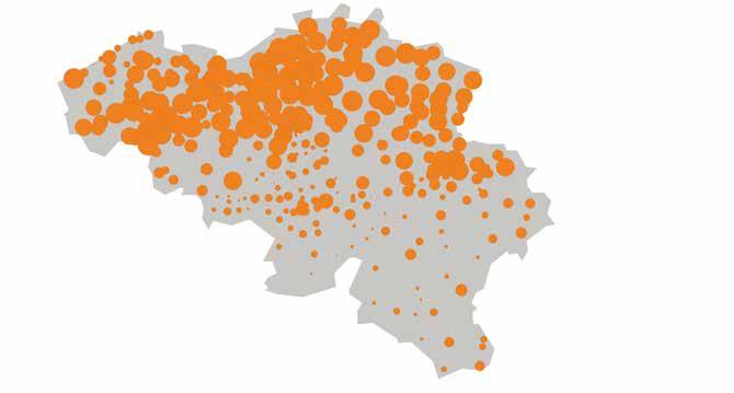
[FIGURE

Data for the end of the mentioned year 0.7 0.9 1.0 1.1 3.0 4.13.3 3.7 4.4 4.9 5.45.1 5.8 6.6 3.7 3.9 4.2 HIGH 360 MW/YEAR Yearly average increase CENTRAL 240 MW/YEAR LOW 120 MW/YEAR 1.2 1.5 1.7 1.9 2.1 2.3 2.5 The current distribution of wind onshore installations in Bel gium is depicted on Figure 3-22. Note that the locations are corresponding to substations (and not necessarily to the loca tion of the wind farms).

— ‘Low RES’: the commissioning of the second offshore wave was delayed, such that the partial commissioning with +700 MW was assumed to occur by 2027 (instead of 2026) and the full commissioning was assumed to occur by 2030 (instead of Figure2028).3-24 shows the historical increase in the installed capacity of offshore wind and the forecasted installed capacity considered in this study in the ‘CENTRAL’ scenarios and both sensitivities. 3-24]

[FIGURE 3-23]

The geolocation information is based on the closest substation connected in the Elia grid. Installations connected to the same substation are aggregated.

The size of the bubbles illustrates the size of the installed capacity. The bigger the bubble, the higher the capacity. Wind onshore is more spread around the country than PV.

3.3.3.3. Offshore Wind Belgium is a pioneer in the development of offshore wind energy: more than 2 GW of capacity has already been installed in the Belgian Exclusive Economic Zone (in the North Sea). A new area for potential wind farms (see Figure 3-23) shows planned developments in offshore wind over the next decade. The federal government agreement of 30 September 2020 confirmed an acceleration in the develop ment of offshore capacity, so that 4.4 GW should be installed by 2028. The pace of installation will depend on tender proce dures, permitting, construction time and associated permits required for onshore grid reinforcements.

Developments in offshore wind capacity follow the latest plan ning regarding offshore concessions and the government’s ambition in the ‘CENTRAL’ scenario. The installed capacity for offshore wind in Belgium is around 2.3 GW today and will increase with the ‘second offshore wave’, which is expected to occur in two two phases, according to the Federal authorities: — partial commissioning with + 700 MW by 2026 brining the installed capacity to 3 GW; — full commissioning of the second offshore wave by 2028, leading to 4.4 GW of total installed capacity. As requested by stakeholders and given the uncertainties regarding the planning, the following aspects were taken into account in the RES sensitivities:

Scenarios and data Adequacy & Flexibility Study 2022-2032 58 59

Nemo Link UNITED KINGDOM New area for potential wind farms Existing area for offshore wind farms THE NETHERLANDS

BELGIUMMOG

— ‘Low RES’: the growth of onshore capacity was limited to 120 MW per year (-50% compared to the ‘CENTRAL’ sce nario), reaching 4.2 GW in 2032. [FIGURE 3-21] — EVOLUTION OF INSTALLED ONSHORE CAPACITY PER SCENARIO IN BELGIUM [GW] 2010 20182014 2022 20272012 20202016 2024 20292011 20192015 2023 20282013 2021 20262017 2025 2030 2031 2032

04675321

FRANCE

3.3.3.2. Onshore Wind Figure 3-21 shows the historical increase in installed onshore wind capacity and the expected changes included in the WAM scenario from the NECP. This basis was used as a reference for the ‘CENTRAL’ scenario. The average forecasted development amounted to an increase of approximately 240 MW per year in the ‘CENTRAL’ scenario, reaching 5.4 GW in 2032. The assumptions taken in the two sensitivities regarding RES development are:

— EVOLUTION OF INSTALLED OFFSHORE WIND CAPACITY PER SCENARIO IN BELGIUM [GW] 048765321 2010 2011 2012 2013 2014 2015 2016 2017 2018 2019 2020 2021 2022 2023 2024 2025 2026 2027 2028 2029 2030 2031 2032 4.4 3.02.3 0.2 0.4 0.7 0.9 1.1 1.57 2.3 4.4 6.0 HIGHCENTRAL LOW Data for the end of the mentioned year

— EXISTING AND NEW AREAS FOR OFFSHORE WIND FARMS IN BELGIUM

— ‘High RES’: the onshore capacity was set to grow by 360 MW per year (+50% compared with the ‘CENTRAL’ scenario), reaching 6.6 GW in 2032;

[FIGURE 3-22] — GEOGRAPHICAL DISTRIBUTION OF THE BELGIAN ONSHORE WIND INSTALLED CAPACITY (SITUATION BEGINNING OF 2021)

— ‘High RES’: changes in offshore wind capacity were char acterised by an acceleration of the second offshore wave, such that a full commissioning was assumed in 2026. In addition, a third offshore wave (additional 1.6 GW of offshore wind capacity on top of the 4.4 GW) was predicted to occur by 2032, leading to 6 GW of capacity by 2032;

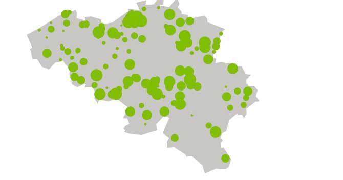
3.3.3.5. Biomass and waste

STORAGENonew storage

In this study, several types of storage capacities are considered and can be grouped together in four categories: 1) existing pumped-storage facilities in Coo and Plate-taille; 2) large-scale batteries (>100 kW), installed nowadays mainly to provide ancillary services; 3) small-scale batteries (<100 kW), usually called ‘home bat teries’ and of which the development in Belgium is very limited today; 4) electric vehicles operation in ‘vehicle-to-grid’ (V2G) mode where the battery can be used as storage.

as from

Data for the end of the mentioned year

WasteBiomass

The following capacity was considered:

The total future storage capacity (in the form of small- or largescale units and V2G) is based on the targets set by the ‘Energy Pact’ of 1.6 GW in 2030 (excluding pumped-storage) [EPA-1]. Although the total power capacity is mentioned in the ‘Energy Pact’, no breakdown or reservoir capacity is provided for. For this reason, additional assumptions were made to split the total capacity set by the ‘Energy Pact’ for large/small-scale batteries and V2G batteries. Those assumptions are explained below. Figure 3-26 shows the changes undergone by storage facilities included in this study.

The capacity for V2G is shared between ‘in-the-market’ and ‘out-of-market’ categories as part of it is assumed to react to market prices and another to local signals or to behind the meter optimisation. This division changes with time; the Figure 3-26 further details the quantified assumptions. [FIGURE 3-26] — EVOLUTION OF INSTALLED CAPACITY OF STORAGE FACILITIES IN THE ‘CENTRAL’ SCENARIO [MW] 3000350025002000150010005000 2030 2031 20322029202820272025202420232022202120202019 2026 1250 1388 1814 2372 2824 2824253253418253253418102311216 676676 520382173 9761 122412241224122412241224

The assumed storage capacity of the ‘CENTRAL’ scenario followed the Energy Pact targets. Several types of storage were modelled (pumped storage, large scale batteries, small scale batteries and V2G). Additional new capacities were taken into account if economically viable

In order to grasp the uncertainties around the development of storage in the form of batteries, 2 sensitivities were simulated: one sensitivity with an assumed additional 500 MW/1000 MWh of large-scale storage (togeth er with additional DSR: ‘DSRBAT-High’) and one sensitivity considering no new storage development after 2022 (together with no new DSR: ‘DSRBAT-noNEW’).

3.3.3.4. Run-of-river hydro Belgium has limited capacity in terms of run-of-river hydro electricity Those consist of small hydro units (installed along rivers) with the ‘biggest’ ones on the river Meuse. The NECP predicts that there will be a small increase with 151 MW in 2030 (compared with the 125 MW - at best - for 2022).

Pumped-storage Large scale storage (“in-the-market”)   Small scale storage (“out-the-market”)   V2G “in-the-market”   V2G “out-the-market”   Total

Scenarios and data Adequacy & Flexibility Study 2022-2032 60 61

3.3.4. STORAGE

Note that storage data is given for the end of the mentioned year. As these values are kept constant for the simulated period in this study, it corresponds to the capacity assumed on 1 September of each simulated winter (each year examined in the study runs from 1 September to 31 August of the following year).

[FIGURE

A linear interpolation (regular growth rate) until 2030 (NECP target) was considered for the target years between 2022 and 2030, followed by an extrapolation for 2031 and 2032. The capacity in 2032 was therefore estimated at 157 MW.

In this study, two kinds of units using biomass (e.g. wood pellets) or waste (e.g. incineration station) in Belgium were —modelled:largerunits which have a CIPU (Coordinating Injection of Production Units) contract; — smaller decentralised units which are usually connected to the distribution grid. A database covering all centralised and decentralised units is maintained by Elia and is updated monthly based on exchanges with DSOs and grid users. This also includes new projects that are being developed. This is used as basis to calculate the installed capacities for the different categories.

— Biomass and waste units without CIPU contracts were modelled in an aggregated way through profiles based on historical generation data. They account for 504 MW for biomass and 46 MW for waste-based. This information is based on the Elia database. More details on the dispatch of biomass and waste units without a CIPU contract based on a historical analysis is presented in Appendix G.2.

CENTRALHigh storage

These technologies are further split into two categories as defined in the ERAA methodology [ACE-2] – Article 4, 5(b) […]: — in-the-market batteries: which are large-scale battery capacities that are traded in day-ahead and intraday mar kets. In-the-market batteries shall be modelled similarly to pumped-hydro storage and shall be subject to the following constraints: maximum power, maximum energy storage, state of charge, charging/discharging efficiency; — out-of-market batteries: which represent small-scale bat teries typically managed behind the meter. Out-of-market batteries shall be modelled as peak-shaving units based on predefined peak-reduction ratios, which are a direct input to the demand prediction process.

— Biomass and waste units with CIPU contracts were mod elled on a unit per unit basis, by taking into account their own characteristics. They account for 273 MW for bio mass and 286 MW for waste These units were modelled with a partial ‘must-run’ level based on the observed level observed in historical generation data. Indeed, those units produce energy even in the case of low prices, which can be explained by support mechanisms (e.g. green certifi cates) or other underlying processes they supply (e.g. heat demand). It is important to note that this modelling choice can overestimate the real contribution of those units to ade quacy, since the historical analysis of generation data and prices shows that the units are not fully dispatched in case of (very) high electricity market prices. More details on the dispatch of individually-modelled biomass and waste units based on a historical analysis is presented in Appendix G.1.

The NECP (WAM scenario) considers an absolute decrease of the biomass capacity between 2020 and 2030 by 300 MW. This decrease is in line with the capacity considered in this study as the biomass unit in ‘Les Awirs’ closed in 2020 (75 MW) and as the closure of one large-scale biomass unit Rodenhuize is assumed after winter 2022-2023 (such as men tioned by ENGIE during the public consultation and agreed to be taken into account as part of the ‘CENTRAL’ scenario of this study in the ‘Comité de Collaboration’ - see also BOX 3-5 and Appendix L). A total of 1109 MW of biomass and waste generation was considered for Belgium in 2022 as shown on Figure 3-25. The assumed closure of Rodenhuize decreases the capacity to 904 MW from the winter of 2023/2024 onwards. 3-25] TOTAL INSTALLED BIOMASS AND WASTE CAPACITY AVAILABLE IN BELGIUM ASSUMED IN 2022 1109 MW of total installed capacity considered as available: 777 MW of biomass 332 MW of waste Herstal32MW non-CIPU65% non-CIPU14% closed February 2023

—

iGreen Power 20 BiostoomMW19MWBiopower18MWLangerbrugge50MW ISVAG 12 MW E-wood 22 MW Beveren Indaver 45 MW Beveren Sleco 41 MW Rodenhuize*205MW Schaerbeek45MW

CIPU35% CIPU86% Ipalle34ThumaideMW 16IVBOMW Ostende * Rodenhuize is considered as

In this study, small-scale batteries are assumed to be man aged behind the meter and are therefore included in the ‘out-of-market’ category. Large-scale batteries are assumed to react to the electricity market prices and are therefore included in the ‘in-the-market’ category.

[FIGURE

— EVOLUTION OF INSTALLED CAPACITY OF STORAGE FACILITIES IN THE ‘CENTRAL’ AND ‘E-DIGITAL ‘ SCENARIO [MW] 1000140012008006004002000 2025 2026 2027 2028 2029 2030 2031 2032 V2G “in-the-market”   V2G “out-the-market” Additional V2G capacity - “V2G EV”   Total Data for the end of the mentioned year e-digitalCENTRAL-EV V2G 70 636 1014 5071014507 253253318216 253253 102352

The total capacity for large scale batteries was assumed to reach 382 MW (with 764 MWh of reservoir) in 2025 and 676 MW (with around 1352 MWh of reservoir) in 2032

The current installed capacity of 1224 MW pumped-storage in Belgium (1080 MW in Coo 1 & 2 and 144 MW in Plate Taille) was considered for all time horizons, with a combined storage capacity of approximately 5800 MWh. Pumped-storage units are typically also used to provide ancillary services. Accordingly, in order to account for the provision of 'black start' services, the total storage capacity available for economic dispatch in this analysis was decreased by 500 MWh, reducing the available storage capacity available for economic dispatching to 5300 MWh A round-trip efficiency of 75% is used.

As indicated before, small-scale batteries are considered ‘outof-market’ and are not assumed to react to market prices. Indeed those are integrated directly in the hourly consump tion profiles for all the countries where such type of storage is taken into account (based on the definition from ENTSO-E). 3.3.4.3. Large-scale batteries

Pumped-storage units store energy in the form of gravitational potential energy of water. When economically sound, the water is pumped from one reservoir to another (situated above the first one). On the contrary, when economically interesting, the water is released from the uphill reservoir and generates electricity. The operating cycles (pumping and turbining) of pumped-storage units were optimised by the model, which determined the ideal moment to use those units based on the hourly market price (i.e. economic dispatch). In order to con sider the limited energy that can be stored, a reservoir volume was associated with each unit but also a round-trip efficiency.

The use of large-scale batteries was optimised by the model depending on the simulated market prices.

The rollout of small-scale batteries (i.e. residential/home bat teries) is assumed to be linked to number of PV installations in the ‘CENTRAL’ scenario. The expected development consid ered in this study was that each year, 0.5% of the PV installa tions will install a battery with a capacity of the size of the PV installation. The following assumptions about these batteries were also made: — an energy content of 3h (based on current and future expected average home-battery sizes) [TES-1]; — a roundtrip efficiency of 90%;

3.3.4.2.

Small scale batteries

Concerning the battery size, this one was increased compared to the previous study (from 1 to 2 hours). Indeed, eventhough historical measures have shown that the existing large-scale batteries in Belgium did not deliver their maximum capacity during more than 1 hour (when looking over the past three years), recent projects (such as one in Bastogne [EST-1]) have longer durations. In view of these elements, the assumption towards a duration of 2 hours for large scale projects instead of 1 hour was therefore used.

Note that one sensitivity with more large-scale battery (+500 MW) combined also with additional DSR capacity (+500 MW) was simulated (‘DSRBAT-High’) and one sensitivity keeping the same level of large-scale battery/DSR as for 2022 was con sidered. These sensitivities are explained in the demand side response section (see Section 3.3.5).

V2G are electric vehicles that allow bi-directional (dis)charging when connected to a bi-directional charger. In order to esti mate the amount of V2G capacity (the battery capacity that would be connected permanently to the grid and that would allow bi-directional charging), it was assumed that: — a certain amount of new EV registrations are capable of bi-directional (dis)charge and are connected permanently to a bi-directional charger; it was assumed that this will cor respond to 1% of new EV registrations in 2021 to 10% in 2030; — in order to calculate the amount of storage (kWh) and capacity (kW), a charger of 7kW and 4 hours storage were Fromassumed.thisvolume and capacity of storage, it was assumed that in 2021, 1% of the V2G amount is reacting to electricity prices and hence modelled ‘in-the-market’. The other 99% is considered as ‘out-of-market’ (and is therefore taken into account in the consumption profile following the ERAA meth odology). The percentage of the ‘in-the-market’ proportion was assumed to evolve up to 50% in 2030 (see Figure 3-27).

Finally, as described in Section 3.3.1.3, a sensitivity on additional digitalization of transport and heating electricity consumption (‘e-Digital’) is performed in this study. One of the levers used to assess the impact of the digitalization of transport electricity consumption is the penetratrion of V2G technology allowing bi-directional (dis)charging. In this sensitivity, it is assumed that the V2G capacity is doubled compared to the ‘CENTRAL’ scenario as illustrated in Figure 3-27. This additional capacity is assumed to be 100% ‘in-the-market’ and thus optimized by the model in the simulation performed. 3-27]

Given the ‘limited’ reservoir size of pumped-storage units in Belgium, they usually follow daily cycles: the reservoirs are filled during the night in order to be able to compensate for the peak demand occurring during the day. This cycle could change in the future, as more PV installations are installed, meaning it could be more beneficial to pump energy during the day (when PV produces the most energy). This was taken into account in the model with the economic optimisation of storage facilities. It is important to note that the planned increase of the res ervoir and the capacity of the Coo 1 & 2 units by 7.5% was not taken into account in the assumptions of this study. Indeed, the approval of this increase happened after the assumptions were freezed. This corresponds to around 80 MW increase of the turbining capacity and 425 MWh of additional reservoir capacity [ENG-1].

Large-scale batteries were quantified based on known pro jects that are being developed which include projections leading up to 2023. It was assumed that they have a roundtrip efficiency of 90%. No limitations in terms of the amount of charge/discharge cycles were considered (the utilisation is only limited by the available energy in the battery at a given time).

Scenarios and data Adequacy & Flexibility Study 2022-2032 62 63

3.3.4.4. Vehicle-to-grid (V2G)

3.3.4.1. Pumped-storage capacity

On this basis, the total capacity for small scale batteries was assumed to reach 170 MW (with 500 MWh of storage reservoir) in 2025 and 420 MW (with 1,250 MWh of reservoir) in 2032

Note that DSR data is given for the end of the mentioned year. As these values are kept constant for the simulated period in this study, it corresponds to the capacity assumed on 1 Sep tember of each simulated winter (each year examined in the study runs from 1 September to 31 August of the following year).

This study takes into account DSR reacting to price signals through shedding and shifting The DSR contracted for ancil lary services is also modelled in order to take into account its participation in the needed flexibility options to balance the grid. DSR volumes can be considered as distributed capacity that can be activated when prices rise above a certain level and for a limited time duration (depending on several con straints). It is important to note that while this category was called ‘Demand-Side Response’ in this study (based on the ERAA terminology), it can also include storage and even small scale generators (those not explicitly taken into account as generation units in the model such as emergency generators). Indeed the starting point to define the ‘demand response’ shedding volume is an assessment of ‘market response’. Note also that in this study, storage capacities are nevertheless con sidered in a separate category.

period]winterin[GWh/day 0.40.81.41.61.21.00.60.20.0 2030 2031 20322029202820272025202420232022202120202019 2026

Shedding Shedding is realised by grid users that can reduce part of their consumption when prices reach a certain level (called the ‘activation price’). This can also be realised by activating emergency generators.

Two sensitivities were performed on the ‘CENTRAL’ scenario based on the feedback provided by stakeholders in the public —consultation:‘DSRBAT-noNEW’: it is assumed that in this sensitivity no new DSR capacity (together with large scale batteries) is installed in Belgium after 2021. In other words, the capacity assumed for large-scale batteries and DSR shedding in all time horizons is set to 2021's volume; — ‘DSRBAT-High’ this sensitivity is performed post-2025 with additional capacity for DSR shedding capacity (max use of 4h, +500 MW) and large scale battery (max use of 2 h, +500MW) compared to the ‘CENTRAL’ scenario. The results of these sensitivities are summarised in Section 5.1.3.5. for pre-2025 and Section 5.1.5 for the impact post-2025.

In order to grasp the uncertainties around the development of demand side response 2 sensitivities were simulated: one sensitivity with an assumed additional 500 MW/ 2000 MWh of demand side response (togeth er with additional large-scale storage: ‘DSRBAT-High’) and one sensitivity considering no new DSR develop ment after 2022 (together with no new large-scale storage: ‘DSRBAT-noNEW’).

Load shifting consists of consumption that can be moved to another moment within the day (unique requirement set in the model). This kind of flexibility option can be used to opti mise the consumption profile in relation to electricity prices or other signals.

— EVOLUTION OF DEMAND SIDE RESPONSE VOLUMES PER YEAR IN THE ‘CENTRAL’ SCENARIO [MW] 300025002000150010005000 2030 2031 20322029202820272025202420232022202120202019 2026

Scenarios and data Adequacy & Flexibility Study 2022-2032 64 65 3.3.5. DEMAND SIDE RESPONSE

The starting point for assumptions on shedding capacity is based on the E-CUBE 2020 market response quantification (also used in the framework of the last strategic reserve vol ume assessment, see [ECU-1]). Based on this quantification covering the next 3 winters, an interpolation is performed with the 2030 ambitions proposed in the ‘Energy Pact’ which is the latest official information known in that respect. During the consultation process of this study, those were checked with the authorities and it was confirmed that no more up-to-date ambitions were available on the matter.

Max use of 1 hour Max use of 2 hours   Max use of 4 hours* Max use of 8 hours No limit Total * The volume for ancillary services is included in the `max use of 4 hours' category Data for the end of the mentioned year 1448 1521 1599 1682 1772 1863 1953 2044 2135 2226 2316 2407 2407 2407 Shifting

[FIGURE 3-29] — TOTAL SHIFTING VOLUME ASSUMED IN THE 'CENTRAL' SCENARIO

The DSR volume can be categorised in two categories as defined in the ERAA terminology [ACE-2] naming ‘explicit demand side response’ and ‘implicit demand side response’. Both are taken into account in this study throught the differ ent assumptions taken on demand-side response shedding, shifting but also with regards to storage.

CENTRALHigh DSR The assumed demand side response capacity of the ‘CENTRAL’ scenario followed the Energy Pact 2030 targets for demand side response. Demand shifting and demand shedding were both modelled. Additional new capacities were taken into account if economically viable.

[FIGURE 3-28]

For this study, as the goal is to assess whether the system can cope with the adequacy and total flexibility requirements, no distinction is made between flexibility provided through the TSO (i.e. ancillary services) and flexibility provided through the market (i.e. as DSR). In the ‘strategic reserve volume’ study, only the DSR participating in the energy market was modelled because the volumes contracted for balancing services were assumed to be unavailable for the day-ahead market. Such approach is also the one done in the MAF2020. In this study, the demand response is complemented with the balancing capacity volumes (ancillary services) procured by Elia from decentral capacity. These can contribute both to adequacy and flexibility.

Sensitivities on these assumptions are performed. Note that the model can also invest in new demand side response if economically viable (see Section 4.4 for more information).

The assumptions used in the ‘CENTRAL’ scenario are based the ‘Energy Pact’ targets for 2025 and 2030: — 0.5 GWh in 2025; — 1.5 GWh in 2030. As shown in Figure 3 29, it can be seen that the major increase of total shifting volume is mainly taking place after 2025 (i.e. from 2025 to 2030 for this study).

The results of these sensitivities are summarised in Section 5.1.3.5. for pre-2025 and Section 5.1.5 for the impact post-2025.

DSRNo new DSR Demand side response (DSR) is a crucial dynamic parameter when difficult situations occur on the electricity grid, especially under demanding conditions when adequacy problems arise. European policymakers (2009/72/EC and 2012/27/EC), national politicians and regulators are all striving towards the further development of DSR.

Fossil fuelLow CHP HP by Thermal@RiskCHP + 1000 MW - 1000 MW - 240 MW

In order to assess the impact of the use of CHP instead of heat pumps for heating, a sensitivity where heat pumps were replaced by CHP was simulated. Around 240 MW is considered as ‘at risk’ of closure in the coming years according to produc ers. A sensitivity considering this capacity as not available was performed.

3.3.6.1. Existing combined heat and power units

Scenarios and data Adequacy & Flexibility Study 2022-2032 66 67 3.3.6.

As requested by stakeholders, two sensitivities with higher (+ 1000 MW) and lower (- 1000 MW) combined heat and power capacity were simulated.

The ‘CENTRAL’ scenario for fossil fuel-based generation (CCGT, OCGT, turbojet and CHP) followed the known clo sures of thermal units These capacities were assessed in the economic viability assessment.

Fossil fuel thermal generation in Belgium is made of — combined cycle gas turbine (CCGT) units and open cycle gas turbine (OCGT) units, which are gas-fired power plants; — turbojets which can be compared to aircraft motors, using oil as fuel; — combined heat and power (CHP) units also called co-gen eration units, that generate electricity and another by-prod uct such as heat at the same time. In addition to those capacities, any type of capacity will be considered in the economic viability assessment The assess ment will consider all existing capacity (to check their eco nomic viability) as well as new capacities (to check whether they would be economically viable ‘in-the-market’). This is further detailed in Section 4.4.

The modelling choices to distinguish small-scale from large-scale capacities were confirmed by historical gen eration data analysis for Belgium. In addition, this analysis showed the following information (detailed results can be found in Appendix G):

i More details on historical generation data and correlation with electricity prices can be found in Appendix G.

CENTRALHigh CHP

Sensitivities As requested by stakeholders, several sensitivities were per formed on evolution of CHP capacity: — ‘CHP-High’: considers +1GW of additional capacity for CHP compared to the ‘CENTRAL’ scenario; — ‘CHP-Low’: considers –1GW of CHP capacity compared to the ‘CENTRAL’ scenario; — ‘CHP-HPbyCHP’: as requested by COGEN Vlaanderen, a third sensitivity was requested to study the link with Power-toHeat. In this sensitivity, it is postulated that the penetration of heat pumps assumed in the load profiles in the ‘CENTRAL’ scenario moves from the WAM to the WEM scenario (i.e. after 2025, see Section 3.3.1) and that the ’heat not served’ by these heat pumps (which represents around 65000 heat pumps) is produced by small-CHPs (it is assumed that the annual heat demand per household is 18200 kWh thermal following the assumptions provided by COGEN Vlaanderen).

Small scale generation’s maximum capacity factor is slightly above 60% confirming the approach chosen by Elia to model it with a profile based on historical generation data;

FOSSIL FUEL GENERATION

The ‘CENTRAL’ scenario for fossil fuels considers all existing capacities, unless a closure has been officially announced. It also takes into account new CHP capacities if those are being under construction (projects with a status ‘acquired’, ‘reserved capacity’ and ‘under construction’ are considered).

[FIGURE 3-30] — INSTALLED THERMAL CAPACITY IN BELGIUM Subject economictoviabilitycheck

BOX 3-4: HISTORICAL GENERATION ANALYSIS CONFIRMS MODELLING CHOICES BUT COULD LEAD TO AN OPTIMISTIC VIEW FOR ADEQUACY

— CCGT and OCGT units are never dispatched at their maximum available capacity which is explained by the need to account for balancing reserves (as today, part of the reserve capacity needs specified in Secton 4.5.3 are assumed to be covered with thermal generation);

— Some thermal units have minimum generation con straints, which are required to be taken into account in the model.

14.2 GW 12.0 GW NUCLEAR 7.9 GW Today D3 D1 D4T3T1D2 T2 CCGT/OCGT >30 y CCGT/OCGT 25<30 y CCGT/OCGT <25 y CCGT - CHPTurbojet CHP Biomass & waste

It can be observed that almost half of the CCGT/OCGT gener ation fleet in Belgium was installed more than 25 years ago.

Large-scale units: CHP units with CIPU contracts were modelled taking into account the ‘CHP credit’ approach as detailed in Section 3.6.8.2. which takes into account (by means of a reduction of the assumed variable cost) the additional revenues they get from other services (heat or steam). In addition, the CIPU units were modelled with a partial ‘must-run’ based on an historical analysis of generation data. More details on the dispatch of individually-modelled CHP units with CIPU contracts based on a historical analysis is presented in Appendix G.1. It resulted from the historical analysis that not all individually modelled CHP capacities are dispatched at full available capacity in case of (very) higher prices. Hence the modelling choice could be seen as overestimating the contribution to adequacy.

Small-scale units: CHP units without CIPU contracts were modelled in an aggre gated way through normalised profiles based on historical generation data and account for 1379 MW This already includes 100 MW of additional capacity compared to end 2020. This capacity was kept constant for the time horizon covered in this study. More details on the dispatch of CHP units without a CIPU contract based on a historical analysis is presented in Appendix G.2. As requested by stakeholders during the public consultation, a sensitivity with higher (+1 GW) and lower (-1 GW) CHP capac ity was also performed in this study.

The capacity of CHP CIPU units accounts for 1356 MW (including Zandvliet Power and Inesco which are CCGTs that are able to operate in ‘CHP’ mode). This capacity also includes new projects compared to the installed capacity end 2020. 50 MW of additional capacity was considered as from 2022. This capacity was kept constant until 2032 (no new projects known in the database as from 2022).

— Large scale CHP and biomass/waste units are never dispatched at their maximum available capacity nei ther. This is not taken into account in this study and could result in 100 to 350 MW over-estimation of contribution to adequacy of these technologies;

Existing CHP units were submitted to an economic viability assessment to determine their future availability based on their market revenues. In addition, new CHP capacities were also always considered in the economic viability assessment.

[GW] 1014161286420

Similarly to biomass, some CHP units having CIPU contracts are usually injecting in the high-voltage grid, while others are connected to the DSO grid. CHP units with CIPU contracts were modelled individually in this study, while CHP units with out CIPU contracts were modelled in an aggregated way with normalised profiles. The CHP capacity was based on the Elia database for centralised and decentralised units (maintained by Elia and updated monthly based on exchanges with DSOs and grid users). This database also includes new projects that are being developed. For CHP this typically shows an overes timation of the forecasted capacity in the short-term, hence it can be seen as an optimistic forecast for the first horizons of this study. Indeed, not all ‘acquired’ & ‘reserved capacity’ projects are commissioned in due time.

The results of these sensitivities are summarised in Section 5.1.5.4.

Jan2021 Jan2023Jul2021 Jul2023Jan2022 Jan2024 Jan2026 Jan2028 Jan2030Jan2025 Jan2027 Jan2029 Jan2031 Jan2032Jul2022 Jul2024 Jul2026 Jul2028 Jul2030Jul2025 Jul2027 Jul2029 Jul2031 Jul2032

The complete list of units can be found in the Excel file pub lished with this report. The list was consulted upon prior to the study (in November 2020) and was updated according to the feedback received by the producers. The total installed capac ity of thermal generation is shown on Figure 3-30. For the sake of completeness and in addition to the fossil based generation, the installed capacity of biomass/waste and nuclear were also added. The age of the CCGT/OCGT units was indicated as it will be a key parameter when considering their economic viability.

It should be noted that this capacity is still available at the time of writing this report and therefore not officially announced as closed by the producer.

THERMAL CAPACITY ‘AT RISK’ OF CLOSURE IN BELGIUM

OCGTTurbojet 116HamMW Zedelgem18MW Noordschote18AalterMW18MW Zelzate18MW Beerse 32 MW 18VoltaMW Angleur 4 128 MW Angleur 3 50 MW Cierreux18MW

NEW CAPACITY TO FILL THE GAP

3.3.6.2. Existing CCGT, OCGT and turbojets

BOXZeebruge18MW3-5:

The letter sent by ENGIE Electrabel can be found in Appendix L. 3.3.7.

The process of determining the new capacities which are via ble in the market is further described in the methodology Section 4.4.

Scenarios and data Adequacy & Flexibility Study 2022-2032 68 69

The installed capacity considered for CCGT, OCGT and tur bojets in this study was based on a consolidation of the gen erating capacity of units with CIPU contracts. The capacity considered for each unit is the capacity mentioned in the CIPU contract. This was also further submitted to public consulta tion and was adapted with the feedback received.

The latest information regarding official closures was also taken into account. The Vilvoorde CCGT is assumed to be available in CCGT mode (GT + ST) for the period 1/10/2021 until 31/03/2023, accounting for 360 MW. After that date, the steam turbine is therefore not considered and the unit will go back to an OCGT operation with 255 MW installed capacity. Vilvoorde Gas Turbine (255 MW) is due to definitively close on 31 October 2025. Moreover, a partial ‘must-run’ for some units was also imple mented in order to capture the observations made from his torical data, which could also be due to balancing reserves requirements. More details on the dispatch of CCGT and OCGT based on a historical analysis is presented in Appendix G.1.

KnippegroenDrogenbosMarcinelle413MW460MWVilvoordeST*105MW305MWRingvaart385MWSaint-Ghislain350MWAmercoeur451MWVilvoordeGT*255MW

[FIGURE 3-31] — TOTAL INSTALLED CCGT / CL / CCGT-CHP CAPACITY AVAILABLE ASSUMED IN BELGIUM IN 2022 4662 MW total installed CIPU capacity considered as available: 4138 MW of CCGT/CL 524 MW of CCGT-CHP i

Vilvoore ST (121 MW) will close in Oct. 2023 and Vilvoorde GT (255 MW) will close by Nov. 2025. ** Zandvliet and Inesco are categorised in CCGT-CHP to reflect their ability to operate in CHP mode. Those capacities are included in the CHP section CCGT/CL considered as available for all time horizons CCGT-CHP considered as available for all time horizons 39HamMW Herdersbrug480MW T-Power425MWZandvliet**Inesco**138MW386MW 470SeraingMW

Turbojets (together with OCGTs) are depicted on the Figure 3-32. Turbojets are oil-fired peaking units integrated in the electricity grid. They function like an aircraft jet engine. Those are individually modelled in the simulations. [FIGURE 3-32] — TOTAL INSTALLED OCGT AND TURBOJET CAPACITY AVAILABLE IN BELGIUM ASSUMED IN 2022 452 MW of total installed capacity considered as available: 294 MW of OCGT 158 MW of TJ i

Regarding thermal capacity, the ‘CENTRAL’ scenario was considering the official closures of Vilvoorde GT and Vil voorde ST as well as the assumed closure of Rodenhu ize (in-line with NECP with regards to biomass installed capacity). In the framework of the public consultation that took place for this study, Elia had requested producers to mention any thermal capacity that was ‘at risk’ of not being available in the coming years. In response to it, ENGIE Electrabel informed Elia by letter that the availability of some capacity is uncertain as from 2025 According to the producer, Elia should not rely on the following capacity in the framework of this study — a part of the turbojets fleet (ca 40 MW) because some of these installations are coming to the end of their operational lifetime and face ageing issues; — a part of cogeneration plants (ca 200 MW) because these CHP facilities are subject to contractual agree ments with industrial customers that may not be renewed.

A sensitivity ‘THERMAL@Risk’ including the information received was performed, with 240 MW of thermal capacity assumed unavailable as from 2025.

Depending on the adequacy results and the economic viability assessment, if a GAP (new capacity needed on top of all exist ing and new capacities assumed in the ‘CENTRAL’ scenario) is required to meet the reliability standard, new capacity will be assumed. This new capacity can be filled by the following technologies: — New CHP units; — New storage; — New demand side response; — New decentralized peaking units (gas engines…); — New CCGT; — New OCGT.

Figure 3-31 gives an overview of the installed CCGT and OCGT capacity. It also includes the CCGT having the ability to run in ‘CHP mode’. In addition to CCGTs, one unit (Knippegroen) of 305 MW burns blast furnace gas and recovers converter gas from the Arce lorMittal steel plant. The unit is usually referred as ‘Classical’.

This is the average amount of outage events that happen per year Average #FO = Average(# FO2011+...+ #FO2020)

3) The average amount of events (only used in the flexibility assessment)

— If the maintenance dates are known in the transparency platforms of the producers in the framework of REMIT (for the first winters analysed in this study), those are explicitly taken into account; — If the maintenance dates are not known yet or beyond the scope of REMIT, then a maintenance rate (in-line with the ENTSO-E common data) is used. The maintenance is then drawn by the model ex-ante the simulation.

Planned unavailability is taken into account the following way:

Concerning forced outages an analysis was carried out for each generation type (CCGT, gas turbine, turbojet, etc.), based on historical unplanned unavailability for the period 2011-2020 (i.e. 10 last years) and using the availability for generation units nominated in the day-ahead market. The available public data from ENTSO-E Transparency Data [ENT-4] was used for his torical years when available (i.e. only for 2015-2020 period).

The assumption taken in the 'CENTRAL' scenario is that elec trolysers are consuming electricity when RES or nuclear is the marginal technology in the system (under 20 €/MWh). Such assumption makes those devices not impacting the adequacy requirements calculated in this study. If electrolysers would also consume electricity during scarcity situations, adequacy requirements would then be increased by a similar amount of capacity assumed in the 'CENTRAL' scenario.

Belgian thermal generation units covered by a CIPU contract are modelled individually in the ANTARES model by taking into account planned unavailability (usually maintenance) and unplanned unavailability (usually caused by an unexpected malfunction).

In-line with Article 4 (6) g (ii) of the newly adopted ERAA meth odology, FCR and FRR estimations for future years were taken into account by deducting their respective capacities from the available supply, split amongst storage, demand side response and thermal generation. Indeed, as will be high lighted in Section 4.1.1, given that the market model used by Elia applies ‘perfect foresight’, it is not able to model the use of balancing reserves in relation with unforeseen imbalances. For this reason, if balancing capacity would not be taken into account as specified by the ERAA methodology, such kinds of models are providing an optimistic view on the adequacy requirements as the system is optimised knowing the exact future RES generation, demand and generation availability. For the future estimations of balancing reserves for Belgium, Section 4.5.3 provides the data taken into account in this study.

This is the average length of a forced outage (FO) expressed in days or hours Average FO duration = Sum(FO duration2011+...+FO duration2020 ) #FO over 2011→2020

While there is no official strategy nor targets for Belgium (yet), assumptions were taken for the future installed capacity of electrolysers in Belgium (and also in Europe – see Appendix N). The values taken in this study are assumptions based on known (pilot) projects. There is no guarantee that those would be developed in due time. As also stated in Section 2.9, those will allow first to decarbonize the existing hydrogen market, but also further achieve the decarbonisation of ‘hard-to-abate’ sectors.

Waste 1.5 1.0% 82 hours (around 3 days)

The average amount of events is particularly relevant for the flexibility assessment as it is important to cover unexpected outage events immediately after those occurred (fast flexi bility) and during intra-day (slow-flexibility). After day-ahead, these fall under the scope of the adequacy analysis, where the duration and the outage rate are used as relevant parameters (i.e. the time a unit is effectively in outage).

2) The average forced outage duration (used for adequacy)

3.3.10. POWER-TO-X

DC links (in each direction) 2.0 6.0% 168 hours (around 7 days)

BALANCING RESERVES TAKEN INTO ACCOUNT

Note that no maintenance is considered on individually mod elled units for Belgium during winter months (November to March) unless provided in the transparency platform of the producers (or bilaterally).

[FIGURE 3-33] — FORCED OUTAGE PARAMETERS (OVER 2011-2020)

1) The forced outage rate (used for the adequacy assess ment) This consists of the amount of unavailable energy due to forced outage (FO) divided by all the other moments when the unit was available and in forced outage.

The resulting outage characteristics for each technology are summarised in Figure 3-33. No planned maintenances are assumed during the winter period (November to March) in the framework of this study For new-built capacity (GT, CCGT, turbojet and CHP), the forced outage rate used by ENTSO-E for European adequacy studies were used.

3 different forced outage parameters are needed for the cur rent study: The definitions of the first two parameters are used in ade quacy studies and are in line with the ENTSO-E methodology.

The HVDC links forced outage rate is set to 6% in order to keep consistency with European studies performed at ENTSO-E level [ENT-1].

3.3.9. FORCED OUTAGES AND MAINTENANCE

GT 3.1 9.2% 201 hours (around 8 days)

CHP 3.8 7.0% 124 hours (around 5 days)

Nuclear 1.6 3.7% 240 hours (around 10 days)

The third one is only used for the flexibility assessment.

Scenarios and data Adequacy & Flexibility Study 2022-2032 70 71

CCGT 7.0 8.4% 101 hours (around 4 days)

Category Number of FO per year Average FO rate [%] Average duration of FO rate [hours]

3.3.8.

Pumped storage 3.0 4.5% 181 hours (around 8 days)

Average FO rate = (FO energy 2011→2020 ) FO energy 2011→2020 + Available energy 2011→2020

As a novelty and following stakeholder feedback, electrolysers were added to the market model used by Elia. Electrolysers should be seen as an additional load for the electricity system. This is not taken into account in the total consumption figures presented in Section 3.3.1.

It is assumed that there would be 210 MW of electrolysers connected to the electricity grid in 2025. This would increase to 510 MW in 2030. A linear interpolation between those two values is assumed for the years in-between.

TJ 2.0 3.6% 98 hours (around 4 days)

Scenarios and data Adequacy & Flexibility Study 2022-2032 72 73 3.3.11. SUMMARY TABLE Figure 3-34 summarises the assumptions that were used for the ‘CENTRAL’ scenario in this study. These assumptions on electricity demand and electrification, demand side response, storage, renewable energy sources and thermal generation were described in details in Section 3.3. [FIGURE 3-34] — SUMMARY OF ASSUMPTIONS FOR BELGIUM IN THE ‘CENTRAL’ SCENARIO 2022 0.1Mio1.0%86.801.70.21.20.26.13.02.30.121.14.93.04.40.50.16 0.144.44.49.80.90.148.03.72.30.9 0.1511.04.94.40.9 0.1612.25.44.40.9 1.21.10.61.2 1.61.2 1.61.2 2.21.10.51.9 2.41.5 2.41.5 0.2Mio1.4%88.90.21 1.0Mio2.7%92.80.39 1.4Mio3.6%95.30.51 1.8Mio4.5%96.50.57 2025 2028 2030 2032 Growth rates based on economic projections from the Federal Planning Bureau and additional electrification based on NECP 0 Possibility to invest in any new capacity if viable (EVA) Possibility to extend lifetime of existing units if viable (economic viability assessment)electrificationDemandandDemandSideResponseRESThermalgenerationNewcapacityStorage Energy Economicefficiencygrowth Amount of electric vehicles Heat Pump (DSM,(incl.PumpedShedding*penetration[GW]SolarNuclearOffshorewindOnshorewindHydroRoRstorage[GW]TotalDemandelectrification)[TWh]Electrolysers[GW]Shifting[GWh/day]Biomass+WasteCHPExistingCCGT-CHP**ExistingCCGT/OCGTTurbojetsNewcapacityTurbojets,CCGT,OCGT,Storage,...) * including ancillary services volume ** Zandvliet and Inesco are categorised in CCGT-CHP to reflect their ability to operate in CHP mode Small, large and V2G batteries [GW]BelgiumforassumptionsKey [GW][GW] 0.164.44.90.5 0.160.52.24.1 Data for the end of the mentioned year

The 27 other European countries considered in this study are modelled with the same granularity as Belgium (generation units, storage facilities, renewables, consumption, demand side response,…).

An overview of the different reference scenarios and sensi tivities is provided in Figure 3 35. The starting point for deter mining all reference scenarios and sensitivities was the latest publicly available ENTSO-E dataset collected among TSOs. This dataset reflects the best estimate provided by the relevant TSOs at the time of the data collection, which occurred at the beginning of 2020 (in the framework of the MAF2020 study).

— ‘UK-not2BE’ and ‘UK-not2EU’ sensitivities, related to uncer tainties regarding the cross-border availability of links to the UK (see Section 3.4.6.2);

For both central scenarios, the economic viability of assumed capacities was verified.

— ‘EU-noCRM’: this reflects a scenario that excludes mar ket-wide capacity mechanism revenues, so assuming that no market-wide capacity mechanisms exist in Europe.

— ‘XB-Delayed’ related to the risks of delays in grid develop ment abroad, e.g. due to the introduction of the minRAM (see Section 3.5.8.2);

— ‘EU-lessCoal’ sensitivities related to the risks around an acceleration of the coal phase-out driven by higher carbon prices (see Section 3.4.6.3).

Figure 3-35 illustrates the process followed to create the 3 main scenarios used throughout the study.

As required by EU Regulation 2019/943, the national resource adequacy assessment must contain the reference central scenarios as referred to for the European resource adequacy assessment. Those scenarios shall include, amongst other things, an economic viability assessment of generation assets.

While the probability of the simultaneous occurrence of those risks can be deemed quite low, an analysis of historical infor mation shows that it is prudent to account for these risks. To this end, an additional scenario was defined by selecting a single sensitivity that was deemed to be representative of the foreign risks identified:

— ‘XB-RAM’ sensitivities, related to the minimum margins given to the market by each TSO and the risks around it (see Section 3.5.8.1);

The dataset was also complemented with the latest known public information and with more recent national studies when available.

While the nuclear and coal installed capacities are generally driven by national policies, the gas-fired capacity considered in this dataset results from assumptions made by each TSO.

— ‘FR-NUC’ sensitivities, related to the actual short notice availability of French nuclear generation in the market (see Section 3.4.6.1);

While those scenarios can be deemed to reflect a possible view of the future parameters of the European electricity system, it could be argued that some of the assumptions reflect a rather optimistic view on the future system, which doesn’t account for specific risks related to uncertainties over which Belgium has no control. The impact of such risks is quantified through several sensitivities related to the availability of capac ities abroad or to the availability of cross-border exchange capacities at times of system stress. Generally, these risks share the trait of only becoming apparent close to operational time frames no longer allowing investors to fully anticipate their effects, and can therefore be referred to as ‘unpredictable short notice events’.

— ‘EU-SAFE’: this reflects a scenario which takes into account short notice risks that are beyond control of Belgium. The selection of the sensitivity which will be assumed as repre sentative of the list of risks is discussed in the results (see Section 5.1).

3.4. European scenario and sensitivities

The methodology for the European resource adequacy assess ment, as adopted by ACER, further specifies that two cen tral reference scenarios are to be defined; one with capacity mechanisms across Europe and the other one without such capacity Consequently,mechanisms.forthisstudy, two scenarios were explored:

— ‘EU-BASE’: this reflects a scenario which takes into account already approved market-wide capacity mechanisms in France, Great Britain, Poland, Italy and Ireland (see Section 2.6) and assumes that these will be in place until the end of this study’s timeframe;

As described above, several sensitivities will be applied to reflect uncertainties on the availability of foreign capacities in the system:

Since the collection of the MAF2020 data, which took place at the beginning of 2020, several national studies and official announcements have been published, which provide updated assumptions for certain countries. Adaptations were made to the initial dataset in order to reflect these updates. Information regarding the sources used to carry out these adaptations is included in the section which outlines the final assumptions for the neighbouring countries.

DISCLAIMER (as written in the MAF2020 study):

Scenarios and data Adequacy & Flexibility Study 2022-2032 74 75 [FIGURE 3-35] — EUROPEAN SCENARIO FRAMEWORK OF THE STUDY

* The MAF2020 dataset only included 2025 & 2030 while this study covers a larger time horizon. Following the disclaimer set in the MAF2020, the data should be taken with care. In addition, this study integrates more recent information from other countries and uses the ERAA methodology to build the scenario framework.

UK-not2EU/BEXB-DelayedXB-RAMFR-NUCEU-LessCoal

As explicitly mentioned in a disclaimer about the published MAF2020 study (see also BOX 3-6), the MAF2020 analysis did not include any economic viability or feasibility checks on the inputs provided. This leads to the conclusion that the MAF2020 results (and therefore also the input data upon which it is based) can be deemed as presenting an optimistic view of the European adequacy situation, given the combination of new capacities assumed to be introduced throughout Europe for the analysed time horizons. In addition the MAF2020 study only simulated two time horizons: 2025 and 2030, while this study covers annual assessments for the years running from 2022 to 2032 (inclusive). Some data is therefore not available in the MAF2020 dataset.

Resultingscenarios EU-SAFE EU-noCRM Additional risks accounted for abroad

Consequently, the MAF 2020 cannot and should not be used for the purposes meant in the CEP and ERAA, namely assessing the need for the introduction of capac ity mechanisms or providing the basis for national ade quacy assessments.” […]

Applying

— The collection of the input data and the scenarios used do not follow the CEP requirements;

— The MAF 2020 is not an ERAA report;

BOX 3-6: MAF2020 AND ASSOCIATED DISCLAIMERS

Resultingscenario→→ As from 2025, countries with a market-wide capacity mechanism at their nationalstandardreliability Economic viability check that no addi tional new capacities are viable marketassessmentEconomicabroad**viabilitywithoutwideCRMsinEurope

The MAF2020 dataset is based on the final National Energy and Climate Plans (NECPs) of the concerned countries. Each country’s data included in the MAF2020 was submitted by each TSO based on the latest known policies and national trends. Therefore, most of the latest policies are included in the MAF2020 dataset.

** If the economic viability check in countries with a CRM shows that all capacity is viable without additional support (or enough new capacity is viable), it will add it to the system. If not, the CRM additional revenues are kept so the country remains at its reliability standard.

BEEU a compliant methodology with the ERAAStarting

EU-BASE

However, the 2020 Mid-term Adequacy Forecast Report (hereinafter “the MAF 2020”) and its findings should not be interpreted in light of the CEP for the following reasons:

— The methodology followed does not yet comply with the important elements of the CEP/ERAA framework which are notably, but not limited to, an economic viability assessment and the implementation of the flow-based methodology.

“Regulation (EU) 943/2019 (hereinafter “Electricity Regu lation”) and Regulation (EU) 942/2019 (hereinafter “Risk Preparedness Regulation”), as part of the Clean Energy Package (CEP) in combination with the European Resource Adequacy Assessment (ERAA) methodologies as approved by ACER on 2 October 2020, have introduced significant changes to the ERAA’s future role. In particular, under the CEP, the ERAA will be the key tool in the detection of adequacy concerns at a European level and the related potential introduction of capacity mechanisms.

→

→

The MAF is a pan-European monitoring assessment of power system resource adequacy of specific years up to 10 years ahead [ENT-1]. The assessment was carried out for two target years, namely 2025 and 2030. The results of the MAF2020 should not be interpreted nor used under the new legal framework of the Clean Energy Package.

ExistingConsultedMAF2020*pointdataNationalstudiessupply&firmprojectsPublicinformationPublicinformation

The MAF2020 dataset was the starting point for determining the assumptions regarding the evolution of the installed gen erating capacities and the electricity demand for the countries in the simulated perimeter. This dataset is the most up-todate available dataset collected by ENTSO-E. It was published in December 2020 and is publicly available via the ENTSO-E website for the target years simulated in the MAF2020 study.

3.4.1. INITIAL DATASET

In order to create the ‘EU-BASE’ scenario, the countries with a market-wide capacity mechanism were calibrated to their reli ability standard by iteratively adding or removing generation capacities in the relevant countries. Such a process ensured that those countries respect their reliability standard (which is the intended objective of their capacity mechanisms) and that additional capacities which are not required to respect the standard do not benefit from capacity mechanism rev enues. This verification was applied for all time horizons as from 2025, where REMIT data on the generation fleet is not yet available. For the first step, a detailed view of adequacy metrics (LOLE) was required and time-consuming adequacy simulations were performed.

The sensitivities related to these short notice uncertainties abroad are defined both in this section and in the section on cross-border exchange capacities. The sensitivity selected for the EU-SAFE scenario as representative of the different risks is the ‘FR-NUC4’ sensitivity. In Chapter 5, the adequacy results for Belgium for these different sensitivities are presented, jus tifying the choice of the FR-NUC4 sensitivity.

[FIGURE 3-37] — ASSUMED FUTURE EVOLUTION OF COAL/LIGNITE AND NUCLEAR CAPACITY IN THE SIMULATED PERIMETER 2021 2022 2026 20302024 2028 20322023 2027 20312025 2029 capacityInstalled 200250150100500

Solar PV  Wind Onshore  Wind Offshore

Secondly, an economic viability verification is performed for the countries without market-wide capacity mechanisms to determine whether additional new capacities would be viable in the market. If additional new capacities were deemed to be viable (on top of the already assumed existing and new capac ities from the initial dataset) according to the methodology defined in Section 4.4, those capacities were added to the respective country’s assumptions. In order not to complicate the process, and to avoid iterations of the first time-consuming step, no assessment was performed regarding existing or new capacities already assumed in the initial dataset that would not be viable in the market; those capacities were therefore left untouched. It is to be noted that this simplification might have led to an optimistic view of future available capaci ties in Europe, potentially leading to an underestimation of potential adequacy concerns. Within the framework of this study, this risk is deemed to be acceptable. EU-noCRM

Scenarios and data Adequacy & Flexibility Study 2022-2032 76 77 3.4.2. DETERMINATION OF THE REFERENCE CENTRAL SCENARIOS EU-BASE

Figure 3-36 highlights the countries on a map with the LOLE criteria which were respected in the ‘EU-BASE’ scenario. Note that some countries have strategic reserves in place to guar antee their adequacy. As these capacities are considered to operate out-of-market as last-resort solutions when a national scarcity situation occurs, these strategic reserves cannot be relied upon by other countries. The results of the market sim ulations were not impacted as these strategic reserves are supposed to be dispatched after the market has depleted all of its in-the-market resources and de facto reaches the price cap. From a model perspective, it did not impact the flows or the market prices.

Europe is currently going through important changes regard ing its available thermal capacities. Several European countries – including Belgium, Germany, Switzerland and Spain – have decided to phase out their nuclear power plants. Nuclear clo sures are also being planned in France and United Kingdom, although not the entire European fleet is expected to be closed and some new nuclear projects are also being developed.

3.4.3. DETERMINATION OF THE ADDITIONAL 'EU-SAFE' SCENARIO EU-SAFE

Many European countries are planning to decommission their coal and lignite power plants in order to reach net-zero emis sions by 2050 as discussed in Chapter 2. Several countries have now announced dates for the phase-out of such plants and when looking at the yearly capacity evolution, more than 70 GW is expected to be decommissioned between 2021 and 2032, the last year covered by this study. After 2030, remaining coal generation is only assumed in Germany and some Eastern European countries.

[FIGURE 3-36]

Data for the end of the mentioned year x 3.7 x 1.7 x 2.5

The determination of the ‘EU-noCRM’ scenario started with the same initial dataset, upon which a full economic viability assessment was performed. In this procedure, given the defi nition of the scenario which excludes capacity mechanism revenues, the simulation of adequacy metrics is not required, and no check with respect to the reliability standards has to be performed. As such, capacities were added or removed in the system up to the point where every monitored capacity present in the market was economically viable, and no addi tional capacity would be viable.

In addition to official targets, coal and lignite closures could be accelerated with higher carbon prices putting the economic viability of the units at risk. This is reflected in the ‘EU-lessCoal’ sensitivity (Section 3.4.6.3).

— COUNTRIES WITH A MARKET-WIDE CAPACITY MECHANISM ARE KEPT AT THEIR RELIABILITY STANDARD 3h 3h 3h3h 8h

The ‘EU-SAFE’ scenario was created by applying an additional sensitivity to the ‘EU-BASE’ scenario. The goal of this scenario is to reflect a realistic view on additional uncertainties abroad beyond Belgium’s control which could significantly impact the adequacy situation in Belgium. Indeed, given the high dependency on imports for Belgium (as will be also illustrated in the results), any event happening abroad can have a signif icant impact on the adequacy requirements of the country.

Nuclear  Hard Coal & Lignite Figure 3-37 illustrates the expected installed capacities of coal, lignite and nuclear in the coming decade over the sim ulated perimeter in the ‘EU-BASE’ scenario. Around 90 GW of thermal capacity of nuclear and coal/lignite is expected to close between 2021 and 2032. This comes on top of the already decommissioned nuclear and coal/lignite capacity prior to 2021. As for renewable energy sources the capacity considered in this study for the simulated perimeter is expected to at least double by 2032 This capacity is based on the MAF2020 data set, but was updated for the short-term (based on the most recent historical data and national studies) and for the last two years (those data were not collected by ENTSO-E). The same annual growth rate as the last year available from ENTSO-E (2029 to 2030) has been considered for the last 2 years. For off shore wind, existing capacities and future ambitions were also updated based on public announcements and WindEurope 2020 dataset [WIN-1]. Belgium's neighbouring countries are further detailed in the next sections. [FIGURE 3-38] — RENEWABLES ARE EXPECTED TO DOUBLE IN INSTALLED CAPACITY BY 2032 2021 2022 2026 20302024 2028 20322023 2027 20312025 2029 capacityInstalled 4008009007006005003002001000

3.4.4. KEY TRENDS FOR THE 'EU-BASE' SCENARIO

Data for the end of the mentioned year - 7020GWGW

Figure 3-39 gives an overview of the installed nuclear capacity and expected evolution in the coming decade. Decided in 2007, the commissioning date of the new nuclear reactor ‘EPR’ (Réacteur Pressurisé Européen) in Flamanville has been postponed several times. The hypothesis used in this study for this reactor is based on the assumptions of RTE. It is apparently likely that the reactor will be commissioned in 2023 (the latest official press release from EDF on the commission ing date dates from October 2019). According to [RTE-1], the reactor should be partially available during winter 2023-2024.

3.4.4.1. France The data for France has been updated based on the latest Bilan Prévisionnel from RTE published in 2021 [RTE-1]. Nuclear The French generation fleet is mainly composed of nuclear capacity which accounts for the largest share of electricity generation. The French nuclear fleet is ageing. Built in the late 60s, Fessenheim’s reactors were the first nuclear units to close in 2020. The French ‘Programmation Pluriannuelle de l’Ener gie’ (PPE) plans the closure of 14 nuclear reactors by 2038 [PPE-1], with two reactors to close by 2027/2028 followed by the 12 others between 2029-2038. A scenario with one reactor closing per year as from 2027 is therefore considered. There is however a risk that the French government asks for the shut down of two reactors already in 2025-2026 (also in-line with the decision of the PPE). This risk is not integrated in the ‘EU-BASE’ scenario of this study but can be accounted for as an additional risk covered by the sensitivity considering the unavailability of additional nuclear units in France (‘FR-NUC’).

Other thermal capacities Besides nuclear, there are also coal, oil and gas-fired units in France. The last coal units in France are considered to be closed by 2022 [RTE-1] and the government has pledged not to build new gas capacities [PPE-1]. Note that the Lan divisiau CCGT currently under construction is considered to be commissioned prior to the horizon analysed in this study. As for other countries with a market-wide CRM, the result ing gas-fired capacity is the result of the process followed in the ‘EU-BASE’ scenario that verified the economic viability of existing and new capacities. RES The RES capacities assumed for France are in line with the lat est RTE Bilan Prévisionnel of 2021 where increases in onshore wind and PV are foreseen. An increase in offshore capacity is also foreseen with the first farms to be commissioned for the first winter analysed in the present study. For other assump tions and more details, the interested reader can refer to the French adequacy report of RTE [RTE-1].

Scenarios and data Adequacy & Flexibility Study 2022-2032 78 79

[FIGURE 3-39]

— INSTALLED NUCLEAR CAPACITY AND EXPECTED COMMISSIONED POWER PLANTS IN FRANCE IN 2021 Gravelines5.4GW 2.9ChoozGW Cattenom5GW Flamanville2.6GW 2.6PenlyGW Dampierresur-Nogent-Seine2.6GW3.6GWBelleville2.6GWLaurentSt-1.8GWFlamanChinon3.6GWPaluel5.2GWville1.6GW Fessenheim1.8GW 2.9CivauxGW Le3.6BlayaisGW St2.6AlbanGW 3.6BugeyGW Tricastin2.6GWGolfech2.6GW 3.6CruasGW Total of 56 reactors in service spread over 18 sites Power plants commissionned Power plant in construction Power plant closed [GW] 60655550 EPR commissioning 1 unit per year is expected to close according to the French PPE 2022 2023 20282026 20312024 20292027 20322025 2030 Source: [BNE-1] [FIGURE 3-40] — EVOLUTION OF INSTALLED CAPACITY ASSUMED IN THE 'EU-BASE' SCENARIO FOR FRANCE 2022 20302025 20322028 12.9 21.2 35.1 41.1 47.1 60.6 62.2 60.4 58.6 56.8 [GW] 20.50.5 25.92.9 33.24.6 36.85.9 40.56.7onshore Capacity assumed at the end of the mentioned year offshore 13.3 10.7 10.7 10.7 10.7

The summary table for France can be found in Figure 3-40. Electricity consumption The electrical load for France has been updated based on the last estimations of RTE used in its national study [RTE-1]. The electricity consumption is expected to reach last years’ level by 2025 followed, by a smooth increase based on several factors, namely the evolution of electric vehicles, electric heatings in buildings and electrolysers (power-to-X). These assumptions imply a lower consumption on the short term than foreseen in MAF2020 or in the previous Belgian ‘10-year adequacy and flexibility study’ of June 2019.

The availability of the French nuclear fleet follows the data from the transparency platforms of the producers in the framework of REMIT for the years where such data is availa ble. In the absence of data, the average over the past 10 years is used for the ‘EU-BASE’ scenario. The average over the past 10 years can be clearly seen as ‘optimistic’ when looking at the most recent 5 years of French nuclear availability. Given the age of the units, the life-time extension works and the fact that the expected unavailability of the nuclear fleet is usually under-estimated by the French nuclear producer, this risk is integrated into the ‘EU-SAFE’ scenario with a sensitivity on the French nuclear availability during winter with 2, 4 or 6 nuclear units considered as unavailable (‘FR-NUC’ sensitivity). A more elaborated analysis can be found in Section 3.4.6.1.

The next year, a long planned outage is foreseen for a first complete inspection and the replacement of the tank cover. A full availability is considered as of 2025.

Scenarios and data Adequacy & Flexibility Study 2022-2032 80 81

While the public consultation is still ongoing for Bradwell B [BRA-1], the application process for Sizewell C has already started [EDF-3] and it is then possible that after around 10 years of construction, the unit will start running by 2032. Therefore, Sizewell C is considered available in this study as of winter The2032-33.MAF2020 included a large amount of new gas-fired capac ity to be commissioned as from 2025 (5.5 GW). These projects are not confirmed, nor under construction yet and would only be under the condition that they would earn a future capacity contract. As for other countries with a market-wide CRM, the resulting gas-fired capacity is the result of the process followed in the ‘EU-BASE’ scenario that verified the economic viability of existing and new capacities while keeping countries with a market-wide CRM at their reliability standard. RES Great Britain is a front runner in wind energy with the high est installed wind offshore capacity in Europe. In this study, offshore wind capacity was assumed to double from 2022 to 2032 and to reach nearly 30 GW in 2032. Onshore wind and solar capacity was continuing to grow to reach respectively 16.2 GW and 17.8 GW in 2032.

3.4.4.2. Great Britain British data has been updated with recent announcements regarding coal and nuclear evolutions. Great Britain had initially planned a complete coal phase-out by 2025. British government now ambitions to reach this objec tive by October 2024. With several closures announced [BNE-2], coal capacity in Great Britain will drop from 10.6 GW beginning 2020 to 2 GW by end 2022 as shown on Figure 3-41, with Rat cliffe-on-Soar remaining the only coal-fired power station that will be operated in Great Britain until the complete phase-out. The nuclear fleet in Great Britain is ageing and the decommis sioning of nuclear units will start in 2022 according to EDF who is running all the nuclear units in Great Britain [EDF-1]. The first unit to stop is Hunterston B in January 2022 followed by Hinkley Point B in July of the same year. By 2024, a decrease of 4.4 GW of nuclear capacity is expected. By 2030, an extra 3.6 GW will be decommissioned. By 2030, it is an extra 3.6 GW that will be decommissioned. Note that the power plant Dungeness B is considered in operation until 2028 in this study, but at the time of writing this report, it is not clear if it will produce again after being on maintenance for several years. EDF has indeed officially announced that all scenarios for Dungeness B were being studied, including an earlier closure [EDF-2]. Regarding new built power plants, the under-construction power plant of Hinkley Point C should start generating power by 2026. EDF is also planning to build two other new nuclear power plants, Sizewell C and Bradwell B, for the early 2030s with no official starting date.

FIGURE 3-42] — EVOLUTION OF INSTALLED CAPACITY ASSUMED IN THE 'EU-BASE' SCENARIO FOR GREAT BRITAIN 2022 20302025 20322028 14.3 15.0 15.9 16.9 17.8 2.07.1 3.6 7.0 4.6 7.9 [GW] 14.013.0 14.419.0 23.515.3 26.215.7 28.916.2onshore Capacity assumed at the end of the mentioned year offshore 38.9 37.4 32.4 35.7 32.7 [FIGURE 3-41] — INSTALLED COAL AND NUCLEAR CAPACITY IN GREAT BRITAIN, EXPECTED DECOMMISSIONNED AND COMMISSIONNED UNITS IN 2021 HinkleyHunterston1GWPointC3.3GW BradWell B 3.2 GWTornessDungenessB1GW1.2GWHeysam1.2GWFiddlersFerry1.9GW Cottam2GWWestBurton A 1.9 GW HeysamTorness1.2GW21.2GW BurtonWest A 1.9 GW Ratcliffe-on-Soar2GW AlberthawHinkleyPointB1GW1.5GW Sizewell C 3.2 GWSizewell B 1.2 GW Coal assumedunitstobe decommissionned by Nuclear assumedunitstobe decommissionned by Nuclear assumedunitstobe commissionned by 2020 2022 2022 20302024 2032 2024 2028 2026 2035 no date

3.4.4.3. Germany As the nuclear phase-out in Germany is due to be completed by 2022 (there are currently six units left to close), no German nuclear capacity was considered in this study.

It is important to note that there are different capacity reserves in Germany for different purposes: ‘capacity reserves’, ‘grid reserves’ and ‘climate reserves’. As these capacities are ‘outof-market’ or contracted for other purposes, they cannot be relied upon by other countries for their security of supply.

— The ‘capacity reserve’ is ‘out-of-market’ capacity to be used by German TSOs after the market clearing in order to safe guard German adequacy in the coming years;

— The ‘grid reserves’ (or ‘Netzreserves’ in German) are con tracted by the German TSOs to cope with congestion management and is not dispatched on the energy market. This capacity may also participate in the ‘capacity reserve’ tender;

— The ‘climate reserve’ (or ‘Sicherheitsbereitschaft’ in Ger man) is a temporary measure where several power units are progressively taken out of the market for a financial compensation. Those units are therefore temporarily shut down but should be available in case of need and will be finally shut down after four years in this mechanism. This mechanism is planned to be stopped in 2023.

As for gas-fired capacity, there is a foreseen increase of 7 GW considered in the study based on the MAF2020 dataset. This increase is mainly linked to assumed new CHP units in Ger many that would partially compensate the coal and nuclear phase-outs although there is no guarantee that those would be developed in the future.

RES Renewable energy sources in Germany were assumed to fol low important increases in the time horizon covered in this study. Solar installed capacity went from around 60 GW in 2022 to 100 GW in 2032, while offshore wind capacity is assumed to triple and to reach 25 MW in 2032. The onshore wind capacity considered in 2032 was 84 GW. Figure 3-44 gives an overview of the installed capacities taken into account for Germany.

[FIGURE3-44] — EVOLUTION OF THE INSTALLED CAPACITY ASSUMED IN THE 'EU-BASE' SCENARIO FOR GERMANY 2022 20302025 20322028 61.0 76.9 87.7 95.1 103 30.0 27.2 22.2 17.0 14.2 [GW] 62.78.7 72.711.7 79.317.3 82.422.3 25.484.1onshore Capacity assumed at the end of the mentioned year offshore 33.3 36.0 37.4 38.9 40.5 [FIGURE 3-43] — OVERVIEW OF HARD COAL / LIGNITE POWER PLANTS AREAS IN GERMANY Source [BNE-3] HardLignitecoal 24plantsplants5 plants 4 plants 12 plants 36 plants 5 plants 12 plants 7 plants 7 plants[GW] 3020100 30 GW of hard coal and lignite spread over 119 power plants, reduced to 17 GW by 2030 2022 2023 20282026 20312024 20292027 20322025 2030

Germany has also committed to a complete hard coal and lignite phase-out by 2038 at the latest (with an option of an earlier complete phase-out in 2035). The plan is for such capacity to shut down gradually (including the units commis sioned over the last decade), with compensation payments made to the operators. Nuclear and coal phase-out planning were already included in the MAF2020 dataset for Germany, leading to the same assumptions being taken into account for this study. There could be small differences in the future depending on the coal exit tenders outcomes. Figure 3-43 gives an overview of the locations of coal and lignite capacities in Germany complemented with the expected evolution of the installed capacity in the coming decade.

Scenarios and data Adequacy & Flexibility Study 2022-2032 82 83

— For the years after 2023, where such data was not avail able, the maintenance was drawn before (ex-ante) the economic dispatch simulation, based on the parameters provided by each TSO to ENTSO-E. If such parameters were absent, it was done by using the ‘ENTSO-E common data’, which is publically available and used in the MAF2020 and TYNDP2020 studies.

As in other European countries, Dutch gas-fired power plants have faced challenging economic conditions in recent years. As indicated in the ‘Low Gas sensitivity’ scenario of the Pen talateral 2020 generation adequacy study [PLE-1], several gas-fired plants (~1.6GW) have been temporarily mothballed and there is a risk that these units stay mothballed or even decommissioned. The evolution of the gas-fired capacities in this study followed the latest assumptions in the TenneT adequacy Regardingassessment. nuclear power, the Borssele nuclear power plant (0.5 GW) is the Netherlands' only nuclear generation facility. It is expected to remain in service throughout the time frame of this study. No new Dutch nuclear power plant projects are due to be undertaken. An overview of the considered capacity is given in Figure 3-45. RES In this study, installed RES capacity in the Netherlands was following important evolutions as onshore capacity was assumed to double (reaching 10 GW) and solar capacity was assumed to more than triple (reaching 31 GW). Offshore capac ity followed the most impressive progression with a capacity, which quadrupled from 2022 to 2032 (from 3.8 GW to 17 GW).

Particular attention was given to the French nuclear fleet. The availability of the French nuclear fleet was also based on the transparency platforms data when available. For the years where these data are not available, the historical average and range observed in the past are used. This is further elaborated in Section 3.4.6.1.

The data used in the scenario for Dutch capacity was updated based on the latest national adequacy study from the Dutch TSO TenneT, the Monitoring LeveringsZekerheid 2020 report (MLZ2020) Non-renewable[TEN-1].electricity generation in the Netherlands is mainly fuelled by gas and coal. The Dutch government is pressing ahead with its plans regarding the coal phase-out, in accordance with the Dutch National Climate Agreement forbids coal firing for electricity generation in coal plants from 2030 onwards. Coal units (amounting to about 3.3 GW) will thus probably either be shut down, be temporarily shut down or be transformed to use biomass by 2030. TenneT therefore assumed there will be 3.3 GW of non-operational coal in 2030 in its national adequacy study (2.7 GW from new coal plants and 0.6 GW from old coal plants) [TEN-1].

— For the years where data is available on producer’s transpar ency platforms (in the framework of REMIT), usually until the end of 2023, those were used for the planned maintenances;

8.9 11.9 19.8 27.2 31.5 4.00.5 3.3 3.3 0.5 0.5 0.5 0.5 [GW] 4.93.8 6.05.2 8.67.1 13.28.6

IN

Scenarios and data Adequacy & Flexibility Study 2022-2032 84 85

3.4.4.4. The Netherlands

Figure 3-45 gives an overview of the installed capacity assump tions taken for the Netherlands. [FIGURE 3-45] ASSUMED THE 'EU-BASE' SCENARIO FOR THE NETHERLANDS 2022 20302025 20322028 10.417.2 13.2

3.4.5. FORCED OUTAGES AND MAINTENANCE

This[KLI-1].agreement

— EVOLUTION OF THE INSTALLED CAPACITY

As was the case for Belgian generation capacities, foreign capacities were modelled by taking into account forced out ages and maintenance outages. The economic dispatch tool used in this study produced the availability profiles based on parameters such as the outage rate and duration.

onshore Capacity assumed at the end of the mentioned year offshore 16.8 15.0 13.9 13.2

As for the Belgian generation fleet, two approaches were fol lowed for the European countries:

— Finally, a third sensitivity considering an acceleration of the coal phase-out in Europe due to economic reasons was considered (‘EU-LessCoal’).

— The uncertainty around support from non-EU countries – and the United Kingdom in particular – to EU countries during scarcity events was covered through a second sen sitivity (‘UK-not2BE’ and ‘UK-not2EU’).

The ‘EU-BASE’ scenario started from the assumption that the French nuclear fleet will follow either the published forecast of the French producer (when available) or will be similar to the observed past 10 year average availability over the year. Indeed, the model used by Elia is fed with historical availability data that allows to draw the unavailability in a probabilistic manner, to fall within the historical observed range while keeping the historical average the same. Such an assumption was also taken in the MAF2020 report, although in that study, only one planned availability profile is used. Such determin istic approach has the drawback to underestimate situations where one or more nuclear units would be unavailable at the same time.

Over the past 5 years, the availability of the French nuclear fleet can be seen to have significantly decreased during winter periods.

As can be seen in Figure 3-47, the French nuclear fleet has experienced significantly higher unavailability rates when compared with the deterministic maintenance profiles used centrally by ENTSO-E. This discrepancy justifies the ‘FR-NUC’ sensitivities assumed in this study (an additional unavailability of 2, 4 or 6 units were used in the simulations). 3-47]

— A first sensitivity focused on the foreseen availability of the French nuclear fleet (‘FR-NUC’); the past couple of winters have proven that the number of planned unavailabilities generally do not match the actual number of unavailabil ities.

Expected availability (based on REMIT*) including a 3% FO rate which is considered in the ‘EU-BASE’ of this study For winter 2021-22 (not simulated in this study) For winter 2022-23 For winter 2023-24

Several reasons can explain such unforeseen planned out ages or unexpected prolongations of planned outages: for example some ‘common mode failures’ due to discoveries of anomalities in one or several reactors, life-extension works that require more time than initially planned, the COVID-19 pandemic which has led to a heavy rescheduling of mainte nances over the coming years, etc.

MarchJanuaryDecemberNovember

The foreign assumptions applied for this study have a signifi cant impact on the results for Belgium as the country is very well interconnected and relies heavily on imports. While these assumptions were based on the most up-to-date public infor mation and policies, important uncertainties around these hypotheses remain. In order to quantify the risks these uncer tainties might pose for Belgium, three types of sensitivities were defined with regards to assumptions on other countries.

3.4.6. SHORT NOTICE RISKS RELATED TO FOREIGN ASSUMPTIONS

The ageing nuclear fleet might require additional maintenance works that could lead to longer unavailabilities than initially expected.

— AVERAGE NUCLEAR UNAVAILABILITY DURING WINTER MONTHS IN FRANCE: HISTORICAL AND FUTURE 100001400018000160001200080006000400020000 W10-11 W11-12 W12-13 W14-15W13-14 W15-16 W16-17 W17-18 W18-19 W19-20 W20-21 W21-22 W22-23 W23-24 [MW]winterduringcapacityunavailableAverage Assumed level in MAF2020 Historical planned and forced outages (average over Nov to Mar of each winter) Planned outages (expected as known March 19) Planned outages (expected as known June 20) Planned outages (expected as known end March 21) Winters

The oldest French nuclear units are reaching 40 years of oper ation. Every decade, each nuclear unit needs to undergo a major inspection called ‘visite décennale – VD’. The duration of these inspections is always uncertain, given increased safety measures and depending on the issues detected during it. The inspections could also lead to required life-extension works that can last several months. The 4th VD (after 40 years of operation) could result in longer inspections. In addition ‘com mon mode failures’ are not to be neglected as those reactors were all built with the same technology meaning that any defect discovered in one reactor could also be present in many of them.

Note that two additional types were also defined with regards to cross-border exchanges capacities (see Section 3.5.8).

Availability used in the MAF2020 study For the year 2025 as done in MAF2020 Historical (2010-20) availability Average Min-Max P10-P90 P40-P60 Despite efforts from French nuclear producers to maximise availability of their units, and to perform the necessary works in due time, there are several reasons to consider a more pru dent and realistic approach with regards to French nuclear availability. These are listed below, alongside analysis which justifies the approach taken.

[FIGURE

3.4.6.1. Availability of the French nuclear fleet

February

The Figure 3-46 illustrates this historical range over the past 10 years compared to the deterministic availability used in the MAF2020. As can be observed, the availability of the MAF2020 follows the 10 year average. The future expected availability for the next 3 winters for the French nuclear are also indicated on the same figure. As already explained in the section for France, the experience of the past years shows important discrep ancies which justify a more prudent and realistic approach. [FIGURE 3-46] — WINTER NUCLEAR AVAILABILITY: HISTORICAL RANGE, EXPECTED REMIT DATA AND MAF2020 [MW] 40000600006500055000500004500035000300002500020000

Scenarios and data Adequacy & Flexibility Study 2022-2032 86 87

— COMPARISON BETWEEN FORECASTED PLANNED OUTAGES AND REALIZED PLANNED OUTAGE OF NUCLEAR UNITS IN FRANCE

[FIGURE 3-49]

[FIGURE 3-48] — COMPARISON BETWEEN FORECASTED PLANNED OUTAGES AND REALIZED PLANNED OUTAGE OF NUCLEAR UNITS IN FRANCE [MW] 2015 2016 2017 2018 2019 2020 Remit @ end of year: 2014 Remit @ end of year: 2015 Remit @ end of year: 2016 Remit @ end of year: 2017 Remit @ end of year: 2018 Remit @ end of year: 2019 Actual Actual_InclFO Each curve (in colour) relates to the predictions made at the end of a specific year in terms of expected planned outages for the upcoming 3 years. The black curve represents the real ised planned unavailability across the years. The dotted black curve includes the forced outages (on top of the planned out ages already included in the black curve). It is obvious from the graph that the planned unavailabilities (which were also used in this study for the first winters analysed) were severely underestimated. This underestimation was worse during the summer months, although a very significant amount of capacity was also unavailable during the winter months, due to outages that were not predicted. In order to illustrate the average amount of capacity that was unavailable but not predicted as part of planned outages, the average difference between actual planned unavailabilities was calculated, focusing solely on the winter months (Novem ber to March included). Figure 3-49 illustrates this ‘forecasting error’. The figure also indicates how many units these amounts of unavailability correspond to. Over the last 6 winters, these underestimations have amounted to at least 4 units. This underestimation further increased over the last three winters to reach an equivalent of more than 6 units.

Based on REMIT data published by EDF

Amount of capacity that was unavailable due to planned outages in the given winter but not foreseen by the forecasts 1 or 2 years in advance 6 units 4 units 2 units MW

The French TSO takes into account additional unavailabilities than those included in public unavailability forecasts published by EDF.

The same observation is made by RTE when looking at the past availability data. The maintenance duration are longer than previously observed.

While not explicitly mentioned in their last ‘Bilan Prévisionnel’ of 2021, there are indications that RTE does take additional outages (or an extension of planned outages) into account in its scenarios. Indeed, when comparing the publicly available data from EDF (of 29 March 2021) and the range as published by RTE in its Bilan Prévisionnel for the winters 2022-23 and 2023-24, it results that the range taken into account is less optimistic than the published data under the REMIT regula tion. It is important to note that the expected REMIT availability data used by RTE is already several months old, hence some differences could be explained by the different date for the upcoming availability taken. Moreover, RTE uses a range of scenarios for the nuclear availability. This confirms that model ling the nuclear fleet with only deterministic planned outages such as done in the MAF2020 or by using REMIT data for the upcoming winters is not realistic based on the observations done on the historical availability data. Indeed, RTE has also written in the framework of the MAF2020 (country comments) the following: “In the MAF, the simulated availability of nuclear power plants do not model the uncertainty on the extension of duration of outages, but take it into account only in a deter ministic manner instead of probabilistically. This can lead to underestimate the occurrence of some simulated situations with very low availability of the nuclear generating fleet" [...]

The French nuclear safety authority (ASN – Autorité de sûreté nucléaire) has taken a position concerning the prolongation beyond 40 years of operation of the 32 reactors of 900 MW under several conditions. Besides major improvements in safety measures already planned by EDF, additional require ments were also prescribed by the ASN. Those will be then applied on a unit per unit basis taking into account unit spe cificities [ASN-1]. Some of the improvements will be carried out after their VD and could lead to additional unavailabilities for the reactors that had their VD planned prior to 2022.

Scenarios and data Adequacy & Flexibility Study 2022-2032 88 89

The nuclear unavailability was underestimated the past 5 years. When looking at REMIT availability data from the past 5 years (which provides information related to the expected unavail ability of each nuclear unit), it is clear that unavailability rates were consistently underestimated when published one or two years in advance. In order to perform the analysis, pub licly available data from EDF was used. This data contains the announcements of planned unavailabilities for each unit. Fig ure 3-48 illustrates the expected planned unavailability for each month based on REMIT data, which was published at the beginning of each calendar year.

For a given winter (November to March) Y-2 planned outage average forecast error Y-1 planned outage average forecast error W15-16 W16-17 W17-18 W19-20W18-19 W20-21

4000800090007000600050003000200010000

4000035000300002500020000150001000050000

JAN

All scenarios explored in this study assumed that the new ‘European Pressurized Reactor’ (EPR) in Flamanville would be online for beginning of 2023 and would be available at 50% from winter 2023-24. The go-live date of this unit was originally planned for 2012, and has been postponed several times over the past years. If any further delays in the commissioning of the unit arise, this could lead to a 1.6 GW drop in French nuclear capacity as taken into account in this study from winter 202324, compared to the assumptions made for the ‘EU-BASE’ scenario. Note that for winter 2024-25, the unit was assumed unavailable for maintenance works and would come back as from winter 2025-26.

The base assumptions applied throughout this study were that when certain countries experience scarcity, electricity will mainly flow into them from countries not experiencing scarcity; moreover, it was assumed that the impact of each scarcity event will be shared between each country experi encing a shortage. The so-called ‘adequacy patch’ is further explained in Appendix C.

Expected availability (based on REMIT*) including a 3% FO rate which is considered in the ‘EU-BASE’ of this study Availability range as taken by RTE in its last Bilan Prévisionnel

The risk of such measures actually being taken is low in the European Union, as several legal rules and principles are in place to avoid such adverse behaviour. However, non-EU countries are not necessarily bound by the same agreements.

Brexit: potential impact on cross-border exchanges during shortages

Despite having a market-wide CRM, the French TSO expects that its reliability standard would not be met in the coming 3 winters The latest ‘Bilan Prévisionnel’ of RTE published in 2021 has identified, in its reference scenario that the system would not be adequate according to their reliability standard. Such results indicate that even though the country has put in place a mechanism to guarantee a certain level of reliability, it is not always guaranteed that the system will be able to cover it. Indeed, there might be externalities that are not covered by the design of the mechanism or the development of new capacities might not be feasible in the required timeframe. Additional uncertainties around the French nuclear fleet commissionings/decommissionings could arise

Belgium and its neighbours share strong electrical links with the UK through Nemo Link, the IFA interconnectors and the Britned cable, which run between the UK and Belgium, France and the Netherlands respectively. Several projects are also being considered (NeuConnect, ElecLink…) and taken into account for the 2025 horizon of this study.

— ‘UK-not2EU’: all electrical interconnectors between the United Kingdom and the European Union were assumed to be unavailable at times of scarcity in the UK (besides the one to the Republic of Ireland).

— ‘UK-not2BE’: the Nemo Link interconnector was assumed to be unavailable at times of scarcity in the UK;

Base assumptions and sensitivities related to EU-UK interconnectors

The United Kingdom recently left the European Union, a move which had a major impact on all levels of interaction between the EU and the UK. Regarding the cross-border trade of elec tricity, Brexit brought about some important changes: the UK is no longer part of the Internal Electricity Market, meaning (for example) that cross-border capacity is no longer allocated through day-ahead implicit market coupling.

*REMIT data 2022-23

The base assumption made throughout this study was that electricity will freely flow over all interconnectors between the UK and the EU mainland, without any political restric tions, both under normal circumstances and when there are Asshortages.arobustness check, and to quantify the impact of reducing market flows on these interconnectors in times of scarcity in the UK (and, assuming that the UK government would decide to avoid unsupplied demand within its borders), two sensitiv ities were defined:

Base assumptions and sensitivities related to the French nuclear fleet

[FIGURE 3-51] — OVERVIEW OF CROSS BORDER EXCHANGES BETWEEN THE UK AND THE EUROPEAN UNION (EXCLUDING THE REPUBLIC OF IRELAND) 1.4 GW +(0 GW) 1.4 GW +(0 GW) 1 GW +(0 GW) GW +(0 GW) 4 GW +(1.4 GW) Cross border capacity assumed in 2025 +(increase of capacity considered for 2030) UK-not2EU -8.82025GW -10.22030GW UK-not2BE -1 GW -1 GW

FEB MARDECNOVOCT

3.4.6.2. Contribution of non-EU countries during times of scarcity

—

EXPECTED NUCLEAR AVAILABILITY IN FRANCE FOR WINTERS WHERE REMIT DATA IS AVAILABLE

JAN

In addition, the PPE considers the possibility to close two addi tional nuclear reactors between 2025 and 2026 (under certain conditions). This could also lower the availability assumed in this study as no closures were assumed for those years.

of 29 March 2021 Winter

A probabilistic forced outage rate is applied to those values; — 10-year average availability distribution when REMIT fore casts were not available (these correspond to the MAF2020 assumptions on average). This is modelled in a probabilistic way by recreating the same distribution as the one obtained on the 10-year average availability data.

While the first assumption will indeed be driven by economical motives, the second assumption is much less straightforward, given that electricity prices in countries experiencing scar city will skyrocket. Indeed, when shortages occur, countries may be encouraged to avoid unsupplied demand within their borders, by (for example) disallowing transit flows through their grids, or blocking electricity exports of electricity through their interconnections. Those measures are against the rules of curtailment sharing and solidarity.

Scenarios and data Adequacy & Flexibility Study 2022-2032 90 91 [FIGURE 3-50]

The ‘FR-NUC’ sensitivities that were applied to the French nuclear availability (to reflect the situation observed over the last 5 winters and take into account the consistent underes timation of French nuclear outages in the forecasts) are as —follows:2units were considered ‘additionally unavailable’ for the whole winter: ‘FR-NUC2’; — 4 units were considered ‘additionally unavailable’ for the whole winter: ‘FR-NUC4’; — 6 units were considered ‘additionally unavailable’ for the whole winter: ‘FR-NUC6’.

[MW] 400006000055000500004500035000300002500020000

FEB MARDECNOVOCT Winter 2023-24 [MW] 400006000055000500004500035000300002500020000

The assumptions made in the ‘EU BASE’ and ‘EU NoCRM’ sce narios regarding the availability of French nuclear generation were based on: — REMIT data for the winters when such information was avail able (2022-23 and 2023-24). Note that the same expected nuclear availability was used for the winter 2024-25 as for winter 2023-24. This is taken into account in a deterministic way meaning that the published availabilities were taken into account for the dates provided by the nuclear producer.

— ‘EU-LessCoal’ for 2025: removal of 12.5 GW capacity across countries with installed coal and lignite capacities; — ‘EU-LessCoal’ for 2030: removal of 9.6 GW capacity across countries with installed coal and lignite capacities. 3.5. Cross-border exchange capacities

Since the publication of the previous 10 year adequacy and flexibility study in June 2019, the flow-based methodology has been improved in order to take changes to the capacity calcu lation method into account. Elia is a front-runner in carrying out flow-based (FB) modelling for adequacy and economic studies. Indeed, the methodology applied in this study is, to our knowledge, ahead of any published European, regional or national adequacy assessment.

[FIGURE 3-52] — OVERVIEW OF THE ‘EU-LESSCOAL’ REMOVED CAPACITY [GW] 40807060503020100 2025 EU-BASE EU-BASE EU-LessCoal EU-LessCoal 2030 -12.5 GW -9.6 GW Total CZ DE DK NL RO BG

In line with European ambitions, several countries have announced coal phase-out dates across Europe. Most coun tries in Western Europe would be coal free by 2025; however quite some countries remain which did not announce a coal phase-out date yet or plan to complete it after 2030. Indeed, some regions across Europe are heavily relying on the coal and lignite industry and socio-economic plans (e.g. related to the loss of jobs) or compensations are being put in place.

3.4.6.3. Accelerated coal phase out throughout Europe

Scenarios and data Adequacy & Flexibility Study 2022-2032 92 93

Another driver is the increased ambitions of several countries, including the European Union, which will further increase the renewable share in the future electricity mix. This will once again reduce the operating hours of coal and lignite units put ting further pressure on their profitability. This was already illustrated in Section 2.4 and Figure 2-2 where an analysis per formed by BloomberNEF highlighted that more than 20 GW of coal capacity could be at risk of closing earlier than current national ambitions. In order to capture this effect, an ‘EU-LessCoal’ sensitivity was performed for 2025 and 2030. Around 20% of the installed coal capacity was removed in 2025 and 2030. The amount corresponds to half the capacity identified by Bloomberg. Only capacities in countries without a market-wide CRM were included in this sensitivity, assuming that in countries with a market-wide CRM those capacities might be replaced by new, less carbon-intensive technologies if the adequacy requirements of the country would not be met. This results in:

Belgium's central location in Europe means that the country's import and export capabilities are defined following the prin ciples of flow-based capacity calculation and capacity alloca tion within market coupling, as introduced by the European guideline on Capacity Allocation & Congestion Management (CACM), hereafter referred to as the ‘FB CACM’ [ENT-5]. In the FB CACM, Belgium’s net position is linked to the net position of the other countries in the Core region and to the flow-based domain which defines the possibilities for energy exchanges between those countries. It is only by replicating the function ing of the electricity market that adequacy and economic indi cators can be accurately calculated. The flow-based method makes it possible to properly take into account interactions between market outcomes and the transmission grid. In the market simulations performed for this study, the commercial exchange capacities were modelled in three different ways, as outlined below. Planned and new interconnection projects for all borders were taken into account based on the TYNDP2020 projects [ENT-6].

— For exchanges between two countries outside the Core region, fixed bilateral exchange capacities (also called NTC – Net Transfer Capacities - as described in Section 3.5.2) were applied;

The major improvements made to the flow-based method ology are outlined in this section. They include the extension of the flow-based ‘zone’ from Central-Western Europe (CWE) to the whole Core region (consisting of most of continental Europe and depicted on the Figure 3-53) and the modelling of external links to the Core region using the ‘Advanced Hybrid Coupling’ (AHC) methodology from 2025. These changes were key to accurately assess the capabilities of Belgium (and other countries) to import and export electricity. 3.5.1. INTRODUCTION

While policies were usually setting coal closures in European countries, several game changers could put further pressure on coal and lignite capacities across Europe. As already intro duced in Section 2.4, with the recent increase of carbon prices in Europe, several closure announcements from producers (such as in the UK) show that it becomes less interesting (from an economic point of view) to operate coal units. Indeed, given high emissions per kWh produced, coal and lignite units’ variable costs are very linked to the carbon price. This has two effects: — An increase of the variable costs changes their position in the supply merit order. This results to a lower amount of hours during which the units will run. Coal and lignite units are not as flexible as gas-fired power plants and will therefore require to start and stop many times or to oper ate at loss (not shutting down between two periods with higher prices); — Combined with the first effect, higher variable costs will reduce their infra-marginal rent. As coal and lignite units have usually higher fixed costs than gas-fired units, those could end up not covering their fixed operation & mainte nance costs.

— For exchanges taking place inside the Core region the flow-based methodology (described in Section 3.5.4) was applied.

— For exchanges between the Core region and bidding zones outside the Core region fixed bilateral exchange capacities were used. A flow-based modelling (also known as ‘Advanced Hybrid Coupling’- AHC) was applied from 2025 onwards. Prior to that date, the links were treated in a similar way to the first category. More information can be found in Section 3.5.3;

3.5.2. NTC MODELLING BETWEEN TWO NON-CORE COUNTRIES

— OVERVIEW OF MAIN CROSS BORDER EXCHANGES CAPACITIES BETWEEN COUNTRIES

The commercial exchange capacities between non-Core countries were modelled using ‘Net Transfer Capacities’ (NTC), corresponding to fixed maximal possible commercial exchange capacities between two bidding zones. The values were taken from the most recent dataset available at ENT SO-E and from bilateral and multilateral contacts with TSOs; they are aligned with those used for studies conducted within ENTSO-E (latest MAF2020 study).

Exchanges* outside of Core are modelled in NTC Exchanges* from non Core countries to Core modelled as external flows (Assumed AHC as from 2025-26) Considered cross border capacity in 2025 (Considered additionnal cross border capacity in 2030) Exchanges inside of Core are modelled via flow-based the value displayed is the NTC in one direction for cross country exchange only (it can sometimes differ for the other Onlydirection)NTCvalues for cross country links were shown on the figure. NTCs are also considered for the bidding zones within Italy, Norway and Sweden.

External flows are flows in the Core grid which are induced by exchanges across bidding zone borders that do not belong to the Core region. As an example, the Nemo Link straddles such a Externalborder.flows can be linked to the flow-based region in one of two ways: — through Standard Hybrid Coupling (SHC) where a capac ity margin is reserved on all Critical Network Element and Contingencies (CNECs) to accommodate for the external flows prior to flow-based market coupling; — Advanced Hybrid Coupling (AHC) where the external flow is part of the flow-based optimisation variables.

Generally, this means that SHC grants priority access to these external flows into the meshed AC transmission grid of the Core CCR by means of the above mentioned reserved capacity margin. Under AHC, however, these external power flows are treated on an equal footing as power flows created by com mercial exchanges between Core bidding zones. This results in the flow-based domain calculation and allocation becoming more complex as any external border considered in AHC will add an extra dimension to the flow-based domains. AHC intro duces a major conceptual and methodological change; under SHC, the impact of the external exchanges as an external flow through each CNEC is reserved from the capacity margin of the CNEC (hence the Remaing Available Margin or RAM of the CNEC is reduced to account for this external flow). However, under AHC, those external flows are considered explicitly as a degree of freedom of the flow-based domain. Today, SHC is used along the borders of the CWE FB perimeter. The target model for the Core-CCM states: “[Art 13 of Core CCM] ‘Core TSOs shall take the impact [..of electricity exchanges outside the Core CCR..] into account with a standard hybrid coupling (SHC) and where possible also with an advanced hybrid coupling (AHC)’ ”. However, AHC is not expected to be fully operational when the Core FB is launched. The best estimate used in this study was for AHC to become operational in 2025 and hence to be used as from the year 2025-26 in this study. Figure 3-53 gives an overview of crossborder exchanges in NTC values for the period running from 2025 to 2030. A distinction is made for the flows that are viewed as external flows to Core. The impact of the external flow treatment on the minRAM calculation is detailed in Appendix B.8.

Scenarios and data Adequacy & Flexibility Study 2022-2032 94 95 [FIGURE 3-53]

Core 1.2 GW +(0 GW) 0.5 GW +(0 GW) 1.5 GW +(1.3 GW) 0.7 GW +(0GW) 1.6 GW +(0 GW) 3.8 GW +(0 GW) 3.2 GW +(0GW) 1 GW +(0 GW) 1 GW +(0 GW) 0.5 GW +(0.2 GW) 0.7 GW +(0 GW) 2 GW +(0 GW) 0.6 GW +(0 GW) 0.6 GW +(0 GW) 0.9 GW +(0 GW) 1.4 GW +(0 GW) 0.5 GW +(0 GW) 4.0 GW +(0 GW) 1.4 GW +(0 GW) 1.4 GW +(0 GW) 1 GW +(0 GW) 1 GW +(0 GW) 4 GW +(1.4 GW) 0 GW +(0.7 GW) 4.2 GW +(0.4 GW) 1.2 GW +(0.5 GW) 0.5 GW +(0.9 GW) 0.7 GW +(1 GW) 1.4 GW +(0 GW) 0.8 GW +(0 GW)0.5 GW +(0 GW) 1.7 GW +(1.1 GW) 3.2 GW +(0 GW) 4.4 GW +(0 GW)2.6 GW +(2.4 GW) 4.2 GW +(0 GW)

3.5.3. EXTERNAL FLOWS: EXCHANGES BETWEEN CORE AND NON-CORE COUNTRIES

[FIGURE 3-54] — CAPACITY CALCULATION ASSUMPTIONS FOR THE CORE ZONE (FLOW-BASED) 2022 2023 2024 2025 2026 2028 2032 Grid reinforcements taken into account for Belgium (Federal grid development plan ID between TreatmentcapacityMinimum[ELI-22]brackets)CNECgiventothemarketofexternalflowsCNECselectionBEexternalimportconstraint(CWE+NEMOLink) MinRAM 70% + actions plans and derogations MinRAM 70% Standard Hybrid Coupling Advanced Hybrid Coupling XB CNECs + internal CNECs 5% Only XB CNECs 7500 MW No external constraints considered for Belgium Zandvliet-Rilland(34&35) Zandvliet-Rilland(34&35) (13,Van EyckMassenhoven-14&15) HTLS -genhoutBugBruegel(16) Ventilus(28) BoucleHainautdu(27) -VanEyckGrammeHTLS(11)GrammeAchêne-PST(43) BRABO III (31 & 32)ZandvlietPST MercatorHTLS Buggenhout-(16)

BOX 3-7 FLOW-BASED PERIMETER

3.5.4. FLOW-BASED FOR CORE COUNTRIES

For later time horizons, the assumption that only cross-border CNECs can limit the flow-based domains was made (see article 5 of the Day-ahead capacity calculation methodology of the Core capacity calculation region [ACE-3]).

A project to install flow-based capacity calculation in the Core region has been launched. The Core-wide FBMC is due to be implemented from February 2022 onwards [JAO-1]. Note that the go-live of Core was delayed from mid-2021 to February 2022. This was decided after the flow-based domains were created for this study. The assumption taken that in winter 2023-24 internal CNECs were not considered for the flow-based domain creation can be seen as optimistic.

Flow-based capacity calculation is a complex process involv ing many parameters. Multiple approaches are possible when building market models where market exchanges adhere to the rules depicted in a flow-based coupled market. For short-term forecasts and analyses, a framework using the flow-based domains calculated within the SPAIC process was developed [SPA-1]. However, this framework relies heavily on historical data, and becomes more complex and less accurate when multiple parameters and inputs are expected to change between the historical flow-based data preparation and the targeted time horizon. It is also not possible to take major evo lutions into account (such as AHC, the extension of the capac ity calculation region (CCR) or the minRAM requirements) within this approach. Elia therefore developed a flow-based framework which does not rely on historical data; instead, it aims to mimic the operational flow-based capacity calcula tion workflow, for which the required inputs are forecasted for the targeted time horizon. One of the key advantages of using such a method is that it enables the modelling of several planned evolutions such as AHC and the impact of minRAM requirements on the domains.

Figure 3-54 provides an overview of the main parameters required to generate flow-based domains across different target years. For further information, see Appendix B.8. For this study, in line with the foreseen market operations, Core was modelled as a flow-based region. Flows outside Core are subject to NTC constraints, and the interaction between the flow-based region and flows over external borders to coun tries beyond Core were modelled using standard hybrid coupling (SHC) until 2024. ALEGrO was always considered as an additional variable (additional degree of freedom) in the flow-based domains, introducing a thirteenth variable into the PTDF matrix, in addition to the 12 variables correspond ing to the Core bidding zones’ net positions. Starting in 2025, external flows were modelled using advanced hybrid coupling (AHC). Doing so increased the complexity of the model as the number of variables (and hence the number of columns of the PTDF matrix) increased by one for each external border and/ or external link treated in AHC. When creating flow-based domains for this study, the follow ing assumption was made: no grid maintenance is planned throughout Europe in the winter periods. In other words, while the impact of single contingencies was taken into account through the CNEC definition process, it was assumed that prior to a contingency, the European transmission grid is always fully available and operational. For winter months (when focusing on the representation of scarcity events), this optimistic assumption was retained; for summer months, however, assuming that there wouldn’t be any grid mainte nance was deemed unrealistic. As a proxy for this reduced availability of the transmission grids, the domains generated for the summer months assumed a fixed RAM of 70% applied to the fully available transmission grid. This approach does not impact the adequacy requirements calculated in this study, as the stress situations occur during winter periods for Belgium.

the selection of CNECs for determining the flowbased domains, for the 2022 time horizon cross-border CNECs and internal CNECs that show a 5% or more sensitivity to at least one net position change were included (‘XB CNECs+’).

The best way of incorporating Switzerland’s grid limitations into the Core flow-based capacity calculation is currently being explored; it is likely to be implemented sometime between 2022 and 2025. Similarly, ACER has asked TSOs to analyse whether it seems logical to move the bidding zone borders between Europe and the UK from the Channel CCR into the Core CCR. Next, a merger between Core, HANSA & Italy North may be investigated. The outcome of all of these projects is still quite uncertain. The best estimate that could therefore be applied in this study was to consider the flow-based perimeter to be equal to the Core CCR up to 2032.

Scenarios and data Adequacy & Flexibility Study 2022-2032 96 97

3.5.5. FLOW-BASED PARAMETERS

The flow-based domain creation process will be described in the next section. Part of this process aims to determine initial loadings on all branches monitored in the flow-based market coupling. This approach assumes a decent approximation of the actual general market tendencies when determining such initial flows. In order to mitigate inaccuracies linked to flow reversals resulting from large approximation errors, the final RAMs were capped to the technical transmission capacity of each ConcerningCNEC.

Finally, the external constraint for Belgium is set to increase to 7500 MW until 2023-24. For this study, the assumption was taken that no external constraint would remain in Belgium after that year. Such assumption is not to be interpreted as a conclusion on the need or not of such constraint, this being out of scope of the present study. For more details about the flow-based parameters, refer to Appendix B.8.

The perimeter defines the zone in which flow-based market coupling is in effect. In 2015, the first European flow-based market coupling was established in the CWE region (BE+DE/LU/AT+FR+NL). In 2018, the Germany-Luxembourg-Austria bidding zone was split into separate Germany-Luxembourg and Austria bidding zones. In 2020, the flow-based perimeter contained 5 bidding zones: BE+DE/LU+FR+NL+AT.

BOX 3-8 MINRAM, DEROGATIONS AND ACTION PLANS

STEP 3: Clustering on shape As the market simulation performed in STEP 1 creates an estimation of the dispatch and corresponding initial loadings within Core for each hour of the simulated year, this would result in 8760 different flow-based domains. For the present study, the amount of flow-based domains was limited for each time horizon in order to obtain feasible computation times by reducing the complexity of the simulations.

Slovenia 70

Romania

Czech

Determine representative domains to be used in the market simulation by a 2 level step Clusteringclusteringonshape

The flow-based framework developed for this study aims to mimick the currently applied operational framework as well as integrate the predicted flow-based evolutions. This pro cess is illustrated in Figure 3-56 and further explained in the following paragraphs.

Up to the end of 2019, a 20% minRAM requirement was in place in the CWE flow-based area. This minRAM relates to the minimum share of the CNEC's thermal capacity which has to be offered to the market for CWE exchanges. Since the beginning of 2020, the ‘Clean Energy for all Euro peans Package’ has been in effect. As a consequence, a 70% minRAM now has to be offered to the market for 1. Coun tries are not expected to apply this minRAM change over night; the package outlines 2 options: installing a national action plan or applying for a derogation. However, from 31/12/2025 onwards, the 70% minRAM requirement has to be applied rigorously to all CNECs. In addition, countries with an action plan have to meet the linear increase in their minRAM targets on the road to 70%. The assumptions made when creating the flow-based domains for this study were based on the information available at the time of the creation, with only the Neth erlands and Germany having provided an action plan. Belgium requested an exemption that is expected to be reintroduced until the externalities justifying such dero gation have been resolved. The table below summarises the assumptions taken regarding the introduction of the minRAM across different countries in Core. After the calculation of the flow-based domains was completed, other countries requested an exemption and three more countries presented an action plan: Poland, Romania and Austria. This new information could mean that domains created and applied in this study could be too optimistic for the years before 2025. A number of sensitivities are addressed later in this study in order to assess the impact of this new information on the cal culation of the domains.

Croatia 70

Austria 70

Determine climatic correlation for Correlationrepresentativeeachdomainanalysis

STEP 1: Estimation of the dispatch

For each time horizon STEP 1 GridforconstraintstheCorezone minimalApplymargins STEP 2 STEP 3 STEP 4

[FIGURE 3-55]

In a next step, combining geographical information on the location of load and generation within Core with the hourly market dispatch from STEP 1, the loadings of grid elements associated with the hourly commercial exchanges resulting from the market simulation in STEP 1 can be determined for each hour. For determining the market domain, initial loadings of grid elements in the absence of commercial exchanges are required. Using the bidding-zone GSK, the net position of each of the bidding zones is scaled to zero. Commercial exchanges between bidding zones are thus cancelled, and the remaining flow on grid elements equalled the initial loadings (loop flows and potentially some internal flows). The process used to scale the net positions of all bidding zones to zero is the same as the one used in flow-based operations today.

STEP 3.1: Smart slicing

[FIGURE 3-56] — PROCESS FOR THE DEVELOPMENT OF THE FLOW-BASED DOMAINS

Determine initial loading of grid elements without cross-bidding zone commercial exchange Small zone simulation and scaling using GSK

The first simulation, called ‘flow estimation’, aims to determine the set points of the different controllable devices, i.e. HVDCs and PSTs. This first run is crucial for grid feasibility. The second run, or ‘base case simulation’ mimics the capac ity allocation and congestion management (CACM) capacity calculation (CC) process and allows for a good estimation of the pre-loading on CNECs. Once fully set up, the flow-based framework performs an initial simulation to determine the initial loading of each CNEC. In this simulation, around 1/2 of the PST tap ranges in Belgium and about 1/3 for other countries were used to optimise initial flows compared to their prede fined set points in order to maximise the socioeconomic ben efits of the system. The flows from this simulation determined the 'Reference Flows'.

— MINRAM TRAJECTORIES ASSUMED IN THIS STUDY Country 2022 2023 2024 2025 to 2032 Justification Netherlands 45 53 61.5 70 Action plan for most constraining XB CNEC Belgium* 70 70 70 70 *With the application of a derogation Germany 40.8 50.5 60 70 Action plan France 70 70 70 70 No submitted action plan/derogation when building the flow-based domains 70 70 70 70 70 70 70 70 70 70 70 70 70 Republic 70 70 70 70 70 70 70 70 70 70 70 70 70 70 70 3.5.6. FLOW-BASED DOMAIN CREATION PROCESS

STEP 2: Initial loading of grid elements

Scenarios and data Adequacy & Flexibility Study 2022-2032 98 99

Hungary 70

Estimation of the dispatch within the Core zone in two Hourlysteps:marketsimulation

Enumerating full-dimensional polytopes is impossible with the current domain dimensionality (12 Core biding zones + ALEGrO + (if applicable) AHC dimensions). Nine dimensions (9D) were deemed most relevant to Belgian security of supply (CWE + ALEGrO + interconnectors BE-UK, NL-UK and FR-UK). The positions of the other dimensions were considered by the procedure of ‘smart slicing’ and thus fixed for each hour to the market simulation results obtained in STEP 2. Through 'smart slicing', the full dimensional polytope was then reduced to a 9D polytope describing the feasible net positions of these nine most relevant dimensions for Belgium. Vertices enumeration was then performed by considering these nine-dimensional polytopes at each hour.

Slovakia

Poland

Such initial loadings could potentially pre-use a significant portion of the physical capacity of grid elements, and thereby restrict market operations. Since 1 January 2020, the ‘Clean Energy for all Europeans Package’ has been effective. It intro duced specific requirements related to the availability of trans mission capacity for market exchanges. To model the appli cation of those rules for future time horizons, virtual minimal margins were applied to each grid element for determining the final hourly flow-based domains.

STEP 3.2: Clustering of domains Applying a clustering algorithm requires a metric that can be used to assess the similarity of domains. The clustering of the 8,760 domains is based on their geometrical shape by means of comparing the Euclidian distance between verti ces. A pre-cluster data split is applied to reduce cluster group size and hence computational complexity whilst respecting time-related trends. In this split, summer and winter domains are separated, weekends and week days are separated, and within the week days the peak & off peak hours are separated as well. This resulted in the creation of 6 groups to be clustered individually.

domain 70% fixed RAM Summer domains 1104daynonworkingdomains24medoids1medoid 8 2(offpeak)medoidsmedoids 1664

— FLOW-BASED DOMAIN CLUSTERING PROCESS 8760

Just as it is impossible to capture all details of the 3-dimen sional shape of an object (e.g. a pyramid), it is generally not possible to capture all dimensions of a flow-based n-polytope by a 2-dimensional surface projection with just one of its pro Untiljections.now, due to the low number of dimensions considered in the flow-based market coupling (e.g. within CWE), 2D pro jections of the full-dimensional flow-based polytope were (almost) fully representative. As introduced in the sections above, the flow-based complexity significantly increased, reaching 44 dimensions (Core + ALEGrO + AHC) in this study. With such a high number of dimensions, it was no longer possible to create fully representative 2D projections of the n-polytope (i.e. create 2D projections while allowing all 44-dimensions of the polytope to take any possible value Therefore,simultaneously).thedomain illustrations following in this section cannot be compared with previously produced flow-based domains. Furthermore, in order to even make these pro jections possible, it was necessary to select a subset of ‘rel evant’-desired dimensions for the 2D representations while fixing the rest of the dimensions. For the sake of clarity, this ‘reduction’ in the number of dimensions was only necessary in order to be able to create 2D representations of the n-polytope, for illustration and clustering purposes, but it was not needed when implementing the flow-based linear constraints in the assessment (44D PTDF-RAM linear constraints were provided for the model).

Figure 3-58 illustrates the five different domains for the tar get year 2025. Both working day peak domains are the most constraining ones in the third quadrant (in the situation where both FR and BE are importing, as shown in the bottom left of the figure) for this projection, while the others (non-working day and working day offpeak) are less constraining in this 2D projection when looking at the third quadrant.

In this section, the figures will only focus on the 5 winter domains, as these are the most important for adequacy; one for the weekend, two for peak hours during week days and two for off-peak hours during week days. While other projec tions are possible, the figures presented only display FR-BE projections. This choice was made to retain consistency with previously presented figures and because FR and BE are key dimensions for examining Belgium adequacy due to high cor relation of scarcity situations between both countries.

[FIGURE 3-58] — FLOW-BASED DOMAINS: WINTER TYPICAL DAYS FOR 2025 BE net position towards Core + external links [MW] 2025 -10000 non working day working day offpeak working day offpeak 2 working day peak 1 working day peak 2

2000015000100005000 0 5000-5000 -20000-10000-50000-15000

10000

[FIGURE

[MW]linksexternal+CoretowardspositionnetFR

ILLUSTRATION OF FLOW-BASED DOMAINS

domains 3600 winter domains

A flow-based domain is defined by a certain number of ine quality constraints representing the limits of critical network elements at a given time. Keeping the complexity at an accept able level is key to successfully carry out the simulations. A simplification algorithm is therefore chosen based on the Manhattan distance of two hyperplanes. This step allowed the identification of the smallest set of CNECs that could be used to describe the entire domain, without any loss of quality or representativeness. Finally this set was kept as the PTDFRAM linear constraints to be set into the model.

The ‘Monte Carlo’ approach used in this study generated pos sible future states, called 'Monte Carlo' years. The method used for relating typical days to the climatic conditions as they occur in the ‘Monte Carlo’ years was developed by the French TSO RTE (see reference documents [ANT-3] and [ANT-4]), and was also implemented in RTE's adequacy study (Bilan Prévision nel since 2017 [RTE-2]), as well as in the Pentalateral Energy Forum - GAA 2020 Report (PLEF 2020) and the latest MAF 2020 report [ENT-1].

STEP 3.3: Resizing and approximating the domains for computational efficiency

This method can be understood as follows. The k-medoid algorithm not only selects the representative domains for each of the clusters, but also identifies for each day the cluster to which it belongs. Thus, for the climatic variables in scope, thresholds can be defined (typically at the 33rd and 66th per centiles) which lead to the creation of climatic groups. As such, it is possible to identify, for every day, the climatic group to which it belongs. By counting the amount of times a domain appears in a specific climatic group, it is possible to define a probability matrix. This matrix represents the probability of being in a given cluster of domains under certain climatic conditions. Using the climatic conditions encountered at a given hour in the model we can then map the clusters back to the hours in the model. It is this interpretation that is used when mapping the typical days onto the ‘Monte Carlo’ years.

Level

medoids h0 h0... ... h23 Level

Next, the number of centroids to retain are defined. For week ends, one centroid is calculated to represent the entire group, whereas for week days, per group, 2 clusters are created, each with its own centroid (see Figure 3-57). The clustering was per formed by means of a k-medoid algorithm. Here the centroids were elements which were part of the initial domains, and therefore had physical meaning. This process was performed in two steps in order to be able to reduce the set and ultimately find the representative centroids. The level 1 clustering produced a first set of medoids that were further refined in level 2 in order to reach the targeted number of clusters. 3-57] hourly 1 + 832 working day 16 medoids (peak) 2 1 2

offpeak domains

The domains are subsequently restored back to their full dimensions of 12 Core biding zones + ALEGrO + (if applica ble) AHC dimensions prior to plugging them back into the ANTARES model. In general, the number of CNECs in the framework's domains is too large to be of practical use in market simulations.

This kind of systematic approach makes it possible to link spe cific combinations of climatic conditions expected in future target years, e.g. high/low wind infeeds in CWE (Germany, France, etc..) or high/low temperature and demand in France and Belgium, with the representative domains for these con ditions.

For each time horizon, a correlation analysis between the domain clusters and several input parameters was applied in order to link a given market situation to the flow-based domain to be applied. This analysis resulted in the selection of German wind infeed and French consumption as the most rel evant parameters in determining the selection of the domain. Therefore, in the final simulations, the hourly choice of the applied domain was based on this correlation with said exter nal parameters. The probability of finding a domain given a certain set of climatic conditions can be derived from the clus ter process' results as explained above. 3.5.7.

STEP 4: Incorporating multiple flow-based domains into the adequacy assessment

Scenarios and data Adequacy & Flexibility Study 2022-2032 100 101

A first sensitivity will focus on the assumptions related to the available RAM for the cross-border market in the flow-based region. The impact of delays to planned grid investments throughout Europe is the subject of a second sensitivity sim ulated throughout this study. 3.5.8.1. Reduced cross-border capacity available to the market BOX 3-8 described the rules and principles that are in place related to the minimum availability of transmission capaci ties for cross-border trade. In exceptional circumstances, the minRAM factor can however be set below the targeted legal threshold by a TSO if required to maintain operational secu rity (see CEP article 16.3 [EUR-1]). This type of event cannot be excluded and a 70% minRAM can therefore not be guaranteed at every hour and on every CNEC.

[MW]CoretowardspositionnetFR 10000150005000 -4000 -2000 2000 4000 6000 8000 10000-6000 -10000-50000 0-8000 working day peak 1 2022 working day peak 2023 20232022 BE net position towards Core [MW]

The aforementioned arguments justify the application of the following sensitivities in this study, to assess the impact of such events:

— Two sensitivities for the years 2025, 2028, 2030 and 2032: fixed RAM 50% and fixed RAM 70% as part of the ‘EU-SAFE’ scenario called respectively ‘XB-RAM50’ and ‘XB-RAM70’ These sensitivities are in line with Art 3.6(f) ‘variations on crosszonal capacities’ of the ERAA methodology.

Scenarios and data Adequacy & Flexibility Study 2022-2032 102 103

Several reasons can be put forward to justify the addition of sensitivities on the applied cross-border exchange capacities as part of the ‘EU-SAFE’ scenario in the context of this study. Two types of such sensitivities will be introduced in this sec tion, both focusing on events that might happen at relative short notice, making it difficult for the market, or for countries to handle these short notice risks in a reactive way, and hence requiring some form of anticipation.

2000015000100005000 0 5000-5000 -20000-10000-50000-15000 10000-10000 BE

3.5.8. SHORT NOTICE RISKS RELATED TO AVAILABLE CROSS-BORDER EXCHANGE CAPACITIES

1

— FLOW-BASED DOMAINS COMPARIONS IN AHC FOR 2025 AND 2030, WORKING DAY PEAK

Furthermore, the current legislation does not exclude the inclusion of grid elements internal to a bidding zone in the CNE list, if it is demonstrated through a Cost Benefit Analysis (CBA) that adding the internal grid element is a more economically efficient solution in comparison to a bidding zone reconfig uration (amongst other solutions). Given that the flow-based domains calculated in this study only consider cross-border CNECs, decreasing the available margin on those cross-border CNECs can be considered as a proxy to the inclusion of internal constraints in the market coupling.

Figure 3-59 displays the 2D projection for 2 domains, 2022 and 2023, for a working day peak hour in which the external flows are treated in SHC and hence these dimensions are not represented in the domain. The axes of the figure represent the net position of Belgium and France towards Core. Figure 3-60 displays the 2D projection for 2 domains: 2025 and 2030 for a working day peak hour. The external flows are considered in AHC and each of them is considered as an extra dimension of the domain. The axes entail hence the net position towards ‘Core + the external links’. In summary, in SHC, imports from external borders were simply not integrated into the flowbased domain calculation, while in AHC, these external bor ders were considered in the flow-based domain calculation as extra dimensions (see Appendix B.8.2 for more details).

— FLOW-BASED DOMAINS COMPARION SHC FOR 2022 AND 2023, WORKING DAY PEAK

If a country is facing systemic difficulties in meeting the CEP requirements, a bidding zone split could be used as a solution. It can be expected that such a bidding zone split will neither be decided upon nor be applied overnight. As an example, the split of the German-Austrian bidding zone took about 2 years to implement, starting in November 2016 when ACER issued a legally binding decision for the German-Austrian border, followed by an agreement between the German and Austrian regulatory authorities (BNetzA and E-Control) in May 2017; the split between Germany and Austria took effect on 1 October 2018 [APG-1]). The impact of such a bidding zone split would be difficult to estimate: while it might have a mitigating impact on initial flows affecting the flow-based domain, in general splitting bidding zones will lead to additional constraints to market coupling, as former internal grid elements will become cross-border elements.

The complexity and uncertainties linked to the forecasting of remedial actions (RA) are one of the main factors justifying that such operational security exceptions could occur during the period covered by this study. Such exceptional circum stances might arise during near-scarcity periods. Such a situa tion was observed during the cold wave that hit Central Europe in 2020, leading to a reduction in cross-border capacities by Tennet NL Sensitivities([JAO-2]).related to the applied flow-based domain could be further justified in order to capture the potential delay in meeting the 70% minRAM target. Any country that would be facing unforeseen difficulties to meet the legal target, could still legally request an exemption after 2025.

Finally, as mentioned earlier, in determining the flow-based domains for winter periods, the optimistic assumption that the transmission grid is always fully available was made for this study. While covering the potential impact of any single contingency taking place, prior to such a contingency, a Euro pean transmission grid without planned outages and without forced outages that cannot be quickly repaired was assumed.

[FIGURE 3-60]

[MW]linksexternalCore+towardspositionnetFR net position towards Core+ external links [MW] 20302025 working day peak 2025 working day peak 1 2030

[FIGURE 3-59]

— One sensitivity applied for the years 2022, 2023 and 2024 as part of the ‘EU-SAFE’ scenario considering a fixed RAM 20% for all cross-border CNECs: ‘XB-RAM20’;

• Beznau – Tiengen project, increasing the NTC capacity of 400 MW from Germany to Switzerland (project ID 231);

• Eleclink – a cable between France and the UK, expected commissioning for 2023. The project was already announced to be completed in 2019 [NAT-1].

• France-Alderney-Britain is a new HVDC subsea intercon nector between France and United Kingdom with 1400 MW capacity. The project is delayed due to uncertainty of regulatory decisions (project ID: 153);

• NeuConnect – 1400 MW between Germany and the UK (project ID: 309). The website of the project announces it to be completed by mid 2020s while it was taken into account in the TYNDP for 2022/23;

• Northconnect – a cable between Norway and Scotland increasing the NTC capacity of 1400 MW (project ID: 190);

• Celtic Interconnector project - HVDC link with 700 MW capacity between France and Ireland (project ID: 107).

• WestCoast project, increasing the capacity between Ger many and Denmark by 1000 MW, expected commission ing by 2023;

Illustration of the flow-based domains applied for the sensitivities Figure 3-61 shows the fixed RAM 20% domains in comparison with a working day peak domain and the non-working day domain for the 2022 target horizon. The external constraint was also added in light grey on the left of the figure covering from -6.5 GW to -8.5 GW to take into account all possible net positions of Nemo Link (not taken into account in the flow-based domain under SHC).

• Viking Link – 1400 MW between Denmark and the UK. Expected commissioning by 2023;

[MW]CoretowardspositionnetFR 10000150005000 -2500 -500 3500 5500 7500 constraintExternal -10000-50000-6500 working day peak non working day fixed 20% RAM BE net position towards Core [MW] 2022 -4500 1500 Figure 3-62 displays the fixed RAM 50%, 70% and 100% domains in comparison with a working day peak domain and the non-working day domain for the 2025 target horizon. [FIGURE 3-62] — FLOW-BASED DOMAINS FIXED RAM SENSITIVITIES COMPARED TO DOMAIN WORKING DAY PEAK AND NON WORKING DAY FOR 2025 links[MW]externalCore+towardspositionnetFR 2000015000100005000 0 5000-5000 -10000-50000 10000 working day peak 1 non working day fixed 50% RAM fixed 70% RAM fixed 100% RAM BE net position towards Core + external links [MW] 2025 -20000-15000 -10000 Similar to the illustration for 2025, Figure 3-63 illustrates the 2030 sensitivity in comparison with a working day peak domain and a non-working day domain. One can notice that the import capacity of the two domains illustrated are well within the 70% fixed RAM and the 100% fixed RAM and are hence not constrained by the capping. [FIGURE 3-63] — FLOW-BASED DOMAINS FIXED RAM SENSITIVITIES VS DOMAIN WORKING DAY PEAK AND NON WORKING DAY FOR 2030 [MW]linksexternal+CoretowardspositionnetFR 2000015000100005000 0 5000-5000 -10000-50000 10000 working day peak 1 non working day fixed 50% RAM fixed 70% RAM fixed 100% RAM BE net position towards Core + external links [MW] 2030 -20000-15000 -10000

Scenarios and data Adequacy & Flexibility Study 2022-2032 104 105

Cross-border transmission capacities are obviously key param eters for assessing the adequacy of an interconnected sys tem. The base assumption applied throughout this study contains the timely realisation of all planned grid projects as communicated to ENTSO-E by all concerned TSOs. Many of these projects have not been confirmed yet, and even in cases when they have, several reasons could lead to delays, such as permitting Additionally,delays.andin line with the legal arrangements described above, focus is placed on the elimination of bottlenecks inter nal to a bidding zone. As further cross-border reinforcements generally increase potential internal bottlenecks, TSOs could be incited to delay interconnector projects in order to first reinforce the internal grids.

— the planned internal and cross-border reinforcements as well as the minimum RAM applied within Core were left untouched, hence those corresponds to the same assump tions as in the ‘EU-BASE’ scenario; — Some of the planned increase in cross-border capacity between the Core bidding zones and the other regions were reduced. The reduction was based on links and projects which are not yet commissioned but which were taken into account for the 2025 reference grid taken into account in this study (which was based on the TYNDP):

For 2025 (reduction of 5600 MW cross-border capacity between Core and non-Core bidding zones):

For 2030, same grid as in 2025 for the Core region and some links from/to Core reduced by 7600 MW: — the same grid as in 2025 for the Core region was assumed; — increases of several capacity between 2025 and 2030 were not considered:

• An increase of NTC capacity between Austria and Swit zerland of 500 MW;

• Biscay Gulf project is a HVDC underground cable (mainly subsea) between France (Aquitaine) and Spain (Basque Country) increasing the NTC capacity between the two countries of 2200 MW (project ID: 16);

Some of the projects already assumed for the different time horizons are not yet under construction. Recent history has indicated that some projects were already delayed by their promoter (for diverse reasons).

• Greenconnector, an underground HVDC cable of 1000 MW between Italy (Lombardy) and Switzerland (Graubünden). The project is delayed due to local oppo sition (project ID: 174);

3.5.8.2. Delayed transmission grid investments European transmission grids are continuously being devel oped. New interconnectors are constructed, existing cross-bor der links are reinforced, and transmission grids internal to the bidding zones must be upgraded as well in order not to create internal bottlenecks. Especially the latter is key in the context of EU Regulation 2019/943, and the agreements concluded related to the Core capacity calculation region.

[FIGURE 3-61] — FLOW-BASED DOMAINS : FIXED RAM SENSITIVITIES VS DOMAIN WORKING DAY PEAK AND NON WORKING DAY FOR 2022

In order to assess the risks that might arise for Belgium’s secu rity of supply, a ‘XB-Delayed’ sensitivity was applied (as part of the ‘EU-SAFE’ scenario) on the set of planned transmission grid investments. This sensitivity was constructed for 2025 and 2030 and are illustrated on Figure 3-64. [FIGURE 3-64] — ‘XB-DELAYED’: OVERVIEW OF THE CAPACITY REDUCTION TAKEN INTO ACCOUNT -0.7 GW -0.4 GW -2.2 GW -0.8-0.5GWGW -1.4-1.4GWGW-1.4GW -1.4 GW -1 GW -1 GW -1 GW forSensitivityforSensitivity20252030

• Swiss Ellipse – increase of the NTC capacity between Germany and Switzerland by 800 MW. Project is already announced to be delayed according TYNDP website and will not be ready by 2025 (project ID: 266);

— The cost of emission to be accounted for depending on the fuel – Section 3.6.2;

COALGAS

— The fuel costs needed to generate electricity – Section 3.6.1 ;

Years

Assumed future prices based on the WEO2020

[FIGURE 3-66] — MONTHLY FUEL PRICE MODULATION APPLIED TO THE AVERAGE YEARLY PRICE JAN FEB MAR APR MAY JUN JUL AUG SEP OCT NOV DEC [-]FactorModulationMonthly -10%-8%-4%10%12%8%6%4%2%0%-2%-6% Gas Coal

4.06.07.05.03.02.01.00.0

BeginningForwardofMarch '21

FUEL COSTS

— The activation costs considered for demand side response – Section 3.6.4. Secondly, the fixed costs (split between the fixed O&M costs and the investment costs) of the different technologies were estimated. Those were used to assess the cost of a given sce nario and the economic viability of existing and new capacity and are detailed in Section 3.6.6.

For the first three years of the considered time horizon (up to 2024), the forward prices at the beginning of March 2021 of oil, gas and coal were used. They are based on public prices found on several exchange platforms and yearly contracts for the given delivery period.

All cost figures in this study are in real terms in ‘Euros 2019’. 3.6.1.

— COAL AND GAS PRICES ASSUMED IN THIS STUDY 2015 2016 2017 2018 2019 2020 2021 2022 2023 2024 2025 2026 2027 2028 2029 2030 2031 2032

Only one price is assumed for all countries in the studied perimeter for gas, oil, coal, and nuclear. This is a simplification given different markets and shipping costs depending on the location, but in line with the best practice in ENTSO-E studies (such as the MAF or the TYNDP).

Scenarios and data Adequacy & Flexibility Study 2022-2032 106 107

It is important to note that the figures in this section are the reflection of a literature review consisting of publically available information. They were submitted to a public consultation, which was held in November 2020. They might not reflect specificities for a particular unit. Future projections of prices were exclusively based on public sources.

Changes in gas, oil and coal fuel costs Fuel costs make up the biggest part of the variable cost of fossil fuel technologies. Variations in fuel prices (coal, gas, oil) depend on worldwide or regional supply and demand, geo politics and macroeconomic indicators.

[€/GJ]

[FIGURE 3-65]

3.6. Economic assumptions

— The variable operation & maintenance costs (VOM) which are costs associated with the operation of the unit that are proportional to its generation output – Section 3.6.3.;

Lignite and nuclear fuel prices were taken from the MAF2020/ TYNDP2020 and it was assumed they would remain stable until 2032: — Nuclear: 0.47 €/GJ; — Lignite: 1.1 €/GJ. Monthly fuel price modulation As fuel costs make up the biggest part of the variable cost of fossil fuel technologies, taking into account the variation in fuel prices during the year is relevant to better reflect the seasonal variations of prices. A monthly fuel price modulation was therefore applied - which was a novel approach under taken by Elia in terms of adequacy studies. In order to provide such a monthly fuel price modulation, an analysis of 10 historical years (from 2010 to 2019) was performed for gas, coal and carbon prices, using different time frames (daily/weekly/monthly/yearly). Historical data from Bloomberg was used as a source (Coal ARA, Gas TTF). Based on this analysis, a monthly fuel price modulation was applied for gas and coal, as presented in Figure 3-66. It is also worth noting that no intra-year modulation was applied on carbon prices as no clear trend was observed based on the historical analysis performed. The complete analysis can be found in Appendix I.

Firstly, the variable costs of generation (or ‘activation costs’ for certain technologies) were determined. These were based on four components:

Historical yearly price

For the years after 2024, given the absence of forward prices, the prices were based on the most recent ‘World Energy Outlook’ (WEO) which was published at the end of 2020 by the International Energy Agency [IEA-3]. The ‘Stated Policies’ scenario from the WEO was chosen for the future years as a basis for oil, gas and coal prices. This scenario was consulted upon during the public consultation and no suggestions were received for the use of an alternative source. Figure 3-65 gives an overview of the assumed prices for gas and coal in the present study.

Economic parameters need to be defined in order to perform economic dispatch simulations. In addition, those assump tions were also used in several aspects of this study, such as the economic viability assessment or the market welfare analysis.

The hurdle rate (consisting of an industry-wide weighted aver age cost of capital (WACC) and a technology-specific hurdle premium) used in the economic viability assessment is quan tified in Section 3.6.6.3. Market price cap assumptions used in the economic dispatch model and in the economic viability assessment are further detailed in Section 3.6.7. Finally, revenue streams other than selling electricity in the wholesale market are detailed in Section 3.6.8.

In addition, the oil prices were further split into 2 categories (in line with the categories used by ENTSO-E in its MAF and TYNDP studies): ‘heavy oil’ and ‘light oil’. The details on how the split was made for the prices are further described in Appendix I.

Evolution of lignite and nuclear fuel costs

3.6.2. THE COST OF EMISSIONS: CARBON PRICE Assumed future evolution

Emission factors In addition to the carbon price, the emission factor of each fuel type needs to be determined. Both elements (combined with the unit efficiency) will determine the carbon content and hence the cost that will be assumed by each unit. The assumptions for each fuel category were based on the ENT SO-E common data used in the framework of the TYNDP and MAF studies and can be found in public data publications provided by ENTSO-E [ENT-1].

CentralHighLow

[€/tCO2030inpriceExpected2] 1009080706050403020100

CentralHighLow

For non-thermal technologies which were also dispatched by the model, no additional variable costs were considered. Hydro storage or other storage capacities were dispatched by the model in order to minimise the system costs. For storage, a round-trip efficiency was considered, amounting to 90% for battery storage (large-scale batteries, small-scale batteries or V2G). For pumped storage, this amounted to 75%, or followed the value provided by the different TSOs to ENTSO-E and used in the MAF and TYNDP studies. Demand shifting followed the same approach as storage, but assuming a 100% round-trip efficiency. The energy can therefore be shifted to any time within a day. For demand side response shedding, which consists mainly of industrial load or large consumers which are ready to stop consuming a part of their load, an activation price was con sidered. The activation price is the price at which the load is disconnected. It ranges from €300 per MWh to €3000 per MWh. Those assumptions are the same as the ones taken into account in the MAF2020 study for Belgium.

Source: MSR Review: Expert Workshop (3rd December 2020) and IEA

The different carbon price scenarios were constructed as fol —lows:the 'Central price' scenario was based on the average of the IEA-WEO2020 SDS (Sustainable Development Scenario) and STEPS (Stated Policies Scenario) scenarios; — the 'Low price' scenario was based on the STEPS scenario; — the 'High price' scenario was based on the SDS scenario. It is also worth noting that one CO2 price was used for the whole geographical perimeter under consideration (also for the UK). All three scenarios depicted in Figure 3-68 were systematically used for the economic analyses performed throughout this study.

2015 2016 2017 2018 2019 2020 2021 2022 2023 2024 2025 2026 2027 2028 2029 2030 2031 2032 [€/tCO2]

The greenhouse gas emissions from the power sector are managed by the EU Emissions Trading System (ETS) and prices are set by the supply/demand of carbon allowances. Other sectors such as commercial aviation or energy-intensive industries are also part of the ‘cap and trade’ system. Estimat ing the carbon price for future years is a complex exercise. Dur ing the public consultation on the scenario to be used for this study, only one scenario was provided as a basis (the ‘Stated Policies from the WEO 2020). Following comments received from stakeholders about the uncertainty of future CO2 prices and recent changes in the carbon market, the following prices for CO2 were used as follows: — for the years up to 2024, the forward prices of beginning of March 2021 were used (EUA EEX), following the same approach as used for the other fuel prices; — for the years after 2024, one ‘Central’ scenario was used, combined with two additional scenarios (‘High’, ‘Low’) to reflect the uncertainty around future changes in the carbon price. Indeed, fluctuations in the carbon price are hard to estimate, as reflected by the wide range of forecasts that can be found. This is illustrated in Figure 3-67, where several outlooks (published at the end of December 2020) are reflected and compared to the scenario range chosen for this study. 3-67] CARBON PRICES IN 2030 ACCORDING TO SOURCES COMPARED TO THE SCENARIO RANGE

USED IN THIS STUDYICIS

Historical Forward beginning of March '21 Assumed future prices based on WEO2020 3.6.3.

The Variable Operation and Maintenance (VOM) costs of units are costs that are linked to the electrical output of a generation facility (excluding fuel, emissions and personnel costs). The VOM costs were taken from a study performed by the Joint Research Centre of the European Commission for CCGT and OCGT units [ETR-1] and from the ENTSO-E database for the other generation units, as shown in Figure 3-69. [FIGURE 3-69] — VOM PER TECHNOLOGY Technology [€/MWh] Source CCGT 2 ETRI OCGT 11 ETRI Gas engines 11 assumed same as OCGT Oil 3.3 ENTSO-E Coal 3.3 ENTSO-E Lignite 3.3 ENTSO-E Nuclear 9 ENTSO-E 3.6.4. ACTIVATION COSTS

For new demand side response shedding, which can be invested within the economic viability assessment, the acti vation price was set to €300 per MWh (the lowest activation price considered for DSM) which produced the most optimis tic view of economic viability of such type of capacity.

[FIGURE

— EXPECTED

Scenarios and data Adequacy & Flexibility Study 2022-2032 108 109

The price of CO2 is a key component of the variable cost for several fossil fuel technologies. The more a unit emits, the higher the contribution of the cost of emissions, which will affect its place in the merit order. The CO2 price that was taken into account for the simulations does not represent the ‘societal carbon price’, but instead reflects the carbon price the different generation units would need to pay for their emissions based on the European carbon market. Indeed, it is the price traded on that market that will determine the cost of emissions and hence the unit’s position in the Euro pean merit order.

Years

VARIABLE OPERATION AND MAINTENANCE COSTS

[FIGURE 3-68] — CARBON PRICE SCENARIOS

Energy Aspects BloombergNEF Refinity IEA-WEO (SDS) IEA-WEO (STEPS)

SEVERAL

1009080706050403020100

For new generation and storage capacities, CAPEX represents the total investment costs (engineering, procurement and construction (EPC), construction works and other costs for the owner). Several sources were used for new capacities, result ing in a range of values, which were consulted upon. They are mentioned in Figure 3-71. As already mentioned, these numbers can vary depending on the project and the unit.

For each type of capacity considered in the economic analysis, the above parameters were used to determine the economic viability of existing and new capacities in the electricity market.

Scenarios and data Adequacy & Flexibility Study 2022-2032 110 111 3.6.5. RESULTING VARIABLE COSTS FOR THERMAL TECHNOLOGIES

— The Capital Expenditures (CAPEX) for new capacities or existing capacities requiring investments to extend their lifetime. In addition, in order to evaluate the economic viability of exist ing and new capacities, other economic parameters related to the fixed costs need to be defined: — the WACC and hurdle premium — the economic lifetime of each investment.

As consulted upon, additions in demand side response (on top of the already assumed new capacity in the scenarios) are possible for each country (including Belgium). These were considered based on the results of the economic viability assessment. In order to evaluate the costs associated with new demand side response, a step-wise fixed cost merit-or der was assumed. Each new block of 500 MW capacity was assigned a yearly fixed cost. This fixed cost is to be considered as an annualised cost of the CAPEX and other costs that such capacity would need to be available in the market. The choice to express it as a yearly fixed cost and not as CAPEX was based on the sources (detailed in this section) used as a reference where such an approach was also adopted. Indeed, calculating only one CAPEX cost for demand side response is complex and subject to uncertainty or misrepresentation, given the

3.6.6.

Ranges for CCGT and OCGT refurbishment costs were based on public figures for the Belgian market. It is important to note that in reality, such costs may vary depending on the mainte nance policy of the unit, its operating mode, the number of starts, the specific technology, etc.

SCENARIO 2015

— Fixed Operation and Maintenance (FOM) costs are expenses needed to operate or to make any generation, storage or demand side response capacity available. These costs do not depend on the output of the unit;

FOM assumptions were based on several sources, as outlined in Figure 3-71; these were publicly consulted upon. These costs are key for evaluating the economic viability of existing capaci ties, as owners could decide to shut down or temporarily close capacities if their expected revenues are insufficient compared to the fixed O&M costs. In addition, the level of the fixed O&M costs also affects the economic viability of new capacities in the market, as these costs are also to be taken into account by investors in those capacities.

The demand side response figures used in this study for Bel gium were based on the evolution as described in Section 3.3.5. and based on the latest known policy ambitions. The same holds for the other countries simulated in this study, where the assumptions are taken from the MAF2020 study as a starting point. This forms the basis for demand side response considered for all the target years of this study. The demand side response assumed as part of the ‘EU-BASE’ scenario was therefore not included in the economic viaibility assessment, despite the fact that most of the volume has not yet been developed (and its development is uncertain). This is an optimistic assumption to keep in mind when interpreting the results of the economic viability assessment.

In addition, they were also used to define the total cost of the system in the context of market welfare calculations.

Fixed O&M

3.6.6.2. CAPEX for new capacities or extensions of existing capacities

The dispatch decision will be linked to the place of the unit in the merit order. It is common practice to describe a scenario by the relative position of coal and gas units in the merit order. If gas units are cheaper to run than coal units, this is commonly described as a ‘gas before coal’ scenario, and vice versa. The variable cost of each unit in the system can therefore be cal culated for the three price scenarios. In order to illustrate the variable costs of coal and gas units, Figure 3-70 shows the variable costs calculated for new and existing gas and coal units for the ‘Central CO2 price scenario.

A similar figure for the ‘Low CO2 and ‘High CO2 scenarios can be found in Appendix I. In the ‘Low CO2’ scenario, a ‘coal before gas’ set-up is observed over the whole time horizon, while in the ‘High CO2 scenario’, the ‘gas before coal’ set-up is more pronounced than in the ‘Central CO2 scenario.

New demand side response

The Fixed Operation and Maintenance (FOM) costs do not directly depend on the capacity usage. The cost of a technical lifetime extension of a capacity is not included and should be taken into account on top of the FOM costs. They are dealt with in the next section about Capital Expenditure (CAPEX)

2 With the evolution assumed in the ‘Central CO2 sce nario, the efficient CCGTs are expected to be cheaper in terms of variable costs than the most efficient coal units. Some older CCGTs could compete very closely with the most efficient coal units. Older coal units would be dispatched after CCGT units (newer or older). Such behaviour is expected over the whole time hori zon of this study in this scenario.

100140160120806040200

Fixed costs can be split into two categories:

MARGINAL COSTS OF GAS AND COAL FIRED UNITS FOR THE ‘CENTRAL

Investments in new generation or storage capacities

Investments in operational lifetime extension or refurbishment of existing capacities For capacities requiring a lifetime extension, the costs include the different works and parts of installations that need to be replaced in order to extend their lifetime.

FIXED COSTS OF EXISTING AND NEW CAPACITIES

The variable cost computation can be described as presented in the equation below: Variable cost [€⁄MWh] = Variable O&M cost [€⁄MWh] + CO2 emission factor [tons⁄GJ] x 3.6 [GJ⁄ MWh] (efficiency [%] ) + Fuel price [€⁄GJ] x 3.6 [GJ⁄MWh] (efficiency [%] ) x CO2 price [€⁄tCO2]

[[FIGURE 3-70] — CO2’ 2016 2017 2018 2019 2020 2021 2022 2023 2024 2025 2026 2027 2028 2029 2030 2031 2032 [€/MWh]

Years Historical (yearly basis) Forward beginning of March '21 ‘Central’ scenario 1 2 4 OCGT new CCGT new CCGT old Hard coal new Hard coal old OCGT old 3 1 In the past, given low carbon prices, coal units had lower marginal costs than gas-fired units. This is commonly called a ‘coal before gas’ set-up. As the carbon price increases, the merit order switches, making gas units cheaper to run than coal units (this has been observed several times in the recent past). This is commonly called a ‘gas before coal’ set-up.

3 With the slight increase in gas prices assumed in the scenarios (as from 2025), the variable cost of gas units is expected to grow faster than for coal, making older gas-fired units less attractive than efficient coal units (according to their marginal costs).

4 With the increase in the carbon price over time, the marginal cost gap between coal and older gas units and between OCGTs and very old coal units will be reduced.

Investment costs for developing and constructing a new capacity or for the lifetime extension of existing capacities (refurbished capacities) are quantified in the CAPEX figures.

Given that it is impossible to determine the exact costs for each new or existing capacity individually, a central value was used based on several sources. However, in order to assess individual investment decisions, more detailed information was taken into account.

3.6.6.1.

Only existing CCGT and OCGT units that will be older than 25 years for a given target year were assumed to require a life time extension (excluding the CCGT unit of Seraing which was assumed to require no lifetime extension costs for the simu lated horizon). All other existing capacities (storage, demand side response, CHP, turbojets, etc.) were assessed without considering additional refurbishment costs (which might not be the case in reality). To take into account that investors might anticipate additional revenues due to price cap increases in the near future, we assumed an investment lifetime of three years for these units in the economic viability assessment.

— For demand side response (existing and new), the sources are detailed in Section 3.6.6.2; — For new thermal units and storage, several sources were consulted such as Bloomberg, AFRY, “ETRI 2014 - Energy Technology Reference Indicator projections for 2010-2050 ” [ETR-1], the study performed by Fichtner in the framework of the Belgian CRM discussions “Cost of Capacity for Cali bration of the Belgian Capacity Remuneration Mechanism (CRM) ” [FIC-1] or the study “Technology pathways in decar bonisation scenarios” [ASE-1];

— For new pumped-storage the public information found in press around a third reservoir in Coo was used.

PumpedStorage All existing capacity 30 9.0% AFRY Existing (assum ing costsextensionneeded)

[FIGURE 3-71]

premium)(WACCrate+

If one were to simply transpose the values found for the French market to the Belgian context, taking into account the higher peak load in France, this would lead to lower values in terms of capacity blocks assumed (here blocks of 500 MW were assumed for Belgium with a given fixed cost). Therefore, the cost evolution proposed here for demand side response is expected to be at the lower end of the range for Belgium, as per direct projection the investment costs for the same capacity volume would be higher than the one proposed here for this study.

Technologies part of the structural block (economic viability assessment) Applies to CAPEX [€/kW]

Cost of life-time extension of Seraing (Trends Tendance article 27/08/14) with inflation

3.6.6.3. Hurdle Rate

— For new CCGT and OCGT CAPEX values, an overview of the different sources can be found in Appendix K. (also based on the above mentioned studies);

The hurdle rate is the threshold that the internal rate of return (IRR) needs to equal or exceed for a project to be economically viable, in line with the methodology developed by Professor K. Boudt (see section 4.4 for more details)

very different types of consumers and processes which could offer such a type of services.

New capacity 1500 < 2000 MW 80 14.0% DSM sources (see below)

Several sources consulted ETRI [ETR-1], ASSET [ASE-1]; EnergyVille [ENE-1]; I-SEM [ISE-1]; PwC [PWC-1]; Bloomberg; Press [RTB-1]; Fichtner [FIC-1]

New capacity 1000 < 1500 MW 60 14.0% DSM sources (see below)

— INVESTMENTS COSTS AND PARAMETERS FOR THE DIFFERENT TECHNOLOGIES ASSUMED IN THIS STUDY

Sources AFRY AFRY - peer review study presented to the TF CRM on 30/10/2020 [AFR-1]

The sources used to corroborate such an approach are studies performed for France or Poland, for which such cost assump tions were made. Indeed, no sources were found covering the Belgian market. Three different studies from institutions abroad were found and used. The first one is from the Agence de l’Environnement et de la Maitrise de l’Energie a French public institution providing expertise in the areas of the envi ronment, energy and sustainable development [ADE-1]. The second document Elia used is one which the Commission de Régulation de l’Energie, the French administrative authority for the regulation for gas and electricity, published on their website based on a document made by the French TSO (RTE) for the French capacity mechanism [CRE-1]. Despite the fact that they were developed for the French market, these doc uments are considered reliable and relevant. Another source used was published by Compass Lexecon for the Polish mar ket: ‘Assessment of the impact of the Polish capacity mecha nism on electricity markets’ [COM-1]; a similar approach was used by steps of around 800 MW with several price steps. This confirms that the proposed approach for DSR based on yearly fixed costs is common practice.

CCGT Existing units <25 years 30 7.0% AFRY OCGT 20 8.0% AFRY CHP All existing capacity 60 7.0% several sources consulted Turbojets All existing capacity 30 8.0% AFRY ResponseDemand All existing capacity in 2020 10 9.0% DSM sources

Source for the costsHurdle (assumedExistingno ex tension costs)

CCGT Existing units >25 years 100 30 15 9.5% AFRY for FOM and public extension cost of Seraing OCGT 80 40 15 11.0% AFRY for FOM

1) Reference WACC: A reference industry-wide WACC was calculated, in line with the non-binding principles set in the European methodology. This resulted in a (real and pre-tax) WACC of 5.53%.

overhauls)(includingFOMmajor[€/kW/y]

DSM sources ADEME [ADE-1], CRE [CRE-1]

Scenarios and data Adequacy & Flexibility Study 2022-2032 112 113

— For refurbishment costs of CCGT and OCGT units, the public information on the Seraing refurbishment performed in 2008-2009 was used (and adjusted for inflation);

New Diesels New capacity 300 15 15 14.0% several sources consulted Gas engines New capacity 400 15 15 14.0% several sources consulted CCGT >800 MW 600 25 20 12.0% FOM from AFRY + several sources consulted 400 < 800 MW 750 30 20 12.0% FOM from AFRY + several sources consulted < 400 MW 850 30 20 12.0% FOM from AFRY + several sources consulted OCGT >100 MW 400 20 20 14.0% FOM from AFRY + several sources consulted <100 MW 500 20 20 14.0% FOM from AFRY + several sources consulted CHP New capacity 800 60 20 12.0% several sources consulted DemandResponseSide New capacity 0 < 500 MW All includedcostsintheFOM 20 14.0% DSM sources (see below)

Batteries/Storage Large scale batteries 100 10 10 14.0% several sources consulted Enabling new V2G 130 10 10 14.0% several sources consulted StoragePumpednewunit New unit in Coo 900 30 25 14.0% Data found in press and AFRY for FOM

The hurdle rate equals the sum of an industry-wide reference WACC (Weighted Average Cost of Capital) and a hurdle pre mium. All capacities (of any technology) will be subject to the same WACC, whereas the hurdle premium is differentiated between the technologies according to the identified risks and uncertainties and the assumed market design. The hur dle rates in this study were built under the assumption of an energy-only market (EOM).

2) Hurdle premium: The hurdle premium makes up for price risks going beyond the typical factors and risks covered by a standard WACC calculation and was based on the study from Professor K. Boudt, as further detailed in section 4.4.

New capacity 500 < 1000 MW 40 14.0% DSM sources (see below)

The table in Figure 3 71 provides a summary of the proposed hurdle rate (composed of the WACC and the hurdle premium) per technology in an energy-only market setting. Both the values for the WACC and the hurdle premium were part of the public consultation process. 3.6.6.4. Fixed costs summary table for all capacity types The Figure 3-71 gives an overview for each technology of the: — CAPEX costs; — FOM costs; — Investment economic lifetime considered; — Hurdle rate (in an EOM). This table is based on several sources (outlined in the Figure 3-71) based on a literature review:

— For existing capacities, the report from AFRY ‘Peer Review of “Cost of capacity for calibration of Belgian CRM” study’ published in the framework of the discussions around the Belgian CRM [AFR-1] was mainly used;

Investmenteconomiclifetime[years] EOM setting

Scenarios and data Adequacy & Flexibility Study 2022-2032 114 115

Revenues earned by capacities in the energy market as cal culated via the ANTARES model excluded any revenues those capacities could have by participating in the ancillary services markets. In the remainder of this section, only frequency-re lated ancillary services are considered. Other services, such as black start, voltage control and congestion management, are assumed to be remunerated in a cost-reflective manner, not generating additional net revenue that should be further accounted for.

The ancillary service revenue analysis starts by differentiating between the different balancing service products and con cludes the following.

Obviously, not all capacities participate in these markets as they may lack the technical capability to deliver the respec tive services and/or the volumes (MW) needed are far below the level of total installed capacity in the system (e.g. order of magnitude for upward reserves is about 1 GW compared to a peak load of about 14 GW to be covered).

In order to reflect this key aspect of the electricity market, the price cap in this study was set as outlined below (see also Fig ure 3-72 for a graphical representation of these assumptions).

— MARKET PRICE CAP ASSUMPTIONS USED

In order to determine a net revenue assumption, towards a proposal for several parameters that are necessary for the first auction in the context of the Belgian CRM, Elia recently per formed a more refined analysis of ancillary service revenues in its calibration report which focuses on the first CRM auction in 2021 [ELI-12]. From this analysis, based on the principles laid out in a Royal Decree [LAW-1], some technologies currently in the market are assumed to earn additional (i.e. net) revenues from the provision of ancillary services that have to be consid ered on top of the energy market revenues. At the same time though, other technologies are not expected to earn any such additional ancillary service (net) revenues, e.g. because of the trade-off to be made between the reservation of capacity and the provision of energy.

— From the provision of the aFRR product, no net revenues are earned. This conclusion follows from the observation that the technologies that generally provide aFRR, arbitrage between the provision of aFRR and the sale of energy (i.e. as commodity via the energy market). Consequently, no addi tional (net) revenues are derived from the provision of aFRR;

The market modelling used for this study required a price cap to be set, i.e. a maximum energy price at which the modelled market can clear. Although the prevailing day-ahead price cap is currently set at 3000 €/MWh, the rules governing this price cap also foresee that it could increase over time via an automatic adjustment mechanism. In particular, when in one of the concerned markets a price of 60% of the prevailing price cap is reached, the price cap increases with €1000 per MWh. In theory, the price cap could increase over time until it is high enough to cover the Value of Lost Load (VoLL). Estimations on the VoLL vary greatly, but could easily reach ranges from €10000 to €20000 per MWh and beyond, depending on the estimations and the applied methodology. Note also that VoLLs are nationally set (but according to a common ACER defined methodology), while the price cap is set at EU-level.

Year Maximum price cap for all analysis = 20000 €/MWh

5000 6000

— From the provision of the FCR product, only a negligible amount of net revenues is earned. This is mostly due to the fact that while the Belgian FCR need to be covered is already small, only a minor share of this need is actually tendered within Belgium. The rest of the Belgian FCR need is covered via the FCR Common Auction and may therefore be provided by foreign FCR providers. In general, the FCR market is deemed very competitive. Therefore, no net rev enues from the provision of FCR are assumed in this report;

and

3.6.7. MARKET PRICE CAP ASSUMPTIONS

First an initial price cap per horizon was set, based on the aver age number of price cap increases found in the simulations starting from 2025, where it corresponded to the European harmonised maximum clearing price for the day-ahead mar ket in Belgium and all other modelled markets as set accord ing to a decision from ACER following a proposal by the NEMOs (i.e. the power exchanges), in line with Art. 41 of the CACM guidelines [CAC-1] [NEM-1]: — for 2025, it was set to minimum 3000 €/MWh; — for 2028, it was set to minimum 5000 €/MWh; — for 2030, it was set to minimum 6000 €/MWh; — for 2032, it was set to minimum 8000 €/MWh.

— From the provision of the mFRR product, net revenues are earned by certain specific technologies that typically pro vide this product, as explained in what follows.

[€/MWh]cappriceMarket 20000180001600014000120001000080006000400020000

DIFFERENT

The average yearly historical corrected (i.e. excluding mFRR reservation prices higher than 10 €/kW/h as explained in Elia’s calibration report [ELI-12]) reservation costs for the mFRR Standard and Flex product amount to 38.6 and 28.9 €/kW/yr respectively. After an evaluation per technology, it is assumed that additional ancillary service revenues amount to:

To assess net revenues from the provision of mFRR, the anal ysis starts from the average historical reservation cost for the mFRR product over the last three years, i.e. from October 2017 until September 2020. However, only a percentage of this aver age reservation cost is considered as additional (net) reve nues, for the following reasons. Firstly and most importantly, as already explained earlier, opportunity costs are associated to the provision of balancing services, meaning that not all reser vation costs translate into additional (net) revenues. Secondly, the installations of the considered technologies do not provide the service 100% of the time, because the installed capacity is larger than the contracted need, because of unavailabilities for maintenance reasons and/or because installations may not always win the tender due to competitive pressure. Finally, costs are associated to the submission of bids.

— for the existing OCGT technology: 30% of the average yearly historical corrected reservation cost for the mFRR Standard product, resulting in approximately 11.5 €/kW/yr; and

The market price cap can be increased in the EVA calculations over the lifetime of the investment (depending on the Monte-Carlo sequence for the IRR calculation) based on 3000 8000 3.6.8. ADDITIONAL REVENUE STREAMS 3.6.8.1. Ancillary services revenues

the observed prices in the simulation Initial price cap for the different time horizons

For all time horizons, the maximum final price cap was set to €20000 per MWh as a proxy for the VoLL. When simulating the expected lifetime revenues of a capacity, price cap increases are triggered, starting from the initial price cap, if the simulated hourly price reaches 60% of the prevailing price cap in one of the monitored bidding zones. This impact was taken into account through an ex-post approach, given the limitations of the model, meaning it could not be applied during the simulations themselves. Multiple increases per simulated year are allowed if the triggering event happens outside of a 5-week period. More detailed information on the methodology applied can be found in Section 4.4. [FIGURE 3-72] IN THE HORIZONS ON WHICH ECONOMIC ANALYSIS WAS PERFORMED 2025 2026 2027 2028 2029 2030 2031 2032

Furthermore, it should be noted that participation in ancil lary service products such as FCR (Frequency Containment Reserves), aFRR (automatic Frequency Restoration Reserves) and mFRR (manual Frequency Reserves) require capacity to remain available while not necessarily being used. By being reserved for those products the energy that could be deliv ered by the concerned capacity can no longer be sold in the energy (i.e. commodity) market and therefore no revenue can be earned there. This implies that there is a trade-off to be made and that by opting for participation in (and revenues from) the ancillary service market, the opportunity for reve nues from the energy market is lost. One should therefore be careful not to double count revenues and consider that market players are arbitraging between both markets. At overall market level, the reservation cost of ancillary services in any case remains limited. In 2019 and 2020, the total reser vation cost for FCR, aFRR and mFRR combined amounted to approximately 81 M€/yr and 78 M€/yr respectively. Assuming an installed capacity in Belgium of about 15 GW and an equal distribution, without taking into account that not all capacities may be technically capable of delivering such services, this would only amount to about 5 €/kW/yr. This is to be considered as a maximal gross revenue, and is hence not comparable to inframarginal rents, as it also includes the foregone revenues on the energy market that are dealt with separately through the economic dispatch modelling in this study.

In order to take a representative dataset into account, two subsequent full years (2018 and 2019) were selected. The choice of years was driven by the availability of offshore wind power time series modelled by the Technical University of Denmark (DTU). Due to the planned offshore developments, which will almost double the installed generation capacity, the advan tage of having more accurate offshore generation and forecast projections outweighed the use of the latest measurement and prediction data from 2020.

Additional streams (other than those specified in earlier sec tions) were not taken into account. This means that subsidies of any kind were not considered when assessing economic via bility. This being said, the units which receive or are expected to receive subsidies were not assessed in the economic via bility assessment. This is compliant with ERAA methodology (Article 6, 9 (d)), which states that when such subsidies or sup port schemes are available, one can assume that they ensure that the installed capacity target is reached and the EVA may not be performed in such cases for those technologies. It is also worth mentioning that there is no guarantee that the capacities receiving subsides today will receive them for all the target years assessed in this study.

3.7. Flexibility assumptions 3.7.1. PREDICTION DATA

With respect to the future, it is hard to determine exactly how such revenues will change because many evolutions will take place concurrently and interact with one another. For instance, once the inflexible nuclear fleet has disappeared and has been replaced by (at least partly) more flexible capacity, competitive pressure could increase and may impact prices and volumes. Since such effects are difficult to assess, it is important to re-evaluate the ancillary service market characteristics fre quently and update the revenue assumptions accordingly.

Scenarios and data Adequacy & Flexibility Study 2022-2032 116 117

In order to assess the additional revenues that CHP units could generate from combined heat and power generation, the method applied by Fichtner in their study entitled ‘Cost of Capacity for Calibration of the Belgian Capacity Remuner ation Mechanism’ published in April 2020 [FIC-1] was applied.

Such a method - which was called ‘CHP credit’ - considers a reduction of the variable costs of the CHP units for their dispatch decision in the electricity market. By reducing the variable cost at which the unit is dispatched, it increases the margin that such units would make (based on electricity market revenues and the decreased variable costs), which mimics the additional revenues they would get from selling heat or steam.

The heat and steam revenues were therefore taken directly into account in the ‘electricity market’ revenues calculated by the model.

Even if such an approach takes into account the benefits of combining heat and power generation, the detailed gains will greatly depend on the supplied process (heat genera tion, steam generation, industrial process, heat/steam profile required…) and on a case by case basis, the resulting benefits could greatly vary.

The CHP credit is built upon the reasoning that heat needs to be generated for a certain process and that if not provided by the CHP, it would be provided by a gas boiler. The benefit in marginal cost for the CHP is therefore the ‘avoided’ cost of generating the same amount of heat with a gas boiler. In order to calculate these avoided costs, the following assumptions were made: — boiler efficiency: 99%; — heat generated per MWh electric produced by the CHP: 1.5 MWhth /MWhel Depending on the gas and carbon prices, the ‘CHP credit’ is calculated and then subtracted from the CHP marginal cost.

Total load, real-time onshore wind and solar power gener ation as well as the other distributed generation forecasts were corrected with forecast improvements towards 2032. An average cumulative improvement factor of 1% per year was taken into consideration between 2018-19 and 2032. This means that the forecast error was corrected to 99.00% of its value towards 2020, 98.01% for 2021 by means of a factor = (1-0.01)y (in which ‘y’ is the year for which the forecast errors are calculated). This resulted in the original forecast errors from 2018-19 being reduced to 87.8% of their original value in 2032. These improvements made to forecasting accuracy are mainly attributed to increasing geographical dispersion, which smooths out prediction errors. For this reason, no forecast improvements were attributed to the offshore wind power as this was explicitly accounted for in the modelled time series.

3.6.8.2. Revenues from steam and heat

As also observed when analysing historical dispatch decisions made by CHP units (See Appendix G), there is quite a number of CHPs still running when electricity prices are low (below their variable costs). During such moments, it is possible that those units might not make any profit or even present losses.

3.6.8.3. Subsidies or other support mechanisms

— Time series for the estimated real-time total load, real-time onshore wind and solar power generation as well as the other distributed generation were based measurements, monitoring and upscaling by Elia. The corresponding time series of forecasted values (day-ahead, intra-day and last forecast) were obtained from external service providers. Note that a correction was made to the forecast error when Elia activated a decremental bid on these units.

— The measured real-time offshore wind power generation and the corresponding forecasted values in this study were based on time series which were used in Elia’s latest study on the system integration of a second wave of offshore generation in Belgium. In this framework, these time series were modelled by the Technical University of Denmark to represent the real-time generation and forecasts for the projected wind power plants in 2020 (2.3 GW), 2026 (3.0 GW) and 2028 (4.0 GW to 4.4 GW). This allowed estimated tech nology and topology of the future offshore wind power fleet to be taken into account. Furthermore, these time series also represent higher resolutions (up to 5 minutes) which is used to study the effect of fast variations. For these rea sons, this data was selected over Elia’s measurement and forecast data. More information on the modelling of the offshore data can be found in the study [ELI-13].

Note that no other significant improvements are expected for the weather forecast models (except for better predicting extreme weather conditions). Furthermore, the integration of new technologies such as electric vehicles, heat pumps and other decentral capacity are expected to result in new patterns which increase the complexity of forecasting algorithms.

— for the existing Turbojet technology: 60% of the average yearly historical corrected reservation cost for the mFRR Standard product, resulting in approximately 23 €/kW/yr; and — for the existing Market response technology: 60% of the average yearly historical corrected reservation cost for the mFRR Flex product, resulting in approximately 17 €/kW/yr. These estimations can be further generalised towards an additional ancillary service revenue budget that is to be split amongst the installed capacities in the market (at that moment in time). As mentioned above, it is important to realise that not all MWs can at all times count on frequency-related ancillary service (net) revenues, given the limited size of that market. Deriving from the above estimations and assuming that the provision of the mFRR product will continue to be dis tributed amongst small thermal generation units and decen tral market response capacities, it is assumed that: — approximately 7 M€/yr is to be split amongst non-energy constrained small generation units. This number is calcu lated as 3.4 M€/yr currently earned by the OCGT technology (11.5 €/kW/yr multiplied by 294,000 kW currently installed OCGT capacity) plus 3.6 M€/yr currently earned by the Tur bojet technology (23 €/kW/yr multiplied by 158,000 kW currently installed Turbojet capacity); and — approximately 6.3 M€/yr is to be split amongst energy-con strained market response capacities. This number is calcu lated under the assumption that 370 MW of mFRR – i.e. the average mFRR Flex volume over the past three years – is provided by market response, earning 17 €/kW/yr.

Predictions made about the total load and renewable gener ation were based on the results of forecasting tools which are published on a real-time basis on Elia’s website. Although the flexibility needs of the system are driven by the predictions and operational decisions of market players, this forecast data is assumed to be representative of the tools which are used by market players.

Firstly, the ability to provide flexibility was determined by the operational characteristics (minimum up/down time, hot/ warm/cold start-up time, transition time from hot to warm / warm to cold, minimum stable power, rated power and the ramp rate). In general, these constraints are particularly rele vant for thermal power plants.

No forced outages for renewable generation, decentralised ‘must run’ generation (e.g. combined heat and power) or demand side management were accounted for. Demand side management volumes were typically based on aggregation and it was assumed that the forced outage probability was taken into account when determining the available capacity.

Asimulations.forcedoutage

Thermal generation Nuclear power units have been shown to provide flexibility, but this flexibility is subject to several technical limitations; for example, only some units are flexible and the flexibility of these units is limited in power, duration and frequency and depends on technical constraints such as the position in the fuel cycle. This makes it difficult to quantify the flexibility in a structural way and these units were therefore considered as non-flexi ble in the calculations. However, one can indeed assume that when assessing the results of the flexibility means, it is not unlikely that additional downward flexibility can be provided by the nuclear units.

3.7.3.

The technical characteristics concerning flexibility were based on a literature review, Elia’s expertise and comments received from stakeholders during the public consultation held on input data. A detailed overview of all the technical character istics of each technology can be found in the Excel file pub lished as an attachment to this report on the Elia website. An overview is summarised in Figure 3-73. The arrows depicted in the figure represent the direction in which the flexibility can be delivered. When the arrow is depicted in orange, the flexibility is not included in the calculations and the results due to uncertainty (e.g. as with nuclear generation units where the flexibility depends on several technical constraints), but can considered as additional flexibility which might be available under exceptional conditions.

Conventional thermal units are considered flexible and can deliver each type of flexibility when dispatched. The main constraint stems from the difference between the day-ahead schedule and their minimum stable power (downward flex ibility) and the difference between the day-ahead schedule and the rated power (upward flexibility). However, most units require a start-up time and cannot deliver fast or ramping flexibility (i.e. old, recent and new CCGT) when not already dispatched. Other types such as new and existing OCGT, tur bojets and diesel generators can deliver fast upward flexibility from standstill by means of a fast start-up time. The ramping flexibility is only provided by units which are effectively dis patched, and limited by the maximum ramp rate of the unit.

Combined heat and power (CHP) units were considered as two different types, i.e. ‘individually modelled’ and ‘profiled’. The latter is considered must run and not considered as being able to participate in flexibility yet. The individually mod elled type can be based on CCGT and OCGT units, which are assumed to have the same technical characteristics towards flexibility as if these would be CCGT or OCGT without CHP capabilities. Additional constraints are that these can only deliver downward flexibility (considered as must run) with an energy limit (considering that other processes cannot last a long time without steam). However, various applications exist for CHP and such a generalisation may be a simplification of reality.

Secondly, where relevant, an energy limit was taken into account to represent the maximum duration a technology can be used to provide flexibility at its rated power. Although this is in general only relevant for non-thermal units (storage, demand side response), it may also apply to combined heat and Thirdly,power.some particular technology assumptions are used to limit, where necessary, the maximum flexibility which can be taken into account for each types of flexibility needs considered in this study: ramping flexibility (able to react on a minutely basis), fast flexibility (able to be activated in 15 minutes) and slow flexibility (able to be activated in 5 hours). In general, this constraint is based on the difference between the scheduled output of the adequacy simulations, and the maximum rated power / minimum stable power of the tech nology unit.

TECHNOLOGY CHARACTERISTICS

Renewable generation When assessing variable renewable generation, the main con tributor in Belgium today is wind power. It is generally consid ered to be able to provide downward flexibility (capabilities for upward flexibility are considered limited as their generation is driven by weather conditions), if they are equipped with appropriate communication and control capabilities. This is only the case for larger installations and this falls within their contractual obligations with Elia. It was assumed that these technologies will mainly provide fast and slow flexibility, although some units may also provide ramping flexibility if properly equipped.

3.7.2. FORCED OUTAGE CHARACTERISTICS

— SUMMARY OF TECHNOLOGICAL CAPABILITIES

In addition to variable renewable generation, biofuel units were assumed to provide all types of downward flexibility (assuming they are always scheduled at maximum power following generation support mechanisms). To provide down ward flexibility, they are subject to the same type of technical constraints as conventional thermal units.

Scenarios and data Adequacy & Flexibility Study 2022-2032 118 119

The forced outages of renewable generation and decentral ised ‘must run’ generation units were implicitly taken into account in the prediction and estimated generation profiles.

CONCERNING FLEXIBILITY Dispatch constraints (accordingtime)start-up Subject to constraintstechnical Energy reservoir Efficiency parameters Mainly for the intraday market and EU balancingplatformsenergy MaxEnergydurationactivationlimits Mainly ‘Profiled’ (only large wind / solar power parks, large CHPs and biofuel) Conventional Thermal CCGT, OCGT, large CHP, diesel and turbojets Nuclear power Doel & Tihange Storage pumped-hydro, small / large batteries, vehicleto-grid Interconnections Demand ManagementSide consumption shifting and shedding Power-to-gas electrolysers RES based on profilesgeneration

The potential flexibility of wind power was capped to 65% of the scheduled output for offshore and 88% for onshore, based on the day-ahead forecast error (the capacity that is considered to be available in real time at least 99.0% of the time follow ing a certain predicted capacity). While no further limits were assumed for fast and slow flexibility, it was assumed that part of the offshore wind power installations can provide up to 400 MW (through the current park) and up to 525 MW (through the Princess Elisabeth zone). Note that these assumptions will be revisited in the next study, based on experience with the participation of these parks in ramping flexibility products such as aFRR. Note that also large solar power installations were assumed to contribute to downward flexibility. For this reason, this capacity was accounted, similar to onshore wind power, in fast and slow downward flexibility, by taking into account a cap set to 90% of the scheduled output.

The forced outage probability of power plants was based on the historical records of power plant outages between 2011 and 2020 (see Figure 3-33 in Section 3.3.9 for more information) in which the parameter is determined per technology type. It was determined based on the historic amount of forced out ages per year and used to determine the forced outage risks accounted for in the flexibility needs analyses. This parameter had to be distinguished from the average forced outage rate and the average forced outage duration, used in the adequacy probability of two incidents per year in each direction was assumed for Nemo Link This probability was selected based on other HVDC link incident rates across Europe (those recorded for BritNed, for example), although the outages experienced by one link are unlikely to be exactly the same as those experienced by another due to differences in technology. These values seem to be confirmed when assess ing the forced outages on Nemo Link since 2019. Note that the outages of other grid elements in the meshed grid were assumed to be covered in the capacity calculation method (by means of the N-1 criterion).

[FIGURE 3-73]

Technologies with energy limits Batteries (small-scale, large-scale and future vehicle-to-grid) and pumped-hydro storage are the most relevant storage technologies for Belgium. Batteries can deliver all types of flexibility in both directions without ramp rate limitations. This even means a potential inversion from full offtake to full injec tion. However, they do face an energy limitation depending on their energy storage capacity. Similar to batteries, pumps and turbines in pumped-storage units can also deliver ramping flexibility, but this was only assumed to be the case when the pump or turbine is dispatched.

— SCENARIOS AND SENSITVITIES ANALYSIS OF NEEDS

AND AVAILABLE FLEXIBILITY MEANS generationExistingfleetCENTRALH/LRESNeedsScenario For a selection of time horizons 2022 2025 2028 2030 2032 Means H/L Demand generationExistingfleet EfficientGas Efficient Gas Existing generation fleet Existing generation fleet Peakers Decentral

Of course, the decision to enter or leave the market and the choice of technology and capacity is decided by the market. However, as these decisions may play a role on the forced outage risk, three extreme cases were investigated in which the remaining ‘GAP’ is covered with large-size units of around 600 – 800 MW (also referred to as ‘Efficient gas’), another case in which it is covered with small-size units of around 100 - 200 MW (referred to as ‘Peakers’) and finally, one case where the capacity is covered with decentralized technologies. Without favouring one or the other, nor elaborating on their economic feasibility, this gives insight into the impact of such choice on the flexibility needs. To analyse the available flexibility means the same selection of years and cases were studied. This includes the different combinations of technology types in the remaining GAP As different technologies face different technical capabilities towards flexibility, this may impact the results.

Electrolysers (power-to-gas technologies) can in principle provide all types of flexibility if properly equipped for it. How ever, most value is expected to be held in long-term storage (e.g. seasonal) rather than in the intra-day and balancing time frame. For this reason, these units were only accounted as upward flexibility when being scheduled for gasification. In such cases, it was assumed that fast and slow upward flexi bility increases can be delivered by reducing offtake without any technical constraints. Demand side response (under the form of consumption shift ing and shedding) can also deliver ramping, fast and slow flexibility, typically only in an upward direction (reduction of consumption). The reaction times depend on the application. It was assumed that a total share of around 40% and 10% of installed market response can participate in respectively fast and ramping flexibility.

THE FLEXIBILITY

FOR THE

Note that it is far from certain that the current cross-border capacities considered as ‘firm’ will increase, since optimisation of the grid use during day-ahead and intra-day may leave less capacity available for the balancing time.

Cross-border flexibility Cross-border flexibility was assumed to be constrained by the remaining available interconnection capacity (ATC) after day-ahead trading This was estimated based on the hourly import/export schedule following the adequacy simulations, which were compared with a reference representing the max imum import/export schedules. Note that to simplify the pro cess, this maximum was fixed at 7500 MW (import) / 8000 MW (export) for the investigated period between 2022 and 2032 but that in reality this value can vary on hourly basis.

Scenarios and data Adequacy & Flexibility Study 2022-2032 120 121

[FIGURE

Two sensitivities (‘High’/’Low RES’ and ‘High’/’Low demand’ (as defined in Sections 3.3.3 and 3.3.1) were conducted for the flexibility needs as these can have an impact on the predic tion risks impacting the flexibility needs. In contrast, these sensitivities are not conducted for the available operational flexibility as non-reserved flexibility is mainly delivered by the marginal generation unit.

As depicted in Figure 3 74, the flexibility needs were analysed for the ‘CENTRAL’ scenario for 2022, 2025, 2028, 2030 and 2032. This included all assumptions for demand growth and the installed capacity of onshore and offshore wind, photovoltaics and must run generators. Also the installed thermal genera tion fleet contributing to the forced outages was aligned with the ‘CENTRAL’ scenario. 3-74]

3.7.4 'CENTRAL' SCENARIO AND SENSITIVITIES

Available cross-border flexibility also depends on the liquidity in cross-border intra-day and balancing markets It is possi ble that not all required flexibility is available in other regions as this flexibility might also be constrained, or already used to deal with unforeseen variations in these countries. For slow flexibility, a liquid intra-day market was assumed and full capac ity was taken into account, unless prices below €0 /MWh and above €300 / MWh indicated a regional excess or shortage (respectively), and limited the available capacity in intra-day and the balancing time frame. For fast and ramping flexibility, the only cross-border flexibility currently in place or foreseen will go through FRR reserve sharing and imbalance netting (iGCC). As from 2022, the European balancing energy platforms will facilitate cross-border balancing energy exchange for aFRR and mFRR. Unfortunately, no estimations or projections are available on the expected liquidity on these balancing energy platforms and TSOs depend on a return on experience after implementa tion. This means that current ‘firm’ reserve sharing of 250 MW (upward fast flexibility) and 350 MW (downward fast flexibility), and 0 MW of iGCC (ramping flexibility) are the starting point for the analyses. These were complemented with sensitivities to understand the potential impact on available flexibility.

The methodology for the flexibility assessment, which was developed and discussed with stakeholders and implemented in the previous study in 2019, was put forward for public con sultation together with the adequacy methodology. Besides a few clarifications, no fundamental modifications to this meth odology were required.

As the reach of this study extends beyond adequacy (since it includes flexibility assessments of the needs and means for Belgium, as well as an assessment of the economic viability of capacity), the different links between the aspects of this study are summarised in Figure 4-1.

Even though it is not required by Belgian law, the methodology used in this study was also put forward for public consultation in November 2020, alongside with the 'CENTRAL' scenario and data for Belgium. An overview of the methodological changes since the publication of the previous version of this study (in June 2019) are described in Section 1.1.5 of this study. The out comes of the public consultation can be found in Section 1.2.

Adequacy & Flexibility Study 2022-2032 122 123

Once the scenario was defined, flexibility needs were quan tified (see Section 4.5.2). Those led to flexibility reservations which were deducted from the available capacity for adequacy calculations (see Section 4.5.3), in line with the ERAA method ology. Indeed the ERAA methodology stipulates that in case a model with ‘perfect foresight’ is used, those can be deducted from the available capacity, this being the case for the model that Elia used. An economic dispatch model was run to derive the different adequacy indicators such as the needed capacity to comply with the reliability standard or the LOLE and EENS indicators. Some of those simulations were run iteratively (e.g. to find the required volume to be adequate). In addition, economic dispatch simulations allowed an assessment of the economic viability of existing and new capacity to be made. This methodology is further described in Section 4.4. Other economic results were also analysed (market welfare, prices, RES shares, etc.) to give indications on the future electricity mix in Belgium. Finally, from the hourly dispatch of each capacity in Belgium, the flexibility means were quantified and compared to the flexibility needs. This allowed an assessment of whether the expected future electricity mix will be able to cope with the expected intra-daily/hourly variations to be made.

This report marks a major step in the methodology used for adequacy studies, since it took into account the newly adopted European regulations and methodologies. Elia would like to highlight that these methodologies have not yet been applied by any other organisation across Europe (e.g. for the ERAA), meaning that Elia is therefore a frontrunner in terms of adopting best practice approaches at European level.

Elia continuously improves the methods and data it uses, ensuring it employs the latest approaches, in order to apply a methodology that is up-to-date and robust.

[FIGURE 4-1] — OVERALL METHODOLOGY FOLLOWED FOR THIS STUDY reservationFlexibility Flexibility needs Flexibility means Adequacy results Economic viability EconomicassessmentEconomicresultsFlexibilityassessmentassessmentAdequacy Scenario Economic dispatch model 4. Methodology 4.1. Economic dispatch model 124 4.2. Adequacy methodology 128 4.3. New climate database compliant with the ERAA methodology 133 4.4. Economic viability assessment (EVA) 139 4.5. Flexibility 146 4.6. Economic indicators 160

Moreover, it is important to keep in mind that: — the first ERAA after the adoption of the new methodologies in October 2020 will be only published at the end of 2021 (after the publication of the current study); — an implementation plan related to the different method ological aspects has been published by ENTSO-E - more information can be found in Section 1.1.5; — the MAF2020 study which was published by ENTSO-E at the end of 2020 (after the ERAA methodology was adopted) is not compliant with the newly adopted ERAA methodology.

i A detailed assessment on this study’s compliance with new European requirements is provided in Appendix D.

ANTARES has been used in several studies, including studies undertaken by ENTSO-E, which uses it as (on of the) market modelling softwares. These ENTSO-E studies —include:theMid-Term Adequacy Forecast (MAF) [ENT-1]; — the future European Resource Adequacy Assessment (ERAA) that will replace the MAF as from 2021; — the assessment related to the 10-year network devel opment plan (TYNDP, [ENT-3]) that ENTSO-E publishes every two years. Moreover, ANTARES is used as the reference market model ling software in many other European projects and national assessments. Besides adequacy studies performed by Elia and the Belgian federal grid development plan, the tool has been used for: — the Pentalateral Generation Adequacy Assessment (PLEF GAA 3.0), the third regional generation adequacy assessment report which was published in 2020 [PLE-1]; — French Generation Adequacy Reports by RTE [RTE-2] including long-term, mid-term and seasonal analyses; — RTE’s analysis of trends and perspectives in the energy sector (transition to low-carbon hydrogen in France or integration of electric vehicles into the power system) [RTE-3]; — the e-Highway2050 study [EHW-1]; — the OSMOSE project [OSM-1]; — the Cigré Working Group C1.35: Global Electricity Net work Feasibility Study [GLO-1]. For the creation of annual scenarios, ANTARES can be pro vided with ready-made time series or can generate those through a given set of parameters. Based on this input data, a panel of Monte Carlo years is generated through the association of different time series (randomly or as set by the user). Then, an assessment of the supply-demand balance for each hour of the simulated year is performed by subtracting wind and solar generation from the load, by managing hydro energy with a heuristic approach and by optimising the dispatch and unit-commitment of thermal generation clusters, storage and demand side response. The main goal is to minimise the total cost of generation on all interconnected areas. The ANTARES software is described in detail in Appendix F.1.

Adequacy & Flexibility Study 2022-2032 124 125 Methodology 4.1. Economic dispatch model

4.1.2. INPUT AND OUTPUT OF THE MODEL

4.1.1. MARKET MODEL DESCRIPTION

SIMULATIONS Hourly dispatch optimi sation to minimise total costs of the system

An electricity market simulator developed by RTE, called ANTARES [ANT-1], was used to perform the simulations for both adequacy and economic assessments. In addition, the output of the tool was also used to assess the flexibility means. ANTARES calculates the optimal unit commitment and gener ation dispatch from an economical perspective, i.e. minimis ing the generation costs of the system while respecting the technical constraints of each generation unit. The dispatch able generation (including thermal & hydro generation, stor age facilities and demand side response) and the resulting cross-border market exchanges constitute the decision vari ables of the optimisation problem.

BOX 4-1: ANTARES MARKET MODELLING TOOL

A key input to be provided is the interconnection capacity between countries. This can be modelled either through flowbased constraints or through bilateral exchange capacities between countries (NTC method). More information on the assumptions taken and the flow-based methodology used by Elia can be found in Section 3.5.

For each of the simulated areas

In addition, it is possible to integrate other types of technolo gies within the ANTARES modelling framework. For instance, the simulation of ‘Power to X’ by means of electrolysers react ing to prices was also taken into account in the present study.

— adequacy indicators (LOLE – Loss of Load Expectation, EENS – Expected Energy Not Served); — economic indicators (market, welfare, total costs, unit rev enues, running hours,...); — sustainability indicators (emissions, RES shares); — dispatch indicators (imports/exports, generated energy per fuel/technology).

The model requires a set of specific parameters for each coun try within the simulated perimeter: — the hourly consumption profiles for each climate year; — the centralised thermal production facilities with their tech nical parameters and costs; — the hourly generation profiles associated with decentralised thermal production facilities; — the hourly generation profiles related to each climate year for RES supply; — the hydro facilities type, installed capacity and their asso ciated technical parameters; — the installed capacity of storage facilities with their associ ated efficiency and reservoir constraints; — the installed demand flexibility/market response capacity and their associated constraints (if any).

MODEL OUTPUT – Hourly dispatch for all units in each area – Commercial exchanges between areas – Hourly marginal prices – Adequacy indicators • LOLE, EENS – Economic indicators • Market welfare, total costs, unit revenues, running hours – Sustainability indicators • Emissions, RES share – Dispatch indicators • Imports/exports, generation per type

Based on the input provided to the model, market simula tions provide the results of the hourly dispatch optimisation, which aim to minimise the total cost of operation of the whole simulated perimeter. When this optimum cost is found, the following output can be extracted:

In order to simulate the European electricity market, several assumptions and parameters must be defined. These ele ments are described in Chapter 3. Figure 4-2 gives an overview of the input and output data of the model.

— locational marginal prices based on market bids (in this study locations were market zones); — hourly dispatch of all the units in each country. This output data provided by the model allowed a large range of indicators to be analysed in the framework of this study:

Antares-Simulator is an Open Source software developed by RTE. It is a sequential Monte Carlo simulator designed for short- to long-term studies related to large intercon nected power grids. It simulates the economic behaviour of a given transmission-generation system, across the period of one year and on an hourly basis.

— INPUT AND OUTPUT DATA FOR THE MODEL INPUT DATA – Consumption – Centralised thermal production facilities – Decentralised thermal production facilities – Renewable production – Hydro – Storage – Demand flexibility – Interconnection capacity between countries (NTC/FB)

[FIGURE 4-2]

— Zone A: no supply, load of 100 MW;

— An optimal solution was sought in order to minimise the total cost of generation (including energy not served) of the whole simulated system.

— Pumped storage units, batteries and market response were dispatched/activated in order to minimise the total cost of operation of the system. In reality, this could be different, as they could be used to net a certain load in a smaller zone or to react to other signals. The modelling approach also assumed that price signals were driving the economic dispatch of those technologies.

— ILLUSTRATION OF THE SUPPLY AND DEMAND CURVES

Decision-making is based on the supply merit order and the demand curve of each bidding zone. For each bidding zone, the demand curve is extracted from the consumption profiles and the supply merit order is determined based on the hourly marginal cost of each unit.

Demand price  Solar  Wind  Nuclear  Coal  Gas-CCGT  Gas-OCGT  Peaking units Regarding the supply side, the decision variables of this opti misation problem are the dispatchable generation (including both centralised thermal production facilities and hydro gen eration modelled as reservoir) and the storage technologies (including batteries and pumped-storage plants), the demand response capacities. The interconnections (represented either with a Net Transmission Capacity (NTC) or with Flow-Based constraints) are also key constraints of the problem. Wind, solar, run-of-river hydro and decentralised thermal production facilities are considered as non-dispatchable ‘must-run’. Addi tional information on this process can be found in Appendix E.

— Prices calculated in the model were based on the marginal cost/activation of each unit/technology while taking into account the flow-based constraints.

Adequacy & Flexibility Study 2022-2032 126 127 Methodology

[FIGURE 4-4] — IMAGINARY EXAMPLE TO UNDERSTAND PRICE FORMATION IN A FLOW-BASED CONTEXT 85 MW 70 MW 15 MW • Load = 100 MW • No supply • Load = 100 MW • 300 MW supply @ 20 €/MWh • Load = 100 MW • 45 MW supply @ 50 €/MWh • Price = 80 €/MWh Price = 20 €/MWh Price = 50 €/MWh B A C

Using an imaginary example with 3 zones as follows:

— Line A to B: 85 MW, impedance set to 1 Ohm; — Line B to C: 85 MW, impedance set to 1 Ohm; — Line A to C: 85 MW, impedance set to 1 Ohm. Given that the branch [A,B] is limiting, the market clearing price in zone A is not only set by the marginal unit but also by the associated PTDF related to the branch. The price is therefore 80 €/MWh, which can be calculated based on the PTDF and other market prices. ANTARES replicates this behavior as well.

— A perfect market was assumed (no market power, bidding strategies,...) in the scope of the model.

Demand[MW]sideresponseshedding

— The efficiency of each thermal unit was considered as fixed and independent of the loading of the unit. In reality, this efficiency depends on the generated power.

It is important to highlight a number of modelling assumptions to correctly interpret the results. These are outlined below.

— Zone C: 45 MW supply at 50 €/MWh, load of 100 MW. The physical interconnection capacities are set as follows:

— Perfect weekly foresight was considered for renewable generation, consumption and unit availability (known one week in advance following an ex-ante draw). This also means that storage, hydro reservoirs and thermal dispatch were optimised knowing all this in advance. This is not the case in reality, where forecasting deviations and unexpected unit and interconnection outages can happen and need to be covered by the system. In line with the ERAA methodology, for each market zone, in order to cope with such events, a part of the capacity was therefore reserved for balanc ing purposes and could not be dispatched by the model.

[FIGURE 4-5] — EXAMPLE OF A SIMULATION DISPATCH OUTPUT FOR A WEEK IN BELGIUM [MW]Production 16 000 14 000 12 000 10 000 8 000 6 000 4 000 2 0000  Nuclear  Biomass/Waste  Run-of-river  Others/Decentralised  Wind  PV  Gas  Oil  Import  Pumped-storage  Energy Not Served Demand ENERGY NOT SERVED

— Zone B: 300 MW supply at 20 €/MWh, load of 100 MW;

The resulting price of the model (also called ‘marginal cost of the system’) is the cost resulting from an additional MW consumption that would be added to the system node. The resulting price takes into account the merit order and the grid constraints. An example is given in BOX 4-2 where the price formation in a ‘flow-based’ context is explained.

The market price calculated by ANTARES is based on the marginal cost of the different units but also on the flowbased constraints. Indeed, the different flow factors (if constraining) will impact the marginal price for each zone. In order to illustrate this, a simple example will be used as described below and in Figure 4-4.

i More information on Unit Commitment (UC) and economic dispatch is available in Appendix F.

— Simulations of the market were performed on the basis that all the electricity is sold and bought on an hourly basis with perfect knowledge of the future RES generation and consumption. Integrating long and/or real-time markets in such a model is not straightforward. Forward markets were assumed to act as financial instruments anticipating dayahead/real-time prices. Depending on the trading strategy and actual market conditions, an arbitrage value may exist between different time frames.

4.1.3. UNIT COMMITMENT

[FIGURE

The details of the capacity reserved in Belgium are further described in section 4.5.3.

ANTARES is a unit commitment (UC) model, which is a kind of mathematical optimisation problem used in the electricity industry to identify which capacities need to be activated in order to minimise the total cost of the system. UC models can become very complex depending on the amount of con straints and the amount of units/variables used.

ANTARES simulates a year by solving fifty-two weekly optimi sation problems in a row along the whole European perimeter for each 'Monte Carlo' year. This results in an hourly dispatch over the whole year for all technologies implemented in the model, taking into account all generation, storage and market response capacities as well as interconnection flows. Figure 4-5 illustrates such a dispatch for every hour of a single week.

Marginal Marginal[€/MWh]costpriceathourh Installed capacity

4-3]

BOX 4-2: PRICE FORMATION

The methodology used for calculating the needed capacity or margin on the system followed the ERAA methodology and built on Elia’s expertise gained over the past decade. Looking for the needed capacity or margin for a given scenario is performed in three steps. The steps were run iteratively until a compliant solution was found.

— Random samples of power plant and HVDC link (not within a meshed grid) availability were drawn by the model by considering the parameters of outage rate and length of unavailability. This resulted in various time series for the availability of the thermal facilities for each area and the availability of each HVDC link under consideration. This availability differed in each future state. Outages were drawn following a Markov chain, where the parameters were the forced outages and the event lengths. A time series of the power plant availabilities was associated to a ‘climate year’ (i.e. wind, solar, hydroelectric and electric ity consumption) to constitute a ‘Monte Carlo year’ or ‘future state’. Such an approach is fully compliant with the ERAA methodology. Figure 4-6 illustrates this process. 4-6] — GENERATION OF A MONTE CARLO YEAR CLIMATE CONDITIONS BASED ON 200 SYNTHETIC CLIMATE YEARS

Random selection from a large set of thermal and HVDC links time series availability Hundred thermal time series (available thermal capacity) 200 wind time series 200 solar time series 200 hydro time series 200 load time series A 'Monte Carlo’ year x

For the horizons where there was known information on the future planned maintenance of units, the planned mainte nance was fixed according to this information. For the other units and for the years where such information was not avail able, the planned outages were drawn by the model based on the parameters provided by the different TSOs or based on ENTSO-E common data (publicly available). Note that for Bel gium, no planned maintenance was assumed during winter months, unless the information was publicly available or was communicated during the public consultation carried out on the scenarios and data.

Each climatic year was simulated a number of times with the combination of random draws of power plant availability. Each future state year carried the same weight in the assessment as the climate database was constructed to have equiprobable years. The LOLE and EENS criteria were therefore calculated on the full set of simulated future states. i More information on the ‘Monte Carlo’ method is available in Appendix F

[FIGURE

3) The third step was to assess the additional capacity needed (100% available) to satisfy the legal adequacy criteria as defined in Section 1.1.2. This capacity was evaluated with an iterative process, as defined in Section 4.2.4.

THERMAL UNIT AVAILABILITY BASED ON PROBABILITY PARAMETERS HVDC LINKS’ AVAILABILITY BASED ON PROBABILITY PARAMETERS year i year year year Selection of year 'i' based on the same climatic year N future states (or 'Monte Carlo' years)

1) The first step was the definition of future possible states (or ‘Monte Carlo years’) covering the uncertainty of the generation fleet (technical failures) and weather condi tions (impacting RES generation and demand profiles due to thermo-sensitivity effects). This step is defined in more detail in Section 4.2.1.

4.2. Adequacy methodology

Adequacy & Flexibility Study 2022-2032 128 129 Methodology

The first step consists of defining the different future states that will be simulated. Each future state (or ‘Monte Carlo’ year) was a combination of the following. — Climate conditions for temperature, wind, sun and precip itation. This data was used to create time series of renewa ble energy generation and of consumption by taking into account the ‘thermosensitivity’ effect. A dedicated section (Section 4.3) further details the climate database used for this study. The correlation between climate variables was retained both geographically and time-wise. For this rea son, the climatic data relating to a given variable (wind, solar, hydroelectric or temperature) for a specific year was always combined with the data from the same climatic year for all other variables, see Appendix F.2. This approach was applied to all countries in the studied perimeter.

2) The second step was the identification of structural short age periods, i.e. moments during which the electricity production on the market was not sufficient to satisfy the electricity demand. Hourly market simulations were per formed to quantify deficit hours for the entire future state. More information is available in Section 4.2.3.

4.2.1. DEFINITION OF FUTURE STATES (‘MONTE CARLO’ YEARS)

— EENS: Average Energy Not Served per year over the simu lated ‘Monte Carlo’ years; — EENS95: 95th percentile of the EENS distribution. These indicators were calculated based on the available mar ket capacity as defined in the scenarios and following the methodology set in the ERAA.

Electricity consumption to be served by the system Available capacity in the form of storage, demand side response, interconnections or thermal capacity

— A smaller amount of Monte Carlo years was simulated for the economic simulations and economic viability assessment (EVA). Indeed, those required full year simulations with all economic constraints activated. The final results of the EVA were calculated simulating the full climate database (200 climate years corresponding to 199 winters);

Hours during which the demand was not fully not served

AvailableLoadcapacity [MW] hours

Once the LOL and ENS are quantified for each Monte Carlo year, one can calculate the following indicators:

The robustness of selecting one third of Monte Carlo years for all economic simulations was assessed when analysing the results (see Section 5.2.6).

[FIGURE 4-8]

— LOLE: Average Loss of Load hours over the simulated ‘Monte Carlo’ years; — LOLE95: 95th percentile of the LOLE distribution, which can also be seen as the 1-out-of-20 value;

The simulation was performed with ANTARES. The optimised dispatch simulation identified periods of structural shortage, i.e. times when available capacities on the supply side were insufficient for meeting the demand. If, for a given hour, the combination of generation capacity, storage, imports and demand side response is short (by 1 MW or more) compared to the capacity required to meet demand, this corresponded to one hour of structural shortage (loss of load hour (LOL)), or an ‘energy not served’ (ENS) situation.

Amount of energy not served by the system

— ≥597 Monte Carlo years for adequacy results (only winters simulated, non-impacting aspects of the ED relaxed);

4.2.3. QUANTIFYING STRUCTURAL SHORTAGE PERIODS

Adequacy & Flexibility Study 2022-2032 130 131 Methodology 4.2.2. CONVERGENCE OF RESULTS AND AMOUNT OF ‘MONTE CARLO YEARS’ FOR EACH TYPE OF SIMULATION

— For some of the aspects, an additional clustering of those years was performed. The clustering allowed the amount of years to be reduced to 25, while keeping the same weights of the analysed parameters. Such an approach was for instance used for some intermediate iterations performed in the EVA or for the flexibility means assessment.

αN = EENSN √Vαr[EENSN] where EENS is the expectation estimate of ENS over N number of Monte-Carlo samples, i.e., EENS= ∑ = = ENS N N , i = 1 …N and Var[EENS] is the variance of the expectation estimate, i.e., Vαr [EENSN] = Vαr ENS] N For this study, the EENS of Belgium was monitored and used for this convergence check. In order to define the amount of ‘Monte Carlo’ years (N) that needed to be simulated, the incre ment coefficient of variation (α) was assessed and compared to a chosen threshold (Θ  ) |αN α n | ≤ Θ α n 1 The threshold chosen for this study equals a Θ below 0.001. An illustration of the convergence for a given simulation is provided in Figure 4-7. [FIGURE 4-7] — CONVERGENCE ASSESSMENT ON THE ENS DEPENDING ON THE AMOUNT OF MONTE CARLO YEARS SIMULATED BASED ON THE CHOSEN THRESHOLD Amount of Monte Carlo years 0 199 398 597 Theta0.001=scale)(logarithmicvariationofcoefficientIncrement

If there are ‘out-of-market’ capacities such as strategic reserves contracted by the country or bidding zone, these can further decrease the LOLE and EENS after the market for the given country or bidding zone only.

Convergence was obtained after simulating around 600 Monte Carlo years for adequacy simulations (three times the full cli mate database combined with different draws of thermal and HVDC availability). When determining the adequacy margin or need, for each iteration this same amount of Monte Carlo years was simulated. These simulations are very computationally intensive. In order to give an indication of the complexity, the optimisation process of each simulation consists of a matrix integrating around 400000 variables and 150000 constraints.

The second part of each iteration step involved identifying periods of structural shortage, i.e. times when the availa ble generation capacity (including storage and demand side response) and imports were not sufficient for meeting demand. To this end, the European electricity market was probabilistically simulated on an hour-by-hour basis, followed by an assessment of the output.

In order to remain within computationally reasonable times, several constraints of the unit commitment not affecting ade quacy results were relaxed. In addition, adequacy simulations were run from September to the end of the winter period, as this period concentrates all the hours with energy not served in Belgium. This allowed the problem and computational time to be optimised and kept within reasonable limits. Indeed, these simulations need to be performed iteratively a large amount of times (e.g. when looking for either the needed capacity or the adequacy margin).

As stipulated in the ERAA methodology in Article 4, paragraph 2 (e), a convergence check needs to be performed. In order to perform the check, the coefficient of variation is defined with the following equation as set in the ERAA methodology:

0.000010.00010.0010.010.1

— 1 MONTE CARLO YEAR: LOLE AND ENS QUANTIFICATION

Hours with loss of load (LOL) Energy Not Served (ENS)

This led to a different amount of Monte Carlo years simulated depending on the type of analysis to be performed:

The Figure 4-8 illustrates how the loss of load hours and the hours with ENS were quantified for one Monte Carlo year.

— The meteorological parameters are available for more than 37000 location points uniformly distributed across Europe based on a 0.2° grid resolution in latitude and longitude (+/- every 20 km). Temperature time series are also available for more than 2000 European cities.

• the goal of synthetic representative climate years under a “constant climate” is to obtain series of climate data which can be considered as equiprobable for a certain climate.

4.3.1. CONTEXT In line with best practices used for European adequacy stud ies, Elia has, to date, always used the full PECD (Pan European Climate Database) from ENTSO-E. This consists of a set of more than 30 historic climate years (e.g from 1982 to 2015, as used in the previous Adequacy and Flexibility study published in 2019). This database was updated once a year at the request of ENTSO-E. The same database is also used for the different MAF and PLEF studies, such as the MAF2020 [ENT-1], which was published at the end of 2020 and the PLEF GAA 2020 report, which was published at the beginning of 2020.

4.3.2. METHODOLOGY TO CONSTRUCT 200 CLIMATE YEARS UNDER CONSTANT CLIMATE

The block size of 100 MW was chosen to be as small as possible, while still ensuring statistically robust results for the determi nation of the volume. Especially when searching for the tail of the distribution (e.g. LOLE criterion), this statistical robust ness was a limiting factor. Choosing a smaller step size might have led to a calculation result that differed depending on the random seeding of the model [ELI-14]. The 100 MW block size was also the resolution used in the scope of the evaluation of strategic reserve volume and the other adequacy analyses performed by other TSOs and within ENTSO-E. Figure 4-9 illustrates the process followed. 4-9] of

A climate database includes time series of climate parameters (temperature, wind, etc.) for several geographical locations and for a certain period of time.

Once the moments of structural shortage were identified for each 'Monte Carlo year' (LOLE and EENS indicators), their dis tribution (quantified in hours) was established. On this basis, the adequacy indicators of the electrical system were evalu ated and compared to the legal adequacy criteria (reliability Thestandard).adequacy

— ITERATIVE PROCESS FOR THE VOLUME CALCULATIONS Input data 1st simulation Increase the margin (blocks

As explained in previous sections, the climate database is used for the construction of thermo-dependent input data, namely the consumption (load) and RES generation (wind, solar and hydro) profiles. In this section, the climate database used in this study is described in more detail than it has been in pre vious studies, as it constitutes a novel approach in order to be compliant with the newly adopted ERAA methodology.

4.3. New climate database compliant with the ERAA methodology

What can be found in the climate database of Météo-France?

Météo-France’s database has the following characteristics.

— It takes into consideration more than 80 meteorological parameters such as:

If the adequacy criteria were not satisfied, additional genera tion capacity (in steps of 100 MW), which is considered 100% available was added in the market of the concerned area.. The adequacy level of the new system obtained was again evaluated (definition of future states and identification of structural shortage periods with verification of the adequacy criteria). This operation was repeated several times, adding a fixed capacity of 100 MW (100% available) each time, as long as the legal criteria were not satisfied. On the other hand, if the simulation without any additional generation capacity complied with adequacy criteria, the margin on the system was examined through a similar approach

Adequacy & Flexibility Study 2022-2032 132 133 Methodology 4.2.4. CALCULATING THE REQUIRED CAPACITY TO MEET THE RELIABILITY STANDARD

• precipitation (rain and snow).

— The time series for each parameter and for each location point is provided on an hourly time step for 200 simulated climate years under a constant climate (see BOX 4-3).

[FIGURE

It is important to note that the content of the climate data base was not developed by Elia, but by external climate experts. The aim of this section is to explain to the reader in a didactic way the content and process followed to con struct such a database, but it does not aim to give all the nuances or assumptions taken to perform such process.

The climate years used in this study are no longer historical climate years but are synthetic (simulated) climate years under a constant climate, with two main differences:

• the goal of synthetic representative climate years is to look further than today and to take a certain evolution of the climate into account;

The meteorological parameters of this climate database are temporally consistent. They describe realistic, albeit fictitious, meteorological situations. The aim of such database is not to predict the exact weather for a given year but to provide a reli able set of data that can be used for probabilistic calculations such as resource adequacy assessments.

criteria used in this study for Belgium as the one set in the Electricity Act and was described in Section 1.1. Given that this indicator consisted of two parts, the most constrain ing indicator was always indicated in the adequacy results.

• temperature, relative humidity and air density at 2m;

• cloudiness, global, direct and diffuse solar radiation;

STOP:AdequacyAnalysis:100MW)criteriasatisfied?SimulationMarginfound Increase the STOP:(blocksvolumeneededof100MW)Analysis:Adequacycriteriasatisfied?SimulationVolumefound LOOKING FOR A MARGINLOOKING FOR A VOLUME NO NO NO YES YES YES AdequacyAnalysis:criteriasatisfied?

The recently adopted ERAA methodology requires that the future PECD reflects the evolution of climatic conditions as depicted in BOX 4-4 (copy of Article 4 (f) of the ERAA method ology). Elia anticipated this methodological evolution in order to already account for the impact of this target requirement included in the ERAA methodology, although ENTSO-E’s final implementation will not be ready for the next few years. ENTSO-E indicated in its implementation plan that the tar geted approach would include the use of a best forecast of future climate projection (the first option described in the ERAA methodology). Elia therefore chose to implement the same option. In order to do so, Elia used the climate data base developed by the French weather and climate service, Météo-France, which is also used by the French TSO (RTE) for its national adequacy assessments. Following the public con sultation, Elia provided information about the methodology from Météo-France to market parties to facilitate their under standing of it. Those documents are available for download on Elia’s website [MET-1]. This section includes some further information about the methodology based on those docu ments, with the aim to give the reader an overview of the applied climate dataset.

• zonal and meridian wind, strength and direction, at 10m and 100m;

In times of climate change, simulated climate years are a relevant tool for modelling the future climate. Furthermore, when it comes to studying the reoccurrence of rare events or events that have never occurred but could occur, it is better to use a constant climate which includes an interest ing range of extreme events which have an equiprobable rate of occurrence [MET-1].

Fictive data Model for simulating Constant climate 200 years or 400 (past or future) Table of locations Usually 1h time step Synthetic climate years with constant climate 200 potential realisations per time step for one target year (past or future)

Historical data Model for reanalyzing Evolving climate Several past years Table of locations 3h, 6h or 1h time step Reanalysedmeasureshistorical 1 realisation per time step for the covered period (only past years)

Observedmeasureshistorical Available climate years in the databases 2000 2010 2025 2040 2050 No future data Used in this study Reanalysed

Adequacy & Flexibility Study 2022-2032 134 135 Methodology

Sea temperaturesurface (IPCC) INPUT OUTPUT

As shown in Figure 4-10, Météo-France has generated synthetic climate years for three target years: — 2000; — 2025; — 2050. In this study, the climate years under the constant climate of 2025 are used for the 10-year period of this adequacy study, namely from 2022 to 2032, as it is the one that best represents the covered period.

As the climate depends to a large extent on the concentration of Greenhouse Gases (GHG), the climate model uses as input the GHG concentration for a target year, together with the temperature of the surface of the sea, as shown in Figure 4-11.

— COMPARISON OF CLIMATE DATABASES

— Finally, the climate years under the constant climate of 2025 were derived with an interpolation based on the climate simulations of 2000 and 2050 RCP 8.5.

EvolvingSensor climate Several past years Specific locations Specific time steps Observedmeasureshistorical 1 realisation per time step for the covered period (only past years)

— FROM CLIMATE YEARS UNDER THE CONSTANT CLIMATE OF 2000 TO CLIMATE YEARS UNDER CONSTANT CLIMATE OF 2025

A real starting situation is given to the model which then calculates the meteorological values according to the physi cal equations of the atmosphere and its exchanges with the earth's surface. The equations for the evolution of the state of the atmosphere included in the model reflect the physical and thermodynamic laws. The model ran until it obtains 200 synthetic (but equiprobable) years. The meteorological values over Europe were archived at hourly time steps.

Climate years are calibrated based on historical data (transfer functions are derived) Climate years 2050 are calibrated with the same transfer functions of climate years 2000 Climate years 2000 Climate years 2050 Climate years 2025 X2 RCP 4.5 RCP 8.5

Greenhouse concentrationgases ~ 80 meteorological parameters for ~37000 locations in EU on 200 climate years with hourly time step

[FIGURE 4-11] — INPUT AND OUTPUT OF THE CLIMATE MODEL OF MÉTÉO-FRANCE CO2 CLIMATE MODEL MÉTÉO-FRANCEOF

Figure 4-10 illustrates the differences between climate database approaches. The key advantage of the climate years under constant climate of Météo-France is that it gives 200 potential realisations for the same target date, while accounting for the climatic evolution between past years and the concerned target date.

— In a second step, climate years were generated for the tar get year 2050, with GHG concentration based on future possible evolutions (RCP pathways). The climate years for 2050 as output of the climate model contain the same kind of biases as the climate years for 2000. Therefore, a similar calibration was done. As two possible evolutions for 2050 were considered by Météo-France (RCP 4.5 and RCP 8.5), this step was performed twice;

Historical data

[FIGURE 4-12]

However, the synthetic climate years with constant climate only focus on one specific target year. Therefore, there is (for example) no data for the year 2001, while the three other databases would have data for the year 2001. This is not a problem, since the climate in 2001 is supposed to have been similar to the climate in 2000. Indeed, the climate years of a target year are deemed representative for a few years around that target year [MET-1].

— A first processing was executed for the target year 2000 as it enables comparing the obtained meteorological parameters with historical ones. A calibration was applied to mitigate the biases of the model and to ensure that the simulated climate years were statistically coherent with the historical ones;

Fictive data Model for simulating Evolving climate 50 or 100 years (past or future) Table of locations Usually 6h time step Synthetic climate years with evolving climate 1 potential realisation per time step for the covered period (past or future)

Météo-France has been developing their own climate model (ARPEGE-Climat) since 1990 [MET-2]. A climate model aims to generate simulations of long periods based on the state of the atmosphere and its evolution.

These three steps are explained in further detail in Appendix J.

If one takes the example for the year 2000, the observed and realised historical measures will give the measured data of the year 2000. For the synthetic climate years with an evolving climate, there is also only one (synthetic) year 2000. However, for the synthetic climate years with a constant climate of the year 2000, 200 climate years are generated which are all plausible realisations that could have taken place over that year, as illustrated in Figure 4-10.

[FIGURE 4-10]

In order to obtain the climate years under the constant climate of 2025, Météo-France processed the data in three steps (see Figure 4-12):

Climate years are generated by climate model based on historical GHG concentration Climate years 2050 are generated by climate model with estimated GHG (RCP) concentration Climate years 2025 are obtained with an interpolation of the simulations of climate years 2000 and 2050 RCP 8.5

SyntheticSyntheticmeasureshistoricalclimateyearswithevolvingclimateclimateyearswithconstantclimate

BOX 4-3: REPRESENTATIVE SYNTHETIC CLIMATE YEARS UNDER CONSTANT CLIMATE

4.3.3. DISTRIBUTION OF COLD WAVES

[FIGURE

Cold waves can have an important impact on adequacy requirements. Therefore it is valuable to look at these con secutive days of low temperature in the new synthetic climate years of 2025 compared to the historical climate years used up to now in ENTSO-E’s and Elia’s adequacy studies. Figure 4 13 shows the distribution of cold waves in Belgium in the two climate year databases. The cold waves are categorised based on their average temperature and their duration. The large majority (>80%) of the cold waves have an average tempera ture above -3°C in both databases. Regarding long cold waves, their occurrence is significantly reduced in the synthetic 200 climate years of 2025 compared to the historical climate years. 4-13] — COMPARISON OF DISTRIBUTION OF COLD WAVES IN BELGIUM [°C]wavecoldduringtemperatureAverage 83.2% 0.5% 85.7% 1.7% 8.0% 2.3% 1.1% 1.1% 12.3% 1.4% 0.2% 2.1% 0.4% < x ≤ 10 10 < x ≤ 20 20 < ≤ 30  Synthetic 200 climate years of 2025  Historical 35 climate years of 1982-2016 Duration of the cold wave [days] BOX 4-4: METHODOLOGY ON PECD The ERAA methodology indicates that the future Pan European Climate Database should reflect the evolution of climatic conditions as depicted below (copy of Article 4 (f)). (f) The expected frequency and magnitude of future cli mate conditions shall be taken into account in the PECD, also reflecting the foreseen evolution of the climate con ditions under climate change. To this effect, the central reference scenarios shall either i. rely on a best forecast of future climate projection; ii. weight climate years to reflect their likelihood of occur rence (taking future climate projection into account); or iii. rely at most on the 30 most recent historical climatic years included in the PECD Other scenarios and sensitivities may rely on climate data beyond the one used for the central reference scenarios, e.g. pursuant to Article 3.6(e).

x

The process to translate meteorological data into electricity generation factors is explained in Figure 4-14. It is first necessary to determine the transfer functions to apply (or also called ‘infeed model’). To do so, RTE compared historical mete orological data with historical load factors and determined transfer functions based on a statistical learning process as explained in [RTE-4]. This was carried out per area and per tech nology. Once the transfer functions had been defined, they were updated to take technological evolutions into account and then applied on the new meteorological data from the 200 cli mate years under the constant climate of 2025, in order to finally get the time series of the new electricity generation factors. These hourly electricity generation factors were then used to calculate the effective electricity produced based on the installed capacities of wind and solar generation, as explained in Appendix F.2.2. FROM WEATHER VARIABLES

4.3.4. FROM WEATHER VARIABLES TO GENERATION VARIABLES

To be used in a study, the meteorological data from the new climate database of Météo-France needs to undergo two main —transformations:thevaluesofthousands of points in Europe must be aggre gated at country level (as modelled in this study); — the wind and solar radation need to be translated into elec trical generation variables (e.g. from wind speed to wind turbine generation factors).

TO ELECTRICITY GENERATION FACTORS Wind CloudSolarTemperaturespeedradiationcoverage Wind CloudSolarTemperaturespeedradiationcoverage Wind generation factors Solar generation factors Historical meteorological data Meteorological data of synthetic climate years of climate 2025 Historical generation data Transfer functions New generation load factors of the climate years of climate 2025 % % % % * Updated to take into account technological evolution New wind generation factors Wind functions*Solarfunctions*transfertransfer New solar generation factors

Adequacy & Flexibility Study 2022-2032 136 137 Methodology

-6°C-3°C0°C-9°C 0

As the French TSO RTE also uses the climate database from Météo-France, they had already carried out the transforma tions of the weather variables. Therefore, Elia opted to reuse their aggregated and translated values.

ERAA

[FIGURE 4-14] —

The average internal rate of return (IRR) and the way it was calculated is further explained under Section 4.4.5 as part of the overall description of the process.

Hurdle premium: The hurdle premium makes up for price risks going beyond the typical factors and risks covered by a standard WACC calculation. Adding such a hurdle premium is in line with ERAA article 6, paragraph 9 (a) (iii), which states that “a market-conform and transparent increase in the WACC for these target years may be used to account for this price risk; the principles underlying the WACC increase shall be con sistent with the WACC calculation guidelines from the CONE methodology ”. As pointed out in Professor Boudt’s study, the main drivers for the level of the hurdle premium are the “reve nue distribution and downside risk”, as well as the “model and policy risk”. Also CEER, the association of European regulators, acknowledges these two principles on which the study of Pro fessor Boudt builds.

Revenue distribution and downside risk covers for the non-normality of the return distribution, driven by the ranking in the merit order: The reference WACC calculation ignores the project-specific risk in terms of both the return variance and the non-normality of the return distribution. The effects for a typical risk-averse investor are significant, given the large deviations of the distribution of the project returns for electricity capacity from the normal (see figure 5-33 for the distribution of the project returns for the different tech nologies).

Given the high amount of renewable energy from variable sources that is installed each year in Europe and the fact that the electricity demand in some countries is highly sensitive to temperature, it is essential to maintain the various geographically correlated and time-correlated weather conditions in the study. Each bubble on the chart relates the average wind pro duction (onshore and offshore) to the average tempera ture over 7 days. The size of the bubble reprensents the solar production in those same 7 days. The chart is based on the climate years used in this study.

— The higher the temperature, lower the level of wind energy production. During winter there is more wind than in the summer;

The meteorological data is also geographically correlated, as European countries are close enough to each other to be affected by the same meteorological effects. A typical example of this is the occurrence of a tense situation due to a cold spell which first spreads over western France, then over Belgium and followed by Germany. It is essential to maintain this geographical correlation between countries in terms of climate variables.

[FIGURE 4-15] — CORRELATION BETWEEN WIND PRODUCTION, SOLAR PRODUCTION AND TEMPERATURE (7-DAY AVERAGE) [%]factorsgenerationwindAverage Average temperature [°C] 40%80%70%60%50%30%20%10% -10 -5 0 5 10 15 20 25 30

The economic viability assessment (EVA) is a crucial but com plex analysis which allows the assessment of the economic viability (under certain conditions) of existing or new capacity in the electricity market. Elia has performed economic viability assessments for past studies. With the recent introduction of the ERAA methodology and based on the feedback received on the previous adequacy and flexibility study of June 2019, several major improvements were introduced to make the metric compliant with the ERAA methodogy, to extend the perimeter to include other countries and to include additional capacity types in the assessment.

Importance of risk aversion when modelling investor behaviour Professor Boudt’s study begins with the need for a risk-averse approach when making investment decisions, substanti ated via two theoretical frameworks that are well known in academic literature, i.e. utility theory and prospect theory. It follows from these frameworks that a risk-averse investor (their aversion to risk is a standard assumption in financial theories) always prefers to receive a given expected return with certainty over receiving the same expected return with uncertainties. These conclusions are particularly relevant for this adequacy study, given the distribution of the simulated inframarginal rents, driven by (very) high spikes that occur with a lower probability and hence greater uncertainty.

The ERAA methodology indicates that the EVA shall either assess the viability for each capacity iteratively or by minimis ing the overall system costs, where all capacities are optimised at once. This second method is defined in the ERAA method ology as a simplification of the EVA methodology.

— During extremely cold periods, wind energy production falls while there is a slight increase in PV generation. This is a key finding that will affect adequacy during very cold weather conditions;

4.4.1. UPDATED METHODOLOGY FOR THE EVA METRIC Basic principle

In line with the ERAA methodology, the metric for the eco nomic viability assessment replicated as closely as possible the actual decision-making process undertaken by investors and market players. Given the high complexity surrounding such a multifaceted investment decision, the updated methodol ogy for the economic viability check was developed with an academic who is a finance expert. The updated methodology was based on an academic study published by Professor K. Boudt, which provides a theoretical and academic framework for investor behaviour [BOU-1]. The study further details how the theory can be applied when undertaking an economic viability assessment so that it is compliant with the ERAA.

Where the methodology makes up for a wide variety of uncer tainties and risks, in the end, the investment decision obviously remains the decision of an individual investor. Inherently, some modelling uncertainties unavoidably remain as it is impossible to fully mimic a complex investment decision.

4.4. Economic viability assessment (EVA)

Decision rule based on the WACC and the hurdle pre mium According to the methodology, a capacity was considered as viable if the average simulated internal rate of return on a project is equal to or exceeds the so-called hurdle rate: Economically viable ⇔  Average internal rate of return ≥ hurdle rate

The hurdle rate is the threshold that the average project internal rate of return needs to equal or exceed for the project to be eco nomically viable. The hurdle rate equals the sum of an indus try-wide reference WACC and a hurdle premium. All capacity (of any technology) was subject to the same WACC, whereas the hurdle premium differentiated between the technologies in accordance with the identified risks and uncertainties.

Reference WACC: A reference industry-wide WACC was cal culated, in line with the non-binding principles set in the Euro pean methodology. This results in a (real and pre-tax) WACC of 5.53%. Appendix H.1 provides a detailed overview of this calculation of the reference WACC value.

Adequacy & Flexibility Study 2022-2032 138 139 Methodology

— When the level of wind energy production is very high, the level of PV generation tends to fall;

The various meteorological conditions that have an impact on renewable generation and electricity consumption are not independent of each other. Wind, solar radiation, temperature and precipitation are correlated for a given region. In general, high-pressure areas are characterised by clear skies and small amounts of wind, while low-pres sure areas have cloud cover and more wind or rain. Given the very wide range of meteorological conditions that countries in Europe can experience, it is difficult to find clear trends between meteorological variables for a given country. Figure 4-15 attempts to show the non-explicit correlation between wind production, solar generation and temperature for Belgium. The graph presents the seven-day average for these three variables for Belgium based on the 200 synthetic climate years of 2025 of MétéoFrance, but similar conclusions can be drawn on historical databases. The hourly or daily trends are not visible because the variables were averaged across each week; however, various seasonal and high-level trends can be observed, as outlined below.

BOX 4-5: CORRELATION OF CLIMATIC CONDITIONS

In this study, a full iterative approach was applied, and is pre sented in this section. For each iteration, the economic via bility of all monitored capacities (or ‘candidates’) is evaluated following the criterion or metric presented in the next section.

— The higher the temperature, the higher the level of PV generation. This is logical given that more solar genera tion can be expected during summer and inter-season months;

3 For each ‘Monte Carlo’ year, several indicators were calcu lated for each capacity type/unit. Those were needed to calculate the IRR metric that determined the economic viability of a given capacity type or unit. In addition, other revenue streams were also taken into account if relevant.

Next, the level of risk was set for the two risk parameters for every technology in the dataset, taking into account a quali tative and quantitative assessment. The higher the total per ceived risk, the higher the hurdle premium that was applied for that technology. An overview of hurdle rates for the tech nologies in the dataset, based on the study from Professor K. Boudt, is presented in Section 3.6.6, which addresses the economic assumptions.

An important driver of the relative magnitude of non-normal behaviour and thus the “revenue distribution and downside risk” is the occurrence of (extremely) high prices over the sim ulation horizon, dependent on the technology’s ranking in the merit order (see Appendix E). The capacities with lower mar ginal costs receive inframarginal rents more often compared to those with a high activation price. The investment case of such capacities with a high activation price depends therefore to a large extent on the occurrence of price spikes. In other words, the higher the activation costs, the fewer hours with actual inframarginal rents, so the more relevant it is that those more limited hours actually occur. Hence, for some technolo gies, the profitability crucially depends on the occurrence of (very) high prices during only a handful of hours, increasing the risk of such an investment.

The model and policy risk obviously increases over the eco nomic lifetime of the technologies, as the related risks and uncertainties grow in importance with time.

8 The process (from 2 to 7) was repeated a large amount of times until convergence of the results was reached.

Starting from the scenarios defined in Chapter 3, the economic viablility of capacity (under different assumptions) was per formed on a given scenario. The process, which is illustrated in Figure 4-17, was very com putationally intensive. For each iteration, the results of an ANTARES simulation were combined with simulation-independent economic parameters to generate a set of possible investment outcomes over the lifetime of a candidate. The set of returns was then used to calculate the Internal Rate of Return (IRR), a metric that can be used to gauge the profita bility of the candidate. Following the approach proposed by Professor Boudt (see Section 4.4.1) investments decisions were made and the model was updated.

Calibration of the hurdle rate was based on a combina tion of quantitative and qualitative assessment

Capturing these risks in a specific modelling set-up aiming to assess investor behaviour is, inevitably, never perfect. This is especially the case, given that the EVA is limited to the bound aries of using a single scenario by construction (in line with the European methodology). The base case scenario represents the best representation of reality, taking into account the expected energy policy, market design, consumer and pro ducer preferences and no market interventions affecting the occurrence of (very) high price spikes. However, it is important to recognise the more nuanced and complex decision-mak ing process of (risk averse) investors when using the model outputs to make conclusions on the economic viability via the hurdle premium. The calibration of the hurdle premium should therefore account for the impact of different scenarios on the profitability of the investment.

The model and policy risk is technology-dependent and increases with the economic lifetime of the asset. When simulations are used to compute the expected project return and risk, model and policy risk inevitably exists. This is for example due to the non-linear dependence between the decisions of various market players (modelled as an iter ative process), the long horizon of the investment, the inter national context of the electricity market, uncertainty about economic and energy policy, and the risk of regulatory and/ or policy-driven market intervention (e.g. in situations where extremely high prices exist for a sustained period of time). Indeed, the electricity market context has proven to evolve quickly over the past few decades, as policy objectives have changed, new approaches and interventions supporting policy objectives have been introduced, changes to market design have been made, etc. In Europe, the liberalisation of the sector to facilitate the internal energy market, the grow ing importance of sustainability targets resulting in a drive to foster an energy transition, the upcoming digitalisation of the sector, emerging security of supply concerns, etc. are clear indicators of model and policy risks.

4.4.2. OVERALL DESCRIPTION OF THE PROCESS

As a first step to obtain a hurdle premium for each technology in the dataset, a reasonable range on the hurdle premium was set. The lower bound for medium and longer term invest ments (> 3 years) was set at 3% based on the values published in academic studies. In the study of Professor K. Boudt, the upper bound was fixed at 10% after discussions with market players, financial investors and fellow academics, which were complemented with numerical analyses.

— ECONOMIC VIABILITY ASSESSMENT

The calibration of the hurdle premium thus takes into account the discussed differences of position in the merit order in rela tion to the occurrence of inframarginal rents and differences of exposure to high prices across technologies.

PROCESS OVERVIEW scenarioInitial 1 generationEconomicandoutputs 3 checkEconomicviabilityofEVAcandidates 6 simulationEconomicdispatch 2 calculationIRR 5EVA candidates and associated costs & hurdle premium Loop until convergence is reached84 investment(De)-decision 7

4 For each scenario and case, candidates for (de)-investment needed to be defined. Depending on the scenario frame work or analysis to be performed, a list of candidates was defined (for instance, the perimeter or the type of units (existing, new, refurbishments,…) that are part of the EVA). Each capacity type was also associated with costs that need to be covered. The study (including a calibration of the hurdle premium) developed by Professor Boudt was used to determine the hurdle premium needed to assess the viability of each capacity type.

6 The average of the IRR over the large amount of draws is then compared to the hurdle rate (i.e. the sum of the WACC and the technology-specific hurdle premium) for each candidate.

1 The process began with the adoption of a starting situation (= given scenario). See also Chapter 3 for more information on the scenario framework and data of this study.

[FIGURE 4-17]

7 The candidates where the average of the IRR’s is below the hurdle rate are removed from the model as these are not economically viable. On the contrary, if the IRR was above the hurdle rate, the candidate remained in the mar ket or was invested in (if not yet in the market). Given the non-linearity of the evolution of revenues (when removing or adding capacity), the amount of capacity to be removed or added in each iteration was limited.

– RANGE ON THE HURDLE PREMIUM +3% +10% (for technologiescurrentlyconsidered)

Adequacy & Flexibility Study 2022-2032 140 141 Methodology

[FIGURE 4-16]

2 An economic dispatch simulation was performed. This is further described in Section 4.1. A full year market simula tion (on an hourly basis) was performed for a large amount of ‘Monte Carlo’ years. The amount used is further elabo rated in Section 4.4.7 (or step 8).

5 Based on the different simulation outputs and candi date parameters, the IRR (Internal Rate of Return) was calculated for each candidate. To calculate the IRR of a candidate, first a large amount of sequences of cashflows that each candidate could obtain for their entire economic lifetime was simulated. For each sequence of cashflows, the IRR was calculated. The average of the sampled IRR’s was then used in the economic decision-making process.

The market clearing price and generation (as well as consump tion in case of storage) of each candidate were extracted from the simulation. Then, the revenues generated on the mar ket as the product between the market clearing price and the amount of energy delivered/consumed were computed. Assuming that the capacities bid at marginal cost, the market bids were subtracted. In case of storage, no variable costs were assumed. For demand side response, a certain activation price was assumed. Finally, inframarginal rents were computed. In this calculation, startup costs were not taken into account, resulting in a possible over-estimation of the inframarginal rents. To take into account possible increases in the market price cap, two additional indicators were extracted from the mar ket simulation. On one hand, the amount of energy that was delivered by the candidates during times when the price was at the price cap of the simulations was extracted. On the other hand, for each possible future price cap, the amount of times this price cap would be increased during a given ‘Monte Carlo’ year was analysed. In line with the explanation given in Section 3.6.7, this was carried out by counting the amount of times 60% of the price cap was reached at least 5 weeks after the previous increase of the price cap. In addition, depending on the time horizon where the economic viability was computed, an initial price cap was assumed as described in Section 3.6.7. 4-18]

— Costs I which represent the outflow of cashflows to cover all fixed costs foreseen over the economic lifetime of the asset: I = CAPEX + ∑ K t = FOM ( 1 + risk ‒ free rate)t-1 These include the fixed costs in terms of capex and FOM, which are known at the moment of the investment decision. These input parameters are detailed in Section 3.6.6.4.

— Inframarginal Rents IR (t) The inframarginal rents over the lifetime of the asset were taken into account. These are a result of the economic dispatch simulations. Simulations were not available for every year of the economic lifetime, so results for the simulated year(s) were extrapolated over the asset’s lifetime. If any, fixed yearly revenues are added to the simulated inframarginal rents.

4.4.5. IRR CALCULATION (STEP 5)

It is important to note that no subsidies were taken into account and hence all units that were ‘policy driven’ or that were expected to get subsidies were outside the scope of the economic viability assessment. This concerns:

4.4.3. ECONOMIC AND GENERATION OUTPUTS (STEP 3)

[€/MWh]

— ancillary services revenues (see Section 3.6.8.1 for more information); — generation from heat or steam (see Section 3.6.8.2 for more information).

8760 0 0 Hours of the year

Yearly variable production costsMarginal price of theHourlyunit marginal prices of an area sorted from highest to lowest for a given year Running hours 4.4.4. EVA PARAMETERS (STEP 4) To determine the economic viability of an investment candi date, an estimation of the costs incurred and revenues gen erated from the moment the decision to invest was made until after its decommissioning needed to be performed. Some of these costs and revenues, like the revenues on the electricity market, depend on the market situation that will actually materialise. It is these uncertain revenues and costs that were estimated using a detailed simulation of the elec tricity market as explained in Section 4.1. Other cashflows, like the investment costs and fixed operational and maintenance costs, were known at the start of the candidates’ lifetime. An overview of these parameters can be found in Section 3.6.6.

The methodology to determine the metric on which each technology/capacity would be assessed was developped by Professor Boudt. In accordance with this methodology, a technology was considered economically viable if the average projects’ internal rate of return exceeded the hurdle rate. This section further elaborates on the IRR (Internal Rate or Return) calculation based on the costs, the revenues and the economic lifetime of the asset.

— Economic lifetime of the asset K which is detailed in Sec tion 3.6.6.4.

The project IRR was calculated for each sampled lifetime, after which the average value of the simulated project IRRs over the different sampled lifetimes was applied in the decision rule.

Yearly inframarginal rent

Other revenues (other than electricity market revenues) were also taken into account in this assessment:

— coal and lignite generation (as they are mostly policy driven): although their profitability is under pressure (as indicated in Section 2.4), their economic viability was not assessed.

Adequacy & Flexibility Study 2022-2032 142 143 Methodology

The potential impact of this assumption is assessed under the sensitivity ‘EU-LessCoal’; — nuclear units which were assumed to be policy driven; — RES generation (biomass, wind, PV, hydro), as it is assumed that the authorities will put in place a framework to achieve the targeted capacities set in the NECP.

For each simulation result in the dataset, the internal rate of return was calculated as the rate R for which the net present value of the sequence of cash flows equals zero: NPV = ‒ I + = 0 IR (t) ( 1 + R)∑ K t = As the formula above illustrates, the main drivers for the expected internal rate of return are:

Average IRR for each unit over the N draws Is the IRR ≥ Hurdle rate

[FIGURE 4-19] — CALCULATION OF THE IRR FOR EACH EVA CANDIDATE

Economic dispatch simulation N Monte Carlo draw on IRR Fixed yearly revenues (if any) CAPEX, FOM, Lifetime Hurdle rate

Distribution of market revenues from the MC years

[FIGURE

— demand side response and storage levels (including new capacities) as defined in the `CENTRAL' scenario for Bel gium. Additional capacities (on top of these amounts) were however assessed as possible candidates for investment.

— ILLUSTRATION OF INFRAMARGINAL RENTS, GENERATION COSTS, MARGINAL PRICE AND RUNNING HOURS FOR A GIVEN UNIT

Generation in scarcity and price cap monitoring Price cap increase monitoring applied in the sequence [#] [€/kW] N lifetimeEconomic

The price cap of the European day-ahead market was set at €3000 /MWh as this report was being prepared. This price cap limits the profit energy producers can make at times of scar city. When considering an investment in the energy market, investors might want to take into account the possibility that this price cap increases during its lifetime. To estimate what correction was needed for a given year, the number of MWh generated in scarcity were counted. Those were multiplied by the difference between the actual price cap (taking into account price cap increases due to scarcity events) and the price cap set in the model. While the maximal price cap is in theory unlimited, the market bids of load will at a certain point be lower than the price cap. By removing the profits higher than this market bid, overcompensation of unit revenues due to price cap increases was avoided. In this study, this “market bid limit” was kept at €20000 /MWh. See Section 3.6.7 for more information about these assumptions.

ECONOMIC VIABILITY CHECK OF EVA CANDIDATES AND (DE-) INVESTMENT DECISION (STEP 6 AND 7)

— For a capacity that was assumed ‘out-of-the-market’ in a given iteration (including any new capacity): • if not economically viable, then it remained ‘out-of-themarket’ (or it was not invested in, in the case of new capac ity); • if economically viable, then it was considered for possible inclusion in the next iteration. The investment and de-investment candidates were sorted from the most profitable to the least profitable. The invest ment decision for the next simulation step consisted of add ing the more profitable capacities (back) ‘in the market’ and removing the ones that were 'in-the-market' but were the least profitable.

The EVA was performed for the years 2025, 2028, 2030 and 2032. For each candidate, its economic lifetime was assessed based on the revenue distribution of the given year. In order to ensure that the results were consistent between time hori zons, the situation obtained chronologically was used as basis for the next time horizon. This means that the EVA for each scenario was performed first on 2025, then on 2028 and so on.

According to the methodology, a capacity is considered viable if the average simulated internal rate of return of a project equals or exceeds the hurdle rate of the technology: Economically viable ⇔ Average internal rate of return ≥ hurdle rate

In order to ensure the convergence of the results, only a lim ited amount of candidates was moved from ‘in-the-market’ to ‘out-of-the-market’ status at each iteration.

In case of oscillations at the end of the full EVA loop, the one that maximised the ‘in-the-market’ capacity was chosen.

[FIGURE 4-21] — EVA LOOP ITERATION SET-UP setCYFull setCYFull setCYFullClustering Clustering setCYFullsetCYReduced setCYReducedsetCYReduced setCYReducedsetCYReduced setCYReducedrevenuesGet setCYReduced k Repeatiterationsntimes until convergence is reached

[FIGURE 4-20]

The average internal rate of return was calculated as the out put of step 5. The hurdle rate was set in accordance with the methodology developed by Prof. K. boudt, as presented in Section 3.6.6. Such a check was performed for all candidates considered in the EVA loop and during each iteration of the loop. At each iteration, the decision to add or remove a capacity to/from the market was undertaken as follows (see Figure 4-20 for an illustration of the process):

— DECISION PERFORMED AT EACH ITERATION OF THE EVA LOOP AND FOR EACH CANDIDATE Stays ‘in-the-market’ Stays ‘out-of-market’ Candidate to be removed from the market Candidate to be added to the market

Finally, to ensure that the final results were robust to the full set of ‘Monte Carlo’ years, the iterative approach was concluded with a 200 ‘Monte Carlo’ year simulation. While some small changes in economic viability could still have occurred at this point, those were limited and were usually resolved after two or three additional full simulations.

— For a capacity that was assumed 'in-the-market' in a given iteration:ifeconomically viable, then it remained in the market; if not economically viable, then it was considered for pos sible removal from the market in the next iteration.

If viable If not viable If not viable If viable For ‘in-the-market’ capacity at iteration N For ‘out-of-market’ capacity at iteration N The least profitable capacity is removed from the market

Tens of such iterations are needed to end up in a situation where all viable capacity is in the market and all non-viable capacity is out of the market. Given that these simulations are very computationally intensive, reducing the computational expense of each simulation (by for example limiting the num ber of Monte Carlo years simulated) significantly reduces the time needed to get a final result. To minimise the loss of infor mation when selecting Monte Carlo Years, these were clus tered based on the revenues generated by capacities in a 200 ‘Monte Carlo’ year simulation. This clustering was performed using the k-medoids method. For each of the clusters, only the medoids were then simulated in subsequent simulations. Each of the medoids had a weight applied to it in proportion to the size of the cluster it represented, which was then used in the calculation of indicators. As the situation changed at each iteration, the original clustering could have lost its relevance after several steps. To avoid this from happening, a full set of ‘Monte Carlo’ years was re-simulated after a given number of iterations (k). The clusters were then recreated based on the outcomes of this simulation.

The most profitable capacity is added to the market removed from the market for the next iteration move to the market for the next iteration 4.4.7. PROCESS/LOOP ITERATION (STEP 8)

Adequacy & Flexibility Study 2022-2032 144 145 Methodology 4.4.6.

4.5.1. INTRODUCTION

4.5. Flexibility

[FIGURE

ELIA MARKETDAY-AHEAD

— Each market party nominates its portfolio per hour in balance based on predictions — This balance is achieved by means of using various sources,flexibilitybymeans of contracts or own flexibility means

MARKETINTRA-DAY — Restoring the balance based on new fore casts•bymeans of intra-day market (until 1 to 2 hours real-time),beforeor • through own flexibility means

Although many definitions exist in the literature, the flexibil ity of a power system is generally defined as: ‘the extent to which a power system can modify electricity production or consumption in response to variability, expected or otherwise’. This is also the definition used by the International Energy Agency [IEA-4]. Note that newer definitions add characteris tics of reliability and cost-effectivity to this definition, as well as stressing the range of timescales from instantaneous stability to long-term security [IEA-5]. As shown in Figure 4 22, power systems and markets need flexibility to cope with three types of uncertainty (also known as ‘flexibility drivers’), as outlined 1)below.

—

— Variability of the demand — Variability of generation — Generation 50 HZ FLEXIBILITY SOURCES

3) Electricity storage: these technologies are generally very flexible and are characterised by an ‘energy’ reservoir with which they can store electricity via another energy carrier, and convert this back to electricity upon request.These tech nologies face limitations concerning their energy reservoir.

Adequacy & Flexibility Study 2022-2032 146 147 Methodology

The variability and uncertainty of the demand: it is not possible to know beforehand the exact electricity demand, as it depends on external variables such as consumer pref erences and weather conditions. Nevertheless, short-term demand forecast tools are used by market parties and sys tem operators to predict the demand on a week-ahead, dayahead and intra-day basis to schedule their portfolios and manage their operations.

3) Unexpected outages of generation units or transmission assets: forced outages are an inherent characteristic of gen eration and transmission systems and are unpredictable. They result in the sudden loss (or excess) of power. Forced outages in decentralised generation sources are gener ally less of an issue due to their dispersed nature, and are typically included in the variable or distributed generation profiles. 4-22] FLEXIBILITY DRIVERS AND FLEXIBILITY SOURCES FLEXIBILITY DRIVERS

— Generation units — Demand-side — Interconnections — Storage In order to keep the system in balance, which is an impor tant prerequisite for system security, these expected and unexpected variations in demand and generation must be covered at all times with flexibility sources, also referred to as the flexibility means of the system. These are delivered by technologies which are controllable, i.e. can alter their gener ation or demand upon request in a relatively short time frame. These capabilities can be provided by the technologies out lined below.

incidentstransmissionornetwork

1) Generation units: all generation units are flexible to a certain extent, but not all of them are managed today in a flexible way. It is assumed that most conventional thermal units can modify their output within an acceptable time frame. An exception is Belgian nuclear power plants, which are typi cally operated as base load units (although some temporary output reductions have proven to be possible). Additionally, non-thermal generation capacity can have flexible capabili ties such as renewable generation, which can, when running, regulate its output downward (upward regulation is consid ered costly, since this would require a capacity reservation). Combined heat and power (CHP) can have constraints as they depend on heat demand.

In this study, these are referred to as consumption shifting and demand response processes respectively. Note that demand side management is generally activated to facilitate demand reductions (a demand increase would imply using more energy than required, which is generally related to electricity storage processes).

Several storage technologies exist, but for the moment the most relevant for Belgium are large pumped-storage units and battery facilities.

4.5.1.1. Definition of power system flexibility

4.5.1.2. Flexibility in the electricity market

4) Interconnections which can import (or export) flexibility from / to other regions by means of cross-border forward, intra-day/day-ahead or balancing markets. Today, the devel opment of a European balancing market is currently under way by means of balancing energy exchange platforms that will facilitate close-to-real-time flexibility exchanges. Note that the availability of this capacity depends on the availa bility of transmission capacity (besides the availability of the generation, storage or demand response in other countries).

The diagram in Figure 4-23 illustrates the main mechanisms of the operation of the current electricity market. Ensuring that the system flexibility needs are covered is as important as making sure that the installed generation capacity is able to cover the peak demand. Shortages in flexibility can equally result in emergency measures to avoid frequency deviations and preventive or real-time generation curtailment or demand shedding. On the one hand, flexibil ity needs have been seen to increase following the increase of renewable generation (e.g. solar photovoltaics) and new demand applications (e.g. electric vehicles). On the other hand, flexibility means are also increasing following the integration of new demand side management (e.g. electric heating) and storage (e.g. batteries) possibilities. Therefore, the aim of this flexibility study is to investigate if the future power system has sufficient technical capabilities and characteristics to deal with variations in demand and generation. [FIGURE 4-23]

— TIME HORIZONS OF FLEXIBILITY MARKET PARTIES

TOINTRA-DAYREAL-TIME — Imbalance settlement tariff of Elia gives incen tive to restore balance — Additional deviations (forced outage, wind power variations) can be dealt with bilaterally or by means of own flexibility means

BALANCINGREAL-TIME — Elia manages the resid ual aggregated system imbalancewithimbalancenettingwithotherregions,withancillaryservices(FCR,aFRRandmFRR),or,withnon-contractedenergybidsfrommarketparties

2) Demand side: demand side management can provide flex ibility through modifying its demand following a reaction to explicit signals, or implicitly by reacting to price signals.

2) The variability and uncertainty of renewable and distrib uted generation: renewable generation such as wind and solar power is characterised by uncertainty, as it is subject to variable and uncertain weather conditions. This is also the case for some distributed generation sources which face variable generation profiles, such as combined heat and power or run-of-river hydro following consumer preferences or weather conditions. Dedicated forecast tools are used by market parties and system operators to predict varia tions as accurately as possible on a day-ahead and intra-day basis, in order to schedule their portfolio and manage their operations.

[FIGURE 4-24] — ACTIVATION PROCESS OF ELIA’S RESERVE CAPACITY aFRR RestorationFrequencyautomaticReserve FCR ContainmentFrequencyReserve mFRR Manual RestorationFrequencyReserve iGCC imbalance netting restorerelievefrequencyreserves Area Control Error relieve reserves Area Control Error Time to Restore Frequency Time(Hz)Frequency(MW)Reserves Frequency contain frequency deviationSYSTEM FREQUENCY AREA BALANCE (total injection = total offtake) FCR aFRR mFRR

The Frequency Containment Reserve (FCR) must restore the balance between the power provided and the power sup plied. It is used to stabilise the frequency at a level greater or smaller than the initial frequency, rather than balancing the Elia LFC block. BOX 4-6 explains how the required FCR volume is dimensioned by ENTSO-E at European level and allocated to the relevant LFC blocks.

Adequacy & Flexibility Study 2022-2032 148 149 Methodology

TSOs use reserve capacity to cover the residual system imbal ance as represented in Figure 4-24. If an imbalance in the system occurs, this results in an increase or decrease in system frequency. Because the control zones of the ENTSO-E network - also called the Load Frequency Control (LFC) blocks of which the Elia LFC block represents the Belgian geographical area - are connected, a frequency disturbance impacts the entire synchronous zone.

The Frequency Restoration Reserve (FRR) must free up the FCR of the synchronous zone to prevent network instability, or even a failure of the entire electricity system, in the event of additional system imbalances. Each control area is therefore obliged to maintain its balance which is monitored by means of quality criteria assessing the Area Control Error (ACE), i.e. the real-time deviation between measured and scheduled cross-border exchanges on a quarter-hourly (and even on a minute-by-minute) basis. Unlike the FCR, the FRR ensures that the frequency in the synchronous zone is restored, and that the control zone is re-balanced. The automatic FRR (aFRR) is mainly used to compensate for short and random imbalances. The manual FRR (mFRR) serves as compensation for long, persistent and/ or very extensive imbalances. — aFRR must be activated automatically within 30 seconds and must be fully available within 7.5 minutes; Elia is inves tigating the possibility of reducing this down to 5 minutes; — mFRR is manually activated and must be fully available within 15 minutes; this is due to be reduced to 12.5 minutes from 2022 onwards. The required capacity of FRR is determined by Elia as explained in BOX 4-6. BOX 4-6: DIMENSIONING PROCESS OF RESERVE CAPACITY

The required FCR volume is dimensioned by ENTSO-E for the synchronous area of continental Europe. It is calculated on the largest contingency, currently the loss of 3000 MW, complemented by a probabilistic analysis. This volume is allocated to the corresponding LFC blocks according to their weight (in terms of consumption and generation) in the synchronous zone. The methodology is specified in the synchronous area operational agreement and is approved by all relevant regulators [ENT-7]. The FCR capacity in for Belgium is 87 MW in 2021. The required FRR capacity is dimensioned by Elia for its LFC block. First, the needs are determined with a method ology presented in the LFC block operational agreement [ELI-15], subject to a public consultation and approval from the CREG. Since February 2020, this methodology has been based on a dynamic methodology with which Elia determines the up- and downward FRR needs each day based on a calculation of the imbalance risk. This risk is derived from historic observations of system conditions and LFC block imbalances with the help of machine learn ing algorithms. Results vary from around 1039 MW for upward FRR (rated power of the largest nuclear unit), and up to 1044 MW for downward FRR (rated export power of the Nemo Link interconnector). Note that the up- and downward aFRR needs are still fixed ‘symmetrically’ at 145 MW, although the implementation of a new ‘dynamic’ methodology is currently under discussion. The up- and downward mFRR needs are calculated as the difference between the total FRR needs and the aFRR needs. The volumes are thereafter allocated towards different products for balancing capacity: aFRR, mFRR standard and mFRR flex. No downward mFRR is contracted at the moment. This allocation takes into account the availabil ity of shared FRR reserve capacity with other TSOs and non-contracted energy bids.

Market players are responsible for balancing injections and offtake in their portfolio. They must currently nominate an energy portfolio one day in advance (day-ahead) that guaran tees an equilibrium and, by moving further closer to real-time, resolve any imbalance in their portfolio. It is therefore necessary for the market to have sufficient flexibility, both intra-day and real-time flexibility, to compensate for forecast errors in gen eration, in particular with regard to renewable energy sources and offtake. In addition, the flexibility available in the system must always allow for the loss of power plants (unavailabilities known a day advance, as well as an unforeseen unavailability after day-ahead). Note that discussions are ongoing relating to the removal of the requirement that requires market parties to communicate a portfolio in balance in the day-ahead time frame. This is expected to enhance flexibility management, so that it moves towards real-time management. The role of the transmission system operator in managing flexibility is complementary to the market’s role, because it neutralises the residual imbalance between injection and offtake that is not covered by market players. By means of the imbalance settlement tariff, Elia incentivises the market to adhere to their balancing responsibility as much as possible. This imbalance tariff is driven by the cost of activating balanc ing energy to resolve the residual system imbalance, both in an upward (to deal with energy shortage) and downward (to deal with energy surplus) direction. Due to this ‘reactive’ balancing mechanism, a large part of the required flexibility is delivered by intra-day markets and real-time actions and not by Elia.

Obviously, this is not necessarily the case. This may result in an underestimation of the impact of the required capacity and flexibility of the system. The proposed methodology in this study therefore focuses on the total flexibility in the system.

closure Flexibility

Figure 4-26 shows the relationship between the flexibility study and the adequacy study. In a first step, only on the total flexibility needs required between day-ahead and real-time were calculated. The approach did not determine whether it is the market or the TSO which has to cover the required Thisflexibility.split is then investigated in a second step by means of making projections on the reserve capacity needs for FCR and FRR to be foreseen by the TSO. The availability of these reserve capacity needs are modelled in the adequacy simu lations to ensure minimum flexibility requirements, during scarcity risk periods. Note that the share of reserve capacity depends largely on the future ability of market players to cover demand and generation variations. Projections are based on assumptions on market performance, and real reserve capac ity requirements are only determined by the TSO closer to real-time based on the observed system imbalances.

— INTEGRATION OF THE FLEXIBILITY AND ADEQUACY ASSESSMENTS

— SCOPE OF THE ADEQUACY AND FLEXIBILITY STUDY ADEQUACY STUDY

reservationsFlexibility enforce requirementsflexibilityduringscarcityperiodsintheadequacysimulations

Long Term Day-ahead Intra-day Real-timeIntra-day FLEXIBILITYReal-timeto STUDY

all

[FIGURE

Scenario Economic dispatch model 4.5.1.4. Best practice

Injection Injection InjectionDemand Demand Demand

1. unexpected variations following forecast errors and forced outages in real time; 2. forecast updates between day-ahead and real time, 3. 15-minute variations in real time.

Adequacy results Economic viability Economic

assessmentEconomicresultsFlexibilityassessmentassessmentAdequacy

As outlined in Figure 4-25, this flexibility analysis focuses on the flexibility required between the day-ahead and the real-time in order to ensure the balance in the Belgian LFC block. The flexibility analysis therefore focuses on short-term flexibility, i.e. the capabilities which are required to cover the expected and unexpected day-ahead and real-time variations in the residual load. In general, long-term variations (yearly, seasonal, daily) are also referred to as flexibility, but are already covered in the adequacy assessment, as these are taken into account in the simulations with several Monte Carlo years representing the day-ahead market schedules with an hourly resolution. Note that long-term outlooks are becoming more important as the share of variable renewable generation continues to grow and renewable generation replaces more of the conventional controllable capacity. Indicators related to a lack of flexibility are typically expressed in terms of expected generation cur tailment and lead to discussions on the integration of new technologies such as power-to-gas technologies and sector coupling.

1) Quick estimates determine some key figures and metrics concerning the flexibility required and the flexibility installed in a system. This may concern an overview of the installed capacity of controllable thermal plants, pumped-storage, demand response and interconnectors; or an analysis of the largest possible power variation in the system. Such approaches, certainly in combination with visualisation tools, allow and provide a comprehensive overview and first understanding of future issues, and allow benchmarking with other regions. However, they do not accurately specify future flexibility needs, and test their availability in the sys tem. A few examples can be found in [NRE-1].

assess schedulesgeneration,flexibilityavailableresultingfromtheunit’sstorageanddemandintheadequacysimulations 1 2 3

Total flexibility needs Flexibility needs for the market Flexibility needs for TSO balancing Uncertainty Portfolio in balance Residual imbalances Intra-dayupdatesprediction

2) Residual load analyses make it possible to assess flexibility needs without a dispatch model - instead these are based on historical variations and forecast errors of demand and variable renewable generation. This is based on a time series analysis of historical data which demands a lot of data (i.e. the availability of at least one year of historical observations and predictions). Maximum variations and forecast errors can be used as metrics allowing them to be cross-checked with available system capabilities. Examples can be found with the Finnish TSO [POY-1], as well as recent academic literature [RTE-5].

Adequacy & Flexibility Study 2022-2032 150 151 Methodology

The residual load is defined in this study as the electricity demand minus generation from variable renewable energy sources (wind, solar and run-of-river hydro-electric plants fol lowing weather profiles) and, other ‘must run’ decentralised generation (combined heat and power and waste incinera tion following operational constraints such as heat profiles). Imports and exports via interconnections are not specifically taken into account.

Before the previous adequacy study undertaken by Elia in 2019, intra-day to real-time variations in the residual load had never been explicitly investigated by Elia. Although the first adequacy and flexibility study in 2016 [ELI-16] highlighted a few characteristics of residual load variations, it mainly focused on estimating the required balancing capacity, and did not investigate in detail whether the system was able to cover:

As the focus of the flexibility needs modelling in adequacy simulations is on scarcity situations, the third step studies the total flexibility available in the market by post-processing the results of the adequacy simulations. These available flexibility means are then compared with the required flexibility needs to analyse and prepare for potential challenges. Note that these calculations can only be conducted after making assumptions about technologies covering the potential GAP. For this rea sons, three extreme assumption cases will be proposed: one case with a few ‘efficient gas’ units; a second case with several small ‘peakers’; and a third case where the missing capacity is covered with ‘decentralised’ technologies (See Section 5.2.7 for more information). 4-26]

By only focusing on the future availability of reserve capacity, this would implicitly assume that part of the flexibility to be delivered by the market is by default available in the system.

Flexibility needs determine flexibility needs (for BRPs and TSO) required after dayahead market means

[FIGURE 4-25]

However, the general impression is that most TSOs have only recently started looking at the issue given the increase in renew able generation. Recent studies in Europe and around the world confirm that flexibility is becoming a crucial area for system adequacy. ENTSO-E provided some first insights into flexibility in one of the previous MAF reports [ENT-8]. At this stage, the literature puts forward three general types of approaches:

Best practice based on studies published by TSOs, utilities, energy agencies, research institutes and academic papers reveal few contributions which facilitate a direct implemen tation of the methodology in Belgium. Most studies focus on the integration of new technologies, such as batteries or demand side management, or on modelling the ideal gen eration mix for a region given the increasing share of renew able integration. Only a few TSOs have published long-term flexibility studies.

4.5.1.3. Scope and objective of the flexibility study

Adequacy & Flexibility Study 2022-2032 152 153 Methodology

RFFFSF

— SCHEMATIC OVERVIEW OF METHODOLOGY TO DETERMINE THE FLEXIBILITY NEEDS Historical Data ConvolutionsExtrapolations and Distributions 2022-25-28-30-32 Historical2018-2019Forecast Data 2011-2020 Forced Outage Records

Total

MUST

4.5.2.

— the technical limitations concerning the start-up time of a unit. In general, most units can start up in a time frame of several hours, allowing them to deliver slow flexibility. However, some units can start up within few minutes. These can therefore deliver fast flexibility even when not being dispatched. As shown in Figure 4-27, the split between slow and fast flexibility was set at 5 hours before real-time, which relates to the start-up time of an existing CCGT unit.

capacityinstalledObservedcapacityinstalledProjectedcapacityinstalledProjected

The flexibility needs assessment was based on a categorisation of three types of flexibility (Figure 4-27), derived from the time frame that new information is received by the market players. This may relate to forecast updates, or information concerning the unexpected unavailability of a power plant.

3) Modelling flexibility in system models allows flexibility to be specified in unit commitment and economic dispatch models and is used for adequacy studies such as the one used by Elia. This integrated approach is obviously the most complex in terms of mathematical efforts (e.g. impact on computation time) and requires the introduction of new criteria to represent the lack of flexibility (e.g. ramping margins, insufficient ramping resource expectations). The results depend strongly on the level of detail according to which the flexibility needs are modelled (e.g. resolution, time horizon). Examples of such an approach can be found in the academic literature [RTE-5]. Recently, the Interna tional Renewable Energy Agency presented a study based on such approaches [IRE-1]. The methodology used by Elia combines elements of the aforementioned approaches: an assessment of the flexibility needs based on historical data and an assessment of the avail able flexibility based on the outputs of its adequacy simula tions. With this approach, Elia used a new methodology based on current best practice. This approach can be improved and adapted in future, based on feedback from stakeholders and analysis following implementation.

— Slow flexibility represents the ability to deal with expected deviations in demand and generation following the intraday forecast update. It concerns information received between the day-ahead market (up to 36 hours before real-time) and the intra-day forecast received several hours before real-time, depending on the forecast service.

type needs to deal with forced outages up to several hours until the providers of slow flexibility can take over. Fast flexibil ity can be provided through generation units which are already dispatched and able to modify their output program within a few minutes, or through units which have start or stop time of a few minutes, as well as storage units (pumped-hydro and batteries) and types of demand side management which are considered very flexible.

The split between slow and fast flexibility was set at 5 hours before real-time. This was determined based on: — the timing of the intra-day forecast update. Different intraday updates are available at predefined moments during the day, depending on the forecast service. As shown in Fig ure 4-27, the most recent intra-day forecast used by Elia was taken as a reference value to make the split between fast and slow flexibility. Currently, this forecast update arrives between 15 minutes and 5 hours before real-time, depend ing on the forecast service.

LOAD AND GENERATION PREDICTIONS Slow flexibility (SF) 36h – 5h ahead Fast flexibility (FF) 5h – 15min ahead Ramping flexibility (RF) 5min variations 5/15min resolution RT ObservationIDForecastDAforecast Day-Ahead (DA) Real-time (RT) Type Flexibilityof SlowSFFlex FastFFFlex RampingRF Flex Definition Capacity which can be started or shut down in intra-day (until a few hours ahead) Capacity which can be regulated upor downward closeto-real-time Capacity which can be regulated upor downward in a timeframe of minutes

Last versus dayahead ∆intra-dayReal-timeforecastversusforecastReal-timeversusintra-dayforecast2022-32 RES forecast errors 2022-32 MUST RUN forecast errors Forced outage per technology Forced outages (5 hours) Forced outage (24 hours)

FLEXIBILITY NEEDS

[FIGURE

— Ramping flexibility represents the ability to deal with realtime variations in the forecast error and in particular the forecast errors of the last intra-day forecast before real-time. It can be expressed as the capacity required for up to 5 minutes, or even per minute (MW/min). Note that, due to the availability of higher resolution data for offshore wind power generation, it recently became possible to increase the resolution to 5 minutes. This type of flexibility does not cover forced outages which are assumed to be covered by FCR, and relieved by fast and slow flexibility. Ramping flex ibility is to be covered by assets which can follow forecast error variations on a minute-by-minute basis and therefore only those units which are already dispatched, as well as some battery storage and demand side management units which are considered very flexible.

Objective Deal with outagesupdateofpredictionintra-dayupdatesresidualloadandonforced Deal with unexpected variations of residual load and forced out ages Deal with fast variations of residual load Indicator Future residual load forecast andbetweenerrorsday-aheadintra-day Future residual load forecast andbetweenerrorsintra-dayreal-time Variations residual load forecast errors between intra-day and real-time

The flexibility needs for each type of flexibility was determined in three steps by: 1) determining the probability distribution of the forecast errors of the demand, renewable and distributed genera tion, aggregated as the residual total load forecast error; 2) determining the probability distribution of the forced out age of generation units and certain transmission assets; 3) determining the flexibility needs based on a convolution of both probability distribution curves. This analysis is represented in Figure 4-28. It was conducted for each future year based on an extrapolation of the relevant time series by means of the demand and generation capacity projections towards that year. 4-28]

— Fast flexibility represents the ability to deal with unex pected power deviations in real time, or deviations for which information is received between the last intra-day forecast and real-time. It concerns information received between several hours up to a few minutes before real-time, depend ing on the forecast service. Additionally, this flexibility [FIGURE 4-27] — TYPES OF FLEXIBILITY Intra-day (ID)

RUN forecasts and observations records (Elia) Onshorewind PVOffshorewind 2022-32 forecastsLOADerrors

Additionally, this flexibility deals with power plant or trans mission asset outages which are announced several hours before real-time (or still not resolved after several hours). This flexibility can be provided with most of the installed capacity, as there are several hours to change the output of a generation, storage or demand unit and even start or stop a power plant.

LOAD forecasts and observations records (Elia) Forced outage records per unit (ENTSO-e TP) RES forecast and observations records (Elia) Residual Load Forecast Error Forced Outage Records Residual Load Forecast Error Distributions Forced Outage Distribution (MONTE CARLO) Flexibility Needs Flexibility criterion (99.9%) needsflexibilityDownward flexibilityUpwardneeds

— Ramping flexibility: Prob(∆t;t-1[Error RT – LF])

[MW]ErrorForecast [MW]ErrorForecast [h] [h]

This also resulted in three probability distributions for 2022, 2025, 2028, 2030 and 2032, taking into account evolutions in the generation fleet (including the nuclear phase-out and the entry of new capacity). 4.5.2.3. Step 3: Convolutions and determination of the flexibility needs

— Fast flexibility Prob(Error RT – LF) + Prob(FO5hours)

4.5.2.1. Step 1: residual load forecast error

Time

— The outage probability and duration: these parameters were based on a historical analysis of forced outages of dif ferent generation types (or HVDC interconnectors). Note that the duration was capped towards 5 hours and 24 hours for fast and slow flexibility, respectively. This is generally below the observed duration, but the slow flexibility was assumed to relieve the fast flexibility after 5 hours (when, for instance, new generation units can be started), and the slow flexibility is relieved by the day-ahead market after 12 - 36 hours.

Time

Error LF - DA Error RT - LF Delta Error RT - LF Total load RT - LF Wind offshore RT - LF Wind onshore RT - LF Must run RT - LF

Note that the first two time series originated from 15-minute time series, while the last time series used the available high resolution time series of the offshore wind power combined with 5 minute interpolations for the other time series for the real-time estimations. The forecasts were kept on a 15 minute Figurebasis.

Shortage Generation surplus Load shortage

All time series values were expressed as a percentage of the monitored capacity (the demand was expressed in terms of the average demand, the renewables and must run genera tion in terms of installed capacity). This enabled Elia to extrap olate the time series towards projected values for the period 2022 to 2032. This extrapolation was conducted by means of the installed capacity and demand projections towards 2032, while taking a forecast improvement factor into account (cf. Section 3.7.1).

The probability distribution curve of the forced outages was created for fast and slow flexibility needs. The probability dis tribution was based on a time series generated with a Monte Carlo simulation, taking into account the generation fleet and relevant HVDC interconnectors for the year for which the simulation was conducted in accordance with the following —parameters:Themaximum generation capacity or transmission capac ity of relevant generating units and interconnectors: the maximum capacity was aligned with the adequacy study assumptions. Note that only Nemo Link was considered relevant, as other interconnector outages result in an import or export via other electrical paths (which is foreseen when calculating operational margins). This is not the case with Nemo Link, since it is the only electrical connection between Belgium and the United Kingdom.

— Slow flexibility: Prob(Error LF – DA) + Prob(FO24hours)

-1-400-2004006002000-600-800000-1200 -1-400-2004006002000-600-800000

This resulted in three new probability distributions per time horizon, for which a reliability level determined the flexibility needs. The 0.1% and 99.9% percentile determined the downand upward flexibility needs. The flexibility needs for every distribution was determined as the percentile of each distri bution. This resulted in up- and downward flexibility needs in MW for the period DA/LF and LF/RT but also in flexibility needs in MW for the delta error LF/RT, which was in turn expressed as MW/min, by dividing the result by 5 minutes.

4-30 illustrates these profiles for a day in June. It also shows that the intra-day forecast does not always result in a better forecast (although it does on average) which may result in opposite forecast errors for the day-ahead and intra-day. Additionally, it highlights how sometimes, the forecast errors of different technologies smoothen each other out, and rein force each other during other periods.

[FIGURE 4-29] — ILLUSTRATION OF THE DAY-AHEAD PREDICTION OF TOTAL DEMAND AND RESIDUAL DEMAND FOR A DAY IN JUNE 2025 (LEFT) AND JANUARY 2025 (RIGHT) [MW]Demand [MW]emandD Time [h] Time [h] 12 000 10 000 8 000 6 000 4 000 2 0000 12 00000010 8 000 6 000 4 000 2 0000Residual demand Total demand Residual demand Total demand 0 2 4 6 8 10 12 14 16 18 20 22 0 2 4 6 8 10 12 14 16 18 20 22 [FIGURE 4-30] — ILLUSTRATION OF RESIDUAL LOAD FORECAST ERRORS AND VARIATIONS (LEFT) AND THE ERROR RT – LF PER FORECAST SERVICE (RIGHT) BASED ON A DAY IN JUNE 2018 0 2 4 6 8 10 12 14 16 18 20 22 0 2 4 6 8 10 12 14 16 18 20 22

Finally, the forecast errors were aggregated over the differ ent drivers, resulting in three aggregated time series per time horizon. These were used to build the three probability dis tributions per time horizon: 2022, 2025, 2028, 2030 and 2032 and for the Error LF - DA, Error RT – LF and the Delta Error RT – LF, used for the slow, fast and ramping flexibility respectively. 4.5.2.2. Step 2: Forced outages

A criteria of 99.9% was selected as the trade-off between accu racy and reliability, as there is no legal framework for covering flexibility needs. Choosing the LOLE criteria for both flexibil ity and adequacy models might have “pushed” the overall

— The residual load subtracts the renewable and decentral ‘must run’ generation from the total load. These profiles include a separate time series per technology for onshore wind, offshore wind, solar photovoltaics and decentral gen eration. The latter aggregates the production of different decentral production sources including CHP, Run-of-River Hydro and Waste Incineration.

The residual load is defined in Section 4.5.1.3 and represents variability both due to total load and generation. This corre sponds to the part of the load (positive or negative) to be cov ered by different means of flexibility, in particular the flexible generation units, purchase and sale of electricity through interconnections, demand management and storage. The calculation of the residual load is based on the assumption that the energy injected by renewables (wind and solar) or the offtake by the demand is not yet impacted by the activation of flexibility. However, it is important to note that production from variable renewable energy sources, as well as the demand side in itself has a potential to contribute to providing flexibility. This was taken into account during the assessment of the available flexibility means.

Surplus Generation shortage Load surplus Opposite forecast errors

— The total load includes a time series based on all the elec trical loads across the Elia grid and in all underlying dis tribution grids (and also includes electrical losses). It was estimated based on a combination of measurements and scaled-up values of injections from production units, includ ing production in distribution networks, to which imports are added. Export and energy used for energy storage were then deducted.

A database was constructed, representing a representative time series of historical real-time production / load estima tions, intra-day forecasts and day-ahead forecasts for the total load, wind onshore, wind offshore, photovoltaics and must run generation. The databases were based on data generated by the forecast tools Elia makes available for the market and is further discussed in Section 3.7.1. By means of this data, three new time series were created per technology — Error Last versus Day-Ahead forecast (Error LF – DA), rep resenting the historical forecast error [MW] between the day-ahead (DA) and the last forecast (LF); — Error Real-time versus Last forecast (Error RT – LF) repre senting the historical forecast error [MW] between the last forecast and the real-time (RT) estimations (or observations); — ∆ (delta) Error RT-LF representing the historical forecast error variations [MW] of the Error RT – LF between two sub sequent periods of 5 minutes.

In this final step, for each time horizon (2022, 2025, 2028, 2030 and 2032), the probability distribution curves representing the forced outage risk and the prediction risk were convoluted. This was done for each type of flexibility need:

Figure 4-29 illustrates the spread between the residual load and the total load for a day with high renewable generation, and a day with low renewable generation:

Adequacy & Flexibility Study 2022-2032 154 155 Methodology

— Part of the flexibility cannot be covered by the market and results in residual imbalances to be covered by FRR (aFRR/mFRR)

4.5.3.2. Reserve capacity needs projections In order to integrate FCR and FRR reserve in the adequacy sim ulations, projections had to be made regarding future reserve capacity needs towards 2032. No specific methodology was developed in the framework of this study, but estimations were based on interpolations and extrapolations of existing —information: FCR needs were determined by means of interpolating the current value of 87 MW in 2021, calculated by ENTSO-E in 2020 based on its yearly assessment method. As this meth odology was based on comparing the total share of load and generation with the total share in the synchronous area of continental Europe, projections towards the future could be made based on estimations of future generation and consumption. For this purpose, results from the MAF for the year 2025 were used. These resulted in a declining volume towards 75 MW in 2025, explained by the phase-out of the nuclear base load in Belgium. Thereafter, the volumes were assumed to remain stable.

— FCR is a separate flexibility type, determined on the level of the synchronous area (including N-1 conditions) 5 h marketFRR FF SF4.5.3.1.RCF

— The split of the upward FRR needs in aFRR needs and mFRR needs is currently determined by Elia by means of static methodology, where the aFRR needs are ‘statically’ deter mined at 145 MW. In 2019, Elia presented a new ‘dynamic’ methodology based on a daily calculation which it plans to implement in 2022. Projections were made towards future capacities, where average upward capacity is expected to be between 139 MW and 159 MW in 2026 and 137 MW and 174 MW in 2028 [ELI-18]. The spread is explained by the uncertainty following the ability of BRPs to balance their portfolio within 15 mintues. For reasons of simplification, one of the two values was put forward at 150 MW in 2026 and 158 MW in 2028. The mFRR needs projections were derived by the difference between the total FRR needs and the aFRR needs. 4-32]

Part of the flexibility needs are explicitly modelled in ANTARES by reserving the FCR and FRR capacity requirements on avail able generation, storage and demand response assets. This is implemented in line with the ERAA methodology Article 4(6)g [ACE-2]

[FIGURE

The reserve capacity requirements are therefore included in adequacy simulations by means of additional constraints, which ensure that available capacity in the system covers elec tricity demand and required reserve capacity needs during periods of scarcity. The adequacy needs of the system are therefore impacted in a way that the system can always cover the day-ahead demand forecast and the balancing require ments (e.g. the loss of the largest power plant). In other words, a capacity meeting the technical requirements of reserve capacity is set aside to cover residual system imbalances that occur after day-ahead. Note that given that this study covers adequacy, only the upward FCR and FRR capacity was taken into account. By modelling only the upward FCR and FRR, still not all flexi bility is facilitated during the adequacy simulations. However, this approach is justified as the flexibility needs during scar city is assumed to be lower following a lower probability for prediction errors of renewable / decentral generation and demand during low renewable generation. This is also con firmed when analyzing the flexibility needs during particular conditions (Section 5.3.2.3).

— PROJECTIONS OF RESERVE CAPACITY NEEDS TOWARDS 2032 2022 2026 20302024 2028 20322023 2027 20312025 2029 [MW]needscapacityreserve 1000140012008006004002000 147 158 160 160 80 75 75 75 935 1088 1090 1090  FCR  aFRR  mFRR

— Total upward FRR needs are currently dimensioned by Elia through a ‘dynamic dimensioning’ methodology deter mining the FRR needs for the next day based on the risks of LFC block imbalances and expected system conditions.

[FIGURE 4-31]

— RELATION BETWEEN FLEXIBILITY AND RESERVE CAPACITY aFRRRF 15 min30 sec

4.5.3.

While the previous section assesses the total flexibility needs for the system, this section elaborates on which share needs to be covered by Elia through reserve capacity. Elia’s objective is to only cover what is needed to ensure system security in line with the European network guidelines, while incentiv ising market players to balance their portfolios as much as possible. For this reason, the FRR reserve capacity require ments are determined closer to real-time: since 2020, Elia has implemented a dynamic dimensioning method, according to which its FRR needs are determined on a daily basis for each block of four hours of the next day.

RESERVE CAPACITY REQUIREMENTS

reliability criteria below the legal criterion of 3 hours per year (or 20 hours in case of the LOLE95). In view of this, a 100% target reliability need to be strived for. However, setting the percentile too high could have made the results too sensitive for extreme events and data problems specific to the historical years considered. Note that the flexibility needs were considered as fixed. In reality, flexibility needs may vary depending on hour of the day, season and may even be related to other system conditions. A few analyses were carried out on specific subsets (high / low renewable generation, total load and time).

Modelling reserve capacity requirements in the adequacy simulations The methodology for the adequacy study simulates the Bel gian day-ahead, while taking into account the European mar ket coupling. ANTARES simulations are based on a perfect foresight. This means all outages and renewable production is known in advance on a week-ahead basis, while forecast vari ations and unexpected outages within a day are not modelled. This means that markets occurring after the day-ahead, such as the intra-day and the balancing markets, are not modelled.

Adequacy & Flexibility Study 2022-2032 156 157 Methodology

One observation is that the FRR needs currently vary around 1039 MW, the rated power of the largest nuclear unit. Simu lations carried out in the framework of the integration study on the 2nd wave of offshore wind demonstrated that the average capacity is expected to increase in a reference case towards 1104 MW in 2026 and 1246 MW in 2028, mainly due to new offshore wind power developments [ELI-17]. It was assumed that this increase will stabilises after 2028.

As represented in Figure 4-31, reserve capacity can be seen as a subset of the fast and ramping flexibility. When establishing a link between the reserve capacity types and the flexibility types, the fast flexibility will contain the FRR (aFRR + mFRR) needs, which shall be at maximum contracted power in 12.5 –15.0 minutes. However, the ramping flexibility will contain the future aFRR, which shall be able to react in 5.0 – 7.5 minutes. Slow flexibility is assumed to be covered by means of intra-day markets. Note that the FCR falls outside the three flexibility categories and should be seen as a separate category, dimen sioned on the level of the synchronous area of continental Europe and therefore considered outside the scope of this national flexibility study.

“Reserve requirements shall be set separately for FCR, FRR and RR. i. For each target year, the dimensioning of FCR and FRR, and the contribution of each TSO, shall reflect reserve needs to cover imbalances in line with Articles 153 and 157 of SO GL. ii. Unless the modelling framework described in paragraph 1(g) is able to model the use of balancing reserves in relation to unforeseen imbalances, FCR and/or FRR (or a part of these balancing reserves) may be deducted from the available capacity resources in the ED […]”

— for renewable capacity the ability to deliver downward flexibility potential was considered. This took the limited predictability of this type of generation into account;

Available capacity [MW] that can be activated upward in a predefined time period Time Ramping flexibility means Fast flexibility means Total flexibility means

In order to be able to interpret the results over 8760 hours and 20 Monte Carlo years, the hourly flexibility profiles were further converted into statistics focusing on the available ramping flexibility (1 minute), fast flexibility (15 minutes) and slow flexibility (5 hours). Note that the method expressed the ramping flexibility in 1 minute compared to 5 minutes in the ramping flexibility needs, but the flexibility needs were re-scaled accordingly to allow comparison. Note also that the total flexibility expressed the capacity which can be used to cover the fast and the slow flexibility, as shown in Figure 4-34.

Ramping flexibility means

— for units with energy constraints (demand side response, pumped storage and batteries, electrolysers), the additional storage limitations were considered in the calculation. The unit provides flexibility (based on its technical parameters, its status on the day-ahead market but also its level of stor age or maximum duration of activation) until its reservoir is completely full or empty, or the demand side management. Therefore, their flexibility is limited across time;

— for thermal capacity, the plant parameters (maximum power, ramp rate, minimum stable load, start-up / shutdown time, minimum up / down time) were used as well as the hourly power schedule of the units to assess the flexi bility that the unit can provide;

The statistics were compared with the flexibility needs: — by means of key statistics such as the average, minimum available flexibility, or by means of percentiles expressing the minimum availability (e.g. 99.0% and 99.9%); — by means of the cumulative probability distribution. The periods 5 hours and 15 min and 1 minute were used as a reference to determine the availability level of total, fast and ramping flexibility. A level of 100% represented a guaranteed availability, while 0% represented that the corresponding flexibility volume is never available in the system.

[FIGURE 4-34] — ILLUSTRATION OF THE AGGREGATION OF AVAILABLE FLEXIBILITY (LEFT) AND INDICATIORS TO ASSESS AVAILABLE FLEXIBILITY PER TYPE (RIGHT)

MW)(meansFlexibility Available capacity [MW] that can be activated upward in a predefined time period Time Ramping flexibility means Fast flexibility means Total flexibility means One curve for 8760 hours 20 Monte Carlo years 2025 [MW] FlexibilityTotal FlexibilityFast flexibilityRamping UP P99.0Average/P99.9 DOWN P99.0Average/P99.9 Available (average,Availablecumulativeflexibilityprobabilitydistributionsfortotal(TF),fast(FF)andrampingflexibility(RF)flexibilityminimum,percentile99.0&99.9)fortotal,fastandrampingflexibility [%]Probability Upward Flexibility [MW] 100%90%80%70%60%50%40%30%20%10%000:00 000:0000:15 20000:1500:30 40000:3000:45 60000:4501:00 80001:0001:15 100001:1501:30 120001:3001:45 140001:4502:00 160002:0002:15 180002:1502:30 200002:3002:45 220002:4503:00 240003:0003:15 260003:1503:30 280003:3003:45 300003:4504:00 320004:0004:15 3400 440004:1504:30 3600 460004:3004:45 3800 480004:4505:00 4000 5000 05:00 4200 3660 1680 48

[MW]Output

Using these results, the amount of up- and downward flexibil ity each unit can deliver in 1 minute, 15 minutes, 30 minutes, …, (up to 5 hours) was determined. When these profiles were aggregated, this determined for every hour in every Monte Carlo year the total flexibility which can be delivered between 1 minute and 5 hours, as shown Figure 4-33 (right). Note the these results were compared the required flexibility needs.

This was based on its technical characteristics, as outlined in Section 3.6.3:

MW)(meansFlexibility

Fast flexibility means Total flexibility means + Time 00:00 00:15 00:30 00:45 01:00 01:15 01:30 01:45 02:00 02:15 02:30 02:45 03:00 03:15 03:30 03:45 04:00 04:15 04:30 04:45 05:00

[FIGURE 4-33] — ASSESSMENT OF AVAILABLE FLEXIBILITY OF ONE UNIT (LEFT) AND AGGREGATED OVER ALL CAPACITY INSTALLED (RIGHT) Pmax Unit 1 Unit 2 Pmax Pmin Pmin Upward DownwardFlexibilityFlexibility MW)(meansFlexibility

4.5.4. FLEXIBILITY MEANS After the flexibility needs were determined, and part of the flexibility needs were included in the adequacy simulations, the available flexibility means in the system were assessed. It is to be well understood that for sake of efficiency, and to avoid any overestimations of the adequacy needs, the adequacy assessment only integrated reserve capacity requirements during scarcity periods. In other words, it did not take into account the full flexibility needs of the system for every hour of the year. Therefore, the ex post analysis was needed to derive the available flexibility means during non-scarcitiy periods. This analysis started from the hourly dispatch of all genera tion, storage, demand side management units resulting from the adequacy simulations. Taking into account their technical characteristics, the available flexibility from hour to hour was assessed and compared with the required flexibility needs (Section 4.5.2). Figure 4-33 (left) shows that for each Belgian unit, the sched uled output of the unit allows the unit to provide up- and downward flexibility to their minimum stable power and maximum available power respectively. This was calculated for each hour of the climatic years run in the adequacy model. For each hour, the available volume of flexibility from this unit over the period (1 min to 5 hours) was determined.

Adequacy & Flexibility Study 2022-2032 158 159 Methodology

— for cross-border flexibility the remaining available inter connection capacity (ATC) after day-ahead. This capacity was assumed to be available for slow flexibility through the intra-day market. For fast flexibility and ramping flexibility, this capacity was capped by means of different sensitivities to take into account the uncertainty towards the available energy on the balancing energy exchange platforms fore seen to be operational in 2022.

Available capacity [MW] that can be activated upward in a predefined time period

The market welfare will always be assessed against a chosen reference case. Only relative deltas on the aforementioned indicators were provided. [FIGURE 4-35] — CONSUMER AND PRODUCER SURPLUS surplusConsumer Supply curve = marginalcostProductionsurplusProducercost[€/MWh]Price Demand Quantity [MWh] 4.6.3. NET MARKET WELFARE

Typically, in Belgium both out-of-market generation assets and out-of-market demand response are eligible. Their cost structure is likely to differ. Also, the cost of DSR participating in a strategic reserve may be different for capacity that already participated in the mechanism or new (out-of-market) DSR that would be developed within the mechanism itself.

4.6.4. COST OF CAPACITY MECHANISMS FOR WELFARE CALCULATIONS

The difference of the cost of the capacity mix and market wel fare is called ‘net market welfare’ and represents the gain in market welfare brought by the investment, taking into account the yearly costs of the investment for the given area: Net welfare = Market welfare – Fixed O&M – Annuity

In January 2021, the consultant Haulogy provided an updated cost study, following a request from the Federal Public Ser vice of Economy. The study took into account the status of the CRM's design and calibration at the moment of the cost analysis. Based on these assumptions, Haulogy put forward a base case (discounted) cost of about 2.5 bn€, or 167 M€/year over a 15-year period (calculated based on the total cost as a yearly value in a manner comparable to the initial 350 M€/ year reported by PWC in 2018). Most alternative scenarios and sensitivities presented in the Haulogy study resulted in lower costs compared to the base case. This yields a cost of around 1.9 €/MWh (i.e. 167 M€/year divided by 89.6 TWh), calculated as a rate on consumed energy to finance the CRM, in line with article 7undecies, § 15 of the CRM Law.

— Annuity: represents the annual payment for an investment or a capacity mix taking into account the hurdle premium and WACC of each capacity type and a given economic lifetime; — Fixed Operation and Maintenance (FOM) costs: the yearly fixed costs of the given investment or capacity mix. Such an approach is also used in the Cost-Benefit Analysis following the methodology as described in the Guideline from the European Commission for Cost-Benefit Analysis of Investment projects for the Cohesion [EUC-9]. In this study, only the installed capacity costs of each scenario/case were assessed. Costs other than those mentioned above were not taken into account.

— The Consumer surplus

Based on public historical cost data [ELI-19] related to the stra tegic reserve in Belgium, a cost of 10 €/MW/h could serve as an appropriate estimate. As these costs are based on a fivemonth winter period, this results in about 36 €/kW for both generation and DSR. If large volumes of new (out-of-market) DSR are required, e.g. beyond a volume of 500 MW, a higher cost may be justified. In this study 50 €/kW was assumed.

In order to assess the societal costs of the system of a certain scenario/case, both the costs and the welfare changes needed to be taken into account. From a cost perspective, the fixed costs of the system mix needed to be taken into account. The costs were annualised into two elements.

The producer surplus is defined as the market price multi plied by the quantity of energy produced, minus the total variable cost of production.

In general, the cost of a capacity mechanism is not straight forward to estimate. The net cost of the mechanism, i.e. when not taking into account other socioeconomic welfare effects, may differ between a strategic reserve (SR) and a market-wide capacity remuneration mechanism (CRM).

The global congestion rent is equal to the sum over all areas’ balances multiplied by the market price of the area, where imports/exports reflect a positive/negative balance.

The market welfare as calculated is an indicator to determine the additional gain/loss induced by an investment or different capacity mix for the consumers, producers and the conges tion rents.

4.6.1. COST OF THE CAPACITY MIX

The Market welfare expresses the gain/loss for the consumer, producer and congestion rent for Belgium as a whole. In order to determine the market welfare generated by the investment or to compare different capacity mixes, two simulations (at least) needed to be performed, as the welfare is always cal culated as a difference between two settings.

The consumer surplus is defined as the difference between the maximum price which the consumer is willing to pay (in this case the price cap of the model) and the actual price they pay.

— The Producer surplus

— The Congestion rents

Firstly, the cost of market-wide capacity mechanisms depends on many aspects, such as the overall design of the mechanism (e.g. which auction pricing rule is applied, are there one or more pricecaps, how the participation of foreign capacity is arranged, split between capacity procured in a first Y-4 auction and in a second Y-1 auction, level of the investment thresholds, level of the payback obligation, etc.). Also the technologies offered and finally selected through the CRM and their respec tive contract durations (how many existing or new capacities there are, is existing capacity being refurbished, how many DSR will clear in the auction) play an important role. Notwithstanding these difficulties, PWC provided a reasoned estimate of the cost of a market-wide capacity mechanism for Belgium in its March 2018 study undertaken for the Federal Public Service of Economy [PWC-1]. PWC put forward a base case (discounted) cost of about 350 M€/year. According to the analysed sensitivities, the amount could vary greatly both up- and downwards. A range of 300-500 M€/year captured a large part of the analysed range, thereby prudently leaving out the more optimistic outcomes.

4.6.2. MARKET WELFARE

Secondly, an estimate of the cost of a strategic reserve depends greatly on the type of assets that are contracted.

Adequacy & Flexibility Study 2022-2032 160 161 Methodology 4.6. Economic indicators

Next, the results of the economic viability assesment are detailed in Section 5.2 This key step allowed an evaluation of whether existing and new capacities which could be required to meet the reliability standard are actually economically viable in the market without any intervention. The ‘non-viable GAP’ (after considering all economically viable capacity) was then calculated for each time horizon. Several sensitivities are also Severalhighlighted.scenarios to fill the remaining GAP were constructed in order to obtain adequate scenarios for Belgium. These were then used in the flexibility analysis and for the economic assessment.

Based on the results of the economic dispatch simulations, the flexibility means were used to determine the operationally available flexibility from hour to hour for each Monte Carlo year. This analysis was preceded by an analysis of the total flexibility installed in the system. This allowed an assessment of whether the flexibility needs are sufficiently covered or if additional measures are needed (Section 5.4).

Finally an economic assessment of different policy options was conducted. This included several capacity mixes to guar antee the needed GAP volume identified in the first step. On top of the resulting energy mix, wholesale prices and imports/ exports into and out of the country, differences in market wel fare and costs of the system were analysed (Section 5.5).

— RES (in line with the latest policies) was considered for all time horizons; this included additions for wind and PV and the decommissioning of one biomass unit by 2023;

Adequacy & Flexibility Study 2022-2032 162 163

— imports/exports were considered by means of flow-based domains combined with assumptions for countries abroad;

5. Results 5.1. Adequacy needs assessment 163 5.2. Economic viability assessment 197 5.3. Flexibility needs 208 5.4. Flexibility means 221 5.5. Economic assessment 230

This chapter is structured as follows: Firstly, the adequacy requirements were assessed (as detailed in Section 5.1). This was done by calculating the capacity needed to maintain Belgium’s reliability standard across several scenarios and a large amount of sensitivities (Euro pean assumptions, grid, national sensitivities). An in-depth analysis of the drivers, scarcity lengths, simultaneous scarcity patterns and impact of further digitalisation is also included in this section.

5.1. Adequacy needs assessment

The flexibility needs outline the evolution of the flexibility needs in the run-up to 2032. These are complemented by an analysis of the drivers of these flexibility needs, as well as a few sensitivities regarding the assumptions taken. Finally, some specific flexibility issues are discussed (Section 5.3).

5.1.1. PROCESS AND DEFINITIONS

The first step required to evaluate whether a system can meet the reliability standard is to evaluate how much margin would exist in the system or if additional capacities were needed for each of the years analysed (on top of all existing and assumed new Aftercapacity).theprocess used is outlined and definitions are pro vided, an outline of Belgium’s assessment as ‘isolated’ is pro vided. This analysis highlighted the country’s dependence on imports. The country’s adequacy needs prior to 2025 are then detailed alongside a large amount of sensitivities performed. The same needs are then outlined for the period after 2025. Based on these results, recommendations concerning the capacity requirements are then developed.

5.1.1.1. Overview of methodology used Starting from the different scenarios (in line with EU regula tions) and applying the methodology defined in this study (which complies with the recently adopted European meth odologies), different adequacy indicators were quantified (e.g. LOLE, EENS…). Given that the current reliability standard in Belgium consists of a twofold LOLE criteria, the average LOLE and its 95th percentile were monitored. If one of the criteria was above the legally defined standard of 3 hours on average or 20 hours for the 95th percentile, additional capacity was added to the system. This process was repeated until both criteria were satisfied for Belgium. On the other hand, if there was an excess of capacity, a margin was sought by looking at the same criteria and with the same iterative process removing capac ities. In order to quantify the required capacity and unless specified otherwise, the following assumptions were made:

In order to understand the key drivers behind the results, sev eral analyses were performed and are detailed in the following sections.

— consumption forecasts were based on the latest policies in terms of energy efficiency and electrification; economic assumptions were also taken from latest available forecasts;

— all existing units that have not officially announced their closure were assumed to remain in the system;

This chapter presents the results of the electricity market modelling and flexibility assessment. The scenarios, assumptions and methodology used are explained in detail in the previous chapters. The presented results are always a combination of multiple climate years and ‘Monte Carlo’ draws on the unavailability of generation units.

LesslinkscoalinEU Less

[FIGURE

5.1.1.3. Scenarios and sensitivities

in EU No EUUKDelayedlinks EU-BASE Isolated

— PROCESS FOLLOWED FOR ADEQUACY AND ECONOMIC ANALYSIS WITH KEY INDICATORS (IN A NUTSHELL) methodologyAdequacy

The scenario framework used is presented in Chapter 3. Fig ure 5-2 summarises the different scenarios and sensitivities that were simulated for each time horizon. Note that all years within the 2022-2032 timeframe were assessed, although not all sensitivities were detailed for all years, given how compu tationally intensive the simulations were. 5-2] EUUK coal view Belgium as if it was an isolated country gives some insight on import dependency. Scenario taking into account the latest known policies of all European countries and countries with a market-wide capacity mechanism at their reliability standard. Additional unavailability of French nuclear ca pacity (of 2, 4 or 6 units) is considered to reflect the real historical and expected availability compared to the projections from the French nuclear producer, that are clearly underesti mated in the past. Lower margins for cross-border capacity is explored as it is not 100% guaranteed that a minimum of 70% will be provided, always and everywhere. In addition, with such regulation, there is a risk that internal grids are first reinforced before cross-border links, leading to delays in foreseen cross-border developments. During scarcity situations, there is no guar antee that links between Europe and UK will be available for cross-border exchange due to Brexit. Grids without Nemo Link or with no EU-UK links are considered. Accelerated coal phase out in Europe is explored, as the foreseen high CO2 price is expected to lead to faster coal closures. European economic viability assuming no market wide CRMs across Europe

Both terms are expressed in MW and assume a 100% availa bility. Indeed, the effective contribution of a given technology to adequacy should be taken into account when filling the GAP (capacity deratings). Both indicators can be expressed either as positive values (indicating a need) or negative values (indicating a margin). In addition to the terms above, the LOLE and EENS calcu lated after the economic viability assessment will be provided alongside the convergence indicators.

SoSmethodologyEVAleveldefined by the Belgian State

Economic viability of existing and new capacity New needcapacity

— OVERVIEW OF SCENARIOS AND SENSITIVITIES FOR EUROPE 2022-23-24 scenarioCENTRALforBelgium availabilitynuclearFrenchXBgridUKlinksEUcoal EU -noCRM EU-noCRM 2 units unavailable 4 units unavailable 6 units unavailableRAM=50RAM=20 RAM=70 No NEMO Link during scarcity Delayed XB–RAM50FR-NUC4FR-NUC2FR-NUC8XB–RAM70XB–DelayedUK-not2BEUK-not2EUEU-LessCoalNo

NonLOLE/EENS*IndicatorsGAPviableGAPLOLE/EENSafterEVA

Identification of possible futures scenarios in Belgium and abroad compliant with the regulation Amount of hours during which adequacy is not guaranteed in a given scenario Needed capacity to ensure the SoS level for which the econom ic signals are not sufficient iterative process

Adequacy & Flexibility Study 2022-2032 164 165 Results

New capacity need (on top of existing capacity and assumed new capacity) to cover the consumption taking the SoS level defined by the Belgian State ? h ? € #MW

[FIGURE

Compliant scenario with the regulation Amount of scarcity hours

* monitored to ensure that the GAP found is compliant with the reliability standard 5.1.1.2. Indicators

Starting from the EU-BASE scenario, the following risks which are beyond control of Bel gium are applied (one by one, not combined) taken as representative for the EU-SAFE scenario BE EU-BASEsensitivities EU-SAFE 2025 2028 2030 2032

this study modelled almost all European countries and con sidered a ‘state-of-the-art’ cross-border capacity calculation which integrated the latest policies and expected changes regarding the matter. The points above were elaborated in previous Chapters. Figure 5-1 sums up the different steps followed to evaluate the adequacy requirements. It also includes the step that was conducted afterwards: the economic viability assessment. This last step was key for evaluating whether the identified needed capacity will require support to be developed. Both analyses should be taken into account when providing rec ommendations on future adequacy needs and the measures that should be put in place. 5-1]

In order to ease the definition of capacities, the two indicators outlined below will be used: — the ‘GAP’ is defined as the additional capacity required (on top of all existing and new capacity already assumed in a certain scenario, imports, RES…), unless specified otherwise; — the ‘non viable GAP’ is the shortage in capacity that would prevail in the Belgian market following an economic viability assessment (assuming no market-wide CRM) on existing and new capacity.

Before 2025, Belgium will depend on imports to stay adequate, in the 'CENTRAL' scenario from 10% of the year in 2022-23 to 20% in 2024-25, with the nuclear unavailability as key driver. Nuclear availability (starting from the 'CENTRAL' assumptions already taking 1 GW unvailability into account)

From 2028 onwards, the amount of running hours of the lower blocks drops due to the second offshore wave which was assumed to be fully operational by 2028 in the ‘CEN TRAL’ scenario (a total capacity of 4.4 GW offshore wind is then reached). The amount of hours during which an addi tional capacity would be required to supply the residual load decreases (as can be seen from the fact that 6 GW would be required for more than 8000 hours a year in 2025 compared to 4 GW after 2025). In 2032, a ‘baseload’ (of more than 6000 hours) capacity of 7 GW was still found to be necessary to meet the demand. 5.1.2.2. Dependence on imports

— HOW MANY HOURS

Adequacy & Flexibility Study 2022-2032 166 167 Results

5.1.2.

400080007000600050003000200010000

0 GW 0 GW 0 GWCENTRAL(-1GW) CENTRAL(-1GW) CENTRAL(-1GW)-2 GW -2 GW -2 GW P10P50P90

This is a major change compared with the previous adequacy and flexibility study of 2019, in which the electricity load was assumed to be more stable over time. This difference can be explained by the fact that additional electrification was taken into account in the final Belgian NECP (published end 2019) which was used as basis for this study (it was not taken into account in the draft version of the NECP (published end 2018), which was used for the previous adequacy and flexibility study). More information can be found in Section 3.3.1.

[FIGURE

The first part of the adequacy results will focus on an isolated view being assumed for Belgium in the ‘CENTRAL’ scenario(-). Such analysis allows an understanding of: — how many hours Belgium requires imports to remain ade quate (according to the reliability standard); — the volume of imports required during these hours 5.1.2.1. Residual load curve analysis and ‘running hours’ As a first step, the residual load curve was assessed to identify the capacity required if Belgium were an isolated country (no imports nor exports being considered). The ‘residual’ (remain ing) electrical load is the load that still needs to be supplied after considering the generation in the country that can be considered as ‘must-run’. In practice, the average residual load curve for each time horizon was calculated by considering, on the one hand: — the electricity consumption requirements and their future expected evolution (load) as explained in Section 3.3.1; — the upward balancing requirements and their future expected evolution (in addition to the load) as explained in Section 4.5.3; and subtracting on the other hand: — the electricity generation of renewable capacities (existing and future ambitions); — the electricity generation of nuclear capacity for the years where it is still present according to the ‘CENTRAL’ scenario.

After 2025, the overall capacity required is seen to further increase with time this is mainly due to the assumed increase in electricity load linked to additional direct electrification

[h]yearaHours

BELGIUM AS ISOLATED AND IMPORT DEPENDENCY

The ‘running hours’ presented in Figure 5-3 are only valid under the assumption that Belgium is an isolated country. In real ity, given that around half of the country’s peak demand can be exported or imported, the running hours during which the capacity (of any type) could be dispatched are heavily influenced by the electricity mixes abroad and the place of a capacity in the merit order.

Explanation of the evolution: From 2022 to 2025, an increase in the capacity needed to supply the ‘residual load’ can be observed, from 10.3 GW to 14 GW. This is mainly linked to the nuclear phase-out: all nuclear units will be closed by 2025, while 5 to 4 GW of nuclear capac ity will still be available for the winter of 2022-23 (with 1 GW assumed unavailable, as explained in Section 3.3.2 as part of the ‘CENTRAL’ scenario). The expected closure of the biomass (RES) unit in Rodenhuize was also taken into account.

Figure 5-4 (which relates to the winter periods before 2025) and Figure 5-5 (relating to winter periods after 2025) demon strate the loss of load hours (LOLE) that would be observed if the country were to be ‘isolated’. This LOLE can be interpreted as the amount of hours for which imports would be needed to avoid any loss of load.

The residual load curve was calculated for each year of the 200 climate years considered for this study (‘CENTRAL’ scenario) on an hourly basis. This indicated how many hours a year Belgium would need a certain amount of capacity for (‘running hours’ for this capacity). The ‘running hours’ for each volume step of 1000 MW were calculated. This volume could be filled by any capac ity, including imports (existing/new demand side response, existing/new CHP, existing/new storage, imports, existing/new gas fired generation, existing/new oil fired generation…).

[FIGURE 5-3] — RESIDUAL LOAD FOR BELGIUM; DURING HOW MANY HOURS IS A CERTAIN CAPACITY REQUIRED, IN ADDITION TO RES AND NUCLEAR CAPACITY ACCORDING TO ‘CENTRAL’ SCENARIO ? 8000 h 8000 h8000 h 8000 h 8000 h 8000 h 8000 h 8000 h 8000 h 8000 h 8000 h 8000 h 7900 h 7200 h 6300 h 5300 h 4100 h 2900 h 1700 h 900 h 350 h 8000 h 7700 h 7000 h 6100 h 4100 h 4100 h 2900 h 1700 h 950 h 400 h 140 h 30 h 8000 h 8000 h 8000 h 8000 h 8000 h 1 GW 1 GW 1 GW 1 GW 1 GW 1 GW 1 GW 1 GW 1 GW 1 GW 1 GW 1 GW 2022 10 GW 15 CapacityGW needed 2025 2028 2030 2032 10300 MW 14000 MW 14500 MW 14800 MW 15000 MW 1 GW 1 GW 1 GW 1 GW 8000 h 8000 h 8000 h 7900 h 7200 h 6300 h 5200 h 4000 h 2700 h 1500 h 750 h 300 h 80 h 10 h 7200 h 5800 h 3900 h 2100 h 800 h 250 h 60 h 5 h 7500 h 6400 h 4800 h 3000 h 1500 h 650 h 200 h 20 h 120 h 20 h

As a second step, it was possible to assess the amount of hours during which the country would require imports to be ade quate. In order to do so, simulations were run without allowing any exchange between other countries and Belgium. Even if such a situation is not realistic, the results in terms of LOLE and EENS illustrate the very high dependence on imports Belgium could face from 2025 onwards.

It should be noted that for these ‘isolated’ simulations, all existing and assumed new capacities from the ‘CENTRAL’ scenario for Belgium were taken into account: existing ther mal units (unless their closure had already been announced); development of new RES; new demand side response; and new storage facilities. From Figure 5-4, it can be concluded that from the winter of 2022-23 to the winter of 2024-25, Belgium would need to rely on imports to remain adequate for around 1000 to 2000 hours per year under the ‘CENTRAL’ scenario. If an extra 1 GW of nuclear capacity were unavailable (on top of the already assumed una vailability in the ‘CENTRAL’ scenario), this dependency would rise by 1500 hours. Assuming a better nuclear availability than the ‘CENTRAL’ scenario would reduce this dependence on imports by 500 to 1000 hours. Such findings confirm that the Belgian nuclear availability will be a key driver to be monitored when calculating adequacy requirements prior to 2025. 5-4] A YEAR DOES BELGIUM REQUIRE IMPORTS TO REMAIN ADEQUATE ? (PRE-2025) 2022-23 2023-24LEGEND = 1/2 of the year = 1/4 of the year 2024-25

A YEAR DOES BELGIUM REQUIRE IMPORTS TO REMAIN ADEQUATE IF NO

[h]yearaHours

Introduction of the second offshore wave LEGEND P10P50P90 As from 2025, Belgium will strongly depend on imports (75% of the year) if no new capacity is invested and while keeping all existing units in the system. With the second offshore wave planned for 2028, the dependency on imports drops but remains higher than 50 % of the year ! Results for the winter of 2025-26 were further analysed in order to provide an overview of the amount of capacity that would be needed during the hours when Belgium requires imports to be adequate. Figure 5-6 displays the amount of ENS (translated into the import needed with Belgium treated as an isolated country) against the amount of hours in 2025. It can be seen that, if no additional capacity is considered from 2025 onwards, import volumes of more than 3 GW will be required for more than 2000 hours. For some hours, this represents an import level of more than 50% of the hourly consumption of the country. If no additional capacity is added to the system, the import requirements will increase over time. With the expected mar gin reductions abroad (due to the planned decommission ing of coal and nuclear capacities), the risk of not being able to cope with externalities in Belgium or abroad will further Inincrease.alatersection of this report, the figures for Belgium (consid ered as an isolated country) were also compared to other coun tries (considered as isolated countries), before as well as after the addition of the new capacities required to be adequate in the ‘EU-BASE’ and ‘EU-SAFE’ scenarios. This is illustrated in Figure 5-16. It will be concluded that Belgium will remain very dependent on imports for its adequacy, even when additional new capacity from 2025 onwards is considered.

[FIGURE 5-6]

— HOW MUCH CAPACITY WOULD BELGIUM NEED TO BE IMPORT DURING HOW MANY HOURS IN 2025 ASSUMING NO NEW CAPACITY (ON TOP OF ALL EXISTING) IS ADDED TO THE SYSTEM 100009000800070006000500040003000200010000 = 1/2 of the year = 3/4 of the year= 1/4 of the year

Hours a year when the indicated import is needed [hours] P90P10Average

During more than 200 hours a year, imports of at least 5 GW will be necessary for Belgium to be adequate in 2025 (without additional new capacity). In 2025, if no additional capacity is foreseen, a minimum of 3 GW of import will be needed for more than 2000 hours a year. 0 1000 2000 3000 4000 5000 6000 7000

— HOW MANY

[MW]neededImport

After 2025, the amount of hours per year for which imports would be needed for Belgium to meet its adequacy require ments (and where no additional capacity is planned) increases strongly due to the nuclear phase-out. Belgium would rely on imports for up to 75% of the year as shown in Figure 5-5. Given this, any event abroad could have a major impact on Belgian requirements. The result does not represent the consequence of an economic optimisation for imports, but the amount of hours during which, without imports, Belgium would not be able to meet its adequacy requirements (without new capac ity, on top of the existing capacity and new capacity already assumed in the ‘CENTRAL’ scenario). From the winter of 2028-29 onwards, Belgium’s dependence on capacity abroad drops in terms of the amount of hours, but still remains higher than half of the year on average. This can be explained by the assumed introduction of the second wave of offshore wind. This illlustrates the future high dependence on imports of the country once the nuclear reactors are closed. A similar graph when the additional new capacity required to fill the adequacy gap is assumed in Belgium is also illustrated in Figure 5-16. [FIGURE 5-5] HOURS NEW CAPACITY 2025 ? 400080007000600050003000200010000 : 2025 2026 2027 2028 2029 2030 2031 2032 = 1/2 of the year = 3/4 of the year = 1/4 of the year

IS INVESTED AFTER

Adequacy & Flexibility Study 2022-2032 168 169 Results

It is worth noting that this is also the first winter (of the three in the lead-up to 2025) where a need is noted in the ‘EU-SAFE’ scenario (when 4 nuclear units are considered as unavaible on top of the REMIT forecasts). The GAP in such a sensitivity is 500 MW. This scenario has been used by the Belgian State for several years now to assess whether a strategic reserve volume would be required. This scenario was approved by the European Commission (see decision SA.48648) as a dimen sioning scenario in such a context.

A similar trend is observed for the sensitivities simulated. The sensitivity regarding the French nuclear availability when 4 units are considered as unavailable, which corresponds to the ‘EU-SAFE’ scenario, reaches 0 MW margin/need. The fixed RAM 20% sensitivity results in a GAP of 1000 MW.

The introduction of minimum margins for cross-border avail ability therefore has a (very) positive and crucial impact on Belgian adequacy. Therefore, ensuring that those margins are provided by each country is key, including in moments of scarcity, to ensure that the physical capacity is available in situations of (near) scarcity.

5.1.3. ADEQUACY REQUIREMENTS PRIOR TO 2025

Adequacy & Flexibility Study 2022-2032 170 171 Results

[FIGURE 5-7] — IMPACT OF SENSITIVITIES ON THE GAP VOLUME IN 'EU-BASE' SCENARIO PRIOR TO 2025 EU-BASE EU-BASE EU-BASEFR-NUC2 FR-NUC2 FR-NUC2FR-NUC4 FR-NUC4 FR-NUC4FR-NUC6 FR-NUC6 FR-NUC6RAM20 RAM20

5.1.3.2. Winter of 2023-24

For the first winter period assessed in this study, results indi cated that the ‘EU-BASE’ scenario leads to a margin of 2200 MW. This scenario assumes that the French nuclear availa bility would correspond to the REMIT data (as published in March 2021) and that the Belgian nuclear fleet would present an unavailability of 1 unit (on top of REMIT forecasts). It is worth noting that the first nuclear reactor to be decommissioned in Belgium is to be taken offline on 1 October 2022 (just prior to the winter period) and the second reactor is due to be decom missioned during the same winter period on 1 February 2023. The risk profile of that winter will therefore differ in case there is a cold spell during the second part of the winter. With a lower amount of French nuclear availability compared to REMIT data (as published in March 2021) – which, as high lighted in Section 3.4.6.1, has happened every winter since 2015 – the margin would decrease to 1400 MW or 400 MW in the case of 2 or 4 units (respectively) being unavailable for the whole winter. In case of 6 units unavailable, there would be no margin anymore, but a need for 600 MW. The French nuclear availability (which represents a large share of the ther mal capacity in Europe) plays a major role in the adequacy requirements of the Belgian system, which relies heavily on Theimports.‘EU-BASE’ scenario assumes that the flow-based perim eter will already be extended to the Core region and that the different countries will fully honor their current action plans (or known derogations). In order to highlight the impact of cross-border availability for Belgium, a sensitivity with a fixed RAM of 20% was simulated. This sensitivity demonstrates again the (very) high dependency that Belgium has on imports, as its needs would reach 800 MW for the first winter. Compared with the ‘EU-BASE’ scenario on which this sensitivity was per formed, this constitutes an increase of 3000 MW on the GAP.

The adequacy results before the planned nuclear phase-out in Belgium (which is due to occur at the end of 2025, in accord ance with the law) are presented below. The results are always expressed as 100% available capacity. A margin is expressed in negative values and a need is expressed in positive values. The GAP in Belgium is provided for each of the three win ters prior to the full nuclear phase-out that will be completed at the end of 2025. Figure 5-7 summarises the findings for the different scenarios and sensitivities simulated. The cal culated GAP took into account all existing capacities as well as new capacities such as RES, storage or DSR which would be developped in line with political ambitions. Moreover, the GAP was calculated in an interconnected system, meaning import capabilities were also taken into account in a detailed manner (as situations in 27 other countries were also simulated alongside the situation in Belgium).

RAM20 Winter 2022-23 NEED MARGIN[+][-] EU-SAFE EU-SAFE EU-SAFE Winter 2023-24 Winter 2024-25 -2200 -1700 -1400 -1200 -1600 -400 -500 500 600 800 1000 1000 1400 1100 0-2500-1500-5001500500 [MW]

5.1.3.1. Winter of 2022-23

5.1.3.3. Winter of 2024-25 Existing plans to decommission large amounts of capacity across Europe prior to or during the winter of 2024-25 explain why the export margin on which Belgium has been relying is seen to decrease further. The effect is limited in the ‘EU-BASE’ scenario, as Belgium can still count on importing margins assumed in France. However, in the ‘FR-NUC’ sensitivities, the impact is more substantial, as in such cases Belgium will ‘compete’ for imports with France. Given the more limited imports to be shared (given lower export margins in other countries), the worsening situation in France will lead to higher capacity requirements in Belgium.

Compared to the previous simulated winter, the margin of the ‘EU-BASE’ scenario decreases by 500 MW, reaching 1700 MW. This decrease can be explained by lower amounts of nuclear availability foreseen in France (compared with the winter before). In addition, several closures are expected in Belgium which also explains the decrease of margin in this scenario; in particular, Rodenhuize is to be closed at the end of the winter period of 2022-23 and the Vilvoorde unit is expected to go back into OCGT mode before winter of 2023-24.

— KEY EVENTS EXPLAINING THE EVOLUTION OF THE GAP VOLUME UNTIL 2025 D3 Oct’22

[FIGURE 5-9] — SENSITIVITIES ON THE GAP VOLUME STARTING FROM THE 'EU-BASE' SCENARIO 2022-23 2023-24 2024-25

Finally, in the last sensitivity, the impact of an earlier closure of Doel 1 and Doel 2 power plants by the end of 2022 results in an increased need of 600 MW for the first winter, 800 MW for the second and 700 MW for the final winter. The differ ence obtained between the three winters can be explained by the expected availability of the units. For instance, the units are expected to be at least available until the end of 2022 (in any case), which already covers the first part of the winter of 2022-23, explaining the lower impact on winter 2022-2023. For the last winter (2024-25), Doel 1 is expected to close (nuclear phase-out) before the end of the winter, also explaining the smaller impact than for winter 2023-24 where both units are assumed to be available during the whole winter.

5.1.3.5. Sensitivities related to national assumptions prior to 2025 The volume requirement for the winters prior to 2025 was also assessed with sensitivities taken into account, as requested by stakeholders. These sensitivities were applied independently from each other in order to properly measure their effect.

In the first sensitivity, assuming that the capacity of demand side response and batteries is kept at the same level as in 2022 leads to an increased need of 100 MW in the first winter and up to 300 MW in the last winter. Indeed, the ‘CENTRAL’ scenario already assumed new capacity developments in DSR and storage based on national ambitions. The non-delivery of those capacities could slightly change the adequacy require ments. The impact would still be limited, given the relatively low amount considered for this short-term horizon.

It is worth noting that any changes to those assumptions can impact the results found in this study for the period prior to 2025.

Assumed same nuclear availability as in winter 2023-24 - 11 GW thermal abroad compared to 2023-24 FebRodenhuize‘23 Vilvoorde ST Apr ‘23 FebT2 ’23 D2 Febmaint‘23 Comissioning of EPR but 50% availability EPR unavailable during winter D1 Feb’25

Adequacy & Flexibility Study 2022-2032 172 173 Results

5.1.3.4.Key events explaining the results

Figure 5-8 highlights the key elements explaining the evolu tion of the need/margin for the first three winters of the anal ysis. These events can be divided into four categories: Belgian events; French events; events in other European countries; and cross-border market capacities. An explanation of the drivers was provided above, and is summarised in the figure below.

[FIGURE 5-8]

Better nuclear availability than in 2021-22 but quite low end Jan/Feb - 15 GW thermal abroad compared to 2021-22 Worse nuclear availability than in 2022-23 Equivalent thermal abroad compared to 2022-23 only XB CNECs considered as from winter 2023-24

In the second sensitivity on the consumption, the impact is of around 100 MW in both directions, depending on whether a higher or lower forecast is considered for the winter of 202223 and 200 MW for the winters of 2023-24 and 2024-25. A slower economic recovery (‘Low load’ sensitivity) could impact electricity consumption and leads to around a 100 MW lower need in the winter of 2022-23 and a 200 MW need during the winters of 2023-24 and 2024-25. A higher consumption (using the WAM scenario for additional electrification defined in the NECP instead of the WEM) would lead to a higher need of 200 MW. Such a scenario highlights the impact of an increase in the speed of electrification in the short-term.

Figure 5-9 summarises the results of the sensitivities per formed on Belgium for the years leading up to 2025; they can be summarised as follows: — a sensitivity where no new demand side response or bat teries were developed in addition to those which are already assumed in 2022; — a sensitivity with the total electricity demand following higher or lower growth rates compared to the ‘CENTRAL’ scenario; — a sensitivity with the Doel 1 and Doel 2 nuclear power plants unavailable, assuming that those would not be granted an extension after end 2022.

WINTER 2022-23 WINTER 2023-24 WINTER 2024-25 Increased minRAM across Europe LEGEND UnitMaintenanceassumed closed

DSRBAT-noNEWLOAD-LowNoD1/D2LOAD-High +600+100+100-100 +800+200+200-200 +700+300+200-200 [MW]

This scenario takes into account short notice risks that are beyond control of Belgium

XB–DelayedXB–RAM50FR-NUC4FR-NUC2FR-NUC6XB–RAM70UK-not2BEUK-not2EU EU-BASEEU-SAFE EU-LessCoal

1 The decrease in need for winter 2022-23 when compared to the previous evaluation in November 2020 can be explained by a lower consumption taken into account in France (based on RTE most recent Bilan Prévisionnel) combined with the use of the new climate database.

2 The difference between the previous 10-year adequacy and flexibility study and this study can be explained by: — an increase of the assumed availability with regard to the nuclear fleet in Belgium; — lower consumptions across Europe (due to the COVID-19 crisis); this was already taken into account during the latest strategic reserve volume evaluation but also for France; — the return of Vilvoorde GT to the market; — the new climate database; — higher volumes of demand side response and CHPs considered in Belgium.

According to the law, the last nuclear unit is expected to be closed at the end of 2025. In the course of 2025, about 4 GW of nuclear capacity is planned to be closed. Such an unprece dent shock to supply in Belgium will lead to an increase in the GAP required to keep the country’s adequacy at the reliability standard set by the authorities.

5.1.4. ADEQUACY REQUIREMENTS AFTER 2025

Figure 5-11 provides an overview of the GAP volume in the different scenarios and sensitivities simulated for the period after 2025. The results are provided in absolute values for the ‘EU-BASE’ scenario and are accompanied by the relative dif ference for the set of sensitivities considered; to be finaly com pleted with the ‘EU-SAFE’ scenario again in absolute terms. These results cannot be dissociated from the following points: — the volumes are always expressed in terms of 100% available capacity — all existing capacities were kept in the system (unless their closure has been announced); — new capacities in the form of DSR and batteries are considered in line with national ambitions. [FIGURE 5-11] — POST-2025: OVERVIEW OF THE NEED IN THE DIFFERENT SCENARIOS AND TIME HORIZONS

2 nuclear units are considered as ‘additionally unavailable’ on top to the unavailable French nuclear capacity assued ‘EU-BASE’ for the whole year 4 nuclear units are considered as ‘additionally unavailable’ on top to the unavailable French nuclear capacity assued ‘EU-BASE’ for the whole year 6 nuclear units are considered as ‘additionally unavailable’ on top to the unavailable French nuclear capacity assued ‘EU-BASE’ for the whole year

Adequacy & Flexibility Study 2022-2032 174 175 Results

5.1.3.6. Comparison of the results with previous adequacy studies covering the same period Figure 5-10 compares the results on adequacy requirements in the ‘EU-SAFE’ scenario (‘FR-NUC4’), also used in the frame work of the Strategic Reserve volume evaluation [ELI-20]. The comparison in the figure includes the latest evaluation of the needed volume for strategic reserves carried out in Novem ber 2020, the previous adequacy and flexibility study and the present study. As not all of the winters were analysed for each of these studies, only the available results are included in the figure. [FIGURE 5-10] — NEED/MARGIN IN THE EU-SAFE SCENARIO (FR-NUC4) COMPARED TO THE PREVIOUS PUBLICATIONS [MW] -40010001400160012008006004002000-200-600 2022-23 2023-24 2024-25 # 1 2 3

Unavailability of the interconnector NEMO between Belgium and Great-Britain

Unavailability of all interconnectors between Great-Britain and European continent

This scenario takes into account the latest known policies of all European countries and countries with a market-wide capacity mechanism at their reliability standard.

It is assumed that only 50% of XB capacity is given for market exchanges (exactly 50%, which means not less and not Itmore)assesses the risks of delays in grid development abroad

Risks around an acceleration of the coal phase-out UK-not2BE UK-not2BE UK-not2BEUK-not2BEUK-not2EU UK-not2EUFR-NUC2 FR-NUC2 FR-NUC2FR-NUC2FR-NUC4 FR-NUC4 FR-NUC4 FR-NUC4FR-NUC6 FR-NUC6 FR-NUC6FR-NUC6XB-RAM70 XB-RAM70 XB-RAM70XB-RAM70XB-RAM50 XB-RAM50 XB-RAM50XB-RAM50XB-Delayed XB-DelayedEU-LessCoal EU-LessCoal 3.6 3.7 4.1 4.6 2 2.3 2.6 3 3.6 2.6 3.2 3.9 +0.6 +0.5 +0.4 +0.4+0.7 +0.2 +1.7 +1.0 +0.7 +0.5 0 0 +0.9 +1.6 +1.1 +2.0 +1.5 +1.4 +1.4 +1.3 +1.1 +1.1 +0.9 +1.3 +0.2 +0.2 +1.1 +0.7+0.9+2.3

It is assumed that only 70% of XB capacity is given for market exchanges (not less, not more). This is different to giving at least 70% which is assumed in the ‘EU-BASE’ scenario

3 There is only a limited difference in terms of GAP obtained in winter 2023-24 with the publication in November 2020 as the changes that were integrated in the ‘EU-SAFE sce nario’ have opposite effects: — lower expected consumption in France (based on RTE updated Bilan Prévisionnel); — additional closures expected in Belgium (Vilvoorde ST and Rodenhuize); — worse nuclear availability in France compared to what was considered in the SR volume evaluation (there was no REMIT data available for the study of Novem ber 2020).

Adequacy & Flexibility study 2020-30 (Jun. 2019) Adequacy & Flexibility study 2022-32 (Jun. 2021) SR volume evaluation (Nov. 2020)

EU-BASEEU-SAFE 2025 2028 2030 20322026 2027 2029 2031

The results show that the impact on the need is limited when considering a fixed 70% RAM instead of a minRAM 70%. Indeed, given that situations of scarcity are driven by moments where most of Belgium’s neighbours are experiencing tight situations, reducing the cross-border capacity available for exchanges has a limited impact of around +200 MW in 2025 and 2028. The impact is reduced to 0 as from 2030. For that target year, the margins available abroad are much lower than could be imported under 70% RAM. On the other hand, further reducing the RAM to 50% has a stronger impact on all target years, highlighting that the grid plays a very important role in Belgian (and European) security of supply. In addition, another sensitivity was simulated considering a delay in grid development for cross-border capacity. The assumptions are elaborated in Section 3.5.8.2. Those delays can increase the need with up to 900 MW.

The availability of nuclear power in France strongly impacts the adequacy GAP in Belgium. The analysis performed in Sec tion 3.4.6.1 highlights that it is unrealistic to consider that this availability will follow the average 10-year observed figures. Historical analysis shows that the unavailabilities are likely to be underestimated for the upcoming years (when looking at publicly available REMIT data).

5.1.4.1. Trends observed in the ‘EU-BASE’ scenario

The impact of the (un)availability of nuclear units in France is higher in the first years of the considered time horizon than in the last years. This can be explained by the simultaneous scarcity situations experienced by both countries. While in 2025, Belgium and France are very correlated in terms of scar city, this tends to decrease over time. Scarcity situations in Belgium become increasingly linked to scarcity in other coun tries (such as the Netherlands and Germany) and the share of hours when France experiences scarcity at the same time as Belgium decreases. The impact of French assumptions is therefore more limited in the last years analysed in this study.

5.1.4.3. Impact of the availability of the French nuclear fleet

The need for new capacity is expected to reach 2 GW in 2025 in the ‘EU-BASE’ scenario. Afterwards, the need increases on an annual basis linked to the expected increase in electricity consumption and reduced imports during periods of scar city in Belgium. This is mainly mitigated by the addition of the offshore wind capacity in 2028 and additions of DSM and storage (which are already taken into account). The increas ing need after 2025 could be further reduced with increased digitalisation of the electricity consumption from heat and transport (see Section 5.1.11). Those drivers lead to a need for 3.2 GW of capacity in 2030, which is 1.2 GW more compared to 2025. The large amount of sensitivities simulated (with the ‘EU-BASE’ as starting point) are then discussed. These were important for assessing the impact of externalities on the required capacity calculated in the ‘EU-BASE’ scenario. Indeed, as already highlighted in the isolated simulations (see Section 5.1.2), the strong dependency of Belgium on imports makes the country vulnerable to any event happening abroad (impacting the available cross-bor der capacity or the margins available abroad). From those sensitivities, one representative sensitivity (the ‘FR-NUC4’) was selected to represent the different risks, defining the ‘EU-SAFE’ scenario 5.1.4.2. Impact of the availability of imports from the United Kingdom In order to illustrate the impact of a hypothetical non-mu tual assistance between the United Kingdom and the rest of Europe, two sensitivities were performed (see Section 3.4.6.2): one in which Nemo link was not used in moments of scarcity in the system and one where none of the links between Great Britain and the European continent can be used during moments of scarcity in the system. Both of these lead to an increase of the GAP for Belgium. In 2025, the need increased by 600 MW, while in 2030, it increased by 400 MW when the link between Belgium and Great Britain is consid ered to be unavailable. When all links between Great Britain and the European continent are considered to be unavailable, an impact of +1700 MW in 2025 and +1400 MW in 2030 was observed. The impact of those sensitivities decreases with time as the simultaneous scarcity between Great Britain and Belgium is expected to decrease in the long run. This is dis cussed in Section 5.1.10.2.

Adequacy & Flexibility Study 2022-2032 176 177 Results

For 2025, the impact of the sensitivity on the availability of French nuclear capacity leads to +1 GW GAP when assuming 2 units to be unavailable for the whole winter, +1.6 GW GAP when this number rises to 4 and +2 GW GAP when 6 units are considered as being unavailable. In 2030, the impact is roughly decreased by half. 5.1.4.4. Impact of the reduced availability of cross-border capacities

5.1.4.5. Impact of the coal phase-out acceleration

The sensitivity ‘EU-LessCoal’ was performed in order to assess the impact of an accelerated coal phase-out through out Europe. As explained in Section 3.4.6.3, there are several reasons to believe in a faster reduction of coal capacity in Europe than foreseen. First, with high CO2 prices, coal units are becoming less profitable and according to Bloomberg up to 20 GW of coal capacity in Europe could be closed earlier than what policies foresee. Then, the increased ambitions in Europe towards carbon neutrality are leading to an increased RES share in the future electricity mix, leading to less running hours for coal generation units. These sensitivities included a reduction by of 9.6 GW for 2025 and 12.5 GW in 2030, which corresponds to around half the capacity at risk identified by Bloomberg. The reduction of coal capacity in 2025 lead to an increase of the need by 2.3 GW in 2025 and 1.3 GW in 2030 compared to the ‘EU-BASE’ sce nario. The difference in impact between 2025 and 2030 can be explained by a higher amount of capacity that was removed in 2025 combined with the fact that margins in countries with coal capacity were found to be disappearing towards 2030, hence Belgium was already relying less on excess of energy from its Eastern neighbours.

As highlighted in previous analyses, the (very) high depend ence of Belgium on imports results in a significantly impacted GAP upon changes in cross-border capacities. While European regulation sets a requirement on the availability of cross-bor der capacities, valid reasons exist why such an availability would not be guaranteed for each hour of the year and for each element of the grid. Reduced values will lead to a higher GAP volume for Belgium. In addition, as already discussed in Section 3.5.8.1, several assumptions were taken into account in the creation of the flow-based domains which could lead to an optimistic view with regard to the availability of cross-bor der capacity.

These sensitivities quantify the impact of a higher (‘LOADHigh’) and lower (‘LOAD-Low’) annual growth of the total electricity consumption on the resulting GAP after 2025. An increase in the total electricity consumption of around 1.5% in 2025, which represents the level assumed in the WAM scenario for 2025, has an impact of around +200 MW. Conversely, a decrease in total consumption of around 1.5% in 2025 has an impact of around -200 MW. In 2032, an increase in the total electricity consumption of around 3% impacts the need for additional capacity by around +500 MW; conversely, a decrease in electricity consumption of 3% (which represents the level assumed in the WEM scenario for 2032) impacts the need for additional capacity by around -500 MW.

The ‘RES-High’ assumed an increase in the penetration of onshore and solar capacity (+150% compared to ‘CENTRAL’).

This sensitivity analysed the impact of storage facilities and DSR on the GAP volume following two configurations as described in Section 3.3.5: — ‘DSRBAT-High’: a higher penetration of DSM 4h (+500 MW) and large-scale batteries (+500 MW) on top of the capacity assumed in the ‘CENTRAL’ scenario was considered. This level of additional capacity can reduce the need by 600 MW in 2025/28/30 and by 500MW in 2032.; — ‘DSRBAT-noNEW’: in contrast to the ‘DSR-High’, this sen sitivity considered the same level of DSM and batteries as were assumed for 2021 for all time horizons. The resulting impact on the GAP is +300 MW in 2025 and up to +800 MW in 2030/32.

5.1.5.4. Sensitivities regarding CHP installations

The ‘CENTRAL’ scenario for Belgium was complemented with additional sensitivities as requested by stakeholders in order to highlight their impact on the GAP. The sensitivities performed can be grouped under 4 categories. The quantified impact is included in Figure 5-12. [FIGURE 5-12] IMPACT OF SENSITIVITIES ON THE GAP VOLUME IN 'EU-BASE' SCENARIO POST 2025 2025 2028 2030 2032

Sensitivities regarding RES penetration

DSRBAT-noNEWDSRBAT-HighLOAD-HighLOAD-LowRES-HighRES-LowCHP-HighCHP-LowCHP-HPbyCHP

Concerning offshore development, a full commissioning of the second offshore ‘wave’ prior to 2028 will have a positive effect (not shown on the figure as only the years 2025 and 2028 were simulated) of around -300 MW, compared to the ‘CENTRAL’ scenario. On the contrary, a delay (full commissioning after 2028) will have a impact of around +300 MW. Additional off shore considered for 2032 in the ‘RES-High’ sensitivity leads to an additional decrease of the need by around -200 MW.

An additional sensitivity called ‘CHP-HPbyCHP’ was also sim ulated for 2030 as requested by a stakeholder. As described in Section 3.3.6.1, this sensitivity assumes that the penetration of heat pumps installation in 2030 follows the WEM scenario instead of the WAM scenario (as taken into account in the ‘CENTRAL’ scenario). This reduction in heat pump capacity allows a reduction of 400 MW of the GAP volume in 2030.

5.1.5. BELGIAN SENSITIVITIES AFTER 2025

CoGen

The3.3.6.1.sensitivities around the installed capacity of CHP capac ity lead to symmetric results in terms of impact on the GAP. Indeed, the ‘CHP-High’ considered an increase of 1000 MW of CHP capacity compared to the ‘CENTRAL’ scenario which lead to a reduction of the GAP volume by 600 MW (if non-CIPU units are assumed) to 900 MW (if CIPU units are assumed) for all time horizons. Similarly, the ‘CHP-Low’ considered a decrease of 1000 MW of CHP capacity and lead to the same deltas on the GAP in the other direction.

Additionally, the heat energy demand that is no longer covered by these ‘removed heat pumps’ represents around 1.2 TWhthe rmal (assuming 18200 kWh of annual heat demand per house hold based on assumptions from COGEN Vlaanderen). This heat demand can be covered by around 200 MW considered as 100% available capacity (assumptions based on COGEN Vlaanderen) or around 200 MW to 300 MW of installed CHP capacity when considering their effective availability. This extra capacity allows to reduce the GAP further by about 200 MW leading to a total reduction of the GAP by 600 MW in 2030.

Adequacy & Flexibility Study 2022-2032 178 179 Results

5.1.5.2. Sensitivities on the consumption growth

5.1.5.3.

The results are mostly driven by the assumptions regarding the additional offshore capacity foreseen in Belgium after 2025. The PV and onshore development have only a (very) limited impact on the results. Those explain the 100 MW vari ations obtained in 2025 and 2030 where the sensitivity on RES only included differences in PV and onshore wind. Indeed, scarcity situations happen when the wind is low and there is no or very little generation from PV (as this happens during winter). This will be also illustrated in the Section 5.1.15 and Section 5.1.13 analysing the scarcity drivers.

Additional sensitivities were performed with assumptions made regarding CHP installations, as described in Section

—

This third set of sensitivities performed on Belgium after 2025 tackled the uncertainties related to the potential evolution of RES (PV, onshore and offshore wind), following two configura tions as described in Section 3.3.3: ‘RES-High’ and ‘RES-Low’.

5.1.5.1. Sensitivities regarding the penetration of DSR and batteries

+600-600+300-600+200-200-100+100to-900to+900 +600-600+400+600-600+300-300-100to-900to+900 +600-600+400+800-600-400-100+100to-900to+900-600 +600-600+800-500+500-500-300+200to-900to+900 [MW]

It is important to keep in mind that, as highlighted in Figure 5-13, GAP volumes reported in earlier sections already include several optimistic assumptions with regards to:

Addition of RES (mainly wind) Additional electrification of heat, transport and industry sectors

Adequacy & Flexibility Study 2022-2032 180 181 Results 5.1.6. CONSIDERATIONS REGARDING EXISTING AND NEW CAPACITIES AND THEIR GAP IMPACT

— Units that were flagged by producers as being at risk of closure before 2025, which is mainly relevant for CHPs and could amount to a 200 MW GAP increase In addition, although not depicted in the Figure 5-13, the contribution of CHP and biomass/waste to adequacy in Elia’s modelling could lead to the need being underestimated. The large units were assumed to reach their maximum capacity during moments of scarcity, while the historical analysis showed that the maxium capacity for such units has never actually been reached (see Appendix G). This could further increase the need by 100 to 350 MW for all time horizons

— The extension of the Coo reservoir (which will lead to a capacity increase of 7.5%, which could lead to the need being reduced by 0 to 100 MW;

3 The additional DSM and storage accounted for in the ‘CENTRAL’ scenario for Belgium limits the increase

Extension of units announced for closure -400 to -500 MW 5.1.7. TRENDS OVER THE ASSESSED TIME PERIOD [FIGURE 5-14] — INCREASE OF THE GAP AFTER 2025 CAN BE MAINLY EXPLAINED BY... 4321 2025 2028 2030 2032

On the other hand, the following elements could further decrease the need compared to the ‘EU-BASE’ scenario:

Addition of new DSM and batteries

2 Additional electrification (as planned in national plans) increases the need In line with the final NECP ambitions outlined by Belgium and submitted to the EC at the end of 2019, additional electrification of the Belgian system is planned to occur after 2025. This leads to a strong increase in Belgium’s expected electricity consumption. It is important to note that such an increase could be managed through fur ther digitalisation and incentives aimed at discouraging additional consumption during stress events. This was covered by a sensitivity and a specific analysis (see Sec tion 5.1.11).

— The extension of units which had previously been announced for closure before 2025 Vilvoorde (which was announced for definitive closure before 2025) and Roden huize (this had an assumed closure date of 2023, linked to the decrease in biomass capacity announced in the NECP).

Impact on the GAP volume as from 2025 No new DSM/batteries as assumed in the 'CENTRAL' scenario + 300 MW (2025) to + 800 MW (2030) Units@risks (mainly CHPs) identified by producers + 200 MW Accounting for the increase of the Coo res ervoir and capacity 0 to - 100 MW

4 The additional RES (mainly offshore wind) limits the increase when the second wave of offshore develop ment is expected to be commissioned

The increase in RES foreseen in Belgium can limit the increase of the GAP volume, although PV and wind have a limited contribution to adequacy. Indeed, moments when simulated scarcity events were observed were closely linked to low wind situations. In addition, as all scarcity events happen in winter (when daylight hours are reduced), PV does not contribute in a significant way to adequacy. This is further explained in Section 5.1.15 (in which a month with low wind/low PV output is analysed) and in Section 5.1.13 (which includes an analysis of the scarcity drivers for 2025).

In line with the latest known ambitions to increase DSM and storage capacities in Belgium (already accounted for in all the results), an increase of around 1500 MW of stor age and 1000 MW of installed DSM shedding and 1500 MWh DSM shifting is foreseen between today and 2030. This development will limit the increase in need with time (if those ambitions are realised). The impact of the addi tion of energy-limited technologies will be nuanced due to their limited energy characteristic. Their contribution to adequacy is not equivalent to their installed capacity, as they might not be able to cover long-lasting scarcity events. This is further analysed in Section 5.1.14.

— IMPACT OF ASSUMPTIONS REGARDING EXISTING AND NEW CAPACITIES

Reduction of the imports @scarcity

1 Margins in the north-east of Europe are expected to disappear given expected coal and nuclear decom missionings. This decreases the average imports that Belgium could rely on during periods of scarcity After 2025, the scarcity patterns in Europe gradually shift from south-west to north-east. The large margins avail able in the north-east are expected to disappear over time. This effect is described more in depth in Section 5.1.10, which covers the evolution of simultaneous scarcity events.

— New DSM and storage capacities assumed to exist in the system (based on national ambitions). The impact of these was captured by a sensitivity (see Figure 5-12); if these capac ities are not available, this could further increase the need by 300 MW in 2025 or 800 MW in 2030

If kept open, both units could decrease the need for new capacity by 400 to 500 MW [FIGURE 5-13]

The trend of the need for additional capacity (GAP) (on top of all existing and newly added capacity assumed in the ‘EU-BASE’) after 2025 increases with time. This is mainly linked to addi tional electrification. This and other drivers explaining the trend are described below (see also Figure 5-14):

In 2025-26 if no new capacity is considered, Belgium’s dependence on imports will be very high: on average, its structural dependence on imports could last for more than 6000 hours. With an additional 2 GW of capacity in Belgium – this corresponds to the amount of capacity required in the ‘EU-BASE’ scenario for Belgium to be adequate, but does not allow the country to respond to risks from abroad – imports would be required for around 2000 hours a year. With a new capacity of 3.6 GW for the same year, which would allow risks from abroad to be taken into account (cf. ‘EU-SAFE’), Belgium will still need to import during around 400 hours a year on average (note that these hours are spread over more than 40 days on average). Compared to its neighbours, it was found that Belgium would still have the highest dependence on Inimports.

[FIGURE 5-16] — HOW MANY HOURS A YEAR WOULD EACH COUNTRY BASED ON THE ‘EU-BASE’ SCENARIO NEED TO IMPORT TO BE ADEQUATE2025-262022-23?2030-31 EU-BASE New capacity in Belgium EU-BASEEU-SAFE No New 70 - 200 h 500 1000 h 200 500 h 200 500 h 500 - 1000 h 2000 3000 h 500 - 1000 h 500 - 1000 h > 6000 h > 4000h 70 - 200 h 0 - 70 h 70 200 h 200 - 500 h 0 - 70 h 0 - 70 h 0 - 70 h 200 - 500 h 0 - 70 h 0 - 70 h 70 200 h LOLE as amongst[hours](averageisolatedallMonteCarloyears)

— additional capacity required to meet the reliability stand ard under the ‘EU-BASE’ scenario; — additional capacity required to cover the risks outside of Belgium’s control justified by the very strong depend ence of the country on imports. Among the different sen sitivities that were simulated, the representative sensitivity ‘FR-NUC4’ determines the ‘EU-SAFE’ scenario.

— a need is detected from the winter of 2024-25 with 500 MW of new capacity required, prior to the completion of the legally planned nuclear phase-out; — from the winter of 2025-26, this need increases to at least 3600 MW due to the nuclear phase-out. The need fluctu ates, reaching 3700 MW in the winter of 2028-29;

— after 2030, the additional capacity required to remain ade quate exceeds 4000 MW As indicated in previous sections, the increase in capacity required between 2025 and 2030/32 could be mitigated by ensuring that additional electrification (which is one of the main drivers of the increase) is accompanied by digitalisa tion and incentivised to avoid moments of system stress. This will also be key for achieving decarbonisation targets, since the electrification of heat and transport are major levers for achieving them. 2028 2029 2030 2031 2032

SUMMARY AND RECOMMENDATIONS REGARDING THE NEED FOR NEW CAPACITIES

[FIGURE 5-15] — EVOLUTION OF THE INSTALLED DE-RATED CAPACITY IN BELGIUM AND NEW CAPACITY REQUIRED TO SATISFY THE BELGIAN RELIABILITY STANDARD 101286420 2021 2022 2023 2024 2025 2026 2027

2022-23 as already highlighted at the beginning of this chapter, Belgium’s dependence on imports is strongly linked to nuclear availability. Belgium will require imports for more than 500 hours per year to remain adequate. This could further increase in case of additional nuclear outages. Compared to its neighbours, this makes Belgium the country with the high est import dependency. Indeed, Germany, the Netherlands and Great Britain are expected to require imports to meet their adequacy requirements for a smaller amount of hours. Higher amounts were observed for France but still well below the values found for Belgium. Although not shown on Figure 5-16, those hours are found to be spread over 70 days (where at least one hour of imports is required) on average per year.

Concerning the results and looking at the ‘EU-SAFE’ scenario (being the sum of the three components):

A summary of the amount of new capacity required to meet Belgium’s reliability standard is included in Figure 5-15. These requirements were determined considering an availability rate of 100% and in line with the assumption that all existing capac ity stays in the market.

Additional capacity required in the 'EU-SAFE' scenario to cover for risks outside of the Belgian zone New capacity required in the 'EU-BASE' scenario without any margin for risks abroad New capacity of DSM and batteries based on Belgian ambitions Existing thermal capacity taking into account only known official closure announcements. Capacity subject to economic viability. 0.5 3.6 3.7 4.1 4.6

The new capacity can be split into three categories:

These results highlight the importance of accounting for risks and uncertainties originating in other countries, which are out of Belgium’s control.

Adequacy & Flexibility Study 2022-2032 182 183 Results 5.1.8.

2030-31, a decrease in the values was observed for Bel gium compared to results for 2025-26. On the other hand an increase is observed for Germany and the Netherlands and reach between 200 and 500 hours, which correspond to similar levels as found for Belgium. These results confirm Belgium’s high dependence on imports even in cases where new capacity is added to the system.

— additional demand side response and storage capacity already considered in the ‘CENTRAL’ scenario for Belgium;

Installed de-rated capacity at the end of each year [GW] CAPACITYCAPACITYNEWEXISTING

It should be noted that even with an additional capacity to cover risks from abroad, Belgium will still depend on imports to remain adequate. Figure 5-16 illustrates this for three target years, alongside a comparison with Belgium’s neighbouring Incountries.

Belgium is not expected to be able to import more than 6000 MW at any time, in any year or under any scenario during peri ods of scarcity. This is not explained by the physical limitations assumed for the maximum possible imports (as described in Section 3.5.7); but it is mainly explained by the fact that Belgium always experiences periods of scarcity with at least one other country (increasing from 2025 to 2032, see Section 5.1.10.2) limiting the energy that can be imported from abroad.

It is important to note that even though the contribution of additional interconnections and additional cross-border capacity to adequacy is limited (since these depend on the available margins in neighbouring countries), the most impor tant benefit brought about by investments of this kind is price convergence, which in turn leads to improved overall market welfare. Interconnections allow for an optimal sourcing of elec tricity from an integrated European market (all year round) and for the maximal utilisation of renewable energy sources, despite their intermittent nature. In some cases – when inter connections are built to connect two markets that have not yet been connected – their contribution to adequacy can be more significant.

5.1.9. COMPARISON WITH OTHER STUDIES

5.1.10. IMPORTS DURING MOMENTS OF SCARCITY

In order to assess where energy is available abroad which can be imported into Belgium in times of need, an in-depth look at the imported energy during scarcity events is provided. The results shown in the following figures are based on simulations where Belgium was assumed to be adequate (according to current national adequacy criteria). This means that the iden tified GAP was filled with 100% available capacity. 5.1.10.1. Import duration curves during periods of scarcity Figure 5-18 gives an overview of the import duration curves for Belgium in situations of scarcity for the ‘EU-BASE’ and ‘EU-SAFE’ scenarios. How were the charts constructed ? The chart shows the import duration curve for Belgium during a moment of scarcity. The imports during all hours of scar city are sorted from the highest import volume to the lowest. These are then clustered in 10 equally sized blocks (containing the same amount of hours) or ‘percentiles’. Only the scarcity hours in Belgium were taken into account (i.e. when there is at least 1 MW of energy not served). The total amount of hours corresponds to 3 hours on average per year, given that the identified GAP volume was filled to respect Belgium’s reliability standard. Main findings The import contribution decreases between 2025 and 2032, as can be seen from the change in percentile distribution in the ‘EU-BASE’ scenario. This also parlty explains the increasing GAP found in Belgium between 2025 and 2032. The import in the ‘EU-SAFE’ scenario remains more stable over time.

Adequacy & Flexibility Study 2022-2032 184 185 Results

[FIGURE

— NEEDED NEW CAPACITY TO ENSURE THAT BELGIAN ADEQUACY REQUIREMENTS ARE MET AFTER 2025 WHEN ALREADY TAKING INTO ACCOUNT NEW RES, NEW DSR AND NEW STORAGE CAPACITIES Benchmark with European studiesElia results Benchmark with other Belgian studies The results obtained by Elia are in-line with studies from academics, national experts and European studies over the past years 2.0 2.1>1 3.85 4.2 3 2.7 Based on lowNUC and lowGAS sensitivities from the PLEF 2020 study MAF Base Case 2025 where BE is adequate with 2.1 GW new capacity assumed Elia 06/2021 Elia - Adequacy & Flexibility2022-32study MAF 2020 & PLEF 2020 ENTSO-E05/202011/2020 & PLEF EnergyVille Central09/2020scenario2025 Plan Bureau Pact_noNuke02/2018 UGent scenarioEnergy02/2018Pact2025 NECP WAMFinal12/2019NECPscenarioforBelgium [GW] 1.6

The results obtained in this study are comparable with the results obtained in a large number of studies performed by academics, consultants or independent experts. Figure 5-17 illustrates the results obtained in different studies with regards to new capacity requirements for Belgium after the nuclear phase-out. These studies (which used different methodolo gies) have identified the need for new capacity (on top of exist ing capacities) to be between 2.7 and 4.2 GW for Belgium for 2025. Some of these studies were performed in 2018 and used ‘Energy Pact’ assumptions for Belgium, but did not include the additional thermal closures that were recently announced across Europe, nor the ‘CEP min70%’ rule. In the ENTSO-E MAF2020, a new capacity of 2.1 GW was already assumed for Belgium. This was arbitrarily included as a new gas-fired capacity. No sensitivities or economic viability assess ments were performed with this assumed new capacity. In the most recent PLEF Generation Adequacy assessment (which used more advanced techniques than the MAF study with regards to flow-based modelling), similar results were found. Those results were complemented with several sensitivities that highlighted the risks of additional thermal decommis sionings or lower nuclear availability. In such cases, the results obtained for Belgium were consistent with the findings in this study. 5-17]

The import contribution in the ‘EU-SAFE’ scenario is lower than the one in the ‘EU-BASE’, since in the first scenario the export margins in other countries are more limited due to the assumptions made regarding nuclear availability in France.

[FIGURE 5-18] — NET POSITION OF BELGIUM (CWE+GB) DURING SCARCITY IN 2025, 2028, 2030 AND 2032 IN 'EU-BASE' AND EU-SAFE' - 'FRNUC4' [MW][MW] 2025 EU-SAFEEU-BASE 2028 2030 2032 0 0.1 0.2 0.3 0.4 0.5 0.6 0.7 0.8 0.9 0 0.1 0.2 0.3 0.4 0.5 0.6 0.7 0.8 0.9 0 0.1 0.2 0.3 0.4 0.5 0.6 0.7 0.8 0.9 0 0.1 0.2 0.3 0.4 0.5 0.6 0.7 0.8 0.9 0 0.1 0.2 0.3 0.4 0.5 0.6 0.7 0.8 0.9 1 0 0.1 0.2 0.3 0.4 0.5 0.6 0.7 0.8 0.9 1 0 0.1 0.2 0.3 0.4 0.5 0.6 0.7 0.8 0.9 0 0.1 0.2 0.3 0.4 0.5 0.6 0.7 0.8 0.9-4000-4000-2000-10000-3000-5000-60000-1000-2000-3000-5000-6000 -4000-4000-2000-10000-3000-5000-60000-1000-2000-3000-5000-6000 -4000-4000-2000-10000-3000-5000-60000-1000-2000-3000-5000-6000 -4000-4000-2000-10000-3000-5000-60000-1000-2000-3000-5000-6000percentilepercentile percentilepercentile percentilepercentile percentilepercentile

It is also interesting to look at the frequency of simultaneous scarcity events experienced by Belgium and its neighbouring countries. Figure 5-19 provides an overview of the distribution of simultaneous scarcity events for Belgium. In order to give a full overview and list all possible situations, all combinations of double, triple, quadruple and quintuple scarcity hours are included. A second chart (see Figure 5-20) summarises the scarcity situations experienced by Belgium and at least one of its neighbours.

It is important to note that in the scenario used to construct these views, Belgium was assumed to respect its adequacy criteria (‘EU-BASE’ scenario when the GAP filled with 100% available capacity is considered). In other words, the total amount of hours analysed were those from all ‘Monte Carlo’ years when there is scarcity (the average of all ‘Monte Carlo’ years LOLE being 3 hours). The figures and ratios shown in the charts vary depending on the scenario chosen. The findings outlined below are similar to those cited in previous figures.

— From 2030 to 2032, the amount of simultaneous scarcity hours which are experienced by all neighbouring countries at the same time slightly decreases. Belgium’s scarcity events become increasingly linked to scarcity experienced by the Netherlands and Germany (18% of the time in 2032).

Adequacy & Flexibility Study 2022-2032 186 187 Results

[FIGURE 5-19] — SIMULTANEOUS SCARCITY EVENTS: CORRELATION BETWEEN BELGIUM AND NEIGHBOURING COUNTRIES ('EU-BASE' SCENARIO)EU-BASEONLYWITH ONLY WITH ONLY WITH ONLY WITH 81%16%0%0%0%0%0%0%0%0%0%0%2%1%0%0% 100%2022 32%10%14%14%12%5%5%5%0%0%0%0%2%0%0%1% 100%202822%31%6%1%8%3%16%3%0%0%0%0%6%0%1%3% 100%2025 37%10%2%2%1%31%12%3%0%0%0%0%1%0%0%1% 100%2030 27%32%18%2%2%2%15%2%0%0%0%0%0%0%0%0% 100%2032

— More and more moments consist of quadruple scarcity situations (around 40% from 2025 onwards). In addition, simultaneous scarcity events experienced by all of Bel gium’s neighbouring countries (i.e. 5 countries) increases up to almost 40% in 2030.

5.1.10.2. Analysis of simultaneous scarcity events ('EU-BASE' scenario)

— In 2022, most of the simultaneous scarcity events occur dur ing hours when only Belgium and France are experiencing scarcity. Indeed, for the period before 2025, there are still some margins in countries to the north-east of Belgium while France is expecting to have tight margins due to low nuclear availability.

— Belgium never experiences a scarcity situation alone. There is always at least one neighbouring country experiencing scarcity with Belgium at the same time.

Direct electrification is seen as a major way to achieve a netzero society. National ambitions regarding the matter plans that a part of transport and heat consumption will shift from fossil fuels to electricity by 2030. This increase in electricity consumption might lead to an increase in adequacy require ments if these are not well managed. Indeed, while in terms of energy consumption, the increase can be seen as ‘limited’, the impact on peak consumption might be more significant if the additional consumption from heat and transport is not appropriately handled.

[%]scarcitySimultaneous ANDANDANDAND 5.1.11.

— The correlation between scarcity events in Belgium and those in Germany and the Netherlands strongly increases with time. In 2032, more than 90% of the scarcity situations in Belgium are linked with those two countries.

Finally, a last sensitivity was performed on the flexibility that heat pumps can provide if they are smartly coordinated. Ena bling the flexibility of this technology can allow the needs of additional capacity to be reduced by 200 MW in 2025 and up to 700MW by 2032 compared to the ‘EU-BASE’ scenario.

[FIGURE 5-21] — IMPACT OF MANAGING THE INCREASED ELECTRIFICATION AFTER 2025 IN THE ‘CENTRAL’ SCENARIO FOR BELGIUM (E-DIGITAL) -0.5-0.1 0.1 0.2 0.3 -0.2 -0.2 -0.2 -0.3 -0.2 -0.3 -0.5 -0.5 -0.4 -0.5 -0.7 -0.9 -1.2 -1.5 capacityAdditionalrequiredifnocoordinatedEVcharging

EV natural: it is assumed that EVs charging profile are not optimized* EV V1G: it is assumed that all EVs charging profile are opti mized with smart meter Heat pump: it is assumed that a part of HP*** elec tricity consumption can be shifted within a day V2G: it is assumed that a higher part of EVs are V2G compared to the 'CENTRAL' scenario**

In addition to the charging flexibility assumed under the ‘EV V1G’ sensitivity, a third sensitivity ‘EV V2G’ assumes that a larger part of the EV fleet (compared to the ‘CENTRAL’ scenario assumptions) can provide V2G (see Section 3.3.1 for detailed assumptions). This sensitivity considers that the share of V2G is doubled compared to the ‘CENTRAL’ scenario. This acceler ated penetration allow the need for additional capacity to be reduced from 200 MW in 2025 to 500 MW in 2030 and 2032 compared to the ‘EU-BASE’ scenario results.

The first sensitivity that was considered was a system where no electric vehicles are optimised: they all follow a natural consumption profile (‘EV natural’). Under this configuration, the load of electric vehicles during peak hours can increase consistently (for example when people arrive back home after work) if the Belgian EV fleet is not managed in a coordinated way to limit the stress on the electricity system. Without any shifting of electric vehicle consumption away from peak hours, an additional capacity ranging from 100 MW by 2028 to 300 MW by 2032 will be needed (compared to the ‘EU-BASE’ sce nario). The increasing impact over time is linked to the amount of EVs assumed in the ‘CENTRAL’ scenario for Belgium.

In order to assess the impact of a coordinated electricity con sumption of the increased electrification over the coming years, a sensitivity was performed post-2025 on the ‘CENTRAL’ scenario for Belgium, as described in Section 3.3.1. This sensi tivity tackles the flexibility that can be provided by two main resources: transport with electric vehicles (EV) and heat with heat pumps (HP).

Adequacy & Flexibility Study 2022-2032 188 189 Results

Reduced additionalrequiredcapacityifchargingcoordinationisassumedforEVsandheatpumps [GW] 20282025 2030 2032 EU-BASE V2G digitalizationWith

In conclusion, increasing the flexibility of the electrification foreseen in the coming years can significantly reduce the need for additional capacity to guarantee the adequacy of the Belgian electricity system. Facilitating the penetration of technologies and incentives allowing the consumption of electric vehicles to be bet ter managed can reduce the need for additional capacity by 300 MW in 2025 to 800 MW by 2032 compared to the ‘EU-BASE’ scenario.

— Additionally, the penetration of devices and incentives ena bling the shifting of electricity consumption of heat pumps during the day can reduce the need for additional capacity by 200 MW in 2025 to 700 MW by 2032 Managing the electrification of electric vehicles and heat pumps and unlocking their flexibility in the years to come can allow the need for additional capacity to be reduced by 500 MW in 2025 and 1500 MW by 2032 compared to the ‘EU-BASE’ scenario.

* A part of EV are already assumed to be gradually V1G in the 'CENTRAL' scenario. In this configuration, it is assumed that all EVs follow natural charging profiles ** The penetration of EV with V2G technology is doubled compared to the 'CENTRAL' scenario *** A proportion of HP can be shifted within a day with the same trend than V2G (follows the penetration of smart meter) -0.50.50-1-1.5-2

MANAGING INCREASED ELECTRIFICATION

— The correlation between scarcity events in Belgium and those in France and Great Britain also changes over time. While France and Belgium’s scarcity events are strongly correlated in the results of the 2022 simulations, a decreas ing trend is observed with time. For Great Britain, a similar trend is observed from 2025 onwards. Nowadays, Belgium mostly counts on margins from the northeast of Europe. In the future, the margins in those countries will disappear during moments when Belgium is experiencing a scarcity event. Belgium’s correlation with the south-west of Europe decreases over time, but still remains important. [FIGURE 5-20] — SIMULTANEOUS SCARCITY EVENTS: BILATERAL SIMULTANEOUS SCARCITY BETWEEN BELGIUM AND EACH NEIGHBOURING COUNTRY ('EU-BASE' SCENARIO) 2022 20282025 2030 2032 100%90%80%70%60%50%40%30%20%10%0%

In contrast to this first sensitivity, the second sensitivity ‘EV V1G’ includes a system under which the charging of all elec tric vehicles in the system are optimised during the day, so flattening out their consumption during peak hours. This con figuration assumes for instance that smart meters and other devices will force EV owners to charge their vehicles later in the evening, during off-peak periods when prices are lower.

To summarise, enabling the flexibility held in additional electrification of the transport sector and supporting the deployment of smart metering (to smoothen consumption profiles) and V2G will allow the need for additional capacity to be reduced from 300 MW in 2025 to 800 MW in 2032 com pared to the ‘EU-BASE’ scenario.

As a starting point, it is important to keep in mind that, in the ‘CENTAL’ scenario, a part of the EV fleet is already considered to undergo ‘coordinated’ charging and that another part of the fleet allows ‘V2G’ operations. In addition, the ‘CENTRAL’ scenario for Belgium already accounts for small-scale bat teries and demand shifting, which are also assumed to be developped with incentives for consumers.

Optimising the consumption of electric vehicles, on top of those already assumed in the ‘CENTRAL’ scenario, can reduce the needs of additional capacity by about 100 and 200 MW in 2025 and 2028 (respectively) to 300 MW by 2032 compared to the ‘EU-BASE’ scenario results.

Scarcity events experienced by Belgium and its neighbours evolves over time. This change can also be observed in Figure 5-20, which shows the evolution of simultaneous scarcity sit uations experienced by Belgium and at least one of its neigh bours. The following can be noted from the chart:

— DISTRIBUTION OF THE

OVER

[FIGURE

2001501009080706050403020100 0.5

Finally, the different adequacy indicators from the ‘EU-BASE’ and ‘EU-SAFE’ scenarios are provided in Figure 5-24. These —include:theLOLE, LOLE95, EENS and EENS95 when no additional capacity or margin is added to the Belgian system; — the resulting need or margin found to comply with the Bel gian reliability standard; — the convergence check; — which criteria was binding for Belgium (average LOLE or LOLE95). A similar table is also available in Figure 5-39 for the results after the economic viability assessment.

Adequacy & Flexibility Study 2022-2032 190 191 Results

Cumulative

[FIGURE 5-24] — OVERVIEW OF ADEQUACY INDICATORS FOR THE ‘EU-BASE’ AND ‘EU-SAFE’ SCENARIOS Following the 'CENTRAL' scenario for Belgium without new capacity in Belgium Need Margin[+]/[-]inMW Convergencecheck reliabilityBindingcriteriaLOLE [h] LOLE95 [h] [GWh]EENS EENS95[GWh] EU-BASE 2022 0.5 2 0.3 0.2 -2200 0.00084 LOLE 3h 2023 0.6 3 0.3 0.8 -1700 0.00085 2024 1.4 6 0.8 2.3 -1600 0.00086 2025 4.4 17 5.1 16.3 2000 0.00087 2028 4.7 17 5.8 20.2 2600 0.00086 2030 7.6 28 8.4 28.9 3200 0.00088 2032 9.5 33 9.9 38.1 3900 0.00089 EU-SAFE 2022 2.3 12 1.0 3 -600 0.00086 LOLE 3h 2023 3.0 16 1.8 8.2 0 0.00087 2024 3.8 15 2.7 8.8 500 0.00087 2025 9.1 34 10.7 43.1 3600 0.00090 2028 8.4 32 11.0 45.4 3700 0.00089 2030 10.1 42 12 48.5 4100 0.00089 2032 13.5 46 14.6 51.2 4600 0.00090

5.1.12.

ADEQUACY INDICATORS Figure 5-22 depicts the distribution of scarcity hours over the different winter months for Belgium. The figure takes into account all simulated scarcity situations and calculates their share in each month. The most critical period for adequacy is the month of January. This is linked to the higher probability of cold waves occurring during that month. A difference in terms of shape is, however, observed for the years before 2022 and after 2025. Prior to 2025 (which is represented by the 2022 curve on the graph), the risk is mostly shifted to the second part of the winter. This is linked to planned maintenance work or closures in Belgium in February and to a low nuclear output in France for that month. 5-22] SCARCITY HOURS THE WINTER MONTHS FOR BELGIUM ('EU-BASE' SCENARIO) Dec Jan Feb Mar 2022 2025 2032 Figure 5-23 illustrates the distribution of LOLE hours per Monte Carlo year for Belgium. It can be observed from the distribu tions that the loss of load probability (amount of Monte Carlo years with at least one hour of scarcity) increases with time. It is worth noting that the distribution of LOLE hours is skewed, with some Monte Carlo years including more than 150 simu lated scarcity hours. [FIGURE 5-23] — DISTRIBUTION OF LOLE HOURS AMONGST THE MONTE CARLO YEARS FOR THE 'EU-BASE' SCENARIO 0.6 0.7 0.8 0.9 1 2022 2025 2032 [h]LOLE distribution

40%60%70%50%30%20%10%0% Nov

— Most scarcity situations (around 70%) happen when the wind load factor is below 15%. Indeed, with the decrease in installed thermal generation and increase in wind capac ity, scarcity situations will become even more dependent on wind conditions. This is already (to a certain extent) the case today.

Wind load factor

Wind load factor Limited available generation abroad (mainly in terms of French nuclear availability) can explain most scar city situations where wind and temperature are not the predominant drivers Several variables were analysed to identify the other drivers explaining scarcity situations. The availability of French nuclear generation appeared to play a role. Given the high correlation between French and Belgian adequacy, this seems to be the third driver for scarcity situations in Belgium. This conclusion justifies the strong focus given to French nuclear availability throughout this study.

T° Low temperature lead to higher consumption WIND Reduced wind AVAIL Reduced generation availability abroad (mainly French nuclear) WIND AVAILT°

— In around 30% of scarcity hours, wind is not the main driver of shortages. Indeed, in such cases, the wind load factor is above 15% (which is still relatively low), but other factors enter the equation. These are discussed in the few sections. These observations could have been expected, as situations with low temperatures are usually linked to low wind gener ation. This is due to the fact that the weather configuration of cold spells is usually linked to anti-cyclonic weather.

The lack of wind is the main driver for more than 70% of the scarcity hours. Low temperatures explain more than 90% of the hours with scarcity. Generation availability abroad (mainly in terms of French nuclear availability) is the sole driver for less than 2% of hours, but constitutes an aggravating factor for around 50% of hours. [FIGURE 5-27] — FROM ALL SCARCITY HOURS, HOW DO THEY DISTRIBUTE WITH WIND AND TEMPERATURE IN 2025 <15% 15 to 30% >30% 32%31%8% 10%2%12%-5°C0°C

5.1.13. SCARCITY DRIVERS

Main scarcity drivers: wind and temperature Temperatures and wind speeds appear to be the main param eters driving scarcity situations in Belgium. The analysis was only performed on Belgium, but given that weather patterns are not limited by country borders, similar conditions as those assumed for Belgium could be assumed abroad.

Temperature

— Most scarcity hours (around 90%) happen when the daily average temperature is negative. This is due to the thermo sensitive nature of electricity consumption. Such an effect could be further exacerbated in the future if the additional electrification of heating is not well managed (e.g. by incen tivising flexibility and consumption outside of critical hours);

The size of the bubble illustrates the innuclearunavailablecapacityFrance.

Figure 5-26 illustrates this correlation. The size of the bubbles represents the relative French nuclear generation unavaila bility during the scarcity hours illustrated in Figure 5-25 (the same distribution with wind and temperature is kept). As it is the unavailability which is plotted, the bigger the circles, the less nuclear capacity there is available in France. The lowest average French nuclear unavailable capacity (out of all scarcity situations) is observed when temperatures are (very) low. As a reminder, this is valid when looking at the relative difference between scarcity situations only. It can also be explained by the fact that the strongest cold waves happen in January when the nuclear availability in France is at its highest as nuclear producers try to maximise availability during those moments. Lower nuclear availability in France leads to a reduction in import capacity available for Belgium (compared to other situations). [FIGURE 5-26] — AVERAGE FRENCH NUCLEAR UNAVAILABILITY DEPENDING ON THE WIND AND TEMPERATURE FOR 2025 <15% 15 to 30% >30% -5°C0°CTemperature Wind load factor

Scarcity drivers summarised The different scarcity situations can be summed up by looking at the temperature and wind load factor. This is illustrated in Figure 5-27. The different drivers are included in the fig ure. While temperatures and wind speeds explain the large majority of shortages, the other situations are also driven by lower imports.

The first graph in Figure 5-25 illustrates these main two drivers by quantifying the events looking at the temperature and the wind load factor (both offshore and onshore combined) in Belgium. Several observations can be made, as outlined below.

Adequacy & Flexibility Study 2022-2032 192 193 Results

[FIGURE 5-25] — FROM ALL SCARCITY HOURS, HOW DO THEY DISTRIBUTE WITH WIND AND TEMPERATURE FOR 2025 <15% 15 to 30% >30% 32%31%8% 10%2%12% 2%3%-5°C0°CTemperature

In order to identify the main drivers behind scarcity events, situations from the adequacy simulations for the target year 2025 in the ‘EU-BASE’ scenario in the ‘EU-BASE’ scenario (in which a shortage is detected) were sorted against different variables. The main drivers of scarcity events were seen to be related to climate conditions. With the increase of variable RES generation and the reduction of thermal generation (which is usually less dependent on climate conditions) in Belgium and Europe, those events will become harder to anticipate more than a few days or weeks in advance (which corresponds to the time window required by weather models for accu rate predictions). This confirms the need to use large climate datasets which allow the simulation of different climate com binations and their associated weights for obtaining robust adequacy results. In contrast, limiting adequacy simulations by analysing only few climate years would lead to biased and unreliable results.

2%3%

By looking at the different hours of scarcity obtained following a simulation, it is possible to analyse the typical duration of scarcity events. This analysis illustrates how those events are distributed based on their duration. This duration of events is one of the key factors determining the deratings of ener gy-limited technologies which, combined with their relative penetration in the system, explains their contribution to ade quacy. It is important to note that the contribution to adequacy is calculated relative to the amount of scarcity hours and not to the amount of events. This is further explained below.

SCARCITY

— DISTRIBUTION OF SCARCITY EVENTS WEIGHTED BY THE EVENT DURATION ('EU-BASE'

40%50%45%35%30%25%20%15%10%5%0% 0%10%20%30%40%50%60%70%80%90%100%hoursofamountthebyweightedeventsofProportion

Adequacy & Flexibility Study 2022-2032 194 195 Results 5.1.14. DURATION OF SCARCITY EVENTS AND CONTRIBUTION OF ENERGY-LIMITED TECHNOLOGIES TO ADEQUACY

— OF EVENTS BY DURATION ('EU-BASE' SCENARIO) 40%50%45%35%30%25%20%15%10%5%0% hours 2025   2028   2030 2032

[FIGURE 5-28]

distributionCumulative 1h 2h 3h 4h 5h 6h 7h 8h to9h15h >15h Duration in hours 2025 2028 2030 2032

The distribution of scarcity event durations only provides an overview of the amount of events, but does not consider their relative weight across the total amount of scarcity hours. By multiplying each event by its duration, the distribution takes also its length into account (amount of hours). The relative weight of shorter scarcity events is much lower when com pared to the first figure. An interesting finding is that the weight of very long scarcity events (lasting more than 15 hours) relative to the full amount of scarcity hours is clearly not negligible. 5-29] SCENARIO)

eventsofProportion 1h 2h 3h 4h 5h 6h 7h 8h to9h15h >15h Duration in

DISTRIBUTION

First, scarcity events can be sorted according to their duration. An event is a combination of one or several consecutive hours. The amount of events is smaller than the total amount of hours of scarcity, since some scarcity events last longer than one hour. The distribution of these events according to their dura tion is presented in Figure 5-28. The different colours depict the distribution of those events in the ‘EU-BASE’ scenario for four target years, starting from 2025. It is important to note that applying other scenarios could lead to different distri butions. From this figure, it can be clearly observed that the probability of occurrence decreases with increasing duration. In addition, it can also be observed that the distribution of event duration changes over time; for example, the proportion of 1-hour scarcity events becomes larger for the target years after 2030.

[FIGURE

[FIGURE 5-30] — ‘DUNKELFLAUTE’ - LOW WIND AND PV INFEED DURING HIGH CONSUMPTION PERIODS Sep Oct Nov Dec Jan Feb Mar Apr May Jun Jul Aug Daily electricity consumption, wind generation and PV generation for 2030 in the ‘CENTRAL’ scenario for Belgium (for a given year of climate condition) Hourly consumption, wind, PV for a month in winter (2 weeks period) 300350250200150100500 10141286420 LOAD   PV: 11 GW WIND: 9.3 GW[GWh/day]generationPV/windandconsumptionDaily [GW]windandPVconsumption,Hourly Most critical period of the year Low wind and PV INFEED 6 10015GWhGWhGWh Existing Pumped 2batteries’1StorageMio‘homeMioEV* How much can be stored in ? if connected permantly to the grid and batteries of EV only used to store energy to balance the system

The economic viability assessment was performed on the ‘CENTRAL’ scenario for Belgium combined with both the ‘EU-BASE’ and ‘EU-SAFE’ scenarios for countries abroad. In addition, a European economic viability assessment was also performed assuming no market-wide CRM revenues in Europe in the ‘EU-noCRM’ scenario. The EVA assessment was per formed for 2025, 2028, 2030 and 2032 for each of the three scenarios. A sensitivity on the carbon prices was also analysed.

In Figure 5-30, the most critical period of the year is shown to occur during the first two weeks of February, with high elec tricity load and very low wind and solar generation. The bottom chart gives an insight into the hourly evolution (instead of daily consumption/generation) throughout these two critical weeks. The low wind and solar generation pattern can be seen to last for nearly 10 days in a row. This means that capacity types other than renewables (such as thermal generation, imports, etc.) have to provide energy. Otherwise, the energy that needs to be stored to cope with this period has to reach 1500 GWh a week. Even if current or future storage technologies are fully used for this purpose, they would not be able to meet this need. During such moments, imports and thermal generation will be key for keeping the lights on.

5.2.1. ASSESSED CAPACITIES

The top chart in Figure 5-30 shows the daily consumption over an entire year in 2030 (in the ‘CENTRAL’ scenario) for a given climate year of the climate database with the corresponding wind and solar generation (with an assumed installed capac ity as in the ‘CENTRAL’ scenario: 11 GW solar; 4.9 GW onshore wind; and 4.4 GW offshore wind). As can be seen from the fig ure, there is a higher amount of solar generation during the summer months and wind generation is more volatile and less stable compared to solar generation: wind generation can be high one day and drop to very low values the day after. Wind generation usually follows patterns that last several days (with higher generation over a few days followed by lower generation over the next days). Despite the fact that wind farms generally produce more power on average during winter months, it can be seen that the most critical period for adequacy results from the combination of high consumption (usually linked to low temperatures) and low wind infeed. Such situations arise on a yearly basis with different severity levels. A noticeable period was (for example) experienced during the month of January 2017, as covered in the media [ENT-9]).

Having evaluated the necessary capacity to comply with Bel gian adequacy standards, an economic viability assessment was then performed on all existing and new capacities to ver ify whether the capacity requirements found in the previous sections would be fulfilled without additional ‘in-the-market’

Adequacy & Flexibility Study 2022-2032 196 197 Results 5.1.15. CONTRIBUTION OF WIND AND PV TECHNOLOGIES TO ADEQUACY

Note that an economic viability assessment is performed on new DSM and storage capacities, on top of the planned devel opments set by Belgian authorities.

Performing an economic viability assessment is very com putationally intensive. It involves a large amount of iterations, each requiring a large amount of economic dispatch simula tions. After each iteration, ‘Monte Carlo’ draws over the entire economic lifetime were performed to calculate the average Internal Rate of Return (IRR) of each capacity that was being Themonitored.goalof this process was to find the equilibrium where all capacities which would remain ‘in-the-market’ are econom ically viable, and no additional capacities would be viable. Indeed, it is important to mention that the economic viability of a capacity is subject to the assumption that the identified ‘non-viable GAP’ is not filled. If this equilibrium is surpassed by filling the ‘non-viable GAP’, the revenues for all capaci ties in the system would decrease and would be at risk of becoming insufficient to ensure their economic viability.

Cold periods are critical moments of the year for adequacy, since there is an increase in electricity consumption for heat ing purposes and less natural light / shorter daylight periods. Therefore, these periods are dimensioning moments for ade quacy. A typical characteristic of a cold spell is that it is usually accompanied by low wind generation. This is what is called ‘Dunkelflaute’. These periods can last between a few days to one or two weeks and include very little wind and solar generation, which, is an aggravating factor when considered alongside increases in consumption.

This implies that as long as there is a ‘non-viable GAP’, the assumed market design (i.e. an energy-only market design) does not appear capable of fostering the necessary capacity to attain the reliability standard. Some investments could be triggered, but those are clearly insufficient for reaching the targeted adequacy criteria.

The economic viability assessment was performed on all capacity types besides RES generation, existing and planned DSM and existing and planned storage. New storage and DSM (on top of the planned increase set out in Belgian plans) were assessed in the EVA. Figure 5-31 gives an overview of the exist ing and new capacities taken into account in the economic viability loop. Note that neither coal nor nuclear units were taken into account in the economic viability assessment when performed on other countries. Those were considered to be ‘policy driven’, although as already highlighted in Section 2.4, with the increase in carbon price, coal and lignite units might be insufficiently economically viable to remain open in the coming years (which led to a separate sensitivity being defined, see Section 5.1.4.5).

5.2. Economic viability assessment

The assumptions regarding fixed costs and other parameters used in the calculations can be found in Section 3.6.6.

Theintervention.methodology

In line with this reasoning, the amount of economically viable capacity is a theoretical concept. Additional capacity in the system would result in making some of the other capacities not viable anymore. This is known as the ‘market cannibalization’ effect. As an example, let’s assume that there are 2 units of the same size that could be introduced into the market. One unit would be economically viable in the market if present alone, but introducing the second unit to the market would reduce revenues for both units, leading them both to lose viability.

is explained in detail in Section 4.4. It took into account fixed costs and a certain hurdle rate per technol ogy. An average internal rate of return over the economic life time of each capacity was calculated. The simulated electricity market revenues as well as the estimated net revenues from delivering balancing services and heat/steam net revenues were taken into account. Subsidised capacities were excluded from the economic via bility assessment and were assumed to be viable for the whole period assessed in this study. This also holds for new DSM and storage capacities already assumed for Belgium as part of the ‘CENTRAL’ scenario, even though no dedicated subsidy mechanisms are currently in place. The assumption of their economic viability follows national plans which outline the ambitions related to those capacities installed in Belgium.

5.2.2. NON-VIABLE CAPACITY IN THE ‘EU-BASE’ SCENARIO

The economic viability assessment was first performed on the ‘EU-BASE’ scenario for the years 2025, 2028, 2030 and 2032. The ‘Central’ prices scenario was used for this assessment.

5.2.2.1. Results overview and main findings

Adequacy & Flexibility Study 2022-2032 198 199 Results [FIGURE 5-31] — LIST OF CANDIDATES FOR THE EVA (AS FROM 2025) Capacity type Initial capacity (de-rated) In the EVA CENTRALscenarioNEW 3.5 GWExisting CCGTs New CCGT 0.3 GWExisting OCGTs New NewExistingOCGTRESStorage 0.1 GWExisting TJs (peakers) New peaking units Existing & planned DSM New CHP 1.2 GWExisting CHP (incl. CCGT-CHP) New DSM Existing & planned storage assumptionsCENTRALscenarioStartat0GW All units All AllYesunitsunitsYesOnly big units. Small units as sumed viable Yes – gas/diesel engines Yes – new capacities on top of the ones already assumed in the ‘CENTRAL’ (national ambitions) Assumed viable (including new DSM and storage part of national ambitions) Yes with 3 operationmust-runmodes

The results in Figure 5-32 depict the following elements, from top to bottom: — which existing capacities were viable ‘in-the-market’. As a starting point for the analysis, all existing capacities in Belgium (unless their closure had already been announced) were taken into account. These included CCGT, CCGT-CHP, OCGT, Turbojets (TJ) and large scale CHPs. Non-viable capacities were removed throughout the analysis; — which new capacities were viable ‘in-the-market’ and their available volume (in derated GW). Candidates for invest ments are explored in previous sections; — the results in terms of non-viable GAP. This is the capacity required for Belgium to be adequate that would not be via ble in the market without additional support. As mentioned earlier, this value is only relevant in case the non-viable GAP is not filled in the market, as by filling this gap other existing or new capacities might not remain viable; — After the EVA equilibrium was found, the LOLE and EENS indicators were calculated (this obviously does not result in Belgium meeting the reliability standard if a non-viable GAP remains).

[FIGURE 5-32] — RESULTS OF THE EVA FOR THE ‘EU-BASE’ SCENARIO [GW]capacityde-ratedInstalledHow much of economicallycapacityexistingisviableHowmuchnewcapacitiesareeconomicallyviablecomparedtotherequiredvolumestobeadequate?ResultingnonviableGAPAdequacyindicators LOLE [h] LOLE95 [h] EENS [GWh] EENS95 [GWh] [GW]capacityde-ratedInstalled[GW]capacityde-ratedInstalled 4.04.504653213.53.02.52.01.51.00.50.03.53.02.52.01.51.00.50.0 5.1 3.9 3.2 2.6 0.32.02.24.9195.520.6 25.85.5227.1 24.36.6246.7 15.94.86.622 2.8 2.8 2.1 0.3 0.30.2 1.6 0.5 0.31.90.30.3 0.3 0.2 0.2 0.2 0.2 1.2 1.20.50.71.6 1.7 2.3 2.7 2.0 0.5 0.5 0.1 0.1 1.90.1 4.6 4.6 5.0 5.0 LEGENDLEGENDLEGEND PeakersDSMexistingNonnewNonrequiredNewTJ/PeakersCCGTCCGTCHPCCGT-CHPOCGT>25y<25ycapacity(GAP)viablecapacityviablecapacityAll (beforeexistingEVA) 2025 2028 2030 2032 2025 2028 2030 2032 2025 2028 2030 2032

— The other new capacity types had a lower IRR-hurdle com pared to the peaking capacities. This is further discussed with the overview of the IRR-hurdle distributions for each technology;

The following observations can be made based on the results.

— The resulting ‘non-viable GAP’ (capacity that would require additional support and is needed to keep the system at its reliability standard) ranged between 2.1 GW and 2.8 GW;

Consequently, Figure 5-33 not only provides the IRR-hurdle distributions obtained for each technology assessed in the EVA, but also includes other indicators which provide further insight into the expected risk profile of an investment.

In addition to the distribution, the scatter plots below each distribution show a set of IRR draws. This allowed a visual assessment of which IRR evaluations were obtained. It is important to note that, to avoid overloading this part of the figure, only a subset of one thousand simulated economic lifetimes is shown. To calculate the numbers in the table next to the graph, the full set of Monte Carlo draws was used for the indicators P(R<0)

Finally, while the average simulated IRR corrected for the hurdle rate can be positive, there can be many situations where the investment in reality will not be viable. Indeed, the average IRR was calculated on a large amount of Monte Carlo draws based on the economic dispatch outputs. The draws represented possible sequences of the revenues per year. It is important to note that the distribution of IRR was driven by variations in climate conditions, unit unavailabilities and increases in the price cap. While the increases in price cap in particular result in a higher variability of the revenues in later years, the time diversification of investments with longer lifetimes reduces the spread in IRR-hurdle observed in the figure. When assessing the risk of such investments, other variables (which can strongly impact the profitability) that were not taken into account here directly (e.g. changes in fuel/ carbon prices, disruptive events, policy changes, lack of perfect insight in decisions of other investors …) become very impor tant. Those were taken into account in general terms when defining the hurdle premiums for each technology.

The methodology developed by Professor Boudt aims to cap ture the decision-making process of an investor when one single decision rule can be applied in the context of a study such as this. The methodology resulted in a heuristic approach and calibration. The single set of hurdle premiums obviously generalises several aspects, while in the eye of the investor the decision-making process is likely to be more complex depending on their individual perception of risks (including revenue distribution) and the weight and relevance of some expected evolutions in their investment decision (e.g. policy aspects). Attention must be paid to the investor’s risk aver sion, as clearly confirmed by the study of Professor Boudt. In this context, whilst developing the methodology, Professor Boudt also considered other risk indicators allowing to flank or nuance the results obtained by applying the single ‘simple’ rule. In particular, the following indicators were also calculated in Professor Boudt’s study: probability of loss, 5% value at risk and 5% expected shortfall (also referred to as conditional value at risk).

How should the chart be read?

— 5% VaR: the 5% value at risk gives an idea of the IRR an investor might expect given unfavorable conditions. There is a 5% chance that the IRR over the lifetime of the capacity will be lower than the given value. The hurdle rate was not considered for this indicator;

— The average LOLE was found to be 4.9 hours in 2025 and fur ther increased to reach 6.6 hours in 2032. The average EENS is more stable over time and oscillates around 6 GWh. A slightly higher EENS in 2028 and 2030 was observed which could be explained by the higher non-viable GAP found.

Adequacy & Flexibility Study 2022-2032 200 201 Results

They therefore reflect a situation where viable existing and new capacities are present in the system, and a non-viable gap remains.

These results confirm that without market intervention (in the form of a market-wide CRM), the Belgian system would not be able to meet the adequacy requirements. Indeed, a non-viable GAP of more than 2 GW is found in every year of the ‘EU-BASE’ scenario It is important to note that this does not mean that only 2 GW of new capacity should be supported to become viable in the market. Indeed, assum ing that 2 GW of new capacity would be invested in (without market-wide intervention) would further decrease the profita bility of other existing or new capacities. This would put some existing or newly added capacities at risk, since they would not be economically viable anymore, and would, in turn, increase the non-viable GAP. This is further discussed in Section 5.5.5, where the profitability for units in an adequate system (where the entire GAP was filled ‘in-the-market’) is discussed. After performing the EVA, it was possible to look at the dis tribution of the IRRs obtained for each capacity type. The average IRR (calculated over the Monte Carlo draws) minus a technology-specific hurdle rate was taken as the indicator to decide whether an investment was economically viable. In addition, it is also important to look at the IRR distribution, as it is an important indicator on the risk that an investor will face for making an investment in such technology.

The table next to the graphs provides several indicators: IRR-hurdle rate: the main indicator used in the economic viability check in this study. If the mean IRR is equal to or exceeds the hurdle rate (or here IRR–hurdle rate ≥ 0), then the capacity is deemed viable;

5.2.2.2. Detailed profitability results per technology

Main findings for all monitored technologies

As already indicated in the EVA results, most existing capaci ties were found to be economically viable. This can be clearly seen from the distribution chart, in which existing CCGTs, OCGTs and TJs have a positive IRR-hurdle. In addition, older CCGTs and OCGTs were close to being viable (close to 0). Fur ther capacity additions would reduce the viability of those capacity types even more. Additional removal of capacities would lead to those capacity types becoming economically viable. The equilibrium was therefore found. The first 500 MW on top of the already planned DSM capacities was also found to be economically viable.

— Most of the existing capacities would stay in the market. Only 1 old CCGT unit would not be viable for 2025 and 2028 and old OCGTs would leave the market for the whole time horizon. This corresponds to a de-rated non-viable capacity of 500 MW for 2025 and 2028 and 100 MW for 2030 and 2032;

Existing peaking units were found to be economically viable (when the non-viable GAP is not fully invested ‘in-the-market’) in addition to some old OCGTs. The main condition for this result is the consideration of revenues from ancillaries. Indeed, removing those revenues would render most of the OCGTs and turbojets economically unviable.

For each technology, the distribution of the IRR minus the hurdle rate obtained (after assessing hundreds of randomly drawn investment sequences over the economic lifetimes of the capacities) was plotted. The average IRR (taking into account the hurdle rate of each technology) was then used as a decision criterion for economic viability. If the average IRR minus the hurdle rate was positive, the capacity was assumed to be economically viable. If the average IRR minus the hurdle rate was negative, the capacity was assumed to be not eco nomically viable. The results in the chart show the situation at the equilibrium found after the EVA as described above.

— Percentile of mean: the percentile of the distribution to which the mean corresponds. This indicator expresses the asymmetry of the distribution, with values above 50% reflecting a distribution that is positively skewed and as such more tailed towards higher values;

— P(R<0): probability of having an IRR smaller than 0, hence the probability of an investment which does not at least cover its costs over its economic lifetime. The hurdle rate was not considered for this indicator;

Increasing carbon prices do not change the main conclusions obtained with the ‘Central’ prices scenario. The main difference observed is that the old CCGT that was found to be not-viable under the ‘EU-BASE’ scenario is now ‘viable’ for the 2025 and 2028 horizon. The other findings remain the same for all the technologies. Indeed, carbon prices mainly affect the profit ability of CCGTs. It appears that the profitability (i.e. the differ ence between the average IRR and the respective hurdle rate) for new CCGTs units was still lower than for peaking capacity, meaning no investment in CCGT took place.

— 5% CVaR: the 5% conditional value at risk or expected short fall gives the expected IRR in the worst 5% of all outcomes. It is another measure that gives an investor an idea of what the return might be given unfavorable conditions. The hur dle rate was not considered for this indicator.

— For the first two years analysed, only new DSM (on top of the already assumed new developments set out in national plans) was found to be economically viable. A volume of 500 MW was invested, corresponding to a derated capacity of around 200 to 300 MW. The other new capacity types were not viable until 2030. From 2030, an investment in peakers was observed. This amounted to 500 MW de-rated new viable capacity in 2030 and 1900 MW (de-rated) new viable capacity for 2032;

— The profit/loss distribution is very skewed. Indeed, the aver age corresponds to the percentile 75% in the first 5 years and increases further with time. This means that only 25% of the simulated sequences were above the average in terms of revenues in the first 5 years of the investment. Looking at the last years of the investment, this proportion is even lower;

NewNewmust−runCCGTpeakerNewOCGTNew CHP partial must-run New large−scale batteries 1 typePlant 5.2.2.3. Results discussion

In order to assess the profitability of new CHP units, three operation modes were simulated:

The existence of certain risks that could lead to some existing capacities closing in the coming years is also worth noting. Indeed, risks (other than economics) also exist for CHPs, as also highlighted in Section 3.3.6.1. For instance, it is possible that some industries would review their processes and not re-enter into contracts with producers.

It can be concluded that for CHP, the existing capacities seem to be economically viable, but it is very hard to estimate their exact viability. Indeed, as highlighted, their operation mode can greatly impact their profitability. On the one hand, a CHP might require additional fixed costs linked to the higher com plexity of the unit. On the other hand, given a higher total effi ciency (electricity + heat generation), it could capture higher electricity revenues as it would run for more hours during the year (compared to standard gas-fired units). Both effects were taken into account in the EVA.

Average Irrhurdle rate spondscorreMean percentileto Probabilitytohavenegativereturn 5% VaR CVaR_5% 34% 62% 35% -42% -43% -14% 58% 59% -56% -57% -5% 62% 4% 0% -1% 11% 67% 52% -45% -49% -1% 60% 23% -6% -9% -9% 59% 23% -5% -8% 42% 68% 35% -23% -24% -4% 58% 36% -8% -10% -9% 59% 36% -11% -15% 5% 69% 59% -38% -38% -7% 58% 61% -7% -8% -13% 57% 67% -9% -10% -17% 53% 72% -12% -18% -23% 49% 92% -20% -22% -1 0 Irr − hurdle rate distribution

— Based on the simulations performed in this study, the profit/ loss that an investor would expect in the first years of the investments’ lifetime is much lower compared to that of later years. Moreover, for a significant number of years at the start of the investments’ lifetime, expected revenues are below the CAPEX/FOM annuity, which might lead to delaying the investment decision.

[FIGURE 5-34]

— The distribution of the revenues and hence profit/loss gets more skewed towards the end of its lifetime; this is explained by the increases in price cap over time;

New DSM, first 500 MW Existing OCGT Existing CCGT Existing Peaker (TJ) New DSM, second 500 MW Old OCGT Old CCGT New CHP no must−run New CHP full

In addition to the distribution of the IRR-hurdle, it is also pos sible to look at the distribution of expected profit/loss that the new CCGTs would be able to capture during their entire economic lifetime. This is depicted on Figure 5-34 and was built as follows:

There are several observations that can be made:

relativelossorprofitYearlytotheCAPEX/FOMannuity

— A full must run is applied. The unit is always running at its maximum capacity assuming it needs to supply a certain process continuously; — A partial must run is applied. The unit is always running at a minimum capacity and can increase its generation output if profitable;

— A distribution of the profit/loss results found for each of the years in the lifetime was constructed. To ease readability, the years were aggregated in sets of 5 years and shown with box plots.

— No must-run is imposed. The unit is only dispatched when the electricity market prices allow to recover its variable

-100%300%250%200%150%100%50%0%-50%

CCGTs As already indicated, most of the existing units would remain in the market (if the remaining non-viable GAP is not filled). New CCGTs were not found to be viable.

P05-P95  P25-75  P40-60  Average 0%: break even that year 100%: profit equal to the annuity that year: (meaning revenues are twice the annuity that year) -50%: half of the annuity can't be paid Y+1 to Y+5 Y+6 to Y+10 Y+11 to Y+15 Y+16 to Y+20 Unit economic lifetime -46% -22% -5% 9%

— ECONOMIC VIABILITY INDICATORS FOR BELGIAN UNITS IN 2025 AT EVA EQUILIBRIUM FOR THE ‘EU-BASE’ / CENTRAL PRICES SCENARIO

Thecosts.results show that the must-run modes that could be imposed to a CHP (which supplies a certain industrial process or heat demand) can affect its profitability. Indeed, during some hours, the prices can be lower than the variable costs of the unit (even when taking into account the heat/steam revenues that the unit could make). During those moments, a loss is accounted for. Even when applying a partial must-run, such behaviour was identified. This can be observed in Figure 5-33 where the IRR-hurdle for new CHPs is lower in case of a full must run. No existing large scale CHPs were removed from the EVA loop.

CHP units Large scale CHPs and new CHPs were taken into account as possible investment candidates. Small scale CHPs (modelled through profiles) were excluded from the EVA.

In addition, the results also show that the ambitious target set by the authorities with regards to storage development might not be achieved without additional support. While small-scale and V2G storage capacities are mostly managed behind-the-meter and could be developed through the use of other incentives (netting local consumption, avoiding grid tariffs, etc.), the business case for large-scale batteries seems less

— The profit/loss was calculated based on the possible reve nue sequences. The 0% line on the Y-axis corresponds to a neutral business case for the concerned year. The calcula tion was made for the different years within the economic lifetime of the unit;

Adequacy & Flexibility Study 2022-2032 202 203 Results [FIGURE 5-33]

New CHPs are found not to be economically viable without additional support. Storage capacities For storage, the EVA results demonstrated that additional new large-scale battery storage would not be viable with out support. It is important to mention that storage facilities that were assumed in this study are in reality not necessarily priced against wholesale market prices. They could benefit from additional incentives or be used for other purposes. It is important to remind that the new 1600 MW of storage which was assumed for 2030 were left untouched; only additional new storage capacity in the form of large-scale batteries (on top of the aforementioned capacity) was assessed in the EVA.

— WHAT PROFIT/LOSS CAN BE EXPECTED BY A NEW CCGT UNIT, COMPARED TO CAPEX/FOM ANNUITY BASED ON 2025 RESULTS FOR THE ‘EU-BASE’ AFTER EVA EQUILIBRIUM

Anotherpositive.finding is that the profitability (even if still negative) was found to increase over time. This is shown on Figure 5-35. Indeed, as will also be discussed in Section 5.5.3, the spread between the higher and lower prices in the electricity market is expected to increase, allowing storage capacities to capture higher spreads.

Peaking units and DSM Most of existing peaking units stayed in the market. A non-negligible proportion of the revenues of peaking units was found to be related to the provision of ancillary services. Without those revenues, more peaking units (turbojets, old OCGTs) would have been found to be not economically viable. New capacities found to be economically viable were peaking units (or DSM) which are the capacities with the lower CAPEX. These units count on revenues from the provision of ancillary services and times of very high prices, usually linked to ‘near scarcity’ situations. In those moments, the price is allowed to reach a level up to the assumed market price cap.

— The LOLE found is higher than the ‘EU-BASE’ scenario for 2025 and 2028 but decreases over time and is lower for 2030 and 2032 compared to the ‘EU-BASE’ scenario. The EENS is around 6 GWh in 2025 and 2028 and decreases to reach 2.5 GWh in 2032;

— The discussion on the findings per technology done under the ‘EU-BASE’ scenario remains valid for the ‘EU-SAFE’ sce nario.

[FIGURE 5-36] — RESULTS OF THE EVA FOR THE 'EU-SAFE' SCENARIO 2025 2028 2030 2032 [GW]capacityde-ratedInstalledHow much of economicallycapacityexistingisviableHowmuchnewcapacitiesareeconomicallyviablecomparedtotherequiredvolumestobeadequate?ResultingnonviableGAPAdequacyindicators [GW]capacityde-ratedInstalled[GW]capacityde-ratedInstalled 4.04.55.004653213.53.02.52.01.51.00.50.03.02.52.01.51.00.50.0 5.1 4.6 4.1 3.7 0.33.62.57.0276.024.9 24.46.46.828 12.64.05.722 4.4182.57.4 2.3 1.5 1.2 0.3 0.32.71.5 1.2 3.2 2.4 3.50.31.2 0.9 0.3 0.2 0.2 0.2 0.2 0.50.71.6 2.4 2.2 1.4 1.1 0.1 0.1 0.1 0.1 1.90.1 5.0 5.0 5.0 5.0 LEGENDLEGENDLEGEND existingNonnewNonrequiredNewTJ/PeakersCCGTCCGTCHPCCGT-CHPOCGT>25y<25ycapacity(GAP)viablecapacityviablecapacityDSMPeakersAll (beforeexistingEVA) 2025 2028 2030 2032 2025 2028 2030 2032 LOLE [h] LOLE95 [h] EENS [GWh] EENS95 [GWh]

Adequacy & Flexibility Study 2022-2032 204 205 Results [FIGURE 5-35] ECONOMIC VIABILITY INDICATORS FOR NEW LARGE-SCALE BATTERIES IN THE ‘EU-BASE’ / CENTRAL PRICES SCENARIO FOR BELGIUM Average Irr hurdle rate spondscorreMean percentileto Probabilitytohavenegativereturn 5% VaR CVaR_5% -23% 49% 92% -20% -22% -18% 51% 73% -13% -15% -12% 53% 36% -7% -9% -6% 52% 10% -2% -4% -0.25 0.25-0.5 0.50 Irr − hurdle rate distribution typePlant New large batteries - 2025 New large batteries - 2028 New large batteries - 2030 New large batteries - 2032 5.2.3. NON-VIABLE CAPACITY IN THE ‘EU-SAFE’ SCENARIO

Similar to the ‘EU-BASE’ scenario, the exercise was also per formed for the ‘EU-SAFE’ scenario. The results are summarised in Figure 5-36. Several findings (complementing those from the ‘EU-BASE’ scenario) are listed below.

— Under the ‘EU-SAFE’ scenario, the observed market prices are generally higher than under the ‘EU-BASE’ scenario (due to a lower amount of available energy abroad, resulting in tighter situations and hence higher prices), leading to the conclusion that all the existing capacity appears to be viable with the exception of some very old OCGTs (amounting to 100 MW de-rated non-viable capacity). Such an observation can be made for all time horizons assessed in this study for the ‘EU-SAFE’ scenario;

— In line with these higher prices, a larger amount of new capacity is viable under the ‘EU-SAFE’ scenario than under the ‘EU-BASE’ scenario. On top of 500 MW of DSM also found in the ‘EU-BASE’ scenario, around 1 GW of peaking capacity (gas engines, diesels) appears to be economically viable in 2025 and 2028. This increases towards 2032 where it reaches 3.2 GW. The IRR-hurdle rate of other new tech nologies were found to be lower than those of new peaking capacity. Due to their better economic viability (in compari son to other technologies), all additional capacity was filled by peaking units;

Enough to meet the adequacy requirements (2025 need): EU-BASE: 2 GW (100% avail.) EU-SAFE: 3.6 GW (100% avail.)

Only used for economictheanalysis

[FIGURE5-40]

The other scenarios assumed a certain intervention ‘in-the-market’ allowing capacity to cover their ‘missing money’ in the market. Under all those scenarios, all exist ing units were always assumed as ‘in-the-market’. Such an assumption was made because the ‘missing money’ of extending the lifetime of existing units (if technically feasible)

The main conclusion is that without market-wide CRMs, addi tional capacity would be found to be non-viable in Europe (when compared to the ‘EU-BASE’ scenario). Figure 5-37 high lights the amount of capacity that was found to be non-viable. It is important to note that the capacity removed is netted, meaning that it is possible that new investments were taken into account in some countries, while in others removals were observed. The non-viable capacity reported also includes the new and existing capacities required in Belgium to meet the reliability standard. The removal of capacities in Europe mainly concerned units that would need additional CAPEX costs to remain or become operational. For Belgium, this resulted in a LOLE of around 5 hours.

NewenginesOCGT/gas

In order to assess the flexibility means and perform the eco nomic analysis, several settings were defined. These were based on the ‘CENTRAL’ scenario for Belgium. The GAP in the ‘EU-BASE’ and ‘EU-SAFE’ scenarios was filled with existing and new capacity.

— ‘Peakers’: peaking units such as OCGT and gas engines were considered. For the simulations, only OCGTs were assumed, although the conclusions are valid for gas engines and similar technologies.

Those results confirm that using a lower amount of MC years for the EVA will not change theyearswithlowerLOLEMCEVAhigherLOLEconclusionsfoundwasinthewithlessyearsfoundwasintheEVAlessMC

RESULTS CONVERGENCE In Section 4.2.2, the amount of Monte Carlo years for economic and adequacy simulations were indicated. For the reasons mentioned in that section (mainly linked to the computation time), a lower amount of Monte Carlo years were simulated for the economic dispatch simulations used in the EVA. In order to assess whether this choice provided sufficiently accurate results, the LOLE hours after 199 MC years (used in the EVA) and 597 MC years (used in the adequacy simulations and where the convergence was checked) were computed. The results, shown in Figure 5-38, confirm that the variations in terms of LOLE are acceptable, with some years and scenarios showing an overestimation, and others an underestimation. However, it is important to note that the revenues of capac ities were not only calculated during scarcity hours, but are determined for the whole year. In addition, hours with loss of load were mainly driving the revenues of peaking capacities, where only small variations were observed. Conversely, small variations in LOLE can lead to bigger var iations in terms of capacity requirements. Therefore, when assessing volume requirements (e.g. finding the needed capacity to comply with certain criteria), more Monte Carlo years should be used (as was applied for all adequacy sim Forulations).calculating the LOLE and EENS after EVA, the full set of Monte Carlo years was also used in order to obtain the same accuracy as performed for adequacy indicators when calcu lating the volumes. [FIGURE 5-38] — HOURS

5.2.6. SUMMARY TABLE WITH RESULTS

Adequacy & Flexibility Study 2022-2032 206 207 Results

Out of market existing and new capacity to guarantee SoS after

The third scenario assessed was the one where no mar ket-wide CRMs were considered in Europe. Under such a scenario, the countries which met their reliability standards under other scenarios were no longer guaranteed to remain adequate. In addition, countries without a market-wide CRM were also fully included in the EVA (in the ‘EU-BASE’ scenario the existing capacities for those countries was left untouched).

5.2.7. CAPACITY MIXES FOR THE FLEXIBILITY MEANS CALCULATION AND FOR THE ECONOMIC ASSESSMENT

The ‘without intervention’ scenario called ‘after EVA’ was defined as the viable capacity ‘in-the-market’ found after the ‘economic viability assessment’ in Belgium. The ‘in-the-mar ket’ viable capacity was complemented with ‘out-of-market’ capacity (existing and new) in order to meet the adequacy criteria of the country. The ‘out-of-market’ capacity was first filled with non-economically viable existing units, followed by new capacities if required.

The results obtained in terms of non-viable GAP, LOLE and EENS for the ‘EU-BASE’ and ‘EU-SAFE’ scenarios are depicted on Figure 5-39. Results for the ‘EU-noCRM’ scenario can be found on Figure 5-37. [FIGURE 5-39] — OVERVIEW OF ADEQUACY INDICATORS IN BELGIUM AFTER EVA IN THE ‘EU-BASE’ AND ‘EU-SAFE’ SCENARIOS LOLE [h] LOLE95 [h] EENS [GWh] EENS95 [GWh] Convergencecheck Non viable GAP [GW] EU-BASE 2025 4.9 19 5.5 20.6 0.00087 2.2 2028 5.5 22 7.1 25.8 0.00087 2.8 2030 6.6 24 6.7 24.3 0.00087 2.8 2032 6.6 22 4.8 15.9 0.00087 2.1 EU-SAFE 2025 7.0 27 6.0 24.9 0.00087 2.5 2028 6.8 28 6.4 24.4 0.00087 2.3 2030 5.7 22 4.0 12.6 0.00086 1.5 2032 4.4 18 2.5 7.4 0.00085 1.2

Calculated during the economic viability assessment

[FIGURE 5-37] — OVERVIEW OF ADEQUACY INDICATORS IN BELGIUM AFTER EVA IN THE 'EU-NOCRM' AND ‘EU-SAFE’ SCENARIOS LOLE [h] LOLE95 [h] EENS [GWh] EENS95[GWh] Convergencecheck Non viable capacity in EU (including BE) compared to the 'EU-BASE' scenario* [GW] EU-noCRM 2025 5.0 20 6.0 24.4 0.00086 5.4 2028 5.1 20 6.5 24.1 0.00086 5.8 2030 6.6 27 6.2 22.8 0.00087 5.1 2032 5.3 20 3.8 13.0 0.00086 4.8 where the GAP in Belgium was filled 5.2.5.

It is important to mention that filling the needed capacity with different technologies will require the installation of more than the 100% available capacity identified in the GAP to account for outages, energy/activation constraints, etc.

HOW DIFFERENT WERE THE SCARCITY

— SCENARIOS TO FILL THE ‘NON VIABLE GAP’ AND USED IN THE ECONOMIC AND FLEXIBILITY ANALYSIS

should be lower than investing in new capacity. Three different settings to fill the need for new capacity were considered in order to reflect investments in different technologies:

EU-SAFE only used for the economic analysis

5.2.4. NON-VIABLE CAPACITY IN EUROPE UNDER THE ‘EU-NOCRM’ SCENARIO

— ‘Decentral’: low CAPEX/high variable cost (activation price) technologies (peaking engines or demand side response shedding). For the simulations, only diesels were assumed, although the conclusions are valid for demand response and similar technologies.

Viable existing All existing (5.1 GW de-rated Viable new Efficientcapacity new CCGT (or CHP)

New demand-sidediesels,response

interventionNo

EfficientEVAgasDecentralPeakers(missingInterventionmoneycovered)

— ‘Efficient gas’: new CCGT (or CHP). For the economic assess ment only CCGTs were considered.

WITH A REDUCED MC DATASET USED IN THE EVA? -10%-8%-4%10%8%6%4%2%0%-2%-6% 2025 2028 2030 2032 differenceRelatitve EU-BASE EU-SAFE EU-BASE EU-SAFE EU-BASE EU-SAFE EU-BASE EU-SAFE

— FLEXIBILITY NEEDS [MW] BETWEEN 2022 AND 2032 IN THE CENTRAL SCENARIO Upward Downward Total Flex [MW/5h] Slow Flex [MW/5h] Fast Flex Ramping[MW/15min]Flex[MW/5min] 280 320 400 420 440 320 340 440 440 460 4140 3340 5100 5280 5480 3060 3360 4360 4560 2700472025802460 1960 1780 294028202720 2300 2040 2020 1980190014001280 254024602380 18401700 2022 2025 2028 2030 2032 2022 2025 2028 2030 2032

3. Improved representation of the offshore wind farms topology in the offshore generation time series: a better model of the future wind farms increases the accuracy of the projections. These accuracy improvements translate into decreasing flexibility needs. This is due to the fact that wind power variations and forecast errors for the two zones are not perfectly correlated (also referred to as geographical smoothing).

The increasing trend in flexibility needs is mainly explained by the increasing forecast risks caused by additional variable renewable generation capacity. Two periods can be distin guished:

2. Updated time series representing the prediction errors: updating the historic demand and generation profiles only slightly impacts the flexibility needs, which shows how the results remain relatively robust when updating the predic tion errors time series. Note that using the latest historical data reduces the potential risk of inaccuracies following extrapolations.

— Period after 2025 In the lead-up to 2032, a large increase in all flexibility needs is observed towards 440 MW (460 MW), 2540 MW (2020 MW) and 2940 MW (2700 MW) for upward ramping, fast and slow flexibility needs respectively. Similarly, the downward flexibility needs increase towards 460 MW, 2020 MW and 2700 MW for ramping, fast and slow flexibility. This increase is mainly due to the increase in offshore wind power expected to be installed between 2025 and 2028. As discussed in Section 5.3.2.2, the effect on the prediction risk is significant as the prediction errors of offshore wind are higher than for other renewable technologies, particularly due to their geographical concen tration. Note that the expected increase in installed capacity of photovoltaics and onshore wind is also increases flexibility needs, but to a lesser extent as with offshore wind.

5.3.1. EVOLUTION OF FLEXIBILITY NEEDS 5.3.1.1. General trends Figure 5-41 shows that flexibility needs will increase towards 2032 . It shows that the total up- and downward flexibility needs in the run-up to 2032 are expected to increase to 5480 MW (up) and 4720 MW (down). Of this, 2540 MW (up) and 2020 MW (down) has to be able to react within 15 minutes (fast flexibility) and 440 MW (up) and 460 MW (down) has to be able to react in 5 minutes (ramping flexibility). The slow flexibility needs can be derived by the difference between the total and fast flexibility, i.e. 2940 MW (up) and 2700 MW (down). Note that the results represent the ‘CENTRAL’ in which the nuclear generation units were assumed to be replaced by three large units of around 800 MW from 2025. The results of a sensitivity where a similar capacity is provided by smaller units of around 200 MW is briefly discussed in Section 5.3.3. Note that the effect of this sensitivity remains relatively limited (slightly decreasing the fast and slow flexibility needs) and does not affect the conclusions.

The fast flexibility needs slightly increase to 1840 MW for upward flexibility and to 1400 MW for downward flexibility in 2025. Note that the upward needs are substantially higher, which is explained by the forced outage risk that is less rel evant for the downward flexibility needs. The same obser vations can be made for the evolutions of the slow flexibility needs, which increase to 2300 MW (upward) and 1960 MW (downward) in 2025.

It is clear that an increase in flexibility needs is inevitable as we transition towards a renewable energy system. However, this increase can only be reduced: through the improvement of forecast tools, while keeping forced outage risks low wher ever possible. 5.3.1.2. Evolution of the results in view of the previous study

The chapters on methodology and input data explain how the approach used for the previous adequacy and flexibility study was modified for the present study. As these modifica tions were mainly related to a more realistic representation of future offshore generation and predictions, it is interesting to understand their impact on the results. Figure 5-42 shows the effect for 2028, which is the year in which the second wave of offshore development is due to be fully commissioned.

Firstly, Section 5.3.1 discusses the changes in the system’s flex ibility needs in the lead-up to 2032. In Section 5.4, these needs are compared with the available flexibility means in the sys tem. Secondly, Section 5.3.2 presents a detailed analysis of the prediction risk and forced outage risk and their impact on the results. Thirdly, Section 5.3.3 presents the relevant sensitivities on the ‘CENTRAL’ scenario. Fourthly, Section 5.3.4 includes a discussion of specific flexibility issues which emerge between 2022 and 2032. Finally, Section 5.3.5 summarises the findings of this chapter.

5.3. Flexibility needs

— Period until 2025 The total flexibility needs increase moderately during the first period due to an increasing capacity of onshore wind power and photovoltaics. The increase remains limited as additional prediction errors remain relatively limited due to the geographically dispersed nature of these generation tech nologies and expected improvements in forecast tools. Note that the nuclear phase-out between 2020 and 2025 reduces the forced outage risk at first due to the decommissioning of several 1 GW nuclear generation units, but that this effect is partially offset if replacing this capacity with large units, such as combined-cycle gas turbines, from 2025 onwards.

The ramping flexibility needs increase slightly up to 320 MW (up) and 340 MW (down). This is driven by the moder ate increase in variable generation, and in particular by the absence of additional offshore wind power, which is found to be an important driver for ramping flexibility needs. Note that the ramping flexibility needs are not impacted by the forced outage risks. [FIGURE 5-41]

4. Increased resolution for offshore wind power time series (to 5 minutes): due to the variable and regionally concen trated nature in Belgium, offshore wind power faces a particular risk (higher as with other more geographically dispersed renewable generation) of inter-15’ variations. The effects on flexibility were therefore be better captured when increasing the resolution from 15 to 5 minutes. The results show an increasing need for upward and downward ramp ing flexibility needs. Note that the results also confirm the flexibility needs pre sented in the MOG 2 system integration study published by Elia in 2020. This already applied the improvements described in points 3 and 4 and used the offshore wind power develop ment scenarios specified in point 1.

Adequacy & Flexibility Study 2022-2032 208 209 Results

1. Updated scenarios regarding installed generation: this includes higher renewable generation installed, particularly offshore generation (increasing from 4.0 GW to 4.4 GW com pared to the scenarios in previous study), which increases the need for all types of flexibility. Note that the reduction in the capacity replacing the nuclear units has a slight decreasing effect on fast and slow flexibility needs.

Probability

[FIGURE 5-43] — FORCED OUTAGE PROBABILITY FOR FAST AND SLOW FLEXIBILITY IN 2032 (LEFT) AND FOR FAST FLEXIBILITY FOR DIFFERENT TIME HORIZONS 2022 AND 2025-2032 (RIGHT)

ONSHOREWIND PV DECENTRALMUSTRUN TOTAL LOAD

When comparing the forced outage distribution for fast flex ibility across different time horizons (as shown on the righthand side of Figure 5-43 ), the effect of the nuclear phase-out can be seen. The probability of a 1000 MW outage reduces as 2025 is approached (only the risk of a Nemo Link outage prevails), and an increased probability of occurrence of around 800 MW or 200 MW can be observed. This is in line with the replacement by alternative capacity (small- and large-sized units) from 2025. The effect on the downward side (forced out ages of up to 1000 MW occur when losing Nemo Link during export) is not demonstrated graphically as this effect remains identical over all time horizons. Note that if new generation units larger than 1 GW (or at least when a risk exists of losing more 1 GW due than to a forced outage) were to be installed, the forced outage risk is expected to further increase.

The chart on the left-hand side of Figure 5-43 shows the forced outage distribution of power plants in 2032. The distribution for the slow flexibility shows exactly the same profile as fast flexibility, but with higher probabilities. Besides the order of magnitude, both curves show identical behaviour.

Forced Outage Capacity [MW] Forced Outage Capacity [MW] 2032 - fast flexibility 2032 - slow flexibility 2022 2025-2032 large units 2025-2032 small units 1200960 1040 1120720 800 880560 640400 480160 240 320800 1020 1080 1200780 840 960600 720420180 240 360600 120 300 480 540 660 900 1140 5.3.2.2. Prediction risks Unexpected variations in total demand, wind power and pho tovoltaic generation are the other driver for flexibility needs. Accurate forecast tools used by market parties are therefore indispensable for managing the flexibility needs of a system.

Figure 5-44 represents the Mean Absolute Error (MAE) for each forecast over 2018-2019. The MAE is the main indicator used for forecast accuracy and is expressed as a percentage of the installed capacity. For most forecasts, the day-ahead forecast error is clearly larger than the last intra-day forecast error. This due to the fact that predictions are generally more reliable as real-time is approached. This is most pronounced for wind power fore casts, and less pronounced for forecasts relating to decentral ised ‘must run’ units. The results show that on average, pre dictions related to photovoltaic generation are more accurate than those related to wind power, while onshore predictions are more accurate than offshore predictions. Forecasts made for decentralised ‘must run’ generation are about as accurate as forecasts made about onshore wind.

5.3.2.1. Forced outage risks

0%4%5%3%2%1%

Adequacy & Flexibility Study 2022-2032 210 211 Results [FIGURE 5-42] — STEP-BY STEP EFFECT OF MODIFICATIONS COMPARED TO THE PREVIOUS STUDY ON THE RAMPING (UPPER), FAST (LOWER LEFT) AND SLOW FLEXIBILITY NEEDS (LOWER RIGHT) FOR 2028 Study2019 1 ScenarioUpdate Time-SeriesUpdate Improvedoffshoretopology ResolutionIncreasedTime 393 453 433 353 440 347 420 393 347 400 RAMPING FLEXIBILITY NEEDS [MW] FAST FLEXIBILITY NEEDS [MW] SLOW FLEXIBILITY NEEDS [MW] 2340 2820 2700 2380 2000 2260 2160 1900 Study2019 ScenarioUpdate Time-SeriesUpdate offshoreImprovedtopology 2600 2780 2780 2720 2240 2400 2680 2460 Study2019 ScenarioUpdate Time-SeriesUpdate offshoreImprovedtopology Downward Upward 5.3.2. ANALYSIS OF FLEXIBILITY DRIVERS

[FIGURE 5-44] — MEAN ABSOLUTE ERROR (EXPRESSED AS PERCENTAGE OF INSTALLED CAPACITY) OF 7.75% 5.81% 4.03% 2.77% 1.87% 1.26% 3.74% 3.63% 1.73% 1.41%

The results mentioned above were calculated based on a con volution of the forced outage risk and the prediction risk This section analyses these to understand their impact as flexibility drivers.

OFFSHOREWIND

— fast and slow flexibility, distinguished by the duration of a forced outage, increasing the forced outage risk by having a higher probability of simultaneous forced outage events.

The forced outages of generating units were modelled by means of a Monte Carlo simulation. This determined the forced outage risk represented by a probability distribution curve that conveys the probability of losing a certain capacity dur ing a certain period. Different Monte Carlo simulations were conducted for: — 2022, while still including the largest part of the nuclear generation fleet, and 2025-32, taking into account the full nuclear phase-out and its replacement with new capacity;

— small-size versus large-size units that were assumed will replace the nuclear generation units as from 2025;

The differences in the accuracy of technologies used for fore casts can be partially explained by the geographical distribu tion across the country, which reduces variability and forecast errors. For instance, offshore wind power is far more geo graphically concentrated as wind power or photovoltaic gen eration. This effect has to be carefully investigated, as forecasts relating to offshore wind power are therefore more prone to errors, especially when taking into account an increase in off shore wind power capacity which is reaching 4.4 GW. During the completion of the first wave of offshore wind development (2.3 GW), Elia took steps to improve predictions related to off shore wind generation (and, in particular, predictions related to storm-induced shut downs and fast output variations).

The lower accuracy of day-ahead forecasts explains the higher amount of slow flexibility needs over fast flexibility needs. Crucially, there need to be sufficient trading possibilities for market players to deal with these updates. In terms of flexibil ity, these were all aggregated, resulting in three distribution curves for the slow, fast and ramping flexibility.

THE FORECAST DATA DA ID DA ID DA ID DA ID DA ID

TO EACH TYPE OF

5.3.2.3. Behaviour of the prediction risk

(2) a study carried out under particular conditions of the ramping, fast and slow flexibility needs (including forced outage risks), i.e. during particularly high and low renewable and demand conditions, and in accordance with the time of day and season. The results of the correlation analysis are represented in Fig ure 5-45. As the results were found to be rather symmetrical for up- and downward prediction risks, the results were repre sented by analysing the absolute value of the prediction errors, allowing a confirmation of whether the prediction risks are generally higher or lower when facing foreseen high / low load, renewable generation or decentralised generation conditions. Note that an analysis of the negative and positive prediction errors did not reveal substantial differences between them. CORRELATION BETWEEN THE PREDICTED SYSTEM CONDITION (X-AXIS) AND PREDICTION RISK RELATED FLEXIBILITY

Figure 5-46 represents the effect on the different types of flexibility in 2032. The blue bars indicate the change in pre diction risk when looking at the lowest periods of renewable generation and demand, while the orange bars only relate to the highest values. Although the resulting trend is not straight forward, in general: — high RES / demand conditions result in higher ramping flexibility needs, both in terms of upward and downward flexibility; — low RES /demand conditions result in lower fast and slow flexibility needs, both in terms of upward and downward flexibility.

(2032) Offshore wind Onshore wind Solar Demand Decentral must run RES ResidualDemand [%]coefficientCorrelation -10%30%20%10%0%

(1) a correlation analysis studying the correlation between the prediction error time series and the day-ahead forecast. The prediction error is calculated as LF-DA; RT-LF; ∆(RT-LF, as specified in the methodology, and representing the pre diction risk relevant for the ramping, fast and slow flexibility needs, respectively.

The objective of the investigation was to see if during these periods, flexibility needs were higher / lower in periods with high / low renewable generation or demand.

Day-ahead forecast Ramping Fast Slow

It was expected to see higher upward fast and slow flexibility during high RES conditions (and more significant downward flexibility during low RES conditions), but this effect is not con firmed. This could be due to the effect of intra-day forecast updates, which do not always converge with the real-time observations , or the effect of non-linearities of the power curve with which renewable sources (e.g. wind) are transformed into power. In general, capturing the relationship between system conditions and flexibility needs is not straightforward; more advanced statistical analyses and the use of more advanced techniques should result in additional insights.

The correlation coefficients show that there seems to be a lin ear relationship between the foreseen system conditions and the prediction risks: the higher the demand / generation, the higher the prediction risks, and therefore also the higher the flexibility needs. The effect is the largest for the prediction error between the day-ahead and the intra-day forecast update (related to the slow flexibility needs), and for the demand, solar generation or when looking at aggregated renewable generation. In general, the correlation remains relatively low and generally does not exceed 20%. Note that when the pre diction risks are expressed in terms of residual demand, the correlation effect disappears. This is explained by the fact that the demand and generation effects balance each other out.

[FIGURE 5-46] — PREDICTION RISK IN PERIODS WITH HIGH VERSUS LOW RES / DEMAND / WIND COMPARED TO ALL PERIODS IN 2032. -50% -25% 0% 25% 50% 75% 100% -50% -25% 0% 25% 50% -50% -25% 0% 25% 50% RES DEMAND WIND Upward Upward Upward Downward Downward DownwardRampRampFastSlowFastSlow RampRampFastSlowFastSlow RampFastSlowRampFastSlow Difference Difference Difference High Low

THE

The relationship between flexibility needs and system condi tions was further analysed by means of a subset study which looked at the needs during periods of high renewable gener ation and demand. For this reason, the 10% highest and 10% lowest renewable generation / demand periods were selected.

It is useful to understand the relationship between flexibility needs and system conditions. This allows market players and Elia to better manage the available flexibility means. Note that Elia’s dynamic dimensioning approach for reserve capacity is built the principle that it allows Elia to tailor its reserve capacity requirements in accordance with the predicted imbalance risk. The analysis in this study was based on:

Adequacy & Flexibility Study 2022-2032 212 213 Results

[FIGURE 5-45] —

The chart on the left-hand side of Figure 5-48 shows the impact of higher and lower renewable installed capacity (corresponding to the upper and lower dotted curves in the chart respectively ) compared to the ‘CENTRAL’ scenario (rep resented by the solid line in the chart). It can be seen that the results are sensitive to the renewable capacity assumptions: higher renewable generation results in higher flexibility needs.

[FIGURE 5-48] — FLEXIBILITY NEEDS FOR THE HIGH AND LOW RENEWABLE SCENARIO (DOTTED LINES) COMPARED TO ‘CENTRAL’ SCENARIO (SOLID LINE)2022 2025 2028 2030 2032 2022 2025 2028 2030 2032 [MW]needsflexibilityUpward [MW]needsflexibilityDownward400080007000600050003000200010000

(99% - P99) IN FUNCTION OF TIME OF DAY AND SEASON FOR 2032 [MW]ErorrsPredictionSlow[MW]ErrorsPredictionFast[MW]VariationsRamping 0 18 20 22161412108642 0 18 20 22161412108642 0 18 20 22161412108642 0 18 20 22161412108642 -3000-2000-2000-1000-1000100015005000-500-150025002000150010005000-500-1500-25003000200010000-1000 Hours of the day Hours of the day Hours of the day Hours of the day Winter Spring Summer Fall P99 P1 AVG+ AVGP99 P1 AVG+ AVGP99 P1 AVG+ AVG-

(1% - P1)) / HIGHEST

Finally,further.the sensitivity on the technology choice (to cover the need for capacity to ensure the system is adequate) shows that larger units have a larger impact on the outage risks, and are expected to increase the fast and slow upward flexibility needs. This is confirmed by the finding that using small-sized units reduces total flexibility needs down to 220 MW compared to a scenario with large-sized units. This effect diminishes over time, in line with the increasing prediction risk following renewable generation. Note that the effect on reserve capacity can be higher, as Elia is legally required to cover the forced outage of the largest generation unit or relevant HVDC-in terconnector. 400080007000600050003000200010000

Total flexibility Fast flexibility Ramping flexibility UPWARD DOWNWARD

Adequacy & Flexibility Study 2022-2032 214 215 Results

It is to be noted that the prediction errors for 6 GW are assumed to follow an extrapolation of the 4.4 GW situation, despite the fact that this may depend on the geographical location of this third wave of offshore capacity. The further this wind park is placed from the locations currently under consideration, the lower the increase in prediction errors. Note that if this new capacity would be built within the relatively small region of the Belgian offshore territorial waters, this effect will be rather low.

[FIGURE 5-47] — AVERAGE PREDICTION RISK (AVG+ / AVG-) AND LOWEST

Three sensitivities were conducted on the ‘CENTRAL’ scenario: — a sensitivity with lower and higher renewable installed capacity (‘RES-High’, ‘RES-Low’); — a sensitivity with higher and lower demand (‘LOAD-High’, ‘LOAD-Low’); — a sensitivity on the technologies assumed to cover the gap (‘Efficient Gas’, ‘Peakers’, ‘Decentral’).

The sensitivities only have a very small effect on the demand, where the high demand scenario increases the total flexibil ity needs up to a maximum of 60 MW compared to the low demand scenario. These results are therefore not discussed

Finally, Figure 5-47 shows the average prediction risk, as well as the lowest (1%) and highest (99%) percentiles in relation to the hour of the day and the season. The prediction risks asso ciated with all types of flexibility are found to be larger during the daytime (when there is high demand and high amounts of renewable generation), and more pronounced during spring and summer (when higher renewable generation occurs). PERCENTILE PERCENTILE 5.3.3. SENSITIVITIES

The effect of having a second wave of offshore wind power capacity commissioned in 2026 (‘RES-High’), 2028 (‘CENTRAL’) or 2030 (‘RES-Low’) is clearly visible, as well as the effect of increasing the offshore installed capacity to 6 GW in 2032.

(RIGHT) BETWEEN

3. Interconnectors allow to export energy to other countries. Note that up to 8GW was assumed in this study that could be exported from 2023 onwards (in reality this can vary and is subject to flow-based constraints), but that the availabil ity also depends on demand and generation levels abroad. Such periods of low demand and generation can occur at the same time across neighboring countries.

[FIGURE 5-51] — EVOLUTIONS OF THE FREQUENCY OF PERIODS WITH ’OVER-GENERATION’ BETWEEN 2022 AND 2032 0 5 10 15 20 0 5 10 15 20 0 5 10 15 20 Power[MW]Average 2 2 2 140003000200010000 Duration [hours] Duration [hours]Duration [hours] 1. ‘Overgeneration’ events which can in principle be covered by large scale storage 2. ‘Overgeneration’ events requiring additional storage and/or exports Overgeneration 31% of the time Overgeneration 7% of the timeOvergeneration : <1% of the time Events of Overgeneration Events of OvergenerationEvents of Overgeneration 2022 20322025

distribution Residual

14121086420

Note that low and negative residual load periods are typically covered by storage and export, and can be characterised by low and negative market prices when these options are con strained. This phenomenon is not new and can be observed over several years around spring when high renewable gener ation occurs during periods of low demand (e.g. during pub lic holidays and weekends). Note that during such periods, 1.typically:Allconventional power plants reduce their output to min imum levels, and even shut down entirely if possible. How ever, some units are bound by technical limits (related to industrial processes, for example) or system requirements (ancillary services). Note that until 2025, this ‘must run’ capac ity is assumed to amount to up to 1.4 GW. After 2025, it is assumed to be reduced to 1.1 GW, as the ancillary service delivery is assumed to become less and less dependent on thermal generation.

Adequacy & Flexibility Study 2022-2032 216 217 Results

[FIGURE

10%14%12%8%6%4%2%0% Residual

0

— EVOLUTION OF RESIDUAL LOAD (LEFT) HOURLY RESIDUAL LOAD PROFILE 2022 AND 2032 -4000 1300013000140005000 6000 7000 8000 900010000110001200040003000200010000-3000-2000-1000 load demand [MW] Time of day [h] Figure 5-50 expresses the lowest percentile per hour and per season for 2022 to 2032. The minimum residual demand of -4.9 GW during the summer might be common in 2032, while a morning downward ramp amounting to 2.7 GW can occur during the summer (between 8 AM and 11 AM), whilst an evening upward ramp of 5.0 GW can occur (between 5 PM and 8 PM). It is to be important to verify if the system can cope with these trends. 5-50] RESIDUAL (1% PERCENTILE) HOUR BETWEEN 2022 AND 2032 [MW]demandResidual 18 20 221618 20 2216 18 20 221618 20 2216

[MW]DemandResidual 0 18 20 2210 12 14 168642 4000800090007000600050003000200010000 2022 2025 2028 2030 2032

THE PROBABILITY DISTRIBUTION OF THE

5.3.4.

1412108642 -6000-30009000600030000 Time of day [h] Winter Spring Summer Fall 2022 2025 2028 2030 2032

SPECIFIC FLEXIBILITY CHALLENGES

Figure 5-51 also shows, based on two years of historic obser vations, the amount of hours where this overgeneration can theoretically be covered by available pumped-hydro storage (represented in the figure by area 1), and the amount of periods which are categorised with large and enduring ‘over’gener ation (area 2). It is seen that compared to 2022, overgenera tion situations become more significant and last for shorter periods of time.

[%]Probability

14121086420

AND AVERAGE

Periods where the residual demand is below the nuclear gen eration and ‘must run’ generation are referred to as ‘overgener ation’ periods, requiring export or storage to avoid renewable generation curtailment or nuclear power modulation. These are calculated and depicted in Figure 5-51 by subtracting the full nuclear capacity and ‘must run’ thermal generation from the residual demand. Figure 5-51 outlines how these periods can occur up to 31% of the time in 2022. It is interesting to see how the frequency of such events will drastically drop in frequency towards 2025 due to the phase-out of the nuclear generation, despite the increase in renewable generation. Thereafter, this effect gradually arises again in line with the further increase in renewable generation (and, therefore, the further reduction in residual demand).

PER

2. Storage facilities store electricity to the furthest extent pos sible, i.e. until their energy content levels reach the maxi mum value. Note that pumped hydro storage units are able to store around 5300 MWh (available for economic dispatch) at the maximum power of the pumps (of around 1.2 GW).

Due to the increasing share of renewables in the generation of electricity, less thermal generation will be needed to cover the demand, at least in terms of energy. However, due to the variable nature of the main renewable generation sources in Belgium (i.e. solar and wind power), this effect is highly variable over time. The chart on the left-hand side of Figure 5-49 confirms how the probability distribution of the residual demand (calculated as the difference between total demand and renewable and decentral must run generation) in Belgium is gradually shifted to lower residual demand. It also demon strates the significant effect of the commissioning of the second wave of offshore generation between 2025 and 2028. The chart on the right-hand side of Figure 5-49 demon strates how this translates into a lower average hourly resid ual demand profile, where a disproportionately large effect is observed between the morning and evening peak. This phenomenon is referred to as the ‘duck curve’ it represents a minimum residual demand during the daytime due to solar power, and an elevated ramp down and up of the residual load during sunrise and sundown. The figure shows that in 2032, the minimum of this average residual demand profile decreases to 3.4 GW during daytime (at 1 PM). Furthermore, this profile shows a morning downward ramp of 2.5 GW (between 8 and 11 AM) and an evening upward ramp of 2.7 GW (between 3 PM and 6 PM). 5-49]

[FIGURE

Hourly average residual load profile

5. Renewable generation is voluntarily curtailed (at least those units which can be controlled individually, which today corresponds to offshore farms and larger onshore farms), following negative prices on the market which exceed the renewable production subsidies.

— EVOLUTION OF THE LOWEST

LOAD PERCENTILES

1412108642 0

4. Nuclear power plants reduce their output to the fullest extent possible. As previously explained, this ability is limited in terms of power and depends on specific conditions (fuel cycle, unit, capacity).

5.3.4.1. Overgeneration

Storm Odetta -868 -316 -1056 -1118 -408 -509 -382

Cut out event -755 -364 -737 -923 -610 -513 -264

— events where the full farm is lost in 1 hour happen once every 6 or 7 years, taking into account the best technology scenario;

Offshore wind power generation may lead to additional flex ibility needs during exceptional situations, i.e. falling outside the percentiles studies outlined in previous sections. Elia’s first offshore integration study [ELI-21] demonstrated that large variations (ramps) due to wind speed variations or storms due to a shut down (‘cut out’) and re-activation (‘cut in’) of wind turbines during a storm may occur over 15 and 60 minutes.

The study concluded that in 2020, when 2.3 GW of offshore wind power is installed: — in the most realistic scenarios, the power loss caused by a storm event often increases beyond 1000 MW (over the duration of the storm), while a severe storm might even cause a power deviation of more than 2000 MW — deviations around 1000 MW can happen in both directions (up and down) over 30 minutes when looking at the max imal ramps observed in both ‘cut out’ and ‘cut in’ phases during a storm event; — power variations (which are not necessarily due to a storm) of 150 MW within 15 minutes are expected to happen around 3 % of the time.

15' variation Lasterrorforecast forecastDay-aheaderror Wind power BRPerrorsportfolio LFC imbalanceblock AreaErrorControl

— these effects cannot be managed entirely through techno logical improvements to offshore infrastructure, so require dedicated mitigation measures.

storm9-2-2020Ciara storm15/16-2-2020Dennis storm 25/26-9-2020OdettaCut out 13-2-2020event Ramp23-2-2020event storm 27-12-2020Bella

The results confirm the predictability of the events in general, but also that large forecast errors and LFC block imbalances / area control errors during such events can occur. These effects are expected to be amplified when commissioning a second wave of offshore wind generation, which will increase the total offshore capacity from 2.3 GW to 4.4 GW. For this reason, Elia started investigating the integration of the second wave of wind power generation into the system in 2020 [ELI-17]. The study revealed that with an offshore fleet that generated 4.4 GW in 2028:

[FIGURE 5-53] — SYSTEM INDICATORS FOR DAYS WITH EXTREME WIND POWER CONDITIONS IN 2020

Adequacy & Flexibility Study 2022-2032 218 219 Results

Flexibility during these particular conditions were managed by investing in dedicated storm forecast tools; increasing the incentives for all BRPs to balance their portfolios by means of an additional component during large imbalances; and a dedicated fallback mechanism to create additional flexibility when Elia observed that BRPs were taking insufficient meas ures to balance the effects of storm.

Figure 5-53 illustrates the ability of the system to cope with extreme wind power conditions in 2020, in which the size of the offshore generation fleet varies between 1550 MW at the

Storm Ciara -380 -209 -96 -185 -217 -181 -105

Storm Bella -1252 -631 -535 -626 -596 -495 -390

P1 P99P10 P25 P50 P75 P90 P99.9

Storm Dennis -257 -134 -204 -269 -454 -397 -141 Ramp event -435 -347 -517 -708 -130 -211 -127

The largest shut down event following storm (observed as a variation over 60 minutes) amounted to up to 1252 MW during storm Bella. This resulted in a variation of 631 MW over 15 min utes. Fortunately, the cut out was predicted, resulting in a fore cast error of only 535 MW compared to the last forecast, and 626 MW compared to the day-ahead forecast. This resulted in an LFC block imbalance of up to 495 MW. Note that storm Odetta, despite facing a lower cut out, was less predictable and resulted in a relatively high LFC block imbalance. Both events resulted in an area control error of almost 400 MW.

Offshore

Another flexibility indicator related to the residual load is the maximum short-term ramp of the residual load. Figure 5-52 shows the residual load variations over 5, 15 and 60 minutes. These are shown to increase in the run-up to 2032. 5min var iations of 220 MW, 15 min variations of 600 MW and 60 min variations of almost 2000 MW will not be uncommon (1% of the time in 2032), whilst on some rare occasions (0.1% of time), these values may exceed 400 MW (5 min), 900 MW (15 min variations) and 2800 MW (60 min variations). Part of these ramping requirements will be covered by means of the ramp ing, fast and slow flexibility, whilst part of them will be covered by the day-ahead market, depending on the predictability of these variations. [FIGURE 5-52] — EVOLUTION OF THE PROBABILITY DISTRIBUTION OF RESIDUAL LOAD VARIATIONS OVER 5, 15 AND 60 MINUTES IN 2022 AND 2032 (REPRESENTED BY MEANS OF PERCENTILES, FOR EXAMPLE P1 (1%)) 2030 2032 -1000100015005000-500-1500 -3000-2000-1000400050003000200010000 5 minute variations [MW] 15 minute variations [MW] -5000-3000-10005000700030001000 60 minute variations [MW] MIN MAXP0.1 5.3.4.2. storm events and fast variations

It is interesting to complement this analysis with an analysis of the lost generation following the economic dispatch sim ulations. This unserved generation is used in the literature as an indicator for the downward flexibility of the system. This indicator represents the energy not served on generation per hour in terms of MW. Note that the results of the economic dispatch simulations, representing the lost generation on an hourly basis in perfect foresight, remains very low (below 0.05% in 2022 and around 0.30% in 2032) and confirms the ability of the system to deal with these periods. Note that this indicator accounts for the use of export, storage and assumed electrolysers installed towards 2032. Note that low residual demand also challenges the remaining downward flexibility and additional variations or prediction errors during low resid ual load can become difficult to manage, particularly when other European countries are facing the same conditions.

offshore generation Day-ahead nominations intra-day nominations System imbalance [FIGURE 5-54] — MAXIMUM VALUES FOR SYSTEM INDICATORS [EXPRESSED IN MW] FOR DAYS WITH EXTREME WIND POWER CONDITIONS IN 2020 Name Event Cut out (60’ variation)

— up- and downward ramps amounting to up to 2.0 - 2.5 GW over an hour can occur multiple times a year, during both days when there is a normal amount of wind days (< 20 m/s) and during stormy conditions (≥ 20 m/s);

2022 2025 2028 2030 2032 2022 2025 2028 2030 2032 2022 2025 2028

begin of the year and 2250 MW at the end of the year. The fig ure depicts the observed offshore generation during all storm and extreme ramp events, the aggregated day-ahead and last nominations received from the offshore wind farm, the imbalance of the BRPs with offshore wind in their portfolios and the LFC block imbalance, andthe area control error. The table in Figure 5-54 complements this figure by showing the maximum values observed during each of these particular events.

[MW]Power -100020002500150010005000-500

With flexibility needs in 2032 of respectively 440 – 460 MW (up- and downward ramping flexibility), 2020 – 2540 (downand upward fast flexibility) and 4780 – 5480 MW (down and upward) flexibility, installed flexibility largely exceed the needs in 2022 and 2032, and this irrespective of which type of capac ity will replace the nuclear power plants after 2025. Conse quently, in an adequate system, the availability of flexibility will depend mainly on operational availability following market decisions, rather than on technology choices.

It should be noted that the 1000 MW threshold is an important criterion, as it relates to the dimensioning incident (nuclear generation units or Nemo Link) and the forced outage dura tion of power plants or transmission assets are assumed to last for up to 5 hours. Such events therefore require slow flexibility and the day-ahead market for re-scheduling. However, this also means that 1000 MW of the fast flexibility should ideally be delivered with capacity which faces no limitations in terms of duration, by means of technology or by means of aggregation. [FIGURE 5-55] — PROBABILITY THAT THE RESIDUAL LOAD PREDICTION ERROR (LAST FORECAST) OF THE LAST FORECAST HAS A DURATION OF UP TO 5 HOURS OR MORE [%]Probability 0 100 200 400 600 800 900 1000700500 Prediction error [MW] 5.3.5.

Some technologies which provide fast flexibility (such as stor age and demand response) face constraints in terms of the duration (also referred to as limited energy resources) for upor downward flexibility. As slow flexibility providers may only replace the fast flexibility providers after an activation time of up to 5 hours, it is useful to know the maximum duration of large forecast errors. Figure 5-55 shows the probability that the intra-day residual load forecast error of a certain capacity will last 5 hours or more in 2022 and 2032. The probability of facing a shortage following a prediction error larger than 1000 MW increases between 2022 and 2032, but remains well below 1% of the time.

[FIGURE 5-56] — INSTALLED FLEXIBILITY MEANS FOR 2022 AND 2032 FOR THE ‘CENTRAL’ SCENARIO Cross border Thermal existing Pumped hydro Renewable Decentral New capacity  Flexibility needs 2022 2032 2022 2032 2022 2032 2022 2032 [MW]flexibilityFast [MW]flexibilitySlow10000140001200080006000400020000 2000025000150001000050000 UP UPDOWN DOWN 2022 2032 2022 2032 [MW]flexibilityRamping 1000080006000400020000 UP DOWN

SUMMARY OF FINDINGS

Until 2025, more periods where the residual demand, specified by the total demand after deducting renewable generation, becomes negative or may even go under the level of ‘must run’ generation needed following power plant constraints (e.g. nuclear units) or system security (ancillary services). These periods are referred to as ‘over-generation’ periods, which are expected to be managed by storage and export availabil ity. This phenomenon is mitigated with the nuclear phaseout, and will gradually return towards 2032. Results from the adequacy simulations confirm that reductions in renewable generation will remain exceptional between 2022 and 2032.

needs seem to be higher during high renewable generation and demand conditions, while all types of flexibility needs are generally lower during low renewable generation and demand conditions. However, the relationship between required flexibility needs and expected system conditions is complex to capture with simple statistics and may require the employment of more advanced techniques. Capturing the ‘dynamics’ of flexibility needs in advance can help to better manage the available flexibility means.

However, a particular analysis undertaken of the second wave of offshore wind power in Belgium (which is due to be fully commissioned by 2028) shows that offshore wind power will experience exceptional power storm cut outs and generation ramping events (up- and downward ramps up to 2.5 GW can occur up to several times a year) and that current measures to manage such events are to be complemented with additional mitigation measures. This will be further discussed with mar ket parties during 2021 and 2022.

It is important to note that the balancing market needs to ensure that flexibility needs remain covered as much as possible by the market. In this way, Elia will continue to only cover the remaining system imbalance and cover at least the dimensioning incident with contracted balancing capacity and non-contracted reserves whenever possible.

5.4. Flexibility means

While Section 5.3 discusses the general flexibility needs, this section compares the results with the available flexibility Sectionmeans. 5.4.1 compares the flexibility needs with the installed flexibility means This allows an analysis of whether, in the studied scenario, and under ideal circumstances, flexibility is present in the system, or measures are needed to ensure the integration of additional flexibility capabilities into the sys tem (e.g. through imposing minimum technical requirements on new build capacity). Section 5.4.2 compares the flexibil ity needs with the available operational flexibility means for each hour of the year. This makes it possible to analyse whether the installed flexibility is also operationally available in the intra-day and real-time, and not already used in the day-ahead energy markets. Sensitivities were conducted regarding the composition of technologies in the capacities expected to be facilitated by the CRM. Section 5.4.3 summarises the findings.

Figure 5-56 represents the flexibility installed in 2022 and 2032. This is based on the ‘CENTRAL’ scenario and where the new build capacity to cover the adequacy needs (‘GAP’) are assumed to be efficient gas units. In contrast to the sections which follow, the day-ahead schedules of these units were disregarded when calculating the maximum flexible capacity of each unit. The maximum flexibility which can be delivered after 5 minutes (ramping flexibility), after 15 minutes (fast flexi bility) and after 5 hours (slow / total flexibility) was determined for each capacity per technology type. This capacity takes into account the technical characteristics of each technology, as specified in Section 3.7.3 (in particular the minimum stable power, the rated maximum power and the maximum ramp rate). The scheduled production level is neglected and the results should be viewed as the maximum flexibility that could theoretically be available under ideal con ditions (for example, in situations where the capacity is not sold in day-ahead markets, the unit is already dispatched or does not face any start-up times and the energy reservoir is entirely available). This installed flexibility cannot be seen as flexibility which is operationally available in the system (following maintenance or day-ahead generation, storage or demand schedules). The installed flexibility only indicates the technical availability of flexibility during periods of scar city and other periods and does not provide any information on the economic efficiency of facilitating this flexibility at the moment it is needed.

Adequacy & Flexibility Study 2022-2032 220 221 Results

The results in this section confirm that flexibility needs will increase in the run-up to 2032 . This is explained by the inte gration of variable renewable capacity into the system, such as wind power and photovoltaics, even when taking into account future forecast accuracy improvements. It appears that the offshore wind power capacity, which is foreseen to increase to up to 4.4 GW by 2028, is an important driver for increas ing needs. For this reason, the methodology and input data used were improved to better take into account the specific characteristics of future offshore wind power farms. Elia’s demand and generation forecasts were complemented with high resolution offshore generation time series developed by the Technical University of Denmark, resulting in lower fast and slow flexibility needs following improved capturing of the geographical smoothing effects and higher ramping flexibility needs through the use of high-resolution data (up to 5 Rampingminutes).flexibility

The impact on the power system greatly depends on the reaction of the market, which largely boils down to the avail ability and accessibility of flexibility in the system during such moments. Section 5.4 (which includes an analysis of the flex ibility means) will therefore further analyse the availability of flexibility during periods of high wind. Elia investigated the potential impact and potential mitigation measures in its lat est offshore integration study. Further updates and discus sions with market players are due to occur in 2021 and 2022. 5.3.4.3. Duration of forecast errors

5.4.1. INSTALLED FLEXIBILITY

300 0%4%5%3%2%1% 2022ExcessShortage2032

Secondly, ramping flexibility needs could in theory be covered when assuming a liquid cross-border balancing energy market for aFRR, which is, similar to mFRR, subject to high uncer tainty. Thirdly, slow flexibility will be covered in liquid European intra-day markets, which is probably a fair assumption to make when there are adequate electricity systems in Europe.

[FIGURE 5-57] — EVOLUTION OF THE AVERAGE (AVG), 99.0 AND 99.9 PERCENTILES (P99, P99.9) OF OPERATIONALLY AVAILABLE FLEXIBILITY MEANS IN THE ‘CENTRAL’ SCENARIO WITHOUT ACCOUNTING CROSS-BORDER FLEXIBILITY [MW] 2022 2025 2028 2030 2032 AVG P99 P99.9 AVG P99 P99.9 AVG P99 P99.9 AVG P99 P99.9 AVG P99 P99.9 UP Ramping 168 3 2 350 3 2 620 4 1 876 4 2 872 4 2 Fast 1605 638 516 2443 1178 577 3159 827 571 4035 910 707 4054 1236 727 Slow 4943 2204 1872 6378 2819 2292 7736 3062 2542 9507 3385 2793 10070 3451 2783 DOWN Ramping -386 -95 -66 -644 -108 -70 -1027 -104 -68 -1340 -104 -68 -1333 -99 -63 Fast -3648 -1151 -850 -5045 -1404 -912 -5784 -1274 -885 -6220 -1162 -779 -6316 -1137 -764 Slow -3759 -1254 -950 -5124 -1477 -978 -5860 -1328 936 -6295 -1213 -831 -6388 -1181 -809 Covered without Cross-Border flexibility Covered with Cross-Border flexibility Not covered

It should be noted that the contribution of interconnections to ramping and fast flexibility types is assumed to remain constrained between 2022 and 2032. Although Elia already uses reserve capacity sharing for FRR with neighboring countries and plans the implementation of cross-border bal ancing energy markets, the effect on the expected available cross-border flexibility is highly uncertain — available capacity will depend on the available cross-border transmission capacity. This will be integrated in the analysis on the operational available flexibility means by compar ing the day-ahead import / export schedules together with maximum import / export capacity assumptions; — available capacity will depend on the available energy bids put on the balancing energy platforms. These will remain very uncertain as the implementation phase is still ongoing and no information or data is available on the volumes of aFRR and mFRR balancing energy bids which will be made available on the platforms.

The previous section demonstrates that, based on the installed flexibility of thermal, storage and demand response capacities, considered in the ‘CENTRAL’ scenario, and the new capacities facilitated by the CRM, there will be sufficient technical capa bilities in the system. However, other key questions include whether these flexibility means will also be operationally available when needed and whether they can be provided in an economically efficient way, or if they are costly, whether upfront reservations are needed. Operational unavailability can occur if units are already fully scheduled in day-ahead, if they are not dispatched and their activation time lasts longer than a few hours, or when their available energy levels are depleted or full. The results for the operational available flexibility means for the ‘CENTRAL’ scenario with new efficient gas units are shown in Figure 5-57 for each hour of each of the 20 Monte Carlo simula tions through the use of key statistic indicators (average – AVG, as well as 99.0% and 99.9% percentiles - P99.0 and P99.9 - to represent the minimum availability). Following the uncertainty of available cross-border flexibility, the analysis was firstly con ducted without accounting for this cross-border capacity. In addition, the results of the same analysis with cross-border flexibility were then used to check whether the flexibility needs can be covered if cross-border flexibility markets are assumed to be liquid (while still taking into account transmission capac ity limitations).

— In 2022, ramping and fast flexibility are mainly provided with thermal and pumped-storage capacity, as well as with controllable wind power capacity for downward flexibility.

— With regard to slow flexibility all installed capacity is assumed to contribute to upward flexibility (except for renewable and nuclear generation capacity). This includes all the remaining interconnection capacity after day-ahead. Furthermore, this also includes the full capacity of thermal units (except when facing must run conditions such as CHP installations), as they can be started within 5 hours. For downward flexibility, this also includes wind, solar power and biofuel (while excluding demand side management, consumption shifting and electrolysers).

Towards 2032, this is complemented with flexibility provided by additional distributed capacity such as battery storage, demand side response and electrolysers (only upward) and wind power (only downward), as well as the flexibility pro vided by the new capacity to cover the remaining adequacy needs after the nuclear phase-out.

5.4.2. OPERATIONALLY AVAILABLE FLEXIBILITY MEANS

In order to take into account the uncertainty on liquidity, the ramping flexibility is capped at a maximum of 100 MW, while fast flexibility is limited at 350 MW. These caps are not to be seen as targets or estimations, but rather as a sensitivity to assess the potential effect of cross-border flexibility. However, it is to be noted that imbalance netting was not available for 17 % (import) - 19 % (export) of the time in 2020-21, while current legal limits on the sharing of reserve capacity are specified in the LFC block operational agreement (these stand at 312 MW for upward, and between 0 – 560 MW for downward).

The table depicts the results in green when the flexibility means are higher than the flexibility needs without taking into account cross-border flexibility; orange if this is the case when taking into account cross-border flexibility; and red when this is not the case.

Adequacy & Flexibility Study 2022-2032 222 223 Results

5.4.2.1. General results

Note that there is no formal reliability criterion and that the percentiles only express the expected ability to cover the flex ibility needs calculated in Section 5.3. Also note that ramping flexibility in this chapter is expressed in MW/min and will be compared with the ramping flexibility needs expressed per minute trough a linear interpolation of the flexibility needs expressed in 5 minutes. Finally, it should be noted that the fast flexibility coverage might be underestimated as the flexibility needs are based on forecast updates between real-time and 15 minutes to several hours before, but are compared to the available flexibility in 15 minutes.

Figure 5-57 shows that although the average availability of all types increases, fast flexibility needs are not likely to be fully covered in a ‘CENTRAL’ scenario with new large-scale gas units, even when taking into account the potentially available cross-border flexibility via the European balancing energy market platform on mFRR which will be implemented.

[FIGURE 5-59] — CUMULATIVE CONTRIBUTION OF TECHNOLOGIES EXPRESSED IN PERCENTAGE OF TIME FOR WHICH THE FLEXIBILITY NEEDS ARE COVERED WITHOUT UPFRONT RESERVATIONS (2032 – ‘CENTRAL’ SCENARIO) Thermal + non-thermal + res + cross border flexibility RAMPING FAST SLOW Availability of the upward flexibility needs [% of time] Availability of the downward flexibility needs [% of time] 6% 0% 45% 75% 94% 72%73% 80% 57% 5% 94% 40% 69% 100% 100%99% 94% 85% 96%100% 100% RAMPING FAST SLOW

5.4.2.2. Distribution of the operationally available flexibility means

Adequacy & Flexibility Study 2022-2032 224 225 Results

Flexibility 88 922540 2020 5480 4720

5.4.2.3. Contribution of technologies to the flexibility means Figure 5-59 assesses the cumulative contribution of different technology types by distinguishing thermal, non-thermal (storage and demand response), renewable generation (wind and solar) and import / export of flexibility for the different types of flexibility. The results are expressed as the percent age of time the flexibility needs can be covered without any upfront reservations (besides the reserve capacity require ments during scarcity). The results show that in the run-up to 2032, thermal capacity units alone can only cover the flexibility needs 6%, 0% and 57% of the time for upward ramping, fast and slow flexibil ity respectively The low contribution for ramping and fast is due to the start-up constraints of these units alongside an expected low amount of running hours. However, when accounting for non-thermal units on top, these contributions increase to 75%, 73% and 94% respectively. In contrast to the thermal units, this capacity does not require long start-up times and can immediately contribute to flexibility as long as its energy limitations are not exceeded. Note that the non-thermal capacity comes from the pumped-hydro units, and to an increasing extent from decentralised generation. It is thus important to realize that the high contribution of these sources depend strongly on the realization of this flexibility in the intra-day and balancing market. Finally, the contribution of cross-border flexibility can push these values to 100%, 85% and 100% respectively, although this is subject to the uncer tainty of future market liquidity. Note that renewable energy is assumed not to participate in upward flexibility. In downward directions, the thermal flexibility contribution is higher i.e. 72%, 45% and 5% for downward ramping, fast and slow flexibility respectively. This is due to the fact that when these units are scheduled, they are generally run at maximum power. Non-thermal capacity increases this contribution to 94%, 80% and 40%. The contribution of renewable energy fur ther pushes these contributions to 99%, 94% and 69%; and 100%, 96% and 100% with cross-border flexibility. Although the contribution of renewable energy is justified by its low reser vation costs, it will face a high cost when effectively activated following the reduction of renewable generation.

The chart on the right-hand side of Figure 5-58 shows that downward fast flexibility means are much higher, reach ing values of 94% without, and 96% with, cross-border flex ibility. These results also mean that still in 2032, even when accounting for non-thermal capacity, reserve sharing with neighbouring countries and potential wind power reductions, some periods still face fast and ramping flexibility shortages. As today, it is expected that downward balancing capacity procurement can be avoided with reactive balancing through imbalance settlements. Of course, changes in this availability are to be monitored closely. cross-border flexibility cross-border

The available flexibility means for ramping, fast and total flexi bility in 2032 are represented in Figure 5-58 as cumulative dis tribution functions. The flexibility needs for ramping flexibility (activated in 1 minute), fast flexibility (15 minutes) and slow/total flexibility (5 hours) are depicted on the same graph. A deviation from the available flexibility means from full availability (100%) for that capacity type will require mechanisms which allow the availability of this capacity to be secured after day-ahead (i.e. with some kind of upfront reservation by market players or Elia). The results are always shown with and without cross-bor der flexibility, allowing the uncertainty of this flexibility source to be taken into account.

[FIGURE 5-58] — AVAILABILITY OF UPWARD (LEFT) DOWNWARD (RIGHT) FLEXIBILITY MEANS IN 2032, WITH AND WITHOUT CROSS-BORDER FLEXIBILITY, EXPRESSED AS PERCENTAGE OF TIME time]of[%Availability time]of[%Availability Full Ramping RampingFast Fast Slow Slow Full None None Upward flexibility [MW] Downward flexibility [MW] 100%90%80%70%60%50%40%30%20%10%0% 100%90%80%70%60%50%40%30%20%10%0% 0 01800 18002000 20002200 22002600 26002800 28003800 3800540056005000 50004400 440052004600 46004000 40003400 34003000 30002400 24003200 32003600 36004200 42004800 48001600 16001400 14001200 12001000 1000800 800600 600400 400200 200 Without

The chart on the left-hand side of Figure 5-58 shows how the available upward fast flexibility means are represented by a curve with a downward slope, where a capacity of 2540 MW (upward fast flexibility needs determined in Section 5.3) corresponds to an availability of 73% without, and 85% with, cross-border flexibility. Such an availability level is insufficient and will require a mechanism ensuring the operational avail ability of this capacity; it is therefore depicted by the red indi cator in the figure. Today, Elia’s contracted balancing capacity ensures this, together with reactive balancing through imbal ance settlement.

With

The upward ramping flexibility is covered 75% of the time, and can even be fully covered when taking into account potential cross-border flexibility. It is marked with an orange indicator, following the high uncertainty of the latter. Reservation mech anisms will remain necessary until the guaranteed availability of the cross-border flexibility can be proven. In contrast, the downward ramping flexibility is expected to be covered 99% of the time, following the potential participation of large wind power farms, and will even able to increase to 100% when accounting for cross-border flexibility.

Results also show that upward slow or total flexibility both up- and downward, are covered when taking into account the import capabilities. However, Figure 5-57 already indi cated that for upward, the 99.9% percentile will not always be reached. In any case, potential shortages are expected to remain relatively small. However, it is to be noted that liquidity problems on the intra-day markets will reduce this coverage.

Figure 5-57 has already shown that available flexibility means increase on average (the distribution curves are shifted to the right), which is mainly due to the integration of additional ‘decentralised’ non-thermal capacity in the ‘CENTRAL’ sce nario. However, it is also observed that this is not necessarily true for the higher 99.0% and 99.9% percentiles. For this rea son, it is interesting to focus on the coverage of the flexibility Figureneeds.

[FIGURE

As expected, the fast available operational upward flexibility is increased due to the fact that ‘Peakers’ (OCGT) or ‘Decen tralised’ units (diesels, turbojets, demand side response) can be fully activated within 15 minutes, which does not limit their contributions to fast flexibility. This is in contrast to ‘Efficient gas’ (CCGT) units, for which the start-up time does not allow the provision of fast flexibility when not dispatched. The results in the figure show that in the sensitivity with addi tional decentralized generation, with more technologies with high response times such as vehicle-to-grid, batteries, demand response, etc., fast upward flexibility needs can be almost entirely covered without upfront reservations. It is to be stressed that the results show the sensitivity by means of extreme cases, as it is not foreseen that all new build capac ity as from 2025 will be provided with decentralized capacity. By contrast, the fast available operational downward flexi bility is only slightly reduced due to the fact that Peakers and Decentralised units face lower hours where scheduled (com pared to CCGT units). Consequently, less downward flexibility can be provided. The available operational ramping flexibil ity is only impacted to a limited extent. This is explained by the fact that there are no fundamental differences between the relevant technologies concerning the ramping flexibility (all except market response) which all have to be dispatched before they can deliver ramping flexibility. The available oper ational slow flexibility is impacted to a small extent, as all technologies show similar slow flexibility characteristics. All flexibility can be started, or stopped, within the same time frame as slow flexibility (i.e. in less than 5 hours). However, the effect of the higher running hours for large gas units will play a role in providing lower remaining upward flexibility and higher remaining downward flexibility. 5-61]

— EVOLUTION OF THE COVERAGE OF THE FLEXIBILITY NEEDS EXPRESSED AS % OF TIME FROM 2022 TO 2032 IN THE ‘CENTRAL’ SCENARIO Without cross-border flexibility With cross-border flexibility

Rampingflexibility RampingflexibilityflexibilityFast

Upward flexibility means 2020 2022 20222025 2025 20252028 2028 20302030 2030 20322032 2032 2028 time]of[%Availability100%80%60%40%20%0% Downward flexibility means 2020 2022 20222025 2025 20252028 2028 20302030 2030 20322032 2032 2028 time]of[%Availability100%80%60%40%20%0% flexibilityFastflexibilitySlow flexibilitySlow

5.4.2.5. Impact of the GAP technology

— IMPACT OF GAP TECHNOLOGY ON THE COVERAGE OF THE FLEXIBILITY NEEDS EXPRESSED AS % OF TIME IN 2032 Without cross-border flexibility With cross-border flexibility Upward flexibility means Efficientgas DecentralPeakers EfficientgasDecentral PeakersEfficientgas DecentralPeakers time]of[%Availability100%80%60%40%20%0% Rampingflexibility flexibilityFast flexibilitySlow Downward flexibility means Efficientgas DecentralPeakers EfficientgasDecentral PeakersEfficientgas DecentralPeakers time]of[%Availability100%80%60%40%20%0% Rampingflexibility flexibilityFast flexibilitySlow

While the upward ramping flexibility faces a slight reduction in availability (mainly due to the increasing needs), the fast flex ibility needs coverage in the ‘CENTRAL’ scenario is expected to substantially increase over time, particularly from 2025 onwards. This is due to the expected integration of additional decentralised capacity in the system, as well as the impact of additional flexibility provided by new thermal units, despite their limited running hours expected. By contrast, the downward fast flexibility is slightly reduced after 2025, which is likely due to lower thermal unit running hours, while the energy reservoirs of pumped-storage units are found to be more often fully charged, limiting the down ward flexibility abilities.

5-60 therefore shows the evolution of the coverage of the flexibility needs between 2022 and 2032 The figure depicts the percentage of time for which flexibility needs are covered, both with and without cross-border contributions.

[FIGURE 5-60]

This section discusses the results of a sensitivity conducted for 2032 different technology types are assumed to be used to cover the new build capacity needs (‘Efficient Gas’, ‘Peak ers’, ‘Decentral’) in the ‘CENTRAL’ scenario. Results for other years depict the same trends as 2032 and are therefore not further discussed. The choice of technology mainly impacts the available operational upward fast flexibility (Figure 5-61).

Adequacy & Flexibility Study 2022-2032 226 227 Results

5.4.2.4. Evolution of the flexibility means in the run-up to 2032

— Surprisingly, wind power conditions have a weak correlation with upward flexibility means. Note that intuitively, high wind conditions were expected to impact day-ahead sched ules of thermal and non-thermal generation and therefore affect the available flexibility means. In contrast, for the downward flexibility means, a high correlation is observed with flexibility means, which is explained by the ability of wind power to reduce its output at these moments.

— Finally, demand seems to slightly affect the available down ward fast and slow flexibility, with a correlation of slightly above 15%. This is explained by increasing available down ward thermal flexibility when these units are scheduled to meet the higher demand. Additionally, analyses show that the correlation between sys tem conditions and cross-border flexibility is almost insignif icant. with Downward Means

(1) in a small and well-interconnected country such as Belgium, the schedules of demand, storage and demand response are determined by prices set at European level, which them selves are set by European system conditions. The weight of the Belgian demand and renewable generation is therefore not the only driver for the unit’s schedules.

Except for the obvious relationship between the available wind and downward flexibility, it is difficult to derive very robust trends, as correlations between different factors rarely exceed 15 - 20%. Two explanations are given

— High demand conditions result in lower remaining cross-border import flexibility. By contrast, no clear rela tionships are derived for periods with high wind and renew able generation. Also, between export and cross-border flexibility, there is no real limit other than legal limits and available energy in other regions.

(2) cross-correlations may play a role, e.g. high wind conditions can be correlated with demand conditions and solar con ditions, which makes the analyses more complex. Simple statistics might therefore be too complex to capture those relationships. To complement the correlation analysis, available thermal, non-thermal and cross-border flexibility needs were studied during particular conditions : high wind, RES and demand conditions (1% highest observations). These were conducted and show is the following:

— By contrast, the total renewable generation seems to impact the upward fast and slow flexibility means, although the correlation factors remain limited and never exceeds 20%. The relationship can be explained by the relationship with the remaining non-thermal flexibility in these moments (e.g. storage facilities are charging or already being fully charged during high renewable conditions). The same effect is observed for downward flexibility, where non-ther mal flexibility is reduced during high renewable conditions. Nevertheless, this is compensated by the flexibility provided by wind power during these moments. Additional analyses show that solar generation also has an effect.

RAMP FAST SLOW RAMP FAST SLOW RAMP FAST SLOW RAMP FAST SLOW RAMP FAST SLOW RAMP FAST SLOW Wind RES Demand Thermal Thermal(excludingNon-thermalRES) (excludingNon-thermalRES)(includingAll RES & cross-borderflexibility) (includingAll RES & cross-borderflexibility)

Adequacy & Flexibility Study 2022-2032 228 229 Results

In a first instance, the installed flexibility means were com pared with the flexibility needs. The analysis shows that over the period 2022 to 2032, there will be sufficient capacity installed in the system to cover the ramping, fast and slow flexibility needs. This is expected to be the case under every scenario and sensitivity where the installed capacity mix ful fills the adequacy needs of the system. Note that the ade quacy assessment takes into account flexibility needs through reserve capacity requirements during periods with a high risk of scarcity, in order to ensure that the system has the capac ity to deal with forced outages and prediction risks during scarcity risk events.

Similar to Section 5.3.2.3 for the flexibility needs, an analysis was conducted to understand the relationship between avail able flexibility means and system conditions. For this reason, Figure 5-62 depicts the correlation between the different types of flexibility means in 2032 and the foreseen wind power conditions, renewable generation conditions and the demand.

— High wind / renewable / demand conditions seem to result in lower upward fast thermal flexibility means In the case of high renewable conditions, this seems to be compen sated by available non-thermal generation. By contrast, high wind / RES / demand provide high downward flexibil ity. In the case of high wind and RES, this is mainly through accounting for the downward flexibility of variable renew able generation.

In the 'CENTRAL' scenario, securing an upfront a volume of operational flexibility to deal with unexpected variations in demand and generation will remain necessary at least up to 2032. This is particularly the case for upward fast flex ibility, which is expected to be covered for 73% to 85% of the time without upfront reservation. By contrast, downward fast flexibility achieves a coverage of 94% to 96%, confirming that there is almost no need to reserve downward capacity upfront. Ramping flexibility can be covered when account ing for cross-border reserve capacity, but the availability of the latter is subject to high uncertainty. Without cross-border flexibility, coverage remains limited to 75%. For downward, the needs are almost covered, even without cross-border flexibility. By contrast, slow flexibility is assumed to be covered when assuming a liquid and well-functioning European intra-day market.

5.4.3. SUMMARY OF FINDINGS

Results demonstrate that for each type of reserves, and particularly for upward types, non-thermal technologies (including decentral technologies such a vehicle-to-grid, batteries, consumption shifting and demand response) con tribute substantially to covering the flexibility needs without upfront reservation. Of course, this will only be the case if these flexible technologies, assumed to be available in the ‘CENTRAL’ scenario, are effectively installed and participating in the intra-day and balancing market. This contribution of decentralized capacity is explained by their cost structure, which allows a reduction in ‘must run’ or reservation costs. Facilitating the further development of these flexibility pro viders and valorising their flexibility will further increase the coverage of flexibility needs, contributing to a cost-efficient integration of renewable energy. This has to be facilitated with a balancing market design which incentivizes market players as much as possible to balance their positions and reserve capacity requirements for residual imbalances.

5.4.2.6. Correlation with system conditions

The installed flexibility does not allow conclusions to be drawn regarding the operational availability and economic efficiency of delivering this flexibility. Therefore, the available operational flexibility means were compared with the flexibility needs for each individual hour of the year for several Monte Carlo years. This allowed an analysis of whether the installed flexibility is also sufficiently available in intra-day and real-time. It is indeed possible that the required flexibility is unavailable when units providing flexibility are not dispatched and require a start-up time of several hours or when energy storage buffers are full or empty.

[FIGURE 5-62] — CORRELATIONS BETWEEN OPERATIONALLY AVAILABLE FLEXIBILITY MEANS AND EXPECTED SYSTEM CONDITIONS (WIND POWER, RENEWABLE GENERATION [RES] AND DEMAND) Correlation with Upward Means [%]Correlation -30%-15%60%45%30%15%0% Correlation

The European electricity mix is undergoing a profound trans formation. The shift from fossil fuel generation towards RES has already started and will be continued over the coming decade. Indeed, while looking at the electricity system, RES generation represented around 34% of all electricity generated in the European Union in 2019; this percentage is expected to grow to represent half of the electricity generation mix by 2025 and more than 60% in 2030. Wind generation (onshore and offshore) is expected to be the most important source of electricity from 2025 onwards. This expected growth in RES generation could be higher if current ambitions are revised. In 2032, low carbon energy sources were found to represent more than 75% of the European electricity mix. In addition, it is worth noting that the share of RES in the electricity mix will also depend on the level of the electricity consumption in Europe. These findings are illustrated on Figure 5-63.

Adequacy & Flexibility Study 2022-2032 230 231 Results

— EXPECTED EUROPEAN CONSUMPTION RESIDUAL CURVE EVOLUTION IN THE NEXT DECADE 400 GW 300 GW 200 GW 100 GW 0 GW -100 GW -200 GW 0% 3% 6% 9% 11% 14% 17% 20% 23% 26% 29% 31% 34% 37% 40% 43% 46% 49% 52% 54% 57% 60% 63% 66% 69% 72% 74% 77% 80% 83% 86% 89% 92% 94% 97%

2025

-

Next to the adequacy and flexibility analysis, the economic results at European level (simulated perimeter) with a par ticular focus on Belgium were assessed. This section provides first a view on the future European electricity mix identify ing the generated electricity per type of generation based on the outputs of the simulated years. Then, a more detailed assessment of the Belgian electricity mix is provided with sensitivities on the fuel/carbon prices and a view on imports/ exports. The evolution of wholesale electricity market prices was also assessed, including analysis of the distribution of prices and how this would evolve over the coming years. The RES-E shares and CO2 emissions were also further analysed with the European and Belgian view provided in this report. An insight is given into revenues and running hours of the different capacities, resulting from an economic dispatch and depending on the economic assumptions. Finally, an analysis of system costs was performed. In addition to the view on prices paid by consumers, a calculation from a system per spective was performed by accounting for the investment costs and the market welfare differences between scenarios. 5.5.1.

[FIGURE 5-63] — EUROPEAN ELECTRICITY MIX EVOLUTION (PAST AND EXPECTED FUTURE) BloombergSources: data for Extrapolation/interpolation2000-2019for 2020-2021 Elia’s simulations for 2022-32 of the ‘EU-BASE’ scenario [TWh] 40003500300025002000150010005000  Coal  Gas  Other (Fossil)  Nuclear  OtherRES  Hydro  Wind  PV Years 202120112001 202220122002 202620162006 203020002010 202420142004 202820182008 2032202320132003 202720172007 20312025201520052000 202920192009 Mix NuclearRESshareRESNuclearFossilFossil16% 22% 38% 62%31% 27% 24% 16%53% 50% 38% 22%

The

- PV - offshore and onshore wind - small biomass 1 2 3

[FIGURE

The change in RES penetration across Europe can also be observed through the expected consumption residual curves calculated for a large part of Europe. Figure 5-64 provides those curves for several future years. Those were calculated by summing up the consumption and removing most of the RES generation in continental Europe and the British Isles. Note that Nordic, Baltic and Balkans countries were not taken into account in this analysis.

Some observations can be made: 1 The residual peak consumption remains stable over time. On the one hand, electricity consumption is expected to increase; on the other hand, the large amounts of addi tional RES generation foreseen are only able to limit the increase during the highest peak moments of the year; 2 Large amounts of RES will mainly affect other moments of the year, during which the impact on the residual curve is more visible; 3 Some moments of ‘generation excesses’ (before any storage facilities are used) can be observed. Those hours were found to be limited to 5% a year on average for the European system in 2032 (less than 500 hours). 5-64] 2022 2028 2030 2032 residual curve was constructed taking into account most continental Europe and the British Isles taking into account the electricity consumption removing: Hydro Run of River (not Hydro reservoirs)

and

5.5. Economic assessment

FUTURE EUROPEAN ELECTRICITY MIX

Historically, Belgium has mostly been a net importer of elec tricity. Imports were at their highest level in years when nuclear generation was significantly reduced. From 2011 to 2015, net imports almost doubled due to the limited availability of gen eration capacity in Belgium (mainly nuclear). In 2016 and 2017, net imports fell back to levels observed before 2012 thanks to the higher availability of the Belgian nuclear fleet. In 2019, Belgium exported more electricity than it imported, which can mainly be explained by the progress made in RES production (mainly offshore wind combined with favorable weather con ditions in summer for solar production and in winter for wind generation) and a more favorable availability of the Belgian nuclear fleet. In 2020, Belgium had a net balance close to zero (exporting slightly more than importing), mainly explained by a lower annual load due to the lockdowns implemented due to the COVID-19 pandemic, and a continued increase in renewable energy production.

RES generation will need to be complemented by other tech nology types to fulfil adequacy requirements. The choice of this complementary capacity mix will have an effect on the import/export electricity balance for Belgium. In order to illustrate this effect, Figure 5-66 shows the electricity mix in Belgium for 2022, 2023 and 2024 and in 4 different settings from 2025 onwards: ‘Low’ and ‘Central’ CO2 prices combined with both the ‘Decentral’ and ‘Efficient gas’ scenarios for the capacity mix. The choice for showing those two price scenar ios was based on the ‘Low’ carbon price setting being a ‘coal before gas’ supply merit order (coal units cheaper to run than gas units) and the ‘Central’ and ‘High’ prices both being a ‘gas before coal’ supply merit order. Hence the ‘Central’ and the ‘High’ price scenarios would lead to very similar electricity mixes in Belgium.

Adequacy & Flexibility Study 2022-2032 232 233 Results 5.5.2. FUTURE BELGIAN ELECTRICITY MIX Electricity mix As described in Section 2.11, nuclear generation was and still is the main source of Belgium’s electricity supply. Until 2012, nuclear generation represented over half of Belgium’s elec tricity mix. From 2012 to 2016, nuclear production dropped, making up under 50% of the total electricity generated (due to outages and safety investigations), before increasing again in 2016. The same situation was experienced a few years later for other reasons. After the nuclear phase-out, renewable energy sources and gas will remain the predominant fuel used for generating elec tricity in Belgium. The level of gas-fired generation will greatly depend on the capacity mix that will be installed in Belgium and abroad, as well as on the merit order (cf. ‘gas before coal’ or ‘coal before gas’ as explained in Section 3.6.5). In Figure 5-65, the historical and future electricity mixes (based on the ‘Efficient gas’ scenario for new capacity) for the ‘EU-BASE’ scenario combined with the ‘Central’ CO2 price are shown. Note that different assumptions lead to different levels of gas-fired generation in Belgium, as highlighted in Figure 5-66. The depicted capacity mix was chosen arbitrarily for illustration; its choice should not be understood as advo cating for any specific mix. [FIGURE 5-65] — HISTORICAL AND FUTURE ELECTRICITY MIX IN BELGIUM IN THE EFFICIENT GAS SCENARIO [TWh]electricityGenerated 100120806040200  Nuclear  Gas  Oil  Coal  Other  Biomass/Waste  Hydro  Solar  Wind Sources: [IEA-2] and Elia Historical Years 20212011200119961995 2022201220021997 202620162006 203020002010 2024201420041999 202820182008 20322023201320031998 202720172007 20312025201520052000 202920192009 Simulated Nuclear BiomassWindPVGas Coal [FIGURE 5-66] — IMPACT OF CAPACITY MIX AND CO2 PRICES ON THE FUTURE ELECTRICITY GENERATION MIX IN BELGIUM 100806040200 2022 CO2 Capacityprice mix 2023 2024 2025 DecentralExisting LowForward LowCEN EfficientCENgas 2028 LowDecentral LowCEN EfficientCENgas 2030 LowDecentral LowCEN EfficientCENgas 2032 LowDecentral LowCEN EfficientCENgas [TWh]  Nuclear  PV  Wind  Other RES  Gas & other non-RES  Net imports 9 38 33 35 34 23 22 21 21 3 3 3 3 7 9 10 11 17 26 27 2829261535 12 36 32 33 33 25 24 23 22 3 3 3 3 7 9 10 11 17 26 27 2829221536 15 25 22 23 23 36 34 33 33 3 3 3 3 7 9 10 11171 26 27 28 28 24 24 24 33 32 32 31 3 3 3 3 7 9 10 11 17 26 27 2820281636

Imports/exports of electricity

Once the first nuclear reactors are closed as planned (in 2022 and 2023), the net balance is expected to become nega tive (more imports are expected than exports). This trend is observed until at least 2032 under all scenarios simulated as illustrated in Figure 5-67. In the long run, two effects cancel each other out. On the one hand, the increase in domestic RES should decrease the amount of imported electricity. On the other hand, the expected increase in electricity con sumption will require more electricity to be imported (all other things remaining equal). As depicted in the Figure 5-67, the combined results lead to similar levels of net imports being observed over the assessed years.

It is important to note that the imports and exports shown in the figure are averaged over all climate years and that varia tions of more than 5 TWh a year were observed depending on the climate year.

It can be observed that nuclear generation will be mostly replaced by imports. Depending on the capacity mix, part of it will be replaced by gas-fired generation. In the long run, the contribution of RES will increase and will mainly compensate for the expected increase in consumption linked to electrifi cation. The share of imports will remain relatively stable over the time period assessed by this study (when looking at the same capacity mix set-up and price set-up). The effective level of gas and net imports will be determined by the composition of the capacity mix in Belgium (and abroad), together with CO2 prices. Depending on those factors, gas generation could range from 23 to 36 TWh on average per year in 2025, while imports would respectively account for 38 and 25 TWh of the electricity consumed.

[FIGURE 5-67] — YEARLY IMPORTS/EXPORTS OF ELECTRICITY FOR BELGIUM IN THE ‘CENTRAL’ SCENARIO (FOR THE ‘DECENTRAL’ AND ‘EFFICIENT GAS’ CAPACITY MIX COMBINED WITH ‘LOW’ AND ‘CENTRAL’ CO PRICES) -40-30-20-1020100-50 201420092008 20152010 2019 202020172012 20162011 20182013 Historical 2022 -177 -911 -1212 -1311 -177 -178 -224 -243 -158 -148 -224 15 14 -101 -13 -16 -38 -33 -33 -34 -36 -32 -34 -33 -28 -24 -25 -24-25 -22 -24 -23 -13 -14 2023 2024 2025 LowDecentral LowCEN EfficientCENgas 2028 LowDecentral LowCEN EfficientCENgas 2030 LowDecentral LowCEN EfficientCENgas 2032 LowDecentral LowCEN EfficientCENgas  import  export  net balance [TWh]

The main drivers that impact the import/export balance of Belgium were found to be: — the electricity mix in Belgium. In the case of ‘Efficient gas’ capacities, imports would reach around 25 TWh a year. In the case of more decentralised technologies (or peaking units), imports could go up to 35 TWh; — the supply merit order in Europe. In a ‘gas before coal’ set ting, Belgian imports would decrease by around 3 TWh compared to a ‘coal before gas’ scenario.

The wholesale electricity price was calculated by the model as the marginal price for each hour of each market zone based on the variable costs of the generation, storage and demand side response fleet and also by taking into account flow-based parameters. The wholesale price does not include any addi tional payments (taxes, subsidies, grid costs...) paid by the consumers nowadays. Average electricity market prices The model simulated the electricity market as if all the energy was sold on an hourly basis (under a ‘perfect foresight’ assump tion). In order to compare the output prices of the model, the average yearly historical prices of the day-ahead market are illustrated. Figure 5-68 illustrates the historical evolution of electricity wholesale prices together with calculated electric ity prices for the different future time horizons. In order to understand the main drivers, the ‘Low’ and ‘Central’ scenarios for CO2 prices are provided, combined with both ‘Decentral’ and ‘Efficient gas’ settings (assuming sufficient investments to remain adequate ‘in-the-market’) for 2025, 2028, 2030 and 2032. For 2022, 2023 and 2024, all existing units were con sidered without any additional new capacity ‘in-the-market’.

[FIGURE 5-69] — EXPECTED DISTRIBUTION OF ELECTRICITY PRICES IN BELGIUM (‘EFFICIENT GAS’ SCENARIO) 100%90%80%70%60%50%40%30%20%10%0% 2022 2023 2024 2025 2026 2027 2028 2029 2030 2031 2032 Share59%in2032> 60 €/MWh 40 to 60 €/MWh 20 to 40 €/MWh < 20 €/MWh 19%13%8%

The results show that the major drivers influencing the whole sale prices are the associated fuel and CO2 prices, thermal decommissionings and the RES penetration in the long run. Over the next decade, the prices will mostly be set by gasfired units, hence a change in the marginal cost of gas-fired plants will have a significant impact on average electricity prices. Increasing the carbon prices will lead to an increase in average wholesale prices. In addition, the planned thermal decommissionings will further exacerbate this effect. However, the large amount of RES which is due to be installed will drive the wholesale prices down with their near-zero marginal cost. When these effects are combined, a slight increase in average prices is expected towards 2032. This increase will be higher if carbon prices increase. The volatility of average annual marginal prices across the sim ulated climate years increases over time, which is mainly linked to RES penetration (whose production is climate dependent) but also to the assumed increase in price caps used in this —study.Asdescribed in Section 3.6.7, the initial price cap is assumed to evolve from 3000 €/MWh in 2025 to 8000 €/MWh in 2032. This trend is visible in the evolution of average whole sale electricity prices and especially in the upper part of the distribution.

Simulated evolution of the hourly prices distribution in the coming decade

— The effect of additional RES can be seen in the bottom part of the distribution, which is expected to become wider over the time leading to lower minimum average prices.

— While the range due to climate conditions is of around 5 €/MWh when looking at the P10-P90 distribution for the first years assessed, this increases to 10 €/MWh in 2025 and 20 €/MWh in 2032 (the larger the installed RES capacity, the larger the volatility of wholesale electricity price) From 2030 onwards, additional closures of thermal genera tion in Europe (combined with higher CO2 prices) lead to an increase in the average wholesale prices. It is important to note that those prices reflect only the wholesale price; any additional costs are not included in the figure. This conclu sion is valid for ‘adequate’ scenarios where the GAP is filled by ‘in-the-market’ capacity. If the GAP is not filled ‘in-the-market’, the average wholesale prices in Belgium will be higher and the price difference with its neighbouring countries (not shown in this figure) will increase. This is tackled in Section 5.5.6.4.

— The amount of hours with very low prices is also expected to increase, but will have a share representing under 10% of the year. This will greatly depend on climate conditions (determining RES generation in the form of wind and PV). This is further illustrated in Figure 5-70.

— The spread between higher and lower prices is expected to increase. Indeed, on the one hand, carbon prices will drive the costs of fossil-based generation up; on the other hand, the number of moments with low prices will increase as well.

— Today and in the run-up to 2032, most of the prices on the electricity market will be set by gas-fired units. As the var iable costs of those units are expected to increase (linked to the expected increase in carbon prices), the prices in the electricity market when those units are marginal are also expected to increase. This can be observed through the shift between the category 40 to 60 €/MWh to > 60 €/ MWh over time. The variable costs of the different thermal technologies are presented in Figure 3 -70.

— The share of prices below 40 €/MWh is expected to grow with the increase in RES generation. On the one hand, RES generation is expected to increase, while on the other hand coal and some nuclear units are expected to leave the mar ket. Those will balance each other out until 2025. From then onwards, more hours with low prices were observed in the simulations.

[FIGURE 5-68] — AVERAGE WHOLESALE ELECTRICITY PRICE IN BELGIUM FOR DIFFERENT CO2 SCENARIOS AND CAPACITY MIX 4080907060503020100 2014 2015 2019 202020172012 2016 20182013 Historical 2022 47 48 41 45 37 45 55 50 51 50 5051 51 54 52 58 55 62 52 5857 55 59 57 60 53 39 32 2023 2024 2025 LowDecentral LowCEN EfficientCENgas 2028 LowDecentral LowCEN EfficientCENgas 2030 LowDecentral LowCEN EfficientCENgas 2032 LowDecentral LowCEN EfficientCENgas [€/MWh]

The changing distribution of electricity prices over time was further assessed by clustering prices in four intervals. Some findings from Figure 5-69 are outlined below.

Adequacy & Flexibility Study 2022-2032 234 235 Results 5.5.3. THE EXPECTED EVOLUTION OF WHOLESALE ELECTRICITY PRICES

Amount of hours with low prices Figure 5-70 focuses on prices below 20 €/MWh, which corre spond to moments when either nuclear generation or RES generation is the marginal technology in the system. The chart illustrates the amount of hours with such prices below 20 €/ MWh. The distribution shown was obtained across all Monte Carlo years that were simulated. Notable findings are outlined below.

The findings are summarised below.

P10-P90  P40-P60  P50

— CO2 INTENSITY OF BELGIAN PRODUCTION PARK AND IMPORTS /kWh](gCOintensityCO22 400500450350300250200150100500  CO2 intensity of Belgian imports  CO2 intensity of Belgian production 2022 2025 2030 2032

[h]yearperhoursofAmount100012008006004002000 2024 2025

The CO2 emissions of a country importing large amounts of its electricity will not have this electricity taken into account when its production intensity is calculated. On the other hand, large exporters of electricity could be penalised, as they gen erate electricity for others while their emissions are calculated nationally. Nevertheless, assessing the carbon intensity of a country can be carried out by assessing both its domestic emissions and its imported/exported emissions.

Expected evolution of European carbon emissions

FOR

mixelectricityEuropeantheofshareRES-E 40%60%70%50%30%20%10%0%

Only direct emissions taken into account. The simulations give an indicative level of emissions under the assumptions taken for this study. Those do not constitue an official or validated assessement by authorities but are aiming to give an indication of the trend.

[FIGURE

P2x capacities present in the system were modelled assuming that they would consume electricity when prices would drop below 20 €/MWh. Indeed, those would be the moments when the CO2 intensity in the electricity market would be the lowest (or even close to zero) with few/no gas unit running and ‘green hydrogen’ could be produced thanks to a ‘green’ generation mix. Moreover, those are also the moments when electric ity would be cheapest, meaning the generation of hydrogen would be economically the most interesting to be produced. Those installations – if they were to follow a ‘least emission profile’ – would only run for a few hundred hours per year in Belgium. Increasing the price at which they would run could result in higher running hours, although the CO2 content of produced hydrogen would also increase and the hydrogen cost increase. 5-70] OF HOURS WHEN PRICES ARE BELOW 20 €/MWH BELGIUM 2029 2030 2031 203220272022 2026 20282023

5.5.4. RES AND CO2 EMISSIONS

0 50 100 150 200 250 300 350 400 450 CO2 intensity of the European electricity mix [gCO e/kWh] 75 to 97 gCO2e/kWh: indicative level for a net 55% reduction Simulated 2022-2032*2020 2004-2019 Sources: 2004-2019: EEA (EU28 data) 2020: EMBER (EU27 data) Simulated: EU28 (excluding Malta & Cyprus). 2022 corresponds to the period from Sep 2022 to Aug 2023. Indicative levels: EEA (based on publication which states that the range is consistent with the EU climate ambition).

The CO2 intensity of imported electricity was calculated via a specific simulation of the electricity market, where Belgium would not be able to export nor import electricity. In such a case, the emissions from other European countries are quan tified and compared to the ones in the case where Belgium is interconnected. The difference between both cases rep resents the additional emissions that the European system had to emit in order to supply Belgium with imports. This represents one of the ways to calculate the carbon intensity of imports, there might be other ways which could lead to different results.

[FIGURE 5-71] — RES-E SHARE AND CO2 INTENSITY OF THE EUROPEAN ELECTRICITY MIX

The carbon intensity of the European electricity mix, as well as the RES-E share (shares of renewable energy in the electric ity), are depicted in Figure 5-71. The simulated CO2 intensity is expected to strongly decrease over the coming years, coming from levels above 250 gCO2/kWh observed prior to 2019, to values around 100 gCO2/kWh by 2030. This is mainly due to the expected decommissioning of coal units and the increase in the RES share in the system. The RES-E share is expected to almost double from more than 30% in 2020 to more than 60% around 2030. It is important to note that these results are based on simulation outputs and only represent direct carbon emissions (i.e. burning fuels to produce electricity).

Expected evolution of Belgian carbon emissions

It is important to note that given the interconnected system and the fact that carbon emissions are dealt with within the ETS (with targets set for the whole of Europe), it is therefore less relevant to look at individual countries’ emissions with out considering imports and exports in those calculations.

For Belgium, as already highlighted, there are no electricity sector targets for emissions. This has to be kept in mind when interpreting the chart in Figure 5-72.

— The domestic CO2 intensity is expected to increase over the coming 5 years due to the nuclear phase-out. In the run-up to 2030, this level was found to return to similar levels as those recorded before the phase-out;

— The second observation concerns the increased variabil ity that is expected in the coming decade. While before 2026/2027, the spread of low-price situations was found to be between 50 to 400 hours per year depending on climate conditions, after 2027, this spread increases from about 400 to 1000 hours per year. It is important to note that this view does not represent the amount of hours with too much energy in the system, which requires generation to be curtailed. These are generally much lower; for example the amount of hours with excess electricity in the Belgian system was observed to be between 10 and 50 hours in 2032.

— As already observed in the previous figure, the amount of hours with low prices remains below 400 hours per year (in the most extreme cases) until 2026 and grows afterwards up to 1000 hours per year (in the most favourable years for wind conditions).

— The carbon intensity of imported electricity was found to be higher than that of domestic generation. However, the carbon intensity was also found to sharply decrease in the coming decade, which was linked to the RES increase abroad and the phase-out of carbon intensive generation. This decreasing trend is expected to continue after 2032 with the increasing share of low carbon energy sources in the system. 5-72]

[FIGURE

Adequacy & Flexibility Study 2022-2032 236 237 Results

— DISTRIBUTION

High RES  CENTRAL  Low RES

— The running hours for existing CCGT units (less efficient than the new built ones) in Belgium are expected to be between 4000 and 5000 hours in 2025 but are expected to decrease to around 2000 hours in 2032 in the ‘Efficient gas’ configuration. In the ‘Decentral’ configuration, the running hours of recent CCGT are higher due to higher market prices (see Figure 5-68) with around 5000 hours in 2025 and 3000 hours in 2032;

2024 2025 2029 2030 2031

— Finally, for the old CCGT units in Belgium (least efficient CCGT), the running hours in the ‘Efficient gas’ configuration are around 1000 hours in 2025 and slightly decrease to 600 hours in 2032. These results are higher in the ‘Decentral’ configuration with around 1400 hours on average for all years.

Based on the results obtained for all scenarios from 2025 to 2032, it can be stated that — The most efficient CCGT in Europe, if installed in Belgium would run for around 7000 hours on average in 2025 (in ‘EU-BASE’) but will decrease to around 4000-5000 hours in 2032 for both GAP mixes (‘Efficient gas’ and ‘Decentral). This decrease is mainly explained by the increased penetration of RES foreseen in the system;

— Belgium has a limited RES potential, when compared to other countries. This is due to its topography, population density and the small size of its exclusive economic zone in the North Sea. Despite those constraints, the share of RES in the electricity system is expected to reach a bit more than 40%;

Adequacy & Flexibility Study 2022-2032 238 239 Results

5.5.5. REVENUES AND RUNNING HOURS Based the ‘GAP volume’ identified in Section 5.1.4.1 to ensure an adequate system, the choice of the technology to fill this gap will determine the amount of hours during which it will be dispatched. The dispatch decision (hence the running hours) are the result of an economic optimisation representing the actual functioning of the electricity market and is mainly driven by three factors: 1) the marginal cost of the technology considered to fill the ‘GAP volume’; 2) the supply merit order (hence fuel and carbon prices, capac ity mix abroad, etc.) for each hour; 3) the consumption level that has to be met at each hour.

RES-E share of selected countries in Europe The Figure 5-73 provides a view on the RES-E share of Belgium and a selected amount of countries in Europe. The chart pro vides the level achieved in 2010 and the expected simulated level in 2022, 2025 and 2030. The countries were sorted from the highest expected share in 2030 to the lowest. Some obser vations can be made:

at es nl de gb fr be pl 2030202520222010

[FIGURE 5-75] — RUNNING HOURS FOR THE MOST EFFICIENT CCGT, EXISTING AND OLD CCGT UNITS INSTALLED IN THE SYSTEM IN BELGIUM FOR 2025, 2028, 2030 AND 2032 - ‘EU-BASE’ SCENARIO IN ‘EFFICIENT GAS’ AND ‘DECENTRAL’ 2025 2030 20322028 gasEfficient [hours] 400080007000600050003000200010000 averageP10P90 2025 2030 20322028  most efficient CCGT  existing CCGT  old CCGT Decentral [hours] 400080007000600050003000200010000 Legend

5-73] — EXPECTED RES-E SHARE EVOLUTION FOR A SELECTION OF COUNTRIES [%]shareRES-E

[FIGURE 40%80%90%70%60%50%30%20%10%0%

SimulatedHistorical

— From all the countries depicted in the figure, Austria holds (and will hold) the highest position in the figure thanks to hydropower; — The biggest increase in RES-E share in 2025 compared to 2010 level from the countries displayed on the chart was found to be in Germany and Great Britain; — Further RES additions are planned for all the countries. The strongest increase is expected in the Netherlands (if the ambitions are realised).

Belgian RES-E share expected evolution Finally, Belgium’s RES-E share evolution under the ‘CENTRAL’ scenario and the two RES sensitivities is depicted in Figure 5-74. The main driver explaining the expected trend of the RES-E share is offshore development. An acceleration in off shore development will increase the share of renewable elec tricity produced in Belgium, while a delay will significantly slow down the expected increase. The range between the most optimistic and pessimistic scenarios is about 15 percentage points in terms of RES-E share. It is important to note that the RES-E share was calculated with Belgian electricity consumption as a reference. The share of electricity generated by RES compared to all generated electricity in Belgium would be higher if the electricity gen eration was taken as reference. Indeed, given that Belgium was found to be a net importer of electricity in the future, the total amount of electricity generated in Belgium is lower than the total amount of electricity consumed in Belgium; hence for a given volume generated by RES, its relative share on the generated electricity will be higher than the share of RES on the consumption. [FIGURE 5-74] — RES-E SHARE IN THE DIFFERENT SCENARIOS FOR BELGIUM 40%60%50%30%20%10%0% 203220272022 2026 20282023

For a country such as Belgium which is very well intercon nected, the running hours of a given technology are mostly driven by its place in the European merit order In order to provide an indication on how many hours a given technol ogy would be dispatched, Figure 5-75 provides the running hours for the most efficient CCGT, an existing CCGT and an old CCGT units in Belgium (on average with the percentiles P10 and P90) following two scenarios of GAP filling: ‘Efficient gas’ and ‘Decentral’.

To obtain adequate ‘in-the-market’ settings, an intervention was assumed in the form of a market-wide CRM. All needed capacity, including newly developed capacity, was therefore considered ‘in-the-market’. First, all existing capacity (unless announced for closure) was assumed to stay in the market.

Based on the results obtained for both the ‘Decentral’ and ‘Efficient gas’ mixes from 2025 to 2032, it can be stated that

FIGURE 5-76] VIABILITY INDICATORS FOR NEW CCGT’S IN THE ‘EU-BASE’ / CENTRAL PRICES SCENARIO FOR BELGIUM Average Irr hurdle rate percentilepondscorres-Meanto Probabilitytohavenegativereturn 5% VaR CVaR_5% -10% 63% 46% -4% -4% -8% 63% 19% -2% -2% -9% 63% 36% -4% -5% -7% 64% 12% -1% -2% -8% 61% 32% -4% -5% -6% 63% 6% 0% -1% -7% 63% 20% -3% -4% -4% 65% 1% 1% 0% -0.3 0.0-0.2 -0.1 Irr − hurdle rate distribution 2025 (Efficient gas) 2032 (Efficient gas) 2028 (Decentral) 2025 (Decentral) 2032 (Decentral) 2030 (Efficient gas) 2028 (Efficient gas) 2030 (Decentral) 0.1 0.2 CCGTNew

— New CCGT units will not be economically viable (when purely looking at revenues from the wholesale electricity market) in Belgium for all the studied time horizons and scenarios in an adequate scenario;

— For all studied time horizons, the economic viability of new CCGT units is better in the ‘Decentral’ mix than in the ‘Effi cient gas’ mix, mostly due to higher prices in the ‘Decentral’ mix which can be captured by the new CCGTs;

Adequacy & Flexibility Study 2022-2032 240 241 Results

It is important to note that there is no guarantee of finding such large volumes of strategic reserve capacity, in particular if newly developed volumes are required. The installed capacity to be found ‘out-of-market’ followed a least cost approach. This consisted of: — keeping all existing units that were not economically viable according to the EVA; — keeping the units announced for closure (for around 500 MW). The amount of new capacity to be found ‘out-of-mar ket’ is therefore reduced by this amount; — installing new demand side response and peaking units.

Additionally, the identified new capacity was filled with two different capacity mixes: ‘Efficient gas’ and ‘Decentral’. Those consisted of the most extreme cases with regard to the impact on electricity market prices and hence the market welfare that Belgium could face. Indeed, in the ‘Efficient Gas’ setting, the lowest electricity market prices were expected, contrasted with the ‘Decentral’ setting, leading to the highest electricity market prices. Such reasoning did not yet take the costs of the capacities into account; this was carried out as the next step of the calculation.

The cost of the ‘in-the-market’ capacity was calculated as the sum of the annuities (for new and refurbished capacities) and FOM (for existing and new capacities), taking into account the hurdle rate. Note that all capacities monitored in the EVA were taken into account to calculate the yearly fixed costs of the Belgian system. This was carried out both for the existing and new capacities to be developed.

ECONOMIC

The cost of ‘out-of-market’ capacity was quantified follow ing a least cost approach. First, the non economically viable existing units and the units announced for closure were taken into account. Afterwards, new capacity was assumed to be developed following a least cost approach based on the fixed costs. This led to the development of DSM and peakers.

Indeed, given that these would be developed ‘out-of-market’, no inframarginal rents were expected and only fixed costs would be required. Note that the activation costs of ‘out-ofmarket’ capacities were ignored when quantifying those costs.

5.5.6. WELFARE ANALYSIS IN DIFFERENT MARKET DESIGN SETTINGS

Two different cases for the capacity mix can be looked at: the ‘EOM + SR’ case where an energy-only market with strate gic reserve is assumed, and the ‘EM + CRM’ case where an energy market with a capacity remuneration mechanism is considered. ‘EOM + SR’ case (simulation after the EVA equilibrium is found) After the ‘EVA’: only the economically viable capacity ‘in-the-market’ was retained. This was calculated in Section 5.2 and amounts to (in 2025): — 4.6 GW (100% available) in the ‘EU-BASE’ scenario. This cor responds to a nominal installed capacity of 5 GW; — 5.1 GW (100% available) in the ‘EU-SAFE’ scenario. This cor responds to a nominal installed capacity of 5.5 GW;

— The profitability of new CCGT units increases over time. This is in part explained by the higher market initial price caps and higher carbon prices that were assumed in later years;

Yearly fixed costs of capacities For each setting, the investment and fixed costs were quanti fied based on the economic assumptions presented in Section 3.6.6.4. The FOM for each capacity type was used. In addition, for units which were assumed to require refurbishment costs, the FOM was complemented with an extension CAPEX and a hurdle rate.

5.5.6.1. General assumptions and explanations

The comparison started with a calculation of the needed capacity in Belgium to be adequate (which is the same for all the settings (in a given scenario)). For the ‘EU-BASE’ scenario, this amounts to 2 GW in 2025 (100% available), while for the ‘EU-SAFE’ this amounts to 3.6 GW (100% available). All the other results can be found in Section 5.1. Those are used as basis to define the new installed capacities required for the system.

— The mean IRR - hurdle rate is larger than its median, imply ing that the actual IRR experienced by the investor will in most cases (here in more than 60%) be lower than the average IRR.

‘EM + CRM’ case (adequate scenarios)

The ‘CENTRAL’ scenario for Belgium was used for all other assumptions on installed capacities. Both the ‘EU-BASE’ and ‘EU-SAFE’ scenarios for European assumptions were used to quantify the different indicators, as outlined in this section.

In order to evaluate the differences between the current ‘ener gy-only’ market design complemented with strategic reserves and an energy market complemented with a market-wide CRM, the capacity mixes defined in Section 5.2.7 were used.

Capacity mixes

The ‘non-viable GAP’ identified is assumed to be ‘out-of-mar ket’ in a strategic reserve mechanism and amounts in 2025 to: — ‘EU-BASE’: 2.2 GW of strategic reserves – 100% available (of which 1.7 GW assumed newly developed capacity); — ‘EU-SAFE’: 2.5 GW of strategic reserves – 100% available (of which 2.4 GW assumed newly developed capacity).

Adequacy & Flexibility Study 2022-2032 242 243 Results

differencewelfare

transferWelfare -330 M€ +1.4 €/MWh +1.4-200€/MWhM€-130M€ 210 -2.4-230M€M€€/MWh 1.9 €/MWh -0.5 to +0.1 €/MWh50-1.8-300M€M€€/MWh -440 M€ 0 M€ -350 M€ 0 M€InstalledDeliveringFromFromCapacityScenariocoststhesystemperspectiveaconsumerperspectiveMarketWelfaresecurityof supplycapacityINthemarketOUTofmarket 2025 – ‘CENTRAL’/’EU-BASE’ scenario EOM + ConclusionsSR EM + market wide CRM No intervention, only viable capacity in the market High volatility. >2 GW strategic reserve needed of which at least half new capacity Robust security of welfare‘In-the-market’guaranteed by design.supplycapacitybringsmarketandwhosalepricereductionwhich at least compensates the cost of the marketwide mechanism and brings additional market benefits. Efficient gas Decentral €€

PS, CR) Compared

Annuity

The benefit goes up to 100 M€ (in case of an ‘Efficient Gas’ electricity mix) per year compared to the ‘EOM+SR’ setting. Note that as will be shown in Figure 5-78, these benefits increase over time; the 2025 ‘EU-BASE’ scenario used to con struct the table therefore represents the most pessimistic case Fromobtained.aconsumer perspective, a benefit of at least 1 €/MWh is observed under the ‘EM+CRM’ setting (which accounts for the reduction of the electricity market prices and the transfers from consumers to producers in the form of capacity mech anism payments (SR or market-wide CRM). This benefit, rep resenting around 100 M€ per year for the consumer, further increases over time. 5-77] neededcapacitynew? of 'in-themarket' capacity of 'out-ofmarket' capacity Market (CS, to the [EOM-SR] Net market (the higher, the better) to the [EOM-SR] (the lower, the better)

case Net DifferencePrice

Cost of capacity mechanisms (when calculated on the wholesale price) When evaluating consumers’ or producers’ perspectives, the assumed transfer between consumers and producers (i.e. the capacity remuneration payments) needed to be considered (see Section 4.6.4 for more information). It was assumed that a market-wide CRM would cost 167 M€ per year (based on the most recent Haulogy study). The cost of the strategic reserve that would be required to keep and develop new capacities out of the market was expected to be the annual fixed costs of the considered capacities. Both costs were then divided by the expected electricity con sumption for Belgium. For simplification, the value of 89.6 TWh was taken into account for all time horizons (corresponding to the expected electricity consumption in 2025 for Belgium in the ‘CENTRAL’ scenario). Market welfare The market welfare is the sum of the consumer surplus, pro ducer surplus and the part of the congestion rents allocated to Belgium (see Section 4.6.2 for more information). It results from the market simulation based on the hourly prices, gen eration and cross-border exchanges. The market welfare is always defined as a delta. In this comparison, the first case (‘EOM+SR’) was taken as the reference (note that the choice of the reference has no impact on the results).

— ECONOMIC ASSESSMENT OF DIFFERENT MARKET DESIGN AND CAPACITY MIXES FOR 2025 Market design Existing = 5 GW New DSM = 0.5 GW All existing = 5.6 GW New CCGT = 2.1 GW All existing = 5.6 GW New diesel = 2.1 GW Existing (not viable) = 0.6 GW Existing for closure = 0.5 GW New DSM = 0.5 GW New peakers = 1.1 GW Which kind of capacity delivers the

BE

5.5.6.2. Detailed results for one scenario and horizon The results for the 2025 – Central prices, ‘EU-BASE’ scenario are depicted in Figure 5-77. The table includes the different indicators and calculation components that were required to define the total costs of the system: the cost of the existing capacity in/out of the market; the cost of new capacity in/out of the market; and the market welfare resulting from the eco nomic dispatch simulations. Such calculation was done for all time horizons and scenarios and will be further summarised in the next paragraphs. From those indicators, two perspectives can be looked at: — the total costs of the system summing up the benefits (market welfare) brought about by a given scenario and its associated fixed costs; — the consumer’s point of view where the electricity prices (or consumer surplus) is evaluated together with the transfer costs for the capacity mechanism (market-wide CRM or strategic reserves).

It can already be concluded from the figure that the ‘EM+CRM’ setting is more interesting from a total system perspective, which includes the total fixed costs and the market welfare.

[FIGURE

differenceWelfare

Annuity

case

Wholesalevariationprice Compared

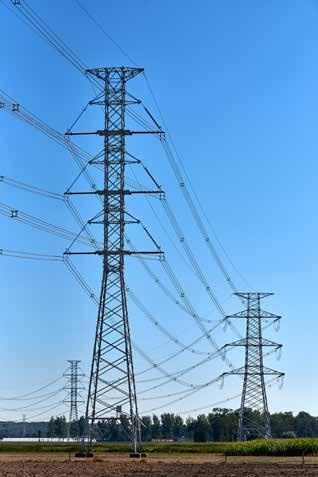
mixelectricityondependingRangethe

This view already took into account the market welfare differ ences and the costs associated with the development of new capacities (in or out of the market) and with keeping existing units available (in or out of the market). The evolution of the benefits for the system over time can be explained by the change in the non-viable gap volume but also by a higher price cap assumed in the system (which increases over time). It can be clearly concluded that the introduction of a market-wide CRM, whatever the outcome of the capacity mix, will have a positive effect on the system The calculations for ‘EM+CRM’ cases do not yet account for the fact that for investors the ‘EM+CRM’ typically presents lower risks and hence lower hur dle rates can be applied, which obviously has a dampening effect on the financing cost and hence would further improve overall welfare.

Gain brought to the Belgian system by introducing a CRM (all costs and market welfare taken into account) mixelectricityondependingRangethe

[FIGURE 5-80] — AVERAGE ELECTRICITY MARKET PRICE DIFFERENCE BETWEEN BELGIUM AND ITS NEIGHBOURS (ON A YEARLY BASIS) 2022 2023 2024 2025 2026 2027 2028 2029 2030 2031 2032 [€/MWh] 0489765321

dependingRange on the electricitymixAverage price difference with Belgian neighbours in case of no market-wide CRM Average price difference with Belgian neighbours in case of market-wide CRM

It is also important to keep in mind general differences between a setting with strategic reserves versus a setting with a market-wide CRM. Boom-bust cycles in terms of price spikes and ‘in-the-market’ investments in new capacity are strongly dampened in an ‘EM+CRM’, as any need for new ‘in-the-mar ket’ capacity is streamlined through the ‘market-wide CRM’ via forward auctions. As investors exhibit myopic behaviour (i.e. react by investing only when actual high prices are expe rienced, rather than anticipating future high prices), in a sec tor which is characterised by some investment inertia due to potential long lead times for the development of new capacity, boom-bust cycles in energy prices and investments in new ‘in-the-market’ capacity are much more likely to occur in an ‘EOM(+SR)’ setting than in an ‘EM+CRM’ setting.

— HOW MUCH DOES THE CONSUMER NEED TO PAY ? 2025 20252032 20322030 20302028 2028

Net consumer gain by introducing a market-wide CRM (compared to no market-wide CRM) Cost of the (estimatedmechanismCRMbyHaulogy)

Adequacy & Flexibility Study 2022-2032 244 245 Results

The market welfare and system costs were computed for 2025, 2028, 2030 and 2032 under the ‘EU-BASE’ and ‘EU-SAFE’ scenarios. From a system perspective, the ‘EM+CRM’ cases illustrated by the range depending on the electricity mix out come (in grey) in Figure 5-78 have a net market welfare gain which increases over time. For 2030, it represents about 300 M€ benefits on average in the ‘EU-BASE’ scenario and around 250 M€ in the ‘EU-SAFE’ scenario. [FIGURE 5-78] — NET MARKET WELFARE BETWEEN A MARKET-WIDE CRM AND NO CRM 2025 20252032 20322030 20302028 2028 EU-SAFE EU-BASE [M€] 4006005003002001000

EU-SAFE EU-BASE

[M€] 4008007006005003002001000

Finally, as in a market-wide CRM typically longer term con tracts could be provided under certain conditions, it may facil itate the new entry of market players and thereby contribute to enhancing overall competition (in what is today a rather concentrated market). 5.5.6.4. The consumer perspective In order to analyse the impact from the perspective of the consumer, the previous exercise was repeated while only accounting for the consumer surpluses and congestion rents to calculate the ‘market benefit’ for the consumers. In a mar ket-wide CRM, the consumer surplus will be higher due to lower electricity market prices. In addition, there are costs to be covered in both market designs (‘EOM + SR’ or ‘EM + CRM’). Indeed, in one case, the non-viable capacity will need to be contracted out of market to ensure the system remains adequate. This would imply keeping existing units but also developing new capacity. Such costs are assumed in this study to be paid by consumers. In a market-wide CRM, the differ ent costs associated with the capacity contracts needs to be accounted for. In this case, all eligible capacity needs to be remunerated at their missing money. Estimating the costs of the CRM was already carried out by a consultant (Haulogy) contracted by the FPS Economy; this consultant provided a detailed assessment of the expected costs on a yearly basis (see Section 4.6.4). Those estimates were therefore used.

[FIGURE 5-79]

Another way to illustrate the consumer benefit is to compare the electricity market prices between Belgium and its neigh bouring countries. This is depicted on Figure 5-80 where the average difference between the market prices in Belgium and abroad (France, Great Britain, Germany and the Nether lands) was calculated. It can be seen that as from 2025, the introduction of a market-wide CRM in Belgium to ensure an adequate system ‘in-the-market’ will limit the increase of price differences with its neighbouring countries. In the case of no market-wide CRM, the market prices would rise by 1 to 2 €/ MWh and up to 4€/MWh in 2032.

Average difference calculated between the average yearly simulated electricity whole-sale price of Belgium and the Netherlands, France, Great Britain and Germany. If the difference is positive, Belgium prices are higher. EU-BASE

5.5.6.3. System costs and market welfare

Figure 5-79 shows the expected consumer loss when no mar ket-wide CRM is introduced in Belgium compared to the cost of such mechanism. The grey band represents the expected range of results that could be obtained depending on the elec tricity mix. The charts include the change in consumer surplus (and congestion rents) but also the costs of the ‘out-of-market’ mechanism that needs to be put in place to ensure sufficient capacity to keep the lights on. In addition, the estimated cost of the market-wide CRM was also provided. It is clear that the loss (in the case of no CRM) is much higher than the estimated costs of such a mechanism.

Adequacy & Flexibility Study 2022-2032 246 247

LEGAL BASIS AND OBJECTIVE

6. Conclusion

6.1. Study objective and process

This chapter first provides an overview of the study’s objectives, followed by a factual overview of the process and stakeholder engagement. Afterwards, the main assumptions and data used for this study are summarised. Finally, a synthesis of the results and main insights is provided.

The present study is the implementation of Elia’s legal duty to provide a biennial analysis of the country’s adequacy and flexibility for the next 10 years. It is entirely compliant with the relevant clauses of the Belgian Electricity Act. This study provides a very accurate and detailed view of the adequacy outlook for the next 10 years, since state-of-the-art methodology was applied throughout. However, it is impor tant to note that this study is not designed as the basis for the calibration of the parameters or volumes required in the framework of the planned CRM. Calculations related to this calibration are part of a separate process. This calibration pro cess started in 2020 for the first CRM auction which is due to take place in 2021; it underwent a great number of required steps, and was concluded on 30 April 2021, with the auction parameters being fixed in a Ministerial Decree.

Examples of new approaches include the simulation of every year across the 10-year time horizon; applying a flow-based cross-border capacity calculation and allocation in line with the EU regulation requirements; assessing the economic viability of capacities through an approach developed by a renowned academic; and duly taking into account the impact of climate change. This study is therefore fully aligned with the current legal and regulatory framework, including EU legislation, and the recently adopted European Resource Adequacy Assess ment (ERAA) methodology. As required by the Belgian Electricity Act, a flexibility assess ment was conducted to analyse whether the future system is able to deal with expected and unexpected variations in generation and demand (for instance due to the forced out ages of generation units or forecast errors regarding renew able generation). The need for this assessment is becoming increasingly important over time due to the massive integra tion of intermittent renewable generation into the system. The flexibility analysis identified the flexibility needs of the system and investigates whether the system has the means (both in terms of installed capacity and operational availability) at any time to ensure a real-time balance between injection and offtake. This analysis allows future specific flexibility challenges to be identified.

On 22 May 2019, Regulation 943 of the European Parliament and of the Council on the internal market for electricity (recast) was approved as part of the ‘Clean Energy for all Europeans Package’ (CEP). Chapter IV of this Regulation deals with resource adequacy (Articles 20-27). Following one of the requirements described in the EU Regulation, in October 2020 the European Union Agency for the Cooperation of Energy Regulators (ACER) approved a new set of methodologies for performing future European Resource Adequacy Assessments and serving as a basis for national adequacy assessments. ACER stipulated that these new methodologies should be implemented before the end of 2023. Elia decided to proactively apply the new methodologies whilst preparing this ‘10-year adequacy and flexibility’ study.

Methodology and assumptions

PROCESS AND STAKEHOLDER INVOLVEMENT

As stipulated in the Electricity Act, the basic assumptions, sce narios and the methodology used for this study were deter mined by the transmission system operator in collaboration with the FPS Economy and the Federal Planning Bureau (FPB) and in concertation with the Regulator. Several meetings and discussions have therefore been held between the parties mentioned above since October 2020.

In addition, a public consultation for all market parties was organised regarding the input data for the scenarios used in the study and several aspects of the methodology. Stakehold ers were also asked to provide requests for sensitivities. A large amount of feedback was received from market parties (over a hundred remarks and suggestions), which are summarised in a public consultation report. The suggested sensitivities were taken into account (within the limitations of the model) and many other remarks led to concrete changes having been made to the study.

Insights on results

6.1. Study objective and process 247 6.2. 248 6.3. 250

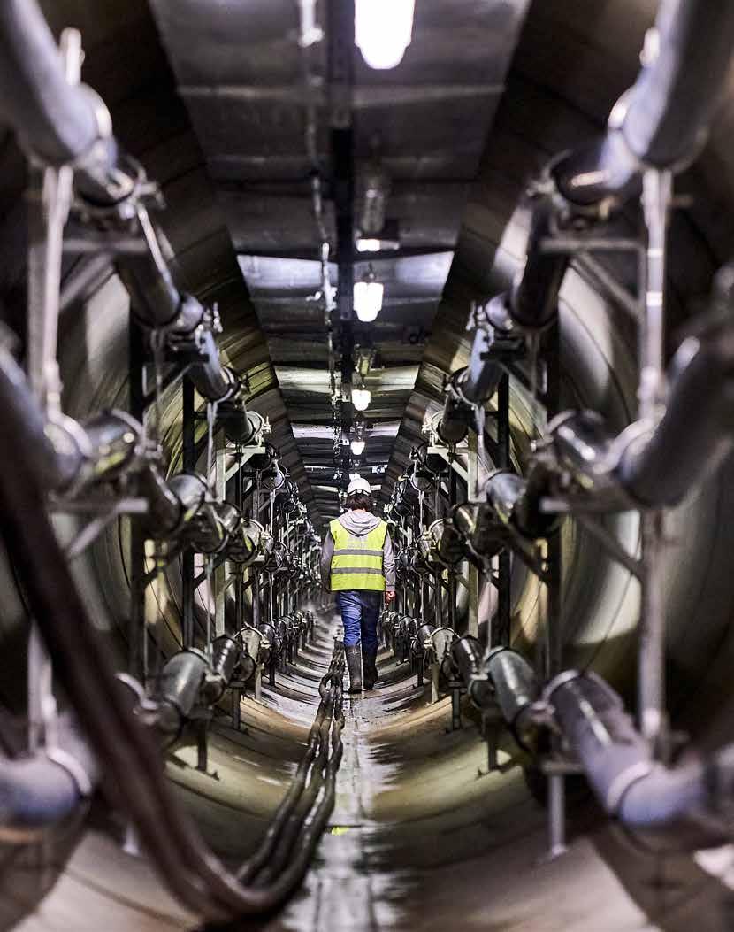
Adequacy & Flexibility Study 2022-2032 248 249 Conclusions 6.2.

Methodology and assumptions

The methodology for the resource adequacy assessment of this study is consistent with the most recent European assessments, i.e. the ENTSO-E Mid-term Adequacy Forecast (MAF). It however contains several important methodological improvements in order to implement the requirements set by EU Regulation 2019/943 and the ERAA methodologies. The method consists of a probabilistic ‘Monte Carlo’ type model with an hourly time resolution applied on 200 different climate years, combined with a large amount of availability draws on generation and HVDC links. It also includes a ‘flow-based’ capacity calculation approach for the countries within the Core region. In total, 28 countries are analysed and taken into account for this study.

Secondly, the reserve capacity requirements in the run-up to 2032 were estimated. In line with the ERAA methodology, Elia’s reserve capacity needs were enforced in the adequacy simulations to ensure sufficient flexibility was available to deal with the forced outage and prediction error risks during peri ods with a high risk of scarcity.

BELGIAN ASSUMPTIONS

The input data was based on the most up-to-date estimations and included the proposed political ambitions with respect to increases in e.g. the development of renewables (solar, onshore and offshore wind), storage, demand side response, interconnection capacity, etc. On the demand side, energy efficiency measures as well as electrification ambitions are taken into account.

SCENARIO FRAMEWORK

In the third and final step, the flexibility needs were compared with the operational availability of this flexibility in the system. This is based on (1) the installed capacity projections regarding generation, storage and demand side response; and (2) the hourly schedules of this capacity following the adequacy sim ulations. This permitted an assessment of whether the system holds at any time the required flexibility means to cover the identified flexibility needs.

The initial dataset was based on the information collected and constructed by ENTSO-E in the framework of the latest ‘MidTerm Adequacy Forecast’. Additional information received from neighbouring TSOs was used in order to update their projections with the latest forecasts.

The data was collected by Elia based on a literature review, and reviewed and added to by stakeholders during the public consultation on the input data.

EUROPEAN AND GRID ASSUMPTIONS

In order to comply with EU Regulation and ERAA method ology requirements, a verification was performed on the datasets of the relevant countries, ensuring that (a) countries with an approved capacity mechanism in place have suffi cient capacities to respect their reliability standards; (b) capac ities in those countries that are not required in order for the country to remain adequate do not benefit from additional revenues from a capacity mechanism; and (c) new capacities were added when those would gain sufficient revenues to be viable in the market, or vice versa capacities were removed from the system if this was not the case.

In addition to three central European scenarios – ‘EU-BASE’, ‘EU-noCRM’ and ‘EU-SAFE’ – a multitude of sensitivities was analysed. The results are robust over this multitude of sen sitivities and scenarios, showing a confirmed need for new capacity in a wide range of possible future situations.

Firstly, the method determined the risks of unpredicted varia tions in demand or generation after the day-ahead time frame. The flexibility needs were then calculated based on an extrap olation of historic forecast errors of demand, renewable and decentral generation, as well as the forced outages of large generation units or HVDC-interconnectors. Different cate gories of flexibility needs were identified: ramping (to react in 5 minutes), fast flexibility (15 minutes) and slow flexibility (5 hours). These flexibility needs are to be covered by market players, or in last instance by Elia by means of reserve capacity.

Finally, the so-called ‘minRAM70%’ rule stipulated in EU Regu lation 2019/943 served as the main future working hypothesis for determining cross-border capacities applied in this study.

The source used for the estimations for Belgium was mainly the final ‘National Energy and Climate Plan’ carried out at fed eral and regional levels, as submitted to the European Com mission at the end of 2019. Furthermore, it was complemented with the ‘Energy Pact’ and the approved Federal Network Development Plan for Belgium.

The new state-of-the-art methodology for undertaking flexibility assessments, introduced in the study of 2019, was incrementally improved. This study is aligned with guidelines published in the ERAA methodologies with regard to includ ing flexibility in the adequacy simulations. Furthermore, the representation of future offshore generation and predictions has been improved, and the potential flexibility provided by electrolysers has been included.

FLEXIBILITY METHOD

ADEQUACY METHOD

Those sources include further RES development to achieve a share of more than 40% RES-E by 2030 (including a ‘second offshore wave’ to reach more than 4 GW in the coming dec ade), the nuclear phase-out based on the law and different proposed measures on energy efficiency. All existing units were taken into account unless their closure was officially announced.

— In the coming decade, 90 GW of coal and nuclear capacity is to be phased out in Europe between 2022 and 2032 (most of which will be phased out in Western and Central Europe);

— The RES share in the electricity system is expected to reach more than 60% on European level by 2030.

Key points of note are as follows:

For the flexibility means assessment, a database was devel oped that included all of the technological capabilities that can achieve flexibility (ramp rate, start-up time, energy limits,…) for all the technology types which were taken into account.

FLEXIBILITY CHARACTERISTICS

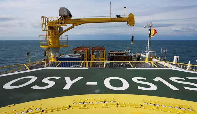
Ensuring robustness: key importance of the European context Belgium relies heavily on electricity imports for ensuring secu rity of supply. This may entail important risks with regard to the adequacy of Belgium’s electricity system, related to two areas: the availability of surplus generation across Europe at times of need in Belgium; and the availability of cross-border transmission capacity needed to bring such power to Belgium.

Nowadays, Belgium mostly counts on margins from the northeast of Europe. In the future, and for the aforementioned rea sons, the margins in those countries will disappear during moments when Belgium is experiencing a scarcity event.

The aforementioned capacity need takes into account impor tant short notice uncertainties over which Belgium has no control, such as the reduced availability of generation or interconnections.

Conversely, the correlation between Belgium’s scarcity events and those in the south-west of Europe decreases over time, but still remains important. With regards to the availability of cross-border transmission capacity, EU Regulation 2019/943 sets a standard of 70% min RAM (Minimum Remaining Available Margin) which needs to be at the disposal of the markets. This study assumes that the 70% rule is fully adhered to by all countries at all times. However, the physical reality of the transmission system should not be ignored. Delayed investments in cross-border reinforcements, limited redispatching means, and account ing for grid infrastructure maintenance are all valid reasons for a country to reduce the availability of their cross-border capacity, potentially leading to fewer energy imports being available for Belgium. In this study, multiple sensitivities were identified and included in an effort to quantify the impact of such uncertainties abroad on Belgian adequacy. Given Belgium’s dependence on imports during times of potential scarcity, this impact is significant, and should be taken into account for guaranteeing a robust coverage of Belgium’s security of supply. For this rea son, an ‘EU-SAFE’ scenario was constructed, selecting one rep resentative sensitivity in order to adequately take into account the identified set of risks. Need for market intervention The economic analysis indicated that without some form of structural market intervention, the energy-only market signals will not provide the necessary investment incentives to ensure that the identified need for new capacity will be fulfilled. There is, therefore, a clear need for structural market intervention to ensure adequacy as from 2025. Indeed, there is a non-viable GAP resulting from the economic viability assessment in both the ‘EU-BASE’ and ‘EU-SAFE’ scenarios for each of the assessed time horizons. Not only is the need enduring and significant in terms of vol ume, it is also clear that without new capacity, Belgian ade quacy will not be guaranteed. This confirms that strategic reserves cannot be considered as the appropriate instrument to ensure adequacy after 2025. According to the assumptions of this study and taking into account overall socioeconomic welfare effects, the need for a market-wide supporting mech anism, such as the Capacity Remuneration Mechanism (CRM) currently being implemented in Belgium, is therefore clear.

The ‘FR-NUC4’ sensitivity was selected to be representative for the risk related to those short notice uncertainties, hence constituting the ‘EU-SAFE’ scenario.

Given the risks mentioned before, Belgium’s adequacy situ ation in the period before 2025 should be closely monitored, since a transitory measure might need to be considered for that period.

It should be noted that this figure does not take into account the planned repowering of the Coo pumped storage power station, which was announced too recently to be included in the simulations. It is expected that this capacity increase will have a positive impact (reaching a 100 MW at most) on the determined need.

In addition, the need for 3.6 GW of replacement capacity assumed the following: on the one hand, no other existing capacities will leave the Belgian market unexpectedly (aside from the plants which have already been identified for closure); on the other hand, more than 800 MW (de-rated capacity) of new demand side response and storage capacities will become available, in line with the ambitions of the Belgian authorities, as outlined in the Energy Pact.

Adequacy & Flexibility Study 2022-2032 250 251 Conclusions 6.3. Insights on results

From 2025, once the nuclear phase-out is completed, a struc tural need for new capacity emerges in Belgium. This need amounts to 3.6 GW in 2025 in the ‘EU-SAFE’ scenario, and grad ually increases to 4.6 GW by 2032. While renewable energy sources will be introduced at an increasing pace across Europe, their integration into the system will be offset by the gradual decommissioning of conventional carbon-intensive genera tion plants. This explains, together with the further decarbon isation of the system through the electrification of demand, the increasing difficulty to keep the system adequate.

Rapid policy developments relating to the phase-out of CO2-intensive generation have occurred over the past few years in Europe. In light of the ‘Green Deal’, it is safe to assume that additional efforts in a similar vein will be undertaken by Member States in the years to come. Additionally, the Euro pean nuclear fleet has not matched its predicted availability over the last few years. This has resulted in further pressure being placed on current generation surpluses in some coun tries - surpluses upon which Belgium counts to safeguard its security of supply.

All volumes are expressed as 100% available

The need for additional capacity can be covered by any kind of technology (on top of the already assumed capacity in the ‘CENTRAL’ scenario for Belgium) such as thermal genera tion, renewable energy sources, or demand-side response and storage. However, the proportional contribution of each technology to adequacy varies according to their respective energy constraints, availability of primary energy, weather conditions, Interconnectionetc. capacity contributes significantly to overall socioeconomic welfare and price convergence during many hours of the year. However, while there is a substantial amount of interconnection capacity assumed to be available for the market, at moments crucial from an adequacy perspective, the (location of the) available energy in neighbouring countries turns out to be the limiting factor instead.

ADEQUACY OF THE BELGIAN SYSTEM [FIGURE 6-1] — NEW CAPACITY REQUIRED IN THE 'CENTRAL' SCENARIO FOR BELGIUM TO MEET THE RELIABILITY STANDARD OVER THE COMING 10 YEARS [GW][+][-]/needmargin -2-104532 2022 pre-2025 post-2025 2023 2024 2025 2028 2030 2032 -2.2 -1.7 -1.6 2 2.6 3.2 3.9 3.6 0.5 0 -0.4 3.7 4.1 4.6 '( )*+, '( )-+*' EU-BASEEU-SAFE taking into account short notice risks that are beyond control of Belgium New capacity needed to ensure adequacy in the ‘CENTRAL’ scenario for Belgium combined with: taking into account the latest known policies of all European countries modelled in this study and the countries with a market-wide capacity mechanism at their reliability standard

Need for new capacity

In the run-up to 2025, the adequacy of the Belgian system will be kept under control. However, absolute vigilance is required, as any capacity that might unexpectedly leave the Belgian market between now and 2025 could create adequacy risks for the country. During the winter of 2024-2025, shortages might also occur if uncertainties abroad reoccur as they were experienced in the past few years.

Putting consumers at the heart of the energy system is not only beneficial for consumers, it will also benefit the energy system. In fact, flexible appliances are necessary features of an energy system that includes a high amount of renewable energy. As the share of intermittent renewable energy sources grows and electrification spreads, supporting demand side participation and flexibility becomes key. Thanks to new tools such as digital meters, cloud computing and the Internet of Things, encouraging demand side participation is now within reach.

THE KEY ROLE OF DIGITALISATION AND CONSUMER CENTRICITY

COPING WITH SHORT-TERM FLUCTUATIONS IN PRODUCTION AND CONSUMPTION

This study confirms that flexibility needs will increase in the run-up to 2032. This is explained by the integration of variable renewable capacity into the system, such as wind power and photovoltaics, even when taking into account future forecast accuracy improvements. It appears that the offshore wind power capacity, which is foreseen to increase to up to 4.4 GW by 2028, is an important driver for increasing needs.

Adequacy & Flexibility Study 2022-2032 252 253 Conclusions

It is important to note that the balancing market needs to ensure that flexibility needs remain covered as much as possible by the market. In this way, Elia will continue to only cover the remaining system imbalance and cover at least the dimensioning incident with contracted balancing capacity and non-contracted reserves whenever possible.

This study concludes that the continued decarbonisation and electrification of the Belgian energy system will increase the adequacy gap between 2025 and 2032. Moreover, differences between injections and offtakes are likely to increase, given the growing share of intermittent energy sources being inte grated into the system. An efficient way of addressing these issues is to harness the potential of all technologies that can contribute to adequacy and flexibility as soon as possible. For example enabling the smart management of electric vehicles and heat pumps to react to electricity market prices can provide important sup port to the adequacy of the system. At the same time, these units can provide a large portion of the operational flexibility means which are needed to deal with unexpected variations after the day-ahead time frame and can balance the grid on a real-time basis. Both require a market design which facilitates the active par ticipation of such decentralised capacities. Elia believes that a consumer-centric market design will empower consumers to move from simply consuming electricity to using energy services that allow for an optimal use of their flexibility. By using the flexibility inherent to these appliances, consumers will be able to optimise their own consumption, capitalise on moments when there are high amounts of renewable energy in the grid and participate in energy communities.

COVERED

UPWARD DOWNWARD 6% RAMPING RAMPINGFAST FASTSLOW SLOW 75% 73% 94% 57% 0% 75% 73% 94% 85% 00% 100% 100% 100%96% 69% 40% 5% 45% 80% 94%94% 72% 99% Thermal + non-thermal + renewable energy sources + cross-border flexibility

[FIGURE

Required flexibility needs

— SHARE OF PERIODS IN 2032 IN THE ‘CENTRAL’ SCENARIO WHERE THE FLEXIBILITY NEEDS ARE WITHOUT UPFRONT RESERVATIONS (EXPRESSED AS % OF TIME, CUMULATIVE PER TECHNOLOGY CONTRIBUTION)

Based on the results of the 'CENTRAL' scenario, securing upfront a volume of operational flexibility to deal with unex pected variations in demand and generation will be necessary at least until 2032. This is particularly the case for upward fast flexibility, which is expected to be covered for 73% to 85% of the time without a need for upfront reservation. By contrast, downward fast flexibility achieves a coverage of 94% to 96%, confirming that there is almost no need to reserve downward capacity upfront. Upward ramping flexibility can be covered when accounting for cross-border reserve capacity, but the availability of the latter is subject to high uncertainty. Without cross-border flexibility, coverage remains limited to 75%. In contrast, the downward ramping flexibility needs are almost covered, even without cross-border flexibility. The slow flexibility needs, as well upward and downward, are expected to be covered, at least when assuming a liquid European intra-day market. Results demonstrate that for each type of reserves, and par ticularly for upward types, non-thermal technologies (includ ing decentral technologies such a vehicle-to-grid, batteries, consumption shifting and demand side response) contribute substantially to covering the flexibility needs without upfront reservation. Of course, this will only be the case if these flex ible technologies, assumed to be available in the ‘CENTRAL’ scenario, are effectively installed and participating in the intraday and balancing market. This contribution of decentralized capacity is explained by their cost structure, which allows a reduction in ‘must run’ or reservation costs. Facilitating the fur ther development of these flexibility providers and valorising their flexibility will further increase the coverage of flexibility needs, contributing to a cost-efficient integration of renewable energy. This can be resolved by a well-functioning intra-day and balancing market, complemented by reserve capacity being contracted by Elia to cover the residual flexibility needs which remain without coverage by the market. 6-3]

Until 2025, more periods where the residual demand, specified by the total demand after deducting renewable generation, goes under the level of 'must run' generation needed following power plant constraints (e.g. nuclear units) or system security (ancillary services), or even becomes negative. These periods are referred to as ‘over-generation’ periods, which are expected to be managed by storage and export availability. This phe nomenon is mitigated with the nuclear phase-out, and will gradually return towards 2032. Results from the adequacy simulations confirm that reductions in renewable generation therefore remain very rare between 2022 and 2032.

A particular analysis undertaken of the second wave of off shore wind power in Belgium (which is due to be fully com missioned by 2028) shows that offshore wind power will experience exceptional power storm cut outs and generation ramping events (up- and downward ramps up to 2.5 GW can occur up to several times a year) and that current measures to manage such events are to be complemented with additional mitigation measures. This will be further discussed with mar ket parties during 2021 and 2022.

Pumped Decentralizedstoragehydro+energyresources

Available flexibility means

Ramping flexibility needs seem to be higher during high renewable generation and demand conditions, while all types of flexibility needs are generally lower during low renewable generation and demand conditions. However, the relationship between required flexibility needs and expected system con ditions is difficult to capture with simple statistics and may require the employment of more advanced techniques. Cap turing the ‘dynamics’ of flexibility needs in advance can help to better manage the available flexibility means.

[FIGURE 6-2] — EVOLUTION OF FLEXIBILITY NEEDS BETWEEN 2022 AND 2032 IN THE 'CENTRAL' SCENARIO UPWARD DOWNWARD Total Flex [MW/5h] Slow Flex [MW/5h] Fast Flex [MW/15min] 2nd wave of offshore RampingwindFlex [MW/5min] 280 320 400 420 440 320 340 440 440 460 4140 3340 5100 5280 5480 3060 3360 4360 4560 2700472025802460 1960 1780 294028202720 2300 2040 2020 1980190014001280 254024602380 18401700 2022 2025 2028 2030 2032 2022 2025 2028 2030 2032

The analysis shows that over the period 2022 to 2032, there will be sufficient capacity installed in the system to cover the iden tified flexibility needs. This is expected to be the case under every scenario and sensitivity where the installed capacity mix fulfils the adequacy needs of the system. The installed flexibility does not allow conclusions to be drawn regarding the operational availability and economic efficiency of delivering this flexibility. Therefore, the available operational flexibility means were compared with the flexibility needs for each individual hour of the year for several Monte Carlo years. This allowed an analysis of whether the installed flexibility is also sufficiently available in intra-day and real-time. It is indeed possible that the required flexibility is unavailable when units providing flexibility are not dispatched and require a start-up time of several hours or when energy storage buffers are full or empty.

j

— AVERAGE, P95 AND P50 LOLE INDICATORS averageLOLE LOLEP95 LOLEP50 Situation 0 0 0 No LOLE observed

the results as

50%

N ∑ ENS jЕS

and

N

the values of these indicators, four situations can be derived

Expected

jth

Adequacy & Flexibility Study 2022-2032 255254 A. How to interpret the LOLE criteria

EENS

[FIGURE 7-1] — EXAMPLE OF A CUMULATIVE DISTRIBUTION FUNCTION OF LOLE [%]Percentile 1009080706050403020100 LOLE [h] 1501251007550250 95% of results are below this value Average results. Sum of results divided by the number of results 50 % of results are below this value P95 P50Average Depending

>0 0 0 LOLE

>0 >0 0 LOLE in

The indicative Figure 7-1 shows how to interpret the adequacy criteria. Many future states (or ‘Monte Carlo’ years) are calcu lated for a given year in a probabilistic assessment. For each future state, the model calculates the LOLE for the year. The distribution of the LOLE among all studied future states can be extracted. For the first criterion (LOLE), the yearly average is calculated from all these LOL results obtained for each future state. For the second criterion (95th percentile), all the LOL results per year are ranked. The highest value, after the top 5% of values have been disregarded, gives the 95th percentile (1 chance in 20 of having this amount of LOLE). Both criteria need to be sat isfied for Belgium, as currently specified in the Electricity Act. on from represented in the table below (see Figure 7-2). [FIGURE 7-2] in any of the future states in less than 5% of the future states more than 5% of future states but less than 50% more than of the future states Energy Not Served (EENS) [MWh/year or GWh/year] is the average energy not supplied per year by the generating system due to the demand exceeding the available generating and import capacity. In reliability studies, it is common that Energy Not Served (ENS) is examined in expectation over a number of 'Monte Carlo' simulations. To this end, EENS is a metric that measures security of supply in expectation and is mathematically described by (1) below: = 1/ (1) where ENS is the energy not supplied of the system state (j Е S) associated with a loss of load event of the Monte Carlo simulation where is the number of Monte Carlo simulations considered.

>0 >0 >0 LOLE in

7. Appendices A. How to interpret the LOLE criteria 255 B. Flow-based methodology 256 C. Adequacy patch 265 D. Compliancy with the methodology: detailed assessmentERAA 266 E. Unit commitment (UC) 271 F. Simulation of the electricity market 273 G. Historical analysis of input data 276 H. EVA metric 286 I. Further assumptions on fuel prices 287 J. Climate years of Météo-France 290 K. Costs figures and comparison with litterature 291 L. Thermal capacity ‘at risk’ in Belgium 292 M. Electricity consumption 294 N. Power-to-X 297 O. Running hours and IRR for OCGT 298

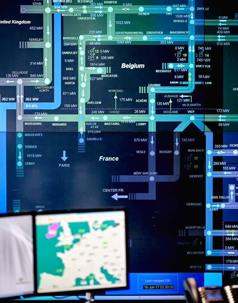
Appendices Adequacy & Flexibility Study 2022-2032 256 257 B. Flow-based methodology B.1. FLOW-BASED OPERATIONAL PROCESS i

For each hour of the year, the impact of energy exchanges on each Critical Network Element (also called critical 'branch' in the past) taking into account the N-1 criterion is calculated (see later in this section the explanation on the N-1 criterion). The combination of Critical Network Elements and Contingencies (CNECs) forms the basis of the flow-based calculation. A reliability margin on each CNEC is considered and, where appropriate, 'remedial actions' are also taken into account. These actions can be taken preventively, or after an outage has occurred, to partly relieve the loading of the concerned critical network element. Those actions make possible to maximise exchanges thanks to changes in the topology of the grid or by the use of phase shifting transformers.

The bidding zones act as 'copper plates' from a market per spective. Within a bidding zone the market price is the same for all market participants (the ‘copper plate assumption’ entails unlimited transmission capacities within the zone). A higher resolution is required in order to simulate the internal flows and consequently assess the loop flows. A finer grid resolution is provided by 'small zones', subsets of the bidding zones which also serve as copper plates. An initial simulation involving these small zones is required in order to take account of the loop flows caused by internal exchanges (between small Finally,zones). due to the extra complexity arising from the large num ber of constraints induced by the modelling of flow-based in the adequacy study, the complexity of the problem must be reduced to a level that is solvable in due time by today’s computers. This whole process will be detailed further in the sections below.

The first step is the calculation of PTDF factors within a given FB geographical area (network parameters and topology are Thedefined).PTDF factors estimate (the increase of) the flow that can be expected in the different Critical Network Elements as a function of a position change of a bidding zone, controllable Let’sdevice.assume the simplified grid example below: [FIGURE 7-3] — REPRESENTATION OF A NODAL SYSTEM AND DISTRIBUTION OF FLOWS A B C D + 100 MW 75 65 25 90 10 - 100 MW

Information about the flow-based rules and methodologies are available by consulting the Capacity Calculation Regions webpage of ENT SO-E [CCR-1].

For example, if an exchange from Node A to Node D of 100 MW occurs, the PTDF factors could be: — 75% of the injection in Node A goes to Node B and 25% of the injection in Node A goes to Node C; — 65% of the injection from Node A goes from Node B to Node C and 10% of the injection from Node A goes from Node B to Node D; — Finally the portion of the total injection in Node A passing through Node C is 25% + 65% = 90%, going to Node D. The PTDFs thus indicate how the energy flows are (unevenly) distributed over the different paths between the different nodes of the network when the X MW injection/extraction occurs at two points of the network. The distribution given by the PTDFs is determined both by the topology of the grid and the technical characteristics (impedances) of the grid. It should be noted that PTDF’s are calculated for the flows over the grid elements in N state as well as when grid con tingencies occur. The first step in the flow-based framework is the calculation of a set of PTDFs. To obtain these, a European grid model is built, which is for this study based on the TYNDP 2020 reference grid, to which grid modifications are applied at the targeted horizon. This grid model is then used to calculate the PTDFs. A PTDF matrix consists of lines/rows representing the different CNEC’s that are taken into account, and columns representing the variables in the flow-based domain. Each CNEC refers to the combination of a Critical Network Element and a Con tingency. The variables can represent the net positions of the market nodes under consideration, the HVDC flows, PST positions, etc; depending on the degrees of freedom of the market coupling algorithm, e.g. whether SHC or AHC, etc... Aside from a PTDF matrix, the flow-based framework also requires the capacity of each Critical Network Element. These capacities correspond to the steady-state seasonal ratings of the network elements.

B.3. CALCULATION OF PTDFS

This procedure finally leads to constraints which form a domain of safe possible energy exchanges between the ‘flow-based’ countries within the relevant Capacity Calculation Region (CCR) under consideration (this is called the flow-based domain). Different assumptions are made for the calculation of this domain, such as the expected renewable generation, con sumption, energy exchanges outside the CCR area, location of generation, outage of units and lines, etc. For every hour there might be a different flow-based domain —because:thetopology of the grid can changes; — outages or maintenance of grid elements can be present; The operational calculation of the flow-based domain for a given day is started two days before real-time operation and is used to define the limits of energy exchange between coun tries for the day-ahead market.

The flow-based method implemented on the day-ahead mar ket coupling uses Power Transfer Distribution Factors (PTDFs) that make the modelling of real flows through the physical network lines possible.

The N-1 security criterion for the grid Interconnection capacity takes into account the margins that transmission system operators (TSOs) must maintain in order to follow the European rules ensuring the security of supply. A line or grid element can be lost at any time. The remaining lines must be able to cope with the changes in electricity flow due to any such outage. In technical terms, this is called the N-1 rule: for a given number N of lines that are transmitting a given amount of energy, there cannot be an overloaded line in case of the outage of one of the lines. This is important to avoid that a chain reaction arises and, by extension, the net work stability of the entire European network can be endan gered. The flow-based domain calculation process therefore accounts for the N-1 principle.

Note however, that European rules stipulate that this criterion must be fulfilled at each moment, including in the event of maintenance or repair works. In such cases, it is possible that interconnection capacity available for exchanges will have to be reduced. Wherever possible, maintenance and repair works are avoided during the most critical periods, e.g. around the peak consumption times of the year, but cannot be ruled out, especially after winter weather conditions. FLOW-BASED ADAPTATION IN THE SIMULATIONS

B.2.

The 2-Days Ahead Congestion Forecast (D2CF) which is pro vided by each of the participating TSOs in the capacity calcu lation process for their grid, provides the best estimate of the state of the CCR (currently CWE) electric system for day D. This D2CF forecast provides an estimation of: — the Net Exchange program between the zones; — the exchanges expected through DC cables; — planned grid outages, including tie-lines and the topology of the grid as foreseen for D+2; — forecasted load and its pattern; — forecasted renewable energy generation, e.g. wind and solar generation; — outages of generating units, based on the latest generator availability info.

B.5. CALCULATING THE INITIAL LOADING OF EACH CNEC

— FRM = Flow Reliability Margin, used by TSOs to account for the uncertainty due to forecast errors.

The zonal PTDF of a connection is the sum of the nodal PTDFs of the zone, multiplied by each nodal TheGSK.GSK provides the relative weight of the given node to a the zonal exchange Zone B Zone A Zone C PTDF PTDF GSK= ∑zone A line a zone A node k node k line akk=n=1 Within each zone, the GSK can be defined as: GSK Zone,Node = NominalZ,NP NominalZ,NP∑ NЕZ where = NGCNominalZ,N ZP∑ NЕZ is equal to the installed capacity within the corresponding zone Z and NominalZ,NP is equal to the installed capacity connected to the node N within zone Z. These ‘pro-rata distribution keys’ are an important assumption for the calculation of the zonal PTDFs since, they fix the geo graphical distribution of generation units per type T at each node N with respect the total installed capacity per type for the given network topology. GSKs therefore define the weight of each of the nodal PTDFs in the definition of zonal PTDFs.

B.4. CALCULATION OF ZONAL PTDFS FROM NODAL PTDFS: APPLYING GSKS

For each CNEC, a procedure is followed to calculate the Remaining Available Margin (RAM) (see Figure 7-5), which is the physical capacity on the CNEC that can be used by the market coupling algorithm to accommodate cross-border exchanges, and which is defined as follows:

[FIGURE 7-4]

— Fmax = The maximal allowable physical flow over the con cerned CNEC branch “i” in order to comply with operational and thermal – structural limits. An important factor determining the final RAM is therefore the ‘initial flow’ Fi, reflecting the flow over the network element when all zones within the CCR (eg Core) are at zero balance. This flow therefore includes: — the flows resulting from internal exchanges in the Bid ding Zone where the CNEC is located (mostly relevant for CNEC’s within a Bidding Zone, but much less important for cross-border (XB) CNECs; — the flows resulting from internal exchanges in other Bidding Zones than the one where the CNEC is located (loop flows).

Appendices Adequacy & Flexibility Study 2022-2032 258 259

— F = Flow over the network element “i”when cross-border exchanges within the CCR (eg Core) are cancelled;

Bidding zones are zones where all generation and consump tion within a given zone have the same wholesale price, hence one ‘zonal’ PTDF should be defined for the entire zone. There fore, a mapping is needed between the market ‘zonal’ level and the grid ‘nodal’ level, in order to define those ‘zonal’ PTDFs. In the example below an illustration between the nodal and zonal representation is provided. A ‘zonal PTDF’ is needed in order to calculate the effect that a commercial exchange between two market zones, will have on any grid element. The calculation of ‘zonal PTDFs’ from ‘nodal PTDFs’ is based on the so-called ‘generation shift keys’ (GSKs). With this GSK, the nodal PTDF can be converted into a ‘zonal PTDF’ by assuming that the bidding zone net position is spread among its nodes according to the GSK. Therefore a ‘zonal PTDF’ is the sum of all ‘nodal PTDFs’ weighted by their nodal GSK. Below an illustration (Figure 7-4) of this relation between ‘zonal PTDFs’, ‘nodal PTDFs’ and GSKs is provided.

Definition of Remaining Available Margin (RAM) for each CNEC

RAM = Fmax (FRM + F ) with F = FRef ∑ PTDF NP j — Fref = Reference flow over the network element in the base grid model where cross-border exchanges are still present;

— PTDF = Zonal PTDF of bidding zone “j” for the considered CNEC branch “i”;

— DEFINITION OF REMAINING AVAILABLE MARGIN (RAM) FRM FRMFRM FRM FRM F thermalmaxloadingofCriticalNetworkElement-CNE 70% flows induced byexchangecross-zonal RAM Market flows within CCR Fuaf Transit flows from other CCRs F0,Core Internal flows & loopflows FRM30% margin for FRM, loop flows & internal flows RAMN-1 N-1 F0,CoreN-1 Internal flows & loopflowsN-1 N-1 RAM RAM RAM RAM

As it will be presented below, the flow-based methodology followed here replicates this principle when calculating the initial loading of each CNEC.

— CALCULATION OF ZONAL PTDFS APPLYING GSKS LoadGenerator

The notion of the initial loading of each CNEC is related to the so-called ‘Reference Flow’ (Fref ) in the operational Flowbased framework. The ‘Reference Flow’ (Fref ) is the physical flow computed from the common 2-Days Ahead Congestion Forecast (D2CF) base case and reflects the loading of the Crit ical Network Elements given the exchange programs of the chosen reference day, thus given the ‘likely market direction’ according to D2CF.

[FIGURE 7-5]

— NP = Net position (Balance) of Bidding Zone “j” inside the CCR (eg Core) in the Reference situation;

B.8.1. Treatment of external flows

Elia is a pioneer in the flow-based approach for adequacy stud ies, and has developed a methodology to model exchanges between countries in the capacity calculation region that repli cates the day-ahead operation. Whereas in the first flow-based assessment of winter 2016-17 (the strategic reserve volume evaluation published end of 2015) only one domain was used to represent the entire winter. That domain was based on an historical situation. Since then, Elia has since improved its modelling by: adding more historical domains; relating the domains to the climatic variables in a system atic incorporatingway; minRAM evolutions within those historical correctingdomains; historical domains for historical grid outages; correcting historical domains for future grid upgrades; integrating the breakup of the DE-AT bidding zone on 1 October 2018; recalculating the domains to include the planned HTLS upgrade of the 380-kV Belgian backbone; modelling the ALEGrO interconnector, which provides addi tional freedom for the flow-based domain. Given the expected evolutions in the generation, grid, flowbased perimeter and regulation, relying on historical domains was not anymore the best option for studies looking up to 10 years ahead. Elia has therefore introduced a new framework which does not rely on historical domains anymore. This was further improved for this study in order to: extend the flow-based perimeter to Core; add the flow-estimation step in the process in which inter nal controllable elements' set points are estimated prior to simulating the FB process by mimicking the operational behaviour in D2CF; integrate the Advanced Hybrid Coupling (AHC) for any external border to the CCR considered (eg Core); Implement a multi-level clustering of high-dimensional domains.

B.7. EVOLUTION OF THE FLOW-BASED METHODOLOGY

Figure 7-6 shows how the FB domain can be determined by combining the calculated remaining available margins (RAMs) and the zonal PTDFs for each relevant Critical Network Ele ment and Contingency (CNEC) pair. The first constraint is determined for line 1, in a situation without contingencies. We draw from the table that the CNEC has a RAM of 150 MW, a zonal PTDF for zone A of -30%, for zone B of 25% and for zone C of 10%. The same exercise is now performed for all other lines and contingency pairs, ultimately resulting in a collection of constraints (RAM, PTDFA, PTDFB, PTDFC). These constraints can be understood as geometrical planes in the dimensions defined by the balances of the difference zones: Balance(A), Balance(B), Balance(C), etc. For the purpose of illustration, the constraints can be plotted between two balances as the projection of these planes, so they reduce to lines. Figure 7-6 depicts such projection for Balance (A) vs Balance (B), where the constraints are represented by the grey dotted lines. Generally the convention is used where positive balances represent net exports and negative balances rep resent net imports. As a final step, the total set of constraints can be reduced by removing all non-relevant constraints. Constraints are consid ered non-relevant when other constraints are always reached earlier. This procedure is also called ‘pre-solving’ the domain, and leads to the final combination of relevant constraints forming the secure domain, colored in yellow. Under perfect foresight conditions, every combination of secure exchanges between all different zones is part of this domain.

In Core, Standard Hybrid Coupling (SHC) flows are considered commercial flows, and therefore are a part of the 70% min RAM that has to be offered to the market. In other words, the minRAM rule has to be applied on CNECs before the RAM is later further reduced to account for SHC flows, ie minRAM is applied in SHC on the RAM + the SHC flows component. The difference is illustrated in the Figure 7-7, which highlights the impact of the AHC modelling since incorporates new dimen sions resulting hence in a visually larger flow-based domain.

[FIGURE 7-7] — HANDLING OF EXTERNAL FLOWS: AHC VS SHC AHCpositionspositionszoneBiddingnetBiddingzonenetflowsALEGrOALEGrO PTDF PTDFflowsCNECCNECflows RAMRAM CNECPTDFflows Variables known beforeoptimisedVariablescouplingmarket in market couplingSHCflowsprocessSHCprocessAHC XX <=<= - x Legend

Appendices Adequacy & Flexibility Study 2022-2032 260 261

B.6. CALCULATING THE FB CAPACITY DOMAIN

B.8. FLOW-BASED PARAMETERS

European legislation requires a minimum capacity of each critical network element (margin) to be made avail able to the market (minRAM) (See Figure 7-5). For this reason, every time a CNEC’s margin after preloading is less than the required minimum margin given to the market, the minimum margin is enforced. These steps are followed in the flow-based methodology of this study.

[FIGURE 7-6] — INITIAL FB CAPACITY DOMAIN CALCULATION -400-300-200-1004003002001000Balance (A) Balance (B) Constraints Active/ Limiting constraint FB domain -300 -200 -100 0 100 200 300 400-400 elementsnetworkCritical Incident (MW)MarginAvailableRemaining Influence of the exchange on each line (PTDF) A B C Line 1 incidentNo 150 -30% 25% 10% Incident 1 120 -17% 35% -18% Incident 2 100 15% 30% 12% Line 2 incidentNo 150 60% 25% 25% Incident 3 50 4% -15% 4% Line 3 IncidentincidentNo4

For Belgium, this distinction is important as the Nemo Link HVDC interconnector is not part of Core. Two effects are there fore visible:

P F

— Since the go-live of ALEGrO end 2020, a maximum import of 6500 MW is allowed; — After the commissioning of additional shunt capacitors, which is expected by end of 2022, the limit can further be increased to 7500 MW;

Other countries' assumption regarding external constraints are following the modelling and assumptions applied in the latest MAF2020 study. B.8.3. CNEC selection for flow-based The CNEC selection defines what lines from the common grid model can be taken into account in the calculation of the flowbased domain. Today in CWE flow-based the 5% PTDF rule (meaning the CNE is at least 5% sensitive to a net position change of any of the CCR bidding zones) is typically used as threshold for the determination of CNECs. Similarly, at the go-live of Core flow-based, the default 5% threshold will still be considered. 18 months after the go-live of Core (from end 2023 onwards) and once the target model is expected to be operational, a different threshold might be considered.

As the Belgian adequacy situation is closely related to French security of supply, it is preferable to show a projection of the flow-based domain onto the Belgium-France plane. An over view of these domains is shown in Section 3.5

The target model for Core flow-based is to have only cross-bor der CNE's limit the market. However, if a TSO can prove that it is more beneficial, from an economical point of view, to incorporate an internal CNE into the flow-based calculation, rather than perform extra RD, perform a bidding zone split or introduce network investments, this internal CNE could be allowed as a market constraint within the CNEC list.

In SHC, all flow-based domain representations only depict Core balances, as opposed to bidding zone balances. Hence, the import possibilities of Core countries from outside Core are not shown. In the ANTARES model used in this study for the SHC simulations, as well as in the day-ahead market coupling, France can for example import from other countries within the limits of the NTC constraints on the concerned borders.

Use of PST in capacity calculation

Figure 7-8 shows a theoretical example of such a projection [SCA1]. Note that not all vertices are part of the convex hull.

B.8.2. External constraints

B.9. WHAT IS A FLOW-BASED DOMAIN, WHAT DOES IT LOOK LIKE MATHEMATICALLY, HOW DO WE VISUALIZE IT, WHAT ARE THE NUMERICAL LIMITATIONS ?

— Maximum import: 6500 MW — Maximum export: 6500 MW The target model is to have no external constraints limiting the market. However, if, using an extensive economic analysis, it can be shown that it is still justified from a welfare point of view to keep it, it will still be allowed. Currently, external con straints will still be allowed during a 2 year transition period after the go live of Core flow-based market coupling. From 2024 onwards no external constraints should be applied. This is also the assumption taken in this study.

The flow-based domains used in this study are polytopes having up to 44 dimensions. For a better understanding of the domains, a two-dimensional representation is used. This representation is to be seen as a projection of the higher-di mensional domain onto a two-dimensional plane. To obtain this, first the domain polytope which is described by its planes is converted into its vertices. Then these vertices are projected onto the desired plane. A convex hull of these points, which can be seen as the smallest convex polytope which contains all points (or more graphically: the polygon you get when you wrap shrink wrap around all points) is then calcu lated. All points which are not on the convex hull are omitted.

Appendices Adequacy & Flexibility Study 2022-2032 262 263

In this study and following the target model for Core flowbased, only cross-border CNECs have been considered as best case reference. However, some flow-based sensitivities (part of the ‘EU-SAFE’ scenario) have been introduced to account for uncertainties around the assumptions mentioned above. B.8.4. Controllable devices

By convention, export is depicted as positive, whereas import is negative. A positive net position thus means a net export position towards Core.

― Belgium can even have a positive Core balance in times of scarcity, yet still have a net import position. In these situa tions, a positive Core balance is offset by a greater import flow over Nemo Link, resulting in a global importing position for Belgium.

― Maximum import cannot be depicted on the two-dimen sional domain representation. Depending on the actual net position of Nemo Link, the Belgian Core balance can, vary between (max import -1000 MW) and (max import +1000 MW) corresponding to maximum import and maximum export over Nemo respectively;

— Before 2020 the external constraint was taken into account in the capacity calculation phase of the CACM process. In Q2 2020, this has evolved to become a capacity allocation constraint. Practically speaking, the max-import constraint is ensured by summing both flow-based imports and exter nal imports (Nemo Link). Similarly in our neighbouring countries, the Netherlands have an import / export constraint, which upon consulting Tennet can be set as:

B.9.1. Understanding 2-dimensional flow-based domain representations

A cross-border PST is a controllable device, which can redis tribute cross-border flows. In the context of CEP, TSO’s can first use PST’s to optimize loopflows to comply to minRAM requirements. If after this initial PST setpoint, some taps of the PST range are still unused, these PST flexibility can still be given to the market for further economic optimization (welfare Inmaximization).thecapacity calculation phase, that part of the range of the PST that can be optimized to increase the domain in the likely market direction is defined per PST. HVDC in capacity allocation Similarly to a PST, an HVDC is a controllable device that can redistribute cross-border and internal flows. Again, both loop flow optimization and welfare maximization are possible uses of an HVDC. For the latter, in the capacity calculation phase, the setpoint of the HVDC can be optimized to increase the domain in the likely market direction. Currently, there are no cross-border HVDC’s that are optimized this way in capacity calculation. Here the market will determine its setpoint in order to optimize welfare at capacity allocation. ALEGrO is the only cross-border HVDC within the Core CCR and will be optimized in the capacity allocation. No other cross-border HVDC's are scheduled in Core until 2030.

External constraints are additional constraints in the flowbased market coupling that are not related to line overloading but to other effects (such as steady state or dynamic voltage Inissues).thiscontext, Belgium currently has a max-import limitation. This limitation is expected to evolve:

The resulting 2-dimensional representation of the flow-based domain should be interpreted as follows: ‘for any point within the 2-dimensional domain, for which the net positions of 2 countries can be read from the axes, a combination of net positions for the dimensions that are not depicted exists so that this point can be attained’ [FIGURE 7-8]

— FLOW-BASED DOMAIN: 2D PROJECTION

B.9.2. Smart slicing

[FIGURE 7-9]

The solution implemented in EUPHEMIA within flow-based market coupling (FBMC) follows the curtailment sharing prin ciples that already existed under ATC/NTC. The objective is to equalize the ratio of curtailment (~Energy Non Served (ENS)) between bidding zones as much as possible.

Appendices Adequacy & Flexibility Study 2022-2032 264 265

If two possible market transactions generate the same welfare, the one having the lowest impact on the scarce transmission capacity will be selected first. It also means that, in order to optimize the use of the grid and to maximize the market wel fare, some sell (/buy) bids with lower (/higher) prices than other sell (/buy) bids might not be selected within the flow-based allocation. This is a well-known and intrinsic property of flowbased referred to as ‘flow factor competition’.

C.3. FLOW FACTOR COMPETITION AND PRICE TAKING ORDERS

Under normal FBMC circumstances, ‘flow factor competition’ is accepted as it leads to maximal overall welfare. However for the special case where the situation is exceptionally stressed e.g. due to scarcity in one particular zone, ‘flow factor compe tition’ could lead to a situation where order curtailment takes place non-intuitively. This could mean e.g. that some buyers which are ready to pay any price to import energy would be rejected while lower buy bids in other bidding areas are selected instead, due to ‘flow factor competition’. These ‘payany-price’ orders are also referred to as ‘Price Taking Orders’, which are valued at the market price cap in the market cou Thispling.would lead to the situation where one bidding area is curtailed while the clearing prices in the other bidding areas are lower or equal to the market price cap. This is the situation that the adequacy patch seeks to mitigate by ‘by-passing’ flow factor competition in such cases and ensuring maximal imports for zones experiencing curtailment.

The curtailment sharing is implemented by adding a large penalty term into the primal problem plus solving a sub-op timization problem for the minimization and sharing of cur tailment, where all network constraints are enforced, but only the acceptance of the price taking volume is considered in the objective function. The curtailment ratios weighted by the volumes of price taking orders are therefore minimized (see EUPHEMIA public description for details [ADQ-1]).

The results of this study are taking into account those curtail ment minimization and sharing rules by applying those after the optimization found by ANTARES.

Within the EUPHEMIA algorithm (PCR Market Coupling Algo rithm [ADQ-1]), a mitigation measure has been implemented to prevent price-taking orders (orders submitted at the price bounds set in the market coupling framework) to be curtailed because of ‘flow factor competition’.

C.4. CURTAILMENT SHARING

—

FLOW-BASED DOMAIN: SMART SLICING P F C. Adequacy patch C.1. IMPLEMENTATION IN EUPHEMIA

Figure 7-9 illustrates the concept of smart slicing. The blue square represent a hyperplane that would cut the multi-di mensional polytope fixing hence the net positions of the other dimensions. Applying this so-called smart-slicing reduces the degree of freedom and results in the grey projections as 2D representations. Of course, the way the smart slicing is applied, i.e. which net position are chosen will visually affect the 2D representation. While building the flow-based domain, the net position chosen for the smart slicing were the ones from the market simulations at the precise hour considered.

As the number of dimensions increases, so does the com plexity. It becomes required to use simplifications in order to represent the flow-based domains in a human readable way e.g. by 2D projection.

The situation becomes more complex when two or more markets are simultaneously in curtailment ie facing a scarcity situation. For these situations, the mechanism put in place aims to ‘fairly’ distribute the curtailments across the involved markets by equalizing the curtailed price-taking orders to total price-taking orders ratio between the curtailed zones.

C.2. FLOW FACTOR COMPETITION

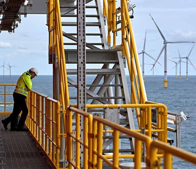
Geographical#2 scope Article 1 Subject matter and scope Paragraph (a) refer ring to the geographical scope} (a) is carried out on each bidding zone level covering at least all MSs; This study covers twenty-eight countries which include all the MSs, as shown in Figure 3-2 in the main text, besides Malta and Cyprus.

With respect to “measure (a)” related to removing regu latory distortions and “measure (g)” related to removing regulated prices, this is a core competence of Member States within their policy choices. In the case of Belgium, the competent authority might use (parts of) this report as guidance for their policy decisions.

This study considers the contribution of all resources as mentioned in paragraph (d); Furthermore in relation to paragraph (e), this study con siders the impact of measures referred in Article 20(3) of Electricity Regulation as follows: the effect of “measures (b)” related to price caps, is considered in Section 3.6 of this study. In particular the assessment considers the increase of the maximum clearing price, reflecting in a realistic manner the expected behavior of the market. Multiple clearing price increases are allowed to occur within a single year and these aspects are considered per simulated Monte Carlo year in the economic viability assessment.

Regulation (EU) 2019/943 mandates the development of an ACER-approved methodology for the European resource adequacy assessment (ERAA). On 2 October 2020, ACER has approved such a methodology for resource adequacy assess ments, after amending the draft methodology submitted by ENTSO-E to ACER on 4th May 2020. An analysis of the main principles of the ACER approved ERAA methodology of 2nd October 2020 is presented below, includ ing an assessment of the compliancy of the current ‘10 year adequacy and flexibility 2022 – 2032’ study of Elia with this methodology. It is key to remind that the present study is not the ERAA and that the first ERAA will be published by ENT SO-E by the end of 2021, about 6 months after the publica tion of the present study. In line with the ERAA methodology, which allows for a step-wise implementation of the different methodological aspects, ENTSO-E has published its imple mentation roadmap spanning a period of multiple years, as illustrated on Figure 1-4 and [ENT-2].

Item Relevant Articles of ERAA methodology Elia study compliance

Article 1 Subject matter and scope Paragraph (c)} (c) contains separate scenarios reflecting the differing like lihoods of the occurrence of resource adequacy concerns which the different types of capacity mechanisms are designed to address; Article 3 Scenario Framework Paragraph (6) referring to (6)Sensitivities}ENTSO-E may complement the central reference scenarios with additional scenarios and/or sensitivities with European relevance

Study#3 Scope Article 1 Subject matter and scope Paragraph (b)} (b) is based on appropriate central reference scenarios of projected demand and supply including an economic assessment of the likelihood of retirement, mothballing, new-build of generation assets and measures to reach energy efficiency and electricity interconnection targets and appropriate sensitivities on extreme weather events, hydrological conditions, wholesale prices and carbon price developments; Article 3 Scenario framework Paragraph 3.(a) referring to National Energy and Climate Plans (NECPs)} (a) national objectives, targets and contributions, and other projections contained in the NECPs, as referred in Article 3 of Governance Regulation Article 5 Data Collection Paragraph 11 referring to the ENTSO-E data collection and the Pan-European Market Modelling Data Base (PEMMDB)} (11) Collected data shall originate from combined top-down and bottom-up collection processes. It shall be checked for completeness and consistency and eventually consoli dated into a PEMMDB This study “is based on appropriate central reference sce narios of projected demand and supply (…) ” and considers data regarding the modelled countries mentioned above from the latest ENTSO-E MAF2020 study, via the PEMMDB data provided by TSOs to ENTSO-E. In case that more up-to-date information was available either publicly or through bilateral contacts with other European TSOs at the time of the assessment, the ENT SO-E MAF2020 PEMMDB data has been updated accord ingly, in order to reflect the most reliable forecast possible. Furthermore the data provided by TSOs to ENTSO-E via the PEMMDB process is well aligned with national objectives, targets and contributions, and other projections contained in the NECPs and also related to other relevant policy choices by Member States.

This study corresponds to the relevant national resource adequacy assessments for Belgium as referred in Para graph (9) of the Whereas.

FrameworkScenario#4

Article 1 Subject matter and scope Paragraph (f)} (f) includes variants without existing or planned capacity mechanisms and, where applicable, variants with such mechanisms; Article 3 Scenario Framework Paragraph (5) referring to considering central reference scenarios: ”with” and ”without” CMs} (5) The ERAA shall rely on the following central reference scenarios: (a) With CMs … (b) Without CMs: This study considers both scenarios including “variants without existin g or planned capacity mechanisms and, where applicable variants with such mechanisms” (see Section 3.4).

The effect of “measure (d)” related to interconnection capacity is considered in Section 3.5 of this study. Elia presents the impact of different values of minRAM (see “Flow-based parameters, minRAM and derogationsaction plans”) and within the results presented for different scenario and sensitivities in Chapter 5. Regarding “measure (e)” related to self-generation, this study duly considers these aspects (see e.g. Section 2.10).

Appendices Adequacy & Flexibility Study 2022-2032 266 267

Article 1 Subject matter and scope Paragraph (d),(e)} (d) appropriately takes account of the contribution of all resources including existing and future possibilities for generation, energy storage, sectoral integration, demand response, and import and export and their contribution to flexible system operation; (e) anticipates the likely impact of the measures referred in Article 20(3) of Electricity Regulation; Article 3 Scenario framework Paragraph 3.(a)} (a)…the assessment shall anticipate the likely impact of the measures referred in Article 20(3) of Electricity Regulation. To this aim, the assumptions of the central reference sce narios shall align with the measures and actions defined by MSs pursuant to Article 10(5) of Electricity Regulation and with implementation plans pursuant to Article 20(3) of Electricity Regulation; Article 7 Economic dispatch Paragraph 9.(a), 9(d)} (a) harmonised limits on maximum and minimum prices pursuant to Article 10(1) and (2) of Electricity Regulation; (d) the impact of cross-zonal capacity allocation (e.g. flow-based, adequacy patch or other demand-curtailment sharing expected to apply in single day-ahead coupling), in line with CACM Regulation

NRAA#1 Whereas Paragraph (9) referring to National resource adequacy assessments} (9) “In line with Article 24 of Electricity Regulation, comple mentary national resource adequacy assessments may be conducted. National resource adequacy assessments have a regional scope and are based on the ERAA methodology (in particular for points (b) to (m) of Article 23(5) of Electric ity Regulation). National resource adequacy assessments may include additional sensitivities.”

Finally regarding to “Measure (c)” and “Measure (f)” which relate to balancing energy and procurement of balancing and ancillary services, these aspects are considered in the assumptions made for this study regarding the volumes on ancillary services and also in relation to the chapter regard ing Flexibility (see Section 3.7).

Variants#6 MechanismsCapacityw/wo

The current 10 year adequacy and flexibility study of Elia considers a large set of separate scenarios and sensitivities to assess the likelihood of possible adequacy concerns within the European system and Belgium in particular (see Section 3.3 for details). It also contains scenarios with and without market-wide capacity mechanisms in Europe.

Item Relevant Articles of ERAA methodology Elia study compliance

D. Compliancy with the methodology: detailed assessmentERAA

Market#5 MeasuresReform

Article 6 Economic viability assessment Paragraph 17} (17) ENTSO-E shall study the stability and trustworthiness of the EVA results. ENTSO-E shall ensure that the assump tions of the model are consistent with relevant national policies, generation capacity forecasts and feedbacks from national market parties, e.g. expressed within the national consultations as referred in Article 9.

Seven target years (2022, 2023, 2024, 2025, 2028, 2030 and 2032) are also considered for a large range of additional sensitivities, based on the outcomes of the public consul tation.

See previous topics #3-12 and also Chapter 4.

The contributions from market parties have been shared and discussed with these institutions, over several exchanges of e-mails and during virtual meeting inter actions. Valuable inputs resulting from these interac tions have been integrated in a consultation report (see Section 1.2) alongside with the received non-confidential stakeholder contributions and were presented on 8 March 2021 to the market parties during the ad hoc Task Force Adequacy & Flexibility study.

assessmentProbabilistic#8

(4) For all central reference scenarios, the Economic Viabil ity Assessment (EVA) shall be performed on the baseline data described in the previous paragraph.

Article 9 Stakeholder interaction}

Article 6 Economic viability assessment Paragraph (6.9 (a) 6(9).(a).iii.1, 6(9).(a) iii.2, 6.15 and (6.9 (b,c,d,e))}, (9. (a)) expected revenues & forward prices (9. (a).iii.1) additional approaches (such as “value at risk”) may be used to account for the price risk due to this lack of forward products (9 (a).iii.2) … a market-conform and transparent increase in the WACC (15) The EVA may be refined to consider the effect of risk management towards price volatility and price spikes (9 (b,c,d,e)), …expected revenues from other electrici ty-related services. In particular, revenues from ancillary services … Additional revenues (e.g. from heat supply) … expected revenues from subsidies … expected revenues from CMs.

Article 1 Subject matter and scope Paragraph(i) } (i) applies a single modelling tool; Elia uses the ANTARES Tool (see Appendix Section F.1) which is one of the reference tools used also within ENT SO-E for the Pan-EU adequacy assessments (ERAA as well as previous editions of the MAF reports).

Target#17 Years Article 4 Resource adequacy assessment Paragraph 1.(b)} (1 (b)) The ERAA shall simulate each target year from SY+1 until SY+10, i.e. the study time period shall start from SY+1 until SY+10 (included).

Regarding out-of-market measures, only local, domestic strategic reserves should be accounted for when comput ing “out-of-market” LOLE/ENS. Since no strategic reserve capacity mechanism has been approved for Belgium for the upcoming years, the calculation of “out-of-market” LOLE /ENS is not relevant for Belgium.

interactionStakeholder#16

Sensitivies#15 & Price formation

Article 5 Data collection Paragraph(9) and (10) and 10 (d)} (9) “..General economic parameters..” (10).. Economic and technical data to perform EVA, (10 (d)) WACC and discount rates

Appendices Adequacy & Flexibility Study 2022-2032 268 269

Article 1 Subject matter and scope Paragraph (k)} (k) identifies the sources of possible resource adequacy concerns, in particular whether it is a network constraint, a resource constraint, or both; Elia includes an in-depth analysis of the results in terms of simultaneous scarcity event, contribution of imports at times of scarcity, probability of occurrence, time of occurrence and duration of occurrence (see Section 5.1.8 and 5.1.12).

Article 3 Scenario framework Paragraph (4)}

Item Relevant Articles of ERAA methodology Elia study compliance

Causal#11 analysis

This study covers each year of the time horizon considered (2022-2032) for the reference scenario.

Item Relevant Articles of ERAA methodology Elia study compliance

DevelopmentNetwork#12

Article 1 Subject matter and scope Paragraph (h)} (h) applies probabilistic calculations; {Article 4.2 Probabilistic assessment}

Article 1 Subject matter and scope Paragraph (m)} (m) ensures that the national characteristics of generation, demand flexibility and energy storage, the availability of primary resources and the level of interconnection are properly taken into consideration.

Article 1 Subject matter and scope Paragraph (j)} (j) includes at least EENS and LOLE indicators; Elia includes many relevant indicators including EENS and LOLE indicators (see Chapter 5).

Modelling#9 tool

See Section 1.2, Elia organized a public consultation from 30/10/2020 to 31/11/2020 regarding this adequacy and flexi bility 2022-2032 study.

Article 1 Subject matter and scope Paragraph (g)} (g) is based on a market model using the flow-based approach, where applicable; Article 4 Resource adequacy assessment Paragraph 6(c) referring to the computation of flow-based domains} (c) Within flow-based capacity calculation, a flow-based domain shall be computed as follows, in line with the expected CCM: Article 5 Data Collection Paragraph 7(a) and 11(g) referring to the data for the computation of flow-based (a)domains}Provide ENTSO-E with the input data required to com pute centrally the flow-based domain pursuant to Article 4.6(c); Aricle 7 Economic dispatch Paragraph 7.9 (d)} (d) the impact of cross-zonal capacity allocation (e.g. flow-based, adequacy patch or other demand-curtailment sharing expected to apply in single day-ahead coupling), in line with CACM Regulation This study considers a state-of-the-art methodol ogy regarding the implementation of a flow-based approach. This is applied to the Core region and includes considerations of the CEP provisions regarding the minimum RAM margin as well as evolutions in market design related to standard and advanced hybrid cou pling (SHC/AHC). The effects of curtailment minimization and curtailment sharing following the EUPHEMIA market coupling algo rithm are duly considered (see Appendix C ‘Adequacy patch’ for details). Elia has developed its own flow-based simulation approach and has performed the flow-based domains calculation (see Section 3.5). This method is currently one of the methods being considered for the central computation of the domains by ENTSO-E for the ERAA approach, following Article 4.6.

Flow-based#7 & Adequacy Patch

Resources#13 characteristicsand

Economic and technical data and other relevant param eters are, to the extent possible, consistent with the assumptions of the EVA approach to be performed by ENTSO-E in ERAA2021. See also Section 5.2 for more details on the EVA applied. This study considers a full EVA assessment following the principles of Art 6. Notably, it duly considers the following -items:Article 6.9. (a) expected revenues & forward prices (see Section 3.6.9); - Article 6.9. (a).iii.1-2 and Article 6.15 regarding EVA and risk (see also Section 3.6.7 for more details); - Article 6.9. (b). expected revenues from other electrici ty-related services: in this respect Elia applies a methodol ogy where during the economic viability assessment, the utilized cost for resources able to deliver also heat and also to provide ancillary services is decreased in order to account for such revenues.

Therefore this study duly considers paragraph (h) and Article 4.2. The probabilistic assessment performed in this study is also fully aligned with Article 4 as well as the work per formed within ENTSO-E regarding probabilistic studies, such as previous MAF reports and the first forthcoming ERAA report.

Article 3 Scenario framework Paragraph 7} (7) additional sensitivity without any indirect restriction to price formation, to identify whether indirect restrictions to price formation may constitute possible sources of resource adequacy concerns … See previous study #5 and e.g. Sections 3.5 and 3.6.8 regarding considerations of the different relevant restric tions to price formation.

Elia is committed to ensuring a high level of consistency between national studies (this study and other relevant NRAAs), regional (PENTA) and Pan-EU adequacy assess ments (ERAA), by developing and applying a common probabilistic methodology and ensuring complementarity of the results obtained between the different studies.

Article 3 Scenario framework Paragraph 8} (8) Definition and prioritisation of any additional scenarios and/or sensitivities pursuant to paragraph (6) shall be sub ject to public consultation by the ENTSO-E. In particular, views of MSs and relevant stakeholders on the evolution of the power system and the relevance of any proposed scenario and/or sensitivity shall be duly taken into account.

The submitted documents for public consultation had been presented and discussed with the FPS Economy and the Federal Planning Bureau with whom this study is performed in collaboration with the CREG, with whom this study is performed in concertation, following Article 7bis 4bis of the Electricity Law.

indicatorsAdequacy#10

assessmentviabilityEconomic#14

Article 1 Subject matter and scope Paragraph (l)} (l) takes into account real network development; Elia uses the latest CGMES TYNDP model for the calcula tion of the flow-based domains used in the simulations and uses the latest values of NTCs from ENTSO-E which include up-to-date info on the real network developments (see Section 3.5).

This study uses the climate database developed by MétéoFrance, made of 200 synthetic climate years under the constant climate of 2025. This database by Météo-France is also used by for RTE in their NRAA. Hence this study is fully compliant with article (4.1.f.i) since, according to Elia, it relies ‘on [the] best fore cast of future climate projections’ which is available at the time of this study.

In this study, one area represents a bidding zone. It is assumed that there are no network congestions inside an area and that the load of an area can be satisfied by any local capacity.

For each 'Monte Carlo' year, ANTARES calculates the most economical unit commitment and generation dispatch, i.e. the one that minimises generation costs while respecting the technical constraints of each generation unit. Dispatchable generation (including thermal and hydro generation), storage technologies (including pumped-storage plant and batteries), demand/market response and interconnection flows consti tute the decision variables of an optimisation problem whose objective function is to minimise the total operational costs of the system. The modelling adopted for the different assets of the system is briefly described below [ANT-1]. Grid topology The topology of the network is described with areas and links.

Each link represents a set of interconnections between two areas. The power flow on each link is bound between two Net Transmission Capacity (NTC) values, one for each direction. Similarly to what is done by ENTSO-E, outages can also be modelled for chosen links. This is applied for HVDCs which are not in the meshed continental grid.

assessmenadequacyResource#19t

Article 4 Resource adequacy assessment Paragraphs from 4.(2) - 4.(7)} {Article 5 Data collection } As described in the study consultation package (see Section 1.2) this study covers/presents all elements listed in the required Art 4.2 ‘Modelling framework’, Article 4.3 ‘Demand’, Article 4.4 ‘Supply’, Article 4.5 ‘Reservoir and storage’, Article 4.6 ‘Network’ and ‘Balance Reserves’ requirements.

PECD#18 ChangeClimate

Demand#20 Article 5 Data collection Paragraph 5.11 (e) } (11 (e)) Demand predictions, built on historical hourly demand profiles and forecast adjustments Regarding demand predictions, hourly demand profiles and forecast adjustments are duly considered for Belgium (see Section 3.3.1). Elia uses a methodology and demand forecasting tool fully consistent with the methodology applied by ENTSO-E for the ERAA study.

The expected frequency and magnitude of future climate conditions shall be taken into account in the PECD, also reflecting the foreseen evolution of the climate condi tions under climate change.

(12) Pan European Climate Database of ENTSO-E

E. Unit commitment (UC)

Article 5 Data collection Paragraph 5.12}

Concerning the technical constraints for must-run, two values can be used: a value considered only if the plant is switched on (minimum stable power) and a value which, if higher than null, forbids the plant from being switched off in the dispatch (must-run).

The variable cost of each unit is determined through a set of parameters including the efficiency, the variable and oper ating maintenance cost and prices (CO2 price, fuel price, fuel price modulation). Moreover, the efficiency of each thermal unit is considered independent of the loading of the unit even though it depends in reality on the generated power.

Item Relevant Articles of ERAA methodology Elia study compliance

Out#22 marketof resourcescapacityandLOLE

Article 4 Resource adequacy assessment Paragraph 4.1 (1.(f))(f)}

concernsofIdentification#21adequacyand RS Article 8 Identifying a resource adequacy concern Paragraph 1 (a)} (1 (a)) the relevant MS or competent authority designated by the MS has set a reliability standard for the target year and modelled zone pursuant to Article 25 of Electricity Regulation, based on the RS methodology No new Reliability Standard (RS) is available for Belgium at the time of performing this study. Therefore the currently double reliability standard of LOLERS = 3h and the LOLE P95 = 20h is used in this study to calculate the volume Itrequirements.willbenoted in the relevant chapters which of the two Belgian reliability standards are binding for the concerned simulation.

Article 8 Identifying a resource adequacy concern Paragraph 1 (b)} (1 (b))if the LOLE after activation of out-of-market capacity resources pursuant to Article 7.11(d) is higher than the LOLE_RS (in at least one central reference scenario).

Elia considers as relevant “out-of-the-market capacity”, the contracted capacity of Strategic Reserves SR which is currently equal to zero for the period 2022-2032 covered by the study.

Thermal generation For each node, thermal generation can be divided into clus ters. A cluster is a single power plant or a group of power plants with similar characteristics. For each cluster, some parameters necessary for the unit commitment and dispatch calculation are taken into account by ANTARES: — the number of units, the nominal capacities and a capac ity modulation (if any), defining the installed capacities for each hour; — the cost, including a variable cost (including modulation within the year) and a start-up cost; — the parameters associated to the availability of units, includ ing forced outage rate and duration, planned outage rate and duration and the planned outage minimum and max imum amounts for each day; — the technical constraints for minimum stable power, (par tial) must-run, minimum up and down durations.

Appendices Adequacy & Flexibility Study 2022-2032 270 271

The latter is given on an hourly step time base, whereas the former is a single value for the whole simulation.

Moreover, in ANTARES, some binding constraints on power flows can be introduced. They take form of equalities or ine qualities on a linear combination of flows. For instance, they have been used to model flow-based domains in the Core market-coupling area. More information regarding flow-based modelisation can be found in Appendix B. Wind and solar generation Wind and solar generation are considered as non-dispatcha ble and come first in the merit order. More precisely, as other non-dispatchable generation, they are subtracted from the load to obtain a residual load. Then, ANTARES calculates which dispatchable units (thermal and hydraulic generation, storage and demand side response) and which interconnection flows can supply this residual load at a minimal cost.

The installed capacity for each hour and the parameters asso ciated to the availability of units are used to generate the time series of available capacity.

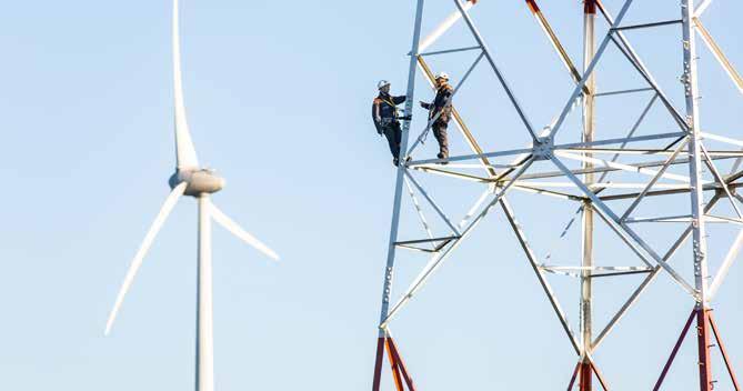
— Hydro management policy parameters: to define how net demand is weighted for energy dispatching from year to months and from month to weeks;

STEP 3: HYDRO STORAGE ENERGY MANAGEMENT

ANTARES optimises the operation of batteries the same way as pumped-storage plants, making sure that the amount of energy stored (taking into account the roundtrip efficiency of batteries) equals the amount of energy generated during the week. Demand-side Response

For each parameter, a random selection of the associated series is performed. This selection can also be made accord ing to user-defined rules (probabilistic/deterministic mixes).

Three categories of hydro plants are defined:

The aim of this step is to assess and provide to the optimiser weekly hydraulic energy volumes to generate from the dif ferent reservoirs of the system, for each week of the current 'Monte Carlo' year. To perform this pre-allocation, the module breaks down annual and/or monthly hydro storage energy into weekly amounts, using a heuristic based on:

F. Simulation of the electricity market

— Storage plants which possesses a reservoir to defer the use of water and whose generation depends on inflows and economic data. For storage plants, the annual or monthly inflows are first split into weekly amounts of energy. The use of this energy is then optimised over the week alongside the other dispatchable units. Each hydro unit can generate up to its maximum turbining capacity;

For each parameter, generation of annual time series, with an hourly resolution is needed. They represent the possible evolutions during the studied year. ANTARES can be fed with ready-made time series or can generate them with a pre-pro cessor. The number of time series for each parameter is usually between 10 to 100 and can be increased if necessary.

— Pumped-storage plant (PSP) whose power depends only on economic data. Pumped-storage plants can pump water which is stored and turbined later. ANTARES opti mises the operation of PSP alongside the other dispatch able units while making sure that the amount of energy stored (taking into account the roundtrip efficiency of the PSP) equals the amount of energy generated during the week. Pumped-storage plants are divided in two categories: open-loop and closed-loop Open-loop pumped-storage plants have a reservoir associated with a free flowing water source whereas closed-loop pumped-storage plants have a reservoir independent from any free flowing water source. Storage Storage includes the different technologies associated with batteries. Electricity can be stored in the batteries to be dis patched later. Batteries are defined by a set of parameters including loading and unloading capacity, a duration of avail ability related to the reservoir size and a roundtrip efficiency.

The market simulator used within the scope of this study is ANTARES (ANTARES: A New Tool for Adequacy Reporting of Electric Systems) [ANT-1], a sequential 'Monte Carlo' multi-area simulator developed by RTE whose purpose is to assess gen eration adequacy problems and economic efficiency issues. This power system analysis software is characterised by these following specifications: — representation of several interconnected power systems through simplified equivalent models. The European elec trical network can be modelled with up to a few hundred of region-sized or country-sized nodes, tied together by edges whose characteristics summarise those of the underlying physical components; — sequential simulation with a time span of one year and a time resolution of one hour; — 8760 hourly time series based on historical/forecast time series or on stochastic ANTARES generated times-series; — for hydro power, a definition of local heuristic water man agement strategies at monthly and annual scales; — a daily or weekly economic optimisation with hourly reso Thislution.tool has been designed to address: 1) generation/load balance studies (adequacy); 2) economic assessment of generation projects; 3) economic assessment of transmission projects.

Appendices Adequacy & Flexibility Study 2022-2032 272 273

A large number of possible future states can be extrapo lated by working with climate time series, on which random samples are carried out in accordance with the 'Monte Carlo' method (see Section 4.2.1).

The simulation scheme behind this process can be described in 4 steps:

STEP 1: CREATION OF ANNUAL TIME SERIES FOR EACH PARAMETER

STEP 2: CREATION OF A 'MONTE CARLO' FUTURE STATE (YEAR)

Generation of time series is needed in particular for wind generation, solar generation, load, hydro power generation or thermal availability. The variables of the offer-demand balance which are not modelled through time series are considered deterministic.

OPTIMISER Two optimisation problems can be addressed in this process: adequacy or economy.

The adequacy study analyses whether there is enough availa ble generation power, following the given state of the system, to meet demand, whatever the prices or costs involved. In other words, no market modelling is needed since the function that has to be minimised is the amount of load that has to be shed in the whole interconnected system. The economy study requires market modelling in order to determine which plants

The model also integrates demand side response shifting which consists in consumption that can be moved to another moment within the day. ANTARES optimizes its operation on a daily basis with the same principle as storage unit but with a 100% roundtrip efficiency.

The data selection process for each parameter provides an annual scenario called a 'Monte Carlo' year. This process is repeated several times (several hundred times) in order to obtain a set of 'Monte Carlo' years representing a set of possible futures. It is also possible to draw outages on other type of units or technologies such as HVDC links or storage facilities.

STEP 4: POWER SCHEDULE AND UNIT COMMITMENT (UC)

Hydro generation

— Reservoir rule curves: to define minimal and maximal curves in order to constrain the dispatching of hydro energy and to define the maximal power variation with the varia tion of the reservoir level.

One way of modelling demand side response in the tool is by using expensive generation units. Those will only be activated when prices are above a certain price (and therefore after all the available generation capacity is dispatched). This makes it possible to replicate the impact of demand side response shedding, which is assumed to be mostly industrial load that can reduce part of its consumption when prices are above a certain activation price, as considered in this study. Duration of availability as well as activations per day and week can be set for this capacity as binding constraints.

— Net demand pattern (Load minus RES and must-run gen eration) calculated from scenario data;

F.1. ANTARES – A MODEL USED TO SIMULATE THE ELECTRICITY MARKET

— Run-of-river (RoR) plants which are non-dispatchable and whose power depends only on hydrological inflows. Runof-river generation is considered as non-dispatchable and comes first in the merit order, alongside wind and solar generation. It is therefore subtracted from the load of each area in order to obtain a country-specific residual load;

This appendix provides a general overview on how the simula tion of the electricity market was conducted for this analysis. First the tool used to perform the simulations is introduced in Section F.1. Next, the way the market simulations are con ducted is detailed. Inputs for the simulations are introduced as well as how they are used in the constructions of the ‘Monte Carlo’ years (Section F.2).

Other variables (see below) might have a potential impact on security of supply but given their nature are disregarded in from the variables of the ‘Monte Carlo’ simulation. However, some events listed below are taken into consideration in this study by means of additional unavailability of units. The Monte-Carlo simulations performed in this study disre gard, the following events (this list is not meant to be exhaus —tive):long-term power plant unavailability (sabotage, political decisions, strikes, maintenance due to additional inspec tions, bankruptcy, terrorist attacks, etc.). Those events are assessed separately by additional unavailability of units (on top of the one drawn by the ‘Monte Carlo’ simulation); — interruption of the fuel supply or cooling of the power plants (low water levels, heatwave, …); — extreme cold freezing water courses used for plant cooling; — natural disasters (tornadoes, floods, etc.). F.2.2. Modelling of electricity generation

are delivering power at a given time. This process is carried out via the economic dispatch method, where the aim is to minimise the operating cost of the overall system by classically considering a 'perfect market' competition (market bids are based on short-term marginal costs) [ANT-1]. Because of the more refined analysis performed in the latter method, the ‘economy’ study mode is the one used in this assessment (including for adequacy simulations).

The correlation between those different climatic variables is further explain in Section 4.3.4.

Appendices Adequacy & Flexibility Study 2022-2032 274 275

F.2. CONSTRUCTION OF THE ‘MONTE CARLO’ YEARS

Another set of key variables are not correlated with the climatic variables, namely:

Year X PV Wind onshore Wind offshore PV Wind onshore Wind offshore

Hourly data for wind and PV, per unit from synthtic climate years Installed capacity Time series for

Individually modelled thermal generation Large thermal generation units, independent of their genera tion types, are modelled individually, with their specific tech nical and economic characteristics. Their individual availability is determined by a probabilistic draw for each 'Monte Carlo' year based on historical availability rates. Moreover, planned outage for future years also take into account the expected unavailabilities. This way, a very high sequence of availabilities can be drawn for each unit to be used in the simulations.

Profiled thermal generation

A first set of key variables consists in climatic variables. The main characteristic of these variables is the mutual correlation between them. In the framework of this study, the following climatic variables are considered:

Wind and solar electricity generation

Hourly wind energy production and solar generation data used are historical data for these production types. The fore casts of installed capacity for each simulated country are com bined with this historical data to obtain production time series for onshore wind, offshore wind and photovoltaic production. This process is illustrated in Figure 7-10. 7-10] — PRODUCTION TIME SERIES FOR WIND AND PV

This section elaborates on the modelling of electricity gen eration for use in market simulations. Each subsection will refer to a different technology modelled in this study wind and solar electricity generation, individually-modelled thermal generation, profiled thermal generation, hydroelectric power generation, storage and demand side response.

ANTARES 'economy' mode aims to find the optimal economic dispatch of each hydro, storage, demand response and ther mal unit, in other words the one that minimises the total system costs taking into account generation constraints and possible energy exchanges. A ‘Value of Lost Load’ (VoLL) needs to be set in the model (called ‘model VoLL’), which will define the price at which the demand would be unserved (if there is not enough capacity in the system to cover it all). This results in minimizing the Energy Not Served, as this ‘model VoLL’ will always be set higher than any other available capacity in the Moresystem.information on the optimization problems formulation, can be found on the ANTARES website [ANT-2].

A probabilistic risk analysis requires the construction of a large number of future states. Each of these states can then be analysed to determine the adequacy indicators. This section begins by indicating which variables are taken into account (Section F.2.1). Next, modelling of electricity generation is illus trated (Section F.2.2). F.2.1. Variables taken into account for the simulation

— parameters relating to the availability of thermal genera tion facilities on the basis of which samples can be taken regarding power plants’ unavailability;

1 2 3 4 5 6 7

[FIGURE 7-11] — HOURLY PROFILED THERMAL GENERATION 40%60%70%50%30%20%10%0%[%]profileProduction 1/01 31/01 2/03 1/04 1/05 31/05 30/06 30/07 29/08 28/09 28/10 27/11 27/12

Small thermal generation units are modelled in an aggregated way by using a fixed generation profile. Examples of such small thermal generation units are small biomass installations or combined heat and power (CHP) generation units. The avail ability of these smaller units is directly taken into account in the generation profile, and is therefore the same for all ‘Monte Carlo’ years. The different generation profiles for each country are collected through bilateral contacts or within the context of ENTSO-E. In Belgium, units without a CIPU contract are also modelled using profiles. Three generation types are differentiated in Belgian profiled thermal generation: biomass, CHP and waste. For each of these types, available power output measurement data was analysed. Furthermore, because no significant dif ference in aggregated behaviour between these categories was discovered, in terms of load factor or seasonal correlation, and to limit the upscaling error due to the ratio of installed capacity over measured capacity, it was decided to combine these three categories into a single generation profile. Based on historical data, this gives the hourly generation profile, dis played in Figure 7-11

— Hourly time series for wind energy generation (onshore and offshore); — Hourly time series for solar energy generation (PV and CHP);

— parameters relating to the availability of HVDC links (exclud ing those within a meshed grid) on the basis of which sam ples can be taken regarding their availability.

— Daily time series for temperature (used to calculate the hourly time series for electricity consumption); — hydro inflows.

[FIGURE

wind and PV40008000600020000100806040200[%]factorLoad[MW]Power

2016 2017 2018 2019 2020 January January January January January

G.1. DISPATCH OF INDIVIDUALLY-MODELLED UNITS

The capacity factor is then compared to the electricity prices observed on an hourly-basis. The process to obtain the capac ity factor is presented on Figure 7-12

This Appendix deals with historical generation data and will highlight several observations that comforts the modelling choices made for the different types of capacities in Belgium. In addition, it also focusses on maximum and minimum gen eration observed in the past and their possible impact ont the adequacy results obtained in this study This analysis shows that: - CCGT and OCGT units are never dispatched at their maxi mum available capacity confirming the need to account for balancing reserves such as done in this study;

of nominal capacity available in the market per technology Availability (FO, PO) Nominal Capacity Hourly

Appendices Adequacy & Flexibility Study 2022-2032 276 277

— METHODOLOGY

In order to analyze the potential price dependence of the capacity factor, the generation over the monitored period is first analysed. Then, a view on the generation and associ ated historical electricity prices is given. A moving average trend line is added in order to provide an indication of the price dependence with the capacity factor. This indicator also includes a focus on capacity factors in case of low or high prices.

For each unit, the hourly electricity generation is evaluated and is compared to its maximum available power. This is obtained by looking at the maximum power of the unit, at the hourly availability status of the unit in order to eliminate periods of planned or forced outage and at its commissioning/decom missioning dates. A capacity factor is obtained by dividing the electricity generated by the power available in the market.

[FIGURE 7-12] TO FACTORS profile capacity factor per technology

First, the generation of CCGT and OCGT is shown on Figure 7-13. Several observations can be already made: — a minimum generation of about 10% can be observed, usu ally during summer months, which is mainly explained by must-runs set to provide ancillary services; — important variation of the energy dispatched within the day, which suggest more intra-day variation linked to elec tricity prices; — a seasonal variation, with higher generation in autumn and winter than in spring and summer, which can be explained by electricity market economics; — a capacity factor never reaching 100%, which could be explained by the fact that some units were contracted to provide ancillary services and hence were kept available for Secondly,those.the capacity factor values are compared to historical prices. The Figure 7-14 illustrates the correlation between the capacity factor and the electricity prices. For CCGT and OCGT, there is a strong correlation of the electricity generation with the electricity market prices. Large scale units mainly react to price signals.

On the low prices side, most of the units are not dispatched on the electricity market as their marginal cost is higher than the market price. Some must-run value should therefore be taken into account. Indeed, a capacity factor between 10 and 40% is observed on historical data. In order to provide a range for the model, the minimum and average value of the capacity factor in case of low prices (below 5 €/MWh) can be consid ered as border for the analysis. Therefore, it appears that a must-run value of 10 to 20% of the installed capacity should be considered.

Hourly

PER TECHNOLOGY Aggregated hourly electricity generation per technology Hourly fromgenerationelectricityhistoricaldata Historical data Historical data per unit Historical data per technology Aggregated hourly

Methodology followed The analysis covers the years 2016 to 2020 and the data used is coming from the ENTSO-E Transparency Platform [ENT4] for the electricity prices and from Elia’s internal database for the unit’s dispatch information of individually-modelled thermal units.

On the high prices side, most of the units are 100% dispatched but some delta remains. This can mainly be explained by the fact that some units are contracted to provide ancillary ser vices. It justify to reserve a part of the installed capacity for this need. This volume is correlated to the volume of balanc ing need to be procured by thermal units and should lead to a percentage of installed capacity between 77% and 95%, which corresponds to the average and maximum values of the capacity factor in case of high prices (above 100 €/MWh).

CCGT and OCGT dispatch

The data were aggregated by different types (note that oilfired and nuclear units were excluded from this analysis): — OCGT and CCGT with a CIPU-contract; — CHP units with a CIPU-contract; — waste and biomass units with a CIPU-contract.

G. Historical analysis of input data

[-]FactorCapacity capacity factor

[FIGURE 7-13] — EVOLUTION OF CCGT/OCGT UNITS HOURLY CAPACITY FACTOR ON THE ANALYSED PERIOD 0.40.80.910.70.60.50.30.20.10

Thermal units are modelled in two different ways in market studies. The units with a CIPU contract (usually larger units) in Belgium are individually modelled whereas other ones are modelled though a profile based on historical data. This sec tion will focus on the first kind of units. The individually modelled units can be dispatched accord ing to their technical and economic parameters. However, it appears that, on the one hand, some of them still generate electricity in case electricity prices are below their calculated marginal cost and, on the other hand, some of them did not produce at full capacity in case of (extra-)high electricity prices. The reasons can be diverse and could be related to ancillary services or underlying industrial processes supplied.

CALCULATE HOURLY CAPACITY

- Large scale CHP and biomass/waste units are never dis patched at their maximum available capacity neither This is not taken into account in this study and could result in 100 to 350 MW over-estimation of contribution to adequacy of this technology; - Small scale generation’s maximum capacity factor is slightly above 60%, confirming the approach chosen by Elia to model it with a profile based on historical data; - Some thermal units have minimum generation constraints which are required to be taken into account in the model.

[-]FactorCapacity

Appendices Adequacy & Flexibility Study 2022-2032 278 279 [FIGURE 7-14] — COMPARISON BETWEEN ELECTRICITY PRICES AND CHP GAS WITH CIPU CONTRACT UNITS CAPACITY FACTOR CORRELATION BETWEEN CAPACITY FACTOR AND PRICES 2 3 1 00,10,20,30,40,50,60,70,80,91 [-]FactorCapacity 1 Baseload generation of about 10% 2 Maximum generation reached with prices around 100 Maximum€/MWhcapacity factor rather round 90% 3 Moving average shows strong price - capacity factor Increasedependenceinmarketprices is the main driver of capacity factor increase

[-]FactorCapacity

The values of capacity factor are higher on average for CHP gas units than for CCGT and OCGT, which can be explained by the higher baseload generation. Moreover, the delta between the average capacity factor in summer and in winter is less important than for CCGT and OCGT, which could be linked to a lower correlation with price signals as some units are pro ducing on a baseload basis whatever the price.

KEY TAKE AWAYS

In order to simulate correctly the dispatch of CCGT and OCGT on the Belgian market zone, it appears that applying a unit-byunit model reacting to price signals is a good representation based on historical correlation between prices and electricity

Secondly and to provide more relevant conclusion regarding CHP gas units, the capacity factor values are compared with historical prices. The correlation and moving average are pre sented on Figure 7-16.

On the low prices side, it is confirmed that some must-run value should be taken into account. Indeed, a capacity factor between 30 and 85% is observed on historical data. In order to provide a range for the model, the minimum and average value of the capacity factor in case of low prices (below 5 €/ MWh) can be considered as border for the analysis. Therefore, it appears that a must-run value of 30 to 55% of the installed capacity should be considered. On the high prices side (above 100 €/MWh), it confirms that this technology can be dispatched at full capacity in case of high prices but that the average capacity factor is equal to 77%, meaning that the side process can potentially influence the dispatch at 100% of its installed capacity of the gas-fired CHP, meaning that allowing the model to dispatch those units at their full capacity might overestimate their real contribution to Betweenadequacy.0€/MWh and 100 €/MWh, the capacity factor seems to slightly increase. The moving average shows an evolution from 50% to 80% between those price ranges. Those effects seems to suggest a slight price dependency. The moving average curve shows that the correlation between prices and capacity factors are less important than for OCGT and CCGT.

— EVOLUTION OF CHP GAS WITH CIPU CONTRACT UNITS HOURLY CAPACITY FACTOR ON THE ANALYSED PERIOD January January January January January 0.40.80.910.70.60.50.30.20.10

— A seasonal variation, leading to lower capacity factor in sum mer period which could be due to the thermosensitivity of the industrial supplied processes; — a maximum capacity factor of around 90%.

The electricity generation is significantly higher from Novem ber to February and is at its lowest from May to September.

Nevertheless,generated. the dispatch should be bounded with a must-run value between 10% and 20% in order to take into account the historical dispatch in case of low prices, in order to capture the must-runs observed historically (which could be due to balancing reserves).

:

Hourly capacity factor 2016 2017 2018 2019 2020

ZOOM 1 CAPACITY FACTOR IN CASE OF LOW PRICES ZOOM 2 : CAPACITY FACTOR IN CASE OF HIGH PRICES Belgian market zone price [€/MWh] -100 -80 -60 -40 -20 0 Belgian market zone price [€/MWh] 100 150 200 250 300 350 400 Price [€/MWh] -100 -50 0 50 100 150 200 Minimum Capacity Factor 0,40,80,90,70,60,50,30,20,10 Average Capacity Factor in case of high prices Minimum Capacity Factor 2 3 1 Average Capacity Factor in case of low prices

— baseload generation of the technology between 30 and 40%, which is mainly explained by the side processes asso ciated to each CHP with unit-by-unit specificities; — lower variation of the energy dispatched compared to CCGT and OCGT, which suggest lower intra-day variation to meet the daily peaks and hence lower reaction to price signals;

Firstly, the analysis of the capacity factor on the whole period presented on Figure 7-15 shows some indications:

0,40,80,910,70,60,50,30,20,10[-]FactorCapacity

Moreover, it shows that the capacity factors do not reach its maximum dispatch in case of high prices. The maximum output is limited to 77% to 95% of the maximum available capacity mainly as a part is reserved for balancing purposes. This clearly confirms the approach followed in this study where balancing reserve capacity is accounted for.

Dispatch of CHP gas units with CIPU-contract

The second part of this analysis is dedicated to CHP gas units with CIPU-contract. The analysis integrates the available metering from CIPU units which are individually modelled in this study.

[FIGURE 7-15]

Hourly capacity

factor 2016 2017 2018 2019 2020 January January January January January

Between 0 €/MWh and 100 €/MWh, the moving average shows that the correlation between prices and capacity fac tors has a lower slope than for OCGT, CCGT and gas-fired CHP, which indicates less variation of this technology according to market signals.

[-]FactorCapacity

The third part is dedicated to biomass and waste units. The analysis integrates the metering from CIPU units which are individually modelled in this study.

Secondly, the capacity factor values are compared with histor ical prices. The correlation and moving average are presented on Figure 7-18.

Firstly, the analysis of the capacity factor on the whole period (see Figure 7-17) reveals some indications:

Dispatch of Biomass & waste units with a CIPU con tract

Average Capacity Factor in case of low prices Minimum Capacity Factor 0.40.80.910.70.60.50.30.20.10[-]FactorCapacity

In order to simulate correctly the dispatch of gas-fired CHP with CIPU contract on the Belgian market zone, it appears that applying a unit-by-unit model reacting to price signals may not be the best representation based on historical correlation between prices and electricity generated. However, applying only an historical thermal profile may also not be the best solution as units can be dispatched at almost 100% of their installed capacity. Therefore, the unit-by-unit model is kept but might overestimate the real contribution of gasfired CHP to adequacy or in case of high prices. Moreover, the dispatch should be bounded with a must-run value between 30% and 55% in order to take into account the historical dispatch in case of low prices which could be mainly explained by the need of the side processes.

[FIGURE 7-17] — EVOLUTION OF BIOMASS & WASTE WITH CIPU CONTRACT UNITS HOURLY CAPACITY FACTOR ON THE PERIOD ANALYSED

KEY TAKE AWAYS

— minimum generation of the technology is around 30 to 40%, which is similar to gas-fired CHP units; — lower variation of the energy dispatched compared to CCGT and OCGT, which suggest lower intra-day variation to meet the daily peaks and hence lower reaction to price signals; — limited seasonal trend with higher values in winter than in summer, with a delta round 5%, which seems to suggest a constant electricity generation through the whole year and a limited price signals reaction; — The maximum generation is slightly above 90% of the capacity factor.

ZOOM 1 CAPACITY FACTOR IN CASE OF LOW PRICES ZOOM 2 CAPACITY FACTOR IN CASE OF HIGH PRICES 0.40.80.910.70.60.50.30.20.10[-]FactorCapacity

On the low prices side, it is confirmed that some must-run value should be taken into account. Indeed, a capacity factor between 37 and 88% is observed on historical data. In order to provide a range for the model, the minimum and average value of the capacity factor in case of low prices (below 5 €/ MWh) can be considered as border for the analysis. Therefore, it appears that a must-run value from 35 to 65% of the installed capacity should be considered.

CORRELATION BETWEEN CAPACITY FACTOR AND PRICES

0.40.80.90.70.60.50.30.20.10

Belgian market zone price [€/MWh] -100 -80 -60 -40 -20 0

On the high prices side (above 100 €/MWh), it confirms that this technology can be dispatched at almost full capacity in case of high prices. By taking the maximum and average value, it means that a capacity reduction of 83 to 91% can be applied on the installed capacity of biomass and waste units. This value also confirms that dispatching the whole installed capacity in the model might lead to overestimation of the real contribution of these technologies.

Belgian market zone price [€/MWh] 100 150 200 250 300 350 400 Average Capacity Factor in case of high prices Maximum Capacity Factor 00.10.20.30.40.50.60.70.80.91

[-]FactorCapacity Price [€/MWh] -100 -50 0 50 100 150 200 1 Baseload generation of about 35% 2 Capacity factor between 60 and 100% above 100 €/ MWh, without clear trend Maximum capacity factor rather round 95% 3 Moving average shows limited price - capacity factor dependence Linear increase of the capacity factor between 0 and 100 €/MWh, leading to an increase of the capacity factor between 50 and 80%. 1 3 2

Appendices Adequacy & Flexibility Study 2022-2032 280 281 [FIGURE 7-16] — COMPARISON BETWEEN ELECTRICITY PRICES ANDCHP GAS WITH CIPU CONTRACT UNITS CAPACITY FACTOR

[-]FactorCapacity

Firstly, an analysis will be performed on the aggregation of all kind of technologies. Secondly, an analysis will be performed by technology. The indicators used are the same than the one described in Section G.1 related to individually-modelled units.

Thermal units are modelled in two different way in the ANTARES model. The units with a CIPU contract are individ ually modelled whereas other ones are modelled though a profile determined on historical data. This section will be ded icated to this second type of units.

00.10.20.30.40.50.60.70.80.91

[FIGURE 7-18] — COMPARISON BETWEEN ELECTRICITY PRICES AND BIOMASS & WASTE WITH CIPU CONTRACT UNITS CAPACITY FACTOR

[-]FactorCapacity

Moreover, the dispatch should be bounded with a must-run value between 35% and 65% in order to take into account the historical dispatch in case of low prices.

Appendices Adequacy & Flexibility Study 2022-2032 282 283

ZOOM 1 : CAPACITY FACTOR IN CASE OF LOW PRICES 0.40.80.910.70.60.50.30.20.10[-]FactorCapacity Belgian market zone price [€/MWh] Minimum Capacity Factor Average Capacity Factor in case of low prices -100 -80 -60 -40 -20 0

Average Capacity Factor in case of high prices Maximum Capacity Factor Belgian market zone price [€/MWh] 100 150 200 250 300 350 400 2 3 1 CAPACITY FACTOR

CORRELATION BETWEEN

ZOOM 2 CAPACITY FACTOR IN CASE OF HIGH PRICES 0.40.80.910.70.60.50.30.20.10

AND PRICES

G.2. DISPATCH OF PROFILED AGGREGATED UNITS

Context In the latest studies published by Elia (Strategic Reserves, CRM calibration report or in the Adequacy & Flexibility study from 2019 [ELI-5]), Elia received comments regarding the historical profile used to model the contribution of profiled thermal Thisgeneration.profile is calculated based on DSO’s input data and are aggregated in order to obtain a hourly capacity factor profile, as presented on Figure 7-12 This profile serves as input data for the profiled thermal generation of “waste”, “biomass” and “gas or other” which are not individually modelled.

Following some feedback received, it was important in the framework of this study to analyse the electricity generated from non-CIPU units in comparison with their maximum avail able capacity in order to verify its potential correlation with the economic activity, i.e. lower heat demand during for CHP during weekend and at night (21-6 hour).

Moreover, the input data have been sometimes criticized but no additional information were provided to Elia in order to improve its data quality if judged necessary. The purpose of this section is therefore to make an assessment of the gen eration from small-scale non-CIPU units based on the most recent data and to justify the relevance of the profile used.

Methodology followed The dispatch information of non-CIPU non-renewable (NCNR) capacities come from Elia’s internal database and the elec tricity prices from the ENTSO-E Transparency platform. These information are aggregated with a hourly time step. The data found in Elia’s database is fed by the DSO’s. It is important to note that Elia does not have hourly metering data for all small-scale units in Belgium (as they are not connected to the Elia grid). Depending on the historical year, the proportion of units with metering data varies between 60 and 70% of the total installed capacity. This amount corresponds to the best available information and is assumed to be sufficiently rep resentative of the whole generation profile of this category.

Results Firstly, the analysis of the capacity factor on the whole period (Figure 7-19) shows some indications: — minimum generation between 20 and 30% during summer and between 40 and 50% during winter can be observed; — lower variation of the energy dispatched, which suggests lower intra-day variation to meet the daily peaks and hence lower reaction to price signals; — seasonal behavior leading to capacity factor of around 55% in winter and 40% in summer; — a maximum capacity factor slightly higher than 60%.

KEY TAKE AWAYS

The findings comfort the approach chosen for biomass and waste units which have a CIPU contract. There are also some observations which tend to demonstrate that allowing those units to reach their full capacity in the model consists in an over estimation in their contribution to adequacy. Indeed, 100% load factor is never reached, even when high prices are observed on the electricity market.

1 Baseload generation of about 40% 2 Capacity factor between 80 and 90% above 100 €/MWh, with constant moving averageUnitsnot dispatched at full capacity even with very high prices 3 Moving average shows limited price - capacity factor dependence Linear increase of the capacity factor between 0 and 100 €/MWh, leading to an increase of the capacity factor between 60 and 85%. Price (€/MWh) -100 -50 0 50 100 150 200

[FIGURE 7-19] — EVOLUTION OF NCNR UNITS HOURLY CAPACITY FACTOR ON THE PERIOD ANALYSED 0.40.80.90.70.60.50.30.20.10[-]FactorCapacity 2016 2017 2018 2019 2020 Hourly capacity factor January January January January January

PROFILE

0.40.80.910.70.60.50.30.20.10

— AVERAGE

Moreover, it make sense to consider an additional indicator which will focus on the weekly behavior of the NCNR profiles. In order to illustrate this, the average weekly profile will be analyzed by taking the average by weeks (from Monday to Sunday) on the whole period analyzed (Figure 7-21). It can be observed on this graph a clear intra-daily modu lation of the energy generated with a difference in capacity factor between day and night of about 10%. The profile varies indeed between 40% and 50% on average. There is a difference between a week day and the weekend but it is quite marginal. An average profile on the day could also be representative for the whole period. [FIGURE 7-21] WEEKLY NCNR

7-20] — COMPARISON BETWEEN ELECTRICITY PRICES AND NCNR WITH UNITS CAPACITY

ZOOM 1 : CAPACITY FACTOR IN CASE OF LOW PRICES ZOOM 2 : CAPACITY FACTOR IN CASE OF HIGH PRICES Belgian market zone price [€/MWh] -100 -80 -60 -40 -20 0 Belgian market zone price [€/MWh] 100 150 200 250 300 350 400 Price (€/MWh) -100 -50 0 50 100 150 200 0.40.80.910.70.60.50.30.20.10[-]FactorCapacity Minimum Capacity Factor Average Capacity Factor in case of low prices 0.40.80.90.70.60.50.30.20.10[-]FactorCapacity Average Capacity Factor in case of high prices Maximum Capacity Factor CORRELATION BETWEEN CAPACITY FACTOR AND PRICES 1 3 2

Regarding the seasonal variation, the average capacity factor delta between summer and winter is equal to around 15%. As NCNR technologies are often linked to a side process, it could mean that the need of the associated process (industry, heat, …) is higher in winter than in summer or that the profile reacts to temperature. However, regarding the amount of different kind of unit type taken into account in this aggregation, it would be difficult to identify clearly the trend associated to the need of the side process. In order to evaluate if NCNR tech nologies react mainly to price signals on the electricity market or to the need of the associated side process, an evaluation of the correlation between the capacity factor and the price in the Belgian market zone is required.

KEY TAKE AWAYS

Secondly, the capacity factor values are compared with histor ical prices. The correlation and moving average are presented on Figure 7-20. For NCNR technologies, the baseload gener ation is higher than 20%, reaching about 30% and the maxi mum capacity factor is below 70%. The generation variation of NCNR technologies is therefore quite limited in terms when looking at the capacity factor. Moreover, the minimum gener ation increase with the prices when the price on the Belgian market zone is above 50 €/MWh which can be explained as a consequence of the seasonal variation. The minimum capacity factor evolves from 20% at 50 €/MWh to 40% at 100 €/MWh and 55% at 200 €/MWh. The maximum capacity factor is quite stable for prices above 20 €/MWh but decreases with lower prices, going from 65% at 20 €/MWh to 50 €/MWh in case of negative prices. The moving average shows a s-curve with an increasing trend of the moving average from 40% at 0 €/ MWh to 60% at 100 €/MWh. [FIGURE FACTOR 00.10.20.30.40.50.60.70.80.91

[-]FactorCapacity

[-]FactorCapacity 1 Baseload generation of about 30% 2 Capacity factor between 55 and 65% above 100 €/ MWh, with constant moving average Units not dispatched at full capacity even with very high prices 3 Moving average shows lim ited price - capacity factor dependenceLinearincrease of the ca pacity factor between 0 and 100 €/MWh, leading to an increase of the capacity factor between 40 and 60%.

The best way to model non-CIPU non-renewable technologies on an aggregated way is to use a profile built on historical data. Such approach is also the one chosen by many TSOs and ENTSO-E for small scale generation. From this analysis, it can be observed that, the maximum capacity factor obtained is slightly above 60%.

Appendices Adequacy & Flexibility Study 2022-2032 284 285

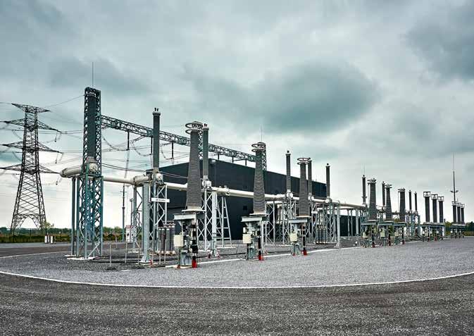
H. EVA metric

Following the study from Professor K. Boudt for long-term investment in electricity capacity in Belgium in 2021, a reason able calibration is to set the risk-free rate at 0.47%, the country premium at 0.36%, the equity premium at 6.1% and the equity beta at 1.02. It follows that CoE = 7.052%.

One One week period Market bid Market clearing price Generator dispatch Variable costs Inframarginal rents

week period

The cost of debt (CoD) is estimated by analyzing the balance sheet of prospective investors. A reasonable assumption here is that CoD = 4%. Assuming a gearing ratio of 40%, a tax rate of 25% and expected inflation of 1.60%, the study obtains a real and pre-tax WACC of 5.53%. These values were also included in Elia’s report on the public consultation.

H.1. OVERVIEW OF THE WACC CALCULATION

[FIGURE 7-22] — CALCULATION OF INFRAMARGINAL RENTS OF INVESTMENT CANDIDATES MWhperEuro (Thousands)Euros(MW)Power406070503020100 406070503020100020406080100120

— Heavy oil prices are based on the historic difference between crude oil and heating oil. This corresponds to around +5% of the crude oil price when looking at historical data; — Light oil prices are based on the historical difference between crude oil and gasoline. This corresponds to around + 28% of the crude oil price when looking at historical data. Given the absence of public traded data on those different oil derivatives in Europe, the IEA data (US) was used to calculate the historical average. Further information on the data can be found in [EIA-1]. This approach is the same as followed by ENTSO-E for its TYNDP or MAF studies. In addition, Estonian Shale Oil prices are assumed to be 2.3 €/ GJ based on the ENTSO-E common data.

VARIABLE COSTS OF THERMAL UNITS IN OTHER PRICE SCENARIOS [FIGURE

For each hour in the economic dispatch simulation, the market bid of the investment candidate was extracted, the market clearing price and the generators dispatch. Under the assump tion that generators bid at their marginal cost, the candidate’s inframarginal rents can be calculated by multiplying its dis patch by the difference between the market clearing price and the plant’s market bid.

The extraction of revenues corresponds to step 3 described in Section 4.4.2, while the correction of revenues for the price cap depends on previous years (as sampled in the Monte Carlo draws) is as such performed in step 5

Appendices Adequacy & Flexibility Study 2022-2032 286 287

I. Further assumptions on fuel prices

I.2. 7-23]

I.1. OIL PRICES

— MARGINAL COSTS OF GAS AND COAL FIRED UNITS FOR THE ‘LOW CO2’ SCENARIO [€/MWh] 100140160120806040200 Years 2031 20322020 2021 2022 2023 2024 2025 2026 2027 2028 2029 203020192018201720162015 Historical (yearly basis) ‘Low’ scenarioBeginningForwardofMarch OCGT new OCGT old CCGT new CCGT old Hard coal new Hard coal old

H.2. EVA : DETERMINATION OF REVENUES

For the reference WACC, the study from Profes sor K. Boudt fol lows the guidelines from the ACER methodology. This includes the use of the well-known Capital Asset Pricing Model (CAPM) for the cost of equity (CoE) calculation CoE= r_f+ β x ERP+CRP where r_f is the long-term risk-free rate, β is the systematic risk of the reference investors, ERP is the equity risk premium and CRP is the country risk premium.

For oil costs, the ‘heavy oil’ and ‘light oil’ prices are derived from the crude oil prices as follows:

Appendices Adequacy & Flexibility Study 2022-2032 288 289 [FIGURE 7-24] — MARGINAL COSTS OF GAS AND COAL FIRED UNITS FOR THE ‘HIGH CO ’ SCENARIO 2031 20322020 2021 2022 2023 2024 2025 2026 2027 2028 2029 203020192018201720162015 [€/MWh] 100140160120806040200 Years Historical (yearly basis) ‘High’ scenarioBeginningForwardofMarch OCGT new OCGT old CCGT new CCGT old Hard coal new Hard coal old

— GAS AND COAL PRICE EVOLUTION FROM 2010 TO 2019 €/tCOor[€/GJPrice2] Years 20192013 2014 2015 2016 2017 2018201220112010 Coal (Monthly Value) Gas (Monthly Value) Coal (Yearly Value) Gas (Yearly Value)

— GAS YEARLY EVOLUTION - MIN, MAX AND AVERAGE

April May June July October November DecemberAugust SeptemberMarchFebruaryJanuary

[FIGURE 7-27]

As fuel costs make up the biggest part of the marginal cost of fossil fuel technologies, analyzing the variation of fuel prices during the year is relevant to assess correctly its impact on economic results. When looking at historical prices, it appears indeed that significant variations are observed for gas, coal and carbon prices. Figure 7-25 shows the monthly average over the last ten years. One initial observation based on this figure is that gas prices variation are much more important than coal prices variation over the same time horizon.

[-]FactorModulationMonthly 0.80.91.41.61.51.31.21.110.70.6

October November DecemberApril May June July August SeptemberMarchFebruaryJanuary

Gas Regarding gas prices, a clear seasonal trend was observed. The gas prices are significantly higher in winter periods and lower in summer. In 40% of the years analysed the U-curve shape is confirmed. In 50% of the years analysed, only one side of the U-curve is mainly observed (either in the beginning or in the end of the year). In the last 10%, no seasonal trend is observed. Based on those findings, a monthly gas price modulation is used for this study which is based on the average of the last ten-years gas prices data. 7-26]

[FIGURE 7-25]

Coal Regarding coal prices, the trend observed is less straightfor ward. The average monthly modulation is flatter but the var iation around this average remains significant. However, coal prices appear to be higher mainly in January and December which impacts the electricity prices in winter periods. In 30% of the years analyzed the U-curve shape is confirmed. In 40% of the years analyzed, only one side of the U-curve is mainly observed (either in the beginning or in the end of the year). In the last 30% of the years, no seasonal trend is observed. It also appears that 2016 seems to be an outlier in this analysis as a significant price increase is observed throughout the year. It leads to the lower factor in January and to the higher in December. Based on those findings, a monthly coal price modulation is used based on the average of the last tenyears data without considering the year 2016. This choice leads to slightly higher factors in the beginning of the year and slightly lower at the end of the year but it better reflects the trend observed on the whole data sample.

I.3. MONTHLY FUEL PRICE MODULATION In complement of Section 3.6.1, this Appendix aims to present the context and methodology followed in order to integrate monthly fuel price modulation in the ANTARES model.

Gas prices from TTF Gas and Coal prices from ARA Coal.

— COAL YEARLY EVOLUTION - MIN, MAX AND AVERAGE VALUES

CO2 No clear trend was observed for CO2 prices. The global trend is an increasing value with time which seems independent from the season or the month. Therefore, no CO2 price modulation was applied in the framework of this study.

[FIGURE

30352520151050

VALUES [-]FactorModulationMonthly 0.80.91.41.61.51.31.21.110.70.6

Météo-France is simulating two RCP scenarios for the climate of 2050, the RCP 4.5 and RCP 8.5. The most pessimistic sce nario for 2050, the RCP 8.5 is the one used in terms of tem perature for the interpolation to 2025 (see after).

Appendices Adequacy & Flexibility Study 2022-2032 290 291

After calibration, the median of the simulated values is matching the median of the historical values and that the simulated-200-years maximum and minimum values are well respectively above and below and the historical-30-years ref erence period. Therefore, the two databases have now similar statistical characteristics.

The transformations applied on the simulated climate years of the climate 2000 are called “transfer functions” that depend on the location point, date of the year and the hour of the day.

As the simulated 2050-CY contains similar biases, the same transfer functions are applied.

— Why and how is the interpolation done for the year 2025 ?

Why and how is a calibration done ? The calibration aims at correcting the biases that are inherent in any model. To do so, the 200 simulated climate years are compared with historical values around the year 2000 and transformations are applied to ensure the simulated climate years have the same statistical characteristics as the reference historical database. In this case, the reference used by MétéoFrance is the historical database HIRLAM/ERA-Interim at a resolution of 0.2° in latitude and longitude over the period 1984-2013 (centered around the year 2000).

J. Climate years of Météo-France

This appendix aims at giving extra information on the follow ing points — Why and how is a calibration done ?

— How are the GHG concentration estimated for 2050 ?

The interpolation done by Météo-France for the 2025-cli mate is based on the simulations of 2000-climate and the 2050-RCP8.5-climate. Indeed, the actual evolution of the GHG concentration seems to follow the RCP 8.5 [MET-2], which leads to a higher increase in temperature.

Why and how is the interpolation done for the year 2025 ? As explained and shown by Météo-France in [MET-3], the inter polation to an intermediate climate between 2000 and 2050 allows a representation of the climate for the target year (2025) to be approached with good plausibility without having to implement a simulation specific to that target year.

K. Costs figures and comparison with litterature [FIGURE 7-28] — COMPARISON OF OCGT CAPEX COSTS FOUND IN THE LITTERATURE WITH THE CHOSEN VALUES IN THIS STUDY [€/kW]inCosts 10009008007006005004003002001000 Etri Lazard Pöyry EnergyvilleBEISPwCFichtner Range for this study400500 [FIGURE 7-29] — COMPARISON OF CCGT CAPEX COSTS FOUND IN THE LITTERATURE WITH THE CHOSEN VALUES IN THIS STUDY [€/kW]inCosts 1000140012008006004002000 EtriAsset Lazard Pöyry Frontier EnergyvilleBEISPwCFichtner Range for this study600850

In order to estimate the GHG concentration in the future, the scientists from the Intergovernmental Panel on Climate Change (IPCC – GIEC) have defined several hypothesis leading to different trajectories called Representative Concentration Pathway (RCP) [IPC-1]. Four different trajectories have been defined for climate change modeling. Each scenario repre sents a different radiative forcing value (2.6, 4.5, 6.0 and 8.5) leading to a possible future, depending on the GHG emissions in the next years. The RCP 8.5 scenario is the one leading to the highest increase in temperature.

The 200 simulated CY under the constant climate of 2000 are adapted for the 2025 constant climate by an interpolation of the statistical distribution of the 2000-CY and 2050-RCP8.5-CY.

How are the GHG concentration estimated for 2050 ?

Appendices Adequacy & Flexibility Study 2022-2032 292 293 L. Thermal capacity ‘at risk’ in Belgium [FIGURE 7-30] — LETTER FROM ENGIE ELECTRABEL ON THE THERMAL CAPACITY 'AT RISK'

As a second step the tool incorporates the effect of addi tional electrification and decentralised storage (‘out-ofmarket’ only), on top of the existing devices already taken into account in the normalised and total consumption profile obtained after the first step: — the different TSOs communicate their assumptions to ENTSO-E, reflecting the estimated evolutions in the market of the different factors driving electricity consumption (e.g., penetration of heat pumps, electric vehicles, additional baseload, sanitary water, out-ofmarket batteries); — these assumptions are translated into inputs for the different electrification technologies and the different components are split into climate-dependent and cli mate-independent components; — the final load profiles are adjusted, taking into account additional consumption from the different electrifica tion technologies.

= Monday Tuesday Wednesday Thursday Friday Saturday Sunday 1014161513121198[GW] Monday Tuesday Wednesday Thursday Friday Saturday Sunday 1014161513121198[GW] Monday Tuesday Wednesday Thursday Friday Saturday Sunday 1014161513121198[GW] Monday Tuesday Wednesday Thursday Friday Saturday Sunday 1014161513121198[GW] Monday Tuesday Wednesday Thursday Friday Saturday Sunday 1014161513121198[GW] National normalised load Re-scaled national normalised load Re-scaled national load with thermosensitivity Re-scaled national load with thermosensitivity and EV Re-scaled national load with thermosensitivity, EV and heat pumps

[FIGURE 7-31] — DEMAND CONSTRUCTION – ILLUSTRATION WITH A WEEKLY PATTERN [GW] +++

Appendices Adequacy & Flexibility Study 2022-2032 294 295 M. Electricity consumption

— multiple historical climate and load time series are used to derive the relationship between electrical load and historical climate patterns for each market node (i.e. the thermosensitivity of the load);

The tool, which is based on the methodology and tools developed in the ENTSO-E adequacy assessment, allows hourly electric load projections to be performed based on a set of input data, carried out in two main steps:

— a normalised profile is constructed for each market node, taking into account ‘average’ climate conditions and incorporating a normalised profile for each day of the year; — the normalised profile is adapted to take into account the consumption growth due to economic growth, population growth and energy efficiency. Additional corrections were made through the incorporation of special days (e.g. corrections are made for holiday peri ods, exceptional events, etc.);

As part of a first step the model maps the historical rela tions between ambient temperatures and electrical load for each simulated country:

Normalised profile is rescaled to EVeffectdemographicmacro-economictake&trendsintoaccountThermosensitivityisaddedtothenormalisedprofilechargingisaddedHeatpumpsareaddedForecastednationalloadprofileforagivenclimateyear

— a set of 200 synthetic climate years incorporating the climate in 2025 are used for the construction of the load series forecast, by applying the observed historical relations between the climate and electrical load for each market node; — the resulting predicted load series therefore include pres ent-day market characteristics in terms of the amount of electrification in heating, cooling and transport.

BOX A ON THE GENERAL METHODOLOGY

The normalisation of a historical year is carried out in two —steps:Firstly, the realised total consumption is normalised based on the observed amount of degree days during that year and a certain reference amount of degree days. This is carried out by comparing the amount of degree days of the realised year and the assumed normalised amount of degree days and applying the thermosensitivity; — Secondly, the amount of working days and total amount of days in a year are also taken into account. For instance, all leap years are normalised to years with 365 days by simply removing the average consumption for 1 day.

85

All yearly consumption is therefore expressed for the same amount of degree days. For this purpose, Elia used the reference amount of degree days from Synergrid, although as will be described below, normalisation can happen on any reference with the same final result. The normalisation process allows the effect of temperature to be removed by looking at the different consumption values, assuming that the temperature (= amount of degree days) over the year was the same. Normalised consumption serves as an input for the creation of the hourly load profiles. In order to construct hourly profiles, the estimated temperatures were also given as input for each climate year. This enables the temperature effect that was isolated during the normalisation to be applied by using again the thermosensitivity, which is estimated to be between 100 and 150 MW/°C for each hour in Belgium. Based on the future temperature estimated for that specific year, a number of degree days (difference between the temperatures – relative) was calculated. Finally, the consumption can then be “de-normalised”.

[FIGURE 7-32] — EXAMPLE OF NORMALISATION AND DE-NORMALISATION OF ELECTRICITY CONSUMPTION Normalisation process: example De-normalisation process: example Historical consumption [TWh] 848085908582 For given Degree Days [°C] Degree Days [°C] 2000 2000 80 (2000-2300*Th) = 85 (2000-2300*Th) 3000 3000 90 (3000-2300*Th) = 85 (3000-2300*Th) 2400 2400 84 (2400-2300*Th) = 85

This shows that normalisation can happen on any reference amount of heating degree days. Hence, if it is expected that these might decrease or increase in the future, the normalised demand would decrease or increase accord ingly, but the future demand based on a given temperature will stay the same. (2400-2300*Th) (2500-2300*Th) = (2500-2300*Th)

2500 2500 85

Normalisation is a way to look at electricity consumption while cancelling the effect of the temperature (which drives a small part of consumption). Even if its impact in terms of electricity consumption is limited in Belgium, it can still result in a non-negligible correction. The normalisa tion process is based on the amount of degree days (see below), the realised total consumption and the amount of days in a year. A degree day is the difference between the reference tem perature in a specific place and the average temperature of that same place and is a figure which corresponds to a period of 24 hours. For the calculations of degree days, Elia relied on the Synergrid methodology and numbers (Synergrid degree days are mainly used by the gas sector to determine consumption patterns).

2200 2200 82 (2200-2300*Th) = 85 (2200-2300*Th) Future consumption [TWh] Normalized to 2300 DD [TWh] Assumed future normalised consumption at 2300 DD [TWh] Th = assumed thermosensitivity in TWh/°C N. Power-to-X [FIGURE 7-33] — ASSUMPTIONS OF INSTALLED CAPACITY FOR POWER-TO-X IN EUROPEAN COUNTRIES MODELLED 2025 2026 2027 2028 2029 2030 2031 2032 BE DE ES FR GB NL PL PT Total [GW] 4035302520151050 4,0 9,4 14,8 20,3 25,7 31,1 33,8 36,5 2,0 2,1 3,1 4,0 5,0 6,0 5,5 0,5 0,9 1,3 1,7 2,1 2,5 2,3 0,5 1,0 3,1 4,3 5,4 6,5 7,6 7,1 1,61,4 2,3 3,2 4,1 5,0 5,9 5,4 1,3 1,4 1,7 2,5 3,2 4,0 4,84,4 1,1 2,0 2,3 2,7 3,0 3,3 3,2 0,9 2,3 3,2 4,1 5,0 5,95,4 0,2 0,3 0,3 0,4 0,4 0,5 0,60,5

Appendices Adequacy & Flexibility Study 2022-2032 296 297 BOX B ON THE NORMALISATION OF ELECTRICTY CONSUMPTION

Appendices Adequacy & Flexibility Study 2022-2032 298 299 O. Running hours and IRR for OCGT [FIGURE 7-34] — RUNNING HOURS FOR A NEW OCGT UNIT INSTALLED IN THE SYSTEM IN BELGIUM FOR 2025, 2028, 2030 AND 2032 - 'EUBASE' SCENARIO IN 'EFFICIENT GAS' AND 'DECENTRAL' GasEfficientDecentral 400400500450350300250200150100500500450350300250200150100500 2025 2028 2030 2032 2025 2028 2030 2032 new OCGT new OCGT NEW CCGT NEW OCGT [FIGURE 7-35] — ECONOMIC VIABILITY INDICATORS FOR NEW CCGT’S IN THE ‘EU-BASE’ / CENTRAL PRICES SCENARIO FOR BELGIUM Average Irr hurdle rate spondscorreMean percentileto Probabilitytohavenegativereturn 5% VaR CVaR_5% -12% 62% 50% -6% -7% -13% 59% 53% -9% -10% -10% 64% 31% -4% -5% -11% 62% 46% -7% -9% -8% 62% 18% -3% -4% -9% 60% 30% -5% -7% -6% 66% 7% -1% -2% -7% 64% 12% -2% -4% -0.4 0.0-0.2 Irr − hurdle rate distribution 2025 (Efficient gas) 2032 (Efficient gas) 2028 (Decentral) 2025 (Decentral) 2032 (Decentral) 2030 (Efficient gas) 2028 (Efficient gas) 2030 (Decentral) 0.2 CCGTNew

— LOLE: Loss Of Load Expectation — LOLE95: Loss Of Load Expectation for a statistically abnormal year (95th percentile)

— WEO: World energy outlook — XB: cross-border

— RES-E: Share of renewable electricity on the electricity consumption — RoR: Run-of-river — RT: real-time — RTE: Réseau de Transport d'Electricité (French transmis sion system operator)

— SR: Strategic Reserves — TSO: Transmission System Operator

— ASN: (French) Nuclear Safety Authority — AVG: average — CAPEX: Capital Expenditure

— CNEC: Critical Network Element with Contingency — CRE: Commission de Régulation de l’Energie (French regulator)

— CEP: Clean Energy for all Europeans Package — CCGT: Combined Cycle Gas Turbine — CCR: Capacity Calculation Region — CHP: Combined Heat & Power — CIPU: Contract for the Injection of Production Units

— CWE: Central West Europe — CY: Climate Years — DA: Day Ahead — EEAG: Environmental and Energy State Aid Guidelines — ENTSO-E: European Network of Transmission System Operators for Electricity — (E)ENS: (Expected) Energy Not Served — (E)ENS95: (Expected) Energy Not Served for a statistically abnormal year (95th percentile)

— MC: Monte Carlo — NTC: Net Transfer Capacity — NECP: National Energy Climate Plan — NEP: Netzentwicklungsplan

— MAE: Mean Absolute Error — MAF: Mid-term Adequacy Forecast

— WAM: ‘With additional measures’ scenario from the NECP — WEM: ‘With existing measures’ scenario from the NECP

Adequacy & Flexibility Study 2022-2032 301300 Most commonly used abbreviations

— RES: Renewable Energy Sources

— OCGT: Open Cycle Gas Turbine — PLEF: Pentalateral Energy Forum — PPE: Planification Pluriannuelle de l’Energie (France)

— CL: ‘Classical’ power plant

— ACE: Area Control Error — ANTARES: A New Tool for Adequacy Reporting of Electric Systems (simulator used in this study)

— TYNDP: Ten Year Network Development Plan (ENTSO-E)

8. commonlyMost abbreviationsused

— V1G: electric vehicles with unidirectional smart charging technology — V2G: electric vehicles with bidirectional smart charging technology (Vehicle-to-Grid)

— EOM: Energy-Only Market

— EPC: Engineering, Procurement and Construction

— ERAA: European Resource Adequacy Assessment — ETS: European Trading System — ‘EU-BASE’: European scenario assuming countries with a market-wide CRM are at their reliability standard — ‘EU-SAFE’: European scenario based on the ‘EU-BASE’ accounting for risks abroad — ‘EU-noCRM’: European scenario assuming there are no market-wide CRMs across Europe — EV: Electric Vehicle — EVA: Economic Viability Assessment — FB: Flow-Based — FBMC: Flow-Based Market Coupling — FCR: Frequency Containment Reserves — FOM: Fixed Operations & Maintenance costs of a unit — FPS: Federal Public Service — FRR: Frequency Restoration Reserves • aFRR: automatic FRR • mFRR: manual FRR — GSK: Generation Shift Keys — HP: Heat pump — HVDC: High Voltage Direct Current — ID: Intra-Day — iGCC: International Grid Control Cooperation — IRR: Internal Rate of Return — LEZ Low Emissions Zones — LF: Last Forecast — LFC: Load Frequency Control

— UC: Unit Commitment

— CREG: Commission for Electricity and Gas Regulation

— SDS: Sustainable Development Scenario (IEA)

— VOM: Variable Operations & Maintenance costs of a unit — WACC: Weighted Average Cost of Capital

— CRM: Capacity Remuneration Mechanism (usually used for a ‘market-wide CRM’)

— RAM: Remaining Available Margin

— PSP: Pumped-storage Plant — PST: Phase Shifting Transformer — PV: Photovoltaic

— ‘CENTRAL’: Central scenario assumed for Belgium

[ACE-1]

[ASE-1] https://ec.europa.eu/energy/sites/ener/files/documents/2018_06_27_technology_pathways_-_finalreportmain2.pdf

odology-the-basis-data-and-scenarios-usedtion/20201030_public-consultation-on-the-methhttps://www.elia.be/en/public-consulta [ELI-7] ro-redefining-energy-and-mobility.pdfies-and-reports/20201120_accelerating-to-net-zeshared/documents/elia-group/publications/studhttps://www.eliagroup.eu/-/media/project/elia/ [ELI-8] https://innovation.eliagroup.eu/projects/a-consumer-centric-system/ [ELI-9] Forecastshttp://www.elia.be/en/grid-data/Load-and-Load[ELI-10] ter-2021-2022odology-of-volumes-of-strategic-reserve-for-wintion/20200603_public-consultation-on-the-methhttps://www.elia.be/en/public-consulta [ELI-11] ro-redefining-energy-and-mobility.pdf?la=fries-and-reports/20201120_accelerating-to-net-zedocuments/elia-group/publications/studhttps://www.elia.be/-/media/project/elia/shared/ [ELI-12] site/users-group/crm-implementation/docuhttps://www.elia.be/-/media/project/elia/elia-ments/20201204_dy2025---y-4-auction---calibration-report_fr.pdf [ELI-13] https://www.elia.be/en/public-consultation/20201001-public-consultation-on-integration-of-additional-offshore-capacity---mitigation-measures [ELI-14] design_EN.pdfpresentations_Elia_adequacy_study_2018_SR_ug/wg-balancing/strategic-reserves/20180709_https://www.elia.be/-/media/project/elia/elia-site/ [ELI-15] tem/system-services/keeping-the-balancehttps://www.elia.be/en/electricity-market-and-sys [ELI-16] electricity-market-and-system---document-lihttps://www.elia.be/-/media/project/elia/elia-site/brary/adequacy---studies/2016/160422_elia_adequacyreport_2017-2027_nl.pdf?la=nl [ELI-17] https://www.elia.be/nl/publieke-consultaties/20200608_public-consultation-on-the-integration-of-additional-offshore-capacity [ELI-18] ing-of-the-afrr-needstion-on-the-methodology-for-the-dimensionsultaties/20200602_public-consultahttps://www.elia.be/nl/publieke-con

Monitoring%20Report%202019%20-%20Electricof_the_Agency/Publication/ACER%20Market%20https://acer.europa.eu/Official_documents/Acts_ity%20Wholesale%20Markets%20Volume.pdf [ACE-2] https://acer.europa.eu/en/Electricity/Pages/European-resource-adequacy-assessment.aspx [ACE-3] Decision%20on%20Core%20CCM.pdfGENCYNo022019/Annex%20I%20-%20ACER%20of_the_Agency/ANNEXESTODECISIONOFTHEAhttps://acer.europa.eu/Official_documents/Acts_ [ADE-1] que-france_2017-synthese.pdfdocuments/effacement-consommation-electrihttps://www.ademe.fr/sites/default/files/assets/ [ADQ-1] euphemia-public-description.pdfhttp://www.nemo-committee.eu/assets/files/ [AFR-1] al-fixed-costs-for-belgian-crm_en.pdfug/crm/2020/20201027_afry_peer-review-of-annuhttps://www.elia.be/-/media/project/elia/elia-site/ [APG-1] https://www.apg.at/en/Energiezukunft/Strompreiszone [ANT-1] https://antares-simulator.org [ANT-2] tion.pdfpage/4NOGQ-optimization-problems-formulahttps://antares-simulator.org/media/files/ [ANT-3] Days-Selection-1.pdfpage/7NY5W-171024-Rte-Typical-Flow-Based-https://antares-simulator.org/media/files/ [ANT-4] mains-in-Antares-for-Adequacy-Studies.pdfZHX0N-171024-Rte-Modelling-of-Flow-Based-Dohttps://antares-simulator.org/media/files/page/ [ASN-1] MWe-au-dela-de-40-anssuite-de-fonctionnement-des-reacteurs-de-900-https://www.asn.fr/Informer/Actualites/La-pour

[ENE-1] downloads/2020/20200918_fullpresentation_0.pdfhttps://www.energyville.be/sites/energyville/files/ [ENG-1] sion-centrale-coo.pdfuploads/page_downloads/brochure-extenhttps://corporate.engie.be/sites/default/files/ [ENT-1] https://www.entsoe.eu/outlooks/midterm/ [ENT-2] implementation_Road_Map.pdfuments/cep/implementation/BZ/201210_ERAA_https://eepublicdownloads.entsoe.eu/clean-doc

[ENT-3] https://tyndp.entsoe.eu/ [ENT-4] https://transparency.entsoe.eu/ [ENT-5] https://www.entsoe.eu/network_codes/cacm/ [ENT-6] https://tyndp2020-project-platform.azurewebsites.net/projectsheets/transmission [ENT-7] https://transparency.entsoe.eu/system-operations-domain/operational-agreements-of-synchronous-areas/show [ENT-8] tive_Report.pdfuments/sdc-documents/MAF/MAF_2018_Execuhttps://eepublicdownloads.entsoe.eu/clean-doc [ENT-9] uations-Success_and_Challenges.pdfments/news/170530_Managing_Critical_Grid_Sithttps://eepublicdownloads.entsoe.eu/clean-docu

Adequacy & Flexibility Study 2022-2032 302 303 References

[BEL-1] Accord_de_gouvernement_2020.pdfhttps://www.belgium.be/sites/default/files/ [BNE-1] maphttps://www.bnef.com/core/country-profiles/FRA/ [BNE-2] https://link.bnef.com/view/60bdd122a700780a965b7d9c60bdd122f8b36d02833170d2/3efed9e6 [BNE-3] maphttps://www.bnef.com/core/country-profiles/DEU/

[BOU-1] professorboudt.pdfpublic-consultations/2020/20201030_200_report_https://www.elia.be/-/media/project/elia/elia-site/ [BRA-1] https://bradwellb.co.uk/about-the-project/ [CAC-1] nemo_committee_files/acer-sdac-anex.PDFhttp://www.nemo-committee.eu/assets/files/ [CCR-1] gions/https://www.entsoe.eu/network_codes/ccr-re [COM-1] tled-108365-ea.pdfhttps://euagenda.eu/upload/publications/unti [CRE-1] load/21610/275050https://www.cre.fr/content/down [ECU-1] inging/taskforce-strategic-reserve/20200708-meethttps://www.elia.be/en/users-group/wg-balanc [EDF-1] tions/hunterston-bhttps://www.edfenergy.com/energy/power-sta [EDF-2] tionnews-releases/update-dungeness-b-power-stahttps://www.edfenergy.com/media-centre/ [EDF-3] build-projects/sizewell-c/abouthttps://www.edfenergy.com/energy/nuclear-new-

[ELI-19] https://www.elia.be/fr/fournisseurs/nos-categories-achat/achats-energie/strategic-reserve-volume-and-prices [ELI-20] serve-2021-22-v_final-1_en.pdfpublic-consultations/2020/20201130_strategic-rehttps://www.elia.be/-/media/project/elia/elia-site/ [ELI-21] electricity-market-and-system---document-lihttps://www.elia.be/-/media/project/elia/elia-site/brary/balance-responsible-party-and-system-imbalance/2018/2018-study-report-on-offshore-integration_en.pdf?la=en [ELI-22] ment-plan-2020-2030jects/investment-plan/federal-develophttps://www.elia.be/en/infrastructure-and-pro

9. References

[ELI-6]

[EHW-1] http://www.e-highway2050.eu/ [EIA-1] htmhttps://www.eia.gov/dnav/pet/pet_pri_spt_s1_m. [ELI-1] https://www.elia.be/en/publications/studies-and-reports [ELI-2] ies/161118_elia_adequacy-report_2017-2027_uk.pdfcompany/publication/studies-and-reports/studhttps://www.elia.be/-/media/project/elia/elia-site/ [ELI-3] gepourlaperiode20.pdftiondubesoindeflexibilitedusystemeelectriquebelies/addendumaletudedeladequationetestimacompany/publication/studies-and-reports/studhttps://www.elia.be/-/media/project/elia/elia-site/ [ELI-4] elia_4584_adequacyscenario.pdfpublic-consultations/annual-report/en/20171114_https://www.elia.be/-/media/project/elia/elia-site/ [ELI-5] en.pdfstudies/13082019adequacy-and-flexibility-study_site/company/publication/studies-and-reports/https://www.elia.be/-/media/project/elia/elia-

[EPA-1] https://pacte-energetique2050.be/ [EST-1] https://estor-lux.be/Estor-Lux-EN.pdf [ETR-1] pdfhttps://setis.ec.europa.eu/system/files/ETRI_2014. [EUC-1] Climact_Target_Emissions_report_FINAL.pdfhttps://climact.com/wp-content/uploads/2020/06/

[IEA-1] https://www.iea.org/reports/offshore-wind-outlook-2019 [IEA-2] BEL/electricity/electricity-generationhttps://www.eia.gov/international/data/country/ [IEA-3] look-2020https://www.iea.org/reports/world-energy-out [IEA-4] ble-renewableshttps://www.iea.org/reports/harnessing-varia [IEA-5] https://www.iea.org/reports/status-of-power-system-transformation-2019 [IPC-1] wg1/drafts/WG1AR5_FOD_Ch11_All_Final.pdfhttps://archive.ipcc.ch/pdf/assessment-report/ar5/ [IRE-1] https://irena.org/publications/2018/Nov/Power-system-flexibility-for-the-energy-transition [ISE-1] https://www.semcommittee.com/sites/semc/files/media-files/SEM-18-156a%20Poyry%20Report%20-%20Cost%20of%20New%20Entrant%20Peaking%20Plant%20and%20Combined%20Cycle%20Plant%20in%20I-SEM.pdf [JAO-1] FB%20DA%20results%20FINAL.pdfCore%20FBMC_MM_Publication%20Core%20https://www.jao.eu/sites/default/files/2021-05/ [JAO-2] https://www.jao.eu/news/cwe-flow-based-market-coupling-information-23 [KLI-1] https://www.klimaatakkoord.nl/ [LAW-1] arrete/2021/04/28/2021041351/justel#LNK0007http://www.ejustice.just.fgov.be/eli/ [MET-1] public-consultations/2020/20201030_201_meteofhttps://www.elia.be/-/media/project/elia/elia-site/rance_userguide.pdf [MET-2] rance_dsm-cs-dc-enr_scenclim2014_t2m_v1-1.pdfpublic-consultations/2020/20201030_202_meteofhttps://www.elia.be/-/media/project/elia/elia-site/ [MET-3] tions-v1-1.pdfrance_dsm-cs-dc-enr_scenclim2014_t2m_stapublic-consultations/2020/20201030_203_meteofhttps://www.elia.be/-/media/project/elia/elia-site/ [MET-4] meteofrance_presentation.pdfsite/public-consultations/2020/20201030_204_https://www.elia.be/-/media/project/elia/elia[NAT-1] downloadhttps://www.nationalgrid.com/document/118641/ [NEC-1] https://ec.europa.eu/info/energy-climate-change-environment/implemen

Adequacy & Flexibility Study 2022-2032 305References304

[WIN-2] our-energy-our-future/https://windeurope.org/about-wind/reports/

national-energy-and-climate-plans_enmate-governance-and-reporting/tation-eu-countries/energy-and-cli [NEC-2] storage/nekp/pnec-partie-b.pdfhttps://www.plannationalenergieclimat.be/admin/ [NEM-1] of%20Maximum%20Clearing%20Price-5f78dfiles/MRC_OTH_06%20-%20Modification%20http://www.nemo-committee.eu/assets/d3c98a57ffbec39704689a7c7a2.pdf [NRE-1] https://www.nrel.gov/docs/fy14osti/61721.pdf [OSM-1] https://www.osmose-h2020.eu/ [PLE-1] PENTAreport_FINAL.pdfhttps://www.benelux.int/files/4515/8998/1576/ [POY-1] pdfgrid_flexibility-study_final-report_v300-id-151641.fi/sahkomarkkinat/kehityshankkeet/dalyve-finhttps://www.fingrid.fi/globalassets/dokumentit/ [PPE-1] tation_du_public.pdfment-durable.gouv.fr/IMG/pdf/ppe_pour_consulhttp://www.consultations-publiques.developpe [PWC-1] back-PwC-20200207.pdfEnergy/Seuils-investissements-CREG-Feedhttps://economie.fgov.be/sites/default/files/Files/

[WIN-1] statisticsuct/wind-energy-in-europe-in-2020-trends-and-https://windeurope.org/data-and-analysis/prod

[EUC-2] pdfpages/com_2018_733_analysis_in_support_en_0.https://ec.europa.eu/clima/sites/clima/files/docs/ [EUC-3] mate-plans-2020-sep-17_ension-publishes-assessment-national-energy-clihttps://ec.europa.eu/info/news/commis [EUC-4] tion/2030_ctp_enhttps://ec.europa.eu/clima/policies/eu-climate-ac [EUC-5] capacity_mechanisms_final_report_en.pdfhttp://ec.europa.eu/competition/sectors/energy/ [EUC-6] https://ec.europa.eu/energy/topics/renewable-energy/eu-strategy-offshore-renewable-energy_en [EUC-7] https://ec.europa.eu/energy/sites/ener/files/hydrogen_strategy.pdf [EUC-8] shareshttps://ec.europa.eu/eurostat/web/energy/data/ [EUC-9] guide_cohesion_policy.pdfhttps://ec.europa.eu/inea/sites/default/files/cba_ [EUR-1] PDF/?uri=CELEX:32015R1222&from=ENhttps://eur-lex.europa.eu/legal-content/EN/TXT/ [FIC-1] public-consultations/2020/20200505_fichtner-rehttps://www.elia.be/-/media/project/elia/elia-site/port-cost-of-capacity-crm_en.pdf [FPB-1] ques_2020_2025_version_de_juin_2020lication-2009-fr-perspectives_economihttps://www.plan.be/publications/pub [FPS-1] reserve-strategique-enrite-dapprovisionnement/penurie-delectricite/https://economie.fgov.be/fr/themes/energie/secu [FPS-2] Energy/Analyse-Elia-2017-2018.pdfhttps://economie.fgov.be/sites/default/files/Files/ [FPS-3] enne-belgeexploitation-en-mer-du-nord/energie-eolisources-denergie/energies-renouvelables/https://economie.fgov.be/fr/themes/energie/ [FPS-4] https://economie.fgov.be/fr/themes/energie/securite-dapprovisionnement/projet-de-report-de-la [FRA-1] rapportsions-de-copourrait-augmenter-significativement-les-emishttps://www.franceinter.fr/environnement/la-5g-2-de-la-france-d-apres-un-nouveau[FTI-1] https://euagenda.eu/upload/publications/untitled-108365-ea.pdf [GLO-1] http://theglobalgrid.info/index.html

[REU-1] https://www.reuters.com/article/climate-change-britain-factbox-idINKBN27Y19F [RTB-1] lesienne?id=9383349un-troisieme-bassin-a-coo-ou-le-retour-d-une-arhttps://www.rtbf.be/info/regions/liege/detail_ [RTE-1] pdfrapport_perspectives%20electriques_2021-2030.https://assets.rte-france.com/prod/public/2021-03/ [RTE-2] ances-et-prospectives/les-bilans-previsionnelshttps://www.rte-france.com/analyses-tend [RTE-3] timates#Thedocumentsses-trends-and-perspectives/projected-supply-eshttps://www.rte-france.com/en/analy [RTE-4] modellingwindsolargeneration.pdfpublic-consultations/2020/20201030_205_rte_https://www.elia.be/-/media/project/elia/elia-site/ [RTE-5] abs/pii/S0306261919302107#!https://www.sciencedirect.com/science/article/ [SCA-1] html#/22https://scaron.info/slides/humanoids-2016/index.

[SPA-1] Framework of the Standard Process to Assess the Impact of significant Changes (SPAIC) within the CWE flow-based consultation group towards market parties. [TEN-1] https://www.tennet.eu/nl/bedrijf/publicaties/rapport-monitoring-leveringszekerheid/ [TES-1] https://www.tesla.com/fr_BE/powerwall [TOM-1] uploads/bsk-pdf-manager/Visienota_-_BE_Interhttps://www.tommelein.com/wp-content/federaal_Energiepact_209.pdf

Conclusions306