An Analysis of Geosynchronous Orbits Using Mathematics and Physics Sehee Oh

An Analysis of Geosynchronous Orbits Using Mathematics and Physics

By: Sehee Oh | Art By: Jessie Gan

Introduction

From the accomplishment of the Wright Brothers by building and flying the world’s first successful airplane in the 1900s, mankind continuously developed their aviation skills; not only staying in the sky that people can observe, but they have also gone out into space. Along with the mass investment and development of space shuttles, establishment of satellites also has progressed, giving tremendous benefits to mankind of knowing more about outer space. With satellites, today people can observe how outer space looks like without the need of going out to space themselves.

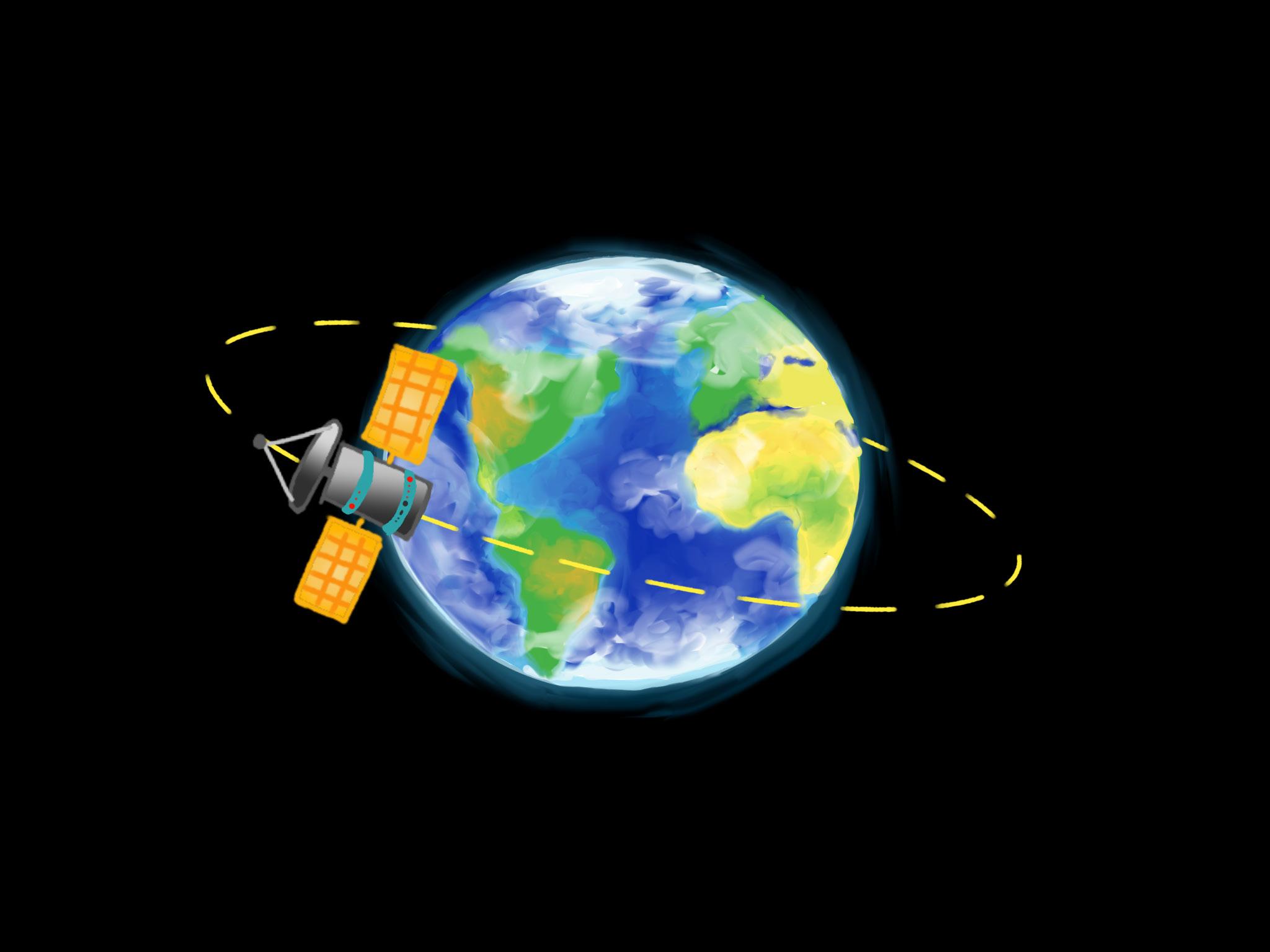
Satellites orbit around the Earth, like the moon. The orbit of satellites that move at the same rate as the Earth does are called geosynchronous[1]. This is the reason why people can watch the information given by satellites continuously even though they are constantly moving. This article will demonstrate the mathematics and physics calculations of a geosynchronous orbit.

Body

Starting with the basic concepts that need to be understood to analyze the orbit, let’s talk about Newton’s laws of motion, Newton’s law of universal gravitation, and circular orbits. Newton’s laws of motion contain three laws. According to the first law of motion, without a force applied, an object remains at rest or uniform movement [2]. Objects that are moving continuously want to move and need to be acted on by an outside force to stop their motion unless the object that was moving would continue to move at the same speed and direction [3]. For example, a runner who was running at her highest speed cannot stop running due to the resultant force, which wants her to remain in the same state. Her muscles must apply a force opposite to her momentum to stop. Next, the second law of motion refers to the famous equation, F = ma , in which F is the result of the forces, m represents the mass of an object, and a is the acceleration. The first law regards specific situations when acceleration is 0, which means that the velocity never changes. The second law expands the first law to general interactions of forces. For instance, when we are standing still, a force called gravity pulls us downwards. However, the reason why we do not go downwards is because there is another force that is maintaining us to remain on the Earth called the normal force. Due to the normal force, the resulting force frequently results 0. However, if this resulting total force changes and is no longer 0, the object begins to move. Here is an example to help you understand how the second law of motion works.

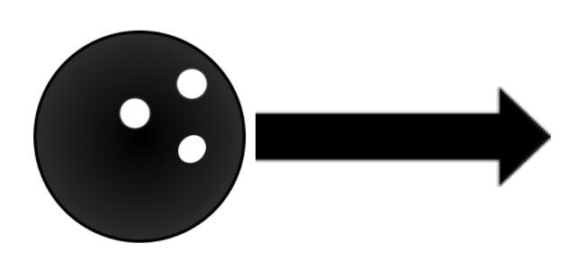
Figure 2: a golf ball with force F

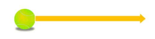
Figures 1 and 2 have one ball each; a bowling ball and a golf ball. If the bowling ball and golf ball were stationary initially, let’s say that we applied the same force of F for 1 second to each of them. The 7kg bowling ball begins to move with a speed of 1m/s and a 0.07kg golf ball begins to move with a speed of 100m/s. Using F= ma, the force is 7N. Thus, this example demonstrates that acceleration differs a lot due to the difference of mass even though they applied the same force. Also, direction is an important aspect in the second law of motion. Since the velocity contains the direction, and acceleration is the rate of velocity difference in a second, it provides more accurate information to write the equation with vector notation.

For convenience, we will eliminate vector notations going forward, but keep in mind that many variables have directions. V

This picture shows a ball with mass m thrown with an angle θ with velocity V. The biggest difference from the example before about bowling ball and golf ball is that the force is applied with an angle in this picture. This makes the approach more complicated, but it can be solved with the same method. First, to figure out where the ball is going, let’s divide the direction of velocity into x-axis and y-axis. In this case, x-axis will refer to the horizontal velocity and y-axis will inform about the vertical velocity. In the x-axis, there is no outside force applied except that which results in the first velocity. Thus, acceleration is 0 due to the equation, F = ma. Hence, it shows that the ball has an uniform motion in its x-axis position. Using trigonometry, the x-axis velocity could be stated as

For the y-axis, the initial velocity is Vsinθ. However the difference with x-axis is that the resultant force is not 0, which implies that another force is being applied after the initial launch. What is that force? It is the gravitational force. This force can be figured out with the second law of motion F = ma. So the force of gravity becomes F = mg, where g is the constant vy =Vsin(θ)-gt

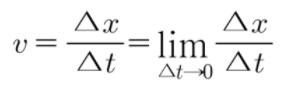
Overall, the picture shows an object with uniform motion in the x-axis and accelerating motion due to gravity in the y-axis. This picture is an example of projectile motion. Satellites have circular motion, but since projectile motion is very similar to circular ones, let’s explore more of projectile motions. First, let’s take a look at velocity. Velocity is a slope of the graph with x-axis of time and y-axis of position of an object. Thus, it can be

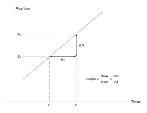
Figure 3: a ball with mass m thrown in an angle θ with velocity

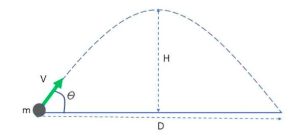
vx=Vcos(θ)

demonstrated with the graph below.

As shown in the graph, velocity is the slope of the timeposition graph. Using some calculus, we can express this limits, assuming time and position are continuous,

This can be written again in different forms.

Thus, it is clear that velocity can be obtained by differentiating the position of an object. Acceleration can be obtained with the same method. Acceleration is defined as the rate of change in velocity with time Δv / Δt.

Applying our expression for velocity,

Thus, we can also differentiate the position of an object to demonstrate acceleration.

Using these formulas, let’s analyze projectile motion. Since acceleration, velocity, and position are able to be differentiated and integrated with respect to time, projectile motion would be much simpler to analyze when expressing it in terms of time. Acceleration on the x-axis is always 0 because there is no change in velocity. Acceleration on the y-axis is negative due to gravity. The formulas for horizontal and vertical acceleration are shown below.

ax=0 ay=-g

We can integrate the above to obtain the velocities of each axis:

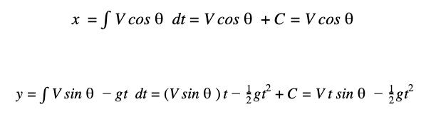
Lastly, let’s express the positions of each axis by integrating our previous results.

Hence, the projectile motion is easily analyzed by expressing acceleration, velocity, and position relative to time, through differentiation and integration.

Next, let’s take a look at Newton’s law of universal gravitation. Newton’s law of universal gravity states that every particle (objects) has a force of attraction to other particles. Gravity, a specific kind of universal gravity, is a force between Earth and an object. Additionally, the magnitude of universal gravity may vary. For example, a person is an object too, though his or her universal gravity is too small to noticeably attract other objects like chairs or desks. In today’s language, this law of universal gravitation is defined between point particles. Point particles are ideal particles that do not take any space and are in 0 dimension. Any object with discrete mass can be represented in physics as a point particle regardless of their shape, size, or structure. Newton’s law of universal gravitation defines that the force of gravity is proportional to each mass and inversely proportional to the distance between the centers of the mass of the point particles. The masses of the point particles are called point mass. We can express the gravitational force pulling the two objects towards each other in an algebraic equation:

where G=6.67384×10-11Nm2/kg2 is the universal gravitational constant, m1 and m2 are the mass of the objects, respectively, and r is the distance between them [4].

Finally, circular motion is the last concept to explore before analyzing satellites. Circular motion deals with any motion that is rotating about a fixed axis. Similar to linear motions, circular motions can be uniform or nonuniform. Uniform circular motion is circular motion with constant speed (note that it is not “velocity” in this case since the direction of the object is constantly changing, and since velocity is defined as the displacement over time, the velocity of the object would vary even if the object was moving at the same speed).

Circular motion is concerned with angles and how the direction of motion changes. The picture below allows us to see the motion of a particle moving in a circle at a certain time. We can derive x and y from the radius and the angle θ.

x=rcos(θ) y=rsin(θ)

Using the Pythago-

rean Theorem, we get

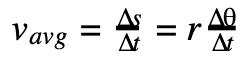
Let’s call s the length of the arc made by point P. Then s=rθ. Thus, θ=sr. Next, we will figure out the speed. The average speed of the particle is distance, the length of arc s, divided by time t:

Differentiating the average speed will result in tangential velocity which is a velocity that is tangent to the circle at a certain point:

But since the velocity is not always tangent to the circle, we need another way to find velocity. In general cases, we will use angular velocity.

Whether or not the angular velocity is positive or negative differs from the angle. Thus, we can substitute angular velocity as tangential velocity to obtain one more equation:

v=rω

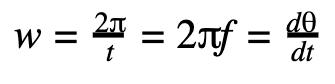
Hence, using this equation, we can obtain a few more properties of circular motion. First, let’s say that the period of circular motion is T and the frequency would be f. It is clear that f=1/T since the period is the time for the object to rotate once and frequency is the number of rotations in a second. In uniform circular motion, the speed is constant. The equation above can be substituted into the angular velocity of uniform circular motion:

Not only angular velocity, but speed, angle, and acceleration of uniform circular motion can also be solved through frequency and period.

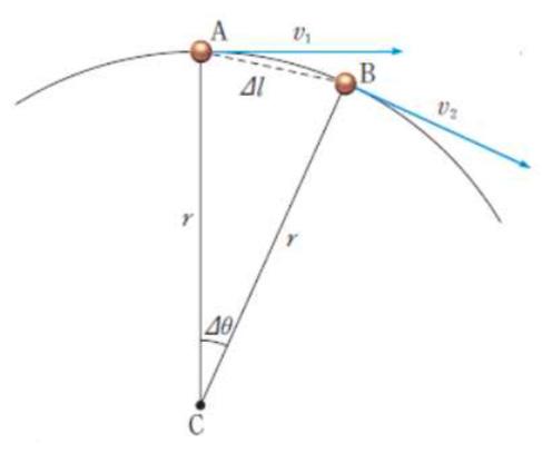
In both nonuniform motion and uniform circular motion, we can see that acceleration actually matters. This is because velocity is not constant, and acceleration plays the role of changing the direction. We call that acceleration centripetal acceleration.Let’s find the equation. Figure 5: point F traveling to D and E (Finney, Advanced Placement Calculus 2016 graphic numerical algebraic fifth edition)

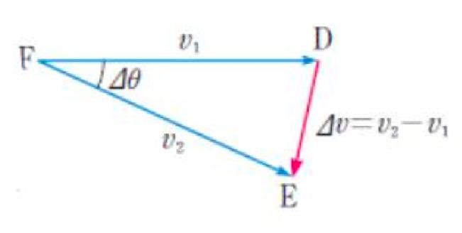
The first picture shows an object that is in uniform circular motion with velocity of v1, v2 in each point A and B during the time ∆t. The second picture of ∆DEF is a picture that transferred ∆ABC to random points. In this case, DE -> is the vector which represents the change velocity. Thus, in these pictures, it is clear that two triangles, ∆ABC and ∆DEF are similar (SAS similarity). Hence, the statement below is true.

As ∆t approaches zero, ∆l, being the distance between point A and B, will converge to v∆t. With this and assuming that ∆t is

an infinitely small number, we can find centripetal acceleration.

Figure 4: object traveling in circular motion

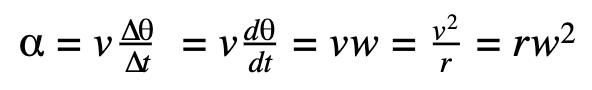
For this, the instantaneous magnitude of centripetal acceleration can be written as,

Finally, we can get centripetal force when substituting acceleration into Newton’s second law. Centripetal force allows for circular motion to be maintained. It is perpendicular to the direction of the motion and is in the same direction as centripetal acceleration.

Conclusion

Now, let’s figure out an analysis of geosynchronous orbit of satellites. Since these satellites match Earth’s rotation, they have an oval-shaped orbit. Thus, there is almost no difference when we think of the orbit as circular motion. Hence, we can use the formulas we derived regarding Newton’s laws of motion, Newton’s law of universal gravitation, and circular motion.

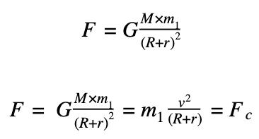
We can apply the universal gravitation formula F = Gm1m2/ r^2 Earth with a mass M and radius R, and the second is the satellite with orbital height r and mass m1:

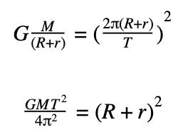
F is the universal gravitational force and Fc is the centripetal force. They are the same force expressed in different variables. When we solve this equation, we get:

Since a period of the geosynchronous force should be a day, we can apply a function of period and frequency in this equation above. As stated in the Body section, v=2πr/T when r is distance between two objects, T is period, and v is velocity. Here, it is clear that r is (R+r). Substituting this,

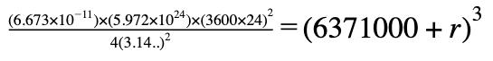
Now, let’s substitute all the values in each variable. Universal gravity constant is G=6.673×10-11, mass of the Earth is M=5.972×1024kg, period is T=3600×24s, π=3.141592…, and radius of the Earth is R=6371000 m.

When you calculate this,

r+6371000=42238000 r= 42238000-6371000 =3586700=35867

Thus, the height of a satellite in geosynchronous orbit is 35867 km, and comparing this to the real geosynchronous orbit that the scientists have observed, 35786 km [17], there is only 0.226% error. We have succeeded in settling a result for the geosynchronous orbit of satellites by using mathematics and physics.

References [1] National Geographic (2009). <Orbit> [2] Canright, Shelly; NASA (2009). <Geosynchronous satellites> [3] Zuber, Maria (2013). <Gravity Field of the Moon from the Gravity Recovery and Interior Laboratory (GRAIL) Mission>, American Association for the Advancement of Science [4] Gundlach, J.H (2007). <Laboratory Test of Newton’s Second Law for Small Accelerations>, Physical Review Letters, Vol. 98 No. 15. [5] Brown, Robert (2013). <Introductory Physics I- Elementary Mechanics>, Duke University Physics Department [6] Marion, Jerry; Stephen Thomton (1995). <Classical Dynamics of Particles and Systems>. Harcourt College Publishers. [7] Symon, Keith (1971), Mechanics. Addison-Wesley, Reading, MA. [8] Atkins, Tony; Escudier, Marcel (2013). A Dictionary of Mechanical Engineering. Oxford University Press [9] Shriki, Atara; David, Hamatal (2011), “Similarity of Parabolas- A Geometrical Perspective”, Learning and Teaching Mathematics. [10] Knudsen, Jens M; Hjorth, Poul G. (2000). Elements of Newtonian mechanics: including nonlinear dynamics (3 ed.). Springer. [11] Vallado, David A. (2007). Fundamental of Astrodynamics and Applications. Hawthorne, CA: Microcosm Press. [12] Rosenthal, Alfred (1968). Venture into Space: Early Years of Goddard Space Flight Center. NASA. [13] Anderson, James. E. (1979). A Theoretical Foundation for the Gravity Equation. The American Economic Review [14] Wang, Liang-qing; Sun, Han-xu. (2007). <Circle Motion Analysis on a Spherical Robot>, School of Mechanical Engineering and Automation, Beihang University. [15] Reynaud, Serge; Jaekel, Marc-Thierry. (2005). <Testing the Newton Law at Long Distances>, International Journal of Modern Physics A, Vol. 20, No.11. [16] Verlinde, Erik (2011). <On the origin of gravity and the laws of Newton>, Journal of High Energy Physics. [17] April 2015 EH 24. <What is a geosynchronous orbit?> Space.com. Accessed July 21, 2020. https://www.space.com/29222geosynchronous-orbit.html