17 minute read
Back to the future? Climate clues from past warm periods


Emilie Capron and Nathaelle Bouttes; illustrations: Cirenia Arias Baldrich
Interglacials* are warm periods in the past that can provide key information about changes in the climate. These periods are particularly useful in getting a better idea of what we should expect in the future. And just why is this?
Advertisement
About 50 warm time intervals, referred to as interglacials, punctuated the Quaternary* (the last 2.6 million years). The one we are living today started about 12 thousand years before present (kyr BP) and is called the Holocene (Fig. 2). Each interglacial lasted between about 5 to 27 kyr. Interglacials are characterized by a relatively small amount of ice on the continents in the Northern Hemisphere. During the last four interglacials, the (air) temperature in Antarctica was either similar to, or warmer than, the temperature during the early 1800s (prior to the Industrial Revolution). Interglacials alternate with glacial periods*, also known as ice ages, during which ice sheets* in the Northern Hemisphere grew to cover large areas of Europe and North America (Fig. 2). The transition from a cold glacial to a warm interglacial is called a deglaciation; this corresponds to a period of significant global sea-level rise and ice-sheet melting. Deglaciations are the largest global climate changes that happened during the Quaternary. To give you an idea of their amplitude and speed, during the Last Deglaciation, temperatures at the surface of the Earth rose by about ~4°C (~7°F) in 10 kyr, while global sea level increased by about 120 m, or almost 400 ft (Fig. 2).
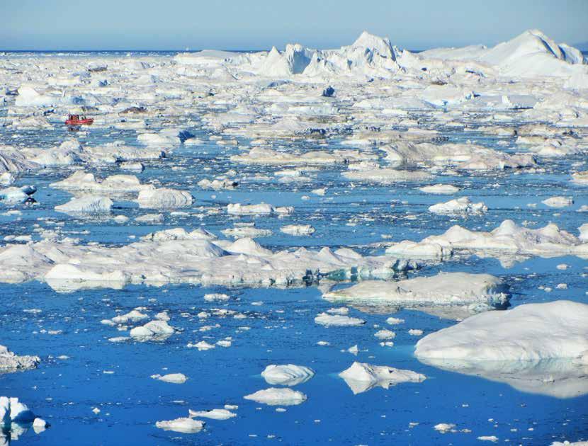
Figure 1. Icebergs from Jakobshavn Glacier. Past warm intervals provide case studies in which we can, for example, assess whether the Greenland Ice Sheet was significantly smaller – this could have caused global sea level to rise by up to 7 m (23 ft)! (Greenland; photo credit: E. Capron).
Past interglacials: natural experiments of warm climate
Past interglacials represent a series of natural experiments to understand how the climate system reacts to what we refer to as “boundary conditions”. The main boundary conditions defining global climate during the Quaternary are: (1) the amount of incoming sunlight, and where on the Earth’s surface this sunlight is directed (orbital forcings; see Box 1); (2) the concentrations of greenhouse gases*, such as carbon dioxide (CO2) and methane (CH4) in the atmosphere; and (3) the continental ice-sheet volume, which influences global sea level and sunlight reflection (also called “albedo”; see Franchini et al. p. 80).
The onset and course of each interglacial is associated with a unique combination of orbital forcing (the tilt of the Earth, for example) and atmospheric concentrations of greenhouse gases. Because both of these factors affect the size and location of the ice sheets, the ice sheets varied from interglacial to interglacial. Such differences in the boundary conditions from one interglacial to another had effects on the climate during each period. Scientists can learn about these past differences in climate by studying samples from “natural archives” such as polar ice or sediments taken from the deep sea (Box 2). These records of paleoclimate reveal large variations between the different climatic parameters (temperature, ice sheets, etc.) during interglacials. Furthermore, the intensity of these parameters, the order in which changes occurred, and the lengths of the interglacial vary from one interglacial to another (Fig. 2). For example, in some interglacials, the temperature reached its maximum early in the period, and soon after the ice sheets began to melt. In other cases, the maximum Interestingly, the temperature records from the ice core drilled in Antarctica at EPICA Dome Concordia (see Vauthier and Foxes in Love p. 66) suggest that Antarctica warmed during some of the past interglacials to a similar extent to what is projected to happen over the coming 78 years by climate simulations (Fig. 2). Past interglacials are not strict analogs for future warming: interglacial polar warming results from changes in the Earth’s orbit (Box 1), while future warming is driven by anthropogenic CO2 emissions from fossil fuels. Still, interglacials are a unique opportunity to assess with data, the effect of warmer-than-pre-industrial* climate on critical parts of the Earth, such as ocean circulation, ice sheets, and sea level.
Box 1: Orbital parameters: how the position of the Earth relative to the Sun controls the amount of sunlight reaching its surface
Slow changes in the tilt of the Earth’s axis and shape of the Earth’s orbit around the sun affect the climate by modifying the total amount of sunlight reaching its Earth. To refer to this physical process that affects the Earth’s climate, scientists commonly refer to the “orbital forcing”. This forcing is made up three main orbital parameters (Fig. B1):
Eccentricity quantifies the deviation of Earth's orbital path from the shape of a circle. Changes in the shape of the Earth’s orbit are important as it affects the amount of solar radiation received by Earth, and it varies on a cycle of about 100 kyr.
Obliquity represents the angle between the Earth's axis and the perpendicular axis to the orbital plan. It doesn’t change much: this angle ranges from 22.1 to 24.5 degrees with a periodicity of ~41 kyr. The obliquity impacts the distribution of solar energy input, which is important for the formation of ice sheets. Precession describes the motion of the axis of rotation of the Earth. Indeed, the Earth’s axis of rotation does not point towards a fixed direction through time. Instead, as Earth rotates, it wobbles slightly upon its axis, like a slightly off-center spinning toy top with a periodicity of about 19 to 23 kyr. Changes in precession impact the distribution of solar energy on the planet’s surface.
About a century ago, the Serbian scientist Milutin Milankovitch hypothesized that over millennia the collective effects of changes in Earth’s position relative to the Sun are a strong driver of Earth’s climate. In particular, he proposed that changes in the amount of summer insolation in the high latitudes of the Northern Hemisphere (Fig. 2) are responsible for triggering the beginning and end of glacial periods. Indeed, summer insolation in the Northern Hemisphere high latitudes drives the summer temperatures in this region, which in turn, control the growth or melting of continental ice sheets. For example, persistently low summer insolation in northern high latitudes over thousands of years may prevent winter snow from melting in the summer, thus allowing for the accumulation of perennial snow and the slow growth of an ice sheet, which can lead to an ice age.
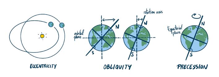
Figure B1. Schematic of the three orbital parameters which change the amount and distribution of energy from the sun (insolation) that reaches the Earth’s surface.
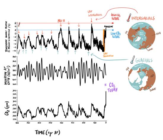
Figure 2. Air temperature changes (°C) in Antarctica compared to the present; summer insolation at 65°N (W/m2); and atmospheric CO2 concentration (ppm) over the past 800 kyr. The temperature and CO2 concentration information are from measurements on the ice and the trapped air in the deep ice core drilled at EPICA Dome Concordia in Antarctica. The time is shown in thousands of years before present (kyr BP). The future temperature is estimated in the 6th IPCC assessment report using CO2
concentrations from two “Shared Socio-Economic Pathways” (SSP*) as inputs. The future temperature in the high-CO2 case comes from the SSP5-8.5 scenario, and the temperature in the low-CO2 case is from the SSP1-2.6 scenario.
The Last Interglacial* as a case study
To illustrate how can we use past interglacials to infer clues about our future, let’s focus on the Last Interglacial, which occurred just before the last ice age, about 125 kyr BP (Fig. 2). During the Last Interglacial, global climate was about 0.8°C (1.5°F) warmer than during the pre-industrial period, meaning that the temperature was close to what it is today. However, records of sea-surface temperature measured on marine sediment cores located near the polar regions, and air temperature from polar ice cores (Box 2) suggest that temperatures during the Last Interglacial were a lot higher on Greenland and Antarctica – at least 3°C (5°F) higher than today. The warmer-than-pre-industrial climate during the Last Interglacial was due to the Earth’s orbital configuration at the time, which caused more direct sunlight over the Northern
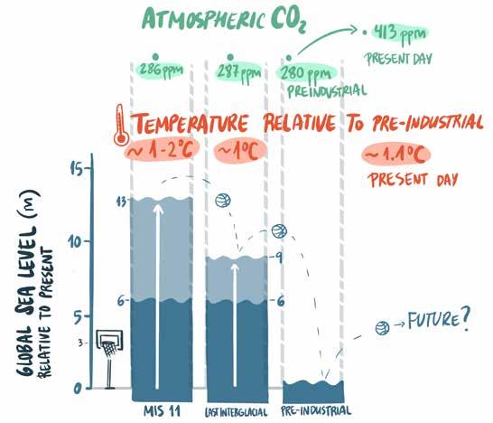
Figure 3. Comparison of the present-day with two past interglacial periods occurring at ~125 (Last Interglacial) and ~400 (MIS 11) kyr BP in terms of global air temperature, atmospheric CO2
concentration, and maximum global sea level. The light blue shading indicates uncertainty in the maximum global sea level. The uncertainty range covers the published estimates that are based on different lines of evidence. Adapted from Dutton et al. (2015).
Hemisphere during summer – the warmth was not due to higher atmospheric greenhouse gas concentrations, which were relatively similar to pre-industrial values. However, climate projections suggest that such high-latitude warming may be reached before the end of our century.
In addition, paleoscientists who study sea-level changes have suggested that global mean sea level during this period was 6–9 m (20–30 ft) higher than today, because some of the ice on Greenland and Antarctica melted (Fig. 3). All this makes the Last Interglacial a time period at the forefront of paleoclimatic research, A lot of work has been done on the Last Interglacial period as part of an international project comparing data from climate archives (Box 2) and climate models from different research groups that can simulate past climates based on changing boundary conditions (Box 3). Figure 4 shows comparisons between two different numerical climate models, and between the models and the available data (Box 4). In particular, the comparison is made
Scientists have many different ways of collecting data about the climate in the past. The different types of materials that they sample, known as natural climate archives, contain substances or features (also referred to as environmental tracers) that can be analyzed using a variety of methods. The records can be interpreted to provide qualitative, and sometimes quantitative, information about climate. For example, the presence of certain species can provide evidence that the climate was warmer, or cooler, than today at a given time and place. In some cases, natural archives can even be used to tell what the absolute temperature (with an attached uncertainty) was, at a given time and place. Figure B2 shows three commonly-used natural archives used to study past interglacials and the main environmental information they provide.
Ice cores drilled in polar regions are vertical cylinders of ice about 10 cm (4 in) in diameter that are drilled out of an ice sheet (see Christ and Bierman p. 56); they can be up to several kilometers (miles) long. Such cores contain information about past air temperature above the ice sheet, and many other aspects of the environment, including the concentrations of gases that were in the atmosphere at some time during the past, when they were trapped in tiny air bubbles (see Bouttes and Capron p. 67). Marine cores are drilled at the bottom of the ocean seafloor. These cores are collected in the “mud” present at the bottom of the ocean seafloor. Their diameter may vary between 6 and 12 cm (2–5 in). They are composed of sediments, a combination of terrigenous particles of various origin (e.g. atmospheric dust, riverine material) and composition, and remains of biological organisms that lived in the surface or deep ocean. They provide information about changes in the ocean (e.g. sea temperature and salinity, intensity of the oceanic circulation) and the nearby continents (e.g. vegetation, precipitation).
Speleothems are found in caves where limestone is present, and are formed when calcium carbonate precipitates out from drip water (see Kimbrough and Becker p. 46). They give us information about the climate and environment just outside the cave (e.g. hydrological cycle, vegetation, temperature).
Studies of past climate are by no means limited to these archives– a wide range of other records also provides insights into past changes, such as lake sediments (see Martínez-Abarca et al. p. 25) and peatlands (accumulation of partially decayed vegetation or organic matter).
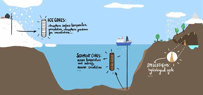
Figure B2. Schematic of three climatic archives, where they are extracted in the Earth system, and some of the main climate information they convey.
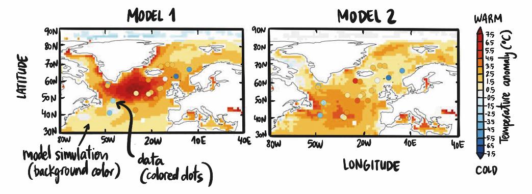
Figure 4. Temperature difference at the ocean surface between the Last Interglacial (at 125 kyr BP) and the pre-industrial period from model simulations (background color) and data (colored dots). Although the two models shown here do not simulate exactly the same pattern, both suggest that the Last Interglacial was a few degrees warmer than the pre-industrial period (i.e. this temperature difference is positive almost everywhere). Adapted from Capron et al. (2014).
for sea-surface temperature, which can be simulated by climate models and also estimated by measuring samples from marine sediment cores.
The comparison suggests that both models are able to represent warmer than today conditions in the North Atlantic during the Last Interglacial, such as also seen in the reconstructed data (Fig. 4). The similarity between the models’ estimations of past temperature and the data from the marine sediments gives us confidence. It also assures us that these models are likely to provide accurate estimates of climate change in the future. However, differences are also observed in the exact amplitude of the warmth between each model and the data, and between the two models. Differences between the data and the model may result from the fact that even the most complicated models are simplifications of what really happens on Earth, so they may not include some processes that could be important for the climate, such as changes in vegetation on land, or the amount and location of sea ice*. Overall, the comparison tells us that the models are on the right track to reproduce the last interglacial climate, but there’s still plenty of work for the next generation of climate scientists, such as figuring out how to model more processes and improving our understanding of others.
Another remarkable interglacial: MIS 11
MIS 11, an interglacial that occurred about 400 kyr BP, stands out in paleoclimatic records as it was particularly long, lasting about 27 kyr (Fig. 1). During this period, prolonged warmth was observed in many locations across the globe. In particular, the polar regions warmed significantly, which was likely responsible for melting of ice on Greenland and Antarctica, leading to a global sea level of 6 to 13 m (20–43 ft) higher than today (Fig. 3; see also Christ and Bierman p. 56). Unfortunately, because MIS 11 is so far back in time, not as many samples are available from this period compared to the Last Interglacial, and it is more difficult to precisely determine the age of those samples. On top of that, there aren’t as many models that have been used to estimate what the climate was like during MIS 11. All of these factors make it challenging to compare data and models in order to better understand the magnitude and the drivers of such enhanced warmth, but scientists are currently working hard towards this goal! We expect that within the next decade, this past warm period will provide new valuable insights into which processes on Earth are most important for the climate and, in particular, what changes we should expect due to prolonged global warming.
Take-home messages
• Interglacials are past warm periods that can provide key information about the processes that cause climate changes and are particularly useful to understand the impacts of warming in the future. Some interglacials were warmer than the present, such as the Last Interglacial (125 kyr BP) and MIS 11 (400 kyr BP). Global sea level during these periods was higher compared to today.
• One of the best ways to learn more about which processes are important for climate change is by comparing output from models, which simulate these processes, with data from the past.
• Studying past interglacials can help us to better estimate global and regional temperature changes, and how these are linked to changes in the polar ice sheets, ocean circulation, and radiative forcing under different types of warm climates.
To investigate which processes could explain the changes that are seen in their data, scientists try to represent the natural physical laws in climate models. Climate models are computer programs with many (often tens of thousands!) lines of code, including numerous equations describing the exchange and transport of energy and water in the main Earth components: atmosphere, ocean, land, and ice. The first models were developed in the 1950s; one of the early pioneers in this field was Syukuro Manabe, one of the winners of the 2021 Nobel prize in physics. Early climate models were very simple, with a focus on the atmospheric component of the climate system. Many features have been added since then, such as the ocean, sea ice, terrestrial biosphere, and the carbon cycle, to name only a few.
Computers are powerful, but even today, it can take weeks or even months for climate models to run. This is because the equations in the models must be solved numerically everywhere around the world and over a long period of time. To make this work manageable, modelers divide the Earth’s surface into small pieces called grid cells (Fig. B3). The equations are then solved for each grid cell. Not everything is computed by the model: modelers prescribe some parameters that are not affected by processes within the Earth system; for example, the insolation from the Sun (which depends on the relative position of the Earth and Sun; see Box 1). Modelers also often prescribe greenhouse gas concentrations such as carbon dioxide (CO2), methane (CH4) and nitrous oxide (N2O): for past simulations it is still difficult to model these accurately. For the future, we use a range of socio-economic scenarios to estimate concentrations of greenhouse gases.
Given this input, the models then compute the values of variables in each grid cell over a given time; for example, 1000 years. Some simple models can run on a normal computer and are very fast, taking only minutes to run 1000 years. Complex models such as those used for future predictions often run on thousands of processors, and can only compute a few simulated years in a full day of processing. Once the simulation is finished, the outputs of the model, typically temperature and precipitation, can be compared to climate information reconstructed from natural archives (Box 3).
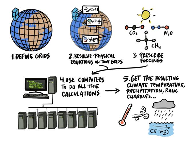
Fig. B3. Schematic representation of the main steps in running a climate model.
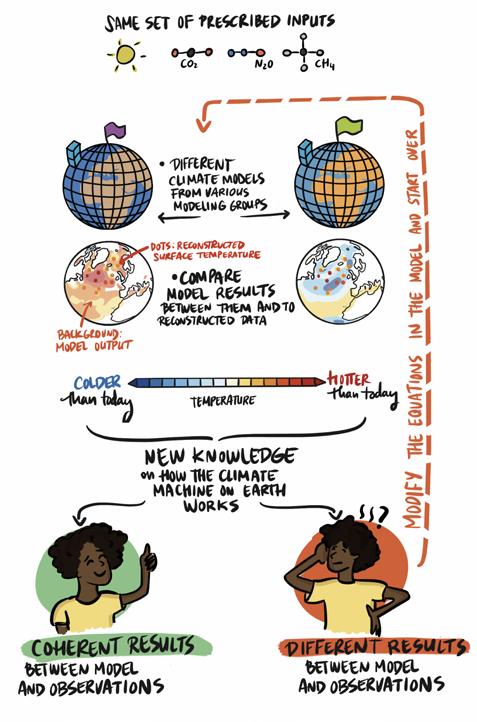
Figure B4. Schematic of model-intercomparison and model-data comparison applied to the Last Interglacial period. The data shown (dots) in the figure represent sea-surface temperature reconstructions from marine sediment cores located in the North Atlantic Ocean at 125 kyr BP. Over the recent decades, scientists studying natural archives and those running climate models have started to work together closely. In particular, the modeling of interglacials and the comparison of model results with paleodata are key to (1) test hypotheses about climate processes using physicsbased models and (2) evaluate how well climate models simulate warm climates, which is important because these models are also used to predict the climate in the future. Also, there is not just one climate model in the world, but many of them: in many cases, scientists in different countries have developed and use different models. The climate models generally have some features in common, such as the main fundamental equations. Yet different choices have been made by the modeling teams; for example, regarding processes that are not well understood yet, such as clouds.
To compare all the model results with the same conditions, i.e. the same forcings (or boundary conditions), scientists have organized themselves in working groups called model intercomparison projects. One of them is dedicated to past climates: the Paleoclimate Modelling Intercomparison Project (PMIP). In these comparisons each model is run using the same values, for example of insolation (orbital parameters), greenhouse gas concentrations, and sometimes the extent of the ice sheets. The model results can then be compared among themselves to understand the similarities or differences, and against observational data, to evaluate if they accurately represent known past changes. When model results differ from observational data, researchers can study these differences to understand why, and to improve the climate models by changing or adding equations in the code (Fig. B4). To do this, researchers focus on time periods for which we have numerous data from the natural archives, such as the Holocene and the Last Interglacial.
References
Capron E et al. (2014) Quat Sci Rev 103: 116-133 Dutton A et al. (2015) Science 349: aaa4019