CEPAL Review Nº117

117

N DECEMBER • 2015

REVIEW

CEPAL

O

ECONOMIC COMMISSION FOR LATIN AMERICA AND THE CARIBBEAN

Meta-analysis of the income and price elasticities of gasoline demand: public policy implications for Latin America Luis Miguel Galindo, Joseluis Samaniego, José Eduardo Alatorre, Jimy Ferrer Carbonell and Orlando Reyes

7

Macroprudential policy: an institutionalist interpretation 25

Gustavo Chagas Goudard and Fábio Henrique Bittes Terra

Export competitiveness in an oil and gas economy: the case of Trinidad and Tobago, 1985-2010 Indira Romero-Márquez and Juan Carlos Moreno-Brid

41

Ecuador: return from migration and entrepreneurship in Loja 65

Silverio Alarcón and Jessica Ordóñez

Paraguay: a housing finance proposal for middleto low-income groups 83

J. Vicente Fruet Cardozo and Guzmán A. Muñoz Fernández

Going through the labyrinth: the political economy of Argentina’s abandonment of the gold standard (1929-1933) 103

Pablo Gerchunoff and José Luis Machinea

Informality and labour market segmentation: the case of Argentina 121

Luis Beccaria and Fernando Groisman

Exchange rate pass-through and inflation targets in Chile 137

Patricio Mujica and Rodrigo Saens

Mexico: industrial policies and the production of information and communication technology goods and services 147

Claudia Schatan and Leobardo Enríquez

Industrial location and sectoral linkages: the case of the Brazilian automotive industry Luciano Ferreira Gabriel, Antônio Cláudio da Gama Cerqueira and Luiz Carlos Ribeiro

165

ISSN 0251-2920

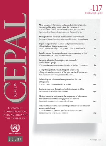
REVIEW ECONOMIC COMMISSION FOR LATIN AMERICA AND THE CARIBBEAN

117

REVIEW

NO DECEMBER • 2015

Alicia Bárcena Executive Secretary Antonio Prado

Deputy Executive Secretary

ECONOMIC COMMISSION FOR LATIN AMERICA AND THE CARIBBEAN Osvaldo Sunkel Chairman of the Editorial Board André Hofman Director Miguel Torres Technical Editor

ISSN 0251-2920

The cepal Review was founded in 1976, along with the corresponding Spanish version, Revista cepal, and it is published three times a year by the United Nations Economic Commission for Latin America and the Caribbean (eclac), which has its headquarters in Santiago, Chile. The Review, however, has full editorial independence and follows the usual academic procedures and criteria, including the review of articles by independent external referees. The purpose of the Review is to contribute to the discussion of socioeconomic development issues in the region by offering analytical and policy approaches and articles by economists and other social scientists working both within and outside the United Nations. The Review is distributed to universities, research institutes and other international organizations, as well as to individual subscribers.

The opinions expressed in the signed articles are those of the authors and do not necessarily reflect the views of eclac.

The designations employed and the way in which data are presented do not imply the expression of any opinion whatsoever on the part of the secretariat concerning the legal status of any country, territory, city or area or its authorities, or concerning the delimitation of its frontiers or boundaries.

To subscribe, please visit the Web page: http://ebiz.turpin-distribution.com/products/197587-cepal-review.aspx The complete text of the Review can also be downloaded free of charge from the eclac web site (www.eclac.org).

This publication, entitled the cepal Review, is covered in the Social Sciences Citation Index (ssci), published by Thomson Reuters, and in the Journal of Economic Literature (jel), published by the American Economic Association

United Nations publication ISSN: 0251-2920 ISBN: 978-92-1-329026-2 (Print) ISBN: 978-92-1-057528-7 (Pdf) LC/G. 2652-P Copyright © United Nations, December 2015. All rights reserved.

Printed in Santiago, Chile Requests for authorization to reproduce this work in whole or in part should be sent to the Secretary of the Publications Board.

Member States and their governmental institutions may reproduce this work without prior authorization, but are requested to mention the source and to inform the United Nations of such reproduction. In all cases, the United Nations remains the owner of the copyright and should be identified as such in reproductions with the expression “© United Nations 2014”.

a r t i c l e s

Meta-analysis of the income and price elasticities of gasoline demand: public policy implications for Latin America Luis Miguel Galindo, Joseluis Samaniego, José Eduardo Alatorre, Jimy Ferrer Carbonell and Orlando Reyes

7

Macroprudential policy: an institutionalist interpretation Gustavo Chagas Goudard and Fábio Henrique Bittes Terra

25

Export competitiveness in an oil and gas economy: the case of Trinidad and Tobago, 1985-2010 Indira Romero-Márquez and Juan Carlos Moreno-Brid

41

Ecuador: return from migration and entrepreneurship in Loja Silverio Alarcón and Jessica Ordóñez

65

Paraguay: a housing finance proposal for middle- to low-income groups J. Vicente Fruet Cardozo and Guzmán A. Muñoz Fernández

83

Going through the labyrinth: the political economy of Argentina’s abandonment of the gold standard (1929-1933) Pablo Gerchunoff and José Luis Machinea

103

Informality and labour market segmentation: the case of Argentina Luis Beccaria and Fernando Groisman

121

Exchange rate pass-through and inflation targets in Chile Patricio Mujica and Rodrigo Saens

137

Mexico: industrial policies and the production of information and communication technology goods and services Claudia Schatan and Leobardo Enríquez

147

Industrial location and sectoral linkages: the case of the Brazilian automotive industry Luciano Ferreira Gabriel, Antônio Cláudio da Gama Cerqueira and Luiz Carlos Ribeiro

165

Guidelines for contributors to the cepal Review

183

Explanatory notes The following symbols are used in tables in the Review: … Three dots indicate that data are not available or are not separately reported.

(–) A dash indicates that the amount is nil or negligible.

A blank space in a table means that the item in question is not applicable.

(-) A minus sign indicates a deficit or decrease, unless otherwise specified. (.) A point is used to indicate decimals. (/) A slash indicates a crop year or fiscal year; e.g., 2006/2007.

(-) Use of a hyphen between years (e.g., 2006-2007) indicates reference to the complete period considered, including the beginning and end years.

The word “tons” means metric tons and the word “dollars” means United States dollars, unless otherwise stated. References to annual rates of growth or variation signify compound annual rates. Individual figures and percentages in tables do not necessarily add up to the corresponding totals because of rounding.

Meta-analysis of the income and price elasticities of gasoline demand: public policy implications for Latin America Luis Miguel Galindo, Joseluis Samaniego, JosĂŠ Eduardo Alatorre, Jimy Ferrer Carbonell and Orlando Reyes

SUMMARY

By means of a meta-analysis, this article sets out to estimate average values for the income and price elasticities of gasoline demand and to analyse the reasons for the variations in the elasticities reported by the literature. The findings show that there is publication bias, that the volatility of elasticity estimates is not due to sampling errors alone, and that there are systematic factors explaining these differences. The income and price elasticities of gasoline demand differ between the short and long run and by region, and the estimation can appropriately include the vehicle fleet and the prices of substitute goods, the data types and the estimation methods used. The presence of a low price elasticity suggests that a fuel tax will be inadequate to control rising consumption in a context of rapid economic growth.

KEYWORDS

Gasoline, supply and demand, prices, consumption, econometric models, Latin America

JEL CLASSIFICATION

AUTHORS

C83, Q41, Q48 Luis Miguel Galindo is Chief of the Climate Change Unit of the Sustainable Development and Human Settlements Division, eclac. luismiguel.galindo@cepal.org

Joseluis Samaniego is Chief of the Sustainable Development and Human Settlements Division, eclac. joseluis.samaniego@cepal.org

JosĂŠ Eduardo Alatorre is an economic affairs officer with the Sustainable Development and Human Settlements Division, eclac. joseeduardo.alatorre@cepal.org

Jimy Ferrer Carbonell is an economic affairs officer with the Sustainable Development and Human Settlements Division, eclac. jimy.ferrer@cepal.org

Orlando Reyes is a researcher with the Sustainable Development and Human Settlements Division, eclac. orlando.reyes@cepal.org

8

CEPAL

REVIEW

117

•

DECEMBER

2015

I Introduction Gasoline consumption is indispensable to the workings of modern economies, but it is also associated with a number of negative externalities, such as vehicle traffic, air pollution and climate change (Steenhof and others, 2006; Galindo, 2008; Reyes, 2009). Different projections based on business-as-usual scenarios suggest that gasoline consumption will increase substantially over the coming years, intensifying these negative externalities (Calthrop and Proost, 1998; Galindo, 2008; Kim and others, 2011). This is particularly relevant to Latin America, where the negative externalities from urban transport, for example, are already particularly large and are very likely to worsen in a context of rapid economic growth (Alves and Bueno, 2003; Galindo, 2008).

In this context, it is essential to identify the factors influencing the evolution of gasoline consumption and the magnitude of their effects. The empirical literature on fuel demand is large and very varied, and encompasses different countries, regions, periods, and even diverse estimation methodologies. This has been reflected in the numerous econometric estimates carried out for the response sensitivities of two fundamental factors in the evolution of gasoline consumption: income elasticity This study is one of a set produced as part of the “Fiscal Policy and Climate Change” programme, with financing from the German Agency for International Cooperation (giz). The opinions expressed herein are the exclusive responsibility of the authors and may not coincide with those of eclac nor reflect the official views of any governments, institutions or donors mentioned in the study. The authors are grateful for the comments of Fernando Filgueira, Gabriel Porcile and José Javier Gómez. The usual error disclaimer applies.

and price elasticity. These elasticities are essential for identifying and simulating, for example, the consequences of different economic growth scenarios or the application of a fuel tax. Accordingly, a vital part of constructing a low-carbon sustainable development strategy is to identify them appropriately.

Systematically reviewing all the information available in the various studies on gasoline demand is a complex task, but it can be synthesized through a metaanalysis that summarizes, integrates and interprets the findings of different empirical studies (Van den Bergh and others, 2010; Cumming, 2012; Stanley, 2001) with a view to obtaining a weighted average estimator that incorporates the combined effect of the values from each study, with weightings allocated to reflect the accuracy (variance or standard error) of their respective results (Sterne, 2009). This method can also be used to arrive at general inferences and explore the heterogeneity of findings across the different studies (Borenstein and others, 2009; Sáez and others, 2001).

Thus, the main purpose of this article is to carry out a meta-analysis for the income and price elasticities of gasoline demand and draw out some public policy implications for Latin America. The article contains four sections. Following the Introduction, section II discusses gasoline demand and the factors determining it, and explains what a meta-analysis is. Section III sets out the estimates of the combined coefficients obtained from the meta-analysis and the results of the meta-regressions, and presents some public policy considerations. Lastly, section IV offers conclusions and general remarks.

II Meta-analysis of gasoline demand Gasoline consumption is an essential input for goods transportation and population mobility in modern economies. The evolution of its demand can be modelled like any other demand function (Deaton and Muellbauer, 1980; Varian, 1993) (equation (1)). In other words, demand

for gasoline is a function of the evolution of spending (for which income is sometimes used as a proxy), its price and the prices of substitute and complementary goods, as well as a set of other factors, such as socioeconomic and demographic characteristics, the vehicle fleet, the

META-ANALYSIS OF THE INCOME AND PRICE ELASTICITIES OF GASOLINE DEMAND: PUBLIC POLICY IMPLICATIONS FOR LATIN AMERICA • LUIS MIGUEL GALINDO, JOSELUIS SAMANIEGO, JOSÉ EDUARDO ALATORRE, JIMY FERRER CARBONELL AND ORLANDO REYES

CEPAL

REVIEW

117

urban structure or specific regulations on urban mobility and automobile use (Kayser, 2000; Dahl, 2012; Galindo, 2005; Reyes, 2009; Alves and Bueno, 2003):

gasit = F(yit, pgit, pit, contjit) (1)

where gasit represents demand for gasoline, yit is the spending or income variable, pgit is its relative price, pit are the prices of goods that are substitutes or complements for gasoline, and contjit are other relevant control variables. Subscript t represents time, i the different agents and j the control variables. The economic literature suggests that income elasticity should be positive and price elasticity negative. In other words, an increase in total spending or income will be accompanied by an increase in gasoline consumption, while a rise in its price translates into a drop in its demand. However, a great variety of econometric estimates have been carried out for equation (1) using different specifications, methods, periods, countries, regions or economic agents (Espey, 1998). This is reflected by differences in the specific values yielded by estimates of the income and price elasticities of gasoline demand, creating a good deal of uncertainty from a public policy perspective.

These different income and price elasticities of gasoline demand, their volatility and any publication bias1 can be analysed and synthesized through a metaanalysis,2 which is a combined statistical analysis of the body of empirical research and findings on a specific subject, incorporating all available information to identify common characteristics, average effects and the sources of heterogeneity in these effects (Stanley, 2001; Lipsey and Wilson, 2001). Each study estimates an effect (θi),3 namely the size effect or the treatment effect, and a corresponding variance (Vθi). These statistics can be used to obtain a weighted average of the studies, known as the summary size effect, with greater weight normally being assigned to more accurate studies, this accuracy being

1 Publication bias exists when studies that are not included in the meta-analysis are systematically different from those that are. There is evidence that this can happen, as studies reporting larger effects (elasticities, for example) are more likely to be published than studies reporting smaller effects.

2 Meta-analyses have also been criticized on the grounds that different findings are difficult to combine and an artificial variability of results may be generated (Lipsey and Wilson, 2001).

3 The objective of meta-analyses is often the coefficient known as the size effect, which identifies the magnitude of the effect being considered in the group of studies: g = (μe - μc)/σ, where g is the size effect, μe and μc are the averages of the experimental and control groups, respectively, and σ is the standard deviation of the control group (Stanley, 2001).

•

DECEMBER

2015

9

associated with the standard error of the effect (Lipsey and Wilson, 2001).4 However, estimates of income and price elasticities may present excessive volatility that is not just a consequence of sampling error, and may also have a publication bias resulting from preference being given to economic estimation studies that are consistent with economic theory, earlier estimates, or both.

Meta-regression analyses (mra) can be used to identify systematic factors affecting the volatility of estimates and publication bias (Van den Bergh and others, 2010; Cumming, 2012). There are different types of metaregression estimates; this study uses a Heckman-type meta-regression based on the mixed-effects model that corrects for publication bias (Van den Bergh and others, 2010; Cumming, 2012; Havranek and others, 2012). Also reported for reference purposes are estimates of fixed, random and Huber-White effects, as these can be used to correct for heteroskedasticity and autocorrelation problems due to production clusters (Williams, 2000; Wooldridge, 2002). In addition, the estimates are weighted by the inverse standard deviation to reduce problems of heteroskedasticity (Lipsey and Wilson, 2001). Each of these estimation methods presents some limitations, with the fixed, random, mixed and Huber-White effects models using a variety of fairly restrictive assumptions, for example (Abreu and Florax, 2005). At the same time, the statistical significance of the fixed- and mixed-effects models needs to be handled with caution, while HuberWhite estimation does not efficiently employ all available information (Abreu and Florax, 2005).

The size effect of the income and price elasticities of gasoline demand is obtained from a regression model represented in equation (2) (Stanley and Jarrell, 1989; Paterson and Canam, 2001):

Y = Xβ + ε (2)

where Y is a vector (nx1) containing the independent variables (e.g., gasoline demand), X is a vector (nxm) of explanatory variables, β is the vector (mx1) of estimated coefficients and ε is a vector (nx1) of the error term.

Thus, the set of estimated elasticities are distributed randomly (in the absence of publication bias) around the real elasticity value, irrespective of the standard error (equation (3)) (Doucouliagos and Stanley, 2009; Stanley, 2008):

bi = β0 + wi (3)

4 There are also multivariate meta-analyses (Lipsey and Wilson, 2001).

META-ANALYSIS OF THE INCOME AND PRICE ELASTICITIES OF GASOLINE DEMAND: PUBLIC POLICY IMPLICATIONS FOR LATIN AMERICA • LUIS MIGUEL GALINDO, JOSELUIS SAMANIEGO, JOSÉ EDUARDO ALATORRE, JIMY FERRER CARBONELL AND ORLANDO REYES

10

CEPAL

REVIEW

117

where bi represents the estimated elasticities and β0 the actual elasticity value, and wi is the error term.

In cases where the estimated elasticities present a publication bias, it is possible to use a meta-regression with mixed effects and Heckman’s two-step procedure (Havranek and others, 2012). This procedure uses the characteristics of a control sample to estimate potential bias with a probit or logit model, so that in a second step the Mills ratio can be included in the final equation (Heckman, 1979; Angrist and Pischke, 2009). There is no counterfactual available in the meta-regression, but the heterogeneity of the standard deviation can be used to identify the econometric equation, replacing the inverse Mills ratio (Stanley, 2001).

Thus, equation (3) can be reformulated5 in the presence of publication bias to include both the real elasticity value and this bias. This is represented in equation (4) (Stanley, 2001; Havranek and others, 2012; Doucouliagos and Stanley, 2009): bi = β0 + β1*SE(bi) + ui, ui/SE(bi)~N(0, δ2) (4) where bi is elasticity, SE is the standard error for each estimate included in the meta-analysis, β0 represents average real elasticity, β1 estimates the magnitude of the bias and ui is the error term. A significant value for β1 implies bias in the estimates (Havranek and others, 2012; Stanley, 2008). Equation (4) is estimated by weighted least squares to reduce possible heteroskedasticity problems (Havranek and others, 2012; Stanley, 2008).

This is represented in equation (5), which identifies publication bias in the β1 coefficient. This equation also allows the statistical significance of real elasticity (β0 coefficient) to be observed, once publication bias has been eliminated. It is worth noting that Monte Carlo simulations have shown its value to have a downward bias (Stanley, 2008; Stanley and Doucouliagos, 2011).

•

DECEMBER

2015

significance of the bias by way of the β1 coefficient and statistical significance, besides the publication bias and the mean effect estimated by the β0 coefficient (Havranek and others, 2012): tij =

b0 * 1 SE _ bij i

+ b1 + p j + fij, fij SE _ bij i, p j + N _ 0, i i (6)

where subscript i and j represent the estimates and studies.

Total errors (zij) thus include the part corresponding to random effects at the study level (ξj) and errors at the estimation level (eij), where var(zij) = y + q and y represents between-studies variance and q within-studies variance. The variance of these two errors is added together because they are deemed to be independent.

Consequently, the real magnitude of average elasticity (β0) can be estimated with an augmented equation, known as Heckman’s mixed-effects meta-regression, which contains a fixed-effects part captured in β1 and a random part (zi) (Stanley and Doucouliagos, 2012),6 and where the relationship between the standard errors and publication bias is assumed to be quadratic (Stanley, 2008; Stanley and Doucouliagos, 2011): tij =

b0 * 1 SE _ bij i

+ b1 SE + p j + fij, p j SE _ bij i + N _ 0, } i , fij SE _ bij i, p j + N _ 0, i i

(7)

where β0 measures the magnitude of average elasticity corrected for bias and β1 represents the magnitude of the bias. It is also possible to identify some of the factors influencing the volatility of the estimates and their publication bias using equation (8) (Havranek and others, 2012; Van den Bergh and others, 2010; Phillips and Goss, 1995):

b0 * 1 bi = ti = + b1 + pi, pi SE _ bi i + N _ 0, v 2 i (5)

SE _ bi i SE _ bi i

Equation (5) can be modified to incorporate the presence of volatility in the estimates across studies (Havranek and others, 2012). Thus, equation (6) can be used to obtain the direction, magnitude and statistical

where β1 represents publication bias and ak are the coefficients of vector Zik in the meta-regression, which includes the variables that affect volatility and are uncorrelated with the selection processes of studies

5 The

6

approximation uses a Taylor polynomial (Apostol, 1967) such k a SE k + v (Stanley and Doucouliagos, 2012). that b1 = b1 + k i i

/

tij =

b0 * 1

SE _ eij i

+ b1 +

/

k k=1

ak Zik + p j + fij (8)

This is similar to a random panel data model (Havranek and others, 2012).

META-ANALYSIS OF THE INCOME AND PRICE ELASTICITIES OF GASOLINE DEMAND: PUBLIC POLICY IMPLICATIONS FOR LATIN AMERICA • LUIS MIGUEL GALINDO, JOSELUIS SAMANIEGO, JOSÉ EDUARDO ALATORRE, JIMY FERRER CARBONELL AND ORLANDO REYES

CEPAL

REVIEW

117

(Doucouliagos and Stanley, 2009; Stanley and Jarrell, 1989). Subscript i indicates the value taken by the variable in each study i. Vector Zik includes a number of factors, such as the fact of an estimate being for an Organization for Economic Cooperation and Development (oecd) country (other than Chile and Mexico), the vehicle fleet, the prices of substitute or complementary goods as an explanatory variable in estimating gasoline demand, and the estimation method

•

DECEMBER

11

2015

used, differentiating between panel, cross-sectional and time series data.

The statistical significance test for a0 is known in the literature as the funnel asymmetry test (fat), and that for the statistical significance of β0 as the precision effect test (pet) (Doucouliagos and Stanley, 2009; Stanley, 2005 and 2008). Thus, meta-regression analysis (equation (8)) is known as fat-pet-mra (Doucouliagos and Stanley, 2009; Stanley, 2008).

III Meta-regressions and public policy The database employed consists of 63 studies of gasoline demand from the international literature, with 227 estimates of income elasticity and 343 of price elasticity being obtained. The studies cover the period from 1960 to 2013 and are from the EconLit, Jstor and ProQuest databases, among others. The studies selected were published in Spanish and English.7 The income and price elasticities of gasoline demand were divided between short- and long-run estimates. It is usual to expect sensitivity to be greater in the long run, since consumers may adjust structurally, for example, to the new relative price structure. Table 1 presents a summary of the statistics for the income and price elasticities of gasoline demand as reported in the international literature.

7

A list of the articles used in the meta-analysis is available from the authors.

TABLE 1

Variable Income elasticity Long-run elasticity Short-run elasticity Price elasticity Long-run elasticity Short-run elasticity

All in all, the elasticities estimated in the studies generally show high volatility, with the randomeffects econometric estimates for short- and long-run income elasticity having a standard deviation-weighted average of 0.30 and 0.62, respectively (see table 2).

The random-effects estimates for short- and long-run price elasticity have a standard deviation-weighted average of -0.20 and -0.39, respectively (see table 3).

These price elasticity estimates are within the range of average price elasticities reported in the meta-analyses of Espey (1998), Hanly and others (2002) and Brons and others (2008).

The histograms and Kernel density plots for income and price elasticities show that the distributions are not symmetrical. In the case of income elasticity, the positive bias is most striking in the short-run estimates (see figure 1), while for price elasticity the bias is most evident in the long-run estimates (see figure 2).

Statistics on the elasticity of gasoline demand in the international literature No. of observations

Average

119 108

0.63 0.34

213 130

-0.44 -0.21

Standard deviation

Minimum

Maximum

0.34 0.19

0.04 0.01

1.19 0.94

0.28 0.19

-1.63 -1.03

-0.32 0.31

Source: Prepared by the authors.

META-ANALYSIS OF THE INCOME AND PRICE ELASTICITIES OF GASOLINE DEMAND: PUBLIC POLICY IMPLICATIONS FOR LATIN AMERICA • LUIS MIGUEL GALINDO, JOSELUIS SAMANIEGO, JOSÉ EDUARDO ALATORRE, JIMY FERRER CARBONELL AND ORLANDO REYES

12

CEPAL

TABLE 2

REVIEW

117

•

DECEMBER

2015

Results from the meta-analysis of the income elasticity of gasoline demand Fixed effects

Parameter

q σq q + 1.96* σq q - 1.96* σq Zq = q / σq

P = 2 :1 − ` U _ Z ijD

Random effects

Long run

Short run

Long run

Short run

0.551 0.002 0.554 0.548 324.52

0.268 0.001 0.270 0.266 3.691

0.625 0.031 0.685 0.565 20.41

0.303 0.017 0.336 0.269 17.77

0.000

0.000

0.000

0.000

Source: Prepared by the authors from the results of the meta-analysis estimations.

TABLE 3

Results from the meta-analysis of the price elasticity of gasoline demand Fixed effects

Parameter

q σq q + 1.96* σq q - 1.96* σq Zq = q / σq

P = 2 :1 − ` U _ Z ijD

Random effects

Long run

Short run

Long run

Short run

-0.131 0.003 -0.136 -0.125 44.77

-0.108 0.002 -0.112 -0.105 63.95

-0.397 0.015 -0.427 -0.367 26.05

-0.204 0.021 -0.245 -0.163 9.75

0.000

0.000

0.000

0.000

Source: Prepared by the authors from the results of the meta-analysis estimations.

FIGURE 1

Distribution of estimates for the income elasticity of gasoline demand A. Long-run income elasticity

B. Short-run income elasticity 2.5

1 2

Density

Density

1.5 0.5

1

0.5

0

0 0

0.2

0.4

0.6 Elasticity

Histogram

0.8

1

1.2

0

0.2

0.4

0.6

0.8

Elasticity Kernel density

Histogram

Kernel density

Source: Prepared by the authors.

META-ANALYSIS OF THE INCOME AND PRICE ELASTICITIES OF GASOLINE DEMAND: PUBLIC POLICY IMPLICATIONS FOR LATIN AMERICA • LUIS MIGUEL GALINDO, JOSELUIS SAMANIEGO, JOSÉ EDUARDO ALATORRE, JIMY FERRER CARBONELL AND ORLANDO REYES

1

CEPAL

FIGURE 2

REVIEW

117

•

DECEMBER

Distribution of estimates for the price elasticity of gasoline demand A. Long-run price elasticity

B. Short-run price elasticity

2

2.5 2

Density

1.5

Density

13

2015

1

1.5 1

0.5 0.5 0

0 -1.5

-1

-0.5

0

-1

-0.5

Elasticity

0

0.5

Elasticity

Histogram

Kernel density

Histogram

Kernel density

Source: Prepared by the authors.

Likewise, the asymmetry funnel plots, where the income and price elasticities are plotted along the horizontal axis and the accuracy of the estimates along the vertical axis (Abreu and Florax, 2005; Sterne and others, 2000),8 show there can be a large publication bias (see figures 8

In the absence of bias, the shape of the asymmetry funnel plots depends on the variable chosen for the axes; in some cases, use is generally made of standard error, inverse standard error, variance, inverse variance, sample size and the logarithm of sample size for the vertical axis and the magnitude of the effect for the horizontal axis, with standard error probably being the best option for the vertical axis (Sterne and Egger, 2001).

FIGURE 3

3 and 4).9 In particular, it can be seen that the distribution of the points representing the relationship between the elasticities and their respective standard deviations is not symmetrical within 95% confidence bounds. This suggests there could be a statistically significant tendency to publish studies that estimate high values for income and price elasticities.

9 Publication bias has often been related to asymmetry in funnel plots;

the literature reports other sources of asymmetry, however, such as selection bias, sample size heterogeneity and data irregularity, among other factors (Egger and others, 1997).

Funnel plots for the income and price elasticities of gasoline demand A. Long-run price elasticities

B. Short-run price elasticities

0

0

Standard deviation

Standard deviation

0.2

0.4

0.6

0.8

0.1

0.2

0.3 -2

0

2

4 Elasticity

6

8

-0.5

0

0.5

1

Elasticity

Source: Prepared by the authors.

Note: The dashed lines in the funnel plots show the 95% confidence bounds and the grey line the fit of the regression relating the gasoline price and income elasticities with their respective standard deviations.

META-ANALYSIS OF THE INCOME AND PRICE ELASTICITIES OF GASOLINE DEMAND: PUBLIC POLICY IMPLICATIONS FOR LATIN AMERICA • LUIS MIGUEL GALINDO, JOSELUIS SAMANIEGO, JOSÉ EDUARDO ALATORRE, JIMY FERRER CARBONELL AND ORLANDO REYES

14

CEPAL

FIGURE 4

REVIEW

117

•

DECEMBER

2015

Funnel plots for the income and price elasticities of gasoline demand A. Long-run price elasticities

B. Short-run price elasticities

0

0

Standard deviation

Standard deviation

0.1

1

2

0.2

0.3

0.4

3

0.5

-10

-5

Elasticity

0

5

-1

-0.5

0

0.5

Elasticity

1

Source: Prepared by the authors.

Note: The dashed lines in the funnel plots show the 95% confidence bounds and the grey line the fit of the regression relating the gasoline price and income elasticities with their respective standard deviations.

Taken together, the available evidence thus suggests the possibility that the volatility across the effects estimated by the studies is not due exclusively to sampling errors and, accordingly, that some volatility originates in systematic factors (Van den Bergh and others, 2010).

The Q statistic and its p-value reject the null hypothesis TABLE 4

Test of heterogeneity Q p-value τ 2 τ I 2

that the distribution is homogeneous for estimates of short- and long-run income and price elasticity (see tables 4 and 5). The p-value of the Q statistic is less than 1% of the significance level for the tests of the estimates for both long-run and short-run income elasticity (see table 4) and price elasticity (see table 5).

Tests of heterogeneity for the income elasticity of gasoline demand Long run

Short run

15 610.00 0.000 0.093 0.306 99.2%

3 691.00 0.000 0.021 0.146 97.1%

Source: Prepared by the authors from the results of the meta-analysis estimations.

Note: τ 2 is defined as the variance in the magnitude of the effects and indicates the variance between studies. I 2 indicates the proportion of the variation observed in the magnitude of the effects that is attributable to the heterogeneity between studies.

TABLE 5

Tests of heterogeneity for the price elasticity of gasoline demand

Test of heterogeneity

Long run

Short run

Q p-value τ 2 τ I 2

3 341.34 0.000 0.031 0.175 93.7%

15 465.27 0.000 0.051 0.225 99.2%

Source: Prepared by the authors from the results of the meta-analysis estimations.

Note: τ 2 is defined as the variance in the magnitude of the effects and indicates the variance between studies. I 2 indicates the proportion of the variation observed in the magnitude of the effects that is attributable to the heterogeneity between studies.

META-ANALYSIS OF THE INCOME AND PRICE ELASTICITIES OF GASOLINE DEMAND: PUBLIC POLICY IMPLICATIONS FOR LATIN AMERICA • LUIS MIGUEL GALINDO, JOSELUIS SAMANIEGO, JOSÉ EDUARDO ALATORRE, JIMY FERRER CARBONELL AND ORLANDO REYES

CEPAL

REVIEW

117

The I2 statistic indicates that over 90% of the observed variation in the magnitude of the effects is attributable to the heterogeneity between the studies, meaning that the variation in the income and price elasticities of gasoline demand is almost wholly due to the differences in the studies included in the meta-analysis. This suggests, then, that meta-regression techniques should be applied to identify the variability ratios for elasticity (see table 8).

On the basis of the maximum likelihood ratio test, the equation (6) estimates show that the null hypothesis of homogeneity in the estimates is rejected (see table 6). This suggests there is substantial heterogeneity in the income and price elasticities and that the mixed-effects model is therefore appropriate. The findings show a positive bias for long-run income elasticity and a negative one for short-run elasticity, although this short-run bias is not statistically significant. The findings for short- and longrun price elasticity (see table 6) indicate a statistically significant negative bias; this is consistent with what is reported in the asymmetry funnel plots. Likewise, the

•

DECEMBER

15

2015

results of the equation (6) estimates show that the effect or the real elasticity is statistically different from zero in all cases (the 1/SE coefficient is statistically significant at 1%). In other words, income and price elasticities are factors affecting the path of gasoline consumption in the short and long run.

The estimates from Heckman’s meta-regression (equation (7)) show that the short- and long-run income elasticities are 0.26 and 0.46, respectively, once publication bias is corrected for. In turn, the short- and long-run price elasticities are -0.10 and -0.31, respectively, including the bias correction (see table 7). The likelihood ratio tests reject the null hypothesis that volatility is only a consequence of sampling error, which means that it is appropiate to use a mixed-effects model.

The international literature on gasoline demand suggests that a number of factors, besides the difference between short- and long-run elasticities already discussed, affect the volatility of estimations of the income and price elasticities of this demand. In principle, the following factors can be considered:

TABLE 6

Publication bias test Income elasticity Dependent variable: t-statistic Constant (1/SE) No. of observations Likelihood ratio test

Price elasticity

Long run

Short run

Long run

Short run

0.767 (1.039) 0.456*** (0.019) 119 561.15***

-0.697 (0.579) 0.270*** (0.005) 108 2 185.27***

-1.500*** (0.268) -0.234*** (0.020) 213 130.07***

-1.973* (1.171) -0.086*** (0.022) 130 14.47***

Source: Prepared by the authors from the estimates of the mixed-effects model.

Note: The values in parentheses are the standard errors. The asterisks ***, ** and * indicate significance at 1%, 5% and 10%, respectively.

The test of joint significance is carried out using χ2. SE is the standard error.

TABLE 7

Dependent variable: t-statistic Corrected elasticity (1/SE) SE No. of observations Likelihood ratio test (χ2)

Income and price elasticity of gasoline demand corrected for bias Income elasticity Long run 0.461*** (0.017) 4.493 (5.178) 119 711.50***

Short run 0.267*** (0.006) 4.646 (4.315) 108 2 323.50***

Price elasticity Long run -0.314*** (0.014) -1.004** (0.520) 213 497.31***

Short run -0.104*** (0.018) -10.978 (9.828) 130 36.06***

Source: Prepared by the authors from the estimates of the mixed-effects model.

Note: The values in parentheses are the standard errors. The asterisks ***, ** and * indicate rejection at the 1%, 5% and 10% significance level, respectively. The test of joint significance is carried out using χ2. SE is the standard error.

META-ANALYSIS OF THE INCOME AND PRICE ELASTICITIES OF GASOLINE DEMAND: PUBLIC POLICY IMPLICATIONS FOR LATIN AMERICA • LUIS MIGUEL GALINDO, JOSELUIS SAMANIEGO, JOSÉ EDUARDO ALATORRE, JIMY FERRER CARBONELL AND ORLANDO REYES

16

CEPAL

TABLE 8

REVIEW

117

•

DECEMBER

2015

Description of the variables included in the meta-regression

Variable

Description

t-statistic

Value of the t-statistic for the estimates reported in each study.

1/se

Variable measuring the accuracy of the estimate as the inverse standard deviation of the estimated elasticity.

Qualitative variable taking the value 1 if the included study was carried out for an oecd country (city, state or region) and 0 otherwise.

Qualitative variable taking the value 1 if the included study was carried out for a Latin American country (city, state or region) and 0 otherwise.

Dummy variable taking the value 1 if the model reported in the study includes the vehicle fleet as an explanatory variable and 0 otherwise.

Dummy variable taking the value 1 if the model reported in the study includes the price of another fuel as an explanatory variable and 0 otherwise.

oecd Latin America Vehicle fleet Substitute Cross-section

Dummy variable taking the value 1 if the model information is cross-sectional and 0 otherwise.

National

Dummy variable taking the value 1 if the included study is carried out nationwide and 0 otherwise.

Dynamic

Dummy variable taking the value 1 if the model specification is for a dynamic model and 0 otherwise.

Source: Prepared by the authors.

Note: oecd means all member countries of the Organization for Economic Cooperation and Development except Chile and Mexico. se is the standard error.

(i) The magnitudes of the income and price elasticities of gasoline demand differ by country or region (Pock, 2007; Bentzen, 1994; Sterner, Dahl and Franzén, 1992). Accordingly, the income elasticity of gasoline demand is expected to be higher in middle-income countries than in developed ones and the price elasticity lower in developing countries than in developed ones (Brons and others, 2008; Havranek and others, 2012). The difference in the price elasticities of gasoline demand may be due to the greater availability of substitutes for private transport in developed countries, among other factors. (ii) The magnitudes of income and price elasticities change depending on the characteristics and evolution of the vehicle fleet (Espey, 1998; Brons and others, 2008). In other words, gasoline demand can be derived from the characteristics of the vehicle fleet (such as fuel expenditure per kilometre) and the number of kilometres driven (Brons and others, 2008):

GASit =

/

i=n i=1

KMit CARit (9)

where gasit represents total gasoline consumption, kmit are the kilometres covered by the vehicle fleet, carit is this fleet, n is the total number of vehicles and subscript i and t represent vehicles and time, respectively. The economic literature also establishes that demand for automobiles is a function of the evolution of spending or income and the relative prices

of vehicles, among other factors. Thus, including the vehicle fleet in the gasoline demand equation means that the effect of income on this demand has an additional channel represented by the vehicle fleet. Accordingly, including automobile ownership and vehicle fleet characteristics (efficiency) gives rise to more inelastic estimates of demand relative to income in the short run, and possibly the long run too (Espey, 1998). (iii) The magnitudes of the price elasticities of gasoline demand change when the prices of substitute fuels are included in the specification of this demand, such as ethanol or biodiesel (Dahl, 1992),10 or when the price of public transport is included. For example, Goodwin (1992) shows that increasing the price of public transport reduces its use, so that there are channels of transmission with the level of private transport usage. (iv) The magnitudes of the income and price elasticities differ depending on the type of data and the estimation methods applied (Graham and Glaister, 2002; Espey, 1998). In other words, it is common for panel data or cross-sectional estimates to translate into lower coefficients than those estimated using time series.

10

Consideration was given to including natural gas in the analysis of gasoline demand because of its importance as a substitute for transportation purposes in some Latin American countries, but there were not enough studies available for these to be incorporated into the meta-regression.

META-ANALYSIS OF THE INCOME AND PRICE ELASTICITIES OF GASOLINE DEMAND: PUBLIC POLICY IMPLICATIONS FOR LATIN AMERICA • LUIS MIGUEL GALINDO, JOSELUIS SAMANIEGO, JOSÉ EDUARDO ALATORRE, JIMY FERRER CARBONELL AND ORLANDO REYES

CEPAL

REVIEW

117

•

Tables 9 and 10 report the results for the metaregression with different estimation methods, where the factors determining the heterogeneity in the magnitude of the long- and short-run income and price elasticities of gasoline demand are identified.

The estimations for income and price elasticities using the fixed, random and mixed Heckman-type effects methods are presented in table 11. The evidence available generally suggests that the mixed-effects model is the most appropriate.11 example, Havranek and others (2012) show that substantially lower price elasticities are obtained with the mixed-effects model than in other price meta-analyses (Brons and others, 2008; Espey, 1998).

Parameter 1/SE oecd Latin America Vehicle fleet Substitute Cross-section National Dynamic Constant No. of observations Adjusted R2 F statistic χ2 Root mse t2 I 2 Log-likelihood

17

2015

Thus, the following can be inferred from the results obtained: • The magnitudes of the short- and long-run income and price elasticities of gasoline demand differ by country or region (Pock, 2007; Bentzen, 1994; Sterner, Dahl and Franzén, 1992). Long-run income elasticity is lower (0.55) for the oecd countries, excluding Chile and Mexico, than for Latin America (0.69), while long-run price elasticities are higher in absolute terms in the oecd countries (-0.41), excluding Chile and Mexico, than in Latin America (-0.31) (see table 12). Short-run income and price elasticities, on the other hand, are similar in the different regions.

11 For

TABLE 9

DECEMBER

Meta-regression: determinants of the income elasticity of gasoline demand Mixed effects Long run 0.473*** (0.014) -9.263*** (1.970) -5.408*** (2.004) 3.205* (1.836) 0.108 (2.556) -11.588*** (2.853) -4.179*** (1.566) -7.147*** (1.543) 10.294*** (1.446) 119

Huber-White

Random effects

Short run

Long run

Short run

Long run

Short run

Long run

Short run

0.271*** (0.005) -2.436* (1.438) -0.338 (1.589) -1.161 (1.622) -1.495 (1.997) -3.091 (4.533) 0.082 (1.424) -0.081 (1.860) 0.776 (1.827)

-0.310*** (0.093) -0.098 (0.081) -0.022 (0.089) -0.042 (0.086) -0.362*** (0.134) -0.087 (0.077) -0.198*** (0.065) 0.951*** (0.055)

-0.019 (0.049) 0.040 (0.073) 0.008 (0.060) -0.061 (0.121) -0.148* (0.082) 0.101 (0.066) -0.039 (0.059) 0.3178*** (0.067)

-0.341*** (0.065) -0.120* (0.070) -0.022 (0.061) -0.040 (0.088) -0.356*** (0.089) -0.084* (0.053) -0.230*** (0.051) 0.961*** (0.044)

-0.065 (0.048) 0.002 (0.052) 0.031 (0.053) -0.045 (0.061) -0.097 (0.130) -0.095** (0.045) -0.025 (0.062) 0.297*** (0.056)

-0.248*** (0.048) -0.107* (0.048) -0.090** (0.042) -0.111 (0.071) -0.526*** (0.054) -0.120*** (0.042) -0.365*** (0.049) 0.983*** (0.028)

0.058 (0.036) 0.170*** (0.043) -0.095*** (0.025) -0.365*** (0.046) -0.032 (0.031) 0.032 (0.037) 0.356*** (0.037)

119 0.42 9.55***

108 0.09

119 54.38 16.07***

108 4.23 1.55

106

101

0.26

0.19

108

1 077.4*** 2 320.1***

484.4*** 0.050 95.20%

-411.84

Fixed effects

267.2***

0.022 89.40%

-339.96

Source: Prepared by the authors.

Note: The values in parentheses are the standard errors. The asterisks ***, ** and * indicate significance at 1%, 5% and 10%, respectively.

Adjusted R2 is the adjusted coefficient of determination of the meta-regression and measures the proportion of the variance between studies that is explained by the variables included in the model. The F statistic proves the null hypothesis that the variables included in the model are jointly equal to zero (β1 = β2 = … = βk = 0), in the case of the random-effects and Huber-White models, while for the fixed- and mixedeffects models the joint significance test is carried out using χ2. τ2 estimates the variance between studies for the random-effects model. I2 indicates the proportion of the variation observed in the magnitude of the effects that is attributable to heterogeneity between studies. Root mse is the square root of the mean quadratic error. oecd means all member countries of the Organization for Economic Cooperation and Development except Chile and Mexico. se is the standard error.

META-ANALYSIS OF THE INCOME AND PRICE ELASTICITIES OF GASOLINE DEMAND: PUBLIC POLICY IMPLICATIONS FOR LATIN AMERICA • LUIS MIGUEL GALINDO, JOSELUIS SAMANIEGO, JOSÉ EDUARDO ALATORRE, JIMY FERRER CARBONELL AND ORLANDO REYES

18

CEPAL

TABLE 10

Parameter 1/SE oecd Latin America Vehicle fleet Substitute Cross-section National Dynamic Constant No. of observations Adjusted R2 F statistic χ2 Root mse t2 I 2 Log-likelihood

REVIEW

117

•

DECEMBER

2015

Meta-regression: determinants of the price elasticity of gasoline demand Mixed effects

Huber-White

Random effects

Fixed effects

Long run

Short run

Long run

Short run

Long run

Short run

Long run

Short run

-0.324*** (0.021) -1.382*** (0.443) -1.426** (0.575) 0.723* (0.452) -0.380 (0.397) -1.051 (0.749) 0.829** (0.415) -0.647* (0.355) -0.158 (0.430)

-0.087*** (0.022) -2.548 (2.359) -3.109 (2.628) 2.206 (2.603) -3.852 (3.188) -2.232 (5.736 3.585 (2.324) -1.665 (3.011) -0.854 (3.056)

-0.132 (0.092) -0.151* (0.089) 0.089 (0.064) -0.123** (0.054) -0.320*** (0.095) 0.059 (0.096) -0.121 (0.091) -0.321*** (0.056)

-0.031 (0.039) -0.022 (0.058) 0.022 (0.058) -0.124 (0.079) -0.319*** (0.073) 0.023 (0.041) -0.025 (0.067) -0.169*** (0.059)

-0.102** (0.045) -0.159** (0.064) -0.062 (0.045) -0.112** (0.046) -0.252*** (0.088) 0.071* (0.042) -0.044 (0.038) -0.334*** (0.040)

-0.071** (0.034) -0.059 (0.039) 0.037 (0.038) -0.109** (0.047) -0.289*** (0.088) 0.033 (0.034) -0.031 (0.043) -0.127*** (0.043)

-0.145*** (0.035) 0.035 (0.041) 0.006 (0.035) -0.131*** (0.028) -0.138** (0.065) 0.167*** (0.031) 0.180*** (0.023) -0.391*** (0.247)

-0.064*** (0.018) -0.008 (0.024) 0.016 (0.017) -0.251*** (0.072) -0.372*** (0.087) -0.047** (0.019) -0.056** (0.024) -0.048** (0.025)

213 9.91 4.23***

130 23.67 4.64***

213 275.44***

130

213 0.16 16.47***

202

27.2***

126

135.8*** 0.26

-414.4

130 0.16 0.18

0.041 90.18%

60.8***

0.016 96.31%

-488.1

Source: Prepared by the authors.

Note: The values in parentheses are the standard errors. The asterisks ***, ** and * indicate significance at 1%, 5% and 10%, respectively.

Adjusted R2 is the adjusted coefficient of determination of the meta-regression and measures the proportion of the variance between studies that is explained by the variables included in the model. The F statistic proves the null hypothesis that the variables included in the model are jointly equal to zero (β1 = β2 = … = βk = 0), in the case of the random-effects and Huber-White models, while for the fixed- and mixedeffects models the joint significance test is carried out using χ2. τ2 estimates the variance between studies for the random-effects model. I 2 indicates the proportion of the variation observed in the magnitude of the effects that is attributable to heterogeneity between studies. Root mse is the square root of the mean quadratic error. oecd means all member countries of the Organization for Economic Cooperation and Development except Chile and Mexico. se is the standard error.

TABLE 11

Model Fixed effects Random effects Mixed effects

Summary of estimates of the income and price elasticities of gasoline demand Income elasticity

Price elasticity

Long run

Short run

Long run

Short run

0.551*** (0.002) 0.625*** (0.031) 0.461*** (0.017)

0.268*** (0.001) 0.303*** (0.017) 0.267*** (0.006)

-0.131*** (0.003) -0.397*** (0.015) -0.314*** (0.014)

-0.108*** (0.002) -0.204*** (0.021) -0.104*** (0.018)

Source: Prepared by the authors.

Note: The values in parentheses are the standard errors. The asterisks ***, ** and * indicate significance at 1%, 5% and 10%, respectively.

META-ANALYSIS OF THE INCOME AND PRICE ELASTICITIES OF GASOLINE DEMAND: PUBLIC POLICY IMPLICATIONS FOR LATIN AMERICA • LUIS MIGUEL GALINDO, JOSELUIS SAMANIEGO, JOSÉ EDUARDO ALATORRE, JIMY FERRER CARBONELL AND ORLANDO REYES

CEPAL

TABLE 12

Income elasticity

Long-run elasticity

Short-run elasticity Price elasticity

Long-run elasticity

Short-run elasticity

REVIEW

117

•

DECEMBER

19

2015

Income and price elasticity of gasoline demand by region oecd countries

Rest of world

Latin America

0.55 0.24

0.79 0.29

0.69 0.26

-0.41 -0.22

-0.37 -0.20

-0.31 -0.17

Source: Prepared by the authors.

Note: Elasticity weighted by the standard deviation was estimated using the random-effects model. In all cases, the Q test rejects the null hypothesis that the estimates are homogeneous. The I 2 statistic indicates that the proportion of the variation in the magnitude of the effects that can be attributed to heterogeneity between studies is greater than 85% for both the long-run and the short-run income and price elasticities. oecd means all member countries of the Organization for Economic Cooperation and Development except Chile and Mexico.

•

•

The magnitudes of the income and price elasticities change depending on the characteristics and evolution of the vehicle fleet. Thus, long-run income and price elasticity is lower in studies that include the vehicle fleet than in those where this explanatory variable is not included (see table 13). In the short run, the capacity to respond to income and price changes is found to be smaller. The reduction in the income elasticity of gasoline demand (when the vehicle fleet is included as an explanatory variable) is partially a consequence of the strong collinearity between the paths followed by income and the vehicle fleet. Changes in price elasticities also suggest the presence of complex adjustment processes among consumers.

The magnitudes of the price elasticities of gasoline demand change when the prices of substitute fuels such as ethanol or biodiesel are included in

TABLE 13

Income elasticity

Long-run elasticity

Short-run elasticity Price elasticity

Long-run elasticity

Short-run elasticity

•

the fuel demand specification (see table 14). As might be expected, the existence of substitute fuels means consumer demand has a greater capacity to respond to price changes in both the long and short run.

The magnitudes of the income and price elasticities also differ depending on the estimation methods applied (Graham and Glaister, 2002; Espey, 1998).

Thus, higher income elasticities are obtained when the meta-analysis is carried out exclusively with studies where the maximum likelihood method is applied than when it includes only studies using ordinary least squares or the generalized method of moments as estimation methods (see table 15).

Price elasticities also differ depending on the estimation method employed, something that is consistent with the studies of Espey (1998) and Havranek and others (2012).

Income and price elasticity of gasoline demand when the vehicle fleet is taken into account Elasticity when the vehicle fleet is taken into account

Elasticity when the vehicle fleet is not taken into account

0.49 0.29

0.67 0.30

-0.35 -0.16

-0.40 -0.21

Source: Prepared by the authors.

Note: Elasticity weighted by the standard deviation was estimated using the random-effects model. In all cases, the Q test rejects the null hypothesis that the estimates are homogeneous. The I 2 statistic indicates that the proportion of the variation in the magnitude of the effects that can be attributed to heterogeneity between studies is greater than 85% for both the long-run and short-run income and price elasticities.

META-ANALYSIS OF THE INCOME AND PRICE ELASTICITIES OF GASOLINE DEMAND: PUBLIC POLICY IMPLICATIONS FOR LATIN AMERICA • LUIS MIGUEL GALINDO, JOSELUIS SAMANIEGO, JOSÉ EDUARDO ALATORRE, JIMY FERRER CARBONELL AND ORLANDO REYES

20

CEPAL

TABLE 14

REVIEW

117

•

DECEMBER

2015

Income and price elasticity of gasoline demand when the price of substitutes is taken into account Elasticity when the price of substitutes is taken into account

Elasticity when the price of substitutes is not taken into account

0.58 0.23

0.62 0.31

-0.48 -0.32

-0.38 -0.16

Income elasticity

Long-run elasticity

Short-run elasticity Price elasticity

Long-run elasticity

Short-run elasticity

Source: Prepared by the authors.

Note: Elasticity weighted by the standard deviation was estimated using the random-effects model. In all cases, the Q test rejects the null hypothesis that the estimates are homogeneous. The I 2 statistic indicates that the proportion of the variation in the magnitude of the effects that can be attributed to heterogeneity between studies is greater than 85% for both the long-run and short-run income and price elasticities.

TABLE 15

Income elasticity

Long-run elasticity

Short-run elasticity Price elasticity

Long-run elasticity

Short-run elasticity

Income and price elasticity of gasoline demand by estimation method Ordinary least squares

Maximum likelihood

Generalized method of moments

0.62 0.33

0.67 0.49

0.27 0.21

-0.46 -0.20

-0.20 -0.08

-0.11 -0.32

Source: Prepared by the authors.

Note: Elasticity weighted by the standard deviation was estimated using the random-effects model. In all cases, the Q test rejects the null hypothesis that the estimates are homogeneous. The I 2 statistic indicates that the proportion of the variation in the magnitude of the effects that can be attributed to heterogeneity between studies is greater than 85% for both the long-run and short-run income and price elasticities.

Some public policy conclusions can be drawn from the results of the meta-analysis. Gasoline consumption is associated with a variety of negative externalities, such as costs deriving from vehicle traffic, air pollution and climate change (Cnossen, 2005; Kayser, 2000).

There are also collateral effects whose incidence is very heterogeneous, such as changes in property values related to air pollution and noise (Verhoef, 1994; Schipper, 1996). The magnitude of these costs in Latin America is certainly significant and will probably carry on rising if the current development style is maintained (Parry and Strand, 2010; Hernández and Antón, 2013). These negative effects are concentrated in urban areas, which is a cause for concern considering that about 80% of the Latin American population currently lives in these and the region’s urban population is expected to rise to 640.1 million by 2050.12 Thus, in Latin America, with its rapid growth in urban living and motor vehicle use, the standards set for

12 According to the population projections of the Latin American and

Caribbean Demographic Centre (celade)-Population Division of eclac.

the concentration of air pollutants are often exceeded.

This situation is considered highly hazardous to public health, since there is evidence that a rise of 10 µg/m3 (micrograms per cubic metre) of particulate matter (pm10) is associated with an increase in morbidity and mortality from respiratory diseases (Cropper and others, 1997; Lozano, 2004).

Thus, the income elasticity of mean gasoline demand derived from the meta-analysis suggests that, under current circumstances, continuous economic growth will translate into a substantial rise in gasoline consumption with all the resulting negative collateral effects, mainly in urban areas. Even more, the evidence of the metaanalysis shows that both income elasticities are higher in Latin America than in developed countries, taking the oecd countries other than Chile and Mexico as the sample. This reflects the fact that the economic growth style or its current phase in the region is closely bound up with gasoline consumption, whereas the developed countries have succeeded in decoupling the relationship somewhat. The evidence from the meta-analysis also shows that income elasticities are altered by the inclusion of the vehicle fleet. Part of this change in the income

META-ANALYSIS OF THE INCOME AND PRICE ELASTICITIES OF GASOLINE DEMAND: PUBLIC POLICY IMPLICATIONS FOR LATIN AMERICA • LUIS MIGUEL GALINDO, JOSELUIS SAMANIEGO, JOSÉ EDUARDO ALATORRE, JIMY FERRER CARBONELL AND ORLANDO REYES

CEPAL

REVIEW

117

•

DECEMBER

2015

21

elasticity of gasoline demand can be explained by the close link between income and vehicle demand, which induces a degree of multicolinearity into the estimation.

Thus, the current development style in Latin America is consolidating a growing demand for private transport that is being reflected by rapid growth in the vehicle fleet. All this suggests that, under current circumstances, gasoline consumption and the negative externalities caused by transport are very likely to intensify in the region’s urban areas.

Short-run elasticities are lower than long-run ones, which suggests that there are adjustment and information costs delaying economic agents’ response to rising gasoline prices. There is even international evidence that consumers respond asymmetrically to price changes (Gately, 1992).

The price elasticity of gasoline demand yielded by the meta-analysis for Latin America suggests that a tax on gasoline consumption has a negative effect, but that this is small and unlikely to be enough to control rising consumption when economic growth is rapid. The low price elasticity of gasoline demand is partially due to the fact that there are fewer suitable substitutes for private transport in the region than in the oecd countries.

For consumption to become more sensitive to relative prices, then, real alternatives to private transport need to be pursued.

There is now a wide range of economic instruments and regulations that are applied to control or induce the path of gasoline demand. For example, there are taxes on things such as car registration, the use of road infrastructure, the externalities caused by transport (air pollution, noise, accidents or congestion), gasoline itself, lane use and imported cars (depending on characteristics or engine capacity), besides systems of tradable permits and additional financial costs reflected in the price of insurance or parking charges (Brons and others, 2008; Markandya and Shibli, 1995).13 There have also been strong moves towards making transport regulations stricter, including rules on efficiency (kilometres per litre of gasoline) and noise, and restrictions on vehicle use on particular days or in particular zones (European Commission, 2014; Alcaldía Mayor de Bogotá, 2000).

The application of fiscal policies to gasoline consumption is, in any event, an important instrument for

controlling or inducing a specific behaviour. For example, the environmental tax take in the oecd countries represents about two percentage points of gdp, although there is considerable variation between countries. Conversely, in Latin America, and particularly in hydrocarbonproducing countries, there is still a tendency to subsidize petroleum-derived products.

Taken together, the evidence presented suggests that a strategy to control gasoline consumption should include at least the following: (i) Higher gasoline prices, considering that prices are often subsidized at present or do not incorporate the externalities caused by gasoline consumption (Cnossen, 2005; Hernández and Antón, 2013). (ii) The application of a set of regulations that affect gasoline consumption14 and are consistent with the pricing strategy and regulations. These might include measures such as special licences, traffic zoning, congestion charging, vehicle restrictions in particular urban zones, improvements to public transport and measures applying only to private vehicles that affect congestion (Van den Bergh and others, 2010). (iii) Explicit strategies to increase the price elasticity of gasoline demand. This means developing a modern, efficient and safe road infrastructure that prioritizes public transport. The development of this infrastructure can also have positive effects on regional income (Rietveld, 1994; Verhoef, 1994). (iv) The development of specific mobility strategies, including the construction of cycle lanes, pedestrian areas and other forms of transport, and the development of a densification and urban land use strategy that optimizes the use of mass transport and reduces travel distances. For example, Phillips and Goss (1995) show in a meta-analysis that, when public services are controlled for, raising taxes in a given metropolitan area reduces economic activity.

This means that different economic instruments can be effective in reshaping urban areas and thence mobility needs. (v) The realization that public policies do not induce automatic adjustments and that there will therefore be a time lag before their full effects are felt, as is shown by the differences between short- and long-run income and price elasticities.

13

14 For example, Goldberg (1998) shows that the system of efficiency

Systems involving economic instruments have even been put in place to restrict car use in certain zones, as in the city of Boston (Gómez-Ibáñez and Futh, 1980).

standards regulation in the United States, known as corporate average fuel economy (cafe), can complement a pricing strategy.

META-ANALYSIS OF THE INCOME AND PRICE ELASTICITIES OF GASOLINE DEMAND: PUBLIC POLICY IMPLICATIONS FOR LATIN AMERICA • LUIS MIGUEL GALINDO, JOSELUIS SAMANIEGO, JOSÉ EDUARDO ALATORRE, JIMY FERRER CARBONELL AND ORLANDO REYES

22

CEPAL

REVIEW

117

•

DECEMBER

2015

IV Conclusions and general comments The international evidence synthesized in this study confirms that estimates of the income and price elasticities of gasoline demand are very diverse and volatile, while the asymmetrical behaviour of their distribution suggests publication bias. The estimates and econometric tests conducted (fat-pet-mra) show that the null hypothesis of differences in the estimates being a consequence of sampling error alone is rejected, that there is genuine heterogeneity and that, consequently, a mixed-effects model needs to be used in the meta-regression.

The meta-regression estimates indicate that the income and price elasticities of gasoline demand are statistically significant, i.e., the mean of the short- and long-run elasticities is different from zero even after correcting for publication bias. They also indicate that there is a positive bias in long-run income elasticity and a negative bias in short- and long-run price elasticities.

Thus, the meta-regression estimates for the whole sample of studies suggest average income elasticities of 0.26 for the short run and 0.46 for the long run. These estimates also suggest short- and long-run price elasticities of -0.10 and -0.31, respectively.

The volatility of the estimates is due, of course, to a whole range of factors. The meta-regression indicates that the income elasticities estimated change depending on a countries’ development level, the vehicle fleet, the type of data used, the estimation zone and the dynamic structure of the models, among other factors.

Meanwhile, the evidence for price elasticities shows that there is also an asymmetrical volatility originating both in publication biases and in other systematic factors.

The meta-regression shows that the price elasticities of gasoline demand vary with the region or vehicle fleet, among other things.

This points up the fact that the average income elasticity of gasoline demand is higher in Latin America than in the oecd countries, while average price elasticity is lower in the region than in the oecd.

This is the result of a complex matrix of factors and interactions. Nonetheless, it could be argued that high income elasticity and low price elasticity reflect the same general phenomenon: the style and phase of economic development in Latin America, with relative prices and a configuration of transport modes and options that do not provide a reasonable substitute for private transport.

What is seen in the region, adjusting for prices, is that economic growth is shaping new groups of consumers who are gradually abandoning public transport for private transport, partly because public transport does not meet their mobility requirements in terms of safety, comfort and travel times.

The consequences of this increase in gasoline consumption have been showing up, especially in urban areas, in the form of acute negative externalities, such as air pollution, noise, road accidents, congestion and climate change. This makes it advisable to apply a tax that internalizes the costs resulting from gasoline consumption. However, the price elasticities inferred for Latin America suggest that the response to higher prices is insensitive, so that consumption is very likely to go on rising in a context of strong economic growth. In any event, low price elasticities can be taken advantage of for revenue-raising purposes. Thus, a strategy to help control demand for gasoline also requires a strategy of relative pricing or taxes that reflect the real cost of consuming it, regulatory measures such as standards for emissions per kilometre travelled, limitations on vehicle travel and an adequate public transport infrastructure, combined with cycle lanes and pedestrian-only areas. Furthermore, urban development styles more generally need to be consistent with these measures. Thus, the creation of efficient public mass transit systems, improvements in fuel quality and performance and technological progress in the automotive industry can not only help to reduce emissions, but can yield health benefits, reduce accidents and cut travel times.

Subsidizing gasoline is a common policy in many countries of Latin America; where environmental goals are concerned, however, it creates a perverse incentive by stimulating consumption of a good that induces a negative externality. Indeed, not only should subsidies for fuel be dismantled, but the social costs of consuming it should be reflected in its pricing. Abolishing these subsidies will increase not just gasoline prices but those of other goods as well. Consequently, this policy would have to be matched by programmes to ease the burden on the lower-income sectors that might be affected as higher gasoline prices fed through to increased prices for food or public transport, and thus require suitable compensation.

META-ANALYSIS OF THE INCOME AND PRICE ELASTICITIES OF GASOLINE DEMAND: PUBLIC POLICY IMPLICATIONS FOR LATIN AMERICA • LUIS MIGUEL GALINDO, JOSELUIS SAMANIEGO, JOSÉ EDUARDO ALATORRE, JIMY FERRER CARBONELL AND ORLANDO REYES

CEPAL

REVIEW

117

•

DECEMBER

2015

23

Bibliography Abreu, M. and R. Florax (2005), “A meta-analysis of B-convergence: the legendary 2%”, Journal of Economic Surveys, vol. 19, No. 3, Wiley.

Alcaldía Mayor de Bogotá (2000), Decreto 1099 de 2000. Por el cual se toman medidas para el mejor ordenamiento del tránsito de vehículos en las vías públicas de Bogotá, D.C., Bogota.

Alves, D. and R. Bueno (2003), “Short-run, long-run and cross elasticities of gasoline demand in Brazil”, Energy Economics, vol. 25, No. 2, Amsterdam, Elsevier.

Angrist, J.D. and J.S. Pischke (2009), Mostly Harmless Econometrics: An Empiricist’s Companion, Princeton, Princeton University Press.

Apostol, T.M. (1967), Calculus, vol. 1, John Wiley & Sons.

Bentzen, J. (1994), “An empirical analysis of gasoline demand in Denmark using cointegration techniques”, Energy Economics, vol. 16, No. 2, Amsterdam, Elsevier.

Borenstein, M. and others (2009), Introduction to Meta-Analysis, John Wiley and Sons.

Brons, M. and others (2008), “A meta-analysis of the price elasticity of gasoline demand. A sur approach”, Energy Economics, vol. 30, No. 5, Amsterdam, Elsevier.

Calthrop, E. and S. Proost (1998), “Road transport externalities”, Environmental and Resource Economics, vol. 11, No. 3-4, Springer.

Cnossen, S. (2005), Theory and Practice of Excise Taxation: Smoking, Drinking, Gambling, Polluting, and Driving, New York, Oxford University Press.

Cropper, M. and others (1997), “The health benefits of air pollution control in Delhi”, American Journal of Agricultural Economics, vol. 79, No. 5, Agricultural and Applied Economics Association.

Cumming, G. (2012), Understanding the New Statistics: Effect Sizes, Confidence Intervals, and Meta-Analysis, New York, Routledge.

Dahl, C. (2012), “Measuring global gasoline and diesel price and income elasticities”, Energy Policy, vol. 41, Amsterdam Elsevier.

(1992), “A survey of energy demand elasticities for the developing world”, Journal of Energy Finance & Development, vol. 18, No. 1, Amsterdam, Elsevier.

Deaton, A. and J. Muellbauer (1980), Economics and Consumer Behavior, Cambridge, Cambridge University Press.

Doucouliagos, H. and T.D. Stanley (2009), “Publication selection bias in minimum-wage research? A meta-regression analysis”, British Journal of Industrial Relations, vol. 47, No. 2, London, London School of Economics.

Egger, M. and others (1997), “Bias in meta-analysis detected by a simple, graphical test”, British Medical Journal, vol. 315, No. 7109, bmj Publishing Group.

Espey, M. (1998), “Gasoline demand revisited: an international metaanalysis of elasticities”, Energy Economics, vol. 20, No. 3, Amsterdam, Elsevier.

European Commission (2014), Communication from the Commission to the European Parliament pursuant to Article 249(6) of the Treaty on the Functioning of the European concerning the position of the Council on the adoption of a Regulation of the European Parliament and of the Council on the sound level of motor vehicles (COM/2014/0107), Brussels.

Galindo, L.M. (2008), Estudio sobre la instrumentación de medidas de eficiencia energética y uso de biocombustibles en el sector transporte y su impacto en la calidad del aire en México. Informe Final, Mexico City, National Autonomous University of Mexico.

(2005), “Short- and long-run demand for energy in Mexico: a cointegration approach”, Energy Policy, vol. 33, No. 9, Amsterdam, Elsevier.

Gately, D. (1992), “Imperfect price-reversibility of world oil demand”, Energy Journal, vol. 14, No. 4, International Association for Energy Economics.

Goldberg, P.K. (1998), “The effects of the corporate average fuel economy standards in the U.S.”, Journal of Industrial Economics, vol. 46, No. 1, Wiley.

Gómez-Ibáñez, J.A. and G.R. Futh (1980), “Downtown auto restraint policies. The costs and benefits for Boston”, Journal of Transport Economics and Policy, vol. 14, No. 2, University of Bath/London School of Economics and Political Science.

Goodwin, P.B. (1992), “A review of new demand elasticities with special reference to short and long run effects of price changes”, Journal of Transport Economics and Policy, vol. 26, No. 2, University of Bath/London School of Economics and Political Science.

Graham, D. and S. Glaister (2002), “The demand for automobile fuel a survey of elasticities”, Journal of Transport Economics and Policy, vol. 36, No. 1, University of Bath/London School of Economics and Political Science.

Hanly, M. and others (2002), Review of Income and Price Elasticities in the Demand for Road Traffic, London, University College London.

Havranek, T. and others (2012), “Demand for gasoline is more priceinelastic than commonly thought”, Energy Economics, vol. 34, No. 1, Amsterdam, Elsevier.

Heckman, J.J. (1979), “Sample selection bias as a specification error”, Econometrica, vol. 47, No. 1, New York, The Econometric Society.

Hernández, F. and A. Antón (2013), “Optimal gasoline tax in developing, oil-producing countries: the case of Mexico”, Working Paper, No. 555, Mexico City, Economic Research and Teaching Centre.

Kayser, H.A. (2000), “Gasoline demand and car choice: estimating gasoline demand using household information”, Energy Economics, vol. 22, No. 3, Amsterdam, Elsevier.

Kim, Y.D. and others (2011), “The empirical effects of a gasoline tax on co2 emissions reductions from transportation sector in Korea”, Energy Policy, vol. 39, No. 2, Amsterdam, Elsevier.

Lipsey, M.W. and D.B. Wilson (2001), Practical Meta-Analysis, Thousand Oaks, Sage Publications.

Lozano, N. (2004), “Air pollution in Bogotá, Colombia: a concentrationresponse approach”, Desarrollo y Sociedad, No. 54, Bogota, Universidad de los Andes.

Markandya, A. and A. Shibli (1995), “Industrial pollution control policies in Asia”, Environment Discussion Paper Series, No. 3, Cambridge, Massachusetts, Harvard Institute for International Development.

Parry, I. and J. Strand (2010), “International fuel tax assessment: an application to Chile”, Discussion Papers, No. 10-07, Washington, D.C., Resources for the Future.

Paterson, B.L. and C. Canam (2001), Meta-Study of Qualitative Health Research: A Practical Guide to Meta-Analysis and Meta-Synthesis, sage Publications.

Phillips, J.M. and E.P. Goss (1995), “The effect of state and local taxes on economic development: a meta-analysis”, Southern Economic Journal, vol. 62, No. 2, Chattanooga, Southern Economic Association.

Pock, M. (2007), “Gasoline and diesel demand in Europe: new insights”, Economics Series, No. 202, Institute for Advanced Studies.

Reyes, M.O. (2009), “La demanda de gasolinas en México: efectos y alternativas ante el cambio climático”, Working Paper, Barcelona, Autonomous University of Barcelona.

Rietveld, P. (1994), “Spatial economic impacts of transport infrastructure supply”, Transport Research, vol. 28, No. 4, Amsterdam, Elsevier.

Saez, M. and others (2001), “Comparing meta-analysis and ecologicallongitudinal analysis in time-series studies. A case study of the effects of air pollution on mortality in three Spanish cities”, Journal of Epidemiology & Community Health, vol. 55, No. 6.

Schipper, Y.J.J. (1996), “On the valuation of aircraft noise: a metaanalysis”, Zurich, European Regional Science Association [online] http://www-sre.wu.ac.at/ersa/ersaconfs/ersa96/ SESSION.D/d217.pdf.

Stanley, T.D. (2008), “Meta-regression methods for detecting and estimating empirical effects in the presence of publication selection”, Oxford Bulletin of Economics and Statistics, vol. 70, No. 1, Oxford, University of Oxford.

META-ANALYSIS OF THE INCOME AND PRICE ELASTICITIES OF GASOLINE DEMAND: PUBLIC POLICY IMPLICATIONS FOR LATIN AMERICA • LUIS MIGUEL GALINDO, JOSELUIS SAMANIEGO, JOSÉ EDUARDO ALATORRE, JIMY FERRER CARBONELL AND ORLANDO REYES

24

CEPAL

REVIEW

117

(2005), “Beyond publication bias”, Journal of Economic Surveys, vol. 19, No. 3, Wiley.

(2001), “Wheat from chaff: meta-analysis as quantitative literature review”, Journal of Economic Perspectives, vol. 15, No. 3, Nashville, Tennessee, American Economic Association.

Stanley, T.D. and H. Doucouliagos (2012), Meta-Regression Analysis in Economics and Business, Routledge.

(2011), “Meta-regression approximations to reduce publication selection bias”, Economics Series, No. 2011/4, Deakin University.

Stanley, T.D. and S.B. Jarrell (1989), “Meta-regression analysis: a quantitative method of literature surveys”, Journal of Economic Surveys, vol. 3, No. 2, Wiley.

Steenhof, P. and others (2006), “Greenhouse gas emissions and the surface transport of freight in Canada”, Transportation Research Part D: Transport and Environment, vol. 11, No. 5, Amsterdam, Elsevier.

Sterne, J.A.C. (2009), Meta-Analysis in stata: An Updated Collection from the stata Journal, Texas, stata Press.

Sterne, J.A.C. and M. Egger (2001), “Funnel plots for detecting bias in meta-analysis: guidelines on choice of axis”, Journal of Clinical Epidemiology, vol. 54, No. 10, Amsterdam, Elsevier.

•

DECEMBER

2015

Sterne, J.A.C. and others (2000), “Publication and related bias in meta-analysis: power of statistical tests and prevalence in the literature”, Journal of Clinical Epidemiology, vol. 53, No. 11, Amsterdam, Elsevier.

Sterner, T., C. Dahl and M. Franzén (1992), “Gasoline tax policy, carbon emissions and the global environment”, Journal of Transport Economics and Policy, vol. 26, No. 2, University of Bath/London School of Economics and Political Science.

Van den Bergh, J.C. and others (2010), Meta-Analysis in Environmental Economics, Springer Science Business Media, B.V. Varian, H.R. (1993), Análisis microeconómico, Barcelona, Antoni Bosch Editor.

Verhoef, E. (1994), “External effects and social costs of road transport”, Transportation Research Part A: Policy and Practice, vo1. 28, No. 4, Amsterdam, Elsevier.

Williams, R.L. (2000), “A note on robust variance estimation for cluster-correlated data”, Biometrics, vol. 56, No. 2, Wiley.

Wooldridge, J.M. (2002), Econometric Analysis of Cross Section and Panel Data, Cambridge, Massachusetts, The mit Press.

META-ANALYSIS OF THE INCOME AND PRICE ELASTICITIES OF GASOLINE DEMAND: PUBLIC POLICY IMPLICATIONS FOR LATIN AMERICA • LUIS MIGUEL GALINDO, JOSELUIS SAMANIEGO, JOSÉ EDUARDO ALATORRE, JIMY FERRER CARBONELL AND ORLANDO REYES

Macroprudential policy: an institutionalist interpretation Gustavo Chagas Goudard and Fábio Henrique Bittes Terra

ABSTRACT

One of the consequences of the recent international economic crisis has been the demand for new economic policy tools, to add to the well-established monetary, exchange-rate, and fiscal policy mechanisms. In particular, more effective ways are needed to regulate the financial system and prevent the emergence of imbalances that affect the real economy.

In that context, macroprudential policy has been singled out as another economic-type public policy which could help maintain financial stability. Nonetheless, the discussions and development of the literature on this topic are founded on pragmatic considerations that are not directly related to the orthodox or heterodox schools of economic thought.

So the aim of this article is to provide an institutionalist reading of macroprudential policy, to understand it in terms of the theoretical content of institutional approaches.

KEYWORDS

Economic crisis, economic policy, financial policy, economic regulation, financial regulation, economic stabilization

JEL CLASSIFICATION

AUTHORS

E60, E61, B52 Gustavo Chagas Goudard is a Ph.D. student in economics on the Postgraduate Programme in Economics of the Federal University of São Paulo, Brazil. gustavogoudard@usp.br Fábio Henrique Bittes Terra is a professor at the Institute of Economics of the Federal University of Uberlândia, Brazil. fhbterra@ie.ufu.br

26

CEPAL

REVIEW

117

•

DECEMBER

2015

I Introduction The recent economic crisis highlighted the need to implement a broader set of economic policies, in addition to the well-established exchange-rate, monetary and fiscal interventions. The excesses that led to the crisis created a demand for new mechanisms to restrict the scope of financial liberalization, with a view to avoiding cyclical tipping points and their serious negative consequences for production, employment and wealth creation. In that context, macroprudential policy has gained importance both in the academic literature on economic policy regimes (Galati and Moessner, 2010; Landau, 2009) and in speeches made by the representatives of multilateral organizations, central banks, and policy makers (Bank of England, 2009; imf, 2011; Blanchard, Dell’Ariccia and Mauro, 2010; and Bernanke, 2011).

Nonetheless, macroprudential policy remains the subject of an inconclusive debate in the economic literature; and, for example, it has not yet been decided whether one should refer to macroprudential policy as such or simply macroprudential measures. 1 In contrast, there is some consensus on the objectives that macroprudential actions should pursue: first and foremost, the supervision and regulation of bank and non-bank financial institutions so as to contain the systemic risk of systemwide insolvency. The rationale consists in mitigating the two dimensions of systemic risk —their procyclical nature and the interlinkage between national and foreign institutions— to achieve more permanent financial stability. The development of the literature on the subject is founded on pragmatic considerations that are not directly related to the orthodox or heterodox schools of economic thought, which means that the debate on macroprudential policies lacks a theoretical

1

A clarification needs to be made at the outset. Although in Brazil the tendency has been to speak of macroprudential measures, the foreign literature gives them policy status. So, are we dealing with a policy, in the sense of a systemized regime for using macroprudential instruments, which is consistent with other economic policies and implemented by a specific institution; or is it simply a matter of individual and circumstantial measures? This article takes the view that macroprudential policies can be considered as a policy, which includes measures to regulate the financial system and is consistent with other policies. Thus, macroprudential measures are ways of applying macroprudential policy. The international literature, both institutional (imf, 2011; Bank of England, 2009, and bis/imf/fsb, 2011) and academic (Caruana, 2010; and Galati and Moessner, 2010), also accords policy status to macroprudential measures.

perspective to underpin their use. This absence justifies the work underlying this article.

Institutionalism stresses the relations that exist between the political and economic spheres of society.

For example, Zysman (1983) argues that the different institutions of the financial system, actively formed by public policies, entail divergent forms of financing and economic growth. North (1990) highlights the institutional dynamic of societies as central to the economic development they achieve. To that end, a number of political elements, such as guaranteed property rights and maintenance of the stability of contracts, would reduce transaction costs and enhance economic efficiency, and thus lead to favourable development paths. Based on the concept of the legal-economic nexus, Samuels (2007) outlines how public policies translate into different strategies within firms, since regulations, defined in the political sphere of society, delineate the profile that markets will have. In an attempt to reconcile the institutionalist and post-Keynesian notions, Conceição and Ferrari-Filho (2001) argue that the Keynesian idea of the socialization of investments can be understood as the construction, through public policies, of an institutional environment that fosters productive investment and in which the cyclical movements that condition monetary economies of production are mitigated. It is therefore no novelty that the institutionalist theory, in its various guises, is used to understand how public policies constitute different institutional frameworks, giving rise to diverse patterns of individual behaviour and, ultimately, different paths for the economic system.

Against that backdrop, this article aims to provide an institutionalist reading of macroprudential policy.

The argument on which it is based stems from the fact that when the aforementioned policy is analysed from an institutionalist standpoint, it can be understood as the source of an institutional framework that shapes a more stable financial system. Despite their disperse nature —owing to the lack of a regime defined in terms of instruments, executing authorities and intermediate targets— it is argued that macroprudential measures can function as a public policy that curtails the higher-risk financial operations of bank and non-bank institutions, and thus helps to prevent financial bubbles and their consequent effects on the real economy. Drawing its inspiration from a paper by Goudard and Terra (2013),

MACROPRUDENTIAL POLICY: AN INSTITUTIONALIST INTERPRETATION • GUSTAVO CHAGAS GOUDARD AND FÁBIO HENRIQUE BITTES TERRA

CEPAL

REVIEW

117

which makes a Keynesian reading of macroprudential policy, this article follows a similar line, but with a view to contributing to the debate from the standpoint of institutionalist theory.

The article is divided into four sections apart from this introduction. Section II presents the approaches of the old or original institutionalism, neoinstitutionalism and the new institutional economics; and it draws on the neo-Schumpeterian contributions

•

DECEMBER

2015

27

that complement the institutionalist theory and the analysis of macroprudential policies. Section III reviews the literature on macroprudential policy, including its origins, objectives, instruments and interactions with the other economic policies. Section IV establishes a link between the second and third sections by analysing macroprudential policy within an institutionalist framework. Lastly, section V presents the final thoughts of the study.

II Institutionalist approaches Samuels (1995) and Conceição (2002a) argue that the richness of institutionalist thinking lies in the plurality of approaches that stem from the different schools that address the topic of institutions, albeit not always on a convergent basis. In those circumstances, the very concept of institution takes on different meanings. An analysis of institutionalism following a single approach impoverishes its theoretical and analytical power, which draws most strongly on multiplicity and interaction. Yet that same breadth makes it hard to expound all of the approaches and raises the risk that the different perspectives may be mutually inconsistent. To overcome this dilemma without losing sight of the virtues of pluralism, this article sketches the history of the approaches and identifies the concept of institution adopted by each one. In particular, the article describes the schools of the old institutionalism, neo-institutionalism and the new institutional economics.

According to Hodgson (1993 and 1998), Conceição (2002a, 2002b and 2008), Samuels (1995) and Villeval (1995), among others, institutionalist thinking stems from the old institutionalism of Thorstein Veblen, John Commons and Wesley Mitchell in the United States.

For those authors, the concept of institution is centred on the set of habits, norms, values, beliefs, symbols and socially learned and shared patterns that imply certain individual and social behaviours, and their evolution.

For Veblen (1919, p. 190), institutionalism is the “theory of the process of consecutive change, which is taken as a sequence of cumulative change, realized to be selfcontinuing or self-propagating and to have no final term”.

Thus the situation prevailing today shapes the institution of tomorrow through a selective and coercive process, by changing the way men habitually see things. According to Commons (1931, p. 648), however, institutions are

collective action in control, liberation and expansion of individual action. Hodgson (1993) characterizes the old institutionalists essentially as evolutionists, and claims that they stress the importance of understanding the processes that change the constituent elements of institutions, as a way of understanding the dynamic of the economic system. They thus reject the neoclassical ideas that see the individual as passive, independent, inert, and with given preferences (according to methodological individualism), and that production technologies are given.

Two concepts formulated by the old institutionalists are particularly important for this study: that of "embeddedness" and what Veblen calls “imbecile institutions”. The first refers to the way institutions become socially embedded after they have been formed.

For Polanyi (1944), institutions arise either unintentionally (“organic” institutions, which are rules and customs that emerge from individual interactions), or else intentionally (“pragmatic” institutions, created to solve a conflict of individual, group or social interest). Once perceived and understood, the institution goes through a process of social acceptance that may or may not become effective, depending on the legitimacy and collective valuation it receives. If the institution is incorporated into the institutional order and becomes shared in habit, it can be said to have become embedded or integrated.

The embedding of institutions that do not generate social benefits forms what Veblen called “imbecile institutions” (Arthur, 1989), intentionally constituted or otherwise, whose results in some way cause difficulties in the systems in which they are inserted. For example, several financial institutions (either the firms themselves or the financial products) turned out to be “imbecile”, because despite the momentary gains they generated

MACROPRUDENTIAL POLICY: AN INSTITUTIONALIST INTERPRETATION • GUSTAVO CHAGAS GOUDARD AND FÁBIO HENRIQUE BITTES TERRA

28

CEPAL

REVIEW

117

caused losses that extended far beyond the financial sector of the economy.2 Having lain forgotten for several decades, institutionalism was rescued in the 1960s by the exponents of two approaches: neo-institutionalism and new institutional economics. The first constitutes a thorough revival of the old institutionalism, including its opposition to neoclassicism; and the institutions are both a shared habit according to Veblen (1919), and collective action according to Commons (1931). Hodgson (2002), one of the pioneers of neo-institutionalism, defined institutions as lasting systems of embedded and established social rules that structure social interactions.3 Their durability stems from the fact that institutions create stability in expectations and individual habits and allow for organized thoughts and actions, because they shape and give consistency to human activities. According to Hodgson (2004, p. 652), in defining the term “institutions” it is essential to take account of the concept of habit, which —in conjunction with the institution itself— represents the hard core of neo-institutionalism and should be understood as the propensity to behave in a given way in a particular kind of situations.

Individuals are influenced by the institutional environment to which they are subject (and in which the manifestation of collective action is found, whether intentional or not), which will involve different predispositions, or diverse habits. For Hodgson (2004), habits are not the individuals’ real behaviour patterns, but their active and reactive propensity or capacity to deal with the complexity, environmental change and uncertainty in which they are inherently circumscribed.

Consequently, despite being closely related, habit and behaviour are not the same thing. If we acquire a habit we do not necessarily use it all the time. A habit is a disposition to engage in a previously-adopted or acquired behaviour or thought, triggered by an appropriate stimulus or context (Hodgson, 2006, p. 6). Thus, habit is a propensity towards a specific way of thinking and behaving, such that the acts in question express the habits, but are not the same as them.

Consequently, the idea of habit encompasses all selective and coercive factors to which the individual is submitted and which, in addition, make it intelligible not 2 The recent economic crisis provides an example of the problems that can arise from financial innovations such as collateralized debt obligations; asset-backed commercial paper and repos, among others.

For examples see Krugman (2009).

3 In this meaning (which has a notable historical pedigree), examples of institutions include language, money, the financial system, the weights and measures system and firms. For further details see Hodgson (2002).

•

DECEMBER

2015

merely as a piece of data but as a multi-determinate and active element, which cannot be reduced to methodological individualism. For that reason, neo-institutionalists rescue the old institutionalism’s explanation for the existence of social, political, economic, cultural institutions in a model of individual behaviour which, nonetheless, is not subordinated to the individual, but highlights human interaction and its social outcomes.

Habits are not merely constraints that inhibit action; they can also encourage activity, because they create socio-institutional stability: institutions both constrain behaviour and enable it. Although the existence of rules implies constraints, these can open up possibilities: they may enable choices and actions that otherwise would not exist (Hodgson, 2006, p. 2). In that sense, the coercive process is more than the inability to do something; it refers, above all, to the most stable path that human action can take, since this entails a solid path along which one can proceed, while also opening up a margin to explore adjacent areas (Conceição, 2002b).

For neo-institutionalists, individual movement and institutional dynamic are reciprocally causal; in other words, individuals shape institutions just as institutions shape individuals. This process is referred to as reconstitutive causation, and can adopt an upward or downward direction in which each stimulus will produce a reaction, entailing institutional change. According to Hodgson (2004) the main point of the argument is to recognize that that process occurs more significantly with respect to habits than with respect to behaviour, beliefs or intentions. Thus, habit becomes the crucial and invisible link of the causal channel (Hodgson, 2004).

The second approach, new institutional economics, defines institutions as mechanisms of collective action that attempt to solve the conflict between individuals and increase the efficiency of businesses to promote greater economic development. A society’s institutional matrix consists of the rules of the game invented by the individuals themselves. These can either be formal (decided upon politically, as laws, codes, resolutions and norms); or else they can be informal (culturally established as conventions, moral and ethics, and religious principles).

Institutions relate to a large degree with mental models, since they are representations of the individual created by the cognitive system to interpret, organize and structure the external environment. Established institutions constrain individual behaviour and determine economic performance (North, 1994).

Villeval (1995) defines new institutional economics as a functional theory that focuses on the solution of problems, such as uncertainty and transaction costs,

MACROPRUDENTIAL POLICY: AN INSTITUTIONALIST INTERPRETATION • GUSTAVO CHAGAS GOUDARD AND FÁBIO HENRIQUE BITTES TERRA

CEPAL

REVIEW

117

which aims to compensate for market failures and set limits on individual behaviour. It thus ends up relating, in general, to the coordination of typically interactive individual actions. The conception of new institutionalist economics serves to structure the social order in a context of asymmetric attributions and information, with a view to stabilizing the commitments involved in property rights and, consequently, individual expectations themselves on collective action.

Given its microfoundations —based on aspects such as transaction costs, opportunism to make quick individual profits to the detriment of activities that offer greater social benefits, and property rights, among others— this perspective is closer to the neoclassical approach, thus positioning itself in the main current of economic thought. The analytical framework of new institutionalist economics is thus a modification of neoclassical theory. It conserves the fundamental hypotheses of scarcity and competition and the analytical tools of microeconomic theory. It also changes the assumption of rationality and adds the time dimension (North, 1994, p. 359). For that reason, some authors, such as Hodgson (1998) and Dugger (1990), advocate caution in incorporating new institutional economics as an “original” institutionalist approach, owing to its closeness to neoclassicism, the target of the opposition of the old institutionalists. In contrast, Samuels (1995) considers that new institutional economics, along with neo-institutionalism, made significant contributions to the institutionalist paradigm, whether of more orthodox or more heterodox influence (Conceição, 2002b, p. 612).

Stanfield (1999) also considers the progress made by new institutional economics to be relevant, particularly in systematizing many aspects that the old tradition dealt with informally, and overcoming the shortcomings of neoclassical theory.

To incorporate more theoretical contributions to the analysis of macroprudential policies in institutionalist terms, various aspects of neo-Schumpeterian theory may be valid, since they provide elements for understanding the behaviour of financial institutions, which are the control target of macroprudential measures. The relation between the institutionalist theory and the evolutionist theory dates back to Veblen, who was probably influenced

by Darwin, given the idea that the role of instincts, habits and institutions in economic evolution is analogous to the role played by genes in biology (Conceição, 2002b, p. 609). Moreover, institutionalism is in practice evolutionist, because it: (i) includes path dependency; (ii) denies equilibrium; (iii) is focused on the process of change (economic, technological, institutional)

•

DECEMBER

2015

29

in a temporal, historical and dynamic vision; and (iv) understands the cumulative nature of social change.

In line with this argument, Samuels (1995) states that technological development is the main source of change in the economic system, which in turn can be interpreted as one of the paths through which society’s institutional organization is modified.

Nelson (2002 and 2008) sought to understand how institutions promote or obstruct the implementation of technological changes. As is widely known, Schumpeter (1952) sees technical progress as the causal factor of economic development, whereas extra-economic aspects, such as legal, political and institutional factors, constrain the innovative capacity of firms (Possas, 2006).

Institutional and technological movements are interrelated, such that institutional evolution leads to the progression of systems and vice versa, in a dynamic that can be explained through the neo-institutionalists’ reconstitutive downward causation (Hodgson, 2000a and 2000b).

According to North (1994, p. 361), it is the interaction between institutions and organizations that shapes an economy’s institutional evolution. If institutions are rules of the game, organizations are the players. In short, there is a circular causation between the institutional matrix, technological change and economic development;, these three elements are interwoven and reciprocally constrain each other all the time. Consequently, evolutionists perceive a strong interrelation between development, growth, technical innovation and the institutional apparatus, which shows that these concepts cannot be understood in isolation. Although institutions are not a central unit of analysis for evolutionists —as they are in institutionalist approaches— they are nonetheless inseparable elements of the dynamic process of growth and technological change (Conceição, 2002a, p. 139).

Considering innovations in the financial system, Minsky (1986) notes that the relation between the institutional scenario that is continuously changing towards greater deregulation and financial institutions seeking higher profits, gave rise to routines of financial innovation. The management of bank balance sheets was consolidated as a strategic way for financial firms to capture resources in different ways and maturities and to sell assets of different kinds. The contributions made by Nelson (2002 and 2008) and Possas (2006) show that the innovation possibilities of firms in the financial system depend on the obstacles and permits defined by the regulation imposed by the economic authorities. Thus, restrictions on the financial market stem not only from the effects that competitive advantages constructed through successful strategies impose on the other competitors

MACROPRUDENTIAL POLICY: AN INSTITUTIONALIST INTERPRETATION • GUSTAVO CHAGAS GOUDARD AND FÁBIO HENRIQUE BITTES TERRA

30

CEPAL

REVIEW

117

and on the demand for credit. Public policies, whether monetary or macroprudential, also have the capacity to restrict or encourage competitive alternatives, which highlights the role of the relation between institutions and the processes and products of the financial system.

For example, Krugman (2009) shows that coprotagonists in the recent economic crisis were firms operating in the so-called “shadow banking system”, which engaged in the typical activities of banks but were not considered as such in the regulatory institutional framework, so they were outside the scope of regulation.

Those firms developed financial services that were leveraged and chained with the traditional banks, which intensified the contagion of the crisis. If the institutions had not allowed operations of that type, the financial bubble that triggered the crisis might not have attained the proportions that it did.

The concept of institutions varies according to the different schools of thought; and, following Fonseca (2003), this article seeks to examine the elements that each can contribute to the analysis of macroprudential policies. According to Fonseca, institutionalisms, although different, are not incompatible, because nothing prevents their joint use in a study, particularly by stressing relevant aspects that the breadth and richness of the term institution may encompass (Fonseca, 2003, p. 135, italics in original). Accordingly, given such diversity, how will a notion of institutions be synthesized, and how will the institutionalist perspectives be articulated to achieve the purposes of this article?

According to the classics and the neo-institutionalists, institutions are essentially individual and social habits which, when interrelated, become agents’ behavioural propensities,4 which are more or less stable, and imply a certain stability in the socioinstitutional profile. In this context, stable in no way means static, either in relation to individuals or in terms of institutions. There is an intensive causal circularity between subject and society, according to the model of upward and downward causalities, which culminates in institutional evolution through time. Depending on the prevailing structural and circumstantial conditions, institutional change can occur radically, completely altering the previous pattern. Firms play a fundamental role in that process by implementing the technological innovations that invigorate institutional change, as can be inferred by relating the institutionalist and neo-Schumpeterian contributions.

4 Behavioural propensities are understood as legal provisions that allow individuals to behave in a certain way in certain situations.

•

DECEMBER

2015

Moreover, based on the theoretical development of new institutionalist economics, the construction and stability of habits, in terms of the elements that define the economic sphere, can reduce transaction costs, thereby helping to stimulate businesses and, ultimately, economic development. The relevant elements for promoting lower transaction costs are not restricted to the aforementioned sphere, but encompass the political, juridical and even cultural domains. Above all, public policies can forcibly construct habits and define behavioural responses — with downward causation which Hodgson (2000b) defines as top-to-bottom. In that regard , macroprudential measures as public policies —considered from an institutionalist standpoint— can promote different habits and rules of the game in the businesses of the financial system, thereby helping to give it greater stability.

In this context, the following articulation between the institutionalisms is suggested: (i) Based on the new institutional economics, macroprudential policy defines a set of rules which, in the short term, regulate individual behaviour, both of persons and of financial institutions. In this domain, the institutional nature of the regulation defines the paths that can be profitably explored and the spaces to which the regulator wishes to prevent access. (ii) Based on the old institutionalists and the neoinstitutionalists, according to the interplay of forces that unfolds between those who formulate the regulations (regulators) and those who directly or indirectly suffer their effects (the regulated),5 the application of regulation is strengthened, and in the medium to long run, it becomes an institutional matrix —in other words a set of individual and social habits which are both formal and informal.

Thus, one is not proposing a hierarchy of institutional approaches ranked according to the relevance of their interpretation of macroprudential policy; on the contrary and as described in the previous paragraph, the combination of the two gives rise to a dynamically constructed institutional matrix. This encompasses institutions in the short term, in other words the rules of the game; and a more permanent institutional framework, despite its inherently dynamic, and thus

5 For example, setting age limits for the purchase of alcoholic beverages

is a direct regulation not on the industry, but on consumer freedom; but by restricting the consumer market, the effects of the regulation affect the industry indirectly. Analogously, by prohibiting the production of a certain good or service, the industry is regulated directly, whereas the consumer is indirectly affected by the nonexistence of supply.

MACROPRUDENTIAL POLICY: AN INSTITUTIONALIST INTERPRETATION • GUSTAVO CHAGAS GOUDARD AND FÁBIO HENRIQUE BITTES TERRA

CEPAL

REVIEW

117

evolutionary, nature. In this context, account is taken of the economic-legal nexus proposed by Samuels (1995), in which the political sphere partially defines the non-economic boundaries of the market, which, nonetheless, imply economic behaviours in firms and

•

DECEMBER

2015

31

consumers. Those behaviour patterns are not neutral and partially define the boundaries of the market. From this constant confrontation, and in repeated cumulative causation, the passage of time spawns habits of behaviour and thought.

III Macroprudential policy The sub-prime mortgage crisis called into question the efficient-market hypothesis, which postulates that the maintenance of the price level alone guarantees efficient resource allocation and, hence, financial stability. With the crisis, macroprudential policy has gained importance and there seems to be consensus (if not theoretical at least pragmatic) on the need to adopt it to maintain financial stability. In the words of Clement (2010, p. 59), “a core element of the international policy response to the crisis is to strengthen the macroprudential orientation of financial regulation and supervision, i.e. an enhanced focus on the financial system as a whole and its link to the macroeconomy.” Along the same lines, Galati and Moessner (2010, p. 2) note: “A failure to appreciate how aggressive risk-taking by different types of financial institutions —against the background of robust macroeconomic performance and low interest rates— supported a massive growth in balance sheets in the financial system. [...] There was also insufficient recognition of the role of financial innovation and financial deregulation in magnifying both the boom and the unwinding of financial imbalances and their consequences on the real economy.”

According to Clement (2010), the term “macroprudential” first appeared in unpublished documents in the late 1970s, and then in published references as from 1980 —a period when the authorities were increasingly worried about the macroeconomic and financial stability implications of the rapid pace of lending to developing countries, and were examining [new] policy options to deal with them (Clement, 2010, p. 60). Initially, the macroprudential perspective focused on the microeconomic environment, in which institutions are analysed individually. That environment was then expanded because microprudential measures proved ineffective and led to analytical errors, for while

the individual growth of a given bank might seem sustainable, the system as a whole might not be, so that the instabilities affecting the market were not evident at the microprudential level. Table 1 shows the difference between the macro- and microprudential perspectives.

As can be seen, the macro level encompasses the financial system as a whole, whereas the micro level corresponds to institutions, both banking and nonbanking, and individuals or customers, separately. This means that the objectives, concerns, risks and, therefore, the instruments are different in the two environments. For the imf (2011) the macroprudential rationale is, apart from an evolution, a complement to the microprudential rationale; and, in practice, it is hard to clearly separate the two prudential levels, because, irrespective of the differences between them, financial stability is a common goal, “reflecting the far reaching consequences of financial crises” (imf, 2011, p. 10).

1.

Objectives of macroprudential policy

In general, macroprudential policy aims to control systemic risk and financial stability and, hence, regulation of the business cycle that can arise from crises that have their origins in the financial market. Nonetheless, there is no consensus as to the definition of such stability and the risk profile. The debate is split between authors who postulate that risk is exogenous, as it is associated with behaviours outside the market that have repercussions inside of it, such as credit rationing (Stiglitz and Weiss, 1981) or asymmetric information (Stiglitz and Weiss, 1992); and those who argue that risk is endogenous, following Minsky (1986) and Keynes (1943).

“Thus, it is possible to separate the different visions into two large groups: the first defines financial stability in terms of the financial system’s robustness to external shocks [...] The second emphasizes

MACROPRUDENTIAL POLICY: AN INSTITUTIONALIST INTERPRETATION • GUSTAVO CHAGAS GOUDARD AND FÁBIO HENRIQUE BITTES TERRA

32

CEPAL

TABLE 1

Immediate objective Final objective Risk characterization Correlations and exposures that are common to the institutions Calibration of prudential controls

REVIEW

117

•

DECEMBER

2015

Comparison of the micro- and macroprudential perspectives Macroprudential

Microprudential

Limit the risk of the financial system as a whole Avoid macroeconomic costs arising from financial instability Endogenous (depends on collective behaviour)

Limit the risk of institutions individually

Important

Irrelevant

In terms of systemic risks

In terms of the risks of each institution

Protect depositors Exogenous (independent of agent behaviour)

Source: Prepared by the authors on the basis of C. Borio, “Towards a macroprudential framework for financial supervision and regulation?”, cesifo Economics Studies, vol. 49, Oxford University Press, 2003.

the endogenous nature of financial distress and describes financial stability in terms of resilience to shocks originating within the system” (Galati and Moessner, 2010, p. 5).

According to Brunnermeier and Sannikov (2009), a central objective of macroregulation is to offset the natural reduction in the estimated risk during an expansionary phase and its subsequent growth in the downswing. According to the Bank of England (2009), although the goal of macroprudential policy should be the stable supply of financial intermediation services for the economy, trying to avoid the boom-bust cycle in the supply of credit and liquidity, in general, this should not be used to avoid bubbles and imbalances. In contrast, Landau (2009) argues that avoiding economic bubbles could be one of the tasks of macroprudential measures.

For Caruana (2010), the aim is to reduce systemic risks by explicitly addressing interconnections and exposures between all agents and the procyclical nature of the financial system. Lastly, Perotti and Suárez (2009) believe macroprudential policy should discourage individual bank strategies that cause systemic risks, in other words those that impose a negative externality on the financial system. Despite a certain degree of dispersion, it can generally be concluded that the control of systemic risk and financial system instability are the most frequent targets of macroprudential policy.

2. The two dimensions of systemic risk and macroprudential instruments

Systemic risk has two dimensions: a time dimension and a cross-section dimension. The first relates to how risk evolves through time; the second, to the way risks are distributed across the institutions of the domestic or

external financial system (the cross-section dimension can be referred to as the cross-border dimension when it involves transactions with the rest of the world) (Crockett, 2000). According to bis/imf/fsb (2011, p. 2), the key issue in the time dimension is to mitigate or dampen the procyclicality of the financial system, whereas in the cross-section dimension, the aim is to reduce the exposure of financial institutions by containing their linkages with other institutions. Under that rationale, instruments are needed to calibrate the systemic importance of individual institutions, taking account of the chances that their problems may be propagated to the system. Lastly, Clement (2010) stresses that, up to the crisis, the macroprudential policy debate focused on the problem of the time dimension, whereas the crosssection dimension gained importance more recently as a result of concerns relating to the problem of institutions that were “too big to fail.”

As in the case of other aspects of macroprudential policy already mentioned, there is still no consensus in the literature over its instruments. Despite research into a number of measures, no primary instrument has been identified nor has a standard taxonomy been created. The distinction between the macroprudential measures and other economic policies is not simple, because ultimately: “One difficulty in delineating the boundaries of macroprudential policy is that other public policies also affect financial stability. While primary responsibility for ensuring the stability of the financial system needs to rest with macroprudential policy, other policies should be able to complement it. No matter how different policy mandates are structured, addressing financial stability and systemic risk is a common responsibility” (imf, 2011, p. 9).

MACROPRUDENTIAL POLICY: AN INSTITUTIONALIST INTERPRETATION • GUSTAVO CHAGAS GOUDARD AND FÁBIO HENRIQUE BITTES TERRA

CEPAL

REVIEW

117

•

Given the difficulty in standardizing instruments that can be considered macroprudential, bis/imf/fsb (2011) created two possible categories, applicable to both bank and non-bank financial institutions: (i) instruments that are specifically conceived to mitigate the time and cross-section dimensions of systemic risk; and (ii) mechanisms that are developed for other purposes, but which can become macroprudential.

Some examples of the latter include compulsory reserves, which control liquidity and can be used to

TABLE 2

DECEMBER

2015

33

alleviate systemic risk; and capital controls, which make the monetary policy interest rate independent of international capital flows as a tool for achieving financial stability. Table 2 summarizes the main macroprudential policy tools. In general, these consist of measurements, observations, reports, disclosures, regulations and limits that reduce systemic risk. Each of the instruments includes various specific regulatory measures that the financial institutions have to comply with.

Macroprudential instruments Risk measurement

Financial institutions Supervisory authority

Calibrated risk measurements over the course of the cycle Cyclical conditionality in classifying the supervision of firms; measures of systemic vulnerability as a basis for calibrating prudential instruments; communication of systemic vulnerability; application of stress tests.

Accounting standards Prudential filters

Less use of procyclical accounting standards.

Adjustment of accounting data to calibrate prudential instruments; normalization or moderation of macroprudential measures through moving averages.

Disclosure of the various types of risk.

Financial reports

Publicity

Regulatory capital Systemic capital surcharge; reduction in the sensitivity of capital requirements to the current point of the cycle; security requirements dependent on the business cycle for the provision of capital reserves of financial institutions; regulatory capital needs for specific types of exposure; relation between the supervision review and the state of the cycle.

Liquidity fund Cycle-dependent liquidity requirements; limits on bank concentration, borrower, type of loan or source of funds; control of loans and reserve requirements in foreign currency to limit foreign exposure.

Guarantee agreements Variable maturity and maximum conservatism in relation to the loan value; evaluation methodologies for collateral purposes; extension of the credit limit on the basis of increases in asset value; safety margin requirement throughout the cycle.

Limits on risk concentration Quantitative limits on the growth of specific types of exposure; increase in the interest rate on certain types of loan.

Remuneration systems Guidelines that connect the payment performance report with an ex ante measurement of long-term risk; expansion of equity with earned profits.

Restrictions on profit distribution Limits on the payment of dividends in good times to help build capital buffers for recessionary periods.

Insurance mechanisms Capital contributions for contingencies; insurance for average systemic risk financed by rates related to the growth of bank assets over a certain limit; insurance deposits with a premium that is sensitive to systemic risk and underpinned by microeconomic parameters.

Management of failures and resolutions Activation points of a more rigid control at times of expansion Source: Prepared by the authors on the basis of G. Galati and R. Moessner, “Macroprudential policy —a literature review”, dnb Working Paper, No. 267, Amsterdam, De Nederlandsche Bank nv, 2010.

MACROPRUDENTIAL POLICY: AN INSTITUTIONALIST INTERPRETATION • GUSTAVO CHAGAS GOUDARD AND FÁBIO HENRIQUE BITTES TERRA

34

CEPAL

REVIEW

117

3. Interaction with other economic policies and the institutional design

An important aspect of macroprudential design is how it relates to other economic policies, particularly monetary, exchange-rate and fiscal policies. For Blanchard, Dell’Ariccia and Mauro (2010), the interaction was strengthened with the outbreak of the economic crisis, because the goals of monetary policy were called into question and it was assumed that this should not only pursue price stability but also affect the real variables of the economy and combat financial imbalances.

Bernanke (2011) notes that, although in exceptional cases, macroprudential measures would be complementary to monetary policy in that sense.

In line with that point of view, Borio and Drehmann (2009) suggest that monetary policy should also be concerned for financial imbalances, because leaving financial instability to be tackled by macroprudential policy alone would be burdensome and difficult. Nonetheless, the very systemization of macroprudential policy interacts with monetary policy for price stability, because those measures can be used to manage the level of liquidity, credit expansion, capital flow and asset prices, which are transmission mechanisms of monetary policy. Inflation will thus be under control during supply and demand crises and, as a result, the sensitivity of interest rates to their variations will be reduced.

Another important point is to choose how monetary policy will be coordinated with macroprudential policy, since the two policies are both complements and substitutes at the same time: in some cases they are used jointly to achieve the established target, whereas at other times one of them is sufficient (Galati and Moessner, 2010). Under this rationale, it should be noted that a well-structured financial system is a prerequisite for an effective monetary policy, just as the quality of the currency is for an effective macroprudential policy. A poorly developed financial system weakens monetary policy and can overload the respective authorities; and an overly discretionary monetary policy can cause financial instability and nullify prudential efforts (Borio and Shim, 2007).

The complementarity between macroprudential measures and exchange-rate policy is more evident when these take the form of regulatory actions that control international capital flows, particularly financial ones. Capital controls seek to reduce external exposure, both through the procyclical dimension of the flows and through the global interlinkage of assets and liabilities between financial institutions. The inherent

•

DECEMBER

2015

volatility of speculative flow movements is reduced, so that: (i) the exchange rate becomes more stable and easier to manage; (ii) the external sector becomes more predictable, which makes it possible to anticipate the risks of exchange-rate crises; (iii) the pass-through of exchange-rate movements to domestic prices is diluted; and (iv) exchange-rate policy management is afforded greater flexibility, because the set of regulations can be amended according to circumstances, which implies countercyclical behaviour by the exchange-rate authority to combat the procyclical nature of capital flows.

Lastly, it is also possible to highlight the interaction with fiscal policy. To the extent that macroprudential policy makes it possible to make basic interest rates less sensitive, it tends to increase the stability of the time structure of interest rates. This helps to make the financial burden of the public debt at least easier to manage through time, because this type of yield curve improves public debt management, in terms of a more predictable servicing profile. It also stresses the coordination between macroprudential, exchange-rate and fiscal policies in which —through macroprudential measures in the foreign-exchange market— capital flows are managed and exchange-rate risk is reduced for countries that cannot issue external debt in their own currency, because the reduction in exchange-rate volatility reduces the fiscal costs of refinancing, amortization and interest payments.

The goals of macroprudential policy thus end up directly or indirectly supporting the conduct of the other economic policies, either by increasing their harmony, efficacy and independence, or by promoting financial stability. Nonetheless, despite the evident complementarity between policies, the institutional design of macroprudential policy is still controversial.

The areas of debate include the following: (i) the question of the macroprudential authority, in other words whether that institution or some other should be the monetary authority (Lastra, 2003; Blanchard, Dell’Ariccia and Mauro, 2010, and imf, 2011); (ii) the need for transparency and accountability by an institution that has agents both outside and inside the government, so as to guarantee effective and impartial application; and (iii) the promotion of international cooperation, with regulations that avoid arbitrariness between countries, thereby guaranteeing greater global financial stability.6

6 For further information on the institutional framework of a number

of countries, see imf (2011).

MACROPRUDENTIAL POLICY: AN INSTITUTIONALIST INTERPRETATION • GUSTAVO CHAGAS GOUDARD AND FÁBIO HENRIQUE BITTES TERRA

CEPAL

REVIEW

117

•

DECEMBER

2015

35

IV Macroprudential policy: an institutionalist reading The last part of the second section discussed how the old institutionalism, neo-institutionalism and new institutional economics were articulated to provide a theoretical framework for interpreting macroprudential measures. Based on the argument developed there, the first step in an institutionalist reading of macroprudential policy consists of defining the broad context in which such policy acts. Macroprudential measures consist, in the first instance and inspired in the new institutionalist economics, in regulating the role of the competitive strategies (in other words financial innovations) of banks and non-banks, ultimately to constitute a more stable financial system that promotes economic development and is not susceptible to economic and financial crises.

In this regard, the public authority that must serve as macroprudential authority will be the regulator, while the firms within the system (banks and non-banks), families and non-financial firms that engage in transactions with assets and liabilities will be the regulated parties.

Institutions arise out of the dispute between those agents as rules of the game. Their permanency and consolidation, in the form of a given institutional framework, will depend on how this dispute is perpetuated in a constant cumulative causation.

In this context, and on the basis of Schumpeter (1952) and Dosi (1988), financial innovations can be understood as an habitual practice of the firms within the system, serving as a competitive strategy in the pursuit of profits, growth and survival through time. As they occur within the confines of the financial market, inspired by the rationale of seeking exceptional profits, these innovations become endogenous to the economic system. Nonetheless, as shown by Zysman (1983), although these innovations in essence are not harmful to financial stability and, consequently, the economic system, they can become so when the new products and financial processes have a very high-risk profile and occur in an institutional framework that does little to inhibit systemic risk.

This does not mean that the agents of the financial system, whether banking or nonbanking institutions or families and non-financial firms, disregard the rules of the game; but that they exploit or avoid them, or

position themselves outside of them, stimulating the construction of habits that can generate a context of greater fragility. In that regard, the supply of assets does not occur independently of the demand for them, so enterprises and non-financial firms are responsible for validating the innovations launched on the market.

By offering profits to their issuers and their holders, the new assets and liabilities end up being incorporated into investors’ portfolios and are disseminated in the system through national and global interconnections.

Isenberg (2006) and Dimsky (2006) illustrate this logic for the United States financial system since the Second World War. As from 1970, the current system, characterized by regulation by segments in terms of modes of funding and the aim of the granting of loans, went through a process of deregulation driven by the search for market niches that would afford firms exceptional profits. Far from being a financial market trend, that process of deregulation was the result of long political debates to define the regulatory institutions. Isenberg cites a speech by then-President of the United States, Richard Nixon, which illustrates the way in which the institutional movement occurred politically: “a strong, efficient and flexible financial system […] is one which allows financial institutions to adapt to the changing needs of borrowers and lenders […] is free to make full use of technological innovations” (Isenberg, 2006, p. 378).

According to Minsky (1986), this process fuelled an intensification of financial crises at the national level and, as shown by Krugman (2009), also on a global scale.

Institutions, as rules of the game, define the paths that can be profitably exploited, such as the financial segmentation in force in the United States until the 1970s, which did not lead that country into any crisis.

On the contrary, the regulations that institute financial liberalization, in other words the elimination of macroprudential regulation, turned out to be promoters of cyclical crises, the recent example of which was the sub-prime mortgage crisis. Thus, institutions that do not set limits on speculative movements involve the formation of a system that allows for procyclical leveraging of risk assets, in the short term, which may be rapidly tradable and allow for series of financial derivatives at the national

MACROPRUDENTIAL POLICY: AN INSTITUTIONALIST INTERPRETATION • GUSTAVO CHAGAS GOUDARD AND FÁBIO HENRIQUE BITTES TERRA

36

CEPAL

REVIEW

117

and global levels. An institutionalist reading would say that, when they are bounded by unrestricted institutional matrices, the habits of the agents of the financial market increase the propensity of the system towards disequilibria, illustrating the casino which Keynes (1943) considered the financial market had become.

The reference to Keynes (1943) draws attention to an important informal institution that is present in financial systems: speculative behaviour. As Keynes (1943) points out, the rationale of these markets is aimed at speculative action which, for the author, means that investors do not observe the fundamentals of the firms quoted on stock markets, but are driven by the attempt to predict more quickly what the average conventional evaluation of market participants will be. To restrict that habit, which is informally established in financial markets, Keynes (1943) suggested using elements that hindered the free movement of agents (such as taxation), in a clear demonstration of how formal institutions can restrict informal ones. The recurrent nature of crises in developed and emerging countries shows, however, that little has been done to set up a long-term institutional framework to reduce speculative habits in the financial market. On the contrary, as noted by Arestis (2006), deregulation or liberalization of finances has increased worldwide.

All institutionalist approaches claim that the market, in this case the financial market, is not self-sufficient or self-regulated. In fact, it is determined by the institutional structure of societies, such that it only complies with the predominant institutions (Conceição, 2002a, p. 126), becoming what it is and fulfilling its specific functions owing to the institutions that operate as social control and are formed and function through it (Samuels, 1995).

Macroprudential policies can, therefore, give financial markets two types of institutionality. At the aggregate level, they will condition the boundaries of the financial system, making it more or less accessible to speculation.

At the individual level, as rules of the game, they will construct individual habits, whether of the creditors or of the debtors, and thus create a framework of incentives and restrictions (Zysman, 1994). This highlights the relation between the micro and macro spheres, between the individual and the whole, which represent the cornerstone of the institutionalist paradigm as noted by Hodgson (1998 and 2004). Plott (1991) follows the same line of thinking by arguing that individual preferences and institutions form economic outcomes.

On this point, it should be noted that macroprudential policy restricts speculative financial activities and, by being politically debated and, after a time, legitimized

•

DECEMBER

2015

(captured by individual preferences and collective behavioural habits given that their ultimate aim is the common good), it becomes integrated or rooted as an institutional framework. Agents then habitually incorporate its presence in decision-making. In the words of North (1994, p. 359): “Institutions form the incentive structure of a society, and the political and economic institutions, in consequence, are the underlying determinants of economic performance.” 7 It is also possible for institutions that permit financial innovations that increase the probability of a crisis to be established and to last. That institutional framework, such as the one which in the current crisis allowed for the existence of the shadow banking system (Krugman, 2009), can be considered a case of “imbecile institutions”.

In that sense, the “lock-in effect”, can occur, according to Arthur (1989), since they are technical changes that are hard to reverse and require institutions to be created or existing ones to be adapted, since financial progress did not occur in a socially satisfactory way.

The imposition of macroprudential measures may cause short-term negative effects, both because of their resonance in preferences and individual behaviours, and because the financial sector can take reprisals against the economic authorities, or take time to adapt to the new rules for the conduct of operations and competitive strategies. Nonetheless, the idea is that the new shortterm rules of the game confer greater stability on the financial system in the medium and long terms. In this context, the time and accumulation variables of industrial evolution are relevant. Firstly, socioeconomic changes take place through time, and it is in time were the learning process occurs. However, the relation between the rules of the game (macroprudential policy) and the players (the financial institutions) configures the profile of what the institutional structure will be. Secondly, according to Veblen, the situation today shapes tomorrow through a coercive and selective process that acts on habits and can change the point of view or mental attitude that is inherited from the past. That means that in the midst of their evolution, institutions are cumulative. In that sense, although the macroprudential constraint can be implemented with the current regulatory structure, that is not always possible due to accumulation, which may require considerable changes to the matrix of rules to establish new paths for financial system development.

7 Hence the importance of the state and its public policies, which hold

a privileged social position by having legitimate power to legislate and guarantee the regulations.

MACROPRUDENTIAL POLICY: AN INSTITUTIONALIST INTERPRETATION • GUSTAVO CHAGAS GOUDARD AND FÁBIO HENRIQUE BITTES TERRA

CEPAL

REVIEW

117

In general, it is impossible to know financial institutions and their results a priori, because it is impossible to precisely define the consequences of actions (Dosi, 1988, p. 222) —a fact that applies to all policies.

For that reason, and owing to the strategic behaviour of financial institutions, macroprudential measures, subject to cumulative causation, need to be constantly adapted to accompany the evolutionary nature of the economic system.. “The Federal Reserve has to be concerned with the effect upon stability of the changing structure of financial relations. […] The Federal Reserve needs to guide the evolution of financial institutions by favouring stability enhancing and discouraging instability augmenting institutions and practices” (Minsky, 1986, p. 314).

It is interesting to note that macroprudential policy acts on the individual and social levels, because it regulates the agents’ demand for risk and the financial institutions’ supply of risk assets, the matching of which entails a greater probability that systemic risks will be incurred. As indicated in the micro and macro rationales of prudential policy, there is no disconnect between the part and the whole. The 2008 crisis showed that an institution that is too large may fail and bring down with it

•

DECEMBER

2015

37

a whole series of institutions with which it does business.

In the view of Keynes (1943), however, the contagion effect and the crisis of mistrust result in a slower pace of economic activity. Thus, the bankruptcy of one or a few firms can pollute the entire economic system; and, as has been seen, macroprudential policy intervenes in the interaction between the part and the whole.

Lastly, the recent debates on macroprudential policy are compatible with the institutional approaches in their various perspectives and definitions of the concept of institutions —rules of the game which, once socially adopted, become habits. The specialized literature on macroprudential policies does not suggest the relation between the instruments and the institutionalist perspective.

Nonetheless, this theoretical approach is relevant, because there is no logical or theoretical divergence, which strengthens the arguments in favour of macroprudential measures as a public policy of an economic nature, the aim of which is the stability of capitalist economies. If the policy goal is to reduce the instabilities inherent in the economic system, institutions need to change, for which macroprudential policies are tools that can give markets an appropriate institutional framework.

V Conclusions Approaching macroprudential economic policy on the basis of the institutionalist theoretical framework is not only an important task, but also necessary given the requirements imposed by the recent episodes of economic instability, including the 2008 crisis. In that regard, both Hodgson (2009, p.3) and Borio (2010, p.1), paraphrasing Friedman,8 state respectively “We are all institutionalists now” and “We are all macroprudentialists now”. Macroprudential policies are still a controversial issue, and the literature review included in this study diagnosed the lack of a theoretical basis to underpin them. There thus remains an apparent perspective of neutrality which leaves them under a pragmatic analysis.

Nonetheless, it can be concluded that macroprudential policy is consistent with institutionalist thinking in its various currents; and it can be interpreted as

8 In

his remark “We are all Keynesians now” (Borio, 2010).

short-term regulations that limit and at the same time stimulate habits, thus forming an institutional matrix.

This encompasses both formal institutions, of which macroprudential institutions form part, and informal ones. In particular, macroprudential measures are public policies of an economic nature with a normative regulatory bias aimed at promoting the stability of the financial system; and, for that reason, they can serve as an important tool to restrict potentially unstable paths and stimulate other more favourable ones for financing with stability.

As a theoretical study of economic policy, this article is naturally highly normative, but an attempt has been made to provide grounding through historical and recent examples. This does not mean, however, that macroprudential policies are the final solution for the financial problems that are afflicting modern capitalist economies, marked by intense and globalized financial flows. Accordingly, although they appear to be efficient

MACROPRUDENTIAL POLICY: AN INSTITUTIONALIST INTERPRETATION • GUSTAVO CHAGAS GOUDARD AND FÁBIO HENRIQUE BITTES TERRA

38

CEPAL

REVIEW

117

economic policy tools and have been present in the literature for a long time, there are still many challenges to be faced with respect to macroprudential policies. These include: (i) more precise definition of its objectives; (ii) preparation of its instruments (particularly those related to the measurement and observation of systemic risks) and an understanding of its transmission channels; (iii) the preparation of an institutional framework and appropriate mechanisms of governance that allow for the constant and effective use of its measures, without the responsible authority suffering reprisals from the financial system; and, lastly, (iv) the promotion of international cooperation to ensure the effectiveness of macroprudential tools in a globalized world.

•

DECEMBER

2015

Macroprudential policy is one way to limit financial fragility and endogenous risk based on an institutional change that can cause a transformation in the institutional structure of the financial system. Consequently, liquidity preference among banks will not only respond to their procyclical analyses, but to a regulatory institution.

Clearly, this could be a viable way to limit the systemic risks posed by competitive strategies and financial innovations —which result in leveraged and financially fragile positions among economic agents— particularly if, as in the institutional paradigm, individual preferences, institutions (in the broad sense) and technological changes are recognized as forming the main drivers of economic performance.

Bibliography Arestis, P. (2006), “Financial liberalization and the relationship between finance and growth”, A Handbook of Alternative Monetary Economics, P. Arestis and M. Sawyer, Cheltenham, Edward Elgar.

Arthur, W.B. (1989), “Competing technologies, increasing returns and lock-in by historical events”, Economic Journal, vol. 99, No. 394, Wiley, March.

Bank of England (2009), “The role of macroprudential policy”, Discussion Paper, London, November.

Bernanke, B.S. (2011), “Implementing a macroprudential approach to supervision and regulation”, speech at the 47th Annual Conference on Bank Structure and Competition [online] http://www. federalreserve.gov/newsevents/speech/bernanke20110505a.htm. bis/imf/fsb (Bank for International Settlements/International Monetary Fund/Financial Stability Board) (2011), “Macroprudencial Policy Tools and Frameworks. Update to G20 Finance Ministers and Central Bank Governors” [online] https://www.imf.org/external/ np/g20/pdf/021411.pdf.

Blanchard, O., G. Dell’Ariccia and P. Mauro (2010), “Rethinking macroeconomic policy”, imf Staff Position Note (spn/10/03), Washington, D.C., International Monetary Fund.

Borio, C. (2010), “Implementing a macroprudential framework: blending boldness and realism”, Working Papers, vol. 49, No. 2, Basel, Bank for International Settlements.

(2003), “Towards a macroprudential frameword for financial supervision and regulation?”, cesifo Economics Studies, vol. 49, Oxford University Press.

Borio, C. and M. Drehman (2009), “Towards an operational framework for financial stability: ‘fuzzy’ measurement and its consequences”, Working Papers, No. 284, Basel, Bank for International Settlements.

Borio, C. and I. Shim (2007), “What can (macro)-prudential policy do to support monetary policy?”, Working Papers, No. 242, Basel, Bank for International Settlements.

Brunnermeier, M. and Y. Sannikov (2009), “A Macroeconomic Model with a Financial Sector”, Princeton, Princeton University, preliminary version.

Caruana, J. (2010), “Macroprudential Policy: Working Towards a New Consensus”, Bank for International Settlements [online] http://www.bis.org/speeches/sp100426.pdf.

Clement, P. (2010), “The term ‘macroprudential’: origins and evolution”, bis Quarterly Review, Basel, Bank for International Settlements, March.

Commons, J.R. (1931), “Institutional economics”, American Economic Review, vol. 21, Nashville, Tennessee, American Economic Association.

Conceição, O.A.C. (2008), “Além da transação: uma comparação do pensamento dos institucionalistas com os evolucionários e póskeynesianos”, Economia, vol. 8, No. 3, National Association of Centers for Post-graduation in Economics (anpec).

(2002a), “Conceito de instituição nas modernas abordagens institucionalistas”, Revista de Economia Contemporânea, vol. 6, No. 2.

(2002b), “A relação entre o processo de crescimento econômico, mudança e instituições na abordagem institucionalista”, Ensaios fee, vol. 23, special issue, Foundation for Economics and Statistics.

Conceição, O.A.C. and F. Ferrari Filho (2001), A noção de incerteza nos pós-keynesianos e institucionalistas: uma conciliação possível?, Nova Economia, vol. 11, No. 1.

Crockett, A. (2000), “Marrying the micro- and macro-prudential dimensions of financial stability”, Bank for International Settlements [online] http://www.bis.org/speeches/sp000921.htm.

Dillard, D. (1980), “A monetary theory of production: Keynes and the institutionalists”, Journal of Economic Issues, vol. 14, No. 2, Association for Evolutionary Economics.

Dimsky, G. (2006), “Banking and financial crises”, A Handbook of Alternative Monetary Economics, P. Arestis and M. Sawyer, Cheltenham, Edward Elgar.

Dosi, G. (1988), “The nature of the innovative process”, Technical Change and Economic Theory, G. Dosi and others (eds.), London, Pinter Publishers.

Dugger, W. (1990), “The new institutionalism: new but not institutionalism”, Journal of Economic Issues, vol. 24, No. 2, Association for Evolutionary Economics.

Fonseca, P.C.D. (2003), “Sobre a intencionalidade da política industrializante no Brasil na década de 1930”, Revista de Economia Política, São Paulo, No. 89.

Galati, G. and R. Moessner (2010), “Macroprudential policy - a literature review”, dnb Working Paper, No. 267, Amsterdam, De Nederlandsche Bank nv.

Goudard, G.C. and F. Terra (2013), “Medidas macroprudenciais: um debate essencialmente keynesiano”, Anais do VI Encontro Internacional da Associação Keynesiana Brasileira, Vitória.

Hodgson, G.M. (2009), “Institutional economics into twenty-first century”, Studi e Note di Economia, vol. 14, No. 1.

MACROPRUDENTIAL POLICY: AN INSTITUTIONALIST INTERPRETATION • GUSTAVO CHAGAS GOUDARD AND FÁBIO HENRIQUE BITTES TERRA

CEPAL

REVIEW

117

(2006), “What are institutions?”, Journal of Economic Issues, vol. 40, No. 1, Association for Evolutionary Economics.

(2004), “Reclaiming habit for institutional economics”, Journal of Economic Psychology, vol. 25, No. 5, Amsterdam, Elsevier.

(2002), “The evolution of institutions: an agenda for future theoretical research”, Constitutional Political Economy, vol. 13, No. 2, Springer.

(2000a), “The hidden persuaders: institutions and choice in economic theory”, Anais do seminário “A situação atual da microeconomia: uma perspectiva metodológica, Curitiba.

(2000b), “What is the essence of institutional economics?”, Journal of Economic Issues, vol. 34, No. 2, Association for Evolutionary Economics.

(1998), “The approach of institutional economics”, Journal of Economic Literature, vol. 36, No. 1, Nashville, Tennessee, American Economic Association.

(1993), “Institutional economics: surveying the ‘old’ and the ‘new’, Metroeconomica, vol. 44, No. 1, Wiley. imf (International Monetary Fund) (2011), “Macroprudential Policy: An Organizing Framework”, Washington, D.C. [online] https:// www.imf.org/external/np/pp/eng/2011/031411.pdf.

Isenberg, D. (2006), “Deregulation”, A Handbook of Alternative Monetary Economics, P. Arestis and M. Sawyer, Cheltenham, Edward Elgar.

Keynes, J.M. (1936), The General Theory of Employment, Interest and Money, London, Macmillan/Cambridge University Press.

Krugman, P. (2009), A crise de 2008 e a economia da depressão, Rio de Janeiro, Elsevier.

Landau, J.P. (2009), “Bubbles and Macroprudential Supervisor” [online] http://www.bis.org/review/r090327e.pdf.

Lastra, R. (2003), “The governance structure for financial regulation and supervision in Europe”, Columbia Journal of European Law, vol. 10 [online] http://www.law.harvard.edu/faculty/hjackson/ alumnipapers/Governance_in_EU.Lastra.pdf.

Minsky, H. (1986), Stabilizing an Unstable Economy, New York, Yale University Press.

Nelson, R. (2008), “What enables rapid economic progress: what are the needed institutions?”, Research Policy, vol. 37, No. 1, Amsterdam, Elsevier.

(2002), “Bringing institutions into evolutionary growth theory”, Journal of Evolutionary Economics, vol. 12, No. 1, Springer.

•

DECEMBER

2015

39

North, D.C. (1994), “Economic performance through time”, American Economic Review, vol. 84, No. 3, Nashville, Tennessee, American Economic Association.

(1990), Institutions, Institutional Changes and Economic Performance, New York, Cambridge University Press.

Perotti, E. and J. Suarez (2009), “Liquidity risk charges as a macroprudential tool”, University of Amsterdam, unpublished.

Plott, C.R. (1991), “Will economics become an experimental science?”, Southern Economic Journal, vol. 57, No. 4, Chattanooga, Tennessee, Southern Economic Association.

Polanyi, K. (1944), The Great Transformation: The Political and Economic Origins of Our Time, Boston, Beacon Press.

Possas, S. (2006), “Concorrência e inovação”, Economia da inovação tecnológica, V. Pelaez and T. Szmrecsáyi (orgs.), São Paulo, Hucitec.

Samuels, W.J. (2007), The Legal-Economic Nexus: Fundamental Processes, New York, Taylor & Francis.

(1995), “The present state of institutional economics”, Cambridge Journal of Economics, vol. 19, No. 4, Oxford University Press.

Schumpeter, J.A. (1942), Capitalism, Socialism and Democracy, New York, Harper & Row. Stanfield, J.R. (1999), “The scope, method and significance of original institutional economics”, Journal of Economic Issues, vol. 33, No. 2, Association for Evolutionary Economics.

Stiglitz, J. and M. Weiss (1992), “Asymmetric information in credit markets and its implications for macroeconomics”, Oxford Economic Papers, vol. 44, No. 4, Oxford, Oxford University Press.

(1981), “Credit rationing with markets with imperfect information”, American Economic Review, vol. 71, No. 3, Nashville, Tennessee, American Economic Association.

Veblen, T. (1919), The Place of Science in Modern Civilization and Other Essays, New York, B.W. Huebsch.

(1899), The Theory of the Leisure Class: An Economic Study in the Evolution of Institutions, New York, Macmillan.

Villeval, M.C. (1995), “Une théorie économique des instituitions”, Theórie de la régulation: l’état des savoirs, R. Boyer and Y. Saillard, Paris, La Découverte.

Zysman, J. (1994), “How institutions create historically rooted trajectories of growth”, Industrial and Corporate Change, vol. 3, No. 1, Oxford University Press.

(1983), Government, Markets and Growth: Financial Systems and the Politics of Industrial Change, Ithaca, Cornell University Press.

MACROPRUDENTIAL POLICY: AN INSTITUTIONALIST INTERPRETATION • GUSTAVO CHAGAS GOUDARD AND FÁBIO HENRIQUE BITTES TERRA

Export competitiveness in an oil and gas economy: the case of Trinidad and Tobago, 1985-2010 Indira Romero-Márquez and Juan Carlos Moreno-Brid

The oil and gas sector has led the economy of Trinidad and Tobago since the late 1970s

ABSTRACT

and, more pronouncedly, since 2000, accounting for a large share of gdp, total exports and tax revenue. Its prospects in the medium term could be negatively affected, however, if oil and gas extraction expands in other countries, and if the United States attains energy self-sufficiency. This paper offers an analysis of the evolution and competitiveness of its oil and non-oil exports to both the United States and global markets, based on the revealed comparative advantage (rca) index used by eclac. Other foreign trade indicators are also included to determine the structure of the country’s trading relations. The period from 1985 to 2010 is analysed and the results presented are intended to advocate the diversification of Trinidad and Tobago’s exports into more dynamic and diversified markets.

KEYWORDS

Petroleum, liquefied natural gas, exports, competitiveness, foreign trade, export policy, export diversification, trade statistics, Trinidad and Tobago

JEL CLASSIFICATION

AUTHORS

F14, N16, N56, O13, O54 Indira Romero-Márquez is an officer at the Economic Commission for Latin America and the Caribbean (eclac) subregional headquarters in Mexico. indira.romero@cepal.org Juan Carlos Moreno-Brid is a full professor at the Faculty of Economics, National Autonomous University of Mexico (unam). mbrid@economia.unam.mx

42

CEPAL

REVIEW

117

•

DECEMBER

2015

I Introduction Situated in the Southern Caribbean, Trinidad and Tobago has one of the highest levels of development among the region’s island States. Since the late 1960s, the oil and gas sector has been the main engine of its growth, accounting for large proportions of the country’s gross domestic product (gdp) (around 40%), exports (75%) and tax revenues (40%). It is currently the world’s fifth largest producer of liquefied natural gas (lng). Between 2000 and 2012, its gdp saw average annual real-term growth of 4.3%, two percentage points above the Latin American average. In 2012, its gross national per capita income of almost US$ 22,000 (purchasing power parity) was more than twice the average for Latin America and the Caribbean as a whole. However, the dependence of its exports and tax revenues on oil and gas makes the Trinidadian economy highly vulnerable to variations in the international market prices for petroleum products.

As will be described below, the Trinidadian economy has low levels of diversification in the trading partners to which it exports and in the products it exports, and it has high levels of specialization in only a few products (most derived from non-renewable resources) which have volatile international market prices.1 Trade is essential for development in a small, open economy such as that of Trinidad and Tobago,2 and so those aspects of its trading relations pose risks that, in the near future, could have a negative impact on its economic performance and on the well-being of its population.

In addition, the country could face economic complications in the medium term, as production of oil and gas in other countries increases and as the United States progresses towards energy self-sufficiency, partially owing to the development of shale gas fields. This concern is compounded by the relatively low levels of Trinidad and Tobago’s oil and gas reserves. In late 2012, its oil reserves-to-production ratio (rpr) was 18.8, which is below the global average (52.9), the average of the Organization of the Petroleum Exporting Countries (opec) (88.5), and that of the non-opec oil-producing countries (25.8).

1 Trinidad and Tobago temporarily enjoys tariff preferences from the

United States, its main trading partner, but in the near future these could be rescinded; that occurred in Jamaica, for example, and had negative repercussions on its foreign trade.

2 At present, total trade in goods and services account for 103% of gdp, down from the figure of 119% recorded in 2006.

Trinidad and Tobago’s rpr for natural gas was 8.9, which is lower than the figures for the United States (12.1) and for the Russian Federation (55.6). Its natural gas situation is further complicated by the recent sizable upswing in production in the United States and other countries.

This gives rise to several questions. How long can Trinidad and Tobago continue to enjoy rapid economic growth based on oil and gas? Will it have to embark, in either the medium or short term, on redirecting its production structure towards other sectors? In fact, as will be seen below, the evolution of the country’s trade indicates that some structural changes may already be under way. Thus, the preponderance of oil in total exports has been falling rapidly: whereas in 1985 oil accounted for 66% of total exports, its share fell to 46% in 2000 and to 39.8% in 2010.

Abundant literature exists about the risks and potential adverse effects on long-term growth of booming economies based on exports of certain primary goods or commodities, such as mineral resources. Such booms are accompanied by the reassignment of investments and other factors to the production of commodities, to the detriment of manufacturing and other marketable sectors. This phenomenon —known as the “Dutch disease,” in reference to the events of the 1970s in the Netherlands following the North Sea oil export boom (Corden and Neary, 1982)— is of interest in understanding crucial challenges that could arise for the economies of Trinidad and Tobago and several other countries in South America. Such processes, in addition to shifting factors of production, lead to real-term currency appreciations that negatively impact growth in other export sectors, particularly manufacturing (Aguirre and Calderón, 2005). Together with those challenges, the dependence of tax revenues on the evolution of commodity exports introduces an additional vulnerability, given the high levels of volatility in their international market prices associated with low price elasticity of supply in the short term. In Trinidad and Tobago, as in Mexico and other countries where this sector accounts for a large percentage of tax revenue, government spending may be subject to sharp fluctuations with negative repercussions for economic growth (see, for example, Loayza and others, 2007).

In light of the foregoing, the aim of this paper is to analyse how the competitiveness of Trinidad and Tobago’s goods exports —both oil and non-oil— has

EXPORT COMPETITIVENESS IN AN OIL AND GAS ECONOMY: THE CASE OF TRINIDAD AND TOBAGO, 1985-2010 • INDIRA ROMERO-MÁRQUEZ AND JUAN CARLOS MORENO-BRID

CEPAL

REVIEW

117

evolved over the past 25 years. The analytical framework is based on the revealed comparative advantage (rca) approach introduced by Balassa (1965, 1977, 1986).3 3 Various eclac documents (see footnote 5) offer a series of concepts

and a methodology for comparative measurements of competitiveness between countries or groups of countries. Thus, competitiveness is defined as the ex post dynamic integration process of countries and products into international markets, depending on the conditions of both supply and demand. By means of the main tools used in this document —Competitive Analysis of Nations (can) and Module for the Analysis of Growth of International Commerce (magic)— competitiveness is analysed in terms of the capacity of a country’s exports to increase their share of the international market; in other words, competitiveness as revealed on the global market. Thus, a sector gains competitiveness if its share of international trade increases, and the gain is even more pronounced if it occurs in sectors where the demand for products of that kind in the target market is dynamic.

Further details on the methodology are set out in section III.

•

DECEMBER

2015

43

The paper is structured as follows: following this Introduction, section II describes the evolution of the country’s economic growth, hydrocarbon exports and non-oil trade performance, which reveals the Trinidadian economy’s vulnerability to fluctuations in the oil market. That vulnerability underscores the importance of examining the competitiveness of the country’s non-oil exports. Section III describes the methodology used and examines several relevant indices. Then, section IV analyses the evolution of the technological contents of the country’s exports, its main trading partners and the competitiveness of its different sectors.

Section V examines the results of the construction of matrices based on the revealed comparative advantage (rca) index. The study’s conclusions are set out in section VI.

II Trinidad and Tobago: economic growth and international trade In 1994, the economy of Trinidad and Tobago finally succeeded in emerging from the long recession that hurt its performance during the 1980s, and it reported significant growth by the end of the 1990s, thanks to rising international oil prices. The impact of the favourable external context on that accelerated recovery, which led to annual growth rates of over 6% and 7%, can be seen in the surge of exports as a proportion of gdp and in the constant hefty surpluses on the balance-of-payments trade account (see figure 1). Also notable during this period was the contraction of imports as a proportion of output, the result of substituting local products for certain specific —and sizable— items in the country’s overseas purchases. Since then, the recovery has displayed the typical characteristics of an export-led boom, in that economic activity has maintained robust growth commensurate with the dynamism of exports, which in turn has closely reflected the evolution of international oil prices. Thus, when export growth fell in 2007, the local economy also slowed. The close relationship between exports and economic activity appeared to break down in 2010 and 2011, when the economy stagnated in spite of an upswing in both exports and oil prices (see figure 2).

Part of the explanation for this lies in the behaviour of imports which, after years of falling as a proportion of gdp, increased their share by more than ten points.

The evolution of Trinidad and Tobago’s foreign trade in recent decades suggests, at first glance, that the growth of its economy was not restricted by the external sector. Thus, for two decades the —at times very rapid— expansion of its production activities was accompanied by trade surpluses.

A closer analysis of the trade balance reveals a less optimistic view regarding the role of the balance of payments as a constraint on long-term growth, since the trade surplus is notably dependent on sales of oil and gas (see figure 2). In fact, although the trade balance reports a surplus, its non-oil component has been running a deficit for some time, which has grown significantly over the past 10 years. In 2006 the non-oil deficit totalled 18% of gdp and, in 2011, it exceeded 50% of gdp (see figure 2).

This deterioration of the non-oil trade balance could be a cause for concern, in that it illustrates the economy’s heavy dependency on oil resources for closing its trade gap and preserving economic growth, and in that oil prices are subject to considerable short-term volatility and, perhaps, to long-term downward trends on account of pressures from the supply of alternative fuels, such as shale gas and others. This highlights the need —if not the urgency— for Trinidad and Tobago to diversify its export basket, as a preventive response to potential external oil shocks.

EXPORT COMPETITIVENESS IN AN OIL AND GAS ECONOMY: THE CASE OF TRINIDAD AND TOBAGO, 1985-2010 • INDIRA ROMERO-MÁRQUEZ AND JUAN CARLOS MORENO-BRID

44

CEPAL

FIGURE 1

REVIEW

117

•

DECEMBER

2015

Trinidad and Tobago: economic growth and share of exports and imports in gdp, 1985-2011 (Percentages) 100

20

90

Percentage share of gdp

70

10

60 50

5

40 0

30 20

Annual growth rate (%)

15

80

-5

10 0

gdpgr

x/gdp

2011

2010

2009

2008

2007

2006

2005

2004

2003

2002

2001

2000

1999

1998

1997

1996

1995

1994

1993

1992

1991

1990

1989

1988

1987

1986

1985

-10

m/gdp

Source: Prepared by the authors, on the basis of information from the Economic Commission for Latin America and the Caribbean (eclac) and the World Bank.

Note: gdp: Gross domestic product; gdpgr: gdp growth rate; x/gdp: Share of total exports in gdp; m/gdp: Share of total imports in gdp.

FIGURE 2

Trinidad and Tobago: gdp growth rate, per barrel oil price and non-oil balance of trade, 1985-2011 20

100 15

80 60

10

40 20

5

0 0

-20 -40

gdp growth rate (%)

Per-barrel price of oil, trade balance excluding oil, percentage of gdp

120

-5

-60 2011

2010

2009

2008

2007

2006

2005

Per-barrel price of oil (U.S. dollars), real

2004

2003

2002

2001

2000

1999

1998

1997

1996

1995

1994

1993

gdpgr

1992

1991

1990

1989

1988

1987

1986

1985

-80

-10

(nox-m)/gdp

Source: Prepared by the authors, on the basis of information from the Economic Commission for Latin America and the Caribbean (eclac) and the World Bank.

Note: gdpgr: gdp growth rate; (nox-m)/gdp: Non-oil exports; m: Imports; gdp: Gross domestic product.

EXPORT COMPETITIVENESS IN AN OIL AND GAS ECONOMY: THE CASE OF TRINIDAD AND TOBAGO, 1985-2010 • INDIRA ROMERO-MÁRQUEZ AND JUAN CARLOS MORENO-BRID

CEPAL

REVIEW

117

•

DECEMBER

2015

45

III Methodologies for studying export performance4 1.

The revealed comparative advantage (rca) index4

This indicator is calculated using data on international trade flows to determine the level of competitiveness of a given product from a specific country. Balassa (1965) used the concept of the rca index to indicate that comparative advantages between countries can be “revealed” through trade flows in goods; those flows, in the final analysis, reflect differences in relative costs and prices and other elements that impact different countries’ comparative advantages, which can go beyond market factors.5 The rca index compares a specific product’s share in a country’s total exports with the share of that product’s exports on the global market, or in a specific regional or national market used as a reference. It is calculated as follows: x ij

IVCR ij =

X oj

x oi X oo

x ij /

x oi

X oj X oo

x ij

where: are the exports of sector or product i from country j; x oi are the exports of product i in the reference market; X oj is the total exports of country j; and X oo is the total of exports in the reference market. All values 4

Although most of the analyses included in this document use the Competitive Analysis of Nations (can) tool, some of them occasionally make use of the World Integrated Trade Solution (wits) software, developed by the World Bank in collaboration with the United Nations Conference on Trade and Development (unctad) and in consultation with several international organizations such as the International Trade Centre, the United Nations Statistical Division and the World Trade Organization (wto). The indicators used in wits and in this analysis include the following: the country’s share of world exports, the share of the product in global exports, the Herfindahl-Hirschman Index (a product diversification metric), the rca index, the index of export market penetration and others. A detailed explanation of those indicators and others may be found in the program’s manual, which can be downloaded from http://wits.worldbank.org/wits.

5 For a detailed description of the methodology, see Hernández and Romero (2009). For empirical studies based on its use, see the study series of the Economic Commission for Latin America and the Caribbean (eclac); including: Buitelaar (1997); Mortimore, Buitelaar and Bonifaz (2000); Dussel (2001 and 2004); Martínez and Cortés (2004), and Hernández, Romero and Cordero (2006).

are given in current dollars. The denominator of the rca index represents the share of one sector or product’s exports in the exports of the reference market. The rca index shows, for a product (or group of products), the comparison between the structure of a country’s exports (the numerator) and the structure of exports in a reference market (the denominator). When the rca index is equal to one for a product (or group of products) from a particular country, the share of the country’s total exports contributed by that product (or group of products) is identical to that in the reference market. When the rca index for a product (or group of products) is greater than one, the conclusion is that the export trade of the country in question is specialized in that product with respect to the reference market. When the rca index is less than one, the conclusion is inverted: in other words, the country lacks a revealed comparative advantage in the trade of that product.

2.

The competitive analysis of nations (can) approach

In order to further analyse the performance of different economies and subregions in international trade, eclac has extended the use of the rca index through a methodology known as can (“Competitive Analysis of Nations”). can is used to construct a series of indicators that extend the rca index using information from the United Nations Commodity Trade Statistics Database (comtrade). In its most recent version, comtrade records time-series information for the 1985-2010 period from a sample of 73 countries, of which 23 are industrialized and the remainder are developing nations. Its records of exports and imports now cover 90% of global trade, expressed in current United States dollars.

With the can methodology, data from comtrade are processed in several ways. First, it calculates regional aggregates of the imports of two broad groups of economies: (i) industrialized countries, and (ii) developing countries. Then, the trade information for each of those two groups is broken down into different subregions. The industrialized countries are separated into three groups: (i) North America, (ii) Western Europe, and (iii) other industrialized nations. The developing

EXPORT COMPETITIVENESS IN AN OIL AND GAS ECONOMY: THE CASE OF TRINIDAD AND TOBAGO, 1985-2010 • INDIRA ROMERO-MÁRQUEZ AND JUAN CARLOS MORENO-BRID

46

CEPAL

REVIEW

117

countries are divided into: (i) Africa; (ii) Asia, and (iii) the Americas.6 Import data are listed by more than 230 product groups in accordance with the Standard International Trade Classification (sitc) revision 2: in other words, broken down to the three-digit level. Then, three-year rolling averages of the comtrade data are calculated, with the exception of the figures from the most recent year (currently 2011), for which an average with the previous year is calculated.

Using descriptive statistics, can builds on the methodology based on revealed comparative advantage (rca) and allows an analysis of the evolution of the sectoral structure of a country’s exports of a product or groups of products, their market shares and the dynamism of the international demand for them. Those indicators are used to draw up a series of matrices that provide summarized indicators of the competitiveness of a country’s exports at a given time and in a specific external reference market.

A country’s competitive position is determined by the evolution of its exports’ share in a given external market

6 This group of countries is further broken down as follows: (i) Andean

Community of Nations; (ii) Caribbean Community (caricom); (iii) Central American Common Market (cacm); (iv) Southern Common Market (mercosur), and (v) other developing countries of the Americas.

•

DECEMBER

2015

during a selected period of time. Similarly, it takes into account the dynamism of the demand for the different products it exports.

Compared to the rca index, can represents significant progress in describing and evaluating the international competitive and comparative situations of different countries for specific sectors or products over a relatively long period. But, like the rca index, it offers only a descriptive approach to the export competitiveness of a given economy. It does not provide an explanatory model for the factors that underlie the competitiveness it detects; it does not indicate whether the attained competitiveness is sustainable in the long term; and it fails to identify how production, transportation and other costs evolve. At the same time, by expressing figures in current dollars, the can analysis ignores the separation of the phenomena of price and volume. Finally, in that it is based on sales at current prices, the can methodology gives no information on the evolution and importance of local or foreign value added in different exported goods.

Because of that, the competitiveness metrics recorded by the can method adopt the same approach both for economies with highly integrated production structures that add significant value to their trade and for those with production processes largely based on assembly (maquila), with minimal value added.

IV Trinidad and Tobago’s international trade: performance between 1985 and 20107 Because it is a small economy,7Trinidad and Tobago’s share of total global exports has systematically been very low, although —as figure 3 shows— it has seen major 7

This document’s period of analysis runs from 1985 to 2010. In general terms, this section provides statistics indicating that the period of analysis covers 1985 to 2010; thus, in addition to 1985 and 2010, intermediate years at five-year intervals are also included: 1990, 1995, 2000 and 2005. In several of the analyses, the period is specified in the following way: 1985/2010 or 2010/1985; in such cases, it is to be understood that the range includes only the first year (that is, 1985, or a rolling average of 1984-1986 for certain indicators) and the final year (2010, or the rolling average of 2009-2011), and that the intermediate years are not included. The competitiveness matrix and its typology cover either the 1985/2010 period as a whole or 2010/1985 and two subperiods: 1985/2000 (or 2000/1985) and 2000/2010 (or 2010/2000).

Note that in these references, the most recent year is invariably the final year, regardless of its position in the expression.

fluctuations. Its 0.13% share in 1985 fell over the ensuing years to reach 0.05% in 1995. Although the following years saw a partial recovery, the country was affected by the global financial crisis of 2008-2009 and, by 2010, its share had shrunk to half the figure reported 25 years earlier.

The main destination of Trinidad and Tobago’s exports over the study period was the United States, although some diversification did take place. Thus, whereas 62% of its exports went to the United States market in 1985, by 2010 that figure had fallen to 48%.

Caribbean countries such as Barbados, Jamaica and Suriname appear among its trading partners, along with certain European and Central American countries. In any event, the individual share of those markets remains low (see figure 4).

EXPORT COMPETITIVENESS IN AN OIL AND GAS ECONOMY: THE CASE OF TRINIDAD AND TOBAGO, 1985-2010 • INDIRA ROMERO-MÁRQUEZ AND JUAN CARLOS MORENO-BRID

CEPAL

FIGURE 3

REVIEW

117

•

DECEMBER

47

2015

Trinidad and Tobago: share of global exports between 1985 and 2010 0.15 0.13

0.09

Percentages

0.10

0.07 0.07

0.06 0.05 0.05

0.00

1985

1990

1995

2000

2005

2010

Source: Prepared by the authors, on the basis of information from World Integrated Trade Solution (wits).

FIGURE 4

Trinidad and Tobago: main trading partners, 1985, 2000 and 2010 1985 Guyana 3.1 United Kingdom 3.8

2000

Barbados 2.9 Spain 3.0 France 3.7 Barbados 4.8

Italy 4.1

Jamaica 7.8

United States 61.9

United States 46.6

2010 Suriname 2.7

Colombia 2.6

Barbados 3.4

Jamaica 6.5

United States 48.1

Source: Prepared by the authors, on the basis of information from World Integrated Trade Solution (wits).

EXPORT COMPETITIVENESS IN AN OIL AND GAS ECONOMY: THE CASE OF TRINIDAD AND TOBAGO, 1985-2010 • INDIRA ROMERO-MÁRQUEZ AND JUAN CARLOS MORENO-BRID

48

CEPAL

REVIEW

117

Trinidad and Tobago is an oil-based economy and, in addition, a major producer of liquefied natural gas, as can be seen in the composition of its exports. Thus, its main exports between 1985 and 2010 came from the gas and oil sector and were highly concentrated in a few products. In 1985, oil, petroleum products and related materials8 accounted for 78.8% of total exports; the remainder was made up of organic and inorganic chemicals, manufactured fertilizers and iron and steel.

The petroleum sector’s share fell over the period, with some fluctuations due to variations in international oil prices. Although oil remained the leading export in 2010, its share in total exports had decreased to 43.7%.

Notably, in 2000, exports of natural and manufactured gas9 attained shares of 13% in the United States market and of 9.2% in the global market, whereas in 1985 the corresponding figures were practically zero for the United States market and 0.7% globally. Other leading products among Trinidad and Tobago’s exports in 2010

•

DECEMBER

2015

were ores10 and metal scrap.11 By then, the country’s main export goods were oil, petroleum products and related materials (43.7%), natural and manufactured gas (17.2%), inorganic chemicals (13.4%), organic chemicals (5.8%) and ores and metal scrap (5.2%). Those five product groups accounted for 85% of total exports.

Table 1 shows the breakdown of Trinidad and Tobago’s exports to both the global market and to the United States (its main trading partner), classified by technology content.

During the study period, its exports to the rest of the world were concentrated in the same two categories, but with different weights: primary products (pp) and resource-based manufactures (rbm) accounted for more than 80% of total exports. The share of medium-technology manufactures (mtm) in the total rose steadily, while lowtechnology manufactures reported fluctuations with an overall downward trend, particularly after 2005. Exports 10 “Ore” refers to a mineral from which an element, generally metal,

8 Division 33 of the Standard International Trade Classification (sitc).

9 Division 34 of the Standard International Trade Classification (sitc).

TABLE 1

can be extracted in viable amounts. A mineral is classified as metal ore when it can be extracted from a deposit by mining and then, through metallurgy, metal can be obtained from it.

11 Division 28 of the Standard International Trade Classification (sitc).

Trinidad and Tobago: exports to the world and to the United States, 1985 to 2010 (Percentages of the total) Trinidad and Tobago: exports to the rest of the world

pp rbm ltm mtm htm ot Oil and gasa

1985

1990

1995

2000

2005

2010

2.33 79.75 3.11 11.9 2.4 0.51 67.2

3.66 63.82 16.2 12.4 3.08 0.84 46.8

8.30 66.26 8.54 14.16 2.44 0.30 41

12.9 63.93 9.59 12.65 0.39 0.54 63.4

14.36 66.75 6.5 10.88 1.02 0.5 70.3

26.79 52.56 4.54 15.67 0.21 0.23 69.4

Trinidad and Tobago: exports to the United States

pp rbm ltm mtm htm ot Oil and gasa

1985

1990

1995

2000

2005

2010

74.85 18.93 1.31 4.28 0.52 0.12 86.5

64.58 29.39 1.65 4.23 0.07 0.09 82.5

45.37 47.69 1.25 4.65 1.03 0.02 56.9

43.99 40.97 4.29 10.81 0.29 0.05 67.4

58.79 26.15 1.07 13.85 0.13 0.01 70.1

38.57 51.07 0.56 9.82 0.00 0.00 62.3

Source: Prepared by the authors, on the basis of information from World Integrated Trade Solution (wits).

Note: pp: Primary products; rbm: Resource-based manufactures; ltm: Low-technology manufactures; mtm: Medium-technology manufactures; htm: High-technology manufactures; ot: Other products. a Four groups from the Standard International Trade Classification (sitc) are included in this category: 333, 341, 334 and 335; the first two are included under pp and the latter two under rbm.

EXPORT COMPETITIVENESS IN AN OIL AND GAS ECONOMY: THE CASE OF TRINIDAD AND TOBAGO, 1985-2010 • INDIRA ROMERO-MÁRQUEZ AND JUAN CARLOS MORENO-BRID

CEPAL

REVIEW

117

to the United States market were also concentrated (even more sharply so) in pp and rbm, although the importance of the former declined more swiftly and the share of resource-based manufactures increased. At the same time, medium-technology manufactures (mtm) grew in importance after 2000 and the share of ltm and htm was almost negligible (see table 1).

As is to be expected, since Trinidad and Tobago’s economy is small, very open and oil-based, the composition of its imports by technology content is more diverse than that of its exports. Thus, purchases of mtm accounted for the largest share of imports during the 1990s, but the figure had dropped by almost ten points by 2010.

Imports of pp grew in importance until accounting for the majority and reaching 52.9% in 201012 (see table 2).

Imports from the United States were concentrated in mtm, with a rising share over the period. Also worthy of note is the share in the total of both rbm and htm, with a (relatively) greater stability in the share of rbm during the study period. Finally, the fall in the share of pp is notable, particularly after 2000; this drop was 12 The growing share of primary products in total imports from the rest of the world is due to the rising quantities of crude oil imported

by Trinidad and Tobago for refining and subsequent re-export.

TABLE 2

•

DECEMBER

49

2015

largely due to lower imports of oil seeds, oleaginous fruits and rice.13 1.

Revealed comparative advantage (rca)

Using the rca index, the figures at the two-digit level for Trinidad and Tobago’s exports indicate that in 1985, only four sectors (out of a total of 67) had a revealed comparative advantage (rca): organic chemicals (52), petroleum, petroleum products and related materials (33), manufactured fertilizers (56), and sugars, sugar preparations and honey (06). Over the following five years, the number of sectors with rca results above one rose to between 9 and 11, although these were still only a few among the total (see figure 5). Thus, by 1990, several additional sectors had joined this group: iron and steel (67), beverages (11), miscellaneous edible products and preparations (09), feeding stuff for animals (not including unmilled cereals) and crude fertilizers 13 The import share of oil seeds and oleaginous fruits fell dramatically.

In 1990 they accounted for 27.1% of total imports and, in 1995, for 23.8%; however, in 2000 they fell to almost 4%, although the figure increased over the following five-year period (12.3%). Finally, in 2010, their share of Trinidad and Tobago’s total imports returned to a level very similar to the start of the decade figure.

Trinidad and Tobago: imports from the rest of the world and the United States, 1985 to 2010 (Percentages of the total) Trinidad and Tobago: imports from the rest of the world

pp rbm ltm mtm htm ot Oil and gasa

1985

1990

1995

2000

2005

2010

21.25 21.49 16.60 29.89 9.35 1.20 5.1

34.36 18.98 13.15 23.59 8.42 1.51 18.7

21.80 14.07 14.81 39.59 7.48 2.25 ...

54.79 11.86 7.64 20.47 4.61 0.63 49.6

50.95 14.87 7.88 20.66 4.95 0.69 48.2

52.85 11.75 8.19 20.79 6.01 0.41 44.4

Trinidad and Tobago: imports from the United States

pp rbm ltm mtm htm ot Oil and gasa

1985

1990

1995

2000

2005

2010

16.14 16.75 14.05 38.84 11.82 2.40 0.4

21.31 15.71 9.89 37.42 14.56 1.11 0.6

16.24 8.20 11.15 47.99 15.28 1.14 0.4

5.15 12.97 10.32 37.78 32.74 1.03 0.7

8.53 14.44 11.54 48.91 15.51 1.07 2.3

10.38 17.22 11.85 42.33 17.34 0.88 4.5

Source: Prepared by the authors, on the basis of information from World Integrated Trade Solution (wits).

Note: pp: Primary products; rbm: Resource-based manufactures; ltm: Low-technology manufactures; mtm: Medium-technology manufactures; htm: High-technology manufactures; ot: Other products. a Four groups from the Standard International Trade Classification (sitc) are included in this category: 333, 341, 334 and 335; the first two are included under pp and the latter two under rbm.

EXPORT COMPETITIVENESS IN AN OIL AND GAS ECONOMY: THE CASE OF TRINIDAD AND TOBAGO, 1985-2010 • INDIRA ROMERO-MÁRQUEZ AND JUAN CARLOS MORENO-BRID

50

CEPAL

REVIEW

117

and crude minerals (excluding coal) (27). Meanwhile, in 1995, 11 sectors had an rca (see figure 3), with the new sectors including natural and manufactured gas (34), organic chemicals (51) and essential oils and resinoids and perfume materials, and toilet, polishing and cleansing preparations (55).

In 2000, this subgroup was reduced to nine sectors, when both the animal feed (08) and essential oils and resinoids (55) sectors stopped reporting an rca. In 2005, the sectors with the highest rca were inorganic FIGURE 5

•

DECEMBER

chemical products (52) and natural and manufactured gas (34). The others with an index greater than one were the same as in 2000, with the addition of tobacco and its manufactures (12). In 2010, inorganic chemicals and natural gas remained the sectors with the highest rca, and they were joined by sectors such as ores and metal scrap (28) and, surprisingly, other transport equipment (79). It should be noted that in 2010, inorganic chemicals were, by far, the sector with the highest rca index (see figure 3).

Trinidad and Tobago: sectors with revealed comparative advantage (rca) higher than one, 1985 to 2010 (rca index and number of sectors) Trinidad and Tobago: rca, 1985

Trinidad and Tobago: rca, 1990

14 12

10

10

8

8 Index

Index

2015

6

6

4

4

2

2 0

0 0

1

2 52

3

33

56

4

0

5

1

06

2

3

52

33

4 56

5 06

67

6

7

11

09

08

8

51

67

9

10

8

9

27

Trinidad and Tobago: rca, 2000 Trinidad and Tobago: rca, 1995

20

20

16

16

12 Index

Index

12 8

8 4

4

0

0 0

1

2

52

3

56

4

33

06

5 34

6 51

7 67

8 11

9 09

10 08

0

11

1

55

2 52

Trinidad and Tobago: rca, 2005

3 34

56

4 33

5 06

6 11

7

09

Trinidad and Tobago: rca, 2010

28

20 24 20 Index

Index

15 10

16 12 8

5

4 0 0

1

2

3

52

34

56

4 33

5 51

6 11

7 06

8 67

9 09

12

10

0 0

1

2 52

3 34

56

4 33

5 28

6 51

7 67

11

8

9

79

Source: Prepared by the authors, on the basis of information from World Integrated Trade Solution (wits).

Note: The size of the circles indicates the relative weight of each sector’s exports in the total exports of Trinidad and Tobago. The numbers along the horizontal axis next to the circles indicate divisions in the Standard International Trade Classification (sitc). rca index: Revealed comparative advantage index.

EXPORT COMPETITIVENESS IN AN OIL AND GAS ECONOMY: THE CASE OF TRINIDAD AND TOBAGO, 1985-2010 • INDIRA ROMERO-MÁRQUEZ AND JUAN CARLOS MORENO-BRID

CEPAL

REVIEW

117

It can therefore be seen that during the analysis period (1985-2010), the economy of Trinidad and Tobago expanded and diversified the number of its sectors with rca. However, with the exception of gas, organic and inorganic chemicals, and iron and steel, the presence of the newly competitive sectors in total exports is quite small. Figure 5 shows the sectors’ relative weight in the country’s total exports through the size of the circles.

It can clearly be seen that over the different five-year periods, most of the new sectors with rca have a low relative weight within Trinidad and Tobago’s overall exports. Thus, oil and gas, as of the year 2000, remained the leading competitive sectors in the country’s exports, although the former had lost weight in the total.

2. Complementary measurement of rca : the Lafay index (lfi)

Lafay (1979) created an index for determining the extent to which a country has a comparative advantage in international trade in a given product or sector that is, in a certain sense, more comprehensive. In contrast to the rca index used in the previous section, lfi incorporates information on imports and the balance of trade, and not only on exports. This indicator of specialization is defined as: R V n S j jW Xi − Mi W SXj − Mj j j i i i=1 S W Xi + Mi j ILF i = 100 − n n SXj + Mj W i S i X ij + M ij X ij + M ij W S W i=1 i=1 T X

/ /

TABLE 3

/

•

DECEMBER

51

2015

where X ij and M ij are country j’s exports and imports of product or sector i to and from the rest of the world, and n is the number of groups or products traded. As indicated by the construction of the index, country j’s comparative advantage in exports of good i is measured by the deviation of the normalized balance of trade for that good in total trade with respect to the total normalized balance of trade. Then, that result is multiplied by good i’s share (exports plus imports) of total trade. Positive values in the Lafay index are taken as indicators of the existence of comparative advantages for product or good i.

Negative values in the index indicate the absence of comparative advantages.

The lfi indicates that Trinidad and Tobago focuses its exports on a relatively small number of sectors, which confirms the results given above. Over the entire study period, its sectors that enjoy success in international trade are limited to three broad groups: food, beverages and tobacco; natural resources, iron and steel; and chemicals. Of a total of 67 sectors, only six had a positive lfi in the first five-year period: (i) sugars, sugar preparations and honey (06); (ii) coffee, tea, cocoa, spices, and manufactures thereof (07); (iii) petroleum, petroleum products and related materials (33); (iv) organic chemicals (51); (v) inorganic chemicals (52) and (vi) manufactured fertilizers (56). In 1990, the sectors with positive indices were practically the same, with the addition of beverages (11). In both 1995 and 2000, the number of sectors where Trinidad and Tobago was concentrated grew (see table 3) with the addition of: fish (not marine mammals), crustaceans, molluscs and aquatic invertebrates, and preparations thereof (03),

Trinidad and Tobago: sectors with a competitive advantage in international trade, 1985-2010 (According to the Lafay index (lfi)) Sector with comparative advantage

Year 1985 1990 1995 2000 2005 2010

Food and beverages

Natural resources and iron/steel

06, 07 06, 07, 11 03, 06, 07, 11 03, 06, 11 —— ——

33 33 28, 33, 34, 67 28, 33, 34, 67 28, 33, 34 28, 33, 34

Organic and inorganic chemicals / fertilizers 51, 52, 56 51, 52, 56 51, 52, 56 51, 52, 56 51, 52, 56 51, 52, 56

Other —— —— 29 —— —— ——

Source: Prepared by the authors, on the basis of information from World Integrated Trade Solution (wits).

Note: The description of the sector codes according to the Standard International Trade Classification (sitc) can be found in the annex, table A.3.

——: Products without a comparative advantage.

EXPORT COMPETITIVENESS IN AN OIL AND GAS ECONOMY: THE CASE OF TRINIDAD AND TOBAGO, 1985-2010 • INDIRA ROMERO-MÁRQUEZ AND JUAN CARLOS MORENO-BRID

52

CEPAL

REVIEW

117

ores and metal scrap (28), crude animal and vegetable materials n.e.s. (29), natural and manufactured gas (34) and iron and steel (67). Over the last two five-year periods, the number of export sectors fell again to six: Ores and metal scrap (28), petroleum, petroleum products and related materials (33), natural and manufactured gas (34), organic chemicals (51), inorganic chemicals (52) and manufactured fertilizers (56).

3.

Hirschman-Herfindahl concentration/ diversification index (hhi)

To complete the analysis of the country’s export performance, the information on its comparative advantages obtained with the Lafay and Balassa indices was expanded with an indicator of their concentration measured with the hhi, which is calculated as follows: J n N 1 K p 2h − n O K j=1 O O IHH = K KK 1 − 1 OO n P L

/

where ph = Xhj XTh is country j’s share in the exports of country h in its total exports to the world XTh . The total of the squares of all the shares is known as the Herfindahl Index. Since this case is corrected for the number of observations, the Hirschman-Herfindahl

FIGURE 6

•

DECEMBER

2015

methodology was adopted, which allows comparisons of results between different products or sectors, export destination countries or both, by presenting them in normalized terms. Thus, a country with a perfectly diversified export portfolio would have an index of close to zero, whereas a country that exports only one product would have an index of one.

The hhi for Trinidad and Tobago’s exports is high, particularly in the first five-year period, which confirms the relatively low number of sectors that account for the bulk of its exports. As described above, although the oil and gas sectors continued to dominate throughout the study period, there was some diversification of exports; this can be seen in an hhi result of around 0.25-0.30, less than half of that recorded in 1985 (see figure 6).

To conclude this section, although the country has attained a certain level of diversification in its exports, oil and gas and organic and inorganic chemicals still account for most of its overseas sales. Similarly, its number of trading partners increased during the period, although the United States remains the main purchaser of Trinidad and Tobago’s exports. In addition, although the total rose, there is still a very limited number of sectors that enjoy an rca. Thus, in 1985 only four sectors had an rca, whereas by 1995 that figure had more than doubled (11).

However, in 2010 only nine sectors had an rca index above one and, once again, the sectors with the largest presence in total exports were still oil and its derivatives, gas and inorganic chemicals.

Trinidad and Tobago: Hirschman-Herfindahl Index (hhi), 1985-2010 1.0

0.8 0.63 0.6

hhi

0.46 0.4 0.31 0.24

0.28

0.25

0.2

0.0

1985

1990

1995

2000

2005

2010

Source: Prepared by the authors, on the basis of information from World Integrated Trade Solution (wits).

EXPORT COMPETITIVENESS IN AN OIL AND GAS ECONOMY: THE CASE OF TRINIDAD AND TOBAGO, 1985-2010 • INDIRA ROMERO-MÁRQUEZ AND JUAN CARLOS MORENO-BRID

CEPAL

REVIEW

117

•

DECEMBER

53

2015

V Competitiveness matrices: analysis by divisions and by technological contents This section examines results derived from the construction of matrices that, based on the rca index, display the export competitiveness of Trinidad and Tobago’s different sectors, taking into account their insertion into dynamic —or static— niches in the global market or in selected important markets, such as the United States.

The competitiveness matrix comprises a double-entry quadrant where the axes represent information on, first, the evolution of the country’s exports and, second, the dynamism of their destination markets: in other words, the dynamism of global market imports or those of selected markets. Thus, the horizontal axis indicates variations in global imports and whether those variations are dynamic or stagnant. In turn, the vertical axis indicates the country’s capacity to adapt the structure of its exports to international market conditions14 (see figure 7).

14 In

the case of can, the vertical axis includes one of the following three variables: market share, percentage of exports and specialization.

For the purposes of this document, only market share is included.

FIGURE 7

This matrix gives rise to four categories or quadrants whereby a product can be classified by the evolution of its exports to a given market and by the relative evolution of international demand for that product, over a specific period.

• Rising stars: Those products whose share in total imports rises during the period, and of which exports by the country —in this case, Trinidad and Tobago— gain share of the respective market: in other words, their share of the reference market increases.

• Falling stars: products that have a declining weight in the reference market’s total imports but in which the exporter’s market share is rising.

• Missed opportunities: those products that increase their percentage share of total imports but in which the country’s market share is falling.

• Retreats: those situations in which both the percentage of total imports and the exporter’s market share show a decrease.

Trinidad and Tobago: export competitiveness matrix Dynamic sectors (+)

Stagnant sectors (-) (percentage)

Market share (percentage)

+

–

+

Rising stars

Falling stars

Missed opportunities

Retreats

Percentage of imports

–

Source: Prepared by the authors.

EXPORT COMPETITIVENESS IN AN OIL AND GAS ECONOMY: THE CASE OF TRINIDAD AND TOBAGO, 1985-2010 • INDIRA ROMERO-MÁRQUEZ AND JUAN CARLOS MORENO-BRID

54

CEPAL

REVIEW

117

Using this methodology, Trinidad and Tobago’s exports were analysed in two ways. First, the product’s classification by technological contents was obtained, and the category of non-oil exports was added. In addition, product classifications were identified for two import markets —the world15 and the United States— and for two subperiods (1985-2000 and 2000-2010) and for the period as a whole (1985-2010). Second, the same classification (or competitiveness matrix) was obtained for the same import markets, but for all the sectors included in the Standard International Trade Classification (sitc): that is, a total of 67 sectors (or “divisions”) and for the same three periods.

The results (see table 4) indicate that on the global market, non-oil products —when the years 2010 and 1985 are compared— are “missed opportunities:” in other words, as imports of those products on the global market were rising, Trinidad and Tobago’s share of that market fell over the same period. If the analysis period is divided into two and the years 2000 and 1985 are compared, then non-oil exports to the world are “rising stars:” that is, imports of them at the global level increased, as did their market share. Between 1985 and 2010, Trinidad and Tobago’s main export products, pp and rbm, did not evolve favourably on the international market. Primary products (pp) behaved as “falling stars” (their market share rose, but global imports of those products did not), and resource-based manufactures (rbm) behaved as “retreats,” in that global imports of them and their market share both fell.

TABLE 4

Trinidad and Tobago: composition of exports (By technology content and competitive position in the world market, excluding the United States) 2000/1985

2010/2000

2010/1985

pp

fs

rs

fs

rbm

re

mo

re

ltm

rs

re

re

mtm

rs

re

rs

htm

mo

re

op

ot

mo

mo

mo

Non-oil

rs

re

mo

Source: Prepared by the authors, on the basis of the can program.

Note: pp: Primary products; rbm: Resource-based manufactures; ltm: Low-technology manufactures; mtm: Medium-technology manufactures; htm: High-technology manufactures; ot: Other products; fs: Falling stars; re: Retreats; rs: Rising stars; mo: Missed opportunities.

15 Excluding

the United States.

•

DECEMBER

2015

At the same time, for the United States market, non-oil exports were a “rising star” during the first period (2000/1985). During the second period they dropped to the “falling star” category and, as a result, that was the classification they earned for the period as a whole (1985-2010). The sectors with the greatest shares in total exports (pp and rbm) behaved differently during the two subperiods (1985/2000 and 2000/2010) and during the period as a whole (between 1985 and 2010).

While pp exports classified as “missed opportunities” in both 2000-2010 and 1985-2010 (see table 5), between 1985 and 2000 they qualified as “retreats:” in other words, both their market share and their share in total imports by the United States market fell. At the same time, rbm fell into the “falling stars” category in both the 1985-2000 and 1985-2010 periods. In the intermediate period (2010/2000), both their market share and their share of total United States imports increased, and accordingly they classified as “rising stars” (see table 5).

TABLE 5

Trinidad and Tobago: sector classifications (Import market: United States) 2000/1985

2010/2000

2010/1985

pp

re

mo

mo

rbm

fs

rs

fs

ltm

rs

re

re

mtm

fs

fs

fs

htm

rs

fs

rs

ot

mo

fs

mo

non-oil

rs

fs

fs

Source: Prepared by the authors, on the basis of the can program.

Note: pp: Primary products; rbm: Resource-based manufactures; ltm: Low-technology manufactures; mtm: Medium-technology manufactures; htm: High-technology manufactures; ot: Other products; fs: Falling stars; re: Retreats; rs: Rising stars; mo: Missed opportunities.

Classifying exports by their technology content provides an initial approach for understanding the different dynamics of how Trinidad and Tobago’s production activities are positioned in international trade, but that level of breakdown does not allow a more detailed identification of those sectors that were successful and those that were not during the period in question. That identification is particularly relevant for a country that, while its exports are concentrated on a few products, has made efforts to diversify its export mix.

EXPORT COMPETITIVENESS IN AN OIL AND GAS ECONOMY: THE CASE OF TRINIDAD AND TOBAGO, 1985-2010 • INDIRA ROMERO-MÁRQUEZ AND JUAN CARLOS MORENO-BRID

CEPAL

1.

REVIEW

117

International competitiveness: results by main export products (sitc two-digit level)

As has been noted repeatedly, Trinidad and Tobago’s main export products between 1985 and 2010 were petroleum, petroleum products and related materials, natural and manufactured gas, organic chemicals, inorganic chemicals and iron and steel16 (with the latter division being of particular importance in the global market).

The behaviour of those products in the competitiveness matrix varied by subperiod and destination market (the United States or the rest of the world). Thus, for the United States market, during the first period (2000/1985) oil classified as a “retreat:” that is, the change in both its market share and its share in the import structure was negative. On the global market, it classified as a “falling star:” in other words, while its market share increased, its weight in the structure of global imports declined. Over the following period (2010/2000), oil exports behaved as “falling stars” in both markets. Taking the years 1985 and 2010, the situation of this group of products in the United States market does not change (see table A.1 in the annex), but in the global market they classified as “retreats.” Thus, the competitive situation of oil was relatively better in the United States market than in the world market.

Natural and manufactured gas exports tended to behave more competitively than oil in both markets.

They were a “rising star” in 2000/1985 on the United States market and in 2010/2000 in the global market; over the remaining periods, they were a “falling star” on both markets.

The competitive situation of organic chemical exports to the United States was ideal, insofar as they classified as a “rising star” throughout the entire study period. Their competitive performance in the global market was similar, except that over the 2010/2000 period the variation in demand was negative (and that of supply positive) and so they were categorized as a “falling star” (see table A.2 in the annex).

Inorganic chemicals faced a generally adverse competitive situation in the global market: only during the intermediate subperiod (2010/2000) they did classify as a “rising star” and, in the 2000/1985 subperiod and the period as a whole (2010/1985), this category of products classified as “retreats.” In the United States

16 Divisions Nos. 33, 34, 51, 52 and 67 of the Standard International Trade Classification (sitc).

•

DECEMBER

2015

55

market they enjoyed a favourable situation (“rising star”) in the intermediate subperiod (2010/2000), but in the other two periods (2000/1985 and 2010/1985) they were “falling stars:” in other words, while their market share rose, their weight in the structure of United States imports declined (see table A.1 in the annex).

Finally, iron and steel did not perform favourably in the global market. Thus, during both the 2000/1985 subperiod and over the period as a whole (2010/1985), this group of products was a “falling star.” Over the intermediate subperiod (2010/2000), its situation deteriorated and it became a “missed opportunity” (see table A.2 in the annex). Its performance in the United States market was no better: in the first period (2000/1985) it was a “falling star” before becoming a “missed opportunity” in the 2010/2000 period; as a result, over the entire 2010/1985 period it was a “retreat.”

2.

Consolidated results

With the United States as the import market, the results for the first period (2000/1985) indicate that those products with highly dynamic growth in their share of the import structure faced one of two scenarios.

Thus, the products considered “rising stars” during the 1985/2000 period saw a considerable increase in their share of total exports, which rose from 2.2% in 1985 to 24.5% in 2000; meanwhile, those products in the “missed opportunities” category saw slight increases in their shares of total exports (see table 6).

In addition, the products classified as “falling stars” accounted for 74.6% of Trinidad and Tobago’s total exports in 1985 and rose to 77% in 2000, although their share of the United States market is relatively low (see table 6). Products categorized as “retreats” accounted for a large proportion of Trinidad and Tobago’s exports in 1985; however, the figure had fallen considerably by the year 2000. Over the following decade (2000/2010), those products with a rising weight in United States imports had a lower weight among the total exports of Trinidad and Tobago, although the percentage share of those same products was significant in both cases. These products’ reduced importance in the United States’ imports was accompanied, in one case (“retreats”), by a reduced weight in Trinidad and Tobago’s total exports (from 5.6% to 0.2%) and, in the other (“falling stars”), by a considerable increase in their importance within the total export volume.

Over the entire period (1985-2010), Trinidad and Tobago’s main exports classified as either “missed

EXPORT COMPETITIVENESS IN AN OIL AND GAS ECONOMY: THE CASE OF TRINIDAD AND TOBAGO, 1985-2010 • INDIRA ROMERO-MÁRQUEZ AND JUAN CARLOS MORENO-BRID

56

CEPAL

TABLE 6

117

•

DECEMBER

2015

Consolidated results for Trinidad and Tobago (Import market in percentages: United States)

Rising stars

Falling stars

Missed opportunities

Retreats

REVIEW

Market share Export structure of Trinidad and Tobago Import structure of the United States Market share Export structure of Trinidad and Tobago Import structure of the United States Market share Export structure of Trinidad and Tobago Import structure of the United States Market share Export structure of Trinidad and Tobago Import structure of the United States

1985/2000

2000/2010

1985/2010

0.6/2.8 2.2/24.5 24.4/34.0 3.6/7.9 10.5/27.1 19.3/14.5 0.2/0.1 0.6/1.1 13.2/18.5 2.7/1.2 86.7/47.4 35.0/25.2

5.7/7.0 25.1/23.2 3.5/5.9 1.7/7.2 12.8/29.4 1.5/1.4 4.1/2.3 56.5/47.2 26.9/39.0 0.5/0.1 5.6/0.2 59.4/45.3

1.2/1.9 2.2/7.1 3.4/6.3 2.6/13.8 7.5/48.0 8.1/6.0 2.3/0.8 85.8/44.4 39.1/51.5 1.0/0.1 4.4/0.5 41.3/26.8

Source: Prepared by the authors, on the basis of the can program.

Note: Market share is calculated by dividing the United States’ total imports of the corresponding group of products from all countries by the volume of products in the same group exported to the United States. Export structure is calculated by dividing the share of total exports of the group of products in question to the United States market by Trinidad and Tobago’s total exports. In other words, the total export structures of the different product groups should total 100%. Import structure is the result of dividing the value of the United States’ imports of a given group of products by that country’s total imports.

opportunities” or “falling stars” (see table 6). While it is true that the share in total exports of products classified as “missed opportunities” fell by more than half (from 85.8% to 44.4%), their weight was still the second largest. In contrast, products classified as “falling stars” saw a notable increase in their share in Trinidad and Tobago’s total exports (from 7.5% to 48%). At the same time, the weight of “rising star” products in total exports increased, but their market share was also small (1.9%). Products in the “retreats” category account for a very small percentage of Trinidad and Tobago’s exports to the United States and they also have a low market share (see table 6).

The competitive situation of Trinidad and Tobago’s exports is relatively stronger in the United States market than in the rest of the global market as a whole, although it is not particularly good. In order to conduct the following comparison, the best approach is to concentrate on the evolution of exports between 1985 and 2010, although their performance was not necessarily equal during the two subperiods examined (1985/2000 and 2000/2010).

First, and as is logical given the different sizes of the two destination markets, Trinidad and Tobago’s exports

in both the “rising stars” and “falling stars” categories expanded their penetration of the United States market by more percentage points than they did in the rest of the global market. Thus, during this period (1985/2010), the “rising stars” increased their presence in the United States market by almost one percentage point (0.7%) and in the global market by only one tenth of a point (0.1%). Similarly, the “falling stars” expanded their share of those markets by 10.5 points and 0.8%, respectively.

Second, in 2010 the “rising star” group accounted for 7.1% of total exports to the United States and only 6.6% of total exports to the rest of the global market.

A greater contrast is provided by the performance of the “retreats” group, which had a percentage share of exports to the United States market of 0.5%, while its share of exports to the global market had risen to 46% at the end of the period (2010) (see table 7). At the same time, the difference in the “missed opportunities” category is again quite sharp, albeit with higher figures in the United States market (44%) than in the rest of the world (2.5%). Finally, the “falling stars” group recorded similar shares in the export structure, slightly below 49%.

EXPORT COMPETITIVENESS IN AN OIL AND GAS ECONOMY: THE CASE OF TRINIDAD AND TOBAGO, 1985-2010 • INDIRA ROMERO-MÁRQUEZ AND JUAN CARLOS MORENO-BRID

CEPAL

TABLE 7

117

•

DECEMBER

57

2015

Consolidated results for Trinidad and Tobago (Import market: world without the United States)

Rising stars

Falling stars

Missed opportunities

Retreats

REVIEW

Market share Export structure of Trinidad and Tobago Import structure of the world Market share Export structure of Trinidad and Tobago Import structure of the world Market share Export structure of Trinidad and Tobago Import structure of the world Market share Export structure of Trinidad and Tobago Import structure of the world

1985/2000

2000/2010

1985/2010

0.4/0.8 6.5/17.5 28.3/34.9 0.5/1.5 74.6/76.6 45.7/30.4 0.1/0.0 1.6/1.0 14.0/27.8 1.5/0.6 17.3/4.8 7.1/5.3

0.7/1.0 12.4/36.2 3.5/5.9 0.1/0.1 0.7/1.0 9.3/7.6 1.4/0.6 72.7/57.2 41.6/49.7 0.9/0.3 14.2/5.7 45.4/36.2

0.1/0.2 2.5/6.6 7.3/9.1 0.3/1.1 7.1/44.9 17.3/13.1 0.2/0.1 4.8/2.5 33.2/49.2 1.9/0.7 85.5/46.0 38.4/28.1

Source: Prepared by the authors, on the basis of the can program.

VI Conclusions This article has shown how the growth path of Trinidad and Tobago’s economy and the performance of its balance of trade over recent decades were closely correlated to the evolution of hydrocarbon exports and how, although oil exports fell as a proportion of the total, exports of gas largely offset that reduction. This process was accompanied by a growing trade deficit in the non-oil sectors, which reveals a major vulnerability in the country’s development path, and the potential the external sector has to act as a significant constraint on long-term economic growth.

Accordingly, it is important that Trinidad and Tobago diversifies its export mix to include products other than those related to hydrocarbons. The results obtained by using different methodologies in this paper indicate that the country has already embarked on a diversification —albeit a moderate and incipient one— of its exports.

In terms of its destination markets, while in 1985 the United States market accounted for 62% of its exports, in 2010 that figure had fallen to 48%. Similarly, at the start of the study period (1985), Trinidad and Tobago’s exports were highly concentrated in petroleum products and natural gas, and that concentration was gradually diluted as regards the United States market. In 1985, those products accounted for 86.5% Trinidad and Tobago’s total exports to the United States, compared to 62.3% in 2010. In contrast, Trinidad and Tobago’s exports to the

rest of the world followed the inverse pattern. Oil and gas accounted for 67.2% of total exports in 1985, while their share in 2010 was slightly higher (69.4%). During the study period (1985-2010), the country expanded and diversified its non-oil industries that had a revealed comparative advantage. However, with the exception of a few sectors (organic and inorganic chemicals, iron and steel), the share of the new competitive sectors in total exports remains relatively low. Thus, oil and gas (after the year 2000) were still the leading competitive sectors within the country’s exports, despite a reduction in their relative weight.

The analysis of the competitiveness matrix reveals that non-oil exports —to both the United States market and the rest of the world— only performed well in the 1985/2000 period, when they were classified as “rising stars.” In the United States market they qualified as “falling stars” in the other two periods examined (2000/2010 and 1985/2010): in other words, they expanded their participation in sectors that were losing weight in total United States imports. In the global market, exports of non-oil products were “retreats” in 2000/2010 and “missed opportunities” in 1985/2010.

Nevertheless, their competitive performance in the United States market was relatively better than in the rest of the world.

EXPORT COMPETITIVENESS IN AN OIL AND GAS ECONOMY: THE CASE OF TRINIDAD AND TOBAGO, 1985-2010 • INDIRA ROMERO-MÁRQUEZ AND JUAN CARLOS MORENO-BRID

58

CEPAL

REVIEW

117

The analysis conducted in this article indicates that the competitive situation of non-oil exports is relatively better in the United States market than in that of the rest of the world, although it is still not particularly good. In the United States market, during the 1985/2000 subperiod, most of the exports classified as “retreats:” their market share fell, as did their share of total United States imports.

Over the following decade (2000/2010), the situation changed notably: most classified as “missed opportunities” and a few as “retreats.” The products categorized as “rising stars” —which is an ideal situation in terms of the competitiveness matrix— saw a considerable increase in their shares if the 1985/2000 and 2000/2010 subperiods are compared. Thus, the results of the competitiveness matrix analysis indicate that the second subperiod was better than the first.

During the first subperiod, most of Trinidad and Tobago’s exports to the rest of the world classified as “falling stars.” Over the following subperiod their competitive position deteriorated and most of them became “missed opportunities:” that is, they lost presence in dynamic markets.

In connection with the relatively better performance of its exports in the United States market, it must be noted that Trinidad and Tobago enjoys preferential access to that country under the Caribbean Basin Economic Recovery Act, periodic renewals of which require authorizations from the World Trade Organization. In May 2009, a renewal expiring in 2014 was issued;17 in other words, it is possible that this preferential access will end in the

17 The

agreement with the United States remains in force.

•

DECEMBER

2015

near future and that Trinidad and Tobago’s exports will have to compete with those of many other countries on an equal footing, and that will create a greater pressure for the country to diversify its products, services or both, as well as its destination markets.

Although the results indicate that progress has been made with diversifying the country’s export basket, those efforts remain limited. Its exports are still dominated by hydrocarbons, and very few other products have gained a presence. Moreover, its competitive performance in the United States and in the rest of the world is far from successful, in that only a few sectors produce exports that have secured a presence in those markets’ dynamic niches. Trinidad and Tobago’s dependence on oil and gas is a challenge that the country will have to resolve if it is to reduce its vulnerability to fluctuations in the international oil price and if it is to address the threats posed by the emergence of new competitors on the global market and by the possible reduction of preferential tariffs by the United States. That is of particular importance, given that its balance of trade, excluding petroleum exports, has deteriorated considerably in recent years. We hope that the empirical analysis and conclusions offered herein will contribute to promoting the diversification strategy of the country’s export basket and orienting it towards dynamic markets, those identified as “rising stars.” Thus, the policy guidelines set out in the eclac document Structural Change for Equality: An Integrated Approach to Development (2012) are of particularly helpful for devising a comprehensive strategy for sustainable economic development and for a strong, diversified and competitive export sector that can support and complement the domestic market.

EXPORT COMPETITIVENESS IN AN OIL AND GAS ECONOMY: THE CASE OF TRINIDAD AND TOBAGO, 1985-2010 • INDIRA ROMERO-MÁRQUEZ AND JUAN CARLOS MORENO-BRID

CEPAL

REVIEW

117

•

DECEMBER

59

2015

ANNEX TABLE A.1

Trinidad and Tobago: classification of exports to the United States market Product classification

sitc code 03 04 05 06 07 09 11 24 27 28 29 33 34 51 52 53 54 55 56 58 59 62 63 64 65 66 67 68 69 71 72 73 74 75 76 77 78 79 81 82 84 87 88 89 94

Exports, share (percentage)

2000/1985

2010/2000

2010/1985

1985

2000

2010

fs mo fs re re rs fs fs fs fs fs re rs rs fs mo mo rs fs rs mo fs rs fs fs fs fs fs rs mo re re rs rs rs mo re rs rs rs rs rs fs mo re

re rs mo mo mo mo mo re re rs re mo fs rs rs re mo mo mo rs mo mo re re re re mo mo re re re re mo re mo re re re fs re re mo re re rs

fs mo fs re re mo fs re re fs fs mo fs rs fs re mo rs rs rs mo mo re fs re re re re re mo re re mo mo mo mo re re rs rs re mo re mo re

0.055 0.018 0.004 0.658 0.192 0.020 0.052 0.001 0.014 0.003 0.001 84.924 0.000 1.535 7.414 0.003 0.010 0.000 0.681 0.001 0.049 0.005 0.004 0.011 0.001 0.013 2.259 0.007 0.033 0.289 0.784 0.017 0.132 0.012 0.015 0.048 0.088 0.347 0.003 0.001 0.002 0.067 0.004 0.223 0.000

0.207 0.048 0.165 0.288 0.065 0.143 0.380 0.006 0.015 0.047 0.065 46.406 12.714 7.097 17.905 0.001 0.005 0.137 1.934 0.024 0.116 0.331 0.016 0.288 0.010 0.052 5.519 0.115 0.199 0.667 0.574 0.014 0.465 0.064 0.092 0.110 0.039 3.032 0.087 0.006 0.069 0.325 0.017 0.140 0.000

0.069 0.055 0.043 0.013 0.026 0.040 0.257 0.000 0.000 1.931 0.012 44.285 29.337 4.895 16.296 0.000 0.000 0.029 2.090 0.038 0.009 0.001 0.000 0.018 0.000 0.013 0.371 0.000 0.001 0.001 0.046 0.000 0.001 0.001 0.002 0.003 0.000 0.008 0.057 0.003 0.000 0.000 0.000 0.047 0.000

Source: Prepared by the authors, on the basis of information from Tradecan.

Note: fs: Falling stars; re: Retreats; rs: Rising stars; mo: Missed opportunities. sitc: Standard International Trade Classification.

EXPORT COMPETITIVENESS IN AN OIL AND GAS ECONOMY: THE CASE OF TRINIDAD AND TOBAGO, 1985-2010 • INDIRA ROMERO-MÁRQUEZ AND JUAN CARLOS MORENO-BRID

60

CEPAL

TABLE A.2

REVIEW

117

•

DECEMBER

2015

Trinidad and Tobago: classification of exports to the global market (1) Classification

sitc code 00 01 02 03 04 05 06 07 08 09 11 12 22 23 24 25 26 27 28 29 32 33 34 41 42 43 51 52 53 54

Exports, share (percentage)

2000/1985

2010/2000

2010/1985

1985

2000

2010

re fs fs rs fs fs re fs fs rs rs fs re fs fs fs fs re fs fs re fs fs fs fs fs rs re mo rs

re mo re re mo re re mo mo mo re fs mo mo fs re re fs rs re mo mo rs mo mo mo mo rs re mo

re fs re fs fs fs re re fs rs fs fs mo re fs re fs re rs re re re fs re rs fs rs re re mo

0.028 0.032 0.056 0.065 0.476 0.186 2.396 0.529 0.008 0.226 1.335 0.030 0.013 0.000 0.006 0.019 0.002 0.752 0.023 0.007 0.001 66.374 0.745 0.000 0.004 0.000 2.209 9.577 0.276 0.038

0.003 0.151 0.224 0.326 1.381 0.772 1.481 0.386 0.398 0.826 3.071 0.454 0.003 0.000 0.027 0.021 0.001 0.083 0.055 0.031 0.000 46.389 9.173 0.000 0.194 0.013 4.254 2.123 0.229 0.122

0.000 0.098 0.033 0.124 0.844 0.660 0.093 0.207 0.063 0.580 1.758 0.687 0.000 0.000 0.024 0.009 0.001 0.243 0.444 0.001 0.000 39.823 30.824 0.000 0.045 0.001 5.208 3.041 0.105 0.008

Source: Prepared by the authors, on the basis of information from Tradecan.

Note: fs: Falling stars; re: Retreats; rs: Rising stars; mo: Missed opportunities. sitc: Standard International Trade Classification.

EXPORT COMPETITIVENESS IN AN OIL AND GAS ECONOMY: THE CASE OF TRINIDAD AND TOBAGO, 1985-2010 • INDIRA ROMERO-MÁRQUEZ AND JUAN CARLOS MORENO-BRID

CEPAL

TABLE A.3

REVIEW

117

•

DECEMBER

Trinidad and Tobago: classification of exports to the global market (2) Classification

sitc code 55 56 57 58 59 61 62 63 64 65 66 67 68 69 71 72 73 74 75 76 77 78 79 81 82 83 84 85 87 88 89 93 94 95

61

2015

Exports, share (percentage)

2000/1985

2010/2000

2010/1985

1985

2000

2010

rs re re rs rs mo mo rs rs fs fs fs re rs mo fs re rs mo mo mo rs fs rs rs rs rs mo rs mo rs mo mo fs

mo rs re mo mo re mo re re re re mo mo mo mo re re mo re mo re fs mo re re re re re mo re re re re re

mo re re rs mo re mo fs fs re re fs mo mo mo re re mo mo mo mo mo mo mo rs mo re re mo re mo mo re re

0.582 4.474 0.003 0.020 0.149 0.002 0.020 0.024 0.284 0.226 0.442 3.947 0.042 0.372 0.337 0.167 0.011 0.203 0.028 0.313 0.205 0.119 1.295 0.013 0.038 0.006 0.165 0.015 0.095 0.016 0.590 0.384 0.001 0.000

1.119 1.048 0.002 0.345 0.258 0.000 0.016 0.451 2.300 0.460 1.482 6.598 0.043 0.851 0.100 0.544 0.011 0.931 0.035 0.179 0.400 0.185 7.877 0.079 0.352 0.011 0.444 0.016 0.250 0.011 1.362 0.046 0.000 0.000

0.608 1.874 0.000 0.188 0.150 0.000 0.003 0.063 1.025 0.022 0.421 8.756 0.031 0.237 0.001 0.053 0.000 0.046 0.000 0.000 0.369 0.025 0.275 0.016 0.141 0.002 0.072 0.000 0.001 0.000 0.696 0.003 0.000 0.000

Source: Prepared by the authors, on the basis of information from Tradecan.

Note: fs: Falling stars; re: Retreats; rs: Rising stars; mo: Missed opportunities. sitc: Standard International Trade Classification.

EXPORT COMPETITIVENESS IN AN OIL AND GAS ECONOMY: THE CASE OF TRINIDAD AND TOBAGO, 1985-2010 • INDIRA ROMERO-MÁRQUEZ AND JUAN CARLOS MORENO-BRID

62

CEPAL

TABLE A.4

REVIEW

117

•

DECEMBER

2015

Description of product codes (sitc)

Code

Description

00 01 02 03 04 05 06 07 08 09 11 12 22 23 24 25 26 27 28 29 32 33 34 41 42

Live animal, chiefly as foodstuffs Meat and meat preparations Dairy products and birds’ eggs Fish (not marine mammals), crustaceans, molluscs and aquatic invertebrates and preparations thereof Cereals and cereal preparations Vegetables and fruit Sugars, sugar preparations and honey Coffee, tea, cocoa, spices, and manufactures thereof Feeding stuff for animals (not including unmilled cereals) Miscellaneous edible products and preparations Beverages Tobacco and tobacco manufactures Oil-seeds and oleaginous fruits Crude rubber (including synthetic and reclaimed) Cork and wood Pulp and waste paper Textile fibres (other than wool tops and other combed wool) and their wastes (not manufactured into yarn or fabric) Crude fertilizers, other than those of division 56, and crude minerals (excluding coal, petroleum and precious stones) Metalliferous ores and metal scrap Crude animal and vegetable materials, n.e.s.

Coal, coke and briquettes Petroleum, petroleum products and related materials Gas, natural and manufactured Animal oils and fats Fixed vegetable fats and oils, crude, refined or fractionated Animal or vegetable fats and oils, processed; waxes of animal or vegetable origin; inedible mixtures or preparations of animal or vegetable fats or oils, n.e.s.

Organic chemicals Inorganic chemicals Dyeing, tanning and colouring materials Medicinal and pharmaceutical products Essential oils and resinoids and perfume materials; toilet, polishing and cleaning preparations Fertilizers, manufactured Plastics in primary forms Plastics in non-primary forms Chemical materials and products, n.e.s.

Leather, leather manufactures, n.e.s., and dressed furskins Rubber manufactures, n.e.s.

Cork and wood manufactures (excluding furniture) Paper, paperboard and articles of paper pulp, of paper or of paperboard Textile yarn, fabrics, made-up articles, n.e.s., and related products Non-metallic mineral manufactures, n.e.s.

Iron and steel Non-ferrous metals Manufactures of metals, n.e.s.

Power-generating machinery and equipment Machinery specialized for particular industries Metalworking machinery General industrial machinery and equipment, n.e.s., and machine parts, n.e.s.

Office machines and automatic data-processing machines Telecommunications and sound-recording and reproducing apparatus and equipment

43 51 52 53 54 55 56 57 58 59 61 62 63 64 65 66 67 68 69 71 72 73 74 75 76

EXPORT COMPETITIVENESS IN AN OIL AND GAS ECONOMY: THE CASE OF TRINIDAD AND TOBAGO, 1985-2010 • INDIRA ROMERO-MÁRQUEZ AND JUAN CARLOS MORENO-BRID

CEPAL

REVIEW

117

•

DECEMBER

2015

63

Table A.4 (concluded) Code 77 78 79 81 82 83 84 85 87 88 89 93 94 95

Description Electrical machinery, apparatus and appliances, n.e.s., and electrical parts thereof (including nonelectrical counterparts, n.e.s., of electrical household-type equipment) Road vehicles (including air-cushion vehicles) Other transport equipment Prefabricated buildings; sanitary plumbing, heating and lighting fixtures and fittings, n.e.s.

Furniture and parts thereof; bedding, mattresses, mattress supports, cushions and similar stuffed furnishings Travel goods, handbags and similar containers Articles of apparel and clothing accessories Footwear Professional, scientific and controlling instruments and apparatus, n.e.s.

Photographic apparatus, equipment and supplies and optical goods, n.e.s.; watches and clocks Miscellaneous manufactured articles, n.e.s.

Special transactions and commodities not classified according to kind Live animals, zoo animals, dogs, cats Arms, weapons and munitions

Source: Prepared by the authors, on the basis of information from Tradecan.

Note: sitc: Standard International Trade Classification; n.e.s.: Not elsewhere specified.

Bibliography Aguirre, Álvaro and César Calderón (2005), “Real exchange rate misalignments and economic performance”, Working Papers, No. 315, Santiago, Central Bank of Chile [online] www.bcentral. cl/eng/studies/working-papers/pdf/dtbc315.pdf.

Balassa, Bela (1986), “Comparative advantage in manufactured goods: a reappraisal”, The Review of Economics and Statistics, vol. 68, No. 2, Cambridge, Massachusetts, The mit Press.

(1977), “‘Revealed’ comparative advantage revisited: an analysis of relative export shares of the industrial countries, 1953-1971”, The Manchester School, vol. 45, No. 4, Wiley.

(1965), “Trade liberalization and ‘revealed’ comparative advantage”, The Manchester School, vol. 33, No. 2, Wiley.

Buitelaar, Rudolf (1997), “La posición de los países pequeños en el mercado de las importaciones de los Estados Unidos: efectos del tlc y la devaluación mexicana”, Desarrollo Productivo series, No. 39 (LC/G.1948), Santiago, Economic Commission for Latin America and the Caribbean (eclac).

Corden, Max and J. Peter Neary (1982), “Booming sector and deindustrialization in a small open economy”, The Economic Journal, vol. 92, No. 368, Wiley.

Dussel, Enrique (2004), “La competitividad de la industria maquiladora de exportación en Honduras. Condiciones y retos ante el cafta” (LC/MEX/R.853), Mexico City [online] http://www. eclac.cl/cgi-bin/getProd.asp?xml=/publicaciones/xml/8/14258/ P14258.xml&xsl=/mexico/tpl/p9f.xsl&base=/mexico/tpl/ top-bottom.xsl.

(2001), “Un análisis de la competitividad de las exportaciones de prendas de vestir de Centroamérica utilizando los programas y la metodología can y magic”, Estudios y Perspectivas series, No. 1 (LC/L.1520-P), Mexico City, eclac Subregional Headquarters in Mexico.

eclac (Economic Commission for Latin America and the Caribbean) (2013), Panorama fiscal de América Latina y el Caribe. Reformas tributarias y renovación del pacto fiscal (LC/L.3580), Santiago.

(2012), Structural Change for Equality: An Integrated Approach to Development (LC/G.2524(SES.34/3)), Santiago.

Hernández, René A. and Indira Romero (2009), “Módulo para analizar el crecimiento del comercio internacional (magic Plus). Manual para el usuario”, Estudios y Perspectivas series, No. 107 (LC/MEX/L.898), Mexico City, eclac Subregional Headquarters in Mexico.

Hernández, René A., Indira Romero and Martha Cordero (2006), “¿Se erosiona la competitividad de los países del dr-cafta con el fin del acuerdo de textiles y vestuario?”, Estudios y Perspectivas series, No. 50 (LC/L.2545-P), Mexico City, eclac Subregional Headquarters in Mexico.

Lafay, Gérard (1979), Dynamique de la spécialisation international, Paris, Economica.

Loayza, Norman and others (2007), “Macroeconomic volatility and welfare in developing countries: an introduction”, World Bank Economic Review, vol. 21, No. 3, Washington, D.C., World Bank.

Martínez, Jorge M. and Enrique Cortés (2004), “Competitividad centroamericana”, Estudios y Perspectivas series, No. 21 (LC/L.2152-P), Mexico City, eclac Subregional Headquarters in Mexico.

Mortimore, Michael, Rudolf Buitelaar and José Luis Bonifaz (2000), “México: un canálisis de su competitividad internacional”, Desarrollo Productivo series, No. 62 (LC/L.1268-P), Santiago, Economic Commission for Latin America and the Caribbean (eclac).

Stiglitz, Joseph (2012), “From resource curse to blessing”, Project Syndicate [online] http://www.project-syndicate.org/commentary/ from-resource-curse-to-blessing-by-joseph-e--stiglitz.

EXPORT COMPETITIVENESS IN AN OIL AND GAS ECONOMY: THE CASE OF TRINIDAD AND TOBAGO, 1985-2010 • INDIRA ROMERO-MÁRQUEZ AND JUAN CARLOS MORENO-BRID

Ecuador: return from migration and entrepreneurship in Loja Silverio Alarcón and Jessica Ordóñez Drawing on data from a survey of returning migrants, this study examines the factors behind

SUMMARY

the decision to launch a business in Loja, Ecuador. The possible explanations fall under various headings: demographic characteristics, work experience abroad, reasons for returning, current situation, intention to re-emigrate, and activity before, during and after migration.

The study also considers different concepts of “entrepreneur”, as own-account worker and as employer. The results are analysed, first, using univariate tests and then estimating probit models. The variables most closely associated with a high probability of starting a business after returning from migration are entrepreneurial experience during the migration, and the fact of having returned voluntarily, as well as having worked in the host country in agriculture or the hospitality sector. Having university training and having worked in public administration before migrating are negative factors. Other influential variables are age and the wage or salary received abroad, but these are more nuanced.

KEYWORDS

International migration, return migration, small enterprises, migrants, entrepreneurship, surveys, econometric models, Ecuador

JEL CLASSIFICATION

AUTHORS

F22, J61, L26 Silverio Alarcón is a professor in the Department of Agrarian Economics, Statistics and Business Management of the Polytechnic University of Madrid, Spain. silverio.alarcon@upm.es Jessica Ordóñez is a teacher and researcher with the Department of Economics of the Universidad Técnica Particular de Loja, Ecuador. jaordonezx@utpl.edu.ec

66

CEPAL

REVIEW

117

•

DECEMBER

2015

I Introduction There are two-way linkages between the economy and migratory phenomena. Thus, economic crises or situations of poverty are the primary motivation for the decision of many individuals and families to emigrate to more prosperous countries. Migrants, for their part, are a key factor in the economic growth of their countries of destination, as they boost production capacity and they expand aggregate demand for goods and services. They also contribute to economic development in their home country, primarily by sending regular remittances to their families. Another contribution to economic development of the home country occurs when migrants return, bringing with them their experience, their savings or their entrepreneurial drive. This study focuses on return migration in Loja, Ecuador, and on aspects relating to the capacity to launch and develop a business.

Over the last two decades, migratory flows in Ecuador have been linked to two major crises. First, the dollarization of the economy in 1999 generated a progressive and massive exodus of Ecuadorians in the late 1990s and during the first decade of the 21st century (Vono, 2011). Loja contributed significantly to this wave of emigration: for example, it fielded 16% of the Ecuadorians who went to Spain, behind only Pichincha with 30% (Correa, 2010). Subsequently the world crisis of 2008, which hit the United States and Europe particularly hard, sparked a return flow of many migrants back to Ecuador. Nevertheless, numerous migrants had returned voluntarily to Ecuador before this crisis. As to the categories of returnees, the International Organization for Migration (iom) reports that returns occur for the most part in three different ways (iom, 2006): (i) voluntary without compulsion, when migrants decide at some point during their stay abroad to return to their country of origin of their own free will and at their own expense; (ii) voluntary but under compulsion, when persons are at the end of their temporary protected status, rejected for asylum, or are unable to stay and choose to return at their own volition; and (iii) involuntary, as a result of a deportation order This study was financed by the Development Cooperation Directorate of the Polytechnic University of Madrid, in the Eleventh Competition for Subsidies and Grants for Activities in University Cooperation for Development (2010).

issued by the authorities of the host country. This study is based on a survey of returnees conducted in 2012, and covers categories (i) and (ii), i.e. those who returned to Ecuador voluntarily and without compulsion, for whom return marks the completion of their migration project; and those who returned under compulsion because of the deteriorating economic situation, and who do not discard the possibility of emigrating again when the crisis is over.

The study addresses the conditions that lead migrants to start a business upon their return. They may well be in a position to contribute financial resources or working experience acquired abroad in ways that will foster local development by introducing innovations, generating jobs, and promoting new forms of organization. However, it is also possible that returnees will not contribute to development because they were working in unskilled jobs, they have received no training, or they fail to employ their savings in productive investments (Gmelch, 1980).

As there is no consensus on the relationship between return and entrepreneurship, and as there are few studies that focus on Latin America, it is useful to examine evidence on the circumstances that enable returnees to promote the development of their home regions (Alarcón and Fernández, 2013). Accordingly, this article seeks to identify the socioeconomic characteristics of migrants returning to the Canton of Loja in Ecuador, with special emphasis on the businesses started after their return and on the factors related with the decision to start a business.

We examine the extent to which the conditions of life abroad and those of return contribute to entrepreneurship.

Specifically, we analyse the relationship between entrepreneurship and characteristics such as gender, age, civil status, level of education, situation abroad (host country, wage level, duration of stay, training received and business experience), conditions of return, current situation in Ecuador, and occupational activity prior to emigration and while abroad. This practical knowledge can help with the design of programmes and strategies that will favour the most productive aspects of return (iom, 2010; López de Lera and Pérez Caramés, 2013).

This article adopts a broad concept of entrepreneurship that embraces any attempt to start a new business, such as self-employment, creation of a firm, or expansion of an existing business (Kelley, Singer and Herrington,

ECUADOR: RETURN FROM MIGRATION AND ENTREPRENEURSHIP IN LOJA • SILVERIO ALARCÓN AND JESSICA ORDÓÑEZ

CEPAL

REVIEW

117

2012). However, as their contributions to development are different, we have considered two levels of analysis: independent or own-account workers and employers.

The first refers to an independent activity that a person might undertake because of the difficulty of finding work; the second relates to small enterprises with employees, which will have a greater impact on local development.

Distinguishing between these two types allows us to identify their different profiles, as well as the public policies that can be targeted at each of them.

•

DECEMBER

2015

67

The article is structured as follows: in the next section we put this research in context, summarizing the literature on return migration; we describe in detail the survey conducted, we discuss the socioeconomic characteristics of the migrants, the situation in the host country and the reasons for returning, and we compare this information for the groups of entrepreneurs and non-entrepreneurs.

We then relate the specification and the most important aspects of the econometric model and discuss the results obtained. The article ends with a statement of conclusions.

II Background Ever since Ravenstein (1885) there has been a growing interest in return migration. The most frequent issues, such as economic impacts, internal circulation, returning retirees and return for ethnic reasons, have been expanded to include new matters such as the psychological and social effects on returnees, reintegration, students and qualified professionals returning to pursue a business career, studies that take a comprehensive approach to economic and sociocultural effects, and return and its linkages with various transnational aspects (Fernández Guzmán, 2011).

Studies on return migration have evolved from a general to a more specific focus. Thus, Lee (1974) studied internal return migration in the United States in the 1960s and 70s, and found that there were differences in the propensity to return and in the effects of return, related with age, sex, race and locational factors such as urban or rural origin. Glaser and Habers (1974) analysed the reasons for remaining or returning, as cited by skilled migrants from developing countries: economic and social motives such as the possibility of greater incomes or more attractive jobs are associated with the decision to stay, while return is related with family, friends, a sense of patriotism, or ethnic or racial discrimination. Cerase (1974) studied return migration from the United States to the South of Italy and produced an interesting typology of the various cases: returnees may be motivated by failure (those who cannot adapt to the host country); by “conservatism” (those who use their savings, for example, to buy land and take up farming back home); by retirement (those who return home to spend their retirement years); and by innovation (those who transfer their know-how and professional experience upon their return to their region of origin).

Gmelch (1980), in addition to reformulating the typologies of returning migrants, reviews the consequences of return migration in the regions of origin. It is frequently the case that returnees have been engaged in unskilled work and have received no training of any kind, and consequently their impact on the local economy upon their return may not be very significant. In other cases, where they have acquired professional experience that could generate value added, it may be difficult to apply that experience in the rural areas to which they return, because of lack of infrastructure. As to how they apply their savings, in the majority of situations they use them not in productive undertakings but rather in building homes and boosting the consumption of current goods.

Gmelch notes some examples of returnees who promote social change (the “innovation” return of Cerase, 1974) but he recognizes that they are not the majority.

Until the 1990s, research was conducted primarily in Europe and the United States, and it focused on those geographic areas (Fernández Guzmán, 2011). In the decade of the 90s, however, new contributions began to appear from Africa, Asia and the Pacific Islands. Thus, the work of Premachandra (1990) provides evidence from Sri Lanka as to how the skills acquired by migrants abroad may not be applicable to the family business environment upon their return.

In a study of French Polynesia, Lockwood (1990) casts doubt on the long-term economic viability of the development projects undertaken by returning migrants, given demographic growth and the scarcity of land in those islands.

Muschkin (1993) studies the labour market for returnees from the United States to Puerto Rico, based

ECUADOR: RETURN FROM MIGRATION AND ENTREPRENEURSHIP IN LOJA • SILVERIO ALARCÓN AND JESSICA ORDÓÑEZ

68

CEPAL

REVIEW

117

on population censuses during the 1970s and 1980s.

Logistic regression estimations offer evidence that returnees face greater difficulties in finding work than do non-migrants.

Thomas-Hope (1999) analyses this phenomenon in the case of Jamaica, highlighting the institutional climate of trust as an element facilitating return, as well as the importance of the positive sociocultural impact of returnees on that country. From a gender focus, Gmelch and Gmelch (1995) conclude that women obtain less satisfaction than men upon their return, because their employment opportunities are fewer.

The 1990s also saw studies for African countries, such as that prepared by Diatta and Mbow (1999), who found that developing the potential of returning migrants had a positive effect in the case of Senegal.

Chandra (1997) illustrates the transitory nature of the migration of a Patidar community from Gujarat (India) to Kenya, and its impact on improving their social status.

Nadeem shows that returnees prefer non-agricultural self-employment to wage work.

Recent years have seen the emergence of analyses of social networks and transnational linkages, as well as the neo-institutional perspective (Fernández Guzmán, 2011). The link between migration and development has been confirmed, and international agencies (World Bank, International Monetary Fund, Inter-American Development Bank) have categorized the role of returnees and remittances as key elements in modernizing their regions of origin (Olesen, 2002). Constant and Massey (2002) use German data to test two theoretical models that establish different motives for undertaking international migration, and they find evidence for both. This leads to the conclusion that migrants are heterogeneous and consequently that we cannot generalize any single vision of return migration. Again using German data, Hunt (2004) analyses the heterogeneity of migrants in terms of their qualifications, which determines their success or failure in the host country, and consequently their return. Amuedo-Forantes and Pozo (2006) have studied the relationships between remittances and entrepreneurial ventures in the Dominican Republic.

Focusing on the return-entrepreneurship connection, the factors most frequently studied relate to the particular features of the stay abroad, and especially to the savings accumulated, the duration of stay, and the work experience acquired. In this regard, Ilahi —in a 1999 study on migrants returning to Pakistan— shows that they have a high tendency towards non-agricultural self-employment, thanks to savings accumulated in the host country; McCormick and Wahba (2001) show for

•

DECEMBER

2015

Egyptian returnees that the probability of becoming an entrepreneur increases with the length of stay and with savings; Black and Castaldo (2009), in their study of Ghana and Côte d’Ivoire, find that the factor contributing most to entrepreneurship by returnees is work experience abroad, although other factors such as accumulated savings, the reasons for return and the frequency of visits to the home country, are also significant; Piracha and Vadean (2010) explore the impact of returnee status on working situation in Albania, distinguishing between those who take up self-employment and those who start a business with employees, and they find that entrepreneurship is positively related to schooling, foreign-language proficiency, and savings accumulated abroad; and Démurger and Xu (2011), find that in the Chinese province of Anhui returnees are more likely than non-migrants to become entrepreneurs, and that likelihood is enhanced both by savings and by the change of occupation in the country of destination.

However, other studies adopt slightly different strategies. Thus, Gubert and Nordman (2011) consider a broader set of explanatory variables, and they show for North Africa (Morocco, Algeria and Tunisia) that entrepreneurial returnees are typically young men with an average education level and that the probability of becoming an entrepreneur after return is greater for returnees with initial experience as an entrepreneur or independent worker, for those who received job training abroad, and for those who made a free and independent decision to return. Montoya, Salas and Soberón (2011), in a study of migrants returning to Mexico, highlight the fact that a portion of returnees have retained the occupational trade they performed abroad, others have acquired new skills that allow them entry to different labour markets, and some of them devote themselves to their new businesses, i.e. migration to the United States gave them the means to capitalize and create a business.

Marchetta (2012) finds, in a study on Egypt, that the status of returned migrant increases the probability that the business venture will survive. And the work of Wang and Yang (2013) in rural China shows that the experience of migration enhances the possibilities of paid employment upon return, but has a negative impact on entrepreneurial activities.

When it comes to Ecuador, there is little empirical research available on return migration. The studies we examined were conducted by Cristian Vasco and Christian Schramm.

Vasco (2011) uses the Survey of Living Conditions 2005-2006 to detect factors associated with the probability that a rural household in Ecuador will

ECUADOR: RETURN FROM MIGRATION AND ENTREPRENEURSHIP IN LOJA • SILVERIO ALARCÓN AND JESSICA ORDÓÑEZ

CEPAL

REVIEW

117

have a rural business or will generate non-agricultural employment. The results show that there is no impact from international migration or from remittances, but that there is indeed an impact from education, credit, and access to basic services. On the other hand, migration boosts the number of household members employed in a rural business.

Schramm (2011) stresses the importance of transnational social networks, and on this basis offers a typology of returnees and their migration history. The data used are drawn from interviews with experts from various organizations and with returning migrants in the cities of Quito, Cuenca and Loja in 2008. The results point to three types of migrants, depending on the decision to emigrate and to return. Type I —“constant”

•

DECEMBER

2015

69

migrants— emigrate with a very specific objective and the clear idea of a temporary stay in Spain, and so for them return is a logical consequence of a migration plan in which the intention to return to Ecuador has always been present. For type II –—“failure-driven” migrants— leaving is more on their minds than returning, and so their decision to return tends to reflect a lack of stability, of economic capital and of prospects in the host society. Type III —the “seekers”— hope to make a new beginning through migration, to find a new life abroad, and in this case the return was not anticipated and is likely associated with external forces that make it unavoidable.

In light of these background factors, Ecuador offers a fertile field for future research on return migration.

III Survey of returnees in the Canton of Loja The 2012 survey of returning migrants in Loja (Alarcón and others, 2013) involved 98 returnees. The Canton of Loja, capital of the Province of Loja, is home to 79% of the province’s total population, according to the Population and Housing Census of the National Statistics and Census Institute (inec, 2010). That same census showed that 89% of the population of the canton emigrated, and that 98% of them were from the urban area. This justifies the use of a sample in this canton, focusing primarily on the urban area. The interviews were conducted in the parishes with the greatest migration flows: San Sebastián, El Valle, Sucre and Sagrario (urban) and Vilcabamba and Malacatos (rural).

Sampling posed some problems, due to the complexity of identifying the number and location of migrants returning to Ecuador, as there are no statistics, either public or private, national or regional, on this topic. To gain an approximation of the weight of returning migrants in Loja vis-à-vis the country as a whole, we conducted the following exercise, taking as reference the 2010 census: the questionnaire accompanying that census contained questions as to where the respondent was born and where he or she lived in the last five years, and included the option “abroad”. This made it possible to identify persons who were born in some province of Ecuador but had been living abroad five years earlier. With this approximation to the concept of “returnees”, we calculate that 8% of the population of Loja fell into that category.

From this perspective, we used the “snowball” sampling method, whereby the participants initially selected provide referrals to others who meet the eligibility criteria. The resulting sample is adequate in cases of difficult access, as in the case of returnees where there is no census or list to identify them. As this is a non-probabilistic sample, the possibility of bias is great. Following the recommendations of Biernacki and Waldorf (1981) we took special care in the initial selection and in guiding the growth of the sample so as to control the variability of the participants and guarantee that the sample would be representative of the population of returnees. In this type of sampling it is the analyst who decides the final number of members included in the group. In the end, 98 interviews were conducted.

The questionnaire consisted of the following sections: (i) Personal information: gender, age, civil status, level of education, and so forth. (ii) Career abroad: origin and destination of migration, motives, timing, labour activity, average wage, entrepreneurship or other. (iii) Return: motives, timing, perceived changes or other. (iv) Current situation: place of residence, degree of satisfaction with the return, labour activity, entrepreneurship, financing, assistance, and so on. (v) Re-emigration: readiness to re-emigrate.

ECUADOR: RETURN FROM MIGRATION AND ENTREPRENEURSHIP IN LOJA • SILVERIO ALARCÓN AND JESSICA ORDÓÑEZ

70

CEPAL

REVIEW

117

•

1. Socioeconomic characteristics, destination and motives for migration and return

Table 1 presents information on the characteristics of the returnees. The questionnaire was administered to a greater proportion of women (54%) than of men (46%), and the respondents were most frequently married (65%). The age structure shows the greatest concentration among persons 29 to 44 years (52%), followed by those over 45 (38%). In terms of education level, a significant portion of the respondents have a university education (42%) but important groups have only secondary (38%) or primary (19%) schooling.

The principal migration destination of those surveyed, by far, was Spain (73%), followed by the United States and the United Kingdom (12% each), and finally Italy (2%) (see table 1). Of the respondents, 82% had stayed abroad for more than nine years.

Before leaving Ecuador, the majority of respondents (81.6%) had lived in urban areas, as opposed to 18.3% in rural areas (see table 2). After return, the urban proportion rose (86.7%) while the rural fell (13.2%). Table 2 shows the urban/rural transition between exit and return. Most returnees returned to the same environment, and those who changed did so primarily from rural to urban.

Over half (64%) of the migrants were working before they left (see table 1), but nevertheless 89% of them

TABLE 1

DECEMBER

2015

emigrated for economic reasons, and to a much lesser extent for family reunification (10%) and other reasons.

Low wages and precarious employment opportunities in the Loja labour market may thus have influenced the decision to migrate. The reasons for returning are many, including reunification with relatives (62%) and the unstable economic situation in the country of destination (17%), while illness (7%), spontaneous decision (7%) and legal problems (5%) figured less prominently.

Migration generates effects in various areas: economic, social and cultural. The economic effects seem to be the most visible, as returning migrants employ part of their saving to acquire assets such as houses, land or vehicles. Thus, 69% of respondents said that, upon their return, they enjoyed a better quality of life or greater comforts (4%) or access to private education (7%), while 19% said they had experienced no economic change. Only 8% said they were in receipt of some kind of income or assistance from the host country. The cultural effects have to do primarily with dietary changes (35%), and more than half declared they had undergone no change (in manner of dressing, religion, musical tastes or other) during their stay abroad.

The social effects become evident in situations where children are performing poorly at school, or in cases of family break-up or psychological problems (see again table 1).

Characteristics of the sample (Percentages) Gender Men 45.9

Women 54.1

Single 12.3

Married 65.3

Divorced 12.3

15-28 10.2

29-44 52

45 and over 37.8

Civil status Widowed 3.1

Cohabiting 7.1

Age (years)

Educationa Primary 19.4

Secondary 37.8

Higher (university) 41.8

Postgraduate 1.0

Destination United States 12.3

Spain 73.5

Italy 2.0

United Kingdom 12.3

ECUADOR: RETURN FROM MIGRATION AND ENTREPRENEURSHIP IN LOJA • SILVERIO ALARCÓN AND JESSICA ORDÓÑEZ

CEPAL

REVIEW

117

•

DECEMBER

71

2015

Table 1 (concluded) Length of stay 3-6 years 7.1

6-9 years 10.2

Over 9 years 81.6

No response 1.0

Reason for migration Work/economic 88.8

Family problems 1.0

Family reunification 10.2

Working 64.3

Unemployed 2.0

Studying 15.3

Illness 7.1

Family reasons 62.2

Unstable economic situation 17.4

Activity before migrating Housewife 17.4

Other 1.0

Legal problems 5.1

Own volition 7.1

Reason for return

Cultural changes Diet 34.7

Manner of dressing 3.1

Other 10.2

None 52.0

Social changes Children doing poorly in school 6.1

Family break-up 6.1

Alcoholism or drug addiction

Mental problems

None

2.0

6.1

79.6

Economic changes Better quality of life 69.4

Comforts 4.1

Access to private education 7.1

None 19.4

Source: S. Alarcón and others, Características socioeconómicas de los migrantes retornados en Loja (Ecuador), Madrid, Polytechnic University of Madrid, 2013 [online] http://blogs.upm.es/gedr/wp-content/uploads/sites/22/2014/06/Migrantes-Retornados-Loja.pdf. a Refers to those who have completed the respective level of education or have obtained the respective certificate.

TABLE 2

Urban-rural transitions before and after migration (Percentages) After return

Before migration

Urban Rural Total

Urban

Rural

Total

79.6 7.1 86.7

2 11.2 13.2

81.6 18.3

Source: S. Alarcón and others, Características socioeconómicas de los migrantes retornados en Loja (Ecuador), Madrid, Polytechnic University of Madrid, 2013 [online] http://blogs.upm.es/gedr/wpcontent/uploads/sites/22/2014/06/Migrantes-Retornados-Loja.pdf.

2.

Business ventures of returning migrants

The variable of interest in this study is the proportion of returning migrants who have undertaken a business venture either as workers on their own account or as

employers. In the survey that proportion is 44%, and employers represent around 20% of this figure. The remainder of respondents are classified in two groups: those who have found paid employment (24%) and those who are unemployed (32%) because they have neither found work nor decided to launch an enterprise.

Among those in paid employment, a third are government employees and two thirds are working for private firms.

The incomes earned from each of these activities differ widely. Thus, government employees are in receipt of the largest incomes, between US$ 350 and US$ 1,000 a month, with US$ 564 as the average. Next come the entrepreneurs, with an average income of US$ 360 a month: there is however greater variability within this group, and 33% of them say they receive no income at all. Lastly, private employees receive an average of US$ 254 a month.

Table 3 shows the proportion of entrepreneurs and non-entrepreneurs according to their characteristics. For each section of the survey we selected those variables

ECUADOR: RETURN FROM MIGRATION AND ENTREPRENEURSHIP IN LOJA • SILVERIO ALARCÓN AND JESSICA ORDÓÑEZ

72

CEPAL

REVIEW

117

of greatest interest or capacity for generating business ventures (Gubert and Nordman, 2011). We also conducted chi-squared or Kruskal-Wallis tests to see whether differences could be identified between entrepreneurs and non-entrepreneurs according to these characteristics.

At first glance, the factors that most influence business ventures are those included in the career abroad and upon return categories.

Although we found that the proportion of women entrepreneurs was greater than that of men, the test indicates that there are no significant differences between the two. Nor are there differences by age or level of education in terms of entrepreneurship, although civil status does seem to have an influence. Thus, being married has a positive effect on the decision to launch a business, which suggests that collaborative work, emotional stability or both are key elements for assuming risks and undertaking projects.

Although the test with all categories of migratory destination shows no significant differences, this is not the case for the United States. Returnees from that country have a greater rate of entrepreneurship upon return than those returning from Spain, Italy or the United Kingdom.

The wage received in the host country is one way of approximating the savings capacity of returnees, and it can increase the capacity to access financial resources for launching a business. In the sample, wages are on average higher among entrepreneurs, but this is so variable as to rob it of significance.

The variables of having spent more than nine years abroad and having received training are not significant, but by contrast the variable of having been an entrepreneur during the stay abroad is significant. Nearly all migrants worked as paid employees, and only a small portion started a business abroad. The majority of those who had or acquired entrepreneurial experience while abroad repeat their experience in their place of origin, and they frequently become employers. Thus, of all the variables analysed in table 3, entrepreneurial experience abroad is the one that turns out to be most significant as a difference between the two groups.

The Kruskal-Wallis statistic, at 8.07, is one of the highest in table 3, and rises even more if self-employment is excluded from the employers variable. Expressed in terms of the original figures from the sample, 10 Lojanos had a business while abroad and of these, one is working as an employee in a private firm, three are working on their own account without employees, three have an enterprise with fewer than 10 workers, and three have created an enterprise with more than

•

DECEMBER

2015

10 workers. The sample contains only three employers with a firm employing more than 10 workers, and those three were already entrepreneurs during their stay abroad.

Thus, everything seems to indicate that entrepreneurial experience abroad is decisive for generating employment upon return.

The reason for returning is also important, as more than half of those who returned voluntarily (for family reasons or by their own decision) decided to launch a business. However, when the cause was illness, most ended up as unemployed; when they returned because of the unstable economic situation, their labour status is equally divided among paid employees, entrepreneurs and jobless; and in the case of return because of legal problems, the principal occupation is as a paid employee.

Another influential factor is the time that has elapsed since return. The category of those who returned more than nine years ago numbers 21 returnees: 13 of them have launched a business, and only three are working for their own account without employees. The remainder are managing businesses with fewer than 10 workers.

Consequently, starting a business is an alternative when one does not find paid employment, but it is also a way of earning higher incomes and getting rich. The passage of time is revealed as decisive for enterprises to take root and grow.

The factors that describe the current situation do not indicate any difference in behaviour between entrepreneurs and non-entrepreneurs. Thus, the majority of returnees (88%) say they are satisfied with their return, and the proportions are similar in both groups.

Knowledge of migration support institutions has been represented through the variable “is familiar with the National Secretariat for Migrants (senami)”, to which only a quarter responded affirmatively, indicating a tenuous integration into society. To the question as to whether they would be prepared to accept help from senami, 45% (divided evenly between entrepreneurs and non-entrepreneurs) said yes, 23% said no, and 32% fell into the “don’t know” or “no response” categories. This unwillingness or indifference with respect to government actions could be interpreted to mean that returnees do not think such help necessary, or perhaps they are dubious about bureaucratic procedures or the counter-obligations they would have to undertake.

We have already noted that a minority (12%) were unhappy with their return. Yet there is a higher proportion (41%) that would be prepared to re-emigrate. There are even some entrepreneurs who would like to go abroad again, although in fewer numbers than non-entrepreneurs.

ECUADOR: RETURN FROM MIGRATION AND ENTREPRENEURSHIP IN LOJA • SILVERIO ALARCÓN AND JESSICA ORDÓÑEZ

CEPAL

TABLE 3

REVIEW

117

•

DECEMBER

73

2015

Characteristics of returnee entrepreneurs (Percentages of the total sample) chi-squared statistic (Kruskal-Wallis)

p-value

Homogeneity rejected

0.01

0.9174

NO

2.56

0.2777

NO

8.44

0.0766

*

4.38

0.0364

**

2.79

0.4249

NO

4.61 2.85

0.2028 0.0911

NO *

1.64 0.332 1.870 8.07

0.2004 0.5644 0.1717 0.0045

NO NO NO ***

33.8 8.2

5.15 3.49

0.0233 0.0617

** *

39.8 12.2 22.5

48.0 13.3 22.5

0.61 0.23 1.20

0.4344 0.6321 0.2727

NO NO NO

15.3

25.5

1.10

0.2932

NO

Entrepreneur

Non-entrepreneur

20.4 23.5

25.5 30.6

2.0 24.5 17.4

8.2 27.6 20.4

2.0 33.7 4.1 4.1

10.2 31.6 11.2 3.1

10.2 17.4 15.3 1.0

9.2 20.4 26.5 0.0

8.2 29.6 0.0 6.1 1 774.46a 34.7 2.0 8.2

4.1 43.9 2.0 6.1 1 181.85a 46.9 7.1 1.0

35.7 13.3

I. Demographic characteristics Sex Male Female

Age (years) 15-28 29-44

45 and over

Civil status Single Married Divorced Consensus union

Level of education Primary Secondary Higher Postgraduate II. Career abroad

Host country United States Spain Italy United Kingdom Wage

Stay > 9 years

Received training

Entrepreneur in host country III. Return

Voluntary return Time since return > 9 years

IV. Current situation

Satisfied with return Familiar with senami Help from senami

V. Re-emigration

Intention to re-emigrate

Source: Prepared by the authors, on the basis of S. Alarcón and others, Características socioeconómicas de los migrantes retornados en Loja (Ecuador), Madrid, Polytechnic University of Madrid, 2013 [online] http://blogs.upm.es/gedr/wp-content/uploads/sites/22/2014/06/ Migrantes-Retornados-Loja.pdf.

Note: The asterisks indicate rejection of the null hypothesis of homogeneously to a significance level of 10% (*), 5% (**) and 1% (***). senami: National Secretariat for Migrants. a Average wage in dollars.

Table 4 shows entrepreneurship rates as a function of labour activity before, during and after migration, along with the corresponding hypothesis tests. Before leaving the country, entrepreneurs were working primarily in transportation (19%), commerce (13%) and agriculture (13%), representing together 45% of the total. During their time abroad these people worked in hotels and

restaurants (23%), domestic service (21%), agriculture (14%) and construction (12%), representing together 70% of the total. Upon their return there is no evidence that they are engaged in domestic service or construction: 39% of the total are working in “commerce, vehicle repair and personal services”, while the remainder are occupied in transportation, and hotels and restaurants.

ECUADOR: RETURN FROM MIGRATION AND ENTREPRENEURSHIP IN LOJA • SILVERIO ALARCÓN AND JESSICA ORDÓÑEZ

74

CEPAL

TABLE 4

REVIEW

117

•

DECEMBER

2015

Branch of activity before and during migration and after return (Percentages of the total sample) Entrepreneur

Non-entrepreneur

VI. Branch of activity before migration

Agriculture, livestock, etc.

Mining and quarrying Construction

Commerce, vehicle repair, etc.

Hotels and restaurants

Transport, storage, etc.

Financial intermediation

Real estate

Public administration Teaching

Social and health services

Other community activities Craftwork

Not specified Total

12.9 0.0 3.2 12.9 9.7 19.4 3.2 3.2 3.2 9.7 3.2 6.5 6.5 6.5 100.0

6.3 6.3 6.3 0.0 6.3 18.8 0.0 0.0 31.3 25.0 0.0 0.0 0.0 0.0 100.0

14.0 4.7 7.0 20.9 2.3 9.3 11.6 2.3 23.3 4.7 100.0

0.0 8.3 4.2 20.8 0.0 8.3 37.5 0.0 16.7 4.2 100.0

4.5 2.3 38.6 9.1 11.4 0.0 2.3 11.4 18.2 2.3 0.0 100.0

4.2 8.3 0.0 12.5 25.0 8.3 12.5 12.5 12.5 0.0 4.2 100.0

VIII. Branch of activity after return Manufacturing Construction

Commerce, vehicle repair, etc.

Hotels and restaurants

Transport, storage, etc.

Public administration Teaching

Social services

Other community activities Craftwork

Not specified Total

p-value

Homogeneity rejected

0.2403

NO

1.33

0.2481

NO

0.0308 1.33 1.62 1.16

0.8608 0.2481 0.2026 0.2807

NO NO NO NO

3.45 1.96 0.138

0.0634 0.1617 0.71

* NO NO

28.46

0.0123

**

5.3 2.55

0.0213 0.1102

** NO

0.837

0.3602

NO

0.533 3.6

0.4653 0.0578

NO *

3.7

0.0545

*

58.27

0.0000

***

0.646 0.138 26 0.533 0.0124

0.4215 0.7100 0.0000 0.4653 0.9114

NO NO *** NO NO

0.597 0.0013

0.4396 0.9715

NO NO

17.3

VII. Branch of activity during migration

Agriculture, livestock, etc.

Social services

Other community activities

Domestic service

Mining and quarrying Manufacturing Construction

Commerce, vehicle repair, etc.

Hotels and restaurants

Transport, storage, etc.

Total

chi-squared statistic (Kruskal-Wallis)

100.00

Source: Prepared by the authors, on the basis of S. Alarcón and others. Características socioeconómicas de los migrantes retornados en Loja (Ecuador), Madrid, Polytechnic University of Madrid, 2013 [online] http://blogs.upm.es/gedr/wp-content/uploads/sites/22/2014/06/ Migrantes-Retornados-Loja.pdf.

Note: The asterisks indicate rejection of the null hypothesis of homogeneously to a significance level of 10% (*), 5% (**) and 1% (***).

Those who do not become entrepreneurs are more likely to have been engaged in more specialized activities before they left. In comparison with those who started businesses, these people worked for the most part in public administration (31%), teaching (25%) and transport and storage (19%), representing together 75% of the total.

In the country of destination, these persons performed activities similar to those of the entrepreneurial group,

i.e. construction (38%), domestic service (21%) and hotels and restaurants (17%). There is clearly a loss of human capital associated with the kind of activity performed in the host country for the time they remained abroad. This is evident in the activity they performed after emigrating, working primarily (in equal shares of 12%) in “transport, storage and communications”, “hotels and restaurants” and “personal and social

ECUADOR: RETURN FROM MIGRATION AND ENTREPRENEURSHIP IN LOJA • SILVERIO ALARCÓN AND JESSICA ORDÓÑEZ

CEPAL

REVIEW

117

services and education”. It is interesting to note that, before leaving, 25% were engaged in teaching, while upon return only 12% pursued this activity.

The tests conducted (see table 4) indicate that the branch of work prior to migration has no influence on entrepreneurship after return, but it does have an influence on the type of work performed during migration and upon returning to the country. The tests indicate in fact that those who worked in “public administration, defence and

•

DECEMBER

2015

75

social security” before emigrating exhibit significantly lower rates of entrepreneurship upon their return. During migration, the activities that significantly boost the probability of future entrepreneurship are agriculture and hotels and restaurants, while persons who engaged in construction have lower rates of entrepreneurship.

With respect to occupational activities after return, entrepreneurship is associated with commerce, vehicle repairs and personal services.

IV Econometric model 1.

Specification

Entrepreneurship involves knowledge, effort and investment. Knowledge refers to practical skills and experience with productive or commercial processes acquired in the past (before, during or after migration).

Effort includes dealing with processes and formalities for starting a business, as well as complementary training, and adapting the products or services of the business to market demand. Investment, for its part, depends on savings and on borrowing capacity, and once made it represents a sunk cost in most cases.

The decision to start a business thus entails costs and risks that not everyone is prepared to assume. A returnee will decide to start a business if the expected benefits are greater than those that could be obtained from paid employment or from being idle. The empirical model proposed is a binary-choice probit model designed to identify and quantify the factors that enhance the probability that a returnee will launch a business: Prob(businessj = 1) = Φ(aiAij + biBij + … + giGij + εit) Prob(businessj = 0) = 1 - Φ(.)

The sub-index i indicates variable and j indicates returning migrant. The variable business takes the value 1 if a business is started, and otherwise is zero (paid employee or unemployed). Φ represents the normal standard distribution function. The explanatory variables are grouped in the same blocks of tables 3 and 4, although in each of them we have taken those that showed the greatest differences between entrepreneurs and nonentrepreneurs. The group H of occupational activities after return has been excluded to avoid problems of

simultaneity with the dependent variable. ai, bi, …, gi are the coefficients of the explanatory variables that are estimated using the maximum likelihood method.

The demographic variables (Ai) include sex, age, civil status and level of education. To avoid introducing too many regressors, in the last two we have taken only civil status and a higher education degree, as these show the greatest differences between entrepreneurs and non-entrepreneurs in table 3. The age variable has been taken in linear and squared form in order to expand the possibilities of its effects.

Career abroad (Bi) includes the migratory destination (in this case the United States), wages —which are considered a proxy for accumulated savings and hence for the capacity for self-financing— and dummy variables that indicate whether the duration of the stay abroad exceeded nine years, whether some type of training was received, and whether a business was launched during the stay abroad. For wages we introduce a squared term in order to consider non-linear effects.

In the return block (Ci) we include a variable that indicates whether the decision was voluntary in the face of legal, economic or health problems, as well as the time elapsed since the return to Ecuador and, specifically whether it exceeded nine years. With respect to these two variables, it must be remembered that the survey was conducted in 2012 and therefore includes not only the most recent crisis-impelled returnees but also many who returned spontaneously.

The current situation block (Di) and the re-emigration block (Ei) include dummies associated with satisfaction with the return, institutional knowledge (familiarity with senami), the willingness to accept institutional aid (senami assistance) and the intention to re-emigrate.

ECUADOR: RETURN FROM MIGRATION AND ENTREPRENEURSHIP IN LOJA • SILVERIO ALARCÓN AND JESSICA ORDÓÑEZ

76

CEPAL

REVIEW

117

In the blocks related to occupational activities (Fi and Gi) we have included only those that showed the greatest differences in table 4, i.e. working in public administration before emigration and working in agriculture and the hospitality industry during the stay abroad.

In an effort to delve further into the decision to start a business, we have also estimated this model at the two levels. To do so, we have taken as explanatory variables the categories of own-account worker and employer.

In the first case, in principle, the intention is to start a small business as a means of livelihood, while in the second case we are dealing with small enterprises that generate jobs and imply a greater capacity in terms of know-how, experience or financing, and that will have a greater impact on local development.

2. Results

The results for the three models are presented in table 5.

The goodness-of-fit measures indicate that the regressors considered are capable of explaining an important part of returnees’ decisions. Thus, McFadden’s pseudo R2 coefficients indicate that the variables as a whole are significant in all three cases, with values greater than those from other studies. For example, Gubert and Nordman (2011) obtain pseudo R-squared values of 0.29, 0.30 and 0.35 for their models of post-return entrepreneurship in Algeria, Morocco and Tunisia, respectively, while Black and Castaldo (2009) report 0.28 for Ghana and 0.58 for Côte d’Ivoire. In this study most of these values are exceeded for the entrepreneurs model (pseudo R-squared = 0.5484) and the employer’s model (0.5606). On the other hand, the proportion of individuals classified correctly using the prediction from the models is also high, varying between 87.23% for employers and own-account workers and 85.71% in the case of entrepreneurs.

Under demographic characteristics, the female gender variable takes a negative value in the entrepreneur and own-account regressions, but it does not reach significance. In other cultures, gender produces significant differences: for example in the countries of North Africa, Gubert and Nordman (2011) find that the probability of becoming an entrepreneur is 25% lower for female returnees in Morocco, and 34% lower in Tunisia, while McCormick and Wahba (2001) show a likelihood 16% higher for men; in this study the values are much lower, and are not backed by statistical evidence. Therefore, no reportable differences between men and women are detected.

•

DECEMBER

2015

Civil status turns out not to be significant, but higher education, by contrast, has a negative impact in relation to primary and secondary education levels.

Thus, the probability of being an entrepreneur is 18% lower among those with a university education, although in the other two models we find that it affects only employers and not own-account workers. A possible explanation is that higher education provides access to paid employment, private or public, with sufficient and stable remuneration for a moderate standard of living. This means that such persons do not need to run the risk of becoming an entrepreneur in order to boost their income level. In other studies, the results are not conclusive: Gubert and Nordman (2011), for example, find that a university education enhances the probability of becoming an entrepreneur among returnees in Algeria and Morocco, but not among those in Tunisia, where the reverse occurs. The findings of McCormick and Wahba (2001) are similar to those of this study: they conclude that the higher the level of education the lower the probability of becoming an entrepreneur in Egypt.

Piracha and Vadean (2010), in their study of Albanian returnees, find that university education improves the probability of paid employment, while a secondary education favours entrepreneurship.

The age factor has been introduced in the probit models with a linear term as well as a quadratic term to capture possible non-linear effects. In the own-account and employer models both terms are significant. Figure 1 (panels A and C) helps to understand how this variable works, showing for each age the probability of being an own-account worker (entrepreneur) in dark grey and the probability of not being one in light grey. This representation allows us to see how the probability of being an own-account worker is greater at the beginning and at the end of working life, as it reaches a maximum between 25 and 30 years of age, declines to a minimum between ages 40 and 45, and then starts to rise again, reaching another peak after age 60. The diagram of the probability of being an employer is different: although it reaches a peak between 30 and 35 years of age, it then declines only to rise progressively to reach its maximum between age 45 and 50, after which age it again declines. Ilahi (1999) finds that age has a negative impact, as it is associated positively with work experience and with higher earnings as an employee.

The idea of a positive effect also seems plausible, as management capacity, and hence the ability to start a business, improves with age (Gubert and Nordman, 2011). Our results exceed these expectations. Thus,

ECUADOR: RETURN FROM MIGRATION AND ENTREPRENEURSHIP IN LOJA • SILVERIO ALARCÓN AND JESSICA ORDÓÑEZ

CEPAL

REVIEW

117

in the own-account model we identify marginally negative effects up to 40-45 years, and positive effects after that age, which indicates that paid employment is indeed preferred but that it is hard to find after 45 years of age, at which point the alternative of becoming

TABLE 5

•

DECEMBER

77

2015

an own-account worker emerges as an alternative for earning a living. The employer model shows marginally positive effects with age for those who have a greater entrepreneurial bent, but it reaches a maximum at age 50.

Probit model estimation of the probability of becoming an entrepreneur, own-account worker or employer after return Entrepreneur

Independent term

Own-account

Marginal effect

z-value

Marginal effect

-0.3344

-0.5010

-0.0859 0.0199 -0.0002 0.1066 -0.1783 -0.0757 -1.1205 -0.2856 -0.0007 0.0000 -0.0095 -0.3692 0.4324

Employmentloyer

z-value

Marginal effect

z-value

1.5220

1.8560*

-2.4556

-2.5690**

-1.0310 0.6940 -0.6510 1.3830 -2.2080**

-0.1112 -0.0840 0.0009 -0.0628 0.0946

-1.3100 -2.3910** 2.3760** -0.8110 1.0980

0.0431 0.1140 -0.0013 0.0781 -0.1733

0.5170 2.6140*** -2.5130** 1.0850 -2.0290**

-0.5150 -0.0160 -1.4980 -2.1590** 2.0310** -0.0990 -1.8310* 2.3080**

0.1359 -0.5822 0.0835 0.0000 0.0000 -0.0314 -1.2132 0.3622

1.1300 -0.0050 0.4930 0.0210 -0.3410 -0.3420 -0.0240 2.4530**

-0.2399 -1.2403 -0.2527 -0.0003 0.0000 -0.0174 0.1792 0.0418

-1.8940* 0.0000 -1.6020 -1.9520* 2.3950** -0.1950 0.7710 0.3110

0.0753 -0.0484

0.9840 -0.4420

0.1454 -0.0349

1.8320* -0.3320

0.3810 1.3830 0.5930

0.1791 0.0677 -0.0289

1.4690 0.8180 -0.2470

-0.0547

-0.6520

I. Demographic characteristics Female Age Age2 Married Higher education II. Career abroad Spain Italty United Kingdom Wage Wage2 Stay > 9 years Received training Entrepreneur during stay III. Return Voluntary return Time since return > 9 years

0.2210 0.0376

2.6370*** 0.3290

0.2228 0.1263 0.1482

1.9080* 1.3930 1.0360

0.0310 0.1322 0.0864

-0.2096

-2.2660**

-0.1991

-0.4177

-2.3320**

0.0817

0.6360

-1.3789

0.0000

0.0709 0.0543 0.3340 87.2%

0.5720 0.4800

0.3142 0.3386 0.5606 87.2%

2.2110** 2.9160***

IV. Current situation Satisfied with return Familiar with senami Assistance from senami V. Re-emigration Intention to re-emigrate

-2.0600**

VI. Branch of activity before migration Public administration VII. Branch of activity during stay abroad Agriculture Hospitality industry Pseudo R2 Correctly classified

0.3951 0.5192 0.5484 85.7%

2.4590** 2.9110***

Source: Prepared by the authors, on the basis of S. Alarcón and others, Características socioeconómicas de los migrantes retornados en Loja (Ecuador), Madrid, Polytechnic University of Madrid, 2013 [online] http://blogs.upm.es/gedr/wp-content/uploads/sites/22/2014/06/ Migrantes-Retornados-Loja.pdf.

Note: The asterisks indicate rejection of the null hypothesis of homogeneously to a significance level of 10% (*), 5% (**) and 1% (***).

ECUADOR: RETURN FROM MIGRATION AND ENTREPRENEURSHIP IN LOJA • SILVERIO ALARCÓN AND JESSICA ORDÓÑEZ

78

CEPAL

FIGURE 1

REVIEW

117

•

DECEMBER

2015

Representation of business decisions as a function of age and wage Panel B. Entrepreneur 1.0

1.0

0.8

0.8

0.6

0.6

No

No

Panel A. Own-account

0.4

0.2

20

25

30

35

40 Age (years)

45

Yes

Yes

0.4

0.2 0.0

0.0 50 55 60 70

0

2 000 4 000

Panel D. Employer 1.0

1.0

0.8

0.8

0.6

No

No

Panel C. Employer

1 000 Wage (dollars)

0.6

0.2

20

25

30

35

40

45

0.0 50 55 60 70

Age (years)

0.4 Yes

Yes

0.4

0.2 0.0 0

1 000

2 000 4 000

Wage (dollars)

Source: Prepared by the authors, on the basis of S. Alarcón and others, Características socioeconómicas de los migrantes retornados en Loja (Ecuador), Madrid, Polytechnic University of Madrid, 2013 [online] http://blogs.upm.es/gedr/wp-content/uploads/sites/22/2014/06/ Migrantes-Retornados-Loja.pdf.

In examining careers abroad, we have taken the United States as the default destination. In the entrepreneur and own-account models, the destinations of Spain, Italy and the United Kingdom take negative values vis-à-vis the United States, although these are not significant. Yet the Spain variable in the employer model is both negative and significant. We find, then, that Lojanos who spent time in that country have a lower tendency to become employers, compared to those who emigrated to the United States.

As was the case with the age factor, wage levels abroad have been introduced in the regressions as a squared term, and non-linear behaviour was identified in the entrepreneur and employer models, where both coefficients (linear and squared) are significant. In fact, panels B and D of figure 1 show a non-linear path that trends downward for lower wage levels and then rises: thus the probability declines at the beginning, as it is slightly lower for wages between US$ 1,000 and US$ 2,000 than for those below US$ 1,000, but after the level of US$ 3,000 for entrepreneurs and US$ 2,000 for employers the probability rises in step with the increase

in wage received in the host country. Therefore, the fact of having secured economic resources abroad is decisive for financing an enterprise. This outcome is consistent with other studies (McCormick and Wahba, 2001; Black and Castaldo, 2009; Démurger and Xu, 2011) which find that savings have a clearly positive and significant influence on business start-ups by returnees.

The duration of the migration has no statistical significance in any of the three regressions. Although in theory a positive link to entrepreneurship seems plausible, as a longer stay allows technical and business skills to be acquired, the empirical studies do not fully support this idea. McCormick and Wahba (2001) study this variable in depth, considering it potentially endogenous, and they find evidence of a positive association but only for those Egyptian returnees with higher levels of education. Gubert and Nordman (2011) discard the impact of the duration of migration on entrepreneurship among returnees to Algeria and Morocco, and find positive evidence only in Tunisia. Nor do Black and Castaldo (2009) find any evidence in sub-Saharan Africa.

ECUADOR: RETURN FROM MIGRATION AND ENTREPRENEURSHIP IN LOJA • SILVERIO ALARCÓN AND JESSICA ORDÓÑEZ

CEPAL

REVIEW

117

The variable of having received some form of training during migration is significant in the entrepreneur model, but it has a negative sign. Once again, the empirical studies find evidence both positive (Gubert and Nordman, 2011) and negative (Black and Castaldo, 2009): depending on the situation on the labour market in the home country, education may be an incentive either to create a business or to continue in paid employment. In the case of Loja, more education would seem to augment the probability of the latter option.

The variable of having been an entrepreneur abroad is positive and significant in the entrepreneur model and in the own-account model: in the former it is positive but not sufficiently so to be significant.

We can confirm, then, that entrepreneurial experience during emigration is an important factor: specifically, it boosts by 42% the probability of becoming an entrepreneur upon return. These marginal effects are greater than those in other studies: for example Gubert and Nordman (2011) report a 27% increase for Algerians (19-18% for Moroccans and Tunisians). McCormick and Wahba, 2001) find a marginal effect of 55%, but in a variable of having been an entrepreneur prior to emigration.

With respect to the conditions of return, voluntary motives (and not those driven by legal, economic or health concerns) show a clearly positive and significant relationship with the dependent variables. Thus, if the returnees came back voluntarily the probability of starting a business rises by 22%, and that of being an employer by 15%. Black and Castaldo (2009) report

•

DECEMBER

2015

79

marginally positive effects of 5% among those who return for family reasons.

As to the current situation, the variable of being satisfied with one’s return is positive in all three cases, but significant only for the entrepreneur model. The variable of institutional familiarity with senami is also positive but does not reach the significance threshold. The variable of being willing to accept senami assistance does not appear significant in any of the cases, but interestingly enough it takes a negative sign for the employer model.

The variable of intending to re-emigrate is negative in the three cases, and significant for the first two models.

This corroborates what would anyway seem normal and logical: plans to emigrate once again effectively exclude the possibility of launching a business in Ecuador and, more concretely, of establishing oneself as an ownaccount worker.

With respect to occupational activities, those who worked in public administration before leaving Ecuador have a significantly lower probability of starting a business.

McCormick and Wahba (2001) obtain a similar result, but they report a marginal effect that diminishes the probability of entrepreneurship by 16%, while in this study the effect is much greater, at 42%. On the other hand, the fact of having worked in agriculture and the hospitality industry during emigration produces marginally positive and significant effects on the probabilities of being an entrepreneur and employer. We find, then, that a productive return is also associated with occupational activities performed abroad and with the experience acquired from them.

V Conclusions This study offers information on the contribution that return migration is making to local development in Ecuador.

Specifically, using a survey of returnees conducted in 2012, we examined which are the factors related with the decision to start a business in the Canton of Loja. We performed a more intuitive analysis, commenting directly on the results of the survey and carrying out univariate tests and, subsequently, a more in-depth multivariate analysis estimating probit models. In order to make the outcomes more robust, we have used different meanings of “entrepreneur:” a broader concept that includes ownaccount workers and employers, and a narrower concept that is confined to employers alone.

Among the demographic characteristics, the most important are age and level of education, and there are no great differences between men and women, and only scant differences by civil status. With respect to age, we found a non-linear behaviour: the probability that a returnee will become an own-account worker declines to age 45 and then rises progressively until retirement. The probability of becoming an employer rises with age until 50 years, and then declines. Persons with a university education are less likely to be entrepreneurs and employers, probably because they can more readily find well-paid work as employees.

ECUADOR: RETURN FROM MIGRATION AND ENTREPRENEURSHIP IN LOJA • SILVERIO ALARCÓN AND JESSICA ORDÓÑEZ

80

CEPAL

REVIEW

117

Among the variables relating to the working career abroad, the most significant is the wage earned in the host country, which we have taken as a measure of saving and self-financing capacity. The probability of becoming an entrepreneur and an employer upon return decreases up to salaries of US$ 3,000 a month, but then rises progressively for higher levels of income. It is this factor that marks the difference between employers and own-account workers: the high level of income earned makes it possible to accumulate more savings, which can be used to start a business and to generate employment.

One variable that turns out to be very influential is entrepreneurial experience, which considerably increases the probability of becoming an entrepreneur or own-account worker.

The reason for return also seems to be a variable that has an impact on the future working career. Thus, those who returned voluntarily, whether for family reasons or by their own volition, have higher rates of entrepreneurship as well as job creation, whereas if the motivation was illness or legal problems the returnee is more likely to end up as an employee or idle. While the univariate analysis offers some evidence that the probability of entrepreneurship rises with the time elapsed since returning to Ecuador, this factor does not appear significant when considered jointly with other variables in the probit regressions. On the other hand,

•

DECEMBER

2015

persons who are thinking of returning to the host country are less likely to start a business or, more concretely, to become own-account workers.

When it comes to the occupational activities performed, we again find clear linkages with the occupational situation after return. Those who worked in public administration before emigrating are less likely to start a business upon return, and the majority of such businesses are launched by Ecuadorians who worked in agriculture or the hospitality industry in the host country.

Lastly, this article shows that migratory experience by itself offers no guarantee of success in entrepreneurial initiatives, nor does it ensure transfers of capital or know-how that will boost economic development in the home region. Only in very specific circumstances may we speak of the capacity to generate employment and development. Consequently, policies intended to foster entrepreneurship should not focus on the community of returned migrants, but should cover the entire Ecuadorian population. This study has however identified the characteristics of certain returnees who indeed make contributions to self-employment or the creation of micro-enterprises. These persons constitute human capital that should be valued and put to use, for they are transferring know-how or capital accumulated during their stay abroad, and they can be considered as engines of development in their home region.

Bibliography Alarcón, S. and M. Fernández (coords.) (2013), Diagnóstico para el fortalecimiento institucional de los gobiernos locales en Ecuador, La Catarata.

Alarcón, S. and others (2013), Características socioeconómicas de los migrantes retornados en Loja (Ecuador), Madrid, Polytechnic University of Madrid [online] http://blogs.upm. es/gedr/wp-content/uploads/sites/22/2014/06/MigrantesRetornados-Loja.pdf.

Amuedo-Dorantes, C. and S. Pozo (2006), “Remittance receipt and business ownership in the Dominican Republic”, The World Economy, vol. 29, No. 7, John Wiley & Sons.

Biernacki, P. and D. Waldorf (1981), “Snowball sampling: problems and techniques of chain referral sampling”, Sociological Methods & Research, vol. 10, No. 2, sage Publications.

Black, R. and A. Castaldo (2009), “Return migration and entrepreneurship in Ghana and Côte d’Ivoire: the role of capital transfers”, Tijdschrift voor economische en sociale geografie, vol. 100, No. 1, John Wiley & Sons.

Cerase, F. (1974), “Expectations and reality: a case study of return migration from the United States to Southern Italy”, International Migration Review, vol. 8, No. 2, John Wiley & Sons.

Chandra, V.P. (1997), “Remigration: return of the prodigals - An analysis of the impact of the cycles of migration and remigration on caste mobility”, International Migration Review, vol. 31, No. 1, The Center for Migration Studies of New York, Inc.

Constant, A. and D.S. Massey (2002), “Return migration by German guestworkers: neoclassical versus new economic theories”, International Migration, vol. 40, No. 4, John Wiley & Sons.

Correa, R. (2010), “Familia y migración: características socio económicas de los migrantes internacionales del Cantón Loja en Ecuador y sus familias”, Revista Fuente, vol. 1, No. 3, Autonomous University of Nayarit.

Démurger, S. and H. Xu (2011), “Return migrants: the rise of new entrepreneurs in rural China”, World Development, vol. 39, No. 10, Amsterdam, Elsevier.

Diatta, M. and N. Mbow (1999), “Releasing the development potential of return migration: the case of Senegal”, International Migration, vol. 37, No. 1, John Wiley & Sons.

Fernández Guzmán, E. (2011), “Revisión bibliográfica sobre la migración de retorno”, Norteamérica, vol. 6, No. 1, Mexico City, National Autonomous University of Mexico.

Glaser, W. and G. Habers (1974), “The migration and return of professionals”, International Migration Review, vol. 8, No. 2, The Center for Migration Studies of New York, Inc. Gmelch, G. (1980), “Return migration”, Annual Review of Anthropology, vol. 9, Palo Alto, Annual Reviews.

Gmelch, G. and S. Gmelch (1995), “Gender and migration: the readjustment of women migrants in Barbados, Ireland, and Newfoundland”, Human Organization, vol. 54, No. 4, Society for Applied Anthropology.

ECUADOR: RETURN FROM MIGRATION AND ENTREPRENEURSHIP IN LOJA • SILVERIO ALARCÓN AND JESSICA ORDÓÑEZ

CEPAL

REVIEW

117

Gubert, F. and C. Nordman (2011), “Return migration and small enterprise development in the Maghreb”, Diaspora for Development in Africa, S. Plaza and D. Ratha (eds.), Washington, D.C., World Bank.

Hunt, J. (2004), “Are migrants more skilled than non migrants? Repeat, return, and same- employer migrants”, Canadian Journal of Economics/ Revue canadienne d’économique, vol. 37, No. 4, John Wiley & Sons.

Ilahi, N. (1999), “Return migration and occupational change”, Review of Development Economics, vol. 3, No. 2, John Wiley & Sons. inec (National Statistics and Census Institute) (2010), “vii Censo de Población y vi Vivienda”, Quito. iom (International Organization for Migration) (2006), “Migración de retorno”, Fundamentos de gestión de la migración, Geneva.

Kelley, D.J., S. Singer and M. Herrington (2012), Global Entrepreneurship Monitor. 2011 Global Report [online] http://www.gemconsortium. org/report.

Lee, A. (1974), “Return migration in the United States”, International Migration Review, vol. 8, No. 2, John Wiley & Sons.

Lockwood, V. (1990), “Development and return migration to rural French Polynesia”, Migration Review, vol. 24, No. 2, The Center for Migration Studies of New York, Inc. López de Lera, D. and A. Pérez Caramés (2013), “Is the Spanish crisis fostering the return of immigrants?”, Migration Studies.

Marchetta, F. (2012), “Return migration and the survival of entrepreneurial activities in Egypt”, World Development, vol. 40, No. 10, Amsterdam, Elsevier.

Martínez Pizarro, J. (2003), “El mapa migratorio de América Latina, las mujeres y el género”, Población y Desarrollo series, No. 44 (LC/G.1974-P), Santiago, Economic Commission for Latin America and the Caribbean (eclac). United Nations publication, Sales No. S.03.II.G.133.

McCormick, B. and J. Wahba (2001), “Overseas work experience, savings and entrepreneurship amongst return migrants to ldcs”, Scottish Journal of Political Economy, vol. 48, No. 2, John Wiley & Sons.

Montoya, J., R. Salas and J.A. Soberón (2011), “La migración internacional de retorno en el estado de México: oportunidades y retos para el aprovechamiento socio productivo de sus capacidades”, Suma de negocios, vol. 2, No. 2, Bogota, Konrad Lorenz Fundación Universitaria.

Muschkin, C. (1993), “Consequences of return migrant status for employment in Puerto Rico”, International Migration Review, vol. 27, No. 1, The Center for Migration Studies of New York, Inc.

•

DECEMBER

2015

81

Nadeem, I. (1999), “Return migration and occupational change”, Review of Development Economics, vol. 3, No. 2, John Wiley & Sons.

Olesen, H. (2002), “Migration, return, and development: an institutional perspective”, International Migration, vol. 40, No. 5, John Wiley & Sons.

Piracha, M. and F. Vadean (2010), “Return migration and occupational choice: evidence from Albania”, World Development, vol. 38, No. 8, Amsterdam, Elsevier.

Premachandra, A. (1990), “International contract migration and the reintegration of return migrants: the experience of Sri Lanka”, International Migration Review, vol. 24, No. 2, The Center for Migration Studies of New York, Inc. Ravenstein, E.G. (1885), “The laws of migration”, Journal of the Statistical Society of London, vol. 48, No. 2, London, Royal Statistical Society.

Schramm, C. (2011), “Retorno y reinserción de migrantes ecuatorianos.

La importancia de las redes sociales transnacionales”, Revista cidob d’ Afers Internacionals, vol. 93-94, Barcelona, Barcelona Centre for International Affairs (cidob).

Thomas-Hope, E. (1999), “Return migration to Jamaica and its development potential”, International Migration, vol. 37, No. 1, John Wiley & Sons. utpl (Universidad Técnica Particular de Loja) (2009), Estudio socioeconómico y de migración en Loja, Loja, Ecuador.

Vasco, C. (2011), “El impacto de la migración internacional y las remesas en la iniciativa emprendedora y la generación de empleo en el Ecuador rural”, paper presented at the IV Congress of the International Migration and Development Network “Global Crisis and Migratory Strategies”, Quito, Latin American Faculty of Social Sciences (flacso).

Verdera, F. and W. Sánchez (2009), Migraciones laborales internacionales: análisis de la metodología y resultados del módulo sobre migraciones laborales internacionales (mli) en la Encuesta Nacional de Empleo y Desempleo Urbano de Ecuador, Lima, International Labour Organization (ilo).

Vono, D. (2011), “Panorama migratorio en España, Ecuador y Colombia a partir de las estadísticas locales”, Migración internacional en América Latina y el Caribe. Nuevas tendencias, nuevos enfoques (lc/r.2170), J. Martínez Pizarro (ed.), Santiago, Economic Commission for Latin America and the Caribbean (eclac).

Wang, Z.C. and W.G. Yang (2013), “Self-employment or wageemployment? On the occupational choice of return migration in rural China”, China Agricultural Economic Review, vol. 5, No. 2, Emerald.

ECUADOR: RETURN FROM MIGRATION AND ENTREPRENEURSHIP IN LOJA • SILVERIO ALARCÓN AND JESSICA ORDÓÑEZ

Paraguay: a housing finance proposal for middle- to low-income groups J. Vicente Fruet Cardozo and Guzmán A. Muñoz Fernández

ABSTRACT

The construction and ownership of homes is fundamental to economic development, the generation of wealth and the formation of the middle class. Although a number of studies have been conducted and programmes implemented in recent decades, there remains a significant housing deficit in Paraguay and Latin America, indicating that such programmes have been unsuccessful. For families unable to document a steady income, the main obstacle to homeownership is often financing. This paper aims to demonstrate the economic and financial feasibility —provided there is sufficient political will and coordination between public and private entities— of a project to build 75,000 homes for 300,000 people (4.5% of the Paraguayan population) with middle to low incomes. The median household income in this segment, for which there is a significant shortage of decent housing, is US$ 396.50. A maximum of US$ 63.44 per month may be set aside for housing costs.

KEYWORDS

JEL CLASSIFICATION

AUTHORS

Housing, housing needs, housing finance, equality, family, income, housing policy, Paraguay

O18, G21, R31 J. Vicente Fruet Cardozo is a professor in the Department of Economics, Sociology and Agrarian Policy at the University of Cordoba, Spain. es1frcaj@uco.es Guzmán A. Muñoz Fernández is a professor in the Department of Statistics, Econometrics, Operational Research, Business Management and Applied Economics at the University of Cordoba, Spain. guzman.munoz@uco.es

84

CEPAL

REVIEW

117

•

DECEMBER

2015

I Introduction Housing is the most important family asset and a basic human need. As essential as food and livelihoods, it has been regarded as a basic indicator of a country’s economic situation. It is probably one of the main social sectors targeted by legislators and public policymakers, who act on the basis that housing is a basic right enshrined in the legislation of leading countries. This right is found in three different articles of Paraguay’s Constitution, according to which the State must promote social housing plans aimed at low-income families through the provision of adequate financing. Yet many citizens live in substandard housing, and some families cannot even afford basic housing. Others have the income to purchase a better house but cannot obtain a mortgage, whether because they are unable to properly document their income, because credit markets are very shallow, or simply because the mortgage is too expensive. In other cases, there are no houses for them to buy (Bouillon, 2012).

The main challenges faced by Paraguay’s housing sector are to eliminate those quantitative and qualitative deficits and to meet the need for the construction of new homes. According to the National Fund for Social Housing (fonavis), most of the housing programmes implemented by government agencies such as the former Paraguayan Institute of Housing and City Planning (ipvu), the former National Housing Bank and the former National Housing Council (conavi) have been directed at socioeconomic strata with an actual payment capacity, attending only sporadically to the needs of low- or no-income families.

Most of these programmes have failed since they went into arrears due to non-payment shortly after, resulting in significant social problems. All this was principally caused by political inaction, corruption or both, and given the distrust that surrounds the misuse of funds, the administration responded by not allocating funds or not fully exploiting the budgeted resources.1 Another significant problem is that housing programmes are unsustainable, both those financed by the government and those financed by non-governmental organizations and foreign institutions.

1 According

to the Integrated Budget Programming System and the Integrated Accounting System (sipp-sico), which form part of the Integrated Financial Administration System (siaf), only 63% of the budgeted 616 billion guaraníes (US$ 135.52 million) was executed in 2012.

The urban population accounts for 59.53% of Paraguay’s population, and 43% of the country’s population lives in metropolitan areas of Asunción, which is made up of 20 municipalities (Páez, 2011).

Nevertheless, most people live in a detached house or “casa” (83.92%), followed by a hut or “rancho” (11.54%) according to the Department of Statistics, Surveys and Censuses (dgeec). These two types of dwelling represent 95.46% of the total housing stock. The predominance of these dwellings has been slowly declining over the last 30 years; however, their prevalence suggests that the land has been urbanized horizontally rather than vertically in Paraguay, reflecting, among other factors, the available options for occupying the existing physical space. There are also a large number of consolidated developing suburbs, which are filled, not with houses to live in, but with bare residential plots interspersed with built-up plots. This occurs even in non-central city areas.

This paper puts forward a financing plan that offers a housing solution for 300,000 Paraguayan citizens. It would help address the deficit and specifically focuses on middle- to low-income families with no access to the housing finance market. Without a doubt, large projects such as this can act as an economic driver, boosting the country’s domestic consumption. They can also make financing available for new economic activities and offer mortgage security tools to many citizens. This proposal is not based on building urban housing estates in the Western sense, whereby a developer builds the houses, the infrastructure and the new services for the houses, which then drives up the house prices, meaning that a large up-front investment is needed. Rather, the emphasis is on self-building and building by small-scale construction companies so as to take advantage of the small plots owned by many Paraguayan families. These are middle- to low-income families who do not have the capacity to fund the construction of decent dwellings, so the proposal outlined below focuses mainly on what is known in the fonavis housing programme rules as “building on own plot.”

For the project to be successful, the authorities would need to take action on two fronts: (i) from a technical perspective, the design must meet the minimum fonavis technical and structural requirements, and progress must be made on the development of district civil works;

PARAGUAY: A HOUSING FINANCE PROPOSAL FOR MIDDLE- TO LOW-INCOME GROUPS • J. VICENTE FRUET CARDOZO AND GUZMÁN A. MUÑOZ FERNÁNDEZ

CEPAL

REVIEW

117

and (ii) the building work should be financed through periodic payments against units of work duly performed and checked. The objective is an annual tendering of 7,500 houses up to 60 m2 in size; their construction should be started each year, but will be completed over a longer period, with the final payment made on project completion.

This paper analyses the financial viability of meeting this objective. Section II contains a review of

•

DECEMBER

2015

85

the economic literature on housing finance. In section III, we calculate Paraguay’s housing deficit, in order to determine the parameters of the population segment under consideration. Section IV sets out the proposed financing and amortization plan for the construction of the homes, and details the economic operators whose involvement would be required. Finally, conclusions and recommendations for housing policy are presented in section V.

II Housing financing and literature review Household incomes are cited in the classical economic literature as one of the main factors that determine the demand for housing (Norton, 1955; Friedman, 1957; De Leeuw, 1971; and Poterba, 1984, among others).

Households consume housing services subject to the limitations imposed by their income and the cost of housing; this logical approach was proposed by Muth (1969) who also put forward the “permanent income” hypothesis. An assured or expected household income will, over a long period of time, encourage families to spend on and invest in durable goods, including houses, which will in turn increase the demand for regular housing.

First though, a distinction must be made between buying capacity and payment capacity. The former refers to the connection between house prices and the average wage, depends on the family’s disposable income, and is closely linked to the average household income and to stable jobs. Payment capacity relates to the strain payments exert on disposable income, and is associated with the following credit conditions: financing availability, financing rate on house appraisal, the attitude of property developers, and the entities in charge of arrears and repayment terms, which will determine the share to be paid by each household. Other key factors are access to loans, the loan terms, and how these resources are subsidized (Fallis and Smith, 1984; Muellbauer and Murphy, 1997; Young, 2007).

Mortgage loans require long-term monthly payments, a demonstrable credit history, and a stable and verifiable source of income— in other words, paid employment in the formal sector. Many households in developing countries on low or middle incomes have fluctuating and often informal sources of income. Very few have

any kind of credit record and many have no legal title to their landholdings. Therefore, property rights and the ability to recover after foreclosures are some of the main problems of traditional mortgage financing. Private financial institutions accordingly have little interest in expanding their mortgage financing plans to this market (Daphnis, 2006). Another significant impediment to the development of the Latin American mortgage market has been the abuse of institutional “no collection” practices, owing to a lack of guidelines on financial recovery in the housing policies run by various agencies. This, for political reasons, has in most cases led to a rise in the “non-payment” culture (Connolly, 1997).

Homeownership is fundamental to countries’ economic development and is especially important in the generation of household wealth and the creation of a middle class (Ferguson and Navarrete, 2003). De Soto (2000) discusses the implications of property rights institutions for economic development. His hypothesis is that secure property rights increase long-term capital accumulation and access to credit, leading to economic growth. Bauer (2000) also argues that capital formation is essential for an economy to progress from subsistence production to market production. Other authors provide theoretical links between the security of property rights and economic development (Acemoglu, Johnson and Robinson, 2002; Kerekes and Williamson, 2008). An appropriate property rights framework helps in turn to strengthen the financial system, because it is a more secure way of issuing private debt and the risks associated with mortgage lending are low. Real estate lending represents over one third of total bank loans in developed countries.

By contrast, developing countries have a shortage

PARAGUAY: A HOUSING FINANCE PROPOSAL FOR MIDDLE- TO LOW-INCOME GROUPS • J. VICENTE FRUET CARDOZO AND GUZMÁN A. MUÑOZ FERNÁNDEZ

86

CEPAL

REVIEW

117

of housing assets, which impacts negatively on their financial systems. Banks that are unable to invest in mortgage lending have to invest a larger proportion of their funds in riskier projects. A dwelling is not just a shelter; it is also a product that provides social security, because it can function as a space for income-generating activities, such as a shop or a workshop that combines shelter with production, and as collateral in the event of financial need (Smets, 2006). Growth of the domestic market also helps to provide an alternative for economies that depend on exports (Ferguson, 2006), especially of raw materials.

Compared to developed countries, where homeownership comes down to renting or buying, most developing nations have an informal housing market consisting of one or more of the following: irregular, self-construction housing projects (either on one’s own land or on illegally occupied land), sublet housing divisions, and shared accommodation (Coccato, 1996).

The main reason why households cannot afford a formal property is lack of income. In Latin America, this is compounded by poorly functioning financial markets, the difficulty of providing reliable income information, and the tight supply of social housing offered by the private sector.

With no access to financing, poor households are limited to buying small quantities of building materials and constructing inferior quality homes. This is a case where microcredit can be used to foster social development and combat poverty. Short-term loans at unsubsidized

•

DECEMBER

2015

interest rates (Serageldin and Driscoll, 2000) of between US$ 500 and US$ 2,000 (Ferguson and Smets, 2010) can be used to buy materials for informally built housing, the ultimate objective of which is to extend and improve the owner’s home (incremental housing). The soundness of the loans, which are channelled through non-governmental organizations, is based on ongoing supervision rather than on real guarantees. The aim is to apply financial resources for housing to the informal house-building sector (González Arrieta, 2005).

However, some literature suggests that microcredit can be used not only to improve homes, but also to provide opportunities for the construction of new, basic housing units. For Hammond and others (2008), many loan applications are submitted for between US$ 2,500 and US$ 10,000, which correspond to lower- and middle-income families, who also lack access to financial services. This impressive potential market could generate as much as US$ 331.8 billion worldwide. Traditional mortgage institutions have not devised mechanisms to serve these markets, nor have institutional bodies offered microcredit or larger loans to buy or improve houses. To satisfy this demand, longer 10-to-30-year loans are needed, along with lower interest rates, new methods (including for funding and servicing loans, and risk management) and institutional innovation (Ferguson and Smets, 2010). A wide range of innovative credit products must therefore be designed in order to meet housing needs in developing countries such as Paraguay.

III The housing sector in Paraguay According to the 2012 annual report published by the National Secretariat for Housing and Habitat (senavitat) and the Department of Statistics, Surveys and Censuses (dgeec), Paraguay’s housing deficit stood at 1.2 million homes on 31 December of that year. This total can be broken down as follows: 150,000 houses to be constructed, 300,000 houses in need of major repairs (these two categories may be considered as urgent problems), 320,000 houses to be extended, and another 430,000 which are not a priority. Paraguay has 6,600,000 inhabitants and 1,652,895 houses (so, an average of four people per house). This means

that 3,080,000 people (46.7% of the total population) have urgent housing problems. The proposal set out in this paper focuses on the construction of 75,000 houses over a period of 10 years (one half of the “to be constructed” segment of figure 1). This represents a target of 300,000 beneficiaries, of the 377,244 found in table 1, decile 5. These families must own land equivalent in value to around US$ 1,600, which will form the counterpart contribution.

The unit cost of this kind of house is estimated at US$ 8,000, on the basis of the unit cost of 38 social houses that were handed over to their new owners by

PARAGUAY: A HOUSING FINANCE PROPOSAL FOR MIDDLE- TO LOW-INCOME GROUPS • J. VICENTE FRUET CARDOZO AND GUZMÁN A. MUÑOZ FERNÁNDEZ

CEPAL

FIGURE 1

REVIEW

117

Distribution of housing deficit, 2012 (Number of houses)

•

DECEMBER

To be constructed

430 000 300 000

To be repaired To be extended Not urgent

320 000

Source: Prepared by the authors, on the basis of Department of Statistics, Surveys and Censuses, Permanent Household Survey, 2012 [online] http://www.dgeec.gov.py/Publicaciones/Biblioteca/ EPH2012/principales_resultados_EPH2012.pdf.

Housing deficit and the population affected

This study focuses on the specific segment of the population found in the fifth line of table 1, which illustrates how disposable per capita income was distributed in 2012 (dgeec, 2012). The results of the table lead to the so-called Lorenz curve, which is a graphical representation of the cumulative distribution function of the empirical probability distribution of wealth.

We have divided Paraguay’s poor population into five groups, according to the distribution of disposable per capita income. Per capita income in Paraguay, based on purchasing power parity (ppp) and expressed in 2012 ppp dollars, is $ 4,545. In table 1, it has been disaggregated into deciles.

2.

senavitat in July 2012. The total investment needed to solve this social problem would therefore be around US$ 9.6 million. This is undoubtedly a huge sum for the weak Paraguayan economy.

The government plays a very limited role in this sector. The State manages some social housing programmes, and builds around 5,000 homes a year, but the actual demand is around 15 to 20 times greater than this, according to a statement made by Francisco Knapps, former senavitat president, in October 2013.

This therefore only establishes a reasonable framework for regulating the parameters of an acceptable housing project and the places where homes could be built.

Official figures confirm that 96.92% of the houses built in Paraguay from 1950 to 2010 were constructed by the private sector.

For this reason, it is clear that unless the Paraguayan government, in conjunction with the private sector, intervenes in the housing sector, the market will never be able to offer a real solution to this alarming situation.

In that respect, the government should take action on three levels: (i) the formulation of a housing policy in Paraguay; (ii) a commitment from the Development Finance Agency (afd),2 in conjunction with senavitat,

87

the main housing agency in Paraguay to participate; and (iii) the acquisition of easy financial resources to finance a building programme for this number of people.

1.

150 000

2015

Classification of the population affected

The population group shown in line 5 of table 1, which we have called “middle- to low-income,” represents families that earn the minimum wage (around US$ 396.50 per month). They do not have access to bank financing due to the high cost of mortgage loans. In order to simplify our calculations, we have rounded the number of people in this group down from 377,244 to 300,000, who are therefore in need of approximately 75,000 houses.

3.

What about the first four deciles?

The other four groups, found in lines 1 to 4, which we have designated as “very low income,” represent about 11.32% of the total population, or around 747,320 people.

They live in the poor outlying areas of the cities and are among the population living under the poverty line.3 This means that they do not have even the US$ 2 needed to buy enough food every day. They have no borrowing capacity owing to their low level of income, and therefore a mortgage programme to finance the 186,830 houses they need would not be viable. Housing programmes for these groups are generally run and funded by foreign agencies or international charities.

2 On 27 July 2005, the date Act 2640 was promulgated, the Development

Finance Agency (afd) was created as the sole second-tier public bank.

It has replaced several public banks, among them Banco Nacional de Ahorro y Préstamo para la Vivienda (bnapv).

3

See undp (2010). This report places 29.8% of the Paraguayan population under the poverty line.

PARAGUAY: A HOUSING FINANCE PROPOSAL FOR MIDDLE- TO LOW-INCOME GROUPS • J. VICENTE FRUET CARDOZO AND GUZMÁN A. MUÑOZ FERNÁNDEZ

10 20 30 40 50 60 70 80 90 100

51.19 106.70 154.57 202.15 259.77 318.44 392.25 501.68 697.05 1 861.20 4 545.00

Average income (2012 PPP dollars) xi

51.19 78.95 104.15 128.65 154.88 182.14 212.15 248.34 298.20 454.50

1.1 2.3 3.4 4.4 5.7 7.0 8.6 11.0 15.3 41.0 100.0 i

i

i

0.4684

1.13 3.47 6.87 11.32 17.04 24.04 32.67 43.71 59.05 100.00 299.32

1 644 850 7 145 972 14 996 030 25 650 477 42 357 285 63 651 278 96 574 544 157 976 675 304 974 449 2 174 329 278 2 889 300 838

Xi * ni

1 644 850 8 790 822 23 786 851 49 437 329 91 794 614 155 445 892 252 020 436 409 997 111 714 971 560 2 889 300 838

Cumulative xi * ni ui 0.06 0.30 0.82 1.71 3.18 5.38 8.72 14.19 24.75 100.00 159.11

1.07 3.17 6.05 9.61 13.86 18.66 23.95 29.52 34.30 0.00 140.21

Qi = ui /un ∑ (pi - qi) (percentages) (percentages)

10 20 30 40 50 60 70 80 90 100

Percentage of ideal distribution

117

/_p − q i /p

74 340 229 289 453 753 747 320 1 124 564 1 587 012 2 156 638 2 885 181 3 897 437 6 600 284

Cumulative Cumulative percentage of population income Ni pi = Ni /N

REVIEW

Gini coefficientb (G) =

74 340 154 949 224 464 293 566 377 244 462 447 569 626 728 543 1 012 256 2 702 847 6 600 284

Cumulative Percentage of Population average income ni income

Distribution of disposable per capita income, 2012a (2012 PPP dollars)

CEPAL •

Source: Prepared by the authors, on the basis of Department of Statistics, Surveys and Censuses, Permanent Household Survey, 2012 [online] http://www.dgeec.gov.py/Publicaciones/ Biblioteca/EPH2012/principales_resultados_EPH2012.pdf. a According to the source, the urban coefficient is 0.47, and the rural, 0.56. Our calculations and the Gini coefficient obtained may therefore be considered correct. b The Gini coefficient is a measure of statistical dispersion intended to represent the income distribution of a nation’s residents. It measures the inequality among values of a frequency distribution (levels of income, for instance).

1 2 3 4 5 6 7 8 9 10

Cumulative Decile percentage of population

TABLE 1

88 DECEMBER 2015

PARAGUAY: A HOUSING FINANCE PROPOSAL FOR MIDDLE- TO LOW-INCOME GROUPS • J. VICENTE FRUET CARDOZO AND GUZMÁN A. MUÑOZ FERNÁNDEZ

CEPAL

REVIEW

117

•

DECEMBER

89

2015

IV Financing options for the housing sector 1.

Financing option for the middle- to lowincome group

(a) General concepts We have developed a housing financing project for this group that involves a 20-year credit line, appropriate terms for their disposable per capita income, and a grace period of four years. The loan would be issued through the Development Finance Agency (afd), which would act as a second-tier bank.4 A total of 12 first-tier entities (intermediary financial institutions) would participate in this proposal: 11 loan cooperatives that are already participating in other afd programmes, and one savings and loan association. The cooperatives are: Lambaré, Mburicaó, Medalla Milagrosa, Copacons, Coomecipar, Universitaria, Educadores, San Juan Bautista, Ayacapé, Ypacaraí and Fuerzas Armadas de la Nación. The savings and loan association is Solar de Ahorro y Préstamo para la Vivienda. Commercial banks have not been considered

4 A second-tier financial institution does not grant loans to borrowers

directly, but rather operates through first-tier institutions such as commercial banks, mortgage banks, savings and loan associations, and loan cooperatives.

TABLE 2

for two reasons: first, because middle- to low-income groups tend not to approach these kinds of institutions; and second, because commercial banks will participate in the project’s secondary market. (b) Amortization table of the loans issued by afd to first-tier entities Table 2 presents the financing granted by afd to the first-tier entities in more detail. It is important to note that the afd policy for financing social housing stipulates the use of fixed interest rates for a maximum of 20 years. Specifically, the entity recommends an annual interest rate of 5.5% for loans to beneficiaries earning up to five times the minimum wage. To this percentage, the intermediary financial institutions can add a maximum of 4%; in other words, the maximum annual interest rate is 9.5%, which results in an annual effective interest rate of 7.25%. (c) Amortization table for each family’s mortgage Presented below is the table corresponding to the mortgage for middle- to low-income families with four members. This scenario assumes that the mortgage is paid by only one person, which is a positive aspect of the project, since often more than one person works in

General data regarding the loans issued by afd to first-tier entities

Number of houses Individual cost of each house

75 000 US$ 8 000

Total project investment

US$ 600 000 000

Total financing by afd through first-tier entities

US$ 480 000 000

Annual project investment

US$ 60 000 000

Annual financing by afd through first-tier entities

80%

US$ 48 000 000

20%

US$ 12 000 000

Amortization term of the loan Beneficiaries’ counterpart

20 years

Fixed interest rate

5.5%

Effective interest rate

7.25%

Grace period

4 years

Modality of payment

Quarterly

Number of years to build the houses Percentage of general and administrative costs Source: Prepared by the authors.

PARAGUAY: A HOUSING FINANCE PROPOSAL FOR MIDDLE- TO LOW-INCOME GROUPS • J. VICENTE FRUET CARDOZO AND GUZMÁN A. MUÑOZ FERNÁNDEZ

10 5% over interest

90

CEPAL

REVIEW

117

a middle- to low-income family. Also, as mentioned in section III, programme beneficiaries must possess a landholding worth around US$ 1,600, which will form the counterpart contribution. In this sector, average household incomes correspond to the minimum wage of US$ 396.50. We estimate that up to 16% of this figure can be set aside for payment of a minimum and decent level of housing —around US$ 63.44 per month, or US$ 761.28 a year—. Beneficiaries may use up to 16% of

TABLE 3

•

DECEMBER

2015

the minimum wage to service their mortgage debt. This percentage represents the cost of a basic monthly food basket for one person. Given that each household is, on average, made up of four members, the four members should be able to subsist on a basic basket for three.

The upside would be the possibility of owning a home.

If they had to pay more than 16%, the project would not be feasible (dgeec, 2011a). The other figures are presented in table 3.

General data regarding the loans granted by first-tier entities to middle- to low-income beneficiaries

Number of houses Unit cost of each house Financing of afd through first-tier entities Beneficiaries’ contribution Deadline for repayment Total interest Fixed interest rate of the loan granted by the first-tier entitya Effective interest rate General and administrative costs Grace period for principal repayment Payment method Number of years to build the houses

80% 20%

75 000 US$ 8 000 US$ 6 400 US$ 1 600 20 years US$ 10 800 9.5% 11.69% 5.0%b 4 years Quarterly First 10 years

Source: Prepared by the authors. a For social projects of this nature, which are aimed at people on middle to low incomes, fixed interest rates are recommended. The loans are granted to first-tier financial institutions by afd at 5.5%. The latter lend to beneficiaries at 9.5%. b This is collected on interest received.

The annual repayment table for each family is shown in annex 1. The last column shows the total amount to be paid annually by families in the middle- to lowincome group. In years 5 to 10, the annual sum to be paid by households slightly exceeds their capacity to pay, calculated as US$ 761.28. However, this situation should resolve itself since the minimum wage rises every year. (d) Cash flow of the housing financing project The cash flow of a project is an economic and financial statement that summarizes the cost-benefit analysis carried out. The main aim is to prove the viability of the project, which means that the addition of future flows updated at a discount rate must be superior to the initial investment. The best component for defining viability is the net present value (npv). In this kind of business venture in the private sector, the matter is simpler: the npv must be positive and the businessman or woman must be happy with it. For social projects, the matter becomes more complex. Another component in the

analysis is the internal rate of return (irr). This is less important than the npv and determines the break-even point of the project.

With regard to cash flow, the following points should be considered: —— The project profile was prepared from the afd point of view.

—— The houses will be constructed over a period of 10 years; from years 0 to 9, an estimated 7,500 houses will be built a year.

—— During those 10 years, afd, through the first-tier entities, will provide mortgages for construction in 10 equal amounts. This represents the initial project investment.

—— Although the loan repayment table covers a 20-year period, the project’s life cycle is 29 years. This is because the loans for the construction of the last group of 7,500 houses are issued in year 9, but there is a grace period of four years in which to start principal repayments, meaning the capital

PARAGUAY: A HOUSING FINANCE PROPOSAL FOR MIDDLE- TO LOW-INCOME GROUPS • J. VICENTE FRUET CARDOZO AND GUZMÁN A. MUÑOZ FERNÁNDEZ

CEPAL

——

——

—— ——

REVIEW

117

repayment of the loans granted in year 9 begins in year 13. Beneficiaries then have another 16 years to pay off the loans. This is the reason it finalizes in year 28.

The initial investment is calculated by multiplying the amount of each loan, US$ 6,400, by the total number of families, 75,000, divided by 10 years, which is the construction period: US$ 48,000,000.

The estimated contribution to be made by each family, US$ 1,600, is not included in the cash flow because it is not technically cash. As stated previously, this amount represents the value of their own land.

The families’ payments in respect of the amortization of principals and interest are included as an income of the project.

The annual general and administrative costs relating to the amortized amount have been estimated at 5%.

FIGURE 2

•

DECEMBER

91

2015

—— A residual value of 10% (US$ 4,800,000) is included from year 10 to 19.

—— The economic life of each group of houses is estimated to be 20 years.

Annex 2 presents the financial evaluation according to the parameters set out above. The results are summarized in table 4. Figures 2 and 3 present the sensitivity and risk analysis, respectively.

TABLE 4

Results of the financial evaluation

Discount rate Net present value (npv) Internal rate of return (irr)

5.5% US$ 52 847 178 7.25%

Source: Prepared by the authors, on the basis of the data in annex 2.

Sensitivity analysis (Dollars) 150 000 000 125 281 026

100 000 000

89 064 102 96 046 297 73 343 742

52 847 178

50 000 000 52 285 165

53 409 192

53 128 185 34 335 108

52 566 172

-

17 609 884

16 630 255

-19 586 669 -50 000 000 -20%

-10%

0% Percentage deviations from the base case

Housing loans

Variable Housing loans Discount rate Residual values

10%

20%

Discount rate

-20% 125 281 026 96 046 297 52 285 165

Residual values

-10%

0%

10%

89 064 102 73 343 742 52 566 172

52 847 178 52 847 178 52 847 178

16 630 255 34 335 108 53 128 185

Source: Prepared by the authors, on the basis of the data in annex 2.

PARAGUAY: A HOUSING FINANCE PROPOSAL FOR MIDDLE- TO LOW-INCOME GROUPS • J. VICENTE FRUET CARDOZO AND GUZMÁN A. MUÑOZ FERNÁNDEZ

20% -19 586 669 17 609 884 53 409 192

92

CEPAL

FIGURE 3

REVIEW

117

•

DECEMBER

Risk analysis

20 000 trials

Split view

19 907 displayed Statistic

0.05

1 000

0.04

800

0.03

600

0.02

400

0.01

200

-Infinite

-50 000 000

0 Certainty:

50 000 000 100.000 %

100 000 000

0

150 000 000

Frequency

Probability

Net present value (nvp) (in dollars)

0.00

2015

Trials Mean Media Mode Standard deviation Variance Skewness Kurtosis Coeff. of variability Minimum Maximum Mean standard error

Forecast values 20 000 53 501 442 53 221 633 …

41 371 649 1 711 613 302 264.1 0.0403 2.99 0.7733 -105 704 341 217 362 493 292 542

Infinite

Source: Prepared by the authors.

(e) Comments regarding cash flow afd, as the entity financing the project, will apply the cost of financing at the discount rate, 5.5%. As shown in table 4, the npv of the project is US$ 52,847,178, meaning the investment is viable. The npv is now even more important, because this is a social project that will not represent a cost to the public finances of Paraguay.

Furthermore, if the project were evaluated from the perspective of the economy as a whole, other income and expenditure would need to be included using “shadow prices” and a social discount rate would need to be applied.5 All these aspects would further improve the npv.

Crystal Ball software was used to analyse sensitivity and risk. Three critical variables were selected: the housing loans in the first year, the residual value of the eleventh year, and the discount rate. Figure 2 (sensitivity analysis) shows that the most sensitive variable is the loans to be granted; the second is the discount rate, and the third, the residual value. Figure 3 (risk analysis) presents the results of 20,000 simulations. The main results are: (i) mean npv, US$ 53,501,442; (ii) standard deviation (risk itself), US$ 41,371,649; (iii) coefficient of variability (standard deviation/mean npv), 77.33%; (iv) minimum value, US$ -105,704,341; and (v) maximum value, US$ 217,362,493. All the results of the risk analysis strongly support our evaluation of the project. In this regard, based on the assumptions of normal probability distribution, there is a 68% probability that the npv 5 The selection of a discount rate to be applied in the cost-benefit analysis of a social project is one of the more controversial aspects of this area of economics.

will range from US$ 12,129,793 (US$ 53,501,442 less US$ 41,371,649) to US$ 94,873,091 (US$ 53,501,442 plus US$ 41,371,649).

2.

Long-term bond issue by afd

(a) How can the first 10 years of negative flows be financed?

This is the main question that remains unanswered, as we can see in table 5 that the results of the flows are negative during the first 10 years.

Article 1 of Act 2640, through which the Development Finance Agency (afd) was created, states that afd can issue bonds in domestic or foreign currency, guaranteed by the State, and authorized by the National Congress in each case, in order to obtain more funds. Paragraph (g) of article 5 adds that afd funds may be used for the development of housing and urban programmes, and other measures aimed at reducing the housing deficit, and furthermore, that afd must provide funds to finance housing programmes and individual houses. According to article 98 of Act 4848/13, through which the general budget for 2013 was adopted, afd is authorized to issue and maintain in circulation registered and tradable bonds worth up to 400 billion guaraníes (approximately US$ 90 million).

In spite of the immaturity of the Paraguayan stock market, the possibility offered under the law can be used in three different dimensions, so that: (i) afd acquires the necessary funds to cover the difference in the flows for the first 10 years; (ii) the consecutive issues stimulate the Paraguayan stock market, facilitating the democratization of capital in the country; and (iii) the country’s analysts

PARAGUAY: A HOUSING FINANCE PROPOSAL FOR MIDDLE- TO LOW-INCOME GROUPS • J. VICENTE FRUET CARDOZO AND GUZMÁN A. MUÑOZ FERNÁNDEZ

CEPAL

TABLE 5

REVIEW

117

•

DECEMBER

93

2015

Negative flows during the first 10 years (Dollars) Years

2015 2016 2017 2018 2019 2020 2021 2022 -45 228 000 -42 456 000 -39 684 000 -36 912 000 -31 140 000 -25 541 250 -20 115 750 -14 863 500

2023 -9 784 500

2024 -4 878 750

Source: Prepared by the authors.

and potential investment advisers realize that the stock market is becoming more active. As mentioned later, this legislation also offers an excellent opportunity to the stock markets in mercosur countries, which could take part in the transaction and thus turn rhetoric about regional solidarity into action. (b) The current status of social housing financing As mentioned in the Introduction, Paraguay has no formal housing policy. Some specific, small-scale social housing programmes have been run by the government and by non-governmental organizations; this paper, however, examines how the government has financed the isolated social housing programmes implemented in Paraguay over the past few decades. Financing has come mainly from external and internal sources, managed by the former National Housing Council (conavi)/Banco Nacional de Ahorro y Préstamo para la Vivienda (bnapv) and supervised by another central government entity. conavi/bnapv channelled the funds through commercial banks and eligible savings and loan associations (s&l), FIGURE 4

which were in charge of managing the credit operations with the beneficiaries. In the great majority of cases loans were granted at subsidized rates, but regrettably, most went to upper-middle income groups. This situation is illustrated in figure 4.

Non-governmental organizations occupy a prominent place in this figure because they played a key role in the country’s housing sector in the 1980s. It may be deduced that the operative structure and the continuity of these programmes were held by public finances. Paradoxically, however, the role of bnapv related only to control over the savings and loan associations, which were only a small component of Paraguay’s financial system. The official institution supervising the participating banks was the Superintendence of Banks.

This financing scheme was unsuccessful because it did nothing to remedy the severe housing shortage. As this paper has shown, there is an urgent housing deficit of 450,000 homes, which directly affects 1.8 million people, or 27.3% of the population. Our paper presents a feasible financial proposal to address this critical situation.

Overview of social housing financing, 1970-2000 Central government

Multilateral institutions (idbb, oasc), international banks

Non governmental organizations (salesian missions, Fe y Alegría, etc.)

bnapva

Beneficiary A

Bank A

Beneficiary B

Bank B ..........

Beneficiary A

..........

Beneficiary B

Beneficiary A

s &l d A

..........

Beneficiary B

s &l d B ..........

Beneficiary A

..........

Beneficiary B

Beneficiary A

..........

Source: Prepared by the authors. a Banco Nacional de Ahorro y Préstamo para la Vivienda. b Inter-American Development Bank. c Organization of American States.

PARAGUAY: A HOUSING FINANCE PROPOSAL FOR MIDDLE- TO LOW-INCOME GROUPS • J. VICENTE FRUET CARDOZO AND GUZMÁN A. MUÑOZ FERNÁNDEZ

Beneficiary B

94

CEPAL

REVIEW

117

(c) Bond issuing proposal for social housing Our proposal concerns a financial engineering transaction in which both public and private sector institutions would participate. It consists of a bond issue by afd, backed by the mortgage loans granted by the intermediary financial institutions to the beneficiaries.

These institutions —acting as first-tier financial entities— charge these loans to afd, which plays the role of secondtier entity. The stages of the process and the participating organizations are set out below. afd thus acquires a strategic role and is at the heart of the proposal. (d) Stages of the process and participating organizations Our financing model brings together the public sector (afd, supported by the central government, the Ministry of Finance, the Central Bank of Paraguay and the National Securities Commission) and the private sector (11 loan cooperatives and one savings and loans association (s&l), as first-tier organizations, and the Asunción Stock Exchange (bvpasa), commercial banks and other financial institutions as traders of issued bonds).

The steps and the organizations involved are as follows: (i) The beneficiaries negotiate and sign up to a mortgage with a cooperative or s&l. In addition to all the other legal requirements, the contract must include beneficiaries’ obligations. (ii) The cooperatives and the s&l bring together the formalized mortgages and sell them to afd, but retain the service rights on the mortgages. (iii) afd buys them and, pursuant to the law governing its creation, it negotiates with the central government regarding two main issues: authorization to issue new securities on the stock market backed by the respective groups of mortgages; and a government guarantee (issued by the central bank or the Ministry of Finance) covering the issue of these securities. In stock exchange terms, this is known as securitization and is regulated by Act 1036/97 (Securitization Companies Act). In order to maintain the name afd uses in its financial statements for this type of social housing (viviendas económicas de interés social, veis), we will refer to these securities as “veis bonds.” (iv) Once the relevant approvals have been obtained from the central government relating to the release on the stock market and the guarantee, afd negotiates with the National Securities Commission, which reports to the Ministry of Industry and Trade, and the Asunción Stock Exchange (bvpasa) regarding the first bonds to be issued in the primary market.

•

DECEMBER

2015

(v) Following an analysis, the National Securities Commission authorizes bvpasa as the first issuer in the secondary market. (vi) The bonds are acquired by commercial banks, the Central Bank of Paraguay,6 the National Development Bank, insurance companies and general investors. (vii) The funds raised in the stock market through the sale of veis bonds are transferred to afd. Simultaneously, afd transfers them to the cooperatives and the s&l in payment of the mortgages sold. (viii) These entities transfer the funds to the accounts of the borrower families, who pay the building companies. (ix) Later, at each maturity, the beneficiaries pay their mortgages to the cooperatives and the s&l. These entities transfer the funds to afd to settle their debt.

For obvious reasons, we have not gone into further detail regarding the dealings between the different institutions and financial engineering matters. (e) Characteristics of the first veis bond issue in 2015 Table 6 presents the estimated characteristics of the first bond issue.

All the general characteristics reflect recent issues of treasury bonds on the Asunción Stock Exchange. For example, the interest rate for the last 10-year treasury bonds issued in January 2013 for US$ 500 million was 4.625%. Therefore, the interest rate of 5% we have proposed for our bond issues is appropriate. Likewise, the tax percentage is in accordance with fiscal legislation (Ministry of Finance, 2013).

General data on the first veis bond issue: • Net afd income at the time of the issue: US$ 44,323,440 • Quarterly interest: US$ 565,350 • Total principal repayment at the time of redemption: US$ 45,228,000 • Each year, a fiscal saving of 35% will be generated on the previous year’s interest. A payment of US$ 791,400 will be made to the Ministry of Finance every June from 2017 to 2026.

• The issue costs will generate, during the following year, a fiscal saving of US$ 31,660.

Table 7 shows that the annual cost of issuing the bond is 4.16%, while the annual gross and net yields for investors are 5.09% and 3.8%, respectively.

6 Pursuant to article 16 of Act 42/89, the Central Bank of Paraguay shall acquire veis bonds from Banco Nacional de Ahorro y Préstamo para la Vivienda (bnapv) worth up to the equivalent of 5% of the savings deposited in savings and loan associations.

PARAGUAY: A HOUSING FINANCE PROPOSAL FOR MIDDLE- TO LOW-INCOME GROUPS • J. VICENTE FRUET CARDOZO AND GUZMÁN A. MUÑOZ FERNÁNDEZ

CEPAL

TABLE 6

REVIEW

117

•

DECEMBER

95

2015

Amount of the first veis bond issue: US$ 45,228,000

Nominal value of the veis bonds Number of bonds issued Type of issue Term of subscription Interest rate Payment modality Subannual periods Date of amortization Number of quarters Number of years Amortization price Fiscal retention Administrative costs rate Income tax rate

US$ 1 000 45 228 Par value 20 days before 31 December 2015 5% Quarterly (March 31, June 30, September 30 and December 30) 4 Total bonds on 31 December 2025 40 quarters 10 years Par value = 0% 25% 2% 35%

Source: Prepared by the authors.

TABLE 7

Cash flow results for veis bond issue 2015

Quarterly cost of bond for afd Annual cost of bond for afd Quarterly profitability for investors (gross and net) Annual profitability for investors (gross and net)

1.02% 4.16% 1.25% 5.09%

0.94% 3.8%

Source: Prepared by the authors.

(f) Global balance of the project for afd In general terms, the bond issue in the first year —US$ 45,228,000— would represent an increase of 11.8% in total afd assets in 2013, and an increase of 42.7% in its bonds and notes liabilities. On 31 December 2013, total afd assets amounted to US$ 384.1 million and bond liabilities stood at US$ 106.0 million. The financial impact of the project on the institution would therefore be significant. The structure of the total project spreads is presented in table 8.

TABLE 8

The spread for afd among its new liabilities (bonds) and assets (loans to financial institutions), would be 3.73%. That is, the effective interest rate for loans, 7.25%, less the effective cost of bond issues, 3.52%.

The spread for the intermediary financial institutions, meanwhile, would be 4.44%, which is the difference between the effective interest rate for the mortgages, 11.69%, and the effective cost of financing, 7.25%. All of these can be considered an adequate margin for a State-owned bank and cooperatives participating in a social housing project in Paraguay.

Structure of the spreads

Nominal interest rate

veis bonds afd to intermediary financial institutions Intermediary financial institutions to beneficiaries

Effective interest rate

Issuing cost

Profitability

Issuing cost

Profitability

5%

5.09% 5.5% 9.5%

3.52%

3.8% 7.25% 11.69%

Source: Prepared by the authors.

PARAGUAY: A HOUSING FINANCE PROPOSAL FOR MIDDLE- TO LOW-INCOME GROUPS • J. VICENTE FRUET CARDOZO AND GUZMÁN A. MUÑOZ FERNÁNDEZ

Spread

3.73% 4.44%

96

CEPAL

REVIEW

117

•

(g) Projected situation As already stated, the bond issues over the first 10 years will total US$ 270.6 million. This represents a perfectly tradable amount in Paraguay’s financial market.

Over the past three years, US$ 350 million in bonds has been traded on the Asunción Stock Exchange. In addition, between January 2013 and August 2014, the government issued US$ 1.5 billion, all of which was traded on the international markets.

Figure 5 shows how the market related to the financing of social housing would be structured.

Although the programme would promote and develop alternative sources of financing, it is fair to say that afd would be exposed to several risks, despite the central government’s guarantee, in particular the liquidity, market, and pre-payment risks.

• The liquidity risk refers to the planned bond issues, which will essentially depend on the

FIGURE 5

DECEMBER

•

•

2015

availability of financial resources in the secondary Paraguayan market.

The market risk concerns a matter beyond the potential volatility of the long-term investments.

Will the Paraguayan stock market be able to absorb the planned annual bond issues? This could be an opportunity for investors from neighbouring countries to participate, and the solidarity of the Southern Common Market (mercosur) should come into play. It would be a good time to turn rhetoric into action, and for the São Paulo Stock Exchange (bovespa) and the Buenos Aires Stock Exchange (merval) to participate actively in the operation. Both are, in fact, already involved in other Latin American bond issues.

The pre-payment risk relates to the possibility of a cut in the market interest rate, which might encourage borrowers to repay their mortgages early.

Markets involved in the financing of social housing merval Main argentine stock exchange

bovespa Main brazilian stock exchange

Commercial bank A

Individual investors

Central Bank of Paraguay

Commercial bank B

Commercial bank C

Asunción Stock Exchange

Commercial bank D

National Development Bank Financial entity B

Financial entity A

Guarantor Central Government Ministry of Finance afd Transfers funds to first-tier entities at 5.5%

First-tier entity A

First-tier entity B

First-tier entity C

First-tier entity D

First-tier entity E

Transfers funds at 9.5%

Transfers funds at 9.5%

Transfers funds at 9.5%

Transfers funds at 9.5%

Transfers funds at 9.5%

B

E

N

E

F

I

C

I

A

R

I

E

Source: Prepared by the authors.

PARAGUAY: A HOUSING FINANCE PROPOSAL FOR MIDDLE- TO LOW-INCOME GROUPS • J. VICENTE FRUET CARDOZO AND GUZMÁN A. MUÑOZ FERNÁNDEZ

S

CEPAL

REVIEW

117

•

DECEMBER

2015

97

V Conclusions Most Latin American countries have no coordinated housing policies. A few specific activities, managed by development agencies and non-governmental organizations, are undertaken with a small number of beneficiaries. afd implements some projects, but these are clearly inadequate.

Our proposal is feasible; at US$ 600 million, or around 2.07% of Paraguay’s gross domestic product (gdp),7 the cost of the project does not represent too large a burden for the Paraguayan economy. The necessary funds can be generated if the institutions involved are properly coordinated. However, the Paraguayan government, through afd, will need to demonstrate commitment and a strong political will. The size of the project could pose some problems for afd in terms of financial management, but the alarming housing deficit in Paraguay requires decisions of this nature to be taken.

Patchwork policies have been implemented for decades.

Around 75,000 middle- to low-income families with limited access to credit in Paraguay’s formal financial system could benefit. Under this project, they would be required to pay 16% of their expected income. The main aim of this proposal is to provide access to a standard home for 4.5% of the population (300,000 people, or

7

According to the World Bank, Paraguay’s gdp in 2013 was US$ 29.01 billion in current terms.

75,000 families with four members). This would also help to stimulate the country’s domestic consumption, through the known multiplier effect of construction on the domestic economy. In addition, it would strengthen the financial system, because more households would have a property to offer as collateral in order to secure further loans; this would increase the wealth of the population and hence of the nation.

The Paraguayan government, through afd, would need to put pressure on the market, break the ice, negotiate with stakeholders, issue the first bonds, and show potential investors and the international rating agencies that the project is viable. The market will recognize and approve the project provided the following two conditions are fulfilled: (i) the construction programme makes progress during the first two years, the investors witness this and realize that they are playing an important role in the real economy; and (ii) the quarterly returns are paid on time.

Our proposal for financing social housing is based on academic research and professional experience in development in several Latin American countries. We realize that this proposal —along with the estimations and the test-error calculations we have performed numerous times— is a global theoretical framework. Each of the processes will need to be submitted to the corresponding technical analysis if it is to be translated into real world practice. Nevertheless, we remain convinced of its economic viability.

PARAGUAY: A HOUSING FINANCE PROPOSAL FOR MIDDLE- TO LOW-INCOME GROUPS • J. VICENTE FRUET CARDOZO AND GUZMÁN A. MUÑOZ FERNÁNDEZ

98

CEPAL

ANNEX 1

117

•

DECEMBER

2015

Amortization table of loans for families (Dollars) Principal

Years 1 2 3 4 5 6 7 8 9 10 11 12 13 14 15 16 17 18 19 20

REVIEW

Interest

General and adminstrative costs

Total for each family

Share

Cumulative

Balance

Annual

Cumulative

Annual

Cumulative

Payment

Cumulative

400.0 400.0 400.0 400.0 400.0 400.0 400.0 400.0 400.0 400.0 400.0 400.0 400.0 400.0 400.0 400.0 6 400.0

0.0 0.0 0.0 0.0 400.0 800.0 1 200.0 1 600.0 2 000.0 2 400.0 2 800.0 3 200.0 3 600.0 4 000.0 4 400.0 4 800.0 5 200.0 5 600.0 6 000.0 6 400.0

6 400.0 6 400.0 6 400.0 6 400.0 6 000.0 5 600.0 5 200.0 4 800.0 4 400.0 4 000.0 3 600.0 3 200.0 2 800.0 2 400.0 2 000.0 1 600.0 1 200.0 800.0 400.0 0.0

608.0 608.0 608.0 608.0 570.0 532.0 494.0 456.0 418.0 380.0 342.0 304.0 266.0 228.0 190.0 152.0 114.0 76.0 38.0 0.0 6 992.0

608.0 1 216.0 1 824.0 2 432.0 3 002.0 3 534.0 4 028.0 4 484.0 4 902.0 5 282.0 5 624.0 5 928.0 6 194.0 6 422.0 6 612.0 6 764.0 6 878.0 6 954.0 6 992.0 6 992.0

30.4 30.4 30.4 30.4 28.5 26.6 24.7 22.8 20.9 19.0 17.1 15.2 13.3 11.4 9.5 7.6 5.7 3.8 1.9 0.0 349.6

30.4 60.8 91.2 121.6 150.1 176.7 201.4 224.2 245.1 264.1 281.2 296.4 309.7 321.1 330.6 338.2 343.9 347.7 349.6 349.6

638.4 638.4 638.4 638.4 998.5 958.6 918.7 878.8 838.9 799.0 759.1 719.2 679.3 639.4 599.5 559.6 519.7 479.8 439.9 400.0 13 741.6

638.4 1 276.8 1 915.2 2 553.6 3 552.1 4 510.7 5 429.4 6 308.2 7 147.1 7 946.1 8 705.2 9 424.4 10 103.7 10 743.1 11 342.6 11 902.2 12 421.9 12 901.7 13 341.6 13 741.6

Source: Prepared by the authors, on the basis of official data from the Department of Statistics, Surveys and Censuses, the Central Bank of Paraguay and the Development Finance Agency (afd).

PARAGUAY: A HOUSING FINANCE PROPOSAL FOR MIDDLE- TO LOW-INCOME GROUPS • J. VICENTE FRUET CARDOZO AND GUZMÁN A. MUÑOZ FERNÁNDEZ

CEPAL

ANNEX 2

Year 0 1 2 3 4 5 6 7 8 9 10 11 12 13 14 15 16 17 18 19 20 21 22 23 24 25 26 27 28

REVIEW

117

•

DECEMBER

99

2015

Paraguay: cash flow for social housing project (Dollars) Total collection Total collection General and of principal of interest adminstrative revenue 0 0 0 0 3 000 000 6 000 000 9 000 000 12 000 000 15 000 000 18 000 000 21 000 000 24 000 000 27 000 000 30 000 000 30 000 000 30 000 000 30 000 000 30 000 000 30 000 000 30 000 000 27 000 000 24 000 000 21 000 000 18 000 000 15 000 000 12 000 000 9 000 000 6 000 000 3 000 000

2 640 000 5 280 000 7 920 000 10 560 000 13 200 000 1 675 000 17 985 000 20 130 000 22 110 000 23 925 000 22 935 000 21 780 000 20 460 000 18 975 000 17 325 000 15 675 000 14 025 000 12 375 000 10 725 000 9 075 000 7 425 000 5 940 000 4 620 000 3 465 000 2 475 000 1 650 000 990 000 495 000 165 000

132 000 264 000 396 000 528 000 660 000 783 750 899 250 1 006 500 1 105 500 1 196 250 1 146 750 1 089 000 1 023 000 948 750 866 250 783 750 701 250 618 750 536 250 453 750 371 250 297 000 231 000 173 250 123 750 82 500 49 500 24 750 8 250

Discount rate Net present value (npv) Internal rate of return (irr)

Residual values

Total cash inflows

4 800 000 4 800 000 4 800 000 4 800 000 4 800 000 4 800 000 4 800 000 4 800 000 4 800 000 4 800 000

2 772 000 5 544 000 8 316 000 11 088 000 16 860 000 22 458 750 27 884 250 33 136 500 38 215 500 43 121 250 49 881 750 51 669 000 53 283 000 54 723 750 52 991 250 51 258 750 49 526 250 47 793 750 46 061 250 44 328 750 34 796 250 30 237 000 25 851 000 21 638 250 17 598 750 13 732 500 10 039 500 6 519 750 3 173 250

Total cash outflows -48 -48 -48 -48 -48 -48 -48 -48 -48 -48

5.50% US$ 52 847 178 7.25%

Source: Prepared by the authors.

PARAGUAY: A HOUSING FINANCE PROPOSAL FOR MIDDLE- TO LOW-INCOME GROUPS • J. VICENTE FRUET CARDOZO AND GUZMÁN A. MUÑOZ FERNÁNDEZ

000 000 000 000 000 000 000 000 000 000

000 000 000 000 000 000 000 000 000 000

Cash flow -45 228 000 -42 456 000 -39 684 000 -36 912 000 -31 140 000 -25 541 250 -20 115 750 -14 863 500 -9 784 500 -4 878 750 49 881 750 51 669 000 53 283 000 54 723 750 52 991 250 51 258 750 49 526 250 47 793 750 46 061 250 44 328 750 34 796 250 30 237 000 25 851 000 21 638 250 17 598 750 13 732 500 10 039 500 6 519 750 3 173 250

100

CEPAL

ANNEX 3

117

•

DECEMBER

2015

Cash flow of veis bond issue 2015 (Dollars) Initial income

30 Dec 15 31 Mar 16 30 Jun 16 30 Sep 16 30 Dec 16 31 Mar 17 30 Jun 17 30 Sep 17 30 Dec 17 31 Mar 18 30 Jun 18 30 Sep 18 30 Dec 18 31 Mar 19 30 Jun 19 30 Sep 19 30 Dec 19 31 Mar 20 30 Jun 20 30 Sep 20 30 Dec 20 31 Mar 21 30 Jun 21 30 Sep 21 30 Dec 21 31 Mar 22 30 Jun 22 30 Sep 22 30 Dec 22 31 Mar 23 30 Jun 23 30 Sep 23 30 Dec 23 31 Mar 24 30 Jun 24 30 Sep 24 30 Dec 24 31 Mar 25 30 Jun 25 30 Sep 25 30 Dec 25 31 Mar 26 30 Jun 26

REVIEW

Interest payment

44 323 440

-565 -565 -565 -565 -565 -565 -565 -565 -565 -565 -565 -565 -565 -565 -565 -565 -565 -565 -565 -565 -565 -565 -565 -565 -565 -565 -565 -565 -565 -565 -565 -565 -565 -565 -565 -565 -565 -565 -565 -565

Fiscal saving on interest

350 350 350 350 350 350 350 350 350 350 350 350 350 350 350 350 350 350 350 350 350 350 350 350 350 350 350 350 350 350 350 350 350 350 350 350 350 350 350 350

791

791

791

791

791

490

490

490

490

490

791 490

791 490

791 490

791 490

791 490

Deferred fiscal saving

Repayment of principal

31 660

31 660

31 660

31 660

-45 228 000

31 660

31 660

31 660

31 660

31 660

31 660

Investor cash flow afd cash flow

Net

-45 228 000 565 350 565 350 565 350 565 350 565 350 565 350 565 350 565 350 565 350 565 350 565 350 565 350 565 350 565 350 565 350 565 350 565 350 565 350 565 350 565 350 565 350 565 350 565 350 565 350 565 350 565 350 565 350 565 350 565 350 565 350 565 350 565 350 565 350 565 350 565 350 565 350 565 350 565 350 565 350 45 793 350

-45 228 000 424 013 424 013 424 013 424 013 424 013 424 013 424 013 424 013 424 013 424 013 424 013 424 013 424 013 424 013 424 013 424 013 424 013 424 013 424 013 424 013 424 013 424 013 424 013 424 013 424 013 424 013 424 013 424 013 424 013 424 013 424 013 424 013 424 013 424 013 424 013 424 013 424 013 424 013 424 013 45 652 013

Quarterly cost for afd of bonds issued

0.87%

Annual cost for afd of bonds issued

3.52%

Quarterly profitability for investors

Annual profitability for investors

Gross

44 323 440 -565 350 -565 350 -565 350 -565 350 -565 350 257 800 -565 350 -565 350 -565 350 257 800 -565 350 -565 350 -565 350 257 800 -565 350 -565 350 -565 350 257 800 -565 350 -565 350 -565 350 257 800 -565 350 -565 350 -565 350 257 800 -565 350 -565 350 -565 350 257 800 -565 350 -565 350 -565 350 257 800 -565 350 -565 350 -565 350 257 800 -565 350 -45 793 350 0 823 150

1.25%

0.94%

5.09%

3.8%

Source: Prepared by the authors.

PARAGUAY: A HOUSING FINANCE PROPOSAL FOR MIDDLE- TO LOW-INCOME GROUPS • J. VICENTE FRUET CARDOZO AND GUZMÁN A. MUÑOZ FERNÁNDEZ

CEPAL

REVIEW

117

•

DECEMBER

2015

101

Bibliography Acemoglu, Daron, Simon Johnson and James A. Robinson (2002), “Reversal of fortune: geography and institutions in the making of the modern world income distribution”, The Quarterly Journal of Economics, vol. 117, No. 4, Cambridge, Massachusetts, The mit Press. afd (Development Finance Agency) (2013a), “Llamado a licitación pública para la emisión, negociación, colocación y mantenimiento en circulación de bonos físicos de la agencia financiera de desarrollo, Ley N° 4.848/13” [online] http://www.afd.gov.py/ userfiles/file/ Emisión%20Bonos%20Físicos%20AFD%20de%20 5%20a%2010%20Años%20(FL181213).pdf.

(2013b), “Estado de la situación patrimonial”, 30 June [online] http://www.afd.gov.py /serfiles/file/Balance%20segundo%20 trimestre%202013.pdf.

Bauer, Peter (2000), From Subsistence to Exchange and Other Essays, Princeton, Princeton University Press. bcp (Central Bank of Paraguay) (2014), “Anexo estadístico del informe económico” [online] https://www.bcp.gov.py/anexo-estadisticodel-informe-economico-i365.

Bouillon, César P. (2012), Un espacio para el desarrollo: los mercados de vivienda en América Latina y el Caribe, Washington, D.C., Inter-American Development Bank.

Coccato, Marcelo (1996), Alternatives to Home Ownership: Rental and Shared Submarkets in Informal Settlements, Montreal, McGill University.

Connolly, Priscilla (1997), “El financiamiento de vivienda en México” [online] http://infonavit.janium.net/janium /UAM/ Documentos/19752.pdf.

Daphnis, Franck (2006), “Microfinanzas para vivienda: hacia una definición”, Microfinanzas para vivienda: una guía para la práctica, Franck Daphnis and Bruce Ferguson (eds.), San Jose, Habitat for Humanity International.

De Leeuw, Frank (1971), “The demand for housing: a review of cross-section evidence”, The Review of Economic and Statistics, vol. 53, No. 1, Cambridge, Massachusetts, The mit Press.

De Soto, Hernando (2000), The Mystery of Capital: Why Capitalism Triumphs in the West and Fails Everywhere Else, New York, Basic Books. dgeec (Department of Statistics, Surveys and Censuses) (2012), “Encuesta Permanente de Hogares (eph)” [online] http://www. dgeec.gov.py/Publicaciones/Biblioteca/EPH2012/principales_ resultados_EPH2012.pdf.

(2011a), “Encuesta Permanente de Hogares (EPH)” [online] http://www.dgeec.gov.py/Publicaciones/Biblioteca/ EPH2011/ Boletin%20de%20Pobreza%20e%20Ingresos%202011.pdf.

(2011b), “Principales resultados de pobreza y distribución del ingreso” [online] http://www.dgeec.gov.py/Publicaciones/ Biblioteca/EPH2011/Boletin%20de%20Pobreza%20e%20 Ingresos%202011.pdf.

Fallis, George and Lawrence B. Smith (1984), “Uncontrolled prices in a controlled market: the case of rent controls”, The American Economic Review, vol. 74, No. 1, Nashville, Tennessee, American Economic Association.

Ferguson, Bruce (2006), “La gran importancia de las microfinanzas para vivienda”, Microfinanzas para vivienda: una guía para la práctica, Franck Daphnis and Bruce Ferguson (eds.), San Jose, Habitat for Humanity International.

Ferguson, Bruce and Jesús Navarrete (2003), “New approaches to progressive housing in Latin America: A key to habitat programs and policy”, Habitat International, vol. 27, No. 2.

Ferguson, Bruce and Peer Smets (2010), “Finance for incremental housing; current status and prospects for expansion”, Habitat International, vol. 34, No. 3.

Fonavis (National Social Housing Fund) (2010), Política de aplicación del Fondo Nacional de la Vivienda Social, Asunción, June.

Friedman, Milton (1957), A Theory of the Consumption Function, Princeton, Princeton University Press.

Fruet Cardozo, Juan Vicente (2013), Nuevos modelos alternativos de financiamiento para el Paraguay, Asunción, A.G.R. Servicios Gráficos S.A., November.

González Arrieta, Gerardo M. (2005), “Mortgage loans and access to housing for low-income households in Latin America”, cepal Review, No. 85 (LC/G.2266-P), Santiago, April.

Hammond, Allen and others (2008), “The next 4 billion - the housing market”, Global Urban Development, vol. 4, No. 2 [online] http://www.globalurban.org/GUDMag08Vol4Iss2/Hammond Kramer.htm.

Kerekes, Carrie B. and Claudia R. Williamson (2008), “Unveiling De Soto’s mystery: property rights, capital formation, and development”, Journal of Institutional Economics, vol. 4, No. 3, Cambridge, Cambridge University Press.

Knapps, Francisco (2013), “Paraguay: déficit habitacional es de 1.200.000 [online] http://ea.com.py/v2/paraguay-deficit-habitacional-esde-1-200-000/.

Lorenz, Max Otto (1905), “Methods of measuring the concentration of wealth”, Quarterly Publications of the American Statistical Association, vol. 9, No. 70, Alexandria, American Statistical Association.

Ministry of Finance (2013), “Se realiza hoy la última licitación de bonos del Tesoro en este año”, 5 December [online] http:// www.hacienda.gov.py/web-hacienda/index.php?c=96&n=5576.

Muellbauer, John and Anthony Murphy (1997), “Booms and busts in the uk housing market”, The Economic Journal, vol. 107, No. 445, Wiley.

Muth, Richard F. (1969), Cities and Housing, Chicago, Chicago University Press.

Norton, William A. (1955), Housing Taxation, Madison, University of Wisconsin Press.

Páez, Katherine (2011), “Población, territorio y desarrollo sostenible: notas de la reunión de expertos 16 y 17 de agosto de 2011”, Projects Documents (LC/W.438), Santiago, Economic Commission for Latin America and the Caribbean (eclac) [online] http:// repositorio.cepal.org/handle/11362/3933.

Poterba, James M. (1984), “Tax subsidies to owner-occupied housing: an asset-market approach”, The Quarterly Journal of Economics, vol. 99, No. 4, Oxford University Press, November. senavitat (National Secretariat for Housing and Habitat) (2012), Déficit habitacional en el Paraguay, Asunción.

(2010), Política de aplicación del Fondo Nacional de la Vivienda Social, Asunción, June.

Serageldin, Mona and John Driscoll (2000), Housing Microfinance Initiatives, Regional Summary: Asia, Latin America and SubSaharan Africa with Selected Case Studies, Center for Urban Development Studies, Harvard University Graduate School of Design, January.

Smets, Peer (2006), “Small is beautiful, but big is often the practice: housing microfinance in discussion”, Habitat International, vol. 30, No. 3, Amsterdam, Elsevier. undp (United Nations Development Programme) (2010), undp in Action 2010/2011, New York.

Young, Cheryl (2007), “Housing microfinance: designing a product for the rural poor”, Working Paper Series, No. 19, Andhra Pradesh, India, Institute for Financial Management and Research, November.

PARAGUAY: A HOUSING FINANCE PROPOSAL FOR MIDDLE- TO LOW-INCOME GROUPS • J. VICENTE FRUET CARDOZO AND GUZMÁN A. MUÑOZ FERNÁNDEZ

Going through the labyrinth: the political economy of Argentina’s abandonment of the gold standard (1929-1933) Pablo Gerchunoff and José Luis Machinea

This article is the short but crucial history of four years of transition in a monetary and

ABSTRACT

exchange-rate regime that culminated in 1933 with the final abandonment of the gold standard in Argentina. That process involved decisions made at critical junctures at which the government authorities had little time to deliberate and against which they had no analytical arsenal, no technical certainties and few political convictions. The objective of this study is to analyse those “decisions” at seven milestone moments, from the external shock of 1929 to the submission to Congress of a bill for the creation of the central bank and a currency control regime characterized by multiple exchange rates. The new regime that this reordering of the Argentine economy implied would remain in place, in one form or another, for at least a quarter of a century.

KEYWORDS

Monetary policy, gold standard, economic history, Argentina

JEL CLASSIFICATION

AUTHORS

E42, F4, N1 Pablo Gerchunoff is a professor at the Department of History, Torcuato Di Tella University, Buenos Aires, Argentina. pgerchunoff@utdt.edu José Luis Machinea is a professor at the Department of Economics, Torcuato Di Tella University, Buenos Aires, Argentina. joselmachi@gmail.com

104

CEPAL

REVIEW

117

•

DECEMBER

2015

I Introduction This is not a comprehensive history of the 1930s —of economic policy regarding State functions and the production apparatus— or of the resulting structural transformations so often emphasised in the literature.

Rather, it is a brief but crucial history of a transition in a monetary and exchange-rate regime that, at its final stage, paved the way for those transformations. Its focus is therefore not on variables of the real economy, but on the tree of laboratory decisions that led to the abandonment of the gold standard in Argentina. The key word in this article is “decisions”, referring to critical junctures at which the government had little time of reflect and lacked an analytical arsenal, technical certainties and political convictions. The four years from December 1929 to November 1933 —the period examined in this article— found the Argentine authorities almost permanently mired in uncertainty and ambiguity, except as regards one point: fiscal discipline had to act as a macroeconomic anchor, even if everything else was in question. It therefore follows that the decisionmaking was not a linear process from the gold standard to fiat money, but instead progressed by fits and starts characterized by contradictions and confusion. The gold standard, although not always enforced, had for decades been an unmoveable regulatory reference point and abandoning it was not easy. At times, the severity of the crisis that began in 1929 pushed in the direction of change; at others, the determination (rather than the rational conviction) to see the problems as temporary and to believe that “normalcy” would eventually return reverted that progress. Thus, years later, Raúl Prebisch wrote: “In 1931 we never lost the belief that recovery was around the corner. That was the phrase used across the world: ‘around the corner’” (Magariños, 1991).

The title of this article points to its central thesis: macroeconomic policy was traversing a labyrinth.

Metaphorically, the entrance to the labyrinth is the past, the not always comfortable but ultimately accepted primacy of the gold standard; the exit is the future: fiat money and the irreversible —and at first distrusted— accommodation to a new global economic reality and new social demands. Historians understand, however, that “entrance” and “exit” are simplistic terms. As events progress, the protagonists do not realize they are entering a labyrinth; neither are they aware that an exit exists

and, if they are, they might well be convinced that the entrance is the exit: in other words, that the way out is to return to the gold standard. That was not the case, but it could have been: for the protagonists, one of the possible paths of history is to go back.

Then come the milestones inside the labyrinth; that is, the sequence of critical junctures that occurred over those four years. Section II provides a summary of the economic collapse of the late 1920s and early 1930s. Section III deals with Hipólito Yrigoyen’s early decision to suspend the operations of the currency board in December 1929, and the repercussions of that decision for the nominal exchange rate. Section IV analyses the national and international situation in April 1931, the deepening crisis and the innovative response of rediscounting commercial paper through the currency board, thereby foreshadowing one of the functions of a central bank. Section V describes how, in October 1931, following the devaluation of the pound sterling, the Argentine government was alarmed by its own currency depreciation —fuelled by the size of its external imbalance and facilitated by the rediscounting policy— and implemented the first currency control mechanism of the twentieth century to prevent an excessive drop in the peso’s value. Section VI examines the surprising combination of currency controls and a return to convertibility under the gold standard that emerged when the authorities pegged the peso to the United States dollar and the French franc in December 1931. That return to traditional policies involved one additional step, which is studied in section VII: when the price of gold rose against the dollar in mid-April 1933, the Argentine government —weathering deflationary pressures— kept the peso tied to the franc, the last of the major world currencies to maintain a fixed gold conversion rate. That, of course, did not last long and, as described in section VIII, in November 1933 the fits and starts came to an end: Argentina emerged from the labyrinth, its currency was devalued, the currency control regime was amended with the introduction of multiple exchange rates and a bill was presented to Congress for the creation of a central bank charged with issuing fiat money. A new regime was born, which would remain in place for at least a quarter of a century.

GOING THROUGH THE LABYRINTH: THE POLITICAL ECONOMY OF ARGENTINA’S ABANDONMENT OF THE GOLD STANDARD (1929-1933) • PABLO GERCHUNOFF AND JOSÉ LUIS MACHINEA

CEPAL

REVIEW

117

•

DECEMBER

105

2015

II The external shock: the deepest peace-time crash in history The unexpected and severe shock with which this story opens began early and affected the main raw-material producing countries in the temperate zones: Australia, Canada and New Zealand. When, in mid-1928, the United States Federal Reserve raised interest rates to quell what appeared to be an unsustainable domestic economic boom, there were two interconnected repercussions that, with time, would become well known and recurrent: capital began to emigrate northwards and international food prices began to fall, as had already happened —almost as a rehearsal of later events— during the counter-inflationary adjustment of 1920-1921. Fortune also conspired against Argentina for climatological reasons: the prospects of very poor harvests in 1930 accelerated capital flight and sowed the seeds of an uncertainty that had not been felt since the outbreak of the Great War. It was therefore no surprise that when the cables reporting panic on Wall Street began to arrive in late October 1929, the Argentine authorities and specialists were already alert, or at least not completely unprepared for the onslaught. This was not an unsuspected bolt of lightning on a sunny day.

They were unsure how long it would last —the general expectation was that it would be short-lived— but it was clear that a storm had arrived.

TABLE 1

And so they entered the labyrinth. According to estimates made in this article1 and shown on table 1, between 1929 and 1932 (the year that reported the decade’s lowest levels) the prices of Argentine exports fell by 60%, more than those of Brazil, Chile, Mexico and Colombia and slightly less than those of Australia.

Table 2 shows how, over the same period, the terms of trade fell by 35%, a drop almost the same as that reported

by Australia. For the analytical strategy used in this study, what happened between the start of the process and its end is not necessarily the most important aspect, because the decisions in the labyrinth were taken at critical junctures when what was going to happen next was unknown. It should therefore be noted that neither the fall in export prices nor the fall in the terms of trade were reverted until 1933. The irony of the story was that the situation was worsening at the same time that, in line with a memory of an economic world that was benign for Argentina, the expectations were for a relatively swift return to the previous “normalcy.” The past weighed heavy.

1 This article makes use of export prices, import prices and, consequently,

terms of trade that differ from previous studies (Gerchunoff and Machinea, 2015).

Average export prices, 1928 to 1938 (Index: 1929 = 100, prices in dollars)

Year

Argentina

Brazil

Chile

Mexico

Colombia

Australia

1928 1929 1930 1931 1932 1933 1934 1935 1936 1937 1938

109.8 100.0 77.8 46.7 39.9 45.8 52.7 52.9 63.3 77.7 70.1

106.5 100.0 64.5 45.2 48.4 48.4 58.1 48.4 54.8 61.3 41.9

103.3 100.0 88.3 60.0 41.7 35.0 30.0 30.0 35.0 41.7 31.7

100.0 100.0 88.2 57.6 56.5 61.2 77.6 74.1 72.9 77.6 56.5

113.6 100.0 78.4 69.3 54.5 37.5 37.5 30.7 30.7 34.1 30.7

111.5 100.0 78.8 51.9 36.5 40.4 63.5 50.0 63.5 76.9 69.2

Source: Department of Statistics and Censuses, Anuario del Comercio Exterior de la República Argentina, Buenos Aires, various years; Economic Commission for Latin America and the Caribbean (eclac), “Relación de precios de intercambio 1928-1976”, Santiago, 1977, unpublished.

GOING THROUGH THE LABYRINTH: THE POLITICAL ECONOMY OF ARGENTINA’S ABANDONMENT OF THE GOLD STANDARD (1929-1933) • PABLO GERCHUNOFF AND JOSÉ LUIS MACHINEA

106

CEPAL

TABLE 2

REVIEW

117

•

DECEMBER

2015

Terms of trade, 1928 to 1938 (Index: 1929 = 100)

Year

Argentina

Brazil

Chile

Mexico

Colombia

Australia

1928 1929 1930 1931 1932 1933 1934 1935 1936 1937 1938

107.4 100.0 89.1 67.5 65.8 66.2 68.4 72.2 93.9 100.7 90.7

100.4 100.0 64.5 59.6 72.6 66.5 71.0 63.9 72.4 67.4 49.4

111.3 100.0 95.1 67.2 54.3 61.3 57.9 62.2 70.0 75.3 53.7

102.4 100.0 90.4 73.4 81.8 85.6 98.8 94.3 90.1 90.6 69.8

115.5 100.0 73.7 84.0 73.1 63.9 81.5 64.4 64.4 67.1 60.4

106.2 100.0 80.2 63.6 64.5 65.5 86.5 73.2 92.9 107.3 92.3

Source: Department of Statistics and Censuses, Anuario del Comercio Exterior de la República Argentina, Buenos Aires, various years; Economic Commission for Latin America and the Caribbean (eclac), “Relación de precios de intercambio 1928-1976”, Santiago, 1977, unpublished.

At the same time, the bad news was not restricted to prices. With each passing day, the developing crisis revealed that the rules of the game and the economic policy practices that had more or less prevailed up to 1929 were being questioned: not so much within official discourse as yet, but certainly in the day-to-day decisions of the authorities. International trade contracted because of the recessionary trend, but also because of public policy decisions that, urbi et orbi, directly affected it: widespread protectionist reactions, competitive devaluations and a growing trend towards bilateralism. The most notable indicators of that reorientation were the Smoot-Hawley TABLE 3

tariff, adopted by the United States Congress in June 1930, and the Abnormal Importations Act, passed by the United Kingdom in November 1931. The costs were not divided equally among nations. Table 3 shows how Argentina was among the countries worst affected: the tariff hikes fell more heavily on foodstuffs than on manufactured goods and, if there was one characteristic that distinguished Argentina, it was that its enormous gains in market shares had made the country the world’s leading food exporter (see figure 1). Although it was not yet entirely clear, that position, which had been 60 years in the making, was now to be lost.

Increased protectionism, 1927 to 1931 (Import tariffs in percentages) Foodstuffs

Country Austria Belgium Bulgaria Czechoslovakia Finland France Germany Hungary Italy Romania Spain Switzerland Yugoslavia

Manufactures

1927

1931

1927

1931

17 12 79 36 58 19 27 32 25 46 45 22 44

60 24 133 84 102 53 83 60 66 88 81 42 75

21 12 75 75 18 26 19 32 28 49 63 18 28

28 13 90 90 23 29 18 43 42 55 76 22 33

Source: Prepared by the authors, on the basis of Ronald Findlay and Kevin O’Rourke, Power and Plenty: Trade, War and the World Economy in the Second Millennium, Princeton, Princeton University Press, 2007.

GOING THROUGH THE LABYRINTH: THE POLITICAL ECONOMY OF ARGENTINA’S ABANDONMENT OF THE GOLD STANDARD (1929-1933) • PABLO GERCHUNOFF AND JOSÉ LUIS MACHINEA

CEPAL

FIGURE 1

REVIEW

117

•

DECEMBER

107

2015

Argentina’s share of world agricultural exports, from 1860 to 1929-1933 (Percentages) 40 36.2 35

32.9

30 23.7

25 20 15 10.3 10 5 1.1

0.0 0

1860

1880

1900

1909-1913

1924-1928

1929-1933

Source: John Hanson, Trade in Transition: Exports from the Third World, 1840-1900, New York, Academic Press, 1980; and Lois B. Bacon and Friedrich C. Schloemmer, World Trade in Agricultural Products. Its Growth, its Crisis and the New Trade Policies, Rome, International Agricultural Institute, 1940.

Note: Includes the following products: wheat, maize, linseed, meat, hides and wool.

III Yrigoyen’s swift reaction: suspension of convertibility and currency depreciation (December 1929 to April 1931) What does a politically weakened government do when faced with adversity and when, at the same time, it is not sure that those adverse conditions will last for long?

The answer is not obvious. Indeed, the bias might lean towards inaction. As noted in the Introduction, the players were not necessarily aware that they had entered a labyrinth and, consequently, they might have believed that the free adjustment of the market would lead them to calmer, more familiar waters. However, Hipólito Yrigoyen was fast to make a decision: in December 1929, he signed a decree suspending the currency board.

Was that decision a watershed for the economic regime?

The answer must be no, for one reason: in 1876, in 1886 and in 1914, internal and external turmoil had forced the adoption of similar measures, moving the country

away from the gold standard rule, and in those three instances it had returned to a new version of the monetary system that enjoyed almost unanimous approval. So, the question is: why was that decision made? In this case, the answer is paradoxical. Yrigoyen was no critic of the monetary institutions of the ninetieth century, but at that juncture, those institutions were causing him problems and he chose to temporarily suspend their adjustment mechanism: more specifically, the loss of international reserves was automatically reducing the money supply and imposing harmful recessionary pressure across the board, but most particularly on the undisputed leader of an incipient democratic experiment.

Yrigoyen’s decision was wiser than he could ever have suspected, from that time until his death in July

GOING THROUGH THE LABYRINTH: THE POLITICAL ECONOMY OF ARGENTINA’S ABANDONMENT OF THE GOLD STANDARD (1929-1933) • PABLO GERCHUNOFF AND JOSÉ LUIS MACHINEA

108

CEPAL

REVIEW

117

1933.2 The early closing of its currency board left Argentina at the top of the world ranking in terms of per capita gold reserves, disconnected its cash supply from the fluctuations in the external sector and allowed for the nominal devaluation of the currency, which was the correct remedy in light of falling export prices and dwindling sources of external funding. And not only was it the correct remedy, one that almost all the world’s countries would adopt shortly after, but also his timing could not have been better.3 Even so, the measure was not entirely original. The other temperate-zone food producers reacted similarly and almost simultaneously: Uruguay suspended its currency board’s operations shortly before Argentina; in December 1928, Canada introduced various restrictions that ultimately meant abandoning convertibility;4 shortly before, Australia had urged its banks to form a cartel that would supply limited amounts of foreign currency. The dynamics of the events culminated with a de facto abandonment of convertibility in December 1929 (Eichengreen, 1995).

Suspending convertibility meant the de facto adoption of a floating exchange rate regime. Given the imbalance in the balance-of-payments current account and the growing obstacles to funding on international capital market, the emerging unknown was the magnitude of the currency’s depreciation. Considering the severity of the shock, in a context of scant depletion of reserves and without quantitative restrictions on imports, the 25% devaluation that occurred between November 1929 and December 1930 was surprisingly moderate (see figure 2).5

2

For a detailed analysis of Yrigoyen’s decision —albeit one that, from the point of view of this article, over-credits him with lucidity regarding the problems of the gold standard— see Campos (2005).

3 Unlike Argentina, most of the countries that abandoned convertibility over the ensuing months and years did so when their reserves were nearing depletion.

4 In December 1928, the Canadian government increased the cost of conversion by changing the gold delivery location to Ottawa and, shortly afterwards, distributing British instead of United States coins.

In March, the commercial banks agreed with the government to halt all further exchanges. However, the Canadian dollar returned to values close to parity during the second half of 1930. Convertibility would only permanently disappear after the devaluation of sterling in October 1931 (Shearer and Clark, 1984).

5 As a consequence of the fall in export prices and the poor harvest, exports in 1930 were US$ 397 million lower than in 1929: a drop of 45%.

This was partially mitigated by the 12% drop in the price of imports, which meant saving some US$ 100 million. In spite of the surplus of US$ 88 million, the current account deficit was US$ 159 million in 1929, which was funded entirely by the drop in international reserves.

To maintain 1929’s level of activity and import volume in 1930 without losing reserves and maintaining a neutral capital account, the current account had to be balanced, which meant reducing the imbalance by some US$ 456 million. That figure is the result of adding the fall in export value to the 1929 current account deficit and subtracting the

•

DECEMBER

2015

Two factors helped achieve that result, thereby enabling the short-term financing of a portion of the imbalance.

First, the government and the railway companies took on short-term loans in the already dwindling international capital market (O’Connell, 1984); and second, many firms were convinced that after a time, the turbulence would cease and the peso would return to parity and, with that argument —erroneously, as events make clear— they delayed the remittance of profits and dividends.

Reality took the opposite path. In early 1931, the global crisis worsened, particularly in the United States.

The margin for securing credit on the international markets disappeared and export prices continued to fall faster than import prices, and all this took place in a context of deflation that affected banks’ balances.

In spite of that, the military regime that had displaced Hipólito Yrigoyen from power and had been ruling since September 1930 decided to reaffirm its commitment to the economic order it had inherited. The decision that made this clear was the announcement that the public debt payments schedule would be respected. That decision has always been perplexing to historians. Why do so when the State’s finances were floundering; when all the region’s countries —with the exception of Haiti and the Dominican Republic— announced partial or total suspensions of payments between 1931 and 1933?

There are three possible —and not mutually exclusive— answers to that question. First, the crisis of 1890, with the default in debt servicing that it brought, had caused a painful (albeit brief) interruption in Argentina’s growth and no one was willing to repeat the experience. Second, since that crisis, Argentina had been the “star pupil” in regional terms, and “one of the stars” if seen globally: why squander that reputation merely in order to avoid a sacrifice that was expected to be of limited duration?

Finally, the ruling class was not yet paying particular attention to Argentina’s Latin American neighbours because they believed their country was in a different league. Australia and Canada, with public debts that had grown between 2.5 and 3.5 times, but with closer ties to the United Kingdom and the United States, respectively,

drop in import value caused by falling prices (US$ 100 million). Since 1929 imports totalled US$ 750 million and exports would not react immediately, imports had to fall by 60%, or by around US$ 450 million.

A reduction of that magnitude required not only an extraordinary hike in the exchange rate, but also a reduction of absorption. Consequently, without a recession or quantitative restrictions, the devaluation to balance the current account was substantially larger than that seen in the markets. In part, this was because the situation was believed to be only temporary. However, the 18% drop in exports in 1931 would show that the imbalance was more than a passing phenomenon.

GOING THROUGH THE LABYRINTH: THE POLITICAL ECONOMY OF ARGENTINA’S ABANDONMENT OF THE GOLD STANDARD (1929-1933) • PABLO GERCHUNOFF AND JOSÉ LUIS MACHINEA

CEPAL

FIGURE 2

REVIEW

117

•

DECEMBER

109

2015

The exchange rate and the main milestones in the labyrinth October 1931 Currency controls start

2.5 April 1931 Issuing based on rediscounts starts

2

April 1933 United States devalues against gold and the peso is pegged to the franc

May 1932 Patriotic Loan December 1931 Peso pegged to dollar

December 1929 Currency board closed

1.5

1

September 1931 United Kingdom abandons sterling convertibility

November 1933 Currency controls reformed and devaluation

Pesos to the dollar

Jul-1934

Sep-1934

May-1934

Jan-1934

Mar-1934

Nov-1933

Jul-1933

Sep-1933

May-1933

Jan-1933

Mar-1933

Nov-1932

Jul-1932

Pesos to the franc

Sep-1932

May-1932

Jan-1932

Mar-1932

Nov-1931

Jul-1931

Sep-1931

May-1931

Jan-1931

Mar-1931

Nov-1930

Jul-1930

Sep-1930

May-1930

Jan-1930

Mar-1930

Nov-1929

Jul-1929

Sep-1929

0.5

Pesos to the pound

Source: Prepared by the authors, on the basis of data from the Revista de Economía Argentina, various years; National Bureau of Economic Research; and Federal Reserve Bank of Saint Louis.

continued to pay what they owed, at least to their foreign creditors.6 Those were the examples to follow.

Above and beyond the potential costs and benefits of José Félix Uriburu’s decision regarding the debt,7 there is one irrefutable fact that brings us back to the dilemmas of economic policy as the protagonists at the time saw them (that is, without the —impossible— benefits of knowing the future): paying the debt was incompatible with a more or less controlled depreciation of the currency.

In the context of a deepening crisis in which foreign borrowing was out of the question, the peso suffered a considerable devaluation in late 1930 and, by midJanuary 1931, its value had fallen by 40% from its level in November 1929, the time taken as the starting point

6

In the case of Australia, at a time of deep recession and with unemployment at 30%, there was an intense political debate, which ended with a decision not to restructure the foreign debt. Since the funds needed to pay the entire debt did not exist, it was decided that local bond holders would contribute to paying off the overseas creditors. This decision was agreed on with local bond holders in a referendum, the result of which was that 97% of them agreed to reduce the interest on local bonds by 22% and to extend the maturity periods by up to 30 years.

7 With the wisdom that comes from history, it would appear that the costs outstripped the benefits, since, among other factors, “good behaviour” did not lead to greater indebtedness: by 1937 the public sector foreign debt had fallen by 35% from its 1930 level.

of the story told in this article.8 If the aim was to avoid a similar or greater devaluation and, at the same time, to honour the country’s debts, one alternative —in the short term at least— was for payments not to pass through the foreign-exchange market, but instead to use the currency board’s gold, which was still in abundant supply thanks to the early abandonment of convertibility. That was the path chosen shortly after José Félix Uriburu assumed the presidency. To this was added the intervention of the Banco Nación, which exported 76 million pesos in gold through direct purchases from the currency board.9 Reopening the currency board to pay off the public debt and the Banco Nación’s intervention had the combined effect of stabilizing the exchange rate for the space of a few months at a level that represented a depreciation of only 26% from its November 1929 value.

But that did not last long: the failed attempt to secure an external line of credit in April 1931 prevented the closure of the economic policy circle to which the government aspired. That loan would have allowed the 8

The real-term devaluation of the exchange rate was similar, if the measure of unsold goods is taken as the consumer price index in the United Kingdom and the United States of America, and the cost of living in Argentina.

9 The Banco Nación acted in accordance with the decree of 31 January 1930, which allowed it to rotate its conversion funds by withdrawing gold from the currency board (Prebisch, 1932a).

GOING THROUGH THE LABYRINTH: THE POLITICAL ECONOMY OF ARGENTINA’S ABANDONMENT OF THE GOLD STANDARD (1929-1933) • PABLO GERCHUNOFF AND JOSÉ LUIS MACHINEA

110

CEPAL

REVIEW

117

cancellation of a significant portion of the floating debt and would have done so by more than offsetting the releases of gold drawn down to reduce pressure on the foreign-exchange market. In 1876, Nicolás Avellaneda had dreamed of an external loan that never materialized; in 1890, Carlos Pellegrini had that same dream, and now it was José Félix Uriburu’s turn. At times of crisis, it is common for frustrated hopes to be placed on hard-to-

•

DECEMBER

2015

materialize lines of credit. In this case, the consequence was a faster rate of depreciation after the first half of 1931.10 10 Prebisch (1932a) states —not without exaggeration, in the opinion

of the authors of this article— that the attempts to secure an external line of credit had to be abandoned at the last minute because of the uncertainty in financial markets caused by the Radicals’ winning the governorship of the province of Buenos Aires on 5 April 1931, only a few months after they had been deposed from the presidency.

IV The rediscounting policy of the Central Bank: April 1931 Distributing gold from the currency board in exchange for pesos prevented pressure on the foreign exchange market, but not the contraction of the money supply. This had a dual detrimental effect: economic activity fell, and the health of the financial system —whose reserve levels were, by then, the lowest for a decade— deteriorated.

In that context, pressured by adverse circumstances, the authorities decided to abandon monetary orthodoxy or, in the terms used in this narrative, distance themselves from the entrance to the labyrinth. Thus, amidst bitter controversy, as of April 25, 1931, they allowed the rediscounting of commercial paper at the currency board and, consequently, money was injected into the economy.11 From this article’s point of view, what triggered that measure was the monetarily contractionary impact of servicing the foreign debt. Agustín P. Justo’s memoirs suggest something similar by indicating that the banks were authorized to “take documents from their portfolios to the currency board and to swap them for banknotes to replace those that the currency board had received in exchange for the exported gold” (Argentine Republic, 1938). Under the floating exchange rate regime, with the currency board closed, the sole destination for gold exports had been public debt service.

Stating that the monetary contraction associated with servicing the debt was the main factor behind the

11 Since the start of the century and, most particularly, since the early

1920s, the Banco Nación had been receiving commercial paper from private banks in rediscounting operations that implied no issuing of currency. In 1929, the Banco Nación’s rediscounts accounted for 16% of its loan portfolio and by 1931, that figure had risen to 27%; as a result, the currency board had to provide liquidity if the Banco Nación was not to face serious strain.

issuing of rediscounts is not to disregard the looming emergency threatening some local banks —and indeed the Banco Nación—. On the contrary, the two were clearly related: with assets already feeling the impact of the recession and deflation, the monetary contraction merely heightened the problem. Within the government, particularly inside the Treasury, there was a growing fear of a financial system collapse similar to the one already under way in the United States. Indeed, 15 years later, Raúl Prebisch would make explicit his interpretation of a measure that foreshadowed the functions of the central bank: “The banking system was on the verge of collapse and we decided —the idea was mine— to revive an old bank rediscounting law that had never been enforced” (Della Paolera and Taylor, 2003, p. 226).12 The measure was to some extent preventive. The fall in deposits would reach 11% by the end of 1931, but between March and April, when the rediscounts began to operate, they were only down 1.5% from the corresponding months in 1930. Although those figures appear to support the idea that what triggered the issuance of rediscounts was the monetary absorption associated with servicing the debt, it must be recalled that the financial system was already in trouble before the drop in deposits. In fact, following a Minskian pattern of behaviour —that is, clearly procyclical through increased leverage to take advantage of the boom— the private banks’ reserves had fallen in the second half of the 1920s.13 At the onset of the crisis, pressure on bank reserves rose for two reasons:

12 The rediscounting law referred to by Prebisch was the emergency rediscounting law of August 1914.

13 Bank reserves fell from 24.8% in June 1928 to 11.4% in March 1931.

GOING THROUGH THE LABYRINTH: THE POLITICAL ECONOMY OF ARGENTINA’S ABANDONMENT OF THE GOLD STANDARD (1929-1933) • PABLO GERCHUNOFF AND JOSÉ LUIS MACHINEA

CEPAL

REVIEW

117

their inability to recover loans during recession and high real interest rates, and the government’s need to place floating debt in the financial institutions because of the drop in tax revenues.14 On the other hand, the value of bank reserves is an average of the system, and some information suggests that various private banks were in greater difficulties. In addition, the Banco Nación was facing a harsh liquidity squeeze. As Prebisch said in his dialogue with Pinedo: “I explained the critical situation facing the Banco Nación to him. The Banco Nación had the deposits of the cheque clearing house, it managed the clearing house. The money that the Banco Nación had on hand was less than the money in the clearing house. That indicates how serious the situation was” (Della Paolera and Taylor, 2003, p. 226).

To summarize, this article emphasizes the relationship between servicing the public foreign debt and the money supply as a trigger for rediscounting; however, any discussion regarding the causes would probably be sterile because, in general terms, the dimensions of the crisis in early 1931 were pushing —not necessarily out of conceptual convictions, but certainly because of the emergency conditions— for a more flexible relationship between fiat money and gold reserves. From that perspective, rediscounts were an instrument that assured two objectives: preventing monetary contraction associated with debt servicing, and bailing out certain banks. In addition, during 1931, the rediscounts allowed a contraction of loans (6.2%) that was significantly smaller than the drop in deposits (11.3%). In any event, a full understanding of the different dynamics followed by loans and deposits requires an additional component. The effect reflects entirely the increase in the Banco Nación’s

•

DECEMBER

2015

111

loans since, in contrast, the loans of the commercial banks fell more sharply than their deposits.15 In analysing the crisis, the policy of rediscounting commercial paper at the currency board and the Banco Nación’s countercyclical policy cannot be seen in isolation. Both were mutually necessary if any impact was to be obtained. Some authors, in particular Della Paolera and Taylor (2003), have seen the rediscount policy as a genuine change in the macroeconomic regime: in other words, an exit from the labyrinth. Looking back from the end of the story, it is difficult not to concur: an expansionary monetary policy was emerging as a result of deflationary pressure, and it was doing so in the context of the floating exchange rate introduced by Yrigoyen and continued by Uriburu. What else was needed? Would it not be expected that deflation would be reversed and the economy would be reactivated, albeit after a certain delay? A later section of this article will examine the impact on prices and the topic of reactivation, but here it must be noted that the reactivation did not occur at that time. The main reason it did not happen was that there was no such change in the regime, but only an isolated measure. For there to be a regime change, it must be understood and maintained as such by the protagonists at the time, and that was not what happened. The rediscount policy was another step in the comings and goings of disoriented authorities faced with a transformation that was unfolding before their eyes but that, as happened elsewhere, they failed to understand in full. Prebisch (1932a) explained it in his own way by describing it not as a monetary policy measure, but as an inescapable imposition by the circumstances.

15

14 Loans to the government rose from 10.7% of total loans in 1926 to 20.5% in 1931.

As analysed by Salama (2000), the Banco Nación acted countercyclically: it increased reserve requirements to 37% of deposits in 1928 and then decreased them to 27%, 17% and 15% in late 1929, 1930 and 1931, respectively.

V A lasting innovation: currency controls and fixed exchange rates (October 1931 to April 1933) In September 1931, five months after the rediscount policy was introduced, a storm struck the world: menaced by severe capital flight, the Bank of England, which in 1925 had returned to the gold standard at the previous

but now uncomfortable peg, was forced to suspend the convertibility of the pound sterling. This was not a “peripheral case” but a currency that was still competing with the dollar for the privileged position of the world’s

GOING THROUGH THE LABYRINTH: THE POLITICAL ECONOMY OF ARGENTINA’S ABANDONMENT OF THE GOLD STANDARD (1929-1933) • PABLO GERCHUNOFF AND JOSÉ LUIS MACHINEA

112

CEPAL

REVIEW

117

main currency, the symbol of stability since the midnineteenth century (Eichengreen and Flandreau, 2009).

In line with the nations of the Commonwealth, with which it shared certain similarities in terms of production patterns and trade flows, Argentina followed the pound’s movement and then, as shown on figure 2, let its currency float freely for a few weeks, while the confusion caused by the British decision reigned. The result was a further heavy devaluation with respect to the dollar. By August 1931, the peso had depreciated against the dollar by 46% compared to its November 1929 level and, by October, by 76%. That figure probably explains why the deflation was less severe than in other countries. Between 1929 and 1932, wholesale prices fell by 10.5% in Argentina, by 35% in Italy, by 32% in the United States, by 31% in France, by 30% in Canada, by 29% in Germany, by 28% in Australia, and by 25% in the United Kingdom (League of Nations, 1933).

After that whirlwind movement came the inevitable fear of floating. On 25 September 1931, at the Buenos Aires Stock Exchange, Treasury Minister Enrique Uriburu —who had originally launched the rediscount policy— announced the shift in his own position: “Depreciation and monetary instability are the result of the economic and financial dislocation we have received. Those who call for the emission of currency are a real danger if they are heeded” (Revista de Economía Argentina, 1931).

What caused that fear? There were several reasons, but one predominated over the others. As shown in figure 3, the devaluation made it difficult for the Treasury to service the debt, and there was a risk that those payments would become unmanageable. However, even if it was not validating the dynamics acquired by the nominal exchange rate, the government was confirming its idea of meeting its external financial obligations, which led to a new risk emerging: plummeting international reserves amid a spiral of contraction. To neutralize that, the economic authorities adopted an institutional innovation that would remain a part of the country’s economic history for almost three decades: currency controls. In their initial manifestation, currency controls were established in October 10, 1931, by means of a decree that aimed at the quantitative administration of the foreign currency available. The order of priorities for access to the foreign-exchange market was the following: (i) external obligations of the national government and of the provincial and municipal governments; (ii) raw materials, fuel and vital consumer goods; (iii) immigrants’ remittances and travellers’ expenses; (iv) non-essential merchandise, including capital goods, and repatriation of profits and dividends of foreign companies. Two points

•

DECEMBER

2015

are worthy of note in this regard: first, the absolute priority given to servicing public debt and, in line with the context of insufficient demand, the absolute lack of priority assigned to capital goods; second, if there was to be a fixed exchange rate and the demand for foreign currency was not totally satisfied, quantitative restrictions would be imposed and, consequently, a parallel market would emerge.

As it happened, for a few weeks currency controls existed alongside the floating exchange rate; accordingly, there was full access to foreign currencies, albeit at rising prices and without a parallel market. The government was counting on the stabilization of the exchange rate as the result of negotiations with the local banks. Those negotiations failed and, as a consequence, the government opted for unilateral stabilization and enforced quantitative restrictions in accordance with the priorities listed above. The way in which it was done, however, made it clear that the government was living in two different worlds. In December 1931, they decided to peg the peso to the dollar and the French franc, the two leading currencies still following the gold standard. An oddity was thus created: currency controls, managed by a Joint Commission, were combined with a fixed exchange rate, but tied to gold through the dollar and the franc (see figure 2). The result was a slight appreciation of the nominal exchange rate and, above all, expectations for the future stability of the peso. Within two months it became clear that the reversion of the deflationary trend had only been temporary; in February 1932, deflation gained momentum and it continued until November 1933 (see figure 4).

This article is not the place for determining whether the recession caused the deflation or whether the deflation caused the recession. What is certain is that the effects of the Great Depression caused recession and deflation and, as Keynes would show shortly afterwards, they also weakened the effectiveness of monetary policy. This was compounded by the effect of the deflation on debt and, in general, on demand (à la Fisher). Both effects worsened the recession and the deflation and further confused the authorities because, among other repercussions, tax revenues began to suffer the depressive impact more intensely. The difficulties that prevented reason from prevailing were numerous. The internal coherence of that forced monetary and exchange-rate architecture was not evident at first sight. Argentina was a de facto member of the gold bloc, but for that decision to be sustainable without it consuming its reserves —which were so healthy in 1929— it had to impose quantitative restrictions on the sale of foreign currency according to pre-established

GOING THROUGH THE LABYRINTH: THE POLITICAL ECONOMY OF ARGENTINA’S ABANDONMENT OF THE GOLD STANDARD (1929-1933) • PABLO GERCHUNOFF AND JOSÉ LUIS MACHINEA

CEPAL

FIGURE 3

REVIEW

117

•

DECEMBER

113

2015

Interest on the public debt (Percentages) 40 35 30 25 20 15 10 5 0

1928

1929

1930

1931

1932

1933

1934

Debt interest as a percentage of total spending

1935

1936

1937

1938

1939

Debt interest as a percentage of exports

Source: National Geographic Committee, Anuario geográfico argentino, Buenos Aires, 1942.

FIGURE 4

Devaluation and wholesale prices (Index: November 1929 = 100) 200 180 160 140 120 100 80

Nov-1934

Jul-1934

Sep-1934

May-1934

Jan-1934

Mar-1934

Nov-1933

Jul-1933

Sep-1933

May-1933

Jan-1933

Wholesale prices Free dollar

Mar-1933

Nov-1932

Jul-1932

Sep-1932

May-1932

Jan-1932

Single official dollar Import dollar

Mar-1932

Nov-1931

Jul-1931

Sep-1931

May-1931

Jan-1931

Mar-1931

Nov-1930

Jul-1930

Sep-1930

May-1930

Jan-1930

Mar-1930

Nov-1929

60

Export dollar

Source: Prepared by the authors, on the basis of Revista de Economía Argentina, various years; and Vicente Vásquez-Presedo, Estadísticas históricas argentinas II (comparadas), Buenos Aires, Ediciones Macchi, 1976.

priorities. Austria was doing something similar at almost the same time as Argentina, and Germany, Hungary and Italy would ultimately do so as well. What invisible thread bound Argentina to those nations ravaged by war and internal turbulence? The crisis itself, the sensation of the labyrinth. In Argentina’s case, what had happened to

the currency board’s rediscounting policy, that spurt of currency emission that seemed to flag a regime change?

It is tempting to say that its appearance of solidity had vanished into thin air. However, the depression was too severe for similar experiments not to be attempted, albeit at smaller scales. In that regard, a reference to an example

GOING THROUGH THE LABYRINTH: THE POLITICAL ECONOMY OF ARGENTINA’S ABANDONMENT OF THE GOLD STANDARD (1929-1933) • PABLO GERCHUNOFF AND JOSÉ LUIS MACHINEA

114

CEPAL

REVIEW

117

•

from the fiscal regime is elucidating. Pressed for funding, which was strictly rationed in the capital markets, the incoming administration of President Agustín P. Justo attempted, in mid-1932, to place the so-called “Patriotic Loan” on the local market for the amount of 305 million pesos. Less than 50% (135 million) was taken up by the

DECEMBER

2015

private sector, the commercial banks included. Paper placed with the currency board made up the remaining 170 million, which meant their counterpart was the issuing of money. Once again, the question arises: a further step towards fiat money or merely a response to the emergency?

VI De facto gold standard: doubling down (April 1933 to November 1933) The end of the gold standard’s history in Argentina —which will be examined in the next section— was only in part due to the initiative of the national authorities. The currency controls of October 1931 contained a technical error that would bring troublesome consequences for international economic relations and macroeconomic management, and it was only during the negotiations for the Roca-Runciman Pact that the costs of that error became apparent and paved the way for a definitive transformation. The problem was that the currency control regime —the work, inevitably, of non-experts— limited the amount of foreign currency handed over to importers, but not their spending. In other words, the Joint Commission and the Treasury authorities were concerned about the foreign-exchange balance, but not about the trade and current account balances.16 Contracts for future payments in foreign currency were entered into, but when payment time arrived it 16 In any case, it was clear that the exchange-rate regime, by creating

uncertainty regarding access to foreign currency, compressed the demand for imports.

TABLE 4

Jan-Jun Jul-Dec Total

was not always possible to meet those commitments.

This led to rising amounts of debt (see table 4), above all with those countries with which Argentina ran a trade surplus, particularly the United Kingdom and Germany. This was compounded by the currency control priorities, under which private companies’ profits and dividends were often not repatriated but were instead frozen in pesos in local banks. The dynamics of this debt became potentially explosive, because the currency control mechanism was designed to keep the peso from depreciating and, as argued by the newspaper La Nación, that encouraged imports and discouraged exports.17 Under those rules, convergence towards a stable situation was not possible.

17 In connection with the currency controls, in the weeks prior to the

November announcements, an editorial in La Nación stated: “Maintaining debt servicing, without attempting to reach any arrangement to reduce it; maintaining the exchange rate, without understanding why imports were being privileged to the detriment of exports; the growing preference given to permits for remittances to pay the public debt: these are, in our view, actions that go against the country’s interests” (Revista de Economía Argentina, 1933).

Differential between imports and foreign-currency sales (Millions of pesos) 1932

1933

Imports

Foreign currency sold

Difference

Imports

Foreign currency sold

Difference

404.7 431.6 836.3

406.4 321.1 727.5

-1.7 110.5 108.8

430.8 466.3 897.1

388.5 273.8 662.3

42.3 192.5 234.8

Source: Prepared by the authors, on the basis of República Argentina, Poder Ejecutivo Nacional 1932-1938, vols. 1 and 2, Buenos Aires, 1938.

GOING THROUGH THE LABYRINTH: THE POLITICAL ECONOMY OF ARGENTINA’S ABANDONMENT OF THE GOLD STANDARD (1929-1933) • PABLO GERCHUNOFF AND JOSÉ LUIS MACHINEA

CEPAL

REVIEW

117

That inconsistency was aggravated in mid-1932 by the Ottawa Pact. Once the imperial trade preferences agreed on by the members of the Commonwealth —a long-standing demand of the non-British members— were put in place, exports of Argentine meat to the United Kingdom would be limited, thus benefiting Australia and English and Scottish producers. The authorities immediately called for the decision to be reconsidered and, with that purpose in mind, a delegation led by Vice-President Roca travelled to London. The details of the Roca-Runciman Treaty will not be examined in this article.18 In the commercial arena, Argentina sought —and largely obtained— less discriminatory treatment for its meat exports; in turn, the United Kingdom requested —and secured— commercial benefits, such as a differentiated (lower) exchange rate for imports from the British Isles and a reduction of tariffs exclusively for its exports. Argentina thus experienced, at first hand, the harshness of British bilateralism.19 No one was more transparent than John Maynard Keynes in explaining this policy that clearly further worsened Argentina’s terms of trade: “We want meat and we are willing to pay 110 pounds for it; Argentina wants a car that costs 110 pounds in the United Kingdom and 100 in the United States; the United States does not want meat: it has placed a tariff on it and will not pay more than 50 pounds; Argentina has meat and would happily accept 100 pounds for it rather than not sell it, but it is not willing to accept less than 100; we, who have no dollars, can only buy the meat if we sell the car. Under a system of free trade, the exchange would not take place, because if we pay for the meat with money, at either 100 or 110 pounds, Argentina would spend that money to buy a car in the United States and we would be left insolvent. Some system whereby our purchase of meat depends on Argentina buying our car is the only way the exchange can take place. Otherwise, both the Argentine meat producers and our car manufacturers would be out of a job” (De Paiva Abreu, 1984).

Most of the historiography has focused on an impassioned debate regarding those commercial aspects of the Treaty. Of equal importance, however, were its financial aspects, which arose specifically from the

•

DECEMBER

2015

Argentine debt that the shortcomings that the October 1931 currency control regime had created. Thus, in the negotiations the United Kingdom secured corrections to the currency control regime so that the accumulation of debts would not reoccur; it also obtained the repayment of current and future debts at a privileged exchange rate compared to that used for other creditors.20 Argentina, for its part, secured the issuing of an “unblocking loan” in sterling at a rate of 4% to meet its debt obligations.21 In addition, the Argentine government also received an amount equal to the amounts used for unblocking as “a loan undersigned by the British investor, having the possibility of increasing it at its entire discretion.”

Those funds were used to pay off the floating debt and to buy back public debt, as part of an domestic debt restructuring process to be undertaken by the government.

Given the irreversible decision to keep up with external obligations, the absence of that loan would not only have caused a greater depreciation of the peso (which at this time they were seeking to avoid), it would also have hindered the lowering of interest rates and consequently the reconversion of domestic debt (Alhadeff, 1985).

While the negotiations between Argentina and the United Kingdom remained under way, with their ups and downs, Franklin D. Roosevelt was sworn in as President of the United States and another 60 days of bank runs and rising demand for gold led to the abandonment of dollar convertibility. In response to that decision, Alberto Hueyo, Argentina’s Treasury Minister, reacted with a final gesture of monetary orthodoxy: not only did he peg the peso to the French franc, the last bulwark of the gold standard, he also —and in contrast to what had happened with the depreciation of sterling— prevented the peso from following the dollar. In other words, in spite of the problems of the external sector, he decided to raise the value of the peso against the dollar and against all the currencies that depreciated in tandem with it. There is no easy explanation for this decision, other than the excessive burden of the debt, now increased by the British loans.22 But the lack of a convincing explanation does not mean that the minister’s convictions were not sincere.

20 As

18 For an assessment of the treaty, officially styled the Convention and

Protocol on Commercial Exchange with Great Britain and Northern Ireland, see Fodor and O’Connell (1973).

19 The United States, which had a trading relation with Brazil similar to the United Kingdom’s with Argentina, also brought pressure to bear on Brazil to secure certain trading and debt-related benefits. However, in spite of Brazil’s refusal to grant those requests, the United States never resorted to specific coercive measures (De Paiva Abreu, 1984).

115

will be seen below, future payments of dividends and interests would be made in full at the official exchange rate, an advantage not available to other countries, the most important of which was the United States.

21 This entailed complex financial engineering. The holders of the blocked funds received government bonds that were bought by the newly founded Argentine Convention Trust, which was in turn funded with bonds placed on the British market.

22 In fact, the subsequent resignation of Alberto Hueyo was on account of his disagreement with Agustín P. Justo’s decision to take the loan.

GOING THROUGH THE LABYRINTH: THE POLITICAL ECONOMY OF ARGENTINA’S ABANDONMENT OF THE GOLD STANDARD (1929-1933) • PABLO GERCHUNOFF AND JOSÉ LUIS MACHINEA

116

CEPAL

REVIEW

117

In response to a question by Senator Matías Sánchez Sorondo, Hueyo firmly rejected depreciation: “Alarm and panic can lead to a catastrophe. In these conditions, the government is similar to an engine-driver at high speed who has lost control of his locomotive, and I doubt there

•

DECEMBER

2015

is one Argentine with an understanding of our financial history whose hand would not tremble upon signing a devaluation decree, thinking of the chaos that such a measure could cause within a country’s economy” (National Congress, 1933).

VII Exiting the labyrinth: fiat money and reformed currency controls (November 1933) Hueyo’s attachment to the gold standard was a fleeting and clearly anachronistic episode. In August the Minister left office and was replaced by Federico Pinedo, the representative of the Independent Socialist Party in the Concordancia following the death of De Tomaso. In November 1933, with Raúl Prebisch’s backing, Pinedo announced his Economic Action Plan. In a bid to revert the appreciation of the exchange rate —compared to November 1929, the peso was down a mere 5%— the authorities implemented a devaluation of around 20% for traditional exports and around 30% for imports with currency-exchange permits.23 Almost simultaneously came the announcement that a bill was to be sent to Congress for the creation of a mixed-ownership central bank that would be responsible for managing monetary policy.

One original feature was that this monetary policy would put in place a new kind of currency controls, seeking to resolve the shortcomings of the model introduced in October 1931 and to satisfy, seven months later, the British demands arising from the Roca-Runciman Treaty.

In early 1934, Pinedo explained the new version of the currency controls, a tool that pursued several objectives: “Our export prospects did not promise the possibility of paying off the foreign-currency debt in the immediate future, since the foreign currency available was not sufficient to cover the current year’s needs.

The government was therefore facing a dual problem: cancelling that mass of past-due commitments, to prevent them from continuing to pressure the currency market, and preventing the continued accumulation in the future of new unmet commitments” (Revista Económica, 1934).

23 These are average values of the exchange rate over the three months

following the devaluation. The free exchange rate at that time was reporting a devaluation of 59%.

An analysis of table 5 and its interesting implications in this light reveals that under the new regime, there was an official exchange rate and a free one. To award access to cheap foreign exchange (at the official exchange rate), prior permits issued by the Currency Control Commission were distributed. That distribution was neither neutral nor innocent: foreign-currency permits were given, on a priority basis, to importers of goods from countries with which payment arrangements had been signed and which sent profits and dividends to those countries.24 With whom had Argentina signed payment arrangements?

At that date, with the United Kingdom alone. In 1934, Belgium, Switzerland, the Netherlands and Germany were added to the list, and several other countries joined their number over the ensuing years. In contrast, those countries with which payment arrangements had not been signed (most importantly, the United States) would bring in their merchandise and take out their profits and dividends in accordance with the official exchange rate only after the priority demand (that coming from countries with payment arrangements) had been satisfied.

Otherwise, they were forced to make use of the free market, which was by definition more expensive: thus, in the first half of 1934, the free exchange rate was on average more than 20% above the official exchange rate.

How were payments distributed between the official and free markets when the new regime came into effect? Over 1934 and 1935, around 60% of imports from countries without payment arrangements entered the country at the official exchange rate and 40% at the

24 Foreign debt servicing is not included because the Roca-Runciman

Treaty clearly stated that payments “in a reasonable amount” were, as had been the case in 1931, the first priority of the currency control regime irrespective of the creditor.

GOING THROUGH THE LABYRINTH: THE POLITICAL ECONOMY OF ARGENTINA’S ABANDONMENT OF THE GOLD STANDARD (1929-1933) • PABLO GERCHUNOFF AND JOSÉ LUIS MACHINEA

CEPAL

TABLE 5

REVIEW

117

•

DECEMBER

2015

117

Currency control reforms of November 1933 Free exchange rate

Foreign currency supply

Foreign currency demand

Non-traditional exports Foreign investments Exports to neighbouring countries Regional crops

Partial imports (approximately 40%) from countries without payment arrangements Partial remittances to countries without payment arrangements

Official exchange rate

Foreign currency supply Traditional exports

Government Exchange differential

Foreign currency demand Total imports from countries with payment arrangements Total remittances to countries with payment arrangements

Partial imports (approximately 60%) from countries without payment arrangements

Partial remittances to countries without payment arrangements

Source: Pablo Gerchunoff, “Circulando en el laberinto: la economía argentina entre la depresión y la guerra (1929-1939)”, Cuadernos de Trabajo ielat, No. 10, Alcalá de Henares, University of Alcalá, 2010.

free exchange rate.25 In those same years, the United Kingdom received 40.2% of the total assigned to the official currency market, compared to 33.7% in 1933, before the reforms made to the currency control regime.

Over time, bilateralism expanded. Several countries with trade deficits with Argentina, including France and Italy, signed trade agreements with a bias towards compensated exchange.

The above paragraphs provide an overview of the British advantages secured in the negotiations of the Roca-Runciman Treaty and enshrined in the design of the new currency control regime. There was, nevertheless, some manoeuvring space for the Argentine authorities to implement their own policies. For example, following the logic of “buying from those who buy from us”, the signing of settlement arrangements with several countries over the ensuing years reduced the British advantages 25 This is an estimate based on Salera (1941), but the percentages traded

on each market would change over time according to the availability of foreign currency. In addition, the percentage of official market authorizations that each country received depended on several factors, including the type of goods being imported. The priority imports were intermediate goods, raw materials and, to a lesser extent, capital goods.

For example, Salera indicates that in the case of imports from the United States, the percentages that passed through the official market were 35% in 1935, 46% in 1936 and 60% in 1937, which yields an approximate average of 50%.

in relative terms, although they remained in place for the most important competitor, the United States. In addition, an exchange margin was set between currency purchases and sales in the official market; this operated as a tax on traditional exports, with a portion of the revenue assigned to servicing the public debt and another used to support farm prices through the National Grain Board, which was set up for that purpose. The tax on traditional exports restricted the potential expansion of the domestic supply of agricultural products and became a classic element in Argentine economic policy over much of the following 80 years. There are two possible explanations for that decision. First, the conviction that given the international context, it was difficult to sell more on international markets and that attempting to do so would cause lower prices for those products as a result of Argentina’s weight in global exports (see figure 1).

Second, that greater protection was needed to promote industrial development, a process that with the passage of time appeared to be the only way to sustain access to manufactured goods, given the change in international markets and its impact on export capacities.

In turn, the free exchange rate would apply to nontraditional exports, to exports to neighbouring countries (naturally, with Brazil being the most attractive target) and to a similarly sized proportion of products from the

GOING THROUGH THE LABYRINTH: THE POLITICAL ECONOMY OF ARGENTINA’S ABANDONMENT OF THE GOLD STANDARD (1929-1933) • PABLO GERCHUNOFF AND JOSÉ LUIS MACHINEA

118

CEPAL

REVIEW

117

economies of the region (upper left-hand quadrant on table 5). This was a more long-term strategy intended to diversify products and export destinations. If it were successful, the country would secure its independence from the British bilateralist impositions. Similarly, when Federico Pinedo returned to the Ministry of the Treasury in 1940, he was very close to reaching a customs union agreement with Brazil; those efforts were frustrated, however, by the mutual distrust and economic nationalism that prevailed between the two countries’ militaries.26 These innovations in Argentine economic policy —such as the creation of the Central Bank, the introduction of fiat money and the new currency control regime with multiple exchange rates (see figure 5)27— were broadly maintained over the ensuing years. However, their application during the 1930s was distinguished by certain hallmarks from what would come later. The Central Bank pursued a countercyclical monetary policy that would not be repeated, at least not as a systematic

DECEMBER

2015

rule. Currency controls, with the main characteristics of the November 1933 regime, would remain in place for almost the entire decade: multiple exchange rates and no quantitative restrictions on imports. This indicates that during those years, there was no parallel currency market.28 In light of the falling exchange rate on the free market, in 1935 a tax was created whereby unauthorized imports or transfers would be carried out at an exchange rate with a differential from the official market rate of no less than 20% (see figure 5).29 That change was in line with the privileges granted to the United Kingdom in 1933 and then extended to all the countries with payment arrangements. It was not until 1938 that restrictions were to be placed on imports through the free currency market, and that was the start of another exchange-rate regime that would define much of the following two decades.

Clearly, the gold standard had been confined to the past. The conviction that this was a definitive solution was based on the two pillars of economic policy referred to and briefly described above: the creation of the Central Bank, with goals that were largely incompatible with

26 This is a reference to the Treaty of Progressive Free Exchange signed

by Argentina and Brazil on November 21, 1941. The project, proposed

by Pinedo, gave advantages to heavy industry on the Brazilian side, which was vetoed by the Argentine military. Argentina’s neutrality during the World War, in contrast to Brazil’s joining the Allies, brought a definitive end to the treaty (Porcile, 1995).

27 Presenting the Central Bank and the currency control regime as innovations only makes sense within the sequence of Argentina’s history.

Other countries in Europe and Latin America, with their individual variations, had adopted them earlier (Ortiz, 2014).

FIGURE 5

•

28 In contrast, the currency control regime of October 1931 had given

rise to a parallel market, known the bolsa negra, with a differential from the official exchange rate of around 40%.

29 The existence of multiple exchange rates triggered the classic mechanism of under-invoicing exports. In 1936, the government decided that exports classified as traditional by the Central Bank’s Exchange Commission would be subject to quotas (De León, 2014).

Multiple exchange rates after November 1933 2

1.8

1.6

1.4

1.2

Free dollar

Import dollar

Export dollar

Import dollar with surcharge

1939

1938

1937

1936

1935

1934

Dec-33

Nov-33

1932

1931

1930

0.8

1929

1

Source: Prepared by the authors, on the basis of Virgil Salera, Exchange Control and the Argentine Market, New York, University of Columbia Press, 1941; and Revista de Estudios Económicos, various issues.

GOING THROUGH THE LABYRINTH: THE POLITICAL ECONOMY OF ARGENTINA’S ABANDONMENT OF THE GOLD STANDARD (1929-1933) • PABLO GERCHUNOFF AND JOSÉ LUIS MACHINEA

CEPAL

REVIEW

117

the gold standard, and the currency control regime with multiple exchange rates. After 1933, the Argentine economy embarked on a period of recovery that, ups and downs notwithstanding, would last the rest of the decade. Did the economic policy innovations of the early 1930s help the economy escape depression and deflation? It appears that they helped, but that they were not the determining factors. The devaluation of the peso encouraged greater import substitution and the resulting industrial growth largely offset the drop in farm prices and, along with the creation of fiat money through the financing of the banks and the Treasury, it prevented higher deflation and a financial crisis. The reduction of the real interest rate associated with the lower deflation and its reversion in late 1933 to positive rates of inflation, together with the refinancing under favourable conditions offered by the Banco Nación and the Banco Hipotecario, were among the factors that encouraged the recovery.

In contrast, finding expansive elements in fiscal policy is difficult, at least before 1933, since the reduction of the fiscal deficit in the midst of the recession was 2.5 percentage points of gdp. After 1933, and in a context where external restrictions had ceased to be the main limiting factor on growth, fiscal policy was slightly

•

DECEMBER

2015

119

procyclical and therefore expansionary, but that feature was partially offset by the Central Bank’s countercyclical policies in the second half of the decade.30 Nevertheless, above and beyond the contributions of economic policy, in the view of this article’s authors, the chief factor in explaining the recovery were the positive symptoms that the world economy was beginning to show. The expression of those global changes in Argentina was an increase in the international prices of its export products and the reversion of negative expectations as of the end of 1932.31 Something had begun to change irreversibly, and very soon that transformation would make itself apparent to all and pave the way for another change: not macroeconomic this time, but structural.

Economy policy had emerged from the labyrinth, notwithstanding other labyrinths that awaited it in the future.

30 The

slight increase in the fiscal deficit as of 1933, in a context of recovering economic activity, means that the structural fiscal deficit was increasing, with the consequent repercussions on aggregate demand.

31 In August 1932, Prebisch (1932b) conjectured that the still incipient improvements in the financial markets and in some export prices would translate, in the short term, into a general expansion of production.

Bibliography Alhadeff, Peter (1985), “Dependencia, historiografía y objeciones al Pacto Roca”, Desarrollo Económico, vol. 25, No. 99, Buenos Aires, Institute of Economic and Social Development.

Argentine Republic (1938), Poder Ejecutivo Nacional 1932-1938, vols. 1 and 2, Buenos Aires.

Bacon, Lois B. and Friedrich C. Schloemmer (1940), World Trade in Agricultural Products. Its Growth, its Crisis and the New Trade Policies, Rome, International Agricultural Institute.

Buenos Aires Stock Exchange (various issues), Boletín Oficial de la Bolsa de Comercio, Buenos Aires.

Campos, Martín (2005), “El cierre de la caja de conversión en 1929.

Una decisión de política económica”, Desarrollo Económico, vol. 44, No. 176, Buenos Aires, Institute of Economic and Social Development.

Central Bank of Argentina (1938), Memoria Anual, Buenos Aires.

Comité Nacional de Geografía (1942), Anuario geográfico argentino, Buenos Aires.

De León, Gonzalo (2014), “Causas y características del control de cambio - Argentina, 1931-1958”, thesis, Torcuato Di Tella University.

De Paiva Abreu, Marcelo (1984), “La Argentina y Brasil en los años treinta. Efectos de la política económica internacional británica y estadounidense”, América Latina en los años treinta. El papel de la periferia en la crisis mundial, Rosemary Thorp (comp.), Mexico City, Fondo de Cultura Económica.

Della Paolera, Gerardo and Alan Taylor (2003), Tensando el ancla. La caja de conversión argentina y la búsqueda de la estabilidad macroeconómica, 1880-1935, Buenos Aires, Fondo de Cultura Económica. eclac (Economic Commission for Latin America and the Caribbean) (1977), “Relación de precios de intercambio 1928-1976”, Santiago, unpublished.

Eichengreen, Barry (1995), Golden Fetters: the Gold Standard and the Great Depression 1919-1939, New York, Oxford University Press.

Eichengreen, Barry and Jeffrey Sachs (1985), “Exchange rates and economic recovery in the 1930s”, The Journal of Economic History, vol. 45, No. 4, Cambridge, Cambridge University Press.

Eichengreen, B. and M. Flandreau (2009), “The rise and fall of the dollar (or when did the dollar replace sterling as the leading reserve currency?)”, European Review of Economic History, vol. 13, No. 3, Oxford University Press.

Federal Reserve Bank of Saint Louis [online] http://research.stlouisfed. org/fred2.

Findlay, Ronald and Kevin O’Rourke (2007), Power and Plenty: Trade, War and the World Economy in the Second Millennium, Princeton, Princeton University Press.

Fodor, Jorge and Arturo O’Connell (1973), “La Argentina y la economía atlántica en la primera mitad del siglo XX”, Desarrollo Económico, vol. 13, No. 49, Buenos Aires, Institute of Economic and Social Development.

Gerchunoff, Pablo (2010), “Circulando en el laberinto: la economía argentina entre la depresión y la guerra (1929-1939)”, Cuadernos de Trabajo ielat, No. 10, Alcalá de Henares, University of Alcalá.

Gerchunoff, Pablo and José Luis Machinea (2015), “Reestimación de los términos de intercambio de la Argentina durante la década de 1930”, unpublished.

Hanson, John (1980), Trade in Transition: Exports from the Third World, 1840-1900, New York, Academic Press.

League of Nations (1933), Statistical Yearbook 1932-1933, Geneva.

Magariños, Mateo (1991), Diálogos con Raúl Prebisch, Mexico City, Fondo de Cultura Económica.

National Congress (1933), Diario de sesiones de la Cámara de Senadores, Buenos Aires.

GOING THROUGH THE LABYRINTH: THE POLITICAL ECONOMY OF ARGENTINA’S ABANDONMENT OF THE GOLD STANDARD (1929-1933) • PABLO GERCHUNOFF AND JOSÉ LUIS MACHINEA

120

CEPAL

REVIEW

117

O’Connell, Arturo (1984), “La Argentina en la depresión: los problemas de una economía abierta”, América Latina en los años treinta. El papel de la periferia en la crisis mundial, Rosemary Thorp (comp.), Mexico City, Fondo de Cultura Económica.

Ortiz, Javier (2014), “Los bancos centrales en América Latina”, Historia de las Instituciones Monetarias Argentinas, Roberto Cortes Conde, Laura D’Amato and Javier Ortiz Batalla (eds.), Temas Grupo Editorial.

Prebisch, Raúl (1932a), “La acción de emergencia en el problema monetario”, Revista Económica, vol. 5, No. 2, Buenos Aires.

(1932b), “El momento presente de la crisis internacional”, Revista Económica, vol. 5, No. 7, Buenos Aires.

Porcile, Gabriel (1995), “The challenge of cooperation: Argentina and Brazil, 1939-1955”, Journal of Latin American Studies, vol. 27, No. 1, Cambridge, Cambridge University Press.

•

DECEMBER

2015

Revista de Economía Argentina (1929-1934), Buenos Aires.

Revista de Estudios Económicos (various issues), Buenos Aires.

Revista Económica (1934), Buenos Aires.

Salama, Elías (2000), “La Argentina y el abandono del patrón oro”, Documento de Trabajo, No. 28, Faculty of Economic Sciences, Universidad Nacional de La Plata.

Salera, Virgil (1941), Exchange Control and the Argentine Market, New York, University of Columbia Press.

Shearer, Ronald and Carolyn Clark (1984), “Canada and the interwar gold standard, 1920-35: monetary policy without a central bank”, A Retrospective on the Classical Gold Standard, 18211931, Michael Bordo and Anna Schwartz (ed.), Chicago, The University of Chicago Press.

Vásquez-Presedo, Vicente (1976), Estadísticas históricas argentinas II (comparadas), Buenos Aires, Ediciones Macchi.

Wells, H.G. (1933), “The Shape of Things to Come”, unpublished.

GOING THROUGH THE LABYRINTH: THE POLITICAL ECONOMY OF ARGENTINA’S ABANDONMENT OF THE GOLD STANDARD (1929-1933) • PABLO GERCHUNOFF AND JOSÉ LUIS MACHINEA

Informality and labour market segmentation: the case of Argentina Luis Beccaria and Fernando Groisman

The document evaluates the presence of segmentation in the Argentinean labour market.

ABSTRACT

The analysis is centred on the comparison of the earnings of formal and informal workers.

Two different approaches to the definition of informality are used. The existence of a formal premium is tested using dynamic data and semiparametric techniques. The period analysed is 1996-2006 for all urban surveyed areas. Our results support the segmentation hypothesis for the Argentine urban labour market: workers with similar probabilities of entering/exiting across sectors obtain different earnings.

KEYWORDS

Employment, labour market, informal sector, urban areas, income, employment statistics, Argentina

JEL CLASSIFICATION

AUTHORS

C14, J42, J31 Luis Beccaria is a researcher at General Sarmiento National University (ungs) in Argentina. labeccari@gmail.com Fernando Groisman is a researcher at the Council of Scientific and Technical Research (conicet) and at the University of Buenos Aires (ubs) in Argentina. groismanf@hotmail.com

122

CEPAL

REVIEW

117

•

DECEMBER

2015

I Introduction The persistence of high levels of informality in Latin America, even during periods of economic growth, has led to numerous investigations on this subject. Much of this research has focused on testing the hypothesis of a dual or segmented labour market,1 largely by means of empirical evaluation of earning gaps between formality and informality. Most of these studies have found a positive premium to formality, a result that usually leads to heated discussions about its implications. Specifically, a line of argument links those results to the existence of segmentation; there are, however, differences regarding the causes of such phenomena.2 From one point of view, earnings gaps are one of the consequences of limitations on competition —labour regulations and/or trade unions­—. Another view, however, holds that in conditions of weak labour demand, some workers have no access to jobs in the formal sector and are forced to accept informal jobs with lower earnings. In these conditions, gaps persist even when unemployment exceeds the frictional level. It is also pointed out that, for several reasons, workers may prefer to evade the costs of protection by entering the informal sector. Under this assumption, however, the earning gap would be in favour of informal workers.3 Another quite common argument is that the lower earnings of informal workers reflect the value of non-pecuniary benefits of these jobs,4 with independent workers preferring autonomous work, secondary workers —women and youth— choosing informal wage jobs because of time flexibility, and older workers and low-skilled youth being compensated with on-the-job training.

Empirical procedures are also questioned. According to the segmentation hypothesis, differences in the market

1

Since Lewis (1954), other relevant papers about the nature of dualistic labour markets are Harris and Todaro (1970), Fields (1975) and (1990), and Pradhan and Van Soest (1995).

2 See Heckman and Sedlacek (1985), Dickens and Lang (1988), Evans and Leighton (1989), Pagés-Serra and Stampini (2007), Maloney (1999), and Pratap and Quintín (2006).

3 The negative formal premium measured would indicate that earnings from informal jobs compensate for the loss of social protection and the lower stability.

4 See Killingsworth (1987), Magnac (1991), Maloney (1999) and Perry and others (2007).

for informal workers and for all other workers may lead to earnings equations of a different functional form for the two groups. There is some evidence to back this idea.

Earning functions that incorporate a variable for the formal/informal sector and tests estimating differences in earning functions from diverse sectors usually yield more parsimonious models of the distribution of the labour earnings than those considering only human capital or single labour market variables. However, it has been argued (see, for example, Heckman and Hotz, 1986) that this may simply reflect the bias induced by the selective composition of the samples of workers.

Under this premise, the better performance showed by segmentation models would be mainly due to the parametric nature of the earnings equations utilized. In other words, ordinary least squares (ols) estimates would be biased by selectivity, because individuals choose the sector in which to work according to the wages on offer and/or productive characteristics that are generally different across sectors.

Other methodologies appear to be more suitable for avoiding the limitations of these techniques. Some alternative approaches employ semiparametric methods or selection bias correction techniques. But even premiums estimated using such procedures may arise from the effect of non-observed (and/or non-observable) variables —formal firms may hire more skilled or more intelligent workers for example— and dynamic data are therefore required in order to take into account non-observable variables. Specifically, this paper evaluates the existence of a formal premium using dynamic data and semiparametric models. We compare changes in earnings experienced by workers who move from formality to informality (and from informality to formality) vis-à-vis those remaining in the formal (informal) sector. To overcome restrictions arising from the selective composition of the samples, the comparisons are made between workers with similar probabilities of sectoral transition based on observable characteristics.

Two different approaches to the definition of informality are employed: the traditional definition employed by the International Labour Organization (ilo) based on numbers of workers (informal sector employment) and the new one considering compliance

INFORMALITY AND LABOUR MARKET SEGMENTATION: THE CASE OF ARGENTINA • LUIS BECCARIA AND FERNANDO GROISMAN

CEPAL

REVIEW

117

with legal and regulating aspects (informal employment).

Furthermore, in order to deepen the analysis on earning gaps, each sector is sometimes disaggregated by some of its components.

Our results support the segmentation hypothesis for the Argentine urban labour market: workers with observably similar probabilities of entering/exiting across sectors obtain different earnings.

•

DECEMBER

2015

123

After this Introduction, this article is structured as follows: section II identifies informality, or the informal sector of the economy, whose extent and recent evolution is discussed in section III. Section IV examines earnings differences between the formal and informal sectors. Section V estimated the formality premium using a semiparametric panel data model. Lastly, section VI concludes.

II Identifying informality Informality —or informal sector or informal economy— is a category used to improve the description and analysis of the functioning of the economy and, in particular, of the labour markets of developing countries. The original description by ilo (1972)5 and later developments, mainly in Latin America, linked the existence of informal units of production in less developed countries to the incapacity of their economies to create sufficient jobs for the labour force. While in developed countries this situation would lead to unemployment, in developing countries it causes the emergence and persistence of a large proportion of employment concentrated in small, low-productivity units. This sometimes consists simply of self-employment and, in other cases, of wage-earners working in small establishments. These production units are able to subsist by exploiting some market “interstices” and/or because of the low remuneration paid and received. In this traditional ilo view, informal units typically operate in easy-entry activities and show an unclear separation between capital and labour.

However, the idea of informality is also associated with other characteristics and explanations for its extent, even in developed countries. For example, informality is identified with non-compliance with labour and other regulations (mainly tax evasion) by certain firms. Portes, Castells and Benton (1989) view the growing significance of informality as an outcome of cost-cutting strategies in a highly competitive environment associated with the

new international division of labour emerging in the late 1980s. In this case, hidden informality may exist even in large firms if they hire workers not registered with the social security system. Other authors —notably, De Soto (1987)— see the non-registration of many small units in underdeveloped countries as a response to cumbersome regulations that are better suited to large firms. There is clearly much overlap between units classified according to this and to the traditional ilo perspective.

Both perspectives are taken into account to some extent in the recent recommendations by the International Conference of Labour Statisticians regarding the definition of informality. These distinguish informal sector employment (in general terms, defined according to the traditional ilo perspective) from informal employment, i.e. those not covered by labour legislation.6 In this paper, we adopt both views in order to differentiate between formality and informality.

Following a long tradition in Latin America, firm size will be considered as the criterion to distinguish between formal and informal establishments. Workers in the formal sector are defined as those in firms having six employees or more.7 Public sector units are also included here —not only public administration but all the agencies at the national, provincial or municipal

6 See

Hussmanns (2005).

Firm size is the usual proxy for productivity when data from household surveys are used. However, a few small firms may be found with high levels of productivity (especially in the information technology (it) sector), which may result in underestimation of the wage gap between formal and informal sectors. Nevertheless, the great majority of microenterprises show low productivity.

7

5 The

term “informality” appears to have been introduced, however, in Hart (1973).

INFORMALITY AND LABOUR MARKET SEGMENTATION: THE CASE OF ARGENTINA • LUIS BECCARIA AND FERNANDO GROISMAN

124

CEPAL

REVIEW

117

levels. In addition, self-employed workers who have completed higher education were treated as part of the formal sector, so as to set a distinction with respect to professionals.8 Informal workers are accordingly non-registered wage earners and the non-professional self-employed. A wage earner will be considered informal if he or she is not registered in the social security system. This group will also include workers in domestic service and the beneficiaries of employment schemes.

8 Consisting mainly of self-employed lawyers, physicians, accountants,

and similar professions.

•

DECEMBER

2015

The following table summarizes the definitions used: Sector of origin Formal non-wage earners Informal non-wage earners Formal registered wage earners Formal non-registered wage earners Informal registered wage earners Informal non-registered wage earners Domestic service workers Family workers Employment schemes

Informal employment

Informal sector employment

x

x

x

x x x

x x x x

Source: Prepared by the authors.

III Extent and recent evolution of informality The existence of income differences along the formal– informal spectrum is a relevant issue in Argentina given the importance of informality in the economic and employment structure and its persistence over time. This short section examines some evidence of the importance of this sector.

Informal employment —as defined above— accounted for some 55% of Argentine urban employment in 2005. Non-registered wage earners made up 24% of that figure, the informal self-employed 18% and domestic servants accounted for almost 8%; the rest were enrolled in employment schemes. On the other hand, 38% of workers were in informal sector employment, 20% of whom were working for small firms (see table 1).

Despite the difficulties that the Argentine labour market faced during 1990s and 2000s, when unemployment increased from 9% in 1993 to 16% in 2003, the relative size of informal sector employment did not change.

This indicates that the structural reforms that took place during these years had an impact on the informal sector, and that many activities in that sector were not typical

“informal” activities (Sánchez, Palmieri and Ferrero 1976). However, there was a significant increase in the number of non-registered wage earners, which explains the spread —although modest in relation to labour difficulties— of informal employment. Between 1990 and 2010, the main feature of labour market structures was the increase in the number of non-registered wage earners (excluding those in domestic service and employment schemes). In 1993, such workers accounted for 29% of the total waged labour force, in 2003, that figure had risen to 41% (excluding employment scheme and domestic service workers).

During the period of economic growth that started at the end of 2002, both informal sector employment and informal employment accounted for less of the total employment rate, mainly as a result of a fall in the number of self-employed workers. The number of non-registered wage earners remained stable (although this group did shrink as a proportion of all wage earners because of the increase in registered occupations).

INFORMALITY AND LABOUR MARKET SEGMENTATION: THE CASE OF ARGENTINA • LUIS BECCARIA AND FERNANDO GROISMAN

CEPAL

TABLE 1

REVIEW

117

•

DECEMBER

125

2015

Argentina: labour market structure, 1993-2005 (All urban areas surveyed, in percentages)

1 2 3 4 5 6 7 8 9

Formal non-wage earners Informal non-wage earners Formal registered wage earners Formal non-registered wage earners Informal registered wage earners Informal non-registered wage earners Domestic service Family workers Employment schemes Total With employment schemes (2+4+6+7+8+9) Informal employment (2+5+6) Informal sector employment Non-registered wage earners + domestic service + employment schemes Non-registered wage earners + employment schemes Non-registered wage earners Without employment schemes (2+4+6+7+8) Informal employment (2+5+6) Informal sector employment Non-registered wage earners + domestic service

Non-registered wage earners

Oct 1993 4.5 23.4 38.7 8.3 5.7 10.3 7.9 1.3 0.0 100

Oct 1998 4.5 19.4 39.1 11.2 5.5 11.8 7.3 1.3 0.0 100

Oct 2001 4.3 21.2 37.9 9.4 5.2 12.1 7.6 0.8 1.4 100

May 2003 4.4 20.7 34.2 9.7 5.0 11.2 6.8 1.0 7.0 100

2nd quarter 2nd quarter 2nd quarter 2003 2003 2005 4.2 4.7 5.4 20.8 19.6 18.4 30.1 30.9 34.1 7.7 8.7 9.5 6.3 5.8 5.9 14.5 14.4 14.0 7.8 7.5 7.7 1.6 1.7 1.2 7.0 6.7 3.7 100 100 100

51.1 39.4 26.5

50.9 36.7 30.2

52.5 38.6 30.5

56.4 36.9 34.7

59.4 41.6 37.0

58.6 39.7 37.4

54.6 38.4 34.9

18.6

23.0

22.9

27.9

29.2

29.9

27.2

18.6

23.0

21.5

20.9

22.1

23.1

23.6

51.1 39.4 26.5

50.9 36.7 30.2

51.8 39.1 29.5

53.1 39.7 29.8

56.3 44.7 32.2

55.6 42.6 32.8

52.8 39.8 32.4

18.6

23.0

21.8

22.5

23.8

24.8

24.5

Source: Prepared by the authors, on the basis of data from permanent household surveys.

IV Formal-informal earnings differences: some facts and previous results The difference between the mean earnings of groups of workers and other disaggregated groups can be calculated from table 2. On average, the hourly earnings of those working in the informal sector are 47% less than of those in the formal sector. The differences between informal and formal employment and between non-registered and registered wage earners are 48% and 42% respectively.

The gaps widen when monthly incomes are considered, as informality is linked to underemployment (see table 2).

Some studies isolate the effects of informality from those caused by other variable income determinants by estimating earning functions using cross-section data. For example, Beccaria and Groisman (2008) calculate hourly earnings gaps of about 40% between wage workers, based on data from 2005, while the gap between formal sector

employment and informal sector employment was lower.

According to Perry and others (2007) the gap between registered and non-registered workers is about 35%, while Pratap and Quintín (2006) calculate that the gap between registered and non-registered wage earners is between 22% and 28%, depending on the model, based on information for Greater Buenos Aires only for the period 1993-1995. These figures are similar to those estimated by Beccaria and Groisman (2008) for 1993.

This approach, based on earnings functions, relies on parametric assumptions. The basic methodological problem, which is not restricted to this issue, is that segmented or dualistic models may fit better because earnings functions are non-linear. If the underlying earnings function is sufficiently non-linear, the segmentation

INFORMALITY AND LABOUR MARKET SEGMENTATION: THE CASE OF ARGENTINA • LUIS BECCARIA AND FERNANDO GROISMAN

126

CEPAL

TABLE 2

REVIEW

117

•

DECEMBER

2015

Argentina: earnings and hours worked, second quarter, 2005 (All urban areas surveyed, in percentages)

Hours per week

Monthly earnings (Argentine pesos)

Hourly earnings (Argentine pesos)

Informal sector employment

Registered wage earners Medium education level High education level Average

42.0 42.5 38.8 42.1

486.8 711.8 936.1 582.1

38.1 39.3 36.1 38.4

417.8 626.6 1 092.2 510.6

3.3 4.5 6.1 3.8

43.1 38.0 36.7 40.8

432.1 531.3 1 155.1 530.8

Hourly earnings (Argentine pesos)

776.2 1 047.8 1 566.9 1 128.2

4.1 6.2 11.3 7.2

Formal employment 48.4 44.7 38.1 43.5

2.6 3.8 10.9 3.8

Monthly earnings (Argentine pesos)

Formal sector employment 47.7 43.1 37.8 42.9

3.2 4.4 10.3 3.8

Non-registered wage earners

Low education level Medium education level High education level Average

Hours per week

Informal employment

Low education level Medium education level High education level Average

897.1 1 112.4 1 567.4 1 205.6

4.7 6.3 10.9 7.4

Registered wage earners 48.3 44.5 36.8 43.7

881.9 1 070.7 1 435.8 1 104.8

4.6 6.1 9.6 6.5

Source: Prepared by the authors, on the basis of data from permanent household surveys.

tests will be more parsimonious. Moreover, it has been suggested that the Heckman correction does not control for selection bias.

Hence, semiparametric methods are used in various studies concerning different countries.9 Beccaria and Groisman (2008) apply such an approach, based on quantile regression and propensity score methods, in the case of Argentina. The formality premium results are similar to those reported in the aforementioned 2008 paper, which used income functions. Pratap and Quintín (2006) also use propensity score matching, an alternative approach that relaxes the parametric assumptions of the earnings functions. In this case, the results show that the formal premium disappears, contradicting those studies that used income functions. The earnings gap between registered and non-registered employees only re-emerges when we compare the wages of employees of firms of different sizes (i.e. when size is excluded from the variables used to estimate the propensity scores).

The effect of unobserved variables is not properly controlled for when cross-section data are used. One popular approach to remedy this is to use fixed effects models. Pratap and Quintín (2006) observe a standard 9 For example, Maloney (1999) in the case of Mexico, Packard (2007)

in the case of Chile, and Perry and others (2007) when examining various Latin American countries.

fixed-effect regression on log real hourly wages that yields a positive and significant formal sector premium.

Another alternative is to use semiparametric panel data models. By applying propensity score matching to panel data we can calculate whether the variation in earnings of formal workers in a particular sector is similar to that of formal workers who moved to an informal occupation.

No difference would indicate that the labour market is not segmented along formal-informal lines. Pratap and Quintín (2006) use this approach, but conclude that the results were inconclusive, owing, among other things, to the small sample size (they use data limited to Greater Buenos Aires for the period 1993-1995).

Perry and others (2007) examine estimates of formalinformal earnings gaps, produced by Arias and Khamis using a propensity score approach applied to panel data, which reveal a significant positive difference between the incomes of registered and non-registered wage earners.

However, these differences become insignificant, or even negative, when the earnings of wage earners and non-wage earners are compared.

In the following section, we seek to build on the work of Pratap and Quintín (2006), by using a broader panel data set (covering all urban surveyed areas and longer periods, specifically 1996-2003 and 2004-2006), and taking into account the two definitions of informality set out in section II.

INFORMALITY AND LABOUR MARKET SEGMENTATION: THE CASE OF ARGENTINA • LUIS BECCARIA AND FERNANDO GROISMAN

CEPAL

REVIEW

117

•

DECEMBER

127

2015

V Estimating the formality premium using a semiparametric panel data model 1. Method

This paper adopts a semiparametric approach to determine whether there is a difference between earnings in the formal and informal sectors. The propensity score method is used to compare the earnings of formal and informal workers with similar characteristics to identify the presence of any differences. To identify those workers that are “most similar,” a score is attributed to each observation. This score is based on the likelihood that a person works in the formal sector according to probability models (such as probit), taking into account the relevant variables available in the data set. Thus, an average of the differences between persons with similar scores —a— is calculated using the following formulation: 1 aM = NF

/ fw −/ h F i

idI

jdI

I ij w j p

where F is the formal sector, I is the informal sector, NF is the number of formal workers and ηij is the weight of informal worker j within the comparison group of formal worker i.

The weight of each observation can be determined by different matching algorithms. One that is frequently used is the nearest-neighbour method, where ηij = 1 for min pi − p j and zero for others, and pk is the propensity score of worker k. An alternative algorithm is radius matching, which establishes a maximum propensity score radius and the average earnings of all workers within that radius are considered. Kernel matching is another variant, whereby the earnings of formal workers (i) are compared to the weighted average earnings of informal workers (j), with the weight inversely related to the distance between the scores of i and j, i.e. pi − p j .

This semiparametric method requires no assumption on the form of earning functions and limits comparisons to observably similar workers.

While this method, as it is usually considered, addresses the selection bias problem, it fails to solve another difficulty (that is also common to parametric methods), namely the effect of unobserved variables.

Segmentation studies are often criticized for failing to

take into account the effect of generally unobserved variables that affect earnings. Therefore, in line with other recent studies, we have adopted the propensity score approach, not to compare the earnings of formal and informal workers at a certain point in time, but rather to evaluate differences in earnings over time. Using panel data, we contrast the difference in the earnings of workers who move from formality to informality from period 0 to period t with that of workers who remain in the formal sector in both periods. Similarly, the earnings differences of informal workers who take up a formal job are compared to those of workers who remain in the informal sector. The average difference is, therefore, calculated as follows: aM =

1 NF

/ >` w t

idF

F i

− 0 w Fi j −

/h `w ij t

jdI

F i

− 0 w iI jH

where 0 and t denote the two periods under consideration.

In this case, rather than referring to the likelihood of working in an informal job, the score indicates the probability of a formal (informal) worker in the first period moving to an informal (formal) job in the second.

Probabilities are estimated using a probit function that considers the following independent variables: age, age squared, gender, education and position in the household.

The panel structure of the data partially controls for the possible impact of unobservable characteristics on earnings, but it does not control for the impact they may have on transitions between sectors.

The nearest-neighbour method is used to weight observations, i.e. the change in the level of earnings of each worker who remains in formality compared to the earnings difference of workers who move from formality to informality and have the same (or the nearest) propensity score.

We compare our results with those obtained using standard earning functions (ols and the fixed effects model) applied to the same data from the two periods under consideration. These models include a dummy variable for informality. The fixed effects model partially controls for the impact of fixed but unobserved earning determinants.

INFORMALITY AND LABOUR MARKET SEGMENTATION: THE CASE OF ARGENTINA • LUIS BECCARIA AND FERNANDO GROISMAN

128

CEPAL

REVIEW

117

2. Data

Although Argentina does not undertake longitudinal surveys, the Permanent Husehold Survey, performed regularly by the National Institute of Statistics and Censuses (indec),10 provides data of that type using a rotating panel sample: responding households are interviewed on four successive occasions. Consequently, by comparing the situation of an individual in those four “waves” one can deduce the changes experienced in a number of variables, including income.

The Permanent Household Survey sample consists of four rotation groups. Until 2003, surveys were carried out twice a year, in May and October, meaning that one group entered and another exited in each of the two “waves” every year. Therefore, 25% of the sample was renewed each time, so 75% of cases can be compared between two successive waves or 50% over a 12-month period. Since the rotation scheme was altered in 2003, when the surveys began to be carried out on a quarterly basis, households are surveyed for two consecutive quarters. They are then removed for two consecutive quarters before being returned to the survey for two more quarters. Hence, 50% of the sample can be compared between the same quarters of two consecutive years.

Although the surveys have been conducted since 1974, microdata for the 28 cities surveyed are only available from surveys carried out since 1996.

Two different subperiods are considered, specifically 1996-2003, when there was an upswing in the number of non-formal waged workers, and 2004-2006, when the size of the informal sector remained largely unchanged. These two periods also correspond to the aforementioned data-collection change for the permanent household survey.

For the period 1996-2003, we used data from the surveys carried out in the month of May that compares the situation of the same household or individual in two successive years, while from 2004 and 2006 we analysed data that registered changes occurring in the first six months (the first and second quarters) of two consecutive years. Consequently, changes are measured by comparing 50% of the sample in both periods. However, the proportion of households and individuals actually reinterviewed is less than that because of attrition for various reasons, such as households leaving the panel or changing address, or difficulties arising in the field work.

10 For a description of the Permanent Household Survey methodology,

see www.indec.gov.ar. The survey scheme was changed substantially in 2003.

•

DECEMBER

2015

As it is more beneficial to work with a large number of cases, rotation groups that entered the sample at different points were aggregated. Hence, the databases consider changes that occurred in different periods.

3.

Main results

Table 3 sets out the earnings functions parameters calculated using the fixed effects model, to control for the impact of unobserved variables, as well as the parameters based on ols. It can be observed that the earnings gaps between formality and informality, derived from both models, differ from zero. The formal premium is, however, less under the fixed effects model, suggesting that those effects account for some of the difference usually measured.

However, as stated previously, gaps computed from earnings functions, even those that consider fixed effects, may be biased as a result of the parametric nature of the income function estimated by ols. Therefore, a semiparametric method that considers unobserved variables, based on panel data propensity scores, was used.

The estimated propensity scores for the three approaches considered —informal employment, informal sector employment and non-registered wage earners— show that, in all cases, there is a negative correlation between moving from a formal to an informal job and age. Similarly, according to most of the probit models, more highly educated workers and women are less likely to enter the informal sector (see table 4). The opposite is not always true, but workers who move from informality to formality are likely to have a higher level of education. Probit models, where the size of the firm was excluded or included as an independent variable, were computed for wage earners. The model where firm size was considered shows that wage earners at larger firms have a lower (greater) chance of being non-registered (registered). The results are therefore as expected: young men and less educated workers are more likely to move from formality to informality, while wage earners employed at small firms are more likely to have precarious working conditions.

Regarding the formal sector premium, the results obtained using the panel data propensity scores approach appear to indicate that there is wage segmentation in both of the scenarios under consideration (see table 5, panel 1), i.e. the earnings of those workers who move from an informal job to a formal one increase more (or decrease less) than the earnings of those workers who remain in the informal sector. Comparing the wages of workers moving from a formal to an informal job with those who

INFORMALITY AND LABOUR MARKET SEGMENTATION: THE CASE OF ARGENTINA • LUIS BECCARIA AND FERNANDO GROISMAN

CEPAL

TABLE 3

REVIEW

117

•

DECEMBER

129

2015

Argentina: earnings functions, 1996-2003 and 2004-2006 (All urban areas surveyed) 1996-2003 ols-fixed effects

ols

b

A. Informal employment Head of household Sex Age Age squared Low education level Hours Public sector Social services Transportation Commerce Construction Industry Greater Buenos Aires Northwest Argentina Northeast Argentina Pampas Cuyo Informal employment Dummy-year 1 Dummy-year 2 Dummy-year 3 Dummy-year 4 Dummy-year 5 Dummy-year 6 Dummy-year 7 Constant

Sig.

0.182 0.051 -0.001 -0.478 -0.013 0.053 0.021 0.063 -0.084 -0.205 -0.063 -0.059 -0.471 -0.565 -0.309 -0.427 -0.414 -0.016 -0.010 -0.046 -0.074 -0.105 -0.340 -0.476 1.608

0.000 0.000 0.000 0.000 0.000 0.000 0.000 0.000 0.000 0.000 0.000 0.000 0.000 0.000 0.000 0.000 0.000 0.001 0.049 0.000 0.000 0.000 0.000 0.000 0.000

B. Informal sector employment

0.115 0.088 0.056 -0.001 -0.474 -0.013 0.029 -0.074 -0.099 -0.166 -0.353 -0.131 -0.138 -0.488 -0.558 -0.360 -0.459 -0.262 -0.014 -0.015 -0.041 -0.064 -0.089 -0.281 -0.426 1.543 0.455

b

0.000

0.440

R squared

b

0.104

R squared

Head of household Sex Age Age squared Low education level Hours Public sector Social services Transportation Commerce Construction Industry Greater Buenos Aires Northwest Argentina Northeast Argentina Pampas Cuyo Informal sector employment Dummy-year 1 Dummy-year 2 Dummy-year 3 Dummy-year 4 Dummy-year 5 Dummy-year 6 Dummy-year 7 Constant

Sig.

0.000 0.000 -0.017 0.033 0.038 0.056 -0.071 0.001 -0.003

-0.169

2.204

0.972 0.115

0.000 0.014 0.001 0.001 0.000 0.953 0.805

0.000

0.000

0.156

0.000 0.000 0.000 0.000 0.000 0.000 0.000 0.000 0.000 0.000 0.000 0.000 0.000 0.000 0.000 0.000 0.000 0.000 0.013 0.007 0.000 0.000 0.000 0.000 0.000 0.000

0.000 0.000 -0.017 0.069 0.062 0.063 -0.056 0.005 0.019

-0.044

2.104 0.107

2004-2006 ols-fixed effects

ols

Sig.

b

0.109

0.000

0.213 0.043 0.000 -0.378 -0.014 0.010 0.027 0.055 -0.107 -0.054 -0.053 -0.210 -0.614 -0.672 -0.345 -0.472 -0.629 0.050 0.100 0.150 0.202

1.338

0.000 0.000 0.000 0.000 0.000 0.035 0.000 0.000 0.000 0.000 0.000 0.000 0.000 0.000 0.000 0.000 0.000 0.000 0.000 0.000 0.000

0.488

0.026 0.000 -0.017 0.011 0.033 0.072 -0.020 0.071 0.014

-0.319

1.405

0.000

0.142 0.088 0.058 -0.001 -0.393 -0.012 0.048 -0.067 -0.098 -0.195 -0.200 -0.094 -0.275 -0.648 -0.683 -0.386 -0.527 -0.370 0.062 0.122 0.187 0.245

1.020 0.486

0.000 0.000

0.000 0.470 0.047 0.001 0.155 0.000 0.369

0.000

0.000

0.233

0.893 0.091

0.000 0.000 0.000 0.000 0.000 0.710 0.144

0.000

0.000

Sig.

0.000 0.000 0.000 0.000 0.000 0.000 0.000 0.000 0.000 0.000 0.000 0.000 0.000 0.000 0.000 0.000 0.000 0.000 0.000 0.000 0.000 0.000

0.000

0.029 0.000 -0.017 0.046 0.054 0.068 -0.010 0.064 0.030

-0.081

1.172 0.089

INFORMALITY AND LABOUR MARKET SEGMENTATION: THE CASE OF ARGENTINA • LUIS BECCARIA AND FERNANDO GROISMAN

0.000 0.000

0.000 0.002 0.001 0.002 0.458 0.000 0.067

0.000

0.000

130

CEPAL

REVIEW

117

•

DECEMBER

2015

Table 3 (concluded)

1996-2003 ols-fixed effects

ols

b

C. Wage earners Head of household Sex Age Age squared Low education level Hours Public sector Social services Transportation Commerce Construction Industry Greater Buenos Aires Northwest Argentina Northeast Argentina Pampas Cuyo Non-registered wage earners Dummy-year 1 Dummy-year 2 Dummy-year 3 Dummy-year 4 Dummy-year 5 Dummy-year 6 Dummy-year 7 Size_1 Size_2 Size_3 Size_4 Constant R squared

Sig.

b

Sig.

0.097 0.097 0.043 0.000 -0.451 -0.014 -0.041 -0.077 -0.048 -0.156 -0.276 -0.143 -0.119 -0.448 -0.512 -0.337 -0.428 -0.363 -0.006 -0.002 -0.025 -0.046 -0.064 -0.266 -0.399 0.112 0.154 0.233 0.264 1.726 0.496

b

0.000 0.000 0.000 0.000 0.000 0.000 0.000 0.000 0.000 0.000 0.000 0.000 0.000 0.000 0.000 0.000 0.000 0.000 0.258 0.702 0.000 0.000 0.000 0.000 0.000 0.000 0.000 0.000 0.000 0.000

0.000 0.000 -0.017 0.030 0.048 0.062 -0.056 0.005 0.008

-0.083

0.085 0.099 0.112 0.128 2.090 0.132

2004-2006 ols-fixed effects

ols

Sig.

b

Sig.

0.937 0.136

0.000 0.027 0.000 0.000 0.000 0.743 0.553

0.000

0.000 0.000 0.000 0.000 0.000

0.101 0.265 0.048 0.000 -0.494 -0.012 0.025 0.109 0.065 -0.081 -0.065 -0.028 -0.241 -0.688 -0.727 -0.372 -0.559 -0.232 0.061 0.111 0.168 0.225

0.254 0.384 0.468 0.435 0.746 0.433

0.000 0.000 0.000 0.000 0.000 0.000 0.000 0.000 0.000 0.000 0.000 0.000 0.000 0.000 0.000 0.000 0.000 0.000 0.000 0.000 0.000 0.000

0.000 0.000

0.000 0.612 0.004 0.000 0.975 0.000 0.063

0.000

0.000 0.000 0.000 0.000 0.000

0.027 0.000 -0.017 0.008 0.049 0.078 0.000 0.078 0.030

-0.113

0.000 0.000 0.000 0.000 0.000

0.087 0.145 0.156 0.138 1.170 0.129

Source: Prepared by the authors, on the basis of data from permanent household surveys.

Note: ols: Ordinary least squares; Sig.: Significance; b: Regression coefficient.

TABLE 4

Argentina: results of probit estimate of propensity scores, 1996-2003 and 2004-2006 (All urban areas surveyed)

1996-2003

Coefficient

2004-2006 Sig.

From formal employment to informal employment Age Age squared Sex: male Low education level Head of household From informal employment to formal employment Age Age squared Sex: male Low education level Head of household

-0.061 0.001 0.246 0.328 -0.058

0.000 0.000 0.000 0.000 0.092

0.002 0.000 0.028 -0.436 0.036

0.691 0.028 0.341 0.000 0.248

Coefficient

Sig.

-0.049 0.000 0.183 0.307 -0.052

0.005 0.000 0.056 -0.491 -0.018

0.000 0.000 0.000 0.000 0.251

0.474 0.030 0.102 0.000 0.618

INFORMALITY AND LABOUR MARKET SEGMENTATION: THE CASE OF ARGENTINA • LUIS BECCARIA AND FERNANDO GROISMAN

CEPAL

REVIEW

117

•

DECEMBER

131

2015

Table 4 (concluded)

1996-2003

Coefficient

2004-2006 Sig.

Coefficient

Sig.

From formal sector employment to informal sector employment Age Age squared Sex: male Low education level Head of household

-0.047 0.001 0.257 0.304 -0.034

0.000 0.000 0.000 0.000 0.252

-0.057 0.001 0.203 -0.400 -0.053

0.000 0.000 0.000 0.000 0.157

0.004 0.000 0.014 -0.382 0.026

0.508 0.007 0.672 0.000 0.420

-0.010 0.000 0.137 -0.372 0.015

0.171 0.731 0.000 0.000 0.699

-0.888 -0.799 -0.683 -0.412 -0.073 0.001 0.242 0.182 -0.133

0.000 0.000 0.000 0.000 0.000 0.000 0.000 0.000 0.001

-1.155 -0.954 -0.837 -0.544 -0.063 0.001 0.156 -0.234 -0.102

0.000 0.000 0.000 0.000 0.000 0.001 0.009 0.000 0.089

1.148 1.508 1.282 0.698 0.006 0.000 -0.106 -0.305 0.083

0.000 0.000 0.000 0.000 0.506 0.484 0.031 0.000 0.096

0.797 1.535 1.333 0.756 0.035 0.000 -0.141 0.318 -0.073

0.000 0.000 0.000 0.000 0.003 0.002 0.014 0.000 0.189

-0.080 0.001 0.046 0.398 -0.148

0.000 0.000 0.225 0.000 0.000

-0.066 0.001 0.071 0.385 -0.111

0.000 0.000 0.167 0.000 0.033

From informal sector employment to formal sector employment Age Age squared Sex: male Low education level Head of household From registered wage earners to non-registered wage earners Firm size: >500 Firm size: 101-500 Firm size: 26-100 Firm size: 6-25 Age Age squared Sex: male Low education level Head of household From non-registered wage earners to registered wage earners Firm size: >500 Firm size: 101-500 Firm size: 26-100 Firm size: 6-25 Age Age squared Sex: male Low education level Head of household From registered wage earners to non-registered wage earners (excluding firm size as an independent variable) Age Age squared Sex: male Low education level Head of household From non-registered wage earners to registered wage earners (excluding firm size as an independent variable) Age Age squared Sex: male Low education level Head of household

0.025 0.000 0.370 -0.594 0.157

0.001 0.002 0.000 0.000 0.000

0.032 0.000 0.354 -0.629 -0.037

0.000 0.000 0.000 0.000 0.424

Source: Prepared by the authors, on the basis of data from permanent household surveys.

Note: Sig.: Significance.

INFORMALITY AND LABOUR MARKET SEGMENTATION: THE CASE OF ARGENTINA • LUIS BECCARIA AND FERNANDO GROISMAN

132

CEPAL

TABLE 5

REVIEW

117

•

DECEMBER

2015

Argentina: hourly earnings differences,a 1996-2003 and 2004-2006 (All urban areas surveyed) 1996-2003

To

From

2004-2006

Treatment

Control

Earning difference

t

Treatment

Control

Earning difference

t

N

N

N

N

fec ie fsee ise

1 859 2 226 2 932 3 095

18 089 15 632 16 906 12 091

-0.139 0.127 -0.078 0.045

-8.544 8.408 -6.215 3.162

800 1 511 1 361 1 791

10 556 9 579 11 725 6 771

-0.169 0.193 -0.092 0.107

-6.846 10.231 -4.933 5.633

frweg irwe fnrwei inrwe

1 087 1 135 480 548

14 308 1 829 1 649 2 567

-0.008 0.008 -0.061 -0.050

-0.633 0.404 -1.588 -1.488

341 443 392 429

7 608 649 1 446 1 633

0.004 0.034 -0.091 -0.014

0.199 1.147 -2.317 -0.374

frwe fnrwe irwe inrwe

511 707 213 258

12 662 1 685 1 641 2 359

-0.066 0.076 -0.118 0.017

-2.487 2.622 -2.904 0.424

270 579 79 156

6 495 1 434 382 1 176

-0.163 0.185 -0.116 0.083

-4.89 5.733 -1.557 1.603

-0.119 0.095

-6.246 4.775

481 1 000

8 431 3 435

-0.194 0.203

-7.138 8.711

Panel 1 ieb fe ised fse Panel 2 irwef frwe inrweh fnrwe Panel 3 fnrwe frwe inrwe irwe Panel 4 4.1 Excluding firm size as an independent variable nrwej rwe

rwek nrwe

1 078 1 347

16 462 4 508

4.2 Including firm size as an independent variable nrwe rwe

rwe nrwe

1 078 1 347

10 019 3 804

-0.109 0.099

-5.544 3.665

429 901

3 176 2 172

-0.197 0.138

-6.273 4.061

380 306 349 363 150 125 793 766

10 995 6 220 1 542 5 639 1 442 4 261 2 441 6 924

-0.184 0.212 -0.155 -0.014 -0.029 0.000 -0.004 -0.117

-4.285 4.310 -3.203 -0.296 -0.550 0.004 -0.131 -3.375

124 172 232 283 47 35 489 477

4 067 2 515 1 231 2 952 221 784 1 728 3 351

-0.244 0.425 -0.067 -0.05 0.053 -0.083 0.001 -0.002

-3.384 6.769 -1.06 -0.888 0.555 -0.731 0.026 -0.058

Panel 5 inwel frwe inwe fnrwe inwe irwe inwe inrwe

frwe inwe fnrwe inwe irwe inwe inrwe inwe

Source: Prepared by the authors, on the basis of data from permanent household surveys.

Note: N: Number; t: Time. a Excluding workers in employment schemes and domestic service. b ie: Informal employment. c fe: Informal employment. d ise: Informal sector employment. e fse: Formal sector employment. f irwe: Informal registered wage earner. g frwe: Formal registered wage earner. h inrwe: Informal non-registered wage earner. i fnrwe: Formal non-registered wage earner. j nrwe: Non-registered wage earner. k rwe: Registered wage earner. l inwe: Informal non-wage earner.

INFORMALITY AND LABOUR MARKET SEGMENTATION: THE CASE OF ARGENTINA • LUIS BECCARIA AND FERNANDO GROISMAN

CEPAL

REVIEW

117

remain in the formal sector produces symmetric results.

This is true for both periods, 1996-2003 and 2004-2006, although earning gaps did increase in the second period, especially for those in informal employment.

The wage differences between formal and informal employment are larger than the differences between formal sector and informal sector employment, which suggests that employees’ legal status is the main cause of such differences. This appears to be confirmed by the large differences seen when the incomes of registered and non-registered workers are compared.

In order to assess the impact of firm size and employment contract type on the earnings gap, the exercise was repeated for other, more restricted groups of workers. Since bigger firms tend to have a larger share of registered employees, the formal wage premium appears to be in fact a size wage premium. However, when the earnings comparisons are made exclusively within the group of registered wage earners or of non-registered wage earners, the earnings difference between workers in the informal and formal sectors is close to zero when we control for the employment contract type (see table 5, panel 2). A significant loss of earnings was only seen when non-registered wage earners moved from a larger firm to a smaller one during the second period.

Interestingly, that loss is equivalent to approximately half of the registration premium.

When the earnings of employees with different labour contracts are compared, based on firm size, there is a significant difference from zero in most of the exercises, controlling for the difference between the formal and informal sector (see table 5, panel 3).

The results are the same when an alternative method is

TABLE 6

•

DECEMBER

133

2015

used to control for the impact of firm size, i.e. where comparisons are made using estimated scores that include independent variables. The average income differences between registered and non-registered wage earners are similar (see table 5, panel 1 and panel 4). This supports the hypothesis that there is widespread segmentation based on workers’ legal status, regardless of the size of the firm where they work.

With regard to job category, there is no difference when non-wage earners are compared to employees working in small firms, regardless of the type of labour contract (except in one comparison). Instead, registered wage earners tend to lose relative income when they become self-employed and, inversely, the earnings of non-wage earners who take up a formal position increase more than if they had remained in informality.

Consequently, these exercises suggest that non-wage earners in the informal sector earn less than employees in the formal sector.

The aforementioned results, which are averages for all types of workers, could hide heterogeneity, as different groups may have different probabilities of moving and/or receive different earnings. However, estimated income gaps for different sub-groups of workers appear to show that segmentation prevails for the different identified groups, as can be seen in table 6.

Even when age, education, sex and different transition probabilities —estimated on the basis of group scores— are taken into account, there is always an income penalty.

While it may not always be a significant penalty, the income of men and those with a low education level will experience greater losses (increases) when they enter (exit) informality.

Argentina: hourly earnings differences, 1996-2003 and 2004-2006 (All urban areas surveyed) 1996-2003

Transition to informal employment Scores Q 1 Scores Q 2 Scores Q 3 Scores Q 4 Female Male Low education level High education level Age <30 Age >30

2004-2006

Earning difference

t

Earning difference

t

-0.088 -0.095 -0.148 -0.168 -0.119 -0.146 -0.174 -0.092 -0.142 -0.137

-2.111 -2.448 -4.739 -6.608 -3.925 -7.581 -7.886 -3.861 -5.295 -6.709

-0.209 -0.030 -0.139 -0.239 -0.088 -0.203 -0.227 -0.123 -0.171 -0.168

-2.782 -0.508 -2.866 -6.765 -1.778 -7.251 -6.058 -3.799 -4.097 -5.515

INFORMALITY AND LABOUR MARKET SEGMENTATION: THE CASE OF ARGENTINA • LUIS BECCARIA AND FERNANDO GROISMAN

134

CEPAL

REVIEW

117

•

DECEMBER

2015

Table 6 (concluded) 1996-2003 Earning difference

t

2004-2006 Earning difference

t

Transition to formal employment Scores Q 1 Scores Q 2 Scores Q 3 Scores Q 4 Female Male Low education level High education level Age <30 Age >30

0.048 0.114 0.109 0.174 0.112 0.136 0.090 0.179 0.132 0.124

1.375 3.382 3.374 7.486 4.617 7.023 4.630 7.658 5.640 6.284

0.132 0.188 0.193 0.212 0.143 0.224 0.214 0.175 0.260 0.141

2.942 4.489 4.988 7.284 4.949 9.094 8.369 6.596 9.208 5.620

-0.068 -0.043 -0.087 -0.096 -0.077 -0.079 -0.098 -0.052 -0.083 -0.076

-2.389 -1.664 -3.691 -4.218 -3.519 -5.162 -5.520 -3.002 -3.727 -4.982

-0.038 -0.061 -0.075 -0.131 -0.036 -0.112 -0.107 -0.077 -0.111 -0.082

-0.762 -1.389 -2.050 -4.538 -0.981 -5.156 -3.898 -3.056 -3.561 -3.504

-0.015 0.068 0.039 0.058 0.052 0.043 0.043 0.045 0.057 0.038

-0.432 2.325 1.336 2.667 1.891 2.589 2.300 2.185 2.298 2.212

0.077 0.078 0.100 0.142 0.074 0.118 0.118 0.096 0.147 0.082

1.513 1.977 2.817 4.533 1.952 5.377 4.315 3.720 4.689 3.458

-0.101 -0.132 -0.081 -0.138 -0.086 -0.131 -0.149 -0.079 -0.113 -0.123

-1.789 -2.874 -2.161 -4.941 -2.673 -5.645 -5.635 -2.946 -3.976 -4.835

-0.245 -0.020 -0.221 -0.227 -0.071 -0.243 -0.247 -0.151 -0.200 -0.189

-3.373 -0.287 -4.068 -5.827 -1.436 -7.577 -5.983 -4.220 -4.607 -5.451

0.092 0.044 0.104 0.119 0.106 0.089 0.081 0.111 0.116 0.072

1.841 1.044 2.962 3.544 3.050 3.787 3.102 3.795 4.350 2.460

0.249 0.140 0.245 0.177 0.174 0.208 0.190 0.213 0.235 0.156

4.592 2.782 5.691 4.341 3.962 7.602 5.619 6.763 7.498 4.525

Transition to informal sector employment Scores Q 1 Scores Q 2 Scores Q 3 Scores Q 4 Female Male Low education level High education level Age <30 Age >30 Transition to formal sector employment Scores Q 1 Scores Q 2 Scores Q 3 Scores Q 4 Female Male Low education level High education level Age <30 Age >30 Transition to non-registered wage earners Scores Q 1 Scores Q 2 Scores Q 3 Scores Q 4 Female Male Low education level High education level Age <30 Age >30 To registered wage earners Scores Q 1 Scores Q 2 Scores Q 3 Scores Q 4 Female Male Low education level High education level Age <30 Age >30

Source: Prepared by the authors, on the basis of permanent household surveys.

Note: t: Tme; Q: Control group.

INFORMALITY AND LABOUR MARKET SEGMENTATION: THE CASE OF ARGENTINA • LUIS BECCARIA AND FERNANDO GROISMAN

CEPAL

REVIEW

117

•

DECEMBER

2015

135

VI Conclusions The existence of earnings differences between formality and informality is a relevant issue in Argentina, given the size and tenacity of the informal labour market.

We explored this issue in this paper, based on two different definitions of informality: the conventional interpretation, based on the ilo perspective, and a second definition, taking into account compliance with legal and regulating aspects. According to the first definition, the informal unit typically operates in easy-entry activities and shows an unclear separation between capital and labour (informal sector employment). Informality can also be defined by the non-compliance by certain firms with labour and other regulations (informal employment). Informal employment accounted for some 55% of urban employment in Argentina in 2005, while informal sector employment represented 38% of total employment.

The empirical evidence on segmentation, based on earnings differentials, is questionable because of the parametric methods used. To counter this, semiparametric techniques were adopted. The propensity score matching applied to the panel data means that we can compare the variation in earnings of formal workers who remain in that sector with the differences experienced by workers who moved from the formal (informal) sector to the informal (formal) sector. If there is no difference, this

is a strong indication that there is no segmentation.

Comparisons are made between workers with a similar propensity for sectoral transition, based on observable characteristics. Two different subperiods are considered, specifically 1996-2003, when there was an upswing in the number of non-formal wage workers, and 2004-2006, when the size of the informal sector remained largely unchanged. These two periods also correspond to the aforementioned data-collection change for the permanent household survey.

The results support the hypothesis the urban labour market in Argentina is segmented. Workers with a similar propensity to enter or exit a particular sector, based on observable characteristics, obtain different earnings.

The earnings differences are greater between formal and informal employment than between formal and informal sector employment, suggesting that employees’ legal status is the main reason for the differences. This is confirmed by the larger differences seen when the incomes of registered and non-registered workers are compared, which indicates that segmentation based on workers’ legal status is widespread. The same trend can be seen when we compare the income gaps for different sub-groups of workers, confirming that non-wage earners in the informal sector earn less than employees in the formal sector.

Bibliography Beccaria, L. and F. Groisman (2008), “Informalidad y pobreza en Argentina”, Investigación Económica, vol. 67, No. 266, Mexico City.

De Soto, H. (1987), El otro sendero, Buenos Aires, Editorial Sudamericana.

Dickens, W. and K. Lang (1988), “The reemergence of segmented labor market theory”, American Economic Review, vol. 78, No. 2, Nashville, Tennessee, American Economic Association.

Evans, D.C. and L.S. Leighton (1989), “Some empirical aspects of entrepreneurship”, American Economic Review, vol. 79, No. 3, Nashville, Tennessee, American Economic Association.

Fields, G. (1990), “Labour market modelling and the urban informal sector: theory and evidence”, The Informal Sector Revisited, D. Turnham, B. Salomé and A. Schwarz (comps.), Paris, Organization for Economic Cooperation and Development (oecd).

(1975), “Rural-urban migration, urban unemployment and under-development and job-search security in lcds”, Journal of Development Economics, vol. 2, No. 2, Amsterdam, Elsevier.

Harris, J.R. and M.P. Todaro (1970), “Migration, unemployment and development: a two-sector analysis”, American Economic Review, vol. 60, No. 1, Nashville, Tennessee, American Economic Association.

Hart, K. (1973), “Informal income opportunities and urban employment in Ghana”, The Journal of Modern African Studies, vol. 11, No. 1, Cambridge, Cambridge University Press.

Heckman, J. and V. Hotz (1986), “An investigation of labor market earnings of Panamanian males”, Journal of Human Resources, vol. 21, No. 4, Wisconsin, University of Wisconsin Press.

Heckman, J. and G. Sedlacek (1985), “Heterogeneity, aggregation, and market wages functions: an empirical model of self-selection in the labor market”, Journal of Political Economy, vol. 93, No. 6, Chicago, The University of Chicago Press.

Hussmanns, R. (2005), “Measuring the informal economy: from employment in the informal sector to informal employment”, Working Paper, No. 53, Geneva, International Labour Organization (ilo).

INFORMALITY AND LABOUR MARKET SEGMENTATION: THE CASE OF ARGENTINA • LUIS BECCARIA AND FERNANDO GROISMAN

136

CEPAL

REVIEW

117

ilo (International Labour Organization) (1972), Employment, Incomes and Equality: A Strategy for Increasing Productive Employment in Kenya, Geneva.

Killingsworth, M. (1987), “Heterogeneous preferences, compensating wage differentials, and comparable worth”, The Quarterly Journal of Economics, vol. 102, No. 4, Cambridge, Massachusetts, The mit Press, November.

Lewis, A. (1954), “Economic development with unlimited supplies of labour”, The Manchester School, vol. 22, No. 2, Wiley.

Magnac, T. (1991), “Segmented or competitive labour markets”, Econometrica, vol. 59, No. 1.

Maloney, W.F. (1999), “Does informality imply segmentation in urban labor markets? Evidence from sectoral transitions in Mexico”, World Bank Economic Review, vol. 13, No. 2, Washington, D.C., World Bank.

Packard, T. (2007), “Do workers in Chile choose informal employment?

A dynamic analysis of sector choice”, Policy Research Working Paper, No. 4232, Washington, D.C., World Bank.

•

DECEMBER

2015

Pagés-Serra, C. and M. Stampini (2007), “No education, no good jobs?

Evidence on the relationship between education and labor market segmentation”, Research Department Working Paper Series, No. 627, Washington, D.C., Inter-American Development Bank.

Perry, G. and others (2007), Informality: Exit and Exclusion in Latin America, Washington, D.C., World Bank.

Portes, A., M. Castells and L.A. Benton (1989), The Informal Economy: Studies in Advanced and Less Developed Countries, Baltimore, Johns Hopkins University Press.

Pradhan, M. and A. van Soest (1995), “Formal and informal sector employment in urban areas of Bolivia”, Labour Economics, vol. 2, No. 3, Amsterdam, Elsevier.

Pratap, S. and E. Quintín (2006), “Are labour markets segmented in developing countries? A semiparametric approach”, European Economic Review, vol. 50, No. 7, sage.

Sánchez, C., H. Palmieri and F. Ferrero (1976), “Desarrollo industrial urbano y empleo en la ciudad de Córdoba (Argentina): un caso de crecimiento desequilibrado”, Geneva, International Labour Organization (ilo), unpublished.

INFORMALITY AND LABOUR MARKET SEGMENTATION: THE CASE OF ARGENTINA • LUIS BECCARIA AND FERNANDO GROISMAN

Exchange rate pass-through and inflation targets in Chile Patricio Mujica and Rodrigo Saens

Using quarterly data on the Chilean economy from 1986 to 2009, this article looks at the

ABSTRACT

effect of gradual implementation of an inflation-targeting regime on exchange rate passthrough to prices. Initially, the introduction of inflation-targeting contributes to substantial reductions in the pass-through coefficient. However, in the second phase of implementation, once the monetary authority extends the policy horizon and introduces greater flexibility into the exchange rate system, the pass-through coefficient rises sharply. The findings of this study show that exchange rate pass-through to prices, in addition to being sensitive to the inflationary environment, is closely tied to the rules of the game that shape the monetary policy framework.

KEYWORDS

Monetary policy, foreign exchange rates, currency, inflation, Chile

JEL CLASSIFICATION

AUTHORS

E31, E52, F41 Patricio Mujica is a professor in the Faculty of Economics and Business, University of Talca, Chile. pmujica@utalca.cl Rodrigo Saens is a professor in the Faculty of Economics and Business, University of Talca, Chile. rsaens@utalca.cl

138

CEPAL

REVIEW

117

â&#x20AC;˘

DECEMBER

2015

I Introduction The theory of purchasing power parity states that any change in the exchange rate brings about a proportional change in price levels. Theoretically and practically, however, the actual magnitude of exchange rate passthrough to prices is determined by a variety of factors, including the pricing power of firms, the degree of economic openness, the composition of imports, the general state of the economy, the inflationary environment and the rules of the game that govern the monetary policy regime.

A number of empirical studies find that exchange rate pass-through to prices not only is partial but also has been falling in nearly every part of the world since the early 1990s. Some studies, such as Dornbusch (1987), suggest that when prices are rigid, they are slow to adjust, which means that pass-through from the exchange rate is incomplete, at least in the short run. Others, such as Goldberg and Knetter (1997) and Burstein, Neves and Rebelo (2003), find that the presence of nontradable inputs and goods, even in open economies, means that exchange rate pass-through to prices will only be partial.

These findings are consistent with those documented

by Campa and Goldberg (2005), who, based on a sample of 23 countries in the Organization for Economic Cooperation and Development (oecd), conclude that exchange rate pass-through is incomplete and that differences in the pass-through coefficient between countries mainly reflect differences in types of imports. Their findings also indicate that a substantial part of the observed decline in pass-through coefficients over the past two decades can be explained by a change in the composition of imports, from commodities to manufactured products.

Devereux, Engel and Storgaard (2004) suggest that in monopolistic or oligopolistic industries, where the pricing power of the dominant firms is significant, the magnitude of the pass-through coefficient depends on the currency being used by the foreign firms, or the local distributors, to set prices for their products. According to Bacchetta and Van Wincoop (2005), if the firms wield significant pricing power, exchange rate volatility is an incentive for firms to set prices in foreign currency, increasing the magnitude of exchange rate pass-through to prices. In this context, exchange rate pass-through is

determined by the structure of the local market and the degree of exchange rate volatility.

Although exchange rate pass-through could essentially be considered a structural and microeconomic mechanism, empirical evidence shows that it is not a stable parameter over time, nor is it separate from the general state of the economy. According to Goldfajn and Werlang (2000), who examined a panel of 71 developed and emerging economies in the period 1980-1998, the magnitude of pass-through is contingent on the business cycle. Likewise, Winkelried (2003), studying Peru between 1992 and 2002, notes that modifications to the monetary policy regime can have significant repercussions on the relationship between the exchange rate and prices.

A host of empirical studies point to a significant reduction in the magnitude of exchange rate pass-through since the early 1990s. Cunningham and Haldane (1999) document a decline in the pass-through coefficient in the United Kingdom of Great Britain and Northern Ireland and Sweden in 1992, during the depreciation of their respective currencies. McCarthy (2000), in a time series study comparing the periods 1976-1982 and 1983-1998, concludes that pass-through fell by more than 50% in the United States of America, the United Kingdom, France and Japan.

Taylor (2000) asserts that the pass-through coefficient depends on the willingness of firms to transfer cost increases to consumers. The lower and, above all, the less persistent the inflation rate, the less willing firms, especially import firms, will be to transfer a hike in the nominal exchange rate to prices. If prices are stable and the central bankâ&#x20AC;&#x2122;s commitment is credible, firms have fewer incentives to transfer changes in the exchange rate to prices. The result, in the words of Edwards (2006), is a sort of virtuous circle: lower inflation reduces the pass-through coefficient, and in turn a lower pass-through coefficient reduces inflation.

However, this virtuous circle is not a foregone conclusion. Given that the sensitivity of inflation to fluctuations in the exchange rate depends on the degree and persistence of inflation, the pass-through coefficient may depend on the parameters governing

EXCHANGE RATE PASS-THROUGH AND INFLATION TARGETS IN CHILE â&#x20AC;˘ PATRICIO MUJICA AND RODRIGO SAENS

CEPAL

REVIEW

117

the monetary policy regime. Analysing quarterly data for 20 industrialised countries between 1971 and 2003, Gagnon and Ihrig (2004) attribute the reduction in the pass-through coefficient to performance improvements made by central banks in the same period. Based on a larger sample of countries, Frankel, Parsley and Wei (2005) find that the pass-through coefficient is sensitive to a combination of variables associated with both the level of economic development and the orientation of monetary policy. Their findings suggest that the observed decline in the magnitude of the pass-through coefficient reflects, among other factors, changes induced in the macroeconomic environment following the adoption of consistent and credible monetary policies for controlling inflation.

Based on data from 34 countries for 64 quarterly periods from 1989-2004, Mishkin and Schmidt-Hebbel (2007) analyse the impact of the introduction of inflationtargeting on several indicators of macroeconomic performance. Their findings clearly show that in emerging countries, an inflation-targeting regime helps reduce exchange rate pass-through to prices, as well as lowering the inflation rate and moderating the sensitivity of domestic prices to shocks in the price of oil. However, the evidence with respect to industrialised countries is not conclusive.

Drawing on quarterly price indices for tradable and nontradable goods for two industrialised economies and five emerging economies for the period 19852005, Edwards (2006) constructs a comparative time series model to look at how effective the exchange rate is at absorbing external shocks. The study findings indicate that the pass-through coefficient is greater for tradable goods than for nontradable goods, and in both cases it decreases once an inflation-targeting regime is established.

In the case of Chile, studies by Bravo and García (2002), Morandé and Tapia (2002), Noton (2003), De Gregorio and Tokman (2005), Edwards (2006) and Álvarez, Jaramillo and Selaive (2008) provide evidence that the exchange rate pass-through to prices fell during the 1990s. Based on monthly data between January 1986 and December 2001, Bravo and García (2002) estimate that the pass-through of a permanent exchange rate shock does not rise about 20%. Similar results are documented by Morandé and Tapia (2002), who find that the pass-through rate fell from 40% in the mid-1990s to between 10% and 15% in the early 2000s. Noton (2003),

•

DECEMBER

2015

139

in the context of a microeconomic model of oligopolistic competition, shows that the pass-through coefficient is endogenous and started to fall in 1991 from around 20% to a range between 5% and 7%. Meanwhile, Edwards (2006) finds that the exchange rate pass-through to prices fell from 21% to 0.8% in Chile following the Central Bank’s adoption of an inflation-targeting regime in 1994.

Lastly, Álvarez, Jaramillo and Selaive (2008), using disaggregated information on import prices, document that long-term pass-through is complete and has not declined over time. In the short term, wholesale prices are more sensitive to exchange rate fluctuations than retail prices, suggesting the presence of nontradable components in the distribution chain.

Most of the evidence documented in these studies corresponds to one period —the 1990s— when Chile’s monetary authorities were implementing an inflationtargeting regime. The focus of this article is on assessing the degree to which the exchange rate pass-through coefficient is determined by the parameters governing the monetary policy regime. One aspect specific to the Chilean context, with its heavily indexed economy, is that inflation-targeting was introduced gradually, which makes it possible to distinguish two monetary policy milestones that could have affected the sensitivity of domestic prices to exchange rate fluctuations: the adoption of an inflation-targeting regime, implicitly in 1990 and explicitly in 1994, and the subsequent modifications that were made to it in September 1999 alongside the decision to float the exchange rate.

This study finds that once the first phase of the inflation-targeting regime had been explicitly implemented in Chile, which involved both a specific inflation target and an exchange rate band, the pass-through coefficient fell sharply. In the second phase, however, when the monetary authority floated the exchange rate, widened the target range and lengthened the policy horizon, the sensitivity of internal inflation to fluctuations in the nominal exchange rate increased significantly. Both findings reveal that the coefficient of the exchange rate pass-through to prices depends heavily on the parameters of the monetary policy framework.

This paper is structured as follows. Section II reviews the stylized facts accompanying the decision to adopt an inflation-targeting regime in Chile. The empirical model and analysis of findings are presented in Section III. Lastly, Section IV summarizes the principal conclusions.

EXCHANGE RATE PASS-THROUGH AND INFLATION TARGETS IN CHILE • PATRICIO MUJICA AND RODRIGO SAENS

140

CEPAL

REVIEW

117

•

DECEMBER

2015

II Stylized facts Over the past three decades, the elimination of fiscal and monetary imbalances, the quest for stability in the external accounts and the charting of an aggregate spending trajectory compatible with the evolution of potential output have been some of the cornerstones of economic policy in Chile.

Monetary policy has been a key ingredient of the successes of the Chilean economy. As explained

by García-Solanes and Torrejón-Flores (2012), the system of inflation targets has served to anchor inflation expectations in Chile, helping to bring down the real inflation rate from nearly 30% per annum in the late 1980s to an average of 3% in recent years.

As illustrated in figures 1 and 2, the Central Bank of Chile adopted a system of inflation targets combined with a system of exchange rate bands in the 1990s. This approach was meant to smooth out fluctuations in the nominal exchange rate and ensure a real exchange rate consistent with the development of the export sector.

The midpoint of the band, which was adjusted for the difference between internal and external inflation, was discretely realigned on several occasions owing to presumed changes in the equilibrium real exchange rate.

The decision to adopt a floating exchange rate system in September 1999 was made following various FIGURE 1

failed attempts to make the inflation-targeting regime compatible with the exchange rate control regime. In fact, the strong capital inflows that characterized the 1990s revealed the limitations of the design of the prevailing monetary policy, with an exchange rate band that had to be adjusted frequently owing to sustained appreciation of the local currency. These adjustments were an implicit acknowledgement of the costs involved in an excessively undervalued local currency, and they introduced an element of uncertainty into the rules of the monetary policy game.

After coping with the initial effects of the Asian crisis, the Central Bank of Chile embarked on a process to gradually expand the exchange rate band in 1998, which culminated in September 1999 with the complete phase-out of the band system and the adoption of a floating exchange rate regime. As explained by Mishkin and Savastano (2001), in order for a monetary policy regime based on an inflation-targeting system to function efficiently, the exchange rate must be allowed to float.

Since September 1999, monetary policy in Chile has been defined by the coexistence of an inflation-targeting system and a floating exchange rate. Although the decision to float the exchange rate and thereby eliminate one of the two nominal anchors was consistent with the monetary policy regime, it coincided with two other changes that

Nominal exchange rate and exchange rate band in Chile 800 700 600 500 400 300 200 100

Jan-2014

Jan-2012

Jan-2010

Jan-2008

Jan-2006

Jan-2004

Jan-2002

Jan-2000

Jan-1998

Jan-1996

Jan-1994

Jan-1992

Jan-1990

Jan-1988

Jan-1986

0

Source: Prepared by the authors, using data from the Central Bank of Chile.

EXCHANGE RATE PASS-THROUGH AND INFLATION TARGETS IN CHILE • PATRICIO MUJICA AND RODRIGO SAENS

CEPAL

FIGURE 2

REVIEW

117

•

DECEMBER

2015

141

Inflation and inflation targets in Chile (Percentages) 35 30 25 20 15 10 5 0

Jan-1986 Nov-1986 Sep-1987 Jul-1988 May-1989 Mar-1990 Jan-1991 Nov-1991 Sep-1992 Jul-1993 May-1994 Mar-1995 Jan-1996 Nov-1996 Sep-1997 Jul-1998 May-1999 Mar-2000 Jan-2001 Nov-2001 Sep-2002 Jul-2003 May-2004 Mar-2005 Jan-2006 Nov-2006 Sep-2007 Jul-2008 May-2009 Mar-2010 Jan-2011 Nov-2011 Sep-2012 Jul-2013 May-2014

-5

Source: Prepared by the authors, using data from the Central Bank of Chile.

the Central Bank of Chile made to the parameters for inflation-targeting in Chile: a specific 12-month target was discarded in favor of a target range —between 2% and 4%— over a 24-month horizon.

As illustrated in figure 2, the second half of 2001 marked the beginning of a period of greater inflationary volatility, with the inflation rate episodically moving out of the range of tolerance self-imposed by the Central Bank of Chile. In October 2003, inflation fell below the floor of the target range and continued sliding until March 2004, when it hit its lowest level. At that point, it reversed its course and began to rise. In 2007, the inflation rate climbed above the target range, to 7.8% in December 2007 and 9.9% in October 2008. Following, however, prices went down again due to a strong contraction in domestic demand triggered by the subprime mortgage crisis, and inflation fell steadily from late 2008. In June 2009, the rate stood at 1.9%, once again well below the Central Bank’s target range.

The question that emerges upon analysing the behaviour of the exchange rate and the inflation rate over the past decade is whether the dual changes that were made in the exchange rate system and the parameters for the inflation-targeting regime governing monetary policy could have altered the transmission mechanism linking fluctuations in the exchange rate with domestic prices in the Chilean economy. Although the changes

made monetary policy more flexible, they may also have generated expectations among economic agents that under the new system the Central Bank of Chile would have more room to accommodate the impact on inflation of an appreciation or depreciation in the exchange rate.

This shift in expectations was likely reinforced over the past decade by recurrent episodes in which the inflation rate went outside the target range set by the monetary authority.

A simple way of illustrating the evolution of the pass-through coefficient over the past three decades is to run a rolling regression between changes in price levels and changes in the exchange rate. Based on monthly data, a 60-month rolling window and a simple regression between inflation and year-on-year rate of change in the exchange rate, figure 3 offers a first look at the sensitivity of the exchange rate pass-through coefficient to changes in the macroeconomic environment.

The facts illustrated in figure 3 show that in Chile over the past 20 years and especially during the second half of the 1990s, the gradual consolidation of a lowinflation environment has contributed to a substantial reduction in exchange rate pass-through to prices. These same facts, however, indicate that the magnitude of this coefficient is not guaranteed and may depend on risk factors including the set of parameters governing the monetary policy regime.

EXCHANGE RATE PASS-THROUGH AND INFLATION TARGETS IN CHILE • PATRICIO MUJICA AND RODRIGO SAENS

142

CEPAL

FIGURE 3

REVIEW

117

•

DECEMBER

2015

Exchange rate pass-through (erpt) to prices 0.700 0.600 0.500 0.400 0.300 0.200 0.100 0.000 -0.100 -0.200

Jan-2014

Jan-2013

Jan-2012

Jan-2011

Jan-2010

Jan-2009

Jan-2008

Jan-2007

Jan-2006

Jan-2005

Jan-2004

Jan-2003

Jan-2002

Jan-2001

Jan-2000

Jan-1999

Jan-1998

Jan-1997

Jan-1996

Jan-1995

Jan-1994

Jan-1993

Jan-1992

Jan-1991

Jan-1990

Jan-1989

Jan-1988

Jan-1987

Jan-1986

-0.300

Source: Prepared by the authors, using data from the Central Bank of Chile.

Note: The erpt 60 corresponds to the exchange rate pass-through coefficient at prices calculated with a simple regression (between inflation and year-on-year variation in the exchange rate) based on a 60-month rolling window.

III Empirical model and results The majority of empirical studies on exchange rate pass-through use variations on the following equation: * D ln pt = b0 + b1 D ln et + b2 D ln p t + b3 D ln pt - 1 (1)

where pt is the consumer price index (cpi), et is the nominal exchange rate and pt* is an external price index.

Short-term pass-through is expressed as β1, and longterm pass-through, as b1 _ 1 − b3 i .1 A number of authors have attempted to determine the effect that adoption of an inflation-targeting system has on the pass-through coefficient, by running the following type of equation:

1

D ln pt = b0 + _ b1 + b4 D1 i D ln et

+ b2 D ln p t* + _ b3 + b5 D1 i D ln pt - 1

(2)

Despite its compelling simplicity, as noted in Meese and Rogoff (1983), equation (1) has a potential problem of endogeneity, the principle being that variations in the exchange rate in equation (1) could be correlated with the error term—which is assumed to satisfy the necessary condition to use the ordinary least squares (ols) method.

where D1 has a value of 1 for the period following adoption of the inflation-targeting regime and a value of 0 for the rest of the sample. After adoption of the inflation target, short-term pass-through in equation (2) is expressed as the sum of the coefficients β1 and β4. If the inflation-targeting regime decreases pass-through, the coefficient β4 should be statistically significant and negative.

In models such as the one expressed in equation (2), it is generally permissible for the coefficient on the lagged inflation rate in the period prior to the structural break to be different from the one estimated for the subsequent period, the purpose being to look at whether a stronger (weaker) commitment by the monetary authority to an inflation target reduces (increases) inflation inertia. As noted by Edwards (2006), a reduction in inertia provides an alternate channel for reducing long-term pass-through. Given that long-term pass-through following the adoption of an inflation-targeting regime is expressed as (β1 + β4)/ [1-(β3 + β5)], the smaller that β3 and β5 are, i.e. the lower the inflation inertia, the lower the rate of long-term pass-through of changes in the exchange rate will be to changes in price levels.

EXCHANGE RATE PASS-THROUGH AND INFLATION TARGETS IN CHILE • PATRICIO MUJICA AND RODRIGO SAENS

CEPAL

REVIEW

117

Empirically, the model used in this study, expressed in equation (3), adds a second dichotomous variable, D2, whose coefficient is intended to measure whether the magnitude of pass-through was or was not affected by two events that may have altered the effectiveness of monetary policy in Chile, namely: (i) liberalization of the exchange rate regime; and (ii) modification of the parameters governing the inflation-targeting regime, or both.

D ln pt = b0 + _ b1 + b4 D1 + b6 D2 i D ln et + b2 D ln p *t

(3) + _ b3 + b5 D1 + b7 D2 i D ln pt - 1 + b8 D lng apt If liberalizing the exchange rate or relaxing inflation-targeting, or both, increase (decrease) passthrough, the β6 coefficient should be statistically significant and positive (negative). In order to control for domestic inflationary pressures, the right side of equation (3) includes the variable gap, indicating the excess of domestic expenditure growth over output growth.

1.

Stationary tests

To analyze whether the series used in the model are stationary or not, two tests were run: (i) the augmented Dickey-Fuller test; and (ii) the Phillips-Perron unit root test. To control for serial autocorrelation of the error,

TABLE 1

•

DECEMBER

143

2015

application of the augmented Dickey-Fuller test included lagged coefficients for the variable xt: Dxt = b1 + b2 t + mxt - 1 + ai

/

N i=1

Dxt - i + ft (4)

where εt is the random term (“white noise”), which is assumed to follow a normal distribution. To detect the existence of the unit root, the null hypothesis H0: λ = 0 is tested. Zivot and Andrews (1992) and Vogelsang and Perron (1998) show that when the series is not stationary, the traditional t-student unit root values are not applicable, i.e., the significance of the coefficient obtained using the ordinary least squares (ols) method follows a nonstandard distribution, so the statistic τ from the Dickey-Fuller test should be used.

Through the Phillips-Perron test, complementary to the augmented Dickey-Fuller test, the same parameter λ = 0 is evaluated, but unlike in the former, the serial autocorrelation of the error is not controlled using lagged coefficients of xt, but rather through direct correlation of the same t-student statistic.

The unit root tests for each one of the series used in this study are presented in table 1. The results show that the domestic inflation, external inflation and exchange rate variation series are stationary.

Dickey-Fuller (adf) and Phillips-Perron (pp) unit root testsa Augmented Dickey-Fuller

Domestic inflation Percentage change in the exchange rate External inflation

Phillips-Perron

adf

Critical value to 5%

pp

Critical value to 5%

-6.94 -7.33 -4.09

-3.45 -3.45 -3.45

-6.95 -6.93 -6.88

-3.45 -3.45 -3.45

Source: Prepared by the authors.

All tests were run using a constant and a trend.

a

2.

Structural change test

For estimation of the proposed model, two monetary policy events must be identified that have proven to affect the magnitude of exchange rate passthrough to price levels: (i) the adoption of an inflation target; and (ii) the modification of the exchange rate regime and of parameters governing the inflationtargeting regime.

Figure 4 illustrates the evolution of the F-statistic in Chow’s test for the base specification of the model: domestic inflation as a function of the rate of change in the price of the dollar, external inflation and lagged domestic inflation for one period. The null hypothesis of Chow’s test is that there is no structural change. The results indicate that the highest probability of a break came in the first quarter of 1994, that is, close to the date on which the Central Bank of Chile made a firm commitment to the inflation-targeting regime.

EXCHANGE RATE PASS-THROUGH AND INFLATION TARGETS IN CHILE • PATRICIO MUJICA AND RODRIGO SAENS

144

CEPAL

FIGURE 4

REVIEW

117

•

DECEMBER

2015

Chow’s test for structural change (Base model: first quarter 1986-fourth quarter 2009) 10 9 8

Statistician F

7 6 5 4 3 2 1 2008 1st quarter

2006 3rd quarter

2005 1st quarter

2003 3rd quarter

2002 1st quarter

2000 3rd quarter

1999 1st quarter

1997 3rd quarter

1996 1st quarter

1994 3rd quarter

1993 1st quarter

1991 3rd quarter

1990 1st quarter

1988 3rd quarter

1987 1st quarter

0

Quarter

Source: Prepared by the authors, using data from the Central Bank of Chile.

3.

Estimation of the model

To analyse exchange rate pass-through to price levels, this study estimates three specifications of equation (3).

The first looks at domestic inflation as a function of the percentage change in the nominal exchange rate, external inflation, the excess of domestic expenditure growth over output growth (gap) and a multiplicative dichotomous variable (D1) that shows the effect on pass-through of the adoption of inflation targets. The third quarter of 1994 was selected because that period coincided with the Central Bank of Chile’s decision to adopt a specific inflation target, and as demonstrated by Chow’s test in figure 4, the probability of structural change hit a peak around that quarter.

The D2 coefficient in specification 2 measures the effect on pass-through of the decision to change the inflation-targeting regime —from a specific 12-month target to a 24-month target range of between 2% and 4%— in a contest of exchange rate liberalization. In order to corroborate the results, a third specification was estimated using the same data as in the first two specifications. However, specification 3 used only the period subsequent to the adoption of inflation targets, that is, from the first quarter of 1994 to the fourth quarter of 2009.

The data used come from the quarterly series published by the Central Bank of Chile and correspond to the consumer price index (p), the consumer price index in the United States of America (p*) and the observed exchange rate (e) for the period running from the first quarter of 1986 to the fourth quarter of 2009. The excess

of domestic expenditure growth over output growth (gap) is calculated using the series for private consumption, government consumption, gross fixed capital formation (gfcf) and gross domestic product (gdp) for the same period. For the percentage variation, the change in the natural logarithm of the quarterly average for each variable was used.

The results obtained are presented in table 2. The three estimated specifications show statistically significant coefficients for the pass-through, trending as expected and of a magnitude in the range of findings reported by Gagnon and Ihrig (2004), Campa and Goldberg (2005) and Edwards (2006). In specification 1, in the period preceding the fourth quarter of 1994, the short-term pass-through coefficient is 0.17, and the long-term pass-through coefficient is 0.48.

The estimates reported in table 2 also show that the adoption of inflation targets reduces the degree of inflation inertia. Whereas in the period prior to the fourth quarter of 1994, the inertia coefficient is 0.65, in the period after that quarter, it falls to 0.50.

In the two specifications (1 and 2) of equation (3), the estimated coefficient for the dichotomous variable D1, which multiplies the pass-through coefficient, is negative and statistically significant. As noted by Taylor (2000) and Winkelried (2003), if economic agents understand and believe in the monetary authority’s commitment to price stability, then pass-through will diminish following the adoption of an inflation-targeting regime. Once the Central Bank of Chile committed to a specific target in June 1994, the coefficient for exchange rate pass-through to domestic inflation fell, from 0.17 to 0.04 in the short

EXCHANGE RATE PASS-THROUGH AND INFLATION TARGETS IN CHILE • PATRICIO MUJICA AND RODRIGO SAENS

CEPAL

REVIEW

117

run and from 0.48 to 0.11 in the long run. These outcomes are consistent with those reported by Gagnon and Ihrig (2004), Frankel, Parsley and Wei (2005), Edwards (2006) and Mishkin and Schmidt-Hebbel (2007): exchange rate pass-through to prices diminishes significantly in countries that adopt an inflation-targeting regime.

The results in table 2 also show that the changes that were made to the inflation-targeting regime in Chile, which became fully operational in December 2000 and were implemented in conjunction with liberalization of the exchange rate, brought about a sizeable increase in TABLE 2

•

DECEMBER

145

2015

the pass-through coefficient. As Taylor (2000) asserts, if exchange rate pass-through to prices depends on inflationary performance, any decrease in the pass-through coefficient could potentially be eliminated by a reversal of conditions in the macroeconomic environment, e.g., due to a change in the parameters for the targeting regime that orients monetary policy. The results reported for specification 3 in table 2 corroborate this: after the first quarter in 2001, the pass-through coefficient rises by a statistically significant margin, 13 and 48 percentage points in the short and long terms, respectively.

Exchange rate pass-through to pricesa

Constant Percentage ∆ in exchange rate External inflation gap Domestic inflation (-1) D1* Percentage ∆ in exchange rate D1* Domestic inflation (-1)

Specification 1

Specification 2

Specification 3

0.000 (0.59) 0.167 (3.12) 0.703 (6.17) 0.127 (4.83) 0.649 (7.88) -0.128 (-2.21) -0.145 (-1.99)

0.002 (0.93) 0.167 (3.10) 0.698 (6.74) 0.125 (4.77) 0.638 (7.62) -0.227 (-3.33) -0.077 (-0.86) 0.122 (2.81) -0.130 (-1.36)

-0.000 (-0.17) -0.070 (-2.93) 0.644 (9.76) 0.087 (6.34) 0.738 (9.43)

0.76 95

0.67 60

D2* Percentage ∆ in exchange rate D2* Domestic inflation (-1) Adjusted R2 No. of observations

0.75 95

0.127 (4.35) -0.216 (-2.26)

Source: Prepared by the authors.

All models were estimated using errors robust to autocorrelation and heteroskedasticity (Newey-West method).

a

IV Summary and conclusions The purpose of this study is to evaluate the effect in Chile of the gradual implementation of an inflation-targeting regime on exchange rate pass-through to prices. The main hypothesis is that changes in the monetary policy regime significantly alter the relationship between exchange rate and prices. It should be noted that the exchange rate pass-through coefficient, as well as other macroeconomic risk factors, is specifically tied to the parameters that shape the monetary policy framework.

In line with the findings of Edwards (2006), Mishkin and Schmidt-Hebbel (2007) and Mishkin (2008), the results documented in this paper confirm that the adoption of an inflation-targeting regime in Chile, through the gradual consolidation of a low-inflation environment, has contributed to a substantial reduction in exchange rate pass-through to prices.

However, this virtuous circle (lower inflation reduces the pass-through coefficient, and in turn a

EXCHANGE RATE PASS-THROUGH AND INFLATION TARGETS IN CHILE • PATRICIO MUJICA AND RODRIGO SAENS

146

CEPAL

REVIEW

117

lower pass-through coefficient reduces inflation) is not a foregone conclusion. As revealed by the findings of this study, exchange rate pass-through to prices, in addition

•

DECEMBER

2015

to being sensitive to the inflationary environment, is strongly tied to the parameters that shape the monetary policy regime.

Bibliography Álvarez, R., P. Jaramillo and J. Selaive (2008), “Exchange rate passthrough into import prices: the case of Chile”, Working Papers, No. 465, Santiago, Central Bank of Chile.

Bacchetta, P. and E. van Wincoop (2005), “A theory of the currency denomination of international trade”, Journal of International Economics, vol. 67, No. 2, Amsterdam, Elsevier.

Bravo, H. and C. García (2002), “Medición de la política monetaria y el traspaso (pass-through) en Chile”, Economía Chilena, vol. 5, No. 3, Santiago, Central Bank of Chile.

Burstein, A., J. Neves and S. Rebelo (2003), “Distribution costs and real exchange rate dynamics during exchange rate-based stabilizations”, Journal of Monetary Economics, vol. 50, No. 6, Amsterdam, Elsevier.

Campa, J. and L. Goldberg (2005), “Exchange rate pass-through into import prices”, The Review of Economics and Statistics, vol. 87, No. 4, Cambridge, Massachusetts, The mit Press.

Cunningham, A. and A. Haldane (1999), “The Monetary Transmission Mechanism in the United Kingdom: Pass-Through and Policy Rules”, Bank of England.

De Gregorio, J. and A. Tokman (2005), “El miedo a flotar y la política cambiaria en Chile”, Economía Chilena, vol. 8, No. 3, Santiago, Central Bank of Chile.

Devereux, M., C. Engel and P. Storgaard (2004), “Endogenous exchange rate pass-through when nominal prices are set in advance”, Journal of International Economics, vol. 63, No. 2, Amsterdam, Elsevier.

Dornbusch, R. (1987), “Exchange rates and prices”, American Economic Review, vol. 77, No. 1, Nashville, Tennessee, American Economic Association.

Edwards, S. (2006), “The relationship between exchange rates and inflation targeting revisited”, nber Working Paper, No. 12163, Cambridge, Massachusetts, National Bureau of Economic Research.

Frankel, J., D. Parsley and S. Wei (2005), “Slow pass-through around the world: a new import for developing countries?”, nber Working Paper, No. 11199, Cambridge, Massachusetts, National Bureau of Economic Research.

Fuentes, M. (2007), “Pass-through to import prices: evidence from developing countries”, Working Papers, No. 320, Santiago, Institute of Economics, Catholic University of Chile.

Gagnon, J. and J. Ihrig (2004), “Monetary policy and exchange rate pass-through”, International Journal of Finance and Economics, vol. 9, No. 4, Wiley.

García-Solanes, J. and F. Torrejón-Flores (2012), “Inflation targeting works well in Latin America”, cepal Review, No. 106 (LC/G.2518-P), Santiago.

Goldberg, P. and M. Knetter (1997), “Goods prices and exchange rates: what have we learned?”, Journal of Economic Literature, vol. 35, No. 3, Nashville, Tennessee, American Economic Association.

Goldfajn, I. and S. Werlang (2000), “The pass-through from depreciation to inflation: a panel study”, Working Paper, No. 5, Central Bank of Brazil.

McCarthy, J. (2000), “Pass-through of exchange rates and import prices to domestic inflation in some industrialized economies”, Staff Report, No. 111, New York, Federal Reserve Bank of New York.

Meese, R. and K. Rogoff (1983), “Empirical exchange rate models of the seventies: do they fit out of sample?”, Journal of International Economics, vol. 14, No. 1-2, Amsterdam, Elsevier.

Mishkin, F. (2008), “Exchange rate pass-through and monetary policy”, nber Working Paper, No. 13889, Cambridge, Massachusetts, National Bureau of Economic Research.

Mishkin, F. and M. Savastano (2001), “Monetary policy strategies for Latin America”, Journal of Development Economics, vol. 66, No. 2, Amsterdam, Elsevier.

Mishkin, F. and K. Schmidt-Hebbel (2007), “Does inflation targeting make a difference?”, nber Working Paper, No. 12876, Cambridge, Massachusetts, National Bureau of Economic Research.

Morandé, F. and M. Tapia (2002), “Exchange rate policy in Chile: from the band to floating and beyond”, Working Papers, No. 152, Santiago, Central Bank of Chile.

Noton, C. (2003), “The pass-through from depreciation to inflation: Chile 1986-2001”, Estudios de Economía, vol. 30, No. 1, Santiago, University of Chile.

Taylor, J. (2000), “Low inflation. Pass-through and the pricing power of firms”, European Economic Review, vol. 44, No. 7, Amsterdam, Elsevier.

Vogelsang, T. and P. Perron (1998), “Additional tests for a unit root allowing for a break in the trend function at an unknown time”, International Economic Review, vol. 39, No. 4, Wiley.

Winkelried, D. (2003), “¿Es asimétrico el pass-through en el Perú?

Un análisis agregado”, Revista Estudios Económicos, No. 10, Lima, Central Reserve Bank of Peru.

Zivot, E. and D. Andrews (1992), “Further evidence on the great crash, the oil-price shock, and the unit-root hypothesis”, Journal of Business & Economic Statistics, vol. 10, No. 3, American Statistical Association.

EXCHANGE RATE PASS-THROUGH AND INFLATION TARGETS IN CHILE • PATRICIO MUJICA AND RODRIGO SAENS

Mexico: industrial policies and the production of information and communication technology goods and services Claudia Schatan and Leobardo EnrĂ­quez

This study investigates the extent to which the digital boom has had repercussions on

ABSTRACT

productive activity, in terms of both manufacturing (ict goods) and services (ict services), in addition to its potential ramifications in the rest of the Mexican economy. Input-output matrices are used and compared to those of Brazil and the United States. Mexico has fallen behind, particularly in the production of ict goods, and the productive chains of this activity have weakened. The ict services sector offers much greater potential than has been exploited thus far, with the advantage that it involves comparatively more value added and has major diversification possibilities. It is considered essential to find more effective industrial policies targeted on the ict goods and services sectors; but the experience of countries such as Brazil, which have applied more proactive approaches with mixed results, suggests that this will be challenging.

KEYWORDS

Communication technology, trade in services, consumer goods, industrial production, industrial policy, Mexico, Brazil

JEL CLASSIFICATION

AUTHORS

C67, L63, L86, L98, O14, O25 Claudia Schatan is an independent consultant. claudiaschatan8@gmail.com Leobardo EnrĂ­quez is a member of the Structural Analysis Group of the Faculty of Economics, National Autonomous University of Mexico (unam), and staff member at the National Science and Technology Council (conacyt). leobardo.enriquez@gmail.com

148

CEPAL

REVIEW

117

•

DECEMBER

2015

I Introduction Information and communication technologies (icts) play a central role in the current global trend towards interpersonal connectivity, the storage of ever larger volumes of information in a smaller space, the facilitation and diversification of financial activities, the enrichment of recreational activities, simpler and more accessible government procedures, and the extension of health and education services, among other contributions.

There is a wide-ranging debate on the repercussions that icts can have on economic development and their potential for enabling less advanced countries to progress towards development more quickly (Niebel, 2014). The main interest of the current study is to analyse the extent to which the digital boom has stimulated productive activity in the manufacturing sector (ict goods) and in the services sector (ict services) in Mexico. More specifically, by using input-output matrices, it investigates whether the productive system has made the most of the characteristic dynamism of the ict sector and its potential ramifications in the rest of the economy.

This analysis used the experiences of Brazil and the United States as comparisons, although more specific references are also made to other countries including China. The study also examines whether the public policies implemented in Mexico have played a relevant role in empowering the effect of the spread of icts on productive activity, for which purpose, the Brazilian experience is considered. The hypothesis is that progress in the production of ict goods and services in Mexico has been relatively slow, while the demand for them by other production sectors has also lagged behind, which suggests that the industrial policy model followed has been inadequate.

From the production standpoint, the electronics industry is the largest manufacturer of consumer goods in the world; and the production equipment used in firms has an increasingly large digital component. Alongside the hardware industry, the information services industry is developing even faster —including the design of The authors are extremely grateful for support, guidance and comments from Martín Puchet, and for the interest, conversations, and comments provided by Isidro Soloaga. Any remaining error is the authors’ exclusive responsibility.

operating systems, telecommunications, data processing, cloud services, and data mining among other activities (Sturgeon and Kawakami, 2010).

In the productive sphere the ict revolution has changed the way manufactured products and services are designed, organized, processed, distributed and marketed. During the production process itself, icts facilitate interconnection between the different stages of production, including the optimization of distribution and transport systems, or support in the design and testing of the product, including computer-aided manufacturing (cam).

The widespread incorporation of icts in the economy can also be appreciated in the huge variety of ict products and services that are embedded in other products: robots, global positioning systems (gps), video cameras, bluetooth, videos, video games, among others. ict content is increasing even in traditional industries such as textiles and agriculture (McNamara, 2008).

If this topic is viewed in terms of input-output matrices, icts should form an increasingly large part of productive linkages. In a globalised economy, these increasing sectoral interactions may not be recorded in the domestic economy, but instead at the international level, reflecting a larger volume of trade in the components and parts of ict goods and services. Nonetheless, if a country succeeds in developing a large ict goods and services producing sector, this could have a dynamic effect on the national economy.

Section II of this study will analyse Mexico’s position in the production of ict goods and services compared to that of other countries; section III examines the role of these sectors in generating value added and employment in the Mexican economy (compared to those of Brazil and the United States). Section IV will review the role of these sectors in the economy’s intermediate operations, again in contrast to Brazil and the United States. The forward and backward productive linkages generated by the analysed sectors will also be examined within the Mexican economy, compared to the aforementioned countries. Section V of the study will review some of the industrial policies that have been applied to the ict goods and services sectors in Brazil and Mexico. Lastly, the sixth section will offer some concluding remarks.

MEXICO: INDUSTRIAL POLICIES AND THE PRODUCTION OF INFORMATION AND COMMUNICATION TECHNOLOGY GOODS AND SERVICES • CLAUDIA SCHATAN AND LEOBARDO ENRÍQUEZ

CEPAL

REVIEW

117

•

DECEMBER

2015

149

II Mexico’s production of ict goods and services compared to other countries 1.

Access to icts

When contextualizing the development of the ict sector in Mexico it is important to consider the specific conditions this sector faces in that country, compared to other nations, while also taking into account the dynamic of the global market in ict goods and services.

The first thing that comes to mind is that ict access in Mexico is relatively poor, both for individuals and for firms, and this restricts the breadth and depth of the ict markets. Mexico has not made sufficient investments to ensure adequate access to these technologies.

For the productive sector, access to broadband, and hence to Internet, is essential if the aim is to optimize competitiveness to gain access to markets, make technological innovations and upgrade training and financial services, among other advances. A study by eclac (2013) shows, for example, that backwardness in the use of mobile broadband in Mexico is mainly due to a deficient supply of investments in 3G networks.

Infrastructure problems are also revealed by the fact that Mexico does not offer access to fixed-line broadband Internet at speeds comparable to those available in other members of the Organization for Economic Cooperation and Development (oecd), where, in 2011, over 70% of Internet access was at high or very high speed. In Brazil, the equivalent figure was 40% in that year, but in Mexico, that access speed did not exist at all (orba, 2011).

A broadband subscription (fixed and mobile) has historically also been more expensive in Mexico than in the vast majority of oecd countries (oecd, 2014).

The shortcomings mentioned, compounded by a lack of digital skills in a large proportion of the population, explain why Mexican firms’ access to broadband is the lowest among all oecd countries: only 50% of firms with 10 or more employees had such access in Mexico in 2012 (oecd, 2014).1 Compared to another 148 countries worldwide, in 2014 Mexico was ranked a lowly 79th in terms of its capacity to benefit from ict development, as measured

1

See oecd Broadband Portal [online] http://www.oecd.org/sti/ broadband/oecdbroadbandportal.htm.

by the countries’ Networked Readiness Index (nri), published by the World Economic Forum (wef). The contrast is particularly acute with its neighbour, the United States, which is ranked seventh, and with several Nordic countries of Europe which occupy the top places.

Nonetheless, Mexico’s ranking is not very different from those of other developing countries —slightly below Brazil (69th) and China (62nd), but above India (83rd)—. The aforementioned source explains Mexico’s specific situation by the lack of a holistic digital agenda, compounded by the high cost of telecommunication services and low education standards. India, which has become the main global exporter of ict services, has a major infrastructure deficit; and, although it is the country where ict access is most internationally accessible, its individual use is among the lowest in the world. Although Brazil and Mexico have similar nris, Brazil has comparatively better infrastructure and reports considerably higher use of icts by the population and firms, which suggests that the Brazilian domestic market is comparatively larger, as will be seen in the following sections. China, on the other hand, displays several subindicators that are similar to Mexico’s, but it has higher skills and a more widespread use of icts, particularly by firms (comparable to Brazil).2 Nonetheless, the value added in global final demand for ict goods from China and Mexico was very low compared to those obtained from Germany, Japan and the United States, at least until 2009, according to information published by the oecd (2014).

Institutional arrangements have not fostered adequate development of the ict sector in Mexico owing to the monopoly practices prevailing in this sector (particularly telecommunications) and the fact that the public sector has had few tools to prevent them. Significant progress has been made in terms of legislation, particularly the new Telecommunications Act, which creates a new institution with responsibility for adequately overseeing competition in this market. Nonetheless, even this new law has significant shortcomings in terms of the independence of the public bodies operating in this domain.

2 See World Economic Forum, 2014 [online] http://www3.weforum. org/docs/WEF_GlobalInformationTechnology_Report_2014.pdf.

MEXICO: INDUSTRIAL POLICIES AND THE PRODUCTION OF INFORMATION AND COMMUNICATION TECHNOLOGY GOODS AND SERVICES • CLAUDIA SCHATAN AND LEOBARDO ENRÍQUEZ

150

CEPAL

REVIEW

117

•

DECEMBER

2015

III ict production in Mexico, Brazil and

the United States The behaviour of the ict goods and services producing sectors in each country is not immune to what happens around the world. Relevant phenomena include the displacement of ict manufacturing activities from oecd countries to Asia, and the reduction in the specific weight of ict goods compared to other products, owing to the fall in their relative prices. The ict services sector, in contrast, has gained special momentum in oecd countries as a result of the increased demand for applications and the management of information technology infrastructure (oecd, 2014).

It is increasingly difficult to distinguish between the production of ict goods and the production of ict services.

Business service providers, hardware manufacturers, and telecommunications and software developers are tending to converge; and the distinction between these two large groupings of goods and services is becoming blurred in line with the dynamic of technological innovation: in practice, all are tending to produce more services.

This section will analyse the production of ict manufactures and services for three countries: Mexico, the main focus of this study; Brazil, the largest producer and consumer of ict goods and services in Latin America and the Caribbean; and the United States, Mexico’s main trading partner and the world’s second largest international exporter of icts after China. In the future, it would be interesting to be able to compare Mexico with other emerging countries, apart from Brazil, to contrast the performance of ict-producing sectors and the policies that accompany them; but the availability of disaggregated information in the national accounts, particularly for ict services, makes this exercise very difficult at the present time.

The information used comes from the national accounts. The figures used are comparable for the three countries analysed in the case of ict goods, but they are not comparable in the ict services sector, so the comparison is performed bilaterally: Mexico-Brazil and Mexico-United States. The production of ict services is probably underestimated, particularly in Mexico and Brazil, since many of these services are produced within firms, so they are not sold in the market and their

real value is frequently not imputed; otherwise they are exported over the Internet, without being recorded in national output accounts, particularly if the transaction is processed in the informal sector.

In the Mexico-Brazil comparison, the ict goods sector includes the manufacture of computer, communications, measurement and other equipment; while the ict services sector includes segments such as Internet; information, data processing and telecommunications services; the film and video industry; the sound industry; radio and television, other than over the Internet; and other telecommunications. In the Mexico-United States comparison the ict goods sector is the same as in the Mexico-Brazil comparison, but ict services include the design of computer systems and related services, the creation and dissemination of content exclusively over the Internet; the provision of Internet access; network search services, and information processing services, among others —in other words a much more targeted universe than in the previous case (see appendix 1).3 Apart from the shortcoming encountered for standardizing the matrices for the three selected countries, the lack of a second input-output matrix in the same year for the three countries means that two of them were in a context of international crisis —Brazil and United States in 2009— compared to Mexico in 2008.

In 2009, gross domestic product (gdp) in the United States shrank by 3.5%, while gdp in Brazil remained broadly flat (-0.3%), whereas it grew by 1.2% in Mexico in 2008.4 Counterintuitively, Mexico suffered a sharp contraction in ict goods production (dragged down by the United States), even though its gdp grew in 2008. In Brazil, the sector performed well, despite that country’s economic stagnation in 2009; and in the United States the sector suffered a sharp contraction, but scaled up technologically in the latter year.

3

Appendices 1, 2 and 3 can be consulted (online) at http://analisis estructural.mx/wp-content/uploads/2014/07/Ap%C3%A9ndiceTIC_ SchatanEnriquez.xlsx.

4 See [online] http://data.worldbank.org/indicator/NY.GDP.MKTP. KD.ZG.

MEXICO: INDUSTRIAL POLICIES AND THE PRODUCTION OF INFORMATION AND COMMUNICATION TECHNOLOGY GOODS AND SERVICES • CLAUDIA SCHATAN AND LEOBARDO ENRÍQUEZ

CEPAL

1.

REVIEW

117

ict goods

The digitalization of communications among people and firms has permeated all countries throughout the world. Given the backwardness of developing countries in this domain, growth in that market is outpacing that of industrialized countries, which have already achieved a very high coverage rate in mobile telephony, Internet and other services (International Telecommunications Unionitu). Nonetheless, the degree to which digitalization is stimulating the national productive sector of the countries in question is another matter. For many developing nations, the greater demand for ict goods and services resulting from digitalization may not have a direct effect on local economic production if these goods and services are imported. In other countries, the stimulus to the production of ict goods is generated by the incorporation of electronics products into the global value chains (gvcs), such as the case of Mexico, although the value added (va) which they contribute tends to be limited if they specialize in the lower value links in that chain, such as the manufacture of generic inputs, assembly, and packaging.5 According to the United Nations Commodity Trade Statistics Database (comtrade), although Mexico is the world’s fifth largest exporter of operating and data processing systems, telecommunications, parts and accessories, and the world’s second largest exporter of television screens, its value added was just 12% in 2008, having fallen in absolute terms since 2003 (see table 1).

5 The segments with highest value added are those at the beginning of the chain: research and development (r&d), new product design, manufacture of strategic inputs; and in the final segments of the chain: manufacture to order, after-sales services, and brand development (producen-Centro de Inteligencia Estratégica, 2006, cited by Peres and Hilbert, 2009).

TABLE 1

•

DECEMBER

Brazil’s strategy is different, in that it has promoted the expansion of the domestic ict market (the world’s third largest market for computers); and it has promoted national integration of the sector, so that it contributes with greater value added to the gvcs; the proportion of gross value of production (gvp) was 25% in 2009 (see table 1). On the other hand, it relies heavily on imports and it is not a competitive exporter. One of the problems it has had is its specialization in traditional cell phones and, as these get replaced by smart phones, Brazil has switched from being a large exporter to a large importer, and its sector-specific trade balance has reversed sharply (it is more competitive in electronics related to health-care activity, industrial equipment and the automotive industry (Sturgeon and others, 2013)).

The United States is integrated into gvcs, but it has positioned itself in the higher value added links.

The proportion of that value in the gvp of the ict goods sector increased from 38% to 63% between 2003 and 2009; and, although in 2009 gvp fell in absolute terms, value added rose by 30% (see table 2). After the crisis of the global electronic sector in 2001, many ict goods manufacturers with little value added relocated from the United States to China to cut costs (Economic Intelligence Unit, 2011).

In short, Mexico, Brazil and the United States have experienced major changes in the ict goods sector, with Brazil being the most dynamic (albeit starting from very low levels) while rising to more sophisticated links in the productive chain. The United States, meanwhile, made a giant leap to the much higher value added niche in 2003-2009, but with a regression in terms of gross value added. Lastly, Mexico fell back both in value added terms and in gvp (see tables 1 and 2).

Value added (va) and gross value of production (gvp) of ict goods and services (US$ million at 2005 prices)

va of goods gvp of goods va/gvp of goods (%)

va of services* gvp of services va/gvp of services (%)

151

2015

Mexico

Brazil

2003

2008

2003

2009

44 916 17

5 472 44 988 12

4 021 19 787 20

12 305 48 879 25

19 263 31 628 61

28 287 44 337 64

25 987 51 405 51

72 021 155 785 46

Source: Prepared by the authors, on the basis of each country’s input-output matrix.

Note: ict services* encompasses a larger number of segments than the ict services considered in the comparison between Mexico and the United States. See appendix 2 (footnote 3).

MEXICO: INDUSTRIAL POLICIES AND THE PRODUCTION OF INFORMATION AND COMMUNICATION TECHNOLOGY GOODS AND SERVICES • CLAUDIA SCHATAN AND LEOBARDO ENRÍQUEZ

152

CEPAL

TABLE 2

REVIEW

117

•

DECEMBER

2015

Value added (va) and gross value of production (gpv) of ict goods and services (US$ million at 2005 prices)

Mexico

va of goods gvp of goods va/gvp of goods (%)

va of services* gvp of services va/gvp of services (%)

United States

2003

2008

2003

2009

7 554 44 916 17

5 472 44 988 12

145 638 380 213 38

189 091 298 545 63

682 986 69

874 1 309 67

184 149 281 915 65

226 455 345 818 65

Source: Prepared by the authors, on the basis of each country’s input-output matrix.

Note: ict services* encompasses a larger number of segments than the ict services considered in the comparison between Mexico and the United States. See appendix 2 (footnote 3).

2.

ict services

As the digitalization of communication has advanced, economic and social activities and the demand for ict services have grown tremendously. Although these services are related to the operation of ict goods, they also reflect the public’s demand, expressed through mobile communications, the growth of social networks and the expansion of cloud computing activities (unctad, 2012).

It is worth noting that the domestic ict services sector accounts for a much larger proportion of va with respect to gvp than that of ict goods (except in the case of the United States in 2009). In fact, the va of ict services is several times larger than that of ict goods in Brazil and Mexico, and grew particularly rapidly in Brazil during the period analysed.

This is not the case when considering the targeted version of services in Mexico (compatible with that of the United States), since Mexican va is very small and contrasts sharply with that of the United States. Greater connectedness through broadband and information technology services are a core feature of the development of the digital economy; and ict services thus become an important productive sector, although an incipient one in Mexico.

It should be clarified that the software segment6 is not included in the ict services sector shown in tables 6 The United Nations Conference on Trade and Development (unctad)

defines software as follows: “Software consists of a set of instructions that enable different hardware (computers, mobile phones, smart phones and tablets, and the like) to perform the operations required.

In this sense, it can be seen as the ‘brain’ of ict devices” (unctad, 2012, p. xiii).

1 and 2. This is because the classification used in the comparison between Mexico and Brazil incorporates software production in the professional, scientific and technical services sector, which is much broader than merely software, making it hard to identify specifically.

Something similar happens in the comparison between Mexico and the United States.

Emerging countries’ increasing incursion into the software and other ict services segment opens a door for an expansion of a high-technology and high-va activity, in contrast to the manufacturing assembly sector. In 2011, the software sector alone was still very small in Mexico (US$ 1,513 million); proportionally it was also small in Brazil (US$ 3,069 million), but in the United States it amounted to US$ 138.491 billion (unctad, 2012).

The most important segment in software production in Mexico is that generated within firms (63%), which easily surpasses the custom software produced by the sector’s specialized firms (8%). The remainder of software production is mainly “packaged” (29%) (Hualde and Mochi, 2009). In terms of its international performance, the United States appeared as the world’s fourth-largest exporter, while Mexico and Brazil were not among the top 15 (unctad, 2012).

3.

Employment and productivity in ict goods and services

The behaviour of employment in the ict goods sector is consistent with the way the three countries analysed have integrated into the changes in the ict industry worldwide. As noted above, the 2008-2009 economic crisis caused ict production to become concentrated

MEXICO: INDUSTRIAL POLICIES AND THE PRODUCTION OF INFORMATION AND COMMUNICATION TECHNOLOGY GOODS AND SERVICES • CLAUDIA SCHATAN AND LEOBARDO ENRÍQUEZ

CEPAL

REVIEW

117

in the most valuable links of the value chain in the United States, which meant that this sector lost 30% of its employment in the period under analysis, although sector wages and capital gains improved. Mexico, highly integrated into the icts and linked to the United States market, lost jobs (14%) and was affected by the global economic crisis; but unlike its northern neighbour, it did not have the flexibility to increase its productivity and value added.

Brazil, meanwhile, which is less dependent on the international market and has sector stimulus policies, managed to increase employment (38%) and productivity per worker (125%) between 2003 and 2009, although it started from much lower productivity levels than Mexico in 2003. Despite the advance, value added per worker was still four times smaller than that of United States workers, although by then it had surpassed Mexico’s productivity in this segment (see tables 3 and 4).

TABLE 3

Mexico

2003 2008-2009

DECEMBER

153

2015

In line with the international trend, employment in the ict services sector grew very strongly in the three countries studied between 2003 and 2008-2009; and by the end of the period this activity employed more workers than ict goods production (except for the limited version in the case of Mexico). In fact, comparing Mexico and Brazil, the latter country is seen as a large employer: 1.8 million people in 2009, whereas Mexico employed 300,000 people in 2008 (albeit with a va per worker nearly three times higher than in Brazil in 2009). In the United States, despite the much more limited definition of ict services, this activity generated 1.8 million jobs in 2009, easily outweighing employment in its ict goods sector. Productivity per worker in ict services also increases in the three countries in the period under study, except in Mexico in the restricted version of these services, which includes a smaller group of services than that used in the comparison between Mexico and Brazil (see tables 3 and 4).

Personnel employed in ict goods and services sectors (Number of persons)

•

Brazil

Mexico

ict goods

ict services

ict goods

ict services

ict goods

312 763 267 088

232 874 299 758

200 289 276 205

1 399 560 1 822 993

312 763 267 088

United States

ict services* 25 356 34 605

ict goods

ict services*

1 341 000 1 125 000

1 620 000 1 778 000

Source: Prepared by the authors, on the basis of each country’s input-output matrix.

Note: ict services* encompasses a larger number of segments than the ict services. See appendix 2 (footnote 3).

TABLE 4

Value added (va) per worker in ict goods and services sectors (US$ thousand)

2003 2008-2009

Mexico

Brazil

Mexico

United States

ict goods

ict services

ict goods

ict services

ict goods

ict services*

ict goods

ict services*

24 20

83 94

20 45

19 40

24 20

27 25

109 168

114 127

Source: Prepared by the authors, on the basis of each country’s input-output matrix.

Note: ict services* encompasses a larger number of segments than the ict services. See appendix 2 (footnote 3).

MEXICO: INDUSTRIAL POLICIES AND THE PRODUCTION OF INFORMATION AND COMMUNICATION TECHNOLOGY GOODS AND SERVICES • CLAUDIA SCHATAN AND LEOBARDO ENRÍQUEZ

154

CEPAL

REVIEW

117

•

DECEMBER

2015

IV Analysis of the ict sector based on input-output matrices It is of particular interest for this study to analyse the economic interrelations between the ict sectors and the other productive sectors, both domestically and internationally. As the economies become increasingly digitalized, these segments strengthen their presence in the countries’ supply and demand and have both direct and indirect effects in other sectors.

1. Methodology

Input-output matrices were used to explore intersectoral relations both domestically and internationally. The analysis will reveal those relationships and the productive linkages, including the forward and backward knock-on effects that these sectors have within the economies.

First, the direct intersectoral relations of intermediate consumption or input purchase by a sector, as those of intermediate demand or sales from one sector to the others.

In order to perform the analysis, the domestic matrices and total matrix of sectoral inter-relations were chosen.

The domestic matrices include the domestic intermediate consumption matrix (mcii) and the domestic intermediate demand matrix (mdii). The mcii records the value of a sector’s purchases from the other productive sectors in the domestic market (excluding imports); the mdii records the sector’s sales of domestic products to other productive sectors (not including imports). The total sectoral interrelations matrix reflects domestic transactions plus imports; in other words the total intermediate consumption matrix (mcit) and the total intermediate demand matrix (mdit). The larger the proportion of imports in the total intersectoral relations matrix, the smaller that sector’s impact on the domestic economy will be, because the stimulus to other productive sectors provided by those imports occurs in their economies of origin.

Secondly, the study uses the Dietzenbacher productive linkage methodology (Dietzenbacher, Van der Linden and Steenge, 1993; Dietzenbacher and Van der Linden, 1997)7 to see how the ict sectors induce knock-on effects

within the mcii and mdii matrices, taking account of both direct and indirect effects. A twin approach is used to measure them: the backward linkage is determined using the Leontief (1930) model with the input absorption matrix; and the forward linkage is identified through the Ghosh (1958) supply matrix. To calculate the impact of demand and supply variations on the other productive sectors, the structure of technology and hence of the intermediate inputs required by each sector is assumed to be stable. The two approaches used make it possible to evaluate the linkages as impulses, induced by demand in the one case and supply in the other.

For the comparative analysis between countries, the sectors of the domestic economy and total input-output matrices of Brazil and Mexico were firstly standardized at the 36-sector level; and then those of the United States and Mexico were standardized at the 57-sector level. There is an input-output matrix for all three countries for 2003, and an input-output matrix for 2009 for Brazil and the United States, whereas the most recent matrix for Mexico is for 2008. Not having a second input-output matrix for the same year for all three countries means that two of them were in a situation of international crisis —Brazil and the United States in 2009— compared to Mexico in 2008. In 2009, in gdp the United States experienced shrank by -3.5%, while Brazil’s gdp remained broadly flat (-0.3%), and in Mexico it grew by 1.2% in 2008.8 2.

Analysis of sectoral inter-relations in the inputoutput matrix

(a) Role of the ict goods and services sectors in the domestic and total inter-relations in the input-output matrices of Mexico and Brazil The electronic goods gvc is widely dispersed internationally, and the fact that trade in its intermediate inputs is growing faster than final products means that the chain is continuing to spread (Sturgeon and others, 2013). At the same time, the geographical location of the production of the different links of the gvc has been changing, so the national integration of ict goods

7

The calculation can also be made for the mcits and mdits; but as the inclusion of imports does not generate greater national linkages, which is the main interest in this section, it was not done.

8 World Bank indicators [online] http://data.worldbank.org/indicator/

NY.GDP.MKTP.KD.ZG.

MEXICO: INDUSTRIAL POLICIES AND THE PRODUCTION OF INFORMATION AND COMMUNICATION TECHNOLOGY GOODS AND SERVICES • CLAUDIA SCHATAN AND LEOBARDO ENRÍQUEZ

CEPAL

REVIEW

117

•

has limits in nearly all countries. Nonetheless, there are significant differences in the specialization of this industry in each country, which also makes a difference in terms of the va contributed in each case. As will be seen below, ict services offer greater possibilities for national integration than ict goods. This study will investigate the role of the ict goods and services sectors in the domestic and total inter-relations of the inputoutput matrices of Mexico and Brazil.

The analysis of those input-output matrices firstly shows that while the intermediate consumption of ict goods had a similar weight in the respective matrices in 2003, the situation changes radically during the period analysed. The domestic intermediate consumption of ict goods decreased in absolute value terms in Mexico in 2003-2008, but in Brazil it grew by about 100% during the same period. When imports are taken into account (mcit and mdit), the importance of the ict goods sector grows considerably in Mexico in both years, but its link with other sectors is very limited (see tables 5 and 6). This contrasts with the case of Brazil, where the national component plays a more important role in the great expansion of intermediate consumption and demand (see table 5). The latter is a more integrated market nationally, but still forms part of the gvc, while the imported component has grown, particularly since 2009 (according to comtrade data).

As a counterpart to the above, Mexico has a much stronger position as an exporter of ict goods, which TABLE 5

DECEMBER

155

2015

represented around 20% of its total exports in 2003, although the percentage had decreased by 2008, as also happened with its surplus. In contrast, Brazil’s exports represented one tenth of Mexico’s in the years considered, and its trade deficit quadrupled in 2003-2009 (Guilhoto and Sesso Filho, 2010).

The sectoral inter-relations of the ict goods sector in the input-output matrices are very modest in terms of domestic intermediate transactions in Mexico and Brazil; and the sector is the largest demander of its own intermediate goods, and to a lesser extent those of technologically sophisticated sectors (see tables 1.A and 2.A of appendix 3).9 In the case of the ict services sector in Mexico and Brazil, which is very vast, the analysis of the input-output matrices shows, among other things, that ict services play a more important role than the ict goods in the mcii in both countries. This activity has the advantage of being more nationally integrated, because the imported component is much smaller in the mcit of services than in that of goods for both countries (see tables 5 and 6).

The ict goods sector make substantial purchases of ict services within the mcii in Brazil, but this relation is weaker in the case of Mexico. Moreover, the ict services sector is an important destination for ict goods in both countries in the years considered (see tables 1.A and 2.A

9 See

footnote 3.

Mexico and Brazil: intermediate consumption (purchases) (US$ million at 2005 prices and percentages) Mexico 2003

Sector

19 27

2008

Domestic

Total

Domestic

Total

Percentage

Percentage

Percentage

Percentage

5 719.09 10 195.21

1.49 2.66

37 340.44 12 276.55

7.10 2.33

1 756.91 14 125.44

0.34 2.72

39 561.68 16 323.76

5.54 2.29

Brazil 2003

Sector

19 27

2009

Domestic

Total

Domestic

Total

Percentage

Percentage

Percentage

Percentage

10 944.64 21 186.92

1.76 3.40

14 195.02 22 968.36

2.07 3.34

25 508.41 68 185.45

1.49 3.98

32 883.19 72 980.55

1.76 3.91

Source: Prepared by the authors, on the basis of input-output matrix of the National Institute of Statistics and Geography (inegi) for Mexico, and the input-output matrix system of the Regional and Urban Economy Nucleus (nereus) of the University of Sao Paulo for Brazil.

Note: Sectors: 19: Manufacture of computing, communication, measurement and other equipment, components and electronic accessories.

27: Internet, information, data processing, publication and telecommunication services.

MEXICO: INDUSTRIAL POLICIES AND THE PRODUCTION OF INFORMATION AND COMMUNICATION TECHNOLOGY GOODS AND SERVICES • CLAUDIA SCHATAN AND LEOBARDO ENRÍQUEZ

156

CEPAL

TABLE 6

REVIEW

117

•

DECEMBER

2015

Brazil and Mexico: intermediate demand (sales) (US$ million at 2005 prices and percentages) Mexico 2003

Sector

2008

Domestic

Total

Domestic

Percentage

Percentage

Total

Percentage

Percentage

19

2 193.25

0.57

33 008.15

6.28

2 315.51

0.45

40 171.87

5.63

27

13 987.30

3.65

14 531.34

2.76

17 361.49

3.34

17 608.60

2.47

Brazil 2003

Sector

2009

Domestic

Total

Percentage

Domestic

Percentage

Total

Percentage

Percentage

19

5 823.43

0.94

9 743.56

1.42

11 988.42

0.70

21 032.57

1.13

27

34 101.22

5.48

35 896.07

5.23

109 878.82

6.42

113 901.93

6.10

Source: Prepared by the authors, on the basis of input-output matrix of the National Institute of Statistics and Geography (inegi) for Mexico, and the input-output matrix system of the Regional and Urban Economy Nucleus (nereus) of the University of Sao Paulo for Brazil.

Note: Sectors: 19: Manufacture of computing, communication, measurement and other equipment, components and electronic accessories.

27: Internet, information, data processing, publication and telecommunication services.

of appendix 3).10 The horizontal incorporation of ict services in productive activities can be seen in their role as a supplier to the other sectors, in both the domestic and the total matrices, in both countries. Lastly, the ict services sector has a close link with itself in both purchases and sales, but this relation is stronger in Brazil than in Mexico (see tables 3.A and 4.A of appendix 3).11 (b) Role of the ict goods and services sectors in the input-output matrices of Mexico and the United States, both domestic and total The economic crisis of 2009 in the United States caused a contraction in the production of ict goods and led various firms to migrate their production to other countries to become more competitive. Mexico experienced a similar phenomenon (albeit less acutely) following the onset of the crisis in the United States and worldwide in 2008.

The behaviour of the value of ict goods transactions in the mcii of Mexico and the United States is consistent with the context described above, since these transactions weakened in the period under study, declining to less than half in United States and to one third in Mexico (see tables 7 and 8) (domestic intermediate sales suffered less). In terms of the mcit, intermediate consumption also dropped sharply in the United States, but not in 10 See 11 See

footnote 3. footnote 3.

Mexico where imports cushioned the fall in this indicator.

In terms of intermediate sales, there was a reduction in the demand for ict goods by the other sectors of the economy, particularly in the mdii of the United States.

These results probably reflect the different stages of the business cycle in which Mexico and the United States found themselves in 2008 and 2009, respectively.

The ict services sector, in the limited classification, has a very incipient role in all of the intermediate interrelations in the case of Mexico, compared to the United States (see tables 7 and 8). Moreover, in the latter country, the ict services sector was very dynamic between 2003 and 2009, in the intermediate consumption and sales matrices, even though the United States economy was in serious difficulties. It can be concluded that the ict goods and services sectors in that country displayed opposing behaviour patterns in these matrices between 2003 and 2009. In Mexico, although the ict services sector grew in the period studied, it did so from a very small base.

The difference in the role played by the ict services sector in intermediate demand in Mexico and in the United States is very substantial. In the latter country, there was high and rising demand for this type of services from the other sectors, which reflects rapid digital technological innovation in the rest of the economy, whereas Mexico was still very backward in this regard (see tables 7.A and 8.A of appendix 3).12 12 See

footnote 3.

MEXICO: INDUSTRIAL POLICIES AND THE PRODUCTION OF INFORMATION AND COMMUNICATION TECHNOLOGY GOODS AND SERVICES • CLAUDIA SCHATAN AND LEOBARDO ENRÍQUEZ

CEPAL

TABLE 7

REVIEW

117

•

DECEMBER

157

2015

United States and Mexico: intermediate consumption (purchases) (US$ million and percentages) Mexico 2003

Sector

Domestic

13 38

2008 Total

Percentage

5 719.09 273.4

1.49 0.07

Domestic

Total

Percentage

Percentage

37 340.44 303.92

7.10 0.06

1 756.91 407.41

0.34 0.08

Percentage 39 561.68 437.79

5.54 0.06

United States 2003 Sector

13 38

2009

Domestic

Total

Domestic

Total

Percentage

Percentage

Percentage

196 112.59 88 441.25

2.33 1.05

238 809.40 92 875.29

2.62 1.02

91 283.39 105 730.61

1.05 1.22

Percentage 111 071.57 113 877.88

1.17 1.20

Source: Prepared by the authors, on the basis of data from the System of National Accounts of the National Institute of Statistics and Geography (inegi) and from the United States Bureau of Economic Analysis.

Note: Sectors: 13: Manufacture of computing, communication, measurement and other equipment, components and electronic accessories.

35: Edition of publications and software other than over the Internet.

36: Film and video industry and sound industry.

37: Radio and television, other than over the Internet, and other telecommunications.

38: Internet, information and data processing services.

TABLE 8

United States and Mexico: intermediate consumption (sales) (US$ million and percentages) Mexico 2003

Sector

13 38

2008

Domestic

Total

Domestic

Percentage

Percentage

2 193.25 798.67

0.57 0.21

33 008.15 798.67

6.28 0.15

Total

Percentage

2 315.51 1 021.12

Percentage

0.45 0.20

40 171.87 1 021.12

5.63 0.14

United States 2003

Sector

13 38

2009

Domestic

Total

Domestic

Total

Percentage

Percentage

Percentage

122 560.70 182 177.97

1.46 2.17

213 700.06 186 091.80

2.34 2.04

102 581.32 221 886.91

1.18 2.56

Percentage 173 723.14 229 668.72

1.83 2.42

Source: Prepared by the authors, on the basis of data from the System of National Accounts of the National Institute of Statistics and Geography (inegi) and from the United States Bureau of Economic Analysis.

Note: Sectors: 13: Manufacture of computing, communication, measurement and other equipment, components and electronic accessories.

35: Edition of publications and software other than over the Internet.

36: Film and video industry and sound industry.

37: Radio and television, other than over the Internet, and other telecommunications.

38: Internet, information and data processing services.

MEXICO: INDUSTRIAL POLICIES AND THE PRODUCTION OF INFORMATION AND COMMUNICATION TECHNOLOGY GOODS AND SERVICES • CLAUDIA SCHATAN AND LEOBARDO ENRÍQUEZ

158

3.

CEPAL

REVIEW

117

Linkages of the ICT goods and services sectors

This subsection uses the Dietzenbacher productive linkages methodology to examine the extent to which a variation in the supply of or demand for ict goods and services is disseminated throughout the economy. This was measured by the direct and indirect effects of an increase in the demand for and supply of ict goods and services on the other productive sectors, or linkages that exist between these sectors and the others.

To perform this analysis, the figures for MexicoBrazil and Mexico-United States were reconciled as described in the methodology. The result of the exercise undertaken shows that, in the case of Brazil, there is a significant backward linkage from the ict goods sector (1.22 and 1.09 in 2003 and 2009, respectively), and forward linkages from ict services (27) (1.50 and 1.68 in 2003 and 2009, respectively). Nonetheless, the knock-on effect towards other ict goods in that country weakens in the period analysed. In contrast, forward linkages from the Brazilian ict services sector strengthen in 2009. As the digitalization process is horizontal, practically all sectors, including agriculture, are increasingly demanding ict services. The fact that these cannot be imported and applied directly means that local ict services are needed, so this sector has forward stimulus effects.

Mexico has an ict goods sector with very weak domestic forward and backward linkages at the two levels of disaggregation used, in both 2003 and 2008. In

•

DECEMBER

2015

contrast, the ict services sector has very strong forward linkages (1.54 in 2003), but they were weaker in 2008 at 1.34. It should not be forgotten that this sector still has a very high value in absolute terms, particularly when using the restricted classification in the comparison with the United States. But its potential effect on the rest of the economy could be important as ict use spreads throughout all productive sectors.

In the case of the United States, the ict goods sector had backward productive linkages in 2003 (1.07), but these had become irrelevant (0.64) by 2009, coinciding with the relocation of low value added links in the chain to lower-cost countries, as described above. In contrast, the ict services sector had forward linkages in 2003 (1.24), and these had strengthened to 1.46 by 2009.

In short, both Brazil and the United States showed significant backward linkages in the face of an increase in the production of ict goods in 2003; but by 2009 this effect had weakened in both countries, although in Brazil the backward knock-on effect continued to be negative.

In the case of Mexico, the backward effect of ict goods was already very weak in 2003, and it had weakened still further in 2008.

The backward linkages of the ict services sector are significant in the three countries, and they strengthened as the various productive sectors introduced icts into their production cycle and required ict services to operate.

This effect strengthened for Brazil and the United States between 2003 and 2009, while weakening in Mexico (although it remains significant).

V Industrial policies in the ict sector The productive sector linked to icts is one of the most dynamic in the world, particularly in the services segment; and it has continued to grow strongly despite the stagnation of the developed economies since 2008.

Nonetheless, each country has followed its own path, and public policies have affected performance to some degree.

The United States has been the global leader in the development of information technologies and networks; but in the middle of the decade of 2000, the country was being challenged by others such as Japan, a number of Asian countries and some from the European Union,

which were actually growing faster in certain segments of these activities. This situation was taken as a challenge to the United States' leadership in research and development (r&d) on icts. The President’s Council of Advisors on Science and Technology (pcast) of 2007 stressed this point, and, in 2012 a strategic plan was put forward to relaunch United States leadership in the sector.

The plan consists of expanding the human-computer partnership on the basis of greater capacities, availability and accessibility; developing the skill to design secure and reliable systems; and generating the human capital needed for a workforce of cyber-capable innovators

MEXICO: INDUSTRIAL POLICIES AND THE PRODUCTION OF INFORMATION AND COMMUNICATION TECHNOLOGY GOODS AND SERVICES • CLAUDIA SCHATAN AND LEOBARDO ENRÍQUEZ

CEPAL

REVIEW

117

(nitrd, 2012). This strategy will intensify the United States economy’s specialization in generating cuttingedge technologies for icts, particularly in the services area, while ict goods will continue to become more sophisticated. This trend was already visible in the period studied in the foregoing sections, but henceforth it will be driven through a much more active state policy. In line with this, the United States government has increased its infrastructure spending considerably (Obama, 2015).

To a greater or lesser degree, public policies prioritize the development of icts in nearly all countries, although in the case of developing ones, such as Brazil and Mexico, actions to encourage the ict sector are much more modest than those mentioned for the United States. But, precisely for that reason, it is interesting to explore the steps taken by these economies of similar development level, even though they have followed different policies since the 1990s.

Although policies alone cannot fully explain the performance of the ict goods and services sector, it is undeniable that they have played a relevant role. There are other elements which, undoubteedly, have affected the way the ict goods and services industry has developed in the three countries analysed here, such as exchangerate policies, among others; nonetheless, the study will not focus on these elements. The following section will compare Mexican and Brazilian policies targeting the ict sector, because their economic development level is similar.

1.

Policies to promote the ict goods sector in Mexico and Brazil

To provide a stimulus for the national electronics industry, Mexico and Brazil applied comparable public policies in the 1970s and 1980s, such as protection for the domestic industry and requirements for foreign direct investment (fdi) to incorporate a minimum percentage of national components, in addition to providing a series of incentives for the expansion of local industry.

The most important programmes were: in Mexico, the Programme for the Development of the Computing Industry and Other Electronics Industries (1983-1998), and in Brazil, the Information Technology Act (1984) (Peres and Hilbert, 2009).

In the long run, this protected industry, which lacked clear efficiency and competitiveness targets but featured high profit margins and a restricted domestic market, retreated in both Brazil and Mexico. In the early 1990s in Brazil, and even earlier in Mexico, electronic products

•

DECEMBER

2015

159

displayed serious problems: their prices were above international levels and they were unable to compete on the world market. Many firms were forced to close or were taken over by multinationals.

From the 1990s onwards, public policies targeting the ict goods and services industries changed towards openness in both Brazil and Mexico; but their approach has been very different, even though both countries have had to specialize particularly in standardized products (such as integrated circuit cards and peripheral devices such as monitors and, in the case of Mexico, flat screens).

Despite greater openness, Brazil has maintained an industrial policy targeting the ict goods sector, whilst also providing incentives for expansion of the domestic market, without integrating into the gvcs.

These policies are consistent with some of the results analysed in the foregoing sections: the relatively higher va in this industry in Brazil compared to that of Mexico, and more intensive sectoral interrelations and stronger knock-on effects from this industry in the first country compared to the second.

Brazil maintained a public policy targeting longterm technological upscaling. For example, under full openness, Law 8248/91 of 1991, offered tax exemptions to firms that agreed to produce certain goods locally, incorporate local content, or undertake research and development (r&d) (Peres and Hilbert, 2009; Junqueira and others, 1999). Industrial development laws have promoted r&d and the generalized use of icts through the 2004 Innovation Act, and the 2005 Goods Act. The latter, among other objectives, has stimulated expansion of the domestic market by reducing taxes on the sale of electronic devices. The Brasil Maior plan (pbm) also stresses technological r&d to strengthen productivity and technology within the productive chains of the industrial sector. This country also even requires certain behaviour from the foreign firms in order to strengthen the local market and innovation. For example, in October 2012, it was announced that the introduction of 4G in Brazil would require 60% of the equipment and systems acquired to have been manufactured in the country, and up to 20% with national technology (st News, undated).

Meanwhile, Mexico has invested in greater openness and export-led industry growth. The ict goods-producing sector has to some extent been favoured by horizontal public policies such as the Science and Technology Act (2002) and the Special Science, Technology and Innovation Programme (2008-2012), along with the

MEXICO: INDUSTRIAL POLICIES AND THE PRODUCTION OF INFORMATION AND COMMUNICATION TECHNOLOGY GOODS AND SERVICES • CLAUDIA SCHATAN AND LEOBARDO ENRÍQUEZ

160

CEPAL

REVIEW

117

Innovation Stimulus Programme, which has particularly favoured the ict (goods and services) sector, according to information from the National Science and Technology Council (conacyt). In general, despite the fact that public-sector efforts to promote r&d and innovation in the ict sector have lacked a greater long-term vision, there has been a shift toward strengthening public policy on science, technology and innovation in recent years, which has benefited the ict sector. The Special Science, Technology and Innovation Programme (2014-2018) is playing a major ict development role in various domains (production, education, among others).

National industrial policies have been much more vigorous in Brazil than in Mexico. Nonetheless, an analysis at the state level in the latter country shows that public policies have been implemented to promote the ict goods sector with positive results. The productive cluster in the state of Jalisco is the largest in the electronics sector, specializing in manufacturing computer hardware after it received an initial boost from ibm and Hewlett-Packard. It includes firms that are original equipment manufacturers (oems), contract manufacturers and electronic manufacturing services, a large number of design centres and hundreds of specialized suppliers. There are also over 150 software firms. The electronics industry in Jalisco developed from a high-volume/low-mix model to a low-volume/ medium- and high-mix one, in other words smallerscale production of higher-va goods (Padilla, 2005; Palacios, 2008). The business and the public sectors jointly developed a strategy to enable Jalisco to upgrade from being exclusively an electronics maquila state, to become a generator of technology and knowledge in this field, following the 2001 global crisis in the industry (Science and Technology Programme of the State of Jalisco in 2003). The results were considerable, since original design manufacturing (odm) emerged in Jalisco, and the state became the leading centre for semiconductor design in Latin America and the Caribbean (Palacios, 2008; Secretariat of Economic Affairs, 2012). Nonetheless, these local efforts were unable to make a significant difference at the national level in terms of the sector’s technological progression.

In Brazil, practical steps have been taken to expand the domestic market, such as that developed by the National Broadband Plan which will connect 70 million students, together with measures to reduce the costs of operating systems. If the latter occurs, it is likely to give a major stimulus to the production of semiconductors, which is the target sector of the ict strategy in the pbm, along

•

DECEMBER

2015

with the software segment.13 In Mexico, recent domestic market expansion measures have also been adopted, although their aim is more to speed up the penetration of digital technology throughout the country, which could provide a stimulus to the productive sector, particularly in relation to ict services (it Decisions, 2012).

2.

Policies to promote the software segment and the ict services sector in Mexico and Brazil

The activities of software and other ict services have gained ground since the 1990s in both Mexico and Brazil, because, firstly, the rapid technological innovation of the hardware industry has required growing and changing incorporation of software in its equipment; and secondly, the functioning of a wide range of firms from highly diverse economic sectors requires digital applications or their adaptation. Thirdly, nearly all government institutions are digitalizing their procedures, so that e-government, which encompasses tasks connected to finance, health, education, customs, and others, requires specific programmes that respond to their particular characteristics.

Brazil has the largest software production market in Latin America and the Caribbean, which was created as part of an ambitious stimulus policy in the 1990s. Most of the software is produced in response to domestic demand; but at an early stage Brazil set the goal of achieving competitiveness on the international market.

For that purpose, in 1993, it created the Association for the Promotion of Brazilian Software Excellence (softex), which, in conjunction with the government, has succeeded in giving a major boost to that industry.

This programme also includes the formation of regional centres to support collaboration between small and medium-sized enterprises (smes) producing software, along with human capital formation and the provision of international links for software export.

Since 2008, a new software and ict promotion policy has been in force, which puts this sector among the government’s priorities In Mexico, as occurred in the hardware segment, the policy on software and ict services was promoted by public-private partnerships in individual states, particularly Jalisco. This served as an important point of reference for the federal software programme: the Programme to

13 it

Decisions, 2012 [online] http://itdecs.com/2011/08/brazilianindustrial-policy-what-it-means-for-it/.

MEXICO: INDUSTRIAL POLICIES AND THE PRODUCTION OF INFORMATION AND COMMUNICATION TECHNOLOGY GOODS AND SERVICES • CLAUDIA SCHATAN AND LEOBARDO ENRÍQUEZ

CEPAL

REVIEW

117

Develop the Information Technology Services Sector (prosoft), which focuses on supporting the software segment, information technology services, business process outsourcing (bpo), and the external contracting of creative digital processes and media.14 The emphasis of Brazil’s policy has been to enable large population groups to participate in this sector and, at the same time help to improve their capacities and stimulate software creativity. Such is the case of the PC Conectado [connected pc] programme of 2005, which supplied one million low-cost computers to students in schools, running on open-code rather than proprietary software, with the aim of stimulating local software development and lowering costs (unctad, 2012). This measure coincides with the strategy for strengthening the domestic ict market and creating a favourable environment for local software development.

In Mexico, recent steps have been taken to achieve a more inclusive digitalization process, particularly through the 2013 constitutional reform in telecommunications, which recognizes the right of the whole population to gain access to icts, including broadband and Internet.

The México Conectado [Mexico connected] project will empower the national digital strategy, facilitating access to Internet in public spaces, including schools, clinics, town halls, community centres, libraries, parks and squares, among others.

While both Mexico and Brazil have financial support programmes for the sector, the latter country has provided much larger volumes of funding for this purpose. The prosoft programme, run by the Brazilian Development Bank (bndes) provides long-term funding to cover up to 85% of the investment, subject to a certain

14

prosoft 2.0 [online] http://www.prosoft.economia.gob.mx/ apoyosprosoft/.

•

DECEMBER

2015

161

limit, in addition to other financing mechanisms for this activity. The ti Maior [Greater it] programme of 2012 involves a US$ 250 million fund to develop the software industry, and expects to be able to provide an additional US$ 750 million for r&d in this field. This new programme will stimulate firms to develop software that is relevant for Brazilian industries, such as oil and gas extraction, agriculture, government, the provision of seed capital for software start-ups, and support for efforts to attract fdi that establishes r&d centres in the ict sphere in Brazil (Newsblog, 2012).

The prosoft programme in Mexico can provide financial support in the areas of training, certification, qualification and technological equipment, standards and models, adoption and production of it, innovation, marketing, studies to develop business strategies, among others. There is also a 30% discount on the annual payment of income tax for any industry that undertakes r&d (conacyt). The software industry in Mexico can also benefit from the National Entrepreneur Fund of the Secretariat of Economic Affairs, and from financing granted by state governments, which provide different types of support in the form of subsidies to services or infrastructure, but also support smes in their computerization process.

As in the case of ict goods, Brazil’s industrial policy strategy for software aims to position the sector as a technologically sophisticated and a nationally and internationally competitive producer. One of the practical ways of surmounting access barriers to technology is through public-private partnerships with firms that are at the frontier in this industry. For example, a partnership between the Brazilian government and Intel will promote r&d in the software sector in 2013-2018. Mexico is also starting to provide more targeted support to the software industry, for example through seed or venture capital channelled through the hir pyme programme.

VI Concluding remarks The ict goods and services production sector plays a growing role in the economies as countries advance towards a digital society. Although this phenomenon is occurring at different paces between sectors and countries, it is without doubt a global event.

Mexico is integrated into the ict gvcs and is a major exporter, particular of ict goods; but its participation

in these chains is generally of low value added, with a few exceptions. At the same time, the domestic sectoral interrelations have been very limited for the ict goods sector, and its knock-on effect in the other sectors is quite weak. These results, obtained from an analysis of input-output matrices, are consistent with the public policy that has predominated for this sector (although

MEXICO: INDUSTRIAL POLICIES AND THE PRODUCTION OF INFORMATION AND COMMUNICATION TECHNOLOGY GOODS AND SERVICES • CLAUDIA SCHATAN AND LEOBARDO ENRÍQUEZ

162

CEPAL

REVIEW

117

there are various other elements that have affected its performance). More than an industrial policy targeting the ict goods sector, efforts were concentrated on attracting fdi, given the country’s cost advantages, proximity to the United States, and the signing of the North American Free-Trade Agreement (nafta). With the progressive geographic dispersion of the industry’s productive chains, many original equipment manufacturers (oems) or contract manufacturers (cms) set up operations in Mexico. This was considered a success, even though they did not bring technologically state-of-the-art production segments into the country or contribute to technology transfer. At the same time, the sector became hostage to decisions made by large multinational enterprises and the world market.

The United States displayed a much more flexible path than Mexico in the ict goods sector prior to the 2001-2003 sectoral crisis. It repositioned itself in the gvcs to a significant degree, considerably increasing its va (although losing many jobs while improving their quality). The knock-on effects also weakened in that country. Since the middle of the decade of 2000, the United States have developed a strategy to regain their momentum in r&d activities and innovation in the ict sector, to maintain their global leadership and strengthen their manufacturing. The fact that the five ict multinationals originating in the United States account for over 50% of r&d and innovation in icts worldwide is also a relevant factor for attracting those firms to develop some of these activities in Mexico.

Brazil’s public policy has been closer to that of the Asian countries, which have planned the sector’s development step-by-step, with controlled liberalization.

But it has not yet succeeded in penetrating international markets or integrating into the industry’s more advanced links, although it has made major efforts to integrate its ict goods industry nationally, without joining the gvcs.

In the period studied (2003-2009), Brazil succeeded in considerably deepening domestic intersectoral relations and has significant knock-on effects, while it has also generated more jobs and increased their productivity (albeit starting from very low levels). This country has deployed targeted industrial policies in this sector, fostering domestic market consolidation and providing significant support to local industry. Nonetheless, it has not achieved international competitiveness and suffers from a growing external deficit, despite spending large amounts of fiscal resources on stimulus to the sector.

One of Brazil’s aims is to position itself in the most advanced semiconductor niches (the “target” sector), since this is the industry that heads innovation activity in ict

•

DECEMBER

2015

goods internationally, dominated by the United States and Europe. But keeping track of the semiconductor sector may be fruitful, because this currently accounts for 33% of the global electronics market.15 Moreover, the products in question will face growing demand as the need for microprocessors increases, given the technological convergence of products such as audio and video players and recorders, digital cameras, digital television sets, and cellphones —a somewhat risky gamble, but one that is important for a country such as Mexico to consider.

In the most recent period, Mexico has made substantial changes to its policy in the ict sector (goods and services). It has adopted measures to improve the infrastructure needed for a much greater penetration of digitalization in society and firms; it has altered the regulatory framework to make the sector more competitive; and it has been designing a policy that is more focused on the ict sector.

The results of this study reveal that the ict services sector differs significantly from and is much more promising than the corresponding goods sector in Mexico, and also in Brazil and the United States. Its vigorous growth is consistent with the rapid advance towards a digital society. Demand for ict services is growing not only because the hardware sector requires an increasing software component and multiple ict services, but also because, as all the other productive sectors become more technology-intensive through icts, they also incorporate these services.

The analysis of the input-output matrices showed that, in Mexico and in the other two countries considered, the ict services industry has stronger domestic sectoral links than the corresponding goods sector, and has proven to be a growing source of jobs. In the comparison of the ict services sector between Mexico and the United States, which only focuses on the design of information technology systems and Internet services, there is a huge gap, which goes way beyond the contrasting size of the two economies. Nonetheless, seen as an opportunity, the development of this sector in Mexico is highly promising in terms of the generation of value added and job creation.

The policies implemented by Mexico and Brazil to promote the ict services sector have been more recent. Brazil’s policies have been more wide-ranging and vigorous than in Mexico, albeit at the state level; and it has had major successes in which public-private 15

Semiconductors, medical and industrial equipment, computing, communications, consumer electronics (Secretariat of Economic Affairs, 2012).

MEXICO: INDUSTRIAL POLICIES AND THE PRODUCTION OF INFORMATION AND COMMUNICATION TECHNOLOGY GOODS AND SERVICES • CLAUDIA SCHATAN AND LEOBARDO ENRÍQUEZ

CEPAL

REVIEW

117

partnerships have played a central role. A much greater impetus is needed however; both Mexico and Brazil need to make a greater effort to improve their competitiveness in ict services, because their exports are still incipient.

The example of India, which has launched a major drive to strengthen its human capital, shows that the potential

•

DECEMBER

2015

163

of a developing country with a robust policy targeted on this sector is much greater than that achieved thus far by those two Latin American countries. It should be noted that this is a sector in which the United States is providing major support to speed up progress, since this to a large degree is what technological ict upscaling is about.

Bibliography Dietzenbacher, E. and J.A. van der Linden (1997), “Sectoral and spatial linkages in the ec production structure”, Journal of Regional Science, vol. 37, No. 2, Wiley.

Dietzenbacher, E., J.A. van der Linden and A.E. Steenge (1993), “The regional extraction method: ec input-output comparisons”, Economic Systems Research, vol. 5, No. 2, Taylor & Francis. eclac (Economic Commission for Latin America and the Caribbean) (2013), “Estrategias de tic ante el desafío del cambio estructural en América Latina y el Caribe: balance y retos de renovación”, Project Document (LC/W.534), Santiago.

Economic Intelligence Unit (2011), Investment for the Future: Benchmarking it Industry Competitiveness 2011, Business Software Alliance [online] http://globalindex11.bsa.org/keyfindings/#continued-us-leadership.

Guilhoto, J.J.M. and U.A. Sesso Filho (2010), “Estimação da matriz insumo-produto utilizando dados preliminares das contas nacionais: aplicação e análise de indicadores econômicos para o Brasil em 2005”, Economia & Tecnologia, year 6, vol. 23, October-December [online] http://www.usp.br/nereus/wp-content/ uploads/Metodologia-guilhoto-sesso-EA-2010.pdf.

Hilbert, M. and P. López (2012), “How to measure the world’s technological capacity to communicate, store, and compute information”, International Journal of Communication, vol. 6, University of Southern California.

Hualde, A. and P. Mochi (2009), “México: producción interna e integración mundial”, Desafíos y oportunidades de la industria del software en América Latina, P. Bastos Tigre and F. Silveira (eds.), Economic Commission for Latin America and the Caribbean (eclac)/Mayol Ediciones. inegi (National Institute of Statistics and Geography) (2013), “Cuenta de bienes y servicios”, Economic Information Bank [online] http://www.inegi.org.mx/sistemas/bie/?idserPadre=1020011 0#D10200110. it Decisions (2012), “Brazil industrial policy: what it means for it” [online] http://itdecs.com/2011/08/brazilian-industrial-policywhat-it-means-for-it/.

Junqueira, A.J. and others (1999), From Industry Protection to Industry Promotion: it Policy in Brazil, Irvine, California, University of California, October [online] http://crito.uci.edu/papers/1999/ brazil-case-10-99.pdf.

McNamara, K. (2008), The Global Textile and Garments Industry: The Role of Information and Communication Technologies (icts) in Exploiting the Value Chain, Washington, D.C., World Bank.

Newsblog (2012), “High hopes for Brazilian science funding windfall” [online] http://blogs.nature.com/news/2012/08/high-hopes-forbrazilian-science-funding-windfall.html.

Niebel, T. (2014), “ict and economic growth. Comparing developing, emerging and developed countries” [online] http://www.iariw. org/papers/2014/NiebelPaper.pdf.

nitrd (The Networking and Information Technology Research and Development Program) (2012), The Networking and Information Technology Research and Development (nitrd) Program 2012 Strategic Plan, Arlington [online] https://www.nitrd.gov/Pubs/ strategic_plans/2012_nitrd_Strategic_Plan.pdf.

Obama, B. (2015), “Remarks by the President in State of the Union Address” [online] https://www.whitehouse.gov/the-press-office/2015/01/20/ remarks-president-state-union-address-january-20-2015. oecd (Organization for Economic Cooperation and Development) (2014), Measuring the Digital Economy. A New Perspective, Paris. (n/d), “oecd Broadband Portal” [online] http://www.oecd. org/sti/broadband/oecdbroadbandportal.htm. orba (Regional Broadband Observatory) (2011), Boletín, No. 2, August.

Padilla, R. (2005), La industria electrónica en México: diagnóstico, prospectiva y estrategia, Mexico City, Autonomous Technological Institute of Mexico [online] http://cec.itam.mx/docs/Electronica_ Mexico.pdf.

Palacios, J.J. (2008), “Alianzas público-privadas y escalamiento industrial. El caso del complejo de alta tecnología de Jalisco, México”, Estudios y Perspectivas series, No. 98 (LC/L.2897-P), Mexico City, eclac Subregional Headquarters in Mexico.

Peres, W. and M. Hilbert (eds.) (2009), Information Societies in Latin America and the Caribbean: Development of Technologies and Technologies for Development, eclac Books, No. 98 (LC/G.2363-P), Santiago, Economic Commission for Latin America and the Caribbean (eclac). producen-Centro de Inteligencia Estratégica (2006), “Presentación sobre cluster de electrónica”, Baja California, November.

Secretariat of Economic Affairs (2012), Monografía: industria electrónica en México, Mexico City, October [online] http://www. economia.gob.mx/files/comunidad_negocios/industria_comercio/ monografia_industria_electronica_Oct2012.pdf. st News (n/d), “Brasil mantendrá política industrial sobre 4G” [online] http://www.signalstelecomnews.com/index.php/contenidos/3029brasil-mantendra-la-politica-industrial-sobre-4g.

Sturgeon, T.J. and M. Kawakami (2010), “Global value chains in the electronics industry: was the crisis a window of opportunity for developing countries?”, Policy Research Working Paper, No. 5417, Washington, D.C., World Bank.

Sturgeon, T.J. and others (2013), Brazilian Manufacturing in International Perspective: A Global Value Chain Analysis of Brazil’s Aerospace, Medical Devices, and Electronics Industries, September [online] http://www.cggc.duke.edu/pdfs/ CNI_Brazil_GVC_Report_Final_2013-09-05.pdf. unctad (United Nations Conference on Trade and Development) (2012), Information Economy Report 2012. The Software Industry and Developing Countries, Geneva [online] http:// unctad.org/es/PublicationsLibrary/ier2012_es.pdf.

World Economic Forum (2014), The Global Information Technology Report 2014, Geneva.

MEXICO: INDUSTRIAL POLICIES AND THE PRODUCTION OF INFORMATION AND COMMUNICATION TECHNOLOGY GOODS AND SERVICES • CLAUDIA SCHATAN AND LEOBARDO ENRÍQUEZ

Industrial location and sectoral linkages: the case of the Brazilian automotive industry Luciano Ferreira Gabriel, Antônio Cláudio da Gama Cerqueira and Luiz Carlos Ribeiro

The aim of this article is to analyse the spatial distribution of the automotive industry in

ABSTRACT

Brazil in terms of its various economic categories between 1995 and 2011, and to shed light on its sectoral linkages through inter-regional input-output matrices. By calculating the coefficient of localization (QLij) for that period, it was found that the third wave of investments, which began in the second half of the 1990s, actually caused a slight spatial deconcentration of this sector in the national economy. The coefficient of geographic association (CAik)calculated for different years revealed a slight reduction, while maintaining a high level of concentration, which suggests that vehicle production is closely integrated with other economic activities. This integration was corroborated particularly in terms of input purchases (backward linkages) in all of the analysed regions.

KEYWORDS

Industrial location, automotive industry, investments, industrial production, industrial statistics, Brazil

JEL CLASSIFICATION

AUTHORS

R11, R12, R30 Luciano Ferreira Gabriel is a Ph.D. student in economics at the Federal University of Minas Gerais (ufmg), Regional Planning and Development Centre (cedeplar), Brazil. lucianofg@gmail.com

Antônio Cláudio da Gama Cerqueira is a Ph.D. student in economics at the Federal University of Minas Gerais (ufmg), Regional Planning and Development Centre (cedeplar), Brazil. antonio.gamacerqueira@gmail.com

Luiz Carlos Ribeiro is a Ph.D. student in economics at the Federal University of Minas Gerais (ufmg), Regional Planning and Development Centre (cedeplar), Brazil. ribeiro.luiz84@gmail.com

166

CEPAL

REVIEW

117

•

DECEMBER

2015

I Introduction The main activity of the automotive sector is vehicle assembly, which constitutes a global oligopoly formed by a few large internationalized firms organized in various productive clusters in different countries. To understand the behaviour of this market, it is essential to take account of the large economies of scale and agglomeration, among other entry barriers, that operate in the process of producing an automobile.

According to Costa and Henkin (2011, p. 4), assembly enterprises generally use various manufacturing plants, sometimes specialized by vehicle type and manufacturing platform, which allows for variations in the models they produce. Ferraz, Kupfer and Haguenauer (1996) and Casotti and Goldenstein (2008) find that this sector is in a permanent process of consolidation that frequently involves newly created firms, mergers, joint ventures and commercial partnerships of the most varied type, which generally reaffirm the sector’s oligopolized market structure.

Aside from this global oligopoly’s great importance for the economy, the firms that participate in the sector have been pioneers in developing new technologies and new factory management models, as noted in Casotti and Goldenstein (2008, p. 149). In technological terms, the automotive sector includes the firms that are most active in technological activities among a group of multinationals encompassing 45 sectors in the Brazilian economy.1 In different countries, automobile production and employment in the sector are generally organized in productive clusters in just a few regions. According to Sturgeon, Biesebroeck and Gereffi (2008, p. 9), in some cases these clusters specialize in specific aspects, such as vehicle design, final assembly, or the manufacture of parts with common characteristics such as the electronic content or labour intensity.

The same authors explain that, in the context of the complex economic geography of the automotive industry, global integration has generated very profound relations between buyers and sellers, particularly in the case of assembly firms and their main suppliers. This process means that production tends to be organized regionally, or nationally for the mass production of specific vehicle

1 Albuquerque (2000) performs this analysis on the basis of an indicator

of the relative internalization of technological activities.

models at sites close to the assembly plants, so as to increase the logistical advantages of delivery time, economies of scale, and labour cost saving.

Within this general framework, Brazil has a large domestic market (both actual and potential), a complete industrial park, a solid engineering base related to the automotive industry, and a network of distributors with widespread presence across the country. The aforementioned characteristics can be clearly seen when the geographical distribution of vehicle production in Brazil and the market share of the main assembly firms are analyzed.

Given this complex economic geography, the present study sets out to analyse the spatial distribution of the automotive industry in Brazil between 1995 and 2011, based on its various economic categories, and also to reveal its sectoral linkages by analysing the Hirschman-Rasmussen linkage indices and production multipliers, based on data from the industry’s interregional input-output matrix for 2004 (the latest available public matrix).

Among the location and specialization measures existing in the bibliography, two are most widely used: the coefficient of localization (QLij) and the coefficient of geographic association (CAik). The QLij coefficient was used to determine the location of manufacturing industry in Brazil between 1994 and 2009 (Rezende, Campolina and Paixão, 2013) and the geographical distribution of creative and cultural industries in Spain, Italy and the United Kingdom (Basset, Griffiths and Smith, 2002; García, Fernández and Zobio, 2003; Lazzeretti, Boix and Capone, 2008). Albuquerque and others (2002) used the CAik coefficient to analyse the linkage between science and technology indicators and urban installations across a wide range of Brazilian municipalities.

To fulfil the proposed objective, the study is divided as follows. Following this brief Introduction, section II presents a number of preliminary considerations on the automotive industry that to some extent help to explain the spatial distribution of the firms (mainly assembly firms).

Section III makes a regional analysis of the automotive industry in Brazil, to evaluate its sectoral linkages.

Section IV reveals the geographical distribution of the automotive industry in Brazil by analysing the coefficients of localization and coefficients of geographic association; and, lastly, section V offers some final thoughts.

INDUSTRIAL LOCATION AND SECTORAL LINKAGES: THE CASE OF THE BRAZILIAN AUTOMOTIVE INDUSTRY • LUCIANO FERREIRA GABRIEL, ANTÔNIO CLÁUDIO DA GAMA CERQUEIRA AND LUIZ CARLOS RIBEIRO

CEPAL

REVIEW

117

•

DECEMBER

2015

167

II The automotive industry: some preliminary considerations The market structure of the automotive industry constitutes an international oligopoly subject to major entry barriers, with differentiated but concentrated oligopolies also operating in each country. There is a division of labour within the automobile product value chain, with decision centres and research and development (r&d) located in the headquarter countries, while manufacturing is internationally dispersed Costa and Henkin (2011, p. 4).

In that context, the industrial plants are situated close to the main consumer markets (an essentially “Weberian” element)2 —owing to freight costs and tariff barriers (elements highlighted by Lösch),3 the various policies to support the sector, lower production costs, and the other advantages related to location—. In addition, Costa and Henkin (2011) explain what share of production is sent to the markets and regions in which the plants are located, thereby configuring regional platforms.

In its current phase, the automotive industry market displays a high level of competition owing to the saturation and greater maturity of certain markets. This is leading large firms to pursue new growth and profit opportunities in emerging countries such as Brazil (Senhoras, 2005).

Given these characteristics, the main strategies adopted by those firms include the pursuit of product differentiation, partnerships, alliances, and, above all, the internationalization of their activities.

The automotive industry displays a number of key characteristics, such as economies of scale and agglomeration, and the level of technological intensity needed to produce a vehicle. This means that a large volume of initial capital is needed for a firm to enter the market, which in turn implies substantial entry barriers.

2 In the context of location theory, the fundamental question that Weber

(1929) seeks to answer is where the location of a productive unit will occur in spatial terms, taking account of the economic conditions of production and distribution. For this purpose, the author constructed a model based on the verifiable empirical finding that raw materials are not distributed homogeneously in spatial terms. Hence, firms seek to locate in the geographical place that optimizes transport costs.

3 Lösch (1954) assumed increasing returns as essential for forming the economic space and developed a model based on monopolistic competition, like Kaldor. Lösch argues that increments in the economies of scale lead to an increase in the firm’s global supply in the economic space, by expanding the market area.

Marshall (1985) stresses the positive effects of agglomeration by studying the industrial district located close to large cities, where various types of externality naturally arise, classified in three main categories: (i) internal economies of scale, relating to the reduction of average costs as production levels increase; within the firm (ii) localization economies to the firms and internal to the sector, related to the benefits generated by the clustering of suppliers, subcontractors and partners, owing to productive specialization; and (iii) spatial economies, external to both the firms and the sector, caused by the expansion of social capital in the region.

The spatial arrangement of economic activities, or industrial concentration, is an outcome of two types of opposing forces: agglomeration and dispersion. Generally, the former tend to be caused by the three “Marshallian” externalities noted above. The dispersion forces (also referred to as congestion effects) consist of lack of labour mobility, transport costs, and environmental externalities, among other factors.

The externality-generating mechanism, related to increasing returns, is based on the market’s interaction forces, according to Freitas (2012), related to the firm’s transactions with its suppliers (backward linkages) and its transactions with consumers (forward linkages).

Marshall’s approach thus focuses on the effect of market mechanisms and accords a pecuniary nature to the externalities, as determinants of the spatial agglomeration and dispersion of industry.

Camargo (2006, p. 115) argues that, in a developing country, the location of firms in the automotive industry depends on situational factors relating to the economies and diseconomies of agglomeration, such as the characteristics of the labour market, the cost of urban land, and the conditions of urban infrastructure and service provision —as manifested in the road structure, the existence of schools and universities, or in logistics, among other characteristics—. In the case of Brazil in particular, fiscal and tax factors also exert a significant influence on the situational structure and the implementation of new production units.

According to Camargo (2006, pp. 116-117), assembly firms generally created an institutional governance structure making it possible to reproduce specialization

INDUSTRIAL LOCATION AND SECTORAL LINKAGES: THE CASE OF THE BRAZILIAN AUTOMOTIVE INDUSTRY • LUCIANO FERREIRA GABRIEL, ANTÔNIO CLÁUDIO DA GAMA CERQUEIRA AND LUIZ CARLOS RIBEIRO

168

CEPAL

REVIEW

117

•

economies for a more intensive exploitation of their assets. Nonetheless, location requirements were later eased substantially, which enabled those firms and their supplier networks to set up in places that were further from the main consumer markets.

The interaction between forward and backward linkages described by Hirschman (1961) enables a series of increasing returns to scale, external to the firm but internal to the local cluster, which include lower transaction costs. Camargo (2006) argues that the possibility of creating economies of specialization reduced the importance of economies of urbanization4 and enabled the assembly firms to avoid diseconomies of agglomeration. They therefore set up in smaller and more distant urban centres, although usually they had to remain in the suburban radius of the metropolitan centre with the higher-level “central place” function.

The automotive industry is also an excellent candidate for generating large multiplier effects in the productive structure, owing to its intersectoral relations with various segments, mainly backward linkages in the productive chain. Ribeiro and others (2010), and Ribeiro, Montenegro and Pereira (2013), for example, claim that in Bahia and Minas Gerais this sector displayed backward linkages that were above average for their respective states.

Based on the study by Freitas (2012, p. 15), the bibliography on agglomeration economies relates the

4

According to Freitas (2012), urbanization can be seen to play a prominent role by the fact that it receives a large proportion of public investments and displays the advantages of agglomeration economies. Given the increase in urban costs in the main production hubs, as a result of their modernization, geographical concentration in the Brazilian economy has been unwinding since the mid-1980s, in a process that has been intensifying in recent years, including in the automotive industry.

DECEMBER

2015

growth of industrial activity to firm-level productivity increases, arising from external economies of scale or local externalities, depending on the region’s productive structure. This author argues that these agglomeration economies can be divided into static and dynamic economies, depending on the context. In a static context, these economies relate to productivity increases caused by the current industrial environment; whereas in a dynamic context they consist of past interactions between agents that affect current productivity.

Combining the macro-location and micro-location factors of the assembly firm and its suppliers, Camargo (2006, p. 118) explains that: “(...) The location decision of a local supplier network depends initially on a macro-location decision, related to the assembly firm’s competitive strategy. The micro-location decision is linked to agglomeration and dis-agglomeration factors, which affect the process of network formation and organization, and influence the concentration of first-tier supplier firms; while the location of the other firms from the subsequent levels in the network hierarchy will depend on the type and nature of their product, its ease of transportability, and the location factors determined by the specifics of the place in which the network is established.”

Given the importance of productive linkages in creating externalities and forming clusters, section III makes a regional analysis of the automotive industry in Brazil, through indicators constructed from the interregional input-output matrices, estimated by Joaquim Guilhoto for 2004,5 following the procedures described in Guilhoto and Sesso Filho (2005) and Guilhoto and others (2010).

5 There are no more recent inter-regional matrices available for Brazil.

III Sectoral linkages of the automotive industry in Brazil According to Miller and Blair (2009), it is preferable to use inter-regional input-output models rather than models specified for a single region. This is because the latter do not capture the inter-relations between spatial units; in other words, the region in question is isolated

or disconnected from the rest of the country in which it is inserted. Moreover, according to those authors, the basic structure of an inter-regional input-output model for two regions can be represented as follows. Assume a model with two regions L and M:

INDUSTRIAL LOCATION AND SECTORAL LINKAGES: THE CASE OF THE BRAZILIAN AUTOMOTIVE INDUSTRY • LUCIANO FERREIRA GABRIEL, ANTÔNIO CLÁUDIO DA GAMA CERQUEIRA AND LUIZ CARLOS RIBEIRO

CEPAL

REVIEW

117

R LL V h Z LM W SZ

Z = S g g g W (1) SS ML W Z h Z MMW T X LM where Z are the inter-regional flows (for example, exports from region L), and ZLL represents the intraregional flows (for example trade within region L). After some algebraic manipulation, the solution to this model can be expressed in the form of equation (2):

x = _ I − A i f (2) -1

where x and f are the vectors of production and final demand, respectively; A represents the matrix of technical coefficients aij, defined as the quantity of products used by sector i as intermediate inputs to produce one monetary unit of output in sector j, for i, j = 1,…, n; and (I-A)-1 is the inverse Leontief matrix.

With the aim of verifying the structure of regional linkages in the automotive industry in Brazil, the following data are presented for 2004: (i) the destination of sales for the components of intermediate and final demand; and (ii) the origin of purchases.

FIGURE 1

•

DECEMBER

169

2015

Figure 1 displays the destination of total automobiles sales in 2004, in terms of the output of the nine main Brazilian states. The destination of production varies considerably between states. Intermediate consumption is the largest proportion in Santa Catarina and in Rio Grande do Sul, but the smallest percentage in Bahia and Goiás. Rio de Janeiro and Santa Catarina were the main export platforms in 2004, in relative terms, with shares of 44% and 32.5% of their total sales, respectively. In contrast, the majority (58.1%) of vehicle production in Goiás was destined for family consumption.

In the selected states, an average of 66.1% of motor vehicle production was absorbed by final demand; so, a small forward linkage effect is likely to be produced in the productive chain for this sector, as shown below.

Figure 2 displays the origin of automotive industry purchases, which display a more homogeneous pattern between the states, unlike the destination of sales.

The import component, for example, is smallest in all of the states analysed (10.9% on average). In 2004, Rio de Janeiro and São Paulo were the states with the largest proportion of imported inputs, at 17% and 15.5% respectively.

Brazil (selected states): destination of automotive industry sales, 2004 (Percentages) 100

80

60

40

20

0

Bahia

Ceará

Minas Gerais

Intermediate consumption

São Paulo Export

Rio de Janeiro

Paraná

Family consumption

Santa Catarina

Rio Grande do Sul

Goiás

Gross fixed capital formation

Source: Prepared by the authors, on the basis of J.J.M. Guilhoto and U.A. Sesso Filho, “Estimação da matriz insumo-produto a partir de dados preliminares das contas nacionais”, Economia Aplicada, vol. 9, No. 2, 2005; J.J.M. Guilhoto and others, Matriz de insumo-produto do Nordeste e Estados: metodologia e resultados, Fortaleza, Banco do Nordeste, 2010.

INDUSTRIAL LOCATION AND SECTORAL LINKAGES: THE CASE OF THE BRAZILIAN AUTOMOTIVE INDUSTRY • LUCIANO FERREIRA GABRIEL, ANTÔNIO CLÁUDIO DA GAMA CERQUEIRA AND LUIZ CARLOS RIBEIRO

170

CEPAL

FIGURE 2

REVIEW

117

•

DECEMBER

2015

Brazil (selected states): origin of automotive industry purchases, 2004 (Percentages) 100

80

60

40

20

0 Bahia

Ceará

Minas Gerais

Same state

São Paulo

Rio de Janeiro Rest of Brazil

Paraná

Santa Catarina

Rio Grande do Sul

Goiás

Imported

Source: Prepared by the authors, on the basis of J.J.M. Guilhoto and U.A. Sesso Filho, “Estimação da matriz insumo-produto a partir de dados preliminares das contas nacionais”, Economia Aplicada, vol. 9, No. 2, 2005; J.J.M. Guilhoto and others, Matriz de insumo-produto do Nordeste e Estados: metodologia e resultados, Fortaleza, Banco do Nordeste, 2010.

The states in which production is most self-sufficient, in the sense of relying above all on inputs sourced from within their borders, were Rio Grande do Sul (70.3%), followed by São Paulo (63.8%) and Ceará (63.1%).

Theoretically, this suggests that those states offered favourable conditions for the establishment of industries supplying raw materials for the automotive sector. In contrast, Paraná, Goiás and Bahia sourced over half of their total purchases from the rest of Brazil, with shares of 53.6%, 53.1% and 51.1%, respectively.

It is well known that upstream relations (input purchases) in the automotive industry mean a larger number of activities, which suggests a greater importance for backward linkages to the detriment of forward linkages.

To test this hypothesis, the Hirschman-Rasmussen linkage indices6 were calculated (see table 1), which show whether the sectors’ purchase and sales ratios are above or below the economy-wide average.

The backward indices of the automotive industry displayed levels above 1 in all of the states analysed; whereas all of the forward regional indices were below 1.

In other words, in 2004, this sector had backward linkages above the economy-wide average in each state and weak forward linkage effects. The forward linkages indicator in the São Paulo state industry was 0.87, which 6 The

formal derivation of those indices is beyond the scope of this article. Further information on the subject can be found in Ribeiro and others (2010), or in Ribeiro, Montenegro and Pereira (2013).

underscores the importance of that state in the supply of motor vehicles.

Nonetheless, linkage relations must be internalized in the region in which the industrial unit is located.

L. Haddad and others (2007) report, for example, that the Fiat plant in Minas Gerais in the 1970s relied on inputs from outside the state, obtained mainly from São Paulo.

In the ensuing decade, however, the firm managed to attract its main suppliers to Minas Gerais in a process the authors refer to as the “minerization” of Fiat. Ribeiro and Britto (2013), note that the automotive industry established in Bahia (Ford) had not yet attained that result, since it depended on inputs located outside the state borders. This is a negative point, because that characteristic tends to cause job losses and income leakages.

To evaluate the degree of that internalization in each of the analysed states, table 2 presents the results of the production multiplier,7 broken down into intra-regional and inter-regional effects, as shown by this indicator’s leakage rate.

The largest total production multiplier is that of the automotive industry of Goiás at 2.61, which means that, to satisfy every additional monetary unit of demand in the sector, the economy as a whole must produce 2.61 units. However, this state also displays the largest n

/

bij , where This indicator can be expressed formally as: Mp j = i=1 bij are the elements of the inverse Leontief matrix.

7

INDUSTRIAL LOCATION AND SECTORAL LINKAGES: THE CASE OF THE BRAZILIAN AUTOMOTIVE INDUSTRY • LUCIANO FERREIRA GABRIEL, ANTÔNIO CLÁUDIO DA GAMA CERQUEIRA AND LUIZ CARLOS RIBEIRO

CEPAL

TABLE 1

REVIEW

117

•

DECEMBER

171

2015

Brazil (selected states): Hirschman-Rasmussen linkage indices of the automotive industry, 2004

Linkages

Bahia

Ceará

Minas Gerais

São Paulo

Rio de Janeiro

Paraná

Santa Catarina

Rio Grande do Sul

Goiás

Backward Forward

1.32 0.61

1.28 0.63

1.32 0.68

1.21 0.87

1.18 0.66

1.29 0.66

1.20 0.70

1.24 0.76

1.34 0.54

Source: Prepared by the authors, on the basis of J.J.M. Guilhoto and U.A. Sesso Filho, “Estimação da matriz insumo-produto a partir de dados preliminares das contas nacionais”, Economia Aplicada, vol. 9, No. 2, 2005; J.J.M. Guilhoto and others, Matriz de insumo-produto do Nordeste e Estados: metodologia e resultados, Fortaleza, Banco do Nordeste, 2010.

TABLE 2

Brazil (selected states): production multiplier of the automotive industry, 2004

Effects

Bahia

Ceará

Minas Gerais

São Paulo

Rio de Janeiro

Paraná

Santa Catarina

Rio Grande do Sul

Goiás

Intra-regional Inter-regional Total Leakages (%)

1.48 1.04 2.52 41.3

1.69 0.72 2.41 30.0

1.66 0.89 2.54 34.9

1.83 0.45 2.28 19.7

1.65 0.51 2.17 23.8

1.41 1.05 2.46 42.6

1.65 0.67 2.32 28.9

1.87 0.49 2.36 20.8

1.45 1.16 2.61 44.4

Source: Prepared by the authors, on the basis of J.J.M. Guilhoto and U.A. Sesso Filho, “Estimação da matriz insumo-produto a partir de dados preliminares das contas nacionais”, Economia Aplicada, vol. 9, No. 2, 2005; J.J.M. Guilhoto and others, Matriz de insumo-produto do Nordeste e Estados: metodologia e resultados, Fortaleza, Banco do Nordeste, 2010.

leakage effect, at 44%, such that 1.16 of those units are generated in the rest of Brazil (inter-regional effect) and only 1.45 are generated within the region. In contrast, São Paulo has the lowest production leakage rate: just 19.7%. This may be partly due to the consolidation of this industrial segment in the state, which is the headquarters of major assembly firms.

As would be expected, the result of the production multipliers shown in table 2 reflects the origin of the

sectors purchases (see figure 2). The states with the largest inter-regional multipliers (Goiás, Paraná and Bahia) and, consequently, those displaying the largest leakage effect, also rely most on inputs sourced from the rest of Brazil. This result shows that the automotive industry in those three states produces substantial interregional effects, which need to be taken into account in sector policies that aim to generate an impact at the national level.

IV Geographical distribution of the automotive industry in Brazil: an analysis by coefficients of localization and coefficients of geographic association Most of the firms that belong to the National Association of Motor Vehicle Manufacturers (anfavea) of Brazil keep their main productive activities in the south east and south regions, except for the Ford and Mitsubishi factories, which are installed in the north-

east and centre-west, respectively. An analysis of the geographical distribution of the main productive unit shows the characteristics of spatial clustering based on the effects of the agglomeration economies mentioned in section II.

INDUSTRIAL LOCATION AND SECTORAL LINKAGES: THE CASE OF THE BRAZILIAN AUTOMOTIVE INDUSTRY • LUCIANO FERREIRA GABRIEL, ANTÔNIO CLÁUDIO DA GAMA CERQUEIRA AND LUIZ CARLOS RIBEIRO

172

CEPAL

REVIEW

117

Prior to the 1990s, the automotive industry was stagnated. The recovery plan for the industry was set out in measures adopted in 1992 and 1993, under the auspices of the Sectoral Chamber of the Automotive Industry, in which the government, workers and the private sector signed an automotive agreement setting various targets for the sector.

According to Santos and Burity (2003), as a result of the new automotive regime, the situation of stagnation eased and a variety of investment plans were announced.

The regime aimed to encourage a resumption of investments in the sector and to enhance competitiveness to increase exports. The new regime was created in 19958 and was reformulated in 1997 to encompass the less developed states. It included tax incentives to set up firms in the country along with differentiated incentives for firms that decided to establish units in less developed regions.

These policies resulted in several factories being set up in other states in the third wave of investments in the sector, starting in the mid-1990s.

Marx and Mello (2008) point out that the automotive industry has been the subject of many studies and the target of various public policies. This reflects its strong and direct influence on gross domestic product (gdp), and its indirect effects, given, primarily, its capacity to generate backward linkages in the productive chain: glass, 8 According to Rodríguez-Pose and Arbix (1999), 16 large assembly enterprises, 150 autopart firms, and 29 firms from other productive sectors have affiliated to the new automotive regime since 1996.

TABLE 3

•

DECEMBER

2015

rubber, iron and steel, aluminium, oil, petrochemicals, chemicals, alcohol and biodiesel, capital goods and others, in addition to forward linkages in various segments of the service sector: commerce, insurance, repair workshops, technical assistance and specialized technical services (engineering and design, among others) as described in section III of this article.

Broadly speaking, Marx and Mello (2008) stress that the sector is formed by firms that assemble automobiles, trucks and bus chassis, along with suppliers of spare parts and components, and a set of heterogeneous segments.

Thus, the automotive industry might not be viable without well-established spare parts and component suppliers.

As explained in Salerno and others (2008) and also in Marx and Mello (2008), the automotive industry extends beyond the economic activity division of motor vehicle manufacturing and assembly, to encompass activities involving the supply of basic inputs ranging from glass and rubber through to specialized services. Table 3 identifies the categories of the National Classification of Economic Activities (cnae) used in this study.

According to Simões (2005, p. 7), there is a set of descriptive and highly exploratory measures that can be used for an initial approach to a large mass of data, which are generally used in diagnostics for industrial decentralization policies and, mainly, to characterize the regional patterns of the spatial distribution of economic activity.

These descriptive measures can be divided into localization and specialization measures. The former, of a sectoral nature, reflect the pattern of location of the

Brazil: description of activities related to the automotive industry according to the National Classification of Economic Activities (cnae) 1.0

Category

Description of activity

25 27 26 29 28 31 34a 35 50 71

Manufacture of rubber and plastic articles Basic metallurgy Manufacture of nonmetallic mineral products Manufacture of machinery and equipment Manufacture of metal products, except machinery and equipment Manufacture of electrical machinery, apparatus and equipment Manufacture and assembly of motor vehicles, trailers and chassis Manufacture of other transport equipment Trade and repair of motor vehicles and motorcycles; and retail trade in fuels Rental of vehicles, machinery and equipment without drivers or operators, and personal and domestic appliances

Source: Brazilian Geographical and Statistical Institute (ibge), Pesquisa Industrial Anual, 2010 [online] http://www.ibge.gov.br.

Nota: The main automotive industry category is 34 (with the corresponding three-digit activity classes). In fact, except for category 34, the other categories do not include economic activities that are exclusive to the automotive industry; and, in some cases, they have closer links with other economic sectors, in addition to their links with the automotive sector, ranging from the supply of basic inputs to higher value-added intermediate goods. a In cnae 2.0 this corresponds to Category 29.

INDUSTRIAL LOCATION AND SECTORAL LINKAGES: THE CASE OF THE BRAZILIAN AUTOMOTIVE INDUSTRY • LUCIANO FERREIRA GABRIEL, ANTÔNIO CLÁUDIO DA GAMA CERQUEIRA AND LUIZ CARLOS RIBEIRO

CEPAL

REVIEW

117

activities between the regions (Haddad, 1989) and seek to describe spatial concentration or dispersion patterns.

The specialization measures, in contrast, focus on the analysis of each region’s productive structure, with the aim of describing the degree of regional specialization and its diversification in different periods.

According to the literature, the two most widely used location and specialization measures are the coefficient of localization (QLij) and the coefficient of geographic association (CAik).

The location coefficient (QLij)9 indicates a state’s relative specialization compared to the concentration level of all producer states selected as representative. An

9 The

formula for the coefficient of localization is as follows:

QLij =

/

where:

/E //E

Eij j

i

Eij Eij

i

ij

j

ij

= Jobs in sector i in state j.

/E /E i

ij

= Jobs in all sectors in state j.

j

ij

= Jobs in sector i in all states.

TABLE 4

•

DECEMBER

173

2015

indicator above 1 means that the sector’s relative share in the state is above its average relative share across all states; and when it is below 1, there is no productive specialization in the state in question. Authors such as Combes (2000); Fochezatto (2010), and Freitas (2012) even consider that that indicator can be taken as a representative variable for identifying Marshall-ArrowRomer (mar) type externalities.

More specifically, QL values between 0 and 0.49 indicate weak location; values between 0.50 and 0.99 show medium localization; and values greater than 1 indicate strong location.

Tables 4 to 9 show that the industry’s location pattern changed substantially as a result of the investments made in the 1990s, which caused the economic activities of this industrial sector to emerge as from 2000 in states other than São Paulo (QL of 2.14) and Minas Gerais (QL of 1.10), such as Paraná (QL of 0.47, which indicates a still low level of localization) and Rio Grande do Sul (QL of 0.93, i.e. a location considered medium).

In 1995, there was weak productive localization in the states of Ceará, Bahia, Paraná and Goiás. The high QL reported for Santa Catarina may be partly due to its motor vehicle industry centred on truck manufacture.

Brazil (selected states): coefficient of localization by categories of the National Classification of Economic Activities (cnae) 1.0 of activities related to the automotive industry, 1995 Location coefficient

cnae 1.0 category

Rio Santa Grande Goiás Catarina do Sul

Ceará

Bahia

Minas Rio de São Gerais Janeiro Paulo

Manufacture of rubber and plastic articles Basic metallurgy Manufacture of machinery and equipment Manufacture of electrical machinery, apparatus and equipment Manufacture and assembly of motor vehicles

0.51 0.20 0.16

0.49 0.43 0.08

0.43 2.74 0.39

0.76 1.02 0.44

1.75 1.19 1.84

0.71 0.29 1.09

1.66 1.29 2.25

1.29 0.68 1.77

0.35 0.28 0.08

1.17 1.16 1.22

0.36

0.12

0.86

0.39

1.91

0.61

1.71

0.98

0.12

1.18

0.05

0.03

1.10

0.17

2.24

0.47

0.68

0.93

0.12

1.23

Manufacture of other transport equipment Trade and repair of motor vehicles and motorcycles; and retail trade in fuels Rental of vehicles, machinery and equipment

0.32

0.13

0.26

3.11

1.28

0.45

0.36

0.20

0.34

1.09

0.72 0.70

0.93 1.41

1.14 1.34

0.82 1.74

1.00 0.96

1.34 0.80

1.23 0.42

1.12 0.54

1.46 1.00

1.04 1.06

Total (activities)

0.39

0.45

1.09

0.71

1.54

0.84

1.38

1.11

0.57

1.15

Paraná

Total

Source: Prepared by the authors, on the basis of Ministry of Labour and Employment, Relação Anual de Informações Sociais, Brasilia, 2006.

INDUSTRIAL LOCATION AND SECTORAL LINKAGES: THE CASE OF THE BRAZILIAN AUTOMOTIVE INDUSTRY • LUCIANO FERREIRA GABRIEL, ANTÔNIO CLÁUDIO DA GAMA CERQUEIRA AND LUIZ CARLOS RIBEIRO

174

CEPAL

REVIEW

117

Table 5 shows the QL calculations for 2000, which reflect the emergence of new specialized hubs in this industrial segment, apart from São Paulo and Minas Gerais, located in the states of Paraná10 and Rio Grande do Sul.11 Between 1989 and 2003, the automotive industry underwent a first productive restructuring and, from

10

According to Rodríguez-Pose and Arbix (1999, p. 66), in March 1996, the state government, together with the municipality of São José dos Pinhais and the Economic Development Fund, signed a protocol with Renault. The conditions of the agreement specified that Renault would build a plant in São José dos Pinhais by early 1999, and put up 60% of the total capital of the project. The French multinational would also create 1,500 direct jobs and would pay a penalty of R$ 50.5 million if the plant was closed down within 20 years. The state of Paraná and the municipality of São José dos Pinhais would grant 2.5 million m² in land and provide the infrastructure and necessary logistics, including rail and road accesses, as well as an exclusive area for the firm in the port of Paranaguá. Energy would be supplied as a 25% discount on the market price. The state would own 40% of the capital invested (with a maximum of US$ 300 million). The official loans to Renault would be linked to the firm’s production levels; they would not be inflation indexed; and repayments would begin 10 years after the start of operations. Renault would also be exempt from local taxes for 10 years, as would all suppliers that set up operations in the same zone, which, incidentally, is an environmental protection area.

11 Rodríguez-Pose and Arbix (1999, p. 67) view the conditions of the agreement between General Motors and the state government of Rio Grande do Sul as extremely generous to the assembly enterprise. The protocol signed envisaged US$ 310 million in official loans to finance land purchase at an interest rate of 6% per year, payable as from 2002. Tax exemption would last 15 years, and the state would supply infrastructure and water, electricity, natural gas and telecommunication services at subsidized rates. In addition, it would construct a private port and a maritime access channel, and also guarantee public transport to the factory.

TABLE 5

•

DECEMBER

2015

2004 to 2010 there was a second stage in which Brazil consolidated its position as a consumer centre and regional platform for the production and distribution of vehicles, according to Costa and Henkin (2011, p. 12).

These authors also note that the new firms in the sector started to invest in the installation of national production.

The “traditional” assembly firms were following a similar path, by setting up new productive units in the country and modernizing existing ones, with the aim of maintaining their positions in the market, which were now threatened by the new assembly enterprises. That process meant that the QL of Rio Grande do Sul in 2000 (QL of 1.19) even exceeded the productive specialization of Minas Gerais (QL of 1.12).

In cni/eclac (2001) the authors note a trend towards intensifying spatial diversification of investments in the industries since 1996. The tax benefits offered by the states, the proximity of the consumer market, and the cost of labour were the key determinants of this process (see table 6).

In that context, as shown by the pattern of factory installations reported in table 4, the effects of agglomeration economies and public sector tax benefits had a major influence on the industrial location of the assembly plants outside the traditional zone consisting of the states of São Paulo and Minas Gerais, in the period analysed.

Moreover, as highlighted in Rodríguez-Pose and Arbix (1999, p. 64), wage differences in the interior of Brazil, together with education improvements across the country in recent years, have led the assembly enterprises

Brazil (selected states): coefficient of localization by categories of the National Classification of Economic Activities (cnae) 1.0 of activities related to the automotive industry, 2000 Location coefficient

cnae 1.0 category

Minas Rio de São Gerais Janeiro Paulo

Rio Santa Grande Goiás Catarina do Sul

Ceará

Bahia

Manufacture of rubber and plastic articles Basic metallurgy Manufacture of machinery and equipment Manufacture of electrical machinery, apparatus and equipment

0.48 0.18 0.31

0.48 0.42 0.12

0.53 2.74 0.48

0.66 0.96 0.41

1.68 1.11 1.81

0.90 0.33 1.17

1.97 1.67 2.13

1.53 0.71 1.90

0.43 0.39 0.21

1.18 1.15 1.22

0.40

0.15

0.87

0.35

1.89

0.96

1.76

1.03

0.20

1.19

Manufacture and assembly of motor vehicles

0.14

0.09

1.12

0.21

2.06

1.23

0.71

1.19

0.19

1.24

Manufacture of other transport equipment Trade and repair of motor vehicles and motorcycles; and retail trade in fuels

0.25

0.25

0.51

1.04

1.85

0.39

0.49

0.26

0.44

1.04

0.74

0.94

1.14

0.80

0.95

1.22

1.24

1.02

1.39

1.01

Rental of vehicles, machinery and equipment

1.16

1.66

1.33

1.57

0.91

0.88

0.48

0.51

0.83

1.04

Total (activities)

0.48

0.54

1.09

0.65

1.43

1.04

1.44

1.18

0.70

1.12

Paraná

Total

Source: Prepared by the authors, on the basis of Ministry of Labour and Employment, Relação Anual de Informações Sociais, Brasilia, 2006.

INDUSTRIAL LOCATION AND SECTORAL LINKAGES: THE CASE OF THE BRAZILIAN AUTOMOTIVE INDUSTRY • LUCIANO FERREIRA GABRIEL, ANTÔNIO CLÁUDIO DA GAMA CERQUEIRA AND LUIZ CARLOS RIBEIRO

CEPAL

TABLE 6

REVIEW

117

•

DECEMBER

175

2015

Brazil (selected states): factors that encouraged the installation of plants in other places, 1998-2002 (Percentages) 1998-1999

Main factors

In another state

Labour cost Labour skills Federal tax benefits State tax benefits Municipal benefits Active labour union in the region of origin Spatial saturation in the region of origin Proximity to raw materials and natural resources Proximity to the consumer market Better infrastructure

40.9 9.1 13.6 54.5 18.2 – 27.3 13.6 50 13.6

2000-2002

Within the state

Total

In another state

Within the state

Total

38.9 27.8 5.6 22.2 22.2 16.7 27.8 27.8 27.8 33.3

44.2 20.9 14 41.9 23.3 9.3 25.6 20.9 41.9 25.6

39 7.3 22 56.1 34.1 2.4 12.2 29.3 56.1 4.9

47.4 15.8 2.6 23.7 50 7.9 31.6 21.1 26.3 31.6

86 23.3 23.3 83.7 83.7 14 39.5 51.2 86 34.9

Source: National Confederation of Industry (cni)/Economic Commission for Latin America and the Caribbean (eclac), Investimentos na Indústria Brasileira 1998-2002, Brasilia, 2001.

to seek regions with lower labour costs. In that regard, workers in the state of São Paulo, in particular the metropolitan region of that state, are at a disadvantage relative to those of the rest of the country in terms of hourly labour cost.

According to Rodríguez-Pose and Arbix (1999, p. 69), once manufacturers have chosen Brazil as the suitable place for their investments, the states that compete with each other to attract the assembly firms actually finance a large proportion of the facilities and even the functioning of the new factories. Following the implementation of the special automotive regime, several assembly firms that had previously announced investments in areas close to São Paulo changed the location of their plants to the north east, north and centre-west regions.

In relation to the automotive sector in particular, Latini (2007) and Santos and Burity (2003) state that the main incentive measures in the sector between 1989 and 1993 were the creation of the Sectoral Chamber of the Automotive Industry in 1992, the automotive agreements of 1992 and 1993 and Decree 799/1993, which offered incentives for the manufacture of vehicles with low-capacity engines.

Santos and Burity (2003) report that a total of 21 instruments were approved between 1990 and 1998 (including administrative regulations, decrees and provisional measures) relating to the reduction of tax rates: the Sales Tax on Merchandise and Services (icms), and the Industrial Products Tax (ipi) at the time of the Sectoral Chamber, along with emergency agreements

and the automotive regime. The 1990s also saw reductions in import duties and in the nationalization indices required for the industry, which dropped from 85% to 60%.

This new location pattern assumed by the automotive industry remained unchanged in the first decade of the twenty-first century. Tables 7 to 9 show that the main specialized hubs of this industrial sector continue to be the states of São Paulo, Minas Gerais, Paraná and Rio Grande do Sul. This result can be associated with the input-output indices calculated in the previous section. The automotive industry in those states displayed above average backward linkage indicators. Moreover, most of the raw materials of this segment were produced in the respective states, so one would expect the sector to have a high QL, both in relation to the vehicle assembly sector itself and in relation to activities that supply inputs. In fact, there is a correlation between states with the highest level of input self-sufficiency and those that reported the highest QL, namely Rio Grande do Sul (70.3%) and São Paulo (63.8%).

As noted above, the backward linkage index of the automotive industry in Bahia is above average. Nonetheless, over half of this sector’s inputs come from outside the state, which is shown both in the input-output analysis and by the QL results (see table 7), which indicate a low concentration of upstream industries. Thus, to increase the competitiveness of this segment, initially mechanisms should be created to attract industries that

INDUSTRIAL LOCATION AND SECTORAL LINKAGES: THE CASE OF THE BRAZILIAN AUTOMOTIVE INDUSTRY • LUCIANO FERREIRA GABRIEL, ANTÔNIO CLÁUDIO DA GAMA CERQUEIRA AND LUIZ CARLOS RIBEIRO

176

CEPAL

TABLE 7

REVIEW

117

•

DECEMBER

2015

Brazil (selected states): coefficient of localization of activities related to the automotive industry by categories of the National Classification of Economic Activities (cnae) 1.0, 2006 Location coefficient

cnae 1.0 category

Minas Rio de São Gerais Janeiro Paulo

Rio Santa Grande Goiás Catarina do Sul

Ceará

Bahia

Manufacture of rubber and plastic articles

0.52

0.65

0.61

0.56

1.62

1.01

1.97

1.46

0.49

1.17

Basic metallurgy

0.38

0.33

2.73

0.86

1.14

0.40

1.63

0.85

0.23

1.16

Manufacture of machinery and equipment

0.30

0.31

0.66

0.49

1.73

1.09

2.10

1.90

0.23

1.22

Manufacture of electrical machinery, apparatus and equipment

0.33

0.33

1.16

0.29

1.81

1.09

1.89

0.98

0.15

1.20

Manufacture and assembly of motor vehicles

0.15

0.41

1.01

0.27

2.04

1.30

0.64

1.51

0.24

1.26

Manufacture of other transport equipment

0.34

0.11

0.30

2.99

1.30

0.28

0.75

0.58

0.14

1.04

Trade and repair of motor vehicles

0.77

0.90

1.10

0.75

0.96

1.24

1.30

1.02

1.24

1.00

Rental of vehicles, machinery and equipment

0.99

1.35

1.24

1.44

1.03

0.73

0.62

0.50

0.67

1.02

Total (activities)

0.52

0.62

1.08

0.69

1.40

1.06

1.45

1.23

0.64

1.12

Paraná

Total

Source: Prepared by the authors, on the basis of Ministry of Labour and Employment, Relação Anual de Informações Sociais, Brasilia, 2006.

TABLE 8

Brazil (selected states): coefficient of localization of activities related to the automotive industry by categories of the National Classification of Economic Activities (cnae) 1.0, 2009 Location coefficient

cnae 1.0 category

Minas Rio de São Gerais Janeiro Paulo

Rio Santa Grande Goiás Catarina do Sul

Ceará

Bahia

Manufacture of rubber and plastic articles

0.43

0.67

0.64

0.60

1.62

1.04

1.96

1.41

0.49

1.17

Basic metallurgy

0.50

0.39

2.65

0.95

1.12

0.44

1.62

0.91

0.23

1.16

Manufacture of machinery and equipment

0.24

0.37

0.60

0.56

1.67

1.14

2.14

2.12

0.31

1.22

Manufacture of electrical machinery, apparatus and equipment

0.35

0.32

1.20

0.21

1.71

1.37

2.16

0.96

0.11

1.19

Manufacture and assembly of motor vehicles

0.15

0.36

1.20

0.30

1.97

1.29

0.69

1.59

0.35

1.27

Manufacture of other transport equipment

0.41

0.09

0.16

2.94

1.15

0.42

0.89

0.47

0.14

0.96

Trade and repair of motor vehicles

0.76

0.94

1.09

0.72

0.93

1.24

1.31

1.06

1.27

0.99

Rental of vehicles, machinery and equipment

0.96

1.21

1.38

1.25

1.02

0.76

0.55

0.52

0.78

1.01

Total (activities)

0.51

0.65

1.08

0.71

1.34

1.10

1.46

1.28

0.69

1.11

Paraná

Total

Source: Prepared by the authors, on the basis of Ministry of Labour and Employment, Relação Anual de Informações Sociais, Brasilia, 2006.

INDUSTRIAL LOCATION AND SECTORAL LINKAGES: THE CASE OF THE BRAZILIAN AUTOMOTIVE INDUSTRY • LUCIANO FERREIRA GABRIEL, ANTÔNIO CLÁUDIO DA GAMA CERQUEIRA AND LUIZ CARLOS RIBEIRO

CEPAL

TABLE 9

REVIEW

117

•

DECEMBER

177

2015

Brazil (selected states): coefficient of localization of activities related to the automotive industry by categories of the National Classification of Economic Activities (cnae) 1.0, 2011 Location coefficient

cnae 1.0 category

Minas Rio de São Gerais Janeiro Paulo

Rio Santa Grande Goiás Catarina do Sul

Ceará

Bahia

Manufacture of rubber and plastic articles

0.41

0.73

0.66

0.64

1.59

1.08

1.96

1.46

0.48

1.17

Basic metallurgy

0.45

0.37

2.61

1.00

1.11

0.57

1.87

0.86

0.22

1.17

Manufacture of machinery and equipment

0.25

0.31

0.68

0.54

1.62

1.20

2.15

2.15

0.38

1.21

Manufacture of electrical machinery, apparatus and equipment

0.36

0.37

1.02

0.23

1.67

1.61

2.43

1.00

0.17

1.20

Manufacture and assembly of motor vehicles

0.17

0.31

1.34

0.34

1.88

1.36

0.60

1.73

0.41

1.26

Manufacture of other transport equipment

0.46

0.23

0.22

2.82

1.11

0.26

1.19

0.72

0.15

0.98

Trade and repair of motor vehicles

0.81

0.96

1.08

0.69

0.93

1.24

1.30

1.08

1.29

0.99

Rental of vehicles, machinery and equipment

0.88

1.16

1.31

1.77

0.90

0.77

0.54

0.53

0.69

1.01

Total (activities)

0.52

0.65

1.10

0.73

1.31

1.15

1.48

1.32

0.72

1.11

Paraná

Total

Source: Prepared by the authors, on the basis of Ministry of Labour and Employment, Relação Anual de Informações Sociais, Brasilia, 2006.

supply inputs to the same zone. This would trigger an increase in the concentration of industries supplying raw materials for the Bahia automotive sector, which would tend to be reflected in a higher QL. The result for Ceará is more worrying, however, for although this state’s automotive sector has above-average backward linkages (1.28) and the third highest self-sufficiency index (63.1%) of the states analysed, that relatively high self-sufficiency is apparently insufficient for the state to increase its competitiveness. The most important development to occur between 2006 and 2000 is the reduction of the QL of São Paulo and the large increase in that of Minas Gerais. According to Rodríguez-Pose and Arbix (1999, pp. 66-67), Mercedes-Benz announced the continuation of a US$ 400 million investment involving the creation of 1,500 direct jobs to set up a new plant in Juiz da Fora. The German assembly enterprise would receive official loans amounting to US$ 100 million and exemption from state and municipal taxes for 10 years, together with a land site of 2.8 million m², infrastructure and urbanization of the banks of the Paraibuna river, construction of access roads, car parks, testing tracks,

development of sanitation infrastructure, a rail terminal and small-scale improvements, such as schools for workers children. The assembly firm also received guarantees from the state concerning the establishment of a more rigid environmental regulation, so as to make it difficult for other firms to develop activities considered prejudicial for vehicle production in the surroundings of the plant.

During the period, the coefficient of localization of the sum of all of the activities grew in the states of Paraná and Rio Grande do Sul to the detriment of Minas Gerais and São Paulo. This means that, in addition to having become less concentrated, the automotive industry became less heterogeneous between the four main producer states in 2011.

Despite this slight deconcentration in the most recent period, the relative importance of the automotive industry can be discerned in the spatial distribution of employment corresponding to the manufacture and assembly of motor vehicles, trailers and chassis by class of economic activity (see table 10). São Paulo accounts for nearly 56% of all of the related classes of economic activity.

INDUSTRIAL LOCATION AND SECTORAL LINKAGES: THE CASE OF THE BRAZILIAN AUTOMOTIVE INDUSTRY • LUCIANO FERREIRA GABRIEL, ANTÔNIO CLÁUDIO DA GAMA CERQUEIRA AND LUIZ CARLOS RIBEIRO

178

CEPAL

TABLE 10

REVIEW

117

•

DECEMBER

2015

Brazil (selected states): distribution of formal labour in the manufacture and assembly of motor vehicles, trailers and chassis, 2011 (Percentages)

Class of economic activity Manufacture of automobiles, vans and utility vehicles Manufacture of trucks and buses Manufacture of cabins, chassis and trailers for trucks Manufacture of chassis for buses Manufacture of cabins, chassis and trailers for other vehicles Manufacture of parts and accessories for the engine system Manufacture of parts and accessories for the drive and transmission systems Manufacture of parts and accessories for the braking system Manufacture of parts and accessories for the steering and suspension system Manufacture of other parts and accessories for motor vehicles not elsewhere specified Repair or restoration of motor vehicle engines Total

Rio Santa Grande Goiás Catarina do Sul

Ceará

Bahia

Minas Rio de São Gerais Janeiro Paulo

Paraná

0.51

3.80

17.09

4.69

54.81

10.42

0.03

4.18

4.46

100

0.00

0.00

0.00

3.64

73.29

13.98

0.00

9.09

0.00

100

1.64

1.56

4.43

5.73

30.10

14.64

11.06

29.36

1.48

100

Total

0.09

0.00

0.13

12.00

18.50

7.69

8.53

53.05

0.00

100

3.06

1.38

35.93

3.22

26.50

10.30

2.73

8.29

8.59

100

0.00

0.93

10.93

1.21

66.19

11.77

6.36

2.27

0.34

100

0.00

0.02

3.20

0.12

76.53

0.19

0.05

19.88

0.00

100

3.50

0.35

8.57

2.36

54.16

1.45

4.47

25.14

0.00

100

1.27

0.03

13.72

6.95

59.56

8.39

2.63

7.23

0.21

100

0.10

1.30

19.85

1.40

60.84

7.05

1.41

7.95

0.10

100

4.37

4.29

19.37

7.84

34.29

9.70

8.51

6.58

5.06

100

0.53

1.57

14.50

3.30

56.04

8.84

2.75

11.21

1.25

100

Source: Prepared by the authors, on the basis of Ministry of Labour and Employment, Relação Anual de Informações Sociais, Brasilia, 2006.

Geographic association of the distribution of the automotive industry in Brazil in relation to vehicle manufacture and assembly

The coefficient of geographic association (CAik)12 shows the geographical association between two sectors (denoted i and k), by comparing the percentage distributions of labour between the producer states. It takes values ranging from 0 —which means that sector i is distributed between the states in the same way as sector k (so the location patterns of the two sectors are deemed to be geographically associated)— to close to 1, which indicates no association.

Specifically, values between 0 and 0.35 are taken as indicating significant association, values between 0.36 and 0.68 medium association, and values of 0.69 and above weak association.

12 The

formula for the coefficient of geographical association is: Sector i Sector k Eij m − c Eij Eij m n d c Eij

CAik =

/

j

/

/

i

2

where: Eij = Jobs in sector i in state j.

Eij = Jobs in all sectors in state j.

/

i

i

The analysis of table 11 shows that sectors related to motor vehicle manufacture and assembly display significant association, which declines slightly over time but still remains at a high level. Those showing the highest association include the manufacture of electrical machinery, apparatus and materials, the manufacture of machinery and equipment, and the manufacture of rubber and plastic articles, which indicates that the national motor vehicle industry has a highly integrated productive process, such that the location patterns of these sectors are geographically associated. As can be seen in tables 7 to 9, the increase in the QL of motor vehicle manufacture in the states was accompanied by a large proportion of the identified activities, thereby demonstrating this industry’s tremendous attraction capacity, which, once again, may also be related to above-average Hirschman-Rasmussen linkage indices.

According to the joint results, obtained from the calculation of localization and specialization measures, the third wave of investments that began in the second half of the 1990s actually produced a slight spatial deconcentration of the national automotive industry, through its expansion from the traditional hubs of São Paulo and Minas Gerais, as can also be seen in table 12 in terms of industry value added (iva).

INDUSTRIAL LOCATION AND SECTORAL LINKAGES: THE CASE OF THE BRAZILIAN AUTOMOTIVE INDUSTRY • LUCIANO FERREIRA GABRIEL, ANTÔNIO CLÁUDIO DA GAMA CERQUEIRA AND LUIZ CARLOS RIBEIRO

CEPAL

TABLE 11

REVIEW

117

•

DECEMBER

179

2015

Brazil: coefficients of geographic association in the manufacture and assembly of motor vehicles in relation to complementary sectors, 1995-2011

cnae 1.0 category

1995

2000

2006

2009

2011

Manufacture of rubber and plastic articles Basic metallurgy Manufacture of machinery and equipment Manufacture of electrical machinery, apparatus and equipment Manufacture and assembly of motor vehicles Manufacture of other transport equipment Trade and repair of motor vehicles Rental of vehicles, machinery and equipment

0.20 0.35 0.20 0.10 0.41 0.35 0.40

0.17 0.36 0.14 0.07 0.18 0.28 0.37

0.14 0.34 0.13 0.09 0.35 0.27 0.32

0.13 0.32 0.14 0.10 0.37 0.25 0.29

0.14 0.31 0.13 0.12 0.37 0.23 0.32

Source: Prepared by the authors, on the basis of Ministry of Labour and Employment, Relação Anual de Informações Sociais, Brasilia, 2006.

TABLE 12

Brazil (selected states): industry value added (iva) of the manufacture and assembly of motor vehicles, trailers and chassis, 1996-2010 (Percentages)

State

1996

1997

1998

Brazil Minas Gerais Rio de Janeiro São Paulo Paraná Rio Grande do Sul Santa Catarina Ceará Bahia Goiás

7.87 8.4 7.96 12.5 13.93 11.07 0.98 1.13 3.91 11.83 12.14 11.49 3.33 4.01 5.49 5.45 6.4 5.12 3.88 4.24 3.96 0.59 0.75 0.72 0.08 0.09 0.04 0.29 0.43 0.34

2007a

2008

2009

2010

6.1 6.95 6.55 7.07 7.48 7.73 7.77 8.03 9.29 9.27 11.2 10.37 9.09 9.42 8.93 9.51 11.47 13.4 2.85 2.93 3.49 3.61 3.4 4.15 4.71 4.27 4.61 8.22 9.45 8.77 9.65 10.6 11.1 10.98 11.16 12.9 8.46 10.7 7.89 11.6 10.8 12.5 11.31 11.73 13.1 4.93 5.98 7.59 6.98 8.21 7.77 7.93 8.42 9.74 4.22 4.62 4.62 3.44 3.53 3.81 4.53 4.59 4.55 0.66 0.53 0.92 1.02 0.78 1.22 1.22 0.85 0.96 0.04 0.03 0.04 4.13 5.79 5.6 6.31 6.19 6.39 0.26 0.4 0.33 1.51 1.95 3.19 4.6 4.38 5.98

9.81 13.6 5.13 13.4 14.9 10.3 5.26 0.93 9.27 6.86

10.1 13.4 4.33 14.3 16.3 11.8 3.47 0.78 10.3 7.23

10.1 11.87 5.05 15.06 15.96 12.04 3.71 0.83 9.71 9.05

1999

2000

2001

2002

2003

2004

2005

2006

Source: Brazilian Geographical and Statistical Institute (ibge), Pesquisa Industrial Anual, 2010 [online] http://www.ibge.gov.br.

As from 2007 the aggregation of the iva is shown according to the National Classification of Economic Activities (cnae) 2.0.

a

It should be noted that not all of the investments undertaken since the 1990s were significant in the sense of contributing to the spatial deconcentration of the industry, as was the case of those undertaken in Paraná and in Rio Grande do Sul. Investments targeting Rio de Janeiro, Bahia and Goiás did not produce the same statistical effect as recorded in the two states mentioned in the south region, although they did succeed in raising the respective coefficients of localization.

The main hypothesis on this discrepancy relates to the fact that the firms that moved to Rio de Janeiro, Bahia and Goiás, namely Ford, Peugeot/Citroën, Mitsubishi and Hyundai, are not the leading companies in the Brazilian market, nor those that grew most in the period, unlike those that chose to locate in Paraná and Rio Grande do Sul: Volkswagen, General Motors and Renault/Nissan.

Another secondary cause that can be adduced to explain the phenomenon is the heavy presence of urban networks in Paraná and Rio Grande do Sul, compared to Bahia and Goiás where their presence is less. Given that the urban network consists of the integrated and hierarchically-arranged system of cities, duly connected by adequate communication highways enabling expansion and integration of the investments, it is easy to see why states in the south region achieved better results than those of the centre-west and north-east regions.

Although it is a relevant piece of information, it does not fully explain the case of Rio de Janeiro, which did not achieve significant integration effects despite having a highly developed urban network.

According to the Ministry of Development, Industry and Foreign Trade, the Brazilian automotive regime, in force from 2013 to 2017, defines new conditions

INDUSTRIAL LOCATION AND SECTORAL LINKAGES: THE CASE OF THE BRAZILIAN AUTOMOTIVE INDUSTRY • LUCIANO FERREIRA GABRIEL, ANTÔNIO CLÁUDIO DA GAMA CERQUEIRA AND LUIZ CARLOS RIBEIRO

180

CEPAL

REVIEW

117

for authorizing assembly firms, as well as rules on the Industrial Products Tax (ipi) and transition rules for attracting investments in vehicle production in Brazil.

Thus far, 43 groups have applied to participate in the program and 33 have been authorized.13 According to the expectations of the aforementioned ministry and anfavea, investments in the sector will attain a level of R$ 60 billion during the period. anfavea (2012b, p. 2) explains that the new regime sets goals of increasing the regional content measured by the volume of purchases of parts and productive inputs from Brazilian firms, investments in engineering and innovation, and an increase in the energy efficiency of the vehicles, with all of these factors being taken into account to obtain the reduction in ipi.

13

Producers: Nissan, Agrale, Caoa (Hyundai), Fiat, Ford, General Motors, Honda, International, Iveco, Man Mercedez-Benz, Mitsubishi (mmc), Peugeot, Citroën, Renault, Scania, Suzuki (svb), Toyota, Volkswagen and Volvo. Importers: SsangYong/Changan (Districar), Rely (Venko), Chrysler, Porsche (Stuttgart Sportcar), Jaguar, Land Rover, Volvo, Bentley (British Cars Brasil) and Aston Martin (sns).

Investors: Chery, jac Mitsubishi (mmc) and Nissan.

•

DECEMBER

2015

According to Maia Júnior (2012), construction projects are under way at Ford (Goiana, Pernambuco), Nissan (Resende, Rio de Janeiro), Chery (Jacareí, São Paulo), Toyota (Sorocaba, São Paulo) and Hyundai (Piracicaba, São Paulo). In addition, the following projects have also been announced: Effa Motors (Manaus, Amazonas), jac Motors (Camaçari, Bahia), cn Auto (Linhares, Espírito Santo) and Suzuki (Itumbiara, Goiás).

These data show that São Paulo remains the state with the largest number of investments in the automotive sector, either under way or announced, which strengthens the concentrated nature of the sector, despite the productive relocation process that unfolded between 1995 and 2011, as described in this article.

This process corroborates the fact that the significant role played by economies of scale and agglomeration in vehicle production also has consequences for business location decisions. The two factors together tend to stimulate a sector that features a concentration of large firms, clustered in not very disperse geographic regions, as noted by Sturgeon, Biesebroeck and Gereffi (2008), among others.

V Conclusions The third wave of investments that began in the second half of the 1990s actually achieved a slight spatial deconcentration as the national automobile industry spread beyond the traditional hubs of São Paulo and Minas Gerais, with positive repercussions on the industry value added (iva) of the states analysed.

Not all of the investments made since the 1990s were significant in terms of spatially deconcentrating the automobile industry, as happened with those undertaken in Paraná and in Rio Grande do Sul. Investments targeting Rio de Janeiro, Bahia and Goiás did not produce the same statistical effect in terms of productive specialization as occurred in the two southern states mentioned, although they did succeed in raising the respective location coefficient and iva indicator.

The main cause of this disparity is probably the fact that the firms that moved to Rio de Janeiro, Bahia and Goiás (Ford, Peugeot/Citroën, Mitsubishi and Hyundai) were neither leaders in the Brazilian market nor those that grew most during the period, unlike the

firms that chose to set up in Paraná and Rio Grande do Sul (Volkswagen, General Motors and Renault/Nissan).

Another explanation could be the heavier presence of urban networks in Paraná and Rio Grande do Sul, compared to Bahia and Goiás. cni/eclac (2001) shows that investments in the industries have been progressively diversifying since 1996. The tax benefits offered by the states, in conjunction with proximity to the consumer market (in international terms) and labour costd were the main determinants of this process.

In that context, the pattern of factory installations shows that the effects of agglomeration economies and tax benefits offered by the public sector had a major influence on the industrial location of the assembly firms in the period analysed, which expanded beyond the states of São Paulo and Minas Gerais. Those tax benefits to a large degree promoted territorial competition processes which, in conjunction with macro- and micro-location factors, were decisive for the establishment of the new assembly firms.

INDUSTRIAL LOCATION AND SECTORAL LINKAGES: THE CASE OF THE BRAZILIAN AUTOMOTIVE INDUSTRY • LUCIANO FERREIRA GABRIEL, ANTÔNIO CLÁUDIO DA GAMA CERQUEIRA AND LUIZ CARLOS RIBEIRO

CEPAL

REVIEW

117

The installation of those new units must be accompanied by policies based on the internalization of the supply chain in the same region. This makes it possible to optimize what Hirschman (1961) called favourable or trickle-down effects. In addition, policymakers must also keep in mind the possible upstream effects of the

•

DECEMBER

2015

181

automotive industry, on both the regional and national scale. Moreover, the global competition process in the automotive sector tends to create global input chains, which means that incentives to internalize inputs (local suppliers) become largely ineffective and only benefit a few services and products of limited technological content.

Bibliography Albuquerque, E. (2000), “Empresas transnacionais e suas patentes no Brasil: resultados iniciais de uma investigação sobre a internalização de atividades tecnológicas”, Revista de Economia Contemporânea, vol. 4, No. 2, Rio de Janeiro, Federal University of Rio de Janeiro.

Albuquerque, E. and others (2002), “Distribuição espacial da produção científica e tecnológica brasileira: uma descrição de estatísticas de produção local de patentes e artigos científico”, Revista Brasileira de Inovação, vol. 1, No. 2, Campinas, State University at Campinas. anfavea (National Association of Motor Vehicle Manufacturers) (2012a), Anuário da indústria automobilística brasileira, São Paulo.

(2012b), Anuário estatístico da Associação Nacional de Fabricantes de Veículos Automotivos, São Paulo. , “Estatísticas” [online] http://www.anfavea.com.br.

Basset, K., R. Griffiths and I. Smith (2002), “Cultural industries, cultural clusters and the city: the example of natural history film-making in Bristol”, Geoforum, vol. 33, No. 2, Amsterdam, Elsevier.

Camargo, O.S. (2006), “As mudanças na organização e localização da indústria automobilística brasileira (1996-2001)”, thesis, Belo Horizonte, Centre for Regional Development and Planning (cedeplar)/Federal University of Minas Gerais (ufmg).

Casotti, B.P. and M. Goldenstein (2008), “Panorama do setor automotivo: as mudanças estruturais da indústria e as perspectivas para o Brasil”, bndes Setorial, No. 28, Rio de Janeiro.

Christäller, W. (1952), Central Places in Southern Germany, Prentice Hall. cni/eclac (National Confederation of Industry/Economic Commission for Latin America and the Caribbean) (2001), Investimentos na Indústria Brasileira 1998-2002, Brasilia.

Combes, P.P. (2000), “Economic structure and local growth: France, 1984-1993”, Journal of Urban Economics, vol. 47, No. 3, Amsterdam, Elsevier.

Costa, R.M. and H. Henkin (2011), Estratégias competitivas e desempenho da indústria automobilística no Brasil [online] http://www.anpec.org.br/encontro/2012/inscricao/files_I/i8-0ef effb91919f560fd57485db2d76124.pdf.

Ferraz, J.C., D. Kupfer and L. Haguenauer (1996), Made in Brazil, desafios competitivos para a indústria, Rio de Janeiro, Editora Campus.

Fochezatto, A. (2010), “Desenvolvimento regional: recomendações para um novo paradigma produtivo”, Três décadas de economia gaucha. O ambiente regional, O. Conceicão and others, Porto Alegre, Foundation for Economics and Statistics.

Freitas, E. (2012), “Economia externas, atributos urbanos e produtividade: evidências a partir do nível salarial industrial das microrregiões brasileiras de 2000 a 2010”, Belo Horizonte, Federal University of Minas Gerais.

García, M., Y. Fernández and J. Zobio (2003), “The economic dimension of the culture and leisure industry in Spain: national, sectoral and regional analysis”, Journal of Cultural Economics, vol. 27, No. 1, Springer.

Guilhoto, J.J.M. and others (2010), Matriz de insumo-produto do Nordeste e Estados: metodologia e resultados, Fortaleza, Banco do Nordeste.

Guilhoto, J.J.M. and U.A. Sesso Filho (2005), “Estimação da matriz insumo-produto a partir de dados preliminares das contas nacionais”, Economia Aplicada, vol. 9, No. 2.

Haddad, P.R. (org.) (1989), Economia regional: teorias e métodos de análise, Fortaleza, Banco do Nordeste.

Haddad. E.A. and others (2007), “Building up influence: post-war industrialization in the state of Minas Gerais, Brazil”, Revista de Economia Política, vol. 27, No. 2, São Paulo.

Hirschman, A.O. (1961), La estrategia del desarrollo económico, Mexico City, Fondo de Cultura Económica. ibge (Brazilian Geographical and Statistical Institute) (2010), Pesquisa Industrial Anual [online] http://www.ibge.gov.br.

Langlois, R. and P. Robertson (1989), “Explaining vertical integration: lesson from the American Automobile Industry”, Journal of Economic History, vol. 49, No. 2, New York, Cambridge University Press.

Latini, S.A. (2007), A implantação da indústria automobilística no Brasil: da substituição de importações ativa à globalização passiva, São Paulo, Alaúde Editorial.

Lazzeretti, L., R. Boix and F. Capone (2008), “Do creative industries cluster? Mapping creative local production systems in Italy and Spain”, Industry and Innovation, vol. 15, No. 5.

Lösch, A. (1954), The Economics of Location, New Haven, Yale University Press.

Maia Júnior, H. (2012), “Por que as montadoras crescem?”, Revista Exame, April.

Marshall, A. (1985), Princípios de economia, vol. 1, São Paulo, Nova Cultural.

Marx, R. and A.M. Mello (2008), Uma agenda de competitividade para a indústria paulista: veículos (automóveis e comerciais leves), São Paulo, Institute for Technological Research of São Paulo.

Miller, R.E. and P.D. Blair (2009), Input-Output Analysis: Foundations and Extensions, New York, Cambridge University Press.

Ministry of Labour and Employment (2006), Relação Anual de Informações Sociais, Brasilia.

Myrdal, G. (1957), Economic Theory and Underdeveloped Regions, London, Gerald Duckworth & Co. Rezende, A.C., B. Campolina and A.N. Paixão (2013), “Clusterização e localização da indústria de transformação no Brasil entre 1994 e 2009”, Revista Econômica do Nordeste, vol. 43, No. 4.

Ribeiro, L.C.S. and others (2010), “Economia baiana em 2005 sob a ótica das relações intersetoriais: uma abordagem insumoproduto”, Revista Desenbahia, No. 12, Salvador, Desenbahia.

Ribeiro, L.C.S. and G. Britto (2013), “Interdependência produtiva e estratégias de desenvolvimento para o estado da Bahia”, Revista Economia Ensaios, vol. 27, No. 2.

Ribeiro, L.C.S., R.L. Montenegro and R.M. Pereira (2013), “Estrutura econômica e encadeamentos setoriais de Minas Gerais: uma contribuição para as políticas de planejamento”, Planejamento e Políticas Públicas, No. 41.

Rodríguez-Pose, A. and G. Arbix (1999), “Estratégias do desperdício: a guerra fiscal e as incertezas do desenvolvimento”, Novos Estudos, No. 54, São Paulo, Brazilian Centre for Analysis and Planning.

INDUSTRIAL LOCATION AND SECTORAL LINKAGES: THE CASE OF THE BRAZILIAN AUTOMOTIVE INDUSTRY • LUCIANO FERREIRA GABRIEL, ANTÔNIO CLÁUDIO DA GAMA CERQUEIRA AND LUIZ CARLOS RIBEIRO

182

CEPAL

REVIEW

117

Salerno, M.S. and others (2008), Uma agenda de competitividade para a indústria paulista: Indústria de Autopeças, São Paulo, Institute for Technological Research of São Paulo.

Santos, A.M. and P. Burity (2003), “O complexo automotivo”, unpublished.

Senhoras, E.M. (2005), “A indústria automobilística sob enfoque estático e dinâmico: uma análise teórica”, Anais do viii semead, São Paulo [online] http://www.ead.fea.usp.br/semead/8semead/ resultado/trabalhosPDF/226.pdf.

•

DECEMBER

2015

Simões, R. (2005), “Métodos de análise regional e urbana: diagnóstico aplicado ao planejamento”, Texto para Discussão, No. 259, Belo Horizonte, Centre for Regional Development and Planning (cedeplar)/Federal University of Minas Gerais (ufmg).

Sturgeon, T., J. Biesebroeck and G. Gereffi (2008), “Value chains, networks and clusters: reframing the global automotive industry”, Journal of Economic Geography, vol. 8, No. 3, Oxford University Press.

Weber, A. (1929), Theory of the Location of Industries, Chicago, The University of Chicago Press.

INDUSTRIAL LOCATION AND SECTORAL LINKAGES: THE CASE OF THE BRAZILIAN AUTOMOTIVE INDUSTRY • LUCIANO FERREIRA GABRIEL, ANTÔNIO CLÁUDIO DA GAMA CERQUEIRA AND LUIZ CARLOS RIBEIRO

CEPAL

REVIEW

117

183

Guidelines for contributors to the CEPAL Review

In order to facilitate the submission, consideration and publication of articles, the editorial board of the cepal Review has prepared the following information and suggestions to serve as a guide for future contributors.

The submission of an article implies an undertaking by the author not to submit it simultaneously to other publications.

The copyright to all articles published in the Review shall be owned by the United Nations.

Each article will be reviewed by the editorial board, which may decide to submit it to external referees.

Papers should be submitted in the original language (English, French, Portuguese or Spanish). They will be translated into the appropriate language by the relevant eclac services.

Each article must be accompanied by a summary, no more than 150 words in length, giving a brief description of its subject matter and main conclusions.

Each article must also carry three jel (Journal of Economic Literature) classification codes. The jel Classification Codes Guide is available online at www.aeaweb.org/jel/jel_class_ system.php.

Papers should be no longer than 10,000 words, including the summary, notes and bibliography. Shorter papers will also be considered.

Articles should be sent by e-mail to revista@cepal.org in Word format. Papers in pdf format will not be accepted.

Style guide:

Tables, figures and other elements should be inserted at the end of the text in the format in which they were designed; they should not be inserted as “pictures”.

Figures in Excel should include the corresponding worksheets.

—

The location of tables and figures in the body of the article should be indicated in the appropriate place as follows:

Insert figure 1 Insert table 1

—

Tables and figures should include an explicit and complete reference to their sources.

—

Tables should indicate the period covered at the end of the title, and should indicate the units in which the data are expressed in a subtitle (in italics and between brackets).

— The symbols referred to in the “Explanatory notes” which appear on the page preceding the table of contents should be taken into account in the preparation of tables and figures.

— Footnotes to tables and figures should be ordered consecutively using superscript lower-case letters.

— Figures should be prepared bearing in mind that they will be printed in black and white.

Acronyms and abbreviations

— Acronyms and abbreviations should not be used unless absolutely necessary, in which case the full name should be written out the first time it occurs in the article.

Bibliography

Titles should not be excessively long.

Footnotes —

—

It is recommended that footnotes be kept to a minimum.

— It is recommended that footnotes not be used to cite bibliographical references; such references should preferably be incorporated into the text.

— Footnotes should be numbered consecutively using superscript Arabic numerals.

Tables, figures and equations —

It is recommended that tables and figures be kept to a minimum, avoiding any redundancy with the text.

—

Equations should be written using the Office equation editor “MathType”; they should not be inserted as “pictures”.

—

Bibliographical references should be directly related to the content of the article and should not be excessively long.

—

At the end of the article, under the title “Bibliography”, all the necessary information should be included accurately and in alphabetical order by author: name of author(s), year of publication, full name of article (if any) and publication (including any subtitle), city of publication, publisher and, in the case of a periodical, month of publication.

The editorial board of the Review reserves the right to make any necessary editorial changes in the articles, including their titles.

Authors will receive a one-year courtesy subscription to the Review, plus 30 offprints of their article in Spanish and 30 in English, at the time of publication in each language.

DECEMBER 2015

Publicaciones recientes de la CEPAL ECLAC recent publications www.cepal.org/publicaciones Informes periódicos / Annual reports También disponibles para años anteriores / Issues for previous years also available •

Estudio Económico de América Latina y el Caribe 2015, 204 p.

Economic Survey of Latin America and the Caribbean 2015, 196 p.

•

La Inversión Extranjera Directa en América Latina y el Caribe 2015, 150 p.

Foreign Direct Investment in Latin America and the Caribbean 2015, 140 p.

•

Anuario Estadístico de América Latina y el Caribe 2014 / Statistical Yearbook for Latin America and the Caribbean 2014, 238 p.

•

Balance Preliminar de las Economías de América Latina y el Caribe 2014, 92 p.

Preliminary Overview of the Economies of Latin America and the Caribbean 2014, 92 p.

•

Panorama Social de América Latina 2014, 296 p.

Social Panorama of Latin America 2014, 284 p.

•

Panorama de la Inserción Internacional de América Latina y el Caribe 2015, 102 p.

Latin America and the Caribbean in the World Economy 2015, 98 p.

Libros y documentos institucionales / Institutional books and documents •

Desarrollo social inclusivo: una nueva generación de políticas para superar la pobreza y reducir la desigualdad en América Latina y el Caribe., 2015, 180 p.

Inclusive social development: The next generation of policies for overcoming poverty and reducing inequality in Latin America and the Caribbean, 2015, 172 p.

•

Guía operacional para la implementación y el seguimiento del Consenso de Montevideo sobre Población y Desarrollo, 2015, 146 p.

Operational guide for implementation and follow-up of the Montevideo Consensus on Population and Development, 2015, 139 p.

•

América Latina y el Caribe: una mirada al futuro desde los Objetivos de Desarrollo del Milenio. Informe regional de monitoreo de los Objetivos de Desarrollo del Milenio (ODM) en América Latina y el Caribe, 2015, 88 p.

Latin America and the Caribbean: looking ahead after the Millennium Development Goals. Regional monitoring report on the Millennium Development Goals in Latin America and the Caribbean, 2015, 88 p.

•

La nueva revolución digital: de la Internet del consumo a la Internet de la producción, 2015, 98 p.

The new digital revolution: From the consumer Internet to the industrial Internet, 2015, 98 p.

•

Panorama fiscal de América Latina y el Caribe 2015: dilemas y espacios de políticas, 2015, 128 p.

Fiscal Panorama of Latin America and the Caribbean 2015: Policy space and dilemmas. Executive Summary, 2015, 14 p.

• Globalización, integración y comercio inclusivo en América Latina. Textos seleccionados de la CEPAL (2010-2014), 2015, 326 p.

•

El desafío de la sostenibilidad ambiental en América Latina y el Caribe. Textos seleccionados de la CEPAL (2012-2014), 2015, 148 p.

•

Pactos para la igualdad: hacia un futuro sostenible, 2014, 340 p.

Covenants for Equality: Towards a sustainable future, 2014, 330 p.

•

Integración regional: hacia una estrategia de cadenas de valor inclusivas, 2014, 226 p.

Regional Integration: Towards an inclusive value chain strategy, 2014, 218 p.

Integração regional: por uma estratégia de cadeias de valor inclusivas, 2014, 226 p.

•

Reflexiones sobre el desarrollo en América Latina y el Caribe. Conferencias magistrales 2013-2014, 2014, 100 p.

•

Cambio estructural para la igualdad: una visión integrada del desarrollo, 2012, 330 p.

Structural Change for Equality: An integrated approach to development, 2012, 308 p.

•

La hora de la igualdad: brechas por cerrar, caminos por abrir, 2010, 290 p.

Time for Equality: Closing gaps, opening trails, 2010, 270 p.

A Hora da Igualdade: Brechas por fechar, caminhos por abrir, 2010, 268 p.

Libros de la CEPAL / ECLAC books 137 Juventud: realidades y retos para un desarrollo con igualdad, Daniela Trucco, Heidi Ullmann (eds.), 2015, 282 p.

136 Instrumentos de protección social: caminos latinoamericanos hacia la universalización, Simone Cecchini, Fernando Filgueira, Rodrigo Martínez, Cecilia Rossel (eds.), 2015, 510 p.

135 Rising concentration in Asia-Latin American value chains: Can small firms turn the tide? Osvaldo Rosales, Osvaldo, Keiji Inoue, Nanno Mulder (eds.), 2015, 282 p.

134 Desigualdad, concentración del ingreso y tributación sobre las altas rentas en América Latina, Juan Pablo Jiménez (ed.), 2015, 172 p.

133 Desigualdad e informalidad: un análisis de cinco experiencias latinoamericanas, Verónica Amarante, Rodrigo Arim (eds.), 2015, 526 p.

132 Neoestructuralismo y corrientes heterodoxas en América Latina y el Caribe a inicios del siglo XXI, Alicia Bárcena, Antonio Prado (eds.), 2014, 452 p.

131 El nuevo paradigma productivo y tecnólogico: la necesidad de políticas para la autonomía económica de las mujeres, Lucía Scuro, Néstor Bercovich (eds.), 2014, 188 p.

Copublicaciones / Co-publications • Gobernanza global y desarrollo: nuevos desafíos y prioridades de la cooperación internacional, José Antonio Ocampo (ed.), CEPAL/Siglo Veintiuno, Argentina, 2015, 286 p.

• Decentralization and Reform in Latin America: Improving Intergovernmental Relations, Giorgio Brosio and Juan Pablo Jiménez (eds.), ECLAC / Edward Elgar Publishing, United Kingdom, 2012, 450 p.

• Sentido de pertenencia en sociedades fragmentadas: América Latina desde una perspectiva global, Martín Hopenhayn y Ana Sojo (comps.), CEPAL / Siglo Veintiuno, Argentina, 2011, 350 p.

Coediciones / Co-editions •

Perspectivas económicas de América Latina 2015: educación, competencias e innovación para el desarrollo, CEPAL/OCDE, 2014, 200 p.

Latin American Economic Outlook 2015: Education, skills and innovation for development, ECLAC,/CAF/OECD, 2014, 188 p.

• Regional Perspectives on Sustainable Development: Advancing Integration of its Three Dimensions through Regional Action, ECLAC-ECE-ESCAP-ESCWA, 2014, 114 p.

• Perspectivas de la agricultura y del desarrollo rural en las Américas: una mirada hacia América Latina y el Caribe 2014, CEPAL / FAO / IICA, 2013, 220 p.

Cuadernos de la CEPAL 101 Redistribuir el cuidado: el desafío de las políticas, Coral Calderón Magaña (coord.), 2013, 460 p.

101 Redistributing care: The policy challenge, Coral Calderón Magaña (coord.), 2013, 420 p.

100 Construyendo autonomía: compromiso e indicadores de género, Karina Batthyáni Dighiero, 2012, 338 p.

Documentos de proyecto / Project documents •

Complejos productivos y territorio en la Argentina: aportes para el estudio de la geografía económica del país, 2015, 216 p.

•

Las juventudes centroamericanas en contextos de inseguridad y violencia: realidades y retos para su inclusión social, Teresita Escotto Quesada, 2015, 168 p.

•

La economía del cambio climático en el Perú, 2014, 152 p.

•

La economía del cambio climático en la Argentina: primera aproximación, 2014, 240 p.

Cuadernos estadísticos de la CEPAL 42 Resultados del Programa de Comparación Internacional (PCI) de 2011 para América Latina y el Caribe. Solo disponible en CD, 2015.

41 Los cuadros de oferta y utilización, las matrices de insumo-producto y las matrices de empleo. Solo disponible en CD, 2013.

Series de la CEPAL / ECLAC Series Asuntos de Género / Comercio Internacional / Desarrollo Productivo / Desarrollo Territorial / Estudios Estadísticos / Estudios y Perspectivas (Bogotá, Brasilia, Buenos Aires, México, Montevideo) / Studies and Perspectives (The Caribbean, Washington) / Financiamiento del Desarrollo/ Gestión Pública / Informes y Estudios Especiales / Macroeconomía del Desarrollo / Manuales / Medio Ambiente y Desarrollo / Población y Desarrollo/ Política Fiscal / Políticas Sociales / Recursos Naturales e Infraestructura / Seminarios y Conferencias.

Revista CEPAL / CEPAL Review La Revista se inició en 1976, con el propósito de contribuir al examen de los problemas del desarrollo socioeconómico de la región. La Revista CEPAL se publica en español e inglés tres veces por año.

CEPAL Review first appeared in 1976, its aim being to make a contribution to the study of the economic and social development problems of the region.

CEPAL Review is published in Spanish and English versions three times a year.

Observatorio demográfico / Demographic Observatory Edición bilingüe (español e inglés) que proporciona información estadística actualizada, referente a estimaciones y proyecciones de población de los países de América Latina y el Caribe. Desde 2013 el Observatorio aparece una vez al año.

Bilingual publication (Spanish and English) proving up-to-date estimates and projections of the populations of the Latin American and Caribbean countries. Since 2013, the Observatory appears once a year.

Notas de población Revista especializada que publica artículos e informes acerca de las investigaciones más recientes sobre la dinámica demográfica en la región.

También incluye información sobre actividades científicas y profesionales en el campo de población.

La revista se publica desde 1973 y aparece dos veces al año, en junio y diciembre.

Specialized journal which publishes articles and reports on recent studies of demographic dynamics in the region. Also includes information on scientific and professional activities in the field of population.

Published since 1973, the journal appears twice a year in June and December.

Las publicaciones de la CEPAL están disponibles en: ECLAC publications are available at:

www.cepal.org/publicaciones También se pueden adquirir a través de: They can also be ordered through:

www.un.org/publications

United Nations Publications PO Box 960 Herndon, VA 20172 USA Tel. (1-888)254-4286 Fax (1-800)338-4550 Contacto / Contact: publications@un.org Pedidos / Orders: order@un.org

C REVIEW

André Hofman Director Miguel Torres Technical Editor

www.eclac.org/revista

EDITORIAL BOARD

Osvaldo Sunkel Chairman José Antonio Alonso Oscar Altimir Renato Baumann Luis Beccaria Luis Bértola Luiz Carlos Bresser-Pereira Mario Cimoli John Coatsworth Robert Devlin Carlos De Miguel Ricardo Ffrench-Davis Daniel Heymann Martín Hopenhayn Akio Hosono Graciela Moguillansky Juan Carlos Moreno-Brid José Antonio Ocampo Carlota Pérez Gert Rosenthal Paul Schreyer Barbara Stallings Andras Uthoff Rob Vos

ECONOMIC COMMISSION FOR LATIN AMERICA AND THE CARIBBEAN United Nations Publication • E 1500948 • December 2015 • ISSN 0251-2920 Copyright © United Nations 2015 • Printed in Santiago, Chile