CEPAL Review no. 125

AUGUST • 2018

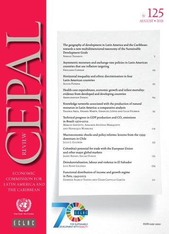
The geography of development in Latin America and the Caribbean: towards a new multidimensional taxonomy of the Sustainable Development Goals Sergio Tezanos

7

Asymmetric monetary and exchange-rate policies in Latin American countries that use inflation targeting Emiliano Libman

29

Horizontal inequality and ethnic discrimination in four Latin American countries Alicia Puyana

45

Health-care expenditures, economic growth and infant mortality: evidence from developed and developing countries Abdelhafidh Dhrifi

69

Knowledge networks associated with the production of natural resources in Latin America: a comparative analysis Valeria Arza, Anabel Marín, Emanuel López and Lilia Stubrin

93

Technical progress in GDP production and CO2 emissions in Brazil: 1970-2012 Márcio Santetti, Adalmir Antônio Marquetti and Henrique Morrone

119

Macroeconomic shocks and policy reforms: lessons from the 1999 downturn in Chile Julio J. Guzmán

133

Colombia’s potential for trade with the European Union and other major global markets Jaime Rafael Ahcar Olmos

153

Deindustrialization, labour and violence in El Salvador Luis René Cáceres

179

Functional distribution of income and growth regime in Peru, 1942-2013 Germán Alarco Tosoni and César Castillo García

211

ISSN 0251-2920

August • 2018

Alicia Bárcena Executive Secretary Mario Cimoli Deputy Executive Secretary a.i.

Raúl García-Buchaca Deputy Executive Secretary for Management and Programme Analysis

Osvaldo Sunkel Chairman of the Editorial Board Miguel Torres Editor

Alicia Bárcena Executive Secretary Mario Cimoli Deputy Executive Secretary a.i.

Raúl García-Buchaca Deputy Executive Secretary for Management and Programme Analysis Osvaldo Sunkel Chair of the Editorial Board Miguel Torres Editor The CEPAL Review was founded in 1976, along with the corresponding Spanish version, Revista CEPAL, and it is published three times a year by the Economic Commission for Latin America and the Caribbean (ECLAC), which has its headquarters in Santiago. The Review has full editorial independence and follows the usual academic procedures and criteria, including the review of articles by independent external referees. The purpose of the Review is to contribute to the discussion of socioeconomic development issues in the region by offering analytical and policy approaches and articles by economists and other social scientists working both within and outside the United Nations. The Review is distributed to universities, research institutes and other international organizations, as well as to individual subscribers.

The opinions expressed in the articles are those of the authors and do not necessarily reflect the views of ECLAC. The designations employed and the way in which data are presented do not imply the expression of any opinion whatsoever on the part of the United Nations concerning the legal status of any country, territory, city or area or its authorities, or concerning the delimitation of its frontiers or boundaries.

To subscribe, please visit the Web page: http://ebiz.turpin-distribution.com/products/197587-cepal-review.aspx The complete text of the Review can also be downloaded free of charge from the ECLAC website (www.eclac.org).

This publication, entitled CEPAL Review, is covered in the Social Sciences Citation Index (SSCI), published by Thomson Reuters, and in the Journal of Economic Literature (JEL), published by the American Economic Association

United Nations publication ISSN: 0251-2920 LC/PUB.2018/6-P Sales No.: E.18.II.G.15 Distribution: G Copyright © United Nations, August 2018 All rights reserved Printed at United Nations, Santiago S.18-00173 Requests for authorization to reproduce this work in whole or in part should be sent to the Economic Commission for Latin America and the Caribbean (ECLAC), Publications and Web Services Division, publicaciones.cepal@un.org. Member States of the United Nations and their governmental institutions may reproduce this work without prior authorization, but are requested to mention the source and to inform ECLAC of such reproduction.

Contents

The geography of development in Latin America and the Caribbean: towards a new multidimensional taxonomy of the Sustainable Development Goals Sergio Tezanos. . . . . . . . . . . . . . . . . . . . . . . . . . . . . . . . . . . . . . . . . . . . . . . . . . . . . . . . . 7 Asymmetric monetary and exchange-rate policies in Latin American countries that use inflation targeting Emiliano Libman. . . . . . . . . . . . . . . . . . . . . . . . . . . . . . . . . . . . . . . . . . . . . . . . . . . . . . 29 Horizontal inequality and ethnic discrimination in four Latin American countries Alicia Puyana . . . . . . . . . . . . . . . . . . . . . . . . . . . . . . . . . . . . . . . . . . . . . . . . . . . . . . . . 45 Health-care expenditures, economic growth and infant mortality: evidence from developed and developing countries Abdelhafidh Dhrifi. . . . . . . . . . . . . . . . . . . . . . . . . . . . . . . . . . . . . . . . . . . . . . . . . . . . . 69 Knowledge networks associated with the production of natural resources in Latin America: a comparative analysis Valeria Arza, Anabel Marín, Emanuel López and Lilia Stubrin . . . . . . . . . . . . . . . . . . 93 Technical progress in GDP production and CO2 emissions in Brazil: 1970−2012 Márcio Santetti, Adalmir Antônio Marquetti and Henrique Morrone. . . . . . . . . . . . . 119 Macroeconomic shocks and policy reforms: lessons from the 1999 downturn in Chile Julio J. Guzmán . . . . . . . . . . . . . . . . . . . . . . . . . . . . . . . . . . . . . . . . . . . . . . . . . . . . . . 133 Colombia’s potential for trade with the European Union and other major global markets Jaime Rafael Ahcar Olmos. . . . . . . . . . . . . . . . . . . . . . . . . . . . . . . . . . . . . . . . . . . . . . 153 Deindustrialization, labour and violence in El Salvador Luis René Cáceres . . . . . . . . . . . . . . . . . . . . . . . . . . . . . . . . . . . . . . . . . . . . . . . . . . . . 179 Functional distribution of income and growth regime in Peru, 1942−2013 Germán Alarco Tosoni and César Castillo García. . . . . . . . . . . . . . . . . . . . . . . . . . . . 211 Guidelines for contributors to the CEPAL Review . . . . . . . . . . . . . . . . . . . . . . . . 228 ECLAC recent publications . . . . . . . . . . . . . . . . . . . . . . . . . . . . . . . . . . . . . . . . . . . 229

Explanatory notes - Three dots (...) indicate that data are not available or are not separately reported.

- A dash (-) indicates that the amount is nil or negligible.

- A full stop (.) is used to indicate decimals.

- The word “dollars� refers to United States dollars, unless otherwise specified.

- A slash (/) between years (e.g. 2013/2014) indicates a 12-month period falling between the two years.

- Individual figures and percentages in tables may not always add up to the corresponding total because of rounding.

The geography of development in Latin America and the Caribbean: towards a new multidimensional taxonomy of the Sustainable Development Goals Sergio Tezanos1 Abstract The Latin America and the Caribbean region has an ambiguous place in the new geography of development: while it is a predominantly middle-income region, it is home to no more than 3% of the world’s poor population. Consequently, there is a risk that the international community will (mis)interpret this situation as meaning that the region need not be prioritized in the 2030 Agenda for Sustainable Development.

Nonetheless, the Sustainable Development Goals are not merely a strategy to combat economic poverty, but also a multidimensional strategy that defines a complex world map of priorities. This article develops a multidimensional taxonomy that addresses the fundamental dimensions of sustainable human development, beyond classifications based exclusively on per capita income. Cluster analysis is used to identify the different challenges faced by Latin American and Caribbean countries and to provide guidance for international cooperation policies.

Keywords 2030 Agenda for Sustainable Development, Sustainable Development Goals, poverty mitigation, economic development, social development, classification, development indicators, Latin America and the Caribbean JEL classification F35, O19, I30, C5 Author Sergio Tezanos Vásquez is a Professor in the Economics Department of the Faculty of Economic and Business Sciences of the University of Cantabria. Email: tezanoss@unican.es.

1

The author thanks José Antonio Sanahuja, Alejandra Kern, Daniela Perrotta, Ainoa Quiñones and an anonymous CEPAL Review referee for their valuable comments and suggestions.

8

CEPAL Review N° 125 • August 2018

I. Introduction The Sustainable Development Goals (SDGs) have begun life in a world in which one in eight people survive on daily incomes of less than US$ 1.25 in purchasing power parity (PPP) terms. So, achieving the formidable goal of eradicating extreme poverty by 2030 means addressing the privations of over 800 million people.

Given this challenge, how important is Latin America and the Caribbean in the global strategy to eradicate poverty? The region, on aggregate, “successfully” attained the Millennium Development Goal (MDG) of halving extreme poverty, by cutting its poverty rate by almost 8 percentage points (from the 12.5% recorded in 1990 to 4.6% today) and by freeing almost 25 million Latin American and Caribbean people from poverty. Having overcome this first test, the region now faces the (probably more complicated) challenge of eliminating the remaining pockets of poverty over the next 15 years, which affect another 30 million.2 Although the number living in poverty in the region is large in absolute terms, the fact is that Latin American and Caribbean countries account for “only” 3% of the poor who inhabit the planet (see table 1). By contrast, over 80% of the world’s poor live in the sub-Saharan Africa and South Asia regions; so to end poverty everywhere —as dictated by the first Sustainable Development Goal— international cooperation policies should prioritize those regions.

Table 1 Distribution of world poverty by regions, 2011a (Percentages and millions of persons) Poverty rate (percentages)

Poverty gap (percentages)

East Asia and the Pacific Europe and Central Asia Latin America and the Caribbean Middle East and North Africa South Asia Sub-Saharan Africa

7.93 0.49 4.63 1.69 24.50 46.81

1.56 0.14 2.17 0.35 5.16

Share of world poverty (percentages) 15.86 0.23 3.00 0.56 39.36

Total

16.98

19.18 5.05

40.99 100.00

160.76 2.35 30.44 5.64 398.95

2 027.27 479.13 657.45 333.78 1 628.38

Coverage of the study (percentages) 92.90 89.00 99.10 15.70 98.20

415.40 1 013.54

887.43 5 952.76

67.50 86.50

No. of poor (millions)

Population (millions)

Source: Prepared by the author, on the basis of data from World Bank, “PovcalNet: An Online Analysis Tool for Global Poverty Monitoring”, 2016 [online] http://iresearch.worldbank.org/PovcalNet/index.htm?0,0. a Poverty line: income less than US$ 1.25 dollars per day in purchasing power parity (PPP) terms.

Nonetheless, the Sustainable Development Goals are more than just a strategy to combat economic poverty; they also include a broad range of universal sustainable human development targets that define a complex global map of priorities.3 In order to help identify these polyhedral priorities and steer international cooperation policies, various multilateral organizations have constructed international classifications that group countries according to their development challenges. Curiously, the most widely used classification is actually the most simplistic one: the World Bank’s annual per capita income ranking. Although simplicity is its main advantage, the fact is that this classification cannot be used to explain the geography of development in the twenty-first century. According to this classification, most of the world’s poor are no longer in lower-income countries; roughly three quarters of them live in the 2

Author’s calculation using disaggregated data on extreme poverty in 2011 from the 25 countries of Latin America and the Caribbean included in the PovcalNet database (World Bank, 2016b). This figure will clearly be affected by the demographic growth of the poor population by 2030.

3

For an extensive review of the strategic scope and geographical connotations of the new Sustainable Development Goals, see Sanahuja and Tezanos (2017).

The geography of development in Latin America and the Caribbean: towards a new multidimensional taxonomy...

CEPAL Review N° 125 • August 2018

9

pockets of poverty that persist in the middle-income population giants (such as Brazil, China, India, Indonesia, Nigeria and Pakistan).4 The location of Latin America and the Caribbean in this new geography of development is, therefore, ambiguous: it is a region in which middle-income countries predominate, but it hardly participates in global poverty. This may be (mis)interpreted by the international community as meaning that the region need not be prioritized in relation to the Sustainable Development Goals —as also happened with their Millennium Development Goal predecessors. As the traditional income classification hardly provides any relevant information on the challenges of regional development, new multidimensional taxonomies, which are more complex and revealing, are needed to shed light on the dissimilar development challenges facing the Latin American and Caribbean countries and to guide international cooperation policies.

This article develops an alternative classification of the countries of Latin America and the Caribbean that goes beyond the traditional income criterion and instead addresses the three dimensions of sustainable development that structure the 2030 Agenda for Sustainable Development (economic development, social inclusion and environmental sustainability), plus the “essential element” of good governance. Following this introduction, section II reviews the international development classifications published by the World Bank, the Organization for Economic Cooperation and Development (OECD) and the United Nations Development Programme (UNDP). Section III proposes a multidimensional taxonomy of the development of Latin American and the Caribbean countries, which includes the four dimensions of sustainable development considered in this article. Cluster analysis is used to classify and characterize three groups of countries, in which the development profiles are similar within each group but dissimilar between them, while also identifying three other countries with unique development challenges that do not resemble those of any of the three groups. The article concludes by summarizing the main results of the classification and the analysis of its relevance for international development policies in this region.

II. Latin America and the Caribbean in international development classifications It is not easy to classify countries by development level, firstly because the definition of “development” itself is complex and multidimensional. Secondly, the fact that the socioeconomic realities of the different countries are highly diverse and changing makes it difficult to perform universally valid and stable analyses over time. As Nielsen (2013) points out, there is no generally accepted classification criterion —whether based on development theory or based on an objective benchmark. Despite these difficulties, development classifications have important analytical and operational potentials (Tezanos and Sumner, 2013).

In terms of analytics, development taxonomies serve to simplify a complex and diverse world by identifying groups of countries that share similar development features. Classifications of this type are common in different domains of knowledge (such as biology, medicine, philosophy, international relations and economics). In the case of development studies, which is a multidisciplinary knowledge domain, country classifications serve both to establish the main differences (and similarities) between countries in terms of development outcomes, and to study the dynamics of progress through time.

4

For reviews of the debate on the new geography of poverty, see Sumner (2012) and Sanahuja (2013).

Sergio Tezanos

10 CEPAL Review N° 125 • August 2018

In relation to operational potentials, international classifications are useful for development agencies, since they make it easier to establish criteria for allocating resources geographically and for designing differentiated cooperation policies that take account of the specific development challenges of the recipient countries. For example, as discussed below, the eligibility of countries for official development assistance (ODA) is based on a development taxonomy.

Nonetheless, there are several international development classifications that use different criteria to define a type of global development threshold that distinguishes between developed and developing countries. The three most influential classifications are those of the World Bank, OECD and UNDP. Since 1978, the World Bank has published a classification of countries according to their per capita income (estimated by per capita gross national product (GNP) calculated using the Atlas method). Although the World Bank itself recognizes that development is more than just income, it does consider that GNP per capita has proven a useful and simple indicator that is highly correlated with other non-monetary measures of the quality of life, such as life expectancy at birth, and the infant mortality and school enrolment rates (World Bank, undated). Thus, in the latest update, the World Bank classifies countries into four income groups: low (with a GNP per capita of less than US$ 1,005 in 2016); lower-middle (with a per capita GNP of between US$ 1,006 and US$ 3,955); upper-middle (US$ 3,956 to US$ 12,235); and high (GNP per capita of US$ 12,236 or more) (World Bank, 2018).

In contrast, the OECD Development Assistance Committee (DAC) distinguishes two groups of countries to provide an objective criterion for granting ODA. These are developed countries (which generally correspond to the high-income countries in the World Bank classification) and developing countries (low, lower-middle, and upper-middle income according to the World Bank). The latter are the potential recipients of ODA (DAC, 2014).

Lastly, UNDP classifies countries according to their human development levels by computing the synthetic Human Development Index (HDI), which partially reflects the multidimensional nature of the human development concept. Specifically, HDI summarizes three dimensions of development: longevity, education and purchasing power.5 The calculation of the corresponding HDI enables each country to be classified on four levels of human development (UNDP, 2015): very high (HDI higher than 0.8 in 2014), high (HDI between 0.8 and 0.7), medium (HDI from 0.55 to 0.7) and low (HDI below 0.55).

To what extent do these three development classifications coincide in the context of Latin America and the Caribbean? Table 2 shows that of the region’s 41 countries, 17 are developed (in other words high-income countries), while the remaining 24 are developing. The latter group contains just one low-income country (Haiti), along with six lower-middle and 17 upper-middle-income ones. In HDI terms, the region has two countries rated very high, 23 high, seven medium and one low (UNDP does not classify the remaining eight countries). In short, Latin America and the Caribbean is a region dominated by countries of upper-middle income and high human development.

Although the lists are broadly consistent with each other, there are several discrepancies between the World Bank and DAC classifications by per capita income and that based on human development (UNDP). Only two of the 17 high-income countries (Argentina and Chile) and none of the 17 uppermiddle-income countries are rated at the very high human development level. Nonetheless, two upper-middle-income countries (Brazil and Panama) are very close to surpassing the per capita GNP threshold of US$ 12,736; accordingly, they will likely be the next two Latin American countries to join the high-income group (developed countries), according to the World Bank and DAC classifications, even though they may not attain the highest level of human development according to UNDP.

5

In fact, the purchasing power dimension of HDI is also calculated using an indicator of per capita income (GDP per capita in PPP terms), which produces a degree of overlap between the three development classifications.

The geography of development in Latin America and the Caribbean: towards a new multidimensional taxonomy...

CEPAL Review N° 125 • August 2018

11

Table 2 Various classifications of the countries of Latin America and the Caribbean

1.

2.

3.

4.

5.

6.

7.

8.

9.

10.

11.

12.

13.

14.

15.

16.

17.

18.

19.

20.

21.

22.

23.

24.

25.

26.

27.

28.

29.

30.

31.

32.

33.

34.

35.

36.

37.

38.

39.

40.

41.

Antigua and Barbudaa Argentinab Aruba Bahamas Barbados Belize Bolivia (Plurinational State of) Brazil Chilea Colombia Costa Rica Cuba Curaçao Dominica Ecuador El Salvador Granada Guatemala Guyana Haiti Honduras Cayman Islands Turks and Caicos Islands United States Virgin Islands Jamaica Mexico Nicaragua Panama Paraguay Peru Puerto Rico Dominican Republic Saint Kitts and Nevis Saint Martin (French part) Saint Martin (Dutch part) Saint Lucia Saint Vincent and the Grenadines Suriname Trinidad and Tobago Uruguaya Venezuela (Bolivarian Republic of)b

World Bank (per capita GNP bracket)

United Nations Development Programme (UNDP) (HDI group)

High High High High High Upper-middle Lower-middle Upper-middle High Upper-middle Upper-middle Upper-middle High Upper-middle Upper-middle Lower-middle Upper-middle Lower-middle Lower-middle Low Lower-middle High High High Upper-middle Upper-middle Lower-middle Upper-middle Upper-middle Upper-middle High Upper-middle High High High Upper-middle Upper-middle Upper-middle High High High

High Very high ..

High High High Medium High Very high High High High ..

High High Medium High Medium Medium Low Medium .. .. ..

High High Medium High Medium High ..

High High .. ..

High High High High High High

Development Assistance Committee (DAC) (developed/developing country) Developed Developed Developed Developed Developed Developing Developing Developing Developed Developing Developing Developing Developed Developing Developing Developing Developing Developing Developing Developing Developing Developed Developed Developed Developing Developing Developing Developing Developing Developing Developed Developing Developed Developed Developed Developing Developing Developing Developed Developed Developed

Source: Prepared by the author, on the basis of data from World Bank, “World Development Indicators”, 2016 [online] http:// databank.worldbank.org/data/home.aspx; United Nations Development Programme (UNDP), Human Development Report 2015: Work for Human Development, New York, 2015 [online] http://www.undp.org/content/undp/en/home/ librarypage/hdr/2015-human-development-report.html; and Development Assistance Committee (DAC), “DAC List of ODA Recipients 2014-2016”, 2014 [online] http://www.oecd.org/dac/stats/documentupload/DAC%20List%20of%20 ODA%20Recipients%202014%20final.pdf. a Antigua and Barbuda, Chile and Uruguay exceeded the high-income threshold between 2012 and 2013. According to DAC regulations, these three countries ceased to be recipients of official development assistance in 2017. b Argentina and the Bolivarian Republic of Venezuela exceeded the high-income threshold between 2013 and 2014. Therefore, they will cease to be recipients of official development assistance as from 2018, provided they are still high-income countries at that time.

Sergio Tezanos

12 CEPAL Review N° 125 • August 2018

III. An alternative classification for Latin America and the Caribbean: taxonomy of the Sustainable Development Goals Once the indicative variable —or the various indicative variables— of development levels have been chosen, different procedures are used to define the country groupings. The World Bank and UNDP use an ordinal ranking. Nonetheless, this procedure does not make it possible to determine the appropriate number of groups, or where to place the thresholds that separate them.6 As will be explained later, cluster analysis offers a more nuanced and objective statistical technique than the mere ordering of a given development indicator.7 The following paragraphs make a different classification of the countries of Latin America and the Caribbean, based on the Sustainable Development Goals. Starting with the main dimensions of sustainable human development, a small set of indicators of these dimensions is then chosen to classify the countries of the region through the statistical technique of cluster analysis. A justification is then provided of the advantages of cluster analysis for establishing an international development taxonomy.

Thirdly, the resulting clusters are analysed and the main development challenges characterizing each of the country groups are identified.

1. Dimensions of the Sustainable Development Goals The process of producing an international classification of development starts by clearly defining the dimensions to be assessed in the classification. Given that global development agendas have the basic task of defining the international community’s priority objectives, the classification is based on the main dimensions of the 2030 Agenda for Sustainable Development. This strategy of 17 major goals combines two convergent agendas: first, the human development agenda inherited from the Millennium Development Goals; and, second, the sustainable development agenda that emerged from the four conferences popularly known as Earth Summits: the United Nations Conference on the Human Environment, held in Stockholm in 1972; the United Nations Conference on Environment and Development and the United Nations Conference on Sustainable Development, held in Rio de Janeiro (Brazil) in 1992 and 2012, respectively; and the World Summit on Sustainable Development, held in Johannesburg (South Africa) in 2002.

The concept of sustainable development has evolved recently as a result of lively debate on the 2030 Agenda. The four conferences gave rise to a three-dimensional definition of sustainable development, which includes the economic, social and environmental dimensions. Nonetheless, the Open Working Group of the General Assembly on the Sustainable Development Goals (United Nations, 2014a) and the United Nations Sustainable Development Solutions Network (SDSN, 2013) proposed a four-dimensional definition that also includes good governance. This was endorsed by the United Nations Secretary General in his Synthesis Report on the Post-2015 Sustainable Development Agenda (United Nations, 2014b), which recommended integrating the “four interdependent dimensions of sustainable development” economic development (including the eradication of extreme poverty and hunger), social inclusion, environmental sustainability and good governance (which includes peace and security). Nonetheless, this four-dimensional definition did not gain the consensus of the General Assembly; so the Sustainable Development Goals as adopted finally recognize three dimensions and one essential element for sustainable development (specifically, democracy, good governance and the rule of law) (United Nations, 2015).

6

For a critique of the arbitrary way in which the World Bank and UNDP define the intervals of each group, see Nielsen (2013).

7

Earlier studies have prepared development taxonomies through cluster analysis. See the study by Tezanos and Quiñones (2012) for the middle-income countries of Latin America and the Caribbean, and the work of Tezanos and Sumner (2013 and 2016) for developing countries as a whole.

The geography of development in Latin America and the Caribbean: towards a new multidimensional taxonomy...

CEPAL Review N° 125 • August 2018

13

Accordingly, obviating the distinction between “dimensions” and “essential element”,8 a taxonomy of the Sustainable Development Goals based on cluster analysis is constructed by assigning one of the 169 goals to each dimension, and then choosing an indicator to proxy each of these goals (see table 3).

Table 3 Dimensions of sustainable development and classification variablesa Development dimension 1. Economic development

SDG target By 2030, eradicate extreme poverty for all people everywhere

Indicator Poverty rate (US$ 1.25 per day, PPP) (percentage of the population) 2. Social inclusion By 2030, progressively achieve and GDP share of the poorest sustain income growth of the 40% of the population bottom 40 per cent of the population at a rate higher than the national average 3. Environmental sustainability Integrate climate change measures Per capita carbon dioxide into national policies, strategies emissions and planning 4. Good governance Substantially reduce corruption and Control of corruption bribery in all their forms

Source World Bank (2016b)

Period 2012 or latest year available

ECLAC (2016) and World Bank (2016a)

2012 or latest year available

ECLAC (2016)

2010

Kaufmann, Kraay and Mastruzzi (2014)

2013

Source: Prepared by the author, on the basis of World Bank, “World Development Indicators”, 2016 [online] http://databank. worldbank.org/data/home.aspx; “PovcalNet: An Online Analysis Tool for Global Poverty Monitoring”, 2016 [online] http://iresearch.worldbank.org/PovcalNet/index.htm?0,0; Economic Commission for Latin America and the Caribbean (ECLAC), “CEPALSTAT”, 2016 [online] http://estadisticas.cepal.org/cepalstat/portada.html?idioma=english; and D. Kaufmann, A. Kraay and M. Mastruzzi, “Worldwide Governance Indicators”, 2014 [online] www.govindicators.org. a Table 1 of Annex A1 displays the descriptive statistics of the variables used in the cluster analysis.

Selecting the most suitable indicators for each dimension is not an easy task, partly because the final set of Sustainable Development Goal indicators has not yet been officially approved. Moreover, as happened before with the Millennium Development Goals agenda, the Sustainable Development Goals start out within the framework of the “statistical fiction” of data availability, which, in most countries, will take several years to prepare and systematize. This will lead to an extensive initial period in which it will be virtually impossible to rigorously evaluate the progress of the agenda. Accordingly, the indicators used in this analysis have been selected on the practical (and inevitable) criterion of data availability.

2. Statistical procedure: analysis of development clusters Cluster analysis makes it possible to classify a sample of heterogeneous countries in a certain number of groups, each of which is internally homogeneous in terms of the similarities between the countries comprising it. The aim of this statistical technique is to provide reasonably objective and stable classifications (Everitt and others, 2011; Mooi and Sarstedt, 2011) —objective in the sense that an analysis of the same sample of countries using the same numerical methods produces the same classification; and stable to the extent that the classification does not change when new countries or new variables are added.

Specifically, hierarchical cluster analysis makes it possible to produce a taxonomy of countries with heterogeneous development levels and divide them into a specific number of groups, so that: (i) each country belongs to one, and only one, of the groups; (ii) all countries are classified; (iii) countries in the same group are, to some degree, homogeneous; and (iv) the countries of different groups are clearly different. This type of analysis also reveals the chain-linking structure that exists between countries, which makes it easier to identify the development characteristics of each cluster.

Cluster analysis also makes it possible to resolve two intrinsic difficulties of international taxonomies. First, it is possible to identify the appropriate number of groups into which the sample should be divided. Second, as the development indicators report different values for each country, 8

Nonetheless, this apparently rhetorical distinction between dimensions and essential elements has doctrinal significance, since it lowers the ambition with which sustainable human development is conceived.

Sergio Tezanos

14 CEPAL Review N° 125 • August 2018

the different indicators can be agglutinated to form a synthetic distribution that makes the variables easier to compare. Nonetheless, cluster analysis poses a specific difficulty when classifying countries (Nielsen, 2013): if the values of the development indicators are evenly distributed across the countries, the analysis does not make it possible to distinguish groups, even if there are marked differences between each country’s indicators. As noted below, this shortcoming is not relevant for Latin America and the Caribbean, however, since the analysis clearly discerns the chain linking structure that exists between the countries and, consequently, makes it possible to identify a small number of groups.

In the present study, hierarchical clusters were analysed using the Ward method, under which the squares of the Euclidean distances between each element are calculated, and the variables to be analysed are pre-standardized to correct for differences in scale.9 The analysis covers 26 of the 41 Latin American and Caribbean countries (63.4%), representing 88.6% of the region’s population.10 Before performing the cluster analysis, a decision must be made on the most appropriate design for producing a taxonomy of Latin American and Caribbean development that is sufficiently robust and stable. This requires evaluating the five aspects listed below.

First, the appropriate number of variables that can be included in the analysis must be determined.

There is no universally accepted criterion for this, although Formann (1984) proposed a simple rule: the sample size (in this case, the number of countries) must be at least equal to 2k, where “k” represents the number of classification variables.11 Thus, with the present sample of 26 countries, no more than four variables should be used (one for each dimension of sustainable development).

Second, checks must be made to see if the variables of the analysis are highly correlated, for, if so, they would be overrepresented in the results. According to Everitt and others (2011) and Mooi and Sarstedt (2011), correlations with absolute values above 0.9 are problematic. In this particular case, there are no especially high correlations among the four classification variables.12 Third, since cluster analysis is sensitive to the presence of atypical cases, checks should be made to verify whether any of the 26 countries is especially “different”. A practical tool for detecting atypical cases is the dendrogram, which graphically displays the distances at which the clusters merge.

The dendrogram is read from left to right: the vertical lines represent the country groupings and their position indicates the distance at which they merge.13 Thus, the dendrogram of the 26 countries in the sample clearly identifies two atypical cases: one is Haiti (the country with the lowest per capita income), which merges at a distance of 11; and the other is Trinidad and Tobago (the country with the highest income), which merges at a distance of 13. So, it is best to consider these two countries as unique and independent cases and apply the cluster analysis to the remaining 24.

Fourth, the optimal number of country clusters must be determined. This decision is based on the following two criteria, which indicate that the optimum number in this case is four:

9

The clustering method used is explained in Annex A2. As the variables used are expressed in different scales, they are standardized to the range [1, -1] which has proven superior to other methods in most situations (Mooi and Sarstedt, 2011). The analysis uses the IBM SPSS Statistics software.

10 The

15 countries excluded from the analysis because of a lack of information are all from the Caribbean: Cuba, Puerto Rico and 13 other Caribbean island states with populations of less than 500,000 (Antigua and Barbuda, Aruba, Bahamas, Barbados, Cayman Islands, Curaçao, Dominica, Saint Martin (Dutch part), Saint Martin (French part), Saint Kitts and Nevis, Saint Vincent and the Grenadines, Turks and Caicos Islands and the United States Virgin Islands).

11 Many

specialists (such as Dolnicar, 2003 and Mooi and Sarstedt, 2011) consider Formann’s criterion to be unduly restrictive; and few studies in the social sciences comply with it.

12 See

the correlations matrix in Annex A3. The variables “Corruption control” and “Share of the poorest 40%” have the highest correlation coefficient (0.414), but still well within the stated limit.

13

See the dendrogram in Annex A4. Note that SPSS Statistics rescales the original distances to fit a range between 0 and 25, so the last merger (which groups all countries in a single cluster) occurs at a distance of 25.

The geography of development in Latin America and the Caribbean: towards a new multidimensional taxonomy...

CEPAL Review N° 125 • August 2018

15

•

Clustering history shows the clusters that combine at each stage and the distance at which they merge.14 A simple scatter plot between these distances and the number of clusters reveals whether there is a break in the dotted line (“elbow”) that indicates which additional combination of two clusters significantly increases the distance, in such a way that the number of clusters prior to this merger is the most appropriate. In this analysis, the scatter chart displays an “elbow” between groups four and five.15 • The dendrogram clearly differentiates four clusters of countries grouped together at a maximum distance of seven units (out of 25), while Jamaica remains the only member of the last cluster to be formed (it is, therefore, the most dissimilar country in this sample of 24). In contrast, a three-cluster grouping would increase the distance to 11 units and a grouping with a larger number would slightly reduce that distance (for example, grouping in five clusters only reduces the distance by two units).

Lastly, it is important to ascertain which variables have the greatest influence on the formation of these four groups of countries. Analysis of the variance of a factor (specifically, the cluster of membership) shows, in contrast, that the four variables used are statistically significant, at a confidence level of 99% (see table 4). Likewise, the magnitudes of the F-statistics (which capture the relationship between inter- and intragroup variability) indicate the relevance of each of the variables in the formation of the groups, which means that the most influential variables are “CO2 per capita” and “Control of corruption”, in that order.

Table 4 Variance analysis of the variables included in the cluster analysis Sum of squares Poverty rate

Intergroup Intragroup Total Participation of the Intergroup poorest 40% Intragroup Total Intergroup CO2 per capita Intragroup Total Control of corruption Intergroup Intragroup Total

712.73 400.50 1 113.22 58.35 71.24 129.59 36.37 14.13 50.50 8.77 3.60 12.37

Degrees of freedom 3 20 23 3 20 23 3 20 23 3 20 23

Quadratic mean

F

p value

237.58 20.03

11.86

0.000

19.45 3.56

5.46

0.007

12.12 0.71

17.16

0.000

2.92 0.18

16.23

0.000

Source: Prepared by the author.

3. Key results As discussed above, the cluster analysis identifies four distinct groups of Latin American and Caribbean countries, plus the two unique cases of Haiti and Trinidad and Tobago (see table 5). The first cluster (C1) contains four countries (two high income and two upper-middle income); the second (C2) has four other countries (two high income and two upper-middle); the third (C3), encompasses 15 countries (nine upper- and six lower-middle income); and the fourth (C4), has a single upper-middle income country (Jamaica). The classification of development clusters diverges sharply from the classification by per capita income levels. Thus, although the C1 and C2 clusters encompass the countries with higher incomes on average, the truth is that C3 also has two of the relatively wealthier countries (Brazil and Panama), along with a large number of countries with very low per capita incomes. Map 1 provides a simple representation of the member countries of each development cluster.

14 The

correlations matrix is shown in Annex A5. For example, in the first stage, Ecuador (country 9) and Guyana (country 13) merge at a distance of 0.003. So, the conglomerate is named with the number of the first country involved in the merger (in this case, country 9, which merges again in stage 2 with country 20, Peru).

15 See

the scatter chart in Annex A6.

Sergio Tezanos

16 CEPAL Review N° 125 • August 2018

Table 5 Summary of the membership clusters of the countries of Latin America and the Caribbean Countrya

capita Membership Per capita GNP Per income cluster rankingb

Per capita income classificationc

Poverty rate

Share of the poorest 40%

CO2 per capita

Control of corruption

5. Chile

1

15 230

2

High

0.83

12.4

4.22

1.52

25. Uruguay

1

15 180

3

High

0.25

17.2

1.97

1.34

11. Granada

1

7 460

12

Upper-middle

2.40

17.0

2.49

0.41

22. Saint Lucia

1

7 090

13

Upper-middle

11.75

15.1

2.31

1.17

26. Venezuela (Bolivarian Republic of)

2

12 550

4

High

5.58

15.6

6.96

-1.28

1. Argentina

2

11 700

5

High

1.41

14.1

4.47

-0.46

17. Mexico

2

9 940

8

Upper-middle

3.26

12.8

3.91

-0.48

23. Suriname

2

9 260

10

Upper-middle

10.52

10.4

4.54

-0.38

4. Brazil

3

11 690

6

Upper-middle

4.53

9.8

2.15

-0.12

19. Panama

3

10 700

7

Upper-middle

3.55

10.6

2.74

-0.36

7. Costa Rica

3

9 550

9

Upper-middle

1.36

11.6

1.67

0.59

6. Colombia

3

7 560

11

Upper-middle

4.95

10.6

1.63

-0.44

21. Peru

3

6 390

14

Upper-middle

2.97

13.4

1.98

-0.44

8. Dominican Republic

3

5 620

15

Upper-middle

2.54

10.8

2.11

-0.85

9. Ecuador

3

5 510

16

Upper-middle

4.04

13.2

2.26

-0.61

2. Belize

3

4 660

18

Upper-middle

11.29

11.0

1.35

0.02

20. Paraguay

3

4 040

19

Upper-middle

4.43

10.0

0.79

-1.04

13. Guyana

3

3 750

20

Lower-middle

5.33

12.7

2.25

-0.64

10. El Salvador

3

3 720

21

Lower-middle

2.82

14.6

1.01

-0.35

12. Guatemala

3

3 340

22

Lower-middle

13.7

9.0

0.77

-0.58

3. Bolivia (Plurinational State of)

3

2 550

23

Lower-middle

6.97

12.2

1.56

-0.59

15. Honduras

3

2 180

24

Lower-middle

16.48

8.6

1.07

-0.95

18. Nicaragua

3

1 780

25

Lower-middle

6.83

12.8

0.79

-0.73

16. Jamaica

4

5 220

17

Upper-middle

32.49

14.4

2.61

-0.37

24. Trinidad and Tobago

...

15 760

1

High

1.15

15.8

37.78

-0.35

14. Haiti

...

810

26

Low

51.6

8.6

0.21

-1.15

Source: Prepared by the author.

Note: Indicators related to per capita income (columns three, four and five) are included as a reference, although they are not part of the cluster analysis. a The number that precedes each country is the same as appears in the dendrogram and in the clustering history. b The position by income levels is computed for the 26 countries of the initial sample. The clusters are numbered in increasing order of per capita income. c Classification by per capita income according to the latest update by the World Bank (2018).

The four clusters can be characterized comparatively in greater detail using the four indicators (see table 6).

The geography of development in Latin America and the Caribbean: towards a new multidimensional taxonomy...

CEPAL Review N° 125 • August 2018

17

Map 1 Taxonomy of the Sustainable Development Goals of the countries of Latin America and the Caribbean

Source: Prepared by the author.

Table 6 Socioeconomic characteristics of the clusters

C1

C2

C3

C4 (Jamaica) Trinidad and Tobago

Mean N Std. deviation Minimum Maximum Mean N Std. deviation Minimum Maximum Mean N Std. deviation Minimum Maximum 15 760

Per capita GNP

Poverty rate

11 240 4 4 581 7 090 15 230 10 863 4 1 524 9 260 12 550 5 536 15 3 095 1 780 11 690 5 220 1.15

3.81 4 5.37 0.25 11.75 5.19 4 3.94 1.41 10.52 6.12 15 4.37 1.36 16.48 32.49 15.80

Share of the poorest 40% 15.43 4 2.23 12.40 17.20 13.23 4 2.21 10.40 15.60 11.39 15 1.73 8.60 14.60 14.40 37.78

CO2 per capita 2.75 4 1.01 1.97 4.22 4.97 4 1.36 3.91 6.96 1.61 15 0.63 0.77 2.74 2.61 -0.35

Control of corruption 1.11 4 0.49 0.41 1.52 -0.65 4 0.42 -1.28 -0.38 -0.47 15 0.41 -1.04 0.59 -0.37

Sergio Tezanos

18 CEPAL Review N° 125 • August 2018

Table 6 (concluded)

Haiti Total (26 countries)

Mean N Std. deviation Minimum Maximum

Per capita GNP

Poverty rate

810 7 432 26 4 387 810

51.60 8.19 26 11.14 0.25

Share of the poorest 40% 8.60 12.47 26 2.50 8.60

15 760

51.60

17.20

CO2 per capita 0.21 3.68 26 7.11 0.21 37.78

Control of corruption -1.15 -0.27 26 0.73 -1.28 1.52

Source: Prepared by the author.

The first cluster (C1) consists of four Latin American and Caribbean countries with high development levels, but also high per capita emissions of carbon dioxide (CO2). They display the highest per capita income and the lowest poverty rates on average, as well as the best indicators of social inclusion and the most effective corruption controls (in fact, they are the only countries in the sample, along with Belize and Costa Rica, which display positive values in this indicator). Their high comparative development level also means that they are the group with the second highest CO2 emissions per capita (especially high in Chile). At the same time, this is the most heterogeneous cluster, as shown by the standard deviations of the indicators. Within the group, Chile and Santa Lucia (the countries with the highest and lowest income, respectively) are the most dissimilar cases and, therefore, the last two that saturate in this cluster (see again the dendrogram in Annex A4). In the case of Chile, the main difference lies in its high CO2 emissions (almost twice the average of the group in per capita terms), while Saint Lucia has the highest poverty rate (three times the group mean).

The second cluster (C2) includes four Latin American countries with intermediate levels of development and problems of corruption and pollution. On average, they have the second highest per capita income and the second lowest poverty rate. Nonetheless, this group of countries has high levels of pollution and very negative records on corruption. Although the group is relatively homogeneous, the most dissimilar country is the Bolivarian Republic of Venezuela, which, despite having the highest per capita income, also has a high poverty rate, along with the highest CO2 emissions and the highest levels of corruption.

The third cluster (C3) is the largest (15 countries) and includes Latin American and Caribbean countries with lower levels of development and problems of poverty, inequality and corruption. This group has the second lowest per capita income and the second highest poverty rate, as well as the greatest economic inequality and the worst corruption records. In contrast, the countries in this group are the least polluting in the sample in per capita terms. The main differences within this group are in their poverty rates: three Central American countries (Belize, Guatemala and Honduras) have poverty rates above 11%, while Costa Rica has a rate below 2%.

In addition to these three groups, the analysis identifies three “unique” countries that warrant separate analysis. The first of these is Jamaica, which is the only member of the fourth cluster (C4) and is unique owing to its high incidence of poverty (the second highest in the sample of 26 countries, after Haiti). On the rest of the indicators, it resembles the C2 countries; in fact, the dendrogram shows that Jamaica would be included in that group in the three-cluster solution.

That leaves the two “atypical” countries of the sample: Haiti and Trinidad and Tobago. Haiti has the worst development indicators: the lowest per capita income (almost 63% less than the next lowest country, Honduras): the highest poverty rate (19 percentage points above that of Jamaica), the least economic participation by the poorest population group (along with Honduras) and the worst corruption record. Yet it is also the country with the lowest CO2 emissions per person —in this case followed by

The geography of development in Latin America and the Caribbean: towards a new multidimensional taxonomy...

CEPAL Review N° 125 • August 2018

19

Guatemala. In contrast, Trinidad and Tobago has the highest per capita income and the third lowest poverty rate (after Uruguay and Chile) and economic inequality (after Granada and Santa Lucia). It is thus a country similar to those of cluster C1, except that its per capita CO2 emissions are by far the highest in Latin America and the Caribbean, which makes it an atypical case.

In relation to the regional distribution of the poor population (see table 7), as expected, most of the poor (almost 60%) live in the countries of the largest cluster (C3), mainly due to the presence of the region’s population giant, Brazil, which contributes almost half of the poor of this group and 30% of those of Latin America and the Caribbean as a whole. The countries of cluster C2 account for 20% of the region’s poor (over half of them living in Mexico). In addition, Haiti —given its very high incidence of poverty— accounts for 17% of all poor. The remaining 1% is distributed between the C1 countries and Trinidad and Tobago.

Table 7 Distribution of poverty among the clusters of Latin America and Caribbean countries (Percentages and millions of persons)

C1 C2 C2 excl. Mexico C3 C3 excl. Brazil C4 (Jamaica) Trinidad and Tobago Haiti High-income countries Upper-middle-income countries Lower-middle-income countries Low-income country (Haiti) Not included in the analysis (15 countries) Total for Latin America and the Caribbean

Poverty rate (percentages) 3.81 5.19 5.84 6.12 6.23 32.49 1.15 51.6 0.74 6.84 8.08

Population (millions) 20.98 187.44 71.48 360.17 163.23 2.62 1.33 10.03 22.02 498.17 52.34

Number of poor (millions) 0.18 6.06 2.28 18.17 9.25 0.85 0.02 5.18 0.17 20.17 4.93

51.60 ...

4.63

10.03 74.89 657.45

5.18 ...

30.44

Share of regional poverty (percentages) 0.58 19.89 7.48 59.68 30.38 2.80 0.05 17.00 0.55 66.25 16.19 17.00 ...

100.00

Source: Prepared by the author.

By contrast with the previous distribution, regional poverty by income levels is more highly concentrated: two thirds of the poor are concentrated in the upper-middle income bracket (along with Brazil and Mexico); and the other third is distributed among high-, lower-middle- and low-income countries. Thus, the classification of countries by income level in Latin America and the Caribbean generates the same incongruity as at the world level: countries with the largest numbers of poor people are not the poorest (low- and lower-medium income countries in the Latin American and Caribbean context), but the upper-middle-income ones.

IV. Conclusions Various international organizations establish development taxonomies that are useful for guiding international development policies, by making it possible to identify groups of countries that face similar challenges. Despite the difficulties inherent in any international classification, the most widely used criterion is precisely the simplest, based solely on an indicator of per capita income, such as that used by the World Bank and DAC. Nonetheless, this classification does little to explain the geography

Sergio Tezanos

20 CEPAL Review N° 125 • August 2018

of development in the twenty-first century, since most of the world’s poor are no longer located in low-income countries, but in the large group of middle-income countries, which include the most heavily populated (mainly, Brazil, China, India, Indonesia, Mexico, Nigeria and Pakistan).

The position of Latin America and the Caribbean in this new geography of development is ambiguous: it is a region in which middle incomes predominate; yet it accommodates just 3% of the world’s poor. As a result, there is a risk that the international community may (mis)interpret this and decide that the region need not be prioritized in the new cooperation agenda —as happened with the Millennium Development Goals.

Nonetheless, the Sustainable Development Goals are not only a strategy to combat economic poverty, but also a multidimensional strategy that defines a complex world map of priorities. In this context, given that the traditional classification of incomes provides little relevant information on the development challenges facing Latin America and the Caribbean, a multidimensional taxonomy of development needs to be designed which identifies the dissimilar challenges facing Latin American and Caribbean countries and helps guide international cooperation policies.

This article has developed an alternative taxonomy of the countries of Latin America and the Caribbean, which provides information to complement the income classification. The proposed taxonomy integrates the three dimensions and one “essential element” of sustainable development: economic development, social inclusion, environmental sustainability and good governance. The multivariate statistical technique of cluster analysis is used to define three groups of countries that have profound differences in their development levels: •

C1: Latin American and Caribbean countries with high levels of development, but also high CO2 emissions per capita (Chile, Granada, Saint Lucia and Uruguay).

•

C2: Latin American countries with medium development levels and problems of corruption and pollution (Argentina, the Bolivarian Republic of Venezuela, Mexico and Suriname).

•

C3: Latin American and Caribbean countries with lower levels of development and problems of poverty, inequality and corruption (Belize, Brazil, Colombia, Costa Rica, Dominican Republic, Ecuador, El Salvador, Guatemala, Guyana, Honduras, Nicaragua, Panama, Paraguay, Peru and the Plurinational State of Bolivia).

In addition to these three groups, the analysis identifies three “unique” countries: •

Jamaica, which would be in C2, if not for its high poverty rate.

•

Haiti, the country of the region that faces the greatest development challenges (in terms of poverty, social inclusion and corruption).

• Trinidad and Tobago, which, despite its similarities with the C1 countries, has by far the region’s highest per capita CO2 emissions.

These results indicate that —beyond unduly simple and economistic classifications, such as per capita income— there is no monotonically increasing distribution of development levels, which runs from a group of countries with the worst records on all indicators to another with better results in all of the variables. Conversely, the present multidimensional taxonomy offers more complex and nuanced groupings, which make it possible to identify both challenges and possibilities for advancement in each of the clusters.

This analysis can make a useful contribution to steering the effective management of development policies in the region, strategically oriented towards achieving specific progress objectives (the Sustainable Development Goals). Thus, the establishment of relatively homogeneous groups of countries makes it possible to exploit opportunities for cooperation in each of the clusters. In particular, classifications

The geography of development in Latin America and the Caribbean: towards a new multidimensional taxonomy...

CEPAL Review N° 125 • August 2018

21

of this type would allow for peer evaluation (that is, between countries in the same group), collective advances and setbacks, and progress in designing specific development strategies for each group, which go beyond the generalist nature of universal development agendas.16 Likewise, the results of this taxonomy of the Sustainable Development Goals for Latin America and the Caribbean can also be useful for guiding South-South and triangular cooperation initiatives, by making it possible to identify both the potentialities of each group (which the countries can exploit in their roles as regional donors), and their weaknesses and development challenges (which should be addressed by the cooperative actions of other countries). In this sense, the countries offering South-South cooperation are distributed among all the development clusters; and these “diagonal” cooperation relations (neither vertical nor horizontal in terms of the donors’ development levels) highlight the synergies existing in a diverse region.

Ultimately, the classifications must serve the purpose for which they were created: to facilitate understanding of a complex world and to guide the design of development policies. In the context of Latin America and the Caribbean, the changes —and complexities— of the new geography of development are such that the challenges of development can only be better understood by modifying the analytical frameworks through which the region is viewed, starting with the way countries are classified.

Bibliography DAC (Development Assistance Committee) (2014), “DAC List of ODA Recipients 2014-2016” [online] http://www.oecd.org/dac/stats/documentupload/DAC%20List%20of%20ODA%20Recipients%20 2014%20final.pdf.

Dolnicar, S. (2003), “Using cluster analysis for market segmentation-typical misconceptions, established methodological weaknesses and some recommendations for improvement”, Australasian Journal of Market Research, vol. 11, No. 2.

ECLAC (Economic Commission for Latin America and the Caribbean) (2016), “CEPALSTAT” [online] http:// estadisticas.cepal.org/cepalstat/portada.html?idioma=english.

Everitt, B. S. and others (2011), Cluster Analysis, Chichester, John Wiley & Sons.

Formann, A. K. (1984), Die Latent-Class-Analyse: Einfuhrung in die Theorie und Anwendung, Weinheim, Beltz.

Kaufmann, D., A. Kraay and M. Mastruzzi (2014), “Worldwide Governance Indicators” [online] www.govindicators.org.

Mooi, E. and M. Sarstedt (2011), A Concise Guide to Market Research, Berlin, Springer-Verlag.

Nielsen, L. (2013), “How to classify countries based on their level of development”, Social Indicators Research, vol. 114, No. 3, Springer.

Peña, D. (2002), Análisis de datos multivariantes, Madrid, McGraw-Hill.

Sanahuja, J. A. (2013), “Las nuevas geografías de la pobreza y la desigualdad y las metas de desarrollo global post-2015”, El reto de la democracia en un mundo en cambio: respuestas políticas y sociales. Anuario 2013-2014, M. Mesa (coord.), Madrid, Centre for Peace Research and Education (CEIPAZ) [online] http:// www.ceipaz.org/images/contenido/4.Sanahuja.pdf.

Sanahuja, J. A. and S. Tezanos (2017), “Del milenio a la sostenibilidad: retos y perspectivas de la Agenda 2030 para el Desarrollo Sostenible”, Política y Sociedad, vol. 54, No. 2, Madrid, Complutense University of Madrid.

SDSN (Sustainable Development Solutions Network) (2014), An Action Agenda for Sustainable Development.

Report for the UN Secretary-General [online] http://unsdsn.org/wp-content/uploads/2013/06/140505An-Action-Agenda-for-Sustainable-Development.pdf.

Sneath, P. H. A. and R. R. Sokal (1973), Numerical Taxonomy, San Francisco, W. H. Freeman.

Sumner, A. (2012), “Where do the poor live?”, World Development, vol. 40, No. 5, Amsterdam, Elsevier.

Tezanos, S. (2011), “Más allá de 2015: Objetivos de Desarrollo del Milenio y desafíos para la nueva agenda internacional de desarrollo”, SISTEMA: Revista de Ciencias Sociales, No. 220, Madrid, Editorial Sistema.

16 For

a proposal of this type, see Tezanos (2011).

Sergio Tezanos

22 CEPAL Review N° 125 • August 2018

Tezanos, S. and A. Quiñones (2012), “¿Países de renta media? Una taxonomía alternativa del desarrollo de América Latina y el Caribe”, Revista Iberoamericana de Estudios de Desarrollo, vol. 1, No. 2 [online] http://ried.unizar.es/index.php/revista/article/viewFile/45/23.

Tezanos, S. and A. Sumner (2016), “Is the ‘developing world’ changing? A dynamic and multidimensional taxonomy of developing countries”, The European Journal of Development Research, vol. 28, No. 5, Springer.

(2013), “Revisiting the meaning of development: a multidimensional taxonomy of developing countries”, The Journal of Development Studies, vol. 49, No. 12, Taylor & Francis.

UNDP (United Nations Development Programme) (2015), Human Development Report 2015: Work for Human Development, New York [online] http://www.undp.org/content/undp/en/home/librarypage/hdr/2015human-development-report.html.

United Nations (2015), “Transforming our world: the 2030 Agenda for Sustainable Development” (A/RES/70/1), Resolution adopted by the General Assembly on 25 September 2015 [online] http://www.un.org/en/ development/desa/population/migration/generalassembly/docs/globalcompact/A_RES_70_1_E.pdf.

(2014a), “Report of the Open Working Group of the General Assembly on Sustainable Development Goals” (A/68/970) [online] https://undocs.org/A/68/970.

(2014b), “The road to dignity by 2030: ending poverty, transforming all lives and protecting the planet.

Synthesis report of the Secretary-General on the post-2015 sustainable development agenda” (A/69/700) [online] http://www.un.org/ga/search/view_doc.asp?symbol=A/69/700&Lang=E. Ward, J. H. (1963), “Hierarchical groupings to optimize an objective function”, Journal of the American Statistical Association, vol. 58, No. 301, Taylor & Francis.

World Bank (2018), “World Bank Country and Lending Groups” [online] https://datahelpdesk.worldbank.org/ knowledgebase/articles/906519.

(2016a), “How we classify countries: a short history” [online] http://data.worldbank.org/about/countryand-lending-groups.

(2016b), “World Development Indicators” [online] http://databank.worldbank.org/data/home.aspx.

(2016c), “PovcalNet: An Online Analysis Tool for Global Poverty Monitoring” [online] http://iresearch. worldbank.org/PovcalNet/index.htm?0,0. (undated), “Why use GNI per capita to classify economies into income groupings?” [online] https:// datahelpdesk.worldbank.org/knowledgebase/articles/378831-why-use-gni-per-capita-to-classifyeconomies-into.

The geography of development in Latin America and the Caribbean: towards a new multidimensional taxonomy...

CEPAL Review N° 125 • August 2018

23

Annex A1 Table A1.1 Descriptive statistics of the variables used in the analysis of clusters GNP per capita Poverty rate Participation of the poorest 40% CO2 per capita Corruption control No. valid (according to list)

No. 26 26 26 26 26 26

Minimum 810 0.25 8.60 0.21 -1.28

Maximum 15 760 51.60 17.20 37.78 1.52

Mean 7 432.31 8.19 12.47 3.68 -0.27

Standard deviation 4 386.83 11.14 2.50 7.11 0.73

Source: Prepared by the author.

Annex A2 Clustering method Given the type of data used in the present analysis (four continuous variables), three clustering algorithms are possible (Everitt and others, 2011; Peña, 2002; Mooi and Sarstedt, 2011): the nearest-neighbour method, the farthest-neighbour method and Ward’s method. Since there is no objective criterion for choosing the most appropriate method, the choice depends largely on ease of interpretation of the final results (Sneath and Sokal, 1973; Everitt and others, 2011; Peña, 2002; Mooi and Sarstedt, 2011).

This analysis uses the method proposed by Ward (1963), who argued that clusters should be constituted in such a way that, when merging two elements, the resulting information loss is minimal.17 To do this, the sum of the squares of the distances of each element is quantified with respect to the centroid of the cluster to which it belongs. Specifically, the method starts by calculating the vector of means of all the variables —“multivariate centroid”— for each cluster. Next, the squares of the Euclidean distances between each element and the centroids (vector of means) are calculated for all clusters.

Then the distances corresponding to all the elements are summed. The general formula for Ward’s distance (W) is expressed as:

W=

/ / Rx g idg

ig

– xr g WlR xig – xr g W

where xg is the mean of group g, and i is a country belonging to that group.

For this research in particular, the Ward method and the farthest-neighbour method both provide similar classifications of the countries of Latin America and the Caribbean, thus supporting the robustness of the results obtained.

17 In

fact, the meta-analysis conducted by Dolnicar (2003), which includes 243 articles on market segmentation using the cluster analysis technique, reveals that the Ward method is the most popular clustering algorithm used in hierarchical cluster analysis (used in 57% of cases).

Sergio Tezanos

24 CEPAL Review N° 125 • August 2018

Annex A3 Table A3.1 Matrix of correlations of the variables used in the analysis Poverty rate Poverty rate

Pearson correlation p-value N Share of the poorest 40% Pearson correlation p-value N Pearson correlation CO2 per capita p-value N Corruption control Pearson correlation p-value N

1 26 -0.361 0.070 26 -0.188 0.357 26 -0.303 0.133 26

Share of the poorest 40% -0.361 0.070 26 1 26 0.346 0.084 26 0.414 0.036 26

CO2 per capita

Control of corruption

-0.188 0.357 26 0.346 0.084 26 1

-0.303 0.133 26 0.414 0.036 26 -0.005 0.980 26 1

26 -0.005 0.980 26

26

Source: Prepared by the author.

The geography of development in Latin America and the Caribbean: towards a new multidimensional taxonomy...

CEPAL Review N° 125 • August 2018

25

Annex A4 Figure A4.1 Latin America and the Caribbean (26 countries): dendrogram of the classification of the region’s countries 0 Colombia

5

10

15

20

25

6

Panama 19 Brazil

4

Suriname 23 Belize

2

Dominican Republic

8

Paraguay 20 Guatemala 12 Honduras 15 Haiti 14 Chile

5

Costa Rica

7

Grenada 11 Uruguay 25 Saint Lucia 22 Argentina

1

El Salvador 10 Guyana 13 Nicaragua 18 Bolivia (Est. Plur. of)

3

Ecuador

9

Peru 21 Mexico 17 Venezuela (Bol. Rep. of) 26 Jamaica 16 Trinidad and Tobago 24 Source: Prepared by the author.

Sergio Tezanos

26 CEPAL Review N° 125 • August 2018

Annex A5 Table A5.1 Detailed clustering history Stage 1 2 3 4 5 6 7 8 9 10 11 12 13 14 15 16 17 18 19 20 21 22 23

Cluster being combined Cluster 1 Cluster 2 9 13 9 20 3 17 4 18 12 14 6 8 1 16 4 6 3 9 3 10 11 23 2 7 4 19 11 21 1 22 2 4 5 11 2 12 1 24 2 3 1 15 1 2 1 5

Coefficients 0.003 0.011 0.022 0.035 0.050 0.067 0.085 0.118 0.165 0.223 0.284 0.356 0.434 0.548 0.678 0.845 1.126 1.429 1.736 2.179 2.892 4.009 5.728

Stage at which the cluster first appears Cluster 1 Cluster 2 0 0 1 0 0 0 0 0 0 0 0 0 0 0 4 6 3 2 9 0 0 0 0 0 8 0 11 0 7 0 12 13 0 14 16 5 15 0 18 10 19 0 21 20 22 17

Next stage 2 9 9 8 18 8 15 13 10 20 14 16 16 17 19 18 23 20 21 22 22 23 0

Source: Prepared by the author.

The geography of development in Latin America and the Caribbean: towards a new multidimensional taxonomy...

CEPAL Review N° 125 • August 2018

27

Annex A6 Figure A6.1 Dispersion between distances and the number of clusters 6

Coefficients (distances)

5

4

3

2

1

0

23 22 21 20 19 18 17 16 15 14 13 12 11 10 9

8

7

6

5

4

3

2

1

Number of clusters Source: Prepared by the author.

Sergio Tezanos

Asymmetric monetary and exchange-rate policies in Latin American countries that use inflation targeting Emiliano Libman

Abstract In recent decades, Latin American countries have adopted more flexible exchange-rate regimes and set inflation targets. Several authors argue that some countries’ monetary and exchange-rate policies suffer from a procyclical bias, whereby central banks are reluctant to reduce interest rates when inflation falls, but are willing to increase them when inflation edges up. Therefore, the exchange rate tends to appreciate a lot and depreciate little. This paper analyses the asymmetry of the monetary and exchangerate policies of the five largest Latin American countries in which inflation targets are used: Brazil, Chile, Colombia, Mexico and Peru. Nonlinear econometric techniques are used to show that there is "fear of floating", except possibly in Chile and Peru, and that the symptoms are more pronounced in Brazil and Mexico.

Keywords Monetary policy, foreign exchange rates, inflation, econometric models, case studies, Latin America, Brazil, Chile, Colombia, Mexico, Peru JEL classification E58, F30, F43 Author Emiliano Libman is a Research Fellow at the Macroeconomic Research for Development Centre (CIMaD) and Professor of Advanced Macroeconomics in the School of Economics and Business at Universidad Nacional de San Martín, Argentina.

Email: emilianolibman@gmail.com.

30 CEPAL Review N° 125 • August 2018

I. Introduction In recent decades, several developed and non-developed countries have adopted inflation-targeting policy regimes, under which the central bank commits to delivering a low and stable rate of inflation, using a short-term interest rate as the main policy instrument. Inflation-targeting countries maintain a relatively open capital account, and the usual prescription is to let the exchange rate float freely and to refrain from foreign-exchange-market intervention.

As monetary policy is used to target inflation (and possibly also the output gap), interest-rate changes may put too much pressure on the foreign-exchange market; and most central banks are unwilling to tolerate very large exchange-rate fluctuations. Interventions to suppress exchange-rate volatility are often the norm. In fact, theory does not necessarily preclude the central bank from buying and selling foreign assets, as long as this policy aims to cushion temporary shocks or other exchangerate movements that are not justified by economic fundamentals.

The largest Latin American countries have all adopted inflation targeting, including Brazil (1999), Chile (1991),1 Colombia (1999), Mexico (2001) and Peru (2002). Although current exchange-rate regimes are much more flexible than in the past, central banks continue to intervene heavily in the foreign-exchange market to cushion wide exchange-rate swings (Chang, 2008).

There are good reasons to believe that this type of intervention has not been implemented with equal intensity during appreciation and depreciation episodes. For example, authors such as Barbosa-Filho (2015) and Ros (2015) argue that the central banks of Brazil and Mexico have conducted an “asymmetric monetary policy”, in which they tighten too much when the economy is booming, and not loosening enough when deflationary pressures arise. As these countries’ balance of payments capital accounts were extremely open, the implied interest-rate changes triggered exchange-rate movements that had a downward bias.2 Asymmetric behaviour can have implications for macroeconomic stability. For example, depending on whether shocks are positive or negative, the economy may adjust inadequately. A negative shock, such as a fall in the terms of trade, which requires a rise in the real exchange rate (a higher relative price for tradable goods) may be impossible if non-tradable goods prices are “sticky” and if the central bank is willing to counteract depreciations. But if the shock is positive, for example, if the terms of trade improve and an appreciation is called for, then the economy may adjust smoothly.

Alternatively, the presence of asymmetries may be a sign of underlying problems: for example, the literature on fear of floating posits that inflation is the underlying reason why central banks dislike depreciations. If inflation-targeting countries display fear of floating then there are good reasons to believe that inflation expectations are not well anchored by monetary policy.

In short, asymmetric behaviour has consequences for macroeconomic performance and is related to several sources of instability. It is therefore interesting to analyse whether the Latin American countries that have adopted flexible exchange-rate regimes fear exchange-rate fluctuations. This paper’s contribution is to explore this asymmetry in monetary and exchange-rate policies in the main Latin American inflation-targeting countries. Nonlinear econometric techniques are used to test whether these countries’ central banks were more willing to tolerate appreciations than depreciations, over the period 1999−2015, using daily data. Specifically, the observed behaviour of the exchange rate is analysed to identify the presence of any asymmetries. Nonetheless, exchange rates may behave 1

Although Chile adopted inflation targeting in 1991, but it only really started to float more or less freely in 1999. This is not a problem as the estimates used in this study start in 1999, the period that combines inflation targeting and floating.

2

This paper abides by the convention of defining the exchange rate as the number of units of domestic currency per dollar; so, a fall in the exchange rate represents an appreciation, while a rise signifies a depreciation.

Asymmetric monetary and exchange-rate policies in Latin American countries that use inflation targeting

CEPAL Review N° 125 • August 2018

31

asymmetrically for non-policy reasons; so, a set of central bank reaction functions for interest rates and reserve accumulation is also estimated, to determine the impact of monetary and exchange-rate policy on the observed behaviour of the exchange rate.

The paper’s results can be summarized as follows. In Brazil and Mexico, exchange-rate changes seem to be anchored to an asymmetric band in which the lower bound is further from the target rate than the upper bound. Appreciations were more persistent than depreciations in all of the countries, except Peru, where both appreciations and depreciations were relatively short-lived (in other words, an appreciating exchange rate would soon be followed by a depreciation, and vice-versa). Appreciations were also a highly persistent phenomena in Brazil, Chile and Mexico. Lastly, in all cases except Chile, reserve accumulation seems to react to exchange-rate depreciations, but not to appreciations, and interest rates show little sensitivity to exchange-rate fluctuations. The overall picture thus suggests that “fear of depreciation” was most likely the norm in Brazil and Mexico; the Chilean central bank seems to operate the most flexible exchange-rate regime of the five; while the overall picture for Colombia and Peru is mixed.

The rest of this paper is structured as follows: section II contains a literature review; section III describes the econometric techniques used and presents the results, and section IV concludes.

II. Literature review Recent macroeconomic thinking has converged on a synthesis, known as the “new consensus macroeconomics”, which agrees on the desirability of an autonomous monetary policy and on how to conduct it. The interest rate has replaced monetary-policy rules based on the quantity of money. It has been shown that a model with explicit microfoundations based on a representative agent framework can determine the equilibrium without any reference to the quantity of money, provided the interest-rate rule is sufficiently sensitive to changes in the inflation rate.

This is known as the “Taylor principle”, which, intuitively, states that the interest rate should be increased by more than inflation when inflation rises above target, to avoid an inflationary spiral, lower real interest rates and higher aggregate demand. Conversely, when inflation falls below the target, the interest rate should be reduced by more than inflation.

When the Taylor principle is satisfied, inflationary expectations are anchored by the inflation target.

Moreover, if there are no real frictions, stabilizing inflation also implies stabilizing the output gap. This is the divine coincidence evoked by Blanchard and Gali (2007). Because inflation targeting appears to stabilize both output and inflation at very little cost, it has become the most popular and appealing macroeconomic regime.3 It is often claimed that the process should operate in a similar way for an open economy. The core propositions for a closed economy presumably also apply, although there are additional complications associated with the existence of external monetary and real shocks. Nonetheless, the effects of exchange-rate fluctuations and the scope of central-bank interventions in the foreign exchange market are subject to intense debate. While some authors argue that inflation targeting requires a fully flexible exchange rate, others are willing to accept a role for temporary interventions by the central bank (see Ball, 1999, for a discussion of these issues).

The largest Latin American countries have all adopted inflation targeting, including Brazil, Chile, Colombia, Mexico and Peru. Although exchange-rate regimes are much more flexible than in the past, central banks still intervene heavily to cushion large movements in exchange rates (Chang, 2008).

3 See

Bernanke and Mishkin (1997) for a more precise description of inflation targeting.

Emiliano Libman

32 CEPAL Review N° 125 • August 2018

There are good reasons to believe that such interventions have not been implemented with the same intensity during episodes of appreciation and depreciation. Calvo and Reinhart (2002) argue that, when the financial system is highly dollarized, the central bank may fear that currency depreciations will trigger bank failures. It is also possible that central banks fear the inflationary effects of depreciations, although exchange-rate pass-through has recently declined by non-trivial amounts. This aversion to depreciation is often called “fear of floating”.

On the other hand, when the competitiveness of the tradable sector is an issue, the central bank may intervene to prevent currency appreciations, a phenomenon known as a fear of appreciation, or the opposite of fear of floating, as exemplified by recent events in East Asia (Levy-Yeyati and Sturzenegger, 2007).

Some observers of the Latin American economies claim that inflation targeting has introduced a bias towards overvaluation, since central banks react more aggressively to curb depreciations, but are more cautiously when responding to appreciations (Barbosa-Filho, 2015;4 and Ros, 2015).5 Unlike the East Asian countries that intervened in the foreign-exchange market to suppress appreciations (Pontines and Rajan, 2011; Pontines and Siregar, 2012), some Latin American countries seem to intervene in the opposite direction.

This paper will analyse the behaviour of exchange rates in the main Latin American countries that have used inflation targeting over the last 15 years. A panel smooth transition autoregressive model with three regimes is estimated, along with a Markov-switching model. These two models will estimate the upper and lower bounds of an exchange rate band, and the probabilities of a transition from depreciation to appreciation, respectively, for a series consisting of the natural logarithm of the rate of variation of the exchange rate. This is the simplest way to test whether monetary and exchange-rate policy in inflation-targeting Latin American countries was in fact asymmetric; and it follows the approach suggested by Pontines and Siregar (2012).

As exchange rates may also be affected by non-policy factors, Pontines and Siregar’s approach is extended by estimating a set of reaction functions for the benchmark interest rate and reserve accumulation, to analyse the role of policy in shaping exchange-rate behaviour. This will provide a more precise answer to the question of whether fear of floating or fear of depreciation (or neither) was the overriding concern among inflation-targeting Latin American countries in the period 1999−2015.

III. Empirical approach and results Central bank interventions in the foreign exchange market have been common in Latin America in recent years. However, as exchange rates may appreciate or depreciate in spite of central bank interventions, it is of interest to gauge the overall pressures on exchange rates by also considering the trends in foreign-exchange reserves and interest rates.

One way to combine these three elements (exchange rates, interest rates, and reserves) in a single index is to construct an exchange market pressure (EMP) index, as proposed by Kaminsky, Lizondo and Reinhart (1998) and by Reinhart and Kaminsky (1999). The index is calculated as follows: 4

“There is a fundamental asymmetry in the way macroeconomic policy deals with changes in the exchange rate in developing economies, especially in Latin America. Because appreciations are deflationary and depreciations are inflationary in the short run, any democratic government tends to tolerate appreciations but fight depreciations of their currencies. In fact, the adjusting period of the economy after a depreciation of its domestic currency may be longer than the mandate of elected officials, and this creates an asymmetric response of democratic governments to changes in the real exchange rate” (Barbosa-Filho, 2015).

5

“To the extent that the Central Bank reacts only to changes in the inflation rate it becomes very tempting for the monetary authority to subordinate the exchange rate to its inflation objectives or to respond in an asymmetrical way to appreciations and depreciations. There is consequently a ‘fear to depreciate’, more than a ‘fear of floating’. This tends to make monetary policy pro-cyclical in the fact of external shocks. For example, in the face of a negative export demand shock, which tends to lower economic activity, the monetary authority tends to moderate the pressure towards depreciation through an increase in interest rates which aggravates the recession” (Ros, 2015).

Asymmetric monetary and exchange-rate policies in Latin American countries that use inflation targeting

CEPAL Review N° 125 • August 2018

EMPit

DEit vE Drit vE

+ − vr rit vInt DIntit Eit

33

(1)

where EMPit is the exchange market pressure index, Eit is the exchange rate, rit denotes gross reserves, Intit is the monetary policy benchmark interest rate, Δ denotes change, and the variables σE, σr, and σInt are the standard deviations of the exchange rate, gross reserves and the monetary-policy rate, respectively.6 A positive EMP implies net pressure towards depreciation, while a negative EMP indicates net pressure for appreciation.

Figures 1 to 5 in the appendix track the EMP index for Brazil, Chile, Colombia, Mexico and Peru over the last 15 years. They also display the natural logarithm of the exchange rate, so the slope of the line captures the rate of depreciation. The figures clearly show that the inflation-targeting Latin American countries experienced significant pressures towards appreciation, but also important pressures for depreciation. The general trend was appreciation, which was only reversed recently by abrupt depreciations; but it is also clear that other factors, such as reserve accumulation, played a role in reversing exchange rate pressures, both upwards and downwards (also documented, for example,

by Chang, 2008).

A more complete story is reported in table 1, which displays summary statistics for the rate of devaluation, the change in the benchmark interest rate and the rate of growth of reserves (with monthly data) for the five countries over the period 1999−2015. The table reveals a number of interesting facts.

For example, it shows that both Chile and Mexico have very volatile exchange rates (consistent with the casual observation that both countries have relatively flexible regimes); but, the exchange rate (and the interest rate) is less volatile in Peru, which has a highly dollarized financial system. It should be noted that the Central Bank of Peru applies several non-conventional monetary policy tools, such as reserve requirements on dollar-denominated assets. As expected, reserves display very little volatility in all five countries.

Table 1 Summary statistics Δln (Exch. rate)

ΔInterest rate

Δln (Reserves)

Mean Standard deviation Maximum Minimum Mean Standard deviation Maximum Minimum Mean Standard deviation Maximum Minimum

Brazil 0.0034 0.0506 0.2532 -0.1477 -0.0254 0.5925 3.0000 -2.5000 0.0127 0.0489 0.2445 -0.3110

Chile 0.0283 0.3692 5.0289 -0.0699 -0.0109 0.4088 3.0000 -2.5000 0.0053 0.0375 0.1301 -0.1646

Colombia 0.0078 0.0864 1.0787 -0.1120 -0.0241 0.3677 2.0000 -2.000 0.0094 0.0191 0.0838 -0.0796

Mexico -0.0277 0.4186 0.1794 -5.7083 -0.0763 0.7462 2.7700 -3.4000 0.0101 0.0272 0.1039 -0.1641

Peru -0.0088 0.1137 0.0486 -1.5357 0.0035 0.2236 0.5000 -1.0000 0.0101 0.0290 0.1043 -0.1142

Source: Prepared by the author on the basis of data from central banks.

Based on empirical observation and a preliminary reading of the data and, to judge from the mean rate of depreciation, there is no suggestion of bias towards either appreciation or depreciation.

In fact, it could be argued that the central banks tried very hard to avoid appreciation, given their large purchases of foreign-exchange reserves.

6

The subscripts represent country “i” in period “t”; 24-month rolling averages are used for the standard deviations. The data are monthly.

Emiliano Libman

34 CEPAL Review N° 125 • August 2018

Yet this casual observation is not enough to obtain a definitive picture. For instance, large reserve purchases may be driven by other motives, and not necessarily carried out during periods of appreciation.7 Moreover, as shown by Pontines and Siregar (2012), in East Asian countries that used inflation targeting, fear of appreciation was the rule. Despite tremendous pressures towards nominal appreciation, the central banks in those countries intervened more heavily when the exchange rate fell than when it rose.

Does a similar or opposite result hold for Latin American countries? This section follows the Pontines and Siregar approach, by estimating a set of nonlinear least-square models and a set of Markovswitching models to discover whether exchange-rate behaviour displayed any signs of asymmetry.

The results are then expanded by asking whether the central bank was responsible for the observed developments, using generalized method of moments (GMM) reaction functions for monetary policy and reserve accumulation.

The sample for the nonlinear models is restricted to the period spanning 1999 to 2015 for Brazil, Chile, Colombia, Mexico, and Peru —the largest inflation-targeting countries in Latin America. But unlike Pontines and Siregar (2012), who use monthly and weekly data for nominal exchange rates, this paper uses daily data.8

1. LSTR2 and Markov-switching models One way to analyse the behaviour of the exchange rate is through a smooth transition autoregressive (STAR) model9 of the following functional form:

yt = a0 +

/

p i=1

ai yi + F #b0 +

/

p i=1

bi yi& + ft (2)

where α0 is the intercept term; αi (with i = 1, …, p) denotes the autoregressive parameters; β0 is the nonlinear intercept and βi represents the nonlinear autoregressive parameters; εt is the error term with the standard properties; and F is the transition function that characterizes the smooth transition dynamics between two regimes.

The F function can take different forms. The natural starting point when describing STAR models is the two-regime LSTR1 model with the following general logistic transition function, which takes values in the interval between zero and one:

F=

1

(3) 1 + e-cS y t-d-cX

where γ > 0 is the slope parameter (which measures the speed of transition between the two regimes); c is the threshold parameter (which indicates the location of the transition) and γt-d is the transition variable with the associated lag parameter d.10 It should be noted that the model is linear if c " 0, whereas if c " 3 it becomes a two-regime model. In the intermediate case, the transition between the two regimes is “smooth” (hence the name of the model).

7

As will be seen in section III.B, in every case except Chile, changes in reserves are related to exchange-rate depreciations, but not to appreciations, despite the presence of an overall positive average rate of reserve accumulation.

8

The data come from the national central banks.

9

See Teräsvirta and Anderson (1992) and Van Dijk, Teräsvirta and Franses (2002), for a discussion of STAR models.

10 In

this study, the transition variable is the lagged exchange rate variation.

Asymmetric monetary and exchange-rate policies in Latin American countries that use inflation targeting

CEPAL Review N° 125 • August 2018

35

It turns out that a variant of the LSTR1 model is well suited for testing whether East Asian and Latin American central banks exhibit fear of appreciation-. In particular, the LSTR2 model proposed by Teräsvirta (1998) can be used:

F=

1

1+e

-cSy t-d-CL XSy t-d-CHX (4)

The main difference is that LSTR2 involves two threshold parameters CL and CH, for the lower and upper threshold, respectively, which capture the switching points between regimes. For example, an upper threshold of 6% and a lower threshold of -2% means that there is a regime switch when the exchange rate moves up by 6% or down by 2%, triggering a central bank reaction that tends to drive the exchange rate in the opposite direction, or keep it constant. The absolute value of these parameters can measure the monetary authorities’ relative tolerance of exchange-rate variations, since they capture the pace at which exchange rates devalue as a result of central-bank intervention in the foreign exchange market (or a change in monetary policy). Pontines and Siregar (2012) estimate CL and CH, and they find that CL 1 CH , thereby indicating that East Asian central banks are appreciation-averse.

Pontines and Siregar confirm their findings using a Markov-switching model to test whether the central banks are averse to currency appreciations based on whether the transition probability of remaining in the upper regime is greater than that of remaining in the lower regime. The following Markov-switching model is used in this study:

yt = a0 R s W +

/

p i=1

ai yi R s W + ft R s W

(5)

A Markov-switching model is an autoregressive model with a state variable S that follows an irreducible ergodic two-regime Markov process with the following transition matrix P:

P =#

p11 p12 (6) p21 p22&

where the p terms denote the transition probabilities. Thus, p11 is the probability that the rate of change of the exchange rate remains in regime 1, given that it was in regime 1 in the previous period, while p12 is the probability that rate of change of the exchange rate will move to the regime 2, assuming it was in regime 1 in the previous period, and so on.

2. Empirical results The estimation cycle for nonlinear models requires testing for nonlinearity and specifying the number of regimes and whether the transition function is exponential or logistic. But first, the lag order for the models must be selected. This is done using the standard Box-Jenkins methodology.

To select the lag length, the Akaike and Bayesian information criteria (AIC and BIC, respectively) are compared, and the model with the lowest AIC value is chosen. As argued by Teräsvirta, use of the Bayesian information criterion, which penalizes large models, often produces residuals with undesirable properties, such as persistent serial correlation, and incorrect acceptance of the nonlinear model, among other problems. Although this results in large autoregressive (AR) models, of between 7 and 19 lags, it is preferable to a bad model. The AIC criteria suggest an AR(16) model for Brazil, an AR(7) for Chile, an AR(15) for Colombia, an AR(17) for Mexico and an AR(19) for Peru.

Emiliano Libman

36 CEPAL Review N° 125 • August 2018

The correct STAR model can be determined by running a nonlinearity test.11 Alternatively, and in keeping with the literature, a specific model is implemented and later validated by the data (see Teräsvirta 1998). The present study adopts the former approach,12 and uses a three-regime logistic model since this is best suited to the needs of the study. As the lag decay length needs to be specified to estimate the model, the specification that maximizes the joint significance of all model parameters is chosen from among all possible lags, from 1 to a maximum of 12.

Table 2 summarizes the results of the estimation of the LSTR2. The coefficients that are not shown are available on request. All the residuals pass the portmanteau test for white noise (using 4, 8 and 12 lags), except for Mexico. The residuals do not pass the heteroscedasticity test, but the estimation uses robust standard errors to correct for this.

Table 2 LSTR2 model Lower threshold Upper threshold Speed of adjustment Linear σ2 Nonlinear σ2 Ratio of σ2 Number of observations R-squared

Brazil -3.8055*** (0.0537) 1.7507*** (0.0873) 4.3972 (7.0863) 0.4139 0.3911 0.9451 4 436 0.3554

Chile -0.3110*** (1.8550) 0.3008*** (0.0026) 7577.5060 (80147.43) 0.1802 0.1780 0.9878 4 436 0.5013

Colombia -0.3459*** (0.0021) 0.0255*** (0.0017) 9327.3200 (59160.59) 0.1727 0.1708 0.9888 4 436 0.7376

Mexico -2.2718*** (0.0026) 1.8378 (.)

86.6119 (.)

0.1364 0.1220 0.8947 4 436 0.1848

Peru -1.1031*** (0.0842) 1.4677*** (0.0986) 12.9158** (6.0913) 0.0453 0.0421 0.9299 4 436 0.5598

Source: Prepared by the author, on the basis of data from central banks.

Note: Robust standard errors given in parentheses. *** p<0.01; ** p<0.05; * p<0.1.

The results show that the lower threshold is larger in absolute terms than the upper one for most countries, Peru being an exception. While the difference is very small for Chile and Colombia, it is large in the cases of Brazil and Mexico. In the case of Brazil, the upper threshold is 1.75% and the lower threshold is -3.81%; whereas in the case of Mexico the equivalent figures are 1.84% and -2.27%. It should be noted that the data represent daily rates of depreciation/appreciation, so they are in fact very large numbers.

Table 2 also reports the ratio of the variance of the residuals of the LSTR2 model to the variance of the residuals in the linear models. In all cases, the nonlinear residual variances are smaller, which supports the use of that model. Lastly, in general, all the thresholds are statistically significant, except for the lower threshold in the estimation for Mexico.

Table 3 shows the results of the estimation of the Markov-switching model. Once again, except in the case Mexico, all the residuals pass the portmanteau test for white noise (using 4, 8 and 12 lags), although they are heteroscedastic. test for nonlinearity, a second-order approximation needs to be taken around γ = 0 (that is, assuming a linear model). In a nutshell, this means estimating an autoregressive model of order p, with interaction terms that multiply each lag by the lag decay length (lag-d), then by lag-d2, then by the lag-d3 and then by the lag-d4. Linearity means accepting the null hypothesis that all interaction terms are statistically equal to zero. An LSTR model is chosen if it is impossible to reject the null hypothesis that the terms multiplied by lag-d3 and lag-d4 are equal to zero, but the terms multiplied by lag-d and lag-d2 are statistically significant. Lastly, for the null hypothesis that all the interaction terms are significantly different from zero, an LSTR2 model should be specified. To choose the lag-d from among these models that pass the nonlinearity test, the one that displays the largest F-value is chosen. To that end, different d-values are chosen, from 1 to 12, and the Lagrange multiplier test is run comparing a linear model with an LSTR model, and an LSTR model with an LSTR2 model.

11 To

12 The

results (available on request) suggest that the LSTR2 model should be preferred for Brazil, Chile and Colombia, but not necessarily for Mexico and Peru.

Asymmetric monetary and exchange-rate policies in Latin American countries that use inflation targeting

CEPAL Review N° 125 • August 2018

37

Table 3 Markov-switching model Brazil Transition probability Duration Variance Transition probability Duration Variance Number of observations

0.9733 (0.0048) 37.4223 (6.7705) 0.3557 0.8983 (0.0222) 9.8320 (2.1457) 1.2112 4 436

Chile

Colombia Lower Regime 0.9696 0.9552 (0.0065) (0.0073) 32.9040 22.3039 (7.0379) (3.6313) 0.2575 0.2091 Upper Regime 0.9057 0.8964 (0.0264) (0.0167) 10.6001 9.6509 (2.9759) (1.5544) 0.7201 0.6836 4 436 4 436

Mexico

Peru

0.9846 (0.0047) 64.9711 (19.9761) 0.2545

0.8832 (0.0146) 8.5613 (1.0669) 0.8431

0.9148 (0.02019) 11.7398 (3.0161) 0.7099 4 436

0.8431 (0.0235) 6.3752 (0.9558) 0.3128 4 436

Source: Prepared by the author, on the basis of data from central banks.

Note: Robust standard errors given in parentheses.

The main interest for this study lies in the transition probabilities. Both the lower and upper regimes are very persistent; but, in general, the lower regime is more so, with the single exception of Peru. Brazil, Chile and Mexico display appreciations that last for very long periods of time (37, 33 and 64 days, respectively) —on average over three times longer than depreciations in Brazil and Chile, and more than six times longer in Mexico.

In the case of Colombia, while appreciations last longer than depreciations, the difference is smaller (22 days compared to 10). Lastly, in Peru, appreciations last only eight or nine days, while depreciations last for an average of six days. This result is interesting and consistent with the fact that the Peruvian economy is highly dollarized and its central bank is extremely averse to both appreciations and depreciations (Dancourt, 2015).

It is also worth noting that as a general rule, the variance of the rate of change of the exchange rate is some three to four times larger for depreciations than for appreciations, which suggests that appreciations represent a less turbulent scenario than depreciations. Here again, the variance of the rate of change of the log of the exchange rate is lower for Peru under both regimes.

To summarize, combining the results of the LSTR2 and the Markov-switching models, the overall picture is consistent with what observers report about inflation-targeting Latin American countries.

In Brazil and Mexico, the de facto exchange-rate bands seem to be asymmetric, as discussed by Barbosa-Filho (2015) and Ros (2015). Interestingly, the upper threshold is larger than the lower for Peru, and the differences are small for Chile and Colombia.

In the period 1999−2015, appreciations lasted longer than depreciations. Once again, this is not true for Peru, which is only country where both appreciations and depreciations have been very short-lived and the variances are smaller under both regimes. This is consistent with Peru’s history; its central bank has been extremely averse to exchange-rate volatility in either direction, to avoid macroeconomic instability associated with liability dollarization and balance-sheet effects.

3. GMM reaction functions The previous subsection presented evidence of asymmetric exchange-rate behaviour, at least in the cases of Brazil and Mexico, with periods of appreciation seeming to last much longer than periods of depreciation. Is monetary or exchange-rate policy responsible for these outcomes? To answer this question, this section estimates the reaction functions for the five largest inflation-targeting Latin American

Emiliano Libman

38 CEPAL Review N° 125 • August 2018

countries, using the behaviour of interest rates and reserves to ascertain whether exchange-rate variations in either direction influence monetary and exchange-rate policies.

Although other policies could be responsible for the observed exchange-rate behaviour, they are much harder to test. For example, capital controls are an additional policy option, but they are difficult to adjust in the presence of short-term fluctuations. Moreover, there is not enough high-frequency data to run a reasonable test using capital controls.

Analysing variations in interest rates and reserves is both interesting and possible with the existing data. As will be shown below, signs of asymmetric interventions appear in the form of changes in reserves. Thus, Latin American central banks seek to combat excessive exchange-rate movements mainly by buying and selling reserves, while using the nominal interest rate to target domestic objectives.

The reaction functions are estimated using an instrumental-variables GMM approach, given the potential correlation between the error term and the independent variable. It is reasonable to assume that policy variables, such as the exchange rate, interest rates and reserves, depend on output and inflation; but they also exert a lagged feedback effect on them.

Instrument variables for GMM are selected from the observable information sets for the central bank. The instruments are the lags from 2 to 12 of all the dependent variables, plus the natural log of the United States federal funds interest rate. The Newey-West heteroscedasticity- and autocorrelation-consistent (HAC) covariance matrix is used to eliminate serial correlation in the error term. Data limitations mean that the samples do not always coincide. The sample includes data as follows, Brazil, April 2000 to July 2015; Chile, January 1999 to January 2014; Colombia, January 1999 to October 2005; Mexico, February 2009 to July 2015; and Peru, October 2004 to May 2014. The following two equations are estimated:

DRATEt = b0 + b1 Drt + b2 R Yt

DRESt = b0 + b1 Drt + b2 R Yt

Yt W + b3 APPt + b4 DEPt + ut Yt W + b3 APPt + b4 DEPt + ut

(7) (8)

where the variables ΔRATE and ΔRES represent the variations in the interest rate and stock of (gross) foreign exchange reserves, respectively. ∆π denotes the increase in the rate of inflation, and (Y – Y ) is the output gap. APP and DEP represent dummy variables that are, respectively, equal to the rate of appreciation when the exchange rate appreciates and zero otherwise, or equal to the rate of depreciation when the exchange rate depreciates and zero otherwise.13 For example, in a situation of depreciation, DEP is equal to the rate of depreciation and APP is equal to zero. Similarly, when there is an appreciation, DEP is equal to zero and APP is equal to the rate of appreciation. In both equations u is the error term; and all variables are lagged by one period.14 The sign and the statistical significance of the β3 and β4 coefficients are the main focus of interest.

Tables 4 and 5 show the results. All the models pass the Hansen misspecification test (which means that the null hypothesis that all the models are correctly specified cannot be rejected). The results discussed below are robust to the use of multilateral exchange rates, with the sole exception of Peru (available on request). This is consistent with the nature of monetary and exchange-rate policies in a country that suffers from dollarization problems. Presumably the bilateral dollar exchange rate is more important than that of a currency basket comprising Peru’s main trading partners.

13 The

output gap is defined as the deviation of monthly output from the HP trend; the inflation-gap is the difference between the annualized rate of CPI inflation and the target; and reserves are gross. The interest rates used are central bank short-term interest rates (which explains why the series is shorter for Mexico and Peru, since they did not target an interest rate until 2002−2003).

14 The

results hold if contemporaneous values are used and the first lag is added to the set of instruments.

Asymmetric monetary and exchange-rate policies in Latin American countries that use inflation targeting

CEPAL Review N° 125 • August 2018

39

Table 4 GMM reaction functions (interest rate) Dependent variable: Ln (interest rate) Constant ΔInflation [t-1] Output gap [t-1] Appreciation [t-1] Depreciation [t-1] Number of observations Hansen J (p-value)

Brazil -0.0013 (0.0043) 0.2949*** (0.0403) -0.0002 (0.0008) 0.1774 (0.1484) 0.2243* (0.1153) 183 0.4992

Chile -0.0065 (0.0060) 0.1344*** (0.0422) 0.0008 (0.0010) 0.3865 (0.3256) 0.3894 (0.2386) 147 0.2695

Colombia -0.0116*** (0.0033) 0.1806*** (0.0391) 0.0008** (0.0003) -0.2248 (0.2249) 0.1224 (0.0969) 82 0.6542

Mexico -0.0017* (0.0010) -0.0109 (0.0092) 0.0019*** (0.0007) 0.2531** (0.1050) -0.1301* (0.0615) 78 0.8652

Peru 0.0125** (0.0042) 0.0788*** (0.0227) 0.0024*** (0.0007) 0.4560 (0.5695) -0.3710 (0.3010) 103 0.8202

Source: Prepared by the author, on the basis of data from central banks.

Note: 2-12 lags for the dependent and the independent variable, plus the natural log of the federal funds rate. Robust standard errors given in parentheses.

*** p<0.01; ** p<0.05; * p<0.1.

Table 5 GMM reaction functions (reserves) Dependent variable: Δ ln(Gross Reserves) Constant ΔInflation [t-1] Output gap [t-1] Appreciation [t-1] Depreciation [t-1] Number of observations Hansen J (p-value)

Brazil 0.0169*** (0.0040) -0.0631* (0.0034) 0.0011 (0.0007) 0.034 (0.1337) -0.3200*** (0.0633) 183 0.3554

Chile 0.0043 (0.0044) -0.0040 (0.0050) 0.0017*** (0.0005) 0.0705 (0.1750) -0.0089 (0.1716) 147 0.5013

Colombia 0.0079*** (0.0017) 0.0235 (0.0194) 0.0006*** (0.0002) -0.2189 (0.1430) -0.2303** (0.0665) 82 0.7376

México 0.0139*** (0.0017) -0.0166* (0.0090) 0.0013*** (0.0003) 0.0914* (0.0502) -0.1707*** (0.0534) 78 0.1848

Peru 0.0144*** (0.0017) -0.0097* (0.0054) 0.007** (0.0003) 0.0892 (0.1440) -0.5477*** (0.2045) 103 0.5598

Source: Prepared by the author, on the basis of data from central banks.

Note: 2-12 lags for the dependent and the independent variable, plus the natural log of the federal funds rate. Robust standard errors given in parentheses.

*** p<0.01; ** p<0.05; * p<0.1.

Table 4 shows that exchange-rate movements are only significant in Brazil and Mexico. In the latter, the coefficients are statistically significant, but the signs are wrong (appreciations trigger a rise in the interest rate, while depreciations cause a fall); in Brazil, only depreciations affect interest rates. The broader picture is that interest rates usually do not react to exchange-rate changes.

Table 5 reveals a very different scenario. The constant term is highly significant and positive, consistent with the large accumulation of foreign exchange reserves. More important for the purposes of this study, depreciations seem to reduce reserve accumulation, and the results on this are significant everywhere except Chile. Peru, which has a highly dollarized economy, seems to be the most depreciation-averse country, closely followed by Brazil. Only in Mexico are appreciations significant, but the effect is small. This suggests that reserve accumulation was significantly affected by currency depreciations, but not by appreciations.

To summarize, the estimation of the reaction functions suggests that foreign-exchange-market interventions were focused mainly on preventing depreciations notwithstanding a constant trend of reserve accumulation. This behaviour seems to explain the asymmetric exchange-rate behaviour, in particular in Brazil and Mexico. Interestingly, the Chilean central bank does not seem concerned about the nature of the exchange-rate fluctuations.

Emiliano Libman

40 CEPAL Review N° 125 • August 2018

IV. Conclusions This paper has analysed the potential presence of asymmetries in exchange-rate behaviour for a group of Latin American countries that adopted inflation targeting. Using daily data spanning 1999−2015, an LSTR2 model was used to estimate the threshold for changes in the exchange rate, and evidence was found that the lower threshold is larger in absolute value than the upper one, in particular for Brazil and Mexico. A Markov-switching model was then implemented to show that appreciations usually last longer than depreciations, and they are less volatile. Interestingly, in Peru alone, appreciations and depreciations were both short-lived and of roughly equal duration. The variance of the rate of depreciation was also smaller under both regimes in that country, consistent with the dollarization problem that characterizes the Peruvian economy.

The results were then extended to analyse the role of policy. A set of GMM equations was used to estimate a reaction function for interest rates and reserve accumulation (using monthly data).

The observed asymmetric behaviour of the exchange rate was found to be attributable to reserve accumulation, but not to interest-rate policies.

The fact that this result does not hold for Chile is consistent with other findings that identify this as the only Latin American country willing to tolerate larger fluctuations in the exchange rate in either direction. However, this does not hold for Mexico, the other economy in which the exchange rate seemed to be extremely flexible (see table 1). This points to the existence of “fear of floating” in inflation-targeting Latin American countries, possibly with just one standout exception: Chile. Moreover, this behaviour seems to be more pronounced for Brazil and Mexico, the main case studies.15 Lastly, Peru seems to be a special case: its dollarization problem means that exchange-rate fluctuations are tightly constrained in both directions (although the variation in reserves seems to be more sensitive to depreciations than to appreciations).

Lastly, there is no evidence that central banks combat appreciations more aggressively than depreciations. Thus, unlike the inflation-targeting East Asian countries that display “fear of appreciation”, “fear of floating” does seem to be present in some Latin American countries.

Bibliography Ball, L. (1999), “Policy rules for open economies”, Monetary Policy Rules, J. Taylor (ed.), Chicago, University of Chicago Press.

Barbosa-Filho, N. (2015), “Monetary policy with a volatile exchange rate: the case of Brazil since 1999”, Comparative Economic Studies, vol. 57, No. 3, Palgrave Macmillan.

Bernanke, B. and F. Mishkin (1997), “Inflation targeting. A new framework for monetary policy?”, Journal of Economic Perspectives, vol. 11, No. 2, Nashville, Tennessee, American Economic Association.

Blanchard, O. and J. Gali (2007), “Real wage rigidities and the new Keynesian model”, Journal of Money, Credit, and Banking, vol. 39, No. s1, Blackwell Publishing.

Calvo, G. and C. Reinhart (2002), “Fear of floating”, The Quarterly Journal of Economics, vol. 117, No. 2, Oxford, Oxford University Press.

Chang, R. (2008), “Inflation targeting, reserve accumulation, and exchange rate management in Latin America”, Borradores de Economía, No. 487, Bogota, Bank of the Republic.

Dancourt, O. (2015), “Inflation targeting in Peru: the reasons for the success”, Comparative Economic Studies, vol. 57, No. 3, Palgrave Macmillan.

Kaminsky, G., S. Lizondo and C. Reinhart (1998), “Leading indicators of currency crises”, IMF Staff Papers, vol. 45, No. 1, Washington, D.C., International Monetary Fund (IMF).

15 As

far as the author is aware no one has made a similar claim for the three other countries in the sample.

Asymmetric monetary and exchange-rate policies in Latin American countries that use inflation targeting

CEPAL Review N° 125 • August 2018

41

Levy-Yeyati, E. and F. Sturzenegger (2007), “Fear of appreciation”, KSG Working Paper, No. 07-047, Cambridge, Massachusetts, Harvard Kennedy School.

Pontines, V. and R. Rajan (2011), “Foreign exchange market intervention and reserve accumulation in emerging Asia: is there evidence of fear of appreciation?”, Economic Letters, vol. 111, No. 3, Amsterdam, Elsevier.

Pontines, V. and R. Siregar (2012), “Exchange rate asymmetry and flexible exchange rates under inflation targeting regimes: evidence from four East and Southeast Asian countries”, Review of International Economics, vol. 20, No. 5, Wiley.

Reinhart, C. and G. Kaminsky (1999), “The twin crises: the causes of banking and balance-of- payments problems”, American Economic Review, vol. 89, No. 3, Nashville, Tennessee, American Economic Association.

Ros, J. (2015), “Central bank policies in Mexico: targets, instruments, and performance”, Comparative Economic Studies, vol. 57, No. 3, Palgrave Macmillan.

Terasvirta, T. (1998), “Modeling economic relationships with smooth transition regressions”, Handbook of Applied Economic Statistics, A. Ullah and D. Giles (eds.), New York, Dekker.

Terasvirta, T. and H. Anderson (1992), “Characterizing nonlinearities in business cycles using smooth transition autoregressive models”, Journal of Applied Econometrics, vol. 7, S1, Wiley.

Van Dijk, D., T. Terasvirta and P. Franses (2002), “Smooth transition autoregressive models. A survey of recent developments”, Econometric Reviews, vol. 21, No. 1, Taylor & Francis.

Emiliano Libman

42 CEPAL Review N° 125 â&#x20AC;˘ August 2018

Annex A1 Figure A1.1 Brazil: exchange market pressure (EMP) index and natural logarithm of the exchange rate 1.4

0.4

1.2

1.0 Ln of xr

EMP Index

0.2

0 0.8

-0.2

0.6

0.4

-0.4 2000m1

2005m1 EMP Index (left scale)

2010m1

2015m1

Natural logarithm of the exchange rate (right scale) Source: Prepared by the author on the basis of data from central banks.

Figure A1.2 Chile: exchange market pressure (EMP) index and natural logarithm of the exchange rate 0.2

6.6

0.1

6.5

0

6.4

6.3

-0.1

6.2

-0.2

6.1

-0.3 2000m1

2005m1

2010m1

2015m1

EMP Index (left scale) Natural logarithm of the exchange rate (right scale) Source: Prepared by the author on the basis of data from central banks.

Asymmetric monetary and exchange-rate policies in Latin American countries that use inflation targeting

CEPAL Review N° 125 â&#x20AC;˘ August 2018

43

Figure A1.3 Colombia: exchange market pressure (EMP) index and natural logarithm of the exchange rate 8.0 0.2 7.9 0.1 7.8 0 7.7 -0.1 7.6

-0.2

7.5

-0.3 2000m1

2005m1

2010m1

2015m1

EMP Index (left scale) Natural logarithm of the exchange rate (right scale) Source: Prepared by the author on the basis of data from central banks.

Figure A1.4 Mexico: exchange market pressure (EMP) index and natural logarithm of the exchange rate 2.8

0.3

0.2 2.6 0.1

0 2.4 -0.1

2.2

-0.2 2000m1

2005m1

2010m1

2015m1

EMP Index (left scale) Natural logarithm of the exchange rate (right scale) Source: Prepared by the author on the basis of data from central banks.

Emiliano Libman

44 CEPAL Review N° 125 â&#x20AC;˘ August 2018

Figure A1.5 Peru: exchange market pressure (EMP) index and natural logarithm of the exchange rate 0.10

1.3

0.05

1.2

0

1.1

-0.05

1.0

-0.10

0.9

2000m1

2005m1

2010m1

2015m1

EMP Index (left scale) Natural logarithm of the exchange rate (right scale) Source: Prepared by the author on the basis of data from central banks.

Asymmetric monetary and exchange-rate policies in Latin American countries that use inflation targeting

Horizontal inequality and ethnic discrimination in four Latin American countries Alicia Puyana

Abstract This article analyses ethnic discrimination in Mexico relative to Chile, Colombia and Peru from a perspective of horizontal inequality. It presents the numerous ways in which such discrimination is perpetuated and shows how far back in history segregation reaches, having taken root in the period of conquest by European nations before becoming entrenched in the colonial era and institutionalized in the constitutions that gave rise to the Latin American republics and in the formal and informal institutions shaped since then. Notwithstanding progress with recognition of political, social, cultural, collective and territorial rights and the creation of institutions to implement anti-discrimination policies, there is a large and enduring social debt. This article also identifies some divides and, by way of policy implications, suggests certain measures for closing them.

Keywords Indigenous peoples, Afrodescendants, ethnic and racial groups, racial discrimination, social indicators, Mexico, Chile, Colombia, Peru JEL classification I320, J150, J710 Author Alicia Puyana is a research professor with the doctoral programme of the Latin American Faculty of Social Sciences (FLACSO), Mexico City. Email: apuyana@flacso.edu.mx.

46 CEPAL Review N° 125 • August 2018

I. Introduction The starting point for this essay was a study of the same title (Puyana, 2015), which has been updated with information from the literature and from the 2015 Intercensal Survey in Mexico and the 2013 National Socioeconomic Survey (CASEN) in Chile. The study analyses the inequality that indigenous and Afrodescendent peoples in Mexico, Chile, Colombia and Peru have suffered and are still suffering and seeks to respond to the desire for a greater understanding of the divides that separate them from the other communities forming the nations of these countries. Horizontal inequality is a good framework for studying this issue since, unlike vertical inequality, which exists between individuals and households irrespective of their intrinsic characteristics, it refers to differences between groups with shared identifications, whether deriving from religion, membership of an ethnic group or other factors that create solidarity, such as regional origin, gender, sexual orientation or even occupation. These identities are constructed and are fluid, shifting in response to changes in the political, economic and social environment, and they are sustained for different purposes, in order to mobilize certain groups politically (Stewart and Langer, 2013).

By horizontal inequality is meant inequalities in economic, social or political dimensions and in cultural status between culturally defined groups (Stewart and Langer, 2013). These dimensions are complex and multifaceted. Neither their roots nor their manifestations can be reduced to a single aspect, such as income.

Consequently, solutions cannot be limited to resource transfers or infrastructure endowment. It is therefore important to stress that membership of an ethnic group is not an individual decision and that the more fragmented a society is, the harder it will be to overcome this discrimination and its after-effects. This is something individuals might achieve in particular circumstances, but history suggests that group mobility is impossible.

There have been three stages on the way to recognition of indigenous peoples’ rights: (i) civil and political citizenship (1948−1979), (ii) social citizenship (1966-1988) and (iii) ethnic citizenship (1989−2007).

Foundational commitments were adopted at each of these stages.1 A landmark in Latin America was the first Inter-American Indigenous Congress, held in the city of Pátzcuaro (Mexico) in 1940, and the Pátzcuaro Convention that came out of it, which was ratified by the four countries covered in this study between 1941 (Mexico) and 1967 (Chile). These are an indigenous policy milestone and, although imbued with paternalism and assimilationism, they gave rise to indigenous institutes and congresses and to indigenism, something that has been seriously criticized at times, but that is beyond the scope of this study. Another important event was the second Inter-American Indigenous Congress held in Cuzco (Peru) in June 1949, in which self-identification was suggested as a way of answering the questions of who and how many in number the indigenous peoples are and where and how they live.

In Latin America, examining ethnic inequality means considering the discrimination suffered by at least two major population groups, indigenous peoples and Afrodescendent populations,2 whose origins go back to the conquest and colonization by European nations. The inequality suffered by indigenous peoples originated in the subjection of the aboriginal population and the confiscation of its lands, and that suffered by Afrodescendent populations in the slave trade carried on for reasons of labour efficiency and profit. This twofold discrimination and exploitation has been at the heart of the development of the Latin American countries’ political, social and economic structures and is believed to be the reason for the region’s relative economic underdevelopment today. Land confiscation and the slave trade reinforced the inequality of Africa and Latin America relative to Europe and laid down a pathway of unequal development, internally and externally.

Among the manifestations of ethnic discrimination is a refusal to admit that it exists, causing indigenous and Afrodescendent populations to become “invisible”. One symptom of this invisibility is the decades-long dearth of basic statistical information by ethnicity, including census information, records of births and deaths and data on these populations’ status, development and participation in the progress made by the region’s countries over their republican history. As will be seen in later sections, 1

See Puyana (2015) for details of this process.

2

This is the term used in population censuses and official documents in the four countries studied and suggested by the Economic Commission for Latin America and the Caribbean (ECLAC).

Horizontal inequality and ethnic discrimination in four Latin American countries

CEPAL Review N° 125 • August 2018

47

it is still recent and uncommon for census data to include information by ethnicity (the country that has had the largest number of censuses including questions on ethnic origin is Mexico, with three). Data are usually incomplete and skewed, often because language has been the preferred criterion for ethnic identification, which reduces the size of the population discriminated against and minimizes the multiethnic character of society and the ethnic discrimination that takes place on the basis of skin colour, thereby also minimizing divides and the resources needed to overcome them.

II. The moment of truth: what censuses reveal Since the late twentieth century, the design of national statistical instruments in Latin American States has included questions intended to ascertain the ethnic composition of their populations. Obtaining this information is the first necessary step towards the adoption of the legal frameworks required by the commitments these States have signed up to and towards the design and implementation of policies aimed at eliminating ethnic discrimination. Identification criteria vary between countries and in some cases between censuses. The key identification criterion used in practically all of them is language, with approaches differing by country. Thus, the question is about a person’s mother tongue in Peru but about the language they use in Colombia and Mexico. Some countries apply two methods, the language spoken and self-identification, while in Chile self-identification predominates. Colombia is a special case among the four countries included in this study, as its population census invites self-identification by the Afrodescendent and Roma populations.

Census and survey information reveals the multi-ethnic character of the Latin American population, provides a snapshot of the economic and political situation of indigenous and Afrodescendent peoples, exposes structural discrimination against them and reveals their position in society. In 2010, there were no less than 671 indigenous peoples and Afrodescendent populations in Latin America and the Caribbean. The indigenous population of Latin America is in excess of 44.8 million people, most of them living in rural areas in conditions of marginalization and inequality. This is a heterogeneous group characterized by great geographical, demographic and cultural diversity and thus great richness. There are peoples living in voluntary isolation, others in urban settlements and others still in transnational groups (ECLAC, 2013). Each group’s situation depends on its demographic weight and political power. The common denominator is structural discrimination, manifested in exclusion and poverty.

In Latin America, the indigenous population represents 8.3% of the total population and the Afrodescendent population 15.8%, so that the two ethnic groups between them form 24.1% of the regional population. This is a large body of people whose segregation entails serious problems for the socioeconomic and political development of the region and of each country (see table 1). The data also show the importance of these four countries when it comes to understanding ethnic horizontal inequality and its severity, considering that the segregated population numbers no less than 50 million people (the figure rises when the Afrodescendent population of Mexico, Peru and Chile is considered). The four countries account for 60.4% of the total indigenous population in Latin America and just 38.1% of the total population, an imbalance that marks them out as having a more indigenous character than the other countries. Following a review of identification concepts (with children aged under 3, not formerly counted, being added to the total of indigenous language speakers), it can be said that Mexico, with 17 million indigenous persons, accounts for 62.4% of the four countries’ indigenous population and 37.7% of the region’s. Peru ranks second among the four countries in terms of the absolute size of its indigenous population, but it has the largest indigenous population share when this is measured by the size of its indigenous population relative to the Latin American indigenous population and the size of its total population relative to the region’s (this ratio is shown in the last column of table 1). Populations representing major civilizations (Maya, Aztec, Inca and Muisca) live in these countries, among other indigenous peoples. The earliest advances in recognizing these peoples’ rights were made in Mexico and Peru. While Mexico abolished its special jurisdictions for indigenous peoples in the nineteenth century, Colombia retained them and is using them for its agrarian reform and to return land in the reservations to the indigenous peoples that originally owned it (DANE, 2006).

Alicia Puyana

1.6

1.6

7.0

27.1

44.8

Chile

Colombia

Peru

Total (four countries)

Latin America

408.5

174.2

22.3

40.9

15.6

95.4

Non-indigenous population (2)

538.2

205.2

29.3

46.4

17.2

112.3

Total population (3)

84.85

…

4.02

…

…

Afrodescendent population (4)

100.0

25.9

5.9

5.8

62.4

Of the four countries’ total indigenous population

8.3

13.2

23.9

3.4

9.1

15.0

Of the total population of the country or region (1/3)

Percentage of population that is indigenous

60.4

15.6

3.6

3.5

37.7

Indigenous population of the country as a percentage of total indigenous population of Latin America (1/1) (A)

38.1

5.4

8.6

3.2

20.9

Total population of the country as a percentage of total population of Latin America (3/3) (B)

1.6

2.9

0.4

1.1

1.8

Ratio A/B

Source: Prepared by the author on the basis of A. Puyana, “Desigualdad horizontal y discriminación étnica en cuatro países latinoamericanos. Notas analíticas para una propuesta de política”, Studies and Perspectives series, No. 161 (LC/L.3973; LC/MEX/L.1174), Mexico City, ECLAC subregional headquarters in Mexico, 2015. For Chile: Ministry of Social Development, CASEN 2013. Pueblos indígenas: síntesis de resultados, 2015 [online] http://observatorio.ministeriodesarrollosocial.gob.cl/documentos/Casen2013_Pueblos_Indigenas_13mar15_publicacion.pdf; for Latin America: Economic Commission for Latin America and the Caribbean (ECLAC), “Mujeres indígenas en América Latina: dinámicas demográficas y sociales en el marco de los derechos humanos”, Project Documents (LC/W.558), Santiago, 2013.

16.9

Mexico

Indigenous population (1)

Population structure (millions of inhabitants)

Table 1 Chile, Colombia, Mexico and Peru: population structure by ethnic origin, according to latest census data

48 CEPAL Review N° 125 • August 2018

Horizontal inequality and ethnic discrimination in four Latin American countries

CEPAL Review N° 125 • August 2018

49

III. Inequality, poverty, distributive justice and horizontal inequality Inequality and its effects on society and the individual are a recurring theme of philosophers, politicians, economists and sociologists, who have defined the concept, first, on the basis of the idea of human dignity and the rights attendant on this and, second, on the basis of Rousseau’s vision of the social contract as renewed by John Rawls and of John Locke’s liberalism as revitalized by Robert Nozick (Stewart and Langer, 2013).

Adam Smith dealt with the inequality of individuals, which affects their ability to work and function in society. He regarded as legitimate a distribution that favoured capital and enabled everyone to dress decently and go to church without embarrassment. In his judgment, economic growth would ease poverty without altering the concentration of wealth, the social order or property rights, always provided it ensured equality of opportunities and freedom of choice, which are central to classical and contemporary economics.

According to the liberal conception, the State is the guarantor of distributive justice, whose rationale is the common humanity of all and individual merit, and no-one should be denied respect or be limited in their social performance because they are poor. Accordingly, no society can develop harmoniously if some of its members live in poverty or want, because then respect and trust disappear, whence the need to move from the egalitarian distribution of respect to the meritocratic distribution of resources, provided this does not perpetuate inequality. Because of the causal link between poverty (capability deprivation) and inequality (denial of opportunities), programmes that focus on poverty eradication while ignoring income concentration reflect a morally narrow conception of equity (Sen, 1993).

Nonetheless, concern about poverty and inequality in large sections of society is a relatively new issue in economics and practical politics, one that is taken up or dropped depending on the business cycle, political atmosphere and dominant paradigms. It arose with the independence of India, South Africa and a number of other African, Asian and Caribbean countries after the First and Second World Wars alongside development economics and was reinvigorated by social and economic human rights guaranteeing minimum access to health care, education and housing. Subsequently, following structural reforms and liberalization of the economy, concern shifted to relief of the acutest forms of extreme poverty, while social ethics treated increasingly insecure employment, real wages and diet and rising income concentration as normal. Social responsibility for the relief of these conditions ebbed, tax burdens and the distributive orientation of taxation and social spending diminished and poverty relief programmes with targeted transfers, criticized by Sen (1993), became widespread.

Inequality is analysed nowadays from the intrinsic and instrumental perspectives. The former builds on arguments about justice and distribution, while the latter focuses the analysis on the effects of inequality on socially accepted goals. From this second perspective, inequality is positive because it encourages emulation and speeds up economic growth, and because all individuals have the right to possess the wealth their labour produces. Negative perspectives stress the inequitable distribution of social capital or the impossibility of securing credit, expanding economic activity and acquiring scale advantages, besides the social and political instability deriving from income concentration.

The concentration of income and ownership makes it hard to bring in reforms to catalyse growth and social welfare (Raghuram, 2010), discourages investment in education and cancels out the growth effects of human capital investments. Lastly, inequality drives distributive struggles, social conflicts and violence.

Alicia Puyana

50 CEPAL Review N° 125 • August 2018

1. The dimensions making up horizontal inequality For analytical purposes, it is possible to distinguish four areas of horizontal inequality that delineate the trend and size of divides: (i) political participation, (ii) economic aspects, (iii) social aspects and (iv) cultural status. Each field is composed of factors of differing importance. Thus, political participation (or the lack of it) is manifested alike in central, regional and local government, in the executive, legislature and judiciary, in police forces and in the army. The economic elements are ownership of all forms of assets (land, financial resources, education), access to jobs and wages. Social factors include access to services, educational attainments and health, for example, while cultural status means the degree of social recognition (or lack of it) for customs and practices (Stewart and Langer, 2013, p. 13). There is a causal relationship and continuous feedback between these areas: lack of access to education results in disadvantageous employment opportunities and limited political participation, which in turn means a lack of government attention and poor socioeconomic infrastructure endowments, leading to poor growth, lower incomes, increased poverty and a lack of cultural appreciation. Ethnic discrimination, sustained over long periods in Latin America, creates circles of poverty from which neither groups nor individuals can easily escape.

This perpetuation of inequality, perceived as unjust by the groups that suffer from it, gives rise to social conflicts that have on occasion turned into the kinds of confrontations and even warfare with which the region’s countries are only too familiar.

2. From vertical to horizontal inequality: new analytical criteria This section discusses the differences between vertical and horizontal inequality and the reasons why it is necessary to move the analysis on from the former to the latter (Stewart and Langer, 2013; Stewart, Brown and Mancini, 2005). Some aspects of vertical inequality (between individuals) that are acceptable on the liberal principles of Rawls and Nozick, among others, are unacceptable when applied to population groups, just as it is unsustainable for horizontal inequality to be mitigated by applying policies designed to rectify vertical inequality.

From an economicist instrumental perspective, a degree of vertical inequality may be acceptable, assuming the social contract ensures equality of opportunities, in which case the optimum distribution would be the one that maximized efficiency and output. Under these conditions, some vertical inequality may encourage emulation and raise productivity and individual incomes. In these instrumental terms, inequality may raise saving and investment and thereby an economy’s potential. The question must be what degree of inequality would induce these efficiency effects, measured by outcomes, and what degree would suppress them. Extreme inequality, like that in Latin America, is negative for production efficiency and effectiveness, limits the domestic market and, far from being a catalyst for emulation, stifles competition and diminishes the human capital of society as a whole, since the poorest are probably malnourished and undereducated, with limited access to health services (Birdsall, 2006). A given distribution of income is desirable and just only if the poorest are better off as a result, and this only happens when the poor capture a larger income than the non-poor and than they would receive under a distribution driven by outcomes.

In terms of horizontal equity, distributive justice cannot be based on distribution driven by outcomes, as this means accepting that groups differentiated by ethnicity, gender, language, religion or other factors have fewer comparative advantages, value effort less or place less value on income.

Thus, if for centuries large population groups have not had access to land or a good education, their poorer efficiency outcomes cannot be attributed to their membership of their ethnic group or some cultural characteristic, since they are the result of factors they had no control over. Likewise, if as a result

Horizontal inequality and ethnic discrimination in four Latin American countries

CEPAL Review N° 125 â&#x20AC;˘ August 2018

51

of poor economic outcomes (poverty, poor health, lack of education) over centuries these groups are discriminated against on the basis of criteria beyond their control, such as ethnic factors or the fact of living in a particular region, merit-based distribution loses any instrumental justification. Thus, groups face unequal opportunities.

This approach entails a need to review the considerations justifying inequality, such as the fairness or legitimacy of sources of ownership or property rights, respect for which is the basis of the social contract. Property inheritance, a primary source of inequalities, is among these legitimate rights. When differentiated social groups have suffered from asset poverty for generations, however, inheritance affects distribution and reproduces inequality, even if legitimate. This is more serious when whole groups have lost their possessions (land, for instance) through violent usurpation or confiscation by means of legal ruses; then the principle of restitution needs to be applied, since the fact that some people have stolen from, defrauded or enslaved others means that their property was not legitimately acquired, including inherited goods if they were originally obtained illegally; rectification and application of redistributive criteria is required (Stewart and Langer, 2013, p. 4). Redistribution will depend on what society does and does not consider legitimate. With regard to the inequality of indigenous and Afrodescendent populations, the question must be for how long illegitimately acquired possessions should be treated as wrongfully held and inherited, how the impact of the devaluation of cultural heritage should be measured, and how the damage should be remedied.

The fact that ethnically diverse societies tend to register lower economic growth is attributed to ethnic inequality of opportunities over long periods (Stewart, Brown and Mancini, 2005, pp. 5-7).

Nonetheless, for the instrumental reasons set out earlier, it is not feasible to reduce individual inequality without remedying group inequality (Easterly and Levine, 2000; Montalvo and Reynal-Querol, 2005).

It is hard if not impossible to reduce the Gini coefficient of overall income concentration without first tackling horizontal inequality.

IV. Horizontal inequality and the indigenous peoples and Afrodescendent populations of Latin America Understanding horizontal inequality in Latin America means considering the systematic discrimination suffered by at least two major population groups: indigenous peoples and Afrodescendent populations (in the case of Columbia, the Roma population, descended from the Gypsy people, has been included).

Although the origins and nature of the horizontal inequality now affecting these peoples are different, the indicators seem to suggest that the inequality affecting Afrodescendants may be severer insofar as, unlike indigenous peoples, they cannot differentiate themselves and self-identify by language to demand certain rights. The inequality of these groups relative to the white or European-descended population goes back to the Conquista and colonial era: in the case of the indigenous population, to the subjection of the original inhabitants and confiscation of their lands, and in the case of the Afrodescendent population, to the slave trade, also of colonial origin, for reasons of labour efficiency and profitability. Dispossession of lands and the slave trade deepened inequality in Africa and Latin America relative to Europe and marked out a pathway of unequal development, internally and externally. Thus, it might be suggested that ethnic discrimination had its starting point in the period of the Conquista, was consolidated in the colonial era and was perpetuated in the republican one by virtue of the inherited power structure and because of policies that recreated horizontal inequality and social practices based on ideologies of a racist character.

Alicia Puyana

52 CEPAL Review N° 125 • August 2018

Ethnic inequality forms part of the fragmentation that has made Latin America the most inequitable region in the world, as manifested in the divides between genders, between town and country and between capital and labour, those affecting people with different capacities or different sexual orientations, and those between regions. Ethnic inequality is among the most serious because it was rendered invisible by the misleading premise that all citizens are equal before the law under the constitution and because formal equality in situations of great real inequality can be a vehicle for the reproduction of divides between those who own everything and those who lack everything. Not long after their creation and well before they had consolidated as nations, almost all the new republics abolished the special jurisdictions for indigenous people that the Spanish crown had created both to protect them and to reduce the growing power of colonial officials or safeguard tax revenues and agricultural production. Under the conditions of great inequity prevailing in the colonial era (Humboldt, 1811), a social covenant based on justice and citizenship for all members of society without distinction was not conceivable. Freedom for slaves was decreed in several countries during the wars of independence so that they could be recruited into the republican armies (Gros, 2001). In the ideology of the local Spanish-descended elites, popular sovereignty and citizenship were indispensable for the exercise of political power, but “constitutions defined, as well as assuming, the ideal citizen, whom they endowed with political rights and thus turned into a member of the nation’s political community” (Zarza, 2010, p. 2640). Thus, in the nineteenth century citizenship embraced the enlightened and financially solvent male elite, which meant that equal citizens were created in a situation of highly unequal rights (Zarza, 2010, p. 2650). Ayala (1995) brilliantly reviews indigenous rights in the constitutions of the new republics and the way they evolved after the International Labour Organization (ILO) initiatives enshrined in the Convention concerning the Protection and Integration of Indigenous and Other Tribal and Semi-Tribal Populations in Independent Countries (No. 107 of 1957), superseded by the Indigenous and Tribal Peoples Convention (No. 169 of 1989).

V. The overwhelming scale of ethnic inequality This section uses census data and other specialized sources to examine the divides separating indigenous peoples and Afrodescendent populations from the rest of the population. The analysis begins with Mexico, which means, first, that these divides can be observed in geographical areas with predominantly indigenous populations as a proxy for one type of poverty trap, the fact of living in depressed areas; and, second, that ethnic discrimination can be estimated using data from three censuses, those of 1990, 2000 and 2010. References to the divides in Chile, Colombia and Peru are presented.

To estimate the divides affecting the indigenous population in territories considered predominantly indigenous, the starting point taken is the classification of municipalities by the indigenous share of the total population. Much of the indigenous population lives in rural communities, engaging in rural activities in depressed areas. The study of social inequality is enhanced when it includes consideration of spatial inequalities, since the place or region of residence affects opportunities for individual and group mobility (Stewart and Langer, 2013; Stewart, 2008; Dutta and Nagarajan, 2005). To better understand the severity of discrimination against indigenous peoples, Mexico’s National Commission for the Development of Indigenous Peoples (CDI) aims to identify what could be called “indigenous regions”, a task whose quantitative complexity “is manifested in the fact that 60% of the indigenous population, or some 6.02 million people, live in indigenous municipalities (those in which the indigenous population is over 40% of the municipal total), while the rest, some 4.2 million, live in municipalities where they are a minority” (CDI/UNDP, 2006, p. 7). There are 24,090 indigenous settlements in these municipalities, and these are often small and dispersed, with high levels of marginality and deprivation. Both types are in

Horizontal inequality and ethnic discrimination in four Latin American countries

CEPAL Review N° 125 • August 2018

53

predominantly indigenous states and form regions with high levels of poverty and inequality in all or some of the dimensions of inequality mentioned, constituting territorial areas in which it is difficult to escape from deprivation (Bird, Higgins and Harris, 2010). For these reasons among others, it is interesting to take a spatial approach to the estimation of horizontal inequality, at least at the municipal level, and this is a perspective that is not sufficiently considered in laws, programmes or plans of development and assistance for indigenous peoples and Afrodescendent populations.

When the issue of horizontal inequality and the divides separating indigenous peoples and Afrodescendent populations from those not so classified is addressed from a regional perspective, it is possible to examine how far and in what way differences in production specialization and the orientation of some economic and social spending policies affect ethnic inequality. It has been detected, first, that rural and agricultural income has been declining as a share of the total and that poverty is greater and poverty gaps are wider in rural areas than in urban ones and nationally, creating an incentive for migration; at the same time, it has been observed that some macroeconomic policies and per capita social spending, oriented by efficiency criteria, tend to be more lavish in regions and states that are more developed, have better economic, social and institutional infrastructure and are less rural (Puyana, 2015).

Going by the classification of the National Commission for the Development of Indigenous Peoples (CDI/UNDP, 2006), the 2,454 municipalities in Mexico were divided for the purposes of this study into the following five groups by the indigenous share of their populations, using data from the 2015 Intercensal Survey:3 A: municipalities where the indigenous population is over 70% of the total; B: municipalities where the indigenous population is between 40% and 69% of the total; C: municipalities where the indigenous population is less than 40% of the total but exceeds 5,000 people; D: municipalities where the indigenous population is less than 40% of the total and is fewer than 5,000 people, including three municipalities in Michoacán and Morelos where inhabitants speak varieties of the Nahuatl language (Puyana and Murillo, 2012); E: municipalities with a scattered indigenous population or none.4 The social deprivation index of the National Council for the Evaluation of Social Development Policy (CONEVAL) was used to measure deprivation in these five types of municipality. The municipalities were grouped into homogeneous categories designed for there to be the largest differences between them. The variable resulting from this stratification is the degree of social deprivation, and five social deprivation categories were established, from very high to very low.

To ascertain the relationship between indigenous status and social deprivation, municipalities were weighted by the presence of indigenous people in the different degrees of social deprivation. The findings for 2015 are presented in tables 2 and 3, which show that this relationship does obtain and is direct and powerful, and likewise that there is an “overfrequency” or overrepresentation of municipalities of types A and B in the three highest degrees of social deprivation and a deficit or lower frequency in the lower degrees of deprivation. This “overfrequency” in the higher and middle degrees of deprivation is found to diminish significantly in B municipalities, turning into a deficit from the C municipalities onward, where the middle and low degrees of deprivation are overrepresented, while there is a large deficit in the very high and high degrees of deprivation. The shaded cells in table 3 indicate where municipalities are overrepresented in a given degree of deprivation.

3

This is a change from Puyana (2015), which applied data from the 2010 Population and Housing Census.

4

There are 22 such municipalities with a total of 17,000 inhabitants.

Alicia Puyana

54 CEPAL Review N° 125 • August 2018

Table 2 Mexico: types of municipality by concentration of indigenous population, 2015 Number of inhabitants Type of municipality A. Over 70% indigenous population B. Between 40% and 69% indigenous population C. Less than 40% indigenous population D. Scattered indigenous populationa Not determined (inadequate sample size) Total

Percentages

777

7 717 348

8 588 248

Distribution of indigenous population by municipality type 28.61

364

5 715 206

10 920 561

21.18

9.87

52.33

455

12 179 995

78 715 329

45.15

71.18

15.47

850

1 365 997

12 364 936

5.06

11.18

11.05

11

0

0

0.00

0.00

0.00

2 457

26 978 546

110 589 074

100.0

100.0

24.40

Number of municipalities

Indigenous population

Total population

Distribution of total population by municipality type 7.77

Indigenous population as percentage of total 89.86

Source: National Institute of Statistics and Geography (INEGI), “Encuesta intercensal 2015” [online] http://www.beta.inegi.org. mx/proyectos/enchogares/especiales/intercensal/.

Note: The indigenous population is defined as persons speaking or understanding an indigenous language or self-classifying as indigenous. a This category includes municipalities of category E (municipalities with a scattered indigenous population or none).

Table 3 Mexico: degree of social deprivation by types of municipality categorized by proportions of indigenous population, 2015 Very high Type of municipality Observed number of municipalities Expected number of municipalities Adjusted residual Type of municipality Observed number of municipalities Expected number of municipalities Adjusted residual Type of municipality Observed number of municipalities Expected number of municipalities Adjusted residual Type of municipality Observed number of municipalities Expected number of municipalities Adjusted residual Observed total

101.0 35.3 13.7 7.0 16.5 -2.6 0.0 20.6 -5.2 3.0 38.6 -7.3 111

Degree of social deprivation Medium Low Very low A. Over 70% indigenous population 367.0 175.0 102.0 32.0 156.9 154.7 182.0 248.1 22.7 2.2 -8.2 -20.1 B. Between 40% and 69% indigenous population 59.0 128.0 101.0 69.0 73.5 72.5 85.3 116.2 -2.1 7.9 2.1 -5.8 C. Less than 40% indigenous population 11.0 40.0 104.0 300.0 91.9 90.6 106.6 145.3 -10.5 -6.6 -0.3 17.2 D. Scattered indigenous population or none 57.0 144.0 266.0 380.0 171.7 169.2 199.1 271.4 -12.1 -2.7 6.7 9.9 494 487 573 781 High

Total 777

364

455

850

2 446

Source: National Council for the Evaluation of Social Development Policy (CONEVAL), “Medición de la pobreza. Pobreza a nivel municipio 2010” [online] http://www.coneval.org.mx/Medicion/MP/Paginas/Medicion-de-la-pobreza-municipal-2010.aspx.

Note: Indigenous population defined by self-classification.

The larger the indigenous share of the total municipal population, the more heavily municipalities are overrepresented in the higher degrees of deprivation, while the smaller the indigenous population share is, the more municipalities are underrepresented in the lower degrees of deprivation. The adjusted residual, or difference between observed and expected frequencies in each column, and the resulting residual are expressed in units of standard deviation above or below the mean. According to Agresti and Finlay (1997), an adjusted residual value greater than -3.0 or 3.0 is strong evidence of association.

Horizontal inequality and ethnic discrimination in four Latin American countries

CEPAL Review N° 125 • August 2018

55

The shaded cells in table 3 contain the most extreme values of the residuals. The frequency values obtained for this study are greater than those yielded by 2010 census data, which means that the overrepresentation of municipalities with larger indigenous population shares in the higher degrees of social deprivation increased between 2010 and 2015, as did the underrepresentation of municipalities with smaller indigenous population shares in the lower degrees of deprivation (Ribotta, 2010).

Table 4 likewise uses 2015 data to illustrate the size and evolution of different types of poverty gaps in order to show how these correlate with municipalities’ indigenous population shares. The persistence of inequalities and ratios is confirmation that there are geographical poverty traps.

Table 4 Mexico: poverty gaps by types of municipality defined by indigenous population shares, 1990−2015 (Percentages and ratios) Municipality type A. Over 70% indigenous population B. Between 40% and 69% indigenous population C. Less than 40% indigenous population D. Scattered indigenous population Ratios A/A B/A C/A D/A

1990

Food povertya 2000 2010

2015

1990

Capability povertyb 2000 2010

2015

1990

Asset povertyc 2000 2010

2015

53.6

69.7

52.7

47.6

62.4

76.0

63.0

57.9

80.8

87.8

84.0

80.2

47.9

58.2

42.6

32.4

56.7

65.3

52.6

41.9

76.5

80.5

75.6

66.2

28.5

31.8

24.0

20.3

36.6

39.2

32.4

28.4

58.7

58.9

56.3

53.1

32.6

36.8

26.1

23.6

41.0

44.0

34.9

32.0

63.0

62.2

59.5

56.5

1990 1.0 0.9 0.5 0.6

2000 1.0 0.8 0.5 0.5

2010 1.0 0.8 0.5 0.5

2015 1.0 0.7 0.4 0.5

1990 1.0 0.9 0.6 0.7

2000 1.0 0.9 0.5 0.6

2010 1.0 0.8 0.5 0.6

2015 1.0 0.7 0.5 0.6

1990 1.0 0.9 0.7 0.8

2000 1.0 0.9 0.7 0.7

2010 1.0 0.9 0.7 0.7

2015 1.0 0.8 0.7 0.7

Source: Prepared by the author on the basis of National Institute of Statistics and Geography (INEGI), Population and Housing Censuses of 1990, 2000 and 2010; and “Encuesta intercensal 2015” [online] http://www.beta.inegi.org.mx/proyectos/ enchogares/especiales/intercensal/.

Note: The indigenous population is defined as persons speaking or understanding an indigenous language or self-classifying as indigenous. a Food poverty: inability to afford a basic food basket even if the whole of the household’s available income were spent on this. b Income does not cover the cost of basic food, health care and education. c Income does not cover the cost of basic food, health care, education, housing and transport.

What stands out in this measurement of divides is that group A municipalities have higher indicators of poverty, especially asset and capability poverty, and while the food poverty situation has improved, that of capability and asset poverty has not. The gap between these municipalities and those with smaller indigenous population shares has widened on all measures, with little change between 2000 and 2015.

To complete this review of horizontal inequality and ethnic divides, summary information based on population censuses will be presented. The emphasis is on Mexico, which has no records of Afrodescendent populations or special institutions dedicated to this ethic group, like the CDI. As regards Mexico’s demographic structure and dynamics, all institutions present figures suggesting a lower intercensal rate of growth in the indigenous population, so that the proportion of people stating they spoke some indigenous language dropped from 10.57% in the 1990 census to 7.13% and 6.60% of the total population surveyed in 2000 and 2010. A general decline in the indigenous proportion of the total population can be inferred from this falling trend in the proportion yielded by the linguistic self-identification criterion, although this is only demonstrated in the case of Mexico, which has had three censuses including this information. Data will now be presented on

Alicia Puyana

56 CEPAL Review N° 125 • August 2018

social and service access issues in Mexico, with references to the other countries. The aim is to show that divides have remained broadly unchanged notwithstanding the many conferences held and agreements reached, laws passed, complex institutions created and programmes instituted in all the countries, with differences in structure and scope that can be deduced from the legal and institutional frameworks operating there (Puyana, 2015). The 2015 Intercensal Survey, which included questions on self-classified ethnic origin, yielded surprising results that bear out those from the 2010 census and suggest that gaps have widened.

1. Demographic divides in Mexico The age structure of the four countries confirms the need for investigations and programmes that are differentiated by country and by the ethnic origin of populations. In Mexico, the proportion of people aged over 60 is greater in the indigenous population than in the non-indigenous population (14% and 12%, respectively) and increased between 2000 and 2010, so that the ratio between the two declined. In the same period, conversely, the proportion of people aged between 3 and 29 declined in the indigenous population and was smaller than in the non-indigenous population. This is important considering that the indigenous proportion of the total population dropped in the intercensal period, suggesting that selfidentification is not something the youngest people care about, or is not an appropriate way of capturing the ethnic origin of the population. In Chile, a larger proportion of the indigenous population is aged over 60 (16%), while in Colombia and Peru it is about 9%. The demographic structure of indigenous peoples and Afrodescendent populations is younger in Colombia and Peru than in Mexico or Chile. The reasons for these divergences are unclear, and it is not plausible to attribute them to greater compliance with national or international agreements, which might prompt higher fertility and lower infant mortality rates, as there is no indication of this in figures for access to health services. What is clear is that fertility is higher in the indigenous than in the non-indigenous population, especially in Colombia and Peru, where the fertility gap between the non-indigenous and indigenous populations is 0.65 and 0.80, respectively, being somewhat greater in rural areas (ECLAC, 2013, p. 58, table 9).

Mexico’s indigenous population has a greater propensity to form households, whether through marriage or cohabitation, and a lesser tendency to divorce or separate (INEGI, n/d), which means that a smaller proportion of indigenous people are single. These differences and their impact on the other horizontal inequality variables cannot be explained. There is a higher proportion of early and continuous pregnancies in the indigenous population, with potentially serious effects on women’s health and life expectancy.

2. Social divides in Mexico, with reference to those in Colombia, Peru and Chile (a) Education The large proportion of Mexico’s indigenous population found in the 2010 census to lack a basic education (about 22%) is alarming, as is the fact that this is almost three times the figure for the non-indigenous population, although the difference between the two narrowed between 2000 and 2010. The improvement was probably due to conditional transfer programmes requiring children to be kept in school. Between 2000 and 2010, the proportion of the indigenous population with no more than a basic education dropped from 96.6% to 90.6%, although this is still an alarming level, given the limitation on young indigenous people’s secondary and higher education options that it reflects. Reducing the educational divide between the two major population groups in Mexico

Horizontal inequality and ethnic discrimination in four Latin American countries

CEPAL Review N° 125 â&#x20AC;˘ August 2018

57

requires a major effort: first, to bring down the proportion of the indigenous population without an education until it is similar to that in the non-indigenous population; second, to eliminate the deficit in basic and upper secondary education. These basic and secondary education levels are essential if a larger proportion of the population is to be able to opt to study at university, the level of education that has been the focus of public policies for the last three or four decades. The situation looks even more serious when the quality of the education provided to the indigenous population is considered, as it does not match either the needs or the world view of that population, besides which educational establishments are deficient and textbooks are in Spanish or are translations of those used in the mainstream system (INEE, 2014). Social scientists and politicians stress the importance of investing in education as part of the effort to expand human capital, and the United Nations Development Programme (UNDP) Human Development Index treats education as the way to increase individualsâ&#x20AC;&#x2122; power to decide their own destiny, prepare them for the exercise of citizen rights and expand their employment options (UNDP, 2014). Consequently, failure to make eliminating the education divide that affects the indigenous and Afrodescendent population in Latin America and the Caribbean an explicit, high-priority goal is unacceptable.

Educational deprivation, meaning the proportion of the population without schooling, is similar for indigenous populations in Colombia and Mexico. In Peru, 91.5% of the total indigenous population only has basic education, as against 25.6% of the rest of the population, with the remainder having been through upper secondary or higher education. Chile has historically had higher levels of education and until 1973 was the most egalitarian country in Latin America, being comparable to developed countries (Bulmer-Thomas, 1996). There is educational inequality nonetheless, since 8.5% of the indigenous population has no schooling whatsoever, as against 6.4% of the non-indigenous population (see tables 4 and 5).

Alicia Puyana

Horizontal inequality and ethnic discrimination in four Latin American countries

8.50 45.70 35.40 10.40 1 369 563

Indigenous (A)

26.30 67.30 3.40 2.00 6 044 547

Indigenous (A)

Whole population

8.80 69.80 12.30 8.10 84 794 454

Whole population

6.40 6.60 35.20 36.10 39.20 38.90 19.20 18.50 15 592 952 16 962 515

Nonindigenous (B)

Chile 2011

7.50 70.10 13.10 8.60 78 381 411

Nonindigenous (B)

Nonindigenous/ indigenous ratio (B/A) 75.29 77.02 110.73 184.62 1 138.53 28.70 56.50 7.70 2.60 1 269 965

8.50 63.80 14.40 12.40 12.40

12.00 62.20 2.40 8.00 4 016 922

9.20 60.49 60.40 16.88 17.40 11.86 12.70 10.12 32 923 297 38 210 184

Nonindigenous (B)

Nonindigenous (B)

Whole population

Peru 2007

7.32 61.28 18.30 13.10 112 498 129

Whole population

2015

… … …

91.50 74.40 77.10 4.90 12.30 11.10 3.50 13.40 11.80 38 210 184 21 764 618 25 810 331

Indigenous (A)

18.97 6.51 69.10 60.73 8.36 19.00 3.57 13.77 7 352 022 105 146 107

Indigenous (A)

Nonindigenous/ indigenous ratio (B/A) 32.06 106.90 225.97 488.46 2 592.46

Nonindigenous/ indigenous ratio (B/A) 34.70 92.58 503.33 436.67 1 406.70

Whole population

Whole population

Colombia 2005

7.60 63.60 15.10 13.10 97 250 211

Nonindigenous (B)

Afrodescendent, Rest of Raizal or populationa Palenquero (B)

21.90 68.70 3.00 3.00 6 913 362

Indigenous (A)

Indigenous (A)

Nonindigenous/ indigenous ratio (B/A) 28.52 104.16 385.29 430.00 1 296.73

Mexico 2010

Nonindigenous/ indigenous ratio (B/A) …

0.81 2.51 3.83 0.57

Nonindigenous/ indigenous ratio (B/A) 34.30 87.89 227.29 385.44 1 430.17

Source: For Mexico: National Institute of Statistics and Geography (INEGI), “Encuesta intercensal 2015” [online] http://www.beta.inegi.org.mx/proyectos/enchogares/especiales/intercensal/; for Chile: Ministry of Social Development, CASEN 2013. Pueblos indígenas: síntesis de resultados, 2015 [online] http://observatorio.ministeriodesarrollosocial.gob.cl/documentos/Casen2013_Pueblos_ Indigenas_13mar15_publicacion.pdf; for Colombia: National Administrative Department of Statistics (DANE), “Censo general 2005” [online] http://www.dane.gov.co/index.php/poblacion-ydemografia/sistema-de-consulta; for Peru: National Institute of Statistics and Informatics (INEI), “Censos nacionales 2007” [online] http://censos.inei.gob.pe/Censos2007/Pobreza/. a Population that is neither indigenous, Roma, Afrodescendent, Raizal nor Palenquero.

No schooling Basic education Upper secondary education Higher education Total (number of people)

Level of education

No schooling Basic education Upper secondary education Higher education Total (number of people)

Level of education

2000

(Percentages of the total population)

Table 5 Mexico, Chile, Colombia and Peru: educational attainments of indigenous language speakers and Spanish speakers, various years

58 CEPAL Review N° 125 • August 2018

CEPAL Review N° 125 â&#x20AC;˘ August 2018

59

(b) Access to health services In Mexico, entitlement to health services in public or private health-care establishments is through work, military service or the purchase of voluntary insurance, or by being a designated family member of someone benefiting from health care in one of these ways (INEGI, n/d). Between 2000 and 2015, this was the area that saw the greatest narrowing of the divide between the indigenous and non-indigenous populations, suggesting that in a context of improvement across the board, coverage expanded more quickly for the indigenous population. In 2015, however, just 88 of every 100 people in the indigenous population were thus entitled to the use of health-care establishments, as against 91 of every 100 in the non-indigenous population (see table 6). However, there is a public insurance scheme, Seguro Popular, which provides access to public health-care services for the uninsured.

Peru has the largest proportion (63%) of indigenous people without social security coverage, this being 20 percentage points more than Mexico in the closest year (2010), while in Colombia 33% of the indigenous population and 22% of the Afrodescendent population lack this entitlement.

In Chile, according to the 2013 CASEN survey, 87.3% of the indigenous population and 77.4% of the non-indigenous population belong to the public health-care system, but the figures are only for eligibility and do not necessarily imply effective access or a high-quality service (see table 6).

Alicia Puyana

16.1 82.9 6 044 547

Indigenous (A)

Chile 2011

43.3 55.7 78 381 411

Nonindigenous (B) 41.3 57.6 84 794 454

Whole population 57.1 42.5 6 913 362

Indigenous (A)

62.9 33.1 1 392 802

74.8 22.0 4 223 468

Indigenous Afrodescendent, or Roma Raizal or (A) Palenquero (B)

Nonindigenous/ indigenous ratio (B/A) 268.60 67.20 12.97 Whole population

Nonindigenous/ indigenous ratio (B/A) 115.30 79.86 14.07

Whole population

Nonindigenous/ indigenous ratio (B/A) 103.20 77.00 14.28

Nonindigenous/ indigenous ratio (B/A) 37 41.7 41 112.70 63 58.3 59 92.54 4 045 713 21 764 618 25 810 331 5.38 Whole population

Peru 2007

90.6 87.9 9.4 12.1 105 427 704 112 809 691

Nonindigenous (B)

2015

NonIndigenous indigenous (A) (B)

87.7 12.3 7 381 987

Indigenous (A)

Rest of Rest of Whole populationa/ populationa/ population indigenous Afrodescendent ratio (C/A) ratio (C/B) 83.1 79.9 132.09 110.97 14.4 15.6 43.65 65.60 34 648 185 41 174 853 24.88 8.20

Rest of populationa (C)

Colombia 2005

65.8 65.2 33.9 34.5 97 250 211 104 781 265

Nonindigenous (B)

Mexico 2010

Source: For Mexico: National Institute of Statistics and Geography (INEGI), “Encuesta intercensal 2015” [online] http://www.beta.inegi.org.mx/proyectos/enchogares/especiales/intercensal/; for Chile: Ministry of Social Development, CASEN 2013. Pueblos indígenas: síntesis de resultados, 2015 [online] http://observatorio.ministeriodesarrollosocial.gob.cl/documentos/Casen2013_Pueblos_ Indigenas_13mar15_publicacion.pdf; for Colombia: National Administrative Department of Statistics (DANE), “Censo general 2005” [online] http://www.dane.gov.co/index.php/poblacion-ydemografia/sistema-de-consulta; for Peru: National Institute of Statistics and Informatics (INEI), “Censos nacionales 2007” [online] http://censos.inei.gob.pe/Censos2007/Pobreza/. a Population that is neither indigenous, Roma, Afrodescendent, Raizal nor Palenquero.

Eligibility

NonNonIndigenous indigenous Whole indigenous/ (A) population indigenous (B) ratio (B/A) Eligible 87.3 77.4 88.5 0.89 Ineligible 12.7 22.6 11.5 1.80 Total (number of people) 427 752 5 550 063 5 977 815 12.97

Eligible Ineligible Total (number of people)

Eligibility

2000

(Percentages of the whole population)

Table 6 Mexico, Chile, Colombia and Peru: indigenous language speakers’ and Spanish speakers’ eligibility for treatment at health-care establishments, various years

60 CEPAL Review N° 125 • August 2018

Horizontal inequality and ethnic discrimination in four Latin American countries

CEPAL Review N° 125 • August 2018

61

(c) The labour market At first sight, there are no significant divides between the proportions of the indigenous and nonindigenous populations that are economically active and inactive in Mexico. Nonetheless, the trend between the two population censuses reveals a growing gap, with the active proportion of the indigenous population declining while the active proportion of the non-indigenous population rose. At the same time, the non-active proportion of the indigenous population rose (see table 7). Symmetry in labour relations, employment type or income levels is not taken for granted. The lower activity of 2015 may be connected to educational underperformance and the larger proportion of the population aged over 60.

Confirming this requires employment to be analysed by age and education groups. The proportion of the employed population earning less than twice the minimum wage or with incomes below the food poverty line is greater in type A municipalities, whose populations are over 70% indigenous, than in those with smaller proportions of indigenous people. One explanation is that these municipalities are predominantly rural and agricultural, and incomes in municipalities of this type have slipped relative to the national average (see tables 2 and 3).

The same is true of Chile and Peru, where the proportions of people who are economically active and inactive are practically the same in the indigenous and non-indigenous populations. As with Mexico, this does not mean there is no horizontal inequality in these countries’ labour markets, for inequality arises with other factors such as income and employment type. In Peru, for example, 51% of the indigenous population are manual labourers, as against just 37% of the rest of the population.

While 15% of the country’s employed indigenous population receive no income whatsoever, the figure is just 5.7% for the non-indigenous population.

In Colombia, a much smaller proportion of the indigenous population than of the rest of the population is economically active (27.3% versus 40.7%), and 47.1% of the former earn less than US$ 230 a month, while only 39.3% of the non-indigenous population do.

Alicia Puyana

44.05

55.90

12 393 016 13 393 116

44.05

44.08

1 000 100

55.90

55.90 12,39

99.93

100.06

Nonindigenous/ indigenous ratio (B/A)

49.30 50.30 69 235 053

Whole population

Whole population

Chile 2011

49.40 50.30 64 019 691

Nonindigenous (B)

NonIndigenous indigenous (A) (B)

49.30 50.40 5 041 137

Indigenous (A)

1 193 609

44.45

27.32

Indigenous or Roma (A)

Nonindigenous/ indigenous ratio (B/A) 100.10 99.80 12.70 52.60 46.70 84 927 468

Whole population

Colombia 2005

53.00 46.50 78 737 666

Nonindigenous (B)

Nonindigenous/ indigenous ratio (B/A) 108.70 92 13.61 44.06 55.94 6 303 029

3 827 966

47.43

37.22 47.23

39.92

31 589 792 36 611 367

47.31

40.72 26,460

106.451

149.033

8,250

99.760

109.405

50.91 49.09 86 940 681

Nonindigenous (B)

3 856 358

54.50

45.50

55.60

44.40 20 307 535 24 163 893

55.80

44.20

Nonindigenous/ indigenous ratio (B/A) 115.50 87.80 13.79

5,27

102.40

97.20

NonWhole indigenous/ population indigenous ratio (B/A)

Perú 2007

50.45 49.55 93 243 710

Whole population

2015

NonIndigenous indigenous (A) (B)

Indigenous (A)

Rest of Rest of Rest of Afrodescendent, Whole populationa/ populationa/ Raizal or populationa population indigenous Afrodescendent Palenquero (B) (C) ratio (C/A) ratio (C/B)

48.80 50.50 5 784 439

Indigenous (A)

Mexico 2010

Source: For Mexico: National Institute of Statistics and Geography (INEGI), “Encuesta intercensal 2015” [online] http://www.beta.inegi.org.mx/proyectos/enchogares/especiales/intercensal/; for Chile: Ministry of Social Development, CASEN 2013. Pueblos indígenas: síntesis de resultados, 2015 [online] http://observatorio.ministeriodesarrollosocial.gob.cl/documentos/Casen2013_Pueblos_ Indigenas_13mar15_publicacion.pdf; for Colombia: National Administrative Department of Statistics (DANE), “Censo general 2005” [online] http://www.dane.gov.co/index.php/poblacion-ydemografia/sistema-de-consulta; for Peru: National Institute of Statistics and Informatics (INEI), “Censos nacionales 2007” [online] http://censos.inei.gob.pe/Censos2007/Pobreza/. a Population that is neither indigenous, Roma, Afrodescendent, Raizal nor Palenquero.

Economically active Economically inactive Total (number of people)

Activity status

Economically active Economically inactive Total (number of people)

Activity status

2000

(Percentages of the whole population)

Table 7 Mexico, Chile, Colombia and Peru: indigenous language speakers and Spanish speakers aged 12 and over, by economic activity status, various years

62 CEPAL Review N° 125 • August 2018

Horizontal inequality and ethnic discrimination in four Latin American countries

CEPAL Review N° 125 â&#x20AC;˘ August 2018

63

(d) Water provision Once again, the indigenous population in Mexico is at a considerable disadvantage when it comes to the proportion with access to piped drinking water that has undergone some degree of decontamination by disinfection or boiling. Table 8 presents this divide and the resulting ratio, which has been falling but is among the largest of any of the aspects analysed. In 2015, 17.1% of the indigenous population in Mexico lacked piped water, as against just 4.5% of the non-indigenous population. The ratio between these proportions dropped from 34.9% in 2000 to 26.1% in 2015 as the provision of piped water to the indigenous population increased more quickly.

In Colombia and Peru, there is also great horizontal inequality in access to this service. In Colombia, almost 80% of the indigenous population lacks piped water, while the proportion for the rest of the population (non-indigenous and non-Afrodescendent) is much lower at 25%. In Peru, 52% of the indigenous population does not have direct access to water, while just over 25% of the non-indigenous population does not have this service. This is an alarming disparity, in that the lack of this infrastructure and service is a cause of severe diseases that affect the whole life course of indigenous people, a disadvantage originating within their own homes that tends to increase with the passage of time.

Alicia Puyana

20.31 79.69 1 397 480

Indigenous or Roma (A)

59.50 38.50 6 011 721

Indigenous (A)

75.31 24.69 34 898 171

74.90 24.60 6 673 117

Indigenous (A)

71.20 28.79 41 468 384

Whole population

Colombia 2005 Rest of populationa (C)

83.70 15.20 84 433 162

Whole population

Afrodescendent, Raizal or Palenquero (B) 56.38 43.60 4 311 757

85.60 13.40 78 065 443

Nonindigenous (B)

Nonindigenous/ indigenous ratio (B/A) 144.00 34.90 12.99

2010

Rest of populationa/ indigenous ratio (C/A) 370.86 30.98 24.97

92.30 7.30 92 868 076

Nonindigenous (B)

Rest of populationa/ Afrodescendent ratio (C/B) 133.58 56.61 8.09

91.10 8.40 100 036 275

Whole population

Mexico

46.70 51.90 4 002 198

Indigenous (A)

Nonindigenous/ indigenous ratio (B/A) 123.20 29.60 13.92

73.80 25.20 21 460 227

69.60 29.40 25 462 425

158.0 48.6 5.36

Non-indigenous/ indigenous ratio (B/A)

Nonindigenous/ indigenous ratio (B/A) 94.71 115.20 5.29 26.10 112 668 035 14.28 Whole population

Whole population

Peru 2007

95.54 4.46 105 293 413

Nonindigenous (B)

Non-indigenous (B)

82.92 17.08 7 374 622

Indigenous (A)

2015

Source: For Mexico: National Institute of Statistics and Geography (INEGI), “Encuesta intercensal 2015” [online] http://www.beta.inegi.org.mx/proyectos/enchogares/especiales/intercensal/; for Chile: Ministry of Social Development, CASEN 2013. Pueblos indígenas: síntesis de resultados, 2015 [online] http://observatorio.ministeriodesarrollosocial.gob.cl/documentos/Casen2013_Pueblos_ Indigenas_13mar15_publicacion.pdf; for Colombia: National Administrative Department of Statistics (DANE), “Censo general 2005” [online] http://www.dane.gov.co/index.php/poblacion-ydemografia/sistema-de-consulta; for Peru: National Institute of Statistics and Informatics (INEI), “Censos nacionales 2007” [online] http://censos.inei.gob.pe/Censos2007/Pobreza/. a Population that is neither indigenous, Roma, Afrodescendent, Raizal nor Palenquero.

Have piped water Do not have piped water Total (number of people)

Access to piped water

Have piped water Do not have piped water Total (number of people)

Access to piped water

2000

(Percentages of the whole population)

Table 8 Mexico, Colombia and Peru: indigenous language speakers and Spanish speakers aged 5 and over by access to piped water in the home, various years

64 CEPAL Review N° 125 • August 2018

Horizontal inequality and ethnic discrimination in four Latin American countries

CEPAL Review N° 125 • August 2018

65

3. Political divides Of all the divides between the commitments accepted and actual progress in reducing the horizontal inequality affecting the indigenous population and Afrodescendants, perhaps the widest is in the area of political discrimination. Statistics on the subject are hard to come by, and few surveys have dealt with it. This is true of all the countries, but particularly of some that have held out against extending genuine citizen rights to ethnic minorities, such as the right of prior consultation on policies and projects that affect their culture, their habitat and even their lives.

The Latinobarómetro survey is one of the few to have included questions on ethnic origin very recently. According to the 2011 Latinobarómetro survey, an average of 22% of people in the four countries perceive themselves as part of a group that is discriminated against. Those belonging to some indigenous people (identified by language) perceive themselves as being more discriminated against in their country than those who speak Spanish. Again, this perception differs by country: some 50% of people belonging to indigenous peoples perceive themselves as being discriminated against in Chile and Peru, while the proportion is lower in Mexico, at 33%, and lowest of the four in Colombia, at 29%.

The reasons are unclear and deserve scrutiny (Latinobarómetro, 2011).

As regards citizen participation, an important factor in strengthening democracy, some 33% of respondents in the four countries as a group mentioned this as a shortcoming in their country’s democracy. Those belonging to indigenous peoples were less likely to bring it up than the rest of the population, which does not mean that it is an unimportant aspect, but there is no way of interpreting this result at present. It may be that political participation is not a latent problem, or that the failure to mention it indicates a lack of legitimacy in the system or is a result of the same discrimination. This is another issue worth analysing and studying. It cannot be concluded from this Latinobarómetro result that indigenous peoples and Afrodescendent populations do not consider it urgent or necessary to strengthen democracy as a way of securing social justice and recognition of their rights.

Indigenous peoples in Chile and Colombia are more likely to emphasize the lack of citizen participation in their countries, and indeed the participation deficit is brought up more often by citizens from indigenous peoples than by the Spanish-speaking population in these two countries. In Peru and Mexico, conversely, a smaller proportion of indigenous than of Spanish-speaking respondents bring up the need for citizen participation.

VI. Conclusions and recommendations The purpose of this study is to examine the main types of inequality affecting indigenous peoples in Mexico, with references to the situation in Chile, Colombia and Peru. The analysis has centred on manifestations of discrimination that can be measured from the perspective of horizontal inequality, particularly in certain categories: economic, social and political inequalities and inequalities in cultural status.

Commitments to eliminating ethnic discrimination entail an obligation, first, to gather relevant and significant information and, second, to refine the usual analysis of social, economic and cultural divides, which is generally carried out by distinguishing between social classes, regions, income deciles, households by the income and educational level of the head, and so on. What is required is, first, the measurement of gaps between specific populations as a whole and the rest of the population when it comes to variables relating to the guarantee of citizen rights and, second, the application of new concepts, alternative forms of measurement and different solutions, such as positive discrimination, usually applied for the benefit of women in policies to mitigate gender discrimination. This does not mean

Alicia Puyana

66 CEPAL Review N° 125 • August 2018

a whole new start in the analysis of discrimination, since the roots of inequality need to be established, not just to measure the accumulated social debt, but also to perceive the multitude of interrelated difficulties involved in overcoming segregation in all its dimensions.

The analysis of divides in the ethnic dimensions of horizontal inequality in this study set out from a detailed review of the Mexican situation, which made it possible to establish the close, direct link between being an indigenous person resident in a municipality with a particularly large indigenous population share and suffering from greater poverty and more acute deprivation.

Macroeconomic and sectoral policies have differentiated effects on different regions, sectors and producers. In areas with larger proportions of indigenous or Afrodescendent inhabitants, the main activity is usually agriculture and the production of basic foodstuffs, these being sectors that have lost out from trade liberalization and currency appreciation, among other things. In both the cities and the countryside, indigenous peoples and Afrodescendent populations are primarily small own-account producers who have not benefited from changing macroeconomic policies. At the same time, major horizontal inequalities of a demographic, social and political nature have been identified.

Bibliography Agresti, A. and B. Finlay (1997), Statistical Methods for the Social Sciences, New Jersey, Prentice Hall.

Ayala, C. (1995), “El Estado constitucional y autonomía de los pueblos indígenas” [online] http://biblio.juridicas. unam.mx/libros/4/1836/29.pdf.

Bird, K., K. Higgins and D. Harris (2010), “Spatial poverty traps: an overview”, CPRC Working Paper, No. 161, London, Chronic Poverty Research Centre.

Birdsall, N. (2006), The World is Not Flat: Inequality and Injustice in Our Global Economy, Helsinki, World Institute for Development Economics Research (UNU-WIDER).

Bulmer-Thomas, V. (comp.) (1996), “El nuevo modelo económico en América Latina: su efecto en la distribución del ingreso y en la pobreza”, Lecturas de El Trimestre Económico, No. 84, Mexico City, Fondo de Cultura Económica.

CDI/UNDP (National Commission for the Development of Indigenous Peoples/United Nations Development Programme) (2006), “Definición de las regiones indígenas de México. Apuntes metodológicos” [online] http://www.cdi.gob.mx/regiones/regs.html.

DANE (National Administrative Department of Statistics) (2006), “La visibilización estadística de los grupos étnicos colombianos” [online] http://www.dane.gov.co/files/censo2005/etnia/sys/visibilidad_estadistica_ etnicos.pdf.

Dutta, P. V. and H. Nagarajan (2005), “Spatial inequality in rural India: do initial conditions matter?”, CPRC Working Paper, No. 29, Chronic Poverty Research Centre.

Easterly, W. and R. Levine (2000), “Africa’s growth tragedy: policies and ethnic divisions”, Quarterly Journal of Economics, vol. 112, No. 4, Oxford University Press.

ECLAC (Economic Commission for Latin America and the Caribbean) (2013), “Mujeres indígenas en América Latina: dinámicas demográficas y sociales en el marco de los derechos humanos”, Project Documents (LC/W.558), Santiago.

Gros, C. (2001), Políticas de la etnicidad: identidad, estado y modernidad, Bogota, Colombian Institute of Anthropology and History (ICANH).

Humboldt, A. (1811), Political Essay on the Kingdom of New Spain, London.

INEE (National Institute for the Evaluation of Education) (2014), El derecho a una educación de calidad.

Informe 2014, Mexico City [online] http://publicaciones.inee.edu.mx/buscadorPub/P1/D/239/P1D239.pdf.

INEGI (National Institute of Statistics and Geography) (n/d), “Encuesta intercensal 2015” [online] http://www. beta.inegi.org.mx/proyectos/enchogares/especiales/intercensal/.

Latinobarómetro (2011), [online] http://www.latinobarometro.org/latNewsShow.jsp.

Montalvo, J. G. and M. Reynal-Querol (2005), “Ethnic diversity and economic development”, Journal of Development Economics, vol. 76, No. 2, Amsterdam, Elsevier.

Horizontal inequality and ethnic discrimination in four Latin American countries

CEPAL Review N° 125 • August 2018

67

Puyana, A. (2015), “Desigualdad horizontal y discriminación étnica en cuatro países latinoamericanos. Notas analíticas para una propuesta de política”, Studies and Perspectives series, No. 161 (LC/L.3973; LC/ MEX/L.1174), Mexico City, ECLAC subregional headquarters in Mexico.

(2013), “Formulación de una propuesta de política pública integral de Estado para los pueblos indígenas de la Amazonía Colombiana: propuesta documento CONPES”, Bogota, unpublished.

Puyana, A. and S. Murillo (2012), “Trade policies and ethnic inequalities in Mexico”, European Journal of Development Research, vol. 24, No. 5, Springer.

Raghuram, R. (2010), “Inequality is untenable”, Finance & Development, vol. 47, No. 3 [online] http://www. imf.org/external/pubs/ft/fandd/2010/09/pdf/ramchara.pdf.

Ribotta, B. (2010), “Diagnóstico sociodemográfico de los pueblos indígenas de Perú”, Project Documents, Santiago, Economic Commission for Latin America and the Caribbean (ECLAC)/Ford Foundation.

Sen, A. (1993), “Capability and well-being”, The Quality of Life, M. Nussbaum and A. Sen (eds.), Oxford, Clarendon Press.

Stewart and Langer, F. (2013), “Justice, horizontal inequality and policy in multiethnic societies”, Mexico City, 17 September. (ed.) (2008), Horizontal Inequalities and Conflict. Understanding Group Violence in Multiethnic Societies, New York, Palgrave Macmillan.

Stewart, F., G. Brown and L. Mancini (2005), “Why horizontal inequality matters: some implications for measurement”, CRISE Working Paper, No. 19, Oxford, University of Oxford.

UNDP (United Nations Development Programme) (2014), Summary. Human Development Report 2014.

Sustaining Human Progress: Reducing Vulnerabilities and Building Resilience, New York [online] http:// hdr.undp.org/sites/default/files/hdr14-summary-en.pdf.

Zarza, G. (2010), “El largo camino hacia la ciudadanía: la población indígena en la Constitución de 1812”, Actas. XIV Encuentro de Latinoamericanistas Españoles Congreso Internacional 1810-2010: 200 años de Iberoamérica, E. Rey Tristán and P. Calvo González (eds.), Santiago de Compostela, University of Santiago de Compostela/Spanish Council of Ibero-American Studies [online] https://minerva.usc.es/ xmlui/handle/10347/13419.

Alicia Puyana

Health-care expenditures, economic growth and infant mortality: evidence from developed and developing countries Abdelhafidh Dhrifi

Abstract This paper investigates the effects of health-care expenditures on child mortality rates using a simultaneous-equation model for 93 developed and developing countries with data spanning the period 1995â&#x20AC;&#x201C;2012. The findings show that health expenditure has a positive effect on reducing child mortality only for upper-middle-income and high-income countries, whereas for low-income and lower-middle-income countries, health spending does not have a significant impact on child health status. It is also found that at lower development levels, public health spending has a greater effect on mortality rates than private expenditure, while at high development levels private health expenditure has a positive impact on child mortality.

Keywords Health, health economics, infant mortality, statistical data, econometric models, developed countries, developing countries JEL classification H51, O47, I12 Author Abdelhafidh Dhrifi is Doctor of Economics at the Faculty of Economics and Management of the University of Sousse, Tunisia. Email: abdelhafidh.dhrifi@gmail.com.

70 CEPAL Review N° 125 • August 2018

I. Introduction Child mortality is a very worrying demographic phenomenon especially in developing countries, which has attracted the attention of various stakeholders including researchers and policymakers. Today, combating this scourge is considered a key policy objective and strategy. At the same time, international organizations, such as the United Nations Children’s Fund (UNICEF), the World Bank and the World Health Organization (WHO) have incorporated the objective of reducing child mortality into most of their future programmes.

According to UNICEF,1 about 29,000 children under the age of five die every day, in other words an average of 21 per minute, mainly from preventable causes. Most of these deaths occur in developing countries. For example, an Ethiopian child is 30 times more likely to die before his or her fifth birthday than a child in Western Europe. Some deaths are the result of diseases such as measles, malaria or tetanus. While malnutrition and the lack of safe drinking water and sanitation are a factor in half of all child deaths. Research and experience show that of the almost 11 million children who die every year, 6 million could be saved by simple measures, such as vaccines, antibiotics, insecticide-treated bed nets, micronutrient supplements, improved family care and breastfeeding. For that reason, reducing the burden of mortality and morbidity among the poor is widely regarded as one of the foremost public health challenges in the world today and has become a major concern of the international community, as was reflected in the Millennium Development Goals2 and now in the Sustainable Development Goals of the 2030 Agenda for Sustainable Development.3 The role of health economics today is crucial because of growing international awareness of the close relationship between economic development and health. Furthermore, as health in childhood is one of the key predictors of health and productivity in later life, child mortality is an important indicator of socioeconomic development. Research of the factors underlying high child mortality around the world has found several upstream factors, including the residential environment, economic region and the parents’ level of education. At the same time, countries have prioritized policies on health-care expenditure in view of the fact that countries with high levels of health spending are those that have succeeded in lowering their mortality rates.

The above provides a backdrop to this study which, unlike the traditional approach that tests only the direct effects of health expenditures on child mortality, aims to test both the direct impact of health-care expenditures —in terms of making it possible to satisfy medical needs—and the indirect effect as evidenced by economic growth. The paper also attempts to break health expenditure down into its private and public components to study their effects on child mortality rates.

Studying this relationship is important because it will afford a better understanding of the effectiveness of health expenditures on childhood health. Analysis of the relationship between healthcare expenditures, economic growth and child mortality can address the issue of health status most thoroughly. Thus, the real challenge in designing a child-mortality reduction policy is to understand these interactions.

This paper analyses the tripartite relationship among developed and developing economies, by comparing low, lower-middle, upper-middle and high-income countries. It uses aggregate annual panel data, obtained from WHO and World Development Indicators on health-care expenditure and 1

See United Nations Children’s Fund (UNICEF), “Goal: Reduce child mortality” [online] https://www.unicef.org/mdg/ childmortality.html.

2

Millennium Development Goal 4 proposed to reduce the under-five mortality rate by two thirds, from 93 deaths per 1,000 live births in 1990 to 31 per 1,000 live births by 2015.

3

Sustainable Development Goal target 3.2: By 2030, end preventable deaths of newborns and children under 5 years of age, with all countries aiming to reduce neonatal mortality to at least as low as 12 per 1,000 live births and under-5 mortality to at least as low as 25 per 1,000 live births.

Health-care expenditures, economic growth and infant mortality: evidence from developed and developing countries

CEPAL Review N° 125 • August 2018

71

child mortality rates, for a sample of 93 developed and developing countries, with data spanning 1995 to 2013, to estimate a model of the interrelationships between the health system and the under-fives mortality rate. Following this introduction, the remainder of the paper is organized as follows: section II provides an overview of the relationship between health-care expenditures and child mortality. Section III presents stylized facts on the causes of child mortality. The following section contains an outline of the model, data descriptions and validation. Section V contains a robustness analysis and a discussion of results, and the paper concludes and presents policy implications in section VI.

II. Literature review This section surveys the related empirical studies in the field of health economics, presenting the main results obtained on the interactions between health-care expenditure, economic growth and child mortality. Some of these studies have shown that health expenditures have no impact on health-care production. Others report a positive impact, and a third group finds the impact to be ambiguous.

1. No health-expenditure effect on child mortality Musgrove (1996) and Filmer and Pritchett (1997) provide evidence that public spending on health is not a factor in reducing child mortality. These authors believe that variables such as income, income inequality, women’s education and degree of ethno-linguistic fragmentation explain nearly all the variation in child mortality rates. Based on these results, they argue that, rather than increasing public health expenditure, policies that encourage economic growth, reduce poverty and income inequality, and increase the level of women’s education should be supported to reduce child mortality. Wagstaff, Van Doorslaer and Watanabe (2003) show that the development of good policy and the quality of institutions are important determinants of the impact of public-health expenditure on the production sector. Roberts and Bogg (2004) show that children born into lowincome households are more likely to experience developmental and health problems from birth and to accumulate health risks as they grow older. Although many researchers have highlighted the links between poverty and mortality, it is important to recognize that this relationship runs in both directions: as Wagstaff (2002) notes, “poverty breeds ill-health, and ill-health keeps poor people poor”. It is also important to be aware of socioeconomic differences in access to health services. There is much evidence that, relative to needs, people in lower socioeconomic groups are less likely to use health services than their higher-income counterparts, and they are more likely to delay seeking treatment.

2. Health expenditure and child mortality: both positive and negative relationships Some studies over the past decade have shown a positive relationship between health spending and health capital (Baldacci and others, 2004). Others reported the opposite (Filmer and Pritchett, 1999), and some, such as Baldacci, Guin-Siu and de Mello (2003) found that the results depended on the types of data and estimation methods used. A final category showed that contribution of health spending to the population’s health status, as measured by child mortality and maternal mortality, is even less statistically significant (Filmer, Hammer and Pritchett, 1998; Musgrove, 1996).

Abdelhafidh Dhrifi

72 CEPAL Review N° 125 • August 2018

Using data from 50 developing and transition countries, Gupta and Baghel (1999) found that health spending reduces child mortality rates. By using specific data on health-care spending in 20 countries of the Organization for Economic Cooperation and Development (OECD) over the period 1960−1992, Berger and Messer (2002) found that mortality rates depend simultaneously on health spending and the type of health insurance coverage. More specifically, an increase in the share of public expenditure allocated to health spending has been associated with a reduction in mortality rates.

Khaleghian and Das Gupta (2005), in a study of over 70 developing and transition economies, show that public health expenditure plays a more important role for the poor in low-income countries than in high-income ones, while also noting that the returns on health expenditure are higher in low-income countries. Harttgen and Misselhorn (2006) show that access to health-care infrastructure significantly reduces child mortality and that socioeconomic factors are the main determinants of child health status (Nolte and McKee, 2004).

Baldacci, Guin-Siu and de Mello (2003) and Gupta, Verhoeven and Tiongson (2002) found that social spending plays a significant role in the health and education sectors. These studies also show that spending on education has more effect on human development indicators than health spending.

This positive relationship between social spending and human development indicators was also corroborated by a study by Ravallion (1997). These authors show that public health expenditures have a positive impact on the health status of low-income groups. Bokhari, Gay and Gottret (2007) also show that, while economic growth is one of the main determinants of health outcomes in developing countries, government spending on health is also an important factor. Lastly, using Demographic and Health Survey data, Wang and Wang (2002) review the determinants of health outcomes in low-income countries both at the national level and in rural and urban areas. They note that public health expenditure at the national level can reduce child mortality significantly.

Nixon and Ulmann (2006) find that increases in health-care expenditure has made a relatively marginal contribution to higher life expectancy in 15 European Union countries over a period of analysis spanning 1980−1995. Also, in cross-sectional data covering 117 countries for 1993, Zakir and Wunnava (1997) find that government spending on health care, as a percentage of gross national product (GNP), does not play a major role in determining child mortality rates.

The divergences in findings suggest that it would be worthwhile to clarify these relationships in the 93 developed and developing countries of the sample. Using simultaneous-equation models, which have not been used in other studies on this subject, has the advantage of decoupling the direct effects of better quality health-care infrastructure from the indirect effects of economic growth.

III. Stylized facts and causes of child mortality According to the Inter-Agency Group for Child Mortality Estimation (2015), the under-five mortality rate decreased by 53%, from 91 deaths per 1,000 live births in 1990 to 43 per 1,000 live births in 2015.

Globally, the average annual rate of reduction in the under-five mortality rate rose from 1.8% in 1990−2000 to 3.9% for 2000−2015, although this was insufficient to attain Millennium Development Goal 4, which required an annual decline of 4.3% over the entire period. Nevertheless, about 19,000 fewer children died per day in 2015 than in 1990 and, among the developing regions, Northern Africa, Eastern Asia and Latin America and the Caribbean all attained the MDG target of reducing the under-five mortality rate by two thirds or more (see figures 1 and 2).4 Yet, even in those regions, many countries missed the target, despite improving the pace of reduction in the under-five mortality rate.

4

The figures in this paper were prepared by the author, on the basis of data from the World Bank and the World Development Indicators.

Health-care expenditures, economic growth and infant mortality: evidence from developed and developing countries

CEPAL Review N° 125 â&#x20AC;˘ August 2018

73

Figure 1 Global child mortality rate and global health expenditure, 1995-2012 (Rate per 1,000 live births and trillions of dollars)

A. Global health expenditure 10.8

10.4

10.0

9.6

9.2

8.8

8.4 1996

1998

2000

2002

2004

2006

2008

2010

2012

2008

2010

2012

B. Global child mortality 60 56 52 48 44 40 36 32 1996

1998

2000

2002

2004

2006

Source: Prepared by the author.

The ratio between the 10 highest national child mortality rates and the 10 lowest is 38. For example, an Afghan child in 2015 was 35 times more likely to die before his or her first birthday than a French child. Recent estimates suggest that nearly 80% of global deaths among children aged under five occur in sub-Saharan Africa and southern Asia; and in 2008 nearly half occurred in five countries: India, Nigeria, the Democratic Republic of the Congo, Pakistan and China (Black and others, 2010). India and Nigeria together accounted for more than a third of under-five deaths in 2013. The fact that a large proportion of child deaths are caused by preventable and treatable infectious diseases is symptomatic of dysfunctional health systems in the developing world. For example, newborns accounted for nearly half (44%) of global under-five deaths. This may be because many sub-Saharan African countries have Abdelhafidh Dhrifi

74 CEPAL Review N° 125 â&#x20AC;˘ August 2018

major deficits in terms of access to basic social services, including education and health services; clean drinking water; adequate nutrition; and hygiene and sanitation services. Thus, life expectancy at birth is among the lowest in the world (see table 1 and figure 3), while the child mortality rate decreased by 21Â percentage points, from 168 deaths per 1,000 live births in 1990 to 126 per 1,000 in 2013. However, progress was insufficient to achieve the target set under MDG 4 across the continent.

Figure 2 Child mortality by region (Rate per 1,000 live births) 120

100

80

60

40

20

0 1996

1998

2000

South-East Asia

Africa

2002

2004

Global

2006

2008

Western Pacific

2010 The Americas

2012 Europe

Source: Prepared by the author.

Figure 3 Average child mortality and life expectancy at birth in the sample countries (Rate per thousand live births and years)a

8

7

6

5

4

3

1996

1998

2000

2002

Life expectancy

2004

2006

2008

2010

2012

Infant mortality rate

Source: Prepared by the author. a Both measures are given by the left scale.

Health-care expenditures, economic growth and infant mortality: evidence from developed and developing countries

CEPAL Review N° 125 â&#x20AC;˘ August 2018

75

Table 1 Life expectancy at birth by region (Years) 1990

2000

2012

2013

Africa region

50

50

58

58

Region of the Americas

71

74

76

77

South-East Asia region

59

63

67

68

European region

72

72

76

76

Eastern Mediterranean region

62

65

68

68

Western Pacific region

69

72

76

76

Global

64

66

70

71

Source: World Health Organization (WHO), World Health Statistics, 2015, Luxembourg, 2015.

Furthermore, some 45% of all under-five deaths are linked to malnutrition among the under-fives; and a child who is exclusively breastfed is 14 times less likely to die in the first six months of life than a non-breastfed child. Countries needed to intensify their efforts to establish a credible vital registration system to improve the quality of health information available and enhance their ability to monitor progress towards Sustainable Development Goal target 3.2. At the micro level, many countries are locked in a poverty trap, which contributes significantly to their poor health status. As a result, equity must be considered in public health policies, which are currently relatively unfavourable to the poor. In high-income countries, per capita health expenditure was over US$ 3,000 on average in 2008, compared to just US$ 30 per capita in resource-poor countries. According to the World Bank, in 2013, over 50 countries spent less than US$ 100 per capita on health. There is also wide variation in health expenditure relative to economic development. Some countries spend more than 12% of their gross domestic product (GDP) on health, while others spend less than 3% (see figures 4 and 5).

Figure 4 Health-care expenditure by region (Billions of dollars) 11 10 9 8 7 6 5 4

1996 World East Asia

1998

2000

2002

2004

European Union (27 countries) Sub-Saharan Africa

2006

2008

2010

Europe and Central Asia Middle East and North Africa

2012 Latin America

Source: Prepared by the author.

Abdelhafidh Dhrifi

76 CEPAL Review N° 125 • August 2018

Figure 5 Health-care expenditure by countries’ income level classification (Billions of dollars) 14

12

10

8

6

4

2 1996

1998

2000

2002

High-income countries Lower-income countries

2004

2006

2008

Upper-middle income countries Lower-middle-income countries

2010

2012

World

Source: Prepared by the author.

IV. Empirical model specification and data description 1. The econometric modelling The objective of this paper is to analyse the interrelationship between health expenditures, economic growth and child mortality, in 93 developed and developing countries using annual data spanning 1995−2013. The sample was chosen on the basis of two criteria: first, the availability of data for the variables used in the model; and second, heterogeneity to test whether the effects of health spending are the same in both developed and developing countries.

The three variables in question are actually endogenous. As noted above, most of the literature generally assumes that health expenditures foster economic growth; but it has also been established that economic growth is often a key determinant of child mortality. So, it is worth investigating the interrelationships between the three variables by considering them simultaneously in a modelling framework.

To empirically investigate the impact of health spending on child mortality, a model needs to be specified that makes it possible to capture both the direct and the indirect effects. A simultaneous equations model is considered the most appropriate for this problem, because it can simultaneously test the effects of health expenditures on child mortality, both directly in terms of satisfying medical needs and indirectly via economic growth. The model’s specification is consistent with those reported in the literature and makes it possible to identify the channels through which total health spending and other variables affect childhood health.

In analysing the effects of health expenditure on child mortality, while also considering the role of economic growth, the two explanatory variables (health expenditure and economic growth) must themselves be explained. An obvious reason for the endogeneity of these two explanatory variables in

Health-care expenditures, economic growth and infant mortality: evidence from developed and developing countries

CEPAL Review N° 125 • August 2018

77

the regression model is simultaneity: in other words, at least one of the explanatory variables is jointly determined with the dependent variable. Models of this type are known as simultaneous equations models.

There are three equations to explain the whole phenomenon: a mortality equation, a growth equation and a health expenditure equation. It is not necessary in this case for all the variables to appear in all the equations, so parameter estimation has features not present in a model that involves only a single relationship. In particular, when a relation is a part of a system, some explanatory variables are stochastic and are correlated with the disturbances. Accordingly, the basic assumption of a linear regression model that the explanatory variable and disturbance terms are uncorrelated, or explanatory variables are fixed, is violated; and the ordinary least squares estimator becomes inconsistent. Just as the variables in a linear regression model are classified as explanatory and dependent, those in simultaneous equation models are classified as endogenous and exogenous.

This distinction is important because a necessary condition for uniquely estimating all the parameters is that the number of endogenous variables is equal to the number of independent equations in the system. Moreover, the distinguishing feature of predetermined variables in parameter estimation is that they are uncorrelated with the disturbance terms in the equations in which they appear.

This paper will simultaneously regress equations for child mortality (1), economic growth (2) and health expenditure (3). The first tests the direct effects, while the two others test the indirect ones. The first basic equation examines the direct impact of health spending on the child mortality rate, as proxied by the under-five mortality rate. In addition to health care expenditures, the specification of the child mortality equations includes seven other variables that are identified by the health economics literature as key determinants of health, namely poverty; per capita GDP growth; life expectancy; water use efficiency; the female literacy rate; urbanization; and CO2 emissions, which capture the cleanliness of the environment.

Following Barro (1996) and Ravallion (1997), a set of macroeconomic variables that are widely used as evidence of economic growth are modelled as a function of economic growth, in addition to the health expenditure variable. These are the Gini coefficient to test the effect of inequality; inflation; trade openness; financial development; the rate of investment; and the labour force. The health economics literature recognizes that the relationship between economic growth and health status is multifaceted and bidirectional.

Drawing on the existing literature on the determinants of health expenditure, the set of explanatory variables includes per capita income (GDP) which has been identified as a very important factor for explaining differences in the level and growth of total health expenditures between countries; and the population age structure (POPSTR), which is often included as a covariate in health expenditure regressions, such as the proportion of young (for example, those aged under 15) and older people (aged over 65 or 75) in the active or total population. These variables have traditionally been flagged as important factors in explaining variations in health expenditure. Physicians density, which is defined as the number of doctors per 1,000 inhabitants and is used to account for the supply of health care, can be considered a factor behind higher health spending. Technological progress (measured by research and development (R&D)) and institutional quality (measured by the rule of law) are also factors determining health expenditure.

The complete model used in this study to estimate the impact of health expenditure (HEXP) on child mortality (CHM) can be expressed as follows:

CHMit=γ0+γ1 GDPGit+γ2 HEXPit+γ3 POVit+γ4 WATRit+γ5 LEXPit +γ6 FemLit+γ7 Urbit+γ8CO2it+ξ1it

(1)

GDPGit=α0+α1INQit+α2 Infit+α3 TRADEit+α4 FDit+α5 HEXPit +α6 RIit+α7 LFit+ξ2it

(2)

HEXPit=β0+β1 GDPGit+β2 TechProgit+β3 DocDensit+β4 Popstrit+β5INSTit+ξ3it (3) Abdelhafidh Dhrifi

78 CEPAL Review N° 125 • August 2018

2. Data descriptions The model specification is consistent with the literature and makes it possible to identify the channels through which health expenditure and other policy interventions affect child mortality over time. The different variables listed above are defined as follows: •

Mortality rate (CHM): proxied by under-five mortality (per 1,000 live births): this measures the proportion of deaths among children under five years of age. It provides an indication of the impact of the socioeconomic situation of the mothers, their lifestyles and characteristics, and the effectiveness of health systems for maternal and newborn health.

•

Health-care expenditures (HEXP): the variable used in this study as a proxy of health expenditure is total per capita health expenditure, including government and private spending. Countries that spend more on health care are likely to have a longer life expectancy and, consequently, a lower mortality rate. According to the health economics literature, an increase in health spending implies broader access to health-care and other services, which helps to reduce child mortality rates. Thus, improving the population’s health status should foster economic growth and hence reduce poverty; and, given the negative relation that exists between poverty and mortality, this may reduce the child mortality rate.5

•

Inequality (INQ): the Gini coefficient is the most widely used index of income inequality and can refer to either household or per capita income. It is expected to be positively correlated with the dependent variables, since greater income inequality within countries reflects unequal access to health care, nutrition and other services, which is likely to reduce mortality rates.

•

Poverty (POV): per capita consumption is used as a proxy for poverty (Odhiambo, 2009; Dhrifi, 2014 and 2015). This is consistent with the definition proposed by the World Bank.

•

GDP growth (GDPG): which represents per capita GDP growth. The advantage of this indicator is that World Bank data cover most countries over a long period of time.

•

Female literacy (FemL): represents the female literacy rate, which is considered an important determinant of child health status, as well as that of the population at large (Baldacci, Guin-Siu and De Mello, 2003).

•

Water access (Water): Access to drinking water is measured by the proportion of households that obtain water considered drinkable from a tap, or from protected wells and boreholes. The indicators consider access conditions, in this case the distance to the water source when the relevant information is available.

•

Environmental degradation: measured by per capita CO2 emissions expressed in metric tons; captures the cleanliness of the environment.

•

Life expectancy at birth: refers to the average number of years a newborn would be expected to live if mortality patterns at the time of birth were to remain constant in the future (World Bank).

•

Labour force: measured by the number of people who are employed plus the unemployed who are seeking work.

•

Urbanization (URB): urban population as a share of the total population proxies for urbanization; Roberts (2003) has emphasized that geographical and demographic factors such as rural or urban location, and the percentage of the population in those locations, affect health outcomes (Schultz, 1993; Baldacci and others, 2004).

•

Inflation (INF): inflation is measured by growth of the consumer price index, for which the data are available from the World Bank. This is included in the model to capture the impact of macroeconomic stabilization on growth.

5

The Commission on Macroeconomics and Health of the WHO supports this view (WHO, 2001).

Health-care expenditures, economic growth and infant mortality: evidence from developed and developing countries

CEPAL Review N° 125 • August 2018

79

•

Trade (TRA): this variable represents trade openness and is defined as the sum of exports and imports relative to GDP. It is included in the model to capture the degree of international openness.

•

Financial development (FD): this is measured by the ratio of private sector domestic credit relative to GDP. A positive and significant relationship is expected between the indicator of financial development and economic growth.

•

Technological progress (TechProg): this is measured by R&D expenditure (as a percentage of GDP).

Scheffler and others (2009) noted that health-care costs are rising because of technology. In many industrialized countries, the enormous growth of health spending is indirectly linked to this factor.

•

Investment rate (IR): this is measured by gross capital formation (as a percentage of GDP), which should have positive effects on economic growth.

•

Population age structure (PopStr): the population age structure is often included as a covariate in health expenditure regressions. Commonly used indicators include the proportion of young people (aged under 15) in the active population.

•

Physicians density (DocDens): this is the number of doctors per 1,000 inhabitants and is used to measure the availability of health care in a country. A larger number of doctors relative to the population indicates easier access to health care and should correlate with a lower mortality rate.

•

Institutions (INST): this is an index reflecting the quality of institutions, as measured by law and order, also referred to as the rule of law. It is based on the International Country Risk Guide, which assesses the strength and impartiality of the legal system and popular observance of the law.

Lastly, this study uses annual time series data covering 1995-2013 for a sample of 93 developed and developing countries. The data are obtained from a variety of sources, including series compiled

by WHO and the World Bank and the International Financial Statistics database of the International Monetary Fund (IMF). The sample size and the period of the study are limited by the availability of data for the control variables.

Summary descriptive statistics of the variables used in the empirical analyses are provided in table 2. Among the variables of interest, the child mortality rate in the sample averaged 42.5 per 1,000 live births, ranging from a minimum of 2.1 per 1,000 live births to a maximum of 192 per 1,000 births. In the case of per capita GDP growth, the average for countries in the sample was about 0.02% during the period considered, ranging from a high of 9.3% to a low of -2%. For the third variable of interest, health expenditure, countries spent between 3.8% and 12.3% of their GDP on health, the average being 7.8%.

Table 2 Descriptive statistics CHM GDPG HEXP Water POV Life expectancy FemL URB CO2 INQ INF TRA FD IR Labour force TechProg

Number of observations 1 767 1 767 1 767 1 767 1 767 1 767 1 767 1 767 1 767 1 767 1 767 1 767 1 767 1 767 1 767 1 767

Minimum 2.10 -2.04 0.00 0.04 0.13 55.70 14.16 1.87 0.10 0.00 -0.91 0.00 8.20 0.62 0.08 0.00

Maximum 192 9.30 0.28 0.67 1.38 83.60 99.88 100 46.70 0.67 8.99 2.21 174.30 2.63 0.34 4.04

Mean 42.500 0.022 0.142 0.390 0.676 71.500 84.530 53.850 5.990 0.039 1.625 0.735 66.450 1.055 0.016 0.374

Standard deviation 6.452 0.047 0.022 0.571 0.147 4.654 2.314 1.089 3.427 0.047 3.874 0.334 8.265 0.153 0.026 0.456

Abdelhafidh Dhrifi

80 CEPAL Review N° 125 • August 2018

Table 2 (concluded) DocDens PopStr INST

Number of observations 1 767 1 767 1 767

Minimum 0.03 0.00 0.00

Maximum 1.00 4.04 1.00

Mean 0.590 0.374 0.550

Standard deviation 0.293 0.456 0.012

Source: Prepared by the author

3. Estimation techniques Simultaneous equation models are normally used when the endogenous variable in one equation becomes an exogenous variable in another. Estimation methods that can be used in the context of simultaneous equation models depend on identification criteria6 for estimating the model and the endogeneity problem.

In the present case, the model is overidentified, so using ordinary least squares (OLS) to estimate the structural equations will result in inconsistent estimates for the model parameters. The model therefore has an endogeneity problem of order two, which is why estimation by OLS would be double-registered.

This estimation method is based on the three-stage least squares (3SLS) technique, which aims to solve endogeneity problems by introducing the problematic variables as instrumental variables. Treatment with STATA 13 gives a solution using the 3SLS method.7

V. Main results and discussion Table 3 sets out the results of the estimation of the simultaneous equations model using the 3SLS method for 1995-2013. The first row shows the results for the child mortality equation, in which the parameters of interest are as follows: the coefficient that represents the effect of health-care expenditure and GDP growth on child mortality. The estimated coefficient on health expenditures which encompasses both private and public spending shows a clear positive relationship between health expenditure and child mortality. The γ3 value for this model measures the elasticity of child mortality with respect to health expenditure. The coefficient of -0.17 indicates that a one-unit increase in health expenditure would result in a 0.17 unit reduction in child mortality, which suggests that an increase in health expenditure per capita implies wider access to health care and other services that help to reduce under-five mortality rates.

The results also demonstrate that per capita income growth has a significant effect on reducing child mortality: a 1% increase in per capita income reduces child mortality by 0.76 of a percentage point.

Low under-five mortality rates seem to suggest that economic growth leads to lower child mortality. A high growth rate would be expected to solve problems of food insecurity, the decrepit nature of buildings and equipment, the lack of adequate social infrastructure and the insufficient budget to reduce child and maternal mortality. Moreover, higher incomes lead to improved public-health infrastructure such as water and sanitation, along with better nutrition, better housing and the ability to pay for health care (Pritchett and Summers, 1996; Cutler, Deaton and Lleras-Muney, 2006).

The explanatory variables all have the expected signs and are statistically significant: the estimated coefficient on poverty shows that a 1 percentage-point reduction in the poverty rate decreases the child mortality rate by 1.05 points. This result is interpreted in accordance with the health economics literature that views poverty as a key determinant of mortality in general, particularly in developing countries. In fact, ill-health can be a catalyst for poverty spirals; and poverty, in turn, can create and perpetuate poor 6

To determine whether a structural equation in a system of linear simultaneous equations is identified, the following rule can be used: G = total number of endogenous variables in the model (i.e. in all equations that comprise the model); K = total number of variables (endogenous and exogenous) excluded in the equation being checked for identification. The order condition is as follows: if K = G – 1, the equation is exactly identified; if K > G – 1 the equation is over-identified; and if K < G – 1 the equation is unidentified.

7

For details on the method used, see Bourbonnais (2002).

Health-care expenditures, economic growth and infant mortality: evidence from developed and developing countries

CEPAL Review N° 125 • August 2018

81

health status. Poor households in developing countries are particularly vulnerable; and periods of ill-health can be viewed as an inherent part of the poverty experience. Serious illness forces people into poverty because they drop out of the labour market. Health is a crucially important economic asset for the poor, since their livelihoods depend on it. When a poor or socially vulnerable person becomes ill or injured, the entire household can become trapped in a downward spiral of lost income and high health-care costs.

The poor are more vulnerable to this downward spiral because they are more vulnerable to disease and have more limited access to health care and social insurance. This means that a country’s development depends on improving its population’s health. Having a well-developed health-care system will thus help to improve labour productivity, which leads to higher wages and GDP and, hence, a lower poverty rate.

Table 3 Effects of health expenditures on child mortality (full sample) Variables GDPG HEXP POV Water Life EXP FemL URB CO2 INQ INF TRA FD IR LF TechProg DocDens PopStr INST Constant Number of observations R2

CHM Equation -0.761 (-3.7)*** -0.171 (-2.69)** 1.052 (4.46)** -0.381 (-1.8)* -1.325 (2.76)*** -2.651 (4.18)*** -0.0364 (-3.3)** 0.23 (4.32)** --------------------5.974 1 767 0.2

GDPG Equation --0.472 (3.46)*** ------------0.724 (1.88)** -0.266 (-1.72)* 0.364 (1.96)** 0.455 (1.46) 1.452 (5.84)*** 0.768 (1.87)** --------7.562 (6.75)** 1 767 0.19

HEXP Equation 0.361 (4.76)*** --------------------------2.263 (1.89)** 0.095 (4.49)** 2.521 (2.05)*** 3.489 (5.24)*** 3.887 (6.54)*** 1 767 0.17

Source: Prepared by the author.

Note: *significant at 10%; ** significant at 5%; *** significant at 1%.

Abdelhafidh Dhrifi

82 CEPAL Review N° 125 • August 2018

The estimated coefficient on women’s literacy rate appears to be significantly negative, suggesting that this is a true determinant of household health, with an impact equal to antenatal and postnatal care in developing countries. This result is consistent with the findings reported by Baldacci, Guin-Siu and de Mello (2003) and Schultz (1993), which showed that the mother’s education level is an important determinant of health status both among children, and among the population at large. In developing countries, women play a more important role in family health and sanitation, quite apart from the fact that women’s education is positively associated with child health and negatively associated with fertility rates.

In the case of urbanization, the coefficient shows that a 1 percentage point increase in the urban population will decrease the child mortality rate by 0.3 percentage points. In this context, Schultz (1993) showed that the child mortality rate is higher among rural, low-income, agricultural households than among their urban counterparts, partly because health care is typically more accessible in urban areas, and because the private cost of accessing health care (such as transport costs) may also be lower for urban households.

The environment variable, measured by CO2 emissions, displays a coefficient of 0.23, significant at the 5% level, which means that a 1 percentage point increase in CO2 emissions is associated with a 0.23 percentage point increase in child mortality.

The second row of table 3 reports the results of the estimation of the economic-growth equation, showing a positive relationship between health expenditure and economic growth. The α5 value for this model, which measures the elasticity of economic growth with respect to health expenditure, appears statistically significant at the 5% level, which indicates that poor health is a major constraint on GDP growth. Better health increases labour productivity by reducing the number of days lost to sick leave, incapacity or disability. Moreover, healthier workers are physically and mentally more energetic and thus more effective in the labour market. Improving health and health indices in society will also encourage individuals to save more, given the reduction in mortality rates and longer life expectancy.

The income inequality variable, measured by the Gini coefficient, has the expected sign and is statistically significant: a 1 percentage point increase in income inequality reduces GDP growth by 0.7 percentage points child mortality rates. The specialist literature argues that, if income is redistributed from the rich, whose health is not greatly affected, to the poor, whose health is more responsive to income, the population’s average health status will improve. Other things being equal, including average income, countries (or other population groups) that have a more equal income distribution will have a better average health status.

The results also show that the inflation variable has a significant and negative effect on poverty reduction processes. A 1% rise in the consumer price index is found to reduce economic growth by about 0.26 points, thus confirming inflation’s negative role. This result is consistent with the theory put forward by Kpodar (2004), which views inflation as a constraint on growth because of its negative impact on the real value of assets and the purchasing power of household incomes.

The trade openness variable appears significantly positive, which supports the idea that a policy of abolishing trade barriers and promoting free capital movements enhances economic growth.

The third row of table 3 reports the estimation of the health-expenditure equation. As expected, the results show that health care is related positively and significantly to per capita GDP growth. This is consistent with theoretical predictions: if health expenditure can be regarded as an investment in human capital, which in turn is a key source of economic growth, an increase in health expenditure must ultimately lead to higher GDP and vice versa.

The coefficient on R&D expenditure, representing technological progress, indicates that R&D is a key determinant of government health spending.

The coefficient on population structure is statistically significant at the 1% level, demonstrating that this variable is very strongly and positively correlated with health-care spending. This means that access to health care has a major positive impact on health spending. The physicians density variable Health-care expenditures, economic growth and infant mortality: evidence from developed and developing countries

CEPAL Review N° 125 • August 2018

83

is also statistically significant at the 5% level; so, a larger number of doctors per 1,000 population indicates more accessible health care and should correlate with a lower mortality rate.

1. Calculating the total effect of health expenditure on child mortality rates As noted above, the main aim of this paper is to test whether health spending can reduce child mortality by positively influencing economic growth, and to evaluate the significance of any such effect.

Mathematically, the direct and indirect effects of health expenditures on the under-five mortality rate can be expressed by calculating the mathematical derivative of CHM with respect to HEXP:

2CHM 2GDPG = c1 + c2 = c1 * a5 + c2 2HEXP 2HEXP

Table 4 summarizes findings for the impact of health expenditures on child mortality: in terms of direct impact, a 1 percentage point increase in HEXP leads to a decrease in child mortality by γ2=0.17 points. The indirect impact of HEXP on child mortality can be calculated as the product of the coefficient on economic growth in the HEXP equation with the coefficient on HEXP in the GDP growth equation (γ1α5= 0.76 * 0.47 = 0.35). The total impact of HEXP on child mortality is equal to the sum of the direct and indirect effects (0.52), which indicates that a 1 percentage point increase in HEXP reduces the CHM rate by 0.52 percentage points.

Table 4 Total effect of health expenditures on child mortality Total impact of HEXP on CHM

γ2

Indirect impact of HEXP on CHM via economic growth γ1*α5

0.17

0.76 * 0.47 = 0.35

0.76 * 0.47+0.17 = 0.52

Direct impact of HEXP on CHM Coefficient Estimate

γ1*α5 + γ2

Source: Prepared by the author.

The results reported in table 4 clearly show that HEXP has a significant impact on child health status by improving economic growth and consequently children’s living conditions. A 1% increase in HEXP can lead to an overall decrease in the child mortality rate of 0.52 percentage point split between a direct impact of 0.17 percentage points and an indirect impact of 0.35 points. This suggests that the indirect impact through economic growth is greater than the direct or traditional impact through access to health care to satisfy medical needs.

Lastly, it should be noted that the conclusions reached in this initial study do not seem to apply to all countries in the sample; and results may depend on the structural characteristics of each economy.

The findings should be treated with great caution because the sample was heterogeneous, containing both developed and developing countries with different structures and economic strategies. Experience shows that higher government health spending is associated with lower child mortality rates, whereas lower government health spending is associated with higher rates.

2. Sample decomposition and robustness analysis It is inappropriate to conduct a study on this subject with a sample of countries that do not have broadly similar characteristics, since it would not be possible to account for the specific nature of each country and might yield erroneous results that cannot be generalized. A sample separation might give more accurate results that reflect the heterogeneous nature of the groups studied.

Abdelhafidh Dhrifi

84 CEPAL Review N° 125 â&#x20AC;˘ August 2018

In the following paragraphs, the results are tested for robustness: first, by subdividing the full sample into four smaller ones. This means the results could be sensitive to sample choice, so the aim is to compare the four samples defined by income level. Following the World Bank classification, a database characterizing four samples can be drawn from countries around the world during 1995-2013: 20 low-income countries, 23 lower-middle-income countries, 25 upper-middle-income countries and 25 high-income countries. Although the economic history of each country is bound to be different, the countries in each grouping have similar economic and health statuses, as well as in political, regulatory and social or cultural circumstances. The aim here is to identify the policy implications that will be adopted by each group of countries. To that end, the same approach and empirical methodology will be used.

(a) Robustness analysis The results of the regression models for the four country subgroupings are reported in tables 5, 6, 7 and 8, and should be interpreted cautiously.

Table 5 High-income countries: effects of health expenditures on child mortality Variables GDPG HEXP POV Water Life EXP FemL URB CO2 INQ INF TRA FD IR LF TechProg DocDens PopStr INST

CHM Equation -1.214 (-5.26)*** -0.32 (-4.28)** 2.84 (2.35)** -0.649 (-2.36)** -2.025 (1.72)* -1.906 (3.12)** -0.046 (-2.62)** 0.235 (2.76)** ---------------------

GDPG Equation --0.752 (2.93)** -------------0.102 (-2.67)** -0.253 (-2.89)** 0.495 (2.04)** 0.952 (3.26)** 2.391 (2.643)*** 1.434 (2.12)** ---------

HEXP Equation 0.238 (3.07)*** --------------------------3.522 (5.27)** 0.205 (2.99)** 2.523 (2.15)** 0.712 (3.64)**

Health-care expenditures, economic growth and infant mortality: evidence from developed and developing countries

CEPAL Review N° 125 • August 2018

85

Table 5 (concluded) Variables Constant Number of observations R2

CHM Equation 10.157 (4.33)*** 475 0.19

GDPG Equation 8.445 (4.751)*** 475 0.17

HEXP Equation 6.367 (4.37)** 475 0.15

Source: Prepared by the author.

Note: * significant at 10%; ** significant at 5%; *** significant at 1%.

Table 6 Upper-middle income countries: effects of health expenditures on child mortality Variables GDPG HEXP POV Water Life EXP FemL URB CO2 INQ INF TRA FD IR LF TechProg DocDens PopStr INST Constant Number of observations R2

CHM Equation -0.961 (-1.99)** -0.242 (-2.19)** 0.852 (2.47)** -0.239 (-1.93)** -0.985 (2.76)** -1.854 (4.18)** -0.043 (-2.41)** 0.213 (3.546)*** --------------------10.524 (7.69)*** 720 0.2

GDPG Equation --2.16 (3.45)** -------------0.223 (-1.18) -0.262 (-2.52)** 0.341 (1.48) 1.895 (1.83)** 2.563 (4.26)** 1.852 (2.31) --------13.562 (3.12)** 720 0.19

HEXP Equation 0.56 (2.94)** --------------------------2.403 (2.29)** 0.133 (3.44)** 2.954 (2.05)*** 0.624 (1.87)** 8.52 (5.2)*** 720 0.16

Source: Prepared by the author.

Note: * significant at 10%; ** significant at 5%; *** significant at 1%.

Abdelhafidh Dhrifi

86 CEPAL Review N° 125 • August 2018

Table 7 Effects of health expenditures on child mortality (lower-middle-income countries) Variables GDPG HEXP POV Water Life EXP FemL URB CO2 INQ INF TRA FD IR LF TechProg DocDens PopStr INST Constant Number of observations R2

CHM Equation -0.76 (-3.73)*** -0.318 (-1.38) 2.62 (2.91)** -0.381 (-3.74)** -2.82 (-2.77)** -2.71 (3.43)*** -0.24 (-3.56)*** 0.238 (5.645)*** --------------------5.974 (5.82)*** 552 0.19

GDPG Equation --0.325 (1.76)* ------------0.176 (1.38) -0.254 (-2.81)** 0.351 (1.97)** 0.845 (1.76)** 1.543 (1.69)* 1.212 (2.11)** --------7.562 (4.95)** 552 0.18

HEXP Equation 0.275 (2.16)** --------------------------1.263 (2.66)** 0.093 (3.17)** 2.215 (1.97)*** 0.649 (1.66)* 11.415 (3.51)*** 552 0.15

Source: Prepared by the author.

Note: * significant at 10%; ** significant at 5%; *** significant at 1%.

Health-care expenditures, economic growth and infant mortality: evidence from developed and developing countries

CEPAL Review N° 125 â&#x20AC;˘ August 2018

87

Table 8 Effects of health expenditures on child mortality (low-income countries) Variables GDPG HEXP POV Water Life EXP FemL URB CO2 INQ INF TRA FD IR LF TechProg DocDens PopStr INST Constant Number of observations R2

CHM Equation -0.082 (-3.7)*** 0.083 (1.44) 0.76 (2.47)** -0.204 (-1.84)** -1.65 (2.76)*** -2.651 (-3.18)* -0.436 (-2.82)** 0.227 (3.471)** --------------------4.547 (9.38)*** 480 0.19

GDPG Equation --0.288 (1.49) ------------0.072 (1.88)** -0.262 (-1.72)* 0.364 (1.26) 0.865 (1.76)** 1.485 (1.46) 1.35 (1.71)* --------6.541 (7.67)** 480 0.17

HEXP Equation 0.344 (2.79)** --------------------------0.26 (1.88)** 0.113 (4.49)** 2.562 (2.77)** 0.89 (1.26) 3.887 (6.54)*** 480 0.15

Source: Prepared by the author.

Note: * significant at 10%; ** significant at 5%; *** significant at 1%.

The results show that the explanatory variables vary according to the sample considered.

Interestingly, the simple regression holds true for the models using the all-countries sample and for the upper-middle- and high-income groupings. Nonetheless, for low-income and lower-middleincome countries, the model is unable to explain the relationship between child mortality and health expenditure. In other words, government health spending has a positive and significant effect in terms of reducing mortality rates for upper-middle- and high-income countries; but its effects are not statistically significant for low- and lower-middle-income countries. This result is logical because, Abdelhafidh Dhrifi

88 CEPAL Review N° 125 • August 2018

according to the specialist literature, health expenditure has a positive effect on child mortality when it exceeds a certain threshold, which is generally assumed to have been reached in emerging and developed countries. In contrast, in lower- and lower- middle-income countries where health systems are still unable to offer medical services to all segments of society, spending may not have beneficial effects in terms of reducing mortality. This may also explain the poor health infrastructure and workforce health across these groups, as limited resources are allocated to the provision and maintenance of health-related infrastructure. It may also be explained by the fact that in upper-middleand high-income countries, higher income promotes accessibility to improved health facilities, better nutrition, sanitation, education and medical care. In contrast, children born in low-income countries are more likely to experience health problems from birth and accumulate health risks as they grow older. Factors such as education, technological change, income and cultural differences can be identified as the key drivers of health outcomes, rather than health spending. Furthermore, in less developed countries where resources are scarcer, health expenditure generally has a lower priority in government budgets.

Individuals belonging to lower socioeconomic groups are also less likely to access health care: an increase in user fees in public clinics will affect the poor more than the better-off. This result is consistent with other studies that found no significant relationship between access to health care and child mortality, but which show that children born into low-income households are more likely to suffer developmental and health problems from birth and to accumulate health risks as they grow older (Filmer and Pritchett, 1999; Thornton, 2002; Roberts, 2003). Still others, such as Viegi and Baldacci (2002), found that their results depend on the dataset and/or estimation methods used, or that the healthexpenditure contribution to health status is either small or statistically insignificant (Filmer, Hammer and Pritchett, 1998).

The absence of significant effects from health expenditures in these less developed countries may be explained by the rising costs of medical technology, while another reason for the difference between developed and developing countries may be inefficiency in health care spending. Moreover, corruption is more common in these less developed countries, and the priority given to health spending is fairly low. At the micro level, households in developing countries are often locked into a poverty trap, which contributes significantly to their poor health status. Institutional variables that reflect the quality of governance, such as property rights, administrative procedures and the functioning of the public sector, may also explain differences in access to medical services. Thus, high levels of institutional quality are synonymous with equal access to services. This means that equity considerations need to be included in public-health policies, which are currently relatively unfavourable to the poor. Thus, the model’s inability to explain the relationship between health-care spending and child mortality suggests that government spending is neither efficient nor effective. Intuitively, the institutional context seems at least as influential as the amount of health spending and is likely to be a decisive factor in the relationship between health expenditure and child mortality. Middle- and high-income countries that have reduced their mortality rates have adopted policies based on fulfilling traditional prerequisites (limits on public deficits, health infrastructure, female literacy, etc.), and especially on the conditions for institutional good governance.

3. Private and/or public expenditure on health and child mortality This study’s findings show that an accurate assessment of the role of health expenditure on child mortality rates requires this expenditure to be broken down into its private and public components.

This section aims to do this and also test their effects on the four country subgroups. The results, set out in table 9 and obtained using the same model, same techniques and same period, reveal a strong Health-care expenditures, economic growth and infant mortality: evidence from developed and developing countries

CEPAL Review N° 125 â&#x20AC;˘ August 2018

89

negative relation between public health expenditure and child mortality rates in low-, lower-middle- and upper-middle-income countries, in which a 1% increase in this expenditure would, on average, reduce child mortality by 0.2 percentage points. By contrast, the study found no significant relationship between public expenditure on health and child mortality rates in high-income countries. This may be explained by the fact that in less developed countries, public expenditure on health is used to provide and develop health-care facilities and improve the functioning of the health system.

Table 9 Summary of the effects of private and public health expenditure on child mortality rates Public expenditure Low-income countries Lower-middle-income countries Upper-middle-income countries High-income countries

Private expenditure

0.002

1.26

(3.45)**

(0.98)

0.002

0.03

(2.87)**

(1.42)

0.001

0.002

(1.95)**

(2.67)***

0.011

0.015

(1.25)

(4.94)***

Source: Prepared by the author.

Note: * significant at 10%; ** significant at 5%; *** significant at 1%.

In terms of the impact of private expenditure, the study revealed a negative and significant relationship between private expenditure and child mortality rates in upper-middle- and high-income countries, but no evidence of such a relationship in the low- and lower-middle-income groups. The extent to which private health-care spending affects the health system seems to depend on the effectiveness of policies and institutions. This is consistent with the results reported by Burnside and Dollar (2004) that there is no significant relationship between private health-care expenditure and changes in child mortality in less developed countries.

Lastly, it can be concluded from this study that public expenditure on health is the main channel through which child health is improved in countries that are in the early stages of development; but as a country attains higher levels of development, private expenditure on health takes over as the primary channel affecting child mortality rates. Gupta, Verhoeven and Tiongson (2001) use evidence from 50 countries to show that public spending on health care is more important for the health of the poor in low-income countries than in high-income ones, which suggests that the returns to health spending are higher in the former countries than in the latter.

VI. Conclusion and policy implications This study set out to test the impact of health-care expenditure on child mortality rates. Although the literature on this subject is vast, theoretical and empirical developments lead to mixed conclusions, this paper sought to clarify the relationship by examining the aforementioned interaction, focusing on the role played by economic growth for 93 developed and developing countries using a simultaneousequations model with data spanning 1995â&#x20AC;&#x201C;2013. The hypothesis of the research was that there would be a negative correlation between health expenditure and child mortality, such that an increase in spending would cut under-five mortality rates. Results show that higher spending was found to be positive and significant only in upper-middle- and high-income countries but not for low- and lower-middle-income ones. The insignificance of health-care spending in the latter country groupings may indicate that Abdelhafidh Dhrifi

90 CEPAL Review N° 125 • August 2018

resources are not being allocated effectively towards health spending. The findings also confirm the importance of GDP growth in explaining both health expenditure and child mortality. They also show that in less developed countries, public expenditure on health has a greater effect on mortality rates than private health expenditure, while at high development levels private expenditure has a positive impact on child health status.

The empirical results obtained in the present study, in conjunction with the ensuing discussion, provide several important lessons and policy implications for those involved in designing health programmes to improve child mortality rates, in particular, and health status in general. Governments should increase the amount of resources allocated to health-service delivery. In addition, establishing effective publicprivate partnerships to develop the health sector could go a long way towards improving the population’s health status. To reduce child mortality rates, economies need to undertake a number of reforms.

Although government spending can contribute to reducing child mortality in the wealthiest countries, health expenditure should not be confined to government spending alone, since private spending and external sources can also improve health-care access to satisfy medical needs. Countries should also increase their spending on education because female literacy can be an important determinant of their children’s health status, and that of the population at large. In short, child mortality can be reduced by strengthening national health systems, expanding immunization programmes, enhancing child growth monitoring, ensuring the survival and improved health of mothers, supporting better mother and child nutrition, and investing in better reproductive health and in infrastructure.

Bibliography Baldacci, E., M. T. Guin-Siu and L. de Mello (2003), “More on the effectiveness of public spending on health care and education: a covariance structure model”, Journal of International Development, vol. 15, No. 6, Wiley.

Baldacci, E. and others (2004), “Social spending, human capital, and growth in developing countries: implications for achieving the MDGs”, IMF Working Paper, No. 04/217, Washington, D.C., International Monetary Fund (IMF).

Barro, R. (1996), “Determinants of economic growth: a cross-country empirical study”, NBER Working Paper, No. 5968, Cambridge, Massachusetts, National Bureau of Economic Research (NBER).

Berger, M. C. and J. Messer (2002), “Public financing of health expenditures, insurance, and health outcomes”, Applied Economics, vol. 34, No. 17, Taylor & Francis.

Black, R. and others (2010), “Global, regional, and national causes of infant mortality in 2008: a systematic analysis”, The Lancet, vol. 375, No. 9730.

Bokhari, F., Y. Gai and P. Gottret (2007), “Government health expenditures and health outcomes”, Health Economics, vol. 16, No. 3, Wiley.

Bourbonnais, R. (2002), Économétrie, Paris, Dunod.

Burnside, C. and D. Dollar (2004), “Aid, policies, and growth: revisiting the evidence”, Policy Research Working Paper, No. WPS 3251, Washington, D.C., World Bank.

Cutler, D., A. Deaton and A. Lleras-Muney (2006), “The determinants of mortality”, Journal of Economic Perspectives, vol. 20, No. 3, Nashville, Tennessee, American Economic Association.

Dhrifi, A. (2015), “Financial development and the ‘growth-inequality-poverty’ triangle”, Journal of the Knowledge Economy, vol. 6, No. 4, Springer.

(2014), “Agricultural productivity and poverty alleviation: what role for technological innovation”, Journal of Economics and Social Studies, vol. 4, No. 1.

Filmer, D., J. S. Hammer and L. H. Pritchett (1998), “Health policy in poor countries: weak links in the chain”, Policy Research Working Paper, No. 1874, Washington, D.C., World Bank.

Filmer, D. and L. Pritchett (1999), “The impact of public spending on health: does money matter?”, Social Science & Medicine, vol. 49, No. 10, Amsterdam, Elsevier.

(1997), “Infant mortality and public spending on health: how much does money matter?”, Policy Research Working Paper, No. 1864, Washington, D.C., World Bank.

Health-care expenditures, economic growth and infant mortality: evidence from developed and developing countries

CEPAL Review N° 125 • August 2018

91

Gupta, S. and A. Baghel (1999), “Infant mortality in the Indian slums: case studies of Calcutta metropolis and Raipur City”, Population, Space and Place, vol. 5, No. 5, Wiley.

Gupta, S., M. Verhoeven and E. Tiongson (2002), “The effectiveness of government spending on education and health care in developing and transition economies”, European Journal of Political Economy, vol. 18, No. 4, Amsterdam, Elsevier.

(2001), “Public spending on health care and the poor”, IMF Working Paper, No. WP/01/127, Washington, D.C., International Monetary Fund (IMF).

Harttgen, K. and M. Misselhorn (2006), “A Multilevel Approach to Explain Infant mortality and Undernutrition in South Asia and Sub-Saharan Africa” [online] https://www.econstor.eu/bitstream/10419/19847/1/Misselhorn.pdf.

Inter-Agency Group for Child Mortality Estimation (2015), Levels & Trends in Child Mortality: Report 2015, New York, United Nations Children’s Fund (UNICEF).

Khaleghian, P. and M. Das Gupta (2005), “Public management and the essential public health functions”, World Development, vol. 33, No. 7, Amsterdam, Elsevier.

Kpodar, K. R. (2004), “Le développement financier et la problématique de réduction de la pauvreté”, Working Paper, No. 200408, Clermont-Ferrand, Centre d’Études et de Recherche sur le Développement International (CERDI).

Musgrove, P. (1996), “Public and private roles in health: theory and financing patterns”, HNP Discussion Paper, No. 339, Washington, D.C., World Bank.

Nixon, J. and P. Ulmann (2006), “The relationship between health care expenditure and health outcomes”, European Journal of Health Economics, vol. 7, No. 1, Springer.

Nolte, E. and M. Mckee (2004), Does Health Care Save Lives? Avoidable Mortality Revisited, London, The Nuffield Trust.

Odhiambo, N. M. (2009), “Finance-growth-poverty nexus in South Africa: a dynamic causality linkage”, The Journal of Socio-Economics, vol. 38, No. 2, Amsterdam, Elsevier.

Pritchett, L. and L. H. Summers (1996), “Wealthier is healthier”, The Journal of Human Resources, vol. 31, No. 4, Madison, University of Wisconsin Press.

Ravallion, M. (1997), “Can high-inequality developing countries escape absolute poverty?”, Economics Letters, vol. 56, No. 1, Amsterdam, Elsevier.

Roberts, R. (2003), “Poverty reduction outcomes in education and health public expenditure and aid”, Working Paper, No. 210, London, Overseas Development Institute.

Roberts, B. W. and T. Bogg (2004), “A longitudinal study of the relationships between conscientiousness and the social-environmental factors and substance-use behaviors that influence health”, Journal of Personality, vol. 72, No. 2, Wiley.

Schultz, T. P. (1993), “Studying the impact of household economic and community variables on infant mortality”, Population and Development Review, vol. 10, New York, Population Council.

Scheffler, R. and others (2009), “Estimates of sub-Saharan Africa health care professional shortages in 2015”, Health Affairs, vol. 28, No. 5.

Thornton, J. (2002), “Estimating a health production function for the US: some new evidence”, Applied Economics, vol. 34, No. 1, Taylor & Francis.

Viegi, G. and S. Baldacci (2002), “Epidemiological studies of chronic respiratory conditions in relation to urban air pollution in adults”, The Impact of Air Pollution on Respiratory Health, G. d’Amato and S. T. Holgate (eds.), European Respiratory Society.

Wagstaff, A. (2002), “Poverty and health sector inequalities”, Bulletin of the World Health Organization, vol. 80, No. 2, Geneva.

Wagstaff, A., E. van Doorslaer and N. Watanabe (2003), “On decomposing the causes of health sector inequalities, with an application to malnutrition inequalities in Vietnam”, Journal of Econometrics, vol. 112, No. 1, Amsterdam, Elsevier.

Wang, Y. and J. Q. Wang (2002), “A comparison of international references for the assessment of child and adolescent overweight and obesity in different populations”, European Journal of Clinical Nutrition, vol. 56, No. 10, London, Springer Nature.

WHO (World Health Organization) (2014), Consultation on Improving Measurement of the Quality of Maternal, Newborn and Child Care in Health Facilities, Geneva.

(2001), “Global Public Goods for Health: New Strategies for the 21st Century”, Commission on Macroeconomics and Health [online] http://www.cid.harvard.edu.

Zakir, M. and P. V. Wunnava (1997), “Factors affecting infant mortality rates: evidence from cross-sectional data”, Applied Economics Letters, vol. 6, No. 5, Taylor & Francis.

Abdelhafidh Dhrifi

Knowledge networks associated with the production of natural resources in Latin America: a comparative analysis1 Valeria Arza, Anabel Marín, Emanuel López and Lilia Stubrin

Abstract The opportunities for innovation that arise from natural-resource production are associated with the formation of knowledge networks that facilitate learning both within and outside the sectors in question. This article identifies the types of knowledge networks associated with innovation activities in the natural-resource domain using four case studies from the region: the livestock sector in Argentina, the mining sector in Chile, agriculture in Paraguay and forestry in Uruguay. The results show that, in all four cases, natural-resource producers form networks in which scientific knowledge is exchanged. While these have heterogeneous characteristics in terms of the capabilities of the participants, their structure and degree of openness, all display potential to disseminate and create knowledge.

Keywords Natural resources, innovations, knowledge management, scientific and technical information, case studies, Latin America, Argentina, Chile, Paraguay, Uruguay JEL classification D83, Q16, L2 Authors Valeria Arza is Director of the Research Centre for Change (CENIT) of the National University of San Martín (UNSAM) and a Research Fellow at the National Scientific and Technical Research Council (CONICET), Argentina. Email: varza@fund-cenit.org.ar.

Anabel Marín is a Research Fellow at the Research Centre for Change (CENIT) of the National University of San Martín (UNSAM) and also at the National Scientific and Technical Research Council (CONICET), Argentina. Email: a.i.marin@fund-cenit.org.ar.

Emanuel López is a PhD grant-holder at the National Scientific and Technical Research Council (CONICET), Argentina. Email: elopez@fund-cenit.org.ar.

Lilia Stubrin a Research Fellow at the Research Centre for Change (CENIT) of the National University of San Martín (UNSAM) and also at the National Scientific and Technical Research Council (CONICET), Argentina. Email: lstubrin@fund-cenit.org.ar.

1

The empirical evidence used in this research is based on four case studies undertaken as part of the project “Opportunities to create value in the production of natural resources: innovation activities and knowledge networks in the Southern Cone”, financed by the MERCOSUR Network. The authors are grateful to all researchers who participated in the project. The study is based on the corresponding national reports: Aboal, Rovira and Veneri (2014); Arza, López and Marín (2014); Benavente and Price (2014) and Servin and Rojas (2014).

94 CEPAL Review N° 125 • August 2018

I. Introduction Until very recently, natural-resource-based activities were viewed as having little potential for economic growth and poor technological dynamism. In the 1950s, this was blamed on the following: deteriorating terms of trade for natural-resource-based products (Prebisch, 1962; Singer, 1950); fluctuations in the prices of commodities based on these resources (Levin, 1960; Nurkse, 1958); the low potential for technical progress in these sectors relative to manufacturing (Prebisch, 1962); and the lack of capacity in industries that work with natural resources to forge linkages with the rest of the economy (Singer, 1950; Hirschman, 1958; Singer, 1975). In the 1960s, the Dutch disease phenomenon, along with a number of subsequent empirical studies, provided additional evidence for the existence of a “natural-resource curse” (Auty, 1993 and 1997; Gelb, 1988; Gylfason, Herbertsson and Zoega, 1999; Nankani, 1980; Sachs and Warner, 1995; Wheeler, 1984). In this context, it became conventional wisdom that natural resources could help overcome the external constraint by exploiting static comparative advantages in the short run; but, in the medium and long terms, they did not foster the creation of dynamic advantages because they offered few opportunities for innovation, and their linkages with other actors in the economy were weak. Thus, natural-resource-rich countries needed to generate a structural change towards other more dynamic activities, such as manufacturing.

In recent decades, however, this view has been changing, as major economic, technological, institutional and social transformations have started to create new opportunities to innovate and add value in natural-resource-related activities (Marín, Stubrin and Da Silva, 2015; Pérez, 2010). These include the following: changing patterns of demand, characterized by greater demand for natural resources, its greater segmentation and the appearance of dynamic niches in the sectors in question; the diffusion of new knowledge-intensive technologies, such as biotechnology, nanotechnology and information and communication technologies (ICTs), which make it possible to diversify and develop new natural-resource-based products; and institutional changes, such as the possibility of patenting living material (Marín, Stubrin and Da Silva, 2015; Pérez, 2010). Along with these changes, there is growing recognition that natural-resource-related activities generate various increasingly important opportunities for value creation (Andersen, 2015; Andersen and others, 2015; Dantas, 2011; Marín, Navas-Alemán and Pérez, 2015; Marin and Stubrin, 2015; Smith, 2007; Ville and Wicken, 2012).

The empirical literature on new opportunities for innovation associated with natural resources is growing but is still limited (Crespi, Katz and Olivari, 2016; Dantas, 2011; Figueiredo, 2010; Iizuka and Katz, 2015; Marín, Stubrin and Da Silva, 2015; Morris, Kaplinsky and Kaplan, 2012). This article contributes to this emerging literature by exploring innovation opportunities associated with four naturalresource-related activities that are important in Latin America. In particular, it focuses on a growing phenomenon: the opportunities that natural-resource-related activities are creating to generate value “upstream”, through networks that emerge to provide the knowledge that the sector needs to innovate.

Expanding the base of scientific knowledge and its applications forms a key element of any economic-development process. In natural-resource production, scientific knowledge is increasingly harnessed to create new products and make the extraction and processing of these resources more efficient and environmentally safe (Marín, Navas-Alemán and Pérez, 2015; Pérez, 2010). The development and application of new knowledge in production activities generally require knowledge networks that involve different types of players from both the production and scientific domains. This type of network facilitates the acquisition and exchange of dispersed knowledge and fosters innovation (Etzkowitz and Leydesdorff, 2000; Lundvall and others, 2002; Mazzoleni and Nelson, 2007).

If natural-resource-related activities enable new knowledge networks to arise or existing ones to expand, there will be an opportunity for firms in the network to scale up towards activities with more value added. There will also be opportunities for participation by other actors that subsequently relate to one of the existing members of this network and, more generally, for expansion of the knowledge

Knowledge networks associated with the production of natural resources in Latin America: a comparative analysis

CEPAL Review N° 125 • August 2018

95

base, which would galvanize the system as a whole. With the aim of analysing the new value creation opportunities that the natural resource sectors are generating, this study makes an in-depth analysis of the collaboration networks that have been established, based on biotechnological scientific knowledge requirements in four selected natural-resource sectors: livestock in Argentina; mining in Chile; agriculture in Paraguay and forestry in Uruguay. The chosen sectors are major players in the four economies studied, and also have a very significant tradition of innovation in the region. Biotechnology was chosen as an area of knowledge and technology that is present in the four sectors, since this will occupy a central place in future growth phases in the global economy (Pérez, 2010) and it has a very fertile field of application in natural-resource production.

To understand the potential value-creation impact of the development of natural-resource knowledge networks, the study characterizes the different networks chosen according to a set of dimensions that the literature identifies as important for explaining their capabilities to innovate and disseminate knowledge.

The results show that networks for the exchange and creation of scientific knowledge associated with innovation activities in the natural-resource domain do indeed exist. In all cases studied, these networks show some of the characteristics, in terms of the capabilities of the players and structure, which the literature have identified as promising for the diffusion and creation of scientific knowledge.

The article is divided into six sections including this introduction. Section II reviews the conceptual framework of the research and the criteria that will guide the empirical work. More specifically, it identifies the characteristics that the literature considers favourable for knowledge creation and diffusion. Section III describes the production sectors chosen in each country, in terms of their recent evolution and the basic features of innovation in each case; and section IV describes the methodology used to collect and analyse the data. Section V analyses the networks and their potential to create and disseminate knowledge, evaluating the capabilities of the players, the structure of the network and its degree of openness. Lastly, section VI draws conclusions and identifies policy implications.

II. Which networks are most favourable for knowledge creation and diffusion?

Innovative activity often develops within knowledge networks, particularly in the course of overcoming complex problems that firms are unable to resolve individually, so they draw on knowledge that can be provided by a multiplicity of players (Mazzoleni and Nelson, 2007). The creation and application of new knowledge in production is generally a costly activity with uncertain results. For that reason, private firms cooperate with other enterprises to spread the costs and risks; and they engage in partnerships with the scientific community to access knowledge not found in the industrial sphere (Lundvall and others, 2002).

The literature has identified numerous examples of knowledge networks that have created learning opportunities for their participants, in developed and developing countries alike (Bell and Giuliani, 2007; Cabral, 1998; Etzkowitz, Carvalho de Mello and Almeida, 2005; Giuliani, 2013; Schmitz and Nadvi, 1999; Stubrin, 2013).2 Nonetheless, the benefits derived from knowledge networks are not confined to their participants, since the new knowledge generated to address innovation problems within the network can also be used in other networks and production activities, which stimulates the system as a whole. In other words, the knowledge and technologies that are created in a specific context, such as natural-resource production, could be useful for other production activities, in a process that Lorentzen (2005) has dubbed “lateral migration”.

2

For example, the literature has documented how, in the case of the South African coal industry, the need to wash the extracted coal (owing to its poor quality) stimulated the development of capabilities and products that migrated to other areas —such as the washing of spirals in the Canadian tar sands (Morris, Kaplinsky and Kaplan, 2012)— through the production and knowledge networks that were created in that activity.

Valeria Arza, Anabel Marín, Emanuel López and Lilia Stubrin

96 CEPAL Review N° 125 • August 2018

Not all networks give rise to the same opportunities to innovate and disseminate knowledge, however. Networks can be differentiated by the types of players (the nodes) that compose them, or else by their capabilities, the distribution of those capabilities in the network and the type of knowledge that is exchanged. Moreover, the links between the nodes produce networks with a variety of structures (hierarchical, centralized, highly embedded, disperse and others) that affect individual performance and that of the network as a whole.

The literature has generally found that the capabilities of network participants are crucial both for generating innovations and for disseminating knowledge inside and outside the network (Giuliani, 2013; Giuliani and Bell, 2005). For example, knowledge exchanges are more likely to occur, and the evolution over time is likely to be positive, in networks that involve firms with higher capabilities. This is because firms endowed with greater capabilities have resources to share, and they generally seek to complement their capabilities with others existing in the network. In the case of firms with more limited capabilities, the opposite effect occurs. Altenburg and Meyer-Stamer (1999) note that, in low-capacity environments, the imitation culture makes entrepreneurs reluctant to share information of any kind and gives rise to opportunistic or even predatory behaviour (p. 1697). Moreover, firms with greater capabilities are more likely to be invited to collaborate on different projects, and they have a greater chance of absorbing and reusing the knowledge that flows across the network in a way that is profitable for themselves and for the network as a whole (Giuliani and Arza, 2009). It could be said, then, that it is particularly important that the central players in the network, which have more opportunities to disseminate knowledge within it, have greater capabilities.

The degree of similarity between the players in terms of knowledge levels has also been identified as an important variable explaining the creation of links and the sharing of knowledge (Giuliani, 2013; Giuliani and Bell, 2005). When firms possess an advanced level of knowledge, they prefer to establish knowledge links with others that have a similar level of technology or knowledge. This is because they only have incentives to establish links if they foresee benefits from the interaction in question (Giuliani, 2007).

If the knowledge bases are too different, cooperating and knowledge-sharing will be less likely. Thus, networks need to have a relatively high minimum capacity.

The literature also notes the need to complement knowledge, since firms search outside for knowledge and skills that are not available internally. In the most technologically dynamic industries, the complexity and extension of the knowledge base needed to compete encourages firms to set up alliances with other agents to gain access to new knowledge. These links are not established between two firms at random, but, above all, between those that share a common knowledge base, but also have some differential knowledge that justifies collaboration (Ahuja and Katila, 2001; Duysters and Schoenmakers, 2006; Gulati and Gargiulo, 1999; Mowery, Oxley and Silverman, 1996).

In terms of structure, networks in which all participants tend to be interconnected (clustering) seem to favour the diffusion and creation of new knowledge within the network (Cowan, 2005). Some authors argue that cooperative networks involving participants with common contacts (a phenomenon known as “structural embedding”) are generally rich in social capital (Coleman, 1988). In this type of network, opportunistic behaviour tends to be minimized, since firms have incentives to preserve their reputation in the network and thus maintain their chances of collaborating and participating. Part of the literature also considers that these characteristics help foster the circulation and exchange of knowledge among network members, which can thus strengthen the capacity of firms to innovate. From an empirical perspective, it has been found that structural embedding is a significant factor explaining the innovation and learning capacity of firms in industries such as textiles (Uzzi, 1996) and biotechnology (Ahuja, 2000; Powell and others, 1999), and in information and communication technologies (ICT) (Hagedoorn and Duysters, 2000).

Knowledge networks associated with the production of natural resources in Latin America: a comparative analysis

CEPAL Review N° 125 • August 2018

97

The literature has also underscored the value of reciprocity (Ahuja, Soda and Zaheer, 2012; Giuliani, 2013), which exists when each firm both gives and receives. This characteristic is seen as fostering the development of links and the sharing of knowledge, since it reduces imbalances and power relations. It also counteracts opportunism, since a reputation for opportunistic behaviour does not encourage the sharing or circulation of knowledge. In contrast, reciprocity fosters the spreading of knowledge and the establishment of new links.

Links with agents outside the network are also critical for promoting and sustaining enterprise competitiveness, since they can renew and expand the knowledge base (Breschi and Malerba, 2001).

External links can be particularly important in new and dynamic activities that are subject to major technological changes, since forging links with agents outside the network (with which there is neither a prior relationship nor an indirect connection) can give access to new and diverse knowledge, as well as to resources that make it possible to gain an advantage in the market or simply avoid technological lock-in. For example, in the biotechnology industry (Rees, 2005) and also in the semiconductor industry (Rosenkopf and Almeida, 2003), alliances with agents located in other regions were found to be valuable for renewing the knowledge base among local players.

In short, the literature highlights several dimensions of knowledge networks, in terms of both the characteristics of the nodes and the links, to enable them to successfully generate innovations and disseminate knowledge. These notions suggest that networks will tend to be more effective when the following criteria are met.

In relation to capabilities: (1) The average capacity of the players is high.

(2) All the players have a high minimum capacity level.

(3) Players occupying a central place in the network as emitters of knowledge have high capabilities.

In terms of cohesion: (4) The network has a high level of clustering.

(5) There is a high level of reciprocity in the network.

(6) There is a high level of structural embeddedness (transitivity).

Relative to network openness: (7) Links are set up outside the central core of the network.

(8) External players have high capabilities relative to those at the core.

In the following paragraphs, after presenting the cases (section III) and the methodology (section IV), this article analyses the networks (section V) in terms of the capabilities of the players, cohesion and degree of openness.

III. The sectors studied and their knowledge networks for innovation Innovative activities and knowledge networks are studied in four natural-resource sectors in four countries: the livestock sector in Argentina; mining in Chile; agriculture in Paraguay, and forestry in Uruguay. Recently, each of these sectors has made major innovations to meet new challenges, as briefly described below.

Valeria Arza, Anabel Marín, Emanuel López and Lilia Stubrin

98 CEPAL Review N° 125 • August 2018

1. The livestock sector in Argentina Historically, the livestock sector has accounted for a large share of Argentina’s agricultural production and in its exports; but, since the 1990s it has faced difficulties associated with land disputes, owing to the spread of agricultural activities, especially those related to soybeans, as well as conflicts with national public policies aimed at guaranteeing the supply of meat to the domestic market at affordable prices.3 Despite these challenges, cattle stocks have remained relatively stable in Argentina (around 50 million head), owing to a process of production intensification to boost efficiency and enhance meat quality through genetic improvement. Biotechnological tools, such as artificial insemination, in-vivo and in-vitro fertilization and the sexing of embryos and semen, have been central elements in this process.4 These tools are used to modify the animal’s genetic profile; and the genetic improvements introduced are then transmitted, along with the ownership of the breeding animal, or else through the sale of semen or embryos of selected breeders. This study chose a network of knowledge on bovine genetic improvement.

2. The mining sector in Chile The mining industry has been key to economic growth in Chile, which is the world’s leading copper producer (34% of world production) and owns nearly 30% of the world’s copper reserves.5 Currently, however, the sector faces numerous challenges, such as declining ore grades and rising energy and water costs. To address these challenges, innovative suppliers are increasingly being used (Fundación Chile, 2012 and 2014), including those that provide services based on scientific knowledge. A key example has been the development of “bioleaching” —a biotechnological process to separate the mineral from the rock that requires less water and energy than other traditional methods. Currently, over 500,000 tons of fine copper (about 10% of all copper production in Chile) is obtained through this new technology; and its use is expected to increase as mineral sources become depleted. In 2009, there were seven bioleaching operations controlled by five different mining groups (COCHILCO, 2009). This study selected a knowledge network associated with biotechnological solutions that are used in mining.

3. The wheat sector in Paraguay Wheat production is a strategic activity in Paraguay, since this grain has a high priority in the food basket. In the late 1980s, thanks to the use of higher-yielding varieties and more efficient production technologies (use of fertilizers, chemical disease control and cultivation at appropriate times, among others), Paraguay managed to supply its domestic market and even export wheat. Today, wheat ranks fifth among the cereal crops produced by the country, with over 600,000 hectares planted. Nonetheless, the major expansion of soybeans nationwide has created the need to maintain wheat production, which functions as an alternate crop in winter. As a result, efficiency has had to be increased and production adapted to areas that are not naturally suited to it.6 With this aim, the wheat sector is implementing major innovations based on the diffusion of new and better agronomic practices and the genetic improvement of seeds. The case study chose a knowledge network associated with both types of activities.

3

To that end, in 2006 the national government started to introduce a series of policies, such as restrictions on meat exports, an increase in withholding rates, control of prices at different stages of the production chain and the establishment of minimum slaughter weights.

4

Quantitative genetics has provided another tool, which is used to evaluate certain characteristics of the animals which are of economic interest (for example, birth weight, weaning weight, meat tenderness, quantity and location of fat, and level of milk production, among others). These measurements are then used in the selection process performed by the firms that “produce” breeding animals (“breeders” or “cabañas”).

5

In 2012, the value of mining production in Chile represented 12% of gross domestic product (GDP), mining exports were equivalent to 60% of total exports, and the sector’s contribution to the public treasury represented 14% of all tax revenues.

6

According to data from the Paraguayan Chamber of Grain and Oilseed Exporters and Marketers (CAPECO), between the 2002/2003 season and 2013/2014, the soybean production area more than doubled from 1.5 million to 3.5 million hectares.

Knowledge networks associated with the production of natural resources in Latin America: a comparative analysis

CEPAL Review N° 125 • August 2018

99

4. The forestry sector in Uruguay In Uruguay, forestry activity has grown vigorously in recent decades, to become the country’s third most important export sector (after meat and soya). This has been associated with the expansion of the forested area and production. The former went from 650,000 to 1 million hectares between 2000 and 2012, and the latter more than tripled in 2000−2011, from roughly 3 million m3 in 2000 to 10 million m3 in 2011. Innovation activity and the introduction of technological advances have been central to this growth (Bervejillo, Mila and Bertamini, 2011). Innovation aims at introducing genetic changes in the species used for production and reduce the time that elapses between the selection of a tree and its commercial exploitation. The case study focuses on the second of these innovation activities, which is done in two stages. The first takes place in micropropagation laboratories, where plant tissues are cultured aseptically, and the volume of microplants grows exponentially in a small time and space. The second occurs in the nursery, where the final propagation is carried out by vegetative reproduction (using grafts) from mother plants.

IV. Methodology 1. Design of the research The main objective of this study is to reconstruct and characterize the networks associated with the knowledge needs of four natural-resource sectors in four of the region’s countries. In each country a key player was selected for knowledge development aimed at solving the problems of the natural-resource suppliers. This key player was identified as the “network ego” and was used to reconstruct the knowledge network, including other players with which the “ego” interacted to exchange knowledge.

In Argentina, the natural-resource firms studied are the cabañas or entities that develop and sell bovine genetics. To reconstruct the cabañas’ knowledge network, a player was identified that was central for the exchange of knowledge on the use of biotechnology for bovine improvement,7 namely the IRAC-BIOGEN enterprise, ego of the livestock network. This firm undertakes two types of activity: research, training and product development (IRAC); and transfer and marketing (BIOGEN).

IRAC does research in the field of in-vivo and in-vitro reproduction, the freezing of semen and embryos, superovulation and the sexing of embryos and spermatozoids, among other biotechnological techniques.

It also formulates work protocols enabling local producers to apply highly complex techniques. Its milestones include the development of in-vitro bovine reproduction technologies, which were applied for the first time in Argentina in 2012. BIOGEN, the commercial pillar of the institution, provides technology transfer services, advice and tailor-made solutions to meet the demands of livestock producers. The export of genetics is another of the firm’s regular activities.

In Chile, the natural-resource producers studied are the large mining companies. The knowledge network was reconstructed around Aguamarina S.A., a firm that provides biotechnological services to mining companies and represents the ego of the mining network. It is a firm based on national capital, providing solutions for medium- and large-scale mining based on the use of microorganisms. One of its key products consists of a biotechnological solution to reduce the amount of particulate matter in suspension. The firm also develops solutions and services in the field of bacterial bioleaching and applications in which bacteria are used to combat pollution (tailings).

7

As noted above, genetic improvement uses two tools: quantitative genetics and biotechnology. In this study, the network was constructed around the second of these, although some entities use the first tool.

Valeria Arza, Anabel Marín, Emanuel López and Lilia Stubrin

100 CEPAL Review N° 125 • August 2018

In Paraguay, the players selected to represent the natural-resource sector are wheat producers, which can be classified into three types: (i) large firms, which produce and market cereals and oilseeds; (ii) medium-sized agricultural cooperatives that undertake activities related to the commercial production of cereals and oilseeds, and also produce agribusiness products (flours, oils and dairy products) and agricultural inputs (fertilizers and agrochemicals); and (iii) independent farmers that are not members of cooperatives. The network studied for this research was formed around a consortium of players that implemented a project entitled “Strengthening Research and Dissemination of Wheat Cropping in Paraguay”, consisting of the Paraguayan Chamber of Grain and Oilseed Exporters and Marketers (CAPECO), the Paraguayan Institute of Agrarian Technology (IPTA) and the Institute of Agricultural Biotechnology (INBIO). This project aims to develop innovations and form technological capabilities in the wheat sector. Its specific goal is the genetic improvement of wheat and the identification of best agronomic practices taking account of local conditions in the country’s various agricultural areas (Kolhi, Cubilla and Viedma, 2009). The project’s ultimate objective is to increase wheat production and enhance its industrial quality. The consortium is the ego of the wheat network.

Lastly, in Uruguay, the firm UPM Forestal Oriental is used to represent the natural resource sector since it encompasses different links in pulp production, and the forestry sector is quite concentrated. The study focuses on the activity of the firm responsible for optimizing forest productivity, specifically through the genetic improvement of varieties. As an integrated multinational, this firm uses its own nurseries and laboratories as its main knowledge source. Therefore, unlike the other networks, the ego of the forest network is part of the same firm that produces natural resources: the Santana nursery and the micropropagation laboratory.

Table 1 summarizes the main characteristics of the knowledge possessed by each network ego, as well as the type of knowledge produced and disseminated within them.

Table 1 Players that constitute the ego of each network and the type of knowledge produced and disseminated Country

Network knowledge

Ego

Activity

Argentina

Genetic improvement IRAC-BIOGEN used in bovine reproduction; network built around a firm that provides genetic services

Sale of services Development and Training Research application of advanced animal reproduction technologies

Chile

Biotechnological Aguamarina S. A. solutions in which microorganisms are used to solve mining problems

Sale of services

Paraguay

Genetic improvement and capacitybuilding in wheat handling techniques; network built around a specific project

Paraguayan Chamber of Grain and Oilseed Exporters and Marketers (CAPECO) Paraguayan Institute of Agrarian Technology (IPTA), scientific advisor

Trade organization

Institute of Agricultural Biotechnology (INBIO)

Research and project management

Research, technology transfer, extension and training

Knowledge milestones Creation of new Development of scientific knowledge in-vitro embryo and recombination of production existing technical technology in knowledge to Argentina facilitate its diffusion and transfer Scientific knowledge Biotechnological and recombination of solution to reduce technical knowledge the amount of particulate matter in suspension.

Bacterial bioleaching Organizational Creation of new wheat varieties by region; and improvements in wheat quality

Area of specialization Knowledge produced

Development and application of technologies for mining based on the use of microorganisms

Development and application of technologies for the genetic improvement and the agronomic management of agricultural varieties Lobbying, diffusion and promotion of biotechnology in Paraguay

Recombination of technical knowledge

Organizational, political

Knowledge networks associated with the production of natural resources in Latin America: a comparative analysis

CEPAL Review N° 125 • August 2018 101

Table 1 (concluded) Country

Network knowledge

Ego

Activity

Area of specialization Knowledge produced

Uruguay

Genetic improvement network to increase forest productivity in cool areas; network created around part of the multinational company UPM Forestal Oriental

UPM Forestal Oriental: Micropropagation laboratory and the Santana nursery

The laboratory multiplies provisional clones.

The nursery performs the vegetative propagation of selected clones of E. dunnii. Both the laboratory and the nursery are part of UPM

Application of Standardization of micropropagation and technical knowledge vegetative propagation technologies

Knowledge milestones Adaptation of the E. dunnii variety to cold weather. The nursery was built with an innovative technology that, for the first time in the country, allowed to adopt vegetative propagation (by stakes) of the species E. dunnii in cold zones

Source: Prepared by the authors.

2. Information sources Fieldwork in the four countries was undertaken between December 2013 and April 2014, and included structured and in-depth interviews. Table 2 shows the number of interviews held in each country, by type of player. The in-depth interviews made it possible to build the initial list of the participants in each network, specify the path for the subsequent work —especially in terms of the selection of the players to be interviewed— and contextualize each case study.

Table 2 Players interviewed in each countrya Country

No. of in-depth interviews

No. of semistructured Ego firm interviews 16 IRAC-BIOGEN

Argentina

4

Chile

4

8

Paraguay

12

12

Uruguay

3

17

Type of player interviewed

Private firm Public research organization University Aguamarina S. A. Private firm Multinational firm Private laboratory Association Other Private firm CAPECO-IPTAINBIOb Public research organization Non-governmental Organization (NGO) Others (cooperatives) UPM Forestal Private company Oriental Multinational firm Public research organization University NGO Other

No. of players 8 2 6 4 1 1 1 1 5 1 1 5 6 4 2 2 1 2

Period of field-work From the last week of December 2013 through February and March 2014 February and March 2014

March and April 2014

From January to April 2014

Source: Prepared by the authors. a Annex A1 contains an exhaustive list of the entities interviewed in each country. b CAPECO is the Paraguayan Chamber of Grain and Oilseed Exporters and Marketers; IPTA is the Paraguayan Institute of Agricultural Technology, and INBIO is the Institute of Agricultural Biotechnology.

Valeria Arza, Anabel Marín, Emanuel López and Lilia Stubrin

102 CEPAL Review N° 125 • August 2018

The questionnaire was designed to capture the different types of knowledge links that each node had with other actors in the list that had been prepared. The interviewees were allowed to point out other nodes that were not on the list, with which they had knowledge links. In Argentina, 135 entities were recognized as network participants; in Chile, 66; in Paraguay, 26, and in Uruguay, 68.8

3. Methods of analysis The following paragraphs describe a set of indicators used to evaluate the empirical propositions defined in section II. As also noted in that section, the indicators are grouped into three types, associated with: (i) the capabilities of the players (linked to criteria 1 to 3); (ii) the cohesion of the network (linked to criteria 4 to 6); and (iii) the openness of the network (linked to criteria 7 and 8).

Table 3 describes the statistics to be used in the analysis and associates them with the empirical propositions that each one illustrates, either individually or jointly.9

1 2

Number of players interviewed Average proportion of knowledge outcomes per player

Number

Definition and comments

Comparability between countries

Notes on comparability

High X

X

X

3

Average ratio of professionals per player

X

4

X

6

Capabilities in the links: relationship between exploration and diffusion Centrality (output proximity) Density

7

Transitivity

5

Openness

Description of indicator

Cohesion

Criteria Capabilities

Indicator number

Table 3 Indicators and statistics

X

1, 2, 3 From a standard list of six possible and 7 outcomes: (i) products, (ii) patents, (iii) other intellectual property rights, (iv) disclosure reports, (v) extension and (vi) others, which includes publications, research and development projects with external financing and others not included. Weighted average according to the total number of players present by type in each network.

1, 2, 3 Average participation of professionals and 8 among those employed in each player, weighted according to the total number of players present by type in each network.

1 Dyads (links between two players) with new knowledge flows and dyads with existing knowledge flows.

3 X

4

X

6

Minimum number of steps needed to get from each player to all the others.

Existing links on the total of possible links.

Probability that two players connected to a third party are connected to each other.

Medium

In the case of the wheat network, a different survey was made of the results of the research, which made it necessary to group the categories to make the indicators comparable.

High

Medium

The activities of the central player were taken into account in the mining network, but not those focused solely on mining activity.

Medium Medium

The wheat network was associated with a specific project, while in the rest of the countries, the networks were built around an player in a research field.

Medium

8

In Paraguay, the total number of players identified is much smaller because they are linked exclusively to a specific project.

9

The empirical analysis of the networks used the “igraph” package (Csardi and Nepusz, 2006), implemented in the “R” language (R Development Core Team, 2014).

Knowledge networks associated with the production of natural resources in Latin America: a comparative analysis

CEPAL Review N° 125 • August 2018 103

8

9

10

Reciprocity: percentage of bidirectional dyads Reciprocity: percentage of unidirectional dyads Openness

X

Number

Openness

Description of indicator

Cohesion

Criteria Capabilities

Indicator number

Table 3 (concluded)

Definition and comments

5

X

X

Dyads (links between two players) with mutual or bidirectional knowledge flows, as a proportion of the total existing (mutual and asymmetric) dyads.

5 Dyads (links between two players) with asymmetric or unidirectional knowledge flows, as a proportion of the total number of existing (mutual and asymmetric) dyads.

7 and 8 In each network there is a group of “core” players made up of natural resource producers and other players who link with them directly, frequently and importantly.

With the opening indicator, the proportion of players (per type) that are outside the core is evaluated, in relation to those that remain inside it.

Comparability between countries

Notes on comparability

Medium

Medium

Medium

In the case of the mining network, the interviews focused on players that were not the producers of natural resources, so the resulting opening values will be high.

Source: Prepared by the authors.

(a) Indicators associated with capabilities To evaluate the capabilities of network participants, two key indicators are used: firstly, the number of knowledge outcomes produced by each participant (indicator 2); and, secondly, the endowment of qualified (professional) human resources (indicator 3). To construct these indicators, values are imputed to players who were identified in the network but not interviewed. This was done according to the type of player, using data provided by those who were interviewed.

These two capacity indicators were then calculated with respect to different groups. Firstly, the capabilities of players in the twenty-fifth percentile were measured (based on indicator 3), since the literature finds that knowledge-sharing and diffusion require most of the network participants to have a relatively high minimum capacity.

The literature also reports that the capabilities of players occupying a central place in the network are particularly important. To evaluate this characteristic, data on capabilities (indicators 2 and 3) and centrality (output proximity) are combined (indicator 5). Output proximity measures the minimum number of steps needed to get from each player to all others, considering the directionality of the knowledge flow (output only). The measure is based on the idea that the participants that can interact more quickly with the rest are more central (Wasserman and Faust, 1998). Thus defined, this indicator, which could only be calculated in relation to the players interviewed (there were no imputations), was divided into three groups to identify players of high, medium and low centrality, considering percentile (1/3) and percentile (2/3) as cut-off points in each case study.10 This made it possible to evaluate the capabilities of each of these groups, in the expectation that the central players were of particularly high capacity.

Another measure used in relation to the capabilities of the players is linked to the type of knowledge that is disseminated among them. An indicator is proposed that measures whether the links between the players are based on the diffusion of existing knowledge or on the exploration of new knowledge (indicator 4). Knowledge creation links include exchanges made under research and development agreements or research contracts; those of existing knowledge are exchanges made through agreements for the provision of services, technical assistance, technology transfer, testing and experimentation, training 10 As

the output proximity values are repeated among each country’s players, the distribution of players by category is not necessarily uniform.

Valeria Arza, Anabel Marín, Emanuel López and Lilia Stubrin

104 CEPAL Review N° 125 • August 2018

and extension. In contrast, links that involve the creation of new knowledge require more sophisticated capabilities. This measure complements the previous ones effectively, since it captures capabilities that are not formalized in university degrees or materialized in research and development products.11

(b) Cohesion-related indicators According to the literature, a high level of clustering guarantees broad and rapid knowledge diffusion. The networks’ level of clustering is measured with a network density indicator (indicator 6), defined as the proportion of links that actually exist in the network (regardless of their directionality) with respect to the total number of possible links (if n is the number of nodes in the network, the maximum number of possible links is the pairwise combinatorial of n, equal to n (n-1)/2).

The clustering measure is complemented by one of structural embeddedness based on a transitivity index, defined as the probability that two players that are linked to a third are themselves connected (indicator 7). This indicator measures the emergence of “triangles” in the network.

An indicator of the reciprocity of exchanges is also included through a dyad census. Dyads are “mutual” where the exchange is bidirectional, “asymmetric” where the exchange is unidirectional and “null” where there is no exchange (Wasserman and Faust, 1998). The dyad census counts all types of dyads. On this basis, the proportion of mutual and asymmetric links is calculated as a percentage of the total bidirectional and unidirectional links present (indicators 8 and 9).

Lastly, cohesion indicators are calculated for sub-networks defined according to the type of knowledge that circulates across them, whether new or existing, as explained in relation to the capacity indicators.

All the cohesion indicators, and also those of openness explained below, were constructed from the data obtained from the interviews held (that is, no imputations were made).

(c) Openness-related indicators To analyse the degree of openness of each network, an indicator referred to as “migration” was constructed. This entailed defining a core of players from each network, consisting of the group of natural-resource producers and the entities that have the most frequent, important and direct links with them; then an evaluation was made of how the network expanded beyond the area of influence of the natural-resource production in each case (indicator 10). This calculation could not be performed for the mining network, because no interviews were held with the mining companies. In the other networks, the proportion of players inside and outside the core was evaluated, along with their composition by type.

V. Empirical results This section makes a joint analysis of the four natural-resource networks studied: the livestock network in Argentina; the mining network in Chile; the wheat network in Paraguay and the forestry network in Uruguay. The objective of the section is to explore the extent to which these networks, which originate in response to the knowledge needs of natural-resource producers, have the potential to create and disseminate knowledge and, eventually, extend applications of that knowledge to other production activities. The section is organized following the order of the criteria mentioned in section II: capabilities, cohesion and, lastly, openness.

11 Field

days were also incorporated into the existing knowledge network of the wheat sector in the “Other” category.

Knowledge networks associated with the production of natural resources in Latin America: a comparative analysis

CEPAL Review N° 125 • August 2018 105

1. The capabilities of network participants The different indicators used to measure capabilities show that networks have varied characteristics.

In the mining network, most of the players interviewed are private firms that have commercial links with a firm that provides biotechnological services for mining. As can be seen in table 4, the selected indicators show that the individual players in this network generally have high capabilities. Moreover, the distribution of capabilities seems quite equitable, and the minimum capabilities of all the participants is high: in 25% of the players with the least capabilities, professional workers account for more than 83% of the total number of employees (see figure 1). This means it is a network which, in terms of capabilities, has very good potential for knowledge diffusion and creation.

Table 4 Average capacity of each network based on the participants interviewed (Percentages)

No. of participants interviewed Livestock network Mining network Wheat networkc Forestry network

16 8 12 17

Average proportion of knowledge outcomes per participanta b 59.3 58.6 53.0 42.3

Professionals Proportion per participant

Proportion in each network interviewed

Average

Percentile 25

Coefficient of variation

53.2 59.4 15.6 31.3

70.3 86.8 18.0 62.9

25.4 83.6 8.4 46.8

43.3 27.2 67.0 41.3

Source: Prepared by the authors. a Average expanded by type of player: in the livestock network, to 114 nodes; in the mining network, to 36; in the wheat network, to 18, and, in the forest network, to 58, using the measurements obtained from the interviewees in each case. b Six categories of knowledge outcomes are considered. c Information on the human resources of 11 of the interviewees is available in the wheat network.

Figure 1 Distribution of the proportion of professionals in the different networks 1.0

Cumulative density

0.8

0.6

0.4

0.2

0 0

20 Wheat network

40 60 80 Proportion of professionals (percentages) Livestock network Forestry network

100 Mining network

Source: Prepared by the authors.

Valeria Arza, Anabel Marín, Emanuel López and Lilia Stubrin

106 CEPAL Review N° 125 • August 2018

The livestock network has highly trained human resources: on average, 70% of those employed in each player are professionals. Nonetheless, the coefficient of variation is 43%, so there is quite a wide dispersion of capabilities within the network. This also means that the minimum capacity in the network is relatively low. Thus, in the 25% of players with the least capacity, the ratio between the number of professionals and the number of employed persons is barely 25%. Although it is impossible to establish the minimum capacity threshold, these two latter characteristics could reduce the potential of the network to disseminate knowledge internally.

In the forestry network, the proportion of professionals in the total number employed per player is high (63%) and the minimum capabilities tend also to be high: in the 25% of players with the least capabilities, professionals account for 47% of all employees. This means that there is a critical mass of knowledge in the network, sufficient for scientific knowledge to circulate easily. Nonetheless, capabilities within the network are not well distributed.

Lastly, the wheat network displays relatively low capacity indicators, especially in terms of the percentage of professionals among the employees of each player; and the distribution of capabilities is poor. Figure 1 shows that, among the human resources of more than 60% of the players interviewed, fewer than 20% are professionals. These characteristics are unlikely to favour the diffusion of knowledge, whether inside the network or outside it.

Table 5 shows the same capacity indicators, but in relation to the players that have a central role in the diffusion of the network’s knowledge. The higher the capabilities of this group, the better will be the potential for knowledge diffusion and creation. The direct relationship between centrality and capabilities would seem to be present in all networks except forestry. This suggests that the livestock, mining and wheat networks offer high potential for knowledge circulation, since the central players have high capabilities in all three cases.

It is also interesting that, except in the case of forestry, the networks’ ego players are among the most central. While this partly reflects the network’s own reconstruction, since it was the ego itself that originally identified the participants, the fact of measuring centrality as output centrality reduces the bias of centrality by methodological design, since it is measured in terms of the emission of knowledge.

The forestry network ego is the subsidiary of a multinational and is a net knowledge recipient. As was verified during the fieldwork, this player has adopted a cautious approach to prevent the knowledge on genetic improvement that it sees as its main competitive advantage from spreading.

Lastly, table 6 shows the type of link that corresponds to each dyad. The fourth column shows that in none of the networks is the relationship between exploration and diffusion greater than 100%, which means that the main activity in all cases is the diffusion of existing knowledge. Nonetheless, there are differences between the individual networks.

Knowledge networks associated with the production of natural resources in Latin America: a comparative analysis

Average proportion of professionals (percentages) Average proportion of knowledge outcomes (percentages) No. of participants Average proportion of professionals (percentages) Average proportion of knowledge outcomes (percentages) No. of participants

No. of participants

Average proportion of professionals (percentages) Average proportion of knowledge outcomes (percentages)

Indicator

6.0

47.2 3.0

38.9

3.0 81.5

3 cabañas 1 private 1 public research organization 1 university

6.0 54.4

72.9

2.0

2 private 1 multinational firm

1 private 1 laboratory 1 other

Mining network Value Players 95.0 Ego 1 association 83.3

50.0

3 cabañas 3 universities

Livestock network Players Ego 1 public research organization 1 cabaña

58.3

64.2

4.0

66.7

Value 87.5

Source: Prepared by the authors.

Note: The shaded cells indicate the position in which the network ego is located in each country.

Low

Medium

High

Output proximity

6.0

50.7

3.0 8.2

55.6

23.9

3.0

4 private 2 cooperatives

1 private 2 cooperatives

Wheat network Value Players 26.0 Ego 1 NGO 1 cooperative 55.6

Table 5 Capabilities of the players that play a central role in network knowledge diffusion

8.0

45.8

5.0 52.5

46.7

72.1

4.0

33.3

Value 68.3

Ego 2 private 1 multinational company 1 public research organization 1 university 1 NGO 1 other

2 private 2 multinational companies 1 university

Forestry network Players 2 private 1 public research organization 1 other

CEPAL Review N° 125 • August 2018 107

Valeria Arza, Anabel Marín, Emanuel López and Lilia Stubrin

108 CEPAL Review N° 125 â&#x20AC;˘ August 2018

Table 6 Distribution of new and existing knowledge links by network

Livestock network Mining network Wheat network Forestry network

Number Percentege of total Number Percentege of total Number Percentege of total Number Percentege of total

Totals 52 100.0 19 100.0 36 100.0 42 100.0

Links New knowledge 15 28.8 9 47.4 1 2.8 16 38.1

Existing knowledge 37 71.2 10 52.6 35 97.2 26 61.9

Ratio between exploration and diffusion 40.5 90.0 2.9 61.5

Source: Prepared by the authors.

In short, the analysis of capabilities seems to indicate good potential for knowledge diffusion in all networks, albeit for different reasons. Although in the wheat network the capabilities are scarce in absolute terms and are less explored, capacity is well distributed within the network and the central players have greater capabilities than the rest.

2. Network cohesion Table 7 shows the cohesion indicators for all the networks and also the sub-networks defined by the type of knowledge that circulates across them. The wheat network is one of high density, reciprocity and transitivity, in which all existing knowledge is exchanged. As can be seen in the second column, there are only two participants in the new knowledge creation network. This suggests a high potential for knowledge diffusion among network participants, although the low capacity level present in it makes this potential somewhat relative.

Table 7 Network structure: density, transitivity and reciprocity (Percentages) Livestock network

Mining network

Wheat network

Forestry network

Density Transitivity Reciprocity (bidirectional) Reciprocity (unidirectional) Number of players Density Transitivity Reciprocity (bidirectional) Reciprocity (unidirectional) Number of players Density Transitivity Reciprocity (bidirectional) Reciprocity (unidirectional) Number of players Density Transitivity Reciprocity (bidirectional) Reciprocity (unidirectional) Number of players

Complete network 40.0 43.9 83.3 16.7 16 39.3 44.1 100.0 0.0 8 65.2 75.7 93.0 7.0 12 32.4 44.0 54.5 45.5 17

New knowledge network 19.2 25.0 93.3 6.7 13 32.1 27.3 100.0 0.0 8 100.0 0.0 100.0 0.0 2 24.2 38.9 68.8 31.3 12

Existing knowledge network 30.8 39.6 64.9 35.1 16 35.7 40.0 90.0 10.0 8 53.0 62.3 82.9 17.1 12 24.8 20.2 19.2 80.8 15

Source: Prepared by the authors.

Note: When the network has a large number of participants, the indicators used take extreme values and their interpretation is not totally reliable. This happens in the case of the new knowledge network in the wheat network.

Knowledge networks associated with the production of natural resources in Latin America: a comparative analysis

CEPAL Review N° 125 • August 2018 109

The livestock, mining and forestry networks are in the opposite situation, with a high capacity level, but reduced cohesion with respect to all the indicators used (except for the reciprocity indicator in the case of the mining network). The reciprocity indicators of the forestry network are particularly low.

In the livestock network, the existing knowledge sub-network is considerably denser than the new knowledge sub-network. There is less of a difference between the forestry and mining sub-networks.

In short, contrary to the findings of the capabilities analysis in the preceding section, the wheat network is the one that has a structure favourable to knowledge creation and diffusion. An example of the opposite is the forestry network, since reciprocity and density are extremely low. This is not entirely surprising, since, while the wheat network was created from a consortium of players with a specific purpose, the forestry network was constructed from the subsidiary of a multinational enterprise, a type of entity that tends to be less inclined to share knowledge.

3. Network openness According to the literature, networks with a higher level of openness are more likely to access a diversity of knowledge, enhance their capabilities and speed up their creativity to generate new knowledge. The results of the analysis are shown in tables 8, 9 and 10.

The livestock network is the only one with a high level of openness: over 50% of the players studied are not natural-resource-producing firms or have direct links with them, of the frequent and important type such as those evaluated in this indicator. The total migration in this network (the growth of the number of players) is 120%. In the wheat network, the equivalent measurement is 8% and, in the forestry network, 9%.

Table 8 Migration in the livestock network Livestock network

Cabañas

Core

Migration

Number

Number

Ratio between the size of the migration and the size of the core (percentages)

23

0

-

Other private

4

12

300

Public research organizations

3

7

233

Universities

5

22

440

Government agencies

1

0

0

Associations

4

7

175

40

48

120

Total Source: Prepared by the authors.

Table 9 Migration in the wheat network

Agricultural producers Other private Public research organizations Non-governmental organizations Total

Core

Wheat network Migration

Number

Number

10 0 1 1 12

0 1 0 0 1

Ratio between the size of the migration and the size of the core (percentages) 0 0 8

Source: Prepared by the authors.

Valeria Arza, Anabel Marín, Emanuel López and Lilia Stubrin

110 CEPAL Review N° 125 â&#x20AC;˘ August 2018

Table 10 Forestry in the wheat network

Forestry enterprises Other private Multinational companies Public research organizations Universities Non-governmental organizations Total

Core

Forestry network Migration

Number

Number

27 6 3 3 3 1 43

0 2 0 1 1 0 4

Ratio between the size of the migration and the size of the core (percentages) 33 0 33 33 0 9

Source: Prepared by the authors.

This indicates that the livestock network has, in principle, a high capacity to gather knowledge from beyond its core (natural-resource-producers and their direct links), and to spread knowledge from the network outward. Conversely, in the forestry and wheat networks, it appears unusual for knowledge to be received and disseminated outside the core. In the case of the wheat network, this situation of poor openness might require attention, because it is a network with relatively low capabilities which, without openness, could face a greater risk of technological lock-in. Nonetheless, this network, unlike the other three, was studied in relation to a specific project, which necessarily biases the openness indicator downward. It is therefore highly likely that the network participants have links with other players in other research projects that were not analysed.

In terms of network openness, effective knowledge creation and diffusion also seems to be associated with the fact that participants that do not belong to the core have relatively higher capabilities.

To evaluate this characteristic, the proportion of professionals and the proportion of knowledge outcomes (indicators 2 and 3 of table 3) were estimated in relation to the groups of core players and those of the migration; the results are shown in table 11. The livestock network displays strong indicators in this regard, with an average proportion of professionals outside the core almost double the number within it. There is also a higher average proportion of knowledge outcomes among participants pertaining to the migration.

Table 11 Capabilities of the core and migration players (Percentages) Livestock network Wheat network Forestry network

Estimation of capabilities Proportion of professionals Proportion of knowledge outcomes Proportion of professionals Proportion of knowledge outcomes Proportion of professionals Proportion of knowledge outcomes

Core 46.9 49.1 16.5 54.5 60.0 40.9

Migration 90.5 67.3 8.5 33.3 55.0 47.3

Source: Prepared by the authors.

Note: The estimate is made by expanding the data obtained from the interviewees, by type of player, to the rest of the node, using the average proportion of professionals and knowledge outcomes. In some cases, certain types of players may belong to the core or to the migration but were not interviewed; in those cases, the data on capabilities are missing.

In the wheat network, the estimates yield diametrically opposing results: capacity in the migration is considerably less than within the core. In this particular case, however, there is only one player outside the core, and it should be remembered that the network was built around a specific project, so the considerations mentioned above must again be taken into account.

Knowledge networks associated with the production of natural resources in Latin America: a comparative analysis

CEPAL Review N° 125 • August 2018 111

Lastly, in the case of the forestry network, the average capacity of the players inside and outside the core is similar. This supports the interpretation of a network that is closed partly because of jealousy over the knowledge outcomes and the desire to protect them as a source of competitiveness. In this sense, both the core and the migration players have high capabilities.

VI. Conclusions and policy implications Natural-resource-related activities have been and remain controversial. Some authors claim that they are harmful to countries, because they create environmental, institutional and economic problems.

Many others, however, maintain that the effect of these activities on countries’ development depends largely on the set of institutions that are used to organize them inside each country. An argument that has gained importance recently looks beyond this discussion to note that current technological and market conditions have changed, and there are new opportunities to take advantage of natural resources as these activities become more knowledge-intensive, have greater potential to encourage other knowledge activities and are less likely to affect the environment.

This article made an in-depth study of four collaborative networks that have been established on the basis of the scientific knowledge requirements of four natural-resource sectors chosen in four countries. The sectors are important for each of the economies studied: the livestock sector in Argentina; mining in Chile; agriculture in Paraguay, and forestry in Uruguay. The cases were also chosen with the aim of embracing a diversity of players that occupy the central place in each network. Thus, in the case of Argentina, the central player is a domestic firm providing biotechnology services for livestock breeders; and, in Chile, it is a firm that provides services for mining. In Paraguay, in contrast, the central player is a public-private consortium and, in Uruguay, it is a laboratory and a nursery integrated into a multinational enterprise.

The study is exploratory in nature. The literature has few studies of scientific knowledge networks associated with natural-resource production; and the authors are unaware of any comparative studies in Latin America. In all the networks chosen, biotechnology plays a key role as a domain of scientific research that has the potential to nurture innovations; although in the wheat network the effective role of biotechnology is, thus far, more incipient. The empirical evidence collected was not exhaustive, since only a group of players from each network was interviewed. Accordingly, the conclusions should be considered in the light of the difficulties of comparing case studies of various kinds and shortcomings in the representativeness of the data collected for each case.

Nonetheless, the empirical analysis reveals some interesting insights that enable an initial approach to be made to the research topic. It also raises some new questions of relevance for future research.

This study found that scientific knowledge is indeed used in natural-resource-related activities, that this is important in their operation and that the need for scientific knowledge fosters the development of knowledge networks of various types. A variety of participants are identified in each network: universities, public research organizations, private entities, private research institutes and others. Different types of knowledge-exchange agreement were also identified (research and development, training, technical assistance, testing and experimentation, among others).

The knowledge networks studied display a number of clearly differentiated characteristics that admit reflection on their potential importance for knowledge creation and diffusion.

Firstly, the analysis of the capabilities of the participants shows that, although the networks are all different, each one has indicators that highlight some potential to spread or create new knowledge.

Drawing on the analysis of the literature, three empirical propositions were formulated for capabilities that, if fulfilled, would help the network to function effectively in terms of knowledge creation and diffusion: Valeria Arza, Anabel Marín, Emanuel López and Lilia Stubrin

112 CEPAL Review N° 125 â&#x20AC;˘ August 2018

(i)Â the average of the capabilities should be high; (ii) the minimum of the capabilities should also be high; and (iii) the capabilities of entities that play a central role in the network should also be high. Although the average and minimum capabilities of the wheat network are very low, the central player in this network has greater capabilities and can, therefore, contribute to the diffusion of knowledge among the other players. In the other three networks, the average capabilities of the participants are moderately high, at least. In the livestock network, the condition that the minimum is high is not fulfilled, but the central player has higher capabilities. In the forestry network, the reverse situation prevails and in the mining network all the conditions associated with capabilities are met.

Secondly, the cohesion level of the natural resource networks was assessed through indicators of density, transitivity and reciprocity. The results show that the networks are heterogeneous, but each has characteristics which the literature indicates as promising. The livestock, mining and wheat networks display a very high level of reciprocity, and this indicator is also moderately high in the forestry network. On the other hand, the wheat network alone also has a high level of transitivity and density.

This indicates that, although exchange between the connected players tends to be symmetrical, which undoubtedly favours cohesion and trust between them, the networks overall still have a way to go in this regard.

Third and last, the study analysed the openness of the networks. The livestock network showed a high level of openness, extending by 120% outside the natural resource core. In the other networks, however, the level of openness is low: 8% in the wheat network (owing partly to the design of the study), and 9% in forestry. The calculation could not be made for the mining network, because no mining firms were interviewed.

In short, the study found solid evidence that there are networks associated with innovation in the field of natural resources, in which a diversity of players with different capabilities participate. These networks can create new knowledge or disseminate pre-existing knowledge or new applications from it. In these networks, the indicators used show that the players that produce natural resources have lower capabilities than other participants and do not usually play a central role in knowledge diffusion or creation. The level of cohesion in the networks is diverse: only one of them displays relatively high values in the three indicators used to assess cohesion. On the other hand, only one network also has a high level of openness outside the natural-resource core, although this is oriented more towards teaching and research than towards other production activities.

Apart from anecdotal reports, no hard evidence was found that these networks are creating knowledge that is used in other sectors of economic activity, although other studies have reported such effects (see Lengyel and Bottino, 2011; Kuramoto and Sagasti, 2008; Velho and Velho, 2008).

Nonetheless, the fact that this study failed to find such evidence may be the result of the design of the research, since the study of the networks will probably need to consider longer time periods and include a multiplicity of players to capture the effects in question. The empirical analysis of social networks is not without weaknesses and has points that could clearly be improved. First, as noted above, the networks reconstructed for each country are not strictly comparable with each other. The last two columns of table 3 show differences in data collection in the various networks and the impact of these differences on comparability between the indicators. In view of this, caution has prevailed and greater weight has been given to the analysis of each network itself than to the comparison between them. Moreover, each of the networks presented is a minimal reconstruction of the true underlying network, which is sure to include more knowledge links, a larger number of participants, and greater diversity in both.

These methodological shortcomings obscure the impact that the use or creation of scientific knowledge pertinent to natural-resource production has on innovation by other entities that are not necessarily part of the same value chain and, therefore, not directly linked to natural-resource producers.

Future research needs to explore this issue in greater depth.

Knowledge networks associated with the production of natural resources in Latin America: a comparative analysis

CEPAL Review N° 125 • August 2018 113

Analytical classifications and simplifications, compounded by resource constraints for exploring each case in greater depth, mean that only an incomplete knowledge of the network can be obtained; but, nonetheless, this has produced interesting lessons.

To conclude, several elements emerged during the research that are important for the design of sector policies. Firstly, the study identified an area of intervention (industrial policy, and science and technology policy) that is not usually considered when thinking about policies for the natural-resource sectors: the knowledge networks that are generated in association with those sectors. The study established that these networks do exist, and they involve private-sector agents in conjunction with academic entities and policy-makers. Moreover, to meet the requirements of the natural-resource sectors, these agents and players apply and disseminate existing scientific knowledge and, to some extent, create new knowledge.

When thinking about policies to exploit the opportunities that arise from natural-resource-based activities, the latter are usually considered as sources of foreign currency or taxes. Yet, insofar as scientific knowledge is used and networks are developed in these sectors, they represent a new potential area of intervention that cannot be ignored.

Policies can be designed to support the construction of knowledge networks related to production and innovation in natural resources. This should be done not only because this study has shown that knowledge networks foster innovation in the natural-resource sector, but also because the literature shows that the more developed and open the networks are, and the greater the capacity of the participants, the better the results in terms of innovation and knowledge creation in innovation systems generally.

Secondly, the participants’ capabilities are related to the role they play in the network. The study found that those with greater capabilities generally play a central role in knowledge diffusion across the network. This finding has implications for the design of intervention tools, since it would be advisable to attract nodes with high-levels of capabilities to participate in the networks that are being promoted.

Thirdly, the study shows that, in general, in the identified networks there is a tendency to use existing knowledge rather than to create new knowledge. The lack of evidence that this new knowledge is migrating to other sectors would be a potential area of policy intervention. Both the natural-resource sector and other activities with which its knowledge matrix could be linked would benefit from intensifying the practices and linkages that foster new knowledge creation. Interventions could encourage cooperative research agreements between firms and the scientific sector, or between firms themselves, or else by promoting the openness of networks and the inclusion of entities with different types of knowledge.

Lastly, there is some indication that the type of players involved seems to affect the structural characteristics of the networks. For example, the only network centred around the subsidiary of a multinational has specific features: the player in question does not occupy a central place in knowledge diffusion, and the network it forms is relatively closed. Thus, the specific characteristics of the participants can condition the potential for knowledge diffusion and creation; and they need to be taken into account when considering policies aimed at encouraging network development.

Valeria Arza, Anabel Marín, Emanuel López and Lilia Stubrin

114 CEPAL Review N° 125 • August 2018

Bibliography Aboal, D., F. Rovira and F. Veneri (2014), “Innovación y redes de conocimiento: el caso de una empresa del sector forestal en Uruguay”, Serie Documentos del Reporte Anual 2014. Recursos Naturales y Desarrollo, Montevideo, South American Network on Applied Economics.

Ahuja, G. (2000), “Collaboration networks, structural holes and innovation: a longitudinal study”, Administrative Science Quarterly, vol. 45, No. 3, SAGE. Ahuja, G. and R. Katila (2001), “Technological acquisitions and the innovation performance of acquiring firms: a longitudinal study”, Strategic Management Journal, vol. 22, No. 3, Wiley.

Ahuja, G., G. Soda and A. Zaheer (2012), “Introduction to the special issue: the genesis and dynamics of organizational networks”, Organization Science, vol. 23, No. 2, INFORMS. Altenburg, T. and J. Meyer-Stamer (1999), “How to promote clusters: policy experiences from Latin America”, World Development, vol. 27, No. 9, Amsterdam, Elsevier.

Andersen, A. (2015), “A functions approach to innovation system building in the South: the pre-proálcool evolution of the sugarcane and biofuel sector in Brazil”, Innovation and Development, vol. 5, No. 1, Taylor & Francis.

Andersen, A. and others (2015), Natural Resources, Innovation and Development, Aalborg Universitetsforlag.

Arza, V., E. López and A. Marín (2014), “Actividades de innovación y redes de conocimiento en recursos naturales. El caso del mejoramiento bovino en Argentina”, Serie Documentos del Reporte Anual 2014.

Recursos Naturales y Desarrollo, Montevideo, South American Network on Applied Economics.

Auty, R. (1997), “Natural resource endowment, the state and development strategy”, Journal of International Development, vol. 9, No. 4, Wiley.

(1993), Sustaining Development in Mineral Economies: The Resource Curse Thesis, New York, Routledge.

Bell, M. and E. Giulani (2007), “Catching up in the global wine industry: innovation systems, cluster knowledge networks and firm-level capabilities in Italy and Chile”, International Journal of Technology and Globalisation, vol. 3, No. 2.

Benavente, J. M. (2014), “El desafío de la innovación en la industria minera: el caso de Chile”, Serie Documentos del Reporte Anual 2014. Recursos Naturales y Desarrollo, Montevideo, South American Network on Applied Economics.

Bervejillo, J., F. Mila and F. Bertamini (2011), “El crecimiento de la productividad agropecuaria 1980-2010”, Anuario OPYPA 2011, Montevideo, Agricultural Planning and Policy Office/Ministry of Cattle, Agriculture and Fisheries.

Breschi, S. and F. Malerba (2001), “The geography of innovation and economic clustering: some introductory notes”, Industrial and Corporate Change, vol. 10, No. 4, Oxford University Press.

Cabral, R. (1998), “From university-industry interfaces to the making of a science park: Florianopolis, Southern Brazil”, International Journal of Technology Management, vol. 16, No. 8.

Chile Foundation (2014), Proveedores de la minería chilena. Estudio de caracterización 2014, Santiago.

(2012), Proveedores de la minería chilena. Estudio de caracterización 2012, Santiago.

COCHILCO (Chilean Copper Commission) (2009), “Biolixiviación: desarrollo actual y sus expectativas”, Desarrollo minero en Chile: análisis y desafíos, Santiago.

Coleman, J. (1988), “Social capital in the creation of human capital”, American Journal of Sociology, vol. 94, Chicago, The University of Chicago Press.

Cowan, R. (2005), “Network models of innovation and knowledge diffusion”, Clusters, Networks and Innovation, S. Breschi and F. Malerba (eds.), New York, Oxford University Press.

Crespi, G., J. Katz and J. Olivari (2016), “Innovación, actividades basadas en recursos naturales y cambio estructural: la emergencia de empresas de servicios intensivos en conocimiento”, La política de innovación en América Latina y el Caribe: nuevos caminos, J. Olivari and J. C. Navarro (eds.), Washington, D.C., Inter-American Development Bank (IDB).

Csardi, G. and T. Nepusz (2006), “The igraph software package for complex network research”, InterJournal, Complex Systems, vol. 1695, No. 5.

Dantas, E. (2011), “The evolution of the knowledge accumulation function in the formation of the Brazilian biofuels innovation system”, International Journal of Technology and Globalisation, vol. 5, No. 3-4.

Duysters, G. and W. Schoenmakers (2006), “Learning in strategic technology alliances”, Technology Analysis & Strategic Management, vol. 18, No. 2, Taylor & Francis.

Etzkowitz, H., J. M. Carvalho de Mello and M. Almeida (2005), “Towards ‘meta-innovation’ in Brazil: the evolution of the incubator and the emergence of a triple helix”, Research Policy, vol. 34, No. 4, Amsterdam, Elsevier.

Knowledge networks associated with the production of natural resources in Latin America: a comparative analysis

CEPAL Review N° 125 • August 2018 115

Etzkowitz, H. and L. Leydesdorff (2000), “The dynamics of innovation: from national systems and “Mode 2” to a triple helix of university–industry–government relations”, Research Policy, vol. 29, No. 2, Amsterdam, Elsevier.

Figueiredo, P. N. (2010), “Discontinuous innovation capability accumulation in latecomer natural resourceprocessing firms”, Technological Forecasting and Social Change, vol. 77, No. 7, Amsterdam, Elsevier.

Gelb, A. (1988), Oil Windfalls: Blessing or Curse?, New York, Oxford University Press.

Giuliani, E. (2013), “Network dynamics in regional clusters: evidence from Chile”, Research Policy, vol. 42, No. 8, Amsterdam, Elsevier.

(2007), “The wine industry: persistence of tacit knowledge or increased codification? Some implications for catching-up countries”, International Journal of Technology and Globalisation, vol. 3, No. 2-3.

Giuliani, E. and V. Arza (2009), “What drives the formation of ‘valuable’ university-industry linkages? An under-explored question in a hot policy debate”, Research Policy, vol. 38, No. 6, Amsterdam, Elsevier.

Giuliani, E. and M. Bell (2005), “The micro-determinants of meso-level learning and innovation: evidence from a Chilean wine cluster”, Research Policy, vol. 34, No. 1, Amsterdam, Elsevier.

Gulati, R. and M. Gargiulo (1999), “Where do inter-organizational networks come from?”, American Journal of Sociology, vol. 104, No. 5, Chicago, The University of Chicago Press.

Gylfason, T., T. Herbertsson and G. Zoega (1999), “A mixed blessing”, Macroeconomic Dynamics, vol. 3, No. 2, Cambridge University Press.

Hagedoorn, J. and G. Duysters (2000), “The effects of mergers and acquisitions on the technological performance of companies in high tech environment”, Maastricht, University of Maastricht, unpublished.

Hirschman, A. O. (1958), The Strategy of Economic Development, New Haven, Yale University Press.

Iizuka, M. and J. Katz (2015), “Globalisation, sustainability and the role of institutions: the case of the Chilean salmon industry”, Tijdschrift voor economische en sociale geografie, vol. 106, No. 2, Wiley.

Kolhi, M. M., L. E. Cubilla and L. Viedma (2009), Segundo Seminario Nacional de Trigo. Del grano al pan, Asuncion, Paraguayan Chamber of Exporters of Cereals and Oilseeds.

Kuramoto, J. and F. Sagasti (2008), “Cleaning pollution: from mining to environmental remediation”, Resource Intensity, Knowledge and Development: Insights from Africa and South America, J. Lorentzen (ed.), Cape Town, Human Science Research Council.

Lengyel, M. F. and G. Bottino (2011), “La producción en red en Argentina y sus fundamentos institucionales”, Desarrollo Económico. Revista de Ciencias Sociales, vol. 1, No. 202/203, Buenos Aires, Institute of Economic and Social Development.

Levin, J. (1960), The Export Economies: Their Pattern of Development in Historical Perspective, Cambridge, Massachusetts, Harvard University Press.

Lorentzen, J. (2005), “Lateral migration in resource-intensive economies: technological learning and industrial policy” [online] http://www.hsrc.ac.za/en/research-data/ktree-doc/1287.

Lundvall, B. L. and others (2002), “National systems of production, innovation and competence building”, Research Policy, vol. 31, No. 2, Amsterdam, Elsevier.

Marín, A., L. Navas-Alemán and C. Pérez (2015), “Natural resource industries as a platform for the development of knowledge intensive industries”, Tijdschrift voor economische en sociale geografie, vol. 106, No. 2.

Marín, A. and L. Stubrin (2015), “Innovation in natural resources: new opportunities and new challenges. The case of the Argentinian seed industry”, Working Paper Series, No. 2015-15 [online] https://www.merit. unu.edu/publications/working-papers/abstract/?id=5654.

Marín, A., L. Stubrin and J. J. da Silva (2015b), “KIBS associated to natural resource based industries: seeds innovation and regional providers of the technology services embodied in seeds in Argentina and Brazil, 2000-2014”, Discussion Paper, No. IDB-DP-375, Washington, D.C., Inter-American Development Bank (IDB).

Mazzoleni, R. and R. R. Nelson (2007), “Public research institutions and economic catch-up”, Research Policy, vol. 36, No. 10, Amsterdam, Elsevier.

Morris, M., R. Kaplinsky and D. Kaplan (2012), “‘One thing leads to another’” - Commodities, linkages and industrial development”, Resources Policy, vol. 37, No. 4, Amsterdam, Elsevier.

Mowery, D. C., J. E. Oxley and B. S. Silverman (1996), “Strategic alliances and interfirm knowledge transfer”, Strategic Management Journal, vol. 17, No. S2, Wiley.

Nankani, G. (1980), “Development problems of nonfuel mineral exporting countries”, Finance and Development, vol. 17, No. 1.

Nurkse, R. (1958), “Trade fluctuations and buffer policies of low-income countries”, Kyklos, vol. 11, No. 2, Wiley.

Pérez, C. (2010), “Technological revolutions and techno-economic paradigms”, Cambridge Journal of Economics, vol. 34, No. 1, Oxford University Press.

Valeria Arza, Anabel Marín, Emanuel López and Lilia Stubrin

116 CEPAL Review N° 125 • August 2018

Powell, W. and others (1999), “Network position and firm performance: organizational returns to collaboration in the biotechnology industry”, Research in the Sociology of Organizations, vol. 16, No. 1.

Prebisch, R. (1962), “The economic development of Latin America and its principal problems”, Economic Bulletin for Latin America, vol. 7, No. 1, Santiago, United Nations.

R Development Core Team (2014), “R: a language and environment for statistical computing”, Vienna, The R Foundation.

Rees, K. (2005), “Interregional collaboration and innovation in Vancouver’s emerging high-tech cluster”, Tijdschrift voor economische en sociale geografie, vol. 96, No. 3, Wiley.

Rosenkopf, L. and P. Almeida (2003), “Overcoming local search through alliance and mobility”, Management Science, vol. 49, No. 6, INFORMS. Sachs, J. and A. Warner (1995), “Natural resource abundance and economic growth”, NBER Working Paper, No. 5398, Cambridge, Massachusetts, National Bureau of Economic Research.

Schmitz, H. and K. Nadvi (1999), “Clustering and industralization: introduction”, World Development, vol. 27, No. 9, Amsterdam, Elsevier.

Servín, M. B. and A. Rojas (2014), “El sector del trigo en el Paraguay: potencialidades de innovación y aprendizajes”, Serie Documentos del Reporte Anual 2014. Recursos Naturales y Desarrollo, Montevideo, South American Network on Applied Economics.

Singer, H. (1975), The Strategy of International Development: Essays in the Economics of Backwardness, London, Macmillan.

(1950), “The distribution of gains between investing and borrowing countries”, American Economic Review, vol. 40, No. 2, Nashville, Tennessee, American Economic Association.

Smith, K. (2007), “Innovation and growth in resource-based economies”, CEDA Growth, No. 58.

Stubrin, L. (2013), “High-tech activities in emerging countries. A network perspective on the Argentinian biotech activity”, Maastricht, Maastricht University.

Uzzi, B. (1996), “The sources and consequences of embeddedness for the economic performance of organizations: the network effect”, American Sociological Review, vol. 61, No. 4, Washington, D.C., American Sociological Association.

Velho, L. and P. Velho (2008), “The development of sugar-based plastic in Brazil”, Resource Intensity, Knowledge and Development: Insights from Africa and South America, J. Lorentzen (ed.), Cape Town, Human Science Research Council.

Ville, S. and O. Wicken (2012), “The dynamics of resource-based economic development: evidence from Australia and Norway”, Industrial and Corporate Change, vol. 22, No. 5, Oxford University Press.

Wasserman, S. and K. Faust (1998), Social Network Analysis: Methods and Applications, New York, Cambridge University Press.

Wheeler, D. (1984), “Sources of stagnation in sub-Saharan Africa”, World Development, vol. 12, No. 1, Amsterdam, Elsevier.

Knowledge networks associated with the production of natural resources in Latin America: a comparative analysis

CEPAL Review N° 125 • August 2018 117

Annex A1 Table A1.1 Players interviewed in each network

Miming network

Livestock network

Network

Player that produces natural resources

Player interviewed 1 2 3 4 5 6 7 8 9 10 11 12 13 14 15 16 1 2 3 4 5 6 7

IRAC-BIOGEN Cabaña Sierras Chicas Tambo Don Antonio Cabaña La Sultana Cabaña Los Socavones Cabaña Las Pencas Cabaña La Lilia Instituto Veterinario Chamical Centro de Excelencia en Productos y Procesos de Córdoba (CEPROCOR) National Institute of Agricultural Technology (INTA) Castelar, Centre for Research in Veterinary and Agronomic Sciences (CICVYA) National University of Córdoba (Agricultural sciences) National University of Villa María (Veterinary) National University of Río Cuarto (Veterinary) University of Buenos Aires (Agronomy) National University of San Martín (Biotechnology) National University of la Plata (Veterinary) Aguamarina S. A. Essbio VialCorp Aplik Harsco NTC Mining cluster

X X X X X X

Wheat network

6 7 8 9 10 11 12

Sem-Agro Hilagro Agro Santa Rosa Dekalpar Semillas Criciuma Paraguayan Institute of Agrarian Technology (IPTA), Paraguayan Chamber of Grain and Oilseed Exporters (CAPECO) and Institute of Agricultural Biotechnology (INBIO) Paraguayan Agricultural Technology Centre (CETAPAR) Cooperativa Pindo Colonias Unidas Cooperativa La Paz Cooperativa de Producción Agroindustrial Santa María Ltda. (COOPASAM) Sociedad Cooperativa Pirapó Agricola Ltda.

Private firm (ego) Private firm (ranch) Private firm (dairy farm) Private firm (ranch) Private firm (cabaña) Private firm (cabaña) Private firm (cabaña) Private firm Public research organization Public research organization

8 Fundación Chile 1 2 3 4 5

Type of player

X X X X

University University University University University University Private firm – Ego Private firm Private firm Private firm Multinational firm Private laboratory Association Other (public-private foundation) Private firm Private firm Private firm Private firm Private firm Public research organization

X X X X X

NGO Cooperative Cooperative Cooperative Cooperative Cooperative

Valeria Arza, Anabel Marín, Emanuel López and Lilia Stubrin

118 CEPAL Review N° 125 • August 2018

Table A1.1 (concluded)

Forestry network

Network

Player interviewed 1 2 3 4 5 6 7 8 9 10 11 12 13 14 15

Theobaldus Jauken Ing. Agrim. Eduardo Guerra de Geofly CSI Ingenieros GeoAmbiente SPT Consultores Turboflow Xternum Technical dept. of UPM in Fray Bentos, Uruguay Montes del Plata Ellegaard Netafim Vivero Santana National Institute of Agricultural Research (INIA), Forestry Department INIA, Micropropagación Universidad del Trabajo del Uruguay (UTU) Department of Forestry Production and Wood Technology, and Soil and 16 Water Department of the Agronomy Faculty (FAGRO) of the University of the Republic (UDELAR) 17 Forestry Research and Studies Institute (IPEF)

Player that produces natural resources

X

X

Type of player Private firm Private firm Private firm Private firm Private firm Private firm Private firm Multinational firm Multinational firm Multinational firm Multinational firm Multinational firm Public research organization Public research organization University University NGO

Source: Prepared by the authors.

Knowledge networks associated with the production of natural resources in Latin America: a comparative analysis

Technical progress in GDP production and CO2 emissions in Brazil: 1970−2012 Márcio Santetti, Adalmir Antônio Marquetti and Henrique Morrone

Abstract In this study, technical progress is analysed in terms of its influence on the mix of inputs of labour, capital and energy that go into the production of gross domestic product (GDP) and carbon dioxide (CO2) emissions. The results of this analysis show that the Brazilian economy exhibited a Marx-biased pattern of technical progress during the period under study. Within the framework of this overall pattern, however, three different phases of technical progress in Brazil can be identified. Between 1970 and 1980, a Marx-biased pattern was observed, followed by the stagnation of technical progress between 1980 and 2003. In the years from 2003 to 2012, the pattern of technical change was Harrod-neutral.

Keywords Economic growth, technological change, industrial production, greenhouse gases, input-output analysis, economic indicators, Brazil JEL classification E01, E23, O33 Authors Márcio Santetti is a Graduate Teaching Assistant in the School of Economics of the University of Utah, United States. He holds a Master of Science in Development Economics from the Catholic University of Rio Grande do Sul (PUCRS), Brazil.

Email: santetti@gmail.com.

Adalmir Antônio Marquetti is a Professor in the Department of Economics and the Postgraduate School of Development Economics of the Catholic University of Rio Grande do Sul (PUCRS), Brazil. Email: aam@pucrs.br.

Henrique Morrone is an Assistant Professor in the Department of Economics of the Federal University of Rio Grande do Sul (UFRGS), Brazil. Email: hmorrone@hotmail.com.

120 CEPAL Review N° 125 • August 2018

I. Introduction The exponential growth of production in capitalist societies has been made possible by the use of natural resources and human labour, the expansion of education and a greater utilization of machines and equipment that incorporate technical innovations.1 Technical progress is a fundamental driver of economic growth. Classical Marxism identifies incentives for the adoption of labour-saving, capital-using technical change as workers and capitalists struggle over value added. Firms adopt technical change to reduce their production costs at prevailing prices so that they can obtain higher profits than their competitors.

Technical progress takes the form of mechanization and is reflected in rising labour productivity and declining capital productivity. The accumulation of capital leads to increasing use of machines and equipment in the production process, which translates into an increase in the capital-labour ratio; Foley and Michl (1999) call this form of technical change “Marx-biased”.

Mechanization-based economic growth inevitably generates adverse environmental impacts, since mechanization requires the inevitably environmentally harmful use of energy to mobilize productive physical capital. According to Kümmel (1989), the idea that the use of mechanization to drive industrial development has irreversible effects on society and nature is fairly recent. For centuries, the waste generation flow was the result of the propagation of solar energy in the atmosphere, which was manifested in heat radiation and was not harmful to the planet. With the advent of the industrial revolution, however, new sources of energy came into use (most importantly, fossil fuels such as petroleum) that heightened the adverse effects which economic activity has on the natural environment.2 The intensive use of these energy inputs –in the place of the more inefficient sources, such as wood, that had been available up until that time– underpinned economic growth during the industrial revolution and have continued to do so ever since (Harvey, 2006). The carbon dioxide emissions3 resulting from the use of those fuels are one of the causes of global warming (Stern, 2006; Foley, 2009).4,5 Thus, the pattern of technical change supports certain hypotheses about the use of energy in the production process and the generation of bad outputs. The Marxist-biased pattern relates to the use of energy and the generation of bad outputs, the productivity of energy (the ratio between good outputs and energy use), the energy-to-labour ratio and the energy-to-capital stocks ratio.

Along classical Marxist lines (Duménil and Levy, 1995; Foley and Michl, 1999; Marquetti and Pichardo, 2013), the model to be used here combines inputs of labour, capital and energy in the production of a good output (gross domestic product (GDP)) and an undesired output (CO2 emissions).6 This approach is used to take an in-depth look at the production of both types of outputs and technical 1

The capitalist system is grounded in a search for ever-increasing profits and the unbounded amassment of wealth. Over time, the capitalist dynamic engendered a deepening rift between the countryside and the cities (Burkett, 2003), and farming areas ceased to receive the effluents from the cities to fertilize them. In other words, the specialization of production and rural/urban bipolarization and interrupted the circular flow of organic material. This breakdown in the nutrient cycle triggered mounting pollution in the cities (Foster, Clark and York, 2010). The ever-greater scale of production and the application of business models to what had been traditional farms accelerated the degradation of the environment.

2

Petroleum is composed of fossilized organic matter (zooplankton and algae) from the Jurassic period (169–144 million years ago).

Because it is so energy-dense and easy to transport and store, petroleum has become the world’s main energy input, and the global system has come to be heavily reliant on that natural resource (Li, 2014). The use of natural resources to fuel exponential economic growth inevitably increases emissions of harmful gases, such as carbon dioxide (CO2) and methane (CH4), into the environment.

3

The terms “carbon dioxide”, “carbonic gas” and “CO2” are used interchangeably throughout this article.

4

On how the concept of global warming has evolved over time, see Arrhenius (1896), Callendar (1938) and Maslin (2004).

5

The production of carbon dioxide is one of the main forms of waste generation in capitalist systems. It makes up 77% of global greenhouse gas emissions, and 57 percentage points of that figure correspond to the burning of fossil fuels (IPCC, 2007). Pollution is an inherent characteristic of capitalist production and is one of the manifestations of an increasing accumulation of capital.

6

Baran and Sweezy (1966) have shown that, in addition to expanding emissions of CO2, capitalist economic activity produces various types of waste, including unnecessary expenditures on fancy packaging and the mounting cost of the escalating advertising needed to boost demand for the system’s products. While these factors are major reasons for the inefficiencies of capitalism and for its environmental impacts, their implications fall outside the scope of this article.

Technical progress in GDP production and CO2 emissions in Brazil: 1970−2012

CEPAL Review N° 125 • August 2018 121

progress in the Brazilian economy in the period 1970–2012. The contribution being made by this study is based on its characterization of energy use as an input and carbon dioxide emissions as an undesired output of the production process.

This approach makes it possible to undertake a more detailed analysis of the pattern of technical progress. One of the main hypotheses of this study is that, in the period under analysis, the Brazilian economy exhibited a Marx-biased pattern of technical progress, particularly during the years of higher economic growth. The results show a larger increase in GDP output than in CO2 emissions, and a pattern of technical progress marked by rising labour productivity, declining capital productivity and a fall in the profit rate in Brazil between 1970 and 2012.

The article is divided into four sections, one of which is this introduction. The second section describes technical progress and the production of GDP and CO2 emissions from a classical Marxian perspective. The third analyses GDP, CO2 emissions and the pattern of technical change in the Brazilian economy between 1970 and 2012. The fourth and final section offers concluding remarks and observations.

II. An approach for studying production and technical progress from a classical Marxian perspective Political and economic changes that began to arise in the 1960s and 1970s have had implications in terms of pollution and the use of natural resources. The reconstruction of advanced countries after the Second World War and the expansion of industry in the United States and the Soviet Union during the cold war called for greater inputs of energy and natural resources and this, in turn, led to increased pollution.

The pioneering studies of Rachel Carson (1962) and Wassily Leontief (1970) and the development of ecological economics (Georgescu-Roegen, 1971; Daly, 1977) laid bare the trade-offs between economic growth and natural resource constraints.

The production process involves the use of energy to transform inputs into final goods and entails exchanges of matter and energy with the environment. This transformative process produces waste, since part of the energy that goes into that process leaks out, and that waste has a negative impact on the natural environment and its ecosystems.

Carbon dioxide is one of the main pollutants generated by economic activity and represents 77% of global greenhouse gas emissions; 57 percentage points of that figure corresponds to the burning of fossil fuels, while 17 points are attributable to deforestation and the decomposition of biomass and the remaining 3 percentage points to other sources (IPCC, 2007). The build-up of carbon dioxide in the atmosphere is an unintended consequence of human activity in a capitalist economic system.7 In the 1960s, some scholars turned back to classical and Marxian lines of analysis (Garegnani and Petri, 1989), one of which focuses on the falling rate of profit as a basis for exploring long-term trends in the global economy (Okishio, 1961; Morishima, 1973; Christiansen, 1976; Roemer, 1977).

The classical Marxian approach to the analysis of capitalism and its development focuses on the conflict between capitalists and workers over the appropriation of the economic surplus and the incentives that competition provides for the adoption of cost-cutting technologies (Foley, 1998). Competition spurs 7

There is evidence of alternating cycles of high and low concentrations of carbon dioxide in the atmosphere that dates back to prehistoric times (Vicente, 2014). In the absence of human interference, natural flows of carbonic gas follow a cyclical pattern.

However, that pattern began to break down around 1750, and the atmospheric concentration of CO2 began to climb quite steeply.

This was the period during which the industrialization process was gaining momentum as fossil fuels came into increasing use as sources of energy. The felling of forests in order to clear the land for farming also boosted the level of emissions (Vitousek and others, 1997).

Márcio Santetti, Adalmir Antônio Marquetti and Henrique Morrone

122 CEPAL Review N° 125 • August 2018

companies on to adopt technical changes that will lower their production costs so that they can attain an above-average profit rate. Marx described this process as the engine of technical change in capitalist systems of production. The expectation of realizing above-average profits is what drives businesses to incorporate labour-saving, capital-intensive technical changes into their production processes.

The increasing mechanization of the economy is evident in the expanded use of machines and equipment, natural resources and energy. The use of labour rises when the rate of capital accumulation is outpacing the rate of growth in labour productivity. This leads to an expansion of GDP production, which boosts capitalists’ profits, and of undesired outputs, which take the form of pollution and waste.

If wages rise in step with labour productivity, however, mechanization may reduce the profit rate.

The classical Marxian theory of the tendency of the rate of profit to fall (TRPF) posits the following long-term trends for a capitalist economic system: (i) An upward trend in the production of GDP and CO2 emissions; (ii) An increase in the capital-labour ratio; (iii) An increase in labour productivity and a decline in capital productivity; and (iv) A reduction in the rate of profit provided that income distribution remains constant.

Foley and Michl (1999) and Duménil and Levy (2003) have developed economic models to explain the trends that arise in capitalist economies. Focusing on accounting entities and the classical Marxian tradition, these authors find that many societies are undergoing Marx-biased technical changes over the long term (Pichardo, 2007). If the energy used in the production process comes from fossil fuels, then carbonic gas emissions will rise.

For the purposes of this analysis of trends in economic growth and technical change, it will be posited that an economy produces a desired output, X, and an undesired output, B. The desired output is represented by GDP, measured in reais at 1995 prices based on data from IBGE (1990) and IBGE (2003) for 1970−1985 and on IBGE (2010) for 1995−2008. For 2008−2012, IPEA (2016) data were used. B represents CO2 emissions. The data on CO2 emissions, in kilograms (kg), for 1970−2008 were taken from Boden, Marland and Andres (2016).

At the end of each period, a portion of the capital stock is depreciated. K-D stands for the amount of capital that remains at the end of the production period. The rate of depreciation is the ratio between depreciation and capital stock (d=D/K).8 Table 1 provides an overview of the use of capital, labour and energy inputs to produce GDP and CO2 emissions.

Table 1 Input-output ratio for the production of GDP and CO2 emissions Capital K

Inputs Labour N

Energy E

GDP X

Outputs CO2 B

Capital K-D

Source: Prepared by the authors.

A production process can be represented by a production function which indicates how inputs are combined to create a final good. Equations (1) and (2) illustrate the Leontief production functions for X and B, respectively.

X = min (ρK, xN, eE) (1)

B = min (aK, bN, cE) (2)

8

The symbols used for the different variables and selected parameters are based on a solid body of literature on economic growth led by Foley and Michl (1999). Marquetti and Porsse (2014) also use these same variables in their study on Latin America.

Technical progress in GDP production and CO2 emissions in Brazil: 1970−2012

CEPAL Review N° 125 • August 2018 123

K represents the net capital stock of fixed assets. It was estimated using the perpetual inventory method and is measured in reais at 1995 prices (Marquetti and Porsse, 2014). The data on gross fixed capital formation were obtained from IBGE (2003) for 1970–1985, IBGE (2010) for 1995–2008 and IPEA (2016) for 2009–2012. N stands for the number of workers. The sources of these data are IBGE (2003) for 1990–1995 and IBGE (2010 and 2015) for 1995–2012. The data for the other years in the study period were taken from the national censuses of 1970, 1975, 1980 and 1985 and from the Heston, Summers and Aten database (2006). E stands for the supply of energy. The data for the domestic energy supply for 1970–2012, expressed in tons of oil equivalent (TOE), were obtained from the full historical series published in the Brazilian Energy Balance compiled by the Energy Research Office (EPE) of the Ministry of Mines and Energy (MME, 2014). x=X/N represents the productivity of labour, measured in 1995 reais per worker; ρ=X/K stands for the productivity of capital, which is a pure number such as an interest rate, measured as an annual percentage; and e=X/E is the productivity of energy, expressed as the ratio between GDP and the energy supply, measured in 1995 reais per TOE. a=B/K represents CO2 emissions per unit of capital, measured in tons/reais at 1995 prices; b=B/N stands for CO2 emissions per unit of labour, measured in tons per worker; and c=B/E represents CO2 emissions per unit of energy, measured in tons per TOE. Finally, o=X/B is the ratio between GDP and CO2 emissions, measures in 1995 reais per ton.

Technology is defined as the full array of production techniques available in an economy at a given point in time. A production technique can be described in terms of technical variables and emissions-intensity variables. The former are represented by the parameters (x, ρ, e), linked to GDP production, while the latter are represented by the parameters (a, b, c), which refer to CO2 emissions.

According to Foley and Michl (1999), a production technique has three characteristics with regard to the production process: (i) the amounts of capital and energy needed to supply one unit of labour, i.e. the capital-labour ratio (k=K/N) and the energy-labour ratio (e=E/N); (ii) the quantity of GDP and CO2 emissions that have been generated by the end of the period in question per worker; and (iii) the capital stock that is depreciated during a given period of production. Table 2 gives the input-output coefficients.

Table 2 Input-output coefficients for the production of GDP and CO2 emissions Capital k

Inputs Energy e

Labour 1

GDP x

Outputs CO2 b

Capital (1 - δ)k

Source: Prepared by the authors.

Technical change consists of variations in at least one of the parameters (x, ρ, e) and (a, b, c) over time and can be represented by growth rates. For example, the growth rate of labour productivity is calculated as gx = ∆x/x, where ∆ represents the variation in the parameter between two periods. Then, gρ = ∆ρ/ρ is the growth rate of capital productivity; ge = ∆e/e is the growth rate of energy productivity; ga = ∆a/a is the growth rate of emissions per unit of capital; gb = ∆b/b is the growth rate of emissions per unit of labour; gc = ∆c/c is the growth rate of emissions per unit of energy; and go = ∆o/o is the rate of increase in the ratio between GDP and CO2 emissions. Technical change is considered to be neutral when its adoption does not change income distribution (Jones, 1979). For example, Harrodneutral technical progress raises the growth rate for labour productivity (gx> 0) without altering the growth rate for capital productivity (gρ = 0). Solow-neutral technical progress raises the growth rate of capital productivity (gρ> 0) without altering the growth rate of labour productivity (gx= 0). Hicks-neutral technical progress creates savings equally in all inputs, implying equivalent increases in their respective productivity growth rates (gx = gρ = ge).

Márcio Santetti, Adalmir Antônio Marquetti and Henrique Morrone

124 CEPAL Review N° 125 • August 2018

According to Marquetti (2003), labour-saving and capital-using technical changes predominated during the twentieth century. In other words, the growth rate of labour productivity rose (gx> 0) and the growth rate of capital productivity fell (gρ< 0). The observed technical changes are consistent with Marx’s analysis (1991) of technical progress in a capitalist system of production. The increasing mechanization of an economy reduces the demand for labour and expands the demand for capital per unit of output, so labour productivity rises and capital productivity declines. This pattern of technical progress is what is known as Marx-biased technical progress (Foley and Michl, 1999; Marquetti, 2003; Pichardo, 2007).

III. Growth, technical progress and emission intensity in Brazil: 1970–2012 This section will look at economic growth in Brazil, its pattern of technical progress and indicators of emissions intensity for the period under study. Between 1970 and 2012, the Brazilian economy grew at an annual rate of 4.13%, while the annual rate of increase in carbon dioxide emissions was 3.87%. As shown in figure 1, however, this timespan can actually be divided into three different growth phases in Brazil. Between 1970 and 1980, GDP grew by 8.27% —with that growth being driven by the “economic miracle” and the Second National Development Plan— and carbonic gas emissions climbed by 6.91%.

Between 1980 and 2003, Brazil’s GDP and carbon dioxide emissions rose at similar rates (2.37% and 2.40% per year, respectively). During what is known as the “lost decade”, low growth rates were coupled with high inflation, and the Brazilian economy’s pace of growth then remained sluggish with the advent of neoliberalism in the 1990s. Between 2003 and 2012, the move towards a policy that combined some elements of neoliberalism with developmentalism spurred economic growth. During these years, the GDP growth rate and the rate of increase in CO2 emissions were similar to the averages for the period as a whole.

Between 1970 and 2012, the use of capital, labour and energy inputs rose at average rates of 5.66%, 2.53% and 3.43% per year, respectively. As may be seen from figure 1, changes in the rates of increase in the use of inputs are consistent with the three growth phases that marked the Brazilian economy’s development during the study period. In fact, the capital stock growth rate fell from 12.39% in the 1970s to 3.45% in 1980–2003.

The rapid accumulation of capital in the 1970s reflected the intensification of the process of import substitution under the Second National Development Plan. A large portion of these investments were financed by international loans and, according to Marquetti and Porsse (2014), waning profits and rising international interest rates were the factors that drove down the capital formation rate in the 1980s.

This downward trend was also evident in the years between 1989 and 2003. The late 1980s were the period when the deindustrialization of the Brazilian economy became evident, as industry’s shares of GDP and exports began to shrink.9 A slight uptick was seen in the rate of capital accumulation between 2003 and 2012, when the stock of capital climbed by an average of 3.83% per year.

The total number of employed workers also rose more rapidly in the 1970s, and the downturn in this growth rate in 1980–2003 was not as steep as it was in the case of the other inputs. Employment increased more sharply in services than in the industrial sector, as is illustrated by the data provided in the table on resources and uses published by IBGE. In 1996, the services sector employed 40.6% of the working population. In 2009, its share had swelled to 45.6%. Meanwhile, employment in industry climbed more slowly, edging up from 18.9% in 1996 to 19.6% by 2009 (Jacinto and Ribeiro, 2015). Between 2003 and 2012, the number of workers rose at lower rates than in the previous phases, which points to the possibility that the 2008 crisis may have had a stronger impact on labour than it did on other inputs.

9 On

the deindustrialization of the Brazilian economy, see Furtado and Carvalho (2005) and Feijó and Lamonica (2012).

Technical progress in GDP production and CO2 emissions in Brazil: 1970−2012

CEPAL Review N° 125 • August 2018 125

Figure 1 Brazil: production of GDP and CO2 emissions and use of inputs of labour, capital and energy, 1970–2012

2010 2010

2000

1995

1990

30 1985

100

1980

45 1975

400

1970

60

2010

700

2005

75

2000

1 000

1995

90

1990

1 300

1985

105

1980

1 600

1975

2005

2010

D. Number of workers (Millions of persons)

C. Capital stock (Millions of reais at 1995 prices)

1970

2005

10 2000

100

1995

30 1990

300

1985

50

1970

500

2005

70

2000

700

1995

90

1990

900

1985

110

1980

1 100

1975

130

1970

1 300

1980

B. CO2 emissions (Billions of kilograms)

1975

A. Gross domestic product (GDP) (Millions of reais at 1995 prices)

E. Energy supply (Millions of tons of oil equivalent (TOE)) 260 220 180 140 100 2010

2005

2000

1995

1990

1985

1980

1975

1970

60

Source: Prepared by the authors.

In the 1970s, energy generation soared by an average annual rate of 5.38%, but it then slipped to an average of 2.44% per year between 1980 and 2003 before strengthening again in 2003–2012.

These variations point to the existence of a link between the Brazilian economy’s growth phases and the expansion of its energy supply.

Brazil’s energy profile is a distinctive one. In 1970, 58.4% of the country’s domestic energy supply came from renewable resources, and the Brazilian economy has diversified its energy matrix further since then. For example, firewood and coal –highly polluting energy sources– accounted for 48% of Márcio Santetti, Adalmir Antônio Marquetti and Henrique Morrone

126 CEPAL Review N° 125 • August 2018

the energy mix in 1970 but had dropped to 12% by 2008, while the share of new energy sources, such as sugar cane bagasse and hydraulic energy, expanded. The country’s dependence on petroleum has changed very little, however, slipping only slightly from 38% in 1970 to 36.6% in 2008, and, in that latter year, 46.1% of its total energy supply came from non-renewable sources such as petroleum and petroleum products, natural gas, coal and uranium (MME, 2014). By way of comparison, renewable sources accounted for 12.7% of the rest of the world’s energy matrix (MME, 2007).

Technical progress can be analysed from the standpoint of GDP production and CO2 emissions by looking at the trends in technical variables (x, ρ, e, k, ε) and in variables relating to the intensity of CO2 emissions (a, b, c, o). Clearly, patterns in technical progress were influenced by the growth of the Brazilian economy between 1970 and 2012.

Figure 2 depicts trends in the relevant technical variables and in the rate of profit between 1970 and 2012, along with the ratio between profits and capital stock.10 During this period, labour productivity gained ground (see figure 2A), capital productivity declined (see figure 2B), the productivity of energy rose somewhat (see figure 2C), the capital-labour ratio increased (see figure 2D), as did the energy-labour ratio (see figure 2E), and the rate of profit fell (see figure 2F). This pattern of technical change can be likened to a Marx-biased pattern.

Figure 2 Brazil: patterns of technical change and the profit rate, 1970–2012 A. Labour productivity (Reais at 1995 prices per worker)

B. Capital productivity (Percentages)

13 000 1.4 11 000 1.1 9 000

C. Energy productivity (Reais at 1995 prices per ton of oil equivalent (TOE))

2010

2005

2000

1995

1990

1985

1980

0.5

1975

2010

2005

2000

1995

1990

1985

1980

1975

1970

5 000

1970

0.8

7 000

D. Capital-labour ratio (Reais at 1995 prices per worker) 18 000

0.0000045

15 000 12 000

0.0000040

9 000 0.0000035

10 See

2010

2005

2000

1995

1990

1985

1980

1975

1970

3 000 2010

2005

1995

1990

1985

1980

1975

1970

0.0000030

2000

6 000

the analysis of the profit rate in Brazil and the exploration of how it tied in with the above-mentioned technical variables during the period studied by Marquetti and Porsse (2014). The unit of measurement for the rate of profit is percentages per year.

Technical progress in GDP production and CO2 emissions in Brazil: 1970−2012

CEPAL Review N° 125 • August 2018 127

Figure 2 (concluded)

E. Energy-labour ratio (Tons of oil equivalent (TOE) per worker)

F. Profit rate (Percentages) 100

3 000 000 80 2 700 000 60

2 400 000

2010

2005

2000

1995

1990

1985

1980

1975

20

2010

2005

2000

1995

1990

1985

1980

1975

1970

1 800 000

1970

40

2 100 000

Source: Prepared by the authors.

Trends in the variables of technical change and the pattern of technical progress reflect three different phases which are aligned with the Brazilian economy’s growth. During the first phase, between 1970 and 1980, there was a rapid mechanization process and labour productivity climbed by 4.88% per year while capital productivity sagged by 4.1% per year and energy productivity rose by 2.89% per year (see table 3). During this phase, the annual growth rates for the three technical variables mentioned earlier were statistically different from zero at a 5% level of significance, and the pattern of technical progress was Marx-biased.

Table 3 Brazil: annual growth rates of gross domestic product (GDP), carbon dioxide (CO2) emissions, inputs, technical variables and CO2 emissions intensity, 1970–2012 (Percentages)

Period 1970-2012 1970-1980 1980-2003 1980-1989 1989-2003 2003-2012

gX 4.13 8.27 2.37 2.62 2.21 4.02

gB 3.87 6.91 2.40 1.49 2.98 4.27

gK 5.66 12.39 3.45 4.72 2.63 3.83

gN 2.53 3.40 2.43 2.88 2.14 2.03

gE 3.43 5.38 2.44 2.75 2.24 3.82

gx 1.60 4.88 -0.06 -0.25 0.07 1.99

gρ -1.53 -4.11 -0.58 -2.10 -0.42 0.19

ge 0.70 2.89 -0.07 -0.12 -0,03 0.20

gk 3.13 8.99 0.94 1.85 0,48 1.80

gε 0.90 1.99 0.01 -0.13 0.10 1.79

ga -1.79 -5.48 -1.05 -3.23 0.35 0.44

gb 1.34 3.51 -0.03 -1.38 0,83 2.24

gc 0.44 1.53 -0.04 -1.25 0.74 0.45

go 0.26 1.37 -0.03 1.13 -0.77 -0.25

Source: Prepared by the authors.

During the second phase, which stretched from the early 1980s to 2003, very little technical progress was made in the Brazilian economy, and technical variables and emissions-intensity variables displayed cyclical variations. As shown in table 3, the annual growth rates for technical variables and for CO2 emissions intensity were very close to zero, and the annual growth rates for labour, capital and energy productivity were not statistically different from zero during that period. This phase can thus be described as one of technical stagnation.

During the third phase, between 2003 and 2012, labour productivity climbed by 1.99% per year, on average, while capital productivity increased by 0.19% and energy productivity by 0.20% per year. Statistical tests show that the annual growth rates for labour productivity were statistically different from zero, while this was not the case for capital or energy productivity. In other words, the Brazilian economy displayed a Harrod-neutral pattern of technical progress during this period (Foley and Michl, 1999).

Márcio Santetti, Adalmir Antônio Marquetti and Henrique Morrone

128 CEPAL Review N° 125 • August 2018

After 2003, the government stepped up its efforts to spur economic growth. The favourable external conditions created by the upswing in commodity prices gave the government more headroom for implementing developmentalist macroeconomic policies and, despite the negative impacts of the subprime crisis, it managed to promote a rapid recovery through countercyclical policies.

When labour productivity and the pace of economic activity are picking up, an increase in the productivity of energy is essential in order to mitigate the upward pressure on emissions exerted by economic growth (Von Arnim and Rada, 2011). In such cases, the energy supply will pave the way for a higher level of GDP production or for the maintenance of the existing rate of growth while using a lower level of energy inputs.

Labour productivity gains can be broken down ex post into two different components: energy intensity and energy productivity (Von Arnim and Rada, 2011).11 12 In Brazil, both of these components increased during the 1970s. During the first phase (1970–1980), energy productivity accounted for 59% of the increase in labour productivity. During the second (1980–2003), the relevant variables exhibited rates close to zero, and the period was thus one of economic stagnation. During the third phase (2003–2012), growth was primarily linked to energy intensity, which accounted for 90% of the upswing in labour productivity. This pattern is similar to the one seen in countries that are having difficulty in curbing CO2 emissions (Von Arnim and Rada, 2011).

Historically, economic growth in developing countries has been associated with an environmentally harmful increase in energy intensity (Taylor, 2008). In the period of interest here (1970–2012), energy intensity accounted for 57% of the increase in labour productivity, with the remainder being accounted for by the other variable of interest.

Figure 3 portrays the intensity of CO2 emissions in 1970–2012. On average, there was a 1.79% reduction per year in emissions per unit of capital (see figure 3A), increases of 1.34% per year in emissions per worker (see figure 3B) and of 0.44% per year in emissions per unit of energy (see figure 3C) and a slight rise of 0.26% per year in the ratio between GDP and CO2 emissions (see figure 3D). The different phases of growth and technical change are not so clearly delineated as they are in the case of the growth of outputs and technical variables.

Figure 3 Brazil: patterns of changes in carbon dioxide emissions, 1970–2012 A. Emissions per unit of capital (Tons per real at 1995 prices)

B. CO2 emissions per worker (Tons)

0.19

1.7

0.16

1.4

0.13 1.1 0.10 0.8

0.07 0.04

2010

2005

2000

1995

1990

1985

1980

1975

1970

2010

2005

2000

1995

1990

1985

1980

1975

1970

0.5

productivity can be represented as: x = e ε, o X/N=(X/E)(E/N). Logarithmic differentiation yields gx=ge+gε. Divisia (1926), Ocampo, Rada and Taylor (2009) and Von Arnim and Rada (2011), among others, have all disaggregated economic growth in this manner.

11 Labour

12 Another

way to disaggregate labour productivity gains is to use the following equation: X/N=(X/K)(K/N)= (ρ)(k). The logarithmic differentiation of this mathematical expression shows that gx=gρ+gk. If we equate this result with the disaggregation noted in footnote 11, then gx=ge+gε= gρ+gk. Thus, if E/K is constant, we find that gε=gk.

Technical progress in GDP production and CO2 emissions in Brazil: 1970−2012

CEPAL Review N° 125 • August 2018 129

Figure 3 (concluded)

2010

2005

2000

1995

1990

1985

1980

7 2010

0.0000003 2005

8

2000

0.0000004

1995

9

1990

0.0000004

1985

10

1980

0.0000005

1975

11

1970

0.0000005

1975

D. GDP-CO 2 ratio (Reais at 1995 prices per ton)

1970

C. CO2 emissions per unit of energy (Tons of CO2 per ton of oil equivalent (TOE))

Source: Prepared by the authors.

On average, emissions per unit of capital declined by 5.48% per year between 1970 and 1980.

The moderate fluctuations in this variable seen between the early 1980s and 2012 can be explained by the slowing growth of CO2 emissions made possible by the moderation of the use of petroleum products in production processes and a lower rate of capital formation. In 2012, the level of emissions per unit of capital was more or less on a par with what it was at the start of the 1980s. Statistical tests show that the growth rate for emissions per unit of capital was negative and different from zero at the 5% level of significance for 1970–1980. The statistical tests also show, however, that the rate of increase in this variable was not significantly different from zero in the phases 1980–2003 and 2003–2012.

CO2 emissions per worker increased by an average of 3.51% per year between 1970 and 1980 —the highest rate recorded in the entire study period— and behaved cyclically, rising during times of more rapid growth and waning when the pace of growth slowed. Emissions thus declined between 1980 and 1984, whereupon they held steady until 1994 and then climbed until 1997, when they again entered into a downward phase that lasted until 2003. Between 2003 and 2012, CO2 emissions per worker expanded by an average of 2.24% per year, with the bulk of this increase being concentrated towards the end of that period. Statistical tests show that the rate of increase in CO2 emissions per worker were different from zero at the 5% level of significance during the first phase (1970–1980), but this was not the case during the following two phases.

As shown in figure 3C, CO2 emissions per unit of energy increased by an average of 0.44% per year during the reference period. This variable was influenced by the phases of the economic cycle and oil prices, as its level climbed steeply during economic booms and appears to have fallen when fossil fuel prices were on the rise. In 2008, emissions per unit of energy equalled 425 kg per TOE, reflecting an increase in the share of non-renewable sources in the energy matrix. In 1970, the value of that variable had been 381 kg per TOE and, after dipping in 2008 and 2009, the growth rate in that variable steepened again. Statistical tests show that the annual rates of increase in CO2 emissions per unit of energy were not substantially different from zero at the 5% level of significance during any of the three phases in question.

Finally, the ratio between the GDP and CO2 emissions (see figure 3D) rose by 0.26% per year between 1970 and 2012. Here again, the variable moved cyclically, although no clear-cut correlation with the economic cycle is apparent.

The sluggish pace of technical progress after 1980 was the result of factors both within the Brazilian economy and outside of it. The main domestic factor was the reduction in capital formation triggered by a weakening profit rate. Two of the chief external factors at work in this regard were rising international

Márcio Santetti, Adalmir Antônio Marquetti and Henrique Morrone

130 CEPAL Review N° 125 • August 2018

interest rates and the level of external debt payments, which eroded the economy’s investment capacity and thus rendering it incapable of sustaining high economic growth rates.

Furthermore, the innovations associated with what is known as the fifth technological revolution (the information and telecommunications era) had few economic repercussions in the country in the 1980s and 1990s and did not bring about any significant structural changes. Pérez (2002) contends that the economic impacts of these innovations were not as great as those engendered by earlier technological revolutions.

Table 3 gives the annual growth rates for the two outputs of interest here, as well as for labour, capital and energy inputs, technical variables and CO2 emissions intensity for 1970-2012 as a whole and for the different growth phases of the Brazilian economy. The highest growth rates were registered between 1970 and 1980, when technical progress displayed a Marx-biased pattern. During the crisis of the import substitution industrialization model in the 1980s and the time of neoliberalism, between the late 1980s and 2003, technical progress stagnated in Brazil.

Growth picked up somewhat after 2003, with increases in GDP, CO2 emissions and the employment of the inputs referred to earlier, while the relevant technical variables and emissions intensity all exhibited a Harrod-neutral pattern. In the period of 1970–2012 as a whole, technical progress followed a Marx-biased and energy-saving pattern.

IV. Concluding observations This study has surveyed technical progress and the production of GDP and carbon dioxide emissions in the Brazilian economy over the period from 1970 to 2012. It has used a classical Marxian approach in analysing the behaviour of technical parameters and emissions intensities.

Economies are an open system in which flows of energy and matter are exchanged with the planet. All processes whereby organic material is converted into final goods require the use of energy.

With the mechanization of production, fossil fuels have taken on a pivotal role in capitalist systems, which is why energy has been included in the model as an input along with labour and capital. This makes it possible to analyse growth and technical progress from a more realistic perspective. Joint production was assumed as the general case. Moreover, the Brazilian economy has been viewed within the context of the larger issue of pollution and the way in which human activity influences the production process in a society that relies on fossil fuels.

The classical Marxian literature identifies a number of different long-term trends that are characteristic of capitalist systems. Based on the case of Brazil, a number of observations can be made: (i) production of both GDP and CO2 emissions increased in line with the country’s economic growth over the period 1970–2012; (ii) both GDP and CO2 emissions increased in step with the more intensive use of labour, capital and energy; (iii) labour productivity and the capital-labour ratio rose, capital productivity declined and energy productivity remained fairly stable between the first and last years of the study period, all of which is consistent with the classical Marxian literature; (iv) the predominant pattern of technical progress was Marx-biased and had an energy-saving profile marked by rising growth rates for labour productivity (gx> 0) and energy productivity (ge> 0) and falling growth rates for capital productivity (gρ< 0); and (v) for the period as a whole, productivity gains were dependent upon increases in energy intensity and in the capital-labour ratio. This pattern is similar to what has been observed in other developing countries.

Within the framework of this pattern, however, three different phases of technical progress in Brazil can be identified during the reference period. Between 1970 and 1980, a Marx-biased pattern was observed, followed by the stagnation of technical progress between 1980 and 2003. In the final years of the period under study, from 2003 to 2012, the pattern of technical progress was Harrod-neutral.

Technical progress in GDP production and CO2 emissions in Brazil: 1970−2012

CEPAL Review N° 125 • August 2018 131

GDP is distributed among the population of a country, but carbon dioxide emissions do not stay within a nation’s borders. CO2 emissions diffuse into the atmosphere and have an unequal impact on the planet’s inhabitants, which complicates the political and economic coordination of efforts to curb its production (Marquetti and Pichardo, 2013). The continuation of this increasingly mechanized pattern of production based on the intensive use of fossil fuels will accelerate climate change and harm future generations. The ever-increasing accumulation of capital must be coupled with increased energy productivity in order to mitigate this system’s adverse effects on the environment.

Bibliography Arrhenius, S. (1896), “On the influence of carbonic acid in the air upon temperature of the ground”, Philosophical Magazine and Journal of Science, vol. 41, London.

Baran, P. and P. Sweezy (1966), Monopoly Capital: An Essay on the American Economic and Social Order, New York, Monthly Review Press.

Boden, T., G. Marland and B. Andres (2010), Global, Fossil-fuel CO2 Emissions, Oak Ridge, United States, Carbon Dioxide Information Analysis Center [online] http://cdiac.ornl.gov/trends/emis/tre_glob.html.

Burkett, P. (2003), “Capitalism, nature and the class struggle”, Anti-capitalism: A Marxist Introduction, A. Saad-Filho (ed.), London, Pluto Press.

Callendar, G. S. (1938), “The artificial production of carbon dioxide and its influence on temperature”, Quarterly Journal of the Royal Meteorological Society, vol. 64, No. 275, Royal Meteorological Society.

Carson, R. (1962), Silent Spring, Boston, Houghton Mifflin.

Christiansen, J. (1976), “Marx and the falling rate of profit”, American Economic Review, vol. 66, No. 2, Nashville, Tennessee, American Economic Association.

Daly, H. (1977), Steady-state Economics, San Francisco, Freeman.

Divisia, F. (1926), “L’indice monétaire et la théorie de la monnaie”, Revue d’économie politique, vol. 40, No. 1, Paris, Editions Dalloz.

Duménil, G. and D. Levy (2003), “Technology and distribution: historical trajectories à la Marx”, Journal of Economic Behavior & Organization, vol. 52, No. 2, Amsterdam, Elsevier.

(1995), “A stochastic model of technical change: an application to the US economy (1869-1989)”, Metroeconomica, vol. 46, No. 3, Wiley.

Feijó, C. A. and M. T. Lamonica (2012), “The importance of the manufacturing sector for Brazilian economic development”, CEPAL Review, No. 107 (LC/G.2536-P), Santiago, Economic Commission for Latin America and the Caribbean (ECLAC).

Foley, D. (2009), “The economic fundamentals of global warming”, Twenty-first Century Macroeconomics: Responding to the Climate Challenge, J. Harris and N. Goodwin (eds.), Cheltenham, Edward Elgar.

(1998), “Simulating long-run technical change”, unpublished.

Foley, D. and T. R. Michl (1999), Growth and Distribution, Cambridge, Harvard University Press.

Foster, J. B., B. Clark and R. York (2010), The Ecological Rift: Capitalism’s War on the Earth, New York, Monthly Review Press.

Furtado, A. and R. Carvalho (2005), “Padrões de intensidade tecnológica da indústria Brazileira: um estudo comparativo com os países centrais”, São Paulo em Perspectiva, vol. 19, No. 1, São Paulo, SEADE Foundation.

Garegnani, P. and F. Petri (1989), “Marxismo e teoria econômica hoje”, História do Marxismo, E. Hobsbawm (org.), vol. 12, Rio de Janeiro, Paz e Terra.

Georgescu-Roegen, N. (1971), The Entropy Law and the Economic Process, Cambridge, Massachusetts, Harvard University Press.

Harvey, D. (2006), The Limits to Capital, New York, Verso.

Heston, A., R. Summers and B. Aten (2006), “Penn world table version 6.2”, Center for International Comparisons of Production, Income and Prices, University of Pennsylvania [online] http://pwt.econ.upenn.edu8.

IBGE (Brazilian Geographical and Statistical Institute) (2015), Sistema de Contas Nacionais. Brazil 2010-2013, Rio de Janeiro, CD-Rom. (2010), Sistema de Contas Nacionais. Brazil 2004-2008, Rio de Janeiro, CD-Rom. (2003), Estatísticas do século XX, Rio de Janeiro, CD-Rom.

Márcio Santetti, Adalmir Antônio Marquetti and Henrique Morrone

132 CEPAL Review N° 125 • August 2018

(1990), Estatísticas históricas do Brazil: séries econômicas, demográficas e sociais de 1550 a 1988, Rio de Janeiro.

IPCC (Intergovernmental Panel on Climate Change) (2007), Climate Change 2007: The Physical Science Basis, Cambridge, Cambridge University Press.

IPEA (Institute of Applied Economic Research) (2016), “Ipeadata” [online] http://www.ipeadata.gov.br.

Jacinto, P. A. and E. P. Ribeiro (2015), “Crescimento da produtividade no setor de serviços e da indústria no Brazil: dinâmica e heterogeneidade”, Economia Aplicada, vol. 19, No. 3, São Paulo, University of São Paulo.

Jones, H. (1979), Modernas teorias do crescimento econômico: uma introdução, São Paulo, Atlas.

Kümmel, R. (1989), “Energy as a factor of production and entropy as a pollution indicator in macroeconomic modelling”, Ecological Economics, vol. 1, No. 2, Amsterdam, Elsevier.

Leontieff, W. (1970), “Environmental repercussions and the economic structure: an input-output approach”, The Review of Economics and Statistics, vol. 52, No. 3, Cambridge, Massachusetts, The MIT Press.

Li, M. (2014), Peak Oil, Climate Change, and the Limits to China’s Economic Growth, New York, Routledge.

Marquetti, A. A. (2003), “A economia Brazileira no capitalismo neoliberal: progresso técnico, distribuição de renda e mudança institucional”, Anais do VIII Encontro Nacional de Economia Política, Florianopolis.

Marquetti, A. A. and G. Pichardo (2013), “Patterns of growth and technical change in the production of good and bad outputs”, Investigación Económica, vol. 72, No. 284, Mexico City, National Autonomous University of Mexico (UNAM).

Marquetti, A. A. and M. Porsse (2014), “Patterns of technical progress in the Brazilian economy, 19522008”, CEPAL Review, No. 113 (LC/G.2614-P), Santiago, Economic Comission for Latin America and the Caribbean (ECLAC).

Marx, K. (1991), Capital, London, Penguin Books.

Maslin, M. (2004), Global Warming: A Very Short Introduction, Oxford, Oxford University Press.

MME (Ministry of Mines and Energy) (2014), Balanço energético nacional, 2014, Brazilia.

(2007), Balanço energético nacional, 2007, Brazilia.

Morishima, M. (1973), Marx’s Economics: A Dual Theory of Value and Growth, New York, Cambridge University Press.

Ocampo, J. A., C. Rada and L. Taylor (2009), Growth and Policy in Developing Countries: A Structuralist Approach, New York, Columbia University Press.

Okishio, N. (1961), “Technical changes and the rate of profit”, Kobe University Economic Review, No. 7, Kobe University.

Pérez, C. (2002), Technological Revolutions and Financial Capital: The Dynamics of Bubbles and Golden Ages, Northampton, Edward Elgar.

Pichardo, G. M. (2007), “Economic growth models and growth tendencies in major Latin American countries and in the United States, 1963-2003”, Investigación Económica, vol. 66, No. 262, Mexico City, National Autonomous University of Mexico (UNAM).

Roemer, J. (1977), “Technical change and the tendency of the rate of profit to fall”, Journal of Economic Theory, vol. 16, No. 2, Amsterdam, Elsevier.

Stern, N. (2006), Stern Review Report on the Economics of Climate Change, London, HM Treasury.

Taylor, L. (2008), “Energy productivity, labor productivity, and global warming”, Twenty-first Century Macroeconomics: Responding to the Climate Challenge, J. Harris and N. Goodwin (eds.), Northampton, Massachusetts, Edward Elgar.

Vicente, M. (2014), “Influencia de la actividad económica en el ciclo natural del CO2 and su impacto en la temperatura terrestre”, Tendencia and ciclo en economía: teoría and evidencia empírica, G. M. Pichardo (org.), Mexico City, Faculty of Economics, National Automous University of Mexico (UNAM).

Von Arnim, R. and C. Rada (2011), “Labour productivity and energy use in a three-sector model: an application to Egypt”, Development and Change, vol. 42, No. 6, Wiley.

Technical progress in GDP production and CO2 emissions in Brazil: 1970−2012

Macroeconomic shocks and policy reforms: lessons from the 1999 downturn in Chile Julio J. Guzmán

Abstract This article analyses the Chilean government’s response to the 1999 recession that followed on from the Asian financial crisis, focusing on the macroeconomic policy reforms adopted and the institutional factors that influenced this response. The analysis is based on a review of previous research on the topic and suggests that some fiscal and monetary policies adopted during 1997−1998 exacerbated the effects of what were initially external shocks. However, fiscal discipline and the robust public institutions developed before and after the recession strengthened Chilean social protection policies. Specifically, public debt reduction in the 1990s, the Copper Revenue Stabilization Fund (FEC) set up in 1985, the structural surplus fiscal rule introduced in 2000 and the new monetary, exchange-rate and fiscal policy mix of that decade reduced the vulnerability of Chile to new shocks.

Keywords Economic conditions, economic recession, macroeconomics, economic policy, public expenditures, fiscal policy, economic indicators, Chile JEL classification H53, J21, J48 Author Julio J. Guzmán is an assistant professor at the School of Government of Adolfo Ibáñez University, Santiago, Chile. Email: julio.guzman.c@uai.cl.

134 CEPAL Review N° 125 • August 2018

I. Introduction1 Chile has been singled out as the leading exemplar of a successful transition to sustained growth in Latin America (Ffrench-Davis and Machinea, 2007). This achievement has been the consequence of economic reforms and macroeconomic policies that have controlled inflation and smoothed economic cycles (OECD, 2015). Thus, the main assets of the Chilean economy are its fiscal discipline, low inflation, considerable trade openness, solid financial system, high institutional quality and good infrastructure (De Gregorio, 2005).2 These economic assets are the result of a learning process that has included both successes and failures in the implementation of government policies. For example, the 1982−1983 crisis, which was associated with macroeconomic disequilibria, generated consensus among political actors about the importance of maintaining fiscal sustainability during the democratic governments of the 1990s (Arellano, 2005).

In this context, the present article assesses the Chilean experience in coping with the 1999 recession triggered by the Asian financial crisis, focusing on the macroeconomic policies adopted and the institutional factors that influenced the government policy response to the recession.3 The purpose of the exercise is to highlight the strengths and weaknesses of the learning process Chile went through during the late 1990s and early 2000s, which influenced macroeconomic policies that are still in place.

In this way, it is possible to provide insights for other countries’ policy reforms and to disseminate crosscountry lessons about government responses during recessions. The analysis is based on a review of previous research on this topic, focusing primarily on Chilean studies.

Chile suffered a severe change in external conditions during 1998. The Asian crisis reached global proportions, reducing capital inflows into Chile to one third of what they had been in 1990−1997.

Likewise, the country’s terms of trade decreased by 12.5% in 1998, the result being a current account deficit that peaked at 6.5% of gross domestic product (GDP) in the third quarter of that year.

Our review of previous research suggests that the adjustment policy adopted by the Chilean authorities during 1998 exacerbated the effects of these initial external shocks. There was a lack of coordination between fiscal and monetary policy, with the monetary adjustment coinciding with an expansionary fiscal policy. Thus, the burden of adjustment fell almost exclusively on monetary policy (Corbo and Tessada, 2003). In addition, there were overblown concerns that high pass-through from depreciation to inflation would jeopardize the inflation target for the following year. This led to a disproportionate monetary adjustment and thence to an illiquidity episode that induced contractionary effects in the economy during 1998 in excess of what was necessary to adjust domestic expenditure. A degree of labour market inflexibility and a three-year plan of increases in the minimum wage intensified the unemployment effects of the initial shocks and the macroeconomic policies adopted. Overall, this resulted in negative GDP growth of -0.8% in 1999, the first year with negative growth since the Latin American debt crisis of 1982-1983, and an increase in the unemployment rate from 6.1% in 1997 to 9.7% in 1999.

1

The author would like to thank an anonymous referee for valuable comments. He is also grateful to Emanuele Baldacci, Polly Jones, Andrew Mason and Truman Packard for helpful comments on a previous version of this paper and to Maris Goldman, Thomas Marhoefer, Divya Mathur, Kathryn McLellan, Claudio Montenegro and Heidi Smith for their assistance. Any remaining limitations and errors in the text are entirely the author’s own.

2

However, the Chilean development model has prompted some concerns regarding its ability to deliver inclusive growth and provide support to the critically vulnerable (see, for example, Contreras, 2009; Mayol, 2012; Atria and others, 2013; Atria, 2014).

3

This paper analyses the 1999 downturn triggered by the Asian financial crisis rather than the more recent 2008 financial crisis (the Great Recession) because this allows the long-term sustainability of the Chilean reforms adopted thereafter to be reviewed, whereas the consequences of the 2008 crisis and the subsequent European crises are ongoing.

Macroeconomic shocks and policy reforms: lessons from the 1999 downturn in Chile

CEPAL Review N° 125 • August 2018 135

Although the adjustment policy adopted during the 1999 recession can be judged inappropriate with hindsight, the fiscal discipline and sound public institutions implemented before and (especially) after the recession strengthened Chilean social protection policies. In particular, this paper identifies four key factors that positively affected Chile’s ability to deal with the effects of the 1999 downturn: (i) public debt reduction during the 1990s, (ii) the Copper Revenue Stabilization Fund (FEC) set up in 1985, (iii) the structural surplus fiscal rule of 2000, (iv) the new monetary and fiscal policy mix of the twenty-first century and (v) the preparatory measures adopted by the central bank prior to implementing the free-floating exchange-rate system. This new policy framework allowed a countercyclical fiscal policy to be implemented during 2000−2003 and the last financial crisis (the Great Recession).

This article discusses three key factors that affected the country’s ability to scale up social protection programmes during the crisis: (i) a lack of systematic interaction between programmes and duplication of functions and objectives, (ii) inadequate installed administrative capacity before the crisis to manage employment programmes and (iii) inertia in fiscal expenditures committed before the crisis.

The rest of the paper is organized as follows. Section II summarizes the nature and macroeconomic consequences of the 1999 downturn. Section III presents an assessment of government policy responses during the recession, including macroeconomic policies, fiscal expenditure and employment programmes. Section IV describes the institutional factors that affected the country’s ability to scale up social protection programmes during the recession. Section V concludes.

II. The 1999 downturn: causes and consequences In 1998, the external conditions faced by Chile changed profoundly from those of previous years.

The Asian crisis initially affected emerging Asian economies but later attained global proportions, spreading to Russia and the Latin American countries. This international financial crisis abruptly reduced capital inflows into Chile from an average of 6.8% of GDP in 1990−1997 to 2.5% of GDP in 1998 (see table 1).

Simultaneously, international markets for Chile’s main exports were being affected by lower growth in Asian economies. Chile’s terms of trade declined by 12.5% during 1998. Overall, the Chilean economy faced particularly severe external conditions after the onset of the Asian crisis, forfeiting resources equivalent to 6.2% of GDP in 1999 as a consequence of the combined effect of the decline in the terms of trade, the fall in export volumes and the reduction in capital inflows (see the External Conditions Index in table 1).

These negative external conditions coincided with overheating in the domestic economy owing to a large expansion of domestic expenditure in 1997. In the first quarter of 1998, for example, domestic expenditure growth was nearly double GDP growth (12.8% versus 6.8%). Consequently, the current account deficit peaked at 6.5% of GDP in the third quarter of 1998.4

4

Although monetary policy centred on an inflation target, it was also aimed at controlling the size of the current account deficit.

Unlike other independent central banks, the Central Bank of Chile is also responsible for the exchange-rate system and exchange-rate policy.

Julio J. Guzmán

3.7 8.0 12.3 7.0 5.7 10.6 7.4 6.6 3.2 -0.8 4.5 3.4 2.2 3.7 6.1

Real domestic expenditure growth (%)a 2.9 6.2 15.0 10.8 5.5 16.2 7.9 7.2 3.7 -5.8 6.0 2.4 2.4 4.8 7.9

4.2 4.3 1.7 -2.2 1.4 2.1 -1.4 -1.7 -2.6 3.3 2.8 2.7 3.5 4.8 9.6

Trade balance (% of GDP)

Current account balance (% of GDP) -1.6 -0.3 -2.3 -5.7 -3.1 -2.1 -4.1 -4.4 -4.9 0.1 -1.2 -1.6 -0.9 -1.5 1.5 2.4 1.8 2.1 1.4 1.5 3.1 2.2 2.1 0.4 -2.1 -0.6 -0.5 -1.2 -0.4 2.2

Public sector balance (% of GDP)b

External Conditions Index (% of GDP)c 5.4 -1.6 1.7 0.0 3.1 0.1 2.1 4.9 -3.2 -6.2 -4.6 -5.8 -4.5 -3.7 -2.6 100.0 94.4 86.6 86.0 83.6 78.9 75.1 69.4 69.2 73.0 76.3 85.0 85.9 92.6 88.0

Real exchange rate (1990=100) 13.3 8.5 8.1 9.2 9.3 8.5 9.3 8.8 11.9 8.2 7.5 6.3 4.4 4.3 3.2

Real interest rate (Annual %)d 27.3 18.7 12.7 12.2 8.9 8.2 6.6 6.0 4.7 2.3 4.5 2.6 2.8 1.1 2.4

Inflation rate (% December to December) 7.8 8.2 6.7 6.5 7.8 7.4 6.5 6.1 6.2 9.7 9.2 9.2 9.0 8.5 8.8

Unemployment rate (%) 4.9 4.5 3.3 4.7 4.8 4.1 2.4 2.7 2.4 1.4 1.6 2.0 0.9 1.8

Real wage growth (%)

15.4

16.6

17.8

19.7

23.2

27.7

33.3

Poverty (% of households)

Source: Central Bank of Chile, Budgetary Affairs Bureau (DIPRES), National Institute of Statistics (INE) and National Socioeconomic Survey (CASEN). a The base years are 1986 for the 1990−1996 period and 1996 for the 1997−2004 period. b The public sector covers total central government. c The External Conditions Index is estimated by the Ministry of Finance. It shows the size of the external shock faced by the economy each year in terms of the amount of resources that can be assigned to expenditures, measured in percentage points of GDP. The index includes (i) the income effect of changes in the terms of trade resulting from changes in the copper and oil prices compared to a “normal” year, (ii) the effect on the volume of non-copper exports of the difference between actual growth and average growth in the world economy and (iii) the difference between actual capital inflows and the long-term trend. See Ministry of Finance (2001) for further details. d Lending operations of 90 to 365 days.

1990 1991 1992 1993 1994 1995 1996 1997 1998 1999 2000 2001 2002 2003 2004

Real GDP growth (%)a

Table 1 Annual macroeconomic variables, 1990−2004

136 CEPAL Review N° 125 • August 2018

Macroeconomic shocks and policy reforms: lessons from the 1999 downturn in Chile

CEPAL Review N° 125 • August 2018 137

In addition, several speculative attacks on the currency took place as a consequence of contagion from the external crises to Latin American markets. The central bank chose to defend the exchange rate to prevent depreciation. However, the monetary adjustment interacted with an expansionary fiscal policy in such a way that monetary and fiscal policy operated at cross-purposes (Corbo and Tessada, 2003).

The adjustment was therefore achieved mostly by a more restrictive monetary policy, resulting in an excessive monetary adjustment that led to an illiquidity episode at the end of 1998.

The external shocks and the 1998 illiquidity episode induced contractionary effects in the economy beyond what was necessary to adjust domestic expenditures. There was an excessive reaction in GDP and the employment rate. After peaking in early 1998, GDP and domestic expenditure (private and public consumption plus total investment) started to decrease rapidly after the adjustment policies were adopted. The annual GDP growth rate declined by more than 10 percentage points in just 12 months, from 8.2% in the fourth quarter of 1997 to -2.3% in the fourth quarter of 1998. By the end of the third quarter of 1998, the high interest rates of the previous months had contributed to a sharp contraction in domestic spending that greatly reduced the current account deficit.

Economic activity bottomed out in the second quarter of 1999, with GDP down by 4.1% and domestic expenditure by 10.1% year on year. The economy thus had four consecutive quarters of negative GDP growth (fourth quarter of 1998 to third quarter of 1999), ending 1999 with a rate of -0.8%. This was the first year of negative growth since the Latin American debt crisis of 1982−1983.

The greatest declines were in private consumption and fixed investment (Corbo and Tessada, 2003).

Investment growth was negative for five quarters (from the fourth quarter of 1998 to the fourth quarter of 1999), with the four-quarter rate falling as low as -25.6% in the second quarter of 1999.

Unemployment began to rise in late 1998, peaking at 11.3% in the third quarter of 1999. It then started to decline slightly, but with large seasonal fluctuations. The average unemployment rate rose from 6.8% during 1994−1998 to 9.7% in 1999. In 2004, six years after the beginning of the slowdown, unemployment was still above the 1990−1997 average despite the pick-up in growth since the end of 2003. The new adverse external conditions faced by Chile in 2001−2002 (see table 1) are also likely to have affected the recovery in employment.5 Table 1 also shows the evolution of the real wage index. It can be seen that real wage growth averaged 1.8% annually over 1999−2001, 1.9% less than the average in the previous five years (3.7% over 1994−1998). On the other hand, the decreasing trend in inflation since 1990 continued, with prices rising by 2.3% in 1999 as compared to 4.7% the previous year. The strong defence of the nominal exchange rate by the monetary authorities and the reduction in domestic spending pressure continued to bear down on inflation, taking it lower than desired or expected in 1999.

The more expansionary domestic policies adopted in 1999, along with a gradual improvement in the external environment, brought on a rapid recovery of economic activity in the latter part of the year.

Overall, while the economic effects of the 1999 recession were moderate and transitory, social impacts such as unemployment lasted longer. In fact, it took only one year for GDP per capita to return to its pre-recession level (measured in both real terms and in Chilean currency), whereas the unemployment rate remained consistently above its pre-recession level.

5

External conditions for the Chilean economy deteriorated in 2001−2002 because of an abrupt slowdown in economic activity in the developed countries and a decline in global trade, aggravated by the terrorist attacks of 11 September 2001.

Julio J. Guzmán

138 CEPAL Review N° 125 • August 2018

III. The government policy response 1. Macroeconomic policies adopted after the initial shocks The combination of severe external shocks and a burgeoning current account deficit in 1998 forced the Chilean authorities to adopt an adjustment policy in order to correct the expenditure path. However, the fiscal and monetary policies adopted after the shocks were uncoordinated, with the period of adjustment coinciding with an expansionary fiscal policy (Corbo and Tessada, 2003).

The fiscal budget for 1998 was planned on the assumption that GDP growth would rise to 7%, but in the end it was 3.2%. Although the authorities retrenched fiscal expenditure three more times during 1998 (Budgetary Affairs Bureau, 1999), the burden of adjustment fell almost exclusively on monetary policy. Furthermore, during 1998 the authorities raised public sector wages by 6% and introduced a three-year plan of annual increases of over 10% to the nominal minimum wage. These measures made policy switching more difficult and costly in terms of unemployment.

Monetary policy faced a trade-off between the inflation target and the downturn in real activity.

After the speculative currency attacks, the central bank was awkwardly placed but opted to defend the exchange rate and not allow a currency depreciation. However, there were overblown concerns that a rapid depreciation of the peso would endanger the inflation target. The central bank thus started to sell foreign reserves and, in January 1998, to increase the policy interest rate. As the external environment worsened and the expectation of depreciation increased, the market interest rate rose far above the policy interest rate, seriously affecting financial market liquidity. In fact, the overnight annual interest rate reached its highest values of the decade, exceeding 23 percentage points in September 1998 (see figure 1).

Figure 1 Market interest rate and policy interest rate, 1997−2000 (Percentage annual overnight interbank rates) 25.0 23-Q1 20.0

15.0 10-Q3 10.0

5.0

0

1997 1997 1997 1997 1998 1998 1998 1998 1999 1999 1999 1999 2000 2000 2000 2000 -Q1 -Q2 -Q3 -Q4 -Q1 -Q2 -Q3 -Q4 -Q1 -Q2 -Q3 -Q4 -Q1 -Q2 -Q3 -Q4 Market real interest rate

Policy real interest rate

Source: Central Bank of Chile.

Macroeconomic shocks and policy reforms: lessons from the 1999 downturn in Chile

CEPAL Review N° 125 • August 2018 139

The decline in Russia’s economy and increasing pressure on the Brazilian currency provoked two new speculative attacks against the peso in June 1998 and August 1998. Following these, the central bank adopted additional measures that included narrowing the exchange-rate band, reducing the reserve requirements for capital inflows and raising the policy interest rate to 14% in September 1998 in order to be able to exert some control over the setting of the market interest rate.6 In 1999, when it became clear that the domestic expenditure reaction had overshot, the authorities began to reorient monetary and fiscal policy towards an expansionary cycle. During 1999, the central bank reduced the policy interest rate several times and fiscal expenditure grew by 4.5%, which was 5.3% more than GDP in the same period (-0.8%).

There is evidence that the adjustment policy response exacerbated the effects of the external shocks of 1998 (Corbo and Tessada, 2003). The 1998 illiquidity episode had contractionary effects in the economy beyond what was necessary to adjust domestic expenditures. This severely affected private sector investment and consumption decisions and had prolonged effects on unemployment.

With the expectation of a further rise in the current account deficit, the appropriate response would have been a monetary and fiscal policy mix aimed at moderating spending while facilitating the real depreciation required for switching. Given that the exchange rate was already at the stronger end of the target band, the correct mix would have been a restrictive fiscal policy and a monetary policy geared towards supporting nominal and real depreciation of the currency. A more restrained fiscal budget for 1998 and smaller wage increases might have helped to adjust domestic spending without exclusive reliance on monetary policy (Corbo and Tessada, 2003).7 Rigid exchange-rate policies without the option of an independent monetary policy may enhance credibility, but they can also make adjusting to shocks more painful when labour markets are inflexible or fiscal policy is inadequate (De Ferranti and others, 2000). This is true of Chile’s initial policy response to the turbulent 1997−1998 period. The defence of the exchange rate against the speculative attacks of 1998 preserved the credibility of monetary policy. However, the authorities’ inability to achieve a balanced mix of monetary and fiscal policies, along with some inflexibility in labour markets, entailed a costly adjustment to the shocks in terms of unemployment.

Chile began to move towards a new monetary and fiscal policy mix in the second half of 1999. In September that year, the central bank redefined its inflation target, announcing that the new objective was to keep annual inflation within the range of 2% to 4%.8 At the same time, it replaced the exchangerate band system with a floating rate. This was aimed at giving the central bank more autonomy to conduct monetary policy and to confront external shocks, including changes in external terms of trade and interest rates. Finally, in 2000, the government introduced a fiscal rule based on a structural surplus of 1% of GDP to reaffirm its commitment to fiscal responsibility.9 Unlike other countries that underwent upheavals in the switch from a fixed to a floating exchange-rate system (e.g. Brazil in 1999 and Uruguay in 2002), Chile had a mostly orderly transition to a floating regime. It was not a sudden change in the way exchange-rate policy was conducted. On the contrary, during much of the 1990s the exchange-rate band mimicked exchange-rate flexibility, with the parameters being shifted to validate market pressures (Morandé and Tapia, 2002). The 6

See Corbo and Tessada (2003) for further details of the measures adopted.

7

De Gregorio and Tokman (2005) even claim that there were no reasons to stay within the exchange-rate band in 1998, arguing that, given the sequence of external shocks, moving faster towards a fully flexible exchange-rate regime would have smoothed the adjustment costs faced by the Chilean economy during the 1999 downturn. On the other hand, Morandé and Tapia (2002) argue that departing from the band during the 1998 attack on the peso could have led to an exchange-rate overreaction, inducing real negative effects.

8

Previously, beginning in 1994, the central bank had set a point estimate for inflation each year.

9

See section IV for further details of the new fiscal rule.

Julio J. Guzmán

140 CEPAL Review N° 125 • August 2018

crawling band was widened over time in response to increases in capital inflows and to changing economic conditions and policy priorities until it was finally abolished in 1999 (Duttagupta, Fernández and Karacadag, 2005; Ötker-Robe and others, 2007).

This gradual transition prevented the negative real effects that could have been caused by an exchange-rate overreaction.10 Morandé and Tapia (2002) show that the Chilean experience following adoption of a flexible exchange rate was relatively calm. Core inflation remained close to the steady-state target with low pass-through from changes in the exchange rate to domestic inflation. Exchange-rate volatility increased only marginally by international standards. Likewise, exchange-rate liberalization did not lead to any severe currency mismatches in the private sector that could have caused balance-sheet effects and financial distress.

These positive results were due to some favourable preconditions present before the fixed-tofloat shift and to the preparatory measures adopted by the central bank prior to floating. The favourable preconditions included several elements already in place before 1999: central bank independence and accountability, a central bank mandate to follow an explicit inflation target as its primary objective, limited dollarization of the banking system (by contrast with the early 1980s) and a well-developed and regulated financial sector. The preparatory measures included, among others, the strengthening of currency mismatch regulations, liberalization of derivatives markets and liberalization of capital inflows (see section IV.1(e) for further analysis of the preparatory measures adopted).

2. Fiscal expenditure and emergency employment programmes The new monetary and fiscal policy mix implemented in 1999 permitted the pursuit of a countercyclical fiscal policy during 2000−2002 even as interest rates were kept substantially low. Figure 2 illustrates this point. Its primary axis shows the evolution from 1996 to 2005 of total fiscal expenditure, social protection expenditure and unemployment expenditure as percentages of GDP. Social protection expenditures are the main category of fiscal expenditure. Unemployment expenditure is one of the items within this category and includes spending on emergency employment programmes. All three ratios are measured relative to their respective values in 1996 (1996=100) to give a picture of their evolution over time.

The chart shows that fiscal expenditures grew by more than GDP in 1998−1999, but the policy interest rate remained quite high during that period. In 2000−2002, by contrast, fiscal expenditures grew at the same rate as GDP while the policy interest rate steadily decreased over time. Thus, the authorities were able to increase the fiscal expenditure-to-GDP ratio by nearly 14% during 2000−2002 as compared to the 1996 value while implementing a non-restrictive monetary policy.

As table 2 shows, the external conditions faced by the Chilean economy in 2000−2003 were similar in magnitude to the external conditions faced in 1982−1983. In 1982−1983, however, both GDP and public spending decreased substantially, affecting public investment and social expenditure severely. In 2000−2003, by contrast, GDP and public spending grew at 3.0% and 4.2%, respectively, which helped to reduce poverty and keep unemployment relatively low by comparison with the crisis of the 1980s.

10 Calvo

and Reinhart (2002) argue that the authorities usually have a “fear of floating”, i.e. are reluctant to implement fully floating systems because of the possible negative effects of exchange-rate volatility on the financial system and firms’ balance sheets.

Macroeconomic shocks and policy reforms: lessons from the 1999 downturn in Chile

CEPAL Review N° 125 • August 2018 141

Figure 2 Fiscal expenditure by type and policy interest rate, 1996−2005 10

259

260

248

9.0%

9

240

8 7.3% 7

Index 100 = 1996

6.9% 200

5.9%

180

188 5.3%

6

160

4.1%

100 80

5 150

148

140

140 120

176

5.1%

3.4% 3

2.7% 118 106

100 100

104 100

100

97

1996

1997

Policy real interest rate

101

115

114

114

114

109

109

109

107

108

1.9% 102 101

101 92

1998

1999

2000 2001 2002 2003 Year Unemployment expenditure Total fiscal expenditure

4

2004

91 2005

Annual interest rate (percentages)

220

2 1 0

Social protection expenditure

Source: Budgetary Affairs Bureau (DIPRES) and Central Bank of Chile.

Table 2 External shocks and their impacts, 1982-1983 versus 2000−2003 External Conditions Index (percentages of GDP) GDP (percentage changes) Unemployment (percentage annual averages) Public spending (real percentage changes) Poverty (changes in percentage rates)

1982−1983 -4.1 -8.5 19.1 -2.1 15.0

2000−2003 -4.4 3.0 8.9 4.2 -1.8

Source: Ministry of Finance, “Exposición sobre el estado de la hacienda pública 2004”, Santiago, 2004.

As a result, the new macroeconomic policy mix, and especially the fiscal policy rule, has attenuated the impact of external shocks on the economy and stabilized the financing of social policies. This was also true during the 2009 Great Recession. Thus, it has become a fundamental element of Chilean social protection policies.

The 2000−2002 countercyclical fiscal policy included a 9% increase in the social protection expenditure-to-GDP ratio relative to 1996. This growth was led by unemployment expenditures, which had steadily increased since the substantial rise in unemployment of late 1998, growing two and half times as fast as GDP from 1996 to 2001−2002 (see figure 2).

Unemployment expenditure increased mainly because of a large escalation in emergency employment programmes during 1999−2002, namely the Employment Programmes with Fiscal Support.

With the experience of the 1970s and 1980s as a precedent (see section IV), public employment programmes modestly re-emerged in 1992 when the new democratic government began a programme of job creation run by the municipalities. However, resources and coverage were modest. In response to the increase in unemployment during the second half of 1998, there was a new impetus to improve public employment programmes in 1999. This included, among other measures, budget reallocations to increase funding for such programmes.

Julio J. Guzmán

142 CEPAL Review N° 125 • August 2018

Before 1999, the installed administrative capacity for employment programmes was inadequate.

This put considerable pressure on the public administration to respond rapidly to the urgent demands arising after the crisis, and the result was a swift expansion of the direct employment programmes already in operation.11 These programmes paid around the minimum wage. Overall, total coverage rose from about 10,000 jobs in April 1999 to a peak of 100,000 in November 1999 (see figure 3). The new government reduced the municipal programmes substantially in 2000, so that by December that year coverage did not exceed 15,000 jobs.

Figure 3 Employment Programmes with Fiscal Support, 1999−2002 (Average jobs financed per month) 180 000 160 000 140 000 120 000 100 000 80 000 60 000 40 000 20 000

Nov 2002

Jul 2002

Sept 2002

May 2002

Jan 2002

Mar 2002

Nov 2001

Jul 2001

Sept 2001

May 2001

Jan 2001

Mar 2001

Nov 2000

Jul 2000

Sept 2000

May 2000

Jan 2000

Mar 2000

Nov 1999

Jul 1999

Sept 1999

May 1999

Jan 1999

Mar 1999

0

Source: Budgetary Affairs Bureau (DIPRES).

In summary, the government used municipalities to implement the first stage of the employment programmes (1999−2000). The basic idea was to provide temporary employment for workers who had lost their jobs. However, the programmes also drew in a large number of people who had previously been outside the labour force. The persistence of the downturn and the relatively attractive wages paid made it difficult to terminate positions in what were intended as temporary employment programmes.

The second stage of the employment programmes began in 2001 when the municipal schemes were reformulated and new programmes were created to bring flexibility to hiring and project execution.

Indirect employment programmes, such as occupational training and time-limited subsidies for job creation in the private sector, were preponderant at this stage.12 The acceleration of investment in labourintensive public infrastructure projects was also used as an instrument to increase demand for labour during the downturn (Guzmán, 2016). This provided indirect support for employment by increasing the demand for (predominantly) unskilled labour as a consequence of the increased investment. Overall, the average number of jobs financed by all these programmes rose from 46,000 in 1999 to 100,000 in 2002, peaking in August 2002 at 163,000 (see figure 3), or nearly 3% of the labour force at that time (Arenas and Guzmán, 2003).

11 These

programmes included the Employment Generation Programme (PGE) and the Programme for Urban Improvement and Communal Infrastructure (PMU).

12 Examples

included the Solidarity and Social Investment Fund (FOSIS) Programme of Labour and Employment Relocation and the private sector employment subsidies provided by the National Training and Employment Service (SENCE).

Macroeconomic shocks and policy reforms: lessons from the 1999 downturn in Chile

CEPAL Review N° 125 • August 2018 143

The flaws of the employment programmes included: (i) the absence of a self-targeting mechanism to include informal workers, (ii) the duplication of functions and administration costs between the programmes because of the overlap in objectives and potential beneficiaries and (iii) the possibly low impact of the programmes in terms of the number of new jobs generated as a result of them, as distinct from the number of jobs financed by them (see Bravo, Contreras and Medrano, 2004; Guzmán, 2016).

IV. Institutional factors that affected the State’s ability to scale up social protection programmes 1. Positive factors (a) The public debt reduction of the 1990s as a self-protection mechanism Between 1989 and 1999, gross central government debt was reduced from 47% to 14% of GDP. This continuous decline in the public debt burden contributed in several ways to the maintenance of stable social spending growth after 1999 and thence to the scope for scaling up social protection programmes during the crisis. First, the reduction in debt meant a decrease in the resources needed to service it, with the direct result that more resources were available to be redirected to social areas.

This has been called the “social dividend” of the fiscal policy (Ministry of Finance, 2004).

Secondly, keeping public debt low constitutes a self-protection mechanism for the country, since there is likely to be less need for severe fiscal adjustments in the event that interest rates rise sharply and capital flows behave procyclically in response to trade shocks. The continuous reduction of public debt during the upturn helped to build confidence in the long-term sustainability of the fiscal policy applied during the crisis. Furthermore, lowering public debt during upturns helps to ensure better external borrowing conditions during recessions (Arenas de Mesa and Guzmán, 2003). Indeed, the government carried out several sovereign bond operations during 1999−2002, raising more than US$ 2 billion at lower spreads than the Latin America and Caribbean region generally.13 Chile had the lowest country risk rating in the region during the period, and its macroeconomic policies were positively evaluated in international competitiveness rankings (see, for example, World Economic Forum, 2004).

(b) The Copper Revenue Stabilization Fund as a self-insurance mechanism The Copper Revenue Stabilization Fund (FEC) was created in 1985 to smooth fluctuations in fiscal revenues produced by changes in the copper price. Its main purpose is to save resources when the current price is above an estimated long-term price (called the reference price) so that these can be used when the current price is lower. In addition, the government has sometimes used the accumulated resources to prepay public debt. The fund is administered by the central bank, which is a safeguard against discretionary use, since that institution is independent of the central government.14 The FEC can be categorized as a country-level self-insurance mechanism that allows resources to be transferred from good to bad states to mitigate the effects of adverse terms-of-trade shocks.

As figure 4 shows, when the stabilizing effects of the FEC scheme are stripped out, copper revenues fluctuate greatly each year. When net flows from the FEC are included, they vary much less.

13 See

Ministry of Finance (2002) for a discussion of this point.

14 See

Arellano (2005) for a detailed description of FEC operations and rules.

Julio J. Guzmán

144 CEPAL Review N° 125 • August 2018

Figure 4 Fiscal revenues from copper before (gross) and after (net) the operation of the Copper Revenue Stabilization Fund (FEC), 1987−2004 (Percentages of GDP) 8 7 6 5 4 3 2

2004

2003

2002

2001

2000

1999

1998

1997

1996

1995

1994

1993

1992

1991

1990

1989

1988

0

1987

1

Gross revenues (before Copper Revenue Stabilization Fund) Net revenues (after Copper Revenue Stabilization Fund) Source: J. P. Arellano, “Del déficit al superávit fiscal: razones para una transformación estructural en Chile”, Serie Estudios Socio/Económicos, No. 25, Santiago, Economic Research Corporation for Latin America; and Treasury General of the Republic of Chile.

Before the creation of the FEC, public spending was likely to increase after a (transitory) rise in revenues, making it difficult to reduce expenditure in the event of a severe terms-of-trade shock. As in other Latin American and Caribbean economies, Chilean governments hitherto had commonly failed to provide for bad times by saving in good times and lacked a sufficiently diversified fiscal revenue base.

The creation of the FEC, together with the fiscal rule explained below, helped to put fiscal expenditure growth on a more sustainable path, thus allowing fiscal policy to play a countercyclical role even during the 1999 downturn. The resources drawn from the FEC averaged US$ 291 million a year during the 1999−2003 period and contributed directly (because of the extra revenues) and indirectly (because prepayments meant that fewer resources were needed to service the debt) to continuing social expenditure growth during this period.

(c) The structural surplus rule as a self-insurance mechanism Since the 2001 budget, the government has incorporated into the stabilization mechanism not only copper price fluctuations but also variations in fiscal revenue caused by fluctuations in GDP growth relative to its long-term trend. This was introduced as an estimate of long-run trend structural revenues so that current expenditure could be calculated from a medium-term base. Thus, the structural balance reflects the amount of revenues and expenditures if the economy were operating at full potential and copper were trading at its medium-term price.15 15 The

FEC system as explained in letter (b) is included in the fiscal rule. See Marcel and others (2001) and Ministry of Finance (2001) for a detailed description of the structural balance methodology and its rules of operation and Larraín and others (2011) for an analysis of more recent changes.

Macroeconomic shocks and policy reforms: lessons from the 1999 downturn in Chile

CEPAL Review N° 125 • August 2018 145

This mechanism includes a self-imposed fiscal rule requiring a structural surplus whose level was initially set at 1% of GDP. This rule allows automatic budgetary stabilizers to operate fully without fine-tuning of fiscal policy at any phase of the cycle. It means that a countercyclical fiscal policy can be followed, since the expenditure path is determined by structural revenues. As a result, the variance of expenditure changes has decreased substantially. Figure 5 shows the results of its application during 1997−2005.

Figure 5 Actual and structural fiscal balances, 1997−2005 (Percentages of GDP) 5

4.6

4 3 2.1

2.1

2 1

1.0

0.8 0.4

0.6

0.6

0.7

1.0

1.0

2004

2005

0.1

0 -1

-0.8

-2 -3

-0.6

-0.4

-0.5 -1.2

-2.1 1997

1998

1999

2000 Actual balance

2001

2002

2003

Structural balance

Source: Budgetary Affairs Bureau (2010).

According to Gill and Ilahi’s (2000) classification, Chile’s fiscal rule can be seen as a country-level self-insurance measure. Like a stabilization fund, it transfers resources from good to bad states.

Furthermore, by pursuing long-term fiscal policy sustainability and giving a clear sign of fiscal discipline to the markets, the rule should operate as a self-protection mechanism, reducing the likelihood of financial contagion from crises affecting other countries in the region. Despite running current fiscal deficits during 2001–2003, Chile had some of the lowest sovereign bond spreads in the region, and correlation with other emerging market spreads fell. This is evidence that a credible and efficient fiscal rule can serve as a protection against macro risk (World Bank, 2005).

(d) The new monetary, exchange-rate and fiscal policy mix Besides implementing the new fiscal rule, Chile moved to a new monetary, exchange-rate and fiscal policy mix. Since 1999, the main policy aim for the central bank has been to keep annual inflation in the range of 2% to 4%. Also in 1999, exchange-rate policy shifted from a band scheme to a free float. Those measures were aimed at obtaining better protection against external shocks and greater monetary policy independence at a time of increasing integration into international financial markets.

Julio J. Guzmán

146 CEPAL Review N° 125 • August 2018

Application of the fiscal rule had major implications for the relationship between fiscal and monetary policy (Budgetary Affairs Bureau, 2000). As mentioned, the fiscal rule allows automatic budgetary stabilizers to operate fully without fiscal policy having to be fine-tuned to phases in the cycle. Given this, the preponderant short-term stabilization role is played by monetary policy, which, in combination with a completely flexible exchange-rate policy, can perform the function of controlling inflation and reducing the variability of output. The scheme therefore requires extensive coordination between fiscal and monetary policy, since the leeway for the monetary policy stabilization role depends on how well the fiscal rule is met.

This new policy framework has been remarkably effective since 2000. In particular, interest rates remained substantially low during the new negative phase of the cycle in 2001−2002. This allowed monetary policy to play a stabilization role via improved macroeconomic policy coordination. Thus, fiscal policy played a countercyclical role from 2000 but, by contrast with 1998−1999, this did not put the interest rate under extra greater pressure. The Chilean economy was thus undoubtedly left better placed to absorb the effects of future shocks.

Likewise, the central bank has shown its commitment to exchange-rate flexibility since the floating system was implemented in 1999, allowing the exchange rate to fluctuate in response to different shocks. The credibility of the floating regime has considerably decreased currency mismatches between assets and liabilities in the corporate sector and enhanced the role played by exchange-rate flexibility in helping the economy to adjust to external shocks (Claro and Soto, 2013).

(e) Preparatory measures adopted by the central bank before implementing the freely floating exchange-rate system The adoption of a freely floating system in September 1999 was based on the assessment that the central bank had a sufficiently credible track record in controlling inflation, that hedge markets were more developed and that there were no serious currency mismatches in the private sector (Claro and Soto, 2013). As mentioned before, these positive conditions were mainly the result of the preparatory measures adopted by the central bank prior to floating.

A successful transition to a flexible exchange rate depends on the correct management of a number of institutional and operational issues. According to Duttagupta, Fernández and Karacadag (2005), the evidence shows that four things are usually needed: (i) a deep and liquid foreign exchange market, (ii) coherent central bank interventions in the foreign exchange market, (iii) an adequate alternative nominal anchor to replace the fixed exchange rate and (iv) effective management and supervision of both public and private sector exposure to exchange-rate risk.

In the light of these requirements, Ötker-Robe and others (2007) analyse the operational aspects of Chile’s transition from a fixed to a floating regime in 1999. First, they argue that the foreign exchange market, including the spot and forward markets, developed steadily during the 1990s, as over time the authorities liberalized the regulations affecting arbitrage operations, authorized swap transactions, eased access to these markets and allowed greater exchange-rate flexibility within the crawling band.

Likewise, in preparation for floating, in 1998−1999 the central bank introduced new exchange-rate hedging instruments in the form of dollar-indexed promissory notes (PRD),16 implemented new derivatives regulations covering futures trading in pesos and other currencies, among other things, and changed certain requirements to improve the currency matching of commercial bank transactions (Central Bank of Chile, 1998 and 1999). Thus, by 1999 the onshore spot, forward and swap markets and the offshore non-deliverable forward (NDF) market were all sufficiently developed (Ahumada and Selaive, 2007).

16 These

notes were replaced by dollar-denominated central bank bonds (BCD) in 2002.

Macroeconomic shocks and policy reforms: lessons from the 1999 downturn in Chile

CEPAL Review N° 125 • August 2018 147

Regarding the second requirement, coherent foreign-exchange market interventions, a government that wants to move towards a flexible regime needs to formulate policies on the objectives, timing and amounts of intervention (Duttagupta, Fernández and Karacadag, 2005). At the time the regime was changed, the authorities announced a new intervention strategy: the central bank indefinitely suspended its formal commitment to the exchange-rate band but retained the right to intervene in exceptional circumstances such as a sudden increase in exchange-rate volatility not justified by fundamentals (see Central Bank of Chile, 1999). As a result, the central bank has intervened a few times since 1999, notably in 2001 and 2002. The interventions have been transparent and preannounced, including details of the specific period during which the central bank might intervene and the maximum amounts to be committed (Ötker-Robe and others, 2007). Pre-announcement and the stipulation of a specific time period showed that the commitment to a fully floating regime was not at risk (Morandé and Tapia, 2002).

The third requirement was the replacement of the fixed exchange rate with an adequate alternative nominal anchor. During the 1990s, monetary policy was conducted by setting declining inflation targets that were explicitly announced each year and using the crawling exchange-rate band as the nominal anchor. When the band was abolished, the central bank announced a new inflation target from the end of 2000: annual inflation was to be held within the range of 2% to 4% (centred on 3%) over a horizon longer than one year (24 months). Thus, a full-fledged inflation target was established with the abolition of the crawling band, and the inflation target became the sole anchor for inflation expectations under the fully floating system (Ötker-Robe and others, 2007). Additionally, in August 2001 the central bank switched from a real to a nominal policy interest rate. This was a natural step after exchange-rate liberalization and capital account opening, given the need to increase transparency in the conduct of monetary policy (Central Bank of Chile, 2001). Previously, the policy interest rate had been indexed to past inflation. This was useful when inflation was high and volatile, as in the 1980s. However, a real policy interest rate is difficult to handle in periods of low inflation and low or negative growth. At such times, the most appropriate policy may be to set a negative real interest rate, but while explicit negative real rates can be used for bank deposits, they cannot be used as a macroeconomic instrument.17 This change therefore widened the range of monetary policy options at a time when such options were progressively narrowing as a result of declining inflation (Fuentes and others, 2003).

The fourth element of the pre-float measures was the effective management and supervision of exchange-rate risk. During the 1990s, the exchange-rate band provided private agents with implicit currency risk insurance, which in turn created moral hazard. Private agents thus tended to take rather risky positions in the form of substantial net currency liabilities. Prior to floating, the central bank strengthened regulations on such net liabilities and on maturity and interest-rate imbalances. For the banking sector, in August 1998 the central bank retained the old currency exposure limit of 20% of core capital, but the computation of mismatches distinguished between currencies (Cowan and De Gregorio, 2007). In 1999, currency mismatch regulations were revised to incorporate all foreign exchange operations, and new rules for managing liquidity and interest-rate risk were introduced. Derivative transactions were allowed, and the authorization requirement to engage in these transactions with external counterparties was abolished by 1999 (Ötker-Robe and others, 2007). The corporate sector had a prudent attitude towards the risk of currency mismatches even in the pre-float period (Cowan and De Gregorio, 2007), and the gradually widening crawling band probably provided a limited implicit guarantee to those holding unhedged foreign liabilities, thereby limiting unhedged exposures (De Gregorio and Tokman, 2005).

Additionally, the forward market was already sufficiently developed, which facilitated management of foreign exchange risks.

17 I

am grateful to an anonymous referee for raising this point.

Julio J. Guzmán

148 CEPAL Review N° 125 â&#x20AC;˘ August 2018

2. Negative factors (a) Absence of systematic interaction between programmes and duplication of functions and objectives The stable progress and financing of the social protection system helped to attenuate the impact of the 1999 downturn on poor households. However, it is likely that the lack of a more developed social protection system affected the scope for scaling up social protection programmes during the 1999 shock.

In particular, the lack of a common institutional framework and systematic interaction between public institutions undermined the efficiency of the employment programmes in terms of coverage and duplication of functions. The employment programmes had considerable overlaps in their objectives and potential beneficiaries, which caused duplication of functions and administration costs.

(b) Inadequate installed administrative capacity before the crisis The inadequacy of installed administrative capacity before the crisis considerably complicated the task of setting up a public apparatus to respond rapidly to the urgent demands arising after it.

Before long, though, a new set of public programmes was scaled up in response to the crisis. The coverage achieved by the programmes in a short time was actually quite remarkable, but this lack of administrative capacity stressed some public institutions, such as the National Training and Employment Service (SENCE) (Bravo, Contreras and Medrano, 2004), which found themselves having not only to deal with their regular programmes but to carry out new human resource relocation tasks, as well as achieving demanding coverage objectives for numbers of beneficiaries covered by the respective programmes each month.

(c) Inertia in expenditures committed before the crisis The ability of institutions to scale up social protection programmes after the onset of the crisis was affected by the rigidity and inertia of a high proportion of fiscal expenditures. A large share of spending was already committed before the onset of the crisis as a result of permanent laws associated with extensive reforms initiated before it. This was the case, for instance, with the judicial and educational reforms initiated in the 1990s. Around 76% of public expenditures included in the 2000 budget were already committed before 2000. This percentage breaks down as follows: (i) 66% of total expenditures already committed as a result of permanent laws on pensions, subsidies and pay for public sector employees and (ii) 10% of total expenditures already committed to delayed investment outlays for projects launched in previous years. Only 24% of the total expenditures in the 2000 budget were not already committed (discretionary expenditure).

In consequence, the increase in resources needed to scale up the programmes was secured in part by reducing discretionary expenditures (i.e. expenditures not previously committed). This delayed some new initiatives not related to the employment programmes and reduced the scope for increasing expenditure on contingency programmes.

It could thus be argued that there were trade-offs between scaling up the employment programmes yet further and honouring commitments relating to reforms already initiated before the crisis (such as the judicial and educational reforms) and new reforms launched after 2000 (such as the health-care reform).

Macroeconomic shocks and policy reforms: lessons from the 1999 downturn in Chile

CEPAL Review N° 125 • August 2018 149

V. Concluding remarks Chilean social protection policies have been through a learning process as a result of several macroeconomic shocks. In particular, the 1982-1983 debt crisis, the 1997−1998 Asian crisis and the Great Recession of 2008 have influenced the macroeconomic policies and economic reforms implemented in Chile during the past decades.

Against this background, the present article is meant to provide an introduction to the Chilean experience of coping with the 1999 recession by analysing how some of the policies adopted at the time have enabled strong social spending growth to be reconciled with a balanced fiscal policy. The Chilean experience could serve as a starting point for exploring innovative social protection solutions in other Latin American countries, with a view to making long-term social investments and medium-term fiscal consolidation mutually supportive and sustainable.

This article argues that the adjustment policy adopted in 1997−1998 can be considered inappropriate with hindsight. The lack of coordination between the fiscal and monetary policies adopted during that period aggravated the effects of the initial external shocks faced by Chile (namely reduced capital inflows, worsening terms of trade and contagion from other countries’ crises). The 1998 illiquidity episode caused the economy to contract by more than was necessary. This severely affected the investment and consumption decisions of the private sector and had prolonged effects on unemployment.

Even though the macroeconomic policies adopted during the recession were inappropriate, the fiscal discipline and strong public institutions developed before and after it improved Chile’s social protection policies. Specifically, the public debt reduction of the 1990s, the Copper Revenue Stabilization Fund created in 1985, the adoption of the structural surplus rule of 1% of GDP in 2000 and the new monetary, exchange-rate and fiscal policy mix adopted since the recession have reduced or mitigated the risk of new upheavals and hence the vulnerability of the Chilean economy to these. As a result, Chile was able to implement a countercyclical fiscal policy during 2000−2003 and the Great Recession.

This paper identifies three main issues that affected the scope for scaling up social protection programmes during the 1999 recession. First, this was limited by the absence of systematic interaction between programmes and duplication of functions and objectives. Second, inadequate installed administrative capacity before the crisis constrained the government’s choices and ability to expand multiple employment programmes with common objectives and overlaps in potential beneficiaries.

Lastly, the inertia of expenditures committed before the recession was a factor that limited the potential for increasing the resources given to contingency programmes.

The Chilean development strategies adopted during the past decades have been successful in terms of economic growth and poverty alleviation. However, large steps still need to be taken to validate them as an effective development model for delivering real social protection and promoting inclusive and more egalitarian long-run growth. To become a role model for other Latin American countries, the Chilean development system should consistently achieve success both in economic growth and in the way this is distributed among citizens (Ffrench-Davis, 2014).

It is therefore critical for Chile to implement high-quality structural reforms combining economic growth, political stability and innovative strategies. These reforms should be based on past achievements but also on the accumulated experience from previous macroeconomic shocks. This paper has sought to draw attention to that accumulated experience so that it is considered in the design of policy reforms and so that cross-country lessons are shared.

Julio J. Guzmán

150 CEPAL Review N° 125 • August 2018

Bibliography Ahumada, L. A. and J. Selaive (2007), “Desarrollo del mercado de derivados cambiarios en Chile”, Revista de Análisis Económico, vol. 22, No. 1.

Arellano, J. P. (2005), “Del déficit al superávit fiscal: razones para una transformación estructural en Chile”, Serie Estudios Socio/Económicos, No. 25, Santiago, Economic Research Corporation for Latin America.

Arenas de Mesa, A. and J. Guzmán (2003), “Fiscal policy and protection in Chile”, CEPAL Review, No. 81, Santiago, Economic Commission for Latin America and the Caribbean (ECLAC).

Atria, F. (2014), Derechos sociales y educación: un nuevo paradigma de lo público, Santiago, LOM Ediciones.

Atria, F. and others (2013), El otro modelo: del orden neoliberal al régimen de lo público, Santiago, Debate.

Bravo, D., C. Contreras and P. Medrano (2004), “Informe final. Evaluación de impacto: programas de empleo con apoyo fiscal”, Santiago, University of Chile [online] www.dipres.cl.

Budgetary Affairs Bureau (2000), “Aspectos macroeconómicos del proyecto de ley de presupuestos del sector público del año 2001” [online] http://www.dipres.gob.cl/597/articles-37473_doc_pdf.pdf.

(1999), “Aspectos macroeconómicos del proyecto de ley de presupuestos del sector público del año 2000” [online] http://www.dipres.gob.cl/598/articles-37476_doc_pdf.pdf.

Calvo, G. and C. Reinhart (2002), “Fear of floating”, The Quarterly Journal of Economics, vol. 117, No. 2, Oxford, Oxford University Press.

Central Bank of Chile (2001), Informe de política monetaria, Santiago.

(1999), Memoria anual 1999, Santiago.

(1998), Memoria anual 1998, Santiago.

Claro, S. and C. Soto (2013), “Exchange rate policy and exchange rate interventions: the Chilean experience”, BIS Papers, No. 73, Bank for International Settlements [online] https://www.bis.org/publ/bppdf/bispap73.pdf.

Contreras, D. (2009), “Poverty, inequality and welfare in a rapid growth economy: the Chilean experience”, The Poorest and the Hungry: Assessments, Analyses, and Action, J. von Braun, R. Vargas Hill and R. Pandya-Lorch (eds.), Washington, D.C., International Food Policy Research Institute (IFPRI).

Corbo, V. and J. Tessada (2003), “Growth and adjustment in Chile: a look at the 1990s”, Working Paper, No. 204, Santiago, Central Bank of Chile.

Cowan, K. and J. de Gregorio (2007), “International borrowing, capital controls, and the exchange rate: lessons from Chile”, Capital Controls and Capital Flows in Emerging Economies: Policies, Practices and Consequences, Cambridge, Massachusetts, National Bureau of Economic Research.

De Ferranti, D. and others (2000), Securing Our Future in a Global Economy, Washington, D.C., World Bank.

De Gregorio, J. (2005), “Crecimiento económico en Chile: evidencia, fuentes y perspectivas”, Estudios Públicos, No. 98, Santiago, Centre for Public Studies.

De Gregorio, J. and A. Tokman (2005), “El miedo a flotar y la política cambiaria en Chile”, Economía Chilena, vol. 8, No. 3, Santiago, Central Bank of Chile.

Duttagupta, R., G. Fernández and C. Karacadag (2005), “Moving to a flexible exchange rate: how, when, and how fast?”, Economic Issues, No. 38, Washington, D.C., International Monetary Fund (IMF).

Ffrench-Davis, R. (2014), “Is Chile a model for economic development?”, Serie de Documentos de Trabajo, No. 392, Santiago, University of Chile.

Ffrench-Davis, R. and J. L. Machinea (2007), Economic Growth with Equity: Challenges for Latin America, Santiago, Economic Commission for Latin America and the Caribbean (ECLAC).

Fuentes, R. and others (2003), “Efectos de la nominalización de la política monetaria en Chile”, Working Paper, No. 197, Santiago, Central Bank of Chile.

Gill, I. and N. Ilahi (2000), “Economic insecurity, individual behavior, and social policy”, Working Document, No. 31522, Washington, D.C., World Bank.

Guzmán, J. (2016), “Social protection during recessions: evidence from Chile”, Journal of Economic Policy Reform, vol. 19, No. 4, Taylor & Francis.

Larraín, F. and others (2011), “Una política fiscal de balance estructural de segunda generación para Chile”, Estudios de Finanzas Públicas, Santiago, Ministry of Finance.

Marcel, M. and others (2001), “Balance estructural del gobierno central: metodología y estimaciones para Chile: 1987-2000”, Estudio de Finanzas Públicas, Santiago.

Mayol, A. (2012), El derrumbe del modelo: la crisis de la economía de mercado en el Chile contemporáneo, Santiago, LOM Ediciones.

Macroeconomic shocks and policy reforms: lessons from the 1999 downturn in Chile

CEPAL Review N° 125 • August 2018 151

Ministry of Finance (2004), “Exposición sobre el estado de la hacienda pública 2004”, Santiago.

(2002), “Exposición sobre el estado de la hacienda pública 2002”, Santiago.

(2001), “Exposición sobre el estado de la hacienda pública 2001”, Santiago.

Morandé, F. and M. Tapia (2002), “Exchange rate policy in Chile: from the band to floating and beyond”, Working Paper, No. 152, Santiago, Central Bank of Chile.

OECD (Organization for Economic Cooperation and Development) (2015), OECD Economic Surveys: Chile 2005, Paris. Ötker-Robe, I. and others (2007), “Moving to greater exchange rate flexibility: operational aspects based on lessons from detailed country experiences”, Occasional Paper, No. 256, Washington, D.C., International Monetary Fund (IMF).

World Bank (2005), Household Risk Management and Social Protection in Chile, Washington, D.C. World Economic Forum (2004), “Executive summary”, Geneva.

Julio J. Guzmán

Colombiaâ&#x20AC;&#x2122;s potential for trade with the European Union and other major global markets Jaime Rafael Ahcar Olmos

Abstract This paper identifies potential for trade between Colombia and the European Union following the implementation of a free trade agreement as from 2013. Predictions of potential are based on estimates produced by the Poisson pseudo maximum likelihood estimator applied to a gravity model, controlling for unobserved omitted variable bias with exporter and importer time-varying fixed effects on a sample of 153 countries, from 1980 to 2012. Untapped potential is found in both directions of trade flows. The results could increase the effectiveness of trade policy and define companiesâ&#x20AC;&#x2122; expansion plans in international markets.

Keywords Free trade, economic agreements, market potential, measurement, stochastic models, Colombia, European Union JEL classification F14, F15, F53 Author Jaime Ahcar is an associate professor in the Economics Department at Pontificia Universidad Javeriana in Cali, Colombia. Email: jahcar@javerianacali.edu.co.

154 CEPAL Review N° 125 • August 2018

I. Introduction Colombia was left behind by Chile and Mexico with their prolific trade policies in the last thirty years, and suffered from a competitive disadvantage in the Latin American and Caribbean region. This, along with relatively weak opposition to the liberal ideas promoted by ruling administrations, gave rise to a wave of trade liberalization negotiations that concluded with important trade agreements with Canada, Central American and European Free Trade Association (EFTA) countries and the United States. In March 2010, Colombia and Peru formally concluded negotiations to liberalize trade and investment with the European Union. This agreement (European Union, 2012) entered into force on 1 March 2013 (WTO, 2015) for Peru and on 1 August for Colombia.

The aim of free trade agreements is to increase trade among signatory countries (Kohl, 2014).

However, is there really a gap between observed and potential trade between Colombia and the European Union? Or, on the contrary, does trade between Colombia and the European Union already exceed what should be considered normal? The aim of this paper is to determine the existence of untapped trade potential between Colombia and European Union countries in both directions: exports from Colombia to European Union countries and exports from European Union countries to Colombia.

To determine the existence of potential for trade between European Union countries and Colombia, we must know what a “normal” bilateral trade relationship constitutes. The gravity model establishes a theoretical framework to tackle this question empirically. We then produce estimates using up-to-date methodologies, mainly the Poisson pseudo maximum likelihood (PPML) estimator.

This paper will provide evidence of overtrading or undertrading in Colombia’s bilateral trade flows to European Union countries and a group of interesting markets, as well as in flows from these markets to Colombia.

Predictions indicating a weaker trade pattern than the one observed can be interpreted in many ways: they could stem from short-term deviations, structural restrictions or even model specification problems. However, an analysis of trade potential, combined with the study of the development and particularities of bilateral relationships, could point to undertrading as a potential gap to be filled by the exporting country.

Trade potential could be a valuable input to focus trade policy on areas where it would be most effective and help define expansion plans in international markets for businesses. We also hope to pave the way for future research on the ex post impact of the agreement.

Records were reviewed for 2013−2015 bilateral trade data on flows between Colombia and the European Union. We found that flows with higher potential grew at a faster rate than those reflecting an overtrading position or with low potential. Exports from Sweden to Colombia —which decreased by 31% on average— were a clear exception. Other cases such as exports from Colombia to France and Poland, which also decreased, reflected an overtrading position or only slim potential based on some specifications.

Considering Colombian exports to the European Union under the time-varying fixed effects specification with PPML, the model successfully predicted the dynamics of 83% of the analysed countries. For European Union exports to Colombia, this rate was 72%.

Section II presents a literature review on trade potential, and is followed by an explanation of the data and methodology used in section III, a presentation of results in section IV, a sensitivity analysis of trade potential in section V, and a summary of conclusions in section VI.

Colombia’s potential for trade with the European Union and other major global markets

CEPAL Review N° 125 • August 2018 155

II. Literature review Some of the pioneering articles on trade potential have focused on Central and Eastern European countries (CEECs). These countries presented a distorted pattern of trade that was supposed to find its natural equilibrium in a more open environment. Working with data for 76 countries from 1984−1986, Wang and Winters (1992) predicted a reconfiguration of cross-border transactions concerning these economies. They found a relative overtrading pattern with Western Europe and projected a rise in exports to Japan and the United States. Using the same sample, Hamilton and Winters (1992) estimated that trade between countries of the former Soviet Union and Eastern Europe and market economies fell dramatically short of potential and that trade, mainly with Germany, the United Kingdom and the United States, had to increase.

Baldwin (1994) found that “even at 1989 CEEC income levels, EFTA-CEEC trade should have been four times greater”, and there were variations across countries. For example, observed trade between Bulgaria and the European Union was five times lower than the potential level, while observed trade for Hungary was closer to equilibrium owing to anticipated trade liberalization programmes.

Grosa and Andrzej (1996) used Baldwin (1994) as a benchmark and focused their attention on the most advanced transition economies, namely Czechia, Hungary, Poland and Slovakia, as data for 1992 found that the potential for trade from CEECs to European Union markets was relatively exhausted, meaning that trade flows had already been redirected. Bullhart and Kelly (1999) focused on Ireland’s trading potential with CEECs. The application of out-of-sample ordinary least square (OLS) estimates to 1994 cross-sectional data for 24 countries determined that trade between the top five CEECs and Ireland was below half the potential level, while Ireland’s bilateral flows with all other countries in the sample were around the normal level.

Christie (2002) applied another gravity model to trade potential for countries in South-Eastern Europe, and estimated pooled cross sections with OLS for 1996−1999. Observed and predicted bilateral flows reflected large deviations, particularly among Balkan countries, in what could be considered unnatural trade relationships deriving from the war.

A review of the integration of countries in Central and South-Eastern Europe into the euro area (Bussière, Fidrmuc and Schnatz, 2008) based on a panel of 61 countries for 1980−2003 and estimates with OLS fixed effects showed that the potential for trade between the new European Union members and the euro area was relatively limited, while there was still considerable potential for Albania, Bosnia and Herzegovina, Croatia and the former Yugoslav Republic of Macedonia, according to the out-ofsample trade potential indicator.

Martínez and Nowak (2003) analysed European Union-MERCOSUR trade potential using panel data. They applied an OLS fixed-effects gravity model to a sample of 20 countries over a 1988−1996 time span. They found that in 1996, MERCOSUR traded below its potential with every single country of the European Union.

On the basis of a 1967−2001 panel of 45 countries, Antonucci and Manzocchi (2006) explored the trade potential between Turkey and European Union countries, and found that bilateral trade flows between them were around the normal rule prediction of the OLS fixed-effects gravity model estimations.

In one of the most recent studies, Péridy (2012) applied an out-of-sample methodology and found that Mediterranean partners have exhausted their trade potential with the European Union. He opted for the Hausman and Taylor estimator, which is a two-stage least squares (2SLS) random effect model, to estimate a gravity equation for 67 countries for 2000−2009. Péridy (2006) also found that

Jaime Rafael Ahcar Olmos

156 CEPAL Review N° 125 • August 2018

although many of the old adherents of the European Neighbourhood Policy or early liberalizers had exhausted their potential, new members such as countries from the South Caucasus and the Balkans still harboured potential for trade. Péridy (2005) revealed limited trade potential among the signatory countries of the Agadir Agreement based on a dynamic Arellano, Bond and Bover (ABB) gravity model, in spite of the fact that only a tiny fraction of total trade took place within this free trade area.

With a view to evaluating African regional integration schemes, Rojid (2006) estimated a gravity model using a Tobit specification on a 1980−2001 panel data set for 147 countries. According to his results, flows between countries belonging to the Common Market for Eastern and Southern Africa (COMESA) reflected overtrading, and the only countries still harbouring potential for trade were Angola and Uganda.

China’s integration into global trade has been achieved, as confirmed by Bussière and Schnatz (2007) through their OLS fixed-effects estimations of a gravity model across 61 countries from 1980 to 2003.

To avoid omitted variable bias, they adjusted residuals with a new empirical indicator of trade integration that took into account country-average trade links or trade intensity. They detected potential for trade between China and India, Luxembourg and Portugal.

Armstrong, Drysdale and Kalirajan (2008) focused on Asia, and compared potential for trade between East Asian and South Asian countries. The authors applied OLS regressions to four crosssections with average values between 1993 and 2004 for a list of 68 trading economies. Their findings suggest that East Asian trade exceeded the global average, while countries in South Asia harboured substantial unrealized trade potential, even within the region.

The potential for trade between Pakistan and Bangladesh, Japan, Malaysia, New Zealand, Norway, the Philippines and Sri Lanka is considerable, as Gul and Yasin (2011) found by using an out-of-sample technique based on a gravity model with fixed effects across 42 countries for 1981−2005.

India’s global trade potential was documented by Batra (2006). He applied OLS to a gravity equation using a sample of 146 countries with cross-sectional data for the year 2000. Trade potential was detected mainly in the Asia-Pacific region, the Commonwealth of Independent States (CIS) and Western Europe. Trade for Georgia, Turkmenistan and Uzbekistan was more than ten times lower than the potential level. Much of the predicted expansion in trade was expected to involve China, France, Italy and the United Kingdom.

Masudur Rahman and Arjuman Ara (2010) used OLS random and fixed-effects models to estimate a gravity equation for a 1995−2007 panel using a sample of 81 countries. Their results indicate “that a large part of Bangladesh’s potential trade has remained unrealized”. Based on these findings, they claim that that country’s trade policy should focus on partner diversification strategies.

Masudur Rahman (2010) also explored the global trade potential of Australia. He used OLS to estimate a regression for a 50-country cross-section based on a gravity equation and data from 2001 and 2005.

His results for 2005 revealed substantial potential for trade with Argentina, Chile, Greece, Portugal, the Philippines and the Russian Federation. Trade with these countries reflected potential for an increase of at least three times the actual level, based on the predicted values of the gravity model.

Using a 1990−2004 pooled cross-section OLS estimation of a gravity model for 88 countries, Boughanmi (2008) concluded that Gulf Cooperation Council (GCC) intra-bloc trade had already attained its potential. Unexpectedly, trade with the countries of the Maghreb was below the potential level after ten years of the Greater Arab Free Trade Area (GAFTA) agreement.

The Russian Federation officially joined the WTO in 2012, and the prospect of its forthcoming commitment to international trade rules generated big expectations. In order to explore this subject Babetskaia-Kukharchuk and Maurel (2004) estimated a gravity equation using the Hausman-Taylor estimator, controlling for individual effects on a 1994−2001 data panel for 42 countries. They found

Colombia’s potential for trade with the European Union and other major global markets

CEPAL Review N° 125 • August 2018 157

that trade between CIS and non-CIS countries in the sample reflected considerable potential. A sharp increase in trade was expected after the Russian Federation’s accession to the WTO owing to institutional improvements.

In the case of the Republic of Korea, Sohn (2005) determined that there was unrealized potential for trade with China and Japan, and suggested further negotiations to conclude a free trade agreement between these nations. Sohn worked with 1995 data on a sample of bilateral exports for 31 countries and 23 desegregated sectors.

The out-of-sample and in-sample computation of trade potential was criticized by Egger (2002) who estimated a gravity model with OLS for a sample of OECD countries and 10 Central and Eastern European countries over the period 1986−1997. He believed that many of the biggest gaps between predicted and observed flows derived from a misspecification of the model. In a previous work (Breuss and Egger, 1999), Egger had also analysed the reliability of CEEC trade potential estimations and concluded that large forecast interval spans around the predicted values for cross-sectional estimations were common; therefore, predictions of a rise in exports in absolute terms were questionable based on predicted versus observed bilateral export ratios.

Other questions concerning sample choice and multilateral resistance bias were raised by Fontagné, Pajot, and Pasteels (2002), who worked with a sample of 74 countries and 1995−1996 average data.

They also suggested that some corrections to obtain a closer adjustment between fitted and observed trade could be needed to achieve a better interpretation of trade potential.

In the same vein, Luca De Benedictis and Claudio Vicarelli (2005), working with a panel of 11 European and 31 OECD countries, estimated a gravity model with OLS and found that results were sensitive to country heterogeneity and dynamics. These authors suggested that the sign of a country’s potential yearly average had to be considered with caution to determine the existence or non-existence of unrealized trade potential.

Cárdenas and García (2004) published one of the most influential papers applying quantitative methods to explain Colombia’s international trade relationships. They estimated a gravity equation with OLS for 178 countries for the period 1948−1999. They found a negative fixed effect for Colombia that they interpreted as a general undertrading position relative to all other countries. As their objective was to determine the expected impact of a free trade agreement between Colombia and the United States, they did not try to identify the countries that offered Colombia untapped potential to increase exports or imports. They predicted a 40% increase in trade between Colombia and the United States after discounting the Generalized System of Preferences (GSP) effect from the regional trade agreement (RTA) effect they found.

In an analysis of the impact of the European Union’s GSP on Colombia’s exports, Correia (2008) found that this system of preferences did little to promote Colombian exports to the European Union.

The results were derived from OLS gravity model estimations including country fixed effects for 167 countries from 1991 to 2005.

Umaña (2011) reiterated the need to better explore Colombia’s international trade. He predicted a positive expected impact of the free trade agreements between Colombia and the United States and between Colombia and the European Union by combining a Computable General Equilibrium model for 45 countries with 2009 data based on results from a gravity equation applied to 208 countries and 1948−2006 data estimated with PPML and fixed effects. Nevertheless, this study does not provide information on trade potential for Colombia.

We are confident that the application of a PPML estimator and the possibility to control for country heterogeneity and multilateral resistance with panel data on a reasonably large group of countries over many years will produce reliable trade potential results.

Jaime Rafael Ahcar Olmos

158 CEPAL Review N° 125 • August 2018

III. Data and methodology 1. Model specification The gravity model explains bilateral international trade flows Xijt from country i to country j, for a given year t, as a function of the size of both economies yit and yjt and transaction cost tijt. Global nominal income is represented by YW and θi and θj are shares of global income. The term σ is the elasticity of substitution between all goods. Distance is considered one of the most important transaction costs.

There are also other geographical, cultural and institutional factors to consider, such as the presence of a common border, the use of a common language, the sharing of historical colonial links, legal systems and free trade agreements.

The following is a theoretical gravity model proposed by Anderson and Van Wincoop (2003):

1 v yi y j tijt − xij = y U Z Pi P j w

(1)

where

Pi = U

/T

tij

Pj = U

/T

tij

j

Pj Y

PY

1 −v

ijZ

1

R 1 −v W

(2)

and

i

1 −v

i

ii Z

1

R1 −v W

(3)

The terms Pi and ∏j are non-observable variables representing multilateral resistance. To avoid endogeneity problems owing to unobservable heterogeneity the introduction of time-invariant fixed effects from importer and exporter countries has become customary. In this paper we also introduce exporter and importer time-varying fixed effects to control for omitted variables derived from multilateral resistance and any other source of non-constant unobserved variation across countries over time.

We estimate our models with the Santos Silva and Tenreyro (2006, 2011) PPML estimator. Another estimator we use is the Simcoe (2008) fixed-effects PPML estimator (XTPQML). This estimator allows us to control for observed and unobserved heterogeneity at the country-pair level that is constant over time.

Our first model (model 1) consists of a PPML specification controlling for a set of dyadic variables, time-varying fixed effects for exporters and importers, time-invariant fixed effects for exporters and importers and year fixed effects.

Xijt = exp S b0 + {g Zijt + at + ai + a j + ait + a jt X uijt (4)

where our dependent variable Xijt represents bilateral FOB export values in millions of current dollars from country i to country j; αt stands for time fixed effects, αi and αj are exporter and importer timeinvariant fixed effects; αit and αjt are time-varying exporter fixed effects and time-varying importer fixed effects respectively; and uijt is an idiosyncratic error term. Likewise, Zijt is a vector of dyadic variables

Colombia’s potential for trade with the European Union and other major global markets

CEPAL Review N° 125 • August 2018 159

that help to minimize possible biases. It consists of RTAijt, contgijt, comlangijt, col45ijt and lndistijt; and φh is a vector of coefficients to be estimated in relation to these dyadic variables where the subscript g indicates the variables. The idiosyncratic error term can be expressed as follows: uijt = exp SR 1- v W fijt X.

More precisely, lndistijt represents the natural logarithm of the weighted distance between countries i and j; contigijt takes on 1 if there is a common land border between i and j, and 0 otherwise; comlangijt takes on 1 if at least 9% of the pair population share the same language, and 0 otherwise; col45ijt takes on 1 if both countries had colonial ties before 1945, and 0 otherwise; and RTAijt takes on 1 if both countries share a free trade agreement, and 0 otherwise.

Our second model in Eq(5) (model 2) is a PPML specification controlling for a set of dyadic and non-dyadic variables. This model does not include time-varying fixed effects while maintaining timeinvariant country fixed effects for exporters and importers and year fixed effects.

Xijt = exp S b0 + {g Zijt + }h Sit + zh M jt + at + ai + a j X uijt (5)

Where Sit and Mjt are vectors of time-varying monadic controls for exporters and importers respectively composed of h variables: lnGDPit, lnpopit, OECDit and GATTit, as well as lnGDPjt, lnpopjt, OECDjt and GATTjt. In this model, ψ and φ are vectors of coefficients to be estimated with respect to the above control variables and the subscript h indicates variables.

Variables lnGDPit and lnGDPjt are the natural logarithms for current dollar GDP of countries i and j; lnpopit, lnpopjt are the natural logarithms for the population of countries i and j. Respectively, GATTit and GATTjt take on 1 if countries i and j are GATT signatories or WTO members. OECDit and OECDjt take on 1 if countries i and j belong to the OECD. We define model 3 and model 4 as the versions of model 1 and model 2, respectively, adjusted by Eq(9).

Our fifth model in Eq(6) (model 5) is a fixed-effects PPML specification controlling for a set of time-varying non-dyadic variables, country-pair fixed effects and year fixed effects.

Xijt = exp S b0 + }h Sit + zh Mit + aij + at X uijt (6)

In Eq(6) αij defines country-pair fixed effects. All time-invariant variables have been eliminated from the equation owing to multicollinearity.

2. Variable sources for the gravity model –

Bilateral export FOB values in millions of current dollars. (Xijt): International Monetary Fund (IMF), Direction of Trade Statistics (DOTS) database (2013).

–

GDP in millions of current dollars, population in number of inhabitants and urban participation in percentages (lnGDPit; lnGDPjt; lnpopit; lnpopjt): World Development Indicators (WDI) database, World Bank (2013).

–

Weighted distance in km, common land border and colonial ties (lndistijt; contigijt; comlang_

eth9ijt; col45ijt): Head, Mayer and Ries (2010), gravity dataset.

–

Regional Trade Agreements (RTAijt): prepared by the author, based on the Regional Trade Agreements Information System (RTA-IS), WTO (n/d). Also de Sousa, J. (2012).

Jaime Rafael Ahcar Olmos

160 CEPAL Review N° 125 • August 2018

–

GATT membership (GATTit; GATTjt): prepared by the author based on WTO (n/d).

–

OECD membership (OECDit; OECDjt): prepared by the author based on information from the OECD.

3. Trade potential: methodological issues An out-of-sample approach was needed to estimate trade potential for transition economies because no suitable counterfactual was discernible from the data available at the time. A sample of 153 countries over 33 years facilitates a within-sample approach for Colombia as this country has remained relatively well integrated in cross-border exchanges, and similar countries are also present in the sample; sufficient country heterogeneity guarantees a good counterfactual in a gravity model. The countries covered by the sample represent more than 96% of Colombian exports and imports.

An intuitive and direct form of presenting trade potential is the ratio between bilateral export fitted values and the respective observed values.

Trade Potential Indicator = #

xt ijt & (7) xijt

where χijt represents the observed bilateral exports from country i to country j for each year t, and xt ijt represents bilateral export fitted values.

Results above one reflect undertrading while those below one indicate overtrading. Nevertheless, comparisons of this indicator are slightly difficult. For example, some countries that are 40% above the normal trade pattern will show a reading of 1.400 while some 40% below will show 0.714.

Another way to present trade potential is to calculate a relative residuals ratio and then multiply that by 100. The following formula proposed by Pasteels (2006) summarizes this indicator:

Trade Potential Relative Residuals Indicator = #

xt ijt – xijt & ) 100 (8) xijt + xt ijt

The within-sample trade potential indicator based on gravity equation residuals, expressed in relative terms, ranges from -100% to +100%. Positive (negative) values of this ratio indicate that country i exports to country j are below (above) the reasonable level predicted by the model.

If the indicator is close to 0%, predicted trade is close to current trade. Negative values imply an overtrading position and positive values indicate undertrading. Some kind of threshold could be useful to reflect bilateral trade positions better. Pasteels (2006) suggests that if the indicator is above 30%, untapped trade potential clearly exists, and if below 30%, current trade is already strong.

Pasteels’ suggestion of a 30% threshold for relative residuals is preferable to the sign of the trade potential statistic as the only criterion to define the existence of potential, because values close to zero should not be easily taken as overtrading or undertrading flows. However, we would relax the 30% threshold as it could be too conservative, in particular when the three-year average and the 2012 relative residuals indicate the same conclusion.

(a) Periods and panel balance Our 1980−2012 panel based on DOTS is unbalanced, owing mainly to new countries emerging and old countries ceasing to exist, but also because of statistical collection restrictions, for example in the cases of Belgium, Luxembourg and South Africa. As time goes by, more countries are reporting a Colombia’s potential for trade with the European Union and other major global markets

CEPAL Review N° 125 • August 2018 161

larger number of trading partners; this means a more balanced panel data structure. At the same time, the proportion of flows declared at zero is diminishing.

Given that a balanced panel configuration would be a preferable approach to making predictions, we also compute statistics for a 2000−2012 panel. This narrower timeframe, although not yet completely balanced, guarantees the inclusion of observations for all the countries in the sample at the same time and a more balanced structure of country-pair relationships. Thus, relative residual trade potential statistics for a 2000−2012 panel will be presented in tables alongside 1980−2012 trade potential. This involves a trade-off, as switching from the wider panel to the narrower one to obtain a more balanced structure results in the loss of historical data.

(b) Averaged vs. snapshot prediction Another issue to consider is the fact that relative residual comparisons for a single-year snapshot —in this case 2012, which is the last year in our sample— could be affected by exogenous transitory shocks. Developing countries are prone to this kind of event as their export base is less diversified, and thus vulnerable to shocks. Hence, we compute an average of relative residual trade potential for the last three years of our sample (2010, 2011 and 2012) to account for sensitivity to this kind of one-off fluctuation. The assumption here is that if trade potential is detected in a three-year average measure, as well as in the 2012 snapshot, it would be less attributable to transitory short-term shocks or measurement errors. We present these results for both periods of analysis (1980−2012 and 2000−2012).

(c) Econometric methods Equations (4) to (6) summarize the three main models we use to compute relative residuals in the detection of trade potential. Given that Eq(6) or the country-pair fixed-effect specification estimated by the XTPQML command in Stata, also known as the Poisson country-pair fixed-effects method (Simcoe, 2008),1 generates fitted values that are not suitable to compute trade potential, Santos-Silva and Tenreyro suggest an adjustment parameter to obtain zero mean residuals. This parameter θij is the ratio between the mean of observed exports by cluster of bilateral exports or pairs and the mean of the respective fitted values. Each fitted value is then adjusted for the respective θ which is a constant for all observations within its cluster. This is comparable to a pair fixed effect.

1 t Adjustment factor: iijt = 1 t

/ /

t t=1 t

Xijt

Xt t = 1 ijt

for each cluster of bilateral exports.

(9)

We also apply this adjustment factor to PPML fitted values to review sensitivity. Nevertheless, PPML adjusted models do not necessarily need to be considered the correct specification to follow. One of the noteworthy consequences of these adjustments concerns zero flows. PPML non-transformed models will predict a positive flow in historical zero flow bilateral relationships that will generate a 100% relative residual or absolute trade potential. Conversely, adjusted PPML models will predict a zero when the historical bilateral relationship is always zero; in these circumstances they will predict no trade potential at all.

We think that PPML with time-varying fixed effects without adjustment is a better benchmark because this specification fully controls for unobserved variable bias and its residuals are zero mean, but it is useful to know its adjusted transformation for comparison purposes.

1

http://people.bu.edu/tsimcoe/data.html.

Jaime Rafael Ahcar Olmos

162 CEPAL Review N° 125 • August 2018

(d) Putting Colombia-European Union trade potential into context To put the potential for trade between Colombia and European Union countries into context, we also present results for 12 other interesting markets, namely Australia, Brazil, Canada, China, India, Japan, Mexico, the Republic of Korea, the Russian Federation, Switzerland, Turkey and the United States. They were selected mainly on the basis of the size of their economies.

To make our tables more comprehensible we have opted to show only statistics for the biggest markets, as the economic value of their possible potential is of greater interest. However, small European Union markets such as Bulgaria, Cyprus, Estonia, Latvia, Lithuania, Luxembourg, Malta, Slovakia and Slovenia are included in the calculation of European Union average relative residuals. Croatia was not an official member of the European Union in 2012.

Five specifications are then calculated to evaluate trade potential relative residuals. The first one stems from Eq(4) and is estimated with PPML and country time-varying fixed effects (TVFE); the second is the specification in Eq(5) which contains country time-invariant fixed effects (TIFE), but not TVFE. Specifications 3 and 4 are adjusted with θijt versions of relative residuals. Finally, specification 5 is derived from Eq(6) which is estimated with XTPQML country-pair fixed effects and is adjusted with θijt.

IV. Results We present regression results for the three different specifications that we selected to compute trade potential (see table 1). Next, four figures show the trade position of bilateral relationships in five categories that reflect the intensity of the gap between predicted and observed bilateral exports.

Because a combined analysis of trade potential and export trends can provide better insight on the strength of this potential, a graphic analysis showing the trends in bilateral trade and projected flows complements the relative residuals or trade potential analysis.

Table 1 PPML and XTPQML regressions for 153 countries for 1980-2012 and 2000-2012 PPML (1) Xijt RTAijt

0.397*** (0.018)

GATTit GATTjt LnGDPit LnGDPjt Lndistijt Contigijt Comlangijt

-0.770*** (0.009) 0.471*** (0.016) 0.261*** (0.016)

1980-2012 PPML (2) Xijt 0.407*** (0.017) 0.280*** (0.039) 0.175*** (0.033) 0.729*** (0.024) 0.644*** (0.022) -0.761*** (0.009) 0.488*** (0.016) 0.258*** (0.016)

XTPQML (3) Xijt

PPML (4) Xijt

0.140*** (0.037) 0.307*** (0.051) 0.196*** (0.054) 0.744*** (0.034) 0.670*** (0.035)

0.365*** (0.021)

-0.792*** (0.012) 0.452*** (0.021) 0.228*** (0.021)

Colombia’s potential for trade with the European Union and other major global markets

2000-2012 PPML (5) Xijt 0.371*** (0.021) 0.188*** (0.069) 0.116* (0.060) 0.624*** (0.040) 0.641*** (0.037) -0.789*** (0.012) 0.459*** (0.020) 0.226*** (0.021)

XTPQML (6) Xijt 0.078*** (0.029) 0.224*** (0.040) 0.158*** (0.043) 0.632*** (0.027) 0.653*** (0.041)

CEPAL Review N° 125 • August 2018 163

Table 1 (concluded) PPML (1) Xijt Col45ijt

0.251*** (0.039)

OECDit OECDjt Lnpopit Lnpopjt Constant Observations R2 Exporter time-invariant fixed effects Importer time-invariant fixed effects Time-varying exporter fixed effects Time-varying importer fixed effects Country-pair fixed effects Time fixed effects

13.144*** (0.125) 606 710 0.906

1980-2012 PPML (2) Xijt 0.244*** (0.041) 0.240*** (0.043) 0.157*** (0.039) -0.193** (0.077) -0.376*** (0.064) 9.121*** (1.640) 588 262 0.899

XTPQML (3) Xijt

PPML (4) Xijt 0.243*** (0.054)

0.258*** (0.096) 0.209*** (0.057) -0.082 (0.101) -0.215*** (0.105)

339 724

14.937*** (0.143) 281 016 0.901

2000-2012 PPML (5) Xijt 0.246*** (0.054) 0.026 (0.106) 0.064 (0.050) 0.113 (0.181) -0.241 (0.150) 2.210 (4.061) 277 483 0.900

XTPQML (6) Xijt

0.014 0.035 0.064 0.056 0.213* (0.116) -0.058 (0.128)

146 297

Yes

Yes

No

Yes

Yes

No

Yes

Yes

No

Yes

Yes

No

Yes

No

No

Yes

No

No

Yes

No

No

Yes

No

No

No Yes

No Yes

Yes Yes

No Yes

No Yes

Yes Yes

Source: Prepared by the author.

Note: Robust standard errors in parentheses, *** p<0.01, ** p<0.05, * p<0.1

Results from the gravity model estimations summarized in table 1 are theoretically sound for columns (1) and (2) corresponding to the PPML estimator and the longer period of analysis. There are some important differences between the PPML and XTPQML estimations: RTA estimates are underestimated in columns (3) and (6). The impact of population size and OECD membership are non-significant in columns (5) and (6) corresponding to models computed in the 2000−2012 sample.

Dyadic variable estimates from PPML are robust to the change in time span. PPML deals better than XTPQML with zero registered flows including more observations in the analysis. Fitted values from the regressions summarized in table 1 are used to calculate trade potential.

1. Potential of Colombian exports to a group of European Union countries Trade potential is calculated using Eq(8) for relative residuals where results can take on values from -100% to +100%. Positive values imply undertrading.

Colombia’s average relative residuals for the last three years of our panel reveal untapped export potential with Austria, Czechia, Finland, France, Germany, Greece, Hungary, Poland, Romania and Sweden (see table 2). These results also suggest that Colombia is overtrading with Belgium, the Netherlands, Portugal and Spain. The United Kingdom and to a lesser extent Ireland are around the normal rule of trade while Italy could harbour some potential.

Switching from the 1980−2012 panel to a more balanced 2000−2012 panel does not change our main findings. The same can be said when considering only 2012 results instead of the average of the last three years.

Jaime Rafael Ahcar Olmos

164 CEPAL Review N° 125 • August 2018

Relative residual results from Poisson country-pair fixed effects on the average of the last three years for the period 1980−2012 show export potential with Austria, Czechia, Finland, France, Germany, Hungary and Sweden. When only 2012 is analysed, Poland and France become more attractive. These results remain valid but are revised downward (except in the cases of Austria and Czechia) when we shift to the 2000−2012 period. Trade potential with Hungary is eliminated, reflecting the fact that there have been no exports from Colombia to this market in the last thirteen years.

Table 2 Relative residuals (-100% to +100%) Consolidated results from Colombia's exports to European Union countries PPML TVFE Panel

1980-2012

Snapshot 3-yr avg.

Austria 100 Belgium -27 Czechia 100 Denmark -30 Finland 25 France 35 Germany 56 Greece 51 Hungary 100 Ireland -16 Italy 10 Netherlands -58 Poland 70 Portugal -22 Romania 73 Spain -27 Sweden 62 United -5 Kingdom

PPML TIFE 1980-2012

PPML adjusted TVFE 1980-2012

PPML adjusted TIFE 1980-2012

XTPQML countrypair fixed effects 1980-2012

2012 100 -24 100 -27 32 43 51 63 100 -25 16 -60 84 -39 80 -59 62

3-yr avg.

100 -35 100 -33 22 29 50 55 100 -11 4 -66 63 -22 70 -31 60

2012 100 -31 100 -29 32 40 47 67 100 -18 16 -69 80 -34 78 -60 62

3-yr avg.

100 16 100 13 41 21 65 -19 100 -9 11 -10 40 -6 24 -15 60

2012 100 20 100 19 48 31 61 -2 100 -19 16 -14 64 -24 36 -50 59

3-yr avg.

100 8 100 9 38 14 60 -15 100 -6 5 -22 23 -7 -7 -19 57

2012 100 13 100 16 47 27 58 3 100 -13 16 -27 53 -20 6 -50 59

3-yr avg.

100 8 100 10 39 15 61 -14 100 -4 6 -21 24 -6 -7 -18 58

2012 100 14 100 18 48 28 58 4 100 -11 17 -26 54 -19 7 -49 60

-11

-9

-14

-8

-14

-13

-18

-12

-17

Source: Prepared by the author.

Note: TVFE: time-varying fixed effects; TIFE: time-invariant fixed effects.

Strong potential.

Some potential.

Around the rule.

While most of Colombia’s exports to European Union countries reflect an increasing trend, which is particularly strong for Ireland, Italy, the Netherlands, Portugal, Spain and the United Kingdom, exports to Germany and France have experienced a slight decline and a weak advance, respectively, over the last three decades.

Special attention should also be paid to Finland and Sweden, as exports to these countries reflect a similar trend to that seen in exports to Germany, so the potential for the gap to be filled seems promising.

Exports to Spain skyrocketed during the last three years, exhausting trade potential. Potential relating to markets such as Czechia, Greece, Hungary, Poland and Romania is harder to evaluate owing to the lack of a clear trend and the absence of trade flows. Combining the analysis of trade potential with the graphic perspective offered in figures 1 to 4 at least confirms how attractive the largest European Union economies are to Colombia.

Colombia’s potential for trade with the European Union and other major global markets

CEPAL Review N° 125 • August 2018 165

Figure 1 Colombia-Germany Exports, PPML time-varying fixed effects fitted and adjusted fitted values, 1980−2012 (Logarithms) 8.0

7.0

6.0

5.0

4.0

Natural logarithm of exports

Natural logarithm of fitted values

2012

2010

2008

2006

2004

2002

2000

1998

1996

1994

1992

1990

1988

1986

1984

1982

1980

3.0

Natural logarithm of adjusted fitted values

Source: Prepared by the author, on the basis of information from International Monetary Fund (IMF), “Direction of Trade Statistics (DOTS)”.

Figure 2 Colombia-France Exports, PPML time-varying fixed effects fitted and adjusted fitted values, 1980−2012 (Logarithms) 7.0 6.5 6.0 5.5 5.0 4.5 4.0

Natural logarithm of exports

Natural logarithm of fitted values

2012

2010

2008

2006

2004

2002

2000

1998

1996

1994

1992

1990

1988

1986

1984

1982

1980

3.5

Natural logarithm of adjusted fitted values

Source: Prepared by the author, on the basis of information from International Monetary Fund (IMF), “Direction of Trade Statistics (DOTS)”.

Jaime Rafael Ahcar Olmos

166 CEPAL Review N° 125 • August 2018

Figure 3 Colombia-United Kingdom Exports, PPML time-varying fixed effects fitted and adjusted fitted values, 1980−2012 (Logarithms) 7.3

6.3

5.3

Natural logarithm of exports

Natural logarithm of fitted values

2012

2010

2008

2006

2004

2002

1998

1996

1994

1992

1990

1988

1986

1984

1982

1980

3.3

2000

4.3

Natural logarithm of adjusted fitted values

Source: Prepared by the author, on the basis of information from International Monetary Fund (IMF), “Direction of Trade Statistics (DOTS)”.

Figure 4 Colombia-Italy Exports, PPML time-varying fixed effects fitted and adjusted fitted values, 1980−2012 (Logarithms) 7.0 6.5 6.0 5.5 5.0 4.5 4.0

Natural logarithm of exports

Natural logarithm of fitted values

2012

2010

2008

2006

2004

2002

2000

1998

1996

1994

1992

1990

1988

1986

1984

1982

1980

3.5

Natural logarithm of adjusted fitted values

Source: Prepared by the author, on the basis of information from International Monetary Fund (IMF), “Direction of Trade Statistics (DOTS)”.

Colombia’s potential for trade with the European Union and other major global markets

CEPAL Review N° 125 • August 2018 167

2. Potential of Colombia’s exports to a group of interesting markets It is worth noting the potential of Colombia’s exports to a group of other interesting markets. Table 3 shows potential to increase exports to Australia, Brazil, Canada, the European Union, Japan, Mexico and the Russian Federation. The Republic of Korea is also appealing, to a lesser extent.

Conversely, Colombia seems to be overtrading with China, India, Switzerland, Turkey and the United States. These results remain stable if either the panel or snapshot time frame is used to observe potential.

Table 3 Relative residuals (-100% to +100%) Consolidated results from Colombia's exports to major global markets PPML TVFE 1980−2012 Panel Snapshot 3-yr avg.

2012 Australia 86 87 Brazil 48 48 Canada 38 57 China -8 -21 European Union 50 48 India -18 -45 Japan 45 57 Mexico 49 47 Switzerland -55 -41 Republic of Korea 16 16 Russian Federation 62 63 Turkey -22 -44 United States -10 1

PPML TIFE 1980−2012 3-yr avg.

86 41 37 -17 48 -35 44 39 -60 7 63 -31 -12

2012 87 40 57 -26 48 -59 57 36 -43 9 67 -51 1

PPML adjusted TVFE 1980−2012 3-yr avg.

3 -7 2 -19 43 -21 20 11 -3 -12 16 -18 -6

2012 4 -7 24 -31 42 -47 36 9 17 -13 17 -41 4

PPML adjusted TIFE 1980−2012 3-yr avg.

2 -15 0 -25 39 -35 19 1 -10 -21 17 -27 -8

2012 4 -15 24 -34 40 -59 34 -3 15 -19 23 -48 5

XTPQML Countrypair fixed effects 1980−2012 3-yr avg.

4 -17 -1 -23 41 -34 20 1 -11 -19 18 -26 -10

2012 6 -18 15 -32 39 -57 35 -2 5 -17 25 -46 -5

Source: Prepared by the author.

Note: TVFE: time-varying fixed effects; TIFE: time-invariant fixed effects.

Strong potential.

Some potential.

Around the rule.

Relative residuals based on Poisson country-pair fixed effects show that a number of interesting countries could already be buying Colombia’s products around reasonable levels. There is unexhausted trade potential with the European Union, Japan and the Russian Federation. These results also reinforce the finding that there is no potential with China, India or Turkey, and cast doubt on the potential for trade with Brazil and the Republic of Korea.

Additional analysis of the trends in Colombia’s exports to Australia, Japan and the Russian Federation over the last three decades shows weak growth. The gap between current export levels and predicted values is increasing over time for these markets. The combined analysis of trade potential (see table 3) with export trends points to substantial trade potential with Japan and the Russian Federation.

Colombia has sharply increased its exports to China and the United States (see figures 5 and 6).

Exports to India and Turkey ballooned from 2008 and 2010, respectively. Exports to Canada, the Republic of Korea and Switzerland were also ramped up, but have experienced trend corrections recently. Potential for trade with these markets appears to have been exhausted.

Jaime Rafael Ahcar Olmos

168 CEPAL Review N° 125 • August 2018

Figure 5 Colombia-United States Exports, PPML time-varying fixed effects fitted and adjusted fitted values, 1980−2012 (Logarithms) 11

10

9

8

Natural logarithm of exports

Natural logarithm of fitted values

2012

2010

2008

2006

2004

2002

1998

1996

1994

1992

1990

1988

1986

1984

1982

1980

6

2000

7

Natural logarithm of adjusted fitted values

Source: Prepared by the author, on the basis of data from International Monetary Fund (IMF), “Direction of Trade Statistics (DOTS)”.

Figure 6 Colombia-China Exports, PPML time-varying fixed effects fitted and adjusted fitted values, 1980−2012 (Logarithms) 8.5 7.5 6.5 5.5 4.5 3.5 2.5

Natural logarithm of exports

Natural logarithm of fitted values

2012

2010

2008

2006

2004

2002

2000

1998

1996

1994

1992

1990

1988

1986

1984

1982

1980

1.5

Natural logarithm of adjusted fitted values

Source: Prepared by the author, on the basis of data from International Monetary Fund (IMF), “Direction of Trade Statistics (DOTS)”.

Colombia’s potential for trade with the European Union and other major global markets

CEPAL Review N° 125 • August 2018 169

3. Potential of European Union exports to Colombia A review of export potential from a group of European Union countries to Colombia points to a very stable result under the PPML time-varying country fixed-effects specification of relative trade residuals.

The traditional big European Union economies seem to have exhausted their potential for trade with Colombia, but a large group of countries —most of them medium or small in size— view the Colombian consumer market as promising. These countries are Czechia, Greece, Hungary, Ireland, Poland, Portugal and Sweden. Trade potential is stable when using a database with a shorter time frame or when taking into account only the last year of the sample instead of the average of the last three years. Of the largest European Union markets, the United Kingdom and to a lesser extent the Netherlands exhibit some room to increase exports to Colombia (see table 4).

Table 4 Relative residuals (-100% to +100%) Consolidated results for exports from European Union countries to Colombia PPML TVFE 1980−2012 Panel Snapshot 3-yr avg.

2012 Austria 2 -4 Belgium -5 -13 Czechia 67 59 Denmark 17 1 Finland 12 3 France -24 -26 Germany -7 -14 Greece 87 62 Hungary 80 70 Ireland 66 66 Italy -7 -10 Netherlands 18 18 Poland 69 67 Portugal 57 47 Romania -16 -41 Spain -5 -11 Sweden 30 31 United Kingdom 25 19

PPML TIFE 1980−2012 3-yr avg.

-1 -5 61 20 19 -22 -11 85 76 67 -8 7 64 54 -24 -11 33 31

2012 -6 -12 51 5 14 -23 -16 55 66 68 -11 7 61 42 -47 -17 38 28

PPML adjusted TVFE 1980−2012 3-yr avg.

-9 -6 22 -4 15 -6 5 44 -8 22 -2 9 38 -17 2 12 27 8

2012 -15 -14 8 -20 6 -7 -2 -69 -30 20 -5 9 34 -31 -24 7 29 2

PPML adjusted TIFE 1980−2012 3-yr avg.

-13 -8 13 -1 21 -5 1 42 -18 22 -3 -2 15 -21 -5 6 30 13

XTPQML countrypair fixed effects 1980−2012

2012 -18 -14 -2 -17 16 -5 -4 -74 -38 24 -6 -2 10 -36 -30 0 35 10

3-yr avg.

-11 -7 14 0 22 -3 2 42 -16 23 -1 0 16 -20 -4 8 31 15

2012 -16 -13 -1 -15 17 -3 -3 -73 -37 26 -4 0 11 -34 -29 2 36 12

Source: Prepared by the author.

Note: TVFE: time-varying fixed effects; TIFE: time-invariant fixed effects.

Strong potential.

Some potential.

Around the rule.

On the basis of Poisson country-pair fixed effects, most European Union countries have no potential for trade with Colombia, regardless of the period or snapshot used. Sweden has significant potential, but only over the longer period. Colombia’s appeal diminishes with the shorter time frame database. Finland and Ireland have an interesting margin and could consider Colombia a potential market to conquer under this specification. In both databases, Greece only has potential based on a three-year average measure, as it reflects strong overtrading when only 2012 is considered.

Big market economies in the European Union, along with Austria, Denmark and Romania, have experienced exponential growth in their sales to Colombia (see figures 7 to 10). A notable exception

Jaime Rafael Ahcar Olmos

170 CEPAL Review N° 125 • August 2018

is the United Kingdom and possibly the Netherlands. These trends mirror the abovementioned trade potential, as among major European Union economies, only the Netherlands and the United Kingdom appear to have room to increase exports to Colombia.

Figure 7 Germany-Colombia Exports, PPML time-varying fixed effects fitted and adjusted fitted values, 1980−2012 (Logarithms) 8.0 7.5 7.0 6.5 6.0 5.5

Natural logarithm of exports

Natural logarithm of fitted values

2012

2010

2008

2006

2004

2002

2000

1998

1996

1994

1992

1990

1988

1986

1984

1982

4.5

1980

5.0

Natural logarithm of adjusted fitted values

Source: Prepared by the author, on the basis of data from International Monetary Fund (IMF), “Direction of Trade Statistics (DOTS)”.

Figure 8 France-Colombia Exports, PPML time-varying fixed effects fitted and adjusted fitted values, 1980−2012 (Logarithms) 7.5 7.0 6.5 6.0 5.5 5.0

Natural logarithm of exports

Natural logarithm of fitted values

2012

2010

2008

2006

2004

2002

2000

1998

1996

1994

1992

1990

1988

1986

1984

1982

4.0

1980

4.5

Natural logarithm of adjusted fitted values

Source: Prepared by the author, on the basis of data from International Monetary Fund (IMF), “Direction of Trade Statistics (DOTS)”.

Colombia’s potential for trade with the European Union and other major global markets

CEPAL Review N° 125 • August 2018 171

Figure 9 United Kingdom-Colombia Exports, PPML time-varying fixed effects fitted and adjusted fitted values, 1980−2012 (Logarithms)

7.0 6.5 6.0 5.5 5.0 4.5

Natural logarithm of exports

Natural logarithm of fitted values

2012

2010

2008

2006

2004

2002

2000

1998

1996

1994

1992

1990

1988

1986

1982

1980

3.5

1984

4.0

Natural logarithm of adjusted fitted values

Source: Prepared by the author, on the basis of data from International Monetary Fund (IMF), “Direction of Trade Statistics (DOTS)”.

Figure 10 Italy-Colombia Exports, PPML time-varying fixed effects fitted and adjusted fitted values, 1980−2012 (Logarithms) 7.0 6.5 6.0 5.5 5.0 4.5

Natural logarithm of exports

Natural logarithm of fitted values

2012

2010

2008

2006

2004

2002

2000

1998

1996

1994

1992

1990

1988

1986

1984

1982

1980

4.0

Natural logarithm of adjusted fitted values

Source: Prepared by the author, on the basis of data from International Monetary Fund (IMF), “Direction of Trade Statistics (DOTS)”.

Smaller European Union countries’ exports to Colombia were not dynamic and continue to reflect a flat trend. Portugal has managed to rebound in the last four years. There are interesting gaps for Ireland, Finland, Poland and Sweden, which are compatible with the relative residual indicator. Colombia could be an interesting commercial opportunity for these markets.

Jaime Rafael Ahcar Olmos

172 CEPAL Review N° 125 • August 2018

4. Potential for trade from a group of interesting countries to Colombia When PPML relative residuals are examined using the model 1 specification, we detect some potential for trade from Australia, Canada, the European Union and the Russian Federation to Colombia. Conversely, Mexico and the Republic of Korea are clearly overtrading. Again, results are robust to the use of the panel or the snapshot time frame to determine potential with this specification.

The relative residuals analysis based on Poisson country-pair fixed-effects reveals almost none of the potential detected using the PPML relative residuals analysis. The Colombian market only appears to harbour considerable potential for Australia. For most countries analysed, product sales to Colombia already seem to be around the reasonable level predicted by the model. If we relax our threshold to determine potential under this specification, Brazil, Canada, the European Union and even Japan could see some room for stronger exports to Colombia (see table 5).

Table 5 Relative residuals (-100% to +100%) Consolidated results for exports from major global markets to Colombia

Panel

PPML TVFE

PPML TIFE

PPML Adjusted TVFE

PPML Adjusted TIFE

XTPQML countrypair fixed effects

1980−2012

1980−2012

1980−2012

1980−2012

1980−2012

Snapshot 3-yr avg.

Australia 90 Brazil 19 Canada 19 China -29 European Union 46 India -32 Japan 3 Mexico -41 Republic of Korea -44 Russian Federation 61 Switzerland -29 Turkey 36 United States -8

2012 91 15 28 -34 43 -41 -2 -44 -45 48 -22 21 0

3-yr avg.

88 17 21 -30 45 -43 10 -50 -47 66 -32 28 -10

2012 91 13 32 -31 42 -50 10 -52 -43 61 -24 10 0

3-yr avg.

36 14 10 -13 14 0 5 -12 -9 -8 16 -5 -3

2012 41 10 19 -18 8 -10 0 -14 -11 -27 22 -21 5

3-yr avg.

30 12 12 -14 11 -12 12 -22 -14 -2 12 -12 -5

2012 41 8 24 -15 6 -21 12 -24 -9 -10 20 -31 5

3-yr avg.

32 9 11 -13 7 -10 13 -21 -12 -1 11 -10 -6

2012 43 6 15 -14 12 -19 14 -23 -8 -8 11 -29 -4

Source: Prepared by the author.

Note: TVFE: time-varying fixed effects; TIFE: time-invariant fixed effects.

Strong potential.

Some potential.

Around the rule.

Exports to Colombia from the United States and China show a steady increase over time (see figures 11 and 12). This is also valid for India, Mexico, the Republic of Korea and Turkey. Exports from the Russian Federation and Switzerland to Colombia have not grown as sharply, but the positive trend also appears to be steady.

The 2009 global economic crisis halted trade expansion temporarily. Exports from Brazil, Canada and Japan to Colombia appear to have lost momentum, thus creating room for recovery.

Exports from Australia are particularly sluggish. The gap between current trade and predicted trade has clearly widened over time. Table 5 indicates considerable potential for trade from Australia to Colombia. Infrastructure and trade policy interventions could help to stimulate trade in both directions.

Colombia’s potential for trade with the European Union and other major global markets

CEPAL Review N° 125 • August 2018 173

Figure 11 United States-Colombia Exports, PPML time-varying fixed effects fitted and adjusted fitted values, 1980−2012 (Logarithms) 10.0 9.5 9.0 8.5 8.0

Natural logarithm of exports

Natural logarithm of fitted values

2012

2010

2008

2006

2004

2002

2000

1998

1996

1994

1992

1990

1988

1986

1984

1982

7.0

1980

7.5

Natural logarithm of adjusted fitted values

Source: Prepared by the author, on the basis of data from International Monetary Fund (IMF), “Direction of Trade Statistics (DOTS)”.

Figure 12 China-Colombia Exports, PPML time-varying fixed effects fitted and adjusted fitted values, 1980−2012 (Logarithms) 10

8

6

4

Natural logarithm of exports

Natural logarithm of fitted values

2012

2010

2008

2006

2004

2002

2000

1998

1996

1994

1992

1990

1988

1986

1984

1982

1980

2

Natural logarithm of adjusted fitted values

Source: Prepared by the author, on the basis of data from International Monetary Fund (IMF), “Direction of Trade Statistics (DOTS)”.

It is not always easy to understand why some cases reveal overtrading while others point to trade potential. Overtrading in the case of Belgium and the Netherlands could be associated with their positions as international logistic hubs. Most Central and Eastern European countries erected strong barriers to trade with Colombia as they focused on the Soviet Union. Potential for trade with France could be influenced by the country’s special relationship with its former colonies. Nevertheless, this study tries hard to control for all these factors through the incorporation of fixed effects into the analysis.

Jaime Rafael Ahcar Olmos

174 CEPAL Review N° 125 • August 2018

V. Trade potential sensitivity analysis This subsection examines the impact on results analysis of changes in the fixed-effects specification, the snapshot and the database time span used, and the inclusion of an adjustment factor for fitted values.

(a) Time-varying fixed effects, time-invariant fixed effects or country-pair fixed effects In the Colombia case study, adding time-varying fixed effects (model 1) to the time-invariant fixed-effect specification (model 2) does not significantly change the final conclusion on trade potential based on the relative residuals analysis. However, results from the country-pair fixed-effects specification (model 5) produce bigger variations. This shift can affect conclusions about the existence of untapped trade potential in some cases.

(b) Snapshot: average potential for 2010−2012 versus 2012 The use of the average 2010−2012 measure of trade potential versus the 2012 measure produces different results, but although the difference can be considerable in some cases, the overall picture remains the same in most cases. This is consistent with volatility, which can cause flows to diverge from their current trend.

(c) Changing the database time span from 1980−2012 to 2000−2012 To verify the sensitivity of results, estimations were made for 2000−2012. Although this period is shorter, the panel is more balanced, mainly because of the emergence of some countries during the 1990s.

The change in the period of analysis had small impacts on relative residual values. Nevertheless, this variation does not affect the final judgment on the existence of trade potential in most cases in this study. One exception is the potential for exports to Hungary. In the end, results are robust to this change in panel structure and are available on demand.

On the basis of PPML results with no adjustments to the Eq(9) procedure, export potential is robust to the change in the period of analysis. The same is true across adjusted models.

(d) The adjustment factor The country-pair PPML model (XTPQML) needs to be adjusted to produce zero mean residuals. This is not the case for the PPML estimator. Nevertheless, we adjust PPML results for comparison. The adjustment factor, which is equivalent to a country-pair fixed effect, is a coefficient of the observed bilateral export average and its respective average fitted values clustered by country pairs over time.

The application of the adjustment factor to PPML reveals the sensitivity of export potential. This sensitivity is amplified when the period of analysis is changed from 1980−2012 to 2000−2012 on the basis of the adjusted results. However, conclusions about trade potential are less sensitive to changes depending on the adjusted model (see results for models 3 to 5 in figures 1 to 4).

Colombia’s potential for trade with the European Union and other major global markets

CEPAL Review N° 125 • August 2018 175

For example, when determining potential for trade from Colombia to European Union countries, shifting from PPML relative residuals to adjusted PPML relative residuals reduces or even eliminates trade potential for some countries. It also diminishes potential for trade from the analysed countries to Colombia.

VI. Conclusions Our analysis of PPML relative residuals shows untapped potential for exports from Colombia to some European Union countries and vice versa.

We believe that Colombia can take advantage of its new trade agreement with the European Union to increase its exports to the following markets: Austria, Czechia, Finland, France, Germany, Greece, Hungary, Poland, Romania and Sweden.

Trade potential variations between the PPML time-varying fixed effects method and the PPML time-invariant fixed effects method are relatively insignificant. Yet this type of potential is sensitive to the adjustment factor. Once adjusted, trade potential is not overly sensitive to changes from one adjusted method (PPML adjusted) to the next (XTPQML adjusted).

Shifting from PPML to adjusted PPML relative residuals is less sensitive for 1980−2012 than for 2000−2012. Trade potential is eliminated with Greece and to a lesser extent with Romania under the more cautious scenario of the adjusted models.

Changes in the database periods from 1980−2012 to 2000−2012 under the same method of relative residual calculations are not as sensitive in models 1 and 2 as they are in the adjusted models.

Hungary is sensitive to this test. The impact from considering the average of the last three years instead of the relative residual for the single year 2012 is generally insignificant across specifications. Bearing in mind Colombia’s potential for trade with the European Union, the impact is minimal, after reasonable thresholds of caution are considered.

Potential for trade with Colombia is less promising for other countries. Most European Union countries are already trading near the normal rule predicted by the models, or even overtrading. This is particularly evident in the case of bigger countries. Yet, there is still some room for the United Kingdom to increase trade with Colombia.

The picture is more encouraging in the cases of Finland, Ireland, Poland and Sweden, which have unrealized potential for trade with Colombia. On the basis of only model 1 and model 2 specifications, Czechia, Greece, Hungary and Portugal also have potential for trade with Colombia.

Our analysis of major global markets excluding the European Union indicates steady potential across models for trade from Colombia to Japan and the Russian Federation. Under the relative residual analysis for models computed with PPML, and no adjustment factor for the entire 1980−2012 period, there is also potential for trade from Colombia to Australia, Canada and Mexico.

As regards flows to Colombia, only Australia presents steady potential for trade with Colombia across all models, followed by Brazil, Canada and the European Union. On the basis of only model 1 and model 2 specifications, there is also potential for trade from the Russian Federation and Turkey to Colombia.

Future research on the ex post effect of the European Union-Colombia free trade agreement would be of interest to determine whether this agreement successfully bridged the gap of unrealised trade potential.

Jaime Rafael Ahcar Olmos

176 CEPAL Review N° 125 • August 2018

Bibliography Anderson, J. and E. van Wincoop (2003), “Gravity with gravitas: a solution to the border puzzle”, American Economic Review, vol. 93, No. 1, Nashville, Tennessee, American Economic Association.

Antonucci, D. and S. Manzocchi (2006), “Does Turkey have a special trade relation with the EU?”, Economic Systems, vol. 30, No. 2.

Armstrong, S. P., P. Drysdale and K. Kalirajan (2008), “Asian trade structures and trade potential: an initial analysis of South and East Asian trade” [online] https://papers.ssrn.com/sol3/papers.cfm?abstract_id=1767686.

Babetskaia-Kukharchuk, O. and M. Maurel (2004), “Russia’s accession to the WTO: the potential for trade increase”, Journal of Comparative Economics, vol. 32, No. 4, Amsterdam, Elsevier.

Baldwin, R. (1994), Towards an Integrated Europe, London, Centre for Economic Policy Research (CEPR).

Batra, A. (2006), “India’s global trade potential: the gravity model approach”, Global Economic Review, vol. 35, No. 3, Taylor & Francis.

Boughanmi, H. (2008), “The trade potential of the Arab gulf cooperation Countries (GCC): a gravity model approach”, Journal of Economic Integration, vol. 23, No. 1.

Breuss, F. and P. Egger (1999), “How reliable are estimations of East-West trade potentials based on crosssection gravity analyses?”, Empirica, vol. 26, No. 2, Springer.

Bullhart, M. and M. J. Kelly (1999), “Ireland’s trading potential with Central and Eastern European Countries: a gravity study”, The Economic and Social Review, vol. 30, No. 2.

Bussière, M., J. Fidrmuc and B. Schnatz (2008), “EU enlargement and trade integration: lessons from a gravity model”, Review of Development Economics, vol. 12, No. 3, Wiley.

Bussière, M. and B. Schnatz (2007), “Evaluating China’s integration in world trade with a gravity model based benchmark”, Open Economies Review, vol. 20, No. 1, Springer.

Cárdenas, M. and C. García (2004), “El modelo gravitacional y el TLC entre Colombia y Estados Unidos”, Working Papers Series, No. 27, Foundation for Higher Education and Development.

Christie, E. (2002), “Potential trade in Southeast Europe: a gravity model approach”, South­East Europe Review for Labour and Social Affairs, No. 4.

Correia, J. (2008), “The determinants of Colombian exports: an empirical analysis using the gravity model”, Desarrollo y Sociedad, vol. 61, No. 1, Bogota, University of the Andes.

De Benedictis, L. and C. Vicarelli (2005), “Trade potentials in gravity panel data models”, The B.E. Journal of Economic Analysis & Policy, vol. 5, No. 1, De Gruyter.

De Sousa, J. (2012), “The currency union effect on trade is decreasing over time”, Economics Letters, vol. 117, No. 3, Amsterdam, Elsevier.

Egger, P. (2002), “An econometric view on the estimation of gravity models and the calculation of trade potentials”, World Economy, vol. 25, No. 2, Wiley.

European Union (2012), “Trade Agreement between the European Union and its member States, of the one part, and Colombia and Peru, of the other part”, Official Journal of the European Union, vol. 55 [online] http://eur-lex.europa.eu/legal-content/EN/TXT/PDF/?uri=OJ:L:2012:354:FULL&from=EN. Fontagné, L., M. Pajot and J. Pasteels (2002), “Potentiels de commerce entre économies hétérogènes: un petit mode d’emploi des modèles de gravité”, Économie & prévision, vol. 152, No. 1.

Grosa, D. and G. Andrzej (1996), “A note on the trade potential of Central and Eastern Europe”, European Journal of Political Economy, vol. 12, No. 4, Amsterdam, Elsevier.

Gul, N. and H. Yasin (2011), “The trade potential of Pakistan: an application of the gravity model”, Lahore Journal of Economics, vol. 16, No. 1, The Lahore School of Economics.

Hamilton, C. and others (1992), “Opening up international trade with Eastern Europe”, Economic Policy, vol. 7, No. 1, Oxford University Press.

Head, K., T. Mayer and J. Ries (2010), “The erosion of colonial linkages after independence”, Journal of International Economics, vol. 81, No. 1, Amsterdam, Elsevier.

IMF (International Monetary Fund) (2013), “Direction of Trade Statistics (DOTS)” [online] http://data.imf. org/?sk=9D6028D4-F14A-464C-A2F2-59B2CD424B85.

Kohl, T. (2014), “Do we really know that trade agreements increase trade?”, Review of World Economics, vol. 150, No. 3, Springer.

Martínez-Zarzoso, I. and F. Nowak-Lehmann (2003), “Augmented gravity model: an empirical application to MERCOSUR-European Union trade flows”, Journal of Applied Economics, vol. 6, No. 2 [online] https:// ageconsearch.umn.edu/bitstream/43996/2/martinez.pdf.

Colombia’s potential for trade with the European Union and other major global markets

CEPAL Review N° 125 • August 2018 177

Masudur, M. (2010), “Australia’s global trade potential: evidence from the gravity model analysis”, International Journal of Business Research, vol. 10, No. 2.

Masudur, M. and L. Arjuman (2010), “Bangladesh trade potential: a dynamic gravity approach”, Journal of International Trade Law and Policy, vol. 9, No. 2, Emerald.

Pasteels, J. (2006), “Using Gravity Models to Calculate Trade Potentials for Developing Countries” [online] http://slideplayer.com/slide/4410241/.

Péridy, N. (2012), “Some new insights into trade potential between the EU and its Mediterranean partners”, Economics Research International, vol. 2012, London, Hindawi. ___(2006), “La nouvelle politique de voisinage de l’Union Européenne: une estimation des potentiels de commerce”, Revue économique, vol. 57, No. 4, Presses de Sciences Po. ___(2005), “Toward a Pan-Arab Free Trade Area: assessing trade potential effects of the Agadir Agreement”, The Developing Economies, vol. 43, No. 3, Wiley.

Rojid, S. (2006), “COMESA trade potential: a gravity approach”, Applied Economics Letters, vol. 13, No. 14, Taylor & Francis.

Santos Silva J. and S. Tenreyro Santos (2011), “Further simulation evidence on the performance of the Poisson pseudo-maximum likelihood estimator”, Economics Letters, vol. 112, No. 2, Amsterdam, Elsevier. ___(2006), “The log of gravity”, The Review of Economics and Statistics, vol. 88, No. 4, Cambridge, Massachusetts, The MIT Press.

Simcoe, T. (2008), “XTPQML: Stata module to estimate fixed-effects Poisson (Quasi-ML) regression with robust standard errors”, Statistical Software Components, Boston College.

Sohn, C. (2005), “Does the gravity model explain South Korea’s trade flows?”, The Japanese Economic Review, vol. 56, No. 4, Wiley.

Umaña, C. (2011), “Una evaluación de la estrategia comercial de Colombia a la luz de un modelo de equilibrio general computable basado en la ecuación de gravedad”, Archivos de Economía, No. 379, Bogota, National Planning Department.

Wang, Z. K. and L. A. Winters (1992), “The trading potential of Eastern Europe”, Journal of Economic Integration, vol. 7, No. 2.

World Bank (2013), “World Development Indicators” [online] https://blogs.worldbank.org/opendata/worlddevelopment-indicators013-now-available.

WTO (World Trade Organization) (n/d), “Regional Trade Agreements Information System (RTA-IS). EU-Colombia and Peru” [online] http://rtais.wto.org/UI/PublicShowRTAIDCard.aspx?rtaid=692.

Jaime Rafael Ahcar Olmos

178 CEPAL Review N° 125 • August 2018

Annex 1 List of Countries Included in the Gravity Model Data Set Albania, Algeria, Angola, Argentina, Australia, Austria, Azerbaijan, Bahrain, Bangladesh, Barbados, Belarus, Belgium, Belize, Benin, Bermuda, Bolivarian Republic of Venezuela, Brazil, Brunei Darussalam, Bulgaria, Burkina Faso, Burundi, Cambodia, Cameroon, Canada, Cape Verde, Central African Republic, Chad, Chile, China, Colombia, Congo, Costa Rica, Cote d'Ivoire, Croatia, Cuba, Cyprus, Czechia, Democratic Republic of the Congo, Denmark, Djibouti, Dominican Republic, Ecuador, Egypt, El Salvador, Equatorial Guinea, Estonia, Ethiopia, Fiji, Finland, France, Gabon, Gambia, Georgia, Germany, Ghana, Greece, Grenada, Guatemala, Guinea, Guinea-Bissau, Guyana, Haiti, Honduras, Hong Kong SAR, Hungary, Iceland, India, Indonesia, Iran, Iraq, Ireland, Israel, Italy, Jamaica, Japan, Jordan, Kazakhstan, Kenya, Kuwait, Kyrgyzstan, Latvia, Lebanon, Liberia, Libya, Lithuania, Luxembourg, Madagascar, Malawi, Malaysia, Mali, Malta, Mauritania, Mauritius, Mexico, Moldova, Mongolia, Morocco, Mozambique, Nepal, Netherlands, New Zealand, Nicaragua, Niger, Nigeria, Norway, Oman, Pakistan, Panama, Papua New Guinea, Paraguay, Peru, Philippines, Plurinational State of Bolivia, Poland, Portugal, Qatar, Republic of Korea, Romania, Russian Federation, Rwanda, Samoa, Saudi Arabia, Senegal, Sierra Leone, Singapore, Slovakia, Slovenia, South Africa, Spain, Sri Lanka, Sweden, Switzerland, Syria, Tajikistan, Thailand, Togo, Tonga, Trinidad and Tobago, Tunisia, Turkey, Turkmenistan, Uganda, Ukraine, United Arab Emirates, United Kingdom, United Republic of Tanzania, United States, Uruguay, Uzbekistan, Viet Nam, Yemen, Zambia, Zimbabwe.

Colombia’s potential for trade with the European Union and other major global markets

Deindustrialization, labour and violence in El Salvador Luis René Cáceres

Abstract This study explores how deindustrialization is influencing the labour market in El Salvador. The variables under analysis are disaggregated by sex in order to permit an analysis of the differences in the ways that women and men react to deindustrialization.

The results indicate that deindustrialization has led to a decline in quality employment and an upswing in self-employment, at the same time that the female labour force participation rate has risen and the male participation rate has fallen. This all occurred in parallel with the economic measures introduced in the 1990s and reflects the role that women have assumed in order to safeguard the well-being of their families.

Deindustrialization has also been associated with increasing violence, since it paves the way for an increase in poor-quality jobs. This article concludes by underscoring the importance of reinstating tariff protections and supporting a reindustrialization process, together with regional integration, gender equality and education.

Keywords Deindustrialization, employment, labour market, self-employment, part-time employment, social problems, violence, gender equality, econometric models, El Salvador JEL classification J24, J46, O17, F16 Author Luis René Cáceres holds a doctorate in economics from the University of Utah, United States. Email: luisrenecaceres@gmail.com.

180 CEPAL Review N° 125 • August 2018

I. Introduction The subject of deindustrialization has received a considerable amount of attention in the economics literature over the past three decades.1 Some of the studies conducted in an effort to determine the causes of deindustrialization have identified both domestic factors, such as intersectoral productivity differentials, and external ones, such as imports of manufactured goods. Others have postulated that the root cause is the overvaluation of the exchange rate, which triggers the onset of Dutch disease and thus a decline in the competitiveness of the manufacturing sector.

Studies have also been done on the social repercussions of deindustrialization for individuals and communities in terms of unemployment, underemployment and difficulties in re-entering the labour market (Whyte, 1985; Belcher and DiBlasio, 1993). Other studies have turned up evidence that a period of unemployment leads to a loss of income throughout a person’s life and leaves permanent scars (Arulampalam, 2001). Evidence has also been gathered on the consequences of underemployment and unemployment in terms of mental disorders, alcoholism, depression and divorce (Darity and Goldsmith, 1996; Sen, 1997; Dooley, 2003). In addition, it has been shown that people who have undergone episodes of underemployment or unemployment tend to die earlier than those who have not (Junakar, 1991).Deindustrialization leads not only to unemployment and underemployment, but also personal experiences of declining physical and psychological well-being and, on a more general scale, to public health problems, the deterioration of communities and regions, a loss of social capital and the eruption of social conflict (Wilson, 1987). It is therefore important to be aware of the high social cost that a slowdown in industrial production activity, outsourcing and downsizing can have for a country.

This study will explore the ways in which deindustrialization alters the behaviour of selected labour-market variables in El Salvador and specifically of self-employment, underemployment, quality jobs, part-time jobs and the labour force participation rate. As part of this analysis, these variables are disaggregated by gender so that the differing responses of women and men to deindustrialization can be tracked. The level of remittances as a percentage of GDP was one of the independent variables that has been factored into the equations with a view to determining what role it plays in the labour market within a deindustrializing economic system.

Section II of this article introduces the subject of deindustrialization in El Salvador, while section III offers a discussion of the relevant data and their statistical properties. Section IV presents the results of estimates arrived at using cointegration equations to gauge the impact of deindustrialization on the behaviour of the labour market. Section V explores the role that deindustrialization may play in heightening social exclusion and the prevalence of violence. Section VI concludes.

II. Deindustrialization in El Salvador El Salvador has been undergoing a deindustrialization process ever since the mid-1990s, and this has been reflected in a decline in the value added to GDP by the country’s manufacturing sector from 25% in 2001 to 20% in 2013. Over the period 1990–2013, the agricultural sector’s share of value added in GDP fell from 14.6% to 10.84%, while the services sector’s share expanded. This course of events has been coupled with economic stagnation since the mid-1990s, with an average economic growth rate of 1.9%. Cáceres (2017) has shown that deindustrialization and the stagnation of the economy are the outcome of economic reforms introduced in the mid-1990s and, in particular, of the drastic rollback of import duties from 22.68% in 1986 to 5.80% in 2009, according to the data presented by 1

“Deindustrialization” is defined here as a reduction in the share of value added by the manufacturing sector to GDP. The references to the causes and consequences of deindustrialization made in this section are drawn from Cáceres (2017).

Deindustrialization, labour and violence in El Salvador

CEPAL Review N° 125 • August 2018 181

Lora (2012). This, in turn, led to a situation in which the consumption of imported goods crowded out manufacturing production. The rollback was paired with other reform measures dealing with financial matters, pensions and social insurance and privatizations. In order to gauge the intensity and scope of these reforms, Lora (2012) has constructed a general reform index for the Latin American countries in which the coefficient for El Salvador rose from 0.43 in 1990 to 0.64 in 2009 (the last year covered in the study). Cáceres (2017) has devised equations for calculating the negative effects that the reductions in average tariffs, together with the variables reflected in the rising coefficient on the general reform index, have had on economic growth, investment and the share of value added by tradable goods sectors as measured in terms of GDP.

III. The model and the data The model to be presented here consists of the estimation of cointegration equations that express Salvadoran labour market variables in terms of annual variations in the manufacturing sector’s share of value added to GDP. The data used here have been drawn from the World Development Indicators database of the World Bank. All of the data correspond to the period 1990−2013 unless otherwise indicated. The definitions of the variables and their average values and standard deviations are given in table 1.

Table 1 Definition of the variables, their average annual values and standard deviations Variable Agricultural sector’s share of GDP (AGRIC) Manufacturing sector’s share of GDP (MANU) Services sector’s share of GDP (SERV) Tradable goods’ share of GDP (AGRIC+MANU) Remittances as a percentage of GDP (REMY) Economic growth rate (GDPGROWTH) Female self-employment rate (SEMPFEMALE) Male self-employment rate (SEMPMALE) Female wage employment rate (QUALITYEMPFEMALE) Male wage employment rate (QUALITYEMPMALE) Female labour force participation ratea (PARTTIMFEMALE) Male labour force participation ratea (PARTTIMMALE) Average tariff (%)b General reform indexb (GENERALINDEX) Number of homicides per 100 000 persons (HOMICIDES) Annual level of remittances divided by GDP (REMITT) Rule of law index (RULELAW) Human Opportunity Index (HOI) Size of the shadow economy, divided by GDP (SHADOW) Coefficient for the percentage of national income received by the fifth income quintile/ the percentage received by the first income quintile (Q5Q1) Per capita social spending (SOCIALEXP) Gender inequality index (GENDER INEQUALITY) Adolescent fertility rate (ADOLESFERTILITY)

Average annual value 12.53 22.69 58.27 35.22 13.81 3.16 48.75 37.86 45.81 61.24 44.10 79.96 8.66 0.57 23.4444 13.8142 -0.4771 74.1177 30.57

Standard deviation 2.38 1.56 2.24 2.60 3.15 2.29 1.62 2.12 5.51 2.96 2.22 2.10 3.58 0.07 21.7817 3.1456 0.6541 14.3696 7.42

16.18

5.16

780.69 0.4340 70.7647

681.61 0.0523 21.2622

Source: Prepared by the author. a Data are for 1993−2013. b Data are for 1990−2009.

Augmented Dickey-Fuller unit root tests were performed on all the variables, and the results indicated that, with the exception of the female and male self-employment rates, they are all integrated of order 1. The unit root tests are detailed in annex A1. With a view to detecting the existence of Luis René Cáceres

182 CEPAL Review N° 125 • August 2018

cointegration, the Johansen test was applied; it indicated that the variables are cointegrated in all the equations that are to be estimated here. Therefore, the estimates were conducted using the fully modified least squares method (Phillips and Hansen, 1990) in order to take into account the fact that, in a cointegration vector, all the variables are endogenous.

1. Deindustrialization and self-employment The following analysis will focus on the impact of deindustrialization on the self-employment rate, which is generally used as a proxy for the informal or shadow economy (Loayza, 1997; Loayza and Rigolini, 2011). Cáceres and Cáceres (2017a) found that the main determinants of self-employment in a sample of six Latin American countries were the economic growth rate and the level of remittances as a percentage of GDP. These two variables will be considered here —along with the change in the manufacturing sector’s share of GDP (D (Manu)) and a qualitative variable (Quali1) representing the drop in GDP in 2009—to be the determinants of self-employment in El Salvador. The results are shown in table 2.

Table 2 Determinants of self-employment (Dependent variable: self-employment rate) Independent variables Constant D (MANU) GDPGROWTH REMY QUALI1 R-squared

Female 51.4940 (37.15) -1.6588 (3.70) -0.2620 (2.17) -0.1877 (2.28) 5.8842 (5.00) 0.80

Male 47.9516 (21.48) -1.5416 (2.15) -0.3710 (1.91) -0.6812 (5.16) 7.4984 (3.95) 0.74

Source: Prepared by the author.

Since the D (MANU) coefficient is negative and significant for female and male self-employment, it can be inferred that deindustrialization contributes to the growth of the informal economy. The high value of the D (MANU) coefficient in the equation for female self-employment is in line with other types of evidence that indicate that women are more likely than men to be employed in low-quality jobs (Lichter and Landry, 1991). A number of studies have provided evidence on the steep increases in self-employment and underemployment seen in the United States as industrial enterprises have closed their doors (Belcher and DiBlasio, 1993), while, using a sample composed of both developed and developing countries, Pietrobelli, Rabellotti and Aquilina (2004) have found that the rate of self-employment tends to decline as the degree of industrialization rises. In the same vein, Acs, Audretsch and Evans (1992) have shown that self-employment tended to rise in a sample of developed and developing countries in parallel with a decline in the manufacturing sector’s share of GDP. An increase in the economic growth rate has a negative impact on female and male self-employment rates, which indicates that economic growth creates better job opportunities for persons who are self-employed in the formal economy. This agrees with the evidence presented by Cáceres and Cáceres (2017a), who found that economic growth drove down the self-employment rate in a sample of panel data for 1993−2012 from six countries in the region.

Deindustrialization, labour and violence in El Salvador

CEPAL Review N° 125 • August 2018 183

The coefficients for remittances are significant and negative in both cases, which indicates that they are a source of liquidity that enables both women and men to exit self-employment. This also is in keeping with the results obtained by Cáceres and Cáceres (2017a), which indicate that an increase in real wages that represents an injection of liquidity similar to what is provided by remittances is reflected in a decrease in the female and male self-employment rates.

2. Deindustrialization and quality employment The way in which deindustrialization influences the rate of quality employment ––which, according to the definition used for the World Development Indicators of the World Bank, is employment affording established pay levels and benefits–– was also analysed. The results of the estimates arrived at using cointegration equations and data for 1993–2012 are shown in table 3. The fact that the D (MANU) coefficients are positive indicates that deindustrialization has a negative effect on the prevalence of quality employment, particularly for women. The GDPGROWTH coefficient is positive and significant for the quality of female employment, but is not significant for the quality of male employment, which would appear to indicate that women are more strongly affected by the business cycle than men are. This, in turn, indicates that economic growth has a different impact on the quality of female employment in the formal sector of the economy (an increase in quality female employment) than it does in the shadow economy (a reduction in female as well as male self-employment). This could be a reflection of the existence of fragmented labour markets. The coefficients for remittances are positive and significant in both cases, a sign of their role in both reducing employment in the shadow economy (see table 2) and in boosting quality employment in the formal economy (see table 3).

Table 3 Determinants of quality employment (Dependent variable: rate of quality employment) Independent variables Constant D (MANU)

Female

Male

22.7123

50.5396

(3.48)

(23.18)

7.6244

1.9188

(3.66)

(2.76)

GDPGROWTH

1.4903

0.1031

(2.31)

(0.48)

REMY

1.4243

0.7737

(3.70)

(6.02)

QUALI1

11.6427

-7.8340

(2.01)

(4.05)

0.31

0.71

R-squared Source: Prepared by the author.

In order to provide a graphic illustration of the results shown in tables 2 and 3, figures 1 and 2, which are taken from Cáceres and Cáceres (2017a), depict, respectively, the drop in female self-employment (SEMFEMALE) and the increase in quality female employment (SALARYWFEMALE) associated with an increase in the manufacturing sector’s share of GDP (VAMANU). The data correspond to panel data for a sample of six countries in the region for 1993–2012.2

2

The countries included in the sample are: Colombia, Costa Rica, Dominican Republic, Ecuador, Jamaica and the Plurinational State of Bolivia.

Luis René Cáceres

184 CEPAL Review N° 125 • August 2018

Figure 1 Female self-employment falls as the level of industrialization rises 70 60

SEMFEMALE

50

40

30

20

10

12

8

16

20 VAMANU

24

28

32

Source: Prepared by the author.

Figure 2 Female wage employment rises as the level of industrialization rises

90

80

SALARYWFEMALE

70 60 50 40 30 20 10

8

12

16

20 VAMANU

24

28

32

Source: Prepared by the author.

Figures 1 and 2 can be construed as providing additional evidence that industrialization results in a decrease in female self-employment and an increase in quality female employment.

Deindustrialization, labour and violence in El Salvador

CEPAL Review N° 125 • August 2018 185

3. Deindustrialization and participation in the labour force Some recent studies have turned up evidence that indicates that, in Latin American countries, many women act as “secondary” workers in the sense that they enter the workforce when the head of household becomes unemployed, or in response to adverse situations that have a negative impact on household well-being (Cáceres and Cáceres, 2017a).3 This trend is not evident in developed countries, where broad-coverage social safety nets (notably unemployment insurance) are in operation. Thus, in the Latin American countries, these types of situations may force children to take over domestic chores from their mothers or to withdraw from school if their mother fails to find work, thereby heightening the transmission of poverty from one generation to the next (Cáceres, 2014).4 In other words, the economic and social maladjustments triggered by deindustrialization, which have been identified by various authors (Wilson, 1987; Belcher and DiBlasio, 1993; Pietrobelli, Rabellotti and Aquilina, 2004), could be forcing women to act as social safety nets, in the absence of other institutional forms of protection, giving rise to a negative correlation between the production of tradables and women’s participation in the workforce.

This trend is depicted in figure 3, which suggests that women tend to enter the labour market in search of work in response to the stagnation of the economy as the manufacturing and agricultural sectors’ shares of GDP shrinks. In El Salvador, the manufacturing sector has a stronger influence on economic growth, while the services sector has a negative impact (Cáceres, 2017). As noted earlier, the Salvador economy has been sluggish ever since the mid-1990s.

As shown in figure 4, the male labour force participation rate exhibits the opposite trend. This could mean that, as tradable goods sectors’ share of GDP contracts, more men become “discouraged workers” and abandon the labour market (Borjas, 2008).

3

Data showing the existence of this type of trend in other Latin American countries, such as Argentina (Cerruti, 2005) and Mexico (Mckenzie, 2003), have also been published.

4

In the United States, The Washington Post (2015) has reported that, based on data from the 2008-2012 American Community Survey, researchers from the Urban Institute have found that nearly one third of the 563,000 teenagers who dropped out of secondary school during that period did so in order to work so that they could help to support their families. Hispanic males made up a disproportionate share of this population of young people between the ages of 16 and 18 who dropped out of school either at the start or nearly at the end of their secondary education. On average, these teenagers’ earnings provided nearly one fourth of the income that their families needed to live, and that money kept 42% of these households from slipping below the poverty line. The study concludes that, given the stagnation of wages and the disappearance of many well-paid blue-collar jobs, more and more low-income families need more of their members to go out to work just to remain afloat (p. A11).

Luis René Cáceres

186 CEPAL Review N° 125 • August 2018

Figure 3 Value added by the manufacturing and agricultural sectors relative to GDP and the female labour force participation rate 51

50

PARTTIMEFEMALE

49 84 48 47 46 45 44 43 30

32

34

36 MANU+AGRIC

38

40

42

Source: Prepared by the author.

Figure 4 Value added by the manufacturing and agricultural sectors relative to GDP and the male labour force participation rate

86

PARTTIMEMALE

85 84 83 82 81 80 79 30

32

34

36 MANU+AGRIC

38

40

42

Source: Prepared by the author.

Table 4 shows the estimates calculated on the basis of cointegration equations that express labour force participation rates in terms of the percentages of GDP represented by the value added by the manufacturing and agricultural sectors.

Deindustrialization, labour and violence in El Salvador

CEPAL Review N° 125 • August 2018 187

Table 4 Determinants of the labour force participation rate (Dependent variable: labour force participation rate) Independent variables Constant QUALI1 REMY MANU+AGRIC

Female 73.7867 (4.72) 1.6115 (0.46) 0.0070 (0.03) -0.8517 (2.15)

GENERALINDEX R-squared

0.60

Male 30.0552 (10.17) 1.2542 (1.46)

59.4692 (5.06) 3.5272 (2.18)

23.7353 (4.80) 0.66

0.63

105.4692 (24.17) 1.9775 (1.56) -0.0080 (0.96) 0.5341 (1.78) -43.9743 (6.01) 0.71

Source: Prepared by the author.

As shown in the table, these equations account for between 60% and 71%of the variability in the female and male participation rates, while the coefficients for remittances are not significant.

The MANU+AGRIC coefficient is negative and significant in the case of the female participation rate, which indicates that deindustrialization and the shrinkage of the agricultural sector tend to push up the female participation rate as women enter the workforce in order to cushion the effect on their households of the contraction of these production sectors.

In the case of the male labour force participation rate, on the other hand, the MANU+AGRIC coefficient is positive and marginally significant, which appears to indicate that, in the face of deindustrialization and the contraction of the agricultural sector, male workers become discouraged and may withdraw from the workforce. Their withdrawal from economic activity could also be attributable to the fact that they have their own system of “unemployment insurance”, which is based on their wives’ or partners’ willingness to save them by throwing them out a “lifeline”. The absence of participation may also be a sign that the men have decided to emigrate, however.

The coefficient for the MANU+AGRIC variable for the female participation rate (-0.8517) is, in absolute terms, nearly double the male participation rate (0.5341); this could be interpreted as signalling a greater responsiveness on the part of women to a deterioration in their households’ level of well-being (as a result of deindustrialization and sluggish economic growth) as they remain true to their commitment to keep their households afloat.

Table 4 also gives the results for the two equations for which the independent variable was the general reform index (GENERALINDEX), whose coefficients were positive for female participation and negative for male participation. This would appear to indicate that, because of the reform process, more women joined the workforce in order to counter the effect of the economic stagnation to which that process gave rise and safeguard their families’ well-being. The negative coefficient for male participation in the labour force could be an indication that, in response to the disturbances generated by the reform measures, many men chose to withdraw from the labour market and were able to do so because of the support provided by women who found ways to become self-employed. It should be noted that the general reform index alone accounted for 66% and 63%of the variance of the female and male labour force participation rates, respectively.

In 2015 and 2016, labour market trends in the region as a whole were similar to those seen in El Salvador in relation to the “secondary worker” phenomenon and especially in regard to the decline in

Luis René Cáceres

188 CEPAL Review N° 125 • August 2018

quality employment and the rise in self-employment as real GDP shrank5 (coupled with the contraction of the manufacturing sector), as well as the decrease in the male labour force participation rate and the increase in the female participation rate.6

IV. Part-time work There is a very close correlation between the general reform index and the part-time employment rates for women and men (see figures 5 and 6). These results attest to the upward trend in underemployment that accompanied the progressive introduction of the reform measures.

Figure 5 The general reform index and the part-time employment rate for women

PART-TIME EMPLOYMENT – WOMEN

28 24 20

16

12

8

4 30

32

34

36 38 GENERALINDEX

38

40

42

Source: Prepared by the author.

5

ECLAC (2016) reported that the increase in the proportion of working women occurred in a context of worsening job quality. On the basis of information from 11 countries showing the contraction of regional output and the concomitant weakness of employers’ demand for labour, it has been estimated that the number of wage workers fell slightly (-0.2%). In contrast, own-account work continued to follow a markedly countercyclical trend, rising by 2.7%.

6

Regarding the drop in the employment rate in 17 countries of the region, ECLAC (2016) noted that: “…the rise in the unemployment rate, averaged over the first three quarters of 2016, was 0.5 percentage points. … this increase was more marked for women than for men (0.7 versus 0.3 percentage points), so that the gender gap for this variable widened. The processes driving up unemployment rates were different for men and women. In the case of men, the decisive factor was the drop in the employment rate, which outstripped the decline in the participation rate. In contrast, what predominated for women was the rise in the participation rate, while the employment rate held steady” (p. 55).

Deindustrialization, labour and violence in El Salvador

CEPAL Review N° 125 • August 2018 189

Figure 6 General reform index and part-time employment rate for men

24

PART-TIME EMPLOYMENT – MEN

20 16

12

8

4

0 40

44

48

52 56 GENERALINDEX

60

68

64

Source: Prepared by the author.

Cointegration equations were estimated that express part-time employment in terms of the general reform index. The results are shown in table 5. The coefficients for the index are significant and positive in both equations and account for 44% and 53%, respectively, of the variance in the part-time employment rates.

Table 5 General reform index and part-time employment (Dependent variable: part-time employment rate) Independent variables Constant GENERALINDEX R-squared

Women -5.1286 (0.62) 41.9871 (3.01) 0.44

Men -16.733 (2.30) 50.1177 (4.09) 0.53

Source: Prepared by the author.

Other equations were estimated while controlling for deindustrialization and economic growth and including the unemployment rates for women and men as independent variables, since there is solid evidence that unemployment is one of the main determinants of part-time employment (Cáceres and Cáceres 2017a). The results, as shown in table 6, indicate that, even when these additional variables were included, the coefficients for the reform index were significant and positive –and were greater in the case of the female underemployment rate. The coefficients for D (MANU) were significant and negative in the case of female underemployment but were not significant for male unemployment, which shows that deindustrialization has helped to drive up the part-time employment rate for women.

In the equation for female underemployment, the coefficients for the female and male unemployment rates were significant and positive. This indicates that, when faced with an upswing in unemployment (whether among women or men), women will resort to part-time work. However, in the case of the male underemployment rate, the coefficients for the female and male unemployment rates were not significant, which could be a reflection of a reluctance on the part of men to accept part-time work.

Luis René Cáceres

190 CEPAL Review N° 125 • August 2018

Table 6 Determinants of part-time employment (Dependent variable: part-time employment rate) Independent variables Constant GENERALINDEX D (MANU) UNEMFEMALE UNEMMALE GDPGROWTH R-squared

Women -68.8701 (10.25) 116.0061 (9.22) -0.9102 (5.48) 2.3188 (5.48) 0.6605 (2.13) 0.5000 (3.57) 0.80

Men 53.1577 (3.35) 92.1577 (4.75) -0.7896 (1.11) 1.0178 (1.56) 0.5921 (1.24) 0.3865 -1.8 0.68

Source: Prepared by the author.

It is surprising to note that, in the case of the part-time employment of women, the coefficient for the economic growth rate is both significant and positive. This could mean that economic growth opens up opportunities for women but primarily on a part-time basis. In the case of part-time employment for men, the coefficient of the economic growth rate was positive and marginally significant. This indicates that the business cycle has a particularly strong influence on women’s underemployment rate.7 It is to be noted that there are no legal provisions in El Salvador governing part-time employment. Cáceres (2014) has presented findings that show that, in the Latin American countries, part-time employment is an outgrowth of the downturn in GDP and is a leading indicator of unemployment.

1. Trade within Central America, self-employment and quality employment In order to gauge the impact of trade within Central America on the labour market in El Salvador, cointegration equations were estimated that included the variable ExpCAy, which measures total Salvadoran exports to other Central American countries as a percentage of GDP. The equations identify the role that this variable plays in determining men’s and women’s self-employment and quality employment rates. The results of these computations are shown in table 7, where it can be seen that all the variables included in the estimates shown in tables 5 and 6 remain significant and have the expected signs.

In the equations for the female and male self-employment rates, the coefficients for EXPCAY are positive but not significant. This means that intra-subregional trade does not influence female or male self-employment rates and thus does not have an impact via that effect on the shadow economy.

A particularly important point to be noted is that the coefficients for EXPCAY are both positive and significant, which leads to the conclusion that Central American integration has contributed to the creation of good-quality jobs for women and men —an objective whose attainment has generally proved to be quite elusive in the subregion. It is significant, in this connection, that El Salvador’s exports to other Central American countries made up 48%of its total exports in 2015 (the highest percentage of any country in the subregion) and that 80%of those exports were manufactured goods.

7

There is evidence that a rise in the part-time employment rate leads to a decline in labour productivity (Cáceres and Cáceres, 2017b).

The drop in productivity could curb economic growth and put downward pressure on the level of value added by the manufacturing sector and, hence, could drive up the part-time employment rate, thereby creating an underemployment trap.

Deindustrialization, labour and violence in El Salvador

CEPAL Review N° 125 • August 2018 191

Table 7 Self-employment, quality employment and exports to other Central American countries Independent variables Constant D (MANU)

Dependent variable: self-employment Women Men 50.1849 46.8954 (64.98) (30.68) -1.3139 -1.3549 (3.34) (2.02)

GDPGROWTH REMY QUALI1 EXPCAY R-squared

-0.2262 (2.57) 7.6687 (12.12) 0.2105 (1.33) 0.80

-0.8113 (4.66) 9.3378 (7.85) 0.3649 (1.17) 0.78

Dependent variable: quality employment Women Men 21.0028 40.1305 3.79) (13.35) 5.2474 2.9566 (2.83) (2.94) 1.9383 0.8460 (3.45) (2.77) 0.2068 0.3816 (0.44) (1.51) 11.8488 0.7942 (2.45) (0.30) 2.9190 1.2879 (2.83) (2.79) 0.48 0.53

Source: Prepared by the author.

Trade with the rest of the countries in Central America played a greater role in the increase in quality employment for women than for men (the coefficients are 2.9190 and 1.2879, respectively). In other words, unlike unilateral tariff rollbacks, subregional integration fuels the creation of good-quality jobs. Hence the importance of supporting the growth of trade within Central America and, more generally, of promoting increasingly close regional integration.

2. Deindustrialization and social exclusion Wilson (1987) advanced the hypothesis that deindustrialization and the changes in the structure of urban economies in the United States that began to occur in the 1970s led to a loss of good-quality jobs which have since been replaced by poor-quality jobs in the services sector. He went on to say that, as a consequence of deindustrialization, poverty and unemployment have been on the rise and the composition of families has been altered. He described this situation as “social disadvantage” and added that it was the chief cause of crime in the United States. This hypothesis has inspired numerous researchers to try to test out and validate his conclusions; their findings indicate that social exclusion, deprivation of employment opportunities and poverty are the most influential determinants of urban crime.8 A number of studies inspired by the work of Wilson are summarized below.

Almgren and others (1998) looked at the causes of homicides committed in 75 different neighbourhoods in Chicago, Illinois, using data from 1970 and 1990.In their initial analysis, they used ordinary least squares (OLS) equations that expressed the 1990s rate of homicides committed by African-American men in terms of the unemployment rates for 1970 and 1990. The results yielded significant coefficients that accounted for 72% of the homicide rate. In estimating the same equation for Caucasian men, the unemployment rate for 1970 was not significant and the variance accounted for by the equation dropped to 56%. Given the higher homicide rate in African-American neighbourhoods, the authors’ computations indicated that this group had a lower life expectancy than the counterpart group of Caucasian men did (on average, the African-American men died 11 years earlier than their Caucasian counterparts). This difference was explained in terms of the higher unemployment rate in African-American neighbourhoods (42.3% in 1990 versus an average rate of 15% in the Caucasian neighbourhoods). This is evidence that unemployment constitutes a violation of the right to life enshrined in the Universal Declaration of Human Rights.

8

See the summaries of the findings of Krivo and Peterson (1996) and of Crutchfield, Matsueda and Drakulich (2002).

Luis René Cáceres

192 CEPAL Review N° 125 â&#x20AC;˘ August 2018

Krivo and Peterson (1996) undertook research into the determinants of crime in neighbourhoods in Columbus, Ohio, using independent variables relating to social exclusion. Their starting point was the work of J. W. Wilson, who argued that changes in the economic structure of the United States, and particularly deindustrialization, had given rise to persistent poverty and unemployment. These authors compiled the data on property crimes (vehicle theft, burglary) and violent crimes (homicide, rape, armed robbery) from each of 177 tracts in the 1990 census. They estimated OLS equations that expressed the crime variable in terms of various indicators of social exclusion and found that, in the case of property crime, the variables that had the highest and most significant coefficients were the indicators of high unemployment and extreme disadvantage. Other variables that had significant coefficients were the percentage of vacant houses (positive) and the percentage of professionals living in the tract (negative). The equations accounted for around 40% of the variance in the crime rate. In the case of the equations for violent crimes, the coefficients for the percentages of households headed by women and for extreme poverty were the highest; other significant variables were the male unemployment rate and the percentage of vacant houses. On average, 70% of the variance was explained by these equations.

These authors also estimated other equations after dividing the sample into two groups by census tract: those with Caucasian populations and those with African-American populations. Their results showed that the rate of property crime was higher in the Caucasian neighbourhoods than it was in the African-American ones but that the differential was not statistically significant. By the same token, the rate of violent crime was higher in the African-American neighbourhoods than in the Caucasian ones, but the differential was not significant in this case either. They concluded that crime is a reflection of the social and economic situation (especially poverty and unemployment) where a person lives and that membership in a given ethnic group does not, in itself, play an influential role. They pointed out that a large part of the racial differential in crime rates is attributable to the fact that Caucasians and African-Americans usually live in communities that are structured very differently. It is more probable that Caucasians will live in less disadvantaged areas and that African-Americans will live in more disadvantaged communities. Consequently, their findings indicate that racially correlated differences in violent crime rates are attributable to structural differences in the communities where they live (pp. 635-636).

Kubrin and Wadsworth (2003) analysed disaggregated statistics on homicides committed by African-Americans between 1985 and 1995 in the city of Saint Louis, Missouri. They constructed a composite indicator for social exclusion that consolidated per capita income and the percentages of the African-American population who were living in poverty, who were unemployed, who did not have a secondary school diploma and whose households were headed by women. Their findings indicate that social exclusion was the determining variable for the various types of homicides. Thus, they concluded that crime is an outgrowth of social exclusion and is not associated with any given ethnic group. They contend that, if the same unmet needs and shortcomings (especially in terms of unemployment) that are typically found in African-American neighbourhoods were present in Caucasian neighbourhoods, then those neighbourhoods would also be exposed to an equivalent level of criminal activity. They went on to assert that social exclusion is the result of the interplay of structural factors that have created and maintained a system of stratification that has given rise to neighbourhoods populated by minorities that are disadvantaged in multiple ways, including poverty, unemployment and broken families. The social, political and economic forces that help to create these structural factors include a legacy of slavery and discrimination, discriminatory practices, residential segregation, globalization and deindustrialization. If these or other forces had placed the Caucasian population at the same type of disadvantage, it would exhibit similar cultural adaptations. This did not happen, however. The overlapping disadvantages found in many urban African-American communities are rarely found in primarily Caucasian neighbourhoods (p. 29).

Parker and Pruitt (2000), for their part, provide evidence that poverty is a motive for criminal activity among both Caucasian and African-American populations in the United States but that it has a stronger impact on the former. In addition, a concentration of poverty, defined as the percentage of persons of the corresponding ethnic group residing in a census tract where the poverty rate is above 40%, was a driver of criminal activity only among Caucasian population groups.

Deindustrialization, labour and violence in El Salvador

CEPAL Review N° 125 • August 2018 193

3. Economic and social repercussions of trade liberalization and deindustrialization Figure 7 depicts the economic and social repercussions of the liberalization of external trade and deindustrialization. The first quadrant shows the monopolistic model of competition in the domestic market, with the y axis representing the average producer price plus the import duty and the x axis representing the number of firms in the domestic market.9 The line marked as CC indicates that, as the number of companies increases, the average cost also climbs, since the client base of each firm will shrink and it therefore loses access to certain economies of scale. The line marked as EE shows that the average price falls as the number of firms rises owing to greater inter-firm competition. The equilibrium point is reached at average price Po, which corresponds to a tariff of To and a number of companies equal to NO. In the scenario depicted in quadrant 1, the tariff is lowered to T1, the price therefore drops to P1 and the number of firms falls to N1.

Figure 7 Repercussions of trade liberalization and deindustrialization Average cost +tariff

Tariff

E

1

6 To Ti

To 45° Ti

E

Ti To

NI

Tariff

7

MANU

Number of companies

NO 2

MANU

3

MANU

Mo

Mi Tariff SHADOW 9 ECONOMY

SHADOW ECONOMY SI SO

8

NI SHADOW ECONOMY

SI

SI

SO

SO

NO Number of companies

Bi SHADOW ECONOMY

5

bo Good-quality jobs 4

45° SHADOW ECONOMY 10 Crime Crime

SHADOW ECONOMY

Tariff 11

Tariff

Good-quality jobs

Number of companies 12

Number of companies

Crime 13

Good-quality jobs

Source: Prepared by the author.

9

This model is based on Krugman and Obstfeld (1991).

Luis René Cáceres

194 CEPAL Review N° 125 • August 2018

Quadrant 2 illustrates the positive relationship existing between the number of firms and the manufacturing sector’s share of GDP; thus, as the number of (formal-sector) companies decreases from N0 to N1, the value of MANU, falls from M0 to M1. In quadrant 3, as a result of the positive relationship between MANU and the creation of good-quality jobs, the latter falls from b0 to b1. Quadrant 4 depicts the negative association between good-quality jobs and the shadow economy (Cáceres and Cáceres, 2017a). On that basis, the negative relationship between the number of firms and the size of the shadow economy is traced in quadrant 5, where it can be seen that a reduction in the tariff from T0 to T1 causes the shadow economy to grow from S0 to S1. Quadrant 6 shows the 45° line used to construct the positive relationship between MANU and the tariff shown in quadrant 7; this is where higher tariffs correspond to higher shares of value added by the manufacturing sector in GDP. Quadrant 8 shows the negative relationship between tariffs and the shadow economy, with a lower tariff being associated with a larger shadow economy. Quadrant 9 traces the 45° line used to show the shadow economy on the x axis in quadrant 10, where the y axis represents the murder rate. Using that as a base, the negative relationship between crime and tariffs is sketched out in quadrant 11, which shows that, as tariffs are lowered, the crime rate tends to climb. In quadrant 12, it can be seen how the reduction in the number of companies is associated with a rising crime rate, while, in quadrant 13, it can be seen that a decrease in the number of good-quality jobs boosts the crime rate.

It could be argued that lower tariffs would help to boost a country’s exports. However, with unilateral tariff rollbacks, there is no guarantee that the country in question will have access to other markets, given its limited supply of exportables and the absence of economies of scale, whereas its companies are having to compete with imports from countries where exporters are subsidized and where companies can take advantage of economies of scale. This is borne out by the evidence for Latin American countries, which indicates that trade liberalization has not led to an expansion of exports or economic growth (Pacheco-López and Thirlwall, 2007 and 2008). In addition, many of the workers who are displaced by imports may not be able to find other decent jobs and will tend to emigrate, to find some type of employment in the shadow economy or turn to crime to make a living.

V. Social exclusion and violence in Latin America The Human Opportunity Index (HOI) is a good indicator to use for gauging social exclusion. It is used by the World Bank (Molinas and others, 2011) to measure the extent to which the children in a given country have access to drinking water, electricity, sanitation, education and housing and the opportunity to finish sixth grade by the expected age of completion, regardless of their parents’ income and regardless of where they live. Thus, the HOI is used to measure the degree of equality of opportunity on a scale that goes from 0 to 1, with 0 representing absolute inequality and 1 being equivalent to full equality of opportunity. This indicator serves as a yardstick for the distribution of social services within a country by income level; in other words, it measures the concentration of public social services by geographic area (urban/rural) and by income distribution.

Use can be made of the 2012 statistics on murder rates per 100,000 persons compiled by the United Nations Office on Drugs and Crime (UNODC) and the 2008 HOI ratings published by the World Bank in order to determine whether there is an association between equality of opportunity and the murder rate. A comparison made using a sample of 16 Latin American countries yields a negative relationship between the two (see figure 8): countries with low HOI ratings, such as El Salvador, Guatemala and Honduras, have high murder rates, whereas countries with high HOI ratings, such as Argentina, Chile, Costa Rica and Uruguay, have low murder rates.

Deindustrialization, labour and violence in El Salvador

CEPAL Review N° 125 • August 2018 195

Figure 8 The Human Opportunity Index and murder rates

50

HOMICIDES/OPPORTUNITY

40 30

20

10

0 40

50

60 70 80 HUMAN OPPORTUNITY INDEX

90

100

Source: Prepared by the author.

Cáceres and Cáceres (2017b) report that their results for a sample of Latin American countries point to a positive association between the HOI and labour productivity. The productivity gains associated with greater equality of opportunity drive up wages and thus reduce violence and poverty rates. This, in turn, further increases productivity, thereby creating a virtuous cycle. Evidence has been compiled in the United States that social mobility, which is a reflection of the presence of equality of opportunity, increases as the quality of primary schools, social capital and family stability increases and residential segregation and inequality of income distribution decreases (Chetty and others, 2014).10 The size of the informal economy can also be used as a yardstick for measuring social exclusion.

For a sample of 10 Latin American countries, figure 9 traces the association between the 2012 rates of homicides per 100,000 persons and the 2007 share of GDP represented by the shadow economy (using data from Buehn and Schneider, 2012). As illustrated in the figure, as the size of the shadow economy grows, the murder rate rises.

The correlation seen in Latin American countries between self-employment (i.e. the shadow economy) and the murder rate fits in with Wilson’s theory that social exclusion leads to anti-social behaviour. Since the role played by deindustrialization in increasing self-employment (i.e. the informal economy) has already been demonstrated in the equations shown in table 2, these results establish a link between deindustrialization and violence.

10 In

short, these authors state that areas of high social mobility have: (i) less residential segregation; (ii) a less unequal income distribution; (iii) better elementary schools; (iv) more social capital; and (v) more stable family structures (p. 1554).

Luis René Cáceres

196 CEPAL Review N° 125 • August 2018

Figure 9 Size of the informaleconomy and murder rates

HOMICIDES/OPPORTUNITY

50

40 30 20

10

0 15

20

25

30 SHADOW ECONOMY

35

40

45

Source: Prepared by the author.

1. Estimation of cointegration equations for identifying determinants of the murder rate in Latin American countries Table 8 shows the results of the estimation of various equations in which the dependent variable is the murder rate (number of homicides per 100,000 persons) in 2012 and various independent variables are used. The estimates include a qualitative variable, Quali1, that takes a value of 1 when a country has a murder rate lower than or equal to 20 per 100,000 and a value of 0 when the murder rate is above 20 per 100,000. Another qualitative variable, Quali2, has a value of 1 when the murder rate is for Honduras and a value of 0 otherwise.

Table 8 Determinants of the murder rate (Dependent variable: murder rate) Independent variables Constant QUALI1

Equation number: (1) 25.1749

(3) 28.4221 (4.71)

-17.0631 (11.83)

QUALI2 REMITT

(2) 3.4338 (3.43)

70.0700 (5.85) 0.8416 (6.65)

TAX2012

(1.65)

TAX1870

0.7027 -2.2487 (1.90)

HOI R-squared

(4) 47.9468 (21.92) -18.1928 (9.31)

0.75

Deindustrialization, labour and violence in El Salvador

0.76

0.28

-0.2580 (4.69) 0.86

CEPAL Review N° 125 • August 2018 197

Table 8 (concluded) Independent variables Constant QUALI1 Female self-employment

Equation number: (5) 10.5328 (9.23) -18.8875 (3.41) 0.1403 (2.53)

Male self-employment

(6) 23.0669 (7.14) -18.2332 (10.81)

(7) 34.8962 (9.91) -18.3068 (10.02)

0.1385 (1.96)

Female quality employment

-0.1085 (1.88)

Male quality employment R-squared

(8) 35.4566 (8.98) -18.2914 (10.95)

0.78

0.74

0.75

-0.11411 (1.72) 0.72

Source: Prepared by the author.

In equation (1), the coefficient for remittances as a percentage of GDP, Remitt, is positive and significant and the R2 is 0.75. This makes it clear that remittances represent a shortage of good-quality jobs and the existence of an insufficient social safety net –two factors that spur emigration and, hence, remittances.

In equation (2), the coefficient for the ratio of tax revenues to GDP in 2012 (TAX2012) is negative and significant at 11%, which means that the greater the tax burden in a Latin American country, the lower its murder rate will be. This suggests that, since a higher level of tax receipts will enable the government to raise the level of social spending, the end result will be a more highly educated population and more good-quality jobs, which will provide employment options for people that are more attractive than engaging in violent behaviour.

In equation (3), the 2012 murder rate is expressed in terms of the per capita taxes paid in the year 1870 in 11 Latin American countries, using data from Sokoloff and Zolt (2004). This variable has a negative and significant coefficient, with the equation explaining 28%of the murder rate. This indicates that the level of violence existing today can be viewed as a legacy of the past, inasmuch as it is a reflection of the effects of a historically low level of social investment that was associated with a low level of tax revenues. In other words, the consequences of low tax rates have been perpetuated over time, as they reflect the historical inequality characteristic of the region, which has generated a cycle of low tax rates, low levels of social spending and violence.

In equation (4), the HOI coefficient is negative and significant, and the R2 is 0.86 —the highest value of any of the equations. This result shows that equality of opportunity plays an important role in the reduction of violence in Latin American countries.

In equations (5) and (6), the coefficients for the female and male self-employment rates are positive and significant and the values of R2 in these equations are high (0.78 and 0.74), which provides evidence of an association between self-employment (i.e. employment in the informal sector) and violence.

In equation (7), the coefficient for the quality employment rate for women is negative and significant.

However, in equation (8), the coefficient for the quality employment rate for men is negative but only marginally significant. This suggests that women who have good-quality jobs have a “pacification” effect that is not seen among their male counterparts. The explanation for this effect may lie in the observation, which is backed up by documentary evidence, that, when a woman has a good income, all the members of her household benefit, which does not occur in the case of men (World Bank, 2011). The irony of this situation is that, in most Latin American countries, fewer women than men have good-quality jobs. If there

Luis René Cáceres

198 CEPAL Review N° 125 • August 2018

were gender equity in terms of access to good, well-paid jobs, crime levels could be expected to decline as a result of the “internalities” associated with women’s propensity to share. A recent study on Mexico reports that women workers in the manufacturing sector have a greater share of decision-making power in the household than they would otherwise have and, when the number of such women increases, children benefit (Majlesi, 2016).11 Mention should be made here of the study done by Klasen (1999), who found evidence that gender disparities in education and employment depress the economic growth rate.12 It would be easier for women to secure good-quality jobs if childcare centres were designed and established where children could receive early developmental support. This would also help women (especially single mothers) to continue their education, which would eventually help them to obtain good-quality jobs. It would also lead to an increase in the female labour force participation rate, which, as shown by Van Ewijk and others (2006), would help to narrow the fiscal deficit.

The foregoing suggests that raising social spending levels with a view to attaining greater equality of opportunity would be an investment of pivotal importance in the reduction of violence. This could be an investment that pays for itself, given the evidence that social mobility helps to boost economic growth and, hence, tax revenues (Molina, Narayan and Saavedra-Chanduvi, 2013).

2. Determinants of self-employment and quality employment Given how significant a role quality employment and self-employment rates play in determining the level of violence in a society, it is important to identify the variables that influence these rates. Table 9 shows the results of the corresponding computations when the independent variable is the per capita level of social expenditure (ECLAC, 2011). In equations (1) and (2), the dependent variables are the self-employment rates for women and men, respectively. As shown in the table, the coefficients for the per capita levels of social spending are negative and significant, and R2 is 0.54 and 0.61, respectively.

In equations (3) and (4), the dependent variables are the quality employment rates for women and men, and, in these equations, the coefficients for per capita social spending are positive and significant, while R2 is 0.67 and 0.60, respectively. Since quality employment rises and self-employment falls as per capita social expenditure increases, it can be deduced that social spending is a “weapon” for fighting crime.

Table 9 Determinants of quality employment Dependent variable: Self-employment Independent variables

Women

Quality employment Men

Women

Men

(3) 39.3271 (13.72) 0.0361 (7.81) 0.67

(4) 43.7550 (16.80) 0.0264 (6.28) 0.60

Equation number: Constant Social expenditure per capita R-squared

(1) 56.9588 (12.51) -0.0332 (6.14) 0.54

(2) 55.0328 (25.41) -0.0254 (7.28) 0.61

Source: Prepared by the author.

11 This

author concludes that, as the relative demand for female labour rises, women gain greater decision-making power regarding their own services and private assets, such as their labour status and the parents’ incomes, as well as gaining greater bargaining power in respect of some public goods.

12 This author states that gender inequality curbs economic growth both directly, by distorting incentives, and indirectly, by influencing

population growth and investment. The extent of these effects is considerable. If South Asia and Sub-Saharan Africa had had more gender-equal levels of educational attainment in 1960 and had done more to promote the expansion of education based on gender equality, these economies’ growth rates could have been as much as 0.9% higher per year than they have been (p. 23).

Deindustrialization, labour and violence in El Salvador

CEPAL Review N° 125 • August 2018 199

3. Inequality, taxation and violence Low taxation rates in El Salvador impede increases in social spending. As a percentage of GDP, tax rates are four percentage points lower than they would need to be in order to be aligned with the rates seen in other Latin American countries that are of a similar level of development (Gómez-Sabaini, 2006; Sen Gupta, 2007).

A number of recent studies have looked at the reasons why tax rates are so low in some Latin American countries. Cárdenas and Tuzemen (2010) and Cárdenas (2010) have found evidence that indicates that, in Latin America, the capacity of the State is greater in countries where there is less inequality. These authors define the capacity of the State in terms of tax collection as a percentage of GDP and an index that measures the capacity of the government bureaucracy to formulate and implement public policies.13 They have also estimated equations that explain these indicators; their results suggest that the unequal distribution of income and political power has a negative impact on State capacity indicators and hence on the ability to mobilize tax revenues.

Ardanaz and Scartascini (2011) have found that the low tax rates on personal income in the countries of Latin America are accounted for by the overrepresentation in their legislatures of districts populated by high-income groups. Accordingly, attempts to raise income taxes run up against strong opposition.14 These authors also found evidence which indicates that this type of political overrepresentation has been made possible, in part, by the unequal distribution of income.

Inequality in income distribution feeds into inequality in the distribution of political power, which in turn has an impact on institutional capacity. A study by the Inter-American Development Bank (IDB) (Scartascini and Tommasi, 2009) uses a model in which the unequal distribution of political power promotes a “policy” of favouritism that generates instability and weakens State institutions. The authors add that if the population perceives the political system as an instrument for protecting privileges and granting favours, some segments of the population will adopt other forms of political expression, such as anti-government demonstrations, strikes, disturbances, political assassinations, guerilla warfare and government crises (p. 26).15 Therefore, the greater the degree of inequality in income distribution, the greater the level of violence in a given country. The correlation between the inequality of income distribution —represented by the result of dividing the income of the fifth quintile by the income of the first quintile (Q5Q1)— and the murder rate shows that inequality is closely related to violence in the region (see figure 10). This may be attributable to the fact that, the greater the level of inequality, the greater opposition there will be to any increase in taxes. This makes it impossible to increase social spending, which in turn blocks human capital formation and the creation of good-quality jobs.16 These links or tie-ins have been building up and growing stronger over time. Figure 11 illustrates the negative relationship existing between the tax rate (tax receipts as a percentage of GDP) in 1972 (TAX 1972) in a sample of 14 Latin American countries (World Bank, 1984) and the 2012 murder rate.

13 Indices

that measure institutional capacity for public policy formulation are constructed and published by the National Resource Governance Institute and the Brookings Institution (see [online] www.govindicators.org).

14 The press release issued by the Inter-American Development Bank (IDB) regarding this study states that: “Legislative malapportionment

increases the weight of districts that favour the wealthy in the electoral process, giving them additional leverage in policymaking.

As a result, they are better able to protect their interests and influence tax policy in their favour … The study also found that economic disparities are a significant driver of political representation bias: the level of legislative malapportionment is significantly higher in countries characterized by more unequal distributions of wealth and income” (IDB, 2011).

15 Regarding

the inequality existing in Latin American countries, Bértola (2011) asserts that a high concentration of power and wealth creates a situation in which it is easier for the elites to appropriate wealth and income and abuse the power that they hold, but this type of situation hinders human capital formation. An asymmetric distribution of income and wealth is likely to curb the accumulation of education and knowledge by a majority of the population and thus impede growth (p. 6).

16 The

estimated equation is: SOCIALEXPPC = 1044.4750 – 35.3796Q5Q1 R2 = 0.21.

(3.60) (2.07)

Luis René Cáceres

200 CEPAL Review N° 125 â&#x20AC;˘ August 2018

Figure 10 Inequality in income distribution and murder rates 50

HOMICIDES

40

30

20

10

0 4

8

12

Q5Q1HOMI

16

20

24

Source: Prepared by the author.

Figure 11 Tax rate in 1972 and murder rate in 2012 22.1 8.5 41.2 39.9 HOMICIDESTAX

21.5 11.3 5.5 12.1 25.1 3.1 30.8 9.6 9.7 7.9 17.9 15.8

11.6

8.9

10.4

12.6

13.1 7.8 17.7 30.2 TAX1972

10.8

16.6 11.5

22.7

Source: Prepared by the author.

4. Gender and violence The relationship between gender inequality and violence is an issue of particular importance. The panel data depicted in figures 12 and 13 point to the existence of negative relationships between the gender inequality index constructed by the United Nations Development Programme (UNDP, 2014) and the murder rates and female self-employment rates for a sample of Latin American countries. The gender inequality index measures the average differentials between women and men in three categories: reproductive health, the labour market and empowerment.

Deindustrialization, labour and violence in El Salvador

CEPAL Review N° 125 • August 2018 201

It may be seen from figure 12 that there is a positive association between gender inequality and violence. The explanation for this may lie in the positive relationship existing between gender inequality and the female self-employment rate, as shown in figure 13.

Figure 12 Gender inequality index and murder rates 100

HOMICIDES

80

60

40

20

0

32

36

40 44 GENDERINEQUALITY

48

52

Source: Prepared by the author.

Figure 13 Gender inequality index and female self-employment rates 70

SELFEMPLOYFEM

60 50

40

30

20

10 32

36

40 44 GENDERINEQUALITY

48

52

Source: Prepared by the author.

As the econometric results show, self-employment is positively associated with crime. Therefore, if gender inequality drives women to opt for self-employment, then it will also be a contributing factor in terms of the crime rate.

Luis René Cáceres

202 CEPAL Review N° 125 â&#x20AC;˘ August 2018

Table 10 shows the results for equations that express the murder rate in terms of the gender inequality index and remittances. These equations include two qualitative variables: QUALI1, which takes a value of 1 when the murder rate is above 20 per 100,000 persons and 0 otherwise; and QUALI2, which takes a value of 1 when the value corresponds to Honduras and a value of 0 otherwise.

Table 10 Gender inequality and the murder rate Dependent variable Constant

Murder rate -20.3307 (1.38) 20.8197 (5.85) 57.4158 (8.06) 71.2805 (2.07)

QUALI1 QUALI2 Gender inequality

36.9490 (2.53) 22.5727 (7.07) 53.7129 (8.51) 103.4636 (3.15) 0.5402 (2.00) 0.94

Remittances R-squared

0.88

Source: Prepared by the author.

Equation (1) shows that gender inequality (and the qualitative variables) account for 88%of the variance in murder rates in Latin America. In equation (2), the coefficient for remittances is positive and significant, which means that the combination of gender inequality and remittances (i.e. emigration, a lack of quality job opportunities) accounts for almost all the variance in the level of violence in the region.

This implies that, in order for the level of violence in Latin American countries to be reduced, progress needs to be made towards gender equality.

The fertility rate among adolescents published by UNDP (2014) represents the number of births per 1,000 women between the ages of 15 and 19 years. The econometric relationships between murder rates and teenage fertility rates are shown in table 11. In equation (1), the fertility rate for adolescents explains 48% of the murder rate in Latin American countries and its coefficient is positive, but it is significant only at 11%. This means that the teenage pregnancy is not in itself a driver of crime, and it would therefore not be valid to associate crime with the absence of access to abortions or contraceptives.

Table 11 Murder rate, gender inequality and adolescent fertility rate Dependent variable Equation number Constant QUALI1 QUALI2 Fertility rate for adolescents

Homicides (1) -3.7363 (0.45) 20.0761 (5.66) 59.2307 (8.50) 0.2000 (1.76)

Rule of law HOI

Gender inequality (2) 0.5212 (13.28)

Fertility rate for the adolescent population (3) -27.4887 (0.64)

-0.0334 (3.16) -0.0013 (7.71)

5.2957 (0.94) -0.2317 (0.96) 276.5893 (3.56) 0.48

Gender inequality R-squared

0.48

Source: Prepared by the author.

Deindustrialization, labour and violence in El Salvador

0.51

CEPAL Review N° 125 • August 2018 203

In equation (2), the dependent variable is the gender inequality index, and the coefficient for the HOI is negative and significant, even when the variable for the prevalence of the rule of law, whose coefficient is also significant and negative, is included in the equation. This indicates that the gender inequality index reflects the access barriers to social services that girls are confronted with, along with the weakness of national institutions. The R2 in this equation is only 0.51, which indicates that gender inequality is more than simply a reflection of unequal access to social services and a weak institutional structure and that it may be associated with “cultural practices” involving abuse, impunity, arbitrariness and oppression.

Equation (3) is particularly important. Its dependent variable is the fertility rate among adolescents, and it shows that the coefficients for the HOI and the rule of law are not significant. Interestingly, the coefficient for gender inequality is significant, while access to social service and the existence of weak institutions are not. This would appear to indicate that the fertility rate among adolescents reflects the arbitrariness, violence and abuse associated with gender inequality, which may be present even in a country with sound institutions and good social service coverage. Figure 14 traces the close association between gender inequality and teenage pregnancy, while figure 15 depicts the positive association between female self-employment rates and fertility rates for adolescents.

Figure 14 Gender inequality index and adolescent fertility rates 120

ADOLESCENTFERTILITY

100 80

60

40

20

0 32

36

40 44 GENDERINEQUALITY

48

52

Source: Prepared by the author.

There does not appear to be any correlation between remittances and fertility rates among adolescents, as is apparent from a reading of figure 16. On the basis of this evidence, therefore, it cannot be argued that emigration is a determinant of teenage pregnancy.17

17 The

estimated equation is: teenage pregnancy = 7.5386 + 0.5663 Remittances (16.07) (0.97)

R2 = 0.05

Luis René Cáceres

204 CEPAL Review N° 125 â&#x20AC;˘ August 2018

Figure 15 Female self-employment and adolescent fertility rates 120

ADOLESCENTFERTILITY

100 80

60

40

20

0 30

32

34 36 REMITTANCES

38

38

38

38

Source: Prepared by the author.

Figure 16 Remittances and adolescent fertility rates 120

ADOLESCENTFERTILITY

100 80

60

40

20

0 30

32

34 36 REMITTANCES

Source: Prepared by the author.

VI. Conclusions The results presented here indicate that the extreme openness of the Salvadoran economy and the ensuing deindustrialization process have had perverse effects on the labour market in terms of both rising levels of self-employment and part-time employment and declining levels of employment in good-quality jobs.

These repercussions have translated into productivity losses which are reflected in flagging aggregate demand and slower economic growth. These factors, in turn, set off another spate of deindustrialization.

In other words, extreme trade liberalization sets in motion a self-sustaining process that creates a deindustrialization trap and, as a result, a persistent trend towards stagnation and self-employment.

Deindustrialization, labour and violence in El Salvador

CEPAL Review N° 125 • August 2018 205

These findings point to the need to promote a reindustrialization process and to roll back the extreme openness of the economy while assigning a high priority to regional integration and to the promotion of human capital formation as a platform for national development. After various decades of extreme openness that has failed to yield tangible benefits, it is imperative that economic policy change its course and plot a new one that is grounded in the history of today’s developed countries, which achieved their developed status by opting for protection, regulation and solid support for human development. It is illusory to believe that the country can become developed while ignoring the social gaps that exist. According to Easterlin (1981), the history of economic development shows us that social development precedes rapid economic development. In fact, he presents historical evidence that rapid economic development only begins to occur once a society has accorded as much priority to education as it does to religion.

The results show that an unequal income distribution impedes any increase in tax receipts and therefore puts a ceiling on social spending, thereby blocking efforts to address social gaps in any effective way. This kind of situation engenders violence, as is reflected in the correlation between inequality and violence that is illustrated in figure 12. As has been shown by a number of different authors (World Bank, 2011), violence holds back economic growth, which in turn reduces tax receipts, setting off another round of declining social spending and the consequent upswing in violence and so on in a vicious cycle of low taxation.

Social exclusion is not the only cause of violence, but it is an important one: the regression equations show that underemployment accounts for 60% of the variance in the murder rate in Latin America, while the HOI explains 70%. The results obtained here provide evidence that the manifestations of social exclusion may account for a large part of the violence occurring in these countries.18 The violence committed by youth gangs cannot be discounted, but the fact remains that the highest murder rates in the region and the areas in which gang violence is expanding the most are found in countries where the tax rates, social spending levels and the HOI ratings are the lowest and where the shadow economy is the largest and self-employment rates the highest. What is more, gang violence may also be viewed from the standpoint of social exclusion, in line with the work done by Wilson (1987).

Crutchfield (1989) and Crutchfied and Pitchford (1997) have presented evidence that parents who are unemployed or underemployed are generally less likely to emphasize the importance of doing well at school to their children, who, as they witness the difficult situation in which their parents find themselves, are inclined to criticize the established order and to refuse to abide by the rules of the game, since they see their families as being second-class members of society and feel that the same fate awaits them. This state of affairs can give rise to a critical mass of people who feel that they have little to lose by entering into a life of violence. All of this suggests that, in the absence of an ambitious development policy that provides for a substantial increase in social expenditure, it will be unlikely that the violence in these societies can be curbed.

Historically, tax revenues have been too meagre to allow the population of El Salvador to attain the levels of human capital formation needed to spur the creation of good-quality jobs, boost productivity or, in more general terms, promote development.19 In some countries of the region, the reluctance to raise taxes and increase social spending may be bolstered by the view that poor people or persons belonging to certain ethnic groups are not responsible enough to lead their lives in a way that would permit them to acquire social public goods.

There is also a misconception that poor people are likely to take decisions that do not help them to lift 18 There

is evidence that, in the United States, the suicide rate among African Americans is higher in those areas where income and employment inequalities are the sharpest (Burr, Hartman and Matteson, 1999).

19 It

suffices to note that, according to data provided by Barro-Lee (n/d), the average number of years of education completed by the population in 1950 –a full 130 years after independence– was one year.

Luis René Cáceres

206 CEPAL Review N° 125 • August 2018

themselves out of poverty. This line of thinking fails to take into account the evidence that shows that poverty is, in large part, a function of the economic status of a person’s parents; poverty is transmitted from one generation to the next because persons with very limited resources cannot provide their offspring with the education or health support required in order for them to position themselves in the workforce advantageously (Cunha and Heckman, 2009; Currie, 2009).

The imperative need for redistributive measures in order to reduce inequality is underscored by the evidence that an unequal distribution of income and political power makes it possible for some groups to block attempts to raise taxes and undermines both the State’s tax collection and policymaking capacity —thereby preventing the expansion of social services and thus fueling violence.

In one study on Latin American countries, González and Martner (2012) demonstrate that inequality declines when there are increases in social expenditure and public investment, pensions, public spending on education, secondary education enrolment rates and direct taxes. This indicates that raising tax rates and social spending can give rise to a more equitable economy, society and political process, thereby helping to shield large segments of the population from the cruel fate that has been theirs for generation after generation.

A World Bank study (2011) found that a 10%reduction in homicides in El Salvador would translate into an additional 1% increase in the economic growth rate. This shows that the fiscal effort required to address the problems faced by the country in the areas of security and human development could pay for itself, since the expansion of the country’s economy would give rise to the creation of new good-quality jobs, along with higher sales and profits for its businesses.

A fiscal compact therefore needs to be achieved on the basis of agreements regarding the additional fiscal effort that is needed, the allocation of the increased tax receipts and a reduction in unnecessary public expenditure. The additional tax revenues should be channeled into substantial increases in spending on safety and security, rural physical infrastructure and the country’s rural schools, along with emergency job creation programmes. A substantial improvement in the quality of education is also imperative; the evidence shows that students in secondary schools of acknowledged quality were 50% less likely to become involved in crime than those who attended schools that were not highly ranked (Deming, 2011). It is therefore extremely important to build a sound preschool system in all parts of the country, as numerous studies have demonstrated that preschool education is a highly valuable means of enhancing children’s cognitive abilities and thus of putting them on a path for obtaining good jobs and higher wages when they reach adulthood and enter the labour market (Chetty and others, 2011). The establishment of a nationwide network of childcare centres should also figure as part of this effort.

The above is not intended to be a “shopping list”. It is the least of what should have been done decades ago to stave off the current wave of violence. It is not only a dream; it underlies a conviction that El Salvador can have a brighter future, that the women and men of the country deserve to live in prosperity and dignity and that the bloodshed can be stopped.

Because every life is important.

Deindustrialization, labour and violence in El Salvador

CEPAL Review N° 125 • August 2018 207

Bibliography Acs, Z. J., D. B. Audretsch and D. S. Evans (1992), The Determinants of Variations in Self-Employment Rates across Countries and over Time, Wissenschaftzentrum Berlin für Sozialorschung.

Almgren, G. and others (1998), “Joblessness, family disruption, and violent death in Chicago, 1970-90”, Social Forces, vol. 76, No. 4, Oxford, Oxford University Press.

Ardanaz, M. and C. Scartascini (2011), “Why don’t we tax the rich? Inequality, legislative malapportionment, and personal income taxation around the world”, IDB Working Paper Series, No. IDB-WP-282, Washington, D.C., Inter-American Development Bank (IDB).

Arulampalam, W. (2001), “Is unemployment really scarring? Effects on unemployment experiences on wages”, The Economic Journal, vol. 111, No. 475, Wiley.

Barro-Lee (n/d), “Educational Attainment Dataset” [online] http://barrolee.com/.

Belcher, J. R. and F. A. DiBlasio (1993), “Economic decline and worker participation”, The Journal of Applied Social Sciences, vol. 17, SAGE Publications.

Bértola, L. (2011), “Institutions and the historical roots of Latin American divergence”, The Oxford Handbook of Latin American Economics, J. A. Ocampo and J. Ros (eds.), Oxford, Oxford University Press.

Borjas, G. (2008), Labor Economics, New York, McGraw-Hill.

Buehn, A. and F. Schneider (2012), “Shadow economies around the world: novel insights, accepted knowledge, and new estimates”, International Tax and Public Finance, vol. 19, No. 1, Springer.

Burr, J. A., J. T. Hartman and D. W. Matteson (1999), “Black suicide in US metropolitan areas: an examination of the racial inequality and social integration-regulation hypothesis”, Social Forces, vol. 77, No. 3, Oxford, Oxford University Press.

Cáceres, L. R. (2017), “Deindustrialization and stagnation in El Salvador”, CEPAL Review, No. 122 (LC/PUB.2017/10-P), Santiago, Economic Commission for Latin America and the Caribbean (ECLAC).

(2014), “Economía subterránea in América Latina”, unpublished.

Cáceres, L. R. and S. A. Cáceres (2017a), “Self-employment in Latin America”, Journal of Developing Areas, vol. 51, No. 3, Nashville, Tennessee, Tennessee State University.

(2017b), “Labor productivity and social policy in Latin America”, Journal of Developing Areas, vol. 51, No. 2, Nashville, Tennessee, Tenessee State University.

Cárdenas, M. (2010), “State capacity in Latin America”, Working Paper, Washington, D.C., Brookings Institution.

Cárdenas, M. and D. Tuzemen (2010), “Under-investment in state capacity: the role of inequality and political instability”, Working Paper, Washington, D.C., Brookings Institution.

Cerrutti, M. (2005), “Economic reform, structural adjustment and female labor force participation in Buenos Aires, Argentina”, World Development, vol. 28, No. 5, Amsterdam, Elsevier.

Chetty, R. and others (2014), “Where is the land of opportunity? The geography of intergenerational mobility in the United States”, The Quarterly Journal of Economics, vol. 129, No. 4, Oxford, Oxford University Press.

(2011), “How does your kindergarten classroom affect your earnings? Evidence from project star”, The Quarterly Journal of Economics, vol. 126, No. 4, Oxford, Oxford University Press.

Crutchfield, R. D. (1989), “Labor stratification and violent crime”, Social Forces, vol. 68, No. 2, Oxford, Oxford University Press.

Crutchfield, R. D., R. L. Matsueda and K. Drakulich (2002), “Race, labor, markets, and neighborhood violence”, Working Paper, Seattle, University of Washington.

Crutchfield, R. D. and S. R. Pitchford (1997), “Work and crime: the effects of labor stratification”, Social Forces, vol. 76, No. 1, Oxford, Oxford University Press.

Cunha, F. and J. Heckman (2009), “The economics and psychology of inequality and human development”, NBER Working Paper, No. 14695, Cambridge, Massachusetts, National Bureau of Economic Research (NBER).

Currie, J. (2009), “Healthy, wealthy, and wise: socioeconomic status, poor health in childhood, and human capital development”, Journal of Economic Literature, vol. 47, No. 1, Nashville, Tennessee, American Economic Association.

Darity, W. R. and A. H. Goldsmith (1996), “Social psychology, unemployment and macroeconomics”, The Journal of Economic Perspectives, vol. 10, No. 1, Nashville, Tennessee, American Economic Association.

Deming, D. J. (2011), “Better schools, less crime?”, The Quarterly Journal of Economics, vol. 126, No. 4, Oxford, Oxford University Press.

Dooley, D. (2003), “Unemployment, underemployment, and mental health: conceptualizing employment status as a continuum”, American Journal of Community Psychology, vol. 32, No. 1-2, Wiley.

Luis René Cáceres

208 CEPAL Review N° 125 • August 2018

Easterlin, R. (1981), “Why isn’t the whole world developed?”, The Journal of Economic History, vol. 41, No. 1, Cambridge, Cambridge University Press.

ECLAC (Economic Commission for Latin America and the Caribbean) (2016), Preliminary Overview of the Economies of Latin America and the Caribbean, 2016 (LC/G.2698-P), Santiago.

(2011), Social Panorama of Latin America, 2010 (LC/G.2481-P), Santiago.

Gómez-Sabaini, J. (2006), “Cohesión social, equidad and tributación: análisis and perspectivas para América Latina”, Social Policy series, No. 127 (LC/L.2641-P), Santiago, Economic Commission for Latin America and the Caribbean (ECLAC).

González, I. and R. Martner (2012), “Overcoming the “empty box syndrome”: determinants of income distribution in Latin America”, CEPAL Review, No. 108 (LC/G.2549-P), Santiago, Economic Commission for Latin America and the Caribbean (ECLAC).

IDB (Inter-American Development Bank) (2011), “IDB study links lower level of personal income taxes to political representation bias”, Washington, D.C., 2 December [online] https://www.iadb.org/en/news/ webstories/2011-12-02/political-representation-bias-and-taxation%2C9710.html.

Junakar, P. N. (1991), “Unemployment and mortality in England and Wales: a preliminary analysis”, Oxford Economic Papers, vol. 43, No. 2, Oxford, Oxford University Press.

Klasen, S. (1999), “Does gender inequality reduce growth and development? Evidence from cross-country regressions”, Working Paper Series, No. 7, Washington, D.C., World Bank.

Krivo, L. J. and R. D. Peterson (1996), “Extremely disadvantaged neighborhoods and urban crime”, Social Forces, vol. 75, No. 2, Oxford, Oxford University Press.

Krugman, P. and M. Obstfeld (1991), International Economics, New York, Harper and Collins.

Kubrin, C. E. and T. Wadsworth (2003), “Identifying the structural correlates of African American killings”, Homicide Studies, vol. 7, New York, SAGE Publications.

Lichter, D. T. and D. Landry (1991), “Labor force transitions and underemployment: the stratification of male and female workers”, Research in Social Stratification and Mobility, R. Althauser and M. Wallace (eds.), vol. 10, Greenwich, JAI Press.

Loayza, N. (1997), “The economics of the informal sector: a simple model and some empirical evidence from Latin America”, Policy Research Working Paper, No. 1727, Washington, D.C., World Bank.

Loayza, N. and J. Rigolini (2011), “Informal employment: safety net or growth engine?”, World Development, vol. 39, No. 9, Amsterdam, Elsevier.

Lora, E. (2012), “Las reformas estructurales in America Latina: qué se ha reformado and cómo medirlo (versión actualizada)”, Working Paper, No. IDB-WP-346, Washington, D.C., Inter-American Development Bank (IDB).

Majlesi, K. (2016), “Labor market opportunities and women’s decision making power within households”, Journal of Development Economics, vol. 119, Amsterdam, Elsevier.

Mckenzie, D. (2003), “How do households cope with aggregate shocks? Evidence from the Mexican peso crisis”, World Development, vol. 31, No. 7, Amsterdam, Elsevier.

Molina, E., A. Narayan and J. Saavedra-Chanduvi (2013), “Outcomes, opportunity and development: why unequal opportunities and not outcomes hinder economic development”, Policy Research Working Paper, No. 6735, Washington, D.C., World Bank.

Molinas, J. R. and others (2011), Do Our Children Have a Chance?, Washington, D.C., World Bank.

Pacheco-López, P. and A. P. Thirlwall (2008), “Has trade liberalization in poor countries delivered the promises expected?”, Working Paper, Canterbury, University of Kent.

(2007), “Trade liberalisation and the trade-off between growth and the balance of payments in Latin America”, International Review of Applied Economics, vol. 21, No. 4, London, Taylor & Francis.

Parker, K. E. and M. V. Pruitt (2000), “Poverty, poverty concentration, and homicide”, Social Science Quarterly, vol. 81, No. 2, Austin, University of Texas Press.

Phillips, P. and B. Hansen (1990), “Statistical inference in instrumental variables regressions with I(1) processes”, Review of Economic Studies, vol. 57, No. 1, Oxford, Oxford University Press.

Pietrobelli, C., R. Rabellotti and M. Aquilina (2004), “An empirical study of the determinants of self-employment in developing countries”, LLEE Working Document, No. 14 [online] http://economiaefinanza.luiss.it/dptea/ files/LLEEWD14_JUNE_2004_0.pdf.

Scartascini, C. and M. Tommasi (2009), “The making of policy: institutionalized or not?”, IDB Working Paper Series, No. IDB-WP-108, Washington, D.C., Inter-American Development Bank (IDB).

Sen, A. (1997), “Inequality, unemployment and contemporary Europe”, International Labour Review, vol. 136, No. 2, Geneva, International Labour Organization (ILO).

Deindustrialization, labour and violence in El Salvador

CEPAL Review N° 125 • August 2018 209

Sen Gupta, A. (2007), “Determinants of tax revenue efforts in developing countries”, IMF Working Paper, No. WP/07/184, Washington, D.C., International Monetary Fund (IMF).

Sokoloff, K. L. and E. M. Zolt (2004), “Inequality and the evolution of institutions of taxation: evidence from the economic history of the Americas”, The Decline of Latin American Economies: Growth, Institutions, and Crisis, S. Edwards, G. Esquivel and G. Márquez (eds.), Chicago, University of Chicago Press.

The Washington Post (2015), “Report: about one-third of dropouts go to work”, April 18th [online] http:// www.pressreader.com/usa/the-washington-post/20150418/281754152855527.

UNDP (United Nations Development Programme) (2014), Human Development Report, 2014, New York, United Nations.

Van Ewijk, C. and others (2006), “Ageing and the sustainability of Dutch public finances”, CPB Special Publication, No. 61, The Hague, CPB Netherlands Bureau for Economic Policy Analysis.

Whyte, W. F. (1985), “New approaches to industrial development and community development”, Industrial Democracy: Strategies for Community Revitalization, W. P. Woodworth, C. Meek and W. F. Whyte (eds.), SAGE Publications.

Wilson, W. J. (1987), The Truly Disadvantaged: The Inner City, the Underclass and Public Policy, Chicago, University of Chicago Press.

World Bank (2011), Crime and Violence in Central America: A Development Challenge, Washington, D.C. (1984), World Development Report, 1984, Washington, D.C.

Luis René Cáceres

210 CEPAL Review N° 125 • August 2018

Annex A1 Table A1.1 Unit root tests Variable AGRIC MANU AGRIC+MANU REMY GDPGROWTH EXPCAY SEMPFEMALE SEMPMALE QUALITYWFEMALE QUALITYMLE TIEMPOPARCIALFEMALE TIEMPOPARCIALMALE ARANCELPROMEDIO GENERALINDEX HOMICIDES RULELAW GENDERINEQUALITY GASTOSOCIAL REMITT Adolesfertility IOH Source: Prepared by the author.

Deindustrialization, labour and violence in El Salvador

ADF statistic 1.8690 2.2036 1.9504 2.1962 3.5353 3.1041 3.5900 4.4362 4.0768 3.9318 1.2115 1.2408 1.4525 1.4558 3.0399 3.5832 2.1483 2.7822 1.6296 1.7712 1.0271

Functional distribution of income and growth regime in Peru, 1942−2013 Germán Alarco Tosoni and César Castillo García1

Abstract This paper begins by reviewing the literature on the relation between economic growth and the functional distribution of income since the time of the classical economists, highlighting the work of Kalecki and the post-Keynesians who develop the growthregimes approach. It reconstructs and analyses statistics on the shares of wages, income from self-employment (or from mixed sources) and profits in Peru’s GDP between 1942 and 2013, and then compares these shares with the averages for Latin America and other economies. The study then makes a comparative analysis of trends in the wage share and rate of growth, and it estimates a simultaneous equations model using three-stage least squares (3SLS) and generalized method of moments (GMM) to determine the growth regime. The conclusion is that growth is wage-led, so distributional policies to increase this component would likely boost the level of economic activity.

Keywords Income distribution, economic growth, measurement, income, wages, gross domestic product, Peru JEL classification E12, E25, F43, J30, O54 Authors Germán Alarco Tosoni is a Research Professor at Pacífico Business School of the Universidad del Pacífico, Lima. Email: g.alarcotosoni@up.edu.pe.

César Castillo García is a Research Assistant at Pacífico Business School of the Universidad del Pacífico, Lima. Email: c.castillog@up.edu.pe.

1

While the final content of this article is the authors’ sole responsibility, they are grateful for comments by Patricia del Hierro and an anonymous referee.

212 CEPAL Review N° 125 • August 2018

I. Introduction The distribution of income is once again a topic on the international agenda and no longer just a matter of concern to classical economists, the regulationist school, post-Keynesians and Marxists. Its importance has even been emphasized in recent studies by the International Monetary Fund (IMF) and other international financial organizations. Excessive inequality erodes demand and the level of economic activity (Kumhof and Rancière, 2010; Ostry, Berg and Tsangarides, 2014; Cingano, 2014; Lakner and Milanovic, 2015); and it disrupts the social order (Figueroa, 2010; Stiglitz, 2015) and undermines the democratic system (Piketty, 2014; Oxfam, 2014).

Although, in recent decades, major efforts have been made to retarget studies towards the personal distribution of income, in the last few years other analyses have been made of how income is distributed between the different factors of production, although such studies for the Latin American economies are still few: Abeles, Amarante and Vega (2014); Alarco (2014); ILO (2012); ECLAC/ILO (2012); Neira (2010); Lindenboim (2008); Frankema (2009); Bértola and others (2008) and Fitzgerald (2009), among others. Most of this research still suffer from the problem that income from self-employment, or from mixed sources, is subsumed within gross operating surplus.

This study has two key objectives. First, it aims to reconstruct long series for the different components of the functional distribution of income in Peru: wages, income from self-employment and profits. While earlier studies covered 1950–2012, this one will span 1942–2013. Moreover, the profits and mixed-income component will be distinguished from the gross operating surplus series. Secondly, in line with post-Keynesian and regulationist studies, it will assess whether or not an increase in the GDP share of wages and mixed income contributes to the level of economic activity. If so, the economic growth regime would be wage-led; otherwise it would be profit-led. It is assumed that individuals reporting income from a mixture of sources (mainly peasant farmers and informal urban workers) can more reasonably be grouped among wage earners than with rentiers (recipients of profits).

The key hypothesis is that the share of wages in output has trended down since the 1980s.

In the second case, the results in terms of the growth regime are useful for defining the distributional emphasis of the public policies which, according to historical evidence, are needed to help the economy continue growing. Since Kalecki (1954), the functional distribution of income has been a central element in explicitly explaining the level and trend of GDP. Starting with Boyer (1988a and 1988b) and Bhaduri and Marglin (1990) the growth regimes approach has been deepened to analyse the different transmission channels through which the wage share affects private consumption, private investment, exports and productivity.

The core of this paper has four sections, apart from the introduction and the conclusions.

Section II discusses the literature that relates the income distribution to growth regimes. Section III displays the statistical series of the different components of income and presents the basic results on the trend of the GDP shares of wages, income from self-employment and profits. It also offers a number of explanatory factors for these shares and analyses Peru’s track record relative to Latin America, the United States and the United Kingdom. Section IV describes the relationship between the wage share and economic growth in Peru, compared to that of Latin America as a whole; and section V describes the simultaneous equations model chosen to identify Peru’s economic growth regime for the period analysed, and it presents and analyses the results obtained.

The study has a macroeconomic focus, but does not consider structural or sociopolitical factors.

It does not analyse relationships between the functional distribution and the personal distribution of income, nor does it consider the influences of technological phenomena and financialization. The paper does not make any policy recommendations for improving the income distribution and boosting economic growth, among other elements.

Functional distribution of income and growth regime in Peru, 1942−2013

CEPAL Review N° 125 • August 2018 213

II. Distribution and economic growth regimes The relationship between distributional variables and economic growth is a longstanding issue; but it is made transparent in the economic flow of Quesnay (1980). Smith (1776) expresses an interest in improving the living conditions of the population and, in particular, the wages of workers who contribute to economic growth and ought to benefit from it. According to Ricardo (1821), economic growth is essentially the work of capitalists, who are the class responsible for the accumulation of capital. Marshall (1890), on the other hand, is unable to resolve the paradox that eliminated the entire distributional problem in the neoclassical school, insofar as an increase in the overall standard of living of the population increases both national welfare and efficiency, so it is not only a social but also an economic matter. After Marshall, any link between the wage share and the level of economic activity is broken.

The relation between the wage share and economic growth reappears with Keynes (1936), albeit implicitly, through the propensity to consume and the expenditure multiplier, and more clearly when general economic policy recommendations are established.2 Wages are the main component of income and determine the propensity to consume and, hence, the expenditure multiplier. Chapter 24 of General Theory of Employment, Interest and Money takes this further by considering the possibility of taxing income and inheritance, with the aim of increasing the community’s propensity to consume.3 Kalecki (1954) explicitly determines the distribution of income, in particular of wages relative to income, from the price-setting process determined by supply, and later linked to the determination of demand and production. In the first phase, the share of wages in income depends on the degree of monopoly in the industrial sector in particular, the relationship between wages and raw materials in that activity (technical relationship) and the industrial structure. Thus, the wage share of income or output depends inversely on elements such as product differentiation (development of sales promotion through advertising), the existence of concentration processes and the presence of tacit agreements or cartels; and it depends directly on the strength of labour unions and another variable relating to the influence that the degree of monopoly has on variations in overheads relative to prime costs.

Kalecki also determines the level of demand and economic activity using profits as the explanatory variable, by applying the principle of effective demand per social group: capitalists earn what they spend, while wage-earners spend what they earn. Gross profits would thus be determined by the levels of consumption (dependent on the level of profits) and investment, net exports (exports minus imports) and the budget deficit.4 Subsequently, assuming that the wage bill depends on the level of output, the latter depends on profits subject to a multiplier that considers the share of wages in output. In short, when private investment, net exports and the budget deficit increase, output increases, depending on the multipliers associated with capitalists’ propensity to consume and the share of wages in output.

The more these increase, the more the latter will grow, and vice versa.

The discussion on growth regimes reappeared on the economics agenda starting with the French Regulation Theory School. In this connection, Bowles and Boyer (1988) developed the argument that the level of employment can respond positively or negatively to the level of real wages, which they call a wage-led or profit-led employment regime, respectively. Bhaduri (2007) and Bhaduri and Marglin (1990), writing from a post-Keynesian standpoint, provided a large part of the theoretical framework that served as a basis for evaluating growth regimes. Their aim was to develop a macroeconomic framework for analysing the relationship between wages and unemployment, evaluating the two basic perspectives in 2

This is pointed out by Kaldor (1955).

3

Taxes on income and inheritance would redistribute income from the rich to the poor, thereby raising society’s average propensity to consume and increasing the expenditure multiplier.

4

This is true insofar as the private sector of the economy receives more through government expenditures than it pays in taxes.

Strictly speaking, it would also be necessary to deduct the gross saving of capitalists and workers from gross profits.

Germán Alarco Tosoni and César Castillo García

214 CEPAL Review N° 125 • August 2018

relation to real wages: either as a production cost (neoclassical approach), or as workers’ purchasing power that stimulates demand. Stockhammer (2011) states that the identification of the dominant economic growth regime (wage- or profit-led) stems from an evaluation of how changes in the wage share affect demand and supply. In the case of demand, consumer spending is likely to be directly related to the wage share. In general, higher real wages will lead to a higher level of consumption expenditure because wage-earners have a higher propensity to consume than rentiers. Secondly, there is the possibility that investment will react negatively to an increase in the wage share (owing to a drop in the profit share or enterprise profit margins). Thirdly, net exports may react negatively to increases in the share of wages because, for a given exchange rate, profitability decreases, or exports become less competitive. Nonetheless, these effects will depend on the degree of trade openness and the type of products that are exported and imported.

In this regard, the net effect cannot be known ex ante, but will depend on the partial results. If the effect on the consumption side outweighs the effect on net exports and investment, the overall result is positive, and the economy is in a wage-led demand regime. Conversely, if investments and net exports react more strongly, the overall effect of an increase in the wage share on demand is negative and the demand regime will be profit-led. On the supply side, the key question is how changes in wage shares or real wages affect productivity growth (technological progress, from a broader perspective).

The contribution could be either positive, in the framework of the Kaldor-Veerdoorn theory, or neutral or negative, according to orthodox economists.

There are many empirical studies on growth regimes, of which Stockhammer and Ederer (2007) highlight two types. The first group address the subject by estimating a structural vector autoregression (VAR) model. The advantage of this approach is that the interactions between the different variables are incorporated; but the disadvantage is that this makes it difficult to identify the effects of the individual variables. In the second group of studies, consumption, investment and net exports equations are estimated in terms of reduced forms, without considering the latest advances in econometrics and ignoring the unit roots problem. Accordingly, there is a tendency to apply error-correction models. The estimated models tend to be restricted to the theoretical models specified. Later, the econometric analysis was deepened, by expanding the range of control variables and incorporating other topics, such as the evaluation of the effects of globalization and financialization.

In the first group, Stockhammer and Onaran (2004) analyse the relationship between effective demand, income distribution and unemployment in the United States, France and the United Kingdom, using a structural VAR model, in the tradition of Kalecki and Kaldor. The second group of models focused on estimating the effects of changes in real wages or the GDP shares of wages and salaries on private consumption, private investment and net exports. These studies include Naastepad and Storm (2007), who evaluated the demand regime in the leading economies of the Organization for Economic Cooperation and Development (OECD) for the 1960−2000 period. Stockhammer and Ederer (2007) analysed the case of Austria; and later Stockhammer, Onaran and Ederer (2009) carried out research on 12 European economies with varied results.

For the specific case of Germany, Stockhammer, Hein and Grafl (2011) find that a reduction in the wage share typically has a contractionary effect on demand, while net exports are expansionary, depending on the degree of openness of the economy. Globalization can thus transform a wage-led regime into a profit-led one, which therefore calls for a detailed analysis. Onaran, Stockhammer and Grafl (2009 and 2011) incorporate the issue of financialization in an open economy into the debate and empirical analysis, considering the case of the United States. Onaran and Galanis (2012) evaluated the economies of the Group of Twenty (G-20) (including Argentina, Canada, China, India, Mexico, the Republic of Korea, South Africa and Turkey) and obtained some interesting findings (ILO (2011) provides a summary on the subject). Alarco (2016), using the Naastepad and Storm model (2007), determined the economic growth regime for 16 Latin American economies using ordinary least squares (OLS) for

Functional distribution of income and growth regime in Peru, 1942−2013

CEPAL Review N° 125 • August 2018 215

the period spanning 1950–2012. Argentina, the Bolivarian Republic of Venezuela, Brazil, Colombia, Costa Rica, Ecuador, El Salvador, Mexico, Paraguay, Peru and Uruguay appear to have a wage-led growth regime, while, Chile, Honduras, Nicaragua, Panama and the Plurinational State of Bolivia are found to be under a profit-led regime.

In critiques of the growth-regimes approach, Nikiforos (2014) argues that an economy cannot be permanently driven by profits or by wages. Palley (2014) notes that it is impossible to classify an economy into one economic growth regime or another, since this depends on the policies that are applied. Moreover, the econometrics used to typify the growth regime can change with economic policy: changes in the property structure, tax policies and financialization and others. The author refers to several cases in which the growth regime could be based on wages or profits when in fact the results show the opposite. Furthermore, the approach can be excessively deterministic by establishing ex ante the policies that are associated with each economic growth regime.

III. Basic statistics, some explanatory factors and comparative analysis The series for the functional distribution of income were reconstructed from official data spanning 1942–2013 obtained from the Central Reserve Bank of Peru (BCRP), the National Institute of Statistics and Informatics (INEI) and the Ministry of Finance and Trade. Nominal GDP and its components on the income side (share of product taxes and subsidies and share of fixed capital consumption) were reconstructed using the formula specified in Pedagua (2009). In the case of income from self-employment, mixed agricultural and non-agricultural income had to be reconstructed from the previous sources and the production index proposed by Seminario (2015). In the case of the non-agricultural component, information from García (2013) was also used. Profits were obtained as a residual. Full details of the methodology used are provided in Castillo (2015).

Figures 1 and 2 show the observed data and the non-linear trend, applying the Hodrick-Prescott filter for the wage share, self-employment income and profits relative to GDP. In the case of the wage share, the peak occurs in the 1960s, followed by falls in the 1970s and 1980s and up to the first five years of the 1990s. The second half of that decade saw a recovery, although with a slight contraction in the last few years of the statistical series. The GDP share of income from self-employment also clearly trends downwards, albeit with slight growth in the 1980s and 1990s. In contrast, the trend of profits is upward, but cyclical, with larger shares in the 1950s and 1970s and again from the second half of the 1990s to the present.

To explain the trends shown in figures 1 and 2, domestic and international structural factors, sociopolitical and institutional elements, external events, technical elements, economic policy outcomes and other short-term issues all need to be considered. This is not a simple matter. To start with, the larger share of wages in GDP in the 1960s reflects the Fordist growth style, which was the international and local practice at the time. The aim was to maintain a balance between profits and wages. This was a period of migration to the cities, urbanization, improvement of social security systems and working conditions, and the growth of the middle class. In the Peruvian case, the initial loss of wage share occurs after the first macroeconomic adjustments and the deterioration of the terms of trade in the 1970s, between the first and second periods of military government. The next significant drop in the wage share occurs in the latter part of the 1980s, when the macroeconomic adjustments that staved off the effects of the Latin American debt crisis in Peru conspired with the severe fiscal and monetary macroeconomic imbalances that formed in 1987 and much of 1988, compounded by the effects of terrorism and the deterioration of the international economic situation. The steepest fall in the wage share occurs with the adjustment and stabilization policies of the Fujimori government in July 1990, Germán Alarco Tosoni and César Castillo García

216 CEPAL Review N° 125 • August 2018

which has sequels throughout that five-year period. Thereafter, the wage share improves until the boom in commodity prices (especially mining products), which increase the share of profits in GDP at the expense of the wage share.

Figure 1 Peru: GDP shares of wages and income from self-employment, 1942–2013 (Percentages) 43

38

33

28

23

1942 1944 1946 1948 1950 1952 1954 1956 1958 1960 1962 1964 1966 1968 1970 1972 1974 1976 1978 1980 1982 1984 1986 1988 1990 1992 1994 1996 1998 2000 2002 2004 2006 2008 2010 2012

18

Share of wages Trend share of wages (Hodrick-Prescott Filter)

Share of income from self-employment Trend share of income from self-employment (Hodrick-Prescott Filter)

Source: Prepared by the authors, on the basis of Central Reserve Bank of Peru; National Institute of Statistics and Informatics (INEI); and N. García, “Fast economic growth and income distribution (Peru 1990-2010)”, Economie Appliquée, No. 1, 2013 [online] http://www.itf.org.ar/pdf/documentos/89_2013.pdf.

Figure 2 Peru: share of profits in GDP, 1942–2013 (Percentages) 38 34 30 26 22 18

10

1942 1944 1946 1948 1950 1952 1954 1956 1958 1960 1962 1964 1966 1968 1970 1972 1974 1976 1978 1980 1982 1984 1986 1988 1990 1992 1994 1996 1998 2000 2002 2004 2006 2008 2010 2012

14

Share of profits

Trend share of profits (Hodrick-Prescott Filter)

Source: Prepared by the authors, on the basis of Central Reserve Bank of Peru; National Institute of Statistics and Informatics (INEI); and N. García, “Fast economic growth and income distribution (Peru 1990–2010)”, Economie Appliquée, No. 1, 2013 [online] http://www.itf.org.ar/pdf/documentos/89_2013.pdf.

Functional distribution of income and growth regime in Peru, 1942−2013

CEPAL Review N° 125 • August 2018 217

The migration and urbanization process, together with the growth of secondary sectors and the deterioration of the terms of trade to the detriment of agriculture, fuel the drastic fall in income from self-employment, mainly in rural areas. Nonetheless, while the share of wages in GDP falls during the 1990s, the urban self-employed (microenterprise owners and the informal economy) increased their GDP share before seeing it decline slightly in recent years. In contrast, the share of profits in output has been trending upwards, with cycles that seem to reflect the improvement and deterioration of the external terms of trade and the greater share of the extractive sector (mining and hydrocarbons) at the end of the 1940s, in the second half of the 1970s and since the last export boom which seems to end in 2012.

The foregoing, more structural, explanation, of trends and fluctuations in the GDP shares of wages, income from self-employment and profits can be supported by other more instrumental economic variables: inflation, external terms of trade, trend of interest rates, minimum real living age and oil prices. Nonetheless, it is impossible to obtain a single function that explains the shares of the various components of the functional distribution of income, since the statistical series that could serve as explanatory variables do not have the same periodicity; or else they are discontinuous, such as the agricultural producer price series, which is useful for explaining the agricultural component of self-employment income. Moreover, when the different exogenous variables are incorporated jointly, autocorrelation problems and other econometric difficulties arise. Table 1 shows some explanatory functions of the share of wages in GDP, which highlight the effects of inflation, external terms of trade, the nominal active interest rate, the real minimum living wage and oil prices.

Table 1 Some explanatory regressions of the share of wages in GDP Equation (dependent variable W/GDP)

Equation 1

Equation 2

Equation 3

Equation 4

Equation 5

c

0.356494 (80.1382)* 0.001294 (2.8833)*

0.259283 (9.3968)* 0.000455 (2.0963)*

0.349882 (13.1080)*

Minimum real living wage

0.318823 (42.4157)* 0.005212 (2.4207)* -0.006496 (-1.8402)

External terms of trade (1954=100)

Nominal Brent oil price

0.0000685 (4.2049)* -0.000504 (-3.4566)*

0.276359 (14.2438)* 0.000533 (0.4095) 0.001171 (0.5410) 0.000157 (6.1852)* -0.000367 (-2.9873)*

-0.040128 (-3.4666)*

Inflation Nominal interest rate on loans

Dummy variable (1979, 1989-2000) Dummy variable (1990-2000) AR(1) R2 F DW Period

-0.084574 (-7.5886)*

0.45528 28.83525 0.507641 1942–2013

-0.0004 (-1.4995)

0.805101 (8.8849)* 0.880755 83.09322 1.712992 1962–2012

0.903094 (15.9866)* 0.849168 168.8968 1.589216 1950–2013

-0.028254 (-2.6915)*

0.866923 27.36059 1.880992 1986–2013

0.479054 7.356676 0.675966 1986–2013

Source: Prepared by the authors, on the basis of Central Reserve Bank of Peru; National Institute of Statistics and Informatics (INEI); International Monetary Fund (IMF); B. Seminario, El desarrollo de la economía peruana en la era moderna. Precios, población, demanda y producción desde 1700, Lima, University of the Pacific, 2015.

Note: t-statistics in parentheses below the parameters; an asterisk indicates that it is significantly different from zero at the 95% confidence level.

Throughout 1942–2013, inflation is a relevant variable for explaining the evolution of the share of wages in GDP. Nonetheless, both in periods of high inflation and hyperinflation; and when there is a clear policy to stifle wage increases (mainly when adjustment or stabilization policies are being implemented), there is a negative relationship that would explain 45% of the observations. If the real minimum living

Germán Alarco Tosoni and César Castillo García

218 CEPAL Review N° 125 • August 2018

wage is added to the previous explanatory function, there is a positive contribution to the wage share.

In that same equation, an improvement of the external terms of trade reduces the wage share, since profits are larger as a result of higher commodity export prices. Profits in the extractive sectors have a positive impact on profits in the economy at large, which reduces the share of wages in GDP. Similarly, both a rise in oil prices and an increase in interest rates on loans reduce the share of wages in output.

Figure 3 illustrates the comparison of the share of wages in Peru and in Latin America (Alarco, 2014) both with and without Peru.5 The Latin American series show a higher wage share than that of Peru alone, reflecting higher wage levels. After reaching a peak in the 1960s, the trend is downward, although falling more steeply in the Peruvian case since the mid-1970s (crisis between 1975 and 1978), while in the region as a whole there is a slight fall before the crisis of the 1980s, after which it climbs to another peak at the end of the first five years of the twenty-first century. The high inflation and hyperinflation registered in Peru between 1986 and 1990, followed by the adjustment programme in 1990–1994, generate a sharp drop in the share of wages in Peru, unlike what happened in the wider region. As from the second five years of the twenty-first century, while the wage share decreases in Peru, it increases regionwide, mainly owing to the boost to wages and the domestic market in Argentina and Brazil.

Figure 3 Peru and Latin America: trend of the share of wages in GDP (Percentages of GDP) 41 39 37 35 33 31

27

1942 1944 1946 1948 1950 1952 1954 1956 1958 1960 1962 1964 1966 1968 1970 1972 1974 1976 1978 1980 1982 1984 1986 1988 1990 1992 1994 1996 1998 2000 2002 2004 2006 2008 2010 2012

29

Latin America excl. Peru

Latin America

Peru

Source: Prepared by the authors, on the basis of Central Reserve Bank of Peru; National Institute of Statistics and Informatics (INEI); Economic Commission for Latin America and the Caribbean (ECLAC), “Statistics and Indicators” [online] http:// estadisticas.cepal.org/cepalstat/WEB_CEPALSTAT/estadisticasIndicadores.asp?idioma=i; World Bank, “World Development Indicators”, 2014 [online] http://databank.worldbank.org/ddp/home.do?Step=1&id=4); and G. Alarco, “Wage share and economic growth in Latin America, 1950–2011”, CEPAL Review, No. 113 (LC/G.2614-P), Santiago, Economic Commission for Latin America and the Caribbean (ECLAC), 2014.

Figure 4 compares the GDP share of wages in Peru (left-hand scale) with those of the United States and the United Kingdom (right-hand scale), as examples of two major developed economies with comparable statistical series. These series are also corrected by the Hodrick-Prescott filter. The first difference to be noted is that the scale for the United States and the United Kingdom (which also include other forms of compensation such as contributions to pension, health and insurance funds) is 5

The three series are presented as non-linear trends having applied the Hodrick-Prescott filter to the observed data.

Functional distribution of income and growth regime in Peru, 1942−2013

CEPAL Review N° 125 • August 2018 219

clearly higher than Peru’s scale. On the other hand, while the wage share fell continuously in Peru, but irregularly for the reasons mentioned above, in the United States the decline began in the 1980s, but has been more clearly visible since the mid-1990s. In the case of the United Kingdom, the share of wages in output began to fall in the 1970s. In Peru it peaked in the 1960s, while in the United States and the United Kingdom this happened in the following decade.

Figure 4 Peru, the United States and the United Kingdom: trend of the share of wages in GDP (Percentages of GDP)

Peru

United Kingdom

2011

2005

2008

1999

2002

1996

1993

1987

1990

48 1981

27 1984

50

1975

29

1978

52

1972

31

1969

54

1966

33

1963

56

1957

35

1960

58

1951

37

1954

60

1948

39

1942

62

1945

41

United States

Source: Prepared by the authors, on the basis of Central Reserve Bank of Peru; National Institute of Statistics and Informatics (INEI); Bureau of Economic Affairs (BEA); and T. Piketty and G. Zucman, “Capital is back: wealth-income rations in rich countries, 1700–2010”, Working Paper, Paris, Paris School of Economics, 2013.

IV. Relation between the share of wages and economic growth Figure 5 shows the decades-long path of economic growth and the GDP shares of wages in Peru and Latin America for the period under analysis. The results are obtained from the average of the wage share and the geometric mean of GDP growth in Peru and the region. It is useful to analyse whether there is a move from a less favourable situation to a better one, in which the wage share and economic growth both increase; or if there is a move from a better situation to a worse one when both variables decline; or if there is a trade-off with economic growth slowing while the wage share of GDP rises. This relationship also serves to graphically identify the periods in which the Latin American economy is wage-led (when the relationship is direct or positive) and when it is profit-led (when the relationship is negative).

The relation in the Peruvian economy clearly fluctuates more widely than that of Latin America as a whole, reflecting Peru’s extreme variability. On the other hand, a general conclusion for Latin America is that between 1950 and 2013 the combination of the distributional structure and the economic growth rate has not been clearly advantageous. Both the share of wages in output and the rate of output growth have decreased. In Peru wages have lost share in the functional distribution of income, but the rate of economic growth has improved only slightly. Another relevant point in the Peruvian case is that only in the 1990s

Germán Alarco Tosoni and César Castillo García

220 CEPAL Review N° 125 • August 2018

does a profit-led economy appear to predominate (shown by the negative gradient), while in the rest of the period —including the twenty-first century— the economy is predominantly wage-led. Economic growth had a high cost in distributional terms. In Latin America this occurs in the 1970s and again in the 1990s.

Figure 5 Peru and Latin America: path of the GDP share of wages and economic growth, 1950–2013 (Percentages) 7 1970−1979

6

2000−2013

1950−1959

5

1950−1959 1990−1999

4 Growth

1960−1969 1960−1969

1970−1979 2000−2013

3

1990−1999

2 1980−1989 1 0 1980−1989

-1 26

28

30

32

34 36 Mean wage share Peru

38

40

42

Latin America

Source: Prepared by the authors, on the basis of Central Reserve Bank of Peru; National Institute of Statistics and Informatics (INEI); Economic Commission for Latin America and the Caribbean (ECLAC); and G. Alarco, “Wage share and economic growth in Latin America, 1950-2011”, CEPAL Review, No. 113 (LC/G.2614-P), Santiago, Economic Commission for Latin America and the Caribbean (ECLAC), 2014.

V. Model and economic growth regime in Peru The basic structural model used to evaluate the growth regime is a variant of that created by Naastepad and Storm (2007), which aims to evaluate the effect of a hypothetical change in output (X) following a change in the GDP share of wages and income from self-employment.6 In equation (1) GDP at constant prices is described through the traditional expenditure-side identity, as the sum of private consumption (C), private investment (I), public consumption and public investment (G) and exports of goods and services (E), less imports of goods and services (M). Equation (2) defines private consumption as the propensity to consume of wage-earners and the self-employed (δw) multiplied by the adjusted wage share plus the sum of capital owners’ (rentiers’) propensity to consume (δπ) out of profits (GDP minus the wage share). Private investment is shown in equation (3) as a linear function of profits and output (representing the accelerator effect of investment), with θ0 and θ1 the parameters of that variable, both of which are expected to be greater than zero. Exports of goods and services are shown in equation (4) as a linear function of global demand (Z), and depend on profits or GDP minus the wage bill, with ε0 and ε1 their respective parameters. Equation (5) expresses imports of goods and services as a linear function of the propensity to import (α1) relative to output. All functions, except private consumption, have a constant term.

6

Hereinafter, this will be referred to as the “adjusted wage share” because the propensities to consume of employees and the self-employed are more similar to each other than to that of rentiers.

Functional distribution of income and growth regime in Peru, 1942−2013

CEPAL Review N° 125 • August 2018 221

X=C+I+G+E-M

(1)

C=δwW+δπ(X-W)

(2)

I=f(π,X)=AI+θ0π+θ1X (3)

E=g(Z,π)=AE+ε0Z+ε1π (4)

M=α0+α1X (5)

These equations are solved to measure the impact of a change in the adjusted wage share and income from self-employment in GDP. Equation (6) expresses the elasticity of output with respect to the adjusted wage bill (EXW), which is obtained by substituting equation (2) in equation (1), taking the derivative of output with respect to the adjusted wage bill relative to GDP. Public expenditure (both current spending and investment) is assumed to be insensitive to changes in the share of wages. The elasticity of private consumption with respect to the adjusted wage share in GDP is denoted by ECW; the elasticity of private investment with respect to the adjusted wage share is represented by EIW; and the elasticity of exports of goods and services with respect to the adjusted wage share in GDP is denoted by EEW.

EXW=(C/X)ECW+(I/X)EIW+(E/X)EEW-αEXW (6)

In equations (7), (8), (9) and (10) ECW, EIW, EEW and EMW are presented, respectively, as a result of differentiating equations (2), (3), (4) and (5) with respect to the change in the adjusted wage share.

Equation (11) expresses the overall elasticity of output with respect to variations in the adjusted wage share, based on equations (6), (7), (8), (9) and (10). This reduced-form equation considers both the expenditure multiplier, which includes the propensity to consume of the owners of the means of production, and the parameters of private investment, exports relative to profits and the economy’s propensity to import. The numerator contains the difference between the propensities to consume of employees and owners, the response of private investment to profits and the reaction of exports with respect to profits multiplied by the adjusted wage share of GDP. If the final result gives EXW> 0, a wage-led growth regime predominates, whereas if EXW <0 the regime would be profit-led.

ECW(C/X)=(δw-δπ)(W/X)+δπEXW (7)

EIW(I/X)=(θ0+θ1)EXW-θ0(W/X) (8)

EEW(E/X)=ε1EXW-ε1(W/X) (9)

EMW(M/X)= α1EXW (10)

EXW=[1/(1-δπ-(θ0+θ1)-ε1+α1)][(δw-δπ)-θ0-ε1](W/X) (11)

The data used to apply the growth regime model was obtained from BCRP and INEI and from Ministry of Finance and Commerce (1959). International data was obtained from the United Nations and Maddison (2001) to complete the initial periods of world GDP. The shares of private consumption, private investment and exports with respect to GDP are represented by their average values for 1942−2013.

Germán Alarco Tosoni and César Castillo García

222 CEPAL Review N° 125 • August 2018

The procedure used to determine the Peruvian economy’s economic growth regime has three stages. First, all the parameters of the functions of private consumption, private investment, exports and imports of goods and services are estimated simultaneously, considering the variables contained in equations (2), (3), (4) and (5).7 The second stage consists of calculating the elasticity of private consumption with respect to the adjusted wage share of GDP (ECW), the elasticity of private investment with respect to the adjusted wage share (EIW) and the elasticity of exports of goods and services with respect to the adjusted wage share (EIW), according to the formulas described in equations (9), (10) and (11).

Lastly, these results are substituted in equation (10) relative to the elasticity of output with respect to the adjusted wage share of GDP (EXW) to evaluate whether EXW> 0, in which case economic growth is wage-led, or if EXW <0, in which case the growth regime is profit-led.

The results for the different parameters have been estimated using two econometric techniques involving simultaneous equations: three-stage least squares (3SLS) and the generalized method of moments (GMM) using the Eviews software; the results are shown in table 2. In both cases, the number of observations is 72 years for each dependent and independent variable. Those considered at the start in equations (2), (3), (4) and (5) have not been augmented by other control or instrumental variables, lagged variables, or dummy variables to maintain the model’s overall logic, comparability of results and ease of obtaining the corresponding elasticities.

Table 2 Peru: main functions explaining private consumption, private investment and exports, 1942–2013 Equation Private consumption

Estimation method 3SLS GMM

Private investment

Independent variables Adjusted wage share 0.9502 (37.4587)*** 0.8683 (35.0889)***

3SLS GMM

Exports of goods and services

3SLS GMM

Imports of goods and services

3SLS GMM

Profits 0.4366 (9.8423)*** 0.6764 (14.3631)*** 0.0820 (1.5290’) -0.1461 (7.1207)*** 0.2891 (6.5644)*** 0.0743 (2.0605)**

GDP

Global demand

Constant

R2 0.9894 0.9790

0.1636 (8.2325)*** 0.1409 (-2.2521)* 0.0012 (14.1005)** 0.0011 (17.0941)** 0.2558 (30.5657)*** 0.1511 (16.8812)***

-7.14E+09 (-4.9842)*** 5.66E+08 (0.6961’) -6.22E+09 (-4.9152)*** -1.44E+09 (-1.6829) -1.12E+10 (-7.3075)*** -1.66E+09 (-2.2626)***

0.9005 0.5386 0.9108 0.7486 0.9290 0.7076

Source: Prepared by the authors, on the basis of World Bank; Central Reserve Bank of Peru; National Institute of Statistics and Informatics (INEI); United Nations; Ministry of Finance and Trade; and A. Maddison, The World Economy. A Millennial Perspective, Paris, Organization for Economic Cooperation and Development (OECD), 2001. * Estimate significantly different from zero at 95%. ** Estimate significantly different from zero at 99%. *** Estimate significantly different from zero at 99.5%.

The results obtained for the different equations and parameters are reasonable, and the fits are better using 3SLS than they are with GMM. With the first method, the goodness of fit of the four equations fluctuates between 0.90 and 0.99, while with GMM it is 0.54 in the case of private investment and between 0.7 and 0.98 for the other equations. In the 3SLS estimation, all parameters are significantly 7

All the variables are expressed in real terms.

Functional distribution of income and growth regime in Peru, 1942−2013

CEPAL Review N° 125 • August 2018 223

different from zero at the 99% confidence level, except for the parameter that relates private investment to profits. In the case of GMM, there are problems in the parameters of the constant term for both private investment and exports. The parameters of private investment with respect to profits and of exports relative to profits are significantly different from zero at the 95% confidence level.

Under both estimation methods, wage-earners’ propensities to consume are higher than those of rentiers —0.95 and 0.44, respectively, under 3SLS, and 0.87 and 0.68, respectively, with GMM. Other parameters worth mentioning are the GDP accelerator in private investment, which reports a value of 0.16 under 3SLS and 0.14 with GMM. The difference in value and sign of the parameter relating private investment to profits is striking: in the case of 3SLS the parameter is 0.08, while under GMM it is -0.15. The parameter of exports with respect to global demand is small because of the magnitude of the numbers in the statistical series of this variable: both estimation methods report a value of 0.001.

Lastly, the economy’s propensity to import is estimated at 0.26 under 3SLS, but 0.16 under GMM. The values of the constant parameters are high.

Table 3 shows the results of the GDP components of private consumption, private investment, imports and exports, and the elasticity of GDP with respect to changes in the wage share of GDP in equation (10). The results for 1942–2013 are presented for both the 3SLS and the GMM methods. All cases consider the effect of a percentage change in the adjusted wage share for each component of demand in the same time period.

Table 3 Peru: components of demand and elasticity of the adjusted share of wages in GDP, 1942–2013 Estimation with 3SLS

Estimation with GMM

Elasticity of GDP with respect to wage share

Elasticities

0.3601

0.3822

Private consumption component

0.6776

0.5481

Private investment component

0.4658

0.6631

Export component

-0.3387

-0.0786

Import component

0.6018

0.3774

Multiplier

2.7286

2.4654

Source: Prepared by the authors, on the basis of World Bank; Central Reserve Bank of Peru; National Institute of Statistics and Informatics (INEI); United Nations; Ministry of Finance and Trade; and A. Maddison, The World Economy. A Millennial Perspective, Paris, Organization for Economic Cooperation and Development (OECD), 2001.

In all cases, the private consumption component is positive owing to the difference between the propensity to consume of wage earners and the self-employed relative to that of owners of the means of production. Thus, an increase in the adjusted wage share increases private consumption. Similarly, the private investment component grows when the wage share increases, and displays procyclicality: the greater the growth of the wage share, the greater is private investment. In contrast, the export component is negative with respect to the wage share since it affects profits (and hence export returns).8 Conversely, an increase in the wage share increases imports and reduces GDP. The final result of the elasticity of output in response to a percentage increase in the wage share incorporates a multiplier of between 2.7 and 2.5 and gives a final value of between 0.36 and 0.38 under 3SLS and GMM, respectively. The elasticity of GDP with respect to changes in the adjusted wage share is positive, but inelastic. The economic growth regime for the period spanning 1942-2013 would therefore be wage-led, so distributional policies in favour of wages would likely boost economic activity.

8

The estimates reflect a positive relation between exports and profits, but it should be remembered that 75–80% of the former are traditional exports which are capital intensive and have grown more in line with the increase in the terms of trade, so this direct relationship could be non-causal.

Germán Alarco Tosoni and César Castillo García

224 CEPAL Review N° 125 • August 2018

VI. Conclusions Although the relation between the functional distribution of income and economic growth was important for classical economists, it disappeared as an issue with the advent of the neoclassical school. The different social groups lost importance and were replaced by the distinction between consumers and producers; and Say’s law dominated, whereby supply always creates its own demand. Only with Keynes, who recommended imposing income and inheritance taxes at times of crisis caused by a lack of demand, does the structure of the income distribution regain a role through its impact on the propensity to consume and then on the expenditure multiplier, which are tools for determining demand and the level of economic activity.

Kalecki transparently divides society into social groups, assigning each one specific functions and behaviour patterns, at both the firm and industry levels and for the macroeconomy in general.

The distribution of income emerges out of the price-setting process, which involves wages, inputs, the market power held by owners of the means of production through the degree of monopoly, and other technical factors and coefficients. At the aggregate level, the economic activity rate depends on the share of wages in output, the different components of internal and external demand, and other elements. Improving the wage share of output will raise the level of demand and boost production.

The work of Boyer, Bhaduri and Marglin expands the range of possible outcomes in response to a variation in the share of wages in output. This is developed further by Stockhammer and other authors. A change in the wage share affects not only private consumption, as Kalecki predicted, but also private investment and net exports. The final effect on demand and on GDP will depend on the response values ​​and the weight of each of the components. As in any approach, the appropriate methodology for evaluating these effects involves several factors.

A key element for analysing the functional distribution of income and determining Peru’s economic growth regime involves constructing the statistical series of its different components. This is not as simple as it might seem, because the functional distribution of income has not been a relevant issue since the 1980s. There are problems of aggregation and in terms of continuity of the series in question.

Long-term official statistics only report GDP on the demand side and by sectors of production, but not on the income side. Attention nowadays is focused on the personal distribution of income, forgetting, owing to the dominance of the neoclassical perspective, that income and distribution firstly depend on the position of individuals in the production process: wage earners, rentiers or owners of the means of production and the self-employed (mixed income). This article has presented and discussed the reconstructed series for these three components, distinguishing gross operating surplus from profits and from self-employment income. The statistical series are presented for the 1942–2013 period, in an exercise that could be applied to other economies in the region.

The non-linear trend of the GDP share of wages in Peru displays a decreasing sinusoidal form, with cycles that peak in the 1960s and start to decline from the mid-1970s onwards (domestic imbalances in the first and second periods of military government and the oil shock), followed by a steep decline lasting from the late 1980s until the mid-1990s (the new outward-looking model). From then on, the share of wages recovers, before flatlining towards the end of the period. In the case of the mixedincome share, the urbanization process and deterioration of agricultural prices generate a downward trend, with a minor upswing towards the end of the twentieth century and the start of the twenty-first.

In contrast, the profit share is trending up, with individual upswings in the early 1950s, the second half of the 1970s, the 1990s and the start of the twenty-first century. These are largely explained by the rise in the prices of exported raw materials.

Both the level of the wage share in Peru’s GDP and its downward trend are more pronounced than their equivalents for Latin America as a whole. Moreover, the regionwide fall is concentrated in the 1980s and 1990s, with recovery only occurring in the twenty-first century, especially as a result of the Functional distribution of income and growth regime in Peru, 1942−2013

CEPAL Review N° 125 • August 2018 225

expansionary wage policies implemented in Argentina and Brazil. The path followed by the region is similar to that of the United Kingdom, where the fall in the wage share starts in the 1980s. The same is true in the United States, but here the sharpest decline has occurred since the 1990s. This is because the decrease in wages and salaries in the 1980s was partly offset by an increase in other employer contributions to workers, through health, insurance and pension funds.

The shares of wages and profits in GDP no longer depend solely on the wage policy, the degree of monopoly or profit margin, or the weight of the extractive sectors in the economy; but in the case of an economy like Peru’s, which exports mining products and other raw materials, they will also depend on the external terms of trade. Higher international prices for these goods increase the share of profits in GDP and hence reduce the wage share. In contrast, a hike in the real minimum wage increases the share of wages in GDP. Both a rise in oil prices and a hike in interest rates on loans reduce the wage share.9 It is interesting to note that, for most of the period analysed, low inflation did not erode the share of wages in output; but at times of high inflation or hyperinflation, the result is significantly negative.

Naturally, the conventional adjustment and stabilization policies also reduce the wage share.

In general, the share of wages in GDP and the economic growth rate have not trended positively, either for Peru or for Latin America as a whole. Between 1950 and 2013 the wage share declined without a significant improvement in the average rate of economic growth. In this regard, the situation is worse for Latin America than for Peru, although variability in the latter is greater than the regional average.

On the other hand, an analysis by decades shows that the two variables clearly move in a direct and positive relationship, which might imply a wage-led growth regime for almost the entire period under analysis. Only in the 1990s would a profit-led regime prevail.10 Based on the Naastepad and Storm (2007) model, a system of five linear simultaneous equations was designed to determine Peru’s economic growth regime. Comprehensive estimates were made for the 1942–2013 period (72 observations) using both the 3SLS method and GMM. In all cases, increases in the adjusted share of wages in GDP are positively associated with demand and the level of economic activity. In practice, however, an increase in the wage share has a negative effect on exports, which partially neutralizes the positive effect on private consumption. Nonetheless, in both estimates, private investment increases with the wage share. The joint result of considering all the effects on the demand side is that GDP increases as the wage share rises. The elasticity of GDP with respect to the wage share fluctuates between 0.36 and 0.38. A 1% increase in the wage share increases GDP between 0.36% and 0.38%, which suggests a predominantly wage-led growth regime.

A wage-led growth regime would require redistributional policies in favour of this component of national income. Yet there are also limits to such policies given their potential adverse effects on prices and the balance of payments, and because, in extreme cases, they could discourage private investment.

Identifying these thresholds or limits is a complex matter, depending not only on economic factors, but also on sociopolitical and institutional ones. Nonetheless, despite these methodological caveats, this study has assumed that econometrics can reasonably be used to identify the economic growth regime. In reality, a change from one regime to another is a continuous and convoluted process that unfolds through time. The crisis in the State-directed industrialization model, adjustment and stabilization policies, and then the neoliberal structural reforms put the wage-led growth model in check. Now, with the external-sector crisis affecting many economies, particularly those that export raw materials, compounded by the new adverse scenarios that could emerge from Brexit and the election of President Trump in the United States, there is an opportunity to design and implement policies associated with a wage-led growth regime. The details and the specific magnitude of distributional policies in favour of wages and income from self-employment, which contribute to economic growth while minimizing the negative effects in other macroeconomic domains, are beyond scope of this article.

9

This effect is considered in the short-term macroeconomic model developed by Dutt and Ros (2007).

10 This

was also the case in Latin America during the 1970s.

Germán Alarco Tosoni and César Castillo García

226 CEPAL Review N° 125 • August 2018

Bibliography Abeles, M., V. Amarante and D. Vega (2014), “The earnings share of total income in Latin America, 1990-2010”, CEPAL Review, No. 114 (LC/G.2629-P), Santiago, Economic Commission for Latin America and the Caribbean (ECLAC).

Alarco, G. (2016), “Distribución factorial del ingreso y regímenes de crecimiento en América Latina, 1950–2013”, International Labour Review, vol. 135, No. 1, Geneva, International Labour Organization (ILO).

(2014), “Wage share and economic growth in Latin America, 1950-2011”, CEPAL Review, No. 113 (LC/G.2614-P), Santiago, Economic Commission for Latin America and the Caribbean (ECLAC).

Bértola, L. and others (2008), “Income distribution in the Latin American Southern Cone during the first globalization boom, ca: 1870–1920”, Working Papers in Economic History, No. 08-05, Madrid, Universidad Carlos III de Madrid.

Bhaduri, A. (2007), “On the dynamics of profit-led and wage-led growth”, Cambridge Journal of Economics, vol. 32, No. 1, Oxford University Press.

Bhaduri, A. and S. Marglin (1990), “Unemployment and the real wage: the economic basis for contesting political ideologies”, Cambridge Journal of Economics, vol. 14, No. 4, Oxford, Oxford University Press.

Bowles, S. and R. Boyer (1988), “Labor discipline and aggregate demand: a macroeconomic model”, The American Economic Review, vol. 78, No. 2, Nashville, Tennessee, American Economic Association.

Boyer, R. (1988a), “Formalizing growth regimes within a regulation approach. A method for assessing the economic consequences of technological change”, Technical Change and Economic Theory, G. Dosi and others (eds.), London, Pinter Publishers.

(1988b), “Technical change and the theory of ‘regulation’”, Technical Change and Economic Theory, G. Dosi and others (eds.), London, Pinter Publishers.

Castillo, C. (2015), “Distribución factorial del ingreso en el Perú 1942–2013”, thesis, Lima, University of the Pacific [online] http://repositorio.up.edu.pe/bitstream/handle/11354/1139/C%C3%A9sar_Tesis_maestria_2015. pdf?sequence=1&isAllowed=y.

Cingano, F. (2014), “Trends in income inequality and its impact on economic growth”, OECD Social, Employment and Migration Working Papers, No. 163, Paris, Organization for Economic Cooperation and Development (OECD).

Dutt, A. K. and J. Ros (2007), “Aggregate demand shocks and economic growth”, Structural Change and Economic Dynamics, vol. 18, No. 1, Amsterdam, Elsevier.

ECLAC (Economic Commission for Latin America and the Caribbean) (2013), “Statistics and Indicators” [online] http://estadisticas.cepal.org/cepalstat/WEB_CEPALSTAT/estadisticasIndicadores.asp?idioma=e.

ECLAC/ILO (Economic Commission for Latin America and the Caribbean/International Labour Organization) (2012), “Labour productivity and distribution issues”, The Employment Situation in Latin America and the Caribbean, No. 6, Santiago.

Figueroa, A. (2010), “Crecimiento versus calidad de vida”, Rutas hacia un Perú mejor. Qué hacer y cómo lograrlo, G. Alarco (ed.), Lima, Graduate Business School (CENTRUM) of the Catholic University of Peru/Aguilar.

Fitzgerald, V. (2009), “La distribución de ingresos y rentas en América Latina durante el siglo XX: un estudio inicial”, Cuadernos Económicos de ICE, No. 78, Madrid.

Frankema, E. (2009), “Reconstructing labour income shares in Argentina, Brazil and Mexico, 1870–2000”, Working Paper, Utrecht, Utrecht University.

García, N. (2013), “Fast economic growth and income distribution (Peru 1990-2010)”, Economie Appliquée, No. 1 [online] http://www.itf.org.ar/pdf/documentos/89_2013.pdf.

ILO (International Labour Organization) (2012), 2012 Labour Overview. Latin America and the Caribbean, Lima, ILO Regional Office for Latin America and the Caribbean.

(2011), “Towards a sustainable recovery: the case for wage-led policies”, International Journal of Labour Research, vol. 3, No. 2, Geneva.

Kaldor, N. (1955), “Alternative theories of distribution”, The Review of Economic Studies, vol. 23, No. 2, Oxford University Press.

Kalecki, M. (1954), Theory of Economic Dynamics. An Essay on Cyclical and Long-Run Changes in Capitalist Economy, London, Allen & Unwin Ltd. Keynes, J. M. (1936), The General Theory of Employment, Interest and Money, New York, Harcourt, Brace and Company.

Functional distribution of income and growth regime in Peru, 1942−2013

CEPAL Review N° 125 • August 2018 227

Kumhof, M. and R. Rancière (2010), “Inequality, leverage and crises”, IMF Working Paper, No. WP/10/268, Washington, D.C., International Monetary Fund (IMF).

Lakner, C. and B. Milanovic (2015), “La distribución global del ingreso de la caída del Muro de Berlín a la Gran Recesión”, Revista de Economía Institucional, vol. 17, No. 32, Bogota, Universidad Externado de Colombia.

Lindenboim, J. (2008), “Distribución funcional del ingreso, un tema olvidado que reclama atención”, Problemas del Desarrollo, vol. 39, No. 153, Mexico City, National Autonomous University of Mexico.

Maddison, A. (2001), The World Economy. A Millennial Perspective, Paris, Organization for Economic Cooperation and Development (OECD).

Marshall, A. (1890), Principles of Economics, London, Macmillan and Company.

Ministry of Finance and Trade (1959), Anuario Estadístico del Perú 1956–1957, Lima, Department of Statistics and Censuses.

Naastepad, C. W. M. and S. Storm (2007), “OECD demand regimes (1960–2000)”, Journal of Post Keynesian Economics, vol. 29, No. 2, Taylor & Francis.

Neira Barría, V. (2010), “Distribución factorial del ingreso en América Latina, 1950-2000: nuevas series a partir de las cuentas nacionales”, Working Paper, Barcelona, Pompeu Fabra University.

Nikiforos, M. (2014), “Distribution-led growth in the long run”, Working Paper, No. 814, New York, Levy Economics Institute of Bard College.

Onaran, Ö. and G. Galanis (2012), “Is aggregate demand wage-led or profit-led? National and global effects”, Conditions of Work and Employment Series, No. 40, Geneva, International Labour Organization (ILO).

Onaran, Ö., E. Stockhammer and L. Grafl (2011), “Financialisation, income distribution and aggregate demand in the USA”, Cambridge Journal of Economics, vol. 35, No. 4, Oxford University Press.

(2009), “The finance-dominated growth regime, distribution, and aggregate demand in the US”, Department of Economics Working Paper, No. 126, Vienna, Vienna University of Economics and Business.

Ostry, J., A. Berg and G. Tsangarides (2014), “Redistribution, inequality, and growth”, IMF Staff Discussion Note, No. SDN/14/02, Washington, D.C., International Monetary Fund (IMF).

Oxfam (2014), Iguales: acabemos con la desigualdad extrema. Es hora de cambiar las reglas [online] http://www.oxfamintermon.org/sites/default/files/documentos/files/InformeIGUALES_Acabemos AcabemosConlaDesigualda.pdf.

Palley, T. (2014), “Rethinking wage vs. profit-led growth theory with implications for policy analysis”, IMK Working Paper, No. 141, Düsseldorf, Macroeconomic Policy Institute.

Pedagua, L. E. (2009), “Alternativas metodológicas para el empalme estadístico de series temporales: caso Venezuela 1950–2005”, Temas de Coyuntura, No. 59, July.

Piketty, T. (2014), El capital en el siglo XXI, Mexico City, Fondo de Cultura Económica.

Piketty, T. and G. Zucman (2013), “Capital is back: wealth-income rations in rich countries, 1700–2010”, Working Paper, Paris, Paris School of Economics.

Quesnay, F. (1980). “La ‘tercera edición’ del ‘Tableau Économique’”, El Tableau Économique de Quesnay, M. Kuczynski and R. L. Meek (eds.), Mexico City, Fondo de Cultura Económica.

Ricardo, D. (1821), On the Principles of Political Economy and Taxation, London, John Murray.

Seminario, B. (2015), El desarrollo de la economía peruana en la era moderna. Precios, población, demanda y producción desde 1700, Lima, University of the Pacific.

Smith, A. (2010), An Inquiry into the Nature and Causes of the Wealth of Nations, London, Strahan.

Stiglitz, J. (2015), La gran brecha. Qué hacer con las sociedades desiguales, Barcelona, Taurus.

Stockhammer, E. (2011), “Wage-led growth: an introduction”, International Journal of Labour Research, vol. 3, No. 2, Geneva, International Labour Organization (ILO).

Stockhammer, E. and S. Ederer (2007), “Demand effects of the falling wage share in Austria”, Department of Economics Working Paper, No. 106, Vienna, Vienna University of Economics and Business.

Stockhammer, E., E. Hein and L. Grafl (2011), “Globalization and the effects of changes in functional income distribution on aggregate demand in Germany”, International Review of Applied Economics, vol. 25, No. 1, Taylor & Francis.

Stockhammer, E. and Ö. Onaran (2004), “Accumulation, distribution and employment: a structural VAR approach to a Kaleckian macro model”, Structural Change and Economic Dynamics, vol. 15, No. 4, Amsterdam, Elsevier.

Stockhammer, E., Ö. Onaran and S. Ederer (2009), “Functional income distribution and aggregate demand in the Euro area”, Cambridge Journal of Economics, vol. 33, No. 1, Oxford University Press.

World Bank (2014), “World Development Indicators” [online] http://databank.worldbank.org/ddp/home. do?Step=1&id=4).

Germán Alarco Tosoni and César Castillo García

Guidelines for contributors to the CEPAL Review

In order to facilitate the submission, consideration and publication of articles, the editorial board of the CEPAL Review has prepared the following information and suggestions to serve as a guide for future contributors.

The submission of an article implies an undertaking by the author not to submit it simultaneously to other publications. The copyright to all articles published in the Review shall be owned by the United Nations.

— Tables, figures and other elements should be inserted at the end of the text in the format in which they were designed; they should not be inserted as “pictures”. Figures in Excel should include the corresponding worksheets.

—

The location of tables and figures in the body of the article should be indicated in the appropriate place as follows:

Insert figure 1

Insert table 1

—

Tables and figures should include an explicit and complete reference to their sources.

—

Tables should indicate the period covered at the end of the title, and should indicate the units in which the data are expressed in a subtitle (in italics and between brackets).

—

The symbols referred to in the “Explanatory notes” which appear on the page preceding the table of contents should be taken into account in the preparation of tables and figures.

—

Footnotes to tables and figures should be ordered consecutively using superscript lower-case letters.

Papers should be no longer than 10,000 words, including the summary, notes and bibliography. Shorter papers will also be considered.

—

Figures should be prepared bearing in mind that they will be printed in black and white.

Articles should be sent by e-mail to revista@cepal.org in Word format. Papers in pdf format will not be accepted.

—

Each article will be reviewed by the editorial board, which may decide to submit it to external referees.

Papers should be submitted in the original language (English, French, Portuguese or Spanish). They will be translated into the appropriate language by the relevant eclac services.

Each article must be accompanied by a summary, no more than 150 words in length, giving a brief description of its subject matter and main conclusions.

Each article must also carry three jel (Journal of Economic Literature) classification codes. The JEL Classification Codes Guide is available online at www.aeaweb.org/ jel/jel_class_system.php.

Acronyms and abbreviations

Style guide:

Acronyms and abbreviations should not be used unless absolutely necessary, in which case the full name should be written out the first time it occurs in the article.

Titles should not be excessively long.

Bibliography

Footnotes

—

Bibliographical references should be directly related to the content of the article and should not be excessively long.

—

At the end of the article, under the title “Bibliography”, all the necessary information should be included accurately and in alphabetical order by author: name of author(s), year of publication, full name of article (if any) and publication (including any subtitle), city of publication, publisher and, in the case of a periodical, month of publication.

— It is recommended that footnotes be kept to a minimum.

—

It is recommended that footnotes not be used to cite bibliographical references; such references should preferably be incorporated into the text.

—

Footnotes should be numbered consecutively using superscript Arabic numerals.

Tables, figures and equations It is recommended that tables and figures be kept to a minimum, avoiding any redundancy with the text.

The editorial board of the Review reserves the right to make any necessary editorial changes in the articles, including their titles.

— Equations should be written using the Office equation editor “MathType”; they should not be inserted as “pictures”.

Authors will receive a one-year courtesy subscription to the Review, plus 30 offprints of their article in Spanish and 30 in English, at the time of publication in each language.

—

Publicaciones recientes de la CEPAL ECLAC recent publications www.cepal.org/publicaciones Informes Anuales / Annual Reports También disponibles para años anteriores / Issues for previous years also available

Estudio Económico de América Latina y el Caribe 2017 Economic Survey of Latin America and the Caribbean 2017 Estudo Econômico da América Latina e do Caribe 2017 Documento informativo

La Inversión Extranjera Directa en América Latina y el Caribe 2018. Documento informativo Foreign Direct Investment in Latin America and the Caribbean 2018. Briefing paper O Investimento Estrangeiro Direto na América Latina e no Caribe 2018. Documento informativo

Balance Preliminar de las Economías de América Latina y el Caribe 2017 Preliminary Overview of the Economies of Latin America and the Caribbean 2017 Balanço Preliminar das Economias da América Latina e do Caribe 2017. Documento informativo

Anuario Estadístico de América Latina y el Caribe 2107 Statistical Yearbook for Latin America and the Caribbean 2017

Panorama Social de América Latina 2017 Social Panorama of Latin America 2017 Panorama Social da América Latina 2017 Documento informativo

Perspectivas del Comercio Internacional de América Latina y el Caribe 2017 International Trade Outlook for Latin America and the Caribbean 2017 Perspectivas do Comércio Internacional da América Latina e do Caribe 2017

El Pensamiento de la CEPAL / ECLAC Thinking

La ineficiencia de la desigualdad The Inefficiency of Inequality La ineficiencia de la desigualdad

Horizontes 2030: la igualdad en el centro del desarrollo sostenible Horizons 2030: Equality at the centre of sustainable development Horizontes 2030: a igualdade no centro do desenvolvimento sustentável

2018 TRIGÉSIMO SÉPTIMO PERÍODO DE SESIONES DE LA CEPAL La Habana 7 a 11 de mayo

Libros y Documentos Institucionales / Institutional Books and Documents

Proyecto de primer informe regional sobre la implementación del Consenso de Montevideo sobre Población y Desarrollo Draft first regional report on the implementation of the Montevideo Consensus on Population and Development

Proyecto de primer informe regional sobre la implementación del Consenso de Montevideo sobre Población y Desarrollo

Acceso a la información, la participación y la justicia en asuntos ambientales en América Latina y el Caribe: hacia el logro de la Agenda 2030 para el Desarrollo Sostenible Access to information, participation and justice in environmental matters in Latin America and the Caribbean: Towards achievement of the 2030 Agenda for Sustainable Development

Estudios sobre financierización en América Latina

Lima, 7 a 9 de agosto de 2018

152

Estudios sobre financierización en América Latina MARTÍN ABELES ESTEBAN PÉREZ CALDENTEY SEBASTIÁN VALDECANTOS

Editores

Los pueblos indígenas en América (Abya Yala): desafíos para la iguadad en la diversidad, Fabiana Del Popolo (ed.)

Páginas Selectas de la CEPAL / ECLAC Select Pages Empleo en América Latina y el Caribe. Textos seleccionados 2006-2017, Jürgen Weller (comp.)

Desarrollo inclusivo en América Latina. Textos seleccionados 2009-2016, Ricardo Infante (comp.)

Desarrollo Económico

Libros de la CEPAL / ECLAC Books

Tercera Reunión de la Conferencia Regional sobre Población y Desarrollo de América Latina y el Caribe

Revista CEPAL / CEPAL Review 124

Series de la CEPAL / ECLAC Series

124

N ABRIL • 2018 O

ISSN 1680-872X

ISSN 1680-9009

61

85

La riqueza regalada a la gran minería del cobre en Chile: nuevas estimaciones, 2005-2014 Gino Sturla Zerene, Ramón E. López, Simón Accorsi O. y Eugenio Figueroa B.

107

Factores sectoriales y regionales que determinan la dinámica empresarial en los países en desarrollo: evidencia sobre las actividades manufactureras de tecnología baja, media y alta en la Argentina Carla Daniela Calá

131

Ciclos económicos, expectativas e inflación en el Brasil: análisis a partir de la curva de Phillips neokeynesiana Elano Ferreira Arruda, Maria Thalita Arruda Oliveira de Olivindo e Ivan Castelar

155

La facilitación comercial y sus efectos en el comercio bilateral chileno de 2006 a 2014 Darcy Fuenzalida-O’Shee, Bárbara Valenzuela-Klagges y Alejandro Corvalán-Quiroz

173

Equidad de género del sistema tributario en la Argentina: estimación de la carga fiscal desglosada por tipo de hogar Darío Rossignolo

193

La sostenibilidad fiscal y la política de balance cíclicamente ajustado: metodología y análisis para Chile Mauricio G. Villena, Cristóbal Gamboni y Andrés Tomaselli

223

COMERCIO INTERNACIONAL

S E R I E

El efecto de la descentralización fiscal sobre el crecimiento, la inflación y la desigualdad en América Antonio N. Bojanic

desarrollo productivo

S E R I E

35

La inversión extranjera directa y el crecimiento en los países en desarrollo: el caso de los países de la Organización de Estados del Caribe Oriental Nlandu Mamingi y Kareem Martin

ABRIL • 2018

ISSN 1680-8754

7

Estimación de los factores condicionantes de la adquisición de competencias académicas en América Latina en presencia de endogeneidad Geovanny Castro Aristizabal, Gregorio Giménez y Domingo Pérez Ximénez-de-Embún

E S E R I

¿Más o menos desiguales? Una revisión sobre la desigualdad de los ingresos a nivel global, regional y nacional Verónica Amarante y Maira Colacce

POBLACIÓN DESARROLL Y O

a innovación exportadora las Panoraen ano parLa ma de la ital Capital hum ción dig pequeñas y medianasinte empresas migración rma rnacio la transfo LatinaProgramas de apoyo y financiamiento y Centr nal en México a oaméric en América Latina en Améric a Docume Raúl L. Katz

Nanno Mulder Andrea Pellandra

nto elab orad Regiona l Latinoam o en el marco de y Experto ericana y Caribeña la Reunión s del Pacto en Migración Inter de Experta Mundial Ordenada para una nacional preparat s Migració oria y Regular n Segura,

Alejandro I. Canales Martha Luz Rojas Cerón Wiesner

Publicación de las Naciones Unidas • S.17-01091 • Abril de 2018 • ISSN 0252-0257 Copyright © Naciones Unidas • Impreso en Santiago

Notas de Población

Observatorio Demográfico Demographic Observatory

notas de

Población Fuentes de datos e indicadores disponibles para medir los entornos sociales y físicos de la calidad de vida en la vejez en España y México Sagrario Garay Villegas Verónica Montes de Oca Vicente Rodríguez-Rodríguez, Fermina Rojo-Pérez Gloria Fernández-Mayoralas

julio-diciembre

2017

año xliv

Nº 105

ISSN 0303-1829

Evolución reciente de las uniones consensuales entre los jóvenes del Uruguay Wanda Cabella Mariana Fernández Soto

Evaluación de la cobertura y el contenido en censos protoestadísticos: el caso del padrón de la ciudad y la campaña de Buenos Aires de 1827 Luis Pablo Dmitruk

Calidad de la declaración de la edad de las personas mayores en países de América Latina y el Caribe: análisis de los censos demográficos de las décadas de 1960 a 2010

¿Qué nos dicen las proyecciones demográficas para Cuba?

Pedro Gomes Andrade Ana Camila Ribeiro Pereira Kelly Cristina de Moraes Camargo Gustavo Pedroso de Lima Brusse Raphael Mendonça Guimarães

Mecanismos de selectividad y destinos principales de emigrantes argentinos y venezolanos: un análisis comparado

Vida doméstica en parejas del mismo sexo en ciudad de México y el Eje Cafetero colombiano Gabriel Gallego Montes José Fernando Vasco Alzate

Diego Enrique González Galbán Humberto González Galbán

Ana Julia Allen González Dimitri Fazito

Migración internacional, envejecimiento poblacional y segunda transición demográfica, ¿hacia dónde va Chile?

Constanza Díaz Franulic

Comisión Económica para América Latina y el Caribe (CEPAL) Centro Latinoamericano y Caribeño de Demografía (CELADE)-División de Población de la CEPAL

Documentos de Proyectos Project Documents

Cuadernos Estadísticos de la CEPAL

Mujeres afrodescendientes

en América Latina y el Caribe Deudas de igualdad

Coediciones / Co-editions

Perspectivas económicas de América Latina 2018 Repensando las instituciones paRa el desaRRollo

Copublicaciones / Co-publications

cionales Libros institu

Libros de la CEPAL

Páginas Selectas

OBSERVATORIO DEMOGRÁFICO

Publicaciones de la CEPAL

PAL Revista CE

Informes Anuales

Suscríbase y reciba información oportuna sobre las publicaciones de la CEPAL

Cuadernos Estadísticos

Notas de Población Manuales de la CEPAL

Libros de la CEPAL

www.cepal.org/es/registro

www.cepal.org/publicaciones facebook.com/publicacionesdelacepal Las publicaciones de la CEPAL también se pueden adquirir a través de:

shop.un.org United Nations Publications PO Box 960 Herndon, VA 20172 USA

Tel. (1-888)254-4286 Fax (1-800)338-4550 Contacto: publications@un.org Pedidos: order@un.org

EDITORIAL BOARD

Osvaldo Sunkel Chairman Miguel Torres Editor

www.eclac.org/revista

José Antonio Alonso Oscar Altimir Renato Baumann Luis Beccaria Luis Bértola Luiz Carlos Bresser-Pereira Mario Cimoli John Coatsworth Robert Devlin Carlos De Miguel Ricardo Ffrench-Davis Daniel Heymann Martín Hopenhayn Akio Hosono Graciela Moguillansky Juan Carlos Moreno-Brid José Antonio Ocampo Carlota Pérez Gert Rosenthal Paul Schreyer Barbara Stallings Andras Uthoff Rob Vos

ECONOMIC COMMISSION FOR LATIN AMERICA AND THE CARIBBEAN United Nations Publication • S.18-00173 • August 2018 • ISSN 0251-2920 Copyright © United Nations • Printed in Santiago