Unit 2-Probability and Data Analysis

OTHM Probability and Statistics for Data Analysis

• Unit Reference Number H /650/5563

• Certificate Qualification Ref. No.: 610/2153/2 • • OTHM SYLLABUS | LEVEL 6 DIPLOMA IN INFORMATION • TECHNOLOGY

Aims of the Unit

The goal of this unit is to provide an overview of fundamental concepts in probability and statistics from first principles.

The unit will introduce the core probability and statistical methods used in data science and a range of data analytics process and techniques

Learners are assumed to have some programming knowledge.

Learning Outcomes

Develop understanding of distribution theory

Develop understanding of classical inference

Develop understanding of Bayesian statistics

Develop understanding of Linear modeling

Learning Outcome 1: Develop understanding of distribution theory

LO1 Assessment Criteria

AC 1.1 Explain probability distribution with example.

AC 1.2 Explain various types of probability distribution with examples.

AC 1.3 Discuss probability distribution fitting with examples.

Best Practice AC 1.1 1.1

Explain probability distribution with example.

Command Verb is Explain- Make something clear to someone by describing or revealing relevant information in more detail.

AC 1.1 Probability distribution :

• Probability distribution, Bernoulli distribution,

• Binomial distribution, Normal distribution,

• Probability measure, Random variable,

• Bernoulli process, Markov chain,

• Observed value, random walk,

• stochastic process.

Best Practice AC 1.1 Explain common terminology in 'data analytics'

AC 1.1 Probability distribution :

• Cumulative distribution function,

• Discrete probability distribution,

• Absolute continuous probability distribution,

• Method of moments,

• Maximum spacing estimation,

• Method of L- moments,

• Maximum likelihood method.

1.2 Explain various types of probability distribution with examples.

Command Verb is Explain- Make something clear to someone by describing or revealing relevant information in more detail.

AC 1.2 Probability distribution Types:

Cumulative distribution function,

Discrete probability distribution,

Absolute continuous probability distribution,

A.C.1.3 Discuss probability distribution fitting with examples.

Command Verb is Discuss - Give a detailed account including a range of views or opinions, which include contrasting perspectives.

AC 1.3 Probability distribution fitting Method of moments,

Maximum spacing estimation, Method of L- moments,

Maximum likelihood method.

Learning Outcome 2: Develop understanding of classical inference

LO2 Assessment Criteria

AC 2.1. Assess how inferential statistical analysis is different from descriptive statistics.

AC 2.2. Distinguish between three levels of modelling assumptions.

AC 2.2. Discuss Frequentist inference with example.

Best Practice AC 2.1. Assess how inferential statistical analysis is different from descriptive statistics.

Command Verb is Assess - Provide a reasoned judgement or rationale of the standard, quality, value or importance of something, informed by relevant facts/rationale.

AC 2.1. Inferential statistical analysis vs descriptive statistics.:

• Inferential Statistics- a point estimate, an interval estimate, a credible interval

• Descriptive Statistics- Uni variate statistics, Bi variate and multivariate analysis

Best Practice AC 2.2. Distinguish between three levels of modelling assumptions..

Command Verb is DistinguishDraw or make distinction between.

AC 2.2. Three levels of modelling assumptions..

Degree of models- Fully parametric, semi-parametric, non- parametric

Best Practice AC AC 2.3. Discuss

Frequentist inference with example.

Command Verb is Discuss - Give a detailed account including a range of views or opinions, which include contrasting perspectives.

AC 2.3. Frequentist inference.

P-value, Confidence interval, Null- hypothesis significance testing.

Learning Outcome 3:

LO3: Develop understanding of Bayesian Statistics

LO3 Assessment Criteria

AC 3.1 Explain Bayes Theorem and its use in statistics

AC 3.2. Evaluate Bayesian experimental design with appropriate examples

AC 3.3 .Discuss Markov Chain Monte Carlo (MCMC) methods and MCMC simulations with examples.

Best Practice AC

3.1 Explain Bayes Theorem and its use in statistics

Command Verb is Explain - Make something clear to someone by describing or revealing relevant information in more detail.

AC 3.1. Bayes Theorem and its use.

• Bayesian inference

• Statistical modeling

Best Practice AC 3.2. Evaluate Bayesian experimental design with appropriate examples

Command Verb is Evaluate - Consider the strengths and weaknesses, arguments for and against and/or similarities and differences. The writer should then judge the evidence from different perspectives and make a valid conclusion or reasoned judgement. Apply current research or theories to support the evaluation when applicable.

AC 3.2. Bayesian experimental design and examples

• Linear Theory

• Approximate Normality

• Posterior Distribution

Best Practice AC 3.3 Discuss Markov Chain Monte Carlo (MCMC) methods and MCMC simulations with examples.

Command Verb is Discuss - Give a detailed account including a range of views or opinions, which include contrasting perspectives.

AC 3.2. Markov Chain Monte Carlo (MCMC) methods and MCMC simulations

Metropolis- Hastlings Algorithm, Slice sampling

Hamiltonian (or Hybrid) Monte Carlo ( HMC)

Learning Outcome 4: Develop understanding of Linear modeling

Best Practice

AC 4.1. Discuss simple and multiple linear regression models with examples.

Command Verb is Discuss - Give a detailed account including a range of views or opinions, which include contrasting perspectives.

AC 4.1. Simple and multiple linear regression models

• Simple Linear Regression

• Multivariable Linear Regression

Best Practice AC

4.2. Discuss various Linear least squares methods with examples.

Command Verb is Discuss - Give a detailed account including a range of views or opinions, which include contrasting perspectives.

AC 4.2. various Linear least squares methods

• Linear Least square methods

• Ordinary Least squares

• Weighted least Squares

• Generalized Least Squares

Best Practice 4.3.

Critically evaluate how

Linear regression models are used in AI/Machine learning.

Command Verb is Critically evaluate- As with evaluate, but considering the strengths and weaknesses, arguments for and against and/or similarities and differences. The writer should then judge the evidence from the different perspectives and make a valid conclusion or reasoned judgement. Apply current research or theories to support the evaluation when applicable.

Critical evaluation not only considers the evidence above but also the strength of the evidence based on the validity of the method of evidence compilation.

AC 4.3. Linear regression models in AI/Machine learning.

• Cost Function

• Gradient Descent

• Forecasting

• Prediction

Suggested reading/web resource materials for OTHM Advanced DataAnalytics

— Kaptein, M., & van den, H. E. (2022). Statistics for Data Scientists: An Introduction to Probability, Statistics, and Data Analysis.

— Gelman, A., Carlin, J. B., Stern, H. S., Dunson, D. B., Vehtari, A., & Rubin, D. B. (2013). Bayesian Data Analysis (3rd ed.). Chapman & Hall/CRC.

— Robert, C. P., & Casella, G. (2004). Monte Carlo Statistical Methods (2nd ed.). Springer.

— Brooks, S., Gelman, A., Jones, G., & Meng, X. L. (2011). Handbook of Markov Chain Monte Carlo. Chapman & Hall/CRC.

Suggested reading/web resource materials for OTHM Advanced DataAnalytics

—Kuhn, M., & Johnson, K. (2016). Applied Predictive Modeling. Springer.

—Long, J. S., & Freese, J. (2014). Regression Models for Categorical Dependent

Stata Press.

Variables Using Stata.

Types of Business Analytics

Decoding Descriptive, Predictive, and Prescriptive Analytics"

Descriptive Analytics

• Quantifies relationships in data.

• Used for classifying customers or prospects into groups.

• Provides simple summaries through statistics or visual graphs.

Predictive Analytics

• Encompasses statistical techniques, modeling, machine learning, and data mining.

• Analyzes current and historical data to make predictions about future events.

• Used in various areas, such as marketing and fraud detection models.

Prescriptive Analytics

• Anticipates, explains why, and suggests decision options.

• Takes in new data to re-predict and represcribe.

• Utilizes hybrid data (structured and unstructured) and business rules.

Data (re-)organisation strategies

Feature (variable) engineering

— new features e.g., missing departure time,

— normalisation e.g., absolute numbers into rates

— transformation e.g., Tukey's ladder3

— simplification e.g., of level or variable names

Statistical Analysis-Process

One way of showcasing this process is: PPDAC Problem, Plan,

Data, Analysis & Conclusion

(Ref Wild, Chris J., and Maxine Pfannkuch. ”Statistical thinking in empirical enquiry.” International statistical

review 67.3 (1999): 223-248.)

Statistical Analysis-Process

A. Problem understand and define the problem, how to answer the question ask

B. Plan What to measure and how?

C. Data Collect it, manage it and clean it (if needed)

D. Analysis Explore the data, test the hypothesis and/or build the model

E. Conclusion Interpret the results, craft conclusions,communicate the results and (sometimes plan the next phase)

Phases of the Analysis task in PPDAC

1. Look at the data Summarise, explore and assess the qualityof the data. Modify if necessary

2. Formulate a sensible model Use the findings from the dataexploration to formulate an approach

3. Fit a model to the data Estimate the model parameters, test hypotheses and check for model fit and diagnostics. Be prepared to modify the model if necessary.

4. Utilise the model and present the conclusions Models can be used for descriptive, predictive or comparative purposes. A summary of the data used, the model fitted and findings need to be communicated.

Types of Analysis

There are two main types of analysis:

Descriptive: describing the data by using numerical summaries or graphical outputs

Inferential: goes beyond describing the data by using the information from a sample of data to make a conclusion about a larger population.

Inferential StatisticsPopulation vs. sample

In Inferential statistics the aim is to use the information from a sample to infer about the larger population.

For example to determine the mean weight of a 12 year old child, it is not necessary to measure all 12 year old children in the UK.

Population of interest: this is the entire group of items or individuals about which we want to estimate its parameters. In the example this is all the 12 year old children in the UK this year.

Sample a smaller set of data from the population of interest,that is available to be analysed and upon which theparameters of the populations can be inferred. In the example these can be a set of 10 classes of 12 year olds in London.

Descriptive Statistics

➢Types of variables

➢How to summarise each type numerically

➢How to visualise each type using plots

Descriptive Statistics - Types of Variables

➢Categorical - This pertains to records indicating which one of a predefined list of possible categories or attributes is observed for a specific sampling unit. In instances where there are only two possible categories, it is referred to as binary.

➢Numerical - This involves data that takes a numerical value and can exist on a discrete, ordinal, or continuous scale. It is alternatively known as interval or continuous data, depending on the specific characteristics of the measurement

Data

Field.Name, Vegetation, Damp are categorical. Area, Slope, Worms are numerical

When you use data make sure to check the metadata or data description - sometimes a number actually can represent a category....

➢Conducting Exploratory Data Analysis (EDA) is essential to gain insights into the content of each variable.

Descriptive Statistics

➢There are different ways of describing or exploring each variable and the approach will depend on their type: categorical vs numerical

In both cases, one can convey information about the variable either through a numerical summary or a graphical representation.

Categorical Data - Descriptive Statistics

There are different ways to numerically summarise a categoricalvariable:

➢Frequencies or counts

➢Relative Frequencies

➢Relative Cumulative Frequencies

Categorical DataVisualising

Categorical Variables can be summarised visually using; BarCharts or Pie charts

➢Bar Charts can be used to represent the frequencies of each of the different categories, The y-axis has the frequency and the x-axis the categories.

➢Pie Charts can be used to represent the frequencies of each of the different categories as different slices of the pie.

Categorical Data- Visualising

Numerical Data - Descriptive Statistics

When describing the characteristics of a numerical variable we can look at different aspects of its distribution, Including:

❖Measures of location - such as the mean

❖Measures of spread and variability

❖Extreme values

Numerical DataDescriptive Statistics -

Measures of Location

Mode the most frequent observation in the data set, there can be more than one

Mean (average) this is calculated as the sum of the observations in the variable divided by the number of the observations.

x¯ = 1nΣni=1xi assuming we have an attribute X which has the following observations x1,x2,...,xn I

Median when the set of observations is ordered from smallest to largest, the median is the value in the middle, or if there are an even number of observations then the mean of the two middle observations is used.

Note: the mean is affected by extreme values, the median is not.

Numerical Data - Descriptive Statistics -

Measures of Variation

There are different ways of quantifying the spread:

➢The range: defined as maximum value in the variable - minimum value

➢The Inter Quartile Range - IQR defined as the 75th Percentile - 25th Percentile, this will measure the spread of the central 50% of the data

➢The Standard Deviation - measures the spread of the observations from the mean

Numerical Data - Visualising - Histogram

A Histogram shows the frequency of values in the data.

For example: the graph on the left, we can read that:

In the data there is only one garden with a worm density of 9

The most frequent values are: 4 and 2. They each appear 3 times in the data.

Numerical Data - Visualising - Box Plot

A Box Plot or Box and Whisker Plot displays the data using the median, the 25th and 75th percentile and the minimum andmaximum.

• A Box Plot can also display extreme observations or outliers

• The middle of the box is the median

• The edges of the box are the 25th and 75th percentiles

In the example to the left:

• the median worm density when Damp is TRUE is higher then when it is FALSE

• the spread of the data is larger when Damp is FALSE

Sampling Distribution of a Statistic

The sampling distribution of a statistic refers to the distribution of that statistic computed from multiple samples taken from the same population. Understanding this concept is crucial in statistics as it forms the basis for making inferences about a population based on sample data.

Key Terms

Sample Statistic: A numerical measure (e.g., mean, variance) calculated from a sample drawn from a larger population. This measure is used to estimate the corresponding population parameter.

Data Distribution: The distribution of individual data points in a dataset. It shows how frequently each value occurs in the dataset.

Sampling Distribution: The probability distribution of a given statistic based on a large number of samples drawn from the same population.

Central Limit Theorem (CLT): A fundamental theorem in statistics stating that the sampling distribution of the sample mean approaches a normal distribution as the sample size increases, regardless of the original population distribution.

Standard Error: The standard deviation of the sampling distribution of a statistic. It measures the variability of the statistic from sample to sample.

Sampling Distribution of a Statistic

When we draw a sample from a population to measure or model something, our estimate might vary if we were to draw a different sample. This variability is called sampling variability. If we had an infinite amount of data, we could observe this variability directly by drawing many samples and examining the distribution of the sample statistic.

Central Limit Theorem (CLT): The central limit theorem states that the sampling distribution of the sample mean (or sum) will be approximately normally distributed, provided the sample size is large enough. This theorem is crucial because it allows us to use normal distribution approximations for inference even if the underlying population is not normally distributed.

Sampling Distribution of a Statistic

Standard Error: The standard error (SE) of a sample statistic is calculated as the standard deviation (s) of the sample divided by the square root of the sample size (n):

Standard Error =����=��/√��

The standard error decreases as the sample size increases, reflecting the fact that larger samples provide more precise estimates of the population parameter.

As the sample size increases, the standard error decreases. The relationship between standard error and sample size is sometimes referred to as the square root of n rule: to reduce the standard error by a factor of 2, the sample size must be increased by a factor of 4.

The validity of the standard error formula arises from the central limit theorem.

Consider the following approach to measuring standard error:

1. Collect a number of brand-new samples from the population.

2. For each new sample, calculate the statistic (e.g., mean).

3. Calculate the standard deviation of the statistics computed in step 2; use this asyour estimate of standard error.

The Bootstrap

The bootstrap is a resampling technique used to estimate the sampling distribution of a statistic by resampling with replacement from the original sample. This method is particularly useful when the theoretical distribution of the statistic is complex or unknown.

Procedure

Draw a Sample with Replacement: Randomly draw a sample of the same size as the original sample, with replacement, from the original data.

Calculate the Statistic: Compute the statistic of interest (e.g., mean, median) for the resampled data.

Repeat: Repeat steps 1 and 2 many times (e.g., 1000 times) to create a distribution of the resampled statistics.

Analyze: Use the distribution of the resampled statistics to estimate the standard error, confidence intervals, and other properties of the statistic.

The Bootstrap

The bootstrap method does not assume any specific distribution for the data. It allows us to estimate the sampling distribution of almost any statistic. For example, to estimate the standard error of the mean, we would:

1.Draw a bootstrap sample from the original data.

2.Calculate the mean of the bootstrap sample.

3.Repeat this process many times (e.g., 1000 times).

4.Calculate the standard deviation of the bootstrap means to estimate the standard error.

The bootstrap can be used with various types of data and statistics, making it a versatile tool in modern statistics and data science.

The Bootstrap

Confidence Intervals

A confidence interval provides a range of values within which we expect the true population parameter to lie, with a certain level of confidence (e.g., 95%).

Calculation Using Bootstrap

Resample: Draw a bootstrap sample from the data and calculate the statistic of interest.

Repeat: Repeat the resampling process many times (e.g., 1000 times) to generate a distribution of the statistic.

Determine the Interval: For a 95% confidence interval, find the 2.5th and 97.5th percentiles of the bootstrap distribution. These percentiles form the endpoints of the confidence interval.

Confidence Intervals

Confidence intervals give us a way to quantify the uncertainty of our sample estimates. For example, if we calculate a 95% confidence interval for the mean income of a population, we expect that 95% of such intervals, constructed from random samples of the same size, will contain the true population mean. The width of the confidence interval depends on the variability of the data and the sample size.

Confidence Intervals

• If we want to compute a confidence interval for an unknown parameter θ (for example this could be the population mean)

Definition

Let X = (X1,...,Xn) be a random sample from f (x,θ). Let A(X) and B(X) be two statistics. Then the interval [A(X),B(X)] is called the 100(1−α)% confidence interval for θ if:

P(A(X) ≤ θ ≤ B(X)) = 1−α

Intuitively the probability that θ is between those two values is 1−α

Typical values for α are 0.05, 0.1, 0.01. 0.05 is equivalent to 95% confidence level.

Confidence Intervals for the proportion

To compute confidence intervals for proportions

• Assuming that π is the population proportion, p the sample population, a sample size of n

• Xi is a random variable such that Xi = 1 if the answer to the question is ”yes”, or Xi = 0 if the answer is ”no”

• The estimated proportion p is therefore Σni=1Xin

• Then the confidence interval is p ±zα/2 ×q p(1−p) n

• Where z is the critical value from the Normal distribution

• This is only valid with large sample sizes, a good heuristic x`np > 5

Confidence Interval -example

❖ This is a density plot

❖ It is a smoothed version of the histogram - using a normal distribution

❖ The area under the curve sums up to 1

Binomial Distribution

The binomial distribution describes the number of successes in a fixed number of independent trials, each with the same probability of success. It is used for binary (yes/no) outcomes.

In a binomial experiment, there are n trials, each with two possible outcomes: success (1) or failure (0). The probability of success is p, and the probability of failure is 1−p.

The binomial distribution's mean is n×p, and its variance is ��×��×(1−��).

For large sample sizes, the binomial distribution approximates a normal distribution.

Confidence Interval from the example

In the density plot →

➢ Approximately 65% of the samples resulted in a proportion between 0.4 and 0.6, se we are 65% confident that the real value for the proportion of red sweets is between 0.4 and 0.6.

➢ Intuitively that 65% is equivalent to the area under the curve between the red lines.

ExampleGumball machine

We have our gumball machine and have taken 100 samples of 10 sweets, counted the number of red sweets in each of the 100 samples, computed the proportion in each sample and then the mean of those proportions. This mean proportion is 0.45.

Lets find a 95% and a 90% confidence interval for the true proportion of red sweets in the gumball machine.

➢ p = 0.45, n = 100 and the values for Z0.025 = 1.96

➢ Recall the equation for the CI for proportions:

ExampleGumball machine

This can be computed in R using:

➢ prop.test(45,100, conf.level=0.9) OR

➢ binom.test

The results are:

• 95% percent confidence interval: (0.350.55)

• 90% percent confidence interval: (0.360.53)

Confidence Intervals for the mean

• If we want to compute the confidence interval for the mean µ given a random sample X1,...,Xn we need to take the following steps:

➢ Compute the sample mean ¯x and the sample standard deviation s

➢ Decide what confidence interval level to use (e.g. 95%, 90% or other) and find the Z value for that level (for 95% Z = 1.96)

➢ Use this formula to compute the interval:

Random Variables

In real world problems we encounter quantities that do not have a fixed value. An example of this is the number ofcake a shop can make each day. In probability, these quantities are called random variables. The numerical values of random variables are unknown before the experiment takes place. In other words we don’t know how many cake will actually be made tomorrow.

• Let S be the sample space, which is the set of all possible outcomes.

• A Random Variable is a function that assigns a real value to each outcome in S. A random variable can be discrete or continuous.

-for example X is the number of cake made by a shop in a day and the sample space could be 0 ≤ X ≤ 200 , if the cake shop can make maximum 200 cake per day,

Random variables are useful to compute probability of events happening, such as what is the probability that X = 99? or that X is greater than or less than a number or in a specific range?

Random Variables

An example of this is in Figure 1 which shows us the density of cake made each day, based on data from 100 days. The x axis represents the number of cake made and the y axis is the probability of that number of cake being made. Most days somewhere between 80 and 120 cake were made.

Cumulative Distribution Function (CDF)

• If X is a Random Variable then F on (−∞, ∞) by F(x) = P(X ≤ x), F is called the Cumulative

Distribution Function (CDF) of X

• 0 ≤ F(x) ≤ 1 for all x

• F is a non decreasing function of x

• limx→∞F(x) = 1, limx→−∞F(x) = 0.

The CDF for our cake example helps us obtain the probability that X ≤ 99, i.e. the probability that on one day 99 or less cake will be made.

Cumulative Distribution Function (CDF)

No of cakes sold per day.

Figure 1: Distribution of number of cakes made each day based on data from 100s of days

- Density function. The area under the curve to the left of the red line is the probability that on a given day 99 or less cakes will be made.

Discrete Random Variables

The Probability Mass Function PMF of a discrete random variable X whose set of possible values is {x1, x2, . . .} is a function from R to R such that:

1. f(x) = 0 if x /∈ {x1, x2, . . .}

2. f(xi) = P(X = xi) and hence f(xi) > 0 for i = 1, 2, 3 . . .

3. Σ∞i=1f(xi) = 1

Intuitively the PMF gives a probability to each possible outcome, for example in the die example the probability of each possible outcome is 1/6.

An example: PMF and CDF for rolling a single fair die

Discrete Random Variables

The Probability Mass Function PMF of a discrete random variable X whose set of possible values is {x1, x2, . . .} is a function from R to R such that:

1. f(x) = 0 if x /∈ {x1, x2, . . .}

2. f(xi) = P(X = xi) and hence f(xi) > 0 for i = 1, 2, 3 . . .

3. Σ∞i=1f(xi) = 1

Intuitively the PMF gives a probability to each possible outcome, for example in the die example the probability of each possible outcome is 1/6.

An example: PMF and CDF for rolling a single fair die

Discrete Random Variables

Discrete Random Variables

• The sample space for a single die is 1,2,3,4,5,6

• The PMF for the die is P r(X = k) = 16 for k = 1, 2 . . . , 6

• The CDF for the die is:

– P r(X ≤ 1) = 1/6

– P r(X ≤ 2) = 2/6

– P r(X ≤ 3) = 3/6

– P r(X ≤ 4) = 4/6

– P r(X ≤ 5) = 5/6

– P r(X ≤ 6) = 6/6 = 1

• Discrete random variable common distributions include: Binomial Distribution, Poisson Distri_x0002_bution, Bernoulli distribution and many more

The binomial distribution describes the number of successes in a fixed number of independent trials, each with the same probability of success. It is used for binary (yes/no) outcomes.

Binomial Distribution

In a binomial experiment, there are n trials, each with two possible outcomes: success (1) or failure (0). The probability of success is p, and the probability of failure is 1−p.

The binomial distribution's mean is n×p, and its variance is ��×��×(1−��).

For large sample sizes, the binomial distribution approximates a normal distribution.

Binomial Distribution

The Binomial Distribution is defined by 2 parameters, B(n, p), n = the no of trials; p = the probability of success each time. An example of a binomial distribution is fair coin toss (p = 0.5) where p is the probability of Heads. The probability mass function for heads for n = 100 coin tosses is in Figure 2. Figure 3 shows the density function when the coin is tossed 10 times and Figure 4 shows the same when the coin is tossed 1000 times.

Binomial Distribution

Figure 3 : Binomial Distribution n=10 and p=0.5

The larger the sample (the higher the number of coin tosses) the closer this probability mass distri_x0002_bution function is to having all its mass closest to 0.5.

Binomial Distribution

Binomial Distribution in R

In R this family of functions is associated with the binom functions and the parameters are n number of trials, p probability of success at each trial.

• the PMF is obtained using dbinom(v, n, p) where v is the specific outcome (i.e. the number of successes)

• the CDF is the probability of up to k successes in n trials with a probability of success p is pbinom(k,n,p)

Poisson Distribution

The Poisson Distribution is used for description of count data. This can be the count of the number of times something happened, but not how many times it did not (e.g. bomb hits). It is a one parameter distribution , defined by λ which is the mean and the variance. The variance is the same as the mean for this type of distributionn.

The Poisson distribution’s λ is the parameter for both the mean and the variance.

Poisson Distribution

Density Function for a Continuous Random Variable

The Probability Density Function - PDF of a continuous random variable X is a function f : R → (0, ∞), such that:

The PDF can help us find the probability that X is between two values, for example if X is the height of 12 year old child, this will tell us the probability that a 12 year old child’s height will be between 145cm and 155cm.

Continuous random variable common distributions include: Normal Distribution, Uniform Dis_x0002_tribution, Exponential distribution and many more

Poisson Distribution

The Poisson distribution models the number of events occurring in a fixed interval of time or space, given a constant mean rate of occurrence (λ).

The Poisson distribution is used to model events that occur independently and at a constant average rate.

The mean and variance of a Poisson distribution are both equal to λ.

It is particularly useful for modeling rare events and is commonly applied in fields such as telecommunications, traffic engineering, and queueing theory.

Normal Distribution:

Key Concepts:

Error: The difference between an observed data point and a predicted or average value.

Standardization: Transforming data by subtracting the mean and dividing by the standard deviation, resulting in standardized values called z-scores.

z-Score: A measure of how many standard deviations a data point is from the mean.

Standard Normal Distribution: A normal distribution with a mean of 0 and a standard deviation of 1.

QQ-Plot: A graphical tool to assess if a dataset follows a specified distribution, such as the normal distribution.

The normal distribution, also known as the Gaussian distribution, is a symmetric, bell-shaped distribution that is widely used in statistics. It has several important properties:

Approximately 68% of the data lies within one standard deviation of the mean.

Approximately 95% lies within two standard deviations.

Approximately 99.7% lies within three standard deviations.

Normal Distribution:

In a standard normal distribution, the mean is 0, and the standard deviation is 1. Transforming data to a standard normal distribution is called standardization or normalization.

Normal Distribution:

A QQ-Plot (Quantile-Quantile Plot) compares the quantiles of the data to the quantiles of a normal distribution. If the data follows a normal distribution, the points will lie approximately along a straight line.

Long-Tailed Distributions

Characteristics

Tail: The extreme ends of a distribution where relatively rare values occur.

Skew: When one tail of a distribution is longer than the other, indicating asymmetry.

Many real-world data distributions are long-tailed, meaning they have more extreme values than a normal distribution.

Long-tailed distributions can be symmetric or skewed.

For example, income data is often right-skewed, with a long tail on the right side. Recognizing and modeling long-tailed distributions is crucial in fields like finance and risk management, where extreme values can have significant impacts.

Student's t-Distribution

The t-distribution is similar to the normal distribution but with heavier tails. It is used to estimate population parameters when the sample size is small and/or the population standard deviation is unknown.

The t-distribution is used in hypothesis testing and constructing confidence intervals for means when the sample size is small. It becomes more similar to the normal distribution as the sample size increases. The t-distribution is defined by its degrees of freedom, which depend on the sample size. For a sample size n, the degrees of freedom are ��−1.

Z or T

➢Student’s t distribution is used instead of the normal distribution when sample sizes are small (n < 30)

➢Student’s t produces bigger intervals ➢t and Z are similar already for df = 5 (see the plot)

The confidence Interval using t:

Chi-Square Distribution

The chi-square distribution measures how observed categorical data differ from expected data under a null hypothesis. It is used in goodness-of-fit tests and tests of independence in contingency tables.

The chi-square statistic is calculated by summing the squared differences between observed and expected frequencies, divided by the expected frequencies. The resulting value is compared to a chi-square distribution with the appropriate degrees of freedom to determine if the observed differences are statistically significant.

F-Distribution

The F-distribution is used in analysis of variance (ANOVA) to compare the variances of group means. It is the ratio of the variance among group means to the variance within groups.

In ANOVA, the F-statistic tests whether the group means are significantly different from each other. The F-distribution is defined by two sets of degrees of freedom: one for the numerator (between-group variance) and one for the denominator (withingroup variance).

The F-test is used to determine if the observed differences among group means are greater than would be expected by chance.

Exponential Distribution

The exponential distribution models the time between events in a Poisson process. It is used to describe the time until the next event, such as the time between arrivals at a service point.

The exponential distribution uses the same rate parameter (λ) as the Poisson distribution. It is memoryless, meaning the probability of an event occurring in the next time period is independent of how much time has already elapsed.

The mean of the exponential distribution is 1/λ , and the variance is 1/λ^2

Weibull Distribution

The Weibull distribution generalizes the exponential distribution by allowing the event rate to change over time. It is characterized by a shape parameter (β) and a scale parameter (η).

The Weibull distribution is widely used in reliability engineering and life data analysis to model time-to-failure data. The shape parameter (β) determines the distribution's behavior:

If β=1, the Weibull distribution reduces to the exponential distribution.

If β>1, the event rate increases over time (e.g., wear-out failures).

If ��<1, the event rate decreases over time (e.g., early-life failures).

The scale parameter (η) stretches or compresses the distribution along the time axis.

Probability Functions applications

• Probability functions can model measurements or real world data

• A smaller set of these are used to model the behaviours of sample statistics

• The Normal distribution belongs to both categories

• Student’s t, χ2and F distributions are important for inference and we will be using them later in the module.

Probability functions in R

There are four basic probability functions for each probability distribution in R.

R’s probability functions begins with one of four prefixes: d, p, q, or r followed by a root name that identifies the probability distribution. For the normal distribution the root name is norm. The

meaning of these prefixes is as follows.

• d is for ”density” and the corresponding function returns the value from the probability density function (continuous) or probability mass function (discrete).

• p is for ”probability” and the corresponding function returns a value from the cumulative distribution function.

• q is for ”quantile” and the corresponding function returns a value from the inverse cumulative distribution function.

• r is for ”random and the corresponding function returns a value drawn randomly from the given distribution.

Hypothesis Testing

➢The null hypothesis or H0 is the hypothesis that is being tested (and trying to be disproved)

➢The alternative hypothesis or H1 represents the alternative value.

Hypothesis Testing

➢The null hypothesis or H0 is the hypothesis that is being tested (and trying to be disproved)

➢The alternative hypothesis or H1 represents the alternative value.

Hypothesis Testing Steps

1. Formulate the Hypotheses: H0 and H1

2. Identify and compute the test statistic used to assess the evidence against the Null Hypothesis H0

3. Compute the p-value which answers the question: If the Null Hypothesis is true, what is the probability of observing the test statistic at least as extreme as the one computed in (2)

4. Compare the p-value to the significance level α that is required (typically 0.05), if p-value ≤ α then we rule against H0

Hypothesis

Testing for the Mean for a Normal population -(step1)

This is often referred to as one-sample t-test.

• Assuming a sample of observations x1,...,xn of a random variable from a normally distributed population N(µ,σ2)

• If we want to test a null hypothesis H0 that the mean µ has a specific value µ0 against an alternative hypothesis that

Our hypotheses are:

Computing the test statistic (step 2)

• The test statistic in this case is based on the sample mean ¯x I

• Intuitively if ¯x is close to µ0 then this is evidence in support of H0

• If H0 is true then

Z = X¯ − µ0 S/√n I

We compute this for the sample by substituting for the sample

mean and standard deviation to obtain a value for zobs

p-value (step 3)

➢The p-value associated to a test is the probability that the test statistics takes a value equal to, or more extreme than the observed value, assuming that H0 is true.

➢When testing a mean the p-value is given by: P(|Z| ≥ |zobs ||H0isTRUE)

The distribution of the test statistic under H0 is below. The area under the curve outside the dashed lines is the p-value. (recall pnorm)

Compare p-value (step 4)

➢ The p-value is the area under the curve for values more extreme that the one in our sample (when it is two sided we look both ways)

➢ If that p-value is greater than α the we conclude that our sample mean is likely enough not to reject the NULL hypothesis H0 I

➢ If the p-value is smaller than α the we conclude that our sample mean is unlikely enough to accept H1

Hypothesis Test for a proportion

➢If we want to test a hypothesis related to a proportion (e.g. proportion of people voting for one political party)

➢the test statistic to use is

➢where p is the sample proportion, π0 is the H0 proportion.

Types of Error

➢When we do hypothesis tests there are two type of error we can make

➢We can reject H0 when it is in fact true

➢We can fail to reject H0 when it is in fact false

α = P(type I error) = P(reject H0|H0 is true)

β = P(type II error) = P(fail to rejectH0|H0 is false)

1. Testing for normality

➢The simplest test for normality is the quantile-quantile or Q-Q plot

➢It plots the ranked samples from the sample available against a similar number of of ranked quantiles from the normal distribution

➢This plot can be easily produced in R

1. Testing for normality - numerical methods

It is not necessary to rely on visual inspection there are some tests that can be applied:

➢ Kolmogorov-Smirnov (K-S) test

➢ Shapiro-Wilks test

➢ The Shapiro-Wilks test is recommended as it provides better power

➢ These are hypothesis tests where H0 : x N(µ,σ) and H1 : x 6 = N(µ,σ)

➢ Therefore is the p-value obtained from the test (shapiro.test) is < 0.05 then we reject H0 and assume the data is not normally distributed.

➢ Tor the sample data from the plots the p-value for the shapiro test is 0.0009 - so this data is not normally distributed!

Comparing Variances

• Before comparing two samples means, we need to test whether the sample variances are different.

• To do so we use Fisher’s F test which involves dividing the larger variance by the smaller one

• In order to determine if this is significant or not the critical value can be obtained from the F-distribution

• The degrees of freedom are n −1 for each sample

• var.test(x,y) will perform this test in R

Two sample Hypothesis testing for means

➢In some cases we may want to compare two samples, that may have been collected under different conditions (perhaps two treatments)

➢We assume X ∼ N(µ1,σ12) and Y ∼ N(µ2,σ22)

➢We can test the following hypotheses:

Wilcoxon Rank-Sum Test

➢ This is the non parametric alternative to the t-test

➢ It is used when we cannot assume a normal distribution

➢ The test works by putting all the measurements into one column (taking note which sample each measurement came from) then assigning a rank to each value

➢ The sum of the ranks in each group is then computed, if the samples are similar in location then the rank sums will be similar.

Data mining

Data mining involves learning in a practical sense the techniques for identifying and describing structural patterns in data. as a tool for supporting to explain that data and make predictions from it.

The data will take the form of a set of examples, such as customers who have switched loyalties, for instance, or situations in which certain kinds of contact lenses can be prescribed.

The output takes the form of predictions about new examples—a prediction of whether a particular customer will switch or a prediction of what kind of lens will be prescribed under given circumstances.

Correlation

• If we have two continuous normally distributed variables x and y

• Correlation is defined in terms of and the covariance of x and y

• The covariance is the way x and y vary together and isdenoted as cov(x,y)

• The correlation coefficient r is defined as: This is computed in R using cor()

Correlationinterpretation

➢ The value of r which is the sample estimate for ρ (the correlation) has values between −1 and 1

➢ a value of r = 0 implies that there is no linear association orcorrelation

➢ a value of r = 1 implies that there is a perfect linear relation or correlation where a higher value for x corresponds to a higher value of y

➢ a value of r = −1 implies that there is a perfect linear relation or correlation where a higher value for x corresponds to a lower value of y

➢ intermediate values imply that there are varying degrees of linear association

When data is not normally distributed then there is the option to use Spearman’s correlation coefficient

Computing correlation in R

➢cor(x,y) computes r - the correlation coefficient

➢cor.test() returns both the correlation coefficient and the p-value of the correlation. The hypotheses being tested are

H0 : r = 0 (i.e. no correlation) and H1 : r 6 = 0 (i.e. there is a correlation)

Regression Analysis

➢ Regression Analysis is the statistical method you use when both the response and the explanatory variable are continuous,

➢ the essence of regression is to use the sample data to estimate parameter values and their standard errors

➢ in its simplest form Linear Regression the relationship between the response variable (y) and the explanatory variable (x) is: y = a+bx

➢ this has two parameters: a which is the intercept or the value of y when x = 0 and b which is the slope

The challenge with Linear Regression is how to get the best fitting line (defined by a and b...)

Regression Analysis

Prediction Versus Explanation in Regression Analysis

Traditionally, regression analysis was primarily employed to uncover and clarify presumed linear relationships between predictor variables and an outcome variable. The objective in these cases is to understand and elucidate a relationship using the dataset on which the regression is fitted. The emphasis here is often on the estimated slope of the regression equation, denoted as ��. For instance:

➢ Economists may use regression to explore the relationship between consumer spending and GDP growth.

➢ Public health officials might examine the effectiveness of a public information campaign in promoting safe sex practices.

Regression Analysis

Modern Use in Predictive Modeling

With the rise of big data, regression analysis has expanded its utility to include forming predictive models that forecast individual outcomes based on new data.

This predictive modeling approach shifts the focus to the fitted values, ��^, which are the predictions generated by the regression model. For example:

➢ In marketing, regression can predict changes in revenue in response to varying ad campaign sizes.

➢ Universities may predict students’ GPA based on their SAT scores.

Regression Analysis

Understanding and Interpreting Regression Models

A well-fitting regression model is constructed so that changes in the predictor variable X correspond to changes in the response variable Y.

However, it is crucial to recognize that the regression equation alone does not establish causation. Determining causality requires a comprehensive understanding of the relationship between the variables beyond the regression model.

For instance, while a regression equation might indicate a strong relationship between the number of clicks on a web ad and the number of conversions, it is our knowledge of marketing processes that leads us to conclude that ad clicks drive sales, rather than the other way around.

Regression Analysis

Key Ideas in Regression Analysis

Modeling Relationships: The regression equation represents the relationship between a response variable Y and a predictor variable X as a linear equation.

Fitted Values and Residuals: A regression model provides fitted values (predictions) and residuals (errors of the predictions).

Method of Least Squares: Regression models are typically fitted using the method of least squares, which minimizes the sum of the squared differences between observed and predicted values.

Dual Purpose: Regression is used for both prediction (forecasting future outcomes) and explanation (understanding relationships between variables).

Regression Analysis

➢the idea is to minimise the total spread of the y values from this line

➢similarly as with the variance, we look at the squared y distances from the line, and sum them up to obtain the Sum of Squared Errors

SSE = Σni=1(yi −y¯i)2

Linear RegressionInterpretation and applications

➢using a sample of data to estimate the regression equation can tell us whether there is a positive or negative relation between the dependent and independent variables

➢the regression equation can also help us predict values for new data points

➢but its important to remember that fitting a line is easy, it does not always makes sense to do so.

The Regression Equation

➢ Simple linear regression estimates how much Y will change when X changes by a certain amount. With the correlation coefficient, the variables X and Y are inter‐changeable.

➢ With regression, we are trying to predict the Y variable from X using a linear relationship (i.e., a line):

Y = b0 + b1X

This is read as “Y equals b1 times X, plus a constant b0”. The symbol b0 is known as the intercept (or constant), and the symbol b1 as the slope for X. Both appear in R output as coefficients, though in general use the term coefficient is often reserved for b1. The Y variable is known as the response or dependent variable since it depends on X. The X variable is known as the predictor or independent variable.

Residuals

➢ the difference between each data point and the value predicted by the model for the same value of x is called the residual

➢ a residual d is defined as d = y −y¯ and we can substitute the equation line so

d = y −(a+b ×x) = y −a−b ×x I

➢ residuals can be positive (when the data point is above the line) or negative (below the line)

➢ the best fit line will is defined by the a and b values that minimise the sum of squares of the ds - the SSE(see box 7.2 for the proof)

➢ residuals help assess how well the regression line fits the data

Diagnostics

➢ sometimes this is referred to as goodness of fit

➢ this tells us whether the straight line that minimises the Sum of Squared Errors SSE gives us an adequate representation of the data

➢ in order to assess this we can find out the proportion of the total variation of the data that is accounted for in the linear trend

➢ the variation explained by the model is called the regression sum of squares SSR and the unexplained variation is the error sum of squares SSE

➢ then SSY = SSR +SSE

Regression Diagnostics - F ratio

➢ The F ratio is the ratio between two variances

➢ the treatment variance (variance of SSR) is in the numerator and the variance of SSE is in the denominator

➢ H0 under test in linear regression is that the slope of the regression line is 0 (x and y are independent)

➢ H1 : β ≠ 0

➢ F is used to test this ratio between variances.

Least Squares

How is the model fit to the data?

In practice, the regression line is the estimate that minimizes the sum of squared residual values, also called the residual sum of squares or RSS

The method of minimizing the sum of the squared residuals is termed least squares regression, or ordinary least squares (OLS) regression.

Regression DiagnosticsDegree of Fit r2

• There is a need to quantify the degree of fit

• Such a measure would be 1 if all the data points fit straight on the linear regression line, and 0 when x explains none of the variation in y

• The metric to achieve this is the fraction of the total variation that is explained by the regression

• This is r 2 = SSR/SSY

• This value is found in the R output using summary(model.lm)

Ordinary and Generalized Least Squares

Ordinary Least Squares Estimation

The Ordinary Least Squares (OLS) method is a fundamental technique for estimating the parameters in a linear regression model. The goal of OLS is to find the parameter estimates that minimize the sum of squared residuals, which are the differences between observed and predicted values.

This formula is derived using matrix calculus, specifically by setting the derivative of S(β) with respect to β to zero and solving for β.

Ordinary and Generalized Least Squares

Verification of the OLS Solution

To confirm that the OLS estimator indeed minimizes the sum of squared residuals, we check the second derivative of S(β):

Since X is of full rank, ��′ X is positive definite, ensuring that ��^ corresponds to a minimum.

Ordinary and Generalized Least Squares

Properties of the OLS Estimator

The OLS estimator has several important properties:

Unbiasedness: If the error terms ϵ have zero mean, the OLS estimator is unbiased:

E[ β^]=β

Variance: Assuming the error terms have constant variance

��2, the variance of the OLS estimator is given by:

Gauss-Markov Theorem: The OLS estimator has the smallest variance among all linear unbiased estimators, making it the Best Linear Unbiased Estimator (BLUE).

Ordinary and Generalized Least Squares

Further Aspects of Regression and OLS

Coefficient of Multiple Determination (��^2 )

The ��^2 statistic measures the proportion of the variance in the dependent variable that is predictable from the independent variables. It is defined as:

where RSS is the residual sum of squares and TSS is the total sum of squares. Adjusted ��^2, which accounts for the number of predictors, is given by:

Testing and Model Selection

In regression analysis, various statistical tests and criteria are used to assess the significance of the predictors and to select the best model. The F-test, for example, can be used to test the overall significance of the model.

Ordinary and Generalized Least Squares

Generalized Least Squares

When the error terms have a non-constant variance or are correlated, the Generalized Least Squares (GLS) method is used. GLS transforms the original model to one with homoscedastic and uncorrelated errors, allowing for more efficient parameter estimation. The transformed model is:

where Σ is the known variance-covariance matrix of the error terms.

Example 1.1: Frisch–Waugh–Lovell Theorem

The Frisch–Waugh–Lovell theorem states that the OLS estimates of a subset of regression coefficients can be obtained by first regressing the dependent variable and the remaining predictors on the subset of interest, and then performing a regression using the residuals of these regressions.

Least Squares Estimation

The least squares criterion is a method for estimating the coefficients of the linear regression model. It aims to find the coefficient values that minimize the sum of the squared differences (residuals) between the observed values and the values predicted by the model.

Mathematical Formulation:

The sum of squared residuals (SSR) is given by:

Steps to Minimize the Sum of Squares:

To minimize SSR, we take the partial derivatives of SSR with respect to each coefficient ���� and set them to zero. This yields a system of normal equations:

Least Squares Estimation

Derivation of the OLS Estimator:

In matrix notation, the least squares solution can be derived as follows:

1. Write the model as ��=����+��

2. The objective is to minimize the cost function SSR=

3. Taking the derivative with respect to β and setting it to zero gives:

4. Solving for β results in:

5. Provided ��^T X is invertible, the ordinary least squares (OLS) estimator is:

Least Squares Estimation

Unbiasedness:An estimator is unbiased if its expected value equals the true parameter value. For the OLS estimator:

(��^)=��

This property holds under the assumption that the errors ϵ have mean zero and are uncorrelated with the predictors.

Efficiency:An estimator is efficient if it has the smallest variance among all unbiased estimators. The Gauss-Markov theorem states that the OLS estimator has the lowest variance among all linear unbiased estimators (BLUE - Best Linear Unbiased Estimator), given the assumptions of the linear regression model.

Consistency:An estimator is consistent if it converges in probability to the true parameter value as the sample size increases. The OLS estimator is consistent if the predictors are not perfectly collinear, meaning that as

Weighted Least Squares

Weighted Least Squares (WLS) is an extension of Ordinary Least Squares (OLS) designed to handle situations where the assumptions of OLS are violated, particularly when there is heteroscedasticity (non-constant variance of the errors). By introducing weights, WLS allows for more accurate and reliable parameter estimates.

Motivation for Using WLS:

In OLS, one of the key assumptions is that the variance of the error terms (����) is constant across all observations, known as homoscedasticity. However, in many real-world scenarios, this assumption is violated, leading to heteroscedasticity, where the variance of the errors varies with the level of the independent variables.

Heteroscedasticity can lead to inefficient and biased estimates of the regression coefficients, affecting hypothesis tests and confidence intervals. WLS addresses this issue by assigning different weights to each observation, giving less weight to observations with higher variance and more weight to those with lower variance.

Weighted Least Squares

Mathematical Representation:

In WLS, the linear regression model is represented as: with ϵ having a covariance matrix Σ that is not proportional to the identity matrix (indicating heteroscedasticity).

Weighted Least Squares

Computation:

The steps to implement WLS in practice are as follows:

• Estimate the Variance of Errors: Before applying WLS, we need an estimate of the variance of the errors for each observation. This can be done using various methods, such as fitting an initial OLS model and analyzing the residuals.

• Calculate Weights: Compute the weights as the inverse of the estimated variances of the errors.

• Formulate the Weighted Design Matrix: Construct the weight matrix �� and use it to transform the design matrix X and the response vector ��.

• Compute the WLS Estimator: Use the weighted design matrix and response vector to compute the WLS estimator using the formula provided above.

Weighted Least Squares

Advantages of WLS:

• WLS provides more efficient estimates of the regression coefficients by accounting for heteroscedasticity, leading to more reliable inference.

• By giving appropriate weights to observations based on their variance, WLS can handle datasets with non-constant error variances more effectively than OLS.

• WLS can be applied in various scenarios, including cases with different types of heteroscedasticity or other violations of OLS assumptions.

Generalized Least Squares (GLS)

Generalized Least Squares (GLS) is a statistical method used to estimate the unknown parameters in a linear regression model when there is a certain structure in the error variance-covariance matrix. GLS extends OLS to handle situations where the assumption of homoscedasticity (constant variance) and no correlation between error terms is violated.

Conditions Under Which GLS is Appropriate:

GLS is used when the error terms in a regression model exhibit heteroscedasticity or autocorrelation, meaning that:

The variances of the error terms are not constant (heteroscedasticity) and the error terms are correlated with each other (autocorrelation).

In such cases, OLS estimators are inefficient and their standard errors are biased, leading to unreliable hypothesis tests and confidence intervals.

Generalized Least Squares (GLS)

Generalized Least Squares (GLS) is a statistical method used to estimate the unknown parameters in a linear regression model when there is a certain structure in the error variance-covariance matrix. GLS extends OLS to handle situations where the assumption of homoscedasticity (constant variance) and no correlation between error terms is violated.

Conditions Under Which GLS is Appropriate:

GLS is used when the error terms in a regression model exhibit heteroscedasticity or autocorrelation, meaning that:

The variances of the error terms are not constant (heteroscedasticity) and the error terms are correlated with each other (autocorrelation).

In such cases, OLS estimators are inefficient and their standard errors are biased, leading to unreliable hypothesis tests and confidence intervals.

Generalized Least Squares (GLS)

Mathematical Representation:

The linear regression model with generalized least squares is written as: y=Xβ+ϵ

where ϵ has a covariance matrix Σ that is not proportional to the identity matrix, indicating heteroscedasticity or autocorrelation.

The goal of GLS is to transform the model so that the transformed error terms have constant variance and are uncorrelated.

Generalized Least Squares (GLS)

Estimation and Computation

Estimation:

To estimate the coefficients using GLS, the following steps are involved:

1.Model Transformation:

Transform the original model to obtain a new model with homoscedastic and uncorrelated error terms. This is done by pre-multiplying both sides of the equation by a matrix = P such that ������^��=��, where I is the identity matrix.

Generalized Least Squares (GLS)

Computation:

The steps to implement GLS in practice are as follows:

Estimate the Covariance Matrix Σ:

The first step in GLS is to obtain an estimate of the error covariance matrix Σ. This can be done using various methods, such as fitting an initial OLS model and analyzing the residuals, or using specialized techniques like feasible generalized least squares (FGLS).

Formulate the Weight Matrix P:

Compute the matrix ��

such thatis the matrix square root of the inverse of Σ.

Transform the Data:

Pre-multiply the design matrix X and the response vector y by P to obtain the transformed data ��∗and ��∗ :

Compute the GLS Estimator:

Use the transformed data to compute the GLS estimator using the formula:

Generalized Least Squares (GLS)

Benefits:

GLS provides more efficient parameter estimates than OLS in the presence of heteroscedasticity or autocorrelation, leading to more reliable inference.

GLS can handle a wide range of error structures, making it a versatile tool in regression analysis.

By accounting for the structure in the error terms, GLS improves the accuracy of hypothesis tests and confidence intervals.

Limitations:

Implementing GLS requires knowledge of the covariance structure of the errors, which may not always be available or easy to estimate.

Estimating the covariance matrix Σ and performing the necessary matrix operations can be computationally intensive, especially for large datasets.

GLS relies on the correct specification of the covariance structure. If the assumed structure is incorrect, the resulting estimates may be biased.

Cost Function

The cost function, also known as the loss function, measures the error of a model in terms of the difference between the predicted and actual values.

Common Formulation for Linear Regression:

Where:

��(��) is the cost function.

���� are the actual values.

��0 and ��1 are the coefficients.

Cost Function

Optimizing the Cost Function:

Optimization involves finding the parameter values that minimize the cost function. In linear regression, this is achieved by solving the normal equations derived from setting the gradient of the cost function to zero.

Gradient of the Cost Function:

The gradient of the cost function with respect to β is:

Gradient Descent

Gradient descent is an optimization algorithm used to minimize the cost function by iteratively moving towards the steepest descent as defined by the negative of the gradient.

Mathematical Formulation:

β:=β−α∇J(β)

Where: α is the learning rate.

∇J(β) is the gradient of the cost function.

Gradient Descent

Explanation of the Algorithm:

Initialize Parameters:

Start with initial guesses for the parameters β, often set to zero or small random values.

Compute the Cost Function:

Calculate the cost function ��(��)to evaluate the current state of the model.

Compute the Gradient:

Calculate the gradient of the cost function, ∇J(β), which indicates the direction and rate of the steepest ascent.

Update Parameters:

Adjust the parameters β by moving in the direction opposite to the gradient, scaled by the learning rate α.

Iterate:

Repeat steps 2-4 until convergence, i.e., when the changes in the cost function or the parameter values are below a predefined threshold.

Gradient Descent

Convergence:

The convergence of gradient descent depends on the learning rate:

Too Small α: Slow convergence, requiring many iterations.

Too Large α: Risk of overshooting and divergence.

Adaptive methods or learning rate schedules can help balance this trade-off.

Variants of Gradient Descent:

Batch Gradient Descent: Uses the entire dataset to compute the gradient at each step.

Stochastic Gradient Descent (SGD): Uses one data point at a time, leading to faster updates but more noise.

Mini-batch Gradient Descent: Uses small batches of data points, balancing between batch gradient descent and SGD.

Multiple Linear Regression

Extended Regression Equation

In multiple linear regression, the model is extended to include multiple predictor variables. The general form of the equation is:

This equation represents a linear relationship where each coefficient bj​ corresponds to a predictor variable Xj, indicating the impact of Xj on the response variable Y.

Multiple Linear Regression

Key Terms and Concepts

Root Mean Squared Error (RMSE): This is the square root of the average squared differences between observed and predicted values. It is a widely used metric for comparing the performance of regression models.

Residual Standard Error (RSE): Similar to RMSE but adjusted for the degrees of freedom. It accounts for the number of predictors in the model.

R-squared (��^2): This metric represents the proportion of variance in the dependent variable that is explained by the independent variables. It ranges from 0 to 1, where a higher value indicates a better fit.

t-statistic: Calculated by dividing the coefficient by its standard error, this statistic helps assess the significance of each predictor variable.

Weighted Regression: A regression technique where different records are assigned different weights, affecting their influence on the model.

Multiple Linear Regression

Fitting the Model

In multiple linear regression, the model fitting process extends the principles of simple linear regression. The fitted values for the response variable Y are calculated as:

The interpretation of each coefficient ���� remains consistent with that in simple linear regression: it indicates the change in the predicted value �� for a one-unit change in X j, holding all other variables constant.

Multiple Linear Regression

Model Assessment

Root Mean Squared Error (RMSE): This metric is crucial for assessing the overall accuracy of the model and is calculated as:

Residual Standard Error (RSE): RSE adjusts RMSE for the degrees of freedom and is calculated as:

Multiple Linear Regression Model

Assessment

The difference between RMSE and RSE is typically small, especially in large datasets.

R-squared (��^2 ): This statistic measures how well the model explains the variation in the data. It is calculated as:

An adjusted R^2 value accounts for the degrees of freedom and is useful when comparing models with a different number of predictors.

Multiple Linear Regression

Statistical Significance of Predictors

Software outputs for multiple linear regression often include additional statistics:

Standard Error (SE): The standard error of each coefficient, used to compute the t-statistic.

t-statistic: This value indicates whether a predictor is significantly different from zero. It is calculated as:

A high t-statistic (and correspondingly low p-value) suggests that the predictor is statistically significant and should be included in the model.

Multiple linear regression extends simple linear regression by including multiple predictors.

Key metrics such as RMSE, RSE, and ��^2 are essential for evaluating model performance.

Multiple Linear Regression

Understanding the significance of predictors through t-statistics and p-values helps refine the model by selecting the most relevant variables. This comprehensive approach enables the development of robust predictive and explanatory models in data analysis.

Multiple Linear Regression

Five types of models

Fitting models is a process of exploration with no fixed rules. The aim is to find the minimal adequate model from a large set of potential models

• the null model

• the minimal adequate model

• the current model

• the maximal model

• the saturated model

Multiple Linear Regression

Parsimony and

Occam’s

Razor in Model Selection

• Model Accuracy vs. Generality: When building models, a key challenge is balancing accuracy with generality. A model must represent reality effectively without being overly complex.

• Parsimony Principle: Parsimony, often guided by Occam's Razor, suggests choosing the simplest model that sufficiently explains the data. This principle advises against including unnecessary variables just because they are available.

Occam’s Razor

• Occam’s Razor is the principle that the simplest explanation is usually the correct one.

• Named after William of Occam, who preferred the simplest explanations.

• Einstein’s Addition: "A model should be as simple as possible, but no simpler." This means simplicity is key, but it should not compromise the model’s accuracy.

Multiple Linear Regression

Applying Parsimony

Model Selection: Prefer models with fewer parameters or explanatory variables:

• Choose a model with n−1 parameters over one with �� parameters.

• Opt for a model with ��−1 explanatory variables over one with k variables.

• Favor linear models over curved models.

• Select smooth models over those with unnecessary complexity.

• Avoid models with interactions unless necessary.

Data quality, trustworthiness, and the ease of obtaining data should also influence model selection.

Multiple Linear Regression

Developing a Minimal Adequate Model

Simplifying a Maximal Model: Start with the most complex model and simplify it by:

• Removing non-significant interaction terms.

• Eliminating non-significant quadratic or non-linear terms.

• Discarding non-significant explanatory variables.

• Grouping similar factor levels or creating an "other" category.

Multiple Linear Regression

Step-by-Step Model Simplification

Fit the Maximal Model: Start with the most complex model and note its goodness of fit.

Begin Simplifications:

• If removing a term doesn’t significantly decrease the goodness of fit, leave it out.

• If removing a term significantly decreases the goodness of fit, keep it in.

Iterate: Repeat the above steps until only significant terms remain.

Minimal Adequate Model: This is the simplest model that still fits the data adequately.

NULL Model Consideration: If the minimal adequate model has no significant parameters, then the NULL model (no predictors) might be the most appropriate.

Multiple Linear Regression

Importance of Deletion Order

Correlation Considerations: The order in which terms are deleted matters, especially when data columns are correlated.

Documentation: Document the process meticulously:

• Assess correlations beforehand.

• Present the final minimal adequate model.

• Record non-significant terms excluded and the resulting changes in goodness of fit.

Alternative Model Selection Methods

• Forward Selection: Start with no variables and add them one by one based on significance (largest t-values).

• Backward Selection: Start with a maximal model and remove terms one by one based on the least significant coefficients.

• Stepwise Selection: A combination of forward and backward methods, re-evaluating variables for inclusion or exclusion at each step. In R, this process can be automated using the step() function.

Model Checking

➢ the final step in appraising a model involves checking the constancy of variance and normality of errors

➢ there is an R function that produces the diagnostic plots required plot(model.lm)

Model Evaluation

Class imbalance problem, which refers to the trouble associated with data having a large majority of records belonging to a single class.”

Predictive accuracy is not sufficient to measure performance, and the performance measures should be used to evaluate the model performance .

A confusion matrix is a table that categorizes predictions according to whether they match the actual value. One of the table's dimensions indicates the possible categories of predicted values, while the other dimension indicates the same for actual values.”

The relationship between positive class and negative class predictions can be depicted as a 2x2 confusion matrix that tabulates whether predictions fall into one of four categories:

Model Evaluation

• True positive (TP): Correctly classified as the class of interest

• True negative (TN): Correctly classified as not the class of interest

• False positive (FP): Incorrectly classified as the class of interest

• False negative (FN): Incorrectly classified as not the class of interest

Model Evaluation

Using confusion matrices to measure performance

• With the 2x2 confusion matrix, we can formalize our definition of prediction accuracy (sometimes called the success rate) as:

Accuracy= TP+TN / TP+TN+FP+FN

In this formula, the terms TP, TN, FP, and FN refer to the number of times the model's predictions fell into each of these categories. The accuracy is therefore a proportion that represents the number of true positives and true negatives divided by the total number of predictions.

The error rate, or the proportion of incorrectly classified examples, is specified as:

Error rate = 1- Accuracy

The kappa statistic

The kappa statistic (labeled Kappa in the previous output) adjusts accuracy by accounting for the possibility of a correct prediction by chance alone.

This is especially important for datasets with severe class imbalance because a classifier can obtain high accuracy simply by always guessing the most frequent class.

The kappa statistic will only reward the classifier if it is correct more often than this simplistic strategy.

The kappa statistic

Kappa values range from zero to a maximum of one, which indicates perfect agreement between the model's predictions and the true values. Values less than one indicate imperfect agreement. Depending on how a model is to be used, the interpretation of the kappa statistic might vary. One common interpretation is shown as follows:

• Poor agreement = less than 0.20

• Fair agreement = 0.20 to 0.40

• Moderate agreement = 0.40 to 0.60

• Good agreement = 0.60 to 0.80

• Very good agreement = 0.80 to 1.00”

The following is the formula for calculating the kappa statistic. In this formula, Pr(a) refers to the proportion of actual agreement and Pr(e) refers to the expected agreement between the classifier and the true values, under the assumption that they were chosen at random:”

• K=Pr(a)-Pr(e)/1-Pr(e)

The kappa statistic

These proportions are easy to obtain from a confusion matrix once you know where to look. Let's consider the confusion matrix for the SMS classification model created with the CrossTable() function, which is repeated here for convenience:”

> k <- (pr_a - pr_e) / (1 - pr_e)

> k==[1] 0.8787494

• The kappa is about 0.88, which agrees with the previous confusionMatrix() output from caret (the small difference is due to rounding). Using the suggested interpretation, we note that there is very good agreement between the classifier's predictions and the actual values.

Sensitivity and specificity

The sensitivity of a model (also called the true positive rate), measures the proportion of positive examples that were correctly classified. Therefore, as shown in the following formula, it is calculated as the number of true positives divided by the total number of positives, both those correctly classified (the true positives), as well as those incorrectly classified (the false negatives): Sensitibity = TP/TP+FN

The specificity of a model (also called the true negative rate), measures the proportion of negative examples that were correctly classified. As with sensitivity, this is computed as the number of true negatives divided by the total number of negatives—the true negatives plus the false positives. Specificty: TN/TN+FP

Sensitivity and specificity

Given the confusion matrix for the SMS classifier, we can easily calculate these measures by hand. Assuming that spam is the positive class, we can confirm that the numbers in the confusionMatrix() output are correct. For example, the calculation for sensitivity is:

> sens <- 152 / (152 + 31)

> sens

[1] 0.8306011

Similarly, for specificity we can calculate:

> spec <- 1203 / (1203 + 4)

> spec

[1] 0.996686

Sensitivity and specificity

The caret package provides functions for calculating sensitivity and specificity directly from vectors of predicted and actual values. Be careful to specify the positive or negative parameter appropriately, as shown in the following lines:

> library(caret)

> sensitivity(sms_results$predict_type, sms_results$actual_type, positive = "spam")

[1] 0.8306011

> specificity(sms_results$predict_type, sms_results$actual_type, negative = "ham")

[1] 0.996686

Sensitivity and specificity

• Sensitivity and specificity range from zero to one, with values close to one being more desirable. Of course, it is important to find an appropriate balance between the two—a task that is often quite context-specific.

• For example, in this case, the sensitivity of 0.831 implies that 83.1 percent of the spam messages were correctly classified. Similarly, the specificity of 0.997 implies that 99.7 percent of non-spam messages were correctly classified, or alternatively, 0.3 percent of valid messages were rejected as spam. The idea of rejecting 0.3 percent of valid SMS messages may be unacceptable, or it may be a reasonable tradeoff given the reduction in spam.”

Precision and recall

The precision (also known as the positive predictive value) is defined as the proportion of positive examples that are truly positive; in other words, when a model predicts the positive class, how often is it correct? A precise model will only predict the positive class in cases very likely to be positive. It will be very trustworthy.

In the case of the SMS spam filter, high precision means that the model is able to carefully target only the spam while ignoring the ham.” Precision= TP/TP+FP

On the other hand, recall is a measure of how complete the results are. As shown in the following formula, this is defined as the number of true positives over the total number of positives. You may have already recognized this as the same as sensitivity; however, the interpretation differs slightly.

Recall= TP/TP+FN

Precision and recall

A model with high recall captures a large portion of the positive examples, meaning that it has wide breadth. For example, a search engine with high recall returns a large number of documents pertinent to the search query. Similarly, the SMS spam filter has high recall if the majority of spam messages are correctly identified.

“We can calculate precision and recall from the confusion matrix. Again, assuming that spam is the positive class, the precision is:

> prec <- 152 / (152 + 4)

> prec [1] 0.974359

And the recall is:----> rec <- 152 / (152 + 31)----> rec--[1] 0.8306011

The caret package can be used to compute either of these measures from vectors of predicted and actual classes. Precision uses the posPredValue() function:

> library(caret)

> posPredValue(sms_results$predict_type, sms_results$actual_type, positive = "spam")===[1] 0.974359

Recall uses the sensitivity() function that we used earlier:

> sensitivity(sms_results$predict_type, sms_results$actual_type, positive = "spam")===[1] 0.8306011

A measure of model performance that combines precision and recall into a single number is known as the F-measure (also sometimes called the F1 score or the F-score).

The F-measure combines precision and recall using the harmonic mean, a type of average that is used for rates of change. The harmonic mean is used rather than the more common arithmetic mean since both precision and recall are expressed as proportions between zero and one, which can be interpreted as rates. The following is the formula for the F-measure:”

The Fmeasure

To calculate the F-measure, use the precision and recall values computed previously:

> f <- (2 * prec * rec) / (prec + rec)

> f===[1] 0.8967552”

This comes out exactly the same as using the counts from the confusion matrix:

> f <- (2 * 152) / (2 * 152 + 4 + 31)

> f [1] 0.8967552

Since the F-measure describes model performance in a single number, it provides a convenient way to compare several models side-by-side

Receiver operating characteristic (ROC)

The receiver operating characteristic (ROC) curve is commonly used to examine the tradeoff between the detection of true positives while avoiding the false positives. The same technique is useful today for visualizing the efficacy of machine learning models.

The characteristics of a typical ROC diagram are depicted in the following plot. The figure is drawn using the proportion of true positives on the vertical axis and the proportion of false positives on the horizontal axis. Because these values are equivalent to sensitivity and (1 – specificity) respectively, the diagram is also known as a sensitivity/specificity plot.

Receiver operating characteristic (ROC)

The points comprising ROC curves indicate the true positive rate at varyingfalse positive thresholds. To create the curves, a classifier's predictions are sorted by the model's estimated probability of the positive class, with the largest values first.

Beginning at the origin, each prediction's impact on the true positive rate and false positive rate will result in a curve tracing vertically (for a correct prediction) or horizontally (for an incorrect prediction).

Receiver operating characteristic (ROC)

The closer the curve is to the perfect classifier, the better it is at identifying positive values. This can be measured using a statistic known as the area under the ROC curve (AUC). The AUC treats the ROC diagram as a two-dimensional square and measures the total area under the ROC curve. AUC ranges from 0.5 (for a classifier with no predictive value), to 1.0 (for a perfect classifier). A convention for interpreting AUC scores uses a system similar to academic letter grades:

• A: Outstanding = 0.9 to 1.0

• B: Excellent/Good = 0.8 to 0.9

• C: Acceptable/Fair = 0.7 to 0.8

• D: Poor = 0.6 to 0.7

• E: No Discrimination = 0.5 to 0.6

Ensemble

The meta-learning approach that utilizes a similar principle of creating a varied team of experts is known as an ensemble. All ensemble methods are based on the idea that by combining multiple weaker learners, a stronger learner is created.

1.Better generalizability to future problems: As the opinions of several learners are incorporated into a single final prediction, no single bias is able to dominate. This reduces the chance of overfitting to a learning

2.Improved performance on massive or miniscule datasets: Many models run into memory or complexity limits when an extremely large set of features or examples are used, making it more efficient to train several small models than a single full model. Conversely, ensembles also do well on the smallest datasets because resampling methods like bootstrapping are inherently part of many ensemble designs. Perhaps most importantly, it is often possible to train an ensemble in parallel using distributed computing methods.”

Ensemble

3.The ability to synthesize data from distinct domains: Since there is no one-size-fits-all learning algorithm, the ensemble's ability to incorporate evidence from multiple types of learners is increasingly important as complex phenomena rely on data drawn from diverse domains.”

4.A more nuanced understanding of difficult learning tasks: Realworld phenomena are often extremely complex, with many interacting intricacies. Models that divide the task into smaller portions are likely to more accurately capture subtle patterns that a single global model might miss.”

Bagging

The idea behind bagging is combining the results of multiple models (for instance, all decision trees) to get a generalized result. Here’s a question: If you create all the models on the same set of data and combine it, will it be useful? There is a high chance that these models will give the same result since they are getting the same input. So how can we solve this problem? One of the techniques is bootstrapping.

Bootstrapping

1) Bootstrapping is a sampling technique in which we create subsets of observations from the original dataset, with replacement. The size of the subsets is the same as the size of the original set.

1.Multiple subsets are created from the original dataset, selecting observations with replacement.

2.A base model (weak model) is created on each of these subsets.

3.The models run in parallel and are independent of each other.

4.The final predictions are determined by combining the predictions from all the models.

Bagging (or Bootstrap Aggregating)

Technique uses these subsets (bags) to get a fair idea of thedistribution (complete set).

The size of subsets created for bagging may be less than the original set.

Although bagging is a relatively simple ensemble, it can perform quite well as long as it is used with relatively unstable learners, that is, those generating models that tend to change substantially when the input data changes only slightly.

Unstable models are essential in order to ensure the ensemble's diversity in spite of only minor variations between the bootstrap training datasets. For this reason, bagging is often used with decision trees, which have the tendency to vary dramatically given minor changes in input data.

Bayes Theorem

Bayes Theorem is a cornerstone of probability theory and statistics, enabling the calculation of conditional probabilities. It provides a way to update the probability of a hypothesis as more evidence or information becomes available.

Bayes Theorem

The theorem is mathematically expressed as:

Bayes Use:

Bayes Theorem is fundamental in Bayesian inference, allowing for the combination of prior knowledge with new data to make informed statistical conclusions. This theorem's flexibility makes it applicable across various fields, providing a robust framework for decision-making under uncertainty.

Bayes Theorem

Applications

1. Medical Diagnosis: A doctor wants to determine the probability of a patient having a disease given a positive test result. By incorporating the prior probability of the disease (based on population prevalence) and the likelihood of obtaining a positive test given the presence of the disease, Bayes Theorem updates the probability of the disease.

Case Study: "The use of Bayesian networks for early detection of diseases in medical diagnostics" (Journal of Biomedical Informatics, 2019) demonstrates the application of Bayes Theorem in improving diagnostic accuracy.

Bayes Theorem

Bayes Use:

2. Spam Filtering:

Email services use Bayesian spam filters to calculate the probability that an email is spam based on the presence of specific words. The filter updates its belief about whether an email is spam by analyzing new data (e.g., words frequently found in spam emails).

Case Study: "Application of Bayesian classifiers in spam filtering: A case study" (Information Sciences, 2018) illustrates how Bayesian methods enhance the accuracy of spam detection systems.

Bayes Theorem

Bayes Use:

3. Decision Making: In finance, investors use Bayes Theorem to update the probability of an asset's return based on new market information. This approach allows for dynamic adjustment of investment strategies in response to new data.

Case Study: "Bayesian decision-making models in financial markets" (Journal of Financial Economics, 2020) explores how Bayesian methods optimize investment decisions.

Bayesian Experimental Design

Bayesian experimental design is a method of planning and analyzing experiments that integrates prior knowledge and updates beliefs as new data becomes available.

This approach contrasts with traditional experimental designs by allowing for more flexible and informed decision-making processes.

Bayesian experimental design is grounded in the principles of Bayesian statistics, which provide a robust framework for incorporating prior information and making probabilistic inferences based on observed data.

Bayesian Experimental Design

Prior Distribution

Represents existing knowledge or beliefs about the parameters before any new data is collected. Priors can be based on historical data, expert opinion, or previous research findings.

Types of Priors

Informative Priors: Based on substantial prior information. These priors significantly influence the posterior distribution.

Non-informative Priors: Also known as vague or diffuse priors, these are used when there is little prior knowledge. They aim to have minimal impact on the posterior distribution.

Conjugate Priors: These are chosen for mathematical convenience because they result in a posterior distribution that is in the same family as the prior distribution.

Bayesian Experimental Design

Formulation:

Discrete Priors: Used when parameters can take on a finite number of values.

Continuous Priors: Represented by continuous probability distributions, such as normal, beta, or gamma distributions.

Role in Bayesian Inference

• Prior distributions allow for the incorporation of existing knowledge into the analysis.

• They serve as a baseline that is updated as new data becomes available, forming the foundation of Bayesian inference.

Bayesian Experimental Design

Posterior Distribution

The updated beliefs about the parameters after incorporating the new data using Bayes Theorem. The posterior distribution combines the prior distribution and the likelihood of the observed data.

Bayes Theorem: where ��(��∣data) is the posterior distribution, ��(data∣��)P(data∣θ) is the likelihood, ��(��)P(θ) is the prior distribution, and ��(data)P(data) is the marginal likelihood.

Bayesian Experimental Design

Posterior Distribution Interpretation:

The posterior distribution provides a complete picture of the parameter estimates, reflecting both the prior information and the evidence from the new data. It allows for probabilistic statements about parameters, such as credible intervals, which are the Bayesian analogs to confidence intervals.

• Posterior distributions are crucial in making decisions and predictions in Bayesian statistics.

• They are used to update beliefs and inform future experiments or decisions.

Bayesian Experimental Design

Loss Functions

These quantify the cost associated with decisions made based on experimental outcomes. In Bayesian experimental design, loss functions help in selecting the optimal experimental setup by minimizing expected losses.

-Loss functions guide the selection of models and experimental designs by evaluating the expected cost of decisions.

-They help in balancing trade-offs between different decision criteria, such as accuracy and cost.

Types of Loss Functions:

• Quadratic Loss -Commonly used, it penalizes the squared difference between the estimated and true parameter values.

• Absolute Loss-Penalizes the absolute difference between the estimated and true values.

• Zero-One Loss- Used in classification problems, it assigns a loss of one for incorrect classifications and zero for correct ones.

Bayesian Experimental Design

Statistical Modeling

Statistical modeling in a Bayesian context involves constructing models that incorporate prior distributions, likelihood functions, and posterior distributions to describe and infer about data-generating processes.

Model Components:

Data: Observations or measurements collected from experiments or surveys.

Parameters: Quantities that characterize the underlying process being studied.

Model Structure: The mathematical form that relates parameters to the data, including prior distributions and likelihood functions.

Bayesian Experimental Design

Statistical Modeling

Linear Theory and Approximate Normality:

• Linear Models

Common in Bayesian analysis, these models assume a linear relationship between the dependent and independent variables.

• Approximate Normality

Many Bayesian methods rely on the assumption that the posterior distribution can be approximated by a normal distribution, particularly when sample sizes are large.

Bayesian Experimental Design

Steps in Bayesian Experimental Design

• Define Prior Distributions: Begin by specifying the prior distributions for the parameters of interest. This step involves gathering all relevant prior information, which can be qualitative or quantitative.

• Design the Experiment: Determine the experimental setup, including the sample size, treatment conditions, and data collection methods. The goal is to maximize the information gained from the experiment while considering practical constraints.

Bayesian Experimental Design

Steps in Bayesian Experimental Design

• Update Priors: Once data is collected, use Bayes Theorem to update the prior distributions with the new data, resulting in the posterior distributions. This step is critical as it refines the parameter estimates based on the observed evidence.

• Decision Making: Make informed decisions based on the posterior distributions. This step may involve selecting the best treatment, optimizing a process, or making policy recommendations. The decisions should aim to minimize the expected loss as defined by the loss function.

Bayesian Experimental Design

Bayesian Linear Regression- Example

In Bayesian linear regression, the goal is to estimate the coefficients of a linear model using Bayesian methods.

1. Model: The linear model can be written as �� = ����+��

y is the vector of observations,

X is the design matrix,

β is the vector of coefficients, and

ϵ is the error term.

Bayesian Experimental Design

Bayesian Linear Regression- Example

2. Prior:

A common prior for the coefficients β is a multivariate normal distribution, ��∼��(��0,Σ0) ​, where ��0 is the mean vector and Σ0 is the covariance matrix.

3. Likelihood:

The likelihood function is based on the assumption that the errors ,ϵ are normally distributed, ��∼�� (0,��2 ��)

4. Posterior:

The posterior distribution of the coefficients is derived by combining the prior distribution with the likelihood using Bayes Theorem.

Markov Chain Monte Carlo (MCMC)

Markov Chain Monte Carlo (MCMC) methods are a class of algorithms used for sampling from probability distributions, particularly when direct sampling is difficult or impossible. MCMC methods are extensively used in Bayesian statistics to estimate the posterior distributions of parameters.

Key Concepts:

Markov Chain

A Markov chain is a sequence of random variables where the probability of moving to the next state depends only on the current state and not on the previous states. This property is known as the Markov property or memorylessness.

Markov Chain Monte Carlo (MCMC)

Markov Chain Monte Carlo (MCMC) methods are a class of algorithms used for sampling from probability distributions, particularly when direct sampling is difficult or impossible. MCMC methods are extensively used in Bayesian statistics to estimate the posterior distributions of parameters.

Key Concepts:

Markov Chain

A Markov chain is a sequence of random variables where the probability of moving to the next state depends only on the current state and not on the previous states. This property is known as the Markov property or memorylessness.

Markov Chain Monte Carlo (MCMC)

Markov Chain Monte Carlo (MCMC)

Monte Carlo Simulation

Monte Carlo simulation is a computational technique that uses random sampling to estimate numerical results.

In the context of MCMC, it is used to approximate properties of a distribution by generating a large number of random samples.

• Basic Idea: Use repeated random sampling to compute results.

• Applications: Estimating integrals, solving optimization problems, and simulating complex systems.

Markov Chain Monte Carlo (MCMC)

MCMC Algorithms

Metropolis-Hastings Algorithm

The Metropolis-Hastings algorithm generates a sequence of samples from a probability distribution by proposing moves and accepting or rejecting them based on an acceptance criterion.

1. Algorithm:

- Initialize: Start with an initial value ��0​.

- Propose: Generate a candidate ��∗from a proposal distribution ��(��∗∣����)

- Accept or Reject: Compute the acceptance probability

Markov Chain Monte Carlo (MCMC)

Metropolis-Hastings Algorithm (contd..)

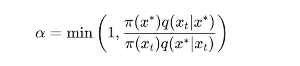
Accept ��∗ with probability ��; otherwise, retain ����.

-Iterate: Repeat the proposal and acceptance steps to generate a sequence of samples.

-General and flexible, can be used for a wide range of distributions.

-May have slow convergence and require tuning of the proposal distribution.

Markov Chain Monte Carlo (MCMC)

Gibbs Sampling

Gibbs sampling is a special case of the Metropolis-Hastings algorithm where each variable is sampled from its conditional distribution given the current values of the other variables.

Algorithm:

Initialize: Start with initial values for all variables.

Iterate: Sequentially sample each variable from its conditional distribution:

✓Simple to implement and efficient for models with known conditional distributions.

✓Not suitable for distributions with complex conditional dependencies.

Markov Chain Monte Carlo (MCMC)

Steps in MCMC Simulation

1. Initialize the Markov Chain: Start with an initial value for the parameter(s).

2. Proposal Step: Propose a new value for the parameter(s) based on a proposal distribution.

3. Acceptance Step: Accept or reject the proposed value based on the acceptance probability.

4. Iterate: Repeat the proposal and acceptance steps to generate a sequence of samples.

Markov Chain Monte Carlo (MCMC)

Example- Bayesian Inference

MCMC methods are widely used in Bayesian inference to estimate the posterior distribution of parameters. For example, in estimating the mean and variance of a normal distribution, MCMC allows for the incorporation of prior knowledge and the computation of credible intervals.

1. Normal Distribution Example:

Markov Chain Monte Carlo (MCMC)

Genetics

In genetics, MCMC methods are used to infer population structures and genetic parameters. Bayesian approaches allow for the incorporation of prior biological knowledge and the estimation of complex models.

Physics

In physics, MCMC methods are used to simulate systems in statistical mechanics where exact solutions are intractable. For example, MCMC can be used to study the behavior of particles in a thermodynamic system.