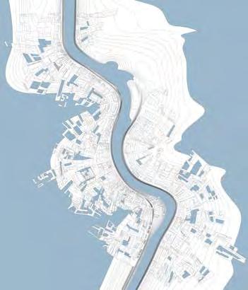
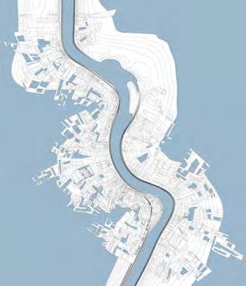
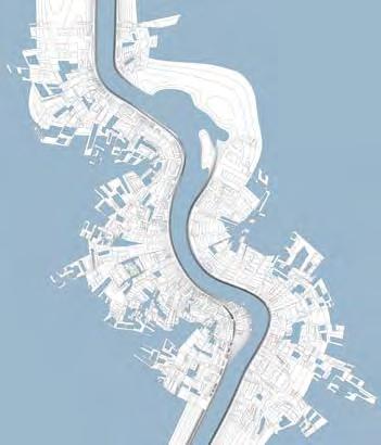
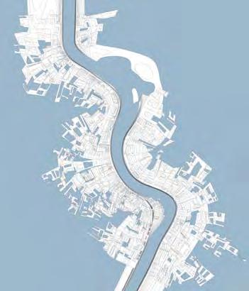
Hydroville
Adaptive Living System in Southeast Asian Riverside
MArch
Emergent Technologies and Design
Qianqian Yu,Yu Chen
Tutors:
Mike Weinstock
George Jeronimidis
Christina Doumpioti
Toni Kotnik
Evan L Greenberg
ARCHITECTURAL ASSOCIATION | SCHOOL OF ARCHITECTURE | GRADUATE SCHOOL PROGRAMMES
COVERSHEET FOR PROGRAMME: Emergent Technologies and Design TERM: 2009-2011
STUDENT NAME: Qianqian Yu, Yu Chen
THESIS TITLE: Hydroville (Adaptive Living System in Southeast Asian Riverside)
SUBMISSION DATE: 14-Feb-2011
DECLARATION:
“I certify that this piece of work is entirely my/our own and that any quotation or paraphrase from the published or unpublished work of others is duly acknowledged.”
SIGNATURE OF STUDENT:
Ackownledgement
I would like acknowledge my supervisor Michael Weinstock for his encouragement and guidance from the initial to the final level of this project. This dissertation would not have been possible without his constant support.
I also thank Professor George Jeronimides for professional technical guidance and advices helping through the whole design process.
It is also my pleasure to thank all the EmTech staff and students for their selfless help and accompany. I really value the friendship with them.
Lastly, I offer my regards and blessing to my family. Their unconditional love and trust are always the best comfort in every difficult time.
Content
Abstract
Chapter 1. The Domain
Chapter 2. Methods
Chapter 3. Research Development
Chapter 4. Design Development
Chapter 5. The Design Proposal
Chapter 6. Evaluations and Revisions/Future develo54pment
Bibliography
Appendices
— 1 —
— 2 —
Abstract
This dissertation aims to investigate an adaptive living system which can transform to adapt to the changing water level in order to offer a stable living area in periodically flooding region. It works mainly as an infrastructure in rural area which accommodates various program requirements and provides with connections.
Periodical flooding is disaster to many river basin areas. The situations are even worse in less developed countries, like countries in Southeast Asian. Some of them are rich in natural source, but flooding brings a lot constrains to their development. The lack of an appropriate infrastructure and adaptive canopies for the residents which can response to the extreme environmental changes in these areas becomes an important issue.
Based on hydrological analysis and climatic analysis, a adaptive urban intervention is proposed integrating material, form, programs and water drainage system. Its adaptability relies on hydrodynamic change, and being a network of component-based system, local arrangements effect on the global organizaion. Variation potential of higher level is investigated when combine the system with context condition and various requirements.
— 3 —
— 4 —
Chapter 1. The Domain
1.0 Introduction
1.1 Flood
1.1.1 The cause of flooding
1.1.2 Types of floods and floods effects
1.1.3 The formation of flood plain
1.2 Site background:Tonle Sap Lake, Mekong river basin
1.2.1 Geomorphologic characters and climate
1.2.2 Local residents’ lifestyle
1.2.3 Current transportation and infrastructures
1.2.4 Stilt houses + Boats
1.2.5 Seasonal variation of occupations
1.3 Case study
1.3.1 Polders in Netherlands
1.3.2 Water network in Venice
1.3.3 Artificial water system in Angkor Wat
1.4 Primary problems to be solved
— 5 —
— 6 —
1.0 Introduction
The civilization of human being is inseparable from aqua system. Natural water body provides us plentiful resources whereas sometimes brings us disasters. In thousands years, a large numbers of projects like dams, bridges, polders, have been done to help us survive. However, as time passing by, more and more ecological problems caused by those huge projects emerge to light, and the high-cost and maintenance is unaffordable for many developing countries. These drawbacks push us to think of another way: Can we passively adapt to the changing environments without building massive projects?
A Cambodian floating village located on Tonle Sap Lake(Mekong river basin) is suffering tropical monsoon annually, and the villagers live in stilt house or boathouse to adapt to the changing water level. In wet season they live on fishing and rice cultivation; in dry season, the original hydro culture makes this village a tourist attraction spot. As a result, their live hood varies according to the periodic season change.
This project aims to solve the conflicts between human beings and their environment which may emerge in the civilization progress, in an integrated way. The strategy we proposed is based on the
combination of simplest components but can perform intelligently to meet varies requirements and adapt to dramatically changing environment to keep a stable living condition for the local residents. It is an urbanism project but the architectural issues we involved in range widely. From architectural scale to urban scale, we investigated different aspects of architecture and urban design when implementing the design strategy. Among the approaches we employed, genetic algorithm is very crucial in generating variations from the same primitive and simple rules to accommodate different living and climatic requirements. And it provided us with plenty of resources for the further implementation.
The final result as a hydrological village in Southeast Asia is an integration of residential blocks, agricultural facilities, public facilities, water defences, water storages and water drainage systems. Its relationship with water can be compared to the permeation of cell membrane as it is defending, storing and retaining water from natural all the time to balance between human’s requirements and environmental capacity.
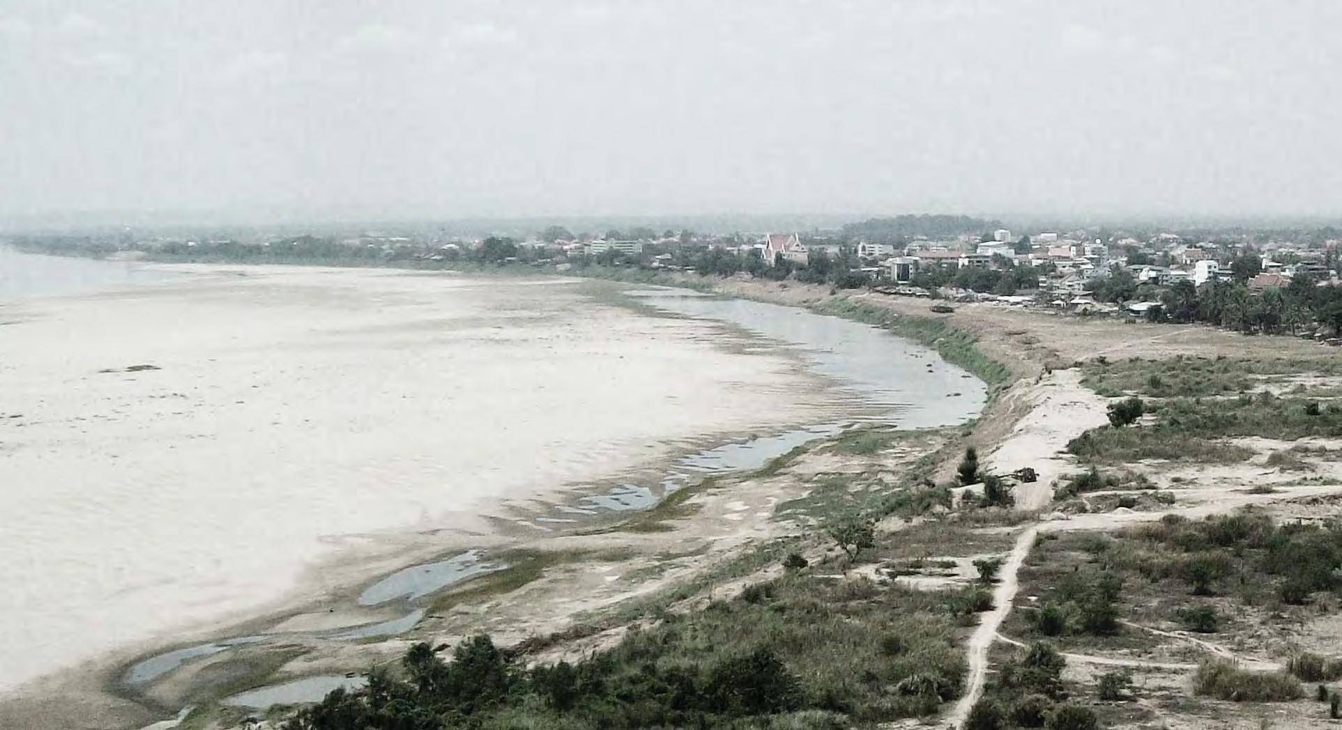
Figure01 The broad flood plain of Mekong river. [Online] Available at http://max-walsh.com/?p=411 [Accessed August 11, 2010].
— 7 —
— 8 —
1.1 Flood
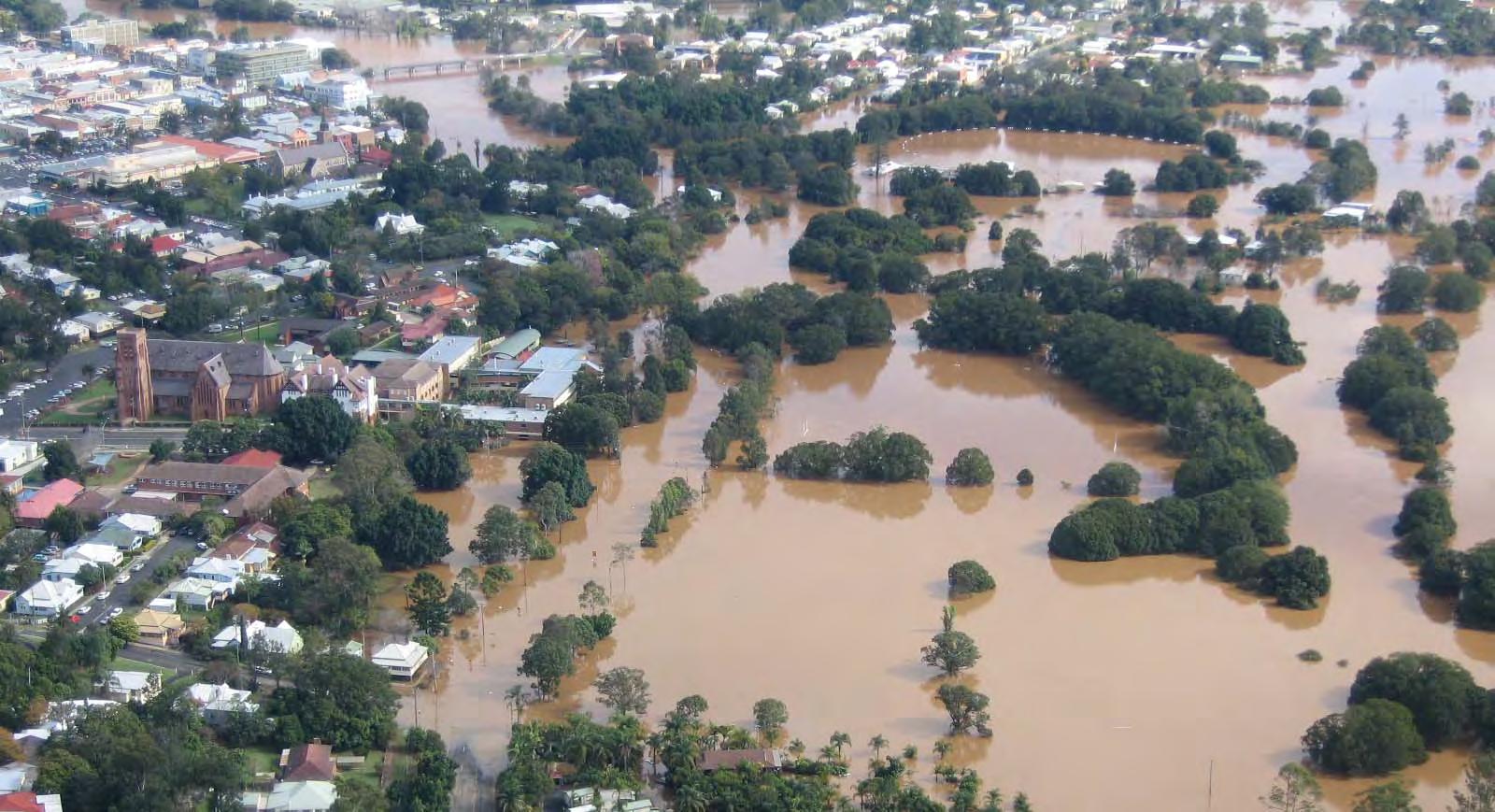
Figure02 Aerial view of the flooded Wilsons River in Lismore, Scotland. [Online] Available at http://www.ses.nsw.gov.au/ multiattachments/9882.html [Accessed September 06, 2010].
1.1 Flood
1.1.1 The cause of flooding
Flooding is a natural process related to changes in weather including high rates of rain falling and high ocean tide. Flooding happens when too much water presents during a short period of time. Excess discharge of water gathering in a river induce the water to move quickly first and then move out onto the surrounding area and a flooding is formed. Flooding can also be caused by man –made factors. People’s building activities near rivers at times contribute to the disaster of river flooding. As more and more sand and porous materials are replaced by man-made building materials, the absorption ability of ground is lowered thereby the probability of flooding is increased. Seasonal flooding is mainly caused by seasonal weather conditions. Large amount of rain falling and heavy winter snows melted by unexpected heat wave can cause river to overflow and induce floods.
— 9 —
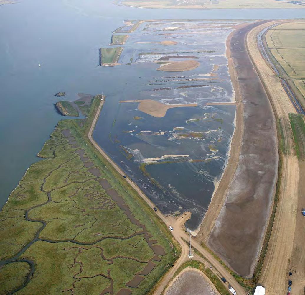
Figure03 Coastal flood: Aerial view of the flooded Wallasea Island in Essex, England. [Online] Available at http://www. geography.org.uk/resources/flooding/wallaseaisland [Accessed September 05, 2010].
1.1 Flood
1.1.2 Types of floods and floods effects
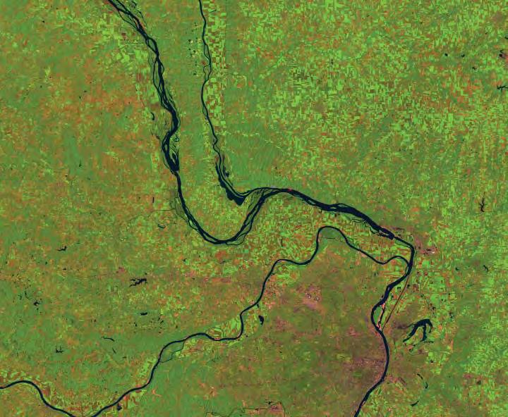
Principle types of flood according to the geographic environments it occurs can be sort into riverine flood, estuarine flood, coastal flood, catastrophic flood and muddy flood. Floods may damage structure, drown people and livestock and spread disease. On the other hand, floods also bring benefits. Floods can afford hydrological energy source, fertilize soil, recharge ground water, etc. Periodic flooding is very essential for people’s well-being in river valley.
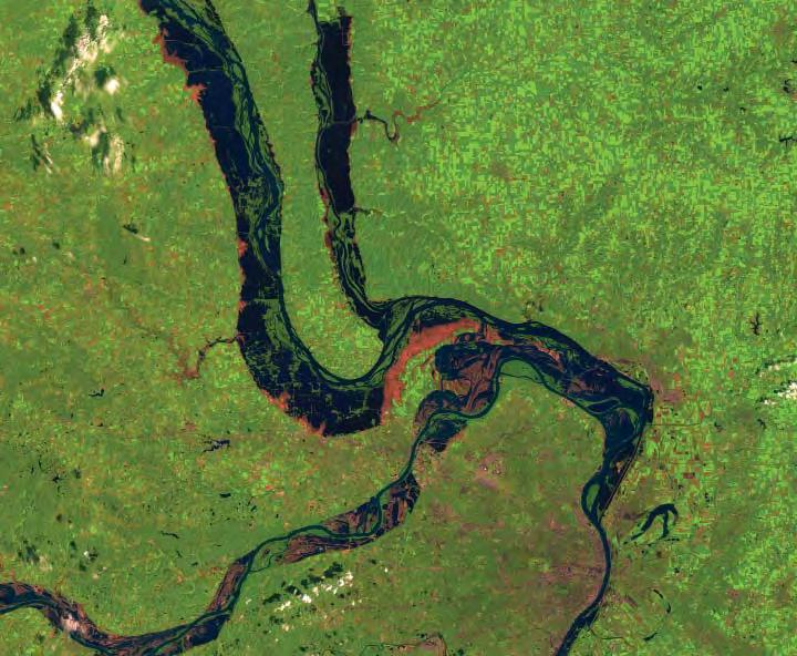
Figure04 Riverine flood:Great Flood of the Mississippi River,USA. Upper:August 14,1991.Lower:August 19,1993.[Online] Available at http://earthobservatory.nasa.gov/IOTD/view. php?id=5422 [Accessed September 01, 2010].
— 10 —
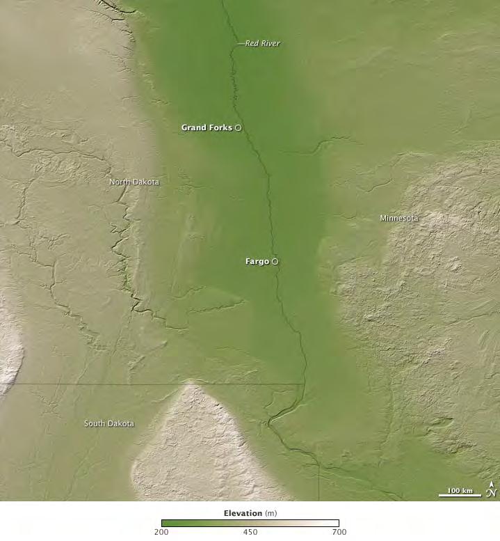
Figure05 The red river flood plain,USA. [Online] Available at http://earthobservatory.nasa.gov/IOTD/view. php?id=37779[Accessed September 06, 2010].
1.1 Flood
1.1.3 The formation of flood plain
Flood plain is formed during a long period of time. When river floods and erodes its bank, large amount of sand, gravel, loam and clay are left behind and create the floor of flood plain. As the sediments accumulate, wide, flat, low-lying area of flood plain is found on sides of the river channel as a result of deposition. Because of the accessibility to fresh water, fertilized farming land and cheap water transportation, many towns are built on flood plain in history.
— 11 —
1.2 Site background:Tonle Sap Lake, Mekong river basin
— 12 —
CambodiaMekongriver
TonlesapLake
SiemReap
TonleSap Lake
Dryseasonarea Wetseasonarea
TonleSapRiver
The Mekong River, which runs through the centre of Cambodia, forms the country’s grand central floodplain of an area of nearly 800,000 km2, is the most important river in Southeast Asia. Along this 4500 km long river, there are many wetlands and lakes; one of them is the Cambodia’s Grand Lake - Tonle Sap, which is also the largest natural freshwater lake in entire Southeast Asia. Due to the influence of monsoon climate, the environmental conditions in Tonle Sap lake region vary annually. Wet season in that area is from May to October, while dry season is from November to April the next year. The maximum flooding area in dry season is 2,500 km2 and this figure increase to 15,000 km2 in wet season. The annual water level fluctuation is around 8 meters, waving between 1m and 9m. This significant change in water depth has two folds: In the dry season, low water makes the river bed sediments expose to the surface, which become the great source of nutrition for the early rice. In the wet
PhnomPenh
Figure06 Tonle sap floodplain. [Online] Available at http:// www1.american.edu/ted/ice/mekong-china.htm[Accessed July 2, 2010].
1.2 Site background:
Tonle Sap Lake, Mekong river basin
1.2.1 Geomorphologic characters and climate
season, large quantity of the microbes and organisms are consolidated at the river bed vegetations, which provides the ideal feed for fisheries. This periodical system combines with great bio-diversity and the river’s extremely rich annual sedimentation, resulted in one of most productive fresh water ecosystems in the world.
KampongChhnang
PrekKdam
KampongThom
Thailand
Vietnam
Sisophon
Battambang
MoungRoessei
Pursat
KampongLuong
— 13 —
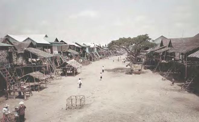
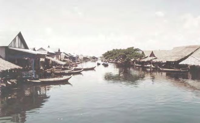
Figure14 Phnom Penh climate,Cambodia. [Online] Available at http://www.adventurebimbling.com/cambodia/cambodia_weather.html [Accessed July 29, 2010].
Figure07,08 Kompong Phluk’s main street in the dry season and the wet season,Cambodia. Left : dry se ason. Right : wet season. From Patrick T. Evans,Melissa Marschke,Kiran Paudyal Flood forest,fish and fishing village,Tonle Sap,Cambodia [2004] .
Jan Max Dry seasonWet seasonDry season Min 0 5 10 15 20 25 30 35 40 FebMarAprMayJunJulAugSepOctNovDec
Rainfall(cm)
x n — 14 —
Temperate( oC)
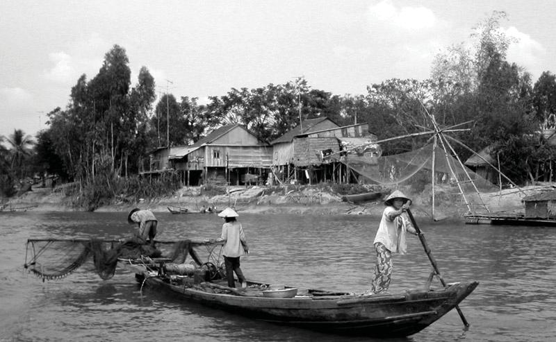
at http://www.heybrian.com/travels/vietnam/mekong_delta.
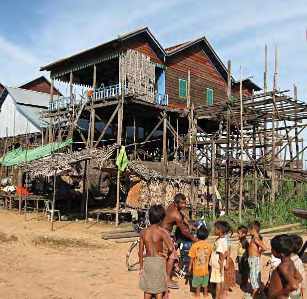
A fishing village by Tonle Sap in dry season. [Online] Available at http://ajt.iki.fi/blog/main/2007/05/28/a_fishing_village_by_tonle_sap [Accessed July 29, 2010].
The lake region is therefore a key area for the country’s agriculture production and a major base for its fishing industry, playing an important part in regional economy. Tonle Sap’s annual fish production is estimated between around 180,00–250,000 tones, which alongside with its rice cultivation, supporting the livelihood of more than 3 million people either directly or indirectly in the region. Due to this seasonal change in water level, local residents around the lake also adapted their lifestyle by living in the stilt house, or boathouse which according to the water levels, can be easily moved by road truck or towed by a boat to a new location. The villagers’ livelihoods are typical tropical. Rice cultivation, fishing takes the biggest proportion, others professions like orchard growth, firewood collection and hand crafting are mainly are mainly for women and children. Most of the houses are temporary boat houses or stilt house. People have to rebuild or reinforce their houses as poor housing quality is a very big potential safety hazard, and the
1.2 Site background: Tonle Sap Lake, Mekong river basin
1.2.2 Local residents’ lifestyle
frequent rainstorm in wet season could damage parts of the houses. However, relatively low building skill and lack of proper material makes it impossible to build permanently safe dwellings. Currently there are two public and marketing places which are not far away from each other. In idle time, people prefer to get together in these two places relax, so most social activities and trading or good exchanging happen here.
Figure09 Fishman of Mekong delta river. [Online] Available
php [Accessed July 29, 2010].
Figure10
— 15 —
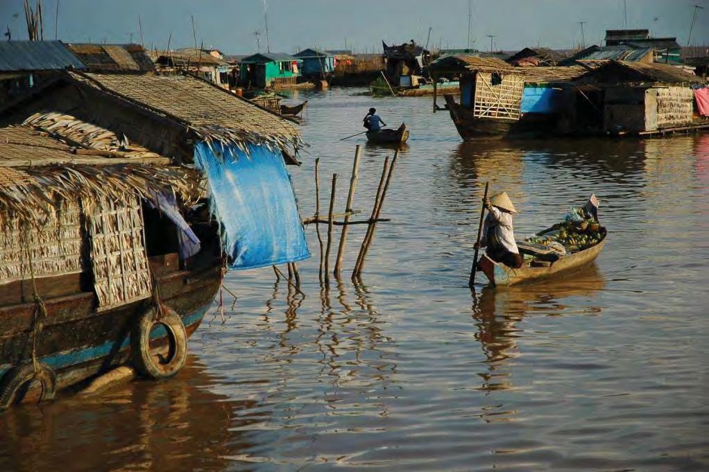
Figure11 Floatingvillage by TonleSap lake. [Online] Available at http://www.prweb.com/releases/cambodia/tours/ prweb2841044.htm[Accessed July 29, 2010].
1.2 Site background: Tonle Sap Lake, Mekong river basin
1.2.3
Current transportation and infrastructures
In the urban scale, the village is half kilometer away from the far end of national high way 53, and the whole area is connected to Angkor Wat in Siem Reap, by the round lake high way 5. Meantime, the developed shipping system makes it possible to travel across the Tonle Sap Lake.
Regionally, it is convenient enough to attract tourists from other hot spots. But inside the village, because of the tropical monsoon climate, water surface occupied most area of the village in wet season; even in dry season, the muddy lake bottom is too soft to walk on. As a result, boat is the only available transportation since the ancient times and the tradition of living in the boathouse is still the most important feature of local’s life. Accordingly, ferries are the most infrastructures for the village as they are the transportation hubs which connect waterway and motorway.
Product trading mainly occurs on boats. The main markets or public spaces are always in the same place due to residents’ habits, but some retails could be anywhere.
— 16 —
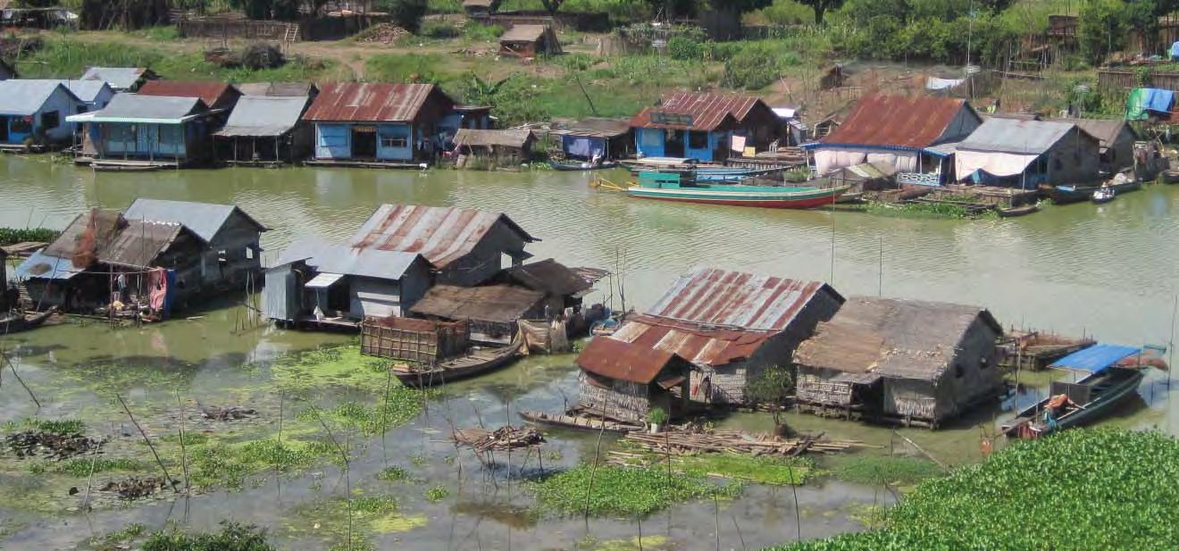
Stilt houses in flood prone rural area are houses raised by sticks to high level. They are very common in Southeast Asia. Stilt house is one of the most important strategies in dealing with the threat of flood in Mekong river catchment area. In Cambodia, stilt houses are generally made of bamboo and thatch by the reason of these materials are very cheap and quite common in this region. Besides this advantage, stilt house is also one of the environmental friendly building types since it causes little negative influence to the surroundings and has adaptability to the environment. In the rainy season, the stilt house villages are always divided into separated parts by annual flood. Boats become the essential transportation way widely existing in the Tonle Sap region.
Stilt houses and water transportation by boats compose a crucial system to adapt to the flood.
On the other hand, stilt houses have some limitations. In the Tonle Sap Lake catchment area, the maximal water level difference between dry season and wet season can reach to 8 M. Thus many
1.3 Site background: Tonle Sap Lake, Mekong river basin
1.3.4
houses here need much higher stilts than other areas. It really causes inconvenience to people, especially for old people and children in dry season. Moreover, stilt house is a quite suitable building type in rural areas in terms of costs because it can be built by any skilled craftsperson without engineer plan. Therefore in another way, we can think that it has some risk to use as public spaces which have a great quantity of people flows.
Stilt houses + Boats
Figure12 Floating village by Tonle Sap Lake . [Online] Available at http://juliannestravels.wordpress.com/ [Accessed July 06, 2010].
— 17 —
Service (Tourism)
Job transition
describing the seasonal variation of occupations.
1.3 Site background: Tonle Sap Lake, Mekong river basin
1.3.5 Seasonal variation of occupations
The local residents and facilities are both impacted in many ways by the periodical changes due to monsoon seasons. In the dry season, the fishing production reduces dramatically, therefore less need for locals on fishing activity. However, the tourists boost in the same period, the local workforce will transfer from fisher man into service workers to meet the increasing tourists demand. However, the lack of local tourists facility increase to match the demand remains the problem.
In wet season, the opposite effect occurs. Increasing fish production and rapidly reducing number of tourists let the locals to re-join the fishing workforce. Again, the facilities are more difficult to match the changing demand as the lacking of fish farm, transportation and infrastructure still pose a greater challenge.
Dry season Fish
Tourist
Figure13 Diagram
breeding
Fishman
Wet season
— 18 —
1.3 Case study
— 19 —
— 20 —
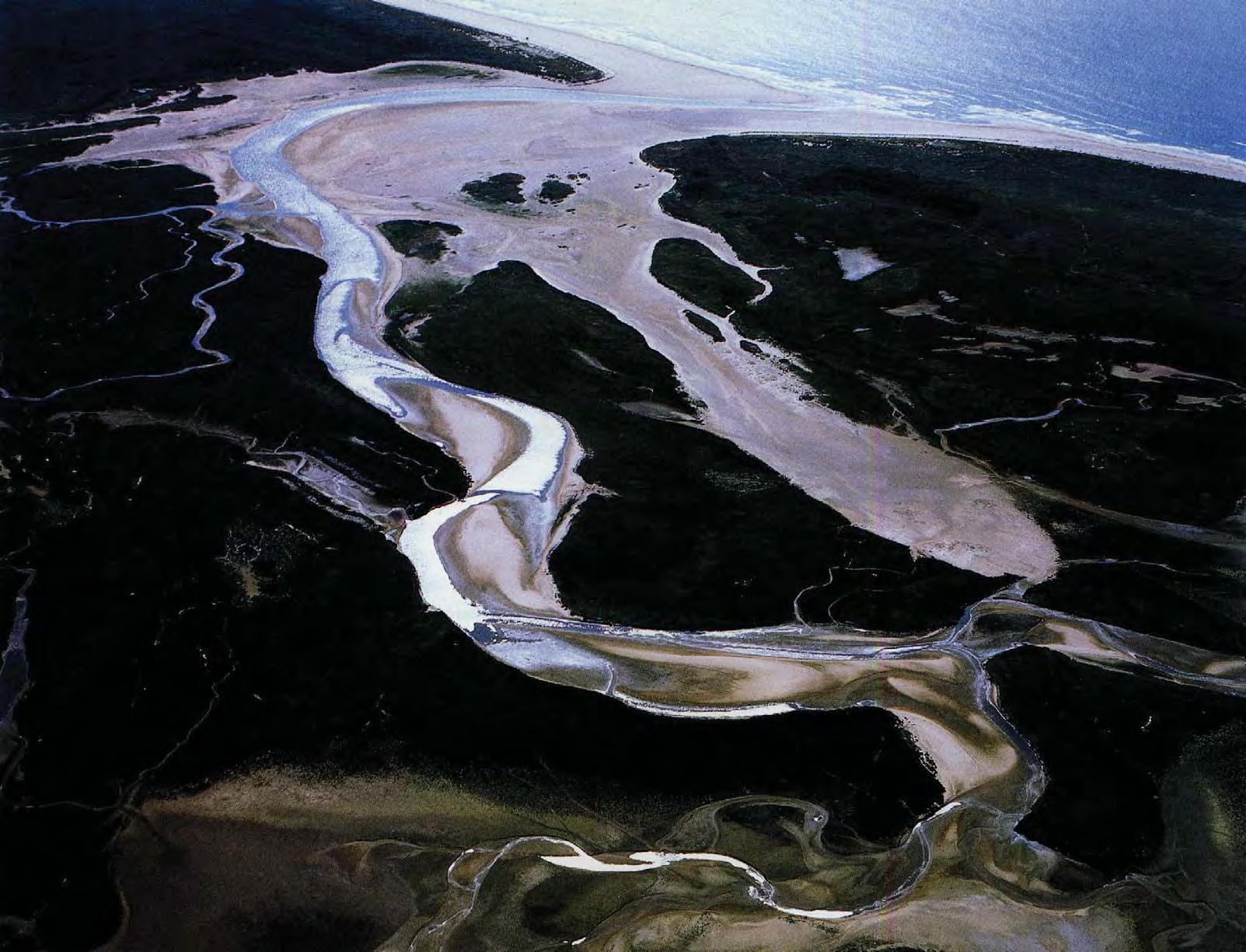
Figure14 De slufter,Texel. Wouter R., Clemens S. and Diderik A., Sea of Land, The polder as an experimental atlas of Dutch landscape architecture, TU Delft, 05/2007.

A polder is an area of land originally lies below the sea level. By pumping the area dry and keep water outside with the aid of enclosed dikes, the land is transformed from swampy wetland to tillable agricultural land and even habitable towns. A polder usually relies on autonomous artificial water management system for farming and settlement.
Being a graphically low-lying country, the Netherlands has constructed more than 3,000 polders for surviving in a water surrounding environment. Now the Netherlands has been famous for its beautiful urban patterns formed by numerous polders together with the implicit architectonic feature of landscape. Although the polder in Netherlands provides many benefits to agricultural industry, housing consumption and social economy, it is facing some pressing problems. The reclamation of natural landscape somehow encroach the habitat wetland of birds, there by seriously violate the local eco-system.
Considering the advantages and disadvantages of previous polder mode and the modernization of water tectonics, polder design nowadays is closely related to urban spatial planning. How to embed the polder artifact-an artificial architectonic system into natural landscape system has become the primary issue of urban design in many water metropolitans. The traditional way of design has been transformed to a water-oriented strategy which would take into consider of ;every climate factors and environment require-


Figure15 The emergence of polders in the Netherlands by building dikes along rivers. [Online] Available at http://www. oasen.nl/drinkwater/schoondrinkwater/Pages/Laatste10000jaar.aspx[Accessed August 16, 2010].
1.3 Case study
1.3.1 Polders in Netherlands
ments as well as the watery tradition in the locality.
Geomorphology of the polders
The contours of Holland’s landscape are formed by a repeat process of balancing between the rivers of the delta and the sea. The hydraulic system of dikes and dams create the framework of polder landscape. However, because of the varied geomorphological conditions, the morphologies of polders are different. Basically, a polder’s shape reflects the development of the delta landscape.
For example, in the Zijpe river basin, the stream and sheet forms of polder are most common. While in the North Holland lagoon and Haarlemmermeer, wind forms are dominant following the natural shape of local lake. The Vecht region is dominated by the round or oval forms of polders. And some IJ polder forms are resulted from dike breaks.
Generally speaking, the basic forms of polders reflect the interplay of natural forces. The forms also to some extend present the interrelations between the polders and the land surrounding it.
Floodplainriver Bog Polder
Floodplainriver
Peatmoor
— 21 —
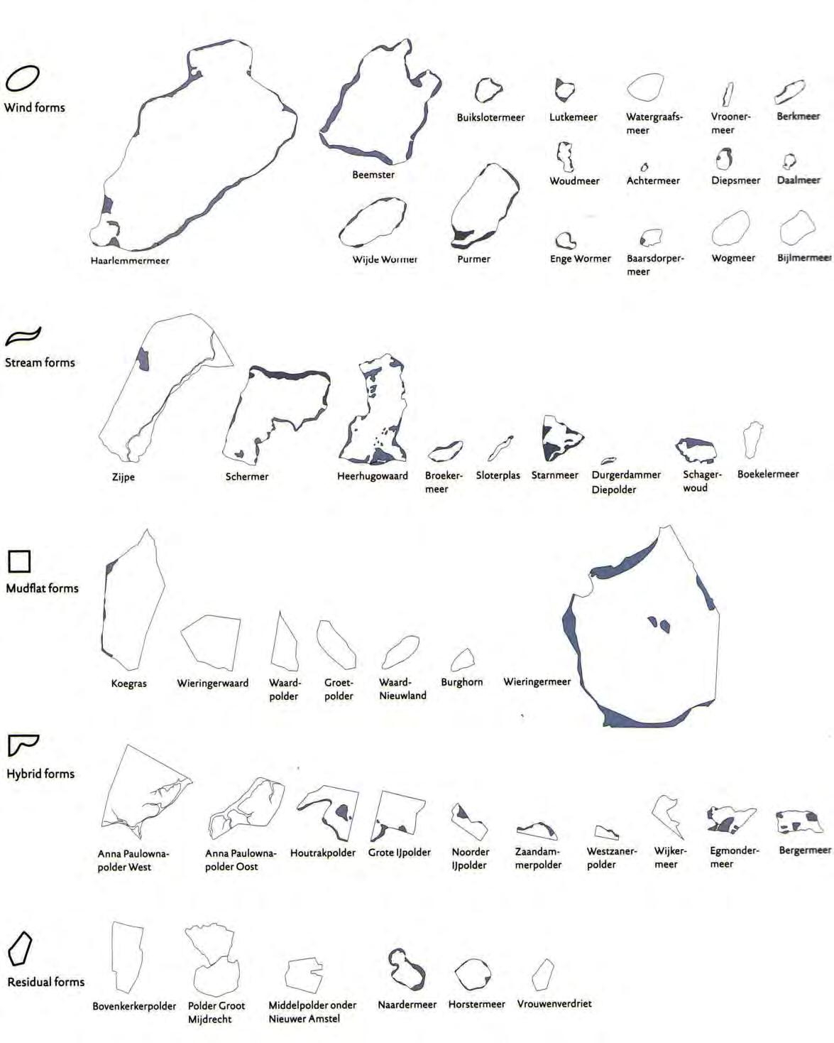 Figure16
— 22 —
Comparison of the polder grammar of the reclamations investigated, Wouter R., Clemens S. and Diderik A., Sea of Land, The polder as an experimental atlas of Dutch landscape architecture, TU Delft, 05/2007.
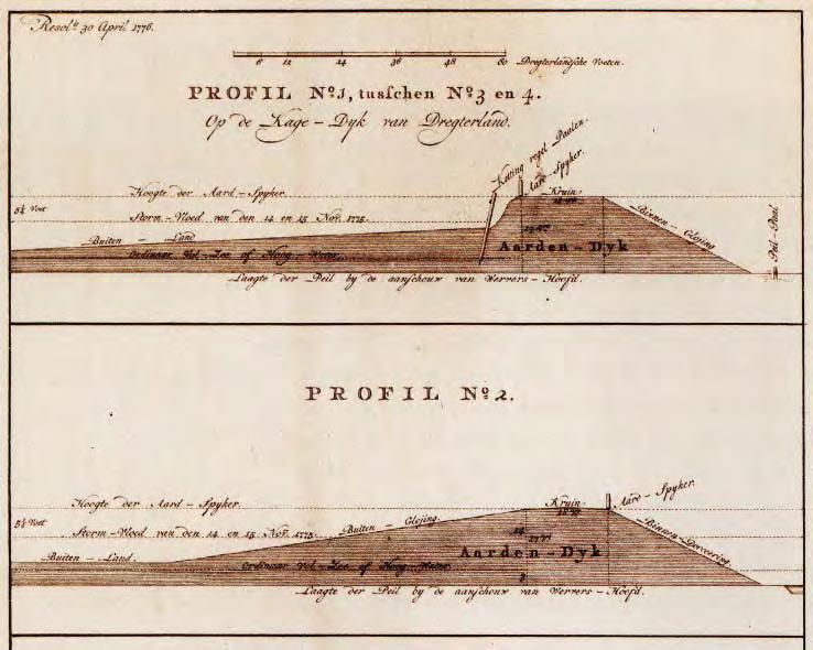
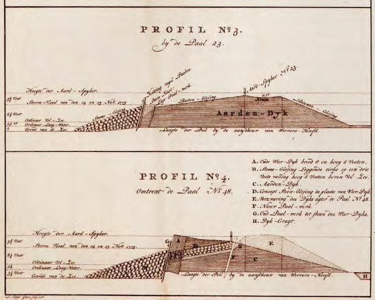
Figure18 Diagram describing the composition of polder. [Online] Available at http://web. me.com/schuffelen/Site/duoutdoors.html [Accessed August 16, 2010]
Polder Mill Dike Ditch Channel
— 23 —
Figure17 Polder technology. Wouter R., Clemens S. and Diderik A., Sea of Land, The polder as an experimental atlas of Dutch landscape architecture, TU Delft, 05/2007.

http://www.estrafalarius.com/2008/01/21/la-ciudad-en-el-mar/

Adriatic Tides
Venice city is not directly connected to the Ocean but surrounded by the Venetian Lagoon. Actually the Adriatic tide controls the water level of the Venetian lagoon and in turn leads influence to water level of the canal system in Venice indirectly. Thus the water level of canals fluctuates with tide-period of Adriatic tide. To be precise, there are three major factors which affect the Venice’s water level: astronomical effect, meteorological effect and morphological Effect.
Astronomical effect
The water level of the canal is influenced by the tides of Venetian Lagoon. And the essential factors of tides are the movements of sun and moon. The Moon’s gravitational force is main cause of tides. The lunar circle is about 29 days long and divided into four phases: full moon, new moon, half waning moon and half waxing moon. The moon in the phase’s full moon and new moon causes more gravitational effect than in other two phases. According to the moon’s circle, we can predict fluctuation in tidal height. The sun also affects the tides. However the distance between the sun and the earth is larger than the distance between the moon and the earth. Therefore compare to moon, it has less effect. Furthermore, the period of sun’s effect is one day.
Meteorological effect
Wind can also affect the fluctuation of tides. There are two major airflow called Bora and Sirocco which influence mainly the tides of Venice. If they blow against the tides, the water will enter the Venice slowly. On the contrary, the velocity of water will be very faster. In addition to this, barometric pressure can lead a small effect to the height of tides.
Morphological effect of canals
The morphology of canal system is another significant factor which affects the water flow through the Venice city. There are 182 inner canals in Venice. The canals distribute over Venice as a network. Since a canal is always intersected by one or more other canals, it is impossible to study hydrodynamic data of one canal individually. The whole canal network is a emergent from these single canals, it generates more potential and more complexity than the simple addition of individual canals.
Transportation network and sewage removal system
The Venice’s canal system constitutes the main transportation network. It is a essential part of daily life in Venice. The canals serve as sewage removal system for the city as well.
1.3.2 Water network in Venice 1.3 Case study
Figure19 (Left) The city by the sea. [Online] Available at
[Accessed October 16, 2010].
— 24 —
Figure20 (Right)Venice city. Guy N., Cathrine S. and Adam Y., On the water: palisade bay, Germany: Hatje Cantz, 2010.
Growth of branches


The formation of urban grid
There is a canal running through the Venice city and dividing it into two parts. Branch channels grow perpendicularly from the canal and make up the waterway system of the whole city. After that, land street networks are built based on the water way grid. The transportation way in Venice is the combination of land transportation and water transportation.
Main canal
Water body
River system
Road network
Figure21 Diagram describing the formation of urban grid in Venice city based on the water system.
— 25 —
1.3 Case study
Artificial water system in Angkor Wat
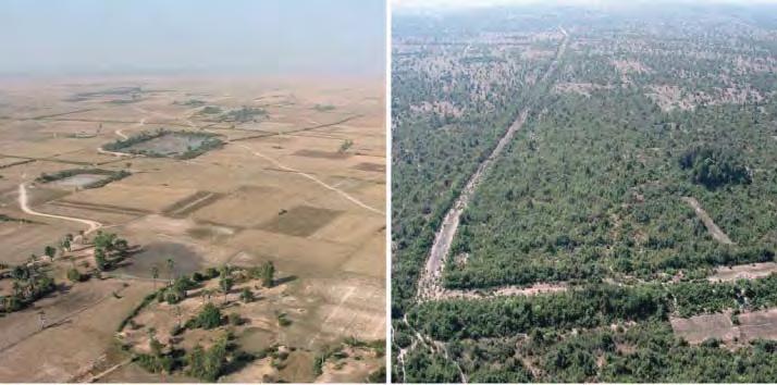
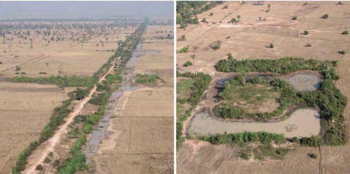
Angkor Wat locates in Tonle Sap lakeside in Southeast Asia and is dominated by monsoon climate. There are two extreme seasons in a year – the dry season and wet season. To deal with the enormous changes in water supply, the residents use reservoir and canal to store water in wet season and supply domestic water use in dry season.
Develping Process
The nature and even the existence of water management at Angkor has been the subject of considerable debate since the 1970s. Recent work at and the Greater Angkor Project has mapped a vast water management network extending across approximately 1000 sq km.
From the new map an outline can be provide of the development of the network between the 8th-9th and the 14th centuries. Each large extension of the network tapped water from a succession of natural rivers flowing from NE to SW. Each river was further north and was tapped further to the west. The network had five major components - E-W embankments that trapped water flowing from the north and northeast; N-S channels that eventually delivered water to large reservoirs (baray); the baray and the large temple moats; embankments and channels oriented from NW to SE that could distribute water back from west to east across the slope of the land; and channels oriented towards the southwest which could dispose of water rapidly to the lake, the Tonle Sap.
Significantly the later major channels, such as the Angkor Wat canal and the canal that predated the current Siem Reap river, were drains that served to dispose of water into the lake.
Water Management in Peak Time
The success of hydraulic system in Angkor city was due to the following reasons:
1. Optimal location. The situation of Angkor is optimal from a hydrological point of view. The Tonle Sap Lake was very close to the city but still it was safe from its floods. The lake offered an excellent source of nourishment and potential for transportation. The floodplain was also very fertile for growing rice.
2. Artificial channels and reservoirs. The very gentle slope of the plain created an excellent terrain for managing the water with artificial channels and reservoirs. The Khmers were exceptionally good
at managing the water and moving it from one place to another. The channel network was built with care and spread over a 1000 km2 area some of the channels and reservoirs. West Baray, thought the water is not flowing to the Baray its original route, are still in use today.
Current Water Body
The demise of the whole system are mainly accepted concluded into two:
1. Sedimentation and erosion. Even though the Khmers were excellent water engineers, they could not avoid normal problems relating to erosion and sedimentation. In Barays and some channels, sedimentation was a major problem. Over time, the settled sediments decreased the capacity of the channels and barays and made the supplying water to the city more difficult.
2. Climate change. The possible climate changes may have affected a lot to the Angkor area. Climate played a role in the emergence of Angkor. The possible changes in temperature, precipitation and evaporation may have affected to the local hydrology in many ways. Too much water may cause floods in the city area. On the other hand, continuous droughts would cause even more severe damage to the city’s operation.
Regional Medieval Climate Variability
Decades of weakened summer monsoon rainfall, punctuated by abrupt and extreme wet episodes that likely brought severe flooding that damaged flood-control infrastructure, must now be considered an additional, important, and significant stressor occurring during a period of decline. Interrelated infrastructural, economic, and geopolitical stresses had made Angkor vulnerable to climate change and limited its capacity to adapt to changing circumstances. Much like the Classic Maya cities in Mesoamerica in the period of their ninth century “collapse” and the implicated climate crisis, Angkor declined from a level of high complexity and regional hegemony after the droughts of the fourteenth and early fifteenth centuries. The temple of Angkor Wat itself, however, survived as a Buddhist monastery to the present day
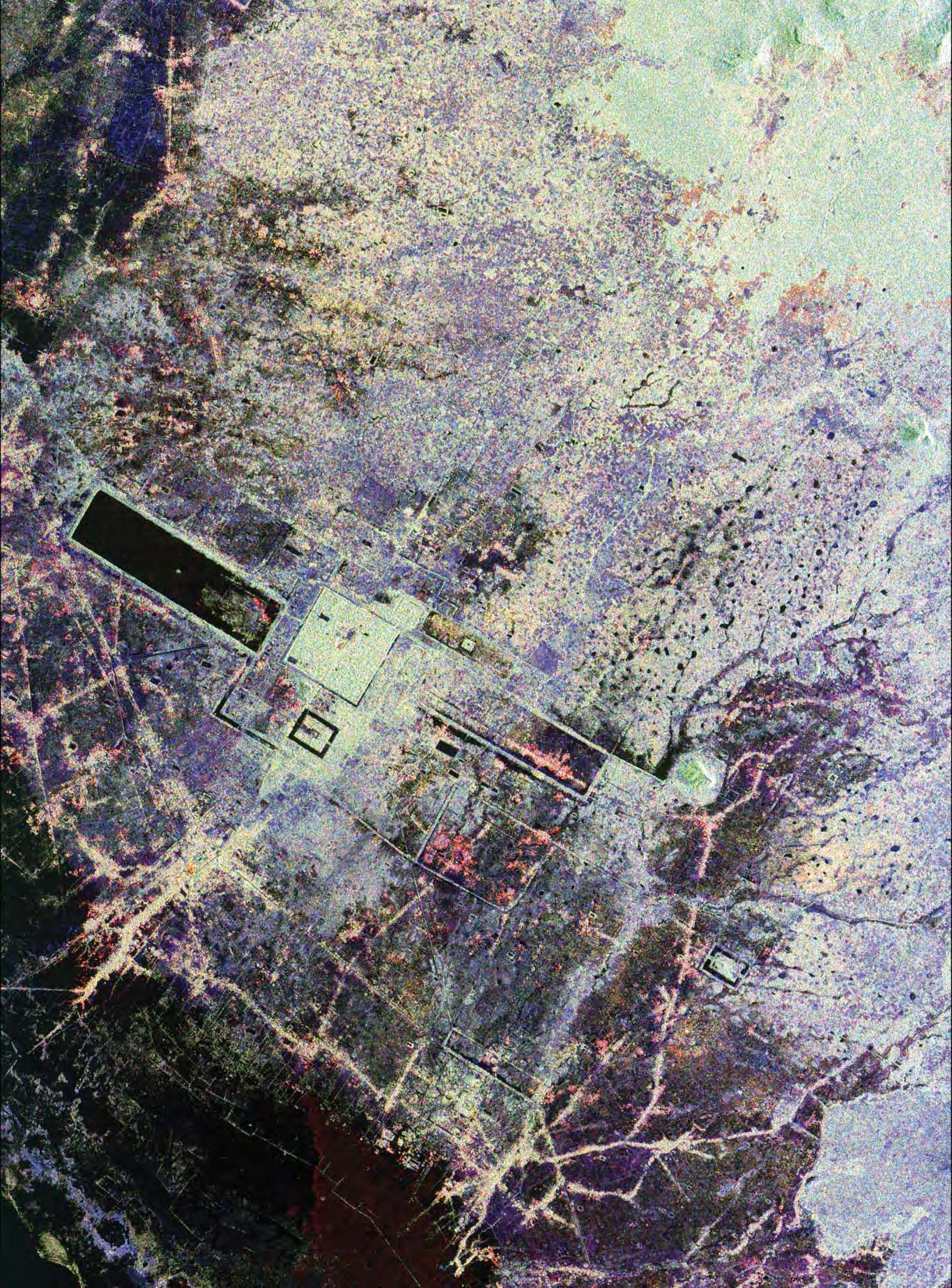
The blue areas in the page 28 and page 29 show the water distribution in two seasons.
1.3.3
— 26 —
Figure22-25 Oblique aerial views of remnant Angkorian urban features. (First) Occupation mounds and ponds. (Second) Canals and embankments.(Third) Multifunction roadway/canals. (Fourth) Classic ‘‘village temple’’ configuration. Damian E., Christophe P., Roland F., Scott H., Ian T., Anthony M. and Michael B., A comprehensive archaeological map of the world’s largest preindustrial settlement complex at Angkor, Cambodia, Yale University, 29/06/2007.
Figure26 Angkor, Cambodia. [Online] Available at http:// visibleearth.nasa.gov/view_rec.php?id=596[Accessed October 19, 2010].
— 27 —
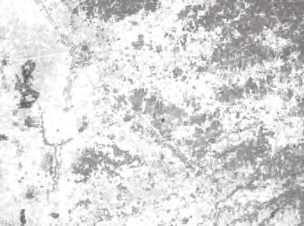
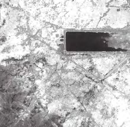

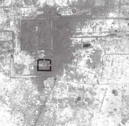
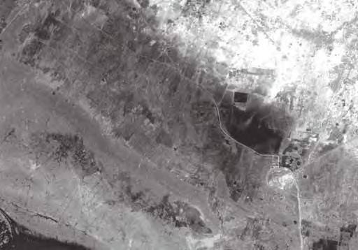
Figure27 The water distribution of Angkor city in wet season. [Online] Available at http://earthobservatory.nasa.gov/ IOTD/view.php?id=4995[Accessed August 16, 2010].


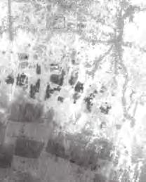
— 28 —
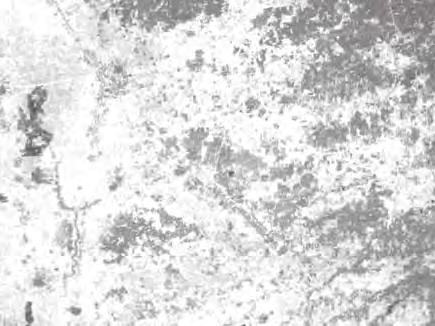


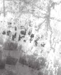
Figure28 The water distribution of Angkor city in dry season. [Online] Available at http://earthobservatory.nasa.gov/IOTD/ view.php?id=4995[Accessed August 16, 2010].
— 29 —
— 30 —
From the mentioned previously, there exist many problems in the current status at Tonle Sap region.
First, local residents’ occupations alternate with the rise and decline of tourism which is radically determined by the amount of precipitation seasonally. They urgently need an improved infrastructure which can provide various living and working facilities under the influence of the changing environmental conditions.
Second, the current facilities and infrastructures have evolved since hundreds of years ago. They have many advantages on the basis of ancient productive levels. However, comparing the distinct diversity of seasonal geomorphologic characters, the existent infrastructure lack adaptive ability to fit the external change. This situation freezes rural areas’ development and reduces floating villages’s activity.
Third, river basin in Cambodia is rich in biological species and ideal for fishing and rice farming, but the economy development in Tonle Sap region is still slow and living conditions are very poor. This inconsistency is to a great extend due to the detachment of different community units. Flooding provides the region with fertilized soil and a productive wetland ecosystem as well as brings many disadvantages. Excessive water submerges farmland and transport system. The isolated fragments of a valley make social communication and economic transaction severely decreased. The problem becomes even more serious in rainy season. People have to rely entirely on water transportations in flooding time. Although many measures have been taken ever since a long time ago, like floating markets, floating rice, river navigation and stilt houses for residing, they are far from enough.
What could be learned from the existing intergrowth modes between water and human civilization?
Polder mode in Netherlands By building polders, the Dutch positively alternates its coastline. The polder has close relationship with landscape in the Netherlands. Along with polder, many related architectonic qualities have been investigated including dikes, pump stations, bridges and water-based structures. It proposes a great issue of the combination of artificial system and landscape architectonic system. The other contribution is its practice of the highly integrated water management system which accounts for changes of climate and modern social requirement.
Water network in Venice city Built on the network of river, bridges, river quay and platform along the river compose of the infrastructure - especially transport connections in accordance with the flow of river and form a clear relationship between occupations and connections. Being a water city, high degree of connectivity provides facilities for economy and culture communication and contributes to the prosperity of Venice.
Angkor Wat The measurement of utilizing artificial water system to maintain a stable water supply in the region where the water amount fluctuates dramatically is very intelligent and helpful. in the case of Angkor Wat, several large reservoirs and canals take charge of balancing the water supply between different seasons. however , this method adopt by Cambodia people is still not efficient enough in front of the big challenge from the nature. Because of the tough environment, the ancient Angkor city is almost extinct after hundreds of years' struggling. Rethinking the reason, we think that a huge centralized water management system is not robust enough when the environmental conditions change. Some local adjustment measurement based on the same principles should be developed to make the system more adaptive.
In conclusion, the environmental conditions and residents’ living behaviors in the site are volatile because of the dominated monsoon climate, however, the existing unchangeable building structures cannot adapt to various requirements in different time around the year. Therefore, a considerate solution is pressing to improve the environmental adaptability and accommodation capacity of local infrastructure system.
— 31 —
1.4 Primary problems to be solved
— 32 —
Chapter 2. Methods
2.0 Introduction
2.1 Current plan for development
2.2 Analytical techniques
2.2.1 Hydrological techniques
2.2.2 Geographic information systems (GIS)
2.2.3 Digital Elevation Models (DEM)
2.2.4 Computational Fluid Dynamics (CFD)
2.3 Design methodologies
2.3.1 Climatic urban design
2.3.2 Diffusion limites aggregation
2.3.3 Component-based adaptive system
2.3.4 Genetic algorithm(GA)
2.3.5 City evolution
2.3.6 Density and urban form
2.4 Computational techniques
2.4.1 Scripting for Algorithm
2.4.2 Dynamic simulation
2.5 Evaluation
— 33 —
at http://www.trekearth.com/gallery/Asia/Bhutan/West/Paro/Paro/photo177408.
2.0 Introduction
This chapter illustrates the method, techniques and tools involved in developing this project. The methods introduced in this chapter as the theoretical tool inform the whole analysis process and design process.
The analytical technique is crucial for two paralleled tasks: site analysis and form finding. Weather data and other relative statistics are the foundation of our design, for the more, fluid analysis decides the key point of the whole system. From simple to complex, a series of physical experiments were made to test several materials and joints in different scales, which help discovering the potential and properties of this adaptive system.
The design methodologies directly inform the design process. Among them, Genetic algorithm guides the experiment of Evo-devo process. Density theory emphasizes the crucial role that density plays
in deciding the type of urban form. City theories are the basis for set up the urban growth rules. And diffusion limited aggregation is a way of learning form complex natural process. The logic behind complex natural form are extracted for the generation of urban form.
The computational technique is essential when it gets deeper to more complex situation. Physical simulation in MAYA provides accurate structural movement and shows the independent effects of all the parameters. In this way, it plays a critical role in both preliminary design and design development.
— 34 —
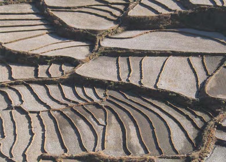
Figure29 Paddy fields. [Online] Available
htm [Accessed 12/10/2010].
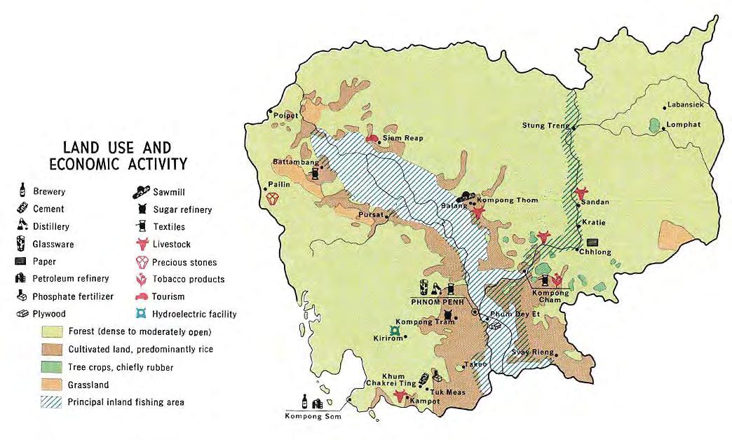
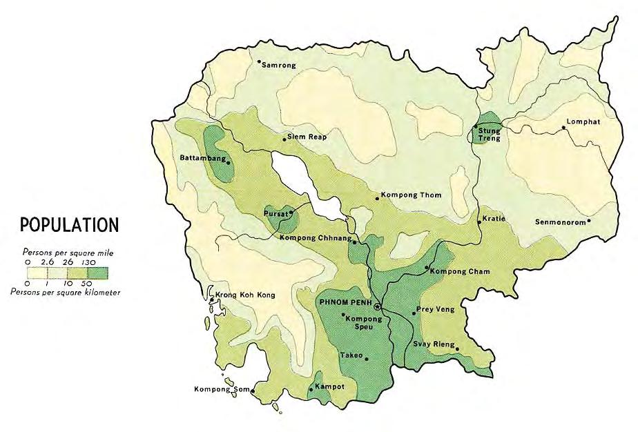
Figure30,31 (Left) Map of Land Use and Economic Activity. (Right) Map of Cambodia Population. [Online] Available at http://www.mapcruzin.com/free-maps-thematic/cambodia_land_1972.jpg [Accessed 12/07/10]
“Decentralization and De-concentration” process
Cambodia has undergone rapid urbanization over the last few years. It has the highest rate of urban population growth in the world - 8.4% annually. The rapid growth of urban population results in the insufficient of urban infrastructure. Confronted with the pressing need of a reorganization of land use the government adopted a “Decentralization and De-concentration” process aiming to distribute land tenure from central to local and manage the land resource at province, district and commune scale. The traditional top-down process in which local implementations are controlled by master plans, could not adapt to the subtle changes in local scale. An appropriate way should evolve from dealing with local issues and then affect the overall development.
De-concentration process means a shift of management way from regional authorities to subnational level. A vertical integration is enhanced between national level and local level, according to which the government agencies are supposed to be guided by and response to the local area dynamics. Besides that, the relationship between social and ecological activities is intensified. The “context-situated approach” take into consider how ecological and social factors actually work together and drive the rearrangement of people and resources.
Laws and policies
The Cambodian land law is released in 2001 by Ministry of Land Management. It is remarkable move in legally improving land management. Accompany with land law, Interim Paper on Strategy of Land Policy Framework, 2002, listed some policies for land management. These bring into attention that many problems resulted from disintegrated urban plan including inappropriate construction, unconscionable use
2.1 Current plan for development
of natural resources seriously impact the sustainable development of fishery and agriculture along with livelihood of local residents and exploitation of tourism.
These approaches are in accordance with the overall Decentralization and De-concentration process and are executed by local commune councils. They focus on facilitating local natural resource employment for a strengthened local community’s well-being. They propose that natural resource should be balanced between agriculture, demographic changes and industrialization and regional development should be embedded in the settlement of local issues.
Basic technical measurements
Due to the limited developments in many aspects of society, there exists some storage which may block the implementation of spatial planning policy. For example, the spatial planning infrastructure was very unclear in most part of the country. That is mainly because of the lack of detailed geo-spatial data. A Balloon Aerial Photo technique is designed to provide high pixel resolution aerial photos of geographic structure in Cambodia. In a poor developing country like Cambodia, this is a low-cost but relatively efficient way for geo-data collection. Other measurements include bringing in knowledge and technologies to expand the development capacity as well as concerning on improving concepts and skills of people for spatial planning.
— 35 —
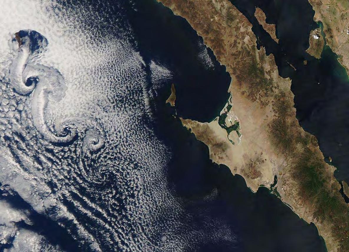
Image of fluid dynamic. [Online] Available at http://alg.umbc.edu/usaq/images/USA%.2006257.aqua.500m. crop.jpg [Accessed 25/07/10]
2.2.1 Hydrological techniques
In the case of this project, the principle of buoyancy is applied at the structural level when a kinetic structure is required to adapt to different depths of water. Specifically, because of the fluctuating water level in the site and the aim of maximizing the potential use of a structure and avoiding it being flooded in rainy season, a floating structure is proposed and some part of it is set to be able to move up and down as the water rise and drop. Base on a framework of bamboo sticks connected with flexible joints, floaters made of light materials are filled in the skeleton to keep the structure floating on the water. Buoyancy force helps to resist the gravity of the structure as well as keep the above-water parts structurally stable. 2.2 Analytical techniques
According to the buoyancy principle, the upward fluid pressure will keep an object afloat when the object’s average density is smaller than that of the fluid it is in. Buoyancy force equals to the weight of fluid the floating objects displaces.
— 36 —
Figure32
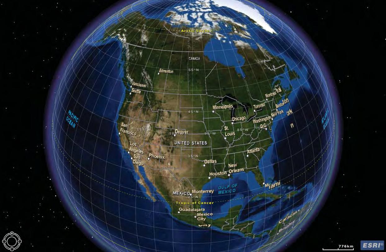
GIS and Geospatial Technology. [Online] http://blog.gispathway.com/ [Accessed 12/07/10]
2.2 Analytical techniques
2.2.2 Geographic information systems (GIS)
“Geographic information systems (GIS), is a set of tools that captures, stores, analyzes, manages, and presents data that are linked to location. In the simplest terms, GIS is the merging of cartography, statistical analysis, and database technology.” (Geographic Information Systems. [Online] Available at http://www.cyberessays.com/Term-Paper-on-Geographic-Information-Systems/16456/ [Accessed 03/10/10] ) Nowadays, this tool is widely used in many fields given that it allowed people to integrate various types of information in a particular spatial context, so a series of analysis, evaluation and conclusion could be done based on comprehensive database rather than individual impact or factor.
As our main subject is environmental adaptive to changing water level and social development, it is vital to set up a proper and accurate spatial model which is the foundation of design proposal. Overlay social mapping such as population density, values of building, and elevation provides visual picture which
enable us to deeply understand social and physical environment and make right developing strategies. For example, the relationship between building density and flood plain could be clearly displayed in one diagram, so it is also possible to forecast influences during flooding scenario.
— 37 —
Figure33
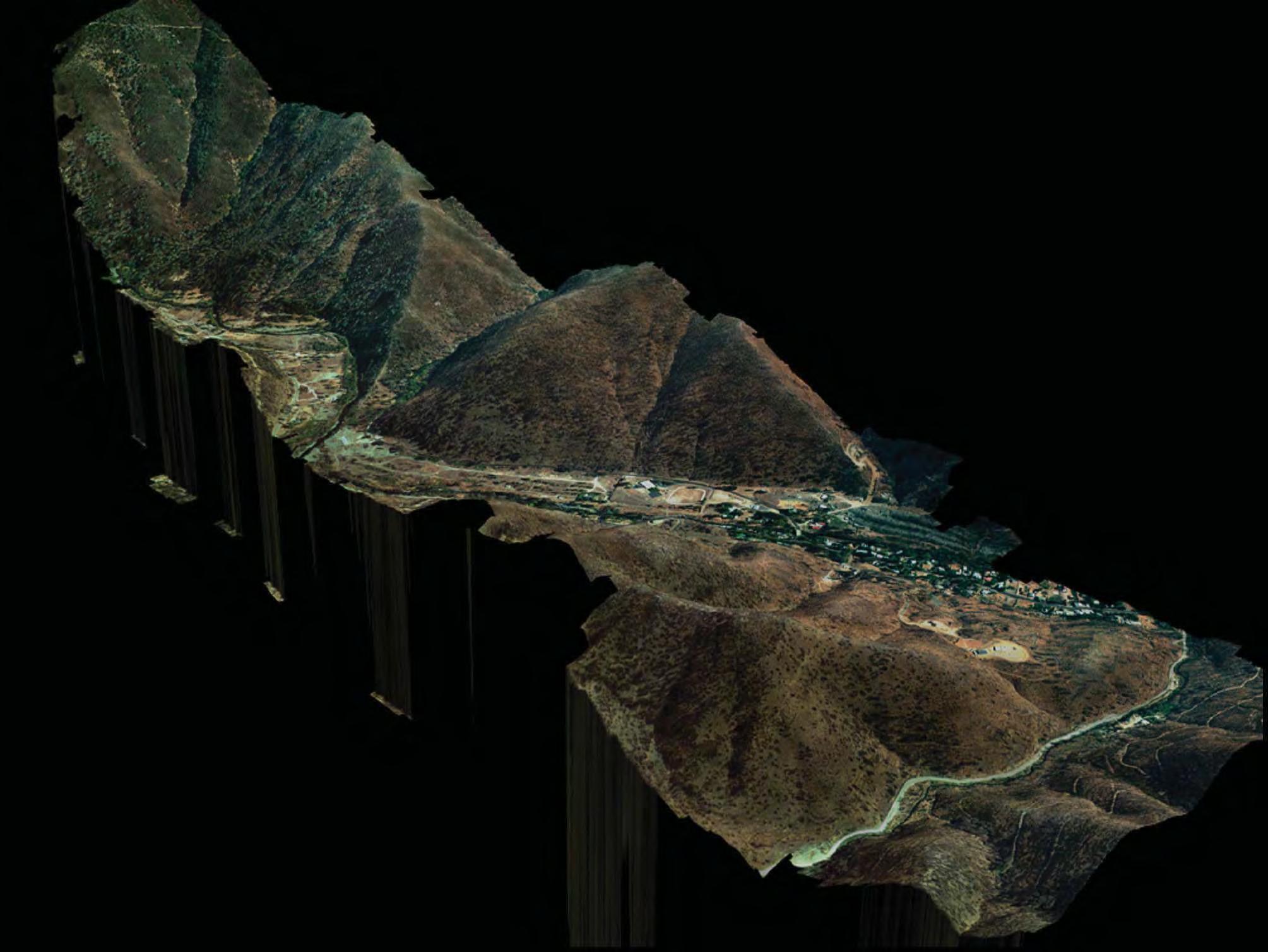
Figure34 High Resolution Digital Elevation Models. [Online] http://resourcemappinggis.com/images_high-res.html [Accessed 03/11/2010]
2.2 Analytical techniques
2.2.3 Digital Elevation Models (DEM)
Digital Elevation Models are database file which contain the elevation information of a specific terrain area. In another word, it is a digital model of ground surface topography and terrain; therefore it is the key to achieve our ambition. Only with the information about land elevation and water depth can we make effort to propose strategies for changing water level.
A DEM could be represented as a raster or as a triangular network. The area is usually divided into grids at fixed intervals over the terrain surface. The level of refinement grid points indicates level of detailed information in the file, as the elevations data are only given in DEM file for those locations at grid points. To capture the details of valleys & peaks on the terrain surface, it is better to use small grid spacing in modeling. As a result the information of the terrain in between grid points need to be interpolated based on the known information of the adjacent points. Therefore dramatic changes of elevations such as peaks
and valleys are not likely to be precisely represented unless they occur at, or very close to the grid points. DEM files usually do not contain other geographical or civil information as roads or buildings associated with the grid points other than elevation. Also there is no elevation contours in DEM file neither, only the specific elevation values at specific grid point locations.
— 38 —
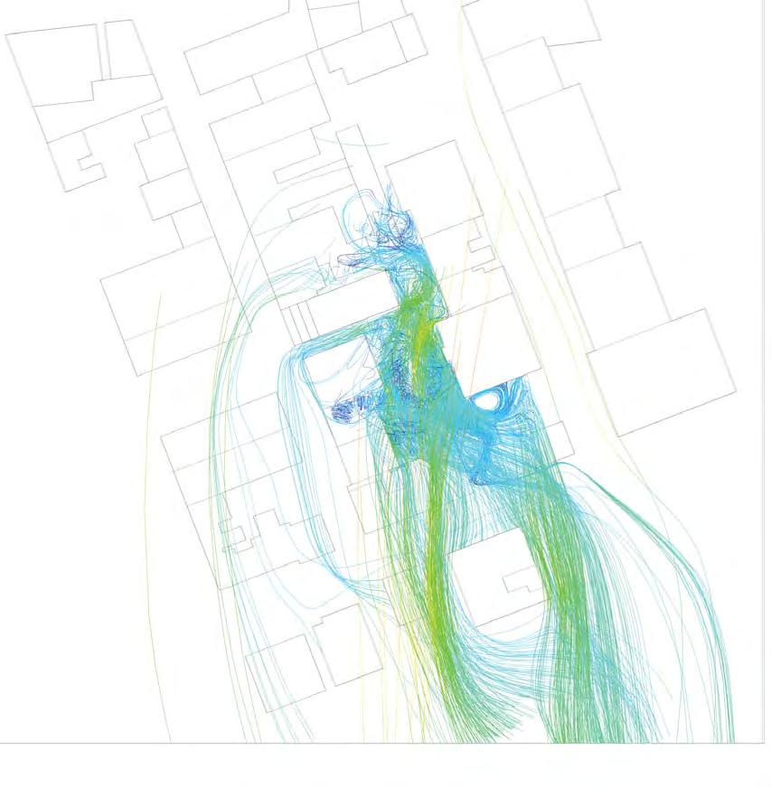

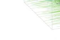
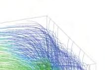
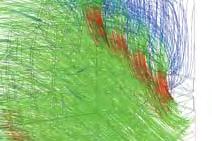
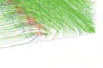


“Computational fluid dynamics (CFD) is one of the branches of fluid mechanics that uses numerical methods and algorithms to solve and analyze problems that involve fluid flows. Computers are used to perform the millions of calculations required to simulate the interaction of liquids and gases with surfaces defined by boundary conditions.”(Computational Fluid Dynamics. [Online] Available at http://www.cadryn.com/index.php?option=com_content&view=article&id=66:computational-fluid-dynamics-cfd&catid=36:cae&Item id=71[Accessed: 29/08/10]) It requires computational models to predict the details of fluid flow and its effects on structures in the flow and interactions with boundary surfaces.
In this project, this tool will be mainly applied in two stages: first is the preliminary design. With a digital elevation model of watersheds, river basin, and bays, we can first simulate water condition in any period.
2.2 Analytical techniques
2.3.5 Computational Fluid Dynamics (CFD)
The results will show the water velocity, turbulence and other circumstances of the specific sector we have chosen. Accordingly, different treatments will be developed to aim one predicted conditions. Then in the stage of experiment and evaluation, this process enables us to check the impact of all the adding artificial constructions, as modifications will also be done to improve the whole system. In this way, CFD will effect on initial strategy and evolution process.
— 39 —
Figure35 A project inform by the ANSYS fluid dynamic simulation, Emtech project, core studios 2.
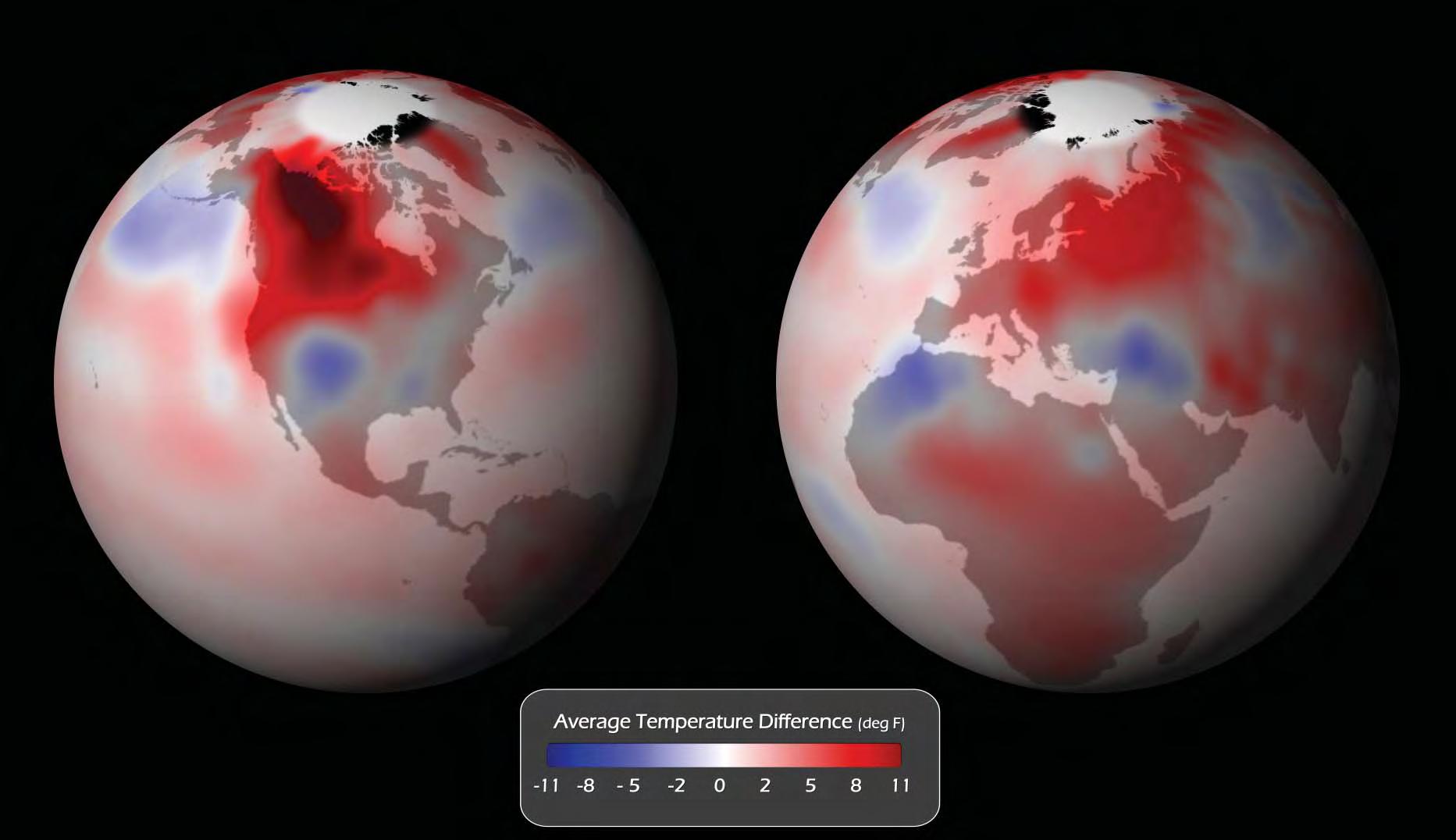
Figure36 Global surface temperature anomalies (degree F) for the month of September 2009. [Online] Available at http:// www.noaanews.noaa.gov/stories2009/20091015_sepglobal-stats.html [Accessed 12/10/2010].
2.3 Design methodologies
2.3.1 Climatic urban design
Climatic urban design approach is new alternative way of sustainability for urban designer and architect when considering energy saving and comfort in cities. It is an interdiscipline integrating several research fields such as environmental sciences, urban climatology and bioclimatic architecture. By emphasizing the role of urban geometry in climate control it aims to reduce the harmful environmental factors and prevent pollution in cities through suitable spatial planning.
How the urban fabric is influencing climate control is represented in the following perspectives. An appropriate level of solar access should be maintained for comfort living conditions for residents; buildings should have a certain capacity for heat store and dissipation; external ventilation and interior cross ventilation should be concerned and the role of vegetation in improving urban microclimate. The urban properties this methodology concerns include plan density, building dimension, solar orientation and
spacing between buildings. The size, shape, opening and the surface/volume ratio the above parameters define determine the exposure level of a building. Similarly, the geometry of opening areas in urban scale is also relevant in climate control. Ventilation conditions are determined by a building’s H/L ratio. Several concepts are constituted as a combination of those geometry parameters and a comprehensive evaluation of all the climatic factors to be considered. They are proposed in 3 levels – urban, architectural and environmental respectively. They are openness to sky, urban reflectance, urban porosity, directionality, building envelop and landscaping. To make the solution more precise, numerical and analogical simulation tools are also applied.
— 40 —
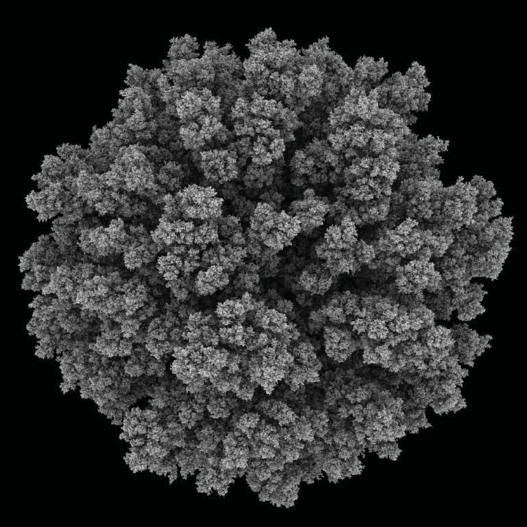
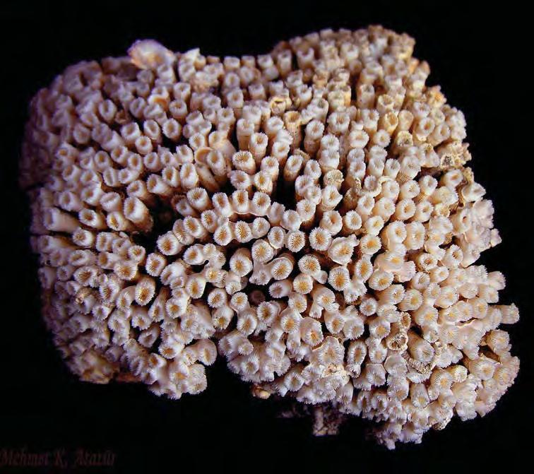
Figure37 Stone coral. [Online] Available at http://www.treknature.com/gallery/photo196672.htm [Accessed 12/10/2010]. Figure38 Aggregation. [Online] Avalible at http://www.andylomas.com/aggregation_012.html [Accessed 08/11/2010]
The concept
Diffusion limited aggregation (DLA) is a physical process driven by chemical and physical forces. It is common process in nature and generates life-like structures. Diffusion means the particles walk randomly under the fluctuation of temperature. Aggregation means the particles are connected together as one moves to the vicinity of another and form a cluster of structure. Many phenomenons in natural such as coral growth, crystal growth, mineral deposit, lightening path, dust of smoke, etc, follow the same process. There is no force between moving particles until they reach the aggregate. The aggregate increases its size by one particle at a time. The aggregation is a very slow process naturally a very slow process naturally.
Simulation
Computational method and technologies have been used to digitally simulate the natural pro-
2.3 Design methodologies
2.3.2
Diffusion limites aggregation
cess of DLA. A common approach is to simulate the random movement of particles. Some seed particles and secondary particles are placed at certain points in a field. The seed particles are still while the secondary particles move in all directions at a certain speed and rebound when they touch the boundary of the field. When a secondary particle meets one seed particle, it sticks to the seed, stops moving and becomes a seed particle itself. The same process repeats until a cluster of particles is generated. Cellular Automata (CA) is a variation of DLA model which is based on grid instead of moving particles.
DLA and city design
The DLA model has been well developed and has become one of the fractal theories in city design for its analogies to urban form. As DLA is a dynamic process concerning time and space, it can be applied to demonstrate and inform the formation of city.
— 41 —
2.3 Design methodologies
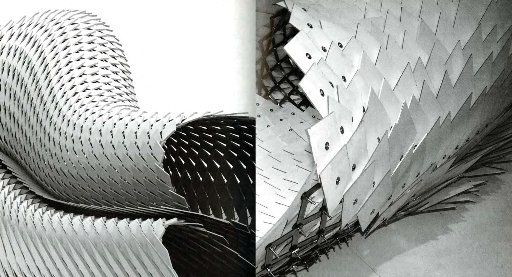
In ancient ages, knights wear hauberks to get protection while maintaining the bodies’ flexibility. A Hauberk can transform freely to match people’s shape. It is good evidence which proves that component – based surfaces have the potential to change forms to adapt to external conditions.
At present, it is possible for us to design component-based architectural structures with the aids of computer technologies. By defining an array of parameters of the components, we can build predictable adaptive structure in a bottom-up process.
2.3.3 Component-based adaptive system
— 42 —
Figure39,40 Component System. Alexia P. Protolepidote, Michael H. and Archim M., Morpho-Ecologies Towards Heterogeneous Space in Architectural Design, AA Publications, 2007.
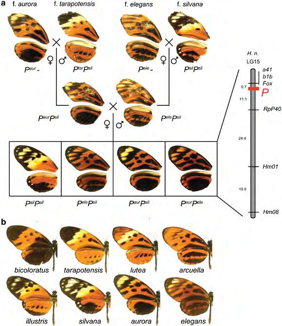
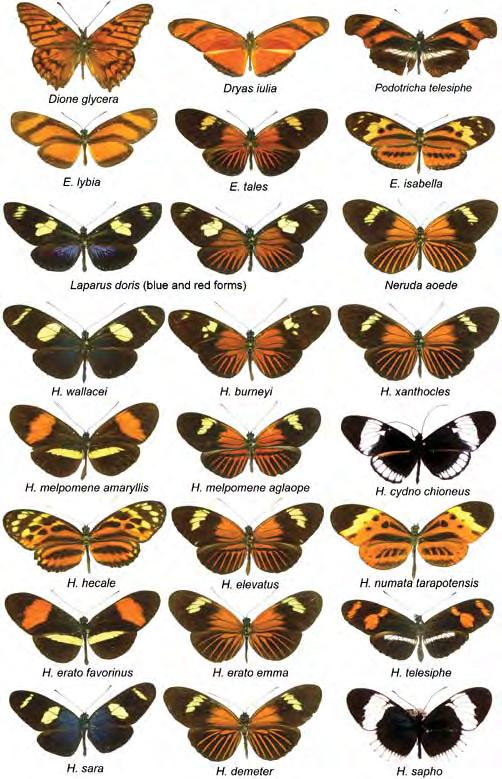
Figure41 Heliconius wing patterns: an evo-devo model for understanding phenotypic diversity. [Online] Available at http:// www.nature.com/hdy/journal/v97/n3/fig_tab/6800873f1.html [Accessed 12/12/2010].
The comcept
Genetic algorithm is a programming method that simulates the natural process of biological evolution. Informed by the Evo-Devo principle, it operates on a series of populations. Each population is generated trough some mutations from the previous population. It inherits the characters of their parents and develops their own characters. Under environmental pressures, the individuals in the population are selected and killed in the process of evolution, and by generations, they approach a best solution as a whole. Genetic algorithm emphasizes the uncertainty of the growth of an individual in a population and the environmental pressure as an invisible hand to guide the development of a population.
The application
2.3 Design methodologies
2.3.4 Genetic algorithm(GA)
GA has been widely used in the field which requires complex search and optimizations. It shows great potential in economics, scheduling, state assignment problem, computer-aided design, etc. In the field of architecture design, it is an advanced design method and has been used to address complicated issues which may not be solved by traditional approaches. By defining building problem such as structure, micro-climate, It is also been embedded in the concept of Emergence to inform architectural design. it show great efficiency in generate forms and a lot of varieties. many unpredictable form and properties emerge from the combinations. With some fitness criteria set as the environmental pressure for the population, the development tendency is regulated. in this way, this method make sure that the pupolation is best adaptive as well as maintain the diversity of the group.
— 43 —
2.3 Design methodologies
2.3.5 City evolution
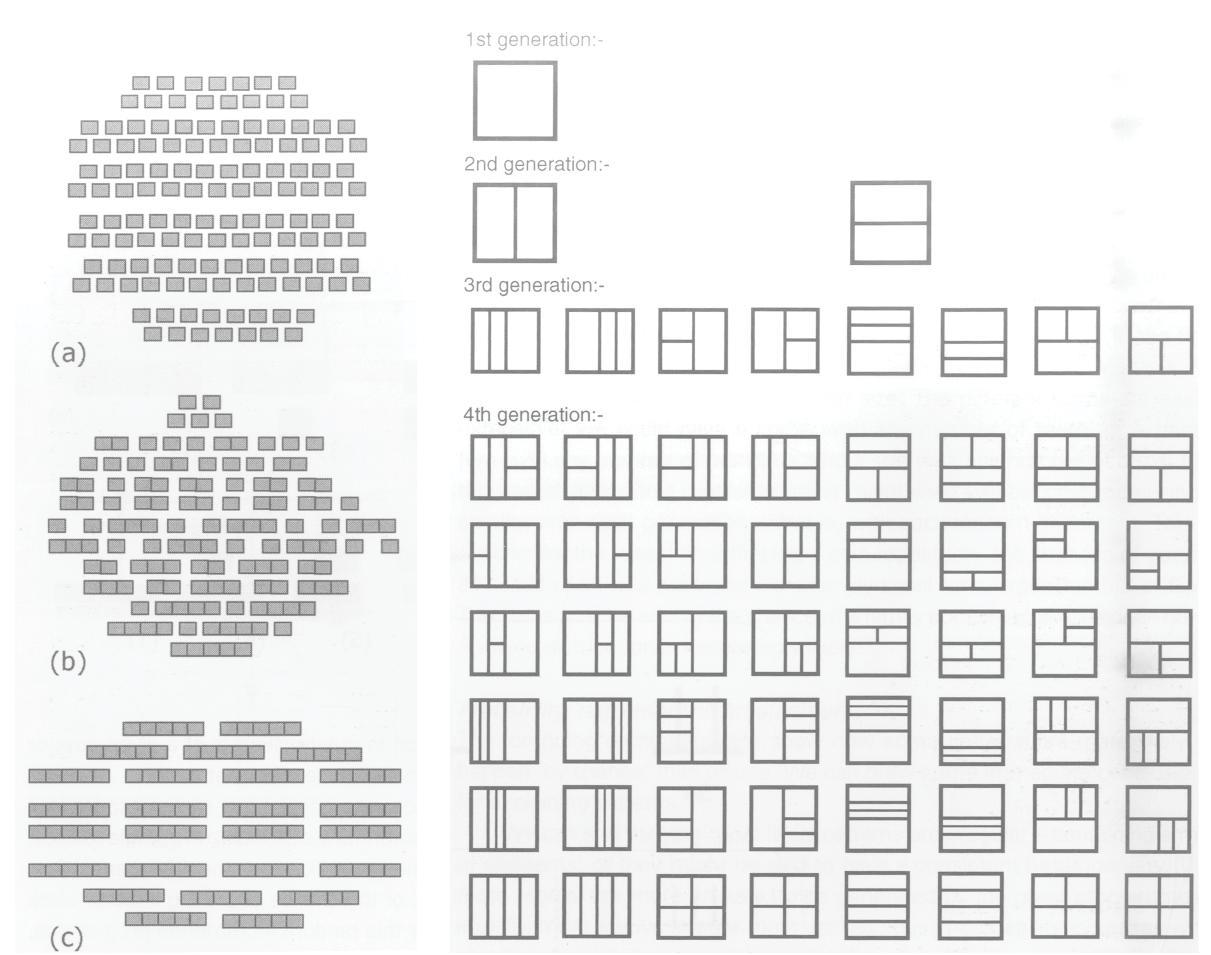
Compared with the traditional unplanned cities, many deliberately planned modern cities are worse in many aspects like livability and environment. This method aims to find the hidden logic of spontaneous city develops in order to inform the contemporary urban design. By looking at the street pattern, it explores the growing structure and order apart from social reasons for the street syntax.
There are two ways of generating street. One is through footprints; the other is through plot subdivision. With the footprints method, buildings are first deposited on the ground on after the other. The space in between automatically become the circulation and public space. The shapes of footprints and the relationship between each of them determine the street’s morphology. With the plot subdivision method,
street id created first by subdividing a plot into many subdivisions. The pattern and the portion of block are related.
No matter footprint method or subdivision method, it can reproduce itself under the same logic for many generations. And the street pattern evolves as the process becomes more and more complicated. After several generations, a clear urban order can be reflected from the phenomenon of street pattern.
Figure42,43 (Left) 130 buildings arranged in three ways. (Right) Set of patterns generated by successive plot biscetions. Stephen M., Cities design and evolution, Urban design and planning, Routledge, 2009
— 44 —
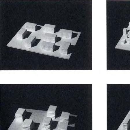
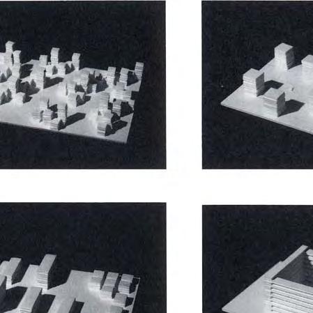
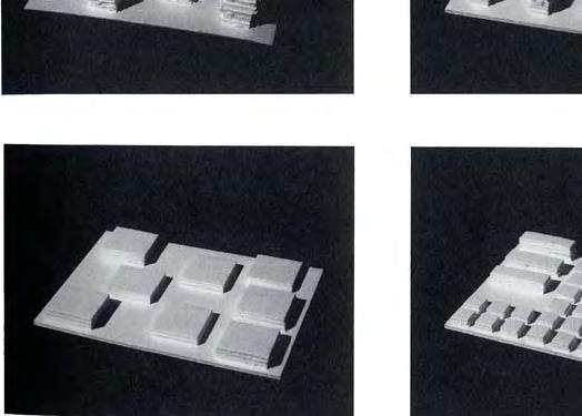

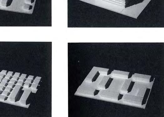
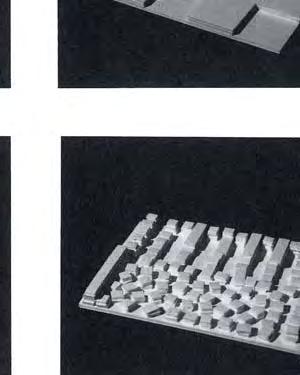
Density exercises limitation on the development of urban form. These limitation can be reflected both in the physical and social aspects.
There are two ways of considering the relationship between density and urban form. One is that a certain density is prescribed and designers are required to design urban forms within the given density conditions. This relationship is common in planned city where the type of urban form serve the density requirements. The other is using density to describe a built urban form. The density becomes the descriptive outcome of the existing form.
The methods to investigate the relationship between density and urban form include explorative
2.3 Design methodologies
2.3.6 Density and Urban form
research and empirical research. Explorative research use formulas and variables to capture the
ric properties and make clear measurement of the differences between different types. A number of urban indicators can define the detailed properties from every aspect. Empirical research is much more intuitive. It uses genetic knowledge to inform the urban practice. The two methods are always applied together to investigate the influence of the design conventions.
geomet-
— 45 —
Figure44 Students work with identical FSI value in Delft University of Technology.Meta Berghauser P., Per H., Spacematrix: Space, Density and Urban Form, NAI PUBL, 2010
Figure45 (Left) Fluid particle simulation. [Online] Available at http://t-linked.com/node/10 [Acessed 25/07/10] Figure46 (Right) Cracking algorithm. [Online] Available at http://ncodescripting.blogspot.com/2010/06/subdivision.html [Accessed 25/07/10]

2.4 Computational techniques
Scripting for Algorithm
As our aim is to achieve an adaptive system, it is crucial to set up inputs, in another words, to figure out the factors which drive the structural change. By programming a specific algorithm, all the parameters related to the local climate and site scenario are clearly exhibited and will effect on the behavior of the whole system. Because the structural change is subtle and interactional, obviously, it is always easier to rewrite the value of a parameter then modify the physical prototype. Generally speaking, set the proper algorithm is not only important for the physical simulation and testing in preliminary design, but also the basis for all the evaluation for the whole system.
Dynamic simulation
Dynamic simulation is the simulation for a system which is free or partly free to move in 3-dimension under certain forces. Recently, Dynamic simulation is widely used in computer animation to help animators to generate realistic motion. In architectural aspect, by understanding the components’ moving principles, it is possible to program in MAYA mel which provides convenient platform for architects and engineers. The benefits are mainly as follows:
Firstly, architects can easily predict the performance of a particular prototype and modify the design to achieve a certain purpose. Secondly, when the cases get more complex, the dynamical simulation will reduce the reliance on the time-consuming and expensive physical prototype. Thirdly, animation is visually easier for viewers to understand a continuous structural change.
2.4.1 Scripting for algorithm
— 46 —
2.4.2 Dynamic simulation
2.5 Evaluation
Methodology plays a fundamental role in the design process and offers a convincing supporting that goes through the research in next chapters, whereas there are still some restrains in the way. The previous research and application of generative algorithm and evolution methode in architectural field are seldom. There is still a huge gap between natural adaption to kinetic mechanism that in human scale or larger scale, and the translation will be time and power consuming.
Analytical technique provides qualitative and quantitative analysis which is indispensable for a project, but it require plenty software skills. Dynamic simulation is even more complicated. Theoretically, it is impossible to all the variables into ac¬count, and in reality, physical test is not always exactly the same as we expected. So, people should discover trends and conclude regular pattern from a computational result, instead of over relying on it.
To sum up, It is very important to define the boundary and fine tuning is nec¬essary in the design approach
— 47 —
— 48 —
Chapter 3. Research development
3.0 Introduction
3.1 Design strategy
3.2 Experiment 1
3.2.1 Genetic algorithm
3.2.2 Evolution and development on small scale
3.2.3 Evaluation 1
3.2.4 Evolution and development on medium scale
3.2.5 Evaluation 2 and conclusion
3.3 Experiment 2
3.3.1 Water flow test
— 49 —
3.0 Introduction
This Chapter is the exploration of the methodologies specified to the site conditions and design strategy. At the beginning of this chapter, the “polder block” design strategy is proposed. It is based on all the site analysis and inspirations from urban design theories and previous works. The strategy of “Polder block” is believed to have the potential to solve many problems in a creative way. To explore the concept, in the second part of this chapter, we conducted a series of experiments digitally and physically. Those include genetic algorithm and ANSYS fluid simulation. Genetic algorithm is the most critical and fundamental part in this project. Its irreplaceable role lies in the complete process of evolving families of individual with different properties and performances which are applied on the site according to section conditions, programmatic requirements, etc. ANSYS fluid simulation focuses on the artificial structure’s environmental effects mainly considering the differences produced by the structure's dimension.
This chapter is crucial for its preparative role for the subsequent design development.
— 50 —
3.1 Design strategy
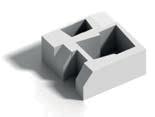
As has been stated in the previous chapter, the Dutch have built rings of closed dikes for the purpose of blocking water outside and reclaiming land from the sea. There the dike has solely the defensive function. Residential block is the basic living unit. There are certain standards for a block’s dimension, orientation and distance to other blocks in accommodation varies programmatic requirements. In this project, for a village on the water, Inhabitancy and water defense could be the most two important factors needed to be considered. We were trying to take these two components as a whole – a thickened ring of dikes from its appearance but with both defensive function and residential function. That is how we come up with the concept of “polder block”.
An explored axonometric diagram further explains the concept. The outside ring of walls is for water defense. They are solid and can safely resist water. Under the protection of outer surface, inner part is safe and inhabitable. The same with the oriental quadrangle, the residential part are centripetal with the courtyard in the middle becoming the open space for public activities. To solve the transportation, top surface is taken as road to serve internal and external transport and constitute the infrastructure network with other blocks.
circulation residential block inhabitable wall defensive wall on roof road block
block polder
polder
— 51 —
Figure47 A diagram explaining the origin of the design strategy and the components of a "polder block".
3.2 Experiment 1
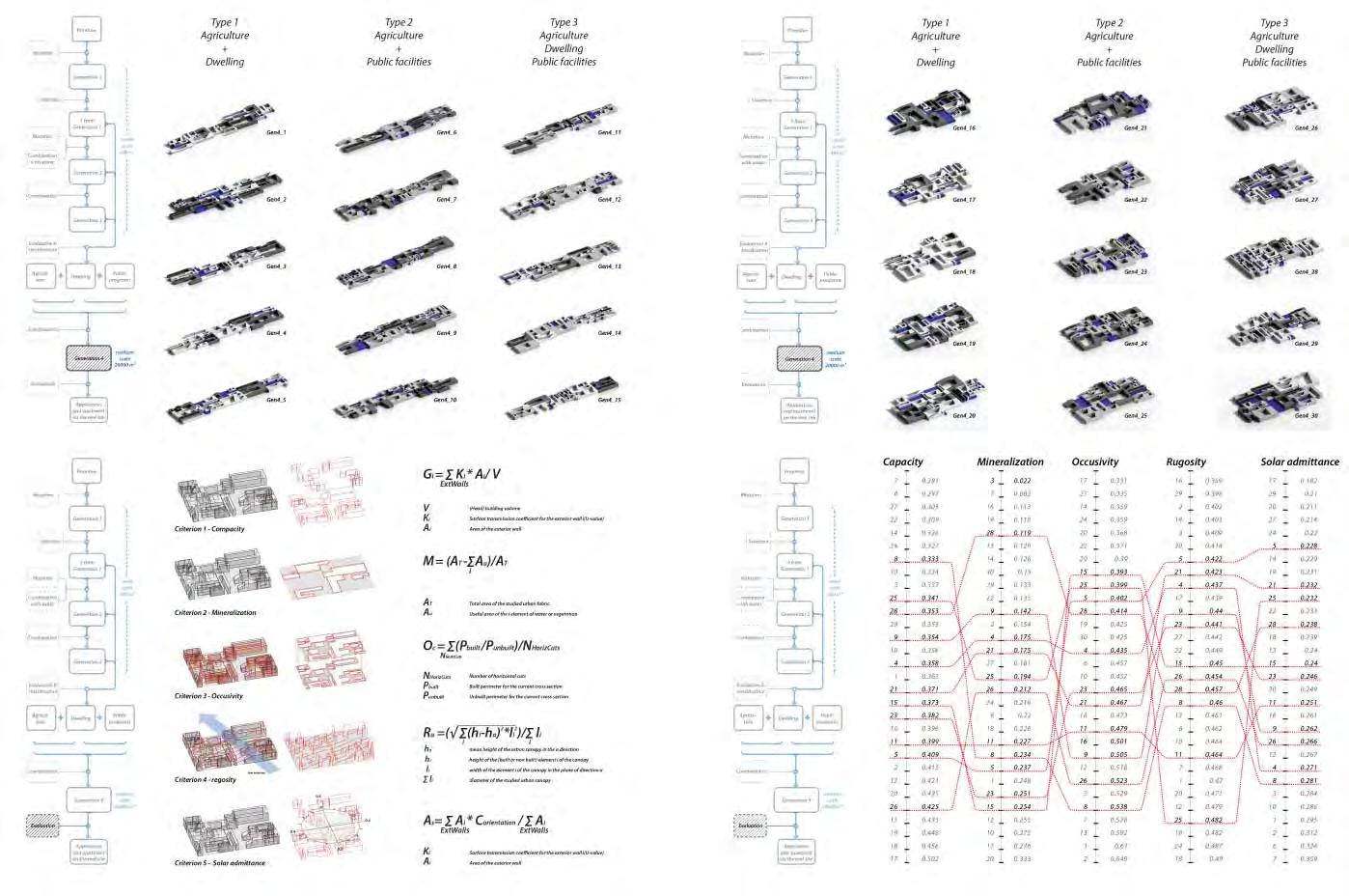
With the principle of genetic algorithm, four generations are evolved from four mutations and two evaluations. Each mutation aims to explore different aspects from both the architectural view and climatic view. The first evaluation considers the livability on the architecture scale and the second evaluation considers climatic effects on the urban scale. There are two main steps in this experiments. they are different in the ways of generation, evaluation criteria and scale. The aim of the first step is to produce a large number of architectural blocks and match them to different programs. The aim of the second is to sort select the fit urban fabrics under the regulations of climatic performances. The final result of this part of experiments is a family of 20,000m² large urban patches with relatively appropriate climatic performance. These are the preparation for the urban planning on the real site.
The details of the process of Genetic Algorithm are explained thoroughly in the next several pages.
3.2.1 Genetic algorithm
— 52 —
Figure48 An overview of the Genetic Algorithm process.
Generation1 Generation1 5 from Generation2 Generation3 Generation4 Application and ajustment on the real site Primitive Dwelling Agricultrue Public facilities Mutation Mutation Combination with water Selection CombinationCombination Evaluation Classification Evaluation small scale 20m 20m medium scale 20000 m
The flow chart descrbing the steps included in the Genetic Algorithm process. — 53 —
Figure49
3.2 Experiment 1
3.2.1
Evolution and development on small scale
From primitive to generation 1
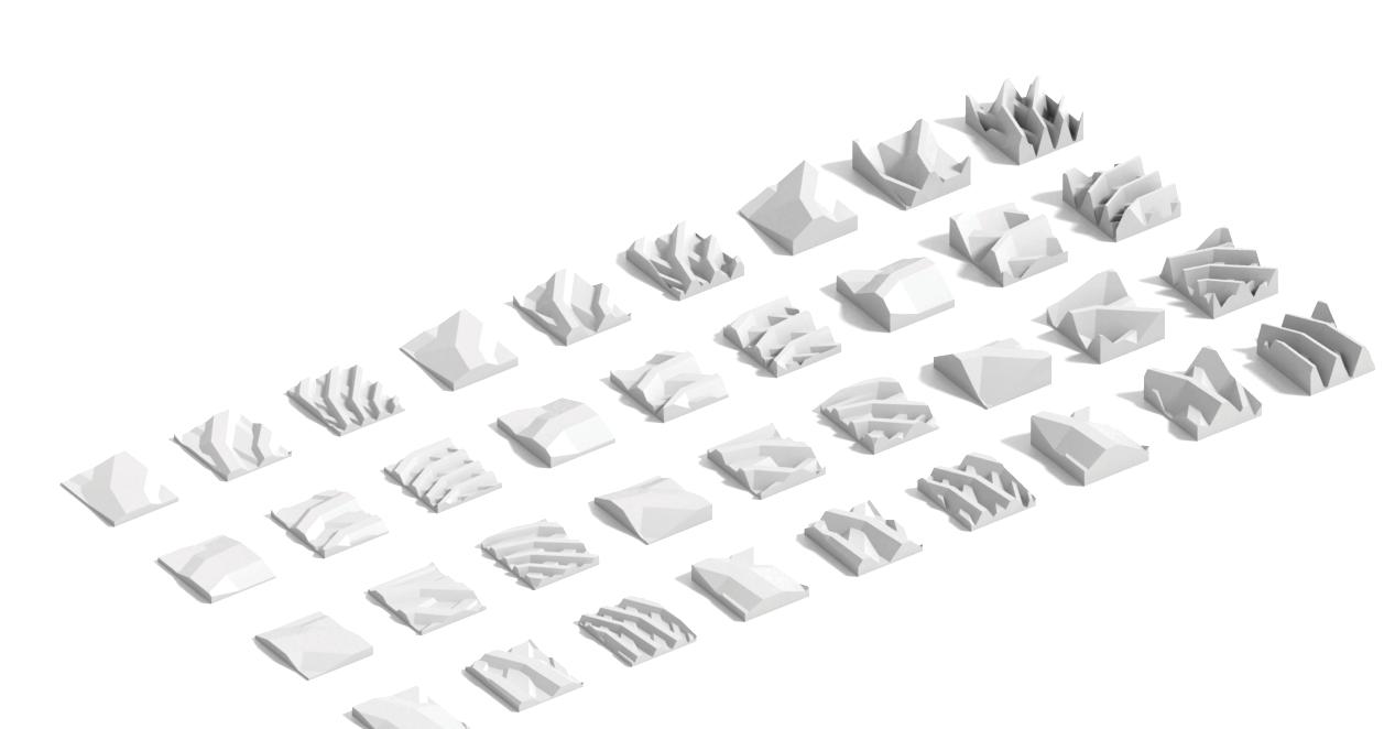
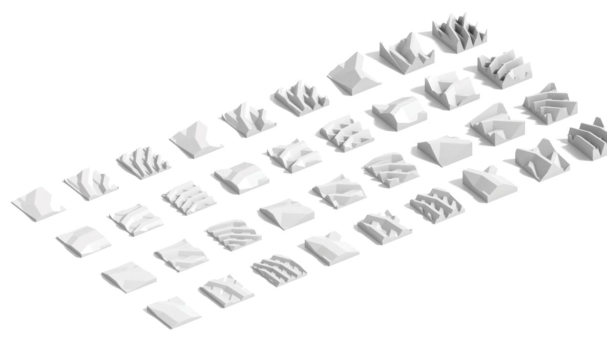
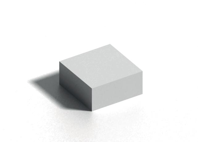
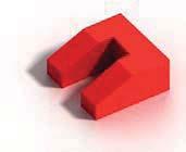
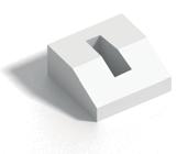
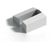
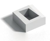
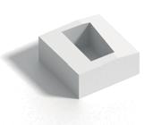
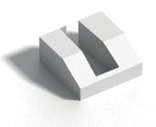
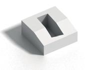
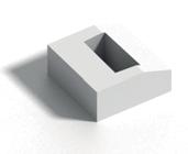
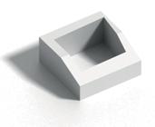
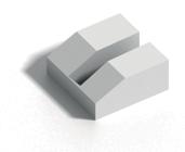
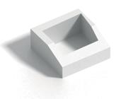
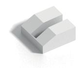
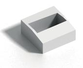
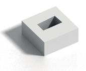
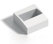
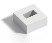
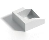
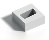
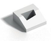
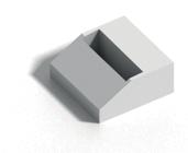
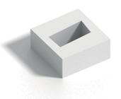
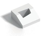
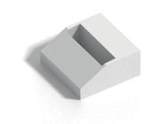
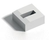
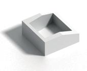
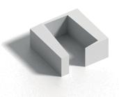
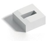
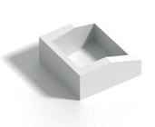
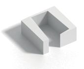
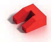
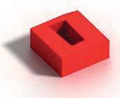
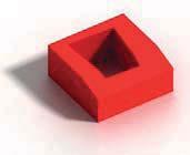
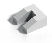
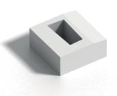
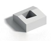
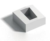
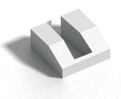
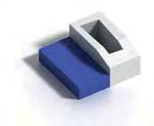
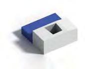
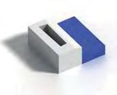
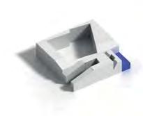
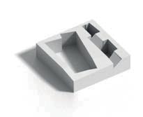
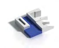
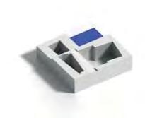
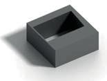
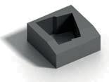
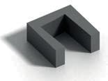
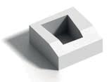
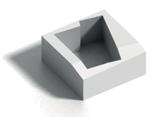
At the starting point of the whole process of genetic algorithm, the simplest geometry was chosen to be the primitive of all the generations. It is a cube. It is 20m×20m×9m which is the scale of a block. To produce the first generation, several mutations are conducted. In the modeling software, these mutations are represented by the command of scaling, rotating, trimming and Boolean operation. The aim is to create a courtyard in the middle of the block for the ventilation and sun exposure on the inner surfaces and for public activities as an open space. On the other hand, by cutting the quadrangle with a rotated surface, the blocks are assigned different height and with a sloping top surface for transportation. The parameters here are the shape and dimension of the courtyard, the thickness of the building entity, the height and the inclination of the roof-road.
Script helps to generate a large amount of results with the same logic but quite randomly. There are 20 individuals generated in the first generation. They show the great variety that could be produce with simple principles. five of them are selected from generation one as the parents of the second generation.
Generation 2
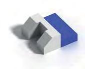
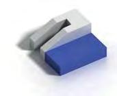
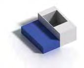
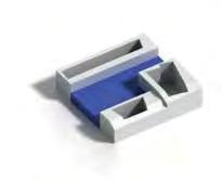
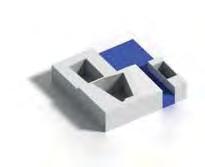
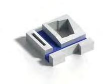
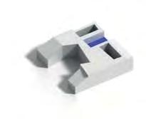
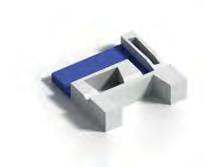
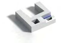
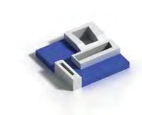
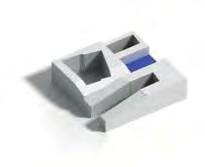
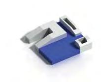
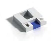
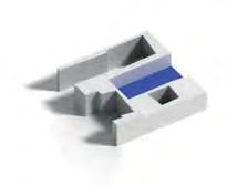
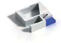
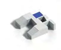
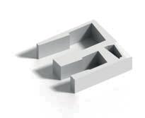
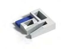
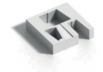
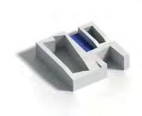
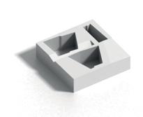
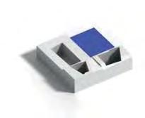
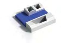
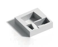
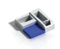
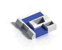
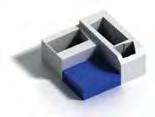
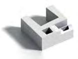
With the five blocks selected from the previous generation, several mutations are conducted for the second time to produce generation two. In the second generation, the mutations of each individual are based on is body plan, which means the individual begin to evolve by the different parts of the body, and each part changes independently but the results of all the parts affect each other, There are two groups of mutations at this step. The first group, including commands of dividing, rotating, trimming and filling in the modeling software, is to create more sophisticated inner surfaces with various orientations. the reason is that the inner surface is inhabitable most of the time and its livability should be explored. The other group of mutation is to bring in the element of water and to create a family of half water-half building blocks. This step is to explore the morphology of water and the relationship between residential building and water. There are all together 20 individuals under two catalogue in the generation, they are still limited in the boundary of a 20m×20m rectangle. But the conditions and performance are getting more complicated.
Generation 3
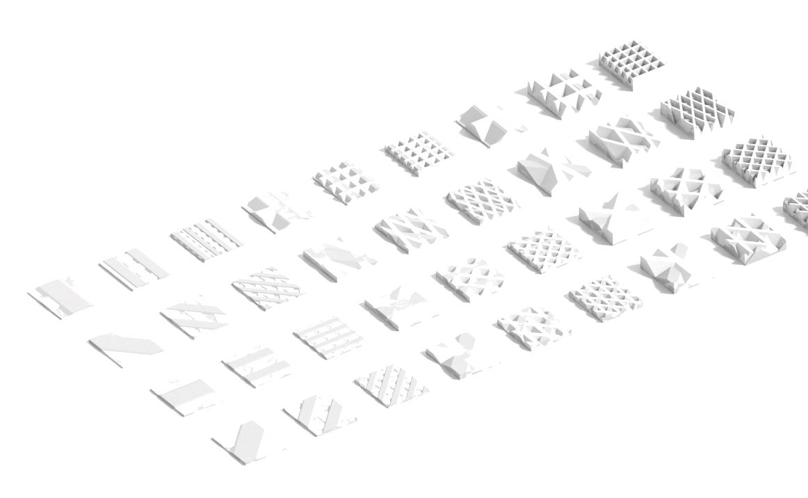
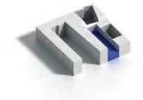
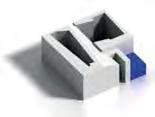
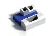
Generation three is the combination of the previous two generations. The combination logic is subdivision logic. The same 20m×20m rectangle is firstly divided into two 10m×10m rectangle. Secondly, one of them is divided the second time into two smaller rectangle. With the gird produced by subdivision, blocks from generation one and generation two are scaled and filled into the grid. After the combination, the new blocks become much more complicated. The water morphology and building entity morphology vary in each block. Some building blocks are several smaller building blocks with different shapes connection together. The water morphology is no more regular.
— 54 —




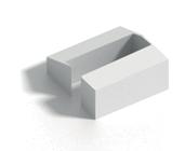

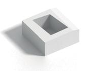

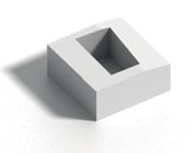

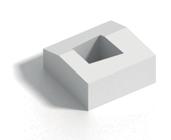

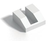
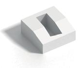
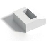
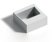
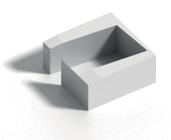
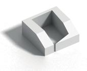
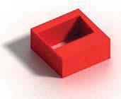
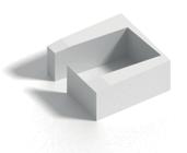
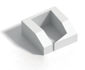
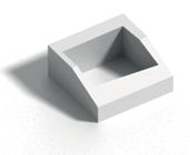
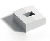
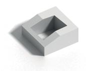
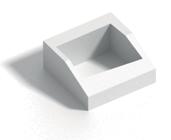
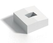
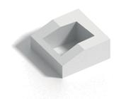
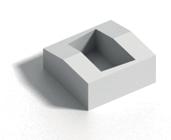


Primitive Generation 1 5 from Generation 1 Generation 2 Generation 3 Programs Generation 4 Mutation 1 Selection Mutation 2 Mutation 3 Evaluation 2 Mutation 4 Evaluation 2 9 m Primitive Primitive Scale Boolean Generation 1 Mutation Gen1_1 Gen1_2 Gen1_3 Gen1_4 Gen1_5 Gen1_6 Gen1_7 Gen1_8 Gen1_9 Gen1_10 Gen1_11 Gen1_12 Gen1_13 Gen1_14 Gen1_15 Gen1_16 Gen1_17 Gen1_18 Gen1_19 Gen1_20 Gen1_21 Gen1_22 Gen1_23 Gen1_24 Gen1_25 Gen1_26 Gen1_27 Gen1_28 Gen1_29 Gen1_30 Gen1_1 Gen1_2 Gen1_3 Gen1_4 Gen1_5 Gen1_6 Gen1_7 Gen1_8 Gen1_9 Gen1_10 Gen1_11 Gen1_12 Gen1_13 Gen1_14 Gen1_15 Gen1_16 Gen1_17 Gen1_18 Gen1_19 Gen1_20 Gen1_21 Gen1_22 Gen1_23 Gen1_24 Gen1_25 Gen1_26 Gen1_27 Gen1_28 Gen1_29 Gen1_30 20m 20m Figure50 Genetic Algorithm - the primitive, the mutations from primitive, the family of first generation and the selection in generation 1. — 55 —










Primitive Generation 1 5 from Generation 1 Generation 2 Generation 3 Programs Generation 4 Mutation 1 Selection Mutation 2 Mutation 3 Evaluation 2 Mutation 4 Evaluation 2
Mutation - type1 Mutation - type2
water
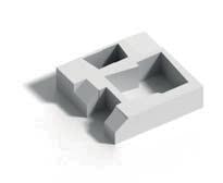
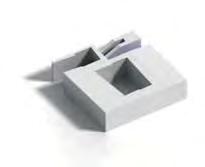
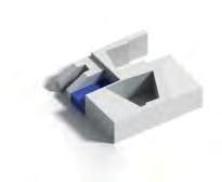
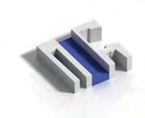
Bring in water Subivide&scale Combine Gen1_1 Gen1_5 Gen1_12 Gen1_21 Gen1_23 Gen2_2 Gen2_3 Gen2_4 Gen2_5 Gen2_6 Gen2_7 Gen2_8 Gen2_9 Gen2_10 Gen2_1 Gen2_2 Gen2_3 Gen2_4 Gen2_5 Gen2_6 Gen2_7 Gen2_8 Gen2_9 Gen2_10 Gen2_1 Figure51 Genetic Algorithm - 5 blocks from generation 1 and the two types of mutations to produce generation 2. — 56 —
5 blocks from Generation 1 Generation 2
Body plan Divide Scale Rotate Cut away Fill up
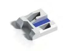
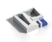
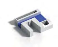
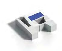
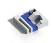
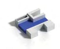
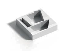
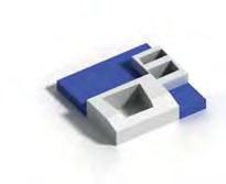
Primitive Generation 1 5 from Generation 1 Generation 2 Generation 3 Programs Generation 4 Mutation 1 Selection Mutation 2 Mutation 3 Evaluation 2 Mutation 4 Evaluation 2
& scale Combine 5_3neG 4_3neG 3_3neG 2_3neG 1_3neG 0 1_3neG 9 _3neG 8 Ge 7 6_3n Ge Gen3_11Gen3_12Gen3_13Gen3_14Gen3_15 Gen3_16Gen3_17Gen3_18Gen3_19Gen3_20 Gen3_21Gen3_22Gen3_23Gen3_24Gen3_25 Gen3_26Gen3_27Gen3_28Gen3_29Gen3_30 Gen3_31Gen3_32Gen3_33Gen3_34Gen3_35 Gen3_36Gen3_37Gen3_38Gen3_39Gen3_40 Generation 3 Subdivision water Figure52 Genetic Algorithm - the mutation to produce generation 3 from generation 4. — 57 —
Blocks from previous generations Subdivide
3.2 Experiment 1
3.2.3 Evaluation 1
After three generations, the first evaluation is brought in to as the environment pressure to restrict the growth of the population. The fitness criteria being considered are density, accessibility and open space ratio. They are related to the livability of the blocks at the architectural scale which means if one block is suitable for people to live in.
Density
Density reflects the building intensity in a residential area. Over high density causes too much pressure on people’s daily activities and environmental resources. Over low density is a waste of building land area. Density is calculated as the summation of gross floor area divided by the area of aggregation.
Accessibility
Accessibility is the average level of convenience for people travelling from one point to another. Accessibility determines the frequency of people’s communication. It is calculated as the summation of number of branches at each junction divided by the number of junctions.
Open space ratio
The last criterion is the open space ratio. It is calculated as the open space area divide by the total area of aggregation.
The above three urban indicators are highly related to the quality of a block. From these indicators, we can decide which program one block can accommodate. For dwelling, high open space ratio is required. For public facilities, high density is required. For agriculture, density, accessibility and open space ratio could be very low. According the requirements of each type of program, the 65 blocks from generation one to generation three are divided into three groups. Each group of blocks is suitable for one program from agriculture, dwelling and public space. After this step, there are 15 agriculture blocks, 25 residential blocks and 25 pubic blocks.
— 58 —
5.9644.895.5177.0016.109
G2_1G2_2G2_3G2_4G2_5G2_6G2_7G2_8G2_9G2_10G2_11G2_12G2_13G2_14G2_15G2_16G2_17G2_18G2_19G2_20
5.6595.6594.7646.5435.2945.2943.534.0876.2164.7495.9644.895.5187.0026.1086.1084.895.5187.0026.108
5.8896.0994.8214.8216.635.4115.0455.9625.8585.9786.6685.8286.1297.1125.9816.055.5135.7736.3345.164
G3_21G3_22G3_23G3_24G3_25G3_26G3_27G3_28G3_29G3_30G3_31G3_32G3_33G3_34G3_35G3_36G3_37G3_38G3_39G3_40
6.376.0926.5215.3975.3215.3695.8246.4285.1985.635.437.6434.6226.6845.3515.5965.0496.1916.1375.513
G1_1G1_2G1_3G1_4G1_5
G2_1G2_2G2_3G2_4G2_5G2_6G2_7G2_8G2_9G2_10G2_11G2_12G2_13G2_14G2_15G2_16G2_17G2_18G2_19G2_20 GEN1 GEN2
1.51.5221.51.51.5221.51.52221.51.52221.5
GEN3 G3_1G3_2G3_3G3_4G3_5G3_6G3_7G3_8G3_9G3_10G3_11G3_12G3_13G3_14G3_15G3_16G3_17G3_18G3_19G3_20
2.22.22.22222.22.1821.82.22.251.8182.1822.52.22221.6361.8332.182222.5
G3_21G3_22G3_23G3_24G3_25G3_26G3_27G3_28G3_29G3_30G3_31G3_32G3_33G3_34G3_35G3_36G3_37G3_38G3_39G3_40 1.52221.5
2.22.421.62.42.2221.83322.22.52.52.422.52.4442.422.2222.52
G1_1G1_2G1_3G1_4G1_5
G2_1G2_2G2_3G2_4G2_5G2_6G2_7G2_8G2_9G2_10G2_11G2_12G2_13G2_14G2_15G2_16G2_17G2_18G2_19G2_20 GEN1 GEN2
0.310.5750.4440.2650.4110.3810.6070.5330.30.4720.2580.4560.3520.2080.3210.2580.4560.3520.2080.321
GEN3 G3_1G3_2G3_3G3_4G3_5G3_6G3_7G3_8G3_9G3_10G3_11G3_12G3_13G3_14G3_15G3_16G3_17G3_18G3_19G3_20
0.4390.4250.5280.3840.3810.4550.3560.3740.4420.3670.3250.4290.4180.320.3730.4470.3670.4140.3870.511
G3_21G3_22G3_23G3_24G3_25G3_26G3_27G3_28G3_29G3_30G3_31G3_32G3_33G3_34G3_35G3_36G3_37G3_38G3_39G3_40 0.2580.4560.3520.2080.321
0.3640.3850.3560.4510.3830.4320.2840.340.4860.4770.4750.2630.5710.3670.460.4070.4940.3670.3650.345
Figure53 Genetic Algorithm - the explaination of three fitnness criteria and the scores for each individual from the previous generations.
Primitive Generation 1 5 from Generation 1 Generation 2 Generation 3 Programs Generation 4 Mutation 1 Selection Mutation 2 Mutation 3 Evaluation 2 Mutation 4 Evaluation 2 Density Accessibility nbranch=3 nbranch=2 Open space ratio 2 2 2 2 3 3 3 3 A =
O =
ax D =
ax ax fx ax bx N number
junctions
number
branches at one junction ax area of aggreagation gross floor area fx ax area of aggreagation bx open area
(∑nbranch) / N
(∑bx) /
(∑fx) /
of
nbranch
of
G1_1G1_2G1_3G1_4G1_5
GEN1
GEN3 G3_1G3_2G3_3G3_4G3_5G3_6G3_7G3_8G3_9G3_10G3_11G3_12G3_13G3_14G3_15G3_16G3_17G3_18G3_19G3_20
GEN2
— 59 —


Gen1_1Gen1_2Gen2_1Gen2_3Gen2_5


Gen2_6Gen2_7Gen2_8Gen2_10Gen2_11


Gen2_12Gen2_17Gen3_7Gen3_24Gen3_33


Gen1_3Gen2_2Gen2_13Gen2_18Gen3_1


Gen3_2Gen3_3Gen3_5Gen3_6Gen3_9


Gen3_12Gen3_13Gen3_16Gen3_17Gen3_18


Gen3_20Gen3_25Gen3_26Gen3_29Gen3_30


Gen3_31Gen3_35Gen3_36Gen3_37Gen3_40 Gen1_4Gen1_5Gen2_4Gen2_9Gen2_14


Gen2_15Gen2_16Gen2_19Gen3_4Gen3_8


Gen3_10Gen3_11Gen3_14Gen3_15Gen3_19


Gen3_21Gen3_22Gen3_23Gen3_27Gen3_28


Gen3_32Gen3_34Gen3_38Gen3_39Gen2_20
Primitive Generation 1 5 from Generation 1 Generation 2 Generation 3 Programs Generation 4 Mutation 1 Selection Mutation 2 Mutation 3 Evaluation 2 Mutation 4 Evaluation 2 Dwelling Public programs Agriculture Density ces
c Acc ss Open space Accessibility ratio r spa
e sib b
Density Agriculture Dwelling Public facilities AccessibilityOpen space ratio Figure54 Genetic Algorithm - the scores for each individual expressed in the 3 dimensional coordinate system, the selection standard for each specific program, and an overview of the sorted population. — 60 —
3.2 Experiment 1
3.2.4 Evolution and development on medium scale
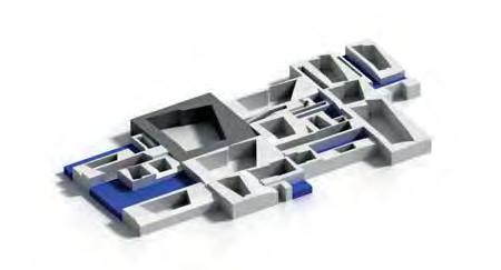
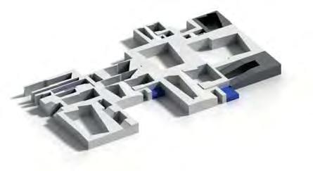
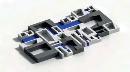
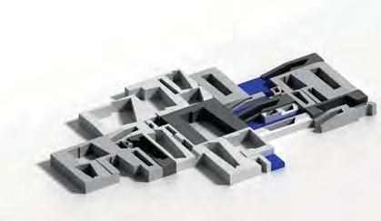
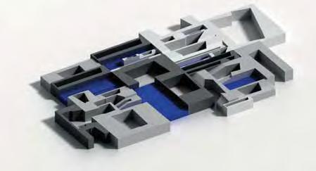
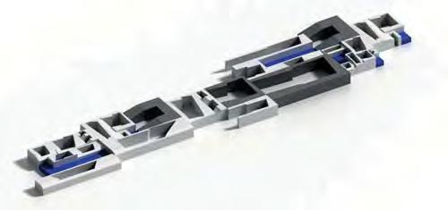
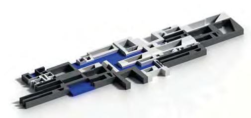
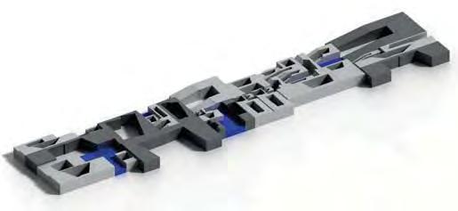
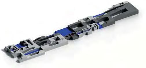
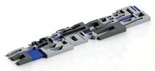
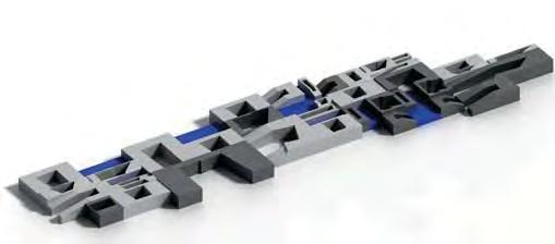
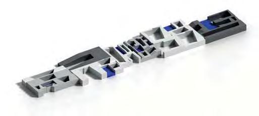
The first the generations are on the architectural scale. The second scale of the experiments is the urban scale. At this step, the evolved and evaluated blocks are combined to be a patch of urban fabric. There are three types of urban fabric. They are the combination of agriculture and dwelling, the combination of agriculture and public facilities and the combination of agriculture, dwelling and public facilities. The subdivision logic is used to create the urban pattern. After several times of subdivision on the 4×5 grid, an non uniform pattern is created with various scales. Blocks from previous generations are scaled and filled into the pattern. Because some of the blocks are already the combination of the others, the underlying pattern is not easy to recognize from the phenomenon of the cluster of blocks.
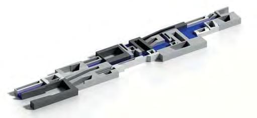
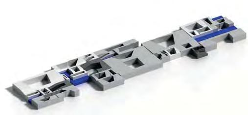
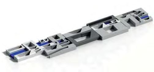
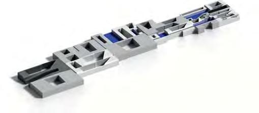
30 patches of urban fabric are produced in the fourth generation. These include three types of combination mentioned before. A narrow shape and a wide shape have been investigated to apply on different topologies.
The evaluation of the generation four focus on its climatic performance. The criteria introduced are capacity, mineralization, occusivity, rugosity and solar admittance wich will be explained one by one in with the later diagrams.
In genetic algorithm, these criteria can be taken as the environmental pressures which restrict the arbitrary growth of the population.
The table on page 70 records the scores each patch gets in the five criteria. Their distribution follows the Normal Distribution. The individuals with all its five scores located at the middle parts of the bell curves are reserved and others are killed. After the selection, twelve patches with optimized climatic and architectural performances are going to be matched to the certain locations on the site.
— 61 —
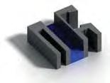
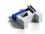

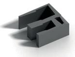
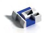
Primitive Generation 1 5 from Generation 1 Generation 2 Generation 3 Programs Generation 4 Mutation 1 Selection Mutation 2 Mutation 3 Evaluation 2 Mutation 4 Evaluation 2 1st subdivision 2nd subdivision Water Dwelling
Subdivision grid 3rd subdivision agriculture2agriculture4agricultrue9agricultrue14agriculture15 dwelling1dwelling3dwelling6dwelling8dwelling10dwelling12dwelling22dwelling23dwelling24dwelling25
Agricultrue
— 62 —
Figure55 Genetic Algorithm - the combination logic of the blcoks on the urban patch.
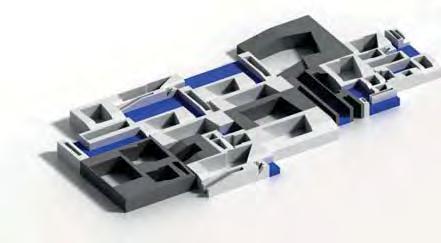
Type 1 Combination of Dwelling and Agriculture

Type 2
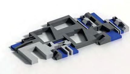
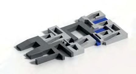
Combination of Public facilities and Agriculture
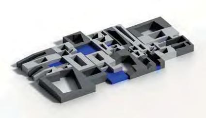
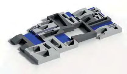
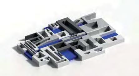
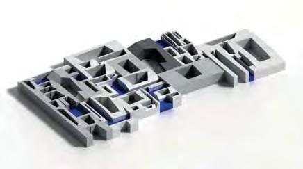
Type 3
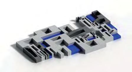
Combination of Dwelling, Public facilities and Agriculture

Primitive Generation 1 5 from Generation 1 Generation 2 Generation 3 Programs Generation 4 Mutation 1 Selection Mutation 2 Mutation 3 Evaluation 2 Mutation 4 Evaluation 2
Gen4_1
Gen4_6
Gen4_11
Gen4_2
Gen4_7
Gen4_12
Gen4_3
Gen4_8
Gen4_13
Gen4_4 Gen4_9
Gen4_14
Gen4_5 Gen4_10
Gen4_15
— 63 —
Figure56 Genetic Algorithm - the patches of urban fabric generated from different combination of programs - wide shape.
Type 1 Combination of Dwelling and Agriculture
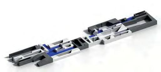
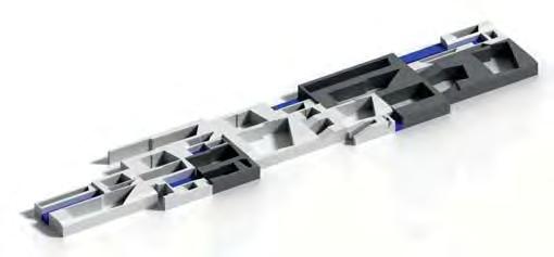
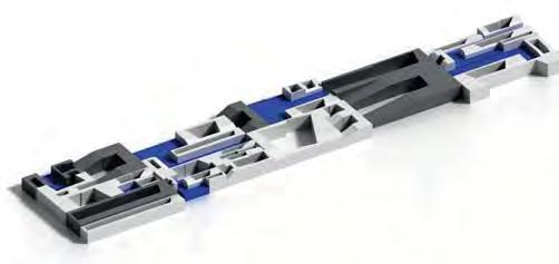
Type 2 Combination of Public facilities and Agriculture
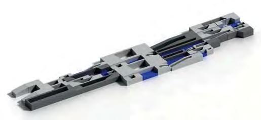
Type 3 Combination of Dwelling, Public facilities and Agriculture
Primitive Generation 1 5 from Generation 1 Generation 2 Generation 3 Programs Generation 4 Mutation 1 Selection Mutation 2 Mutation 3 Evaluation 2 Mutation 4 Evaluation 2
Gen4_16
Gen4_21
Gen4_26
Gen4_17
Gen4_22
Gen4_27
Gen4_18
Gen4_23
Gen4_28
Gen4_19
Gen4_24
Gen4_25
Gen4_29
Gen4_20
Gen4_30
— 64 —
Figure57 Genetic Algorithm - the patches of urban fabric generated from different combination of programs - narrow shape.
Bell curve of the population
mean value = 0.3728 standard deviation = 0.052378 mean value = 0.3728
Compacity
Compacity is quite similar to surface/volume ratio. It relates to heat island effect and natural lighting. It reflects the building’s ability to transfer heat through its envelope. For a given plot, more compacity means less heat gained or lose through the building. Compacity is affected by the parameter of surface transmission coefficient for the exterior wall
Primitive Generation 1 5 from Generation 1 Generation 2 Generation 3 Programs Generation 4 Mutation 1 Selection Mutation 2 Mutation 3 Evaluation 2 Mutation 4 Evaluation 2 Gl = ∑ Ki * Ai/ V Ex tWalls V Ki Ai (Head) building volume Area of the exterior wall Surface transmission coefficient for the exterior wall i (U- value) Criterion 1 - Capacity Formula lenge. CAPACITY
GEN4_1 0.363 GEN4_16 0.396 GEN4_2 0.415 GEN4_17 0.502 GEN4_3 0.337 GEN4_18 0.456 GEN4_4 0.358 GEN4_19 0.448 GEN4_5 0.409 GEN4_20 0.425 GEN4_6 0.297 GEN4_21 0.371 GEN4_7 0.281 GEN4_22 0.309 GEN4_8 0.333 GEN4_23 0.382 GEN4_9 0.354 GEN4_24 0.327 GEN4_10 0.356 GEN4_25 0.341 GEN4_11 0.399 GEN4_26 0.425 GEN4_12 0.421 GEN4_27 0.305 GEN4_13 0.435 GEN4_28 0.353 GEN4_14 0.326 GEN4_29 0.353 GEN4_15 0.373 GEN4_30 0.334 0 5 10 15 20 25 0.20.250.3 0.320422 0.425178 0.35 0.4 0.45 0.5
fit individuals standard deviation = 0.052378
Compa
Figure58 Genetic Algorithm - fitness criterion one - Compacity. — 65 —
cit y
Bell curve of the population
Mineralization
Mineralization is to calculate the ratio of water or vegetation in a plot. A high mineralization keeps the stable heat storage making the maximum temperature and minimum temperature delayed in that area. there are three effects of mineralization: energy storage, decreased evaporation and ground waterproofing. The mineralization is easy to calculate. It is the area of water or vegetation divided by the total area of studied urban fabric.
Primitive Generation 1 5 from Generation 1 Generation 2 Generation 3 Programs Generation 4 Mutation 1 Selection Mutation 2 Mutation 3 Evaluation 2 Mutation 4 Evaluation 2 M = (AT -∑Au)/AT i AT Au Total area of the studied urban fabric Useful area of the i element of water or vegetation 0 5 10 15 20 25 00.050.1 0.117772 0.150.20.25 0.255094 0.30.35 mean value = 0.186433 standard deviation = 0.068661 fit individuals mean value = 0.186433 standard deviation = 0.068661 GEN4_1 0.248 GEN4_16 0.113 GEN4_2 0.154 GEN4_17 0.276 GEN4_3 0.022 GEN4_18 0.226 GEN4_4 0.175 GEN4_19 0.118 GEN4_5 0.237 GEN4_20 0.333 GEN4_6 0.22 GEN4_21 0.175 GEN4_7 0.082 GEN4_22 0.135 GEN4_8 0.234 GEN4_23 0.251 GEN4_9 0.142 GEN4_24 0.216 GEN4_10 0.275 GEN4_25 0.194 GEN4_11 0.227 GEN4_26 0.212 GEN4_12 0.255 GEN4_27 0.181 GEN4_13 0.128 GEN4_28 0.119 GEN4_14 0.128 GEN4_29 0.133 GEN4_15 0.254 GEN4_30 0.13
ZATION
MINERALI-
Criterion 2 - Mineralization Formula
Figure59 Genetic Algorithm - fitness criterion two - Mineralization. — 66 —
Criterion 3 - Occusivity
Oc = ∑(Pbuilt /Punbuilt)/NHorizCuts
Occlusivity
Occlusivity concerns the openness to sky of a plot. Openness is closely related to solar incoming, wave radiation, ventilation, etc. it also evaluate the interactions between canopy, sky and roof area. it could be taken as a 3 dimensional express of the height/width ratio.
Primitive Generation 1 5 from Generation 1 Generation 2 Generation 3 Programs Generation 4 Mutation 1 Selection Mutation 2 Mutation 3 Evaluation 2 Mutation 4 Evaluation 2
OCCUSIVITY
GEN4_1 0.61 GEN4_16 0.501 GEN4_2 0.649 GEN4_17 0.331 GEN4_3 0.529 GEN4_18 0.473 GEN4_4 0.435 GEN4_19 0.425 GEN4_5 0.402 GEN4_20 0.368 GEN4_6 0.457 GEN4_21 0.467 GEN4_7 0.578 GEN4_22 0.371 GEN4_8 0.538 GEN4_23 0.465 GEN4_9 0.505 GEN4_24 0.359 GEN4_10 0.457 GEN4_25 0.399 GEN4_11 0.479 GEN4_26 0.523 GEN4_12 0.518 GEN4_27 0.335 GEN4_13 0.592 GEN4_28 0.414 GEN4_14 0.359 GEN4_29 0.39 GEN4_15 0.393 GEN4_30 0.425 mean value = 0.458233 standard deviation = 0.083604
Formula
Bell curve of the population
NHorizCuts NHorizCuts Pbuilt Punbuilt Number of horizontal cuts Built perimeter for the current cross section Unbuilt perimeter for the current cross section 0 5 10 15 20 25 0.2 0.3 0.4 0.5 0.6 0.374629 0.541837 0.7 mean value = 0.458233 standard deviation = 0.083604 fit individuals Figure60 Genetic Algorithm - fitness criterion three - Occusivity. — 67 —
mean height of the urban canopy in the a direction height of the (built or non built) element i of the canopy width of the element i of the canopy in the plane of direction a diameter of the studied urban
Rugosity
The indicator of rugosity concerns the degree of airflow on the ground is influenced by urban obstacles. The higher the wind speed in an area, the lower the rugosity that area is. There are absolute rugosity and relative rugosity. Absolute rugosity is calculated by the mean height of the urban plot, neglect ing the orientation. While relative rugosity considers the orientation factor by calculating the mean square deviation of the values at each cross section plane. People also use rugosity rose to record the performance of a plot.
Primitive Generation 1 5 from Generation 1 Generation 2 Generation 3 Programs Generation 4 Mutation 1 Selection Mutation 2 Mutation 3 Evaluation 2 Mutation 4 Evaluation 2 Ra =(√ ∑(hi-ha)2*li2)/∑ li ii ha hi li ∑ li
mean value = 0.4463 standard deviation = 0.030079 GEN4_1 0.47 GEN4_16 0.369 GEN4_2 0.402 GEN4_17 0.439 GEN4_3 0.409 GEN4_18 0.49 GEN4_4 0.437 GEN4_19 0.482 GEN4_5 0.422 GEN4_20 0.471 GEN4_6 0.462 GEN4_21 0.423 GEN4_7 0.468 GEN4_22 0.449 GEN4_8 0.46 GEN4_23 0.441 GEN4_9 0.44 GEN4_24 0.487 GEN4_10 0.464 GEN4_25 0.482 GEN4_11 0.464 GEN4_26 0.454 GEN4_12 0.479 GEN4_27 0.442 GEN4_13 0.461 GEN4_28 0.457 GEN4_14 0.403 GEN4_29 0.398 GEN4_15 0.45 GEN4_30 0.414 RUGOSITY
Formula Bell curve of the population Wind (a direction) 0 5 10 15 20 25 0.30.350.40.450.5 0.4162110.476379 0.55 mean value = 0.4463 standard deviation = 0.030079 fit individuals Figure61 Genetic Algorithm - fitness criterion four - Rugosity. — 68 —
canopy
Criterion 4 - Rugosity
Bell curve of the population
Solar admittance
Solar admittance calculates the amount of incoming solar energy all the walls gain. The orientation is quite importance. There are factors for walls with different orientations. And the wall facing to north and the wall facing to south perform differently. Solar admittance also concerns the shading ratio, reflected to incoming radiation ratio and the ratio of adjacent walls to total wall.
Primitive Generation 1 5 from Generation 1 Generation 2 Generation 3 Programs Generation 4 Mutation 1 Selection Mutation 2 Mutation 3 Evaluation 2 Mutation 4 Evaluation 2 0.6 0.4 0.2 0.4 Gl = ∑ Ki * Ai/ V Ex tWalls V Ki Ai (Head) building volume Area of the exterior wall Surface transmission coefficient for the exterior wall i (U- value)
- Solar admittance Formula SOLAR
Criterion 5
ADMITTANCE
GEN4_1 0.295 GEN4_16 0.261 GEN4_2 0.312 GEN4_17 0.182 GEN4_3 0.284 GEN4_18 0.239 GEN4_4 0.271 GEN4_19 0.231 GEN4_5 0.228 GEN4_20 0.211 GEN4_6 0.324 GEN4_21 0.232 GEN4_7 0.359 GEN4_22 0.233 GEN4_8 0.281 GEN4_23 0.246 GEN4_9 0.262 GEN4_24 0.22 GEN4_10 0.286 GEN4_25 0.232 GEN4_11 0.251 GEN4_26 0.266 GEN4_12 0.267 GEN4_27 0.214 GEN4_13 0.24 GEN4_28 0.238 GEN4_14 0.229 GEN4_29 0.21 GEN4_15 0.24 GEN4_30 0.249 mean value = 0.2531 standard deviation = 0.037254 0 5 10 15 20 25 0.1 0.15 0.2 0.25 0.3 0.215846 0.290354 0.35 mean value = 0.2531 standard deviation = 0.037254 fit individuals
Figure62 Genetic Algorithm - fitness criterion five - Solar admittance. — 69 —
Primitive Generation 1 5 from Generation 1 Generation 2 Generation 3 Programs Generation 4 Mutation 1 Selection Mutation 2 Mutation 3 Evaluation 2 Mutation 4 Evaluation 2 170.182 290.21 200.211 270.214 240.22 50.228 140.229 190.231 210.232 250.232 220.233 280.238 180.239 130.24 150.24 230.246 300.249 110.251 160.261 90.262 260.266 120.267 40.271 80.281 30.284 100.286 10.295 20.312 60.324 70.359 170.331 270.335 140.359 240.359 200.368 220.371 290.39 150.393 250.399 50.402 280.414 190.425 300.425 40.435 60.457 100.457 230.465 210.467 180.473 110.479 160.501 90.505 120.518 260.523 30.529 80.538 70.578 130.592 10.61 20.649 70.281 60.297 270.305 220.309 140.326 240.327 80.333 300.334 30.337 250.341 280.353 290.353 90.354 100.356 40.358 10.363 210.371 150.373 230.382 160.396 110.399 50.409 20.415 120.421 200.425 260.425 130.435 190.448 180.456 170.502 30.022 70.082 160.113 190.118 280.119 130.128 140.128 300.13 290.133 220.135 90.142 20.154 40.175 210.175 270.181 250.194 260.212 240.216 60.22 180.226 110.227 80.234 50.237 10.248 230.251 150.254 120.255 100.275 170.276 200.333 160.369 290.398 20.402 140.403 30.409 300.414 50.422 210.423 40.437 170.439 90.44 230.441 270.442 220.449 150.45 260.454 280.457 80.46 130.461 60.462 100.464 110.464 70.468 10.47 200.471 120.479 250.482 190.482 240.487 180.49 Capacity Mineralization Occusivity Rugosity Solar admittance Figure63 Genetic Algorithm - the list of all the values in five fitness critetia and their comparation and selection.
— 70 —
Compacity
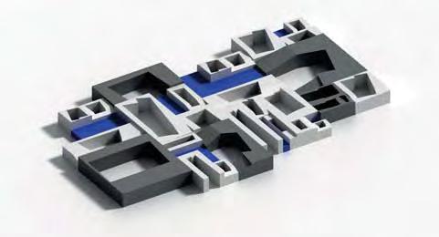
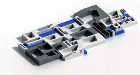
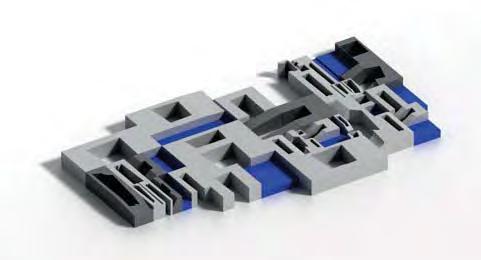

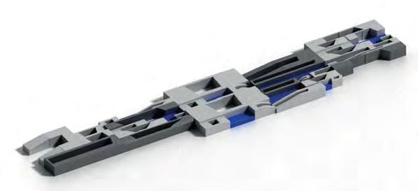
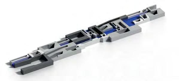
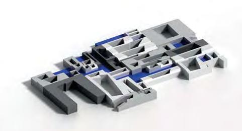

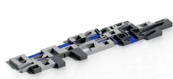
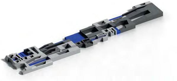

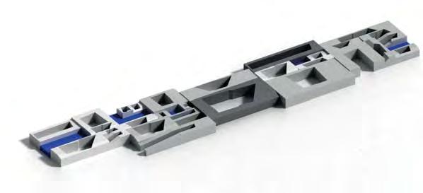
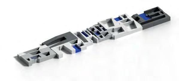
3.2 Experiment 1 3.2.5 Evaluation 2 and conclusion
After the grading, all the five values for each patch are listed together. Showing from the 5 indicators, every patch performs quite uniquely. But we can still find the individuals with all 5 score in the relatively fit range. Such individual are kept for their benefiting role in urban micro climate. The plots left with their better climatic performance are presentation in the above of this page.
Primitive Generation 1 5 from Generation 1 Generation 2 Generation 3 Programs Generation 4 Mutation 1 Selection Mutation 2 Mutation 3 Evaluation 2 Mutation 4 Evaluation 2 Capacity Mineralization Occusivity Rugosity admittance Solar 0.358 0.175 0.435 0.437 0.271 Capacity Mineralization Occusivity Rugosity admittance Solar 0.409 0.237 0.402 0.422 0.228 Capacity Mineralization Occusivity Rugosity admittance Solar 0.333 0.234 0.538 0.46 0.281 Capacity Mineralization Occusivity Rugosity admittance Solar 0.354 0.142 0.505 0.44 0.262 Capacity Mineralization Occusivity Rugosity admittance Solar 0.399 0.227 0.479 0.464 0.251 Capacity Mineralization Occusivity Rugosity admittance Solar 0.373 0.254 0.393 0.45 0.24 Capacity Mineralization Occusivity Rugosity admittance Solar 0.371 0.175 0.467 0.423 0.232 Capacity Mineralization Occusivity Rugosity admittance Solar 0.382 0.251 0.465 0.441 0.246 Capacity Mineralization Occusivity Rugosity admittance Solar 0.341 0.194 0.399 0.482 0.232 Capacity Mineralization Occusivity Rugosity admittance Solar 0.425 0.212 0.523 0.454 0.266 Capacity Mineralization Occusivity Rugosity admittance Solar 0.353 0.119 0.465 0.457 0.238 Capacity Mineralization Occusivity Rugosity admittance Solar 0.334 0.13 0.425 0.414 0.249
Figure64
Genetic Algorithm - the final 12 urban patches selected after the series of mutations and evaluations.
— 71 —
large-scaleblock greateffectinwaterdefensive andlargeswirlisgenerated
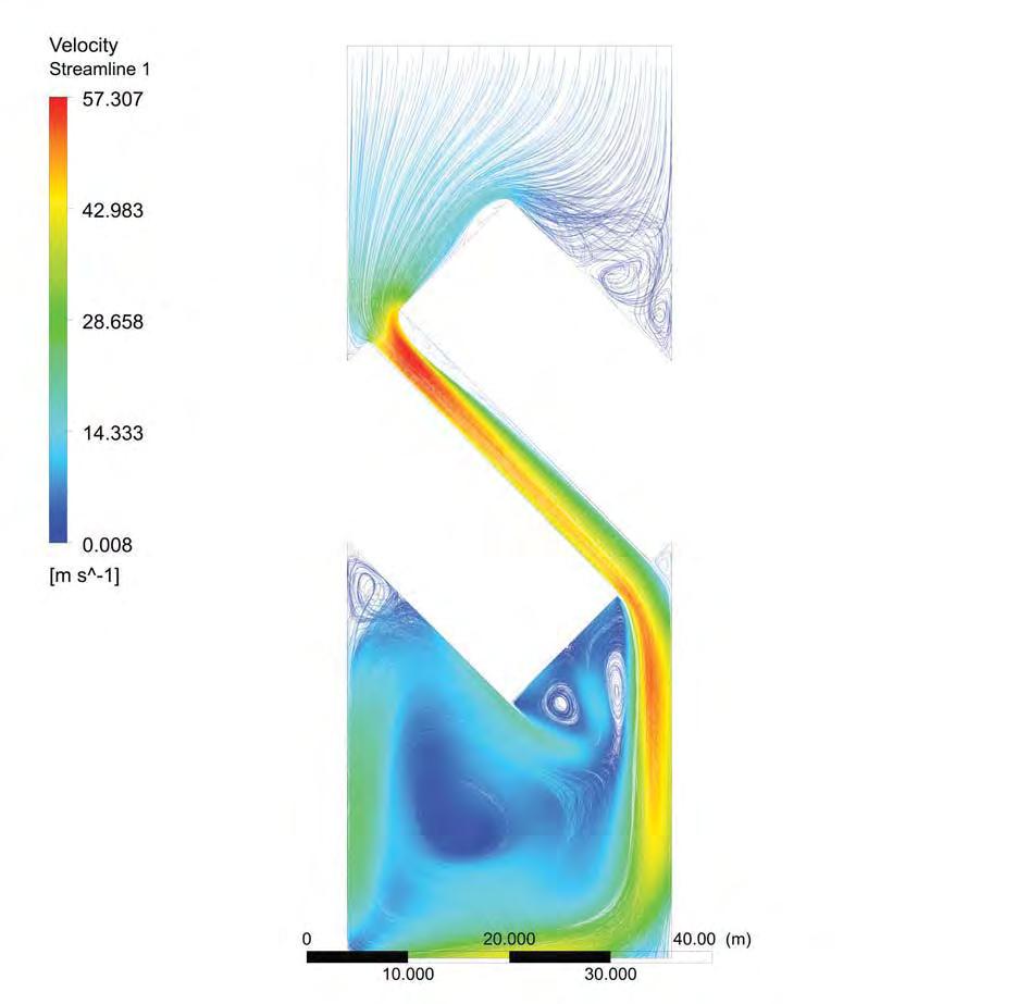
middle-scaleblock obviouseffectinwaterdefensive andswirlisgenerated
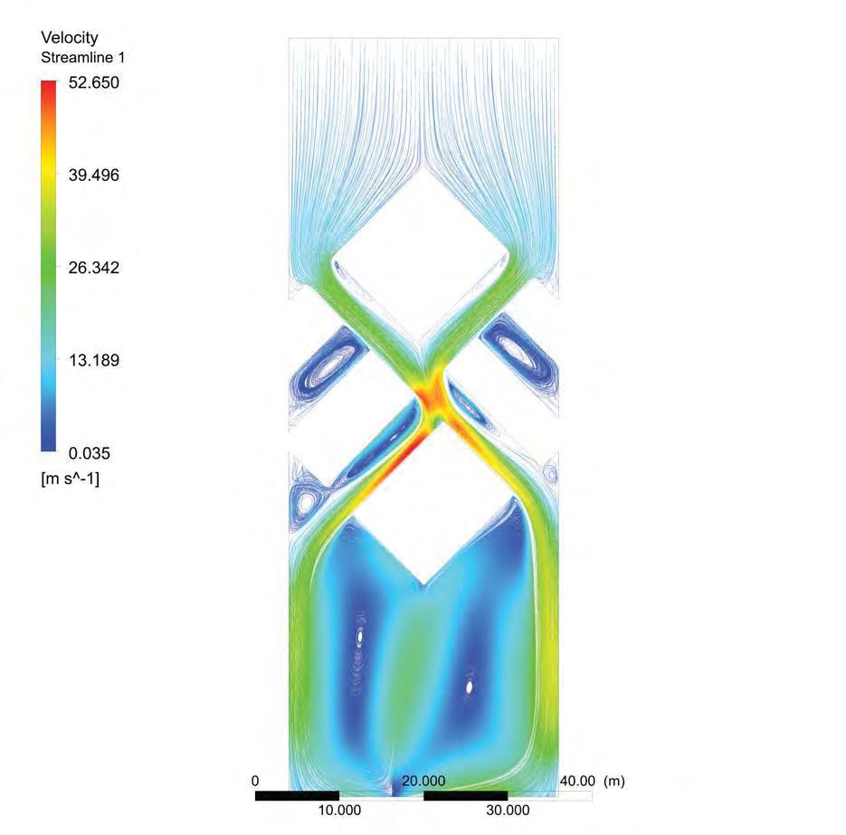
The ANSYS fluid simulation of the blocks environmental effect on the velocity of water flow.
3.3 Experiment 2
3.3.1 Water flow test
The second part of experiments is physical simulation on water flow which is conducted in ANSYS. In the part of genetic algorithm, a great amount of blocks with various dimensions are produced. In the aspect of fluid dynamic, when an object is placed into a water current, it will affect and redirect the flow. The level of influence is highly related to the size of the object. In the ANSYS simulation, we compared the block clusters composed of different size of blocks. From the top view of the result, we can see that the monolithic form of block cluster obstructs the water and makes the water velocity increase sharply when changing the water flow’s direction. The fragmentary form of block cluster, instead of simply obstructing the water, provides many small channels for the water to go through and thus decrease the impact and erosion from the water. This experiment helps us decide the position of blocks with different sizes according to the local water velocity.
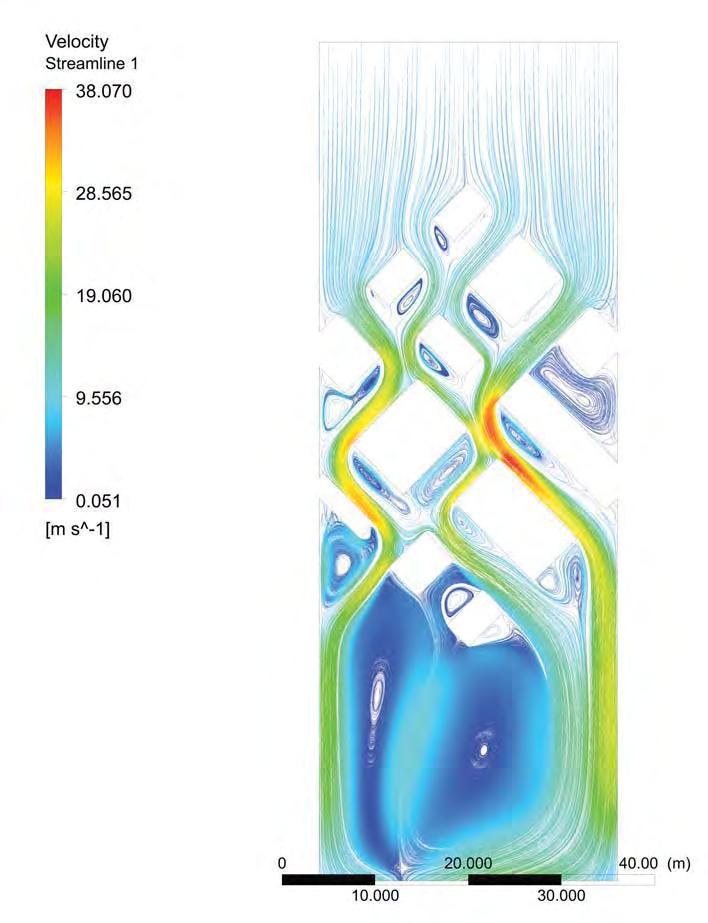
small-scaleblock changedirectionandspeedof waterflow
5.307 4.908 3.212 1.504 0.008 5.265 3.946 2.634 1.318 0.035 3.807 2.856 1.906 0.955 0.051
Figure65
— 72 —
— 73 —
— 74 —
Chapter 4. Design Development
4.0 Introduction
4.1 Site context
4.2 From experiment to application
4.2.1 Section conditions
4.2.2 Adjustment and match of urban plots
4.3 Urban grid generation
4.3.1 The factor of water flow
4.3.2 The distribution of starting points
4.3.3 The application of diffusion limited aggregation
4.3.4 The pattern growth of Hydroville
4.4 Evaluation
— 75 —
4.0 Introduction
This chapter exhibits exploration on how to realize the structural deformation achieved in the real scale. Considering the local economic conditions and Industrial Development, bamboo with banding techniques is chosen to be the most proper material. By defining rigid joint and pin joint, it is able to control the degree of deformation and eliminate the unexpected movement, which will make the whole structure more stable and efficient for the users. On the other hand, supporting method is also carefully studied according to the village’s topography and soil conditions.
For the floating device, recycled empty plastic bottles combined in a membrane deflated system proved to be an ideal choice. The calculation is done under the guide of design criteria of office building, so we will know the minimal depth of each pad. Shading variations are embodied in the color and interval of bottles. After addressing the technical details, some prototypes are developed to fit on the specific site for typical
scenarios to meet the requirements such as pedestrian bridge, fishing facilities and entertainment. In a higher hierarchy, the unban-scale spread mainly follows the index of programmatic configuration. These design developments are conducted based on experiments and lead to design proposal.
— 76 —
The site we choose locates on the riverside to the southwest of the ancient Angkor Wat city. It is on the branch of Tonle Sap Lake. The local agriculture depends heavily on the irrigation from natural water body. Due to the changing water level, the agriculture shows great seasonal difference. The area is surrounded by vast flood forest which also benefits from the annual fluctuation of Tonle Sap Lake. In terms of the existing infrastructure, two main roads have been constructed along the river running straight to the Angkor city. They connect this lakeside region to the inland. In terms of the existing program arrangement, with the river running through in the middle, the residential district is situated along the main roads for the transportation consideration. Agriculture district is at the back of the dwelling where close to water resource. The turning points of the river, where the earth
4.1 Site context
deposits as the river slow down to form small areas of plain, become the public areas for the commercial, industry and community activities.
This model was built according to landscape contours and topographic data. It is quite clear the slop of the inner river bank is quite sharp; on the contrary, lands next to flood forest have very gentle photography. Curvature of slops mainly follows the river shape. In wet season these parts are merged in the flood for most of the time; in the dry season they will emerge from water surface.
Flood forest Flood forest
to TonleSap lake Flood forest Flood forest Flood forest Main street FloodplainFloodplain 0 M250 M500 M FloodplainFloodplain Main street Main street Flood forest Flood forest tre t st s str n ns a Ma M in ain ai i Existing public space
public space
to Angkor Wat
Existing
— 77 —
Figure66 The environmental and social context of the site.
Section 1 Section 2 Section 3 Section 4 Section 5 Section 6 Section 7 Section 8
eight sections. — 78 —
Figure67 The topview of the site and the positions of the
4.2 From experiment to application
4.2.1 Section conditions
A further understanding is made by studying the section conditions of the river. To start our proposal, we chose 8 key locations in terms of river geomorphology and hydrology. Due to erosion, sedimentation, and water pressure caused by turbulence, the most critical situation usually occurs on the parts of river which has bigger curvature. 8 particular sections are extracted perpendicular to the river. They vary in river width, orientation and bank condition; so generally speaking, these 8 sections mainly covered all the characters of this area. They are put in the same coordinate grid to visually compare these sections. The range of river width, bank slope, and geographic features are very clear to read.
Section 1 Section 2 Section 3 Section 4 Section 5 Section 6 Section 7 Section 8
Figure68 The profiles of the urban plots on the coordinate system background for the mophology comparation
— 79 —
Section 1 Section 3 Section 5 Section 7 Total area: 60365 M 2 (100%) Maximal available area: 42186 M 2(70%) Minmal available area: 8650 M 2(14%) Length: 600 M Width: 100 M Orientation to north: 88.2 O Existing streets: 1 Length: 600 M Width: 100 M Orientation to north: -87.2 O Existing streets: 2 Length: 600 M Width: 100 M Orientation to north: -80.8 O Existing streets: 2 Length: 600 M Width: 100 M Orientation to north: -50.1 O Existing streets: 2 Total area: 60605 M 2 (100%) Maximal available area: 44071 M 2(73%) Minmal available area: 13162 M 2(22%) Total area: 60314 M 2 (100%) Maximal available area: 49065 M 2(81%) Minmal available area: 15760M 2(26%) Total area: 60232 M 2 (100%) Maximal available area: 48084 M 2(80%) Minmal available area: 8727 M 2(14%)
Figure69 (left page) The detailed section information of plots 1-4 and the comparataion of the conditions in dry season and wet season.
— 80 —
Figure70 (Right page) The detailed section information of plots 5-8 and the comparataion of the conditions in dry season and wet season.
4.2 From experiment to application
4.2.1 Section conditions
Based on these 8 sections, 8 pieces of 600m X 100m slots are studied carefully. The details of the sections are investigated. The information collected for each of the sections includes the length, width, area, orientation and number of roads. The diagrams also compare the situation and available land area in dry season and wet season respectively. The detailed information is the basis of the urban intervention.
In the next page, the urban patches generated in genetic algorithm experiments are placed on the sections according to their programmatic and climatic performance and the section conditions of the site.
All the categories studied refer to the criteria in experiment part. For example, the orientation of axis has a tight relationship with our criteria: rugosity, which is one of the most important indicators for ventilation; and solar admittance, which describes heat gain and loss. Similarly, available area and water condition in both seasons are the key factors for program finding. The slot that has relatively high percentage of exposed area and convenient transportation is more suitable for public and commercial, however those have extreme changes are perfect for agriculture, as it is the ideal environment for floating rice’s growth.
Though certain manipulations, such as height adjustment, grid alignment, shape shifting, suitable individuals are fitted on site to meet all the requirements from those 8 plots. However this is starting, as there are still lots of issues to consider about, and more study is needed for further global form finding.
Section 2 Section 4 Section 6 Section 8 Length: 600 M Width: 100 M Orientation to north: -70.5 O Existing streets: 1 Length: 600 M Width: 100 M Orientation to north: 44.3 O Existing streets: 2 Length: 600 M Width: 100 M Orientation to north: -60.8 O Existing streets: 2 Length: 600 M Width: 100 M Orientation to north: -27.9 O Existing streets: 2 Total area: 60243 M 2 (100%) Maximal available area: 26854 M 2(46%) Minmal available area: 6862 M 2(11%) Total area: 60960 M 2 (100%) Maximal available area: 44285M 2(73%) Minmal available area: 12377 M 2(20%) Total area: 60517 M 2 (100%) Maximal available area: 43524 M 2(72%) Minmal available area: 13800 M 2(23%) Total area: 60267 M 2 (100%) Maximal available area: 44885 M 2(74%) Minmal available area: 7402 M 2(12%)
— 81 —
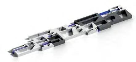
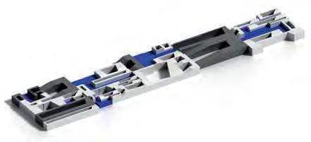
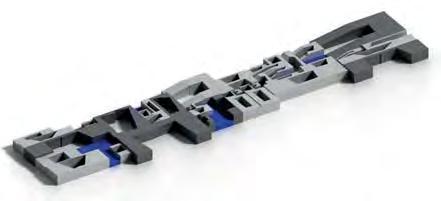
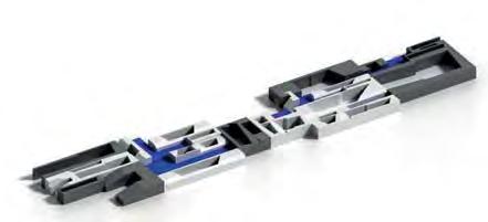
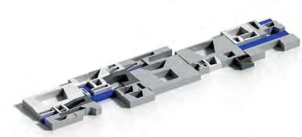
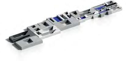
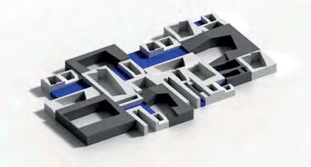
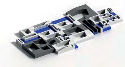
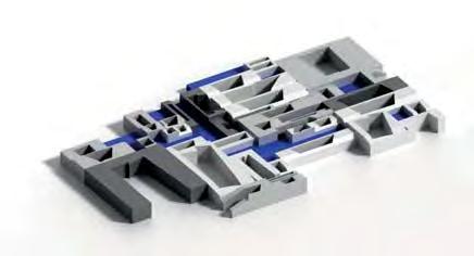
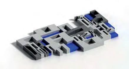
Section 1
Section 3
Section 5
Section 7
Section 2
Section 4
Section 6
Section 8
— 82 —
Figure71 Urban patches generated in the Genetic Algorithm experiment are matched to the specific stie plots.
4.2 From experiment to application
4.2.2 Adjustment and match of urban plots
The patches of urban fabric selected in the Genetic algorithm process are adjusted and matched with the urban plot extracted from the site according to the section conditions studies previously.
— 83 —
Maya simulation on water flow in dry season and wet season respectively.
Urban grid generation
4.3.1 The factor of water flow
To grow a village along the river, the primary factors need to be considered are the water flow and river curvature. This page is to map the site in the aspects of water flow. First of all, the water flow in that area is simulated in software. The blue arrow in the diagrams expresses the water velocity by its length and flow direction by its orientation. The two pictures compare the situations in dry season and wet season respectively.
In wet season most of the land is merged in water and turbulences mainly occur on the left bank. In dry season, water condition is less complicated and velocity is much lower. Generally, to understand the
water conditions in two scenarios, such as water area, velocity, and direction are essential in the whole process.
As has been stated in the previous chapter (ANSYS simulation experiments, Chapter 3), water velocity and direction affect the size and orientation of the blocks. In the area water velocity is high, is better to place smaller blocks to avoid erosion from the water. And conversely larger blocks can placed in the area water velocity is low.
4.3
Figure72
— 84 —
bank and river curvature points distribution
growth of streets
vcv
The diffusion limited aggregation algorithm (introduced in Chapter Two) informs the process of urban growth. The pictures explain how the positions of seed points are decided. A series of seed points are fixed first then the street gird is grows from these points in the normal direction of the river curve. To be suitable for inhabitancy, the density of street should be controlled in a certain range. According to the geometric relationships, streets from the concave parts of the curve tend to converge and from the convex parts of the curve tend to diverge. Therefore, to keep a relatively even street distribution, curvature and
4.3 Urban grid generation
4.3.2 The distribution of starting points
bending direction of the river should be considered in deciding the position of starting points. That is, in the concave areas the seed points are scattered sparsely and the high the curvature, the sparse the points. On the contrary, in the convex areas the seed points are scattered densely and the high the curvature, the dense the points.
Based on this principle, a logical solution was raised to make sure all the main streets are in a reasonable interval, which means they could cover reasonable area. In another word, the main streets will not be too far or too closed to each other.
Figure73 The starting points distribution and its relationship with river curvature and bending directions.
— 85 —
Environment pressure
River form
Contour lines
Vgrow Vmin. Vmax.
Condition 1
River form
If Driver < Dcertain then Vmin.<Vgrow<Vmax.
Driver : distance to river
Dcerta n : certain distance (influence distance of river)
Vgrow : vector of the growth
Vmin : minimal vector (curvature vector of river - tolerance)
Vmax. : maximal vector (curvature vector of river + tolerance)




Condition 3

Test area


If Dent < Dencertain then Branchnew
Dent : density of the test area
Dencerta n : certain density (according to program)
Vgrow : vector of the growth
Branchnew. : new branch
Parameter 1
Length of the growth vector
|Vgrow| = Dimpolder ± tolerance
|Vgrow| : length of the growth vector
Dimpolder : dimension of the polder(according to programs)
Vgrow : vector of the growth
Vgrow
Vgrow |Vgrow|
— 86 —

Condition 2
Closest contour line
If Driver > Dcertain
Driver : distance to river
Dcertain : certain distance (influence distance of river)
Vgrow : vector of the growth
Vmin : minimal vector (curvature vector of closest contour - tolerance)
Vmax. : maximal vector (curvature vector of closest contour + tolerance)
Paramter 2
Infrastructure branch
Gnumber : number of gerenation depends on water area of dry season and position of floodforest
G3 : Gerenation 3 Vgrow
4.3 Urban grid generation
4.3.3 The application of diffusion limited aggregation
The growth of a small patch from the site illustrates how the process of diffusion limited process is applied. With the starting points fixed for an appropriate street density, the next factors that will affect the growth of the grid pattern are the river curve and contour lines’ morphology. The principle is at the beginning of the growth, the growth vector is in the normal direction of the river. After several generations, the vector will always try to be perpendicular to the nearest contour line within a tolerance. The vector length is also limited in a certain range. In this way, a street is generated in a zigzag shape. When two streets starting from two adjacent points diverge and get far away from each other, there will be a branch street growing from one of them. Where the street stop growing or the number of growing generations are decided by the water area in dry season and the position of flood forest.
In the history of urbanism, the similar relationship between the street distribution and river morphology could also be found in the formation of many cites built on water. The Venice city (Case study, Chapter 1) is one of the best known examples.
Vmin.<Vgrow<Vmax.
then
Vmin. Vmax G0 G1 G2 G3 G4 G5 G6 G7 G8 G9 G10 G11 G12
Figure74-79
The six steps of generation streets pattern under the priciple of diffusion limites aggregarion,
— 87 —


Point distribution
Initial growth








Main structure (diffusion limited aggregation)
Figure80-83 (Left page and right page) The generation of global grid and the subdivision according to water velocity. — 88 —




Secondary networks according to water velocity (subdivision)
Infrastructural network
— 89 —
4.3 Urban grid generation
4.3.3 The pattern growth of Hydroville
The previous pages demonstrate the global growth informed by diffusion limited algorithm. The same with the small part we have explained before, first of all, the starting points are distributed according to the degree of concave and convex of the river. Then, the street’s growth is initiated in the direction of river curvature. After that, the growth vector always tries to keep perpendicular to the nearest contour line as the street’s length increases. When the branches are generated, they are connected at each node transversely forming a deformed gird system. This is the first hierarchy of street grid. The street grid is going to be filled with blocks. Considering the influence of water flow, the grids locate at the area with high water velocity are subdivided into smaller grids. Based on water diverting experiments in chapter 3, subdivisions are necessary for areas have high water velocity. By reducing block size and adding more channels, both maximal velocity and average velocity can be largely reduced to a reasonable range, which is safe and comfortable for further urban developments. In this way the global infrastructure network pattern is generated.
4.4 Evaluation
The adaptivity
The material and architectural form fully reflect the local environmental conditions. With is extreme change of contemporary climate, the issue of whether the existing structure can survive and adapt to the environment is becoming more and more important. It is very necessary to change mind and search for new methodologies and techniques in architecture design, as the traditional monotonous architectural form and construction way cannot satisfy the adaptive requirements from the changing society and nature.
Material
The stability, accessibility and cost should be considered together in the material selection. Under this principle, most of the time, many kinds of material are used together and work according to different requirements and conditions. The material gradient is another parameter in parametric design.
Cost
The GDP per capita of Cambodia is US$ 774.95, which is relatively low compared to its neighbors. It means budget would be a very critical part of this project. The roughly calculated cost for this projects is 200-300 US$, given that all materials are local. Although it is much cheaper than regular constructions, a project in this scale would still face financial problems.
Unpredictable effect for tourism
Working as infrastructure for float¬ing villages, this adaptive living system is unique enough to attract people worldwide. Sometimes the boost in tourism is not good for the original lifestyle of locals. For example, pollution may disturb ecological system then reduce the production of fish and rice, and culture intrude may bring unstable factors into local society. These side effects should be carefully considered in the whole design process.
Population Growth
Population growth is the primary problem for de¬veloping country to solve. This adaptive living system should also adapt to social environment apart from natural variations. Some of the functions will be in greater demand than others, like dwelling and public spaces, etc.So how to balance all the inputs and configurations will become a new topic. These foreseeable questions will place more obstacles in front of us.
— 90 —
Chapter 5. Design Proposal
5.1 Programmatic organization
5.2 Global configuration
5.2.1 Artificial water system
5.2.2 Transportation
5.3 The detailed design on a piece of urban plot
5.4 Water drainage system
5.5 Material gradient
5.6 Time dimension of the urban intervention
5.7 Renderings
— 91 —
5.1 Programmatic organization
The village in less developed country is unlike metropolitan city. The most significant difference is the urban program planning. Urban zones are the main character of metropolitan city in which different programs like dwelling and industry are demarcated in a certain area. There is no overlap, and the connections of different zones are fixed and monotonous. The situations in rural area are different. Generated spontaneously, many programs are smaller in scale and are overlapped and mixed in a heterogeneous area. In this project, the program organization follows the same principle.
There are three main programs in this project – agriculture, dwelling, public facilities. In deciding the position of agriculture, the adjacency to water resource is considered first. The unique character in the site is the vast flood plain form by the annual flooding. Considering the fertile soil and adequate water, the agriculture land is arranged in the periphery of the site. Public facilities are scattered sparsely on the site for the easy accessibility. And dwellings are arranged near two the river for transportation convenience. Given that most local residents are farmers, a proper scale of residential district with sufficient infrastructures, multiple programs and easy access to their working fields will definitely their demands.
Generally speaking, at this stage, there is no obvious variation in different parts; all the three programs are organized together according to natural environment. By weaving into each other organically, all the urban patches play an essential role in the development of this area.
— 92 —
Public facilities
Agriculture
Dwelling
— 93 —
Figure84 The three layers of axonometric drawings describing the global program organization.
Water storage
Artificial water system
Existing street
Circulation
Agriculture (fishfarming ,floating rice)
Drainage channel (gravity-based)


Axonometric view
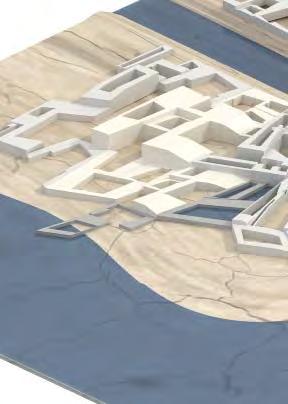


Schematic drawing(dry season)
5.2 Global configuration
5.2.1 Artificial water system

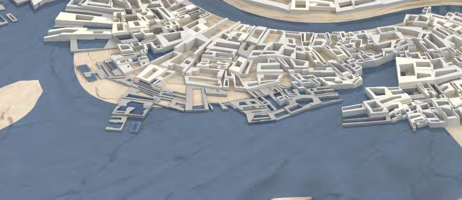


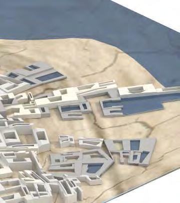


As we stated in the design strategy, the “polder block” are designed to have both the defensive function and the resident function. A single block unit is already the integration of multi functions. However, in the combination, the situations are much more complicated. When several blocks are combined together with different height, their relationship with water can be various. Generally speaking, the periphery walls will become water defense, and the inner walls are protected and in habitable. But as the water level rises, some periphery blocks with low height are submerged at one time (normally these blocks are agricultural blocks for rice paddy or fish farming). When the water level falls in dry season, water in the block will not fall with the outside water body. In this way the blocks capture a certain amount of water and become water storage. So with the combination of blocks, the functions of a block can be water defense,
water storage and inhabitable residence. And different functions sometimes are interconvertible responding to the outside water level changes.
The first layers of these two axonometric drawings mark out the different blocks with three basic functions. In wet season, the system are composes of defensive wall, semi-defensive wall, inhabitable wall and water storage. In dry season, the blocks for water storage could also benefit the water drainage system. (The details on artificial water drainage system will be discussed later in this chapter).
The bottom layer is the bird view of the design proposal. Urban patches dispersed along the river with tentacles reach in to surrounding water body.
Connection (on the ground )
Connection (on the roof )
Figure85 The three layers of axonometric drawings describing the artificial water system and tranpostation ways in the dry season.
— 94 —
Artificial water system Water


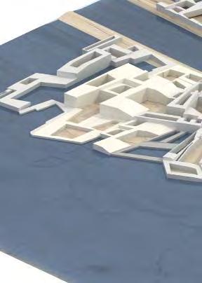


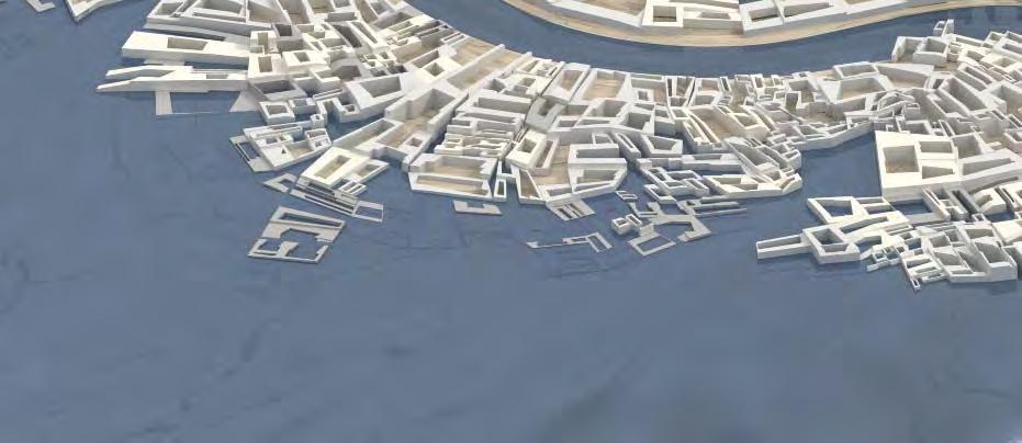


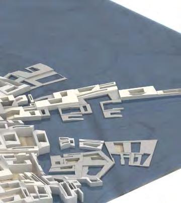


5.2 Global configuration
5.2.2 Transportation
The three types of blocks compose the urban infrastructure network with the roofs becoming roads for transportation. The second layers of the two axonometric drawings show the transport organization and transformation. Here we consider the transportation in the two extreme seasons as the situations are significantly different under the influence of the water level difference. In dry season, as large area of land appears out of the water, the transportation way is a combination of roof roads and ground roads. In the wet season, as water floods, the transportations way is a combination of water way and roof roads. The roof roads guarantee the smooth connections between different parts of the village.
storage Existing street Semi-watredefence Waterdefence Boat route
Connection (on the roof )
Circulation
Axonometric view
Schematic drawing(wet season)
Figure86 The three layers of axonometric drawings describing the artificial water system and tranpostation ways in the wet season.
— 95 —
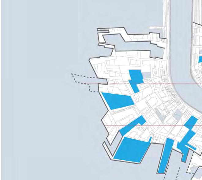
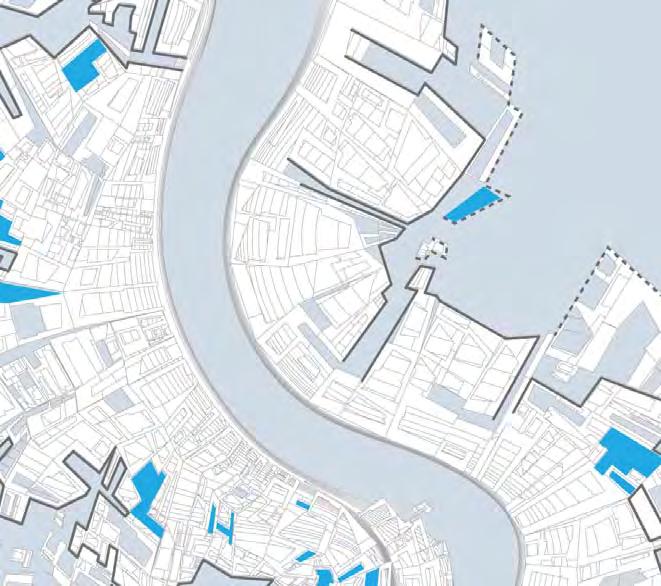
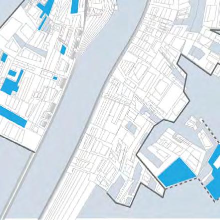
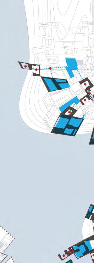
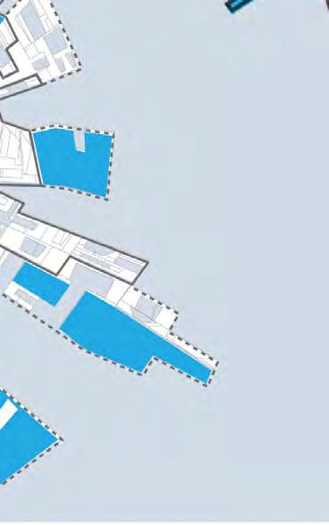
— 96 —
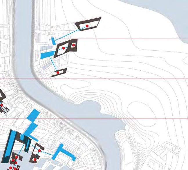
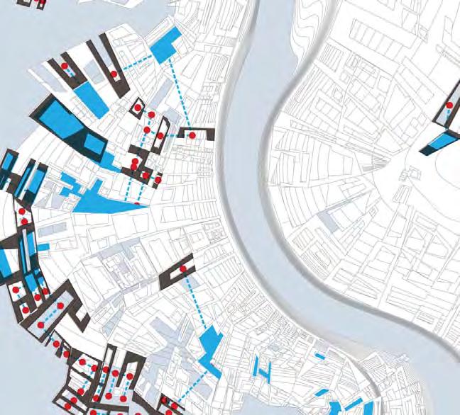
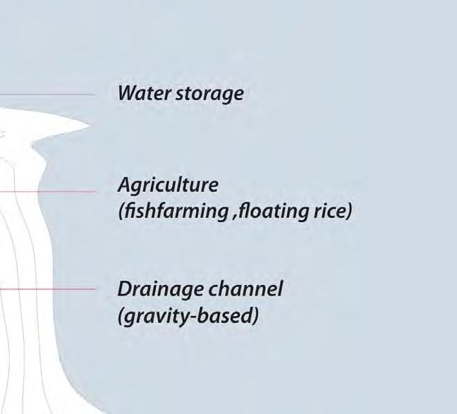
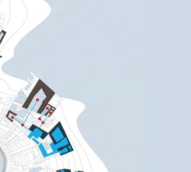
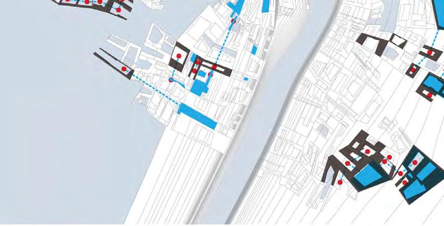
— 97 —
Figure87 The topview of artificial water system in wet season adn dry season.
F i
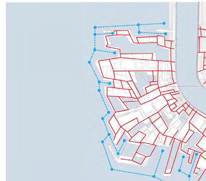
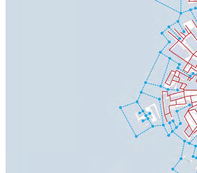
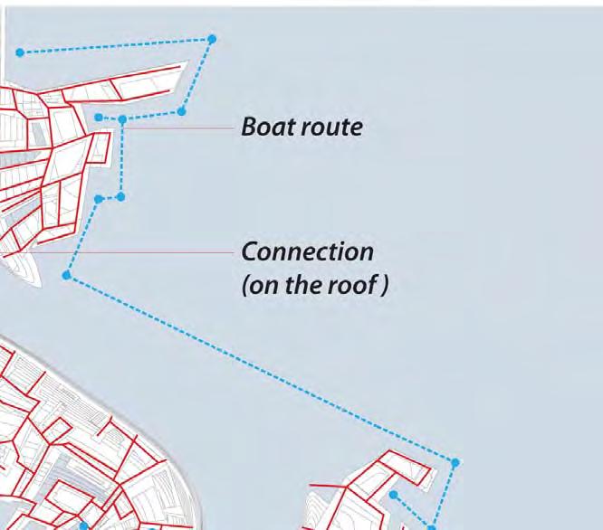
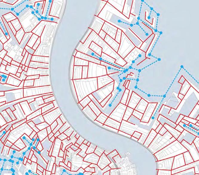

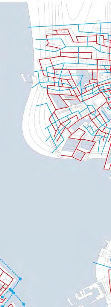
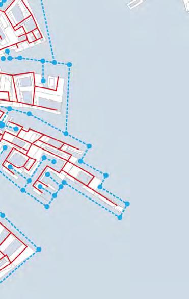
— 98 —
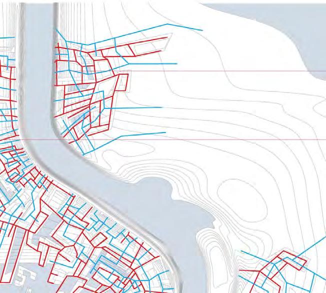
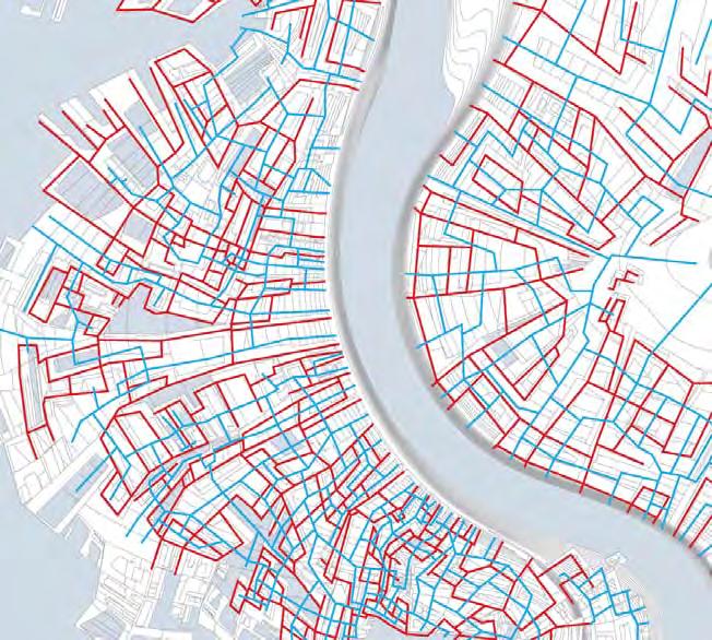
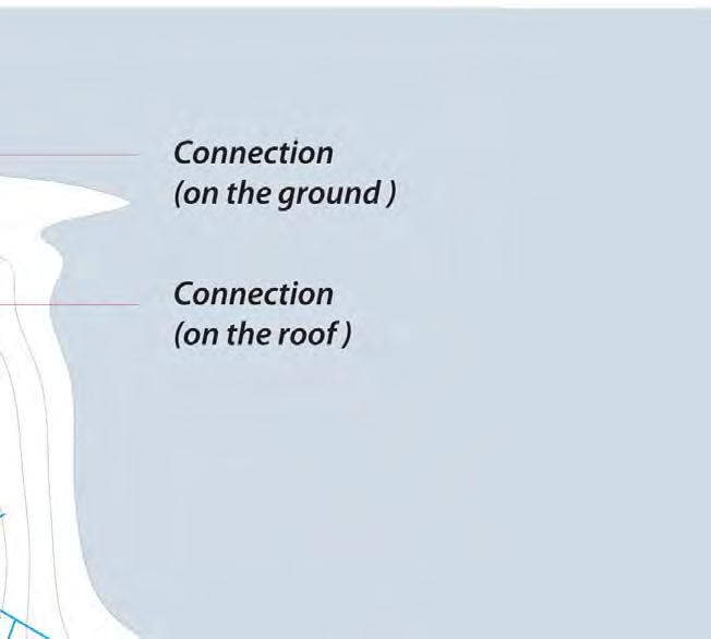
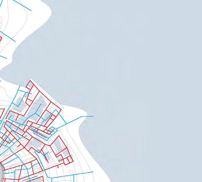
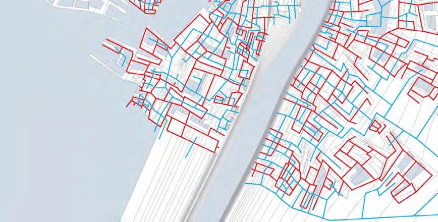
F
— 99 —
Figure88 The topview of transportation management in wet seaon and dry season.
m
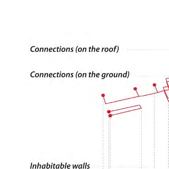
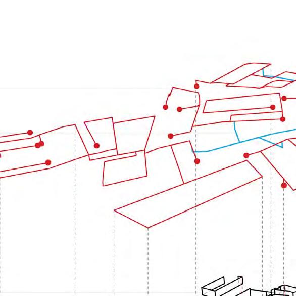
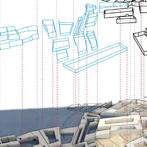
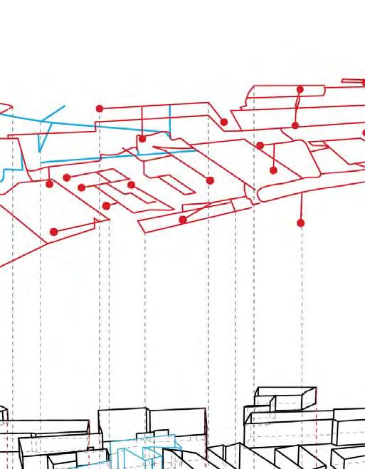
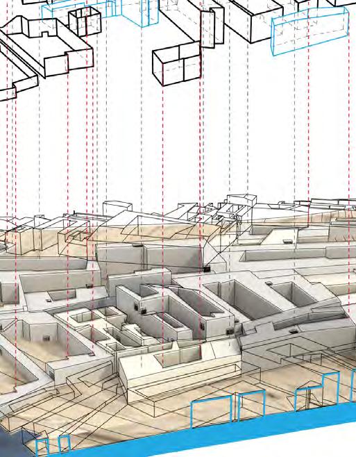

— 100 —
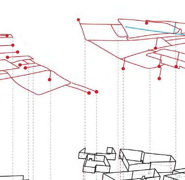
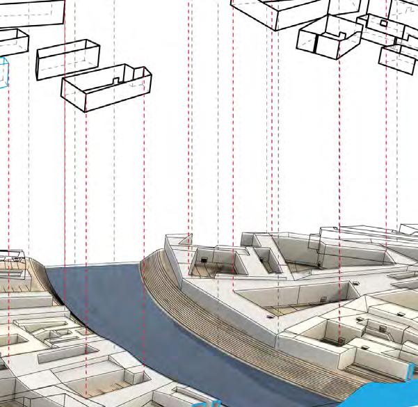
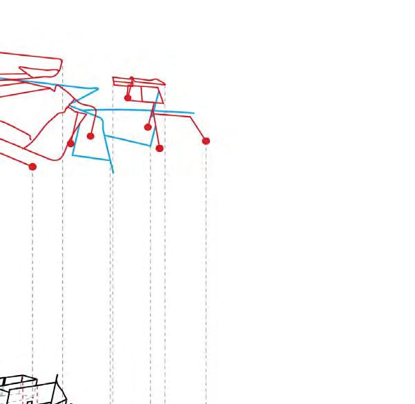
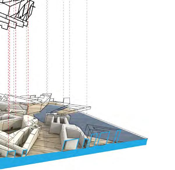


Figure89 A small area of the composite from the global plan describing in detail the transport organization and water management system in dry season.
5.3 The detailed design on a piece of urban plot
For the detailed design, a patch of urban plot is selected. The architectural issues considered here include the realization of traffic on the roof, and the distinction between different functions of the exterior walls. The blocks are always with different height determined by the program and water management consideration. To make sure the smooth traffic on the uneven roof surface, ramps and stairs are used to connect different height. As in this small rural area, the roads are mainly for people walking through, motor traffic are not considered. Transport way in dry season in the combination of roof road and ground road. And in wet season is the combination of roof road and water way.
— 101 —
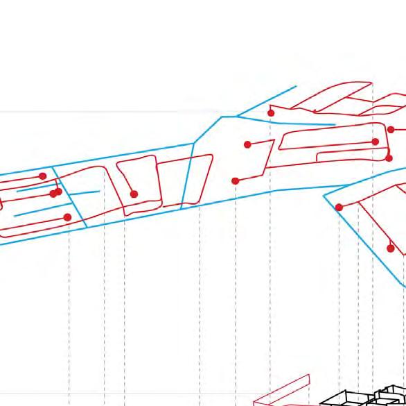
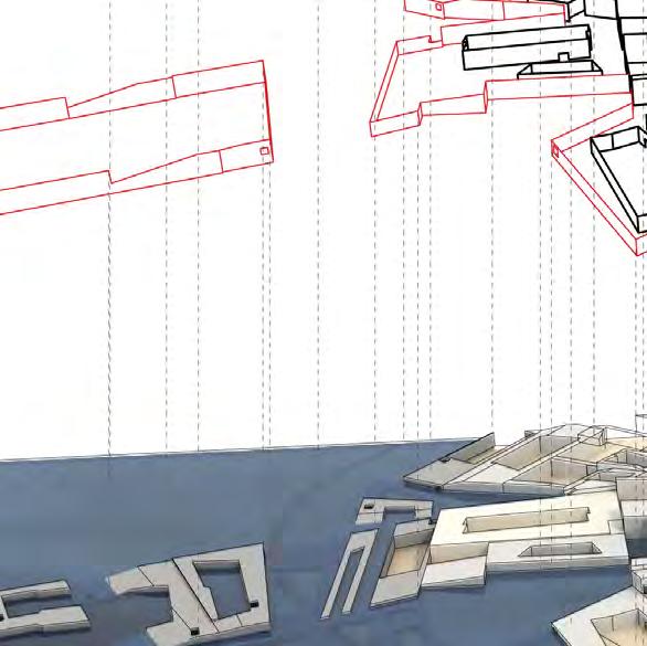


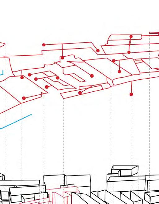
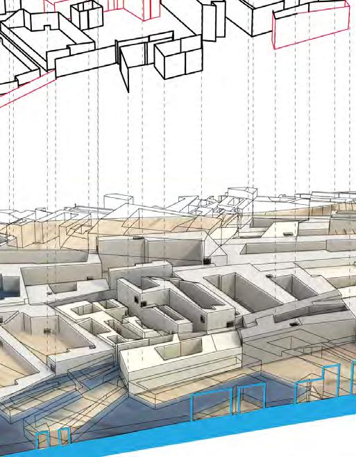

— 102 —
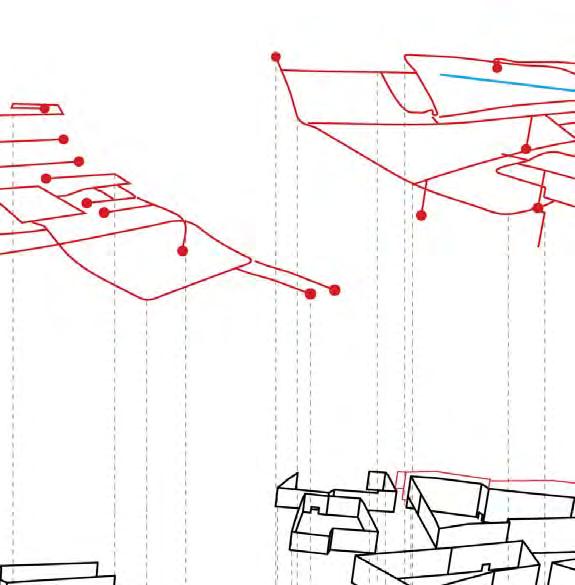
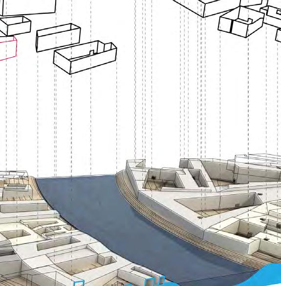
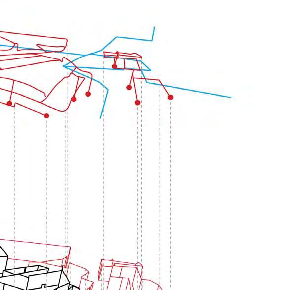
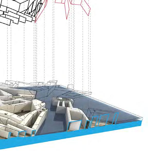


Figure90 A small area of the composite from the global plan describing in detail the transport organization and water management system in dry season.
5.3 The detailed design on a piece of urban plot
The other aspect is the artificial water system. The same with the previous strategy, as a “polder block” is the integration of multi - functions; the function of every exterior wall could be for residents’ inhabitancy, water defense and water storage. The distinctions are made according to the water condition of each block. Generally speaking, the periphery rings of walls are water defensive in wet season. And the inner walls of each block are eight for water store or inhabitable, decided by the height of the block. Most of the agriculture blocks are low and need water irrigation most of the time, so they mainly water storage to retain water even in the dry season.
— 103 —
5.4 Water drainage system
A big problem facing the courtyard like urban form is its water drainage. As it is centripetal, water is easy to be collected into the court but excessive water is difficult to be drained out. In the case of polder, Dutch people use windmill to pump the water out to the artificial canal above. In this project, we also try to find a local and cheap way to solve the problem.
An advantage from the site and topography is that there is a huge water level difference between dry season and wet season. The water difference is directly used for drainage. Specifically, there are blocks as water storages scatter on the whole site. Each storage serves several surrounding blocks. The bottom of the storage is lower than the surrounding blocks’ but higher than the outside water level in dry season. Driving by the gravity force, the excessive water in living blocks is drained through drainage pipes to the lower storage and is temporarily stored there in wet season. In the dry season, when outside water level is low, the water in the storage can be drainage to the outside. In this the whole drainage process is completed. There is no driving force needed for the process except for gravity.

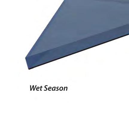
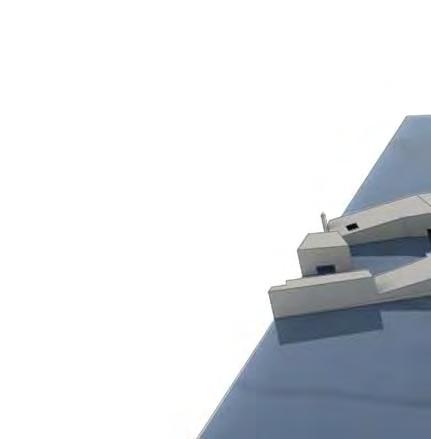
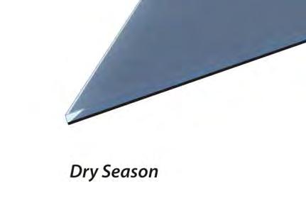
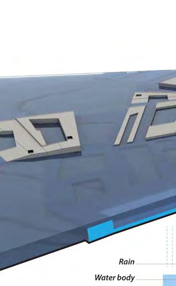
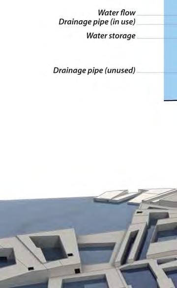
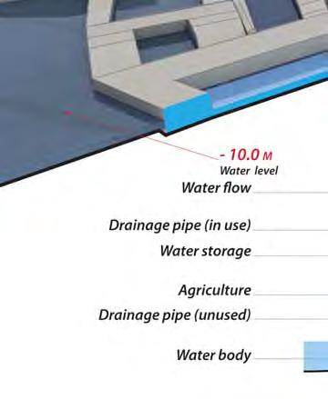 Figure91,92 Profiles showing how the water dainage system based on the water level difference and gravity works in dry season and wet season.
— 104 —


— 105 —


water water clay e efed-ret a w e defe -ret a wsotf m e efed-ret a w tfos eter co ret wa e r co clay vegetation vegetation
— 106 —
Figure93 The details showing the mixed use of local materials and industrial matarials and the soft - semi soft- hard material gradient.


5.5 Material gradient
I n the case study of polder in the Netherlands, many dikes are made of soft material like earth, grass, coral, etc. They are not completely impermeable and easy to be built and rebuilt. The soft material with it affinity to water and nature, is good for agriculture in maintaining the species diversity for the farming. In this project, there is large number of agriculture blocks adjacent to water. Agriculture blocks have fewer requirements on water proof of the dike. Consequently, some cheap and organic material can be used to build dikes for these types of blocks.
And in the area between agriculture and inner edge blocks, semi soft material are used to proof water as well as keep an soft relationship with the environment. For the residential blocks, they are highly fixed and the requirements of water proof it very high, hard material like concrete are used to build the dike for the protection.
This page shows the material gradient by the section. Generally, the soft- semi soft- hard material change is in accordance with the distance with water resource.
— 107 —


the
- semi
— 108 —
Figure94 The overview of
global configuaration showing the soft
soft- hard material gradient.


— 109 —

State 1


State 2 State 3 State 4 State 5
5.6 Time dimension of the urban intervention
To explain better the whole system, five significant states are given at different time of the year. In every year, from December to March the next year are the dry season, the water level at this time are really low. Then affected by the monsoon climate, the water level sharply rises. Within two to three month, the water level reach the high state and keep the same for 4 month during the wet season. After the wet season, the water level rapidly decreases and goes back to the state of dry season. The whole system in this project works like a semi permeable membrane for the whole site. By defending water in the wet season and retaining water in the dry season with the deliberately arranged block heights, it keeps a stable water supply for the village. The water morphologies in every time of the year are defined by neither the dike boundary nor the contour lines. They are the result of the block heights, water level, block shapes working together.
In the next five pages, the first one and the last one are the states in dry season and wet season respectively. The pages in the middle are the middle states in the transition from dry state to wet state.
JANFEBMARAPRMAYJUNJULAUGSEPOCTNOVDEC 0.0 M 1.2 M 2.4 M 3.6 M 4.8 M 6.0 M water level time
Figure95 The time demesion of the whole system as water mophology changing with time through the year.
— 110 —
JANFEBMAR APR MAYJUNJULAUGSEPOCTNOVDEC 1.2 M 2.4 M 0.0 M 3.6 M 4.8 M 6.0 M water level time
State
April. — 112 —
Figure97
in
JANFEBMARAPR MAY JUNJULAUGSEPOCTNOVDEC 2.4 M 3.6 M 4.8 M 1.2 M 0.0 M 6.0 M water level time
May. — 113 —
Figure98
State in
3.6 M 4.8 M JANFEBMARAPRMAY JUN JULAUGSEPOCTNOVDEC 2.4 M 1.2 M 0.0 M 6.0 M water level time
State in June. — 114 —
Figure99


5.7
— 116 —
Figure101 Rendering.
Renderings


— 117 —
Figure102 Rendering.


— 118 —
Figure103 Rendering.


— 119 —
Figure104 Rendering.


— 120 —
Figure105 Rendering.


— 121 —
Figure106 Rendering.
— 122 —
Chapter 6. Evaluations and Future development
6.0 Conclusion
6.1 Future development
— 123 —
6.1 Conclusion
In the site plan, a conceptual global model about adaptive living system is proposed. The system focuses on water-utilization and water-defensive under periodic monsoon climate. The main idea is to develop a structure which can passively adjust its own capability to accommodate the multi - functions such as water defence, water storage and drainage under the influence of the different conditions and demands. The traditional architecture existing here can only response to flood passively with no ability to adapt to the changing water level. And the strategy in former works like the polder in Netherlands is also not suitable for our site. Cambodia is a country where the economy highly relies on agriculture. Therefore massive polder will be lack of flexibilities for rural area and will bring inconvenience to field irrigation.
By propose the “polder block” design strategy, this project provide a component – based living system which can adjust and adapt to environmental changes at the very local scale. However, the effect of local adaptivity is extremely significant as the global output can maintain a stable water supply by defending water in the wet season and retaining water in the dry season. The working principle is similar to cell membrane which is neither completely defensive nor completely transparent, but selective permeation.
In general, the benefits of the system are as follows:
Multi-Function
The new structure integrates water defensive, water storage, residential blocks and pedestrian streets together. Beside, the combinations of different block pattern could generate countless kinds of architecture space to met varied demands of people.
Relatively low technologies but huge effect
The structure could be built with local material such as clay or local soil. The technologies are not complicated and could be widely used in rural area. Comparing to low technologies, this kind of architectural strategy could improve the utilization of field and expand the scope of people’s activities to face the development of local population.
New passive water-utilization system
Our design proposal includes a new set of water cycle system, which works passively with gravity. In short, this water cycle system keeps water in reserve during wet season and provides saved water to fishfarming and field irrigation in dry season.
— 124 —
However, there is still a long way to go to achieve our initial concept. Because of the nontraditional strategy and construction techniques, many crucial parts are remaining uncertain. For example, to what scale should we focus more? Are there other better options for structural and functional realization? How to keep balances between local production and tourism? Those challenges will be conquered in further stage.
As this system showed great potential on solving complex and conflict among population growth, urban developing, and local industries, we will aim on a more uni¬versal scenario rather than the extreme rural area, so optimizing the urban strategies and algorithm will be the primary work for the next stage. By defining specific con¬figurations, it is possible figure out the new growing logic to accelerate urbanization process. This in return will provide a strong and logical foundation of for the whole system and open a door for following research.
6.1 Further development
More prototypes should be developed based on the quantitative analysis of local relative data. In this way, architectural part will be considered more and play a significant role in problem-solving aspects. On the other hand combinations of those prototypes will be carefully investigated and evaluated in order to find the proper ex¬pand logic. The structural realization will still be critical. A new figuration of material, joints, fabrication, should be more proper in terms of mechanics, cost, performance and asthmatics.
— 125 —
— 126 —
Bibliography
— 127 —
1. Flooding - Causes of Floods, http://science.jrank.org/pages/2757/Flooding.html, Date accessed 30/6/10.
2. Bratkovich S., Burban L., et al. “Flooding and its Effects on Trees”, USDA Forest Service, Northeastern Area State and Private Forestr y, St. Paul, MN, September 1993.
3. A brief overview of the processes behind the formation of a river’s floodplain, http://scienceray com/earth-sciences/the-formation-of-a-floodplain/, Date accessed 16/7/10.
4. Shannon K., Meulder B., D’Audia V. and Gosseye J.,Eds. Water Urbanisms, UFO Series, Amsterdam:2008.
5. Damnoen Saduak Floating Market, http://www.bangkok com/beyond-the- city/damnoensaduak.htm, Date accessed 27/7/10.
6. Hafiz R. Adapting Traditional Housing Design to Cope With Natural Hazards: Stilt Houses for Flood Prone Areas of Bangladesh, the Proceedings of H&H 2000 Conference, Dhaka & Exeter, 2000.
7. LansingJohn J., Miller H. Cooperation in Balinese Rice Farming, 07/05/03.
8. Varis O. and Keskinen M. Socioeconomic analysis of the Tonle Sap Region, Cambodia—building links and capacity for targeted poverty alleviation, Thesis - Helsinki University of Technology, Water Resources Laborator y, Espoo, Finland:2002.
9. Kite G. ‘Modeling the Mekong: hydrological simulation for environmental impact studies’, Journal of Hydrology, 253, 1-13, 2001.
10. Campbell I., Poole C., Giesen W., and Valbo-Jorgensen J. ‘Species diversity and ecology of Tonle Sap Great Lake, Cambodia’, Aquatic Science, 68, 355-373, 2006.
11. Nikula J. ‘Review and integration of hydrological, ecological and socio-economic information in The Tonle Sap Lake’, Master’s Thesis, Water Resources Laborator y, Helsinki University of Technology, 2005.
12. Mund J. Symann R. and Seang T. Urban and Peri-urban Land Management - Examples from Provincial Cambodian Cities, Thesis, South East Asia Survey Congress, Cambodia: 2005.
13. Keskinen M. ‘Socio-economic survey of the Tonle Sap Lake, Cambodia’, Master’s Thesis, Department of Civil and Environmental Engineering, Helsinki University of Technology. 106-118, 2003
14. Sarkkula J., Baran E., Chheng P., Keskinen M., Koponen J., and Kummu M. ‘Tonle sap pulsing system and fisheries productivity ’, the XXIX International Congress of Limnology, Finland, 2004.
15. Thomas S. The D ynamics of Buoyant Objects, http://www.physicsmyths.org.uk/, Date accessed 15/8/10.
16. Toudert F. and Bensalem R. A Methodology for a Climatic Urban Design, Thesis - The 18th International Conference on Passive and Low Energy Architecture, Florianópolis, Brazil: 2001.
17. Dunkelberg K. Bamboo - Bamboo as a building material, the team of the IL, Stuttgart: Institut fur Leichte Flachentragwerke, Germany: 2003.
18. Martín H., Lope J. Maravall, D. ‘Adaptation, Anticipation and Rationality in Natural and Artificial Systems: Computational Paradigms Mimicking Nature’, Natural Computing, 8(4), 757-775, 2009.
19. Hübler A. and Wotherspoon T. ‘Self-Adjusting Systems Avoid Chaos’, Complexity, 14(4), 8 – 11, 2008.
20. Bilow M., Klein, T. and Knaack U. ‘Imagine 02 Deflateables’. Rotterdam: 010 publishers, 8-16, 2007.
21. Tessellation, http://mathworld.wolfram.com/Tessellation.html, Date accessed 12/07/10.
22. Zalinge N., Degen P., Pongsri C., Nuov S., Jensen J., Hao N. and Choulamany X. The Mekong River System, the Second International Symposium on the Management of Large Rivers for Fisheries, Phnom Penh, 1114/02/2003.
23. Poffenberger M. and Smith-Hanssen K., Eds. Flood Forest, Fish, and Fishing Villages, Asia Forest Network, 2004.
24. Zalinge N., Thuok N. and Nuov S. Status of the Cambodian Inland Capture Fisheries Sector with Special Reference to the Tonle Sap Great Lake.
25. Fang W. Stilt House Building Technology for Flood Disaster Reduction, Academy of Disaster Reduction and Emergency Management, Ministr y of Civil Affairs & Ministr y of Education, PRC, Beijing 100875, China.
26. Economy Watch, ‘GDP Per Capita (Current Prices, US Dollars) Statistics for Cambodia , Year 2009 - In Detail’, http://www.economywatch.com/economic-statistics/countr y/Cambodia/, Date accessed at 01/10/10.
27. Guy N., Catherine S., and Adam Y., On the Water: Palisade Bay. Germany: Hatje Cantz, 2010.
— 128 —
28. Michael W., The Architecture of Emergence: The Evolution of Form in Nature and Civilisation, John Wiley & Sons, 2010.
29. Michael W., Emergent Technologies and Design, Routledge, 2010.
30. Michael H., Achim M. and Michael W., Emergence: Morphogenetic Design Strategies, John Wiley & Sons, 2004.
31. Kelly S., Bruno De M., Viviana D.and Janina G., Water Urbanisms, Sun Publishers, 2008.
32. Ila B., and Mona EL K. URBANBuild Local Global, San Francisco: William Stout, 2009.
33. Brendan B., Kevin A., Daniel P., Roland F., Edward C., Masaki S., Le N., Aroonrut W., Ton M., and Truong M. H., ‘Climate as a contributing factor in the demise of Angkor, Cambodia’, PNAS Direct Submission, 02-16, 2009.
34. Damian E., Christophe P., Roland F., Scott H., Ian T., Anthony M., and Michael B. ‘A comprehensive archaeological map of the world’s largest preindustrial settlement complex at Angkor, Cambodia, PNAS Direct Submission, 06-29, 2007.
35. ‘The Natural Environment and Historical Water Management of Angkor’, Cambodia, http://users.tkk.fi/u/mkummu/publications/kummu_WAC_WashingtonDC_2003.pdf, Date accessed 08/10/2010.
36. Yagama R. ‘The Salutar y Influence of Irrigation on Human Settlement, Economy, and Political Power in Pre-modern Southeast Asia’, Asian Agri-Histor y, 9(4), 275-289, 2005.
37. Solieng M. ‘Paddy cultivation -the traditional way ’, CRBOM Small Publications Series, 05-21, 2010.
38. Meta Berghauser P., Per H., Spacematrix: Space, Density and Urban Form, NAI PUBL, 2010.
39. Stephen M., Cities design and evolution, Urban design and planning, Routledge, 2009.
40. Franz Oswald, P. Baccini and Mark M., Netzstadt: designing the urban, Birkhauser Verlag AG.01/09/03.
41. Michael H. and Achim M., Morpho-ecologies: Towards Heterogeneous Space in Architectural Design, Architectural Association Publications, 2006.
42. Iain S. and Tim O., Classifying urban climate field sites by "local climate zones": the case of Nagano, Japan, University of British Columbia, Vancouver, Canada, 2009.
43. Fazia A. and Rafik B., A METHODOLOGY FOR A CLIMATIC URBAN DESIGN, Florianópolis, Brazil, 2001.
44. Bill H., Alasdair T., Tao Y. and Hoon-Tae P., Metric and topo-geometric properties of urban street networks:some convergences, divergences and new results, Proceedings, 6th International Space Syntax Symposium, İstanbul, 2007.
45. Luc A., A simplified model of urban morphology : application to an analysis of the environmental performance of cities, School of Architecture de Toulouse.
46. Gideons G., Urban design morphology and thermal performance, The Pennsylvania State University, Pennsylvania U.S.A., 1996
47. Wouter R., Clemens S. and Diderik A., Sea of Land, The polder as an experimental atlas of Dutch landscape architecture, TU Delft, 05/2007.
— 129 —
— 130 —
Appendices
Rhino script
Processing script
Mel script
Grasshopper
Screenshots of the movie
DVD
— 131 —
script
— 132 —
Rhino
Option Explicit
‘Script written by <insert name>
‘Script copyrighted by <insert company name>
‘Script version Thursday, 11 November 2010 13:29:03
Call Main()
Sub Main()
Dim initialGeo,coGeo
Dim i,n
n = rhino.GetInteger(“enter the number”,30,1,100)
Dim col,row
Dim oriGeo
oriGeo = rhino.GetObject(“sel the initial grometry”,16)
For i=0 To n-1
initialGeo = rhino.CopyObject(oriGeo,array(0,0,0),array(0,0,0))
coGeo = Deformation_1(initialGeo) ‘First Deformation non-uniform scale
coGeo = Deformation_2(coGeo)
coGeo = Deformation_3(coGeo,initialGeo)
Dim cutGeo
cutGeo =cutter(initialGeo)
initialGeo=rhino.BooleanDifference(array(initialGeo),array(coGeo))(0)
Dim intersect
intersect = rhino.IntersectBreps(initialGeo,cutGeo)
col = int(i/5)
row = i Mod 5
If Not Isnull(intersect) Then Call rhino.DeleteObjects(intersect)
initialGeo = rhino.BooleanDifference(array(initialGeo),array(cutG eo))
If Not isarray(initialGeo) Then Call rhino.MoveObject(initialGeo(0),array(0,0,0),array(col*50,row*50,0))
Else
Call rhino.MoveObjects(initialGeo,array(0,0,0),array(col* 50,row*50,0))
End If
Else
Call rhino.DeleteObject (cutGeo)
Call rhino.MoveObject(initialGeo,array(0,0,0),array(col*50,r ow*50,0))
End If Next End Sub
Private Function Deformation_1(ByVal strGeo)
Dim strCoGeo
Dim dblScaleX, dblScaleY
dblScaleX = rnd()*0.8+0.2
dblScaleY = rnd()*0.8+0.2
strCoGeo = rhino.ScaleObject(strGeo,rhino.SurfaceVolumeCentroid(strGeo)(0),arra y(dblScaleX,dblScaleY,2),True)
Deformation_1= strCoGeo
End Function
Private Function Deformation_2( strGeo)
Dim arrBBpts
Dim dblRadius
arrBBpts = rhino.BoundingBox(strGeo)
Dim dblDistU,dblDistV
dblDistU = rhino.Distance(arrBBpts(0),arrBBpts(1))
dblDistV = rhino.Distance(arrBBpts(1),arrBBpts(2))
If dblDistU <= dblDistV Then dblRadius = dblDistU/10
Else dblRadius = dblDistV/10
End If
Dim arrNewBBpts()
Dim i
For i=0 To 3
ReDim Preserve arrNewBBpts(i)
arrNewBBpts(i) = movept(arrBBpts(i),dblRadius)
Next
Dim strSrf
strSrf = rhino.AddSrfPt(arrNewBBpts)
Dim strline
strline= rhino.addline(arrBBpts(0),arrBBpts(4))
Call rhino.DeleteObject(strGeo)
strGeo = rhino.ExtrudeSurface(strSrf,strline)
Call rhino.DeleteObject(strSrf)
Call rhino.DeleteObject(strline)
Deformation_2 = strGeo
End Function
Private Function Deformation_3(coGeo,initialGeo)
Dim arrCenPt
arrCenPt = rhino.SurfaceVolumeCentroid(initialGeo)(0)
Dim dblDist
dblDist = 0.5
Dim newCent : newCent = movePt(arrCenPt,dblDist)
Call rhino.MoveObject(coGeo,arrCenPt,newCent)
Deformation_3 = coGeo
End Function
Private Function cutter(strGeo)
Dim coGeo
coGeo= rhino.ScaleObject(strGeo,rhino.SurfaceVolumeCentroid(strGeo) (0),array(5,5,1),True)
Dim dblCase
Dim arrAxis
Dim dblAngle :dblAngle = -30+60*rnd()
dblCase =rnd()
If dblCase<0.5 Then arrAxis=array(1,0,0)
Else arrAxis = array(0,1,0)
End If
Rhino script for experiments — 133 —
Call rhino.RotateObject(coGeo,SurfaceVolumeCentroid(strGeo)(0),dblAngle,arrAxis)
Call Rhino.MoveObject (coGeo,array(0,0,0),array(0,0,9+2*rnd()))
cutter = coGeo
End Function
Private Function movePt(arrPt,dblRadius)
Dim PI
PI = rhino.Pi
Dim newVec:newVec = array(dblRadius*sin(rnd()*2*PI),dblRadius*sin(rnd()*2*PI),0) movePt = rhino.VectorAdd(arrPt,newVec) End Function
Option Explicit
‘Script written by <insert name> ‘Script copyrighted by <insert company name> ‘Script version Wednesday, November 17, 2010 2:08:34 PM
Call Main()
Sub Main()
Dim oriGeo,arrNewGeo oriGeo= rhino.GetObjects(“pick geometries”) Dim i,j For i=0 To ubound(oriGeo)
Dim cen cen=rhino.SurfaceVolumeCentroid(oriGeo(i)) oriGeo(i)=rhino.ScaleObject(oriGeo(i),array(cen(0)(0),cen(0)(1),0),array(rn d()*1+0.5,rnd()*1+0.5,rnd()*0.33+0.6))
Dim cutter1, cutter2 cutter1=cutter(oriGeo(i),0) cutter2=cutter(oriGeo(i),1) arrNewgeo=split(oriGeo(i),cutter1,cutter2) rhino.DeleteObject cutter1 rhino.DeleteObject cutter2
Dim n For j=0 To 3 n=int(rnd()*4)
Select Case n Case 0
arrNewGeo(j)=rotate(arrNewGeo(j),cen(0)) Case 1
arrNewGeo(j)=scale(arrNewGeo(j)) Case 2
arrNewGeo(j)=move(arrNewGeo(j)) Case 3
arrNewGeo(j)=arrNewGeo(j) End Select Next
rhino.DeleteObject oriGeo(i) Next End Sub
Function cutter(geo,n) Dim arrBox arrBox=rhino.BoundingBox(geo)
Dim pt1,pt2,line,path
If n Mod 2=0 Then pt1=array((arrBox(0)(0)+arrBox(1)(0))/2,arrBox(0)(1),0) pt2=array((arrBox(2)(0)+arrBox(3)(0))/2,arrBox(2)(1),0) line=rhino.AddLine(pt1,pt2) line=rhino.MoveObject(line,array(0,0,0),array(0,0,-30)) path=rhino.AddLine(array(pt1(0),pt1(1),pt1(2)-30),array(pt1(0),pt1(1),30)) cutter=rhino.ExtrudeCurve(line,path) rhino.DeleteObject line rhino.DeleteObject path Else pt1=array(arrBox(0)(0),(arrBox(0)(1)+arrBox(3)(1))/2,0) pt2=array(arrBox(1)(0),(arrBox(1)(1)+arrBox(2)(1))/2,0) line=rhino.AddLine(pt1,pt2)
Rhino script for experiments — 134 —
line=rhino.MoveObject(line,array(0,0,0),array(0,0,-30)) path=rhino.AddLine(array(pt1(0),pt1(1),pt1(2)-30),array(pt1(0),pt1(1),30))
cutter=rhino.ExtrudeCurve(line,path) rhino.DeleteObject line rhino.DeleteObject path
End If
End Function
Function split(geo,cutter1,cutter2)
Dim arrGeo1, arrGeo2,arrGeo3
Dim geo1,geo2,geo3,geo4 arrGeo1=rhino.SplitBrep(geo,cutter1) rhino.CapPlanarHoles arrGeo1(0) rhino.CapPlanarHoles arrGeo1(1) arrGeo2=rhino.splitBrep(arrGeo1(0),cutter2) arrGeo3=rhino.SplitBrep(arrGeo1(1),cutter2) rhino.CapPlanarHoles arrGeo2(0) rhino.CapPlanarHoles arrGeo2(1) rhino.CapPlanarHoles arrGeo3(0) rhino.CapPlanarHoles arrGeo3(1) rhino.DeleteObjects(arrGeo1) split=array(arrGeo2(0),arrGeo2(1),arrGeo3(0),arrGeo3(1))
End Function
Function rotate(geo,pt)
Dim a a=rnd()*15 rotate=rhino.RotateObject(geo,pt,a) End Function
Function scale(geo)
Dim x,y,z x=rnd()+0.5 y=rnd()+0.5
z=rnd()+0.5
Dim cen
cen=rhino.SurfaceVolumeCentroid(geo) scale=rhino.ScaleObject(geo,array(cen(0)(0),cen(0)(1),0),array(x,y,z)) End Function
Function move(geo)
Dim x,y,z x=rnd()*5 y=rnd()*5 z=0
move=rhino.MoveObject(geo,array(0,0,0),array(x,y,z)) End Function
Option Explicit ‘Script written by <insert name> ‘Script copyrighted by <insert company name> ‘Script version Sunday, December 12, 2010 3:16:24 PM
Call Main()
Sub Main() Dim recs recs=rhino.GetObjects(“pick”) Dim i,n For i= 0 To ubound(recs)
Dim points points=rhino.CurveEditPoints(recs(i))
Dim a
Dim b a=abs(points(0)(0)-points(1)(0)) b=abs(points(0)(1)-points(2)(1))
Dim cen cen=rhino.CurveAreaCentroid(recs(i)) n=cen(0)(0) n=int(rnd()*n/30)
If n=0 Then n=int(rnd()*2) If n=0 Then rhino.AddPolyline array(points(0),points(1),array(cen(0) (0)+a/2,cen(0)(1),cen(0)(2)),array(cen(0)(0)-a/2,cen(0)(1),cen(0)(2)),points(0)) rhino.AddPolyline array(array(cen(0)(0)-a/2,cen(0) (1),cen(0)(2)),array(cen(0)(0)+a/2,cen(0)(1),cen(0)(2)),points(2),points(3),array(cen(0) (0)-a/2,cen(0)(1),cen(0)(2))) Else
rhino.AddPolyline array(points(0),array(cen(0)(0),cen(0) (1)+b/2,cen(0)(2)),array(cen(0)(0),cen(0)(1)-b/2,cen(0)(2)),points(3),points(0)) rhino.AddPolyline array(array(cen(0)(0),cen(0) (1)+b/2,cen(0)(2)),points(1),points(2),array(cen(0)(0),cen(0)(1)-b/2,cen(0)(2)),array(cen(0) (0),cen(0)(1)+b/2,cen(0)(2)))
‘rhino.AddLine array(cen(0)(0),cen(0)(1)-b/2,cen(0) (2)),array(cen(0)(0),cen(0)(1)+b/2,cen(0)(2))
End If rhino.DeleteObject(recs(i))
End If
Rhino script for experiments
Next
— 135 —
End Sub
Rhino script for experiments
Option Explicit
‘Script written by <insert name>
‘Script copyrighted by <insert company name>
‘Script version Sunday, December 12, 2010 6:35:10 PM
Call Main()
Sub Main()
Dim geos(64)
Dim patterncrvs Dim boxes()
Dim i
For i=0 To 64 geos(i)=rhino.GetObjects(“pick geos”) Next
patterncrvs=rhino.GetObjects(“pick recs”) Dim arrboxes()
For i= 0 To ubound(patterncrvs)
ReDim Preserve boxes(i) boxes(i)=rhino.ExtrudeCurveStraight(patterncrvs(i),array(0,0,0),arr ay(0,0,15))
rhino.CapPlanarHoles boxes(i)
ReDim Preserve arrboxes(i) arrboxes(i)=rhino.BoxPoints(boxes(i)) rhino.DeleteObject(boxes(i)) Next
For i=0 To ubound(patterncrvs)
Dim n n=int(rnd()*65) rhino.BoxMorphObject geos(n),arrboxes(i),True Next
End Sub
— 136 —
Option Explicit
‘Script written by <insert name>
‘Script copyrighted by <insert company name>
‘Script version 05 January 2011 15:36:42
Call Main()
Sub Main()
Dim strRiver
Dim arrHighlines
strRiver = rhino.GetObject(“sel the river “,4) arrHighlines = rhino.GetObjects(“sel the highlines”,4)
Dim arrStartPts arrStartPts = rhino.GetObjects(“sel the points”,1)
Dim i
For i =0 To ubound(arrStartPts)
Call growBranch(arrStartPts(i),strRiver,arrHighlines) Next End Sub
Function growBranch (arrStartPt,strRiver,arrHighlines)
Dim arrPtPara arrPtPara = rhino.CurveClosestPoint(strRiver,rhino.PointCoordinates(arrStartPt))
Dim arrTagent arrTagent = rhino.CurveTangent(strRiver,arrPtPara)
‘ General Setup
Dim maxTimeSteps : maxTimeSteps = 2000
If isNull(maxTimeSteps) Then Exit Function
Dim numParticles : numParticles =150
If isNull(numParticles) Then Exit Function
‘ Environment Size
Dim envsizeX : envsizeX = 160
Dim envsizeY : envsizeY = 160
Dim envsizeZ : envsizeZ = 0
‘ Particle Variables
Dim maxVel : maxVel = 1.0 ‘ Maximum speed of the partcle
Dim dblGravity : dblGravity = -0.0 ‘ Gravity push on the particles
‘ Aggregation Variables
Dim dblRng : dblRng = 3 ‘ If particle is this close to a cell then create a new aggregate
‘ReDim Preserve aggregateCells(-1)
rhino.Print “ “ rhino.Print “!!! SCRIPT STARTED !!!”
‘ Set and Draw Environment
Call Rhino.ViewDisplayMode(“Perspective”,0) rhino.addLayer “WORLD” rhino.CurrentLayer “WORLD”
Call makeEnvironment(envsizeX,envsizeY,envsizeZ)’ build the box of 100*100*100
‘--------------------------------------------------------------------------------
‘ MAKE STARTING AGGREGATE CELL
rhino.addLayer “AGGREGATES”, RGB(255,0,0)
rhino.CurrentLayer “AGGREGATES”
‘ReDim Preserve aggregateCells(0)
‘aggregateCells(0) = rhino.addPoint( Array(envsizeX/2, envsizeY/2, envsizeZ/2 ) ) ‘ build the first point
Dim aggregateCells: aggregateCells = arrStartPt
‘--------------------------------------------------------------------------------
‘ MAKE PARTICLES
‘Each agent is described as -- Array( pos(0), vel(1), maxVel(2) )
rhino.addLayer “PARTICLES” rhino.CurrentLayer “PARTICLES”
Dim i
Dim arrParticles()
For i = 0 To numParticles -1
Dim rndStart : rndStart = randomStart(envsizeX,envsizeY,envsizeZ)
Dim rndVel : rndVel = randomVelocity()
ReDim Preserve arrParticles(i)
arrParticles(i) = Array( Array( rnd*envsizeX, rnd*envsizeY, rnd*envsizeZ ), rndVel, maxVel )
‘arrParticles(i) = Array( rndStart, rndVel, maxVel )
Next
‘ ITERATE SIMULATION
Dim j,k
Dim particleCloud
particleCloud = Null
For j = 0 To maxTimeSteps-1
rhino.enableRedraw False
‘-------------------------------------------------------------
‘ UPDATE EACH PARTICLES’S POSITION
For k = 0 To ubound(arrParticles)
‘ FORCES ON THE PARTICLE
‘ Any force acting on the particle - e.g. gravity - is added to the particle’s acceleration
Dim arrAcc, fGravity, arrNewVel
arrAcc = Array(0,0,0)
fGravity = Array(0,0,dblGravity)
arrAcc = rhino.VectorAdd( arrAcc, fGravity )
‘ Add acceleration to current particle velocity
arrNewVel = rhino.VectorAdd( arrParticles(k)(1), arrAcc )
‘ Limit velocity to maxVel
arrNewVel = vectorLimit( arrNewVel, arrParticles(k)(2) )
arrParticles(k)(0) = rhino.VectorAdd( arrParticles(k)(0), arrNewVel )
Rhino script for global growth
‘--------------------------------------------------------------------------------
Next ‘--------------------------------------------------— 137 —
‘ CHECK AGGREGATES & DRAW PARTICLES
‘ generate array of all particle coords
Dim m
Dim arrPosToroid
ReDim arrParticlePos(-1)
For m = 0 To ubound(arrParticles)
arrPosToroid = borders( arrParticles(m), envsizeX, envsizeY, envsizeZ )’ let particle always in the area
arrParticles(m)(0) = arrPosToroid
ReDim Preserve arrParticlePos(m)
arrParticlePos(m) = arrParticles(m)(0)
‘-----------------------------------------------
‘ Check position against all current aggregates
Dim tmpCell : tmpCell = checkAggregates(arrParticles(m)(0), aggregateCells, dblRng,arrTagent,arrHighlines,arrStartPt)
‘ If location is good then make new cell If Not isNull(tmpCell) Then ‘ReDim Preserve aggregateCells( ubound(aggregateCells) +1)
‘aggregateCells( ubound(aggregateCells)) = tmpCell aggregateCells = tmpCell
‘ reset the particle to a new starting position & new velocity
arrParticles(m)(0) = randomStart(envsizeX,envsizeX,env sizeX)
arrParticles(m)(1) = randomVelocity()
End If Next
‘-----------------------------------------------------
‘ Delete old pointcloud and draw new one If Not isNull(particleCloud) Then rhino.deleteObject particleCloud End If
rhino.CurrentLayer “PARTICLES” particleCloud = Rhino.AddPointCloud(arrParticlePos)
‘ redraw to update view Rhino.EnableRedraw True rhino.Print “Current time step is : “ & j+1
Next
rhino.Print “!!! SCRIPT COMPLETE !!!” End Function
Function
checkAggregates(POS, AGGS, RNG, arrTagent,arrHighlines,startPt)
Dim gateLength :gateLength =5
Dim tolerance :tolerance = 0.5
checkAggregates = Null
Dim arrStart :arrStart = rhino.PointCoordinates(startPt)
Dim testLength
‘ Variables
Dim i, index, distClosest, arrPtTest, distTest, strNewObj
Dim testVec,dblAngle index = 0
distClosest = 9999999
‘ Loop to find nearest aggregate
‘For i = 0 To ubound(AGGS)
arrPtTest = rhino.pointCoordinates( AGGS ) distTest = rhino.Distance(POS,arrPtTest) If distTest < distClosest Then distClosest = distTest index = i
End If testLength = rhino.Distance(arrPtTest,arrStart)
If testLength>gateLength Then arrTagent = newTangent(POS,arrHighlines)
End If
testVec = rhino.VectorSubtract(pos,rhino.pointCoordinates( AGGS )) dblAngle = rhino.VectorAngle(testVec,arrTagent)
‘ Next
‘ If in range make a new aggregate
If (distClosest < (RNG+tolerance) And distClosest>(RNG-tolerance)) And ((dblAngle>70 And dblAngle<110) Or (dblAngle>250 And dblAngle<290)) And(testVec(0)<0)Then
rhino.CurrentLayer “AGGREGATES”
strNewObj = rhino.addPoint(POS)
‘ make a line rhino.addLine pos, rhino.pointCoordinates( AGGS )
‘ return new cell
checkAggregates = strNewObj
Exit Function
Else
End If
End Function
checkAggregates = Null
Exit Function
Function newTangent(arrPt,arrHighlines)
Dim i
Dim closestDist :closestDist = 9999999
Dim arrPtPara,tmpPt,dist
Dim index ,closestPara
For i= 0 To ubound(arrHighlines)
arrPtPara = rhino.CurveClosestPoint(arrHighlines(i),arrPt) tmpPt = rhino.EvaluateCurve(arrHighlines(i),arrPtPara) dist = rhino.Distance(arrPt,tmpPt)
If dist <closestDist Then closestDist =dist index = i closestPara = arrPtPara
End If
Next
newTangent = rhino.CurveTangent(arrHighlines(index),closestPara)
End Function
Function randomStart(envX, envY, envZ)
randomStart = Null
Dim xyToggle, kToggle, zToggle, arrVec
xyToggle = rnd*1
kToggle = rnd*1
zToggle = rnd*1
Rhino script for global growth
— 138 —
If xyToggle > 0.5 Then
‘ random XX & constant YY value
If kToggle > 0.5 Then arrVec = Array(rnd*envX, envY, envZ)
Else
End If Else
arrVec = Array(rnd*envX, 0, 0)
‘ constant XX & random YY value
If kToggle > 0.5 Then
Else
End If
arrVec = Array(0, rnd*envY, 0)
arrVec = Array(envX, rnd*envY, envZ)
End If randomStart = arrVec
End Function
‘ Returns a vector with values between -1 & 1
Function randomVelocity()
randomVelocity = Null
Dim i
‘ An array of negative or positive operators
ReDim switch(2)
For i = 0 To 2
Dim rndNum : rndNum = rnd*1
ReDim Preserve switch(i)
If rndNum > 0.5 Then switch(i) = 1
Else switch(i) = -1
End If Next
randomVelocity = Array( switch(0)*(rnd*1), switch(1)*(rnd*1), switch(2)*(rnd*1) )
End Function
‘ Toroidal space - if particle leaves the environment it returns on the opposite Function borders(PARTICLE, XX, YY, ZZ)
borders = Null
Dim newX, newY, newZ
‘ Solve for X coordinate
If PARTICLE(0)(0) < 0 Then newX = XX
ElseIf PARTICLE(0)(0) > XX Then newX = 0
Else newX = PARTICLE(0)(0)
End If
‘ Solve for X coordinate
If PARTICLE(0)(1) < 0 Then newY = YY
ElseIf PARTICLE(0)(1) > XX Then newY = 0
Else newY = PARTICLE(0)(1)
End If
‘ Solve for X coordinate
If PARTICLE(0)(2) < 0 Then newZ = ZZ
ElseIf PARTICLE(0)(2) > ZZ Then newZ = 0
Else newZ = PARTICLE(0)(2)
End If
borders = Array(newX, newY, newZ)
End Function
‘ Limits the magnitude of a vector to a given limit Function vectorLimit(V1, LIMIT)
vectorLimit = Null
Dim arrVec
Dim dblLength : dblLength = Rhino.VectorLength(V1)
If dblLength > LIMIT Then arrVec = rhino.VectorUnitize(V1) vectorLimit = rhino.VectorScale(arrVec, LIMIT)
Else vectorLimit = V1
End If
End Function
‘ Draws a box the size of the defined environemnt Function makeEnvironment(XX,YY,ZZ)
makeEnvironment = Null
Dim arrCnrs(7)
arrCnrs(0) = Array(0,0,0)
arrCnrs(1) = Array(XX,0,0)
arrCnrs(2) = Array(XX,YY,0)
arrCnrs(3) = Array(0,YY,0)
arrCnrs(4) = Array(0,0,ZZ)
arrCnrs(5) = Array(XX,0,ZZ)
arrCnrs(6) = Array(XX,YY,ZZ)
arrCnrs(7) = Array(0,YY,ZZ)
rhino.addBox arrCnrs
End Function
Rhino script for global growth
— 139 —
Option Explicit
‘Script written by <insert name>
‘Script copyrighted by <insert company name>
‘Script version Wednesday, January 05, 2011 11:52:51 PM
Call Main()
Sub Main()
Dim strCrv
strCrv = rhino.GetObject(“sel the river”,4)
Dim startPt
startPt = rhino.GetPoint()
Dim startPara
startPara = rhino.CurveClosestPoint(strCrv,startPt)
Dim count :count =50
Dim i ,j
Dim arrCurvature
‘Dim newPara:newPara=startPara
Dim newPt:newPt =startPt
Dim tmpPt
Dim intVel
Dim tmpTengent
For i =0 To count
arrCurvature = rhino.CurveCurvature(strCrv,rhino.CurveClosestPoint(strCr v,newpt))
If Isnull(arrCurvature) Then arrCurvature =array(100,100,100,100,100)
End If
intVel = velocity(arrCurvature,strCrv)
For j =0 To intVel
tmpTengent = rhino.VectorScale(rhino.CurveTangent(strCrv,rhino. CurveClosestPoint(strCrv,newpt)),0.5)
tmpPt= rhino.VectorAdd(newPt,tmpTengent)
tmpPt = rhino.EvaluateCurve(strCrv,rhino.CurveClosestPoint(strC rv,tmpPt))
newPt= tmpPt
Next
Call rhino.AddPoint(newPt)
Next
End Sub
Function velocity(arrCurvature,curve)
Dim intDist: intDist =20
Dim tmpLine
Dim intsect
Dim torelance
Dim x : x = rnd()
If x<0.33 Then torelance =-1
ElseIf x>0.66 Then torelance =1
Else torelance =0
End If
If arrCurvature(3) > 95 Then velocity = 10+torelance
Else
‘tmpLine = rhino.addline(refPt,arrCurvature(2))
If arrCurvature(4)(0)<0 Then velocity =20-sqr(arrCurvature(3))+torelance
Else velocity =sqr(arrCurvature(3))+torelance
End If
End If
End Function
Rhino script for global growth — 140 —
Option Explicit
‘Script written by <insert name>
‘Script copyrighted by <insert company name>
‘Script version Wednesday, November 17, 2010 2:08:34 PM
Call Main()
Sub Main()
Dim oriGeo,arrNewGeo oriGeo= rhino.GetObjects(“pick geometries”)
Dim i,j
For i=0 To ubound(oriGeo)
Dim cen cen=rhino.SurfaceVolumeCentroid(oriGeo(i)) oriGeo(i)=rhino.ScaleObject(oriGeo(i),array(cen(0)(0),cen(0)(1),0),array(rn d()*1+0.5,rnd()*1+0.5,rnd()*0.33+0.6))
Dim cutter1, cutter2 cutter1=cutter(oriGeo(i),0) cutter2=cutter(oriGeo(i),1) arrNewgeo=split(oriGeo(i),cutter1,cutter2) rhino.DeleteObject cutter1 rhino.DeleteObject cutter2
Dim n For j=0 To 3 n=int(rnd()*4)
Select Case n
Case 0
Case 1
arrNewGeo(j)=rotate(arrNewGeo(j),cen(0))
arrNewGeo(j)=scale(arrNewGeo(j))
Case 2
Case 3
arrNewGeo(j)=move(arrNewGeo(j))
arrNewGeo(j)=arrNewGeo(j)
End Select Next
rhino.DeleteObject oriGeo(i) Next End Sub
Function cutter(geo,n)
Dim arrBox arrBox=rhino.BoundingBox(geo)
Dim pt1,pt2,line,path
If n Mod 2=0 Then pt1=array((arrBox(0)(0)+arrBox(1)(0))/2,arrBox(0)(1),0) pt2=array((arrBox(2)(0)+arrBox(3)(0))/2,arrBox(2)(1),0) line=rhino.AddLine(pt1,pt2) line=rhino.MoveObject(line,array(0,0,0),array(0,0,-30)) path=rhino.AddLine(array(pt1(0),pt1(1),pt1(2)-30),array(pt1(0),pt1(1),30)) cutter=rhino.ExtrudeCurve(line,path) rhino.DeleteObject line rhino.DeleteObject path
Else
pt1=array(arrBox(0)(0),(arrBox(0)(1)+arrBox(3)(1))/2,0) pt2=array(arrBox(1)(0),(arrBox(1)(1)+arrBox(2)(1))/2,0) line=rhino.AddLine(pt1,pt2)
line=rhino.MoveObject(line,array(0,0,0),array(0,0,-30)) path=rhino.AddLine(array(pt1(0),pt1(1),pt1(2)-30),array(pt1(0),pt1(1),30)) cutter=rhino.ExtrudeCurve(line,path) rhino.DeleteObject line rhino.DeleteObject path End If
End Function
Function split(geo,cutter1,cutter2)
Dim arrGeo1, arrGeo2,arrGeo3 Dim geo1,geo2,geo3,geo4 arrGeo1=rhino.SplitBrep(geo,cutter1) rhino.CapPlanarHoles arrGeo1(0) rhino.CapPlanarHoles arrGeo1(1) arrGeo2=rhino.splitBrep(arrGeo1(0),cutter2) arrGeo3=rhino.SplitBrep(arrGeo1(1),cutter2) rhino.CapPlanarHoles arrGeo2(0) rhino.CapPlanarHoles arrGeo2(1) rhino.CapPlanarHoles arrGeo3(0) rhino.CapPlanarHoles arrGeo3(1) rhino.DeleteObjects(arrGeo1) split=array(arrGeo2(0),arrGeo2(1),arrGeo3(0),arrGeo3(1))
End Function
Function rotate(geo,pt)
Dim a a=rnd()*15 rotate=rhino.RotateObject(geo,pt,a)
End Function
Function scale(geo)
Dim x,y,z x=rnd()+0.5 y=rnd()+0.5 z=rnd()+0.5 Dim cen cen=rhino.SurfaceVolumeCentroid(geo) scale=rhino.ScaleObject(geo,array(cen(0)(0),cen(0)(1),0),array(x,y,z))
End Function
Function move(geo)
Dim x,y,z x=rnd()*5 y=rnd()*5 z=0 move=rhino.MoveObject(geo,array(0,0,0),array(x,y,z))
End Function
Rhino script for global growth
— 141 —
Processing script
— 142 —
int sp1Amount=4; int sp2Amount=2; int ep1Amount=3; int ep2Amount=3; int numAgs1=150; int numAgs2=150; int numAgs=numAgs1+numAgs2; int numS1,numS2,numE1,numE2; ArrayList startPoints1X; ArrayList startPoints1Y; ArrayList startPoints2X; ArrayList startPoints2Y; ArrayList endPoints1X; ArrayList endPoints1Y; ArrayList endPoints2X; ArrayList endPoints2Y; boolean time1=false; boolean time2=false; boolean time3=false; boolean time4=false; boolean timeT=false; float factor1=0.5; float factor2=2; Agent[] ags = new Agent[numAgs]; PVector springVec = new PVector(0,0); PVector pos; PImage img; void setup() { size (736,457); pos = new PVector(0,0); startPoints1X=new ArrayList(); startPoints2X=new ArrayList(); endPoints1X=new ArrayList(); endPoints2X=new ArrayList(); startPoints1Y=new ArrayList(); startPoints2Y=new ArrayList(); endPoints1Y=new ArrayList(); endPoints2Y=new ArrayList(); } void draw() { frameRate(60); noStroke(); fill (255); rect (0,0,width,height); if(!(timeT)){ img=loadImage(“x.jpg”); image(img,0,0,736,457); }
if(time1){ for(int i=0;i<startPoints1X.size();i++){ noFill(); strokeWeight(2); smooth(); stroke(50); ellipse((Float)startPoints1X.get(i),(Float)startPoints1Y.get(i),10,10); } }
//draw starting points if(time2){ for(int i=0;i<startPoints2X.size();i++){ noFill(); strokeWeight(2);
smooth(); stroke(50); ellipse((Float)startPoints2X.get(i),(Float)startPoints2Y.get(i),10,10); } }
//draw tour points if(time3){ for(int j=0;j<endPoints1X.size();j++){ noFill(); strokeWeight(2); smooth(); stroke(50); ellipse((Float)endPoints1X.get(j),(Float)endPoints1Y.get(j),10,10); } }
if(time4){ for(int j=0;j<endPoints2X.size();j++){ noFill(); strokeWeight(2); smooth(); stroke(50); ellipse((Float)endPoints2X.get(j),(Float)endPoints2Y.get(j),10,10);
} } //draw end points if(timeT){ for (int i=0;i<ags.length;i++){ println(i); ags[i].display(i,numAgs1); for (int j=0 ;j<ags.length;j++){ if(i!=j) { ags[i].addLine(ags[j].x,ags[j].y); } } } } if((frameCount%50)==0){ saveFrame(“circle-#####.tif”); } }
void mousePressed(){ if ((mouseButton==LEFT)&&(numS1<sp1Amount)){ time1=true; startPoints1X.add((float)mouseX); startPoints1Y.add((float)mouseY); numS1++; println(“--start”+numS1+”--”); } if ((keyPressed==true)&&(mouseButton==LEFT)&&(numS2<sp2Amount)){ time2=true; startPoints2X.add((float)mouseX); startPoints2Y.add((float)mouseY); numS2++; println(“--tour”+numS2+”--”); } if ((mouseButton==RIGHT)&&(numE1<ep1Amount)){ time3=true; endPoints1X.add((float)mouseX); endPoints1Y.add((float)mouseY); numE1++; println(“--end”+numE1+”--”);
Processing script — 143 —
} if ((keyPressed==true)&&(mouseButton==RIGHT)&&(numE2<ep2Amount)){ time4=true; endPoints2X.add((float)mouseX); endPoints2Y.add((float)mouseY); numE2++; println(“--end”+numE2+”--”); } if((numS1==sp1Amount)&&(numE1==ep1Amount)&&(numS2==sp2Amount)&&(numE2==ep 2Amount)){ for (int i=0;i<(numAgs1);i++){ ags[i]= new Agent(pos,springVec,startPoints1X,startPoints1Y, endPoints1X,endPoints1Y,numS1,numE1,factor1); } for (int i=numAgs1;i<(numAgs);i++){ ags[i]= new Agent(pos,springVec,startPoints2X,startPoints2Y, endPoints2X,endPoints2Y,numS2,numE2,factor2); } timeT = true;
class Agent{ PVector vel,starting,springVec,destination,direction,newPos,newDes,temp,ptPos; float x, y; float lineLength; int indexStart,indexEnd; ArrayList startsX; ArrayList startsY; ArrayList endsX; ArrayList endsY; float tmpX,tmpY,fac; float[] arrStartsX; float[] arrStartsY; float[] arrEndsX; float[] arrEndsY; int numS,numE; boolean distance=true; boolean tmp = false; Agent(PVector position ,PVector spring,ArrayList startPointsX,ArrayList startPointsY, ArrayList endPointsX,ArrayList endPointsY,int n1,int n2,float factor){ springVec = spring; startsX = startPointsX; endsX = endPointsX; startsY = startPointsY; endsY = endPointsY; numS = n1; numE = n2; fac=factor; indexStart =int(random(numS)); tmpX =(Float)(startsX.get(indexStart)); tmpY = (Float) (startsY.get(indexStart)); starting=new PVector(tmpX,tmpY); ptPos=new PVector(tmpX,tmpY); indexEnd =int(random(numE)); tmpX = (Float)(endsX.get(indexEnd)); tmpY = (Float)(endsY.get(indexEnd)); destination = new PVector(tmpX,tmpY); } void display(int num,int Agsnum1) { if(distance){ newPos=starting; newDes=destination; } else{ newPos=destination; newDes=starting; } direction = new PVector ((newDes.x-ptPos.x),(newDes.y-ptPos.y)); direction.normalize(); direction.mult(0.5); fill(0); vel=new PVector(random(-1,1),random(-1,1)); vel.mult(fac); springVec.normalize(); springVec.mult(sq(60-lineLength)*0.00001); vel.add(direction); vel.add(springVec); vel.mult(3); ptPos.add(vel); if(PVector.dist(ptPos,newDes)<10){ distance=!(distance); } x=ptPos.x;
} }
Processing script — 144 —
y=ptPos.y; if(num<Agsnum1){ noFill();
strokeWeight(0.5); stroke(0,255,0); ellipse (x,y,4,4); } if(num>=Agsnum1){ noFill(); strokeWeight(0.5); stroke(0,0,255); ellipse (x,y,4,4); } }
void addLine(float nx,float ny)
{ lineLength =sqrt(sq(ptPos.x-nx)+sq(ptPos.y-ny)); if (lineLength < 60) { stroke(0,20); line(ptPos.x,ptPos.y,nx,ny); springVec = new PVector((nx-ptPos.x),(ny-ptPos.y)); } else{ springVec = new PVector(0,0);
int sp1Amount=5; int sp2Amount=2; int ep1Amount=6; int ep2Amount=2; int numAgs1=1000; int numAgs2=100; int numAgs=numAgs1+numAgs2; int numS1; int numS2; int numE1; int numE2; Agent[] ags= new Agent[numAgs]; PVector springVec=new PVector(0,0); PVector pos; CA ca; float x,y; float[] startPt=new float[2]; float[] endPt=new float[2]; ArrayList startPoints1X; ArrayList startPoints1Y; ArrayList startPoints2X; ArrayList startPoints2Y; ArrayList endPoints1X; ArrayList endPoints1Y; ArrayList endPoints2X; ArrayList endPoints2Y; boolean time3=false; float factor1=0.5; float factor2=1.2; PImage img; void setup(){ background(255); size(736,457); img = loadImage(“x.jpg”); image(img, 0, 0,736,457); colorMode(HSB,1); ca=new CA(); pos=new PVector(0,0); startPoints1X=new ArrayList(); endPoints1X=new ArrayList(); startPoints1Y=new ArrayList(); endPoints1Y=new ArrayList(); startPoints2X=new ArrayList(); endPoints2X=new ArrayList(); startPoints2Y=new ArrayList(); endPoints2Y=new ArrayList(); } void draw(){ noStroke(); fill(255,0,0); if (time3){ for (int i=0;i<ags.length;i++){ ags[i].display(); for (int j=0 ;j<ags.length;j++){ if(i!=j) { ags[i].addLine(ags[j].x,ags[j].y); } } } ca.run(); } if((frameCount%100)==0){
} } }
Processing script — 145 —
saveFrame(“colorpattern2types-####.tif”);
void mousePressed(){ if ((mouseButton==LEFT)&&(numS1<sp1Amount)){ startPoints1X.add((float)mouseX); startPoints1Y.add((float)mouseY); noFill();
strokeWeight(2); stroke(0.8,0.2,0.35); ellipse(mouseX,mouseY,10,10); numS1++;
println(“--start”+numS1+”--”);
} if ((keyPressed==true)&&(mouseButton==LEFT)&&(numS2<sp2Amount)){ startPoints2X.add((float)mouseX); startPoints2Y.add((float)mouseY); noFill();
strokeWeight(2); stroke(0.8,0.2,0.35); ellipse(mouseX,mouseY,10,10); numS2++;
println(“--start”+numS2+”--”);
} if ((mouseButton==RIGHT)&&(numE1<ep1Amount)){ endPoints1X.add((float)mouseX); endPoints1Y.add((float)mouseY); noFill();
strokeWeight(2); stroke(0.5,0.1,0.3); ellipse(mouseX,mouseY,10,10); numE1++;
println(“--end”+numE1+”--”);
} if ((keyPressed==true)&&(mouseButton==RIGHT)&&(numE2<ep2Amount)){ endPoints2X.add((float)mouseX); endPoints2Y.add((float)mouseY); noFill(); strokeWeight(2); stroke(0.5,0.1,0.3); ellipse(mouseX,mouseY,10,10); numE2++; println(“--end”+numE2+”--”);
} if((numS1==sp1Amount)&&(numS2==sp2Amount)&&(numE1==ep1Amount)&&(numE2==ep 2Amount)){ for (int i=0;i<(numAgs1);i++){ ags[i]= new Agent(pos,springVec,startPoints1X,startPoints1Y, endPoints1X,endPoints1Y,numS1,numE1,factor1); } for (int i=numAgs1;i<(numAgs);i++){ ags[i]= new Agent(pos,springVec,startPoints2X,startPoints2Y, endPoints2X,endPoints2Y,numS2,numE2,factor2); } time3=true; } }
- 111numE2++; println(“--end”+numE2+”--”); } if((numS1==sp1Amount)&&(numS2==sp2Amount)&&(numE1==ep1Amount)&&(numE2==ep 2Amount)){ for (int i=0;i<(numAgs1);i++){ ags[i]= new Agent(pos,springVec,startPoints1X,startPoints1Y, endPoints1X,endPoints1Y,numS1,numE1,factor1);
} for (int i=numAgs1;i<(numAgs);i++){ ags[i]= new Agent(pos,springVec,startPoints2X,startPoints2Y, endPoints2X,endPoints2Y,numS2,numE2,factor2); } time3=true;
} } class CA { float[][][] cell; CA(){
cell=new float[width][height][2]; for(int x=0;x<width;x++){ for(int y=0;y<height;y++){ cell[x][y][1]=random(1); } } }
void run(){ for(int x=0;x<width;x++){ for(int y=0;y<height;y++){ cell[x][y][0]=cell[x][y][1]; set(x,y,color(1-cell[x][y][1],cell[x][y][1],cell[x][y][1])); } } for(int x=0;x<width;x++){ for(int y=0;y<height;y++){ float nVal=neighbors(x,y); cell[x][y][1]=nVal/8.01; } } }
float neighbors(int x, int y){ float val; if(x>0&&x<width-1&&y>0&&y<height-1){ val=cell[x+1][y][0]+ cell[x-1][y][0]+ cell[x+1][y+1][0]+ cell[x+1][y-1][0]+ cell[x][y-1][0]+ cell[x][y+1][0]+ cell[x-1][y+1][0]+ cell[x-1][y-1][0]; } else{ val=4; } return val; }
}
} }
Processing script — 146 —
class Agent{ PVector vel,starting,springVec,destination,direction,newPos,newDes,temp,ptPos; ArrayList startsX; ArrayList startsY; ArrayList endsX; ArrayList endsY; float x,y; float lineLength; int indexStart,indexEnd; float tmpX,tmpY,fac; int numS,numE; float[] arrStartsX; float[] arrStartsY; float[] arrEndsX; float[] arrEndsY; boolean distance=true; Agent(PVector position ,PVector spring,ArrayList startPointsX,ArrayList startPointsY, ArrayList endPointsX,ArrayList endPointsY,int n1,int n2,float factor){ springVec = spring; startsX = startPointsX; endsX = endPointsX; startsY = startPointsY; endsY = endPointsY; numS = n1; numE = n2; fac=factor; indexStart =int(random(numS)); tmpX =(Float)(startsX.get(indexStart)); tmpY = (Float) (startsY.get(indexStart)); starting=new PVector(tmpX,tmpY); ptPos=new PVector(tmpX,tmpY); indexEnd =int(random(numE)); tmpX = (Float)(endsX.get(indexEnd)); tmpY = (Float)(endsY.get(indexEnd)); destination = new PVector(tmpX,tmpY); } void display() { if(distance){ newPos=starting; newDes=destination; }else{ newPos=destination; newDes=starting; } direction = new PVector ((newDes.x-ptPos.x),(newDes.y-ptPos.y)); direction.normalize(); direction.mult(0.5); vel=new PVector(random(-3,3),random(-3,3)); springVec.normalize(); springVec.mult(sq(80-lineLength)*0.0001); vel.mult(fac); vel.add(direction); vel.add(springVec); ptPos.add(vel); if(PVector.dist(ptPos,newDes)<10){ distance=!(distance); } x=ptPos.x; y=ptPos.y; if(ptPos.x>0&&ptPos.x<width-1&&ptPos.y>0&&ptPos.y<height-1){ ca.cell[round(ptPos.x)][round(ptPos.y)][1]=1; } }
void addLine(float nx,float ny){ lineLength =sqrt(sq(ptPos.x-nx)+sq(ptPos.y-ny)); if (lineLength < 80) { springVec = new PVector((nx-ptPos.x),(ny-ptPos.y)); } else{ springVec = new PVector(0,0); } } }
Processing script
— 147 —
Mel script for water flow simulation
$fluidPara = `getAttr fluidShape1.fdm`; $fluidCord = `getAttr fluidShape1.fdp`; $fluidVel = `getAttr fluidShape1.fdv`;
int $m; for ($m=0;$m < size($fluidPara);$m++){ //sphere -r 1 -p $fluidVel[3*$m] $fluidVel[3*$m+1] $fluidVel[3*$m+2] ; curve -d 1 -p $fluidCord[3*$m] $fluidCord[3*$m+1] $fluidCord[3*$m+2] -p ($fluidCord[3*$m]+$fluidVel[3*$m]) ($fluidCord[3*$m+1]+$fluidVel[3*$m+1]) ($fluidCord[3* $m+2]+$fluidVel[3*$m+2]); //particle -p ($fluidPara[3*$m]+$fluidVel[3*$m]) ($fluidPara[3*$m+1]+$fluidVel[3*$m+1]) ($flui dPara[3*$m+2]+$fluidVel[3*$m+2]); }
Maya Mel
— 148 —
— 149 —
Grasshopper for Solar elevation test
Grasshopper for Solar elevation test
N N N N N N N N N N Solar elevation angle 30° Orientation to North 1° Openning area 29.3m² Solar elevation angle 30° Orientation to North 18° Openning area 289.0m² Solar elevation angle 30° Orientation to North 36° Openning area 594.7m² Solar elevation angle 30° Orientation to Nor th 54° Openning area 845.3m² Solar elevation angle 30° Orientation to North 72° Openning area 860.9m² Solar elevation angle 30° Orientation to North 90° Openning area 896.4m² Solar elevation angle 30° Orientation to Nor th 108° Openning area 855.7m² Solar elevation angle 30° Orientation to North 126° Openning area 798.4m² Solar elevation angle 30° Orientation to North 144° Openning area 415.2m² Solar elevation angle 30° Orientation to Nor th 162° Openning area 256.8m²
— 150 —


Grasshopper for Solar elevation test — 151 —
Screenshots of the movie for diffustion limited aggregation growth
— 152 —


Screenshots — 153 —


Screenshots — 154 —


Screenshots — 155 —
Option 2 of Genetic Algorithm
— 156 —


Option 2 - Group 1 Option 2 - Group 2 Option 2 — 157 —


Option 2 - Group 3 Option 2 - Group 4 Option 2 — 158 —


Option 2 - the Combination of Group 1 & Group 2 Option 2 - the combination of Group 1 & Group 3 Option 2 — 159 —


Option 2 - the combination of Group 1 & Group 4 Option 2 - the combination of Group 2 & Group 3 Option 2 — 160 —


Option 2 -the combination of Group 2 & Group 4 Option 2 - the combination of Group 3 & Group 4 Option 2 — 161 —


Grasshopper for generaring option 2 — 162 —
— 163 —


 Figure16


 Figure91,92 Profiles showing how the water dainage system based on the water level difference and gravity works in dry season and wet season.
