Fibre AdaptiveComposite Systems
Maria Mingallon | Konstantinos Karatzas [MSc]
|
|
|
Sakthivel Ramaswamy [MArch] Emergent
Technologies + Design
Architectural Association
London
2008/09
ARCHITECTURAL ASSOCIATION SCHOOL OF ARCHITECTURE GRADUATE SCHOOL PROGRAMMES
COVERSHEET FOR COURSE SUBMISSION 2008/2009
PROGRAMME: Emergent Technologies and Design
TERM: Autumn 2009
STUDENT NAME(S): Konstantinos Karatzas, Maria Mingallon
SUBMISSION TITLE MSc Dissertation | Fibre Composite Adaptive Systems
COURSE TUTOR Mike Weinstock, Michael Hensel
SUBMISSION DATE: 12/10/2009
DECLARATION:
“I certify that this piece of work is entirely my/our own and that any quotation or paraphrase from the published or unpublished work of others is duly acknowledged.”
Signature of Student(s):
Date: 12/10/2009
1
Contents
Biomimetics Research 9
Organisation Strategies in Nature Thigmo-Morphogenesis
Fibre
Nature
Smart Systems
Technology 27 Base Material Sensing Actuation Energy Control 3 Experiments 49 Preparation Actuation Actuation +Control Sensing + Control Sensing + Actuation + Control 4 Geometry 81 Local Geometry 83 Precedents Topology Actuation Global Geometry 115 Precedents Morphology Material configuration 5 Environmental Performance 141 Global Morphology Local Geometry Information Processing 6 Conclusion + Further Research 149 Appendixes 155 A: Technology B: Geometry C: Manufacturing Bibliography 241 Illustration Credits 244 Glossary 245
Adaptive Systems in
Precedents
2
Acknowledgments
We would like to thank our tutors; Mike Weinstock for his involvement and invaluable guidance, and Michael Hensel for his help and encouragement. George Jeronimidis, for his immense help in developing our research and performing the physical experiments. His research on biomimetics is the foundation for this project. We would also like to thank Stylianos Dristas, for his essential input in evolving the geometry. Prof. Kevin Kuang and W.J.Cantwell for sharing their knowledge and research on shape memory alloys and fibre optics. Finally, we would like to thank Evan Greenberg, Tryfon Mantsos, Trystrem Smith and all our Emtech colleagues for their support and feedback.
Abstract‘Thigmo-morphogenesis’ refers to the changes in shape, structure and material properties of biological organisms that are produced in response to transient changes in environmental conditions. This property can be observed in the movement of sunflowers, bone structure and sea urchins. These are all growth movements or slow adaptations to changes in specific conditions that occur due to the nature of the material: fibre composite tissue. Nature has limited material; remarkably all of them are fibres, cellulose in plants, collagen in animals, chitin in insects and silk in spiders. Natural organisms have advanced sensing devices and actuation strategies which are coherent morphomechanical systems with the ability to respond to environmental stimulus.[1.0]
Architectural structures endeavour to be complex organisations exhibiting highly performative capabilities. They aspire to dynamically adapt to efficient configurations by responding to multiple factors such as the user, functional requirements and the environmental conditions. Existing architectural smart systems are aggregated actuating components assembled and externally controlled, whose process of change is essentially different from that of Thigmo-morphogenesis. For example in a leaf, the veins account for its form, structural strength and nourishment, nevertheless they are an integral part of the sensing and the actuation function. This process of a coherent self-autonomous multi-functionality could be termed as ‘Integrated functionality’. Emulating such a Morpho-mechanical system with sensors, actuators, computational and control firmware embedded in a fibre composite skin is the core of this research.
Performative abilities and intelligence of the fibre composite adaptive system proposed, springs from the integrated logics of its material behaviour, fibre organisation, topology definition and the overall morpho-mechanical strategy. The basic composite consists of glass fibres and a polymer matrix. The sensing function is carried out through embedded fibre optics which can simultaneously sense multiple parameters such as strain, temperature and humidity. These parameters are sensed and processed as inputs through artificial neural networks. The environmental and user inputs, inform the topology to dynamically adapt to one of the most efficient configurations of the ‘multiple states of equilibrium’ it could render. The topology is defined as a multi-layered tessellation forming a continuous surface which could have differentiated structural characteristics, porosity, density, illumination, self-shading and so on. The actuation is carried out through shape memory alloy strips which could alter their shape by rearranging their micro-molecular organisation between their ausentic and martensitic states. The shape memory alloy strip is bi-stable, but a strategic proliferation of these strips through a rational geometry could render several permutation and combinations creating multiple states of equilibrium, thus enabling continuous dynamic adaptation of the structure.


Aim
Self-organisation is a process through which the internal organisation of the system adapts to the environment to promote a specific function without being controlled from outside. Biological systems have adapted and evolved over several billion years into efficient configurations which are symbiotic with the environment.
To emulate this self-organisation process by developing a fibre composite material system that could sense, actuate and hence efficiently adapt to changing environmental conditions is the primary aim of this research.
Hypothesis
Form, structure, geometry, material, and behaviour are factors which cannot be separated from one another. For example, the veins in a leaf contribute to the overall form of the leaf, its structure and geometry. At the micro scale the fibre material organisation compliments to the responsive behaviour of the leaf. Therefore, the veins display an integral coherence within the multiple functions they perform which could be termed as ‘Integrated Functionality’. Integrated Functionality occurs in nature due to multiple levels of hierarchy in the material organization.
The premise of this research is to integrate sensing and actuation functions into a fibre composite material system. Fibre composites which are anisotropic and heterogeneous offer the possibility for local variations in their material properties. Embedded fibre optics would be used to sense multiple parameters and Shape memory alloys integrated into composite material for actuation. The definition of the geometry, both locally and globally would complement the adaptive functions and hence the system would display ’Integrated Functionality’.
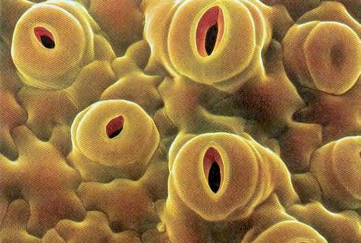
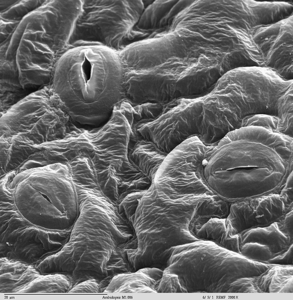
0.1 - Images from top, Showing the form of hibiscus leaves, Structure at the bottom of lily pad, Vein pattern of a leaf, Microphoto of stomatawhich aid photosynthesis,
8
1 Biomimetics Research
This chapter is a comprehensive study of adaptive systems in nature. Fibre organisation strategies in biological systems , which allow for changes in shape and material properties with respect to transient changes in the environment are investigated. The process of Stimulus-Response co-ordination, in biological organisms range from simple to complex configurations. Such configurations of sensing devices, actuators and controllers are studied, both in biology and man-made precedents.
Adaptive Systems Precedents Smart Systems
Thigmo-Morphogenesis
Fibre Organisation
Fibre Organisation Strategies in Nature
Biology makes use of remarkably few materials and nearly all loads are carried by fibrous composites. There are only four types of fibers: cellulose, collagen, chitin and silks. These are the basic materials of biology and they have much lower densities than most engineering materials. They are successful not so much of what they are but because the way in which they are put together. The bulk of the mechanical loads in biology are carried by these polymer fibres. The fibres are bonded together by various substances such as polysaccharrides, polyphenols and so on, sometimes in combination with minerals such as calcium carbonate (eg.mollusk shells) and hydroxyapatite (eg. bone). The organisation of the fibres and the degree of interaction between them provides the means of tailoring their properties for specific requirements. For example, It is the same collagen fibre that is used in low modulus and highly extensible structures such as blood vessels, intermediate modulus tissues such as tendons and high modulus, rigid materials such as bone. [1.1]
The reason for all biological organisms being made of polymers is probably that the synthesis of long polymer chains based on carbon, oxygen, nitrogen and hydrogen makes use of readily available chemicals and can be controlled by enzymes at low temperatures. The man-made counterparts of these biological fibrous materials are high-performance fibres such as nylon, aramid and highly-oriented polyethylene. The use of fibres for making structural materials offers a great deal of scope and flexibility in design. Fibres and fibre-reinforced materials have an inherent property of anisotropy of physical and mechanical properties and heterogeneity. If properly exploited, they can provide higher levels of optimisation than would be possible with isotropic, homogeneous materials because
stiffness and strength can be matched to the loads applied, not only in magnitude but also in direction.
In biology this is extremely common and happens as a result of “growth under stress”. The magnitude and direction of the loads that the organism experiences as it develops provide the blueprint for the selective deposition of new material, where it is needed and in the direction in which it is needed. The best known examples of this are the “adaptive” mechanical design of bone and trees. In bone, material can be removed from the under stressed parts and re-deposited in the highly stressed ones ; in trees a special type of wood, with different cellulose microfibril orientation and cellular structure are produced in successive annual rings when mechanical circumstances demand. Growing a structure by producing and organising fibres under the control of the loads that it has to carry is extremely efficient.
Numerous patterns of load-bearing fibre architectures are found in nature, each one of them being a specific answer to a specific set of mechanical conditions and requirements. In a sense there are no general design solutions in biology but case specific ones, governed nevertheless by common general principles. In conventional engineering practices this process is replaced by stress and structural analysis which is not always accurate and often very complex. In recent years, numerical techniques based on Finite Elements have provided new tools to simulate the adaptive design of nature and this approach has proved to be very successful. [1.2]
10

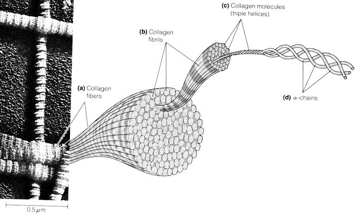
1.1 - Four basic types of fibres in nature, namely, collagen, cellulose, chitin and silks.
Collagen- The fibre material composition of the human femur shows the close packing of fibres in parts which are highly stressed.
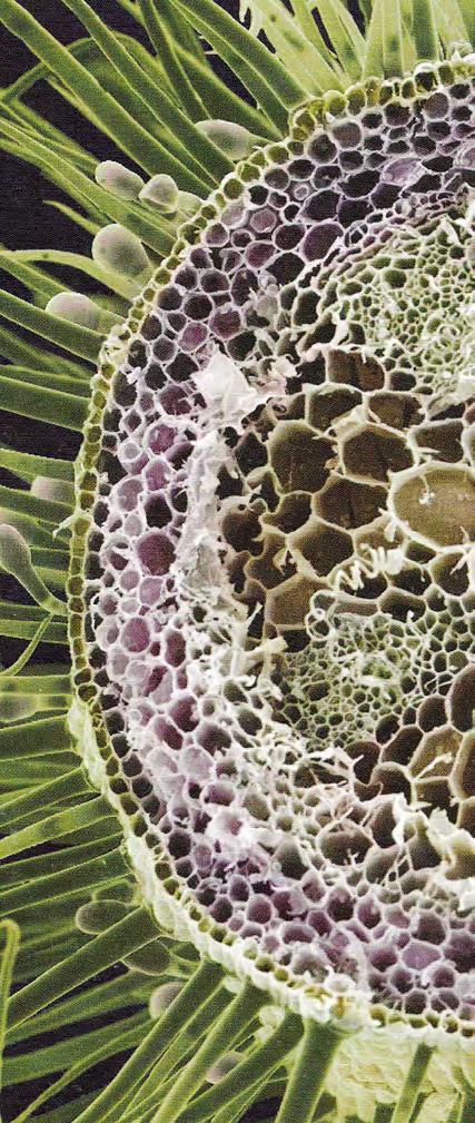
Cellulose- The section through the stem of a germanium reveals the closely packed bundles of vessels and cells. The geometrical arrangement of closepacked integration produces a complex structure, strong but flexible and capable of differential movement. The large pale tubes in the centre are xylem vessels that transport water and nutrients up from the root. The five bundles of pale green vessels are phloem cells, part of the vascular system for the distribution of carbohydrates and hormones, and the smaller purple cells on the perimeter are parenchyma cells, which are thin walled and flexible and can increase and decrease in size by taking up or losing water. These changes cause deformations, which is how the plant achieves movements such as bending towards light or turning around an obstacle

11
Collagen
Cellulose
Chitin
Silks
material hierarchies
Fibres are most efficient when they carry pure tensile loads, either as structures in their own right such as ropes, cables, tendons, silk threads in spider’s webs or as reinforcement in composite materials. Being slender columns, fibres cannot carry loads in compression because of buckling, even when partially supported laterally by the matrix in composites. In the case of polymer fibres, micro buckling at the micro-fibrillar level within the fibre results also in very poor compressive strengths. This problem is common to both man-made and biological composites. Since nature had no alternatives to fibres as building blocks, it had to find ways of offsetting the low efficiency of fibres in compression in order to expand life beyond the limits of squidgy invertebrate species or aquatic environments. There are four solutions available in nature to this problem: pre-stress the fibres in tension so that they hardly ever experience compressive loads; introduce high modulus mineral phases intimately connected to the fibres to help carry compression; heavily cross-link the fibre network to increase lateral stability, and change the fibre orientation so that compressive loads do not act along the fibres.
Jim Gordon, says in ’ The New Science of Strong Materials and Structures’, when one is dealing with very heterogeneous fibre reinforced composite systems, the distinction between materials and structures becomes one of convenience rather that of fact. This distinction becomes even more elusive in biology because between the polymer macromolecular chains at the nano metre level and the functional organ at the millimetre or metre levels there is a multiplicity of structures which represent different levels of aggregation of the load bearing materials. These hierarchical
organisations are the rule rather than the exception in all biological composites. They are probably the result of growth by successive deposition of fibres and other materials. They are difficult to analyse because of their complexity but, by varying the degree of interaction between sub elements within a hierarchical level and between levels, stiffness, strength, toughness, etc. are modulated, tailored and optimised for specific requirements. This kind of integrated sub-structuring is a common theme in biology, far more subtle and extensive than in any manmade material or structure. [1.3]
Familiar biological materials such as tendons, bones, muscles, skin and wood provide amazing arrays of hierarchies spanning in typical dimensions from 10-9 metres at the molecular level, to typically 10-3 - 10-2 at tissue level and 100 and beyond at the organ level. In trees, for example, the representative diameter of the various sub structures covers a range from 101 metres at the diameter of trunk down to 10-8 metres diameter of cellulose protofibril; i.e. ten orders of magnitude with perhaps eight hierarchical levels: organ (trunk), tissue (wood), wood cell, laminated cell walls, individual walls, cellulose fibres, microfibrils and protofibrils.
12
1.2 - The upper image shows collagen fibres of various sizes in a scanning electron microscope. At bottom a much higher magnification image from a transmission EM shows characteristic “banding” pattern of individual fibrils that make up the larger anatomic fibre.
Fibre
Thigmo-morphogenesis
Thigmo-morphogenesis refers to the changes in shape, structure and material properties that are produced in response to transient changes in environmental conditions. We are all familiar with the fact that many plants are capable of movement, sometimes slow as in the petals of flowers which open and close, tracking of the sun by the sunflowers, the convolutions of bindweed’s around supporting stems, snaking of roots around obstacles, sometimes visible to the eye as in the drooping of leaves when mimosa pudica is touched, exceptionally very rapid, too fast to be seen as in the closing of the leaves of the venus flytrap.
In all these examples, movement and force are generated by a unique interaction of materials, structures, energy sources and sensors. The materials are the cellulose walls of perenchyma cells ,nonlignified, flexible in bending but stiff in tension; the structures are the cells themselves and their shape with the biologically active membrane that can control the passage of fluid in and out of the cells; the energy source is the chemical potential difference between
the inside and the outside of the cells; the sensors are as yet unknown. These systems are essentially working as networks of interacting mini hydraulic actuators, liquid filled bags which can become turgid or flaccid and which, owing to their shape and mutual interaction translate local deformations to global ones and are also capable of generating very high stresses. Similar mechanisms can be seen in operation when leaves emerge from buds and deploy to catch sunlight. How to package the maximum surface area of material in the bud and to expand it rapidly and efficiently is the result of very smart folding geometry, turgor pressure and growth. [1.4]


13
1.3 - Undisturbed delicate leaves of the sensitive plant,
Mimosa pudica when lightly touched, responds to stimulus.
14
1.4 - Micrograph of stomata cells in a leaf, which open and close during the process of photo-synthesis in response to sun light.
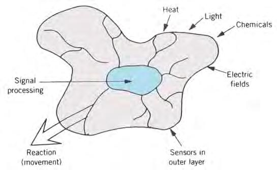
Energy Input (Stimulus)
Morpho-Mechanical Computation
Adaptive mechanical design in biology deals with the design output arising from a set of inputs on the evolving or growing organ or organism. The inputs can be external and internal loads, environmental changes, etc., which are superimposed on the genetic information available. The evolutionary time-scale is a long one and what we observe as a response in biological organisms is the result of all these inputs over long periods of time. This complex process of sensing and actuation could be termed as ‘Morpho-Mechanical Computation’. The energy input or stimulus received from the environment is transduced into electric signals by biological sensing devices. The electric signals are further processed for an appropriate responsive behavior.
Two other aspects of ‘Morpho Mechanical Computation’ which
occur over much shorter timescales and which involve individuals as opposed to whole species, are Thigmo-morphogenesis, such as various forms of tropism, the opening and closing of stomata cells in leafs and bone-remodelling. What they show is the intrinsic design flexibility due to fibres and fibre architectures, hierarchies and the modulation of interactions between them, together with growth, converging to the a specific solution required for a specific situation. In order to adapt to the changes in circumstances, change in fibre orientations, modifications in structure and material properties and the shapes in local and global scales are altered. [1.5]
1.5 - Diagram showing the process of Morpho-Mechanical Computation
15
Device
Electrical Signal Filtering Processing Response Behaviour
(Transduction)
16
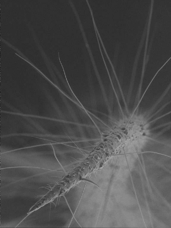
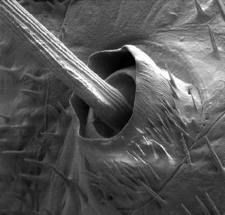
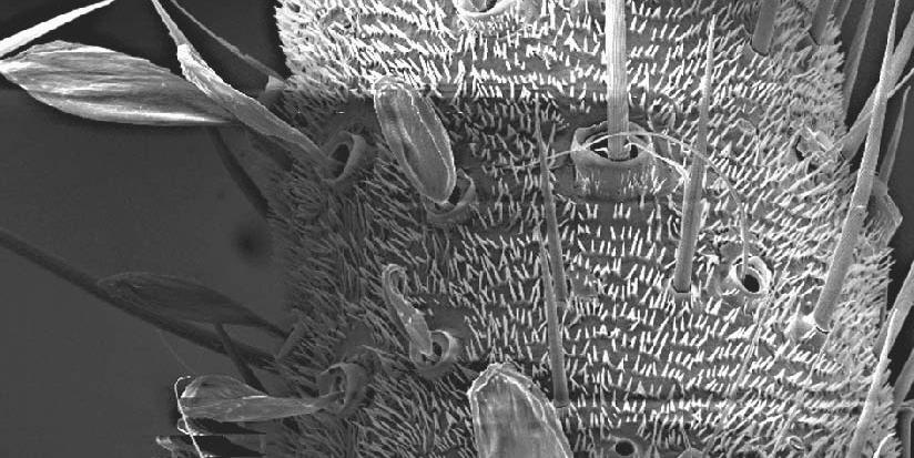
1.6 - Micrograph showing , Sensory filiform hairs of crickets for detection of predators. Filiformhair length varies between 100 and 1500 μm
Biological Sensing Devices
One of the most interesting aspects of multifunctionality and integration in biology is the way in which receptors detect and amplify mechanical strains and displacements. These devices are called as mechanoreceptors. They do exist in all creatures, plants and animals as shown in the table 1.7.
The vibration amplifications in case of insects, arthropods and crustaceans is further elaborated. These species have exoskeletons which, in their rigid state, are stiff laminated composite structures made of chitin fibres embedded in a highly crosslinked matrix of proteins and phenolic substances. The exoskeleton acts also as the load, strain or displacement detector via specialised organs, called sensilla, parts of which are local modification of the laminated structure of the exoskeleton to amplify the strain information for the detector organ connected to the nerve cell. These local modifications are a combination of changes in thickness, material stiffness and fibre orientation function as strain concentrations and mechanical signal amplifiers. These are equivalent to drilling holes into structural
Chemical (most animals and some plants)
Vibration (hair sensors in insects, spiders, scorpions, hearing)
Infrared (beetles, snakes)
Fluid-flow (various insects, spiders, crustaceans, fish, amphibians)
Strain (insects, arthropods)
Pressure (fish)
Touch (most animals and some plants)
Electrical (fish)
Magnetic (fish, birds)
Radiation(most animals –photoreceptors / vision)
Mechano-Receptors
components and embedding strain gauges in the regions near the holes to get an amplification of the remote state of strain of the structure.
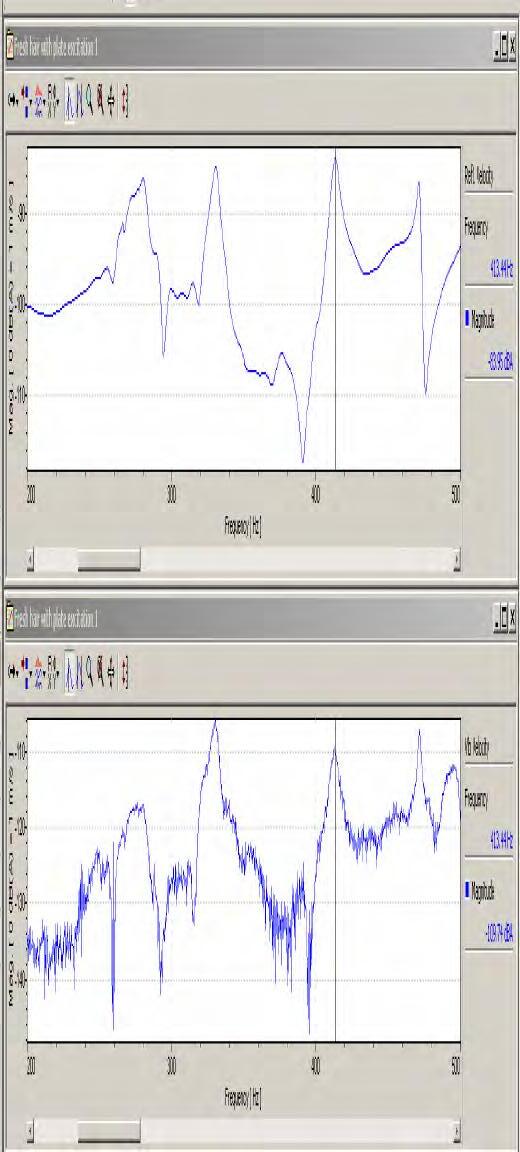
The comparison between the vibration graphs shows the efficiency of mechanoreceptors in crickets which have a highly precise vibration sensing as against man-made sensing devices which pick up vibrations. [1.8]
17
1.8 - Comparison between an Input (tapped metal plate) sensor and cricket hair response (frequency range 200-500 Hz) 1.7- Table showing Mechano- Receptors of several organisms
s a e Sensing Actuation Energy
Adaptive systems in nature
Adaptive systems in nature have an incredible Stimulus-Response coordination. The simplest type of response is a direct one-to-one stimulusresponse reaction. A change in the environment is the stimulus; the reaction of the organism to it is the response.
Natural adaptive systems range from simple to complex configurations of sensing devices, actuators, controller logics and inherent energy generators. The adaptive potential is a resultant of continuous evolutionary processes to the environmental pressures under gone by the organism. Lower level organisms such as amoeba, fungi and plants display a simpler process of stimulus response co-ordination as against higher level organisms such as animals which respond to multiple stimuli.
Lower-level Organisms
In case of lower level organisms such as nonlignified plants adaptive behavior is entirely dependent on control of turgor pressure inside the cells to achieve structural rigidity, pre-stressing the cellulose fibres in the cell walls at the expense of compression in the fluid. Trees pre-stress their trunks with the outermost layers of cells being prestressed in tension to offset the poor compressive properties of wood. [1.7]
In single-celled organisms, adaptive behavior is the result of a property of the cell fluid called irritability. In simple organisms, such as algae, protozoan’s, and fungi, a response in which the organism moves toward or away from the stimulus is called taxis.
Therefore the sensing and actuation functions are integrated within the definition of the material properties itself. The adaptive behavior emerges through the strategic definition of the fibre material hierarchies in multiple scales.
The energy required for actuation is also generated within the material system, In case of plants, through the process of photosynthesis and distribution of nourishment to alter the osmotic pressure and chemical disintegration in case of single celled organisms.
18
1.9 - Microgaph showing Parenchyma cells in plants which act as mini hydraulic actuators, by changing the osmotic pressure inside their cell walls.
Sensing Actuation Control Energy
Higher-level Organisms
In higher level organisms, adaptive behavior involves the synchronization and integration of events in different parts of the body, a control mechanism, or controller, is located between the stimulus and the response. In multi-cellular organisms, this controller consists of two basic mechanisms by which integration is achieved, chemical regulation and nervous regulation.
In chemical regulation, substances called hormones are produced by well-defined groups of cells and are either diffused or carried by the blood to other areas of the body where they act on target cells and influence metabolism or induce synthesis of other substances. The changes resulting from hormonal action are expressed in the organism as influences on, or alterations in, form, growth, reproduction, and behaviour.
In animals, in addition to chemical regulation via the endocrine system, there is another integrative system called the nervous system. A nervous system can be defined as an organized group of cells, called neurons, specialized for the conduction of an impulse, an excited state from a sensory receptor through a nerve network to an actuator, the site where response occurs.[1.8]
Organisms that possess a nervous system are capable of much more complex behaviour. The nervous system, specialized for the conduction of impulses, allows rapid responses to environmental stimuli. Many responses mediated by the nervous system are directed toward preserving the status
quo, or homeostasis, of the animal. Stimuli that tend to displace or disrupt some part of the organism call forth a response that results in reduction of the adverse effects and a return to a more normal condition. Organisms with a nervous system are also capable of a second group of functions that initiate a variety of behaviour patterns. Animals may go through periods of exploratory or appetitive behaviour, nest building, and migration. Although these activities are beneficial to the survival of the species, they are not always performed by the individual in response to an individual need or stimulus. Finally, learned behaviour can be superimposed on both the homeostatic and initiating functions of the nervous system.[1.9]
Therefore, higher level organisms have far more sophisticated and complex system for sensing and actuation functions. There is a multifarious integration between sensors, controllers and actuators. To maintain homeostasis of the organism, the stimulus generated by multiple sensor inputs, go through filter processing which leads to decision making capabilities in higher level organisms. An equivalent to this in the man-made world would be artificial neural networks which have multiple inputs fed into processors which generated multiple outputs based on predefined rules.
The energy required for actuation is again generated within the organism by the process of metabolism.

19 s
a e c
1.10 - Neurons, forming neural networks in the nervous system and a neuron cell group responsive to multiple stimuli.
Precedents
“The ultimate smart structure would design itself. Imagine a bridge which accretes materials as vehicles move over it and it is blown by the wind. It detects the areas where it is overstretched and adds material until the deformation falls back within a prescribed limit… The paradigm is our own skeleton where material deposition happens in parts which require greater strength.”[1.10]
- Adriaan Beukers and Van Hinte
Architectural structures or building envelopes could be viewed as systems which need to self-regulate, adapt to the environmental changes and respond to natural elements such as sun, wind, rain etc. to achieve a comfortable micro climate. Environmentally responsive buildings, also called as intelligent buildings employing IBMS (Intelligent Building Management Systems) function as a collection of devices such as louvers and shades, controlled by a central computer that receives data from remote sensors and sends back instructions for activation of these mechanical systems.
On the contrary, natural systems are quite different wherein most of the sensing, decision making and reactions are entirely local and the global behavior is the product of these local actions. This is true across all scales, from small plants to large mammals. When we run for a bus, we do not have to make any conscious decisions to accelerate our heartbeat, increase our breathing rate and volume or open our pores to regulate the higher internal temperature generated. This concept of local decision making and reacting to external conditions is termed as cybernetics.[1.11]
Noebert Wiener introduced the term ‘Cybernetics’ in 1949. The concept of cybernetics includes information theory and practice, from transmission to reception, as well as subsequent manipulation and utilization of the information to control regulatory processes of living organisms, societies, buildings and engineering situations. Information plays a decisive role in the operation of both living organisms and buildings. The emissions and transmissions which constantly emanate from infinitely many sources such as the environment are converted into information by the agents which can use them as a basis for action or inaction. Information can reach the receiver without
being passed along and manipulated within; so that the system governs itself by adjusting accordingly. However, information can also have its origin within the living organism or buildings (such as functional and spatial requirements). This feedback within a system is a special form of information in living processes which allows growth, adaptation or rather self-regulation.
Living organisms perceive information through their senses. The senses serve the organism by obtaining information about the environment, like needs for survival, namely food, safety and reproduction. The acquisition of information is partly conscious. Living organisms react to many external as well as internal signals without involving consciousness, by assimilating them unconsciously or subconsciously like the tanning of skin by deposition of melanin when exposed to sunlight does not involve the brain.[1.12]
It is this flexibility, reactive and transformational capacities of biological organisms that scientists are now seeking to replicate in materials, computers, robotics and buildings. In biomimetics, scientists look at everything from the way the brain learns through trial and error, (so that robots may do the same), to the way a fish moves through water (so the submarines can become similarly more flexible and efficient by reducing central control). This level of biomimicry takes into understanding the aspect of self-organization in biological organisms.[1.13]
There are some precedents which have endeavoured to achieve the self -organisational process observed in nature. We shall briefly discuss the system configuration of sensors, actuators, control and energy deployed in these precedents in relation to the higher and lower level organisms discussed in the previous section of adaptive systems in nature.
20
Hypo-Surface

The sensors, actuators and the control technology were developed to react within milliseconds to pulses racing from one side to another at speeds of 50 kilometres an hour. The surface was fractioned into small plates interconnected by rubber squids. The geometry of the curved plane (during actuation) is defined by triangular plates to enable double curvatures.
[1.14]
The responsive behaviour of the hyposurface is different from the self-organisation process of adaptive systems in nature. The system consists of sensors and actuators, but the information processing or control and the energy required for the actuation of the pneumatic pistons are sourced externally.
‘Hyposurface’ was developed by Mark Goulthorpe of Decoi architects as an interactive installation in Birmingham Hippodrome in 1999. The responsive wall measures approximately 8 metres wide and 7 meters high. The project was collaboration between architects, mathematicians, computer programmers and multimedia experts. The hyposurface transforms from being a flat plane into a curved plane by moving the components up and down by up to 60cm. The surface, extremely varied in its motions and highly dynamic, reacts to environmental influences. The stimuli are picked up by sensors responsive to video, sound, light, heat, movement and so on. The actuation was carried out through arrays of pneumatic pistons, which are activated in real time to the stimuli. The control system processing the information from sensors calculates and signals to each piston a precise instruction at real-time speed. The wall responds in sympathy with a clap from an observer and does not simply respond as a delayed reaction.
21
a e c
s
1.11 -Active responsive wall ‘Hypo-surface’ developed by Mark Goulthorpe with motion sensors and pneumatic actuators.
1.12 -Diagram showing the configuration of sensors and actuators forming a responsive system with external control and energy input.
Cartesian wax is a material system developed by Neri Oxman for the exhibition ‘Design and the Elastic Mind’ at the MoMA - Museum of Modern Art in 2008. The project explores the notion of material organization as it is informed by structural and environmental performance. It is a prototype for an environmentally responsive skin and an exploration into building envelope design. The material system defined, integrates structural and environmental elements of the building skin. The structural elements provide for an optimized distribution of load, while the environmental elements allow for the infiltration of light and heat to and from within the skin. Integrated solutions may prove to be more sustainable as they are in the natural and biological world. Less redundant and more custom-fit to their environment, space and structure can now be shaped and manufactured using state-of-the-art fabrication techniques and technologies. It is a well known fact that in nature, shape is cheaper than material. In manmade design, this was never the case. Material is traditionally assigned to a shape by way of post-rationalizing its geometry. By using softwares to create new composite materials Oxman has been able to replicate the processes of nature, creating materials that are able to adapt to light, load, skin pressure, curvature and other ecological elements.[1.15]

The topology is defined as a continuous tiling system, differentiated across its entire surface area to accommodate for a range of conditions accommodating for light transmission, heat flux, and structural support. The surface is thickened locally where it is structurally required to support itself, and modulates its transparency according to the light conditions of its hosting environment. Twelve tiles are assembled as a continuum comprised of multiple resin types, rigid and flexible. Each tile is designed as a structural composite representing the local performance criteria as manifested in the mixtures of resin. [1.16]
In this case the material system is predefined with sensing and actuation functions. The changes in the environmental heat flux are used to change the state of the resin from flexible to rigid and hence manipulate the transparency of the surface. The adaptive mechanism here is similar to that of lower level organisms, where the sensing, actuation and the energy required for the actuation is generated within the system. There is no information processing or decision making involved and the material seamlessly responds to the changes in the environmental conditions. load, while
22
Cartesian Wax
1.13 -Resposive material system ‘Cartesian Wax’ developed by Neri Oxman.
1.14 -Diagram showing the configuration of sensors, actuators and energy forming an integral part of the material system.
NASA is currently working with Boeing and the U.S. Air Force on the Active Aero-elastic Wing (AAW) F/A-18 project in a quest for developing a morphing aircraft that changes its shape in flight. The Aircraft of the future will not be built of traditional, multiple, mechanically connected parts and systems. Instead, aircraft wing construction will employ fully integrated, embedded “smart” materials and actuators that will enable aircraft wings with unprecedented levels of aerodynamic efficiencies and aircraft control. The availability of strong, flexible composite structures and miniaturized computers and motors point the way toward seamless wings that will one day bend to achieve flight control as effortlessly as a bird does. [1.17]
The smart plane would respond to the constantly varying conditions of flight, sensors will act like the “nerves” in a bird’s wing and will measure the pressure over the entire surface of the wing. The response to these measurements will direct actuators, which will function like the bird’s wing “muscles.” Just as a bird instinctively uses different feathers on its wings to control its flight, the actuators will change the shape of the aircraft’s wings to continually optimize flying conditions. Active flow control effectors will help mitigate adverse aircraft motions when turbulent air conditions are encountered.
Intelligent systems composed of these sensors, actuators, microprocessors, and adaptive controls will provide an effective “central nervous system” for stimulating the structure to affect an adaptive “physical response.”The central nervous system will provide many advantages over current technologies. The proposed AAW Vehicles will be able to monitor their own performance, environment, and even their operators in order to improve safety and fuel efficiency, and minimize airframe noise. They will also have systems that will allow for safe takeoffs and landings. Researchers at NASA Langley Research Center are taking the lead to explore these advanced vehicle concepts and revolutionary new technologies. [1.18]
The process of morpho mechanical computation in the smart plane is similar to that of higher level organisms. There are multiple inputs from the environment such as temperature, drag coefficient, turbulence and so on; these multiple sensor inputs would be processed by controllers similar to that of the central nervous system. Then the actuation would be carried out through the actuators strategically positioned long the surface of the wing span. load, while

23
Smart Plane
of sensors ,
and energy forming and integrated and cohesive smart adaptive
1.15- Morphing smart plane , developed by NASA Dryden Flight Research Centre shows advanced concepts for the aircraft of the future 1.16 -Diagram showing
the configuration
actuators, controllers
system.
Smart systems
All around us are living things that sense and react to the environment in sophisticated ways. As structures have become more complex and are being asked to perform ever more difficult missions, there has been an ever increasing need to build “intelligence” into them so that they can sense and react to their environment. Examples include buildings that can sense, react and survive earthquakes and spacecraft that can sense and repair damage autonomously. To perform these functions successfully a “nervous system” is required that performs in a manner analogous to those of living things sensing the environment, conveying the information to a central processing unit (the brain) and reacting appropriately. Fiber optic technology has enabled the nerves of the system to be realized. Using hair-thin glass fibers as information carriers and sensors that may be built directly into the fibers with no increase in the overall size, it is possible to create long strands of fibre sensors capable of measuring strain, pressure, temperature, and other key parameters. These sensor “strings” may then be embedded into the structural materials with no degradation in overall strength, resulting in “smart structures” with built in nervous systems. Such structures could achieve active control, where a structure senses environmentally induced structural changes and reacts in real time.[1.19]
The term smart materials and structures are used to describe this unique collaboration of material and their structural properties with fibre optic sensors and actuation control technology. Smart structures constructed from materials with fibre optic nerves could continuously monitor the loads imposed on them as well as their vibration state and deformation. In addition, strain sensing may be capable of assessing damage and warning of impending weakness in structural integrity or improving quality control of thermo set composite materials during fabrication through cure monitoring. This could lead to greater reliance in the use of advanced composite materials and the usage of optimum material based on specific loading conditions.
A large scale research effort is currently underway to use advanced composite materials extensively in bridges. This research is addressing issues of corrosion, rehabilitation, and monitoring and involves new concepts and designs in bridge repair and construction. One of the most significant advances is the replacement of steel pre-stressed tendons with ones made of advanced composite materials. These fiber reinforced polymers are practically immune to corrosion and also lead themselves to internal monitoring by means of embedded fiber optic sensors. A structurally integrated sensing system could monitor the state of the structure, throughout its working life. It could determine the strain, deformation, load distribution and temperature or environmental degradation experienced by the structure. The first smart bridge to be built with structurally integrated fiber optic strain and temperature sensors was opened in 1993 in Calgary.
In more advanced smart structures the information provided by the built-in sensor system could be used for controlling some aspect of the structure, such as its stiffness, shape, position or orientation. These systems could be called adaptive (or reactive) smart structures to distinguish them from the simpler passive smart structures. A more appropriate term for structures that only sense their state might be “Sensory Structures”. Smart structures might eventually be developed that will be capable of adaptive learning and these could be termed “Intelligent Structures”. Indeed, if we consider the confluence of the four fields- structures, sensor systems, actuator control systems, and neural network systems- we can appreciate that there is the potential for a broad class of structures such as, Controlled Structures, Self-learning Reactive Structures, Smart Structures and Self-learning Smart Structures. Therefore smart structures open up a new panorama for biomimetic systems.
As Eric Udd says, “This era would see the marriage of fibre optic technology and artificial intelligence with material science and
structural engineering. Major structures constructed in this period would be constructed with built-in optical neuro-systems and active actuation control that would make them more like living entities than the inanimate edifices we are familiar with today. To carry this biological paradigm one step further, it may even be possible to contemplate future structures that have the capacity for limited self-repair. Indeed, if we think of the new frontiers for engineering as being in space or underwater, self-diagnosis, self-control, and self- healing may not be so much esoteric as vital”. [1.20]

24
1.17
-Calgary bridge built with embedded fibre optic sensors.
Structures
Controlled Structures Smart Structures Smart Adaptive Structures
Actuator Systems
Intelligent Adaptive Structures Selflearning Reactive Structures Selflearning Smart Structures
Sensor Systems
Neural Network Systems
25
1.18 -Diagram showing Smart Systems possible by the confluence of four disciplines: materials and structures, sensing systems, actuator control systems, and adaptive learning neural networks.
2 Technology
This chapter will explore all the different technologies used for our research and development of the project. For building our physical models and achieving the desired functionality of the system -both in theory and in practice-, many possibilities were open and specific choices had to be made. Here we explain our choices and give a thorough background of the technology behind our material system.
Sensing Actuation Energy Control Base Material
Base Material
Fibre Composites
Man made composites are not new. The first composite materials were developed many years ago:
• Mud bricks reinforced with straw (antiquity)
• Glass Reinforced Plastic - GRP (1940s)
• Carbon Fibre Reinforced Plastic – CFRP (1960s)
In its most basic form a composite material is one which is composed of at least two elements working together to produce material properties that are different to the properties of those elements on their own [2.1]. In practice, most composites consist of a bulk material (the ‘matrix’), and a reinforcement of some kind, added primarily to increase the strength and stiffness of the matrix [2.2,2.3,2.4]. This reinforcement is usually in fibre form.
Today, the most common man-made composites can be divided into three main groups:
Polymer Matrix Composites (PMC’s): These are the most common and have been selected for the construction of this project. Also known as FRP - Fibre Reinforced Polymers (or Plastics) - these materials use a polymer-based resin as the matrix, and a variety of fibres such as glass, carbon and aramid as the reinforcement.
Metal Matrix Composites (MMC’s) - Increasingly found in the automotive industry, these materials use a metal such as aluminium as the matrix, and reinforce it with fibres such as silicon carbide.
Ceramic Matrix Composites (CMC’s) - Used in very high temperature environments, these materials use a ceramic as the matrix and reinforce it with short fibres, or whiskers such as those made from silicon carbide and boron nitride.
Resins are divided into two major groups known as thermoset and thermoplastic.
Thermoplastic resins become soft when heated, and may be shaped or molded while in a heated semi-fluid state and become rigid when cooled. Thermoset resins, on the other hand, are usually liquids or low melting point solids in their initial form. When used to produce finished goods, these thermosetting resins are “cured” by the use of a catalyst, heat or a combination of the two. Once cured, solid thermoset resins cannot be converted back to their original liquid form. Unlike thermoplastic resins, cured thermosets will not melt and flow but will soften when heated (and lose hardness) and once formed they cannot be reshaped. Heat Distortion Temperature (HDT) and the Glass Transition Temperature (Tg) is used to measure the softening of a cured resin. Both test methods (HDT and Tg) measure the approximate temperature where the cured resin will soften significantly to yield (bend or sag) under load.
The most common thermosetting resins used in the composites industry are unsaturated polyesters, epoxies, vinyl esters and phenolics. There are differences between these groups that must be understood to choose the proper material for a specific application.
Polyester
Unsaturated polyester resins (UPR) are the workhorse of the composites industry and represent approximately 75% of the total resins used. Thermoset polyesters are produced by the condensation polymerization of dicarboxylic acids and difunctional alcohols (glycols). In addition, unsaturated polyesters contain an unsaturated material, such as maleic anhydride or fumaric acid, as part of the dicarboxylic acid component. The finished polymer is dissolved in a reactive monomer such as styrene to give a low viscosity liquid. When this resin is cured, the monomer reacts with the unsaturated sites on the polymer converting it to a solid thermoset structure [2.5].
The primary functions of the resin are to transfer stress between the reinforcing fibers, act as a glue to hold the fibers together, and protect the fibers from mechanical and environmental damage.
A range of raw materials and processing techniques are available to achieve the desired properties in the formulated or processed polyester resin. Polyesters are versatile because of their capacity to
28
PMC | Resins
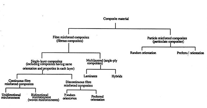
2.1 Classification of composite materials
2.2
Diagram
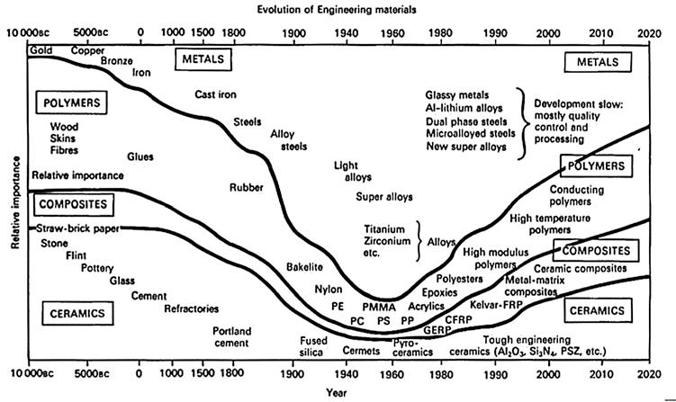
showing the evolution of engineering materials
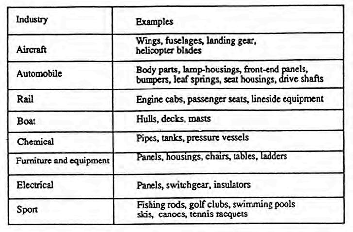
2.3 Examples of composite materials uses
be modified or tailored during the building of the polymer chains. They have been found to have almost unlimited usefulness in all segments of the composites industry. The principal advantage of these resins is a balance of properties (including mechanical, chemical, electrical) dimensional stability, cost and ease of handling or processing.
Unsaturated polyesters are divided into classes depending upon the structures of their basic building blocks. Some common examples would be orthophthalic (“ortho”), isophthalic (“iso”), dicyclopentadiene (“DCPD”) and bisphenol A fumarate resins. In addition, polyester resins are classified according to end use application as either general purpose (GP) or specialty polyesters. [2.5]
Epoxy
Epoxy resins have a well-established record in a wide range of composite parts, structures and concrete repair. The structure of the resin can be engineered to yield a number of different products with varying levels of performance. A major benefit of epoxy resins over unsaturated polyester resins is their lower shrinkage. Epoxy resins can also be formulated with different materials or blended with other epoxy resins to achieve specific performance features. Cure rates can be controlled to match process requirements through the proper selection of hardeners and/or catalyst systems. Generally, epoxies are cured by addition of an anhydride or an amine hardener as a 2-part system. Different hardeners, as well as quantity of a hardener produce a different cure profile and give different properties to the finished composite.
Epoxies are used primarily for fabricating high performance composites with superior mechanical properties, resistance to corrosive liquids and environments, superior electrical properties, good performance at elevated temperatures, good adhesion to a substrate, or a combination of these benefits. Epoxy resins do not however, have particularly good UV resistance. Since the viscosity of epoxy is much higher than most polyester resin, requires a post-cure (elevated heat) to obtain ultimate mechanical properties making epoxies more difficult to use. However, epoxies emit little odor as compared to polyesters.
Epoxy resins are used with a number of fibrous reinforcing materials, including glass, carbon and aramid. This latter group is of small in volume, comparatively high cost and is usually used to meet high strength and/or high stiffness requirements. Epoxies are compatible with most composite manufacturing processes, particularly vacuumbag molding, autoclave molding, pressure-bag molding, compression molding, filament winding and hand lay-up.
Vinyl Ester
Vinyl esters were developed to combine the advantages of epoxy resins with the better handling/faster cure, which are typical for unsaturated polyester resins. These resins are produced by reacting epoxy resin with acrylic or methacrylic acid. This provides an unsaturated site, much like that produced in polyester resins when maleic anhydride is used. The resulting material is dissolved in styrene to yield a liquid that is similar to polyester resin. Vinyl esters are also cured with the conventional organic peroxides used with polyester resins. Vinyl esters offer mechanical toughness and excellent corrosion resistance. These enhanced properties are obtained without complex processing, handling or special shop fabricating practices that are typical with epoxy resins.
Phenolics are a class of resins commonly based on phenol (carbolic acid) and formaldehyde. Phenolics are a thermosetting resin that cure through a condensation reaction producing water that should be removed during processing. Pigmented applications are limited to red, brown or black. Phenolic composites have many desirable performance qualities including high temperature resistance, creep resistance, excellent thermal insulation and sound damping properties, corrosion resistance and excellent fire/smoke/smoke toxicity properties. Phenolics are applied as adhesives or matrix binders in engineered woods (plywood), brake linings, clutch plates, circuit boards and more.
Benefits of using composites
superior mechanical properties compared to the matrix
low density – weight saving
corrosion resistance
fatigue expansion coefficient
Composite’s properties depend on:
• fibre content (volume fraction)
• fibre alignment (unidirectional gives highest value)
• fibre length (discontinuous OK if l/d > 30)
• fibre distribution
• fibre orientation; multi-axial loads (lay-up, stacking sequence)
29
Phenolic
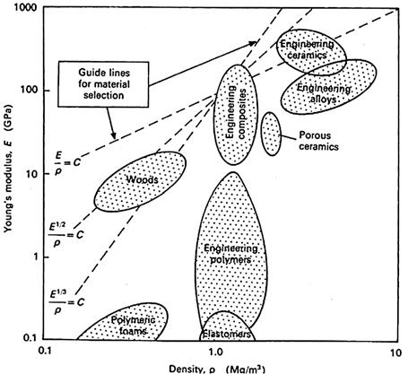
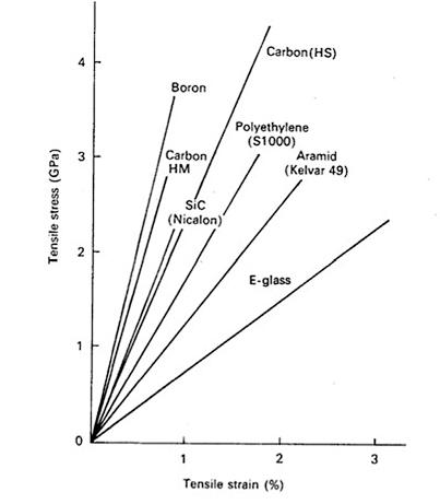
2.5 Stress-strain curves for a selection of fibres 2.6 Directionality of fibres 2.4 Young’s Modulus-Density graph
Polyurethane
Polyurethane is a family of polymers with widely ranging properties and uses, all based on the exothermic reaction of an organic polyisocyanates with a polyols (an alcohol containing more than one hydroxl group). A few basic constituents of different molecular weights and functionalities are used to produce the whole spectrum of polyurethane materials. The versatility of polyurethane chemistry enables the polyurethane chemist to engineer polyurethane resin to achieve the desired properties.
Polyurethanes appear in an amazing variety of forms. These materials are all around us, playing important roles in more facets of our daily life than perhaps any other single polymer. They are used as a coating, elastomer, foam, or adhesive. When used as a coating in exterior or interior finishes, polyurethane’s are tough, flexible, chemical resistant, and fast curing. Polyurethanes as an elastomer have superior toughness and abrasion is such applications as solid tires, wheels, bumper components or insulation. There are many formulations of polyurethane foam to optimize the density for insulation, structural sandwich panels, and architectural components. Polyurethanes are often used to bond composite structures together. Benefits of polyurethane adhesive bonds are that they have good impact resistance, the resin cures rapidly and the resin bonds well to a variety of different surfaces such as concrete.
Thermoplastics
A thermoplastic is a polymer that turns to a liquid when heated and freezes to a very glassy state when cooled sufficiently. Most thermoplastics are highmolecular-weight polymers whose chains associate through weak Van der Waals forces (polyethylene); stronger dipole-dipole interactions and hydrogen bonding (nylon); or even stacking of aromatic rings (polystyrene). Thermoplastic polymers differ from thermosetting polymers (Bakelite; vulcanized rubber) as they can, unlike thermosetting polymers, be remelted and re-moulded.
Thermoplastics are elastic and flexible above a glass transition temperature Tg, specific for each one—
the midpoint of a temperature range in contrast to the sharp melting point and melting point of a pure crystalline substance like water. Below a second, higher melting temperature, Tm, also the midpoint of a range, most thermoplastics have crystalline regions alternating with amorphous regions in which the chains approximate random coils. The amorphous regions contribute elasticity and the crystalline regions contribute strength and rigidity, as is also the case for non-thermoplastic fibrous proteins such as silk.
Thermoplastics can go through melting/freezing cycles repeatedly and the fact that they can be reshaped upon reheating gives them their name. This quality makes thermoplastics recyclable. [2.7]

30
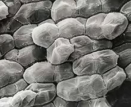
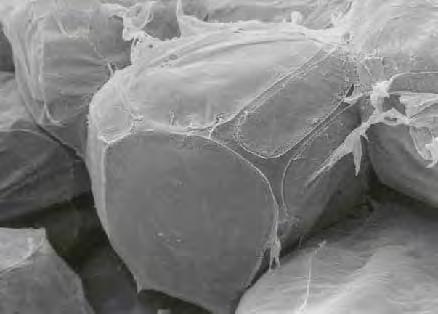
2.7 Close-up of a glass fibre mat
Reinforcements
The primary function of fibers or reinforcements is to carry load along the length of the fiber to provide strength and stiffness in one direction. Reinforcements can be oriented to provide tailored properties in the direction of the loads imparted on the end product. Reinforcements can be both natural (Appendix) and manmade. Many materials are capable of reinforcing polymers. Some materials, such as the cellulose in wood, are naturally occurring products. Most commercial reinforcements, however, are man-made. Of these, by far the largest volume reinforcement measured either in quantity consumed or in product sales, is glass fiber. Other composite reinforcing materials include carbon, aramid, UHMW (ultra high molecular weight) polyethylene, polypropylene, polyester and nylon. Carbon fiber is sometimes referred to as graphite fiber. The distinction is not important in an introductory text, but the difference has to do with the raw material and temperature at which the fiber is formed. More specialized reinforcements for high strength and high temperature use include metals and metal oxides such as those used in aircraft or aerospace applications.
Development of Reinforcements - Fibers
Early in the development of composites, the only reinforcements available were derived from traditional textiles and fabrics. Particularly in the case of glass fibers, experience showed that the chemical surface treatments or “sizings” required to process these materials into fabrics and other sheet goods were detrimental to the adhesion of composite polymers to the fiber surface. Techniques to remove these materials were developed, primarily by continuous or batch heat cleaning. It was then necessary to apply new “coupling agents” (also known as finishes or surface treatments), an important ingredient in sizing systems, to facilitate adhesion of polymers to fibers, particularly under wet conditions and fiber processing.
Most reinforcements for either thermosetting or thermoplastic resins receive some form of surface treatments, either during fiber manufacture or as a subsequent treatment. Other materials applied to fibers as they are produced include resinous binders to hold fibers together in bundles and lubricants to protect fibers from degradation caused by process abrasion. [2.8]
Glass Fibers
Based on an alumina-lime-borosilicate composition, “E” glass produced fibers are considered the predominant reinforcement for polymer matrix composites due to their high electrical insulating properties, low susceptibility to moisture and high mechanical properties. Other commercial compositions include “S” glass, with higher strength, heat resistance and modulus, as well as some specialized glass reinforcements with improved chemical resistance, such as AR glass (alkali resistant).
Glass fibers used for reinforcing composites generally range in diameter from 9 to 23 microns. Fibers are drawn at high speeds, approaching 200 miles per hour, through small holes in electrically heated bushings. These bushings form the individual filaments. The filaments are gathered into groups or bundles called “strands.” The filaments are attenuated from the bushing, water and air cooled, and then coated with a proprietary chemical binder or sizing to protect the filaments and enhance
the composite laminate properties. The sizing also determines the processing characteristics of the glass fiber and the conditions at the fiber-matrix interface in the composite.
Glass is generally a good impact resistant fiber but weighs more than carbon or aramid. Glass fibers have excellent characteristics, equal to or better than steel in certain forms. The lower modulus requires special design treatment where stiffness is critical. Composites made from this material exhibit very good electrical and thermal insulation properties. Glass fibers are also transparent to radio frequency radiation and are used in radar antenna applications.
Carbon Fibers
Carbon fiber is created using polyacrylonitrile (PAN), pitch or rayon fiber precursors. PAN based fibers offer good strength and modulus values up to 85-90 Msi. They also offer excellent compression strength for structural applications up to 1000 ksi. Pitch fibers are made from petroleum or coal tar pitch. Pitch fibers extremely high modulus values (up to 140 Msi) and favorable coefficient of thermal expansion make them the material used in space/satellite applications. Carbon fibers are more expensive than glass fibers, however carbon fibers offer an excellent combination of strength, low weight and high modulus. The tensile strength of carbon fiber is equal to glass while its modulus is about three to four times higher than glass.
Carbon fibers are supplied in a number of different forms, from continuous filament tows to chopped fibers and mats. The highest strength and modulus are obtained by using unidirectional continuous reinforcement. Twist-free tows of continuous filament carbon contain 1,000 to 75,000 individual filaments, which can be woven or knitted into woven roving and hybrid fabrics with glass fibers and aramid fibers.
Carbon fiber composites are more brittle (less strain at break) than glass or aramid. Carbon fibers can cause galvanic corrosion when used next to metals. A barrier material such as glass and resin is used to prevent this occurrence. [2.9]
Aramid Fibers (Polyaramids)
Aramid fiber is an aromatic polyimid that is a man-made organic fiber for composite reinforcement. Aramid fibers offer good mechanical properties at a low density with the added advantage of toughness or damage/impact resistance. They are characterized as having reasonably high tensile strength, a medium modulus, and a very low density as compared to glass and carbon. The tensile strength of aramid fibers are higher than glass fibers and the modulus is about fifty percent higher than glass. These fibers increase the impact resistance of composites and provide products with higher tensile strengths. Aramid fibers are insulators of both electricity and heat. They are resistant to organic solvents, fuels and lubricants. Aramid composites are not as good in compressive strength as glass or carbon composites. Dry aramid fibers are tough and have been used as cables or ropes, and frequently used in ballistic applications.
31
Reinforcement Forms
Regardless of the material, reinforcements are available in forms to serve a wide range of processes and end-product requirements. Materials supplied as reinforcement include roving, milled fiber, chopped strands, continuous, chopped or thermoformable mat. Reinforcement materials can be designed with unique fiber architectures and be preformed (shaped) depending on the product requirements and manufacturing process.
Multi-End and Single-End Rovings
Rovings are utilized primarily in thermoset compounds, but can be utilized in thermoplastics. Multi-end rovings consist of many individual strands or bundles of filaments, which are then chopped and randomly deposited into the resin matrix. Processes such as sheet molding compound (SMC), preform and spray-up use the multi-end roving. Multi-end rovings can also be used in some filament winding and pultrusion applications. The single-end roving consists of many individual filaments wound into a single strand. The product is generally used in processes that utilize a unidirectional reinforcement such as filament winding or pultrusion.
Mats
Reinforcing mats are usually described by weight-per-unit-of-area. The type and amount of binder that is used to hold the mat together dictate differences between mat products. In some processes such as hand lay-up, it is necessary for the binder to dissolve. In other processes, particularly in compression molding, the binder must withstand the hydraulic forces and the dissolving action of the matrix resin during molding. Therefore, two general categories of mats are produced and are known as soluble and insoluble.
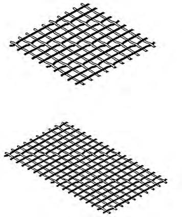
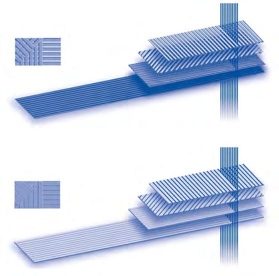
Woven, Stitched, Braided Fabrics
There are many types of fabrics that can be used to reinforce resins in a composite. Multidirectional reinforcements are produced by weaving, knitting, stitched or braiding continuous fibers into a fabric from twisted and plied yarn. Fabrics refer to all flat-sheet, roll goods, whether or not they are strictly fabrics. Fabrics can be manufactured utilizing almost any
reinforcing fiber. The most common fabrics are constructed with fiberglass, carbon or aramid. Fabrics are available in several weave constructions and thickness (from 0.0010 to 0.40 inches). Fabrics offer oriented strengths and high reinforcement loadings often found in high performance applications.
Fabrics are typically supplied on rolls of 25 to 300 yards in length and 1 to 120 inches in width. The fabric must be inherently stable enough to be handled, cut and transported to the mold, but pliable enough to conform to the mold shape and contours. Properly designed, the fabric will allow for quick wet out and wet through of the resin and will stay in place once the resin is applied. Fabrics, like rovings and chopped strands, come with specific sizings or binder systems that promote adhesion to the resin system. [2.10]
Fabrics allow for the precise placement of the reinforcement. This cannot be done with milled fibers or chopped strands and is only possible with continuous strands using relatively expensive fiber placement equipment. Due to the continuous nature of the fibers in most fabrics, the strength to weight ratio is much higher than that for the cut or chopped fiber versions. Stitched fabrics allow for customized fiber orientations within the fabric structure. This can be of great advantage when designing for shear or torsional stability.
Woven fabrics are fabricated on looms in a variety of weights, weaves, and widths. In a plain weave, each fill yarn or roving is alternately crosses over and under each warp fiber allowing the fabric to be more drapable and conform to curved surfaces. Woven fabrics are manufactured where half of the strands of fiber are laid at right angles to the other half (0o to 90o). Woven fabrics are commonly used in boat manufacturing. [2.11]
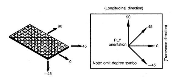
Stitched fabrics, also known as non-woven, non-crimped, stitched, or knitted fabrics have optimized strength properties because of the fiber architecture. Woven fabric is where two sets of interlaced continuous fibers are oriented in a 0o and 90o pattern where the fibers are crimped and not straight. Stitched fabrics are produced by assembling successive layers of aligned fibers. Typically, the available fiber orientations include the 0o direction (warp), 90o direction (weft or fill), and +45o direction (bias).
Economic aspects
Composite materials are expensive:
design costs are higher higher cost of analysis
higher cost of component testing certification and documentation testing but
costs may be lowered by innovative design concepts which consider manufacturing lower part count
reduction in number of fasteners used use of automation
Woven Fabrics (2-D weaving)
Genrally more expensive than UD tapes but significant cost savings during manufacturing fabrics are generally described according to the types of weave and the number of yarns per inch – first in the warp direction (parallel to length of fabric) and then in the fill (or weft) direction (perpendicular to the warp)
Unidirectional Fabric
warp strands are as straight as tape improved drapability over tape minimal reduction of fibre strength improved fibre alignment
Plain Weave Fabric
some loss of properties due to fibre crimping provides reproducible laminate thickness good drapability
speedier lay-up easier to handle
wet-out difficulties with tightly woven fabrics
width limitations thicker than tape
good damage tolerance
Advantages:
enhanced toughness (fewer layers, kinked fibres deflect interlaminar cracking)
damage tolerant due to fibre-interlocking
convenience of handling no weak transverse direction
superior drapability of some weaves
Disadvantages:
more expensive (based on 3K tow to ensure a thin uniform sheet – 6K and 12K tows typical in UD tape)
involve additional manufacturingweaving kinked fibres limit full strength potential
lower fibre volume fraction than ud tape
fabric distortion (bowing and skewing) causes part warpage
32
The assembly of each layer is then sewn together. This type of construction allows for load sharing between fibers so that a higher modulus, both tensile and flexural, is typically observed. The fiber architecture construction allows for optimum resin flow when composites are manufactured. These fabrics have been traditionally used in boat hulls for 50 years. Other applications include light poles, wind turbine blades, trucks, busses and underground tanks. These fabrics are currently used in bridge decks and column repair systems. Multiple orientations provide a quasi-isotropic reinforcement.
Braided fabrics are engineered with a system of two or more yarns intertwined in such a way that all of the yarns are interlocked for optimum load distribution. Biaxial braids provide reinforcement in the bias direction only with fiber angles ranging from ± 15o to ± 95o. Triaxial braids provide reinforcement in the bias direction with fiber angles ranging from ± 10o to ± 80o and axial (0o) direction.
Unidirectional
Unidirectional reinforcements include tapes, tows, unidirectional tow sheets and rovings (which are collections of fibers or strands). Fibers in this form are all aligned parallel in one direction and uncrimped providing the highest mechanical properties. Composites using unidirectional tapes or sheets have high strength in the direction of the fiber. Unidirectional sheets are thin and multiple layers are required for most structural applications.
In some composite designs, it may be necessary to provide a corrosion or weather barrier to the surface of a product. A surface veil is a fabric made from nylon or polyester that acts as a very thin sponge that can absorb resin to 90% of its volume. This helps to provide an extra layer of protective resin on the surface of the product. Surface veils are used to improve the surface appearance and insure the presence of a corrosion resistance barrier for typical composites products such as pipes, tanks and other chemical process equipment. Other benefits include increased resistance
to abrasion, UV and other weathering forces. Veils may be used in conjunction with gel coats to provide reinforcement to the resin.
Prepreg
Prepregs are a ready-made material made of a reinforcement form and polymer matrix. Passing reinforcing fibers or forms such as fabrics through a resin bath is used to make a prepreg. The resin is saturated (impregnated) into the fiber and then heated to advance the curing reaction to different curing stages. Thermoset or thermoplastic prepregs are available and can be either stored in a refrigerator or at room temperature depending on the constituent materials. Prepregs can be manually or mechanically applied at various directions based on the design requirements. [2.11]
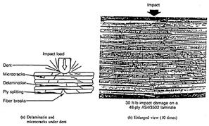
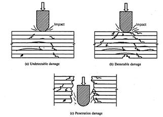
Impact – composites are very susceptible to impact damage.
Impact damage :
caused by dropped tools, runway debris, hail or bird impact damage, ballistics.
more critical in compressively loaded structures
BVID and CAI
damage tolerance may be improved by:
minimising grouping of plies of same orientation using more ±45° plies (soft skin design) using ±45° plies on the outer surfaces thermoplastics
33
2.9 Woven fabrics
2.8 Impact Damage
Sensing
An optical fiber (or fibre) is a glass or plastic fiber that carries light along its length. Fiber optics is the overlap of applied science and engineering concerned with the design and application of optical fibers. Optical fibers are widely used in fiber-optic communications, which permits transmission over longer distances and at higher bandwidths (data rates) than other forms of communications. Fibers are used instead of metal wires because signals travel along them with less loss, and they are also immune to electromagnetic interference. Fibers are also used for illumination, and are wrapped in bundles so they can be used to carry images, thus allowing viewing in tight spaces. Specially designed fibers are used for a variety of other applications, including sensors and fiber lasers. [2.12, 2.14]
Light is kept in the core of the optical fiber by total internal reflection. This causes the fiber to act as a waveguide. Fibers which support many propagation paths or transverse modes are called multi-mode fibers (MMF), while those which can only support a single mode are called single-mode fibers (SMF). Multimode fibers generally have a larger core diameter, and are used for short-distance communication links and for applications where high power must be transmitted. Single-mode fibers are used for most communication links longer than 550 metres
History
Fiber optic technology experienced a phenomenal rate of progress in the second half of the twentieth century. Early success came during the 1950’s with the development of the fiberscope. This image-transmitting device, which used the first practical all-glass fiber, was concurrently devised by Brian O’Brien at the American Optical Company and Narinder Kapany (who first coined the term ‘fiber optics’ in 1956) and colleagues at the Imperial College of Science and Technology in London. Early all-glass fibers experienced excessive optical loss, the loss of the light signal as it traveled the fiber, limiting transmission distances.
This motivated scientists to develop glass fibers that included a separate glass coating. The innermost region of the fiber, or
core, was used to transmit the light, while the glass coating, or cladding, prevented the light from leaking out of the core by reflecting the light within the boundaries of the core. This concept is explained by Snell’s Law which states that the angle at which light is reflected is dependent on the refractive indices of the two materials ‘ in this case, the core and the cladding. The lower refractive index of the cladding (with respect to the core) causes the light to be angled back into the core.
The fiberscope quickly found application inspecting welds inside reactor vessels and combustion chambers of jet aircraft engines as well as in the medical field. Fiberscope technology has evolved over the years to make laparoscopic surgery one of the great medical advances of the twentieth century.
The development of laser technology was the next important step in the establishment of the industry of fiber optics. Only the laser diode (LD) or its lower-power cousin, the light-emitting diode (LED), had the potential to generate large amounts of light in a spot tiny enough to be useful for fiber optics. In 1957, Gordon Gould popularized the idea of using lasers when, as a graduate student at Columbia University, he described the laser as an intense light source. Shortly after, Charles Townes and Arthur Schawlow at Bell Laboratories supported the laser in scientific circles. Lasers went through several generations including the development of the ruby laser and the helium-neon laser in 1960. Semiconductor lasers were first realized in 1962; these lasers are the type most widely used in fiber optics today.
Because of their higher modulation frequency capability, the importance of lasers as a means of carrying information did not go unnoticed by communications engineers. Light has an information-carrying capacity 10,000 times that of the highest radio frequencies being used. However, the laser is unsuited for open-air transmission because it is adversely affected by environmental conditions such as rain, snow, hail, and smog. Faced with the challenge of finding a transmission medium other than air, Charles Kao and Charles Hockham, working at the Standard Telecommunication Laboratory in England in 1966, published a landmark paper proposing that optical fiber

34
conductive paste optical ber inner core outer core 1.5cm 125μm 635μm
2.10 Diagram of a fibre optic cable 2.11 Fibre optic cables
Fibre Optics
might be a suitable transmission medium if its attenuation could be kept under 20 decibels per kilometer (dB/km). At the time of this proposal, optical fibers exhibited losses of 1,000 dB/ km or more. At a loss of only 20 dB/km, 99% of the light would be lost over only 3,300 feet. In other words, only 1/100th of the optical power that was transmitted reached the receiver. Intuitively, researchers postulated that the current, higher optical losses were the result of impurities in the glass and not the glass itself. An optical loss of 20 dB/ km was within the capability of the electronics and optoelectronic components of the day.
Intrigued by Kao and Hockham’s proposal, glass researchers began to work on the problem of purifying glass. In 1970, Drs. Robert Maurer, Donald Keck, and Peter Schultz of Corning succeeded in developing a glass fiber that exhibited attenuation at less than 20 dB/km, the threshold for making fiber optics a viable technology. It was the purest glass ever made. [2.16]
The early work on fiber optic light source and detector was slow and often had to borrow technology developed for other reasons. For example, the first fiber optic light sources were derived from visible indicator LEDs. As demand grew, light sources were developed for fiber optics that offered higher switching speed, more appropriate wavelengths, and higher output power. For more information on light emitters see Laser Diodes and LEDs.
Fibre Optic Sensors
Most people, incorrectly, assume fibre optic cables are only used for telecommunication purposes; there are actually many other uses for fibre optic cables. While telecommunications is a very common, visible, use of fibre optics, it is also very common to use them as sensors. [2.15]
Because of the various properties of light, all of which also occur within a fibre optic cable, fibre optics can be used to measure strain, temperature, or pressure. This can happen
by designing a fibre optic cable to be sensitive to a specific element. This will then affect the light pulse sent through the fibre optic cable, the change pulse received after passing through the fibre can then be analyzed to determine the amount of strain or the temperature, or whatever is being measured. This can be advantageous due to the fact that no electricity passes through the cable; in some sensitive environments this is a necessity.
There are a variety of fiber optic sensors. These can be classified as follows.
A) Based on the modulation and demodulation process a sensor can be called as an intensity (amplitude), a phase, a frequency, or a polarization sensor. Since detection of phase or frequency in optics calls for interferometric techniques, the latter is also termed as an interferometric sensor. From a detection point of view the interferometeric technique implies heterodyne detection/coherent detection. On the other hand intensity sensors are basically incoherent in nature. Intensity or incoherent sensors are simple in construction, while coherent detection (interferometric) sensors are more complex in design but offer better sensitivity and resolution.
B) Fiber optic sensors can also be classified on the basis of their application: physical sensors (e.g. measurement of temperature, stress, etc.); chemical sensors (e.g. measurement of pH content, gas analysis, spectroscopic studies, etc.); biomedical sensors (inserted via catheters or endoscopes which measure blood flow, glucose content and so on). Both the intensity types and the interferometric types of sensors can be considered in any of the above applications.
C) Extrinsic or intrinsic sensors is another classification scheme. In the former, sensing takes place in a region outside of the fiber and the fiber essentially serves as a conduit for the to-and-fro transmission of light to the sensing region efficiently and in a desired form. On the other hand, in an intrinsic sensor one or more of the physical properties of the fiber undergo a change as mentioned in A above.
Extrinsic Fibre Optic Sensors
35
Linear and angular position Pressure Flow Damage Liquid Level Pressure Pressure Accoustics Vibration Temperature Viscosity Chemical analysis Temperature Pressure Acceleration Vibration Rotary position Temperature Flow Temperature Strain Encoder Plates/ Disks Re ection and transmission Total Internal Re ection Gratings Fluorescence Evanescent Laser Doppler Velocimetry Absorption Band Edge Photoelastic E ects Pyrometers Strain Pressure Vibration Temperature Rotation Acceleration Acoustics Magnetic Fields Electric Fields Strain Temperature Pressure Current Acoustic Acceleration Strain Magnetic eld Temperature Temperature Strain Pressure Temperature Temperature Strain Microbend Sensors Distributed Sensors Blackbody Sensors Interferometric Sensors Rayleigh Raman Mode Coupling Quasidistributed
Intrinsic Fibre Optic Sensors
2.12 Classification of Fibre Optic Sensors
Fiber optic sensors are used in many ways. The most common are:
1. Monitor the manufacturing process of composite strucures.
2. Check out the performance of any part or point of the structure during assembly.
3. Form a sensor network and serve as a health monitoring and performance evaluation system during the operational period of the structure. [2.15]
on the basis of refractive index changes due to cross linking when the curing takes place while continuous strain monitoring during service is achieved using a Fabry-Perot Interferometric (FPI) technique. The combined sensor is embedded into the composite during fabrication. The sensor is as shown in fig.6. [2.15]
2.Applications in civil engineering
Current applications
1. Process\cure monitoring of composites
Due to advantages such as high strength-to-weight ratios, good fatigue and corrosion resistance and flexibility to tailor mechanical properties, composite materials find application in many industries including aircraft, automobile, building and container industries. One important issue in their use is the need to demonstrate the reliability of composite structural members . To assure on this score it is necessary to evaluate the effects of impact damage, environmental effects and/or processing defects. Nondestructive evaluation of the above is both costly and time consuming. If sensors can be directly integrated into composite materials it will help monitor the internal state of the composite structural members and reduce the uncertainty and doubts as regards the status of the material. Such integrated sensors can generate quantitative data which will indicate the state of the cure of an epoxy matrix resin initially and later continuously monitor the in-service condition. Fourier Transform Infrared (FTIR), ultrasonic measurements and fluorescence spectroscopy are some of the known methods used in cure sensing. A fiber optic combined cure and in-service strain sensor was reported recently by May et al[ ]. The cure state is monitored
Using a microbend sensor as shown in fig.8, pressure, load and displacement measurements can be made on civil structures such buildings and bridges. Such a sensor is attractive because it is simple to use, low cost and very rugged. Initial calibration could be done with a compression testing machine.
Advantages of Fibre Optic Sensors
• Passive (all dielectric)
• Light-weight
• Small size
• Immunity to electromagnetic interference
• High-temperature performance
• Large bandwidth
• Environmental ruggedness to vibration and shock
• High sensitivity
• Electrical and optical multiplexing
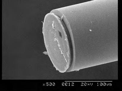
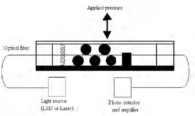

36
2.13 Digital Microscope image of a fibre optic sensor 2.14 Fibre Optic Sensor Structure 2.15 Fibre Optic Cable

37 2.16 Fibre Optic Cables
A thermocouple (or thermocouple thermometer) is a junction between two different metals that produces a voltage related to a temperature difference. Thermocouples are a widely used type of temperature sensor and can also be used to convert heat into electric power.
Any circuit made of dissimilar metals will produce a temperature-related potential. Thermocouples for practical measurement of temperature are made of specific alloys, which in combination have a predictable and repeatable relationship between temperature and voltage. Particular alloys are used for different temperature ranges. Other properties, such as resistance to corrosion, may also be important when choosing which type of thermocouple is most appropriate for a given application. Where the measurement point is far from the measuring instrument, the intermediate connection can be made by extension wires, which are less costly than the materials used to make the
sensor. Thermocouples are standardized against a reference temperature of 0 degrees Celsius; practical instruments use electronic methods of coldjunction compensation to adjust for varying temperature at the instrument terminals. Electronic instruments can also compensate for the varying characteristics of the thermocouple, and so improve the precision and accuracy of measurements.
[2.19, 2.20]
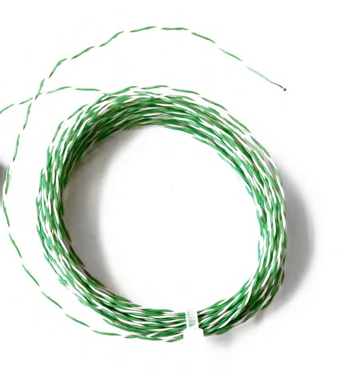


38
Type Temperature range °C (continuous) Temperature range °C (short term) Tolerance class one (°C) Tolerance class two (°C) IEC Color code BS Color code ANSI Color code K 0 to +1100 180 to +1300 ±1.5 between 40 °C and 375 °C ±0.004×T between 375 °C and 1000 °C ±2.5 between 40 °C and 333 °C ±0.0075×T between 333 °C and 1200 °C J 0 to +700 180 to +800 ±1.5 between 40 °C and 375 °C ±0.004×T between 375 °C and 750 °C ±2.5 between 40 °C and 333 °C ±0.0075×T between 333 °C and 750 °C N 0 to +1100 270 to +1300 ±1.5 between 40 °C and 375 °C ±0.004×T between 375 °C and 1000 °C ±2.5 between 40 °C and 333 °C ±0.0075×T between 333 °C and 1200 °C R 0 to +1600 50 to +1700 ±1.0 between 0 °C and 1100 °C ±[1 + 0.003×(T 1100)] between 1100 °C and 1600 °C ±1.5 between 0 °C and 600 °C ±0.0025×T between 600 °C and 1600 °C Not defined. S 0 to 1600 50 to +1750 ±1.0 between 0 °C and 1100 °C ±[1 + 0.003×(T 1100)] between 1100 °C and 1600 °C ±1.5 between 0 °C and 600 °C ±0.0025×T between 600 °C and 1600 °C Not defined. B +200 to +1700 0 to +1820 Not Available ±0.0025×T between 600 °C and 1700 °C No standard use copper wire No standard use copper wire Not defined. T 185 to +300 250 to +400 ±0.5 between 40 °C and 125 °C ±0.004×T between 125 °C and 350 °C ±1.0 between 40 °C and 133 °C ±0.0075×T between 133 °C and 350 °C E 0 to +800 40 to +900 ±1.5 between 40 °C and 375 °C ±0.004×T between 375 °C and 800 °C ±2.5 between 40 °C and 333 °C ±0.0075×T between 333 °C and 900 °C Chromel/AuFe 272 to +300 n/a Reproducibility 0.2% of the voltage; each sensor needs individual calibration.
2.17 Thermocouple 2.18 Thermocouple Types
Thermocouples
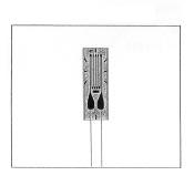
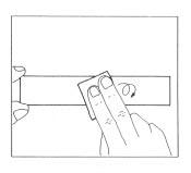
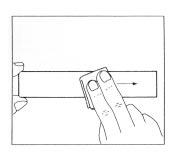
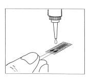
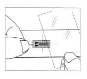
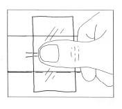
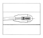
A strain gauge is a resistance-based sensor used by mechanical engineers to measure strain in an object. Strain is defined as the change in length of a component divided by the length of a component. Strain, therefore, does not officially have a unit of measurement, but for reference purposes, the unit of “strain” is used. Because the changes in length are often very small, the unit of microstrain, or strain times 10 to the 6th power, is often used.
A strain gauge is the primary sensor type used to measure strain. The primary type of strain gauge is a metal foil gauge. A strain gauge consists of a long thin “wire” of metal foil that is wrapped back and forth across a grid, called a matrix. The matrix is attached to a thin flexible backing material with an adhesive, often a cyanoacrylate. The strain gauge is bonded to the part to be evaluated, and the matrix is oriented in the direction of the applied strain. The strain exerted in the part is also exerted on the strain gauges, and the wire that makes up the matrix stretches or compresses.
Strain Gauge Configurations
Strain gauges are available in a wide variety of sizes in a wide variety of sizes and configurations, depending on the material and geometry of the part to be tested and the expected strain levels. Matrix lengths can vary from a few millimeters to several inches.
While one strain gauge measures strain along a single axis, multiple strain gauge matrices can be combined into a single sensor. The most common multiple matrix configuration is the bi-axial strain gauge. In this case, two individual strain gauges are oriented at a right angle, with their axes passing through a common point. Other multiple matrix orientations include gauges for measuring
shear strain, residual stresses, and hole stresses.
Strain Gauge Functionality
A strain gauge is a resistive sensor. A voltage is passed through the wire, and any variation in resistance is calculated based on a measured voltage. If the part is compressed, the wire that makes up the strain gauge matrix is compressed, and its cross-section area increases. This reduces the resistance of the wire. If the part is stretched, the wire that makes up the strain gauge matrix is compressed, and its cross-sectional area decreases. This increases the resistance of the gauge. In these terms, if tensile strain is considered positive, then resistance is proportional to strain. The measured voltage is converted to strain using a circuit called a Wheatstone Bridge.
Temperature
Compensation
Active-Dummy Method
The active-dummy method uses the 2-gage system where an active gage, A, is bonded to the measuring object and a dummy gage, D, is bonded to a dummy block which is free from the stress of the measuring object but under the same temperature condition as that affecting the measuring object.
The dummy block should be made of the same material as the measuring object. As shown in Fig. , the two gages are connected to adjacent sides of the bridge. Since the measuring object and the dummy block are under the same temperature condition, thermally-induced elongation or contraction is the same on both of them. Thus, gages A and B bear the same thermally-induced strain, which is compensated to let the output, e, be zero because these gages are connected to adjacent sides.
[2.21, 2.22, 2.23]
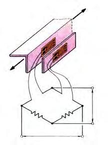
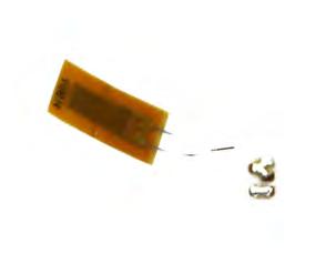
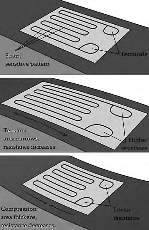
39
Strain Gauges
2.19 Installation of a strain gauge
2.20 Strain gauge
2.22 Strain Gauge Structure
2.21 Strain Gauge Half-Bridge Configuration
Actuation
Shape Memory Alloys
The Shape Memory Effect is the ability of a material to remember the shape it had above a certain characteristic temperature, even though it has been deformed severely at a lower temperature (below the characteristic). The material, after being deformed at the lower temperature, recovers its original shape on being heated to the characteristic temperature.
Shape Memory Alloys (SMAs) are a group of metallic materials that demonstrate the Shape Memory Effect. There has been a considerable interest in the recent years in developing shape memory alloy actuators because of their advantages in producing large plastic deformations, high force-to-weight ratio and low driving voltages.
We can distinguish two types of the Memory Effect. The Mechanical Memory Effect is initiated through an external force and leads to huge elastic strains of the alloy. The Thermal Memory Effect occurs upon heating of a Memory metal, which has been previously deformed plastically. A high specific mechanical work is generated.
Both effects can be achieved in the same alloy by special thermomechanical treatment. This special metallurgical treatment gives the alloys their particular properties and is of high importance for the success of the respective application.
One-Way Shape Memory Effect
This specific temperature is related to a martensitic phase transition. The terms ‘austenite’ and ‘martensite’ are used in a generic sense for the higher-temperature phase and the lowertemperature phase, respectively. The SME arises primarily due to the accommodative reorientation of the austenitic and the martensitic phases. []
Superelasticity is the ability of a material to be able to undergo large but recoverable strains, provided the deformation is carried out in a characteristic range of temperatures. This property is an example of a purely field-induced phase transition (at a fixed temperature). When the deforming stress is applied at a temperature (within the characteristic temperature range) at
which it is in the austenitic phase, the stress sends the material to the martensitic phase, with an accompanying large deformation. When the stress is removed, the material recovers its shape because it reverts back to the austenitic phase.
A typical shape-memory cycle runs as follows, assuming that the material is in the martensitic phase at room temperature. It is first heated towards the temperature of the martensiteaustenite phase transition. Since this is typically a case of firstorder phase transition, there is a range of temperatures in which the martensitic and the austenitic phase coexist. There is thus a temperature As at which the austenitic phase starts forming. Further increase of temperature converts more and more of the martensitic phase to the austenitic phase. Finally at a certain temperature Af, the transition is complete.
At the end of the cooling down process, the SMA usually does not recover its original plastically deformed shape. Since the shape is remembered only on heating and not also on cooling-down to the martensitic phase, this is called one-way shape memory effect.
Two-Way Shape Memory Effect
If the alloy remembers its shape in both the austenitic and the martensitic phases, it exhibits the two-way shape memory effect.
To obtain this behavior, a specimen has to be trained. A variety of training protocols have been described in the literature. Most of the amount to creating a network of dislocations in the specimen. These dislocations have an associated strain field, and that martensitic configuration develops on cooling to the other phase for which the overall strain energy is the least. This can happen repeatedly across the heating and cooling cycles.
Training procedures include: repetition of the one-way SME cycle, constrained cycling across the phase transition, thermal cycling at constant applied stress and superelastic cycling.
[2.24, 2.28, 2.30]
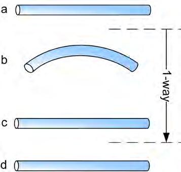
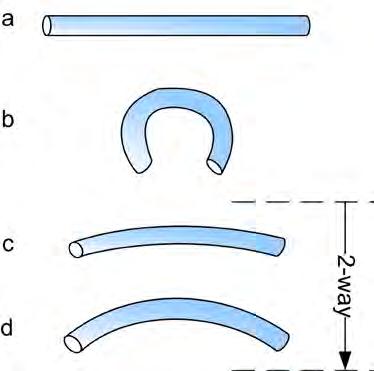

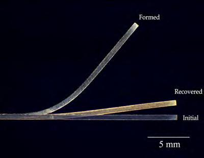
40
2.23 One and Two Way shape memory effect 2.24 SMA light 2.25 States of a SMA
Heat Treating and Shape Setting
Nitinol and other shape memory alloy mill products - bar, wire, ribbon and sheet are normally finished by cold working to achieve dimensional control and enhance surface quality. Cold working suppresses the shape memory response of these alloys. It also raises the strength and decreases the ductility. However, cold work does not raise the stiffness of the material. Heat treating after cold working diminishes the effects of cold working and restores the shape memory response of these alloys. Therefore, in order to optimize the physical and mechanical properties of a Nitinol product and achieve shape memory and /or superelasticity, the material is cold worked and heat treated.
The mill product supplier normally provides the material in the cold worked condition. The maximum practical level of cold work will be limited by the alloy and by the product section size. Binary superelastic NiTi alloy fine wires with As in the range of –25 to +95°C are typically supplied with cold reduction after the final anneal in the range of 30 to 50%. Higher reductions are sometimes used for very fine wires. These same alloys will be limited to about 30% maximum cold reduction in larger diameter bar sizes. Binary NiTi alloys with very low As in the range of –50 to –60 °C will not sustain the higher levels of cold work without cracking. [2.24]
Both superelastic and shape memory properties are optimized by cold work and heat treatment. This thermo-mechanical process is applied to all Nitinol alloys although different amounts of cold work and different heat treatments may be used for different alloys and property requirements.
Shape setting is accomplished by deforming the Nitinol to the shape of a desired component, constraining the Nitinol by clamping and then heat treating. This
is normally done with material in the cold worked condition, for example cold drawn wire. However, annealed wire may be shape set with a subsequent lower temperature heat treatment.
In shape setting cold worked material, care must be taken to limit deformation strain to prevent cracking of the material. Another approach is to partially anneal the wire prior to shape setting. Yet another option is to shape set in incremental steps. Smith et al. reviewed the types of furnaces and fixturing hardware or mandrels that have been used in heat treatment. Many types of furnaces have been used including box furnaces, continuous belt hearth furnaces, tube furnaces, heated platen presses, vacuum furnaces, induction heaters, salt baths and fluidized bed furnaces. The electrical resistance of Nitinol makes it a good candidate for self heating by electric current. Nitinol will be oxidized when heat treated in air. Therefore, surface requirements and atmosphere control are important considerations.
[2.28]
Shape setting can be done over a wide temperature range from 300 °C to 900°C. However, heat treating temperatures for binary NiTi alloys are usually chosen in the narrower range of 325 to 525°C in order to optimize a combination of physical and mechanical properties. Heat treating times are typically 5 minutes to 30 minutes. Consideration must be given to the mass of the heat treating fixture as well as the mass of the product. Sufficient time must be allowed in the furnace to get the entire mass to the desired temperature.
The shape setting heat treatment changes the physical and mechanical properties of Nitinol. Morgan and Broadly mapped the effect of temperature and time at temperature on shape set wire properties. Their response curves illustrate that physical and mechanical property do not always change in the same direction.
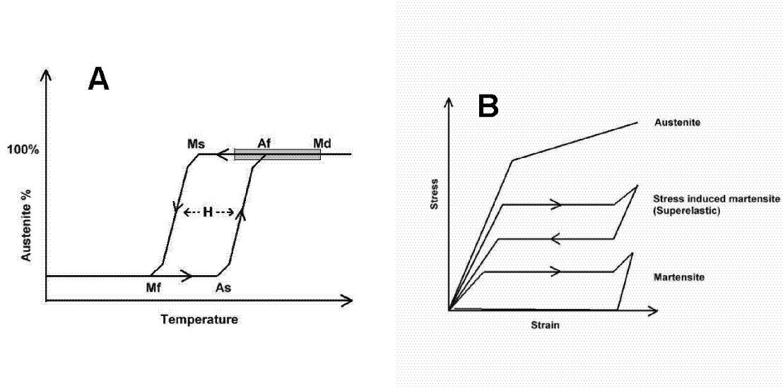
41
NiTi Stainless SteelTitanium Ti-6Al-4V AusteniticMartensitic Ultimate tensile strength (Mpa) 800 - 1500103 - 1100483 - 1850 540 - 740 920 - 1140 Tensile yield strength (Mpa) 100 - 800 50 - 300 190 - 1213 390 830 - 1070 Modulus of elasticity (GPa) 70 - 110 21 - 69 190 - 200 105 - 110 100 - 110 Elongation at failure (%) 1 - 20 up to 60 12 - 40 16 8 * Lowest and highest values have been compiled from picked references (Buehler l. 1967, Funakubo 1987, Breme et al. 1998, Van Humbeeck et al. 1998).
Analytical
2.26 Changes in the molecular level during shape change
2.27
Graphs 2.28 Table of Comparison
Also, some properties are not monotonic functions of time at temperature. For example, upper plateau stress goes through a minimum as a function of time at temperature when heat treating a superelastic alloy in the range of 450°C to 550°C. This can be understood in terms of the complex precipitation response of the nickel rich Ni – Ti alloys.
Precipitation processes in nickel rich NiTi were studied in detail by Nishida et al. Their TTT diagram shows that in a Ti – 52 atomic % Ni alloy heat treated below 820oC, precipitation starts as fine Ti11Ni14 transitions over time to Ti2Ni3 and terminates after long time as TiNi3 in equilibrium with the NiTi matrix. All the while, the NiTi ratio in the matrix is being shifted towards higher Ti content and higher transformation temperature. Pelton et al. reported on the combined effects of nonisothermal and isothermal heat treatment on the physical and mechanical properties of Nitinol wire. This work suggests that for a 50.8 atomic % Ni alloy Ti11Ni14 dissolves at about 500oC and Ti2Ni3 will start to precipitate at 550oC. This results a minimum or maximum in properties as NiTi ratio in the
matrix goes through a peak. Furthermore, this analysis suggests that the temperature for transition from Ti11Ni14 precipitation to Ti2Ni3 precipitation occurs at higher temperatures for higher Ni content alloys.
Brailovski used measurement of latent heat measured by DSC and Vickers hardness to map mechanical and physical properties as a function of heat treatment. He obtained maximum fatigue performance when the combination of transformation temperature and hardness were optimized.
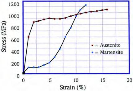
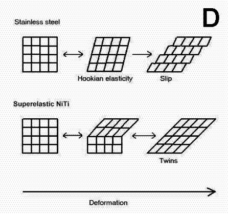
42 Properties of Nitinol Density 6.45 gm/cm3 0.23 lb/in3 Thermal Conductivity 10 W/moK 5.78 Btu/hr ftoF Specific Heat 322 j/kgoK 0.08 Btu/lboF Latent Heat 24,200 J/kg 10.4 Btu/lb Ultimate Tensile Strength 750-960 Mpa 110-140 ksi Elongation to Failure 15.5% 15.5 % Yield Strength (Austenite) 560 Mpa 80 ksi Young’s Modulus (Austenite) 75 Gpa 11 Mpsi Yield Strength (Martensite) 100 Mpa 15 ksi
2.29 Stress-Strain Curves
2.30 Molecular level Comparison with Stainless Steel
Shape-memory polymers.
The shape memory effect is not related to a specific material property of single polymers; it rather results from a combination of the polymer structure and the polymer morphology together with the applied processing and programming technology.
Shape memory behavior can be observed for several polymers that may differ significantly in their chemical composition. However, only a few shapememory polymers are described in the literature. The process of programming and recovery of a shape is shown schematically in Figure 1. First, the polymer is conventionally processed to receive its permanent shape. Afterwards, the polymer is deformed and the intended temporary shape is fixed. This process is called programming. The programming process either consists of heating up the sample, deforming, and cooling the sample, or drawing the sample at a low temperature (so called cold drawing). The permanent shape is now stored while the sample shows the temporary shape. Heating up the shape-memory polymer above a transition temperature Ttrans induces the shape-memory effect. As a consequence, the recovery of the stored, permanent shape can be observed. Cooling down the polymer below the transition temperature leads to solidification of the material, however, no recovery of the temporary shape can be observed. The effect described is named as a oneway shape-memory effect. By further programming, including mechanical deformation, the work piece can be brought into a temporary shape again. This new temporary shape does not necessarily match the first temporary shape.
In Figure a picture sequence demonstrates impressively the performance of shape-memory polymers. The permanent shape of the polymers formed from 1 and 2 is that of a rod, which has been deformed to a spiral (temporary shape) during the programming process.
Under the influence of hot air having a temperature of 70 C the permanent shape is recovered as soon as the switching temperature Ttrans is reached. The permanent shape is recovered with a precision of more than 99% with appropriately optimized programming conditions. This precision makes these materials suitable for highly demanding applications.[2.38,2.41]
A substantially new development in connection with the design of shape-memory polymers are polymer systems. These are families of polymers in which macroscopic properties (for example, mechanical properties or Ttrans) can be controlled by a specific variation of molecular parameters. This makes it possible to tailor the specific combination of the properties of the shape-memory polymers that are required for specific applications just by a slight variation of the chemical composition.
There are also other classes of materials such as ceramics and gels that show thermo-responsive shape-memory properties.
Polymers Vs Alloys
Shape memory polymers differ from shape memory alloys by their glass transition or melting transition from a hard to a soft phase which is responsible for the shape memory effect. In shape memory alloys Martensitic/ Austenitic transitions are responsible for the shape memory effect. There are numerous advantages that make SMPs more attractive than shape memory alloys. They have a high capacity for elastic deformation (up to 200% in most cases), much lower cost, lower density, a broad range of application temperatures which can be tailored, easy processing, and potential biocompatibility and biodegradability.
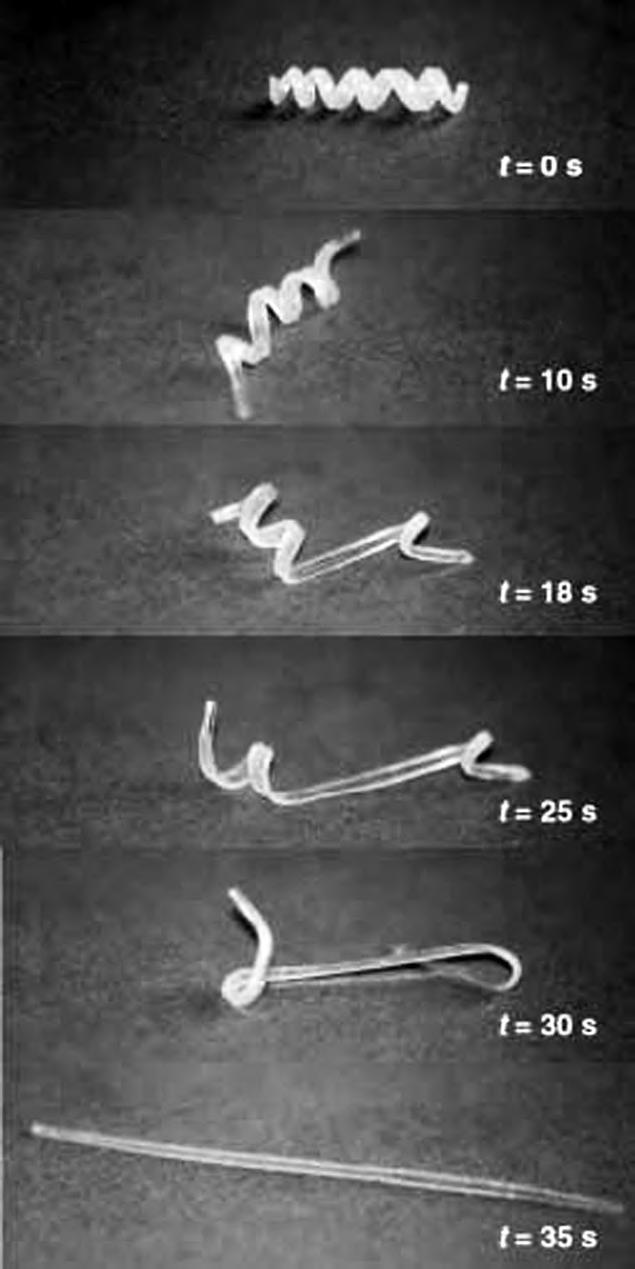
43
2.31 Schematic representation of the thermally induced one-way shape-memory effect. 2.33 SMP shape change 2.32 Table of Comparison Permanent Shape Programming Recovery Temporary Shape Permanent Shape
The Energy that needs to be provided to our system, is going to supply the actuation process. Since our actuators are shape-memory alloys, the actuation energy could be direct or indirect. In the case of direct energy, that would be the heating of the SMAs by a heating source. On the other hand we can consider the indirect heating of the actuators, by providing electrical current that would pass through the alloys and consequently heat them.
Piezoelectricity
One of the options considered for the indirect actuation, was that of piezoelectricity. The most interesting point about it, is that the energy would be provided by the material system itself without the need of any external sources. That of course, would enhance the autonomy and sustainability of the system in total.
Piezoelectricity is the ability of some materials (notably crystals and certain ceramics, including bone) to generate an electric potential in response to applied mechanical stress.
The reversal of this effect is called the inverse piezoelectric effect, i.e. the same materials undergo dimensional change under the influence of an electric field.
In 1880, Jacques and Pierre Curie discovered an unusual characteristic of certain crystalline minerals: when subjected to a mechanical force, the crystals became electrically polarized. Tension and compression generated voltages of opposite polarity, and in proportion to the applied force. Subsequently, the converse of this relationship was confirmed: if one of these voltage-generating crystals was exposed to an electric field it lengthened or shortened according to the polarity of the field, and in proportion to the strength of the field. These behaviors were labeled the piezoelectric effect and the inverse piezoelectric effect, respectively, from the Greek word piezein, meaning to press or squeeze.
Although the magnitudes of piezoelectric voltages, movements, or forces are small, and often require
amplification (a typical disc of piezoelectric ceramic will increase or decrease in thickness by only a small fraction of a millimeter, for example) piezoelectric materials have been adapted to an impressive range of applications. The piezoelectric effect is used in sensing applications, such as in force or displacement sensors. The inverse piezoelectric effect is used in actuation applications, such as in motors and devices that precisely control positioning, and in generating sonic and ultrasonic signals.
In the 20th century metal oxide-based piezoelectric ceramics and other man- made materials enabled designers to employ the piezoelectric effect and the inverse piezoelectric effect in many new applications. These materials generally are physically strong and chemically inert, and they are relatively inexpensive to manufacture. The composition, shape, and dimensions of a piezoelectric ceramic element can be tailored to meet the requirements of a specific purpose. Ceramics manufactured from formulations of lead zirconate / lead titanate exhibit greater sensitivity and higher operating temperatures, relative to ceramics of other compositions, and “PZT” materials currently are the most widely used piezoelectric ceramics. [2.47,2.48]
For the case of our system, piezoelectricity was discarded due to the fact that the electric potential generated is far less than the amount needed for the actuation of the shape memory alloys.
Crystal Structure of a piezoelectric ceramic
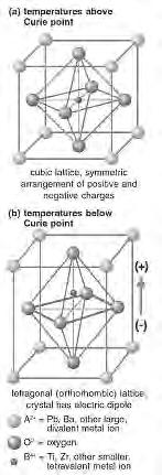
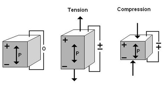
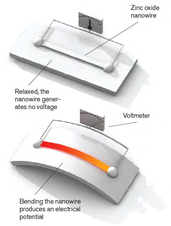
44
2.34
Energy
Piezoelectricity 2.35 Piezoelectricity test configuration 2.36
Laser Energy
There is a lot of research around laser energy carried within fibre optic cables. This could be a very interesting option for our system, since the laser energy could heat the SMAs just by placing the fibre optic cable over it. [2.49]
External Power Source
Any kind of external electrical power source could be used to provide current to the shape memory alloys.
Heating
Things are simpler in the case of direct heating of the SMAs. The two options that we found more efficient, were those of silicon heating patches and rope heatersattached to the alloys or wrapped around them.
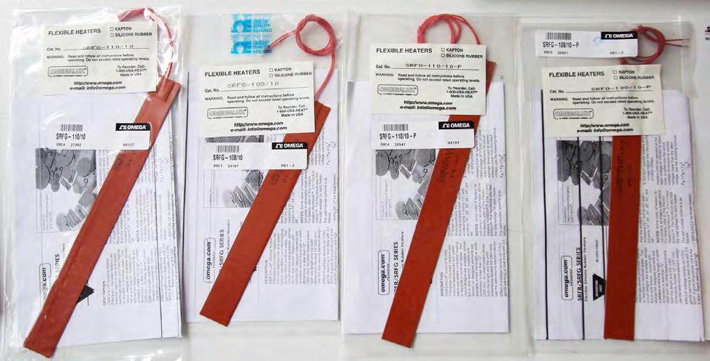

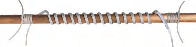
Maximum Temperature: 482°C
Diameter: 5 mm
Voltage: 120 or 240V
Linear Wattage: 4 Watts/in.
Heater Length: 0.9m
Lead Length: 609 mm
Termination: Stripped leads
45
Silicon Heating Patches
Rope Heaters
Lightweight, Thin, Flexible 2.5W/in2 Operating Temperature: up to 232°C 2.37 Fibre Optic Cable
Energy - Work
Energy is the capacity of a physical system to perform work. It exists in several forms such as heat, kinetic or mechanical energy, light, potential energy, electrical, or other forms.
According to the law of conservation of energy -first law of thermodynamics-, the total energy of a system remains constant, though energy may transform into another form.
Having the option of providing either heat or current to achieve the shape change (work) in the system, we come to the question of efficiency.
A work-to-work process would be more efficient for the system than an energy-to-work transition, in the case of the heating the SMAs directly.
During the heating of the alloys, a significant amount of energy is ‘lost’. This happens towards the material (composite) surrounding the heating patches and alloys. As a consequence, the energy needed for the system to actuate is more and the entire process slower.
In theory, our choice would clearly be to provide current to the SMAs and achieve a faster and more efficient actuation. In terms of the physical models though, this
is not as easy as thought. The most important issue that we have to deal with is the safety of working with the physical models, in the case of providing current. The amount of electricity needed to pass through the alloys and thus heat them, would be on a level of high risk. Working with such current, requires very safe facilities and a lab environment. That was not an option for us because the means and facilities we had access to, did not meet this level of standards.
That led us to plan our physical experiments with heat being the energy provided to the system for the actuation process.

Work is force times distance.
According to the work-energy theorem if an external force acts upon an object, causing its kinetic energy to change from Ek1 to E k2, then the mechanical work (W) is given by: where m is the mass of the object and v is the object's speed.
46
Introducing Control into our system is essential for achieving our aim. For every step of the system configuration and built up, we have the need for control.
The controllers used for our experiments could be devided into two main categories: The single input - output controllers, and the processing units.
How each one of them was utilized for the different stages and experiments, is extensively elaborated in the next chapter ‘Experiments’.


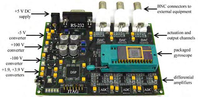

47
2.39
Temperature, Process, & Strain Meter & PID Controller
Processing
Fibre Optic Sensors Processing
DIN Temperature/Process
2.41 Strain Gauges
Unit 2.40
Unit 2.38 1/16
Controller with Fuzzy Logic
Control
3 Experiments
This chapter will present in detail all the experiments we undertook and explain the results. It will start from the basic initial experiments of actuation and gradually lead to the manufacturing and testing of our final model, which proves that our system is possible to be constructed and applied in practice. Sensing, actuation and control are the key functions of the system and areas of exploration for all the experiments.
Preparation Actuation Actuation + Control Sensing + Control Actuation + Sensing + Control
Preparation
The initial experiments were setup with the aim of understanding the process of shape setting in SMAs, actuation behavior against temperature, to evaluate the degree of shape change, its force to weight ratio and the force- time graph. Two kinds of SMAs were used to setup these experiments, a ribbon of dimensions 1.2 (thick) X 4.6 (wide) X 270 mm (long) with actuation temperature 65°C and a wire of .05 mm dia X 1000mm (long) with actuation temperature 35°C.
Shape setting process
The Ni-Ti ribbon and wires were trained by rolling them around metal pipes and maintaining them in position while they were placed in an oven.
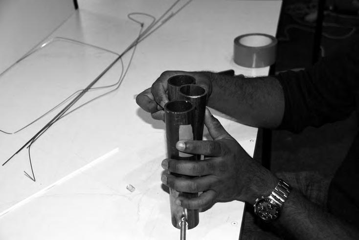
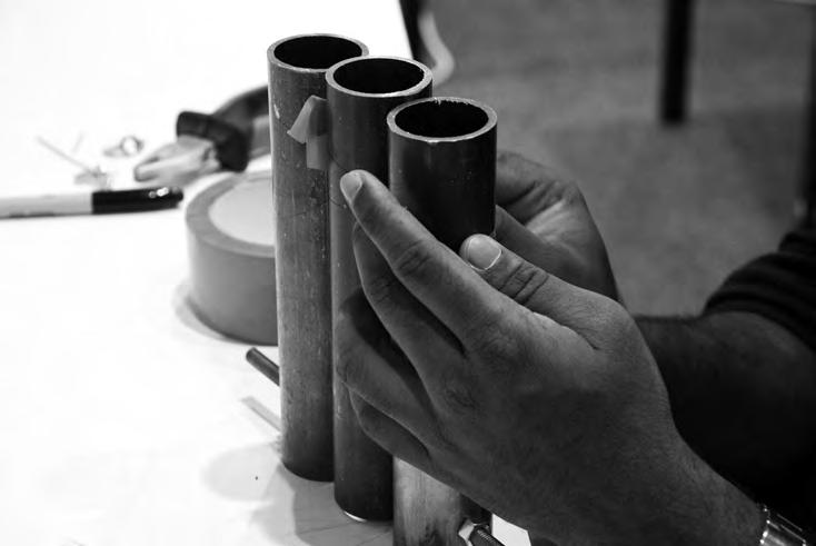
The shape setting temperature in SMAs range between 325- 500 °C. In our case, the oven was heated up to 500°C and the temperature was maintained for 5 minutes. The SMAs were subsequently removed from the oven and immediately immersed in cold water whilst maintaining the imposed bend shape throughout the cooling procedure.
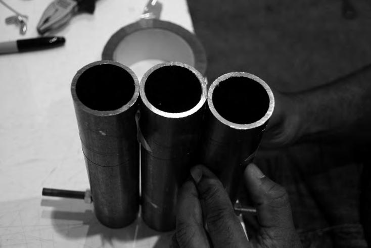
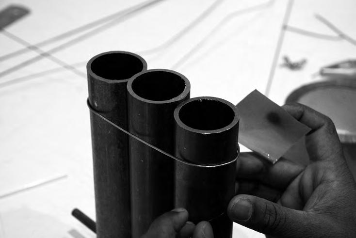
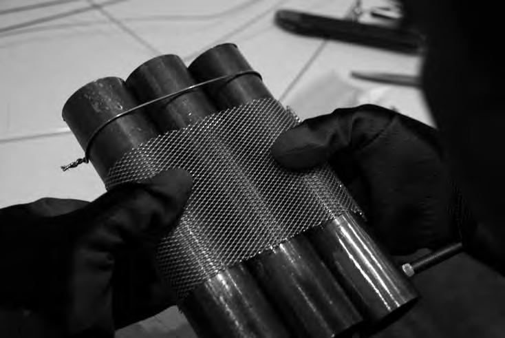
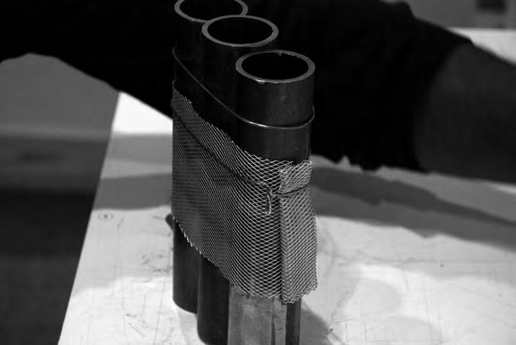
50
Shape setting Preparation
3.1

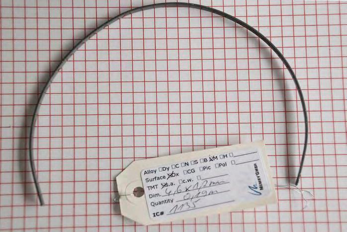
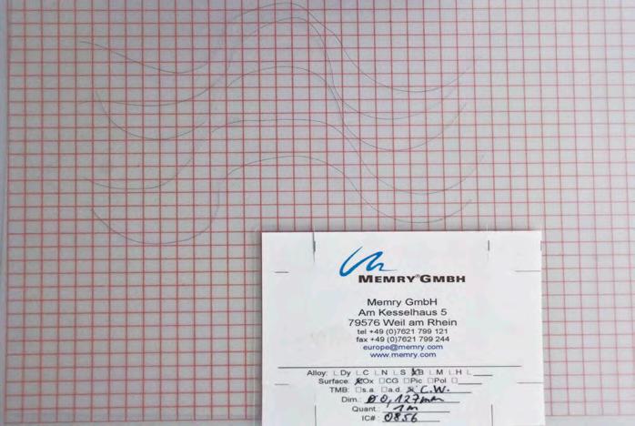

51
3.2 Programming unit of kiln
3.3 SMAs after shape setting
3.4 Kiln used for the shape setting
The shape setting of the Nitinol ribbon was carried out by rolling it over a steel pipe of 80mm diameter.
When the setup was removed from the oven the ribbon had opened up but had a considerable curvature forming an arc (Figure 3.5), it was then mechanically flattened. The ribbon was attached to a clip on one end against a grid to observe the change in curvature. The SMA ribbon was heated up to the actuation temperature of 65°C with a hot air gun.
It was observed that the SMA ribbon had regained the exact same curvature of the set shape. It was apparent that the SMA ribbon was much softer and easily deformable at room temperature but got stiffer and hardened when heated (Figure 3.3).
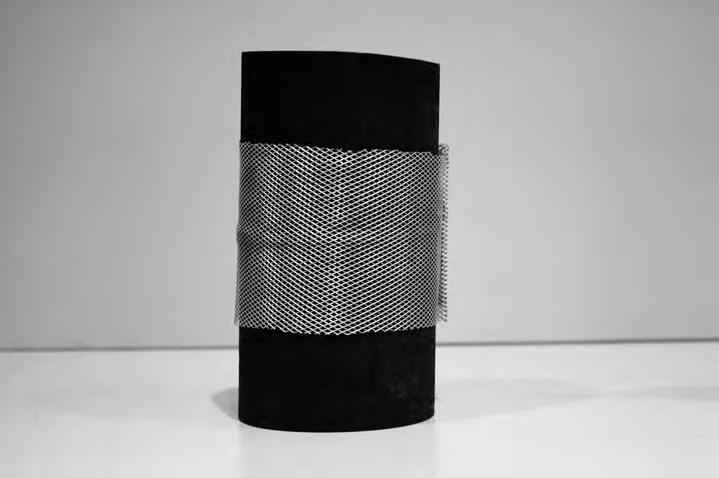
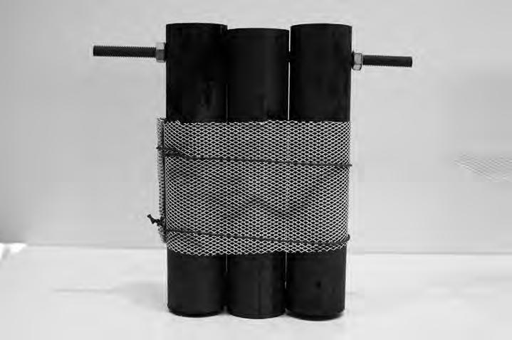
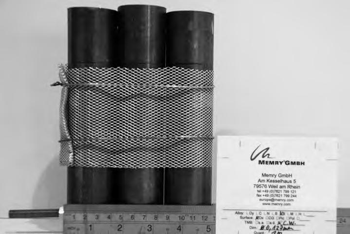
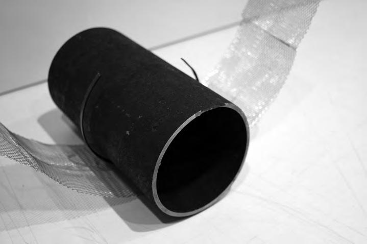
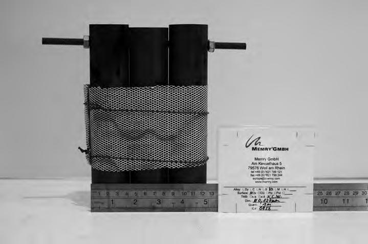
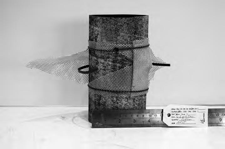
52
3.5 SMA ribbon after removing it from the kiln
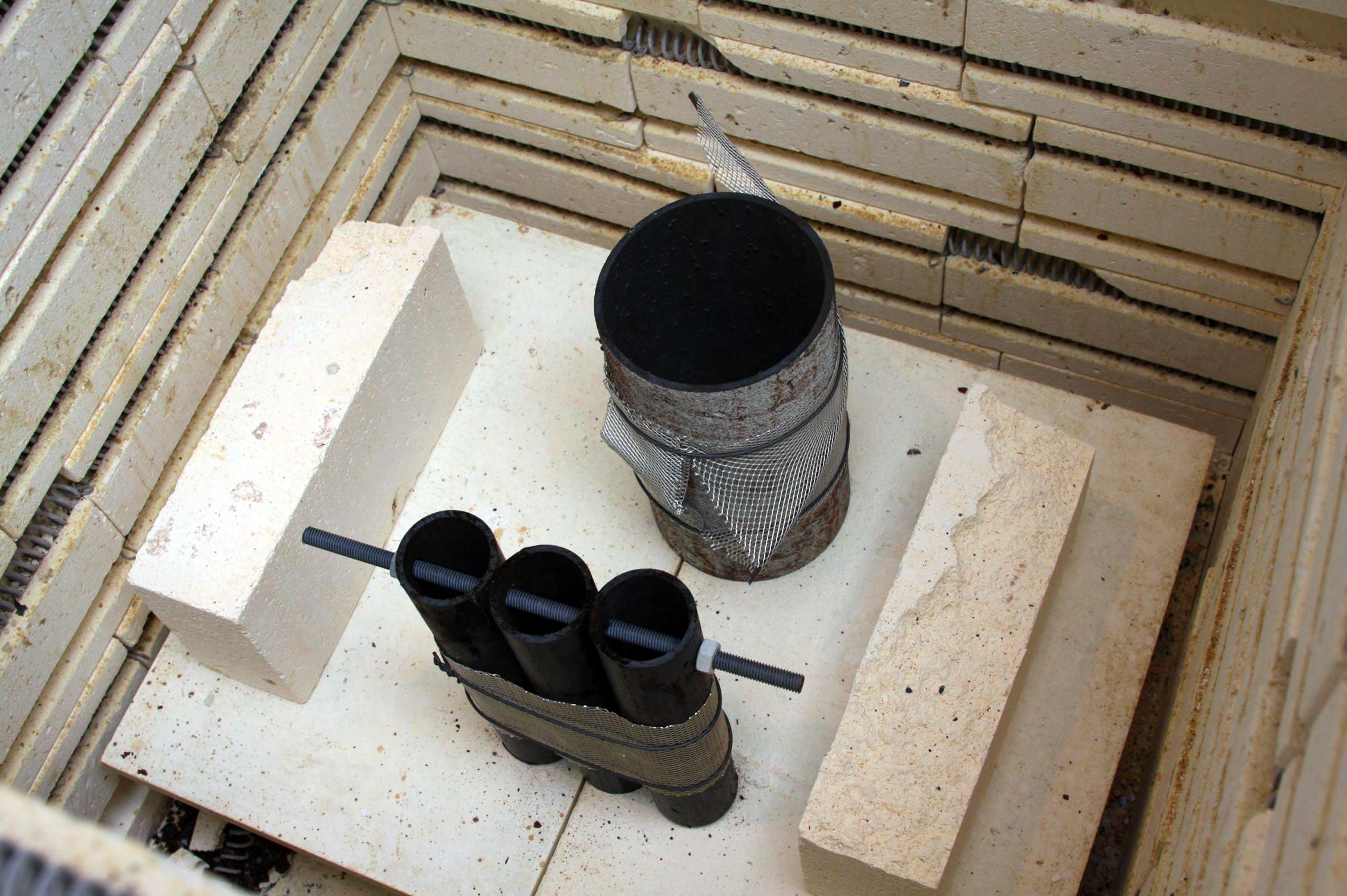
53 3.6 The SMAs placed inside the kiln
Actuation
Our first experiment was a simple testing of the actuation. We wrapped the SMA ribbon with a piece of felt to give a better visual result of the shape change, and heated it with the heat gun. The result (Figure 3.7) was exactly what we expected, with the SMA taking the ‘memorised’ shape in a few seconds.
3.7 Perspective views of the model after the actuation
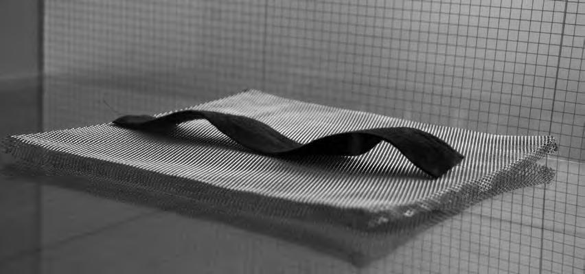


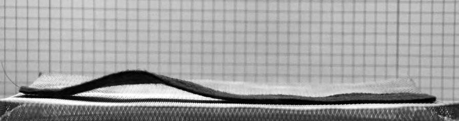
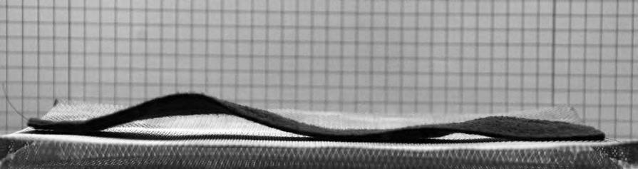
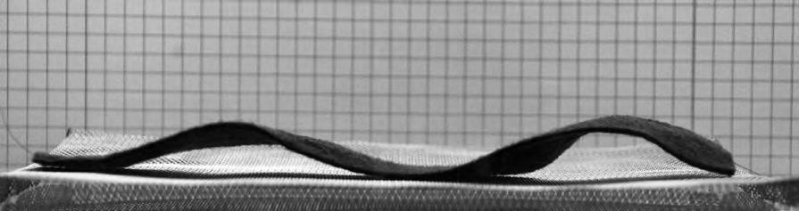
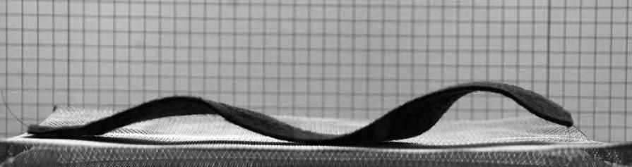
54
3.8 Sequential photos of the actuation experiment
Wanted to introduce a surface element and test the shape change in relation to that, we placed the SMA under a thin tensioned fabric. The fabric was attached on a circular frame and the heating of the SMA was from the top with a heat-gun.
The surface (Figure 3.9) followed the curvature change of the alloy as expected until the point where due to the high temperature, the SMA burned the fabric and finally teared it apart.
At this point, the important factor of temperature resistant materials arouse. Any material used in the same system as the SMAs, should be able to take the high temperature -65 in our case- during the actuation process. Fortunately, since our aim is to implement the alloys in a fibre composite, high temperatures will
most likely not be a problem. Most of the polymers, have working temperatures higher than the actuation temperatures of the SMAs. In any case though, this is a crucial parameter that needs to be carefully considered in the further development of the system.


55
3.9 Sequential photos of the actuation experiment
Weight-Lifting Experiments
Cantilevered Support
These set of experiments were focused on extrapolating the Force to Weight ratio and Force-Time graph. It was observed that the SMA ribbon of 9 gm in a cantilevered position could lift load up to 114 gm. As observed in the graph the phase change happens in short interval. The test was carried out in sequential increments by adding 56 gm weights. The restoring capacity of the initial degree of curvature reduced when the loads were increased.
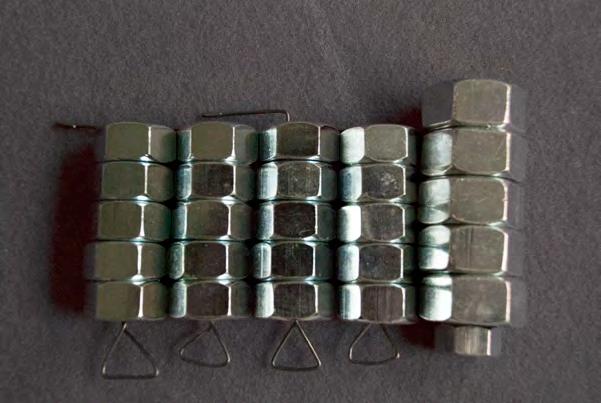

56
3.10 Weights used for the weight-lifting experiments
3.11 Sequential photos of the actuation experiment | 0.56 N
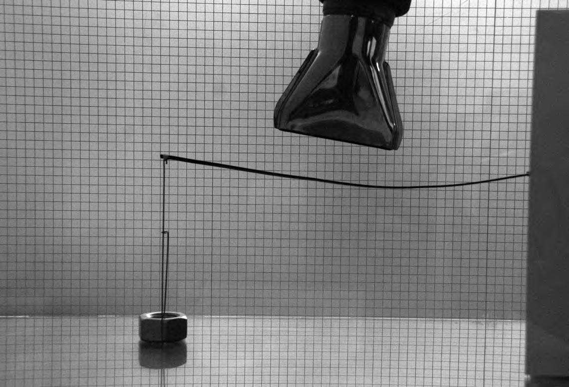
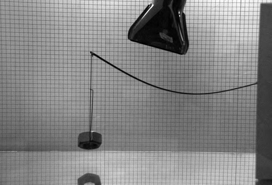
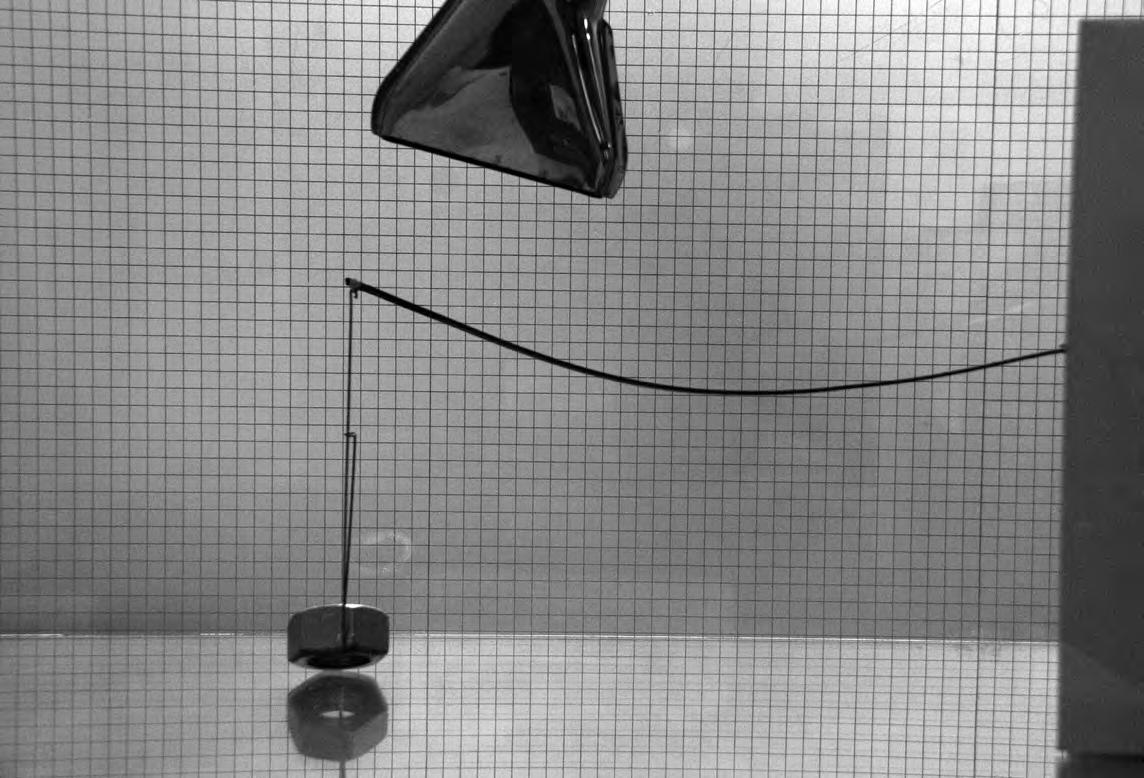
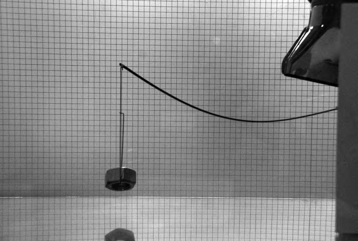
57
Simply Supported
The load carrying capacity of the SMA ribbon improved significantly when the strip was simply supported.
The ribbon of 9 gm could lift a load of 883 gm - almost 100 times it self-weight.
This indicates that when the SMAs are embedded within a fibre composite, they would have the ability to induce high stresses on the surface; enabling it to redistribute the stresses and reorganise the components. The test was carried out in sequential increments by adding weights. The restoring capacity of the initial curvature of the strip reduced to a greater degree with the increase
in weights. The ultimate load of 883 gm did not allow the ribbon to take any curvature and it barely managed to get back to a straight line.
The retrieval of the original shape (martensitic state) occurs quicker when the loads are increased. The change in shape during phase change from austenite to martensitic state is more gradual, while the other way around is much quicker. The simply supported SMA ribbon displays a much higher force to weight ratio.
58
1.12 N 1.12 N 0.56 N
Simply
Cantilevered
Supported

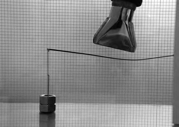
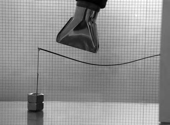


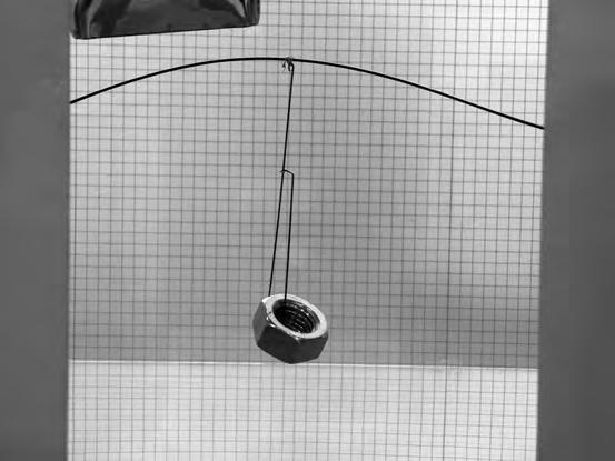
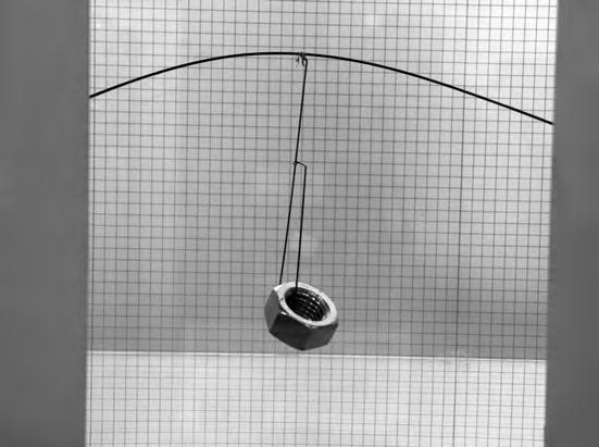
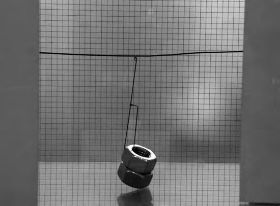

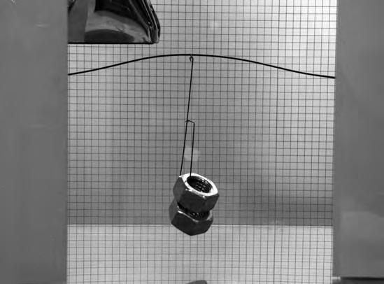
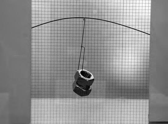
59
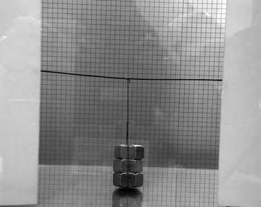

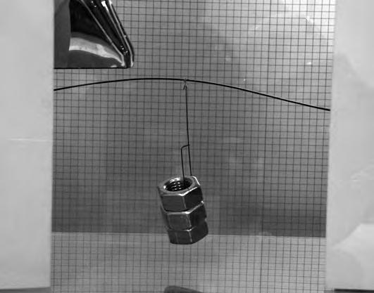
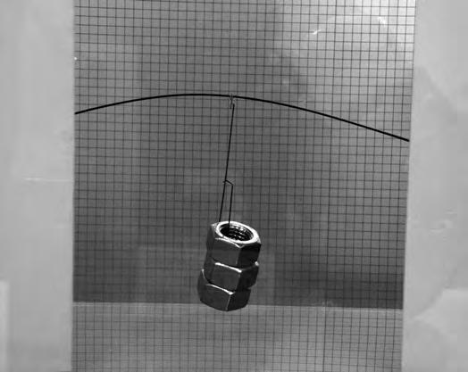
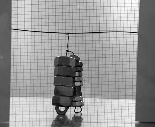
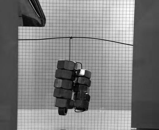

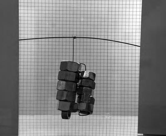
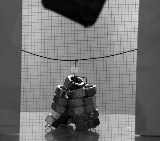
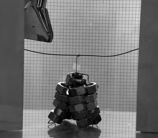
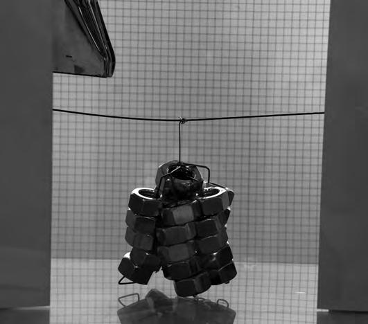

60 1.68 N 4.4 N 8.46 N
3.12 Graphs showing the time needed for the weights to be lifted (up), touch the ground after we stop heating, and return to their initial position (full rest)
3.13 Table of all the measurements (time, weights) for the whole series of experiments.
The results of this series of experiments were carefully stored in an excel sheet and analysed. (Figures 3.12,3.13)
One of the surprising outcomes -besides the impressive force to weight ratio of the ribbon- was the time needed for the actuation to take place. For example, the 9 grams SMA ribbon needed 18 seconds to lift 850 grams of weights. As shown in the graphs (Figure 3.12), the time needed for the weights to touch the ground was 85 sec and another 35 for the full rest.
TYPENUT
SIZEF(N)
N1
(g)BIG
NUTS
N N2
(g)MEDIUM
NUTS
N3
(g)SMALL
NUTS
N
N
UPDOWN
-‐
ONE
POINTDOWN
-‐
FULL
REST N1
(BIG
nuts)n2
(medium
nuts)*n3
(small
nuts)F(N)t
(s)N1
(BIG
nuts)n2
(small
nuts)*n3
(small
nuts)F(N)t
(s)N1
(BIG
nuts)n2
(small
nuts)*n3
(small
nuts)F(N)t
(s) 1000.56111000.5625801000.563480 2001.12122001.126052001.12727 3001.68133001.681313001.68329 4002.24124002.241744002.24311 5012.95135012.951385012.95208 5514.4145514.41075514.4194 51015.851551015.8512451015.85185 51517.31751517.310951517.3148 51918.461851918.468551918.46118 52018.75-‐52018.75-‐52018.75-‐
61
0.56
0.29
0.15
*There
are
also
intermediate
nuts
1
of
them
when
we
use
5
nuts
and
after *n1
big
nuts *n2
medium
size
(smaller
than
n1)
bought
by
Sakthi
in
Leylands
on
the
07th
Aug
2009 0 3 6 9 12 15 04.5913.518 UP Force (N) Time (sec) 0 2.25 4.5 6.75 9 0750150022503000 DOWN
-‐
ONE
POINT Force (N) Time (sec) 0 2.25 4.5 6.75 9 01000200030004000 DOWN
-‐
FULL
REST Force (N) Time (sec)
Actuated Canopy
The morphology of the Emtech canopy was finalized after several environmental simulations. The structure was optimized by strategically negotiating between these parameters, such as reducing wind loads, maximizing exposure to sun and still providing a covered shelter for the rain.
A smart fibre composite -similar to the system we are developing- would allow the strip morphology of the canopy to dynamically reorganise, open and close based on current environmental conditions. Such a dynamic response would enable the structure to evaluate the parameters and prioritize the shape change. For example, close it when there is a strong wind, tilt it to drain off the rain water or shrink the coverage and allow more sunlight.
The second round of shape setting was done to suit the strip morphology of the canopy. The picture shows the process of actuation and changes in the curvature of the strip morphology.
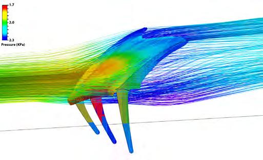
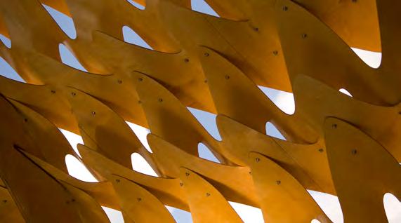
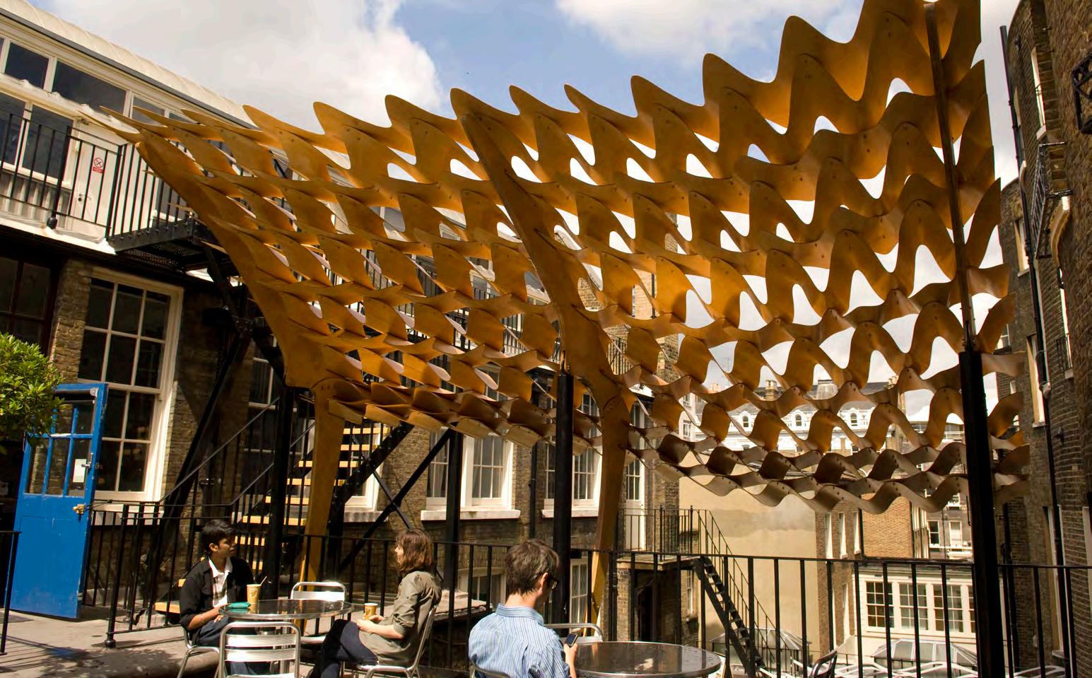
62
3.14 CFD analysis of the canopy
3.15 Close-up of the canopy on site
3.16 View of the AA Terrace and the Emtech canopy

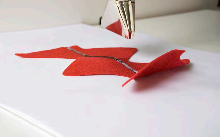
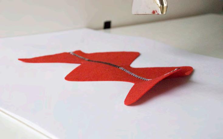
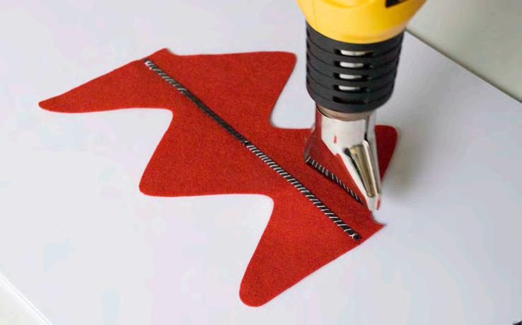
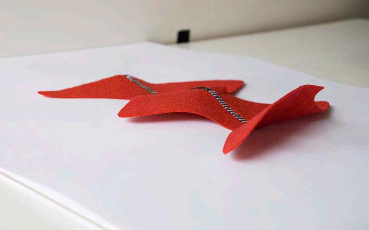
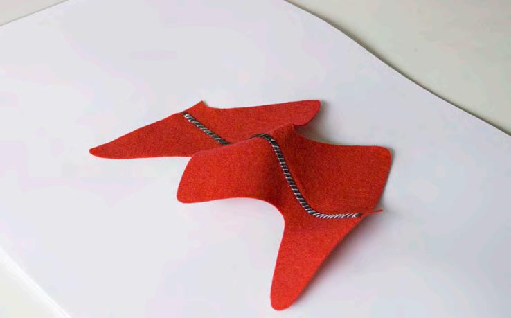
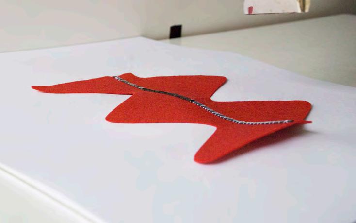

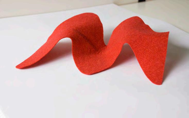
63
3.17 Sequential photos of the actuation experiment
An important detail of the experiments, is the type of the shape memory alloys used. The range of the SMAs in general is mainly based on their actuation temperature. The temperatures vary from 30 to 95 degrees and the type of alloys used throughout our experiments, have a value of 65.
The other differentiating factor between the setup of the experiments is the shape change. This is set during the curing process explained earlier (p.nn) and so far we have seen two different ‘memorised’ shapes.
Actuation temperature of SMA
Alloy N Superelastic Alloy Superelastic standard alloy, 'colder' than alloy S (Af ca. -15° C)
Alloy S Superelastic Alloy Superelastic standard alloy, 'softer' than alloy N (Af ca. 0° C)
Alloy C Superelastic Alloy Cr-doped superelastic alloy, 'stiffer' than alloy S and N
Alloy B Actuator Alloy Body temperature alloy (Af ca. 35° C)
Alloy M Actuator Alloy Actuator Alloy with intermediate transformation temperatures (Af ca. 65° C)
Alloy H Actuator Alloy High temperature actuator alloy (Af ca. 95° C)
Flexinol Wire Actuator high fatigue Especially optimized actuator wire with high fatigue resistance (Af ca. 100° C)
Shape Setting
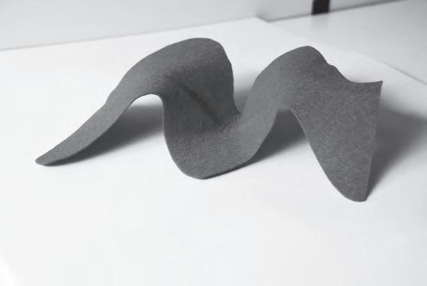

64
Actuated Openings
The previous experiments were focused on shape change or changes in the curvature on a surface, hence a setup was made to explore openings on a surface. The SMA wires were cut and bundled together forming arcs. A bundle of three fibres was woven to the felt to create openings. As they were heated the surface opens of both on the inside and outside.
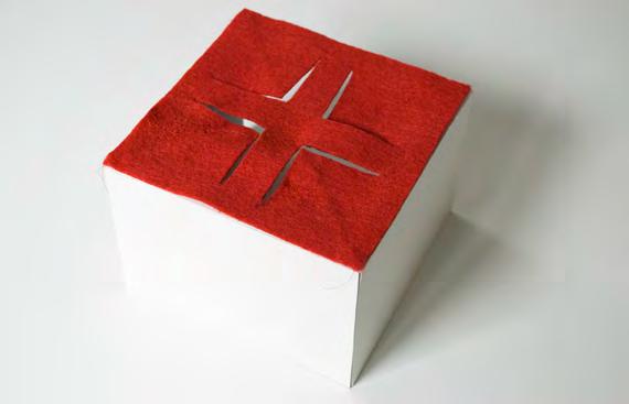

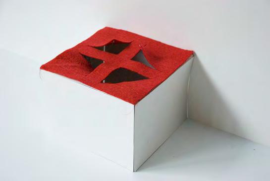
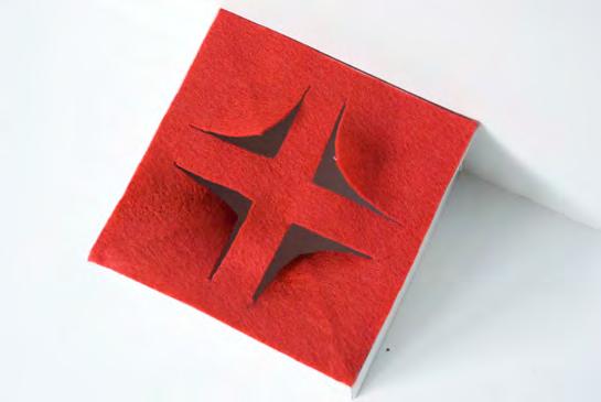
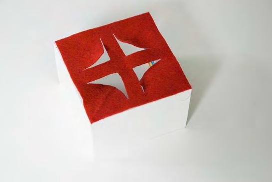
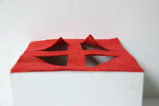
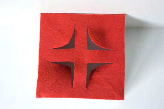
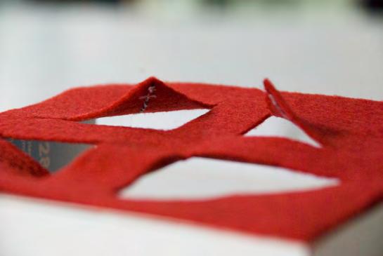
65
3.18 Sequential photos of the actuation experiment
Actuation + Control
This was the first experiment that the element of control was introduced to the system. The same SMA ribbon that was used for the actuated canopy experiment, is attached on a silicon heating patch. Because the patches are designed to work with 110 Volts, two of them have to be connected in series in order to reach the 220 Volts of the power supply. One end of the patches is connected together with the live cable to the plug, and the other to the controller.
A thermocouple is also used to measure the temperature on the SMA.
The controller has a single input (temperature of the thermocouple) and one output (turn on/off the heating patches). In the beginning of the experiment, we give a set temperature to the controller -which is the actuation temperature of the SMA, 65 degrees. By turning the system on, the controller reads the process temperature from the thermocouple and as long as the value is smaller than the set value (65), the heating is turned on. When the temperature reaches the set value, we have full shape change and the system stops heating the SMAs.
This experiment helped us understand how we could control the actuation of the system and gave us some very interesting results:
The temperature of the alloys raised from room temperature to 65 degrees in less than 15 seconds. That means that in a potential application of the SMAs with heating patches, the shape change could be very fast and the system would be able to respond to any external stimuli almost instantly. Also, the accuracy of the control was high. Were were able to measure the temperature efficiently and that type of controller could respond accurately to even slight differentiation of the values.

Actuation
1 SMA Ribbon
Silicon Heating Patches
Control
Thermocouple (Temperature)
Single Input Control Unit
(Temperature Set Value
Temperature Process Value)


66
40
53
65 degrees
degrees
degrees
3.19
Experiment setup
4 SMA Ribbons Rope Heaters
Control
Thermocouple (Temperature)
Single Input Control Unit
(Temperature Set Value
Temperature Process Value)
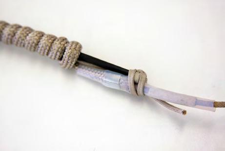
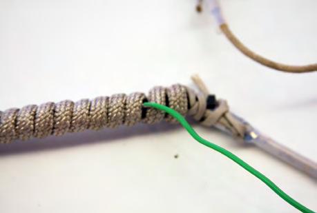
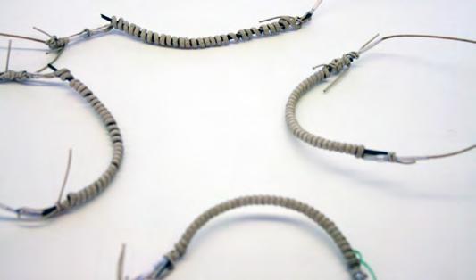
The next step of the physical experiments, was the integration of more SMAs into a model. We made a silicon rubber model and while casting it, we placed four SMAs inside. The alloys had rope heaters wrapped around them (Figure 3.20) and one of them had also a thermocouple connected (Figure 3.21).
The process of the experiment is similar to the one explained in the previous page, with the main differences being that for the heating we utilized rope heaters instead of patches, and that we have four alloys instead of one.
The results were not the expected. Only a small amount of shape change was observed (Figure 3.23) and that can be explained by two reasons. First of all, the material used for the model -silicon rubber- was inappropriate since it was very flexible and with no structural integrity. Besides that, the placement of the SMAs inside the model was not designed accurately. The alloys were orientated more towards the side instead of the upper-lower part of the rubber and at the same time they had no support due to the high flexibility of the surrounding material.
Revising this experiment, was the first step to design and set-up our final fibre composite piece. Placing the alloys was rethought and also the rope heaters were discarded because of their thickness (more than 1cm), which would be impossible to integrate into a composite.
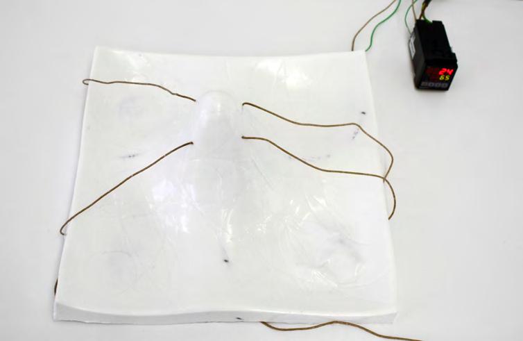
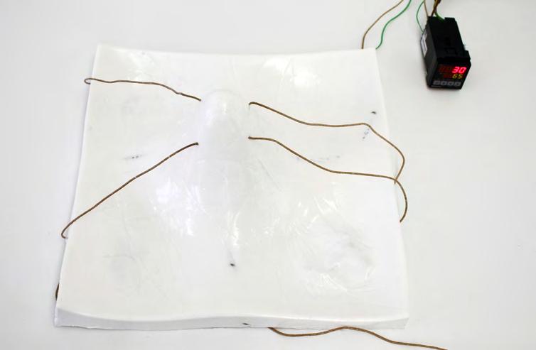
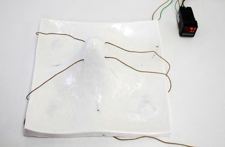
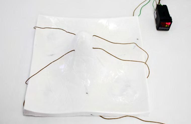
67
Actuation
3.21
3.22
3.20 Rope heater wrapped around the SMA ribbon
Thermocouple attached on the SMA
All four SMAs connected in series, after actuation
3.23 Sequential photos of the actuation experiment
Sensing + Control
Since the actuation system was tested in all our previous experiments and already set for our final model, the challenge shifted to the sensing.
In theory, our system uses fibre optics for all the sensing functions. In practice though, things turned to be more complicated.
Fibre optics technology is widely spread and applications of fibre optic sensors have been established for years. There is currently a lot of research on simultaneous sensing of multiple parameters and the results are very promising. So, even though all we needed is already out there, it was not possible for us to find a fibre optics processing unit and use it for experiments.
This was the reason why we chose to use strain gauges. Fortunately, our tutor George Jeronimidis offered his help and experience on the matter, and made the facilities of the Engineering Department of Reading University available for us.
Although our previous rubber model was not functional, we decided to test wether we could set up the sensing circuit on it. At the same time, we tried on a separate piece of fibre reinforced polyester resin that proved to be much more efficient.
After calibrating the strain gauges processing unit and completing all the wiring needed, we attached the gauges on the two models and tested successfully the circuit. The final step was to link it to the actuation circuit and then everything would be set and ready to be implemented into our final model.
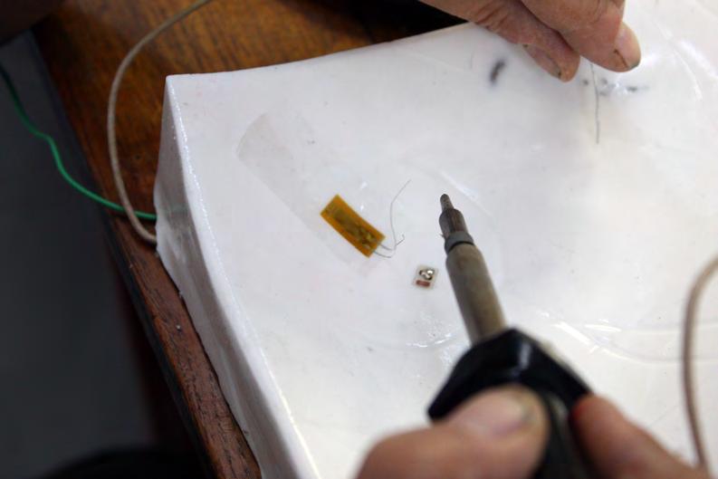
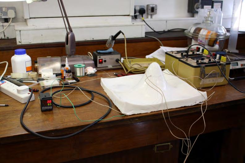

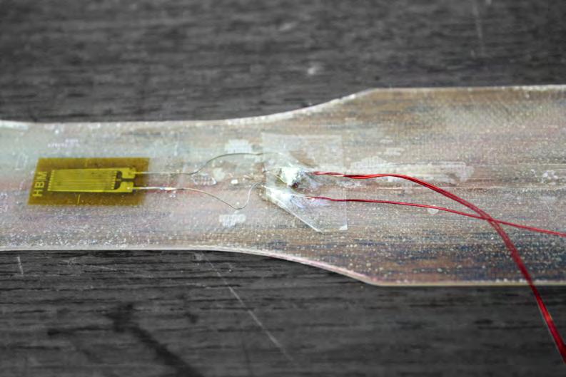
68
Sensing Thermocouple (Temperature) Strain Gauges (Strain) Control Single Input Control Unit (Temperature Set Value Temperature Process Value) Strain Gauges Processing Unit
3.24 Strain gauge attached on the rubber model
3.25 Testing the actuation circuit
3.26 Testing the sensing on a polyester piece
3.25 Calibrating the processing unit
Curvature Calibration
A very crucial task that we had to accomplish, was the calibration of the curvature change of the SMA. The amount of curvature change in every step of the temperature difference had to be measured, so that we could control the shape change and also calculate the thickness and the expected shape change of the final model.
A simple experiment was set (Figure 3.28 with the temperature controller used for all the actuation experiments, a thermocouple and the same SMA ribbon that would be used for the final model.
The results -as shown in the tableshowed a slightly different behavior than what is described in the literature. The shape change was more linear than expected and started at 38 degrees. The full change was reached at 58-60 degrees and not in 65, which is the actuation temperature of the alloy.


69
TemperatureRadiusCurvature 30 ∞ 0.000 35 1000 0.001 40 38 0.026 45 20 0.050 50 8 0.125 55 4 0.250 60 3.8 0.263 65 3.8 0.263 0 0.08 0.15 0.23 0.30 14 28 42 56 70 SMA Actuation Curvature Temperature
3.27 Results of the curvature change calibration
3.28 Measuring the curvature of the
SMA
while raising the temperature
Sensing
+ Actuation + Control
Final Model
The base material for our Final Model is a glass fibre reinforced epoxy resin. It is a sandwich structure with four SMA ribbons embedded (with their silicon heating patches) and strain gauges attached on the surface. We also use a thermocouple to measure real time the temperature on the alloys.
The strain gauges are attached on the bottom of the surface, in order to sense the strain due to vertical eternal loads on the surface. The configuration used for the strain gauges is a half-bridge. There are two gauges used -one active and one dummy- in order to achieve temperature compensation. The active is attached directly on the surface of the model and the dummy on a piece of stiff thermoplastic, so that it doesn’t get any curvature change as the model is deformed by the external force. The use of the dummy gauge is crucial for our system, because the active is placed very close to the SMA. This means that as the temperature would raise while actuating, the active gauge would sense a false curvature change.
When there is curvature change on the gauge, a signal is sent to the processing unit. When the signal arrives at the unit it is read, measured and translated accordingly to a voltage output -in our case the output was 0-2 Volts. One of the crucial procedures for setting up the system, is the calibration of the processing unit. There are a series of parameters that need to be set with very high accuracy, which include the zero-curvature of the gauges, the relation between the μstrains sensed and the voltage output, the exact gauge factor and other.
The Voltage from the processing unit acts as an input for the single input controller. When a value higher
than the programmed tolerance (0.1) is received , the controller turns on/off the actuation circuit that follows. This is done by passing the live wire of the actuation circuit, through this controller.
The final step is the actuation process controller. This controller has two inputs. The set value and the process value of the temperature on the SMAs. When it is switched on by the previous controller, it starts heating the alloys by turning on the heating patches, which are connected in series. The heating process stops, when the process temperature becomes equal to the set temperature of the system. This means that the actuation temperature of the SMAs has been reached and as a result, we have full shape change. For measuring the temperature on the alloys, we used a thermocouple directly linked to the controller.
Sensing
Strain Gauges (Strain)
Actuation
4 SMA Ribbons
Silicon Heating Patches
Control
Thermocouple (Temperature)
Single Input Control Unit
(Temperature Set Value Temperature Process Value)
Strain Sensing Control Unit (Voltage Input)
Strain Gauges Processing Unit
Strain Gauges Processing Unit
70
Single Input Controller Main Controller 0-2 Volts ON / OFF Thermocouple Actuation Circuit Shape memory alloys Strain gauge
3.29 Diagram of the final model setup
Preparation of the Model
The Glass Fibre mat was placed on the mould, after the cutting pattern needed for the double-curved surface was determined. Consequently, the resin was prepared and the four SMA ribbons were glued to the heating patches, as shown in figure...
A first layer of resin was applied on the glass-fibre mat and the SMAs were placed as planned. Then, a second layer was applied on top and the alloys were sandwiched.
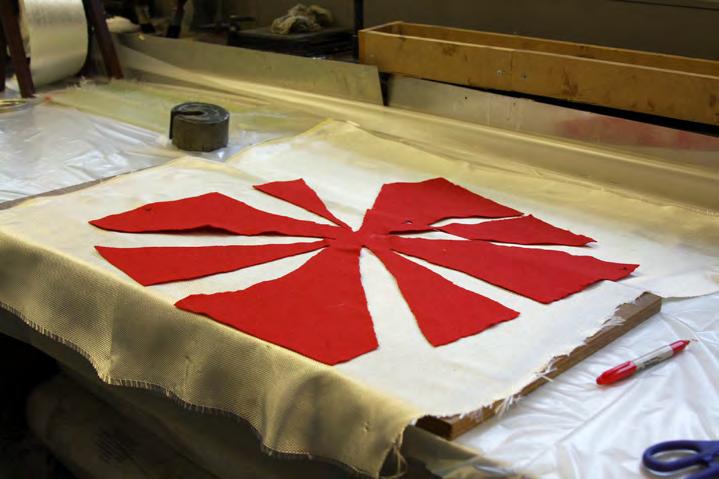
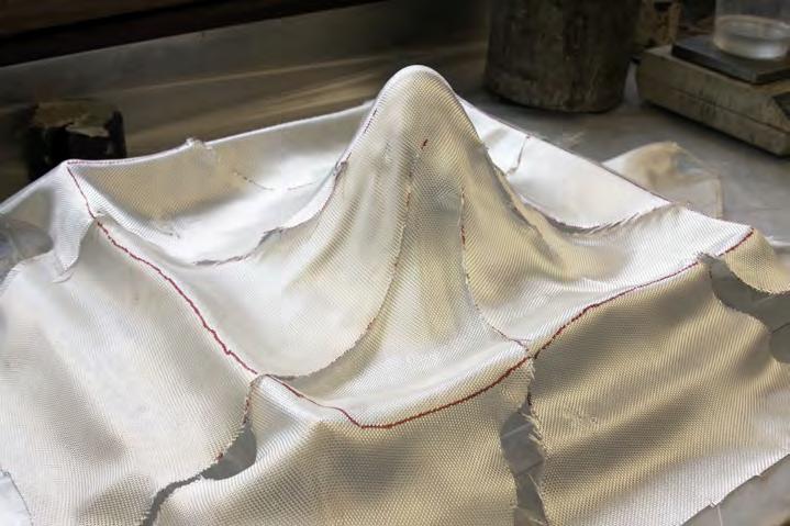
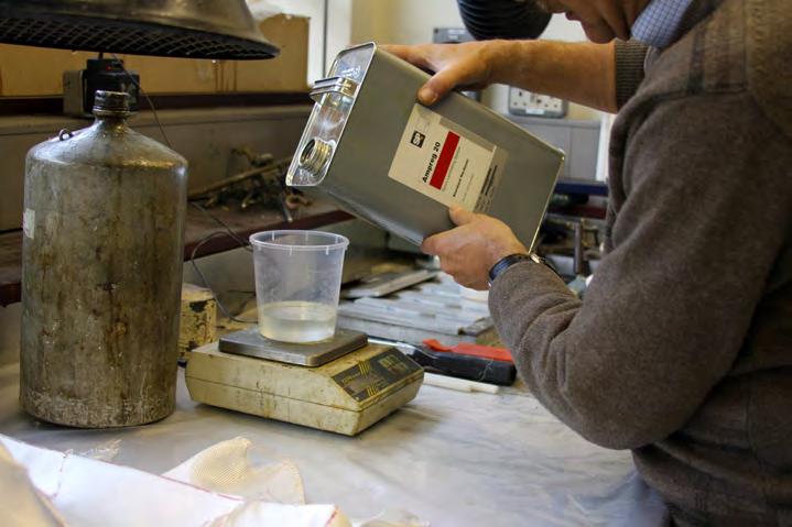
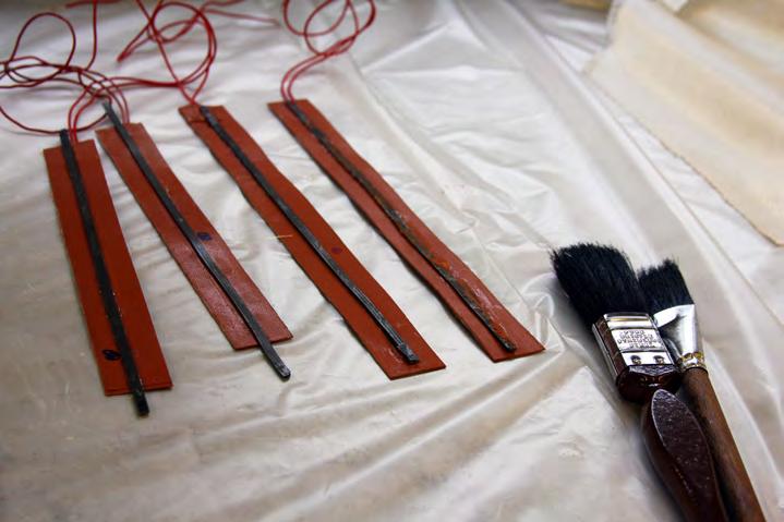
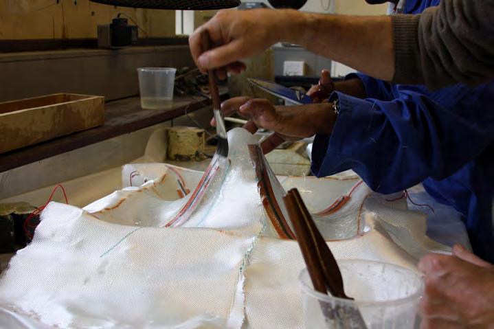
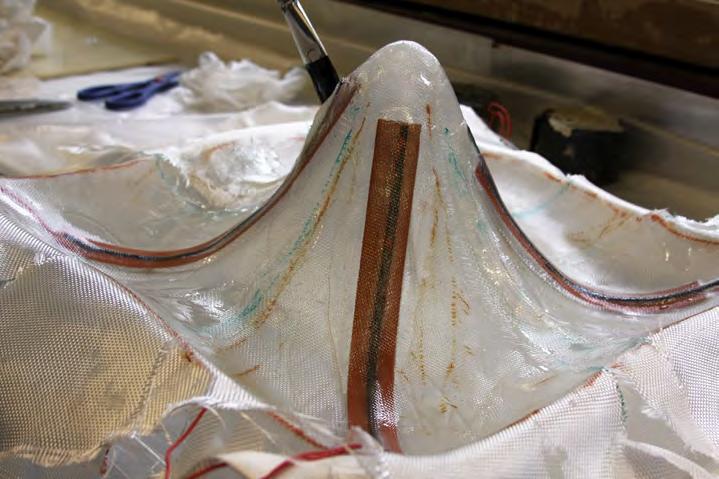
71
3.30 Cutting pattern of the glass fibre mat
3.31 Glass fibre mat placed on the mould
3.33 The SMAs attached on the heating patches
3.35 Applying the second layer
3.34 Applying the resin
3.32 Measuring the resin needed for the model
After the curing of the model in the oven for approximately one hour, it was removed and ready for un-moulding. The curing process had to be done very carefully by controlling the temperature of the oven, because if it went over 35 degrees the SMAs would start actuating. That would consequently cause a shape change and the model would deform before it was cured.
Due to this, the curing time was longer than it usually is for resin models that are cured in much higher temperatures (around 90).
After the removal of the model from the mould, all the wiring was configured and the actuation circuit was tested successfully.
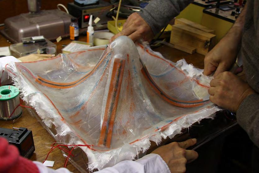
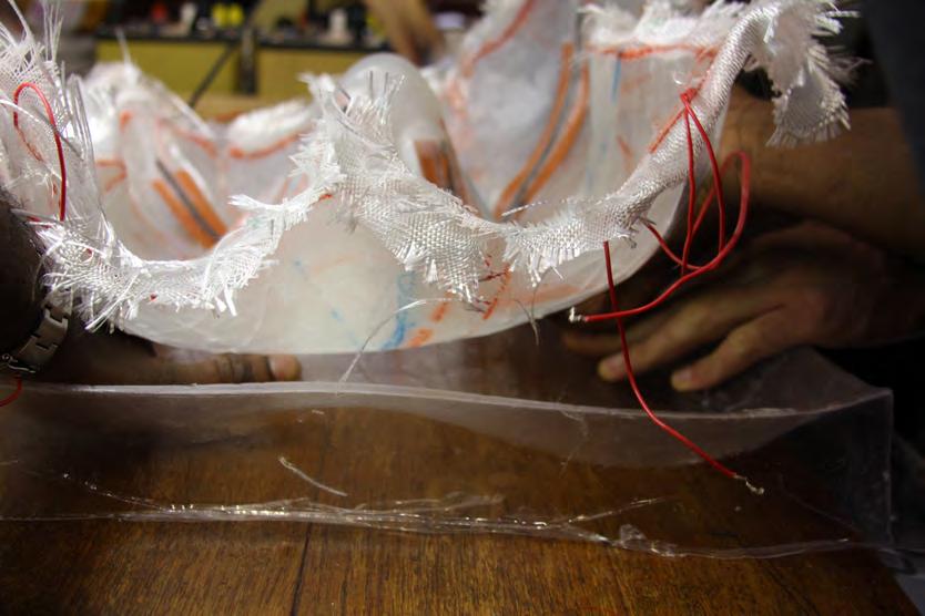

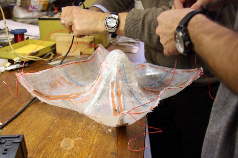
72
3.36 Un-moulding the model
3.38 Fixing the wires of the actuation circuit
3.39 Connecting the heating patches in series
3.37 Un-moulding the model
The next step was the setting up and testing of the sensing. Using a soldering device, all the wires were prepared and a first test was done on another piece of resin (Figure 3.41). Then the two gauges were set. The active one was attached with a resin glue on the surface of the model and the dummy gauge on a piece of stiff thermoplastic.
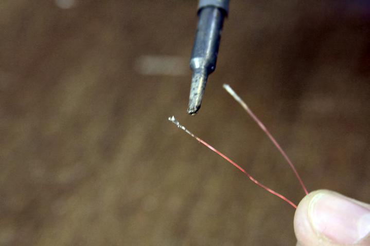
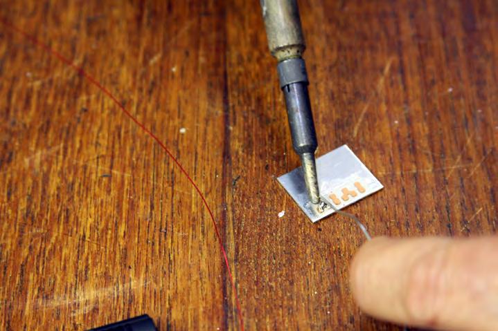
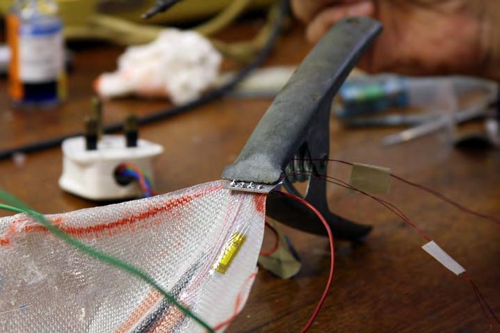
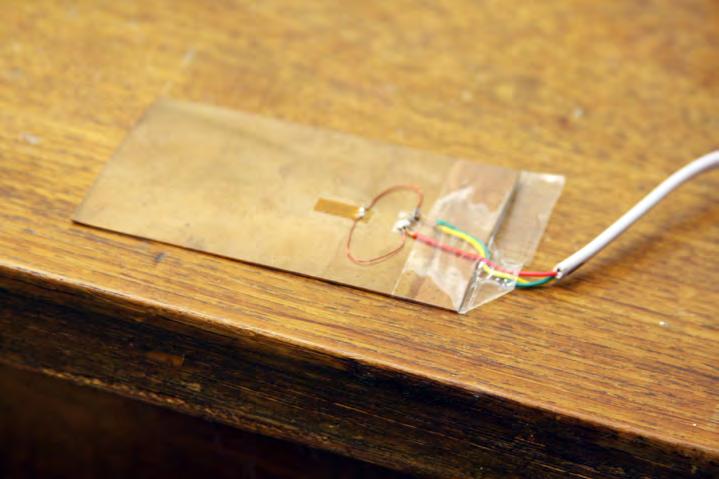
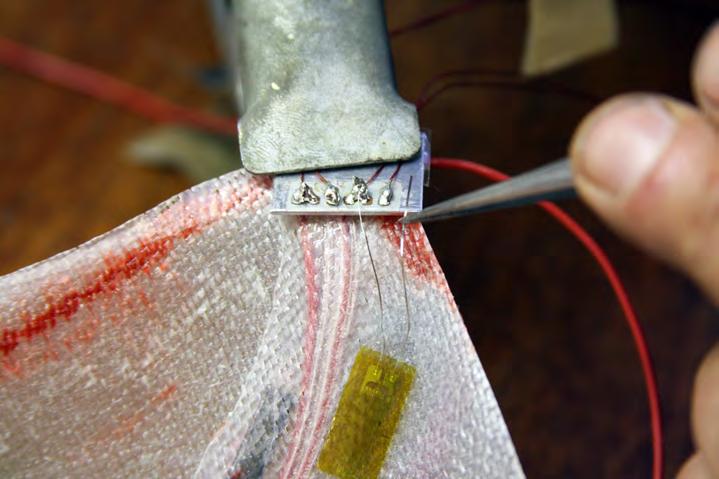
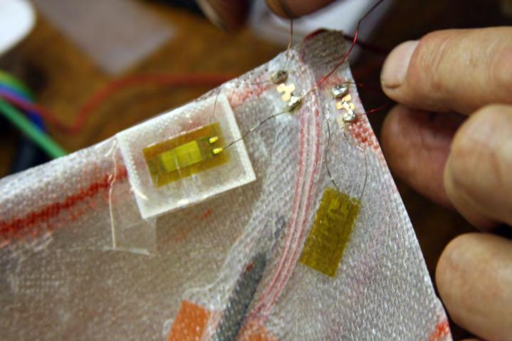
73
3.40 Soldering the edges of the strain gauge wires
3.41 Testing the processing unit by using a trial piece
3.43 Connecting the gauges to the wires
3.42 Soldering
3.44 Attaching the strain gauges
3.45 Attaching the dummy gauge
The final step was to connect both the sensing and actuation circuits and test the whole system. As shown in figure 3.46, the shape change happened as expected and both the sensing and actuation were calibrated properly.
Last, the setup of the final model was designed and built for the whole experiment to be repeated and at the same time properly measured and evaluated as shown in the next two pages.
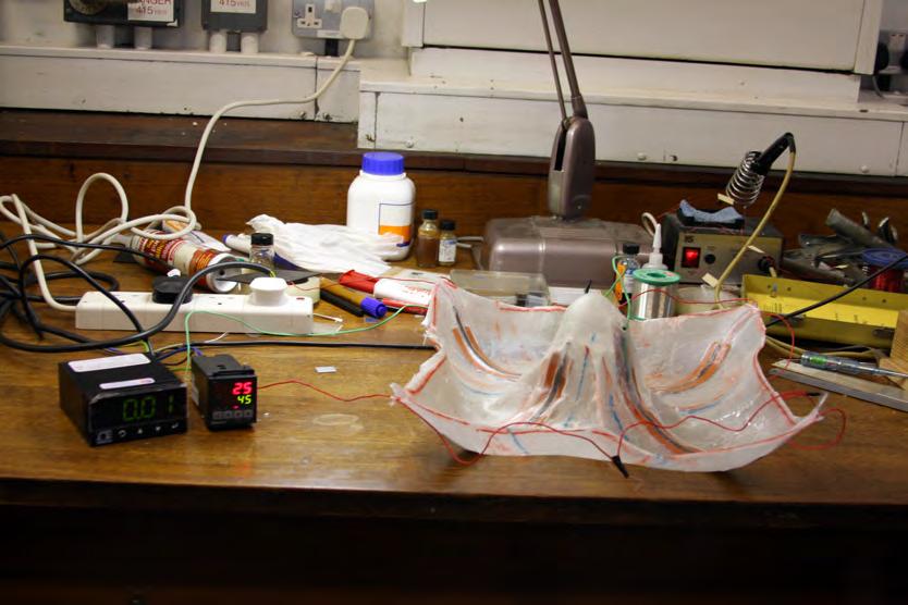
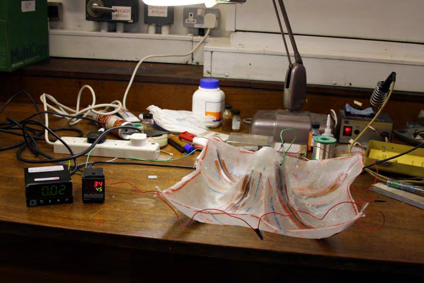
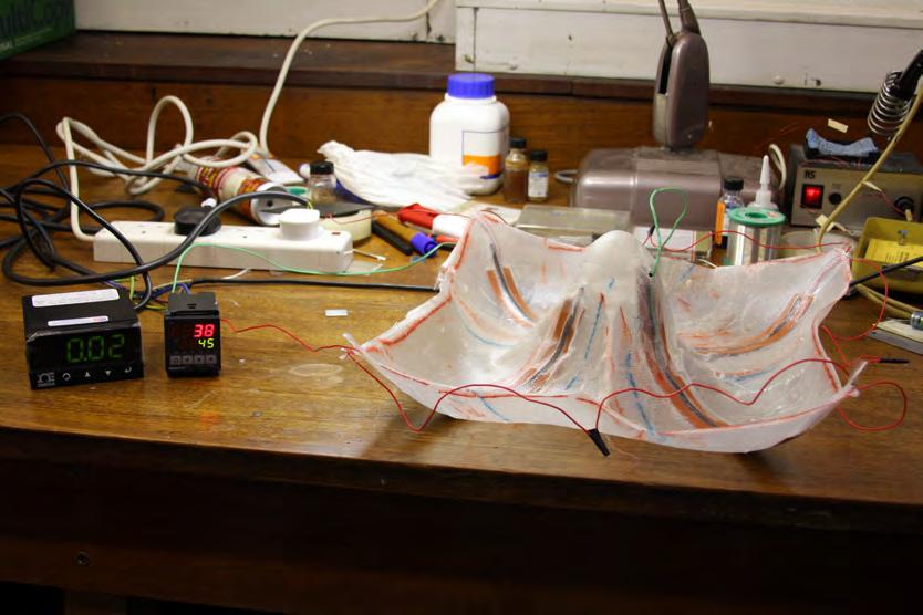
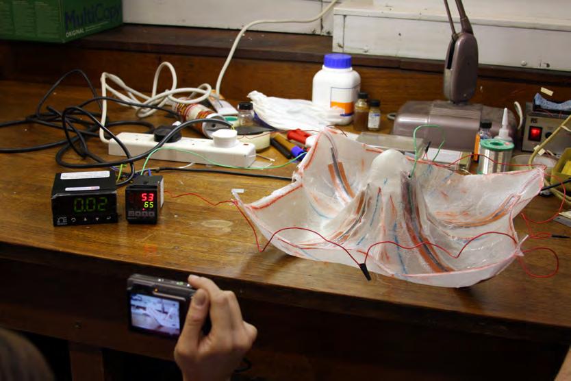
74
3.46 Sequential photos of the actuation circuit testing
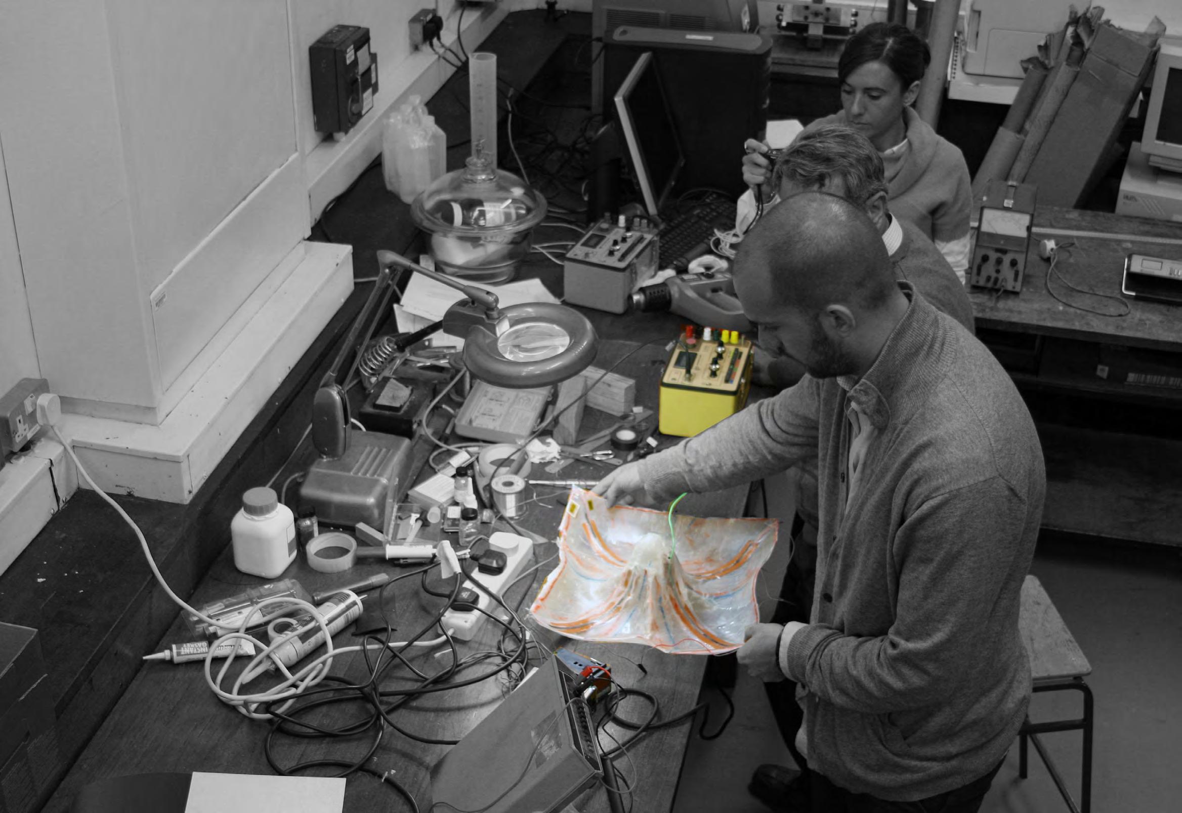
75
Strain Gauges Processing Unit
Actuation Controller
Strain Gauges
Thermocouple
3.47 Working at Reading
Model
Strain Gauges Processing Unit
As the signal from the strain gauges arrives at the processing unit, it is read, measured and translated accordingly to a voltage output. In our case the output was 0-2 Volts.
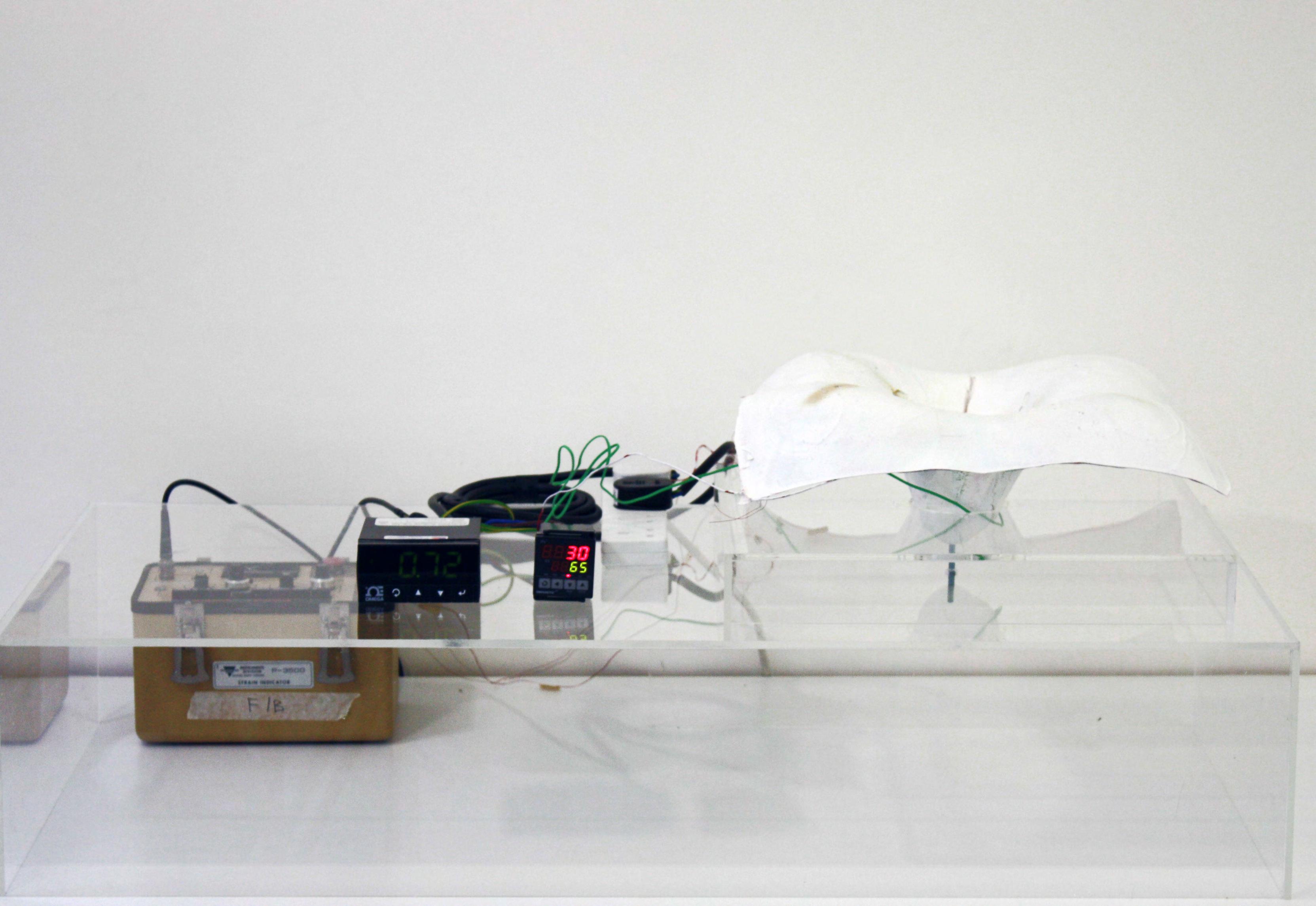
Single Input Controller
The Voltage from the processing unit acts as an input for the controller. When a value higher than the programmed tolerance (0.1) is received , the controller turns on/off the actuation circuit that follows
Actuation Temperature Controller
This controller has two inputs. The set value and the process value of the temperature on the SMAs. When it is switched on by the previous controller, it starts heating the alloys by turning on the heating patches, which are connected in series. The heating process stops, when the process temperature becomes equal to the set temperature of the system. This means that the actuation temperature of the SMAs has been reached and as a result, we have full shape change. For measuring the temperature on the alloys, we used a thermocouple.
76
3.48 Setup of our final model

77 58 degrees 42 degrees 30 degrees 3.49 Diagram showing the shape change
Remarks
Our final model was very successful in terms of functionality and performance. We managed to fulfill the initial aim we set for our physical experiments, which was to built a functional system that could sense, actuate and also manage the flow of information while taking basic decisions.
A very critical detail of the model is its stiffness. Thinking of the scale in relation with the actuation function, one can understand the importance of the ratio of curvature change and stiffness of the composite. In our case, the stiffness of the model was very high for the size of the alloys and the curvature.
A minor issue of the model was the paint, which was not the appropriate choice to make. Even though the spray-paint used was very high-temperature resistant, the parts of the composite that were heated repeatedly started burning the paint. It would have been better if we added a pigment to the resin, which would produce any visual effect and not have any problems because of the high temperatures.
One of the issues that the sensing-actuating cycle had, was the response time of the SMAs. That happened because of the connectivity
of the heating patches (in series) and the heat transfer losses from the patches to the alloys. Using heating patches of 220V instead of the 110V in series, would lead to faster heating of the alloys and hence shape change of the model. The only way around all the possible problems that could arise in regards to the heating and the response time of the actuation, is the use of electricity. As discussed earlier in the document (p. 46), this would make the actuation more efficient and the response time faster.
78
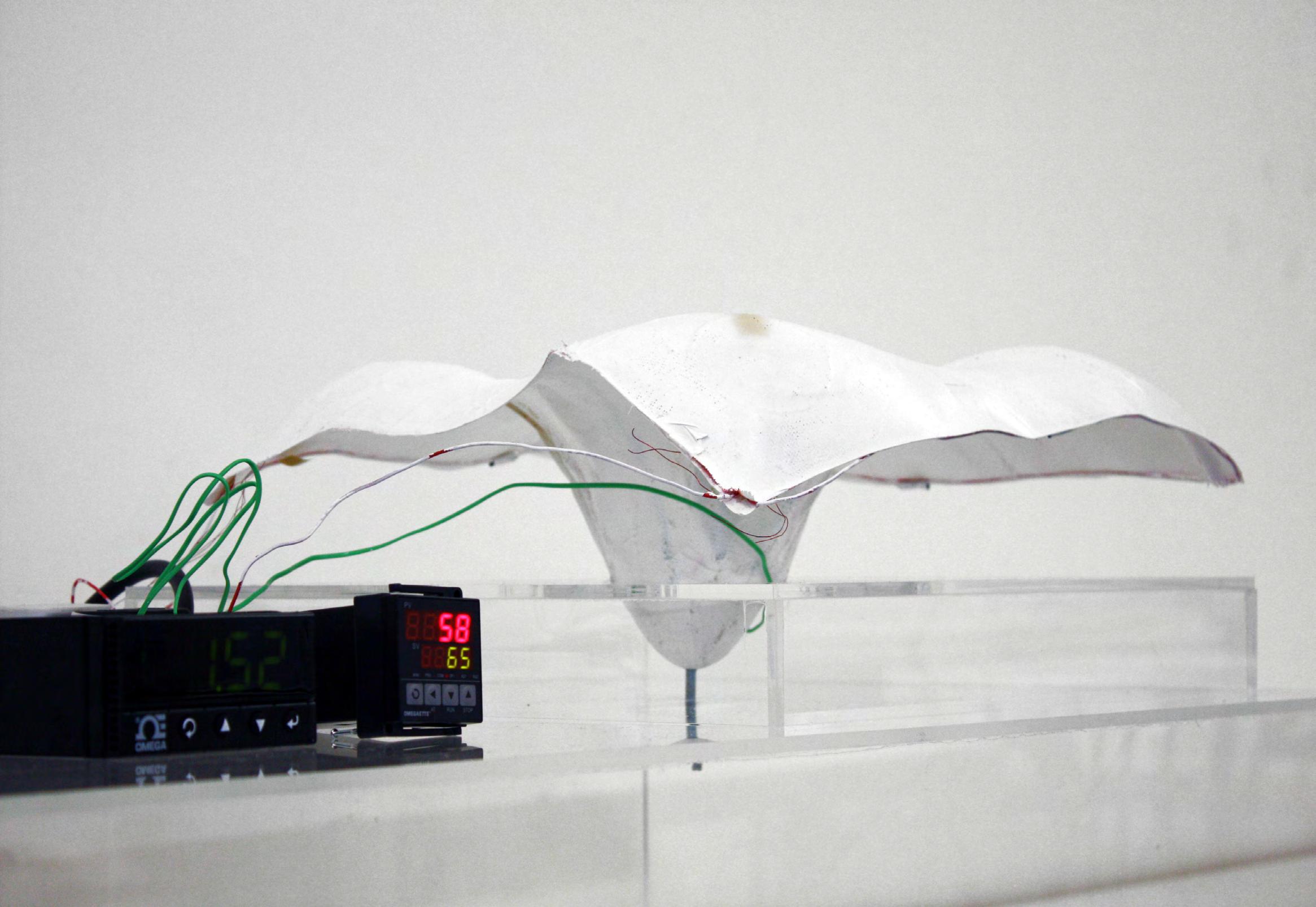
79
Geometry
The geometry has been elaborated with the ambition to fully embrace the benefits offered by the material. One of the main contributions fibre composite materials offer to architects and engineers is the possibility of achieving extremely thin surface geometries. However, from the structural point of view these geometries can be quite controversial since they might lead to ‘early’ structural failure, i.e. collapse of the structure occurs before the ultimate strength of the material is reached. For example, under compressive loads this type of surface-like geometries might lead to buckling depending on how and where are the external loads applied. Therefore, the aim of this chapter is to find a smart geometrical configuration that allows a ‘surface-like’ geometry to become stiffer where and when required.
As a result, the geometry is approached from two different scales: local and global. The first part of this chapter focuses on the local geometry which emerges from the topological definition of a single cell as the smallest unit within the material system. The proliferation of these single cell topologies responds to very specific rules which govern the fusion of the local and global geometries with the fibre composite material. The second part is dedicated to the global geometry. It mainly deals with the rules employed to generate the overall form and how the integration of the local geometry is accomplished.
4
Global
Local Geometry
Geometry
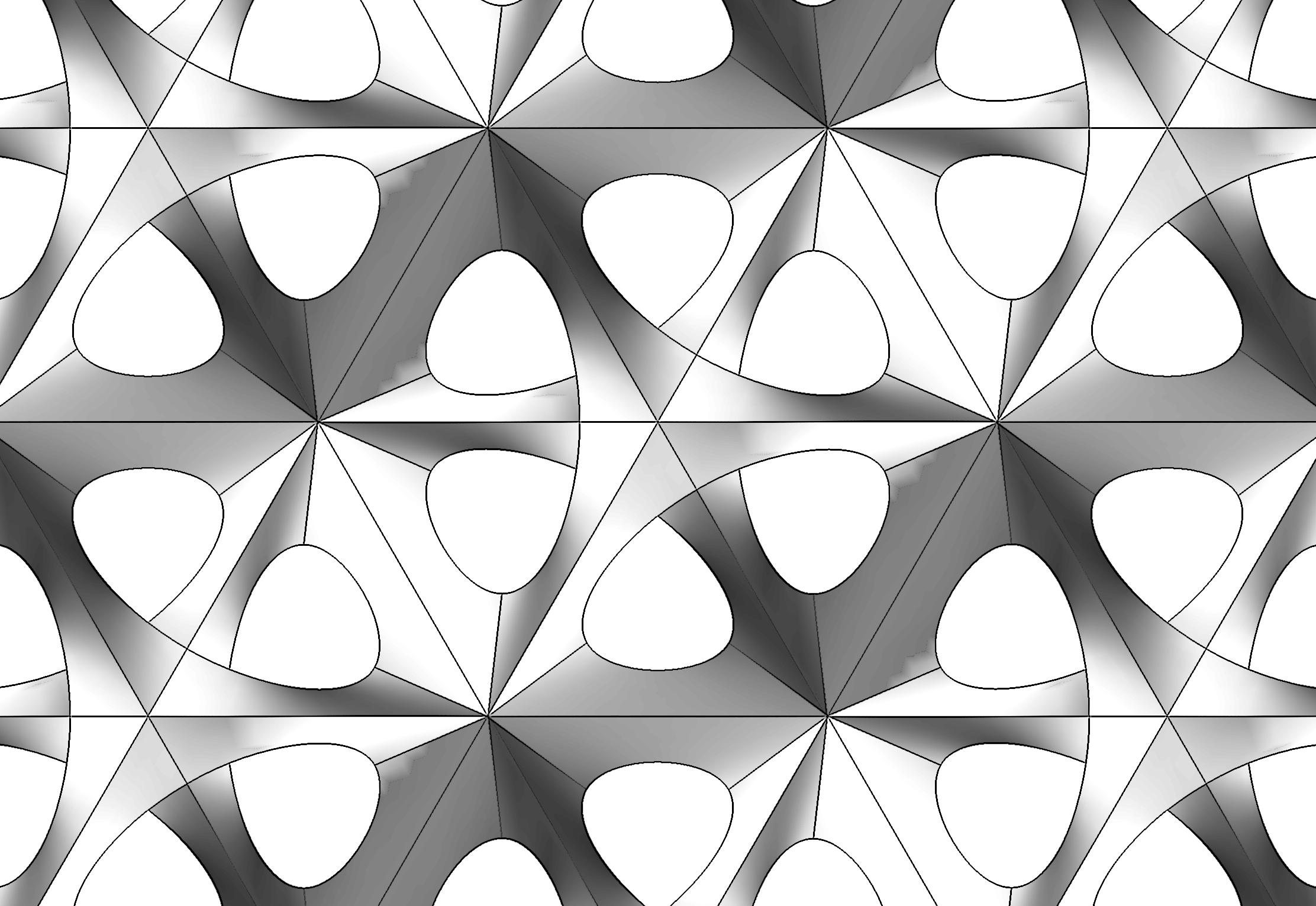
82
Local Geometry
Fibre composites are characterised for achieving high ultimate strength values which lead to the production of extremely thin surface-like geometries. These are very useful for the development of shell structures where all the external loads travel across the surface and thus, there are not out-of-plane forces to be considered -or these can be neglected. For those cases where out-of-plane effects cannot be neglected, reduced thicknesses would not contribute to transferring the loads and thus, the strategy needs to be reconsidered.
Instead of increasing the surface thickness –which will lead to a bulkier design- a more convenient strategy for dealing with this problem is to carefully reassess the geometry. The aim must be to generate ‘structural depth’ in the out-of-plane dimension; in other words, the material should be re-distributed away from the hypothetical ‘neutral axis’ originally positioned half way through the surface thickness. This arrangement can easily be achieved through the use of corrugations where the stiffness of the structure mostly depends on the height of the ‘waves’. Varying the local height of the corrugations would therefore lead to a structure with stiffer differentiated areas which ultimately contribute to the structure as a whole. This approach constitutes the base of the investigation for the development of the local geometry.
Actuation
Topology Precedents
Precedents
Continuous Surface Geometries
The investigation of different surface geometries led us to instigate on the study of mathematically defined continuous surfaces. Contemporary architectural projects suggest an overwhelming interest in this type of surface geometries which effortlessly bind together organisational, spatial and aesthetic features through continuity in surface and material. Spatiality is then transformed by the fluidity of a continuous surface comprising a family of interrelated forms. From the architectural point of view this type of geometries offer the possibility of modulating the spatial atmosphere, opening the door to new architectural paradigms [4.2].
Nevertheless, mathematically defined surfaces are not new to architecture and engineering. Antoine Gaudi was the first architect to use the hyperbolic parabola to inform masonry construction. Twentieth century reinforced concrete pioneers exploited the possibilities of linear ruled geometries to stretch the limits of wood formwork. In addition many artist and sculptors explored similar constructions; for instance the Russian Constructivist ‘Naum Gabo’ and the screen patterns of Erwin Hauer. However, the visualisation and modelling of equation based surfaces through computer tools has very much enhanced the way this type of geometries are utilised within the architectural field. Computerised modelling facilitates the investigation of surface geometries based on the pure logic of mathematics that were previously unattainable.
Parametrically-derived surfaces provide their own unique topological signatures of internal organisation. These principles can be used to embed performance qualities inherent to the surface logic suggesting new possibilities in contemporary architectural practice.
For the purpose of this project a total of six continuous non-orientable surface topologies have been selected. These are the ‘Klein bottle’, ‘Mobius strip’, ‘Boy surface’,
‘Roman’, ‘Cross-cap’ and ‘Bours minimal surface’.
A surface such as the Möbius strip or Klein bottle on which there exists a closed path such that the directrix is reversed when moved around this path [4.1]. The real projective plane is also a non-orientable surface, as are the ‘Boy surface’, ‘cross-cap’, and ‘Roman surface’, all of which are homeomorphic to the real projective plane.
There is a general method for constructing nonorientable surfaces which starts by choosing three homogeneous polynomials of positive even degree considering the map defined by:
f = (f1 (x,y,z), f2 (x,y,z), f3 (x,y,z) ) : R3 --> R3.
Then restricting x,y,z to the surface of a sphere by writing:
x = cos
sin
and restricting θ to [0,2π] and to [0, π/2], defines a map of the real projective plane to R3. In three dimensions, there is no unbounded non-orientable surface which does not intersect itself [4.1, 4.3].
4.1 Comparison between orientable and non-orientable continuous surfaces. Mobius strip and Klein bottle are both non-orientable surfaces, while the cylinder and torus are clear example or orientable surfaces which do not intersect with themselves.
84
φ
φ
φ
θ sin
y =
θ sin
z = cos
orientable cylinder Mobius Strip torus Klein Bottle real projective plane non-orientable

The use of this type of geometries has been beautifully realised in the design of the Mercedes-Benz Museum in Stuttgart, by Ben Van Berkel (UNStudio). In this case organisational and spatial strategies are combined to yield an elegant form. Its presence, formal balance and refinement of features, along with its continuity of surface, create a building that is spatially opulent.
The geometry of the plan, with its three overlapping circles, is suggestive of a trajectory subject to centrifugal forces which propel the visitor around. The trefoil is a
variation of the same mathematical model belonging to the field of knot theory on which the Mobius strip and its three-dimensional variant, the Klein Bottle, are based.
The trefoil possesses topological qualities: movement, orientation and direction are intrinsic to its structure. Within it the visitor is always located at some point on a curve, thus there are no abrupt transitions, no discontinuities. This sensation of being followed by space is a new type of experience [4.2].
85
4.2 Interior of the Mercedes-Benz Museum in Stuttgart, Germany. The concept is inspired on the fluidity achieved by a Mobius Surface -continuous surface.
4.3 Another view of the interior of the MercedesBenz Museum in Stuttgart, Germany.
Continuous Surface Geometries
The Klein bottle is a closed non-orientable surface of Euler characteristic ‘0’ that has no inside or outside [4.4]. It can be constructed by gluing both pairs of opposite edges of a rectangle together giving one pair a half-twist, but can be physically realised only in four dimensions, since it must pass through itself without the presence of a hole. It can be represented by connecting the side of a square in the orientations illustrated in figure 4.5.
It can be cut in half along its length to make two Möbius strips [4.6] but it can also be cut into a single Möbius strip [4.7, 4.8]. Figure 4.5 shows an immersion of the Klein bottle in the three-space [4.10]. There are also other possible immersions; however these have not been selected as part of this research since they belong to dimensional spaces beyond the three-dimensional one. Refer to the Geometry section of the Appendix for further data and mathematical formulation.
In addition, two strips on top of each other, each with a half-twist, give a single strip with four twists when disentangled [4.17].
The topological result of attaching a Möbius strip to a disk along its boundary is a real projective plane, which cannot be embedded in the three-dimensional space (R3) [4.18, 4.19]. However, there are three surfaces that are representations of the projective plane in the threedimensional space with self-intersections, namely the Boy surface, cross-cap, and Roman surface [4.21]. Refer to the Geometry section of the Appendix for further data and mathematical formulation.
Cross-Cap
The cross-cap can be thought of as the object produced by puncturing a surface a single time, attaching two zips around the puncture in the same direction, distorting the hole so that the zips line up, requiring that the surface intersect itself, and then zipping up [figure 4.8].
The Möbius strip -also called the twisted cylinder- is a one-sided non-orientable surface obtained by cutting a closed band into a single strip, giving one of the two ends produced a half twist, and finally reattaching the two ends [Figure 4.4]. The strip bearing his name was invented by Möbius in 1858, although it was independently discovered by Listing, who unlike Mobius published the research years later [4.9, 4.10]. Similarly to the cylinder, it is not a true surface, but rather a surface with boundary [4.11, 4.15].
A torus can be cut into a Möbius strip with an even number of half-twists, and a Klein bottle can be cut in half along its length to make two Möbius strips [4.16].
The cross-cap can also be described as a circular hole which, when entered, exits from its opposite point -from a topological viewpoint, both singular points on the cross-cap are equivalent [4.22, 4.24].
The cross-cap is one of the three possible surfaces obtained by sewing a Möbius strip to the edge of a disk. The other two are the Roman and Boy surface, figures 4.6 and 4.7 respectively.
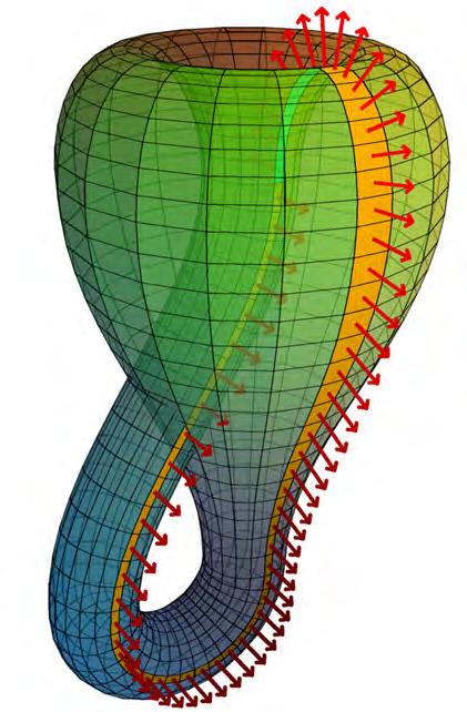
86 4.4 Mobius Strip 4.5 Klein Bottle
Klein Bottle
Mobius Strip
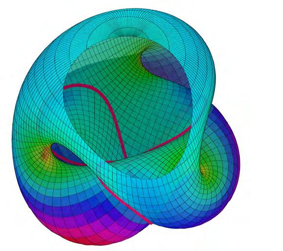
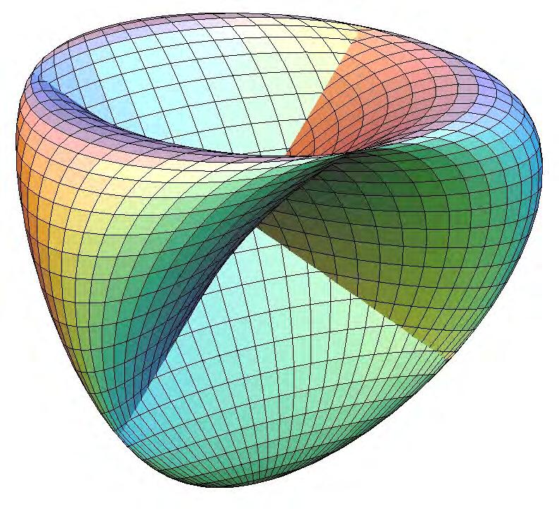
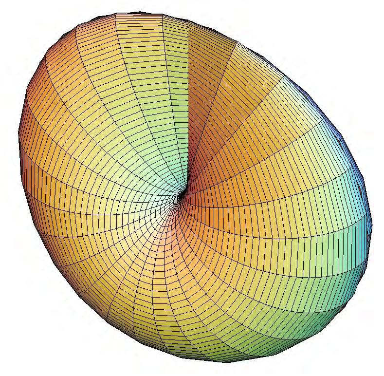
A sphere with two cross-caps having coinciding boundaries is topologically equivalent to a Klein bottle [4.20]. The surface with three cross-caps is known as Dyck’s surface [4.21]. Refer to the Geometry section of the Appendix for further data and mathematical formulation.
Roman Surface
The Roman surface [figure 4.6] is one of the three possible surfaces obtained by sewing a Möbius strip to the edge of a disk –the other two being the boy surface and cross-cap [figures 4.7 and 4.8 respectively]. It is a quartic non-orientable surface and it is also known as the Steiner surface [4.22,4.23].
The centre point of the Roman surface is an ordinary triple point with (±1,0,0) = (0, ±1,0) = (0,0, ±1), and the six endpoints of the three lines of self intersection are singular pinch points, also known as Whitney
singularities [4.23]. The Roman surface is essentially six cross-caps stuck together and contains a double infinity of conics [4.20]. Refer to the Geometry section of the Appendix for further data and mathematical formulation.
Boy Surface
The Boy surface [figure 4.7] is a non-orientable surface which constitutes one possible parametrisation of the surface obtained by sewing a Möbius strip to the edge of a disk.
Two topologically equivalent parametrisations are the cross-cap and Roman surface. The Boy surface is a model of the projective plane without singularities and surface [4.24, 4.25]. Refer to the Geometry section of the Appendix for further data and mathematical formulation.
87 4.7 Boy Surface
4.6 Roman Surface
4.8 Cross-Cap
Continuous Surface Geometries
Further information on the mathematical formulation is provided in the Appendix, under the section referring to Geometry.
A short vbscript algorithm was written in Visual Basic for visualisation purposes. A selection of the surfaces generated with this method is shown in the following pages.
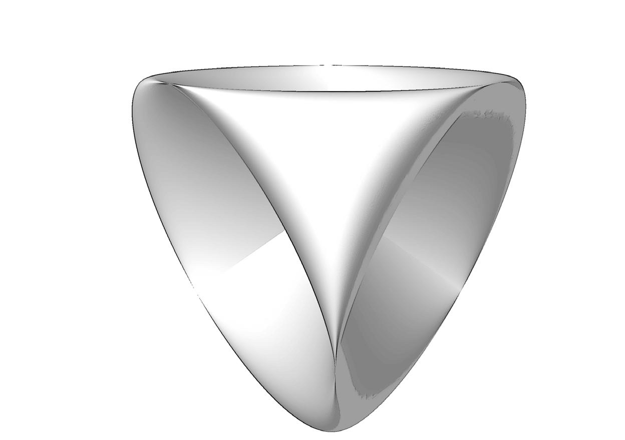
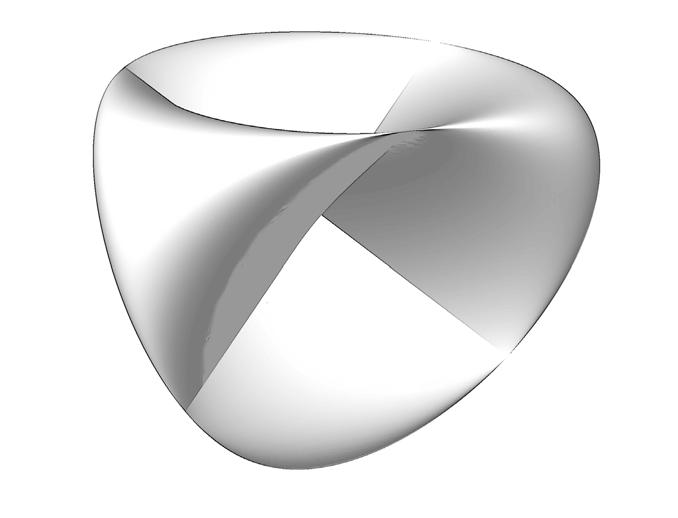
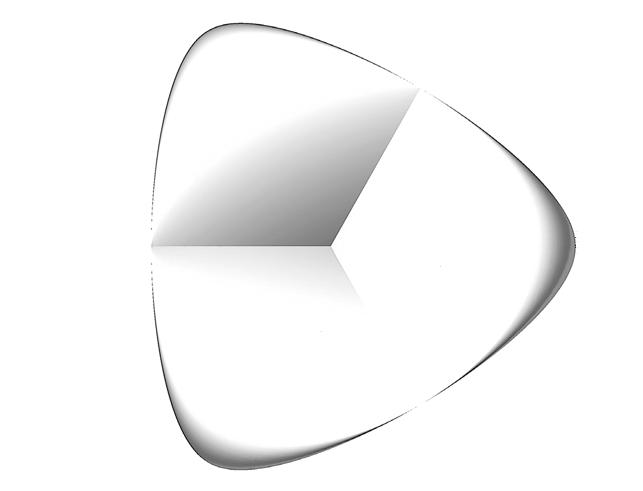
88
Roman Surface
Cross-Cap Surface
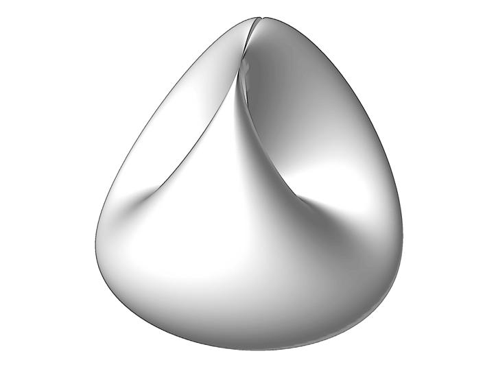
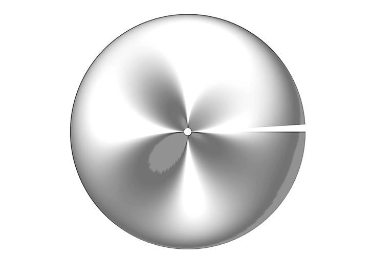
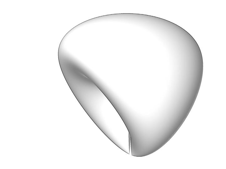
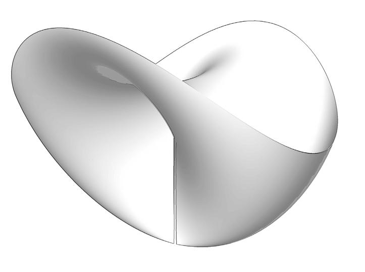
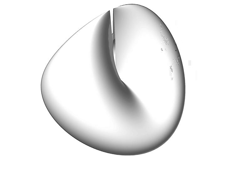
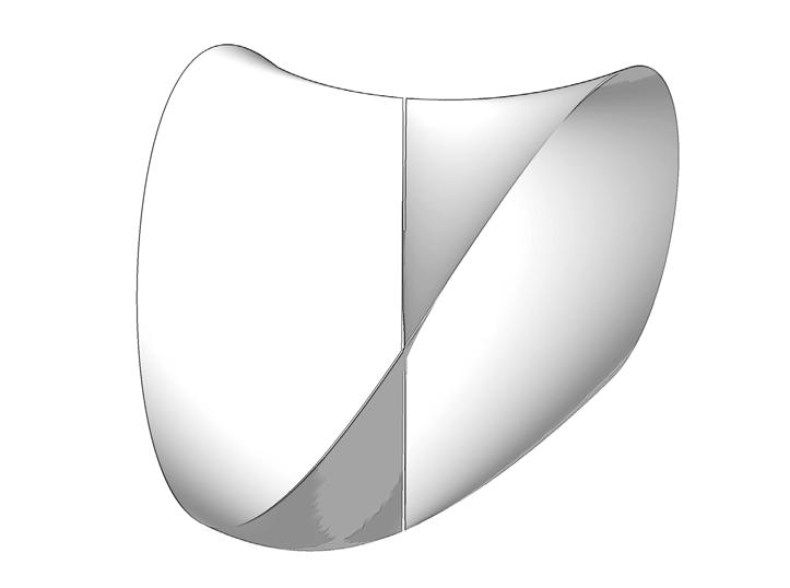
4.9 Different immersions of a Roman Surface
and a Cross
Surface
These have been generated using a short algorithm in Vbscript. Further mathematical data is provided in the Appendix, Geometry section.
89
(left)
Cap
(above).
Boy Surface & Mobius Strip
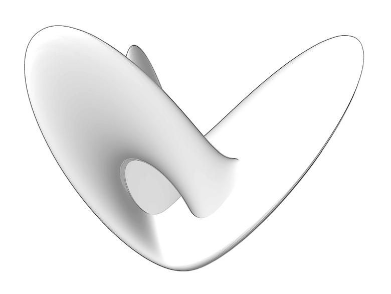

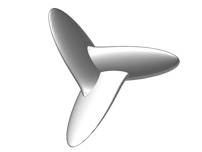
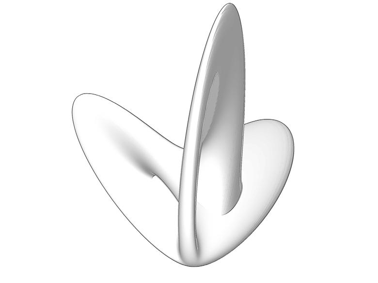
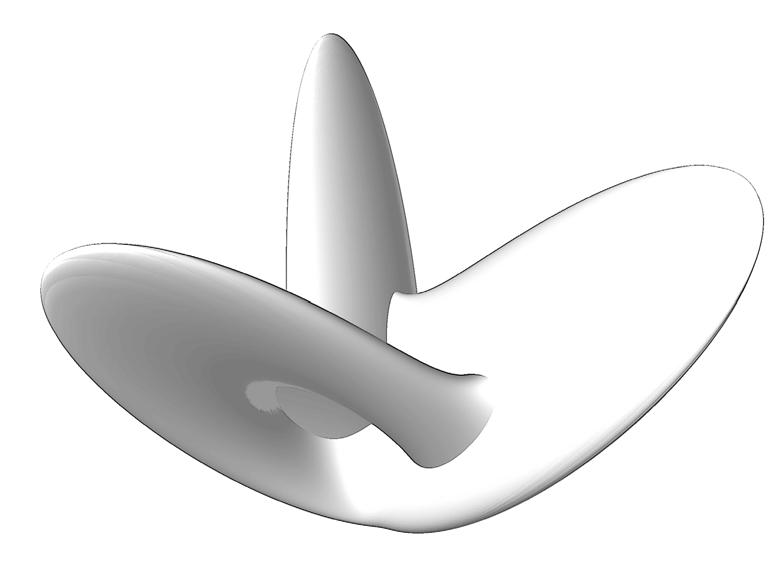
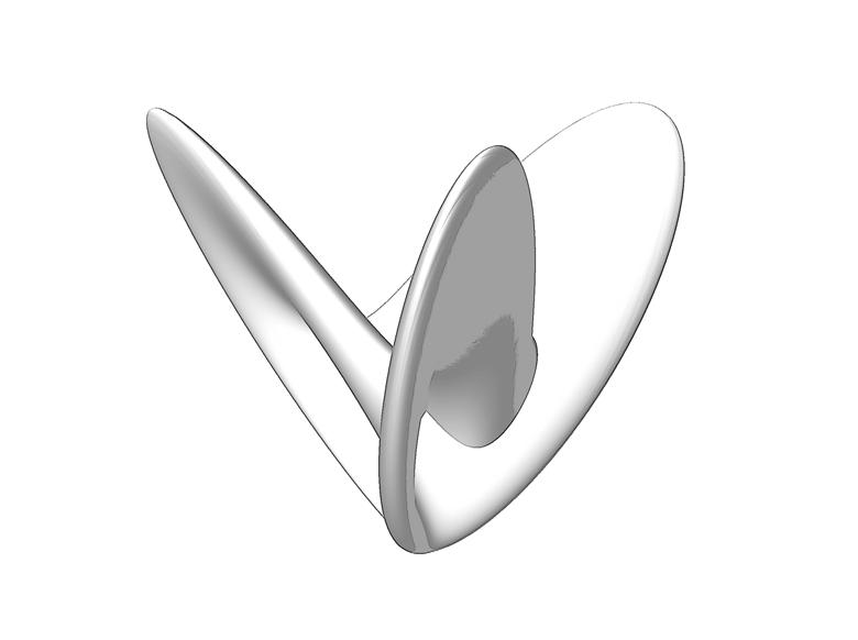
90
4.10 Different immersions of a Boy Surface (below) and of a Mobius Strip Surface (right).
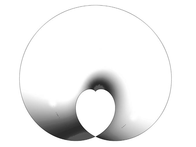
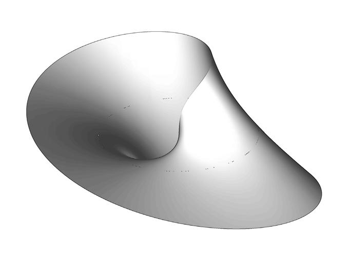
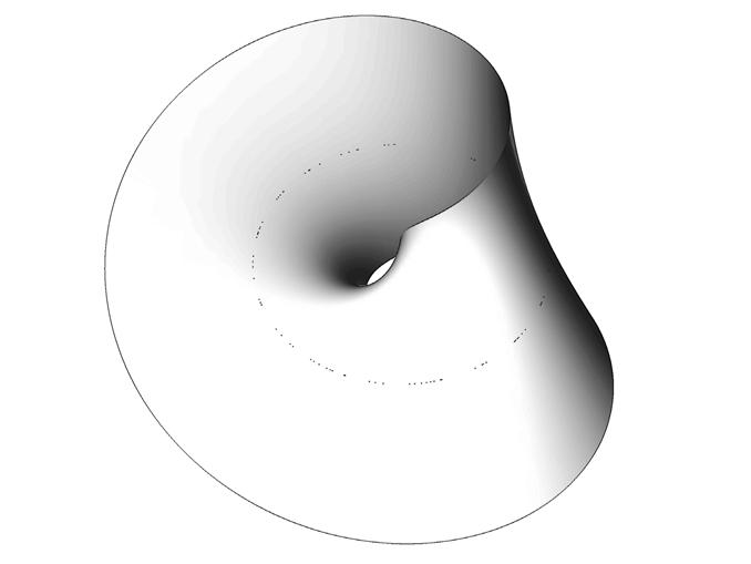
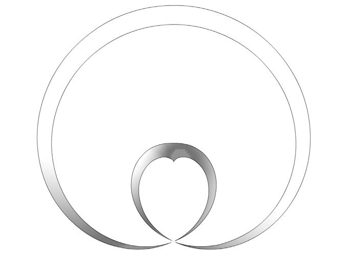
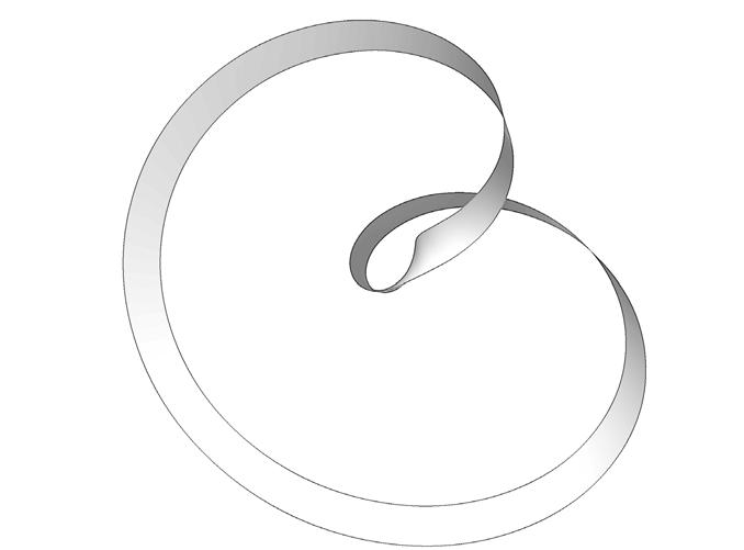
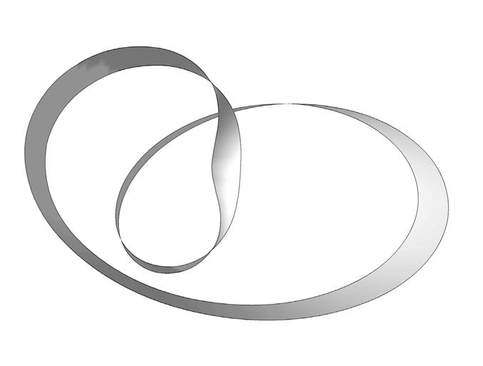
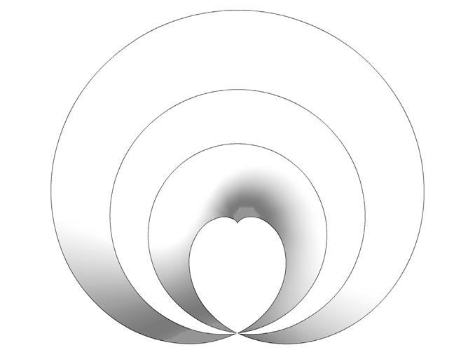
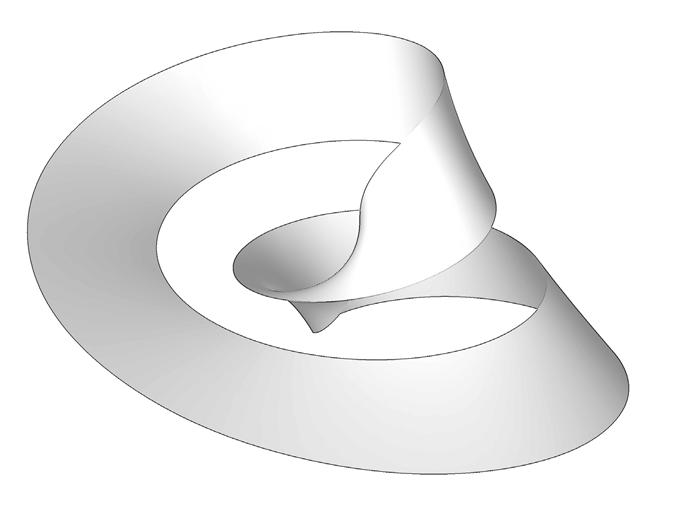
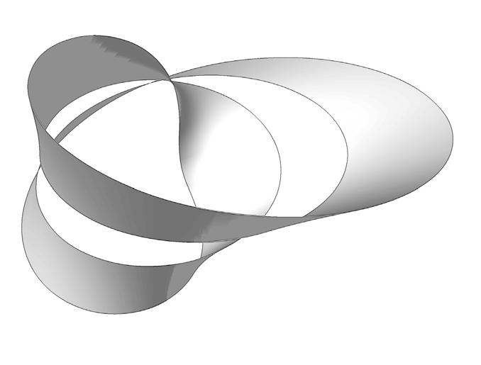
91
Erwin Hauer - Continua
Following the investigation of continuous nonorientable surfaces, our research led us to the work of Erwin Hauer. He was born in Austria and dedicated part of this life to sculpting, beginning to explore infinite continuous surfaces in the 1950s. His research started with the study of mathematically defined surfaces such as the Mobius strip or the Klein bottle which led to his inclusion within the movement known as ‘modular constructivism’: a style of sculpture based on carefully structured modules which allow for intricate and in some cases infinite patterns of repetition. These are used to create limitless, basically planar, screen-like formations which can also be employed to produce multidimensional structures [4.25].
The development of these topologies involves an extensive study of their mathematical formulation and the combinatorial possibilities of curvilinear and fluidly shaped modules, which are capable of creating a seamless, quasi-organic unity that can be either rounded and self-enclosed, or open and potentially infinite. In an article published in Architecture Week (4th August 2004), Hauer explains that “continuity and potential infinity have been at the very centre of my sculpture from early on.”
Hauer was also very much influenced by the work of Henry Moore and the fluid curves and porosity of his
sculptures, as well as by the arch-formalist Josef Albers, who was also his professor at Yale University [4.25].
Hauer’s research is quite extensive and covers many different aspects that range from the start of the conceptual design to the fabrication of these modules. However, the part of his work that interested us the most is the way these topologies are conceived and the algorithmic rules that generate the system; how a thin surface turns into a tissue-like webbing pattern interconnecting convex and concave surface curvatures –saddle surfaces- and thus, allowing for smooth self-combination in multiple dimensions.
The result is an interwoven of continuous surface-like geometries in different layers which ultimately form a space truss. A set of thin surfaces prone to buckling is therefore transformed into a robust structure by means of altering its topological definition; a compendium of interwoven surfaces defines now a continuous space truss capable of withstanding a wider range of loading conditions.
In addition, Hauer’s designs have proved useful and very attractive for use in eye-catching architectural walls and screens, often featuring complex patterns, with apertures which transmit and filter light, while generating delicate patterns of shadow [4.25].
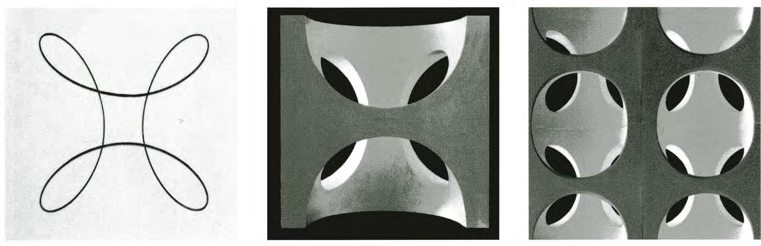
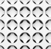
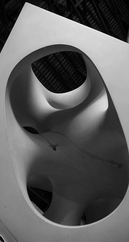
92 4.13 View from the interior.
4.12 Circular screen walls
4.11 Continuous surface topologies developed by Erwin Hauer as part of his work ‘Continua’


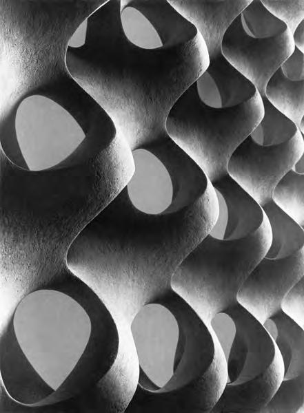
93 4.15 Screen
separating office spaces.
wall
4.14 Screen wall design developed during the 1950s.
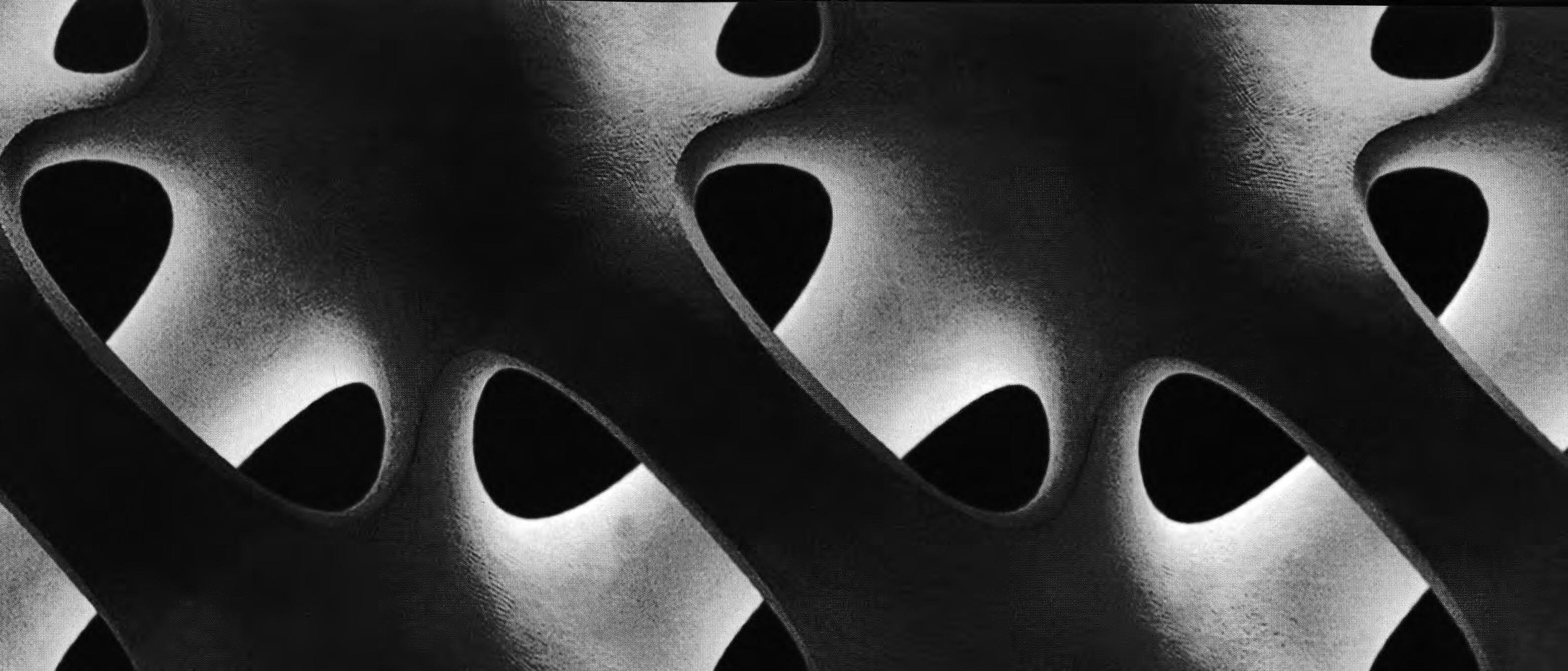
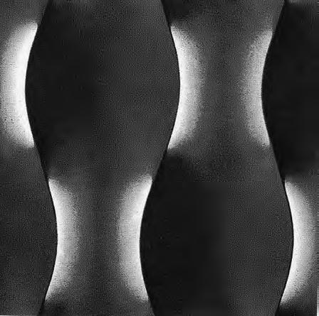
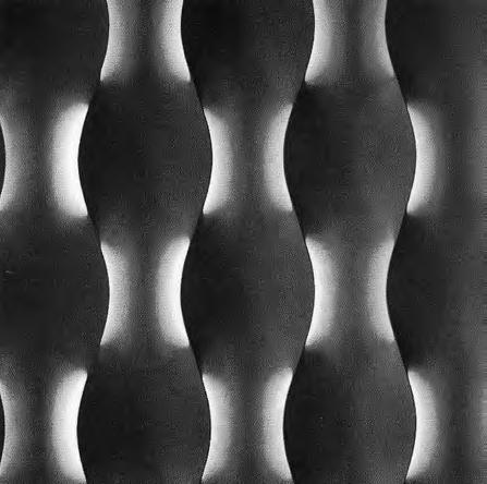

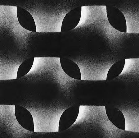
94
4.16 Different variations developed as part of the work ‘Continua’
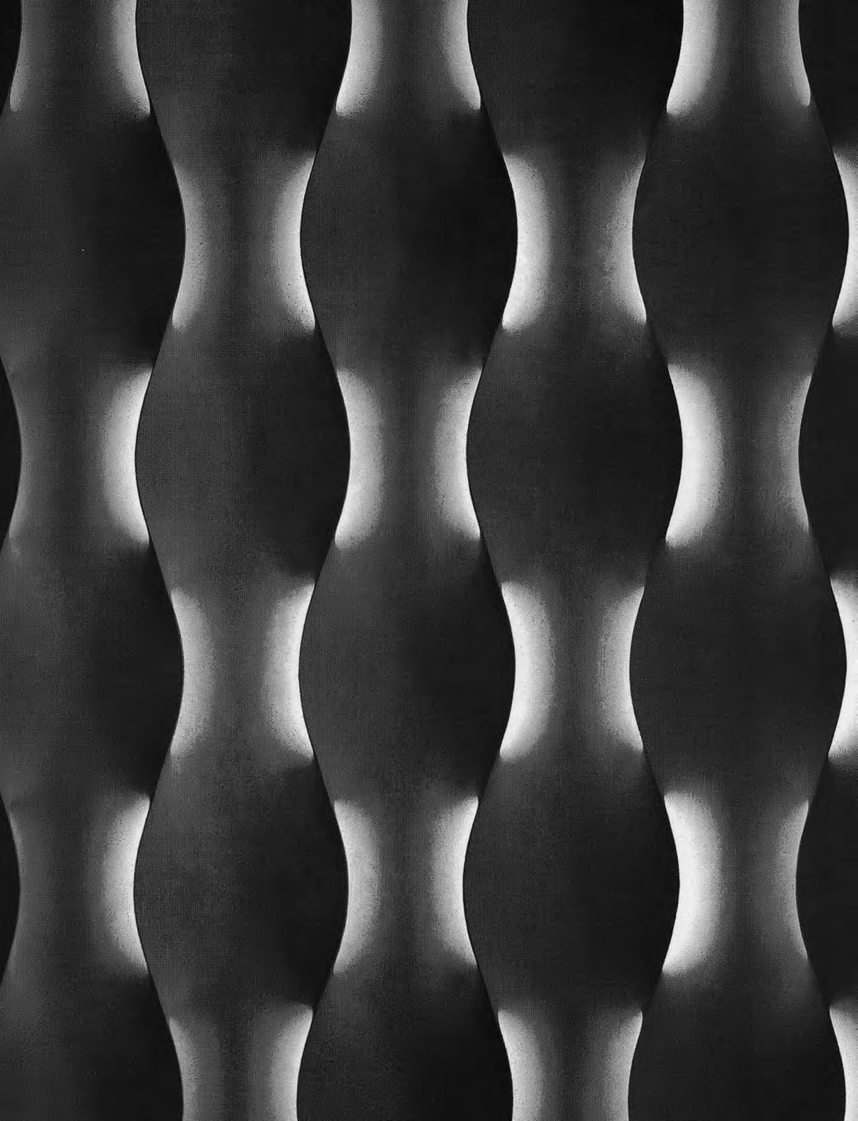
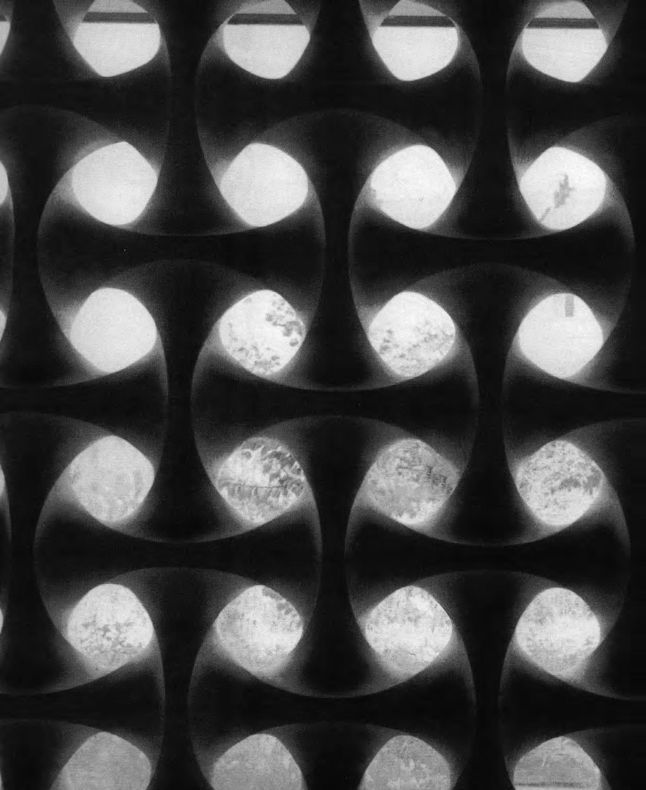
95
Fuzzy Logic Actuation
Unlike the modular static screens cast in concrete by Erwin Hauer, our material system is characterised by its dynamism and capacity of adaptation to external stimuli. It is capable of sensing stimuli, processing this data and actuating accordingly. This process occurs by means of a shape change from one initial state to another which rather than being instantaneous, happens gradually throughout a range of time. The set of sensors, controllers and actuators that form part of our material system are all governed by the twentieth century developed theory known as ‘fuzzy logic’.
The fuzzy logic theory is a form of multi-valued logic derived from fuzzy set theory to deal with reasoning that is approximate rather than precise. In contrast with binary sets having binary logic -also known as crisp logic- the fuzzy logic variables may have a membership value of not only 0 or 1; instead they can range -inclusively- between 0 and 1 [figure 4.18].
Most of the electrical devices that we use nowadays are conceived using this logic, as it is the case for the
controllers used for the experiments shown in the second and third chapters.
Fuzzy controllers consist of an input stage, a processing stage, and an output stage. The input stage maps sensor or other inputs, such as switches –‘on-off’ inputs- to the appropriate membership functions and truth values. The processing stage invokes each appropriate rule and generates a result for each; these are logic rules in the form of ‘if-then’ statements, where the ‘if’ part is called ‘antecedent’ and the ‘then’ part is called the ‘consequent’. As part of the processing stage each rule and result are combined and these data is then used in the output stage which converts the results back into a specific control output value.
The most common shape of membership functions is triangular, although trapezoidal and bell curves are also used. In our case, the actuation curve approximates to a trapezoid where any corners have been smoothened up. The changes in shape from one to another occur through a gradual variation governed

4.18 At a point in time (cyan line) there is a range of values rather than absolute values. These are ‘0’ and ‘1’ and are the extremes of the different intervals.
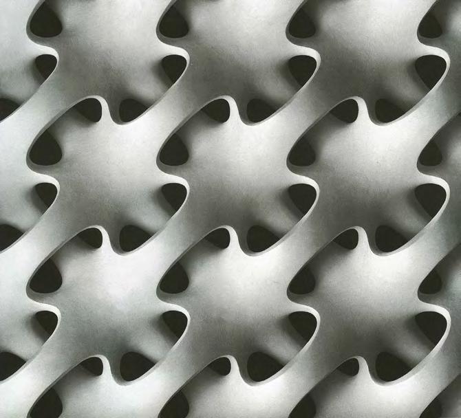
96
4.19 Continuous surface topology by Erwin Hauer.
4.17 Continuous surface topology (by Erwin Hauer) cast in white concrete indicating the location of the integrated actuator in cyan (shape memory alloy ribbon along ‘suture curve’).
0 1
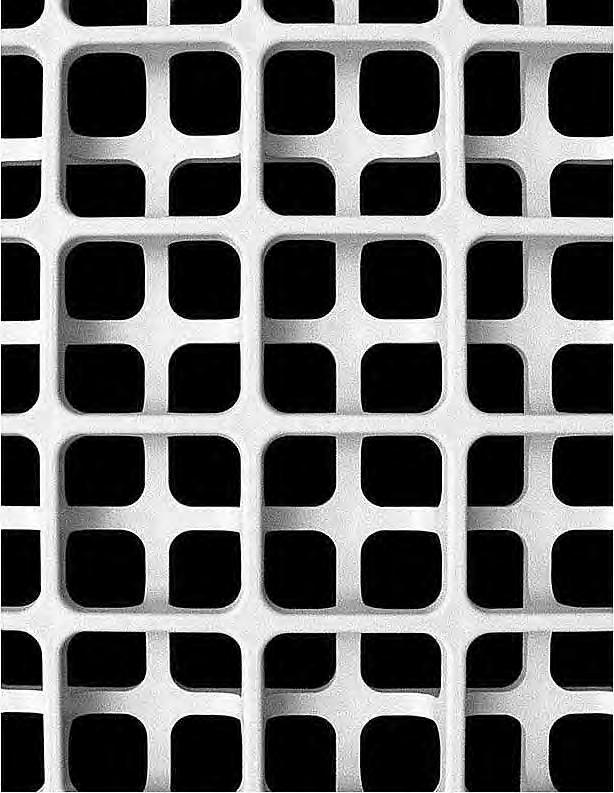
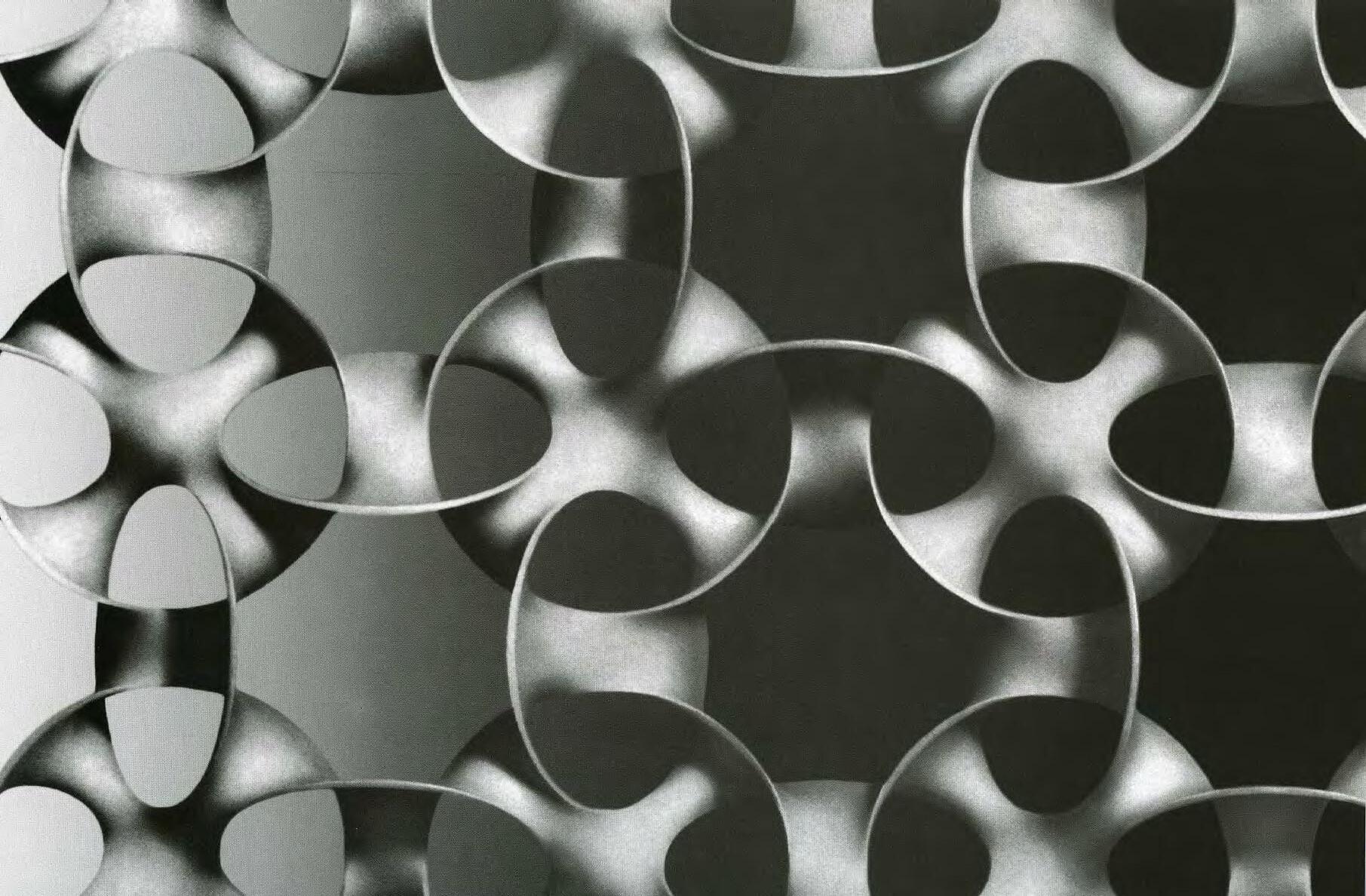

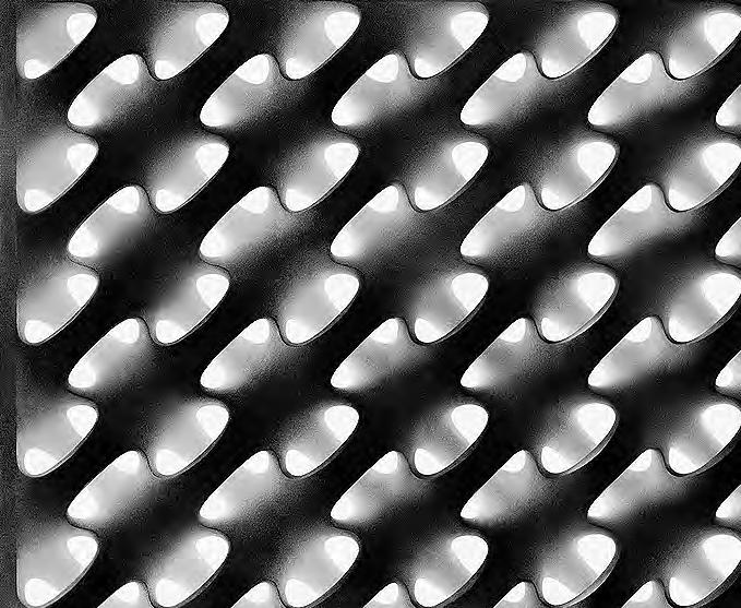
by the functioning rules imposed by the sensing and controlling devices.
The fuzzy logic is therefore associated with the concept of gradual adaptation. The combination of both, synthesises how this novel material system could enhance the ‘space-truss’ topologies originally developed by Erwin Hauer [Figure 4.17]. However, the ‘adaptation’ of the material system should be carefully structured into different fields of action or what we would refer to as ‘actuation variables’. These constitute the set of parameters that can be altered within the material system in order to adapt to novel situations. For this particular case, these have been set to be as follows:
• Size of openings which would regulate the light and air transferred through,
• Overall curvature which allows the material system to adapt to doubly curved surfaces if necessary,
• and finally, the height of the undulating pattern which from the structural point of view must be seen as the structural depth of the space-truss.
Although these three actuation variables will be discussed in detail later on, it is worth introducing here how these are actually achieved. After a rigorous investigation of the system’s topology, we ascertained that the edge curves of the interwoven surfaces were the true controllers of the system. Altering these curves or the points that control them would incur into altering the final system geometry. Therefore, we decided to strategically locate the actuators along these ‘suture curves’ establishing the negotiation logic in between Hauer’ static topologies and our fibre composite adaptive system.
97
4.23 Topology developed from the combination of both orthogonal and hexagonal grids.
4.21 Another variation of a continuous surface topology
4.22 One of the latest designs by Erwin Hauer.
by Erwin
Hauer,
included in ‘Continua’.
4.20 Orthogonal morphology part of the work ‘Continua’
Topology
Introduction
After having broadly studied the topologies developed by Erwin Hauer we focused on developing a variation based on hexagonal grids rather than orthogonal. The entire topological definition is best explained following the logic used to construct it [figure 4.24]:
1. The first level consists of two hexagonal grids displayed in two levels: top and bottom. The origin of one of the grids is offset with respect to the other one; the appearance when looking at the plan view is that the vertices of the hexagons in one grid coincide with the centre of the hexagons in the other one [Figure 4.24 (1)].
2. These grids are then linked to each other with two set of ‘tripods’. The first set goes from the top grid to the bottom one and vice-versa for the second set of tripods. For the first set of tripods –top to bottom-, the top vertex is located at the centre of the top grid hexagons while its three legs are resting on the perimeter vertices of the bottom grid hexagons. The same logic is followed by the bottom to top set of tripods [Figure 4.24 (2) & (3)].
3. These tripods hold the control points defining the ‘suture curves’. The entire topology of these curves is based on the spatial arrangement of the tripods and their geometrical association with the hexagonal grids [Figure 4.24 (4)].
4. Removing the auxiliary grids will help visualising how the suture curves construct the space-frame [Figure 4.24 (5)]. This effect is emphasised and the local geometry is finally displayed by means of lofting between these curves [Figure 4.24 (6)]. The result is a space truss out of a thin layer of fibrous material.
98
(2) (1)
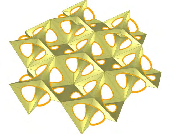
99
topology.
(4) (5) (6)
4.24 Construction of the local geometry
(3)
100
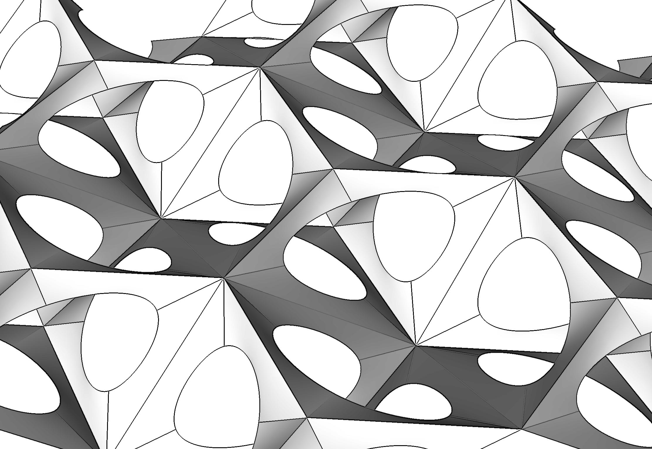
Actuation Variables
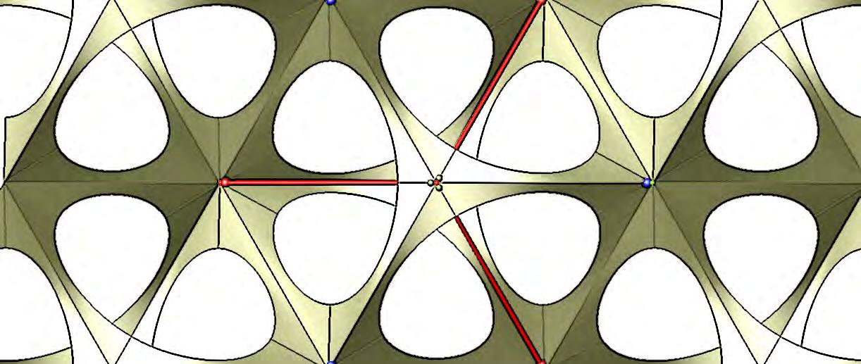
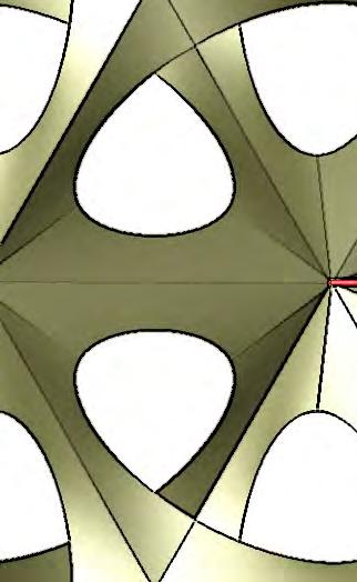
Although we have already mentioned what the ‘actuation variables’ are we have not yet discussed in detail how they are defined and controlled within the system. This will be the purpose of this section which in addition envisages the set of rules established to formulate the digital model.
Associative design software has been used to digitally simulate the behaviour of the system. In this particular case, the model has been set up in Grasshopper and used within the 3D modelling package Rhinoceros. The interface of the simulation model is shown through pictures and diagrams included in the Appendix under the section dedicated to Geometry.
102
Grids
Height h a Actuation
Opening Suture Curves Grids Distortion
Spacing Variables Curvature
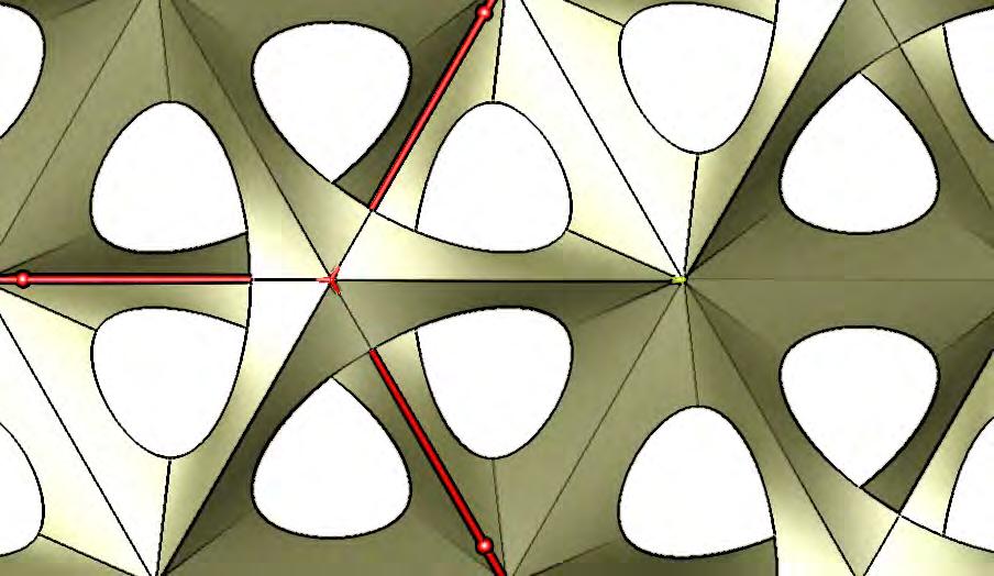
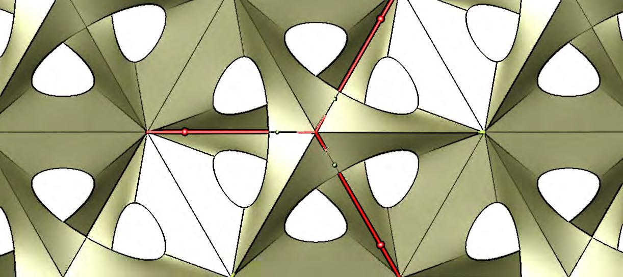
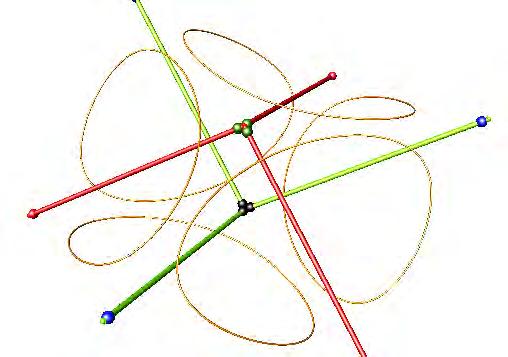
Size of Openings
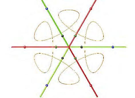
Varying the size of the openings will result on increasing or decreasing the amount of light and air transferred. The topological definition of the suture curves allows for such variation by simply altering the position of the control points along the tripods defining each cell. These consist of two tripods one going from the top to bottom grid and a second one from bottom to top grid.
The control points are a total of eighteen, from which twelve share their location in space and are positioned closer to the perimeter of the cell; the other six points left are located nearer the centre of the cell. Each tripod leg hosts a total of two points which are spaced out along its length –one closer to the top end and the other one closer to the bottom end.
the movement of these points had to be studied in detail and a specific set of rules established accordingly.
These consist on grouping the movement of the points in four sets of three. The first set has been highlighted in red in figure 4.25. The second, third and fourth sets are shown in black, green and blue respectively [Figure 4.25]. The movement of the red set is coupled with the movement of the blue set and thus, when the height is reduced the red set of points travel downwards along the tripods while the blue set is travelling upwards. The same rule is applied to the black and green sets of points.
4.25
Moving the control points along the legs of the tripods results on altering the curve’s curvature locally and hence, reducing or increasing the size of the openings. However, in order to avoid unrealistic curvature changes,
In addition, the length of the tripod legs is maintained through the process and hence, when the height is reduced the horizontal spacing of the legs increases –tripod expands- and vice-versa –tripod contracts- when the height is increased.
103
Location of ‘suture curves’ control points.
Suture Curves - Openings
Figure 4.26 features different openings as a result of displacing the control points along the tripods. These have been extracted from the digital model created to simulate the adaptive abilities of the material system developed. Further details about the model are provided in the Appendix under the section Geometry.
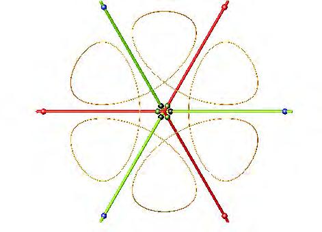
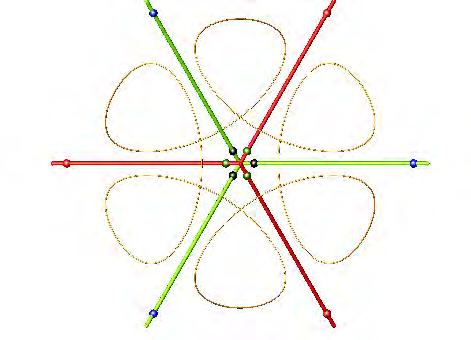
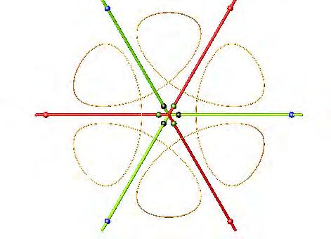
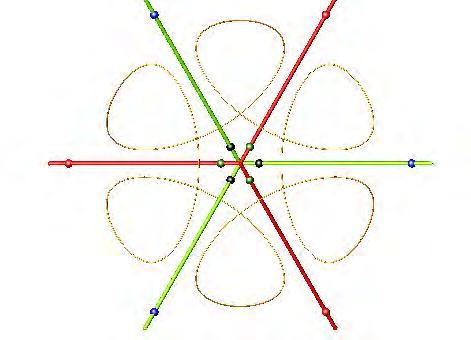
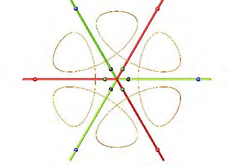
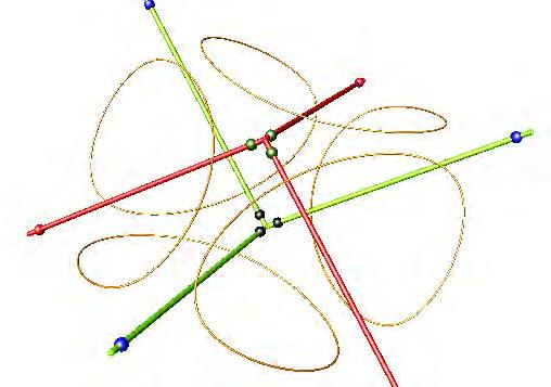
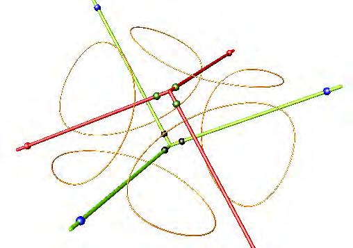
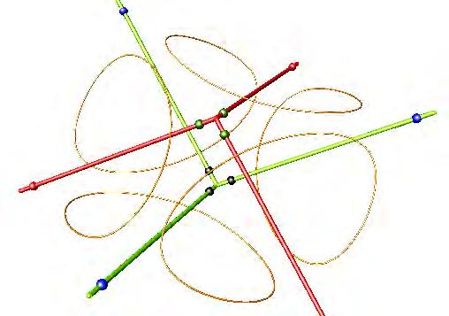
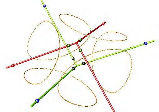
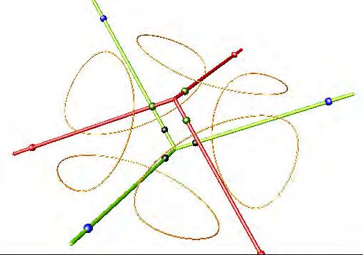
4.26 Location of ‘suture curves’ control points.
104
Top
perspective
(above) and
(below) views.
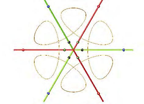

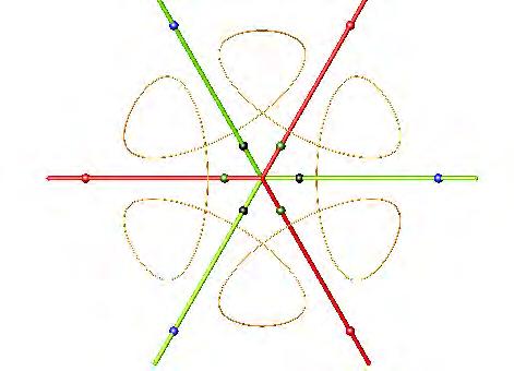
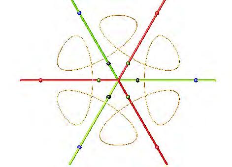
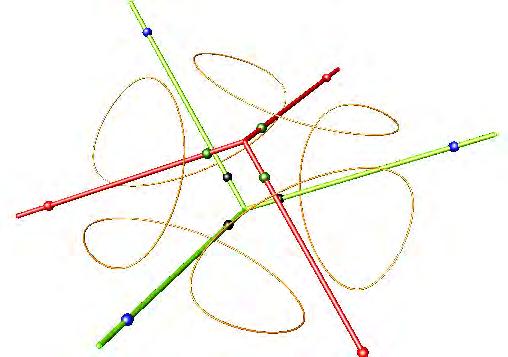

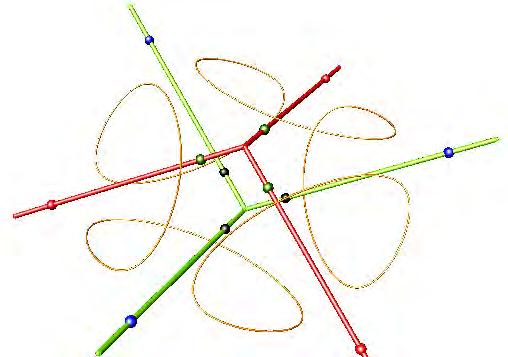
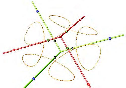

105
Overall Curvature
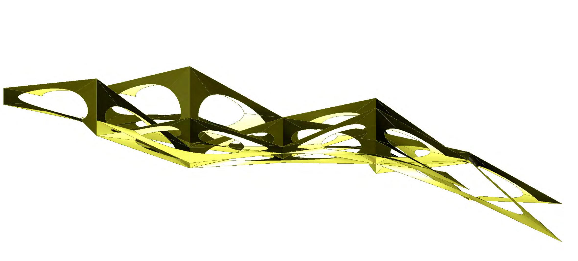
The overall curvature is controlled by the distribution of the grid points in the space. Through a controlled distortion of the position of a group of points forming the primary hexagonal grids, the overall spatiality of the space-truss can be altered. This ‘controlled distortion’ is realised by the use of attractor curves which mark the changes of curvature that the originally flat space-truss needs to undertake to transform into a doubly curved geometry.
The process starts by extracting the isocurves from a ‘mother’ surface defining the overall form of the global geometry [figure 4.27]. These isocurves are then set to
be the attractor curves. The points on the grids will then move in the z direction until their distribution matches that of the attractor curves. Also, the closer the points are to the curves the higher would the attractor force be. In addition, the effect of this force can be altered by increasing or reducing the attractor factor [figure 4.28].
This tool is vital for the combination of the local and global geometries and it also augment the adaptability of the entire system to a wide range of global forms.
106
4.27 Local geometry following the principal curvature lines of a given surface; in this case the ‘mother’ surface would be extracted from digital form finding.
Grids Distorsion - Curvature
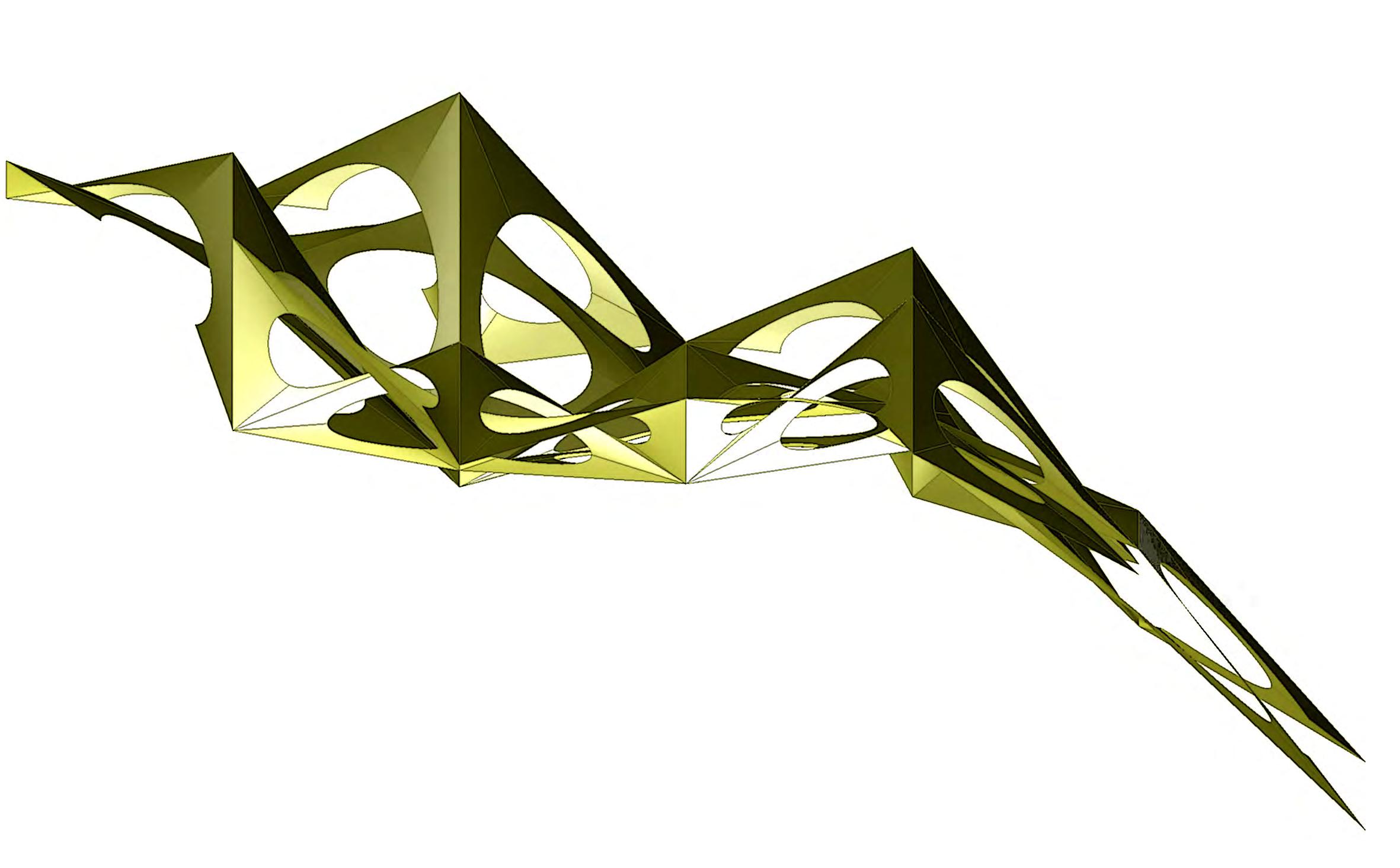
4.28 In this case the ‘mother’ surface has sharper curvatures which are reflected on the overall
107
curvature resulting on the local geometry model.
Grids Spacing - Height
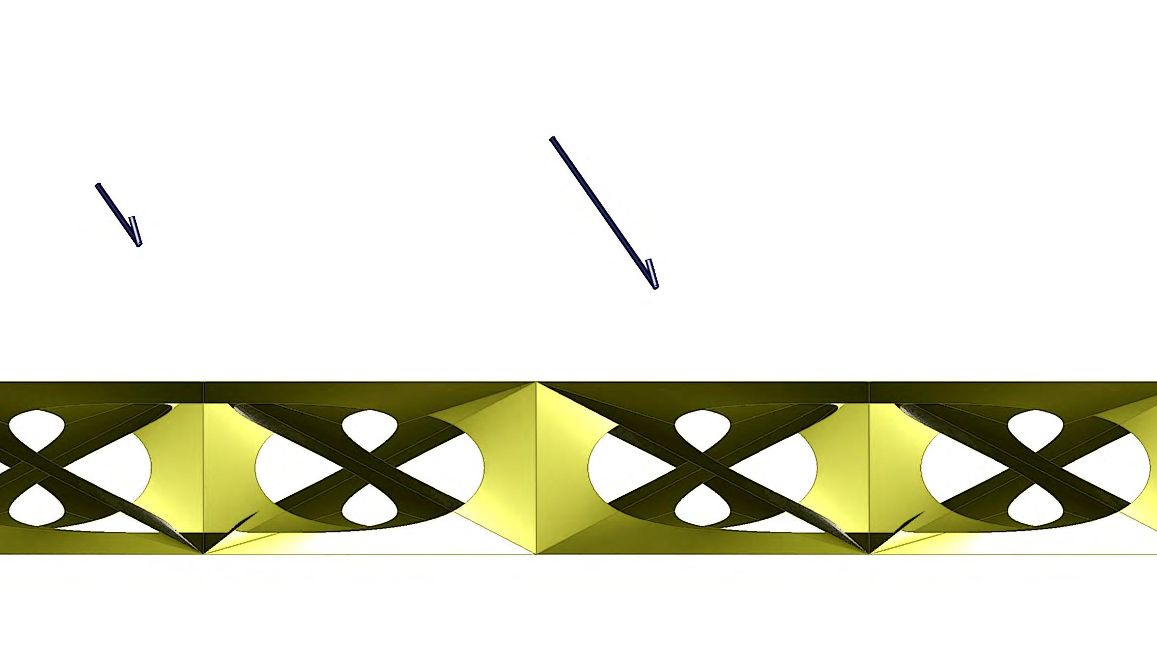
Height
Finally the algorithm allows for the manipulation of the height of the space-truss or in other words its structural depth. This is perhaps the simplest mechanism and it consists of varying the spacing in between the two hexagonal grids in the z direction. This coincides with the height of the tripods which is also coupled with the opening and closing of the tripod legs.
The logic behind a change on the structural depth is regulated by the external forces that act upon the system. For instance, if there is wind load acting on a certain area, the sensing devices would identify this
and the actuators would be set to act accordingly [figures 4.29 and 4.30].
The actuation will consist on an increment of the structural depth locally, where the action has been identified. In the digital model this has been simulated with the help of attractor points. The affected points of the grid will re-organise accordingly to provide a greater structural depth in the direction of the load vector which would be proportional to the magnitude of the force inherited.
4.29 Local geometry in its initial state. Wind load is here represented as a two point loads (for simplification purposes) one being greater than the other one. The model is however prepared to process not only point load configurations but also uniformly distributed loads.
108
4.30 Resultant geometry as a response to the to the applied loading. Note how the structural depth has locally increased where the point loads are applied and thus, adapted to the new loading conditions.
109
In addition to the graphical and written information provided about the construction of the digital models, the DVD included with this submission contains a video which would help visualising the three adaptation variables described above. Further information is also provided in the Appendix under the section dedicated to Geometry.
110
4.31 Perspective view of the local geometry in its initial state.
4.32
111 Actuation Simulation
Perspective view of the resultant geometry as a response to the applied loading.
Remarks
A space-truss gains its structural stability from combining compression and tension members. Shear effects are not completely eliminated but are transformed into either compression or tension along the diagonal members. This is therefore a very smart procedure to organise the material available and deal with the applied loads.
In our case, the resultant space-truss is made of a thin layer of a fibre composite which in addition, has the ability to adapt to different stimuli.
The weaving of a continuous layer of fibre composite provides the structure with the stability necessary to withstand large compression loads, something that a thin section of the same material could not do without buckling.
The smartness of the system resides on its topological definition. The arrangement of paired grids and tripods constitutes the skeleton framing the ‘suture curves’. Controlling the position of the points which define these curves has been proved to be vital to integrate sensing and actuation capabilities within the system.
The result is an intricate of continuous interwoven surfaces featuring large and small openings, different overall curvatures and various heights, all local effects that occur as a response to external stimuli.
112
4.34 Perspective view of the resultant geometry when the hexagonal grids follow the overall curvature of the ‘mother’ surface.
113
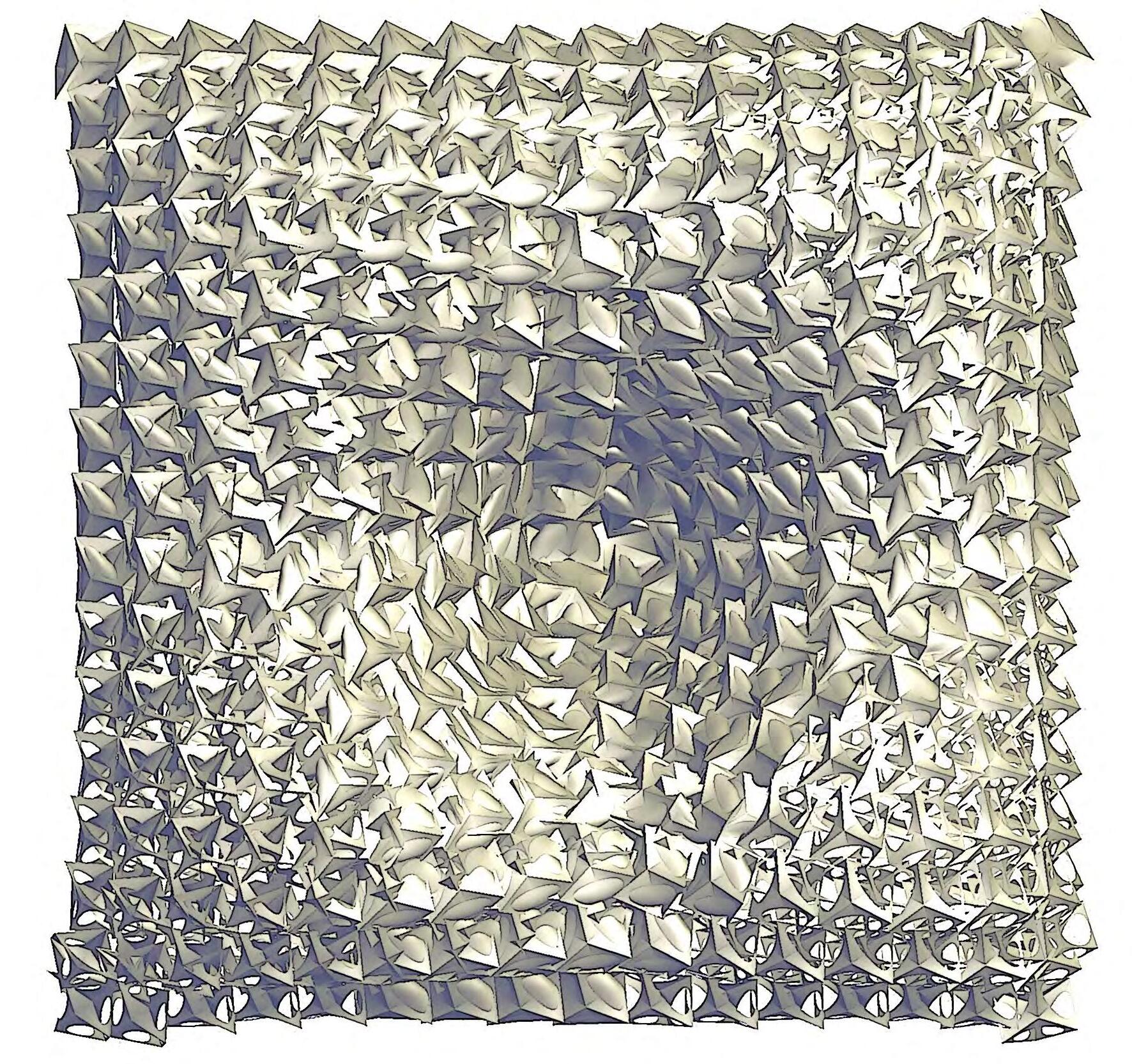
4.34
114
Top view of the final design, integrating aspects discussed atboth local and global levels.
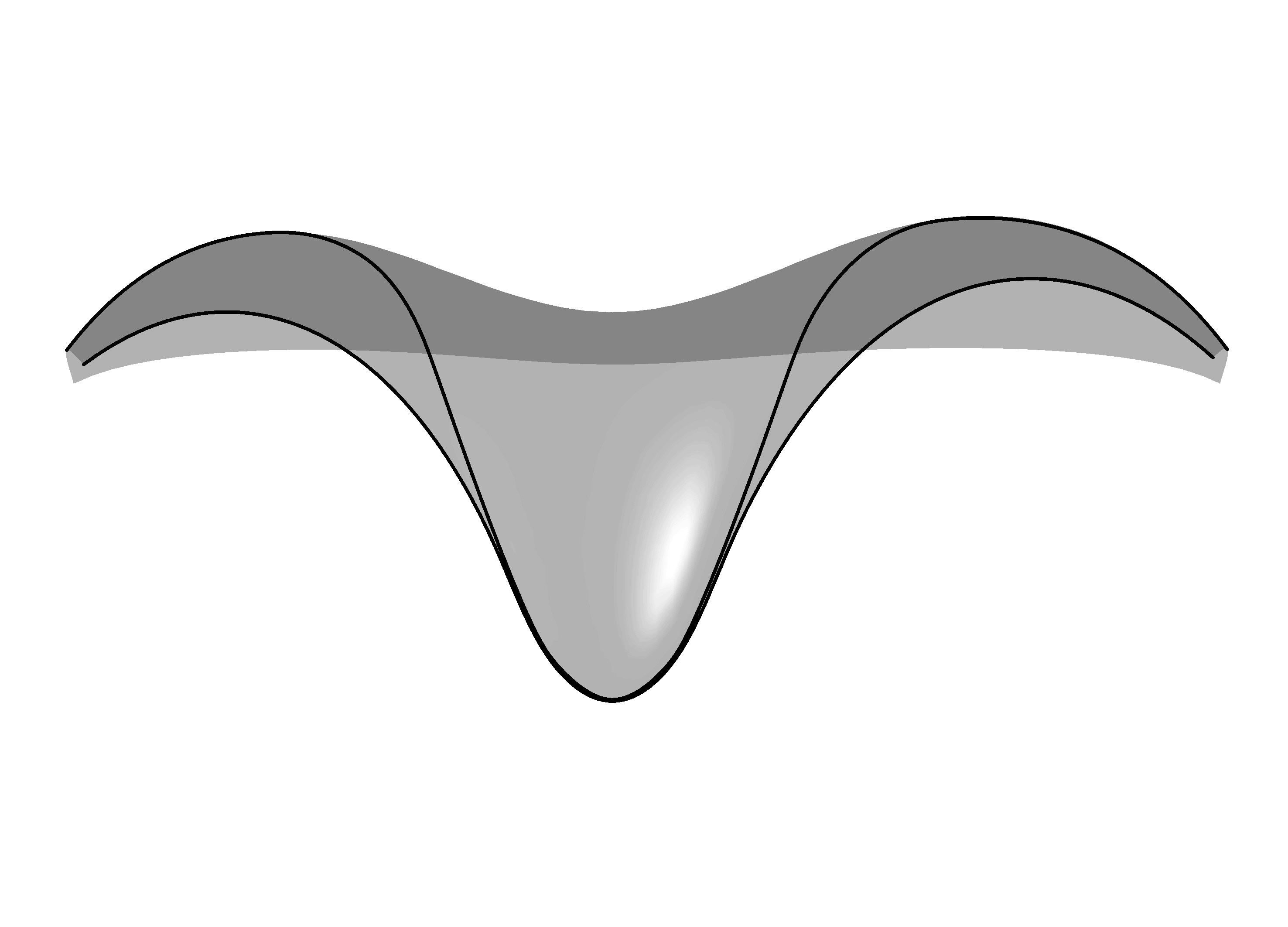
Global Geometry
Material Configuration
The global geometry –similarly to the local- needs to be formulated on the basis of form resulting from the interaction between material and force. In natural constructions, material is being continuously removed from places where it is not required anymore and deposited where it can contribute the most to the whole structure. This concept was summarised by D’Arcy Thompson in three words: “growth under stresses”. Throughout the different hierarchical levels present in natural materials, the above concept is constantly implemented.
Our strategy has been structured into two main parts. The first one consists of extracting the set of specific rules that need to be formulated to simulate these natural processes in a digital environment. The second one focuses on how this would affect the arrangement of the different hierarchical levels present in our fibrous material.
Front view of the global morphology developed thourhg the use of digital form finding.
4.35
Precedents
Ross Lovegrove – Water Bottle
Through the course of the investigation, the work of Ross Lovegrove for the design of ‘Ty Nant water bottle’ was also examined. In this project, Lovegrove designed a sophisticated water bottle made of a thin transparent layer of PTE which acquires rigidity through the use of softly curved corrugations running across the surface which ultimately encloses the water volume [Figure 4.36].
In his own words the work of Ross Lovegrove belongs to what he calls ‘organic essentialism’ –an approach to the design and manufacture of things that combines logic and beauty [4.36]. Generally the work of Ross Lovegrove is characterised by his high respect for the incomparable, eternal beauty of natural things and great knowledge and appreciation of how things exist in nature [Figure 4.37].
The conceptual design of this water bottle led part of the research concerning the use of extremely thin surfaces prone to suffer buckling and how this could inform the development of the global morphology.
The work of Ross Lovegrove reinforce the argument of curvature -and most importantly curvature continuitybeing the main geometrical agent responsible of yielding stiffness when working with thin surface-like materials.

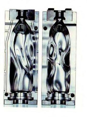
116
4.36 Ty Nant Waterbottle Production Tool. This single production tool was produced to make an initial run to test the quality of the liaison between the two halves and the appearance of the non-linear part line on the blown bottle shape.
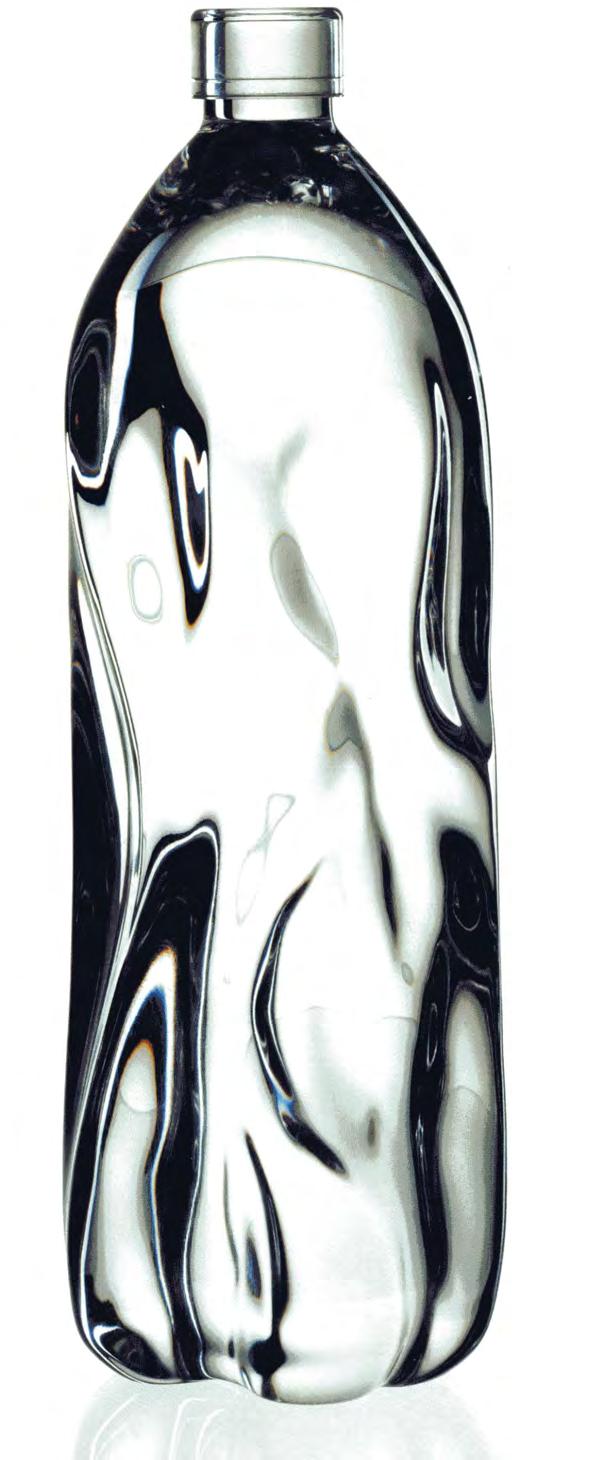
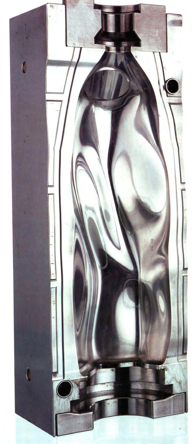
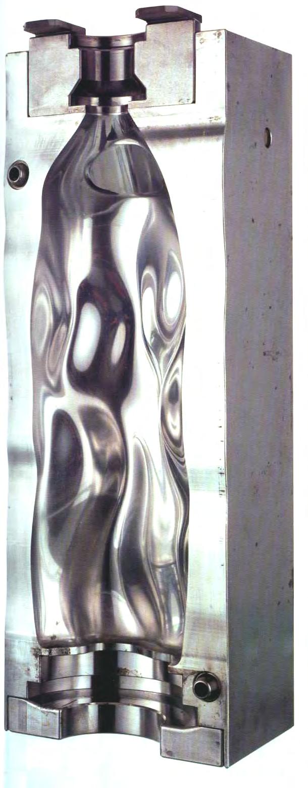
117
4.37 Ty Nant Waterbottle Study Model. Machined from the data acquired from the scanning and refinement of the surfaces of the initial foam sculptures. It is made from solid acrylic and was used to demonstrate the optical qualities that could be achieved when a transparent PET vessel is filled with pure filtered water.
Morphology
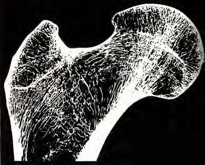
Growth Under Stresses
Frei Otto was one of the first architects who explored the idea of form being generated as a result of force acting upon a specific material. He gave this technique the name ‘form finding’. Behind each of his built structures there would be a series of experiments which would ensure the final form follows the rules imposed by material and forces.
This technique is in reality a simulation of a process that has always being present in living tissue, where material distribution is being continuously optimised. Living cells have been proved to be stimulated by pressure to increase and multiply. The proof is that our skin grows thicker when we force it to hold greater loads; thus a callus is nothing else but accumulation of material driven by a sudden change in pressure. When the high pressures are reduced to their previous level, the excess in material will be removed. The material density is therefore affected by the strains to which it has been submitted, and hence the properties of the material do not only depend on the nature of the substances that constitute it but also on its history. Pressure and by extension strain are direct encouragement of growth [4.26].
D’Arcy Thompson has extensively written about this concept, using a large number of examples present in the natural world. One of his most useful examples is the discussion held on bone constructions where he analyses the configuration of a femur from both the macro and the micro scales [4.26].
Bone tissue is a type of dense connective tissue which internal organisation consists of a three-dimensional honeycomb-like structure which allows for a variety of shapes and renders lightweight structures, yet rigid and strong enough to carry the weight load of the body [figure 4.29].
Bone is first deposited as woven bone –also known as ‘coarse fibred’-, in a disorganised immature structure present in young bones and in healing injuries. Woven bone is weaker, with a small number of randomly oriented coarse collagen fibres clearly visible by polarisation microscopy [figure 4.27]; it forms quickly and it is used by the organism as a temporary structure while the final structure is being built. It is the osseous tissue first deposited on the calcified matrix in endochondral ossification [figure 4.28].
Fibres
Density
Continuous
Orientation Variable Stiffness Single Material
118
4.39
4.38
Cut of a femur at the head level, revealing the organisation of the tubercular tissue within the bone.
Fibre distribution in a femur as revealed through polarisation microscope.
m
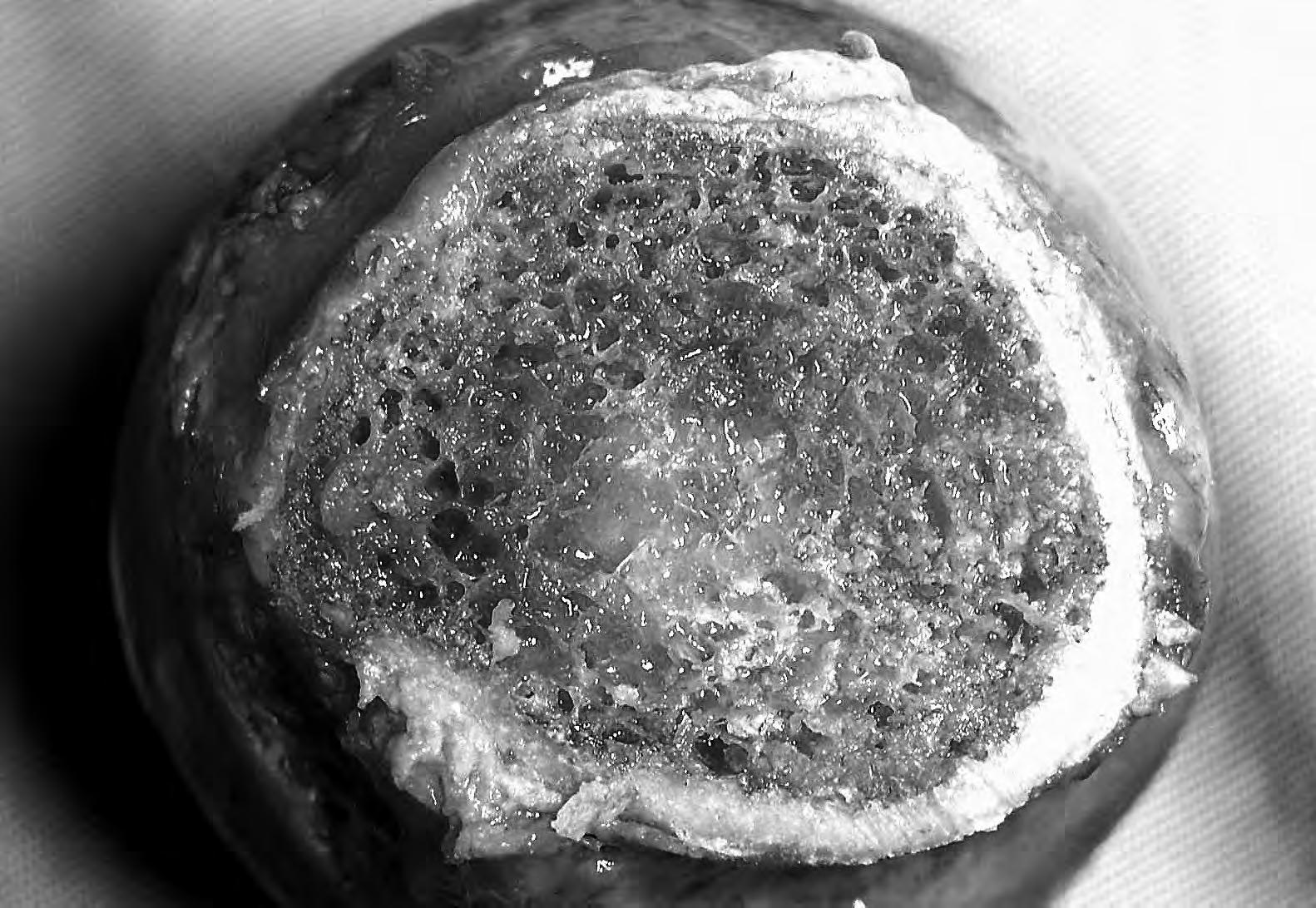
119
Growth Under Stresses
Woven bone is rapidly replaced by lamellar bone, which is highly organised in concentric sheets. Lamellar bone –also known as ‘mature bone’- is stronger and is characterised by the presence of collagen fibres arranged in parallel layers or sheets (lamellae), forming columns parallel to each other, readily apparent when viewed by polarisation microscopy [figure 4.38]. Lamellar bone would be the final structure of the bone and is present in both structured types of adult bone, cortical (compact) bone and cancellous (spongy or trabecular) bone [4.29].
Lamellar bone needs to be able to resist the main type of forces which will act on the bone throughout its life: bending, torsion and compression. The first two forces require the fibres to run diagonally with different angle orientations and in opposite directions, while organising in alternating layers. In these cases cortical (compact) bone tissue is developed, forming a dense outer layer –the cortex- around the bone [figure 4.40]. When there is also compression loads –the weight of the body- cancellous (spongy or trabecular) bone tissue is developed in the interior of mature bones following the direction of functional pressure according to Wolf’s Law [figure 4.41]].
Wolff’s law is essentially the observation that bone changes its external shape and internal architecture to produce minimal-weight structures that adapt in response to the stresses acting on it [4.32, 4.29].
The process starts with trabecular tissue being secreted and laid down fortuitously in any direction within the substance of the bone. If it lies in the direction of one of the lines of principal stress, it will be in a position of comparative equilibrium –minimal disturbance- with regards to the rest. However, if it is inclined obliquely to the lines of principal stress, the shearing force will
tend to act upon it and since fibres are linear elements which cannot withstand shear forces, the fibre will be moved away until it coincides with a line of principal stress [4.32].
Trabecular bone tissue spreads in curving lines from the head to the hollow shaft of the femur. These linear bundles are regularly crossed by others, where each inter-crossing is as nearly as possible an orthogonal one; similar to how the lines of maximum compression cross the lines of maximum tension [4.28, 4.29].
The above ideas can be summarised in a single sentence: “Nature stretches the bone tissue in precisely the manner and direction in which strength is required” [D’Arcy Thompson, 4.32].
However, bones do not stop growing once they are formed. Bone tissue is continuously being recycled and it is capable to adapt to new loading conditions. Repeated stress, such as weight-bearing exercise or bone healing, results in the bone thickening at the points of maximum stress.
It has been hypothesised that this is a result of the piezoelectric properties of bones, which cause bone to generate small electrical potentials under stress.
Bone structure and as a result its overall form is clearly the result of the diagram of forces acting upon it. In the macro scale –external form- we observe continuous curved topologies whose overall curvature is the result of the internal fibre organisation in the micro scale and by extension, the internal forces acting upon the system [4.29].
4.40 Diagram showing the hierarchical organisation of fibres used for the construction of bones.
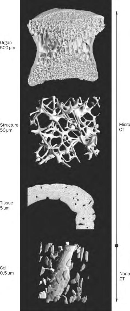
120
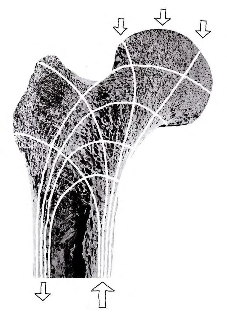

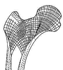
4.41 Diagram showing the arrangement of the principal lines of tension and compression in a femur. Fibre distribution in natural constructions has been proved to follow this arrangement while being continuously stimulated by the external pressures.
121
Design Concept
The concepts discussed above aim to help identifying the main variables present in the formation of bones, leading to lightweight but rigid constructions [figure 4.43].
One is the fibre directionality and the other one the fibre density. Fibre directionality accounts for the orientation of the internal loads that would need to be withstood by the material: ‘force travelling paths’. Fibre Density responds to the variable magnitude of those forces across the bone, being denser where there is a concentration of load as higher load will need to travel through [figure 4.42].
These mechanisms act in the micro level, but are also responsible for the overall form. Smooth or sharp curvatures in the overall form –macro scale- are the result of the fibre organisation in the micro level.
Our global geometry aims to reproduce this system. In the micro level fibres are oriented following the
direction of the lines of principal pressure which by extension are the lines of principal strain also known as principal stresses. In other words, the direction of the fibres responds to the direction of the internal forces present in the material. Also in the micro level, fibre density is increased or decreased according to the scalar value of the forces locally. There would be areas where there is a concentration of load and thus, a higher density of fibres will be supplied. In the contrary, material should be saved in areas where loads are lower. The macro level would be the result of the two mechanisms explained above.
This process was simulated digitally through the use of two algorithms written to fit the specifications of the project. Due to technical requirements the theoretical process described above needed to be reorganised. The process started by ‘form finding’ the overall form, for which the optimum fibre organisation will be subsequently found.
Design Principles - Global Geometry
4.43 Microscope images showing different fibrous organisation present in other mammal bones.
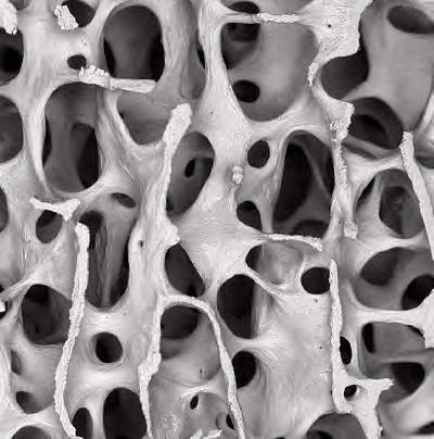
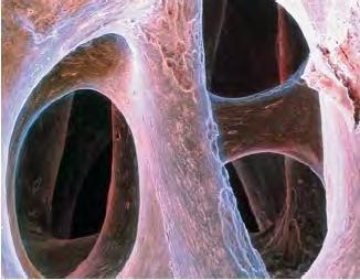
122
Principal
Form
Global Form
Stresses
Finding
Fibre Organisation
4.42 Scanning microscope image of the fibrous structure present in a Cactus.
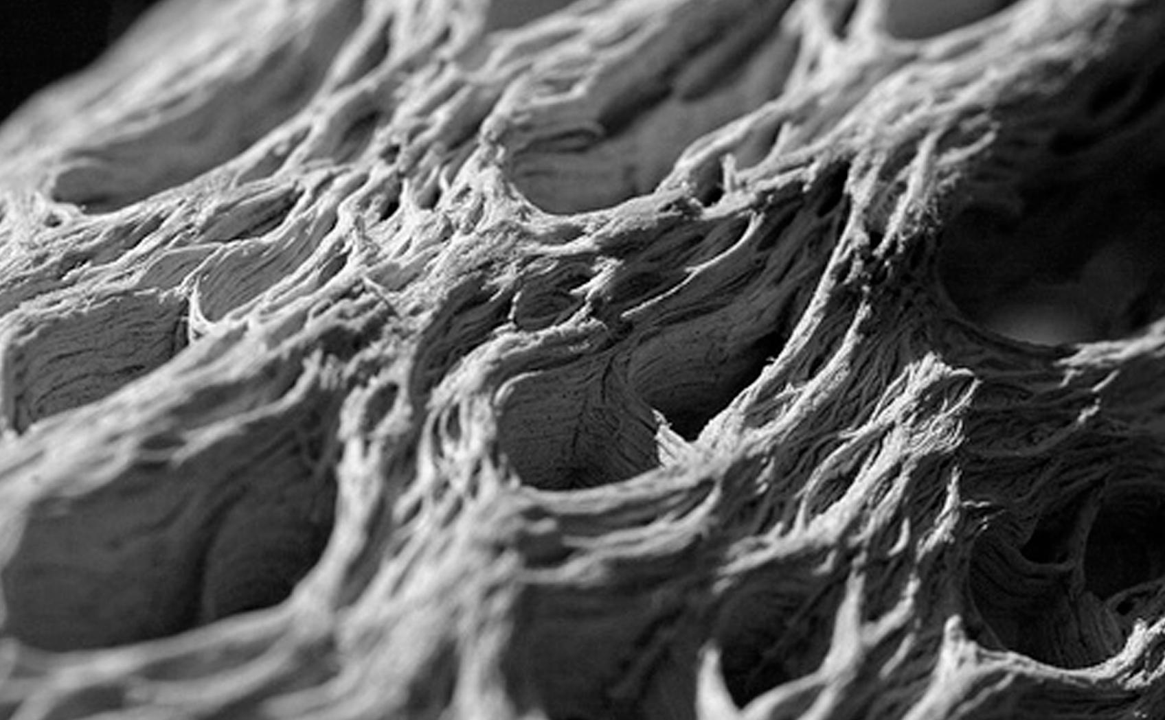
123
Form Finding
Prior to progressing with the digital form finding of the external form it was necessary to decide what structural typology would interests us the most. A very frequent case is the design of a pavilion or some sort of covering structure which simplistically could be seen as a roof and a vertical support [Figure 4.44].
Roofs are usually formed by horizontal spanning elements which require vertical supports to bring loads to ground level. The morphology developed in this case integrated the roles of the individual elements that would have traditionally formed the structure –horizontal spanning members and vertical columnswithin one continuous surface.
The process starts with a flat surface located at the height of what would have been a simple roof. Vertical loads are applied around the perimeter of a fictitious central column, responsible for transferring the loads to the ground. The rest of the parameters of the system are input in the algorithm and the roof starts curving.
There is a time when the points defining the surface start oscillating. A few seconds later, equilibrium is found and the overall form has been found. The roof surface has curved in response to the applied loads and it now integrates both roof and column within a single continuous arched surface [figure 4.44].
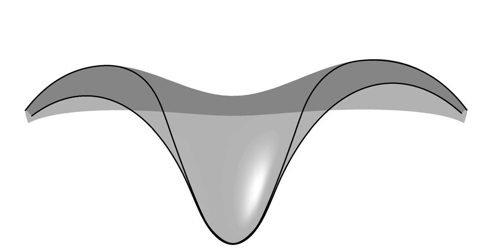
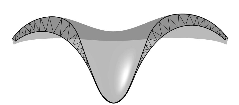
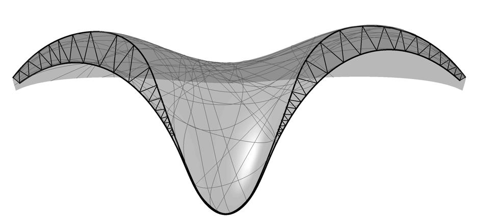
124
Surface
Continuous
Space Truss Fibre Distribution
4.44 Diagrams showing of the three different levels of organisation present in the strategy to develop the global geometry.
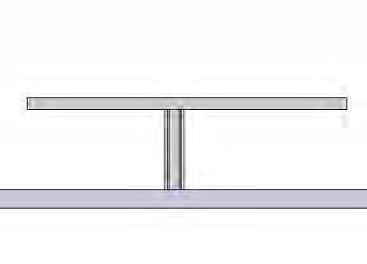
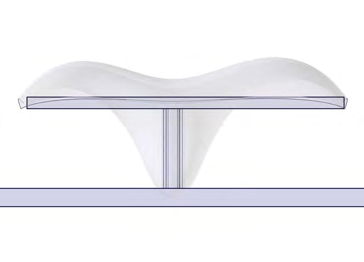
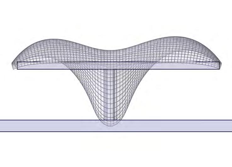
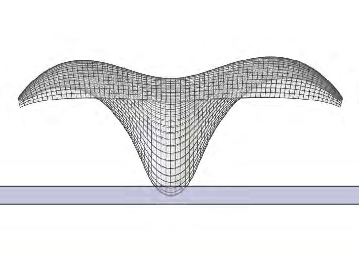
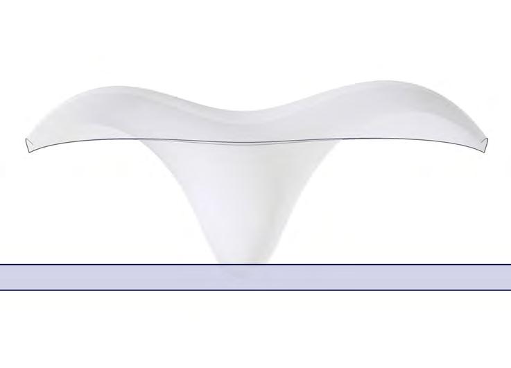
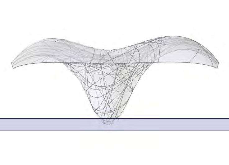
125
Form Finding
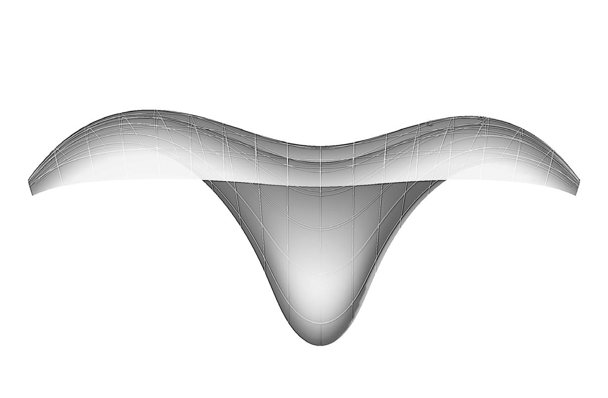
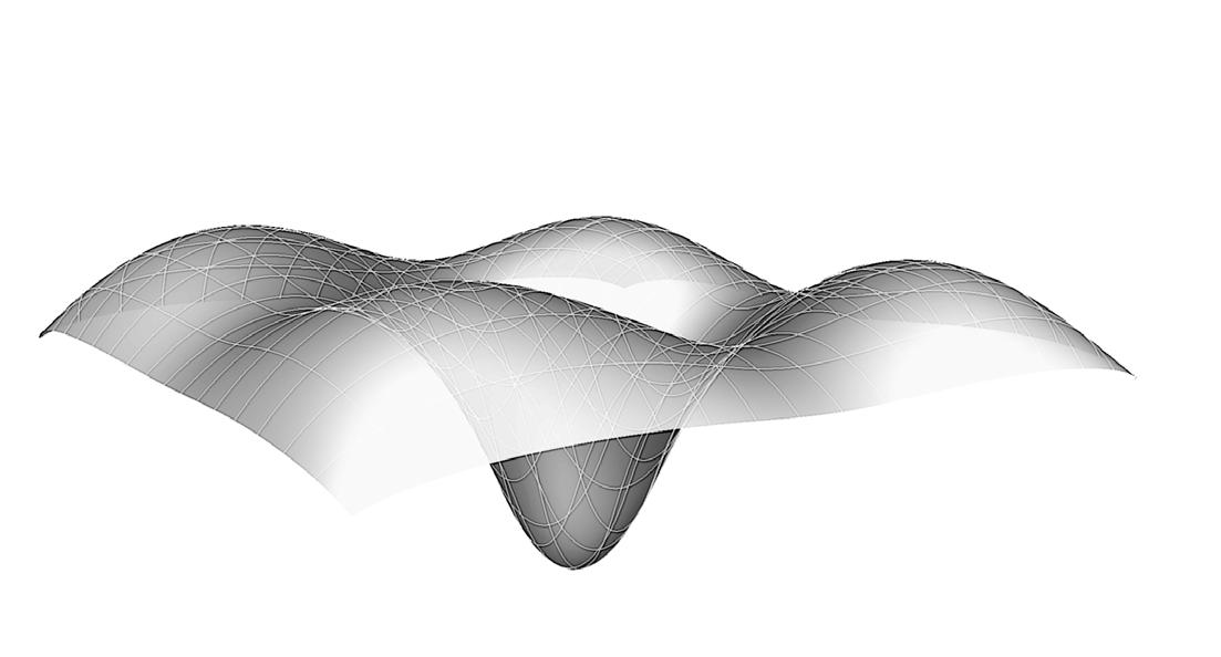
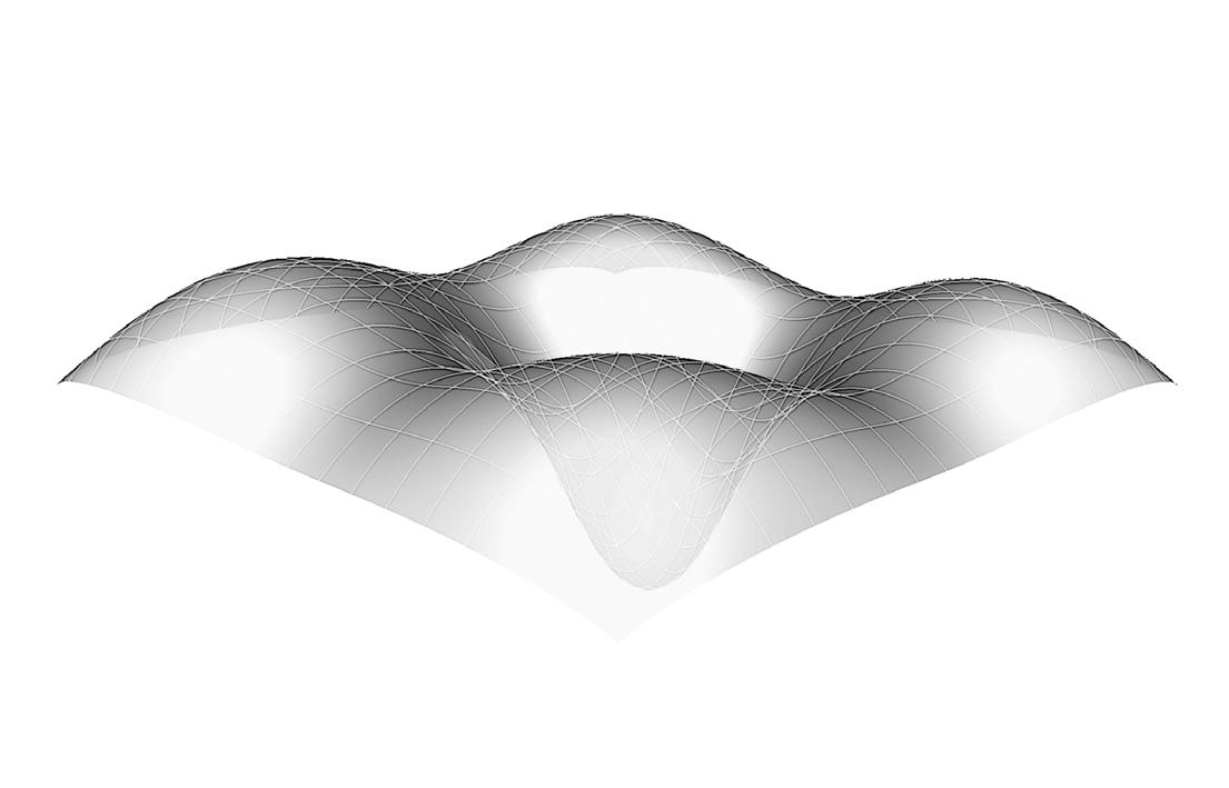
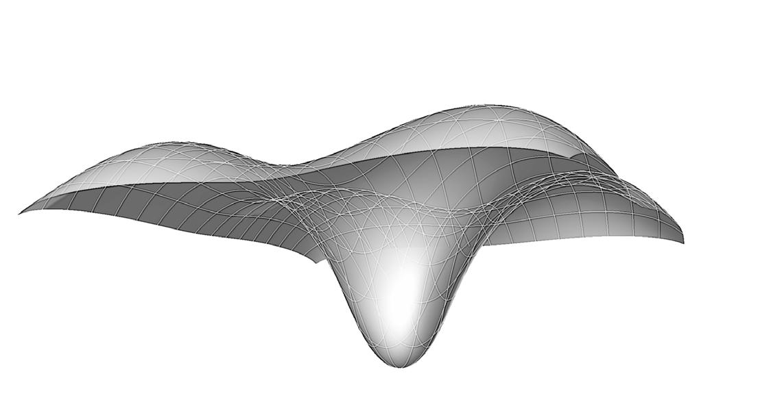
126
generated
digital form finding.
4.45
Different views of the global geometry
through
4.46 Image extracted from the FEM model developed in GSA for the post-analysis of the form found geometry, aimed to obtain the magnitude and direction of the principal stresses.
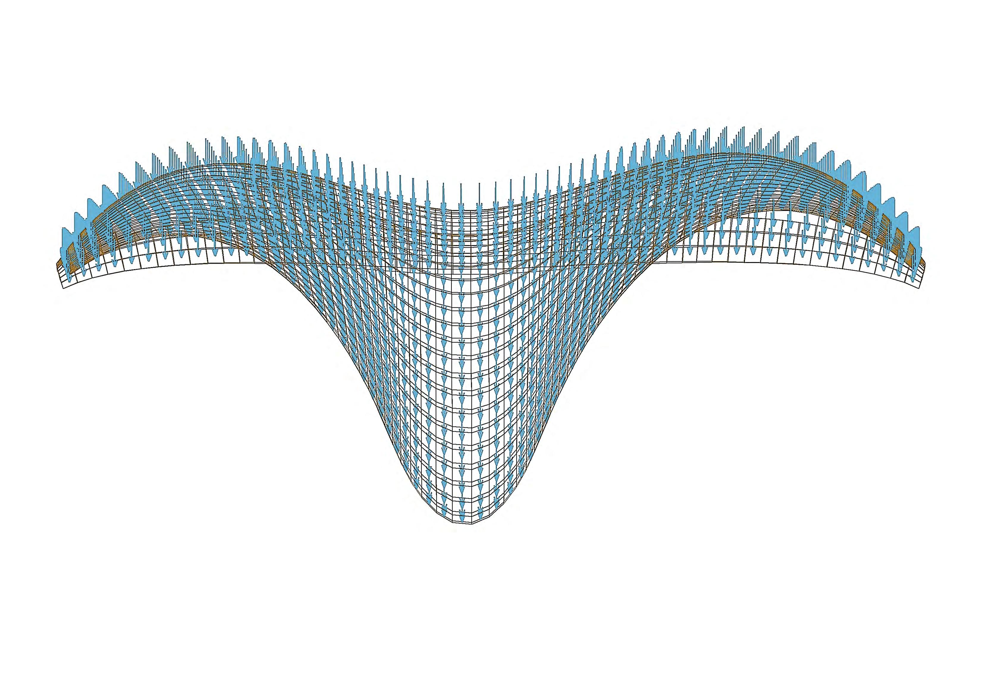
127
Fibre Distribution
The second algorithm was written to simulate the growth of the fibres. In bones fibres are distributed following the direction of the lines of principal pressure whose equivalent in structural engineering are the principal stresses [4.34]. The principal stresses are obtained by rotating the ‘Cauchy stress tensor’ -originally oriented in Cartesian coordinates- into such a coordinate system that shear stresses are zero and only normal stresses remain.
Shearing forces are those which produce ‘angular distortion’ in a figure or in other words, it is a force that tends to cause particles to slide over one another. While shearing stresses can by no means be suppressed, the danger of rupture under shearing stress is lessened the more we arrange the fibres along the lines of principal stresses since there is no shearing stress along or perpendicular to these lines.
The shearing stress is greatest in the ‘neutral zone’,
where neither tension nor compression are manifested; the neutral zone is defined by the line which cuts at equal angles of 45 degrees the orthogonally intersecting lines of pressure and tension. Therefore, laying the fibres along the lines of principal stress will diminish the adverse effects of the shearing forces and will contribute to minimising the amount of fibre material utilised.
Traditionally, fibre layout in a composite is made with fibre mats where shearing effects are dealt with by allocating a higher number of fibres in many directions. In contrast with our methodology, this results on employing a greater amount of material. For cases where the dimensions of the final piece are considerably small this may still be worthwhile since laying fibre mats is a relatively quick and easy process which is fully mechanised nowadays.
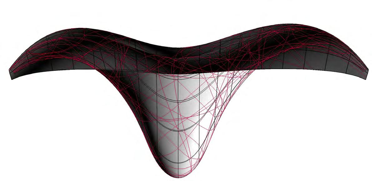
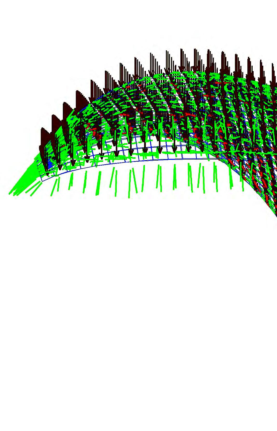
128
4.47 Front view of the global geometry generated through digital form finding after running the fibre distribution algorithm.
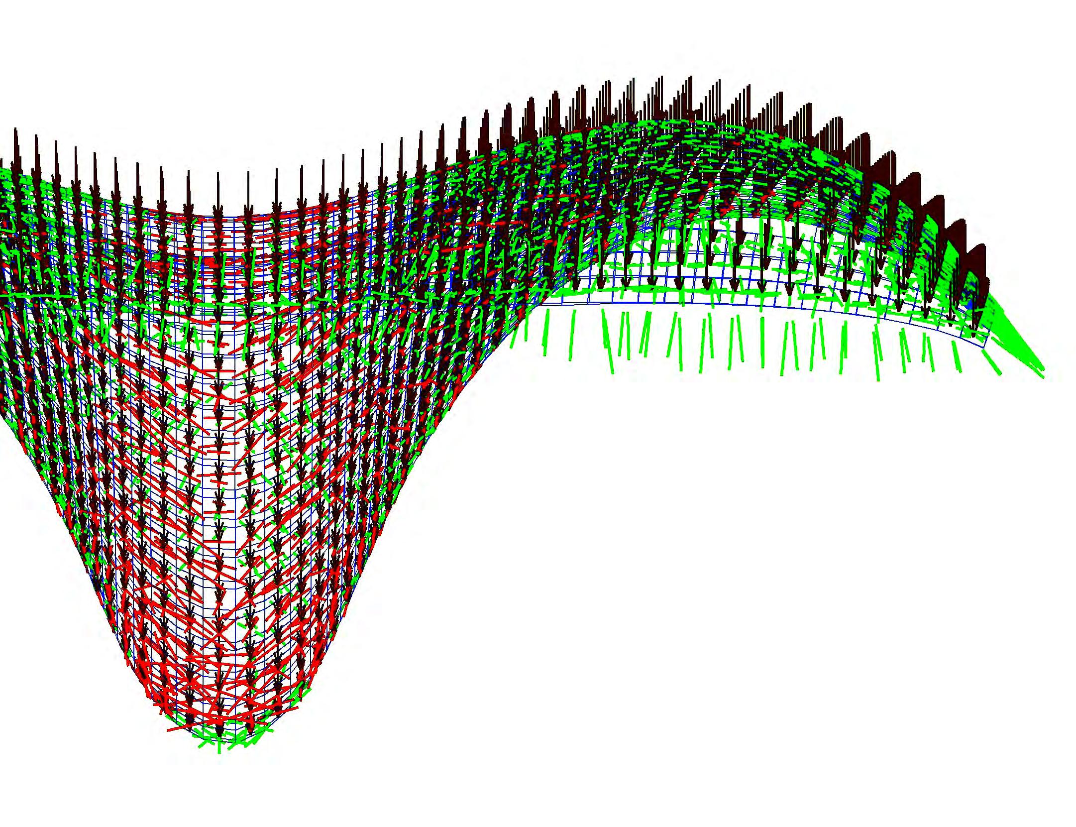
However, for large scale applications it is essential to ensure that the amount of material used is minimised. Laying the fibres along the lines of principal stress minimises the amount of fibres required but increases the cost towards manufacturing. Currently, this method is only used in the boat racing industry; however, there is a growing interest in the use of fibre composites for large scale applications which will definitely help improving this manufacturing technique, reducing the cost involved [figure 4.47].
In our case the combination of both techniques –fibre mat and principal stresses- in different scales is used to integrate the local and global geometries. Structural fibres have been organised in two levels: macro and micro. In the macro level fibres are laid following the lines of principal stresses. Micro fibres consist on a 0-90 fibre mat whose principal orientation will coincide with
the direction of the nearest macro fibre. Organising the fibres into these two different levels helps the mechanisation of the fabrication technique and the integration of the local and global geometries [figure 4.51].
The digital simulation of the fibre growth starts by calculating the principal stresses on a given structure. This data –principal stresses, orientation and magnitude- was extracted from a Finite Element Model in GSA –in-house Arup software package for structural analysis. The model used the global geometry previously modelled through digital form finding. The values obtained in GSA where exported into an Excel file. Once these preparations were finished the algorithm could start running [figure 4.48].
129
4.48 Image extracted from the FEM model developed in GSA showing the direction of the principal stresses.
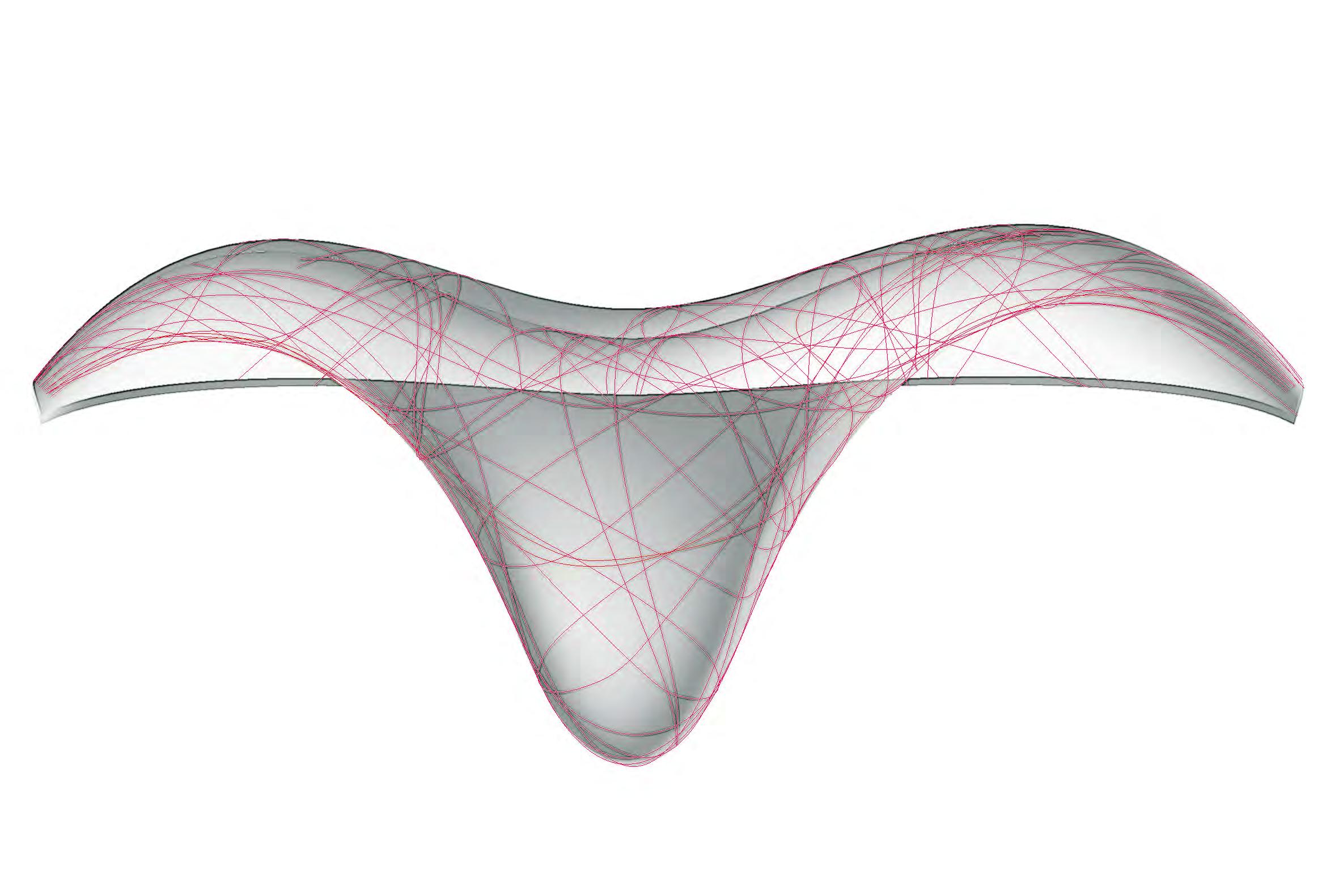
130
Fibre Distribution
4.49 Front view of the global geometry with the fibres running along the direction of the principal stresses
4.50
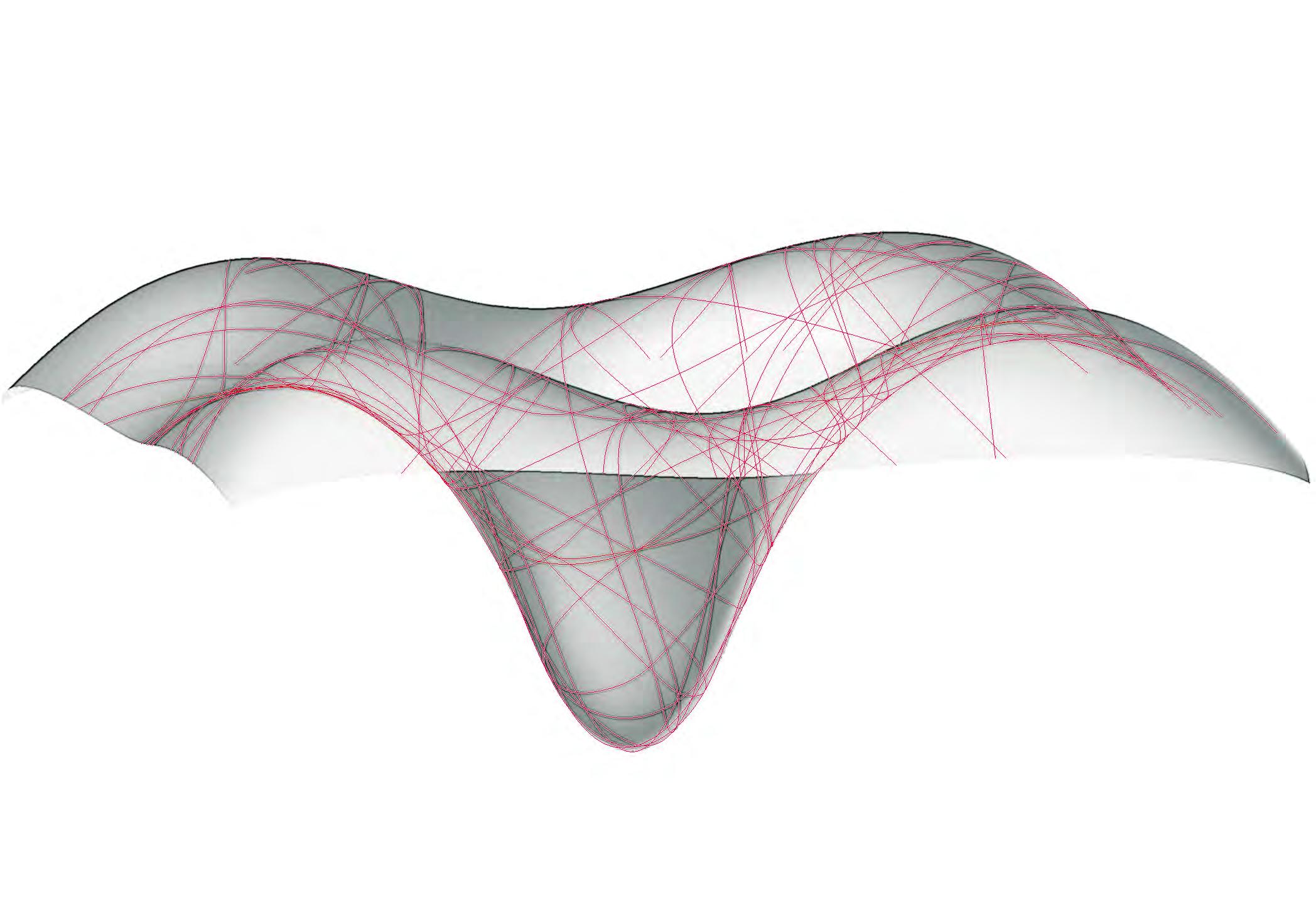
131
Perspective view of the global geometry with the fibres running along the direction of the principal stresses
The algorithm starts by asking the user to select a ‘surface’; in this case, the previously form found surface should be the one chosen. It then continues by importing the data from the Excel file where the direction of the vector principals were stored. Before the fibres can be laid, the algorithm needs to sort out the lists of points by direction and magnitude. Fibres are then laid by ‘linking’ points with similar directions of the principal stresses. The higher the stress value the greater the number of fibres that would be supplied [figure 4.52].
The result is a compendium of fibres wrapped around the periphery of the central column previously modelled through form finding to simulate a traditional vertical support. Fibres curve and cross orthogonally with one another, exactly following the lines of principal stress previously extracted from GSA. They distribute around the cylindrical trunk, becoming denser the closer they are to the end of the support. In the contrary, fibres spread out as soon as they abandon the column zone, travelling across the extension of the roof and fading around the corners [figures 4.49 and 4.50].
The idea was to generate a design where the distribution of fibres together with the overall form could create a single continuous surface featuring different degrees of flexibility. The corners were found to be the most flexible zones in comparison with the area surrounding the vertical support. This was essential in order to integrate the actuation technology within the whole system. The geometry both in local and global levels had to be conceived in such a way that actuators could be ‘activated’. The corner areas being more flexible than the surrounding zones were intended to be the ones with intense actuation, ranging different apertures and closures within the local geometry. In the contrary, the area around the column required higher densities and thus, actuation had to be restricted to the minimum.
The resulting structure is a space-truss made out of an interwoven of continuous surface which in the global scale acquires stiffness from combining convex and concave curvatures. The structural depth of the spacetruss grows bigger towards the mid-span areas of the roof, yet capable of adapting its height in response to any change in the loading conditions.

4.51 Diagram outlining the fibre organisation witihin the global geometry: micro and macro levels.
4.52 Diagram explaining the rules used to construct the algorithm responsible for distributing the fibres on the global geometry.
132
4 3 2 1 1 as (i) - as(ii) < tolerance (0.01) & 2 3 4 as (i) - as(ii) < tolerance (0.01) as (i) - as(ii) < tolerance (0.01) as (i) - as(ii) < tolerance (0.01) smax - A < s(i) < s(ii) < smax & smax - 2*A < s(i) < s(ii) < smax - A & smax - 3*A < s(i) < s(ii) < smax 2*A & smax - 4*A < s(i) < s(ii) < smax -3*A a(ii) s(ii) bre a(i) s(i)
Fibre Distribution

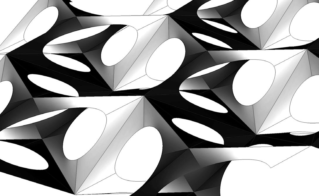
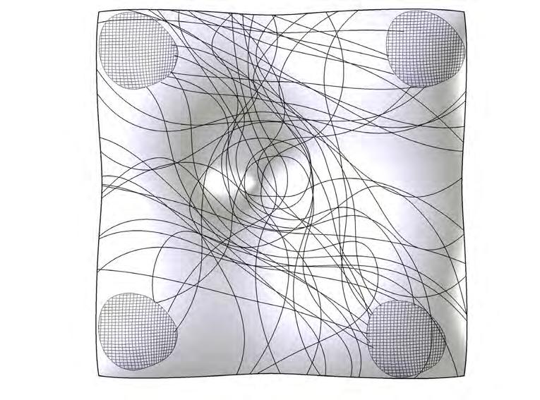
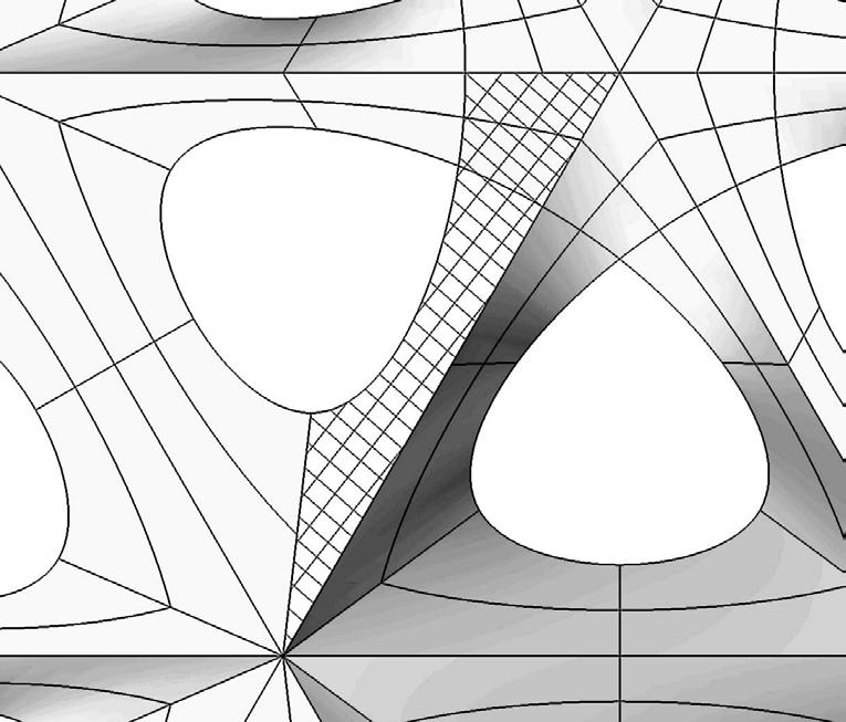
133 Macro Micro Fibre Distribution
Material Configuration
The material configuration refers here to how the different elements are located within the system: actuator, sensors and structural fibres.
Actuators which are shape memory alloy fibres are positioned along what we have previously referred to as ‘suture curves’. Sensors which ideally would be optical fibres are located in close proximity to the actuators [figure 4.53].
Finally the structural fibres are organised into two levels: macro and micro. Macro fibres are laid following
the lines of principal stresses previously determined by means of the fibre layout algorithm. Micro fibres consist on a 0-90 fibre mat whose principal orientation coincides with the direction of the nearest macro fibre.
Organising the fibres into these two different levels helps with the mechanisation of the fabrication technique [figure 4.51]. For further details, refer to the section Manufacturing included in the Appendix.
Shape Memory Alloy Actuation
4.53 Diagram explaining the configuration of the material and the integration of sensors and actuators with structural fibres.
134
m
e
Sensing Material Fibre Optic Structural Fibres s m a
s a
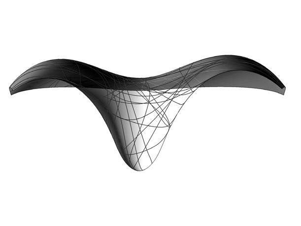
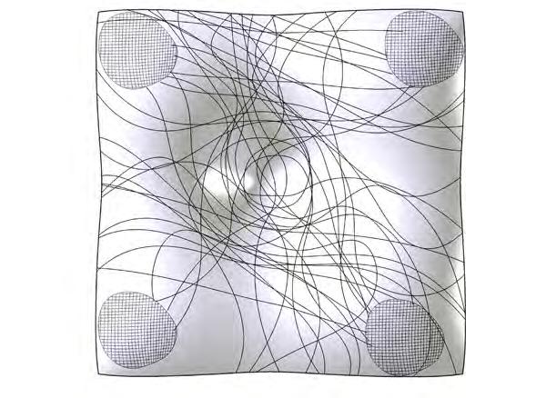
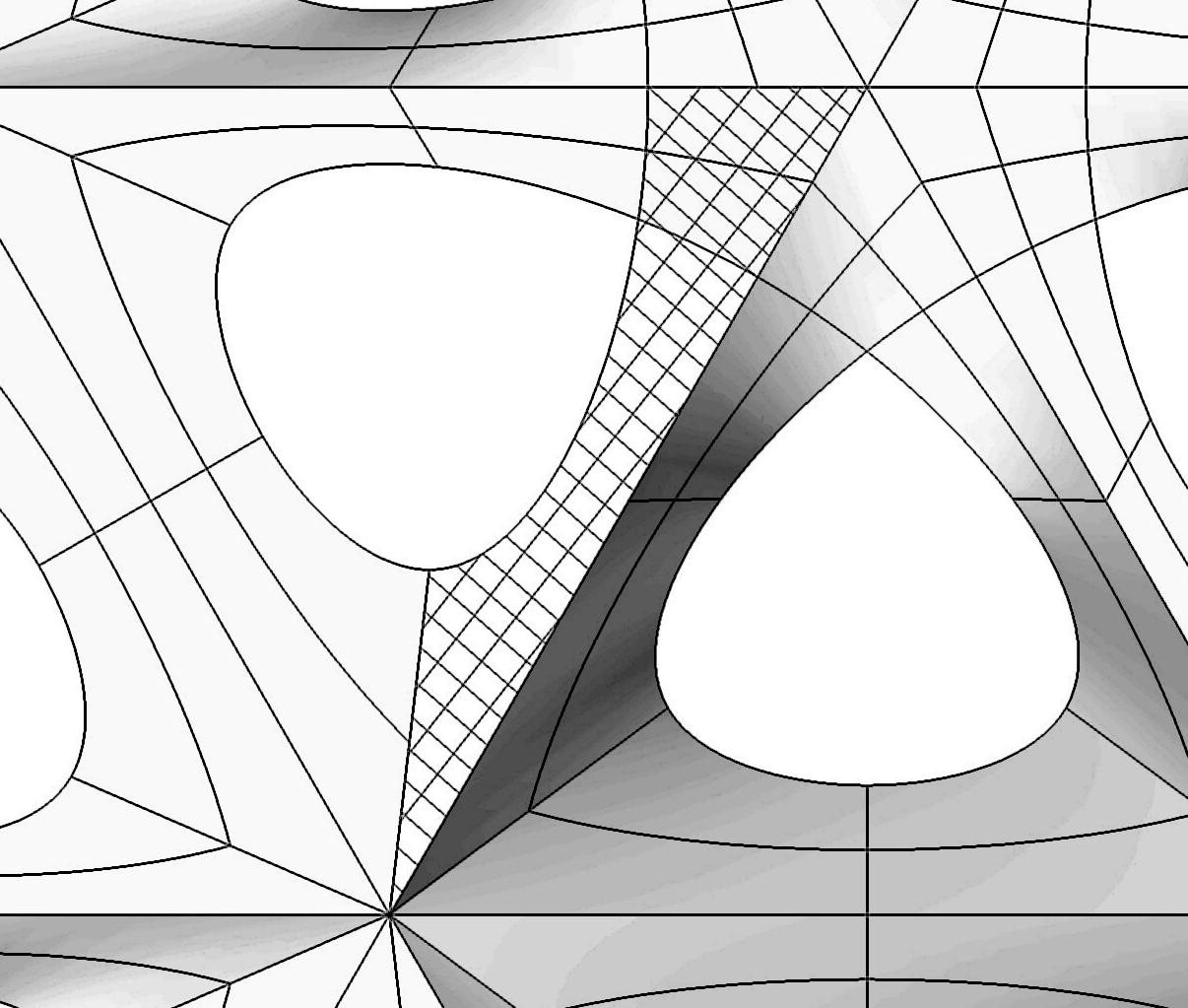
135 a a’ a a’
Remarks
The geometrical discussion both at the global and local scales has been driven by the use of continuous surface typologies throughout. Erwin Hauer inspired our understanding of the local topology and provided a firm foundation upon which the final local design could be developed. The optimisation of the global form to transform a traditional roofed supported structure through form finding simulation rendered a single continuous surface whose curvature was direct consequence of the loads acting upon it. This surface constitutes the outer skin of the hypothetical building previously abstracted as centrally supported roof.
In mathematics, the term ‘surface’ refers to a twodimensional topological manifold. If we limit our understanding of the surface to the above definition, there would be no consideration whatsoever of any of the possible implications of a surface in the threedimensional space, that is, the space where we exist. This is because in our dimensional space everything has volume and thus, surfaces are just a theoretical simplification used when one of the three dimensions defining the volume is considerably small with respect to the other two to such extent that it can be ignored. However, beyond a strict geometrical context, a surface has powerful abilities within the threedimensional space -albeit of being a two-dimensional object. A surface represents an edge that separates volumetric entities; it can be hermetic or partially opened, enclosing different volumes and determining different types of spatiality. Such ‘edge’ is rarely defined with such clarity outside the world of mathematics and geometric theories. In the world where we build
projects a surface ‘grows’ a third dimension and becomes a volume. Perhaps a more appropriate term to designate a surface in a three-dimensional space could be ‘envelope’. Architectural practice makes use of this term when referring to the threshold present in between the inside and outside realities of a building.
Alejandro Zaera Polo -co-founder of Foreign Office of Architects-, in his recently published paper ‘The politics of the envelope’, discusses how different building typologies are very much influenced by the processes that take place around the ‘envelope’ enclosing the private space and thus, differentiating it from outer public areas. He argues that these processes have an important political load and concludes that architecture is by extension a reflection of the political trends that exist at the moment the building is conceived.
As per Zaera’s words: “The envelope exceeds the surface by incorporating a much wider set of attachments. It includes the crust of space affected by the physical construction of the surface, by the scale and dimension of the space contained” [4.33]. It is also where exchange between interior and exterior environments takes place.
The envelope is thus how a surface ‘comes to life’. Our system can be described as an intricate of interwoven continuous surfaces; what would transform it into an architectural artefact is the consideration of the envelope with regards to its environmental performance.
136
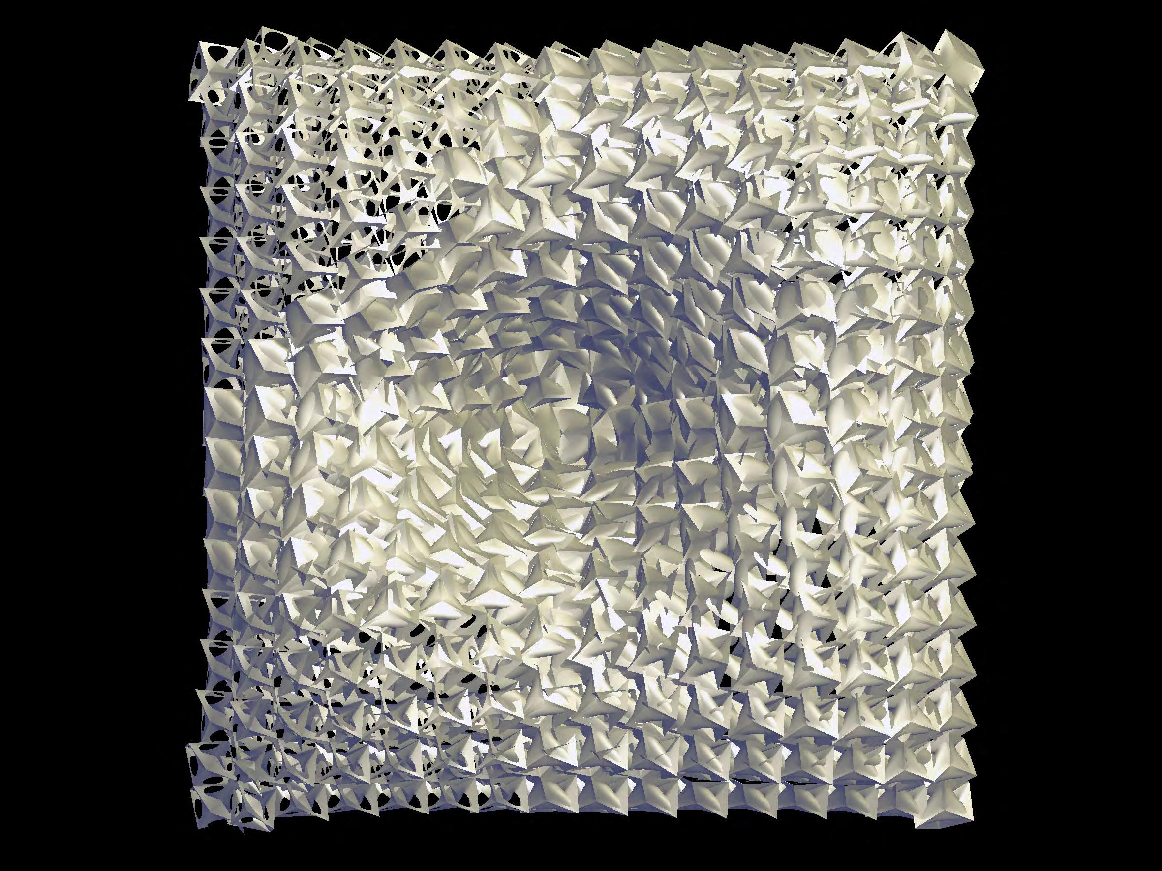
137
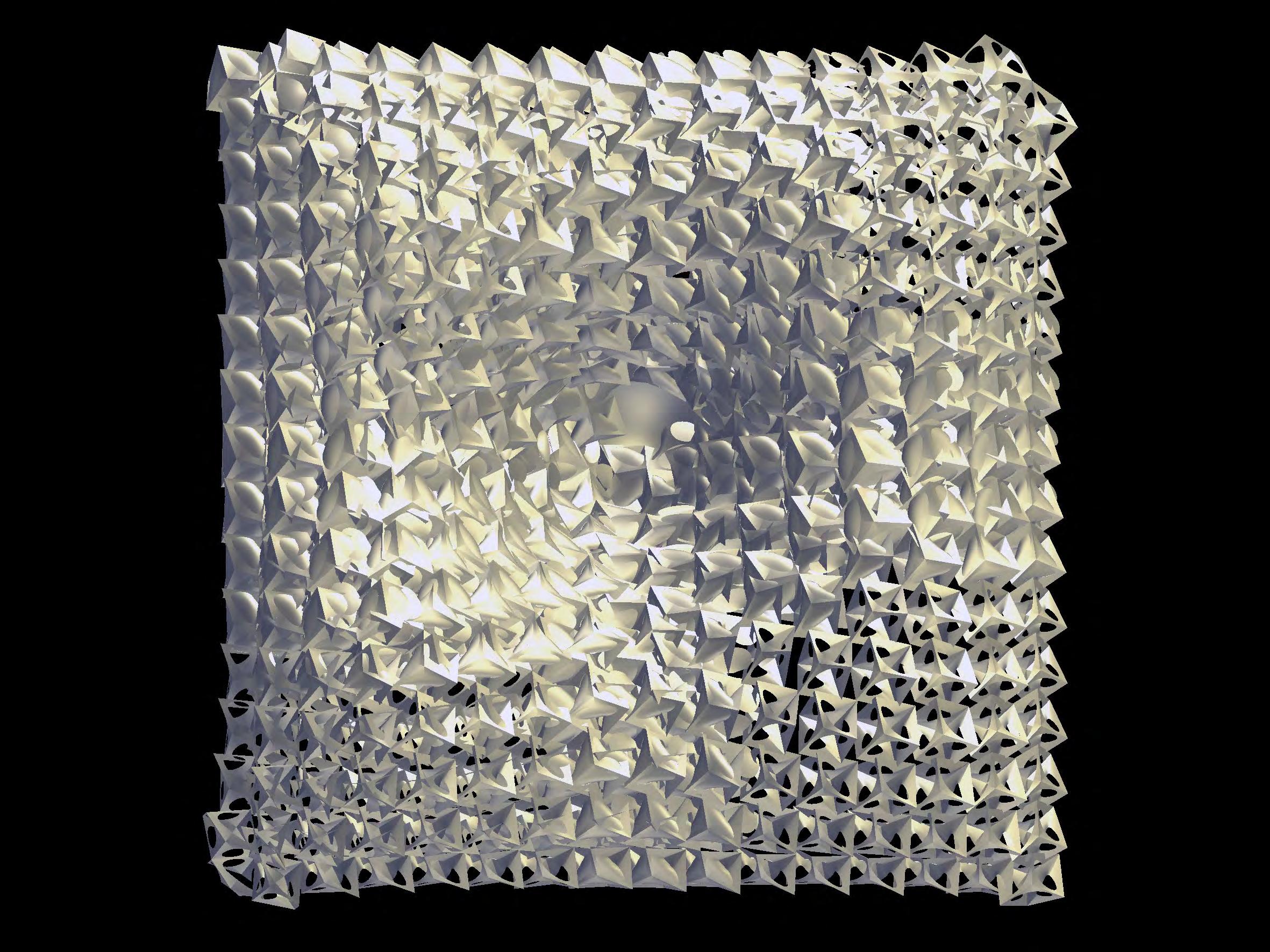
138
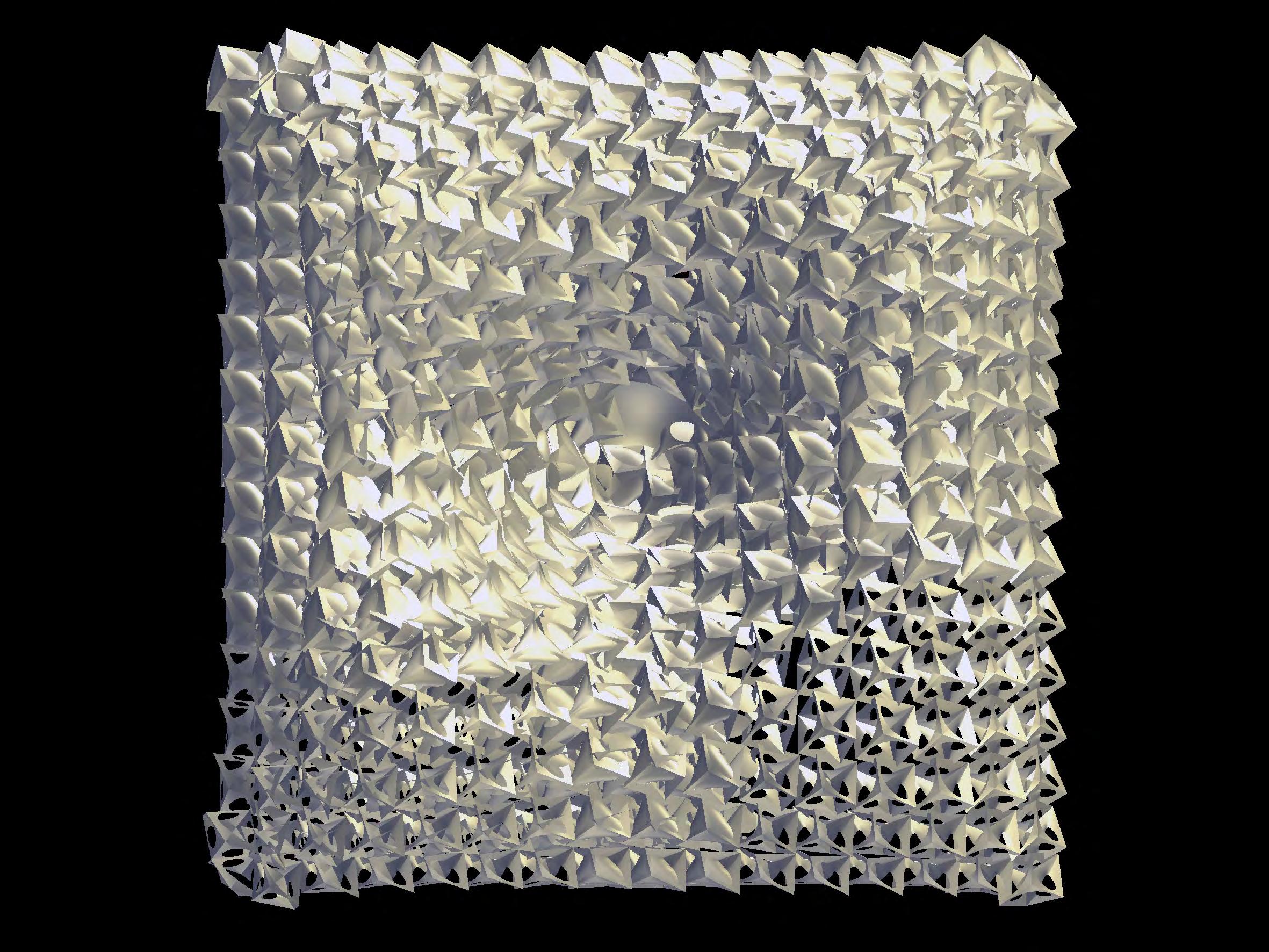
139
5 Environmental Performance
Local geometry Information Processing Global Morphology
This chapter enunciates the synergy between the actuation logics, global morphology and the local geometry. The potential of the system to efficiently adapt in response to the environment conditions are further elaborated. The information obtained from the embedded fibre optic sensors could be processed through artificial neural networks to gain suitable adaptation. Hence the geometrical range of actuation of each suture curve actuator would be shape set based on computation models derived from context specific climatic analysis.
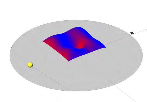
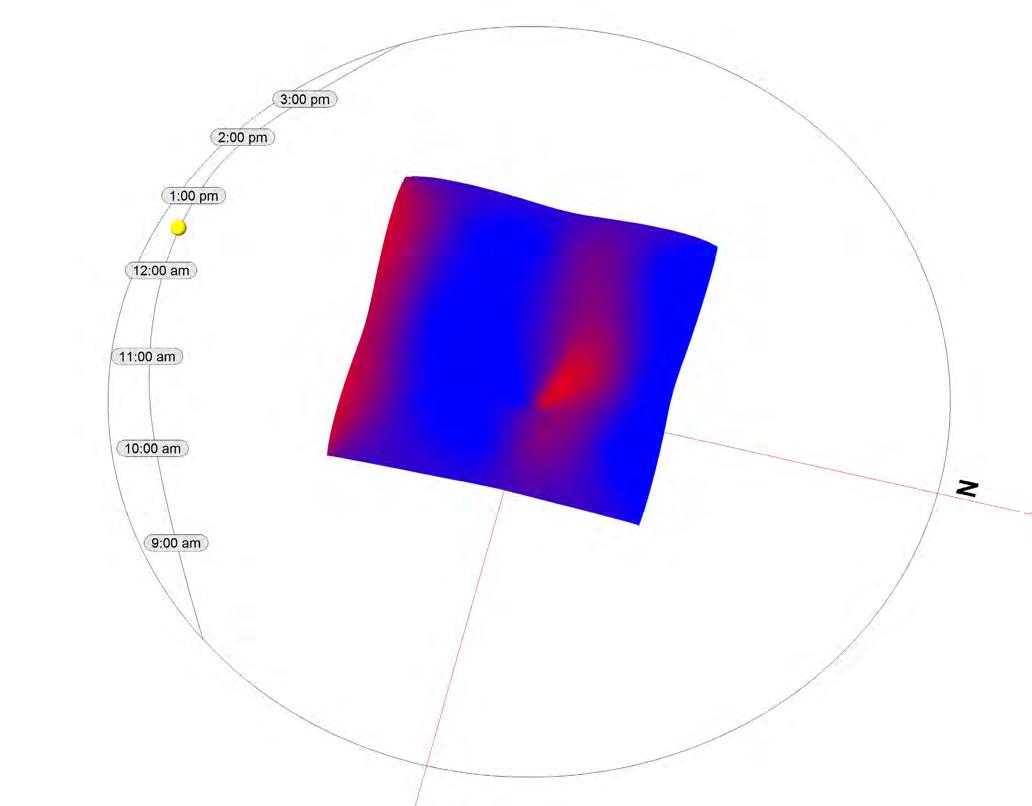
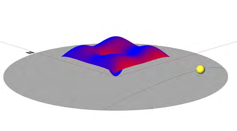
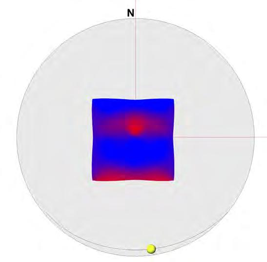
142
5.1 -Diagram showing the climatic analysis of the building envelope to access zones with maximum solar gain.
Global Morphology
The hypothetical roof structure has variable stiffness properties at different zones based on two parameters, the changes in curvature along the surface and the fibre distribution density, as discussed in the previous chapter. The local geometry defined as a dynamically adaptive fibre composite system should be strategically placed on the less stiff zones and zones with less fibre density. Such selection and strategic positioning of the actuators would depend on the analysis of the surface based on the climatic data obtained from the environment.
The surface/ envelope could be analysed based on any context specific climatic data to comprehend the degree of solar gain, shading and self-shading potential. For example, the image of the left shows a generic climatic analysis of the roof structure based on sun path. To maximize the solar gain the zones that receive the maximum solar radiation could have a higher level of porosity, which would essentially be the most appropriate zones to position the actuators. The image on the right shows the possible actuator zones indicated with green colour. The transparency level of the fibre composite material could also be modulated to increase the heat gain through ‘green house effect’. Therefore fibre composites also offer the potential to alter their material properties to achieve comfortable microclimatic conditions.
To reduce the heat gain in case of hot climates, the global morphology could be defined based on the self- shading potential of the form. The orientation of the global form based on the sun path is crucial.
The envelope could have an east-west orientation to minimize the solar gain on the east and west faces which receive maximum radiation. Also the corrugation is the local geometry could augment for the self- shading potential like in the case of many cacti which are protected against solar radiation. The ribs of cacti are one of the means by which the plant had adapted to heat and excessive sunlight.
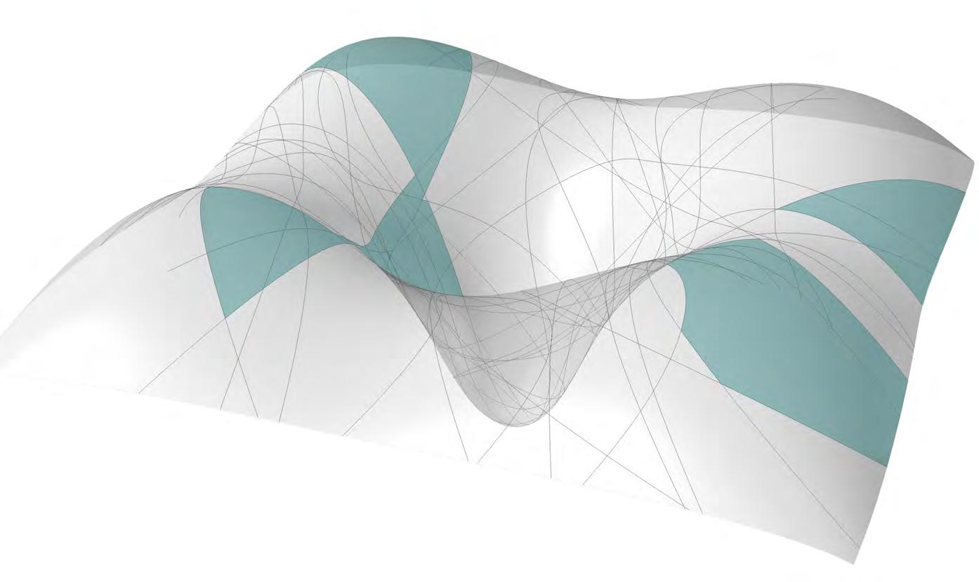
143
5.2 -Diagram showing zones to strategically position the opening actuators on the surface to maximise solar gain
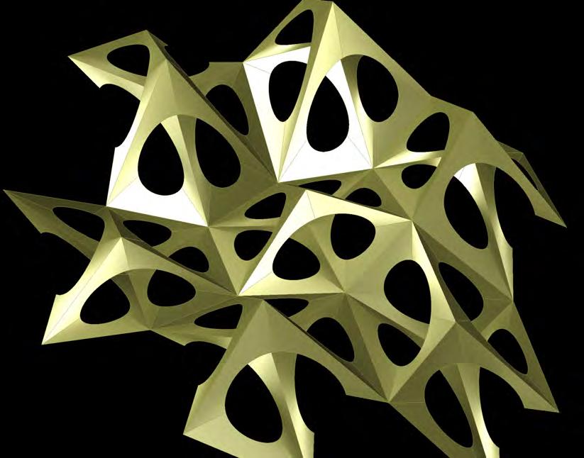
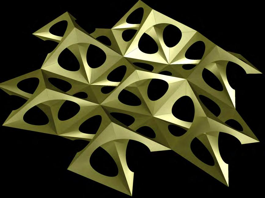

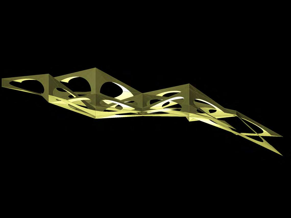
144
Local Geometry
As elaborated in the local geometry chapter, varying the size of the openings will result on increasing or decreasing the amount of light and air transferred. The actuators placed along the suture curves have to potential to alter multiple parameters, such as the degree of porosity, the orientation of the local cluster, the structural depth of the space truss and the overall curvature of the global form. These controllable parameters do not function autonomously, the geometrical definition is such that the degree of porosity and the structural depth are coupled and the orientation of the local cluster and the overall curvature are coupled. Hence these four types of actuation are essentially two.
When this actuation potential is extrapolated against the environmental conditions such as solar radiation and wind pressure, the suture curve actuators could adapt only to a preferential condition. When the openings are in a closed state the structural depth is minimal and Vice versa. Therefore the adaptive system has to prioritize the appropriate change in shape to efficiently suit the environmental condition in real time.
For example when there are high temperatures and heavy wind pressures the adaptive system has to take a decision to create larger openings and obtain the maximum structural depth to maintain a comfortable micro-climate and structural equilibrium. In the above
mentioned case the shape change is complimentary but with other environmental conditions it can be contradicting. Hence there is a need for a higher level of information processing as observed in higher level organisms controlled by a central nervous system processing multiple inputs and multiple actuation signals.
Orientation Porosity
Structural Depth
Overall curvature
145
Sun Wind
5.4 -Diagram showing the coupling of actuation variables within the system

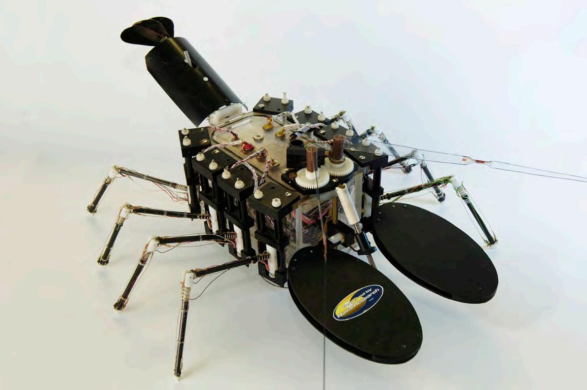
5.5 -Neural networks in human brain.A neural network describes a population of physically interconnected neurons or a group of disparate neurons whose inputs or signalling targets define a recognizable circuit. Communication between neurons often involves an electrochemical process. and biomimetic robot developed by US Navy.
146
Information Processing
Biological organisms are able to perform sophisticated functions as their sensing and actuation functions are controlled by neural networks. In the Artificial Intelligence paradigm, complex information processing happens through artificial neural networks. Therefore it is essential to look into the logics of information processing in artificial neural networks to deploy them for the proposed fibre composite adaptive system.
An artificial neural network usually called “neural network”, is a mathematical model or computational model that tries to simulate the structure and/or functional aspects of biological neural networks. It consists of an interconnected group of artificial neurons and processes information using a connectionist approach to computation. In most cases an artificial neural network is an adaptive system that changes its structure based on external or internal information that flows through the network during the learning phase. Neural networks are non-linear statistical data modeling tools. They can be used to model complex relationships between inputs and outputs or to find patterns in data.[5.1]
Simple nodes are connected together to form a network of nodes. Artificial neural networks are quite different from the brain in terms of structure. Like a brain, however, a neural net is a parallel collection of small and simple processing units. However in terms of scale a brain is massively larger than a neural network and the units used in a neural network are typically far simpler than neurons as well as the learning algorithms. A typical neural network consists of a set of nodes. Some of these are designated input nodes, some output nodes, and those which are neither are referred to as hidden nodes. There will be connections between the neurons and a weight is associated with each connection. When the network is in operation, values will be applied to the input nodes; these are then passed through weights and a simple computation is performed in each node; taking the sigmoid of the sum of products of the inputs and the weights is typical. These results are then passed through each node in turn until it reaches the output node.
Typically the weights in a neural network are set to small random values; this represents the network knowing nothing. As the training process proceeds, these weights will converge to values allowing them to perform a useful computation. When a neural net is first started, it is nothing but a set of input nodes, hidden nodes, and output nodes.
A node is just the term for one of the pseudo-neurons. An outside system such as environmental sensors could provide the input by placing values in the input nodes. By performing a set of calculations upon those nodes, the internal nodes are calculated, and then the output nodes.
Multi-layer perceptron networks use a variety of learning techniques, the most popular being back propagation. Here the output values are compared with the correct answer, and through various techniques the error is fed back through the network, which adjusts the calculation performed by each node to make it slightly closer to correct. It is provable that a multi-layer perceptron network (given sufficient nodes) is capable of learning any continuous real function to arbitrary ac¬curacy. Neural Network can be also classified in two general categories according to the type of learning algorithm, supervised learning which incorporates an external teacher and unsupervised learning which is based upon only local information. It is also referred to as self-organization, in the sense that it self-organizes data presented to the network and detects their emergent collective properties. [5.2]
As the fibre composite system is based on adaptation to local information, the system definition could occur based on unsupervised learning algorithms. This means the shape change range of the shape memory actuators should be set during the shape setting process. The shape and geometrical organization of each suture curve actuator should be organized and shape set based on an efficient computational model derived based on context specific climatic analysis.
147 Input Hidden Output
5.6 -Diagram of Artificial Neural Networks
6 Conclusion + Further Research
Fibre Optics
Shape Setting
Sensing
Shape Memory Alloys
Actuation
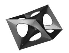
Fibres
Matrix E Glass
Epoxy Resin Cell
Proportion Calibration
Material Element Input
Structural Data
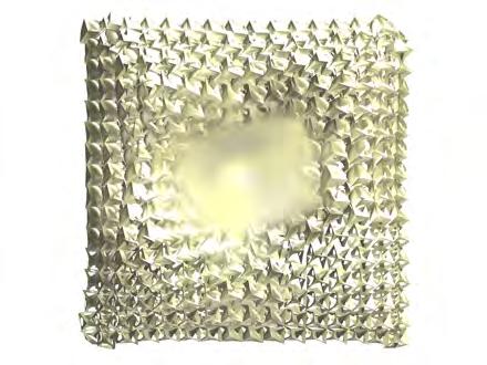
Porosity Calibration
Positioning of Sensors + Actuators
150
Austenite Martensile
Input
1
5
Hierarchy
Environmental Performance
2 3 4
System
Conclusion
The fibre composite adaptive system developed displays, ‘Integrated Functionality’, the factors such as form, structure, geometry and behaviour form a cohesive synergetic whole which complement one another. Biological organisms display emergent properties as they are organised in complex assemblies over several hierarchical scales.
The self-organisation of biological material systems is a process that occurs over time, a dynamic that produces the capacity for changes to the order and the structure of the system and for those changes to modify the behaviour of that system. Studies of biological systemic development suggest that the critical factor is the spontaneous emergence of several distinct organisational scales and the interrelations between lower or local levels of organisation, the molecular and the cellular level, and higher or global levels of structure or organism as a whole. The evolution and development of biological self organisation of system proceeds from small simple components that are assembled together to form larger structures that have emergent properties and behaviour, which in turn selfassemble into more complex structures.[6.1]
The proposed fibre composite adaptive system possesses multiple organisational scales that have different assembly logics at each scale which augment to their behaviour and performative abilities. Hence the system displays emergent behaviour which is not a mere sum of the parts but larger. The diagram on the left shows the ‘System Hierarchy of the Fibre Composite Adaptive System’, where the logics of assembly is differentiated over multiple organizational scales.
Level one is the definition of the shape at a molecular level of the shape memory alloy actuators. Shape memory alloys have the ability to alter between their bi-stable states of equilibrium, the inherentmartensile state and the shape set-austenite phases. Level two is the materials that make up the smart fibre composite. Level three is at the composite material level, embedded with fibre optic cables for sensing, shape memory alloys for actuation within a glass fibre and polymer matrix. Level four is the local geometry scale, defined as a continuous interwoven space truss which modulates the illumination and the wind flow through the envelope. Level five is that of the global morphology, the overall changes in curvature and fibre organisation density creates a system with differential stiffness properties. The synergy between assembly logics in all the four scales results in a system which has the potential to adapt and self-organize efficiently to the transient changes in the environmental conditions.
151
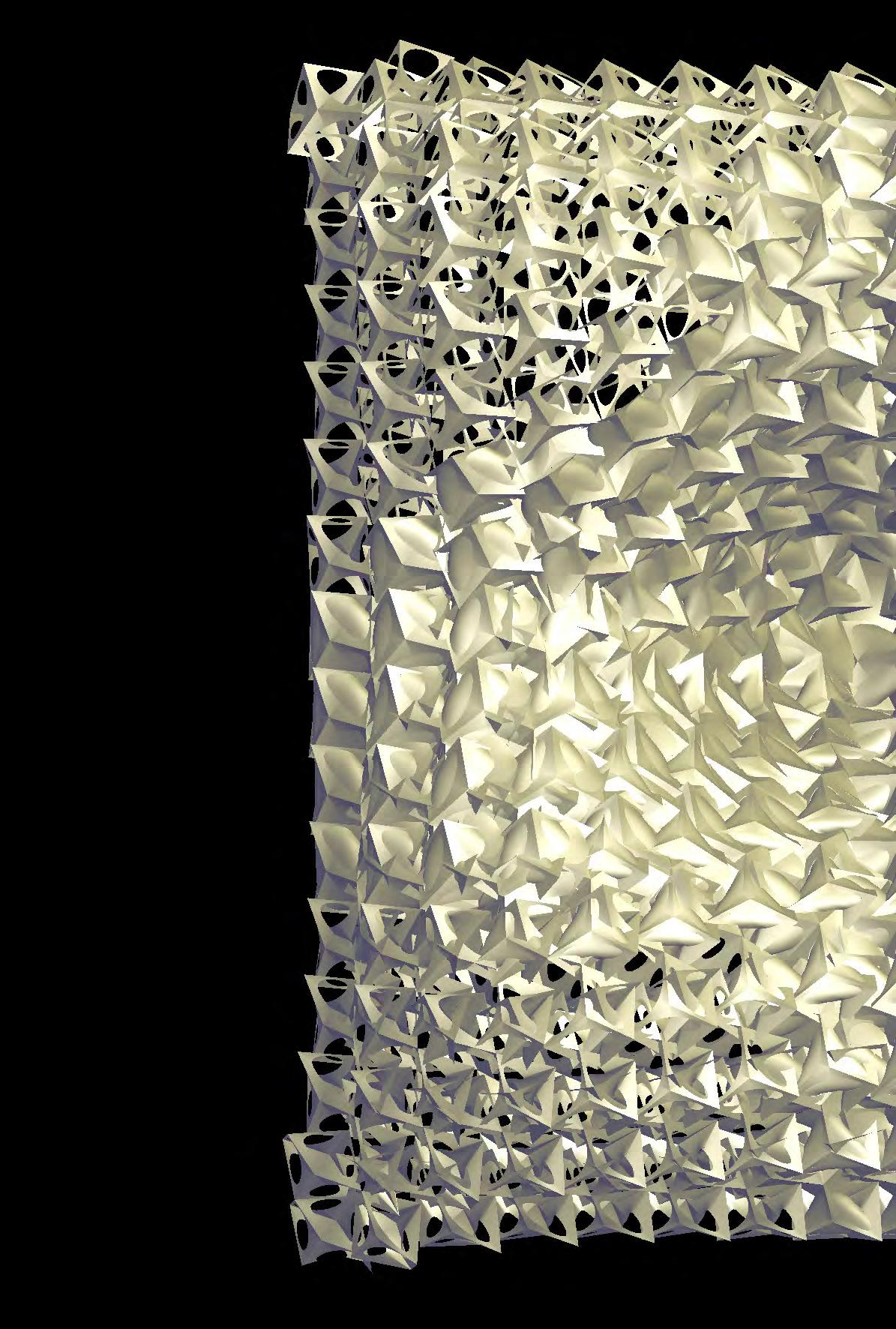
152
Further Research
The realization of the proposed active fibre composite structure embedded with fibre optic sensors and shape memory alloy actuators would lead to two important fields of further research. The first one would be to custom develop a design with a context reference and specific climatic data and the second one would be to explore the manufacturing process of continuous multilayer casting.
The geometrical definition of the topology has a versatile potential for efficient functioning in several environmental contexts. The adaptive potential of the geometry could be enabled by the passive energy acquired from the environment. Hot and dry climates which have a considerable diurnal variation in temperature would be the most appropriate to exploit the environmental energy for the functioning of the adaptive system. For instance, the variation in the atmospheric temperature would be between 14°C to 30°C in the summer months in hot and dry climatic zones. Therefore, the surface temperature of the shape memory alloys could easily reach the actuation temperature of 35°C. By defining the logic of the way the structure opens and closes at different time intervals the diurnal variation is temperature could be exploited for maintaining a comfortable micro climate.
The continuous surface being woven in multiple layers, poses challenging problems for developing a radical and novel manufacturing technique. As the continuous surface is a multilayer tessellated geometry, conventional positive and negative moulds cannot be employed. Tensioned fabrics could be explored to develop a multiple layer moulds. The suture curves which are the generators of the complex continuous surface geometry could be used as frames for stretching
fabric between cells. The thermo set fibre composite could be cast over the fabric mould through manual or computer supported -manual laying up process.
Thermo set fibre composites undergo curing process only at specific temperatures, if the connections are maintained lower than these temperatures, continuous casting could be explored for their fabrication potential. It is also essential to maintain the fibre continuity along the entire surface to protect the integrity and stability of the structure, therefore continuous multi-layer casting would be investigated as a fabrication method.
153
Appendix
A: Technology
B: Geometry
C: Manufacturing
Appendix A: Technology
4. Biocomposites
1. ICCM 17
2. I mperial College London
3. Shape M emory Alloys


International Conference in Composite Materials
Our decision to participate in the International Conference of Composite Materials in Edinburgh, proved to be very helpful for the progress of our work. It gave us a much wider perspective of the research done all over the world in composites in general, but also specifically in smart composites, adaptive smart systems and fibre optic technology.
We clearly understood the difficulties of designing and building a system that integrates sensing and actuation, but it also made it clear that what we had in mind and were planning to develop was possible and on the right direction.
Another very important aspect of our visit, was the fact that we had the opportunity to discuss our project with professors and researchers from very different backgrounds. Their feedback was crucial for the continuation of our work and the revision of certain parts of our system.
158
Themes Covered in the Conference
Industry Focused
A1. Advanced Composite Materials in Construction
A2. Aerospace Applications
A3. Automotive Applications and Recycling
A4. Marine Composites
A5. Offshore Applications
A6. Other Applications
A7. Wind Turbine Applications
Applications
B1. Biomedical Applications
B2. Composite Pressure Vessels
B3. Composites for Fuel Cells and Alternative Energy
B4. Electronic Composites
B5. Multi-functional Composites
B6. Sandwich Structures
B7. Smart Composites and Applications
B8. Structural Health Monitoring
B9. Thermal Applications and Heat Transfer
Manufacturing
C1. Composites Forming
C2. Flow Processes in Composite Materials
C3. Manufacturing Technologies
C4. Residual Stresses and Processing
Materials
D1. 3D Textiles and Composites
D2. Biomimetic Composites
D3. Carbon/Carbon Composites
D4. Ceramic Matrix Composites
D5. Fibre-metal Laminates and Hybrid Composites
D6. High Performance Fibres
D7. Interphases and Interfaces
D8. Metal Matrix Composites
D9. Natural Fibre Composites
D10. New Resins and their Performance
D11. Textile Composites
D12. Thermoplastic Matrix Composites
Nanocomposites
E1. Carbon Nanotube Composites
E2. Modelling and Analysis of Nanocomposites
E3. Multifunctional Nanocomposites
E4. Nanoclay/Nanosilicate Composites
E5. Nano-structured Surfaces and Coatings
E6. Polymer Nanocomposites for Structural Applications
E7. Processing of Nanocomposites
Behaviour
F1. Aging, Moisture and Viscoelastic Properties
F2. Analysis for Flight Certification of Composite Structure
F3. Buckling and Postbuckling Behaviour of Laminated
Shell Structures
F4. Composites in Fire
F5. Composites Testing and Model Identification
F6. Damage Mechanics and Multiscale Modelling
F7. Damage Tolerance and Impact
F8. Deformation and Fracture of Composites
F9. Delamination
F10. Dynamic Failure and Blast
F11. Energy Absorbtion and Crashworthiness
F12. Failure Criteria for Design
F13. Fatigue of Composites
F14. Full Field Measurement Methods
F15. Interlaminar Reinforcement
F16. Joining of Advanced Composites
F17. Mechanics of Short Fibre Composites
F18. Micromechanics/Nanomechanics
F19. NDE
F20. Probabilistic Analysis and Reliability
F21. Repair
F22. Structural Analysis and Optimisation
F23. Sustainable Green Composites
F24. Wear


159

In the first weeks of the project, we arranged a visit at the Composite Materials Centre of the Department of Aeronautics at Imperial College. The introduction and further explanation of the facilities and all the manufacturing and testing methods, was done by Tryfon Mantsos -a graduate of the MSc in Composites Materials of the department.
It was very interesting and helpful for us to see all the technology used to fabricate and test composite materials. We gained a better understanding of the traditional techniques and only by doing so, we were later on able to design and develop our project.
The facilities, testing devices and processes we engages with include:
Unidirectional Prepreg Epoxy Carbon Fibre Hand Lay Up
Vacuum (Used after hand lay up to remove air between layers of prepreg) - 0/0/0/90 are the directions of the fibre of each of the 4 individual layers
Cured quasi-isotropic carbon fibre specimen
Stitched woven quasi-isotropic carbon fibre fabric
Autoclave
Strain gauded carbon fibre specimens
Ultrasonics as (NDE) Non Destructive Evaluation of Carbon Fibre Specimens for defects
C-scan examples from ultrasonics
Cured unidirectional carbon fibre specimen with 60% volume fraction
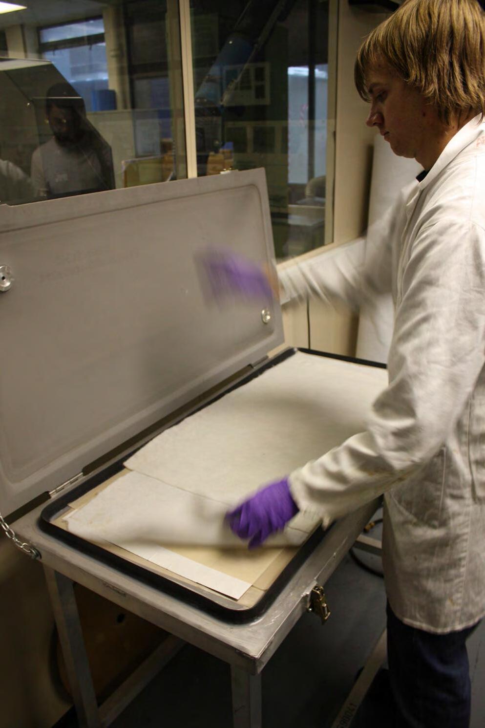
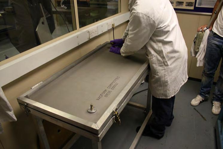
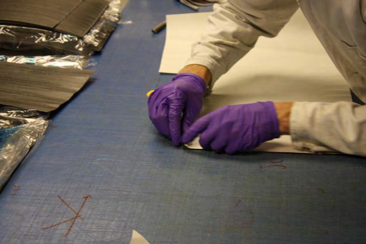
160
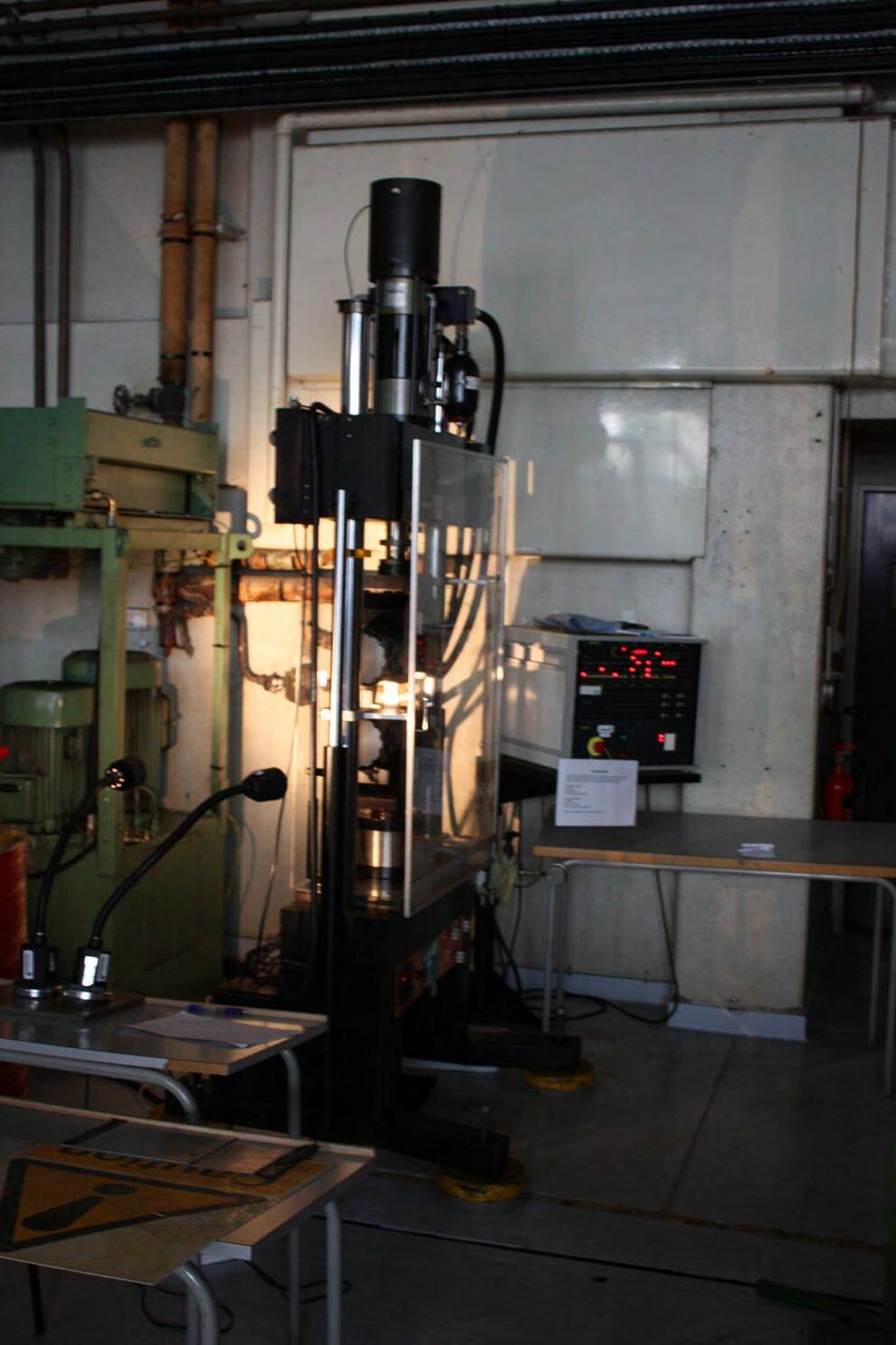
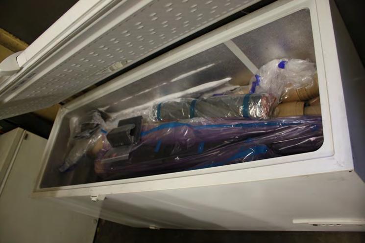
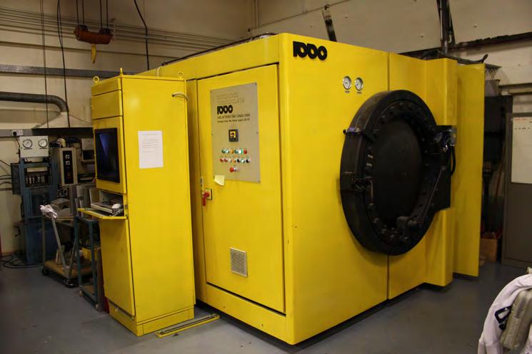
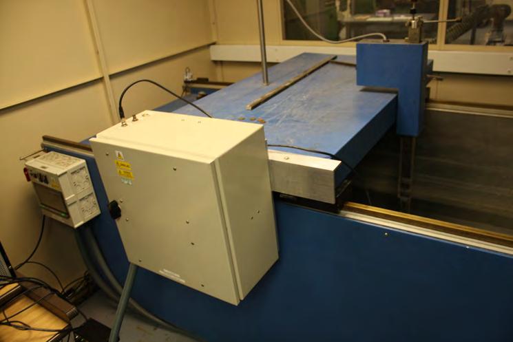
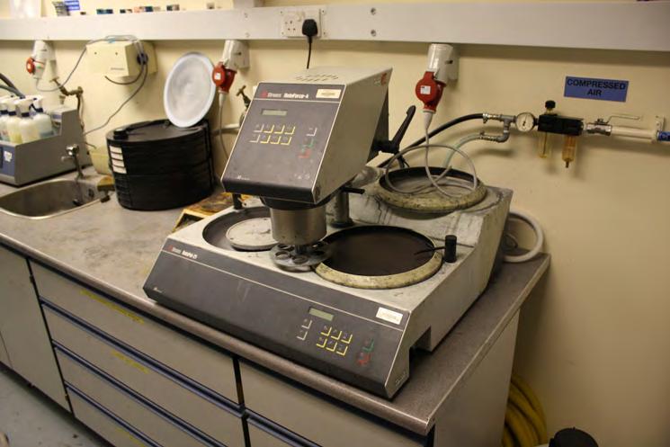
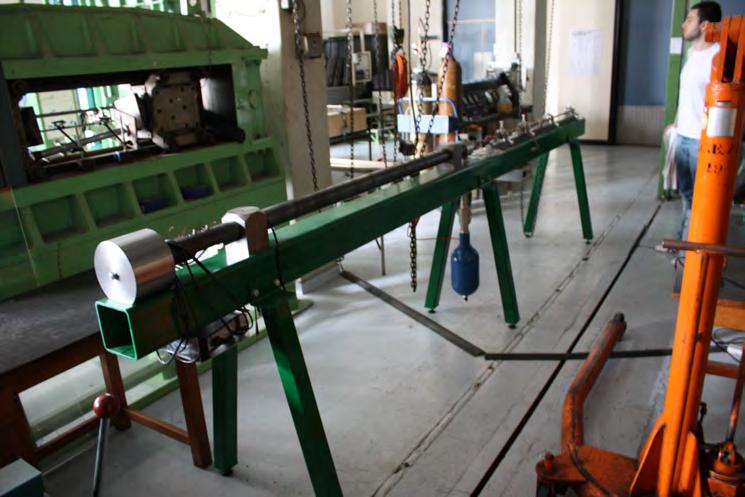

161
Memory-Metalle GmbH
I N F O S H E E T No. 10
Proprties of NiTi SMA
Transformation temperatures and strains:
Transformation temperature range
Transformation enthalpy
Transformation strains up to 1 cycle
up to 8 % up to 100 cycles
up to 5 % up to 100.000 cycles
Surface Strains in Wire, Ribbon and Sheet
Industry Standards
ASTM Standards
F2004-03 Standard Test Method for Transformation Temperature of NickelTitanium Alloys by Thermal Analysis
F2005-00 Standard Terminology for NickelTitanium Shape Memory Alloys
F2063-00 Standard Specification for Wrought Nickel-Titanium Shape Memory Alloys for Medical Devices and Surgical Implants
.ca. 2 %
up to 3 % above 100.000 cycles
Thermal hysteresis**
Physical properties:
Melting point
Density
Thermal conductivity of the Martensite
Thermal conductivity of the Austensite
electrical resistivity
lin. thermal expansion factor α of the Martensite
lin. thermal expansion factor α of the Austenite
Corrosion properties and biocompatibilty
Magnetic permeability
Magnetic susceptibility
Mechanical Properties:
Youngs modulus*** of the Austenite
Youngs modulus*** of the Martensite
Ultimate tensile strength (cold worked condition)
Ultimate tensile strength (fully annealed condition)
Plateau stress („Pseudo“-Yield stress) Martensite
Plateau stress Austenite
„conventional“ Yield stress Austenite
Transversal contraction factor
Tensile strain (fully annealed)
Tensile strain (cold worked)
Hot workability
Cold workability
Machinability
.30 - 80 °C
ca. 1310 °C
6,45 kg/dm3
ca. 9 W/m K
ca. 18 W/m K
50 - 110 μΩcm
6,7 x 10⁻⁶ 1/K
10 - 11 x 10-6 1/K
excellent
<1,002
3,0 x 10⁶
ca. 70 - 80 GPa
ca. 23 - 41 GPa
up to 1.900 MPa
ca. 900 MPa
70 - 200 MPa
200 - 650 MPa
.550 - 700 MPa
0,33
20 - 60 %
20 %
reasonable
difficult (work hardening)
F2082-03 Standard Test Method for Determination of Transformation Temperature of Nickel-Titanium Shape Memory Alloys by Bend and Free Recovery
F XXXX - XX Standard Test Method for Tension Testing of Nickel - Titanium Superelastic Materials
Japanese Industrial Standards
JIS H 7001 1989: Glossary of Terms Used in Shape Memory Alloys
JIS H 7101 1989: Method for Determining the Transfomation Temperatures of Shape Memory Alloys
JIS H 7103 1991: Method of fixed temperature tensile test for wires of Ti - Ni shape memory alloys
JIS H 7104 1991: Method of fixed temperature load test for coil springs of shape memory alloys
CE
NFA51-080: Alliages a memoire de forme Vocabulaire et measures
162
. . . . . . . . . . . . . . . . . . . . . . . . -200* - + 110 °C
. . . . . . . . . . . . . . . . . . . . . . . . . . . . . . . 0,47 - 0,62 kJ/Kg K
. . . . . . . . . . . . . . . . . . . . . . . . . . . . . . . . . . . . . . . . . . . . . . . . .
. . . . . . . . . . . . . . . . . . . . . . . . . . . . . . . . . . . . . . . . . . . . . . . .
. . . . . . . . . . . . . . . . . . . . . . . . . . . . . . . . . . . . . . . . . . . .
. . . . . . . . . . . . . . . . . . . . . . . . . . . . . . . . . . . . . . . . . . . .
. . . . . . . . . . . . . . . . . . . . . . . . . . . . . . . . . . . . . . . . . .
. . . . . . . . . . . . . . . . . . . . . . . . . . . . . . . . . . . . . . . . . . . . . . . .
. . . . . . . . . . . . . . . . . . . . . . . . . . . . . . . . . . . . . . . . . . . . . . . . . .
. . . . . . . . . . . . . . . . . . . . . . .
. . . . . . . . . . . . . . . . . . . . . .
. . . . . . . . . . . . . . . . . . . . . . . . . . . . . . . . . . . . . . .
. . . . . . . . . . .
.ca.
. . . . . . . . . . . .
. . . . . . . . . . . . . . . . . . . . . . . . .
. . . . . . . . . . . . . . . . . . . . . . . . . . . . . . . . . . . . . . . . . .
. . . . . . . . . . . . . . . . . . . . . . . . . . . . . . . . . . . . . . .
. . . . . . . . . . . . . . . . . . . . . . . .
. . . . . . . . . . . . . . . . . . . . . . .
. . . . . . . . . . .
. . . . . . . . . . . . .
. . . . . . . . . . . . . . . .
. . . . . . . . . . . . . . . . . . . . . . . . . . . . . . . . . . .
. . . . . . . . . . . . . . . . . . . . . . . .
. . . . . . . . . . . . . . . . . . . . . . . . . . . . . . . . . . . . . . .
. . . . . . . . . . . . . . . . . . . . . . . . . . . . . . . . . . .
. . . . . . . . . . . . . . . . . . . . . . . . . . . . . . . . . . . . .. . . 5
-
. . . . . . . . . . . . . . . . . . . . . . . . . . . . . . . . . . . . . . . . . . . . .
. . . . . . . . . . . . . . . . . . . . . . . . . . . . . . . . .
. . . . . . . . . . . . . . . . . . . . . . . . . . . . . . . . . . . . . . . . . . . . . . . .
very poor
Manufacturing of SMAs
Manufacture of Nickel-Titanium Alloys
Nickel-titanium alloys can be manufactured using a number of different techniques. These include vacuum melting techniques such as:
· Electron beam melting
· Vacuum arc melting
· Vacuum induction melting
· Plasma arc melting
Vacuum techniques are preferred due to the high reactivity of titanium, although inert atmospheres can also be used successfully.
Hot Working
Ingots are usually hot worked between 700 and 900°C as the next stage on the way to wire, bar or sheet formation. Processes such as press forging, rotary forging, bar rolling and extrusion are used for tis process. Alloys can be hot worked in air as they do not react readily with air.
Cold Working
Most cold working techniques can also be used, of which wire drawing is probably the most common, producing diameters as small as 0.05mm with excellent surfaces. However, work hardening occurs readily and constant annealing is usually required.
Deformation stress can be reduced by work hardening and suitable heat treatment. This process can also improve the strength of the austenitic phase as well as giving the alloy two way shape memory effect.
Fabrication
Welding
Welding of nickel-titanium alloys is possible but tends to produce brittle joints. Brittleness can be reduced by stress relieving, but degradation of the shape memory effect may occur due to the high temperatures that are required. Welding should also be carried under inert gases to prevent passive oxide buildup.
Soldering
Like welding, passive oxide buildup can be problematic when soldering nickel-titanium alloys. While being difficult, it can be done using a Sn – 3.5Ag solder with an aggressive flux. Alternatively, plating with nickel or gold prior to soldering can
result in good solder joints.
Joining
Nickel-titanium alloys can be joined using adhesives such as cyanoacrylates, epoxies, etc. Mechanical methods such as crimping and swaging have also been successful. The shape memory effect itself can be used and has been employed commercially in couplings.
Machining
Machining is possible using conventional methods, but high wear are not uncommon so carbide tools are recommended.
Other techniques such as electrodischarge machining and electro polishing can be used under the right conditions.
Coating and Plating
Coating and plating of nickel-titanium alloys is possible, but good adhesion is necessary to allow for the high strains encountered in some applications.
Other coating techniques can also be used, but high curing temperatures can degrade shape memory properties.
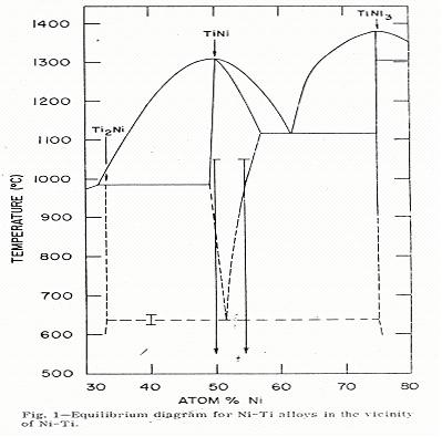
163
2
Natural Fibres | Biocomposites
When we were designing our material system, the factor of sustainability was one of the important factors in the choice of materials. Exploring this aspect, we did a research on natural fibres and biocomposites. Unfortunately, it was not possible to test and eventually use the appropriate biomaterials -fibres, biopolymers- due to a series of reasons such as availability in the market and cost.
Partly ecofriendly
Biocomposites
Ecofriendly/ Green
Bio bre + Petroleumbased plastic
Bio bre + Bioplastic
Hybrid biocomposites (Fibre / Matrix Blending)
Biocomposites
In a sense, bricks made of mud and straw are natural-fibre composites that can be traced to the dawn of civilization. In a polymer or plastic matrix, natural-fibre composites date to the early 1900s when cotton phenolics were widely used as insulating materials.
The most recent “new wave” of natural-fibre composites began in the 90s, when Mercedes-Benz introduced jute-based door panels in the E-Class vehicles. Since the 1990s, natural fibre composites are emerging as realistic alternatives to glass-reinforced composites in many applications. Natural fibre composites such as hemp fibre-epoxy, flax fibre-polypropylene (PP), and china reed fibre-PP are particularly attractive in automotive applications because of lower cost and lower density.
German auto-makers continue to lead in the use of these materials. For example, Daimler Chrysler’s Global Natural Fibre Initiative benefits Third World nations by developing products made from indigenous agricultural materials. The use of natural fibres as a filler or reinforcement in plastics is increasing at a healthy rate.
The disposal of composites after their intended life span is becoming critical and expensive. The recycling as well as reuse of composite materials is not easy since they are made of two dissimilar materials.
Broadly defined, biocomposites are composite materials made from natural fibre and petroleum-derived non-biodegradable polymers. Composite materials derived from biopolymer and synthetic fibres such as glass and carbon also come under biocomposites. Biocomposites derived from plant fibres and crop/bio plastics are likely more eco-friendly, and such composites are sometimes termed “green composites”.
Biocomposites can supplement and eventually replace petroleum-based composite materials in several applications, thus offering new agricultural, environmental, manufacturing and consumer benefits.
The main motivation for developing biocomposites has been and still is to
create a new generation of fibre-reinforced plastics competitive with glass fibre composites but which are environmentally compatible in terms of production, use and removal.
Extant studies comparing life cycle environmental performance of natural fibre composites with glass fibre reinforced composites find that natural fibre composites are environmentally superior
The future of natural fibre composites appears to be bright because they are cheaper, lighter and environmentally superior to glass fibre composites in general. Future research should hence focus on achieving equivalent or superior technical performance and component life.

Renewable Resource
Polyhydroxy- alkanoates
Polylactides (PLA)
Cellulode Esters
Starch Plastics
Successful materials such materials biobased biodegradable
164
Figure
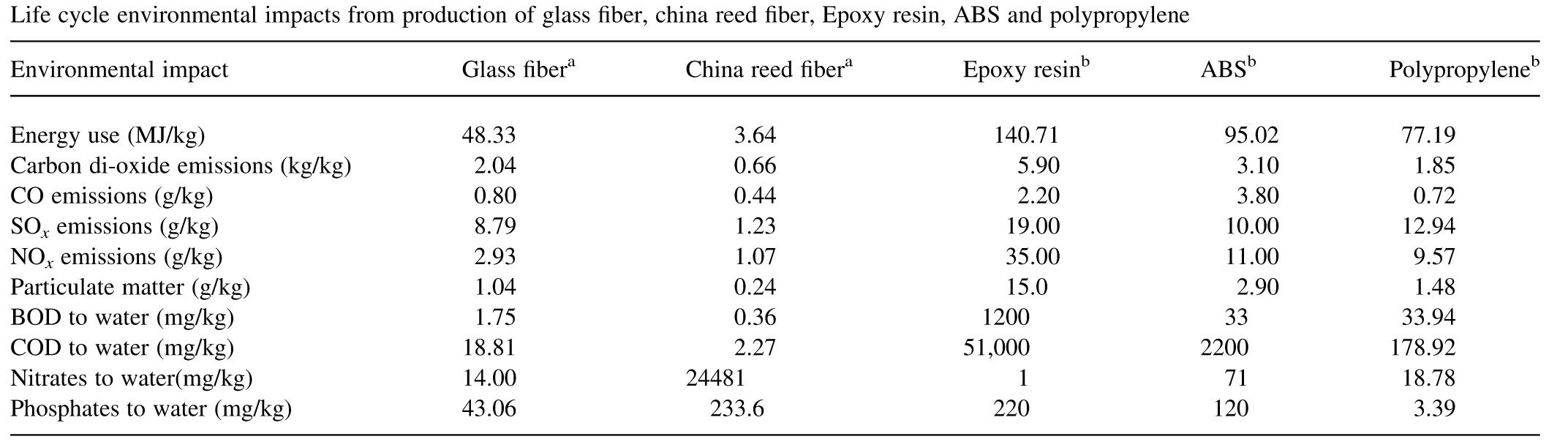
Fibres
Natural fibres are emerging as viable alternatives to glass fibres either alone or combined in composite materials for various applications in automotive parts, building structures and rigid packaging materials.
The advantages of natural fibres over synthetic or manmade fibres such as glass are:
Low cost
Low density
Competitive specific mechanical properties
Carbon dioxide sequestration
Sustainability
Recyclability
Biodegradability
The leading driver for substituting natural fibres for glass is lower material cost. Glass fibres used for composites have density of ,2.6 g/cm3 and cost between $1.30 and $2.00/kg. In comparison, flax fibres have a density of ,1.5 g/cm3 and cost between $0.22 and $1.10/kg [1]. While, natural fibres traditionally have been used to fill and reinforce thermosets, natural fibre reinforced thermoplastics, especially polypropylene composites, have attracted greater attention due to their added advantage of recyclability [2].
Natural fibre composites are also claimed to offer environmental advantages such as reduced dependence on nonrenewable energy/material sources, lower pollutant emissions, lower greenhouse gas emissions, enhanced energy recovery, and end of life biodegradability of components.
In automotive industry, composites made of natural fibres reduce the mass of the components and lower the energy needed for production by 80%. [4]
Biodegradable | Biobased Polymers
ral fibres can vary from one batch to the next. Growing conditions affect fibre properties. For instance, attack by mold and variations in moisture content can influence performance of the finished part. There are no generally agreed upon standards for properties or performance of these fibre feedstocks.
Modeling Issues with Natural Fibres
Disadvantages | Limitations
Renewable Resource Based
Natural fibres are grown as agricultural products and do not consume the energy required to melt and process glass. For disposal, even if burned the plant fibres leave little residue and return no more carbon dioxide to the atmosphere than they removed when grown.
Polyhydroxy- alkanoates (PHAs)
Polylactides (PLA)
Cellulode Esters
Starch Plastics
The main physical limitation of bast fibres when compared to glass is heat sensitivity. All plant fibres contain natural sugars and cannot survive temperatures above 400F. Processing temperatures must remain below this range, limiting their use to reinforcement in polypropylene, styrenics, and other low-melting-point resins.
Natural fibres also do not have the strength of glass. Generally, tensile and flexural strength and impact resistance are about half that of comparable glass-filled materials. However, this is a broad generalization. Actual comparisons vary widely depending on materials and processing.
Petroleum/ Fossil BasedMixed Resource Based
Non-uniform fibres
Difficult to characterize fibre source
Aliphatic Polyesters
Cross-section may be different between fibres and within a single fibre
Aliphatic-aromatic polyesters
Single fibres versus fibre bundles, both may be present
Poly (ester amide)
Non-rigid fibres
Poly (alkyene succinate)s
Long flexible fibres
Poly (vinyl alcohol)
SORONA (condensation polymer of corn-derived 1,3 propane diol + petroleum-derived terephthalic acid
Rigidity can change with temperature, moisture content
Blendings of:
Fibre Attrition
Breakage can depend upon temperature, moisture content
Successful blending: new polymeric materials of desired properties
A part made with natural fibres will not be as strong as a glass-fibre composite, but in many applications strength is more than adequate. It is often possible to make the part thicker using natural-fibre composites, compensating for the loss of intrinsic strength while maintaining cost and weight savings.
such materials may be termed as biobased + may or may not be biodegradable
Another limitation, at present, is that the properties of natu-
Two/more biodegradable polymers (ex. starch plastic + PLA)
One biodegradable + one fossil fuel-made polymer
Epoxidized soybean oil + petrobased epoxy resin

Figure 2
Hybrid biocomposites (Fibre / Matrix Blending)
Bio bres
Non-wood Bio bres
Straw Fibres
Rice
Wheat
Corn straws
Kenaf
Flax
Jute Hemp
Henequen
Sisal
Pineapple leaf
Cotton
Coir
Bamboo
Switch grass
Elephant grass
Soft and Hard Woods
Newspaper Magazine bres
BastLeafSeed/ Fruit
Grass Fibres
Recycled
Wood Fibres

Plant Fibres
Among the natural fibres are cellulose -the primary structural component of plants and bacterial cell walls-, animal fibres -such as wool and silk- and biochemical fibres.
Plant fibres are composed of cellulose, lignin, or similar compounds; animal fibres are composed of protein.
Cellulose, the most widespread organic molecule on Earth, is the major component of plant cell walls. Plants produce approximately 50 kilograms of cellulose daily for each person on Earth. A linear polymer made up of 10,000 to 15,000 glucose molecules bonded in a 1 → 4 glycosidic linkage, it is made up almost entirely of glucose. Cellulose molecules contain many polar hydroxyl groups, which allow them to interact with adjacent molecules to form fibres. These fibres are structurally strong and resistant to chemical attack, so wood products are widely used in construction and production of paper.
Cotton, a vegetable fibre that is almost pure cellulose, grew to become an important industrial commodity during the nineteenth century. Composed of cellulose strands in small springlike coils, cotton fibres have no surface scales and are softer than wool and less likely to provoke itching. First used as a textile material in India, cotton is now grown in every temperate part of the world and has been an important commodity in the southern United States. Cotton plants grow seed cases called bolls that yield tangled masses of fibres which are easily collected and spun. Processing cotton fibres is done in much the same way as wool.
Animal hair composed of protein is a common biological fibre. Numerous types of hair have been used commercially for weaving, production of ropes, padding, and insulation.
Wool fibres are made of animal hair, principally from sheep. Each hair is a complex structure made up of layers of protein molecules. Cloth made from wool has excellent insulating properties and resists wrinkling. Wool fibres can be stretched, dyed, and woven.
For centuries, sheep have been bred for their wool-bearing qualities. Production of woolen fabrics is a highly technical process. In its simplest form, sheep are sheared and the wool sorted and cleaned, then the wool is carded to straighten the fibres, spun into thin cords, and woven into fabrics. Each step in this process has been refined to provide a high-quality product of vast commercial importance.
[1] Foulk JD, Akin DE, Dodd RB. New low cost flax fibres for composites. SAE Technical paper number 2000-01-1133, SAE 2000 World Congress, Detroit; March 6–9, 2000.
[2] Mohanty AK, Drazl LT, Misra M. Engineered natural fibre reinforced polypropylene composites: influence of surface modifications and novel powder impregnation processing. J Adhes Sci Technol 2002; 16(8):999–1015.
[4] Broge J.L, Natural Fibres in automotive components, Automotive Eng. Int, 2000, p.108
166
Animal Fibres
Biocomposite stampable sheet process
Injection Moulding
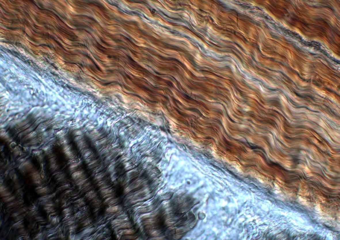
Compression moulding
treatment
treatment
Water emulsionbased sizing
Biocomposite Processsing
Synergism E cient
treatment Water emulsionbased sizing Maleated matrix as compatibiliser Reactive
Low-cost e cient surface treatments of natural bres Polymer Matrix modi cation High Performance biocomposite formulation
Green composites from natural bres and bioplastic
Conventional composites from glass- bre and traditional plastic Fibre
Injection Moulding Biocomposite stampable sheet process
Low-cost e cient surface treatments of natural bres
E cient
Biocomposite Processsing
Synergism
Compression moulding
Reactive Blending Extrusion
Polymer Matrix modi cation
High Performance biocomposite formulation Life Cycle Assessment (LCA) Crop
Maleated matrix as compatibiliser
Green composites from natural bres and bioplastic
Conventional composites from glass- bre and traditional plastic
of life management (recycling)
part manufacture
bre manufacture Composite part use End of life management
167
Silane
Alkali
Production
Fibre Petroleum
Re ning
extraction
Silane
Alkali
Extrusion
Crop Production
treatment
Blending
Life Cycle Assessment (LCA)
Petroleum
Plastic
Glass-
extraction Bioplastic manufacture Green composite part manufacture Composite part use End
extraction Re ning
manufacture Glass- bre pastic composite
Sunlight
Natural Resources
Polymer
Production
Processing
Biodegradation
Use and Discard
Transportation (Auto-parts)
Renewable Resource Based
Biodegradable | Biobased Polymers
Petroleum/ Fossil BasedMixed Resource Based
Packaging
Bio-Polymers
Producing chemical products and new materials from renewable resources is not a new idea. Most of the chemical products and materials came from renewable resources until the early part of the 20th century [1]. The success and tremendous growth of the petrochemical industry in the 20th century, however, slowed the growth of biobased products. Environmental as well as economic factors are now driving the trend toward greater utilisation of biobased polymers and materials. [2,3]
The persistence of plastics in the environment, the shortage of landfill space, concerns over emissions during incineration, and entrapment and ingestion hazards from these materials have spurred efforts to develop biodegradable plastics.
Biobased polymers may be obtained from renewable resources and are gaining much importance over petroleum-based biodegradable polymers in recent years. Biopolymers have started migrating into the mainstream and biobased polymers may soon be competing with commodity plastics. Some of the examples for biopolymers include: cellulosic biopolymers derived from renewable cellulose,
starch plastics, corn-derived plastics, and bacterial polyesters.
The need to produce 100% biobased materials as substitutes for petroleum-based polymers is not immediate. Biocomposites that contain a significant content of biobased materials can presently achieve this at an affordable cost-performanve ratio to compete with petroleum-based materials and still maintain a positive balance among ecology, economy, and technology.
[1] Wedin R, Chemistry on a high-Carb diet, American Chemical Society, Washington DC, 2004, p.30-35
[2] Gross R.A. and Karla B, Biodegradable polymers for environment, Science 297, 2002, p.803-807
[3] Netravali A.N. and Chabba S, Composites get greener, Mater. Today, April 2003, p.22-29
Polyhydroxy- alkanoates (PHAs)
Energy / Environment
Polylactides (PLA)
Cellulode Esters
Starch Plastics
Substitute of petroleum-based materials
Aliphatic Polyesters
Information / communication
Aliphatic-aromatic polyesters
Poly (ester amide)
Poly (alkyene succinate)s
Performance
Poly (vinyl alcohol)
Processing synthesis
Expanding biocomposite materials complexity
Successful blending: new polymeric materials of desired properties
Structure composition
such materials may be termed as biobased + may or may not be biodegradable
Value-added agricultural products
Interface chemistry
SORONA (condensation polymer of corn-derived 1,3 propane diol + petroleum-derived terephthalic acid
Blendings of:
Civil infastructure (green housing)
Two/more biodegradable polymers (ex. starch plastic + PLA)
One biodegradable + one fossil fuel-made polymer
Value-added forest products
Epoxidized soybean oil + petrobased epoxy resin
Natural Composites
Material
Wood
Sponge body wall
Stony corals
Sea anemone mesolgea
Mollusk shell
Chiton radular teeth
Echinoid teeth
Bird eggshells
Cartilage
Bovid horn
Bone
Tooth enamel
Arthropod cuticle
Hard Component Matrix
cellulose (polysaccharide) lignin, hemicelluloses
calcareous, siliceous spicules, collagenmiscellaneous organic aragonite crystals chitin fibril network
collagen fibrils protein/polysaccharide gel calcite, aragonite protein, chitin
magnetite crystals organic, chitin + protein
dolomite organic
calcite crystals protein
collagen fibrils mucopolysaccharide
keratin fibres wet, amorphous keratin
hydroxyapatite collagen, other organic hydroxyapatite organic
chitin fibrils + cross linked protein + calcite
168
Substitute of petroleum-based materials Energy / Environment
Transportation (Auto-parts)
Material
Examples of
Sea anemone mesoglea
Aorta, pig
Nuchal ligament
Dragonfly tendon
Abductin
Cartilage
Mussel byssus thread
Tendon (collagen)
Horn (keratin)
Tree trunks
Silk (spider)
Wood (dry)
Locust apodeme (chitin)
Bamboo
Teeth (dentine)
Bone
Mollusk shell
Coral skeleton
Teeth (enamel)
Kevlar
Steel
Expanding biocomposite materials complexity
Young’s Modulus

Sea anemone mesoglea
Nuchal ligament
Abductin
Mussel byssus thread
Sea anemone mesoglea
Horn (keratin)
Silk (spider)
Nuchal ligament
Abductin
Locust apodeme (chitin)
Mussel byssus thread
Horn (keratin)
Teeth (dentine)
Mollusk shell
Silk (spider)
Locust apodeme (chitin)
Teeth (enamel)
Teeth (dentine)
Steel
Mollusk shell
Teeth (enamel)
Steel
Sea anemone mesoglea
Aorta, pig
Nuchal ligament
Sea anemone mesoglea
Dragonfly tendon
Abductin
Cartilage
Mussel byssus thread
Tendon (collagen)
Horn (keratin)
Tree trunks
Silk (spider)
Mussel byssus thread
Wood (dry)
Locust apodeme (chitin)
Bamboo
Teeth (dentine)
Bone
Mollusk shell
Coral skeleton
Locust apodeme (chitin)
Mollusk shell
Coral skeleton
Tensile Strength
169
Performance
Packaging
Information
communication
synthesis Interface chemistry Structure composition
Value-added agricultural products Value-added forest products Civil infastructure (green housing)
/
Processing
Young’s
of Elasticity
of tensile strength of materials
Moduli
Examples
Young’s Modulus (MPa) Material Tensile Strength (MPa) 0.01 Aorta 2 0.5 Brick, concrete 5 1.0 Abductin 10 1.8 Teeth (enamel) 35 4.0 Coral skeleton 40 20 Teeth (dentine) 50 100 Mussel byssus thread 50 1500 Wood 100 4000 Tendon (collagen) 100 6400 Bone 200 10000 Hair, human 200 10000 Mollusk shell 500 12000 Cellulose Fibre 750 15000 Nylon fibre 1000 15000 Steel (typical) 1000 18000 Silk (spider) 2000 50000 Steel (high tensile) 3000 60000 Kevlar 3600 60000 130000 200000
Young’s Modulus
4,000
0 50000 100000 150000 200000
Appendix B: Geometry
Local Geometry
Global Geometry
1. Continuous Surfaces
2. Algor ithms
Continuous Surface Geometries
The Klein bottle is a closed non-orientable surface of Euler characteristic ‘0’ that has no inside or outside. It can be constructed by gluing both pairs of opposite edges of a rectangle together giving one pair a half-twist, but can be physically realised only in four dimensions, since it must pass through itself without the presence of a hole. It can be represented by connecting the side of a square in the orientations shown in the diagram.
It can be cut in half along its length to make two Möbius strips but it can also be cut into a single Möbius strip. Figures show an immersion of the Klein bottle in the three-space. There are also other possible immersions; however these have not been selected as part of this research since they belong to dimensional spaces beyond the three-dimensional one.
The equation for the usual immersion is given by the implicit equation:
where its correspondent parametric equation is formulated as follows:
x = cos u [ cos (1/2 u) ( 21/2 + cos v) + sin(1/2 u) sin v cos v] y = sin u [ cos (1/2 u) ( 21/2 + cos v) + sin(1/2 u) sin v cos v] z = - sin (1/2 u) ( 21/2 + cos v) + cos(1/2 u) sin v cos v
A short vbscript algorithm was written in Visual Basic for visualisation purposes.
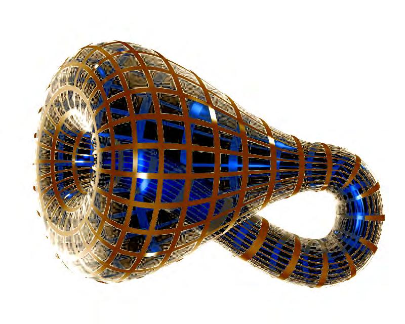
172
y2
z
(x2 + y2 + z + 2y -1) [(x2 +
+
+ 2y -1)2 – 8z2 ] + 16x z (x2 + y2 + z + 2y -1) = 0
Klein Bottle
Option Explicit
‘Script written by <insert name> ‘Script copyrighted by <insert company name> ‘Script version 05 June 2009 20:34:27
Call Main()
Sub Main()
Dim arrCount(1), arrPoints(), n,m,l,ustep,vstep,u,v,x,y,z,ustar t,uend,vstart,vend,num
Dim u_star t,u_end,d,surface,v_start,v_end,dd Dim i,j,u_list(),v_list() Dim num_step1,num_step2
Dim arrItems, arrValues, scale_factor
u_star t= Rhino.RealBox (“Enter where ‘u’ should start”, 0, “Define parameters range (u)”)
u_end= Rhino.RealBox (“Enter where ‘u’ should end”, 2*pi(), “Define parameters range (u)”)
j=-1
For i=u_start To u_end Step pi()/2 j=j+1
ReDim Preserve u_list(j) u_list( j)=i
Next
v_star t= Rhino.RealBox (“Enter where ‘v’ should start”, 0, “Define parameters range (v)”)
v_end= Rhino.RealBox (“Enter where ‘v’ should end”, 2*pi(), “Define parameters range (v)”)
j=-1
For i=v_start To v_end Step pi()/2 j=j+1
ReDim Preserve v_list(j) v_list( j)=i
Next
m= Rhino.RealBox (“Enter tolerance for partitions in u direction”,5, “Step u direction”)
l= Rhino.RealBox (“Enter tolerance for partitions in v direction”,5, “Step v direction”)
scale_factor= Rhino.RealBox (“Enter scale factor for final continuous surface”, 1, “Scale Factor”)
arrItems=array(“U_Start”,”U_End”,”V_Start”,”V_End”,”Partitio ns_U”,”Partitions_V”)
arrValues=array(u_start,u_end,v_start,v_end,m,l)
Rhino.PropertyListBox arrItems, arrValues,”Check that values are correct”, “LIST OF PARAMETERS”
d=0
‘ For i=0 To ubound(u_list)-1
ustar t=u_start ‘ dd=0
For j=0 To ubound(v_list) vstart=v_list(j)
ustep= (u_end-ustart)/m vstep= (v_end-vstart)/l
For u = ustart To u_end Step ustep
For v = vstart To v_end Step vstep
x= (cos(u)*(cos(u/2)*((2)^1/2+ cos(v))+sin(u/2)*sin(v)*cos(v))) y= (sin(u)*(cos(u/2)*((2)^1/2+ cos(v))+sin(u/2)*sin(v)*cos(v)))
z= -sin(u/2)*((2)^1/2+cos(v))+ cos(u/2)*sin(v)*cos(v)
ReDim Preserve
arrPoints(n)
arrPoints(n) =
Array(scale_factor*x, scale_factor*y, scale_factor*z) n = n + 1
Next Next arrCount(0)=m arrCount(1)=l
CheckLayer “Surface”,1,1,1 Rhino.AddSrfPtGrid arrCount,arrPoints sur face=Rhino.LastObject Rhino.MoveObject surface, array(0,0,0),array(d*10 ,dd*10,0)
CheckLayer “Info”,0,0,0 Rhino.AddText “(U = “&CStr(ustart)&”,”&CStr(u_ end)&”)”&”(V = “&CStr(vstart)&”,”&CStr(v_end)&”)”,array(10*d,(4+10*dd),0),0.5,,1
Rhino.ZoomExtents Rhino.CurrentView
n=0
ReDim arrPoints(n) dd=dd+1 Next
End Sub
173
The Möbius strip -also called the twisted cylinder- is a one-sided non-orientable surface obtained by cutting a closed band into a single strip, giving one of the two ends produced a half twist, and finally reattaching the two ends. The strip bearing his name was invented by Möbius in 1858, although it was independently discovered by Listing, who unlike Mobius published the research years later. Similarly to the cylinder, it is not a true surface, but rather a surface with boundary.
A torus can be cut into a Möbius strip with an even number of half-twists, and a Klein bottle can be cut in half along its length to make two Möbius strips. In addition, two strips on top of each other, each with a half-twist, give a single strip with four twists when disentangled.
The topological result of attaching a Möbius strip to a disk along its boundary is a real projective plane, which cannot be embedded in the three-dimensional space (R3). However, there are three surfaces that are representations of the projective plane in the threedimensional space with self-intersections, namely the
Boy surface, cross-cap, and Roman surface.
A Möbius strip of half-width w with mid-circle of radius R and at height z=0 can be represented parametrically by:
x= [R + s * cos(1/2 t) ] * cos (t)
y= [R + s * cos(1/2 t) ] * sin (t)
z= s * sin(1/2 t)
where s Є [-w,w] and t Є [0, 2π]. In this parametrisation, the Mobius strip is therefore a cubic surface with equation:
-R2y + x2y + y3 – 2 R x z – 2x2 z – 2 y2 z + y z2 = 0
A short vbscript algorithm was written in Visual Basic for visualisation purposes.
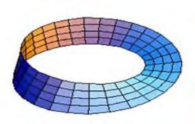
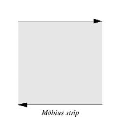
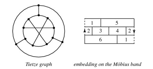
174
Klein Bottle
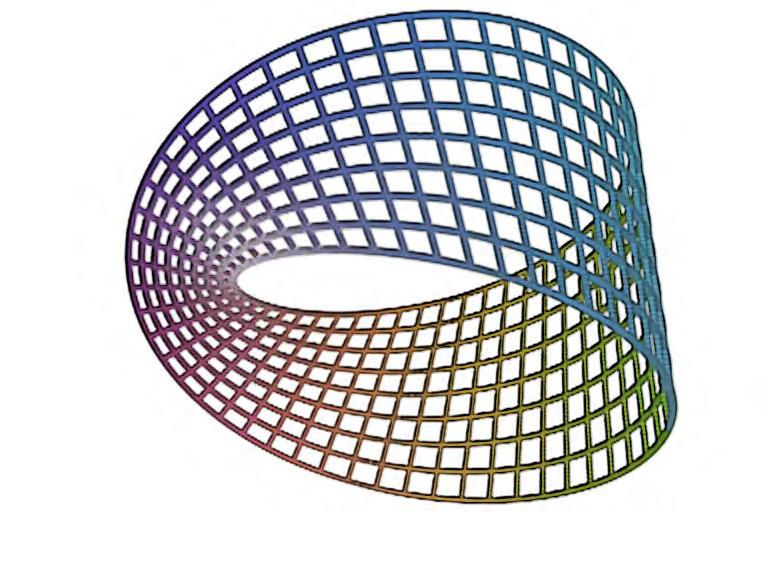
Option Explicit ‘Script written by <insert name> ‘Script copyrighted by <insert company name> ‘Script version 05 June 2009 20:34:27
Call Main() Sub Main()
Dim arrCount(1), arrPoints(), n,m,l,ustep,vstep,u,v,x,y,z,ustar t,uend,vstart,vend,num
Dim u_star t,u_end,d,surface,v_start,v_end,dd Dim i,j,u_list(),v_list() Dim num_step1,num_step2
Dim arrItems, arrValues, scale_factor
u_star t= Rhino.RealBox (“Enter where ‘u’ should start”, 0, “Define parameters range (u)”)
u_end= Rhino.RealBox (“Enter where ‘u’ should end”, 8*pi(), “Define parameters range (u)”)
j=-1
For i=u_start To u_end+0.1 Step pi() j=j+1
ReDim Preserve u_list(j) u_list( j)=i Next
v_star t= Rhino.RealBox (“Enter where ‘v’ should start”, -2, “Define parameters range (v)”) v_end= Rhino.RealBox (“Enter where ‘v’ should end”, 2, “Define parameters range (v)”)
j=-1
For i=v_start To v_end Step 0.5 j=j+1
ReDim Preserve v_list(j) v_list( j)=i
Next
m= Rhino.RealBox (“Enter tolerance for partitions in u direction”,10, “Step u direction”)
l= Rhino.RealBox (“Enter tolerance for partitions in v direction”,10, “Step v direction”)
scale_factor= Rhino.RealBox (“Enter scale factor for final continuous surface”, 1, “Scale Factor”)
arrItems=array(“U_Start”,”U_End”,”V_Start”,”V_End”,”Partitio ns_U”,”Partitions_V”)
arrValues=array(u_start,u_end,v_start,v_end,m,l)
Rhino.PropertyListBox arrItems, arrValues,”Check that values are correct”, “LIST OF PARAMETERS” d=0
‘ For i=0 To ubound(u_list)-1
ustar t=u_start ‘ dd=0
For j=0 To ubound(v_list) vstart=v_list(j) ustep= (u_end-ustart)/m vstep= (v_end-vstart)/l
For u = ustart To u_end Step ustep
For v = vstart To v_end Step vstep
x= (Sin(u)*(2+v*Sin(u/2)))
y= (Cos(u)*(2+v*Sin(u/2)))
z= (v*Cos(u/2))
ReDim Preserve
arrPoints(n)
arrPoints(n) = Array(scale_factor*x, scale_factor*y, scale_factor*z) n = n + 1 Next Next arrCount(0)=m arrCount(1)=l
CheckLayer “Surface”,1,1,1 Rhino.AddSrfPtGrid arrCount,arrPoints sur face=Rhino.LastObject Rhino.MoveObject surface, array(0,0,0),array(d*10 ,dd*10,0)
CheckLayer “Info”,0,0,0 Rhino.AddText “(U = “&CStr(ustart)&”,”&CStr(u_end)&”)”&”(V = “&CStr(vstart)&”,”&CStr(v_ end)&”)”,array(10*d,(-4+10*dd),0),1,,1 Rhino.ZoomExtents Rhino.CurrentView
n=0
ReDim arrPoints(n) dd=dd+1 Next
End Sub
175
The Roman surface is one of the three possible surfaces obtained by sewing a Möbius strip to the edge of a disk –the other two being the boy surface and cross-cap. It is a quartic non-orientable surface and it is also known as the Steiner surface.
The centre point of the Roman surface is an ordinary triple point with (±1,0,0) = (0, ±1,0) = (0,0, ±1), and the six endpoints of the three lines of self intersection are singular pinch points, also known as Whitney singularities. The Roman surface is essentially six cross-caps stuck together and contains a double infinity of conics.
The Roman surface can be given by the equation: (x2 + y2 + z2 – k2 ) =[ (z –k)2 – 2x2] [ (z + k)2 – 2 y2]
The Roman surface can also be generated using the general method for non-orientable surfaces using the polynomial function: F(x,y,z) = a (x,y,yz, zx)
Where by setting x = cos u sin v y = sin u sin v z = cos v in the former equation renders x(u,v) = ½ a sin(2u) sin2 v y(u,v) = ½ a sin u cos (2v) z(u,v) = ½ a cos u sin (2v) where u Є [0,2π] and v Є[-π /2,π /2] A short vbscript algorithm was written in Visual Basic for visualisation purposes.
176
Roman Surface
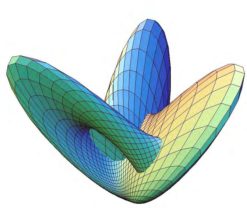
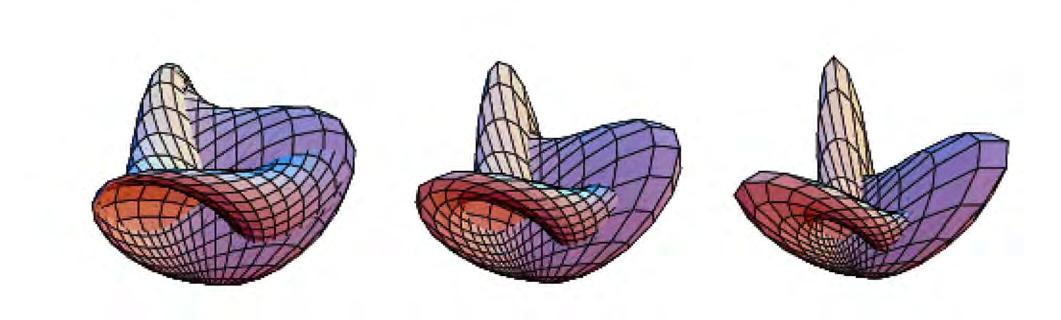
Option Explicit
‘Script written by <insert name>
‘Script copyrighted by <insert company name> ‘Script version 05 June 2009 20:34:27
Call Main()
Sub Main()
Dim arrCount(1), arrPoints(), n,m,l,ustep,vstep,u,v,x,y,z,ustar t,uend,vstart,vend,num
Dim u_star t,u_end,d,surface,v_start,v_end,dd
Dim i,j,u_list(),v_list() Dim num_step1,num_step2
Dim arrItems, arrValues, scale_factor,alfa
alfa= Rhino.IntegerBox (“Enter alfa value --> (0) for Roman Surface or (1) for Boy surface”,0, “alfa”)
u_star t= Rhino.RealBox (“Enter where ‘u’ should start”, 0, “Define parameters range (u)”)
u_end= Rhino.RealBox (“Enter where ‘u’ should end”, 2*pi(), “Define parameters range (u)”)
j=-1
For i=u_start To u_end Step pi()/2 j=j+1
ReDim Preserve u_list(j) u_list( j)=i Next
v_star t= Rhino.RealBox (“Enter where ‘v’ should start”, 0, “Define parameters range (v)”)
v_end= Rhino.RealBox (“Enter where ‘v’ should end”, 2*pi(), “Define parameters range (v)”)
j=-1
For i=v_start To v_end Step pi()/2 j=j+1
ReDim Preserve v_list(j) v_list( j)=i Next
m= Rhino.RealBox (“Enter tolerance for partitions in u direction”,50, “Step u direction”)
l= Rhino.RealBox (“Enter tolerance for partitions in v direction”,50, “Step v direction”)
scale_factor= Rhino.RealBox (“Enter scale factor for final continuous surface”, 1, “Scale Factor”)
arrItems=array(“U_Start”,”U_End”,”V_Start”,”V_End”,”Partitio ns_U”,”Partitions_V”)
arrValues=array(u_start,u_end,v_start,v_end,m,l)
Rhino.PropertyListBox arrItems, arrValues,”Check that values are correct”, “LIST OF PARAMETERS”
d=0
‘ For i=0 To ubound(u_list)-1
ustar t=u_start
‘
dd=0
For j=0 To ubound(v_list)
vstart=v_list(j)
ustep= (u_end-ustart)/m vstep= (v_end-vstart)/l
For u = ustart To u_end Step ustep For v = vstart To v_end Step vstep
x= (((2)^(1/2))*(cos(2*u))*(cos( v))^2+cos(u)*sin(2*v))/(2-alfa*((2)^(1/2))*sin(3*u)*sin(2*v)) y = (((2)^(1/2))*(sin(2*u))*(cos(v))^2-sin(u)*sin(2*v))/(2-alfa*((2)^(1/2))*si n(3*u)*sin(2*v)) z= (3*(cos(v))^2)/(2-alfa*((2)^( 1/2))*sin(3*u)*sin(2*v))
ReDim Preserve
arrPoints(n)
arrPoints(n) =
Array(scale_factor*x, scale_factor*y, scale_factor*z) n = n + 1 Next Next arrCount(0)=m arrCount(1)=l
CheckLayer “Surface”,1,1,1 Rhino.AddSrfPtGrid arrCount,arrPoints sur face=Rhino.LastObject Rhino.MoveObject surface, array(0,0,0),array(d*10 ,dd*10,0)
CheckLayer “Info”,0,0,0 Rhino.AddText “(U = “&CStr(ustart)&”,”&CStr(u_ end)&”)”&”(V = “&CStr(vstart)&”,”&CStr(v_end)&”)”&” “&”alfa = “&CStr(alfa),array(10*d,(-4+10*dd),0),0.5,,1 Rhino.ZoomExtents Rhino.CurrentView
n=0
ReDim arrPoints(n) dd=dd+1 Next
End Sub
177
Cross-Cap
The cross-cap can be thought of as the object produced by puncturing a surface a single time, attaching two zips around the puncture in the same direction, distorting the hole so that the zips line up, requiring that the surface intersect itself, and then zipping up. The crosscap can also be described as a circular hole which, when entered, exits from its opposite point -from a topological viewpoint, both singular points on the cross-cap are equivalent.
The cross-cap has a segment of double points which terminates at two “pinch points” known as Whitney singularities. A cross-handle is homeomorphic to two cross-caps. A sphere with one cross-cap has traditionally been called a real projective plane. While this is appropriate in the study of projective geometry when an affine structure is present, J. H. Conway advocates use of the term cross surface in a purely topological interpretation.
The cross-cap is one of the three possible surfaces obtained by sewing a Möbius strip to the edge of a disk. The other two are the Boy surface and Roman surface.
A sphere with two cross-caps having coinciding boundaries is topologically equivalent to a Klein bottle. The surface with three cross-caps is known as Dyck’s surface.
The cross-cap can be generated using the general method for non-orientable surfaces using the polynomial function:
F(x,y,z) = (x*z,y*z, ½ * (z2 – x2))
The transformation of the above equation into spherical coordinates gives:
x (u,v) = ½ *cos u * sin (2*v)
y (u,v) = ½ *sin u * sin (2*v)
z (u,v) = ½ *(cos2 v – cos2 u * sin2 v)
for u Є [0,2π] and v Є [0,π/2].
A short vbscript algorithm was written in Visual Basic for visualisation purposes.
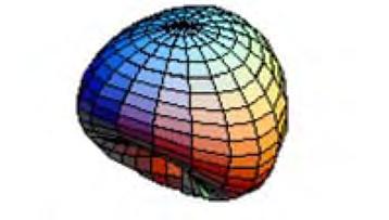

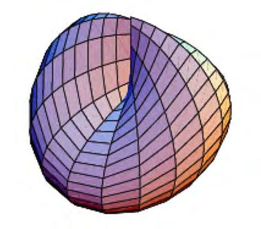
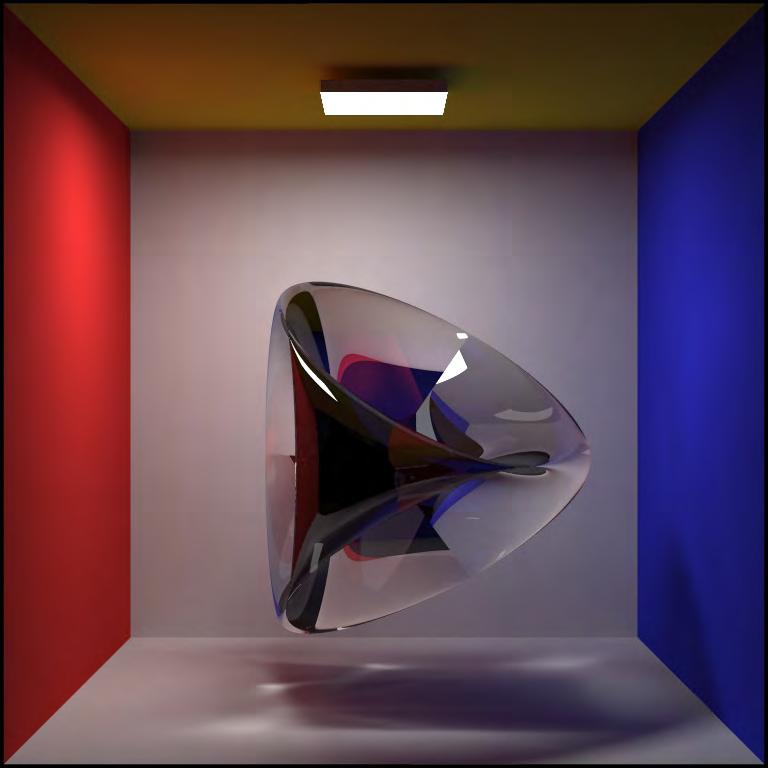
178
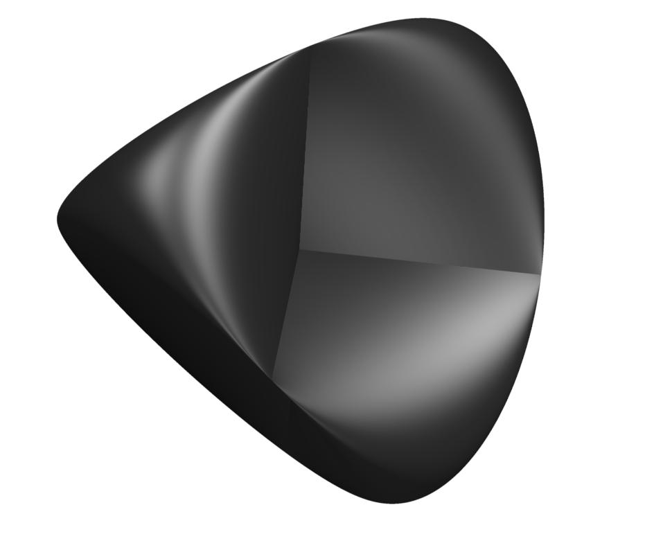
Option Explicit ‘Script written by <insert name> ‘Script copyrighted by <insert company name> ‘Script version 05 June 2009 20:34:27
Call Main() Sub Main()
Dim arrCount(1), arrPoints(), n,m,l,ustep,vstep,u,v,x,y,z,ustar t,uend,vstart,vend,num
Dim u_star t,u_end,d,surface(),v_start,v_end,dd Dim i,j,u_list(),v_list() Dim num_step1,num_step2
Dim arrItems, arrValues, scale_factor
u_star t= Rhino.RealBox (“Enter where ‘u’ should start”, 0, “Define parameters range (u)”)
u_end= Rhino.RealBox (“Enter where ‘u’ should end”, 2*pi(), “Define parameters range (u)”)
j=-1
For i=u_start To u_end Step 2*pi() j=j+1
ReDim Preserve u_list(j) u_list( j)=i
Next
v_star t= Rhino.RealBox (“Enter where ‘v’ should start”,0, “Define parameters range (v)”) v_end= Rhino.RealBox (“Enter where ‘v’ should end”,pi()/2, “Define parameters range (v)”)
j=-1
For i=v_start To v_end+0.1 Step pi()/2 j=j+1
ReDim Preserve v_list(j) v_list( j)=i
Next
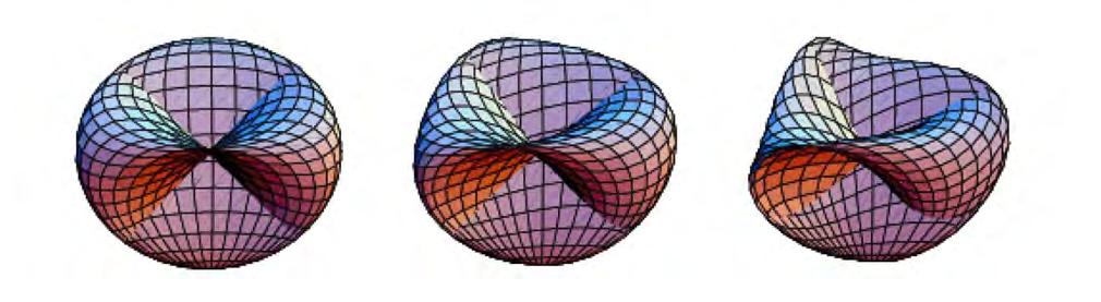
m= Rhino.RealBox (“Enter tolerance for partitions in u direction”,100, “Step u direction”)
l= Rhino.RealBox (“Enter tolerance for partitions in v direction”,100, “Step v direction”)
scale_factor= Rhino.RealBox (“Enter scale factor for final continuous surface”, 1, “Scale Factor”)
arrItems=array(“U_Start”,”U_End”,”V_Start”,”V_End”,”Partitio ns_U”,”Partitions_V”)
arrValues=array(u_start,u_end,v_start,v_end,m,l)
Rhino.PropertyListBox arrItems, arrValues,”Check that values are correct”, “LIST OF PARAMETERS”
d=0
‘ For i=0 To ubound(u_list)-1
ustar t=u_start
‘ dd=0
Dim k k=0
For j=0 To ubound(v_list) vstart=v_list(j) ustep= (u_end-ustart)/m vstep= (v_end-vstart)/l
For u = ustart To u_end Step ustep For v = vstart To v_end Step vstep
x= (1/2)*(cos(u))*(sin(2*v)) y= (1/2)*(sin(u))*(sin(2*v))
z= (1/2)*((cos(v))^2(((cos(u))^2)*((sin(v))^2)))
ReDim Preserve arrPoints(n) arrPoints(n) = Array(scale_ factor*x, scale_factor*y, scale_factor*z) n = n + 1
Next Next arrCount(0)=m arrCount(1)=l
CheckLayer “Surface”,1,1,1
ReDim Preserve surface(k) s urface(k)=Rhino.AddSrfPtGrid (arrCount,arrPoints)
If Rhino.IsSurface(surface(k)) Then Rhino.MoveObject rhino.lastobject, arrP oints(0),array(d*10,dd*10,0) Else
Rhino.AddText “No possible surface”,array(10*d,-1+10*dd,0),0.5,,1 End If
CheckLayer “Info”,1,1,1
Rhino.AddText “(U = “&CStr(ustart)&”,”&CStr(u_ end)&”)”&”(V = “&CStr(vstart)&”,”&CStr(v_end)&”)”,array(10*d,1+10*dd,0),0.2,,1
Rhino.ZoomExtents Rhino.CurrentView n=0
ReDim arrPoints(n) dd=dd+1 k=k+1 Next
End Sub
179
Boy Surface
The Boy surface is a non-orientable surface which constitutes one possible parametrisation of the surface obtained by sewing a Möbius strip to the edge of a disk. Two topologically equivalent parametrisations are the cross-cap and Roman surface. The Boy surface is a model of the projective plane without singularities and surface .
A sculpture of the Boy surface as was installed in front of the library of the Mathematic Forschungsinstitut Oberwolfach library building on January 28, 1991.
The Boy surface can be described using the general method for non-orientable surfaces, but this was not known until the analytic equations were found in 1986:
f1(x,y,z) = ½ [(2 x2 – y2 – z2) ( x2 + y2 + z2) + 2 y z (y2 – z2) + z x (x2 – z2) + x y (y2 – x2)]
=
-
) + x y (y2 – x2)]
f3(x,y,z) = 1/8 (x + y + z) [( x + y + z)3 + 4 (y – z) (z – y) (x – z)]
x = cos u sin v
y = sin u sin v
z = cos v where u Є [0,π] and v Є [0,π] to give the Boy surface from which three views are included in these section.
A short vbscript algorithm was written in Visual Basic for visualisation purposes.
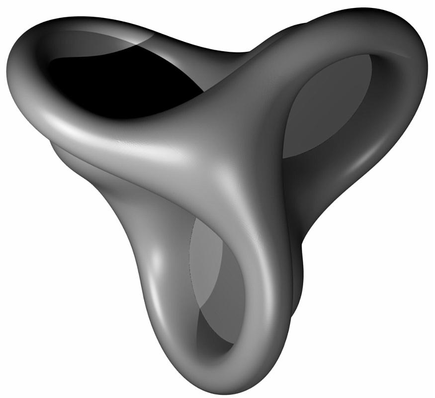
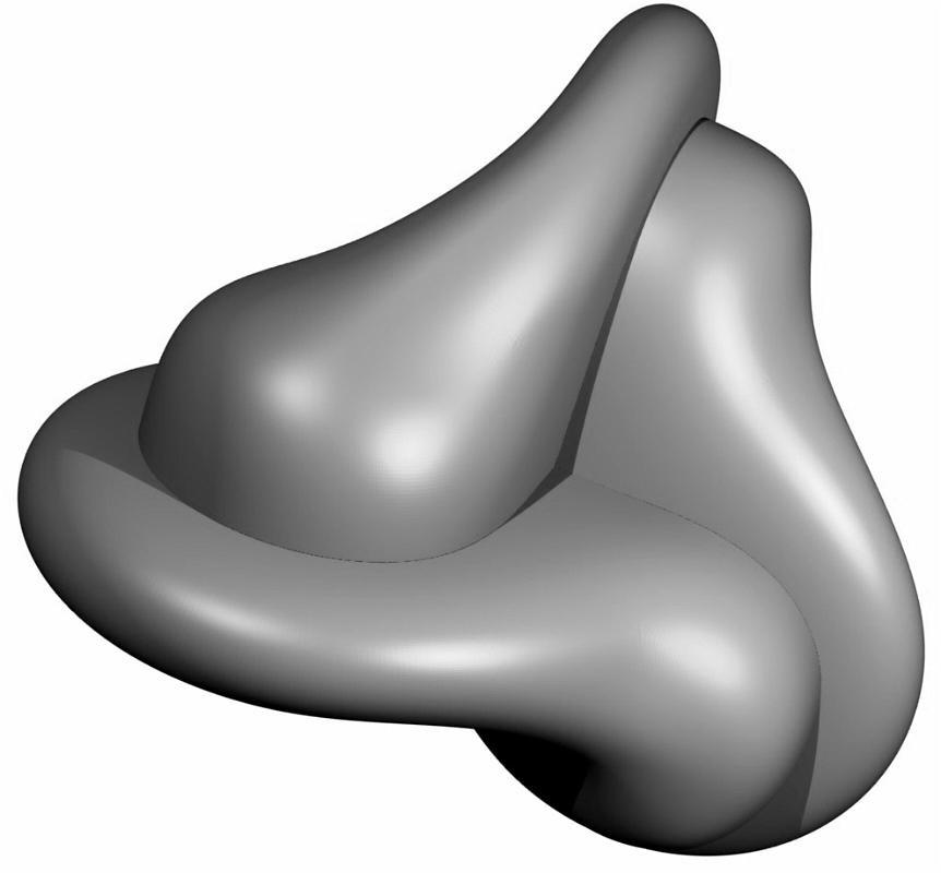
180
x2
x
f2(x,y,z)
½ (3)1/2 [ (y2 – z2) (
+ y2 + z2) + z
(z2
x2
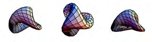
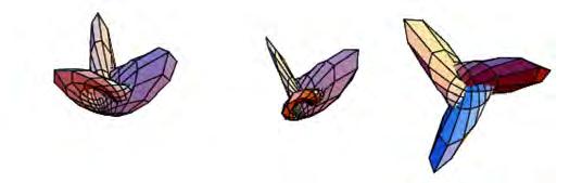

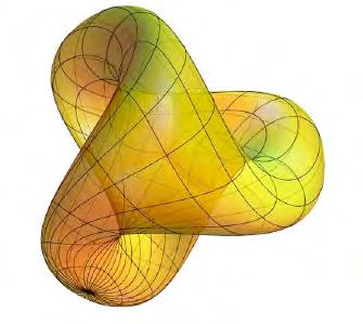
Option Explicit
‘Script written by <insert name>
‘Script copyrighted by <insert company name> ‘Script version 05 June 2009 20:34:27
Call Main()
Sub Main()
Dim arrCount(1), arrPoints(), n,m,l,ustep,vstep,u,v,x,y,z,ustar t,uend,vstart,vend,num
Dim u_star t,u_end,d,surface,v_start,v_end,dd
Dim i,j,u_list(),v_list() Dim num_step1,num_step2
Dim arrItems, arrValues, scale_factor,alfa
alfa= Rhino.IntegerBox (“Enter alfa value --> (0) for Roman Surface or (1) for Boy surface”,0, “alfa”)
u_star t= Rhino.RealBox (“Enter where ‘u’ should start”, 0, “Define parameters range (u)”)
u_end= Rhino.RealBox (“Enter where ‘u’ should end”, 2*pi(), “Define parameters range (u)”)
j=-1
For i=u_start To u_end Step pi()/2 j=j+1
ReDim Preserve u_list(j) u_list( j)=i Next
v_star t= Rhino.RealBox (“Enter where ‘v’ should start”, 0, “Define parameters range (v)”)
v_end= Rhino.RealBox (“Enter where ‘v’ should end”, 2*pi(), “Define parameters range (v)”)
j=-1
For i=v_start To v_end Step pi()/2 j=j+1
ReDim Preserve v_list(j) v_list( j)=i Next
m= Rhino.RealBox (“Enter tolerance for partitions in u direction”,50, “Step u direction”)
l= Rhino.RealBox (“Enter tolerance for partitions in v direction”,50, “Step v direction”)
scale_factor= Rhino.RealBox (“Enter scale factor for final continuous surface”, 1, “Scale Factor”)
arrItems=array(“U_Start”,”U_End”,”V_Start”,”V_End”,”Partitio ns_U”,”Partitions_V”)
arrValues=array(u_start,u_end,v_start,v_end,m,l)
Rhino.PropertyListBox arrItems, arrValues,”Check that values are correct”, “LIST OF PARAMETERS”
d=0
‘ For i=0 To ubound(u_list)-1
ustar t=u_start
‘
dd=0
For j=0 To ubound(v_list)
vstart=v_list(j)
ustep= (u_end-ustart)/m vstep= (v_end-vstart)/l
For u = ustart To u_end Step ustep For v = vstart To v_end Step vstep
x= (((2)^(1/2))*(cos(2*u))*(cos( v))^2+cos(u)*sin(2*v))/(2-alfa*((2)^(1/2))*sin(3*u)*sin(2*v)) y = (((2)^(1/2))*(sin(2*u))*(cos(v))^2-sin(u)*sin(2*v))/(2-alfa*((2)^(1/2))*si n(3*u)*sin(2*v)) z= (3*(cos(v))^2)/(2-alfa*((2)^( 1/2))*sin(3*u)*sin(2*v))
ReDim Preserve
arrPoints(n)
arrPoints(n) =
Array(scale_factor*x, scale_factor*y, scale_factor*z) n = n + 1 Next Next arrCount(0)=m arrCount(1)=l
CheckLayer “Surface”,1,1,1 Rhino.AddSrfPtGrid arrCount,arrPoints sur face=Rhino.LastObject Rhino.MoveObject surface, array(0,0,0),array(d*10 ,dd*10,0)
CheckLayer “Info”,0,0,0 Rhino.AddText “(U = “&CStr(ustart)&”,”&CStr(u_ end)&”)”&”(V = “&CStr(vstart)&”,”&CStr(v_end)&”)”&” “&”alfa = “&CStr(alfa),array(10*d,(-4+10*dd),0),0.5,,1 Rhino.ZoomExtents Rhino.CurrentView
n=0
ReDim arrPoints(n) dd=dd+1 Next
End Sub
181
Algorithms
Local Geometry
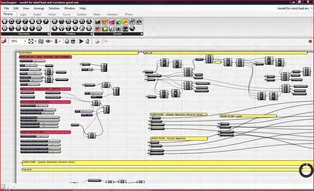
Suture Curves & Continuous Surfaces
This section covers the modelling of the local geometry in Grasshopper, the associative design software designed to work with Rhinoceros.
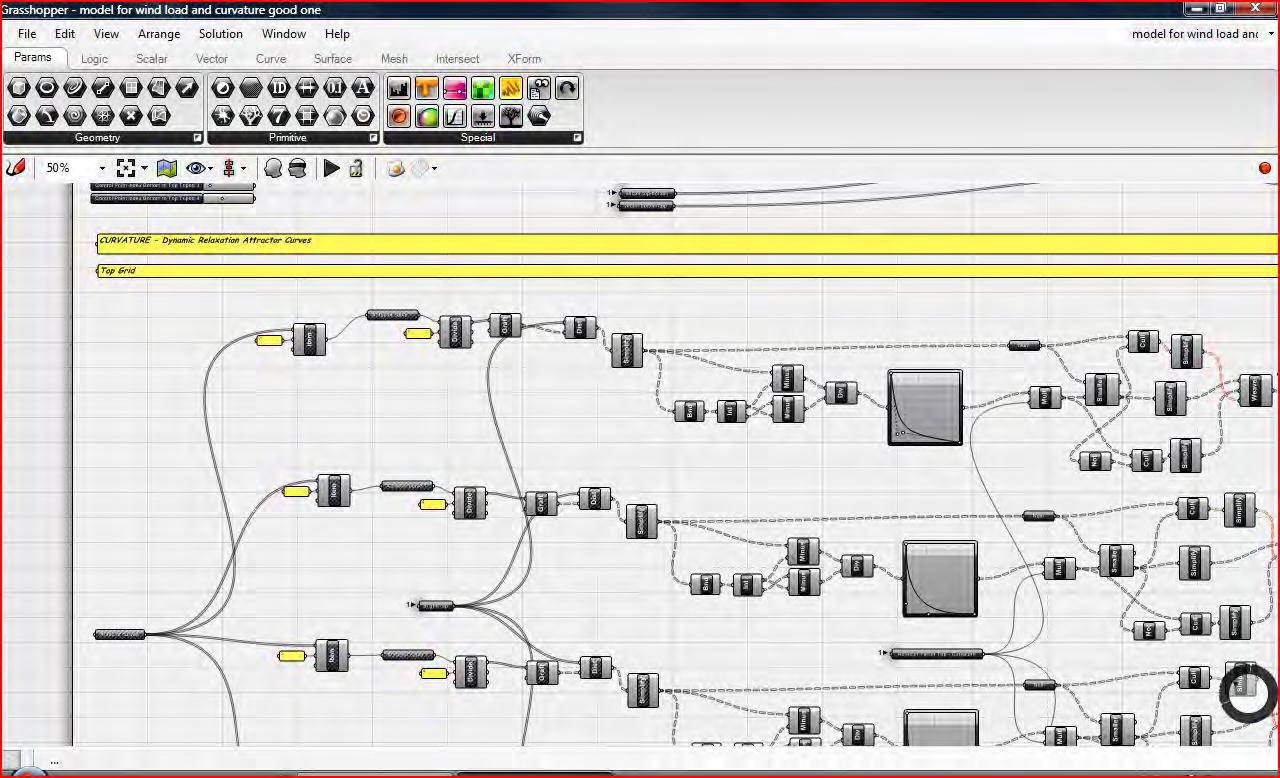
182
Grasshopper Model
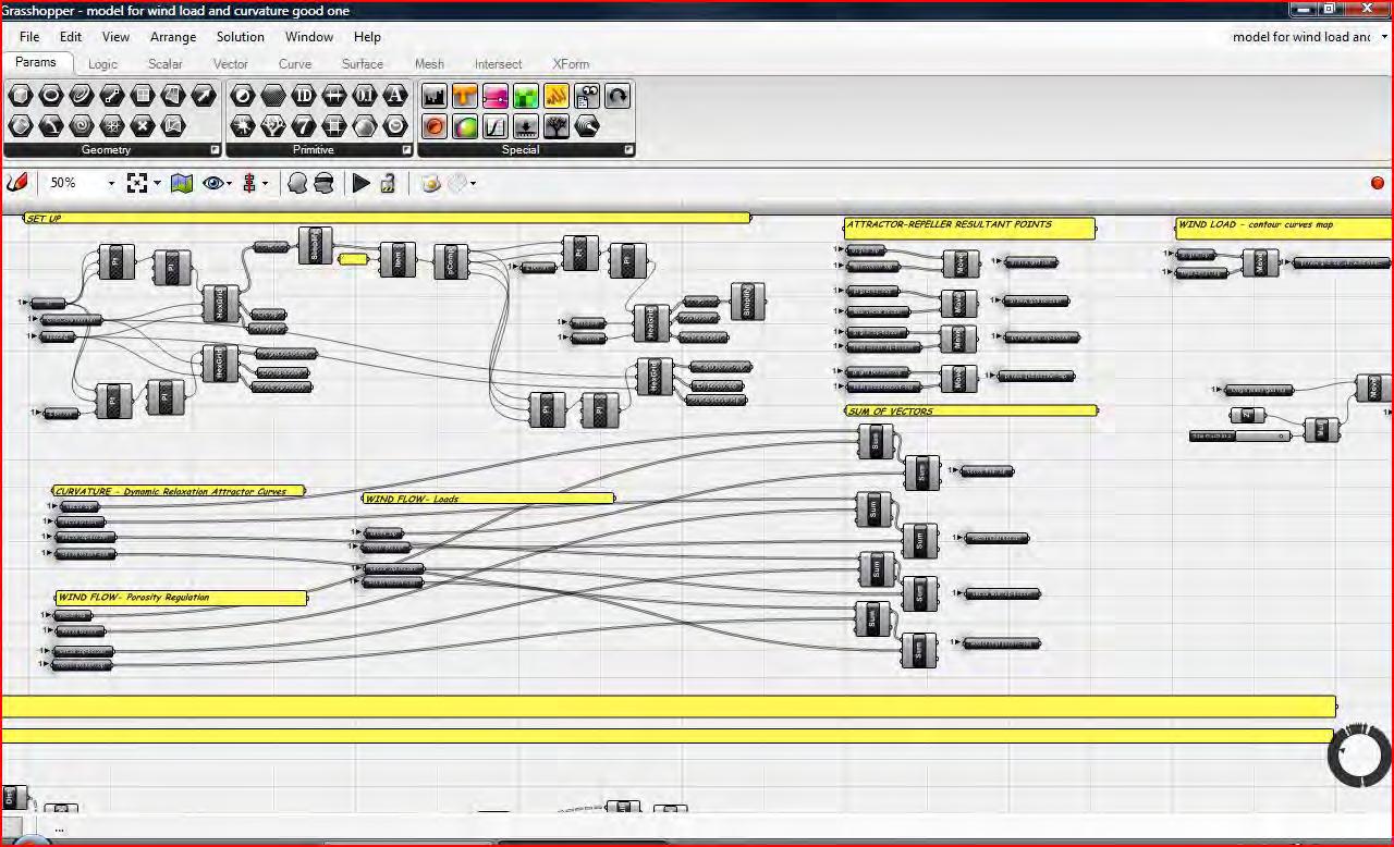
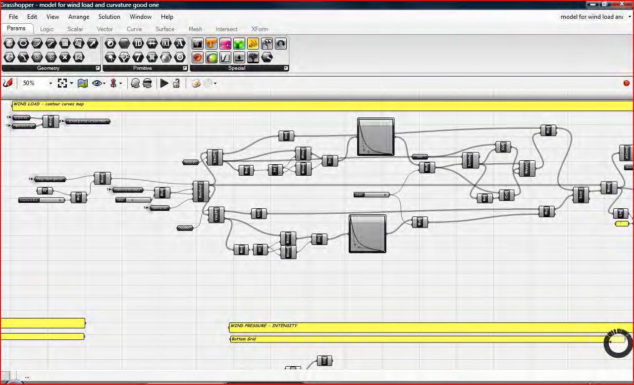
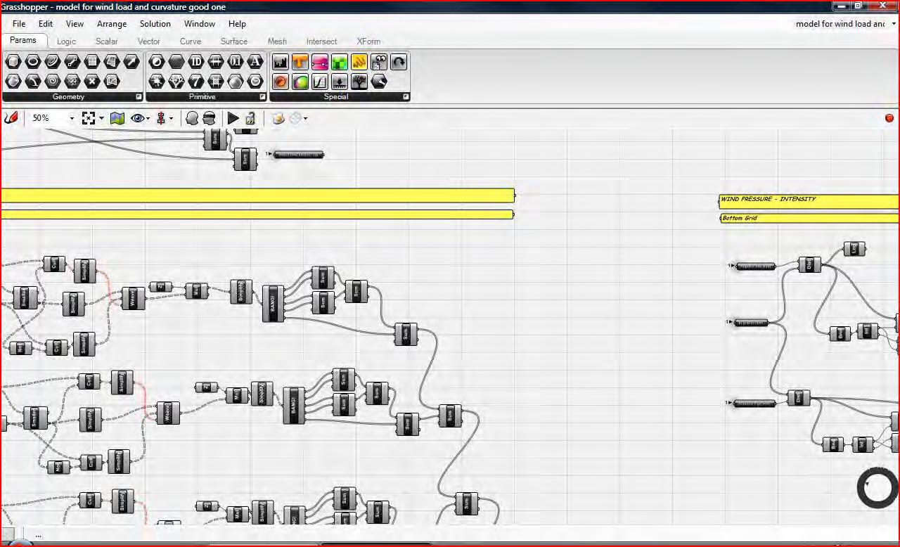
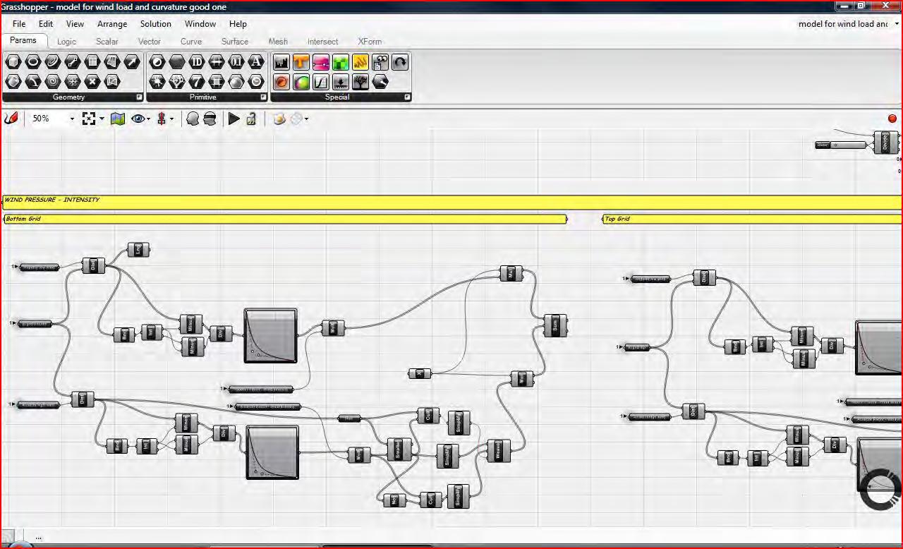
183
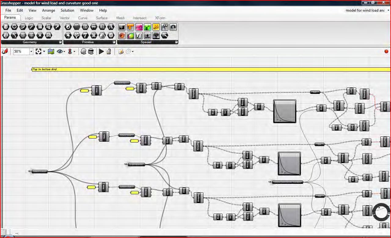
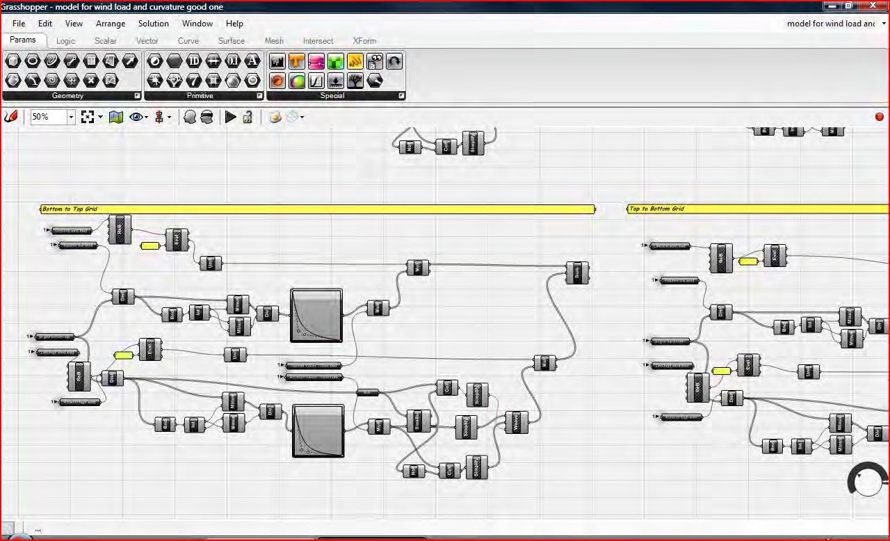

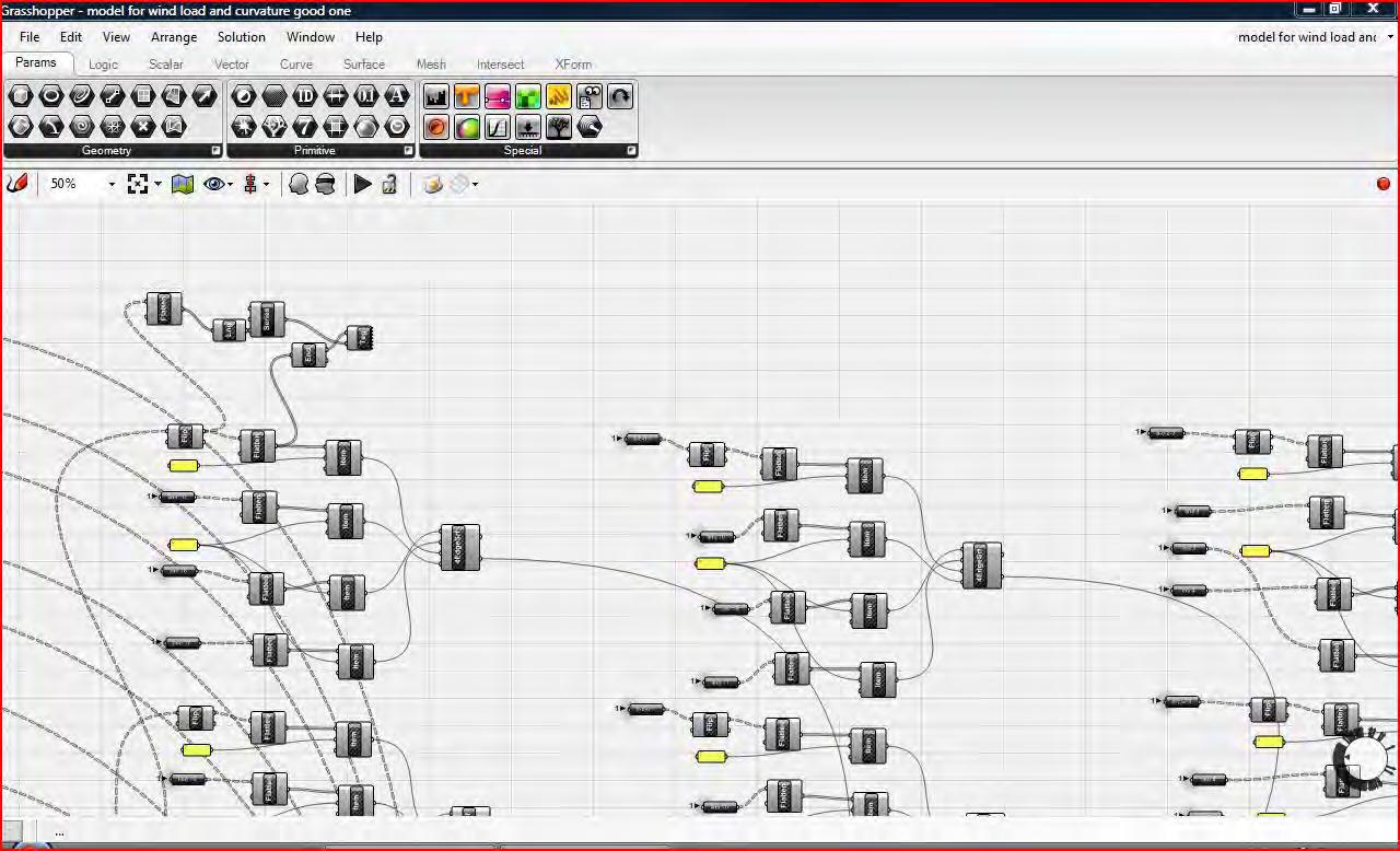
184
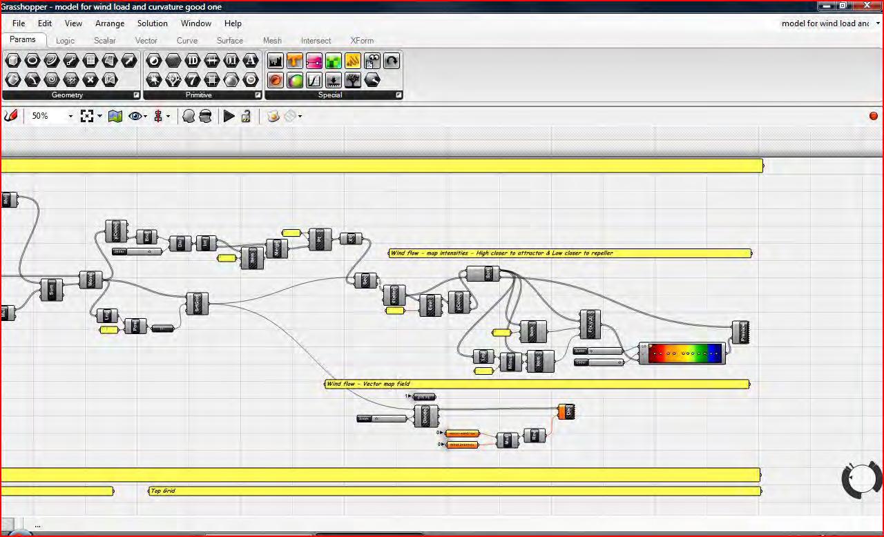
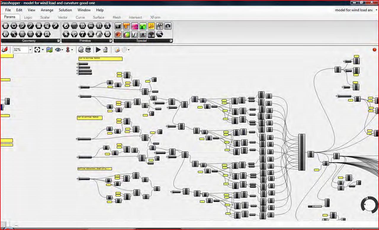
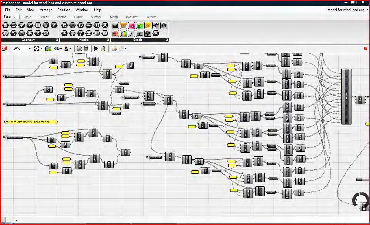

185
Global Geometry

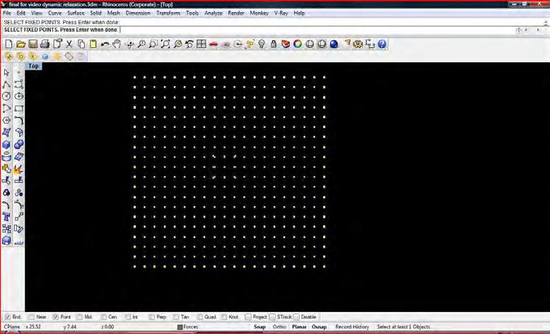
Form Finding
This section covers the ‘form finding’ algorithm written in visual basic to generate the morphology of the global geometry.
A visual diagram accompanies the code and shows the ‘in-house’ designed interface of the algorithm.
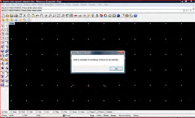

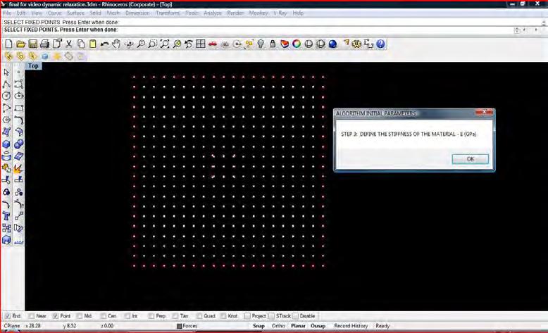
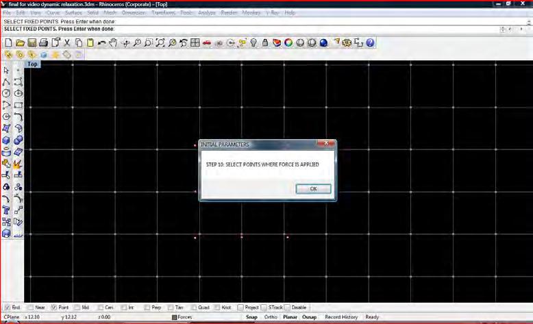
186
Vbscript Model
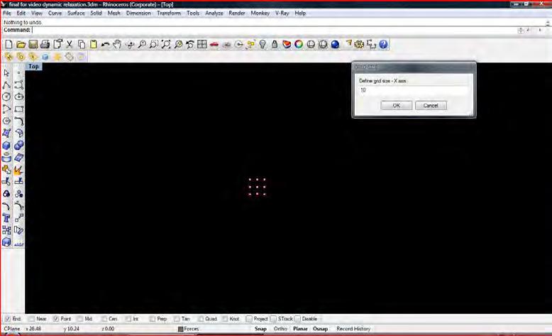

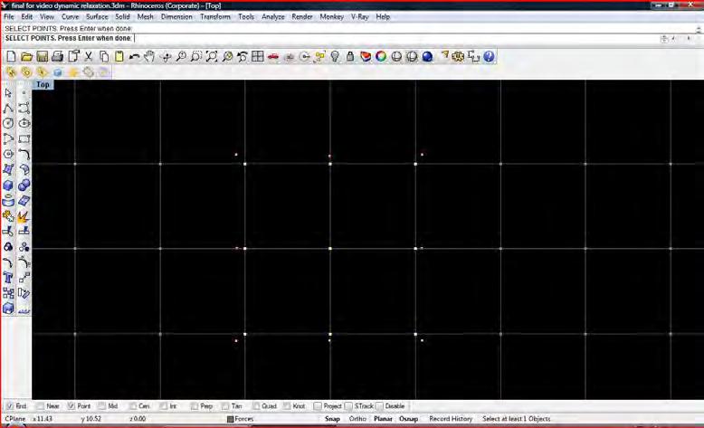
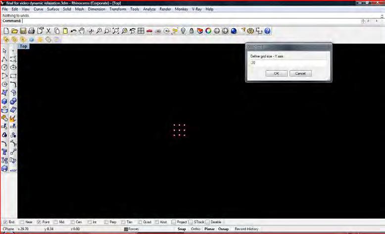

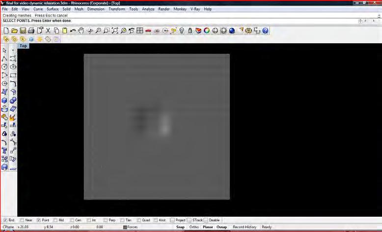

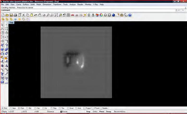
187
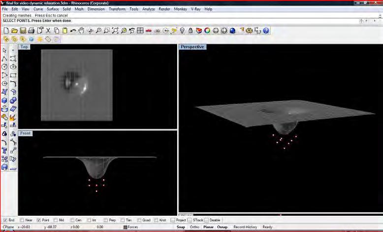
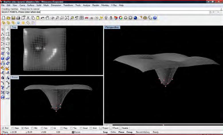
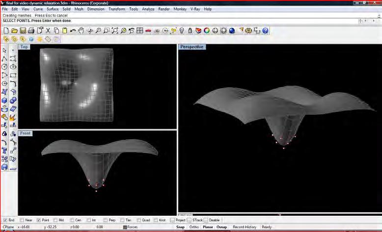

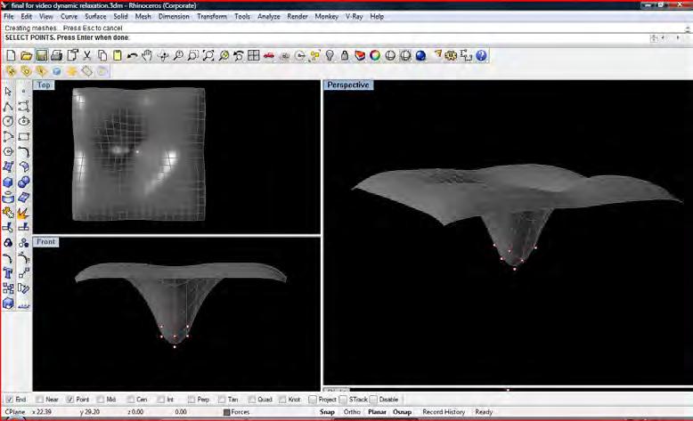


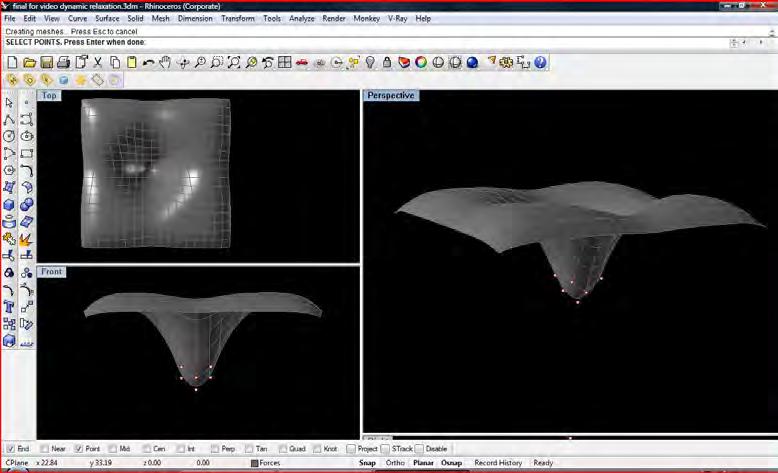
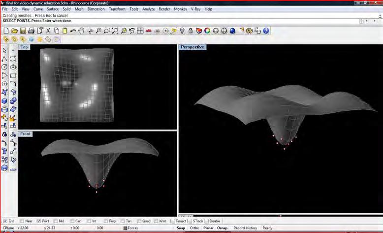
188
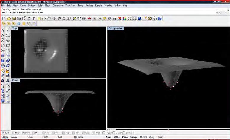
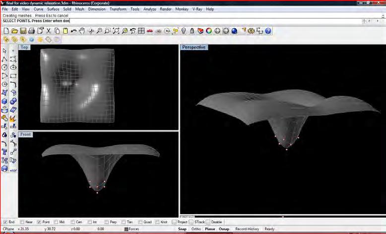
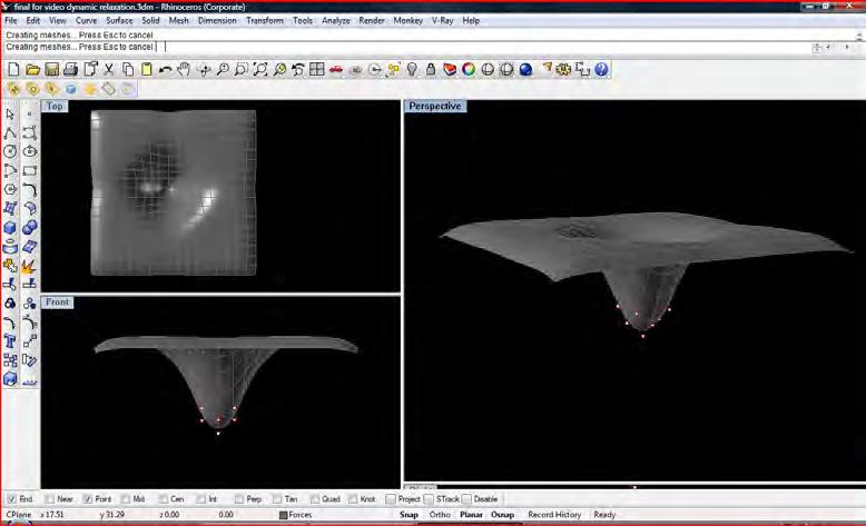

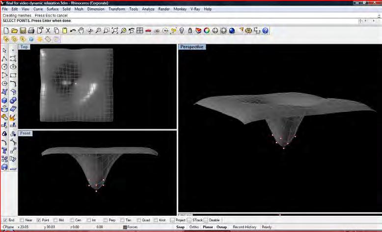

189
Option Explicit
‘Script written by <Maria Mingallon>
‘Script version 29 July 2009 - London UK
Call Main()
Sub Main()
Dim nx,ny,mx,my
Dim npr t,prts(),i,iy,ix
Dim x,y,z
Dim p,v,a,m,o
‘’-- block screen (for speed)
rhino.enableredraw False
‘’{{{-- SYSTEM SETUP ----------------------------------------------------
‘’-- define grid size
Rhino.MessageBeep 2
Rhino.MessageBox “STEP 1: DEFINE THE GRID SIZE”,0, “ALGORITHM INITIAL PARAMETERS”
nx=Rhino.IntegerBox (“Define grid size - X axis”, 10, “GRID SIZE”)
ny=Rhino.IntegerBox (“Define grid size - Y axis”, 10, “GRID SIZE”)
mx = nx-1
my = ny-1 ‘’----------------------------------------------------------------------------
‘’-- define points/particles/nodes npr t = nx * ny
Dim gridcount(1),pgrid()
gridcount(0)=nx
gridcount(1)=ny
i = 0 for iy = 0 to my for ix = 0 to mx
‘’-- par ticle coordinates
x = ix y = iy
z = 0
‘’-- particle properties: position, velocity, acceleration, mass, graphic
p = array( x, y, z )
v = array( 0.0, 0.0, 0.0 )
a = array( 0.0, 0.0, 0.0 )
m = 1.0
o = rhino.addpoint( p )
ReDim Preserve prts(i)
pr ts( i ) = array( p, v, a, m, o )
‘’--prepare array for printing a surface from control points in the grid
‘’--prepare the array prts into pgrid which contains only the initial position of the points
ReDim Preserve pgrid(i) pgrid(i)=prts(i)(0) i = i + 1
Next
Next rhino.enableredraw True
‘’--print Grid as a NURBS SURFACE from Control points, KnotU, KnotV, degree of surface and weights at each point
Dim gridsurface
Dim arrDegree arrDegree=array(3,3)
Dim arrKnotU(),KnotUcount
‘number of elements in arrKnotU = arrPointCount(0) + arrDegree(0) - 1
KnotUcount=gridcount(0)+arrDegree(0)-1
For i=0 To KnotUcount-1
ReDim Preserve arrKnotU(i) arrKnotU(i)= (gridcount(0)/(KnotUcount))*i
Next
Dim arrKnotV(),KnotVcount
‘number of elements in arrKnotV = arrPointCount(0) + arrDegree(0) - 1
KnotVcount=gridcount(1)+arrDegree(1)-1
For i=0 To KnotVcount-1
ReDim Preserve arrKnotV(i) arrKnotV(i)= (gridcount(1)/(KnotUcount))*i
Next
‘Set up weights for each control point of the surface ‘At this moment all points are set up with equal weight (min value = 1)
Dim arrWeights()
For i=0 To ubound(pgrid)
ReDim Preserve arrWeights(i) arrWeights(i)=1
‘’-- define fixed points --> zero mass
Dim fixed_points,j,ii
Rhino.MessageBeep 2
Rhino.MessageBox “STEP 2: SELECT FIXED POINTS (SUPPORTS)”,0, “ALGORITHM INITIAL PARAMETERS”
fixed_points=Rhino.GetObjects (“SELECT FIXED POINTS”,1)
For j=0 To ubound(fixed_points) For ii=0 To nprt-1 If prts(ii)(4)=fixed_points(j)Then pr ts(ii)(3)=0.0 arrWeights(ii)=1
Rhino.ObjectColor fixed_ points(j), RGB(255,0,0)
End If Next Next
rhino.enableredraw False
‘’-- par ticle property mnemonic
Dim PRT_P,PRT_V,PRT_A,PRT_M,PRT_O
PRT_P = 0 ‘’ position
PRT_V = 1 ‘’ velocity
PRT_A = 2 ‘’ acceleration/force
PRT_M = 3 ‘’ mass
PRT_O = 4 ‘’ point object
‘ for num_of_fixed = 0 to 5
‘ pr ts( int( rnd * mx ) + int( rnd * my ) * nx )( PRT_M ) = 0.0 next
Dim ia,ib,ic,id
Dim k,l,d
‘’--get stiffness
Rhino.MessageBeep 2
Rhino.MessageBox “STEP 3: DEFINE THE STIFFNESS OF THE MATERIAL - E (GPa)”,0, “ALGORITHM INITIAL PARAMETERS”
Rhino.RealBox “E (GPa)”,3.1,”ALGORITHM INITIAL PARAMETERS”
k=5
‘’--get damping ratio
Rhino.MessageBeep 2
Rhino.MessageBox “STEP 4: DEFINE THE DAMPING RATIO OF THE SYSTEM - d (no units)”,0, “ALGORITHM INITIAL PARAMETERS”
d=Rhino.RealBox (“d (no units)”,0.5,”ALGORITHM INITIAL PARAMETERS”)
‘’-- define edges/springs/lines
Dim nedg,edgs()
nedg = ny * mx + nx * my
i = 0 for iy = 1 to my for ix = 1 to mx
‘’-- get global offset from local offset in particle grid
‘’-- the following is to draw the lines in the grid:
‘’-- starting from a point, back, then in diagonal and then above
ia = ( ix - 0 ) + ( iy - 0 ) * nx ‘’-- current
- 1 ) * nx ‘’-- above
k = 2.00 ‘’-- stiffness = 1.00 ‘’-- rest length d = 0.50 ‘’-- damping
‘’--with the following an ‘L’ is drawn ‘’-- current->before
CheckLayer “Lines”,1,1,1
o = rhino.addline( prts( ia )( PRT_P ), prts( ib )( PRT_P ) )
ReDim Preserve edgs(i)
edgs( ) = array( ia, ib, k, l, d, o ) = i + 1
‘’-- current->above
o = rhino.addline( prts( id )( PRT_P ), prts( ia )( PRT_P ) )
REdim preserve edgs(i) edgs( ) = array( id, ia, k, l, d, o ) = i + 1
‘’draw first column (it was left by the code above)
‘’-- handle first column f( ix = 1 ) Then
o = rhino.addline( prts( ib )( PRT_P ), prts( ic )( PRT_P ) )
REdim preserve edgs(i) edgs( i ) = array( ib, ic, k, l, d, o ) i = i + 1 end if
‘’draw first row (it was left by the code above)
‘’-- handle first row f( iy = 1 ) Then
o = rhino.addline( prts( ic )( PRT_P ), prts( id )( PRT_P ) )
Next
REdim preserve edgs(i) edgs( i ) = array( ic, id, k, l, d, o ) i = i + 1 end if
190
‘’----------------------------------------------------------------------------
ib = ( ix - 1 ) + ( iy - 0 ) * nx
ic = ( ix - 1 ) + ( iy - 1 ) * nx
id =
iy
‘’-- before
‘’-- diagonal
( ix - 0 ) + (
‘’-- spring property mnemonic
Dim EDG_s,EDG_E,EDG_K,EDG_L,EDG_D,EDG_O
EDG_S = 0 ‘’-- start
EDG_E = 1 ‘’-- end
EDG_K = 2 ‘’-- stiffness
EDG_L = 3 ‘’-- rest length
EDG_D = 4 ‘’-- damping
EDG_O = 5 ‘’-- line object ‘’-------------------------------------------------------------------------}}}
‘’{{{-- OBTAIN THE REST OF THE INITIAL PARAMETERS PRIOR TO START SIMULATION --
Dim iteration,iterations
Dim iedg edg,si,ei,sp,ep
Dim u,f,s,sf,ef,iprt
Dim g
Dim delta
Dim ext_f_vector(),ext_f_vector_x,ext_f_vector_y,ext_f_ vector_z,ext_f_values(),ext_f_number
‘Get iterations
Rhino.MessageBeep 2
Rhino.MessageBox “STEP 5: DEFINE MAX NUMBER OF ITERATIONS”,0,”INITIAL PARAMETERS”
iterations=Rhino.RealBox (“iterations”,1000,”ALGORITHM INITIAL PARAMETERS”)
‘Get gravity value
‘Rhino.MessageBeep 2
‘Rhino.MessageBox “STEP 6: DEFINE ACCELERATION OF GRAVITY - Low value for slow variation”,0,”ALGORITHM INITIAL PARAMETERS”
‘g=Rhino.RealBox (“GRAVITY”,0.005,”ALGORITHM INITIAL PARAMETERS”)
g=0.005
‘’Get External forces (Point of application, direction and value)
‘How many forces to be applied (ONE BY DEFAULT)
Rhino.MessageBeep 2
Rhino.MessageBox “STEP 8: NUMBER OF EXTERNAL FORCES TO BE APPLIED”,0,”INITIAL PARAMETERS”
ext_f_number=Rhino.IntegerBox (“NUMBER OF FORCES”,1,”ALGORITHM INITIAL PARAMETERS”)
For i=0 To 7
ReDim Preserve ext_f_vector(i) ext_f_vector(i)=array(0,0,-1)
ReDim Preserve ext_f_values(i) ext_f_values(i)=0.7
Next
rhino.enableredraw True
Dim ext_f_points,ext_f_indexes()
Rhino.MessageBeep 2
Rhino.MessageBox “STEP 10: SELECT POINTS WHERE FORCE IS APPLIED”,0, “INITIAL PARAMETERS”
ext_f_points=Rhino.GetObjects (“SELECT POINTS”,1)
For j=0 To ubound(ext_f_points)
For ii=0 To nprt-1 If prts(ii)(4)=ext_f_points(j)Then
ReDim Preserve ext_f_ indexes(j)
ext_f_indexes(j)=ii
Rhino.ObjectColor ext_f_ points(j), RGB(255,0,0) End f Next Next
Dim points_start()
For iprt=0 To nprt-1
ReDim Preserve points_start(iprt) points_start(iprt)=prts(iprt)(PRT_O) Next
Rhino.AddLayer “Points”, RGB(0, 0, 255)
Rhino.ObjectLayer points_start, “Points” Rhino.LayerVisible “Points”, False
gridsurface=Rhino.AddNurbsSurface (gridcount, pgrid, arrKnotU, arrKnotV, arrDegree, arrWeights)
rhino.enableredraw False
‘’{{{-- SIMULATION -------------------------------------------------------
pr ts( iprt )( PRT_A )( VECTOR_X ) = 0.0
pr ts( iprt )( PRT_A )( VECTOR_Y ) = 0.0
pr ts( iprt )( PRT_A )( VECTOR_Z ) = 0.0 next
are opposite!)
For iteration = 0 To iterations
‘’-- reset forces/accelerations
‘’-- all the grid points to have starting acceleration of 0,0,0 at the start of each iteration for iprt = 0 to nprt - 1
‘’COMPUTE INTERNAL FORCES
‘’-- compute spring forces
‘’-for iedg = 0 to nedg - 1
‘’-- select edge edg = edgs( iedg )
si = edg( EDG_S ) ‘’-- index of start particle
ei = edg( EDG_E ) ‘’-- index of end particle
sp = prts( si ) ‘’-- particle at start of spring
ep = prts( ei ) ‘’-- particle at end of spring
‘’-- spring position and velocity differences
u = vector_create( ep( PRT_P ), sp( PRT_P ) ) ‘’-- displacement (used for force)
v = vector_create( ep( PRT_V ), sp( PRT_V ) ) ‘’-- relative motion (used for damping)
‘’-- par ticle distance -> displacement
‘’-- lo --> length at rest
l = vector_length( u )
‘’-- spring law F = k * ( Lf -lo ) --> lo length at rest and Lf length when compressed
‘’-- formula is usually F= -k * x --> in this case the (-) sign comes from (Lf- lo) assuming Lf < lo
f = edg( EDG_K ) * ( l - edg( EDG_L ) )
‘’-- damping (force against motion/ velocity between particle hence dot/l)
‘’-- damping = - c * v in our case c = d (constant) and v is the velocity
‘’-- the dot product is u . v = ¦u¦*¦v¦*cos (tita)
‘’-- if tita = 90, then u . v = 0
‘’-- if tita = 0 (parallel displacement and velocity) then u v = ¦u¦*¦v¦ and then
‘’-- ( u v) / l = (¦u¦ * ¦v¦ )/ ¦u¦ --> damping force = d = c * v
d = edg( EDG_D ) * ( vector_dot( u, v ) / l )
‘’-- sum spring force
s = f + d
‘’-- start/end particle force vectors (they
sf = vector_rescale( u, -s )
ef = vector_rescale( u, s )
‘’-- accumulate forces
pr ts( si )( PRT_A ) = vector_add( prts( si ) ( PRT_A ), sf )
pr ts( ei )( PRT_A ) = vector_add( prts( ei ) ( PRT_A ), ef ) next
‘’-- compute gravity force ‘’--
g = 0.5 ‘’ acceleration of gravity
For iprt = 0 To nprt - 1
‘’-- gravity force ( F = m * g ) f = vector_new( 0.0, 0.0, ((g) * prts( iprt )( PRT_M )) )
‘’-- accumulate forces pr ts( iprt )( PRT_A ) = vector_add( prts( iprt )( PRT_A ), f ) Next
‘’-- compute external forces
‘’-- external forces defined as a vector by the user ‘’’’’number of forces ‘’’’’direction (x,y,z) components -- unit vector ‘’’’’value (KN)
For i = 0 To ubound(ext_f_indexes) ipr t=ext_f_indexes(i)
For ii = 0 To ubound(ext_f_vector)
f = array(ext_f_vector(ii) (0)*ext_f_values(ii),ext_f_vector(ii)(1)*ext_f_values(ii),ext_f_vector(ii) (2)*ext_f_values(ii))
‘’-- accumulate forces pr ts( iprt )( PRT_A ) = vector_ add( prts( iprt )( PRT_A ), f ) arrWeights(iprt)=1
191
‘’-----------------------------------------------------------------
‘’-----------------------------------------------------------------
‘ ‘’-----------------------------------------------------------------
Next Next Next
a = vector_new( 0.0, 0.0, 0.0 )
‘’-- zero mass -> zero acceleration/force
end if pr ts( iprt )( PRT_V ) = vector_add( prts( iprt )( PRT_V ), a )
next
‘’-- compute viscous drag (aka friction) ‘’-d = 1.2 ‘’ drag coefficient for iprt = 0 to nprt - 1
‘’-- drag force ( F = - d * v ) force = agaist a fraction of velocity
f = vector_scale( prts( iprt )( PRT_V ), -d )
‘’-- accumulate forces pr ts( iprt )( PRT_A ) = vector_add( prts( iprt )( PRT_A ), f )
‘’-- draw forces
‘ for iprt = 0 to nprt - 1
‘ p = pr ts( iprt )( PRT_P )
‘ f = pr ts( iprt )( PRT_A )
‘ = rhino.addline( p, vector_add( p, f ) )
‘ if( not isnull( l ) ) then call rhino.objectcolor( l, vbred )
‘ next
‘’-- integrate positions using an euler solver
‘’-- this induces errors for large time steps!
‘’--
Dim dt
dt = 0.01 ‘’-- time step for iprt = 0 to nprt - 1
‘’-- position ( p_new = p_old + dp/dt = p_old + v )
v = vector_scale( prts( iprt )( PRT_V ), dt )
pr ts( iprt )( PRT_P ) = vector_add( prts( iprt )( PRT_P ), v )
‘’-- velocity ( v_new = v_old + dv/dt = v_old + a = v_old + f / m )
if( pr ts( iprt )( PRT_M ) <> 0 ) then
a = vector_scale( prts( iprt )( PRT_A ), dt / prts( iprt )( PRT_M ) ) else
) = ymax
) then
) = zmin
‘’-- some safety rules against explosions
‘’-- or pseudo inelastic collision
‘’-- ie don’t allow particles outside a maximum volume
‘’--
Dim xmin,ymin,zmin
Dim xmax,ymax,zmax
Dim reset
delta = u or v (at least) ‘’-- a bounding cube size
delta=nx
xmin = - delta: xmax = delta
ymin = - delta: ymax = delta zmin = - delta: zmax = delta
Rhino.AddLayer “Lines”, RGB(225, 100, 20)
Rhino.LayerVisible “Lines”, False
for iprt = 0 to nprt - 1
‘’-- on explosion reset velocity reset = false
‘’-- xmin < position.x < xmax
if( prts( iprt )( PRT_P )( VERTEX_X ) < xmin ) then
pr ts( iprt )( PRT_P )( VERTEX_X ) = xmin
reset = true
elseif( prts( iprt )( PRT_P )( VERTEX_X ) > xmax ) then
pr ts( iprt )( PRT_P )( VERTEX_X ) = xmax
end if
reset = true
‘’-- ymin < position.y < ymax
if( prts( iprt )( PRT_P )( VERTEX_Y ) < ymin ) then
pr ts( iprt )( PRT_P )( VERTEX_Y ) = ymin
reset = true
elseif( prts( iprt )( PRT_P )( VERTEX_Y ) > ymax ) then
pr ts( iprt )( PRT_P )( VERTEX_Y
end if
reset = true
‘’-- zmin < position.z < zmax if( prts( iprt )( PRT_P )( VERTEX_Z ) < zmin
pr ts( iprt )( PRT_P )( VERTEX_Z
reset = true elseif( prts( iprt )( PRT_P )( VERTEX_Z ) > zmax ) then
) = zmax
pr ts( iprt )( PRT_P )( VERTEX_Z
reset = True
end if
‘’-- exploded! if( reset ) then pr ts( iprt )( PRT_V )( VERTEX_X
rhino.deleteobject edgs( iedg )( EDG_O )
si = edgs( iedg )( EDG_S ) ei = edgs( iedg )( EDG_E )
sp = pr ts( si )
ep = pr ts( ei ) edgs( iedg )( EDG_O ) = rhino. addline( sp( PRT_P ), ep( PRT_P ) )
Rhino.ObjectLayer edgs( iedg ) ( EDG_O ), “Lines” Next
‘’-- ok show! rhino.enableredraw True
) = 0.0
) = 0.0
) = 0.0
pr ts( iprt )( PRT_V )( VERTEX_Y
pr ts( iprt )( PRT_V )( VERTEX_Z
end if next
‘’-- unblock screen rhino.enableredraw True
Rhino.AddLayer “Supports”, RGB(255, 0, 0)
Rhino.AddLayer “Forces”, RGB(0, 255,0)
If( iteration Mod 10 = 0 ) Then
‘’-- graphics time! rhino.enableredraw False
‘’-- update particles and control points of grid(just update) for iprt = 0 to nprt - 1 rhino.pointcoordinates prts( iprt )( PRT_O ), prts( iprt)( PRT_P ) ReDim Preserve newpgrid(iprt) n ewpgrid(iprt)=prts(iprt) (PRT_P)
Next
‘’-- delete previous grid surface and redraw it with new coordinates rhino.deleteobject gridsurface
g ridsurface=Rhino.AddNurbsSurface (gridcount, newpgrid, arrKnotU, arrKnotV, arrDegree, arrWeights)
‘’-- update
edges (delete and redraw) For iedg = 0 To nedg - 1
For i=0 To ubound(fixed_points)
Rhino.ObjectLayer fixed_points(i), “Supports” Next
For i=0 To ubound(ext_f_points)
Rhino.ObjectLayer ext_f_points(i), “Forces” Next
Rhino.AddLayer “Grid Surface”, RGB(255, 255, 255)
Rhino.ObjectLayer gridsurface, “Grid Surface” Rhino.LayerVisible “Grid Surface”, True
Dim pointsA(),pointsB()
Dim i1,i2
Dim half_limit half_limit=((ubound(newpgrid)+1)/2)-1
For i1=0 To half_limit
ReDim Preserve pointsA(i1) pointsA(i1)=newpgrid(i1) Next
192
‘’-----------------------------------------------------------------
End If Next ‘’-------------------------------------------------------------------------}}}
Next ‘’-----------------------------------------------------------------
next ‘’-----------------------------------------------------------------
‘’-----------------------------------------------------------------
’-----------------------------------------------------------------
Dim counter counter=-1
For i2=half_limit+1 To ubound(newpgrid) counter=counter+1
ReDim Preserve pointsB(i2) pointsB(counter)=newpgrid(i2) Next
Dim i3, geodesics()
‘ Rhino.AddLayer “Geodescis”, RGB(255, 255, 255)
CheckLayer “Geodesics”,1,1,1
For i3=0 To ubound(pointsA)
Redim preserve geodesics(i3) geodesics(i3)=Rhino.ShortPath (gridsurface, pointsA(i3),pointsB(i3))
Rhino.UnselectAllObjects
Rhino.SelectObject gridsurface
Rhino.SelectObject CStr(geodesics(i3))
Rhino.Command “_ExtendCrvOnSrf”
Rhino.UnselectAllObjects Next
CheckLayer “Grid Surface”, 1,1,1
Rhino.LayerVisible “Geodesics”, False
‘ Rhino.ObjectLayer geodesics, “Geodesics”
Function vector_dot(va,vb)
Dim VECTOR_X:VECTOR_X=0
Dim VECTOR_Y:VECTOR_Y=1
Dim VECTOR_Z:VECTOR_Z=2
vector_dot=(va( VECTOR_X )*vb( VECTOR_X ))+(va( VECTOR_Y ) * vb( VECTOR_Y ))+(va( VECTOR_Z )* vb( VECTOR_Z )) End Function
Function vector_new( x, y, z )
vector_new = vertex_new( x, y, z ) End Function
Function vector_create( va, vb )
vector_create = vector_new(vb( VECTOR_X ) - va( VECTOR_X ),vb( VECTOR_Y ) - va( VECTOR_Y ),vb( VECTOR_Z ) - va( VECTOR_Z )) End Function
Function vector_length( vector )
vector_length = sqr(vector( VECTOR_X ) * vector( VECTOR_X ) +vector( VECTOR_Y ) * vector( VECTOR_Y ) + vector( VECTOR_Z ) * vector( VECTOR_Z )) End Function
Function vector_add( va, vb )
vector_add = vector_new(va( VECTOR_X ) + vb( VECTOR_X ), va( VECTOR_Y ) + vb( VECTOR_Y ),va( VECTOR_Z ) + vb( VECTOR_Z ))
End Function
Function vector_scale( vector, factor )
vector_scale = vector_new(vector( VECTOR_X ) *
factor,vector( VECTOR_Y ) * factor,vector( VECTOR_Z ) * factor)
End Function
Function vector_rescale( vector, length )
Dim length_: length_ = vector_length( vector ) If( length_ = 0.0 ) Then
vector_rescale = vector_new( 0.0, 0.0, 0.0 )
Else
vector_rescale = vector_new(length * vector( VECTOR_X ) / length_,length * vector( VECTOR_Y ) / length_,length * vector( VECTOR_Z ) / length_)
End If End Function
Function vector_dot( va, vb )
vector_dot = va( VECTOR_X ) * vb( VECTOR_X ) +va( VECTOR_Y ) * vb( VECTOR_Y ) +va( VECTOR_Z ) * vb( VECTOR_Z )
End Function
‘’ My own functions
Sub CheckLayer(ByVal layername,ByVal red,ByVal green,ByVal blue)
If Rhino.IsLayer(layername) Then
Rhino.CurrentLayer (layername)
Rhino.LayerColor layername,RGB(255*red,255*gr een,255*blue)
Else
Rhino.AddLayer (layername)
Rhino.CurrentLayer(layername)
Rhino.LayerColor layername,RGB(255*red,255*gr een,255*blue)
End If
End Sub
Sub UnCheckLayer(ByVal layername)
If Rhino.IsLayer(layername) Then
f Rhino.LayerVisible(layername) = True Then Rhino.LayerVisible layername, False
End If
End If End Sub
193
End
‘’
Sub
Functions from STYLIANOS DRITSAS LIBRARY
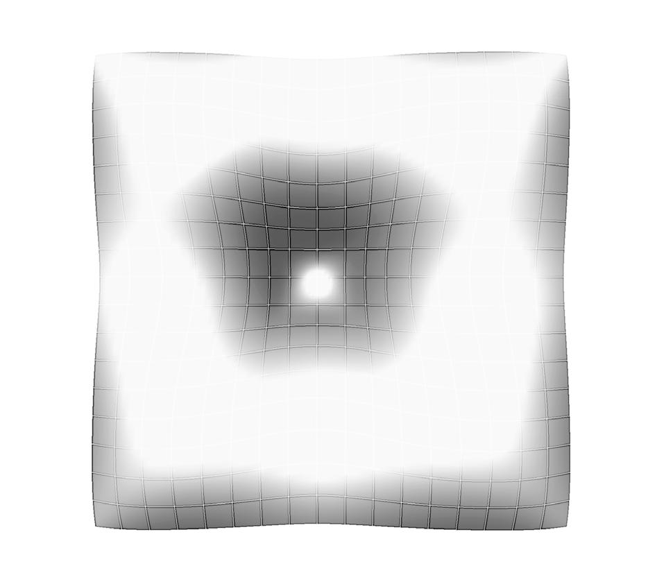
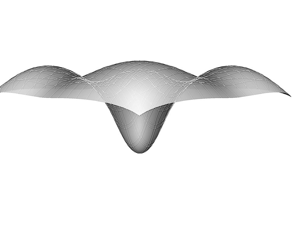
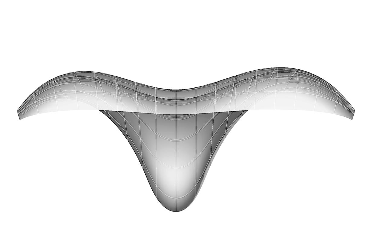
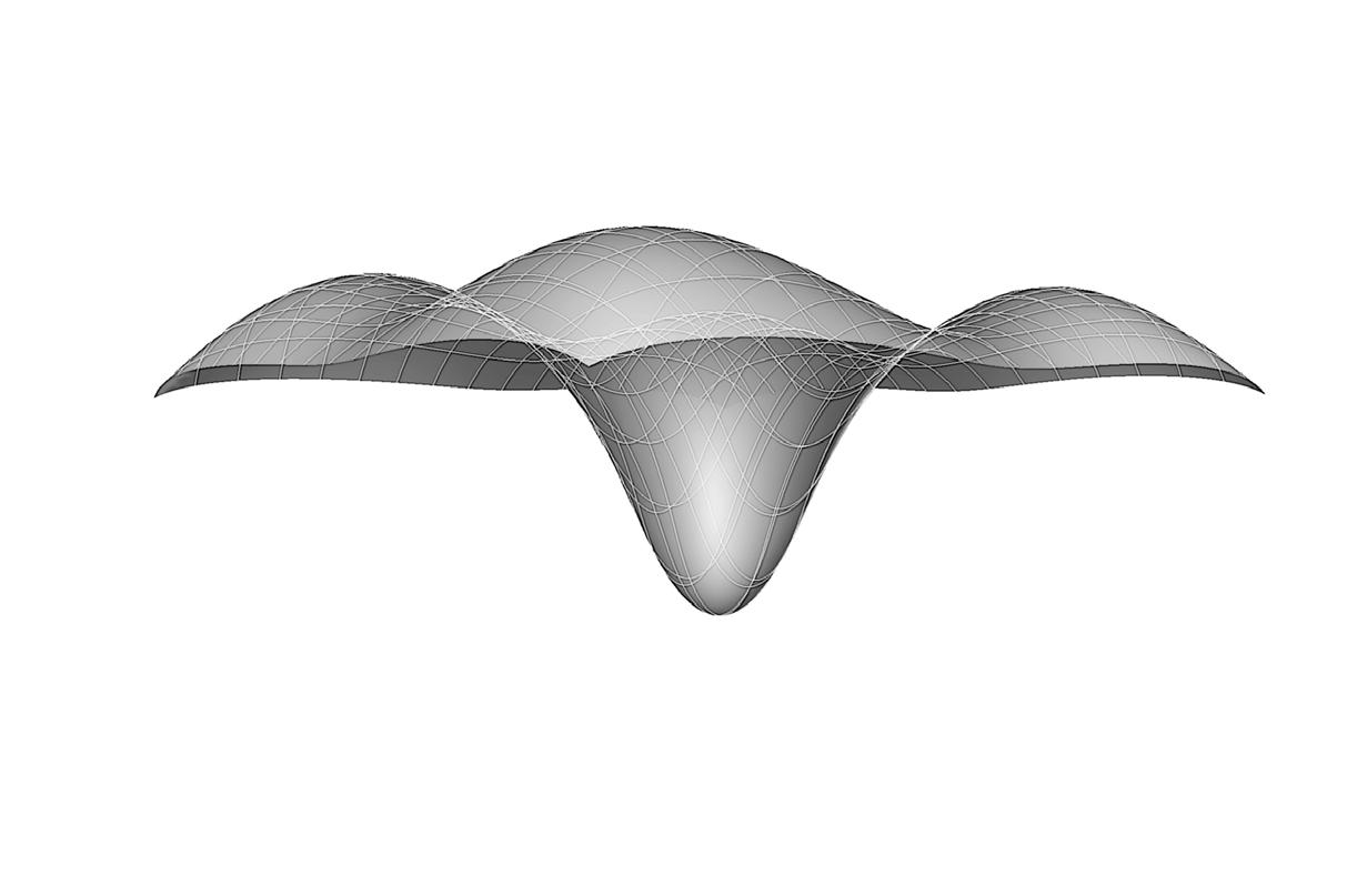
194
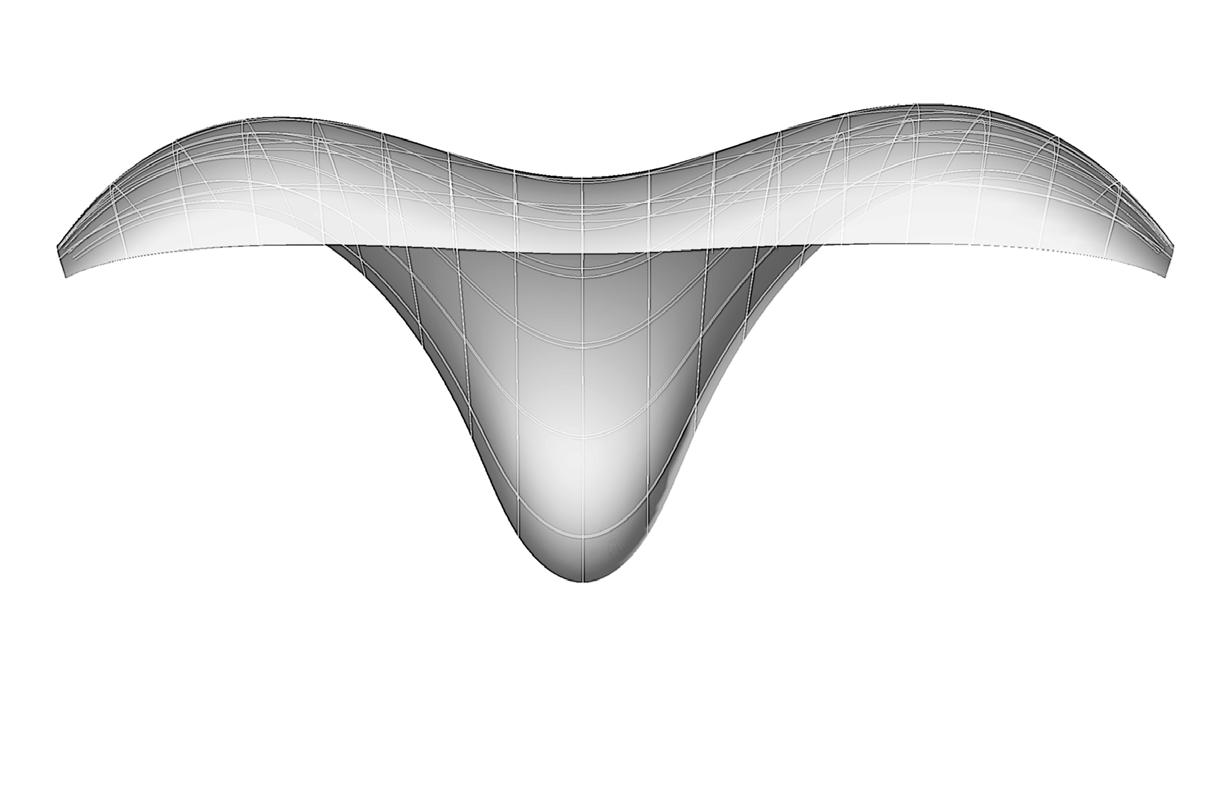
195
Global Geometry
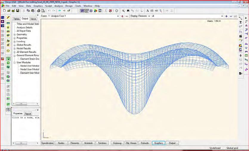
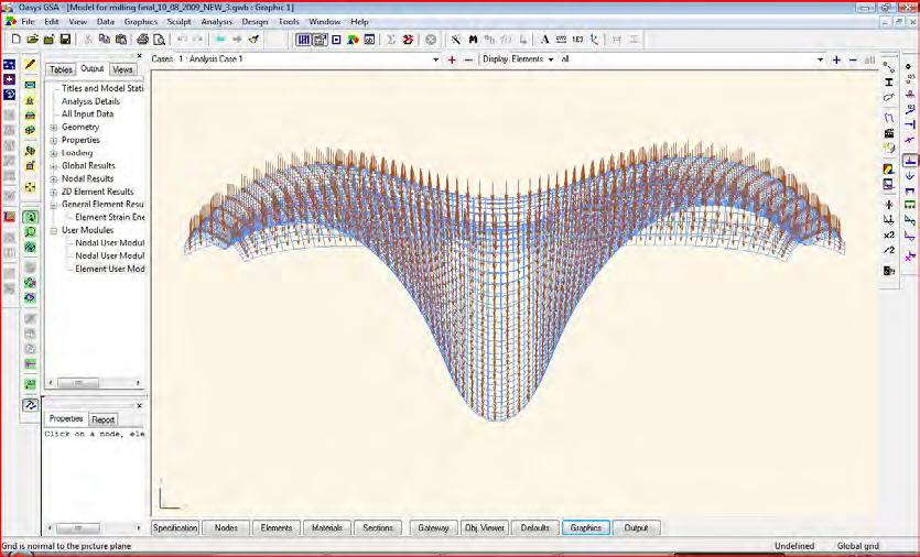
Distribution
Vbscript Model
This section covers the ‘fibre distribution’ algorithm written in visual basic to distribute the fibres in the direction of the principal stresses.
A visual diagram accompanies the code and shows the ‘in-house’ designed interface of the algorithm.
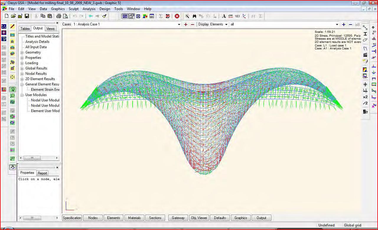
196
Fibre

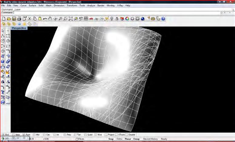
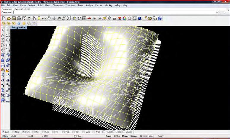
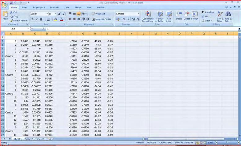

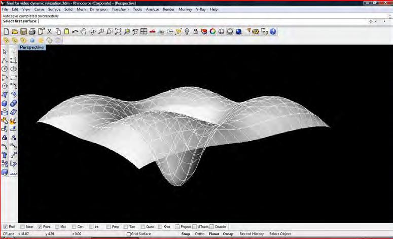
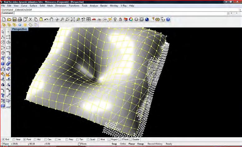

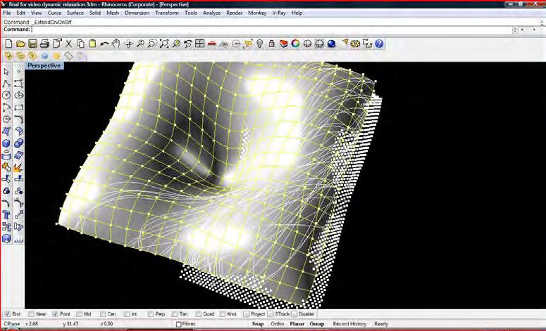
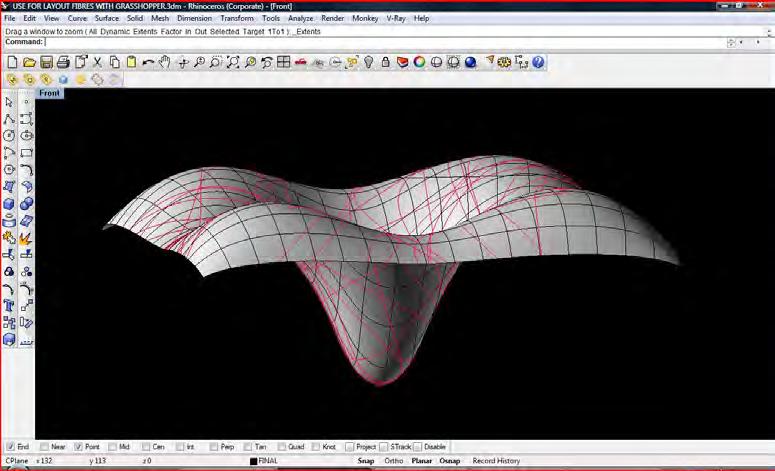
197
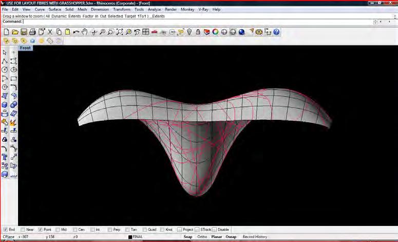
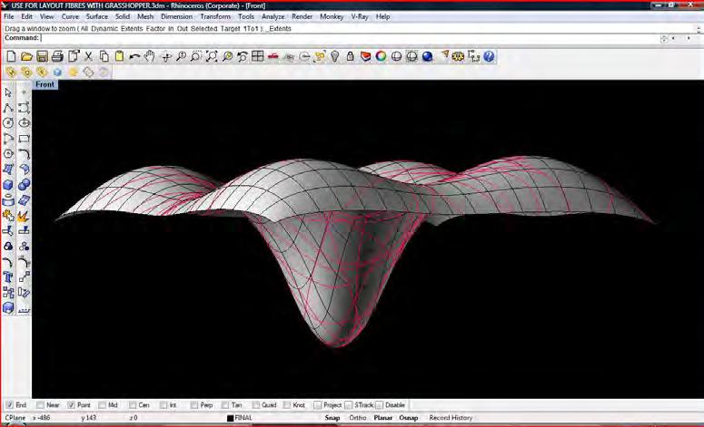
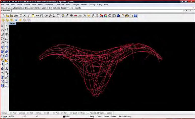
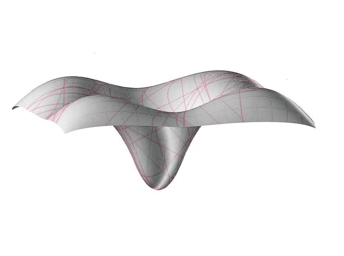
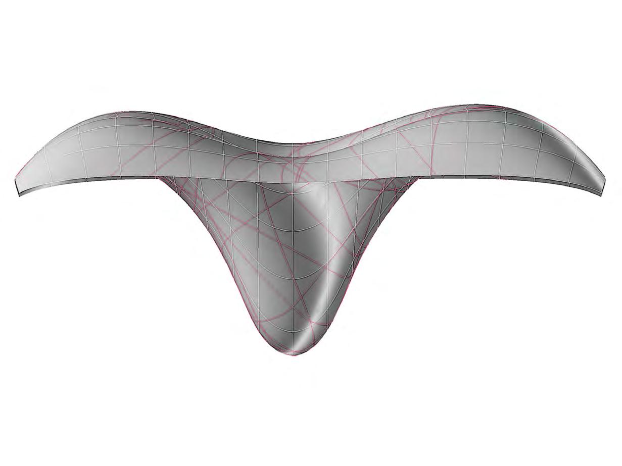
198
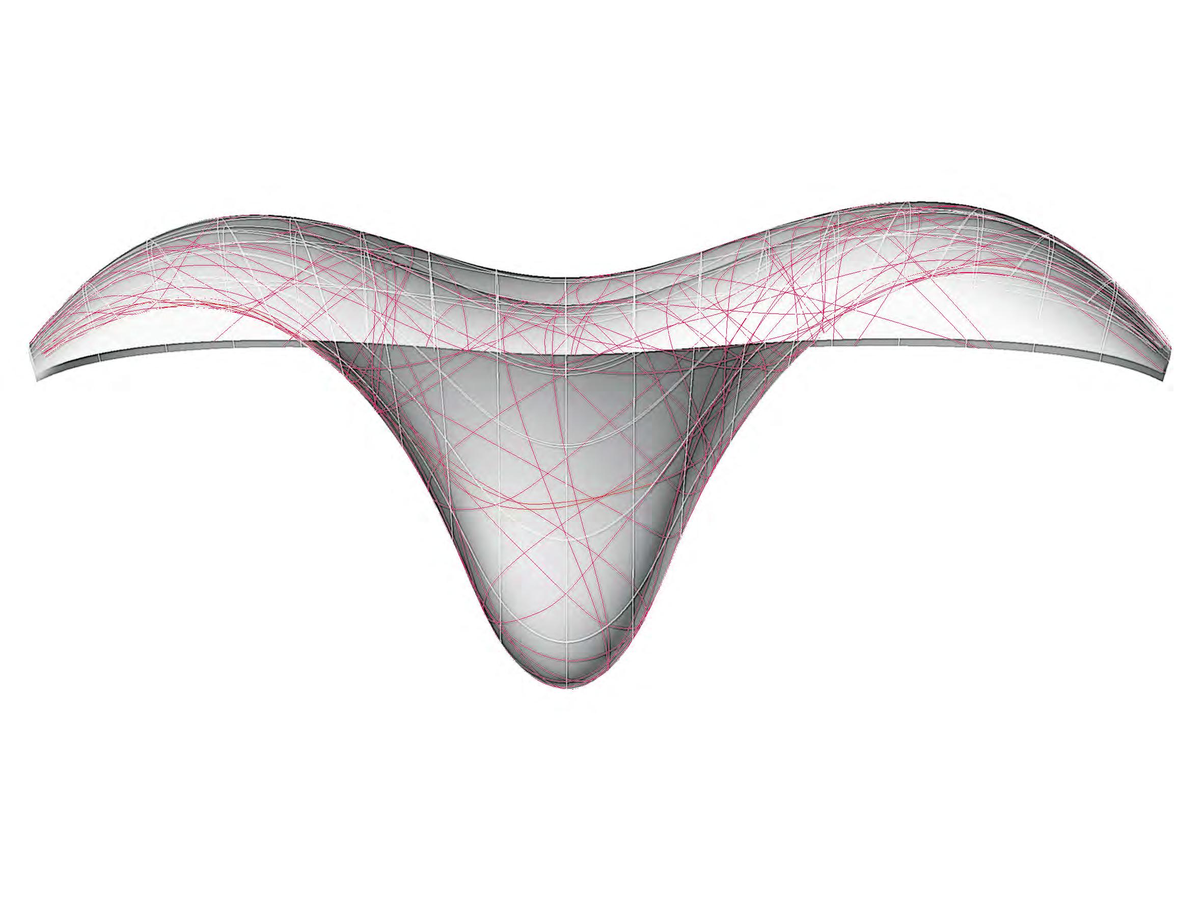
199
bres_stresses_path
bres_stresses_path
200
Input σ1,2,3 max (vector & module) Points of σ1,2,3 max tension (vector & module) σyield polymer σyield bres Point Coordinates Output Input Output get_tension_ bres
Function
Function check_stress check_stress_populate
of σ1,2,3 max
module) tension exceeding σyield polymer and, σyield
Input Output σ1,2,3
σyield
module
direction Function Input Output σ1,2,3
module)
points exceeding σyield
extra
required Input Surfaces σyield polymer & bres Import σ1,2,3 data from Excel Tolerance 3 4 Function draw_tension_
populate_tension_
Input Output Fibres are drawn joining points with similar σ1,2 or 3 in module and direction Extra bres are drawn where σyield bres is exceeded; the number of extra bres is proportional to the excess registered Function Input Output 5 6 1 2
Function get_tension_yield
Points
(vector &
bres
(vector & module) of points exceeding
polymer, organised in lists of similar values in
and
(vector &
of
bres, where
bres are
points,stension,stension_vector,syield_fibres,smaxyield_ fibres,smaxyield_fpoints,smaxyield_f_tension_vector
‘Script written by <Maria Mingallon>
‘Script version 19 March 2009 21:04:13
Call Main() Sub Main()
Dim sur face1,i
sur face1=rhino.getobject(“Select first surface”)
Dim stension_points(),stension(),stension_vector()
Dim syield_fibres,syield_polymer
Dim smaxyield_polymer(),smaxyield_fibres()
‘Dim scale_factor,thickness
Dim n()
‘Enter properties of the material: polymer and fibres
syield_polymer=Rhino.RealBox (“Specify syield polymer (MPa): “,7, “Yield Stress - Polymer”)
syield_polymer=(syield_polymer)*10^(3)
syield_fibres=Rhino.RealBox (“Specify syield fibres (MPa): “,7, “Yield Stress - Fibres”)
syield_fibres=(syield_fibres)*10^(3)
‘Enter scale factor and thickness
‘scale_factor=Rhino.RealBox (“Density of fibres at max tension points: “,0.01, “FIBRES DENSITY”)
‘thickness=Rhino.RealBox (“Specify max thickness at max tension points: “,2.0, “THICKNESS MAIN VEINS”)
Dim aPoints(),s1Values(),s2Values(),angleValues()
Dim smaxyield_fpoints(),smaxyield_f_tension_vector()
Dim smaxtension_check_points_sorted,smaxtension_ check_vector_sorted
Dim smaxyield_fibres_check_points_sorted,smaxyield_ fibres_check_vector_sorted,smaxyield_fibres_check_values_sorted
Dim Max_fibre_yield_s,Min_polymer_yield_s,Max_ fibre_s,Min_fibre_yield_s
ImportFromExcel 2,2,aPoints,s1Values,s2Values,angleValu es
Dim s1Vector(),s2Vector(),s1Values_new(),s2Values_ new(),centre()
get_vectors surface1,aPoints,s1Values,s2Values,angleValue s,s1Vector,s2Vector,s1Values_new,s2Values_new,centre
create_list 3,n
get_tension_fibres centre,s1Values_new,s1Vector,s2Values_ new,s2Vector,syield_polymer,stension,stension_points,stension_ vector
get_tension_fibres_yield stension_
max_min stension,Max_fibre_yield_s,Min_polymer_yield_s
max_min smaxyield_fibres,Max_fibre_s,Min_fibre_yield_s
For i=0 To ubound(n)
check_stress surface1,Max_fibre_yield_s,Min_ polymer_yield_s,n,i,syield_fibres,stension,stension_points,stension_ vector,smaxtension_check_points_sorted,smaxtension_check_ vector_sorted
Next
CheckLayer “Edge Surface”,1,1,1 Rhino.DuplicateEdgeCurves surface1
Rhino.LayerVisible “Surface”, False Rhino.LayerVisible “Supports”, False Rhino.LayerVisible “Fibres”, False Rhino.LayerVisible “Points”, False
End Sub
Sub ImportFromExcel(ByVal startrow,ByVal startcolumn,ByRef aPoints(),ByRef s1Values(),ByRef s2Values(),ByRef angleValues())
‘Define constant for the maximum number of rows in the Excel file ---’Do not change this value’’ Const xlDown = -4121
‘Define new variables for extracting data from Excel file
Dim oExcel, oSheet, nRow, nRowCount, sFileName
‘Get the name of the file to import
sFileName = Rhino.OpenFileName(“Select File”,”Excel Files (*.xls)|*.xls||”)
If IsNull(sFileName) Then Exit Sub ‘Launch Excel and open the specified file
Set oExcel = CreateObject(“Excel.Application”)
oExcel.Workbooks.Open(sFileName)
‘Set the active worksheet
Set oSheet = oExcel.ActiveSheet
‘Count the number of rows that need to be processed
nRowCount = oSheet.Range(“a”&CStr(startrow), oSheet. Range(“a”&CStr(startrow)).End(xlDown)).Rows.Count
If (nRowCount = 0 ) Then
Rhino.Print “No data range found in file.”
Exit Sub
ElseIf (nRowCount < 2 ) Then
Rhino.Print “Not enough points to create curve.”
Exit Sub
End f
‘Re-dimension the resulting array of points accordingly
‘Process all rows
Rhino.Print “Importing data...”
‘Define the variables for the data to be imported from Excel Dim s1,x,y,z,s2,angle
These are the arrays where the node coordinates, the s1 tension values and vectors will be stored
Read the values from columns, starting with “startcolumn” defined by the user
Read the values from the rows, starting from “startrow” defined by the user
For nRow = startrow To nRowCount+startrow-1 ‘Get coordinates of the nodes x=oSheet.Cells(nRow,startcolumn).Value y=oSheet.Cells(nRow,startcolumn+1).Value z=oSheet.Cells(nRow,startcolumn+2).Value
‘Get the value of the s1 principal stress s1 = oSheet.Cells(nRow, startcolumn+4).Value
‘Store values in arrays
ReDim Preserve aPoints(nRow-startrow)
aPoints(nRow-startrow)=array(x,y,z)
ReDim Preserve s1Values(nRow-startrow) s1Values(nRow-startrow)=s1
‘Get the value of the s2 principal stress s2 = oSheet.Cells(nRow, startcolumn+5).Value
‘Store values in arrays
ReDim Preserve s2Values(nRow-startrow) s2Values(nRow-startrow)=s2
Next
‘Get the value of the angle to x global angle = oSheet.Cells(nRow, startcolumn+7).Value
‘Store values in arrays
ReDim Preserve angleValues(nRow-startrow) angleValues(nRow-startrow)=angle
‘Close Excel and disassociate object variables oExcel.Quit
Set oSheet = Nothing
Set oExcel = Nothing
CheckLayer “Points”,1,1,1 rhino.addpoints aPoints End Sub
Sub get_vectors(ByVal surface1, ByVal aPoints(),ByVal s1Values(),ByVal s2Values(),ByVal angleValues(),ByRef s1Vector(),ByRef s2Vector(),ByRef s1Values_new(),ByRef s2Values_new(),ByRef centre())
Dim arrParameter, arrPlane(),arrNormal,planesrf
Dim ux,vy,i
Dim end_point,s2v
Dim cur vatures,r1,r2
Dim arrSurface,arrPoint
Dim quads(),j,point1,point2,point3,point4
Dim s1Vector_1
Dim arrDomainU,arrDomainV
Dim diagonal
Dim end_point2
j=-1
For i=0 To ubound (aPoints) Step 5
point1=aPoints(i) point2=aPoints(i+1) point3=aPoints(i+2) point4=aPoints(i+3)
j=j+1
ReDim Preserve quads(j) quads( j)=Rhino.AddSrfPt (array(point1,point2,poi nt3,point4))
ReDim Preserve centre(j) centre(j)=aPoints(i+4)
a rrPoint=Rhino.ProjectPointToSurface (centre(j),quads(j), array(0,0,-1))
arrDomainU=Rhino.SurfaceDomain (quads(j), 0) arrDomainV=Rhino.SurfaceDomain (quads(j), 1)
d iagonal=((arrDomainU(1))^2+(arrDomai nV(1))^2)^(1/2) ux = abs(cos(angleValues(i+4)))*diagonal/2
201 Option Explicit
vy = abs(sin(angleValues(i+4)))*diagonal/2
end_point=Rhino.EvaluateSurface (quads(j), array(ux,vy))
‘arrNormal=Rhino.SurfaceNormal (quads(j), array(ux,vy))
ReDim Preserve s1Vector(j)
s1Vector_1=Rhino.VectorCreate (centre(j), end_ point)
s1Vector(j)=Rhino.VectorScale (s1Vector_1, s1Values(i+4))
ReDim Preserve s1Values_new(j)
s1Values_new(j)=s1Values(i+4)
‘s2v=Rhino.VectorCrossProduct (arrNormal, s1Vector(j))
e nd_point2=rhino. evaluatesurface(quads(j),array(-ux,vy))
s2v=rhino.vectorcreate (centre(j),end_point2)
s2v=Rhino.VectorUnitize (s2v)
ReDim Preserve s2Vector(j)
s2Vector(j)=array(s2v(0)*s2Values(i+4),s2v(1)*s2V alues(i+4)*s2v(2)*s2Values(i+4))
ReDim Preserve s2Values_new(j)
s2Values_new(j)=s2Values(i+4)
Next
rhino.deleteobjects quads
End Sub
Sub max_min(ByVal stension(),ByRef Maxs,ByRef Mins)
‘Find out maximum And minimum principal tension stresses Dim stension_sorted
stension_sorted=Rhino.SortNumbers (stension)
Mins=stension_sorted(0)
Maxs=stension_sorted(ubound(stension))
End Sub
Sub CheckLayer(ByVal layername,ByVal red,ByVal green,ByVal blue)
If Rhino.IsLayer(layername) Then Rhino.CurrentLayer (layername)
Rhino.LayerColor layername ,RGB(255*red,255*gr een,255*blue)
Else Rhino.AddLayer (layername)
Rhino.CurrentLayer(layername) Rhino.LayerColor layername ,RGB(255*red,255*gr een,255*blue)
End If
End Sub
Sub UnCheckLayer(ByVal layername)
If Rhino.IsLayer(layername) Then
f Rhino.LayerVisible(layername) = True Then Rhino.LayerVisible layername, False End If End If End Sub
Sub get_tension_fibres(ByVal centre(),ByVal s1Values(),ByVal s1Vector(),ByVal s2Values(),ByVal s2Vector(),ByVal syield_ polymer,ByRef stension(),ByRef stension_points(),ByRef stension_ vector())
‘Counters (auxilliar) Dim i,j,l
‘Define variables for examinating the s1yield of the fibres and the polymer and storing the values j=-1
For i=0 To ubound(s1Values)
f s1Values(i)>s2Values(i) And s1Values(i)>0 And (abs(s1Values(i))>syield_polymer) Then j=j+1
ReDim Preserve stension(j) stension(j)=s1Values(i)
s1tension stores values of principal stress s1 if in tension
ReDim Preserve stension_points(j) stension_points(j)=centre(i)
s1tension_points stores the 3D points that register a negative value of s1, i.e. are in tension
ReDim Preserve stension_vector(j) s tension_vector(j)=Rhino.
VectorUnitize(Rhino.VectorCreate(s1Vector(i), stension_points(j)))
s1tension_vector stores the 3D vector of the principal stress s1, which will be afterwards used to draw the fibres
End If Next
For i=0 To ubound(s2Values)
f s2Values(i)>s1Values(i) And s2values(i)>0 And (abs(s2Values(i))>syield_polymer) Then j=j+1
ReDim Preserve stension(j) stension(j)=s2Values(i)
s1tension stores values of principal stress s1 if in tension
ReDim Preserve stension_points(j)
stension_points(j)=centre(i)
s1tension_points stores the 3D points that register a negative value of s1, i.e. are in tension
ReDim Preserve stension_vector(j)
s tension_vector(j)=Rhino.
VectorUnitize(Rhino.VectorCreate(s2Vector(i), stension_points(j)))
s1tension_vector stores the 3D vector of the principal stress s1, which will be afterwards used to draw the fibres
End If Next
End Sub
Sub get_tension_fibres_yield(ByVal stension_points(),ByVal stension(),ByVal stension_vector(),ByVal syield_fibres,ByRef smaxyield_fibres(),ByRef smaxyield_fpoints(),ByRef smaxyield_f_ tension_vector())
Counters (auxilliar)
Dim i,l
l=-1
For i=0 To ubound(stension) ‘Store the fibres that are over the syield of the fibres,i.e. more fibres would be required at these positions If abs(stension(i))>syield_fibres Then l=l+1
ReDim Preserve smaxyield_fibres(l)
smaxyield_fibres(l)=stension(i) ‘s1yield_fibres stores values of principal stress s1 if syield of the fibre is exceeded
ReDim Preserve smaxyield_fpoints(l) smaxyield_fpoints(l)=stension_points(i)
‘s1yield_fibres stores values of principal stress s1 if syield of the fibre is exceeded
ReDim Preserve smaxyield_f_tension_ vector(l)
s maxyield_f_tension_vector(l)=Rhino. VectorUnitize(Rhino.VectorCreate(stension_vector(i), smaxyield_ fpoints(l)))
‘s1yield_fibres stores values of principal stress s1 if syield of the fibre is exceeded
End If
Next
End Sub
Sub create_list(ByVal m,ByRef n()) dim For i=0 To m-1
ReDim Preserve n(i) n(i)=i+1
Next
End Sub
Sub check_stress(ByVal surface1,ByVal Maxs,ByVal Mins,ByVal n(),ByVal t,ByVal syield_fibres,ByVal smaxyield_fibres(),ByVal smaxyield_fpoints(),ByVal smaxyield_f_tension_vector(),ByRef smaxyield_fibres_check_points_sorted(),ByRef smaxyield_fibres_ check_vector_sorted())
Dim spar t,up_bound,k,low_bound,j,i Dim smaxyield_fibres_check_points(),smaxyield_fibres_ check_vector(),bigarray
spar t=(Maxs-Mins)/(ubound(n)) up_bound=Maxs j=-1
For k=0 To ubound(n) low_bound=Maxs-n(k)*spart
For i=0 To ubound(smaxyield_fpoints)
f (abs(low_bound)<abs(smaxyield_ fibres(i)))And (abs(smaxyield_fibres(i))<=abs(up_bound)) Then j=j+1
ReDim Preserve smaxyield_ fibres_check_points(j)
s maxyield_fibres_check_ points(j)=smaxyield_fpoints(i)
ReDim Preserve smaxyield_ fibres_check_vector(j) s maxyield_fibres_check_ vector(j)=smaxyield_f_tension_vector(i)
End If Next up_bound=low_bound Next
Dim smaxyield_fibres_check_vector_s()
bigarray=array(smaxyield_fibres_check_points,smaxyield_ fibres_check_vector) s maxyield_fibres_check_points_sorted=Rhino. SortPoints(smaxyield_fibres_check_points)
For i=0 To ubound(smaxyield_fibres_check_points) For j=0 To ubound(smaxyield_fibres_check_ vector)
f bigarray(0)(i)(0)=smaxyield_fibres_ check_points(j)(0)And bigarray(0)(i)(1)=smaxyield_fibres_check_ points(i)(1)And bigarray(0)(i)(2)=smaxyield_fibres_check_points(i)(2) Then
ReDim Preserve smaxyield_ fibres_check_vector_s(i)
s maxyield_fibres_check_ vector_s(i)=smaxyield_fibres_check_vector(j)
End If Next
Next smaxyield_fibres_check_vector_sorted=smaxyield_fibres_ check_vector_s
‘Draw fibres at points where the tensile stress exceeds the syield of the polymer, following the stresses path,
‘’’’’’’’’’’i.e. the points With similar tensile stresses Or within a range. This range Is determined by ‘m’
‘ This function will also increase the density of the fibres depending on how much tension over the syield of the fibre is felt at that point
draw_tension_fibres_stresses_path surface1,smaxyield_ fibres_check_points_sorted,smaxyield_fibres_check_vector_sorted
End Sub
Sub check_stress_populate(ByVal surface1,ByVal Maxs,ByVal Mins,ByVal n(),ByVal t,ByVal syield_fibres,ByVal smaxyield_ fibres(),ByVal smaxyield_fpoints(),ByVal smaxyield_f_tension_
202
vector(),ByRef smaxyield_fibres_check_points_sorted(),ByRef smaxyield_fibres_check_vector_sorted(),ByRef smaxyield_fibres_ check_values_sorted())
Dim spar t,up_bound,k,low_bound,j,i
Dim smaxyield_fibres_check_points(),s1yield_fibres_ check_vector(),s1yield_fibres_check_values(),bigarray
spar t=(Maxs-Mins)/(ubound(n)) up_bound=Maxs j=-1
For k=0 To ubound(n) low_bound=Maxs-n(k)*spart
For i=0 To ubound(smaxyield_fpoints)
If (abs(low_bound)<abs(smaxyield_ fibres(i)))And (abs(smaxyield_fibres(i))<=abs(up_bound)) Then j=j+1
ReDim Preserve smaxyield_ fibres_check_points(j)
s maxyield_fibres_check_ points(j)=smaxyield_fpoints(i)
ReDim Preserve smaxyield_ fibres_check_vector(j)
s maxyield_fibres_check_ vector(j)=smaxyield_f_tension_vector(i)
ReDim Preserve smaxyield_ fibres_check_values(j)
s maxyield_fibres_check_ values(j)=smaxyield_fibres(i) End If Next up_bound=low_bound Next
Dim smaxyield_fibres_check_vector_s(),smaxyield_fibres_ check_values_s()
bigarray=array(smaxyield_fibres_check_points,smaxyield_ fibres_check_vector)
s maxyield_fibres_check_points_sorted=Rhino. SortPoints(smaxyield_fibres_check_points)
For i=0 To ubound(smaxyield_fibres_check_points)
For j=0 To ubound(smaxyield_fibres_check_ vector)
If bigarray(0)(i)(0)=smaxyield_fibres_ check_points(j)(0)And bigarray(0)(i)(1)=smaxyield_fibres_check_ points(i)(1)And bigarray(0)(i)(2)=smaxyield_fibres_check_points(i)(2) Then
ReDim Preserve smaxyield_ fibres_check_vector_s(i)
s maxyield_fibres_check_ vector_s(i)=smaxyield_fibres_check_vector(j)
ReDim Preserve smaxyield_ fibres_check_values_s(i)
s maxyield_fibres_check_ values_s(i)=smaxyield_fibres_check_values(j) End If Next
Next
smaxyield_fibres_check_vector_sorted=smaxyield_fibres_ check_vector_s
smaxyield_fibres_check_values_sorted=smaxyield_fibres_ check_values_s
‘Draw fibres at points where the tensile stress exceeds the syield of the polymer, following the stresses path, ‘’’’’’’’’’’i.e. the points With similar tensile stresses Or within a range. This range Is determined by ‘m’
‘ This function will also increase the density of the fibres depending on how much tension over the syield of the fibre is felt at that point
p opulate_tension_fibres_stresses_path surface1,smaxyield_fibres_check_values_sorted,syield_ fibres,smaxyield_fibres_check_points_sorted,smaxyield_fibres_ check_vector_sorted
End Sub
Sub draw_tension_fibres_stresses_path(ByVal surface1,ByVal smaxyield_fibres_check_points_sorted(),ByVal smaxyield_fibres_ check_vector_sorted())
Dim arrpoints(),pointsrf1,pointsrf11,crvonsrf,crvonsrf1,initi al_point1
Dim i
Dim projected_points
‘Draw the fibres where the value there is tension and it is over the syield of the polymer
For i=0 To ubound(smaxyield_fibres_check_vector_sorted) CheckLayer “Fibres”,1,1,1 ReDim Preserve arrpoints(i) a rrpoints(i)=array(smaxyield_fibres_check_ points_sorted(i)(0)+smaxyield_fibres_check_vector_sorted(i) (0),smaxyield_fibres_check_points_sorted(i)(1)+smaxyield_fibres_ check_vector_sorted(i)(1),smaxyield_fibres_check_points_sorted(i) (2)+smaxyield_fibres_check_vector_sorted(i)(2)) nitial_point1=Rhino.EvaluateSurface(surface1, array(0,0))
f IsArray(initial_point1) And IsArray(arrpoints(i)) Then pointsrf1=Rhino.PullPoints (surface1,arr ay(arrpoints(i),initial_point1)) pointsrf11=Rhino.PullPoints(surface1,ar ray(smaxyield_fibres_check_points_sorted(i),initial_point1))
If Not (IsNull(Rhino.PullPoints (surface1, array(arrpoints(i),initial_point1)))) Then
If Not (IsNull(Rhino.PullPoin ts(surface1,array(smaxyield_fibres_check_points_sorted(i),initial_ point1)))) Then
If Rhino.
IsPointOnSurface(surface1, pointsrf1(0))And Rhino.
IsPointOnSurface(surface1, pointsrf11(0)) Then
f VarType(Rhino.
AddInterpCrvOnSrf (surface1,array(pointsrf11(0),pointsrf1(0))))=vbSt ring Then
crvonsrf=Rhino.AddInterpCrvOnSrf (surface1,array(pointsrf11(0),poi ntsrf1(0)))
UnselectAllObjects
SelectObject surface1
R hino.
R hino.
R hino.
SelectObject CStr(crvonsrf) R hino.
Command “_ExtendCrvOnSrf” R hino.
UnselectAllObjects End If End If End If End If End If Next
203
End Sub
Appendix C: Manufacturing
1. Cases Studies
2. M anufacturing Techniques
3. Exper imental Fabrication
Case Studies
Case Studies
Bridges
Many cases studies where fibre composites have been used can be found in the bridges industry. Some of them have been selected for detailed study because of their relevance overall to the main subject of this dissertation. There are other cases where specific techniques or uses of composites have been found; these would be briefly described focusing on the relevant aspect.
The structure of this section will be as follows:
Detailed Case Studies:
-Lechlade Bridge, Gloucestershire (UK)
-Aberfeldy Footbridge, Scotland (UK)
Brief Case Studies
-A19 Tees viaduct, Teeside, UK
-Andel Bridge, Netherlands
-Bonds Mill Lift Bridge, Gloucestershire, UK
-Autovia del Cantabrico, Spain
-Den Dungen Draw Bridge, Netherlands
-Friedberg B3 Highway Bridge, Netherlands
-Friesland Bridge, Netherlands
-Garstang Mount Pleasant M6 Bridge, Lancashire, UK
-Halgavor Bridge, Cornwall, UK
-Kolding Bridge, Denmark
-Lleida footbridge, Spain
-Moscow Arched Footbridge, Russia
-Norre Aaby, Denmark
-St Austell Railway Bridge, Cornwall, UK
-Strait of Gibraltar Bridge, Mediterranean Sea, Spain
-West Mill Bridge, Oxforshire, UK
-Winterthur Cable-stayed Bridge, Switzerland
Bridges constructed in Europe with structural fibre composites manufactured either by pultrusion or infusion. A number of them have been selected for a detailed study and some others for a brief analysis.
Reference: http://www.tech.plym.ac.uk/sme/MATS324/bridges.htm
206 Bridge Location Year Lechlade Bridge Gloucestershire (UK) 1993 Aberfeldy Footbridge Scotland (UK) 1993 A19 Tees viaduct Teeside (UK) 1989 Andel bridge Netherlands 1995 Bonds Mill Lift Bridge Gloucestershire 1995 Autovia del Cantabrico Spain 2008 Cueva de Oñati-Arrikrutz walkway Spain 2008 Den Dungen draw bridge Netherlands 2003 Friedberg B3 highway bridge Germany 2008 Friesland bridge Netherlands 2002 Garstang Mount Pleasant M6 bridge Lancashire (UK) 2006 Halgavor bridge Cornwall (UK) 2001 Kolding bridge Denmark 1997 Lleida footbridge Spain 2004 Moscow arched footbridge Russia 2008 Nørre Aaby Denmark 2008 St Austell railway bridge Cornwall 2007 Strait of Gibraltar bridge Mediterranean Sea Future West Mill Bridge Oxfordshire 2002 Winterthur cable-stayed bridge Switzerland 1996
-....
Scale model showing the proposal and its integration with the surrounding environment.
Ref: Wells, M; Pearman, H; “Puentes”, Ed. Laurence King Publishing Ltd, London, 2002.

Lechlade Bridge, Gloucestershire, United Kingdom; Studio E Architects/Alistair Lenczner – Ove Arup & Partners, 1993
Brief Description
Span 22 m
Typology Arch / box section beam
Material Carbon Fibre Composite
Observations Not built
Introduction
The competition required the participants to propose a bridge of a simple form with a short span and a reduced budget. These conditions made the designer to propose a 22m span arch bridge in line with the typical canal bridges found across England.
Structural Features
The structure consists of a box beam spanning between the canal banks which also constitutes the walking platform. The box beam is quite shallow and it is composed of two internal pentagonal cells. The cross section of the beam is quite interesting. The division of the box into two cells is made to improve the behaviour of the bridge under torsion; the dividing panel constitutes an intermediate web which would help transfering the shear originated by the torsional moment. At the same time, the pentagonal section is carefully used here to increase the structural depth of the member withouth damaging the lightweigth effect driving the proposal.
The box beam was proposed to be a carbon fibre composite which allow the box section panels to be just 10mm thick. It is important to highlight here that if the proposal would have been made using steel, such a thin section would have been impossible to achieve just from
the shape limitations stated by the BS 5400 pt 3 for the design of steelwork components in bridges. These are shape restrictions are driven by the tendency of thin steel panels to buckle under compressive loads.
The parapets are solid panels made of stiffened glass which are connected to the main box beam.
Although plastics are quite strong structurally they are generally sensible to the UV rays and they are usually covered with a resin. A diamond powder treatment was proposed instead for this particular bridge which contributed to the aesthetics as well as the improved performance against impact and rain. The parapets and the floor of the structure were treated with this technique which also helped forming a self-cleanning layer which reduced the need for long term maintenance considerably. The proposal defended that the initial expenditure made on these type of treatment could be easily recovered after the first years of its design life. The total amount of diamond powder that would have been used for the entire structure would have been 3Kg.
Construction Highlights
The bridge was proposed to be prefabricated off-site to ensure high quality finishes. Being the span only 22m, it could have transported to site in one day and erected on the same night without the need of heavy cranes or any expensive equipment on site.
Design Issues
Although the use of the materials and the structural design were carefully considered throughout the development of the proposal, this bridge was not finally selected. The reasons behind include the uncertainty of the authorities in the use of such an innovative material.
Critical reflexions
207
In Engineering reinforced plastics have been marginally used since their invention in the fifties. Although these plastics offer high structural resitance as well as high elasticity, they result extremely expensive for an industry stuck in traditional construction methods developed many years ago for steel and concrete.
One of the tendencies of modern engineering is that future designs will be re-defined by the use of these innovative materials. The more the technology of the material evolves, the greater the feasibility of these type of engineering projects would be.
Another consideration is the use of the fibre composite in this proposal. The exact same typology could have been proposed in steel, concrete or wood with certain variations on the overall geometry or the addition of extra members. The proposal uses fibre composites for the box beam instead of any of the above materials. It does mimick a traditional bridge typology and introduces fibre composites as an innovative feature. However, the use of fibre composite could open the door to novel structural typologies that could have never been imagined with the use of steel or concrete.
-Another example is the bridge next to the historic iron bridge of Coalbrookdale in Shropshire, which proposes a carbon fibre structure making direct reference to the original one of Abraham Darby. The design in this bridge explores the use of a new material by trying also new forms, in contrast to the bridge in Aberfeldy employs a very well used typology (cable-stayed) and uses carbon fibres instead of steel or concrete.
Ref: Wells, M; Pearman, H; “Puentes”, Ed. Laurence King Publishing Ltd, London, 2002.
Aberfeldy Bridge, Scotland, United Kingdom; Maunsell Structural Plastics, 1992
Span 64 m (central span)
Typology Arch / box section beam
Material Carbon Fibre Composite
Observations Not built
Introduction
The Aberfeldy footbridge is a cable-stayed structure that spans over the river Tay joinng the two halves of the municipal golf course in Aberfeldy. The bridge counts with a main span of 63m and two back spans, and it has at total length of 113m.
The slab, the towers and even the handrailings are made of glass-reinforced composites with cables being aramid fibres. It weights only 14.5 tonnes.
Maunsell Structural Plastics worked closely with Dundee University whose final-year bridge engineering students provided the bridge erection team.
Structural Features
The design of the bridge is done following a conventional cable-stayed typology which could have been constructed in concrete and/or steel; however, all the elements of this bridge were manufactured using fibre composites.
The UK-based engineering company Maunsell Structural Plastics, developed what is known as the Advanced Composites Construction System (ACCS); a system of six interlocking structural pultrusions that can be assembled into many configurations to produce load bearing structures.
208

View of Aberfeldy Bridge. reference http://www.ksci.com/graphics/aberf.gif
The deck was constructed using 600mm wide longitudinal ACCS panels stiffened by edge and cross beams. The basic component of the glass reinforced plastic pultrusions is a unit cell, approximately 80mm square, which features a keyway running down each side. This receives a toggle bar which links the cell to its neighbours. The joint is filled with adhesive to provide a permanent rigid bond between components. Wider planks, composed of seven cells side by side, form the bulk of the structure, with single cell units being used to provide additional stiffness at edge beams and in the joints between units.
The bridge is stayed from two 18m high ‘A’ shaped GRP pylons holding the parafil cables which support the deck. These consist of Kevlar aramid fibres parallel laid and sheathed in a protective low density polyethylene coat.
Parafil ropes have a core of parallel filaments contained within a polymeric sheath. In the case of the ropes used for the Aberfeldy Bridge, Kevlar 49 yarns, with a stiffness of 126 KN/mm2 and a breaking strength of 1930 N/mm2 were used. The ropes are fitted with terminals in which the fibres are gripped between a central spike and a matching external barrel [Figure ?]. This ensures that all fibres are equally gripped, and tests shown that the termination achieves the full strength of the rope.
The parapets were pultruded GRP sections and the design was completed by the addition of GRP handrailing and a wear-resistant deck finish, providing a life to first maintenance of over 20 years.
All components apart from the handrails were made by the pultrusion process, and incorporate high volume fractions of fibres, with most of the fibres running longitudinally, but with some arranged in the form of ribbons and tapes so that transverse stregth can be provided to the cells. The pultrusion system allowed for different
amounts of fibre to be placed in the different faces of the cells, to reflect the different stresses (axial, shear or flexure) that arise in each face; extra reinforcement could be provided in areas of high stress concentration, such as the toggle keyways.
The bridge is designed to carry pedestrian loading of 5.6 kN/m2 and result to have a dead load of 2.0 kN/m2 with a superimposed load of 1.0kN/m2. Wind and temperature design loads were to BD37/88.
Construction Highlights
The 113m-long deck was assembled on site in only eight weeks. The lightweigth of its components made possible the use of a unique method of erection of towers, cables and deck with no site craneage. The minimal foundations required for such a light structure together with the rapid site assembly made the solution very cost effective for the client.
The ACCS components designed by Maunsell consist of pultruded sections of GRP which are linked together by mechanical interlocks and fixed by adhesive bonding, with no need for drilling or welding. These sections were manufactured by GEC Reinforced Plastics, and typically contain 60% by weight glass fibre in a isophthalic polyester. The assembly system is easily completed without special tools or lifting equipment, whilst the low weight enables easy handling and positioning.
Design Issues
The main concern with such a lightweight structure has to do with its dynamic behaviour. Studies carried out during the desing of the bridge demonstrated that the dynamic response could be controlled by calibrating the magnitude and distribution of the mass of the deck and
209
tailoring the dampiing of the parapets, cables and surfacing.
However, according to a recent structural surve the bridge is very lively even at a gentle walking pace and soon develops a highly noticeable bounce. The Kevlar cables appeared to be under quite low tension and the dynamic problem exhibited is clearly partly a result of the low mass of the system.
Within the first year the bridge withstood hurricane winds, unprecedented snowfall and flooding to above the deck level spans with no damage being caused. However, after five years the deck had to be strengthened with GRP pultruded plates due to overloading causing cracking on the deck surface.
Although the primary structure of bridge continues to perform very well after 10 years of life, there have been some superficial weathering effects. The surface layer of the parapets and hanrails has been heavily eroded exposing the glass fibres. Note that these were not ACCS sections and illustrate how imporatant the detailed specification of resin and manufacture is in practice. In contrast, the ACCS GRP panels have weathered extremely well.
In addition, the connections between parapet rails and posts have worked loose and most of the post-to-deck connections are loose. These are due to the movement cycles of the deck and could have been avoided by giving the parapet connections greater movement capacity or by reducing the displacement of the deck by means of a stiffer cable system.
Both parapets and primary structure have been affected by mould and moss growth due to standing surface moisture due to the damp climate. A future strategy might be to consider the colour of the composite used to minimise the visual impact of the mould growth; another option could be
the use of mould-inhibiting additives in the resin system.
The cantilevered handrails are very wobbly and can be moved laterally by several tens of millimetres. Parts of the handrails also rattle when walking over the bridge. Some of the components are poorly fitting and seem to have loosened up considerably with gaps of 15 to 20mm in places. As a result of this the line of the parapet is crocked. Glass fibres were visible on the tops of some of the handrails and a number of end caps to the posts were missing.
Critical reflexions
The key benefits from using composites for the design and construction of the present bridge were using a fully bonded composite structure made of modular lightweight but durable components, which allowed for rapid erection withouth the need of craneage.
Associated benefits are the shallow foundations required which also minmise considerably the environmental impact and the disruption caused to the golf course (key consideration from the client’s side). This also facilitates the approval of the Rivers and Environment agencies as well as other authorities.
On the other hand, a number of unplanned issues have arised since the bridge was built. Its dynamic behaviour, the connection between the aramid cables and the deck as well as the sensitivity of the material to mould growth are all problems related to the use of reinforced plastics which would have never been foreseen withouth the construction of this project.Current designs using fibre composites -among which this dissertation falls- would need to address the above issues.
Parafil rope terminations ref: Burgoyne, C.J.; Head, P.R.; “Aberfeldy bridge: an advanced textile reinforced footbridge”. Engineering Department, University of Cambridge in collaboration with Maunsell Structrual Plastics, April 1993.
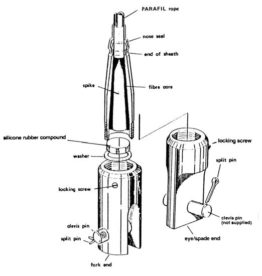
210
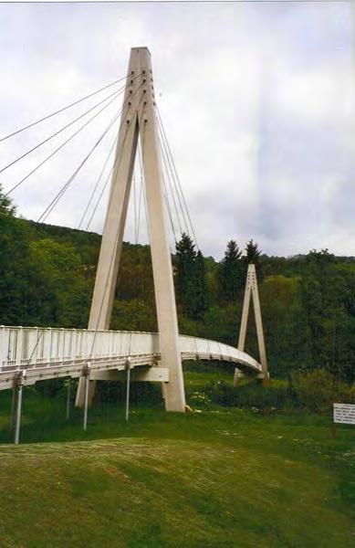
One of the main features observed from studying the pultrusion system employed in this case study is that it provides the designer with additional freedom. By far the largest cost associated with pultrusion relies on the cost of the die, which has to be very accurately machined from wear resistant chrome steel. Therefore, although the shape is variable there are high costs associated with changing the shape of the structur, whilst it is relatively easy to vary the amounts of reinforcement, which can be altered to suit different structural requirements.
When we come to use new materials, we can find ourselves in a vicious circle where we cannot use the material unless a code is available, the code cannot be produced until the test data is available and the testing will not be carried out until there is a certainty that the material will be used.
In order to avoid this situation, Maunsell went back to first principles to produce a limit state desing method for the use of the new system, and carried out basic testing to provide the strength and variability information necessary to allow the various partial safety factors to be determined.
This allows designs to be produced with sufficient assurance to satisfy the technical approval authority and is likely to form the basis of future codes of practice for the new generation of materials.
Illustration credits: {OLD ONE} Figure 1 reference http://www.ksci.com/ graphics/aberf.gif {MORE NEW ONE} Figure 2 reference http://en.structurae. de/photos/index.cfm?JS=51628
Main source of information: Case Studies
Bridges - Brief Case Studies
Many cases studies in the bridge industry have been found. Some have been selected for detailed study because of their relevance overall. However, there are some other cases where specific techniques or uses of fibre composites have been found of interest for the purpose of this document. These will be briefly discussed in this section, focusing on their main innovative aspect.
A19 Tees viaduct, Teeside, UK, 1987 - Structural Membrane
[I dont have photo of this one...]
In September 1987, the UK Department of Transport awarded a contract for the refurbishment of the A19 Tees viaduct by the installation of a 16000 m2 ACCS structural membrane (total weight 250 tonnes) below the road deck. The relatively high capital cost of the membrane was offset by the inclusion of access walkways along the underside of the bridge producing substantial savings in subsequent inspection and maintenance costs, not least in that the need for road closure was eliminated and the enclosed space provided a protected working environment at all times of the year. The road passes over an area with a number of chemical plants and the structure was subject to significant corrosion. The corrosion rate was reduced by 90% after installation of the membrane.
References:
PR Head and AE Churchman, Design, specification and manufacture of a pultruded composite construction system, Proceedings ot the Symposium on Mass Production Composites, Imperial College London, 19-20 September 1989, pages 117-162.
Bonds Mill Lift Bridge, Gloucestershire, 1995 - ACCS pultrusion for deck
211
The Bonds Mill Lift Bridge crosses the Stroudwater Navigation canal close to Stonehouse and is 8m long by 4m wide. The structure, constructed using the ACCS pultrusion system designed by Maunsell [refer to Aberfeldy Bridge Case Study above] weighs 4.5 tons and yet can support loaded trucks up to 44 tonnes to permit access to the adjacent industrial estate for articulated trucks. It is operated hydraulically to allow water traffic to pass underneath. The lightweight of composite materials permitted the use of a smaller lift mechanism than would have been required otherwise.
Images from http://www.stroudwater.co.uk/cpsn/ bonds%20mill%20bridge%203.jpg (left), and http:// www.ksci.com/graphics/bond.gif (right-with car)
ref: Bonds Mill Lift Bridge (BRE projects/NGCC)
Autovia del Cantabrico, Acciona, Spain
Autovia del Cantabrico, the first carbon-fibre composite bridge in Spain, was constructed by Acciona Infraestructuras of Madrid. The composite elements are three parallel spans of 0.8 m deep hollow trapezoidal section. The low weight composite structure (100 kg/m supporting 2500 kg/m of concrete road deck) was easy and quick to assemble. The composite structure was installed using a 50 tonne crane (the equivalent structure in concrete would require a 400 tonne crane) and completed in 10 hours.
Images from the Javier Bonilla presentation. Javier Bonilla, Innovations in the Construction Sector: Acciona R&D, The International Construction Fair, PoznanPoland, 22 January 2008.
http://www.pptb.pl/konferencja/prezentacje/ Francisco_J_Bonilla_Diaz_ACCIONA.pdf
The three designs that are presented underneath have
a main structure manufactured by vacuum infusion or hand lay-up. The projects aimed at the manufacturing of a one-off bridge structure and the main argument for the selection of these processes is the low mould costs. The designs are all vehicular bridges, either VOSB1995 Class 600 [1], i.e. designed for three axle loads of 200 kN, or VOSB1995 Class 450, i.e. three axle loads of 150 kN. The three designs (named after their location Andel, Den Dungen, Friesland) show an evolution in structural design, in which a tendency is shown towards simpler elements.
Andel Bridge, Netherlands, 1995 - Hand lay-up & Wheel Load Testing
Andel bridge is a lift bridge whith a two layers structure, the deck and the main beams. The later are Z-shaped members, that are placed with lapped flanges back to back and face-to-face, to create closed triangular sections. These large members of 1380 mm height and a width of 505 mm are dimensioned for manufacturing by hand lay-up.
This process was selected to make the structure feasible for a large number of manufacturers in the Netherlands. At that time the number of companies that mastered vacuum infusion was very limited.
The deck consists of small rectangular box-elements with dimensions of 50 mm x 169 mm. The road deck cannot be made by hand-lay up. By using a very light precut foam core as a plug and applying saw cuts in the foam acting as resin flow channels, this structure can be made by vacuum infusion in a well controlled manner. Deck elements of one meter in width with twenty box beams were manufactured in one step.
A prototype structure was manufactured to carry out full
General Arrangement drawings. Burgoyne, C.J.; Head, P.R.; “Aberfeldy bridge: an advanced textile reinforced footbridge”. Engineering Department, University of Cambridge in collaboration with Maunsell Structrual Plastics, April 1993.
212
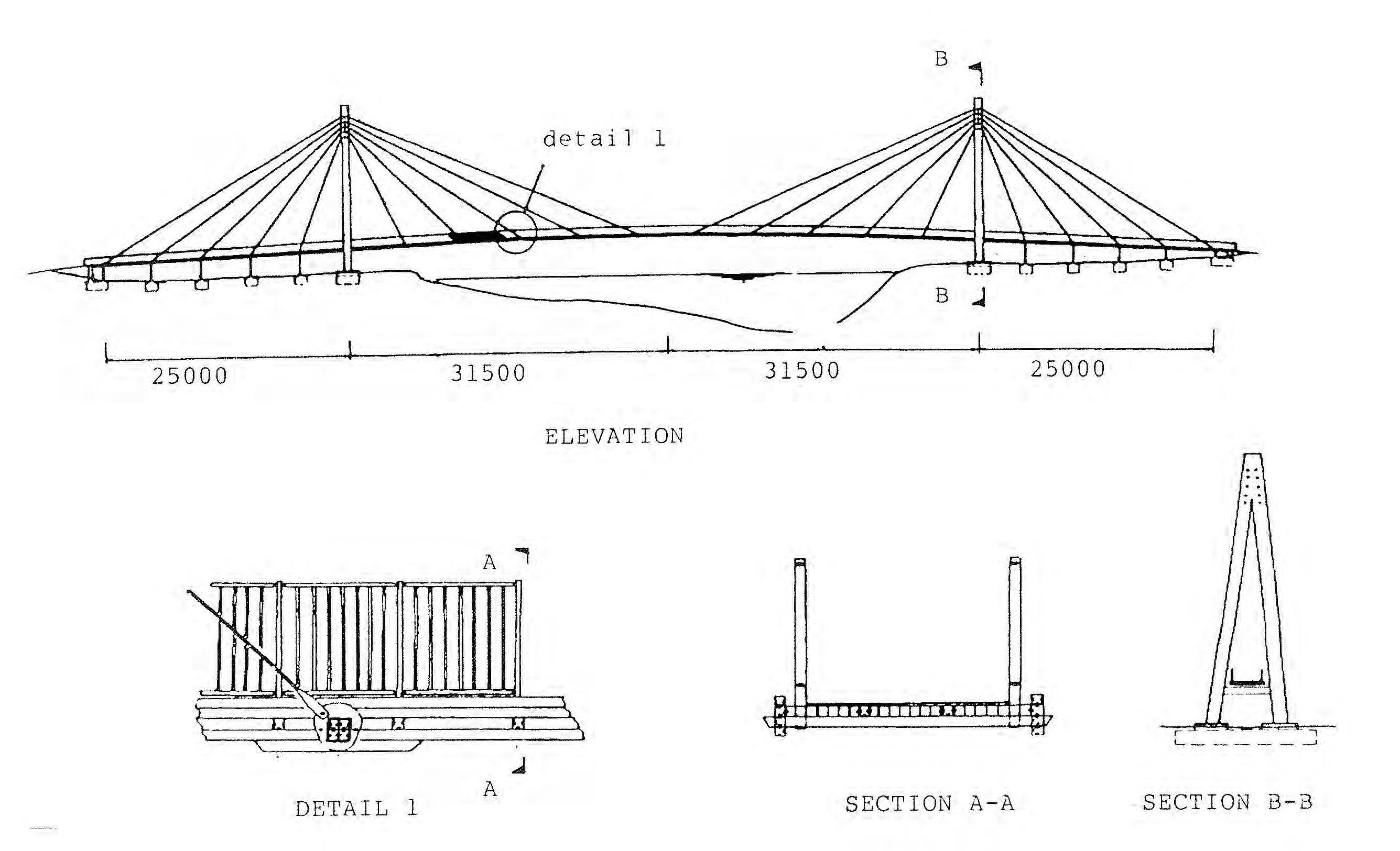
scale wheel load testing [fig ...]. A static and dynamic test representative for the traffic loads proved the durability of the structural concept.
Friesland, Netherlands, 2002 - Modular elements
This bridge is a fixed structure to be constructed with modular elements.From the design of the Andel bridge deck -explained above- it became clear that the manufacturing of a closed cell deck structure in vacuum infusion is possible, but quite elaborate. In the past years, more and more pultruded road deck profiles have become commercially available. Therefore, this design combines a pultruded deck with an infused main structure.
The main structure was made of two elements in order to facilitate the inspection after the injection process. These consisted of an omega-shaped beam and a flat top plate; both elements were made in simple moulds and were fully inspected before assembly [Fig. xx].
References for the three previous bridges [1] ‘NEN 6788 ‘Het ontwerpen van stalen bruggen (VOSB 1995)’, December 1995, NNI, The Netherlands [2] ‘Design of a composite draw bridge’, E. Tromp, W.H.M. Souren, in Proc. 14th ICCM, Conf. San Diego, July 2003, Society of Manufacturing Engineers, 2003, p.158 [3] ‘Design Verification and Failure analysis: Tests on a Composite Bridge Structure’, W.H.M. Souren, E. Tromp, in Proc. 14th ICCM, Conf. San Diego, July 2003, Society of Manufacturing Engineers,2003, p.160 [4] ‘CUR recommendation 96: Fiber Reinforced Plastics in Civil Engineering Structures’, CUR, 2003, the Netherlands Garstang Mount Pleasant M6 bridge, Lancashire, 2006
A new lightweight ‘plastic’ bridge was installed over the M6 motorway in Lancashire allowing rapid construction and reduced disruption road users. The new bridge will
213
replace the 40-year-old farm access bridge at Mount Pleasant near Garstang in a £2 million project. The bridge elements were fabricated onsite roadside, then the assembled structure was lifted into position with minimum disruption to motorway traffic.
The new bridge is half the weight of the old bridge but twice as strong and offers cost savings through reduced maintenance in the future. It will support 40 metric tonnes -the standard required weight capacity for network road bridges. The bridge uses the ASSET (Advanced Structural Systems for Tomorrow’s Infrastructure) pultruded triangulated profiles made from glass- and carbon-fibre reinforced polymer.
The main benefits observed by the Highways Agency when acepting the proposal were as follows:
-Lightweight bridge allows rapid installation reducing disruption during construction.
-New bridge has a superior strength/weight ratio to steel or concrete.
-Non-corrosive properties with water and salt, thus reducing future maintenance.
-Reduced future maintenance means road users will see fewer road works and experience less disruption.
-Reduces whole life costs
-Demonstrates the Highways Agency’s commitment to using innovative techniques.
Halgavor, Cornwall, UK, 2001 - Enhancec corrosion resistance
The 47 metre span Halgavor suspension bridge which spans the A30 road near Bodmin is one of the longest curved composite structures in Europe. The bridge deck (designed to carry pedestrians, cyclists and horses) is constructed of composite materials with bonded structural joints. The 4 metre wide deck is supported from four cranked steel masts at the abutments using suspen-
sion cables along the length.
The FRP deck was manufactured by Vosper Thornycroft using resin infusion with vinyl ester resin (for its enhanced corrosion resistance and mechanical properties) and an ultraviolet (UV) resistant gel-coat. Polyester pultrusions were also used longitudinally to locate the deck.
The principal reasons for choosing the composite solution were low maintenance, ease of installation (the FRP site work took four days with the road - one of the busiest sections of dual carriageway in the country - closed for just 24 hours), and the freedom given to the architects to easily design the required shapes, colours and lines.
References:
Ian Firth and David Cooper, New Materials for New Bridges—Halgavor Bridge, UK, Structural Engineering International, 1 May 2002, 12(2), 80-83.

214

ApATeCh arched bridge production by vacuum infusion
Vernadskogo Subway Station, Moscow, Russia; Lightweight Structures B.V & Applied Advanced Technology, ApATeCh, 2008
Brief Description
Span 22 m
Typology Arch plus deck slab
Material Fibre Composites by Vacuum infusion
Observations Full composite exept metal hinges and fence fasteners
Introduction
On 18 of June of 2008, the first vacuum-infused footbridge in Russia was installed on site. The Vernadskogo footbridge provides access to the subway station which gives it the name.
The structure was designed by Lightweight Structures BV in the Netherlands and installed by Applied Advanced Technology (ApATeCh) Company Ltd.
Structural Features
The structure consists of two arched below-deck box beams braced by transverse I-beams. The total length of the bridge is 22.6m with a width of 2.8m. The bridge weigths only 5.5 tonnes, less than a tenth of the weight of the same structure built in concrete.
Construction Highlights
At the park ‘50 years of October’ in Moscow the installation of the footbridge consisiting of the central arc and two beams was accomplished without the need for heavy craneage [Figures construction sequence].
This one of the main advantages of constructing the full
bridge structure with composites. It can also be observed from the figures that the sizes of the arched box-beams are quite small as well as the concrete foundations located on the embankments.
The complete structure was subdivided into three parts for erection. First the arched beams and the central portion of deck were erected. The two ends of the deck were erected separately [Figures construction sequence].
Design Issues
The bridge was fully manufactured in composite material. Fibre glass reinforcement was used in combination with a polymeric resin.
The composite material was manufactured by vacuum infusion. This technic improves the resin impregnation of the reinforcing materials. It consists on positioning a vacuum film (bag) inside the work space of the mould which is gradually deflated. The deflection of the bug imposes certain pressure on the resin improving the ration of impregnation of the fibres. This process will be explained in detail in chapter ....
The entire central section of the bridge was casted using one single mould. One of the advantages highlighted by the manufacturer is that the mould used for casting some of the parts of the bridge could be re-used for bridges of different dimensions. The two box beams and the transverse elements situated in between, together with the deck beams were casted in one single operation.
The development of a mathematical piece of software for the simulation of the vacuum infusion optimised the design of the mould. This tool made also possible the further improvement of the vacuum infusion technology employed by ApATeCh.
The designer also benefits from the flexibility offered by
215

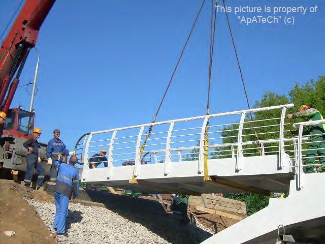
moulding casting in contrast to pultrusion, where the sections are rigidly defined and the density of the fibre is the only parameter that can be altered.
In addition, the use of vacuum infusion made possible to include a volume of glass fibres of over a 60%. In addition, the porosity of the plastic achieved was not less than 1%.
With regards to cost, the use of vacuum infusion reduces considerably the production price as compared to prepeg technologies.
Critical Reflexions
The project resulted in the development of the product line of the arched bridges for small rivers with the span length ranging from 15 to 30m providing a design life of 100 years.
The implementation of vacuum infusion technology gave possibility to reduce manufacturing steps, avoid assembling activities and thus decrease the cost of the structure. The production technology used for this bridge provides new possibilities in aesthetic design and creation of new unsual and good-looking forms.
Transportation and assembly on site was not a complicated process due to the light weight of the materials and the small number of required connections in between the parts. This results on additional benefits with
regards to maintaining the structure. Joints are usually the origin of fatigue problems, leaks of water and corrosion. Reducing the number of joints between components is definitely one of the main advantages fibre composites can offer to the bridges industry.
References:
ApATeCh - Applied Advanced Technologies Arched Footbridge
http://www.apatech.ru/ves_komp_eng.html
http://www.apatech.ru/vacuum_infusion_eng.html
http://www.apatech.ru/yauza_arc_eng.html
AE Ushakov, SN Ozerov and SV Dubinsky, Development of Modular Arched Bridge Design, 5th International Engineering and Construction Conference (IECC), Irvine CA, 27-29 August 2008, paper 116.
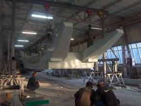
216


217
Den Dungen Draw Bridge, Den Dungen, Netherlands; Lightweight Structures B.V, 2003
Brief Description
Span 10m
Typology Draw Bridge
Material Infused Resin
Observations Hybrid draw bridge; steel upper llifting structure with composite deck
Introduction
The Den Dungen is a draw bridge where a fibre composite deck has been combined with the existing steel upper lifting structrue [Fig 1]. Lightweight Structures B.V., by assignment of the Dutch Ministry of Transport, Public Works and Water Management, designed this bridge.
The bridge needed to withstand vehicle loading of 450 KN in total with 150KN axle load. It has a span of 10m and a width of 3m, crossing the river Zuid-Willemsvaart.
The aim of the development was to provide a safe highly loaded composite structure that could be manufactured cost effectively by means of a resin infusion process. The main motivation for the Ministery was to achieve reduced maintenance costs and to provide local manufacturers and designers with the opportunity to develop manufacturing techniques for the use of composite materials within the civil engineering industry.
Structural Features
The bridge is supported on four points, two points at each end, and by the two rods that carry the balance weights. The bridge is opened by a single cylinder locat-
ed near the main vertical beams and the two points of rotation of the lifting structure.
The structural design was driven by the weight limitation -less than 9,500 kg- and obviously the cost. Within the range of structural concepts the possibility of separating the road deck (platform where vehicles will drive on) and structrual deck (beam-truss) were investigated [Fig xx].
A first selection was made based on reducing the number of elements in an attempt to reduce labour cost for manufacturing and assembly. The selected proposal had a single row of 16 longitudinal beams coupled by means of adhesion, i.e. without a separate road deck. The thicknesses of the top and bottom plates were 14mm and 24mm repectively [Fig xx]. The ends of the beams are closed separately by bonded end caps and connected by an integrally manufactured end wall.
The choice for a single layer concept meant that the strict impact and fire requirements needed to be carefully considered. Furthermore the most critical load paths needed to be fully tested prior to construction.
Construction Highlights
Since vacuum infusion was the technique used the deck could have been fabricated in one single operation; instead the manufacturer decided to cast the beams separately in order to be able to inspect the webs after the infusion. The second step was to bond the beams together with the use of an adhesive. In order to achieve a well defined outer surface the beams are made in a female mould with a flexible inner mould.
Design Issues
Integrating the road surface and the structural deck into one single component required extra tests for im-
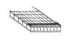
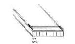
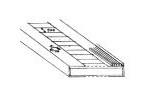
Different slab configurations reference: http://www. lightweight-structures.com/ index.php?option=com_ content&task=view&id=32

Sample of a box beam
http://www.lightweight-structures.com/index. php?option=com_content&task=view&id=76&I temid=70
218
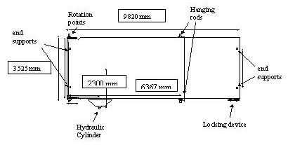
Draw bridge configuration.
http://www.lightweight-structures.com/index. php?option=com_content&task=view&id=32
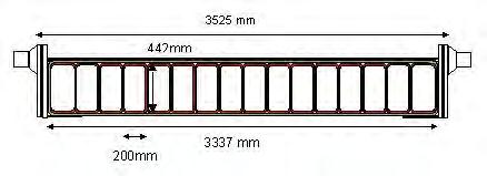
Overal bridge cross section at the rotation points. http://www.lightweight-structures.com/index. php?option=com_content&task=view&id=32
pact, since damage suffered on the road surface will also cause damage on the deck structure.
Impact tests were carried out to verify the residual structural performance of the structure. Different loadcases were considered and the most critical one resulted to be the combination of a wheel print load and impact damage, for example caused by a truck losing a load. In order to check the residual strength of the top layer, impact tests were performed on a reference specimen consisting of the toplayer, and approx. 50 mm of webs. A cylindrical weight of 50 kg was dropped on the top surface from a height of 1.3 m [Fig xx].
A damaged region of approximately 60 mm with delaminations (white area) could be seen on the lower side of the top surface for the glass polyester specimen (fig. 6). For the glass epoxy specimen, no whitening of the laminate could be observed. The test proved that using a granulate top surface for the bridge deck could contribute to the dissipation of energy, as it crushes at the contact with the impactor and thus, protects the underlying composite structure.
Another main requirement had to do with the design of the joints. The many opening and closing cycles of the bridge imposed fatigue loads on the joints of the hydraulic cylinder and hanging supports, but the main fatigue load is of course caused by the traffic. Fatigue is the most critical factor when dimensioning the joints [Fig xx and xx]. Figure xx shows the interface of the steel parts of the rotation point and the composite structure. This type of connection using close tolerance bolts was used at the rotation point and the locking mechanism. At the joint of the cilinder, and the hanging rods, a different type of load introduction was applied [fig... ].
Design rules and safety factors were applied to dimen-
sion and determine the strength of the joints. The test set up is shown in figure 9. Loads were applied including all safety factors. The beam to beam bonded joint is also considered a primary load path and this joint was also tested on ultimate strength, see figure 10. The ultimate strength test of the bolted joint showed a margin in strength of 76%, at 397 kN. The joint failed in the steel plate. The composite had some initial failure, [Fig x] but had not failed.
On fatigue however, the steel bolts failed due to the bending introduced by the eccentricity of the single lap. The composite part of the joint sustained. It showed some delaminations and ovalisation of the hole, but did not fail. The double lap joint on the lower side of the specimen did not show any damage. It was concluded that this type of joint could be applied if the rotation of the bolts was prevented, i.e when the single lap supported.
The bonded joint was not tested on fatigue, but on ultimate strength. The joint failed in the upper corner of the triangulair adhesive area and from there grows along the edge downwards, see figure 12. The beam to beam adhesive joint showed a safety margin of 20%. The specimen failed at 144 kN, whereas 120 kN was required.
Critical Reflexions
Fibre reinforced plastics are increasingly popular for use in civil structures such as bridge structures. In the past years several composite bridges have been realised: pedestrian bridges, but also traffic bridges such as in the USA, Australia and the United Kingdom. From these examples it is seen that each situation and location has its own motivation for using composites. Low weight in combination with high strength means lower transportation costs and allows for a quicker placement of the
219
bridge, using lighter equipment and with a much lower economic impact. In an outback situation maintenance is the problem to be solved and in countries with harsh winters, de-icing salts cause major damage to concrete and steel bridges [ref 1].
When comparing to steel, which is commonly used in movable bridges such as this type of draw bridge, the greatly improved durability and low maintenance of composite materials are a great advantage. Most of the presently realised composite bridge projects are structures based on pultruded elements. This is at present without doubt the most cost effective manufacturing method for realising composite profiles, however with this method usually a large percentage of lower grade materials such as random mat, is used. For movable bridges, the points of load introduction require high strength and local reinforcements have to be applied. Using fabrics and especially +/- 45 orientation complicates the process of pultrusion, and local reinforcements require a special surface treatment. These reinforcements can then only be made externally and will therefore have a less optimum ply stacking.
This study aims on realising a structure made with a low cost resin infusion technique, such as vacuum infusion or film infusion, because with this technique high quality stitched fabric can be used and variations in material lay up can be integrated in the structure.
A single layer concept as shown in figure 4 can be used for this type of bridge. Critical aspects are the transverse stiffness, fatigue of the load introductions and the damage tolerance of the structure after impact. These items have been succesfully demonstrated with tests. The weight of the composite structural parts is 7,780 kg.
References:
the Ministry of Transport [ref 2], [ref3].
Because of the small width to length ratio of this bridge (3.5 m / 10 m), an integrated deck and main structure was designed (single layer structure). The width of the beams is determined by the size of the wheel loads, and the height of the beams is determined by the stiffness requirement of the bridge.
References
BRAILSFORD B.,MILKOVICH S.M., PINE D.W., FILDES J.M. HOPWOOD T. , HARIK I.,Definition of infrastructure specific markets for composite materials: Topical Report, Northwestern University BIRL, Project P93-121/A573, 1995
NNI, NEN 6788 ‘Het ontwerpen van stalen bruggen (VOSB 1995)’, december 1995, The Netherlands NNI, NEN 6786 ‘Voorschriften voor het ontwerpen van beweegbare bruggen (VOBB 1995)’, december 1995, The Netherlands CEN, ENV 1991-3, Eurocode 1 Basis of design and actions on structures, Part 3: traffic loads on bridges, 1991 CUR, CUR ‘Aanbeveling vezelversterkte kunststoffen in civiele draagconstructies’, 2002, Gouda, The Netherlands
220
A draw bridge has also been executed
in assignment of
221
Manufacturing Techniques
The following provides an overview of the current techniques being used for the manufacturing of plastics and fibre composites. This study was accomplished at the very begining of the dissertation to gain sufficient understanding and knowledge on the current manufacturing possibilities. This will therefore serve as a firm foundation upon which the fabrication of the final structure would be developed.
Plastics & Rubber
Blow Moulding
-Mass produce packaging containers – thin walls.
-Three ways: extrusion blow moulding, injection blow moulding and injection stretch blow moulding interior cavities and thin walls are created by blowing air into the pre-form mould.
-Interesting the case study in page 27 of the production of a deodorant bottle with rotation of the parts and the use of different moulds
Thermoforming
-Thermoplastic sheet materials formed with the use of heat and pressure.
-Low pressures – inexpensive; higher pressures more expensive and finishes similar to injection moulding
-Two categories: sheet fed and roll fed
-Sheet fed for heavy duty: baths, shower trays, etc
-Roll fed: roll sheet from a reel – ‘in line’ process: thermoforms, trims and stacks in a continuous operation
-Four processes in thermoforming: vacuum forming,
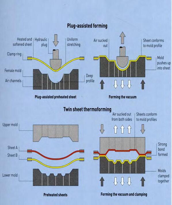
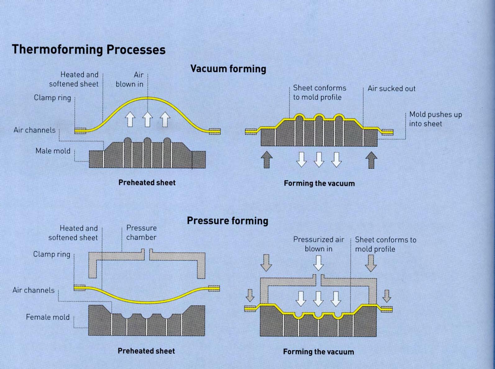
pressure forming, plug-assisted and twin sheet thermoforming.
-Vacuum forming: simple and cheap. Sheet of material heat fed to its ‘softening point’. The sheet is blown into a bubble, which stretches it in a uniform manner. The airflow is reversed and the tool is pushed up into the sheet. The material is drawn onto the surface of the mould by vacuum.
-Pressure forming: reverse of vacuum forming. Sheet is formed on the mould and then drawn down to it by vacuum.
-Plug-assisted forming: similar to pressure forming but using a male hydraulic plug which ensures an adequate wall thickness for deep profiles.
-Twin sheet thermoforming: is used for enclosed thin walled products. Two sheets are thermoformed similarly to pressure forming and clamped together. However, this is a more complicated process and expensive than conventional thermoforming.
-There would be a side with a better finish (the vacuum side) and another one with poor finish.
-In vacuum forming mould can be made from: metal, wood or resin. Wood and resin ideal for prototyping and
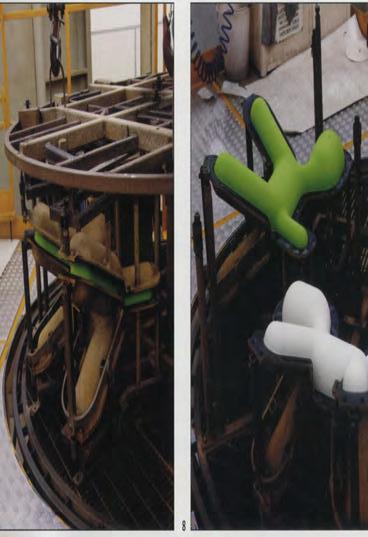
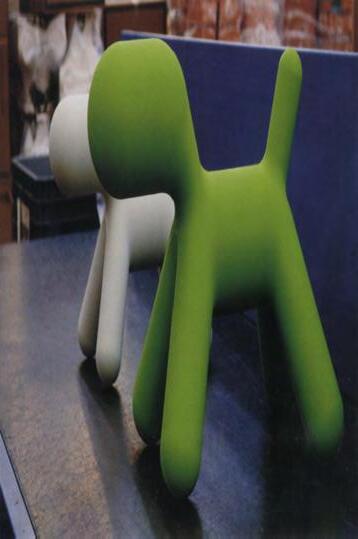
222
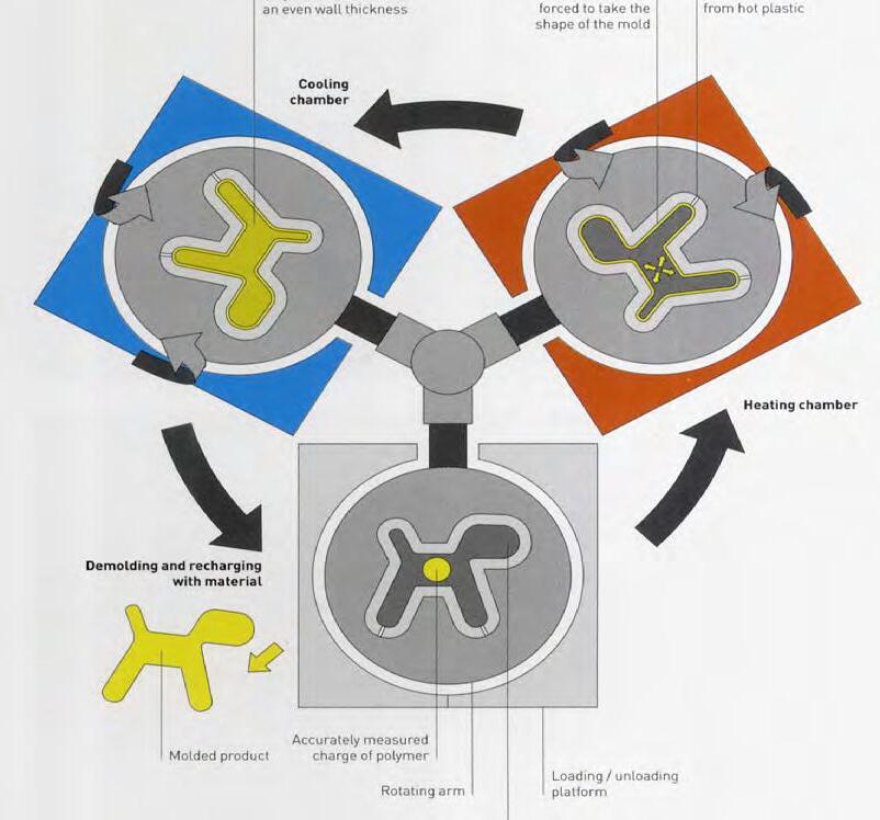
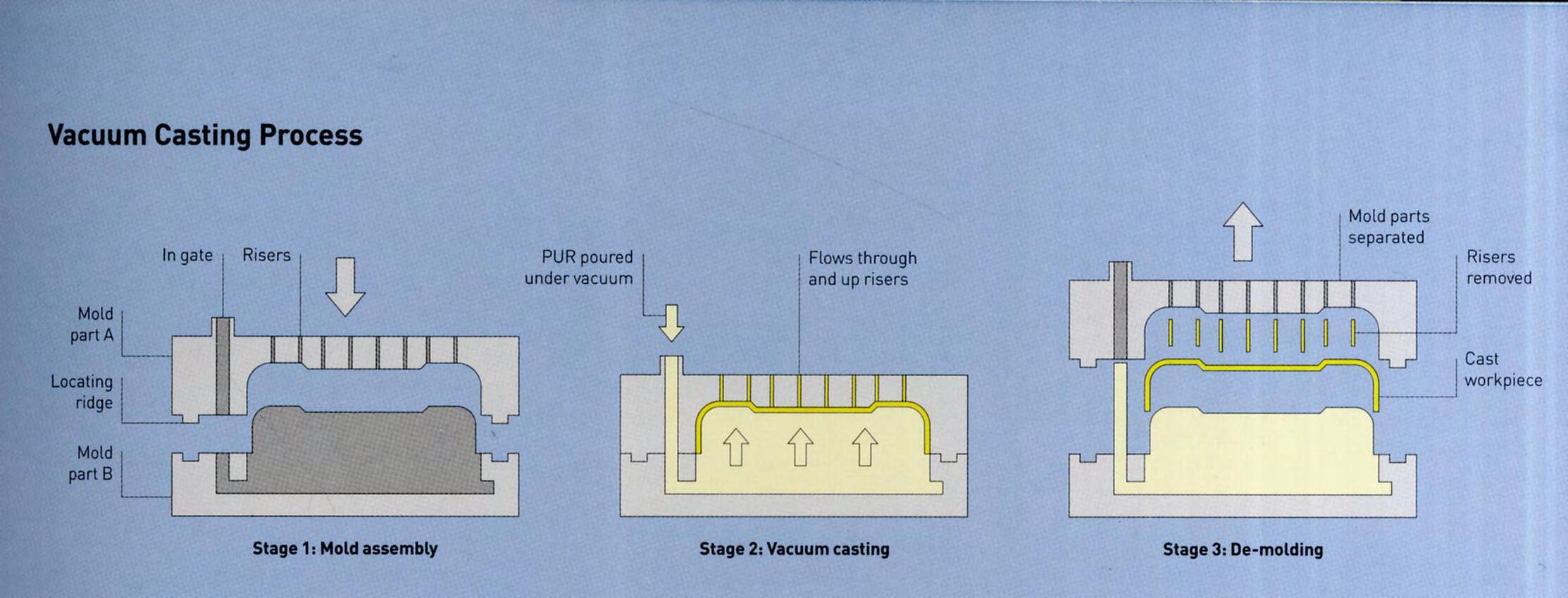
low volume production. Resin mould will last between 10 and 500 cycles, depending on complexity of shape.
-Compatible materials: thermoplastic materials like ABS, polyethylene terephthalate (PET) and PETG (transparent) which is PET modified with glycol (reduces brittleness and premature ageing), polypropylene (PP), polycarbonate (PC, transparent), high impact polystyrene (HIPS). PETG and PC used for lighting diffusers and medical packaging.
-Costs: Pressure forming is 30-50% more expensive than vacuum forming, but cheaper than tooling for injection moulding. Usually tooling costs are 3 times the materials cost.
-Speed of production: depends on selected process and thickness of material. Sheet fed processes typically produce 1-8 parts per minute. Roll fed machines are generally faster and multiple cavity tools can make hundreds of parts per minute. Roll fed machines: automated, while sheet fed machines are loaded by hand.
Rotation Moulding
-Hollow forms with constant wall thickness.
-Medium cost tooling and unit cost of 3 to 4 times the cost of the material.
-Boat hulls, canoes, kayaks, toys, furniture containers, bollards, planters, pet houses, etc
-Larger parts than blow moulding and seamless in contrast with thermoforming using two sheets.
-Surface finish is good.
-Moulded product is almost stress free and has an even wall thickness.
-Plastic shrinks 3% during process.
-Suitable for large products up to 10m3
-Rotation moulding starts with assembly of metal moulds on the rotating arm. Powder is dispensed in moulds then these are closed and clamped and rotation starts in the heating chamber. Time 25 minutes of constant rotation, about both horizontal and vertical axes. Rotation speed of 20 revolutions per minute.
-Cycle time usually between 30 and 90 minutes
-No internal core so changes can be made easily
-Steel moulds are the most expensive, followed by aluminium. Resin tools are the least expensive and can do up to 100 parts.
-Polyethylene (PE) is the most commonly rotation moulded material. Many other thermoplastics can be used: PA, PP, PVC, EVA
-Overmoulding of one material onto another premould reduces assembly costs and produces seamless finishes.
-Additives can be mixed into powder to make the material UV or weather resistant.
Vacuum Casting
-Same finishes as injection moulding.
-Used to mould 2 part thermosetting polyurethane (PUR) for prototyping and one-off production.
-Two separate parts of PUR are stored at 40 degrees. Mixing them together causes a catalytic and exothermic reaction and PUR warms up to 65 degrees.
-Moulds in two halves. Liquid PUR is drawn into the mould by a vacuum. The material has no porosity, will flow through the mould cavity and will not be restricted by air pressure. While pouring, it flows through the gate and into the runner. The liquid flows up into the risers to ensure that the mould is evenly and completely filled.
-First the mould needs to be produced usually with silicone and directly from the master (pattern).
-Advantages: versatile tooling, many variations and applications, tooling flexible silicone moulding.
-Size affects cycle time: large parts have to be cured slowly to avoid the exothermic reaction causing shrinkage and distortion. Parts typically less than 2.5 Kg and can be cured in 1hour or less.
-Wall thicknesses recommended to be between 1mm and 3mm. Thicknesses down to 0.5mm can be produced in small areas.
-A mould usually takes between 0.5-1 day to make in silicone and need to be replaced after 20-30 cycles.
-Materials: cast polyamide (PA) and wax patterns for investment casting.
-Very sharp details such as knife edges should be avoided.
-Low tooling costs. Moderate unit costs.
223
Compression Moulding
-Rubber and plastic shaped by compressing them into a preheated die cavity.
-Used for thermosetting materials.
-Sequence for compression moulding rubber is identical to compression moulding plastic except that the cycle time is longer.
-Two halves mould: upper and lower mould. Rubber placed in lower mould. Two halves or mould are brought together and pressure applied gradually to encourage the material to flow. After 10 min rubber is fully cured. Moulds separate and parts are peeled from the die cavity.
-Compression moulding is reserved for materials with demanding applications such as heat and electrical insulation. Electrical housing, kitchen equipment, ashtrays, handles and light fittings.
-Thermosetting rubber can be formed by compression moulding, injection moulding and vacuum casting. Flexible keyboards, keypads, etc.
-Compression moulding and injection moulding are related; although tooling for compression is cheaper. Injection moulding is used for thermoplastics and compression moulding for thermosetting plastics.
-Compression moulding long strand fibre reinforced plastics (FRP) is known as DMC and SMC moulding. (page 45)
-Thermosetting materials can be filled with glass fibre, talc, cotton fibre or wood dust to increase their strength, durability and resistance to cracking, dielectric resilience
and insulating properties.
-Used to produce parts with different levels of flexibility. Live hinges and tear lines can be integrated into the design avoiding secondary operations.
-Slight re-entrant angles are possible.
-Wall thickness for parts range between 1mm (or 0.3mm in rubber) up to 50mm or more.
-Thermosetting plastics require higher moulding temperatures, between 170-180 degrees.
-Environment: Not possible to recycle thermosets directly; any scrap produced has to be disposed of.
-Moderate tooling costs. Low unit costs: 3 to 4 times material costs.
Injection Moulding
-Ideal for high volume production of identical products.
-Variations include gas assisted, multishot and in-mould decoration.
-Found in automotive, industrial and household products. Shopping baskets, stationery, garden furniture, keypads, etc.
-Very high tooling costs but depends on complexity and number of cavities. Very low unit costs -Great variety of forms can be created. Restrictions come down to economics.
-Undercuts from the sides, top or bottom can be made using retractable cores controlled by cams or hydraulics.
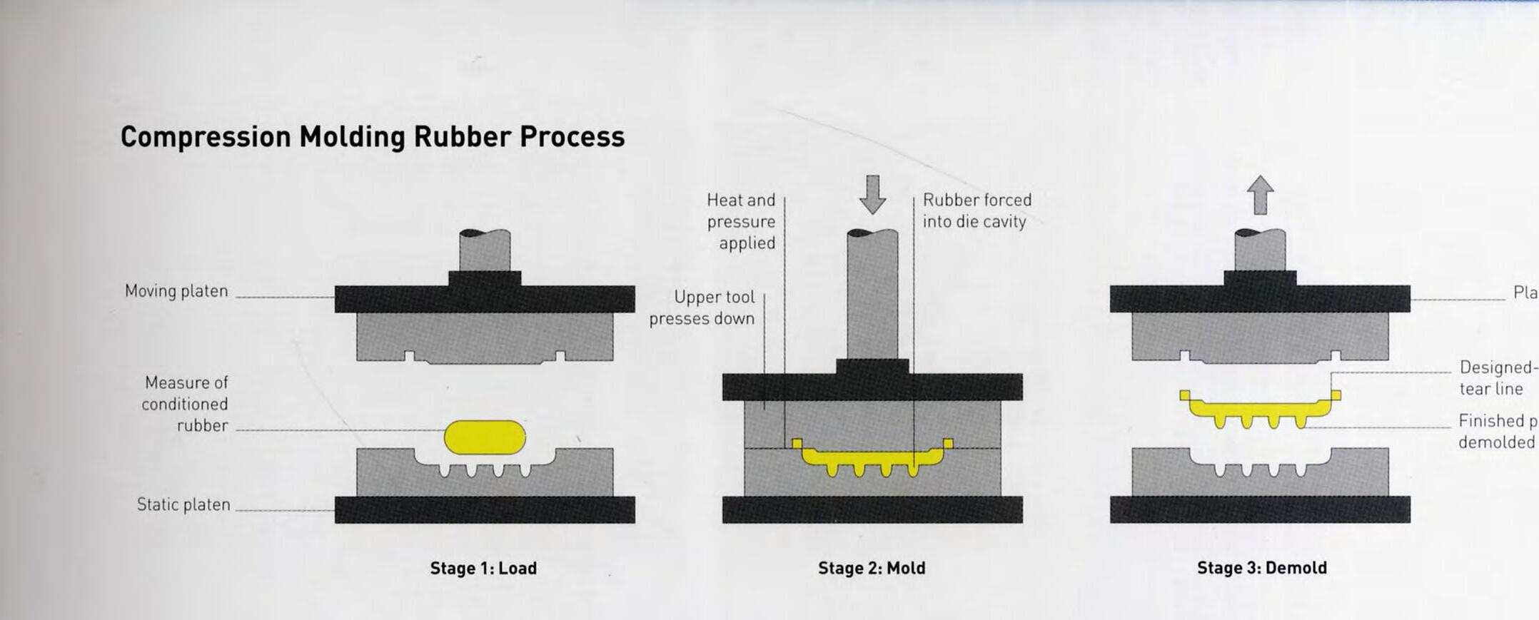
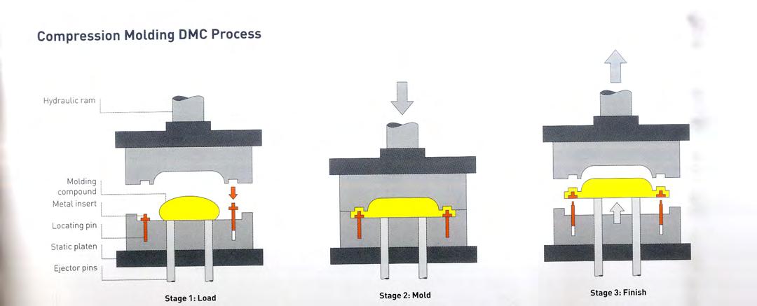
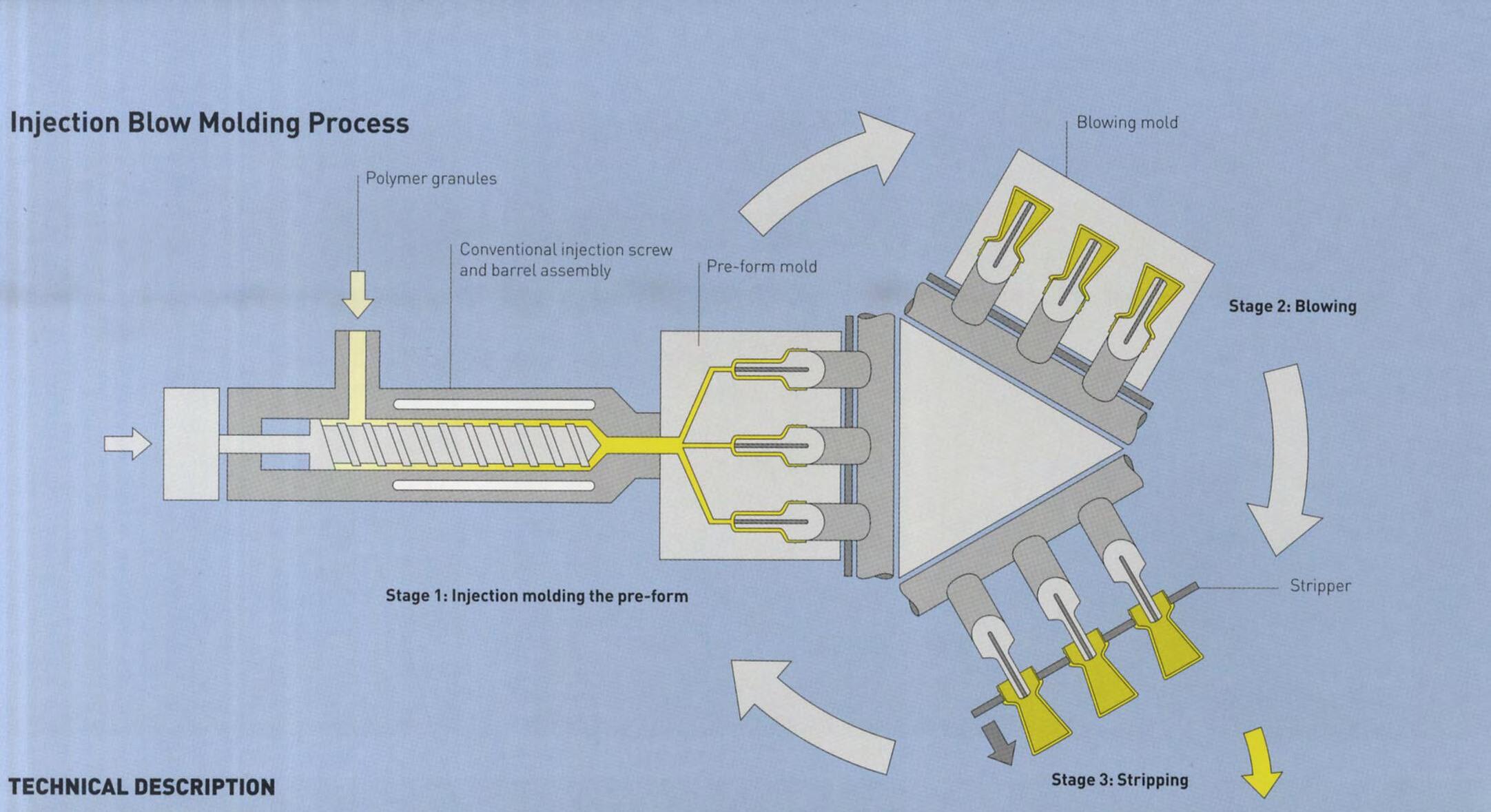
224
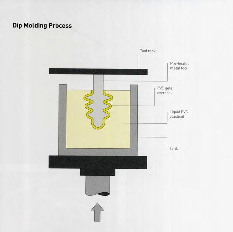
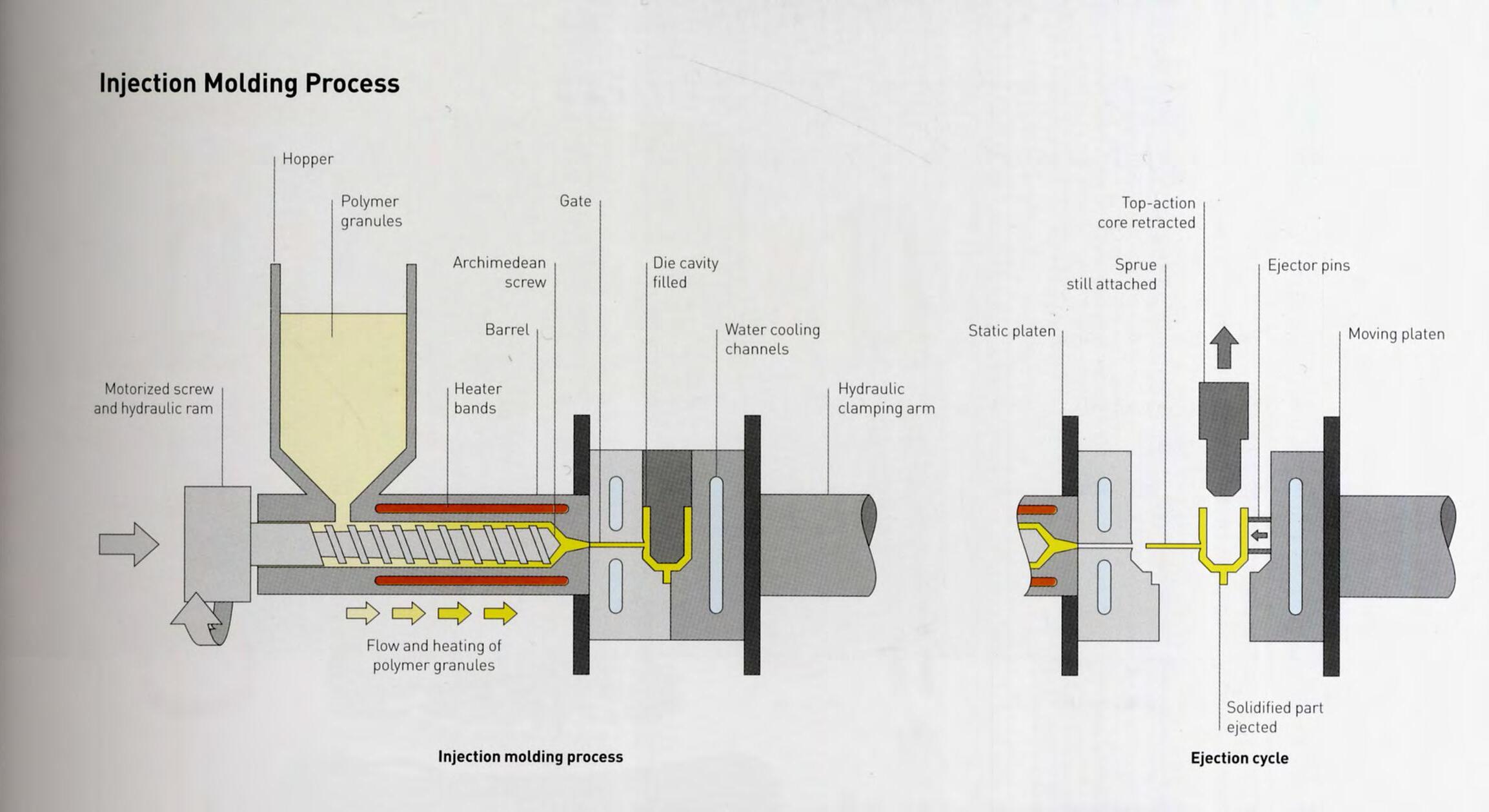
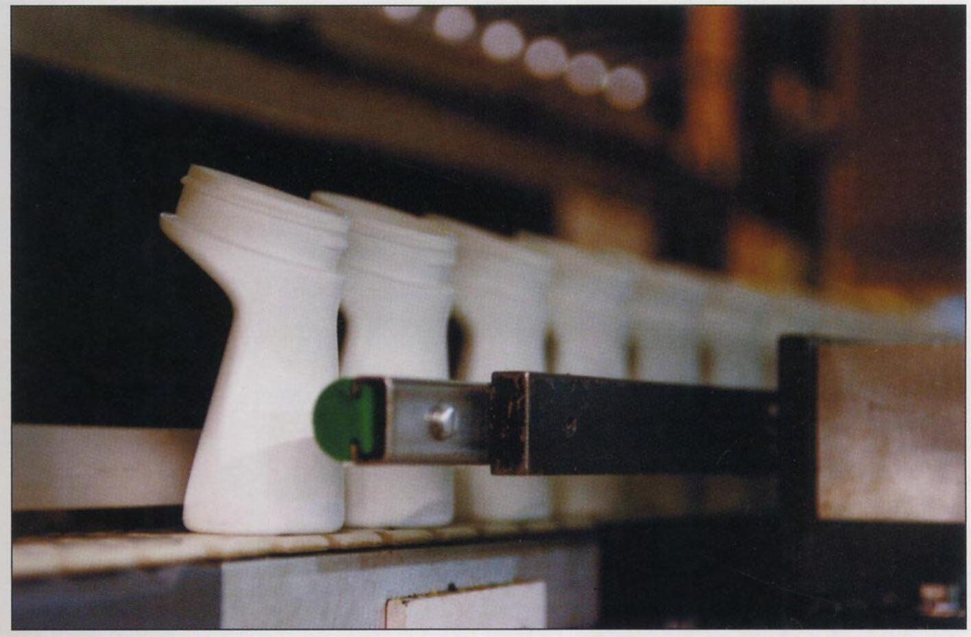
-Material fed into barrel. Mixture is heated, mixed and moved towards the mould by the rotating action of the Archimedean screw. Melted polymer held in barrel until pressure builds up ready for injection into the mould cavity. Correct pressure achieved and polymer is injected into the die cavity.
-Cycle time between 30 and 60 seconds (depends on size)
-Almost all thermoplastics can be injection moulded. Also possible to mould certain thermosetting plastics and metal powders in a polymer matrix.
-Cost very high and depend on number of cavities and cores and the complexity of the design.
Reaction injection moulding (RIM)
-Includes cold cure foam moulding.
-Shape thermosetting foam by injecting thermosetting polyurethane resin (PUR) into a mould where it reacts to form a foamed or solid part.
-Cost: Low to moderate tooling, depending on size and complexity of moulding.
-Low pressure cold cure processes
-Cold cure foam moulding is used with PUR foam; while RIM covers moulding all types of PUR including foam
-Used for bumpers, under-bonnet applications and car interiors.
-Tooling can be GRP, etched or alloyed steel.
-Even though is low pressure process, liquid PUR reproduces fine surface textures and details very well.
-Two halves moulding required. The two components that will form PUR are stored in separate containers. As they mix they begin a chemical exothermic reaction to form PUR. Polymer begins to expand to fill the mould. Only pressure on mould is from the expanding liquid so moulds have to be designed and filled to ensure even spread of the polymer while it is still in its liquid state. As polymer expands the runners allow trapped air to escape.
Dip moulding
-Very low tooling costs. Low to moderate unit costs.
-Low cost method to produce thermoplastic products is used to produce hollow and sheet geometries in flexible and semi-rigid materials.
-It consists of preheating, dipping and baking. Automated and continuous production is rapid
-Smooth and seamless finish. Single male tool so no split lines.
-Thermoforming and dip moulding are quite similar. Main difference being that dip moulding is used to produce flexible parts. It is also less expensive for low volumes.
-Advantage: hollow profiles and parts with re-entrant angles if material is flexible.
225
Composites

Composites are made from two or more constituent materials with significantly different physical or chemical properties which remain separate and distinct on a macroscopic level within the finished structure. In particular, fibre composites are constitued by a polymer or resin matrix which is reinforced with fibres. Nowadays there are many manufacturing techniques avialable in the market to manufacture fibre composites products. The use of these technologies is usually driven by the nature of the fibres and the matrix material, as well as cost and application required. This chapter will illustrate the variety of technologies available, providing also an idea of the applications currently fabricated -via case studiesand a number of manufacturing companies.
Composite Laminating
High performance applications: racing cars, aeropolanes, sailing boats
Strong fibres and rigid plastics can be amalgamated to form ultra light weithgt but high performance material
Three main types of lamintaing: wet lay-up, pre-impregnation with resin (pre-preg) and resin transfer moulding (RTM), also known as resin infusion. Resins used are usually thermosetting and will cure at room temperature.
Composite laminating is unequalled in its versatility and performance. Other processes that can produce similar geometries are dough molding compound (DMC) and sheet molding compound (SMC), injection moulding and thermoforming.
The mechanical properties of the product are determined by the combination of materials and lay-up method. all of them produce products with long stran fibre reinforcement. The resins used include polyester, vinylester, epoxy, phenolic and cyanate. They are all thermosetting and have high resistance to heat and chemicals as well as very high fatigue strength, impact resistance and rigidity.
Laminates cured under pressure have the least porosity.
Processes other than RTM use single sided moulds, which produce a gloss finish on only one side. However, by joining two 3D sheet geometries together a 3D hollow part is made with an all over moulded finish. The surface finish of wet lay-up and RTM products is improved by using a gel coat.
Materials and method of lamination are selected according to the budget and application, which makes these processes suitable for a wide range of prototyping production applications.
Synthetic fibres are usually glass, aramid, carbon or a combination. Different weaving patterns provide various strengths. The direction of weave will affect the mechanical properties of the final product.
Certain weaves have better drape an so can be formed into deeper profiles.
Fibre alingment is critical since a difference of just 5 degrees can have reduce or increase the strength by 20%.
Core materials are used to increase the depth of the parts and thus, increase torsional strenght and bending stiffness. The role of the core material is to maintain the integrity of the composite skin. Examples of core material include DuPont Nomex honeycomb (trademark for aramid fibre sheet), foam and aluminium honeycomb. Cores make changes in wall thickness possible.
Carbon and aramid fibres are very expensive so every effort to minimise material expenditure is worthy. Wall thickness is limited to 0.25 to 10mm. Any ticker surface in combination with the exothermic reaction will be too dangerous. Carbon fibre is generally between 0.5mm and 0.75mm and is only ever built up in areas that need density of material.
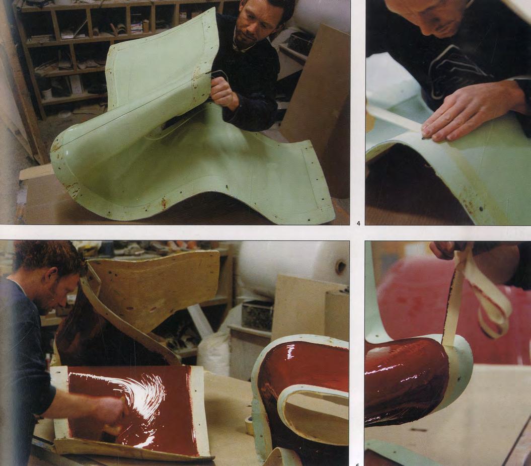
226
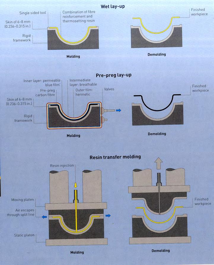
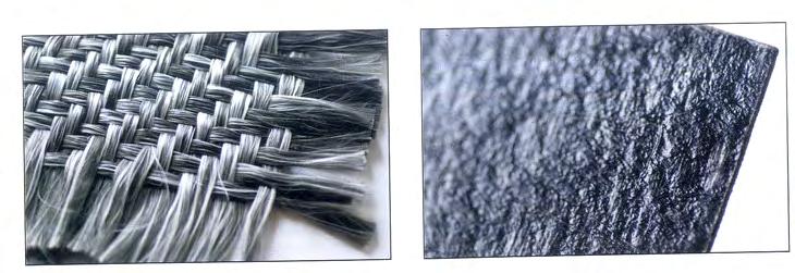
Composite laminates are also limited by the maximum surface area that can be cured in one go which is around 16m2. Usually, larger products are manufactured using more than one piece. Monocoque boat hulls, for example are made in stages -each area being laminated and cured one at a time.
Manual lay-up methods are labour intensive and expensive. Each product may have between 1 and 10 layers of fibre reinforcement, and each layer is applied by hand. A complex product may be constructed from 10 different parts, which makes it really expensive.
Moulds shoudl be made from the same material as the part to be laminated. This will ensure that the moulds have the same coefficient of expansion as the materials. Their wall thickness is tipically 6 to 8mm. When the moulds parts are joined together, the fibre reinforcement is overlapped. This is usually a skilful and timeconsuming process. In order to maximise the strenght, each layer of the lamination is overlapped at a different point to create a staggered lap joint.
Overall, the tooling costs for these technique is moderate to high, as mouldmaking is a labour intensive process. Cost depends on the size and complexity of the product since the tooling needs to have the same geometry as the laminated product. However, it is possible to form the mould from almost any material and then fill, spary, paint and polish the surface to produce the required finish.
Cyble time depends on the complexity of the part and these can vary from an hour (for a small part) to hundreds of them if the part is relatively large and has lots of undercut features and cores.
Environmentally, laminated composites reduce the weight of products and minimise the fuel consumption. However, harmful chemicals are used in their production and it is not possible to recycle any of the offcuts or
scrap material.
Material developments are reducing the toxicity of the products and thus, reducing the environmental impacts caused. For example, hemp is being researched as an alternative to glass fibre, and in some cases thermoplastics are replacing thermosetting materials.
Wet Lay-up
All types of weave and thermosetting resin can be applied by wet lay-up, which is the least precise of all the laminating methods. The mould is single sidedand is made up of a skin of the composite material supported by a rigid framework. It is essential that the mould is not only strong and supportive during lay-up, but is also sufficiently flexible to allow the moulding to be removed post-curing.
Wet lay-up is typically started with a gel coat. The gel coat is a thermosetting resin (the same as in lamination), which is painted or sprayed over the surface of the mould prior to lamination. Gel coats are anaerobic: in other words, the cure when not in the presence of oxygen, which is ideal for the mould face. Mats of woven fibre reinforcement are laid onto the gel coat, and then thermosetting resin is painted or sprayed onto it. It is important to achieve the right balance of resin to fibre reinforcement. Rollers are used to remove porosity.
Pre-preg lay-up
Pre-preg lay-up is the more time consuming, precise and expensive process among composite lamination. It is most commonly used to form carbon fibre. Unlike wet lay-up, no gel coat is needed because this would increase weight; instead the carbon fibre is cut to predetermined patterns, which are laid into the pre-preg mould. Because the fibres are sticky, they can be rubbed together to form a lamination that is free of porosity.
227
Composites
After lay-up the whole mould is covered with three layers of material. The first is a blue film, which is permeable, while the intermediate layer is a breathable membrane. These two are sealed in with a hermetic film, and a vacuum is applied. These layers ensure that an even vacuum can be applied to the whole surface area, becuase if a vacuum was applied under one layer of film it would stick and air pockets would be left behind.
The pre-preg lay-up is placed into an autoclave, which is raised to a pressure of 4 to 5 bar and a temperature of 120 degrees for two hours. The pressure and temperature are lowered when core materials are used.
Resin transfer moulding (RTM)
RTM is used for larger volume manufacturing. Unit price is reduced by accelerated production as a result of using split moulds, heat and pressure and dividing the labour force into specialised areas of production.
This technique uses matched moulds to produce parts with a high quality finish on both sides, known as ‘doubly A side’. the moulds are typically made from metal. Small moulds are machined from solid. Moulds larger than 1m3 are typically electroformed because at this size this process is less expensive than machining and is capable of producing parts with a surface area up to 16m2.
The moulds are preheated, then the fibre reinforcement is laid into the open mould. When closed, resin is injected under pressure. Alternatively, the resin can be drawn through the mould under vacuum or it can simply be poured in prior to moulding.
Because RTM is basically a wet lay-up process, gel coats are required for glass fibre products. For high volume production a thermoplastic-thermosetting combination is used, which produces a very high quality finish be -
cause as the thermosetting resin cools and shrinks the thermoplastic takes the place and forms a ‘low profile’ surface finish.
In the building and construction sector, vacuum infusion (another name for RTM) has been used together with pultrusion for the construction of bridges. In comparison to pultrusion, RTM (vacuum infusion) will result in a higher price per unit weight of material by approximately a factor of 2.5. However, the flexibility in geometry (curvatures) and size is almost unlimited and there are no restrictions in types of reinforcement. Although for reasons of structural efficiency, resin infused bridges make use of conventional structural shapes such as C-profiles or omega profiles, non-conventional and even organic shapes can be realized as part of the load bearing structure, making way for new architecture in bridges.
Manufacturer Companies
Wet lay-up technologies: Radcor - www.radcor.co.uk
Pre-preg technologies: Lola Cars International - www. lolacars.com
All types of composite laminating: ApATeCh - www.apatech.ru
DMC and SMC moulding
Compression moulding is used to form dough moulding compound (DMC) and sheet moulding compund (SMC) into structural and lightweight parts. These processes bridge the gap between injection moulding and composite laminating.
DMC and SMC are typically glass reinforced thermosetting materials such as polyester, epoxy and phenolic resin. DMC is also referred to as BMC (bulk moulding compound). There are thermoplastic alternatives such as GMT (glass mat thermplastic), which is fibre reinforced
228
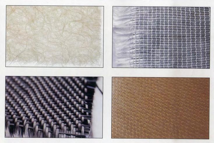
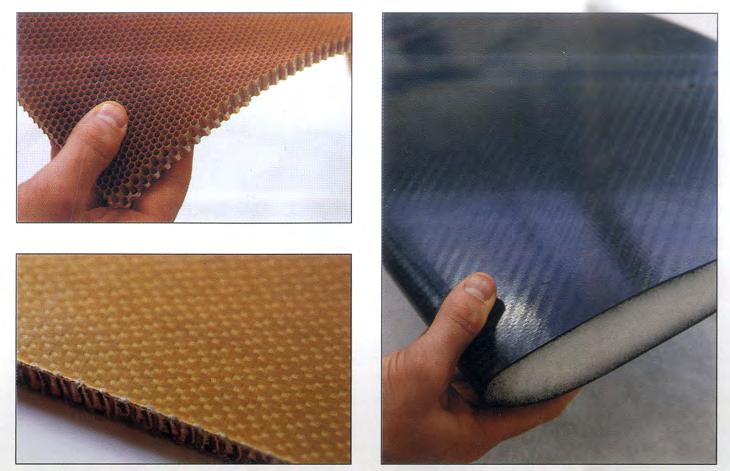
polypropylene (PP). Other types of reinforcement include aramid and carbon fibre. In recent years natural mateirials with suitable properties, such as hemp, have been trialled in an attempt to reduce the environmental impact of these materials.
DMC is compression moulding to form bulk shapes, whereas SMC is used to form lightweight sheet components with a uniform wall thickness. Fibre lenght is longer in SMC: the raw materials are available with different weave patterns for different structural applications. Thsi has significant mechanical advantages, similar to those of laminated composites.
Thermosetting composite materials have high resilience to dielectric vibration, high mechanical strength and are resistant to corrosion and fatigue. These qualities make DMC and SMC very useful in electrical and telecommunication applications. Some examples include enclosures, insulating panels and discs.
The high volume, high strength and lighteweight charcatheristics of DMC and SMC make them suitable for automotive parts, from body panels to structural beams. These materials are also used for electric cars because they combine mechanical strength with lightweight and high dielectric strength.
In the buildig and construction sectors, DMC and SMC are suitable for flooring, door panels and roofs. They are very durable and suitable for public space furniture.
The process of forming in both DMC and SMC starts with the moulding compound being a mixture of fibre reinforcement and thermosetting resin; in DMC this mixture is made up of chopped fibre reinforcement, whereas in SMC it contains sheets of woven fibre reinforcement. The sequence of operation is the same for both and includes loading, moulding and de-moulding. In stage 1, a measure of DMC or SMC is laoded into the die cavity in the lower mould. Metal inserts with locating pins are
loaded into slots. They are in line with the direction of ejection, otherwise the part would not release from the mould.
In stage 2, the upper tool is gradually forced into the die cavity. It is a steady process that ensures even distribution of material througout the die cavity.
Thermosetting material plasticizes at approximately 115 degrees and is cured when it reaches 150 degrees, which takes approximately 2 to 5 minutes. In stage 3, the parts of the mould separate in sequence. If necessary, the part if relieved from the lower or upper tool with ejector pins.
It is a simple operation but it is suitable for the production of complex parts. It operates at high pressure, ranging from 40 to 400 tonnes, although 150 tonnes is generally teh limit. The size and shape of the part will affect the amount of pressure required. Greater pressures will ensure better surface finish and reproduction of detail.
A design opportunity that this technique offers is that the type of fibre reinforcement and length of strand can be modified to suit the requirements of the application. This helps to reduce weight and maximise the efficiency of the process.
Step changes with DMC are not a problem.
Colours are applied by spray painting because the thermosetting resisns in DMC and SMC have a limited colour range.
When working with compression moulding, draft angles can be reduced to less than o.5degrees, if both the tool and the ejector system are designed carefully.
The size of the part can be from 0.1 to 8 Kg on a 400 tonne press. The dimensions are limited by the pressure
229
Composites
that can be applied acrosss the surface area, which is affect by part geometry and design. Another major factor affecting the size of the part is venting gases from the thermosetting materials as it cures and heats up. This plays an important role in design which aims to eliminate gassses with the use of vents and smart rib design. Wall thicknesses can range from 1mm to 50mm. It is limited by the exothermic nature of the thermosetting reaction because thick wall sections are prone to blistering and other defects as a direct result of teh catalytic reaction. It is generally better to reduce wall thickness and minimise material consumption, so bulky parts are hollowed out or inserts are added.
Materials that can be used with these techniques are thermosetting materials such as polyester, epoxy and phenolic resins. On the other hand, thermoplastic composites are generally polypropylene; the moulding process for these is different because they have to be plasticised and formed.
Fibre reinformecement can be glass, aramid, carbon or a natural fibre such as hemp, jute, cotton, rag and flax. Other fillers include talc and wood.
Tooling is generally less expensive than for injection moulding because less pressure is applied and the tooling process tends to be simpler.
Cycle time is 2 to 5 minutes depending on the size of the part and the amount of time it takes to cure.
Labour costs are moderate because teh process requires a great deal of manual input.
Environmentally, the impacts arise as a result of the materials used. Themosetting plastics require higher moulding temperatures, typically between 170 and 180 degrees. It is not possible to recylce them directly due to their molecular strucutre, which is cross-linked. This
means that any scarp produced, such as flash and off cuts, has to be disposed of.
Manufacturer Companies
Cromwell Plastics - www.cromwell-plastics.co.uk
ApATeCh - www.apatech.ru
Filament winding
In filament winding, layers of carbon fibre monofilaments, coated in epoxy resin, are wound onto a shaped mandrel to give the ultimate strength characteristics. The mandrel is either removed and reused, or permanently encapsulated by the carbon fibres.
Filament winding is used to produce continuous, sheet and hollow profiles for applications that demand the high perforamnce characteristics of carbon fibres. They are produced by winding a continuous lenght of fibre with thermosetting resin to produce high strength and lightweight shapes.
The fibres which can be glass, carbon or aramid are appplied as a tow that contains a set number of fibre monofilaments or strands.
There are two main types of winding: ‘wet’ and ‘pre-preg’. Wet winding draws the fibre tow through an epoxy bath prior to application. Pre-preg winding uses carbon fibre tow pre-impregnated with epoxy resin, which can be applied directly to the mandrel without any other preparation.
Filament winding is used to produce low volumes of cylindrical parts. The benefit of filament winding is that the direction of the strand can be adjusted precisely throughout production from almost 0 degrees up to 90. The limitation is that the geometry of the final product is always a solid of revolution.
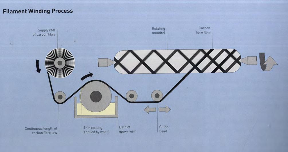
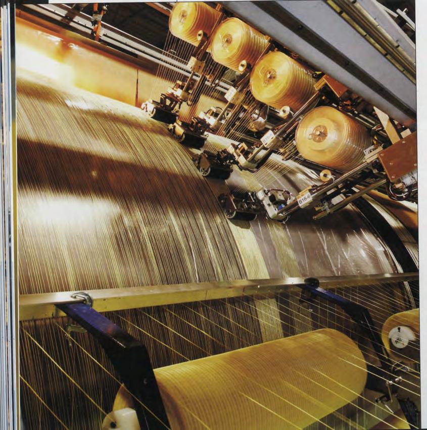
230
However, North Sails, manufacturer of sails, has devel-
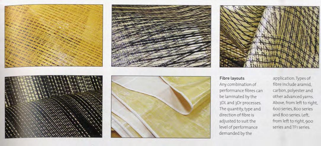
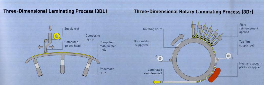
oped a method similar to filament winding which allows the formation of varied surface geometries. It is known as 3D thermal laminating and will be fully explained in the next section. The difference with filament moulding is that filaments are laid onto a static mould in a process known as tape laying. In this case, the moulds can be very large and up to 400m2. 3D thermal laminating is best suited for sheet parts, whereas filament moulding is better to form hollow components.
In filament moulding there are four types of finish: wound, taped, machined and epoxy gel coat; wound being the less treated and thus the rougher finish whereas smooth, glossy finishes can be achieved with epoxy gels.
Winding is computer guided, making it quite a precise process. The angle of application will determine whether the layer is providing longitudinal, torsional (twist) or circumferential (hoop) strength. Layers are built up to provide the required mechanical properties. Products cannot be interchanged between applications because their properties will be designed specifically for each.
As previously mentioned this technique is limited to cylindrical and hollow parts. but they need not to be rotationally symmetrical; oval, ellipctical, sharp edged and flat-sided profiels can also be formed.
Parallel-sided and conical mandrels can be removed and reused, while three-dimensional hollow products that are closed at both ends can be made by winding the filament tow over a hollow liner, which reamins as part of the final product. This technique is known as bottle winding and is used to produce pressure vessels, housing and suspension systems.
Other than shape, the benefits of winding over a liner include forming a water, air and gas tight skinn.
Parallel-sided parts can be made in long lengths and cut to size. Conventional filament winding is typically limited to 3m long a up to 1m in diameter. However, much larger forms are produce by filament winding, such as space rockets, which may take several weeks to make.
Winding over a liner will increase the cost of the process because a new liner is manufactured for each cycle.
Winding over a hollow liner produces parts that have inward and outward facing corners such as bottleneck profiles. Even though it is possible, it is generally not recommended to wind over outward facing corners with a radius of less than 20mm because product performance will be affected. There is no lower limit on the radius for inward facing corners.
In terms of cost, filament winding is a high cost process for low volumes of production which can be slightly reduce if larger volume is to be manufactured. Tooling costs can be low to moderate but encapsulating the mandrel will increase the cost. On the other hand, labour costs are moderate to high due to the high level of manual input required. In addition, materials are also quite expensive and thus, every effort is made to reduce material consumption while maximising strength.
Environmentally, they are quite similar to composites laminates and thus, not very recyclable or environmentally friendly.
Manufacturer Company Crompton Technology Group - www.ctgltd.com
3D Themal Laminating
This technique was developed by North Sails to make ultra lightweight, seamless three-dimensional sails. The fibre reinforcement is continuous over the entire over
231
Composites
the entire surfaces of the sail, replacing traditional methods of cutting, stitching and gluing.
Sails have a 3D ‘flying shape. In conventional sailmaking, cut patterns are stitched or glued together to produce the optimum shape. In 3DL, the sails are moulded in the optimum flying shape and so eliminate cutting and joining. This poroduces sails that are up to 20% lighter than conventional equivalents. They are also stronger and seamless.
The 3DL process combines the benefits of composite laminating with filament winding. the three-dimensional sheet geometries are formed over computerp-guided moulds. The fibre reinforcement (aramid and carbon) are laid down individually along pre-determined lines of stress. They are sandwiched between thin sheets of polyethylene therephthalata (PET) coated with a specially developed adhesive.
3DL manufacturing is a long process, and demand within the industry is verhy high. Therefore, three-dimensional rotatory laminating (3DR) was developed as a method for conitous poroduction. Instead of many large threedimensional moulds, 3DR sailmaking is carried out on a single rotating drum. The shape of the drum is manipulated as the sail is constructed over it. The process is a very recent development and so is still undergoing refinement.
Although these techniques are currently focused on sailmaking, there is potential for application in a variety of products such as high altitude balloons, dirigibles, tension structures, temporary structures and inflatable structures.
The only processes capable of producing very large and seamless shapes are 3DL and 3DR. Circular, conical, elliptical and similar shapes, however, can be produced by filament winding, composite laminating and stitching.
These sails are built to perform a very specific function. they are required to hold their shape, even in strong winds, be durable and lightweight and produce minimum resistance to the flow of air over the surface.
Aerospace vacuum and pressure techniques are used to cure the laminates on the mould. This ensures that the composite will not delaminate, even when extreme loads are applied. The thermally formed PET maintains the position of the fibres, which are laid down in alignment with the direction of stress across the sail.
Each sale has an individual 3D shap. The designer produces a CAD file, which is transferred onto the surface of the mould by a series of pneumatic rams. The shape of the mould will determine the ‘flying shape’ of the sial when it is made.
A PET film is laid over the mould and put under tension. It is coated with a specifically developed adhesive, designed for North Sails by its industrial patners fo the 3DL process. Strands of fibre reinforcement are applied by a fibre placement head guided by a computer controlled overhead gantry. It operates on 6 axes, so can follow the profile of the mould exactly. The fibres follow the anticipated ‘load lines’. Adhesive is applied to the fibres as they are laid down onto the mould, which helps to keep them in place.
A second layer of film is laid on top of the fibres and forced to laminate under pressure at approximately 12.5 psi form a vacuum bag. Heat is then applied with a blanket to cure the adhesive. After curing, the composite sail is removed from the mould and brought to the curing floor for a further 5 days to ensure the adhesive is fully cured and will not delaminate.
The 3DR process is carried out on a rotating drum as oppossed to the static horizontal mould used in 3DL. This
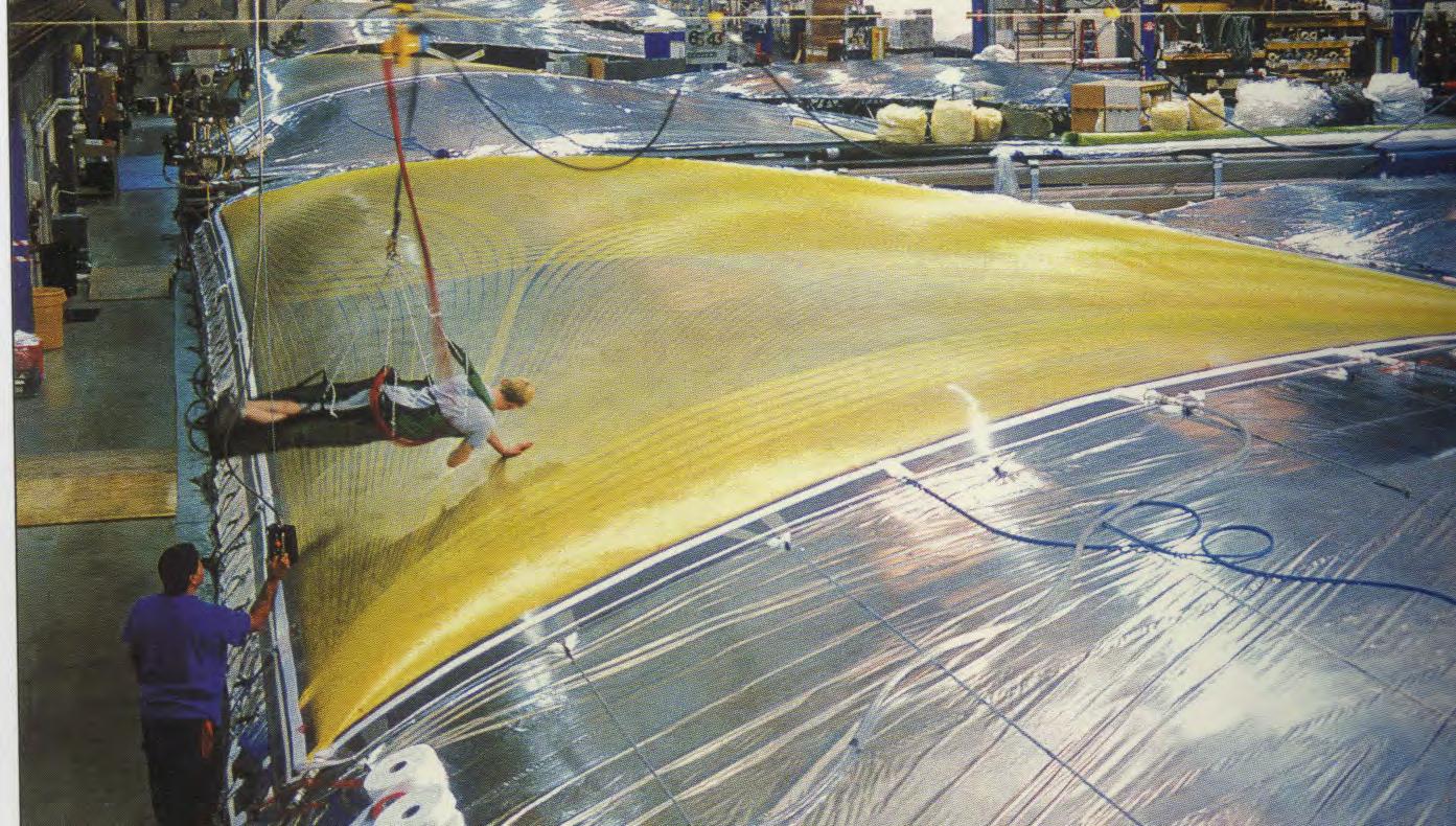
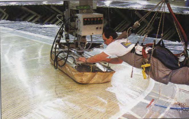
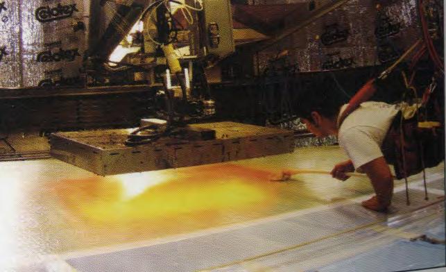
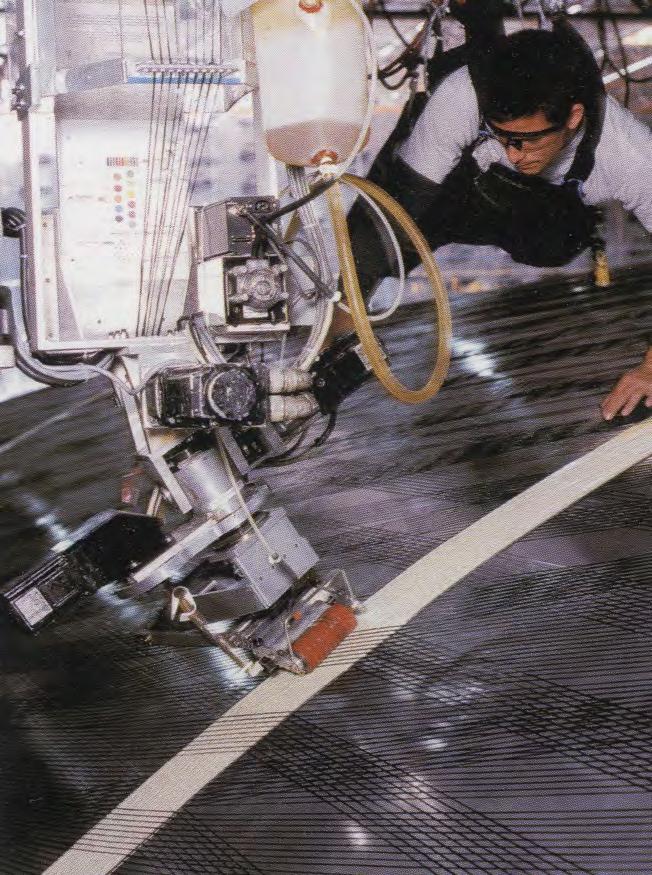
232
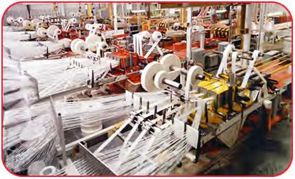

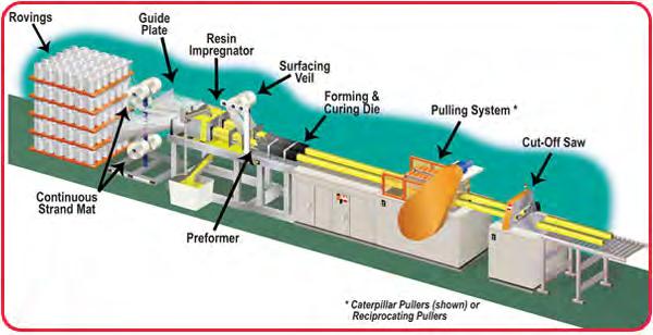
enables the sails to be put together much more quickly.
Teh composite sail is formed as teh drum rotates and leaves the drum completed. The shape of the drum is computer controlled to produce two-directional curvature; the flying shape of the sail.
At present, opportunities for designers are limited because these processes are restricted to sailmaking. In the future, there is a potential for application of these techniques in other industries.
The quantity, type and direction of fibre is adjusted to suit the level of performance demanded by the application. Types of fibre include aramid, carbon, polyester and other advanced yarns. Among the most used types are the 600, 800 and 900 series together with the TF1 series. The 600 series is made up of high-modulus aramid fibres and laid down along the lines of stress to mantain shape and durability. the flowing shape produced in the catenary curves joins areas of stress with smooth, flowing lines of fibre reinforcement. the 800 and 900 series combine carbon fibre with the aramid to reduce weight and stretch. Different films can be used on the outside surfaces to protect against tearing and chafing and provide UV stability. plain weave polyester, known as taffeta, is used on the outside surface of the TF1 series to increase durability.
The material and manufacturing processes employed in 3DL are expensive and therefore limited to high performance applications.
Sails are designed to be strong under tension. Therefore, this process is not suitable for use in applications that require resistance to compression. The sails are not
moulded with a uniform wall thickness, instead it varies with the intended application. Minimum wall thickness is limited by the thickness of the PET film and fibre reinforcement.
Tooling costs are quite high because the male mould is computer guided and adjusted to the flying shape of the sail being made. They are also very large, up to 400m2.
Cycle time is up to 5 days for that surface area because of the lengthy curing process.
Labour costs are high due to the level of skill required to make reliable products.
From the environmental point of view, these techniques save material and produce very lightweight products; but are nowadays limited to a very specific industry.
Reference: Thompson, R.; “Manufacturing Processes for design professionals”. Ed. Thames & Hudson, London, 2007.
Manufacturer Companies North Sails - www.northsails.com
Pultrusion
Pultrusion is a manufacturing process for producing continuous lengths of reinforced polymer structural shapes with constant cross-sections. Raw materials are a liquid resin mixture (containing resin, fillers and specialized additives) and flexible textile reinforcing fibers.
233
Composites
The process involves pulling these raw materials (rather than pushing, as is the case in extrusion) through a heated steel forming die using a continuous pulling device.
The reinforcement materials are in continuous forms such as rolls of fiberglass mat and doffs of fiberglass roving. As the reinforcements are saturated with the resin mixture (‘wet-out’) in the resin bath and pulled through the die, the gelation, or hardening, of the resin is initiated by the heat from the die and a rigid, cured profile is formed that corresponds to the shape of the die.
While pultrusion machine design varies with part geometry, the basic pultrusion process concept is described in the schematic shown below.
Pultrusion is the most cost-effective process for the fabrication of prismatic structural profiles. It is an automated process with a good quality control.
Pultrusion Process
The creels position the reinforcements for subsequent feeding into the guide plate. The reinforcement must be located properly within the composite and this is the function of the reinforcement guides.
The resin bath saturates (wets out) the reinforcement with a solution containing the resin, fillers, pigment, and catalyst plus any other additives required. The interior of the resin impregnator is carefully designed to optimize the wet-out of the reinforcement.
On exiting the resin bath, the composite is in a flat sheet form. The preformer is an array of tooling which squeezes away excess resin as the product is moving forward and gently shapes the materials prior to entering the forming and curing die. In the forming and curing die, the thermosetting reaction is heat activated (energy is primarily supplied electrically) and the composite is cured (hardened).
On exiting the die, it is necessary to cool the hot part before it is gripped by the pull blocks (made of durable urethane foam) to prevent cracking and/or deformation by the pull blocks. Strongwell uses two distinct pulling systems, one that is a caterpillar counter-rotating type and the other a hand-over-hand reciprocating type to pull the cured profile to the saw for cutting to length.
In certain applications an RF (radio frequency wave generator) unit is used to preheat the composite before entering the die. When in use, the RF heater is positioned between the preformer and the die.
In the particular case of bridge structures, pultrusion is more cost-effective for deck structures than vacuum infusion. Because of the durability composite deck structures can compete with conventional deck materials such as wood and steel. Because of the low weight especially for rehabilitation of bridges composite decks are a good and economic solution.
For many bridge structures, both pultrusion and vacuum infusion are interesting. Depending on the type of bridge it must be evaluated which is best. Under certain conditions, full composite bridge structures can be cost competitive with conventional materials other than concrete, such as wood and steel. For the main structure, hybrid material can result in a cheaper structural solution.
Manufacturer Companies ApATeCh - www.apatech.ru Strongwell - www.strongwell.com
Reference text and images: Thompson, R.; “Manufacturing Processes for design professionals”. Ed. Thames & Hudson, London, 2007.
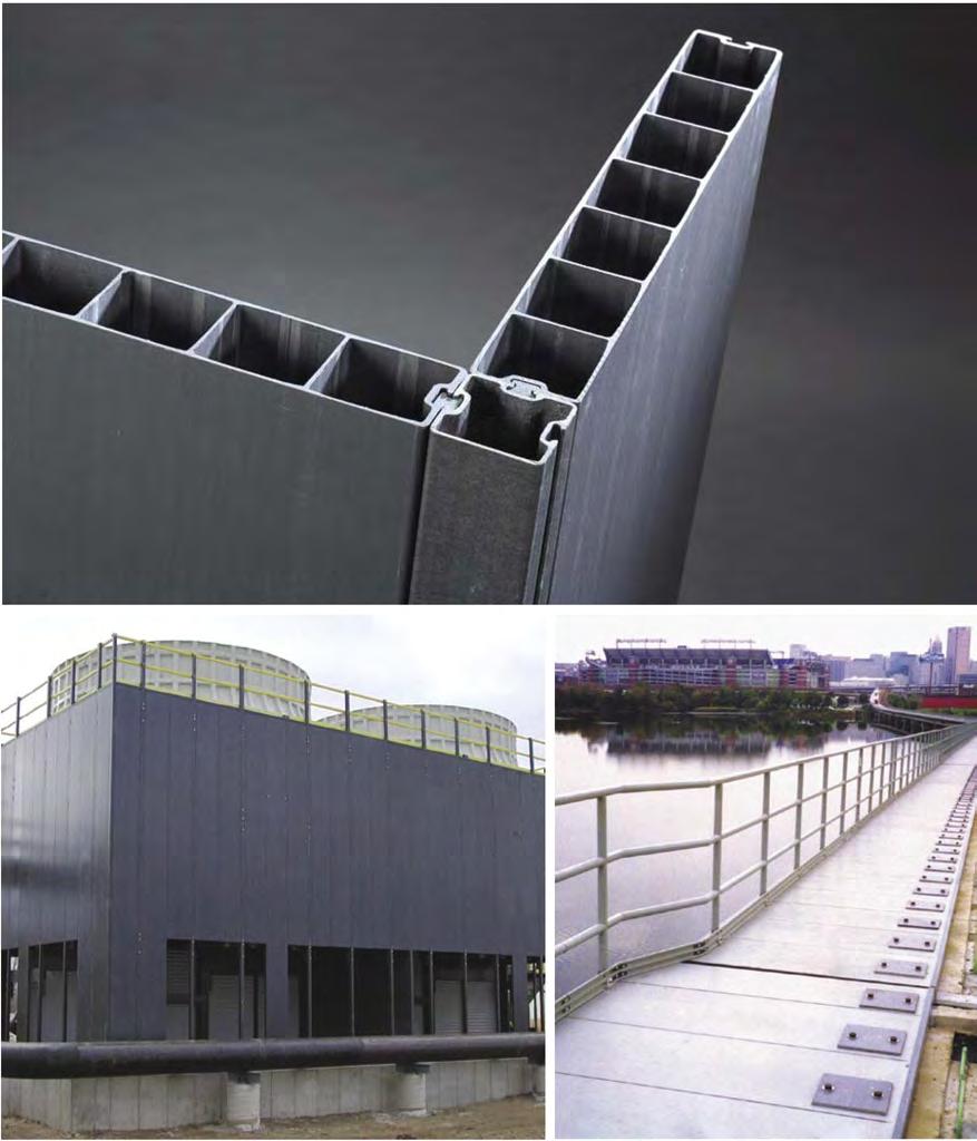
234
235
Experimental Fabrication
Construction of the Physical Model
This section has been complemented with the realisation of a physical model. It is a thermoplasitc fibre composite where glass fibres are laid in the direction of the principal stresses. The piece was casted into a polyurethane foam mould using vacuum forming and sequentially the glass fibres were laid manually. We could have most probably mechanised this process by using a robotic arm similarly to the way a sail is fabricated for racing boats [refer to the manufacturing techniques section, 3D Modelling, North Sails]. Unfortunately we did not have access to those facilities and we decided that by doing the process by hand we could at least identify the main difficulties that could arise from the fabrication. The following pictures aim to illustrate the construction process.
236
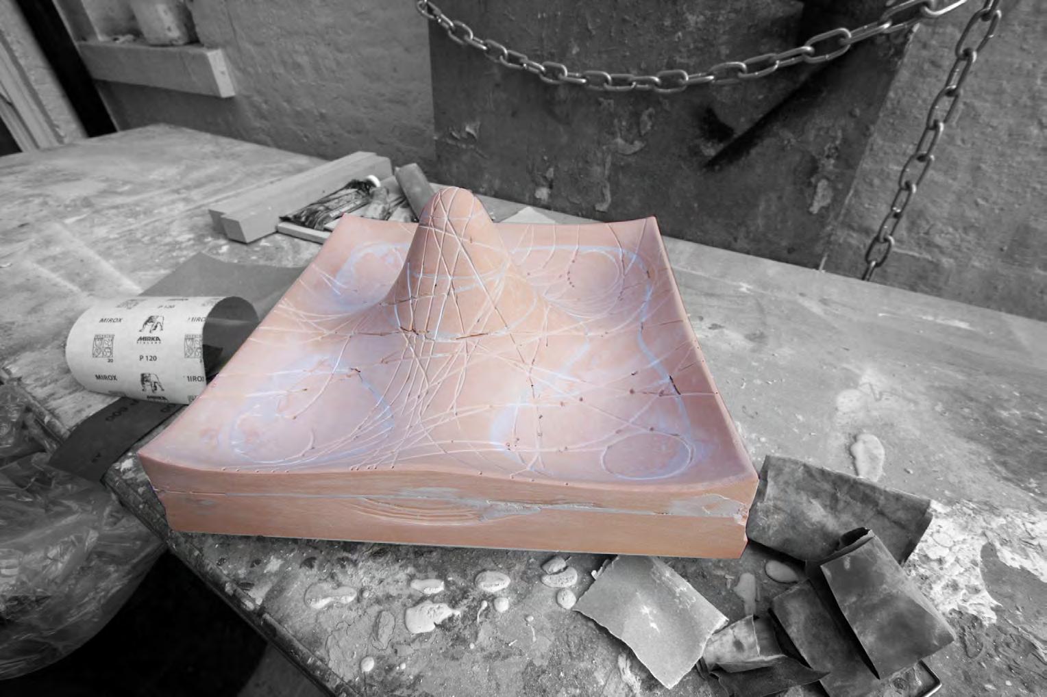
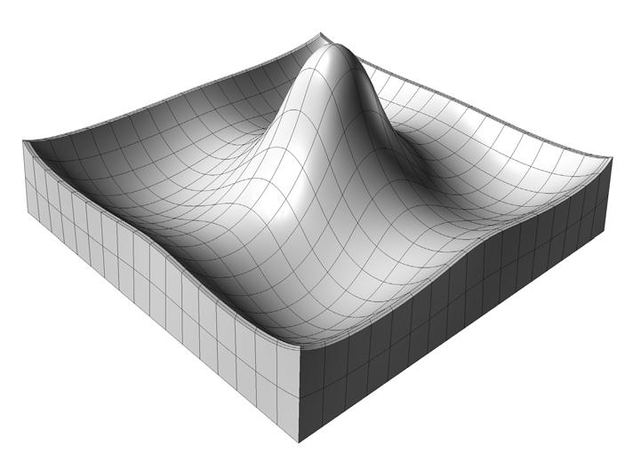
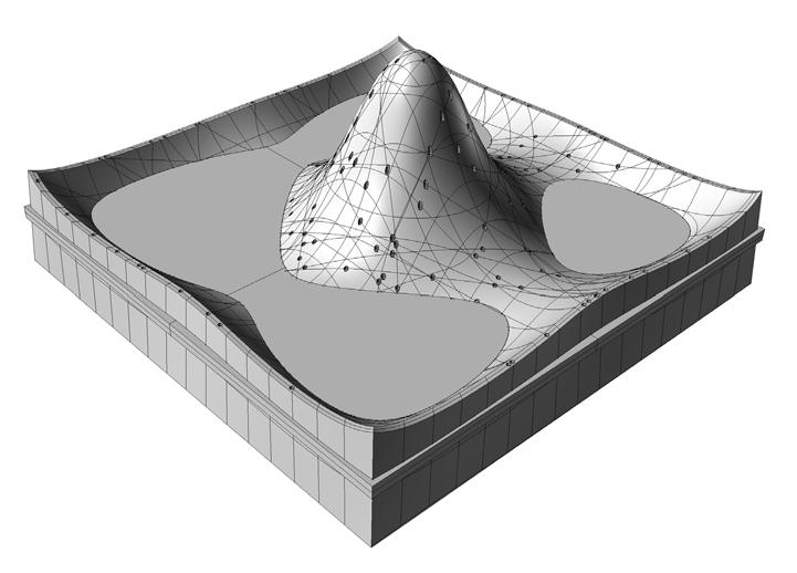
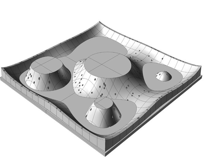
237
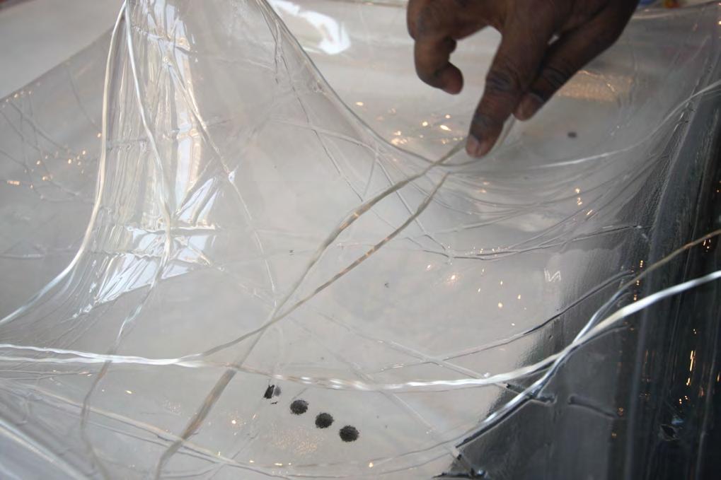
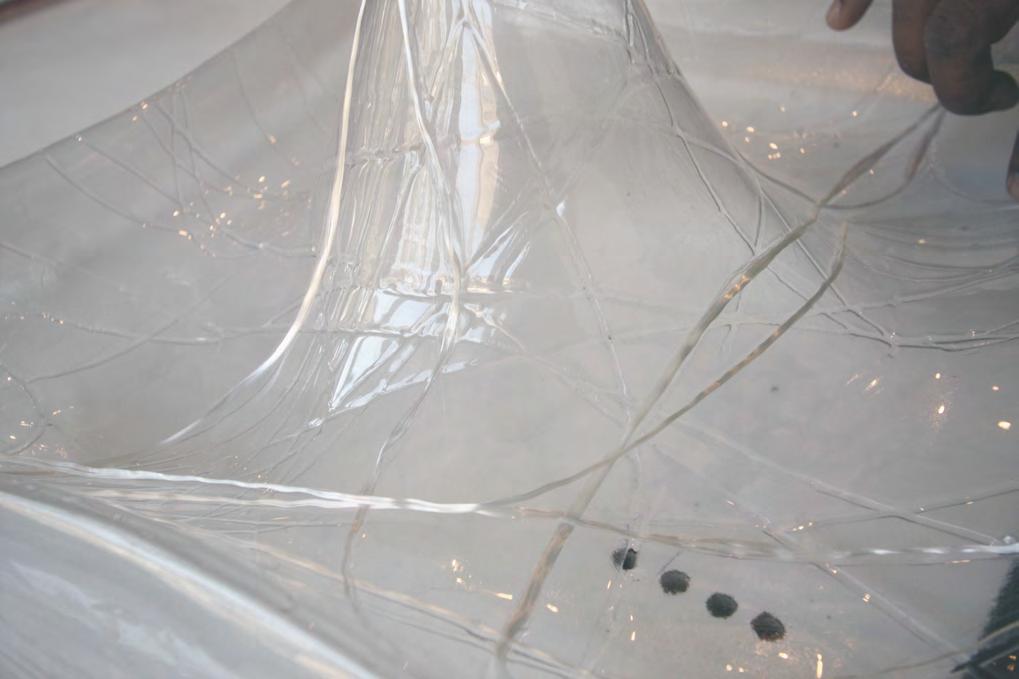
238
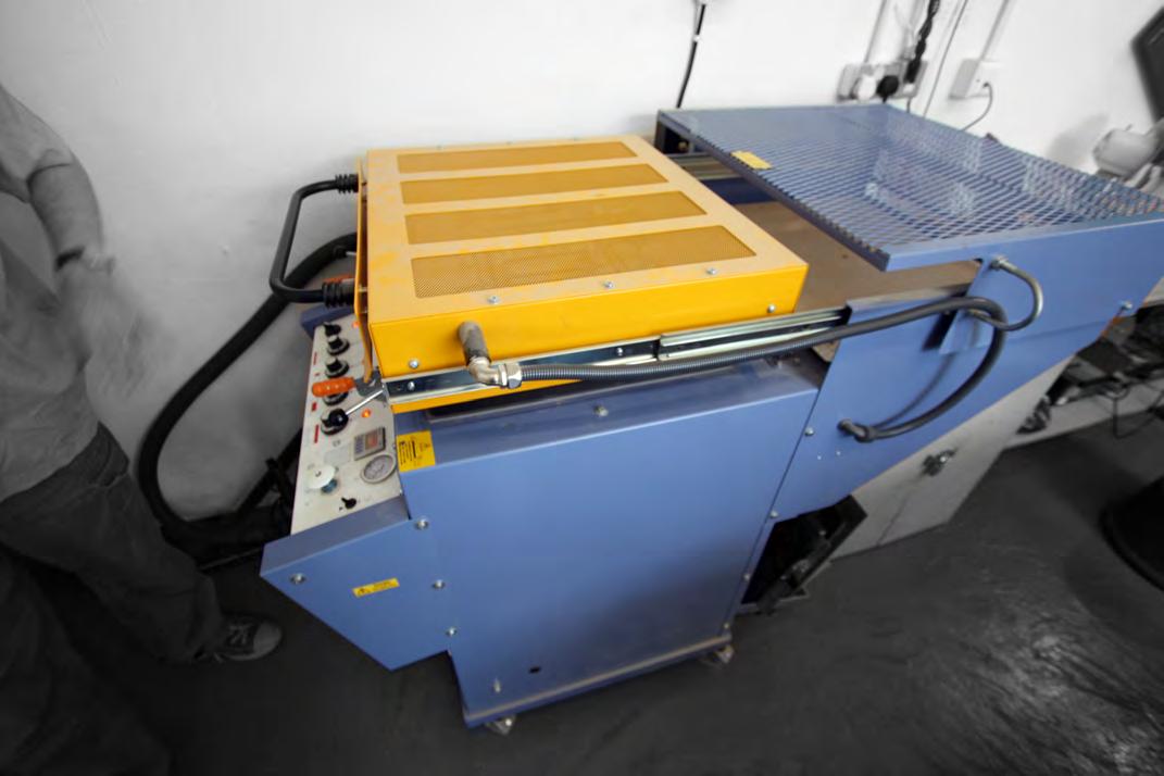
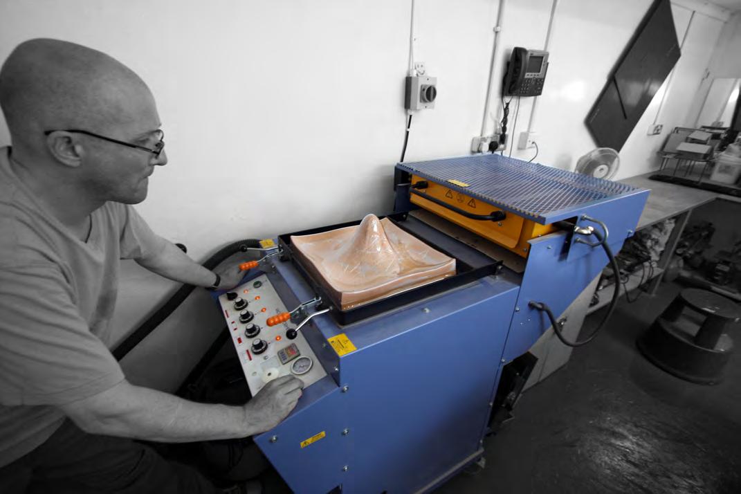
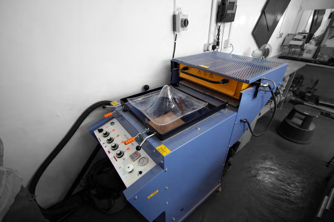
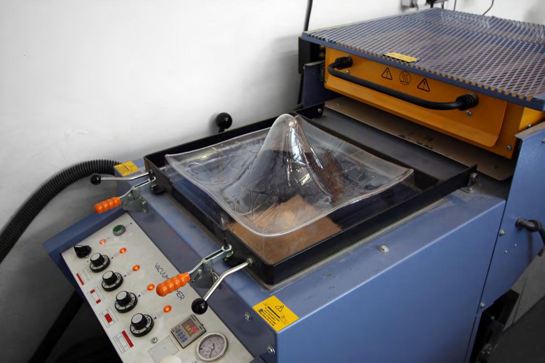
239
Bibliography
[1.0] Jeronimidis,George- ‘Biodynamics’- Emergence: Morphogenetic Design Strategies-Architectural Design Journal edited by Michael Hensel, Achim Menges and Michael Weinstock, Academy Editions, London, Vol. 74 No 3 Issue –May/June 2004.
[1.1],[1.2] Jeronimidis, George, ‘Biomimetics:Lessons From Nature For Engineering’, The 35th John Player Memorial Lecture, The Institution of Mechanical Engineers- Materials and Mechanics of Solids Group, 22 March 2000,London.
[1.3] Gordon, J.E., The New Science of Strong Materials. 2nd Ed, 1976 (Penguin Books.London).
[1.4] Vincent, J.F.V., Deployable structures in nature: potential for biomimicking, 2000, Proc. Instn. Mech. Engineers., 214, 1-10.
[1.5] Jeronimidis, George, ‘Biomimetics -Differentiation / Integration / Emergence,Sensing –Actuation –Control’ - Lecture at the Architectural Association, 2009, London.
[1.6] Jeronimidis, G. (b), Functional holes in fibrous structures: a biomimetic approach to integrated deformation sensors, In Inspiration from NatureThe Emerging Science of Biomimetics; Bionics Biomimetics Symposium 4, Wissenschaftskolleg, Berlin, 2000, in press.
[1.7] Archer, R.R., Growth stresses and strains in trees, 1986 (Springer Verlag. Berlin).
[1.8] http://www.scienceclarified.com/Mu-Oi/Nervous-System. html#ixzz0SXBpP2UN
[1.9] http://www.britannica.com/EBchecked/topic/409665/nervous-system
[1.10] Beukers, Adriaan and Hinte Van- Lightness, Rotterdam, 1999, p.32
[1.11] Hertel, Heinrich- Biology and Technology- Form- Structure –Movement, Reinhold, New York,1966, p. 14
[1.12] Jeronimidis,George- ‘Biodynamics’- Emergence: Morphogenetic Design Strategies-Architectural Design Journal edited by Michael Hensel, Achim Menges and Michael Weinstock, Academy Editions, London, Vol. 74 No 3 Issue –May/June 2004.
[1.13] Hagan, Susannah- Taking Shape- A New Contract between Architecture and Nature, Architectural Press, Oxford, 2001, p. 39
[1.14] Burry, M.; “Between Surface and Substance”, Architectural Design, MarchApril 2003 issue, pp 8-19, Wiley-Academy, London, 2003
[1.15] http://www.materialecology .com
[1.16] http://www.contructioninvivo.com
[1.17] http://www.strangemilitary.com/content/item/10443.html
[1.18] http://www.nasa.gov/centers/langley/news/factsheets/21stcentury.html
[1.19],[1.20] Udd, Eric- ‘Fiber Optic Smart Structures’, John Wiley and sons,1995, p.172, 240
[2.1] Tsai, S.W., Composite Design, Think Composites, Daytopn, Ohio, 1988.
[2.2. Hepworth, D. G.; Vincent, J. F. V., et al. ‘The penetration of epoxy resin into plant fibre cell walls increases the stiffness of plant fibre composites’. Composites Part a-Applied Science and Manufacturing, vol. 31(6), pp: 599-601. Great Britain, 2000.
[2.3] Hepworth, D. G., Bruce, D. M., et al. ‘The manufacture and mechanical testing of thermosetting natural fibre composites’. Journal of Materials Science, vol. 35(2), pp: 293-298. Great Britain, 2000.
[2.4] Santulli, C. ‘Critical length measurements in carbon fibres during single fibre fragmentation tests using acoustic emission’. Journal of Materials Science vol 39, pp: 2905-2907. Great Britain, 2004.
[2.5] Hollaway, Leonard (Editor), 1994, Handbook of Polymer Composites for Engineers, Woodhead Publishing, Cambridge, England.
[2.6] Kaw, Autar K., 1997, Mechanics of Composites Materials, CRC Press, New York, NY.
[2.7] Miller, Tara, 1998, Introduction to Composites, 4th Edition, Composites Institute, Society of the Plastics Industry, New York, NY.
[2.8] Murphy, John, 1998, Reinforced Plastics Handbook, Elsevier Science, Oxford, England.
[2.9] Richardson, Terry, 1987, Composites: A Design Guide, Industrial Press, New York, NY.
[2.10] Rosato, Dominick V., 1997, Designing with Reinforced Plastics, Hanser/ Gardner, Cincinnati, Ohio.
[2.11] Schwarz, M.M., 1992, Composite Materials Handbook, McGraw Hill, Inc., New York.
[2.12] John Crisp and Barry Elliott,“Introduction to Fiber Optics”, Newnes, Uk, 2005
[2.13] D. A. Krohn, “Fibre Optic Sensors Fundamentals and Applications”, Instrument Society of America, USA, 2000
[2.14] Lecoy Pierre, Fibre-Optic Communications, ISTE Ltd, 2008
[2.15] Eric Udd, “Fiber Optic Smart Structures”, WileyBlackwell, 1995
[2.16] Richard O. Claus, “Fiber Optic Sensor-based Smart Materials and Structure”s, Institute of Physics Publishing, 1992
[2.17] Eric Udd, “Fiber optic sensors: an introduction for engineers and scientists”, Wiley, Uk, 1991
[2.18] Francis T.S. Yu and Shizhuo Yin, “Fiber optic sensors”, CRC Press, 2002
[2.19] Daniel D. Pollock, “Thermocouples: theory and properties”, CRC Press, 1991
[2.20] http://www.temperatures.com/tcs.html
[2.21] John P. Bentley , “Principles of measurement systems”, Pearson Education, 2005
[2.22] Béla G. Lipták, “Instrument Engineers’ Handbook: Process control and optimization”, CRC Press, 2006
[2.23] A. L. Window, “Strain gauge technology”, Springer, 1992
[2.24] K. N. Melton, “Ni-Ti Based Shape Memory Alloys”, in Engineering Aspects of Shape Memory Alloys, ed by T. W Duerig et al., Butterworth , London, 1990, pp 28 – 34.
[2.25] A. R. Pelton, “Optimization of Processing and Properties of Medical Grade Nitinol wire”, Minimally Invasive Therapy and Applied Technology, Vol 9 (1), 2000, pp 107 – 118.
[2.26] V. Brailovski, “Optimization of Post-deformation Annealing Heat treatment for NiTi Shape Memory Alloys” in SMST 2000, Proceeding of the International Conference on Shape Memory and Superelastic Technologies, April, 2000, Edited by Russell Pelton, pp 33 – 42.
[2.27] N. B. Morgan and M. Broadley., “Taking the Art Out of Smart!—Forming Processes and Durability Issues for the Application of NiTi Shape Memory Alloys in Medical Devices”, in Proceedings of the Materials and Processes for Medical Devices Conference, edited by S. Shrivastava, ASM International, Sept., 2003, “, pp 247 – 252.
[2.28] S. A. Smith et al., “Shape Setting Nitinol”, in Proceedings of the Materials and Processes for Medical Devices Conference, edited by S. Shrivastava, ASM International, Sept., 2003, “, pp 266 – 270.
[2.29] T. Todoroki and H Tamura, “Effect of Heat Treatment after Cold Working on the Phase Transformation in TiNi Alloys”, Trans. Japan Institute of Metals, Vol. 28, No. 2, 1987, pp 83 – 94.
[2.30] Y. Okamoto et al., “Reversible Changes in Yield Stress and Transformation Temperature of a NiTI Alloy by Alternate Heat Treatments”, Scripta Metallurgica, Vol.22, 1988, pp 517 – 520.
[2.31] X. Huang and Y Liu, “Effect of Annealing on the transfromation behavior and superelasticity of NiTi Shape Memory Alloy”, Scripta Materialia, Vol.45, 2001, pp 153 160.
[2.32] T. Saburi et al., “Effects of Heat Treatment on the Mechanical Behavior of Ti – Ni Alloys”, Journal De Physique, Colloque C4, supplement au No 12, Tome 43, Decembre 1982, pp C4-261 – C4-266.
[2.33] Miyazaki, S., “Thermal and stress cycling effects and fatigue properties of Ni-Ti alloys”, in Engineering Aspects of Shape Memory Alloys, ed by T. W Duerig et al., Butterworth , London, 1990, pp 394 – 414.
[2.34] J. Zang et al., “Reversible Changes in Transformation Temperature of a
242
Ti-51at% Alloy Associated with Alternating Aging”, Scripta Materialia, Vol. 41, No. 10, 1999, pp 1109 – 1113.
[2.35] M. Niashida et al., “Precipitation Processes in Near-Equiatomic TiNi Shape Memory Alloys”, Metallurgical Transactions A, Vol. 17A, Sept., 1986, pp 1505 –1515.
[2.36] W B Cross, “Nitinol Characterization Study”, NASA CR-1433, September, 1969, p vii, Table II.]
[2.37] C M Jackson, Nitinol – The Alloy With a Memory, Its Physical Metallurgy, Properties and Applications – A Report”, NASA SP5110, 1972
[2.38] Havens, E., Snyder, E.A., Tong, T.H.,Light-activated shape memory polymers and associated applications, Proc. SPIE 5762, 48 (2005), DOI:10.1117/12.606109
[2.39] Liu Y et al., Review of progress in shape-memory polymers, J. Mater. Chem, 2007, 17, 1543-1558
[2.40] Czichos H. Adolf Martens and the Research on Martensite. The Martensitic Transformation in Science and Technology (Ed. E. Hornbogen & N. Jost). pp 3–14, Informationsgesellschaft (1989).
[2.41] Brennan, Mairin Chemical and Engineering News, 2001, 79, p. 5.
[2.42] Monkman. G.J. & P.M. Taylor Memory Foams for Robot Grippers Robots in Unstructured Environments Proc. 5th Intl. Conf. on Advanced Robotics, pp. 339 342, Pisa, June 1991.
[2.43] H. Tobushi et al. Sci. Technol. Adv. Mater. 9 (2008) 015009 “Shape recovery and irrecoverable strain control in polyurethane shape-memory polymer” free download
[2.44] Lendlein, A., Langer, R.: Biodegradable, Elastic Shape Memory Polymers for Potential Biomedical Applications, Science 296, 1673-1675 (2002).
[2.45] Monkman. G.J. - Advances in Shape Memory Polymer Actuation - Mechatronics - Vol 10, No. 4/5, pp. 489–498 - Pergamon June/August 2000.
[2.46] Bellin, I., Kelch, S., Langer, R. & Lendlein, A. [1]. Proc. Natl. Acad. Sci. U.S.A. 103, 18043-18047 (2006. Copyright (2006) National Academy of Sciences, U.S.A.
[2.47] Walter Heywang, Karl Lubitz, Wolfram Wersing , “Piezoelectricity”, Springer, 2008
[2.48] Jiashi Yang, “An Introduction to the Theory of Piezoelectricity”, Springer, 2005
[2.49] Vinod K. Wadhawan, “Smart Structures: Blurring the Distinction Between the Living and the Nonliving, OUP Oxford, 2007
[4.1] Weisstein, Eric W. “Nonorientable Surface.” From MathWorld--A Wolfram Web Resource. http://mathworld.wolfram.com/NonorientableSurface.html
[4.2] Van Berkel, B Bos, C; “Everything is curved”, Architectural Design, January-
February 2007 issue, pp 46-53, Wiley-Academy, London, 2007.
[4.3] Dodson, C. T. J. and Parker, P. E; “A User’s Guide to Algebraic Topology”. Kluwer. Dordrecht, Netherlands, 1997.
[4.4] Weisstein, Eric W. “Klein Bottle.” From MathWorld--A Wolfram Web Resource. http://mathworld.wolfram.com/KleinBottle.html
[4.5] Dickson, S. “Klein Bottle Graphic.” http://library.wolfram.com/infocenter/ MathSource/4560/.
[4.6] Geometry Center. “The Klein Bottle.” http://www.geom.umn.edu/zoo/toptype/klein/.
[4.7] Geometry Center. “The Klein Bottle in Four-Space.” http://www.geom.umn. edu/~banchoff/Klein4D/Klein4D.html.
[4.8] Gramain, A.; “Topology of Surfaces”. BCS Associates. Moscow, Russia, 1984.
[4.9] Pappas, T.; “The Moebius Strip & the Klein Bottle. The Joy of Mathematics.” Wide World Publ./Tetra, pp. 44-46. San Carlos, California, USA, 1989.
[4.10] Under wood, M; “Mobius Scarf, Klein Bottle, Klein Bottle ‘Hat’.” http:// www.woolworks.org/patterns/klein.txt.
[4.11] Gardner, M; “Mathematical Magic Show: More Puzzles, Games, Diversions, Illusions and Other Mathematical Sleight-of-Mind from Scientific American”. Vintage, pp. 123-136. New York, USA,1978.
[4.12] Derbyshire, J; “ Prime Obsession: Bernhard Riemann and the Greatest Unsolved Problem in Mathematics”. Penguin. New York, USA, 2004.
[4.13] Henle, M. A; “Combinatorial Introduction to Topology”. Dover, p. 110. New York, USA, 1994.
[4.14] Dodson, C. T. J. and Parker, P. E.; “A User’s Guide to Algebraic Topology”. Kluwer, pp. 121 and 284. Dordrecht, Netherlands, 1997.
[4.15] Bool, F. H.; Kist, J. R.; Locher, J. L.; and Wierda, F. M. C. “Escher: His Life and Complete Graphic Work”. Abrams. New York, USA, 1982.
[4.16] Nordstrand, T; “Moebiusband.” http://jalape.no/math/moebtxt.
[4.17] Dick au, R; “Spinning Möbius Strip Movie.” http://mathforum.org/advanced/robertd/moebius.html
[4.18] Weisstein, Eric W; “Möbius Strip.” From MathWorld--A Wolfram Web Resource. http://mathworld.wolfram.com/MoebiusStrip.html
[4.19] Francis, G. K. and Weeks, J. R.; “Conway’s ZIP Proof.” Amer. Math. Monthly 106, 393-399, 1999.
[4.20] Francis, G. and Collins, B. “On Knot-Spanning Surfaces: An Illustrated Essay on Topological Art.” Ch. 11 in The Visual Mind: Art and Mathematics (Ed. M. Emmer). MIT Press. Cambridge, Massachussets, USA,1993.
[4.21] Dhar wadker, A.; “Heptahedron and Roman Surface.” http://www.egmod-
els.de/models/Surfaces/Algebraic_Surfaces/2003.05.001/.
[4.22] Fischer, G.; “Mathematische Modelle aus den Sammlungen von Universitäten und Museen, Kommentarband”. Vieweg, p. 19. Braunschweig, Germany,1986.
[4.23] Apéry, F.; “The Boy Surface.” Adv. Math. 61, 185-266, 1986.
[4.24] Apéry, F.; “Models of the Real Projective Plane: Computer Graphics of Steiner and Boy Surfaces”. Vieweg. Braunschweig, Germany, 1987.
[4.25] Hauer, E.; “Continua--Architectural Screens and Walls”. Princeton Architectural Press, New York, 2004.
[4.26] Rhinelander, FW; “Circulation in bone. TheBiochemistry and Physiology of Bone”. Academic Press. London & New York,1972.
[4.27] Hoehn, K .; Marieb, E. N.; “Human Anatomy & Physiology”. Benjamin Cummings. San Francisco, USA, 2007.
[4.28] Netter, F. H.; “Musculoskeletal system: anatomy, physiology, and metabolic disorders”. Ciba-Geigy Corporation. New Jersey, 1987.
4.29] Derrickson, B.H.; Tortora, G. J. “Principles of anatomy and physiology”. Wiley. New York, 2005.
[4.30] Schofield and G.W.S. Blari, “On Dough”, Proc. Roy. Soc. A., 1931.
[4.31] Ross Harrison’s. “Croonian Lecture” ,1933.
[4.32] Thompson, D’Arcy; “On Growth and Form”, Ed. Cambridge University Press, First Edition 1961; reprinted 1994.
[4.33] Zaera Polo, A; “The Politics of the Envelope” Log 13/14 (Fall 2008), 195.
[4.34] Reyner Banham, “The Machine Aesthetic”, The Architectural Review, Vol. 447, No. 700, 1955.
[4.35] Bizley, G; ”The envelope gets political”, 17 July, 2009.
[4.36] Lovegrove, Ross. Supernatural, The work of Ross Lovegrove. Phaidon Press Limited, 2004.
[5.1] Gurney, K.- ‘An Introduction to Neural Networks’, Routledge, London, 1997.
[5.2] Grossman.G,Barry and Michael H. Thursby-‘ Neural Network processing for fibre optic sensors and smart systems’. Florida Institute of Technology, Wiley,Canada, 1995
[6.1] Weinstock, Micheal – Self- Organisation and Material ConstructionsTechniques and Technologies in Morphogenetic Design, Architectural Design Journal edited by Helen Castle, Academy Editions, London, Vol. 76 No 2, IssueMarch/April 2006p.35
243
Illustration Credits
[1.0].a -http://cybele.bu.edu/index/leaf.jpg
[1.0]..b-http://www.buffalogardens.com/historical/Crystal_Palaces/body_crystal_palaces.html
[1.0]..c -http://www.mjausson.com/2003/img/ walk24Jun03/14gunnera_dt.jpg
[1.0]..d - http://universe-review.ca/I10-22a-stomata.jpg
[1.1a] - Emergence: Morphogenetic Design Strategies- Architectural Design Journal edited by Michael Hensel, Achim Menges and Michael Weinstock , Academy Editions, London, Vol. 74 No 3 Issue May/June 2004, p.4
[1.1b] - Drew, Philip- Frei Otto – Form and Structure, Granada, London,1976 ,p. 22
[1.1c] -http://nanotechweb.org/articles/news/1/11/5/1/0611102
[1.1] d- http://upload.wikimedia.org/wikipedia/commons/a/ab/ Spider_web_with_dew_drops04.jpg
[1.2a]- http://education.vetmed.vt.edu/Curriculum/VM8054/Labs/ Lab5/Lab5.htm
[1.2b]- http://www.bio.miami.edu/~cmallery/150/physiol/physiology.htm
[1.3]- http://www.tucsongardener.com/Year02/Fall2002/photos/ sensitivefold.JPG
[1.4]- http://hawaii.hawaii.edu/laurab/generalbotany/images/stomata.jpg
[1.5], [1.7] – Diagram redrawn from the lecture presented by George Jeronimidis at the Architectural Association, 2009
[1.6], [1.8], [1.9] – Images obtained from the lecture presented by George Jeronimidis at the Architectural Association, 2009
[1.10a]- http://skitterbot.com/blog/?cat=49
[1.10b]- Fiber Optic Smart Structures, John Wiley and sons, 1995, p.3
[1.12] - Between Surface and Substance, Architectural Design, March-April 2003 issue, pp 8-19, Wiley-Academy, London, 2003
[1.13]- http://www.materialecology .com
[1.15]- http://www.nasa.gov/centers/langley/news/ factsheets/21stcentury.html
[1.17]-http://farm1.static.flickr.com/230/502263398_2bf0535d5d. jpg
[1.18]- Fiber Optic Smart Structures, John Wiley and sons, 1995, p.172
[2.1]-[2.6] D. Hull and T.W. Clyne, “An introduction to composite materials”, Cambridge, Uk, 1996
[2.7] http://www.sxc.com
[2.9] http://www.hexcel.com/
[2.12] E. Udd, “Fiber Optic smart structures”, Wiley, Uk, 1995
[2.15], [2.16] http://www.sxc.com
[2.18] wikipedia.org
[2.33] Andreas Lendlein and Steffen Kelch, “Shape Memory Polymers”
[4.1] Weisstein, Eric W; “Non-orientable Surface.” From MathWorldA Wolfram Web Resource. http://mathworld.wolfram.com/NonorientableSurface.html
[4.2, 4.3] Van Berkel, B Bos, C; “Everything is curved”, Architectural
Design, January-February 2007 issue, pp 46-53, Wiley-Academy, London, 2007.
[4.4] Gardner, M; “Mathematical Magic Show: More Puzzles, Games, Diversions, Illusions and Other Mathematical Sleight-of-Mind from Scientific American”. New York, 1978.
[4.5] Underwood, M; “Mobius Scarf, Klein Bottle, Klein Bottle ‘Hat’.”
[4.6] Dharwadker, A; “Heptahedron and Roman Surface”. Electronic Geometry Model
[4.7] Apéry, F; “The Boy Surface.” Adv. Math, 1986.
[4.8] Apéry, F; “Models of the Real Projective Plane: Computer Graphics of Steiner and Boy Surfaces”. Braunschweig, Germany, 1987.
[4.11-4.17; 4.19-4.23] Hauer, E; “Continua--Architectural Screens and Walls”, Princeton Architectural Press. New York, USA, 2004.
[4.36, 4.37] Lovegrove, Ross; “Supernatural, The work of Ross Lovegrove”. Phaidon Press Limited. London, 2004.
[4.38] Netter, Frank H; “Musculoskeletal system: anato
[5.5a] http://technology.desktopnexus.com/wallpaper/48950/
[5.5b] http://www.onr.navy.mil/media/releases/image_gallery/ images/051206-N-7676W-082a.jpg
[5.6] - http://andrianext.wordpress.com/2008/01/
244
Glossary
Shape Memory Alloys
Af-Temperature: Temperature, above which the phase transformation from Martensite to Austenite is fully completed during heating of the alloy.
Actuator: Device made out of a shape memory alloy, which is able to provide a significant amount of mechanical work due to the occurance of the phase transformation during heating. Actuation force and displacement are functions of the actuator geometry and design.
Apeak- or Ap-Temperature: Temperature, at which the phase transformation from Martensite to Austenite shows the maximum of heat flow during heating. The alloy needs a certain amount of energy (heat flow) to initiate the phase transformation and to move the phase boundary through the alloy. The maximum is a value which can be accurately measured in a DSC equipment, whereas the Asand Af-temperature measurements are sometimes lacking reproduceability.
As-Temperature: Temperature, at which the phase transformation from Martensite to Austenite is initiated during heating of the alloy.
Austenite: Crystallographic description of the high temperature phase of a shape memory alloy, which starts to form during heating of the low temperature phase Martensite when the As-temperature is passed. The formation of Austenite is completed above the Aftemperature.
Biocompatibility: General expression for the suitability of a material for use in the human body and in the endogenous fluids. For NiTinol, a multitude of clinical studies and long clinical history have shown that the biocompatibility
is excellent, especially in terms of cytocompatibility, haemocompatibility, genocompatibility, and corrosion performance. The most current studies report that the overall biocompatibility of NiTi alloys is comparable to stainless steel and Titanium alloys. In some applications, such as stents, recent studies suggest that the biocompatibility of NiTi alloys may be even superior to stainless steel.
DSC (Differential Scanning Calorimetry): Calorimetric method for the characterization of a shape memory alloy with respect to its transformation temperatures. The DSC measures the specific heat flow, which changes constantly during the phase transformation. The overall accuracy and the ease of usage of the DSC equipment together with the high reproduceability makes it the most suitable method for alloy characterization. The main disadvantage of the DSC is the fact, that material deformation and external load cannot be simulated with this measurement.
Hysteresis:
a) thermal hysteresis: The thermal hysteresis means generally the difference between the Apeak- and the Mpeak-temperatures. The hysteresis appears during passing of the transformation temperatures and is affected by a number of parameters (alloy composition, thermo-mechanical treatment, external load, etc.).
b) mechanical hysteresis:
The mechanical hysteresis appears during loading and unloading of a shape memory component in its high temperature phase above Af. The NiTinol component shows a large amount of strain during loading, which recovers during unloading. The necessary force to initiate the transformation during loading is higher as the released
force during unloading.
Martensite: Crystallographic description of the low temperature phase of a shape memory alloy, which starts to form during cooling of the high temperature phase Austenite when the Ms-temperature is passed. The formation of Martensite is completed below the Mftemperature. But the Martensite can also be induced during loading of the Austenite above Mf. This is related to a large amount of recoverable strain and is called ‚Superelasticity‘. NiTiNOL: Common trade name for the commercially most important family of shape memory alloys (NiTi alloys).
One way effect (or „thermal shape memory“): The one way effect occurs in a shape memory alloy, which has been deformed below its lower transformation temperature Ms. The obvious deformation is called pseudoplastic because the alloy recovers shape during subsequent heating into its austenitic high temperature phase. During this shape change the shape memory alloy is capable of providing a significant amount of work output and can be used as an actuator. The subsequent cooling in to the austenitic phase is normally not subject to a reverse shape change, as long as there is no external stress during Austenite - Martensite transformation.
Phase transformation (here: martensitic phase transformation): Physical mechanism, which is the metallurgical basis of the shape memory effect. The term martensitic phase transformation describes the formation of Martensite during cooling OR during loading with an external stress of the austenitic high temperature phase.
R-Phase: Phase, which appears under certain conditions in for instance NiTinol alloys and which is still considered
as being a ‚pre-martensitic‘. The R-phase is related to some anomalies of certain functional properties. The R-phase transformation shows a very narrow thermal hysteresis, but at the same time a very small amount of work output.
Superelasticity: Sometimes compared to a rubber-like deformability of shape memory alloys, which occurs during application of an external stress on the austenitic high temperature phase above Af. Thus, the superelastic effect is related to about 8% of recoverable elastic stress, for which temperature changes are not necessary. The superelasticity occurs basically in the same alloys as the thermal shape memory (one way effect).
Thermomechanical treatment:
Treatment of a shape memory alloy consisting out of a combination between colk working steps and annealing processes. The purpose of the thermomechanical treatment is the adjusting of a number of functional properties, like e.g. the phase transformation temperatures. Usually the annealing of the component or the semi-finished shape is the last step of the fabrication process.
Transformation temperatures: Temperature values, at which start and finish of the phase transformation can be measured (Ms-, Mf-, As-, Af-temperature).
Two way effect: Special form of the thermal shape memory effect, in which not just the heating but also the cooling of the shape memory element are subject to shape changes. This effect is induced either by a special thermomechanical treatment (‚Training‘) or through external stresses during cooling. For design and industrial application of actuators this latter option is highly preferred for as multitude of reasons.
245
