LTspice Essentials (Extract) by Elektor

LTspice Essentials

An Introduction to Circuit Simulation

Dogan Ibrahim

booksbooks

LTspice Essentials

An Introduction to Circuit Simulation

● Dogan Ibrahim

● This is an Elektor Publication. Elektor is the media brand of Elektor International Media B.V. PO Box 11, NL-6114-ZG Susteren, The Netherlands Phone: +31 46 4389444

● All rights reserved. No part of this book may be reproduced in any material form, including photocopying, or storing in any medium by electronic means and whether or not transiently or incidentally to some other use of this publication, without the written permission of the copyright holder except in accordance with the provisions of the Copyright Designs and Patents Act 1988 or under the terms of a licence issued by the Copyright Licencing Agency Ltd., 90 Tottenham Court Road, London, England W1P 9HE. Applications for the copyright holder's permission to reproduce any part of the publication should be addressed to the publishers.

● Declaration

The author and publisher have used their best efforts in ensuring the correctness of the information contained in this book. They do not assume, or hereby disclaim, any liability to any party for any loss or damage caused by errors or omissions in this book, whether such errors or omissions result from negligence, accident or any other cause.

● ISBN 978-3-89576-622-0 Print

ISBN 978-3-89576-623-7 eBook

Prepress Production: D-Vision, Julian van den Berg

Printers: Ipskamp, Enschede, The Netherlands

Elektor is the world's leading source of essential technical information and electronics products for pro engineers, electronics designers, and the companies seeking to engage them. Each day, our international team develops and delivers high-quality content - via a variety of media channels (including magazines, video, digital media, and social media) in several languages - relating to electronics design and DIY electronics. www.elektormagazine.com

● 4

Contents ● 5 Contents Preface ........................................................... 10 Chapter 1 • Introduction ............................................. 11 1.1 Why simulate? ................................................ 11 1.2 Electronic Simulation ............................................ 13 1.3 The LTspice Simulator ........................................... 13 1.3.1 Schematic capture ............................................ 13 1.3.2 DC analysis ................................................. 14 1.3.3 AC analysis ................................................. 14 1.3.4 Transient analysis ............................................. 14 1.3.5 Plotting the results ............................................ 14 1.3.6 Transient noise analysis ......................................... 14 1.3.7 Fourier analysis (FFT) .......................................... 14 1.3.8 Digital simulation ............................................. 14 1.3.9 Laplace transform based analysis .................................. 14 1.3.10 Expression editor ............................................ 15 1.3.11 Parameter sweeping .......................................... 15 1.3.12 AC sweep .................................................. 15 1.3.13 DC sweep ................................................. 15 1.3.14 SPICE models ............................................... 15 1.3.15 Netlist . . . . . . . . . . . . . . . . . . . . . . . . . . . . . . . . . . . . . . . . . . . . . . . . . . . . 15 1.3.16 Online help................................................. 15 Chapter 2 • Getting Started with LTspice ................................. 16 2.1 Overview 16 2.2 Installing LTspice on Windows 16 2.3 Running LTspice 16 2.4 Creating a New Schematic 17 2.5 Simulator Settings 26 2.6 Example Schematics 26 2.7 Online Help 26

LTspice Essentials ● 6 Chapter 3 • Basic DC Circuit Analysis and Simulation . . . . . . . . . . . . . . . . . . . . . . . 27 3.1 Overview 27 3.2 Simple 4-Resistor Circuit 27 3.3 A More Complex Resistor Circuit 30 3.4 Resistive Potential Divider – Sweep a DC Voltage 33 3.5 Resistive Potential Divider – Sweep a Resistor Value 35 3.6 Power Dissipation in a DC Circuit 37 3.7 Resistor-Capacitor (RC) Transient Circuit 39 3.8 Resistor-Inductor-Capacitor (RLC) Transient Circuit 41 3.9 Input Resistance, Output Resistance, and Transfer Function 46 Chapter 4 • Basic AC Circuit Analysis and Simulation ....................... 49 4.1 Overview .................................................... 49 4.2 Resistor – Capacitor Circuit ........................................ 49 4.3 Resistor – Inductor Circuit ........................................ 50 4.4 Resistor – Inductor – Capacitor Circuit ................................ 51 4.5 Thevenin’s Theorem – AC Circuit Analysis .............................. 54 4.6 Three-Phase Circuits ............................................ 56 4.6.1 Star with resistive loads ........................................ 57 4.6.2 Star with resistive and inductive loads ............................... 59 4.7 Mutual Inductance .............................................. 60 4.7.1 Circuit with mutual inductance .................................... 61 4.8 Using a Transformer............................................. 63 4.9 Frequency Sweeping ............................................ 63 4.10 Fast Fourier Transform (FFT) ...................................... 65 4.11 Input & Output Impedance, and Gain ................................ 66 Chapter 5 • Diode Circuits ............................................ 74 5.1 Overview .................................................... 74 5.2 Half-Wave Rectifier ............................................. 74 5.3 Full-Wave Rectifier .............................................. 76 5.4 Full-Wave Rectifier with a Transformer ................................ 78 5.5 Zener Diode Voltage Regulator ..................................... 79

Contents ● 7 5.6 Diode Clamp 81 5.7 Voltage Multiplier 82 5.8 I-V Characteristic of a Diode 85 Chapter 6 • Transistor Analysis, Design and Simulation ..................... 87 6.1 Overview 87 6.2 Bipolar Junction Transistor (BJT) I-V Curve 87 6.3 Common-Emitter Transistor Amplifier – Analysis 88 6.4 Common-Emitter Transistor Amplifier – Design 91 6.5 Audio Power Amplifiers 93 6.5.1 Class A audio power amplifier simulation 94 6.5.2 Class AB audio power amplifier .................................... 96 6.6 BJT Switch ................................................... 98 6.7 JFET Common-Source Amplifier .................................... 100 6.8 MOSFET I-V Characteristic Curve ................................... 102 Chapter 7 • Thyristors, Diacs and Triacs – Importing a SPICE model........... 105 7.1 Overview ................................................... 105

Thyristors, diacs, and triacs ...................................... 105 7.2.1 Triac – diac phase control ....................................... 106 7.3 Inserting a Potentiometer – Using a Potentiometer Model .................. 109 Chapter 8 • Oscillators .............................................. 113 8.1 Overview ................................................... 113 8.2 Transistor Sinewave Oscillators .................................... 113 8.2.1 Colpitts oscillator ............................................ 113 8.2.2 Hartley oscillator............................................. 115 8.3 Sine Wave Oscillators with Operational Amplifiers ....................... 116 8.3.1 Phase-shift oscillator .......................................... 117 8.3.2 Wien bridge oscillator ......................................... 120 8.3.3 Colpitts oscillator ............................................ 122 8.5.4 Hartley oscillator............................................. 124 8.4 Op-Amp-Based Square Wave Oscillator .............................. 126 8.5 The 555 Timer................................................ 127

7.2

LTspice Essentials ● 8 8.5.1 The 555 astable multivibrator 127 8.5.2 Blinking an LED 128 8.5.3 Metronome 130 8.5.4 Parametric sweep 131 Chapter 9 • Simulating Other Analog Circuits ............................ 134 9.1 Overview 134 9.2 The LT1086 Voltage Regulator 134 9.3 10 V Output 135 9.4 DC Boost Converter 135 9.5 Optocoupler Simulation 137 9.6 Operational Amplifier with Single Supply ............................. 138 9.7 Sweeping a Resistor Value ....................................... 139 Chapter 10 • Filters – Hierarchical Blocks ............................... 141 10.1 Overview .................................................. 141 10.2 Low-Pass Filter .............................................. 141 10.3 Filter Design Tool ............................................. 142 10.3.1 Low-pass active filters ........................................ 142 10.4 Hierarchical Blocks – 2nd-Order Low-Pass Filter Block .................... 146 10.4.1 Using the filter block ......................................... 147 10.5 Passing Parameters to Hierarchical Blocks ............................ 149 10.5.1 Using the programmable block .................................. 149 10.6 Create Your Own Symbol ....................................... 151 10.7 LTspice Filter Library........................................... 152 Chapter 11 • Digital Logic ........................................... 154 11.1 Overview .................................................. 154 11.2 Digital Components ........................................... 154 11.3 Half Adder Using Logic Gates .................................... 154 11.4 Full Adder from Two Half Adders .................................. 156 11.5 Importing the 74HC Family ...................................... 158 11.6 Two-Input Multiplexer.......................................... 161 11.7 4-Bit Binary Counter .......................................... 162

Contents ● 9 11.8 More Inputs 164 11.9 Full Adder 165 11.10 Monostable Multivibrator 166 11.11 Square Wave Oscillator 168 Chapter 12 • SPICE models .......................................... 170 12.1 Overview 170 12.2 The Structure of SPICE Models 170 12.3 Passive Components 170 12.4 Active Components 172 12.4.1 Diodes 172 12.4.2 Bipolar transistors ........................................... 174 12.4.3 MOSFETs ................................................. 175 12.4.4 Creating a new diode model .................................... 176 12.5 Logic Gates ................................................. 178 12.6 SPICE Directives ............................................. 178 Chapter 13 • Some Useful Tools and Functions ........................... 180 13.1 Overview .................................................. 180 13.2 Generating Triangular and Sawtooth Waveforms ....................... 180 13.3 Generating a Periodic Arbitrary Waveform............................ 181 13.4 The Voltage-Controlled Switch .................................... 184 13.5 Laplace-Transform Based Simulation ............................... 185 Appendix A – Third-Party SPICE Models ................................ 189 Appendix B – Useful Resources ....................................... 191 Index ........................................................... 193

Preface

Electronic circuit simulation is essential in all branches of electrical and electronic engineering. Students put into practice the complex theory they have learned in their courses, and this gives them the chance to apply the theory to real-world experiments. Practicing engineers simulate and optimize electronic circuits before constructing them for final testing.

Circuit theory is a core subject that is the fundamental part of all electrical and electronic engineering courses. In conventional engineering laboratory experiments, electronic components and instruments must be purchased and then assembled to build circuits for experimentation and validation. Usually, it may be costly and sometimes difficult to obtain the real components required for an experiment, especially during the development cycle. Simulating a circuit is much cheaper and faster. Components and instruments cannot be broken and an unlimited amount of them is available.

LTspice, developed by Analog Devices, is a powerful, fast, and free SPICE simulator, schematic capture, and waveform viewer with a large database of components supported by SPICE models from all over the world. Drawing a schematic in LTspice is easy and fast. Thanks to its powerful graphing features, you can visualize the voltages and currents in a circuit, and also the power consumption of its components and much more.

LTspice is a powerful electronic circuit simulation tool with many features and possibilities. Covering them all in detail is not possible in a book of this size. Therefore, this book presents the most common topics like DC and AC circuit analysis, parameter sweeping, transfer functions, oscillators, graphing, etc. Although this book is an introduction to LTspice, it covers most topics of interest to people engaged in electronic circuit simulation.

The book is aimed at electronic/electrical engineers, students, teachers, and hobbyists. Many tested simulation examples are given in the book. Readers do not need to have any computer programming skills, but it will help if they are familiar with basic electronic circuit design and operation principles. Readers who want to dive deeper can find many detailed tutorials, articles, videos, design files, and SPICE circuit models on the Internet.

All the simulation examples used in the book are available as files at the webpage of this book. Readers can use these example circuits for learning or modify them for their own applications.

I hope you enjoy reading the book and use LTspice in your next electrical/electronic simulation project.

Prof Dogan Ibrahim

April

2024

London

LTspice Essentials ● 10

Chapter 1 • Introduction

1.1 Why simulate?

One of the major differences of engineering courses from many other courses is that engineering courses highly depend on practical work, such as laboratory work. Laboratories are essential parts of every engineering course, and it is a major requirement for all students in such courses to complete all laboratory work successfully before they are allowed to graduate.

Students learn the mathematics and theories of electronics in classes, and they are then expected to apply this knowledge by carrying out relevant experiments in the lab. This is true for all engineering courses, whether it is chemical engineering, mechanical engineering, electrical/electronic engineering, etc. For example, electronic engineering students learn the circuit theory in great detail in the class. They are then expected to carry out experiments in laboratories using real components, real measuring tools, and real power supplies and put the learned theories into practice.

Although real laboratory experiments are very useful, they have some problems associated with them:

• The purchase of real electronic components and instruments can be very costly. Many pieces of the same instruments are usually required for a class of students, and this can be very costly.

• The characteristics of electronic components and electronic equipment can change with aging and temperature and as a result, unexpected or wrong results can be obtained.

• It is not always easy to find the required components, and students may have to wait for long times before they can develop and test their projects. For example, an experiment may require a certain model of transistor and this transistor may not be available in the laboratory stock.

• Real components and real equipment can easily be damaged by improper use, for example by applying large voltages, or by passing large currents through them, or by short-circuiting them. It may be costly to replace or repair them in time.

• Students can get accidents (e.g. electric shock) in laboratories by not following the safety regulations. Thus, an instructor must always be present in a laboratory to make sure that students connect the components correctly and use the mains-powered instruments by following the established safety rules.

• Laboratory instruments usually need to be recalibrated from time to time and this can be costly and also inconvenient.

Chapter 1 • Introduction ● 11

• Students following distant education courses may not be able to attend laboratories.

Computer simulation is an alternative to carrying out experiments using real hardware. A simulator is basically a computer program that predicts the behavior of a real electronic circuit. Software models (e.g. SPICE models) of real components and virtual instruments are used in a simulation. Typically, in a simulation, students run the simulator program and pick the required components and virtual instruments from a software library. For example, the value of a resistor can be changed by the click of a button. Students then connect the components and the instruments by using the provided software tools to build the circuit. The simulation process is then activated and the AC- and DC response, transient response, noise response, Fourier transform, and many other responses of the circuit can easily be tabulated, plotted, or recorded.

Although simulation is an alternative and an invaluable tool in designing and developing electronic circuits. Some of its advantages are:

• Any component, whatever its cost, can be modeled and simulated. Virtual instruments are computer programs and thus there are no cost issues.

• Virtual instruments and components used in a simulation cannot be damaged by connecting wrongly or by applying large voltages or passing large currents through them.

• Simulator instruments do not need calibration, since they’re simply computer programs. They are available at all times and always operate with the same specifications.

• Simulation allows measurements of internal currents and voltages in a circuit that can be complicated or even impossible to do when using real components. For example, the voltage across part of a circuit could be very large and provide a health hazard.

• Simulation can easily be used in distant education courses. Students can be supplied with copies of the simulator program, or they can be given access codes to use a simulator program over the web. LTspice is a freely available circuit simulator program, and it can be used by all students. Experiments can then be carried at e.g. home and at any moment.

However, simulation also has some inconveniences:

• A simulation is only as good as its model. Simulation does not usually consider the component tolerances, aging, or temperature effects. Users may think that all components are ideal at all times.

LTspice Essentials ● 12

• Simulation results may not be accurate at very high frequencies. For example, concepts like the skin effect are not normally considered in a high-frequency simulation.

• A simulator may have bugs or particularities that may result in incorrect results when not dealt with properly.

• Simulation programs constantly evolve as new components and features are introduced and bugs are corrected. This requires updating the software from time to time.

1.2 Electronic Simulation

The history of electronic simulation dates back to the 1970s. Before the availability of personal computers, electronic simulation was carried out in analog form using operational amplifiers and passive components. This type of simulation was very limited, was not accurate, and was mainly used in analyzing automatic control systems.

One of the earliest simulation programs was SPICE (Simulation Program with Integrated Circuit Emphasis), designed to simulate analog electronic circuits. Developed at the U. C. Berkeley in the late 1960s, version 2 of SPICE was released to the public domain. Version 3 was released in March 1985. This version was written in FORTRAN, which was the most commonly used programming language at the time.

Most professional electronic simulation programs nowadays are based on SPICE. There are many sources of information on SPICE modeling on the Internet, such as books, tutorials, videos, examples, and interested readers should refer to them. Also, Chapter 13 of this book is devoted to SPICE modeling.

1.3 The LTspice Simulator

There are many professional circuit simulators in the market, and some can be quite expensive. Some educational establishments or private individuals offer simulators free of charge that can be downloaded from the Internet. Some currently available popular circuit simulators are: LTspice, TINA, Altium, Proteus, PSPICE, SiMetrix, CircuitLab, Multisim, PLECS, CircuitLogix, and many others.

LTspice is a simulator developed by and made available for free by Linear Technology, now Analog Devices. Some features of LTspice are summarized in the next sections.

1.3.1 Schematic capture

Circuit diagrams are entered using an easy to use schematic editor. Component symbols chosen from the Component bar are positioned, moved, rotated and/or mirrored on the screen easily by the mouse and keyboard. LTspice’s component catalog includes many electronic components. Thousands of additional components can be added from many sources on the Internet. You can open any number of circuit files or subcircuits, cut, copy and paste circuit segments from one circuit into another, and, of course, analyze any of the currently open circuits. LTspice makes it straightforward to create blocks of electronic

Chapter 1 • Introduction ● 13

circuits (called subcircuits or hierarchical blocks) that can be included in other circuits so that large circuits can be constructed from simple blocks. For example, you can create a block of a second order low-pass filter and then make higher order low-pass filters by simply cascading such blocks.

1.3.2 DC analysis

The DC analysis calculates the DC operating point and the transfer characteristic of analog or digital circuits. The user can inspect the calculated (“measured”) DC nodal voltages and loop currents at any node or mesh by tabulating a list of all currents and voltages in the circuit.

1.3.3 AC analysis

The AC analysis allows calculating and plotting complex voltage, current, and power transfer functions. Bode diagrams with a logarithmic frequency axis and a decibel vertical axis are easily drawn.

1.3.4 Transient analysis

The transient analysis lets you calculate and then plot the circuit response against time. Users have the option of simulating using sine wave input, pulse input, piece-wise-linear input or any other type of user-defined input from a file.

1.3.5 Plotting the results

The waveform plotting options of LTspice are powerful. They allow the time or frequency responses to be plotted of any point in a circuit by simply clicking on the desired point. In addition to current and voltage plot, the power consumption can also be plotted easily by simply clicking on a component whose power dissipation is to be plotted. You can display the frequency of a waveform, its peak value and display the voltage or time at any point of a voltage, current, or power curve. You can zoom in or out any part of a waveform, change the color of waveforms plotted, insert text, plot multiple waveforms on the same graph, plot waveforms on top of each other in different graphs, etc.

1.3.6 Transient noise analysis

With LTspice you can analyze the noise at the input or output of a circuit and plot it.

1.3.7 Fourier analysis (FFT)

In addition to the calculation and display of the responses, the Fast Fourier Transform (FFT) of an output can easily be plotted.

1.3.8 Digital simulation

LTspice includes tools to simulate digital circuits. Although the supplied number of digital components is rather limited, thousands of digital components can easily be imported and used.

1.3.9 Laplace transform based analysis

LTspice enables a circuit transfer function represented in Laplace transform to be used in a simulation.

LTspice Essentials ● 14

1.3.10 Expression editor

The Expression Editor is a powerful tool enabling mathematical operations to be performed on any waveform. For example, with the help of the Expression Editor, two waveforms can be multiplied and the result plotted.

1.3.11 Parameter sweeping

In addition to voltage sweeping, LTspice allows users to change the values of components and carry out parameter sweeping analysis by plotting the results.

1.3.12 AC sweep

LTspice allows AC sweeping to be carried out for linear, octave, and decade sweeps.

1.3.13 DC sweep

DC sweep allows you to do various sweeps of your circuit to see how it responds to various conditions. The sweep is available for voltage, current, and temperature.

1.3.14 SPICE models

There are thousands of freely available compatible SPICE component models that can be used with LTspice. Additionally, you can create and use your own models.

1.3.15 Netlist

You can export SPICE the netlist of your schematic so that they can be used for example with a PCB design program.

1.3.16 Online help

Detailed online help is available by pressing the F2 button. Additionally, there are many tutorials, books, YouTube videos, example simulations, and articles on the Internet free of charge for interested readers.

Chapter 1 • Introduction ● 15

Chapter 2 • Getting Started with LTspice

2.1 Overview

In this chapter, you will be learning how to install the latest version of LTspice on a computer running Windows (it can also be installed on macOS 10.14 and forward). Additionally, you will be learning how to use some of its menu options. At the end of this chapter, we will draw the schematic of an interesting multivibrator circuit and then simulate it using LTspice. In the remaining chapters of the book, detailed schematic drawing and simulation techniques will be discussed starting from the first principles.

2.2 Installing LTspice on Windows

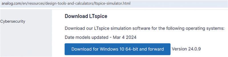
At the time of writing this book, the latest version of LTspice was 24.0.9, known as Version 24. The installation steps are:

• Go to the website: https://www.analog.com/en/resources/design-tools-and-calculators/ LTspice-simulator.html

• Scroll down and click on the Download link to download the installation file (Figure 2.1). At the time of writing this book, the installation file was named (for 64-bit PCs): LTspice64.msi

• Double-click on the file to install LTspice. After the installation, the icon shown in Figure 2.2 should appear on your desktop,

2.3 Running LTspice

Double-click on the icon to start LTspice. Figure 2.3 shows the start-up screen. At this stage, you will see that almost all the menu options are grayed out and are not available, except for File, View, Tools, and Help. We will cover these options in a later chapter. For now, click Help → About LTspice to display the version number (Figure 2.4)

LTspice Essentials ● 16

Figure 2.1 Click to download the installation file Figure 2.2 LTspice icon

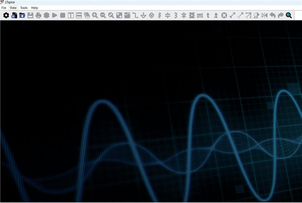
2.3 LTspice startup screen

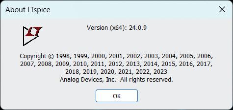
2.4 LTspice version number

2.4 Creating a New Schematic

Before creating a new schematic, it is important to know how to specify the values of resistors, capacitors, and inductors to be used in our circuit. Table 2.1 shows the available value prefixes. Note that they are not case-sensitive. For example, k and K are both interpreted as kilo.

Table 2.1

● 17

Figure Figure

Prefix Name Multiplier T tera 1012 G giga 109 Meg mega 106 k kilo 103 m milli 10-3 u micro 10-6 n nano 10-9 p pico 10-12 f femto 10-15

LTspice

LTspice units Chapter 2 • Getting Started with

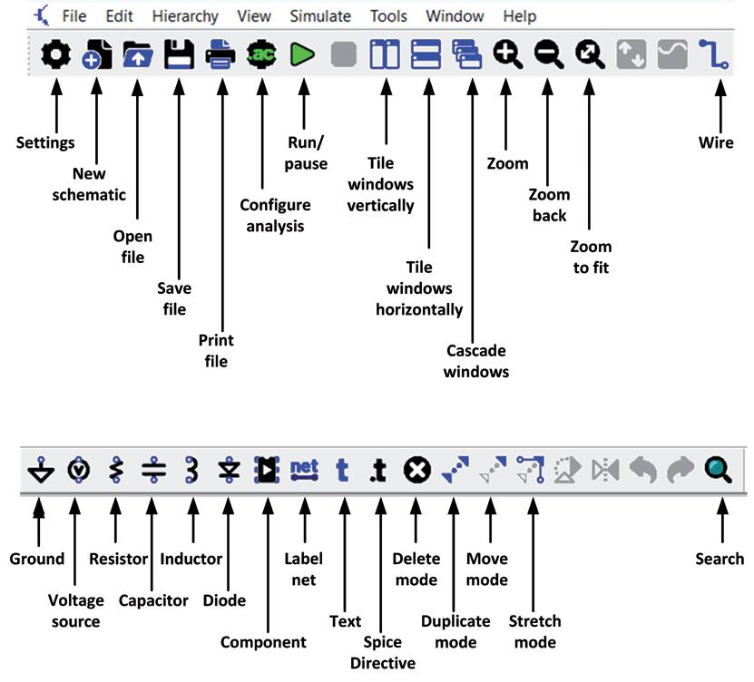
To create a new schematic, click File → New Schematic, or press Ctrl+N, or click the icon with the ‘+’ sign at the left-hand side of the top menu. You will be presented with a screen as shown in Figure 2.5. At the top part of the screen, we have the menu items and below them are the buttons or icons (in the figure, the screen is cut into two for clearness). A function brief is shown for each button as a quick reference.

2.5

The following key combinations can be used to access the menu buttons (in between parentheses are the LTspice XVII ‘classic’ keyboard shortcuts. They can be activated through the Tools → Settings menu, on the Schematic tab and then the Keyboard Shortcuts button):

New schematic - Ctrl+N

Open - Ctrl+O

Save - Ctrl+S

Print - Ctrl+P

Configure analysis - A (n/a)

Zoom - Z (Ctrl+Z)

Zoom back - Shift+Z (Ctrl+B)

Zoom to fit - Space (n/a)

Wire - W (F3)

Ground - G

Resistor - R

Capacitor - C

Inductor - I

Diode - D

Component - P (F2)

Label net - N (F4)

Text - T

Spice directive - . (S)

LTspice Essentials ● 18

Figure New schematic screen

Delete mode - DEL (DEL or F5)

Duplicate mode - Ctrl+C (F6)

Move mode - M (F7)

Stretch mode - S (F8)

Search - Ctrl+F

Example schematic

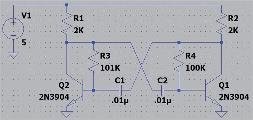
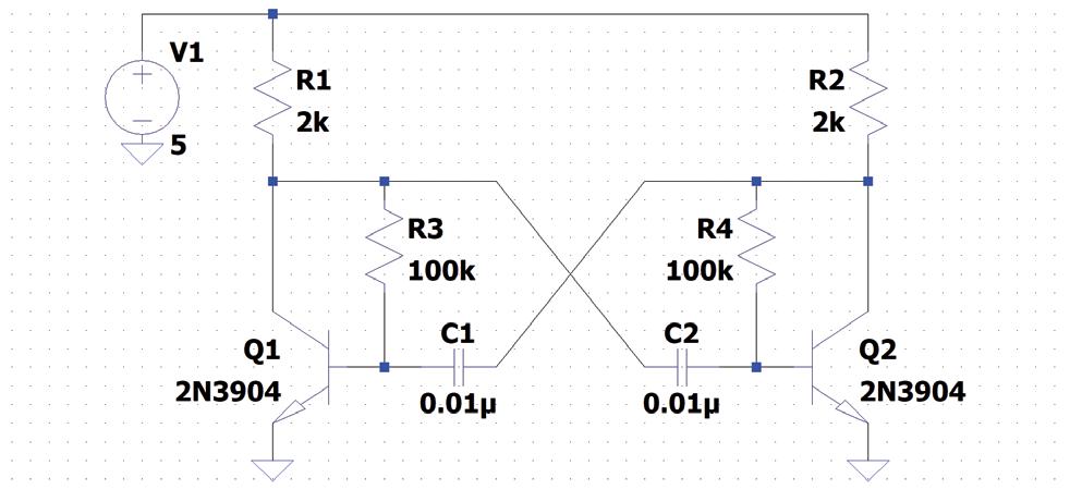
Perhaps the easiest way to learn how to create a schematic is to go through an example circuit. The schematic we will be drawing is a multivibrator circuit (also known as an astable circuit), taken from the LTspice Educational Examples folder. The multivibrator is a simple square wave oscillator circuit with two transistors, four resistors, and two capacitors, and of course, a power supply (e.g. a battery). The actual operation of the circuit is not relevant at this stage, and the author assumes that most readers are familiar with multivibrator circuits. A step-by-step approach is given below that explains how to draw and then simulate the circuit shown in Figure 2.6.

• Start LTspice.

• Click File → New Schematic.

• We will make the wire color black, and the screen background color white, to improve visibility for this book. To change the wire color, click Tools → Color Preferences, Select Wires as the Selected item and set the red, green and blue to 0 so that the wire color is black. Also, select Background as the Selected item and set Red, Green and Blue to 255 so that the background color is white.

• You can also make the graph lines thicker by clicking Tools → Settings and then click to select tab Waveforms. Set the Data trace width to a higher value (e.g. 3).

• Click on the resistor symbol and place resistors R1, R2, R3 and R4 approximately at the same positions as in Figure 2.6 (See Figure 2.7). Press ESC on the keyboard or do a right-click to exit. You can zoom in or out by scrolling the mouse wheel. Move the drawing by pressing the left mouse button and keeping it pressed down. If you want to change the position of a

Chapter

• Getting Started with LTspice ● 19

Figure 2.6 Example multivibrator circuit

component, click on button Move Mode (M), click on the component to be moved and move it to the desired position. (Use Stretch Mode to move a part while keeping it connected) Press ESC on the keyboard or do a right mouse click to exit Move Mode.

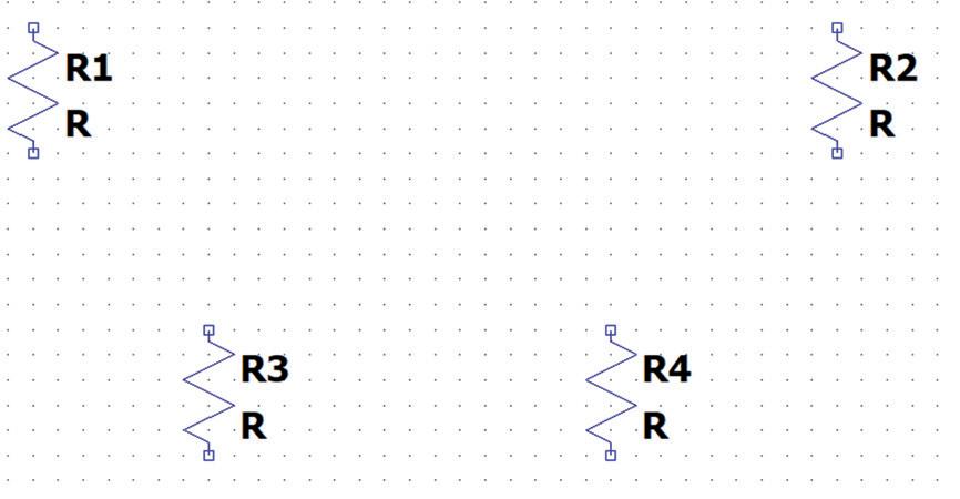
Figure 2.7 Place the resistors

• Now, we will place the two capacitors. Click on the capacitor symbol. In our drawing, the capacitor should be rotated by 90 degrees. This is done by pressing Ctrl+R before it is placed in its final position. Place capacitors C1 and C2 as in Figure 2.8. Press ESC on the keyboard or right click to exit.

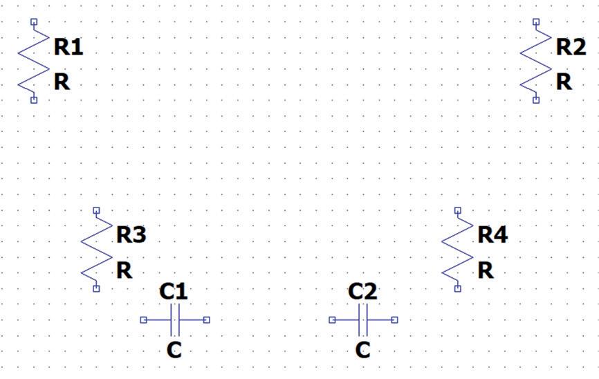
Figure 2.8 Place the capacitors

• Now, place the two NPN transistors. Click Component and select npn, noting that there are different symbols for NPN transistors. Place Q1 as in Figure 2.6. The mirror image of transistor Q2 should be taken before it is placed. Press Ctrl+E to mirror the symbol and place it as in Figure 2.9. Press ESC on the keyboard or do a right-click to exit. You may have to move some of the components to place them exactly as in Figure 2.9.

LTspice Essentials ● 20

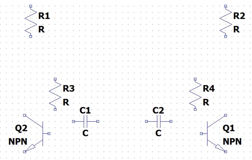
Figure 2.9 Place the transistors

• We will now insert the DC voltage source, which is a battery in this application. Click Voltage Source (V) and place it next to R1 as in Figure 2.6. Press ESC on the keyboard or right click to exit.

• We will now connect all the components as in Figure 2.6. Click Wire (W) and connect the components as shown in Figure 2.10. Notice that a part of the connections between C1 and R4 and between C2 and R3 is not horizontal or vertical, but has an angle. This can be done by for example connecting C1 to R4 using horizontal and vertical wires and then selecting Stretch Mode (S). Now you can move the wires to create slopes as shown in Figure 2.10. Alternatively, you can press and hold down the Ctrl key on the keyboard while drawing a line, and the line will be drawn at an angle.

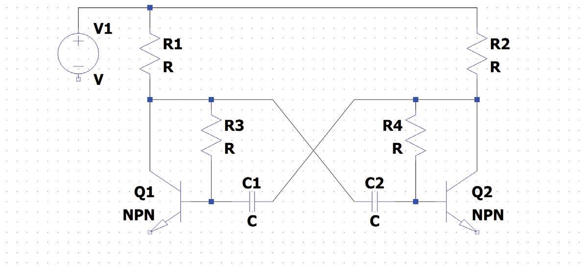
Figure 2.10 Connect the components

• Every circuit must have a ground point. Without a ground point, it cannot be simulated. Connect the ground points by clicking on the Ground button. Press ESC to exit as before. Figure 2.11 shows the completed schematic. You can move the schematic up or down on the screen by clicking at any point on the schematic using the left mouse button, and moving the mouse while the mouse button is kept pressed. The size of the schematic can be made smaller or larger by using the mouse wheel.

Chapter

• Getting Started with LTspice ● 21

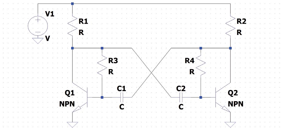
2.11 Completed schematic

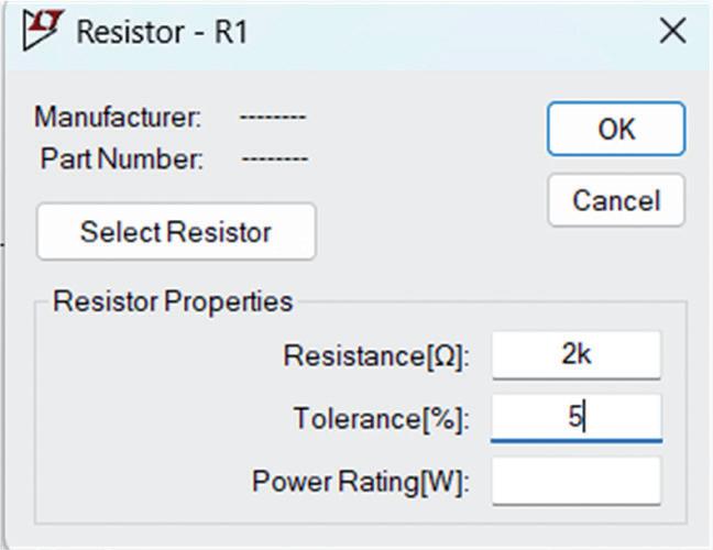
• The next stage is to set the values of the components. Right-click on the resistors and set their values to: R1 = R2 = 2k, R3 = R4 = 100k. You can set the tolerances to 5%. See Figure 2.12 for setting the value of R1 to 2k. Set the capacitors similarly by right-clicking on them. You can select various other parameters for capacitors, such as the working voltage, etc., but this is not required in this example. Set the voltage source to 5V.

• Set the transistor model to 2N3904. The final circuit is shown in Figure 2.13. You should now save your schematic. By default, the filename is given the extension asc.

LTspice Essentials ● 22

Figure Figure 2.12 Setting R1 to 2k Figure 2.13 Final schematic

Simulating the circuit

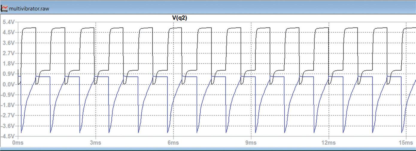
By simulating the circuit, we can display the DC and AC voltages at different parts of the circuit, plot the voltage and current waveforms and so on. In this simulation, we expect the voltage at the transistor collectors to be a square wave.

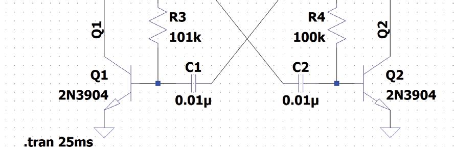
Simulating oscillators can be problematic, as they may not start because the simulation assumes perfect component values and no noise. The easiest way to ensure that our multivibrator will start to oscillate is to change say resistor R3 slightly. We can make R3 = 101 kΩ, for example.

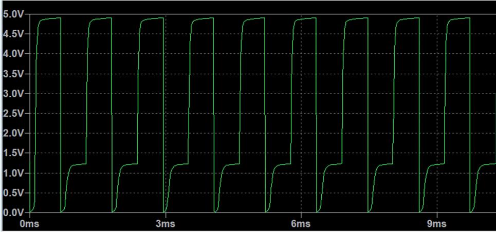
To start the simulation, click the Run/Pause (Alt+R) button and set the simulation time, say to 25 ms. The voltage or the current can easily be plotted by placing the mouse pointer on the required point in the circuit, in this example the collector of a transistor. You should notice that a voltage probe or a current probe is displayed when the mouse pointer is placed at a node (or on a wire) or on a component, respectively. Select the voltage probe, and you should see the square wave output as shown in Figure 2.14 (only part of the display is shown).

Inserting labels

You may like to insert labels at required points in the circuit so that it becomes easier to identify these points. For example, let us insert labels with the names Q1 and Q2 at the collectors of transistors Q1 and Q2. Click NET (F4) and then type Q1 and OK. Move the mouse pointer on the collector of Q1 and press the left button of your mouse. Click ESC to exit. Repeat for transistor Q2. You should now have labels at the collectors as shown in Figure 2.15. When you display the output voltage at the collector of Q1 now, you should see V(q1) as the graph identifier. Notice that you can also place labels by right-clicking on a node or on a wire on the schematic.

Chapter

• Getting Started with LTspice ● 23

Figure 2.14 Voltage at the transistor collector Figure 2.15 Labels at the collectors of the transistor

Changing scale of the time axis

Move the mouse pointer on the time axis (x-axis) and you should see a small ruler displayed. Do a right-click and set the required axis limits. Figure 2.16 shows how to change the x-axis ticks so that they are displayed on a 5-millisecond grid.

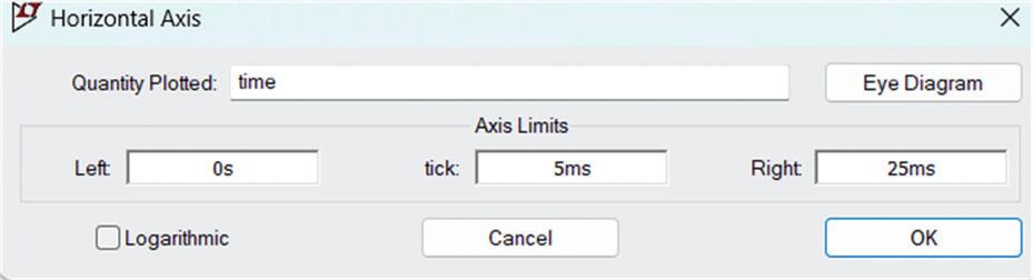
Figure 2.16 Changing the x-axis limits

Displaying the frequency

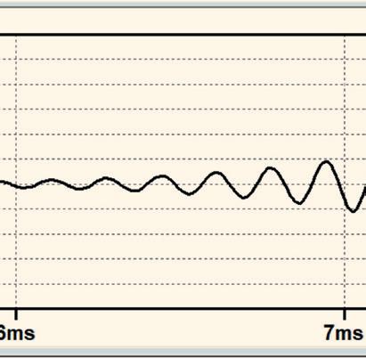
Move the mouse pointer to one point on the graph and press the left button. While pressing the button, move the pointer to another point one period later. You should see a rectangle shape. The frequency will be displayed at the bottom of the screen as shown in Figure 2.17. In this example, the frequency was displayed as 886.62791 Hz.

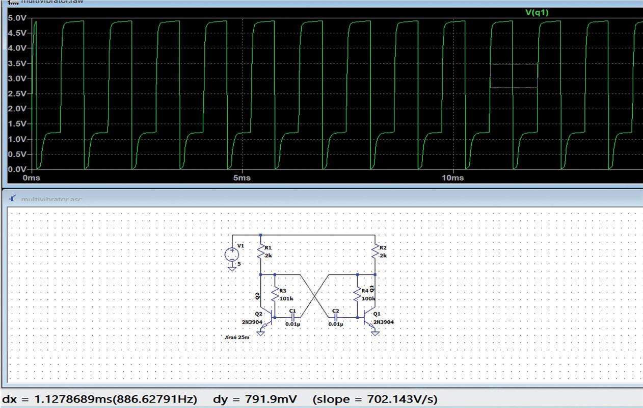
Figure 2.17 Displaying the frequency

Displaying values at different points on the graph

You may want for example to display the voltage at different points of the graph. Click on where it says V(q1). You should see a cross grid with vertical and horizontal dashed lines. Move the intersection of the two dashed lines to anywhere you want to display the voltage. A window at the bottom right will display the values as you move the cursor (Figure 2.18)

LTspice Essentials ● 24

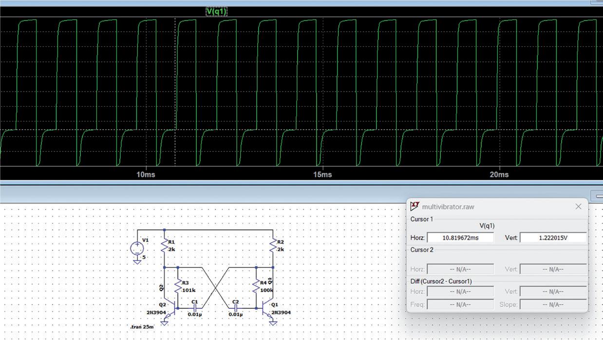
Figure 2.18 Displaying values on the graph

Multiple graphs

You can draw multiple graphs on the same axis. For example, click to plot the collector voltage. Then, also click to plot the voltage at the base of the transistor. The resultant graph is shown in Figure 2.19, where the green plot is the collector voltage and the blue plot is the voltage at the base of the transistor (only part of the graph is shown).

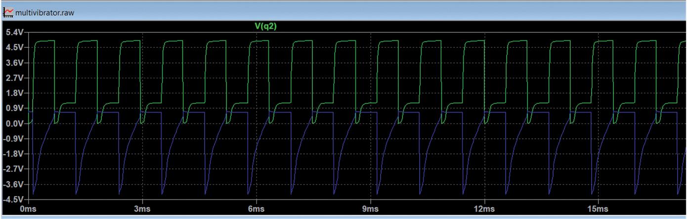
Figure 2.19 Multiple graphs

You can change the color of the waveforms or the background if you wish. For example, to change the graph background to white and the first plot to black:

• Click Tools → Color Preferences

• Select Waveform at the top tap

• Select Background in Selected item and set the red, green and blue to 255 so that the background is white. Then, select Trace V(1) in Selected item and set the red, green and blue to 0 so that the first plot becomes black.

Figure 2.20 shows the new plot.

Chapter

• Getting Started with LTspice ● 25

There are many more plotting options available, and these will be covered in later chapters.

2.5 Simulator Settings

There are many options that the user can select to configure the simulator. Normally, the default options provided should be fine for most types of simulations. Click on the settings menu (a gear shaped icon at the top left part of the screen) and you can see the available options. You are, however, advised not to change any options at this stage.

2.6 Example Schematics

Many example schematics are supplied with the simulator to help users become familiar with using it. Click File → Open Examples to open the examples folder. Two subfolders are provided with the names Applications and Educational. The Applications are for more advanced users, and it contains many example schematics using Analog Devices advanced components. The subfolder Educational contains many interesting examples, such as amplifiers, oscillators, filters, transformers, etc.

2.7 Online Help

The Help menu provides several menu options. There are help options on using LTspice, help on keyboard shortcuts, support on EngineerZone, a link to the Analog Devices website, LTspice update check, and displaying the version of the program.

LTspice Essentials ● 26

Figure 2.20 New plot

Index ● 193 Index A AC amplitude 51 AC analysis 14 Active components 172 Add traces 38 Astable multivibrator 127 Audio power amplifier 94 B Binary counter 162 BJT 87 BJT switch 98 Boost converter 135 C Class A 94 Class AB 94 Class B 94 Colpitts oscillator 113,122 Common emitter 88, 91 Computer simulation 12 Current probe 23 D Damped frequency 43 DC analysis 14 DC opt pnt 31 DC sweep 34, 87 Delta connection 58 Diac 105 Digital logic 154 Diode clamp. 81 E Electric shock 11 Expression editor 15 F Fast Fourier transform 65 Feedback ratio 114 Filters 141 Filter design tool 142 Filter library 152 Fourier spectrum 44 FFT 66 Frequency sweeping 63 Full-adder 156, 165 Full-wave bridge 77 Full-wave rectifier 76 G Gain 69 H Half-adder 154 Half-wave rectifier 74 Hartley oscillator 115, 124 Hierarchical blocks 146 I Input impedance 67, 70 Input resistance 46 J JFET 100 L Label net 28 Laboratory experiments 11 Laboratory instruments 11 Laplace transform 185 Line voltage 57 Logic gates 178 Low-pass filter 141 M Metronome 130 Monostable multivibrator 166 MOSFET 103 Move mode 20 Multiple graphs 25, 45 Multiplexer 161 Mutual inductance 60 N Natural frequency 43 Netlist 15 New diode model 176

Essentials ● 194 New schematic 17 Noise analysis 146 Notes and annotations 40 O Online help 15, 26 Optocoupler 137 Output impedance 68, 71 Output power 94 Output resistance 46 P Parameter sweep 15, 131 Passing parameters 149 Passive components 170 Periodic waveform 181 Phase control 106 Phase shift oscillator 117 Phase voltage 57 Potential divider 33 Potentiometer 109 Power dissipation 37 R RC transient 39 Resistor circuit 27 Resistor inductor 41 S Sawtooth waveform 180 Schematic capture 13 Simulator settings 26 Sinewave oscillator 113 Smoothing 75 SPICE models 170 Software model 12 Square wave oscillator 126 Star connection 57 Start frequency 55 Step param 37 Stop frequency 55 Stretch mode 20 T Text 27 Thevenin theorem 54 Three-phase circuit 56 Thyristor 105 Transfer function 46 Transformer 63 Transient analysis 14, 29 Transient noise analysis 14 Transistor analysis 87 Triac 105 Triangular waveform 180 Type of sweep 55 V Virtual instrument 12 Voltage controlled switch 184 Voltage difference 30 Voltage multiplier 82 Voltage probe 23 Voltage regulator 134 W Wien bridge oscillator 120 Z Zener diode 79

LTspice

LTspice Essentials

An Introduction to Circuit Simulation

This book is about learning to design and simulate electronic circuits using LTspice. Among others, the following topics are treated:

> DC and AC circuits

> Signal diodes and Zener diodes

> Transistor circuits including oscillators

> Thyristor/SCR, diac, and triac circuits

> Operational amplifier circuits including oscillators

> The 555 timer IC

> Filters

> Voltage regulators

> Optocouplers

> Waveform generation

> Digital logic simulation including the 74HC family

> SPICE modeling

All the simulation examples used in the book are available as files at the webpage of this book. Readers can use these example circuits for learning or modify them for their own applications.

Prof Dr Dogan Ibrahim has a BSc degree in electronic engineering, an MSc degree in automatic control engineering, and a PhD degree in digital signal processing. Dogan has worked in many industrial organizations before he returned to academic life. Prof Ibrahim is the author of over 70 technical books and published over 200 technical articles on microcontrollers, microprocessors, and related fields. He is a Chartered electrical engineer and a Fellow of the Institution of the Engineering Technology. He has been an amateur radio operator for several decades and also holds an Arduino certification.

Elektor International Media www.elektor.com

booksbooks