#define PWM 5 // PWM pin #define DIR 4 // DIR pin volatile unsigned long Count = 0; // Encoder count TCCR2B = TCCR2B & B11111000 | B00000011; pinMode(DIR, OUTPUT); // Direction is output digitalWrite(DIR, LOW); pinMode(PWM, OUTPUT); // PWM is output pinMode(PhaseB, INPUT); // Phase B is input pinMode(PhaseA, INPUT); // Phase A is input attachInterrupt(digitalPinToInterrupt(PhaseB), EncoderISR, attachInterrupt(digitalPinToInterrupt(PhaseA), EncoderISR2,floatSerial.begin(19200);sk,Kp,Ti,Td,pk, T, pk_1, ek, ek_1, a, b, yk, qk, wk, uk; float conv = 150.0 / 90.0; // Configure PWM pin and Initialize variables #define PhaseB 3 // Phase B #define PhaseA 2 // Phase A void setup() books Dogan Ibrahim PID-based Practical Digital Control With Raspberry Pi and Arduino Uno


PID-based Practical Digital Control With Raspberry Pi and Arduino Uno ● Dogan Ibrahim
● 4 ● This is an Elektor Publication. Elektor is the media brand of Elektor International Media B.V. PO Box 11, NL-6114-ZG Susteren, The Netherlands Phone: +31 46 4389444 ● All rights reserved. No part of this book may be reproduced in any material form, including photocopying, or storing in any medium by electronic means and whether or not transiently or incidentally to some other use of this publication, without the written permission of the copyright holder except in accordance with the provisions of the Copyright Designs and Patents Act 1988 or under the terms of a licence issued by the Copyright Licencing Agency Ltd., 90 Tottenham Court Road, London, England W1P 9HE. Applications for the copyright holder's permission to reproduce any part of the publication should be addressed to the publishers. ● Declaration The Author and Publisher have used their best efforts in ensuring the correctness of the information contained in this book. They do not assume, and hereby disclaim, any liability to any party for any loss or damage caused by errors or omissions in this book, whether such errors or omissions result from negligence, accident, or any other Allcause.the programs given in the book are Copyright of the Author and Elektor International Media. These programs may only be used for educational purposes. Written permission from the Author or Elektor must be obtained before any of these programs can be used for commercial purposes. ● British Library Cataloguing in Publication Data A catalogue record for this book is available from the British Library ● ISBN 978-3-89576-519-3 Print ISBN 978-3-89576-520-9 eBook ● © Copyright 2022: Elektor International Media B.V. Editor: Jan Buiting Prepress Production: D-Vision, Julian van den Berg Elektor is part of EIM, the world's leading source of essential technical information and electronics products for pro engineers, electronics designers, and the companies seeking to engage them. Each day, our international team develops and delivers high-quality content - via a variety of media channels (including magazines, video, digital media, and social media) in several languages - relating to electronics design and DIY electronics. www.elektormagazine.com
Contents ● 5 PrefaceContents............................................................ 9 Chapter 1 • Control Systems .......................................... 11 1.1 Open-loop and closed-loop 11 1.2 Microcontroller in the loop ........................................ 12 1.3 Control system design 15 Chapter 2 • Sensors ................................................. 16 2.1 Sensors in Computer Control ...................................... 16 2.2 Temperature Sensors ............................................ 18 2.2.1 Analog Temperature Sensors ..................................... 18 2.2 Digital Temperature Sensors ....................................... 25 2.3 Position Sensors ............................................... 26 2.4 Velocity and Acceleration Sensors 28 2.5 Force Sensors ................................................. 30 2.6 Pressure sensors 30 2.7 Liquid Sensors................................................. 32 2.8 Flow Sensors 35 Chapter 3 • Transfer Functions and Time Response ........................ 37 3.1 Overview 37 3.2 First-order Systems ............................................. 37 3.2.1 Time Response 39 3.3 Second-order Systems ........................................... 43 3.3.1 Time Response ............................................... 45 3.4 Time Delay ................................................... 50 3.5 Transfer Function of a Closed-loop System ............................. 51 Chapter 4 • Discrete Time (Digital) Systems .............................. 53 4.1 Overview .................................................... 53 4.2 The Sampling Process 53 4.3 The Z-Transform ............................................... 57 4.3.1 Unit step function 57 4.3.2 Unit ramp function ............................................ 58
PID-based Practical Digital Control ● 6 4.3.3 Tables of z-Transforms.......................................... 58 4.4 The z-Transform of a function expressed as a Laplace Transform .............. 58 4.5 Inverse z-Transforms ............................................ 60 4.6 Pulse transfer function and manipulation of block diagrams ................. 61 4.6.1 Open-loop systems 62 4.7 Open-loop time response ......................................... 63 4.8 Closed-loop system time response 67 Chapter 5 • The PID Controller in Continuous-Time Systems ................. 69 5.1 Overview 69 5.2 Proportional-only Controller with a First-Order System ..................... 70 5.3 Integral-Only Controller with a First-order System 71 5.4 Derivative-only Controller with a First-order System ...................... 72 5.5 Proportional + Integral Controller with a First-order System 73 5.6 Proportional + Integral + Derivative controller with a First-order System ........ 74 5.7 Effects of Changing the PID Parameters ............................... 75 5.8 Tuning a PID Controller .......................................... 76 5.8.1 Open-loop Ziegler and Nichols Tuning ............................... 77 5.8.2 Open-loop Cohen-Coon PID Tuning 78 5.8.3 Closed-loop Tuning ............................................ 82 5.8.4 Practical PID Tuning 84 5.9 The Auto-tuning PID Controller ..................................... 85 5.10 Increasing and Decreasing PID Parameters 85 5.11 Saturation and Integral Wind-up ................................... 85 5.12 Derivative Kick 86 5.13 Using the PID Loop Simulator ..................................... 86 Chapter 6 • The Digital PID Controller ................................... 88 6.1 Overview .................................................... 88 6.2 Digital PID ................................................... 88 6.3 Choosing a Sampling Time, T ...................................... 89 6.4 Microcontroller Implementation of the PID Algorithm ...................... 90 Chapter 7 • On-Off Temperature Control ................................. 92 7.1 Overview .................................................... 92
Contents ● 7 7.2 Temperature Controllers .......................................... 92 7.3 Project 1: ON-OFF Temperature Control with Arduino Uno .................. 93 7.4 Project 2: ON-OFF Temperature Control with Hysteresis and Arduino Uno ....... 98 7.5 Project 3: ON-OFF Temperature Control with Button Control – Arduino Uno ..... 100 7.6 Project 4: ON-OFF Temperature Control with Rotary Encoder and Arduino Uno 103 7.7 Project 5: ON-OFF Temperature Control with Raspberry Pi 4 ................ 108 Chapter 8 • PID Temperature Control with the Raspberry Pi ................ 118 8.1 Overview ................................................... 118 8.2 Project 1 - Reading the temperature of a thermistor 118 8.3 Project 2: Open-loop Step-input Time Response ........................ 122 8.4 Project 3: PI Temperature Control 129 8.5 Project 4: PID Temperature Control ................................. 135 8.6 Using the PID Loop Simulator 141 Chapter 9 • PID Temperature Control with the Arduino Uno ................. 143 9.1 Overview ................................................... 143 9.2 Project 1: Reading the Temperature of a Thermistor ..................... 143 9.3 Project 2: PID Temperature Control ................................. 145 9.4 Project 3: PID Temperature Control with Arduino Uno and Timer Interrupts 151 9.5 Project 4: PID Temperature Control using the Arduino Uno PID Library ........ 154 Chapter 10 • DC Motor Control with Arduino and Raspberry Pi ............... 159 10.1 Overview .................................................. 159 10.2 Types of Electric Motors 159 10.3 Brushed DC Motors ........................................... 160 10.3.1 Permanent-magnet BDC Motors 160 10.3.2 Series-wound BDC Motors ..................................... 161 10.3.3 Shunt-wound BDC Motors 162 10.3.4 Compound-wound BDC Motors .................................. 162 10.3.5 Separately-excited BDC Motors .................................. 162 10.3.6 Servo Motors .............................................. 163 10.3.7 Stepper Motors ............................................. 163 10.4 Brushless DC Motors .......................................... 164 10.5 Motor Selection .............................................. 164
PID-based Practical Digital Control ● 8 10.6 Transfer Function of a Brushed DC Motor ............................ 165 10.7 The DC Motor Used in the Projects ................................. 167 10.8 Project 1: Motor Speed and Direction Control Using an H-Bridge Integrated Circuit . 169 10.9 Project 2: Displaying the Motor Speed with Arduino Uno.................. 176 10.10 Project 3: Displaying Motor Speed on LCD with Arduino Uno 180 10.11 Project 4: Displaying Motor Speed with Raspberry Pi ................... 183 10.12 Project 5: Displaying Motor Speed on LCD with Raspberry Pi 185 10.13 Project 6: Identification of the DC Motor with Raspberry Pi ............... 187 10.14 Project 7: PID Motor Speed control with Raspberry Pi 190 10.15 Project 8: PID Motor Speed Control with Arduino Uno .................. 194 Chapter 11 • Water Level Control ..................................... 198 11.1 Overview .................................................. 198 11.2 Ultrasonic Transmitter-Receiver Module 198 11.3 Project 1: Measuring Distance using the HC-SR04 Ultrasonic Module with Arduino Uno ................................................ 198 11.4 Project 2: Measuring Distance using the HC-SR04 Ultrasonic Module with Raspberry Pi ................................................ 202 11.5 Project 3: Step Input Response of the System with Raspberry Pi 205 11.6 Project 4: PID-based Water Level Control with Raspberry Pi ............... 208 11.7 Project 5: PID-based Water Level Control with Arduino Uno 214 Chapter 12 • PID-based LED Brightness Control .......................... 218 12.1 Overview 218 12.2 Project 1: Step Time Response of LED Brightness Control using the Raspberry Pi 218 12.3 Project 2: PID-Based LED Brightness Control using the Raspberry Pi 222 12.4 Project 3: PID-based LED Brightness Control using the Arduino Uno ......... 227 12.5 Project 4: PID-based LED Brightness Control using the 230 Arduino Uno Library .............................................. 230 Index ........................................................... 233
Preface
The Raspberry Pi 4 is one of the latest credit-card sized popular computers that can be used in many applications such as in audio and video media centers, as a desktop computer, in industrial controllers, robotics, games, and many domestic and commercial applications. In addition to rich set of features found in other Raspberry Pi computers, the Raspberry Pi 4 also offers Wi-Fi and Bluetooth capability which makes it highly desirable for incorporation in remote and Internet-based control and monitoring applications. This book is about using both the Raspberry Pi 4 and the Arduino Uno in PID-based auto matic control applications. The book starts with basic theory of the control systems and feedback control. Working and tested projects are given for controlling real systems using PID controllers. The open-loop step time response, tuning the PID parameters, and the closed-loop time response of the developed systems are discussed in depth together with the block diagrams, circuit diagrams, PID controller algorithms, and the full program list ings for the Raspberry Pi as well as the Arduino Uno. The projects given in the book should teach the theory and applications of PID controllers. They can be modified easily as desired for other applications. The projects given for Raspberry Pi 4 should work with all other models of Raspberry Pi family. It is expected that the readers have some programming experience with the Arduino Uno using the Arduino IDE. The same for the Raspberry Pi with the Python 3 programming lan guage. Some basic electronic hardware experience and knowledge of basic mathematics will also be useful.
● 9
Microcontrollers are highly popular integrated circuits commonly used in many domestic, commercial, and industrial electronic monitoring and control applications. It is estimated that there are more than 50 microcontrollers in every home in developed countries. Do mestic equipment having embedded microcontrollers include microwave ovens, printers, keyboards, computers, tablets, washing machines, dishwashers, smart televisions, smart phones, and many more.
Arduino Uno is an open-source microcontroller development system incorporating hard ware, an Integrated Development Environment (IDE), and a large number of libraries. The Arduino Uno is supported by a large community of programmers, electronic engineers, enthusiasts, and academics. There are many different designs of the basic Arduino Uno board. Although they are intended for different types of applications, they can all be programmed using the same IDE and in general, programs can be transported between different boards. This may be one of the reasons for the popularity of the Arduino family, which is also supported by countless software libraries for many peripherals that can easily be included in your programs. These libraries make programming a doddle and speed up the programming time. Using libraries also make it easier to test your programs since most of them come as fully tested and working.
PID-based Practical Digital Control ● All10programs discussed in the book are contained in an archive file you can download free of charge from the Elektor website. Head to: www.elektor.com/books and enter the book title in the Search box. I hope that you enjoy reading the book and at the same time learn the theory and practical applications of the PID controllers. Dogan London,Ibrahim2022
In contrast to open-loop control system, in a closed-loop control system (Figure 1.2) the actual plant output is measured and compared with what we would like to see at the plant output. The measure of the output is called feedback signal. The difference between the desired output value and the actual output value is called the error signal. The error signal is used to force the system output to a point such that the desired output value and the actual output value are equal, i.e., the error signal is zero. One of the advantages of closed-loop control, or feedback control is the ability to compensate for disturbances and yield the correct output even in the presence of disturbances. Also, the plant output settles
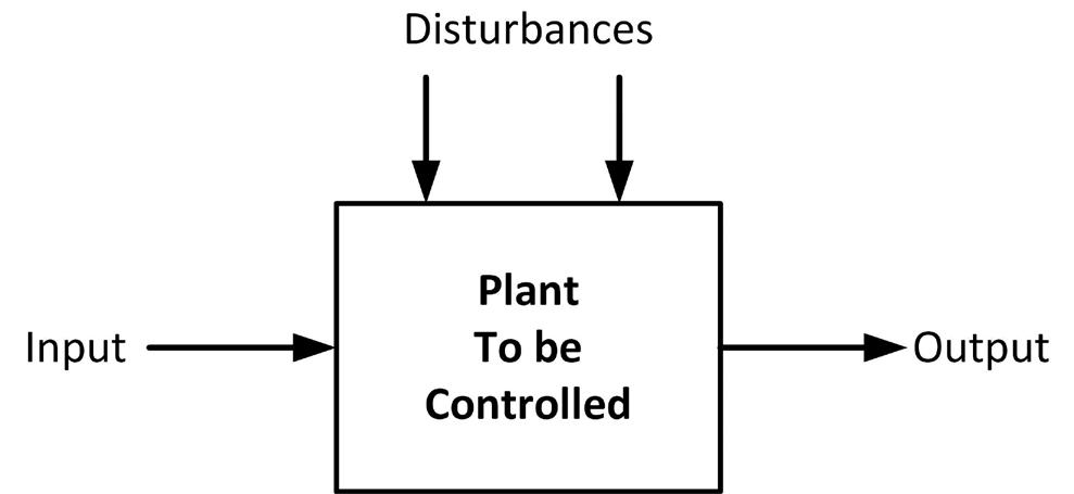
A plant is normally an open-loop system (Figure 1.1) where an actuating device is used to control the plant directly without using feedback. For example, a motor is expected to rotate when a voltage is applied across its input terminals, but we do not know by how much the motor rotates since there is no knowledge about its output. If the motor shaft is loaded and the motor slows down, there is no knowledge about this. As shown in Figure 1.1, a plant may also have external disturbances affecting its behavior, and in an open-loop system there is no way of knowing or minimizing such disturbances.
1.1 Open-loop and closed-loop Control engineering covers all aspects of governing a dynamic system, also called a plant or a process. A plant can be a mechanical system, an electrical system, a thermal system, a fluid system, or a combination of such systems.
Control engineering is based on the theories of system modelling, feedback, system response, and stability. As a result, control engineering is not limited to only one engineering discipline, but is equally applicable to mechanical, chemical, aeronautical, civil, and electri cal engineering disciplines.
Figure 1.1: Open-loop system
Chapter 1 • Control Systems ● 11 Chapter 1 • Control Systems
A plant can have one or more inputs and one or more outputs. The dynamic behavior of a plant is described by differential equations. Given the model (or the differential equations), inputs, and initial conditions of a plant we can easily calculate its outputs. Generally, a plant is a continuous-time system with its inputs and outputs also continuous in time. For example, an electromagnetic motor is a continuous-time plant whose input (e.g., voltage or current) and its output (e.g., speed or position) are also continuous in time.
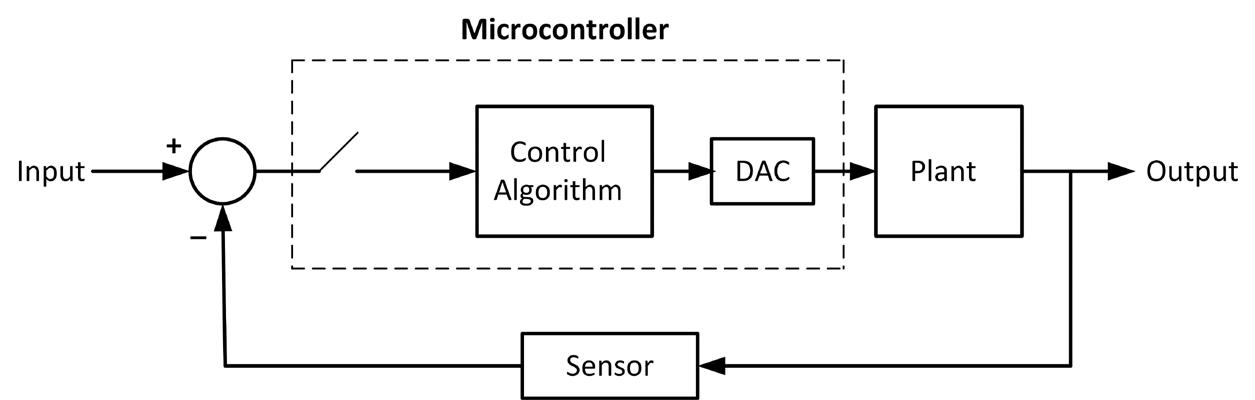
Nowadays, practically all control systems are microcontroller based, where a microcon troller is used as the central control device. Some sensors (e.g., temperature, pressure, humidity etc.) provide digital outputs and can be connected directly to a microcontroller. Analog sensors cannot be connected directly to a microcontroller. An analog-to-digital con verter (ADC) is needed to convert the analog signal into digital form so that it can be fed to a Figuremicrocontroller.1.3showsadigital control system where the input and the output of the sensor are assumed to be analog. An ADC is used to periodically convert the error signal into digital form and this is fed to a digital controller which is usually a microcontroller. The microcon troller implements a control algorithm (e.g., PID algorithm) and its output is converted into analog form using a digital-to-analog converter (DAC) so that it can drive the plant to set the plant output to the desired value. Figure 1.3: Digital control system.
As you'll discover in a later Chapter, most sensors are analog devices giving analog voltage or current outputs. These sensors can be used directly in analog systems where the inputs, controller, plant, and the outputs are all analog variables.
1.2 Microcontroller in the loop
PID-based Practical Digital Control
● and12remains at the desired value. For example, in a motor speed control system the speed of the motor remains the same when load is applied to the motor shaft. A controller (or compensator) is usually used to read the error signal and drive the plant in such a way that the error tends to zero.
Sensors are devices which measure the plant output. For example, a thermistor is a sensor used to measure the temperature and it can be used in a closed-loop thermal plant control. Similarly, a tachometer or an encoder can be used to measure the rotational speed of a motor and they can be used in closed-loop motor speed control applications. Notice that in electrical systems a power amplifier may be required after the DAC to drive the plant.
Figure 1.2: Closed-loop system
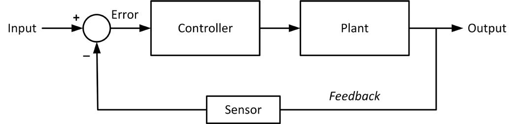
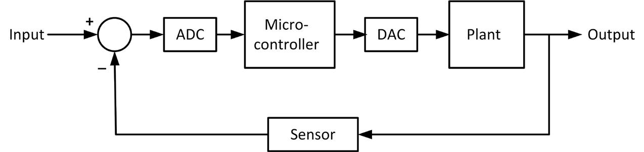
Figure 1.6: Analog speed control system.
Figure 1.4 shows the block diagram of a digital control system where the ADC is shown as a sampler. Most microcontrollers incorporate ADC and DAC modules and these are shown as part of the microcontroller in Figure 1.4.
Figure 1.4: Block diagram of a digital control system.
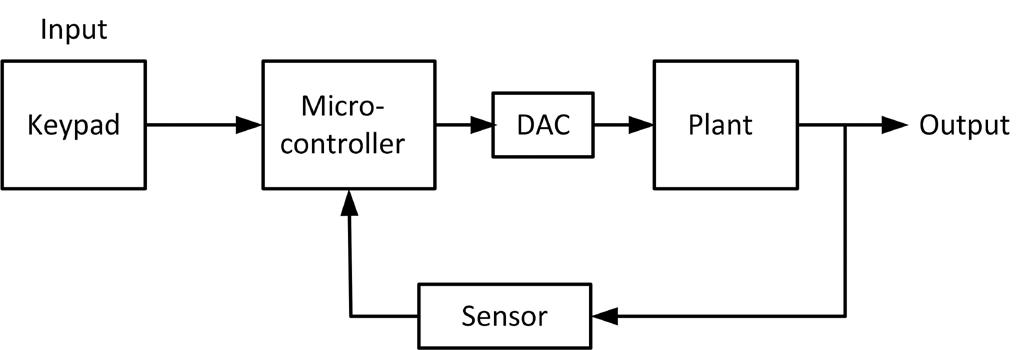
In Figure 1.4 the input and the sensor output are analog signals. A variation of this system is shown in Figure 1.5 where the input is digital and is either hardcoded to the microcon troller software or is input using a suitable input device such as a keypad. Here, a sensor with digital output is used and is connected directly to the microcontroller.
Chapter 1 • Control Systems ● 13
Figure 1.5: Another variation of digital control. Figure 1.6 shows a typical analog speed control system. Here, the desired speed is set using a potentiometer. The speed of the motor is measured using a tachometer and is fed back to a difference amplifier. The output of this amplifier is the error signal which is input to an analog controller consisting of operational amplifiers. The output of the controller drives the motor through a power amplifier to achieve the desired speed.

PID-based Practical Digital Control
●
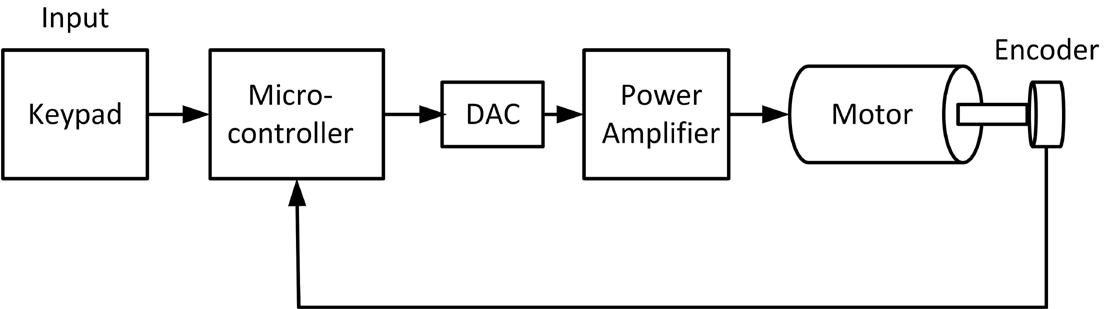
Figure 1.7: Digital speed control system.
• The cost of digital controllers are lower than the analog ones, especially if additional control loops have to be added to the system.
• It is easy to tune digital controllers. All that is required is to change pertinent parameters in software.
• Digital controllers are more dependable than the analog ones and they are not affected by environmental factors such as component aging, component tolerances, etc.
Figure14 1.7 shows the digital equivalent of Figure 1.6. Here, a digital encoder is used to measure the motor speed and this is fed to the microcontroller together with the desired speed where the speed is set using a keypad. The microcontroller implements the control algorithm and sends its output to the power amplifier in the form of a Pulse Width-Modulat ed (PWM) signal which in turn provides power to the motor to set the speed at the desired value.
• Almost all analog controllers have been replaced over time by digital ones.
Since a plant can be controlled using an analog approach, you might be tempted to ask why use digital control? In the 1960s, computers and microcontrollers were bulky and very expensive devices and their use as digital controllers was not justified. They were only used in large and expensive plants, such as large chemical processing sites or oil refineries. Since the introduction of microcontrollers in 1970s, the cost and size of digital controllers have dropped dramatically. As a result of this, also from the drop in the price of other digital components such as memories, interest in using digital control has soared in the past few Digitaldecades.controllers have several advantages compared to analog controllers:
• Digital controllers can be configured to be adaptive. Complex controller algorithms can easily be implemented using digital controllers.
• Digital controllers can be modified easily through software. Modification of an analog controller on the other hand usually require re-wiring or the use of different or additional components.
• Improved user interface. Digital controllers can display the system parameters and response graphically on a monitor.
• Draw
• Choose
Control design is an engineering process and it must be carried out systematically. major steps to design a physical control system can be summarized by the following steps: the system input and output the variable to be controlled a mathematical model (differential equations) of the system whether analog or digital control is to be used a suitable sensor a microcontroller (if digital control is to be used) other components such as power supply, op-amp, power amplifier etc. a block diagram of the system the controller to be used and develop the control algorithm the parameters of the chosen controller the overall system (if simulation tools such as MATLAB are available) the system and observe its behavior. If the system response is as desired, that concludes the project. If on the other hand the system does not behave as required, go back to choose a different controller or to re-adjust the controller parameters, re-simulate and re-test.
Chapter 1 • Control Systems ● 15 1.3 Control system design
• Derive
• Adjust
• Assemble
• Choose
• Decide
• Simulate
• Define
• Choose
system
The
• Define
• Describe
Sensitivity: The sensitivity of a sensor is defined as the slope of the output characteris tic curve. More generally, it is the minimum input of physical parameter that will create a detectable output change. For example, a typical temperature sensor may have a sensi tivity rating of 1 ºC. This means that the output voltage will not change if the temperature change is less than 1 ºC .
PID-based Practical Digital Control ● 16 Chapter 2 • Sensors
Similarly, a liquid level sensor gives a signal proportional to the level of liquid in a container. Such a sensor is used in controlling the level of a liquid in a container.
Chapter 2 • Sensors
Range: The range of a sensor specifies the upper and lower limits that can be measured by the sensor. For example, if the range of a temperature sensor is specified as 10 – 60 ºC then the sensor should only be used to measure temperatures within this range.
Sensors are important parts of all closed-loop systems. A sensor is a device that outputs a signal which is related to the measurement (i.e., is a function of) a physical quantity, such as temperature, humidity, speed, force, vibration, pressure, displacement, acceleration, torque, flow, light or sound. Sensors are used in closed-loop systems in the feedback loops, and they provide information about the actual output of the plant they are attached to. For example, a speed sensor gives a signal proportional to the speed of a motor and this signal is subtracted from the desired speed reference input in order to obtain the error signal.
The choice of a sensor for a particular application depends on several factors such as the availability, cost, accuracy, precision, resolution, range, and linearity of the sensor. Some important sensor related parameters are described below.
Sensors can be divided into two groups: analog or digital. Analog sensors are widely used and their outputs are analog signals (e.g., voltage or current) proportional to the physical quantity to be measured. Most environmental variables in the world are analog by nature, for example the temperature, humidity, pressure etc. An analog temperature sensor gives an analog voltage directly proportional to the measured temperature. Analog sensors can only be connected to microcontrollers using ADC converter modules. Digital sensors are not very common and they give digital logic level outputs which can be directly connected to a computer. The advantage of using digital sensors is that they are more accurate and stable than the analog ones and they can directly be connected to a computer. Digital sensors also tend to me more expensive than their analog equivalents.
2.1 Sensors in Computer Control
Resolution: The resolution of a sensor is specified as the largest change in measured value that will not result in a change in sensor's output. i.e., the measured value can change by the amount quoted by the resolution before this change can be detected by the sensor. In general, the smaller this amount the better the sensor is, and sensors with a wide range have less resolution. For example, a temperature sensor with a resolution of 0.01 ºC is better than a sensor with a resolution of 0.1 ºC.
Physical size: The physical size of a sensor can be important in some applications. Users should check the dimensions of a sensor before it is considered for use.
Linearity: An ideal sensor is expected to have a linear transfer function. i.e., the sensor output is expected to be exactly proportional to the measured value. For example, the LM35 temperature sensor chip output is linear and is specified as 10mV/ºC. At 10 ºC the output voltage is 100 mV, at 20 ºC it is 200 mV and so on. In practice all sensors exhibit some amount of nonlinearity depending upon the manufacturing tolerances and the measurement conditions.
Offset error: The offset error of a sensor is defined as the output that will exist when it should be zero. For example, the output of a force sensor should be zero if there is no force applied to the sensor.
Repeatability: The repeatability of a sensor is the variation of output values that can be expected when the sensor measures the same physical quantity with the same conditions. For example, if the voltage across a resistor is measured at the same time several times you may get slightly different results.
Dynamic response: The dynamic response of a sensor specifies the limits of the sensor characteristics when the sensor is subject to a sinusoidal frequency change. For example, the dynamic response of a microphone may be expressed in terms of the 3-dB bandwidth of its frequency response.
Self-heating: The internal temperatures of some sensors may increase when used con tinuously for long times and this is called self-heating. Self-heating is not desirable as it may cause the output of the sensor to change. For example, a temperature sensor with self-heating feature may give wrong and fluctuating outputs as the sensor is used over time.
Response time: Sensors do not change their output states immediately when an input parameter change occurs. For example, a temperature sensor does not give new reading as soon as the temperature changes, but rather, it will take some time before the output changes. The response time can be in microseconds, milliseconds, or seconds depending upon the sensor used. Sensors with short response times, although more expensive, are preferred in most applications.
Operating voltage: This is also an important factor to consider before a sensor is used. The operating voltage, as well as the minimum and maximum voltages that can be applied to the sensor should be known before a sensor is used. For example, if the operating volt age is specified as +3.3 V then this value must not be exceeded.
Chapter 2 • Sensors
● 17 Accuracy: The accuracy of a sensor is the maximum difference that will exist between the actual value and the indicated value at the output of the sensor. The accuracy can be expressed either as a percentage of full scale or in absolute terms.
PID-based Practical Digital Control ● In18the remainder of this Chapter, the operation and characteristics of some popular sensors are discussed.
Temperature is one of the fundamental physical variables in most chemical and process control applications. Accurate and reliable measurement of the temperature is important in all process control applications. The choice of a temperature sensor depends on the required accuracy, temperature range, response time, cost, and the environment where it will be used (e.g., chemical, electrical, mechanical, environmental etc.). Temperature sensors are available as either analog or digital. Both sensor types are described briefly in the following sections.
2.2.1 Analog Temperature Sensors
Sensor Temperature range ( ºC ) Accuracy (± ºC ) Cost Robustness Thermocouple –270 to +2600 1 Low Very high RTD –200 to +600 0.2 Medium High Thermistor –50 to +200 0.2 Low Medium Integrated circuit –40 to +125 1 Low Low Table 2.1: Analog temperature sensors.
Some of the most commonly used analog temperature sensors are: thermocouples, resistance temperature detectors (RTDs), thermistors, and sensors in te form of chips (integrated circuits). Table 2.1 shows the basic characteristics of different types of analog temperature sensors.
2.2 Temperature Sensors
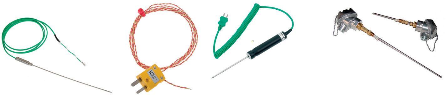
Thermocouples Thermocouples (Figure 2.1) are best suited to very low and very high temperature meas urements. They have the advantages that they are low-cost, very robust, and they can be used in chemical environments. The typical accuracy of a thermocouple is ±1 ºC. Thermo couple temperature sensors can be made with various conductor materials for different temperature ranges and output characteristics. Thermocouple types are identified with sin gle letters of the alphabet. Figure 2.1 shows the temperature ranges of various thermocou ples. Notice that lead color codes are used to identify thermocouples. The materials used to form thermocouples is shown in Figure 2.2. For example, one of the commonly used low-cost thermocouples is Type K which is made from chromel/alumel junction, identified with green lead color, and has temperature range of –180 ºC to +1300 ºC .
Chapter 2 • Sensors ● 19
Figure 2.1: Thermocouple types.
Figure 2.2: Materials used in different thermocouples.
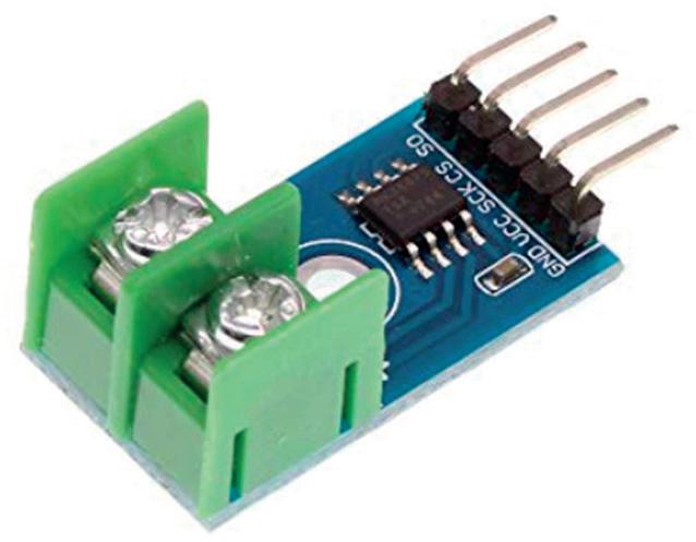
To get the temperature from a thermocouple a thermocouple amplifier is generally used. The temperature output from the thermocouple amplifier depends on the voltage of the reference junction. The voltage at the reference junction depends on the temperature dif ference between the reference junction and the thermal junction. Therefore, you need to know the temperature at the reference junction. The MAX6675 thermocouple amplifier module (Figure 2.3) comes with an on-board temperature sensor to measure temperature at the reference junction and also amplifies the small thermocouple voltage at the reference junction so that you can read it using a microcontroller.
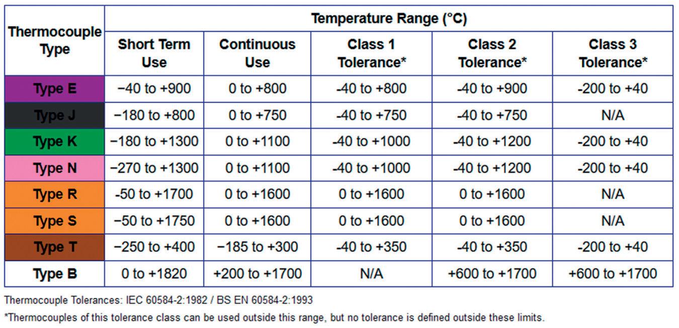
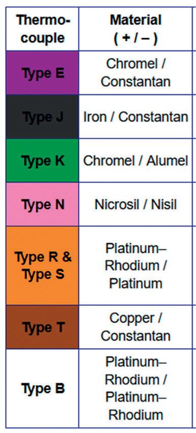
Figure 2.4: Some thermocouples.
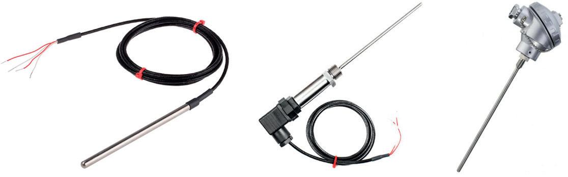
RTDs RTDs (Resistance Temperature Detector) are sensors whose resistance changes with tem perature. The resistance increases as the temperature of the sensor increases. The resist ance vs temperature relationship is well known and repeatable over time. RTDs are passive devices and they do not produce any output. Usually, the resistance of an RTD is measured by passing a small electrical current through it and then measuring the voltage across the sensor. Care should be taken not to pass large currents as self-heating of the sensor may occur. Typically, 1 mA or less current is passed through the sensor. Figure 2.5 shows some RTD sensors. RTDs have excellent accuracies over a wide temperature range and some RTDs have accuracies better than 0.001 ºC . another advantage of the RTDs is that they drift less than 0.1 ºC /year.
PID-based Practical Digital Control ● 20
Thermocouples are available in various shapes and forms. Some sensors are equipped with 2-way plugs for ease of connecting to a measuring device. Figure 2.3 shows some of the commonly available thermocouples.
Figure 2.5: Some RTDs.
Figure 2.3: MAX6675 thermocouple amplifier module.
Thermistors
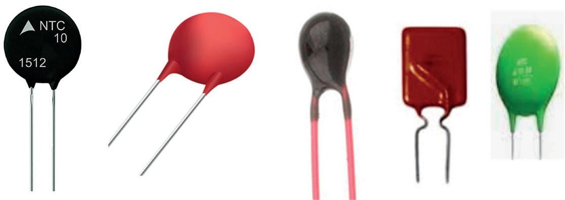
The name thermistor derives from the words thermal and resistor. Thermistors are temperature sensitive passive semiconductors which exhibit a large change in electrical resistance when subjected to a small change in body temperature. Thermistors are man ufactured in a variety of sizes and shapes (Figure 2.7). beads, discs, washers, wafers, and chips are the most widely used thermistor sensor types.
In order to achieve high stability and accuracy, RTD sensors must be contamination free. Below about 250 ºC the contamination is not much of a problem, but above this tem perature, special manufacturing techniques are used to minimize the contamination. RTD sensors are usually manufactured in two forms: wire wound, or thin film. Wire-wound RTDs are made by winding a very fine strand of platinum wire into a coil shape around a non-conducting material until the required resistance is obtained. Thin-film RTDs are made by depositing a layer of platinum in a resistance pattern on a ceramic substrate. The most commonly used RTD standard is the IEC 751 which is based on platinum with a resistance of 100 Ω at 0 ºC.
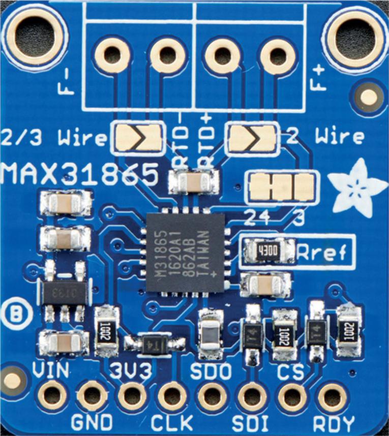
it is recommended to use an RTD-to-digital converter module like the MAX31865 module (Figure 2.6). This chip is optimized for platinum RTDs. An accurate ref erence resistor is used to set the sensitivity for the RTD. An on-chip ADC returns the ratio of the RTD resistance to the reference resistance in digital form. Knowing the reference resistance, you can easily calculate the RTD resistance and hence the measured temperature either from temperature-resistance tables or using a library function.
Chapter 2 • Sensors ● 21
Figure 2.6: MAX31865 RTD converter module.
For high accuracy
PID-based Practical Digital Control ● 22
Figure 2.7: Different shapes of thermistors.
Ruggedness: Most thermistors are rugged and can handle mechanical and thermal shock and vibration better than other types of temperature sensors.
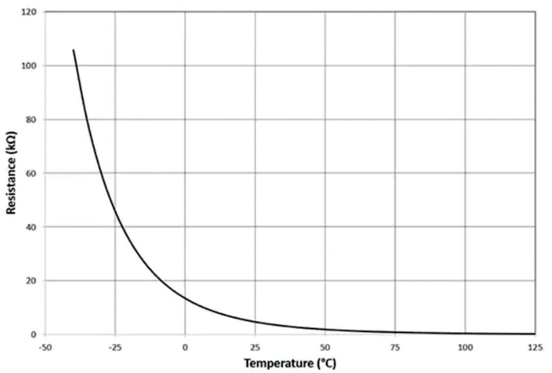
Figure 2.8: Typical thermistor R/T characteristic. The advantages of NTC thermistors are:
Sensitivity: One of the advantages of thermistors compared to thermocouples and RTDs is their large change in resistance with temperature, typically –5% per ºC. Small size: Thermistors have very small sizes and this makes for a very rapid response to temperature changes. This feature is very important in temperature feedback control systems where a fast response may be required.
Thermistors are generally available in two types: Negative Temperature Coefficient (NTC) and Positive Temperature Coefficient (PTC). PTC thermistors are generally used in power circuits for inrush current protection. NTC thermistors exhibit many desirable features for temperature measurement. Their electrical resistance decreases with increasing temperature (Figure 2.8) and the resistance-temperature relationship is very nonlinear. The resistance of a thermistor is referenced to 25 ºC and for most applications the resistance at this temperature is between 100 Ω and 100 kΩ.
Whereor
Low-cost: Thermistors cost less than most other types of temperature sensors.
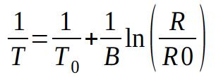
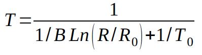
Thermistors can be used in circuits in series with a known accurate fixed resistor. By measuring the voltage across the thermistor, you can calculate its resistance. Alternatively, constant current, bridge, or operational amplifier circuits can be designed to measure the resistance of a thermistor. After finding the resistance of a thermistor, you can calculate the temperature using tables (if available), or a library function (if available), or use the standard Steinhart-Hart equation given below:
T0 is the room temperature in K (298.15), B is the thermistor temperature constant, R0 is the thermistor resistance at room temperature, and R is the measured resistance of the thermistor. An example is given below.
Chapter 2 • Sensors ● 23
Interchangeability: Thermistors can be manufactured with very close tolerances. As a result, it is possible to swap thermistors without having to recalibrate the measurement Thermistorssystem. can suffer from self-heating problems as a result of current passing through them. When a thermistor self-heats, the resistance reading drops relative to its true value and this causes errors in the measured temperature. It is therefore important to minimize the electrical current through a thermistor.
Remote measurement: Thermistors can be used to sense the temperature of remote locations via long cables because the resistance of a long cable is insignificant compared to the relatively high resistance of a thermistor.
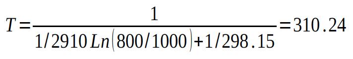
Solution Here, you know that B = 2910, T0 = 298.15, R = 800 Ω, and R0 = 1000 Ω
Example The temperature constant of a thermistor is B = 2910. Also, its resistance at room tem perature (25 ºC ) is 1 kΩ. This thermistor is used in an electrical circuit to measure the temperature and it is found that the resistance of the thermistor is 800 Ω. Calculate the measured temperature.
PID-based Practical Digital Control ● 24 Kelvin or T = 310.24 – 273.15 = 37.09 ºC
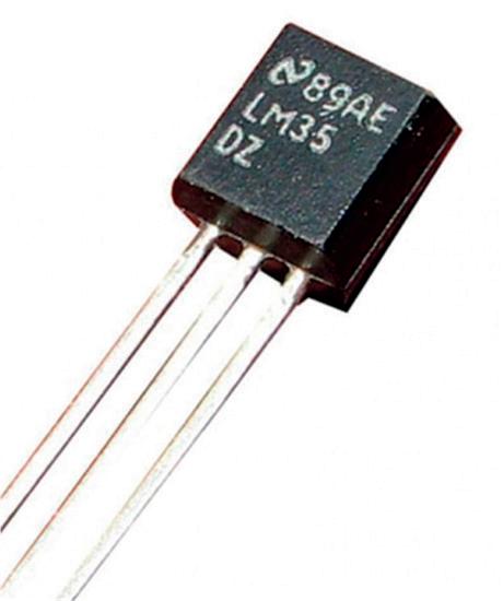
Figure 2.9: The LM35DZ temperature sensor.
Integrated circuits
Integrated circuit analog sensors are semiconductor devices. they differ from other sensors in some fundamental ways: They have relatively small physical sizes. Their outputs are linear. The temperature range is relatively limited. The cost is relatively low. They often lack good thermal contacts with the outside world and as a result it is usually more difficult to use them other than measuring the air temperature.
•
•
•
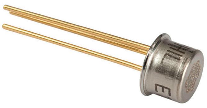
The LM34 is similar to the LM35DZ but it measures in degrees Fahrenheit. The LM134, AD590, and AD592 are current-output temperature sensors where the output current is di rectly proportional to the measured temperature. For example, the output of AD590 (Figure 2.10) is given as 1 μA/K.
LM35DZ This is a popular 3-pin temperature sensor (Figure 2.9) chip whose output voltage is linear, given by 10 mV/ ºC . For example, at 10 ºC the output voltage is 100 mV, at 20 ºC it is 200 mV and so on. this sensor has the range 0 ºC to +100 ºC (the CZ version of this sen sor has a wider temperature range like –20 ºC to +120 ºC ). The accuracy of this sensor is ±1.5 ºC and the operating voltage is 4 to 30 V.
• A power supply is required to operate these sensors.
•
•
Analog integrated circuit temperature sensor can be voltage output or current output. In this section you will look at the characteristics of some commonly used sensors.
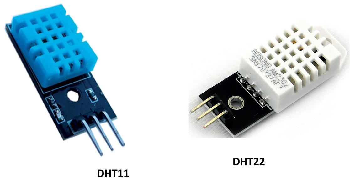
Chapter 2 • Sensors ● 25 Figure 2.10: AD590 temperature sensor. TMP36 This is another popular analog integrated circuit temperature sensor chip. The size and configuration of the sensor is same as in Figure 2.9. The output of TMP36 is linear with the measured temperature given by: Vo – 500 /10, where Vo is the sensor output voltage in millivolts. 2.2 Digital Temperature Sensors These sensors produce digital outputs and therefore they can be directly connected to microcontrollers. The outputs are non-standard and the measured temperature can be extracted in software by using a suitable algorithm. Table 2.2 gives a list of some popular digital output temperature sensors. Sensor Output Maximum error Temperature range LM75 I2C ±3 ºC –55 ºC to +125 ºC TMP03 PWM ±4 ºC –25 ºC to +100 ºC DS18B20 1-Wire ±0.5 ºC –55 ºC to +125 ºC AD7814 SPI ±2 ºC –55 ºC to +125 ºC MAX6575 1-Wire ±0.8 ºC –40 ºC to +125 ºC DHT11 Serial 1 wire ±2 ºC 0 ºC to +50 ºC DHT22 Serial 1 Wire ±0.5 ºC –40 ºC to +80 ºC Table 2.2: Some digital-output temperature sensors. DHT11 and DHT22 (Figure 2.11) are highly popular 3-terminal digital output sensors. Both devices can measure temperature as well as relative humidity. Arduino and Raspberry Pi li braries are available for both sensors for reading the temperature and humidity data easily.
PID-based Practical Digital Control ● 26
2.3 Position Sensors
Position sensors are used to measure the position of moving objects. These sensors are basically of two types: sensors to measure linear movement, and sensors to measure an gular movement.
Figure 2.12: Linear potentiometer.
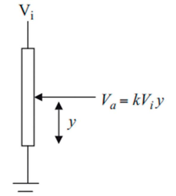
The simplest position sensor is a potentiometer. Potentiometers are available in linear and rotary forms. In a typical application, a fixed voltage is applied across the potentiometer and the voltage across the potentiometer arm is measured. This voltage is proportional to the position of the arm, and hence by measuring the voltage you know the position of the arm. Figure 2.12 shows a linear potentiometer. If the applied voltage is Vi , the voltage across the arm is given by: Va = k Vi y where y is the position of the arm from the beginning of the potentiometer, and k is a constant.
Figure 2.11: The DHT11 and DHT22 sensors.
Index ● 233 IndexA A201 30 Absolute pressure sensors 31 Acceleration 29 Accuracy 17 AD590 24 AD592 24 ADC 12 ADXL203 29 Analog sensors 16 Analog Temperature Sensors 18 attachInterrupt 177 Auto-tuning 85 B BDC Motors 160 Bluetin_Echo 203 BMP280 32 Brett Beauregard 154 Brushed DC Motors 160 Brushless DC Motors 164 C Chien-Hrones-Reswick 80 chromel/alumel junction 18 Ciancone-Marline 80 Cohen-Coon 78 commutator 160 Compare match register 151 compensator 12 Compound-wound 162 Compute 155 continuous-time system 11 control algorithm 12 controller 12 D DAC 12 Dahlin 69 damping ratio 45 DC Motor Control 159 dead-beat 69 derivative control 69 Derivative Kick 86 Derivative-only Controller 72 Desktop mode 131 DHT11 25 DHT22 25 DIFCUL 205 Differential pressure sensors 31 digital control system 13 digital encoder 14 Digital PID Controller 88 Digital sensors 16 digital system 53 Digital Temperature Sensors 25 DIR 190 displacement flow meters 33 Distance to object 199 disturbance 230 disturbance response 140 Disturbance response 230 disturbances 11 duty cycle 123 Dynamic response 17 dynamic system 11 E Echo pin 202 Electric Motors 159 EMG30 167 EncoderISR 177 error signal 11 e-Tape Liquid Level Sensor 34 F feedback 11 feedback control 11 First-order Systems 37 FlexiForce 30 Flow Sensors 35 Force Sensors 30 FS2012 36 FT-210 36 G gauge 30 GetDirection 155
PID-based Practical Digital Control ● GetKd234 155 GetKi 155 GetKp 155 GetMode 155 H Hall-effect 28 Hall Sensor Encoder 168 H-Bridge 169 HC-SR04 198 hotbed 118 Hysteresis 98 I Identification of the DC Motor 187 initial slope 41 integral control 69 Integral-Only Controller 71 Integral Wind-up 85 Integrated circuits 24 Interchangeability 23 Internal Model Control 80 Inverse z-Transforms 60 ISR 151 J JST connector 168 L Lambda 80 LDR 218 lead-lag 69 LED Brightness Control 218 LED-LDR 226 light detector 28 linear encoder 28 Linearity 17 liquid level sensor 35 Liquid Sensors 32 LM34 24 LM35DZ 24 LM134 24 LMD18200 169 Load cells 30 logic level converter 185 lux 219 LV170 34 LVDT sensors 27 M magnetic core 27 magnetic flow meters 33 MAX6675 19 MAX31865 21 Maximum overshoot 47 MC3002 108 Microcontroller Implementation 90 millis 177 MOSFET switch 122 Motor Selection 164 Motor Speed 183 MPL3115A2 31 MPRLS 3965 31 N natural frequency 45 NTC 22 NTC 3950 118 numerator polynomial 60 O obstacle 198 ODD/SIGN 109 Offset error 17 On-Off Temperature Control 92 Operating voltage 17 Optical encoders 28 overshoot 75 P paddlewheel sensors 33 parallel structure 88 PCF8574T 93 Peak time 47 permanent-magnet 160 PhaseA 194 PhaseB 194 photo-transistor 32 Physical size 17 PID library 154 PID Loop Simulator 86 piezoelectric sensor 30
Contents ● 235 plant parameters 77 plastic wheel 167 pole assignment 69 Position Sensors 26 potential divider circuit 202 potentiometer 26 Power series 60 Practical PID Tuning 84 Prescaler 151 Pressure sensors 30 process control systems 69 Program Description Language 91 Proportional + Integral + Derivative controller 74 Proportional + Integral Controller 73 proportional control 69 proportional-only controller 70 PTC 22 pull-up resistor 176 Pulse transfer function 61 Pulse Width Modulated 122 purple wire 183 PWM 14 R ramp input 55 Range 16 reference junction 19 Relative pressure sensors 31 Repeatability 17 reservoir 209 Resistance Temperature Detector 20 Resolution 16 Response time 17 rise time 41, 75 Rise time 47 Rotary Encoder 103 rotor 160 RPLCD 112 RTDs 18 S sampled signal 55 sampler 53 Sampling Proces 53 Sampling Time 89 Saturation 85 SCL 180 SDA 180 Second-order Systems 43 self-heating 23 Self-heating 17 Sensitivity 16, 22 Sensors 12, 16 Separately-excited 162 Serial Plotter 147, 158 Series-wound 161 Servo Motors 163 SetMode 155 SetOutputLimits 155 set-point 77 SetSampleTime 155 SetTemp 92 settling time 41 Settling time 47 SetTunings 155 SetupPlot 190 SGL/DIFF 109 Shunt-wound 162 speed of sound 204 SPI bus 108 stator 160 Steinhart-Hart 23 step change 77 Step-input 122 Stepper Motors 163 Strain gauges 30 system modelling 11 T tachometer 28 tank 209 TCCR0B 172 TCCR1B 172 TCCR2B 172 Temperature Sensors 18 Thermal shutdown 170 thermal systems 50 thermistors 18 Thermistors 21 thermocouple amplifier 19 Thermocouples 18
PID-based Practical Digital Control ● THIGH236 98 Thin-film RTDs 21 Thonny IDE 131 time constant 40 Time Delay 50 Time Response 39 timer interrupts 151 TLOW 98 TMP36 25 Tools 158 torque 159 Trig input 202 tuning the controller 75 two-phase encoder 168 TXS0102 109 Type K 18 Tyreus-Luyben 80 U ultimate gain 82 ultrasonic techniques 33 Ultrasonic transmitter-receiver 33 Unit ramp function 58 Unit step function 57 V Velocity and Acceleration Sensors 28 W water level 205 Water Level Control 198 water pump 205 Wire-wound RTDs 21 Y YF-S201 35 Z zero-order hold 55 Ziegler and Nichols 76 Z-Transform 57
The Arduino Uno is an open-source microcontroller development system encompassing hardware, an Integrated Development Environment (IDE), and a vast number of libraries. It is supported by an enormous community of programmers, electronic engineers, enthusiasts, and academics. The libraries in particular really smooth Arduino programming and reduce programming time. What’s more, the libraries greatly facilitate testing your programs since most come fully tested and working.
The Raspberry Pi 4 can be used in many applications such as audio and video media devices. It also works in industrial controllers, robotics, games, and in many domestic and commercial applications. The Raspberry Pi 4 also o ers Wi-Fi and Bluetooth capability which makes it great for remote and Internet-based control and monitoring applications.
Prof Dogan Ibrahim has a BSc, Hons. degree in Electronic Engineering, an MSc degree in Automatic Control Engineering, and a PhD degree in Digital Signal DoganProcessing.hasworked in many industrial organizations before he returned to academic life. He is the author of over 70 technical books and has published over 200 technical articles on electronics, bookwww.elektor.comfrommayprojectsThemicrocontrollers,microprocessors,andrelatedfields.fullprogramlistingsofallthediscussedinthebookbedownloadedfreeofchargetheElektorStorewebsite,(searchfor:title).
> Open-loop
books
> Analog
> Transfer
> First-order
and
www.elektor.com PID-based Practical Digital Control With Raspberry
The projects given for the Raspberry Pi 4 should work with all other models of Raspberry Pi family. The book covers the following topics: and closed-loop control systems and digital sensors functions and systems and second-order time responses temperature control with Raspberry Pi and Arduino Uno temperature control with Raspberry Pi and Arduino Uno DC motor control with Raspberry Pi and Arduino Uno water level control with Raspberry Pi Arduino brightness control with Raspberry Pi and Arduino Uno International Media BV Pi Arduino Uno
> PID-based
> Discrete-time digital systems > Continuous-time PID controllers > Discrete-time PID controllers > ON-OFF
and
> PID-based LED-LDR
Elektor
> PID-based
system
> PID-based
continuous-time
This book is about using both the Raspberry Pi 4 and the Arduino Uno in PID-based automatic control applications. The book starts with basic theory of the control systems and feedback control. Working and tested projects are given for controlling real-life systems using PID controllers. The open-loop step time response, tuning the PID parameters, and the closedloop time response of the developed systems are discussed together with the block diagrams, circuit diagrams, PID controller algorithms, and the full program listings for both the Raspberry Pi and the Arduino Uno. The projects given in the book aim to teach the theory and applications of PID controllers and can be modified easily as desired for other applications.