
15 minute read
Teacher’s notes for Speed of Sound


Speed of Sound
Teacher’s notes for Speed of Sound
Read
Sound is a vibration that travels through an elastic substance. The vibration causes areas of compression and rarefaction forming a longitudinal wave, which will show properties of reflection and diffraction. The speed of sound varies with the density of the material it travels through. As a general rule the greater the elastic properties of the material the faster the speed of sound. In air (a mixture of gases) at a temperature of 0ºC sound travels at 331.1 metres per second, as temperature increases the speed also increases (by approximately 0.607 m/s per ºC). The speed of sound in air is nearly independent of pressure and density. Speed travels about 4 times faster in water than air; the exact multiple is temperature dependant. In solids additional waves to do with shear can be propagated. The presence of these additional waves can lead to widely varying speeds being quoted in tables of comparison. Many tables express the theoretical values while others use values calculated by experiment
The speed of sound c is given by
B is the elastic property; it is normally the bulk modulus in fluids and solids ρ is the density
This tells us that the speed of sound increases with the bulk modulus of the material, and decreases with the density. In a solid, transverse waves are also propagated, with a different velocity to the longitudinal waves. A flat surface, such as a bench top, will contain many different velocities and wave echoes. The cross section (and area) of the material being tested will also have an influence. If the solid is a rod, then the velocity of sound will be dependent upon the Young’s modulus of the material. The quoted speed of sound in air is often from calculated values rather than practical measurement. The formula used to calculate the speed of sound in air produces good results over a wide range of temperatures, but starts to fail at high temperatures. Good predictions of the speed in the atmosphere are possible, especially in the colder, drier, low pressure stratosphere. When the temperature inversion of the atmosphere is reached the predictions are increasingly less valid. Changes in temperature and density associated with wind can create acoustic lenses which will alter the speed of sound, direction and distance of sound propagation. This will usually be misinterpreted as the wind “blowing” the sound. Students may well have heard of the Mach number, this is a value quoted for the speed of aircraft; it is popular to assume the Mach number is the number of times faster than the speed of sound the aircraft is travelling. The Mach number is a ratio of the objects speed to the speed of sound of the medium through which it is passing. A value of Mach one is therefore when the object is travelling at the same speed as sound could travel through the medium. The Mach number is a relative value not an absolute value.
Speed of Sound
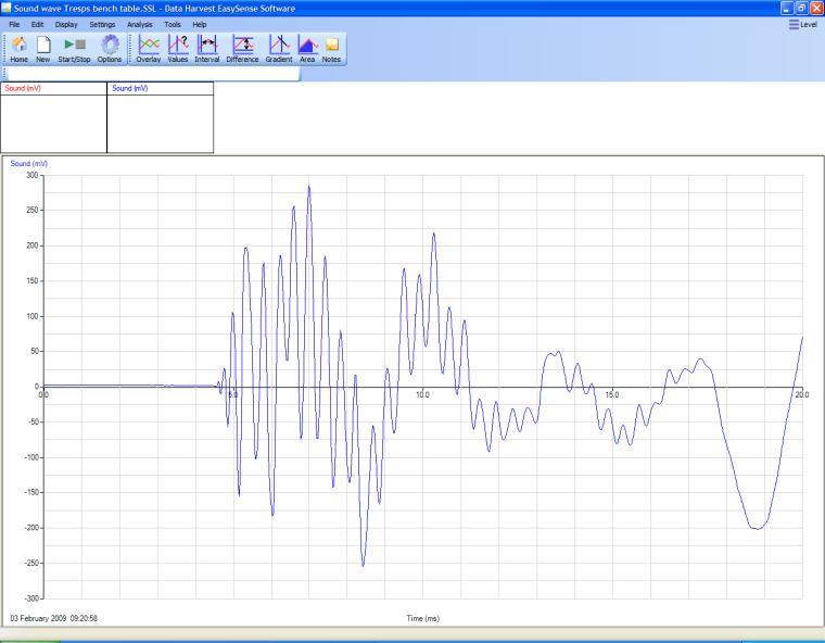
The way the material is mounted will affect the pattern of sound waves seen. E.g. the samples below show the wave pattern in piece of lab top (Trespa) mounted on base units and fixed to a wall and the same material mounted on a table frame.
Sound wave in Trespa mounted on a steel frame as a table / bench.
Sound wave in Trespa mounted on equipment cabinets. The difference in the sound wave pattern from the same material mounted in different ways should not affect speed of sound measurements as we are looking for differences between times of arrival of the sound wave.
Experiment(s)
The experiments described in the practical sheets use a method not dissimilar to the one used by William Derham in late 17th early 18th century. William Derham was the first recorded person to measure the speed of sound; he used a simple method of creating a sound and measuring how quickly it reached two far points. Knowing the distance separating the far points from the noise and the time taken to reach the points the speed was
Speed of Sound
calculated. In these experiments modern technology is used to reduce the distance between the listening points. Two microphones are placed a known distance apart, a noise is made and the time taken for the noise to travel between the two microphones is recorded. A simple calculation of distance / time gives the speed.
Apparatus
For use in all experiments 1. An EASYSENSE logger capable of fast recording 2. 2 Smart Q Stethoscope sensors 3. Masking tape or modelling clay 4. An expandable measuring tape
1. A large container at least 1 m long. 2. Large leak proof polythene bag.
1. A Smart Q Voltage sensor ±12 or 20 V. 2. A signal generator (sine wave, variable frequency). 3. A loudspeaker with matched impedance to the signal generator. 4. Patch leads.
Set up of the software for experiments 1 to 3
When Graph is started a New Recording Wizard will start, enter the information below on the correct pages.
Recording mode Length of recording Intersample time Trigger event Pre trigger amount
Graph 50 ms 50 µs When Sound sensor 1 Rises above 100 mV 25%
Intersample time availability depends upon the logger being used and /or the number of sensors connected. You want the shortest available time. The Pre-trigger value may need adjusting to account for ambient noise in and around the experiment location. To change this value click on New, and when the wizard starts click on Next until you are at the Start Condition page, enter the new value and Finish.
Which range to use
For speed of sound measurements we would normally advise using the Sound range. If the recorded trace appears to have small peaks, try using Autoscale to make the graph data as big as possible. If this still fails to reveal the information required change the range to Stethoscope and repeat.
Speed of Sound
Table 1 Ranges to use in speed of sound experiments
Material Sensor Range Suggested distance between sensors
Wooden bench top Aluminium Glass Wood Concrete Air Water Sound Sound Stethoscope Sound Stethoscope Stethoscope Sound At least 1 m At least 1.5 m At least 1 m At least 1 m At least 3 m At least 1 m At least 1 m
Note: It is very difficult to verify the validity of the calculated speeds. Speed of sound in a solid will vary with the bulk modulus of the material, and decreases with the density. Small sections of materials give values which are close to published tables; there will however be differences between theoretical and experimental values. Showing that speed is significantly higher in dense materials will be easy to show.
Table 2 Speed of sound in various solid materials
Solids v (m/s) Solids v (m/s)
aluminium beryllium brass brick
copper cork diamond glass, crown glass, flint glass, pyrex gold granite (293 K) iron lead lucite marble Neoprene 5100 12,890 4700 3650 4760 500 12000 5100 3980 5640 3240 5950 5950 2160 2680 3810 1600 rubber, butyl
1830 rubber, vulcanized 54 silver 3650
steel, mild steel, stainless titanium wood, ash wood, elm wood, maple wood, oak wood, pine 5960 5790 6070 4670 4120 4110 3850 3313
Speed of Sound
Liquids v (m/s)
alcohol, Ethanol alcohol, Methanol mercury water, distilled water, sea water vapour 1207 1103 1450 1497 1531 494
Gases (STP)
air, 0°C air, 20°C argon carbon dioxide (293 K) helium (273 K) hydrogen (H2) (273 K) neon nitrogen nitrous oxide oxygen (O2) water vapour, 134°C v (m/s)
330 343 319 259 965 1284 435 334 263 316 494
The values of some materials will vary widely in published literature. The speed of sound will depend upon the purity, cross sectional area and frequency used. Aluminium will have published values ranging from 5100 to 6240. In some cases the values are theoretical and others they have been calculated from practical measurement. The tables above are an amalgam of several sources. For some materials an average of published values is used.
To get good values (in agreement) by experiment
1. Have at least 1 m between the sensors, the bigger the distance the better. 2. Measure the distance to the nearest mm. Errors in the distance measurement have a big effect in the calculation. 3. Use the fastest recording time possible. 4. Use a trigger. 5. When measuring a solid make sure the stethoscope is lying flat on it. 6. If you are using a non-flat or narrow object try to get as much of the bell of the stethoscope over the surface as possible. Make sure the microphone is over the surface and not displaced to one side.
You need to arrange the apparatus so that the point where you will create the noise is first, then the first sensor and then the second sensor.
Speed of Sound
Use a chalk line or a length of tape to mark out the expected path of the sound and the recording line. To help with the maths try to get a separation of ‘sensible’ units e.g. 1.0 m, 1.2 m, 1.5 m, etc. Try to avoid distances like 1.25 m, 1.98 m if possible. It may be that you want the students to use more complex values, but for an introductory demonstration simple distances are better. Students will need to use the following formulae,
Speed = Distance
Time
Wavelength = Velocity Frequency
The students should be confident to re-arrange the formulae to calculate the unknown value. A check to see that the students understand the terms velocity, speed, frequency and wavelength could also prevent difficulties in calculations.
Speed of Sound in Air
Sample result
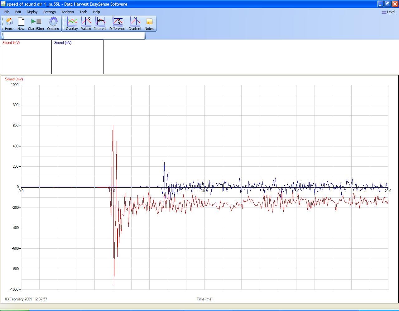
Separation of Stethoscope sensors of 1.0 m.
Speed of Sound
Analysis

Use the Interval tool used to select the time from the first recording of the wave (sensor 1) to the second recording (sensor 2). Interval = 2.90 seconds Stethoscope sensor separation = 1.0 m
Calculation
Speed of sound (calculated from sample results) = 1.0 / 0.0029 = 344.8 m/s Temperature of room = 22ºC. Correction for temperature = (0.607 x 22) + 331.1 = 344.45. (Speed of sound increases by 0.607 m/s per degree Celsius)
Speed of Sound in Water
Note: You must use a polythene bag to contain the immersed sensor. The bag must be waterproof and leak proof. 1. While it should be possible to record the speed of sound in liquids other than water, the speed of the logging and size / volume of the container will normally mean that water is the only liquid used. You may want to compare fresh with salt water. 2. You will need a long container, the volume can be small. You only need enough depth of water to cover the immersed sensor. 3. A minimum of 0.5 m is required if you wish to simply show that speed is faster in water. If you wish to collect empirical data you need to be looking a distance of at least 1.5 m between sensors. The speed of sound in water is approximately 4 times faster than air. The time difference between the sensors will be small, the sample rate and the accuracy of the measurement of the distance separating the sensors will be introducing potentially large errors with a distance of 1 m or less.
Speed of Sound
4. Take the temperature of the water, the speed of sound in water is temperature dependant. If you refer to published values you will need to compare values for the same temperature. 5. The container needs to be made of a stiff material. Polythene containers tend to dampen the noise and produce echoes. A polypropylene box was found to give easier to understand results compared to a similar length polyethylene container.
Sample results and analysis
Path between stethoscope sensors was 0.6 m. Box made of polypropylene.
Note how the water smooths the waveform, this does make the difference between the two traces ambiguous. You may wish to use Zoom to help find the two start points of the sound.
Zoom applied to the first part of the data. Interval has been used to mark the beginning of the sound wave on each trace and reveal the time difference. With this data the time
Trace from submerged sensor
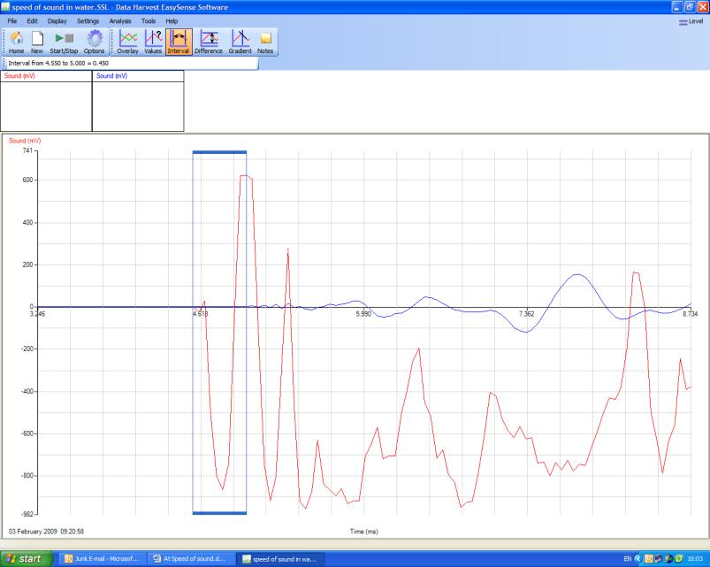

Speed of Sound
resolution gave a value of 0.450 ms or 0.500 ms, use the mean of the two estimates for calculation i.e. 0.475 ms.
Calculations
In this example the distance between the Stethoscope sensors was measured at 0.60 m. The Interval tool revealed the time for the sound to reach the second sensor after reaching the first was 0.475 ms Speed of sound = distance / time = 0.6 / 0.000475 (time corrected from ms to s) = 1263 m/s This is considerably faster than the speed of sound in air. No correction has been made for temperature; the errors in the estimate of time are sufficiently large that we can only look at the gross idea of the sound travelling faster in water. If the container had been longer the time interval would have had greater certainty. In analysing the results there is always the danger of manipulating the values to produce the result required, this is good opportunity to raise the issue of the impartial observer. Speed of sound in water is normally quoted as 4 x faster than in air. Air value = 331.1, x4 = 1325. The results are not far off.
Speed of Sound by phase difference
The student’s notes show how to conduct the experiment using a Voltage sensor to record the output of the signal generator. The experiment can be done using a pair of Stethoscope sensors. When using a pair of sensors have one as a fixed sensor close to the loud speaker, this will record the reference wave form. Move the second sensor slowly away from the fixed sensor, pause every 10 cm or so to check the phasing. The experiment works well; ideally you need a short wavelength to reduce the effects of volume attenuation distorting the produced wave from the moving speaker. Which frequency you use will depend upon the frequency response of the loudspeaker, the response of the loudspeaker and the irritation factor of the audible tone. Do be careful when picking the tone / frequency, some are particularly distressing (especially with a younger audience) and have the potential to cause hearing damage. (Check with local safety guidelines for any frequencies to avoid). In testing, a frequency of about 460 Hz was used this gave a theoretical wavelength of approx. 0.76 m. It is an idea to calculate the theoretical wavelength of the frequency chosen, for practical reasons (attenuation of signal, restrictions of work area) avoid anything with a wavelength of over 80 cm and under 30 cm. At the shorter wavelengths it can become more difficult to find the in phase node with accuracy.
Frequency
400 450 500 550 600
Wavelength (m) at 23ºC
0.86 0.77 0.69 0.62 0.58
Wavelength (m) at 0ºC
0.82 0.74 0.66 0.60 0.55
Speed of Sound
Wavelength at frequencies in the range 400 – 600 Hz at 23 and 0ºC.
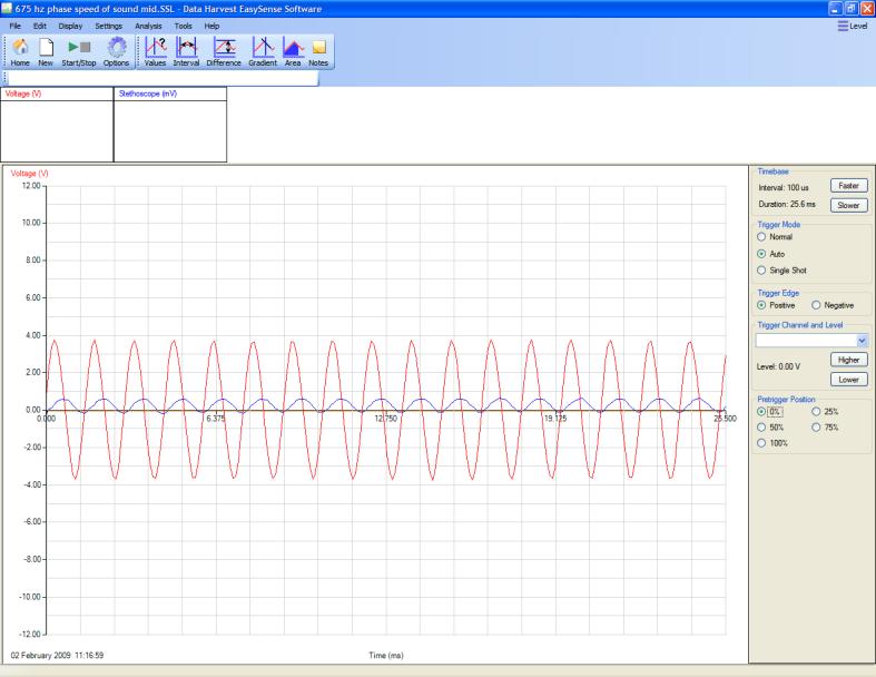
Sample data
Voltage and sound in phase with Stethoscope at its closest point to the speaker in the experiment.
Sound and voltage out of phase, as the Stethoscope is moved away from the loud speaker.
Sound and Voltage back in phase when the Stethoscope is at its most distant from the speaker in this experiment.
You will need to use Autoscale at this point to check the phase difference.


Speed of Sound
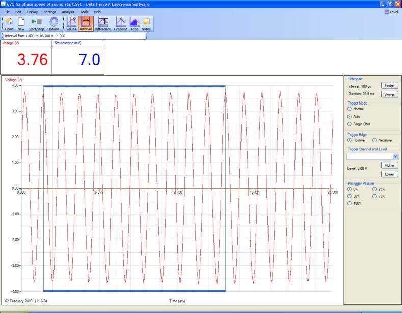
Using Autoscale on the data to see if the waves are in phase. Use the Values tool to check the alignment.
Calculations
Frequency from voltage wave. a. Taking a single wave. Use the Interval tool to find the interval between two adjacent peaks. b. Calculate 1/interval (in seconds) = frequency in Hz. Take several peaks and produce an average.
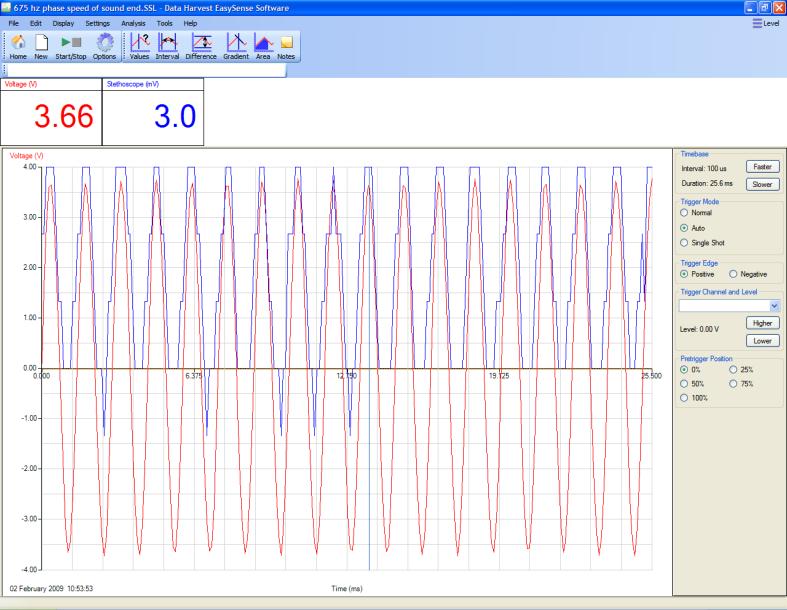
Selecting 10 peaks to calculate frequency. In the sample data the interval was 1.5 ms, this gave a calculated frequency of 666.66 Hz. Using several peaks allowed an average to be calculated. A frequency meter confirmed the frequency was 675 Hz. Using 10 peaks to find the time gave a value of 672 (14.8 ms over 10 peaks) suggesting that this was a more accurate method of determining the frequency. 1. Using multiple waves. a. Use the Interval tool to find the time interval for 10 peaks.
Speed of Sound
b. Divide the time interval by the number of peaks to find the time for one cycle 2. Calculate 1/interval (in seconds) = frequency in Hz
Calculate the speed of sound
Values taken from a recorded practical. 1. f = 672 Hz 2. L = 0.525 m (initial in phase distance 23 cm – final in phase distance 75.5 cm) 3. f/l = 352 m/s Temperature of the room = 25ºC, correction = 0.607 m/s per 1ºC = 25 x 0.607 = 15.2. Expected value = 331.3 (speed at standard pressure and 0ºC) + 15.2 = 346.5. Experimental value =352. (2% error over theory) Note. With the speaker being used the first “in phase” was 23 cm in front of the speaker at this frequency. This is due to a lagging phase shift between the sound wave and the changing voltage frequency driving the speaker. The lag is created by impedance within the coil magnet system driving the speaker cone. The lag can be up to 45 degrees, producing a phase difference of 45/360 = 12.5%.


