VOL VII Issue II SPRING 2022

JUST VOL VII // ISSUE II // SPRING 2022 Journal of Undergraduat e Science & TechnologyJ Cover photograph by Shin-Tsz Lucy Kuo

LETTER FROM

When I joined JUST during my freshmen year, I was welcomed by a small team. Over the past few years, as JUST’s campus presence has magnified, not only has student engagement with research and science communication increased but the JUST team has also grown! The team has grown in number and in skill as we have gained valuable experience in disseminating scientific research and the academic editing and publishing process. We believe that these experiences are an invaluable supplement to a traditional undergraduate education, especially for those students who wish to learn about research and JUSTcommunication.istheonly peer-reviewed research and science communication journal on campus. The entirety of the publication is curated by undergraduates with the help of our wonderful faculty advisors, Dr. Joan Jorgensen, and Dr. Todd Newman. UW-Madison is a thriving research institution, as a result, most undergraduates participate in research at some point during their studies. JUST offers a unique platform to these undergraduates to publish their research and get a glimpse into the academic publication process.

The second part of the JUST mission is centered around science literacy. Everything around us is science, which is why we believe fostering scientific curiosity is important. Within this issue, you will find editorials exploring urgent scientific issues such as the detrimental environmental effects of road salt usage as well as the health implications of high concentrations of ground-level ozone and the famine crisis. You will also find interesting editorials on how plants converse, the similarities between the brain and the space, and if the 2015 viral dress is blue or gold. All these editorials have been written passionately by the JUST staff writers and thoughtfully edited by the JUST content editors. We hope that these editorials will help you gain a deeper understanding of the natural world, and help you understand how our shared actions can affect our neighbors and the environment. We are honored to be a small part of a much larger effort to make research more accessible to audiences beyond academia.

In this JUST issue, we are celebrating the contributions of excellent student researchers who have meaningfully immersed themselves in research domains as diverse as ecology, neurobiology, psychology, and microbiology.

JUST VOL VII // ISSUE II // SPRING 2022 3 J

Dear Reader, I must confess, as I am writing this note, my final note, I am quite emotional.

Putting together the JUST issues within the span of a single semester is a mammoth task and the only reason it has been successfully accomplished time and again is because of the amazing JUST team. I would like to express my gratitude to the JUST team that have chosen to make JUST a part of their undergraduate experience and worked diligently to bring you this issue. I would also like to extend my sincerest gratitude to the undergraduate researchers for submitting their work for this JUST issue along with the faculty and staff who supported them. Additionally, without the generous support of the Associated Students of Madison and the College of Agriculture and Life Sciences, the publication of this JUST issue would not have been possible.

EDITOR-IN-CHIEFTHE

Although my time with JUST is ticking, yours has just begun! I hope that as you read this publication, you allow it to open your mind and inspire you, just as it did me when I first stumbled upon it, and as it continued through my journey from staff writer to Editor in Chief. Please join us in recognizing the incredible research and thoughtfully written pieces presented by UW-Madison undergraduates, and in our larger pursuit of supporting science literacy.

UW-Madison's only undergraduate STEM research & communication journal is RECRUITING for FALL 2022! editors | staff writers | designers and accepting submissions for: research reports | editorials | photographs www.justjournal.org | contact@justjournal.org Journal of Undergraduat e Science & TechnologyJ

I joined the Journal of Undergraduate Science and Technology (JUST) in the Fall of 2018. As I reflect on the progress JUST has made in these past four years, the progress the JUST team and I have made, as we have lived and grown through this publication, I am astonished. Perhaps in the momentum of building and moving the individual pieces of what constitutes this publication, we forgot to take a step back and gaze at how far it has come.

TABLE OF CONTENTS REPORTS 36. People, Parks, and the Pandemic: How Public Green Spaces Have Shaped Human Wellbeing During COVID-19 Katelyn McVay 42. The Comparison of the Proportion of Antibiotic-Producing Soil Bacteria Isolated from the Shores of Lake Mendota and Lake Michigan Stephanie Frisch 48. The Effect of Demographic Variables on Brain Symptom Networks and Psychopathology in Children Olivia Otremba 54. The Effects of Fishing on Herbivory around Patch Reefs in a Belizean Marine Reserve: Increased Herbivory Rates in a Marine Protected Area Luis Manuel Abreu-Socorro PIXELSEDITORIALS 32. Leta Landucci, William Vuyk 6. How Bad Neighbors Cause Lakeshore Ozone Sarah Kamal 10. Preventing the Slip: Road Salt Usage’s Effect on Environment Britta Wellenstein 14. The Immunological Effects of Famine Carter Wood 18. The Mystery Behind the Dress – A Neuroscientific Conundrum Mahak Kathpalia 21. The Space Your Brain Takes Up Natalie Martinson 26. Translating Stress Signals Into Blazes of Light Leta Landucci

SCIENCE + SOCIETY:

Thank

We would like to sincerely thank the Integrated Stud ies in Science, Engineering, and Society Undergraduate Certificate Program [ISSuES] at UW-Madison; The Col lege of Agriculture and Life Sciences [CALS]; The Wis consin Institute for Discovery; the Associated Students of Madison (ASM) and Wisconsin Alumni Research Foundation for financially supporting the production of JUST’s Spring 2022 issue. you!

How to be creative and effective in a rapidly changing environment

The Journal of Undergraduate Science and Technology (JUST) is an interdisciplinary journal for the publication and dissem ination of undergraduate research conducted at the University of Wisconsin-Madison. Encompassing all areas of research in science and technology, JUST aims to provide an open-access platform for undergraduates to share their research with the university and the Madison community at large.

JUST VOL VII // ISSUE II // SPRING 2022 5 J 4 JUST VOL VII // ISSUE II // SPRING 2022 J SPONSORS & PARTNERS EDITOR-IN-CHIEF Aadhishre Kasat MANAGING EDITOR Jaitri Joshi DIRECTOR OF MARKETING Hannah Landsly MARKETING ASSISTANT Chloe Hansen MARKETING TEAM Amy ClaudiaLi Liverseed Daniel Molina DIRECTOR OF DESIGN Ashley Harris DESIGN ASSISTANT Jennifer Schaller WEBMASTER Louis Griffin WEBMASTER ASSISTANT Ethan Wang EDITORS OF CONTENT Adina SamanthaNabaManasiLucasDimaCatherineShaikhNguyenHamdanChiniSimhanRaoBebel STAFF WRITERS Myra Mohammad, Head Staff Writer Tala Shaibi, Head Staff Writer Leta SarahNatalieMahakCarterBrittaLanducciWellensteinWoodKathpaliaMartinsonKamal

and premature death from respiratory diseases (US Envi ronmental Protection Agency, 2013). It is also found that the inhalation of other air pollutants alongside ozone ex acerbates the body’s reaction to ozone compared to the inhalation of ozone alone (American Lung Association).

Figure 1. Lakeshore ozone concentrations display a spatial gradient, with the highest concentrations found directly over Lake Michigan and along parts of the shoreline. The concentration progressively decreases as the distance from the lake increases. Source: Bulletin of the American Mete orological Society 102, 12.

"States containing lakeshore ozone cannot attain national standards alone; this attainment requires the participation and cooperation of upwind states in significantly cutting down emissions. "

By Sarah Kamal

6 JUST VOL VII // ISSUE II // SPRING 2022

EDITORIAL JUST VOL VII // ISSUE II // SPRING 2022 7 J EDITORIAL J CHEMISTRY Although the term ‘pollution’ is generally asso ciated with large, densely populated cities, ozone poses a notable public health risk in urban areas and rural areas alike, making it a particularly unique pollutant. Depend ing on where it is found in the Earth’s atmosphere, ozone can be either beneficial or harmful to human health. Ozone that occurs in the upper atmosphere, called strato spheric ozone, occurs naturally and acts as protection from the Sun’s ultraviolet rays. On the other hand, ozone that occurs in the lower atmosphere, called tropospheric or ground-level ozone, is a man-made pollutant that af fects air quality. Thus, it is important to understand the mechanism by which ground-level ozone is produced and transported across vast areas in order to develop effective control strategies.Exposure to ground-level ozone must be con trolled as it poses a significant health risk to individuals in both the short-term and long-term. Exposure can cause immediate symptoms such as cough, sore throat, or diffi culty breathing, as well as an increased frequency of asth ma attacks, and inflammation of the airways (Centers for Disease Control). Moreover, long-term ozone exposure is associated with the development or aggravation of asthma

Ground-level ozone is not directly emitted into the air, but rather a product of a chemical reaction that occurs between ozone precursors and sunlight. Substances called volatile organic compounds (VOCs) and nitrogen oxides (NOx) are emitted into the atmosphere by indus trial processes, power generation, automobiles, and fuels. VOCs and NOx then react with heat and sunlight to form ground-level ozone (Lake Michigan Air Directors Consor tium). Therefore, it is not uncommon to find high ozone levels in urban areas, particularly Chicago, that exhibit high emissions of volatile organic compounds and nitro gen oxides. However, high ambient ozone concentrations are also observed along the shoreline of Lake Michigan, away from urban and industrial sources of ozone precur sors. This highlights a unique characteristic of ground-lev el ozone: high levels can occur far from the source (com pared to other pollutants, where high levels are usually found near the source). In other words, while one may expect ozone levels to be concentrated in urban areas with significant emissions, the reality is that ozone can occur anywhere.The main cause of lakeshore ozone is the sur face temperature gradient between Lake Michigan and its surrounding land, creating a lake-land breeze pattern that transports pollutants to the lake. During the night and early morning, the temperature of the lake is higher than the surrounding land. This creates a land breeze that transports precursors from industrial sources on the south end of the lake to directly over the lake. As the sun rises, these precursors chemically react with sunlight to form ground-level ozone. By early afternoon, the temperature of the lake cools, and the lake breeze transports the newly formed ozone inland, along the lakeshore (Lake Michigan Air Directors Consortium). This meteorological process explains how areas along the shoreline of Lake Michigan, which lacks large industrial sources, have one of the high est ambient ozone concentrations in the eastern United States (Cleary et. al., 2021). As seen in Figure 1, lakeshore ozone concentrations display a spatial gradient, with the highest ozone concentrations found directly over Lake Michigan at 76ppb and along parts of the shoreline at 7175ppb. The ozone concentrations progressively decrease as the distance from the lake increases (State of Wisconsin Department of Natural Resources). Therefore, it is very likely that Wisconsin counties on the shoreline of Lake Michigan have difficulties attaining national standards be cause of the interstate transport of ozone precursors from neighboring states. Considering the variety of health risks associated with un safe concentrations of ground-level ozone, it is critical that non-attainment areas, specifically along the shoreline of Lake Michigan, reduce emissions and adopt control mea sures. However, the reality is that upwind states must take responsibility for the interstate transport of ozone pre

For sensitive groups, such as children, older adults, and individuals with pre-existing lung disease, these risks are even higher. Children are particularly vulnerable; their lungs are still developing, they spend more time outdoors (translating to more exposure), and they are more likely to have asthma (US Environmental Protection Agency, 2013). Hence, attainment of the national standards is nec essary to avoid the health risks arising from high ambient ozone concentrations.The2015National Ambient Air Quality Stan dards for ground-level ozone is 70 parts per billion (ppb) for both primary and secondary standards (US Environ mental Protection Agency, 2015). States are responsible for creating a State Implementation Plan to monitor and control ground-level ozone concentrations within their state. Areas that do not meet the air quality standards are considered non-attainment areas. Non-attainment areas have additional requirements including actionable mea sures to reduce emissions in a timely manner in their State Implementation Plan. However, before effective control strategies can be developed, it is important to understand how ground-level ozone is distributed.

How Bad Neighbors Cause Lakeshore Ozone

References American Lung Association. (n.d.). Ozone. Centers for Disease Control and Prevention. (2019, Sep tember 4). Ozone and your health.

Preventing the Slip: Road Salt Usage’s Effect on Environment

By Britta Wellenstein

If you were to ask students and faculty of UW-Mad ison their thoughts on the Midwestern winter, you would mostly be met with repulsive looks. The snowy weather makes the trek up Bascom and around campus so pain ful that most days students have to kick themselves to get to class. Commuting in the winter is difficult as is, but it becomes an adventure sport with ice in the equation. Students shudder at the thought of sliding on the ice and falling in front of everyone, or worse, slipping and sliding back downOneBascom.ofthe best and most common ways to pre vent slips on ice is to use road salt. Walking around cam pus though, you see a variety of ice-prevention measures, from salt to sand, or a mixture of both. Or you see the dreaded nothing. The lack of consistent salt usage in Mad ison isn’t because of a lack of salt or lack of caring, but rather due to an overall concern about road salt usage in the City of MadisonMadison.lies on an isthmus, located between two bodies of water: Lake Monona and Lake Mendota. Road salt use has a drastic impact on nearby bodies of water, which can consequently affect drinking water and sewage systems. Even the slightest amount of salt has a large im pact on water. For example, a single teaspoon of salt can make five gallons of freshwater toxic to various ecosys tems. However, road salts don't have just an impact here in Madison, but also on the greater bodies of water, like Lake Michigan.

Figure 2. Dangerous ground level concentrations of ozone can have severe health impli cations. These ozone levels are higher at warmer temperatures. Source: Center for Disease Control and Prevention.

Cleary, P. A., Dickens, A., McIlquham, M., Sanchez, M., Geib, K., Hedberg, C., Hupy, J., Watson, M. W., Fuoco, M., Olson, E. R., Pierce, R. B., Stanier, C., Long, R., Valin, L., Conley, S., & Smith, M. (2021, November 11). Impacts of lake breeze meteorology on ozone gradient observations along Lake Michigan Shorelines in Wisconsin. Atmo spheric Environment. Lake Michigan Air Directors Consortium. (n.d.). High concentrations of ground-level ozone are a problem in and near urban areas and along the Lake Michigan shore line.

State of Wisconsin Department of Natural Resources. (2017, April 20). 2015 Ozone National Ambient Air Qual ity Standards Area Designations. United States Environmental Protection Agency. (2015, October 1). Overview of EPA's updates to the air quality Unitedstandards.States Environmental Protection Agency. (2013, March 22). The Clean Air Act in a nutshell: How It Works.

cursors over Lake Michigan. States containing lakeshore ozone cannot attain national standards alone; this attain ment requires the participation and cooperation of up wind states in significantly cutting down emissions. Ideally, these states should work together to control ground-level ozone and protect the future of public health.

"The fear of slipping down Bascom will never go away, and neither will road salt. "

8 JUST VOL VII // ISSUE II // SPRING 2022

EDITORIAL JUST VOL VII // ISSUE II // SPRING 2022 9 J EDITORIAL J

ENVIRONMENT

By adding salt, the freezing temperature of water drops to 20°F (-7°C). Therefore, salt becomes ineffective when the temperature drops below 20°F, which in Wis consin it often does! For this reason, sand is seen as the more popular slip-prevention measure. Sand does not affect the temperature at which water freezes, but rath er, provides surface friction and foot grip to prevent slips (Pollock, 2019).

How does Road Salt Work: Road salt was first used as a method to combat snow and ice in 1936. It provided a cheap and effective way to help clear roads and sidewalks in a booming industrial America. The chemical composition of road salt is incredi bly similar to what is sitting on your dining table, sodium chloride. However, in addition to sodium chloride, road salt also contains a few other minerals. Although sodium chloride is the most commonly used road salt, potassium chloride and magnesium chloride can be used as well. One of the most common misconceptions about road salt is that it melts ice. However, road salt doesn’t melt ice, it prevents water from freezing. Water normally freez es at 32°F (0°C). When salt is added to water, the freezing point lowers because salt ions block water molecules from crystallizing. Thus, putting salt on plain ice isn’t as effec tive. Sun or friction from cars would need to help melt the ice before salt can be effective (Pollock, 2019).

Madison’s Dilemma Madison is located near many bodies of water, be sides Lake Monona and Mendota. It lies in a large lake system, the Yahara system, consisting of Lake Monona, Lake Mendota, Lake Wingra, Lake Waubesa, Lake Kegon sa, and the Yahara River. Therefore, Madison limits its salt usage to “300 pounds of salt per lane mile,” a guideline put into place in 1978. Under this policy, only main or more dangerous roads are salted, such as the main bus routes, hills, and outside of hospitals. This is why University and Johnson may be clear, but your little one way in the soph omore slums or by Mifflin isn’t as clear. The University of Madison also limits its salt usage. Salt is still used, but often a salt-sand combination is used on walkways and en trances (Outdoor Salt Use Policy, 2015). Certain walkways and staircases are closed in the winter in an effort to limit salt usage, as Figure 1 shows. However, these salt measures have been in place since 1978, and the chloride levels in the Yahara system have only grown since then, as seen in Figure 2. Lake Wingra has the highest concentration out of this system, partially because of its small size. Since 1981, Wingra chlo ride levels have risen 200% and increased to 400 mg/L. This is well past Madison's “chronically toxic” level, which is 395 mg/L. The chloride concentration of Lake Wingra has decreased by 5% over 5 years, partly due to increased precipitation which dilutes chloride concentrations. How ever, as a whole, chloride levels in the Yahara system are still growing. There has been a 5% increase between 2013to 2018 (Wenta, Furthermore,2020).groundwater in Madison has been affected by road salt usage. In the past 40 years, sodium and chloride levels have increased in both upper and lower groundwater wells, according to Dane County’s 2019 Road Salt report (Wenta, 2020). These levels are maintained Figure 1. Madison blocks off paths in the winter to avoid salt usage. Here, a staircase on the State St. side of Humanities is blocked off.

Although there is no health guideline for groundwater chloride levels, there are levels to regulate the aesthetics of drinking water, that being taste and smell, both of which are affected by chloride (Hintz & Relyea, 2021). Road salt is also an economic issue because of the damage it causes to infrastructure. Ice causes not only cars to rust, but larger structures to corrode, like bridges. It also can corrode pipes, causing other harmful metals, like lead, to leak into the water system, which is what happened in Flint, Michigan during their water crisis (Hinsdale, 2018). These damages combined resulted in $5 billion in repairs (Sherwell,Currently,2021). chloride levels are measured to keep up with the EPA limit of 230mg/L, a number set in 1988 and has not changed since. However, many studies sug gest these measures are outdated and lower chloride lev els have an impact on ecosystems. Furthermore, chloride’s impact is somewhat individual, and context-dependent based on individual bodies of water and their chemical properties and ecosystems (Hintz & Relyea, 2021).

EDITORIAL JUST VOL VII // ISSUE II // SPRING 2022 11 J EDITORIAL J

Environmental and Structural Costs of Road Salt Road salt, despite its effectiveness, has a larger eco logical footprint. It may seem like the salt put out by your apartment building is little and doesn’t have a large effect. However, millions of pounds of salt are used each year in the United States –all of which end up in the water. Salinity, the amount of salt in freshwater, is of great con cern to many, as it can have a drastic impact on freshwater ecosystems and drinking water by affecting pH and water quality respectively. High sodium levels in drinking water affect people with high blood pressure, and high chloride levels are toxic to some fish, bugs, and amphibians (Sher well, 2021).Inwildlife, high salt concentration can disrupt food chains and affects species’ ability to grow and devel op. In water bodies specifically, road salt can cause oxygen depletion. Salt tends to sink towards the bottom of the water body, creating a dense layer that can inhibit gas ex change with the overlying water. This can lead to the de velopment of low oxygen conditions that are detrimental to fish and other aquatic organisms such as tadpoles. Ad ditionally, road salt can also harm wildlife that consumes salt on the side of roads (Hinsdale, 2018). Road salt doesn’t only contaminate water bodies but can also run off into nearby soil and agriculture, im pacting plant growth. Long-term soil contamination de creases soil fertility and permeability, affecting the soil’s ability to hold and carry water. Salt can also travel through plant roots and affect plant growth by causing premature senescence and reduction in overall photosynthetic area (Hinsdale, 2018) (Lee, M.K et al. 2008). It is estimated that lakes in America will have extremely high salt concentra tions by 2050, becoming destructive to local ecosystems as well as drastically impacting drinking water quality (Sum mers & Valleau, Groundwater,2017). and thus drinking water, is also impacted by road salt. Once chloride enters the water, it is very difficult to remove and accumulates over time.

Figure 2. Graph of chloride levels in the Yahara Lake system from 1948-to 2018. Source: Dane County 2019 Road Salt Report.

10 JUST VOL VII // ISSUE II // SPRING 2022

Conclusion

References

Road salt alternatives Road salt alternatives are vast, varying from beet juice to sand, to other forms of salt (besides sodium chlo ride). However, there are not many alternatives to typi cal road salt that do not have environmental effects. Beet juice can be effective in certain climates, but still has en vironmental implications in wetlands. Salt alternatives like magnesium chloride and calcium chloride are much more expensive than sodium chloride and don’t pose a large benefit to the environment. In certain climatic con ditions, they can be even more toxic to the environment. All in all, there isn’t a salt alternative that is cost-efficient, environmentally friendly, and can be implemented on a large scale (Summers & Valleau, 2017). The best way then to reduce road salt usage is to do just that, reduce it by being more mindful of how and when we use road salt. States like New Hampshire have reduced their salt usage by 20%, using a “closed-loop sys tem”. As part of this system, the amount of salt used is closely monitored, the usage of snow tires is made manda tory and speed limits are decreased (Sherwell, 2021). Mix ing salt with substances like sand, which is what is done here at UW-Madison, also helps, as also mandated by Wis consin’s Salt Wise Partnership. More efficient road salt storage facilities that pre vent road salt run-off can also be built. The frequency of anti-icing can be increased to further reduce salt usage. This involves the applications of brines and pre-wetting liquids which help reduce the salt needed on roads, espe cially the sides of roads. The frequency of snow removal vehicles can also be increased. Salt is still needed for pub lic safety, but as salt levels increase, environmental safety must be addressed as well (Hintz & Relyea, 2021).

Arnott, S. E., Celis-Salgado, M. P., Valleau, R. E., DeSellas, A. M., Paterson, A. M., Yan, N. D., ... & Rusak, J. A. (2020). Road salt impacts freshwater zooplankton at concentra tions below current water quality guidelines. Environ mental Science & Technology, 54(15), 9398-9407.

There’s no way to avoid the winters in Wisconsin. We all face the icy sidewalks and slushed roads every year. As of now, there isn’t an alternative available for road salt that is just as economic and efficient. However, there are ways to limit our salt use and therefore make its usage more environmentally friendly. As chloride concentra tions grow in Lake Michigan, it is important to be mindful of road salt usage, otherwise, the growing salinity could have disastrous effects on the ecosystem and our health.

EDITORIAL JUST VOL VII // ISSUE II // SPRING 2022 13 J EDITORIAL J

Regulations on road salt usage and implemen tations of those regulations can be enforced via the EPA chloride standards, however since these standards have not changed since 1988, they do not reflect the impact salt has on the environment. Road salt usage is currently harming the environment and will continue to do so. Stricter or individualized standards would help address the increased salinity seen in smaller, more local ecosystems like Lake Wingra.The fear of slipping down Bascom will never go away, and neither will road salt. However, we must do what we can to find a balance in protecting our roads and personal safety, as well as the planet.

12 JUST VOL VII // ISSUE II // SPRING 2022

Dugan, H. A., Rock, L. A., Kendall, A. D., & Mooney, R. J. (2021). Tributary chloride loading into Lake Michigan. Limnology and Oceanography Letters. Dramm, S. (2021, December 28). Don’t be salty: The neg ative effect of road salts on water and Madison’s efforts to reduce it. Friends of Lake Wingra. Hinsdale, J. (2018, December 11). How Road Salt Harms the Environment. State of the Planet. Hintz, W. D., Fay, L., & Relyea, R. A. (2021). Road salts, human safety, and the rising salinity of our fresh waters. Frontiers in Ecology and the Environment, 20(1), 22–30. Outdoor Salt Use Policy (UW-6069) (2015). UW-Madison Policy Pollock,Library.J.T.C. (2019, February 12). Salt Doesn’t Melt Ice—Here’s How It Makes Winter Streets Safer. Scientific American. Romines, C. (2020). Snow and Ice Procedures. City of Madison, Department of Public Works Streets Sherwell,Division.S.(2020). Winter is Coming! And with it, tons of salt on our roads. US EPA. Summers, J., & Valleau, R. (2017). Road salt makes winter driving safer, but what does it do to the envi ronment? The Conversation. Wenta, R. (2020). Road Salt Report. Public Health De partment: Madison and Dane County. mainly for taste reasons, set at a max of 230 mg/L. Well 14 on University Ave currently has the highest chloride concentrations and is predicted to exceed recommended levels in around 17 years. (Road Salt and Madison, 2022). Such drastic environmental impacts draw further attention to road salt usage in Madison and Dane County. Despite knowing these impacts for some time, little has been done to decrease salt usage, as we still adhere to the 1978 300-pounds-per-lane policy. This begs the question of what policies Madison can implement to decrease salt usage or at least find a reasonable solution to address the increasing chloride levels in the city’s water. The Greater Midwest Dilemma Even outside of Madison, salt usage is a big area of concern, especially for the Great Lakes. Hilary Dugan, an assistant professor of aquatic biology and ecology at UW-Madison, has been studying chloride levels in Lake Michigan. In 2018, Dugan collected samples from 234 Lake Michigan tributaries, meaning an area of water that flows into a large body, like the Milwaukee River flowing into Lake Michigan. Her findings: Lake Michigan is sali nating, rising from 1-2 milligrams of chloride per liter in the 1800s to 15 milligrams of chloride per liter today, and expects the number to rise to 24 milligrams per liter over the next two centuries. This number is no cause for con cern as it is well below a level that affects drinking water or severely affects aquatic ecosystems. (Dugan, 2021). However, certain tributaries are much more con centrated than others, much like in Madison where Lake Wingra is more concentrated than the other tributaries. Another example is the Milwaukee River, which contrib utes to 8% of Lake Michigan's total tributaries. It has much more concentrated chloride levels, reaching 120 mg per L annually. This notion furthers the idea that chloride is not equally distributed around Lake Michigan, and many con nection basins have much higher concentrations than the Lake as a whole. A recent 2020 study found that chloride levels as low as 5 to 40 mg/L had severe negative impacts on local zooplankton (Arnott, 2020). Zooplankton are essential to ecological hierarchies and food chains, serv ing as “nutrients for higher trophic levels.” Disruptions in their populations thus has consequential effects on their environment.Dugan’s study is only a snapshot of the state of Lake Michigan since it only considers the impact of road salt on chloride concentrations. However, there are several other variables such as groundwater sewage and fertilizer runoff that also contribute to chloride in the lake. Such a complex system has encouraged many, like Dugan, to ad vocate for more stricter chloride measurements and reg ulations, and to find more environmentally friendly road salt alternatives before the problem causes serious damage to our health and environment (Dugan, 2021).

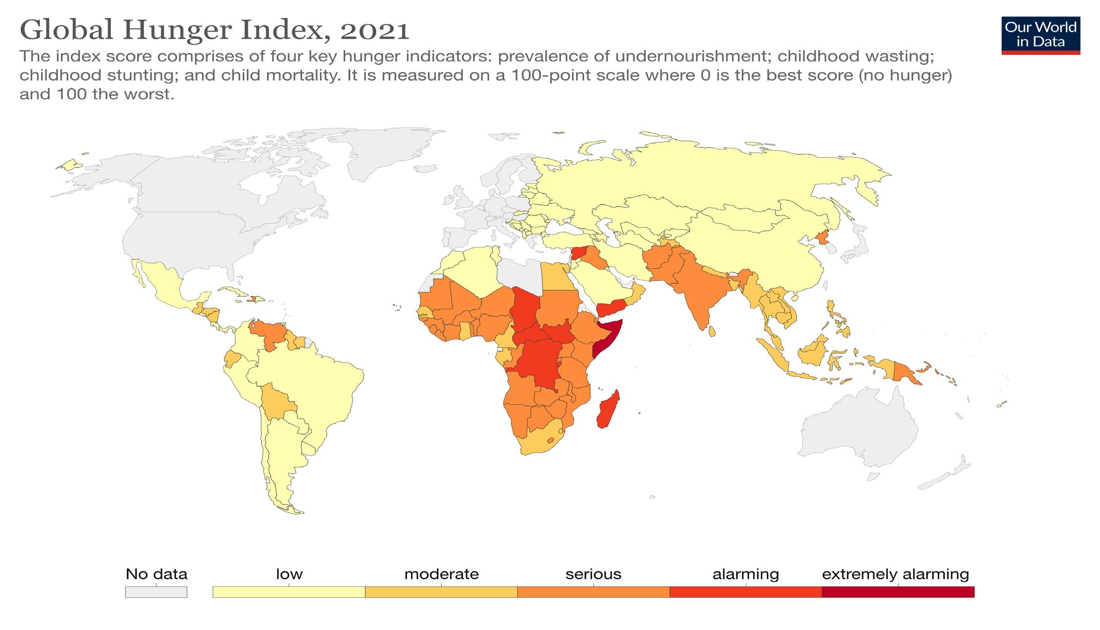
Each year, the hunger epidemic causes 13 to 18 million deaths, claiming the lives of both young, otherwise healthy individuals as well as the elderly at a rate of 35,000 deaths a day (Bush, 1996). These deaths disproportionately affect low-income, impoverished families (frequently citizens of developing countries) who are the most susceptible to changes in food availability (Bush, 1996). Unfortunately, and quite ironically, food insecurity is most prevalent in the families and communities where food for the globalized market is produced (Bush, 1996).

"Food shortages are much more impactful on physiological health than meets the eye, with countless cells and cellular processes relying on the nutrients a typical balanced diet provides to help maintain and protect the body.

Figure 2. A diagram overview on differing types of cells in innate and adaptive immune systems. Source: Oncology Pro.

14 JUST VOL VII // ISSUE II // SPRING 2022 JUST VOL VII // ISSUE II // SPRING 2022 15

The immune system is composed of various cell types that work together to fight invading pathogens. All the involved cell types can be classified into two main overarching categories: the innate immune system and the adaptive immune system.

Hunger, and by extension famine, have other consequences on human wellbeing. In terms of physiological health, famine makes the body more susceptible to infection from diseases that typically run rampant through communities (Ó Gráda, 2007). It is these diseases, not the actual lack of food, that typically cause food insecurity deaths worldwide (Ó Gráda, 2007). While death may occur directly from malnutrition in instances of starvation or consumption of unsafe food alternatives, famine is more often the precursor of diseases since it allows for easier infection of the starving. These disease-caused deaths may occur from cholera, influenza, malaria, dysentery, and more (Ó Gráda, 2007). But how does starvation specifically influence our immune system? What is our immune system?

The Immunological Effects of Famine

"

Prevalence of Hunger and Famine

meaning that the cells involved have a more generalized approach to protection, fighting any pathogen regardless of its identity. They can attack a wide range of invaders to resolve an infection quickly and efficiently. Examples of key immunological forces working within innate immunity consist of mucous membranes, epithelial linings, phagocytes (cells that consume and destroy invaders), the cellular signaling molecules cytokines, and chemokines (which direct immune responses to specific areas). All these cells work in tandem to help coordinate the immediate, innate immune response. (Aristizábal & González,The2013).adaptive immune system, on the other hand, is in many ways contrasts with innate immunity. While the innate response is quick and generalized, the adaptive immune system is slower and reacts to specific types of threats. It is often invoked when the innate response is incapable of preventing the proliferation of the pathogen within the host body. T-cells and B-cells work together to initiate the adaptive response, identifying and destroying pathogens with increased accuracy. More importantly, the adaptive immune system has the unique ability to form memory cells and antibodies. These cells assist in the recognition of the pathogen in the future and allow for an even swifter, more efficient elimination of the invader (Institute for Quality and Efficiency in Health Care, 2020). While unique systems, the innate and adaptive components of the immune system often work together. Each system supports the other by promoting effector responses and signaling to one another.

According to the Cleveland Clinic, the immune system is “a large network of organs, white blood cells, proteins (antibodies) and chemicals [that work] together to protect you from foreign invaders (bacteria, viruses, parasites, and fungi)” (Cleveland Clinic, 2020).

EDITORIAL EDITORIAL J J

The innate immune system is the body’s first line of defense against invading pathogens. It is non-specific,

By Carter Wood

Figure 1. A map of Global Hunger in 2021. Source: Our World in Data.

The Immune System

References Aristizábal, B., & González, Á. (2013, August 18). NCBIInnate Immune System. NCBI. Bush, R. (1996). The politics of food and starvation. Review of African Political Economy, 23(68), 169–195. Cleveland Clinic. (2020, February 22). Immune System: Parts & Common Problems. Dranoff G. Nat Rev Center. (2004). The Immune System [Illustration]. Oncology Pro. Drug Target Review. (n.d.). Macrophage [Illustration]. Drug Target Review. França, T., Ishikawa, L., Zorzella-Pezavento, S., ChiusoMinicucci, F., da Cunha, M., & Sartori, A. (2009). Impact of malnutrition on immunity and infection. Journal of Venomous Animals and Toxins Including Tropical Diseases, 15(3), 374–390.

EDITORIAL EDITORIAL J J

16 JUST VOL VII // ISSUE II // SPRING 2022 JUST VOL VII // ISSUE II // SPRING 2022 17

Extreme malnutrition is the most common source of secondary acquired immunodeficiency worldwide (França.et al., 2009). Malnutrition’s effects are seen at both the innate and adaptive immune response levels, which prevents effective elimination of invading pathogens and often results in host death. Within the innate immune system, malnutrition prevents the immediate destruction of invaders. Epithelial tissue integrity is reduced during periods of starvation, allowing for easier access to the host body’s organs and more efficient invasion of the pathogen. Once the pathogen invades the body, a primary issue that arises is the inhibition of cytokines, which are responsible for the activation of other immune system components (Somech, 2014). This inhibition leads to an immediate decreased immunological response, as cytokines are paramount in recruiting and providing directions to innate response cells towards the site of infection.Malnutrition also affects another branch of innate immunity: the complement system. This pathway is involved in tagging bacteria for destruction by phagocytic cells in a process known as opsonization. Malnutrition causes a reduction in the principal molecule needed for this identification, the C3 component, while simultaneously preventing phagocytic cells from functioning properly. These effects drastically reduce the uptake and destruction of the invading pathogen (França.et al., 2009).

Figure 4. An illustration of the Complement System. Source: PhysioPathoPharmaco/Youtube.InstituteforQualityandEfficiency in Health Care. (2020, August 30). NCBI -The Innate and Adaptive Immune Systems. NCBI. Ó Gráda, C. (2007). Making Famine History. Journal of Economic Literature, 45(1), 5–38.

PhysioPathoPharmco. (2017, July 15). The Complement System [Illustration]. Youtube. Roser, M., & Ritchie, H. (2021). Global Hunger Index, 2021 [Chart]. Our World in Data. Somech, R. (2014). Malnutrition, Vitamin Deficiencies, the Immune System and Infections: Time to Revisit Our Knowledge. Semantic Scholar.

The Effects of Malnutrition on the Immune System

Figure 3. An animated image of a phagocytic macrophage engulfing a pathogen. Source: Drug Target Review.

The adaptive immune system is also severely hindered by malnutrition, primarily through the destruction of the system’s key components. Malnutrition inhibits the formation of the cells required for an adaptive response, causing atrophy of lymphoid organs, bone marrow, the thymus, and the spleen. This is problematic because it is within these locations that adaptive cells form and are trained in their proper effector functions. Cells that do develop have increased deactivation and necrosis (unprogrammed cell death) and are incapable of carrying out their adaptive functions (França.et al., 2009). The memory components of the adaptive response are also affected, with antibody concentrations decreasing and the destruction of memory cells. This leads to a weaker, more exposed host that lacks the ability to respond to pathogens with which they have previously interacted (França.et al., 2009). When the poor functionality of the innate and adaptive immune systems combine, malnutrition can cause a devastating blow against a host body’s ability to fight off even the most common illnesses. Without a proper immune system response, the 30% of the world that experiences hunger each year is placed within a heightened risk category of death and illness, despite often having no other physiological conditions. Food shortages are much more impactful on physiological health than meets the eye, with countless cells and cellular processes relying on the nutrients a typical balanced diet provides to help maintain and protect the body.

Figure 2. #TheDress became a worldwide meme trend as millions of tweets bombarded the Internet. Source: BuzzFeed News.

scientific community? Well, that’s probably because you think that everyone sees it the way you do. However, there still exists a large-scale disagreement on whether the color of the dress is blue-and-black or white-and-gold. This debate which was earlier limited to the small island of Colonsay, Scotland but soon expanded once shared over Tumblr by a Scottish artist performing at the wedding (Benedictus, 2015).

Even though this mechanism works well most of the time, the results of the study suggest that this particular image introduces some chromatic bias (Webster, 2000). In other words, one’s visual system only partially adjusts to the actual color of the image, and the dress’s true colors are not entirely preserved. This happens because the photograph was taken in the presence of a light source unfamiliar to our brain: a mixture of both natural light and artificial light in the store.

Neuroscientists have been actively studying the interpretations of visual attributes. An area that has sparked the interest of many researchers in this field is the extent to which external environmental factors can influence human color perception. “The Dress” went viral on the internet in 2015. Viewers all over the world split into two groups based on their perception of the dress color. This social media controversy provided researchers the means to investigate human color perception more closely.

As a result, various international franchises saw the trend as a marketing strategy and included references to the dress in advertisements (Warzel, 2016). Owing to such extensive publicity, the dress had made it to MTV’s most notable memes by the end of the year (Grant, 2015).

Overnight Popularity

Conway and other scientists on the project predicted that this multistability was induced by variations in how each subject’s brain processes the hues of the daylight sky. Light enters our eye through a lens and hits the retina at the back of our eye. This signal is then communicated to the visual cortex, the part of the brain that makes sense out of these stimuli to form an image, via the nervous system. Usually, the first burst of light that bounces off the retina during image formation is daylight reflected from the surface of the object we are seeing. Our visual system is designed in a way that subtracts the color of the daylight from the entity’s “real” colors. According to Jay Neitz, a neuroscientist at the University of Washington, "our visual system is supposed to throw away information about the illuminant and extract information about the actual reflectance" (Rogers, 2015).

“The Dress” is a washed-out photograph that became a viral phenomenon back in 2015 across almost all social media platforms. This infamous dress, designed by Cheshire Oaks Designer Outlet in England, was purchased by a woman to wear at her daughter’s wedding. Prior to the wedding she clicked a picture of the dress and sent it to her daughter. You might wonder, looking at this low-resolution image right now, what is so special about this dress that it garnered such traction and ignited curiosity amongst the "It is fascinating to watch the idea of colors and tones be redefined as subjective and relative than ever before. After all, appearances are really deceptive, aren’t they?"

While the meme faded and lost relevance over time, the scientific dilemma persisted. Although the outlet that designed the uncanny dress confirmed that the true colors were blue-black, perplexed neuroscientists set forth on solving the puzzle of why people viewed it differently.

One of the first studies conducted on the dress was led by Bevil Conway, a researcher at MIT and Wellesley College. He surveyed 1400 people, 300 of whom had never seen the picture before. 57% of the respondents saw the dress as blue and black, 30% saw it as white and gold, and 10% saw it as black and brown (Lafer-Sousa et al., 2015). On a retest, some subjects saw a different color combination than they had originally seen, suggesting that the image is multistable (a physical stimulus that is perceived differently at different times because of changes in surroundings) (Schwartz et al., 2012).

The Tumblr post went viral as views and comments skyrocketed. Soon, BuzzFeed picked up the story, and it was only a matter of time before the internet was set aflame. Within just 24 hours of, the dress had been shared and reshared around 4.4 million times. A wide range of celebrities from Ellen DeGeneres to Taylor Swift started participating in the discussion and giving their opinions.

The Dress – An Optical Illusion: How did it begin?

18 JUST VOL VII // ISSUE II // SPRING 2022

Neuroscientific Theories

Figure 1. The Dress – Blue/black or white/gold? What colors do you see? Source: Karlsson and Allwood (2016).

By Mahak Kathpalia

EDITORIAL JUST VOL VII // ISSUE II // SPRING 2022 19 J EDITORIAL J The Mystery Behind the Dress –A Neuroscientific Conundrum PSYCHOLOGY

Warzel, C. (2016, February 26). 2/26: How two llamas and a dress gave us the internet's greatest day. BuzzFeed News.

20 JUST VOL VII // ISSUE II // SPRING 2022

The Grant,Guardian.S.(2015, December 9). 24 memes that took the internet by storm in 2015. MTV News.

Karlsson, B. S. A., & Allwood, C. M. (2016). What is the correct answer about the dress’ colors? Investigating the relation between optimism, previous experience, and answerability. Frontiers in Psychology, 7, Article 1808.

Lafer-Sousa, R., Hermann, K. L., & Conway, B. R. (2015). Striking individual differences in color perception uncovered by ‘the dress’ photograph. Current Biology, 25(13), R545-R546.

Rogers, A. (2015, February 27). The science of why no one agrees on the color of this dress. Wired.

Sample, I. (2015, May 14). #thedress: Have researchers solved the mystery of its colour? The Guardian.

As a result, people disregard distinct colors of the daylight axis due to disparities in the environment they are commonly around and how their visual cortex has adapted.

Figure 3. Our visual system: Light entering our eyes generates signals sent via the optic nerve to the brain where the visual cortex processes colors. Source: BrainHQ.

Webster, M. A., & Wilson, J. A. (2000). Interactions between chromatic adaptation and contrast adaptation in color appearance. Vision research, 40(28), 3801-3816. References Benedictus, L. (2015, December 22). #Thedress: 'it's been quite stressful having to deal with it ... we had a falling-out'.

"So, people either discount the blue side, in which case they end up seeing white and gold, or discount the gold side, in which case they end up with blue and black," stated Conway in an interview with Wired (Rogers, 2015).

EDITORIAL JUST VOL VII // ISSUE II // SPRING 2022 21 J EDITORIAL J

P. (2017, April 12). Two years later, we finally know why people saw "The dress" differently. Slate Magazine.

Another peculiar finding was a greater likelihood of women and older people perceiving the dress as white and gold (Lafer-Sousa et al., 2015). Although the cause behind this observation is still unclear, one plausible hypothesis for the difference between age groups was made by David Brainard, director of the Vision Research Center at the University of Pennsylvania. He noted that the density of lenses in our eyes increases with age, which could possibly induce disproportion in the rates at which certain wavelengths of light are filtered over others (Sample, 2015). Since the signal communicated to the visual cortex is primarily dependent on the light the lens allows to enter the eye, such a trend can be expected. Based on a similar concept, a study conducted by Pascal Wallisch, a psychology professor at New York University, found a subtle but statistically reliable relationship between one’s sleep schedule and their interpretation of the dress’s color combination. Early risers were more likely to assume that the dress was lit by natural light which overly represents shorter wavelengths that coincide with the blue color. As a result, early risers subtract the blue shade and tend to view the dress as white and gold. In contrast, people who go to bed much later have a greater probability of seeing blueblack colors owing to their exposure to the relatively long wavelengths of artificial and incandescent light (Wallisch,Despite2017). all these convincing findings and substantial speculation, there is no consensus amongst the scientific community regarding why the dress elicits such conflicting perceptions. “What I think is most important is that this internet craze wasn’t an artifact of people looking at different displays. These are real individual differences,” said David Brainard in his interview with the Guardian (Sample, 2015). As further research continues to guide and direct us in the future, it is fascinating to watch the idea of colors and tones being redefined as subjective and relative than ever before. After all, appearances are really deceptive, aren’t they?

Schwartz, J. L., Grimault, N., Hupé, J. M., Moore, B. C., & Pressnitzer, D. (2012). Multistability in perception: binding sensory modalities, an overview. Philosophical Transactions of the Royal Society B: Biological Sciences, 367(1591), 896Wallisch,905.

Figure 4. The dress is seen as blue-black under a yellow-tinted illumination and gold-white under a blue-tinted illumination. Source: Wikimedia Commons.

Something as small and confined as a brain, and something as vast as space could not possibly be connected –or so it was assumed. The neural network of the brain and the networking of the cosmic web are, in reality, extremely similar. These similarities allow for discoveries about the cosmic web to be applied to a system much smaller, and more difficult to study: the brain. Both systems, the cosmic web and the brain, share similarities in their connectivity, size of connective fields, chemical make-up, and memory capacity. In fact, they are the only two systems that follow a different pattern than the rest of the universe.

"The discovery that the brain does not organize in fractals, as expected, and instead shares commonalities with the only other non-fractal part of the universe, the cosmic web, implies a deep connection between the two systems."

Figure 1. An example of how node communicate with each other. Source: CC-BY-SA-4.0.

Studies have been conducted to find the percent composition of both the brain’s network and that of the cosmic web. A strikingly odd similarity is that 75% of both the brain and the cosmic web are made of a passive material. A passive material is one that does not have a significant effect on the structure of either system but does permeate throughout the system. In the brain, this passive ingredient is water, and in the cosmic web, this ingredient is dark energy (Vazza & Feletti, 2020). Although these ingredients differ across systems, both the cosmic web and the brain have proportional amounts of passive material that function in the same way. This suggests that the similarities extend beyond the scope of information transmission and connectivity of nodes and also apply to the “empty” spaces of both systems.

EDITORIAL JUST VOL VII // ISSUE II // SPRING 2022 23 J EDITORIAL J

The Space Your Brain Takes Up By Natalie Martinson

NEUROLOGY

Although the brain and cosmic web do not seem to relate to the rest of the universe, they do have a lot in common with each other. One main similarity can be seen in their connectivity. This idea is evident as both systems have nodes, depicted as the circles in Figure 2, with connections to many other nodes either directly or indirectly, shown as the lines. The grouping of same-colored circles represents areas where nodes are extremely well connected (Brown, 2021). In the brain, these nodes are comparable to neurons, cells that receive and send information to other cells, and these lines (referenced from Figure 1) or connections are similar to axons and dendrites which are linked to the cell body

The Organization of the Brain and Cosmic Web

22 JUST VOL VII // ISSUE II // SPRING 2022

The last, and perhaps the most interesting relationship between the brain and the cosmic web is that they share the same memory capacity. Max Karl Planck, a notable theoretical physicist, had revolutionary ideas about the universe where this parallel has been drawn. The entirety of memories that a human brain can contain are able to be distributed across all of the galaxies of the cosmic web. Notably, this also applies in the other way: all of the complex “memories” of the entire cosmic web can, hypothetically, fit into a single human brain. This concept describes the aforementioned idea, stating that both systems share similar connectivity, distributions of of neurons in order to send/receive information to/from other neurons, respectively. In the cosmic web, these nodes are similar to galactic hubs which are essentially the neurons of space. Galactic hubs are connected by galactic filaments which can be referred to as the axons/ dendrites of space (Brown, 2021). Furthermore, both systems have large voids between the clusters of nodes (seen as the free space in Figure 1). This similar nodal connectivity between the brain and cosmic web suggests that they both transport information across their individual systems in the same way. One way or another, information passes through nodes to get from its start to its end-point.Tocontinue, the brain and the cosmic web also share similarities in their respective quantities and distributions of these nodes; the cosmic web contains only 30 times more galaxies than the brain does neurons. This small difference compared to their large size difference is not to be overlooked, as it suggests again that these systems are heavily related to each other. Besides this obvious quantitative similarity, the nodes of each system are also grouped in odd clusters instead of being uniformly spread out. In the brain and cosmic web, collections of neurons and galaxies exist largely in specific areas. (Vazza & Feletti, 2020.). These discoveries further solidify the similarities between the connectivity and information transfer routes between both systems.

24 JUST VOL VII // ISSUE II // SPRING 2022 JUST VOL VII // ISSUE II // SPRING 2022 25

EDITORIAL EDITORIAL J J nodes, and chemical make-up. All of those similarities mixed with Planck’s energy theories and calculations are what lead to the conclusion that the capacity of the memory of both the brain and the cosmic web is equal despite the great difference in size (Haramein, et al., 2019).

How These Systems Differ from the Make-Up of the Rest of the Universe

Many scientists have come to accept the observation that the entire universe follows a fractal organizational pattern (see Figure 2), at least in part. This means that the universe is composed of many simple forward and backward functions that generate complicated patterns (Brown, 2020). This pattern exhibits an intriguing relationship that can be most easily understood through visualization. For example, zooming in on any of the smaller circles depicted in Figure 2 will eventually lead you to an exact replica of the original image, and the same would apply to the idea of zooming out. Essentially, the pattern repeats itself over and over again to form this complex fractal. If the entire universe was, indeed, ordered in fractals, the same level of complexity would exist across all parts of the universe, independent of the varying sizes. We could then study the connectivity of smaller fractal systems, such as snowflakes, lightning, and seashells, and apply those concepts to a large part of the universe, like the cosmic web (Gunther, 2020). It would be the perfect solution for the gaps in our technology that prevent us from measuring the complexities of the human brain on an extremely microscopic level (Brown, 2020). However, astrophysicist Franco Vazza and neuroscientist Alberto Feletti have adopted a new view: the cosmic web and brain do not, in fact, appear to be fractally organized (Vazza & Feletti, 2020).

What’s Next?

The main researchers in this field, Franco Vazza and Alberto Feletti, have addressed the possibility that these findings will prompt technological advances to help further analyze the structures of both systems (Neustaeter, 2020). Due to the cosmic web being much larger than the brain, it is easier to study its small details compared to the small details of the brain. Knowing how these two systems are connected will allow us to apply cosmic discoveries to the field of neuroscience and can help us better understand the brain itself. This better understanding of the brain could lead to further research and discoveries into neurological disorders, the development of better neural prostheses to aid in motor function for those who have lost it, and much more. What we do know for sure is that both Vazza and Feletti exhibit an exuberant passion for this interdisciplinary field of science and are not likely to give up their groundbreaking research anytime soon. That being said, they aren’t the only scientists out there. Nobody knows what will be next, except maybe the cosmos. After all, it is essentially just a big brain.

The pair’s research on their individual specialties shows that fractal patterns are scale dependent. While the difference in the size of most natural occurrences in our universe is not extreme enough to discourage fractal organization, the scale of the cosmic web is. The brain, on the other hand, is similar enough in size to other fractal systems (such as the snowflakes, seashells, and lightning previously mentioned) that it should follow a fractal pattern. The discovery that the brain does not organize in fractals, as expected, and instead shares commonalities with the only other non-fractal part of the universe, the cosmic web, implies a deep connection between the two systems. The mysterious connection between these two systems, however, does not end here.

References Brown, W. (2021, May 5). The Universe Organizes in a Galactic Neuromorphic Network. Resonance Science Gunther,Foundation.S.(2020, May 7). 14 Amazing Fractals Found in Nature. Haramein,Treehugger.N.,Brown, W., & Val Baker, A. (2019, February 13). The Unified Spacememory Network: from Cosmogenesis to Consciousness. Neustaeter, B. (2020, November 18). Cosmic and cerebral lookalikes: Study finds structures of the universe and human brain are similar. CTVNews. Vazza, F., & Feletti, A. (2020). The Quantitative Comparison Between the Neuronal Network and the Cosmic Web. Frontiers in Physics, 8. Figure 2. A representation of the complex pattern of a fractal. Source: Pixabay

Figure 1. Caterpillar eating a leaf. Source: Pexels.

Tapping into the conversations of plants 26 JUST VOL VII // ISSUE II // SPRING 2022 JUST VOL VII // ISSUE II // SPRING 2022 27

Molecular messages warn of danger A caterpillar munches happily on the leaves of the mustard plant, Arabidopsis. Meanwhile, scientists at the University of Wisconsin-Madison watch in amaze ment as the plant’s response to this leaf theft becomes visible through propagating waves of flaring green light. Plants communicate in marvelously complex ways, using signals invisible to the naked eye. These UW-Madison researchers, Simon Gilroy and Masatsuga Toyota, were able to watch warning signals being sent in real-time, from the wounded leaves to the rest of the plant in the form of rapid bursts of information. The plant was frantically communicating that it was under attack (Figure 1) (Toyota, 2018; Hamilton, 2018). Plants receive a constant onslaught of biotic and abiotic information from their environment – herbivore and pathogen attacks, water levels, temperature fluctua tions, and nutrient availability all have the capacity to stress the plant (Galieni, 2021; Roper, 2021; Lee, 2021). External signals are processed by plants and then inte grated into microscopic molecular messages that are transmitted throughout their bodies; these messages

GENETICS

EDITORIAL EDITORIAL J J

Calcium as a messenger – visualized through light Gilroy and Toyota developed special plants that enabled them to see calcium as it transferred important information from the caterpillar-induced wound site throughout the rest of the plant. They developed these plants by engineering them to produce a green fluores cent-labeled protein called GCaMP3, a protein to which calcium binds, as illustrated in Figure 2 (Toyota, 2018, Hamilton, 2018). The binding of Ca2+ to GCaMP3 causes the protein to change its shape (conformation), as it folds in on itself, almost like a clamshell around a pearl, or in this case around Ca2+. The folding of the protein upon Ca2+ binding produces bright bursts of green light; in this way, the GCaMP3 protein acts as a calcium indicator in living plants (Lee, 2021; Krogman, 2020). This novel technique has enabled researchers to track the move ment of calcium within plants and to understand how Ca2+ concentrations fluctuate in response to wounding (Toyota, 2018; Hamilton, 2018). These experiments have revealed key information about how plants communi cate when they experience various forms of stress. In the case of the caterpillar eating the Arabi dopsis leaves, the damage inflicted upon plant tissues causes the amino acid, glutamate (which in animals acts as a vital neurotransmitter) to spill out of the wound site, as shown in Figure 3. Subsequently, glutamate molecules bind to ion channels, permitting them to open and allow certain molecules, like calcium, to pass through and flow rapidly into the plant cells. The increase in Ca2+ concen tration within cells triggers a massive wave of calcium to travel through the vasculature, or veins of the plants, from the wound site to distant leaves (Toyota, 2018; Lee, 2021; Qiu, 2020). Calcium acts as a signal to warn the rest of the plant that it is under attack. This vital signaling molecule initiates a plant-wide effort to rapidly build an arsenal of toxic chemical compounds to wage war and prevent further damage by the hungry caterpillar (Toy ota, 2018; Lee, 2021; Hamilton, 2018; Qiu, 2020). Just as they are able to protect themselves, plants can also alert neighboring plants species of danger through the release of volatile aromatic compounds, or by secreting chemi cals from their roots into the soil – further promoting the upregulation of defensive mechanisms on a commu nity-wide scale (Ninkovic, 2020; InnerPlant, 2022).

By Leta Landucci

"Plants can be designed to produce fluorescent stress sensor molecules by manipulating their DNA. These sensors are safe for human consumption and are integrated within particular plant stress pathways."

Translating stress into light

Translating Stress Signals Into Blazes of Light

initiate the survival responses necessary to confront the challenge (Lee, 2021; Galieni, 2021; Toyota, 2018). Cal cium (Ca2+) is an integral messenger molecule within plant communication networks. Certain external stimu li cause rapid fluctuations in Ca2+ concentration within plant cells. This feature played a vital role in Gilroy and Toyota’s visualization of these complicated information transfers (Lee, 2021; Toyota, 2018; Hamilton, 2018).

ricultural practices could be substantially more efficient and environmentally friendly. The ability to tap into the communication of plants could have profound impacts on large-scale food production systems and could con tribute to alleviating food insecurity by fostering more robust and resilient systems of agriculture. The growth in our understanding of plant stress communication often begins with basic science and experiments conducted in the laboratory. Researchers at UW-Madison, fascinated while watching a caterpillar munch on an Arabidopsis leaf, revealed hidden networks of warning signals vital to imagining novel technologies that have the potential to drastically improve the future of agriculture.

Figure 2. The blue and green protein above is the crystal structure of GCaMP3. The blue domain is the region of the protein to which calcium ions (orange spheres) bind, while the green domain is the fused green fluorescent protein. When calcium binds, the shape of the blue protein domain changes as it folds around the ions. This conformational shift activates the fuorescence of the green fluorescent protein domain, which emits light that can be detected with spectrophotometric devices. GCaMP3 crystal strucutre, ID 4IK9, was retrieved from the World Wide Protein Data Bank, processed using PyMOL modeling software, and was originally generated and solved by Chen et al., 2013.

J. M., Garcia, J. F., & Tsutsui, H. (2021). Emerging technologies for monitoring plant health in vivo. ACS omega, 6(8), 5101-5107.

Toyota, M., Spencer, D., Sawai-Toyota, S., Jiaqi, W., Zhang, T., Koo, A. J., ... & Gilroy, S. (2018). Glutamate triggers long-distance, calcium-based plant defense signaling. Sci ence, 361(6407), 1112-1115.

Zhongming, Z., Linong, L., Xiaona, Y., Wangqiang, Z., & Wei, L. (2018). Blazes of light reveal how plants signal danger long distances.

EDITORIAL EDITORIAL J J

Researchers are becoming interested in har nessing stress signaling pathways to engineer plants to communicate with humans about their needs (Roper, 2021; Galieni, 2021; InnerPlant, 2022). Plants can be de signed to produce fluorescent stress sensor molecules by manipulating their DNA. These sensors are safe for hu man consumption and are integrated within particular plant stress pathways. This technology would allow for a plant’s inherent communication signal to be amplified and detectable by researchers and farmers to alert them of the crop’s needs (Roper, 2021; InnerPlant, 2022; Lee, 2021). For example, if a plant was to experience scarcity of water or was being feasted upon by pests, the associ ated stress pathways would cause the engineered stress sensor molecules to emit light, as shown in Figure 4. This light could be detected with special spectrophotometric devices that capture fluorescence invisible to the human eye. Spectrophotometric devices in use and currently being tested include smartphones for a plant-by-plant inspection, and both drones and satellites for field-wide surveillance (InnerPlant, 2022; Roper, 2021). Research groups and small biotech start-ups, such as InnerPlant, have begun to explore how particu lar stress pathways could be paired with designated fluo rescent colors. These techniques would make it possible to decode patterns of plant stress by color and to under stand what plants are experiencing days to weeks before they show physical indications and visible symptoms of distress (InnerPlant, 2022; Roper, 2021; Galieni, 2021).

Figure 3. A caterpillar eats the leaf of a plant, wound ing the tissue. Glutamate (red) spills out from the dam aged region and binds to an ion channel (dark blue), converting it to its active open state. Calcium (orange) is free to flow from outside of the cell to the inside, pass ing through the open ion channel embedded in the cell membrane (light blue). This influx results in waves of calcium that propagate throughout the plant and trav el to distant leaves. This induces an increase in calcium concentration within plant cells that ultimately triggers survival and defensive responses. Figure 3 was modified from a figure in Lee et al., 2021.

Lee, H. J., & Seo, P. J. (2021). Ca2+ talyzing initial re sponses to environmental stresses. Trends in Plant Sci ence, 26(8), 849-870. Ninkovic, V., Markovic, D., & Rensing, M. (2021). Plant volatiles as cues and signals in plant communica tion. Plant, cell & environment, 44(4), 1030-1043.

For instance, the production of red light from plants could indicate the first signs of pathogenic attack, while blue could signal that the plants aren’t receiving suffi cient nutrients. Farmers may only need to grow a small cluster of these so-called living sensor plants, a concept coined by InnerPlant, within their fields to have an effec tive early warning system telling them how their plants are doing and to act accordingly (InnerPlant, 2022).

28 JUST VOL VII // ISSUE II // SPRING 2022 JUST VOL VII // ISSUE II // SPRING 2022 29

Improving agricultural practices These technologies may have huge implications for the future of agriculture, with the potential to make practices more sustainable, environmentally conscious, and efficient (InnerPlant, 2022; Galieni, 2021; Roper, 2021). Many farmers have become dangerously reliant on an ever-expanding “cocktail of chemicals” to target weeds, insects, and compensate for diminishing fertility by using synthetic fertilizers. However, this immense ap plication of chemicals is extremely harmful to the envi ronment in countless ways, degrading the diversity and health of soil microenvironments, terrestrial ecosystems, and aquatic life (InnerPlant, 2022; Galieni, 2021; Rop er, 2021). By developing technologies that allow for the detection of plant stress signaling, pesticides, herbicides, fertilizers, and even water could be administered only as needed, rather than in wasteful excess. Plants communicate through profoundly com plex and efficient signaling mechanisms. In response

to stress exposures, plants trigger integrated cascades of chemical messages, preparing themselves to scrounge up resources for survival or to produce compounds for self-defense (Galieni, 2021; Ninkovic, 2020; Toyota, 2018). Learning and harnessing these innate stress com munication pathways creates an opportunity to be re markably attuned to the ever-changing needs of plants, enabling growers to respond adaptively. In this way, ag

Galieni, A., D'Ascenzo, N., Stagnari, F., Pagnani, G., Xie, Q., & Pisante, M. (2021). Past and future of plant stress detection: an overview from remote sensing to positron emission tomography. Frontiers in Plant Science, 11, InnerPlant.1975. (2022, January 5). InnerPlant – Design the seed technology stack of tomorrow. InnerPlant – Making Living Krogman,Sensors.W.,Sparks, J. A., & Blancaflor, E. B. (2020). Cell type-specific imaging of calcium signaling in Arabidop sis thaliana seedling roots using GCaMP3. International journal of molecular sciences, 21(17), 6385.

Qiu, X. M., Sun, Y. Y., Ye, X. Y., & Li, Z. G. (2020). Signaling role of glutamate in plants. Frontiers in plant science, 10, Roper,1743.

References Chen, Y., Song, X., Ye, S., Miao, L., Zhu, Y., Zhang, R. G., & Ji, G. (2013). Structural insight into enhanced calcium indicator GCaMP3 and GCaMPJ to promote further im provement. Protein & cell, 4(4), 299-309.

Figure 4. Calcium waves signaling visualized with the ge netically encoded fluorescent calcium sensor, GCaMP3. This Arabidopsis leaf, undamaged, but neighboring a wounded leaf, demonstrates the propagation of calcium messenger molecules that warn of danger and signal for an upregulation of survival and defensive responses throughout the plant. Source: CC BY-NC 2.0.

PHOTO

JUST VOL VII // ISSUE II // SPRING 2022 31 J 30 JUST VOL VII // ISSUE II // SPRING 2022 J

Plains Garter Snake (Thamnophis radix) William Vuyk The plains garter snake (Thamnophis radix) is listed as a species of special conservation concern by the Wisconsin DNR. Very similar to the common garter snake (Thamnophis sirtalis) it is thought the two species occupy different thermal niches. A population of T. radix was identified at Prairie Ridge Conservation Park in Madison during a survey of snake species occupancy in Madisonarea prairies this summer. (Azolla

Azolla

Arabidopsis seedlings (Arabidopsis thaliana)

Leta Landucci

Letacaroliniana)Landucci The small floating aquatic fern, Azolla, growing in liquid media in the laboratory. Azolla has a symbiotic relationship with a atmosphericisthat(Anabaenacyanobacteriumazollae)liveswithinitandresponsibleforfixingnitrogen.Azollaisoneofthefastest-growingplantsontheplanetandgarnersgreatinterestfromthescientificcommunitybecauseofitsabilitytodrawlargequantitiesofCO2fromtheatmosphere.

Moss-coveredmooseskullandmandible

A well-camouflaged mosscovered moose skull and mandible discovered and unburied on a Moosewatch expedition. The specimens were collected and brought back to the island’s research station. Scientists will use the teeth and bones to assess the age and health of the moose when it died. This data allows researchers to gain an understanding of moose population fluctuations over time in relation to predation.wolf

Leta ArabidopsisLanduccithaliana seedlings growing on agar media in a labo ratory growth chamber. Once the seedlings matured and began to de velop buds, they were transformed using andonpossibletheseandinpolymersynthesis.oftransformationagrobacterium-mediatedtoexpressenzymesinterestinvolvedinsuberinbioSuberinisacomplexplantandwaxysubstancefoundplants.Itactsasanimpermeableprotectivebarrier.Studyingenzymesinplantamakesittoinvestigatetheirimpactssuberinlocalization,composition,quantity. SUBMISSIONS

Leta Landucci & William Vuyk

PIXELS where science and art collide

REPORTS REPORTS 32 JUST VOL VII // ISSUE II // SPRING 2022 JUST VOL VII // ISSUE II // SPRING 2022 33 J J REPORTS

After the participants filled out the quantitative part of the study on paper, they were asked three questions in regard to how they experience green spaces and if their visits to green spaces helped them cope with any stress or complications related to the COVID-19 pandemic. While the primary investigators conversed with the participants, a scribe typed the participants’ responses.

2. INTRODUCTION:

People, Parks, and the Pandemic: How Public Green Spaces Have Shaped Human Wellbeing During COVID-19

2. Assess how user experiences outdoors have potentially mitigated deleterious mental health effects of the pandemic

The study uses an intercept interview approach to data collection for human subjects. Intercept interviews are a completely random form of data collection that is typically used in marketing research studies in order to recruit a diverse group of participants [7]. The interviews allow researchers to gain insight into the demographic characteristics of people who would be frequenting a green space on a random day.

ABSTRACT:

1. Measure how the participants’ usage and experiences in outdoor spaces have differed before and during the pandemic

Quantitative Analyses

Interview Set-Up Participants in this study filled out a questionnaire on paper and answered a series of demographic, openended, yes/no, and Likert scale questions. The demographic questions asked participants to self-identify their gender, race, ethnicity, and age. Participants then answered openended questions that asked about their transportation habits and how often they accessed outdoor spaces before the start of the COVID-19 pandemic, which has been defined as March 2020 for the purposes of this study.

The last part of the quantitative data collection process asked subjects to use a 5-point Likert scale to rate the importance of specific greenspace activities and qualities in relation to their livelihoods and health during the pandemic. A response of 1 indicated “low importance” in regard to the green space characteristic while an answer of 5 was indicative of “high importance.” 5-point Likert scales are frequently used in social science interviews because they give the participant a defined range to report their objective reality and subjectivity toward a particular subject [7].

The quantitative analysis for this study uses descriptive statistics due to the discrete nature of the questions being asked and their respective variables. The statistics were calculated using STATA. Multiple choice and yes/no questions were assessed using count data and percentages. Likert scale data were analyzed by using mean, median, mode, t-tests, p-values, skewness, Kurtosis, and standard deviation. This collection of statistical descriptors can interpret the Likert results and show how data can be explained by the most common responses and averages with regard to their statistical 1.

The nature of the interview style and mixed methods approach to the study will define and target the specific goals of this thesis which are outlined below.

While the mental health implications and the increased use of public parks during the pandemic are evident, it is unknown whether the positive impacts of using the outdoors during the pandemic had a direct impact on mental health. With visits to green spaces on the rise during this psychologically demanding time, this research will investigate if spending more time outdoors during the pandemic allowed people to cope with their pandemic-related life stressors. The common, shared experiences of human life during the pandemic (increased isolation, city-wide lockdowns, increased tensions, fear, etc.) allows for this study to explore what these experiences mean for human interactions with the world around them and specifically in outdoor spaces like public parks, natural areas, and urban green spaces.

3. METHODS: Recruitment of Participants and Interview Style

Studies suggest that time spent in public parks and gardens are linked to positive mental health outcomes and improved health and wellbeing [4]. The concept of using “nature as therapy” has been highly regarded in medical settings due to the simple, accessible aspects of green spaces that promote public health and quality of life [5]. According to Kuo’s paper “Coping with Poverty”, people who lived in impoverished areas were more likely to cope with the life circumstances of poverty if they lived in an area that was more exposed to green spaces and trees [6]. Although poverty is not being measured in this study, the pandemic sets the stage for an assessment of how the outdoors can be used to cope with another type of life difficulty, which in this case, revolves around living during a pandemic.

By reaching these goals, this study will greatly impact how we look at the shift in human-environment interactions during the pandemic and how outdoor spaces can potentially accommodate people who are using them to cope with outside stressors.

Katelyn McVay

3. Develop the knowledgebase in environmental psychological literature through a study that investigates an important period in this human lifetime

REPORTS JUST VOL VII // ISSUE II // SPRING 2022 35 J REPORTS 34 JUST VOL VII // ISSUE II // SPRING 2022 J

Next, the questionnaire assessed the effects of the outdoors and the pandemic on the subjects’ health and wellbeing through yes or no questions.

The COVID-19 pandemic has reshaped how we use green spaces and how we perceive the health benefits of visiting them. With limited access to indoor gathering spaces due to pandemic restrictions, studies show significant increases in visits to public parks. Spending time at the park has been shown to elevate the perceived mental and physical health of the user. If more people have been visiting green spaces, could the health benefits from these visits potentially outweigh the negative health effects attributed to pandemic-related stress? To investigate this, random intercept interviews were performed at the University of Wisconsin Arboretum. This study uses a mixed-methods approach to survey techniques and data collection with the primary forms of analysis being Likert scales, yes/ no questions, and open-ended responses. Data collection occurred in Madison, WI which may limit how the findings can be applied to more urban and rural populations. Results show that subjects have experienced significant health benefits from visiting public parks during the pandemic, and these visits have decreased pandemicrelated life stressors overall. This study will further our understanding of how the outdoors can be used as a coping mechanism and why visits to the outdoors during stressful life events are necessary.

To research the knowledge gap above, intercept interviews conducted at the University of WisconsinMadison Arboretum assessed how often people have been using public green spaces during the pandemic and if their perceived sense of wellbeing has been improved as a direct result of their visits to outdoor spaces. Using a mixed-methods approach of quantitative and qualitative data collection, 44 people were surveyed to determine the potential benefits of their access to public parks during the pandemic.

The COVID-19 pandemic has significantly altered the lives of people around the world, and its impacts have been both devastating and long-lasting. Aside from COVID19's impacts on society’s medical health due to the direct contraction of the illness, the pandemic has exacerbated other realms of human wellbeing. Visiting restaurants, shopping complexes, tourist attractions, and workplaces are a part of daily life. However, once these activities became unavailable due to social distancing and lockdowns issued by public health departments, people became mostly restricted to their homes. While this provided people with greater working and lifestyle flexibility, being confined to the same walls has greatly impacted the health and wellbeing of society. “Relatively high rates of anxiety, depression, PTSD, psychological stress, and stress symptoms are reported in the general population during the COVID-19 pandemic...” [1]. Prolonged isolation and limited movement can have deleterious effects on individuals as well as the population as a whole. In addition to the health impacts of decreased movement during the pandemic, the pandemic’s financial recession and widespread uncertainty have further exacerbated human health during a disproportionately stressful period [2]. Due to restrictions on indoor gatherings and other safety precautions associated with reducing the spread of COVID-19, people are moving their once indoor events to the outdoors. This translates into more time being spent in public parks and green spaces. According to Geng, public parks have seen significant upticks in the number of visitors over the past year during the pandemic [3]. This could be due to people willingly spending more time outdoors during the pandemic or people resorting to outdoor activities because there were very few options for social gatherings and social distancing. Either way, the outdoors has continued to serve as a haven for many people during this time. Insight into how time spent in green spaces is invaluable to the existing literature on humanenvironment interactions due to the context and partially controlled circumstances of the COVID-19 pandemic.

The University of Wisconsin-Arboretum served as the site for data collection. A folding table was set up in a high-traffic area of the Arboretum to attract potential participants while they were entering the space. In exchange for a ten-minute interview, participants were offered a $10 Amazon gift card for their contribution. Participants were read an IRB-approved script stating participants’ rights, the scope of the study, and the use of its results. 44 persons in total were interviewed.

The Likert scale assessment shows that the most common answer was “5” for all 11 questions [Figure 3]. The median fell between 4-5, and the data is also highly skewed to the right, showing that the majority of responses fell between the 4-5 range. Overall, this shows that participants indicated a high level of agreeability regarding the importance of relaxation, health, and nature regarding their experience of greenspaces. This shows how certain elements of a person’s “outdoor experience” may be meaningful or not meaningful in regard to how they coped in these spaces during the pandemic.

Fig. 5: Correlation matrix assessing the relationship between the effects of the pandemic on people’s lives and the potential relief of pandemic-related stressors as a result of visiting green spaces. 84% of participants indicated that the pandemic had significantly impacted their life and that visiting green spaces impacted their ability to handle pandemic-related complications in their life.

From the various figures, relationships between the pandemic, health, and green spaces were studied. The various types of questions allowed for cross-examination of theories and conclusions drawn from each question to minimize bias toward certain questioning styles and to control for human error of self-assessment.

Using Grounded Theory saturation methods, the theme of using the green spaces to promote mental health and wellbeing emerged [Figure 6]. Surrounding this theme, there are common sentiments that were expressed by a significant number of visitors. The sentiments focus on mental clarity, relaxation, and stress relief in order to cope with the circumstances of COVID-19. Having a conversational dialogue with the participants toward the end of the study allowed for the collection of many phrases, concepts, and themes that the participants expressed, and overall, these findings confirm what was found in the yes/no and Likert scale analysis. The collection of this thorough, mixed-methods approach presents a substantial amount of evidence that people have been utilizing and benefitting from the health promotion of green spaces. This supports and builds upon the existing literature on environmental psychology, and this study furthers the field and the general public’s understanding of how people may use outdoor environments to cope with life stressors. These findings have the potential to influence other studies that investigate how more rural and/or urban populations may experience positive connections to green spaces, as Madison, WI is a mid-size city. The broader implications of this study allow public entities to visualize how green spaces have positively correlated with human wellbeing during the pandemic and how investments into health-promoting green spaces can contribute to equity, accessibility, and improved quality of life for visitors.

6. CONCLUSION: The results of this study suggest that people have been using public green spaces more frequently during the pandemic and these visits have allowed people to improve their overall wellbeing. Analysis of Likert Scale questions has shown that a statistically significant number of people cited green spaces as a place that has promoted their overall health and wellbeing during the pandemic. Multiple choice and yes/no questions have also revealed that people have been spending more time in green spaces and that these visits have helped them cope with the stressful circumstances of the COVID-19 pandemic. In order to verify the qualitative responses of the survey, Grounded Theory methodology reached a saturation point that concluded that green spaces have greatly impacted human lives and that they served as a coping mechanism for the people who visited them. From the wide range and varied-types of questions asked, this study was able to confirm that within this particular pool of people, visiting green spaces during the pandemic effectively correlated with lower perception of pandemicrelated life stressors due to the many health and coping benefits that outdoor spaces possess.

7. ACKNOWLEDGEMENTS: I would first like to thank my mentor Dr. Samuel F. Dennis, Jr., and the Environmental Design Lab for continuously supporting my project and providing me with the tools to succeed as a researcher. I would also like to thank the Ronald E. McNair Scholars Program (TRIO grant #P217A180158), the Hilldale Undergraduate Research Fellowship, and the CALS Honors in Research program for training me in scientific processes and providing me with the funding and resources to make this project possible. Lastly, I want to extend my gratitude to the University of Wisconsin Arboretum for serving as a research site.

The first measure of green space usage was assessed using a multiple-choice question that asked participants whether they visited green spaces more, the same, or less during the pandemic [Figure 1]. 75% of people indicated that they used green spaces more during this time, this is a significant number of the participants. This data shows policy officials and entities how public green spaces can adapt to higher frequency of visits, as a statistically significant number of people were using the spaces more than they usually would. Additionally, this statistic depicts that people have chosen to spend more of their time in these places based on the self-assessment of their usage.

As part of this study, access to green spaces was investigated since the pandemic brought forth issues relating to transportation equity. Participants were able to select as many modes of transportation as they wished in order to assess how they physically arrived at green spaces during the pandemic [Figure 2]. Walking and driving were the most selected answers, while the frequency of bus riders paled in comparison as only three participants selected this option. From this data, it can be concluded that there may be an equity issue regarding how people get to this particular green space and other green spaces in Madison. Riding the bus is an affordable and accessible transportation option for a wide range of demographic groups. If getting to the Arboretum and other Madison green spaces was more accessible for visitors, then this may attract a more diverse population. This is important because public parks are theoretically made for “the public” and should be equitably accessible for all.

Fig. 1: Pie chart indicating visit frequency to green spaces. This pie chart depicts participant answers regarding their frequency to green spaces during the pandemic in relation to their frequency before the pandemic. 75% of responses indicated that they have increased their visit frequency, 20% said it stayed the same, and 5% stated that they have visited green spaces less due to the pandemic.

REPORTS JUST VOL VII // ISSUE II // SPRING 2022 37 J REPORTS 36 JUST VOL VII // ISSUE II // SPRING 2022 J significance and if the null hypothesis can be rejected [9].

5. DISCUSSION:

Qualitative Analysis

The participants answered a series of yes/no questions to gauge how the pandemic has impacted their lives and if green spaces have helped them cope with the circumstances of the pandemic [Figure 4]. A large proportion of participants indicated that the pandemic has significantly impacted their life since its inception. 43 out of 44 people surveyed expressed that visiting green spaces has helped them handle the complications that the pandemic may have caused in their lives. This data portrays how green spaces have acted as a place for human wellbeing during this time, and it shows that green spaces can impacted the strength of human-environment relationships during a stressful period of time in modern history. This correlation matrix [Figure 5] shows a potential inter-reliance between answers to two different questions. The matrix assesses whether or not visiting green spaces during the pandemic positively impacted the lives of people who experienced significant life complications directly related to pandemic stressors. With 84% of people answering “yes” to both of these questions, a statically significant number of people have alleviated very stressful life conditions with outdoor visits. This finding in particular uses a simple quantitative approach to show a strong correlative relationship between a causal stressor and an outdoor coping mechanism.

Fig. 2: Bar graph depicting modes of transportation when accessing public green spaces during the pandemic. Participants were asked to describe how their mode of transportation regarding their access to green spaces during the pandemic. Participants could choose as many different modes as they wished. Count data shows that a large majority of participants walked or drove to green spaces while a very small number of people took the bus.

Grounded Theory methodology was used to analyze participant responses to open-ended questions. This type of data analysis is commonly used in urban research and within this type of interview style because it allows the researchers to construct theories to research questions based on a significant number of responses [10]. Grounded Theory is applied to the open-ended responses by coding the transcribed answers. Multiple people code these answers and look for keywords and themes within the data [10]. After common themes are drawn from the answers, the themes are counted up to a “saturation point,” which is set at 70% for the purposes of this study. For example, 70% of people express a similar response to an open-ended question in the study, the theme from that data is counted as statistically significant and a theory can therefore be drawn.

Furthermore, these statistical summaries can depict how the data is skewed and tailed. A standard error calculation has also provided additional verification for these results.

Fig. 3: Statistical descriptors. These statistics describe the series of data from the 5-point Likert scale questions. The participants were asked to rate how important each category was in relation to their green space visits during the pandemic. The combination of these statistical indicators shows overall high agreement with the questions and low margins of error.

Fig. 6: Common themes from open-ended responses. This visual depicts common themes and words that were expressed by participants, and the theories based on the data were drawn using Grounded Theory methodology.

Fig. 4: Yes/ No bar chart. The bar chart shows counts of responses for the yes/no response portion of the questionnaire.

4. RESULTS: The figures below depict answers to all questiontypes used in the interview and depict them through a series of charts, tables, and visualization models. This varied type of representation captures the different types of questions and how to best communicate them to a broad audience for whom this work can impact.

8. Joshi A, Kale S, Chandel S, Pal D. Likert Scale: Explored and Explained. BJAST. 2015 Jan 10;7(4):396–403.

6. Kuo FE. Coping with Poverty: Impacts of Environment and Attention in the Inner City. Environment and Behavior. 2001 Jan 1;33(1):5–34.

Dealing with stress stressfuland/or events 4.545 5 5 -1.928 3.439 0.791 0.119

FIGURES AND TABLES

Improving physical wellbeing 4.591 5 5 -1.863 3.171 0.726 0.109

Figure 6. Common themes from open-ended responses. This visual depicts common themes and words that were expressed by participants, and the theories based on the data were drawn using Grounded Theory methodology.

Figure 5. Correlation matrix assessing the relationship between the effects of the pandemic on people’s lives and the potential relief of pandemic-related stressors as a result of visiting green spaces. 84% of participants indicated that the pandemic had significantly impacted their life and that visiting green spaces impacted their ability to handle pandemic-related complications in their life.

Figure 3. Statistical descriptors. These statistics describe the series of data from the 5-point Likert scale questions. The participants were asked to rate how important each category was in relation to their green space visits during the pandemic. The combination of these statistical indicators shows overall high agreement with the questions and low margins of error.

3. Geng, D. C., Innes, J., Wu, W., & Wang, G. (2021). Impacts of COVID-19 pandemic on urban park visitation: a global analysis. Journal of forestry research, 32(2), 5534.567.Barton J, Rogerson M. The importance of greenspace for mental health. BJPsych Int. 2017 Nov 1;14(4):79–81.

1. Xiong J, Lipsitz O, Nasri F, Lui LMW, Gill H, Phan L, et al. Impact of COVID-19 pandemic on mental health in the general population: A systematic review. Journal of Affective Disorders. 2020 Dec 1;277:55–64.

9. Harpe SE. How to analyze Likert and other rating scale data. Currents in Pharmacy Teaching and Learning. 2015 Nov 1;7(6):836–50.

REPORTS JUST VOL VII // ISSUE II // SPRING 2022 39 J REPORTS 38 JUST VOL VII // ISSUE II // SPRING 2022 J REFERENCES:

Participating recreationplay,exercise,and/orin 4.523 5 5 -1.084 0.057 0.664 0.100

Experiencing nature sounds and scenic views 4.500 5 5 -1.154 -0.235 0.762 0.115 To get ‘out of the house’ 4.591 5 5 -1.376 0.720 0.658 0.099 Relaxing 4.568 5 5 -1.341 0.462 0.695 0.105

7. Pelletier JE, Caspi CE, Schreiber LRN, Erickson DJ, Harnack L, Laska MN. Successful customer intercept interview recruitment outside small and midsize urban food retailers. BMC Public Health. 2016 Oct 5;16(1):1050.

Figure 1. Pie chart indicating visit frequency to green spaces. This pie chart depicts participant answers regarding their frequency to green spaces during the pandemic in relation to their frequency before the pandemic. 75% of responses indicated that they have increased their visit frequency, 20% said it stayed the same, and 5% stated that they have visited green spaces less due to the pandemic.

Figure 2. Bar graph depicting modes of transportation when accessing public green spaces during the pandemic. Participants were asked to describe how their mode of transportation regarding their access to green spaces during the pandemic. Participants could choose as many different modes as they wished. Count data shows that a large majority of participants walked or drove to green spaces while a very small number of people took the bus.

Figure 4. Yes/ No bar chart. The bar chart shows counts of responses for the yes/no response portion of the questionnaire.

Spending time with friends, family, and/or pets 4.205 4 5 -0.822 -0.321 0.904 0.136

Enjoying safe, distantspacessocially 4.364 5 5 -1.250 0.790 0.865 0.130

FIGURES AND TABLES Figure 2 Question Mean Median Mode Skewness Kurtosis DeviationStd. ErrorStd. Outdoor spaces that are convenient to where live and/or work 4.705 5 5 -1.756 2.304 0.553 0.083

Improving mental wellbeing 4.705 5 5 -1.756 2.304 0.553 0.083 1

5. Song C, Ikei H, Miyazaki Y. Physiological Effects of Nature Therapy: A Review of the Research in Japan. International Journal of Environmental Research and Public Health. 2016 Aug;13(8):781.

Connecting with nature 4.545 5 5 -1.247 0.245 0.697 0.105

10. Allen N, Davey M. The Value of Constructivist Grounded Theory for Built Environment Researchers. Journal of Planning Education and Research. 2018 Jun 1;38(2):222–32.

2. Nochaiwong S, Ruengorn C, Thavorn K, Hutton B, Awiphan R, Phosuya C, et al. Global prevalence of mental health issues among the general population during the coronavirus disease-2019 pandemic: a systematic review and meta-analysis. Sci Rep. 2021 Dec;11(1):10173.

Four soil samples were gathered from both Lake Mendota and Lake Michigan. To easily differentiate between lakes, Lake Mendota samples were labeled 1 to 4 and Lake Michigan samples were labeled A to D. The Lake Mendota Samples were gathered from locations along the southern edge of the lake near the University of Wisconsin–Madison. Sample 1 was gathered on February 6, 2020 at coordinates 43.077, -89.402 between rocks at the lake shore 2” below the surface. Sample 2 was gathered February 6, 2020 at 43.076, -89.405 along the lakeshore path at the lake edge 4” below the surface. Sample 3 was gathered February 9, 2020 at 43.086, -89.425 on the shoreline of University Bay 2-3” below the surface. Sample 4 was gathered February 13, 2020 at 43.078, -89.394 under a tree near 2” below the surface. The four Lake Michigan samples were collected February 8, 2020 at 43.616, -87.752 on the western shore near a boat launch outside of Oostburg, WI at a depth of 3 inches. Each Lake Michigan sample was gathered in separate locations on the beach to create four individual samples, independent of one another.

Serial Dilutions and Spread Plating To harvest bacterial colonies from soil samples, serial dilutions by factors of 10 were conducted. 1 gram of each sampled soil was mixed with 9mL of water. Once in a 1/10 solution, 100 microliters of the solution were diluted with 900μL of water to create a 1/100 solution. Consecutive 100μL solutions were diluted with 900μL of water to make 1/1,000, 1/10,000, and 1/100,000 dilutions. 100μL of soil solution was plated on PDA with plating beads. The plating beads were vigorously shaken within the plate 1. ABSTRACT: Understanding what types of soils should be studied and how to efficiently identify antibiotic-producing bacteria are critical to combating the antibiotic crisis. Lake Michigan, a Great Lake in the midwestern United States, and Lake Mendota, a land-locked lake located in Madison, Wisconsin, were studied due to their differences in salinity. It was expected that the bacteria found in the soil near Lake Michigan would yield more antibiotic-producing bacteria as opposed to Lake Mendota because Lake Michigan’s increased salinity would promote bacterial species to form stronger defensive mechanisms and increased production of secondary metabolites. In this study, antibiotic-producing bacteria were discovered at similar rates in Lake Mendota and Lake Michigan soils. Seasonal turnover experienced in both lakes may be one explanation for these results as it can impact environmental abiotic factors. Future studies of bacteria from higher saline environments would advance the understanding of salinity’s effect on antibiotic production.

Antibiotic-producing bacteria from the shores of lakes have not been widely studied. Thus, increasing knowledge about what ecosystems may lead to antibiotic discovery can help combat the antibiotic crisis. Lake Michigan, a Great Lake in the midwestern United States, and Lake Mendota, a land-locked lake located in Madison, Wisconsin, were studied due to their differences in salinity, and therefore pH. Lake Michigan is connected to the Atlantic Ocean by the St. Lawrence River and contains brackish water meaning the water has an elevated salinity compared to a normal freshwater lake, such as Lake Mendota. Increased salinity of marine water in cell culture was found to induce a drop in pH [17]. Additionally, salinity negatively affects microorganisms by causing osmotic stress and increasing toxins within the soil [20]. Less microorganism activity leads to a reduction in plant growth and thus, a decrease in soil nutrients, causing further strain on microorganisms [20]. However, some microbes have been found to tolerate salinity by producing osmolytes, ion-regulating compounds [20]. This suggests that when provoked by environmental pressures, bacterial species synthesize compounds, such as antibiotics, to protect their survival. Further supporting these findings, another study suggested soil bacteria could help to promote crop growth in high salinity soil due to their ability to decrease toxicity and increase nutrients [18]. In addition, a study of halotolerant actinomycetes, salt-tolerant bacteria, found more than 50% of the bacteria isolates tested showed antibacterial activity [1]. Together, these studies suggest that an increase in salinity might translate to a higher proportion of APB.

In order to test if the bacteria produce antibiotic compounds, the isolates were challenged with growing in the presence of ESKAPE relatives. ESKAPE pathogens, a group of multi-antibiotic-resistant pathogens, are among the largest infectious threats faced today. ESKAPE is an acronym that stands for six antibiotic-resistant bacterial pathogens that make up the majority of antibiotic-resistant infections in hospitals: Enterococcus faecium, Staphylococcus aureus, Klebsiella pneumoniae, Acinetobacter baumannii, Pseudomonas aeruginosa, and Enterobacter species [3, 12]. Safe relatives of ESKAPE pathogens are used by scientists and medical professionals to discover new antibiotics. These safe relatives include: Enterococcus raffinosus, Staphylococcus epidermidis, Escherichia coli, Acinetobacter baylyi, Pseudomonas putida, and Enterobacter aerogenes [12]. The relatives can be used to test the ability of APBs against ESKAPE pathogens as they have many of the same anatomical and physiological features [12]. Due to the similarity in traits, there is confidence that the APBs discovered using safe relatives may be relevant to human health and fighting ESKAPE pathogens. To analyze the effects of lake salinity on antibioticproducing bacteria, soil samples were plated to isolate bacterial colonies and were tested for antibiotic activity using safe relatives of ESKAPE pathogens. If a zone of inhibition was observed, colonies were determined to be APB. A Chi-Squared test for independence was conducted on the data to determine statistical significance. The null hypothesis was that the lake and proportion of soil bacteria screened that produced antibiotics are independent, showing no statistical significance, and the alternative hypothesis was that there is a relationship between the lake and APB. It was expected that the bacteria found in the soil near Lake Michigan would yield more antibiotic-producing bacteria as opposed to Lake Mendota, a land-locked lake, because Lake Michigan’s increased salinity would promote bacterial species to form stronger defensive mechanisms and increased production of secondary metabolites. Therefore, the null hypothesis would be rejected, and a relationship between the lake and APB would be established.

Stephanie Frisch

found to be affected by multiple factors including soil type, plant species, and plant root density [15]. Since pH samples of Lake Mendota and Lake Michigan were unable to be collected due to winter conditions, understanding the relationship between salinity and pH, descriptions of the soil and surrounding environment where the samples were gathered can provide information about APB. The understanding of what types of soils should be studied can be refined by studying ecological niches. Therefore, two lakes were studied due to their varying ecosystems.

The Comparison of the Proportion of Antibiotic-Producing Soil Bacteria

REPORTS JUST VOL VII // ISSUE II // SPRING 2022 41 J REPORTS 40 JUST VOL VII // ISSUE II // SPRING 2022 J

3. METHODS: Soil Sampling

2. INTRODUCTION: Symbiotic relationships between humans and bacteria are essential to human health, however, bacterial pathogens can be detrimental to such relationships. When harmful bacteria threaten health, antibiotics are used to disrupt bacterial growth and replication. Antibiotic overuse and the abuse of antibacterial products have caused antibiotic resistance, which occurs when bacterial pathogens that could be treated with an antibiotic no longer respond to treatment [5, 6]. According to the Centers for Disease Control and Prevention (CDC) 2019 Antibiotic Resistance Threats in the United States report, 2.8 million antibiotic-resistant bacterial and fungal infections occur annually in the United States and lead to 35,000 deaths. In addition, of the eighteen currently monitored antibioticresistant pathogens, seven strains show resistance to multiple groups of antibiotics. These multi-antibioticresistant pathogens are termed superbugs [4]. Superbugs present a larger problem than other infections because they cannot be treated with common antibiotics. They form resistance by adapting and evolving rapidly for survival and have developed four common resistance mechanisms: enzymatic inactivation or structural modification of the antibiotic, prevention of cell wall penetration, rapid expulsion of the antibiotic out of the bacterium, and production of alternate targets that distract the antibiotic from inhibiting the bacterium [14, 11]. These resistance techniques and mutations of superbugs have created the antibiotic crisis in the world today. Soil bacteria are a promising source of new antibiotics. Over 80% of antibiotics in clinical use originate from soil microbes. Soil bacteria have evolved with many adaptation mechanisms and specialized molecules, such as molecular secondary metabolites, that allow them to safely interact with their surroundings [7]. Antibiotics are one of the secondary metabolites produced by bacteria to increase the likelihood of their survival by inhibiting the growth of other bacteria [12]. Unlike DNA, antibiotics are non-essential for bacteria to live, thus, not found in all strains [12]. Through laboratory testing, antibioticproducing bacteria (APB) found in soil can lead to the discovery of new antibiotics that can combat antibioticresistantAlthoughpathogens.discovering APB through soil screening is important, developing an understanding of what types of soils should be studied and how to efficiently identify APB are critical to combating resistance. Soil permits controlled by the United States government limit the ability to transfer soil samples making it difficult to study the effects of soil type—clay, sand, and silt—on bacteria diversity [19]. As a result, other aspects of soil composition have been studied. Neutral soil pH has been found to provide the best soil bacteria diversity and richness [9]. Comparatively, acidic soils were found to support the least diversity. Recent studies suggest that diversity and community composition of Eubacterial species were

Isolated from the Shores of Lake Mendota and Lake Michigan

Although no statistically significant difference between APB in Lake Mendota and Lake Michigan was found, studying lake soil helps further develop an understanding of what soils should be studied and how to efficiently discover APBs critical for combating the antibiotic crisis. Further studies on the effects of greater salinity differences on bacterial colonies, such as marine ecosystems, to test if this environmental factor can stimulate the production of antibiotics are important. The future study could be completed synthetically in a lab to control the concentration of salinity present in the isolates’ environment.Research focused on the APB identified within this study could lead to the discovery of new antibiotics. It would be important to further study the effect of salinity on bacterial colonies to test if this environmental factor can stimulate the production of antibiotics. Future work could determine the taxonomic assignment of identified APB via DNA extraction and 16S rRNA PCR amplification and sequencing. Additionally, chemical extraction of antibiotics could be done to determine the structure of the antibiotics and if they are novel. Together, these procedures would determine the antibiotics produced by the isolates and could help fight the antibiotic crisis.

REPORTS JUST VOL VII // ISSUE II // SPRING 2022 43 J REPORTS 42 JUST VOL VII // ISSUE II // SPRING 2022 J to evenly distribute the solution on the agar surface. Once plated, all plates were labeled with a Lake sample ID, date, and dilution and placed lid-down in a 26°C incubator for 48 hours. To prevent continued bacterial growth and maintain bacteria, all plates were placed in the -20°C freezer after the 48-hour incubation period Master Plate Creation The dilution plates for each sample were examined for isolated, unique colonies of bacteria and plated on a master plate. Master plates were made by touching a sterile toothpick to the isolated colony on the serial dilution plate and then to a new PDA plate while leaving the agar intact. Approximately 24 isolates were placed on each master plate. Master plates were placed lid-down in a 26°C incubator for 48 hours. To prevent continued bacterial growth and maintain bacteria, all master plates were placed in the -20°C freezer after the 48-hour incubation period. Master Plates were re-made every 2 weeks over a span of 8 weeks to sustain bacteria colonies. Screen for Antibiotic-producing Isolates Following master plate creation, screen plates were made to test isolated colonies for antibiotic activity against safe relatives of ESKAPE pathogens. Select dilutions of Escherichia coli, Acinetobacter baylyi, and Staphylococcus epidermidis were used for most successful growth to show antibiotic production. 150μL of the safe strain was plated before replicating each isolated colony from the master plate onto the treated agar using sterile toothpicks. Screen plates were placed lid-down in a 26°C incubator for 48 hours. To prevent continued bacterial growth and maintain bacteria, all screen plates were placed in the -20°C freezer after the 48-hour incubation period. Screen plating was repeated using each safe relative. Isolates with a zone of inhibition around them were recorded as APB (Figure 1). Once screened for antibiotic production, data was gathered to determine the number of antibioticproducing and non-producing colonies within each sample. Statistical Analysis In order to determine if the lake and proportion of APB were independent, a Chi-Squared test for independence was conducted. If independence was identified, the calculated p-value would be greater than 0.05. The independent variables were the lakes where the samples were collected, and the dependent variables were the proportion of antibiotic-producing bacteria found in each lake.

5. DISCUSSION: Due to the increasing amount of antibiotic-resistant bacteria, it is important to not only discover novel soil bacteria that produce new antibiotics but to develop an understanding of the types of soils that can aid in the discovery of APBs. Antibiotic-producing bacteria from the bodies of water with varying salinity have not been widely studied. Thus, two lakes, Lake Mendota and Lake Michigan, were studied due to their differences in salinity. It was expected that the bacteria found in the soil near Lake Michigan would yield more antibiotic-producing bacteria because the increased salinity would promote bacterial species to form stronger defensive mechanisms and increase production of secondary metabolites. A Chi-Squared test comparing the proportion of APB from the shore of each lake found a p-value of 0.5055. The p-value calculated does not support the hypothesis that Lake Michigan will yield more antibiotic-producing bacteria as opposed to Lake Mendota and shows the lakes and proportion of APB to be independent. The results suggest that antibiotic-producing bacteria are affected similarly in both Lake Mendota and Lake Michigan ecosystems. Sources of error within this study could stem from having a limited number of soil samples from each lake, contamination from the use of non-sterile equipment, or testing a limited number of ESKAPEOnepathogens.explanation

from Lake Mendota and Lake Michigan were compared. A Chi-Squared test was performed on the data. The test found a p-value of 0.5055, therefore the null hypothesis is not rejected and the lake and proportion of APB are independent.

for these results could be due to seasonal turnover as both lakes experience this phenomenon at different rates due to their relative sizes. During the summer lakes stratify indicating that layers of warm water form at the surface while deeper layers stay cool. Stratified layers can lead to changes in environmental factors such as water temperature, dissolved oxygen, pH, nitrate, ammonium, sulfate, and phosphate [8]. In response, lake turnover occurs naturally to mix the stratified layers of water in the spring and fall of every year reestablishing a uniform temperature [16]. In addition to varying compound concentrations, according to Diao et al., bacterial composition in lake sediment was found to vary due to the productivity, fertility, and redox conditions of the ecosystem [8]. When comparing soils from lakes, unique lake ecology, such as species present, should be considered because it can alter the chemistry of the water and in turn, the bacteria in the soil.

In a related study of ciliate bacteria in three oxygendeficient lakes, the quality nutrients and diversity of food sources were found to lead to increased bacterial diversity within lake ecosystems [10]. Additionally, this study found that high sulfate and sulfide levels can increase populations of anaerobic phototrophic and heterotrophic bacteria [10]. Anaerobic phototrophic bacteria undergo photosynthesis without producing oxygen and heterotrophic bacteria

4. RESULTS: When analyzing the soil sample colonies, producers and non-producers were counted for each lake: Lake Mendota had 25 producers from 123 bacteria isolates and Lake Michigan had 32 producers from 130 isolates (Figure 2). The proportion of antibiotic-producing bacteria colonies consume organic carbon. These anaerobic phototrophic bacteria feed the ciliate bacteria, allowing this ecosystem to overcome the anoxic qualities of the lakes studied. Therefore, it is possible that the quality of the micronutrients in Lake Mendota and Lake Michigan may be similar and have a greater impact on bacteria community diversity and antibiotic production than salinity. Another study found that bacteria are more affected by environmental factors than the spatial size of the lake [2]. This study is further supported by the findings of antibiotic-producing bacteria in Lake Mendota and Lake Michigan since no significant APB proportion was found (Figure 2). Furthermore, Joergensen & Emmerling (2006) found that human development and agriculture can influence bacterial communities and the health of the soil [13]. Thus, the nutrients, ecosystem, and human impact on the soil have a large impact on bacteria colony variation and should be further studied.

4. Centers for Disease Control and Prevention [Internet]. More People in the United States Dying from AntibioticResistant Infections than Previously Estimated. Centers for Disease Control and Prevention. 2019 Nov 13. Available from: antibiotic11.Journalgeneralcommunities10.2006;Academyof9.FrontiersstratifiedSuccession8.Currentantibiotic7.2019;microbialthe6.htmlhttps://www.cdc.gov/antibiotic-use/antibiotic-resistance.ControlResistance5.p1113-antibiotic-resistant.htmlhttps://www.cdc.gov/media/releases/2019/CentersforDiseaseControlandPrevention.AntibioticQuestionsandAnswers.CentersforDiseaseandPrevention.2020Jan31.Availablefrom:CyconM,MrozikA,Piotrowska-SegetZ.AntibioticsinSoilEnvironment—degradationandtheirimpactonactivityanddiversity.FrontiersinMicrobiology.10:1–45.D’CostaVM,GriffithsE,WrightGD.Expandingthesoilresistome:exploringenvironmentaldiversity.OpinioninMicrobiology.2007;10(5):481–489.DiaoM,SinnigeR,KalbitzK,HuismanJ,MuyzerG.ofBacterialCommunitiesinaseasonallylakewithananoxicandsulfidichypolimnion.inMicrobiology.2017;8:1–15.FiererN,JacksonRB.Thediversityandbiogeographysoilbacterialcommunities.ProceedingsoftheNationalofSciencesofTheUnitedStatesofAmerica.103(3):626–631.GuhlBE,FinlayBJ,SchinkB.Comparisonofciliateintheanoxichypolimniaofthreelakes:featuresandtheinfluenceoflakecharacteristics.ofPlanktonResearch.1996;18(3):335–353.HawkeyPM.Theoriginsandmolecularbasisofresistance.Bmj.1998;317(7159):657–660.

REPORTS JUST VOL VII // ISSUE II // SPRING 2022 45 J REPORTS 44 JUST VOL VII // ISSUE II // SPRING 2022 J REFERENCES:

1. Ballav S, Kerkar S, Thomas S, Augustine N. Halophilic and halotolerant actinomycetes from a marine saltern of Goa, India producing anti-bacterial metabolites. Journal of Bioscience and Bioengineering 2015; 119(3):323–330.

FIGURES AND TABLES

13. Joergensen RG, Emmerling C. Methods for evaluating human impact on soil microorganisms based on their activity, biomass, and diversity in agricultural soils. Journal of Plant Nutrition and Soil Science. 2006; 14.169(3):295–309.LindsayJA,Holden MTG. Understanding the rise of the superbug: investigation of the evolution and genomic variation of Staphylococcus aureus. Functional & Integrative Genomics. 2006; 6(3):186–201.

15. Marschner P, Yang C-H, Lieberei R, Crowley D. Soil and plant specific effects on bacterial community composition in the rhizosphere. Soil Biology and Biochemistry. 2001; 33(11):1437–1445.

National Geographic Society. Lake Turnover. National Geographic Society. 2012 Nov 9. Available from:

3. Boucher HW, Talbot GH, Bradley JS, Edwards JE, Gilbert D, Rice LB, et al. Bad bugs, no drugs: no ESKAPE! An update from the Infectious Diseases Society of America. Clinical Infectious Diseases. 2009; 48(1):1–12.

12. Hernandez S, Tsang T, Bascom-Slack C, Broderick N, Handelsman J. Tiny Earth: A Research Guide to Studentsourcing Antibiotic Discovery. Ann Arbor:XanEdu Publishing Inc; 2018.

2. Beisner BE, Peres-Neto PR, Lindström ES, Barnett A, Longhi ML. The role of environmental and spatial processes in structuring lake communities from bacteria to fish. Ecology. 2006; 87(12):2985–2991.

2015;Internationalof19.processinformation/permits/plant-pests/sa_soil/ct_soil_permit_www.aphis.usda.gov/aphis/ourfocus/planthealth/import-Soil18.Journalbacteriaenvironmental17.BiogeosciencesbenthicLinshy16.www.nationalgeographic.org/media/lake-turnover/https://SaraswatR,KouthankerM,KurtarkarS,NigamR,VN.EffectofsalinityinducedpHchangesonforaminifera:alaboratorycultureexperiment.Discussions.2011;8:8423–8450.ShrivastavaP,KumarR.Soilsalinity:Aseriousissueandplantgrowthpromotingasoneofthetoolsforitsalleviation.SaudiofBiologicalSciences.2015;22(2):123–131.USDAAPHIS.SoilPermitProcess.USDAAPHIS|PermitProcess.2019Jul25.Availablefrom:https://YanN,MarschnerP,CaoW,ZuoC,QinW.Influencesalinityandwatercontentonsoilmicroorganisms.SoilandWaterConservationResearch.3(4):316–323.

Figure 2. Unique, isolated bacteria colonies from the eight soil samples—Lake Mendota 1, 2, 3, 4 and Lake Michigan A, B, C, D—were subjected to 150μL solutions of safe relatives of ESKAPE pathogens to test for antibiotic production. 123 bacteria isolates were tested for Lake Mendota and 130 isolates were tested for Lake Michigan.

Figure 1. A screen plate of soil sample Mendota 3 against ESKAPE relative A. baylyi shows a ring of inhibition around isolate 26, 32, 35, and 37 demonstrating antibiotic-producing activity.

The aforementioned networks are likely relevant to this study in order to observe how differences in living situations change the function of children’s brains, and their corresponding connectivity. For example, do the children who grow up poor and have less access to education have differential connectivity in important brain networks (Dorn et al., 2020)? Do children of color face a greater struggle to learn and develop divergent connectivities amidst the trauma of racism (Zhou et al., 2020)? If age, biological sex, race, and parent income do affect the connectivity of brain symptom networks in children, then different demographics will indicate either an increase or decrease of connectivity in certain brain networks. To continue, the increase or decrease as well as the severity of each will change and directly correspond to the different demographics. This study is proposed to examine how these demographics are related to child psychopathology and how they may change brain symptom networks and their connectivity.

3. RESULTS: Two brain symptom networks were detected using the sCCA: brain symptom network 1 and brain symptom network 2. Brain symptom network 1 is depicted in Figure 1. The two regions that make up symptom network 1 are the left calcarine gyrus and the right inferior occipital gyrus. Figure 2 shows brain symptom network 2, which is composed of the left angular gyrus and the right middle temporal gyrus. After conducting a piecewise Pearson correlation test, we found three demographics held statistically significant effects on brain symptom network connectivity. These significant demographics were child age, parent income, and combined parent income. With an alpha value of 0.05, the demographics that we found significant had a p-value less than 0.05. Our results concluded that child age and symptom network 2 (p= 0.005) had a significantly positive relationship, with a 0.95 confidence level for a correlation of 0.033 (Figure 3). The positive correlation number and trendline indicate that as the child age increases, the connectivity of symptom network 2 also increases. We also found that parent income and symptom network 1 (p=0.046) were statistically significant, and had a correlation of 0.023, with the same confidence level of 0.95. Lastly, combined parental income and symptom network 1 (p=0.013) were found to be statistically significant, the correlation that we found for combined parental income and symptom network 1 was 0.292. Figure 4 is a graph of our correlation results for both parent income and combined parent income, as they are so similar. Because this graph also has a positive correlation trendline, we conclude that the connectivity of symptom network 1 increases as the income of the parent(s) of the child increases.

Olivia Otremba

The situations that these children have been raised in has an effect on their neurological development. The goal of this study is to find out what demographics are related to these changes, and what effect they have specifically on the brain symptom networks in developing children.

The ABCD study surveyed around 10,000 children from ages 6-18. Our data only has approximately 7,000 children ages 9-10. The children took the CBCL questionnaire. Afterwards, their answers and demographic information were imported into R and Rstudio (RStudio Team, 2012, RStudio: Integrated Development for R. RStudio, Inc.). From the data provided by the CBCL, we selected child age, child sex, child race, parent race, parent age, parent income, and combined parent income as our demographic variables. Using the sCCA, Grace George was able to map the significant symptom networks. The demographics selected from the CBCL were then correlated to the symptom networks with a piecewise Pearson test.

2. INTRODUCTION: Approximately two thirds of all children have experienced some form of childhood trauma (Herringa, 2017). Trauma occurring at a young age can cause severe neurological and developmental setback, which can often manifest in poor school or behavioral performance (George et al., 2021a). Therapists and concerned guardians want to help these children, but to do so, they need to first understand what is happening in the child's brain. The idea of a healthy brain structure has been established by past research on how a typical child develops, but extreme or chronic stressors or trauma can change that trajectory.

Demographic

ABSTRACT: Children who have experienced traumatic situations are more likely to also experience neurological and developmental hindrance (George et al., 2021a). This connection between trauma and neuro-developmental hindrance is different in every child and can be measured to see a reoccurring pattern of effect in the brain. By understanding these connectivities and any patterns that may arise, we can then learn what contributes to them and how they affect children. With this information care providers of children with trauma can better understand how to help and support their children. Connectivity networks are found and observed through functional magnetic resonance imaging (fMRI), which are then correlated with behavior surveys of children from the Adolescent Brain Cognitive Development (ABCD) study (Casey et al., 2018). Connectivity networks are areas of the brain that are active in ways that are related, either active at the same time or opposite times. The two symptom-connectivity networks we found correlated to two different behaviors and external factors. Symptom Network 1 depicted a correlation between parental income and externalizing behaviors. We hypothesize that these correlations are from or relating to parents with more income-having higher expectations, and those children then taking more risky actions. Thus, raising the correlation between parent income and externalizing behaviors. The results for Symptom Network 2 showed a connection between child age and anxious/depressed symptoms. We believe this result can partially be explained by children aging and experiencing more global and interpersonal issues and perhaps struggling to cope with their trauma, leading to increased symptoms of anxiety/depression.

5. DISCUSSION: Our research found that child age increases the connectivity of brain symptom network 2. We believe that this is a result of the brain being used for a longer period of time, as the child has been alive longer, increasing the strength of the connectivity between the regions. It is also believed that the increase of anxious/depressed symptoms results from the struggle to cope with trauma experienced earlier in life, or through the process of learning more of the world as one ages, and subsequently learning of overwhelming global issues and interpersonal or local issues. Also, we found that parental income and symptom network 1 are positively correlated. We believe this results from the parents having the resources and money to access better educational resources for their child as well as having the financial freedom to stimulate their child’s brain development and connectivity in various ways. The more income the parent has, the more access they 1.

The 3 Network System consists of the Default Mode Network (DMN), Salience Network (SN), and the Central Executive Network (CEN) (Menon, 2011). The DMN, mainly active when the subject is at rest, is related to self-awareness and self-perception. Furthermore, the DMN consists of the posterior cingulate cortex, medial prefrontal cortex, medial temporal lobe, and the angular gyrus (Whitfield-Gabrieli and Ford, 2012). The SN is the main network related to emotion, learning, and empathy; this network is generally hyperactive in adults with anxiety and other emotional processing psychopathology (Winters et al., 2021). The SN is made up of the dorsal anterior cingulate cortex, the frontal insular cortex, anterior insular cortex, amygdala, and ventral lateral prefrontal cortex (Menon, 2015). The final network that is heavily implicated in psychopathology is the CEN. The CEN is used during active cognitive functioning, such as during working memory, problem solving, and decision making. The CEN includes the dorsolateral prefrontal cortex, posterior parietal cortex, and the thalamus (Haut et al., 2017). Effect of Variables on Brain Symptom Networks and Psychopathology in Children

REPORTS JUST VOL VII // ISSUE II // SPRING 2022 47 J REPORTS 46 JUST VOL VII // ISSUE II // SPRING 2022 J

Psychopathology is the abnormal behavior or cognitive function that differs from the established social norms (American Psychiatric Association, 2013). When a person experiences psychopathology, their brain connectivity networks change. Connectivity is when two or more parts of the brain are being used at the same time, indicating that they are working together. This can be measured by using functional magnetic resonance imaging (fMRI) which measures blood flow in the brain (Blood Oxygen Level Dependent signal). If two or more regions are active, or are receiving blood flow at similar times, they have a high connectivity. Conversely, when there is an opposite pattern or seemingly no pattern at all, there is anti-correlation or low correlation, respectively (Xia et al., There2018).arethree main networks that show differential functionality in people who experience psychopathology.

3. METHODS: Data for this project was collected from the Adolescent Brain Cognitive Development (ABCD) study (Casey et al., 2018). The ABCD study is a longitudinal multisite study that uses fMRI to track brain development and other demographic information over time (George, 2021b). To assess both the mental state and psychopathology symptoms of the children who are being studied, the Child Behavior Checklist (CBCL) was used (Achenbach, 1999). The CBCL is a form with 131 questions pertaining to different behaviors a child can express with questions answered on a scale of 0-2, 0 being “never present”, 1 being “occasionally”, and 2 being “frequently occurring” by the caregiver. Questions ranged from asking if the child is shy, to if the child steals from family members or stores. Given these questions, the caregiver or parent analyzed their child’s behavior and rated it. Once we had the data of the child’s actions, we investigated the correlation between these symptoms and their brain connectivity networks. To do this, we used the Sparse Canonical Correlation Analysis (sCCA). The sCCA correlates two types of data: clinical and connectivity data. The sCCA took these two data sets and found which variables in each set of the data were related to each other. Then it correlated different iterations of groupings from each set of variables until it found the maximum correlation between the two variables. The output of the sCCA indicated the groups of brain regions that are highly correlated to groups of clinical symptoms, which are the brain symptom networks (George, 2021b). To conduct this study my mentor, Grace George, was given access to the data of children from the ABCD study.

The

9. Dorn, E., Hancock, B., Sarakatsannis, J., Viruleg, E. (2020, December 8). COVID-19 and learning loss— Disparities grow and students need help.

Risky Behavior in Affluent Youth: Examining the Cooccurrence and Consequences of Multiple Problem 33.Behaviors.RCore Team. (2016). R: A Language and Environment for Statistical Computing. R Foundation for Statistical 34.Computing.RSTudio Team. (2012). RStudio: Integrated Development for R. RStudio, Inc.

25. Marusak, H. A., Peters, C. A., Hehr, A., Elrahal, F., & Rabinak, C. A. (2017). A novel paradigm to study interpersonal threat-related learning and extinction in children using virtual reality.

18. Insel, T., Cuthbert, B., Garvey, M., Heinssen, R., Pine, D. S., Quinn, K., Sanislow, C., & Wang, P. (2010). Research domain criteria (RDoC): Toward a new classification framework for research on mental disorders.

23. Marin, M.-F., Hammoud, M. Z., Klumpp, H., Simon, N. M., & Milad, M. R. (2020). Multimodal Categorical and Dimensional Approaches to Understanding Threat Conditioning and Its Extinction in Individuals With Anxiety Disorders.

21. Korosi, A., & Baram, T. Z. (2010). Plasticity of the Stress Response Early in Life: Mechanisms and 22.Significance.Kujawa,A., Hajcak, G., Danzig, A. P., Black, S. R., Bromet, E. J., Carlson, G. A., Kotov, R., & Klein, D. N. (2016). Neural Reactivity to Emotional Stimuli Prospectively Predicts the Impact of a Natural Disaster on Psychiatric Symptoms in Children.

24. Marusak, H. A., Hehr, A., Bhogal, A., Peters, C., Iadipaolo, A., & Rabinak, C. A. (2021). Alterations in fear extinction neural circuitry and fear-related behavior linked to trauma exposure in children.

26. Menon, V. (2011) Large-Scale Brain Networks and Psychopathology: A Unifying Triple Network Model.

29. Monaco, A. P. (2020). An epigenetic, transgenerational model of increased mental health disorders in children, adolescents and young adults. 30. Pärnamets, P., Espinosa, L., & Olsson, A. (2020). Physiological synchrony predicts observational threat learning in humans.

1. Achenbach, T. M. (1999). The Child Behavior Checklist and related instruments.

16. Haut, K. M., Mittal, V. A., Shankman, S. A., & Hooker, C. I. (2017, June 2). Cognitive training in Schizophrenia. The Science of Cognitive Behavioral Therapy.

15. Herringa, R. J. (2017). Trauma, PTSD, and the Developing Brain.

27. Menon V. (2015) Salience Network. In: Arthur W. Toga, editor. Brain Mapping: An Encyclopedic Reference, vol. 2, pp. 597-611. Academic Press: Elsevier.

6. Bustamante, A. S., Dearing, E., Zachrisson, H. D., & Vandell, D. L. (2021). Adult outcomes of sustained highquality early child care and education: Do they vary by family income?

11. Franklin, T. B., Russig, H., Weiss, I. C., Gräff, J., Linder, N., Michalon, A., Vizi, S., & Mansuy, I. M. (2010). Epigenetic transmission of the impact of early stress across generations.

28. Modabbernia, A., Janiri, D., Doucet, G. E., Reichenberg, A., & Frangou, S. (2020). Multivariate Patterns of BrainBehavior-Environment Associations in the Adolescent Brain and Cognitive Development Study.

5. Birn, R. M., Patriat, R., Phillips, M. L., Germain, A., & Herringa, R. J. (2014). Childhood maltreatment and combat posttraumatic stress differentially predict fearrelated fronto-subcortical connectivity.

31. Pfeifer, J. H., & Blakemore, S.-J. (2012). Adolescent social cognitive and affective neuroscience: Past, present, and future. 32. Racz, S.J., McMahon, R.J. & Luthar, S.S. (2010).

7. Casey, B. J., Cannonier, T., Conley, M. I., Cohen, A. O., Barch, D. M., Heitzeg, M. M., Soules, M. E., Teslovich, T., Dellarco, D. V., Garavan, H., Orr, C. A., Wager, T. D., Banich, M., T., Speer, N. K., Sutherland, M. T., Riedel, M. C., Dick, A. S., Bjork, J. M., Thomas, K. M., … Dale, A. M. (2018). The Adolescent Brain Cognitive Development (ABCD) study: Imaging acquisition across 21 sites.

REPORTS JUST VOL VII // ISSUE II // SPRING 2022 49 J REPORTS 48 JUST VOL VII // ISSUE II // SPRING 2022 J have to childcare, toys and other brain stimulating activities, and education (Bustamante et al., 2021). This connectivity promotes externalizing behaviors and is believed to stem from higher expectations on children of more affluent families, who are given more freedom and less consequence when they act out, resulting in more externalizing behaviors as parental income increases (Racz et al., 2010)Through our research we have found that increasing age and parental/combined parental income in children is related to increases in connectivity between brain regions in brain symptom networks 2 and 1 respectively. However, collection of this data could contain errors. The data is reported by the parents of the children and may be biased. The parents may unconsciously downplay the symptoms expressed by their children when they fill out the CBCL, or they may not know the exact distinction between “happens occasionally” and “happens often” as both are subjective. In addition, two children could display the same symptoms at the same frequency, but one parent thinks it happens often while the other thinks it only happens occasionally. Further research should be conducted into what differentiates “occasionally” and “often” to make the parameters clearer for the people taking the survey. Also, in this vein, more studies should be conducted with more frequent observations of children to obtain more accurate measures of how often certain behaviors occur. Research should also be conducted into the significance of the connectivity in these brain regions. As child age increases, so does the connectivity of symptom network 2. Because symptom network 2 is closely linked to anxious/depressed symptoms, more research should investigate why children have increased anxious/depressed symptom connectivity as they age. Further studies should also focus on what possible reasons parent income increases symptom network 1 connectivity and therefore externalizing behaviors in children.

6. CONCLUSION: Overall, significant correlation was found between child age and symptom network 2, and parental income and symptom network 1. As child age increased, so did symptoms of anxious/depressed, and as parental/guardian income increased, externalizing behaviors also increased.

The understanding of how this connection increases with age and guardian income is crucial to the understanding of what treatments can then be prescribed and utilized to help children in similar situations to improve their cognitive function. Each child is an individual and a unique case, and therefore no treatments are guaranteed. However, understanding the risks and the brain functions associated with certain demographics can help therapists and treatment providers to better assess and contribute to a remedy for each child. In order to provide adequate care to these children, it is critical to study and more importantly understand the psychological basis of the struggles they face and the pitfalls that they may encounter.

12. Funkhouser, C. J., Chacko, A. A., Correa, K. A., Kaiser, A. J. E., & Shankman, S. A. (2021). Unique longitudinal relationships between symptoms of psychopathology in youth: A cross-lagged panel network analysis in the ABCD study.

14. George, G. (2021[b]) Proposal: Understanding the Neurobiological Correlates of Parent-Child Interactions in Psychopathology: The Role of Caregiver Mental Health.

3. Arroyo, A., Segrin, C., & Andersen, K. K. (2018). Examining the Role of Expressed Emotion in the Intergenerational Transmission of Mental Health 4.Problems.Bassett,D. S., & Bullmore, E. T. (2009). Human Brain Networks in Health and Disease.

19. Jenness, J. L., Peverill, M., Miller, A. B., Heleniak, C., Robertson, M. M., Sambrook, K. A., Sheridan, M. A., & McLaughlin, K. A. (2020). Alterations in neural circuits underlying emotion regulation following child maltreatment: A mechanism underlying trauma-related 20.psychopathology.Karcher,N.R., Michelini, G., Kotov, R., & Barch, D. M. (2020). Associations Between Resting-State Functional Connectivity and a Hierarchical Dimensional Structure of Psychopathology in Middle Childhood.

17. Hyde, J., Ryan, K. M., & Waters, A. M. (2019). Psychophysiological Markers of Fear and Anxiety.

35. Sheynin, J., Duval, E. R., Lokshina, Y., Scott, J. C., Angstadt, M., Kessler, D., Zhang, L., Gur, R. E., Gur, R. C., & Liberzon, I. (2020). Altered Resting-State Functional Connectivity in Adolescents is Associated with PTSD Symptoms and Trauma Exposure.

8. Conway, C. C., Forbes, M. K., Forbush, K. T., Fried, E. I., Hallquist, M. N., Kotov, R., Mullins-Sweatt, S. N., Shackman, A. J., Skodol, A. E., South, S. C., Sunderland, M., Waszczuk, M. A., Zald, D. H., Afzali, M. H., Bornovalova, M. A., Carragher, N., Docherty, A. R., Jonas, K. G., Krueger, R. F., … Eaton, N. R. (2019). A Hierarchical Taxonomy of Psychopathology Can Transform Mental Health Research.

10. Fitzsimons, E., Goodman, A., Kelly, E., & Smith, J. P. (2017). Poverty dynamics and parental mental health: Determinants of childhood mental health in the UK.

13. George, G., Dilworth-Bart, J., Herringa R., (2021[a]) Potential Socioeconomic Effects of the COVID-19 Pandemic on Neural Development, Mental Health, and K-12 Educational Achievement.

2. American Psychiatric Association. (2013). Diagnostic and statistical manual of mental disorders: DSM-5.

7. ACKNOWLEDGEMENTS: I would like to thank my mentor Grace George, the Building Resilience to Adversity & Violent Experiences (BRAVE) research lab, and Dr. Ryan Herringa for allowing me into their lab and allowing me to work with their data. REFERENCES:

REPORTS JUST VOL VII // ISSUE II // SPRING 2022 51 J REPORTS 50 JUST VOL VII // ISSUE II // SPRING 2022 J 36. Silvers, J. A. (2020). Extinction Learning and Cognitive Reappraisal: Windows Into the Neurodevelopment of Emotion Regulation.

Figure 4. Pictured here is the graph of the correlation between combined parental income and symptom network 1 connectivity score. The demographic of combined income and symptom network 1 had a p-value of 0.023 and a correlation of 0.292. The positive correlation line indicates that as the income of the parent(s) increases, so does symptom network 1 connectivity. The scale for combined income is from 1-10; 1 = $0 - $5,000, 2 = $5,001 - $10,000, 3 = $10,001$15,000, 4 = $15,001 - $25,000, 5 = $25,001 - $35,000, 6 = $35,001 - 50,000, 7 = $50,001 $75,000, 8 = $75,001 - $100,000, 9 = $100,001 - $150,000, and finally 10 = $150,000+. The blue color gradient indicates the number of observations at that location. The lighter the blue, the more observations were observed together at that location.

FIGURES AND TABLES

FIGURES AND TABLES Figure 2. Brain Symptom Network 2 connects the left angular gyrus and the right middle temporal gyrus, which was mapped with connectivity for Anxious/Depressed symptoms.

39. Xia, C. H., Ma, Z., Ciric, R., Gu, S., Betzel, R. F., Kaczkurkin, A. N., Calkins, M. E., Cook, P. A., García de la Garza, A., Vandekar, S. N., Cui, Z., Moore, T. M., Roalf, D. R., Ruparel, K., Wolf, D. H., Davatzikos, C., Gur, R. C., Gur, R. E., Shinohara, R. T., … Satterthwaite, T. D. (2018). Linked dimensions of psychopathology and connectivity in functional brain networks.

Figure 1. Brain Symptom Network 1 is made up of the left calcarine gyrus and the right inferior occipital gyrus. The two regions between which the connectivity for externalizing behaviors was measured.

40. Zhou, S.-J., Zhang, L.-G., Wang, L.-L., Guo, Z.-C., Wang, J.-Q., Chen, J.-C., Liu, M., Chen, X., Chen, J.-X. (2020). Prevalence and socio-demographic correlates of psychological health problems in Chinese adolescents during the outbreak of COVID-19.

37. Whitfield-Gabrieli, S., & Ford, J. M. (2012). Default mode network activity and connectivity in 38.psychopathology.Winters,D.E., Pruitt, P. J., Gambin, M., Fukui, S., Cyders, M. A., Pierce, B. J., Lay, K., & Damoiseaux, J. S. (2021, September 13). Cognitive and affective empathy as indirect paths between heterogeneous depression symptoms on default mode and salience network connectivity in adolescents.

Figure 3. Child age and symptom network 2 connectivity score with significant trendline. The demographic of child age and symptom network 2 had a p-value of 0.005 and a correlation of 0.033. The positive correlation line indicates that as child age increases, so does symptom network 2 connectivity. The blue color gradient indicates the number of observations at that location. The lighter the blue, the more observations were observed together at that location.

I constructed seagrass assays to measure total herbivory rates in both the general use and conservation zones. These assays were made up of two to three clothing pins, which were attached to either a metal or bamboo skewer using zip ties. The assays were placed at randomly selected patch reef halos in both zones. To measure herbivory, I attached 4 blades of epiphytic free Thalassia testudinum (Turtle Grass), which I picked out from the seagrass beds right next to the dock of Middle Caye. The four pieces of grass were attached to the clothing pins in pairs of two. Every assay had a total of 44 cm of turtle grass attached, but only 10 cm were available to herbivores as the clip covered the bottom 1 cm of the turtle grass blade.

2. INTRODUCTION: My study aims to determine whether there is a significant difference in herbivory between the conservation zone, a marine protected area (MPA), where fishing is restricted, and the general use zone, where fishing is non-restricted, in the Glover’s Reef Marine Reserve, Belize. Fishing activities in coral reef habitats have negative consequences on the abundance and biomass of fish species in these zones; a study conducted in Ningaloo Marine Park, Australia shows that recreational fishing depleted fish populations when compared to MPAs in the same habitat (15). Another study in the Exuma Cays Land & Sea Park (a marine protected area) showed that parrotfish in the MPA had significantly higher biomass levels (total mass per fish) compared to the non-reserve areas in the reef (7). Higher parrotfish biomass levels resulted in higher grazing rates and thus decreased macro-algal cover in the MPA. Increased grazing of macro-algae since then has influenced the establishment of juvenile coral and has increased their density (7). These studies demonstrate that MPAs enhance the abundance and biomass and promote the biodiversity of different fish species, higher herbivory rates in MPAs result in healthier and more coral dominated reefs (14).

The

I conducted this study on patch reefs in the Glover’s Reef Marine Reserve within the Mesoamerican Barrier Reef from July 22nd to July 25th, 2022 in Middle Caye, Belize. My study sites are made up of patch reefs within the Glover’s Reef Atoll in both the conservation zone, where fishing is not permitted, and the general use zone, where fishing is less restricted (Figure 2). Though fishing is allowed in the general use zone, there are still restrictions in place. Examples of these restrictions include banning the use of gill nets, traps and longlines; spear fishing has been banned (though enforcement is still an issue); fishing for parrotfish is now illegal and there is now a minimum and maximum size limit for catching Nassau groupers (1). The fishers come to Glover’s Reef by sailboat, disperse in 7-14 dories per sailboat, and individually fish for fin-fish (using spearguns or Hawaiian sling gear) and conch and lobster (by free diving) (1).

5. DISCUSSION:

At the beginning of this study, I hypothesized that herbivory would decrease as distance from the patch reefs increases, and that herbivory rates would be highest in the fishing zone. However, our results indicate that distance had no significant effect on the consumption of seagrass within both the general use and conservation zones in the Glover’s Reef Marine Reserve. Although not significant, there was still a slight decline in the amount of seagrass consumed as the distance from the patch reef increased in both zones. However, my results show that herbivory is significantly higher in the conservation zone at each distance. Future studies could potentially consider increasing the distance between the assays as I only set my assays 1 meter apart from each other. This distance could have been too short to determine a significant difference in seagrass consumption as the popsicles were still relatively close to each other and the patch reef halo. By potentially increasing the distances between the assays to 5 or 10 meters and measuring the halo size, future studies can confirm whether herbivory rates decrease as the distance from the reef increases.

However, it is also important to note that fishing areas have lower abundances of predatory piscivorous fish (4). Since fishers typically target these larger species, they will decrease in abundance which could lead to an increase in the abundance of smaller grazing fish (4). Assuming that fishing areas may support higher abundances of herbivorous fish due to the lack of predation, I hypothesize that patch reefs in the general-use zone will have higher rates of herbivory compared to the conservation zone. My study also aims to determine whether herbivory rates decrease or increase as the distance from patch reef halos increases. Patch reefs are small, isolated reefs that are typically found between fringing and barrier reefs. They are often surrounded by bare sand that appear as light-colored “halos” (9) from above (Figure 1). There is a positive relationship between herbivore density and halo size, and herbivorous fish density and halo size. Herbivore density is limited directly by predation; herbivores will be more likely to reside within the safety of the reef halo, rather than foraging beyond it (3). However, herbivores are not the only organisms that reside within the safety of the halo. Predatory fish also tend to avoid the open sand bed areas as they also fear predation from larger piscivores, which emphasizes the importance of understanding trophic systems in coral reef ecosystems (13). Considering that most organisms will reside within the patch reefs due to fear of predation, I hypothesize that herbivory rates will decrease as the distance from the patch reef halo increases. Effects of

3. METHODS:

REPORTS JUST VOL VII // ISSUE II // SPRING 2022 53 J REPORTS 52 JUST VOL VII // ISSUE II // SPRING 2022 J

Luis Manuel Abreu-Socorro

I also hypothesized that total seagrass consumption would be higher in the fishing zone when compared to the conservation zone, considering that fishers are known to target predatory fish; with less predation pressure from these predatory fish, herbivores will have a better ability 1. ABSTRACT: Herbivory, the process in which organisms consume plants, is the biological process of primary focus in this research study. My study took place in the conservation and general use zones of the Glover’s Reef Atoll, Belize. The conservation zone is a marine protected area (MPA) with set restrictions on fishing activities and the general use zone has very few restrictions on fishing activity. Previous studies in coral reef ecosystems have shown that fishers typically target larger piscivorous species, lowering the abundance and densities of predatory fish. Predators also affect the distance that herbivores are willing to travel to feed. My study sites were patch reefs within the Glover’s Reef Atoll. Patch reefs are surrounded by sand beds where predators hunt for prey. The sand beds surrounding the patch reefs are shaped like a halo. My study aims to determine whether there is a significant difference in herbivory rates between the general-use and conservation zone and whether predation influences herbivory rates as distance increases from the patch reef halos. Seagrass assays and the program ImageJ were used to calculate herbivory rates, measured as the percentage of seagrass consumed. Non-parametric tests were used to determine significance. My results indicated a more significant amount of seagrass was consumed in the conservation zone. There was no significant difference in the amount of seagrass consumed as the distance from the patch reef increased.

On the first day (June 22nd), I set up 15 total seagrass assays in the conservation zone in the afternoon. The following two days (July 23rd and July 24th), 15 assays were set up in the fishing zone in the morning and 15 assays were set up in the conservation zone in the afternoon. The last day (July 25th), 15 assays were set up in the fishing zone in the morning. Each day, the assays set up during the previous day were collected; 4 blades of seagrass per popsicle were clipped in clothing pins and collected in bags that respectively differentiated the distances from the patch reef.The software, ImageJ, was used to calculate the area of the consumed seagrass blades and the percentage of seagrass consumed was calculated from this. Afterward, I carried out a KruskalWallis Test to compare how the different treatment distances affected the average percentage of seagrass consumed within the conservation and general use zones. A Mann-Whitney U Test was also conducted to determine whether there was significant difference between seagrass consumption within both zones.

The median consumption of seagrass in the conservation zone was 100% at all distances (the seagrass was completely consumed), a non-significant difference (Kruskal-Wallis, chi-squared = 0.43387, df = 2, p-value = 0.805; Figure 3).

Fishing on Herbivory around Patch Reefs in a Belizean Marine Reserve: Increased Herbivory Rates in a Marine Protected Area

To test the hypothesis that herbivory rates will decrease as the distance from the patch reef halo increases, I skewered three seagrass assays per halo. The first assay was inserted into the sand within 50 cm of the reef, and the additional two assays were set up in line with each other, away from the reef, 1 meter apart. There were 5 groups of 3 assays set up around the patch reefs, at least 2 meters apart, to differentiate the groups from each other.

3. RESULTS: A total of 88 seagrass assays of the intended 90 seagrass assays were analyzed for herbivory. One assay, corresponding to two meters from the patch reef in the non-fishing zone, was lost during the skewering process. A second assay was collected but could not be processed in ImageJ as the images taken of the four blades were of bad quality. Herbivory was significantly higher in the conservation zones at all distances in the patch reefs (Conservation v. General-Use at 0 m: median = 100% v. 1.73%, 1m: 100% v. 0.48%, 2m: 100% v. 2.31%; p < 0.0001 for all comparisons Mann Whitney U).

Despite the apparent decline in herbivory with distance from the patch reef in both zones, the data were not normally distributed, medians for all distances were 100% and no significant differences were found. Combining all distances, herbivory was significantly higher in the conservation zone (mean = 10.7%) than the general use zone (mean = 87.4%) (Mann-Whitney U = 110, p < 0.0001; Figure 4).

REPORTS JUST VOL VII // ISSUE II // SPRING 2022 55 J REPORTS 54 JUST VOL VII // ISSUE II // SPRING 2022 J to graze (4). However, herbivory was significantly higher in the non-fishing zone, which rejects my hypothesis. Though the null hypothesis of there being no difference between grazing in both the conservation and fishing zone was rejected, it is important to note that the halo effect did not significantly affect this difference.

6. McClanahan TR, Muthiga NA. Change in fish and benthic communities in Belizean patch reefs in and outside of a marine reserve, across a parrotfish capture ban. Marine Ecology Progress Series. 2020 Jul 9;645:25-40.

11. Robinson JP, McDevitt-Irwin JM, Dajka JC, HadjHammou J, Howlett S, Graba-Landry A, Hoey AS, Nash KL, Wilson SK, Graham NA. Habitat and fishing control grazing potential on coral reefs. Functional Ecology. 2020 12.Jan;34(1):240-51.SammarcoPW.

P, Hyndes G. Differences in recreationally targeted fishes between protected and fished areas of a coral reef marine park. Journal of experimental marine biology and ecology. 2003 Oct 16.14;294(2):145-68.WildC,Hoegh-Guldberg

10. Paddack MJ, Cowen RK, Sponaugle S. Grazing pressure of herbivorous coral reef fishes on low coralcover reefs. Coral Reefs. 2006 Aug;25(3):461-72.

I would like to acknowledge Dr. Catherine Woodward, Dr. Joe Meisel, Teal Guetschow, Adrian Martinez, and Isabel Field for their continued support in this project. Without their mentorship and assistance in the field, this project would not have been possible. This project is supported in part by TRIO grant #P217A180158.

14. Topor ZM, Rasher DB, Duffy JE, Brandl SJ. Marine protected areas enhance coral reef functioning by promoting fish biodiversity. Conservation Letters. 2019 15.Jul;12(4):e12638.WesteraM,Lavery

O, Naumann MS, ColomboPallotta MF, Ateweberhan M, Fitt WK, Iglesias-Prieto R, Palmer C, Bythell JC, Ortiz JC, Loya Y. Climate change impedes scleractinian corals as primary reef ecosystem engineers. Marine and Freshwater research. 2011 Feb 17.24;62(2):205-15.WilliamsJP,

Effects of fish grazing and damselfish territoriality on coral reef algae. I. Algal community structure. Marine ecology progress series. Oldendorf. 1983 Jan 1;13(1):1-4. 13. Sweatman H, Robertson DR. Grazing halos and predation on juvenile Caribbean surgeonfishes. Marine ecology progress series. Oldendorf. 1994 Aug 1;111(1):1-6.

6. CONCLUSION: Higher grazing pressure in the conservation zone could be attributed to the overall health of the patch reefs in the conservation zone. Healthier reefs have more coral cover, less algal cover and can support higher populations of different grazers by providing them with critical habitat (7). Though my study did not directly measure reef health, it is important to note that the reefs in the general use zone had visibly higher algal cover when compared to the reefs in the conservation zone. It is also important to note that previous coral bleaching events and increased nutrification from Hurricane Mitch have decreased coral cover on these patch reefs and thus influenced the domination of algal reefs (5). However, the implementation of the parrotfish fishing ban and other fishing regulations, have increased the abundance of grazers in Glover’s Reef (6). The increased abundance of herbivorous species with the implementation of the MPA (regardless of predator presence in the protected reef) have thus increased herbivory rates, allowing the reef to shift from being algae dominated to coral dominated again. Herbivores are essential to a healthy coral reef ecosystem as they can act as keystone species by maintaining coral cover and preventing algae dominance, thus providing critical habitat for a wide variety of species; a study conducted by William et al. evaluated the reduction of harmful algae by reintroducing an important herbivore, Diadema antillarum (The LongSpined Sea Urchin) (17). Thus, shifting conservation strategies by further expanding the marine protected area and setting stricter restrictions on catches in the general use zone of the marine reserve, can help support a greater diversity of herbivorous organisms, thus increasing herbivory rates in these zones, and improving the health of these reefs.

2. Bell SY, Fraser MW, Statton J, Kendrick GA. Salinity stress drives herbivory rates and selective grazing in subtidal seagrass communities. Plos one. 2019 Mar 3.21;14(3):e0214308.DiFiore,B.P.,Queenborough, S. A., Madin, E. M., Paul, V. J., Decker, M. B., & Stier, A. C. (2019). Grazing halos on coral reefs: predation risk, herbivore density, and habitat size influence grazing patterns that are visible from space. Marine Ecology Progress Series, 627, 71-81.

7. ACKNOWLEDGEMENTS:

4. Hawkins JP, Roberts CM. Effects of artisanal fishing on Caribbean coral reefs. Conservation Biology. 2004 5.Feb;18(1):215-26.McClanahan,T., McField, M., Huitric, M., Bergman, K., Sala, E., Nyström, M., ... & Muthiga, N. (2001). Responses of algae, corals and fish to the reduction of macroalgae in fished and unfished patch reefs of Glovers Reef Atoll, Belize. Coral Reefs, 19(4), 367-379.

7. Mumby PJ, Harborne AR. Marine reserves enhance the recovery of corals on Caribbean reefs. Plos one. 2010 Jan 8.11;5(1):e8657.MumbyPJ, Hastings A, Edwards HJ. Thresholds and the resilience of Caribbean coral reefs. Nature. 2007 9.Nov;450(7166):98-101.OgdenJC,BrownRA, Salesky N. Grazing by the echinoid Diadema antillarum Philippi: formation of halos around West Indian patch reefs. Science. 1973 Nov 16;182(4113):715-7.

REFERENCES: 1. Babcock, E. A., Coleman, R., Karnauskas, M., & Gibson, J. (2013). Length-based indicators of fishery and ecosystem status: Glover's Reef Marine Reserve, Belize. Fisheries Research, 147, 434-445.

Claisse JT, Pondella II DJ, Williams CM, Robart MJ, Scholz Z, Jaco EM, Ford T, Burdick H, Witting D. Sea urchin mass mortality rapidly restores kelp forest communities. Marine Ecology Progress Series. 2021 Apr 15;664:117-31.

Figure 3. Comparing the median percentage of seagrass consumed at dif ferent distances in the general use and conservation zones. The median consumption of seagrass was 100% at all distances in the conservation zone; a non-significant difference (p = 0.805).

Figure 4. Comparing the median percentage of total sea grass consumed in the general use and conservation zones. Consumption of sea grass was significantly higher in the conservation zone (p < 0.0001).

Figure 1. Diagram of a jet engine [9] Figure 1. Aerial drone image of a coral patch reef halo in the Glovers Reef Marine Reserve, Belize.

FIGURES AND TABLES

Figure 2. A map displaying the Glover’s Reef Atoll and the corresponding zones; the Conservation and General Use zones are conveyed with their respective outline according to the legend.

REPORTS REPORTS 56 JUST VOL VII // ISSUE II // SPRING 2022 JUST VOL VII // ISSUE II // SPRING 2022 57 J J

Picture Credits: Teal Guetschow.

FIGURES TABLES

AND