Data Pipelines (or Pointless Programming)��������������������������������������������������������������������

■ IntroduCtIon

Software Development

Software and package development is then covered in the following seven chapters: • Chapter 8, More R programming. In which you’ll return to the basics of R programming and get a few more details than the tutorial in Chapter 1. • Chapter 9, Advanced R programming. In which you explore more advanced features of the R programming language, in particular, functional programming. • Chapter 10, Object oriented programming. In which you learn how R models object orientation and how you can use it to write more generic code. • Chapter 11, Building an R package. In which you learn the necessary components of an R package and how to program your own. • Chapter 12, Testing and checking. In which you learn techniques for testing your R code and checking the consistency of your R packages. • Chapter 13, Version control. In which you learn how to manage code under version control and how to collaborate using GitHub. • Chapter 14, Profiling and optimizing. In which you learn how to identify hotspots of code where inefficient solutions are slowing you down and techniques for alleviating this.

These chapters are then followed by the second project, where you’ll build a package for Bayesian linear regression.

Getting R and RStudio

You will need to install R on your computer to do the exercises in this book. I suggest that you get an integrated environment since it can be slightly easier to keep track of a project when you have your plots, documentation, code, etc., all in the same program.

I personally use RStudio (https://www.rstudio.com/products/RStudio), which I warmly recommend. You can get it for free—just follow the link—and I will assume that you have it when I need to refer to the software environment you are using in the following chapters. There won’t be much RStudio specifics, though, and most tools for working with R have the same features, so if you want to use something else you can probably follow the notes without any difficulties.

Projects

You cannot learn how to analyze data without analyzing data, and you cannot learn how to develop software without developing software either. Typing in examples from the book is nothing like writing code on your own. Even doing exercises from the book—which you really ought to do—is not the same as working on your own projects. Exercises, after all, cover small isolated aspects of problems you have just been introduced to. In the real world, there is not a chapter of material presented before every task you have to deal with. You need to work out by yourself what needs to be done and how. If you only do the exercises in this book, you will miss the most important lessons in analyzing data. How to explore the data and get a feeling for it; how to do the detective work necessary to pull out some understanding from the data; and how to deal with all the noise and weirdness found in any dataset. And for developing a package, you need to think through how to design and implement its functionality so that the various functions and data structures fit well together.

xxvi

■ IntroduCtIon

In this book, I go through a data analysis project to show you what that can look like. To actually learn how to analyze data, you need to do it yourself as well, and you need to do it with a dataset that I haven’t analyzed for you. You might have a dataset lying around you have worked on before, a dataset from something you are just interested in, or you can probably find something interesting at a public data repository, e.g., one of these: • RDataMining.com • UCI machine learning repository (http://archive.ics.uci.edu/ml/) • KDNuggets (http://www.kdnuggets.com/datasets/index.html) • Reddit r/datasets (https://www.reddit.com/r/datasets) • GitHub awesome public datasets (https://github.com/caesar0301/awesomepublic-datasets)

I suggest that you find yourself a dataset and that after each lesson, you use the skills you have learned to explore this dataset. Pick data that is structured as a table with observations as rows and variables as columns, since that is the form of the data we consider in this book. At the end of the first seven chapters, you will have analyzed this data, you can write a report about your analysis that others can evaluate to follow and maybe modify it. You will be doing reproducible science.

For the programming topics, I describe another project illustrating the design and implementation issues involved in making an R package. There, you should be able to learn from just implementing your own version of the project I use, but you will, of course, be more challenged by working on a project without any of my help at all. Whichever you do, to get the full benefit of this book you should make your own package while reading the programming chapters.

xxvii

CHAPTER 1

Introduction to R Programming

We will use R for our data analysis so we need to know the basics of programming in the R language. R is a full programming language with both functional programming and object oriented programming features. Learning the language is far beyond the scope of this chapter and is something we return to later. The good news, though, is that to use R for data analysis, you rarely need to do much programming. At least, if you do the right kind of programming, you won’t need much.

For manipulating data—and how to do this is the topic of the next chapter—you mainly just have to string together a couple of operations. Operations such as “group the data by this feature” followed by “calculate the mean value of these features within each group” and then “plot these means”. This used to be much more complicated to do in R, but a couple of new ideas on how to structure such data flow—and some clever implementations of these in a couple of packages such as magrittr and dplyr—has significantly simplified it. We will see some of this at the end of this chapter and more in the next chapter. First, though, you need to get a taste for R.

Basic Interaction with R

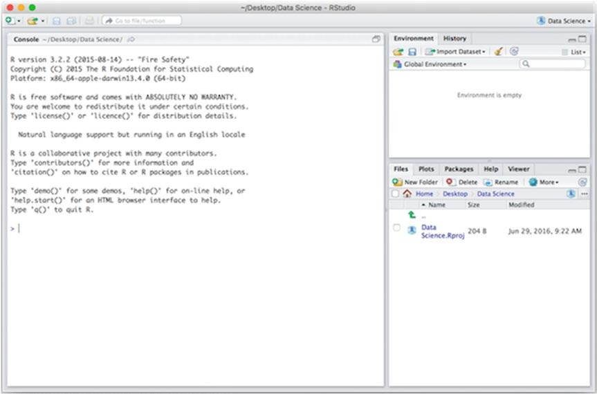
Start by downloading RStudio if you haven’t done so already (https://www.rstudio.com/products/ RStudio). If you open it, you should see a window similar to Figure 1-1. Well, except that you will be in an empty project while the figure shows (on the top right) that this RStudio is opened in a project called “Data Science”. You always want to be working on a project. Projects keep track of the state of your analysis by remembering variables and functions you have written and keep track of which files you have opened and such. Choose File ➤ New Project to create a project. You can create a project from an existing directory, but if this is the first time you are working with R you probably just want to create an empty project in a new directory, so do that.

Chapter 1 ■ IntroduCtIon to r programmIng

Figure 1-1. RStudio

Once you have opened RStudio, you can type R expressions into the console, which is the frame on the left of the RStudio window. When you write an expression there, R will read it, evaluate it, and print the result. When you assign values to variables, and you will see how to do this shortly, they will appear in the Environment frame on the top right. At the bottom right, you have the directory where the project lives, and files you create will go there.

To create a new file, choose File ➤ New File. You can select several different file types. We are interested in the R Script and R Markdown types. The former is the file type for pure R code, while the latter is used for creating reports where documentation text is mixed with R code. For data analysis projects, I recommend using Markdown files. Writing documentation for what you are doing is really helpful when you need to go back to a project several months down the line.

For most of this chapter, you can just write R code in the console, or you can create an R Script file. If you create an R Script file, it will show up on the top left, as shown in Figure 1-2. You can evaluate single expressions using the Run button on the top-right of this frame, or evaluate the entire file using the Source button. For longer expressions, you might want to write them in an R Script file for now. In the next chapter, we talk about R Markdown, which is the better solution for data science projects.

2

Chapter 1 ■ IntroduCtIon to r programmIng

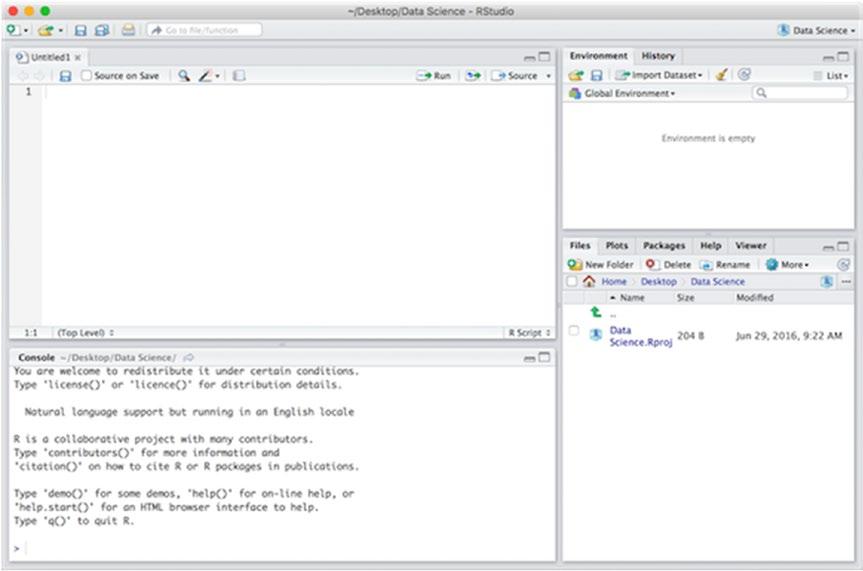
Figure 1-2. RStudio with a new R Script file

Using R as a Calculator

You can use the R console as a calculator where you just type in an expression you want calculated, press Enter, and R gives you the result. You can play around with that a little bit to get familiar with how to write expressions in R—there is some explanation for how to write them below—moving from using R as a calculator in this sense to writing more sophisticated analysis programs is only a question of degree. A data analysis program is really little more than a sequence of calculations, after all.

Simple Expressions

Simple arithmetic expressions are written, as in most other programming languages, in the typical mathematical notation that you are used to.

1 + 2 ## [1] 3 4 / 2 ## [1] 2 (2 + 2) * 3 ## [1] 12

3

Chapter 1 ■ IntroduCtIon to r programmIng

It also works pretty much as you are used to. Except, perhaps, that you might be used to integers behaving as integers in a division. At least in some programming languages, division between integers is integer division, but in R, you can divide integers and if there is a remainder you will get a floating-point number back as the result.

4 / 3 ## [1] 1.333333

When you write numbers like 4 and 3, they are interpreted as floating-point numbers. To explicitly get an integer, you must write 4L and 3L.

class(4) ## [1] "numeric" class(4L) ## [1] "integer"

You will still get a floating-point if you divide two integers, although there is no need to tell R explicitly that you want floating-point division. If you want integer division, on the other hand, you need a different operator, %/%:

4 %/% 3 ## [1] 1

In many languages % is used to get the remainder of a division, but this doesn’t quite work with R, where % is used to construct infix operators. So in R, the operator for this is %%:

4 %% 3 ## [1] 1

In addition to the basic arithmetic operators—addition, subtraction, multiplication, division, and the modulus operator you just saw—you also have an exponentiation operator for taking powers. For this, you can use ^ or ** as infix operators:

2^2 ## [1] 4 2^3 ## [1] 8 2**2 ## [1] 4 2**3 ## [1] 8

There are some other data types besides numbers, but we won’t go into an exhaustive list here. There are two types you do need to know about early, though, since they are frequently used and since not knowing about how they work can lead to all kinds of grief. Those are strings and “factors”.

Strings work as you would expect. You write them in quotes, either double quotes or single quotes, and that is about it.

"hello," ## [1] "hello," 'world!' ## [1] "world!"

4