Bayesian Linear Regression�����������������������������������������������������������������������������������������

Chapter 14 ■ profiling and optimizing

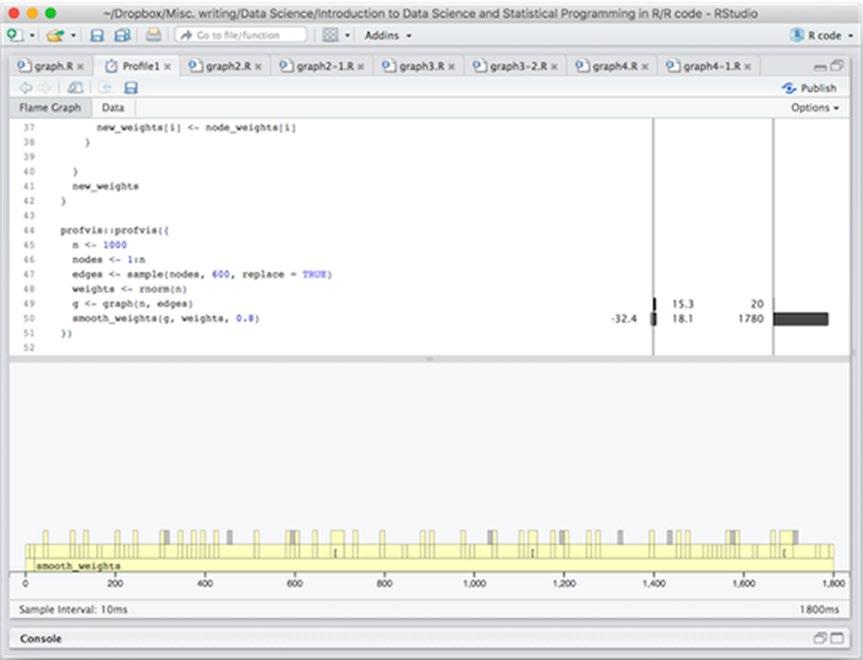
Running this code will open a new tab showing the results, as shown in Figure 14-1. The top half of the tab shows your code with annotations showing memory usage first and time usage second as horizontal bars. The bottom half of the window shows the time usage plus callstack.

We can see that the total execution took about 1800 ms. The way to read the graph is that, from left to right, you can see what was executed at any point in the run with functions called directly in the code block we gave profvis() at the bottom and code they called directly above that and further function calls stacked even higher.

We can also see that by far the most time was spent in the smooth_weights() function since that stretches almost all the way from the leftmost part of the graph and all the way to the rightmost.

If you move your mouse pointer into the window, either in the code or in the bottom graph, it will highlight what you are pointing at, as shown in Figure 14-2. You can use this to figure out where the time is being spent.

Figure 14-1. Window showing profile results

306

Chapter 14 ■ profiling and optimizing

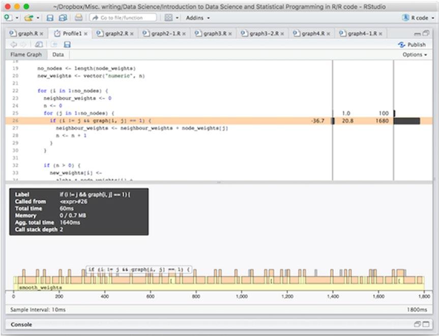
Figure 14-2. Highlighting executing code from the profiling window

In this particular case, it looks like most of the time is spent in the inner loop, checking if an edge exists. Since this is the inner part of a double loop, this might not be so surprising. The reason that it is not all the body of the inner loop, but the if statement is probably that we check the if expression in each iteration but we do not execute its body unless it is true. And with 1000 nodes and 300 edges it is only true with probability around 300/(1000*1000) = 3 × 10-4 (it can be less since some edges could be identical or self-loops).

Now if we had a performance problem with this code, this is where we should concentrate our optimization efforts. With 1000 nodes we don’t really have a problem. 1800 ms is not a long time, after all. But the application I have in mind has around 30,000 nodes so it might be worth optimizing a little bit.

If you need to optimize something, the first you should be thinking is—is there a better algorithm or a better data structure? Algorithmic improvements are much more likely to give substantial performance improvements compared to just changing details of an implementation.

In this case, if the graphs we are working on are sparse, meaning they have few actual edges compared to all possible edges, then an incidence matrix is not a good representation. We could speed the code up by using vector expressions to replace the inner loop and hacks like that, but we are much better off considering another representation of the graph.

Here, of course, we should first figure out if the simulated data we have used is representative of the actual data we need to analyze. If the actual data is a dense graph and we do performance profiling on a sparse graph, we are not getting the right impression of where the time is being spent and where we can reasonably optimize. But the application I have in mind, I claim, is one that uses sparse graphs.

307

Chapter 14 ■ profiling and optimizing

With sparse graphs, we should represent edges in a different format. Instead of a matrix, we will represent the edges as a list where, for each node, we have a vector of that node’s neighbors.

We can implement that representation like this:

graph <- function(n, edges) { neighbours <- vector("list", length = n)

for (i in seq_along(neighbours)) { neighbours[[i]] <- vector("integer", length = 0)

no_edges <- length(edges) if (no_edges >= 1) { for (i in seq(1, no_edges, by = 2)) { n1 <- edges[i] n2 <- edges[i+1] neighbours[[n1]] <- c(n2, neighbours[[n1]]) neighbours[[n2]] <- c(n1, neighbours[[n2]])

for (i in seq_along(neighbours)) { neighbours[[i]] <- unique(neighbours[[i]])

structure(neighbours, class = "graph")

We first generate the list of edge vectors, then we initialize them all as empty integer vectors. We then iterate through the input edges and updating the edge vectors. The way we update the vectors is potentially computationally slow since we force a copy of the previous vector in each update, but we don’t know the length of these vectors a priori, so this is the easy solution, and we can worry about it later if the profiling says it is a problem.

Now, if the edges we get as input contains the same pair of nodes twice, we will get the same edge represented twice. This means that the same neighbor to a node will be used twice when calculating the mean of the neighbor weights. If we want to allow such multi-edges in the application that is fine, but we don’t, so we explicitly make sure that the same neighbor is only represented once by calling the unique() function on all the vectors at the end.

With this graph representation, we can update the smoothing function to this:

smooth_weights <- function(graph, node_weights, alpha) { if (length(node_weights) != length(graph)) stop("Incorrect number of nodes")

no_nodes <- length(node_weights) new_weights <- vector("numeric", no_nodes)

for (i in 1:no_nodes) { neighbour_weights <- 0 n <- 0 for (j in graph[[i]]) { if (i != j) {

308

Chapter 14 ■ profiling and optimizing

neighbour_weights <- neighbour_weights + node_weights[j] n <- n + 1

if (n > 0) { new_weights[i] <alpha * node_weights[i] + (1 - alpha) * neighbour_weights / n } else { new_weights[i] <- node_weights[i]

} new_weights

Very little changes. We just make sure that j only iterates through the nodes we know to be neighbors of node i.

The profiling code is the same as before, and if we run it, we get the results shown in Figure 14-3.

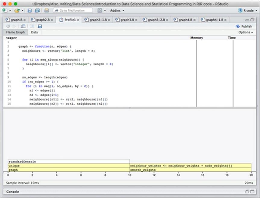
Figure 14-3. Profiling results after the first change

309

Chapter 14 ■ profiling and optimizing

We see that we got a substantial performance improvement. The execution time is now 20 ms instead of 1800 ms. We can also see that half the time is spent on constructing the graph and only half on smoothing it. In the construction, nearly all the time is spent in unique() while in the smoothing function, the time is spent in actually computing the mean of the neighbors.

It should be said here, though, that the profiler works by sampling what code is executing at certain time points. It doesn’t have an infinite resolution, it samples every 10 ms as it says at the bottom left, so in fact, it has only sampled twice in this run. The result we see is just because the samples happened to hit those two places in the graph construction and the smoothing, respectively. We are not actually seeing fine details here.

To get more details, and get closer to the size the actual input is expected to be, we can try increasing the size of the graph to 10,000 nodes and 600 edges.

profvis::profvis({ n <- 10000 nodes <- 1:n edges <- sample(nodes, 1200, replace = TRUE) weights <- rnorm(n) g <- graph(n, edges) smooth_weights(g, weights, 0.8) })

The result of this profiling is shown in Figure 14-4.

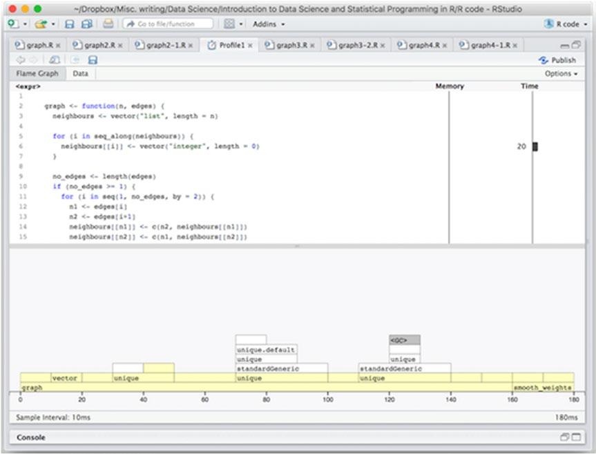
Figure 14-4. Profiling results with a larger graph 310

Chapter 14 ■ profiling and optimizing

To our surprise, we see that for the larger graph we are actually spending more time constructing the graph than smoothing it. We also see that this time is spent calling the unique() function.

Now, these calls are necessary to avoid duplicated edges, but they are not necessarily going to be something we often see—in the random graph they will be very unlikely, at least—so most of these calls are not really doing anything.

If we could remove all the duplicated edges in a single call to unique() we should save some time. We can do this, but it requires a little more work in the construction function.

We want to make the edges unique, and there are two issues here. One is that we don’t actually represent them as pairs we can call unique() on, and calling unique() on the edges vector is certainly not a solution. The other issue is that the same edge can be represented in two different ways: (i, j) and (j, i).

We can solve the first problem by translating the vector into a matrix. If we call unique() on a matrix we get the unique rows, so we just represent the pairs in that way. The second issue we can solve by making sure that edges are represented in a canonical form, say requiring that i < j for edges (i, j).

graph <- function(n, edges) { neighbours <- vector("list", length = n)

for (i in seq_along(neighbours)) { neighbours[[i]] <- vector("integer", length = 0)

no_edges <- length(edges) if (no_edges >= 1) { sources <- seq(1, no_edges, by = 2) destinations <- seq(2, no_edges, by = 2)

edge_matrix <- matrix(NA, nrow = length(sources), ncol = 2) edge_matrix[,1] <- edges[sources] edge_matrix[,2] <- edges[destinations]

for (i in 1:nrow(edge_matrix)) { if (edge_matrix[i,1] > edge_matrix[i,2]) { edge_matrix[i,] <- c(edge_matrix[i,2], edge_matrix[i,1])

edge_matrix <- unique(edge_matrix)

for (i in seq(1, nrow(edge_matrix))) { n1 <- edge_matrix[i, 1] n2 <- edge_matrix[i, 2] neighbours[[n1]] <- c(n2, neighbours[[n1]]) neighbours[[n2]] <- c(n1, neighbours[[n2]])

structure(neighbours, class = "graph")

311

Chapter 14 ■ profiling and optimizing

The running time is cut in half and relatively less time is spent constructing the graph compared to before. The time spent in executing the code is also so short again that we cannot be too certain about the profiling samples to say much more.

The graph size is not quite at the expected size for the application I had in mind when I wrote this code. We can boost it up to the full size of around 20,000 nodes and 50,000 edges and profile for that size. Results are shown in Figure 14-5.

On a full-size graph, we still spend most of the time in constructing the graph and not in smoothing it—and about half of the constructing time in the unique() function—but this is a little misleading. We don’t expect to call the smoothing function just once on a graph. Each call to the smoothing function will smooth the weights out a little more, and we expect to run it around ten times, say, in the real application.

We can rename the function to flow_weights_iteration() and then write a smooth_weights() function that runs it for a number of iterations:

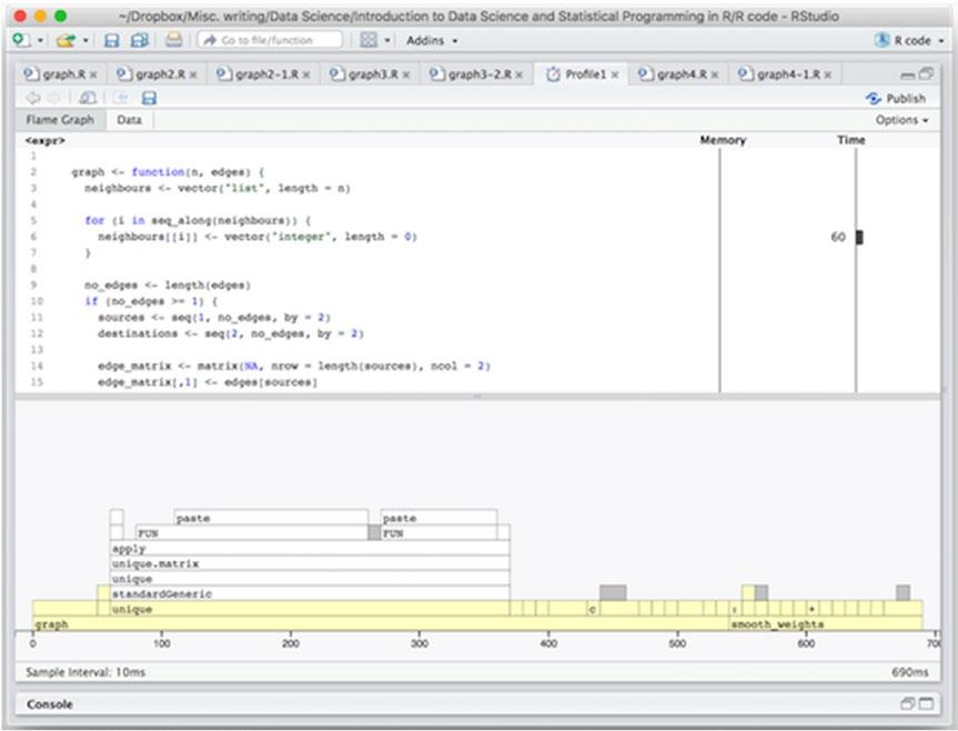
Figure 14-5. Profiling results on a full-time graph

flow_weights_iteration <- function(graph, node_weights, alpha) { if (length(node_weights) != length(graph)) stop("Incorrect number of nodes")

312