Formulas and Their Model Matrix���������������������������������������������������������������������������������

Chapter 14 ■ profiling and optimizing

no_nodes <- length(node_weights) new_weights <- vector("numeric", n)

for (i in 1:no_nodes) { neighbour_weights <- 0 n <- 0 for (j in graph[[i]]) { if (i != j) { neighbour_weights <- neighbour_weights + node_weights[j] n <- n + 1

if (n > 0) { new_weights[i] <- (alpha * node_weights[i] + (1 - alpha) * neighbour_weights / n)

} else { new_weights[i] <- node_weights[i]

} new_weights

} smooth_weights <- function(graph, node_weights, alpha, no_iterations) { new_weights <- node_weights replicate(no_iterations, { new_weights <- flow_weights_iteration(graph, new_weights, alpha)

}) new_weights

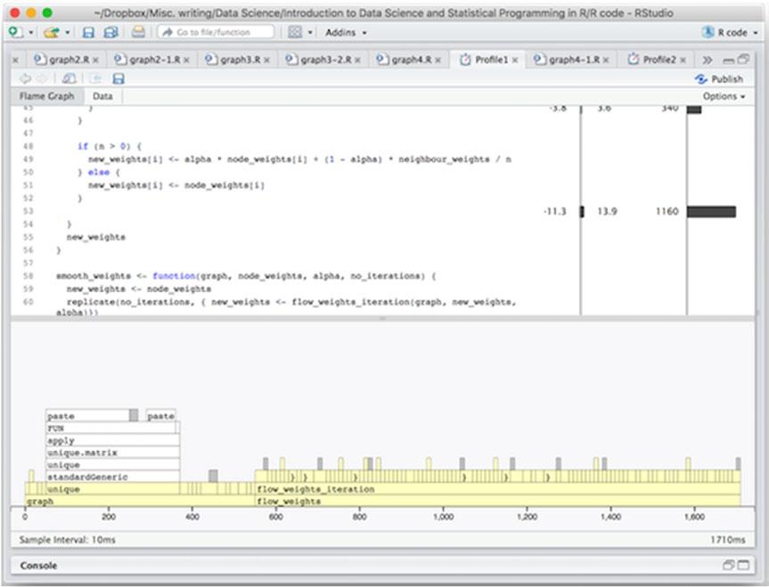
We can then profile with 10 iterations:

profvis::profvis({ n <- 20000 nodes <- 1:n edges <- sample(nodes, 100000, replace = TRUE) weights <- rnorm(n) g <- graph(n, edges) smooth_weights(g, weights, 0.8, 10) })

The results are shown in Figure 14-6. Obviously, if we run the smoothing function more times the smoothing is going to take up more of the total time, so there are no real surprises here. There aren’t really any obvious hotspots any longer to dig into. I used the replicate() function for the iterations, and it does have a little overhead because it does more than just loop—it creates a vector of the results—and I can gain a few more milliseconds by replacing it with an explicit loop:

smooth_weights <- function(graph, node_weights, alpha, no_iterations) {

new_weights <- node_weights

313

Chapter 14 ■ profiling and optimizing

for (i in 1:no_iterations) { new_weights <smooth_weights_iteration(graph, new_weights, alpha)

} new_weights

I haven’t shown the results, so you have to trust me on that. There is nothing major to attack any longer, now, however.

If you are in that situation where there is nothing more obvious to try to speed up, you have to consider if any more optimization is really necessary. From this point an onwards, unless you can come up with a better algorithm, which is hard, further optimizations are going to be very hard and unlikely to be worth the effort. You are probably better off spending your time on something else while the computations run than wasting days on trying to squeeze a little more performance out of it.

Of course, in some cases, you really have to improve performance more to do your analysis in reasonable time, and there are some last resorts you can go to such as parallelizing your code or moving time-critical parts of it to C++. But for now, we can analyze full graphs in fewer than two seconds so we definitely should not spend more time on optimizing this particular code.

Figure 14-6. Profiling results with multiple smoothing iterations

314

Chapter 14 ■ profiling and optimizing

Speeding Up Your Code

If you really do have a performance problem, what do you do? I will assume that you are not working on a problem that other people have already solved—if there is already a package available you could have used then you should have used it instead of writing your own code, of course. But there might be similar problems you can adapt to your needs, so before you do anything else, do a little bit of research to find out if anyone else has solved a similar problem, and if so, how they did it. There are very few really unique problems in life, and it is silly not to learn from others’ experiences.

It can take a little time to figure out what to search for, though, since similar problems pop up in very different fields. There might be a solution out there that you just don’t know how to search for because it is described in terms entirely different from your own field. It might help to ask on mailing lists or stack overflow (see http://stackoverflow.com), but don’t burn your Karma by asking help with every little thing you should be able to figure out yourself with a little bit of work.

If you really cannot find an existing solution you can adapt, the next step is to start thinking about algorithms and data structures. Improving these usually have much more of an impact on performance than micro-optimizations ever can. Your first attempts at any optimization should be to figure out if you could use better data structures or better algorithms.

It is, of course, a more daunting task to reimplement complex data structures or algorithms—and you shouldn’t if you can find solutions already implemented—but it is usually where you gain the most performance. Of course, there is always a trade-off between how much time you spend on reimplementing an algorithm versus how much you gain, but with experience, you will get better at judging this. Well, slightly better. If in doubt, it is probably better to live with slow code than spend a lot of time trying to improve it.

And before you do anything make sure you have unit tests that ensure that new implementations do not break old functionality! Your new code can be as fast as lightning, and it is worthless if it isn’t correct.

If you have explored existing packages and new algorithms and data structures and there still is a performance problem you reach the level of micro-optimizations. This is where you use slightly different functions and expressions to try to improve the performance, and you are not likely to get massive improvements at this level of changes. But if you have code that is executed thousands or millions of times, those small gains can still stack up. So if your profiling highlights a few hotspots for performance you can try to rewrite code there.

The sampling profiler is not terribly useful at this level of optimization. It samples at the level of milliseconds, and that is typically a much coarser grained measurement than what you need here. Instead, you can use the microbenchmark package that lets you evaluate and compare expressions. The microbenchmark() function runs a sequence of expressions several times and computes statistics on the execution time in units down to nanoseconds. If you want to gain some performance through microoptimization, you can use it to evaluate different alternatives to your computations.

For example, we can use it to compare an R implementation of sum() against the built-in sum() function:

library(microbenchmark) mysum <- function(sequence) { s <- 0 for (x in sequence) s <- s + x s

microbenchmark( sum(1:10), mysum(1:10)

) ## Unit: nanoseconds

315

Chapter 14 ■ profiling and optimizing

## expr min lq mean median uq ## sum(1:10) 194 202 300.10 233.5 349.5 ## mysum(1:10) 1396 1592 2280.47 1750.0 1966.5 ## max neval cld ## 2107 100 a ## 11511 100 b

The first column in the output is the expressions evaluated, then you have the minimum, lower quarter, mean, median, upper quarter, and maximum time observed when evaluating it, and then the number of evaluations used. The last column ranks the performance, here showing that sum() is a and mysum() is b so the first is faster. This ranking takes the variation in evaluation time into account and does not just rank by the mean.

There are a few rules of thumbs for speeding up the code in micro-optimization, but you should always measure. Intuition is often a quite bad substitute for measurement.

One rule of thumb is to use built-in functions when you can. Functions such as sum() are actually implemented in C and highly optimized, so your own implementation will have a hard time competing with it, as you saw previously.

Another rule of thumb is to use the simplest functions that get the work done. More general functions introduce various overheads that simpler functions avoid.

You can add together all numbers in a sequence using Reduce(), but using such a general function is going to be relatively slow compared to specialized functions.

microbenchmark( sum(1:10), mysum(1:10),

Reduce(`+`, 1:10, 0)

) ## Unit: nanoseconds ## expr min lq mean median ## sum(1:10) 207 258 356.03 324.5 ## mysum(1:10) 1611 1892 2667.25 2111.0 ## Reduce(`+`, 1:10, 0) 4485 5285 6593.07 6092.0 ## uq max neval cld ## 409.0 1643 100 a ## 2369.0 11455 100 b ## 6662.5 15497 100 c

We use such general functions for programming convenience. They give us abstract building blocks. We rarely get performance boosts out of them and sometimes they can slow things down.

Thirdly, do as little as you can get away with. Many functions in R have more functionality than we necessarily think about. A function such as read.table() not only reads in data, it also figures out what type each column should have. If you tell it what the types of each column are using the colClasses argument, it gets much faster because it doesn’t have to figure it out itself. For factor() you can give it the allowed categories using the levels argument so it doesn’t have to work it out itself.

x <- sample(LETTERS, 1000, replace = TRUE) microbenchmark( factor(x, levels = LETTERS), factor(x)

) ## Unit: microseconds

316

Chapter 14 ■ profiling and optimizing

## expr min lq ## factor(x, levels = LETTERS) 19.211 20.8975 ## factor(x) 59.458 61.9575 ## mean median uq max neval cld ## 22.03447 21.6175 22.610 32.981 100 a ## 66.70901 62.9135 67.946 132.306 100 b

It is not just when providing input, to help functions avoid figuring something out, this is in effect. Functions often also return more than you are necessarily interested in. Functions like unlist(), for instance, will preserve the names of a list into the resulting vector. Unless you really need those names, you should get rid of them since it is expensive dragging those names along with you. If you are just interested in a numerical vector, you should use use.names = FALSE:

x <- rnorm(1000) names(x) <- paste("n", 1:1000) microbenchmark( unlist(Map(function(x) x**2, x), use.names = FALSE), unlist(Map(function(x) x**2, x))

) ## Unit: microseconds ## expr ## unlist(Map(function(x) x^2, x), use.names = FALSE) ## unlist(Map(function(x) x^2, x)) ## min lq mean median uq ## 484.866 574.248 704.2379 660.3140 716.2325 ## 659.355 722.974 825.7712 813.3855 891.4630 ## max neval cld ## 3141.598 100 a ## 1477.028 100 b

Fourthly, when you can, use vector expressions instead of loops. Not just because this makes the code easier to read but because the implicit loop in vector expressions is handled much faster by the runtime system of R than your explicit loops will.

Most importantly, though, is to always measure when you try to improve performance and only replace simple code with more complex code if there is a substantial improvement that makes this worthwhile.

Parallel Execution

Sometimes you can speed things up, not by doing them faster, but by doing many things in parallel. Most computers today have more than one core, which means that you should be able to run more computations in parallel.

These are usually based on some variation of lapply() or Map() or similar, see the parallel package as an example, but also check the foreach package, which provides a higher level looping construct that can also be used to run code in parallel.

If we consider our graph smoothing, we could think that since each node is an independent computation we should be able to speed the function up by running these calculations in parallel. If we move the inner loop into a local function, we can replace the outer look with a call to Map():

smooth_weights_iteration_map <- function(graph, node_weights, alpha) { if (length(node_weights) != length(graph)) stop("Incorrect number of nodes")

317

Chapter 14 ■ profiling and optimizing

handle_i <- function(i) { neighbour_weights <- 0 n <- 0 for (j in graph[[i]]) { if (i != j) { neighbour_weights <- neighbour_weights + node_weights[j] n <- n + 1

if (n > 0) { alpha * node_weights[i] + (1 - alpha) * neighbour_weights / n } else { node_weights[i]

unlist(Map(handle_i, 1:length(node_weights)))

This is not likely to speed anything up—the extra overhead in the high-level Map() function will do the opposite if anything—but it lets us replace Map() with one of the functions from parallel, for example clusterMap():

unlist(clusterMap(cl, inner_loop, 1:length(node_weights)))

Here cl is the “cluster” that just consists of two cores I have on my laptop:

cl <- makeCluster(2, type = "FORK") microbenchmark( original_smooth(), using_map(), using_cluster_map(), times = 5

Where the three functions refer to the three different versions of the algorithm, gave me these result. On my two-core laptop, we could expect the parallel version to run up to two times faster. In fact, it runs several orders of magnitude slower:

Unit: milliseconds expr min lq original_smooth() 33.58665 33.73139 using_map() 33.12904 34.84107 using_cluster_map() 14261.97728 14442.85032 mean median uq max 35.88307 34.25118 36.62977 41.21634 38.31528 40.50315 41.28726 41.81587 15198.55138 14556.09176 14913.24566 17818.59187 neval cld 5 a 5 a 5 b

318