Examples of Reading and Formatting Datasets �������������������������������������������������������������

Chapter 1 ■ IntroduCtIon to r programmIng

Defining functions from combining other functions is called “tacit” or “point-free” programming (or sometimes even pointless programming, although that is a little harsh), referring to the way you are not storing the intermediate steps (points) of a computation. You write:

f <- . %>% cos %>% sin

Instead of:

f <- function(x) { y <- cos(x) z <- sin(y) z

Naturally, this is mostly used when you have a sub-pipeline that you intend to call on more than one dataset. You can just write a function specifying the pipeline like you would write an actual pipeline. You just give it . as the very first left side, instead of a dataset, and you are defining a function instead of running data through a pipeline.

Anonymous Functions

Pipelines are great when you can call existing functions one after another, but what happens if you need a step in the pipeline where there is no function doing what you want? You can, of course, always write such a missing function but if you need to write functions time and time again for doing small tasks in pipelines, you have a similar problem to when you needed to save all the intermediate steps in an analysis in variables. You do not want to have a lot of functions defined because there is a risk that you use the wrong one in a pipeline—especially if you have many similar functions, as you are likely to have if you need a function for every time you need a little bit of data-tweaking in your pipelines.

Again, magrittr has the solution: lambda expressions. This is a computer science term for anonymous functions, that is, functions that you do not give a name.

When you define a function in R, you actually always create an anonymous function. Any expression of the form function(x) expression is a function, but it doesn’t have a name unless you assign it to a variable.

As an example, consider a function that plots the variable y against the variable x and fits and plots a linear model of y against x. You can define and name such a function to get the following code:

plot_and_fit <- function(d) { plot(y ~ x, data = d) abline(lm(y ~ x, data = d))

x <- rnorm(20) y <- x + rnorm(20) data.frame(x, y) %>% plot_and_fit

Since giving the function a name doesn’t affect how the function works, it isn’t necessary to do so. You can just put the code that defined the function where the name of the function goes to get this:

data.frame(x, y) %>% (function(d) { plot(y ~ x, data = d) abline(lm(y ~ x, data = d)) })

26

Chapter 1 ■ IntroduCtIon to r programmIng

It does the exact same thing, but without defining a function. It is just not that readable either. Using . and curly brackets, you can improve the readability (slightly) by just writing the body of the function and referring to the input of it—what was called d above—as .:

data.frame(x, y) %>% { plot(y ~ x, data = .) abline(lm(y ~ x, data = .))

Other Pipeline Operations

The %>% operator is a very powerful mechanism for specifying data analysis pipelines, but there are some special cases where slightly different behavior is needed.

One case is when you need to refer to the parameters in a data frame you get from the left side of the pipe expression directly. In many functions, you can get to the parameters of a data frame just by naming them, as you have seen with lm and plot, but there are cases where that is not so simple.

You can do that by indexing . like this:

d <- data.frame(x = rnorm(10), y = 4 + rnorm(10)) d %>% {data.frame(mean_x = mean(.$x), mean_y = mean(.$y))} ## mean_x mean_y ## 1 0.4167151 3.911174

But if you use the operator %$% instead of %>%, you can get to the variables just by naming them instead.

d %$% data.frame(mean_x = mean(x), mean_y = mean(y)) ## mean_x mean_y ## 1 0.4167151 3.911174

Another common case is when you want to output or plot some intermediate result of a pipeline. You can of course write the first part of a pipeline, run data through it, and store the result in a parameter, output or plot what you want, and then continue from the stored data. But you can also use the %T>% (tee) operator. It works like the %>% operator but where %>% passes the result of the right side of the expression on, %T>% passes on the result of the left side. The right side is computed but not passed on, which is perfect if you only want a step for its side-effect, like printing some summary.

d <- data.frame(x = rnorm(10), y = rnorm(10)) d %T>% plot(y ~ x, data = .) %>% lm(y ~ x, data = .)

The final operator is %<>%, which does something I warned against earlier—it assigns the result of a pipeline back to a variable on the left. Sometimes you do want this behavior—for instance if you do some data cleaning right after loading the data and you never want to use anything between the raw and the cleaned data, you can use %<>%.

d <- read_my_data("/path/to/data") d %<>% clean_data

I use it sparingly and prefer to just pass this case through a pipeline, as follows:

d <- read_my_data("/path/to/data") %>% clean_data

27

Chapter 1 ■ IntroduCtIon to r programmIng

Coding and Naming Conventions

People have been developing R code for a long time, and they haven’t been all that consistent in how they do it. So as you use R packages, you will see many different conventions on how code is written and especially how variables and functions are named.

How you choose to write your code is entirely up to you as long as you are consistent with it. It helps somewhat if your code matches the packages you use, just to make everything easier to read, but it really is up to you.

A few words on naming is worth going through, though. There are three ways people typically name their variables, data, or functions, and these are:

underscore_notation(x, y) camelBackNotation(x, y) dot.notation(x, y)

You are probably familiar with the first two notations, but if you have used Python or Java or C/C++ before, the dot notation looks like method calls in object oriented programming. It is not. The dot in the name doesn’t mean method call. R just allows you to use dots in variable and function names.

I will mostly use the underscore notation in this book, but you can do whatever you want. I recommend that you stay away from the dot notation, though. There are good reasons for this. R actually put some interpretation into what dots mean in function names, so you can get into some trouble. The built-in functions in R often use dots in function names, but it is a dangerous approach, so you should probably stay away from it unless you are absolutely sure that you are avoiding its pitfalls.

Exercises

Try the following exercises to become more comfortable with the concepts discussed in this chapter.

Mean of Positive Values

You can simulate values from the normal distribution using the rnorm() function. Its first argument is the number of samples you want, and if you do not specify other values, it will sample from the N(0,1) distribution.

Write a pipeline that takes samples from this function as input, removes the negative values, and computes the mean of the rest. Hint: One way to remove values is to replace them with missing values (NA); if a vector has missing values, the mean() function can ignore them if you give it the option na.rm = TRUE.

Root Mean Square Error

If you have “true” values, t = (t1, …, tn) and “predicted” values y = (y1, …, yn), then the root mean square error is defined as RMSE , ty ( ) å = -( )1 =1 2 n t y i n i i .

Write a pipeline that computes this from a data frame containing the t and y values. Remember that you can do this by first computing the square difference in one expression, then computing the mean of that in the next step, and finally computing the square root of this. The R function for computing the square root is sqrt().

28

CHAPTER 2

Reproducible Analysis

The typical data analysis workflow looks like this: you collect your data and you put it in a file or spreadsheet or database. Then you run some analyses, written in various scripts, perhaps saving some intermediate results along the way or maybe always working on the raw data. You create some plots or tables of relevant summaries of the data, and then you go and write a report about the results in a text editor or word processor. It is the typical workflow. Most people doing data analysis do this or variations thereof. But it is also a workflow that has many potential problems.

There is a separation between the analysis scripts and the data, and there is a separation between the analysis and the documentation of the analysis.

If all analyses are done on the raw data then issue number one is not a major problem. But it is common to have scripts for different parts of the analysis, with one script storing intermediate results that are then read by the next script. The scripts describe a workflow of data analysis and, to reproduce an analysis, you have to run all the scripts in the right order. Often enough, this correct order is only described in a text file or, even worse, only in the head of the data scientist who wrote the workflow. What is even worse, it won’t stay there for long and is likely to be lost before it is needed again.

Ideally, you always want to have your analysis scripts written in a way in which you can rerun any part of your workflow, completely automatically, at any time.

For issue number two, the problem is that even if the workflow is automated and easy to run again, the documentation quickly drifts away from the actual analysis scripts. If you change the scripts, you won’t necessarily remember to update the documentation. You probably don’t forget to update figures and tables and such, but not necessarily the documentation of the exact analysis run. Options to functions and filtering choices and such. If the documentation drifts far enough from the actual analysis, it becomes completely useless. You can trust automated scripts to represent the real data analysis at any time—that is the benefit of having automated analysis workflows in the first place—but the documentation can easily end up being pure fiction.

What you want is a way to have dynamic documentation. Reports that describe the analysis workflow in a form that can be understood both by machines and humans. Machines use the report as an automated workflow that can redo the analysis at any time. We humans use it as documentation that always accurately describes the analysis workflow that we run.

Chapter 2 ■ reproduCible analysis

Literate Programming and Integration of Workflow and Documentation

One way to achieve the goal of having automated workflows and documentation that is always up to date is something called “literate programming”. Literate programming is an approach to software development, proposed by Stanford computer scientist Donald Knuth, which never became popular for programming, possibly because most programmers do not like to write documentation.

The idea in literate programming is that the documentation of a program—in the sense of the documentation of how the program works and how algorithms and data structures in the program works—is written together with the code implementing the program. Tools such as Javadoc and Roxygen (http:// roxygen.org) do something similar. They have documentation of classes and methods written together with the code in the form of comments. Literate programming differs slightly from this. With Javadoc and Roxygen, the code is the primary document, and the documentation is comments added to it. With literate programming, the documentation is the primary text for humans to read and the code is part of this documentation, included where it falls naturally to have it. The computer code is extracted automatically from this document when the program runs.

Literate programming never became a huge success for writing programs, but for doing data science, it is having a comeback. The results of a data analysis project is typically a report describing models and analysis results, and it is natural to think of this document as the primary product. So the documentation is already the main focus. The only thing needed to use literate programming is a way of putting the analysis code inside the documentation report.

Many programming languages have support for this. Mathematica (https://www.wolfram.com/ mathematica/) has always had notebooks where you could write code together with documentation. Jupyter (http://jupyter.org), the descendant of iPython Notebook, lets you write notebooks with documentation and graphics interspersed with executable code. And in R there are several ways of writing documents that are used both as automated analysis scripts as well as for generating reports. The most popular of these approaches is R Markdown (for writing these documents) and knitr (for running the analysis and generating the reports).

Creating an R Markdown/knitr Document in RStudio

To create a new R Markdown document, go to the File menu, choose New File and then R Markdown. Now RStudio will bring up a window where you can decide which kind of document you want to make and add some information, such as title and author name. It doesn’t matter so much what you do here; you can change it later. But try making an HTML document.

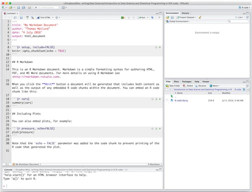
The result is a new file with some boilerplate text in it, as shown in Figure 2-1. At the top of the file, between two lines containing just --- is some meta-information for the document, and after the second --is the actual text. It consists of a mix of text, formatted in the Markdown language, and R code.

30

Chapter 2 ■ reproduCible analysis

Figure 2-1. A new R Markdown file

In the toolbar above the open file, there is a menu option called Knit HTML. If you click it, it will translate the R Markdown into an HTML document and open it, as shown in Figure 2-2. You have to save the file first, though. If you click the Knit HTML button before saving, you will be asked to save the file.

31

Chapter 2 ■ reproduCible analysis

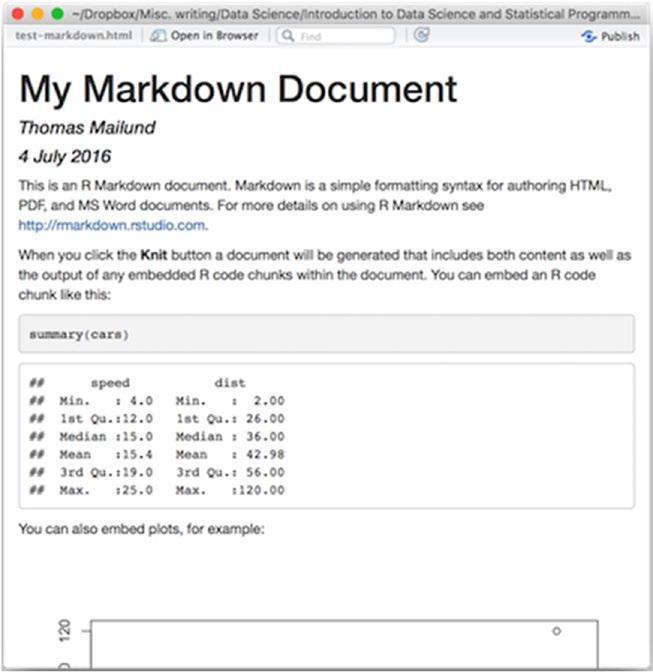
Figure 2-2. Compiled Markdown file

The newly created HTML file is also written to disk with the name you gave the R Markdown file. The R Markdown file will have suffix .rmd and the HTML file will have the same prefix, but with the suffix .html.

If you click the gear logo next to Knit HTML (in earlier versions of R Studio this is a down-pointing arrow), you get some additional options. You can ask to see the HTML document in the pane to the right in RStudio instead of in a new window. Having the document in a panel instead of a separate window can be convenient if you are on a laptop and do not have a lot of screen space. You can also generate a file or a Word file instead of an HTML file.

If you decide to produce a file in a different output format, RStudio will remember this. It will update the Knit HTML to Knit or Knit Word and it will update the metadata in the header of your file. If you manually update the header, this is reflected in the Knit X button. If you click the gear icon one step farther right, you get some more options for how the document should be formatted.

The actual steps involved in creating a document involves two tools and three languages, but it is all integrated so you typically will not notice. There is the R code embedded in the document. The R code is first processed by the knitr package that evaluates it and handles the results such as data and plots according to options you give it. The result is a Markdown document (notice no R). This Markdown document is then processed by the tool pandoc, which is responsible for generating the output file. For this, it uses the metadata in the header, which is written in a language called YAML, whereas the actual formatting is written in the the Markdown language.

32

Chapter 2 ■ reproduCible analysis

You usually don’t have to worry about pandoc working as the back-end of document processing. If you just write R Markdown documents, then RStudio will let you compile them into different types of output documents. But because the pipeline goes from R Markdown via knitr to Markdown and then via pandoc to the various output formats, you do have access to a very powerful tool for creating documents. I have written this book in R Markdown where each chapter is a separate document that I can run through knitr independently. I then have pandoc with some options take the resulting Markdown documents, combine them, and produce both output and Epub output. With pandoc, it is possible to use different templates for setting up the formatting, and having it depend on the output document you create by using different templates for different formats. It is a very powerful, but also a very complicated, tool and it is far beyond what we can cover in this book. Just know that it is there if you want to take document writing in R Markdown further than what you can readily do in RStudio.

As I mentioned, there are actually three languages involved in an R Markdown document. We will handle them in order—first the header language, which is YAML, then the text formatting language, which is Markdown, and then finally how R is embedded in a document.

The YAML Language

YAML is a language for specifying key-value data. YAML stands for the (recursive) acronym YAML Ain’t Markup Language. So yes, when I called this section “The YAML Language,” I shouldn’t have included language since the L stands for language, but I did. I stand by that choice. The acronym used to stand for Yet Another Markup Language but since “markup language” typically refers to commands used to mark up text for either specifying formatting or for putting structured information in a text, which YAML doesn’t do, the acronym was changed. YAML is used for giving options in various forms to a computer program processing a document, not so much for marking up text, so it isn’t really a markup language.

In your R Markdown document, the YAML is used in the header, which is everything that goes between the first and second line with three dashes. In the document you create when you make a new R Markdown file, it can look like this:

--title: "My Markdown Document" author: "Thomas Mailund" date: "17 July 2016" output: html_document ---

You usually do not have to modify this header manually. If you use the GUI, it will adjust the header for you when you change options. You do need to alter it to include bibliographies, though, which we get to later. And you can always add anything you want to the header if you need to and it can be easier than using the GUI. But you don’t have to modify the header that often.

YAML gives you a way to specify key-value mappings. You write key: and then the value afterward. So above, you have the key title referring to My Markdown Document, the key author to refer to "Thomas Mailund" and so on. You don’t necessarily need to quote the values unless they have a colon in them, but you always can.

The YAML header is used both by RStudio and pandoc. RStudio uses the output key for determining which output format to translate your document into and this choice is reflected in the Knit toolbar button. pandoc, on the other hand, uses the title, author, and date to put that information into the generated document.

33

Chapter 2 ■ reproduCible analysis

You can have slightly more structure to the key-value specifications. If a key should refer to a list of values, you use -. So if you have more than one author, you can use something like this:

... author: - "Thomas Mailund" - "Christian Storm"

Or you can have more nested key-value structure, so if you change the output theme (using Output Options after clicking on the tooth-wheel in the toolbar), you might see something like this:

output: html_document: theme: united

How the options are used depends on the tool-chain used to format your document. The YAML header just provides specifications. Which options you have available and what they do is not part of the language.

For pandoc, it depends on the templates used to generate the final document (see later), so there isn’t even a complete list that I can give you for pandoc. Anyone who writes a new template can decide on new options to use. The YAML header gives you a way to provide options to such templates, but there isn’t a fixed set of keywords to use. It all depends on how tools later in the process interpret them.

The Markdown Language

The Markdown language is a markup language—the name is a pun. It was originally developed to make it easy to write web pages. HTML, the language used to format web pages, is also a markup language but is not always easily human readable. Markdown intended to solve this by formatting text with very simple markup commands—familiar from e-mails back in the day before e-mails were also HTML documents—and then have tools for translating Markdown into HTML.

Markdown has gone far beyond just writing web pages, but it is still a very simple and intuitive language for writing human-readable text with markup commands that can then be translated into other document formats.

In Markdown, you write plain text as plain text. So the body of text is just written without any markup. You will need to write it in a text editor so the text is actually text, not a word processor where the file format already contains a lot of markup information that isn’t readily seen onscreen. If you are writing code, you should already know about text editors. If not, just use RStudio to write R Markdown files, and you will be okay.

Markup commands are used when you want something else than just plain text. There aren’t many commands to learn—the philosophy is that when writing you should focus on the text and not the formatting—so they are very quickly learned.

34