Manipulating Data with dplyr �����������������������������������������������������������������������������������������

Chapter 2 ■ reproduCible analysis

Formatting Text

First, there are section headers. You can have different levels of headers—think chapters, sections, subsections, etc.— and you specify them using # starting at the beginning of a new line.

# Header 1 ## Header 2 ### Header 3

For the first two, you can also use this format:

Header 1 ========

Header 2 --------

To have lists in your document, you write them as you have probably often seen them in raw text documents. A list with bullets (and not numbers) is written like this:

* this is a * bulleted * list

The result looks like this:

• this is a

• bulleted

• list

You can have sublists just by indenting. You need to move the indented line in so there is a space between where the text starts at the outer lever and where the bullet is at the next level. Otherwise, the line goes at the outer level. The output of this:

* This is the first line * This is a sub-line * This is another sub-line * This actually goes to the outer level * This is definitely at the outer level

Is this list:

• This is the first line

– This is a sub-line – This is another sub-line

• This actually goes to the outer level • Back to the outer level

35

Chapter 2 ■ reproduCible analysis

If you prefer, you can use - instead of * for these lists and you can mix the two.

- First line * Second line - nested line

• First line

• Second line

– nested line

To have numbered lists, just use numbers instead of * and .

1. This is a 2. numbered 3. list

The result looks like this:

1. This is a

2. numbered

3. list

You don’t actually need to get the numbers right, you just need to use numbers. So

1. This is a 3. numbered 2. list

Would produce the same (correctly numbered) output. You will start counting at the first number, though, so

4. This is a 4. numbered 4. list

Produces:

4. This is a 5. numbered 6. list

To construct tables, you also use a typical text representation with vertical and horizontal lines. Vertical lines separate columns and horizontal lines separate headers from the table body. This code:

| First Header | Second Header | Third Header | | :------------ | :-----------: | --------------: | | First row | Centered text | Right justified | | Second row | *Some data* | *Some data* | | Third row | *Some data* | *Some data* |

36

Will result in this table:

First Header Second Header Third Header

First row Centered text Right justified Second row Some data Some data Third row Some data Some data

Chapter 2 ■ reproduCible analysis

The : in the line separating the header from the body determines the justification of the column. Put it on the left to get left justification, on both sides to get the text centered, and on the right to get the text right justified.

Inside text, you use markup codes to make text italic or boldface. You use either *this* or _this_ to make this italic, while you use **this** or __this__ to make this boldface.

Since Markdown was developed to make HTML documents it, of course, has an easy way to insert links. You use the notation [link text](link URL) to put link text into the document as a link to link URL. This notation is also used to make cross-references inside a document—similar to how HTML documents have anchors and internal links—but more on that later.

To insert images into a document, you use a notation similar to the link notation, but you just put a ! before the link. So  will insert the image pointed to by URL to image with a caption saying Image description. The URL here will typically be a local file, but it can be a remote file referred to via HTTP.

With long URLs, the marked-up text can be hard to read even with this simple notation and it is possible to remove the URLs from the actual text and place them later in the document, for example, after the paragraph referring to the URL or at the end of the document. For this, you use the notation [link text] [link tag] and define the link tag as the URL you want later.

This is some text [with a link][1]. The link tag is defined below the paragraph.

[1]: interesting-url-of-some-sort-we-dont-want-inline

You can use a string here for the tag. Using numbers is easy, but for long documents, you won’t be able to remember what each number refers to.

This is some text [with a link][interesting]. The link tag is defined below the paragraph.

[interesting]: interesting-url-of-some-sort-we-dont-want-inline

You can make block quotes in text using notation you will be familiar with from e-mails.

> This is a > block quote

Gives you this: This is a block quote

37

Chapter 2 ■ reproduCible analysis

To put verbatim input as part of your text, you can either do it inline or as a block. In both cases you use backticks `. Inline in the text, you use single backticks `foo`. To create a block of text you write:

block of text ```

You can also just indent text with four spaces, which is how I managed to make a block of verbatim text that includes three backticks.

Markdown is used a lot by people who document programs, so there is a notation for getting code highlighted in verbatim blocks. The convention is to write the name of the programming language after the three backticks, then the program used for formatting the document will highlight the code when it can. For R code you write r, so this block:

```r f <- function(x) ifelse(x %% 2 == 0, x**2, x**3) f(2) ```

Is formatted like this:

f <- function(x) ifelse(x %% 2 == 0, x**2, x**3) f(2)

The only thing this markup of blocks does is highlight the code. It doesn’t try to evaluate the code. Evaluating code happens before the Markdown document is formatted and we return to that shortly.

Cross-Referencing

Out of the box, there is not a lot of support for making cross references in Markdown documents. You can make cross-references to sections but not figures or tables. There are ways of doing it with extensions to pandoc—I use it in this book—but out of the box from RStudio, you cannot. Although, with the work being done for making book-writing and lengthy reports in Bookdown (https://bookdown.org/yihui/ bookdown/), that might change soon.1

The easiest way to reference a section is to put the name of the section in square brackets. If I write [Cross referencing] here, I get a link to this cross-referencing section. Of course, you don’t always want the name of the section to be the text of the link, so you can also write [this section][Cross referencing] to get a link to this section.

This approach naturally works only if all section titles are unique. If they are not, you cannot refer to them simply by their names. Instead, you can tag them to give them a unique identifier. You do this by writing the identifier after the title of the section. To put a name after a section header, you write:

### Cross referencing {#section-cross-ref}

Then you can refer to the section using [this](#section-cross-ref). Here you do need the # sign in the identifier. That markup is leftover from HTML, where anchors use #.

1In any case, having cross-references to sections but not figures is still better than Word, where the feature is there but buggy to the point of uselessness, in my experience.

38

Chapter 2 ■ reproduCible analysis

Bibliographies

Often you want to cite books or papers in a report. You can, of course, handle citations manually, but a better approach is to have a file with the citation information and then refer to it using markup tags. To add a bibliography, you use a tag in the YAML header called bibliography.

... bibliography: bibliography.bib ... ---

You can use several different formats here; see the R Markdown documentation (http://rmarkdown. rstudio.com/authoring_bibliographies_and_citations.html) for a list. The suffix .bib is used for BibLaTeX. The format for the citation file is the same as BibTeX, and you get citation information in that format from nearly every site that will give you bibliography information.

To cite something from the bibliography, you use [@smith04] where smith04 is the identifier used in the bibliography file. You can cite more than one paper inside square brackets separated by a semicolon, [@smith04; doe99], and you can add text such as chapters or page numbers [@smith04, chapter 4]. To suppress the author name(s) in the citation, say when you mention the name already in the text, you put - before the @, so you write As Smith showed [-@smith04].... For in-text citations, similar to \citet{} in natbib, you just leave out the brackets: @smith04 showed that... and you can combine that with additional citation information as @smith04 [chapter 4] showed that....

To specify the citation style to use, you use the csl tag in the YAML header.

... bibliography: bibliography.bib csl: biomed-central.csl

Check out the citation styles list at https://github.com/citation-style-language/styles for a large number of different formats. There should be most, if not all, of your heart desires there.

Controlling the Output (Templates/Stylesheets)

The pandoc tool has a powerful mechanism for formatting the documents it generates. This is achieved using stylesheets in CSS for HTML and from using templates for how to format the output for all output formats. The template mechanism lets you write an HTML or LaTeX document, say, that determines where various part of the text goes and where variables from the YAML header is used. This mechanism is far beyond what we can cover in this chapter, but I just want to mention it if you want to start writing papers using R Markdown. You can do this, you just need to have a template for formatting the document in the style a journal wants. Often they provide LaTeX templates, and you can modify these to work with Markdown.

There isn’t much support for this in RStudio, but for HTML documents, you can use the Output Options command (click on the tooth-wheel) to choose different output formatting.

39

Chapter 2 ■ reproduCible analysis

Running R Code in Markdown Documents

The formatting so far is all Markdown (and YAML). Where it combines with R and makes it R Markdown is through knitr. When you format a document, the first step evaluates R code to create a Markdown document. This translates an .rmd document into an .md document, but this intermediate document is deleted afterward unless you explicitly tell RStudio not to do so. It does that by running all the R code you want to be executed and putting it into the Markdown document.

The simplest R code you can evaluate is part of a text. If you want an R expression evaluated, you use backticks but add r right after the first. So to evaluate 2 + 2 and put the result in your Markdown document, you write `r and then the expression 2 + 2 and get the result 4 inserted into the text. You can write any R expression there to get it evaluated. This is useful for inserting short summary statistics like means and standard deviations directly into the text and ensuring that the summaries are always up to date with the actual data you are analyzing.

For longer chunks of code, you use the block-quotes, the three backticks. Instead of just writing:

```r 2 + 2 ```

which will only display the code (highlighted as R code), you put the r in curly brackets.

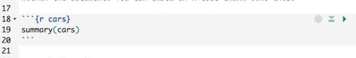
This will insert the code in your document but will also show the result of evaluating it right after the code block. The boilerplate code you get when creating an R Markdown document in RStudio shows you examples of this (see Figure 2-3).

Figure 2-3. Code chunk in RStudio

You can name code chunks by putting a name right after r. You don’t have to name all chunks, and if you have a lot of chunks, you probably won’t bother naming all of them. But if you give them a name, they are easily located by clicking on the structure button in the bar below the document (see Figure 2-4). You can also use the name to refer to chunks when caching results, which we will cover later.

40

Chapter 2 ■ reproduCible analysis

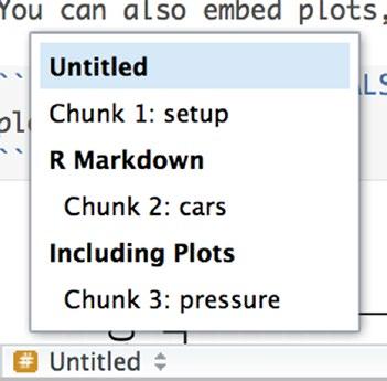
Figure 2-4. Document structure with chunk names

If you have the most recent version of RStudio, you should see a toolbar to the right on every code chunk (see Figure 2-5). The rightmost option, the Play button, will let you evaluate the chunk. The results will be shown below the chunk unless you have disabled that option. The middle button evaluates all previous chunks down to and including the current one. This is useful when the current chunk depends on previous results. The tooth-wheel lets you set options for the chunk.

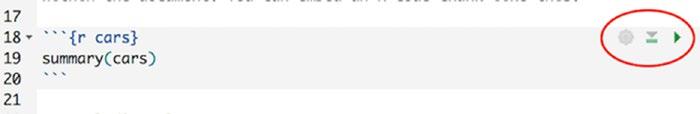
Figure 2-5. Code chunk toolbar

The chunk options, shown in Figure 2-6, control the output you get when evaluating a code chunk. The Output drop-down selects what output the chunk should generate in the resulting document, while the Show Warnings and Show Messages buttons determine whether warnings and messages, respectively, should be included in the output. The Use Custom Figure Size button is used to determine the size of figures you generate. We return to these later.

Figure 2-6. Code chunk options

41

Chapter 2 ■ reproduCible analysis

If you modify these options, you will see that the options are included in the top line of the chunk. You can of course also manually control the options here, and there are more options than what you can control with the window in the GUI. You can read the knitr documentation for all the details (http://yihui.name/ knitr/).

This dialog box will handle most of your needs, though, except for displaying tables or when you want to cache results of chunks, both of which we return to later.

Using Chunks when Analyzing Data (Without Compiling Documents)

Before continuing, though, I want to stress that working with data analysis in an R Markdown document is useful for more than just creating documents. I personally do all my analysis in these documents because I can combine documentation and code, regardless of whether I want to generate a report at the end. The combination of explanatory text and analysis code is just convenient to have.

The way code chunks are evaluated as separate pieces of analysis is also part of this. You can evaluate chunks individually, or all chunks down to a point, and I find that very convenient when doing an analysis. There are keyboard shortcuts for evaluating all chunks, all previous chunks, or just the current chunk (see Figure 2-7), which makes it very easy to write a bit of code for an exploratory analysis and evaluate just that piece of code. If you are familiar with Jupyter or similar notebooks, you will recognize the workflow.

Figure 2-7. Options for evaluating chunks

Even without the option for generating final documents from a Markdown document, I would still be using them just for this feature.

42

Chapter 2 ■ reproduCible analysis

Caching Results

Sometimes part of an analysis is very time-consuming. Here I mean in CPU time, not thinking time—it is also true for thinking time, but you don’t need to think the same things over and over. If you are not careful, however, you will need to run the same analysis on the computer again and again.

If you have such time-consuming steps in your analysis, then compiling documents will be very slow. Each time you compile the document, all the analysis is done from scratch. This is the functionality you want since this makes sure that the analysis does not have results left over from code that isn’t part of the document, but it limits the usability of the workflows if they take hours to compile.

To alleviate this, you can cache the results of a chunk. To cache the result of a chunk, you should add the option cache=TRUE to it. This means adding that in the header of the chunk similar to how output options are added. You will need to give the chunk a name to use this. Chunks without names are actually given a default name, but this name changes according to how many nameless chunks you have earlier in the document and you can’t have that if you use the name to remember results. So you need to name it. A named chunk that is set to be cached will not only be when you compile a document if it has changed since the last time it was evaluated. If it hasn’t changed, the cached results of the last evaluation will just be reused.

R cannot cache everything, so if you load libraries in a cached chunk they won’t be loaded unless the chunk is being evaluated. That means there are some limits to what you can do, but generally it is a very useful feature.

Since other chunks can depend on a cached chunk, there can also be problems if a cached chunk depends on another chunk, cached or not. The chunk will only be re-evaluated if you have changed the code inside it, so if it depends on something you have changed, it will remember results based on outdated data. You have to be careful about that.

You can set up dependencies between chunks, though, to fix this problem. If a chunk is dependent on the results of another chunk, you can specify this using the chunk option dependson=other. Then, if the chunk other (and you need to name such chunks) is modified, the cache is considered invalid, and the depending chunk will be evaluated again.

Displaying Data

Since you are writing a report on data analysis, you naturally want to include some results. That means displaying data in some form or other.

You can simply include the results of evaluating R expressions in a code chunk, but often you want to display the data using tables or graphics, especially if the report is something you want to show to people not familiar with R. Luckily, both tables and graphics are easy to display.

To make a table, you can use the function kable() from the knitr package. Try adding a chunk like this to the boilerplate document you have:

library(knitr) kable(head(cars))

The library(knitr) imports functions from the knitr package so you get access to the kable() function. You don’t need to include it in every chunk you use kable() in, just in any chunk before you use the function—the setup chunk is a good place—but adding it in the chunk, you write now will work.

The function kable() will create a table from a data frame in the Markdown format so it will be formatted in the later step of the document compilation. Don’t worry too much about the details in the code here; the head() function just picks out the first lines of the cars data so the table doesn’t get too long.

Using kable() should generate a table in your output document. Depending on your setup, you might have to give the chunk the output option result="asis" to make it work, but it usually should give you a table even without this.

43

Chapter 2 ■ reproduCible analysis

We will cover how to summarize data in later chapters. Usually, you don’t want to make tables of full datasets, but for now, you can try just getting the first few lines of the cars data.

Adding graphics to the output is just as simple. You simply make a plot in a code chunk, and the result will be included in the document you generate. The boilerplate R Markdown document already gives you an example of this. We will cover plotting in much more detail later.

Exercises

Try the following exercises to become more comfortable with the concepts discussed in this chapter.

Create an R Markdown Document

Go to the File menu and create an R Markdown document. Read through the boilerplate text to see how it is structured. Evaluate the chunks. Compile the document.

Produce Different Output

Create from the same R Markdown document an HTML document, a document, and a Word document.

Add Caching

Add a cached code chunk to your document. Make the code there sample random numbers, e.g., using rnorm(). When you recompile the document, you should see that the random numbers do not change.

Make another cached chunk that uses the results of the first cached chunk. Say, compute the mean of the random numbers. Set up dependencies and verify that if you modify the first chunk, the second chunk gets evaluated.

44

CHAPTER 3

Data Manipulation

Data science is as much about manipulating data as it is about fitting models to data. Data rarely arrives in a form that we can directly feed into the statistical models or machine learning algorithms we want to analyze them with. The first stages of data analysis are almost always figuring out how to load the data into R and then figuring out how to transform it into a shape you can readily analyze. The code in this chapter, and all the following, assumes that the packages magrittr and ggplot2 have been loaded (just to avoid explicitly doing so in each example).

Data Already in R

There are some datasets already built into R or available in R packages. Those are useful for learning how to use new methods. If you already know a dataset and what it can tell you, it is easier to evaluate how a new method performs. It’s also useful for benchmarking methods you implement. They are of course less helpful when it comes to analyzing new data.

Distributed together with R is the package dataset. You can load the package into R using the library() function and get a list of the datasets in it, together with a short description of each, like this:

library(datasets) library(help = "datasets")

To load an actual dataset into R’s memory, use the data() function. The datasets are all relatively small, so they are ideal for quickly testing the code you are working with. For example, to experiment with plotting x-y plots (see Figure 3-1), you could use the cars dataset that consists of only two columns—a speed and a breaking distance:

data(cars) head(cars) ## speed dist ## 1 4 2 ## 2 4 10 ## 3 7 4 ## 4 7 22 ## 5 8 16 ## 6 9 10 cars %>% qplot(speed, dist, data = .)