Tidying Data with tidyr ���������������������������������������������������������������������������������������������������

Chapter 3 ■ Data Manipulation

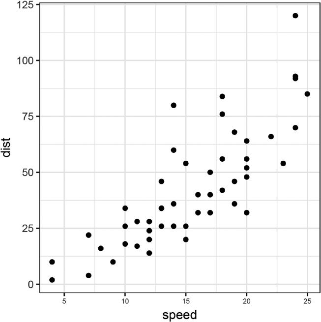
Figure 3-1. Plot of the cars dataset

Don’t worry about the plotting function for now; we return to plotting in the next chapter.

If you are developing new analysis or plotting code, usually one of these datasets is useful for testing it.

Another package with several useful datasets is mlbench. It contains datasets for machine learning benchmarks so these datasets are aimed at testing how new methods perform on known datasets. This package is not distributed together with R, but you can install it, load it, and get a list of the datasets in it like this:

install.packages("mlbench") library(mlbench) library(help = "mlbench")

In this book, I use data from one of those two packages when giving examples of data analyses.

The packages are convenient for me for giving examples, and if you are developing new functionality for R they are suitable for testing, but if you are interested in data analysis, presumably you are interested in your own data, and there they are of course useless. You need to know how to get your own data into R. We get to that shortly, but first I want to say a few words about how you can examine a dataset and get a quick overview.

46

Chapter 3 ■ Data Manipulation

Quickly Reviewing Data

I have already used the function head(), which shows the first n lines of a data frame where n is an option with default 6. You can use another n to get more or less this:

cars %>% head(3) ## speed dist ## 1 4 2 ## 2 4 10 ## 3 7 4

The similar function tail() gives you the last n lines:

cars %>% tail(3) ## speed dist ## 48 24 93 ## 49 24 120 ## 50 25 85

To get summary statistics for all the columns in a data frame, you can use the summary() function:

cars %>% summary ## speed dist ## Min. : 4.0 Min. : 2.00 ## 1st Qu.:12.0 1st Qu.: 26.00 ## Median :15.0 Median : 36.00 ## Mean :15.4 Mean : 42.98 ## 3rd Qu.:19.0 3rd Qu.: 56.00 ## Max. :25.0 Max. :120.00

It isn’t that exciting for the cars dataset, so let’s see it on another built-in dataset:

data(iris) iris %>% summary ## Sepal.Length Sepal.Width Petal.Length ## Min. :4.300 Min. :2.000 Min. :1.000 ## 1st Qu.:5.100 1st Qu.:2.800 1st Qu.:1.600 ## Median :5.800 Median :3.000 Median :4.350 ## Mean :5.843 Mean :3.057 Mean :3.758 ## 3rd Qu.:6.400 3rd Qu.:3.300 3rd Qu.:5.100 ## Max. :7.900 Max. :4.400 Max. :6.900 ## Petal.Width Species ## Min. :0.100 setosa :50 ## 1st Qu.:0.300 versicolor:50 ## Median :1.300 virginica :50 ## Mean :1.199 ## 3rd Qu.:1.800 ## Max. :2.500

47

Chapter 3 ■ Data Manipulation

The summary you get depends on the types the columns have. Numerical data is summarized by their quartiles and meanwhile categorical, and Boolean data is summarized by counts of each category or TRUE/ FALSE values. In the iris dataset there is one column, Species, that is categorical, and its summary is the count of each level.

To see the type of each column, you can use the str() function. This gives you the structure of a data type and is much more general than you need here, but it does give you an overview of the types of columns in a data frame and is very useful for that.

Reading Data

There are several packages for reading data in different file formats, from Excel to JSON to XML and so on. If you have data in a particular format, try to Google for how to read it into R. If it is a standard data format, the chances are that there is a package that can help you.

Quite often, though, data is available in a text table of some kind. Most tools can import and export those. R has plenty of built-in functions for reading such data. Use this to get a list of them:

?read.table

These functions are all variations of the read.table() function, just using different default options. For instance, while read.table() assumes that the data is given in whitespace-separated columns, the read. csv() function assumes that the data is represented as comma-separated values, so the difference between the two functions is in what they consider being separating data columns.

The read.table() function takes a lot of arguments. These are used to adjust it to the specific details of the text file you are reading. (The other functions take the same arguments, they just have different defaults.) The options I find I use the most are these: • header—This is a Boolean value telling the function whether it should consider the first line in the input file a header line. If it’s set to true, it uses the first line to set the column names of the data frame it constructs; if it is set to false the first line is interpreted as the first row in the data frame. • col.names—If the first line is not used to specify the header, you can use this option to name the columns. You need to give it a vector of strings with a string for each column in the input. • dec—This is the decimal point used in numbers. I get spreadsheets that use both . and , for decimal points, so this is an important parameter to me. How important it will be to you probably depends on how many nationalities you collaborate with. • comment.char—By default, the function assumes that # is the start of a comment and ignores the rest of a line when it sees it. If # is actually used in your data, you need to change this. The same goes if comments are indicated with a different symbol. • stringsAsFactors—By default, the function will assume that columns containing strings should really be interpreted as factors. Needless to say, this isn’t always correct. Sometimes a string is a string. You can set this parameter to FALSE to make the function interpret strings as strings. This is an all or nothing option, though. If it is TRUE, all columns with strings will be interpreted as factors and if it is FALSE, none of them will.

48