Functions����������������������������������������������������������������������������������������������������������������������

Chapter 7 ■ UnsUpervised Learning

partition <- function(df, n, probs) { replicate(n, split(df, random_group(nrow(df), probs)), FALSE)

I will use a variation of the prediction accuracy function we wrote there for cars but using wines and the accuracy() function instead of rmse():

accuracy <- function(confusion_matrix) sum(diag(confusion_matrix))/sum(confusion_matrix)

prediction_accuracy_wines <- function(test_and_training) { result <- vector(mode = "numeric", length = length(test_and_training)) for (i in seq_along(test_and_training)) { training <- test_and_training[[i]]$training test <- test_and_training[[i]]$test model <- training %>% naiveBayes(type ~ ., data = .) predictions <- test %>% predict(model, newdata = .) targets <- test$type confusion_matrix <- table(targets, predictions) result[i] <- accuracy(confusion_matrix)

} result

We get the following accuracy when we split the data randomly into training and test data 50/50:

random_wines <- wines %>% partition(4, c(training = 0.5, test = 0.5)) random_wines %>% prediction_accuracy_wines ## [1] 0.9747615 0.9726070 0.9756848 0.9729147

This is a pretty good accuracy, so this raises the question of why experts cannot tell red and white wine apart.

Dan looked into this by determining the most significant features that divide red and white wines by building a decision tree:

library('party') tree <- ctree(type ~ ., data = wines, control = ctree_control(minsplit = 4420))

The plot of the tree is too large for me to show here in the book with the size limit for figures, but try to plot it yourself.

He limited the number of splits made to get only the most important features. From the tree, we see that the total amount of sulfur dioxide, a chemical compound often added to wines to prevent oxidation and bacterial activity, which may ruin the wine, is chosen as the root split.

200

Chapter 7 ■ UnsUpervised Learning

Sulfur dioxide is also naturally present in wine in moderate amounts. In the EU the quantity of sulfur dioxide is restricted to 160 ppm for red wine and 210 ppm for white wines, so by law, we actually expect a significant difference of sulfur dioxide in the two types of wine. So he looked into that:

wines %>% group_by(type) %>% summarise(total.mean = mean(total.sulfur.dioxide), total.sd = sd(total.sulfur.dioxide), free.mean = mean(free.sulfur.dioxide), free.sd = sd(free.sulfur.dioxide)) ## # A tibble: 2 × 5 ## type total.mean total.sd free.mean free.sd ## <fctr> <dbl> <dbl> <dbl> <dbl> ## 1 red 46.46779 32.89532 15.87492 10.46016 ## 2 white 138.36066 42.49806 35.30808 17.00714

The average amount of total sulfur dioxide is indeed lower in red wines, and thus it makes sense that this feature is picked as a significant feature in the tree. If the amount of total sulfur dioxide in a wine is less than or equal to 67 ppm, we can say that it is a red wine with high certainty, which also fits with the summary statistics.

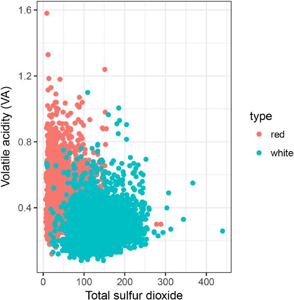
Another significant feature suggested by the tree is the volatile acidity, also known as the vinegar taint. In finished (bottled) wine a high volatile acidity is often caused by malicious bacterial activity, which can be limited by the use of sulfur dioxide, as described earlier. Therefore we expect a strong relationship between these features (see Figure 7-18).

qplot(total.sulfur.dioxide, volatile.acidity, data=wines, color = type, xlab = 'Total sulfur dioxide', ylab = 'Volatile acidity (VA)')

201

Chapter 7 ■ UnsUpervised Learning

Figure 7-18. Sulfur dioxide versus volatile acidity

The plot shows that the amount of volatile acidity as a function of the amount of sulfur dioxide. It also shows that, especially for red wines, the volatile acidity is low for wines with a high amount of sulfur dioxide. The pattern for white wine is not as clear. However, Dan observed, as you can clearly see in the plot, a clear difference between red and white wines when considering the total.sulfur.dioxide and volatile. acidity features together.

So why can humans not taste the difference between red and white wines? It turns out that sulfur dioxide cannot be detected by humans in free concentrations of less than 50 ppm. Although the difference in total sulfur dioxide is very significant between the two types of wine, the free amount is on average below the detection threshold, and thus humans cannot use it to distinguish between red and white.

wines %>% group_by(type) %>% summarise(mean = mean(volatile.acidity), sd = sd(volatile.acidity)) ## # A tibble: 2 × 3 ## type mean sd ## <fctr> <dbl> <dbl> ## 1 red 0.5278205 0.1790597 ## 2 white 0.2782411 0.1007945

202

Chapter 7 ■ UnsUpervised Learning

Similarly, acetic acid (which causes volatile acidity) has a detection threshold of 0.7 g/L, and again we see that the average amount is below this threshold and thus is undetectable by the human taste buds.

So Dan concluded that some of the most significant features which we have found to tell the types apart only appear in small concentrations in wine that cannot be tasted by humans.

Fitting Models

Regardless of whether we can tell red wine and white wine apart, the real question we want to explore is whether the measurements will let us predict quality. Some of the measures might be below human tasting ability, but the quality is based on human tasters, so can we predict the quality based on the measurements?

Before we build a model, though, we need something to compare the accuracy against that can be our null-model. If we are not doing better than a simplistic model, then the model construction is not worth it.

Of course, first, we need to decide whether we want to predict the precise quality as categories or whether we consider it a regression problem. Dan looked at both options, but since we should mostly look at the quality as a number, I will only look at the latter.

For regression, the quality measure should be the root mean square error and the simplest model we can think of is just to predict the mean quality for all wines.

rmse <- function(x,t) sqrt(mean(sum((t - x)^2)))

null_prediction <- function(df) { rep(mean(wines$quality), each = nrow(df))

rmse(null_prediction(wines), wines$quality) ## [1] 70.38242

This is what we have to beat to have any model worth considering.

We do want to compare models with training and test datasets, though, so not use the mean for the entire data. So we need a function for comparing the results with split data.

To compare different models using rmse() as the quality measure we need to modify our prediction accuracy function. We can give it as parameter the function used to create a model that works with predictions. It could look like this:

prediction_accuracy_wines <- function(test_and_training, model_function) {

result <- vector(mode = "numeric", length = length(test_and_training)) for (i in seq_along(test_and_training)) { training <- test_and_training[[i]]$training test <- test_and_training[[i]]$test model <- training %>% model_function(quality ~ ., data = .) predictions <- test %>% predict(model, newdata = .) targets <- test$quality result[i] <- rmse(predictions, targets)

} result

Here we are hardwiring the formula to include all variables except for quality which is potentially leading to overfitting, but we are not worried about that right now.

203

Chapter 7 ■ UnsUpervised Learning

To get this to work we need a model_function() that returns an object that works with predict(). To get this to work, we need to use generic functions, something we will not cover until Chapter 10, but it mostly involves creating a “class” and defining what predict() will do on objects of that class.

null_model <- function(formula, data) { structure(list(mean = mean(data$quality)), class = "null_model")

predict.null_model <- function(model, newdata) { rep(model$mean, each = nrow(newdata))

This null_model() function creates an object of class null_model and defines what the predict() function should do on objects of this class. We can use it to test how well the null model will perform on data:

test_and_training <- wines %>% partition(4, c(training = 0.5, test = 0.5)) test_and_training %>% prediction_accuracy_wines(null_model) ## [1] 49.77236 50.16679 50.11079 49.59682

Don’t be too confused about these numbers being much better than the one we get if we use the entire dataset. That is simply because the rmse() function will always give a larger value if there is more data and we are giving it only half the data that we did when we looked at the entire dataset.

We can instead compare it with a simple linear model:

test_and_training %>% prediction_accuracy_wines(lm) ## [1] 42.30591 41.96099 41.72510 41.61227

Dan also tried different models for testing the prediction accuracy, but I have left that as an exercise.

Exercises

Try the following exercises to become more comfortable with the concepts discussed in this chapter.

Exploring Other Formulas

The prediction_accuracy_wines() function is hardwired to use the formula quality ~ . that uses all explanatory variables. Using all variables can lead to over-fitting so it is possible that using fewer variables can give better results on the test data. Add a parameter to the function for the formula and explore using different formulas.

Exploring Different Models

Try using different models than the null model and the linear model. Any model that can do regression and defines a predict() function should be applicable. Try it out.

Analyzing Your Own Dataset

Find a dataset you are interested in investigating and go for it. To learn how to interpret data, you must use your intuition on what is worth exploring and the only way to build that intuition is to analyze data.

204

CHAPTER 8

More R Programming

In this chapter, we leave data analysis and return to programming and software development, topics that are the focus of the remaining chapters of the book. Chapter 1 gave a tutorial introduction to R programming but left out a lot of details. This chapter covers many of those details while the next two chapters will cover more advanced aspects of R programming: functional programming and object oriented programming.

Expressions

We begin the chapter by going back to expressions. Everything we do in R involves evaluating expressions. Most expressions we evaluate to do a computation and get the result, but some expressions have sideeffects—like assignments—and those we usually evaluate because of the side-effects.

Arithmetic Expressions

We saw the arithmetic expressions in Chapter 1, so we will just give a very short reminder here. The arithmetic expressions are operators that involve numbers and consist of the unary operators + and -:

+ x - x

where + doesn’t really do anything, while - changes the sign of its operand. Then there are the infix operators for addition, subtraction, multiplication, and division:

x + y x - y x * y x / y

Division will return a floating-point number even if both its operands are integers, so if you want to do integer division, you need the special operator for that:

x %/% y

If you want the remainder of integer division, you need this infix operator instead:

x %% y

Chapter 8 ■ More r prograMMing

Finally, there are operators for exponentiation. To compute xy, you can use either of these two operators:

x ^ y x ** y

In all these examples, x and y can be numbers or variables referring to numbers (actually, vectors of numbers since R always works on vectors), or they can be other expressions evaluating to numbers. If you compose expressions from infix operators, you have the same precedence rules you know from arithmetic. Exponentiation goes before multiplication that goes before addition, for example. This means that you will need to use parentheses if you need to evaluate the expressions in another order.

Since the rules are the ones you are used to, this is not likely to cause you troubles, except if you combine these expressions with the operator :. This isn’t really an arithmetic operator but it is an infix operator for generating sequences, and it has a higher precedence than multiplication but lower than exponentiation. This means that 1:2**2 will evaluate the 2**2 expression first to get 1:4 and then construct the sequence:

1:2**2 ## [1] 1 2 3 4

The expression 1:2*2 will evaluate the : expression first to create a vector containing 1 and 2 and then multiply this vector with 2:

1:2*2 ## [1] 2 4

Since the unary - operator has higher precedence than : it also means that -1:2 will give you the sequence from -1 to 2 and not the sequence containing -1 and -2. For that, you need parentheses:

-1:2 ## [1] -1 0 1 2 -(1:2) ## [1] -1 -2

Functions are evaluated before the operators:

1:sqrt(4) ## [1] 1 2

Boolean Expressions

For Boolean values—those that are either TRUE or FALSE—you also have logical operators. The operator ! negates a value:

!TRUE ## [1] FALSE !FALSE ## [1] TRUE

206