Portfolio of Yongqin Zhao 2025 Design Technology by Yongqin Zhao

PORTFOLIO OF YONGQIN ZHAO DESIGN COMPUTATION

2021-2025

DESIGN COMPUTATION

PORTFOLIO OF YONGQIN ZHAO

ACADEMIC A

Pennington Park: Integrated Design Work Architecture + Landscape

Call of River:

A2 A3

Landscape Urbanism and research

Design Technology:

Grading Design and Remote Sensing with GIS

PROFESSIONAL

Professional Design Work: Landscape, Urbanism, Architecture

Detailing & Computational Design: Detailed Streetscape Design & Parametric Design

Construction Documentation: Drawing of landscape details

How can Landscape - Architecture interfaces be designed not merely as transitional spaces, but as vibrant settings that encourage diverse activities?

Accessibility & ADA

Sensory Experience

Circulation Design

Detailing

How can Buildings and Open Spaces be strategically woven to create vibrant, engaging urban environments?

Programming & Functional Layout

Mixed-Use Integration

Pedestrian-friendly Design

Public Space Activation

Information Retrieval Strategy Development Geometry Exploration Evaluation & Feedback designed activities?

How to Boost the efficiency of Design tasks at various phases? woven together

How do Urban Landscape quantitatively influence human behavior?

Streeview Image Point of Interest

Computer Vision

Spatial Aggregation

Spatial Regression

T R

T1 R1 T2 T3

TOOL & DEV

CRAG4LAUD: A RAG for Design Knowledge

A RAG platform for design professionals to navigate data, project precedents or site-specific strategies.

ArchiGesture: Gesture-Driven Modeling Interface

Sculpt digital forms intuitively using natural hand movements for rapid design exploration

CityEcho: Virtual Civic Engagement Platform

Simulate and capture local contextualized community feedback to guide urban and landscape design.

De-Polarization:

A Graph-based New Paradigm for Browsing and Sharing Experience in Social Media

RESEARCH

Urban Built Envinornment and Mobility:

Measuring the seasonal variations of associations between streetscape and dockless bikeshare trip volume

PENNINGTON PARK

A1

Pennington Park

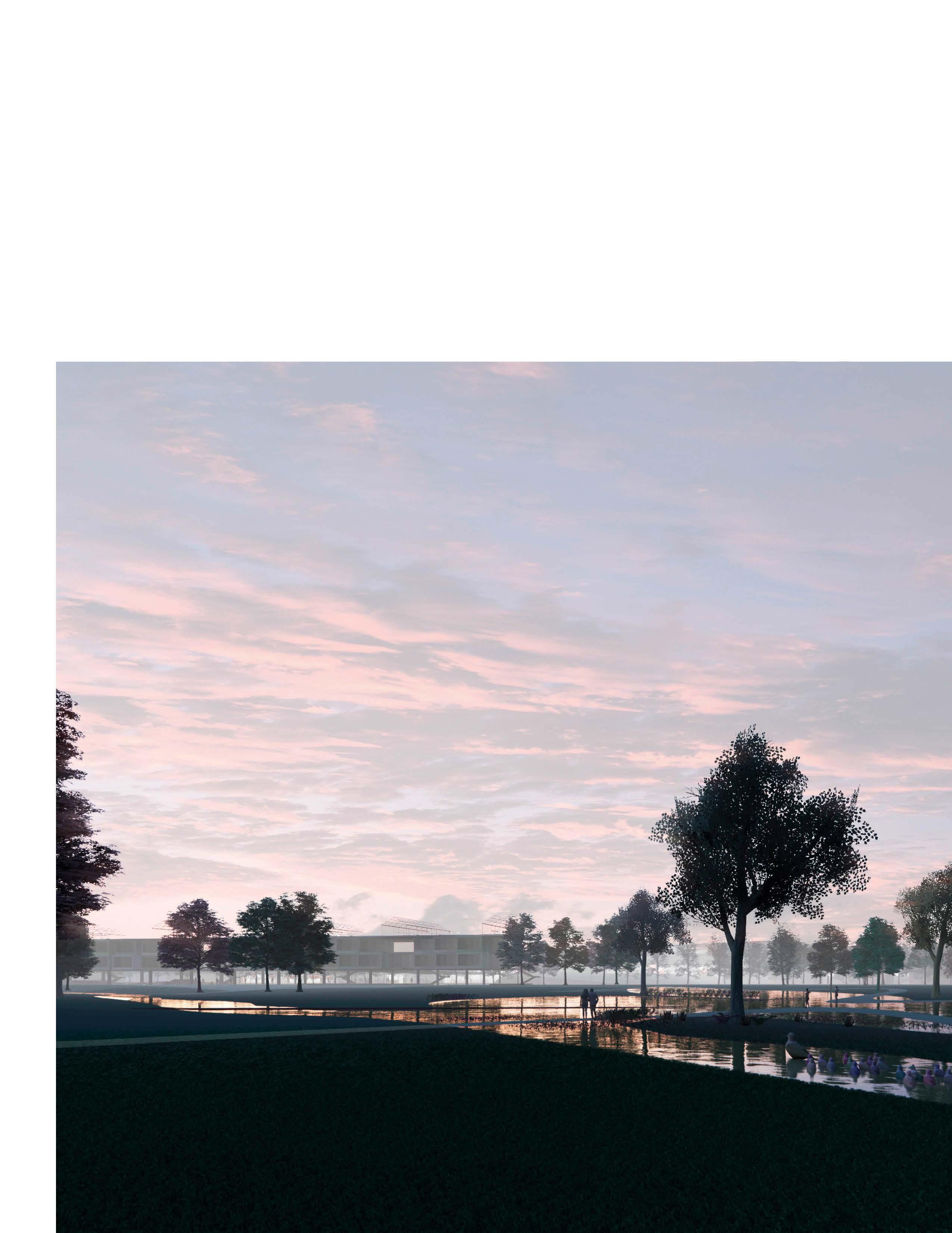
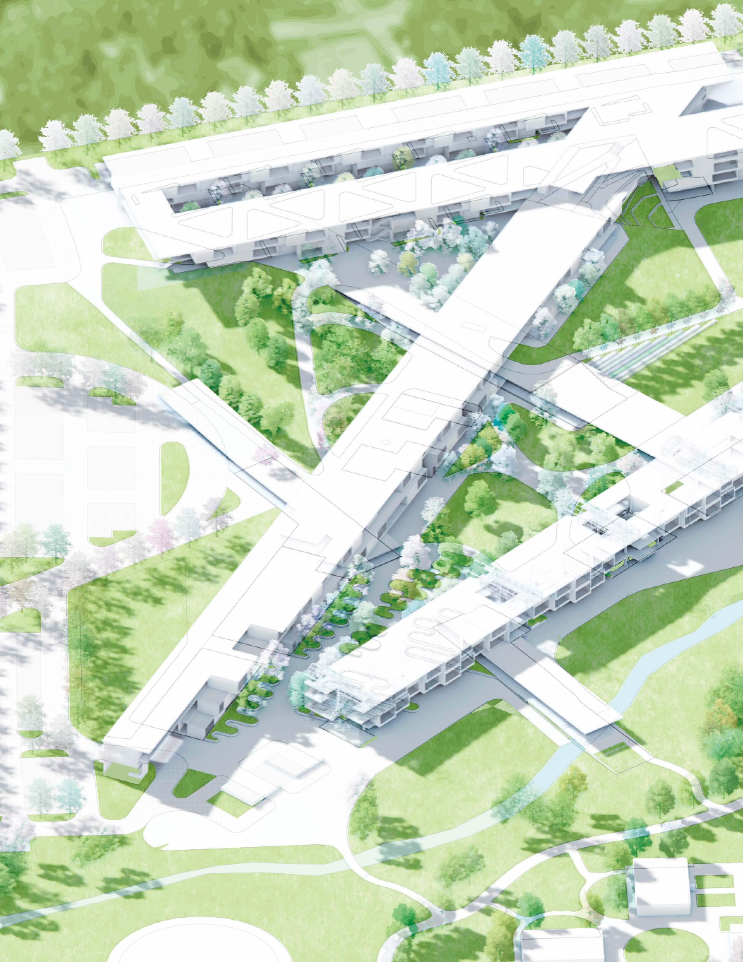
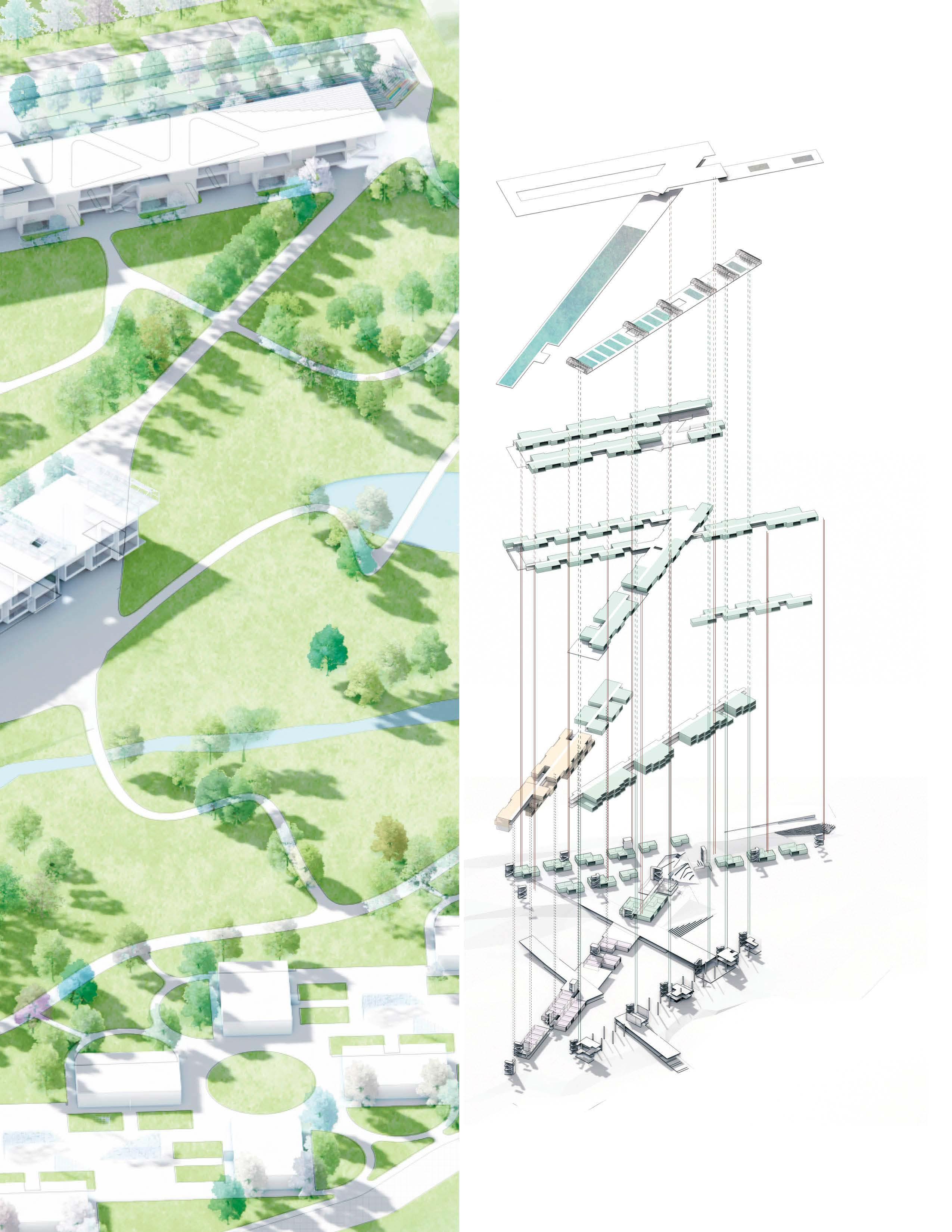
Celebrating Active Senior Living through Seamless Blending Architecture and Landscape

2020 Spring

Professor: Bruce G. Sharky

Individual Design

Graduate Studio Design Award for Design Excellence

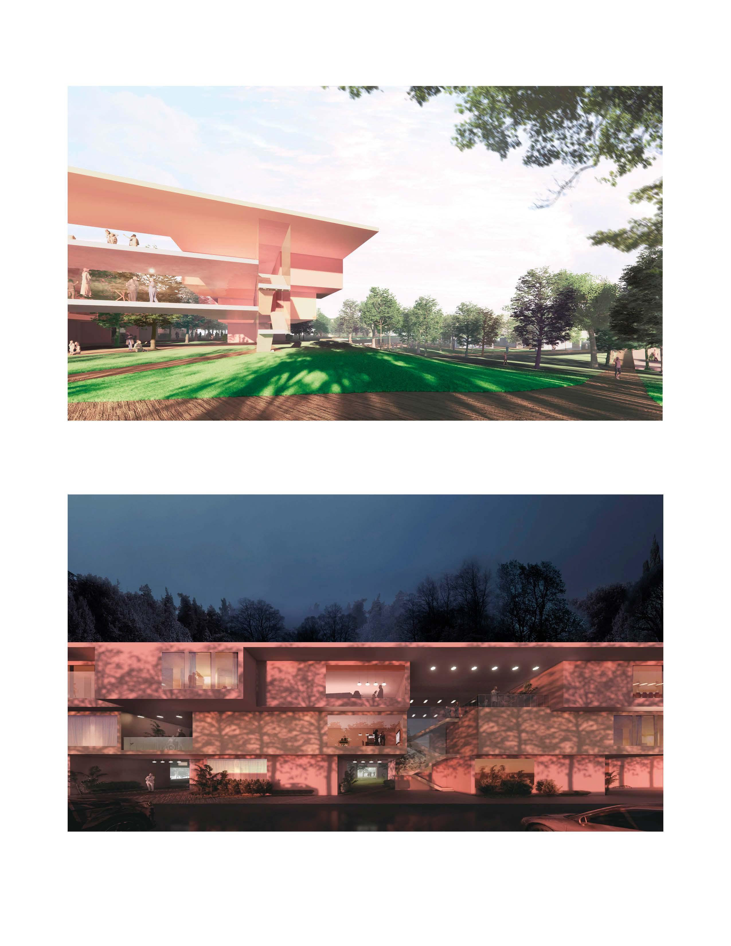
Care for senior residents should holistically integrate healthcare services with active living environments. This design moves beyond traditional institutional designs toward creating spaces that inspire vitality, autonomy, and meaningful social engagement. Senior living is re-envisioned as an organic integration of architectural and landscaped spaces, fostering diverse interactions at multiple scales—from indoor living areas and outdoor natural settings to thoughtfully designed transitional interfaces.

Inspired by globally recognized best practices, this design adopts the Continuing Care Retirement Community (CCRC) concept, accommodating a spectrum of housing solutions ranging from independent living to assisted care, memory care, and rehabilitation services. Within this integrated community, residents receive tailored support that seamlessly adapts to their evolving care requirements, maintaining continuity and enhancing dignity.

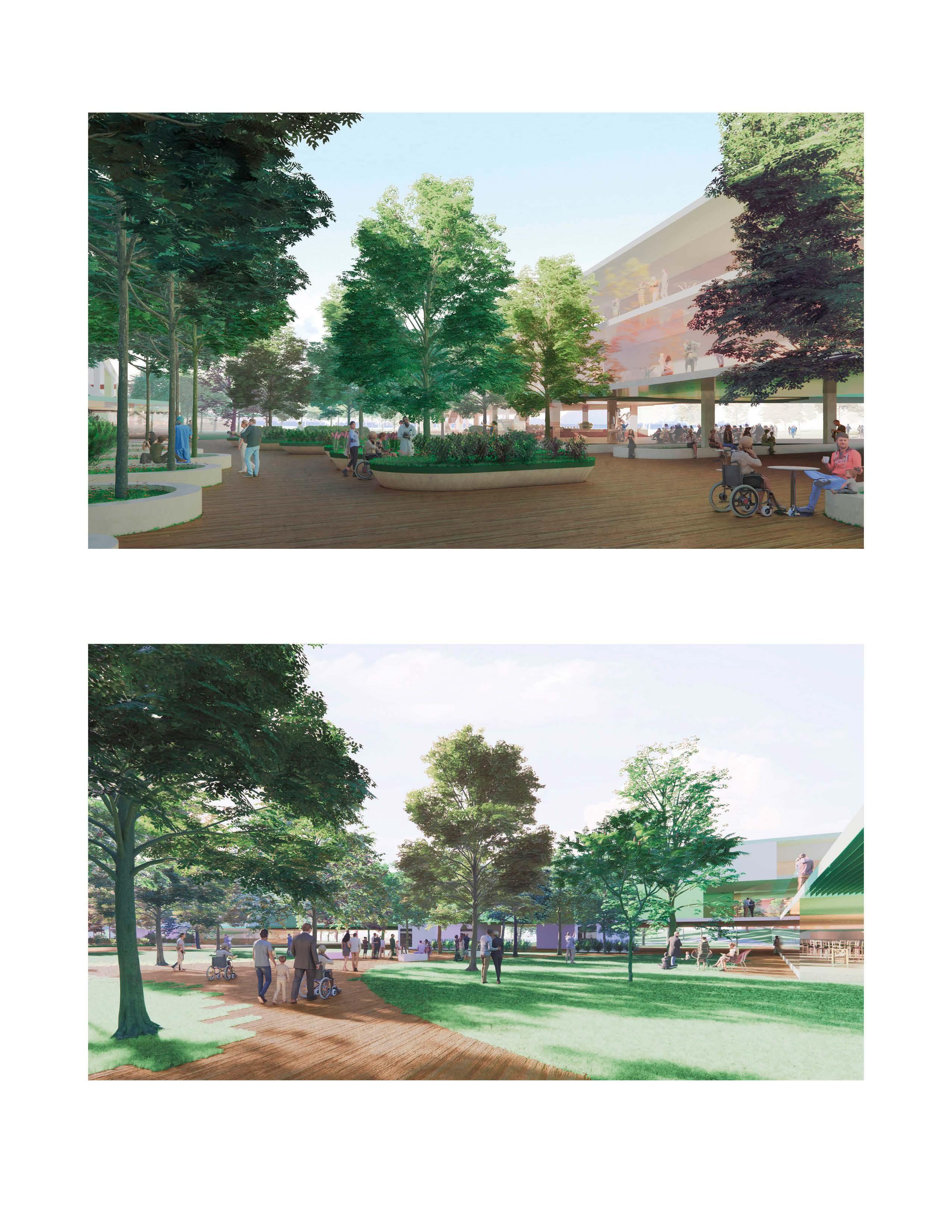
The design emphasizes a purposeful blending of architectural and landscaped spaces, curating a variety of spatial experiences tailored to seniors of varying activity levels and preferences Richly designed outdoor areas invite residents to enjoy abundant sunlight, lush greenery, fresh air, and stimulating sensory environments. A carefully crafted range of landscape-architecture interfaces—from peaceful gardens and intimate courtyards to vibrant communal spaces—encourages residents to regularly engage with outdoor settings and maintain an active lifestyle.

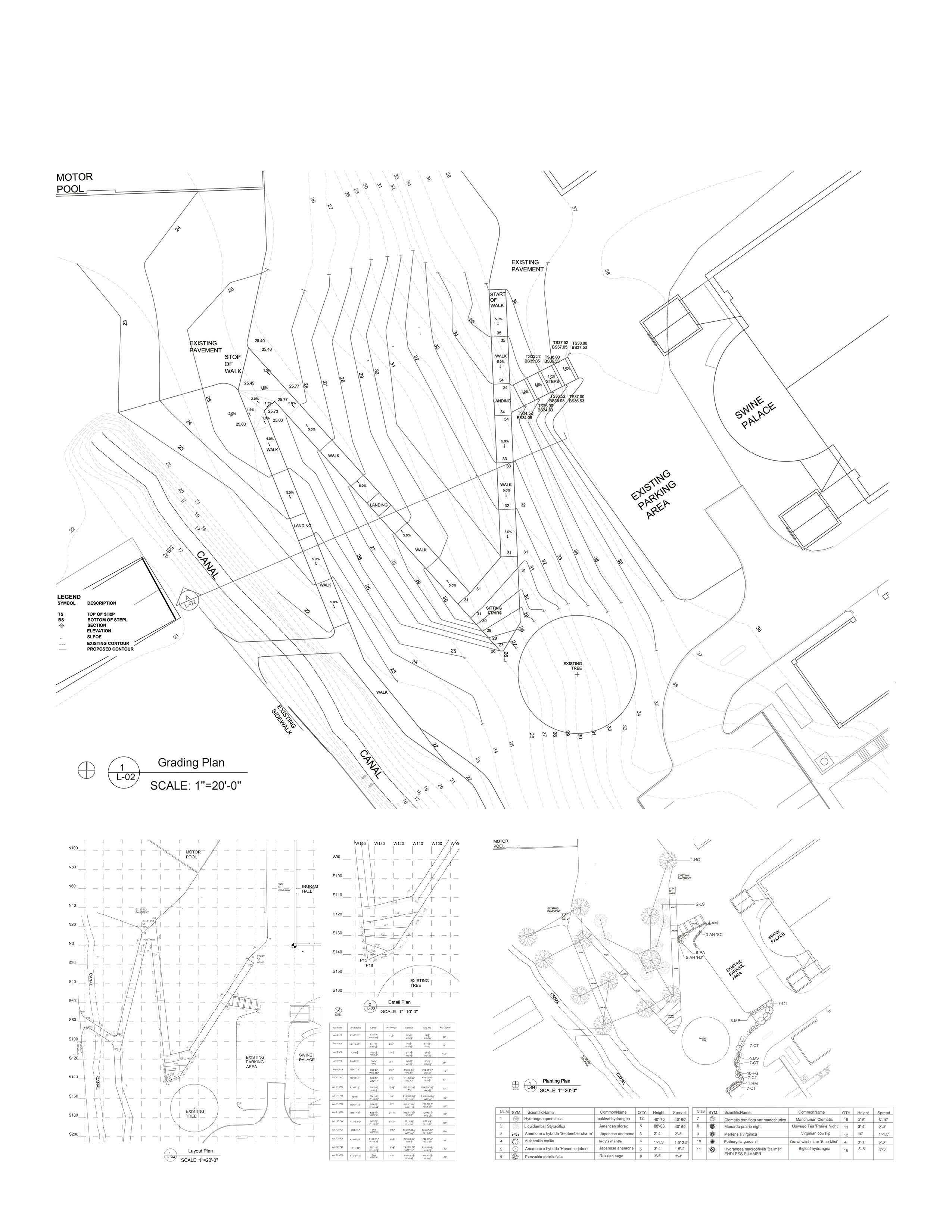
Meticulous attention is given to the connectivity and navigability between diverse spaces. The design incorporates accessible, intuitive, and aesthetically pleasing pathways and transitions. Key details include non-slip paving, outdoor furniture, ample shading structures, strategically placed resting spots, and carefully integrated planting schemes to promote safe and comfortable navigation. Complementary indoor spaces further encourage community participation and social interaction. Collectively, these carefully considered design interventions greatly enhance residents’ autonomy, safety, and overall well-being, celebrating and enriching the senior living experience.

Design an Active Living Spectrum

Classic Senior Living

Isolated Housing or housed in cube

Passively receiving service

Medical centered society.

Mobility and Activity of Various Caring Group

Independent Home Independent Living

Assisted Living Memory Care highest Mobility highest mobility limited mobility high mobility

Senior Campus

The units are group into mini cluster, offering different level of accessibility and activeness could be achieved.

Dynamic Interface

Landscape and Architecture are weaved when they meet, forming a dynamic interface that celetrate active lifestyle.

Active living

The spectrum of space provide active connection from living unit to collective space, to activities and landscape. Clustered Units

Lawn Park Garden

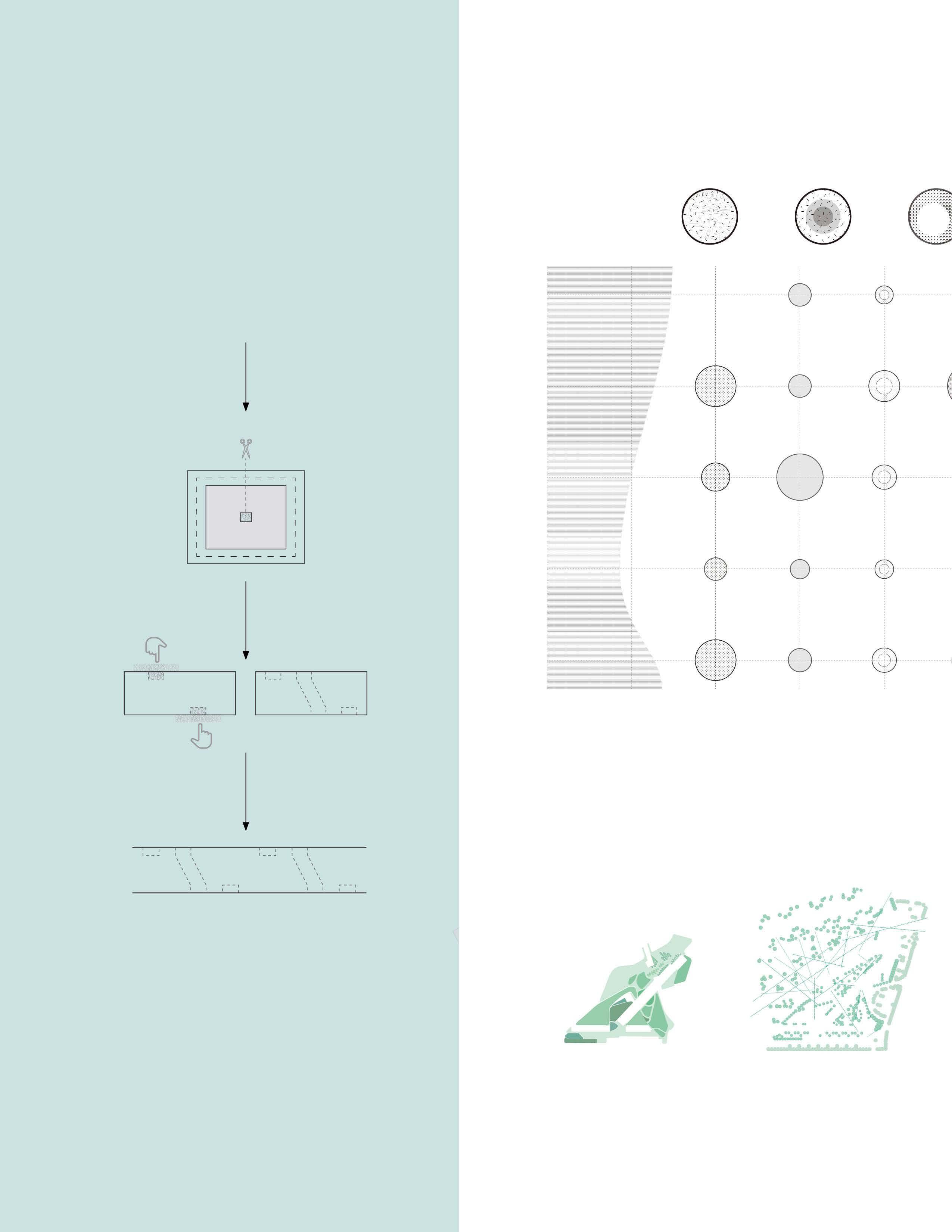
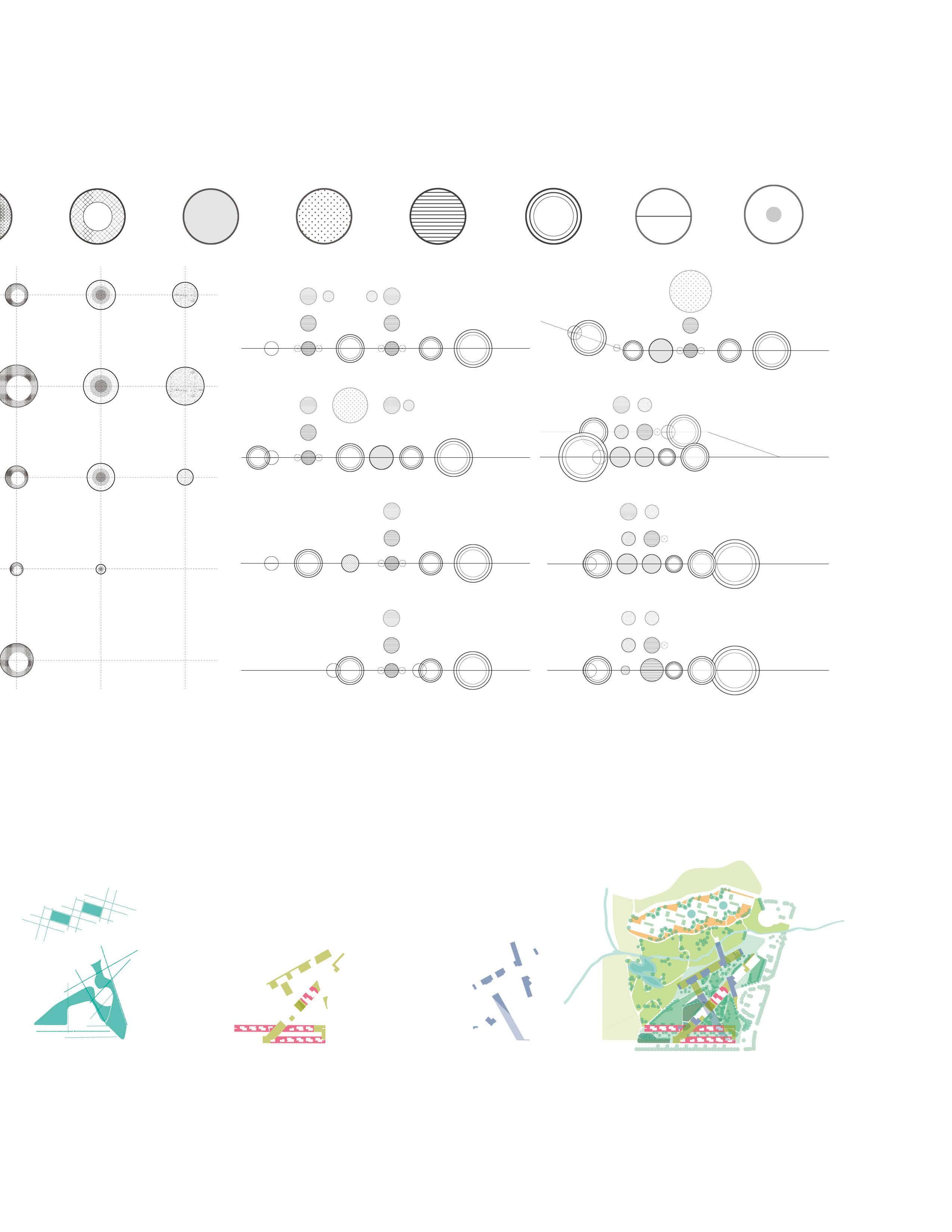
Landscape and Accessibility

Pavement Lawn Slope Sitting Tree Massing Tree Visual Buffer

Outdoor Space

Designing outdoor space should consider the radius(or other option), weaving different highest activity

Master Plan

The Forest Lawn ADA Path

Assisted

Independent Living Memory Care & Medical Service

Rooftop Garden

Sit N’ Chat

Admin + Store

The Studio Healing Yard

Ground Floor Plaza

Independent Living

Assisted Living Independent Living

Central Lawn and Plaza

Admin and Store

The Enjoyment

The Forest

Independent Living

Drop Off

The Tunnel

Assisted Living The Enjoyment

Collective Space

Independent Living The Courtyard

The Forest

Call of River: Relink New Orleans to the Mississippi River

2018

Professor: Lake Douglas

Individual Design

The waterfront of New Orleans, which historically served as one of the city’s most vibrant areas, is now marginal and underutilized.

This project explores a dual-directional design strategy: bottom-up, emphasizing community-driven aspirations for public space, and top-down, considering the visions and interests of developers, commercial entities, and urban stakeholders. By analyzing and recombining these multi-layered perspectives, the design establishes a flexible yet coherent typology for urban parks along the riverfront. Ultimately, the project aims to transform the fragmented waterfront into a cohesive, active urban belt, reconnecting the people, the city fabric, and the Mississippi River—seamlessly linking Audubon Park with the downtown waterfront.

Seeking

Next Parks!

Grown spine

A smooth walk along waterfront from Woldenberg to Audubon

A new way to experience NOLA & embrace life.

A smooth & walkable belt all along waterfront from Woldenberg to Audubon Park

Radiation

BOOM!

Frontier

Potential spot

1.Cruise terminal

2.Convention center

3.Tulane River & Coastal Center

4.Mardi Gras world (Kern studio)

5.River City Venue

6.Power plant (developer purchased)

7.Apartment

8.Shopfront

9.Walmart

10.Gretna-Jackson Avenue ferry

11.Camp Bow Wow

Vacant lot

Unrelated

1.Used car dealer

2.Warehouse

3.NOPD traffic division

4.Auto repair

5.Equipment supplier

Mixed-use medium density

Mixed-use low density

Context of Selected Sites

Further distance

Current user & potential user

Potential place for development or connection (offsite)

Downtown, French Quarter, hotels, riverfront open space & facility, cruise terminal, Convention center, Mardi Gras World, event venue, St. Charles Ave.

CBD office workers, local residents, toursit, visitors from current waterfront

riverfront open space & facility, supermarket Development powerplant, warehouse, vacant lot

Magazine St. Jackson Ave. Louisiana Ave. St. Charles Ave.

Local residents visitors from Magazine St. pet owners.

Connection Magazine St., neighborhood business Development warehouse, vacant lot

Magazine St. Artistic workshop Louisiana Ave. Napoleon Ave. St. Charles Ave.

from Magazine St.

Connection Magazine St., Lyons recreation center, warehouse, music & cultural venue Development warehouse, vacant facility

A epitaxy for inner vitality, making use of 3 main street encircling.

Potential

Deconstruction

From upstream - Interrelationship

Recombination

A_Downtown Connection

Entertainment Function Events Tourism Activity Renewal Additive Heritage Access

Amphitheatre

From downstream - Request

B_Neighborhood Connection

Entertainment Replenish Events Activity Additive Access

C_Urban+scenery

Entertainment Connection Events Function Activity Tourism Additive Heritage Access Attraction

Attraction

Service center

Floating work Canopy Skywalk

Playground

Retail & art

Existing heritage

Festival activity Live show

Exhibition Forum

Rentable pavilion Bazaar

Playground Service center

Festival activity Bazzar Lawn Canopy

Lawn Jogging loop

Attraction

Sports field Canopy Skywalk

Amphitheatre Retail & art

Service center

Existing heritage

Festival activity Live show

Bazaar

Exhibition

Park Plans

A.Potential spot

1.Shop & building

B.Potential spot

DESIGN

A3

Grading Design

GIS Modeling

Remote Sensing in Landscape

Landsat 8 level-1 OLI

Methodology

Based on Landsat 8 data of prefire, post-fire, and 1-year postfire, two vegetation index were introduced to get NBR (Normalized Burn Ratio) and NDVI (Normalized Difference Vegetation Ratio) to compare different method of study forest fire. More info

Conclusion and Discussion

-Data dispersion (histgram)

-NBR can distinguish better and show more sensivity. Especially between the moderate‐extreme classes

-NBR and dNBR are more suitable for detecting different severity levels.

-Suspected similarity between dNBR-dNDVI (right post-fire and 1-year post-fire) and dNBR (pre-fire

Media: ERDAS Imagine, QGIS with SCP plugin and DOS1 atmospheric correction. https://issuu.com/zyq3/docs/yongqin_zhao_project

Park Above the Tracks: Revitalizing an Underground Hub into a Thriving Public Space through TOD Design

2022, Tianhua Urban Design Lab

Concept Design, Master Planning and Site Design

Design: Yongqin Zhao

Render: Yongqin Zhao

Supervisor: Jie Bao

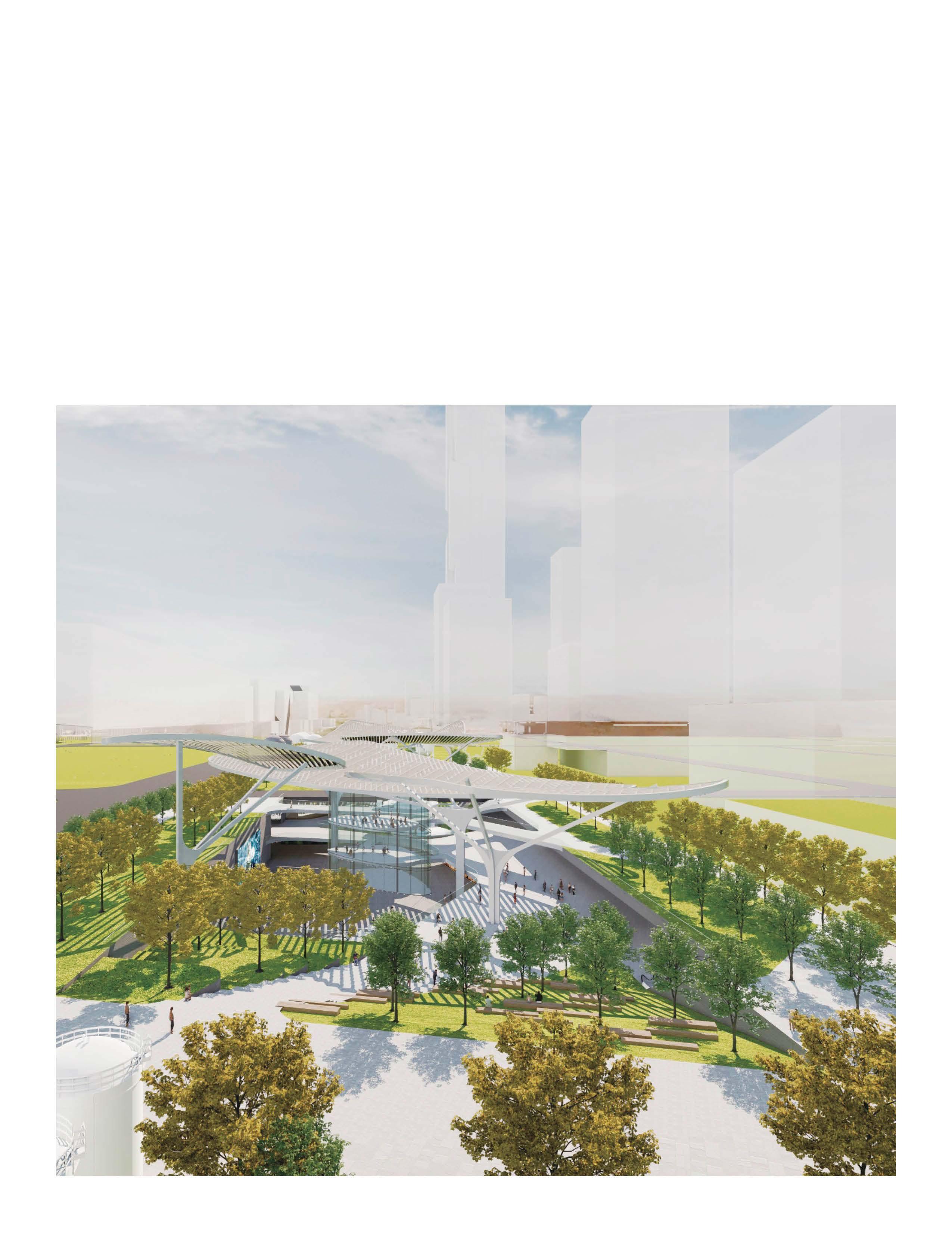
Could a subway station become a vibrant urban park?

Leveraging the exceptional connectivity provided by the intersection of three subway lines and the surrounding urban context, including underground office spaces, this design opens up the traditionally enclosed subway station to create a dynamic public space.

Context

Foundation pit & Landscape

CN Baoshan

Foundation Pit Foundation Pit in this design Proposed Extended Landscape Building Basemennt - B1

Basemennt - B2

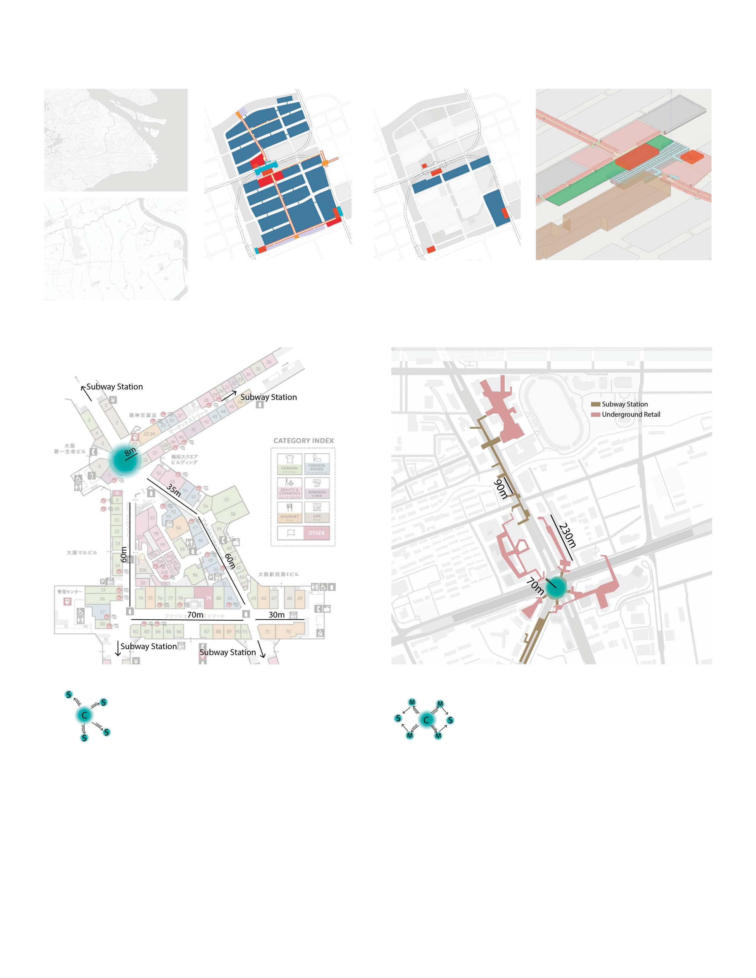
Case Study of Underground Street: Subway x Retail

Case Study 1: Diamor Osaka, Osaka, JP

Case Study 2: Wujiaochang Station, Shanghai, CN

Circulation

Scale

Sunken Plaza as "Core"

Circulation

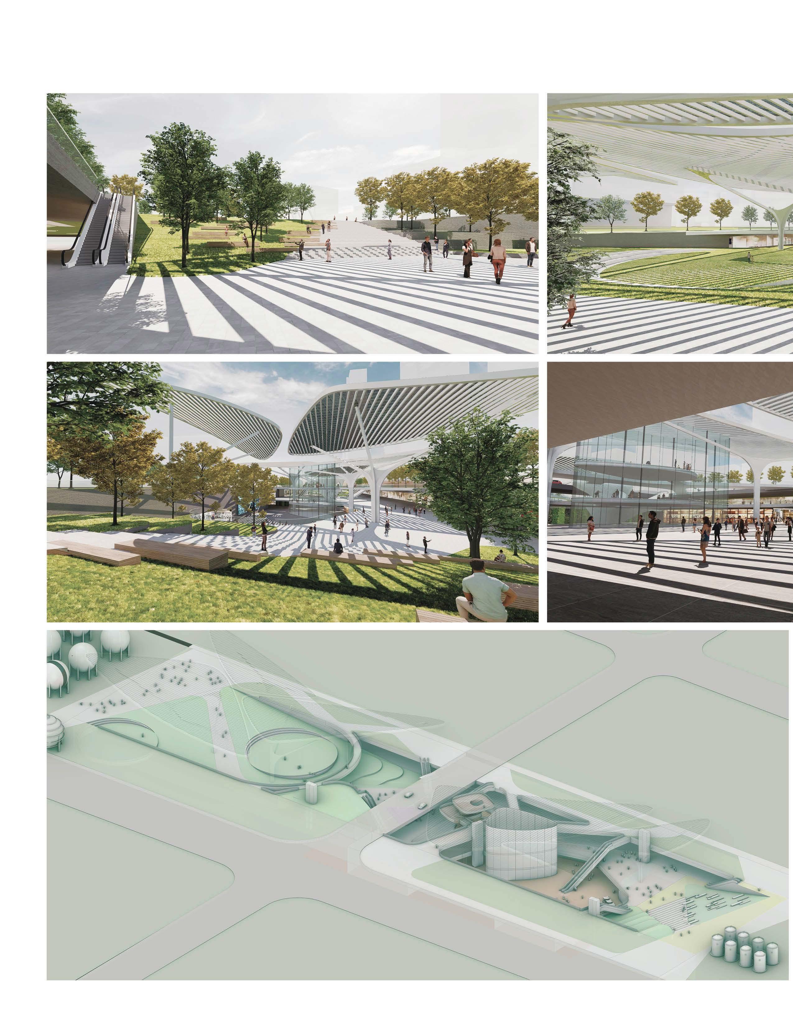
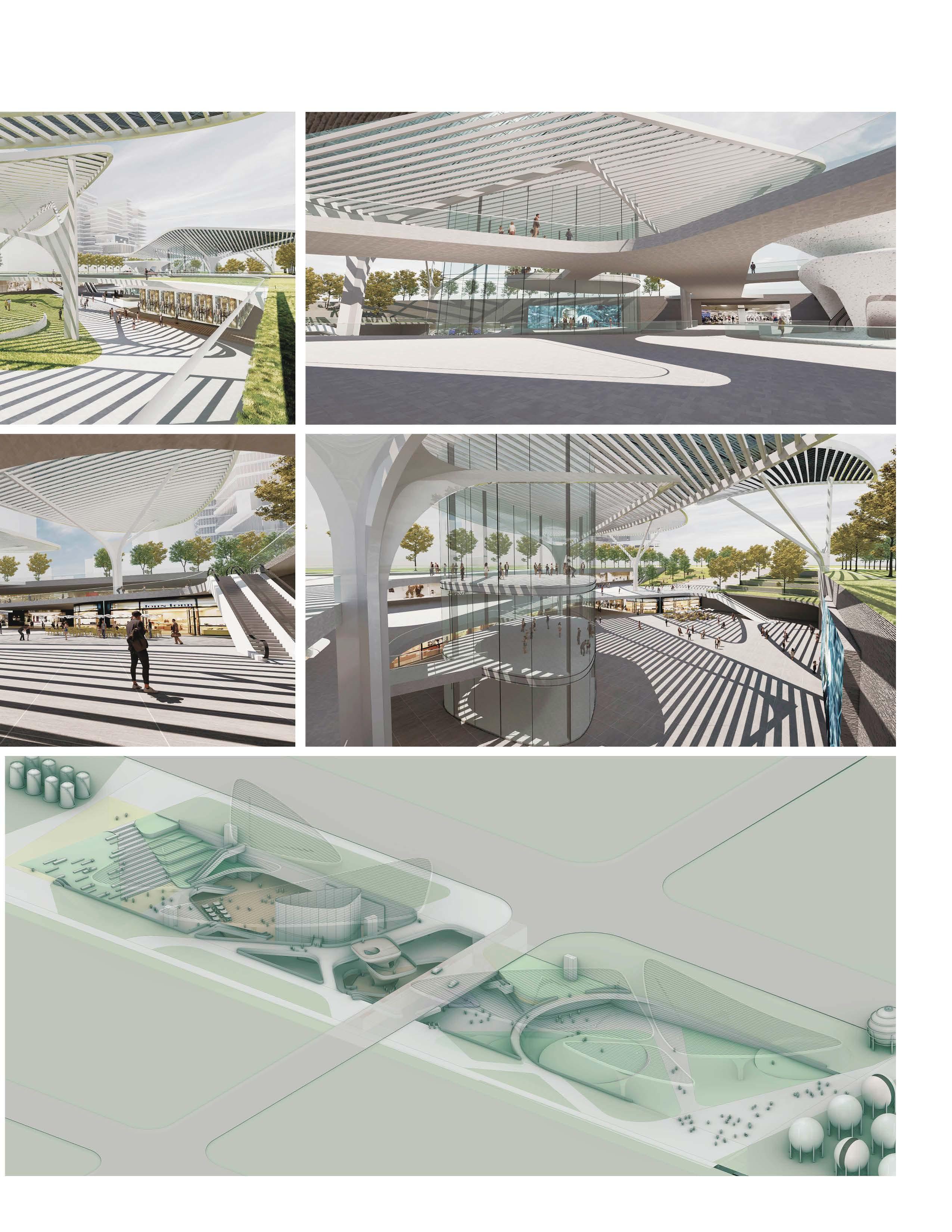
Transform the Foundation Pit to a “Core” that organizes pedestrian flow and connect the subway, office, and surrounding urban spaces with landscape, ensuring quick access to all surrounding blocks within 50 meters.

Place Making into Circulation

Pedestrian

Paved

Pedestrian

Circulation through different level

P1 Heritage Reconnected:

PROFESSIONAL DESIGN WORK 2 .2

Harmonizing Ancestral Heritage with Contemporary Community Hubs and Public Spaces

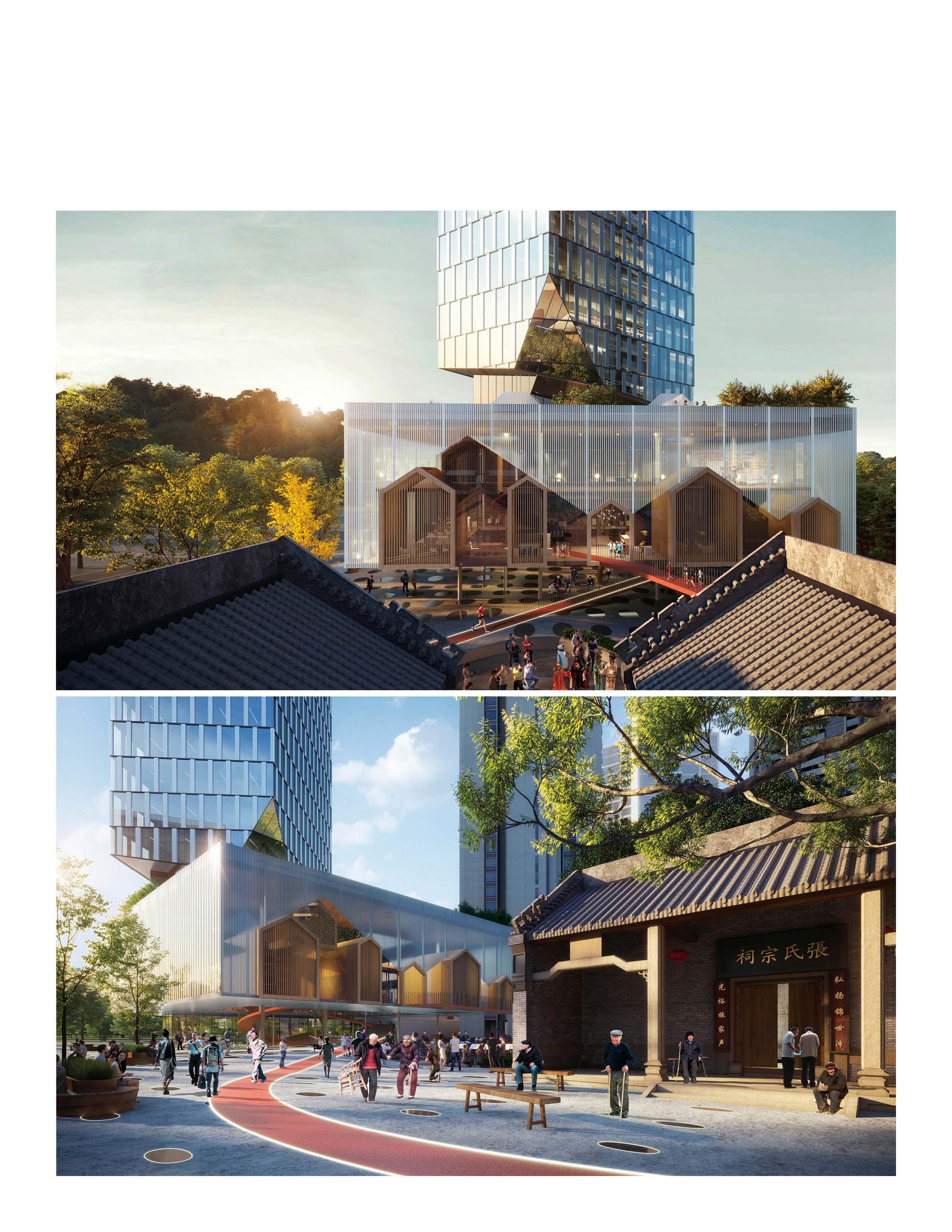
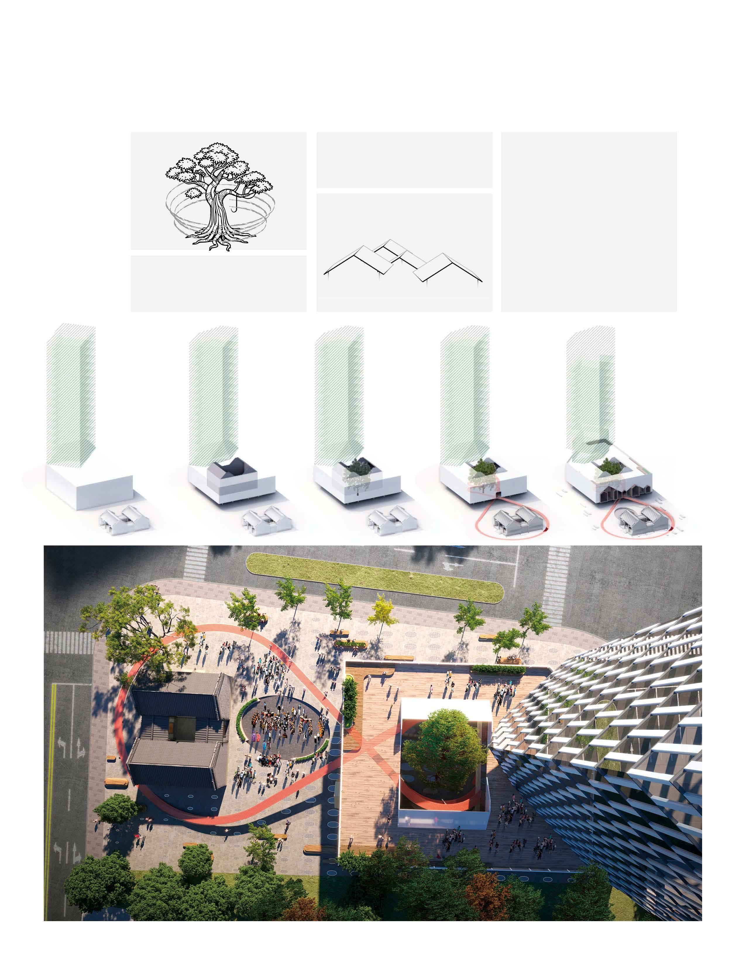
2021, Tianhua Urban Design Lab Concept Design, Civic Community Center

Design: Yongqin Zhao Supervisor: Jie Bao

Cantonese communities maintain strong connections, symbolically anchored by ancestral halls and banyan trees. A modern community center is designed adjacent to the ancestral hall, connecting both structures through similarities in form, spatial arrangement, and circulation patterns.

Concept: Banyan & Ancestral halls

Facade

Massing Mirror the ancestral hall

Banyan

Connect Open & Echo Connect !

PROFESSIONAL DESIGN WORK 3

Design

Competition & Strategy

Park Interface

Professional Work at Dreiseitl Singapore

An integrated design of park’s interface with its urban context, including material, pavement, grading design, etc.

Park Interface Design: Dreiseitl Team,Yongqin Zhao Drawing: Yongqin Zhao

Section drawing Graphic: Yongqin Zhao

Levee Strategy

Design for grading and terrain strategies, including retention pond, sunken plaza, terraced boardwalk, amenities, and some urban design features.

Levee Strategy

Design: Yongqin Zhao, Panpan Zhu

Graphic: Yongqin Zhao

Urban design Framework

Graphic: Yongqin Zhao

Spatial map

Spatial structure

Detailing & Computational Design

Systematic Design of Urban Streetscape & Optimization for Computational Geometry

Parametric Design - Freeform Geometry Rationalization

Professional Work at Tianhua

A freeform geometry is reconfigured into a buildable form by applying a process that imposes finite constraints, ensuring the design maintains its original organic intent while being optimized for construction.

Design: Yongqin Zhao, Jiayan Bao Grasshopper & Detail: Yongqin Zhao Render: Yongqin Zhao, Jiayan Bao

01.Set Magnetic field

Generate magnetic lines of induction along the surface of the pavilion.

02.Filter Magnetic lines

Remove part of the magnetic field lines in the high-density area according to the frequency distribution in the x direction

03.Classify & Regularize lines

Classify lines of magnetic induction into 3 types according to their length, and convert them into 2, 4, and 6 arcs. Screen out arcs with appropriate lengths. The arcs are again grouped into intervals by length. Normalize the length of arc again in each interval.

04.Classify & Extrude

The distribution of the final arc lengths is shown below. Based on the angular proximity between the arc and the surface of the pavilion frame, 4 different sizes of section depth are set.

Pavilion & Planting design (Day)

Lighting(pavilion+pavement) Night

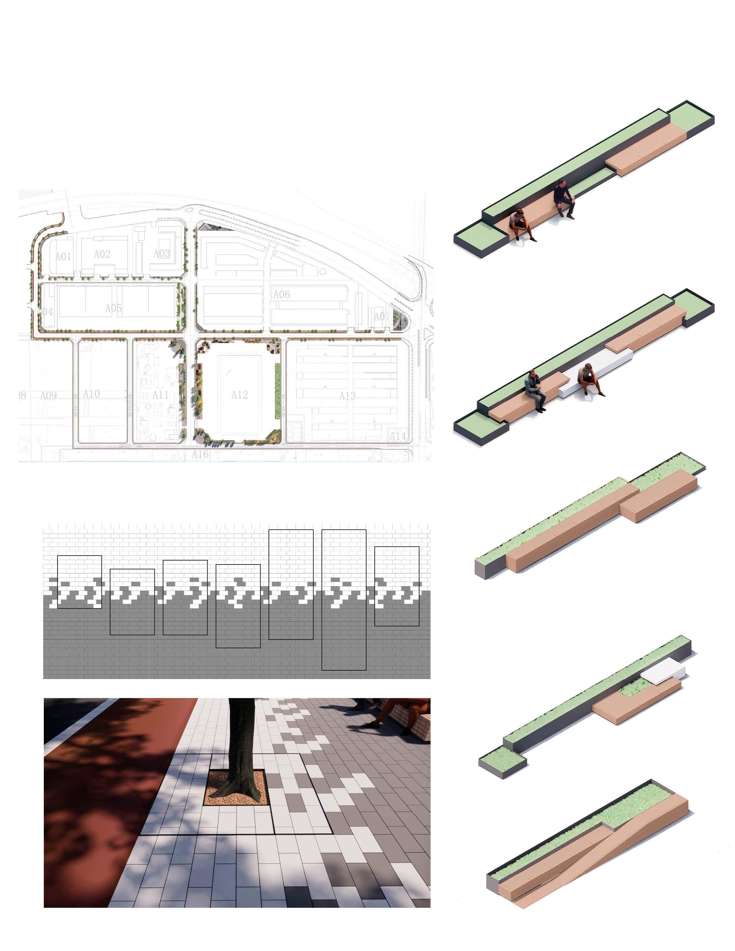
Detailing Design - Pavement, Outdoor Furniture

Professional Work at Tianhua

Under standardized segment scale, the design seamlessly integrates the furniture system, street trees, lighting fixtures, and paving to create a unified and cohesive streetscape.

Design: Yongqin Zhao, Jiayan Bao

Grasshopper & Detail: Yongqin Zhao

Render: Yongqin Zhao, Jiayan Bao

Sidewalk Planning

Paving Design

Planter Bench & Paving Detail

Comb

Landscape Details

Professional Work at Z+T

2019

Professional Work at Z+T Landscape Architect

Water Feature with patterned bricks

Design: Yongqin Zhao, Siyuan Lou Dawing: Yongqin Zhao, Siyuan Lou Supervisor: Hua Zhao

Details of outdoor furnishing Drawing: Yongqin Zhao Supervisor: Hua Zhao 1, 3 2 3

Construction Documentation

Facade Design

Professional Work at Z+T

1-3 3 2 1

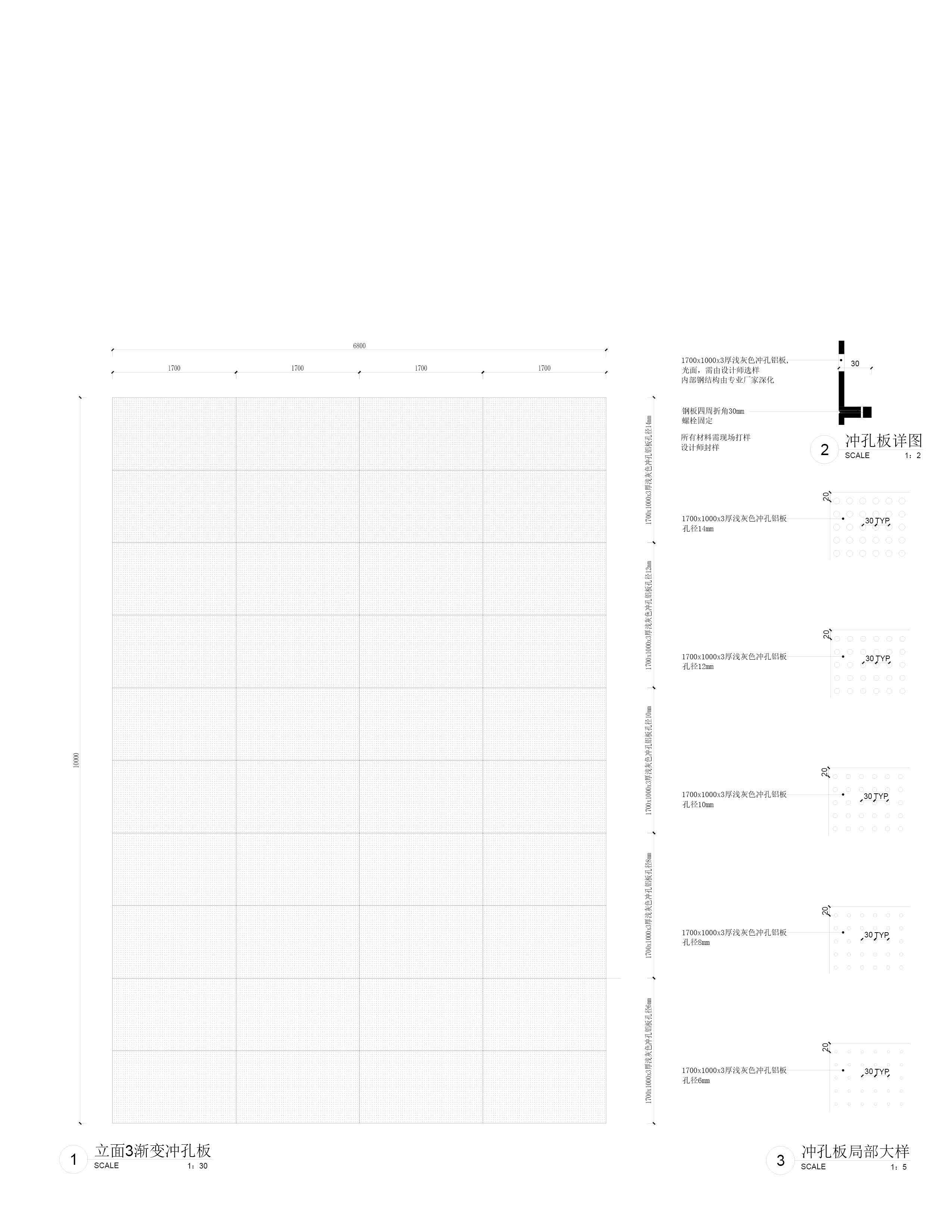
Perforated Plate of Ventilation Facility for Subway Design: Yongqin Zhao, Cheng Xie

Supervisor: Min Xu

TOOL & DEVELOPMENT

TTool Development

A set of Design Technology to enhance current design tasks and streamline the design workflow

2024 - 2025, Individual Work, Implemented Web Tool

Design technology should emphasize a seamless integration of intuitive creativity with structured, data-informed decision-making.

This approach advocates for digital tools and processes that enable fluid transitions between spontaneous ideation and precise execution, promoting rapid prototyping, iterative feedback, and continuous refinement. Accessible and collaborative workflows are prioritized, engaging diverse stakeholders and ensuring technology functions as an extension rather than an obstruction of the creative process.

This section contains a set of tools that leverage technology to amplify designer insight and creativity, fostering richer explorations and more impactful design outcomes.

CRAG4LAUD: A Chatbot RAG for Designers

A RAG platform for design professionals to pinpoint relevant project precedents, regulatory guidelines, or site-specific strategies.

2024 - 2025 ARC Fellowship Research + M.S. Design Technology Thesis, Individual Work, Implemented Web Tool

Thesis Committee ARC Fellowship

Embedding, VectorDB, Frontend & Backend, Data Visualization

Narjes Abbasabadi, Heather Burpee ZGF Firm Advisor Flavia Grey, UW faculty advisor Karen Chen

LangChain, OpenAI, Multer(local), Pinecone(Cloud), React.js, Flask Cytoscape/D3

Project Link & Demo: https://github. com/JornsenChao/ CREG4LAUD

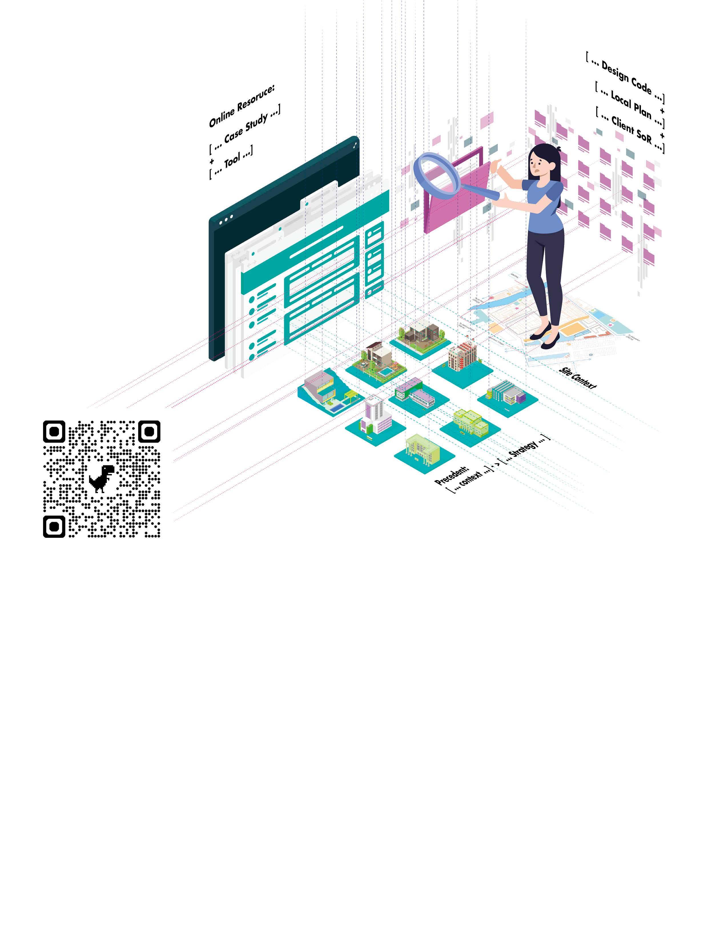
In today’s architectural and landscape projects, designers grapple with vast troves of unstructured documents—lengthy reports, site analyses, and emails without clear indexing. This unstructured mass of text makes it difficult to search for specific strategies or important details, often burying valuable insights within pages of narrative.

A related challenge is the lack of structured, database-driven knowledge. Project experiences are rarely organized with consistent tags or stored in a centralized repository, forcing teams to manually compare disparate files. Without a unified system, it’s hard to draw parallels or build on similar strategies across projects, leading to fragmented lessons and missed opportunities for innovation.

Moreover, hidden links between precedents are often overlooked. When extracting information from multiple sources, inadequate documentation and poor indexing can cause critical connections—such as recurring design principles or regulatory patterns—to go unnoticed. This gap weakens strategy formation, as essential lessons remain isolated rather than forming a cohesive knowledge base.

Early communication suffers, too. During the RFP or conceptual design phase, teams must explain the project environment, needs, and rationale to clients and users. Without a structured body of precedents to reference, articulating well-founded strategies becomes laborious and slow, delaying decision-making and hindering clear, effective collaboration.

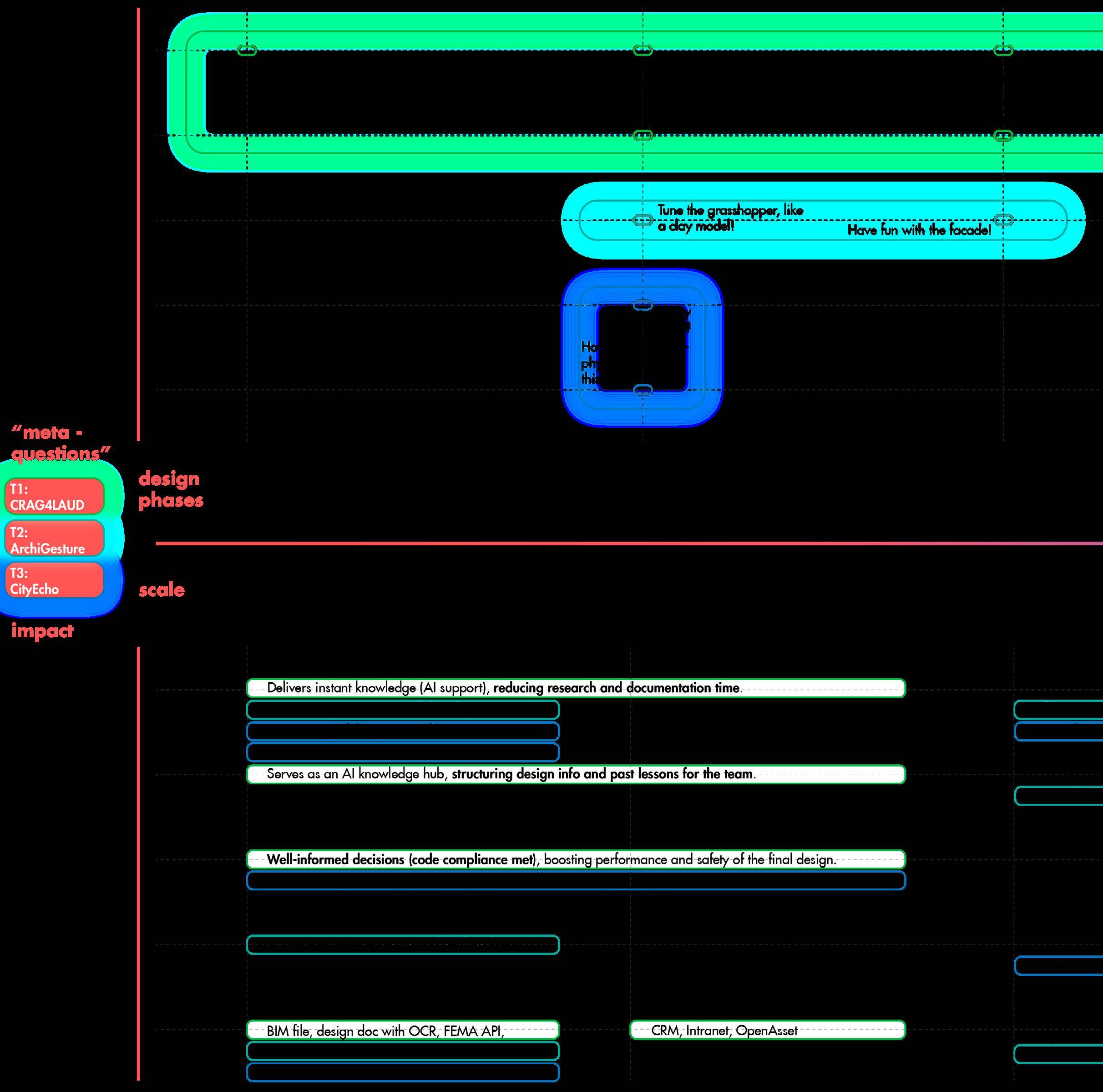
CREG4LAUD (Chatbot RAG for Landscape Architects, Architects, and Urban Planners), a Holistic LLM- Integrated Design Platform, is a specialized platform that integrates large language models (LLMs) with real-time data to streamline architectural and landscape workflows. By allowing users to upload design documents like PDFs or CSVs, it quickly identifies relevant precedents, site strategies, and regulatory guidelines, enabling professionals to accelerate conceptual planning and decision-making. The platform supports knowledge reuse, helping teams leverage past projects to inform new designs efficiently. By retrieving relevant project documents, codes, and firm-specific standards, the platform provides context-aware responses and suggestions that eliminate the typical search overhead.

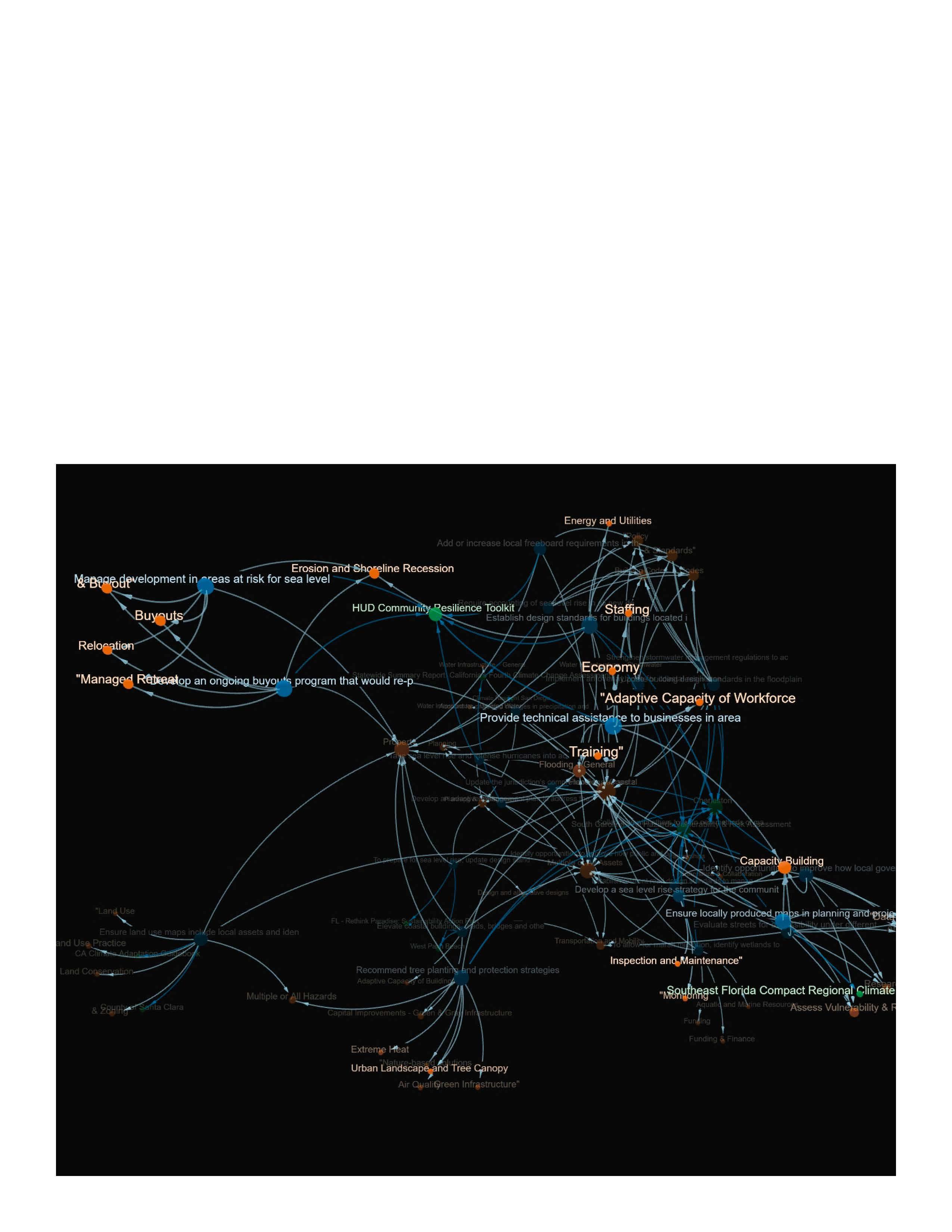
Key features include context-aware responses, the ability to pull insights on zoning regulations, summarize site constraints, and suggest climate-appropriate materials. With tools like graph visualizations and Pinecone VectorStore for relevant search results, CREG4LAUD consolidates fragmented project data into a unified interface. Its RAG workflow ensures that AI-generated responses are always based on up-to-date knowledge, fostering accurate, informed decision-making throughout the design process without the typical search burden. CREG4LAUD enhances collaboration and innovation, accelerating the architectural design journey.

A Comprehensive Resilience Research Workflow

Resilience Step

Task

Informationn Flow

Deliverable

Factors, Questions at each Workflow Step

Factors

Resource (not Project specific)

Other Tools What Factors would be used at each step?

Resource (Project specific)

Precedent & Knowledge

Connsiderations at each Workflow Step

What Questionns will designer ask at each step?

User Questions

'meta-question"

Core Functions

Workflow -> Tool -> Component

Design Phase

Workflow Step

User Questions

User Steps

Tool Components at Frontend

Tool Components at Backend & Database

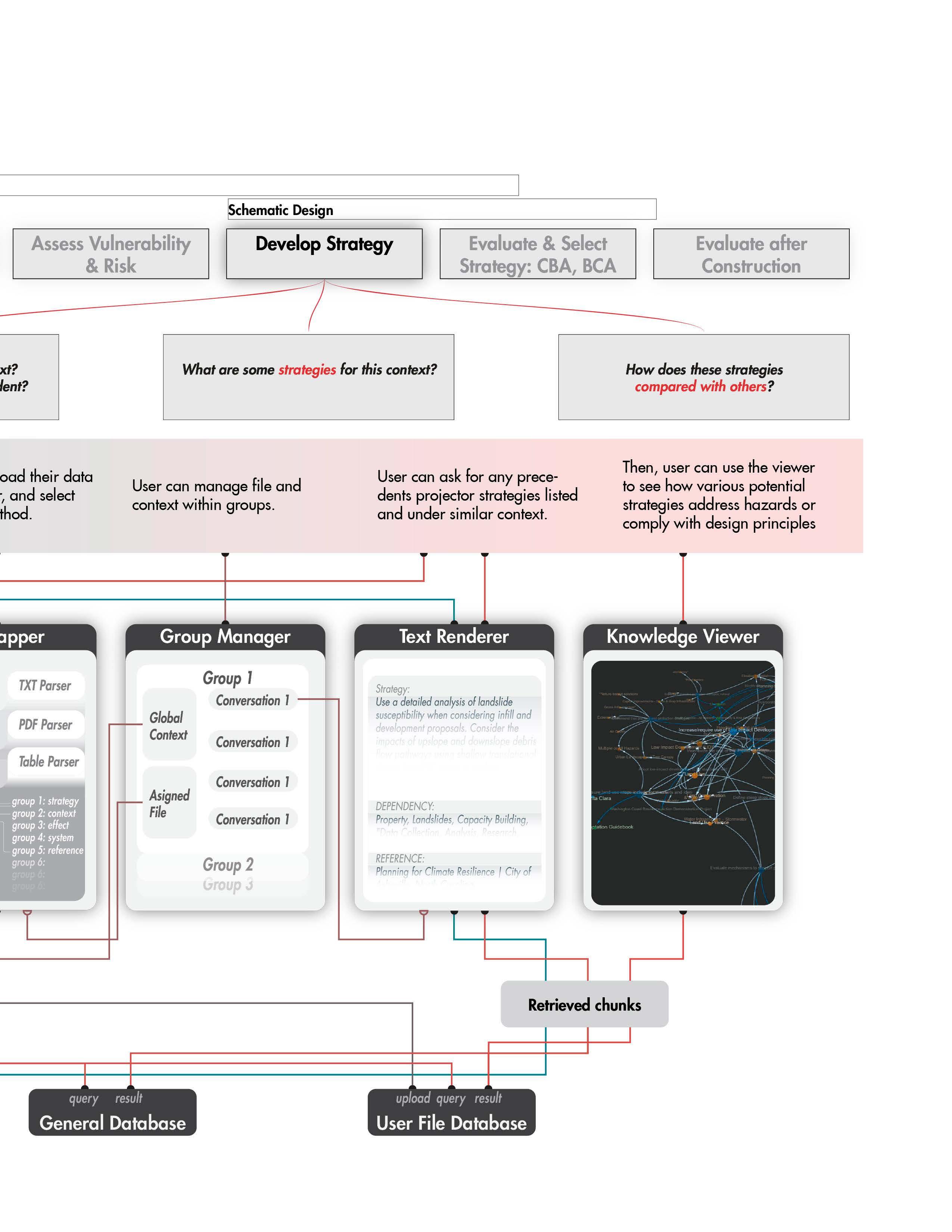
Technical Framework (Example of tabular file)

User Steps

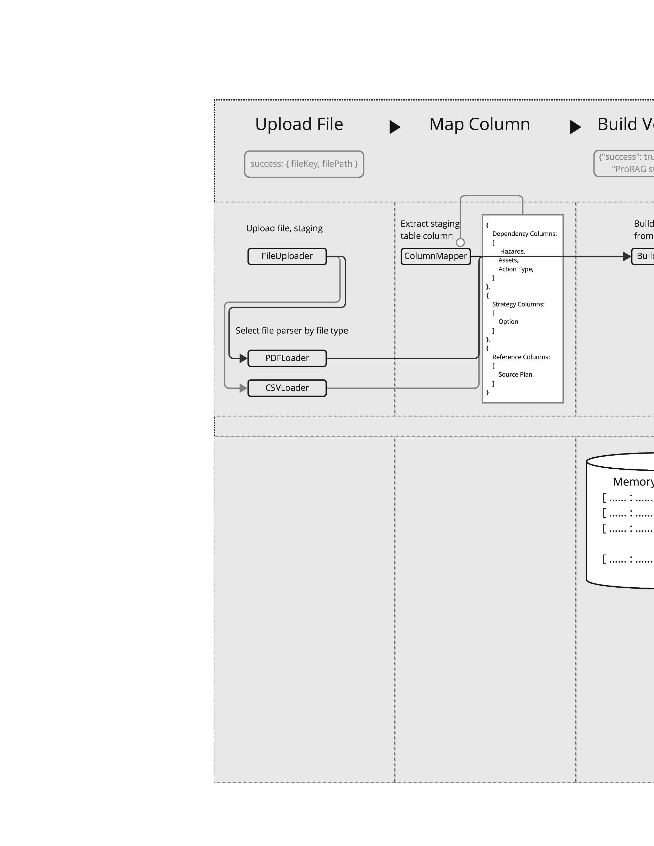
Componenet

Data Generated in the backend

Sculpt digital forms intuitively using natural hand movements for rapid design exploration

2024 - Ongoing

Frontend

Geometry

Motion Capture

Individual, Implemented Web Tool React, Three.js, Mediapipe

Project Link & Demo: https://github.com/ JornsenChao/FingerRender

In the early phases of architectural design, professionals strive to balance aesthetic ambitions with practical constraints. Parametric tools, while essential for exploring a wide range of possibilities, can feel cumbersome during rapid idea sketching. Adjusting a simple slider to alter building height or curvature often seems detached from the creative impulse that fuels innovation. Moreover, the process of converting rough sketches into digital models—complete with coordinates, angles, and numeric inputs—can slow iteration and dampen the free flow of ideas.

These digital environments may also intimidate those less familiar with advanced technology. Reliance on specialized commands, scripts, and nodes creates barriers that can stifle spontaneous creativity . As a result, teams sometimes bypass brilliant shape manipulations or façade variations simply because the digital workflow demands too much technical know-how. Some seasoned architects miss the tactile satisfaction of physically molding materials, finding it challenging to connect a digital representation with the intuitive gestures that once sparked design insights.

Moreover, standard parametric controls typically restrict adjustments to predefined sliders or numeric fields, leaving little room for the organic distortions and emergent forms that can give a project its signature character. Even advanced scripting demands extensive planning and coding, which can sap the spontaneity of onthe-fly experimentation. The result is a digital design pipeline that often feels more analytical than expressive, lacking the dynamic energy of traditional hand sketching. Architects increasingly call for an interface that removes technical hurdles while preserving the intuitive nature of early creative exploration.

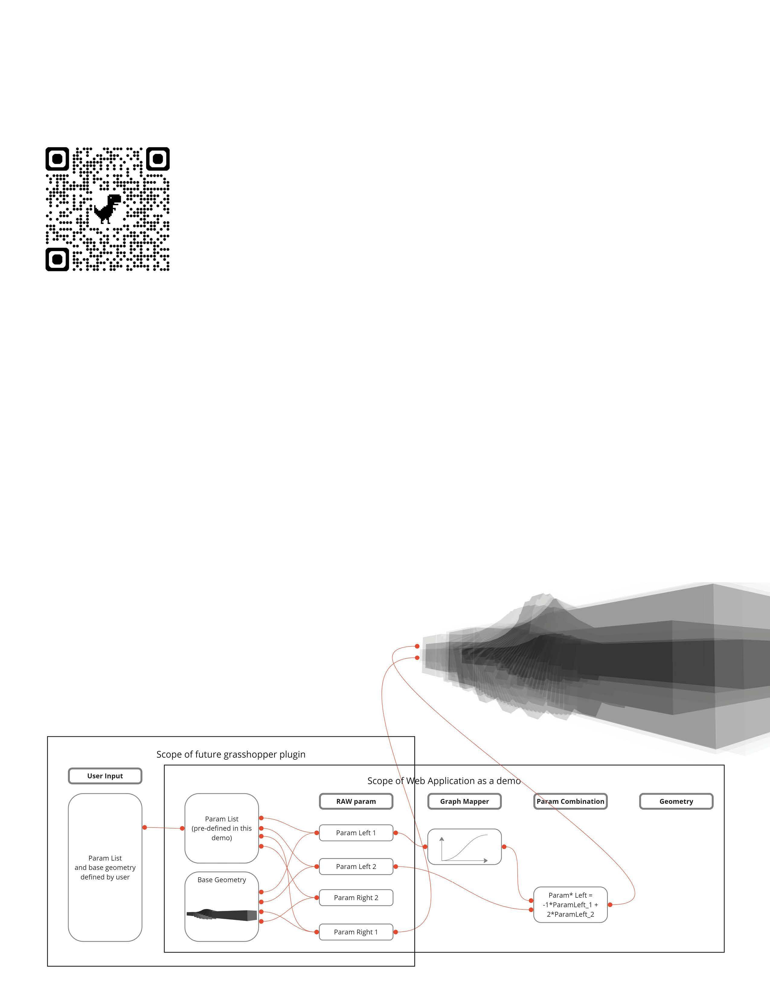
ArchiGesture addresses these challenges through an innovative design interface empowering architects to shape 3D models with intuitive hand movements. Instead of traditional mouse clicks or parametric sliders, users perform mid-air gestures—such as pinching, twisting, or spreading fingers—to manipulate building forms directly. This tactile interaction fosters a playful, sculptural approach to modeling, bridging physical intuition with digital precision. By enabling architects to effortlessly scale volumes, rotate massing, and modify façade patterns in real-time, ArchiGesture promotes iterative experimentation and rapid idea testing.

This gesture-based workflow also democratizes the design process, making parametric experimentation accessible to non-experts and facilitating broader team collaboration. Ultimately, ArchiGesture aims to redefine early conceptual design as immersive, dynamic, and human-centered, enhancing how designers collaboratively shape space and form.

T3

CityEcho: Virtual Civic Engagement Platform

Simulate and capture local contextualized community feedback to guide urban and landscape design.

2024 - Ongoing Individual, Implemented Web Tool

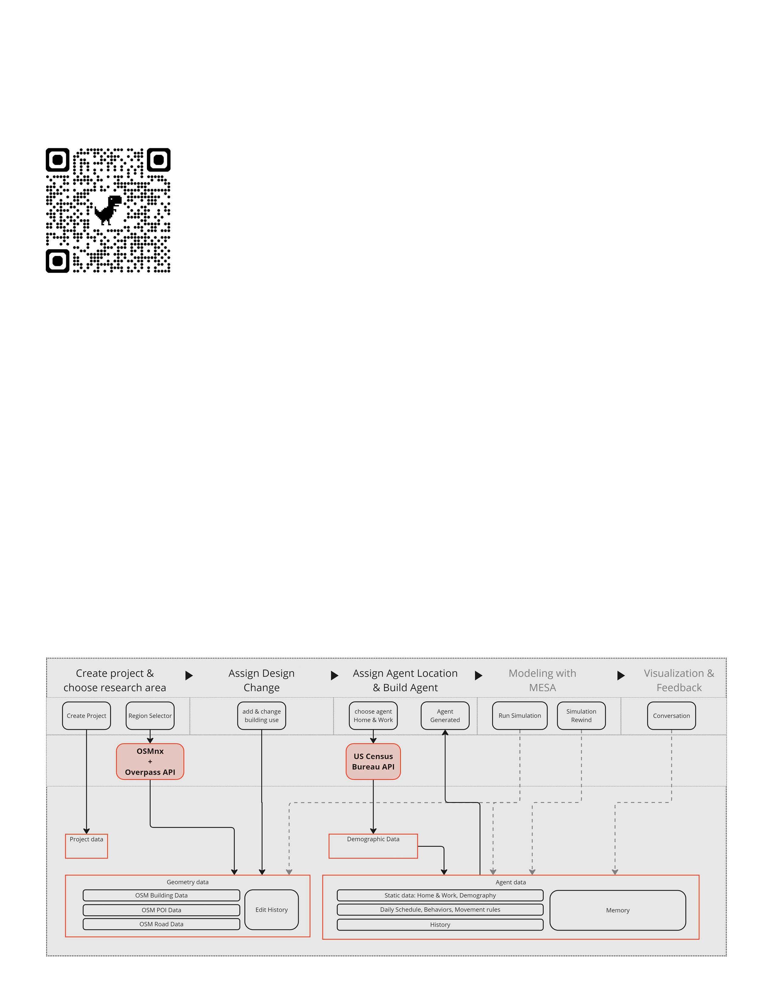
Data Agent Generation Database Modeling Framework

OSMnx, Overpass API, US Census Bureau API, OpenAI API, Posrges + PostSQL, MESA

Project Link & Demo:

https://github.com/ JornsenChao/community-agent-sim-for-designer

Contemporary urban and landscape design faces the ongoing challenge of aligning professional plans with genuine public acceptance. Traditional methods—such as community meetings, questionnaires, and public hearings—often struggle with limited participation and slower feedback. Many residents, including those with mobility challenges, language barriers, or busy schedules, find it difficult to attend in-person events, which can result in proposals that may not fully capture the diverse needs and everyday experiences of the community.

Moreover, public input gathered from conventional surveys is sometimes abstract or fragmented, making it challenging to incorporate nuanced insights into early design stages. Decision-makers may receive a mix of varied suggestions and even contradictory opinions, complicating efforts to predict collective behaviors like pedestrian flows or the use of open spaces.

Current agent-based modeling tools, such as MassMotion, provide valuable insights into observable behaviors but often overlook the richer, subjective experiences of individuals in diverse urban settings. By focusing primarily on movement and aggregated patterns, these models can miss how residents from different backgrounds actually experience their environments—an aspect that is crucial for creating spaces that truly resonate with the community.

CityEcho addresses these challenges by embedding a virtual “community” at the heart of the design process. Rather than waiting for real-life feedback after construction, planners can test ideas early by observing how thousands of digital residents might behave and react. Each resident is endowed with personalized traits, such as household size, mobility preferences, or daily routines, allowing CityEcho to reflect nuanced demographic realities.

During simulation, designers can explore what happens if they add a bike lane, build affordable housing, or adjust park layouts—instantly seeing potential shifts in foot traffic, satisfaction, and resource allocation. This continuous, iterative testing mimics real-world complexity, enabling teams to fine-tune proposals before major budgets are committed. The platform also synthesizes subjective feedback, presenting intangible factors like perceived safety or community sentiment in a visual format that complements quantitative data.

By revealing social dynamics and lived experiences, CityEcho closes the gap between professional planning and grassroots realities, empowering design teams to create more equitable spaces.

De-polarization: A Graph-based New Paradigm for Browsing and Sharing Experience in Social Media

2022 Fall Individual Research + Individual Design

NLP, graph, UI, clustering Media Skill

Kaggle Dataset+ Personal Processing, twarc, nltk, kmeans, keyBERT, Adobe Suites, Gephi, Figma

A new kind of social media architecture to empower individuals’ information control, and a new kind of interface for browsing, reflection, and sharing.

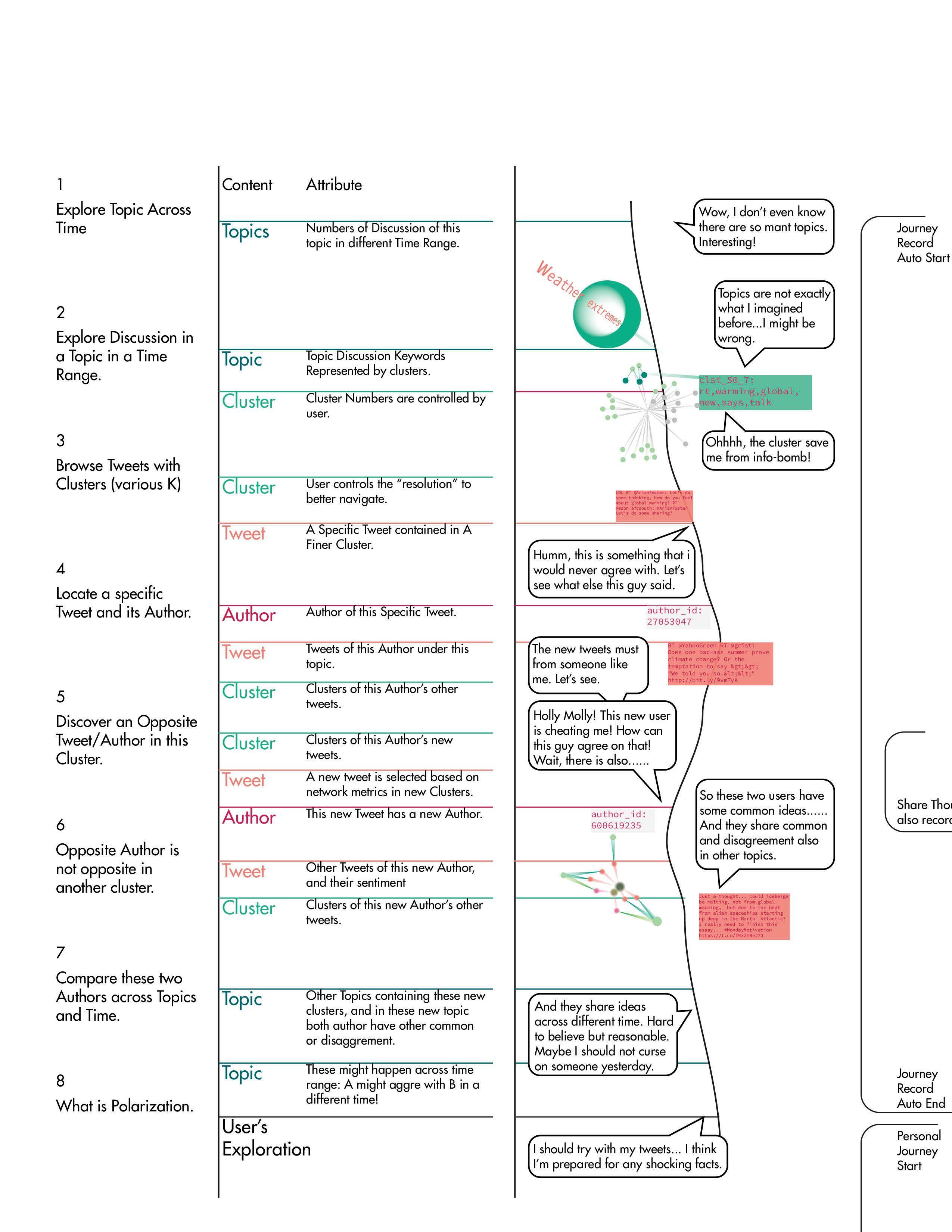
The design of zoom levels displays different levels of detail and attribute of a topic, subtopic, emotion orientation, and even specific tweet. Users can overview the debate while sharing their browsing journey and other evoked thoughts.

Thus, a new social media paradigm is come into existence: a rational and constructive datascape for people to embrace differences while cherish the common.

Data Preparation for Building the Graph and EDA

* Dimitrios Effrosynidis, Alexandros I. Karasakalidis, Georgios Sylaios, Avi Arampatzis, The climate change Twitter dataset, Expert Systems with Applications, Volume 204, 2022, 117541, ISSN 09574174, https://doi.org/10.1016/j.eswa.2022.117541.

* Effrosynidis D, Sylaios G, Arampatzis A (2022) Exploring climate change on Twitter using seven aspects: Stance, sentiment, aggressiveness, temperature, gender, topics, and disasters. PLOS ONE 17(9): e0274213. https://doi.org/10.1371/journal.pone.0274213

A New Type of Data Architecture: Store and Explore

4 Nodes:

4 Edges:

Notes

Building edges between topic and cluster is essential to display complex discussion with high fidelity Tweets under one topic can be clustered in multiple cluster, user could then better navigates their journey in the

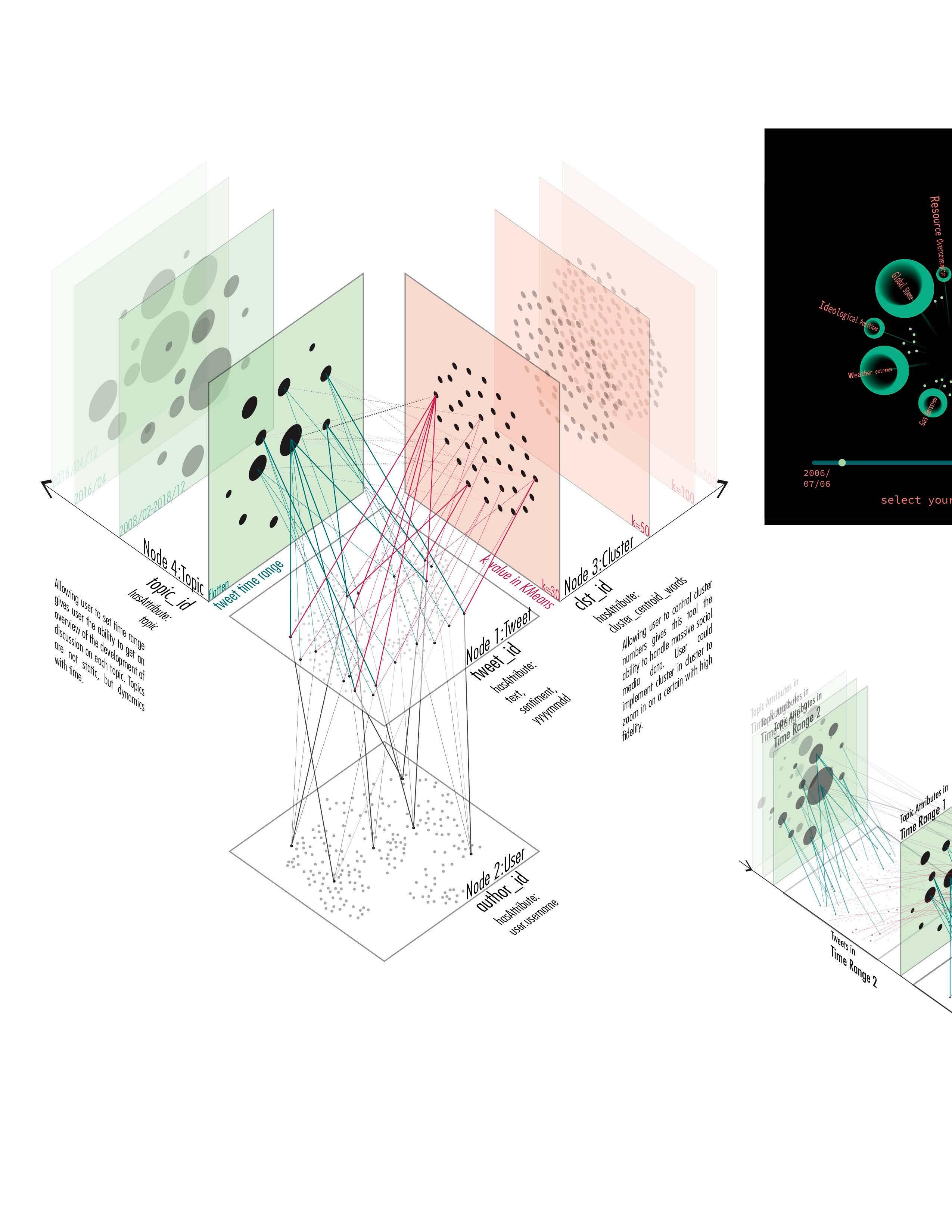
Topics are evolving over time, in time range A but unfashionable Thus, I design the first zoom topic development throughout selects, attributes like number cluster detected with these tweets, terface.

Data Structure & Interface

ZOOM LEVEL 2

ZOOM LEVEL 3

time, a new topic can be popular unfashionable in time range B. zoom level to allow user explore throughout time. In the time range user number of tweets under this topic, tweets, are displayed in the in-

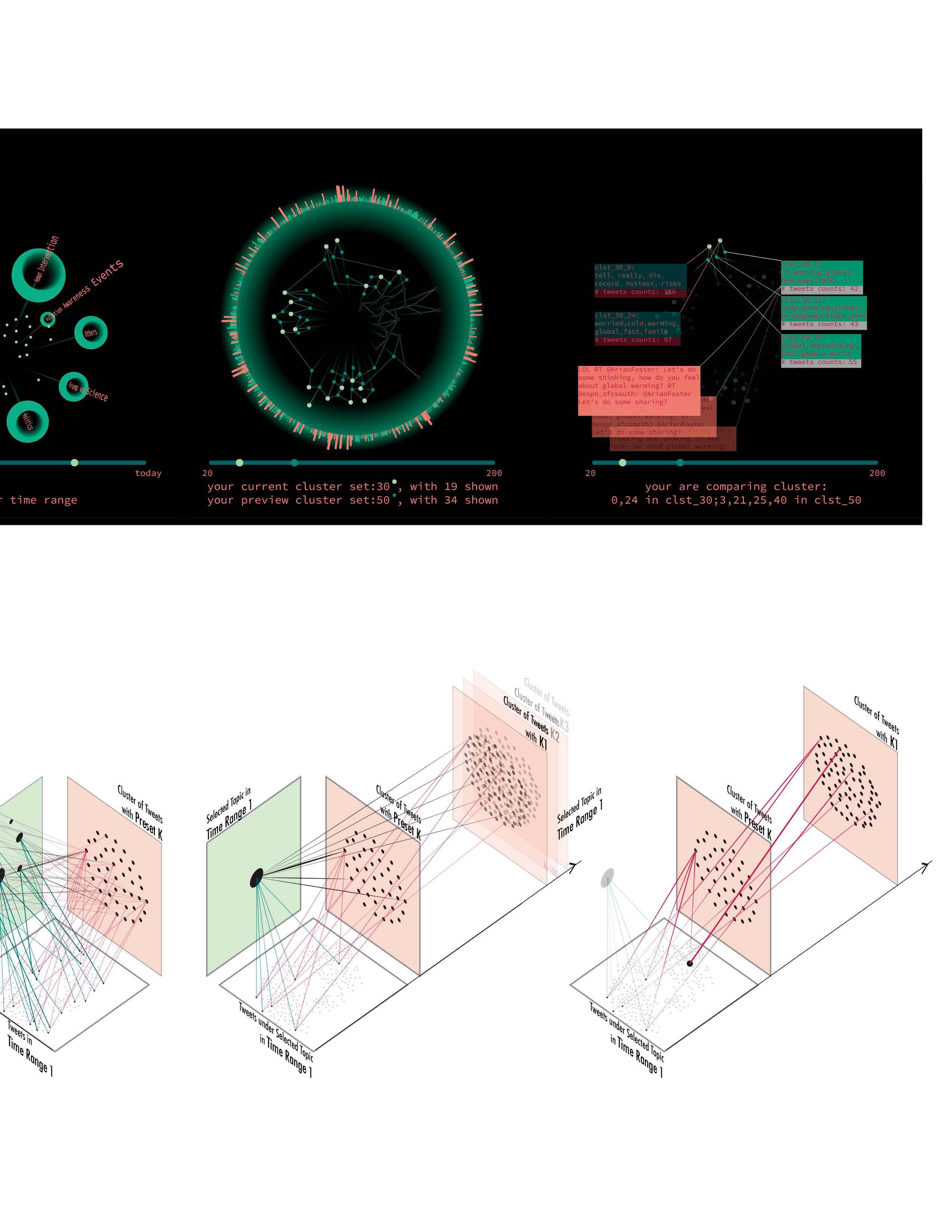
After choosing a topic in a specific time range, user would explore the clusters to navigate his/her browsing experience.

Centroid point of cluster would provide keywords in a cluster. With the user continue his/her experiment on more finer clustering result, discussion in a cluster would have higher fidelity, providing more specific description of a content within a cluster.

Continuing his/her exploration in the clusters, user would finally find a cluster with concrete information, and a limited number of tweets under this cluster.

Zoom Level: Data Structure & Interface

ZOOM LEVEL 4

Locate a specific Tweet and its Author.

ZOOM LEVEL 5

Discover an Opposite Tweet/Author in this Cluster

After choosing a specific tweet, more attributes of this tweet would pop up: author of this tweet, and other tweets from this author “author1” under the chosen topic in the chosen time range. And cluster (k is what the user set at last step) of the new tweets.

Under a cluster of other tweet from “author1”, another tweet is recommended, based on graph metrics like betweenness, tweet numbers, and sentiment. This new tweet from “potential hater” would have opposite sentiment with “author1”.

An ideal “potential hater” would have tweets with an overlap in clusters with that of “author1”, and under a same cluster tweets from both authors can be similar or opposite.

Opposite Author is not opposite

But other tweets from this “potential similar sentiment with “author1”. cluster can have have consensus

ZOOM

ZOOM LEVEL 7

opposite in another cluster. Compare these two Authors across Topics and Time.

ZOOM LEVEL 8

Polarization and Depolarization.

“potential hater” could have “author1”. Opposite authors in one consensus in another cluster.

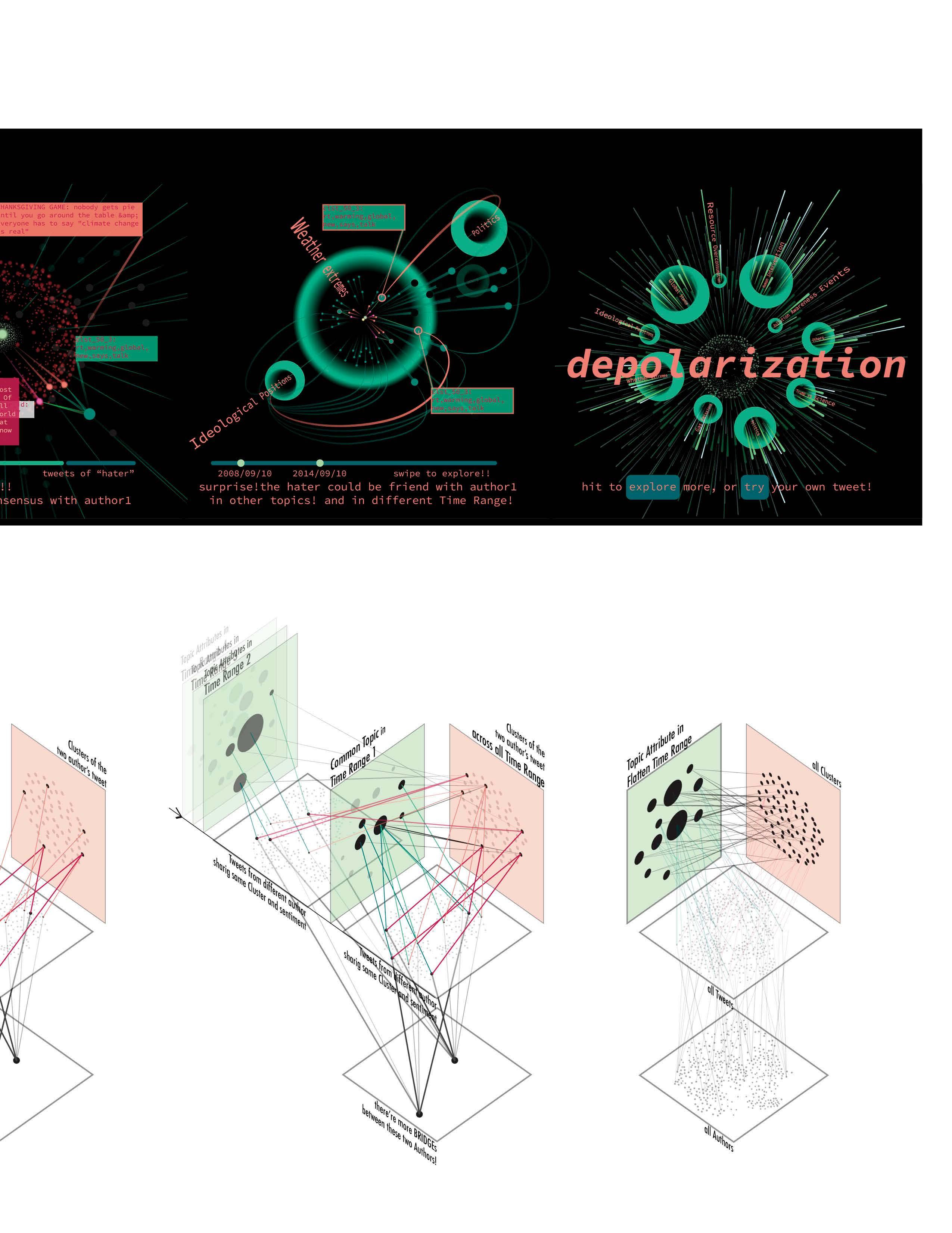
The comparation continues in more topics and more time ranges, the two authors did have more commons in other topics, some even across time range: “author1” in time range C would agree with “potential hater” in time range D.

After this initial exploration, user would have a more concrete image of polarization and echo chambers in social media. He/she is then encourage to continue the exploration with other discussion or try his/her own tweet, or bring this holistic graph browsing to other tweets he/she might be interested.

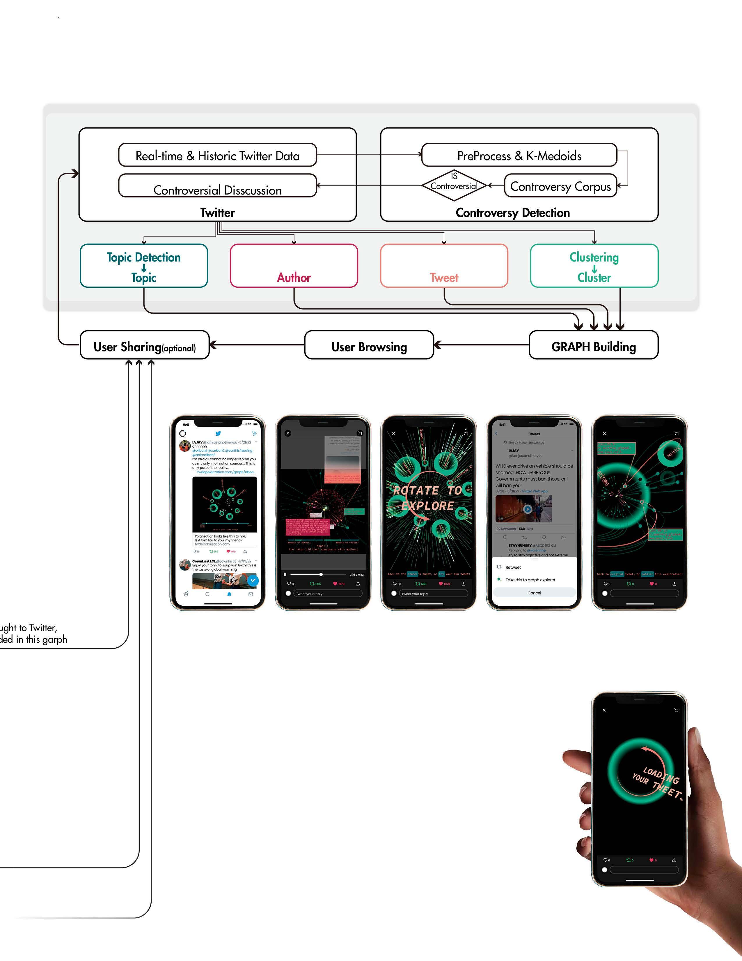
Further Application: A New Paradigm for Social Media

Encapsulation in Twitter

User finds someone sharing their thought with this tool in twitter and gets interested. User see a short interactive demo of this graph, during which detailed tweet can pop up and allow user to get more concrete context. Content in this demo can be “adder to later”.

At the end of the demo, user is encouraged to continue explore the discussion, or with the user’s own tweets.

User explores content “adder to later” in more detail, here the user explore a tweet and its author’s other tweets.

User brings another tweets to the graph browsing tool, and plays with it.

User adds this function to his/her own page, starts loading his/her content in the graph, and start explores his latent datascape (or ideology).

This graph view tool can be shared as

an browsing journey that links tweets in a discussion, where other users can witness the change of stance and browse the detailed information in it

a portal to explore other’s tweets in their context

a introspective tool to navigate user’s own stance, throughout discussion topics and time range

Built Enviornment and Mobility:

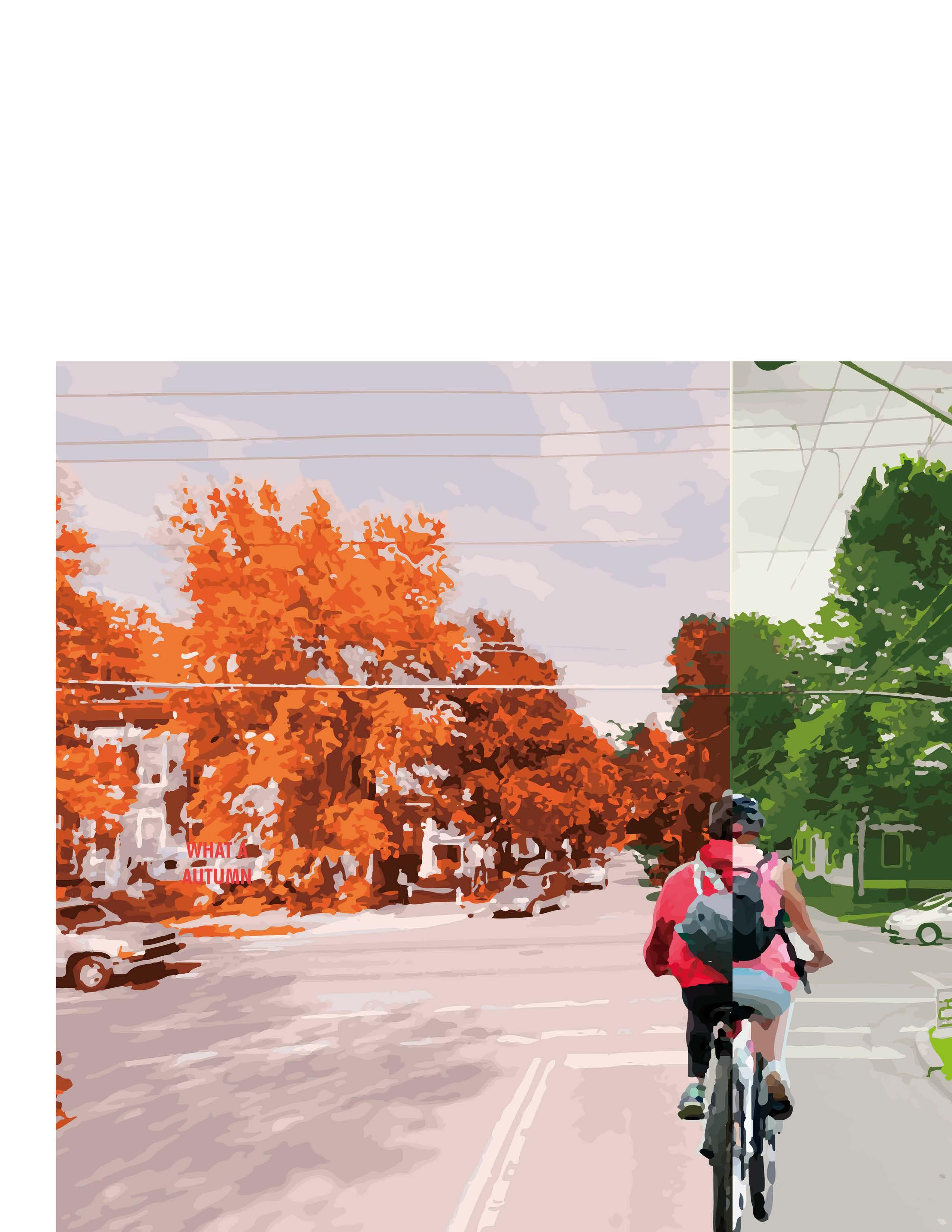
Measuring the seasonal variations of associations between streetscape and dockless bikeshare trip volume

2023 - Ongoing

Team Leader of 5

Tool & Task

Computer Vision (MaskRCNN, Color Analysis), Model Building (OLS, SFE, SLX), Analysis & Writing, Visualization (Mapbox)

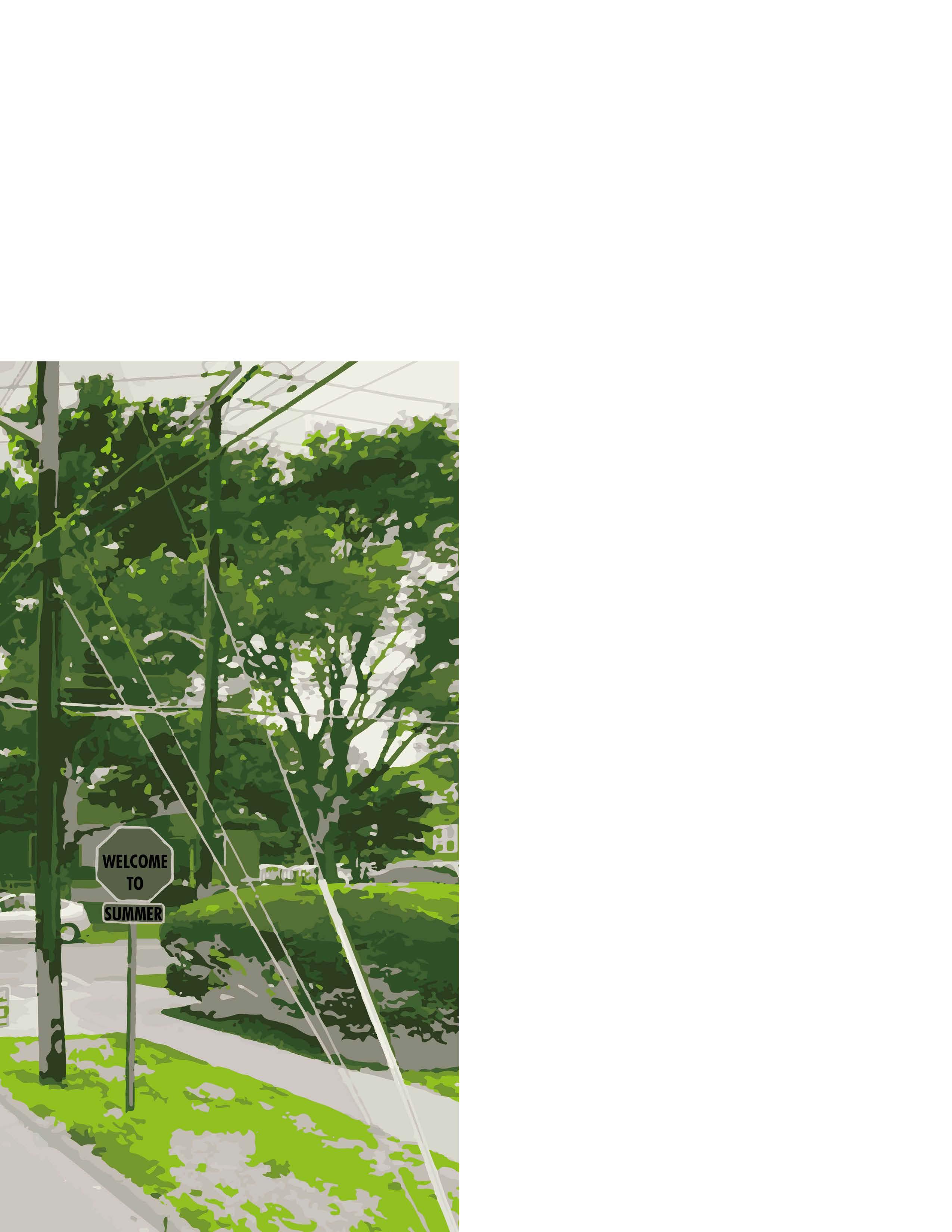
Streetscape plays a significant role in the cycling experience and the impact varies across different seasons. Most prior studies of streetscape ignored its temporal dynamic of it. And for studies of urban public mobility route choices, there has not been much focus on variables within a seasonal scale. In this paper, using a large amount of GPS bike trajectory data collected from LIME, a DBS system in Ithaca USA, we study the correlation between dockless bike sharing and streetscape, plus spatial elements in different seasons. Ordinary Least Squares Model (OLS), Spatial Fix Effect Model (SFE), and Spatial Lag Model (SLX) are built respectively.

The results show that seasonal streetscape factors, such as road, car, sidewalk, grass deviation, tree lab color, and tree color deviation, have significant impacts on the DBS trip volume. But how significantly these seasonal factors influence SWR varies across summer and autumn models. Non-seasonal factors, such as land use mixed score, station, school, street network connectivity, etc., are significant for both summer and autumn models. Some non-seasonal factors only impact the DBS trip volume of one season. Seasonal subjective perception, when added in models of both seasons, helps improve the explanatory significantly. But the improvement is very slight.

The study provides a valuable reference to policymakers, urban planners, and operating companies to jointly cooperate towards a sustainable cycling-friendly city.

Related Publication:

Zhao, Yongqin , Sijia Wang, Difan Chen, Kaijie Huang, Siyuan Zhang, Waishan Qiu, and Wenjing Li. Phygital Intelligence , 211–224. Computational Design and Robotic Fabrication. Singapore: Springer Nature, 2024. https:// doi.org/10.1007/978-981-99-8405-3_18.

Background and Literature Review

1.1

DBS and street built environment

1.2

Seasonal variations and cycling behaviors

Factors influencing cycling activities can be categorized into these domains: (1) demography. (2) the integration of bike sharing and public transportation. (3) land use and point of interest(POI). (4)built environment. Built environment factors have shown significant explanatory power in understanding travel choices (Cervero, 2002). Eye-level greenness has a positive association with cycling occurrence(Lu et al., 2019), and aquatic areas have a similar effect (Krenn et al., 2014). However, few studies specifically focus on DBS behaviors.

Seasonality in climate, affecting the natural environment and human comfort, would have an impact on outdoor activities and behavior (Ahas et al., 2007; Guan et al., 2021; Hadwen et al., 2011). However, there is a dearth of studies focusing on how seasonal change in the urban built environment, influences cycling behavior.

Focus on landscape elements that are sensitive to seasonality and essential for the cycling experience is valuable but not receiving too much attention. Which specific built environment factors have a temporal impact on bike sharing usage? Is this impact positive or negative in a particular season, and how huge is this impact? What is the difference in this impact in different seasons? These are the problems few studies have answered yet. In this paper, we are looking at the temporal change of streetscape at a seasonal scale.

SVI, CV, and ML for measuring street built environment

1.3 1.4

Research gap and contribution

The rapid development of Machine Learning methods like Computer Vision (CV) offers many emerging and state-of-art methods to process SVI in large batches automatically (Ito & Biljecki, 2021). The integration of SVI and CV is giving researchers increasing power to access and understand urban environments computationally.

The characteristics of the human perceived environment can be measured objectively using SVIs. Perception is a subjective measure of the environment that describes a “sense of place” (Kang et al., 2021). However, the impacts of subjective street quality perception on cycling behavior need more in-depth understanding.

To conclude, there are observed research gaps in the seasonal study of DBS: (1) dockless bike sharing (DBS) has received far less research attention compared with docked bike sharing. (2) most precedent studies are based on the geolocation where a trip starts and ends, and thus less on the cycling experience itself during the trip. (3) little has been done to investigate how the seasonality of streetscape elements would influence DBS. This study contributes to the literature in these following points: (1) a quantitative study of DBS that focuses on perceived environmental elements along the trip. (2) seasonality of the streetscape elements on DBS usage at a fine spatial scale. (3) Previously ignored seasonal environmental features are taken into consideration, like vegetation color and its spatial temporal change. (4) seasonal subjective perceptions of streetscape.

1.5

Study area Fig.1. Study area

The study area - Greater Ithaca -includes several adjacent neighborhoods around the Town of Ithaca. The city of Ithaca is the seat of Tompkins County in New York State, its area is 5.39 mile² (2010). As of 2019 when the bike sharing data was collected, the population of the City of Ithaca is 30,837, of which 49.9% were female, 68.4% were white (U.S. Census Bureau QuickFacts, n.d.), and 87.8% were US citizens. With a student population of more than 20,000, Ithaca is home to Cornell University.

Research Framework

(1) Seasonal Weighted Rides (SWR) is calculated from the proportion of aggregated volume in a specific season on one road segment in total volume of all segments in this season.

For Summer and Autumn models, dependent variables are ln(SWR), the natural log of corresponding SWR; dependent variables are the combination of seasonal variables in corresponding season and non-seasonal variables.

For Autumn-Summer-Difference(ASDiff) model, dependent variables are the remainder of autumn ln(SWR) minus that of summer; dependent variables are the combination of remainder of autumn seasonal variables minus that of summer, and non-seasonal variables.

Ordinary Least Square(OLS) model does not consider spatial relationship (assuming variables as i.i.d.)

Spatial Fixed Effect(SFE) gives unique constant to points within a same neighborhood.

Spatial Lag of X (SLX) helps describe how other points in a set nearest range (the spatial weighted matrix is calculated with KNN) would affect current point.

Fig.2. Analytical framework

Data and Methodology

Dependent variable:

Seasonal Weighted Rides (SWR)

Data Validation

The DBS trips data in this research is provided by Lime. The dataset was collected from mobile phones with enabled AUTO-GPS function through the Lime app. A validation process went through to remove the following raw records: (1) trips that started or end outside the Greater Ithaca area, (2) trips whose distances were shorter than the length of a city block in Ithaca(0.05mi or 264ft) , (3) trips with too short or long duration. Finally, 102,178 trip records were left.

Then, based on the method developed by Qiu & Chang, 2021, road central lines were deconstructed into several road segments interrupted by any kind of intersection of roads or routes.

Points Sampling

Segments are selected:

Total Volume ≥ 500; and Length ≥ 25m

Points are sampled:

8m offset from vertex; and 25m sampling distance

CDF Plot

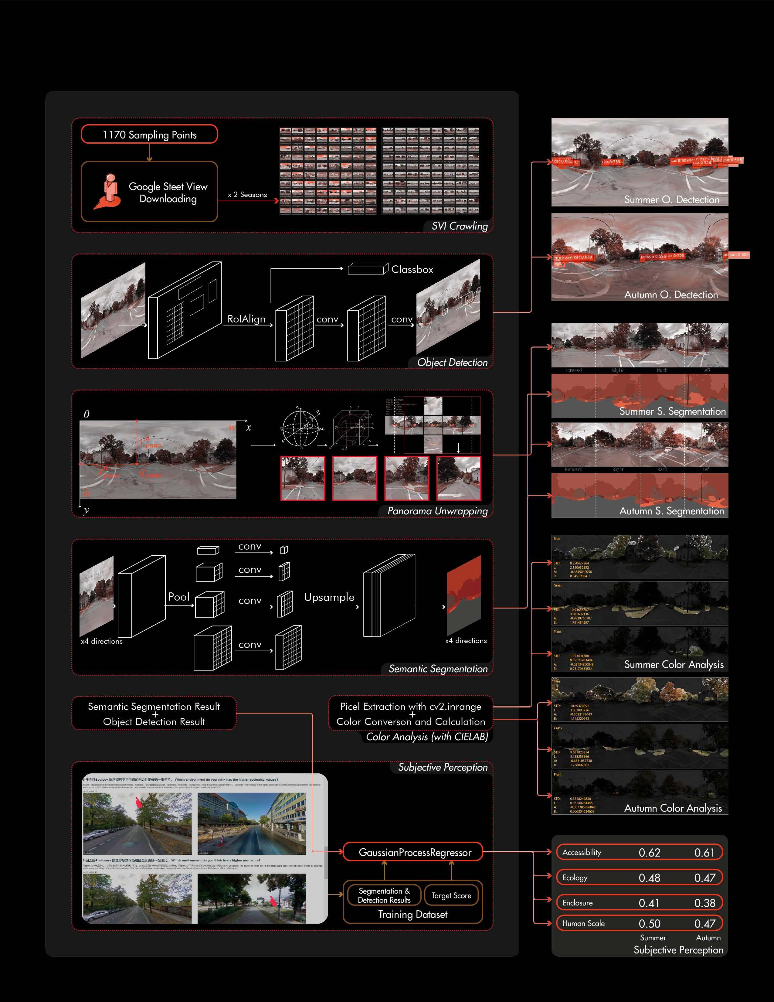
1170 Points on 452 Segments

1170 Points

452 Segments

CDF Plot

Points on Segments

SWR Conversion

Seasonal Weighted Rides captures how popular a segment is in this season.

Seasonal Difference Calculation

For single season models, X in CDF plot is SWR/Aggregated Volume of DBS ridership in that season. For Seasonal Difference model, X in CDF plot is (autumn SWR - summer SWR) Similar for other seasonal variables in the seasonal difference mode, including SWR as dependent variable, streetscape segmentation and object detection result in the independent variables.

CDF Plot

Cumulative Distribution Function is the probabilities that volume of a random segment is less than or equal to X (reveals the distribution of volume on road segments.)

1170 Points on 452 Segments

SWR Conversion

CDF Plot

Data and Methodology

3.2

Inependent variable: SVI and Visual

Object Detection and Semantic Segmentation

We traverse all Google Street View (GSV) taken in all seasons for all these sampling points, but only got GSV in summer (Jun, July, Aug) and fall (Sept, Oct, Nov). 1,170 sampling points that have GSV in both seasons finally remained.

We use Pyramid Scene Parsing Network (PspNet) (H. Zhao et al., 2017) under the open source deep learning framework MXNet in the GluonCV to conduct image segmentation, witha specific pre-trained model psp_resnet101_ade. To avoid potential distortion near the top and button of a panorama image, we use the py360convert package to unwarp the panorama into images in 6 directions before semantic segmentation.

Color Space Analysis

of humans). This dataset is collected from expert panel by a crowdsourcing visual survey). The dataset includes a set of view indices extracted from SVI (as input explanatory variables) and the corresponding perceptual scores（as output labels）. We split the dataset by 75% (225) and 25% (75) for training and testing purposes.

Subjective Measure of streetscape

In this paper, we use CIELAB to understand a general tendency of color (and its change) of street plants from urban cyclists’ perspective. Here we first extracted pixels that are identified as “Tree” from PspNet. Then we used the color convert function under python-colormath library to transform the color space of these pixels from RGB to CIELAB, calculated the average L, A, and B values in CIELAB color space, and the overall standard deviation of difference between the actual value the and average value.

We choose multiple ML algorithms which included K-Nearest Neighbors (KNN), Support Vector Machine (SVM), Random Forest (RF), Gaussian Process (GP), Gradient Boosting Regression (GB), ADA boost, and Bagging Regression, to predict the seven perceptions. Those algorithms are classical and mature in supervised learning. In urban related studies, they have been extensively used as a baseline in the prediction of a numerical target feature based on other features of an instance and have shown effectiveness and robustness (Naik et al., 2014; Safat et al., 2021; Zhang et al., 2018). Prediction results are compared by the balance performance judged by R-squared (R2), Mean Absolute Error (MAE), and Root Mean Square Error (RMSE). The training result can be found in Appendix 1. On average, GP is the optimal model for predicting the target dataset as a whole, and we used the Gaussian Process Regression method in Sklearn to learn the mapping from streetscape elements to perception, and apply the model to get the prediction of target perception scores.

3.3.2.5

of humans). This dataset is collected from expert panel by a crowdsourcing includes a set of view indices extracted from SVI (as input explanatory perceptual scores（as output labels）. We split the dataset by 75% (225) testing purposes.

In this research, we used the ML-based framework developed by related research (Qiu et al., 2023; Su et al., 2023; Xu et al., 2022) to evaluate the subjective perceptions score of the streetscape from street elements.

We use a dataset of 300 pre-labeled points to predict these perception scores: (1) Accessibility, (2) Ecology, (3) Enclosure, (4) Scale. The dataset includes a set of view indices extracted from SVI (as input explanatory variables) and the corresponding perceptual scores (as output labels). We split the dataset by 75% (225) and 25% (75) for training and testing purposes.

Measuring the seasonal variations of associations between streetscape and dockless bikeshare trip volume

Appendix

Measuring the seasonal variations of associations between streetscape and dockless bikeshare trip volume

Data in models

of humans). This dataset is collected from expert panel by a crowdsourcing visual survey includes a set of view indices extracted from SVI (as input explanatory variables) and the perceptual scores（as output labels）. We split the dataset by 75% (225) and 25% (75) testing purposes.

We choose multiple ML algorithms which included K-Nearest Neighbors (KNN), Support Machine (SVM), Random Forest (RF), Gaussian Process (GP), Gradient Boosting Regression (GB), boost, and Bagging Regression, to predict the seven perceptions. Those algorithms are classical mature in supervised learning. In urban related studies, they have been extensively used as a baseline the prediction of a numerical target feature based on other features of an instance and have effectiveness and robustness (Naik et al., 2014; Safat et al., 2021; Zhang et al., 2018). Prediction are compared by the balance performance judged by R-squared (R2), Mean Absolute Error (MAE), Root Mean Square Error (RMSE). The training result can be found in Appendix 1. On average, optimal model for predicting the target dataset as a whole, and we used the Gaussian Process Regression method in Sklearn to learn the mapping from streetscape elements to perception, and apply the get the prediction of target perception scores.

Appendix

Table 1. Performance of GaussianProcessRegressor (GP) predictions.

Table 1 Performance of GaussianProcessRegressor (GP) predictions.

We choose multiple ML algorithms which included K-Nearest Neighbors Machine (SVM), Random Forest (RF), Gaussian Process (GP), Gradient boost, and Bagging Regression, to predict the seven perceptions. Those mature in supervised learning. In urban related studies, they have been the prediction of a numerical target feature based on other features effectiveness and robustness (Naik et al., 2014; Safat et al., 2021; Zhang are compared by the balance performance judged by R-squared (R2), Mean Root Mean Square Error (RMSE). The training result can be found in Appendix optimal model for predicting the target dataset as a whole, and we used method in Sklearn to learn the mapping from streetscape elements to percepti get the prediction of target perception scores.

Appendix 1. ML model performance

3.3.2.5

We choose multiple ML algorithms which included K-Nearest Neighbors (KNN), Machine (SVM), Random Forest (RF), Gaussian Process (GP), Gradient Boosting Regression boost, and Bagging Regression, to predict the seven perceptions. Those algorithms mature in supervised learning. In urban related studies, they have been extensively used the prediction of a numerical target feature based on other features of an instance effectiveness and robustness (Naik et al., 2014; Safat et al., 2021; Zhang et al., 2018). Prediction are compared by the balance performance judged by R-squared (R2), Mean Absolute Error Root Mean Square Error (RMSE). The training result can be found in Appendix 1. On average, optimal model for predicting the target dataset as a whole, and we used the Gaussian Process method in Sklearn to learn the mapping from streetscape elements to perception, and apply get the prediction of target perception scores.

Appendix 1. ML model performance

The results discussed in this section (semantic segmentation, objection detection, color analysis, and objective perception) are seasonal variables and will be fitted in their corresponding seasonal model. Additionally, we compute the seasonal difference for these seasonal variables with Eq. (4).

Appendix 1. ML model performance

Table 1. Performance of GaussianProcessRegressor (GP) predictions.

Table 1. Performance of GaussianProcessRegressor (GP)

Table 1. Performance of GaussianProcessRegressor (GP) predictions.

Table 1. Performance of GaussianProcessRegressor (GP) and other ML predictions.

Data in models

3.3.2.5 Data in models

3.3.2.5

Data in models

We tried commonly used machine learning models, including Even though for Accessibility ADA boost (R2=0.42) and Bagging Regression(R2=0.42) had better R2 than GP(R2=0.4), for Enclosure Decision Tree (R2=0.54) had better R2 than GP(R2=0.53), and for Scale RF(R2=0.44) and GB(R2=0.42) had better R2 than GP(R2=0.39), GP had acceptable R2 (range from 0.39-0.53) for all perception scores, and outperformed all other models in very low RMSE(range from 0.16 to 0.18) and MAE(range from 0.13 to 0.15).

We tried commonly used machine learning models, including for Accessibility ADA boost (R2=0.42) and Bagging Regression(R2=0.42) had better R2 than GP(R2=0.4), for Enclosure Decision Tree (R2=0.54) had better R2 than GP(R2=0.53), and for Scale RF(R2=0.44) and GB(R2=0.42) had better R2 than GP(R2=0.39), GP had acceptable R2 (range from 0.39-0.53) for all perception scores, and outperformed all other models in very low RMSE(range from 0.16 to 0.18) and MAE(range from 0.13 to 0.15).

The results discussed in this section (semantic segmentation, objection detection, color and objective perception) are seasonal variables and will be fitted in their corresponding seasonal Additionally, we compute the seasonal difference for these seasonal variables with Eq. (3).

The results discussed in this section (semantic segmentation, objection and objective perception) are seasonal variables and will be fitted in their Additionally, we compute the seasonal difference for these seasonal variables

The results discussed in this section (semantic segmentation, objection detection, and objective perception) are seasonal variables and will be fitted in their corresponding Additionally, we compute the seasonal difference for these seasonal variables with Eq. (3).

(4)

Here, for sampling point �� , �� is autumn results of seasonal variables, �� is autumn results of seasonal variables, and �� is the difference between autumn and summer seasonal variables.

Here, for sampling point �� , �� is autumn results of seasonal variables, �� is autumn of seasonal variables, and �� is the difference between autumn and summer seasonal variables.

Here, for sampling point �� ,

3.3.3 POI, landmark, and infrastructure

Here, for sampling point �� , �� is autumn results of seasonal variables, of seasonal variables, and �� is the difference between autumn and summer

3.3.3 POI, landmark, and infrastructure Eq. (4). Here, for sampling point , is autumn results of seasonal variables, is autumn results of seasonal variables, and is the difference between autumn and summer seasonal variables. of humans). This dataset is collected from expert panel by a crowdsourcing visual survey). The includes a set of view indices extracted from SVI (as input explanatory variables) and the corresponding perceptual scores（as output labels）. We split the dataset by 75% (225) and 25% (75) for training testing purposes.

is autumn results of seasonal variables, �� is of seasonal variables, and �� is the difference between autumn and summer seasonal

3.3.3 POI landmark and infrastructure

Here we assume that POIs, landmark, and infrastructure would not change too much

* SVI Crawling and Unwraping, and PSPNet segmentation was done by Difan Chen

Original data of POI, Infrastructure, Landuse Mix was prepared by Sijia Wang.

Data and Methodology

Inependent variable:

Object Detection and Semantic Segmentation

Color Space Analysis Subjective Measure of streetscape

Visual Variable summary

We capture different types of POIs within a 500m radius buffer of each sampling point. We also take into account landmark-like destinations, which are unique in the city and can be attractive at different distances for people. To capture these, the buffer zone radius for these landmarks is set to 1000m (typical 5 min rides on a bicycle) and 3000m (typical 15 min rides on a bicycle). For infrastructure information, we choose number of transit facility, bicycle parking, traffic signals, and type of road. The buffer radius is set to 100m.

Land use is a common data source in bike studies to learn about the built environment context (Krenn et al., 2014; Ma et al., 2020; Noland et al., 2016). We used formula derived from the Shannon Index which can capture the entropy of data in a given set.

From USGS we download high resolution(1-meter) Digital Elevation Model (DEM). To reduce interference from potential outlier on the slope raster map, we use the medium slope within 5 meters forward and backward of each sampling point.

Appendix 2. Data Description

Street network, as a way to demonstrate the structure of the built environment is another aspect influencing cyclists’ behavior. After calculating the VIF we remove space syntax score with high multicollinearity (VIF>10), and finally choose Connectivity, Normalized Angular Choice (Nach), and Angular Integration (with segment length weighted, or SLW). Nach and Angular Integration(SLW) both have two radius: 250m and 1000m.

Appendix Table 2.1 Description of seasonal variables of summer (for model M1_Summer, M2_Summer, M3_Summer, M4_Summer)

Table 2 Description of

car, road, sidewalk, water, wall, grass color deviation, tree color deviation, tree LAB a value, and nonseasonal variables such as land use mix score. (2) some variables show their significance for the first time, this applies to variables such as number of education POI. (3) for landmark variables, some are no longer significant while some start to be. (4) street network variables maintain their significance (5) the terrain factor continues to be insignificant in all 6 models up to now.

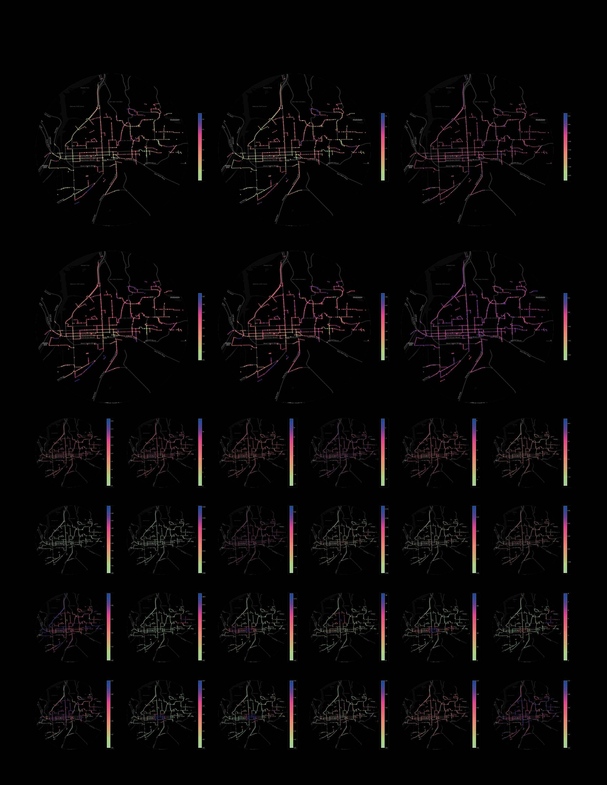
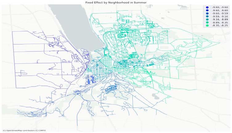
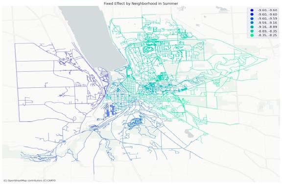
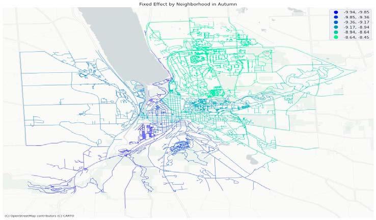
Fig. 10 shows the spatial fixed effect by neighborhood in summer and autumn and Table 5 shows the neighborhood ranking of fixed effect. The lower the SFE is, the lower the inherent attractiveness of the neighborhood is, and the harder it is to witness a ride in this neighborhood. For spatial fixed effects value, spatial fixed effects of most neighborhoods in autumns are lower than that in summer, except Downtown, South Hill and West Hill. For spatial fixed effects ranking, it’s very consistent between summer and autumn for the top seven neighborhoods, North Campus/Northeast and Maplewood/East Hill are the two easiest neighborhoods to witness a ride for both seasons, while North Campus/Northeast being highest in autumn and Maplewood/East Hill in summer. Similar consistency also applies to 8th to 13th neighborhoods, with the only exception being 8th and 13th. IFM/Stewart Park being 8th in summer has only 13th in autumn, and West Hill vice versa. These two can be considered as “seasonal neighborhoods”.

The regression diagnosis results indicate that: (1) Autumn models have higher R2 than Summer models, suggesting that our current variables lack more summer information that can explain the dependent variables than autumn information, regardless of whether this information is seasonal or not. (2) ASDiff models outperform both Autumn and Summer models under the same regression method, indicating that the difference in seasonal variables between summer and autumn can better explain the seasonal change in bike sharing. (3) Model 2 shows improved explanatory power compared to Model 1, demonstrating the effectiveness of subjective human-perceived streetscape features in enhancing prediction ability (4) Incorporating spatial fixed effects significantly improves the performance of all three models, which support our previous assumption that a systematic neighborhood “unevenness” could impact DBS usage in Ithaca.

Most significant variables in at least one season keep their sign in another, and all significant variables in both seasons keep same sign. Many variables show consistent significance in summer and autumn, such as visual ratio of tree, road, car, sidewalk, water, lab b value of tree color, grass color diversion, Number of commercial POI, land use mix score, typical Landmark POI, Connectivity, Normalized Angular Choice and integration degree of the road network. Some variables only show significance in only one season, such as visual ratio of building, wall in summer, and tree color deviation and LAB value of tree and grass color in autumn.

4.5 SLX model regression results

The completed SFE model result can be found in Appendix 5-1 and Appendix 5-2

Taking the spatial lag of x into account would improve model performance significantly. While some variables are consistent in their coefficient and significance across different models, some show inconsistency when different spatial effects or observation ranges With the addition of seasonal different model, some variables reveal their hidden significance in making seasonal cycling different.

It’s very consistent for the top seven and 9th to 12th neighborhoods, with the only exception being 8th and 13th. IFM/Stewart Park being 8th in summer has only 13th in autumn, and West Hill vice versa. These two can be considered as “seasonal neighborhoods”. In terms of value, spatial fixed effects of most neighborhoods in autumns are lower than that in summer, except Downtown, South Hill and West Hill. The above result shows that spatial fixed effect in Ithaca is also sensitive to seasonal change.

4.5.1 Variables at current location within neighboring range

Specifically, SLX models with the closer k value show similar significance and coefficient. For example, M4(k=5) and M4(k=2) or M4(k=10) have higher alignment than with other SLX models, so does M4(k=20) with M4(k=10) or M4(k=30). However, certain variables are not continuous in their significance across different neighboring ranges, like sidewalk which is significant in OLS, only shows significance when k=5; person only when k=20. Some variables will not be significant until k reaches a threshold value, road in autumn is significant in OLS, but in SLX it only starts to be significant until k reaches 10 and higher; nevertheless, ct_dog is no longer significant when k is larger than or equal to 20.

Noticeably, road, car, and sidewalk, are consistently significant locally at all ranges in both seasons, which is same as their performance in OLS and SFE. However, while their coefficient are close to what they have in OLS or SFE in a corresponding season and consistently positive, coefficient in SLX presents different pattern. Coefficient for road’s lag are increasing with observation range all the way from 2 to 30, car’s lag in both seasons reach a peak when k = 5, and sidewalk’s lag have a bottom at 5 (summer) and 10 (autumn). SLX also reveals a divergent significant range. For instance, ceiling, being significant in summer in both OLS and SFE models, is only significant at larger range in SLX.

4.5.2 Variables within a neighboring range from the current location

First, some streetscape elements’ impact on SWR can be implicit in one single season, which is not shown in any of the single-season models but only in ASDiff models. Second, the addition of seasonal difference models greatly improves model performance at all modeling methods (OLS, SFE, and SLX). The fact that huge model improvement happens when SWR and seasonal independent variables are all replaced with their corresponding seasonal difference suggests that other variables we haven’t taken into the model might not be as important as what we have in current models in terms of explaining the seasonal change of bike sharing.

Significance and coefficient between models with the nearest k value are much less similar compared with variables at the current location, which means that variables within the neighboring range are more sensitive to change in the observation range. What’s more, variables within different neighboring ranges have shown a very diverse consistency pattern, which is not even close to what we observe at the current location.

The continued consistency that we discussed before still exists, but only van stays consistent across all observation ranges. Other consistent variables can only maintain their continued significance within limited ranges. For example, road and grass in summer when the observation range is large (k=20 and 30), car in summer when the observation range is small to medium large(k=2, 5 and 10), ct_traffic_light in autumn when the observation range is not small(k=5,10,20, and 30), etc.

Table 4. SFE Neighborhood in Different Seasons.

(a) Fixed effect by neighborhood in summer

(b) Fixed effect by neighborhood in Autumn Fig. Spatial Fixed Effect result from SFE models in two seasons

Table 5. Fixed Effect of Neighborhood in Different Seasons Models (M2_Autumn and M2_Summer)

Modeling and Result

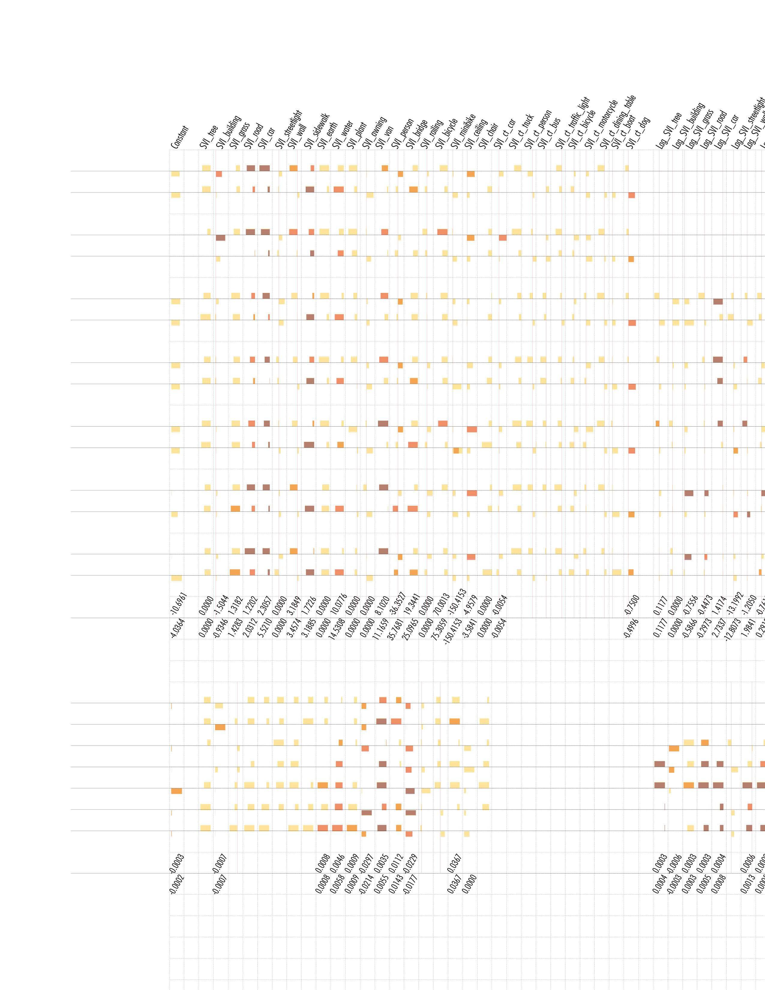
Notes & Label

a: 0.01

b: 0.05

c: 0.1≥

d: p≥0.1

Magnitude

Results * P value Sign

e: Positive Coeff.

f: Negative Coeff.

g: Same variable has different sign in temporal mode

h: Maxium Coeff. in all temporal mode

i: Minimum Coeff. in all temporal mode

j: Width of cell is normalized magnitude in Coeff. range

Variables in different spatial modes

Certain variables are significant in one season across all spatial modes, like sidewalk and water in autumn; Certain variables are inconsistently significant in one season, like wall and ceiling in summer; Most variables are consistent at their sign of coeff.; SLX models shows the change of effective influence range of elements, which applies to bridge, ceiling, etc.

Variables in different temporal modes

ASDiff show that variables significant in single season models might not effective enough to make seasonal change, while some not significant in neither single season models actually influence seasonal behavior change.

2021-2025

DESIGN COMPUTATION

PORTFOLIO OF YONGQIN ZHAO

PORTFOLIO OF YONGQIN ZHAO DESIGN COMPUTATION

2021-2025