Climate Sensitive Design and the Urban Morphology
Integration of Morphological Parameters in Bio-Climatic Urban Planning
Architectural Association
Emergent Technologies & Design 2010
MArch Phase II, Thesis
Radhika Radhakrishnan, Sebastian Nau
-
i -
- ii -
Acknlowledgements
We would like to thank,
Mike Weinstock for his guidance and support throughout the entire year and for his relentless advice throughout the development of this thesis. His experience and precious assistance was the catalyst for achieving progress and for acquiring knowledge and experience.
Toni Kotnik, our studio master. His commitment and steady support enabled us to constantly explore new directions in the design and allowed us to take maximum advantage of the course. Especially, his help with mathematical problems enabled us to push the boundaries of the project and to develop it in ways we did not anticipate.
George Jeronimidis and all EmTech teaching staff, as well as all guest lecturers and consultants; the knowledge and experience we gained during the first phase of the course provided us with the tools and skills necessary to progress on this project.
Qibing Jiang, our friend and peer, who was always at hand to assist us with problems related to computation and scripting.
Fazia Ali-Toudert, who, as an urban climatologist, provided us with valuable insights into the field.
Janet Barlow, who assisted us with any questions related to the urban microclimate.
Finally, we would like thank our families, friends and peers for constant moral support and encouragement.
- iii -
- iv -

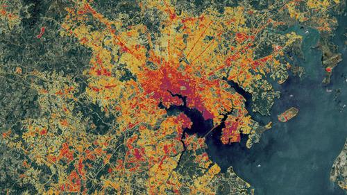
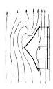
Morphological indicators: The diagram depicts approximated travel routes to parks along the street network. These can be evaluated and used as latent design information to draw conclusions about the performance of the fabric.
Abstract
Reducing the energy demands of cities will be one of the biggest challenges for architects and urban planners in the coming decades. Tackling the urban microclimate, by addressing the urban morphology in design processes, could play a crucial role in this process; it is likely the most suitable way to enforce means of passive energy saving onto urban agglomerations.
The design research project presented in this thesis investigates the current methods in microclimatic research and proposes how such strategies, which so far have only been used in urban analysis, can be implemented in design processes. The complex interaction of physical processes that result in urban microclimates leads to the adaptation of simplified morphological indicators. Such indicators that reveal latent microclimatic characteristics of urban morphologies will be analysed and further explored. Coupled with a genetic algorithm it is subsequently shown how they can be utilized to simultaneously generate and evaluate urban layouts as part of generative design processes.
The project thus introduces a bio-climatic approach to urban planning that incorporates microclimatic considerations. Throughout the project strategies are developed that approach urban design from the patch/block level. It will be shown how patch morpholo-
gies can be optimized according to microclimatic considerations and how such patches may aggregate to form coherent urban structures. By implementing different indicators at different stages of the design it is revealed how different parameters for evaluation might come into play at different stages of the project. The result is a hierarchical planning approach from schematic urban patches all the way down to the building level.
In addition, the method of using morphological indicators will be extended to draw conclusions about urban qualities inherent to patch morphologies. Together with microclimatic considerations it will be shown through a series of design experiments how these can be utilized as latent information within urban planning.
- v -
- vi -
of Contents Domain Computation and the City 1 World Growth and Urbanization Prospects 11 Climate Classifications 21 Climate Change and its Consequences 27 ‘Sustainable’ Cities ............................................................................................................................................... 31 Urban Microclimates ............................................................................................................................................. 41 Cities and Climate ................................................................................................................................................ 51 Methods Concepts of Microclimatic Analysis 67 Evolved and Planned Cities 85 City Data Sets 89 City Data Set - Evaluations 127
Experiments A Genetic Algorithm for Creation and Evaluation of Urban Patches 137 Design Development Patch Typologies, Patch Aggregation and Urban Qualities 159 Design Proposal Site 01: Darjeeling, India .................................................................................................................................... 187 Site 02: Kinshasa, Democratic Republic of the Congo ....................................................................................... 209 Bio-Climatic Urbanism - Kinshasa ...................................................................................................................... 219 Design Revisions Evaluations/Future Development 251 Conclusions 273 Appendices Appendix 01: World and Urban Growth Prospects (by major country and region) 277 Appendix 02: Script Files 287 Appendix 03: Sun shadow studies for different latitudes 327 Appendix 04: Patch Aggregation Studies 333 Bibliography Bibliography 335 - vii -
Table
First
Domain
Computation and the City
Computational methods, like Fractals, Cellular Automata, Genetic Algorithms, etc., have become common tools in order to simulate and understand the underlying complex patterns and processes in urban morphologies. Whereas mostly such tools are used for analysis and prediction of possible urban developments they are rarely implemented in urban planning. The reason for this is that with most of such techniques only selected aspects of the complex overall urban organization/structure can be evaluated, isolated from other relevant factors that need to be considered when planning urban space.
The logics of computation imply that only quantitative data can be evaluated, whereas social and aesthetic factors, which are not measurable, remain untouched. Important human considerations, like the perception of space, remain un-computable. The problems with too rational approaches to urban design have become evident through the mistakes that evolved out of ‘Modernism’ during the last century where the re-organization of urban space has often resulted in ‘sterile’ arrangements that completely failed in social terms.
The problems with using digital methods as generative design tools nowadays often results in processes of post-rationalization where the outcome of conventional urban planning is justified through the use of computational analysis. Such approaches leave the impression of optimized design solutions that are gen-
erated from the bottom up by evaluating and assessing ‘all’ design parameters. The notion of ‘evolutionary methods’, where all possible scenarios are evaluated against each other mimics the diversity that can be observed in evolved cities.
The following chapter introduces some of the most acknowledged computational methods that are currently utilized in urban analysis; in addition, environmental and microclimatic software packages are introduced. Frequently used by architects and climatologists they allow to draw conclusions about the environmental performance of buildings and urban fabrics. Some of them, nevertheless, imply complex calculations as they couple Computational Fluid Dynamics with energy balance models; this is necessary in order to reflect complex processes of energy exchange and interaction that constitute urban microclimates. It will be shown that, at least at the urban scale, limits exist in terms of computation and that calculations are generally time consuming and currently more suitable for analysis than design.
- 1Computation and the City
URBAN GROWTH MODELS:
Arithmetic strategies such as Fractals, Cellular Automata and Genetic Algorithm are increasingly used in understanding urban models of growth in terms of organizational patterns with respect to time. Thus when applied on computational models, predictions of future growth can be achieved.
Computational methods, like Fractals, Cellular Automata, Genetic Algorithms, etc., have become common tools in order to simulate and understand the underlying complex patterns and processes in urban morphologies. Whereas mostly such tools are used for analysis and prediction of possible urban developments they are rarely implemented in urban planning. The reason for this is that with most of such techniques only selected aspects of the complex overall urban organization/ structure can be evaluated isolated from other relevant factors that need to be considered when planning urban space. The logics of computation imply that only quantitative data can be evaluated, whereas social and aesthetic factors, which are not measurable, remain untouched. Important human considerations, like the perception of space, remain un-computable. The problems with too rational approaches to urban design have
become evident through the mistakes that evolved out of ‘Modernism’ during the last century where the re-organization of urban space has often resulted in ‘sterile’ arrangements that completely failed in social terms.
The problems with using digital methods as generative design tools nowadays often result in processes of post-rationalization where the outcome of conventional urban planning is justified through the use of computational analysis. Such approaches leave the impression of optimized design solutions that are generated from the bottom up by evaluating and assessing ‘all’ design parameters. The notion of ‘evolutionary methods’, where all possible scenarios are evaluated against each other mimics the diversity and that can be observed in evolved cities.
Evolutionary concepts are highly associated with this where it is argued that through computation all possible scenarios can be simulated and evaluated to find the most suitable one.
CELLULAR AUTOMATA

- 2Domain
CELLULAR AUTOMATA
Artificial processes for locating urban activities based on simple rules pertaining to local circumstances give rise to complex global patterns that mirror the spatial organization of cities. These systems are called Cellular Automata (CA). They provide a useful means of articulating the way highly decentralized decision-making can be employed in simulating and designing robust urban forms. 1
Simulations of existing urban fabric and providing solutions as potential design strategy were two separate areas of work, the combination of which has only been done in recent times. Rulebased procedures were used to replace mathematical functions thus striping the integrated tissue to the most basic, yet complex in its approach to optimization.
1 Batty, Michael; Cellular Automata and Urban Form: A Primer; Journal of the American Planning Association, Vol. 63, No.2, Spring 1997. “American Planning Association, Chicago, IL.
Cellular Automata is one such tool in this discipline. Using a system of pixilation or adjoined cell system, wherein the transition of one cell to the next and its state is dependent on rules. These rules of growth or decline are determined by the neighbourhood cells and their state. This thus is a dynamic growth model, often applied on a two dimensional grid to portray in an Urban setting, the growth or decline of a city in relation to the neighbour and neighbourhood.
- 3Computation and the City


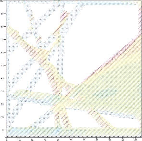
Diagrams above: Envi-Met analysis run on an urban patch sample measuring 250 x 250m. The left hand diagram depicts the surface temperature (k) at 10.00am; built areas are shown in black. The right hand diagram depicts the ‘sky view factor’ in form of isopaths or contour lines. The Envi-Met model allows to calculate a multitude of different parameters that relate to the urban microclimate. It is highly accurate, however, calculation times are considerably long.
< 301.16K
301.16 - 303.79K
303.79 - 306.42K
306.42 - 309.05K
309.05 - 311.67K
311.67 - 314.30K
314.30 - 316.93K
316.93 - 319.56K
319.56 - 322.19K > 322.19K
Artificial processes for locating urban activities based on simple rules pertaining to local circumstances give rise to complex global patterns that mirror the spatial organization of cities. These systems are called Cellular Automata (CA). They provide a useful means of articulating the way highly decentralized decision-making can be employed in simulating and designing robust urban forms.
Simulations of existing urban fabric and providing solutions as potential design strategy were two separate areas of work, the combination of which has only been done in recent times. Rulebased procedures were used to replace mathematical functions thus striping the integrated tissue to the most basic, yet complex in its approach to optimization.
Cellular Automata is one such tool in this discipline. Using a system of pixilation or adjoined cell system, wherein the transition of one cell to the next and its state is dependent on rules. These rules of growth or decline are determined by the neighbourhood cells and their state. This thus is a dynamic growth model, often applied on a two dimensional grid to portray in an Urban setting,
the growth or decline of a city in relation to the neighbour and neighbourhood.
- 4Domain

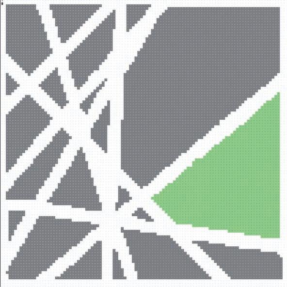
Eni-Met is one of most advanced computational softwares for urban microclimatic analysis. Developed by the University of Bochum, it is a freeware package that allows to analyse urban patches in their microclimatic performance. Envi-Met does not allow to import 3D model data (e.g. In DXF format); the Envi-Met ‘area input file’ is drawn from plan and height information is subsequently assigned by numbers (see diagrams above). To test Envi-Met an example file was set up using one of the early patches created with a genetic algorithm (refer to First Experiments chapter for more information); for all grid cells the soil is set to asphalt; a park (right hand corner) is assigned ‘grass’ as surface material.
Area Input File:
Dimensions: 105x105x25 Grids
Horizontal Grid Size: 2.00m
Vertical Grid Size: 2.00m
Rotation out of North: 0.00
Location:
Latitude (+: Northern Hem.,-: Southern Hem.): +51.31
Longitude (-: Western L., +: Eastern L.): +0.05
Time Zone GMT
Time interval for Output (min): 60
Simulation Timing:
Start Date (DD.MM.YYYY): 23.06.2001
Start Time (HH:MM:SS): 06:00:00
Simulation Time (h): 24
Sun heights for changing dt: I: 0to40.00°,II:40.00 to 50.00°, III: above 50.00°
Time steps assigned: I10.00s,II: 5.00s, III: 2.00s
Basic Meteorology:
Wind Speed in 10 m (m/s): 3.00
Inflow Direction (180=South): 90
Initial Temperature Atmos. (K): 293.00
Spec. Humidity in 2500m (g/Kg): 7.00
Relative Humidity in 2m (%): 50.00
Cloud Cover (low/mid/high): (/8) 0/0/0
Adjustment Factor for Solar Input 1.00
Boundary Condition Type T,q: Open (Default)
Boundary Condition Type TKE: Forced (Default)
Turbulence closure 3D model: TKE Model, Normal Model
Building Properties:
Inside Temperature (K): 293
Heat Transmission Walls: 1.940
Heat Transmission Roofs: 6.000
Albedo Walls: 0.200
Albedo Roofs: 0.300
Soil Properties:
Temperature:
Upper Layer (-20cm): 293.00K
Middle Layer (20-50cm): 295 K
Deep Layer (below 50cm): 293 K
Relative Soil Humidity:
Upper layer (-20c,): 50.00%
Middle Layer (20-50cm): 60.00%
Deep layer (below 50cm): 60.00%
Calculation/Duration:
Time (HH:MM:SS): 17:05:06
Above: Input information for Envi-Met analysis; in order to return data Envi-Met requires a large range of input parameters for calculations. Precise site information about e.g. wind speeds, humidity or soil characteristics are therefore required in order to obtain usable results. Factors such as location, date and time can be set; calculation times are, however, long: it took just over 17 hours to calculate a 24 hour cycle for the test patch shown above. There are also limitations to size, i.e. the urban area that can be analysed: The largest urban patches that can be currently calculated measure 250 x 250m.
- 5Computation and the City

Wind Speed (m/s); 10.00am
0.20 m/s
0.40 m/s
0.60 m/s
0.80 m/s 1.00 m/s
Variables for Atmosphere (calculated during simulation):
Classed LAD and Shelters
Flow u (m/s)
Flow v (m/s)
Flow w (m/s)
Wind speed (m/s)
Wind speed Change (%)
Wind direction (deg)
Pressure Perturbation (Diff)
Pot. Temperature (k)
Pot. Temperature (Diff K)
Pot. Temperature Change (K/h)
Spec. Humidity (g/Kg)
Relative Humidity (%)
TKE (m2/m2)
Dissipation (m3/m3)
Vertical Exchange Coefficient Impulse Km (m3/s)
Horizontal Exchange Coefficient Impulse Km (m3/s)
Absolute LAD (m2/m3)
Direct SW Radiation (W/m2)
Diffuse SW Radiation (W/m2)
Reflected SW Radiation (W/m2)
LW Radiation Environment (W/m2)
Sky View Factor Buildings (/)
Sky View Factor Buildings and Vegetation (/)
Temperature Flux (K*m/s)
Vapour Flux (g/kg*m/s)
Sensible Heat Flux (W/m²); 10.00am
W/m²
W/m²
W/m²
W/m²
W/m²
Water on Leaves (g/m2)
Wall Temperature on Cell border x (K)
Wall Temperature on Cell border y (K)
Wall Temperature on Cell border z (K)
Leaf Temperature (K)
Local Mixing Length (m)
PMV Value
PPD Value
Mean Radiant Temperature (K)
Gas/Particle Concentration (mg/m3)
Gas/Particle Concentration (mg/s)
Deposition Velocity (mm/s)
Total Deposed Mass (mg/m2)
Deposed mass Time averaged (mg/(m2*s)
TKE normalised 1D
Dissipation normalised 1D
Km normalized 1D
TKE Mechanical Turbulence term of the E/eps equation
Stomata Resistance of leafs (m/s)
CO2 (mg/m3)
CO2 (ppm)
Plant CO2 Flux (mg/kg*m/s)
Div Rlw Temp change (K/h)
Local Mass Balance (mg/(s*m3)
Envi-Met analysis allows to extract large quantities of data from urban sample sites; the range of parameters that was calculated during the test run, introduced on the previous page, is depicted above. Data can subsequently presented graphically in form of 2D maps or 3D models. The diagrams at the top of the page show such representational diagrams for wind speed and sensible heat fluxes at 10 o’clock in the morning.
70.00
140.00
210.00
280.00
350.00
- 6Domain
ENVIRONMENTAL SIMULATION SOFTWARE:
Tools for Modelling the dynamic urban microclimate system can become challenging in terms of calculations and strategizing apart from mere computational limitations. However, recent developments in the area seek to perform dynamic simulations of the coupled surface-plant- atmosphere system on regular computers. This can prove to be extremely useful in terms of urban and architectural planning aiming at a balanced environmental model.
ECOTECT
Ecotect is a conceptual design tool that couples an intuitive 3D design interface with a comprehensive set of performance analysis functions. It can help in terms of vizualising the effect of the sun and shadow patterns. However in terms of using this as a real time analysis tool, it does not provide with a very strong base.
ENVI-MET
Of the most advanced available tools for fluid flow simu-
lation models is ENVI- met. It is much advanced and accurate as compared to tools like ECOTECT, in terms of giving a more complete diurnal cycle including all the heating and cooling processes taking place in the urban environment. ENVI –met is a3D coupled computational fluid dynamics and energy balance model.
It can be used to calculate the wind flow around different urban forms as well as all the parameters associated with energy balance and atmospheric transfer processes(shadows, reflections, turbulence, transfer, plant evaporation etc). The results have been proven to be fairly accurate when tested on models used in the design experiments.
The input model is however requires a largely pixilated version to be read. This is setback in terms of using this as part of a design tool. Another setback maybe the time involved in the completion of a single simulation, thus increasing the time of a feedback loop within evaluation and design.
- 7Computation and the City
Image references :
Fig1 : http://1.bp.blogspot.com/_gss1sFcUYg4/RlMGxrPFgBI/ AAAAAAAAAHQ/UM8fejIrD8s/
Fig. 2 : http://29.media.tumblr.com/tumblr_kzeli4H6cU1qaqm2ao1_500.jpg
Fig. 4 : http://www.dlr.de/caf/Portaldata/60/Resources/images/2_dfd_la/2_dfd_la_sl/temp_wind_e
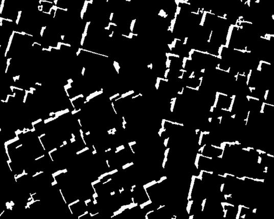
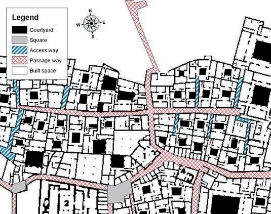
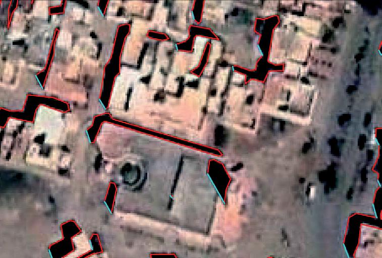
Figs. 5-8 : Peeters, Aviva ; Etzion, Yair; Israel, Sept 2010; GIS Based Object Recognition Model for Analyzing the Urban Form
Fig 9 : http://www.casa.ucl.ac.uk/andy/blogimages/helsinki2050. jpg

- 8Domain
- 9Computation and the City
- 10Domain
World Growth and Urbanization Prospects
It is predicted that the global population will increase to just over 9 billion by the year 2050. This exponential growth will, however, not be the same in all parts of the world and it is especially African and Asian countries, which will encounter rapid increase in population numbers in the next decades. Godfray reports that Europe’s population will decline, Africa’s will double, while China’s will peak in 2020 to be overtaken by India’s population at around 2030 (Godfray, 2010). It is especially the young average age of people (under 30) in these countries that leads to exponential growth and enormous space requirements; while demographic changes will require cultural adaptations it is especially the vast expansion of such societies that will put enormous pressure on architecture and urbanism.
The world’s population today is over 50% urban (Kennedy, 2009). This trend of urbanization is certain to continue and the last few decades have seen the rise of megacities in developing countries such as Mumbai, Sao Paulo or Mexico City that all peak 16 million inhabitants (Godfray, 2010). Mills (Mills, 2006) points out that the highest rates of urbanization are occurring in poorer parts of the world and Arnfield (Arnfield, 2003) adds to this that
most of such areas are located in the tropical world (Population Reference Bureau, 2001b; United Nations, 2001). It can therefore be assumed that most of the expected urban growth is happening in regions with rather extreme climates; Golany describes the most sensitive ones as the hot-dry, the cold-dry and the hothumid ones (Golany, 1996). Urban development in such regions will likely enforce high environmental pressures that will affect local economies and the exploitation of natural resources. It is therefore necessary to come up with innovative urban concepts that address the metabolisms of cities; such concepts need to be tailored to the specific regional settings and must in particular respect the prevailing climatic conditions.
- 11World Growth and Urbanization Prospects
Average Increase in 10 Years
The Global population reached the first billion in 1804. Until 1900 there were 1,6 Billion people on the earth, growing to 2 Billion in 1927 and 3 Billion in 1960. Fourteen years later there were 4 Billion and in 1987 5 Billion people were counted. In 1999 the global population reached 6 Billion people. As a result the global population almost quadrupled during the 20th Century. Future growth is expected to exclusively happen in third world countries. (Source: DeutscheStiftungWeltbevoelkerung/United Nations World Population Prospect: The 2008 Revision, 2009)
World Population (Billion) 1700 1750 1800 1850 1900 1950 2000 Increase in Millions 2050 0 10 20 30 40 50 60 70 80 90 100
2050:9,14 B 1804:1 B 1927:2 B 1960:3 B 1974:4 B 1987:5 B 1999:6 B 2012:7 B 2025:8 B 2046:9 B
- 12Domain
Global Population: Distribution per Region/Area 2009 & 2050. Source: United Nations, Department of Economic and Social Affairs, Population Division, Prospect 2009
Africa
Europe
Latin America and the Caribbean
Nothern America
Asia Oceania
100 - 280%
80 - 100%
60 - 80%
40 - 60%
20 - 40%
0 - 20%
-30 - 0%
Global Population Increase/Decrease in per cent per country; 2009 - 2050. Source: United Nations, Department of Economic and Social Affairs, Population Division, Prospect 2009
2009 Global Population:
2050 Global Population:
6.829 billion
9.150 billion
- 13World Growth and Urbanization Prospects
Distribution of Urban Population by Size of Urban Settlement (Global). Diagram adopted from United Nations (2009)
Percentage Distribution of Urban Population by Development Region. Diagram adopted from United Nations (2009)
Percentage Urban by Development Region. Diagram adopted from United Nations (2009)
Percentage Urban by Major Area. Diagram adopted from United Nations (2009)
Source: United Nations, Department of
0 100 100% 100 90 80 70 60 50 40 30 20 10 0 80% 60% 40% 30% 0% 90 80 70 60 50 40 30 20 10 0 1950 19501960197019801990200020102020 19501960197019801990200020102020203020402050 1960197019801990200020102020203020402050 100 90 80 70 60 50 40 30 20 10 0 19501960197019801990200020102020203020402050
Countries Africa Asia Latin America & The Caribbean Europe Oceania Northern America
Fewer than 0.5 million 0.5 - 1 million 1 - 5 million 5 - 10 million 10 million or more More Developed Regions
Developed
City Size 2009 2025 Percentage of world’s urban population Increase 10 million or more* 21 29 Accounted for 9.4% of the world urban population and are expected to account for 10.3% of the world urban population in 2025. 8 5-10 million 32 46 Three quarters of these ‘mega-cities in waiting’ are located in developing countries and account for just 6.6% of the urban population 14 1-5 million 376 509 Account for 22% of the urban population 133 500.000 to 1 million 509 667 Account for only 10% of the overall population 158 *Mega-Cities/Agglomerations
Least Developed
Other Less Developed Countries More Developed Countries
Other
Regions Least Developed Regions
Economic
and Social Affairs, Population Division, Prospect 2009
- 14Domain
Los Angelos
30-40 million Sao Paulo Mexico City New York-Newark
20-30 million
10-20 million

Climate Shifts and the Metabolism of Cities
Kennedy points out that the metabolism and the greenhouse gas emissions of a city are strongly dependent upon its location (Kennedy, 2009). Local temperatures, wind conditions as well as humidity and radiation have a direct impact on the energy requirements of urban areas. They directly influence the indoor energy demands in terms of heating and cooling but indirectly also have an effect on the urban energy consumption related to transportation. It is the outdoor comfort as well as travel distances that determine how people commute; both are directly related to the morphology of a city. Salat points out that there is a strong correlation between population density and energy consumption (Salat, 2007). Other authors agree with this (Kennedy, 2009) and regard densification as one of the key strategies in order to create ‘sustainable’ cities.
As much as high urban densities might mitigate high energy demands related to urban sprawl it needs to be mentioned that most studies do not take into account the energy demands related to vertical transportation in high-rise conglomerations. It also needs to be pointed out that energy requirements for buildings in the domestic and non-domestic sector exceed those for transportation and industrial processes. Salad points out that in urbanized countries like the UK buildings represent half of the energy consumption and together with transportation cities represent more than three quarters of the energy consumption (Salat 2007).

Largest (25) Urban Agglomerations in 2025. Source: United Nations, Department of Economic and Social Affairs, Population Division, Prospect 2009
Appropriate adaptation of the morphology of a city is therefore clearly necessary in order to mitigate high-energy requirements; the urban geometry not only affects the density and related travel behaviours but also alters urban climatic conditions, which in turn affect energy demands related to indoor and outdoor climatic conditions. It is the interaction of geometries, surface materials and local weather conditions that determine whether an urban fabric is heating up or cooling down; whether it is desirable to lower or rise temperatures in urban areas hereby clearly depends on the location. Golany therefore argues that each climatic region necessitates a distinct urban form and configuration in order to make a city or neighbourhood cooler or warmer and that urban designers should borrow knowledge from other disciplines such as urban climatology, botany, geography, etc. in order to enhance urban comfort (Golany, 1996). Currently Urban Microclimates often evolve uncontrolled through the interaction of the local climate and geography in relation to the urban morphology. As microclimates develop at various levels and scales within an urban fabric it is mainly due to the poor inter-disciplinary work between architecture and urbanism that microclimates are not addressed in urban planning. Ali-Toudert points out in this context that there is a clear lack of guidelines that can help planners and architects in the process of improved microclimatic urban design (Ali Toudert, 2001).
Karachi Lagos
Shenzhen Cairo Istanbul Paris Jakarta
Osake/Kobe
Buenos Aires Rio De Janeiro
Beijing Manila Chongqing
Dhaka
Shanghai Tokyo Bombay
Guangdong Kinshasa
Calcutta
- 15World Growth and Urbanization Prospects
Largest Urban Agglomerations (millions) in 2025 (2009 projections); Source: United Nations, Department of Economic and Social Affairs, Population Division, Prospect 2009
*incl. Long Beach-Santa
Source: United Nations, Department of Economic and Social Affairs, Population Division, Prospect 2009
Tokyo 40 35 30 25 20 15 10 05 00 Delhi Bombay Sao Paulo Dhaka Mexico City New YorkNewark Calcutta Shanghai Karachi Lagos Beijing Kinshasa Manila Buenos Aires Los Angelos Cairo Rio de Janeiro Istanbul Osaka-Kobe Chongqing Shenzhen Guangdong Paris Jakarta Moscow Lima Chicago 2050 2009 1.6% 31.8% (+0.6 mill.) 31.0% (+6.1 mill.) 8.5% (+1.7 mill.) 46.2% (6.6 mill.) 7.3% (+1.4 mill.) 6.7% (+1.3 mill.) 31.4 % (+4.8 mill.) 22.7% (+3.7 mill.) 46.1% (+5.9 mill.) 54.9% (+5.6 mill.) 23.0% (+2.8 mill.) 78.6% (+6.6 mill.) 30.7% (+3.5 mill.) 5.4% (+0.7 mill.) 7.9% (+1.0 mill.) 7.9% (+ 2.6 mill.) 23.8% (+0.9 mill.) 16.3% (+1.7 mill.) 0.9% (+0.1 mill.) 19.4% (+1.8 mill.) 26.1% (+2.3 mill.) 26.4% (+2.3 mill.) 4.8% (+0.5 mill.) 18.7% (+1.7 mill.) 1.9% (+0.2 mill.) 19.3% (+1.7 mill.) 8.8% (+0.8 mill.) 1975 2009 2025 Rk. Agglomeration Population (million) Agglomeration Population (million) Agglomeration Population (million) 1 Tokyo 26.6 Tokyo 36.5 Tokyo 37.1 2 New York-Newark 15.9 Delhi 21.7 Delhi 28.6 3 Mexico City 10.7 Sao Paulo 20 Bombay 25.8 4 Osaka-Kobe 9.8 Bombay 19.7 Sao Paulo 21.7 5 Sao Paulo 9.6 Mexico City 19.3 Dhaka 20.9 6 Los Angelos* 8.9 New York-Newark 19.3 Mexico City 20.7 7 Buenos Aires 8.7 Shanghai 16.3 New York-Newark 20.6 8 Paris 8.6 Calcutta 15.3 Calcutta 20.1 9 Calcutta 7.9 Dhaka 14.3 Shanghai 20 10 Moscow 7.6 Buenes Aires 13 Karachi 18.7 11 Rio de Janeiro 7.6 Karachi 12.8 Lagos 15.8 12 London 7.5 Los Angelos* 12.7 Kinshasa 15 13 Chicago 7.2 Beijing 12.2 Beijing 15 14 Bombay 7.1 Rio de Janeiro 11.8 Manila 14.9 15 Seaul 6.8 Manila 11.4 Buenos Aires 13.7 16 Cairo 6.4 Osaka-Kobe 11.3 Los Angelos* 13.7 17 Shanghai 5.6 Cairo 10.9 Cairo 13.5 18 Manila 5 Moscow 10.5 Rio de Janeiro 12.7 19 Beijing 4.8 Paris 10.4 Istanbul 12.1 20 Jakarta 4.8 Istanbul 10.4 Osaka-Kobe 11.4 21 Philadelphia 4.5 Lagos 10.2 Shenzhen 11.1 22 Delhi 4.4 Seoul 9.8 Chongqing 11.1 23 St Petersburg 4.3 Chongqing 9.3 Guangdong 11 24 Tehran 4.3 Chicago 9.1 Paris 10.9 25 Karachi 4 Jakarta 9.1 Jakarta 10.8 26 Hong Kong 3.9 Shenzhen 8.8 Moscow 10.7 27 Madrid 3.9 Lima 8.8 Bogota 10.5
Detroit 3.9 Guangdong 8.7 Lima 10.5 29 Bangkok 3.8 London 8.6 Lahore 10.3
Lima 3.7 Kinshasa 8.4 Chicago 9.9
28
30
Ana
- 16Domain
Percentage Urban in 2009. Source: United Nations, Department of Economic and Social Affairs, Population Division, Prospect 2009
Percentage Urban in 2050. Source: United Nations, Department of Economic and Social Affairs, Population Division, Prospect 2009
80-100% 60-80% 40-60% 20-40% 00-20% 80-100% 60-80% 40-60% 20-40%
00-20%
- 17World Growth and Urbanization Prospects
600-700%
500-600%
400-500%
Urban Population: Size of Urban Population per country; increase in percent from 2009 to 2050. Source: United Nations, Department of Economic and Social Affairs, Population Division, Prospect 2009
Percentage Urban; increase in percent from 2009 to 2050. Source: United Nations, Department of Economic and Social Affairs, Population Division, Prospect 2009
-30-00%
50-62.5%
25-37.5% 12.5-25%
300-400% 200-300% 100-200% 0-100%
75-87.5% 87.5-100% > 100% 62.5-75%
37.5-50%
00-12.5%
- 18Domain
Nations, Department of Economic and Social Affairs, Population Division *(thousands)
**(as percentage of urban population)
In terms of absolut numbers mostly African and Asian countries are projected to show the largest increase in per cent from 2009 to 2050
United Nations Urbanization Prospects
The diagrams on the previous pages confirm that much of the world’s increase in population over the next forty years is expected to happen in the poorer parts of the world (refer to appendix 01 for additional information); especially Asian and African will encounter massive increases in population. This is also true regarding urbanization where especially African countries are expected to go through a massive shift as people migrate to cities. As the diagrams, which were drawn from data provided by the United Nations (United Nations, 2009), illustrate graphically the tendencies for future urbanization additional information is provided by the United Nations:
“The world urban population is expected to increase by 84% by 2050, from 3.4 billion in 2009 to 6.3 billion in 2050. By mid-century the world urban population will likely be the same size as the world’s total population was in 2004. Virtually all of the expected growth in the world population will be concentrated in the urban areas of the less developed regions, whose population is projected to increase from 2.5 billion in 2009 to 5.2 billion 2050. Over the same period, the rural population of the less developed regions is expected to decline from 3.4 billion to 2.9 billion. In the more developed regions, the urban population is projected to increase modestly, from 0.9 billion in 2009 to 1.1 billion in 2050.”
(United Nations, 2009)
“The sustained increase of the urban population combined with the pronounced deceleration or rural population growth will result in continued urbanization, that is, in increased proportions of the population living in urban areas. Globally, the level of urbanization is expected to rise from 50% in 2009 to 69% in 2050. The more developed regions are expected to see their level of urbanization increase from 75% to 86% over the same period. In the less developed regions, the proportion urban will likely increase from 45% in 2009 to 66% in 2050.” (United Nations, 2009)
“The world urban population is not distributed evenly among cities of different sizes. Over half of the world’s 3.4 billion urban dwellers (51.8%) lived in cities or towns with fewer than half a million inhabitants. Such small cities account for 53.2% of the urban population in the more developed regions and for 51.3% of that in the less developed regions. Between 2009 and 2025, small urban centres with fewer than half a million inhabitants are expected to account for 45% of the expected increase in the world urban population.” (United Nations, 2009)
“Over the next four decades, Africa and Asia will experience a marked increase in their urban populations. In Africa the urban population is likely to treble and in Asia it will almost double. By mid-century, most of the urban population of the world will be concentrated in Asia (54%) and Africa (20%).” (United Nations, 2009)
“The increases in the world urban population are concentrated in a few countries, with China and India together projected to account for about a third of the increase in the urban population in the coming decades, Between 2009 and 2025, the urban areas of the world are expected to gain 1.1 billion people, including 231 million in China and 167 million in India, which account together for 36% of the total increase. Nine additional countries are projected to contribute 26% of the urban increment, with increases ranging from 16 million to 52 million. The countries involved are: Nigeria and the Democratic Republic of the Congo in Africa; Bangladesh, Indonesia, Pakistan and the Philippines in Asia, Brazil and Mexico in Latin America, and the United States of America. Among them, those in Africa and Asia will experience high rates of urban population growth, usually surpassing 2% or even 3% per year.” (United Nations, 2009)
Country Urban Population by Major Area (thousands) Increase 2010 2050 Largest Agglomeration Population* Population** 1 Niger 2,719 21,431 688.23% Niamey 1004 38.7 2 Uganda 4,493 30,596 580.94% Kampala 1535 35.8 3 Burkina Faso 4,184 23,991 473.41% Quagadougou 1777 45.4 4 Malawi 3,102 17,729 471.53% Lilongwe 821 27.9 5 Timor-Leste 329 1,767 436.40% Dili 166 53 6 Burundi 937 4,951 428.42% Bujumbura 455 51.3 7 Afghanistan 6,581 34,749 428.07% Kabul 3573 56.9 8 United Republic of Tanzania 11,883 59,109 397.44% Dar es Salaam 3207 28.3 9 Chad 3,179 15,761 395.84% N'Djamena 808 26.6 10 Rwanda 1,938 9,480 389.22% Kigali 909 49 11 Eritrea 1,127 5,405 379.50% Asmara 649 60.6 12 Ethiopia 14,158 65,149 360.16% Addis Adaba 2863 21 13 Kenya 9,064 41,112 353.60% Nairobi 3375 38.8 14 Solomon Islands 99 446 348.88% Port Vila 44 72.5 15 Papua New Guinea 863 3,829 343.77% Honiara 72 75.5 16 Somalia 3,505 14,972 327.22% Mogadishu 1353 40.1 17 Nepal 5,559 23,319 319.50% Kathmandu 990 18.7 18 Yemen 7,714 32,303 318.75% Sana'a' 2229 30.3 19 Guinea 3,651 15,087 313.27% Conakry 1597 45.5 20 Vanuatu 63 258 310.60% Port Vila 44 72.5 Urban Population in absolute numbers (thousands); Increase/Decrease by Major Area; 2010 - 2050; Source: World Urbanization Prospects: The 2009 Revision; United
- 19World Growth and Urbanization Prospects
Ouagadougou:
Expeceted growth
81% until 2020

Climate Zone
Sahel Zone
Countries within Sahel Zone
Largest four African Megacities in 2020
Fastest growing cites in Africa (average growth rate 51%)
Sub
Urbanization prospects for Africa; largest Megacities and fastest growing cities. Source: World Urbanization Prospects: The 2009 Revision; United Nations, Department of Economic and Social Affairs, Population Division
City 2010-2020* Absolute Growth (000s)
Kinshasa 4,034
Lagos 3,584
Luanda 2,308
Dar es Salaam 1,754
Nairobi 1,669
*Projections
City 2010-2020* Absolute Growth (000s)
Ouagadougou 1,548
Cairo 1,539
Abidjan 1,375
Kano 1,100
Addis Ababa 1,051
*Projections
Africa’s 10 Fastest Growing large Cities (2010-2020). Source: World Urbanization Prospects, The 2009 Revision
According to the UN Habitat report, with an urban growth rate of 3.41 per cent, Africa is the fastest urbanizing continent in the world and will in 2030 cease being predominantly rural. The increase in urban populations will lead to an exponential increase in the demand for shelter and services. But as the authors point out African cities are already inundated with slums; a tripling of urban populations could spell disaster, unless urgent action is initiated today. (UN Habitat 2010):
• “Cairo, with 11 million inhabitants is still Africa’s largest urban agglomeration. But not for much longer. In 2015, Lagos will be the largest with 12.4 million inhabitants. In 2020, Kinshasa’s 12.7 million will also have overtaken Cairo’s then 12.5 million population. Luanda has recently surpassed Alexandria and is now Africa’s fourth largest agglomeration. It is projected to grow to more than 8 million by 2040.” (UN Habitat 2010)
• “Up to 2020, Kinshasa will be the fastest-growing city in absolute terms, by no less than four million, a 46 percent increase for its 2010 population of 8.7 million. Lagos is the second-fastest with a projected 3.5 million addition, or a 33.8 per cent increase. Dar es Salaam, Nairobi, Ouagadougou, Cairo, Abidjan, Kano and Addis Ababa will all see their populations increase by more than one million before 2020.” (UN Habitat 2010)
• “In the case of some African cities, projected proportional growth for the 2010−2020 period defies belief. Ouagadougou’s population is expected to soar by no less than 81 per cent, from 1.9 million in 2010 to 3.4 million in 2020. With the exception of the largest cities in the Republic of South Africa and Brazzaville in Congo, from 2010 to 2020, the populations of all sub-Saharan million-plus cities are expected to expand by an average of 32 per cent.” (UN Habitat 2010)
Nairobi Kampala
Lunada
Lagos Cairo
es Salaam Bamako Niamey
Abuja Lubumbashi
Mbuji-Mayi
Kinshasa
Dar
Monsoon Tropical
-Tropical Desert
- 20Domain
Climate Classifications
Climate Causes:
The energy content of the atmosphere is constantly driven towards equilibrium, occurring as a natural phenomenon. This includes factors such as solar radiation in the upper atmosphere; albedo, or reflection of the radiation from clouds, snow, ground and water surfaces; distribution of water and landmasses; and topography including the elevation and distribution of land features. The regional or macroclimate is a resultant of the net effect of these factors.
Climatic classifications:
One of the most wide used and popular climatic classification is the Koppen climate classification , later the Koppen- Geiger climate classification system. The same is widely used also as reference to predict the shifts in the climate in the future. This system of classification is primarily based on the vegetation prevalent in the area (biomes) 1
In terms of the architecture, characteristics right from the ancient civilizations through Vitruvius to Cerda’s Eixample indicated the considerations of select climatic parameters as design determinants. This sensitivity found in vernacular architecture towards climate, and the apparent consequences of the same contributing to the micro climate have been used as a basis for identifying regions or macroclimate. It considers the climate, location in terms of distance from the edge of the continent, and topography.
1 Köppen climate classification. (2011). In Encyclopædia Britannica. Retrieved fromhttp://www.britannica.com/EBchecked/topic/322068/Koppen-climateclassification
For the distinction of vernacular architectural regimes, the world climate zones have been divided into the 9 zones, namely:2 3 (i)
Arctic and Sub Arctic:
- All areas north of the Arctic Circle at 66.33 °N belong to this zone. The region immediately south of this is the Sub- arctic. Although no human settlements prevail in the Antarctic, the conditions are similar to the Arctic.
- There are 4 distinct biomes found inthis zone: the polar seas and the glaciers, the coasts and islands, the treeless tundra plains, the taigathe large coniferous forests of most parts of Canada, Alaska, Scandinavia and Siberia.
- Air temperature and radiation are key factors to human habitation: outgoing radiation takes away much of the incoming solar energy because of clear air and water vapour.
- Winters are long and cold with incoming solar radiation at very low angles. The presence of sea or Ocean has major climatic influence on the temperature.
Observed Vernacular Responses:
- Continuity in blocks.
2 Oliver, Paul; Encyclopedia of Vernacular Architecture 3 http://www.worldclim.org/
−160−140−120−100−80−60−40−20020406080100120140160180 −160−140−120−100−80−60−40−20020406080100120140160180 −80 −70 −60 −50 −40 −30 −20 −10 0 10 20 30 40 50 60 70 80 −90 −80 −70 −60 −50 −40 −30 −20 −10 0 10 20 30 40 50 60 70 80 90 Af Am As Aw BWk BWh BSk BSh Cfa Cfb Cfc Csa Csb Csc Cwa Cwb Cwc Dfa Dfb Dfc Dfd Dsa Dsb Dsc Dsd Dwa Dwb Dwc Dwd EF ET World Map of Köppen−Geiger Climate Classification updated with CRU TS 2.1 temperature and VASClimO v1.1 precipitation data 1951 to 2000 Main climates A: equatorial B: arid C: warm temperate D: snow E: polar Precipitation W: desert S: steppe f: fully humid s: summer dry w: winter dry m: monsoonal Temperature a: hot summer b: warm summer c: cool summer d: extremely continental h: hot arid k: cold arid F: polar frost T: polar tundra http://gpcc.dwd.de http://koeppen-geiger.vu-wien.ac.at Resolution: 0.5 deg lat/lon Version of April 2006 Kottek, M., J Grieser, C. Beck, B. Rudolf, and F. Rubel, 2006: World Map of KöppenGeiger Climate Classification updated. Meteorol. Z., 15, 259-263. EF EF ET Dfc Dfb Dfa Cfa Cfb Dsc Csb BSk BWh BSh Aw Af Am Aw As Cfa Cfb BSk Af ET Cfb Csb Cfc Cwa BSh BWk BWh Aw Aw Af Am Csa Csb Cfb Dfb Dfc Csa ET ET Dfa Dfd Dwd Dwc Dwb BWk BSk Dwa Cfa Cwa Cwb Dfc Cwa BSh Csa BWh Aw Aw Am Am Af Aw Cfa Csb Csa BWh BSh BSk Aw Aw Af Cfa Cfb Cwa BSh BWk BWh Csb Am Af Aw Am BWh BSh Cwb Cwb Cfb Af BWh
- 21Climate Classifications
A STUDY OF VERNACULAR ARCHITECTURE


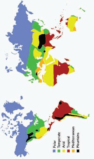
PROFILE ISSUES DESIGN RESPONSE URBAN FORM POLAR TEMPERATE ARID TROPICAL MEDITERRANEAN MOUNTAINS
MINOR TEMPERATURE RANGEHOT DIURNALLY -HEAVY RAIN -SNOWY, WINDYBLIZZARDEXTREME COLD NIGHTS -STRESSFUL & UNCOMFORTABLESTRONG DRY COLD WINDSINTENSE SOLAR RADIATIONSLARGE DAY-NIGHT TEMP. DIFFERENCEDUSTY STORMSTORRENTIAL RAININTENSE DEHYDARATION; HIGH SALINATION -WINDY &STORMYBREEZE SYSTEMHIGH HUMIDITYEROSIVE -WINDY & INCREASING AIR CIRCULATIONHIGHER REL. HUMIDITY COMP TO LOWLANDSSOMETIMES PRONE TO EARTHQUAKEPROVIDE HEATHY, MODERATE CLIMATE -EXCESSIVE HEATHIGH HUMIDITY -LOW TEMPERATUREWINTER AND SUMMER HIGH PRECIPITATION -WINDY --EXCESSIVE LOW TEMPERATURE ASSOCIATED WITH DRYNESSSTRESSFUL WIND -EXCESSIVE DRYNESS -HIDH DAY TEMPERATURE -DUSTY AND STORMYHIGH HUMIDITYWINDY -WINDY -VENTILATION: OPEN ENDS; DISPERSED FORM; WIDE STREETS -EXTENSIVE SHADOW -DISPERSAL OF HIGH RISE; VARIATION OF BLDG HTSWIDE, SHADOWED OPEN SPACES, PLANNED TREE ZONES COMPACT AND CLUSTERED FORMS PROTECTED URBAN EDGES NARROW WINDING ROADS ALLEYS UNIFORM CITY HT;SMALL DISPERSED OPEN SPACES CIRCUMFERENTIAL INTERSECTING TREE ZONES HEATING(PASSIVE& ACTIVE)MIX OF OPEN AND ENCLOSED FORMSPROTECTION AGAINST WINTER WINDWARD UNIFORM BLDG HTS MEDIUM DISPERSED OPEN SPACES CIRCUMFERENTIAL/INTERSECTING TREE STRIPS COMPACT FORMSSHADOWINGEVAPORATIVE COOLINGPROTECTED URBAN EDGE FROM HOT WINDS MIX OF BLD HTS TO SHADOW CITYSMALL DISPERSED PUBLIC OPEN SPACES CIRCUMFERENCING/INTERSECTING TREES DISPERSED FORM WITH OPEN ENDS TO SUPPORT VENTILATION COMPACT AND AGGRGRATES FORMS CLUSTERED FORMS MIXED OPEN AND CONTROLLED ENCLOSURE FORMS COMPACT FORMS -MODERATE DISPERESED FORM -OPEN URBAN EDGES WIDE STREETS TO ALLOW BREEZE FLOWVARIED BLDG HTS WIDE OPEN SPACES SHADOWING TREES SEMICOMPACT FORM: MIX OF COMPACT/DISPERSED HORISONTAL STRESS/ ALLEYS FOR VIEW LOW HT BLDG SMALL DOSPERSED OPEN SPACES NON OBSTRUSICE TREE ZONE SEMI COMPACT FORM MIX OF COMPACT AND CLUSTER HUMID REGIONS:MODERATELY DISPERSED FORMS DRY REGIONS:COMPACT AND PROTECTIVE TOWARDS INLAND FLAT ROOFS SLOPED ROOFS THICK WALLS OPEN SPACES/ PLANNED TREES UNIFORM BLDG HT COMPACT DISPERSED CLUSTERED OPEN URBAN EDGE CLOSED URBAN EDGE NON-UNIFORM BLDG HT VENTILATION SHADOW INSULATION DRAINAGE IGLOO SLOPED ROOF; WINDOWS TO CAPTURE MAX SUNLIGHT MULTILEVEL PDWELLINGS INSULATION; SHADOW (MEXICO) THICK WALLS WIND CATCHERS(IRAN) DISPERSED; CLOSE EDGE URBAN PLAN STONE DWELLINGS IN IRELAND SLOPED WALLS; CENTRAL COURTYARD( INDIA) DOGTROT HOUSE (U.S) HOUSES ON STILTS SLOPED ROOFS;(AMAZON) TIBETAN VERNACULAR EARTHQUAKE RESISTANT HIMALAYAN REGION: HEAVIER BOTTOM, LIGHTER TOP SEMI COMPACT FORM BHUTAN WIND CATCHERS(PAKISTAN)
VERNACULAR EXAMPLES
- 22Domain
GLOBAL CLIMATOLOGICAL REGIONS BASED ON LOCATION AND TOPOGRPAHY
- Orientation
(ii) Continental:
- Large flat, open terrain : subject to exposure of winds and major storm systems..
- Major difference between the seasons.
- Between the Taiga region , through the mid latitude grasslands and hardwood forest; from semi arid mid latitude areas towards the hot deserts to subtropical edge.
- Southern Hemisphere: 20 °S to 40 °S
Observed Vernacular responses:
- Protection against wind : use of trees and earth.
- Planted landscapes as windbreakers
- Low profile, earth embraced and aerodynamic in form to reduce surface exposure
- Lowered floors in pit houses with earth covered walls, airtight fabric or skin construction to avoid wind and also use thermal capacity of earth.
- Entrance facing east. Steeper rear side braced against prevailing westerly winds.
- Continuous wind breakers , also usually tall (10 ft )
- Insulation in walls
(iii) Desert:
- Extreme differences in the temperatures
between night and day.
- Evapo-transpiration is the major factor of concern.
- Strong sun and high temperatures.
- An average of 3000hrs of sunshine annually.
- Due to the low water vapour presence in the atmosphere, both incoming solar radiation and the outgoing radiation are high, thus causing rapid air temperature changes as much as 3 ° C per hour. Resulting from this are sunny hot days and rapidly cooling nights.
- Rainfall occurrence is erratic. The sparse vegetation also leads to flooding.
- Erratic winds, with speed between 15 and 30 mph; dust haze, sand storms.
Observed Vernacular responses:
- Massive defensive built structures; blank walls , shuttered openings, courtyards, narrow streets to baffle winds.
- Heavy construction material to delay thermal flux.
- Intensive solar heating reduced by reflective surfaces/ ventilated double construction.
- Vaulted or domed roofs better than flat roofs as they can reradiate heat better at night.
- Shade roofs, Arbors, Armadas
- Cross ventilation is not the usual summer cooling strategy because of the high temperature of winds( more than skin temperature). Instead the use of wind towers is common, made to capture winds
ARCTIC/ SUBARCTIC MEDITERRANEAN SUBTROPICAL CONTINENTAL MARITIME MONTANE DESERT MONSOON TROPICAL
- 23Climate Classifications
and diffuse into the building.
(iv) Maritime:
- Most maritime climates are restricted by coastal climates with the exception of Western and Central Europe, leaving the mainland open to wind and moisture effects of the Atlantic. Europe: continuous westerly and northwestern winds
- Four distinct seasons are characteristic of this region.
Observed Vernacular responses:
- Built forms are made sensitive to dampness.
- Pitched roofs are common. Large roofs of insulated material and limited wall areas to reduce thermal loss and maximize the internal heat are a common feature.
- Maritime effects from the North and West.
- Entrance is most commonly places on the South side.
- Linear pattern of blocks in a single row, with broadside to the sun.
- No openings in the northern walls as protection against winds.
(v) Mediterranean:
- Moderate and coastal with sunny, dry, warm summers, and mild or cool, damp winters.
- Latitude: 45 ° N to 30 ° N; west coast of all the continents.
- Area around the Mediterranean sea; deep, thermally stable water surrounded by land and mid latitudes.
- Warm water stabilizes air temperature and reduces diurnal swings.
- The rugged terrain and broken surrounding highlands leads to the rise of many a microclimate.
- Sirocco, Mistral and Bora are some of the local winds- the warm dry blowing in from the Sahara, the cold northerly winds from in France and Greece respectively.
Observed Vernacular responses:
- Heavy masonry for insulation
- Conical roofs
- Entrance and small openings in the south, very small opening to the north.
- Reflective white surfaces
- Courtyards
- Narrow streets
(vi) Monsoon:
- 3 seasons
- Wind that reverses itself seasonally , blows continuously between land and adjacent water body
- Prevailing winds from north east .
- High humidity during most parts of the year.
- Increased precipitation during most parts of the year.
Observed Vernacular responses:
- One storey design typically on raised floor
- Deep, well sheltered porch at least on one side, deep overhangs on all sides encouraging ventilative cooling and convective dissipation of the attic heat from gabled roof.
- Hot dry season: massive walls on the ground floor, with a storey of light weight construction above.
- Elements such as porches provide shade and also rain protection
- Shared perimeter walls thus only narrow front wall exposed to weather facing narrow streets.
- Rugosity increased to reduce solar gain and also as options for thermal control.
- Fresh air allowed only when air is cooler than the building.
- Lower levels are cooler.
(vii) Montane:
- The altitude of land and orientation of slope is an influential factor on the local climate, irrespective of the latitude.
- Frequent precipitation, dominant diurnal wind patterns , distinct seasons, many local microclimate and seasonal flow.
- Impact of large mountain ranges to the global climate is profound. They act as barriers to the flow of winds and this causes climatic shifts on both the windward and leeward regions.
- The interrelated mountain and valley systems are important to human settlement due to the resulting microclimate.
- The altitude primarily causes a drop in the air temperature. Also the rainfall and snowfall is much higher.
- Uplift of airstreams on the windward sides causes condensation of moisture and increases precipitation. Gaps in mountains causes strong flow of winds.
Observed Vernacular responses:
- Aerodynamic form
- Multi-storied
- Expansive roof with generous overhangs
- Raised porches
- Relatively shallow roofs.
- Massive tapering external walls
(viii) Subtropical
- 24Domain
- Humid warm coastal; warm but outside the tropics.
- Multiple seasons
- Cool or mild winter is short and damp with rain, but seldom snows, and the frost free period is at least nine months.
- Humid summer is long, warm and muggy.
- Considerable humidity throughout the year
- Similar conditions with variable seasons also characterize the uplands and plateaux within the tropics including at the Equator.
- Large lowland areas with humid warm climates are on the east and southeast coasts of four continents, between latitudes 25 ° and 38 °
- Average monthly temperature is above 25 ° C
- Cool humid winters with average monthly temp below 10 ° C
- Continuous humidity provides a narrow annual range of temp
Observed Vernacular responses:
- Well spaced buildings with generous garden and large canopy shade trees.
- White lime plastered on thick rammed earth walls tempers summer heat.
- Few windows towards the sun. Windows are places deep and high in the walls.
- Full solar penetration in the winter is desirable.
- Incoming and outgoing radiation are stronger so there is an increased use of thick walls for thermal mass.
(ix) Tropical:
- Warm and wet throughout the yr with little variation.
- No distinct seasons
- Slight difference between day and night conditions
- High humidity continuously; high precipitation throughout the year.
- 10 ° of the equator; 23 ° North at the Tropic of Cancer to 23 ° S at the Tropic of Capricorn
- Trade winds affect these regions
- Stable conditions, with narrow range of temperature daily and annually. Mean temp for year is around 18 ° C
- Max air temp between 27 ° and 32 ° C
- Relative humidity : 55 %- 100%
- Lack of wind or strong storms
- Skies normally clear
- Atmospheric turbidity due to high relative humidity which prevents solar heat from dissipating.
- Frequent rain storms can be accompanied by thunder and lightning
Observed Vernacular responses:
- Extensive roofs for shading, well sloped for the rain.
- Increased natural convection including stack ventilation by the use of gable vents.
- Frame construction adopted, to maximize the cross ventilation with the slightest breeze.
- Lightweight construction
- 25Climate Classifications
Climate Change and its Consequences
A Bio-Climatic design approach to urbanism requires a thorough analysis of all relevant climatic parameter; this not only with respect to current climatic conditions but also with regards to potential future changes and shifts.
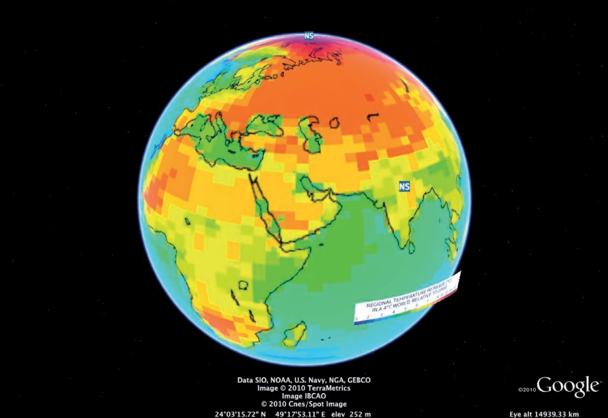
Today different climate models and theories exist that predict changes to the global climate over the next 50 to 100 years. As much as there is disagreement, whether the earth will warm up, cool down, or whether the global climate will remain static, it seems that the concept of global warming is the most widely accepted. Van Esch (Van Esch) reports that according to an IPCC 2007 report heat stresses will generally increase due to a global temperature rise between 1.1°C and 6.4°C. A joint study conducted by the UK Met office in cooperation with Google Earth (2009) predicts even more radical changes in temperature until the year 2050; here temperature increases are predicted to be in average at around 5°C, however some of the polar regions are projected to experience a rise in temperature of up to 12°C.
Projected increases in global temperature will have a drastic effect on the fossil fuel consumption of cities and urban agglomeration; as much as higher energy consumption due to increased cooling loads could result in massive problems, it is the change in weather patterns and the associated problems that impose a real threat to urban (and rural) societies. According to the UK Met Office changes over the next 40 years will include extreme temperatures, that in certain regions will lead to shortages in terms of crop production and water availability; as most urban develop-
ment is predicted to take place in regions with already extreme climates, continuous urban growth could result in the literal starvation of cities. Extreme temperature rises in polar regions, on the other hand, could further accelerate the already rapid decrease of the polar ice caps; associated rises in global sea levels could likely result in permanent flooding and in this way have an impact on many coastal cities. Overall, shifts in temperatures will have an impact on current climates. Williams reports that key risks associated with projected climate trends for the 21st century include the prospects of future climate states with no current analog and the disappearance of some extant climates (Williams, 2007). Climate shifts projected by the Met Office include the shift of monsoon regions and increased occurrence of tropical cyclones. The effects of such weather phenomena on human settlements can already be witnessed today.
Cities that are planned today therefore need to respond to such scenarios and need to incorporate strategies that can mitigate the effects of climate change. Future climate projections should therefore be studied by urban planners and urban strategies need to be deployed that allow for careful planning and adaptation over time.
- 27Climate Change and its Consequences

- 28Domain
By 2055, shifts in climate zones are predicted unless greenhouse emissions are drastically reduced. Global temperature increase in °C.
Source: UK Met Office/Google Earth, 2009
By 2055, climate change is likely to have warmed the world by a dangerous 4 °C; drastic implications are predicted including sea level rises, droughts and water availability. Source: UK Met Office/Google Earth, 2009

Permafrost:
• Almost complete disappearance of near-surface permafrost from Nothern Siberia. Reduction of Permafrost in Canada and Alaska.
Water Availability:
• Water resources affected by up to 70% reduction in run-off around the Mediterranean, southern Africa and large areas of South America.
• Complete disappearance of glaciers from many regions in South America. In Peru’s Cordillera Blanca summer run-off from glaciers reduced by up to 69% as the glacial area falls by 75%.
• Half of all Himalayan glaciers significantly reduced by 2050. The Indus river basin obtains 70% of its summer flow from glacial melt. In China, 23% of the population lives in the western regions where glacial melt provides the principal dry season water source.
Crops:
• Maize and wheat reduced by up to 40% at low latitudes.
• Soybean yield could decrease in all regions of production, including North and South America, southern and eastern Asia.
• Decrease in rice yield of up to 30% in China, India, Bangladesh and Indonesia.
Drought:
• Drought events occur twice as frequently across southern Africa, South-East Asia and the Mediterranean basin.
Sea Level Rise:
• Sea levels could rise as much as 80cm by the end of the century. Longer term, 4°C would result in a much higher rise in sea level. Sea level increases are likely to be even greater at low latitudes, disproportionately affecting tropical islands and low-lying regions such as Bangladesh.
• For the population at 2075, a mean sea-level rise of 53cm means that up to an additional 150 million people per year would be flooded due to extreme sea levels. Three-quarters of these people live Asia. Up to 56 million people would be flooded along the Indian Ocean coast, 25 million along the east Asian coast and 33 million people would be flooded along the South-East Asian coast. Other vulnerable regions include Africa, Caribbean Islands, Indian Ocean Islands and Pacific small Islands.
• Greenland Ice Sheet has a 60% likelihood of irreversible decline. This would result in a very long-term sea-level rise of up to 7 meters globally.
• It is not known how stable the West Antarctic Ice Sheet is, or whether a 4°C global temperature rise will send it into irreversible decline. If this ice sheet did melt it would contribute a further 3.3 metres to long-term sea-level rise globally. Sea-level rise combined with storm surges could pose a serious threat to people and assets in the Netherlands and south-eastern parts of the UK.
Tropical Cyclones:
• Tropical cyclones could be more intense and destructive. Global population increases, particularly in coastal areas, and sea-level rise mean greater cyclone and hurricane related losses, disruptions to infrastructure and loss of life as a result of storm surges. For major cyclone disasters flooding from storm surges has been the primary cause of death.
Extreme Temperature:
• Hottest days of the year could become as much as 10-12°C warmer over the eastern North America, affecting Toronto, Chicago, Ottawa, New York and Washington DC.
• Hottest days of the year across Europe could be as much as 8°C warmer
• Hottest days of the year could be as much as 6°C warmer over highly populated areas of eastern China.
The impact of a global temperature rise of 4°C - Projected for 2055. Diagram adopted from UK MET Office/Google Earth, 2009
- 29Climate Change and its Consequences +13ºC +15ºC +11ºC +9ºC +7ºC +5ºC +3ºC +1ºC +7ºC +8ºC +7ºC +6ºC +3ºC +6ºC +6ºC +6ºC +5ºC +5ºC +6ºC +6ºC +6ºC +6ºC +6ºC +6ºC +6ºC +6ºC +6ºC +3ºC +5ºC +3ºC +5ºC +5ºC +5ºC +6ºC +6ºC +6ºC +7ºC +7ºC +7ºC +12ºC +7ºC +7ºC +8ºC +8ºC +8ºC +9ºC +11ºC +11ºC +4ºC +6ºC +5ºC +7ºC +4ºC +6ºC +8ºC +6ºC +5ºC +7ºC +6ºC +7ºC +7ºC +8ºC +10ºC +10ºC +10ºC +9ºC +6ºC +7ºC +8ºC +13ºC +14ºC +15ºC +7ºC +5ºC +5ºC +4ºC +3ºC
- 30Domain
‘Sustainable’ Cities
In recent years there has been growing public awareness for the need of ‘sustainable urban design’ in order to mitigate energy consumption and waste production of cites. The US Environmental protection agency concluded in 2001 that ‘…the urban form directly affects habitat, ecosystems, endangered species, and water quality through land consumption, habitat fragmentation, and replacement of natural land cover with impervious surfaces. In addition, urban form affects travel behaviour, which, in turn, affects air quality; premature loss of farmland, wetlands, and open space; soil pollution and contamination; global climate; and noise’ (Jabareen, 2006).
As much as it is attempted to develop and implement concepts for ‘environmental-friendly’ cites, there is disagreement of what appropriate solutions are. As a result, different concepts for sustainable urban forms exist. In the 1960’s Jane Jacobs was at the forefront to argue for diversity and against urban sprawl. As a result, a variety of different urban movements evolved that criticise the monotony and lack of urban qualities that were in many cases linked to modernistic ideas; the ‘Neo-traditional Movement’, as well as other concepts, such as ‘Urban Containment’, the ‘Compact City’, or the ‘Eco-City’, can be seen as an reaction to urban planning that was implemented in the 1960s and 1970s.
They all argue for alternative ways in order to improve urban qualities and to mitigate energy consumption.
Nevertheless, with growing environmental awareness and energy prices soaring, recent concepts for ‘sustainable cities’ focus much more on the metabolism of cities; i.e. the reduction of energy consumption via renewable energies and the mitigation of waste produced. Currently, the most well known example for such a zero-carbon/zero-waste ecology is the proposed master plan for the city of Masdar in the United Arab Emirates. In the following chapter different concepts for ‘sustainable’ urban development will be introduced. In addition characteristics of urban sprawl, densification and satellite towns will be explained.
- 31‘Sustainable’ Cities
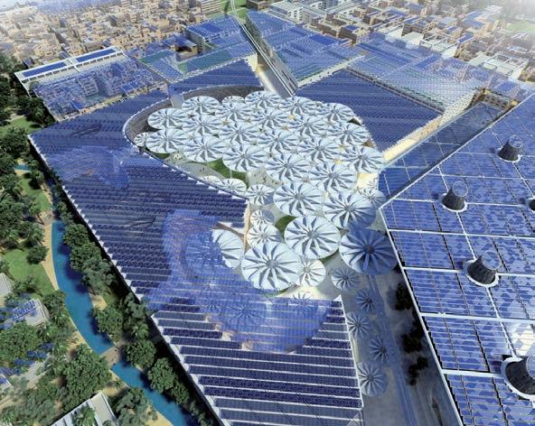
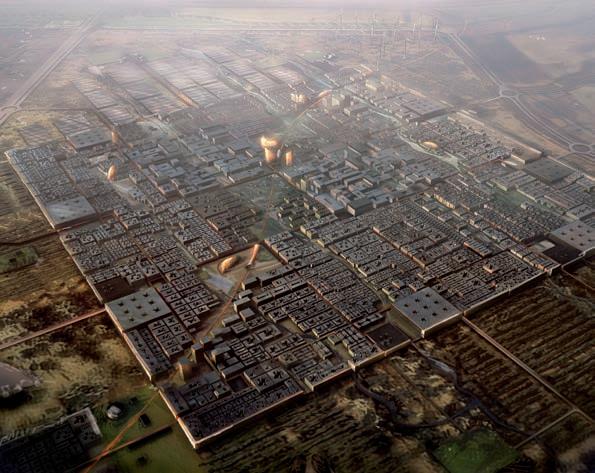
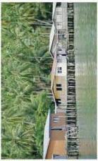
A Sustainable City in the Desert
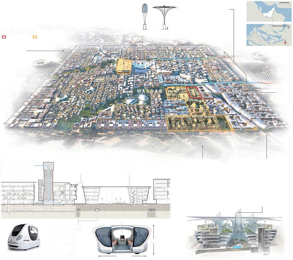
Images above: Masdar City, United Arab Emirates. The master plan is advertised a paradigm for sustainable urbanism. Designed by Foster & Partners, the city will rely entirely on solar energy and other renewable energy sources, with a sustainable, zero-carbon, zerowaste ecology (Source: Wikipedia). Located in the desert, 17km outside Abu Dhabi, the design is currently executed. Once it is completed it will have to proof its high ambitions (Diagram: www.nytimes.com).
The
help mitigate windblown dust
sand. Complete this fall Under construction Approx. 1 Mile Computer
Surrounding trees will
and
rendering of the planned city
a public
water
Automated cars with room for four adults Automated transportation Masdar will be using an automated system of electric vehicles, including passenger cars and freight trucks. The city’s ground level was elevated 23 feet, and the vehicles will operate underneath Narrow streets allow for some sunlight, but overhangs create shade Street Courtyard Control panel 12.5 feet 6.4 feet Max Speed 25 m.p.h.
The Wind tower funnels wind to ventilate
square at its base. The air is cooled with
sprays.
power the buildings and provide shade to keep roofs cooler.
Photovaltic panels
power
facilities, parking garages and food production areas A light rail line will pass through the center of Masdar, linking it to downtown Abu Dhabit and providing transport within the new city. Wind cones will provide natural ventilation and soft daylight to the building’s interior. Masdar Headuarters Photovoltaic panels on Masdar Headquartes, the city’s biggest office building, are expected to produce more energy than the building consumes. It is scheduled to be finished in 2013
The City is surrounded by recreation areas,
generation
Pahse 1 Masdar Institute
The area being completed this fall has some design features common to the entire project.
Solar Farm Streets are laid out at angles that optimize shading. Long, narrow parks catch and cool the prevailing winds and assist in ventilating the city. Saudi Arabia Abu Dhabi Dubai Iran Miles Miles 150 10 Arabian Sea Oman Masdar Arabian Gulf Central Abu Dhabi UAE Up To 98.5 feet in diameter
cells
Masdar Institute
Photovoltaic
Plaza
Headquarters Neighbourhoods will have distinct buildings and design elements. Masar Plaza, for example, will have 54 sunshades that open and close automatically at dawn and dusk.
Masdar
Masdar
of Masdar, a city under constuction near Abu Dhabi, say that it will be the world’s first carbon-neutral city. It will be home to a research institute focused on renewable energy and sustainability, and eventually, if all goes as planned, to various clean-technology companies, and to a projected 45,000 residents and another 45,000 commuters. Domain - 32 -
Promoters
Concepts for ‘sustainable’ urban form
As the urban population is predicted to drastically grow over the next four decades cities will encounter a rapid increase in size and number. This tendency has massive implications on energy demands that are related to infrastructure, heating and cooling. The development of appropriate design strategies that take the reduction of energy consumption into account should therefore be the main challenge for architects and urban planners.
Poor urban qualities of cities that were developed in the post war area have resulted in new approaches to urbanisms that include e.g. the eco city or the neo-traditional development. As much as these strategies try improve urban living conditions strategies are lacking that incorporate geography and climate into urban design. Key to establishing a bio-climatic urban approach is to identify the parameters that need to be considered for mitigating the energy demands of an urban fabric. In this context Jabareen (Jabareen, 2006) points out seven factors that should be considered for any ‘sustainable’ urban planning approach:
Compactness:
Compactness of urban form is for many planers one of the key strategies in the approach to sustainable urban design. It can help to prevent urban sprawl and can help to minimize transport of energy, water, materials and products. (Jabareen, 2006). For example, Dumreicher et al. argue that a sustainable city should be compact, dense, diverse, and highly integrated. Compactness goes hand in hand with the goal of livability and works to prevent commuting, one of the most wasteful and frustrating aspects of city life today.
Sustainable Transport:
The size of contemporary cities is only possible because of modern means of public transportation, including buses, subways and elevators. Such infrastructures allow cities to expand in the horizontal as well as in the vertical extent and allow for a separation of living and working. The form of the city thus reflects the transport technologies that were dominant at a specific time.
Infrastructural networks and technologies have enabled urban agglomerations to reach unprecedented sizes; nevertheless they impose enormous energy demands and put enormous strains on the environment. Jabareen suggests that a restructuring of the urban and metropolitan transportation system can help conserve energy in several ways as compact and transit orientated development shorten trips and encourages non-motorized travel.
Density:
Density is an important measure that allows to draw important conclusions about, e.g. the compactness of an urban fabric; in this way it is highly related to sustainability. Dense urban morphologies suggest shorter travel distances and, depending on a city’s geographic location, density can be used as an indicator regarding the energy requirements of a fabric; in cold climates shared party walls can reduce heat loss whereas in hot and humid areas isolated buildings can improve the ventilation potential of a fabric und thus reduce cooling needs.
Different concepts of measuring density exist, though. In general density can be defined as a ‘numerical measure of the concentration of individuals or physical structures within a given geographic unit.’ (Ng, 2010)
According to the above definition a common concept of measuring density is to look at the ratio of population to land area. Density can, nevertheless, also be expressed in other ways. Planners often look at the relationship between occupied land (or floor area) to un-built land. The later method is often used as a way of measuring building density; the plot ratio or floor area
ratio combined with site coverage can thereby give indications about the morphology of an urban fabric: High plot ratios combined with low site coverage tend to suggest tall and free standing buildings, whereas lower plot ratios and high site coverage might indicate urban sprawl (compare diagrams on page 180).
As much as density can be associated with sustainability it needs to be stressed that there is different opinions among scholars whether high or low densities are beneficial in terms of reducing energy consumption.
Mixed Land Use:
Many scholars and planners believe that concepts of mixed land use should be (re-) introduced into cities in order to reduce travel distances and to enhance social activities. The classic model of live-work, where residential and commercial activities are intertwined within the same neighbourhood or block has in the past often been replaced by rigid zoning structures that separate such activities. Jabareen argues that imposed zoning reduces the diversity in local areas and results in increased traffic and less safe streets; he resumes (Jabareen, 2006): “For a sustainable urban form, mixed uses should be encouraged in cities, and zoning discouraged.”
Diversity:
Car orientated post-war urban planning has often resulted in monotonous urban landscapes with poor neighbourhood qualities. The paradigms of modernity have therefore let to new planning approaches, such as ‘new urbanism’, ‘smart growth’ or ‘sustainable development’. In the early 1960s Jane Jacobs was one of the first to challenge current planning regimes by advocating urban strategies that are formed around the central idea of diversity. Diverse development thereby implies a mixture of land uses, building and housing types, architectural styles, and rents; by introducing diversity it is hoped to break with the homogeneity and monotony of urban form and to enhance social interaction and activities.
Passive Solar Design
According to Jabareen passive solar design is central to achieving sustainable urban form. He argues (Jabareen, 2006): “…architects have a larger share of responsibility for the world’s consumption of fossil fuel and global warming gas production than any other professional group.”
As pointed out earlier the morphology of an urban fabric has large implications on its ability to absorb or reflect solar radiation. In other words, the capacity of an urban structure to store or release heat is highly dependent on its morphological characteristics. Jabareen points out that the reduction of energy demand due to heating or cooling should be central to an urban design; passive solar design can therefore be achieved by specific design measures that relate to the constitution of the urban fabric. Orientation of buildings as well as densities should be carefully considered when planning an urban fabric. Factors such as built form, the street canyon, building design as well urban materials should also be added to this.
Greening:
Greening is an important consideration towards improving the qualities of an urban fabric. Besides it’s social and recreational values it has important implications on the microclimate of an urban area. Compared to hard surfaces vegetation has the ability to store water; this can help mitigating sewer systems in areas with a lot of rain and prevent surface water run-off. In warmer climates parks and green areas can act as cool islands as they release heat through evapo-transpiration and shade can be provided through vegetation. Urban pollution and smog can also be acted against by appropriate green planning.
- 33‘Sustainable’ Cities
Hot-Humid
Equatorial Zone
Cold-Humid
U.S.A and souther Canada
Hot Diurnally and Seasonally with minor temperature Range.
Heavy rain
More Comfort at High Elevation
Exessive Heat
High Humidity
Hot-Dry
Middle East and North Africa
Snowy
Windy, Blizzard Condidtions
Very Cold Nights
Low Temperature
Winter and Summer
High Precipitation
Windy
Cold-Dry
Inland Plateau
Intense Solar Radiation
Large Temperature
Amplitude between Day and Night
Dusty Storms
Torrential Rain
Low Cloudy Days
Intense Dehydration
High Salinization
Evaporation exceeding Precipitation
Excessive dryness
combined with high day temperature
Dusty and Stormy
Ventilation: Open Ends and Dispersed Form
Widely Open Streets to support ventilation
Combined vatiation of Building Heights
Wide, yet shadowed open Spaces
Shadowing, planned tree zones
Heating (Passive & Active):
Mixture of open and enclosure forms
Protected Edges at Winter Windward Side (with structures or trees)
Uniformed Building Heights
Medium Dispersed Open Space
Circumfernetial and Intersecting Tree Strips
Compact Forms:
Shadowing
Evaporative Cooling
Protected Urban Edges from Hot Winds
Windward Location near a Body of Water
Narrow Winding Neighborhood Roads and Alleys
Mix of Building Height to Shadow the City
Small Dispersed, and protected public open Spaces
Cicumferential and Intersecting Tree Zones
Use of Geo-Space City Concept
Dispersed Form with open ends to support ventilation
Stressful and Uncomfortable Strong Dry and Cold Wind
Excessive Low Temperature associated with Dryness
Stressful Wind
Compact and Aggregate Forms, Clustered Forms
Protected Urban Edges
Narrow Winding Neighborhood Roads and Alleys
Uniformed City Height
Small, Dispersed, and Protected Public Open Spaces
Circumferential and Intersecting Tree Zones
Use of Geo-Space City Concept
Classification of Major Climate Types and Urban Morphologies, adopted from Golany (Golany 1996)
Mix of Open and Controlled Enclosure Forms
Compact Form
Compact and Aggregate Form, Clustered Forms
Main Climates, Example Basic Profiles Major Problems (Issues) Basic Urban Design
Prefered Urban Form
Response
Domain - 34 -
Seashore Strips Desert Coasts
Windy and Stormy Breeze System High Humidity Erosive
High Humidity Windy
Mountain Slopes Lower, Middle and High Slopes
Windy and Increasing Windy Air Circulation Higher relative Humidity than the Lowland
Provide Healthy and Moderate Climate
Enhance attractive View
Windy
In Humid Region: Moderately dispersed Form
Open Urban Edges
Wide Streets perpendicular to the Shore to receive the Breeze
Dispersed High Rise
Buildings to receive Ventilation
Variety of Building Heights
Wide Public Open Space
Shadowing, Planned Tree Zones
In Dry Regions:
Open Towards the Sea, Compact and Protected toward the Inland
High Rise Buildings mixed with low Height
Small protected and dispersed Public Open Spaces
Shadowing, planned tree zones
Semi-Compact Form: Mix of Compact and Dispersed
Horizontal Stress and Alleys to enhance the view
Low height Buildings
Small Dispersed Public Open Spaces
Non Obstructive Protected Tree Zones
Use of Geo-Space City Concept
Classification of Major Climate Types and Urban Morphologies, adopted from Golany (Golany 1996)
In Humid Regions: Moderately Dispersed Form
In Dry Regions: Compact and Protective toward the Inland
Semi-Compact Form: Mix of Compact and Clusterd Forms
Golany argues that different climate zones require specific urban forms in order to best respond to the environment. The diagrams above and on page 34 provide a catalogue of environmental criteria and corresponding design responses (Golany, 1996).
Main
Example Basic Profiles Major Problems (Issues) Basic Urban
Prefered
Climates,
Design Response
Urban Form
- 35‘Sustainable’ Cities
The beginnings of cities may be thought of as agglomeration points of peoples where in there were material exchanges coupled with some kind of administrative structuring. Chronologically, they may be classified into two broad categories as before and after the Industrial Revolution in the 18th and 19th centuries.
The ‘Evolved city’ of ancient civilizations to the pre industrial era came about into being over long periods of time, developing in patterns under the influence of various factors, such as climate , culture and political confinements through time. The ‘Planned City’, of the post industrial, post-war and till date, on the contrary, was an implementation of detailed land use strategies and plans laid out directly aiming at building centers of economic foci by governments in collaboration with urban planners. However both cases reflect are emergent phenomena due to the dynamic flows of people and energy.
The determinant factors of location and persistence of a polis have in all cases been in relation to Mercantile, Governance and/ or Microclimate pertaining to the geographic location (mainly in the case of evolved cities).
City forms are material constructs that are composed of a spatial array of dwellings, a pattern of street and public spaces together with differentiated buildings of varying sizes associated with the regulation of energy and material flow, and the extension of metabolic network across the surrounding territory.[MW, The Architecture of Emergence].
‘Urban Microclimates’ evolve locally through the interaction of the built environment and the local climate. There is no clear delineation for the size and extent of Microclimates; they can range from individual facets of the urban environment, through streets and city blocks to neighbourhoods. In this sense the city consists of a patchwork of microclimates. All local microclimates together comprise the overall microclimate of the city.
The control and optimization of Urban Microclimates is currently not addressed in design.
We argue that the only way to optimize the ‘Urban Microclimate’ in a design process is by using simplified parameters; in other words we believe that the use of complex computational analysis tools like e.g. Fluid Dynamics are currently still too time consuming to be used in generative design processes. We therefore believe that simplified Urban Parameters (Morphological Indicators, such as e.g. Rugosity or Porosity) should be used to rapidly extract indicative results.
These urban parameters are set in different proportions against the global factors of climate and topography. In order to set these proportions, the performance of an evolved city against that of its planned counterpart, in each of the 9 global zones, is assessed with respect to the morphological indicators. We believe these results reveal key information to feed our optimization tool to respect the needs of not just the local built environment, but their overall setting in any given geographic location.
We however do acknowledge that apart from the above mentioned quantifiable morphological indicators, there exist certain other non- quantifiable factors of culture, and social preference and identity related to an urban setting . Kevin Lynch describes this attribute as “a sense of place”. Lynch specifically describes how to achieve a sense of place regardless of the purpose and structures. [Lynch: What Time is This Place? And Site Planning] Often culture and familiarity are associated with these ideas.
Urban
City/
Fabric Definition:
Domain - 36 -
URBAN
SPRAWL


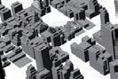

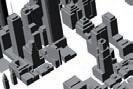
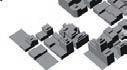
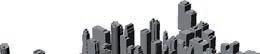
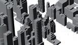
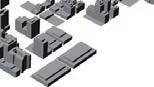
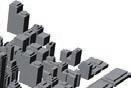
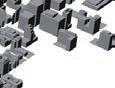

Current approaches to urbanization:
URBAN DENSIFICATION
At present, 2% of the world’s land surface is covered by cities and yet the people living in them consume 75% of the resources consumed by mankind. The ‘ecological footprint’ of cities is many times larger than the areas they physically occupy (Rees, 1999).
Urban Sprawl
Sprawl is the spreading out of a city and its suburbs over more and more rural land at the periphery of an urban area. This involves the conversion of open space (rural land) into built-up, developed land over time.
From the standpoint of urban planning institutions, the style of that conversion can sometimes be more important than the amount of the conversion. Organizations whose chief concerns involve urban planning goals may tend to emphasize qualitative attributes of sprawl -- such as attractiveness, pedestrian-friendliness and compactness.
However, the effect of sprawl on the natural environment and agricultural resources, the more important overall measure of sprawl is the actual amount of land that has been urbanized. Knowing the actual square km of urban expansion (sprawl) provides a key indicator of the threat to the natural environment, to the nation’s agricultural productivity and to the quality of life of people who live in cities and in the small towns and farms that are near cities
Precendent: US cities:
Between 1982 and 1997 America converted approximately 25 million acres (39,000 square miles) of rural land — forests, rangeland, pastures, cropland, and wetlands — to developed land: that is, sub-divisions, freeways, factories, strip malls, airports, and the like.
Over a 20-year period (1970-1990), the 100 largest Urbanized Areas in the United States sprawled out over an additional 14,545 square miles. That was more than 9 million acres of natural habitats, farmland and other rural space that were covered over by the asphalt, buildings and sub-divisions of suburbia. And that was just for the half of Americans who live in those 100 cities. This strategy of urban plan has now become a topic of concern.
[Source: NumbersUSA]
URBAN B O YRADNU RURALLAND URBANBOUNDARY
DIRECTIONALITY MINERALIZATION OPENESS TO SKY REFLECTANCE POROSITY SINUOSITY SOLAR ADMITTANCE BUILDING GEOMETRY OCCLUSIVITY DENSITY Inferred ratios. MICROCLIMATIC RESPONSE
- 37‘Sustainable’ Cities
URBAN DENSIFICATION


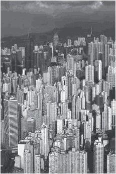
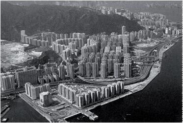


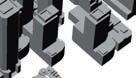
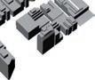

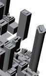

URBANBOUNDARY
Urban Densification
Instead of expanding the boundary, cities often respond to development pressure by setting targets for increased urban densities. The result is reflected by the establishment of high rise cityscape and compact urban settings. The effects of urban density on the total energy demands of a city are complex and conflicting ( Givoni,1998). Highly concentrated load centres and compactness of land use patterns will bring benefits to energy distribution and transport system design, buut crowded conditions may create congestion and undesirable local microclimate.
Precedent: Hong Kong
DIRECTIONALITY MINERALIZATION OPENESS TO SKY REFLECTANCE POROSITY SINUOSITY SOLAR ADMITTANCE BUILDING GEOMETRY OCCLUSIVITY DENSITY DIRECTIONALITY MINERALIZATION OPENESS TO SKY REFLECTANCE POROSITY SINUOSITY SOLAR ADMITTANCE BUILDING GEOMETRY OCCLUSIVITY DENSITY Inferred ratios. **Inferred ratios. MICROCLIMATIC RESPONSE MICROCLIMATIC RESPONSE MICROCLIMATIC
High rise cityscape of Hong Kong (north of Hong Kong Island)
Eastern District of the Hong Kong Island (maximum plot ratio 8 to 10)
Domain - 38 -
[Source: Low energy Building Design in High Density Urban Cities- Sam C.M. Hui]
SATELLITE CITIES
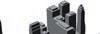


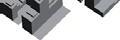


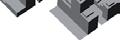


Satellite cities
Satellite cities are usually conceived as new developments or major expansions to existing settlements that are separated from metropolitan core by belts of rural land. Planners argued that restrictions should be placed on central growth, and the development of separate centres within the metropolitan region encouraged.
The Greater Plan of London, 1944 was one of the pioneers of the type.
Precedent: Tokyo
The rapid sub urban expansion from the WW1 to the mid 30s combined with the setting up extensive railway networks saw the development of satellite towns to Tokyo. This was advanced rapidly with the involvement of the private sector.
U R B A N YRADNUOB U R B A N YRADNUOB R U R A L DNAL R U R A L DNAL R U R A L DNAL U R B A N YRADNUOB
DIRECTIONALITY MINERALIZATION OPENESS TO SKY REFLECTANCE POROSITY SINUOSITY SOLAR ADMITTANCE BUILDING GEOMETRY OCCLUSIVITY DENSITY DIRECTIONALITY MINERALIZATION OPENESS TO SKY REFLECTANCE POROSITY SINUOSITY SOLAR ADMITTANCE BUILDING GEOMETRY OCCLUSIVITY DENSITY DIRECTIONALITY MINERALIZATION OPENESS TO SKY REFLECTANCE POROSITY SINUOSITY SOLAR ADMITTANCE BUILDING GEOMETRY OCCLUSIVITY DENSITY **Inferred ratios. **Inferred ratios. Inferred ratios. MICROCLIMATIC RESPONSE MICROCLIMATIC RESPONSE MICROCLIMATIC RESPONSE
SubcentresandSatelliteCities 17 Figure3. The rstcapitalregionimprovementplanof1958,andtheFourthNCRDP of1986. - 39‘Sustainable’ Cities
Domain - 40 -
Urban Microclimates
A lot has been published about sustainable architecture in recent years. Whereas most of such publications look at buildings as single entities, less is known about the mutual interactions of buildings within an urban context. It is certain, however, that the complex arrangement of urban surfaces and materials has an effect on the local micro-climatic conditions and that energy demands of buildings can be reduced by appropriate urban design. Studies by various authors have shown that the urban morphology strongly affects a building’s solar accessibility and it’s capacity to absorb and reflect radiation (Oliveira Panao, 2008). The arrangement and distribution of urban entities further influences wind speeds and directions; Golany points out that the configuration of the city can ease wind velocity and can support the increase or decrease of temperature (Golany, 1996).
The morphology therefore not only has clear implications on the energy budget of buildings but also on the comfort levels of the surrounding streets and public places.
Radiation, Wind, Temperature and Humidity are important factors that change the climate at a local scale through the interaction with the complex urban morphology. The Urban Microclimate can therefore be described as small-scale mutual interactions of the built urban elements with the regional climate:
‘An urban microclimate may be defined as the distinctive climate in a small-scale urban area (neighbourhood) or space, and is constituted by the influence of the built environment on the larger scale climatic conditions of solar radiation, temperature, humidity, precipitation (type, frequency, and amount), atmospheric pressure, and wind (speed and direction). In other words: the spatial layout of a city and its neighbourhoods sets the conditions for their microclimates (Van Esch).’
- 41Urban Microclimates
Urban Microclimate
Urbanism
Local Climate & Geography
Architecture
Urban Microclimates evolve, mostly uncontrolled, out of the interaction of three key components: Architecture, Urbanism and Local Climate & Geography; microclimates occur at different scales and hierarchies. The lack of inter-disciplanary work between urban planning and architecture means that micro-climatic aspects are not addressed in design and that urban fabrics are rarely set out to respond to local climatic conditions. In addition clear guidelines are lacking that allow designers to optimize urban morphologies according to the regional context; the complexity of the topic makes it difficult for designers implement design strategies that address the urban morphology, mineralization as well as building materials in order to reduce the energy demands of cities.
Urban Microclimates clearly have an effect on the energy consumption of cities. With energy resources becoming more and more precious and an increasing awareness for sustainability the Urban Microclimate is therefore central in reducing the energy requirements of cities. Addressing the Urban Microclimate can be seen as one of the key strategies in reducing the energy budgets of urban agglomerations.
Urbanization is correlated with both, economic growth and increased resource consumption (Mills, 2006). Jack points out that one-third of the total energy and two-thirds of the US’s petroleum consumption are directly related to settlement patterns (Jack, 1981). Steemers adds that the use of air conditioning and artificial light can typically double a buildings energy use and that buildings account for half of our total energy budget. He further points out that poor urban microclimates have significant implications on energy use as well as health (Steemers, 2000). In this sense the Urban Microclimate is not only responsible for the amounts of energy used for indoor heating, cooling and artificial lighting but it also controls the comfort levels outdoors and thus the tendency
to use outdoor spaces. In this sense the Microclimate affects also peoples’ likeliness to walk, cycle or use public means of transportation. Christopher Kennedy points out that urban form has also a strong impact on the urban metabolism (Kennedy, 2009): ‘As previous researchers have shown, transportation energy use is inversely correlated with urban population density’.
Incorporating the Urban Microclimate as design parameter within Urban Planning should therefore be one of the key strategies to tackle future urban problems.
Domain - 42 -
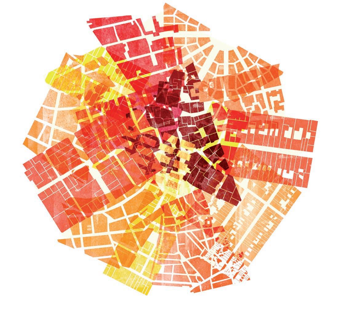
Microclimates evolve at different scales and hierarchies; scales of influence range from individual buildings and materials to regional conditions such as bodies of water or winds. An urban fabric therefore is characterized of a multitude of small-scale climatic zones that respond to the characteristics of the local fabric. Fazia Ali-Toudert therefore describes the city as a patchwork of individual microclimates (Ali-Toudert 2007).
As mentioned previously the Microclimate of an Urban area is the result of many complex processes, most importantly the interaction between the urban morphology and the local climate. Golany states that on the urban scale, natural, passive methods and the urban morphology are almost the only urban tactics available for improving the thermal performance of cities (Golany, 1996). Reduction of the energy budget of cities can therefore only be achieved by smarter ways of urban planning that are based on a better understanding of how the urban geometry reacts with the local climate. It can only be achieved by altering the urban fabric in ways that optimize the use of natural resources, like e.g. wind and sun, in the best optimal way.
Currently, microclimates evolve uncontrolled as a consequence of decisions that are taken at different scales within different disciplines. Especially architecture and urbanism need to work closer together in order to better control microclimates, which are a product of discipline-specific decisions. In this sense decision taken at the building scale (surfaces, materials, etc.) and urban decisions made at the metropolitan level (e.g. zoning) should be
coordinated in a coherent and homogenous way. Golany also points out that it is necessary for the urban designer to borrow knowledge from other disciplines such as urban climatology, botany, geography, etc. and to bring them into urban design in order to enhance urban comfort (Golany, 1996). Ali-Toudert summarizes (Ali Toudert, 2001):
‘The research done in urban climatology shows that the urban geometry is responsible of the global urban climate; particularly the appearance of the urban heat island and local wind systems due to the effects of heat storage in the urban fabric, modified energy balance and obstruction effects to sun and wind.
The urban geometry has been recognized as having a decisive influence on these phenomena and urban microclimatic conditions in general. So the choices of urban morphology and building shapes made at the early stage of the design appears to be essential. As a consequence, the introduction of climate in urban design requires the understanding of the dependence between urban geometry and resultant microclimates.’
City: Macroscale Communities: Mesoscale Land Use Ordinate Zones: Microscale Local Sample Zones
- 43Urban Microclimates

Analysis of Urban Microclimates
SCIENTISTS (CLIMATOLOGIST,METEREOLOGIST)
ANALYSIS CONCEPTS PARAMETERS
• ENERGY TRANSFER MODELS
• LAND USE ZONES
SOLAR RADIATION (LOND- & SHORT-WAVE)
TEMPERATURE (AIR & SURFACE)
AIR HUMIDITY WIND (SPEED & DIRECTION)
URBAN PLANNERS AND ARCHITECTS
ANALYSIS CONCEPTS PARAMETERS
• MORPHOLOGICAL INDICATORS
AnalysisScaleVaries AnalysisScaleVaries
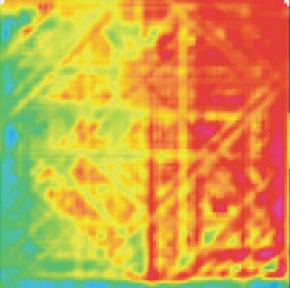
SURFACE ALBEDO SKY VIEW FACTOR
SOLAR ADMITTANCE
URBAN STREET CANYON SHAPE COEFFICIENT BUILDING ORIENTATION
PASSIVE ZONES DENSITY
BUILDING HEIGTH POROSITY
Urban microclimates are complex phenomena and there is currently no consent between climatologists how to best approach the topic. It is nevertheless clear nowadays that the traditional distinction between the rural and the urban is not sufficient and that new models of urban micro-climatic analysis need to be developed. Such models, like e.g. land use zones, will be introduced in more detail in the ‘Methods’ chapter. The research in urban climatology should lead to design parameter that can be used as rules of engagement by urban planners and architects in order to incorporate microclimatic aspects into the design. Overall there should be more inter-disciplinary work between designers and climatologists in order optimize urban fabrics in relation to the regional geography and climate.
Urban Planning
2-Dimensional
Conventional Energy Use
Air pollution
Urban Functions
Population Density
Urban Climatology
3-Dimensional
Renewable Energy Use
Urban Effect
Urban material/structure
Urban material/structure
Urban Climatology/Interaction with Planners&Architects (Mills)
Urban Design
Urban Climatology
Daytime Night-time
Indoor Outdoor
Comfort
Urban effect
Engineer/Artisic Science
Applied
Theoretical
Urban Climatology/Interaction with Planners&Architects (Mills)
UCL UBL RADIATION
TRANSPIRATIONEVAPORATIONPRECIPATION
Domain - 44 -
Climatologists agree that urban microclimates are aggregated at different scales ranging from the urban canyon up to the overall city. Morgan (Morgan, 1977) gives a classification of scales that ranges from local sample-zones to the macro-scale (compare diagram on page 43 ). The above diagram depicts ‘fundamental morphological units’ that may be aggregated hierarchically: Scales of consideration range from 1² to 14m. Even though climatologists try to classify characteristic zones of influence there is currently very little knowledge about their meaning and relevance within the overall urban climatic system.
Even though a good understanding of how various climatic factors act on the urban microclimate has been gathered through research and analysis in the last couple of decades it is still the complexity of the topic that has prevented implementation of such knowledge into urban design. Panao points out that urban analysis is often restricted to a single parameter and that a method for optimal urban design is still missing (Oliveira Panao, 2008). AliToudert adds in this context that several authors have underlined the lack of clear guidelines that can help the urban designer and architect in the process of urban conception (Ali Toudert, 2001).
The urban mircoclimate has evolved as an area of research more or less over the last four decades. In this sense it is still a relatively young field of research. It is clear by today that urban areas show different climatic characteristics compared to the
countryside and that such characteristics are rarely beneficial; the urban heat island is probably the best-known phenomenon in this context.
The complexity of micro-climatic interactions nevertheless means that there is still very little knowledge about how microclimates evolve and how they can be alternated and controlled through urban planning and architecture. Further research is therefore necessary and experiments that range from field studies (often small scale) to wind tunnel test and computer simulations need to be combined to get a clearer picture of how microclimates evolve. Further work is also necessary to establish clear guidelines for designers and planners and to come up with a catalogue of design principles that respect different climatic zones. All in all designers and researchers should work much more closely together in order implement knowledge into the design of urban
CityScale 10.000m Neighborhood Scale 1000m
UC 10m
City Block Scale 100m
- 45Urban Microclimates
Objective Impacts
Indoor Comfort Buildings
Outdoor comfort and Health Building Groups
Energy Use
Air Quality
Protection from Extremes
Settlement
Limits
Buildings
• Location
• Materials
• Design (e.g. Shape, orientation, etc.)
• Local Cllimate Change
• Emmissions
• Material/Surfaces
• Building Deimensions - Flow interference & Shadow Areas
• Energy efficiency
• Air quality
• Urban climatie effect
Building Group Groups Settlement
• Access to sunlight and Wind
• Air Quality Building Codes
• Building Placement
• Outdoor Landscaping, materials and surfaces
• Street Dimensions & Orientation Guidelines on :
• Densities
• Heights
• Land Use
• Green Spaces
• Mode and intensity of traffic flows
• Ennergy efficiency
• Air Quality
• Urban Climate Effect
• Zoning
• Overall Extent and Shape
• Transport Pollcy
A summary of the tools (gray diagonal) employed at the building, building group and settlement scales to achieve climatic objectives at those scales. The application of tools at each scale has a climate impact, shown below the diagonal cells, and places limits on decisions made at other scales, shown above the diagonal cells. Diagram adopted from Mills (Mills 2006).
Urban Microclimates – Scale and Extent
As pointed out before, climatologists try to establish different scales and hierarchies in order to investigate and analyse urban microclimates. The complexity of the phenomenon makes this approach valid as it provides rules of engagement. Quantification and qualification of microclimates and how they interact with each other is almost impossible. Microclimates develop as the interaction of the various surfaces and materials within the urban fabric. They evolve at various scales and the overall microclimate of a city is made up of a patchwork of microclimates at different levels. Traditionally there has been a distinction between the urban and the rural; more recent approaches, however, look at urban patches and try to organize them into typologies that show specific micro-climatic characteristics. Besides trying to organize the urban fabric into smaller areas with distinct climatic features, i.e. in plan, it is also necessary to consider the vertical dimension; microclimates are distinct three-dimensional phenomena and the height of buildings as well as their roughness at roof level has an important impact on the evolving climatic conditions. In the following paragraphs different concepts of demarcating micro-climates, i.e. the horizontal and vertical extents, will be discussed.
Microclimates - Horizontal Extent
Golany states that the differentiation of physical forms within the city, orientations, heights, compositions, conglomerates of its buildings’ density, proximity to the city centre or its periphery, and most importantly the intensity of human activities, create pockets of urban micro-climates within the city. Consequently, each part of the city differs in its thermal performance from its other parts (Golany, 1996). Oke (Oke, 1987) points out that every surface and object has its own microclimate, which will affect its immediate vicinity. He further states that surface and air temperatures may vary by several degrees in very short distances, even millimetres, and that airflow can be greatly perturbed by even small objects. The complexity of interacting elements at different scales makes it very difficult to delineate the Urban Microclimate. Besides the fact that there is a clear distinction between ‘the rural’ and ‘the urban’ it becomes very difficult to describe the urban microclimate in terms of its extent. Morgan states that the geographic delineation of various microclimates within an urban area is determined by the transfers of energy, mass and momentum at the city surface. He employs a strategy where the city is progressively divided into smaller integral segments: The city,
Domain - 46 -
MicroScale
Microlimates evolve as complex 3-dimensional phenomena. The differentiation of micro-climates at different scales and levels therefore must not only to be addressed in plan but also in the vertical dimension. The most important distinction in vertical terms is between the ‘Urban Canyon Layer’ and the ‘Urban Boundary Layer” (Oke 1987).
communities, land use zones and local sample sites. (Morgan, 1977). Various other authors agree with this categorization of urban elements at different scales.
Oke states that typical scales of urban microclimates relate to the dimensions of individual buildings, trees, roads, streets, courtyards, gardens, etc. Typical scales therefore extent from less than one meter to hundreds of meters or kilometres (Oke, 1987).
Arnfield describes ‘fundamental morphological units’ that may be aggregated hierarchically and that range from 12 to 14 meters, corresponding to the individual facets of the urban environment (Arnfield, 2003). In this sense some authors distinguish specific urban scales that range from micro-scale, to meso-scale and macro-scale of a metropolitan area (e.g Morgan 1977). In more detail such units might range from the regional and metropolitan levels to the city level, the community level and to the building level (Jabareen, 2006). The relationship of such units is however complex. Arnfield states (Arnfield, 2003):
“These fundamental morphological units may be aggregated
hierarchically. Building walls and elements lying between buildings, for example, define the urban canyon (UC). UCs and roofs of adjacent buildings define city blocks, which in turn scale up to neighborhoods, land-use zones and, ultimately, the entire city. At each scale, units will possess distinctive energy balances that, in general, represent more than the area-weighted average of the budgets of individual elements but also incorporate the distinctive interaction among their constituent units. Moreover, each unit interacts with adjacent ones in the same scale category by advection. As spatial scale increases, spatial variability is likely to be reduced; that is, there is probably less difference among two land-use zones in a city than between the north- and southfacing walls of an individual building within one of them.”
Mills agrees with this approach and proposes a hierarchical approach that distinguishes between three distinctive urban categories at consecutive scales: The building, building group and group settlement scale (Mills, 2006). He argues that design objectives are different at each scale and that decisions taken at one scale will likely have an affect on other scales. In this
PBL UBL UCL Mixing Layer Surface Layer Urban Rural Rural Surface Layer Urban ‘Plume’ Rural BL UCL Roughness Sub Layer Roughness Sub Layer Inertial Sub Layer MesoScale Local Scale PBL: Planetary Boundary Layer UBL: Urban Boundary Layer UCL: Urban Canopy Layer
- 47Urban Microclimates
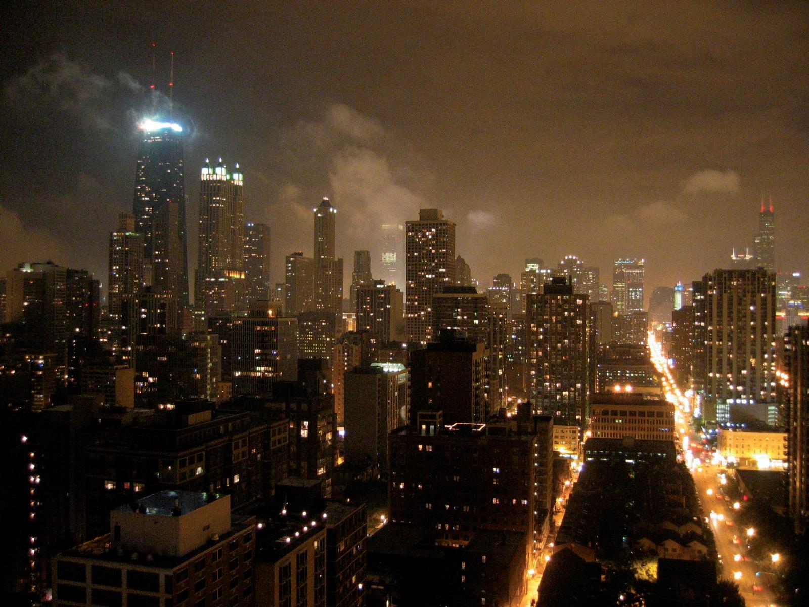
Cities show distinct climatic variations that are clearly distinguishable from the regional climate of the surrounding rural areas. Golany argues that every city creates its own micro-climate, which differs from that of the outer open space of its macro-region (Golany, 1996). Different surface qualities, e.g. albedo or imperviousness of materials, as well as the complex arrangement of urban entities are the main reasons why cities develop their own local small-scale climates. Small-scale climates that evolve through the interaction of the urban morphology and regional atmospheric conditions are referred to as Urban Microclimates. Image: Chicago Skyline at night.
Vertical Extent
sense decisions taken at the building scale will have an influence on the urban conditions at larger urban scales. He points out, however, that the proposed scale hierarchy does not necessary correspond with traditional decision making in architecture and urban planning.
Ali Toudert proposes that the design of the city should be approached in microclimatic terms from the large, regional scale, down to consecutive smaller scales (Ali-Toudert, 2007).
Several authors therefore agree that the word microclimate does not describe a single phenomenon, but that the microclimate of a city is made up of multitude of microclimates that are characterized through different scales and might overlap or aggregate to form larger climatic phenomena. Ali-Toudert therefore describes the microclimate as a patchwork of local microclimates (Ali-Toudert, 2007)
Besides scale and horizontal extent of urban microclimates climatologists distinguish between two distinct vertical layers, the Urban Canopy Layer (UCL) and the Urban Boundary Layer (UBL). The vertical differentiation is mainly related to wind and has to do with the fact that wind fields within an urban area are distinct from the ones of the surrounding country side; the drag caused by urban elements results in a reduction of wind speed. The transitional zone between the ground and the undisturbed ‘free’ wind is therefore referred to as the Urban Boundary Layer. The boundary layer is then divided into two sub-zones, with the Urban Canopy Layer describing the zone from ground to the average roof height of the buildings. Givoni describes well how the concept of an Urban Canopy can best be understood (Givoni, 1989):
‘It is convenient to consider the fabric of the structures in a city analogous to a ‘canopy’ of a tree, where the impinging solar radiation is gradually absorbed and where specific conditions of air temperature and humidity may exist, distinct from those prevailing in the surrounding space. Therefore the space bounded by the urban buildings up to their roofs, is often referred to as the ‘urban canopy’.’
Domain - 48 -
Altered energy balance terms leading to positive thermal anomaly
1 Increased absorption of short-wave radiation
2 Increased long-wave radiation from the sky
3 Decreased long-wave radiation loss
Features of urbanization underlying energy balance changes
Canyon geometry - Increased surface area and multiple reflection
Air pollution - Greater absorption and re-emission
Canyon geometry - Reduction of sky view factor
4 Anthropogenic heat source Building and traffic heat losses
5 Increased sensible heat storage
6 Decreased evopotranspiration
7 Decreased total turbulent heat transport
Construction materialsIncreased thermal admittance
Construction materialsIncreased ‘water-proofing’
Canyon geometry - Reduction of wind speed
Commonly hypothesized cause of the canopy layer urban heat island (Oke, 1982)
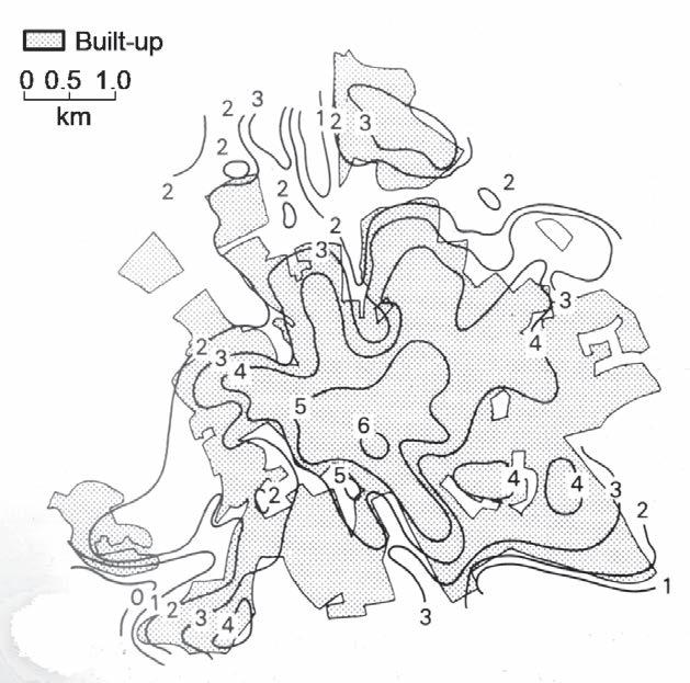
Canopy layer heat island in Uppsala, Sweden at 2330 hrs on 20 September 1976. Wind less then 1ms-1, direction variable, almost cloudless skies. Isotherms are in degrees Celsius (Oke,1987)
The vertical differentiation reflects different climatic conditions, which often evolve at a micro-scale inside the canyon and at a more global level within the boundary layer. Arnfield describes how the two zones are characterized (Arnfield, 2003):
‘In the UCL processes of airflow and energy exchange are controlled by micro-scale, site-specific characteristics and processes. The UBL, above roof level, in contrast, is that part of the planetary boundary layer whose characteristics are affected by the presence of the urban surface (or its land use zones) below and is a local- to meso-scale phenomenon controlled by processes operating at larger spatial and temporal scales. The distinction goes beyond mere scale, therefore: it reflects different assemblages of processes.’
Oke describes how air flowing from the countryside encounters a set of very different boundary conditions when it reaches an urban area; the term Boundary Layer therefore reflects a city’s distinct characteristics that result in an internal boundary layer, which develops downwind from the leading edge of a city (Oke, 1987). Givoni points out that the boundary layer phenomenon can actually be seen in many cities from a distance in form of a layer of turbid air over a city’s boundaries (Givoni, 1989).
- 49Urban Microclimates
Domain - 50 -
Cities and Climate
The weather we experience is an expression of the highly complex interactions of various physical processes that occur in the earth’s atmosphere; it is the result of a constant supply of energy. The sun supplies the earth with this energy in form of radiation at different wavelengths. Objects on the earth surface as well as in its atmosphere react to this radiation in different ways. Depending on their relative position to the sun as well as their physical properties they will e.g. heat up or cool down in different ways. The difference in temperature of various matter results in processes of exchange that aim for a constant equilibration. Depending on the characteristics of material such exchanges can occur in different ways through e.g. advection or convection. The movement of air molecules is one of the most well known examples where pressure differences (which result from hot air rising and cooler air sinking) lead to the exchange of matter, which we experience as wind. Depending on the magnitude of such pressure (i.e. temperature) differences we experience strong or light winds. Other aspects of the weather we experience relate to temperature und humidity (clouds, rain, snow, etc.), which in turn are directly connected to the interaction of incoming radia-
tion and the different surface elements of the earth; the different properties of bodies of water and land for example are the main parameters that result in weather patterns at a global scale. Besides its relative position to the sun (the trajectory of the earth and its related seasonal characteristics) it is the rotation of the earth and its associated Coriolis effect that not only leads to the daily pattern of day and night but also forces winds at a global scale to deflect. Overall it can be said that the global earthocean-atmosphere system is solely powered by the radiation it receives from the sun.
Like all entities on the earth’s surface cities are subject to global forces. In other words, the different bodies and surfaces that constitute a city’s fabric interact with global weather patterns. Surfaces as well as the orientation and arrangement of different urban bodies are in mutual interaction with e.g. winds and incoming solar radiation. To gain a better understanding about these complex processes this chapter is dedicated to explain the most important physical parameter that have an affect on the urban climate and microclimate.
- 51Cities and Climate

The earth is subject to a constant supply of energy in form of heat, i.e radiation from the sun. It is the interaction of this radiation with the earth’s surfaces and it’s atmosphere that results in the weather we experience.
When the radiation emitted by the sun hits the earth’s atmosphere a complex process of interactions is started. Some of the radiation is absorbed and other parts are reflected. The incoming solar radiation therefore only represents about 75% of the overall extra-terrestrial radiation with the remaining part being scattered back into space or downwards to earth as diffuse radiation. Together with the direct radiation from the sun this diffuse radiation is the second major component of the global radiation. The main energy inputs in the global climatic system are therefore the short-wave radiant energy from the sun and the long-wave radiant energy exchanges between various elements and the atmosphere.
The different wavelengths of radiation are characterized by intrinsic properties. Certain parts of the spectral range illuminate the world as visible light whereas other parts are responsible for the transfer of heat in form of radiant energy. The different wavelengths also determine how parts of the radiation react with the earth. Whereas clouds and pollutant filter out some of the shorter wavelengths large parts of the ultra-violet spectrum are lost at high levels due to scattering and absorption. The spectrum of electromagnetic radiation striking the earth’s atmosphere is 100 to 106 nanometers (nm). This range is typically divided into five regions of increasing order of wavelengths (Wikipedia):
• Ultraviolet C (UVC); 100 to 280nm; the term ultraviolet refers to the fact that the radiation is at higher frequency than violet light. It is not visible to the human eye. Owing to absorption by the atmosphere very little reaches the Earth’ surface.
• Ultraviolet B (UVB): 280 to 315 nm. It is also greatly absorbed by the atmosphere, and along with UVC is responsible for the photochemical reaction leading to the production of the Ozone layer.
• Ultraviolet A (UVA): 315 to 400 nm. Used for tanning and PUVA therapy.
• Visible range (light): 400 to 700 nm. Range of visible light
• Infrared: 700 to 106 nm. It is responsible for an important part of the electromagnetic radiation that reaches the earth.
- 52Domain
Visible Sunlight
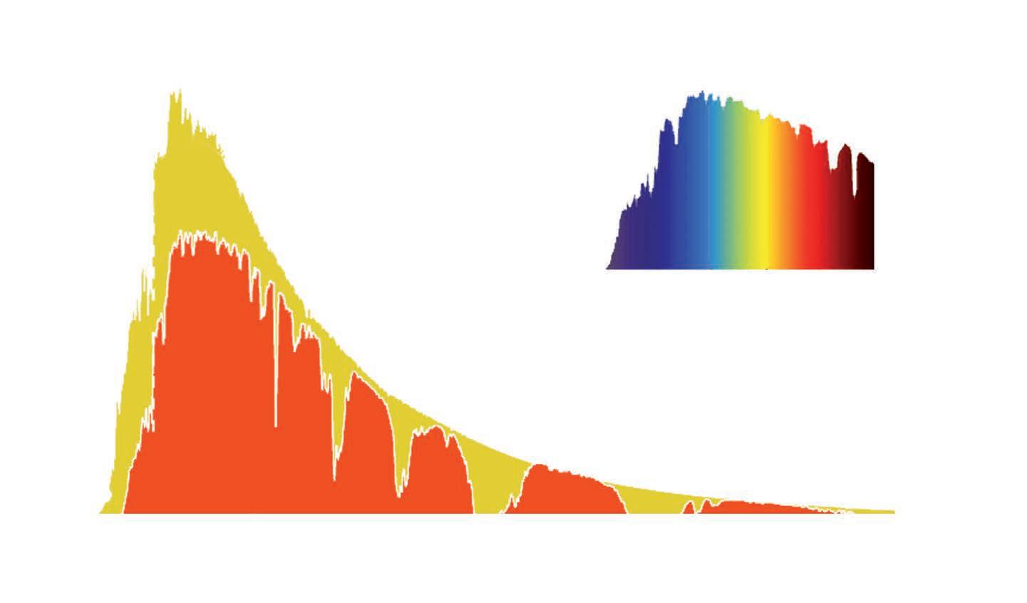
Wavelength (nm)
Wavelength (nm)
sunlight at top of atmosphere radiation at sea level 5250˚C black body spectrum
The solar spectrum: As the solar radiation passes the atmosphere, a part of the incident energy is removed by absorption or scattering by molecules, clouds and aerosols. Wavelengths less than 300 nm are filtered out by molecules like ozone, nitrogen and oxygen. Dips in the infrared area are caused by water and CO2. Diagram adopted from http://org.ntnu.no/solarcells/pages/Chap.2.php?part=1
Short Wave Radiation:
Any exposed surface on the earth gains heat from solar radiation (short-wave) and looses heat by outgoing long-wave radiation. The incoming solar radiation is subdivided into two fractions: the radiation that is absorbed at some point and converted into heat (sensible and latent) and the fraction that is reflected back into space. The bandwidth of short-wave radiation is not clearly defined; nevertheless, it covers the visible, near-ultraviolet and near-infrared spectra; it is responsible for illuminating the earth as well as for providing heat energy.
(Outgoing) Long-Wave Radiation:
Outgoing long-wave radiation is the energy leaving the earth as infrared radiation at low energy; it is not visible. The amount of long wave radiation from a material depends on the temperature of the surroundings. Long wave radiation is emitted from gases and aerosols as well as from the ground and oceans. Therefore the clouds and the clear atmosphere also radiate long-wave radiation. The influence of clouds on long-wave radiation exchange depends upon the height of the clouds; the lower the clouds, the warmer the cloud temperature and thus the bigger the contribu-
tion to the sky radiation:
‘The long-wave radiation loss is the major cooling factor of an area as a whole. The amount of long-wave radiation loss from the ground level differs in an open country from that in a densely built up area. This is one of the major factors that generate the differences between the urban and the country climatic conditions. Long-wave radiation fluxes are the main factor in nocturnal cooling; the net-outgoing long-wave radiation fluxes responsible for air-cooling are directly affected by the urban geometry, i.e. the sky view factor.’ (Sass, 2009)
Net Radiation:
The earth’s net radiation, sometimes called net flux, is the balance between incoming and outgoing energy at the top of the atmosphere. As described above energy will enter the earth via direct short-wave radiation or deflected diffuse radiation; in turn it can leave the earth either via reflection of radiation through aerosols or clouds or via thermal radiation (long-wave), i.e. heat emitting surfaces and the atmosphere. The net radiation therefore is an indicator of the earth’s energy balance and weather it heats up or cools down. It depends on all factors that influence radia-
250 300400500600700 5007501000125015001750200022502500 0 0.5 1.0 1.5 2.0 2.5 1.0 0.8 0.6 0.4 0.2 0.0 Spectral Irradiance (W/m²/nm) relative intensity
visible infrared UV
- 53Cities and Climate
Source: QF Store: ΔQS
1 Canopy Layer
2 Boundary Layer
Q* Net Wave Radiation Flux
QE Turbulent Latent Heat Flux
QH Turbelent Sensible Heat Flux
ΔQA Horizontal Energy Transport in the air per unit horizontal area
QF Anthropogenic Heat Flux Density due to combustion
ΔQS Net Moisture storage; rate per unit volume
Schematic representation of energy fluxes of an urban air volume. Diagram adopted from Oke (Oke, 1987)
Source: F Store: ΔS
1 Canopy Layer
2 Boundary Layer
P Total Athmospheric Pressure
E Evapotranspiration
F Anthropogenic water release due to combustion
ΔQS Net moisture storage; rate per unit volume
ΔA Net moisture advection, rate per unit volume
Δr Net run off
Schematic representation of water balance of an urban air volume. Diagram adopted from Oke (Oke, 1987)
tion fluxes, such as the sun’s elevation, the cloudiness, albedo, temperature and humidity of the atmosphere and the altitude. Daily mean net radiation is positive in summer, reaching its peak at about the time of the summer solstice. In winter, the daily mean net radiation is negative since daytime solar energy receipts are low and the nights are long (El Nahas, 1996).
Albedo:
As mentioned above the geometry of objects as well as the material properties determine how much of the incoming radiation is absorbed or reflected; they determine the amount of energy that is stored and the time it takes to release this energy again. The reflectivity of materials is therefore a major component in the Earth’s net radiation balance; the total fraction of the solar radiation that is reflected by a surface is referred to as its albedo. It is evaluated by the ratio of reflected and incident solar energies. The higher the albedo the more energy is reflected and less is absorbed. Often lighter coloured materials are characterized by higher albedos that store less energy. In urban terms the use of materials with high albedos could be utilized to optimize the energy budgets in certain climates. This is a strategy that can be observed from evolved cities in certain climatic regions like the Mediterranean where white colours are dominant. Typical albedos for urban and rural materials are shown in the table on page 56.
Urban and rural areas are characterized through different geometric properties as well as material albedos; they therefore behave differently in terms of their energy balances. The net energy
obtained by a city is much higher due to much lower average albedos. The surface albedo of urban materials is therefore a very important factor in urban heating and could be addressed by a more sophisticated use of construction materials. Sass states that the average albedo of a city could increase as high as 0.400.50 if roofing and paving materials were replaced by higher reflecting materials (average albedo of 0.65/0.70): ‘This change would reduce the net solar energy absorbed by the city surface almost by 40% and result in temperature changes in the city similar to that caused by a substantial cloud cover’ (Sass, 2009).
Anthropogenetic Heat Production:
Another important factor that is responsible for different energy budgets of urban and rural areas is the heat produced from domestic and industrial sources. Cities consume large amounts of energies; heating, cooling, artificial lighting and transportation all consume energy. As a result large amounts of heat are released and stored in the urban fabric. This additional energy released from man-made sources is referred to as Anthropogenetic Heat. It can be measured by dividing the overall anthropogenetic heat produced in a city by the number of citizens; the result is the average per capita consumption of energy. Anthropogenetic heat production is often related to density; nevertheless, there are different arguments whether higher or lower densities contribute to increases or decreases in energy consumption. Whereas some statistics show that higher densities result in an increase in anthropogenetic heat production, it is also argued that lower densities, i.e. urban sprawl, result in higher energy consumptions due to transportation.
Q* P QE ΔQA ΔA Δr QE E E
2 2 1 1
- 54Domain


CLOUDS REFLECT INCOMING RADIATION


L on -waveg dra i atio n ntioaidaravew-rtohSe-wavtrsho(sky)irectndI
Direct shot-warev Short-Wave ra dia tion


Short-wave radiation Long-wave radiation Long-waveradiationfrom surroundingsemitted reflected from body re flec ted fro m c louds f r mo ks y iotiadra n noatiidar dtecelfer
The Components of the Urban and the Human Heat Balance
Conduction
‘The process of urbanization produces radical changes in the nature of the surface and atmospheric properties of a region. It involves the transformation of the radiative, thermal moisture and aerodynamic characteristics and thereby dislocates the natural solar and hydrological balances. For example the seemingly inevitable increase of air pollution affects the transfer of radiation, and supplies extra nuclei around which cloud droplets may form; the dense urban construction materials make the system a better heat store and waterproof the surface; the block-like geometry creates the possibility of radiation trapping and air stagnation, and gives a very rough surface; and the heat and water released as ‘waste’ products of human activities supplements the natural sources of the heat and water in the urban system’ (Oke, 1987).
SHORTWAVE
SUN
RADIATION DIRECT SHORT WAVE RADIATION
LONG WAVE RADIATION FROM SURROUNDINGS CANOPY LAYER BOUNDARYLAYER Long-Wave Radiation Evaporation Long-Wave Radiation Evaporation Ventilation Ventilation Convectio n Convection C noitcevno niotcevnoC Convection Convectio n Convectio n Convection LONG WAVE RADIATION
Natural
forced convection Long-wave radiation from ground Evaporation
and
- 55Cities and Climate
Radiative properties of typical urban materials (Oke 1987)
Surface Alebdo ά Emissivity ἐ
Roads
Asphalt 0.05 - 0.20 0.95
Wall
Concrete
0.10 - 0.35 0.71 - 0.90
Brick 0.20 - 0.40 0.90 - 0.92
Stone 0.20 - 0.35 0.85 - 0.95
Wood 0.90
Roofs
Tar and Gravel 0.08 - 0.18 0.92
Tile 0.10 - 0.35 0.90
Slate 0.10 0.90
Thatch 0.15 - 0.20
Corrugated Iron 0.10 - 0.16 0.13 -0.28
Windows Clear Glass Z* < 40° 0.08 0.87 - 0.94 Clear Glass Z* 40° to 80° 0.09 - 0.52 0.87 -
Paints
0.02 - 0.15 0.90 - 0.98
Radiative properties of natural materials (Oke 1987) Surface Remarks Alebdo ά
Agricult. Crops, Tundra
Orchards
Forests
Urban Areas†
* Zenith Angle
† Base on mid-latitude cities in snow-free conditions
Typical albedo values for urban and natural materials. Diagram adopted from Oke (Oke, 1987)
- 0.20
Latent heat and vaporization of water:
In meteorology, latent heat flux is the flux of heat from the Earth’s surface to the atmosphere that is associated with evapotranspiration of water at the surface and subsequent condensation of water vapour (Wikipedia). Evapotranspiration is a combination of two processes: The direct evaporation of standing and soil water and transpiration, which is the movement of water through plants into the atmosphere. The energy needed for both processes is the same. As energy is used to evaporate water from a surface, heat is withdrawn with the water; as a result a surface cools (Sass, 2009).
The extent of evapotranspiration is dependent on the moisture content of the soil and the ability to transport water through surfaces. Urban and rural areas therefore show very different behaviour in terms of latent heat fluxes. Surfaces in urban environments are mostly sealed and impermeable to water; there is also much less vegetation. As a result the capability to release heat
via vaporization of water through the soil or plants is drastically reduced. The impermeability of surfaces in urban areas not only affects the energy and heat balance of cities but also can result in other weather related problems, like e.g. flooding.
Conduction, Convection and Advection:
Sensible heat is the energy exchanged by a thermodynamic system during a change of temperature (Wikipedia); it is heat that can therefore be felt or sensed. In meteorology sensible heat refers to the transfer of heat between various surfaces and the atmosphere. Depending on the physical properties of the elements that are involved in such processes it is common to distinguish between conduction, convection and advection: Conduction describes the heat transfer between parts of the same material or different materials which are adjacent to each other; e.g. a surface which is partly covered in shadow would show temperature differences that result in conduction. Convection describes the
0.92
0.50
Red,
Black
White, whitewash
- 0.90 0.85 - 0.95
brown, green 0.20 - 0.35 0.85 - 0.95
0.10
Average
Range
- 0.27 0.85 - 0.96
0.15 ~0.95
ἐ Soils Dark, wet 0.05 - 0.98Light, dry 0.40 0.90 Desert 0.20 - 0.45 0.84 - 0.91 Grass Long (1.0 m) 0.16
0.90
Short (0.02m) 0.26 0.95 0.90
Emissivity
-
-
0.18 - 0.25 0.90
0.99
-
0.15
Deciduous
0.20 0.98 Coniferous 0.05 - 0.15 0.97 - 0.99 Water Small Zenith Angle 0.03 - 0.10 0.92 - 0.97 Large Zenith Angle 0.10 - 1.00 0.92 - 0.97 Snow Old 0.40 - 0.82 Fresh 0.95 0.99 Ice Sea 0.30 - 0.45 0.92 - 0.97 Glacier 0.20 - 0.40
Bare 0.15 - 0.97Leaved
- 56Domain
Roof Facets Wall Facets

Ventilation Energy Transfer
Patchwork of Horizontal Elements
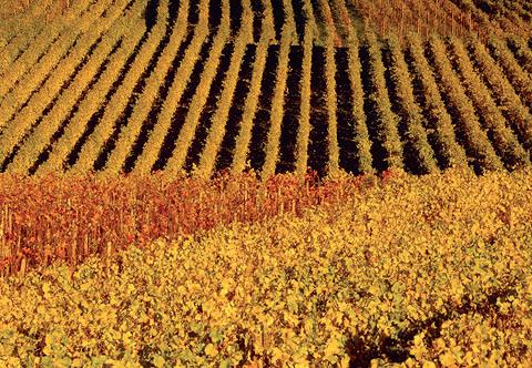

Different surface elements possess diverse Energy Budgets that generate contrasts in surface characteristics (e.g. ‘skin temperature’) and lead to mutual interactions by radiative exchange and small-scale advection: Horizontal Ground Surfaces can be seen as patchwork of elements, such as irrigated gardens and lawns, non-irrigated greenspace and paved areas with contrasting radiative, themal, aerodynamic and moisture properties. (Arnfield, 2003)
heat transfer from one material to another via a medium, such as air or water. Vertical air motion through warm air rising is a typical example for convection; as surfaces on the ground are heated up via radiation the heat is transferred through the molecules of the air.
Advection refers to the transport of some property of the atmosphere such as heat or humidity by the horizontal movement of an air mass. In other words sensible heat associated with advection describes the horizontal transfer of energy via wind; it depends on speed, direction, temperature and humidity of the moving air.
- 57Cities and Climate
Isolated Roughness Flow:
‘When buildings are wide apart their flow fields do not interact. At closer spacing, the wakes are disturbed and the flow regime is known as “Isolated Roughness Flow” ‘(Oke, 1987).
Wake Interference Flow:
‘When the height and spacing of the array combine to disturb the bolster and cavity eddies, the regime changes to one referred to as “Wake Interference Flow” ‘(Oke 1987).
Skimming Flow:
‘At even greater H/W and density, a stable circulatory vortex is established in the canyon because of the transfer of momentum across a shear layer of roof height and transition to a “skimming” flow regime occurs where the bulk of the flow does not enter the canyon’ (Oke 1987).
Characteristic airflow patterns related to the spacing of buildings; for airflows perpendicular to the long axis of the canyons (±30˚). Diagrams adopted from Oke (Oke, 1987).
Terrain
Scattered settlement (farms, villages, trees, hedges)
z0(m)
0.2-0.6
Suburban (low density residences and gardens) 0.4-1.2 (high density)
Urban (high density, <5 storey row and block buildings) 1.5-2.5
(urban high density plus multistorey blocks) 2.5-10
Typical roughness length (z0) of urbanized terrain (Oke 1987)
Typical form of the spatially and temporally averaged velocity profile within and above the urban canopy (H denotes the mean building Height). Diagram adopted form Mills (Mills)
0.8-1.8
~2H H Canopy UH U(Z) Z
- 58Domain
The Urban Wind Field:
Next to radiation wind is one of the major factors in any climatic system. As pointed out above it is an important component in sensible heat fluxes that are related to the movement of energy via advection. Ambient wind conditions therefore have implications on the energy budgets of cities and are directly related to the heat island phenomenon; wind influences temperature and humidity as well as the air quality in an urban fabric. Wind also characterizes outdoor comfort levels; it can contribute to pleasant ventilation or strong, uncomfortable winds that can even become a hazard for pedestrians. In addition wind conditions determine the potential for natural ventilation of individual buildings. In cold climates heat losses resulting from uncontrolled ventilation of buildings constitute a large part of the total heat load. On the other hand, wind driven natural ventilation can be utilized to improve human thermal comfort in warm seasons and reduce the need for mechanical cooling and hence reduce the energy use in buildings. Givoni states that of all the climatic elements wind conditions are modified to the greatest extent by urbanization. The urban wind is also the climatic element, which can be controlled and modified more by urban design than any of the other climatic elements (Givoni, 1989). A thorough understanding of how an urban fabric reacts with prevailing winds should therefore be an important aspect of urban planning strategies.
Aerodynamic Roughness:
The urban geometry has a complex effect on the prevailing wind: ‘When free air flowing over a rural area approaches the boundaries of an urban area it encounters a higher surface roughness created by the buildings. The increased flow resistance resulting from the higher roughness decelerates the airflow at the urban canopy layer. The airflow above and around buildings is characterized by a lower average speed but higher speed variations (turbulence) as compared to the wind flow over open rural areas. Above roof level, there is a sharp increase in the wind speed until the wind reaches the speed it has in the open country at the same height (Givoni, 1989).’
The pattern of wind speed with elevation above ground is known as the wind speed profile; several empirical formula have been developed to measure the variation of wind speed with height (refer to diagram above).
As seen above, a city is constituted of roughness elements, mainly buildings, which affect ‘rural’ winds. The roughness ratio as well as the distribution of roughness elements have implications on the speed of the wind. Cities that show a gradual increase of building heights towards the centre, i.e. a city with pyramidal cross section, will cause less drag on the wind than one with a line of high rises at the edge of the city (El Nahas, 1996). In addition, isolated tall buildings can deflect the wind downwards resulting in high increases of wind speeds; Oke reports that pedestrians can encounter up to a sixteen-fold increase in wind force at the base of tall buildings (Oke, 1987). Whereas the roughness of elements at roof level determines the overall change of wind speed due to drag, dimensions, shape and spacing of buildings further influence wind conditions. El Nahas reports that arrays of buildings can deflect the wind or channel it: Where buildings converge in the direction of flow, the wind speed is locally increased; where the gap between buildings gets wider in the direction of flow, the wind speed is decreased (El Nahas, 1996). The proportions and size of the open elements within the Canopy Layer are therefore important aspects that influence the potential for infiltration and ventilation of wind into the Urban Canopy Layer.
600m 500m 400m 300m 200m 100m 0m Gradient Wind Gradient Wind Gradient Wind 100 100 100 89 76 59 49 90 91 79 70 77 61 24 32
u ∞ Z0.40 u ∞ Z0.28 u ∞ Z0.16
Vertical Wind speed profiles for urban and rural areas. Diagram adapted from Chandler (Chandler, 1976)
- 59Cities and Climate
For perpendicular wind flows the spacing between buildings determines the wind characteristics within the canyon. See also diagram below and diagrams on page 58.
Wind direction in relation to the canyon orientation will result in different wind conditions inside the canyon; these range from a parallel ambient flow to spiral vortices.
The flow regime associated with air flow over building arrays of increasing H/W.The transitions between these three regimes occur at critical combinations of H/W and L/W. Diagram adopted from Santamouris (Santamouris, 2002).
Fraction built-up area
‘The physical design of cities will affect surface-air exchanges. This graph illustrates the affect of building spacing (fraction of built-up area) on the momentum flux as shown by the roughness length (z0). The graph is for a set of cube-shaped buildings (with a characteristic dimension, h) in a grid arrangement’ (Mills 2004).
01234 L/H
WAKE INTERFERENCE FLOW ISOLATED ROUGHNESS FLOW Cube Canyo H/W 5678 0.25 0.33 0.50 1.00 2.00 4.00 *1 *2 *3 *1 *3 *2 30° W L H W H W H 60° 60° 0.001 0.01 0.01 0.11 0.1 Z0/h
SKIMMING FLOW
- 60Domain
Urban Canyon Aspect Ratio:
Oke points out that the wind effects within the urban canopy layer depend on the arrangement of the individual elements within an urban fabric. Especially the height and width of open elements such as streets, as well as their direction and arrangement in relation to the prevailing wind determines in how far wind is able to penetrate into the urban canopy layer or not. The urban canyon, expressed through a ratio of height and width (H/W, where H is the mean building height and W is the along-wind spacing), is therefore regarded as one of the fundamental morphological parameters related to wind – next to the surface roughness. Oke distinguishes between three characteristic types of wind flows that are related to the geometry of the urban canyon (Oke, 1987):
‘When the buildings are relatively widely spaced (H/W < 0.4 for cubic and < for row buildings) their flow pattern appears almost the same as if they were isolated. At closer spacing (H/W up to about 0.7 for cubes and 0.65 for rows) the wake of any building interferes with that of the next downstream leading to a complicated pattern. At spacings closer than these the main flow starts to skim over the building tops and drives a lee vortex in the cavity (often a street). This is a lee eddy characteristically found in separated flow behind sharp obstacles but here it is reinforced by the downward deflection produced by the windward face of the succeeding obstacle (compare diagrams on opposite page). The preceding flow types are found when the wind is normal to the long axis of the street. If the wind is oriented at some other angle the vortex takes on a ‘cork-screw’ motion with an elongation along the street. If the approach flow is parallel to the street the shelter is destroyed and channeling may cause a jetting effect so that speeds are greater than in the open.’
Santamouris points out that the climate of an urban canyon is primarily controlled by micro-meteorological effects of the canyon geometry rather than the meso-scale forces controlling boundary layer climatic systems (Santamouris, 2002). In other words, it is the proportions of the canyon that are directly responsible for the resulting microclimate. Within the context of the three flow regimes established by Oke it is therefore possible to establish threshold lines that relate to the two main morphological parameters, the building (L/H) and the canyon (H/W) geometry; such threshold lines shown on page 60, bottom left.
Orientation of the Urban Canyon:
Besides aspect ratio and length the orientation of the canyon is crucial. As described by Oke different flow pattern can develop depending on whether a street runs parallel or perpendicular to the prevailing wind direction; this has direct implications on comfort levels as well as the ventilation potential of streets. Santamouris points out that according to specific regions different street orientations might be beneficial; in hot-dry climates particular street orientations may be chosen to mitigate dust and heat problems, whereas in colder regions street configurations that lead to high winds and gusts may be avoided (Santamouris, 2002). Nevertheless, there is often a conflict between wind and solar considerations for optimizing street orientations and aspect ratios; the problem goes even further as for both, wind and solar radiation, parameters are likely to change over the course of the year. Optimized solutions can therefore often only be a compromise between different parameters. Within this context Ali-Toudert points out that solar orientation is more important than wind direction for optimizing street orientations (Ali Toudert, 2001):
‘Solar orientation is more decisive than wind incidence for determining the layout direction because solar access is strongly dependent on the position of the sun while ventilation admits a wide range of incidences (30° to 60°). Also, ventilation can be sufficient when large ‘spacements’ are planned regardless of wind incidence.’
The orientation of a street affects the urban climate in several ways (Santamouris, 2002):
• Wind conditions in the urban area as a whole
• Ventilation potential of the buildings along the streets
• Sun and shade in the streets and the sidewalks
• Solar exposure of buildings along the streets
Summing up it can be said that the wind within an urban area is characterized overall by a reduced average wind speed but higher speed variations, i.e. turbulences. Within the urban canopy the wind speed is much lower than in the open country at the same height, with relatively small speed variations with height (Givoni, 1989). Above the urban canopy there is a sharp increase in wind speed until it reaches the same speed of the free undisturbed air.
- 61Cities and Climate
Urban canyons are characterized by three main parameters: the mean height of the buildings in the canyon, the width of the canyon, the length of the canyon. The orientation of the canyon is another important factor that affects wind conditions as well as solar radiation and shading; the orientation therefore has a strong impact on the microclimate.
Height: 1
Width: 2.5
Ratio: 0.4
Height: 1
2
0.5
Height: 1
0.6
Height: 1
1
Height: 1 Width: 1 Ratio: 1
Height: 1
Width: 0.75
Ratio: 1.3
Height: 1
Width: 0.5
Ratio: 2
Different canyon geometries, described through the height to width ratio. Wide streets with, proportionally small adjacent buildings result in low ratios whereas narrow streets with tall adjacent building result in high ratios.
Environment&Calendar:
Street Orientation: Canyon Aspect Ratio:
Sky Condition: Direct & Diffuse Solar Irridiance
Ratio: 0.25
Ratio: 0.5Ratio: 1Ratio: 2Ratio: 3Ratio: 4
Different parameters can give an indication about its urban characteristics related to wind and radiation; the street orientation and well as its aspect ratio will have the biggest impact on surface temperatures and the ventilation potential. Geographical aspects, as well as regional weather patterns and seasons add to this.
0° 5° 10° 15° 20° 25° 30° 35° 40° 45° 50° 55° 60° 65° 70°
Latitude
Time Date
East-West North-South Gridiron 7
Width:
Ratio:
Ratio:
Width: 1.667
Width:
Ratio: 1
- 62Domain
Opposing Pressures: The Canyon Geometry and Orientation need to be in good balance that takes into account the global location (latitude) as well as prevailing wind directions. Ali-Toudert points out that there commonly is a conflict between seasonal needs, i.e. the protection from sun in summer and the need for solar access in winter (Ali-Toudert 2007).
Canyon Top: Potential location for solar collectors
Pedestrians: Affect on human comfort conditions at street level
As demonstrated above the street orientation as well as its dimensions has a large impact on wind conditions as well as the capacity to receive and release radiation. The street can therefore be seen as the interface of architectural and urban scales as it consists of shared surfaces between buildings and the urban open canopy; it is regarded as one of the key components in microclimatic research. In terms of analysis the street is often referred to as an ‘Urban Canyon’, which is described as a simple rectangular profile of infinite length (Ali-Toudert, 2007). Due to its shared surfaces the urban canyon is commonly acknowledged as the ‘principal’ structural unit in much climate research and it has been widely adopted in microclimatic analysis, both measurement and modelling based (Arnfield A. J., 1990).
An urban canyon is described by three main parameters: the mean height of buildings in a canyon, the canyon width and the Canyon Length. The geometrical features of an urban canyon can therefore be described through the height to width ratio and the length to height ratio. Santamouris adds to this the building density as a supplementary parameter which is described as follows: j=Ar/A1; where ‘Ar’ is the plan of roof area of the average building and A1 is the lot area or unit ground area occupied by each building (Santamouris, 2002). Arnfield points out that in many applications, the absolute dimensions of the canyon are not relevant and that its geometry is mostly characterized by its ‘aspect ratio’ (Arnfield A. J., 1990).
Canyon Floor: Influence on thermal & moisture status of low vegetation and thermal stress placed on paving materials, modifying possibly the ice incidence on urban streets.
General Illumination levels for pedestrians and road traffic.
Canyon Walls: Energetic cost of heating & cooling of buildings boardering the street. Affect on interior day light levels.
The canyon geometry has strong affect on both, the indoor and outdoor climate: It affects comfort levels for pedestrians in the street as well as the ventilation potential and heat gain for indoor environments.
The orientation of the canyon is another crucial factor as it has a direct impact on wind conditions as well as solar exposure. Oke points out that there are two canyon orientations in a city with a grid-like street pattern, and that each will possess a different microclimate as a result of differences in the angle of solar incidence and the angle of the prevailing wind (Oke, 1987). Besides the geometry of the canyon and construction materials, which affect radiative, thermal and moisture characteristics the orientation of the canyon is therefore one of the most crucial factors that influences both, outdoor and indoor environments.
Polution Diffusion Solar Access Shelter Warmth
of Street Level Air
- 63Cities and Climate
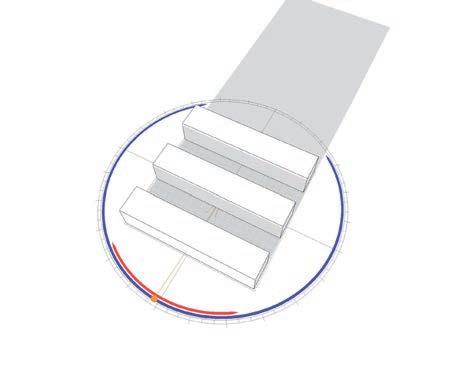
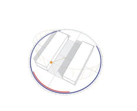
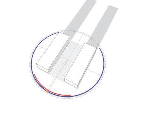
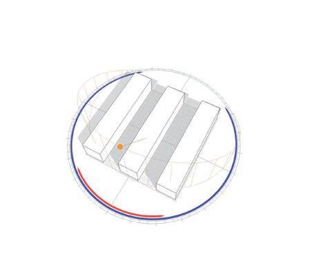
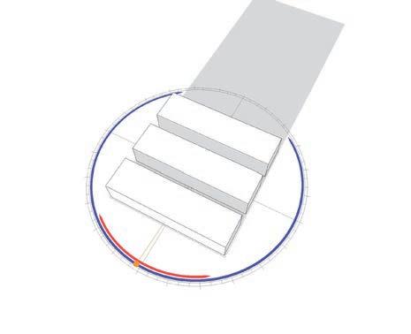
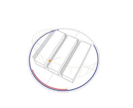
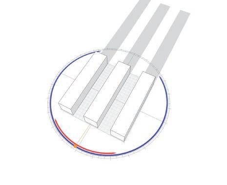
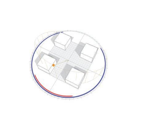
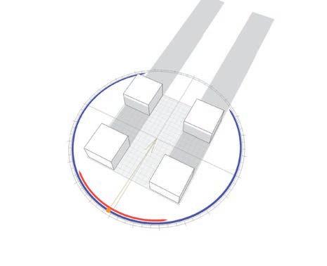
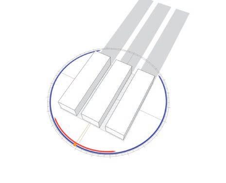
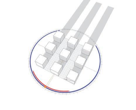
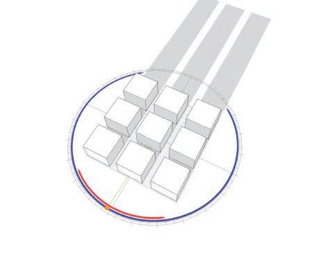
Diagram above: Shadow studies (Ecotect) for different street orientation and aspect ratios at 60° latitude (Winter and summer solstice). For a full range of shadow studies for different latitudes refer to Appendix 03.
Latitude 60˚ Latitude 60˚ Latitude 60˚ Urban Canyon Ratio - 64Domain
Example of wide canyon combining motor traffic and pedestrian areas protected by deciduous trees (Winter). Diagram adopted from Ali-Toudert (Ali-Toudert 2005).
Example of wide canyon combining motor traffic and pedestrian areas protected by deciduous trees (Summer). Diagram adopted from Ali-Toudert (Ali-Toudert 2005).
Example of an asymmetrical canyon combining summer comfort at street level, winter solar access and high density. Diagram adopted from Ali-Toudert (Ali-Toudert 2005).
Example of wide street canyon oriented E-W, combining comfortable pedestrian zones and motor traffic. Diagram adopted from Ali-Toudert (Ali-Toudert 2005).
INDOOR CLIMATE
INDOOR CLIMATE
StreetSidewalk Sidewalk (Gallery) (Gallery)
indoor climate zone outdoor climate zone
Scheme on the subdivision of a street canyon volume according to climatic design needs. Diagram adopted from Ali-Toudert (AliToudert 2005)
June 21 December21
Urban Design on access to the solar beam between 9am and 3pm throughout the year (Matus 1988)
Plot Garden Street Plot
- 65Cities and Climate
- 66Domain
Methods Concepts of Microclimatic Analysis
The complex physical processes within a city that result in microclimates make it very difficult for climatologists to analyze and predict how urban climates at different scales evolve. Delineating characteristic zones that demarcate the three-dimensional extent of microclimates allow to study different scales hierarchally via field studies or computer simulations.
Traditionally climatologists distinguished between the urban and the rural. The discovery of, e.g. urban heat islands, led to a realization that there are distinct variations in climates between urban and rural landscapes. Such broad classification at the macroscale does, however, not take into account the patchiness of urban landscapes, which are characterised through a multitude of different climatic conditions that occur at the micro-scale. More recent approaches in urban climatology therefore try to look at the urban fabric as an agglomeration of patches with specific climatic features. Such a classification into urban typologies might open the way to a better understanding of how small-scale mircoclimates evolve and interact.
This chapter is looking at recent methods of studying and analysing urban fabrics in microclimatic terms. Due to the complexity of the topic the approaches described try to draw connections between the morphology of the fabric and its microclimatic characteristics; in this way it is attempted to break down complexity by looking at the most relevant urban parameters that have an effect on the microclimate. Such parameters, or ‘indicators’, like e.g. sky-view factors or the relation between built and un-built areas allow to draw fast conclusions about the expected climatic characteristics of an urban fabric. They avoid complex and timeconsuming simulations and provide much faster ways of analysis.
- 67Concepts of Microclimatic Analysis
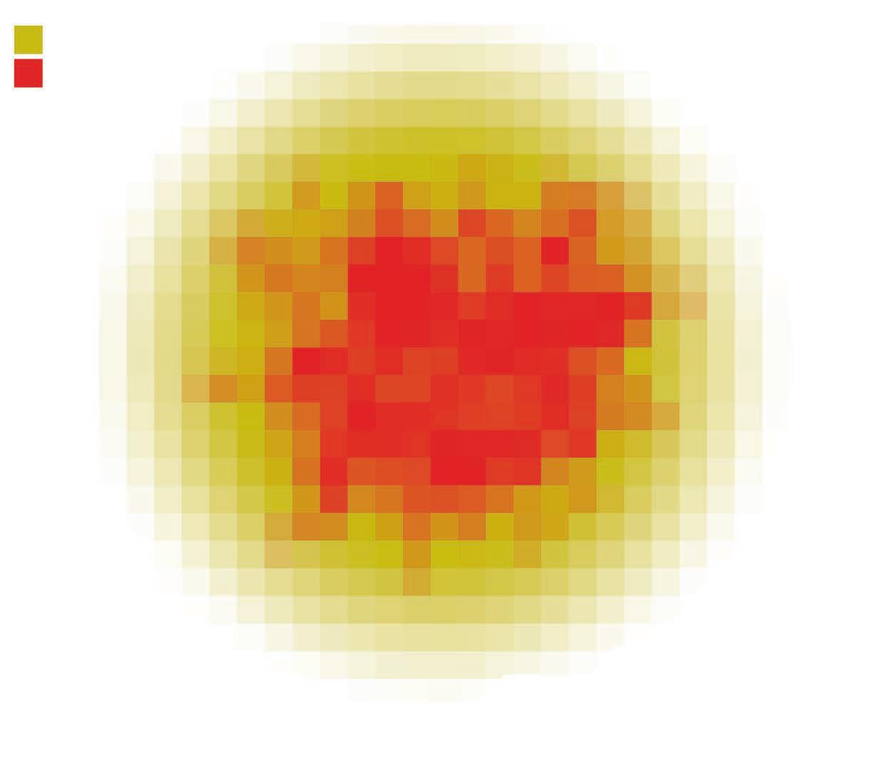
Traditionally climatologists distinguished between the urban and the rural. Such classification reflects the distinct climatic differences between urban and rural sites; it does, however, not take into account the patchiness of an urban landscape, which includes green areas and distinct small-scale microclimates.
Concepts of Microclimatic Analysis
As described earlier the microclimate of an urban area is distinct and different to climatic conditions of the surrounding countryside. Traditionally the distinction between ‘rural’ and ‘urban’ therefore is used to classify and demarcate land zones on the macro-scale. In reality, however, the boundaries between a city and its surrounding countryside are often blurred. Edges of a city maybe clearly defined on maps, but they are often fuzzy in terms of their morphological characteristics. In addition cities often feature larger inner-city areas, which might be termed rural in form of parks, or derelict areas. The patchiness and complexity of combined rural and urban landscapes has recently led to new concepts of microclimatic analysis. Such concepts avoid large-scale classifications and investigate landscape in form of meso-scale patches. This is also related to advances in microclimatic research that happened over the last four decades. Field measurements as well as computational simulations have led to a better understanding of what factors and elements of the urban fabric influence the climate at various scales. Many research-
ers therefore agree on common indicators (parameters) that are quantifiable and that have an impact on certain aspects of the microclimate at various scales. This distinction allows to analyze climatic effects at a much smaller scale.
?
Rural Urban
? ?
Methods - 68 -
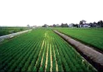
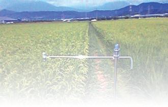
Urban:
Urban downtown area near Nagano city railway station. Buildings 6-10 stories. Vegetation scarce. SVF = 0.78. Built fraction > 95%. μ =1,241
Urban:
Quiet residential/business area of Toyono town. Buildings 1-2 stories. Few trees. SVF =0.87. Built fraction 60%. μ = 1,222
Rural:
Apple orchards in spring. Soils dry. Tree height 3-5m. SVF from orchard road 0.80. Road fraction < 5%.
Albedo 0.20
Rural:
Integrated paddy fields in spring. Green rice in water ponds. SVF = 1. Road fraction < 5%. Albedo 0.08 - 0.10.
Rural:
Drained paddy fields in summer. Mature rice in wet soils. Crop height 1m. SVF = 1. Road fraction < 5%.
Albedo 0.18.
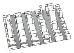
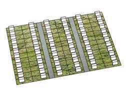
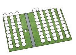
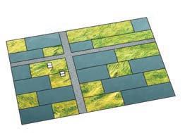
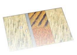
Compact skyline of mid- and high-rise buildings. Surface cover mostly paved. Buildings dense, solid construction. High space heating/cooling demand. Heavy traffic flow.
Detached, close-set dwellings, 1-3 stories tall, separated by private gardens or lawn. Low space heating/cooling demand. Medium traffic.
Regularly spaced close-set trees. Tree rows uniform in height and width. Sky view reduced by overhead canopy. Few roads and small, scattered buildings. Low traffic flow. Anthropogenic heat flux nil.
Interlocking fields of paddy rice or flooded farmland. Soils submerged by shallow water. Fields demarcated by dikes, waterways, roads. Few small, scattered buildings. Low traffic flow.
Low, uniform crop cover. Fields interlocking, demarcated roads, fences, hedge lines, narrow woods. Few small, scattered buildings. Low traffic flow.
SVF: Mean sky view factor from ground level. Varies with height and density of buildings, trees.
Zh: Average height of main roughness elements (trees, buildings, crops).
u: Thermal admittance of surface materials. Varies with surface type and wetness.
Q: Local-scale mean annual anthropogenic heat flux from combustion processes and space heating/cooling.
Urban Climate Zones; recent approaches in climatology try to look at the city as small-scale patches that show characteristic freatures in terms of their morphology. The classification into such typologies opens up a new approach that diverts from the classic distinction between urban and rural. Diagram adopted from Stewart (Stewart, 2009)
Land Use Zones
Ian Stewart proposes a model for microclimatic classification and analysis that deviates from the traditional categorization of ‘urban’ and ‘rural’. He argues that the traditional distinction between macro-scale areas of land does not convey any of the micro- and local-scale site properties that actually influence the surface-layer climate (Kennedy, 2009):
‘The site and settings of urban climate observation are remarkably diverse, from small towns to sprawling cities, and from street canyons to building rooftops.
…(while ‘urban’ and ‘rural’) might accurately describe the regional settings of an urban climate investigation, they poorly describe the local ‘sites’ of observation. The popular use of “urban” and “rural” in modern climate literature to characterize both site and setting has now eclipsed faithful reporting of surface properties— such as cover, exposure, and wetness—that actually determine local climate differences.
Stewart argues for an alternative approach where land is divided into much smaller areas, which he describes as ‘local climate zones’. Patches of land are grouped into sub-classes that might range in size from 102 to 104 meters. A range of parameters is used to classify and form such climatic typologies. He argues that the main factors of consideration should be the surface cover, the surface structure and the cultural activity (anthropogenic heat flux). Stewart therefore proposes to look at surface properties in order to organize land into categories that share common attributes. He proposes to use the following parameters in order to obtain quantitative data for evaluation and classification:
• Mean Sky View Factor from Ground Level1
• Proportion of Zone Surface covered by impervious materials2
• Average height of main roughness elements3
• Weighted average reflectivity of zone surface4
• Thermal admittance of surface materials5
• Local Scale anthropogenic heat flux6
Site Photograph Traditional Classification &
Local Climate Zone SVF % built Zh μ Qf
Metadata
0.40
0.60 >90
-
>25 1,2001,700 > 100
0.70
0.90 40 - 70 5-10 5001,500 10-15
0.60
0.90
10
5 600
1,400
-
<
<
-
0
> 0.95 < 10 < 1 2,0002,500 0
>
0.95 < 10 < 2 1,4002,200 0
- 69Concepts of Microclimatic Analysis
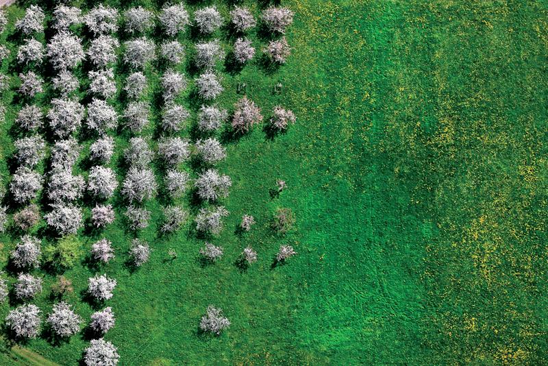
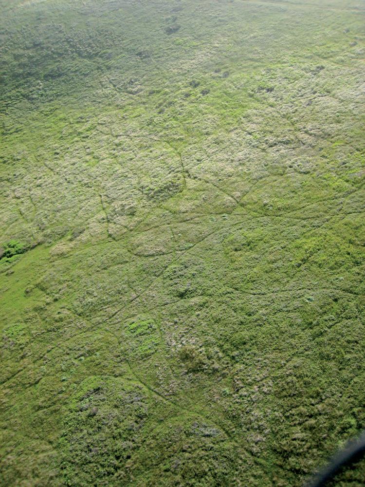
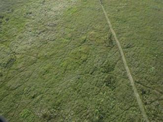
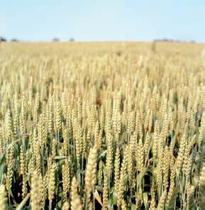


The arrangement of parcels of land has an impact on radiation fluxes within the city. Stone (Stone 2006) reports that the contribution of individual land parcels to the regional heat island formation could be reduced by approximately 40% through the adoption of specific land use planning policies, such as zoning and subdivision regulations (with no modifications to the size and albedo of the residential structure). The diagrams illustrate the concept of Land Use Zones proposed by Stewart. Diagrams adopted from Stewart (Stewart, 2009).
City Series:
250m 250m 250m 250m 250m 250m 250m 250m 250m 250m 250m 250m 250m 250m 250m 250m Modern Core Industrial Processing House & Garden
Old Core Blocks Shantytown Compact Housing Extensive Lowrise Extensive Lowrise
Methods - 70 -
Physical processes of radiative exchange and wind interactions are complex and there is currently no real strategy in what ways the arrangement of different parcels of land can be beneficial in terms of controlling the urban microclimate.
Mixed Series:
Open Grounds
Agricultural Series:
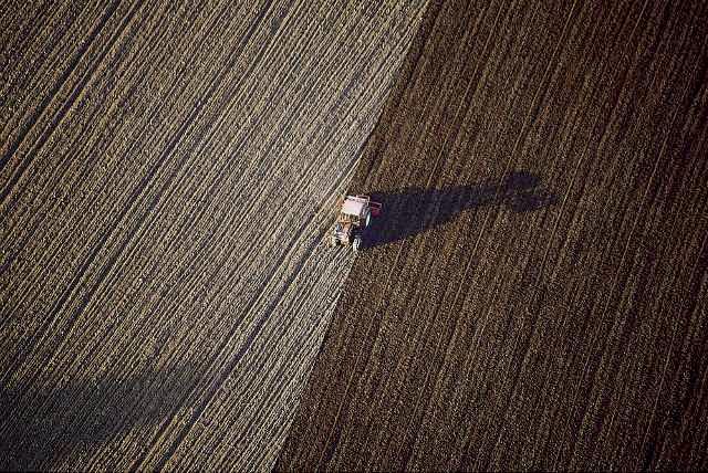
Dispersed Settlement
250m 250m 250m 250m 250m 250m 250m 250m 250m 250m 250m 250m
Flooded Fields
Orchard & Tree Plantations
Cropped Fields
Bare Fields
- 71Concepts of Microclimatic Analysis
Using the above method Stewart proposes a catalogue of 19 local climate zones, which are further organized into four subclasses. In this way he distinguishes between a ‘city series’, a ‘mixed series’, an ‘agricultural series’ and a ‘natural series’. For each of these climate zones a range is specified for all of the six parameters described above. By evaluating an urban fabric it is therefore possible ‘match’ and organize sample tissues according to their specific urban characteristics.
Climate zones are organized and represented in form of a diagram that allows easy use and comparison. Besides the parameter range, photos of real urban tissue and schematic axonometric representations give clear indications how the different morphologies are characterized. Short paragraphs of text further illustrate the specific characteristics for each climate zone. Morphological characteristics are in this sense described as well
Kennedy tested the concept of ‘Urban Climate Zones’ on a field site in Nagano, Japan. Urban patches were roughly 250 meters by 250 meters. In order to classify land a combination of different methods was applied. Besides direct field observations that include building/tree heights, sky view factor or soil thermal admittance, maps and photographs were used to obtain data and to classify urban land. Outside the field additional data was obtained using online portals for digital mapping and satellite imagery, like Google Earth (Kennedy, 2009):
‘Like all classifications, the local climate zone system is a simplification of reality. We therefore sought the best, not the exact, representation of the Nagano field sites using the information provided in the zone datasheets. In some cases, site metadata were incomplete or poorly aligned with the datasheets, and so the process of selecting “best fit” zones became one of skilled judgement rather than automated matching.’
1The Sky View Factor (SVF) indicates the proportion of sky hemnisphere visible from ground level. In field measurements the SVF is often determined using a fish eye lens. It’s values range from 0 to 100%. The SVF indicates the amount of solar access and radiation escape for Urban Canyons. It is therefore used as an indicator for solar access and nocturnal cooling.
2Indicates the area of materials that cannot be penetrated by water. It therefor indicitaes an area’s moisture availability and thus it’s heating/cooling potential. Water run-off is another factor that is determined by this indicator.
3Roughness is a measure of the texture of a surface. It is quantified by the vertical deviations of a real surface from it’s ideal form (wikipedia). In microclimatology the roughness is measured at roof level and indicates in how far the ambient wind gets slowed down by the morphology of the urban landscape.
4The reflectivity of a material is also refered to as the Albedo. The Albedo is evaluated by the ratio of reflected and incident solar energies. The greater the albedo, the smaller is the energy stored by an urban surface. Refer also to page 56 for Albedos for typical urban and rural materials.
5The Thermal Admittance of a surface material varies with surface type and wetness.
6Indicates the heat flux density from combustion processes. It varies significantly with latitude, season, and horizontal scale.
250m 250m 250m 250m 250m 250m 250m 250m 250m 250m
Natural Series:
Forest Tundra
Wetland
Hot Desert
Grassland
Methods - 72 -
Radiation Characteristics: Type of Climate Latitude Season
SOLAR CONTROL
Solar Access inside Buildings
Solar Access in Open Spaces
Nocturnal Cooling of Buildings Urban Albedo Lighting
Heat Gain/Loss From Buildings

Wind Characteristics: Wind Incidence Speed/Velocity
WIND CONTROL
Ventilation in Open Spaces Dispersion of Polutants
Potential of Internal Ventilation
Control of Aerodynamic Effects of Buildings
OPENESS TO SKY
URBAN REFLECTANCE
DIRECTIONALITY
BUILDING ENVELOPE
MORPHOLOGICAL PARAMTERES
Urban Profile H/L Solar Orientation Plan Density (Roof Surface/Total Surface)
Building Geometry (Size: S/V, Shape: P/A%)
URBAN POROSITY
DIRECTIONALITY
BUILDING ENVELOPE
MORPHOLOGICAL PARAMTERES
Spacing between Buildings (Ratio H/L Frontal: Wind/ Ratio H/L Lateral Wind) Building Geometry (Height/Width) Height Differences
LANDSCAPING
ENVIRONMENTAL FACTORS
UNITS UNITS
GEOMETRICAL PARAMETERS CLIMATIC CONTROL GOALS
PARAMTERES
Type of Trees
Density and Height
Volume of Crown Foliage Cycle
Location/Buildings
Number of Trees
Fazia Ali-Toudert points out that the most important parameters that should be adressed in urban planning are: openess to sky, urban reflectance, urban porosity, directionality, the building envelope and landscaping (Ali-Toudert 2001). For more information refer to page 75.
Parameters of Urban Analysis
The analysis of an urban fabric via indicators as described before is based on the ability to measure and extract data from its morphology. Unlike field measurements that allow to directly acquire data sets such as temperature or wind speed, indicators provide an indirect way of evaluating the same information. By weighing certain elements of the urban geometry against each other it is possible to make good-enough assumptions about e.g. how much radiation is able to penetrate into the fabric and what wind conditions are likely to occur within the Canopy Layer. The advantage of using Urban Parameters for evaluation is that it
provides a very rapid means of analysis that can even be applied remotely through the use of GIS data sets.
Parameters used for morphological evaluation are mostly metric data sets that provide information about length, area and volume of different elements of the urban fabric; they can often be organized according to scale. In case of Adolphe’s approach, described later, parameters for evaluation can be grouped according to scale into ‘overall urban fabric level’, ‘urban canyon level’ and individual buildings. In addition Adolphe employs a fourth
- 73Concepts of Microclimatic Analysis
set of parameters that contains surface related information, such as U-Values and Albedo, and environmental properties such as e.g. wind directions. For a schematic representation of the parameters used refer to page 83. The list of parameters allows for extraction of specific data that can be used to evaluate the performance of a given urban area according to particular environmental aspects. As ratios are calculated the results are always relative values that require further evaluation and interpretation. Nevertheless, since obtaining absolute values via simulations or field measurements is time consuming, the use of parameters gives good indications about microclimatic conditions that can be expected; the word indicator therefore expresses the indicative nature of such tools.
Climatic Variables and the Urban Geometry
As shown from Stewart’s analysis concept the use of ratio’s are common approaches to obtain information about the microclimatic performance of urban areas. Ali-Toudert presents a similar methodology that puts climatic control variables (solar access, shadowing, nocturnal cooling, exterior and interior ventilation, etc.) in relation to the geometric properties of the urban fabric (vertical profile H/L, plan density, spacing between buildings, building dimensions, wind incidence, solar orientation, etc.) (Ali Toudert, 2001). Whereas Adolphe’s approach (page 77) is designed to evaluate urban areas at the meso-scale level, Ali-Toud-
ert’s methodology is more suitable at the street of block level; the computationally extensive nature of calculating aspects such as shadowing or sky view factors for each element of the fabric will result in a very detailed analysis which is likely to be limited to a much smaller sample area.
Adolphe introduces his set of parameters purely for analysis. AliToudert, on the other hand, argues that microclimatic aspects are currently not part of architectural or urban planning considerations (Ali Toudert, 2001).
On this background it is argued that a better understanding of the dependence between urban geometry and the resulting microclimate is necessary. Similar to Adolphe, Ali-Toudert points out that Wind and Solar Radiation are the most significant climatic variables that need to be considered within planning processes. In relation to this a set of six (06) indicators is proposed that include:
• Openness to Sky
• Urban Reflectance
• Urban Porosity
• Directionality
• Building Envelope
• Landscaping
Methods - 74 -
tives
Openness to Sky (1)
Solar and Energetic Control:
Solar Access: Ratio H/L Orientation/Sun
Solar Access
Nocturnal Cooling
Urban Reflectance (2)
Control of the potential of the energy available
Nocturnal Cooling: Ratio H/L
N/S
E/W
Urban Porosity (3) Wind Control:
Control of ventilation in open spaces
Dispersion of Pollutants
Control of ventilation inside buildings
Plan density (Roof Surface/Total Surface) H/L, secondary
For solar access: Increase of sky view enables on optimal exploitation of sunshine on the south wall
• The profile H/L depends strongly on the solar orientation. The south offers the best exposition according to solar access inside buildings.
• Distinction between street level and the upper part of buildings is recommended.
• Solar access indices are to be used to estimate insolation in both open spaces for pedestrian comfort (street level) and solar gains inside buildings.
• Sky view factor (SVF) is the indicator of the potential rate of nocturnal cooling. It depends directly on H/L.
For nocturnal cooling: The sky view is the most relevant parameter
High plan density: High reflectance
External Ventilation:
Plan Density Spacing between buildings Ration H/L Wind incidence
Low plan density: Low reflectance
Wind direction Isolated flow
Wake interference flow
Better ventilation obtained with oblique angle
• Solar orientation has no influence on the potential rate of nocturnal cooling, while influences the quantity of energy stored.
• Urban reflectance increases with high densities.
• High urban reflectance means a reduction in the global energy stored by the urban fabric and consequently decreases the urban temperatures.
• H/L has less impact in comparison with plan density, but globally energy storage increases with deep profiles.
• Important Horizontal spacings between buildings are recommended to guarantee a good ventilation.
• The transversal ratio H/L determines the type of wind flow between buildings in the direction of the wind: isolated, wake interference or skimming flow.
• Oblique incidence allows the best wind flow in the urban structure and enhances the potential of internal ventilation by a good distribution of pressure fields around buildings.
Ventilation inside buildings: CF.
+ Building Geometry (width)
Skimming flow
Longitudinal Shape Compact Geometry/Low Potential for Ventilation
Enhanced with appropriate roof design
• Longitudinal geometries enable a good natural ventilation (cross ventilation) in interior spaces than compact ones.
• For compact buildings, atrium buildings should be preferred to courtyard ones to exploit the depression field on the roof to improve the internal ventilation.
Summary of the conceptualized methodology for a climatic urban design; adopted from Ali-Toudert (Ali-Toudert, 2001)
relevant
Concepts & Objec-
Urban and Environmental
Parameters General Recommendations
- 75Concepts of Microclimatic Analysis
tives
Directionality (4)
Establishes the orientation of the urban structure, compromises between solar control and wind control
Solar Orientation Wind incidence
Built envelope (5)
Estimate the impact of architectural options (building geometry: size and shape) Estimate the impact of building associated on climatic performance of the urban fabric
Building geometry:
Size and Shape (Height,Width)
Solar orientation OPtimal Exposition: South N
Size of building (same shape)
S/V decreases, P/A decreases
Wind direction for better ventilation/incidence between 30˚ And 60°
Landscaping (6)
Improves the urban microclimate by the exploitation of climatic properties of vegetation:
E.g. Shading, Evapotranspiration and Reduction of wind speed
Type of tree (Foliage cycle, crown density and shape, height)
Number of trees
Location in relation to buildings
Passive/active area
Shape of building (same vol.)
S/V increases, P/A increases
Basic Unit
Urban association
• Solar orientation is more decisive than wind incidence for determining the layout direction because solar access is strongly dependant on the position of the sun while ventilation admits a wide rance of incidences (30˚ to 60˚).
• Ventilation can be sufficient when large spacements are planned regardless of wind incidence.
• The ratio Surface/Volume (S/V) determines the building’s compacity.
• Compact buildings are more isolated from external environment, allowing better conservation of heat or cold but reduces at the same time their potential for passive cooling or heating.
S/V reduced, P/A reduced
S/V increased P/A increased
Summer: Winter:
• The ratio passive area/ active area (P/A) indicates the exposition level of the building and its potential to use natural energies. Longitudinal forms are the most suited for passive approach.
• Climatic performances at urban level of a group of buildings depend on the solar and wind control in external spaces as discussed in the previous concepts (1), (2) and (3)
• The use of vegetation is a complementary disposition for improving urban microclimates.
• It should be well located in relation to buildings, West for solar protection. South location is also interesting but attention must be paid to solar access and ventilation when necessary
• Shading is the most important condition in hot climates, thus trees should be of large crowns, in great number but with low density and well dispersed in the urban fabric.
• For cold climates, the reduction of wind speed is more important, preferably trees with high density, small and high crowns, located facing the prevailing winter winds.
Summary of the conceptualized methodology for a climatic urban design; adopted from Ali-Toudert (Ali-Toudert, 2001)
relevant
General
Concepts & Objec-
Urban and Environmental
Parameters
Recommendations
N
N Sun
Hot
(shading)
Climate
Cold Climate
Reduction of Wind
Methods - 76 -
Direction Speed
m/s degrees (0-359)
UNITS TEMPERATURE
AIR & SURFACE TEMPERATURES
degrees C
RUGOSITY
POROSITY SINUOSITY DENSITY
COMPACITY CONTIGUITY OCCLUSITIVITY SOLAR ADMITTANCE MINERALIZATION
PARAMETERS
ENVIRONMENTAL FACTORS GEOMETRICAL PARAMETERS
Luc Adolphe proposes a set of nine indicators that relate to the four most important environmental parameter that affect the urban microclimate; I.e.wind, temperature, solar radiation and humidity (Adolphe, 2001)
Bio-Climatic Urbanism:
Like Stewart other climatologists have referred to the use of Indicators (p arameters) to assess and evaluate urban fabrics. Adolphe proposes a set of 9 ‘Morphological Indicators’, which he intends to use at the district or city scale (Adolphe, 2000). He claims that because of the complexity and heterogeneity of processes at the building scale it seems more appropriate to zoom out and work at a ‘macroscopic’ level. Identifying Wind, Temperature, Solar Radiation and Humidity as the main environmental forces that have an impact on the urban microclimate Adolphe proposes a simplified model of urban morphology that gets assessed via the following parameters:
• Density
• Rugosity
• Porosity
• Sinuosity
• Occlusitivity
• Compacity
• Contiguity
• Solar Admittance
• Mineralization
The above parameters will be explained in more detail in the next section. It is important to stress again that Adolphe proposes a simplified model that is based on a set of hypothesis that make certain overall assumptions for global climatic phenomena. In this manner he e.g. considers the air above roofs as a lid above the
canopy, which is a clear simplification of the complex processes encountered in real urban environments. Nevertheless, his approach is more than valuable as it is one of the first attempts to create a ‘user-friendly’ model that actually considers more than one microclimatic factor. At the system level Adolphe argues for the following criteria:
Completeness (by covering the entire ensemble of dimensions of the climate-urban form relation)
Non-redundancy (by searching for indicators as independent from each-other as possible)
Operationality (by limiting the number of indicators)
At the Indicator level he argues for the following criteria:
• Physical consistency (by looking for indicators consistent with the physical phenomenona they are supposed to cope with.
• Spatial Consistency (with indicators consistent with geographical (macroscopic) scale.
• Measurability (By defining indicators requiring data readily derived from standard urban community databases.
• Legibility (with indicators easy to interpret)
• Comparability (by choosing indicators for which absolute values are not highly significant, but for which relative variations (range and direction) are significant.
WIND
SOLAR
RADIATION
AIR HUMIDITY
g/m3
SHORT- & LONGWAVE RADIATION FLUXES
watts
HUMIDITY
- 77Concepts of Microclimatic Analysis
Wind conditions in an urban environment are changed due to the characteristic urban morphology. Variations in height of the mineral and vegetal canopy change the speed of the ambient air flow; the orientation of streets in relation to wind direction has an impact on the wind conditions at floor level. Adolphe therefore proposes a series of parameters that are related to wind phenomena: The Rugosity, Porosity and Sinuosity.
Absolut Rugosity:
The Absolute Rugosity, also known as ‘roughness’ describes the surface properties of an urban landscape at roof level. A city characterized through flat roofs with similar building heights will have less affect on the speed of the ambient wind compared to a fabric with a very un-even and rough surface. In the later case obstacles in the flow of air will slow down the quadratic speed of air, which has a global effect on the reduction of wind speed at floor level. In general it can be said that the higher the Rugosity the slower the mean speed of air.
The mean height of the urban canopy is the most important factor for evaluation of the Absolut Rugosity (Adolphe, 2000): ‘As it (the mean height of the urban canopy) is often lower than the mean height of buildings, because nonbuilt spaces must be integrated the absolut rugosity Hm is given by the product of the height of buildings and their area, divided by the total (built and non-built) area.’
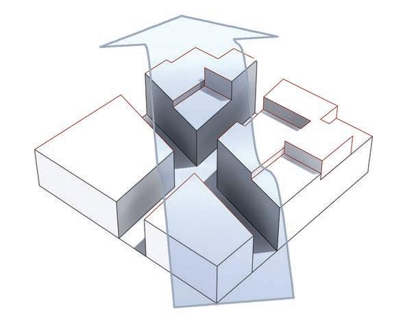
Rugosity: Smooth Roof Surface Rough Roof Surface Wind
The Absolute Rugosity Factor is determined by:
Ai footprint area of building i
hi height of building i
Aj area of non built elements j
Relative Rugosity:
As indicated above the ‘Absolute Rugosity’ factor indicates in how far the ambient wind gets slowed down or not through interaction with the urban fabric at a global level. In order to ‘distinguish very regular fabrics from small variations in building height, and less regular variations from more significant ones’ Adolphe introduces the Relative Rugosity factor. It uses the mean square deviation instead of the mean deviation and can be plotted against wind directions on a polar diagram. Long branches in such a diagram correspond to directions of high rugosity (significant reduction in wind speed) and vice versa.
The Relative Rugosity Factor is determined by:
h a Mean height of urban canopy in direction α
hi height of (built or non built) element of the canopy
l width of the element I of the canopy in the plane of direction α diameter of studied fabric
Porosity and Sinuosity:
The ability of the ambient wind to penetrate into spaces within the urban canopy layer depends on size and direction (in relation to the air flow) of such spaces. Adolphe therefore distinguishes between two parameters related to wind, which he terms ‘Porosity’ and ‘Sinuosity’:
Porosity:
Adolphe describes the urban fabric as a ‘porous medium with solid skeleton’; he therefore distinguishes between ‘open’ (streets) and ‘closed’ (equivalent to cavities such as backyards or private gardens) urban spaces, arguing that closed spaces can be neglected in terms of wind evaluation. The Porosity factor looks at the speed of air independent of the angle of the main wind direction (Adolphe, 2000): ‘If we consider the pressure-gradient flow across the urban canopy in a direction parallel to the street axis, the porosity, in a plane perpendicular to this direction, will be proportional to the open area (height x width) of these streets.’ Adolphe, however, does not simply adopt the common ‘Urban Canyon Ratio’ but introduces the ‘Hydraulic Equivalent Radius’ to better evaluate the wind speed within the street. The ‘Hydraulic Equivalent Radius’ takes into consideration that the wind speed is higher in the centre of the street and gets slowed down along the surfaces of adjacent structures.
Adolphe argues that the advantage of using the Hydraulic Radius is that it is able to distinguish different street profiles (Adolphe, 2000): ‘A canyon street will, for the same front area, have a smaller hydraulic radius than a square section street. We can then appraise the ‘useful area’ of a street by the following expression’:
h height of canopy for the street (mean height of the adja cent built and non built spaces
l mean street width
Hm = Ai * hi built Ai + Aj nonbuilt built [m]
Ra = 2 (hi ha) * 2li i *li i [ m] li rh = l * h l + h [ m] Methods - 78 -
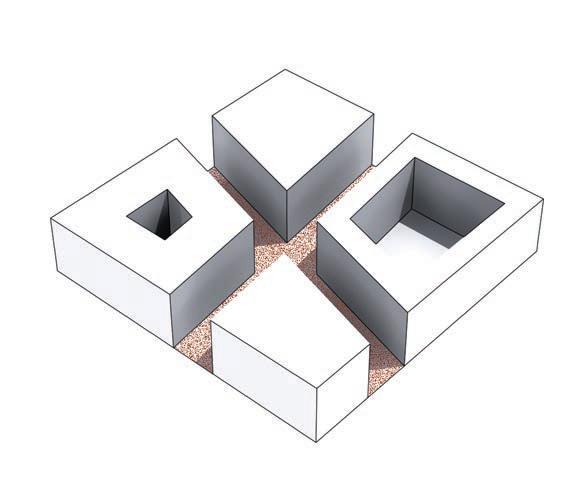
Porosity:
‘Open Pores’
‘Closed Pores’
The Porosity, as a global parameter, is therefore determined through the following expression:
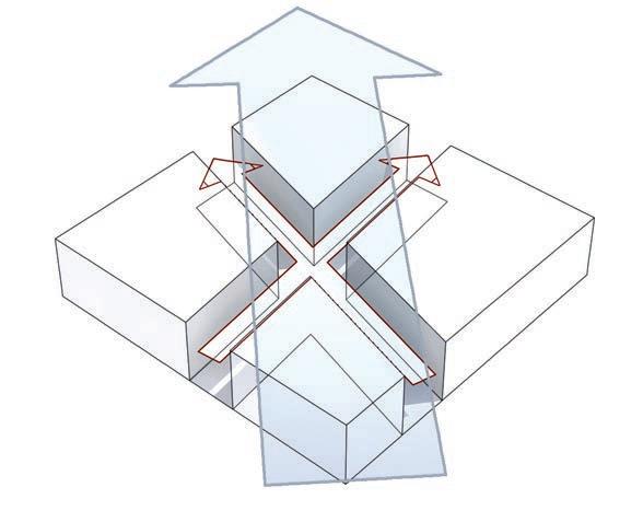
Sinuosity: Street Direction Wind Direction
Li Length of open space i
rhi height of building i
V mean volume of the built volume j
Vj mean canopy volume above open space i
Sinuosity:
The Porosity factor therefore only indicates, at a global level, the potential of high or low wind speed within streets, independent of the direction of the wind. Adolphe introduces the Sinuosity parameter to evaluate the direction of a street (q) against the direction of the airflow (Adolphe, 2000): ‘Therefore a factor equal to (cosq)2, called ‘Sinuosity’, can be derived from this phenomenon. In the case of a flow normal to the street, the sinuosity is equal to zero, which is consistent with the fact that this street can be considered to be (a) lateral cavity, and its influence on the sinuosity factor can be neglected.’ The Sinuosity ratio is calculated as follows:
In the same way as Rugosity, the relative Rugosity can be plotted against the wind direction on a polar diagram (Sinuosity Rose). Long branches of this rose correspond to directions of high Sinuosity (high resistance to wind speed), and vice versa (Adolphe, 2000): ‘The superposition of this rose onto the rugosity rose may point out the potential ventilation properties of an urban space: an azimuth with high rugosity and sinuosity will correspond to an azimuth where the wind speed is slowest, and vice versa.’
The second climatic consideration is the dry air temperature; the Indicators Compacity and Contiguity relate to this parameter:
Compacity:
A buildings ability to receive and store heat (or to stay cool) is firstly related to the shape and form of its exterior envelope. Commonly, the surface to volume ratio is therefore used to determine a buildings compacity. Adolphe proposes a more elaborate Compacity indicator, which also takes into consideration a buildings ability to transmit energy through its exterior envelope; he therefore proposes to include the U-Value as part of the ‘Volume Transmission Coefficient’. The Volume Transmission Coefficient takes into consideration the (heated) building volume, the U-Value and area of the exterior wall. It is given as follows:
Li length of street linear segment i
θi angle between the given direction (of flow) and the direction of the street linear segment i
V (heated) building volume
Ki surface transmission coefficient for exterior wall
Ai area of exterior wall i
P0 = p * r 2 hi open space * Li Vi open space + Vj built [/] ! S0 = Li * cos2 (qi street segm ) Li street segm [/] G1 = Ki *A i Ext.Walls V [Wm 3 ] - 79Concepts of Microclimatic Analysis
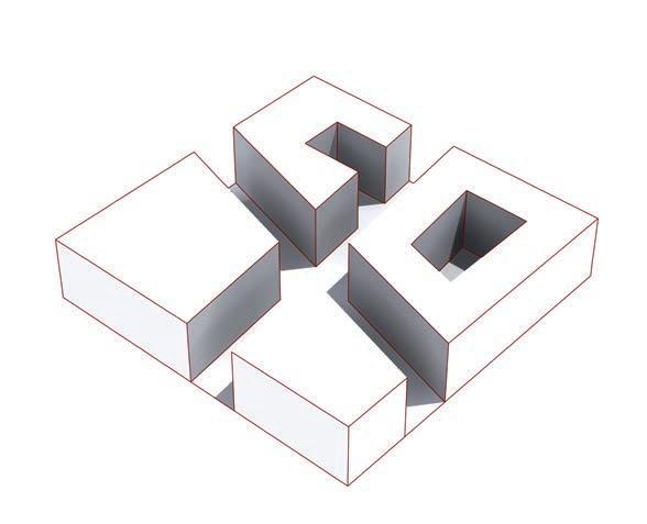
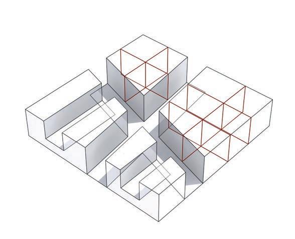
Compacity: Compact Form Less Compact Form
Since the shape of a building will not only have an impact on heat transmission through the envelope but also on available natural light for the occupier it is common to also measure the ratio of active and non-active zones. An active zone is defined as an area offset six meters from the envelope of the building. It is assumed that within this active zone natural resources can be used and that there is reduced requirements for artificial heating and cooling as well as artificial light. Adolphe does not adopt the active- passive-zone indicator but proposes a slightly different way to determine the maximum distance of an occupant to the building envelope (Adolphe, 2000): ‘By using a simple mathematical artifice we can split the volume into a product of V1/3, which is proportional to the radius of the equivalent sphere, corresponding to the maximum distance of an occupant to the building envelope surface.’ The following expression can be derived:
Contiguity: Large Exterior Envelope Shared Party Walls
Contiguity:
Another important factor to determine a buildings potential for heat gain and loss, as well as it’s ability to receive natural sun light, is to look at it’s relationship to neighbouring buildings and whether party walls are shared or not. Adolphe claims that especially in historical centers buildings are characterized by high vertical adjacencies with their neighbours whereas in modern urban cores parts of buildings are often isolated objects. The contiguity factor is calculated by taking the ratio of envelope area adjacent to other buildings to the overall envelope area: ‘…the mean contiguity is derived from elementary building contiguity by weighing it with its floor area to lower the effect of large buildings.’ It is calculated as follows:
Aadj * Afloor
Avert buildings
C1 =
Aext exterior area of non-contiguous building envelope
CF compacity coefficient [/]
CT scale coefficient [m-1]
The mean Compacity factor can be determined by averaging directly the Compacity of all buildings in the area of concern. Adolphe claims that the advantage over the the traditional Surface/ Volume ratio is that it gives greater importance to large buildings than to small ones. The Compacity factor is derived via the following expression:
Afloor buildings [/]
Avert exterior area of vertical envelope for given building
CF area of vertical envelope adjacent to other building
CT floor area of building
Occlusitivity:
The Occlusitivity factor is closely related to the well-established sky view factor (SVF), which is commonly used to determine the amount of solar access and radiation escape in an urban canyon. The SVF factor is directly related to the canyon geometry as it indicates the proportion of sky hemisphere visible from the ground. In order to avoid calculation of the mean Sky View Factor for each individual street segment via 3D angle calculation Adolphe proposes the Occlusitivity factor as a more comprehensive indicator of a fabrics’ global potential for solar access and escape. The Occlusitivity factor is calculated by evaluating the distribution of built elements with height above ground, calculated by a series of horizontal cuts.
€ Cf = Aext V2 / 3 [/] buildings ∑ G1 = Km * Aext 2 / 3 V = Km * Aext 2 / 3 V * 1 1/ 3 V = Km * Cf * CT[ W / m 3 ]
Methods - 80 -
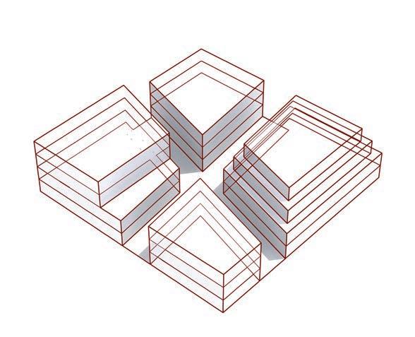
Occlusitivity:
Big Solar Access
Small Solar Access
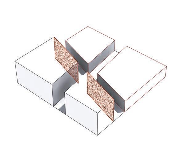
Solar Admittance: South Facade East Facade
The Occlusitivity is determined via the following expression:
Nhoriz Cuts * Pbuilt Punbuilt Nhoriz Cuts [/] !
NhorzCuts number of horizontal cuts
Pbuilt built perimeter for current cross section
Punbuilt unbuilt perimeter for current cross section
Solar admittance:
Total area of the studied urban fabric A u useful area of element I of water or vegetation Oc = 1
‘Each vertical or roof area of a building is able to capture part of the incoming solar radiation’ (Adolphe, 2000). Traditional tools for simulating indoor climatic conditions, like e.g. Ecotect, seem appropriate at the building level but are not applicable at the urban scale due to a lack of databases and the complexity of calculation. Adolphe therefore proposes a simplified parameter called ‘Solar Admittance’; it is evaluated by taking the following parameters into account: the orientation of the façade, the adjacency rate for each building façade, a mean shading effect of the immediate environment (derived from its density and simple geometrical considerations, such as the mean street profile for a given density) and typical reflectance values, i.e. the albedo. The Solar Admittance factor is derived as follows:
and bodies of waters are in themselves complex three dimensional objects Adolphe proposes a simplification by evaluating what he calls the ‘useful area’ of an object. The useful area is thereby evaluated as the direct area of a lawn or body of water, or the trunk of a tree, respectively. The Mineralization factor set the overall area of the urban tissue in relation to the overall useful area. It is derived as follows:
Mineralization:
Mineralization determines the ratio of natural surfaces vs. man-made surfaces and is an important aspect in microclimatic analysis. Adolphe claims that (Adolphe, 2000): ‘…,vegetation and bodies of water play a specific role in highly mineral urban spaces, in terms of moderation of solar heat storage in horizontal and vertical surfaces, of modification of the humidity and heat balance (effects of evaporation and evapotranspiration), and of alteration of the substrate waterproofing with complex impacts on humidity, heat island or pollution confining.’ Since vegetation

Mineralization: Building Vegetation
AT
Ai = Ai * Cc * Co * Cs * Cr Ext Walls Ai Ext Walls M = Ar Au i Ar [/]
- 81Concepts of Microclimatic Analysis
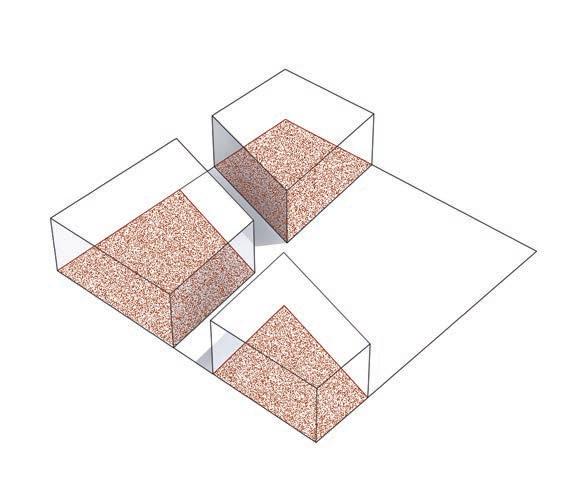
Density: Built Area Overall Area
Density:
Adolphe determines density by dividing the built area (footprint area of all built elements) by the total area. We will later see that there are different ways of calculating density and that Adolphe’s approach might not be the most suitable one:
D = Afloor built Ai built + Aj unbuilt [/]
Afloor floor area of building i Ai built element i Aj unbuilt element i
The nine indicators proposed by Adolphe can be organized in three major groups. A first group relates to wind and includes Rugosity, Sinuosity and Porosity. A second group relates to solar radiation and includes Contiguity, Compacity, Occlusitivity and Solar Admittance. A third group includes density and mineraliztion and therefore relates to urban areas and how they are used in terms of un-built and open spaces. The classification into sub groups allows for further improvement regarding the analysis as major parameters can be looked at separately.
Listing the parameters that are involved in determining the various indicators also reveals that certain parameters are used several times in order to determine various data (see diagram on
next page). The involved parameters can be broken up in 4 major groups that reveal a certain hierarchy. A first set of parameters is related to overall urban areas that include built and un-built elements as well as bodies of water and vegetation. The second set relates to buildings and includes building footprints, heights and volumes. The third set is related to the urban canyon and includes information about street lengths and widths. The final set of parameters provides miscellaneous data that relate to e.g. wind directions and the solar orientation.
Even though Adolphe’s approach is designed to analyze wider areas of urban tissue from e.g. GIS data (Global Information System) it reveals that certain hierarchies in the approach are re-
Methods - 82 -
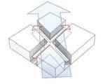
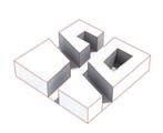
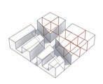
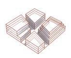
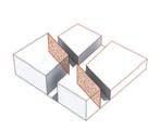
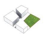
Mineralization
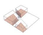
Density
Urban Area:
Area (overall) of Urban Element (Mineralization, Density)
Area of open/un-built Element (Rugosity)
Area of Vegetation/Water Element (Mineralization)
Built Element:
Area of Built Element (Rugosity, Contiguity, Density)
Area of Exterior Wall for Built Element (Compacity, Contiguity, Solar Admittance)
Area of Party Wall for Built Element (Contiguity, Solar Admittance)
Height of Built Element (Rugosity)
Volume of Built Element (Porosity, Compacity)
Number of Horizontal Cuts of Built Element (Occlusitivity)
Length of Perimeter for Cut Section (Occlusitivity)
Length of un-built Perimeter for Cut Section (Occlusitivity)
Urban Canyon:
Height of Urban Canyon (Porosity)
Width of Urban Canyon (Porosity)
Length of Urban Canyon (Porosity)
Volume of Urban Canyon (Porosity)
Miscellaneous:
Angle between Wind Direction on Street/Building (Rugosity, Sinuosity)
Angle between Polar Direction and Envelope of Built Element (Solar Admittance)
U-Value for Envelope of Built Element (Compacity)
Shading Ratio* (Solar Admittance)
Albedo (Solar Admittance)
Indicators utilize different morphological information in various combinations to draw conclusions about a fabric. The parameters used in this process can be broken up and organized hierarchically according to scale and type of information.
spected; as discussed in the previous chapter scales of analysis range from the urban canyon to the macro-scale, i.e. the city as a whole.
Adolphe’s approach of using indicators reveals how underlying information that is inherent to the urban fabric can be utilized to draw conclusions about the qualities and performance of the morphology. We will later see that the use of indicators can be extended, beyond microclimate analysis, to gain latent information about other qualities of the urban fabric, such as e.g. the connectivity of urban street networks or the distances to certain areas of interest.
Rugosity Porosity Sinuosity Compacity Contiguity Occlusitivity Solar
Admitt.
- 83Concepts of Microclimatic Analysis
Evolved and Planned Cities
In order to create a genome to inform the optimization tool so that it would not only respond to the immediate environment ,but also the global setting, it is essential to study the performances of existing cities in different parts of the world.
This involved first, the identification of these global zones that combined both the climatic categorization with topography, thus giving us 9 zones. Within each of these zones , a tissue sample of an evolved city and its planned counterpart was abstracted. All cities chosen are functional to date adhering to their original intended use. All of the evolved city was intended for residential use. To draw conclusive analysis, care was taken to select similar samples of high density residential spaces within the planned city fabric. It should also be noted that the scale chosen for an evolved city sample was 0.5 times the scale of planned city due to the scale of the latter.
With the combined information provided by satellite images (Google Earth), landuse plans, photographs and available data, a 3 dimensional information database of 18 cities were created.
These were namely :
(1)Arctic/ sub arctic : (E)Dragor (P)Stockholm (2)Continental : (E)Kabul (P)Chicago (3)Desert (E)Yazd (P)Phoenix (4)Maritime: (E)Bath (P)Tokyo (5)Mediterranean: (E)Mazzara del Valo (P)Barcelona (6)Monsoon (E)Zanzibar (P)Navi Mumbai (7)Montane (E)Potala (P)Quito (8)Subtropical (E)Karaikudi (P)Buenos Aires (9)Tropical (E)Malacca (P)Bangkok
*(E)- Evolved City; (P) – Planned City
4000BC 3000BC2000BC1000BC 0 1000 11001200130014001500 1700 1600 180019001950 2000 YAZD BATH KARAIKUDI ZANZIBAR CHICAGO STOCKHOLM QUITO
DRAGOR
MELACCA MAZARRA DEL VALO
PHEONIX
NAVI MUMBAI
BANGKOK CHRONOLOGY OF CITY DEVELOPMENT
BARCELONA POTALA KABUL
- 85Evolved and Planned Cities


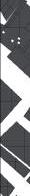


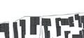
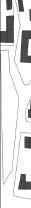

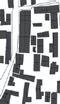
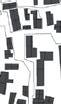
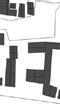
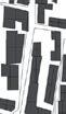
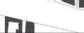
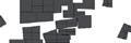


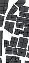
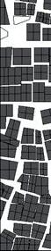
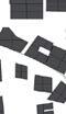
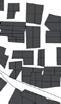
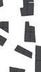

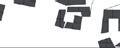


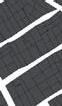
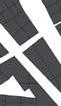


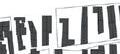


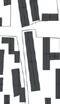
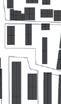
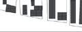


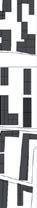
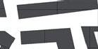
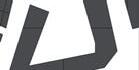
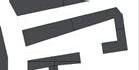
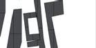
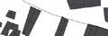

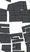
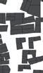
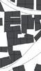
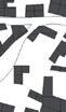


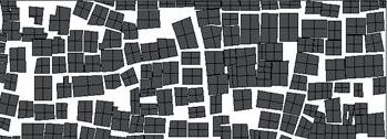
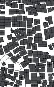
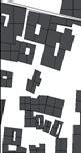
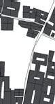
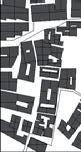
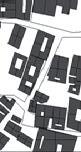


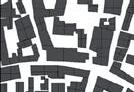
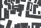
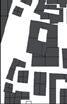
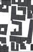
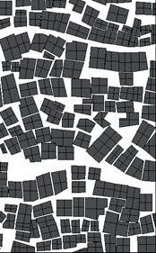


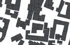
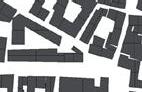
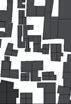
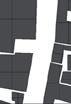


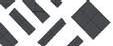

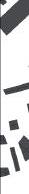


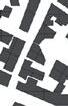
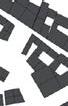
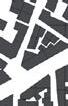
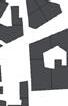
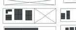
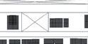
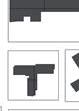
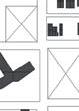

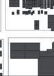
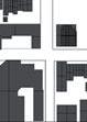

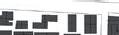
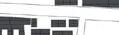


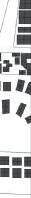
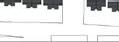

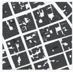

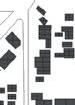
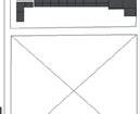
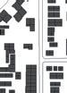
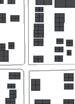
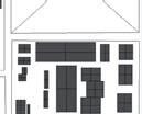
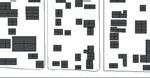
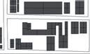


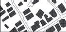
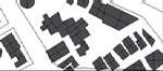 CHICAGO
KABUL
CHICAGO
KABUL
YAZD PHOENIX
AIRES
BANGKOK
MELACCA BUENOS
KARAIKUDI
DRAGOR
POTALA
STOCKHOLM
QUITO
NAVI MUMBAI ZANZIBAR
BATH
TOKYO
BARCELONA
DEL
- 86Methods
MAZARA
VALLO
CONTINENTAL
Kabul, Afghanistan Chicago, United States
DESERT
Yazd, Iran Phoenix, United States
MARITIME
Bath, United Kingdom Tokyo, Japan
MEDITERRANEAN
Mazzara Del Vallo, Siicily Barcelona, Spain
MONSOON
Zanzibr, Tanzania Navi Mumbai, India
MONTANE
Potala, Tibet Quito, Equador
SUBTROPICAL
Karaikudi, India Buenos Aires, Argentina
TROPICAL
Melacca, Malaysia Bangkok, Thailand
PLANNED CITY EVOLVED CITY PLANNED CITY EVOLVED CITY - 87Evolved and Planned Cities
City Data Sets
Selection Criteria and Methodology:
Existing and functional cities built as early as 3000 BC were chosen from each climate zone. 3D information data were particularly hard to find for these. Thus with a compiled information from various vernacular references, single unit information and photographic images, information was extracted to create 3D models, which later on are to be used in evaluations of microclimatic indicators.
Planned cities, most of which had their master plan formulated after the WW2, were selected from the corresponding climate zones. A detailed research was carried out on the land use pattern with the help of building codes, master plans and administration documents. Thus with the information gained from this, the residential areas with both single family and multi-family dwellings were identified. This was done to make the closest possible comparison in terms of building usage in addition to the building material used and surrounding hard and soft landscape. While building codes and FAR information was available to extract the building height information, photographs and particularly Google street view on Google earth proved as a very useful tool in determining exact no. of stories. The planned city area analyzed was a 1000X1000 sq.m, double that of the 500 X 500 sq.m sample of the evolved city. This was due to the scale of buildings and streets within the modern fabric as compared to the older ones.
Floor heights in all cases are assumed as 3m. Elevation of ground was ignored in taking the building roof height.
- 89City Data Sets
ARCTIC/ SUB ARCTIC
EVOLVED CITY DRAGOR, DENMARK

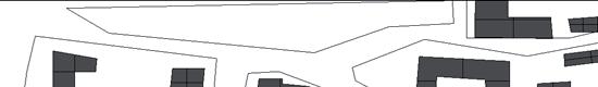
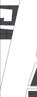
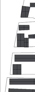
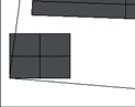
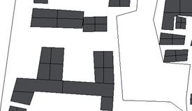
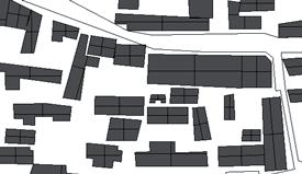
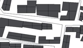
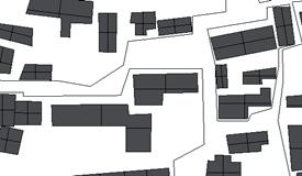
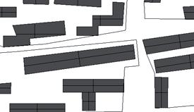
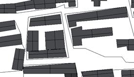
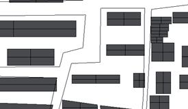
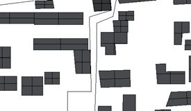
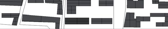
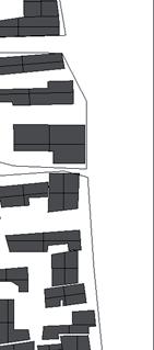
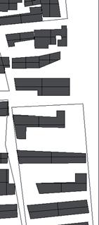
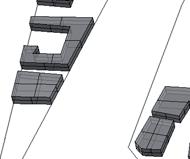
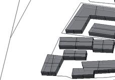
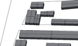
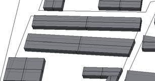
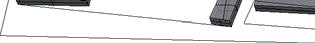
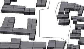
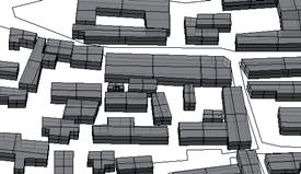
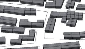
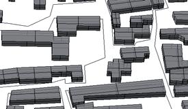
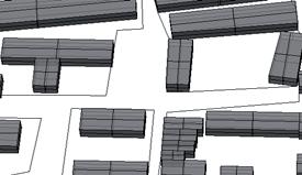
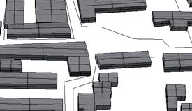
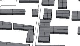
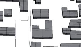
LOCATION : SOUTH EAST COAST OF ISLAND AMAGER. HISTORIC PORT CITY
TIME OF CONSTRUCTION : MID 13th - 15th CENTURY; REBUILT 17- 18th CENT

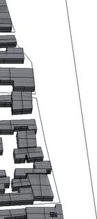

CLIMATE : FLAT LANDSCAPE & UNIFORM BUILDING HTS PROVIDE NO SHELTER FROM THE PREVAILING WESTERLY WINDS
POPULATION DENSITY : 11, 573
ARCHITECTURAL CHARACTERISTICS : 2 PATTERNS OF URBAN BLOCK: (a) LONG, PARALLEL ROWS, ENTRY :N/S; (b) NUMEROUS SHORT PARALLEL ROWS; ENTRY: E/W. COBBLESTONE STREETS.
6 0 3
0 100 250
N - 90Methods
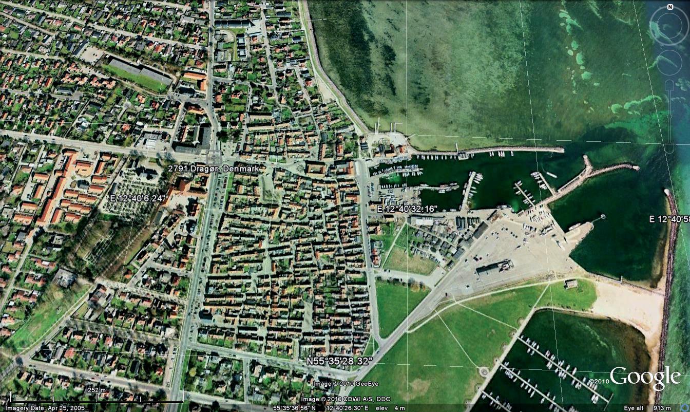
References:
Oliver, Paul, Encyclopedia of Vernacular Architecture, pg 1385
PLOT SIZE : 500m X 500m
- 91City Data Sets
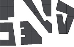
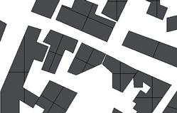
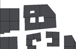
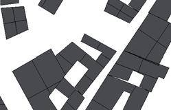
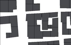
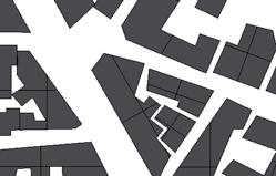
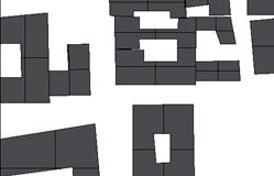
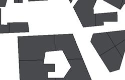

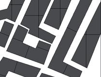
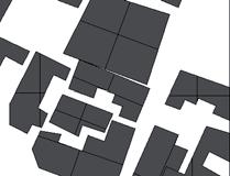
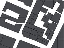
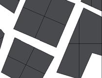

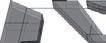
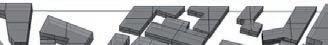
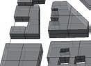
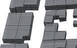
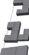
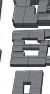
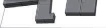

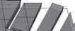
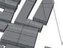
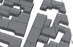
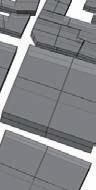
LOCATION : S.E COAST OF SWEDEN WHERE LAKE MALARAN MEETS BALTIC SEA. NETWORK OF 14 ISLANDS. 30% OF THE CITY CONSISTS OF WATERWAYS.
TIME OF URBAN PLAN FORMULATION: 1930-1950
CLIMATE: RELATIVELY MILD WEATHER COMPARED TO OTHER AREAS OF THE REGION. SUMMER AVG TEMP : 20-22 deg C. WINTER
AG. TEMP : -5-1 deg C
POPULATION DENSITY : 4,411.8/km2
URBAN CHARACTERISTICS : THE “NARROW BLOCK” HOUSING AREAS WITH BLOCKS PARALLEL AND OPEN PLAN PATTERNS AS NEIGHBOURHOOD UNITS AND WITH MULTI FAMILY HOUSING BLOCK GROUPS IN MORE CLOSED FORM LAYOUTS. EXTENSIVE CARE IN PRESERVING NATURAL VEGETATION
0 250 500 27 0 18 21 12 PLANNED CITY STOCKHOLM, SWEDEN ARCTIC/SUBARCTIC N - 92Methods
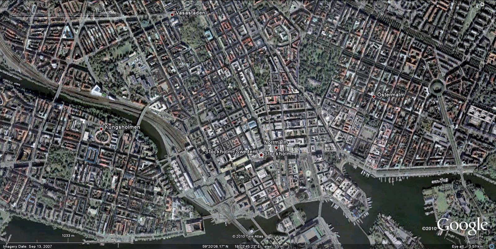
References: http://en.academic.ru/dic.nsf/enwiki/360976
PLOT SIZE : 1000m X1000m
- 93City Data Sets
CONTINENTAL
EVOLVED CITY KABUL, AFGHANISTAN


NOTE: ELEVATION NOT TRUE. SETTLEMENT ON SLOPED TERRAIN. UNIFORM HEIGHT OF BLDS : 6M (SEMI- BASEMENT, FIRST AND 2ND FLOOR)
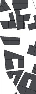

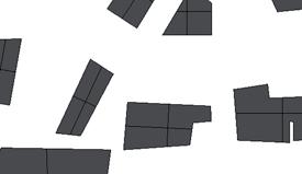
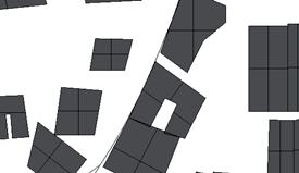
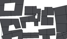
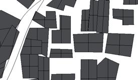
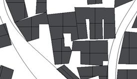
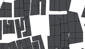
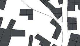
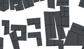
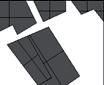
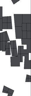
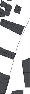

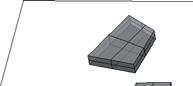
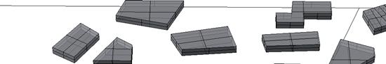
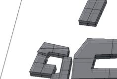
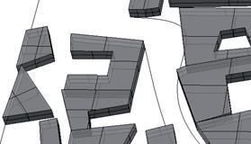
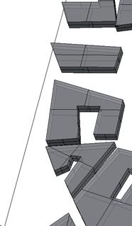
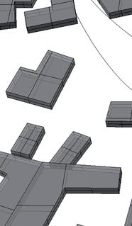
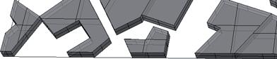
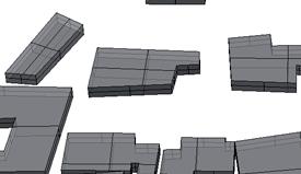
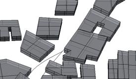
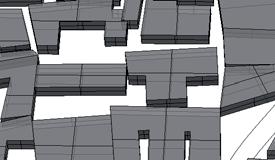
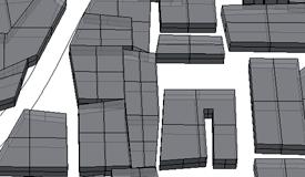
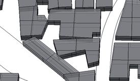
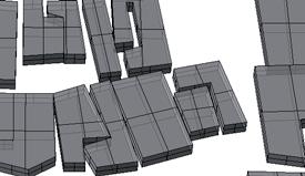
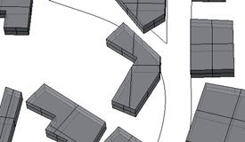
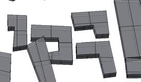
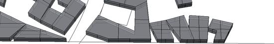
ALTITUDE : 1,800m ABOVE SEA LEVEL
LOCATION : SLOPE OF SHER DARWAZA MOUNTAIN
TIME OF CONSTRUCTION : 2000-1500 BC
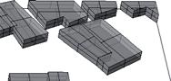
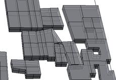
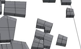
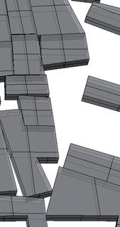
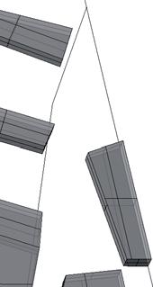
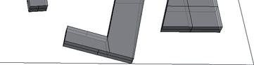
CLIMATE : SEMI ARID. PRECIPITAION DURING WINTER. AVG MAX ANNUAL TEMP: 19.6 deg C, AVG. LOW: 4.3deg C; AVG PRECIPITAION : 312mm
ARCHITECTURAL CHARACTERISTICS : CLUSTERED BUILDINGS WITH SHARING WALLS TO REDUCE EXPOSURE TO WINDS. COURTYARDS ARE A COMMON FEATURE. SOUTH FACING WINDOWS TO ALLOW MAXIMUM SUNLIGHT.
MATERIALS USED: MUD, TIMBER, CLAY. THESE HAD HIGH LEVELS OF INSULATION PROPERTY.
0 100 250
- 94Methods
N

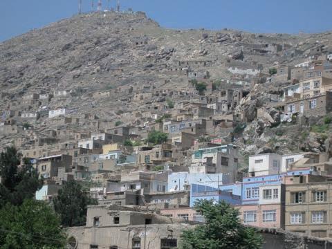
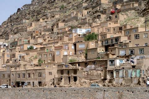
References:
http://www.archinomy.com/case-studies/674/traditionalhouse-in-kabul-afghanistan
PLOT SIZE : 500m x 500m
- 95City Data Sets
AVERAGE NO OF FLOORS FOR BLDS IN RESIDENTIAL AREA: 1-2 3-8 9-12
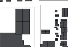
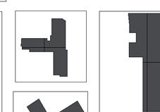
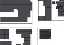
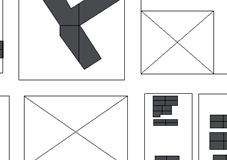
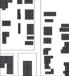
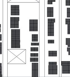
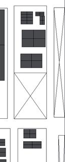
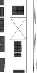
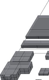
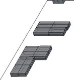
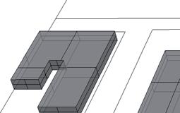
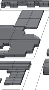
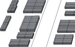
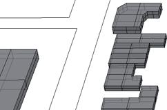
ALTITUDE : 176m ABOVE SEA LEVEL
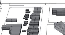
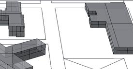
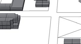
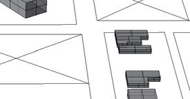
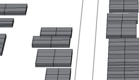
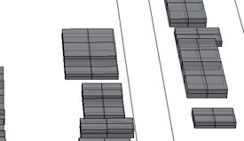
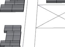
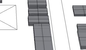
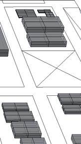

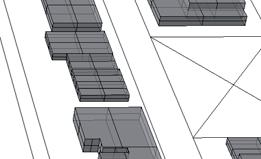
LOCATION : BESIDE FRESHWATER LAKES AND 2 RIVERS.
TIME OF URBAN PLAN FORMULATION: 1909, 1950s
CLIMATE: 4 SEASONS. WARM HUMID SUMMERS.; TEMP : 27-29 deg C. SNOW IN WINTER. THE LAKE LARGELY MODERATES THE CLIMATE OF THE CITY
POPULATION DENSITY : 8,711,000
TOTAL AREA: 5,498 sq km
URBAN CHARACTERISTICS : GRID PLAN. MOST HIGH RISE LIMITED TO THE METROPOLITAL AREA, LARGE NO OF PLANTED TREES.
SUBSTANTIAL OPEN GREEN SPACES
0 250 500 27 0 12 6 3 18
CONTINENTAL N - 96Methods
PLANNED CITY CHICAGO, IL, USA
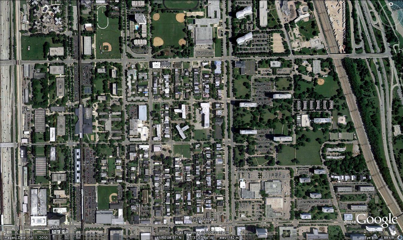
PLOT SIZE : 1000m x 1000m
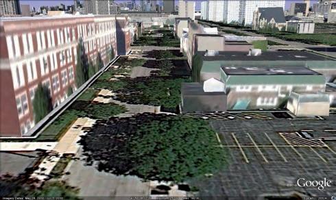
References:
EPA Urban Heat Island Pilot Project City Profile: Chicago (Archived Page), 1998-2002
CHICAGO AREA CASE STUDY
R. Warlam (2005), URBAN AND SOCIOECONOMIC CHARACTERISTICS OF CHICAGO AND BARCELONA
http://encyclopedia.chicagohistory.org/pages/300006.html
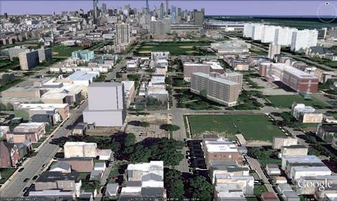
- 97City Data Sets
DESERT
EVOLVED CITY YAZD, IRAN
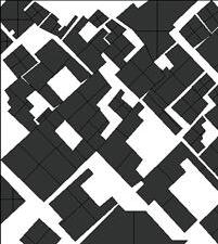
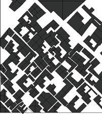
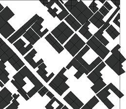

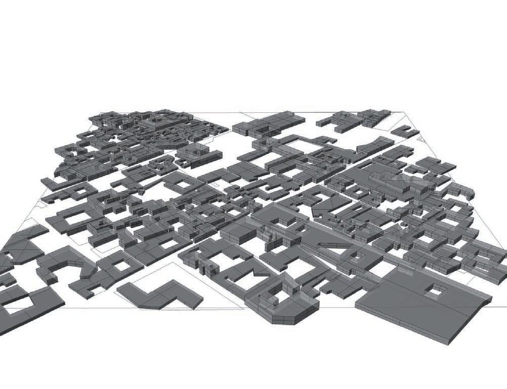
ALTITUDE : 1,203m ABOVE SEA LEVEL
LOCATION : OASIS BETWEEN DASHT E-KAVIR AND DASTH E-LUT DESERTS
TIME OF CONSTRUCTION : 3000BC
CLIMATE : DRY THROUGHOUT YEAR. ANNUAL RAINFALL ONLY 60mm; HOT SUMMERS, DAY- NIGHT TEMP : 40 -BELOW 0 deg c
POPULATION DENSITY : 70,000 IN THE AREA OF ADRAKAN
ARCHITECTURAL CHARACTERISTICS : COURTYARDS, WINDCATCHERS AND LARGE UNDERGROUND AREAS TO COPE WITH THE HOT CLIMATE. LARGEST NETWORK OF QANATS(SHADED PATHS ) IN THE MARKET PLACE
0 100 250 9 6 3 0
N - 98Methods

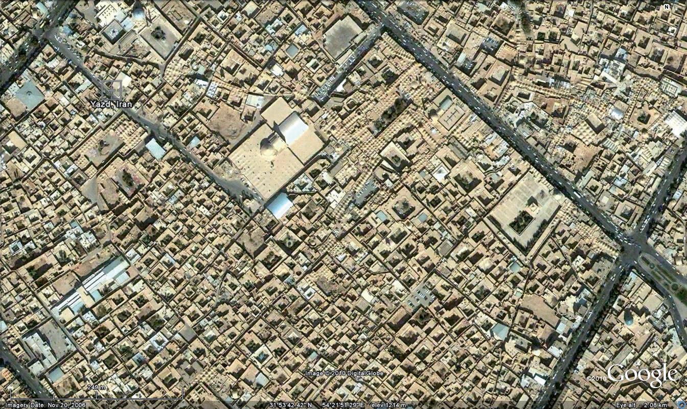
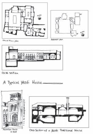
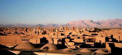
References:
Kamyar Tolou Behbood et al. , Energy Efficient Architectural Design Strategies in Hot‐Dry Area of Iran: Kashan
Dr. Abdel-moniem El-Shorbagy, Design with Nature: Windcatcher as a Paradigm of Natural Ventilation Device in Buildings, International Journal of Civil & Environmental Engineering IJCEE-IJENS Vol:10 No: 03
PLOT SIZE : 500m x 500m
- 99City Data Sets
AVERAGE NO OF FLOORS OF RESIDENTIAL BLDGS: 1-5 :90% 5-10:10%
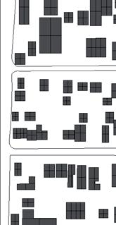
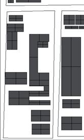
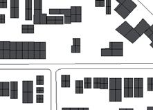
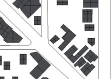
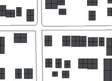
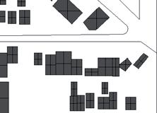
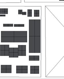
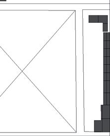
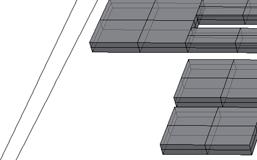
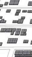
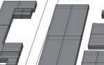
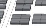
ALTITUDE : 340m ABOVE SEA LEVEL
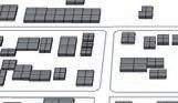
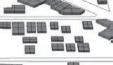
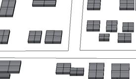
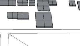
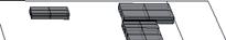
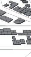
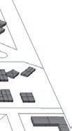
LOCATION : SALT RIVER VALLEY, CENTRAL AZ; FLAT TOPOGRAPHY; SURROUNDED BY MOUNTAINS IN THE N.E, W, FAR E, SW.
TIME OF URBAN PLAN FORMULATION: 1986, 2004
CLIMATE: EXTREME HOT SUMMERS, WARM WINTERS. AVG ANNUAL TEMP: 38degC, AVG HIGH: 43 deg C, AVG. LOW : 16.61 degC; ANNUAL RAINFALL : 8.29mm
POPULATION DENSITY : 1.5million
TOTAL AREA: 1,2330 sq km; 0.05%- WATER
URBAN CHARACTERISTICS : PRECISE GRID LAYOUT WITH WIDE OPEN SPACED ROADWAYS. OPEN AREAS DISTRIBUTED IN RESIDENTIAL AREA.
0 250 500
0 9 46
DESERT N - 100Methods
PLANNED CITY PHOENIX, AZ, USA
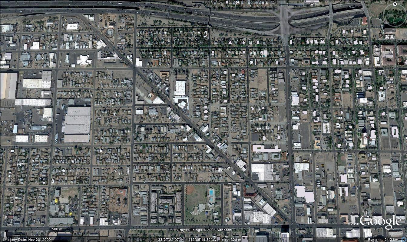
SIZE : 1000m x 1000m
References:
Planning Department, April 2010, N:\GIS_Team\Villages\ vplanners.mxd
N:\PDF_Maps\VillageMaps\vplanners.pdf
http://www.ncbi.nlm.nih.gov/books/NBK22960/
PLOT
- 101City Data Sets
EVOLVED CITY BATH, UK
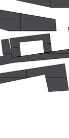
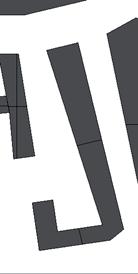
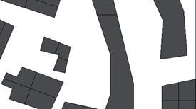
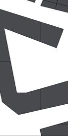
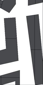
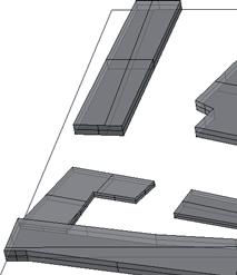
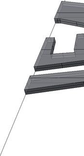
AREA: 29 sq km
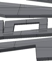
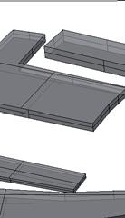

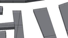
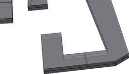
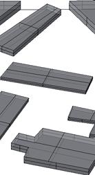

LOCATION : BOTTOM OF AVON VALLEY, EDGE OF LIMESTONE HILLS. PRESENCE OF GEOTHERMAL SPRINGS
TIME OF CONSTRUCTION : EARLY 16TH CENTURY
CLIMATE : WETTER AND MILDER THAN THE REST OF ENGLAND. 10deg C - ANNUAL MEAN TEMPERATURE. THERE ARE BOTH SEASONAL AND DIURNAL TEMPERATURE VARIATION.
POPULATION DENSITY : 83,992
ARCHITECTURAL CHARACTERISTICS : NORMAN, MEDIEVAL AND TUDOR TYPE ARCHITECTURE. LINEAR STRETCHES OF BUILDINGS. EXTENSIVE OPEN GREEN SPACES.
0 100 250 3 9 6 0
MARITIME N - 102Methods
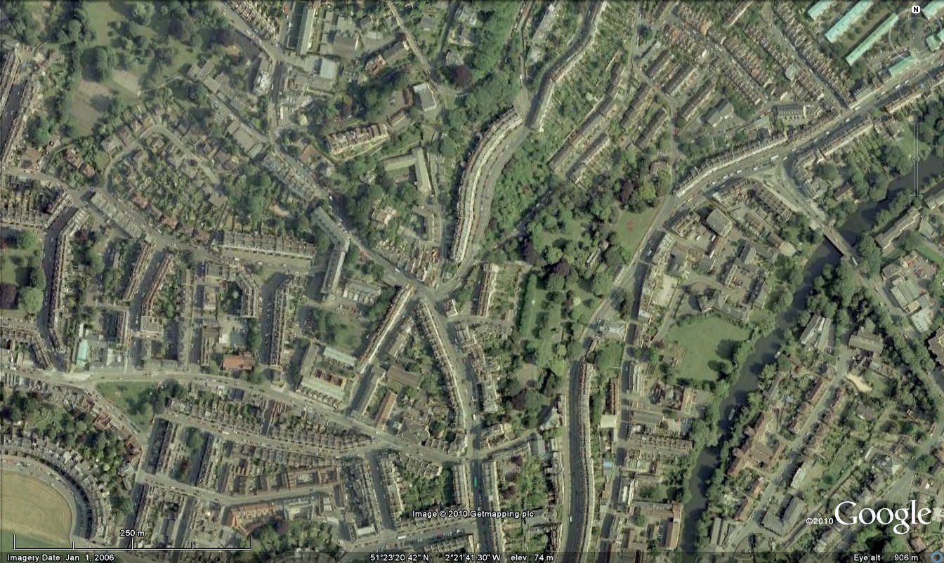
PLOT SIZE: 500m x 500m
References:
http://web.archive.org/web/20070614100836/http://www. bathnes.gov.uk/worldheritage/2.3Des.htm
- 103City Data Sets

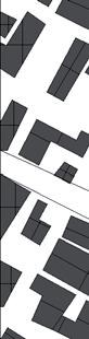
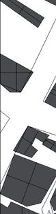

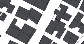
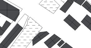
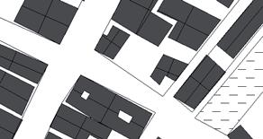
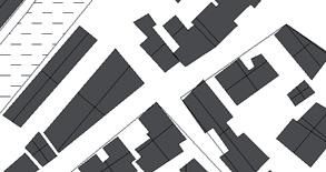
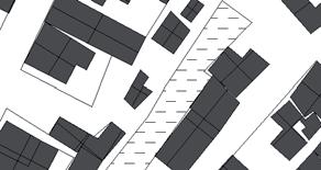
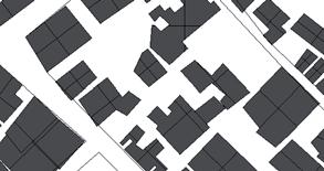
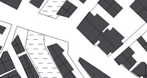
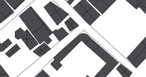

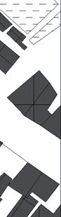
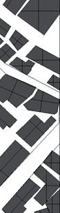


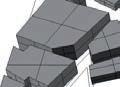
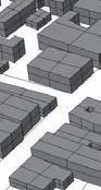
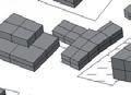
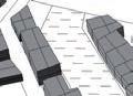

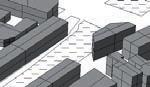
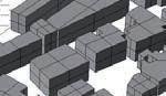
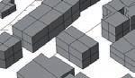
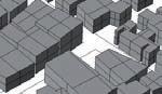
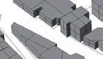
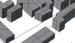
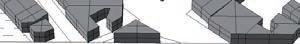
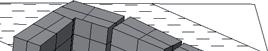
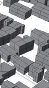
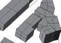
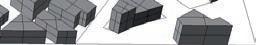
LOCATION : NORTHWEST OF TOKYO BAY, RECLAIMED LAND FROM SEA
TIME OF URBAN PLAN FORMULATION: 1995, 2000- CITY PLANNING LAW FOR HIERARCHIAL DIVISIONS OF PLANNING, APPROVAL AND IMPLEMENTATION
CLIMATE: AVG ANNUAL TEMP (HIGH) : 19.7 deg C, (LOW) : 12.5 deg C; ANNUAL RAINFALL : 1, 470mm, SNOWFALL IS SPORADIC. TYPHOONS ARE COMMON IN THE AREA.
POPULATION DENSITY : 9654 people/ sq.km; DAYTIME POP : 650,000, RESIDENTIAL POP: 108, 943
TOTAL AREA: 10.15 sq km
URBAN CHARACTERISTICS : CITY IS DIVIDED INTO WARDS, SAMPLE FROM CHUO WARD.
0 250 500
FLOORS FOR BLDS
RESIDENTIAL AREA:
36 18 0 24 PLANNED CITY TOKYO, JAPAN MARITIME N - 104Methods
AVERAGE NO OF
IN
1-4 5-7 8-12
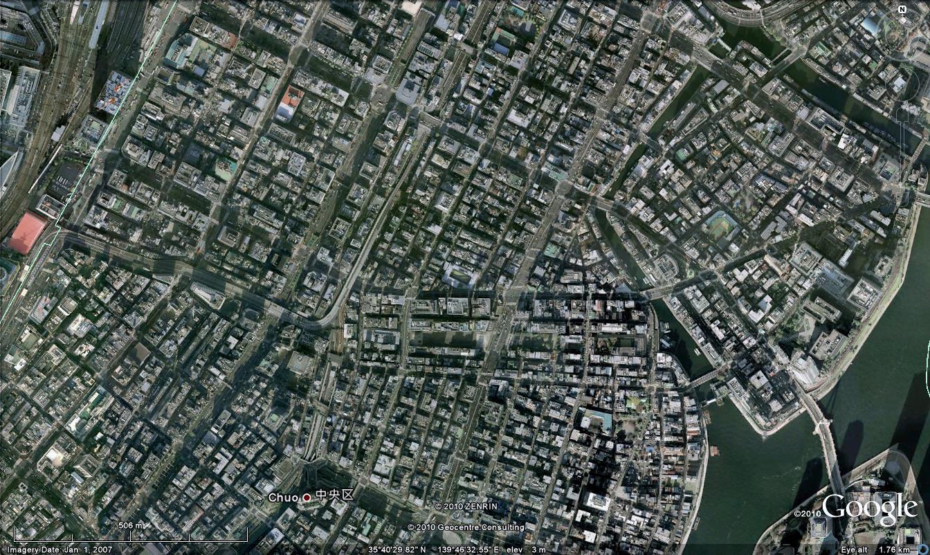
References:
Yasunobu Ashie et al. , Climate Analysis For Urban Planning in Tokyo
Estelle Ducom, Tama New Towb, West of Tokyo: Analysi of a shrinking Suburb
Section 4 Land Use Changes and Issues in Metropolitan and Local Areas, tochi.mlit.go.jp/…/setsu_1-1-4_eng.html
Bureau of City Planning Tokyo Metropolitan Government, Transition in City Planning in Tokyo
Junko ABE-KUDO, VERTICAL GATED COMMUNITIES IN TOKYO
TOKYO | 23 Wards Highrise Projects - S…, …skyscraperpage.com/showthread.php…
IWATA, Shizuo, ALMEC Corporation, Introduction to Japan’s Urban and Land- use Planning Systems and Their Practices
http://www.japanorama.com/tokyoprf.html
PLOT SIZE: 1000m x 1000m
- 105City Data Sets
MEDITERRANEAN
EVOLVED CITY MAZARA DEL VALLO, SICILY


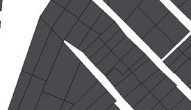
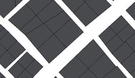
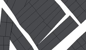
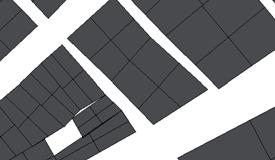
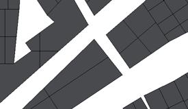
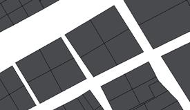
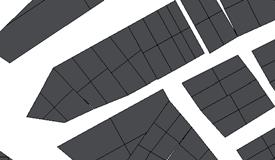
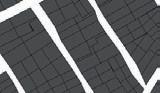

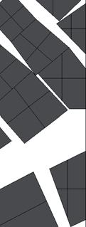
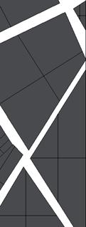

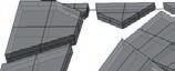
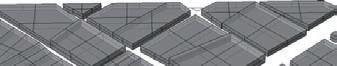
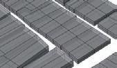
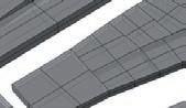
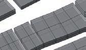
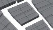

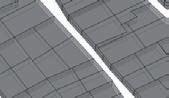
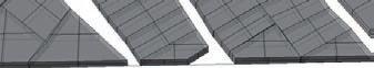
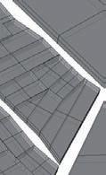
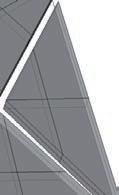
ALTITUDE : 8m ABOVE SEA LEVEL
LOCATION : SOUTH WEST SICILY. LEFT BANK AT MOUTH OF MAZARO R.
TIME OF CONSTRUCTION : 1713
CLIMATE : MILD TO WARM , WET WINTERS. WARM- HOT DRY SUMMERS
POPULATION DENSITY : 186.8/sq km
ARCHITECTURAL CHARACTERISTICS : INFLUENCED BY ARAB, NORMAN AND ROMAN ARCHITECTURE. STREET NETWORK FORMING BLOCKS
0 100 250 9 6 0
N - 106Methods
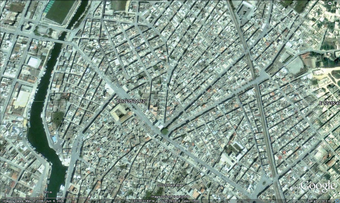
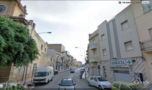
References: Oliver, Paul, Encyclopedia of Vernacular Architecture
PLOT SIZE : 500m x 500m
- 107City Data Sets
MEDITERRANIAN
PLANNED CITY BARCELONA, SPAIN

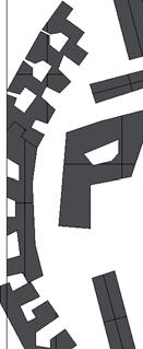
AVERAGE NO OF FLOORS FOR BLDS IN RESIDENTIAL AREA: 3-5 5-9 9-17
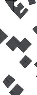
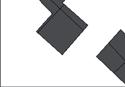

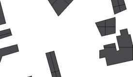
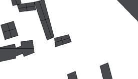
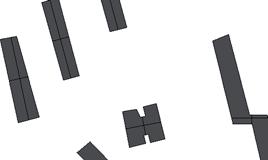
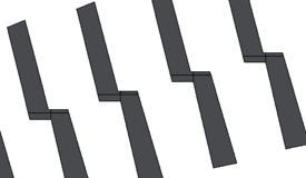

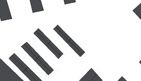
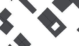
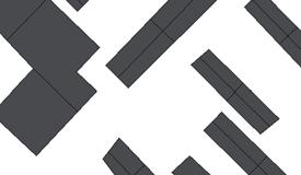
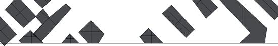
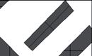
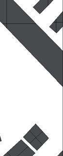
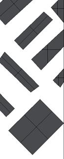

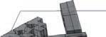
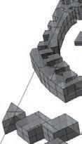
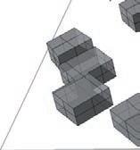
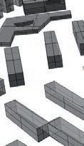
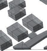
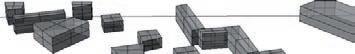
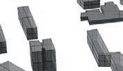
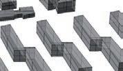
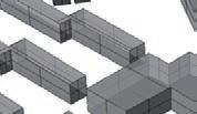
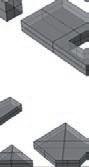
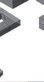
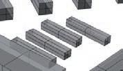
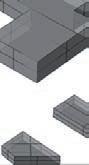
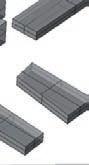
LOCATION : N.E COAST OF THE IBERIAN PENINSULA, FACING THE MEDITERRANEAN SEA, ON A PLATEAU APPROXIMATELY 5KM WIDE LIMITED BY MOUNTAINS AND RIVERS ALONG THE SOUTH WEST AND NORTH.
TIME OF URBAN PLAN FORMULATION: 1992 ONWARDS, AFTER THE BARCELONA OLYMPICS.
CLIMATE: MILD HUMID WINTERS AND WARM DRY SUMMERS. AVG SUMMER TEMPERATURE : 20deg C. AVG. WINTER TEMP: 14.5deg C. ATLANTIC WINDS FROM THE WEST WITH LOW HUMIDITY. RAINFALL MAX IN THE MONTHS OF AUG- NOV.
POPULATION DENSITY : 15,991/ sq km
TOTAL AREA: 101.4 sq km
URBAN CHARACTERISTICS : RENOWNED AS A SUCCESSFUL CITY IN URBAN DESIGN. MAJOR PARTS OF THE CITY ARE COMPRISED OF 520 BLOCKS AS PART OF THE GARDEN CITY EXPANSIONS OF 1859. THE MODERN URBAN PLAN POST THE OLYMPICS AIMED AT CONVERTING THE ABANDONED INDUSTRIAL AREAS INTO RESIDENTIAL BLOCKS. BUILDING UNITS MOSTLY TAKE LEAN RECTILINEAR FORM IN PLAN WITH AN AVERAGE HEIGHT OF 27m
51 0 15 9 27 30
0 250 500
N - 108Methods

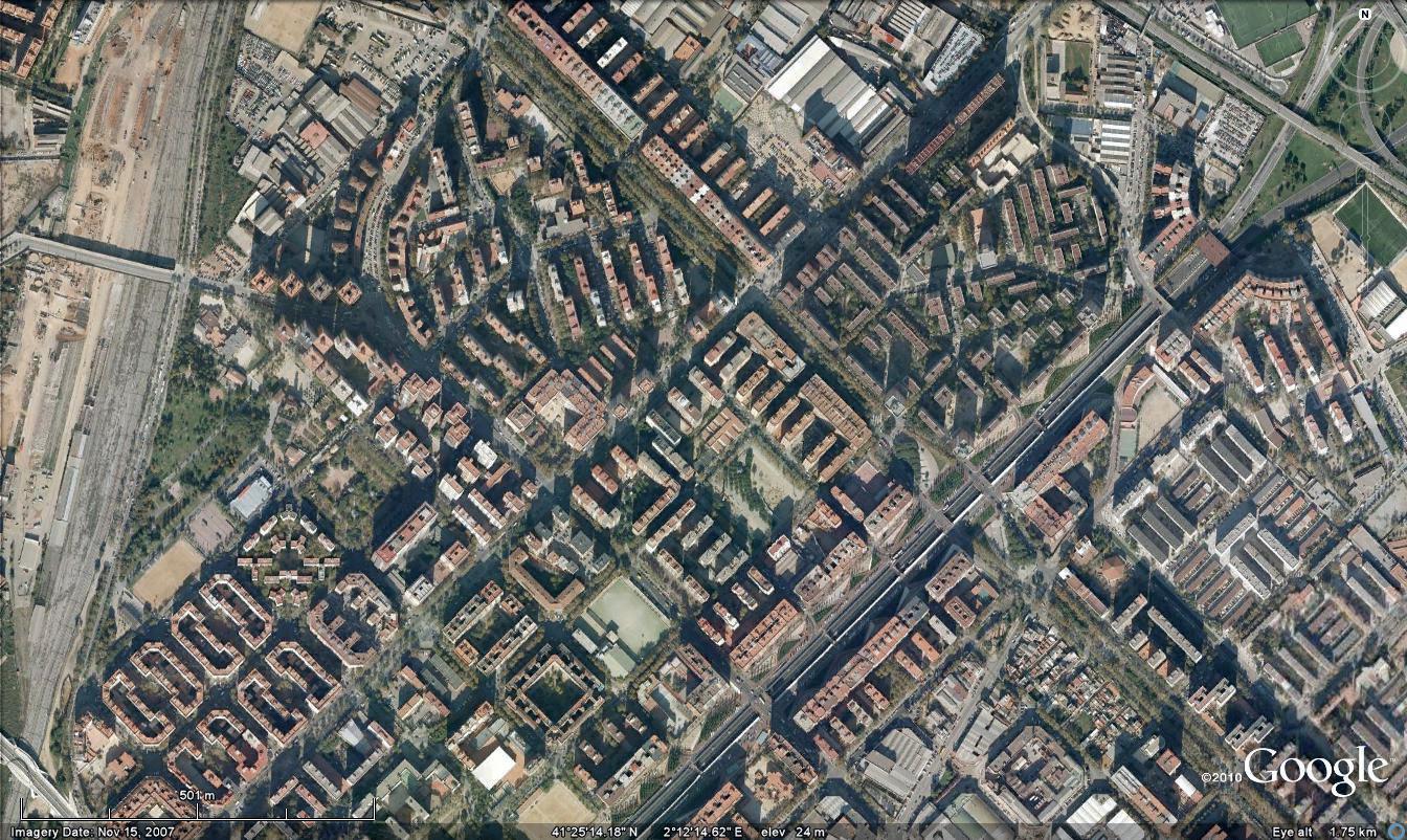
SIZE : 1000m x 1000m
References:
Acebilo, Josep A. ; Barcelona : Toeards a new Urban Planning Approach, UDC 711.5 (460.235) “1980/2006”.
Nelson, Peter; Barcelona, Spain – The Complete Integrated City
Land Use Planning and Transformation of Space; www. ccqc. pangea.org/eng/…/tereng.htm
http://geographyfieldwork.com/barcelona.htm
PLOT
- 109City Data Sets
EVOLVED CITY ZANZIBAR, TANZANIA ( “STONE TOWN”)
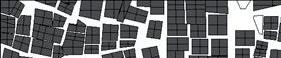
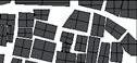
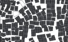

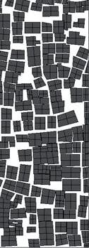
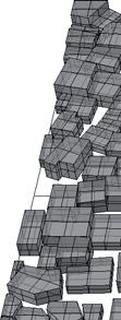
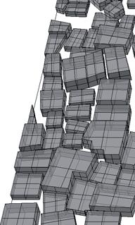
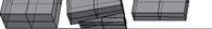
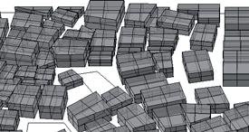
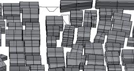
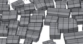
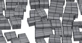
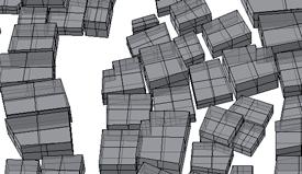
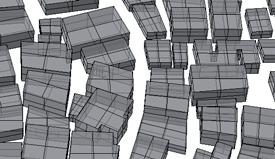
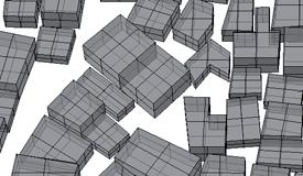
ALTITUDE : 120m ABOVE SEA LEVEL
LOCATION : LOW LYING ISLAND IN INDIAN OCEAN. STOWN TOWN IS THE ONLY FUNCTIONING ANCIENT TOWN IN EAST AFRICA. AREA : 2,461 sq km
TIME OF CONSTRUCTION : 1830
CLIMATE : WARM ALL YEAR ROUND. SUMMER HEAT COOLED OFF BY WINDY CONDITIONS. PREVAILING SEA BREEZES. 3
SEASONS- SUMMER , WINTER AND RAINY , RAIN IN THE MONTHS OF APRIL, MAY.
POPULATION DENSITY : 206, 292
ARCHITECTURAL CHARACTERISTICS : HIGH DENSITY SETTLEMENTS. VERY NARROW WINDING PATHS, BUILDINGS MOST OFTEN WITH GROUND PLUS 2- 3 FLOORS. TOTAL LACK OF VEGETATION IN THE AREA.
MATERIAL USED: STONE IS USED EXTENSIVELY. FOR BOTH BUILDINGS AND STREETS.
12 9 0 6
N - 110Methods
MONSOON
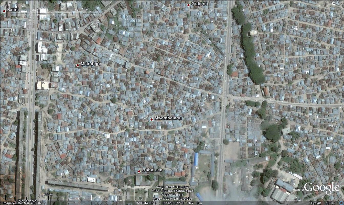
PLOT SIZE : 500m x 500m
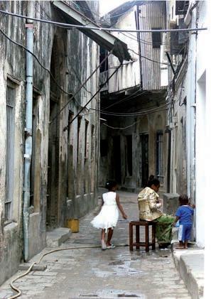
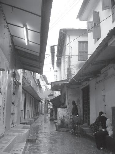
References:
Siravo, Francesco; ZANZIBAR: A plan for the Historic Stone Town http://www.zanzibarstonetown.org/gallery.htm
- 111City Data Sets
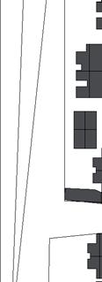
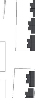
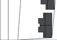

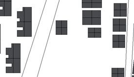
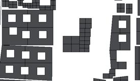
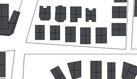
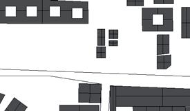
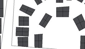
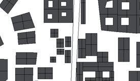
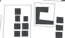
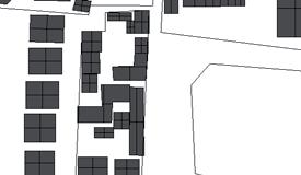
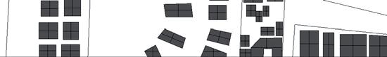

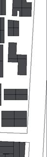
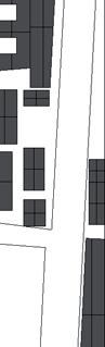


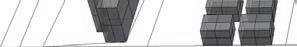
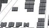
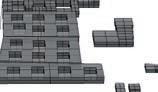
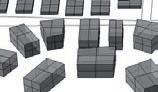
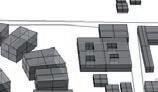
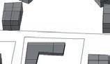
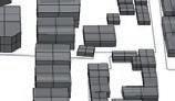
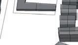
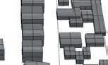
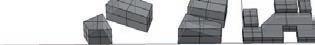
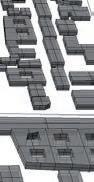
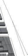

LOCATION : MAINLAND ON EASTERN SHORE OF THANE CREEK. KONKAN COAST ; HILLS ON THE EAST.
TIME OF URBAN PLAN FORMULATION: 1972
CLIMATE: HIGH RAINFALL DAYS WITH FEW DAYS OF EXTREME TEMP. HIGH HUMIDITY: 61- 86%. MAX AVG TEMP: 31deg C, MIN TEMP: 21degC, RAINFALL: 2400.4mm
POPULATION DENSITY : 800,000
TOTAL AREA: 163 sq km
URBAN CHARACTERISTICS : TWIN CITY TO MUMBAI. LARGEST PLANNED CITY IN THE WORLD
0 250 500 54 24 6 0 12 PLANNED CITY NAVI MUMBAI, INDIA MONSOON N - 112Methods
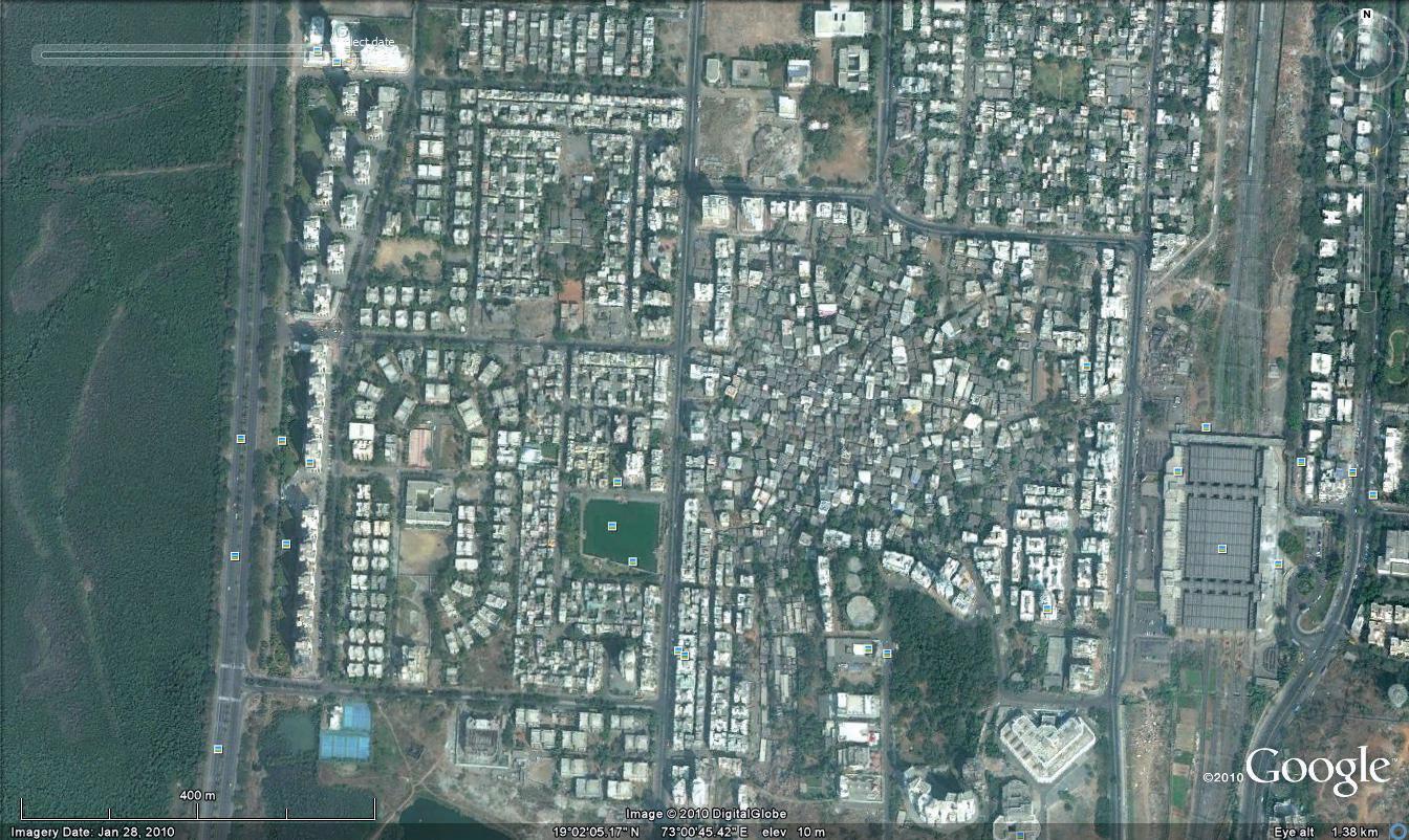
PLOT SIZE : 1000m x 1000m
References:
Urban Land Policy, Part 2 Chapter 9
Regional Plan - 1973 : Land use Plan, Part 3 Chapter 13
Arun Kumar Acharya, Parveen Nangia; POPULATION GROWTH AND CHANGING LAND-USE PATTERN IN MUMBAI METROPOLITAN REGION OF INDIA, Caminhos de Geografia 11(11)168-185, Fev/2004, CAMINHOS DE GEOGRAFIA - revista on line
www.ig.ufu.br/caminhos_de_geografia.html ISSN 1678-6343
Ananthakrishnan, Malathi; April , 1998 Blacksburg, Virginia; The Urban Social Pattern of Navi Mumbai, India
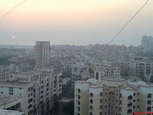
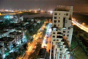
- 113City Data Sets
EVOLVED CITY POTALA, TIBET
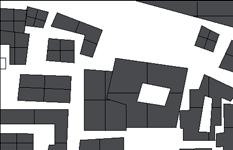
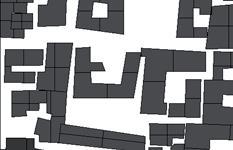
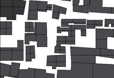
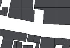
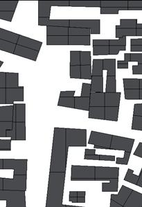
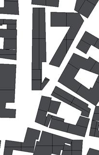
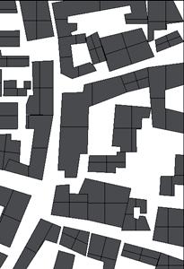
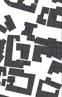
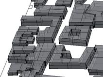
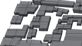
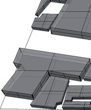
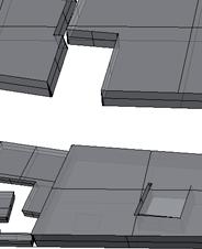
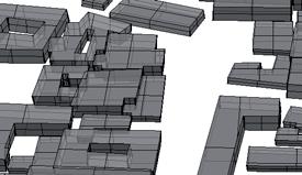
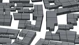
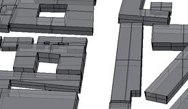
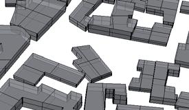
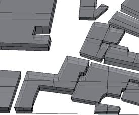
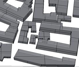

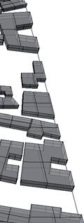
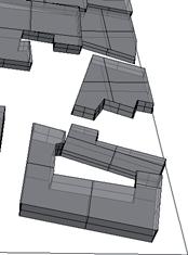
ALTITUDE : 3,648m ABOVE SEA LEVEL
LOCATION : VALLEY BETWEEN RIVERS KYICH AND BRAHMAPUTRA; PLAIN OF MARSHY GROUND
TIME OF CONSTRUCTION : 1500- 2000 BC
CLIMATE : LHAHSA VALLEY IS SHELTERED FROM HARSH WINDS THAT ROAM MUCH OF THE TIBETAN PLATEAU. THUS GIVING IT A VERY MODERATE MICROCLIMATE. IT IS ALSO CHARACTERISTICALLY DRY
POPULATION DENSITY : 50, 000 RESIDENTS; DENSER THAN REST OF CITY
ARCHITECTURAL CHARACTERISTICS : LOFTY, TAPERED BUILDINGS; STONE FINISH; FLAT ROOFS
0 100 250 9 6 4 0
MONTANE N - 114Methods
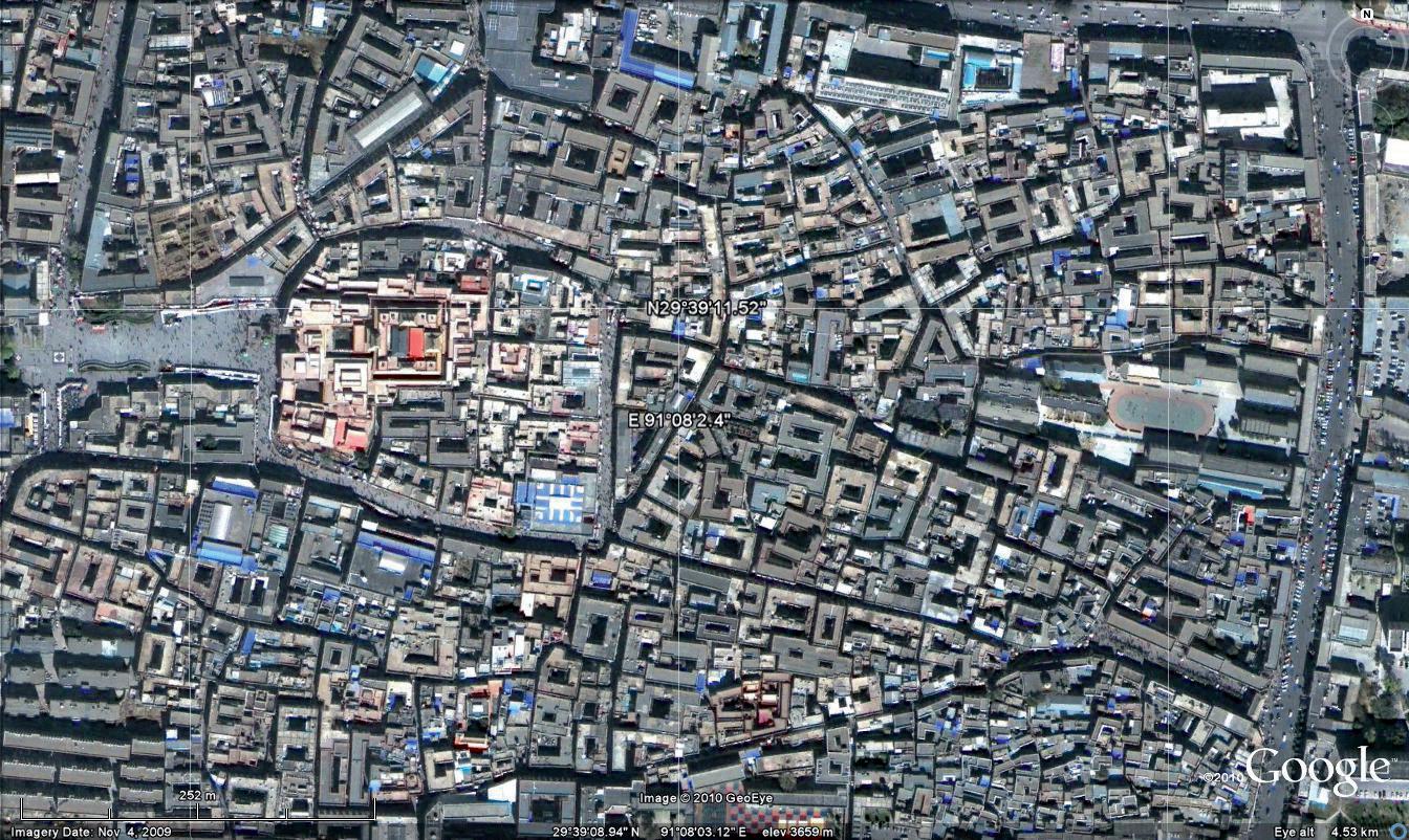
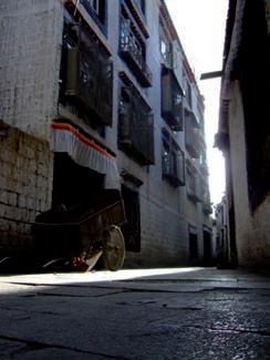
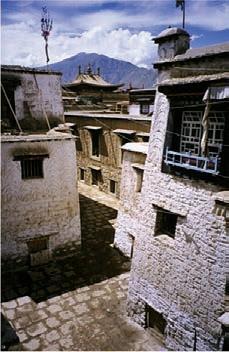
References:
PLOT SIZE : 500m x 500m
- 115City Data Sets
Alexander, Andre; The temples of Lhasa
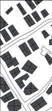
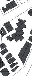
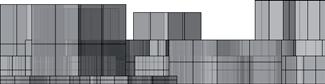
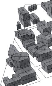
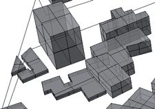
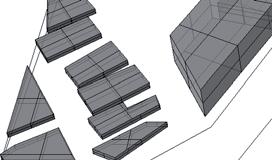
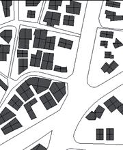
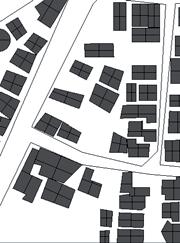
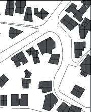
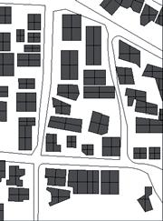
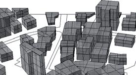
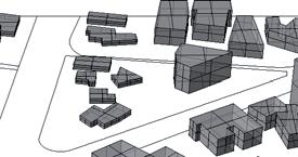
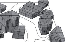
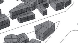
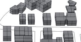
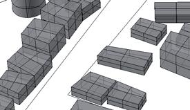
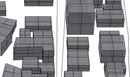
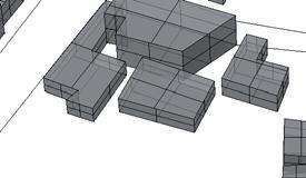
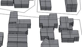
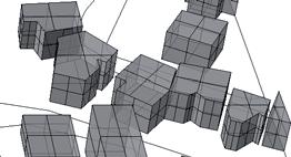
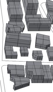
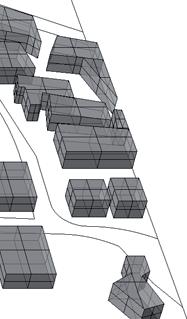
ALTITUDE : 2850m ABOVE SEA LEVEL
LOCATION : ANDES MOUNTAIN RANGE; AREA OF INTENSIVE VOLCANIC AND SEISMIC ACTIVITY
TIME OF URBAN PLAN FORMULATION: 1945, 1967, 1971, 1973, 1981, 1985
CLIMATE: CONSTANT COOL CLIMATE THROUGHOUT YEAR, AVG DAY NIGHT TEMP: 18.7- 9.3 degC; 2 SEASONS:DRY AND WET; ANNUAL PRECIPITATION: 1, 010mm
POPULATION DENSITY : 1,500,000
TOTAL AREA: 29,000 ha
URBAN CHARACTERISTICS : CITY DEVELOPS NORTH- SOUTH; 40-50 KM LONG AND 6-12 KM WIDE. DUE TO THE SLOPPED TERRAIN, AND CURVED SHAPE OF THE REGION, GRID LAYOUT IS DIFFICULT TO IMPLY. HOWEVER, HISTORIC CENTRE OF CITY HAS BEEN LAID OUT IN GRID DESPITE THIS.
0 250 500 60 AVERAGE NO OF FLOORS: 2-7 7-11 18-23 PLANNED
EQUADOR MONTANE N - 116Methods
CITY QUITO,
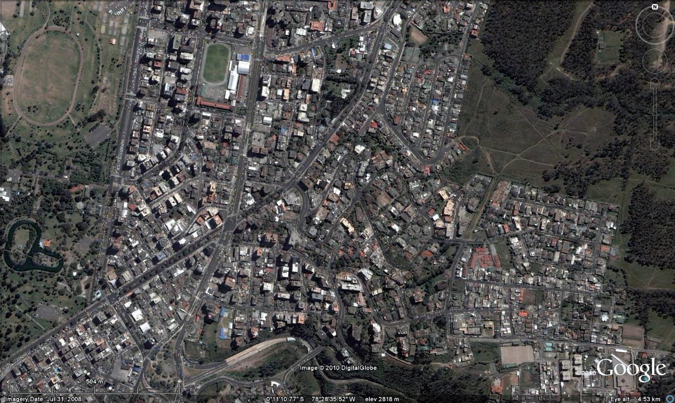
PLOT SIZE : 1000m x 1000m
References:
Title: Urban and peri-urban forestry in Quito, Ecuador..., fao. org/docrep/w7445e/w7445e07.htm
APPENDIX B: TYPOLOGY OF URBAN SPACES AND WOODY
SPECIES SUITABLE FOR DIFFERENT PLANTING SITES IN QUITO
APPENDIX D: SUMMARY OF PUBLIC AND PRIVATE ACTORS IN
THE URBAN FOREST ECOSYSTEM IN QUITO
Presentación del Plan de intervenciones urbanas, D i s t r i t o M e t r o p o l i t a n o d e Q u i t o http://www.fao.org/docrep/w7445e/w7445e03.htm
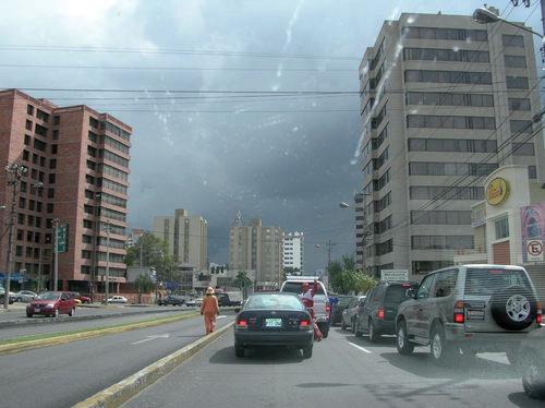
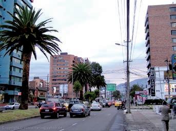
- 117City Data Sets
EVOLVED CITY KARAIKUDI, TN, INDIA
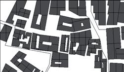
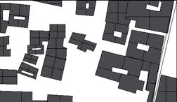
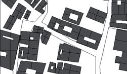
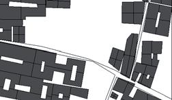
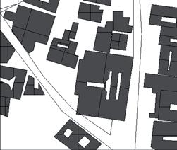
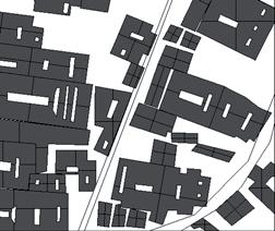
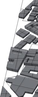
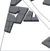
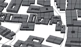
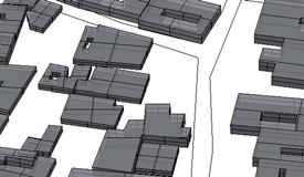
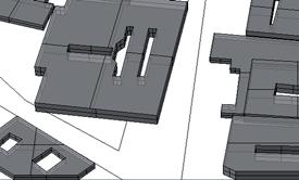
ALTITUDE : 82m ABOVE SEA LEVEL
TIME OF CONSTRUCTION : 18TH CENTURY
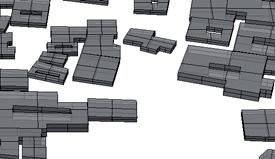
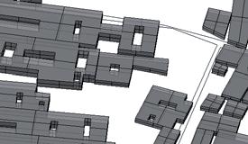
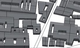
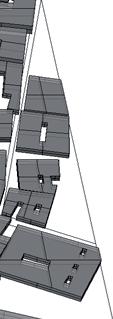
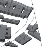
CLIMATE : TEMP RANGE: 21.75- 35.5 deg C; AVG ANNUAL RAINFALL : 36-867.0 mm.MAX RAINFALL DURING THE MONTH OF NOV. MIN IN JUNE/JAN
POPULATION DENSITY : 1,35,442
ARCHITECTURAL CHARACTERISTICS : RECTANGULAR TRANSVERSAL PLOTS, LARGE DOUBLE/ MULTIPLE COURTYARDS; WELL VENTILATED. HOUSES RAISED ON “THINAI” TO PROTECT AGAINST SUN & RAIN. SINGLE AND DOUBLE STOREYED BUILDINGS PRESENCE OF LARGE PUBLIC POOLS AT REGULAR INTERVALS.
MATERIAL USED : WOOD, STONE, PLASTER(EGG WHITE PASTE), METAL , MARBLE
0 100 250
4 6 0
SUB
N - 118Methods
TROPICAL
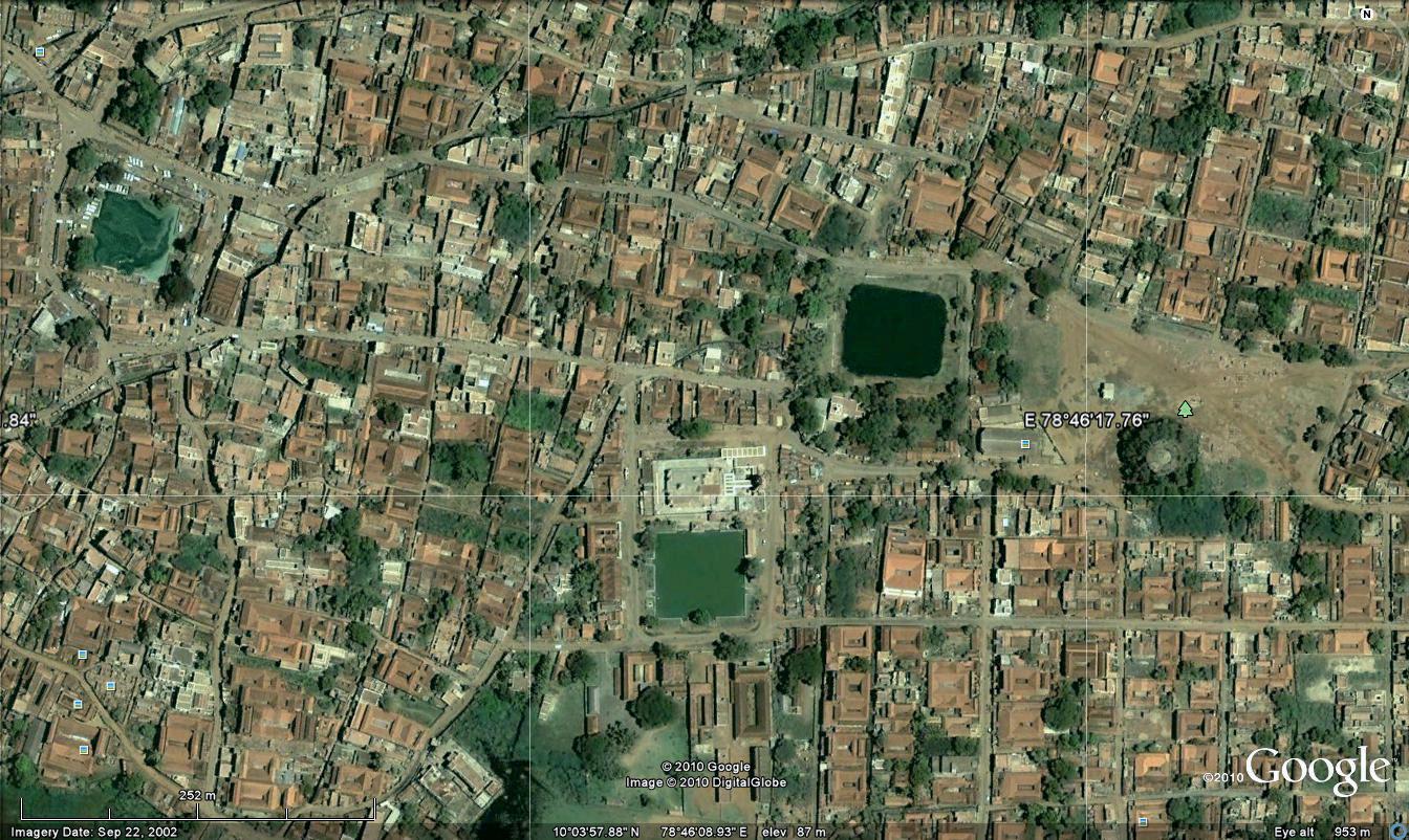
References: world66.com/asia/southasia/…/climate http://en.academic.ru/dic.nsf/enwiki/360976
PLOT SIZE : 500m x 500m
- 119City Data Sets
PLANNED CITY BUENOS AIRES, ARGENTINA SUBTROPICAL

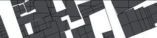
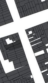
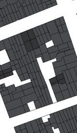
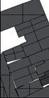
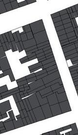
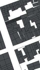
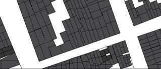
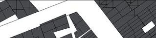
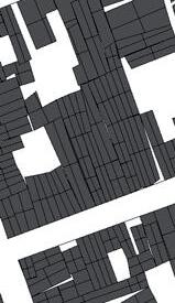
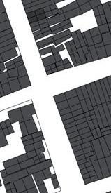

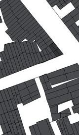

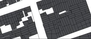
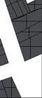
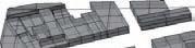
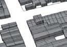
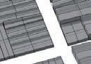
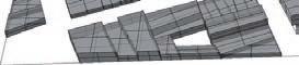
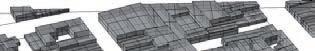
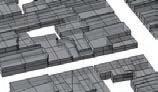
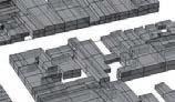
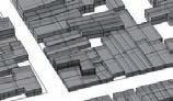
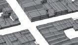
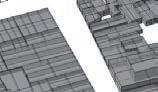
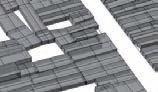
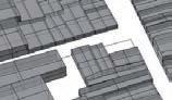
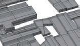
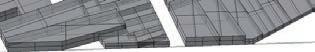
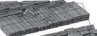
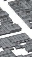
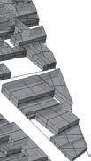
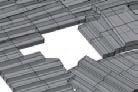
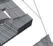
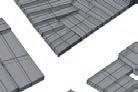
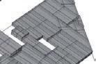
LOCATION : PART OF THE “PAMPAS” ,FLATLAND. EASTERN SIDE- LOWLANDS, PART OF THE SOLADO BASIN. UNDULATED PLAIN
TIME OF URBAN PLAN FORMULATION: 1970-90s
CLIMATE: 4 SEASONS. ANNUAL TEMP 17.2deg C. WARMEST IN JAN, AVG 24.1degC, COLDEST IN JULY WITH 9.6 °C 1,242.6 mm OF RAINFALL YEARLY
POPULATION DENSITY : 14,219.8/km2
TOTAL AREA: 203 sq km .
URBAN CHARACTERISTICS : RIGID GRID SYSTEM. HIGHLY DENSIFIED BLOCKS. UNIFORM HT OF BUILDINGS.
0 250 500
IN RESIDENTIAL AREA: 2-3 4-6 24 0 9 6
AVERAGE NO OF FLOORS FOR BLDS
N - 120Methods
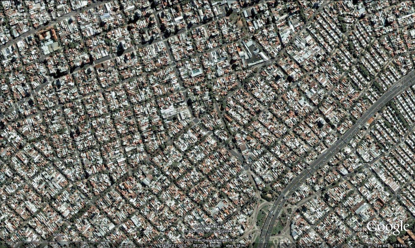
PLOT SIZE : 1000m x 1000m
References:
2009 by Dirección General de Interpretación Urbanística / SSPAN / MDU/ Gob. CABA; CIUDAD AUTÓNOMA DE BUENOS AIRES
Pirez, Pedro, Buenos Aires : fragmentation and privatization of the metropolitan city, Environment&Urbanization Vol 14 No 1 April 2002
Silvia de Schiller, Microclimate and design qualities for sustainable urban transformation
http://www.fallingrain.com/world/AR/07/Buenos_Aires.html http://www.ess.co.at/SUTRA/CITIES/buenosaires.html
- 121City Data Sets
EVOLVED
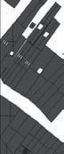
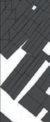

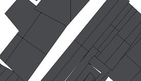
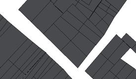
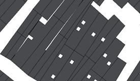
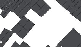
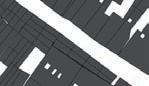
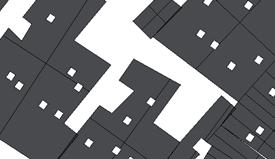
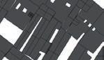
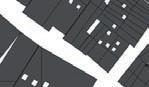
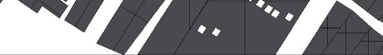
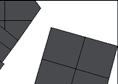
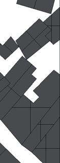

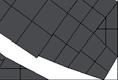
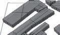
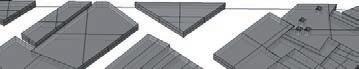
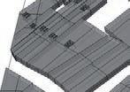
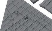
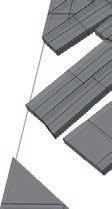
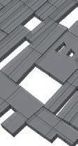

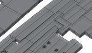
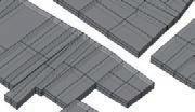
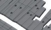
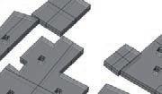
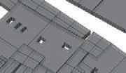
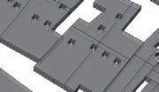
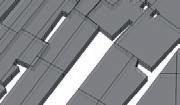

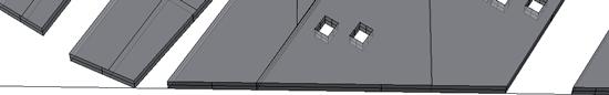
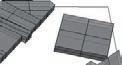
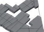

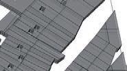
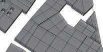
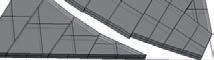
LOCATION : SOUTHERN REGION OF MALAY PENINSULA, ON STRAITS OF MELACCA
TIME OF CONSTRUCTION : 1400S-1600S
CLIMATE : HIGH TEMPERATURE THROUGHT YEAR( AVG. 27 degC), HIGH HUMIDITY. RAINFALL MOST PARTS OF THE YEAR.
AREA : 148ha ARCHITECTURAL CHARACTERISTICS : HISTORICAL COLONIAL TOWN. DENSE LAYOUT OF TOWNHOUSES AND SHOPHOUSES.
0 100 250 6 0
CITY MELAKA, MALAYSIA TROPICAL N - 122Methods

References:
Gaik, Lim , Spring 2009, “Melaka & George Town –Historic Cities of the Straits of Malacca ”, UNESCO
John Miksic, Southeast Asia: ancient centre of urbanization?
Michael E. Smith, Ancient Cities, The Encyclopedia of Urban Studies (R. Hutchison, ed., Sage, 2009)
PLOT SIZE : 500m x 500m
- 123City Data Sets
TROPICAL
PLANNED CITY BANGKOK, THAILAND
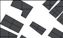
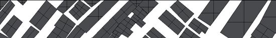
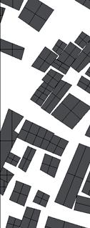
AVERAGE NO OF FLOORS FOR BLDS IN RESIDENTIAL AREA: 2-4
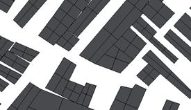
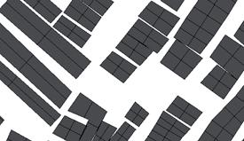
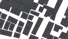
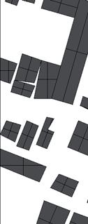


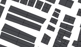
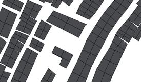
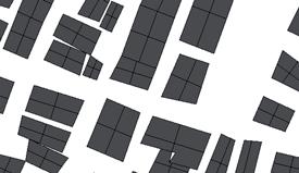
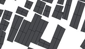

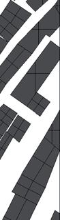
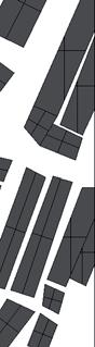

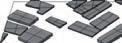
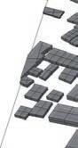

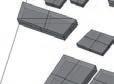
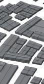
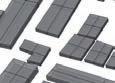
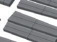

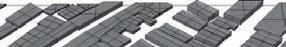
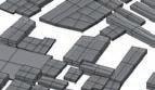
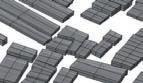
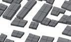
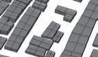
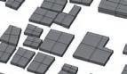
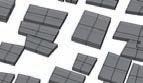
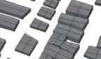
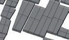
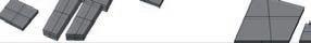
ALTITUDE : 2M ABOVE SEA LVL. PRONE TO FLOODS DUE TO THE LOW ALT.
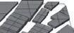
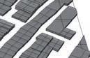
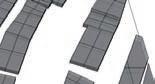
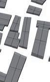
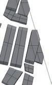
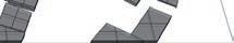
LOCATION : RIVER CHAU PHRAYA IS A KEY FEATURE.NO. OF CANALS THROUGH THE CITY OFTEN REFERRED TO AS THE ‘VENICE OF THE EAST’.
TIME OF URBAN PLAN FORMULATION: 1999- BANGKOK COMPREHENSIVE PLAN
CLIMATE: AVG HIGH: AVG TEMP -HIGH :32.7 deg C, LOW : 24.1 deg C, AVERAGE ANNUAL RAINFALL : 1, 496.8 mm
POPULATION DENSITY : 9,752 /sq. km
TOTAL AREA: 1, 568.7 km
URBAN CHARACTERISTICS : POLYCENTRIC URBAN PLAN. MIXED DISTRIBUTION OF RESIDENTIAL AND COMMERCIAL ZONE. OPEN SPACES DISTRIBUTION- FOR THE PURPOSE OF RECREATION IN ADDITION TO FLOOD PREVENTION. HIGH BARRIERS AGAINST SOME CANALS TO PREVENT FLOODS. MOST URBAN BLOCKS TAKE SIMPLIFIED RECTILINEAR FORM.
0 250 500 0 12 6 9
N - 124Methods
SIZE : 1000m x 1000m
References:
March 2009, Panya Consultants Co. Ltd, Climate Change Impact and Adaptation for Bangkok Metropolitan Region
2001-2002 Department of City Planning, Bangkok Metropolitan Administration, The Bangkok Comprehensive Plan(1st Revised Edition) in 1999 ; .bma-cpd.go.th/cpd/eng-map2.html www.bma-cpd.go.th/cpd/eng-compare-map.html http://www.mlit.go.jp/kokudokeikaku/international/spw/general/ thailand/index_e.html
PLOT
- 125City Data Sets
City Data Set - Evaluations
3D models were created with all the extracted information of the city samples. Analysis tools were set up using rhinoscript to inspect and evaluate the elements of each of the urban fabric for their performances for each of the morphological indicators, namely: rugosity, density, porosity, compacity, contiguity, sinuousity, solar admittance, occlusivity, and mineralization. The factors of rugosity and density, being the least complex were the first ones to be evaluated. Following this the more complex evaluations were carried out.
The results are then analyzed first, in terms of the performances of all evolved cities versus the planned cities. This gives an overall performance range. Another set of comparisons were later drawn of each evolved city to its corresponding planned city in their respective climate one.
- 127City Data Set - Evaluations
CITIES RUGOSITY DENSITY POROSITY COMPACITY CONTIGUITY SINUOSITY OCCLUSIVITYSOL.ADMITTANCEMINERALIZATION 1 STOCKHOLM 9072 3024 0503 0 3821 365309 38719884 02169 099426 MICROCLIMATE INDICATOR ANALYSIS
relative value 0.901461575 0.902651779 0.502109705 0 0.474567302 0.224020298 0.992401091 0.217719016 0.98477817 2 DRAGOR 1.819 0.606 0.691 553.442 3.436 598.652 90519.099 0.0429 0.95195 relative value 0.046558227 0.058967202 0.898734177 0.406660975 0.424876418 0.406467755 0.050533305 0.002718399 0.872576838 CTIC/SUBARCTI 3 CHICAGO 2.414 0.806 0.672 167.137 n/a 284.247 205157.266 0.0407 0.62291 relative value 0.11669024 0.128750872 0.858649789 0.122809789 N/A 0.160639113 0.414474557 0 0 4 KABUL 2.55 0.85 0.58 263.96 4.513 434.932 122936.35 0.85 0.99629 CAR NTALE relative value 0.132720415 0.14410328 0.664556962 0.193953894 0.563881826 0.278457497 0.1534482 1 0.9901615 5 PHEONIX 1.424 0.437 0.726 126.21 6.982 381.968 143519.46 0.0422 0.9215137 NCONTINE 1 424 0 437 0 726 126 21 6 982 381 968 143519 46 0 0422 0 9215137 relative value 0 0 0.97257384 0.092737236 0.88254882 0.237045725 0.218793303 0.001853454 0.791863216 6 YAZD 2.567 0.856 N/A 456.058 7.12 813.819 146359.92 0.0427 0.97623 relative value 0.134724187 0.14619679 N/A 0.335104655 0.900360098 0.574703665 0.227810898 0.002471271 0.93696465 DESERT 7 TOKYO 9.908 3.303 0.607 358.073 4.105 504.967 206317.88 0.2165 0.93089 relative value 1 1 0.721518987 0.26310673 0.511222396 0.333216832 0.418159153 0.217224762 0.816728102 8 BATH 2.138 0.773 0.593 0 7.892 78.796 389592.427 0.0448 0.76545 relativevalue 0084158416 0117236567 0691983122 0 1 0 1 0005066107 0377999947 TIME relative value 0 084158416 0 117236567 0 691983122 0 005066107 0 377999947 9 BARCELONA 5.693 1.898 0.739 0 1.674 243.993 314183.584 0.1345 0.91001 lil 0503182461 0509769714 1 0 0197459957 0129165103 0760599899 0115902632 0761356705 TMARI NA relative value 10 MAZZARA DEL VALO 5.388 1.796 0.265 127.63 0.146 260.008 165538.58 0.1288 0.99543 relative value 0.467232438 0.474180042 0 0.093780631 0.000245228 0.141686996 0.2886973 0.108859508 0.987880877 MEDITERRANEA 11 NAVI MUMBAI 4.766 1.596 0.718 299.013 2.182 500.282 165908.142 0.1293 0.84288 relative value 0.393917963 0.404396371 0.955696203 0.219710318 0.26302611 0.3295537 0.289870547 0.109477326 0.583335543 12 ZANZIBAR 5.807 1.936 0.333 1360.942 3.893 1079.304 74601.57 0.1294 0.98886 relative value 0.516619519 0.523028611 0.143459916 1 0.483860143 0.78228248 0 0.10960089 0.970457981 M SOONN 13 QUITO 7.517 2.506 0.671 0 2.295 527.37 173568.25 0.1325 0.74017 relative value 0.718175389 0.721912073 0.856540084 0 0.277610707 0.350733408 0.314189056 0.11343136 0.310960248 MO 14 POTALA 3.747 1.206 0.416 211.988 6.441 544.763 150478.02 0.043 1 relative value 0.273809524 0.268318214 0.318565401 0.155765639 0.812723448 0.364332739 0.240884611 0.002841962 1 MONTANE 15 BUENOS AIRES 3.91 1.304 N/A 864.109 n/a 1357.756 153907.439 no data 0.88241 relative value 0.293022159 0.302512212 N/A 0.634934479 n/a 1 0.251771971 N/A 0.688164629 16 KARAIKUDI 2.67 0.725 0.581 495.078 3.887 541.884 122103.018 0.7246 0.6321 relative value 0.146864686 0.100488486 0.666666667 0.363775973 0.483085739 0.362081691 0.150802625 0.845051279 0.02437084 TROPICALB 17 BANGKOK 3.86 1.29 0.48 672.18 5.283 627.1 214232.66 0.1255 0.91146 relative value 0.287128713 0.297627355 0.453586498 0.493907896 0.663263594 0.428710828 0.443286168 0.10478191 0.765201941 18 MELACCA 417 139 0432 41608 01441 514802 14703444 00957 098569 TSUB LA 4 17 1 39 0 432 416 08 0 1441 514 802 147034 44 0 0957 0 98569 relative value 0.323668081 0.332519191 0.352320675 0.305729414 0 0.340906674 0.229952294 0.067959965 0.9620515 TROPICA MIN MAX A B Density 0.437 3.303 0.348918353 -0.15247732 y - 128Methods
C
ZANZIBAR BATH KABUL KARAIKUDI MAZZARA DEL VALLO MELACCA DRAGOR YAZD POTALA NAVI MUMBAI TOKYO CHICAGO BARCELONA BANGKOK STOCKHOLM PHOENIX BUENOS AIRES QUITO ∑bldg footprint*height of bldg ∑bldg footprint +∑unbuilt area Rugosity = 5.634 1.928 2.561 2.323 5.015 4.201 1.852 3.789 10.331 1.598 5.393 3.628 8.393 1.195 URBAN MORPHOLOGICAL ANALYSIS Rugosity Factor The higher the rugosity value, the slower the mean air speed. 5.827 2.175 1.737 7.0815 ZANZIBAR BATH KABUL KARAIKUDI MAZZARA DEL VALLO MELACCA DRAGOR YAZD POTALA NAVI MUMBAI TOKYO CHICAGO BARCELONA BANGKOK STOCKHOLM PHOENIX BUENOS AIRES QUITO 1.873 0.590 0.842 0.773 1.655 1.379 0.613 1.248 3.411 0.537 1.610 1.198 2.739 0.397
MORPHOLOGICAL ANALYSIS Density Factor ∑built area ∑bldg footprint +∑unbuilt area Density = 0.683 0.531 1.948 2.341 - 129City Data Set - Evaluations
URBAN
ZANZIBAR BATH MAZZARA DEL VALLO MELACCA DRAGOR YAZD POTALA KABUL KARAIHUDI 1079.304 URBAN MORPHOLOGICAL ANALYSIS Sinuosity Factor ∑Lenght of street *cos^2(angle of st. against given azimuth) ∑Length of streets Sinuosity = NAVI MUMBAI TOKYO BARCELONA BANGKOK STOCKHOLM PHOENIX QUITO CHICAGO BUENOS AIRES 1048.828 78.796 434.932 412.875 541.884 260.008 514.802 498.652 813.819 544.763 500.282 504.967 284.247 1357.756 243.993 627,1 365.309 381.968 527.37 800.860 524.311 498.925 270.959 229.358 PREVAILING WIND DIRECTIONS ZANZIBAR BATH MAZZARA DEL VALLO MELACCA DRAGOR YAZD POTALA KABUL KARAIHUDI 3.893 URBAN MORPHOLOGICAL ANALYSIS Contiguity factor: NAVI MUMBAI TOKYO BARCELONA BANGKOK STOCKHOLM PHOENIX QUITO CHICAGO BUENOS AIRES 7.892 4.513 3.887 0.146 0.141 3.436 6.441 2.182 4.105 N/A 1.674 5.283 3.821 2.295 7.120 ∑(adjacentarea*floorarea) / vertical exposed area ∑floor area Contiguity = 6.982 N/A The Contiguity factor has a direct impact on the transmission of heat and accessibility to direct sunlight. Note : The building envelope outline derived from satellite imagery, may vary in site condition. - 130Methods
URBAN MORPHOLOGICAL ANALYSIS
Porosity factor:
ZANZIBAR BATH MAZZARA DEL VALLO MELACCA DRAGOR YAZD POTALA KABUL KARAIHUDI 0.333
NAVI MUMBAI TOKYO BARCELONA BANGKOK STOCKHOLM PHOENIX QUITO CHICAGO BUENOS AIRES 0.593 0.580 0.581 0.265 0.432 0.691 0.416 0.718 0.607 0.672 0.739 0.480 0.503 0.671 N/A ∑ (useful open volume) ∑(total volume) Porosity = 0.726 N/A ZANZIBAR BATH MAZZARA DEL VALLO MELACCA DRAGOR YAZD POTALA KABUL KARAIHUDI 1360.942
MORPHOLOGICAL ANALYSIS
factor: NAVI MUMBAI TOKYO BARCELONA BANGKOK STOCKHOLM PHOENIX QUITO CHICAGO BUENOS AIRES 0 263.96 495.078 127.63 416.08 553.442 211.988 299.013 358.073 167.137 0 672.18 0 456.058 ∑(adjacentarea*floorarea) / vertical exposed area ∑floor area Compacity****** = 126.21 864.109 The Compacity factor has a direct impact on the transmission of heat and accessibility to direct sunlight. Note The building envelope outline derived from satellite imagery, may vary in site condition. 0 - 131City Data Set - Evaluations
URBAN
Compacity
ZANZIBAR BATH MAZZARA DEL VALLO MELACCA DRAGOR YAZD POTALA KABUL KARAIHUDI 0.1294 URBAN MORPHOLOGICAL ANALYSIS Solar Admittance factor: NAVI MUMBAI TOKYO BARCELONA BANGKOK STOCKHOLM PHOENIX QUITO CHICAGO BUENOS AIRES 0.0448 0.85 0.7246 0.1288 0.0957 0.0429 0.043 0.1293 0.2165 0.0407 0.1345 0.1255 0.2169 0.1325 0.0427 ∑(adjacentarea*floorarea) / vertical exposed area ∑floor area Contiguity = 0.0422 N/A 0.05 0.1 0.15 0.2 0.25 0.05 0.1 0.15 0.2 0.25 ZANZIBAR BATH MAZZARA DEL VALLO MELACCA DRAGOR YAZD POTALA KABUL KARAIHUDI 0.1294 URBAN MORPHOLOGICAL ANALYSIS Mineralisation factor: NAVI MUMBAI TOKYO BARCELONA BANGKOK STOCKHOLM PHOENIX QUITO CHICAGO BUENOS AIRES 0.0448 0.85 0.7246 0.1288 0.0957 0.0429 0.043 0.84288 0.93089 0.62291 0.91001 0.91146 0.99426 0.74017 0.0427 Total area - ∑(useful area of water and vegetation) Total area Mineralization = 0.921514 0.88241 0.5 0.6 0.7 0.8 0.9 1.0 0.5 0.6 0.7 0.8 0.9 1.0 Note Mineralization being dependent on the useful green and water presence, may not be complete in the case of certain cities where there exists water bodies in very close proximity, just not in the region selected: Tokyo( Reclaimed Land); Mazzara Del Valo(Canal within 600m); Karaikudi ( Distribution of artificial pools in even intervals); Dragor(Port city); Navi Mumbai(Next to sea); Stockholm(Sea). - 132Methods
Rugosity: This indicates the roughness of the overall roof surface of the fabric. The higher value in rugosity indicates a lower speed of wind above the fabric. The results portray a much higher range of difference between all the planned cities in comparison to the evolved ones. Te difference in values of the highest results between the two categories also shows a large difference.
Density: Density calculated is based on the built volume to the overall volume. The resulting values from density calculations show very similar trends to rugosity, where in the values are in most cases corresponding with respect to order/rank.
Sinuosity: This factor indicates the penetration as well as determines the speed of air movement within a fabric. Calculations are done with respect to the prevailing wind direction in each city. These winds are subject to seasonal changes, thus in most cases the calculation is done for the two main wind directions. The results for both sets of cities fall somewhat in the same range.
Contiguity & Compacity: These are both indicators of the rate of transfer of temperature between buildings. It must be noted that in both cases the evaluation are done onto models derived from satellite imagery and other sources, thus the accuracy of the actual sharing walls may be incomplete.
Porosity: This factor indicates how porous the built form is, in terms of air and temperature penetration. The trend of the graph in both evolved as well as planned indicates the range of both to be very similar.
Solar Admittance: This indicates the extent of solar penetration into the blocks. Two of the results of the evolved city set (Kabul, Karaikudi) show extremely high values, that are much above the range of the rest of the results. It may be noted that both these cities have either well spaced out buildings with the inclusion of courtyards.
Mineralization: This factor is determined by the area of vegetation and water body within the tested sample. A low value of mineralization indicates a higher presence of the same. However, it may be noted here that some of the samples are in close proximity of water bodies, if not within the area of the tested sample. Thus this factor may lower the mineralization value considerably in real terms.
Next, each climate zone was considered and the a comparison was drawn between the performance of the two samples , of evolved and planned, within it. In order to draw a comparison for all the indicators which do not fall in the same range, relative values were calculated and used for evaluation. Certain features, it may be noted, such as the extreme values of solar admittance for the 2 evolved cities, are lost in this process.
Graph trends:
- 133City Data Set - Evaluations
Arctic/SubArctic
RUGOSITYDENSITYPOROSITYCOMPACITYCONTIGUITYSINUOSITYOCCLUSIVITY S.ADMITTANCE MINERALIZATN
Dragor 0.0465582270.0589672020.8987341770.4066609750.4248764180.4064677550.0505333050.0027183990.872576838
Stockholm 0.9014615750.9026517790.50210970500.4745673020.2240202980.9924010910.2177190160.98477817
RUGOSITYDENSITYPOROSITYCOMPACITYCONTIGUITYSINUOSITYOCCLUSIVITY SADMITTANCE MINERALIZATN 0 0.2 0.4 0.6 Relative Values
Kabul 0.1327204150.144103280.6645569620.1939538940.5638818260.2784574970.153448210.9901615
Chicago 0.116690240.1287508720.8586497890.12280978900.1606391130.4144745570 0 1.2
RUGOSITYDENSITYPOROSITYCOMPACITYCONTIGUITYSINUOSITYOCCLUSIVITY S.ADMITTANCE MINERALIZATN
Yazd 0.1347241870.1461967900.3351046550.9003600980.5747036650.2278108980.0024712710.93696465
Pheonix 0 00.972573840.0927372360.882548820.2370457250.2187933030.0018534540.791863216
0.6 0.8 1 1.2
alues
0 0.2 0.4 Relative Values 08
1.2 Continental
1
Desert
0 0.2 0.4 0.6 0.8 1 Relative Values
- 134Methods
Mazarra Del Valo 0.4672324380.47418004200.0937806310.0002452280.1416869960.28869730.1088595080.987880877 Barcelona 0.5031824610.5097697141 00.1974599570.1291651030.7605998990.1159026320.761356705
RUGOSITYDENSITYPOROSITYCOMPACITYCONTIGUITYSINUOSITYOCCLUSIVITYS.ADMITTANC E MINERALIZAT N.
Zanzibar 0.5166195190.5230286110.14345991610.4838601430.7822824800.109600890.970457981
Navi Mumbai 0.3939179630.4043963710.9556962030.2197103180.263026110.32955370.2898705470.1094773260.583335543
1 1.2 Maritime RUGOSITYDENSITYPOROSITYCOMPACITYCONTIGUITYSINUOSITYOCCLUSIVITY
0 0.2 0.4 0.6 0.8 Relative Values Bath
1 0 10.0050661070.377999947 Tokyo
1.2 Mediterranean 0.2 0.4 0.6 0.8 1 e lative Values
S.ADMITTANCE MINERALIZATN
0.0841584160.1172365670.6919831220
1 10.7215189870.263106730.5112223960.3332168320.4181591530.2172247620.816728102
RUGOSITYDENSITYPOROSITYCOMPACITYCONTIGUITYSINUOSITYOCCLUSIVITYS.ADMITTANC E MINERALIZAT N.
0 Relative Monsoon 0.4 0.6 0.8 1 1.2 ve Values
0
Relative - 135City Data Set - Evaluations
0.2
0.6 0.8 1 1.2 a lues
Potala
Quito
0 0.2 0.4 Relative Values 06 0.8 1 1.2 e s Sub‐tropical
E MINERALIZAT N. Karaikudi 0146864686 0100488486 0666666667 0363775973 0483085739 0362081691 0150802625 0845051279 002437084 0 0.2 0.4 Relative Values 0.1468646860.1004884860.6666666670.3637759730.4830857390.3620816910.1508026250.8450512790.02437084
10.25177197100.688164629 1 1.2 Tropical RUGOSITYDENSITYPOROSITYCOMPACITYCONTIGUITYSINUOSITYOCCLUSIVITY S.ADMITTANCE MINERALIZATN 0 0.2 0.4 0.6 0.8 Relative Values Melacca
- 136Methods
Montane RUGOSITYDENSITYPOROSITYCOMPACITYCONTIGUITYSINUOSITYOCCLUSIVITYS.ADMITTANCE MINERALIZATN.
0.2738095240.2683182140.3185654010.1557656390.8127234480.3643327390.2408846110.0028419621
0.7181753890.7219120730.85654008400.2776107070.3507334080.3141890560.113431360.310960248
RUGOSITYDENSITYPOROSITYCOMPACITYCONTIGUITYSINUOSITYOCCLUSIVITYS.ADMITTANC
Buenos Aires 0.2930221590.30251221200.6349344790
0.3236680810.3325191910.3523206750.30572941400.3409066740.2299522940.0679599650.9620515 Bangkok 0.2871287130.2976273550.4535864980.4939078960.6632635940.4287108280.4432861680.104781910.765201941
First Experiments A Genetic Algorithm for Creation and Evaluation of Urban Patches
The application of indicators, as described in the previous chapter, has been so far restricted to the use for urban analysis purposes. They have not been implemented in generative, i.e. design and planning, orientated processes. In general, the urban microclimate is a topic that is currently not addressed in urban planning; this is mainly due to its complexity and the lack of guidelines (Ali-Toudert, 2001) that would allow the designer to implement strategies that would optimize the urban morphology according to given climatic conditions.
Clear guidelines for the designer are therefore required. These need to be established in conjunction with urban climatologists. At the same time tools and approaches need to be devised that allow designers to implement and evaluate the performance of their designs. In the following chapter a design experiment is described that allows to do this at a very schematic urban level. It is based on the design of a genetic algorithm that allows for rapid production and evaluation of urban patches.
A genetic algorithm has been chosen as a tool as it allows for integration of fitness criteria and for optimization of solutions over series of generations. Panao describes a genetic algorithm as (Oliveira Panao, 2008): “…a search technique used to find approximate solutions to optimization problems by similarity to genetic natural evolution using selection, cross-over and mutation concepts. Solutions are traditionally represented in binary strings, representing the genotype of each individual.’”
During the development of the genetic algorithm, basic urban patches are created that consist of the two fundamental urban units, the street and the block. Indicators from the previous chapter are then chosen as fitness criteria within an ‘evolutionary’ process. In other words, density and rugosity values are determined for individuals that are created; an overall fitness value is determined from theses values that regulates the selection of individuals for ‘cross-breeding’ in the next generation. By running the algorithm over series of ‘urban patch generations’ information about the performance of different street layouts and block sizes can be gathered and it will be tested how the overall fitness values change over time.
Refer to Appendix 02 for all script files.
- 137A Genetic Algorithm for Creation and Evaluation of Urban Patches
Basic Set-up:
A base Area is provide by selecting a four-sided polygon.
Underlying Rules: Division Grid. The Base Area is divided according to information provided in the genome. At the intersections of the resulting division lines, points are created. The points will later be used as starting points for lines that will define streets. In the above example the Division Number is set to 5.
Underlying Rules: Zoning Grid. The Base Area is divided according to Information provided in the Genome (Division for Zoning). The result is a number Of Fields with inherent information about the extrusion heights. In the above example the Division for Zoning number is set to 3.
Step01:
Base Area: Base Area is provided In Form of a four-sided polygon..
Step02:
Zoning Grid: The Zoning Grid is Created by dividing the Base Area according to the division number given in the Genome..
Step03:
Point Grid: The Base Area is again Divided to create a grid. The division number is taken from the Genome. At grid intersections, points are created.
Pseudo-Code (Logic of Script): The above script takes the perimeter of on urban area (a four-sided polygon) as in-put information to rapidly create patches that consists of the most fundamental urban units, the island and the street. All information that is required to evolve patches (street offset values, extrusionheights, street orientations, etc.) is stored in two-dimensional arrays. Therefore each patch stores all data required for its creation in a genome; the set-up allows to create whole generations of city patches that pass on their genetic information. Concepts like mutation and selection can be utilized to in order to evolve city blocks according to given fitness criteria.
Genetic Algorithm:
A first experiment is set up in order to test in how far Morphological Indicators, as proposed by e.g. Adolphe and Salat, can play an active role in generative design processes in order to optimize microclimatic conditions. In order to do this a ‘Genetic Algorithm’ is written that generates, evaluates and ‘mates’ simple urban morphologies over a predefined number of generations.
For the experiment a basic urban morphology is assumed that consists of streets, islands and extruded blocks.
Prior to the creation of the initial urban population, or ‘ancestor generation’, three distinctive steps are necessary:
First, the ‘base area’, i.e. site, needs to be defined. In order to comply with the rules of the script this needs to be done in form of a four-sided polygon. There are no restrictions as to size and form of this polygon.
Once the ‘base area’ is passed on into the script a function will create a matrix of grid points which will subsequently be used to determine the location of streets. Each of the four sides of the
A C B D EQ EQ EQ EQ EQ EQ EQ EQ EQ EQ EQ EQ EQ EQ EQ EQ EQ EQ EQ EQ 1 2 3 4 5 6 7 8 9 10 11 12 13 14 15 16
EQ EQ EQ EQ EQ EQ EQ EQ EQ EQ EQ EQ 1 2 3 4 5 6 7 8 9
- 138First Experiments
Step04:
Creation of line at specific angle through (‘on’) point:
Condition of point (on/off) is taken from genome. If point is ‘on’ ,a line is drawn at a certain angle that is also taken from the genome.
A
Step07:
Subsequent Offset: Step06 is repeated For each island to determine the building block perimeters.
Step05:
Subsequent Lines: Subsequent Lines are drawn in this fashion. Once all Lines are drawn they are used as ‘cut lines’ in order to divide the base area into individual ‘islands’
Step06:
Evaluation of Offset: The min. distance from the area centroid to the border of the island is evaluated for each island. If the min. distance is larger than the offset value the border of the island is not offset. Otherwise the border is offset by the distance set in the genome to form the parameter of the block.
Step08:
Extrusion according to Zoning Grid: Each building block perimeter is evaluated against the underlying Zoning Grid. By evaluating the location of the centroid of each building block perimeter against its location on the Zoning Grid the extrusion height of the block is determined.
‘base area’ polygon is divided into a predefined number of segments. By connecting the corresponding division points of the two vertical and horizontal boundary lines a grid is created inside the ‘base area’; the intersection points of the grid result in the points of the matrix.
The number of division points can be set as input information in the main subroutine and the size of the matrix grid can thus be defined by the user.
As a third step a ‘Zoning Grid’ is created. The Zoning Grid divides the ‘base area’ into equal surfaces and assigns specific IDs and
Step09:
Subsequent Extrusion: Step08 is repeated until all building Blocks are Extruded. The result is a basic urban morphology that consists of (extruded) islands and streets.
extrusion values that are stored in an array. The zoning grid will act as latent information in the subsequent generation of urban typologies; by evaluating the location of specific blocks against the zoning grid the amount of extrusion is determined. The process of creating the Zoning grid is similar to the one described above: A function subdivides the edges of the ‘base area’, however, this time the output is an array of equal surfaces instead of an array of points. The division number for the Zoning Grid can be again specified in the main subroutine.
- 139 -
for Creation and Evaluation of Urban Patches
Genetic Algorithm
aa: Density: 0.9


aa: Rugosity: 3.8


Individual aa Individual bb Individual cc Area Height Result Area Result Area Result 852.6 * 4 = 3410.4 105.4 * 4 = 421.6 61.3 * 4 = 245.2 14.9 * 4 = 59.6 14.5 * 4 = 58 11.1 * 4 = 44.4 11.1 * 4 = 44.4 14.5 * 4 = 58 14.9 * 5 = 74.5 61.3 * 4 = 245.2 105.4 * 2 = 210.8 2.9 * 4 = 11.6 2.9 * 2 = 5.8 18.5 * 4 = 74 52.9 * 1 = 52.9 5.9 * 4 = 23.6 68.7 * 2 = 137.4 10.8 * 4 = 79.2 2.9 * 3 = 8.7 14.5 * 4 = 58 14.5 * 2 = 29 68.7 * 4 = 274.8 10.8 * 1 = 10.8 2.9 * 4 = 11.6 18.5 * 1 = 18.1 52.9 * 4 = 211.6 5.9 * 1 = 5.9 6.1 * 4 = 24.4 0.3 * 3 = 0.9 37.9 * 4 = 151.6 26.7 * 1 = 26.7 78.1 * 4 = 312.4 9.6 * 1 = 9.1 27.5 * 4 = 110 32.6 * 3 = 97.8 3.5 * 4 = 14 4.4 * 5 = 22 9.3 * 4 = 37.2 9.3 * 5 = 46.5 4.4 * 4 = 17.6 27.5 * 5 = 137.5 0.8 * 4 = 3.2 6.1 * 5 = 30.5 0.1 * 4 = 0.4 37.9 * 5 = 189.5 4.9 * 4 = 19.6 78.1 * 4 = 312.4 32.6 * 4 = 130.4 3.6 * 5 = 18 22.9 * 4 = 91.6 0.8 * 1 = 0.8 9.6 * 4 = 38.4 0.1 * 1 = 0.1 26.7 * 4 = 106.8 22.9 * 3 = 68.7 0.3 * 4 = 1.2 4.9 * 3 = 14.7 Sum 852.6 3410.4 649 2632 649 1876.7 Base Area 900 900 900 Abs. Rugosity 3410.4 / 900 = 3.8 2632 / 900 = 2.9 876.7 / 900 = 2.1 Density 852.6 / 900 = 0.9 649 / 900 = 0.7 649 / 900 = 0.7 Overall Fitness 3.8*0.6 + 0.9*04 = 2.64 .9*0.6 * 7*0.4 = 2.02 .1*0.6 * .7*0.4 = 1.54 Individual
Overall
Individual
Individual
Overall
Individual
Individual cc:
Overall Fitness:
Individual cc:
- 140 -
Fitness: 2.64
bb: Rugosity: 2.9
Fitness: 2.02
bb: Density: 0.7
Rugosity: 2.1
1.54
Density: 0.7
First Experiments
Individual aa: Density: 3.79
A Genetic Algorithm for Creation and Evaluation of Urban Patches
Individual aa: Density: 2.88
Individual aa: Density: 2.07
Individual aa: Density: (/)
Individual aa: Density: (/)
Individual aa: Density: (/)
Diagrams above and top row of left hand side: Different ways of calculating density. Ng describes physical density as a “numerical measure of individuals or physical structures within a given geographic unit” (Ng, 2010). The diagrams depict how density can be measured in different ways by setting floor/built area or people in relation to a geographic unit.
Diagrams on page 140: Rugosity and Density Evaluation for created patches according to Adolphe (refer to Methods Chapter). The diagrams depict different rugosity and density values for urban patches that vary in their morphology
Once the matrix of grid points and the zoning grid are created the script will continue to build the first generation of individuals, i.e. urban patches.
The initial step is to evaluate the previously created matrix grid and to randomly assign ‘On/Off’ values to each point of the grid. This ‘On/Off’ Information is stored simultaneously in an array, which becomes the first section of the individuals ‘genome’, called the homeobox. As a result the individual carries a specific piece of information about which grids cells are turned on or off. This information is then used in the next step to draw a specific range of lines. A loop runs through all grid points of the matrix and evaluates whether a point within the individuals genome is turned on or off. If a point is turned ‘off’ no action is taken and the loop carries on to the next point. If a point is turned ‘on’ a vector is created that starts at the point’s coordinates and points towards the positive x direction. The vector is then rotated and transformed into a line that extends on both sides to the boundary of the ‘base area’. The rotation angle is randomly created (a number between 0 and 180) in this first generation and stored in the second section of the genome.
This second section of the genome is another array that corresponds in size with the first section that carries the on/off information. It is important to mention that within the ‘ancestor generation’ rotation angles are created for all grid points, no matter whether they are ‘on’ or ‘off’. It is crucial that the first two sections
of the genome that carry on/off information and the rotation angles have equal-sized arrays and contain data in all positions of the array as this becomes important during the later crossover and mutation processes.
Once the loop has run through the first section of the genome a certain number of lines will have been created. These lines are used in the next step to divide the original ‘base area’ into individual islands. All islands are then offset to the inside by the same amount for each individual. The offset value is determined beforehand by a function that will create a number and assign it to the third section of the genome. The user can define absolute minimum and maximum numbers for the offset in the main subroutine; in this way he can control the minimum and maximum possible widths for the resulting streets. The function will automatically generate a number that is located between the predefined range.
In order to guarantee that the offset of each island results in a smaller closed polygon another function is evaluating the shortest distance from the centroid of the island to the closest point of each boundary line. If the shortest distance is smaller than the offset value no offset will take place and the island is skipped in the offset process. In this fashion a loop runs through all islands and offsets the islands to the inside if the size allows for it. The result of this process is a clear delineation of islands and streets.
- 141 -


Rugosity Evaluation according to Adolphe:


Rugosity
Density Evaluation according to Adolphe:
Fitness evaluation for design experiment. Factors taken into consideration are density and rugosity; calculated according to Adolphe. Rugosity is related to the wind velocity and takes into account variations in height in the mineral vegetal canopy; it gives an indication about the quadratic speed of wind which is usually slower in an urban setting compared to an undisturbed countryside - the higher the rugosity, the slower the mean air speed.
Fitness values for each individual are thus determined independently for rugosity and density; set at a (for the moment random) 60 to 40 ratio, they return the overall fitness of the individual. Urban parameters taken into consideration for determining fitness values are the footprint area of each building, the building height, the floor area as well as the area of non-built elements.
Abs. Rugosity: 0.39
Grid: 4*4
Offset: 0.75
Extrusion: 1.5 - 3
Abs. Rugosity: 0.69
Grid: 3*3
Offset: 0.75
Extrusion: 1.5 - 3
Abs. Rugosity: 0.34
Grid: 3*3
Offset: 1
Extrusion: 1.5 - 3
Abs. Rugosity: 0.28
Grid: 4*4
Offset: 0.75
Extrusion: 1.5 - 2
Abs. Rugosity: 0.52
Grid: 3*3
Offset: 0.75
Extrusion: 1.5 - 2
Abs. Rugosity: 0.28
Grid: 3*3
Offset: 1
Extrusion: 1.5 - 2
Abs. Rugosity: 0.24
Grid: 4*4
Offset: 0.75
Extrusion: 1.5
Abs. Rugosity: 0.45
Grid: 3*3
Offset: 0.75
Extrusion: 1.5
Abs. Rugosity: 0.23
Grid: 3*3
Offset: 1
Extrusion: 1.5
Study layouts with varying extrusion heights and street densities (and widths) to better understand the morphological relationships of the rugosity parameter
Density 60% 40%
Hm = Ai * hi built Ai + Aj nonbuilt built [m] D = Afloor built Ai built + Aj unbuilt [/]
- 142First Experiments
A Genetic Algorithm for Creation and Evaluation
In the last step all of the islands are extruded according to the information in the genome and the underlying Zoning Grid. The centroid of each island is used to determine the islands position against the zoning grid. Each individual carries extrusion information in the fourth section of the genome. The size of this array corresponds with the number of grid cells generated for the Zoning Grid. A random value is assigned for each position; the minima and maxima of the range can be assigned again by the user in the main subroutine. By evaluating the position of each island against the zoning grid a specific extrusion value is taken from the fourth section of the genome. In this fashion all islands are extruded differently according to the predefined information within the genome.
As a result the first individual of the ancestor generation is characterized by a specific number of streets that run at specific angles and divide the initial ‘base area’ into a number of island that are extruded by specific values. All relevant information for creating this characteristic urban patch is stored within the genome as one single long array.
Evaluation:
After the creation of the first Individual its fitness is evaluated according to it’s environmental performance in terms of Density and Rugosity. Density and Rugosity were chosen from the range of Morphological Indicators (Adolphe, 2000) for the sake of the argument and not because they seem the most crucial in terms of evaluating the environmental performance of the created patch. It is important to stress here that the set up of this ‘first experiment’ is to demonstrate that morphological indicators can be included within a generative optimization tool, i.e. a Genetic Algorithm, and not to argue about the relevance and weight of specific parameters. Density and Rugosity are chosen as they seem the fasted ones to calculate. For a detailed description of the Density and Rugosity Indicators please refer to the Methods Chapter.
The overall fitness of an individual is then calculated by setting the evaluated Density and Rugosity Fitness in relation to each other. For the experiment a ratio of 40/60 is assumed. Again it is important to mention that this ratio is completely random and only applied to test the behaviour of the algorithm. The final overall fitness is eventually stored in the fifth section of the genome.
Creation of Subsequent Individuals:
After the first individual has been created the same process is repeated to create all individuals for the ‘ancestor generation’. The number of individuals can be set by the user in the main subroutine. A loop then takes this information and creates the predefined number of individuals including their genomes. An overall genome is then stored in form of a big two-dimensional array for the entire generation.
The overall array that contains the entire generations’ genome subsequently gets sorted according to the overall fitness values. In other words, a function looks at the fitness values in the fifth column of the genome and shuffles the genome in a way that the fittest individual is located at the top of the array and the least fit individual is located at the bottom of the array. This is necessary for the crossover in the next step where the genome of fit and non-fit individuals gets mixed during crossover operations.
Crossover:
For this experiment it is assumed that 50% of the genome of a generation is passed on to the next generation. Along this assumption it is decided that the genomes of the two fittest and the two least fit individuals will be used to generate the genome for the next generation.
In order to create and mix the Genome for the next generation a classic 50/50 crossover approach is applied to certain sections of the genome. The 50/50 crossover is applied to the ‘HomeoBox’, i.e. ‘on/off’ information, section and the Zoning extrusion height section of the genome. A dedicated function now pairs the selected fit and non-fit individuals for crossover; once pairs of two individuals are formed 50% of each individual’s genome (only selected areas of the genome) will be passed on to his partner. In exchange this part of the genome that is handed over is replaced by a corresponding gene sequence from his partner. As a result of the crossover process each pair of individuals results in four children that form the next generation. In other words, the four individuals selected for crossover produce eight children that form the subsequent generation; the parent individuals are killed and are not part of the new generation.
The result of the crossover process is a mixing of the genome and the creation of a new, subsequent generation, where each individual has a slightly different genome, based on the information from the previous generation.
Mutations:
The above paragraphs describe the basic steps that are necessary to create generations of individuals, i.e. urban patches. The process of fitness evaluation, selection of fit individuals and crossover can now be run endlessly to create generation after generation. Nevertheless, a test run of 50 generations of eight individuals shows that the overall fitness of the generations would settle after about 25 generations and be exactly the same after this point. It is realized that the lack of mutations results in a back-and-forth shuffling of the same information; as a result the crossover process does not create really new individuals (that are really distinct in their fitness) after some time. The fitness graph flattens out in the experiment after 25 generations.
It is therefore realized that mutations need to be introduced into the process in order not to exchange the same set of information (from the ancestor generation) over and over. A first mutation type that is added to the script is a ‘translocation mutation’ function. The function selects two random individuals before crossover and exchanges gene strings randomly in each section of the genome. In this way not only the selected individuals can pass on their genome but also gene-sequences from other individuals can enter the gene pool.
A second mutation strategy that is introduced to the algorithm is a point mutation function. The point mutation function goes through the genome after the translocation mutation and selects randomly single positions within the array, i.e. the genome. In the first section of the genome this leads to the ‘on/off’ position being swapped for selected positions. In all other sections of the genome values are altered (within the possible range of each section). This second kind of mutation is considered more important than the translocation mutation; it constantly adds completely new information to the genome and thus prevents the fitness of the population to become stable.
- 143 -
of Urban Patches
First Experiments
Over the next pages the way the algorithm works is explained by creating urban patches over a series of three generations (including the ancestor generation); patches measure 250m x 250m. The algorithm is set up to produce 8 individuals for each generation. All ‘genetic’ information that is required to reproduce an urban patch is stored in arrays. The genome for each generation is provided in tables that show the on/off information for points, the rotation angle of streets, the offset values for streets, the extrusion heights of the zoning grid as well as the fitness.
Ancestor Generation
Individual 01:
1.543
Individual 02:
1.816
Individual 03: Rugosity: 2.497 Density: 0.553 Fitness: 1.719
Individual 04:
Rugosity: 1.128 Density: 0.376 Fitness: 0.827
Individual 05:
0.787
2.207
Individual 06: Rugosity: 1.394 Density: 0.519 Fitness: 1.044
Individual 07: Rugosity: 2.672 Density: 0.716 Fitness: 1.89
Individual 08: Rugosity: 1.105 Density: 0.427 Fitness: 0.834
Ancestor Generation - Genome Indiv. HomeoBox - On/Off Switch Rotation Angle 01 off on off off on on off off off on on off on off off off 98 11 89 133 2 118 179 02 off on on on on on on off off off on on on on on off 35 60 166 30 27 83 96 03 off off on off off off off on off on on off off off off off 46 136 47 86 65 128 118 04 off off on off on off on off on off off off off on on off 140 137 12 25 35 6 93 05 off off off off off on on off off off off off off off off off 52 143 1 161 44 166 65 06 off on on off on on off on off off off on off on on off 128 3 149 159 130 36 137 07 off on off off on off off off off off off off off on off off 34 13 77 66 146 89 126 08 off on on off off off on on on off on off on on on off 52 153 79 24 9 150 40 Indiv. Rotation Angle (cont.) Off. Zoning Extrusion Height Fitness 01 130 144 53 12 3 163 45 35 114 0.7 6 1 6 1 2 4 6 6 1 1.543 02 106 77 164 36 10 135 72 80 152 0.3 1 3 4 6 2 1 5 2 5 1.816 03 16 92 178 150 137 177 56 107 1 1 6 3 2 5 6 3 6 6 1 1.719 04 146 120 65 2 10 81 0 16 64 1.3 4 6 3 3 6 1 2 6 2 0.827 05 8 45 66 52 93 152 23 49 54 0.6 5 4 2 2 6 6 3 4 2 2.207 06 63 55 173 133 24 171 139 7 43 0.7 3 1 1 5 6 1 4 1 4 1.044 07 147 133 174 52 55 130 135 168 69 0.8 1 3 1 1 4 5 3 1 6 1.89 08 7 156 23 59 180 179 134 87 0 0.9 6 1 5 1 6 6 3 2 1 0.834
Overall Density:
Overall Fitness:
Ancestor Generation: Overall Rugosity: 2.082
0.589
1.485
Density:
Fitness:
Rugosity: 2.167
0.608
Density:
Fitness:
Rugosity: 3.153
Density:
Fitness:
Rugosity: 2.541
0.7929
- 144 -
A
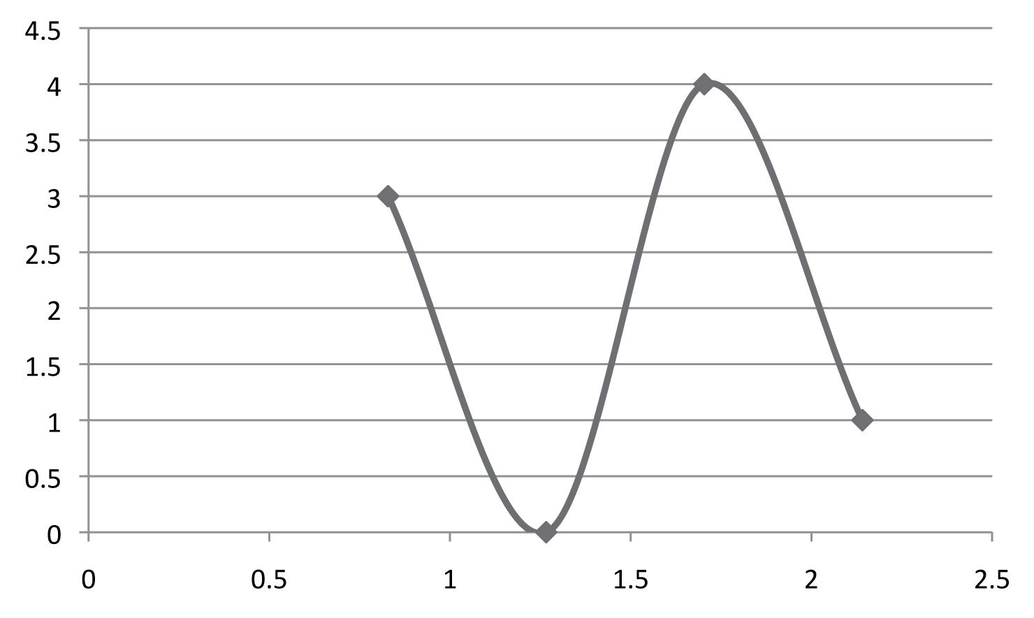
Ancestor population - fitness distribution
The Genome of the ancestor generation is sorted according to its fitness values. This is accomplished by a function within the script that sorts the array of the genome according to its fitness values. The two fittest and the two least fit individuals are then selected for crossover, i. e. sexual reproduction. As a first step in the experiment the on/off sections as well as the extrusion height sections of the genome are selected for a 50/50 crossover process; each of the selected individuals share 50% of the section of the specified genome with a another individual. A dedicated function within the script runs the crossover process and reorganizes the array of the genome. The exact process of crossover for this experiment is depicted in the diagram below
Ancestor Generation - Genome sorted according to fitness Indiv. HomeoBox - On/Off Switch Rotation Angle 01 off off on off on off on off on off off off off on on off 140 137 12 25 35 6 93 02 off on on off off off on on on off on off on on on off 52 153 79 24 9 150 40 03 off on on off on on off on off off off on off on on off 128 3 149 159 130 36 137 04 off on off off on on off off off on on off on off off off 98 11 89 133 2 118 179 05 off off on off off off off on off on on off off off off off 46 136 47 86 65 128 118 06 off on on on on on on off off off on on on on on off 35 60 166 30 27 83 96 07 off on off off on off off off off off off off off on off off 34 13 77 66 146 89 126 08 off off off off off on on off off off off off off off off off 52 143 1 161 44 166 65 Indiv. Rotation Angle (cont.) Off. Zoning Extrusion Height Fitness 01 146 120 65 2 10 81 0 16 64 1.3 4 6 3 3 6 1 2 6 2 0.827 02 7 156 23 59 180 179 134 87 0 0.9 6 1 5 1 6 6 3 2 1 0.834 03 63 55 173 133 24 171 139 7 43 0.7 3 1 1 5 6 1 4 1 4 1.044 04 130 144 53 12 3 163 45 35 114 0.7 6 1 6 1 2 4 6 6 1 1.543 05 16 92 178 150 137 177 56 107 1 1 6 3 2 5 6 3 6 6 1 1.719 06 106 77 164 36 10 135 72 80 152 0.3 1 3 4 6 2 1 5 2 5 1.816 07 147 133 174 52 55 130 135 168 69 0.8 1 3 1 1 4 5 3 1 6 1.89 08 8 45 66 52 93 152 23 49 54 0.6 5 4 2 2 6 6 3 4 2 2.207 Range No. Of Indiv. X Value Y Value 0.61 3 0.82875 3 1.0475 0 1.26625 0 1.485 4 1.70375 4 1.9225 1 2.14125 1 2.36 Average 1.485 Average Dev. 0.4375 Crossover
A B A C Fitness 01 A B B D Fitness 02 E F D B Fitness 03 X Y C A Fitness 04 X Y E G Fitness 05 X Y F H Fitness 06 X Y H F Fitness 07 C D G F Fitness 08 G H E F C D G H No. Of Individuals Overall Fitness
- Gene Exchange
- 145 -
Evaluation of Urban
Genetic Algorithm for Creation and
Patches
First Experiments
The diagram illustrated the re-arranged genome after the crossover process. It is at the same time the new genome that was used to create the first successor generation, i.e. generation 01
Generation01
1.347
0.674
1.078 Individual 06:
4.124
0.687
Rugosity:
Density:
Fitness:
Rugosity:
Density:
Fitness:
Rugosity:
Density:
Fitness:
Rugosity:
Density:
Fitness:
Individual 08: Rugosity:
Density:
Fitness:
Individual 02:
2.749 Individual 03: Rugosity: 0.481 Density: 0.481 Fitness: 0.481 Individual 07:
1.874
0.625
1.374 Individual 04:
0.611
0.611
0.611
0.679
0.679
0.679
Generation 01: Overall Rugosity: 1.689 Overall Density: 0.591 Overall Fitness: 1.25 Individual 01: Rugosity:
Density:
Fitness:
Individual 05: Rugosity: 2.608 Density: 0.522 Fitness:
Ancestor Generation after Crossover/Genome for Generation 01 Indiv. HomeoBox - On/Off Switch Rotation Angle 01 off off on off on off on off off on off off on off off off 140 137 12 25 35 6 93 02 on off off off off on on off off off off off off on off off 34 13 77 66 146 89 126 03 off off off off off on off off on off off off off on on off 140 137 12 25 35 6 93 04 off on off off on off off off off off on off on off on off 34 13 77 66 146 89 126 05 off on on off off off on on off off off off off on on off 52 153 79 24 9 150 40 06 on off on off on on on off off off off off off off off off 52 143 1 161 44 166 65 07 off off off off off off off off on off on off on on on off 52 153 79 24 9 150 40 08 off off off off off on on off off on on off off off on on 52 143 1 161 44 166 65 Indiv. Rotation Angle (cont.) Off. Zoning Extrusion Height Fitness 01 146 120 65 2 10 81 0 16 64 1.3 4 6 3 3 1 3 1 1 4 1.254 02 147 133 174 52 55 130 135 168 69 0.8 1 2 6 2 4 5 3 1 6 1.078 03 146 120 65 2 10 81 0 16 64 1.3 5 3 1 6 6 1 2 6 2 0.481 04 147 133 174 52 55 130 135 168 69 0.8 1 3 1 1 4 6 3 3 6 0.611 05 7 156 23 59 180 179 134 87 0 0.9 6 1 5 1 5 4 2 2 6 1.774 06 8 45 66 52 93 152 23 49 54 0.6 6 3 2 1 6 6 3 4 2 2.749 07 7 156 23 59 180 179 134 87 0 0.9 6 3 4 2 6 6 3 2 1 1.374 08 8 45 66 52 93 152 23 49 54 0.6 5 4 2 2 6 1 5 1 6 0.679
1.791
0.448
1.254
1.774
- 146 -
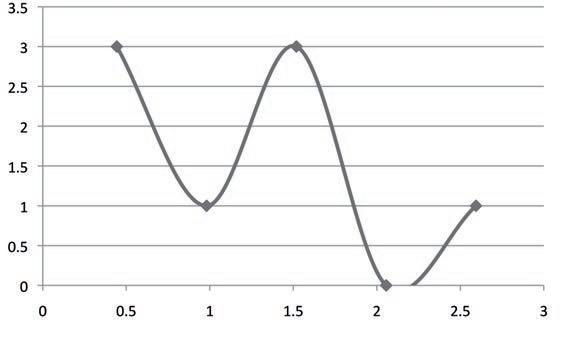
The genome of generation 01 (compare previous page) is sorted according to its fitness values. The two fittest and the two least fit indiviudals (red) are selected for crossover, i.e. the parents for the next generation
Range No. Of Indiv. X Value Y Value 0.1745 3 0.443375 3 0.71225 0 0.981125 1 1.25 4 1.518875 3 1.78775 1 2.056625 0 2.3255 2.594375 1 2.86325 Average 1.25 Average Dev. 0.53775 Genome Generation 01 Sorted Indiv. HomeoBox - On/Off Switch Rotation Angle 01 off off off off off on off off on off off off off on on off 140 137 12 25 35 6 93 02 off on off off on off off off off off on off on off on off 34 13 77 66 146 89 126 03 off off off off off on on off off on on off off off on on 52 143 1 161 44 166 65 04 on off off off off on on off off off off off off on off off 34 13 77 66 146 89 126 05 off off on off on off on off off on off off on off off off 140 137 12 25 35 6 93 06 off off off off off off off off on off on off on on on off 52 153 79 24 9 150 40 07 off on on off off off on on off off off off off on on off 52 153 79 24 9 150 40 08 on off on off on on on off off off off off off off off off 52 143 1 161 44 166 65 Indiv. Rotation Angle (cont.) Off. Zoning Extrusion Height Fitness 01 146 120 65 2 10 81 0 16 64 1.3 5 3 1 6 6 1 2 6 2 0.481 02 147 133 174 52 55 130 135 168 69 0.8 1 3 1 1 4 6 3 3 6 0.611 03 8 45 66 52 93 152 23 49 54 0.6 5 4 2 2 6 1 5 1 6 0.679 04 147 133 174 52 55 130 135 168 69 0.8 1 2 6 2 4 5 3 1 6 1.078 05 146 120 65 2 10 81 0 16 64 1.3 4 6 3 3 1 3 1 1 4 1.254 06 7 156 23 59 180 179 134 87 0 0.9 6 3 4 2 6 6 3 2 1 1.374 07 7 156 23 59 180 179 134 87 0 0.9 6 1 5 1 5 4 2 2 6 1.774 08 8 45 66 52 93 152 23 49 54 0.6 6 3 2 1 6 6 3 4 2 2.749 No. Of Individuals Overall Fitness Generation 01 - fitness distribution - 147A Genetic Algorithm for Creation and Evaluation of Urban Patches
First Experiments
1.963
0.393
2.252
Genome Generation 01 after Crossover/Genome for Generation 02 Indiv. HomeoBox - On/Off Switch Rotation Angle 01 off off off off off on off off off on on off off off on on 140 137 12 25 35 6 93 02 on off off off off on on off off off off off off on on off 52 153 79 24 9 150 40 03 off off off off off on on off on off off off off on on off 140 137 12 25 35 6 93 04 off on on off off off on on off off off off off on off off 52 153 79 24 9 150 40 05 off on off off on off off off on off on off on on on off 34 13 77 66 146 89 126 06 off off on off on off on off off off off off off off off off 52 143 1 161 44 166 65 07 off off off off off off off off off off on off on off on off 34 13 77 66 146 89 126 08 on off on off on on on off off on off off on off off off 52 143 1 161 44 166 65 Indiv. Rotation Angle (cont.) Off. Zoning Extrusion Height Fitness 01 146 120 65 2 10 81 0 16 64 1.3 5 3 1 6 6 1 5 1 5 1.335 02 7 156 23 59 180 179 134 87 0 0.9 1 2 6 2 5 4 2 2 6 0.966 03 146 120 65 2 10 81 0 16 64 1.3 4 2 2 6 6 1 2 6 2 0.671 04 7 156 23 59 180 179 134 87 0 0.9 6 1 5 1 5 3 1 6 6 0.562 05 147 133 174 52 55 130 135 168 69 0.8 1 3 1 1 6 3 2 1 6 2.252 06 8 45 66 52 93 152 23 49 54 0.6 6 3 3 6 6 6 3 4 2 3.079 07 147 133 174 52 55 130 135 168 69 0.8 6 3 4 2 4 6 3 3 6 1.55 08 8 45 66 52 93 152 23 49 54 0.6 6 3 2 1 1 3 1 1 4 0.657 Individual 02: Rugosity: 1.208 Density: 0.604 Fitness: 0.966 Individual 06: Rugosity: 4.619 Density: 0.77 Fitness: 3.079
03: Rugosity:
Density: 0.42 Fitness: 0.671 Individual 07: Rugosity:
Density: 0.705 Fitness: 1.55
04: Rugosity:
Density:
Fitness:
08: Rugosity:
Density:
Fitness:
Overall Rugosity:
Overall Density:
Overall Fitness:
Rugosity:
Density:
Fitness:
Rugosity:
Fitness:
The genome of generation 02. The diagram depicts the crossover process using the genome of selected individuals from generation 01 - 148 -
Individual
0.839
2.114
Individual
0.562
0.562
0.562 Individual
0.657
0.657
0.657 Generation02:
1.918
0.584
1.384 Individual 01:
1.335 Individual 05:
3.378 Density: 0.563
A
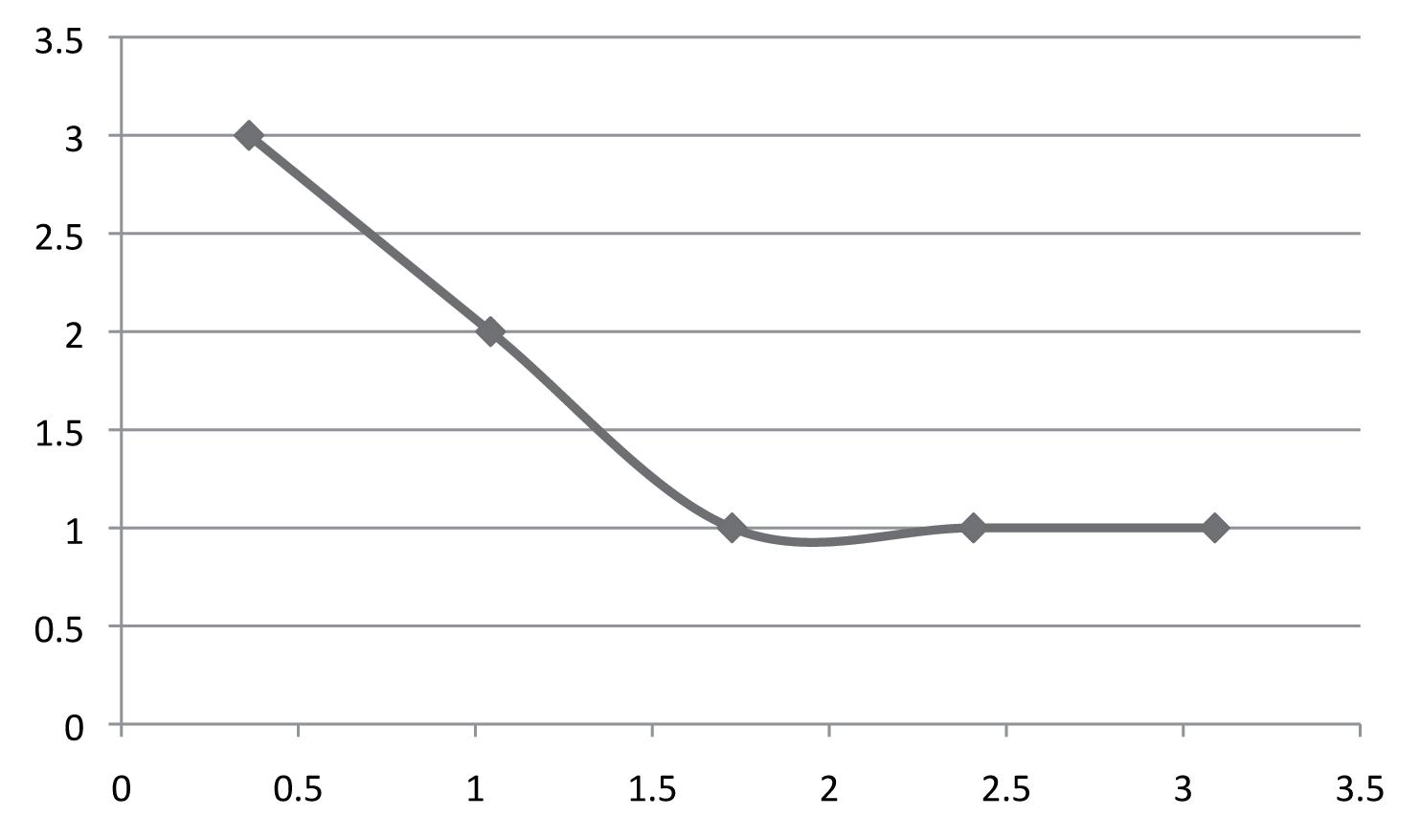
The Diagram shows the genome of generation 02 sorted according to its fitness values. Generation 02 is the last generation in this short demonstration of how the algorithm works. The genome would now go again through the selection (red individuals) and crossover processes in order to form the genome for the next generation; this process can be repeated indefinitely Experiments over 50 generations, however, revealed that the fitness curve tends to flatten out after 25 generations. It is assumed that this is due to the lack of mutations, which do not exist in the current set up. The introduction of mutations will be explained over the following pages.
Range No. Of Indiv. X Value Y Value 0.0195 3 0.360625 3 0.70175 2 1.042875 2 1.384 1 1.725125 1 2.06625 1 2.407375 1 2.7485 1 3.089625 1 3.43075 Average 1.384 Average Dev. 0.68225
Of
Overall Fitness Generation 02 - fitness distribution Genome Generation 02 sorted - Genome for subsequent generation Indiv. HomeoBox - On/Off Switch Rotation Angle 01 off on on off off off on on off off off off off on off off 52 153 79 24 9 150 40 02 on off on off on on on off off on off off on off off off 52 143 1 161 44 166 65 03 off off off off off on on off on off off off off on on off 140 137 12 25 35 6 93 04 on off off off off on on off off off off off off on on off 52 153 79 24 9 150 40 05 off off off off off on off off off on on off off off on on 140 137 12 25 35 6 93 06 off off off off off off off off off off on off on off on off 34 13 77 66 146 89 126 07 off on off off on off off off on off on off on on on off 34 13 77 66 146 89 126 08 off off on off on off on off off off off off off off off off 52 143 1 161 44 166 65 Indiv. Rotation Angle (cont.) Off. Zoning Extrusion Height Fitness 01 7 156 23 59 180 179 134 87 0 0.9 6 1 5 1 5 3 1 6 6 0.562 02 8 45 66 52 93 152 23 49 54 0.6 6 3 2 1 1 3 1 1 4 0.657 03 146 120 65 2 10 81 0 16 64 1.3 4 2 2 6 6 1 2 6 2 0.671 04 7 156 23 59 180 179 134 87 0 0.9 1 2 6 2 5 4 2 2 6 0.966 05 146 120 65 2 10 81 0 16 64 1.3 5 3 1 6 6 1 5 1 5 1.335 06 147 133 174 52 55 130 135 168 69 0.8 6 3 4 2 4 6 3 3 6 1.55 07 147 133 174 52 55 130 135 168 69 0.8 1 3 1 1 6 3 2 1 6 2.252 08 8 45 66 52 93 152 23 49 54 0.6 6 3 3 6 6 6 3 4 2 3.079 - 149 -
No.
Individuals
Genetic Algorithm for Creation and Evaluation of Urban Patches
Ancestor Generation; overall fitness: 15.53
Generation 05; overall fitness: 17.05
Generation 10; overall fitness: 12.03
Generation 15; overall fitness: 11.99
Generation 20; overall fitness: 9.58
The fitness gradually settles after 25 generations and remains the same from there. It is believed that this is due to the fact that mutations did not take part so far.
A sequence of 50 test generations run with the genetic algorithm described on the previous pages. The fitness graph flattens out after 25 generations and fitness values remain the same from there. It is believed that the lack of mutations leads to this phenomenon. The same information (in the genome) is shuffled back and forth from the ancestor generation; no new information is added and the population will gradually settle towards a fitness value. As a result mutations have been introduced to the script.
Generation
fitness:
20 16 12 08 04 00 Fitness [/] Anc.Gen.Gen.01Gen.02Gen.03Gen.04Gen.05Gen.06Gen.07Gen.08Gen.09Gen.10Gen.11Gen.12Gen.13Gen.14Gen.15Gen.16Gen.17Gen.18Gen.19Gen.20Gen.21Gen.22Gen.23Gen.24Gen.25
20; overall
9.38
- 150First Experiments
Crossover Types
Different types of mutations as they occur in nature. Crossover is the typical gene exchange that occurs during sexual reproduction; a 50/50 crossover, where 50% of the genome is exchanged from one individuum to the next is a common. Other types of crossover, e.g. single point crossovers are also typical. Different types of mutations occur where strings of the genome are exchanged in different ways. ‘Duplication’ copies a sequence of the genome twice instead of once. ‘Deletion’ ignores to copy parts of a gene or gene sequence. ‘Insertion’ can be seen as a ‘cut and paste’ operation in the computer where parts of the genome are cut out and transferred. ‘Inversion’ mirrors a gene or gene sequence during the copy operation. ‘Translocation’ exchanges two parts of a genome. The mutation types depicted above can be used as a reference to design mutation strategies that can be integrated into a genetic algorithm.
Mutation Types
Duplication Before Before After After Deletion Before After Insertion Before After Inversion Before After Translocation 50/50 Crossover Before After Single Point Crossover Before After Double Point Crossover Before
- 151 -
Genetic Algorithm for Creation and Evaluation of Urban Patches
A
Translocation Mutation: Genome Generation ‘A’ after Crossover/New Genome for Next Generation Indiv. HomeoBox - On/Off Switch Rotation Angle 01 off off off on off off off off off off off off off off off off 116 148 150 144 161 109 85 02 off off off off off off off off off off off off off off off on 84 156 74 90 139 127 67 03 off off off off off off off on off off off off off off off off 116 148 150 144 161 109 85 04 off off off off off off off off off off off on off off off off 84 156 74 90 139 127 67 05 off on on off off on off on off on off off off off off off 84 156 74 90 139 127 67 06 on on on on off on on off off off off on off off off off 41 135 32 76 126 61 122 07 off off off on off off off off on on on on off on on off 84 156 74 90 139 127 67 08 off on off off off off off off off on on off off on off on 41 135 32 76 126 61 122 Indiv. Rotation Angle (cont.) Off. Zoning Extrusion Height Fitness 01 110 34 9 102 51 107 120 126 32 0.6 2 5 5 6 1 6 5 6 4 02 113 21 21 116 146 9 106 175 103 0.9 6 5 6 1 4 2 6 6 3 03 110 34 9 102 51 107 120 126 32 0.6 2 6 6 3 1 6 5 6 1 04 113 21 21 116 146 9 106 175 103 0.9 1 6 5 6 2 5 5 6 1 05 113 21 21 116 146 9 106 175 103 0.9 6 3 4 3 5 5 5 6 2 06 73 87 177 136 127 106 169 159 57 0.4 6 4 6 4 2 5 5 6 6 07 113 21 21 116 146 9 106 175 103 0.9 5 5 6 6 3 6 4 6 4 08 73 87 177 136 127 106 169 159 57 0.4 5 5 5 6 6 3 4 3 3 Generation ‘A’ after Crossover Individual 02 Individual 03 Individual 04 Individual 05 Individual 06 Individual 07 Individual 08 Individual 01 - 152 -
First Experiments
First Individual for Translocation: 01
Start Position for Translocation; HomeoBox and Rotation Angle: 05
Second Individual for Translocation: 05
Start Position for Translocation; Zoning Extrusion Height: 06
Above and left hand side: A translocation mutation (compare also page 151) is integrated into the algorithm. Two individuals are chosen randomly after crossover and a specified range of genes in each section of the genome is selected for a translocation mutation process; i.e. selected genes are swapped with the corresponding genes of the other individual.
- 153Translocation Mutation: Genome Generation ‘A’ after Translocation Mutation/New Genome for Next Generation Indiv. HomeoBox - On/Off Switch Rotation Angle 01 off off off on off on on off off off off off off off off off 116 148 150 144 161 61 122 02 off off off off off off off off off off off off off off off on 84 156 74 90 139 127 67 03 off off off off off off off on off off off off off off off off 116 148 150 144 161 109 85 04 off off off off off off off off off off off on off off off off 84 156 74 90 139 127 67 05 off on on off off on off on off on off off off off off off 84 156 74 90 139 127 67 06 on on on on off off off off off off off on off off off off 41 135 32 76 126 109 85 07 off off off on off off off off on on on on off on on off 84 156 74 90 139 127 67 08 off on off off off off off off off on on off off on off on 41 135 32 76 126 61 122 Indiv. Rotation Angle (cont.) Off. Zoning Extrusion Height Fitness 01 73 87 177 102 51 107 120 126 32 0.4 2 5 5 6 1 6 5 6 6 02 113 21 21 116 146 9 106 175 103 0.9 6 5 6 1 4 2 6 6 3 03 110 34 9 102 51 107 120 126 32 0.6 2 6 6 3 1 6 5 6 1 04 113 21 21 116 146 9 106 175 103 0.9 1 6 5 6 2 5 5 6 1 05 113 21 21 116 146 9 106 175 103 0.9 6 3 4 3 5 5 5 6 2 06 110 34 9 136 127 106 169 159 57 0.6 6 4 6 4 2 5 5 6 4 07 113
21 116 146 9 106 175 103 0.9 5 5 6 6 3 6 4 6 4 08 73 87 177 136 127 106 169 159 57 0.4 5 5 5 6 6 3 4 3 3
21
Generation ‘A’ after Translocation Mutation Individual 02 Individual 01 Individual 03 Individual 04 Individual 05 Individual 06 Individual 08 Individual 07
Ancestor Generation; overall fitness: 1.06
Generation 05; overall fitness: 1.49
Generation 10; overall fitness: 1.28
Generation 15; overall fitness: 1.45
Generation 20; overall fitness: 1.43
Fitness [/]
50 test generations of eight individuals are created in just under 1.5 hrs on a labtop computer. The experiment confirms that the algorithm is stable and can produce large numbers of individuals with corresponding information. In the above example test patches measure 250 x 250 meters; density and rugosity are again chosen as fitness evaluation parameter and set at at 60/40 ratio. A translocation mutation
- 1541.0 1.5 2.0
Anc.Gen.Gen.01Gen.02Gen.03Gen.04Gen.05Gen.06Gen.07Gen.08Gen.09Gen.10Gen.11Gen.12Gen.13Gen.14Gen.15Gen.16Gen.17Gen.18Gen.19Gen.20Gen.21Gen.22Gen.23Gen.
Generation 25; overall fitness: 1.46
Generation 30; overall fitness: 1.611
Generation 35; overall fitness: 1.70
Generation 40; overall fitness: 1.78
Generation 45; overall fitness: 1.76
Generation 49; overall fitness: 1.67
Gen.24Gen.25Gen.26Gen.27Gen.28Gen.29Gen.30Gen.31Gen.32Gen.33Gen.34Gen.35Gen.36Gen.37Gen.38Gen.39Gen.40Gen.41Gen.42Gen.43Gen.44Gen.45Gen.46Gen.47Gen.48Gen.50
function has been integrated into the script (see page 153). The fitness graph now confirms that the overall fitness does not become a fixed number after a while. Nevertheless, the experiment shows that there is still little variation after 25 generations; the genome is soon exploited and no new information is added. Individuals therefore look pretty much the same.
- 155 -
- 156Genome Generation ‘A’ after Crossover/New Genome for Next Generation Indiv. HomeoBox - On/Off Switch Rotation Angle 01 off on off off on on off on off off off off off off off off 129 123 75 88 156 89 13 02 off off on on on on on off off off off off off on off off 129 0 140 88 64 89 13 03 off off off off off on off off off off on on on on on off 129 123 75 88 156 89 13 04 off off off off off off off off off on off off on on off on 129 0 140 88 64 89 13 05 off on off off on off off on off off on off off on on off 129 123 140 88 64 89 13 06 on off off off off off off on off off off off off off off off 26 147 145 101 101 15 106 07 off off off off off off off off on off off off off off off on 129 123 140 88 64 89 13 08 off off on off off on on off off on off off on off off on 26 147 145 101 101 15 106 Indiv. Rotation Angle (cont.) Off. Zoning Extrusion Height Fitness 01 107 56 112 125 134 105 11 112 38 9 36 24 45 57 6 57 15 33 33 02 107 56 122 125 134 105 11 112 38 9 30 42 42 24 33 18 60 57 21 03 107 56 112 125 134 105 11 112 38 9 18 60 57 21 15 30 42 42 24 04 107 56 122 125 134 105 11 112 38 9 6 57 15 33 36 24 45 57 15 05 107 56 112 125 134 106 11 112 38 9 27 15 36 27 45 36 57 21 57 06 89 6 74 2 86 143 9 149 140 6 18 27 51 57 57 42 57 15 33 07 107 56 112 125 134 106 11 112 38 9 42 57 15 33 57 18 27 51 57 08 89 6 74 2 86 143 9 149 140 6 45 36 57 21 27 15 36 27 57 Genome Generation ‘A’ after Point Mutations Indiv. HomeoBox - On/Off Switch Rotation Angle 01 off on off off on on off on off off off on off off on off 129 123 75 88 156 94 13 02 off off off on on on on off on off off off off on off off 129 0 140 88 64 89 24 03 on off off off off on off off off off on on on on off off 129 52 75 88 156 89 13 04 off off off off off off on off off on off off on on off off 129 0 140 88 64 89 13 05 off on off off on off off on off off on on off on on on 129 123 140 88 64 89 13 06 on off off off off off off on off off off off off off off off 26 147 145 101 101 15 106 07 off off off off off off off off off off off off off off off off 129 123 140 88 64 89 13 08 off off on off on on off off off on off off on off off on 26 147 145 101 101 15 106 Indiv. Rotation Angle (cont.) Off. Zoning Extrusion Height Fitness 01 107 56 112 125 55 105 11 112 38 9 36 24 45 57 6 57 27 36 33 02 107 56 122 125 174 105 11 112 38 9 30 24 42 24 54 18 60 57 21 03 107 56 98 125 134 105 11 112 38 9 18 60 57 21 15 42 42 42 24 04 107 48 13 125 134 105 11 112 38 9 6 54 24 12 36 24 45 57 15 05 107 56 112 172 134 106 11 112 38 8 27 15 57 18 45 36 57 21 24 06 127 6 74 2 86 143 9 149 45 6 18 27 51 36 12 45 57 15 33 07 107 56 112 125 151 106 72 112 38 9 42 57 15 57 57 48 27 51 57 08 89 6 78 2 86 143 9 149 140 6 45 36 57 21 36 15 36 27 42 Generation ‘A’
after Point Mutations (& Crossover) Individual 01 Individual 01 Individual 02 Individual 02 Individual 03 Individual 03 Individual 04 Individual 04 Individual 05 Individual 05 Individual 06 Individual 06 Individual 07 Individual 07 Individual 08 Individual 08
Generation ‘A’
A Genetic Algorithm for Creation and Evaluation of Urban Patches
Diagrams on facing page: The experiment on page 154 confirms that a translocation mutation by itself is not sufficient to still produce variation after twenty odd generations. The problem remains that the same gene information from the selected ancestor parents is still shuffled back and forth; no new information is added to the genome. In order to address this problem a second mutation type is added to the algorithm: The point mutation function locally introduces mutations in all sections of the genome; in the example the Homeobox and the Rotation Angle section were set for 2 mutation for each section for each individual. Via random selection the function changes two positions in each section: In the homeobox “on” is set to “off” for two items in the array (and vice versa). In the rotation angle section two numbers per individual are changed in the same way. A similar process is applied for the Zoning extrusion height section where a maximum of three numbers per array are changed. The offset section of the genome is treated slightly different; as there is only one integer in this section that carries the offset information a probability function is introduced. In the above example the probability for change is set to 20%; therefore the value is changed for only one individual. All parameters (amount of mutations per individual and probability)can be set in the main subroutine of the script.
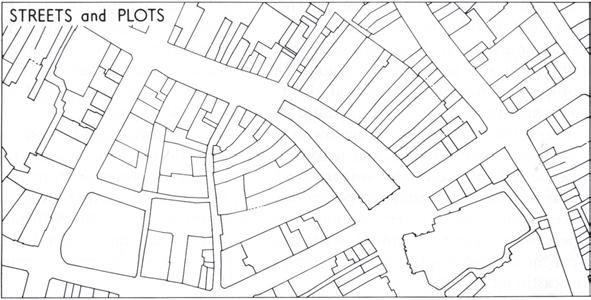
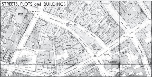
Jeremy Whitehand (Whitehand, 1981) describes the fundamental units of urban form as the street and the plot. Buildings are seen as a third level in this hierarchy. The algorithm utilizes the basic principle of the street on the plot. Further development is necessary to introduce buildings at the next hierarchical level.
The development of the genetic algorithm confirms that it is possible to generate and evaluate urban tissue at the same time. It also shows that it is possible to integrate Adolphe’s Indicators and that e.g. the roughness of the roof surface of an urban patch can be used as a fitness value next to density. The rather rapid process of generation and evaluation makes the algorithm very suitable as a design tool; next to the fitness, all data (in this case rugosity and density values) is printed below the generated patches and the designer is able to quickly select suitable layouts for further development.
It needs to be mentioned that the optimization process, as described by Panao in the introduction to this chapter, does not quite seem to take place yet. Different mutation types have been added to the algorithm and further experimentation is necessary in order end up with a target-oriented tool; design targets also need to be specified more concrete. Nevertheless, the algorithm seems promising as a start. Even though the optimization process does not quite work yet as desired it still allows for rapid production of patches that can be selected according to fitness criteria and subjective design considerations.
Whereas the algorithm has so far been based on a very basic urban structure, i.e. the street and the island, questions arise how further development should take place. The development from the so far ‘schematic’ patch layouts to more sophisticated urban morphologies will be addressed in the next chapter.
- 157 -
Design Development
Patch Typologies, Patch Aggregation and Urban Qualities
The development of the algorithm, as described in the previous chapter, opened up a series of questions and new design objectives.
Approaching urban planning from the meso-scale, i.e. the urban patch, it is necessary to investigate how such heterogeneous patches can be aggregated in order to form a larger, homogeneous urban fabric. The random creation of street angles, which is set up in the algorithm in order to evaluate the microclimatic performance of various street and block layouts causes a problem once patches are assembled to form a larger whole. This problem is addressed through further development and a hierarchy of street elements is finally introduced to provide a continuous superstructure, i.e. a street network that allows for the required connectivity between patches. Refer to page 171.
The schematic morphology of patches, i.e. streets and islands, is also further developed in order to investigate how schematic blocks can be broken up in the script to form real urban typologies. Different functions are developed that transform the islands into distinct morphologies that range from, e.g. a neighbourhood type with gardens to an inner-city high rise area. Besides urban consideration this step is necessary as some environmental parameter such as contiguity or compacity take, e.g. shared building party walls, into consideration. In order to determine such parameters, functions need to be developed that provide a higher level of detail for analysis. For the development of block typologies refer to page 177.
Finally, the development of the algorithm and the study of microclimatic indicators showed that the use of parameters could also be extended to evaluate other aspects of the urban morphology than the microclimate. A series of studies is set up to see in how far ‘Urban Qualities’ can be measured objectively and incorporated as latent design information into the algorithm. The evaluation of urban qualities looks at factors such as ‘recreational parameters’ or the ‘connectivity’ of the street network. They are described in more detail on the following pages, starting on page 160.
For all script files refer to Appendix 02.
- 159Patch Typologies, Patch Aggregation and Urban Qualities
Reference point/park
Shortest distance
Urban Qualities/Recreation Indicator
Closest points on streets at intervals on shortest distance line
Closest points on streets at intervals on shortest distance line
Approximated route
The ‘Recreation Indicator’ evaluates the distance from each urban block to an area of interest of a specified size; this can be a park or piece of infrastructure, such as a railway station. In the following example the distance to a park of a specific size is measured and evaluated. For accessibility to parks in urban areas Salat (Salat, 2010) provides the following design objectives: Access to a green space of more than 1000m² at less than 200m (reachable by foot every day). Access to a green space of more than 5000m² at less than 750m (reachable from time to time by foot). Access to a green space of more than an hectare and to a green corridor at less than 2km (reachable by bike). Access to a green space of more than 10 hectares at less than 4km (reachable by public transport).
Park 01: 7697m²
Park 02: 645m²
Park 03: 184m²
Block01/Travel Distances to Parks:
Park 01: 222m
Park 02: 247m
Park 03: 174m
Block02/Travel Distances to Parks:
Park 01: 220m
Park 02: 224m
Block03/Travel Distances to Parks:
Park 01: 140m
Park 02: 190m
Park 03: 166m
Block04/Travel Distances to Parks:
Park 01: 105m
Park 02: 169m
Park 03: 126m
Block05/Travel Distances to Parks:
Park 01: 143m
Park 02: 131m
Park 03: 70m
Blocks Located further away than 150m travel distance from Green Space of at least 1000m².
Block06/Travel Distances to Parks:
Park 01: 95m
Park 02: 53m
Park 03: 77m
- 160 -
Development
Design
Individual 01:
Built Area: 22.649m²
‘Good Area’*: 18.866m²
Green Area: 9.162m²
Sample Area: 62.500m²
Ratio (Rec.): 0.83
Individual 05:
Built Area: 22.004m²
‘Good Area’*: 0m²
Green Area: 810m²
Sample Area: 62.500m²
Ratio (Rec.): 0.00
Individual 02: Built Area: 29.592m² ‘Good Area’*: 0m²
Ratio (Rec.): 0.00
Individual 06: Built Area: 31.043m² ‘Good Area’*: 29.089m² Green Area: 8.528m² Sample Area: 62.500m²
Ratio (Rec.): 0.94
Individual 03:
Built Area: 34.023m² ‘Good Area’*: 0m²
Green Area: 315m²
Sample Area: 62.500m²
Ratio (Rec.): 0.00
Individual 07:
Built Area: 28.351m² ‘Good Area’*: 26.037m² Green Area: 1.076m² Sample Area: 62.500m²
Ratio (Rec.): 0.92 Individual 04:
Individual 08:
Above: Test population. Blocks that are outside the specified range to a park of a specified size are coloured orange.
Example 01:
Built Area: ~46.875m²
‘Good Area’*: ~15.625m²
Green Area: ~15.625m²
Sample Area: ~62.500m²
Ratio (Rec.): 0.33
Example 02:
Area: ~15.625m²
Area’*: ~15.625m²
Area: ~46.875m²
Area: ~62.500m² Ratio (Rec.): 1.00
Example 03:
Ratio (Rec.): 0.66
The Diagrams above and on page 160 illustrate how the ‘Recreation Indicator’ works: A Function is designed that draws the shortest, direct connection lines between each block (centroid) and each park within a given area of interest. By finding the closest point of the connection line to the underlying street network roughly approximated walking paths are determined; without being 100% precise this methods allows a rather quick way of approximating travel distances and it also avoids the ‘travelling salesman problem’ which would not be computable.
Therefore, for each block the walking paths to all parks are determined. The park sizes and walking distances are then evaluated. If a block is within a certain range of a park of a certain size it is considered ‘good’; in the above example it is assumed that parks, larger than 1000m², should be within a walking distance of less than 200m. If a block is considered ‘good’ the footprint area of the block is calculated; if it is considered ‘not good’ it is coloured orange and ignored. The recreation factor is finally determined by setting the area of good blocks against the overall built area. The range is from 0 (bad) to 1 (excellent), compare diagram above. In addition to the value , the colour coding gives a good indication for the designer about the area of blocks that is considered ‘not good’.
Built
‘Good
Green
Sample
Built Area: ~46.875m² ‘Good Area’*: ~31.250m² Green Area: ~15.625m² Sample Area: ~62.500m²
Green Area: 239m² Sample Area: 62.500m²
Built Area: 25.866m² ‘Good Area’*: 6.954m² Green Area: 4.794m² Sample Area: 62.500m²
Ratio(Rec.): 0.27
Built Area: 39.728m² ‘Good Area’*: 3.947m² Green Area: 10.547m² Sample Area: 62.500m²
250m 250m 250m 250m 250m 250m
Ratio (Rec.): 0.10
- 161Patch Typologies, Patch Aggregation and Urban Qualities
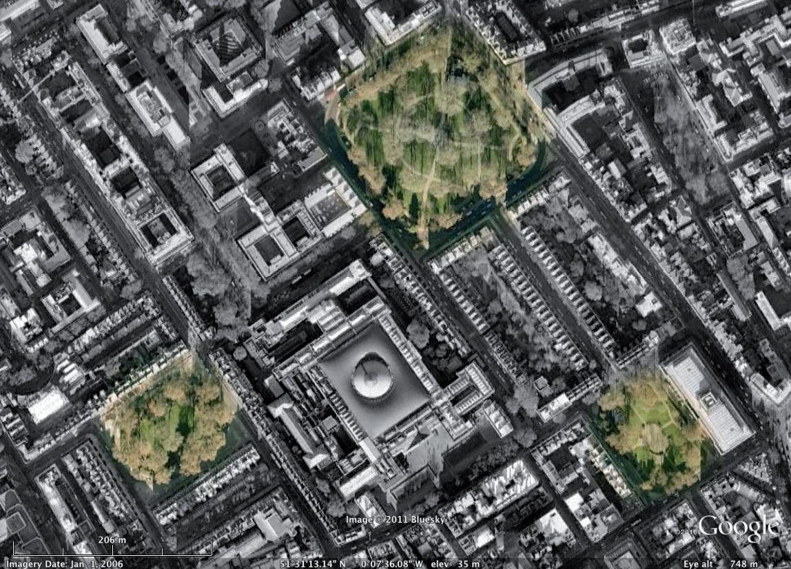
Aerial view of Georgian Squares in central London. Small parks are located within walking distance from each other and gives residents access to private and public green spaces. The ‘Recreational Indicator’ evaluates the distance from each block to all parks and evaluates the size of the park in relation to the walking distance. Image from Google Earth.
The ‘Recreation Indicator’ measures the footprint area of blocks that are located within a specified distance to areas of interest of a specified size. It then evaluates the performance of the fabric by setting the area of blocks, which are considered ‘good’ in relation to the overall built area. The recreation factor is determined by the following formula:
Recreation: Ai Area of Building i (within ‘good’ range) Aj Area of Building j
€ R = A built ∑ A built ∑
- 162Design Development
Street intersections Distance between street intersections
Urban Qualities/Plaza Indicator
Min. distance between intersections results in cluster, i.e. plazas
Shortest distance from building(i) to nearest plaza
Travel distance to nearest plaza
Evaluation of patches created by the algorithm demonstrates that in some conditions special urban features are created. These are the result of intersection events of various streets that sometimes result in small urban islands. In reality such urban features do exist and often create ‘hot-spots’ within the urban fabric; Herald Square in New is such an example (compare page 164). The formation of such intersection events is investigated in the script and termed a ‘Plaza Indicator ’.
A function is designed to study street intersection events. If more than on street intersection falls within a specified radius a ‘Plaza Event’ is recognized (orange circles). Similar to the ‘Recreational Indicator’ on page 160, distances from each block are evaluated by approximating walking paths. Blocks which are located within a specified distance to a Plaza are considered good; otherwise blocks are colourcoded in orange. The ‘Plaza Indicator’ then evaluates the footprint area of blocks that fall into a good range against the overall built area; it is determined according to the formula on page 164.
Block01/Distances nearest Plaza:
Travel Distance : 54m
Block Area: 1.586m²
Block02/Distances nearest Plaza:
Travel Distance : 57m
Block Area: 145m²
Block04/Distances nearest Plaza:
Travel Distance : 238m
Block Area: 5.786m²
Block05/Distances nearest Plaza:
Travel Distance : 145tm
Block Area: 4.746m²
Block03/Distances nearest Plaza:
Travel Distance : 202m
Block Area: 30.220m²
travel
from
Plaza
Blocks Located further away than 150m
distance
nearest
- 163Patch Typologies, Patch Aggregation and Urban Qualities
Individual 01:
Built Area: 29.797m²
‘Good Area’*: 18.387m²
‘Bad Area’**: 11.410m²
Sample Area: 62.500m²
Ratio: 0.62
Individual 05:
Built Area: 42.483m²
‘Good Area’*: 6.476m²
‘Bad Area’**: 36.007m²
Sample Area: 62.500m²
Ratio: 0.15
Individual 02:
Built Area: 25.045m²
‘Good Area’*: 17.575m² ‘Bad Area’**: 7.471m² Sample Area: 62.500m² Ratio: 0.70
Individual 06: Built Area: 42.289m²
‘Good Area’*: 0m²
‘Bad Area’**: 42.289m² Sample Area: 62.500m² Ratio: 0.00
Individual 03:
Built Area: 42.812m²
‘Good Area’*: 42.812m²
‘Bad Area’**: 0m²
Sample Area: 62.500m² Ratio: 1.00
Individual 04:
Individual 07:
Built Area: 33.599m²
‘Good Area’*: 15.935m²
‘Bad Area’**: 17.663m² Sample Area: 62.500m² Ratio: 0.47
Above: Sample Population illustrating the calculation of the ‘Plaza Indicator ’. Below: Formula used for determining the ‘Plaza Indicator’.
Individual 08: Built
Ai Area of Building i (within ‘good’ range) Aj Area of Building j
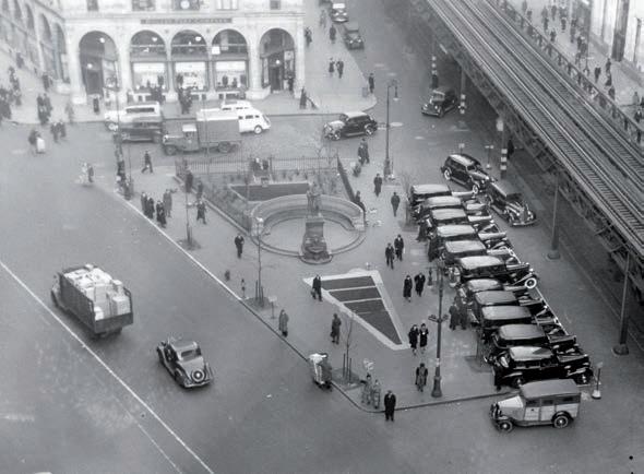
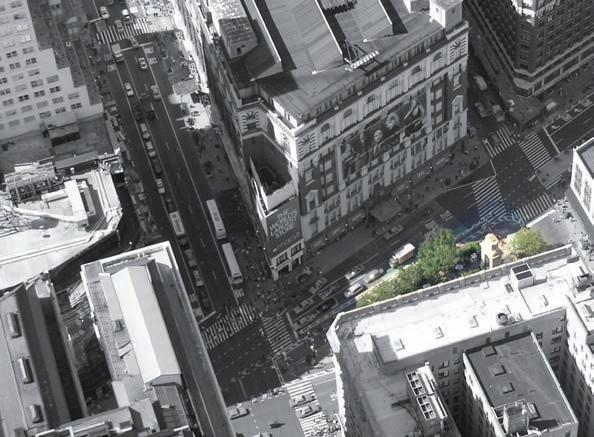
0.00
Built Area: 54.976m² ‘Good Area’*: 0m² ‘Bad Area’**: 54.976m² Sample Area: 62.500m² Ratio:
44.738m²
17.192m² ‘Bad Area’**: 27.546m² Sample Area: 62.500m² Ratio: 0.38 € R = Ai built ∑ Aj built ∑
Area:
‘Good Area’*:
Herald Square in Manhattan, New York; 1930s and today. Islands that are created through street intersection events can result in special urban features that often form attractor points within the fabric.
- 164Design Development
Range (± 10m)
Good Street Length*: 40
Example Streets; 4 Streets with different street lengths:
Mean Street Lenght: 38.75m
Mean Deviation: 23.75m
The ‘Connectivity Indicator’ evaluates the street network according to the following formula:
C(connectivity) = 1 deviation goodarea
Urban Qualities/Connectivity Indicator
The length of street segments can give an indiction about the connectivity of an urban fabric; if street segments are too long walking is discouraged and car travel is encouraged. Too long street segments can therefore have an impact on social aspects and human interaction within an urban fabric.
The above example assumes that a good street length is 40m (±10m). The four streets in the example are in average 38.75m long. The mean deviation equals 23.75m. In order to evaluate the quality of the street network the bad area is set in relation to the overall area. The inverse then gives the good area; the calculation therefore is as follows:
1-(15+12.5)/(23.75+23.75) = 0.421 (Ratio from 0 to 1)
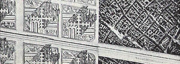
10m
20m 45m 80m
40m 10m10m
38.75m mean street length mean deviation 23.75m mean deviation 23.75m 15m 12.5m 40m
Paris, Plan Voisin by Le Corbusier. The image compares the proposed, modernistic, high rise scenario against the existing urban fabric. The image illustrates differences in the street network and the connectivity of the fabric.
- 165Patch Typologies, Patch Aggregation and Urban Qualities
Individual 01:
Mean Street Length: 85.85m
Length all Streets: 429.29m No of Streets: 5 No of Intersect.: 1
Connectivity: 0.1073
Individual 05:
Mean Street Length: 36.63m
Length all Streets: 842.47m No of Streets: 22 No of Intersect.: 9
Connectivity: 0.5149
Individual 02:
Mean Street Length: 28.81m
Length all Streets: 1296.89m No of Streets: 44 No of Intersect.: 19
Connectivity: 0.4602
Individual 06:
Mean Street Length: 26.01m Length all Streets: 1066.41m No of Streets: 40 No of Intersect.: 17
Connectivity: 0.3928
Individual 03:
Mean Street Length: 30.72m
Length all Streets: 1320.97m No of Streets: 59 No of Intersect.: 19
Connectivity: 0.5221
Individual 04:
Mean Street Length: 24.91m
Length all Streets: 1420.22m No of Streets: 53 No of Intersect.: 19
Connectivity: 0.3597
Individual 07:
Mean Street Length: 55.64m Length all Streets: 500.84m No of Streets: 9 No of Intersect.: 3
Connectivity: 0.3799
Sample Population demonstrates how the ‘Connectivity Indicator’ is evaluated on urban patches.
Individual 08:
Mean Street Length: 54.38m Length all Streets: 489.40m No of Streets: 9 No of Intersect.: 3
Connectivity: 0.4053
Salat (Salat, 2010) talks about the connectivity of an urban network, referring to links: “Links are ways between two nodes (intersections). A big number of links includes a big number of nodes and more possibility of different ways from one point to another. Nevertheless, the number must not be too big, so that the city do not become a maze. Objective found in literature: if P=number of inhabitants, number of links should be between (1/2) P. ln (P) (minimum) and (1/2)P².”
Example 01:
Mean Street Length: 83.30m
Length all Streets: 1000m
No of Street Segments: 12 No of Intersect.: 4
Connectivity: 0
Example 02: Mean Street Length: 62.50m
Length all Streets: 1500m No of Street Segments: 24 No of Intersect.: 9
Connectivity: 0
Example 02:
Mean Street Length: 50.00m
Length all Streets: 2000m No of Street Segments: 40 No of Intersect.: 16
Connectivity: 1
250 250 250 250 250 250 83.3 62.5 50 83.3 62.5 50
- 166 -
Development
Design
SPATIAL ANALYSIS
CONNECTIVITY WITH RESPECT TO DENSITY : ACCESSIBILITY DISTANCE
SEQUENCING OF OPEN & BUILT SPACE
CONNECTIVITY AS A DRIVING FACTOR OF MORPHOLOGY
Street and road networks are an important driving factor of the urban morphology. Spatial connectivity has underlying influence on the block size, circulation pattern, and the integration or separation of the urban fabric. Most often in traditional settings, they are formed by the juxtaposition of green areas to circulatory paths between blocks.
Street patterns are usually a resultant of decisions rooted from Topography/Geographical features, administrative purposes, or Cultural preferences. The latter, often the most appropriate, is however also the least quantifiable.
Based on the number of exterior nodes, their varied weightage depending on street size and hierarchy, certain patterns can be identified through most cities. These indicate the levels of penetration into each type of fabric.
The 6 usual types as elaborated in the following figure are:
• Minimum primary street yet high circulation.
• Distributed and hierarchical system with non permeable blocks
• Well connected to the perimeter, and hierarchical system
• Street pattern as driven by terrain
• Rigid street pattern of equal width, thus the tissue as a whole being highly permeable but absolutely non-permeable at block level.
• Highly permeable blocks with distribution of both pedestrian and motor ways.
The key question in devising urban growth would be the decision to adapt existing street patterns, or establish a rule based system of connections depending on the hierarchy of street patterns to the perimeter of a given sample.
Towards the incentive of optimizing effect of built form to the environment, the aim would be to cause the least disruption to existing land patterns, and also encourage a fabric where both vehicular and pedestrian movement is taken into consideration.
- 167Patch Typologies, Patch Aggregation and Urban Qualities
CASE 1 : MIN. MAJOR STREETNODES TO PERIPEPHERY PERMEABLE BLOCKS, HIGH PEDESTRIAN SUITABILITY
4:
CASE 5:
GOOD CONNECTIVITY TO PERIPHERY, STREET HIERARCHY IN STREET DISTRIBUTION, SEMI PERMEABLE BLOCKS
CASE 2:
DISTRIBUTED STREET NODES TO PERIPHERY, HIERARCHY OF STREETS, NON- PERMEABLE BLOCKS
RIGID STREET NETWORK, NON- PERMEABLE BLOCKS
CASE 3:
GOOD CONNECTIVITY TO PERIPHERY, STREET HIERARCHY, SEMI PERMEABLE BLOCKS, STREET FOLLOWING TOPOGRAPHY.
BUENOS AIRES
CASE 6:
PERMEABLE BLOCKS, HIGH CONNECTIVITY, PEDESTRIAN &MOTORWAY SUITABLE, SEQUENCING OF OPEN SPACES
ZANZIBAR, TANZANIA
POTALA, TIBET
YAZD, IRAN
CHICAGO
TOKYO, JAPAN
CASE
A B C D E F G H D A C E B C D A B B C A M L H G F E D I J K B C D A F G E D E F C B A K J I G H L M N O - 168Design Development
Urban Scale/Approach for Design at different Scales
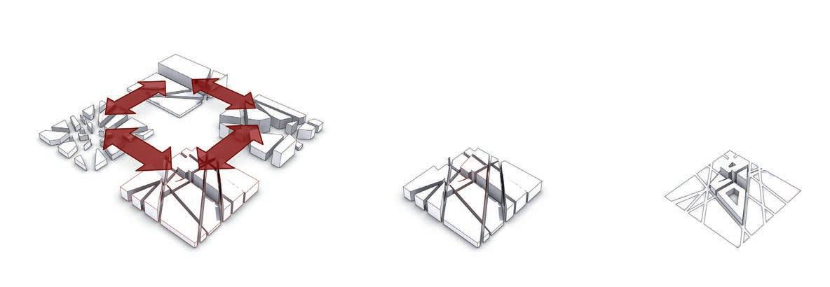
Settlement/Zoning Scale
Building Neighbourhood Scale
Building/Block Scale
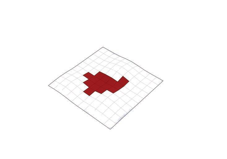
Settlement/Zoning Scale
Corresponding Site Selection (According to direction taken above)
Building Neighbourhood Scale
RegionalScale
New City (‘from scratch’)
RegionalScale
Patch Aggregation and Urban Typologies:
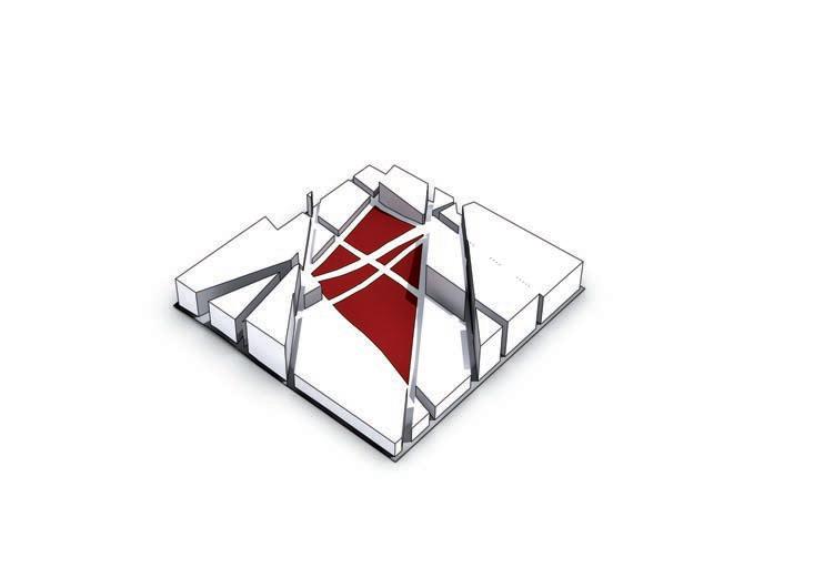
NeighourhoodScale
Existing Urban Patch (Brown Field Site)
Neighbourhood Scale
Diagrams above and on page 170: From the outset it was not clear what the best approach would be to assess an urban fabric using microclimatic design parameters. Even though some climatologists claim that the city should be approached from the outside to the inside, i.e hierarchically from the macro- to the micro-scale it is not clear how such strategies can be implemented. From a design point of view questions therefore opened up whether to look at the city from the patch level or whether to zoom in further to the block and street.
Overall it becomes clear that certain aspects need to be resolved from a design point of view; in particular the development of urban typologies as well as strategies for aggregation of patches. The diagrams depict these early design questions.
~10.000m
~1000m ~100m ~10.000m
~1000m ~100m
- 169Patch Typologies, Patch Aggregation and Urban Qualities
Scale
City/Neighbourhood Scale (Streets***)
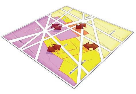
City Block Scale (Plots***)
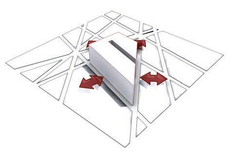
Lot Scale (Buildings***)
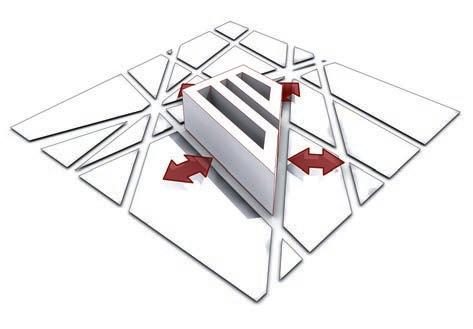
Microclimatic Indicators Urban & Architectural Indicators* Radiation Wind
• Directionality
• Mineralization (Basic Zoning)
• Street Density
• Density
• Rugosity
• Porosity
• Relative Sinuosity
• Urban Reflectance (@ Roof Level)
• Solar Access/Nocturnal Cooling
• Number of Links
• Cyclomatic Number
• Solar Admittance (Building/Street)
• Occlusitivity
• Compacity
• Albedo
• Contiguity
* To some degree related to sustainable urban and architectural objectives
• Plan Density/FAR
• Active & Non-Active Zones
• Density
• Facade Materials
• Building Form and Orientation
** Several authors (e.g. Morgan and Ali-Toudert) agree that the city should be approached from the exterior to the interior
*** Typomorphical entities of settlements (Conzen 1960)
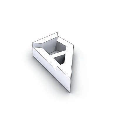
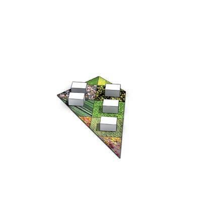
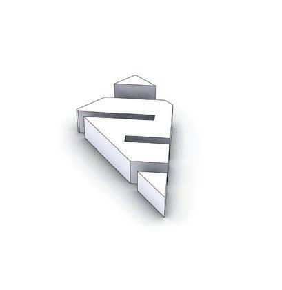
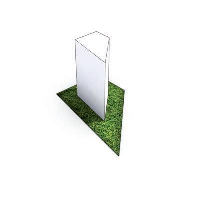
Alleys
Streets House&Garden Block
Courtyards Highrise Park & Public Space
Subdivision:
&
&
*
Possible block typologies; the diagram was used for the development urban block typologies (refer to page 177)
Direction of Approach**
- 170 -
Development
Diagram above: Early strategies of how blocks can be evaluated hierarchically by evaluating sets of indicators.
Design
Patch Aggregation:
An urban strategy that looks at larger urban development by aggregation of smaller patches imposes the question how such patch aggregation can happen in a suitable way. The aggregation of patches created by the genetic algorithm does not deliver satisfying results as they remain heterogeneous entities and do not form a homogenous urban fabric; this is due to the lack of continuity between streets.
In order to test how patches can be aggregated to form a homogeneous overall a first experiment is set up, where a sequence of patch generations is rapidly created. Fit patches are then chosen to be ‘morphed’ into the street pattern of a larger urban patch. The grey rectangle indicates the layout that was chosen as a template for this process; the rectangle gets scaled up to form a ‘master plan template’.
The genome of each selected individual (patch) is stored in an Excel sheet. This information is used subsequently to re-generate the individuals using the new base areas (islands) from the master plan template.
Overall Parameter Settings for Sample Generations: divisionnum = 5 divisionForZoning = 3
Individual chosen as larger urban template
Sample Generation01; Parameter Settings: minBlockOffset = 5; maxBlockOffset = 10; minBuildingHeight = 6; maxBuildingHeight = 24
Sample Generation02; Parameter Settings: minBlockOffset = 6; maxBlockOffset = 8; minBuildingHeight = 6; maxBuildingHeight = 18
Sample Generation03; Parameter Settings: minBlockOffset = 6; maxBlockOffset = 10; minBuildingHeight = 6; maxBuildingHeight = 24
Sample Generation04; Parameter Settings: minBlockOffset = 6; maxBlockOffset = 12; minBuildingHeight = 24; maxBuildingHeight = 32
Sample Generation05; Parameter Settings: minBlockOffset = 10; maxBlockOffset = 12; minBuildingHeight = 24; maxBuildingHeight = 48
Sample Generation06; Parameter Settings: minBlockOffset = 12; maxBlockOffset = 13; minBuildingHeight = 32; maxBuildingHeight = 48
Sample Generation07; Parameter Settings: minBlockOffset = 5; maxBlockOffset = 6; minBuildingHeight = 3; maxBuildingHeight = 9
Sample Generation08 ; Parameter Settings: minBlockOffset = 6; maxBlockOffset = 8; minBuildingHeight = 9;
= 12
maxBuildingHeight
- 171Patch Typologies, Patch Aggregation and Urban Qualities
Design
(Selected) Genome for City Generation
The genome for selected individuals shown on page 171 is stored in an Excel file. It is subsequently used to recreate individuals on a larger urban area (below).
Diagram on page 173 (bottom): Morphing patches into a bigger unit does not resolve the problem of the connectivity amongst individual patches and does not create a homogeneous overall urban structure. A different approach is therefore tested that gives priority to the street network; it proposes a hierarchy of streets at three consecutive levels. The script is modified to ‘read in’ primary streets. These are considered through roads and are forced onto individual patches. From there patches are created with random street orientations. As a third step the islands of the patches are further divided according to lot width and lengths in order to create a third level of cross streets. The approach allows the individual development of patches as they can be replaced at any given moment. In other words, patches can be generated and optimized as they always follow the logic of the primary street pattern.
250m 1000m 250m 1000m
Indiv. HomeoBox - On/Off Switch Rotation Angle 01 off on on off off off on on on off on on off on off off 124 133 104 10 63 37 163 02 off on on off off off off on on off on on off on on off 120 91 178 50 24 150 87 03 off on off on off off off off on on on on on off off off 83 54 141 13 168 113 50 04 off off off on off off on off on off on on on on off off 94 111 59 35 60 165 29 05 off on off on off off on on on on on on on on off off 15 167 73 174 100 93 30 06 off on on on on off off on off off off on on on off off 121 89 138 174 114 112 68 07 off on on on off off on on on off on off off on off off 53 98 95 152 164 174 145 08 off on off on off on off on on off on on on on off off 168 92 137 135 10 23 32 Indiv. Rotation Angle (cont.) Off. Zoning Extrusion Height Fitness 01 100 108 180 98 114 162 17 90 137 5 6 12 6 6 9 9 9 9 9 3.42 02 95 167 85 101 149 137 77 124 32 8 15 15 6 12 18 12 6 9 18 5.47 03 58 130 48 64 112 100 40 87 176 8 15 18 24 15 21 15 24 9 21 3.91 04 27 83 96 105 76 163 35 9 135 8 30 24 30 30 24 27 30 33 30 2.52 05 171 61 28 177 44 80 20 19 155 11 39 42 48 36 45 36 48 33 36 17.01 06 68 163 12 56 154 41 150 53 115 12 33 33 48 36 36 42 36 39 42 2.61 07 51 104 78 23 141 149 39 139 155 6 3 9 3 6 6 3 3 6 3 3.65 08 3 90 143 117 62 180 7 79 178 7 12 9 12 12 12 9 12 9 9 378.31
-
172 -
Development
Diagram above: The sequence describes the same process as on the previous page. Selected individuals are ‘morphed’ one by one into a ‘master plan structure’ using the genome of the individuals; this time into a rectangular grid.
1) Area of interest/Major (existing or planned) roads
2) Division into islands (here 250m by 250m)
3) Sub-division of islands to incorporate major roads
5) Sub-division of patches (according to size) to form lots and tertiary road system; random assignment of green patches
4) Random creation of secondary street pattern and division of islands to form patches 6) Block offset and extrusion according to zoning grid
- 1731000m 500m 250m 250m 01 02 03 05 07 08 06 04 250m 250m 250m 250m 250m 250m 250m 250m
10.000 10.000
In order to test the approach of ‘interchangeable’ patches that respond to a higher street network an experiment is set up where patches are rapidly generated around a major street super structure (see also text on page 172). Three evaluation parameter are set and the fitness is calculated by evaluating the deviation from set target values; the higher the deviation from the target value the smaller is the fitness for the parameter. Evaluation parameters taken in consideration are density, connectivity and recreation (see above). The diagrams on the following pages depict how generations of accumulative urban patches are rapidly created and evaluated. Due to the approach patches become interchangeable and can be subsequently re-arranged to form a larger whole that consists of the fittest individuals. Refer to Appendix 04 for additional patch populations.
- 174250m 250m 250m 250m 250m 250m Base Area: 62.500m² Built (Floor) Area: 95670m² Target Value: 2 Density: 1.53 Number of Streets: 20 Mean Street Length: 77.77m Mean Deviation: 33.42m ‘Good Street Length’: 40m Target Value: 1 Connectivity: 0.18 Number of Parks: 2 Park Area 01: 10337m² Park Area 02: 359m² ‘Good Blocks’: 14183.9m² Built Area overall: 21764.2m² Target Value: 1 Recreation: 0.65
- 175 -
Density: 1.63 Connectivity: 0.40 Recreation: 0.65 Fitness: 2.17 Patch
Density: 1.03 Connectivity: 0.50 Recreation: 1.61 Fitness: 0.79
Density: 1.41 Connectivity: 0.21 Recreation: 1.27 Fitness: 1.42
06:
01 Density: 2.04 Connectivity: 0.36 Recreation: 0.35 Fitness: 0.37
Density: 1.86 Connectivity: 0.36 Recreation: 0.62 Fitness: 0.54 Patch
01 Density: 1.36 Connectivity: 0.46 Recreation: 1.18 Fitness: 2.08 Patch 04: Individual 01 Density: 1.50 Connectivity: 0.10 Recreation: 1.10 Fitness: 1.01 Patch 08: Individual 01 Density: 1.43 Connectivity: 0.50 Recreation: 1.06 Fitness: 0.97
01: Individual 02 Density: 1.50 Connectivity: 0.52 Recreation: 1.61 Fitness: 1.35 Patch 05: Individual 02 Density: 1.64 Connectivity: 0.45 Recreation: 1.62 Fitness: 2.08 Patch
02 Density: 2.16 Connectivity: 0.30 Recreation: 0.01 Fitness: 0.28 Patch 06:
02 Density: 1.63 Connectivity: 0.45 Recreation: 0.24 Fitness: 1.94
02 Density: 1.32 Connectivity: 0.59 Recreation: 2.11 Fitness: 0.98
07:
02 Density: 1.62 Connectivity: 0.31 Recreation: 0.48 Fitness: 1.89 Patch 04: Individual 02 Density: 1.89 Connectivity: 0.35 Recreation: 0.95 Fitness: 0.18 Patch
02 Density: 1.79 Connectivity: 0.33 Recreation: 0.00 Fitness: 26.95 Individual 01 Individual 02
Patch 01: Individual 01
05: Individual 01
Patch 02: Individual 01
Patch
Individual
Patch 03: Individual 01
07: Individual
Patch
02: Individual
Individual
Patch 03: Individual
Patch
Individual
08: Individual
- 176250m 250m 250m 250m 250m 250m 250m 250m 250m 250m 250m 250m 250m 250m 250m 250m Patch: 01 Individual: 05 Fitness: 2.17 Patch: 03 Individual: 04 Fitness: 3.21 Patch: 05 Individual: 06 Fitness: 10.54 Patch: 07 Individual: 04 Fitness: 4.78 Patch: 04 Individual: 03 Fitness: 3.53 Patch: 06 Individual: 02 Fitness: 1.94 Patch: 08 Individual: 02 Fitness: 26.95 Patch: 02 Individual: 04 Fitness: 2.74 Aggregation of a larger urban unit using fit ‘individuals’
Next to the aggregation of patches it is studied how different urban typologies can evolve out of schematic block morphologies. The study is necessary not only in order to create ‘real’ urban layouts that reflect inhabitable patterns, but also, since some of the indicators proposed by Adolphe (refer to Methods Chapter) require urban information at a much higher resolution. The Compacity and Contiguity Indicators, for example, look at individual buildings and whether they share party walls or not. Therefore functions need to be incorporated into the algorithm that can divide ‘schematic’ patches further into building typologies. The initial diagrams, as shown on page 170, have been used, quite playfully, to investigate into the urban rules of lot division and building typologies. The result is a series of scripts that create different urban scenarios according to set rules; six different morphologies are illustrated over the next three pages.
Single offset: Islands that are large enough to allow for an offset are offset once to the inside according to a building depth specified in the script.
Urban Typologies:
Original ‘schematic’ block pattern without block subdivision. This is the basic algorithm that was developed in ‘First Experiments’ chapter.
- 177Patch Typologies, Patch Aggregation and Urban Qualities
Design Development
Double offset: The script follows the same logic as the previous one. This time, however, the offset can take place more than once, depending on the depth of the island. According to the building depth as well as the street width that is set in the script, buildings are offset until no further offset is possible. Larger inner areas as witnessed in the previous layout are thus avoided. Further development would require cuts in the block structure to make the inner street rings accessible.
Free standing buildings with inner gardens/fields: A single offset is done according to specified building depths. From there the island is cut in an outer patch (buildings) and an inner patch (gardens). The outer patch is divided (using the bounding box) on all sided equally to create the lots. Within the newly formed lots, the lot perimeters are offset again by a specified distance to create free standing buildings.
Strip pattern: Using the bounding box of each island the island is cut once along its short side. The two resulting split islands are then further sub-divided along the long side of the bounding box according to specified lot widths. Along the resulting lot pattern buildings are extruded with varying extrusion heights. The result is rows of buildings on two sides of the island.
- 178 -
Cross streets: Using the bounding of each island, islands get sub-divided with cross streets in both directions. Lot widths, lot depths as well as street widths are specified in the script. The result are free-standing buildings/small blocks that are connected to streets on all sides.
High Rise: Islands are sub-divided once along their long sides. The resulting lots are offset and extruded according to their sizes. Only large enough lots are used for extrusion. The size of the lot determines the offset value and the extrusion height of the resulting buildings.
Typical urban typologies. Diagrams adopted from Steemers (Steemers, 1997)
Pavillions : (11 Floors)
Terrace-Courts: (5 Floors)
Slabs: (9 Floors)
Pavilion - Courts: (6 Floors)
Terraces: (6 Floors)
Courts: (5 Floors)
- 179Patch Typologies, Patch Aggregation and Urban Qualities
Plot ratio = 1.0 Site coverage = 25 per cent
Plot ratio = 1
coverage = 25 per cent
Density: The diagrams above explain the concepts of plot ratio and site coverage. Both important indicators that allow to draw conclusions about the structure of an urban fabric. Looked at in combination they can give hints about whether a fabric tends be high-rise or low rise. Diagrams adopted from Ng (Ng, 2010)
Low-rise; Parallel rows of singlestorey houses:
Medium-rise; Medium rise buildings in central courtyard form:
Same density in different layouts. Diagram adopted from Rogers (Rogers, 1999)
High-rise: Multi-storey towers:
Site
Units: 76 Unit Area: ~60m² Built area: 35.5%
Units: 76 Unit Area: ~60m² Built area: 22.4%
Units: 76 Unit Area: ~60m² Built area: 6.5%
ratio
Site coverage
ratio
Site coverage
cent Site coverage = 50 per cent Site coverage = 100 per cent Plot ratio = 1.5 Plot ratio = 2.0 100m 100m 100m 100m 100m 100m
Plot
= 1
= 100 per cent Plot
= 1.5
= 25 per
- 180 -
Development
Design
Corresponds to Urban Climate Zone***: Medium Development, low density sub-urban with 1 or 2 storey houses; e.g. Sub-urban housing
townhouses:
Corresponds to Urban Climate Zone***: Highly developed, medium density urban with row or detached but close-set houses, stores & apartments; e.g. Urban housing
Corresponds to Urban Climate Zone***: Intensely developed high density urban with 2-5 storey, attached or very close-set buildings, often of brick or stone; e.g. Old city core.
*Aspect Ratio: Average height of mean roughness elements/average spacing
**Density: Gross Floor Area/Overall Area
Corresponds to Urban Climate Zone***: Intensely developed urban with detached closeset high-rise buildings with cladding; e.g. Downtown towers.
*** Correspondence to Urban Climate Zones as proposed by Oke; refer to Diagram x.
Four different urban typologies that show distinct densities. Diagrams and data adopted from Ng (Ng, 2010) and set in relation to Urban Climate Zones proposed by Oke (refer also to page 182).
Multi-storey
Units/net hectare: 50-100 Average Height: 12m Average Spacing: 10m Aspect Ratio*: 1.2 Units: 96 Density**: 1.4
Multi-storey
blocks: Units/net hectare: 120-250 Average Height: 36m Average Spacing: 35m Aspect Ratio*: 1.03 Units: 240 Density**: 2.9
apartment
High-rise apartment blocks: Units/net hectare: 1000 Average Height: 81m Average Spacing: 15.3m Aspect Ratio*: 5.29 Units: 972 Density**: 7.9
100m 100m 100m
Units/net hectare: 25-40 Average Height: 6m Average Spacing: 22.3m Aspect Ratio*: 0.3 Units: 44 Density**: 0.4
100m
100m Single Family Houses:
- 181Patch Typologies, Patch Aggregation and Urban Qualities
1 Intensely developed urban with detached close-set highrise buildings with cladding; e.g. downtown towers
2 Intensely developed high density urban with 2-5 storey, attached or very close-set buildings, often of brick or stone; e.g. old city core
3 Highly developed, medium density urban with row or detached but close-set houses, stores & apartments; e.g. urban housing
4 Highly developed, low or medium density urban with large low buildings & paved parking; e.g. shopping mall, warehouse
5 Medium development, low density suburban with 1 or 2 storey houses; e.g. suburban housing
6 Mixed use with large buildings in open landscape; e.g. institutions such as hospital, university, airport
7 Semi-rural development, scattered houses in natural or agricultural area; e.g. farms, estates
Key: buildings vegetation impervious ground pervious ground
Simplified classification of distinct urban forms arranged in approximate decreasing order of their ability to impact local climate. Diagram adopted from Oke (Oke, 2004 unpublished)
Urban
Schematic Elevation Roughness Class Aspect Ratio % Built (impermeable)
Climate Zones
8 >2 >90
7 1.0-2.5 >85
7 0.5-1.5 70-85
5 0.05-0.2 70-95
6 0.2 -0.6 up to >1 with trees 35-65
5 0.1-0.5 depends on trees <40
4 >0.05 depends
<10
on trees
- 182 -
Development
Design
Patch size: 250m x 250m
Typology: Ancestor
Random ancestor is chosen as template for different test typologies; the islands of the ancestor are populated according to different rules relating to patch division, offsets and building sizes to form different typologies.
Parameters:
Lot Length: 15m
Lot Width: 4.5m
Street Width: 10m
Building Offset: 1.0m
Building Height: 6m
Typology: Single Family Houses
Rules:
For each island the bounding box is created. The length of the longest Line of the bounding box is assessed depending on how many lots it can incorporate (division distance = (2*lot length)+(0.5*street width)). As a result cross streets are introduced that divide the original island into smaller patches. The newly created patches are then subdivided according to the lot width parameter to create the individual building lots. Buildings are offset by 1m from the lot border to create individual free standing buildings.
Parameters:
Lot Length: 15m
Lot Width: 10m
Street Width: 10m
Building Height: 12m
Typology: Multi-Storey Townhouses
Rules:
For each island the bounding box is created. The length of the longest Line of the bounding box is assessed depending on how many lots it can incorporate (division distance = (2*lot length)+(0.5*street width)). As a result cross streets are introduced that divide the original island into smaller patches. The newly created patches are then subdivided according to the lot width parameter to create the individual building lots. Buildings are extruded according to the Building Height Parameter to form Courtyard Blocks.
Plan Plan Plan Axonometric Axonometric Axonometric
- 183Patch Typologies, Patch Aggregation and Urban Qualities
Parameters:
Lot Length: 25m
Lot Width: 30m
Block Offset: 8m
Street Width: 16m
Building Height: 30m
Plan
Typology: Multi-Storey Apartment Blocks
Rules:
Axonometric
For each island the bounding box is created. The length of the longest Line of the bounding box is assessed depending on how many lots it can incorporate (division distance = lot length+(0.5*street width)). As a result cross streets are introduced that divide the original island into smaller patches. The newly created patches are then subdivided according to the lot width parameter to create the individual building lots. Buildings are offset to create large, free-standing tower blocks.
Parameters:
Lot Length: 35m
Lot Width: 35m
Block Offset: 7.5m
Building Height: 80m
Plan
Typology: High-Rise Apartment Blocks
Rules:
Axonometric
For each island the bounding box is created. The length of the longest line of the bounding box is assessed depending on how many lots it can incorporate (lot length and lot width). No cross streets are introduces but the original island gets sub-divided into smaller patches. For each patch the boundary is offset to form the base for High-Rise apartment blocks.
Diagrams above and on page 183: Starting off from the playful creation of urban typologies as shown on page 177, four refined block typologies are created. These are based on the research on density and urban climate zones as illustrated on page 181. These four typical block patterns have been chosen as the main typologies that will be implemented and tested on selected sites in the next chapter
- 184 -
Development
Design
CLIMATE ZONE
Yazd, Iran
Evaluation of Climatic parameters and associated Urban Qualities:
Rugosity
Porosity
Sinuosity
Compacity
Contiguity
Occlusitivity
Solar Admittance
Mineralization
Density
Phoenix, USA
CLIMATE
BENCHMARK RATIOS ARE BASED ON URBAN MICROCLIMATIC ANALYSIS AND THE RESULTING URBAN QUALITIES
Parameter Range (±10%):
Rugosity: 1.5
Porosity: 2.1
Sinuosity: 1.1
Compacity: 0.9
Contiguity: 1.9
Occlusitivity: 2.1
Solar Admittance: 1.4
Mineralization: 2.2
3.4
CLIMATE ZONE
Evaluation of Fitness parmeter against benchmark ratio:
Deviation from benchmark %
Strategy Diagram: The diagram depicts a concept how research data can be used to inform the genetic algorithm. So far the fitness in the algoritthm was not set according to clear design ambitions, i.e. target values. The main problem is the complexity of urban microclimates. Besides Adolphe’s proposal to establish a catalogue of key morphological indicators that allow to draw conclusions about the performance of an urban fabric there is currently no data base that allows to set clear design targets. In other words, it is the lack of clearly defined target values thatmakes it difficult to set up the algorithm in a target oriented way One of the strategies developed was therefore to utilize the research that was done in the methods chapter, i.e. the study of planned and evolved cities in order to establish target values for the algorithm. Even though it was clear from the outset that cities do not evolve purely according to climatic considerations and that other parameters, such as cultural and economic aspect, have a much higher impact on the urban morphology it is hypothesized that some climatic considerations are still reflected in urban design; especially in evolved cities.
The fitness evaluation is revised in the algorithm to respond to target values; the algorithm evaluates the fitness for selected parameters and calculates the deviation from set target values. The higher the deviation from a given target value the smaller is the fitness and vice versa. The fitness of all parameters is then added up to result in an overall fitness; as previously, the fitness of various parameters can be assigned different ‘weights’, i.e. adding up all parameters for an overall fitness can result in an overall value where some parameters are given more importance than others.
Besides the nine microclimatic indicators proposed by Adolphe other parameters can be included in this process; such parameters could be the ‘Urban Qualities’ described at the beginning of this chapter. Besides the aim for optimization it is clear that the algorithm should be treated as a design aid that allows for
rapid production and selection. The designer is not a slave to the algorithm but should use it in combination with his own intuition. As much as e.g. ‘Urban Quality Indicators’ reveal latent morphological information, the designer remains the only one that can make real judgements about the quality and viability of an urban morphology.
Another important question remains as to what parameter sets would need to be evaluated against each other. The large range of available indicators makes it difficult to drive towards optimization; the research done in the Methods Chapter together with further design experimentation should result in strategies that reveal which parameters to assess at what stage of the planning process. In other words, an approach needs to be developed that includes a methodological and hierarchical approach in order to implement the algorithm. This is tested and explored during the development of the designs in the next chapter.
RESEARCH -ANALYSIS
ZONE TARGET VALUES DESIGN IMPLEMENTATION GENETIC ALGORITHM
Density:
Rugosity Porosity Solar
Density
Admittance
- 185Patch Typologies, Patch Aggregation and Urban Qualities
Design Proposal
Site 01: Darjeeling, India
In order to test the tools and concepts developed during the First Experiments and Design Development stages two different urban sites were selected for further development. The research done in the domain indicated that especially the African and Asian regions of the world will encounter unprecedented urban growth. This lead to the conclusion to develop design proposals for agglomeration that will potentially encounter an increase in population. In addition, climatic consideration were obviously a major criterion. Therefore two distinct sites are selected that fall in distinct climatic regions: The first site is Darjeeling. Located in West Bengal it falls in the Montane Climate region. The second site, Kinshasa, is located in western Africa and falls in tropical climate region.
Site analysis and design proposals for both sites will be introduced in this chapter.
- 187Site 01: Darjeeling, India
INFERENCE
Inferred responses of Urban form
ARCTIC/ SUBARCTIC
Wind ( Rugosity, Porosity, Sinuosity) : Subject to harsh winds, thus windbreakers are necessary. Also a higher rugosity would slow down the speed of the wind. Geometry made as such to reduce the effect of strong winds would make conditions most desirable.
Temperature& Sun (Compacity, Contiguity, Occlusivity, Solar Admittance): Since low temperature, and long nights are characteristic of the region, the built form should be aimed towards the retention of heat within the envelop. For this a higher value of compacity and contiguity may be desirable. Also maximizing the solar admittance should prove to be of advantage.
Density : High density could be useful in terms of the resulting albedo effect for regions with low temperatures. Thus here the rise in temperature of the urban tissue may be a positive factor to the overall comfort of the inhabitants.
Mineralization : Although evapo-transpiration resulting in the cooling down of temperatures may not be required in these areas the differential temperature of water bodies, if not in the way of cold winds may cause convention currents that may help raise the temperature. Vegetation, especially tall species of plants will provide as wind breakers.
CONTINENTAL
Wind ( Rugosity, Porosity, Sinuosity) : This region mostly found in the interior plains of the continents, thus subject to high speed winds most year round. Although the temperature may be not as low as the arctic, form generated such as to reduce the velocity of the wind is desirable.
Temperature& Sun (Compacity, Contiguity, Occlusivity, Solar Admittance): Morphology that allows the maximum solar gain would prove to be most desirable in these zones.
Density : Higher value of built volume density may be desirable in this case as it would raise the temperature of the microclimate of the area.
Mineralization : The presence of vegetation may be desirable as they provide as wind breakers to high velocity winds.
DESERT
Wind ( Rugosity, Porosity, Sinuosity) : Deserts are prone to high temperature air movement, thus direct ventilation may not be the best solution of reducing high temperatures. Thus high value of porosity may provide higher levels to comfort than channeling or increasing wind velocity.
CITIES RUGOSITY DENSITY POROSITY COMPACITYCONTIGUITY SINUOSITY OCCLUSIVITYSOL.ADMITTANCEMINERALIZATION 1 STOCKHOLM 2 DRAGOR 3 CHICAGO 4 KABUL 5 PHEONIX 6 YAZD 7 TOKYO 8 BATH 9 BARCELONA 10 MAZZARA DEL VALO 11 NAVI MUMBAI relative value 12 ZANZIBAR relative value 13 QUITO 14 POTALA 15 BUENOS AIRES 16 KARAIKUDI 17 BANGKOK relative value 18 MELACCA 0.5-0.7 0.5-0.7 0.5-0.7 0-0.30.5-0.7 0-0.3 0.5-0.7 0.3-0.50.7-0.90-0.3 0.5-0.7 0.5-0.7 0.3-0.50.3-0.5 0-0.3 0-0.3 0.5-0.7 0.5-0.7 0.5-0.7 0-0.30.5-0.7 0-0.30.7-0.9 0-0.3 0-0.3 0.3-0.5 0.8-1 0-0.2 0.5-0.7 0.5-0.7 0.5-0.7 0.3-0.7 0.8-10.5-0.70.7-0.9 0.7-1 0-0.3 0-0.2 0.8-1 0.3-0.5 0.5-0.70.5-0.7 0-0.3 0-0.3 0.5-0.7 0-0.3 0-0.3 0.3-0.5 0.3-0.5 0-0.3 0.3-0.7 0.3-0.7 0.8-1 0.5-0.7 0.7-1 0.3-0.5 0-0.3 0.8-1 0.7-0.8 0.3-0.5 0.8-1 0.8-1 0-0.3 0-0.3 0.8-1 0.7-0.9 0.3-0.5 0.3-0.7 0-0.3 0-0.3 0.7-0.8 MONSOON MONTANE SUBTROPICAL TROPICAL 0.8-1 0.7-.9 0.5-0.7 0.5- 0.7 0-0.3 0.7-0.8 MICROCLIMATE INDICATOR ANALYSIS- DESIRABLE VALUES FOR COMFORT(relative values) ARCTIC/SUBARCTIC CONTINENTAL DESERT MARITIME MEDITERRANEAN 0.7-0.9 0.3-0.7 0.7-0.9 0.3-0.5
Design Proposal - 188 -
A HYPOTHESIS OF VALUES OF MORPHOLOGICAL INDICATORS FOR MAXIMUM PERFORMANCE:
Temperature& Sun (Compacity, Contiguity, Occlusivity, Solar Admittance): Protection against heat radiation is a prime factor, thus a high value of compacity and contiguity may provide levels of comfort both by reducing heat gain as well as lowering energy levels required for cooling. Solar penetration likewise, is preferably at lower levels.
Density : Increased built volume may not be very desirable, although a widely set apart fabric may not be the right solution either
Mineralization : Vegetation is important for lowering temperature and providing shadow. Water bodies along the direction of wind may help in lowering temperature to a good extent by means of evapo- transpiration.
MARITIME
Wind ( Rugosity, Porosity, Sinuosity) : Urban fabric that encourages a medium flow of air and not channeling of high velocity wind would be the most desirable.
Temperature& Sun (Compacity, Contiguity, Occlusivity, Solar Admittance): High levels of solar penetration is preferred.
Density : Medium built volume density would be the ideal situation
Mineralization : Presence of vegetation would help in the drainage of rainwater.
MEDITERRANEAN
Wind ( Rugosity, Porosity, Sinuosity) : Urban form created to allow the movement of air and flow of desirable sea breezes into the built fabric would provide for a pleasant condition.
Temperature& Sun (Compacity, Contiguity, Occlusivity, Solar Admittance): Sun penetration is preferable at moderate levels
Density : Built volume density may not be of much importance to this region
Mineralization : The presence of vegetation help lower temperatures to pleasant levels and also help in providing shade.
MONSOON
Wind ( Rugosity, Porosity, Sinuosity) : Movement of air is a desirable quality.
Temperature& Sun (Compacity, Contiguity, Occlusivity, Solar Admittance): Contiguity and compacity may not be of prime importance in this region. However proper drainage of rainwater is a necessity. Solar admittance is preferable at a moderate level.
Density : Density is preferable a medium to low value.
Mineralization : Vegetation may prove to be useful in helping reduction in the chances of floods. However the inclusion of water bodies may be questionable considering the high levels of humidity in the atmosphere.
MONTANE
Wind ( Rugosity, Porosity, Sinuosity) : High altitude regions are prone to high velocity wind movements as well as lower temperatures as compared to the regions within the same latitude. Thus the generation of form that can lower the wind speed by acting as barriers would be desirable. In case of valleys with surrounding mountains, porosity in form may also be incorporated.
Temperature& Sun (Compacity, Contiguity, Occlusivity, Solar Admittance): A higher level of thermal insulation would be advantageous in the retention of internal heat.
Density : A higher density value may be preferable in this region.
Mineralization : Vegetation in abundance is a desirable quality. This helps in the prevention of loose surface soil wash away in certain cases.
SUBTROPICAL
Wind ( Rugosity, Porosity, Sinuosity) : Ventilation is of importance in these regions. Thus form that encourages wind movement may provide a desirable microclimate.
Temperature& Sun (Compacity, Contiguity, Occlusivity, Solar Admittance): Solar admittance to a moderate level may be advantageous
Density : A low to medium dense urban fabric may perform better in this situation.
Mineralization : Presence of vegetation and water bodies may add a desirable quality to the microclimate.
TROPICAL
Wind ( Rugosity, Porosity, Sinuosity) : Ventilation is extremely essential in these highly humid regions. Form that encourages the flow of air and high values of sinuosity would perform better at providing higher levels of comfort.
Temperature& Sun (Compacity, Contiguity, Occlusivity, Solar Admittance): Solar admittance to a moderate level may be advantageous
Density :A low to medium dense urban fabric may perform better in this situation.
Mineralization : Vegetation is desirable in this case with respect to providing shadow and cooling the high temperatures. However water bodies within these regions where high moisture content is present in the atmosphere might not prove to provide any positive contribution to the microclimate.
- 189Site 01: Darjeeling, India
Actic, SubArctic
RUGOSITY DENSITY POROSITYCOMPACITYCONTIGUITYSINUOOUSITYOCCLUSIVITYS. ADMITTANCEMINERALIZATN. upper limit 1 1 0.3 1 1 0.3 0.2 1 0.5 lower limit 0.8 0.8 0 0.7 0.7 0 0 0.8 0.3 mean 0.9 0.9 0.175 0.85 0.85 0.175 0.1 0.9 0.4 0 0.2 0.4 0.6 0.8 1 1.2 Rela ti ve Values
RUGOSITY DENSITY POROSITYCOMPACITYCONTIGUITYSINUOUSITYOCCLUSIVITYS.ADMITTANCEMINERALIZATN. lower limit 0.7 0.7 0.3 0.5 0.5 0.5 0 0.8 0.3 mean 0.8 0.8 0.4 0.6 0.6 0.6 0.1 0.9 0.4 upper limit 0.9 0.9 0.5 0.7 0.7 0.7 0.2 1 0.5 0 0.2 0.4 0.6 0.8 1 1.2 Rela ti ve Values Continental RUGOSITY DENSITY POROSITYCOMPACITYCONTIGUITYSINUOSITYOCCLUSIVITYS.ADMITTANCEMINERALIZATN. upper limit 0.7 0.5 0.9 1 1 0.7 0.9 0.3 0.3 mean 0.6 0.4 0.8 0.9 0.9 0.6 0.8 0.175 0.175 lower limit 0.5 0.3 0.7 0.8 0.8 0.5 0.7 0 0 0 0.2 0.4 0.6 0.8 1 1.2 Rela ti ve Values Desert DESIRED VALUE RANGE FOR EACH CLIMATE ZONE
Proposal - 190 -
Design
RUGOSITY DENSITY POROSITYCOMPACITYCONTIGUITYSINUOSITYOCCLUSIVITYSOL.ADMITTANCEMINERALIZATION lower limit 0.5 0.3 0.3 0.3 0.3 0.5 0.5 0.5 0 mean 0.6 0.5 0.5 0.5 0.5 0.6 0.6 0.6 0.175 upper limit 0.7 0.7 0.7 0.7 0.7 0.7 0.7 0.7 0.3 0 0.2 0.4 0.6 0.8 1 1.2 Rela ti ve Values Maritime RUGOSITY DENSITY POROSITYCOMPACITYCONTIGUITYSINUOSITYOCCLUSIVITYSOL.ADMITTANCEMINERALIZATION upper limit 0.3 0.3 0.9 0.7 0.3 0.7 0.7 0.7 0.3 mean 0.175 0.175 0.8 0.5 0.175 0.6 0.6 0.6 0.175 lower limit 0 0 0.7 0.3 0 0.5 0.5 0.5 0 0 0.2 0.4 0.6 0.8 1 1.2 Rela ti ve Values Mediterranean RUGOSITY DENSITY POROSITYCOMPACITYCONTIGUITYSINUOSITYOCCLUSIVITYSOL.ADMITTANCEMINERALIZATION upper limit 0.8 0.3 1 0.3 0.3 0.9 0.5 0.5 0.3 mean 0.75 0.175 0.9 0.175 0.175 0.8 0.4 0.4 0.175 lower limit 0.7 0 0.8 0 0 0.7 0.3 0.3 0 0 0.2 0.4 0.6 0.8 1 1.2 Rela ti ve Values Monsoon - 191Site 01: Darjeeling, India
Subtropical
RUGOSITY DENSITY POROSITY COMPACITY CONTIGUITY SINUOSITY OCCLUSIVITY SOL.ADMITTANCE MINERALIZATION lower limit 0.8 0.7 0.3 0.3 0.5 0 0.5 0.5 0 mean 0.9 0.75 0.4 0.4 0.6 0.175 0.6 0.6 0.175 upper limit 1 0.8 0.5 0.5 0.7 0.3 0.7 0.7 0.3 0 0.2 0.4 0.6 0.8 1 1.2 Rela ti ve Values Montane RUGOSITYDENSITYPOROSITYCOMPACITYCONTIGUITYSINUOSITYOCCLUSIVITY SOL.ADMITTANC E MINERALIZATIO N upper limit 0.3 0.5 0.8 0.5 0.5 0.9 0.3 0.7 0.7 mean 0.175 0.4 0.75 0.4 0.4 0.8 0.175 0.6 0.6 lower limiit 0 0.3 0.7 0.3 0.3 0.7 0 0.5 0.5 0 0.2 0.4 0.6 0.8 1 1.2 Rela ti ve Values
RUGOSITY DENSITY POROSITYCOMPACITYCONTIGUITYSINUOSITYOCCLUSIVITYSOL.ADMITTANCEMINERALIZATION lower limit 0 0 0.8 0 0 0.7 0.5 0.5 0.5 mean 0.175 0.175 0.9 0.175 0.175 0.8 0.6 0.6 0.6 upper limit 0.3 0.3 1 0.3 0.3 0.9 0.7 0.7 0.7 0 0.2 0.4 0.6 0.8 1 1.2 Rela ti ve Values Tropical Design Proposal - 192 -
THE EFFECT OF WIND AS A PARAMETER OF URBAN MORPHOLOGY:
The speed, level of penetration, directionality and channeling of wind energy may be used to advantage or be avoided for an urban fabric, depending on its energy requirements. The global setting and climate is an indicator for the levels of this requirement. Through the observations made from all the climatic analysis as well as the morphological performance against microclimate indicators, a hypothesis has been drawn which determines that a high value or a low value would be the most desired. In the case of Rugosity, high levels are advantageous in the zones of Arctic/ Sub Arctic, Continental, Monsoon and Montane, implying that form which has a decelerating effect on wind movement is desirable in these areas. Conversely, low values of the same, thus providing a smooth path for wind flow is desired in the Mediterranean, Subtropical and Tropical regions. High lev-
els of Porosity, is advantageous in the Desert, Tropical, Mediterranean, Subtropical and Monsoon regions, while undesirable in the Arctic/ Subarctic zone. Sinuousity, allowing for channeling and high wind speed into the fabric is desired in the hot humid climates of the Monsoonal, Tropical and Subtropical regions, but is best avoided in the Arctic/ Subarctic and Mountainous regions as these are areas that are already subject to harsh winds.
RUGOSITY POROSITY SINUOSITY 1 STOCKHOLM relative value 0.90146 0.50211 0.224 2 DRAGOR relative value 0.04656 0.89873 0.4065 3 CHICAGO relative value 0.11669 0.85865 0.1606 4 KABUL relative value 0.13272 0.66456 0.2785 5 PHEONIX relative value 0 0.97257 0.237 6 YAZD relative value 0.13472 N/A 0.5747 7 TOKYO relative value 1 0.72152 0.3332 8 BATH relative value 0.08416 0.69198 0 9 BARCELONA relative value 0.50318 1 0.1292 10 MAZZARA DEL VALO relative value 0.46723 0 0.1417 11 NAVI MUMBAI relative value 0.39392 0.9557 0.3296 12 ZANZIBAR relative value 0.51662 0.14346 0.7823 13 QUITO relative value 0.71818 0.85654 0.3507 14 POTALA relative value 0.27381 0.31857 0.3643 15 BUENOS AIRES relative value 0.29302 N/A 1 16 KARAIKUDI relative value 0.14686 0.66667 0.3621 17 BANGKOK relative value 0.28713 0.45359 0.4287 18 MELACCA relative value 0.32367 0.35232 0.3409 MONSOON MONTANE SUBTROPICAL TROPICAL WIND ARCTIC/SUBARC TIC CONTINENTA L DESERT MARITIME MEDITERRANE AN
- 193Site 01: Darjeeling, India
MARITIME TOKYO, JAPAN
ARCT, SUBARCTIC STOCKHOLM, SWEDEN
ARCT, SUB-ARCTIC CONTINENTAL
ARCT, SUBARCTIC
JAPAN CONTINENTAL
ZANZIBAR, TANZANIA
BUENOS AIRES, ARGENTINA
MONSOON MONTANE
MONSOON MONSOON
DESERT TROPICAL SUBTROPICAL MEDITERRANEAN
TROPICAL SUBTROPICAL
MONTANE rugosity high val.preferance MONTANE QUITO,
low val.preferance porosity sinuosity
MEDITERRANEAN SUBTROPICAL TROPICAL ARCT, SUBARCTIC ARCT, SUBARCTIC
EQUADOR
MONSOON
MONTANE
MEDITERRANEAN BARCELONA, SPAIN DESERT PHOENIX, US
NAVI MUMBAI, INDIA
QUITO, EQUADOR MARITIME TOKYO,
CHICAGO, US
DRAGOR ,DENMARK SUBTROPICAL
MONSOON
COMPLIANT NONCOMPLIANT Design Proposal - 194 -
THE EFFECT OF SOLAR RADIATION/ TEMPERATURE AS A PARAMETER OF URBAN MORPHOLOGY:
Heat retention or insulation, shading from the sun or the openness to it has a major effect on the mechanical energy consumption of buildings for maintaining temperatures to suit the comfort levels. These may both be for heating as well as cooling. Thus a careful use of morphology such that it, by itself helps in the retention or insulation of the solar radiation can have a drastic impact on the energy requirements of a building , block or the urban fabric itself. Compacity and Contiguity are highly desirable factors in the two extremely hot as well as cold climate zones , as it helps in retaining the interior temperature. However, the same are less desired in a Monsoon and Tropical zone, and Mediterranean, Monsoon and Tropical regions respectively. High occlusivity levels is desired in a Desert situation while un-
desirable in the Arctic, subarctic, Continental and subtropical regions. Solar admittance is of much importance in the colder climates, though should be reduced to minimal in the hot deserts.
COMPACITY CONTIGUITY OCCLUSIVITY SOL. ADMITTANCE 1 STOCKHOLM relative value 0 0.474567302 0.992401091 0.217719016 2 DRAGOR relative value 0.406660975 0.424876418 0.050533305 0.002718399 3 CHICAGO relative value 0.122809789 N/A 0.414474557 0 4 KABUL relative value 0.193953894 0.563881826 0.1534482 1 5 PHEONIX relative value 0.092737236 0.88254882 0.218793303 0.001853454 6 YAZD relative value 0.335104655 0.900360098 0.227810898 0.002471271 7 TOKYO relative value 0.26310673 0.511222396 0.418159153 0.217224762 8 BATH relative value 0 1 1 0.005066107 9 BARCELONA relative value 0 0.197459957 0.760599899 0.115902632 10 MAZZARA DEL VALO relative value 0.093780631 0.000245228 0.2886973 0.108859508 11 NAVI MUMBAI relative value 0.219710318 0.26302611 0.289870547 0.109477326 12 ZANZIBAR relative value 1 0.483860143 0 0.10960089 13 QUITO relative value 0 0.277610707 0.314189056 0.11343136 14 POTALA relative value 0.155765639 0.812723448 0.240884611 0.002841962 15 BUENOS AIRES relative value 0.634934479 n/a 0.251771971 N/A 16 KARAIKUDI relative value 0.363775973 0.483085739 0.150802625 0.845051279 17 BANGKOK relative value 0.493907896 0.663263594 0.443286168 0.10478191 18 MELACCA relative value 0.305729414 0 0.229952294 0.067959965 MARITIME MEDITERRANE AN MONSOON MONTANE SUBTROPICAL TROPICAL TEMPERATURE ARCTIC/SUBARC TIC CONTINENTA L DESERT
- 195Site 01: Darjeeling, India
MARITIME BATH, UK
MARITIME BATH, UK
YAZD, IRAN
PHOENIX, US
ARCTIC, SUBARCTIC STOCKHOLM, SWEDEN
MEDITERRANEAN
MAZARRA DEL VALO, SICILY
POTALA, TIBET
CONTINENTAL KABUL, AFGHANISTAN
SUBTROPICAL KARAIKUDI, INDIA
SUB-ARCTIC DESERT DESERT CONTINENTAL ARCT, SUB-ARCTIC DESERT ARCT, SUB-ARCTIC
MONSOON MONSOON TROPICAL MEDITERRANEAN ARCT, SUBARCTIC CONTINENTAL SUB TROPICAL DESERT compacity high val.preferance low val.preferance MONSOON
contiguity occlusivity solar admittance
ARCT,
TROPICAL
ZANZIBAR, TANZANIA
DESERT
DESERT
MONTANE
NONCOMPLIANT COMPLIANT Design Proposal - 196 -
THE EFFECT OF DENSITY AND MINERALIZATION AS PARAMETERS OF URBAN MORPHOLOGY:
The ratio of built volume to open volume is desirably high in the regions belonging to the Arctic/subarctic, Continental and Montane zone, while kept to the minimal in a Mediterrnean, Monsoonal and Tropical setting. Density may also be coupled with other factors that determine a more rough texture to the urban fabric as an efficient way to heighten levels of performance climatically.
Mineralization is a very important factor as it determines the effect of water and vegetation in an urban fabric thus impacting the other factors of temperature, wind and humidity. A low level is desired in most regions in particular the Mediterranean, Desert, Maritime, Montane, and Monsoonal.
DENSITY MINERALIZATION 1 STOCKHOLM relative value 0.902651779 0.98477817 2 DRAGOR relative value 0.058967202 0.872576838 3 CHICAGO relative value 0.128750872 0 4 KABUL relative value 0.14410328 0.9901615 5 PHEONIX relative value 0 0.791863216 6 YAZD relative value 0.14619679 0.93696465 7 TOKYO relative value 1 0.816728102 8 BATH relative value 0.117236567 0.377999947 9 BARCELONA relative value 0.509769714 0.761356705 10 MAZZARA DEL VALO relative value 0.474180042 0.987880877 11 NAVI MUMBAI relative value 0.404396371 0.583335543 12 ZANZIBAR relative value 0.523028611 0.970457981 13 QUITO relative value 0.721912073 0.310960248 14 POTALA relative value 0.268318214 1 15 BUENOS AIRES relative value 0.302512212 0.688164629 16 KARAIKUDI relative value 0.100488486 0.02437084 17 BANGKOK relative value 0.297627355 0.765201941 18 MELACCA relative value 0.332519191 0.9620515 MONSOON MONTANE SUBTROPICAL TROPICAL MISC. ARCTIC/SUBARC TIC CONTINENTA L DESERT MARITIME MEDITERRANE AN
- 197Site 01: Darjeeling, India
MONTANE POTALA, TIBET
MARITIME TOKYO, JAPAN
CONTINENTAL CHICAGO, US
ARCTIC, SUBARCTIC STOCKHOLM, SWEDEN
MONTANE QUITO, EQUADOR
ARCT, SUB-ARCTIC
SUBTROPICAL
KARAIKUDI, INDIA
MEDITERRANEAN
MONTANE QUITO, EQUADOR
MEDITERRANEAN CONTINENTAL
MONTANE
MONSOON TROPICAL DESERT MARITIME MONTANE MONSOON
minerlization
density
high val.preferance low val.preferance
COMPLIANT NON-COMPLIANT Design Proposal - 198 -
CONCLUSIONS:
In recent years, our planet has experienced a heightened change in climate. Several studies have been able to establish a direct relation between this factor and the rapid urbanization across the globe. This can be determined by the synchronized growth of the population and the economy, as supported by various projected data; which in turn determines that Urbanization is ostensibly the way forward. This also makes obvious the rise in pressure on the environment. Reminiscent glimpses of the collapse of highly developed cities at the peak of their architectural advancements provide us with clues for a deeper understanding to address and tackle this issue.
A conscious morphological organization has been in practice since the earliest civilizations known to man. Nonetheless, it is not fully known if their justifications are rooted in organization with a perspective on governance, culture, or an actual awareness of the microclimatic effect of the urban morphology. 1In certain cases, detailed building codes exist, which are implemented on both a single building level, and at a master plan level. These rules indicate a conscious use of hierarchical organization for governance, as well as a strategic master planning for functional purposes and circulation. A sharp understanding and coupling of the effects of nature with built form are also shown. Excavated remains illustrate an incredibly advanced and complex system of land use and drainage. Studies have also concluded that these cities were inhabited by large populations, and were rightfully urban centers of the time. The lifespan of these cities and their boundary extents are considerably large. This may be due to the success of the morphology adapted within these cities. Yet, all of them disappeared abruptly. Most research point towards an increased pressure on the ecology and thus the tipping of the Critical Thresholds
The earth’s climate is a non linear, dynamic system.2 Energy balance is the rule of nature in such a sytem. Due to which, adjustments are made within the ecology to accommodate increasing pressures on the environment. Intrinsically, these ‘adjustments’ have a drastic effect on life forms, and make regions uninhabitable. Case in point: Cities of the Mesopotamian Civilization, the Mayan Civilization, and Angkor Wat complex in Cambodia are historical examples which have experienced a complete collapse of organization. Excessive deforestation for the purpose of agriculture has been cited as the reason for the collapse of the Mayan civilization. 3
The microclimate within an urban tissue is the resultant of two entities: the combined effect of the global climate and setting, and the morphology of the elements that make up for the tissue. Numerous studies in the area of climatology have successfully identified phenomena, such as the Urban Canyon effect, that alters the immediate conditions surrounding the locale. The causes for these alterations have been linked to certain characteristic features of the urban fabric. These Morphological Indicators, as termed by climatologists, are: rugosity, porosity, density, sinuousity, compacity, contiguity, solar admittance, occlusivity and mineralization. 4
City samples in each climate zone were inspected for their
1 Dagens, Robert.”Mayamata”
2 Rial, Jose A. et al., Oct 2003, Non linearities, feedbacks, and critical thresholds within the earth’s climate system.
3 http://science.nasa.gov/science-news/science-at-nasa/2004/15nov_maya/
4 Adolphe, Luc, A simplified model of Urban Morphology: application to an analysis of the environmental performance of cities.
performances with respect to each of these indicators. The criteria of selection was such that comparison could be drawn between a currently functional evolved city and a part of a planned city from the latter half of the 20th century, corresponding to the former in its usage, thus correlating the longevity of the evolved sample as an indication of its success. Being successful, however, was relative in terms of climatic performances, that are quantifiable, or it could also arise from non- quantifiable cultural factors or the combination of the two, implying a less conscious reason for the morphology.
The result stipulates a model of irregular compliance of both, the planned and the evolved cities. As a result, the evolved cities do not clearly indicate that their sustenance is merely due to full compliancy to the hypothesized desired values. Conversely, there is likelihood that the hypothesis based on climatological references is incomplete. The effect of overlaid morphological indicators is much more complex at an integrated level to be deduced at this stage of research. This currently may only be calculated by the actual physical validation of comfort levels in each scenario.
However, with the knowledge of these indicators and their individual effects, a dynamic system of urban morphology generation can be initiated. Thus, a careful and adroit approach to maximizing energy management within the forms will serve as an initiatory platform toward the reduction of environmental pressures posed by human settlements.
- 199Site 01: Darjeeling, India
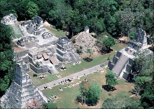
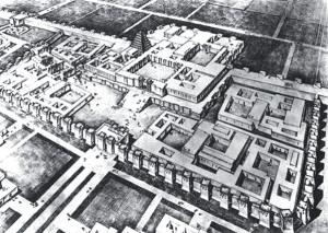
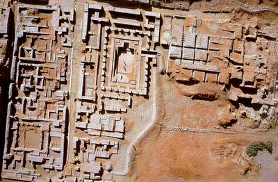
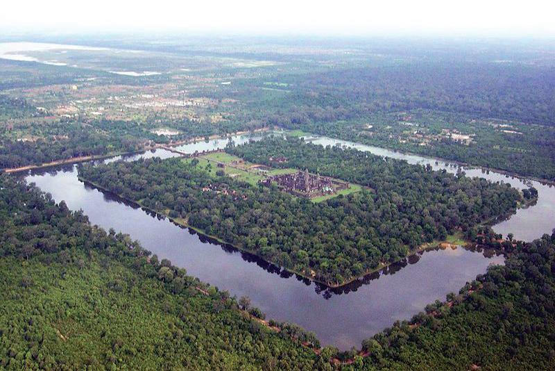
COLLAPSED ORGANIZED MORPHOLOGIES
Image references:
Sketch of Mesopotamian civilization : Alma Luna-Reyes, 10/02/09, Asia: The birthplace of civilization; forumasian.com;
Angkor Wat : Charles J Sharp, Aug 2005, Taken from helicopter above Angkor Wat
Mayan Civilization: http://science.nasa.gov/media/ medialibrary/2009/10/06/06oct_maya_resources/ruins.jpg
Indus Valley Civilization : http://brhectorshistoryworld.blogspot. com/2009/06/indus-valley.html
Mayan Civilization
Mesopotamia
Indus Valley Civilization
Angkor Wat
Design Proposal -
200 -
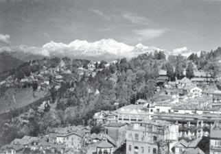
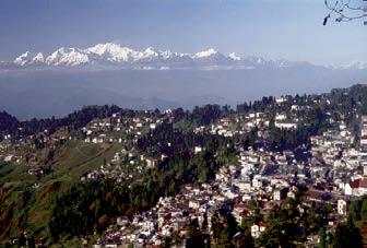
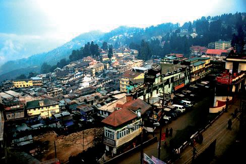
SITE
The site chosen for the design context is the high altitude area of the Northern part of the state of West Begal , India. The relief varies from 100 m above sea level to the mighty Kanchenjunga. The site is situated at the end of the Indo Gangetic plain which is currently experiencing one of the highest rate of population growth in the country, coupled with Urbanization programmes
Located in the Darjeeling district along the Mahananda River, the city of Siliguri forms the commercial hub of North Bengal and is the second largest city after Kolkata, the capital of West Bengal. Located in the base of the Eastern Himalayas, Siliguri forms the gateway into North-eastern India, Sikkim and her neighboring countries like Nepal, Bhutan and Bangladesh. Its strategic location plays a significant role in making it one of the fastest growing cities in India. Siliguri is situated in the eastern extension of the “terai” (hindi, for foothill) region, which is characterized by a belt of marshy grasslands and forests, generally present between the Himalayas and the river plains of Ganga, Brahmaputra and its tributaries.
Historically, Siliguri was a village with primary occupation as agriculture. But over the last century, it has grown to become one of the important centers in trade and commerce, a major tourist destination and an Educational centre. One of the factors that led to this spurt in development was the partition of India in 1947 and creation of Bangladesh in 1971, where Siliguri became one of the major refugee centers.
Due to the unprecedented growth of population in the past decades, there has been a trend for haphazard construction of settlements. This growth has had a direct bearing an in-
creased rate of deforestation. As the Himalayan region consists of relatively recent rock structure, the rapid removal of vegetation, makes the area extremely prone to topsoil run off. Another rising problem related to the land use pattern and the subsequent landslides, is that the terrain of these hilly regions have been interfered increasingly to pave way for vehicular movements. Thus heavy vehicular movement causing vibrations , along with heavy rainfall have been found a prime cause for landslide occurrences.
PROPOSAL
In order to accommodate the increased growth of population and requirements of urbanization, a careful design strategy has to be adopted so that there is minimum interference in the fragile ecology of this region as well as reduce the pressures on environmental resources. Also providing measures for controlled vehicular movements and increased pedestrian considerations is a key strategy in the design logic of the Neighbourhood Patch
References : www.darjeeling.gov.in/geography.html
Siliguri ODP, Govt of India
Fig 1 :(Photo courtesy Edmund Jonah molijonah@013.net)
Fig 2 : http://www.earth.ox.ac.uk/~mikes/sikkimphotos.html
Fig 3 : Photo © Dr. Sean Cridland
Contour map source : Center for Environmental Planning and Technology, Ahmedabad, India
Fig 1 : Darjeeling in the 1950s
Fig 2 : Darjeeling town
- 201Site 01: Darjeeling, India
Fig 3 : Darjeeling town
REGIONS OF HIGHEST DENSITY IN POPULATION
2050 : (Pop Division, UN Secretariat, World Pop prospects, 2009 rev.)
EXPECTED RISE IN URBAN POPULATION IN INDIA : 54.2 %
EXPECTED RISE IN URBAN POPULATION IN STATE OF W. BENGAL ~50%
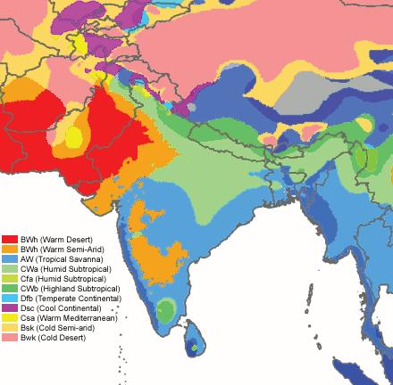
References :
Fig 1 :http://people.eng.unimelb.edu.au/mpeel/koppen.html
Fig 2, fig 3 : Geographic Information Science & Technology Group (GIST), http://www.ornl.gov/sci/knowledgediscovery/ WarGaming/
http://www.censusindia.net/ http://www.unhabitat.org/pmss/Publications.aspx?page=ByT heme&parentcategoryID=630&categoryID=550 http://www.censusindia.gov.in/default.aspx http://www.darjeeling.gov.in/ http://www.darjeeling.gov.in/geography.html
Urban World, Nov 2008, Harmonious cities
20 300 Miles
DARJEELING
Fig 1
RURAL ANNUAL GROWTH RATE : - 1.29% URBAN ANNUAL GROWTH RATE :
%
1.64
Design Proposal - 202 -
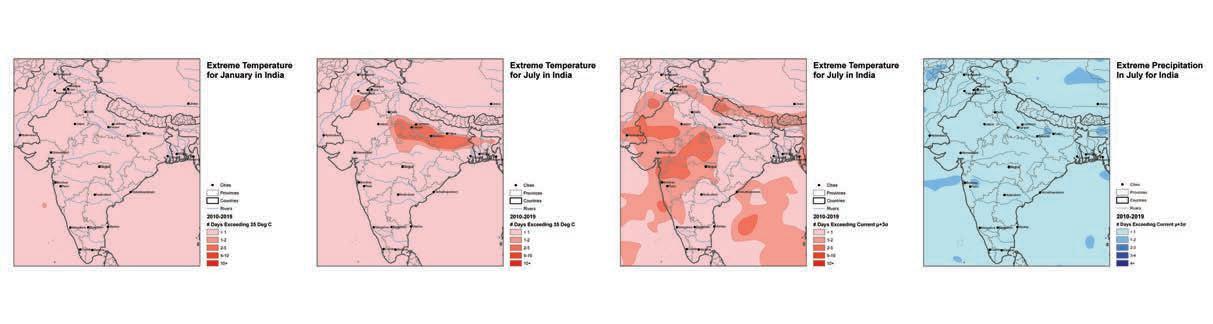
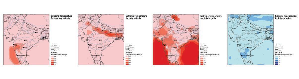
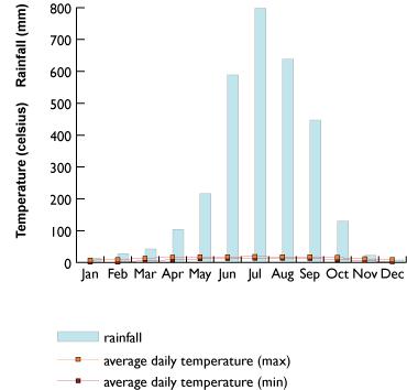
TOTAL AREA : 12. 77 sq.km
AVERAGE ELEV : 2, 050m
LOCATION : LOWER HIMALAYAS
CLIM : Temperate climate
5 Seasons : spring, summer, autumn , winter & Monsoons
Avg Max- min temp : 24.9 - 12 deg C
Avg Rainfall : 309.2cm; 126 days/ year.
POPULATION :
Total : 1, 609, 172
Urban : 520, 432
Density : 8, 548 person/ sq.km
The maximum and minimum average temperatures that this area faces are 24 deg C and 12 deg C respectively, with May to July being the hottest months and December to February being the coldest months. Surrounded by hill stations which are suitable for tea plantations, Darjeeling is also one of the biggest producers and marketers of tea.
Fig 3 : CLIMATE CHANGE PROJECTIONS : 2040 - 2049
Fig 2 : CLIMATE CHANGE PROJECTIONS : 2010 - 2019
210 200 190 180 170 SITE ELEVATION
Fig 4
- 203Site 01: Darjeeling, India
MICROCLIMATIC PERFORMANCE EVALUATIONS:
RUGOSITYDENSITYPOROSITYCOMPACITYCONTIGUITYSINUOSITYOCCLUSIVITYS.ADMITTANCE MINERALIZATN.
Potala 0.2738095240.2683182140.3185654010.1557656390.8127234480.3643327390.2408846110.0028419621
Quito 0.7181753890.7219120730.85654008400.2776107070.3507334080.3141890560.113431360.310960248
HYPOTHESIZED
0.6 0.8 1 1.2 a lues
Montane
0 0.2 0.4 Relative Values 06 0.8 1 1.2 e s
tropical
E MINERALIZAT N. Karaikudi 0146864686 0100488486 0666666667 0363775973 0483085739 0362081691 0150802625 0845051279 002437084 0 0.2 0.4 Relative Values 0.1468646860.1004884860.6666666670.3637759730.4830857390.3620816910.1508026250.8450512790.02437084 Buenos Aires 0.2930221590.30251221200.6349344790 10.25177197100.688164629 1 1.2 Tropical RUGOSITYDENSITYPOROSITYCOMPACITYCONTIGUITYSINUOSITYOCCLUSIVITY S.ADMITTANCE MINERALIZATN 0 0.2 0.4 0.6 0.8 Relative Values RUGOSITY DENSITY POROSITY COMPACITY CONTIGUITY SINUOSITY OCCLUSIVITY SOL.ADMITTANCE MINERALIZATION lower limit 0.8 0.7 0.3 0.3 0.5 0 0.5 0.5 0 mean 0.9 0.75 0.4 0.4 0.6 0.175 0.6 0.6 0.175 upper limit 1 0.8 0.5 0.5 0.7 0.3 0.7 0.7 0.3 0 0.2 0.4 0.6 0.8 1 1.2 Rela ve Values Montane 0.4 0.6 0.8 1 1.2 Rela ve Values Subtropical
QUITO,
Sub
RUGOSITYDENSITYPOROSITYCOMPACITYCONTIGUITYSINUOSITYOCCLUSIVITYS.ADMITTANC
POTALA, TIBET
EQUADOR EXISTING MONTANE CITIES:
FOR HIGH
Design Proposal - 204 -
VALUE RANGE
MICROCLIMATIC PERFORMANCE:
SPATIAL
MICROCLIMATIC
CULTURE
ADMISTRATION
RUGOSITY
POROSITY
DENSITY
COMPACITY
CONTIGUITY
SINUOSITY
OCCLUSIVITY
SOLAR ADMITTANCE
MINERALIZATION
DESIGN PARAMETERS:
TOPOGRAPHY 1:8 X
Spatial criteria: The mountainous terrain is considered as the priority in the case of Darjeeling. As adopted from evolved cities, the natural contour is used as a guide for street network. Thus the setting up of a system that determines the best suitable street pattern, while maintain a slope ratio of 1:8 is the primary goal.
Microclimatic criteria: From the inferences, it can be concluded that the most important factor in a mountainous region is the wind. These areas of high altitude are subject to strong winds. Thus a morphology, that lowers the wind speed – this can be achieved by increasing the undulation of the top surface of the fabric, thus a high variation in the heights of buildings. This approach should increase the value of rugosity , and also the density.
Variation in height may reduce the wind speed at the top surface of the fabric. However this does not avoid the channeling of winds through the patch. In order to avoid this phenomenon a lower value of sinuosity is aimed at.
Apart from these indicators, it is also evident from the site conditions that top soil erosion is a common problem. This situation can be reduced by having a lower value of mineralization, in other words, having a high level of vegetation and ground cover.
DIFFERENTIAL HT, THERE BY INCREASING THE ROOF LEVEL ROUGHNESS.
HIGH % OF LAND COVER
MINERALIZATN. 0.7181753890.7219120730.85654008400.2776107070.3507334080.3141890560.113431360.310960248 MINERALIZAT 002437084 10.25177197100.688164629 MINERALIZATN 0.2871287130.2976273550.4535864980.4939078960.6632635940.4287108280.4432861680.104781910.765201941
- 205Site 01: Darjeeling, India
STREET GROWTH STRATEGY
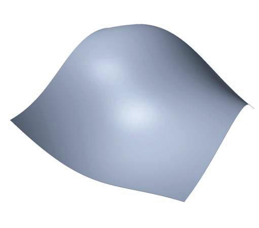
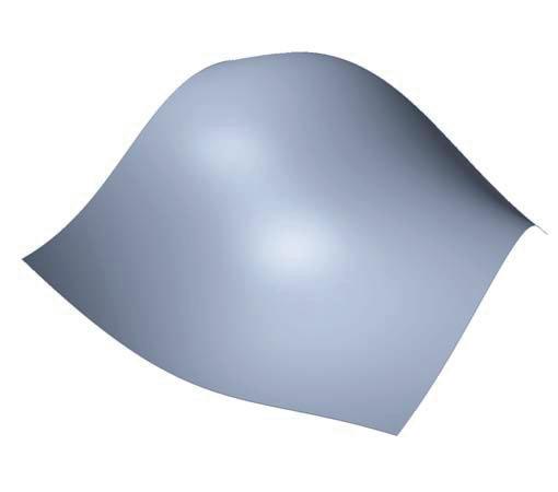
Direction
Search Radius
Horizontal Vector
Favourable Vector
D : Favourable slope angle
x : Search Radius
SUCCESSFUL PATHS
STREETS AND ISLANDS
B A x D Iteration 0 B A x D A’ Iteration 1
Design Proposal - 206 -
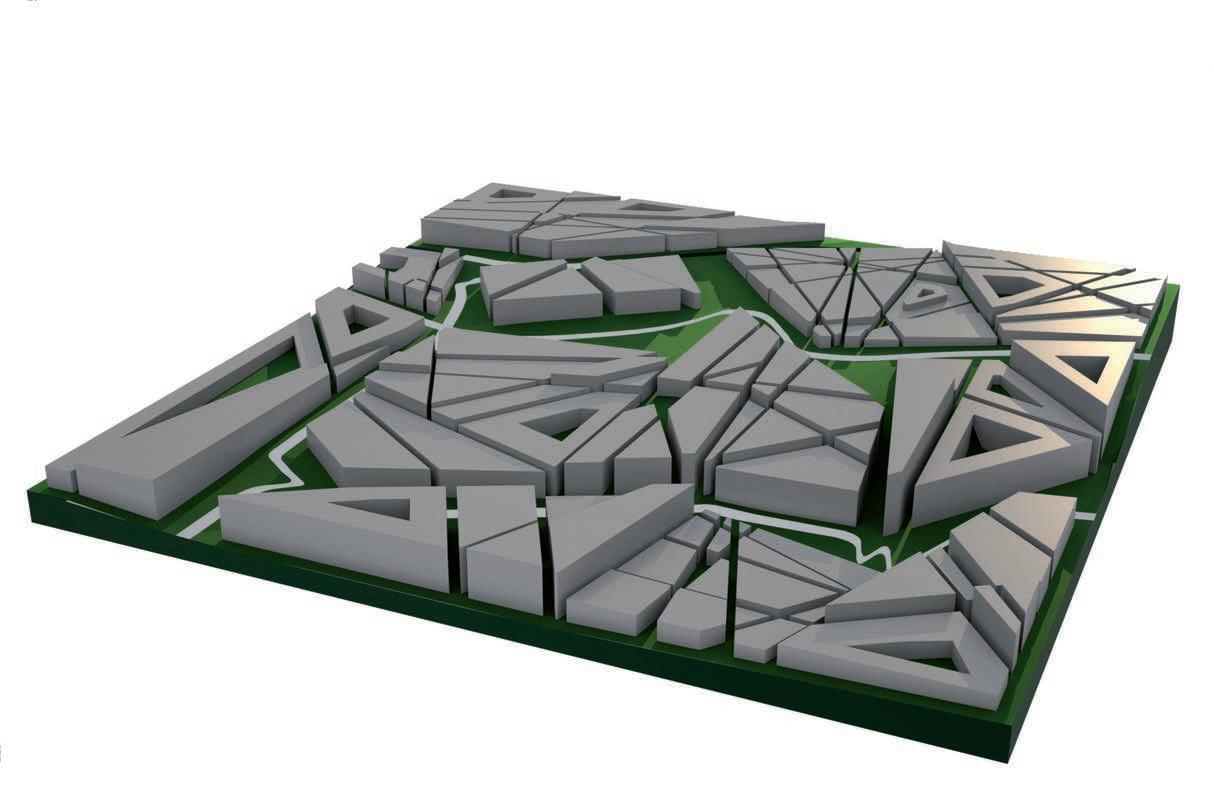
THE NEIGHBOURHOOD
The aim is to start the set up of an urban fabric, and thus proposing morphological principles that would help in maximizing the sensitivity of environmental responses.
Plot size:
An exact measurement of what makes an area, a neighbourhood is not defined. Using perceptive sense with respect to time in movement as a measure of extents, a neighbourhood can thus be described as a walking distance of 20 mins Considering an average of 1 km as the distance coverable by foot in 20 min, a plot size of 750m X 750m is chosen as a “Neighbourhood Patch’. The pedestrian is thus a plays a key role as an urban design driver.
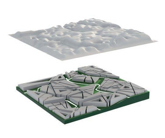
Distribution of building usage and a deliberate irregularity in their heights would offer a highly undulated top surface forthe urban fabric, that would reduce the effect of strong winds, a common problem faced in areas of high altitude.
LOW RISE RESIDENTIAL AVG BUILDING HT : 3-9m INTERIOR STREET WIDTH: 1.8-3m 170m 210m LOW RISE PUBLIC/ SEMI PUBLIC AVG BUILDING HT : 6-12m INTERIOR STREET WIDTH: 3-5m
RISE MIXED USE AVG BUILDING HT : 9-30m INTERIOR STREET WIDTH: 2.5-6m LOW RISE MIXED USE AVG BUILDING HT : 3-9m INTERIOR STREET WIDTH: 1.8-3m 750m 750m
HIGH
- 207Site 01: Darjeeling, India
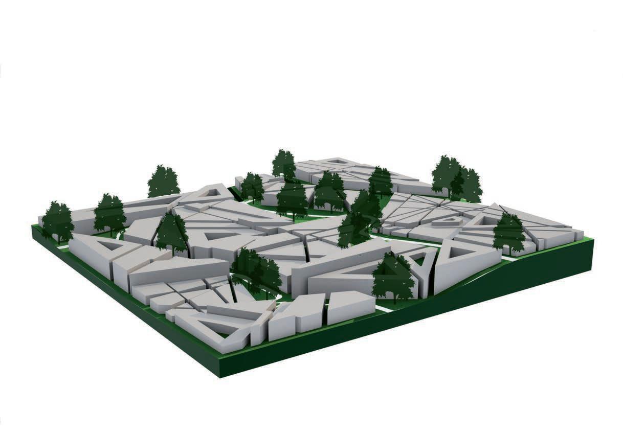
RUGOSITY DENSITY POROSITYCOMPACITYCONTIGUITYSINUOSITYOCCLUSIVITYSOL.ADMITTANCEMINERALIZATION lower limit 0.8 0.7 0.3 0.3 0.5 0 0.5 0.5 0 mean 0.9 0.75 0.4 0.4 0.6 0.175 0.6 0.6 0.175 upper limit 1 0.8 0.5 0.5 0.7 0.3 0.7 0.7 0.3 0 0.2 0.4 0.6 0.8 1 1.2 Rela ti ve Values Montane 0.537 0.76552 0.3261 0.4462
PERFORMANCE Design Proposal - 208 -
MORPHOLOGICAL
Site 02: Kinshasa, Democratic Republic of the Congo
Kinshasa has been selected as a site to test the development of a bio-climatic design approach to urban planning based on the research on urban growth prospects within the next forty years; refer to page 20 for more information.
Africa is the fastest urbanizing continent in the world and will in 2030 cease being predominantly rural (Un Habitat, 2010). Up to 2020 Kinshasa will be the fastest growing city in absolute numbers and will undergo enormous urban growth. Currently the growth rate is at 8km² per year.
The rapid expansion of the city is mostly chaotic and uncontrolled. This leads in many areas to urban sprawl and urban morphologies that will impose massive problems onto the city. Long travel distances as well as the dimension of infra-structural networks will result in much higher energy demands that can lead to collapse. In addition, the tendency of rapid expansion lacks the incorporation of urban structure; public spaces for recreation and local centres that serve the population are mostly missing. This will not only have an impact on the quality of the urban fabric, but can also result in social and cultural problems. The 2010 UN Habitat report states that in 2005 there were no affordable plots of land available within a radius of 40 to 50 km from central Kinshasa.
Urban problems, as witnessed in Kinshasa, demand the implementation of clear planning strategies that work against the current tendencies of urbanization. As much as it is arguable how such strategies could be implemented it is important to address the problems and to develop urban planning concepts that work against otherwise inescapable collapse or dispersal.
In the following chapter the city of Kinshasa will be introduced and evaluated in terms of its climate; growth prospects as well as possible climatic changes over the next four decades will be analysed.
- 209Site 02: Kinshasa, Democratic Republic of the Congo
River Congo
Settlement Sample 02
Refer to page 254
Settlement Sample 01
Refer to page 254
Kinshasa (formerly Léopoldville) is located on the river Congo, at the western edge of central Africa. It is the capital and largest city of the Democratic Republic of the Congo. In 2009 the urban area of Kinshasa had a population of 10,076,099 inhabitants (Source: Wikipedia). It is one of Africa’s four mega-agglomerations and will experience the biggest urban growth in absolute numbers until the year 2020. Together with Brazzaville, located on the opposite side of the river, Kinshasa has nearly 12 million inhabitants - making it the most populous trans-border metropolitan region in the world. Flanked by the river and a large area of swamp most urban expansion is currently taking place towards the south-east.
According to the ‘Koeppen-Geiger’ climate classification Kinshasa is located in the tropical climate zone. Temperatures are in their midtwenties throughout the year. The humidity is relative high at around 80% all year round. Radiation and precipitation patterns are roughly correlated, showing a drop during the summer months (Refer to page 211 for more information). According to recent climate models no major shift in terms of the climate zone is to be expected during the next four decades (Refer to page 212 following); even though some models predict a shift in the monsoon pattern that could affect the region.
210 -
Kinshasa
Brazzaville
Swamp
1km5km
Design Proposal
-
Wind direction WSW WSW WSW WSW WSW WSW WSW WSW WSW WSW WSW WSW
Weather Data Kinshasa; Source: M. Müller, 1983: Handbuch ausgewählter Klimastationen der Erde. Universität Trier.
Jan 1* 2* 3* 4* 5* 40 200 190 180 170 160 150 140 130 120 110 100 500 480 460 440 420 400 380 360 340 320 300 30 20 10 FebMarAprMayJunJulAugSepOctNovDez JanFebMarApr May JunJul Aug Sep Oct NovDez JanFebMarAprMay Jun Jul AugSepOctNovDez 1* 1* 1* Jan 100 90 80 70 60 50 40 30 20 10 0 FebMarAprMayJunJulAugSepOctNovDez 500 400 300 200 100 0 JanFebMarAprMayJunJulAugSepOctNovDez Air Temperature (°C): 1* Mean Air Temperature 2* Mean Maximum Air Temperature 3* Mean Minimum Air Temperature 4* Absolute Maximum Air Temperature 5* Absolute Minimum Air Temperature Precipitation (mm): 1* Mean Precipitation 2* Maximum Precipitation 3* Minimum Precipitation 4* Maximum Precipitation in 24 hrs Humidity (%): 1* Mean Relative Humidity Radiation (Ly/d): 1* Mean Relative Humidity Mean Sunshine (hrs): 1* Mean Sunshine hrs 1* 2* 3* 4* Parameter Jan Feb Mar Apr May Jun Jul Aug Sep Oct Nov Dec Year Mean air temperature (°C) 26.0 26.2 26.7 26.8 26.0 23.4 22.0 23.3 25.6 26.2 26.1 25.9 25.3 Mean maximum air temperature (°C) 30 31 31 32 30 28 27 28 30 30 30 30 30 Mean minimum air temperature (°C) 22 22 22 22 22 19 17 18 20 22 22 22 21 Absolute maximum air temperature (°C) 34 35 35 34 34 33 32 34 36 35 34 33 36 Absolute minimum air temperature (°C) 18 19 19 20 19 15 13 11 16 17 19 20 11 Mean relative humidity (%) 82 80 80 82 83 81 76 69 69 76 81 83 79 Mean precipitation (mm) 128 139 181 209 134 5 1 4 33 137 236 171 1378 Maximum precipitation (mm) 321 330 429 379 280 38 34 24 100 282 348 327 1824 Minimum precipitation (mm) 2 49 58 59 22 0 0 0 2 20 84 47 1124 Maximum precipitation in 24 hrs (mm) 128 105 108 131 111 29 34 24 73 155 147 73 155 Days with precipitation 10 10 13 15 11 1 0 1 4 11 16 14 106 Mean sunshine (hrs) 132 134 150 166 140 139 125 146 129 132 142 135 1670 Radiation (Ly/d) 385 427 448 445 374 332 319 364 375 381 418 380 387 Potential evaporation (mm) 130 122 141 136 131 94 76 86 110 131 122 130 1409 Mean wind speed (m/s) 1.1 1.4 1.1 1.1 1.1 1.1 1.4 1.7 1.4 1.4 1.4 1.1 1.4
- 211Site 02: Kinshasa, Democratic Republic of the Congo
GROUP A: Tropical/megathermal climates pronounced dry season, with dry months having precipation less than 60mm and also less than (100-[total annual precipation{mm}/25])
*projected using IPCC A1FI Tyndall SC 2.03 temperature and precipitation snenarios.
http://koeppen-geiger.vu-wien.ac.at
Main Climates Precipitation Temperature
A: equatorial W: desert h: hot arid
B: arid S: steppe k: cold arid
C: warm temperate f: fully humid a: hot summer
F: polar frost T: polar tundra Projected Cllimate Change: Period 2001 to 2025*
D: snow s: summer dry b: warm summer
E: polar w: winter dry c: cool summer m: monsoonal d: extremely continental
0 AfAmAsAwBWkBWhBSkBShCfaCfb CfcCsaCsbCscCwa 20 -20 40 60 Cwb Cwc Dfa DfbDfc DfdDsaDsbDscDsdDwaDwbDwcDwdEFET 0 10 -10 -20 -30 -40 20 30 40
Kinshasa
Design Proposal - 212 -
Projected Cllimate Change: Period 2026 to 2050*
GROUP A: Tropical/megathermal climates pronounced dry season, with dry months having precipation less than 60mm and also less than (100-[total annual precipation{mm}/25])
*projected using IPCC A1FI Tyndall SC 2.03 temperature and precipitation snenarios.
http://koeppen-geiger.vu-wien.ac.at
Main Climates Precipitation Temperature
A: equatorial W: desert h: hot arid
B: arid S: steppe k: cold arid
C: warm temperate f: fully humid a: hot summer
D: snow s: summer dry b: warm summer
E: polar w: winter dry c: cool summer m: monsoonal d: extremely continental
F: polar frost T: polar tundra
0 AfAmAsAwBWkBWhBSkBShCfaCfb CfcCsaCsbCscCwa 20 -20 40 60 Cwb Cwc Dfa DfbDfc DfdDsaDsbDscDsdDwaDwbDwcDwdEFET 0 10 -10 -20 -30 -40 20 30 40
Kinshasa
- 213Site 02: Kinshasa, Democratic Republic of the Congo
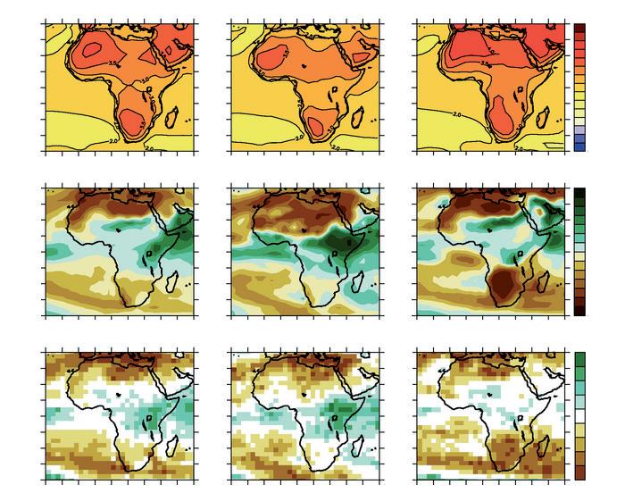
Temperature and precipitation changes over Africa from the MMD-A1B simulations. Top row: Annual mean, DJF (Summer)and JJA (Winter) temperature change between 1980 to 1999 and 2080 to 2099, averaged over 21 models. Middle row: same as top, but for fractional change in precipitation. Bottom row: number of models out of 21 that project increases in precipitation.
Temp
(°C) Prec
(%) Num of Models > 0 40°N 40°N 40°N 40°N 40°N 40°N 40°N 40°N 40°N 10°C 7 5 4 3.5 2.5 2 1.5 1 0.5 0 -0.5 -1 50% 30 20 15 10 5 0 -5 -10 -15 -20 -30 -50 21 Models 19-20 17-18 14-18 14-16 8-13 5-7 3-4 1-2 0 Annual DJF JJA 20°W 20°W 20°W 20°W 20°W 20°W 20°W 20°W 20°W 20°E 20°E 20°E 20°E 20°E 20°E 20°E 20°E 20°E 40°E 40°E 40°E 40°E 40°E 40°E 40°E 40°E 40°E 60°E 60°E 60°E 60°E 60°E 60°E 60°E 60°E 60°E 0° 0° 0° 0° 0° 0° 0° 0° 0° 20°N 20°N 20°N 20°N 20°N 20°N 20°N 20°N 20°N 20°S 20°S 20°S 20°S 20°S 20°S 20°S 20°S 20°S 40°S 40°S 40°S 40°S 40°S 40°S 40°S 40°S 40°S 0° 0° 0° 0° 0° 0° 0° 0° 0° Design Proposal - 214 -
Response
Response
‘In 2005, the urbanised area of Kinshasa extended over more than 500 km2, expanding by 8 km2 every year and almost exclusively by dint of illicit, informal, ‘self-help’ urbanization. Far from being ‘anarchic’, as often claimed, occupation follows an orthogonal urban pattern inherited from the colonial period. Plots are relatively large, at 300 to 500 m2, while the built-up areaoften with fairly good quality construction - does not exceed 100
Kinshasa Urban Growth 2010 - 2050 (Scenario01):
2010 Urban Area: 540km2*
2025 Urban Area**: 660km2
2050 Urban Area**: 860km2
2010 Density: 8.754.000/540km2 = 16.211 person/km2
2025 Density: 15.041.000/660km2**= 22.789 person/km2
2050 Density: 24.890.000***/860km2**= 28.941 person/km2
* Urban Area 2005 (500km²) + 5*8km² = 540km²
** Assuming the current growth rate of 8km² per year
*** Assuming (hypothetical) linear growth rate at 403.000 people a year (urban increase 2010-2020 is projected at 4.034.000 person/year)
Source: UN-Habitat, The State of African Cities 2010
Kinshasa Urban Growth 2010 - 2050 (Scenario02):
2010 Urban Area: 540 km2*
2025 Urban Area**: 928 km2
2050 Urban Area***: 1535 km2
2010 Density: 8.754.000/540 km² = 16.211 person/km²
2025 Density**: 15.041.000/928 km² = 16.211 person/km²
2050 Density**: 24.890.000***/1535 km² = 16.211 person/km²
* Urban Area 2005 (500km²) + 5*8km² = 540km²
** Assuming 2010 density: 8.754.000/500km2 = 16.211 person/km2
***
Assuming (hypothetical) linear growth rate at 403.000 people a year (urban increase 2010-2020 is projected at 4.034.000 person/year)
Source: UN-Habitat, The State of African Cities 2010
m2. This results in urban sprawling, with low densities (between one and five individuals per 100 m2) (Flouriot. 2005). In 2005, no affordable plots (i.e., between US $300 and 500) were available within a radius of 40 to 50km from central Kinshasa. Subserviced plots of 750m2 located 20km away from the city centre would still cost about US $1,000 (Flouriot, 2010)’ (UN-Habitat, The State of African Cities 2010).
River Congo Swamp 22.36km 8km² 2km 2050 2025 2010 2050 2025 2010 Brazzaville River Congo Swamp 22.36km 8km² 2km Kinshasa 540 km² 660 km² 860 km² Kinshasa 540 km² 928 km² 1535 km²
Brazzaville
-
Site 02: Kinshasa, Democratic Republic of the Congo
215 -
Area:
City/Province = 9965km² (Density 878 person/km²)
Residential Land = 600km² (Density 14590 person/km²)
Wikipedia states a density of 955 person/km²
Density
Hong Kong, China 220 29,400
Macau, China 23 23,350
Beijing, China 4300 4300
Shanghai, China 2396 5700
Singapore 479 8350
Manila, Philippines 1425 13,450
Mumbai, India 777 21,900
Delhi, India 1425 10,700
Tokyo-Yokohama 7835 4350
Sydney, Australia 1788 2050
Urban area and density: Comparison of major
Kinshasa Urban Growth 2010 - 2050 (Scenario03):
2010 Urban Area: 600 km2*
2025 Urban Area**: 1031 km2
2050 Urban Area**: 1706 km2
2010 Density: 8.754.000/600 km² = 14.590 person/km²
2025 Density**: 15.041.000/1031km² = 14590 person/km²
2050 Density**: 24.890.000***/1706 km² = 14590 person/km²
* Assumption based on various references
** Assuming 2010 density: 8.754.000/600km2 = 14.590 person/km2
*** Assuming (hypothetical) linear growth rate at 403.000 people a year (urban increase 2010-2020 is projected at 4.034.000)
Source: UN-Habitat, The State of African Cities 2010
Urban Density
Tehran, Iran 635 12,300
Cairo, Egypt 1269 12,800
Sao Paulo, Brazil 2590 7200
Paris 3043 3400
London 1623 5100
Berlin 984 3750
New York 11,264 1750
San Francisco-San Jose 2497 2150
Toronto, Canada 2500 2500
Mombassa, Kenya 57 14,050
(Source: demographia.com)
Brazzaville River Congo Swamp 22.36km 8km² 2km 2050 2025 2010 540 km² 600 km² 1031 km² 1706 km²
City Urban Area
Urban Density (person/km
)
Kinshasa Urban
(km²)
²
City Urban Area (km²) Urban Density (person/km²)
cities
Design Proposal - 216 -
global
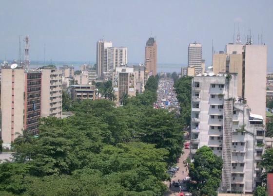
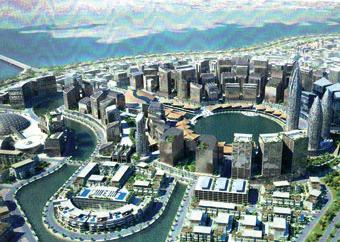
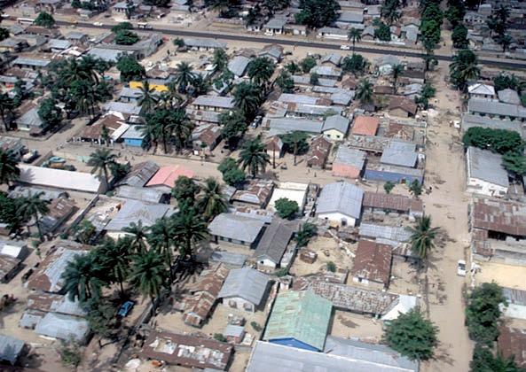
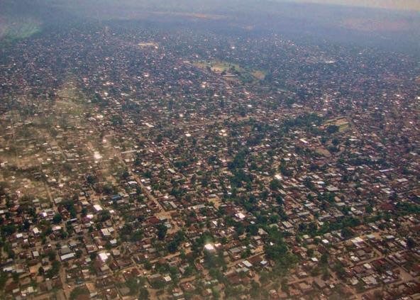
Impressions of Kinshasa. Top left: Central Kinshasa; some of the old, colonial parts are characterized by high-rise developments and to some degree reflect western urban standards. Top right: ‘City of the River Congo’; the developer proposal for a 25th township is welcomed by the Minister of Decentralization and Regional Planning, Antipas Mbusa Nyamwisi. Bottom row: The reality; urban sprawl characterizes the urban development on the periphery of the city. Slums and informal settlements are proliferating in areas that are not claimed by customary or other owners and are, mostly, unsuitable for urbanization (UN Habitat, 2010).
- 217Site 02: Kinshasa, Democratic Republic of the Congo
Design Proposal
Bio-Climatic Urbanism - Kinshasa
Implementation of the algorithm as described on page 185 soon results in unforeseen struggles; these are mainly a consequence of computational problems.
The algorithm is refined to produce four different kinds of typologies; a single family house typology, a multi-storey town house typology, a multi-storey apartment block typology and a high-rise apartment block typology (Compare previous chapter). In other words, the type of urban layout is incorporated into the genome of each individual with the idea that a certain typology would be selected and optimized over time.
Including more detailed urban form into the algorithm, however, imposes a manifold increase in computation. Even before complex evaluation parameter, such as porosity or solar admittance (which in themselves were quite time consuming to calculate), are added to the algorithm it is realized that the computational process would become to slow and time-consuming. The system would simply crash.
In order to test the initial concept of evaluating urban layouts against the performance of evolved and planned cities from the same climate zone the strategy is revised. The algorithm allows the rapid creation of distinct urban morphologies. Since running these over multiple generations is not possible, it is decided to create families of urban typologies in a ‘one by one’ process. The evaluation parameter are then determined in a subsequent process, which allows, at least, to evaluate different morphologies against each-other and to evaluate which ones are most suitable in micro-climatic aspects for the selected climate zone, i.e. the
tropical climate.
In this fashion, as a first step, target values for the tropical climate zone are determined by evaluating the cities Malaka and Bangkok (page 220). Subsequently, four different families of urban patches are created and evaluated against the calculated target values:
• Single Family Houses (page 221)
• Multi-Storey Town Houses (page 225)
• Multi-Storey Apartment Blocks (page 229)
• High-Rise Apartment Blocks (page 233)
As described in the previous chapter, the fitness is then calculated by measuring the deviation from the set target values. Evaluation of the overall fitness of the four typologies reveals that the single family house type as well as the multi-storey town house type are the ones that perform closest to the selected reference cities Malaka and Bangkok.
- 219Bio-Climatic Urbanism - Kinshasa
Calculation of Target Values; Climate Zone: Tropical
In order to test the design approach described in the Design Development chapter (page 185), six reference indicator are calculated from the Cities Malaka (Malaysia, evolved) and Bangkok (Thailand, planned). The data is subsequently used for the evaluation of different urban typologies in the attempt to determine which urban layout is best suited in microclimatic terms. For each indicator a deviation range of ± 10% is established; if a value falls within this range it is considered ‘on target’. The greater the deviation from the range in both directions the less is the fitness for that parameter.
50m 2.14* 1.47* 0.26 4.16 6.72 0.10 1.29 3.86 4.16 1.39 0.12 1.77 0 1 2 3 4 5 6 7 [/] 100m 500m 25m50m 250m OcclusitivityContiguityCompacitySolar AdmittanceDensity Rugosity
Malaka
Bangkok
Bangkok (Planned City)
Parameter Malaka Bangkok Target Value Deviation(±10%) Target Value Deviation(±10%) Density 1.39 1.251/1.529 1.29 1.161/1.419 Rugosity 4.17 3.753/4.587 3.86 3.474/4.246 Compacity 416.08 374.47/457.69 672.18 604.962/739.398 Contiguity 0.27 0.24/0.30 1.77 1.593/1.947 Occlusitivity 147034.44 132331/161737.88 214232.66 192809.394/235655.926 Solar Admittance 0.1 0.09/0.11 0.13 0.177/0.143
Melaka (Evolved City)
Design Proposal - 220 -
Single Family House Population
Single Family Houses_Morphological Parameter
*possible angle of street orienation in degrees
Parameter set for the creation of a single family house population. Different street widths, as well as lot widths and depths are set. In addition street directions are in some cases restricted; they range from totally random to orthogonal layouts.
Individual01 Single Family Houses Parameter Value Density 0.62 Rugosity 1.87 Compacity 1220.94 Contiguity 0 Occlusitivity 30764.03 Solar Admittance 0.05 Individual03 Single Family Houses Parameter Value Density 1.43 Rugosity 4.29 Compacity 1619.36 Contiguity 0 Occlusitivity 38100.97 Solar Admittance 0.15 Individual02 Single Family Houses Parameter Value Density 0.69 Rugosity 2.06 Compacity 1526.91 Contiguity 0 Occlusitivity 30078.29 Solar Admittance 0.05 Individual04 Single Family Houses Parameter Value Density 1.28 Rugosity 3.84 Compacity 1298.16 Contiguity 0 Occlusitivity 39974.63 Solar Admittance 0.15
individual min. block offset max. block offset min building height max building height lot depth lot width street width offset street orientation* Individual01 5m 8m 6m 9m 10m 7.5m 5m 1m 45/90/135/180 Individual02 5m 6m 6m 9m 11m 6m 5m 1m 45/90/135/180 Individual03 3m 4m 6m 12m 13m 6m 5m 0.5m 45/90/135/180 Individual04 4m 6m 6m 9m 13m 6m 4m 0.5m 0/90 Individual05 4m 6m 6m 9m 13m 10m 3m 2m 0/90 Indiviudal06 5m 7m 6m 9m 13m 10m 3m 1m 30/60/90/120.. Individual07 5m 6m 6m 9m 8m 8m 3m 0.5m 30/60/90/120 Individual08 5m 6m 6m 9m 8m 8m 3m 0.5m random Individual09 5m 6m 9m 15m 12m 12m 3m 1m random Individual10 5m 6m 9m 15m 12m 10m 3m 1.5m random
- 221Bio-Climatic Urbanism - Kinshasa
Individual05 Single Family Houses Parameter Value Density 0.61 Rugosity 1.83 Compacity 690.21 Contiguity 0 Occlusitivity 37290.91 Solar Admittance 0.05 Individual07 Single Family Houses Parameter Value Density 0.94 Rugosity 2.82 Compacity 1640.77 Contiguity 0 Occlusitivity 29687.68 Solar Admittance 0.05 Individual09 Single Family Houses Parameter Value Density 1.67 Rugosity 5.00 Compacity 1113.76 Contiguity 0 Occlusitivity 40146.21 Solar Admittance 0.15 Individual06 Single Family Houses Parameter Value Density 1.12 Rugosity 3.35 Compacity 1045.05 Contiguity 0 Occlusitivity 40785.50 Solar Admittance 0.05 Individual08 Single Family Houses Parameter Value Density 0.79 Rugosity 2.36 Compacity 1464.8 Contiguity 0 Occlusitivity 30670.37 Solar Admittance 0.05 Individual10 Single Family Houses Parameter Value Density 1.18 Rugosity 3.54 Compacity 1111.96 Contiguity 0 Occlusitivity 35436.21 Solar Admittance 0.05 Design Proposal - 222 -
*value within target range
Fitness (Single Family Houses): Density and Rugosity parameters show different fitness values, whereas compacity, contiguity and occlusitivity are all in the same range.
Absolute values (Single Family Houses) compared to target values (Malaka) -
-
average density ind.10 ind.03 ind.04 ind.06 ind.09 ind.07 ind.08 ind.02 ind.01 ind.05 10 [/] [/] 8 6 4 2 0 0 3 6 9 12 15 rugosity compacity occlusitivity contiguity solar admittance density rugosity compacity occlusitivitycontiguity solar admittance average 1.03 3.096 12.73 3.53 0.00 0.08 malaka 1.39 4.16 4.16 1.47 0.26 0.26 Deviation from Target Values&Fitness: Single Family Houses density dev. density fitness rug. dev. rug. fitness comp dev. cont. fitness cont. dev. cont. fitness occl. dev. occl. fitness solar. dev. solar. fitness Ind.01 0.63 2.22 1.88 2.22 763.25 0.55 0.24 1.12 101566.97 1.44 0.85 0.12 Ind02 0.69 2.5 1.69 2.44 1069.22 0.39 0.24 1.12 102252.71 1.42 0.85 0.12 Ind.03 (0.01) * 142.85 (0.01) * 500 1161.67 0.36 0.24 1.12 94230.03 1.56 0.04 2.5 Ind.04 (0.01) * 142.85 (0.01) * 500 840.47 0.5 0.24 1.12 92356.37 1.59 0.04 2.5 Ind.05 0.64 2.17 1.92 2.17 232.52 1.79 0.24 1.12 95040.09 1.54 0.85 0.12 Ind.06 0.13 11.11 0.4 10 587.37 0.71 0.24 1.12 91545.5 1.61 0.85 0.12 Ind.07 0.31 4.55 0.93 4.55 1183.09 0.35 0.24 1.12 102643.32 1.42 0.85 0.12 Ind.08 0.46 3.03 1.39 3.03 1007.12 0.41 0.24 1.12 101660.63 1.45 0.85 0.12 Ind.09 0.14 10 0.41 10 656.08 0.63 0.24 1.12 92184.79 1.59 0.04 2.5 Ind.10 0.07 20 0.21 20 654.27 0.64 0.24 1.12 96894.79 1.52 0.85 0.12
223
Bio-Climatic Urbanism - Kinshasa
ind.01ind.02ind.03ind.04ind.05ind.06ind.07ind.08ind.09ind.10
Population: Single Family Houses; Comparison of different fitness assessment combinations
1: Average Fitness: Density, Rugosity, Compacity, Contiguity, Occlusitivity, Solar Admittance
2: Average Fitness: Density, Rugosity, Compacity
3: Average Fitness: Compacity, Contiguity, Occlusitivity, Solar Admittance
4: AVerage Fitness: Density, Solar Admittance
Average Fitness: Density, Rugosity, Compacity, Contiguity, Solar Admittance
ind.01ind.02ind.03ind.04ind.05ind.06ind.07ind.08ind.09ind.10
Population: Single Family Houses; Fitness
Population sorted according to Fitness
2 0 1 3 4 5 6 7 8 2 4 6 8 10 12 2 1 3 4
1.25 1.31 4.804.82 1.47 4.39 2.14 1.54 4.85 6.38 [/] [/]
1) Individual10 5) Individual06 6) Individual07 7) Individual08 8) Individual05 2) Individual09 3) Individual04 4) Individual03
Design Proposal - 224 -
Storey Town-Houses_Morphological Parameter
*possible angle of street orienation in degrees
Parameter set for the creation of a multi storey town-house population. Different street widths, as well as lot widths and depths are set. In addition street directions are in some cases restricted; they range from totally random to orthogonal layouts. Multi Storey Town-House Population
Individual01 Multi Storey Town-Houses Parameter Value Density 2.40 Rugosity 7.14 Compacity 777.32 Contiguity 2.13 Occlusitivity 37916.74 Solar Admittance 0.15 Individual03 Multi Storey Town-Houses Parameter Value Density 2.62 Rugosity 7.85 Compacity 518.57 Contiguity 1.81 Occlusitivity 47118.6 Solar Admittance 0.24 Individual02 Multi Storey Town-Houses Parameter Value Density 2.36 Rugosity 7.07 Compacity 712.85 Contiguity 1.1 Occlusitivity 39894.3 Solar Admittance 0.15 Individual04 Multi Storey Town-Houses Parameter Value Density 1.90 Rugosity 5.71 Compacity 404.62 Contiguity 1.12 Occlusitivity 47594.73 Solar Admittance 0.15
individual min. block offset max. block offset min building height max building height building depth building width street width offset street orientation* Individual01 5m 8m 9m 18m 12m 4.5m 5m - random Individual02 5m 10m 12m 18m 10m 8m 5m - random Individual03 5m 10m 9m 18m 14m 7.5m 7m - random Individual04 6m 10m 12m 18m 12m 10m 7m - 30/60/90/120 Individual05 6m 10m 12m 15m 12m 6.5m 5m - 30/60/90/120 Indiviudal06 6m 10m 12m 15m 10m 4.5m 6m - 0/90 Individual07 6m 8m 12m 21m 12m 6m 4.5m - 0/90 Individual08 5m 6m 12m 21m 12m 4.5m 4m - 45/90/135/180 Individual09 5m 7m 9m 12m 15m 6m 5m - 45/90/135/180 Individual10 6m 8m 12m 18m 10m 10m 6m - 45/90/135/180
Multi
- 225Bio-Climatic Urbanism - Kinshasa
Individual05 Multi Storey Town-Houses Parameter Value Density 1.67 Rugosity 5.02 Compacity 512.21 Contiguity 1.46 Occlusitivity 41916.52 Solar Admittance 0.15 Individual07 Multi Storey Town-Houses Parameter Value Density 2.07 Rugosity 8.11 Compacity 678.48 Contiguity 1.56 Occlusitivity 39670.35 Solar Admittance 0.24 Individual09 Multi Storey Town-Houses Parameter Value Density 2.57 Rugosity 7.71 Compacity 551.25 Contiguity 2.04 Occlusitivity 44496.74 Solar Admittance 0.24 Individual06 Multi Storey Town-Houses Parameter Value Density 1.82 Rugosity 5.46 Compacity 786.26 Contiguity 1.72 Occlusitivity 32961.37 Solar Admittance 0.15 Individual08 Multi Storey Town-Houses Parameter Value Density 3.82 Rugosity 9.84 Compacity 931.46 Contiguity 2.02 Occlusitivity 36842.01 Solar Admittance 0.24 Individual10 Multi Storey Town-Houses Parameter Value Density 2.04 Rugosity 6.12 Compacity 526.32 Contiguity 0.82 Occlusitivity 46322.67 Solar Admittance 0.15 Design Proposal - 226 -
*value within target range
Fitness (Multi Storey Town Houses): Besides contiguity and occlusitivity, there is a much broader distribution of values within parameters, compared to the Single Family House population.
Absolute values (Multi Storey Town-Houses) compared to target values (Malaka); the curves roughly correspond in shape.
average ind.05 ind.06 ind.04 ind.02 ind.01 ind.09 ind.03 ind.07 ind.08 ind.10 10 [/] 8 6 4 2 0 [/] 0 1 2 3 4 5 6 7 8 density rugosity compacity occlusitivity contiguity solar admittance density rugosity compacity occlusitivitycontiguity solar admittance average malaka 1.39 2.36 7.00 6.39 4.14 1.58 0.19 4.16 4.16 1.47 0.26 0.26 Deviation from Target Values&Fitness: Multi Storey Town-Houses density dev. density fitness rug. dev. rug. fitness comp dev. cont. fitness cont. dev. cont. fitness occl. dev. occl. fitness solar. dev. solar. fitness Ind.01 0.87 1.59 2.55 1.64 319.64 1.3 1.83 0.15 94414.26 1.56 0.85 0.12 Ind02 0.83 1.69 2.48 1.69 255.16 1.64 0.8 0.34 92436.7 1.59 0.85 0.12 Ind.03 1.09 1.28 3.26 1.28 60.88 6.66 1.51 0.18 85212.4 1.67 0.04 2.5 Ind.04 0.37 3.7 1.12 3.7 (0.01)* 500 0.82 0.33 84736.27 0.58 0.04 2.5 Ind.05 0.14 10 0.43 10 54.52 7.69 1.16 0.23 90414.48 1.64 0.85 0.12 Ind.06 0.29 4.76 0.87 4.76 328.26 1.27 1.42 0.19 99369.63 1.47 0.85 0.12 Ind.07 1.17 1.19 3.52 1.19 220.79 1.89 1.26 0.21 92660.65 1.59 0.85 0.12 Ind.08 1.75 0.79 5.25 0.79 473.77 0.88 1.72 0.16 95488.99 1.54 0.85 0.12 Ind.09 1.04 1.33 3.12 1.33 93.56 4.55 1.74 0.15 87834.26 1.67 0.04 2.5 Ind.10 0.51 2.7 1.53 2.7 68.63 6.25 0.52 0.52 86008.33 0.58 0.85 0.12
- 227Bio-Climatic Urbanism - Kinshasa
ind.01ind.02ind.03ind.04ind.05ind.06ind.07ind.08ind.09ind.10
Population: Multi Storey Town-Houses; Comparison of different fitness assessment combinations
1: Average Fitness: Density, Rugosity, Compacity, Contiguity, Occlusitivity, Solar Admittance
2: Average Fitness: Density, Rugosity, Compacity
3: Average Fitness: Compacity, Contiguity, Occlusitivity, Solar Admittance
4: AVerage Fitness: Density, Solar Admittance
Average Fitness: Density, Rugosity, Compacity, Contiguity, Solar Admittance
ind.01ind.02ind.03ind.04ind.05ind.06ind.07ind.08ind.09ind.10
Population: Multi Storey Town-Houses; Fitness
Population sorted according to Fitness
0 0 1 2 3 4 5 6 7 8 2 4 6 8 10 2 1 3 4
1.44 1.57 2.03 4.04 6.08 2.70 1.05 0.68 1.62 2.93 [/] [/]
1) Individual05 5) Individual03 6) Individual09 7) Individual02 8) Individual01 2) Individual04 3) Individual10 4) Individual06
Design Proposal - 228 -
Multi Storey Apartmen Block Population
Multi Storey Apartment Blocks_Morphological Parameter
*possible angle of street orienation in degrees
Parameter set for the creation of multi storey apartment block populations. Different street widths, as well as lot widths and depths are set. In addition street directions are in some cases restricted; they range from totally random to orthogonal layouts.
Individual01 Multi Storey Apartment Blocks Parameter Value Density 2.62 Rugosity 7.86 Compacity 168.15 Contiguity 0 Occlusitivity 91300.44 Solar Admittance 0.24 Individual03 Multi Storey Apartment Blocks Parameter Value Density 3.32 Rugosity 9.95 Compacity 141.84 Contiguity 0 Occlusitivity 110631.32 Solar Admittance 0.24 Individual02 Multi Storey Apartment Blocks Parameter Value Density 1.99 Rugosity 5.98 Compacity 187.97 Contiguity 0 Occlusitivity 85152.34 Solar Admittance 0.15 Individual04 Multi Storey Apartment Blocks Parameter Value Density 3.68 Rugosity 11.04 Compacity 68.00 Contiguity 0 Occlusitivity 149105.88 Solar Admittance 0.24
individual min. block offset max. block offset min building height max building height lot length lot width street width Block offset street orientation* Individual01 6m 8m 30m 36m 25m 30m 5m 8m random Individual02 6m 10m 21m 36m 25m 30m 5m 10m random Individual03 6m 10m 27m 36m 20m 35m 6m 6m random Individual04 6m 10m 27m 36m 20m 35m 6m 6m 30/60/90/120 Individual05 8m 10m 24m 36m 20m 40m 6m 8m 30/60/90/120 Indiviudal06 8m 10m 24m 36m 25m 30m 8m 5m 0/90 Individual07 7m 10m 24m 32m 40m 45m 8m 10m 0/90 Individual08 7m 10m 21m 36m 25m 30m 5m 8m 45/90/135/180 Individual09 10m 12m 21m 36m 25m 30m 7m 6m 45/90/135/180 Individual10 10m 12m 21m 36m 25m 30m 8m 8m 45/90/135/180
- 229Bio-Climatic Urbanism - Kinshasa
Individual05 Multi Storey Apartment Blocks Parameter Value Density 3.73 Rugosity 11.19 Compacity 81.97 Contiguity 0 Occlusitivity 129214.29 Solar Admittance 0.24 Individual07 Multi Storey Apartment Blocks Parameter Value Density 3.71 Rugosity 10.11 Compacity 43.01 Contiguity 0.05 Occlusitivity 212838.05 Solar Admittance 0.24 Individual09 Multi Storey Apartment Blocks Parameter Value Density 2.32 Rugosity 6.97 Compacity 108.71 Contiguity 0 Occlusitivity 112821.4 Solar Admittance 0.15 Individual06 Multi Storey Apartment Blocks Parameter Value Density 2.47 Rugosity 7.4 Compacity 87.52 Contiguity 0 Occlusitivity 112356.41 Solar Admittance 0.15 Individual08 Multi Storey Apartment Blocks Parameter Value Density 2.85 Rugosity 8.55 Compacity 150.30 Contiguity 0 Occlusitivity 95786.68 Solar Admittance 0.24 Individual10 Multi Storey Apartment Blocks Parameter Value Density 2.17 Rugosity 6.50 Compacity 178.14 Contiguity 0 Occlusitivity 94797.76 Solar Admittance 0.15 Design Proposal - 230 -
*value within target range
Fitness (Multi Storey Apartment Blocks); the fitness distribution is roughly the same for all parameter, besides occlusitivity, which shows a broad range of values. Absolute values (Multi Storey Apartment Blocks) compared to target values (Malaka)
average ind.05 ind.07 ind.04 ind.03 ind.08 ind.01 ind.06 ind.09 ind.10 ind.02 10 [/] 8 6 4 2 0 [/] 0 2 4 6 8 10 density rugosity compacity occlusitivity contiguity solar admittance density rugosity compacity occlusitivitycontiguity solar admittance average malaka 1.39 2.89 8.56 1.21 0.01 0.20 4.16 4.16 1.47 0.26 0.26 Deviation from Target Values&Fitness: Multi Storey
Blocks density dev. density fitness rug. dev. rug. fitness comp dev. cont. fitness cont. dev. cont. fitness occl. dev. occl. fitness solar. dev. solar. fitness Ind.01 1.09 1.28 3.27 1.28 206.32 2 0.24 1.12 41030.56 3.57 0.13 0.77 Ind02 0.46 3.03 1.39 3.03 186.5 2.22 0.24 1.12 47178.66 3.125 0.04 2.5 Ind.03 1.79 0.78 5.36 0.78 232.63 1.79 0.24 1.12 21699.68 6.67 0.13 0.77 Ind.04 2.15 0.65 6.45 0.65 306.47 1.35 0.24 1.12 (0.01)* 500 0.13 0.77 Ind.05 2.2 0.63 6.6 0.63 292.5 1.43 0.24 1.12 3116.71 50 0.13 0.77 Ind.06 0.94 1.47 2.81 1.49 286.95 1.45 0.24 1.12 19974.59 7.14 0.04 2.5 Ind.07 2.18 0.64 5.52 0.76 331.46 1.25 0.19 1.43 51100.12 2.86 0.13 0.77 Ind.08 1.32 1.05 3.96 1.05 224.17 1.85 0.24 1.12 36544.32 4 0.13 0.77 Ind.09 0.79 1.75 2.41 1.72 265.76 1.56 0.24 1.12 19509.6 7.69 0.04 2.5 Ind.10 0.64 2.17 1.95 2.13 196.33 2.13 0.24 1.12 37533.24 3.85 0.04 2.5
Apartment
- 231Bio-Climatic Urbanism - Kinshasa
strong deviation due to high occlusitivity values
ind.01ind.02ind.03ind.04ind.05ind.06ind.07ind.08ind.09ind.10
Population: Multi Storey Apartment Blocks; Comparison of different fitness assessment combinations
1: Average Fitness: Density, Rugosity, Compacity, Contiguity, Occlusitivity, Solar Admittance
2: Average Fitness: Density, Rugosity, Compacity
3: Average Fitness: Compacity, Contiguity, Occlusitivity, Solar Admittance
4: AVerage Fitness: Density, Solar Admittance
Average Fitness: Density, Rugosity, Compacity, Contiguity, Solar Admittance
ind.01ind.02ind.03ind.04ind.05ind.06ind.07ind.08ind.09ind.10
Population: Multi Storey Apartment Blocks; Fitness
Population sorted according to Fitness
0.5 0.5 1.0 1.5 2.0 2.5 1.0 1.5 2.0 2.5 3.0 3.5 2 1 3 4
1.29 2.38 1.05 0.91 0.92 1.61 0.97 1.17 1.73 2.01 [/]
1) Individual02 5) Individual01 6) Individual08 7) Individual03 8) Individual07 2) Individual10 3) Individual09 4) Individual06 Design Proposal - 232 -
High-Rise Apartment Block Population
High-Rise Apartment Blocks_Morphological Parameter
*possible angle of street orienation in degrees
Parameter set for the creation of a high-rise apartment block population. Different street widths, as well as lot widths and depths are set. In addition street directions are in some cases restricted; they range from totally random to orthogonal layouts.
Individual01 High-Rise Apartment Blocks Parameter Value Density 6.57 Rugosity 19.7 Compacity 96.07 Contiguity 0.1 Occlusitivity 127717.86 Solar Admittance 0.34 Individual03 High-Rise
Blocks Parameter Value Density 6.33 Rugosity 18.99 Compacity 97.26 Contiguity 0 Occlusitivity 129413.59 Solar Admittance 0.34 Individual02 High-Rise Apartment Blocks Parameter Value Density 6.06 Rugosity 18.19 Compacity 98.60 Contiguity 0.08 Occlusitivity 129374.03 Solar Admittance 0.34 Individual04 High-Rise Apartment Blocks Parameter Value Density 4.98 Rugosity 14.94 Compacity 95.39 Contiguity 0 Occlusitivity 125021.31 Solar Admittance 0.34
Apartment
min. block offset max. block offset min building height max building height lot length lot width street width block offset street orientation* Individual01 10m 12m 72m 81m 50m 50m 15m random Individual02 10m 14m 60m 81m 50m 50m 15m random Individual03 10m 14m 60m 81m 50m 50m 10m random Individual04 10m 14m 30m 81m 50m 50m 10m 30/60/90/120... Individual05 8m 10m 30m 81m 50m 50m 10m 30/60/90/120... Indiviudal06 7m 10m 42m 81m 50m 50m 10m 0/90 Individual07 7m 10m 45m 81m 50m 50m 10m 0/90 Individual08 8m 10m 36m 81m 50m 50m 10m 45/90/135/180 Individual09 8m 10m 36m 90m 50m 50m 10m 45/90/135/180 Individual10 9m 12m 33m 70m 50m 50m 10m 45/90/135/180
individual
- 233Bio-Climatic Urbanism - Kinshasa
Individual05 High-Rise Apartment Blocks Parameter Value Density 3.24 Rugosity 9.72 Compacity 145.05 Contiguity 0 Occlusitivity 91092.5 Solar Admittance 0.24 Individual07 High-Rise Apartment Blocks Parameter Value Density 3.35 Rugosity 10.06 Compacity 121.53 Contiguity 0 Occlusitivity 97684.21 Solar Admittance 0.24 Individual09 High-Rise Apartment Blocks Parameter Value Density 4.01 Rugosity 12.02 Compacity 65.94 Contiguity 0 Occlusitivity 138397.11 Solar Admittance 0.34 Individual06 High-Rise Apartment Blocks Parameter Value Density 2.19 Rugosity 6.59 Compacity 148.48 Contiguity 0 Occlusitivity 83034.48 Solar Admittance 0.15 Individual08 High-Rise Apartment Blocks Parameter Value Density 3.34 Rugosity 10.02 Compacity 96.02 Contiguity 0 Occlusitivity 111358.86 Solar Admittance 0.24 Individual10 High-Rise Apartment Blocks Parameter Value Density 5.83 Rugosity 17.50 Compacity 67.50 Contiguity 0 Occlusitivity 162819.38 Solar Admittance 0.34 Design Proposal - 234 -
*value within target range
Fitness (High-Rise Apartment Blocks); the fitness distribution is roughly the same for all parameter, besides occlusitivity, which shows a broad range of values. The fitness distribution is remarkably similar to the multi-storey apartment block population.
Absolute values (High-Rise Apartment Blocks) compared to target values (Malaka) -
average ind.01 ind.03 ind.02 ind.10 ind.04 ind.09 ind.07 ind.08 ind.05 ind.06 10 [/] 8 6 4 2 0 [/] 0 3 6 9 12 15 density rugosity compacity occlusitivity contiguity solar admittance density rugosity compacity occlusitivitycontiguity solar admittance average malaka 1.39 4.59 13.77 1.03 1.19 0.02 0.29 4.16 4.16 1.47 0.26 0.26 Deviation from Target Values&Fitness: High-Rise Apartment Blocks density dev. density fitness rug. dev. rug. fitness comp dev. cont. fitness cont. dev. cont. fitness occl. dev. occl. fitness solar. dev. solar. fitness Ind.01 5.04 0.28 15.11 0.28 278.4 1.49 0.14 1.92 4613.14 33.33 0.23 0.43 Ind02 4.53 0.31 13.6 0.31 275.87 1.52 0.16 1.69 2956.97 50 0.23 0.43 Ind.03 4.8 0.29 14.4 0.29 277.21 1.49 0.24 1.12 2917.41 50 0.23 0.43 Ind.04 3.45 0.4 10.35 0.4 279.08 1.49 0.24 1.12 7309.69 20 0.23 0.43 Ind.05 1.71 0.81 5.13 0.81 229.42 1.82 0.24 1.12 41238.5 3.57 0.13 0.77 Ind.06 0.66 2.13 1.99 2.08 225.95 1.95 0.24 1.12 49296.52 2.94 0.04 2.5 Ind.07 1.82 0.76 5.47 0.76 252.94 1.64 0.24 1.12 34646.79 4.17 0.13 0.77 Ind.08 1.81 0.77 5.43 0.77 278.45 1.49 0.24 1.12 20972.14 7.14 0.13 0.77 Ind.09 2.48 0.56 7.43 0.56 308.53 1.35 0.24 1.12 (0.01)* 500 0.23 0.43 Ind.10 4.3 0.32 12.91 0.32 306.97 1.35 0.24 1.12 1081.5 100 0.23 0.43
Bio-Climatic Urbanism - Kinshasa
235 -
ind.01ind.02ind.03ind.04ind.05ind.06ind.07ind.08ind.09ind.10
Population: High-Rise Apartment Blocks; Comparison of different fitness assessment combinations
1: Average Fitness: Density, Rugosity, Compacity, Contiguity, Occlusitivity, Solar Admittance
2: Average Fitness: Density, Rugosity, Compacity
3: Average Fitness: Compacity, Contiguity, Occlusitivity, Solar Admittance
4: AVerage Fitness: Density, Solar Admittance
Average Fitness: Density, Rugosity, Compacity, Contiguity, Solar Admittance
ind.01ind.02ind.03ind.04ind.05ind.06ind.07ind.08ind.09ind.10
Population: High-Rise Apartment Blocks; Fitness
Population sorted according to Fitness
0.0 0.5 1.0 1.5 2.0 0.5 1.0 2.0 3.0 1.5 2.5 3.5 2 3 1 4
0.88 0.85 0.72 0.77 1.07 1.96 1.01 0.98 0.80 0.71 [/] [/]
1) Individual06 5) Individual01 6) Individual02 7) Individual09 8) Individual04 2) Individual05 3) Individual07 4) Individual08 Design Proposal - 236 -
Comparison (absolute values): Target Values (Malaka) to mean Values for each Population.The Multi-Storey Town-House Population seems to follow the provided values the closest.
a: Target Values for Tropical Zone (Malaka)
b: Single Family Houses
c: Multi Storey Town-Houses
d: Multi Storey Apartment Blocks
e: High-Rise Apartment Blocks
Comparison (fitness values): Mean Values for each Population. The graphs reflect how well different parameter for each population respond to the set target values; high amplitudes indicate that parameters are very close to the set target values. The multi-storey and high-rise Apartment block populations show high fitness values for occlusitivity. Single family houses break out in the density fitness. This can be traced back to fact that they respond quite well to the density determined for Malaka.
[/] 0 3 6 9 12 15 [/] 0 1 2 3 4 5 6 7 8 density rugosity compacity occlusitivity contiguity solar admittance density rugosity compacity occlusitivity contiguity solar admittance b b a
c c d d e e
Cross
all
Typologies; fitness
absolute values - 237Bio-Climatic Urbanism - Kinshasa
Evaluation of
four
and
(sorted):
A): Single Family Houses
B): Multi Storey Town-Houses
C): Multi Storey Apartment Blocks D): High Rise Apartment Blocks
A) B) C) D) 10 05 02 06 05 07 08 01 02 09 04 03 10 10 06 03 09 02 01 07 05 04 04 10 06 03 09 0201 0708 090403 06 07 0805 0201 0 1 2 3 4 5 6 7 8 [/] Fitness: Density, Rugosity, Compacity, Contiguity, Solar Admittance
Fitness
Highest Ranking Individuals of all four populations:
Generations) Ranking Fitness Value Individual Population 1 6.376* 10 Single Family Houses 2 6.084* 05 Multi Storey Town-Houses 3 4.85* 09 Single Family Houses 4 4.824* 04 Single Family Houses 5 4.796* 03 Single Family Houses 6 4.39* 06 Single Family Houses 7 4.046* 04 Multi Storey Town-Houses 8 2.934* 10 Multi Storey Town-Houses 9 2.696* 06 Multi Storey Town-Houses 10 2.38* 2 Multi Storey Apartment Blocks *Fitness: Average (Density, Rugosity, Compacity, Contiguity, Solar Admittance
Individual10 Single Family Houses Fitness: 6.376 Fitness ranking for individuals from all four populations (Average: Density, Rugosity, Compacity, Contiguity, Solar Admittance) 4) Individual04 Single Family Houses Fitness: 4.824 5) Individual03 Single Family Houses Fitness: 4.796 6) Individual06 Single Family Houses Fitness: 4.39 2) Individual05 Multi Storey Town Houses Fitness: 6.084 3) Individual09 Single Family Houses Fitness: 4.85 Design Proposal - 238 -
Fittest Individuals (all
1)

Integration of detailed urban morphologies into the algorithm leads to computational problem. In addition, the evaluation of some of the microclimatic indicators is time consuming and memory intensive. It is therefore not possible to use the algorithm at this level for optimization processes as it forces computers (today) to crash.
The process of creating distinct patch families and evaluating them against target values taken from the city of Malaka reveals that the town house population seems to follow the most closely the absolute values provided. Nevertheless, in terms of fitness it is mostly the neighbourhood type that achieves the highest ranking individuals. As both populations are highly related in terms of their morphology it reveals at least, that a certain type of morphology, in terms of building pattern, seems to be most suited for the specified climate zone. The discrepancy, described above, might be related to the fact that values determined for the various parameter are within a wide range of values. So far these have not been set in a relative relation to one another, i.e. whether they achieve a relative high or low value compared to other parameter.
The study so far has shown that a certain urban typology might be most suited for urban patches in a particular region; it does not take into account the requirement for changing density that would have to be incorporated into a planning strategy over time. Higher densities would likely lead towards different urban typologies which would have to be evaluated and optimised for this purpose.
With a selected typology in mind urban patches can now be arranged and aggregated at a master plan level. As ‘urban qualities’ are not taken into consideration, such indicators are now brought into play for the assembly of larger urban areas (compare Design Development Chapter)
Even though the current development of Kinshasa is described as un-planned and chaotic, a valuable urban structure seems to prevail. The orthogonal grid, which dates back to colonial times, is still continued in most places. This logic is utilized in the patch assembly as it provides a means of continuity throughout the patch assembly. The orthogonal grid is thus used as a primary network that is ‘imprinted’ on the development of patches. It not only resolves the connectivity between patches but allows for a smooth connection to the existing fabric.
The strategy devised is therefore an aggregation of patches that measure 250 x 250 meters. Utilizing the algorithm it is shown that patches can be created rather rapidly. The grid logic of the patch also opens up opportunities over time as areas can be left out for preservation or redeveloped and modified at later stages.
The diagrams on the following pages illustrate how the patch logic can work at a master plan level. They give an indication of the rapid creation process that is possible. The patches shown in the drawings are based on the morphological parameter from fit populations selected on the previous page.
Patches shown in the drawings are still at a diagrammatic level and would have to be developed in more detail according to specific urban requirements, e.g. pockets of higher densities.
The process of target orientated patch development will be explained in more detail in the next chapter.
- 239Bio-Climatic Urbanism - Kinshasa
Currently, the urbanized area of Kinshasa is expanding by 8km² per year (density: 0.4).
Annual urban growth rate at 1.5 density.
Annual urban growth rate at 2.0
Currently, Kinshasa is growing by 8km² per year. Optimised urban planning could drastically reduce urban sprawl.
Annual urban growth rate at 3.5 density.
8km² 2.1km² 1.6km² 0.9km² 1.46km 1.27km 0.96km 0.96km 1.27km 1.46km 2.82km 500m1000m 2000m
2.82km
density.
Design Proposal - 240 -
250m
250m
Adaptation of the colonial grid into the patch structure provides continuity amongst patches and allows a homogenous connection to the existing urban fabric.
Colonial Grid Extended Urban Develpment 2020
Urban Boundary 2010 500m
Scale: 1/50.000
- 241Bio-Climatic Urbanism - Kinshasa
Kinshasa master plan: Patches aggregate along the colonial grid and existing rivers. Design
Scale: 1/7500
- 242 -
Proposal
50m100m 200m - 243Bio-Climatic Urbanism - Kinshasa
Design Proposal
Kinshasa master plan: At an urban density of 2.0 about 25 patches a year would have to be developed (assuming the current urban growth rate)
Scale: 1/7500
- 244 -
50m100m 200m - 245Bio-Climatic Urbanism - Kinshasa
Design Proposal
The drawing depicts how ‘urban qualities are evaluated at the aggregated patch level as latent design information. Distances from blocks to parks along the street network are calculated; blocks that fall within a range of less than 150m to parks over 1000m² are colour-coded in red. The length of each street segment is evaluated to determine the connectivity of the street network.
Scale: 1/2500
Length: 67.18 Length: 169.84 Length: 2.14 Length: 48.88 Length: 15.74 Length: 104.76 Length: 132.8 Length: 7.58 Length: 48.54 Length: 58.21 Length: 110.59 Length: 6.84 Length: 50.91 Length: 11.42 Length: 55.82 Length: 114.78 Length: 36.82 Length: 3.06 Length: 136.28 Length: 4.32 Length: 51.56 Length: 177.3 Length: 26.47 Length: 54.99 Length: 41.38 Length: 107.99 Length: 55.76 Length: 76.55 Length: 78.25 Length: 81.01 Length: 46.66 Length: 15.86 Length: 51.24 Length: 30.66 Length: 2.84 Length: 62.86 Length: 61.36 Length: 6.81 Length: 130.51 Length: 149.16 Length: 9.03 Length: 46.46 Length: 34.02 Length: 40.98 Length: 50.63 Length: 52.44 Length: 40.41 Length: 34.79 Length: 53.55 Length: 43.05 Length: 79.8 Length: 42.13 Length: 19.55 Length: 1.7 Length: 55.24 Length: 1.72 Length: 122.11 Length: 5.96 Length: 120.24 Length: 17.16 Length: 20.84 Length: 15.2 Length: 83.55 Length: 2.17 Length: 55.11 Length: Length: Length: Length: Length: Length: Length: Length: 0.29 Length: 28.41 Length: 9.27 Length: 16.15 Length: 19.02 Length: Length: Length: Length: Length: Length: Length: Length: 64.29 Length: 103.12 Length: 112.47 Length: 46.28 Length: 125.23 Length: 5.9 Length: Length: 140.58 Length: 7.62 Length: 57.85 Length: 4.08 Length: 35.76 Length: 40.39 Length: 36.84 Length: 111.76 Length: 18.92 Length: 68.87 Length: 82.67 Length: 19.67 Length: 74.29 Length: 101.7 Length: 123.95 Length: 61.86 Length: 77.53 Length: 153.12 Length: 60.03 Length: 44.92 Length: 58.15 Length: 50.5 Length: 28.18 Length: 25.55 Length: 48.64 Length: 55.29 Length: 74.85 Length: 125.82 Length: 30.24 Length: 127.73 Length: 8.53 Length: 75.66 Length: 13.77 Length: 44.96 Length: 130.03 Length: Length: 48.76 Length: 143.34 Length: 62.11 Length: 61.16 Length: 112.23 Length: 77.21 Length: 73.16 Length: 140.36 Length: 40.58 Length: 32.52 Length: 46.13 Length: 37.56 Length: 39.63 Length: 67.22 Length: 34.55 Length: 56.7 Length: 87.48 Length: 23.42 Length: 89.18 Length: Length: 91.19 Length: 42.38 Length: 54.12 Length: 52.35 Length: 34.88 Length: 51.43 Length: 50.34 Length: 51.9 Length: 49.37 Length: 47.96 Length: 34.8 Length: 77.37 Length: 44.21 Length: Length: 62.98 Length: 17.87 Length: 50.61 Length: 62.97 Length: 24.93 Length: 73.7 Length: 99.96 Length: 91.65 Length: 83.33 Length: 52.36 Length: 53.08 Length: 34.1 Length: 46.27 Length: 44.27 Length: 36.63 Length: 54.18 Length: 73.33 Length: 98.68 Length: 83.69 Length: 31.11 Length: 37.92 Length: 79.06 Length: 112.78 Length: 18.33 Length: 47.51 Length: 58.44 Length: 43.54 Length: 27.97 Length: 63.12 Length: 93.26 Length: 28.57 Length: 36.3 Length: 44.02 Length: 51.75 148.16 & 2320.08 69.57 & 1175.03 138.14 & 1390.53 51.33 143.09 136.09 & 4386.02 81.83 & 1516.46 110.93 & 1516.46 73.33 & 1175.03 138.27 & 1175.03 103.49 & 1175.03 70.89 & 1175.03 132.01 & 1175.03 117.17 & 1516.46 83.1 & 1175.03 113.86 & 1516.46 99.96 & 1175.03 143.27 & 4386.02 59.4 & 1516.46 122.66 & 1175.03 147.26 & 1516.46 58.33 & 1175.03 41.52 & 1175.03 11.72 & 1175.03 103.03 & 1175.03 37.37 & 1175.03 59.36 & 1175.03 107.87 & 4386.02 73.03 & 1516.46 63.97 16.97 & 1516.46 134.69 105.13 & 1516.46 146.16 & 1516.46 100.7 & 1175.03 130.87 & 1175.03 136.71 & 2320.08 13.94 & 2320.08 59.93 & 2320.08 57.06 & 2320.08 54.63 & 2320.08 105.14 & 2320.08 119.78 & 2320.08 69.56 & 1175.03 51.43 & 2320.08 67.54 & 2320.08 99.65 & 2320.08 147.5 & 1175.03 147.07 & 2320.08 19.29 & 2320.08 60.27 & 2320.08 121.61 & 2320.08 121.17 & 11929.57 116.91 & 11929.57 134.71 & 2320.08 107.11 & 11929.57 125.27 & 2320.08 142.2 & 11929.57 108.68 & 2320.08 44.91 & 2320.08 115.8 & 11929.57 142.44 & 2320.08 59.35 & 11929.57 18.16 & 11929.57 74.43 & 11929.57 72.83 & 11929.57 100.13 & 1390.53 23.99 & 11929.57 89.86 & 1390.53 147.43 & 4386.02 94.21 & 1516.46 140.56 & 11929.57 137.14 & 11929.57 137.33 & 11929.57 134.73 & 1516.46 117.27 & 1516.46 64.56 & 11929.57 43.95 & 11929.57 56.91 & 11929.57 114.38 & 11929.57 88.42 & 11929.57 105.18 & 11929.57 117.14 & 11929.57 131.38 & 11929.57 111.77 & 11929.57 130.12 & 11929.57 130.99 & 11929.57 109.6398.66 136.11 146.13 14.75 & 11929.57 137.33 & 1516.46 108.06 & 1516.46
- 246 -
Length: 144.37 Length: 29.33 Length: 73.52 Length: 2.68 Length: 59.12 Length: 50.19 Length: 19.86 Length: 27.54 Length: 36.12 Length: 117.24 Length: 98.27 Length: 23.78 Length: 35.56 Length: 56.14 Length: 77.91 Length: 74.47 Length: 5.1 Length: 7.02 Length: 29.52 Length: 11.83 Length: 111.44 Length: 64.15 Length: 38.18 Length: 63.73 Length: 58.33 Length: 66.79 Length: 62.63Length: 41.02 Length: 41.47 Length: 64.04 Length: 120.82 Length: 31.8 Length: 18.52 Length: 9.92 Length: 48.56 Length: 60.87 Length: 21.99 Length: 39.97 Length: 10.03 Length: 31.88 Length: 51.87 Length: 66.25 Length: 18.87 Length: 21.26 Length: 9.87 Length: 21.33 Length: 49.81 Length: 36.42 Length: 34.71 Length: 35.47 Length: 11.77 Length: 19.47 Length: 108.43 Length: 62.6 Length: 10.11 Length: 0.98 40.41 Length: 4.69 Length: 136.88 Length: 58.53 Length: 37.95 Length: 79.83 Length: 41.02 Length: 34.53 Length: 104.85 Length: 64.48 Length: 25.87 Length: 57.72 Length: 21.26 Length: 26.79 Length: 1.8 Length: 15.8 Length: 2.66 Length: 117.22 Length: 25.07 Length: 1.95 Length: 50.9 Length: 15.89 Length: 9.71 Length: 56.92 Length: 24.23 Length: 86.6 Length: 62.47 Length: 6.27 Length: 80.78 Length: 35.44 Length: 81.41 Length: 38.35 Length: 125.96 Length: 2.57 Length: 13.4 Length: 37.53 Length: 43.73 Length: 23.64 Length: 39.06 Length: 50.14 Length: 40.52 Length: 100.92 Length: 1.31 Length: 51.53 Length: 8.68 Length: 67.04 Length: 49.48 Length: 21.52 Length: 59.4 Length: 57.39 Length: 17.19 Length: 67.39 Length: 44 Length: 11.51 Length: 67.86 Length: 34.21 Length: 72.95 Length: 45.18 Length: 80.63 Length: 50.24 Length: 96.74 Length: 108.31 Length: 143.33 Length: 5.15 Length: 29.19 Length: 219.17 Length: 6.94 Length: 24.51 Length: 276.06 Length: 2.74 Length: 30.22 Length: 45.48 Length: 67.11 Length: 7.94 Length: 56.4 Length: 61.5 Length: 13.46 Length: 69.71 Length: 134.12 Length: 92.69 Length: 94.2 Length: 119.48 Length: 24.07 Length: 54.94 Length: 61.36 Length: 59.29 Length: 4.06 Length: 81.14 Length: 150.89 Length: 39.48 Length: 48.28 Length: 13.59 Length: 12.78 Length: 45.12 Length: 20.47 Length: 3.62 Length: 46.54 Length: 135.65 Length: 5.3 Length: 64.82 Length: 39.99 Length: 6.4 Length: 4.8 Length: 35.24 Length: 52.12 Length: 4.71 Length: 199.13 Length: 83.27 Length: 12.83 Length: 31.97 Length: 1.68 Length: 35.37 Length: 90.84 44.92 130.03 Length: 80.94 Length: 16.53 32.27 Length: 76.44 Length: 26.87 Length: 43.71 Length: 14.49 Length: 39.23 Length: 48.46 Length: 50 Length: 34.98 Length: 14.74 Length: 24.58 Length: 30.36 Length: 30.02 Length: 81.52 Length: 44.03 Length: 42.13 Length: 40.01 Length: 95.01 Length: 125.62 Length: 51.82 Length: 147.6 Length: 95.32 Length: 92.29 Length: 109.06 Length: 57.81 Length: 40.42 Length: 27.47 Length: 48.94 Length: 24.76 Length: 38.25 Length: 50 Length: 50 Length: 30.77 Length: 19.51 Length: 23.78 Length: 45.83 Length: 77.43 Length: 67.95 Length: 47.15 Length: 32.32 Length: 81.6 Length: 57.61 Length: 96 Length: 42.65 Length: 76.89 Length: 62.78 Length: 56.59 Length: 99.25 Length: 97.89 Length: 53.3 Length: 43.1 Length: 24.18 Length: 22.31 Length: 55.83 Length: 0.92 Length: 11.79 Length: 2.86 Length: 89.73 Length: 0.1 Length: 50.43 Length: 16.63 Length: 29.86 Length: 33.06 Length: 44.82 Length: 43.01 Length: 27.63 Length: 74.71 Length: 93.2 Length: 62.26 Length: 27.11 Length: 21.27 Length: 33.48 Length: 59.66 Length: 67.31 Length: 25.92 Length: 61.45 52.36 33.4 & 1085.85 134.22 & 1066.72 139.43 & 1066.72 111.2 & 3130.26 60.21 & 1066.72 118.38 & 3130.26 63.53 & 1066.72 92.93 & 3130.26 52.28 & 1066.72 43.36 & 3130.26 75.6 & 1066.72 140.21 & 1066.72 53.62 & 3130.26 12.07 & 1066.72 37.33 & 3130.26 16.85 & 1066.72 13.48 & 3130.26 48.16 & 1066.72 69.97 & 3130.26 124.52 & 1066.72 122.11 & 3130.26 92.97 & 1066.72 120.24 & 1066.72 119.63 & 1085.85 97.13 & 3130.26 82.06 & 3130.26 134.97 & 3130.26 144.29 & 3130.26 53.22 & 4386.02 84.32 & 1516.46 13.18 & 4386.02 51.33 & 1516.46 116.05 & 1085.85 123.47 & 4386.02 126.54 & 1085.85 115.59 & 4386.02 140.78 & 1085.85 91.92 & 4386.02 66.72 & 4386.02 66.35 & 1085.85 66.08 & 4386.02 77.22 & 1085.85 74.78 & 4386.02 137.95 & 1085.85 92.59 & 4386.02 134.03 & 1085.85 133.22 & 4386.02 122.53 & 4386.02 102.34 & 4386.02 37.66 & 4386.02 131.37 & 1516.46 65.23 & 1085.85 58.98 & 4386.02 140.25 & 1516.46 15.81 & 4386.02 107.83 & 1516.46 147.27 & 1085.85 84.97 & 4386.02 143.09 & 1516.46 81.46 & 4386.02 145 & 1516.46 94.63 & 4386.02 54.37 & 4386.02 142.33 & 1516.46 88.4 & 3130.26 146.56 & 4386.02 4386.02 1516.46 63.97 & 1516.464386.02 & 4386.02 1516.46 142.58 & 1085.85 137.41 & 1085.85 97.95 & 1085.85 127.51 & 1085.85 11.74 & 4386.02 64.8 & 1516.46 123.74 & 1085.85 15.11 & 4386.02 35.24 & 1516.46 61.2 & 1085.85 89.57 & 1085.85 108.76 & 1085.85 132.48 & 1085.85 92.38 & 4386.02 78.99 & 1085.85 57.37 & 1085.85 138.73 & 4386.02 20 & 1085.85 130.46 & 4386.02 94.21 & 1085.85 120.94 & 4386.02 122.49 & 1516.46 73.58 & 4386.02 42.06 & 1085.85 90.68 & 1085.85 147.31 & 1085.85 63 & 1085.85 70.84 & 1085.85 97.53 & 4386.02 38.31 & 1085.85 110.37 & 4386.02 98.66 & 4386.02 & 1516.46 136.11 & 4386.02 146.13 & 1516.46 56.59 & 4386.02 139.91 & 1085.85 25m50m 100m - 247Bio-Climatic Urbanism - Kinshasa
- 248 -
Kinshasa master plan: Perspective View Design Proposal
- 249Bio-Climatic Urbanism - Kinshasa
Design Proposal - 250 -
Design Revisions
Evaluations/Future Development
The design proposal, as shown in the previous chapter, was still characterized by further design development. At the time of the design certain aspects, like e.g. the logic of patch aggregation, as well as the development and evaluation of patch typologies had to be further developed. Overall, the hierarchy of the approach, i.e. what indicators need to be implemented and evaluated at what stage of the process, was not clear. As a result, the master plan development, shown in the previous chapter, was not satisfactory from a design point of view. It indicated the potential and rapid approach of generating patches via the algorithm and how such patches could be aggregated in a more homogeneous way by adopting the existing logic of an orthogonal grid structure. Nevertheless, patches remained heterogenous entities and were randomly created, without going into the detailed level of patch typologies. There was also quite a discrepancy in street lengths, comparing the master grid system with streets inside patches. As a result, urban growth was contained by applying higher densities; nevertheless, the master plan reflected a different kind of urban sprawl that was characterized by a monotonous assembly of patches that did not reflect any hierarchies and did not respond to urban growth criteria, such as changing densities.
A refined design approach that addresses some of the problems pointed out above will be shown in the following chapter. Starting from an evaluation of the existing design and new design objectives, it will be shown how different patch typologies are developed through a hierarchical methodology. A refined site analysis reveals that the existing is neither satisfactory in terms of density, urban or environmental criteria (page 254).
Focusing on a single urban patch it is shown how a neighbourhood is developed in more detail: Initially a whole sequence of patches is rapidly created and evaluated according to selected fitness criteria such as sinuosity and the connectivity of the street network.
A chosen patch is then further refined; adjustments are made by the designer by modifying the street network and the location of public area. This is done manually in an intuitive process; constant re-evaluation according to the chosen parameters allows to assess some of the latent design objectives in combination with architectural considerations of the designer. Once a patch is considered ‘good’ in its schematic layout it is shown how it is developed into distinct urban typologies; the four schemes developed in the previous chapter (single family houses, multistorey town houses, multi-storey apartment blocks and high-rise apartment blocks) are utilized for this process.
Once patches are transformed into refined urban typologies different design parameter can come into play. These include some of Adolphe’s morphological indicators that require a more detailed urban fabric for evaluation; e.g. compacity or solar admittance. Further design development can then take place by modifying and evaluating typologies at the detailed patch level.
Finally, it is shown at the end of the chapter how different typologies may be aggregated in a more suitable way by introducing urban centers and pockets of higher densities. Stewart’s concept of ‘urban climate zones’ (compare page 69) is adopted in this process. By assembling 10 distinct urban patches it is indicated how they may aggregate to result in coherent urban fabric.
Following a zoning logic that responds to overall wind fields, patches are assembled to form urban centers that are characterized by taller buildings and centralized urban amenities. Nevertheless, besides the proposal to arrange patches in order to improve ventilation, further research in urban climatology is necessary to study what the most suitable way of patch aggregation is, in order to control the urban microclimate at the global urban scale.
- 251Evaluations/Future Development
Urban and Environmental Problems
The current urban development of Kinshasa is imposing enormous stresses on the city as well as on its natural environment. The rapid growth rate combined with inefficient land use will not only lead to monotonous landscapes with poor urban qualities but it will also impose massive stresses on the infrastructure. Long travel distances combined with excessive service networks will result in higher energy consumption and inevitably result in problems regarding the supply of electricity and water, as well as food and waste. The lack of planned public areas combined with the lack of integration of agricultural land and industrial processing plants that can serve the city will add to this. It is therefore a question not if, but when the city will reach crucial tipping points that will lead to collapse or dispersal.
In addition social and environmental problems can easily arise as the majority of people is not able to afford land anywhere near the city centre; currently, according to UN Habitat affordable plots of land are nowhere to be found within a radius of 40 to 50 km from the centre of Kinshasa (UN Habitat, 2010). Uncontrolled slum development along the fringes of the city can be regarded as the source of many of the problems described above and imposes immanent dangers to the nearby natural ecology. With the surrounding jungle being pushed back further and further by uncontrolled urban growth it is not only the threat to the environment but also the threat to the city by the environment that could add to the many problems; pollution, water run off and changes in the local micro climate are only few of the threats to mention here.
Design Objectives
Kinshasa therefore urgently is in need for urban design strategies that can mitigate the so far un-controlled growth of the city and tackle the many problems that are associated with it. A flexible approach is required that allows for adjustment over time and that allows for optimized urban layouts at the microto meso scale level. In other words a growth logic is required that can adapt to changing parameters such as the local climate or different expansion rates in different areas. This can only be achieved through an integrated approach that takes into account architecture, urbanism, the geography and the local climate.
The current urban development therefore needs to be carefully analysed in terms of its urban performance; this in relation to densities, green areas, travel distances or microclimatic performances. It is therefore required to challenge the historic grid morphology in terms of its size, orientation and density. Alternative layouts need to be developed that can be tested and evaluated against the existing. Changes in street orientation, building typology and mineralisation could already have drastic effects on a fabric’s ability for ventilation and storage/release of energy. Combined with reduced travel distances this could not only lead to improved urban qualities, but also result in reducing the cost of life; higher densities can make land more affordable and an optimized microclimatic approach will benefit in reducing fuel consumption.
A Bio-Climatic approach – such as described above – should therefore take place at the urban micro-scale, i.e. the patch level. In this fashion local parameter such as bodies of water, geography and wind directions can best be taken into account. Local, urban typologies can be developed and assessed in order to generate morphologies that show an optimized response to the local environment. Taking the most basic urban components – the street and the ‘island’ – schematic layouts can be developed, as a first step, that show optimized street patterns in terms of their orientation to local winds and travel distances. In subsequent steps selected patches can be further developed and refined
by testing different building configurations and typologies. This approach allows for a constant improvement that takes into account the increased complexity of the fabric at the building scale level and its associated computational problems.
A catalogue of urban typologies should therefore be used for aggregation of patches at a larger urban scale. This will result in a hierarchical approach where selected patches are aggregated according to superior urban rules, such as e.g. a zoning grid. With the aim of improving the quality of the urban fabric as well as to conserve energy such a strategy would look at the same design objectives at a higher level, always with the aim to contain urban growth. The connectivity of the street network as well as its relationship to environmental factors, such as wind, would be the driving forces. In this way altering densities periodically could result in clusters that can serve as urban hotspots that can contain public amenities. Pockets of lower densities on the other hand could then be utilized to provide land for agricultural use or industrial processing.
By organizing the aggregation of patches according to higher urban and environmental factors such wind the urban morphology could further be organized to improve ventilation by controlling the roughness of the fabric and by providing pockets of cool air. In this manner wind, radiation and the geography would inform the way selected patches are organized within a given area. The size of patches as well their growth pattern should then respond to specific needs and demands over time.
Design Objectives:
• Careful Analysis of existing fabric according to urban and environmental parameter.
• Generation and analysis of new patches in order to improve performance; this should happen at different hierarchies starting from simple schematic morphologies that get refined to become more complex ones and that incorporate urban qualities as well as different building typologies. Environmental analysis of patches will subsequently get refined in this process by looking at more morphological indicators.
• Aggregation of patches; once patches have been developed rules for aggregation should be developed. At a larger urban scale these should incorporate again urban qualities as well as environmental aspects. Creation of clusters/ urban centres as well the incorporation of agricultural and recreational land should be considered; prevailing winds, for example, could further inform the distribution of different densities to guarantee and optimal flow of air and to create ‘cool pockets’. The existing geography – e.g. rivers – would be part of this process.
• Further integration into a dynamic growth model that can consider changing factors and demands over time and result in a flexible master plan.
Kinshasa Master plan: Design Objectives
(revised)
Design Revisions - 252 -
Sinuosity Indicator: The Indicator evaluates the direction of street segments against the prevailing wind direction. The relative sinuosity of street segments can be plotted against the wind direction on a polar diagram, a sinuosity rose. Long branches of this rose correspond to directions of high sinuosity (high resistance to wind) and vice versa.
Sinuosity: 0.96
Sinuosity: 0.03
Sinuosity: 1.00
Sinuosity: 0.96
Sinuosity: 0.03
Sinuosity: 1.00
Sinuosity Indicator: High values indicate that the direction of street segments follows the wind direction (blue arrows). Low values indicate that streets run perpendicular to the wind and are therefore distinct in terms of their ventilation behavior (compare diagrams on page 60).
Mineraliztion: 0.75
Mineraliztion: 0.50
Mineraliztion: 0.25
Mineralization Indicator: Values are inverse to the overall area of mineralization (vegetation and bodies of water); the smaller the value the larger the area of mineralization.
10° 100° 0° 100° 0° 10° Area = 2500m² Area = 5000m² Area = 7500m² 100m 100m 100m 100m 100m 100m
60° 60° 60° 53° 53°
500m 500m 500m 500m 500m 500m
Morphological Indicators: Sinuosity & Mineralization
- 253Evaluations/Future Development
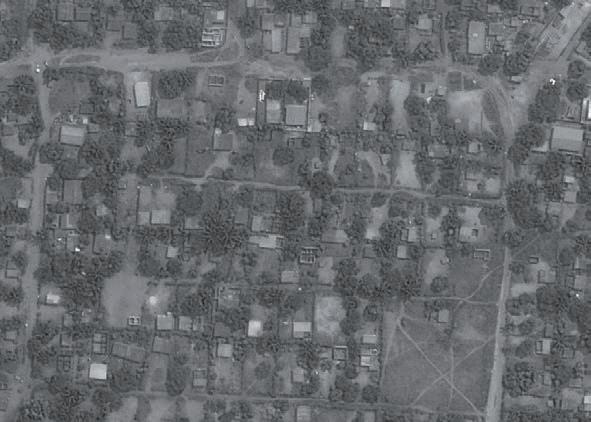
Kinshasa: Urban Analysis; Fabric Sample 01 (new development; for location refer to page 210)
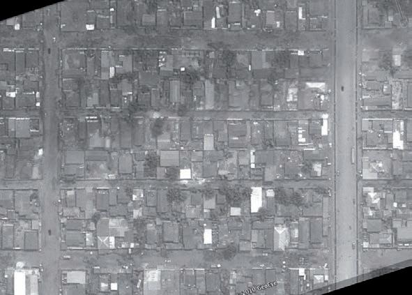
Kinshasa: Urban Analysis; Fabric Sample 02 (colonial area; for location refer to page 210)
25m 25m 200m 200m Parameter Evaluation Factor Density 0.25 Rugosity 0.75 Compacity 288.27 Contiguity 0.45 Parameter Evaluation Factor Density 0.56 Rugosity 1.67 Compacity 400.36
data Parameter Evaluation Factor Occlusitivity 65448.66 Solar Admittance 0.0363 Sinuosity 0.5 Mineraliztion 0.67 Parameter Evaluation Factor Occlusitivity 79568.92 Solar Admittance 0.0335 Sinuosity 0.4 Mineraliztion 0.94 Design Revisions - 254 -
Contiguity No
25m 200m
Kinshasa: Urban Analysis; Fabric Sample 03 (schematic*)
* According to the UN Habitat 2010 report plots of land in the new developed areas of Kinshasa are relatively large, at 300 to 500m². The built up area does often not exceed 100m². The orthogonal grid structure that dates back to colonial times is even today continued in the new developments.
The Diagram is based on the above information; the basic street/ block structure is based on an orthogonal grid layout. Plots are 400m² Large with built up areas of 100m².
No data
Diagram above: The diagrams confirm that urban development is adopting the orthogonal pattern of the colonial grid. Schematic layout according to data provided by the 2010 UN Habitat report. The layout could not be confirmed through satellite imagery. Densities are rather low at 0.34.
Diagrams on page 254: Two sample site. One located in the old colonial area (fabric sample 02) and the other one located further outside in an area of recent development (fabric sample 01). Both evaluations were based on satellite imagery provided by Google Earth. The second site shows low densities, even though plot sizes and built areas do not respond to the data provided by the UN. It has to be assumed that the UN report refers to areas that are located even further away from the center of Kinshasa. Nevertheless, densities are still very low in these areas. The ventilation potential is probably not bad due to the porosity of the fabric; nevertheless, sinuosity values are relatively low. A subsequent densification in such areas would therefore worsen the potential for natural ventilation.
Parameter Evaluation Factor Density 0.34 Rugosity 1.01 Compacity 1222.74 Contiguity
Parameter Evaluation Factor Occlusitivity 41000 Solar Admittance 0.0362 Sinuosity
no data Mineraliztion no data
- 255Evaluations/Future Development
Test Patch 01:
secondary streets: random block cross streets: @45° Test Patch
Test Patch 02:
Test Patch 03:
Test Patch 04:
Test Patch 05:
2.36
0.26
1.13 secondary streets: random block cross streets: @45°
Patch 09:
Fitness: 1.49 connectivity: 0.29* sinuosity: 0.41 density: 1.99 recreation: 0.93
Fitness: 2.33 connectivity: 0.19 sinuosity: 0.52 density: 1.44 recreation: 1.00 secondary streets: random block cross streets: @0/90°
07: Fitness: 2.21 connectivity: 0.16 sinuosity: 0.50 density: 3.71 recreation: 0.00 secondary streets: random block cross streets: @0/90° Test
Fitness: 2.23 connectivity: 0.19 sinuosity: 0.50 density: 2.14 recreation: 0.33 secondary streets: random block cross streets: @0/90°
Fitness: 2.73* connectivity: 0.25** sinuosity: 0.58* density: 2.15 recreation: 0.64 secondary streets: random block cross streets: @0/90°
Fitness: 2.38 connectivity: 0.20 sinuosity: 0.53 density: 2.06 recreation: 0.91 secondary streets: random
streets: @0/90°
06:
Test Patch
Patch 08:
Test
Test Patch 10:
block cross
Fitness: 2.25 connectivity: 0.23 sinuosity: 0.50 density: 2.19 recreation: 0.53
secondary streets: random block cross streets: @45°
Fitness:
connectivity: 0.24 sinuosity: 0.53 density: 1.80 recreation:
2.41
0.96
secondary streets: random block cross streets: @45°
Fitness:
connectivity: 0.24 sinuosity: 0.52 density: 2.91 recreation: 0.29
2.35
secondary streets: random block cross streets: @45°
Fitness:
connectivity:
sinuosity:
density:
recreation:
Wind direction:
25m Block Park Block within 150 distance to Park larger than 1000m² 100m Scale 1/7500 * highest connectivity value * highest fitness; highest connectivity value ** high connectivity value
0.52
2.20
WSW N
Design Revisions - 256 -
Rapid Creation and Evaluation of Schematic Patches
Test Patch 11:
Test Patch 12:
Test Patch 13:
Test Patch 14:
secondary streets: grid block cross streets: @0/90°
Test Patch 15:
2.08
0.06
2.02
0.79
secondary streets: grid block cross streets: @0/90°
Patch
Patch
Patch
Fitness:
connectivity: 0.12 sinuosity: 0.49 density: 1.64 recreation: 0.87
Fitness: 1.68 connectivity: 0.05 sinuosity: 0.36 density: 2.14 recreation: 0.26 secondary streets: 45/90/135° block cross streets: @45°
17: Fitness: 1.98 connectivity: 0.11 sinuosity: 0.45 density: 1.54 recreation: 0.33 secondary streets: 45/90/135° block cross streets: @45°
Fitness: 2.44 connectivity: 0.20 sinuosity: 0.54 density: 2.15 recreation: 1.02 secondary streets: 45/90/135° block cross streets: @45°
Fitness: 2.38 connectivity: 0.28 sinuosity: 0.52 density: 2.30 recreation: 0.33 secondary streets: 45/90/135° block cross streets: @0/90°
Fitness: 2.32 connectivity: 0.17 sinuosity: 0.52 density: 1.64 recreation: 1.31 secondary streets: 45/90/135° block
2.15
secondary streets: grid block cross streets: @45° Test
16:
Test Patch
Test
18:
Test
19:
Test Patch 20:
cross streets: @0/90°
Fitness:
connectivity: 0.11 sinuosity: 0.56 density: 1.82 recreation: 0.96
block
2.52
secondary streets: grid
cross streets: @45°
Fitness:
connectivity: 0.18 sinuosity: 0.44 density: 2.69 recreation: 1.30
grid block cross
1.98
secondary streets:
streets: @45°
Fitness:
connectivity:
sinuosity:
density:
recreation:
2.11
0.12
0.48
2.44
0.54
connectivity:
density:
recreation:
Fitness:
sinuosity: 0.48
Wind direction: WSW N 25m Block Park Block within 150 distance to Park larger than 1000m² 100m Scale 1/7500 - 257Evaluations/Future Development
Further Development of selected Patch
Selected Schematic Patch: Patch 09; Fitness 2.73
Evaluation:
Blocks are too small for further development.
Area of mineralization is fairly large (mineraliztion: 0.79). Recreational areas are not distributed well over the site; all park area is situated in one corner of the site. Park areas: 10429m², 5514m², 233m²: Parks are fairly large, however, due to their joint location they only serve part of the site (recreation: 0.64).
Blocks are too small for further development.
Division results in undeveloped/unused land.
Blocks are too small for further development.
Blocks are too small for further development.
Test Patch 09:
blocks within range to park (<150m) above 1000m²
*travel routes to parks
blocks within range to park (<150m) above 1000m²
Rapid generation of patches enables the designer to evaluate the fitness; the orientation of streets as well as the connectivity of the street network are regarded as the main selection parameter in this first schematic step.
Once a patch is evaluated as ‘good’ in terms of the above parameter further development can take place over a series of steps. The designer is here not a “slave to the tool”, but manual adjustments can be made according to common sense. The main design criteria are here still the same as in the first step: the connectivity of the street network, the orientation of streets according to prevailing winds; density as well as the accessibility of blocks to open space.
Revision 01; Reorganization of green areas
Evaluation:
Blocks are too small for further development.
Park Area: 2598m²; improved recreation value (recreation: 0.71)
Blocks are too small for further development.
Blocks are too small for further development.
Blocks are too small for further development.
Test Patch 09_revision 01:
street length:
length all streets:
Following this approach a first step is to evaluate the mineraliztion parameter in combination with the size and location of open areas (e.g. parks). By eliminating and relocating open areas improvements in terms of accessibility can be made.
Further evaluation is carried out by looking at block sizes. Too small blocks are regarded as un-fit for later steps, i.e. the generation of more refined morphologies. The designer is therefore free to adjust the pattern adopted from the algorithm. By re-locating streets as well as by unifying fragmented blocks better layouts can be achieved.
Fitness: 2.73 connectivity: 0.25 sinuosity: 0.58 density: 2.15 recreation: 0.64
connectivity: 0.0014 sinuosity: 0.59 density: 2.92 recreation: 0.71 mean
85.41m
2904m
Design Revisions - 258 -
blocks within range to park (<150m) above 1000m²
Revision 02; Modification of street pattern and blocks
Evaluation:
Block division/street pattern is adapted.
Street shifted to eliminate small patches.
Sidewalks too wide (currently 12m).
Street shifted to eliminate small patches.
blocks within range to park (<150m) above 1000m²
Re-evaluation of the fabric is carried out frequently while adjustments are carried out. In this way the designer can use common sense and confirm his design decisions by constant reevaluation of the fabric.
The result is an optimized block layout that shows better performance in terms of the ventilation potential and street network; i.e. the walking distances between blocks. The approach combines the evaluation of the fabric according to selected indicators together with an empirical development. It therefore combines the intuition of the designer together with measurable data regarding climatic performance and urban qualities.
Test Patch 09_revision 02:
*good street length changed to 80m
Revision 03; Modification of street pattern and blocks
Evaluation:
Side walk width adjusted on all streets.
Blocks and parks adjusted to sidewalk width.
Test Patch 09_revision 02:
*good street length changed to 80m
0.30* sinuosity: 0.60 density: 3.00 recreation: 0.75 mean street length: 72m
streets: 2738m
connectivity:
Length all
connectivity: 0.30* sinuosity: 0.60 density: 3.00 recreation: 0.75 mean street length: 72m
streets: 2738m
Length all
Further Development of selected Patch - 259Evaluations/Future Development
Patch Development: Single Family Houses
Revised Patch 09; schematic layout as template for neighbourhood population
Optimized (schematic) blocks are rapidly transformed into a ‘neighbourhood typology’; i.e. cross streets are inserted into the block and free standing buildings are created around the perimeter of newly created patches.
Values for e.g. Lot depth and width, as well as distance between buildings were taken from the earlier evaluations, i.e. the creation of families of neighbourhood typologies that were evaluated against the target values of the tropical climate zone.
Revised Patch 09; neighbourhood population
Cross streets have been introduced to the blocks; in some cases this leads to too small lots that do not allow an offset to create a courtyard inside. The division of the patch to create free standing buildings results in a building typology that is considered not fit. Re-arrangement or removal of cross street could remedy this situation. In some cases blocks can also be extruded as single entities; such movement makes sense as it can create larger units within the fabric that can serve public amenities such as supermarkets or a sport venues.
Whereas in previous steps the evaluation of the fabric focused on factors related to the street layout (connectivity, sinuosity or recreation) the more detailed level of the fabric now allows for further evaluation that incorporates factors such as compactness, contiguity or porosity.
Revised Patch 09; neighbourhood population (revised)
Blocks that were considered unfit for creation of free standing buildings have been extruded as solid entities; such blocks can house public function such as supermarkets, schools or sport venues.
Further revision of the fabric should take into account factors such as compactness, contiguity, porosity or occlusitivity.
Once a satisfactory solution is found further development has to take place at the patch level that takes architectural considerations such as plan layouts and building materials into account.
Design Revisions - 260 -
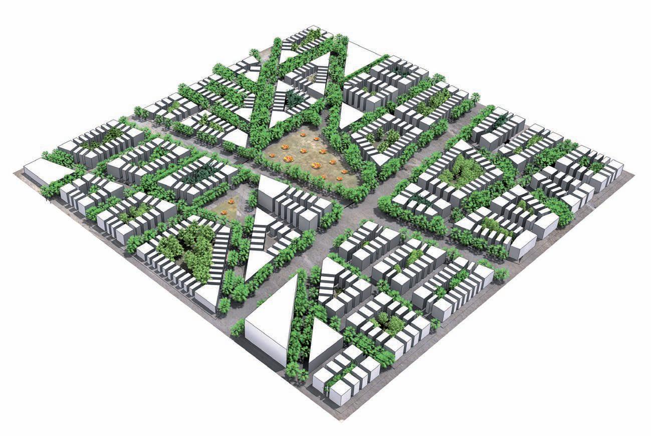
Comparison of Indicators for the proposed typology: Graph shows relative values for reference cities in the topical climate zone (range for all cities evaluated); other indicators can now be evaluated according to the more detailed morphology. In some cases the complex morphology still imposes problems in terms of computation; therefore some values are not yet available.
parameter value rugosity 2.08 sinuosity 0.60 porosity no data compacity 2508.88 contiguity No data solar Admittance 0.045 Neighbourhood Layout (evaluation) parameter value occlusitivity no data mineralization 0.89 density 0.69 connectivity 0.30 mean street length 72.07m recreation 0.68 Neighbourhood Layout (evaluation)
Rugosity Typology under development
Bangkok *value out of range *no data *no data *no data Sinuosity Porosity Compacity Contiguity Solar Admitt. Occlusitivity Density Mineral. 0 1 0.8 0.6 0.4 0.2 [/]
Patch Development: Single Family Houses
Malaka
- 261Evaluations/Future Development
Revised Patch 09; schematic layout as template for town house population
Optimized (schematic) blocks are rapidly transformed into a ‘town house typology’; i.e. cross streets are inserted into the block and buildings are extruded around a central courtyard.
Values for e.g. Lot depth and width, as well as width of cross streets were taken from the earlier evaluations, i.e. the creation of families of town house populations that were evaluated against the target values of the tropical climate zone.
Revised Patch 09; town house population
Cross streets have been introduced to the blocks; in some cases this leads to too small lots that do not allow an offset to create a courtyard inside. The division of the patch to create free standing buildings results in a building typology which is considered not fit. Re-arrangement or removal of cross street could remedy this situation. In some cases blocks can also be extruded as single entities; such movement makes sense as it can create larger units within the fabric that can serve public amenities such as supermarkets or a sport venues.
Whereas in previous steps the evaluation of the fabric focused on factors related to the street layout (connectivity, sinuosity or recreation) the more detailed level of the fabric now allows for further evaluation that incorporates factors such as compactness, contiguity or porosity.
Revised Patch 09; town house population (revised)
Blocks that were considered unfit for creation of courtyard blocks have been modified by removing cross streets.
Some blocks that were too small to create courtyard blocks have been extruded as solid entities; such blocks can house public function such as supermarkets, schools or sport venues.
Further revision of the fabric should take into account factors such as compactness, contiguity, porosity or occlusitivity.
Once a satisfactory solution is found further development has to take place at the patch level that takes architectural considerations such as plan layouts and building materials into account.
Design Revisions - 262 -
Patch Development: Multi-Storey Town Houses
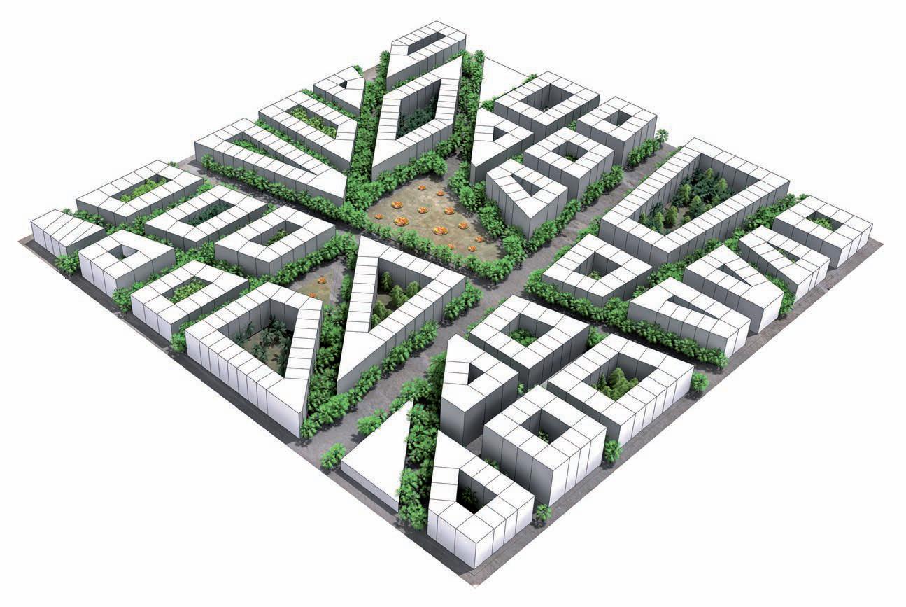
Comparison of Indicators for the proposed typology: Graph shows relative values for reference cities in the topical climate zone (range for all cities evaluated); other indicators can now be evaluated according to the more detailed morphology. In some cases the complex morphology still imposes problems in terms of computation; therefore some values are not yet available.
parameter value rugosity 5.61 sinuosity 0.59 porosity no data compacity 901.62 contiguity no data solar Admittance 0.1351 Town House Layout (evaluation) parameter value occlusitivity 36558.21 mineralization 0.86 density 1.87 connectivity 0.30 mean street length 71.76m recreation 0.68 Town House Layout (evaluation)
Rugosity Typology under development Malaka Bangkok *value out of range *no data *no data Sinuosity Porosity Compacity Contiguity Solar Admitt. Occlusitivity Density Mineral. 0 1 0.8 0.6 0.4 0.2 [/]
Patch Development: Multi-Storey Town Houses
- 263Evaluations/Future Development
Patch Development: Multi-Storey Apartment Blocks
Revised Patch 09; schematic layout as template for multistorey block population
Optimized (schematic) blocks are rapidly transformed into a ‘multi storey block typology’; i.e. cross streets are inserted into the block, lots are offset to create free space between buildings and resulting lots are extruded.
Values for e.g. Lot depth and width, as well as width of cross streets were taken from the earlier evaluations, i.e. the creation of families of multi-storey block populations that were evaluated against the target values of the tropical climate zone.
Resulting blocks often do not result in ‘usable’ architectural layouts. In some areas the division of lots to create multi-storey blocks works fine, in other areas revisions by the designer are necessary to optimize the layout. This is carried out by slight modifications to the street layout and by removal of previously introduced cross streets.
Triangular patches often result in problems regarding usable architectural space. To address this, such patches can be treated differently by introducing low rise scenarios that cover the whole site (to be used for e.g. Schools and other public amenities). Another strategy to deal with triangular patches is slightly re-adjust the street pattern
Whereas in previous steps the evaluation of the fabric focused on factors related to the street layout (connectivity, sinuosity or recreation) the more detailed level of the fabric now allows for further evaluation that incorporates factors such as compactness, contiguity or porosity.
Areas that did not create useable block layouts have been modified by joining patches and removing cross streets.
Modifications to the street layout have been made to reduce triangular shaped patches and to optimize the block pattern.
Further revision of the fabric should take into account factors such as compactness, contiguity, porosity or occlusitivity.
Once a satisfactory solution is found further development has to take place at the patch level that takes architectural considerations such as plan layouts and building materials into account.
Revised Patch 09; multi-storey block population
Revised Patch 09; multi-storey block population (revised)
Design Revisions - 264 -
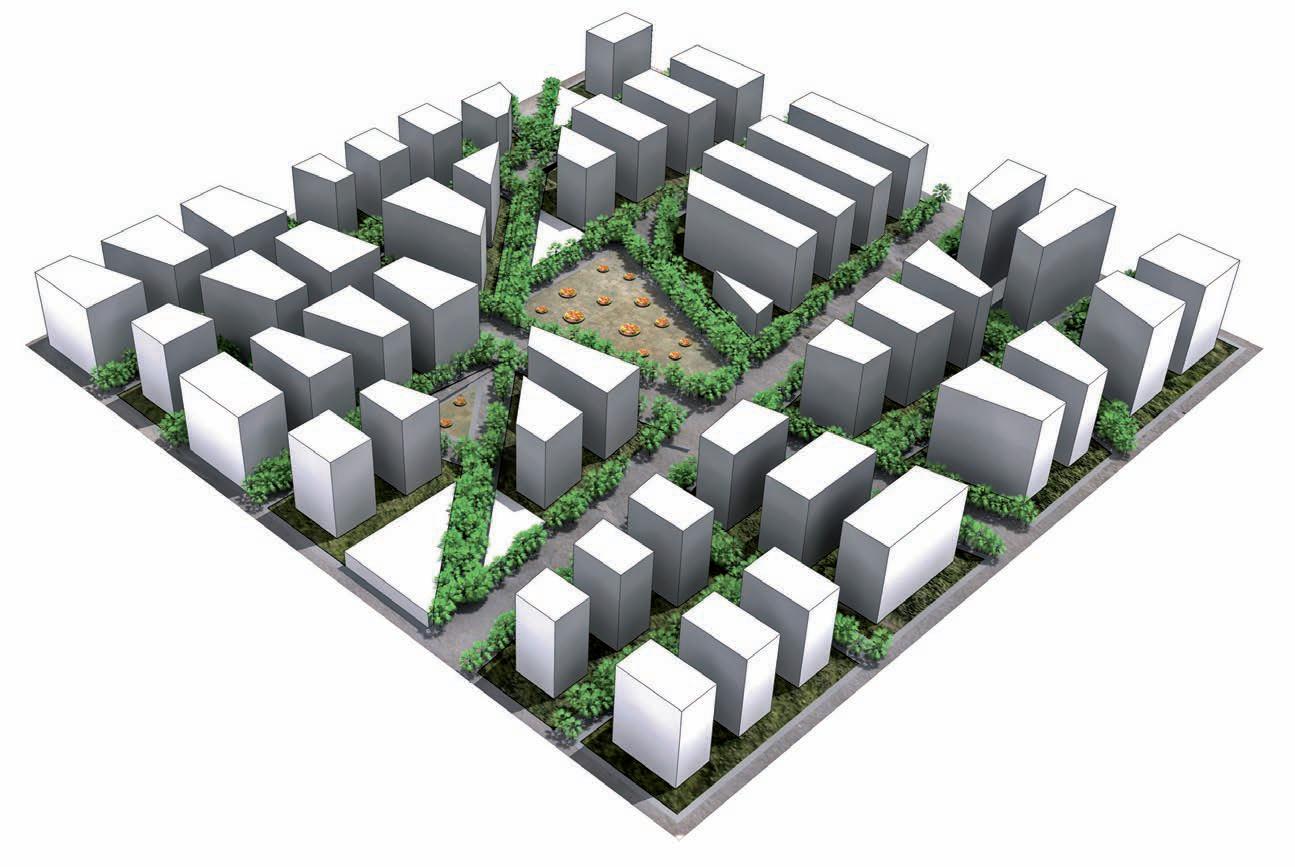
Comparison of Indicators for the proposed typology: Graph shows relative values for reference cities in the topical climate zone (range for all cities evaluated); other indicators can now be evaluated according to the more detailed morphology. In some cases the complex morphology still imposes problems in terms of computation; therefore some values are not yet available.
parameter value rugosity 6.99 sinuosity 0.57 porosity 0.58 compacity 0 contiguity 0 solar Admittance no data Multi Storey Block Layout (evaluation) parameter value occlusitivity 900011.32 mineralization 0.66 density 2.32 connectivity 0.29 mean street length 72.12m recreation 0.68 Multi Storey Block Layout (evaluation)
Rugosity Typology under development Malaka Bangkok *value out of range Sinuosity Porosity Compacity Contiguity Solar Admitt. Occlusitivity Density Mineral. 0 1 0.8 0.6 0.4 0.2 [/]
Patch Development: Multi-Storey Apartment Blocks
- 265Evaluations/Future Development
Patch Development: High-Rise Apartment Blocks
Revised Patch 09; schematic layout as template for highrise block population
Optimized (schematic) blocks are rapidly transformed into a ‘high-rise block typology’; i.e. Patches are divided, offset and buildings extruded.
Values for e.g. Lot depth and width, as well as offset values were taken from the earlier evaluations, i.e. the creation of families of high-rise block populations that were evaluated against the target values of the tropical climate zone.
Revised Patch 09; high-rise block population
Running the script on the patches did generally not result in satisfactory results. Blocks were on the hand distributed in too dense arrangements; on the other hand too big offset values resulted in many cases in blocks that were too slim and not suitable for later architectural development.
As a general observation it is to mention that both, multi-storey blocks and high-rise apartment blocks seem to create the best results on an orthogonal street layout. This however implies a total revision of the chosen street/schematic block layout and reevaluation.
Whereas in previous steps the evaluation of the fabric focused on factors related to the street layout (connectivity, sinuosity or recreation) the more detailed level of the fabric now allows for further evaluation that incorporates factors such as compactness, contiguity or porosity.
Revised Patch 09; high-rise block population (revised)
As the ‘faceted’ patch pattern did not create suitable layouts revisions had to be made by re-moving and re-arranging streets.
In order to ensure appropriate architectural layouts the designer has to step in and re-adjust the block pattern; further adjustment will need to be made according to architectural considerations.
Further revision of the fabric should take into account factors such as compactness, contiguity, porosity or occlusitivity.
Once a satisfactory solution is found further development has to take place at the patch level that takes architectural considerations such as plan layouts and building materials into account.
Design Revisions - 266 -
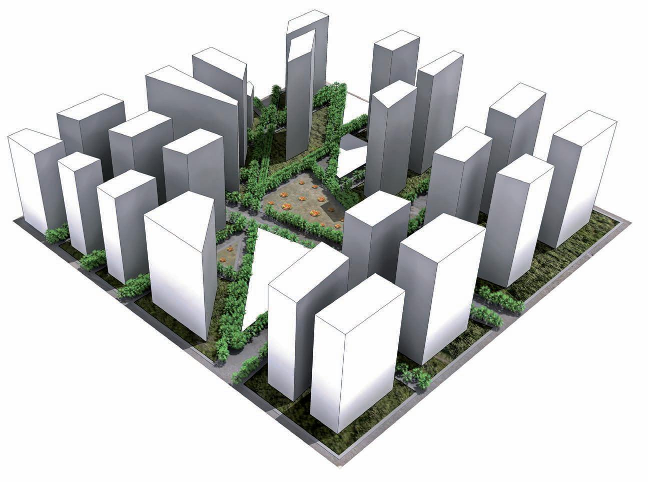
Comparison of Indicators for the proposed typology: Graph shows relative values for reference cities in the topical climate zone (range for all cities evaluated); other indicators can now be evaluated according to the more detailed morphology. In some cases the complex morphology still imposes problems in terms of computation; therefore some values are not yet available.
parameter value rugosity 13.04 sinuosity 0.59 porosity 0.65 compacity 0 contiguity 0 solar Admittance no data High Rise Block Layout (evaluation) parameter value occlusitivity 115031.61 mineralization 0.61 density 4.32 connectivity 0.27 mean street length 70.64m recreation 0.74 High Rise
Layout (evaluation)
High-Rise
Rugosity Typology under development Malaka Bangkok *value out of range Sinuosity Porosity Compacity Contiguity Solar Admitt. Occlusitivity Density Mineral. 0 1 0.8 0.6 0.4 0.2 [/] *no data
Block
Patch Development:
Apartment Blocks
- 267Evaluations/Future Development
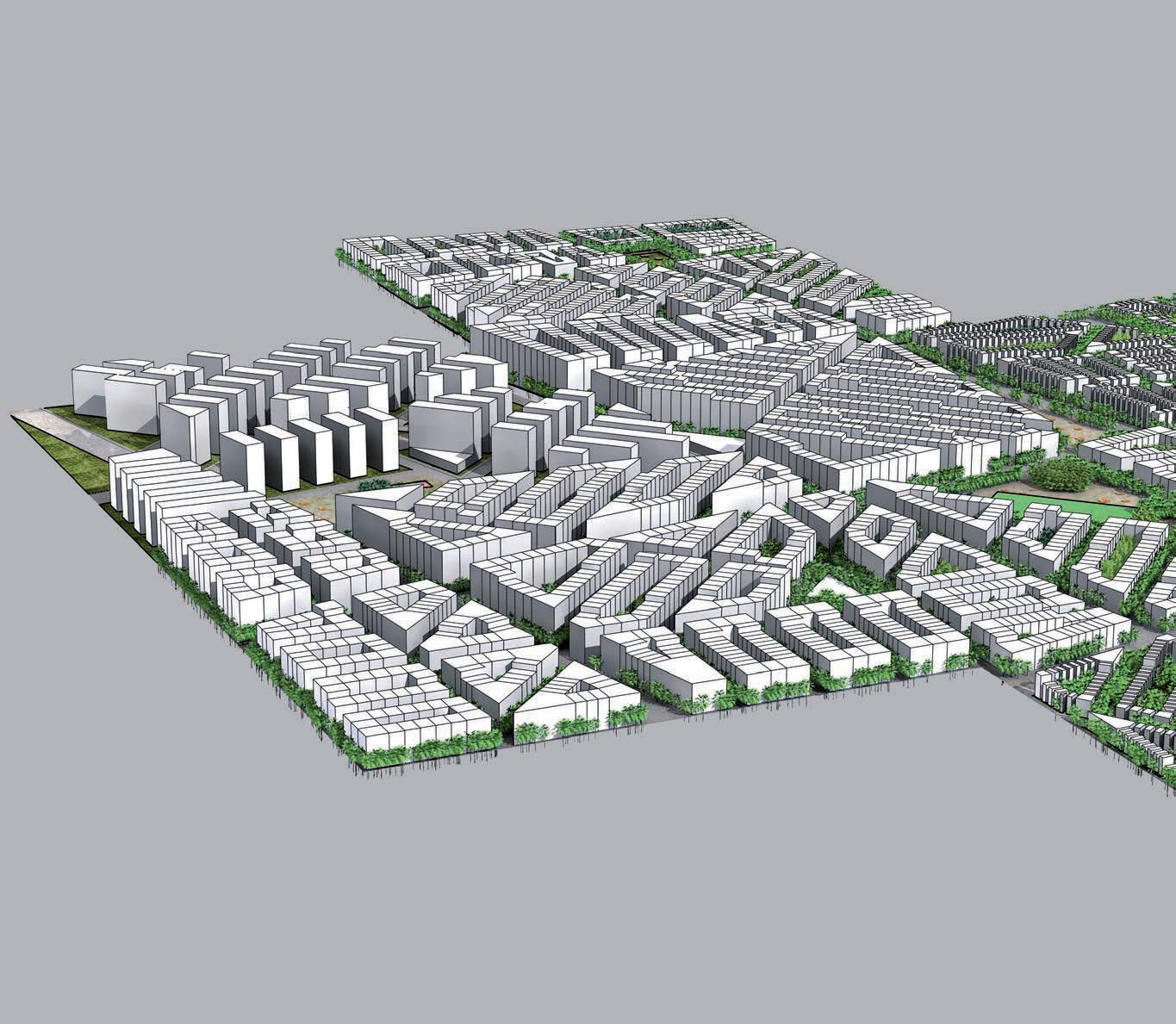
The development of patch typologies shown on the previous pages illustrates a hierarchical design approach that addresses different parameter at different stages of the process. Starting from the schematic patch level, i.e. streets and islands, aspects like street lengths and directions are first addressed. This is accomplished through rapid production of test patches and the evaluation of parameters, such as sinuosity or connectivity. ‘Fit’ patches are subsequently further developed and improved in an intuitive design process; streets are eliminated, newly introduced or relocated in order to form a more coherent fabric. The designer can here use his experience in order to evaluate form and size of islands to assess how suitable they are for later urban development. By running evaluation scripts on manually modified layouts it is possible to re-evaluate some of the latent design characteristic described above. Other aspects for consideration at this stage may include the location of public areas or infrastructural elements; the ‘recreational indicator’ may help to get an idea how accessible such entities are.
Once patches are considered ‘good’ at the schematic level, they can be further developed to form distinct urban typologies.
Scripts can be utilized, again, to generate different scenarios in a rapid way. By ‘reading-in’ the previously created islands, different urban typologies can be generated from a schematic layout. Similar to the initial step, algorithms can be used to quickly produce a range of possible morphologies; again, a process of selection includes the evaluation of morphological indicators as well as the experience and creativity of the designer.
Typologies created via algorithms undergo a process of subsequent modification and improvement; this is mostly accomplished ‘by hand’ in order to give the designer maximum control over urban characteristics. Blocks might be considered too big or too small, or a building’s shape might be not suitable in economic terms. Re-adjustments therefore take place according to intuition.
The more detailed morphologies that have been created at this stage not only allow for better assessment from a design point of view, but they also provide the opportunity to evaluate other parameters that relate to the urban microclimate. Factors that relate to solar radiation, such as solar admittance, compacity,
Patch aggregation to form ‘local climate zones’
Design Revisions - 268 -
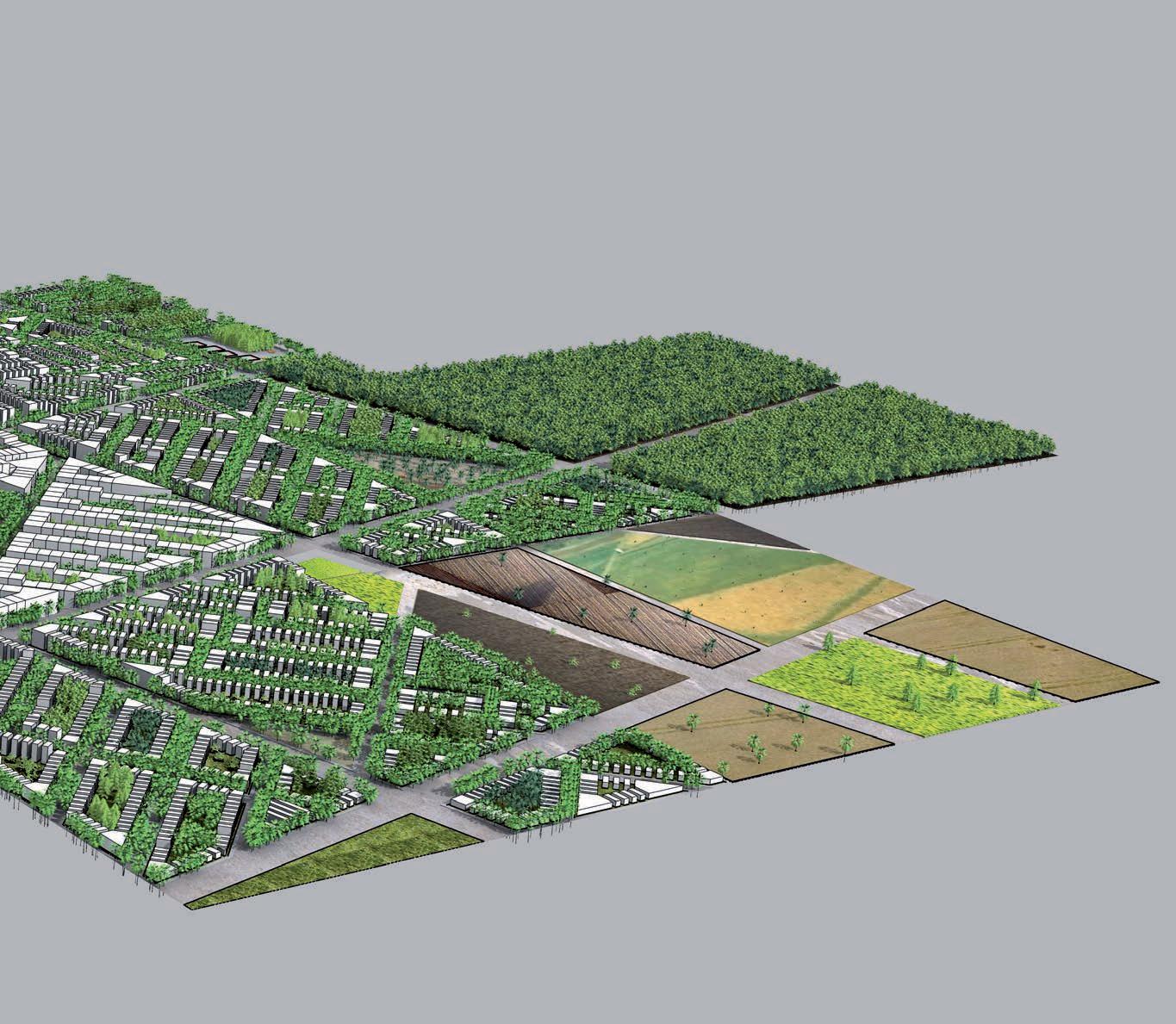
contiguity or occlusitivity, all require detailed information at the building level; they assess the orientation of walls and whether building envelopes are shared or not. The detailed morphology at this stage allows for assessment of such parameters. According to an initial hypothesis they can be compared to the values of evolved and planned cities that fall in the same climate zone. Nevertheless, close cooperation with urban climatologists at this stage would likely lead to more sophisticated result and designers and planners would benefit at this stage from a data base that sets clear target values for different climatic zones.
Once clear target values are set further modification and optimiztion can take place at the building/block level. Building depths can be altered to change the porosity of the fabric or spacings between buildings can be adjusted to respond to contiguity or compacity.
The development of the patch therefore is a hierarchical process, from the schematic layout (i.e. streets and islands) all the way down to the block and the individual building. The approach shows that it makes sense to evaluate different parameter at
different stages of the process, as they relate to different levels of urban information (compare also diagram on page 83). Further development can subsequently take place at the building level in order to, not only address morphological characteristics, but also building materials (i.e. the albedo). In this way, the indoor and the outdoor climate can be addressed; energy requirements can be potentially reduced and urban qualities improved.
Aggregation of patches should then follow a global logic that respects the connectivity of patches, urban structure as well as microclimatic considerations at the macro-scale. The assembly of ‘local climate zones’ should, again, happen in close collaboration with urban climatologists in order to address the global climatic interaction of patch agglomerations. In the above example patches are aggregated to form a center of higher density and to include areas of forest and agriculture within the city. Additionally, a zoning envelope is proposed that can respond to overall wind conditions above the urban canopy - Refer to page 270 for more information.
- 269Evaluations/Future Development
ClimateZone
Proposal for a latent zoning grid; optimized for wind and ventilation. El Nahas reports that cities that show a gradual increase of building heights towards the center, i.e. a pyramidal cross section, will cause less drag on the wind than ones with a line of high rises at the perimeter (El Nahas, 1996). Strategies that respect regional wind conditions could be implemented in form of a zoning grid. The diagram shows a proposal how pockets with higher densities (and higher building heights) form patterns that could direct wind flow over the urban canopy. Such strategies could easily be linked to the concept of ‘urban climate zones’ (see Stewart, page 69): The patch arrangement, i.e. different typologies could happen according to information from the zoning grid. Building heights gradually increase towards the center; extrusion heights are taken from the zoning grid when the algorithm is run. The approach is tested on the patch layout shown on page 268; next to influencing wind it can also provide structure to an urban fabric by forming urban centers and by incorporating other land use zones, such as agriculture or forest.
ClimateZone
Similar Concept as above. This time pockets of higher densities are stretched according to the direction of flow in order to cause less drag. The idea of such measures is to influence the velocity of the wind at roof level, which will likely also affect wind conditions within the Urban Canopy Layer. The diagrams have to be understood as a conceptual proposal. The complex interactions of wind with urban morphologies are not fully understood. Further research is necessary by climatologists via field studies and wind tunnel test. Concepts as shown above would also have to be proven by means of e.g. computer simulation and analysis (CFD).
Opposite page: Urban climate zones; the diagrams show an example how different patch typologies may be aggregated. Densities and building heights gradually increase from the bottom right to the top left; the arrangement follows the idea of better response to wind conditions via a smooth urban canopy (see diagrams above). Further research is necessary to understand how urban climates zones, i.e. patch typologies, interact and how they aggregate in the best way
Climate Zone
Climate
Zone
Design Revisions - 270 -
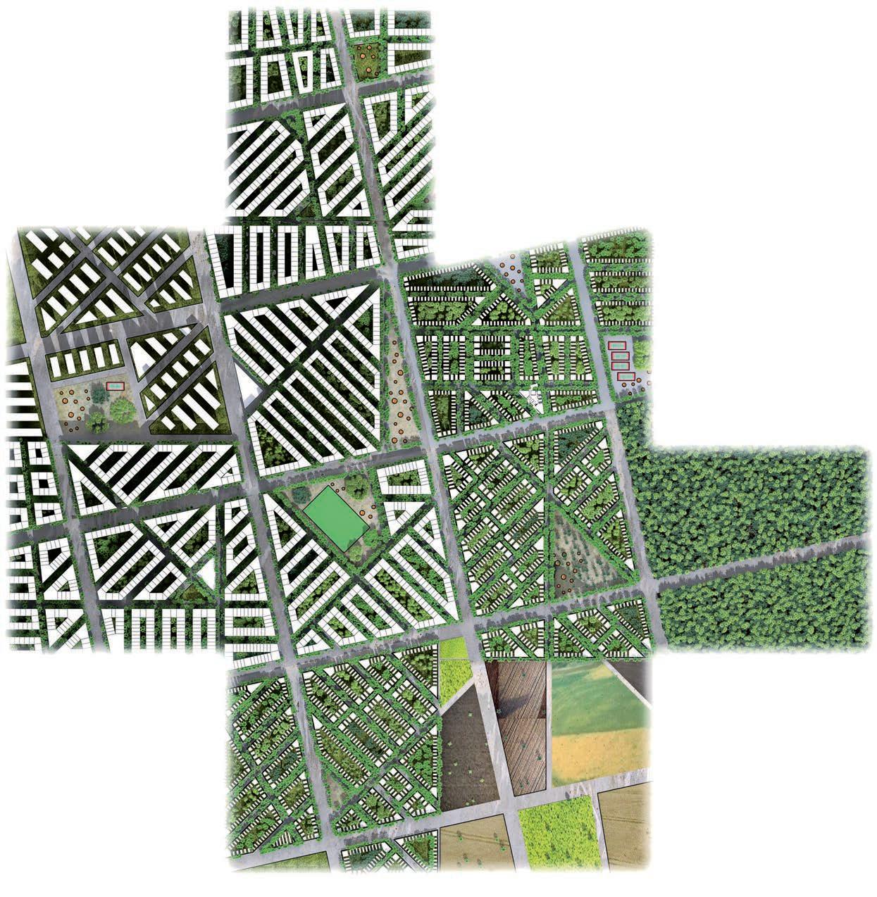
Urban Climate Zones:
Multi-Storey Apartment Blocks
Multi-Storey Town Houses
Multi-Storey Town Houses
Multi-Storey Town Houses
Single Family Houses
Multi-Storey Town Houses
Single Family Houses
Single Family Houses Forrest Fields
- 271Evaluations/Future Development
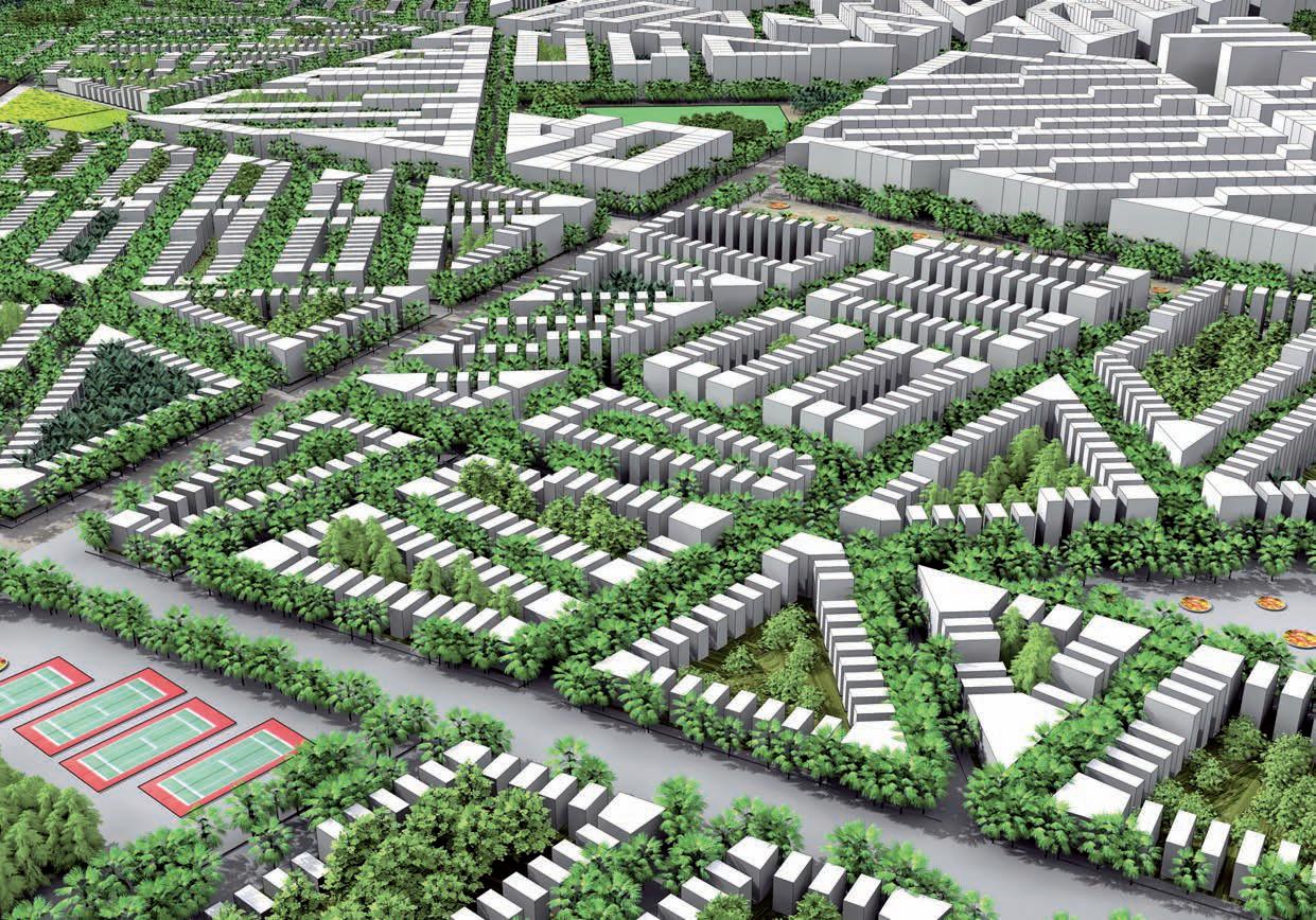
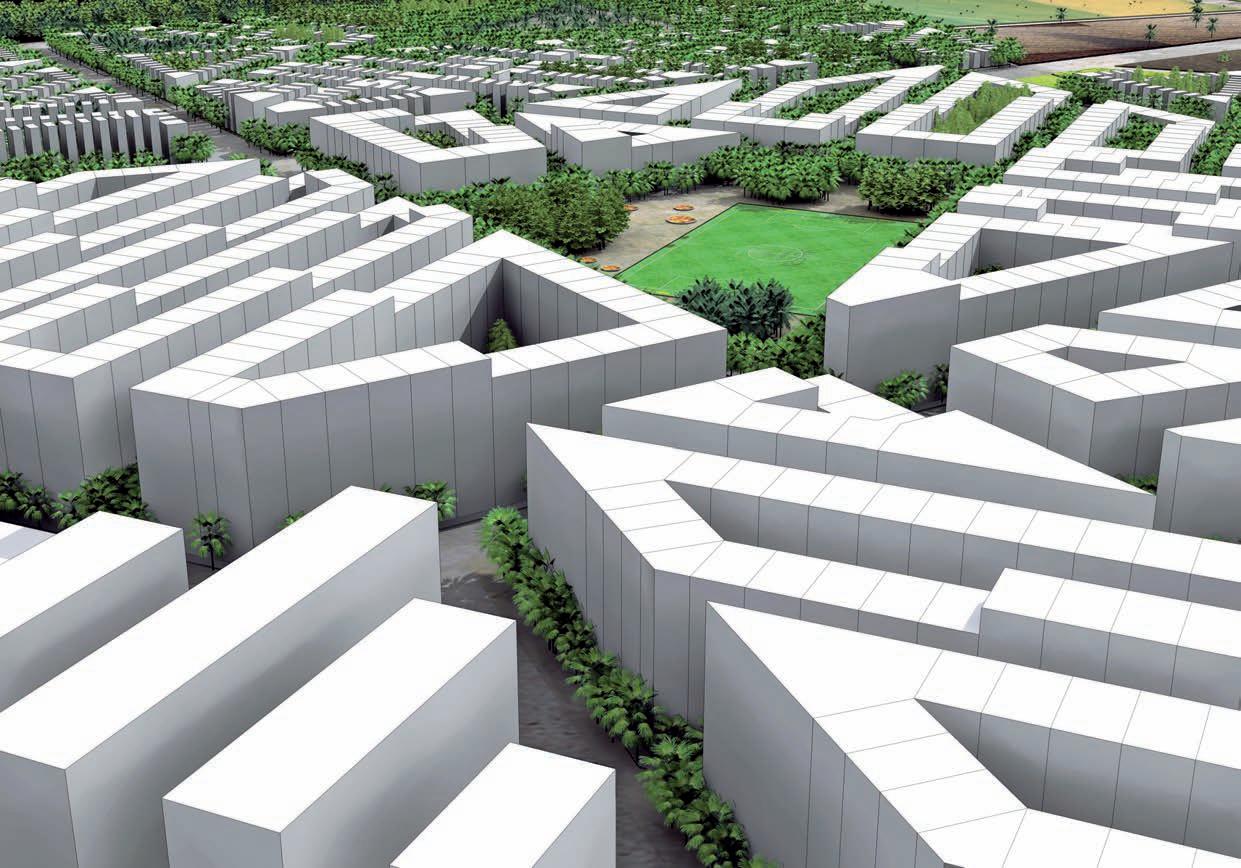
Images depict the morphology and the associated urban qualities of proposed patch aggregations.
Conclusions
Reducing the energy demands of cities will be one of the biggest challenges for architects and urban planners in the coming decades. Tackling the urban microclimate, by addressing the urban morphology in design processes, could play a crucial role in this process; it is likely the most suitable way to enforce means of passive energy saving onto urban agglomerations.
The design research project, introduced in this thesis, proposes approaches how such strategies can be implemented. Currently, the lack of design guidelines, as well as the complexity of the topic, makes it difficult to address urban microclimates in urban planning. Based on the research on current microclimatic knowledge, methods are proposed that relate to ‘simplified’ morphological parameters, or indicators. Whereas such models have been so far solely used for microclimatic analysis, it is shown, how they can be implemented in generative design processes. By coupling a Genetic Algorithm with morphological indicators, to provide fitness criteria, it is shown how creation and evaluation of urban patches can happen at the same time in very rapid processes. Throughout the design, strategies are refined of how to approach urban planning in microclimatic terms. At the same time, problems are revealed, that relate to computational aspects, as well as to the complex phenomenon of urban microclimates.
The biggest challenge during the design is the lack of clear target values that relate to the various parameters. In other words, even though it is proven, that morphological indicators can be utilized to inform and optimize bio-climatic design processes, it is the lack of clearly defined design targets for various climate zones that imposes the biggest challenge. Against an initial hypothesis that, especially, evolved cities would reflect microclimatic aspects through their morphology the analysis done did not result in a profound database. The information required to inform a genetic algorithm in order to optimize urban morphologies over multiple generations was therefore not possible. The multitude of parameters, i.e. nine microclimatic indicators adopted from Adolphe (Adolphe, 2000), as well as indicators that relate to other urban qualities added to this problem. Whereas usually no more than two parameters are used for optimization, attempted multi-parameter optimization results in problems of defining clear design targets. Nevertheless, as a result, different strategies are developed that give an idea how urbanism can be approached in bio-climatic terms using morphological indicators. A hierarchical method is introduced that allows the development of patches from schematic layouts all the way down to the block and building level. Throughout this process it is revealed how various parameter (that respond to different scales of the urban morphology) may be implemented for evaluation. The rapid generation of patches can therefore still be utilized in order to quickly create different ranges of options that can be evaluated at the same time according to set parameters. Together with the intuition of the designer this leads to a coherent design approach.
In general, it is the lack of a database with clearly defined design targets for various climate zones that currently hinders the implementation of bio-climatic design strategies into urban planning. A catalogue of clear target values therefore needs to be established that refers to factors such as sky view factors, urban reflectance or porosity. At the urban macro-level this could be extended to include morphological indicators, such as proposed by Adolphe. Close collaboration between architects, urban planners and climatologists is therefore necessary. Clear guidelines that include e.g. solar admittance, occlusitivity or compacity factors could then be implemented, either by manual adaptation or through optimization processes that rely on genetic algorithms.
Working at the urban level also reveals some of the computational limits that are associated with the complexity of urban morphologies. Whereas the initial algorithm allows to create more than 400 patches (250m by 250m) in less than two hours, further development soon results in computational problems. The more complex geometry of distinct urban typologies currently creates too ‘heavy’ geometries; with current hardware technology computers reach their limits and crash long before satisfactory results are obtained. Long calculation times add to this; it can be summarized that the utilization of an algorithm to generate and evaluate urban patches only makes sense if calculation processes are fast enough and do not result in waiting periods for the designer. It is shown in the last chapter that the exploration of computational limits in combination with a better understanding of various microclimatic indicators leads to a design approach that utilizes the power of the algorithm in the best possible way. It also illustrates that an algorithm should be seen as a design aid that can assist in design processes, but that it should not be treated as an automated process without interaction of the designer. It is still the experience, creativity and intuition of the designer that should drive the design; algorithms should be utilized in the best possible way to support this process.
Next to the amount of geometry that is produced when working on the urban patch level it is also the way of calculating various indicators that reveals further computational problems; these should be addressed during further development. Whereas the computer is really fast in mathematical calculations it is the associated processes of using more complex geometrical methods that results in long calculation times. In other words, in order to evaluate e.g. the area of shared party walls, time consuming ‘Rhino Methods’ such as Boolean operations are utilized. Another example is the creation of very fine evaluation meshes for e.g. the porosity evaluation, which turns out very time consuming. Therefore, better ways need to be developed to extract and calculate data from the urban morphology. Such ways should avoid, as much as possible, complex geometric operations and rely on fast mathematical calculations – even if they only result in approximated results. The indicators used in the initial experiments, i.e. density and rugosity, are fast to calculate and show promising prospects in terms of running them on the genetic algorithm. The evaluation of some of the other parameters therefore needs to be addressed and optimized in order to speed up calculation processes; in this way it should be attempted to allow the rapid evaluation of all parameters as part of optimization processes within a genetic algorithm.
Further development should also take place regarding the rules for patch generation. This relates to the logics of sub-division in order to create streets and islands, as well as to the formation of patch typologies and the overall aggregation of patches. During the design experiments it has been explored how heterogeneous patches can be connected via hierarchies within the street network. It has also been shown how e.g. zoning patterns that respond to global wind conditions can help unifying the fabric. Further work is necessary to study how patch typologies, i.e. local climate zones, are aggregated in best possible way from a microclimatic point of view. This involves further research and close collaboration with climatologists.
At the patch level further development should take place regarding the creation of distinct urban typologies. The design experiment proofed that the formation of characteristic typologies, which respond to specific local climate zones, is possible. Additional research and experiments are now necessary to further explore the inherent logics and rules of patch typologies. These should result in the creation of new typologies that divert from the traditional schemes that have been adopted for this experiment.
- 273Conclusions
It is hoped that additional work in this area will result in the formation of new typologies that are well suited for specific climatic settings.
Finally the fundamental logics of schematic patch creation, as shown in the experiment, should be revisited and further developed. The random creation of street directions should be addressed and connected to other fitness criteria, such as the connectivity of the street network.
Overall, it can be summarized that the design research project presented in this thesis illustrates that new approaches to urban planning are necessary. Such approaches should tackle the energy demands of cities from an urban morphology point of view. It has been shown through the design experiments that its is possible to implement current strategies in microclimatic research in design processes. Further work is necessary to establish clear design guidelines and to set up clear target values for specific climatic zones. Only a combined and coherent approach that includes the joint work of designers and climatologists can lead to planning solutions that address the energy demands of future urban development.
- 274Design Revisions
- 275Conclusions
- 276Design Revisions
Appendix 01
World and Urban Growth
Prospects (by major country and region)
Urban Population (thousands) Percentage Urban Population of the largest urban agglomeration 2010 2050 2009 2025 2050 Agglomeration Population* As Percentage** World 3,486,326 6,285,881 50.1 56.6 68.7 More developed regions 929,851 1,099,730 74.9 79.4 86.2 Less developed regions 2,556,475 5,186,151 44.6 52.3 65.9 Least developed countries 249,442 914,370 28.7 37.6 54.7 Less developed regions, excluding least developed countries 2,307,033 4,271,781 47.4 55.4 68.9 Less developed regions, excluding China 1,913,018 4,139,239 44.1 50.5 64.2 Sub-Saharan Africa 321,400 1,054,427 36.8 45 60.1 Africa 412,990 1,230,915 39.6 47.2 61.6 Eastern Africa 77,194 337,493 23.3 30.3 47.4 Burundi 937 4,951 10.7 17.1 33.3 Bujumbura 455 51.3 Comoros 195 622 28.1 33.3 50.7 Moroni 49 24.6 Djibouti 670 1,249 76.2 78.8 85 Djibouti 567 86.1 Eritrea 1,127 5,405 21.1 30.8 50.1 Asmara 649 60.6 Ethiopia 14,158 65,149 16.5 21.3 37.5 Addis Adaba 2863 21 Kenya 9,064 41,112 21.9 29.6 48.1 Nairobi 3375 38.8 Madagascar 6,082 23,940 29.8 37.9 56.1 Antananarivo 1816 31 Malawi 3,102 17,729 19.3 28.8 48.5 Lilongwe 821 27.9 Mauritius 542 863 41.9 45.3 60.5 Port Louis 149 27.7 Mayotte 100 258 50.1 53.3 66.8 Labattoir 16 16.8 Mozambique 8,996 29,750 37.6 50.1 67.4 Maputo 1589 18.4 Réunion 787 1,067 93.7 96 97.3 Saint-Denis 141 18.2 Rwanda 1,938 9,480 18.6 25.2 42.9 Kigali 909 49 Seychelles 47 74 54.8 63.9 76.2 Victoria 26 56.3 Somalia 3,505 14,972 37 46.3 63.7 Mogadishu 1353 40.1 Uganda 4,493 30,596 13.1 18 33.5 Kampala 1535 35.8 United Republic of Tanzania 11,883 59,109 25.9 35.1 54 Dar es Salaam 3207 28.3 Zambia 4,733 16,898 35.5 41.5 58.4 Lusaka 1413 30.7 Zimbabwe 4,837 14,270 37.8 47.2 64.3 Harare 1606 34 Middle Africa 55,592 185,977 42.5 52.8 68.1 Angola 11,112 34,042 57.6 69 80.5 Luanda 4511 42.3 Cameroon 11,655 29,343 57.6 68.4 79.9 Douala 2053 18.3 Central African Republic 1,755 4,683 38.7 45.2 61.6 Bangui 702 41 Chad 3,179 15,761 27.1 37.5 56.7 N'Djamena 808 26.6 Congo 2,335 5,422 61.7 68.6 79 Brazzaville 1292 56.9 Democratic Republic of the Congo 23,887 93,271 34.6 45.6 63.2 Kinshasa 8401 36.8 Equatorial Guinea 275 901 39.5 46.1 62.4 Malabo 128 47.8 Gabon 1,292 2,311 85.6 89.7 93.5 Libreville 619 49 Sao Tome and Principe 103 243 61.4 71.7 82.1 Sao Tome 60 59.9 Northern Africa 108,912 227,852 50.8 57.9 71 Algeria 23,555 41,425 65.9 74.1 83.5 Algiers 2740 11.9 Egypt 36,664 81,998 43.3 48.1 63.3 Cairo 10902 30.3 Libyan Arab Jamahiriya 5,098 8,565 77.7 81.6 87.2 Tripoli 1095 22 Morocco 18,859 33,234 57.6 66.6 78 Casablanca 3245 17.6 Sudan 17,322 51,365 39.4 51 67.7 Khartoum 5021 30.2 Tunisia 6,980 10,427 66.9 73.2 82 Tunis 759 11 Western Sahara 434 839 81.6 84.9 89.4 El Aaiun 213 50.9 Southern Africa 34,021 51,917 58.2 65.9 77 Botswana 1,209 2,236 60.4 70.3 81.1 Gaborone 196 16.6 Lesotho 560 1,447 26.1 38.5 58.1 Maseru 220 40.7 Namibia 840 2,345 37.4 47.9 65.3 Windhoek 342 42.1 South Africa 31,155 45,199 61.2 69 79.6 Johannesburg 3607 11.8 World Urbanization Prospects: The 2009 Revision; United Nations, Department of Economic and Social Affairs, Population Division
Country or Area
- 277World and Urban Growth Prospects (by major country and region)
Country
Urban Population (thousands) Percentage Urban Population of the largest urban agglomeration 2010 2050 2009 2025 2050 Agglomeration Population* As Percentage** Guinea 3,651 15,087 34.9 45 62.9 Conakry 1597 45.5 Guinea-Bissau 494 1,875 29.9 35.4 52.7 Bissau 302 62.7 Liberia 1,961 6,105 47.7 54.7 69.1 Monrovia 882 47 Mali 4,777 18,458 35.1 47.5 65.3 Bamako 1628 35.7 Mauritania 1,395 3,902 41.2 48.4 64.4 Nouakchott 709 52.3 Niger 2,719 21,431 17 21.1 36.8 Niamey 1004 38.7 Nigeria 78,818 218,018 49.1 60.3 75.4 Lagos 10203 13.4 Saint Helena 2 3 39.7 43.7 59.3 Half Tree Hollow 1 49.4 Senegal 5,450 17,003 42.1 49.3 65.1 Dakar 2777 52.6 Sierra Leone 2,241 7,771 38 45.7 62.4 Freetown 875 40.4 Togo 2,945 9,216 42.7 53.9 69.8 Lome 1593 56.3 Asia 1,757,314 3,382,365 41.7 49.9 64.7 Eastern Asia 784,688 1,189,398 49.4 60.7 74.3 China 635,839 1,037,695 46.1 58.6 73.2 Shanghai 16344 2.6 China, Hong Kong SAR 7,069 8,623 100 100 100 Hong Kong 7022 100 China, Macao SAR 548 593 100 100 100 Macao 538 100 Dem. People's Republic of Korea 14,446 18,307 60.1 63.7 74.5 P'yongyang 2828 19.7 Japan 84,875 81,403 66.6 71.1 80.1 Tokyo 36507 43.1 Mongolia 1,675 2,740 61.5 69.3 79.5 Ulaanbaatar 949 57.7 Republic of Korea 40,235 40,037 82.7 86.7 90.8 Seoul 9778 24.5 South-Central Asia 571,112 1,396,146 31.8 38.8 56 Afghanistan 6,581 34,749 22.3 29 47 Kabul 3573 56.9 Bangladesh 46,149 125,500 27.6 37.4 56.4 Dhaka 14251 31.9 Bhutan 246 650 33.9 46.2 64.2 Phuntsholing 116 48.8 India 364,459 875,193 29.7 36.6 54.2 Delhi 21720 6.1 Iran (Islamic Republic of) 53,120 82,931 70.2 78 85.5 Tehran 7190 13.8 Kazakhstan 9,217 13,540 58.2 64.5 75.9 Almaty 1360 15 Kyrgyzstan 1,918 3,687 34.6 37.5 53.6 Bishkek 854 45 Maldives 126 333 38.9 56.2 73.1 Male 120 100 Nepal 5,559 23,319 18.1 28.2 47.6 Kathmandu 990 18.7 Pakistan 66,318 199,009 35.6 42.5 59.4 Karachi 12817 19.9 Sri Lanka 2,921 6,802 14.3 17.2 31.3 Colombo 681 23.5 Tajikistan 1,862 5,155 26.3 29.8 46.4 Dushanbe 704 38.5 Turkmenistan 2,562 4,865 49 57.4 71.6 Ashgabat 637 25.4 Uzbekistan 10,075 20,411 36.3 39.8 56 Tashkent 2201 22.1 South-Eastern Asia 246,701 501,217 41.4 49.7 65.4 Brunei Darussalam 308 573 75.2 80.9 87.2 Bandar Seri Begawan 22 7.4 Cambodia 3,027 10,430 19.8 26.3 43.8 Phnonm Penh 1519 51.8 Indonesia 102,960 190,007 44 50.7 65.9 Jakarta 9121 9 Lao People's Democratic Republic 2,136 7,310 32 49 68 Vientiane 799 39.5 Malaysia 20,146 34,846 71.3 80.5 87.9 Kula Lumpur 1493 7.6 Myanmar 16,990 39,841 33 44.4 62.9 Yangon 4259 25.8 Philippines 45,781 101,371 48.7 55.4 69.4 Manila 11449 25.6 Singapore 4,837 5,221 100 100 100 Singapore 4737 100 Thailand 23,142 43,984 33.6 42.2 60 Bangkok 6902 30.3 Timor-Leste 329 1,767 27.7 36.4 54.9 Dili 166 53 Viet Nam 27,046 65,867 29.8 40.5 59 Ho Chi Minh City 5976 22.8 Western Asia 154,813 295,604 66.3 70.9 79.5 Armenia 1,984 2,319 64.1 67.1 76.9 Yerevan 1110 56.1 Azerbaijan 4,639 7,323 51.8 56.1 69.2 Baku 1950 42.6 Bahrain 715 1,185 88.6 90 92.8 Manama 163 23.3 Cyprus 619 964 70.1 74.1 82 Nicosia 240 39.3 Georgia 2,225 2,261 52.7 56.4 69.2 Tbilisi 1115 49.7 Iraq 20,822 49,193 66.3 67.7 76.9 Baghdad 5751 28.2 Israel 6,692 10,077 91.8 92.7 94.6 Tel-Aviv 3219 48.9 Jordan 5,083 8,844 78.5 80.8 86.4 Amman 1088 22 Kuwait 3,001 5,187 98.4 98.6 99 Kuwait City 2230 75.9 World Urbanization Prospects: The 2009 Revision; United Nations, Department of Economic and Social Affairs, Population Division - 278Appendix 01
or Area
Country
Urban Population (thousands) Percentage Urban Population of the largest urban agglomeration 2010 2050 2009 2025 2050 Agglomeration Population* As Percentage** Lebanon 3,712 4,652 87.1 89.3 92.4 Beirut 1909 51.9 Occupied Palestinian Territory 3,269 8,692 73.9 77.9 84.7 Gaza 509 16.1 Oman 2,122 4,108 72.8 77.1 84.2 Muscat 634 30.6 Qatar 1,445 2,261 95.8 96.7 97.6 Doha 427 31.6 Saudi Arabia 21,541 39,161 81.9 85.2 89.7 Riyadh 4725 22.4 Syrian Arab Republic 12,545 27,696 55.3 62.7 75 Aleppo 2985 24.6 Turkey 52,728 81,812 69.2 75.9 84 Istanbul 10378 20 United Arab Emirates 3,956 7,567 83.7 87.9 91.7 Dubai 1518 39.4 Yemen 7,714 32,303 31.2 41.7 60.2 Sana'a' 2229 30.3 Europe 533,295 582,265 72.5 76.9 84.3 Eastern Europe 200,938 193,714 68.8 72.4 80.7 Belarus 7,162 6,353 74.2 81 87.3 Minsk 1837 25.7 Bulgaria 5,357 4,497 71.2 75.9 83.4 Sofia 1192 22.2 Czech Republic 7,656 8,581 73.5 76.4 83.4 Prague 1162 15.2 Hungary 6,791 7,339 67.7 73.7 82.1 Budapest 1705 25.2 Republic of Moldova 1,679 1,979 61 63 73.6 Warsaw 1710 7.4 Poland 23,187 23,567 46.2 57.7 72.4 Chisinau 650 39 Romania 12,177 13,368 56.9 65.7 77.4 Bucharest 1933 16 Russian Federation 102,702 95,978 73.1 75.6 82.7 Moscow 10523 10.2 Slovakia 2,975 3,408 55.1 57.1 69.3 Bratisclava 428 14.4 Ukraine 31,252 28,645 68.5 73.5 81.8 Kiev 2779 8.9 Northern Europe 78,217 98,416 78.9 82.1 87.5 Channel Islands 47 76 31.2 36.4 53.1 St Helier 30 63.4 Denmark 4,761 5,133 86.7 89.4 92.5 Copenhagen 1174 24.8 Estonia 931 987 69.5 71.9 80 Tallinn 399 42.9 Faeroe Islands 20 35 40.3 44.1 59.4 Torshavn 20 100 Finland 4,549 5,005 84.8 88.4 91.9 Helsinki 1107 24.5 Iceland 308 391 93.3 94.7 96.1 Reykjavik 198 65.8 Ireland 2,842 4,909 61.6 67.6 78 Dublin 1084 39 Isle of Man 41 48 50.7 52.3 64.2 Douglas 26 63.9 Latvia 1,517 1,448 67.8 69.4 78.1 Riga 711 46.6 Lithuania 2,181 2,030 66.9 69.9 78.7 Vilnius 546 24.8 Norway 3,856 5,296 79 84 89.1 Oslo 875 23 Sweden 7,870 9,549 84.6 86.5 90.3 Stockholm 1279 16.3 United Kingdom 49,295 63,509 79.5 82.6 87.8 London 8615 17.6 Southern Europe 104,209 125,379 67.5 72.8 81.6 Albania 1,645 2,566 50.9 64.3 77.7 Tirana 433 26.9 Andorra 76 121 88.4 84.6 87.8 Andorra la Vella 25 32.9 Bosnia and Herzegovina 1,828 2,206 48 58.5 73.3 Sarajevo 392 21.7 Croatia 2,546 2,895 57.4 64 75.7 Zagreb 685 27 Gibraltar 31 30 100 100 100 Gibraltar 31 100 Greece 6,868 8,485 61.2 67 77.6 Athens 3252 47.6 Holy See 1 1 100 100 100 Vatican City 1 100 Italy 41,083 46,334 68.2 72.7 81.2 Rome 3357 8.2 Malta 388 403 94.5 96.4 97.5 Valletta 199 51.6 Montenegro 384 459 61.5 63.8 74.3 Podgorica 144 37.5 Portugal 6,515 8,009 60.1 69 80 Lisbon 2808 43.6 San Marino 30 32 94.1 94.6 96 San Marino 4 14.9 Serbia 5,525 6,843 55.7 62.3 74.4 Belgrade 1115 20.3 Slovenia 1,002 1,283 49.6 52.1 65.6 Ljubljana 260 26 Spain 35,073 44,325 77.2 80.6 86.5 Madrid 5762 16.6 TFYR Macedonia 1,212 1,389 59.2 63.6 74.8 Skopje 480 39.7 Western Europe 149,931 164,756 79.2 83.7 89.1 Austria 5,666 6,870 67.3 72 80.7 Vienna 1693 30.1 Belgium 10,421 11,306 97.4 97.8 98.4 Brussels 1892 18.2 France 53,398 63,697 84.6 91 94.1 Paris 10410 19.7 Germany 60,598 59,089 73.7 76.9 83.8 Berlin 3438 5.7 Liechtenstein 5 13 14.3 16.2 29.5 Vaduz 5 100 Luxembourg 419 673 84.9 88.3 91.8 LuxembourgVille 90 21.7 World
Economic
- 279 -
Urban
major country and region)
or Area
Urbanization Prospects: The 2009 Revision; United Nations, Department of
and Social Affairs, Population Division
World and
Growth Prospects (by
Country
Urban Population (thousands) Percentage Urban Population of the largest urban agglomeration 2010 2050 2009 2025 2050 Agglomeration Population* As Percentage** Monaco 33 38 100 100 100 Monaco 33 100 Netherlands 13,799 15,976 82.4 87.6 91.8 Amsterdam 1044 7.6 Switzerland 5,591 7,094 73.5 76.3 83.3 Zurich 1143 20.5 Latin America and the Caribbean 468,757 647,683 79.3 83.8 88.8 Caribbean 28,278 40,858 66.3 73.5 82.6 Anguilla 15 20 100 100 100 The Valley 2 10.8 Antigua and Barbuda 27 58 30.3 35.2 51.9 St John's 27 100 Aruba 50 68 46.8 50.4 63.9 Oranjestad 33 66.4 Bahamas 291 414 83.9 87 90.9 Nassau 248 86.4 Barbados 114 167 43.8 54.5 70.4 Bridgetown 112 100 British Virgin Islands 10 18 40.7 48.3 64.3 Road Town 9 100 Cayman Islands 57 66 100 100 100 George Town 32 56.5 Cuba 8,429 8,068 75.3 76.4 83 Havana 2140 25.4 Dominica 45 53 67.1 71.2 80 Roseau 14 31.9 Dominican Republic 7,074 11,436 68.5 76.9 85.1 Santo Domingo 2138 30.9 Grenada 41 63 38.9 47.7 64.5 St. George's 40 100 Guadeloupe 460 471 98.4 98.5 98.9 Les Abymes 59 12.9 Haiti 5,307 12,644 50.6 68.5 81.7 Port-au-Prince 2643 52.1 Jamaica 1,420 1,836 52 55.4 68.4 Kingston 580 41 Martinique 362 362 89.1 89.4 92.2 Fort-de-France 89 24.6 Montserrat 1 2 14.1 19 34.8 Brades Estate 1 98.7 Netherlands Antilles 187 186 93 95.2 96.6 Willemstad 123 67 Puerto Rico 3,949 4,091 98.6 99.5 99.7 San Juan 2730 69.5 Saint Kitts and Nevis 17 38 32.3 38.3 55.3 Basseterre 13 76.9 Saint Lucia 49 109 27.8 33 50.4 Castries 15 32.1 Saint Vincent and the Grenadines 54 85 48.9 57.6 71.9 Kingstown 28 52.8 Trinidad and Tobago 186 489 13.5 20.8 38.3 Port of Spain 57 31.7 Turks and Caicos Islands 31 40 92.7 97.1 98.2 Grand Turk 6 20.4 United States Virgin Islands 104 73 95.1 96.7 97.7 Charlotte Amalie 54 51.4 Central America 110,251 164,514 71.7 76.5 83.6 Belize 164 368 51.8 59.5 72.7 Belize City 67 42 Costa Rica 2,989 5,199 63.9 71.7 81.6 San Jose 1416 48.4 El Salvador 3,983 6,392 63.8 71.5 81.1 San Salvador 1534 39 Guatemala 7,111 19,738 49 57.6 71.8 Guatemala city 1075 15.6 Honduras 3,930 9,173 51 60.6 74 Tegucigalpa 1000 26.3 Mexico 86,113 113,012 77.5 82 87.6 Mexico City 19319 22.7 Nicaragua 3,337 6,116 57 63.3 75.1 Managua 934 28.5 Panama 2,624 4,517 74.1 82.1 88.7 Panama City 1346 52.6 South America 330,228 442,312 83.6 87.7 91.6 Argentina 37,572 48,882 92.2 94.3 96 Buenos Aires 12988 35 Bolivia 6,675 12,261 66.1 73.1 82.2 La Paz 1642 25.2 Brazil 169,098 204,464 86.1 90.4 93.6 Sao Paulo 19960 12 Chile 15,251 19,462 88.8 91.7 94.2 Santiago 5883 39.1 Colombia 34,758 54,061 74.8 79.5 86 Bogota 8262 24.2 Ecuador 9,222 15,045 66.3 74.8 83.6 Guayaquil 2634 29.2 Falkland Islands (Malvinas) 2 3 73.1 80.1 86.7 Stanley 2 100 French Guiana 177 398 76.2 80 86.1 Cayenne 62 36.3 Guyana 218 286 28.5 33.9 51.3 Georgetown 132 60.6 Paraguay 3,972 7,913 60.9 69.6 80.2 Asuncion 1977 51.1 Peru 22,688 34,810 76.6 81.7 87.5 Lima 8769 39.3 Suriname 364 517 68.9 75.5 83.6 Paramaribo 259 72.4 Uruguay 3,119 3,476 92.4 93.9 95.6 Montevideo 1633 52.6 Venezuela (Bolivarian Republic of) 27,113 40,734 93.1 95.5 96.9 Caracas 3051 11.5 Northern America 288,803 404,248 81.9 85.7 90.1 Bermuda 65 63 100 100 100 Hamilton 12 17.8 Canada 27,309 39,042 80.5 82.9 87.9 Toronto 5377 19.9 Greenland 48 46 83.9 87.5 91.3 Godthab 15 31.6 Saint Pierre and Miquelon 5 6 90.4 92.3 94.5 Saint-Pierre 5 100 World Urbanization Prospects: The 2009 Revision; United Nations, Department of Economic and Social Affairs, Population Division - 280Appendix 01
or Area
Wallis and Futuna Islands — —
World Urbanization Prospects: The 2009 Revision; United Nations, Department of Economic and Social Affairs, Population Division
Country
Area Urban Population (thousands) Percentage Urban Population of the largest urban agglomeration 2010 2050 2009 2025 2050 Agglomeration Population* As Percentage** United States of America 261,375 365,093 82 85.9 90.4 New YorkNewark 19300 7.5 Oceania 25,167 38,404 70.2 70.8 74.8 Australia/New Zealand 22,878 31,814 88.5 90.7 93.4 Australia 19,169 26,954 88.9 91.3 93.8 Sydney 4395 23.2 New Zealand 3,710 4,861 86.2 87.5 90.9 Auckland 1360 37 Melanesia 1,614 5,450 18.4 21.6 34.9 Greater Suva 174 39.8 Fiji 443 657 51.5 59 72.2 Noumea 144 100 New Caledonia 146 260 57.4 60.3 71.9 Port Moresby 314 37.3 Papua New Guinea 863 3,829 12.5 15.9 29.8 Honiara 72 75.5 Solomon Islands 99 446 18.2 25.9 44.3 Port Vila 44 72.5 Vanuatu 63 258 25.1 34.4 53.5 Micronesia 390 642 67.8 71.7 80 Hagatna 153 92.4 Guam 168 231 93.1 93.8 95.5 Tarawa 43 100 Kiribati 44 97 43.8 48.8 63.9 Majuro 30 66.8 Marshall Islands 45 78 71.4 77.1 84.6 Palikir 7 27.8 Micronesia (Fed. States of) 25 57 22.6 27.3 44.4 Nauru 10 100 Nauru 10 11 100 100 100 Saipan 79 100 Northern Mariana Islands 81 144 91.2 92.9 94.9 Koror 12 73.9 Palau 17 25 82.4 91.1 94.5 Polynesia 285 498 42.3 46.5 59.9 Pago Pago 60 96 American Samoa 64 104 92.7 95.3 96.8 Rarotonga 15 100 Cook Islands 15 21 74.5 83.4 89.3 Papeete 133 96 French Polynesia 140 239 51.5 54.3 67.4 Alofi 1 100 Niue 1 1 37.1 46.1 63.1 Adamstown 0 Pitcairn — — - - Apia 36 100 Samoa 36 70 20.4 21.8 36.6 Tokelau — — Nuku'alofa 24 100 Tonga 24 55 23.3 27.6 44.5 Funafuti 5 100 Tuvalu 5 8 49.9 58.5 72.4 Matu Utu 1
or
- 281 -
and Urban Growth Prospects (by major country and region)
World
Global Population; relative increase/decrease
Area or Region
Africa
Eastern Africa
Burundi 8303 14846
Comoros 676 1226
Djibouti 864 1469 70.02%
Eritrea
Mauritius
Mayotte
Mozambique
Réunion
Middle Africa Angola
Equatorial Guinea 676 1445 113.76%
Gabon 1475 2471 67.53%
Sao Tome and Principe 163 296
Northern Africa
Algeria 34895 49610 42.17%
Egypt 82999 129533 56.07%
Libyan Arab Jamahiriya 6420 9819 52.94% Morocco 31993 42583 33.10%
Western Sahara 513 938 82.85%
Southern Africa
Botswana 1950 2758 41.44%
Lesotho 2067 2491 20.51%
Namibia
Western Africa
Benin 8935 21982 146.02% Burkina Faso 15757 40830 159.12%
Cape Verde
Côte
2050
increase/ decrease
2009 (thousands)
(thousands)
78.80%
81.36%
5073 10787 112.64%
Ethiopia 82825 173811 109.85%
Kenya 39802 85410 114.59%
117.54%
Madagascar 19625 42693
139.63%
Malawi 15263 36575
10.71%
1288 1426
194 386 98.97%
22894 44148 92.84%
827
32.53%
120.86%
1096
Rwanda 9998 22082
97
157.55%
Seychelles 84
15.48% Somalia 9133 23522
Uganda 32710 91271 179.03%
150.23%
United Republic of Tanzania 43739 109450
123.87%
77.10%
Zambia 12935 28957
Zimbabwe 12523 22178
18498 42267 128.49%
19522 36736 88.18%
African Republic 4422 7603 71.94% Chad 11206 27776 147.87% Congo 3683
86.34%
Congo
Cameroon
Central
6863
Democratic Republic of the
66020 147512 123.44%
81.60%
Sudan 42272 75884 79.51% Tunisia 10272 12711 23.74%
2171 3588 65.27%
South Africa 50110 56802 13.35%
Swaziland 1185 1749 47.59%
506 703 38.93%
d'Ivoire 21075 43373 105.80% Gambia 1705 3763 120.70% Ghana 23837 45213 89.68% Guinea 10069 23975 138.11% Guinea-Bissau 1611 3555 120.67% Liberia 3955 8841 123.54% Mali 13010 28260 117.22% Mauritania 3291 6061 84.17% Niger 15290 58216 280.75% Nigeria 154729 289083 86.83%
Population
2009
Population; relative increase/decrease (sorted) Area or Region 2009 (thousands) 2050 (thousands) increase/ decrease Niger 15290 58216 280.75% Myanmar 17158 63373 269.35% Timor-Leste 1134 3217 183.69% Uganda 32710 91271 179.03% Afghanistan 28150 73938 162.66% Burkina Faso 15757 40830 159.12% Somalia 9133 23522 157.55% United Republic of Tanzania 43739 109450 150.23% Chad 11206 27776 147.87% Benin 8935 21982 146.02% Occupied Palestinian Territory 4277 10265 140.00% Malawi 15263 36575 139.63% Guinea 10069 23975 138.11% Angola 18498 42267 128.49% Yemen 23580 53689 127.69% Zambia 12935 28957 123.87% Liberia 3955 8841 123.54% Democratic Republic of the Congo 66020 147512 123.44% Rwanda 9998 22082 120.86% Gambia 1705 3763 120.70% Guinea-Bissau 1611 3555 120.67% Sierra Leone 5696 12446 118.50% Madagascar 19625 42693 117.54% Mali 13010 28260 117.22% Kenya 39802 85410 114.59% Equatorial Guinea 676 1445 113.76% Eritrea 5073 10787 112.64% Ethiopia 82825 173811 109.85% Senegal 12534 26102 108.25% Iraq 30747 63995 108.13% Côte d'Ivoire 21075 43373 105.80% French Guiana 226 462 104.42% Vanuatu 240 482 100.83% Togo 6619 13196 99.37% Mayotte 194 386 98.97% Guatemala 14027 27480 95.91% Mozambique 22894 44148 92.84% Solomon Islands 523 1007 92.54% Papua New Guinea 6732 12871 91.19% Ghana 23837 45213 89.68% Cameroon 19522 36736 88.18% Nigeria 154729 289083 86.83% Congo 3683 6863 86.34% Pakistan 180808 335195 85.39% Mauritania 3291 6061 84.17% Western Sahara 513 938 82.85% Sao Tome and Principe 163 296 81.60% Comoros 676 1226 81.36% Sudan 42272 75884 79.51% United Arab Emirates 4599 8253 79.45% Burundi 8303 14846 78.80% Zimbabwe 12523 22178 77.10% Kuwait 2985 5240 75.54% Northern Mariana Islands 87 151 73.56% Central African Republic 4422 7603 71.94% Oman 2845 4878 71.46% Djibouti 864 1469 70.02%
Source: United Nations, Department of Economic and Social Affairs,
Division, Prospect
Global
of
and
2009 - 282Appendix 01
Source: United Nations, Department
Economic
Social Affairs, Population Division, Prospect
Global Population; relative increase/decrease
Area or Region
Saint
Sierra Leone 5696 12446 118.50%
Togo 6619 13196 99.37%
Asia
Eastern Asia
China 1345751 1417045 5.30%
China, Hong Kong SAR 7022 8623 22.80%
China, Macao SAR 538 539 0.19%
Dem. People's Republic
South-Central Asia
Afghanistan
Iran
Kyrgyzstan
Maldives
South-Eastern Asia
Brunei Darussalam
Lao People's Democratic Republic 6320 10744 70.00% Malaysia
73361 8.26%
Timor-Leste 1134 3217 183.69% Viet
increase/ decrease
2009 (thousands) 2050 (thousands)
Helena 4 5 25.00%
Senegal 12534 26102 108.25%
29.02%
of Korea 23906 24562 2.74% Japan 127156 101659 -20.05% Mongolia 2671 3446
Republic of Korea 48333 44077 -8.81%
28150
73938 162.66% Bangladesh 162221 222495 37.16%
Bhutan 697 1013 45.34%
India 1198003 1613800 34.71%
(Islamic Republic of) 74196 96975 30.70% Kazakhstan 15637 17846 14.13%
25.54%
5482 6882
309 455 47.25%
29331 49028 67.15% Pakistan 180808 335195 85.39%
Nepal
27488
Sri Lanka 20238 21705 7.25% Tajikistan 6952 11111 59.82% Turkmenistan 5110 6796 32.99% Uzbekistan
36439 32.56%
400
Cambodia
Indonesia
658 64.50%
14805 23795 60.72%
229965 288110 25.28%
27468
Myanmar
Philippines
39664 44.40%
17158 63373 269.35%
91983 146156 58.89% Singapore 4737 5221 10.22% Thailand 67764
Nam 88069 111666 26.79%
Asia Armenia 3083 3018 -2.11% Azerbaijan 8832 10579 19.78% Bahrain 791 1277 61.44% Cyprus 871 1175 34.90% Georgia 4260 3267 -23.31% Iraq 30747 63995 108.13% Israel 7170 10649 48.52% Jordan 6316 10241 62.14% Kuwait 2985 5240 75.54% Lebanon 4224 5033 19.15% Occupied Palestinian Territory 4277 10265 140.00% Oman 2845 4878 71.46% Qatar 1409 2316 64.37% Saudi Arabia 25721 43658 69.74% Syrian Arab Republic 21906 36911 68.50% Turkey 74816 97389 30.17% United Arab Emirates 4599 8253 79.45% Yemen 23580 53689 127.69%
United Nations, Department of Economic and Social Affairs, Population Division, Prospect 2009 Global Population; relative increase/decrease (sorted) Area or Region 2009 (thousands) 2050 (thousands) increase/ decrease Lao People's Democratic Republic 6320 10744 70.00% Saudi Arabia 25721 43658 69.74% Syrian Arab Republic 21906 36911 68.50% Gabon 1475 2471 67.53% Nepal 29331 49028 67.15% Honduras 7466 12402 66.11% Namibia 2171 3588 65.27% Belize 307 506 64.82% Brunei Darussalam 400 658 64.50% Qatar 1409 2316 64.37% Jordan 6316 10241 62.14% Bahrain 791 1277 61.44% Cambodia 14805 23795 60.72% Tajikistan 6952 11111 59.82% American Samoa 67 107 59.70% Andorra 86 137 59.30% Philippines 91983 146156 58.89% Egypt 82999 129533 56.07% Paraguay 6349 9867 55.41% Haiti 10033 15485 54.34% Kiribati 98 151 54.08% Libyan Arab Jamahiriya 6420 9819 52.94% Bolivia 9863 14908 51.15% Luxembourg 486 733 50.82% Israel 7170 10649 48.52% Marshall Islands 62 92 48.39% Swaziland 1185 1749 47.59% Panama 3454 5092 47.42% Maldives 309 455 47.25% Venezuela (Bolivarian Republic of) 28583 42042 47.09% Bhutan 697 1013 45.34% New Caledonia 250 362 44.80% Malaysia 27468 39664 44.40% Algeria 34895 49610 42.17% Nicaragua 5743 8143 41.79% Botswana 1950 2758 41.44% Ireland 4515 6295 39.42% Costa Rica 4579 6373 39.18% Cape Verde 506 703 38.93% Colombia 45660 62877 37.71% Bangladesh 162221 222495 37.16% Peru 29165 39776 36.38% Guam 178 242 35.96% Cyprus 871 1175 34.90% Australia 21293 28724 34.90% India 1198003 1613800 34.71% Anguilla 15 20 33.33% Dominican Republic 10090 13441 33.21% Morocco 31993 42583 33.10% Bahamas 342 455 33.04% Turkmenistan 5110 6796 32.99% Saint Kitts and Nevis 52 69 32.69% Uzbekistan 27488 36439 32.56% Réunion 827 1096 32.53% Malta 312 413 32.37% Canada 33573 44414 32.29% Ecuador 13625 17989 32.03% French Polynesia 269 354 31.60%
United Nations, Department of Economic and Social Affairs, Population Division, Prospect 2009 - 283 -
Urban
(by major country and region)
Western
Source:
Source:
World and
Growth Prospects
Global Population; relative increase/decrease
Area or Region 2009 (thousands) 2050 (thousands) increase/ decrease
Europe
Eastern Europe
Belarus 9634 7275 -24.49%
Bulgaria 7545 5392 -28.54%
Czech Republic 10369 10294 -0.72%
Hungary 9993 8934 -10.60%
Republic of Moldova 3604 2734 -24.14%
Poland 38074 32013 -15.92%
Romania 21275 17279 -18.78%
Russian Federation 140874 116097 -17.59%
Slovakia 5406 4917 -9.05%
Ukraine 45708 35026 -23.37%
Northern Europe
Channel Islands 150 144 -4.00%
Denmark 5470 5551 1.48%
Estonia 1340 1233 -7.99%
Faeroe Islands 50 58 16.00%
Finland 5326 5445 2.23%
Iceland 323 407 26.01%
Ireland 4515 6295 39.42%
Isle of Man 80 75 -6.25%
Latvia 2249 1854 -17.56%
Lithuania 3287 2579 -21.54%
Norway 4812 5947 23.59%
Sweden 9249 10571 14.29%
United Kingdom 61565 72265 17.38%
Southern Europe
Albania 3155 3303 4.69%
Andorra 86 137 59.30%
Bosnia and Herzegovina 3767 3008 -20.15%
Croatia 4416 3825 -13.38%
Gibraltar 31 30 -3.23%
Greece 11161 10939 -1.99%
Holy See 1 1 0.00%
Italy 59870 57066 -4.68%
Malta 312 413 32.37% Montenegro
618 -0.96% Portugal 10707 10015 -6.46% San Marino 31 33 6.45%
Serbia 9828 9193 -6.46% Slovenia 2020 1954 -3.27% Spain 44904 51260 14.15%
TFYR Macedonia 2042
Western
Source:
624
1857 -9.06%
8364 8515
Belgium 10647
France 62343 67668
Germany 82167 70504
36 45 25.00% Luxembourg 486 733 50.82% Monaco 33 38 15.15% Netherlands 16592 17399 4.86% Switzerland 7568 8514 12.50%
America & the Caribbean Caribbean Anguilla 15 20 33.33% Antigua and Barbuda 88 112 27.27% Aruba 107 106 -0.93% Bahamas 342 455 33.04%
Europe Austria
1.81%
11493 7.95%
8.54%
-14.19% Liechtenstein
Latin
Department of Economic and Social Affairs, Population
2009
increase/decrease
2009
2050
increase/ decrease Iran
Republic of) 74196 96975 30.70% Turkey 74816 97389 30.17% Palau 20 26 30.00% Mongolia 2671 3446 29.02% United States of America 314659 403932 28.37% El Salvador 6163 7882 27.89% Antigua and Barbuda 88 112 27.27% Viet Nam 88069 111666 26.79% Argentina 40276 50943 26.48% Saint Lucia 172 217 26.16% Iceland 323 407 26.01% Kyrgyzstan 5482 6882 25.54% New Zealand 4266 5349 25.39% Indonesia 229965 288110 25.28% Saint Helena 4 5 25.00% Liechtenstein 36 45 25.00% Tunisia 10272 12711 23.74% Norway 4812 5947 23.59% China, Hong Kong SAR 7022 8623 22.80% British Virgin Islands 23 28 21.74% Chile 16970 20657 21.73% Turks and Caicos Islands 33 40 21.21% Lesotho 2067 2491 20.51% Cook Islands 20 24 20.00% Azerbaijan 8832 10579 19.78% Lebanon 4224 5033 19.15% Suriname 520 619 19.04% Tonga 104 123 18.27% Cayman Islands 56 66 17.86% Mexico 109610 128964 17.66% United Kingdom 61565 72265 17.38% Montserrat 6 7 16.67% Faeroe Islands 50 58 16.00% Seychelles 84 97 15.48% Micronesia (Fed. States of) 111 128 15.32% Monaco 33 38 15.15% Sweden 9249 10571 14.29% Spain 44904 51260 14.15% Kazakhstan 15637 17846 14.13% South Africa 50110 56802 13.35% Wallis and Futuna Islands 15 17 13.33% Brazil 193734 218512 12.79% Switzerland 7568 8514 12.50% Mauritius 1288 1426 10.71% Singapore 4737 5221 10.22% Nauru 10 11 10.00% Tuvalu 10 11 10.00% Saint Vincent and the Grenadines 109 119 9.17% France 62343 67668 8.54% Thailand 67764 73361 8.26% Uruguay 3361 3637 8.21% Belgium 10647 11493 7.95% Samoa 179 192 7.26% Sri Lanka 20238 21705 7.25% Fiji 849 910 7.18% San Marino 31 33 6.45% China 1345751 1417045 5.30% Netherlands 16592 17399 4.86% Albania 3155 3303 4.69%
Source: United Nations,
Division, Prospect
Global Population; relative
(sorted) Area or Region
(thousands)
(thousands)
(Islamic
Economic
Prospect 2009 - 284Appendix 01
United Nations, Department of
and Social Affairs, Population Division,
Global Population; relative increase/decrease
Area or Region
Source: United Nations, Department of Economic and Social Affairs, Population Division,
Source:
2009 (thousands) 2050 (thousands) increase/ decrease Barbados 256 237 -7.42% British Virgin Islands 23 28 21.74%
Islands 56 66 17.86% Cuba 11204 9725 -13.20% Dominica 67 66 -1.49% Dominican Republic 10090 13441 33.21% Grenada 104 97 -6.73%
465 477 2.58% Haiti 10033 15485 54.34% Jamaica 2719 2683 -1.32% Martinique 405 393 -2.96% Montserrat 6 7 16.67% Netherlands Antilles 198 192 -3.03% Puerto Rico 3982 4103 3.04% Saint Kitts and
52 69 32.69% Saint Lucia 172 217 26.16% Saint Vincent
109 119 9.17%
1339 1278 -4.56%
and
Islands 33 40 21.21%
States Virgin Islands 110 75 -31.82%
307 506 64.82% Costa Rica 4579 6373 39.18% El Salvador 6163 7882 27.89% Guatemala 14027 27480 95.91% Honduras 7466 12402 66.11% Mexico 109610
17.66% Nicaragua 5743 8143 41.79% Panama 3454 5092 47.42%
America Argentina 40276 50943 26.48% Bolivia 9863 14908 51.15% Brazil 193734
12.79% Chile 16970
21.73% Colombia 45660 62877 37.71% Ecuador 13625 17989 32.03%
Islands (Malvinas) 3 3 0.00% French Guiana 226 462 104.42% Guyana 762 588 -22.83% Paraguay 6349 9867 55.41% Peru 29165 39776 36.38% Suriname 520 619 19.04% Uruguay 3361 3637 8.21% Venezuela (Bolivarian Rep. of) 28583 42042 47.09% Northern America Bermuda 65 63 -3.08% Canada 33573 44414 32.29% Greenland 57 50 -12.28% Saint Pierre and Miquelon 6 6 0.00% United States of America 314659 403932 28.37% Oceania
Zealand Australia 21293 28724 34.90% New Zealand 4266 5349 25.39% Melanesia Fiji 849 910 7.18% New Caledonia 250 362 44.80% Papua New Guinea 6732 12871 91.19% Solomon Islands 523 1007 92.54%
Cayman
Guadeloupe
Nevis
and the Grenadines
Trinidad and Tobago
Turks
Caicos
United
Central America Belize
128964
South
218512
20657
Falkland
Australia/New
2009
increase/decrease
Area
2009 (thousands) 2050 (thousands) increase/ decrease Puerto Rico 3982 4103 3.04% Dem. People's Republic of Korea 23906 24562 2.74% Guadeloupe 465 477 2.58% Finland 5326 5445 2.23% Austria 8364 8515 1.81% Denmark 5470 5551 1.48% China, Macao SAR 538 539 0.19% Holy See 1 1 0.00% Falkland Islands (Malvinas) 3 3 0.00% Saint Pierre and Miquelon 6 6 0.00% Niue 1 1 0.00% Tokelau 1 1 0.00% Czech Republic 10369 10294 -0.72% Aruba 107 106 -0.93% Montenegro 624 618 -0.96% Jamaica 2719 2683 -1.32% Dominica 67 66 -1.49% Greece 11161 10939 -1.99% Armenia 3083 3018 -2.11% Martinique 405 393 -2.96% Netherlands Antilles 198 192 -3.03% Bermuda 65 63 -3.08% Gibraltar 31 30 -3.23% Slovenia 2020 1954 -3.27% Channel Islands 150 144 -4.00% Trinidad and Tobago 1339 1278 -4.56% Italy 59870 57066 -4.68% Isle of Man 80 75 -6.25% Serbia 9828 9193 -6.46% Portugal 10707 10015 -6.46% Grenada 104 97 -6.73% Barbados 256 237 -7.42% Estonia 1340 1233 -7.99% Republic of Korea 48333 44077 -8.81% Slovakia 5406 4917 -9.05% TFYR Macedonia 2042 1857 -9.06% Hungary 9993 8934 -10.60% Greenland 57 50 -12.28% Cuba 11204 9725 -13.20% Croatia 4416 3825 -13.38% Germany 82167 70504 -14.19% Poland 38074 32013 -15.92% Latvia 2249 1854 -17.56% Russian Federation 140874 116097 -17.59% Romania 21275 17279 -18.78% Japan 127156 101659 -20.05% Bosnia and Herzegovina 3767 3008 -20.15% Lithuania 3287 2579 -21.54% Guyana 762 588 -22.83% Georgia 4260 3267 -23.31% Ukraine 45708 35026 -23.37% Republic of Moldova 3604 2734 -24.14% Belarus 9634 7275 -24.49% Bulgaria 7545 5392 -28.54% United States Virgin Islands 110 75 -31.82%
Prospect
Global Population; relative
(sorted)
or Region
2009 - 285 -
Urban
Prospects (by major country and region)
United Nations, Department of Economic and Social Affairs, Population Division, Prospect
World and
Growth
Source:
Population; relative increase/decrease Area
2009 (thousands) 2050 (thousands) increase/ decrease Vanuatu 240 482 100.83% Micronesia Guam 178 242 35.96% Kiribati 98 151 54.08% Marshall Islands 62 92 48.39% Micronesia (Fed. States of) 111 128 15.32% Nauru 10 11 10.00% Northern Mariana Islands 87 151 73.56% Palau 20 26 30.00% Polynesia American Samoa 67 107 59.70% Cook Islands 20 24 20.00% French Polynesia 269 354 31.60% Niue 1 1 0.00% Pitcairn 0 0 Samoa 179 192 7.26% Tokelau 1 1 0.00% Tonga 104 123 18.27% Tuvalu 10 11 10.00% Wallis and Futuna Islands 15 17 13.33%
Global
or Region
United
of Economic and Social Affairs, Population Division, Prospect 2009 - 286Appendix 01
Nations, Department
Appendix 02 Script Files
The files provided in this section of the appendix reflect the main script files that were developed during the project. Many of them were adopted and altered during the design process.
Design Experiments: Main script Genetic Algorithm
Option Explicit
'Script written by <Sebastian Nau>
'Script copyrighted by <insert company name>
'Script version Montag, 6. September 2010 09:43:51
'Start by drawing a 4 sided polygon on layer "Default"!!!
'Make sure only layer "Default" exists"
'No of individuals set manually in function!!!
'When changing number of Genes Redim arrays in Functions 'initialGeneration' & 'sortGenomeGen01' & 'crossover'
Call Main()
Sub Main()
Dim polyline
Dim edgecurves
Dim arrGridPoints
Dim arrZoning
Dim linestring02
Dim i
Dim arrGen01
Dim baseArea
Dim arrSortedGenome
Dim genomeCheck
Dim newGenome
'Input parameter:
Dim divisionnum : divisionnum = 5 'this determines the division of the surface,i.e. the number of grid points
Dim divisionForZoning : divisionForZoning = 3 'this determines the division and size of the zoning grid
Dim noOfIndividualsInGeneration : noOfIndividualsInGeneration = 8 'this determines the number of individuals in the generations
Dim minBlockOffset : minBlockOffset = 0.3
Dim maxBlockOffset : maxBlockOffset = 1.3
Dim minBuildingHeight : minBuildingHeight = 1
Dim maxBuildingHeight : maxBuildingHeight = 6
Dim numberOfGenes : numberOfGenes = 4
Dim numberofGenerations : numberofGenerations = 2 'set the number of subsequent generations
genomeCheck = noOfIndividualsInGeneration/2
If genomeCheck Mod 2 Then
MsgBox "Input for noOfIndividualsInGeneration divided by 2 needs to result in an even number for later crossover."
Else ' Launch Excel
Dim app
Set app = CreateObject("Excel.Application")
' Make Excel visible app.Visible = True
Dim x : x = ((divisionnum-1)*(divisionnum-1))-1
polyline = Rhino.GetObject("Get Polyline...",4) baseArea = Rhino.CurveArea(polyline) edgecurves = Rhino.ExplodeCurves (polyline)
'Create linestring in order to create surface from edge curves
For i=0 To 3 linestring02 = linestring02 &" selid " & edgeCurves(i) Next
Rhino.ReverseCurve(edgeCurves(2)) Rhino.ReverseCurve(edgeCurves(3))
arrGridPoints = makeGridPoints(divisionnum,edgeCurves) arrZoning = zoningSurfaces(edgeCurves,divisionForZoning)
'arrGen01_Column0: "on"/"off" information 'arrGen01_Column1: rotation angle information 'arrGen01_Column2: block offset distance information 'arrGen01_Column3: Zoning Information 'arrGen01_Column4: Fitness Evaluation(in this case Rugosity according to Adolphe)
arrGen01 = initialGeneration(noOfIndividualsInGeneration,divisionnum,arrGridP oints,edgeCurves,arrZoning,linestring02,minBlockOffset,maxBlockOffset,baseAr ea,app,divisionForZoning, minBuildingHeight, maxBuildingHeight)
arrSortedGenome = sortGenomeGen01(arrGen01,noOfIndividualsInGeneration ,numberOfGenes)
Call genomeToExcelSortedInitialGen(arrSortedGenome,noOfIndividualsInGener ation,divisionnum,app,divisionForZoning)
Call Rhino.CurrentLayer("default")
newGenome = crossover(arrSortedGenome,genomeCheck,noOfIndividualsInG eneration,divisionnum,divisionForZoning)
Call genomeToExcelAfterCrossoverInitialGen(newGenome,noOfIndividualsInGe neration,divisionnum,app,divisionForZoning)
Call newGeneration(numberofGenerations,noOfIndividualsInGeneration,newGe nome,arrGridPoints,edgeCurves,linestring02, arrZoning,baseArea,numberOfGenes,genomeCheck,divisionnum,divisionForZo ning, app)
Call Rhino.LayerVisible("Ancestor Generation",True)
End If End Sub
Function makeGridPoints(ByVal divisionnum, ByVal edgeCurves)
Dim arrLine01(1), arrLine02(1),arrLine03(1),arrLine04(1)
Dim boundingBoxLine01,boundingBoxLine02,boundingBoxLine03,boundingBo
- 287Script Files
xLine04
Dim divisionPointsA, divisionPointsB, divisionPointsC, divisionPointsD
Dim verticalGridLines
Dim verticalGridLinePoints(1), verticalGridLine
Dim horizontalGridLinePoints(1), horizontalGridLine
Dim i,j
Dim gridpoints
Dim curvepoints
Dim intcount, arrgridpoints()
intcount=0
Call Rhino.EnableRedraw(False)
Call Rhino.AddLayer("pointgrid",128)
Call Rhino.CurrentLayer("pointgrid")
divisionPointsA = Rhino.DivideCurve(edgeCurves(0),divisionn um)
divisionPointsB = Rhino.DivideCurve(edgeCurves(1),divisionn um)
divisionPointsC = Rhino.DivideCurve(edgeCurves(2),divisionn um)
divisionPointsD = Rhino.DivideCurve(edgeCurves(3),divisionn um)
'this part only draws the lines of the division grid
For i=1 To divisionnum-1
verticalGridLinePoints(0) = divisionPointsA(i) verticalGridLinePoints(1) = divisionPointsC(i) verticalGridLine = Rhino.AddCurve(verticalGridLinePoin ts)
horizontalGridLinePoints(0) = divisionPointsB(i) horizontalGridLinePoints(1) = divisionPointsD(i) horizontalGridLine = Rhino.AddCurve(horizontalGridLin ePoints)
For j=1 To divisionnum-1 For i=1 To divisionnum-1
horizontalGridLinePoints(0) = divisionPointsB(j) horizontalGridLinePoints(1) = divisionPointsD(j) verticalGridLinePoints(0) = divisionPointsA(i) verticalGridLinePoints(1) = divisionPointsC(i)
gridpoints = Rhino.LineLineInterse ction(verticalGridLinePoints,horizontalGridLine Points)
ReDim Preserve arrgridpoints(intcount) arrgridpoints(intcount)=gridpoints
intcount = intcount+1 Next
Call Rhino.CurrentLayer("Default")
Call Rhino.LayerVisible("pointgrid", False)
Call Rhino.EnableRedraw(True)
makeGridPoints = arrGridPoints
End Function
Function zoningSurfaces(ByVal edgeCurves,ByVal divisionForZoning)
Dim divisionPointsA, divisionPointsB, divisionPointsC, division PointsD
Dim verticalGridLinePoints(1), verticalGridLine
Dim horizontalGridLinePoints(1), horizontalGridLine
Dim i,j,k
Dim gridpoints, arrGridPoints()
Dim intcount
Dim y : y = divisionForZoning + 2
Dim x : x = (divisionForZoning * divisionForZoning)-1
Dim arrGridpoint(3), arrSurfaces()
Dim corner01, corner02, corner03, corner04
Dim surfaceID
Dim n : n=0
Call Rhino.EnableRedraw(False)
intcount=0
Call Rhino.AddLayer("ZoningMesh",210)
Call Rhino.CurrentLayer("ZoningMesh")
divisionPointsA = Rhino.DivideCurve(edgeCurves(0),divisionFo rZoning)
divisionPointsB = Rhino.DivideCurve(edgeCurves(1),divisionFo rZoning)
divisionPointsC = Rhino.DivideCurve(edgeCurves(2),divisionFo rZoning)
divisionPointsD = Rhino.DivideCurve(edgeCurves(3),divisionFo rZoning)
For i=0 To divisionForZoning
verticalGridLinePoints(0) = divisionPointsA(i) verticalGridLinePoints(1) = divisionPointsC(i) verticalGridLine = Rhino.AddCurve(verticalGridLinePoin ts)
horizontalGridLinePoints(0) = divisionPointsB(i) horizontalGridLinePoints(1) = divisionPointsD(i) horizontalGridLine = Rhino.AddCurve(horizontalGridLin ePoints)
Next
For j=0 To divisionForZoning
For i=0 To divisionForZoning
horizontalGridLinePoints(0) = divisionPointsB(j) horizontalGridLinePoints(1) = divisionPointsD(j) verticalGridLinePoints(0) = divisionPointsA(i) verticalGridLinePoints(1) = divisionPointsC(i)
gridpoints = Rhino.LineLineIntersection(vertical GridLinePoints,horizontalGridLinePoints)
ReDim Preserve arrgridpoints(intcount)
arrgridpoints(intcount)=gridpoints
intcount = intcount+1
For i=0 To Ubound(arrGridPoints)-y
If i Mod (divisionForZoning+1)<> divisionForZoning Then
arrGridpoint(0) = arrgridpoints(i)
arrGridpoint(1) = arrgridpoints(i+1)
arrGridpoint(2) = arrgridpoints(i+(divisionForZoning+1))
arrGridpoint(3) = arrgridpoints(i+(divisionForZoning+2))
corner01 = CStr(arrGridpoint(0)(0) & "," & arrGridpoint(0)(1)
'---------------------------------------------------
Next '------------------------------------------------------------
Next
Next Next
- 288Appendix 02
& "," & arrGridpoint(0)(2))
corner02 = CStr(arrGridpoint(1)(0) & "," & arrGridpoint(1)(1) & "," & arrGridpoint(1)(2))
corner03 = CStr(arrGridpoint(2)(0) & "," & arrGripoint(2)(1) & "," & arrGridpoint(2)(2)) corner04 = CStr(arrGridpoint(3)(0) & "," & arrGridpoint(3)(1) & "," & arrGridpoint(3)(2))
Rhino.Command("_SrfPt " & corner01 & " " & corner02 & " " & Corner03 & " " & corner04 & ")
surfaceID = Rhino.LastCreatedObjects
ReDim Preserve arrSurfaces(n)
arrSurfaces(n) = surfaceID(0)
n=n+1 End If
Dim arrTemp(1), arrZoningInfo() For i=0 To ubound(arrSurfaces)
Dim randomNumZoning
Dim nLow, nHigh
nLow = 1
nHigh = 6
Randomize randomNumZoning = Int((nHigh - nLow + 1) * Rnd + nLow)
arrTemp(0) = arrSurfaces(i) arrTemp(1) = randomNumZoning
ReDim Preserve arrZoningInfo(i) arrZoningInfo(i) = arrtemp
Call Rhino.CurrentLayer("Default")
Call Rhino.LayerVisible("ZoningMesh", False) Call Rhino.EnableRedraw(True)
zoningSurfaces = arrZoningInfo
End Function
Function initialGeneration(ByVal noOfIndividualsInGeneration, ByVal divisionnum,ByVal arrGridPoints,ByVal edgeCurves, ByVal arrZoning, ByVal linestring02,ByVal minBlockOffset,ByVal maxBlockOffset,ByVal BaseArea,ByVal app, ByVal divisionForZoning, ByVal minBuildingHeight, ByVal maxBuildingHeight )
Dim i,j,k,l,m,n,o,p,q,r,s,t,u
Dim arrGeneSwitch(),arrGenes()
Dim MaxNoLines
Dim x : x = ((divisionnum-1)*(divisionnum-1))-1
Dim y : y = noOfIndividualsInGeneration-1
Dim index
Dim arrVectorRotateOrientationAxis
Dim testpoint(2)
Dim gridPointTip(2)
Dim vec1
Dim ptTip
Dim line, extendedLine
Dim linestring
Dim arrLines()
Dim lineOrientation
Dim frame
Dim islands
Dim border
Dim centroid
Dim extrusionheight
Dim edge
Dim shortestDistance
Dim boundaryCurve
Dim arrLineOrientation()
Dim arrZoningForGenome(), zoningIsland
Dim blockOffset
Dim buildingVolume,buildingFootPrintArea
Dim allBuildingVolumesAddedUp
Dim RugosityFittnes
Dim arrPoint, arrPoint02
Dim zoningInformation
Dim printDensity
Dim printRugosityFitness
Dim printFitness
Dim textlock
Dim buildArea
Dim density
Dim sumFitness
Dim arrDensityFitness()
Dim arrRugosityFitness()
Dim arrFitness()
Dim arrGenomeInitialGeneration()
ReDim arrGenomeInitialGeneration(y,4)
ReDim arrRugosityFitness(y)
ReDim arrDensityFitness(y)
ReDim arrFitness(y)
p=0
t=0
Call Rhino.AddLayer ("Ancestor Generation")
Call Rhino.CurrentLayer ("Ancestor Generation")
ReDim arrGeneSwitch(x)
For i=0 To y 'Loop creating x numbers of Individuals for Ancestor Generation
Call Rhino.EnableRedraw(False)
For j=0 To ubound(arrGeneSwitch) 'Loop creating the Geneswitch arrGeneSwitch(j) = "off"
Next
MaxNoLines = rnd()*x MaxNoLines =Rhino.Floor(MaxNoLines)
For k=0 To MaxNoLines'Loop creating the number of lines
index=rnd()*x index=Rhino.Floor(index) If index=0 Then index=1
End If arrGeneSwitch(index) = "on"
Next
'Until here we just created an array that has the on/off information '_______________________________________________________ 'Now we are creating the lines with the rotation information
For r=0 To ubound(arrGridPoints)'Loop creating an ar ray with angles for the line orientation
Dim nLow, nHigh
Next
- 289Script Files
nLow = 0
nHigh = 180
Randomize
lineOrientation = Int((nHigh - nLow + 1) * Rnd + nLow)
ReDim Preserve arrLineOrientation(r)
arrLineOrientation(r) = lineOrientation Next
For l=0 To ubound(arrGridPoints)'loop creating the extended split lines
If arrGeneSwitch(l) = "on" Then arrVectorRotateOrientationAxis = array(0,0,5)
testpoint(0) = arrGridPoints(l)(0)
testpoint(1) = arrGridPoints(l)(1)
testpoint(2) = arrGridPoints(l)(2)
gridpointtip(0) = arrGridpoints(l)(0) + 0.1
gridpointtip(1) = arrGridpoints(l)(1)
gridpointtip(2) = arrGridpoints(l)(2)
vec1 = Rhino.VectorCreate(gridpointtip, test point)
vec1 = Rhino.VectorRotate (vec1,arrLineOrientation(l),arrV ectorRotateOrientationAxis)
'Create Point at Tip of Vector ptTip = Rhino.PointAdd (testpoint,vec1)
'Create line from Vector line = Rhino.AddLine (testpoint,ptTip)
extendedLine = Rhino.ExtendCurve(line,0,0,ed geCurves)
extendedLine = Rhino.ExtendCurve(line,0,1,ed geCurves)
linestring = linestring &" selid " & extendedline
ReDim Preserve arrLines(p) arrLines(p) = extendedline
p = p+1
End If Next
'Create surface to split
Call Rhino.Command("_edgesrf " & linestring02 & "enter") frame = Rhino.LastCreatedObjects
'Split Surface with lines
Call Rhino.Command("_split selid " & frame(0) & " enter " & linestring & " enter ")
islands = Rhino.LastCreatedObjects(vbtrue) blockOffset = blockOffsetValue(minBlockOffset,maxBlockOffset)
'Create Zoning Information zoningInformation = arrZoning
For u=0 ubound(arrZoning)'Loop to create Individual Zoning numbers for each individual
Dim randomNumZoning
minBuildingHeight = 1
maxBuildingHeight = 6
Randomize
randomNumZoning = Int((maxBuildingHeight - minBuild ingHeight + 1) * Rnd + minBuildingHeight) zoningInformation(u)(1) = randomNumZoning Next
buildArea = 0
For n=0 To ubound(islands)'Loop creating the islands, offset, extrusion and rugosity evaluation
border = Rhino. DuplicateEdgeCurves(islands(n)) centroid = Rhino.SurfaceAreaCentroid(islands(n))
For o=0 To ubound(zoningInformation) If Rhino.IsPointOnSurface (zoningInformation(o) (0), centroid(0)) Then extrusionheight = zoningInformation(o)(1) End If Next
shortestdistance = evaluateoffset(islands(n),centroid,bord er) edge = Rhino.JoinCurves(border,True)(0)
If blockOffset < shortestdistance Then
boundaryCurve = Rhino.OffsetCurve(edge,centroid(0),block Offset)(0)
buildingFootPrintArea = Rhino. CurveArea(boundaryCurve)
'Island extrusion
Call Rhino.Command("_extrude selid " & boundaryCurve & " enter " & extrusionheight & " enter")
Call Rhino.DeleteObject(edge)
'Island Evaluation
buildArea = buildArea + buildingFootPrintArea(0) buildingVolume = buildingFootPrintArea(0)*extrusionheight allBuildingVolumesAddedUp = allBuildingVolumesAddedUp +buildingVolume End If Next
density = round(buildArea/baseArea(0),3)
RugosityFittnes = round(allBuildingVolumesAddedUp/baseArea(0),3) allBuildingVolumesAddedUp = 0
For s=0 To ubound(arrZoning)
zoningIsland = arrZoning(s)(1) ReDim Preserve arrZoningForGenome(s) arrZoningForGenome(s) = ZoningIsland Next
sumFitness = fitness(density,RugosityFittnes)
'When changing the number of Genes Redim arrGenomeInitialGen eration
arrGenomeInitialGeneration(i,0) = arrGeneSwitch
arrGenomeInitialGeneration(i,1) = arrLineOrientation
arrGenomeInitialGeneration(i,2) = blockOffset
arrGenomeInitialGeneration(i,3) = zoningInformation
arrGenomeInitialGeneration(i,4) = sumFitness
arrRugosityFitness(i) = RugosityFittnes
arrDensityFitness(i) = density
arrFitness(i) = sumFitness
Rhino.SelectObjects(arrLines) Rhino.Command("_Delete") arrPoint = array(0,-20,0)
Call Rhino.AddText("rugosity fitness: " & rugosityFittnes & " Density: " & density & " /Fitness: " & sumFitness,arrPoint)
- 290Appendix 02
q= i*50
Call Rhino.LayerLocked("Default",True)
Call Rhino.Command("_select all enter")
Call Rhino.Command(("_move 0,0,0 ") & q &(",0,0"))
Call Rhino.Command("_hide ")
Call Rhino.Command("_selNone ")
Call Rhino.LayerLocked("Default",False)
Call Rhino.EnableRedraw(True)
Next
'print and lock overall rugosity fitness
printFitness = overallFitness(arrFitness,noOfIndividualsInGeneration)
printRugosityFitness = overallRugosityFitness(arrRugosityFitness,noOfIndividu alsInGeneration)
printDensity = densityFitness(arrDensityFitness, noOfIndividualsInGeneration)
arrPoint02 = array(0,-25,0)
textlock = Rhino.AddText("overall rugosity fitness: " & printRugosityFitness & " /Overall Density: " & printDensity & " /Overall Fitness: " & printFitness,arrPoint02)
Call Rhino.Command("_lock selid " & textlock & " enter")
Call Rhino.Command( )Call genomeToExcelInitialGen(arrGenomeInitialGenerati on,noOfIndividualsInGeneration,divisionnum,app,divisionForZoning)
initialGeneration = arrGenomeInitialGeneration
End Function
Function evaluateoffset(ByVal island, ByVal centroid, ByVal border)
Dim polygon
Dim centroidLocal
Dim dblParam
Dim pointOnCurve
Dim linelength, line
Dim arrLineLength()
Dim i,j
Dim shortestmember, Linenumber
shortestmember = 999
polygon = border centroidLocal = centroid
For i=0 To ubound(border)
dblParam = Rhino.CurveClosestPoint(border(i), centroidLocal(0)) pointOnCurve = Rhino.EvaluateCurve(border(i), dblParam) line = Rhino.AddLine(pointOnCurve,centroidLocal(0)) linelength = Rhino.CurveLength(line)
ReDim Preserve arrlinelength(i) arrlinelength(i) = linelength Rhino.DeleteObject(line)
Next
For j=0 To ubound(arrlinelength) If arrlinelength(j) <= shortestmember Then shortestmember = arrlinelength(j)
Linenumber = j
End If
evaluateoffset = shortestmember
End Function
Function blockOffsetValue(ByVal minBlockOffset, ByVal maxBlockOffset)
Dim nLow,nHigh
Dim x
nLow = minBlockOffset nHigh = maxBlockOffset
Randomize
x = Rnd * (nHigh - nLow) + nLow x = round(x,1)
blockOffsetValue = x End Function
Function sortGenomeGen01(ByVal arrGen01, ByVal noOfIndividualsInGeneration, ByVal numberOfGenes)
Dim number, arrNumbers()
Dim i,j,k
Dim arrSortedFitness
Dim arrNew()
Dim x,y
x = noOfIndividualsInGeneration-1 y = numberOfGenes
ReDim arrNew(x,y)
For i=0 To ubound(arrGen01) number = arrGen01(i,4)
ReDim Preserve arrNumbers(i) arrNumbers(i)= number Next
arrSortedFitness = Rhino.SortNumbers(arrNumbers,True)
'When changing number of Genes Redim arrNew....!!!!
For j=0 To ubound(arrGen01)
For k=0 To ubound(arrGen01) If arrSortedFitness(j) = arrGen01(k,4) Then arrNew(j,0) = arrGen01(k,0) arrNew(j,1) = arrGen01(k,1) arrNew(j,2) = arrGen01(k,2) arrNew(j,3) = arrGen01(k,3) arrNew(j,4) = arrGen01(k,4) End If Next Next
sortGenomeGen01 = arrNew
End Function
Function crossover(ByVal arrSortedGenome, ByVal genomeCheck, ByVal noOfIndividualsInGeneration, ByVal divisionnum,ByVal divisionForZoning)
Dim firstSectionOfGenome
Dim sectondSectionOfGenome
Dim split 'split for on/off
Dim x : x = (divisionnum-1)*(divisionnum-1)
Dim y : y = x-1
Dim z : z = x/2
Dim i,j,k,l,m,n,o,p,q
Dim number
Dim arrTemp1(), arrTemp2(), arrTemp3(), arrTemp4(),arrTemp5(),arrTemp6(),arr Temp7(),arrTemp8()
Dim newGenome()
Dim w
m = noOfIndividualsInGeneration-1
- 291Script Files
ReDim newGenome(m,4)
n=0
firstSectionOfGenome = (genomeCheck/2)-1 'column01: on/off information sectondSectionOfGenome = (noOfIndividualsInGeneration-1)-firstSectionOfGenome 'columns01: on/off information
split = Rhino.Floor(z) split = split-1 w = split+1
l=firstSectionOfGenome+GenomeCheck+1 'l= second x number of individuals of generation/ k= first x number of individuals of generation
'Crossover for On/Off Information
For k=0 To firstSectionOfGenome 'Loop for crossover through on/off information
If x Mod 2 Then j=0 q=0
'A/C
For i=0 To split 'crossover on/off number = arrSortedGenome(k,0)(i)
ReDim Preserve arrTemp1(j) arrTemp1(j) = number j=j+1
Next
For i=0 To split+1 'crossover on/off number = arrSortedGenome(l,0)(i)
ReDim Preserve arrTemp1(j) arrTemp1(j) = number j=j+1
Next
newGenome(n,0) = arrTemp1
newGenome(n,1) = arrSortedGenome(k,1) newGenome(n,2) = arrSortedGenome(k,2) newGenome(n,4) = arrSortedGenome(k,4)
n=n+1
j=0
q=0
'B/D
For i=split+2 To y 'crossover on/off number = arrSortedGenome(k,0)(i)
ReDim Preserve arrTemp2(j) arrTemp2(j) = number j=j+1
Next
For i=split+1 To y 'crossover on/off number = arrSortedGenome(l,0)(i)
ReDim Preserve arrTemp2(j) arrTemp2(j) = number j=j+1
Next
newGenome(n,0) = arrTemp2
newGenome(n,1) = arrSortedGenome(l,1) newGenome(n,2) = arrSortedGenome(l,2) newGenome(n,4) = arrSortedGenome(l,4)
n=n+1
j=0
q=0
'D/B
For i=split+2 To y 'crossover on/off number = arrSortedGenome(l,0)(i)
ReDim Preserve arrTemp3(j) arrTemp3(j) = number j=j+1
Next
For i=split+1 To y 'crossover on/off number = arrSortedGenome(k,0)(i)
ReDim Preserve arrTemp3(j) arrTemp3(j) = number j=j+1
Next
newGenome(n,0) = arrTemp3
newGenome(n,1) = arrSortedGenome(k,1) newGenome(n,2) = arrSortedGenome(k,2) newGenome(n,4) = arrSortedGenome(k,4)
n=n+1
j=0 q=0
'C/A
For i=0 To split 'crossover on/off number = arrSortedGenome(l,0)(i)
ReDim Preserve arrTemp4(j) arrTemp4(j) = number j=j+1
Next
For i=0 To split+1 'crossover on/off number = arrSortedGenome(k,0)(i)
ReDim Preserve arrTemp4(j) arrTemp4(j) = number j=j+1
Next
newGenome(n,0) = arrTemp4
newGenome(n,1) = arrSortedGenome(l,1) newGenome(n,2) = arrSortedGenome(l,2) newGenome(n,4) = arrSortedGenome(l,4)
n=n+1
Else j=0 q=0
'A/C
For i=0 To split number = arrSortedGenome(k,0)(i)
ReDim Preserve arrTemp1(j) arrTemp1(j) = number j=j+1
Next
For i=0 To split number = arrSortedGenome(l,0)(i)
ReDim Preserve arrTemp1(j) arrTemp1(j) = number j=j+1
Next
newGenome(n,0) = arrTemp1
newGenome(n,1) = arrSortedGenome(k,1)
- 292Appendix 02
newGenome(n,2) = arrSortedGenome(k,2) newGenome(n,4) = arrSortedGenome(k,4)
n=n+1
j=0
q=0
'B/D
For i=split+1 To y 'crossover on/off number = arrSortedGenome(k,0)(i)
ReDim Preserve arrTemp2(j) arrTemp2(j) = number j=j+1
Next
For i=split+1 To y 'crossover on/off number = arrSortedGenome(l,0)(i)
ReDim Preserve arrTemp2(j) arrTemp2(j) = number j=j+1
Next
newGenome(n,0) = arrTemp2
newGenome(n,1) = arrSortedGenome(l,1) newGenome(n,2) = arrSortedGenome(l,2) newGenome(n,4) = arrSortedGenome(l,4)
n=n+1
j=0
q=0
'D/B
For i=split+1 To y 'crossover on/off number = arrSortedGenome(l,0)(i)
ReDim Preserve arrTemp3(j) arrTemp3(j) = number j=j+1
Next
For i=split+1 To y 'crossover on/off number = arrSortedGenome(k,0)(i)
ReDim Preserve arrTemp3(j) arrTemp3(j) = number j=j+1
Next
newGenome(n,0) = arrTemp3
newGenome(n,1) = arrSortedGenome(k,1) newGenome(n,2) = arrSortedGenome(k,2) newGenome(n,4) = arrSortedGenome(k,4)
n=n+1
j=0
q=0
'C/A
For i=0 To split 'crossover on/off number = arrSortedGenome(l,0)(i)
ReDim Preserve arrTemp4(j) arrTemp4(j) = number j=j+1
Next
For i=0 To split 'crossover on/off number = arrSortedGenome(k,0)(i)
ReDim Preserve arrTemp4(j)
Next
arrTemp4(j) = number j=j+1
newGenome(n,0) = arrTemp4
newGenome(n,1) = arrSortedGenome(l,1) newGenome(n,2) = arrSortedGenome(l,2) newGenome(n,4) = arrSortedGenome(l,4)
n=n+1
End If l=l+1
Next
Dim xx : xx = (divisionForZoning)*(divisionForZoning)
Dim yy : yy = xx-1
Dim zz : zz = xx/2
Dim split02 'split for zoning split02 = Rhino.Floor(zz) split02 = split02-1
l=firstSectionOfGenome+GenomeCheck+1 'l= second x number of individuals of generation/ k= first x number of individuals of generation n=0
'Crossover for Zoning For k=0 To firstSectionOfGenome 'Loop for crossover through zoning
If xx Mod 2 Then q=0
'A/C
For i=0 To split02 'crossover zoning number = arrSortedGenome(k,3)(i)'(1)
ReDim Preserve arrTemp5(q) arrTemp5(q) = number q=q+1
Next
For i=0 To split02+1 'crossover zoning number = arrSortedGenome(l,3)(i)'(1)
ReDim Preserve arrTemp5(q) arrTemp5(q) = number q=q+1
Next
newGenome(n,3) = arrTemp5
n=n+1 q=0
'B/D
For i=split02+2 To yy 'crossover zoning number = arrSortedGenome(k,3)(i)'(1)
ReDim Preserve arrTemp6(q) arrTemp6(q) = number q=q+1
Next
For i=split02+1 To yy 'crossover zoning number = arrSortedGenome(l,3)(i)'(1)
ReDim Preserve arrTemp6(q) arrTemp6(q) = number q=q+1
Next
newGenome(n,3) = arrTemp6
- 293Script Files
n=n+1 q=0
'D/B
For i=split02+2 To yy 'crossover zoning number = arrSortedGenome(l,3)(i)'(1)
ReDim Preserve arrTemp7(q) arrTemp7(q) = number q=q+1
Next
For i=split02+1 To yy 'crossover zoning number = arrSortedGenome(k,3)(i)'(1)
ReDim Preserve arrTemp7(q) arrTemp7(q) = number q=q+1
Next
newGenome(n,3) = arrTemp7
n=n+1 q=0
'C/A
For i=0 To split02 'crossover zoning number = arrSortedGenome(l,3)(i)'(1)
ReDim Preserve arrTemp8(q) arrTemp8(q) = number q=q+1
Next
For i=0 To split02+1 'crossover zoning number = arrSortedGenome(k,3)(i)'(1)
ReDim Preserve arrTemp8(q) arrTemp8(q) = number q=q+1
Next
newGenome(n,3) = arrTemp8 n=n+1
Else q=0
'A/C
For i=0 To split02 'crossover zoning number = arrSortedGenome(k,3)(i)'(1)
ReDim Preserve arrTemp5(q) arrTemp5(q) = number q=q+1
Next
For i=0 To split02 'crossover zoning number = arrSortedGenome(l,3)(i)'(1)
ReDim Preserve arrTemp5(q) arrTemp5(q) = number q=q+1
Next
newGenome(n,3) = arrTemp5
n=n+1
q=0
'B/D
For i=split02+2 To yy 'crossover zoning number = arrSortedGenome(k,3)(i)'(1)
ReDim Preserve arrTemp6(q) arrTemp6(q) = number q=q+1
Next
For i=split02+1 To yy 'crossover zoning number = arrSortedGenome(l,3)(i)'(1)
Next
ReDim Preserve arrTemp6(q) arrTemp6(q) = number q=q+1
newGenome(n,3) = arrTemp6
n=n+1 q=0
'D/B For i=split02+2 To yy 'crossover zoning number = arrSortedGenome(l,3)(i)'(1)
ReDim Preserve arrTemp7(q) arrTemp7(q) = number q=q+1
Next
For i=split02+1 To yy 'crossover zoning number = arrSortedGenome(k,3)(i)'(1)
ReDim Preserve arrTemp7(q) arrTemp7(q) = number q=q+1
Next
newGenome(n,3) = arrTemp7
n=n+1 q=0
'C/A
For i=0 To split02 'crossover zoning number = arrSortedGenome(l,3)(i)'(1)
ReDim Preserve arrTemp8(q) arrTemp8(q) = number q=q+1
Next
For i=0 To split02 'crossover zoning number = arrSortedGenome(k,3)(i)'(1)
ReDim Preserve arrTemp8(q) arrTemp8(q) = number q=q+1
Next
newGenome(n,3) = arrTemp8
n=n+1
End If l=l+1
Next
crossover = newGenome End Function
Function newGeneration(ByVal numberofGenerations,ByVal noOfIndividualsInGeneration, ByVal newGenome, ByVal arrGridPoints,ByVal edgeCurves,ByVal linestring02,ByVal arrZoning,ByVal baseArea,ByVal numberOfGenes,ByVal genomeCheck,ByVal divisionnum,ByVal divisionForZoning, ByVal app)
Dim i,j,k,l,m,n,o,p,q
Dim x : x = numberofGenerations-1
Dim y : y = noOfIndividualsInGeneration-1
Dim arrVectorRotateOrientationAxis
Dim testpoint(2)
Dim gridpointtip(2)
Dim arrSwitch
Dim vec1
Dim ptTip
Dim line, extendedLine
Dim arrLines()
Dim linestring
294
Appendix 02
-
-
Dim frame
Dim islands
Dim border, centroid
Dim extrusionheight
Dim shortestDistance
Dim edge
Dim offsetValue, blockOffset
Dim boundaryCurve
Dim buildingFootPrintArea
Dim buildingVolume
Dim allBuildingVolumesAddedUp
Dim arrPoint
Dim RugosityFittnes
Dim Genome
Dim arrSortedGenome
Dim arrRugosityFitness()
Dim printRugosityFitness
Dim arrPoint02
Dim buildArea
Dim printDensity
Dim printFitness
Dim density
Dim sumFitness
Dim arrDensityFitness()
Dim arrFitness()
ReDim arrRugosityFitness(y)
ReDim arrDensityFitness(y)
ReDim arrFitness(y)
Genome = newGenome
l=0
Call Rhino.EnableRedraw(False)
For i=0 To x 'Loop creating x number of generations
Call Rhino.AddLayer ("Generation" & CStr(x+1))
Call Rhino.CurrentLayer ("Generation" & CStr(x+1))
Call Rhino.LayerLocked("Ancestor Generation",True)
Call Rhino.LayerLocked("pointgrid",True)
Call Rhino.LayerLocked("ZoningMesh",True)
Call Rhino.LayerVisible("Ancestor Generation",False)
For j=0 To y 'Loop creating y numbers of Indi viduals for Ancestor Generation
arrSwitch = Genome(j,0) offsetValue = Genome(j,2)
For k=0 To ubound(arrGridPoints) If arrSwitch(k) = "on" Then arrVectorRotateOrientationAxis = array(0,0,5)
testpoint(0) = arrGridpoints(k)(0)
testpoint(1) = arrGridpoints(k)(1) testpoint(2) = arrGridpoints(k)(2)
gridpointtip(0) = arrGridpoints(k)(0) + 0.1
gridpointtip(1) = arrGridpoints(k)(1)
gridpointtip(2) = arrGridpoints(k)(2)
vec1 = Rhino.VectorCreate(gridpointtip, testpoint) vec1 = Rhino.VectorRotate (vec1,Genome(j,1(k), arrVectorRotateOrientationAxis)
'Create Point at Tip of Vector ptTip = Rhino.PointAdd (testpoint,vec1)
'Create line from Vector line = Rhino.AddLine (testpoint,ptTip)
extendedLine = RhinoExtendCurve(line,0,0,edge
Curves)
extendedLine = Rhino.ExtendCurve(line,0,1,edge Curves)
linestring = linestring &" selid " & extendedline
ReDim Preserve arrLines(l)
arrLines(l) = extendedline
l = l+1
End If Next
'Create surface to split Call Rhino.Command("_edgesrf " & linestring02 & " enter") frame = Rhino.LastCreatedObjects
'Split Surface with lines Call Rhino.Command("_split selid " & frame (0) & " enter " & linestring & " enter ")
islands = Rhino.LastCreatedObjects (vbtrue)
buildArea = 0
'Create centroid and check location of centroid against zoning mesh for later extrusion
For m=0 To ubound(islands) border = Rhino.DuplicateEdgeCurves(islands(m)) centroid = Rhino.SurfaceAreaCentroid (islands(m))
For n=0 To ubound(arrZoning)
If Rhino.IsPointOnSurface(arrZoning(n) (0), centroid(0)) Then extrusionheight = genome(j,3)(j)(1)
End If Next
shortestdistance = evaluateoffset(islands(m),cent roid,border)
edge = Rhino.JoinCurves(border,True)(0)
blockOffset = offsetValue
If blockOffset < shortestdistance Then boundaryCurve = Rhino.OffsetCurve(edge,centro id(0),blockOffset)(0)
buildingFootPrintArea = Rhino.CurveArea (boundaryCurve)
'Island extrusion
Call Rhino.Command("_extrude selid " & boundaryCurve & " enter " & extrusionheight & " enter")
Call Rhino.DeleteObject(edge)
'Island Evaluation
buildArea = buildArea + buildingFootPrintArea(0)
buildingVolume = buildingFootPrintArea (0)*ex trusionheight
allBuildingVolumesAddedUp = allBuildingVolume sAddedUp + buildingVolume
End If Next
density = round(buildArea/baseArea(0),3)
RugosityFittnes = round (allBuildingVolumesAddedUp/ba
- 295Script Files
Next
seArea(0),3)
allBuildingVolumesAddedUp = 0
sumFitness = fitness(density,RugosityFittnes)
Genome(j,4) = sumFitness
arrRugosityFitness(j) = RugosityFittnes
arrDensityFitness(j) = density
arrFitness(j) = sumFitness
arrPoint = array(0,-20,0)
Call Rhino.AddText("rugosity fitness: " & rugosityFit tnes & " /Density: " & density & " /Fitness: " & sumFitness, arrPoint)
p = j*50 'offset of individual in x direction
Call Rhino.LayerLocked("Default",True)
Call Rhino.Command("_select all enter")
Call Rhino.Command(("_move 0,0,0 ") & p &(",0,0"))
Call Rhino.Command("_hide ")
Call Rhino.Command("_selNone ")
Call Rhino.LayerLocked("Default",False)
Next
'print and lock overall rugosity fitness
printFitness = overallFitness(arrFitness,noOfIndividualsInGeneration)
printRugosityFitness = overallRugosityFitness(arrRugosityFitness,no OfIndividualsInGeneration)
printDensity = densityFitness(arrDensityFitness, noOfIndividualsIn Generation)
arrPoint02 = array(0,-25,0)
Call Rhino.AddText("overall rugosity fitness: " & printRugosityFitness & " /Overall Density: " & printDensity & " /Overall Fitness: " & printFit ness, arrPoint02)
q= i*50+50 'offset of individual in y direction
Call Rhino.Command("_show ")
Call Rhino.LayerLocked("Default",True)
Call Rhino.Command("_select all enter")
Call Rhino.Command(("_move 0,0,0 0,") & q &(",0"))
Call Rhino.Command("_selNone ")
Call Rhino.LayerLocked("Default",False)
Call Rhino.CurrentLayer ("Default")
Call Rhino.LayerLocked("Generation" & CStr(x+1),True)
Call genomeToExcelNewGen(genome,noOfIndividualsInGeneration,d ivisionnum,app,divisionForZoning,i)
arrSortedGenome = sortGenome(genome,noOfIndividualsInGenerati on,numberOfGenes)
Call genomeToExcelSortedNewGen(arrSortedGenome, noOfIndividu alsInGeneration,divisionnum,app,divisionForZoning,i)
genome = crossover(arrSortedGenome,genomeCheck,noOfIndividual sInGeneration,divisionnum,divisionForZoning)
Call genomeToExcelafterCrossoverNewGen(genome,noOfIndividuals InGeneration,divisionnum,app,divisionForZoning,i)
x=x+1
Call Rhino.EnableRedraw(True)
End Function
Function sortGenome(ByVal genome, ByVal noOfIndividualsInGeneration, ByVal numberOfGenes)
Dim number, arrNumbers()
Dim i,j,k
Dim arrSortedFitness
Dim arrNew()
Dim x,y
x = noOfIndividualsInGeneration-1 y = numberOfGenes
ReDim arrNew(x,y)
For i=0 To ubound(genome) number = genome(i,4) ReDim Preserve arrNumbers(i) arrNumbers(i)= number
Next
arrSortedFitness = Rhino.SortNumbers(arrNumbers,True)
'When changing number of Genes Redim arrNew....!!!!
For j=0 To ubound(genome) For k=0 To ubound(genome)
If arrSortedFitness(j) = genome(k,4) Then
arrNew(j,0) = genome(k,0) arrNew(j,1) = genome(k,1) arrNew(j,2) = genome(k,2) arrNew(j,3) = genome(k,3) arrNew(j,4) = genome(k,4)
End If Next Next
sortGenome = arrNew
End Function
Function genomeToExcelInitialGen(ByVal arrGenomeInitialGeneration, ByVal noOfIndividualsInGeneration, ByVal divisionnum, ByVal app, ByVal divisionForZoning)
Dim arrTemp()
Dim arrRearranged()
Dim w,x,y,z
Dim i,j,k,l,m,n
x = noOfIndividualsInGeneration-1 y = ((divisionnum-1)*(divisionnum-1))-1 z = (divisionnum-1)*(divisionnum-1) w = (divisionForZoning*divisionForZoning)-1
l = z+z+1+w+1 'size the length of the one dimensional array
ReDim arrTemp(l)
ReDim arrRearranged(x,0) For i=0 To x 'loop running through each individual in the generation
k=0
For j=0 To y 'loop running through column 00 of indi vidual i
arrTemp(k) = arrGenomeInitialGeneration(i,0)(j)
- 296Appendix 02
k=k+1
Next
For j=0 To y 'loop running through column 01 of individual i
arrTemp(k) = arrGenomeInitialGeneration(i,1)(j)
k=k+1
Next
arrTemp(k) = arrGenomeInitialGeneration(i,2)
k=k+1
For n=0 To w 'loop running through column 03 of indi vidual i
arrTemp(k) = arrGenomeInitialGeneration(i,3)(n)(1)
K=k+1
Next
arrTemp(k) = arrGenomeInitialGeneration(i,4)
arrRearranged(i,0) = arrTemp
Next
l=l+1
' Add a new workbook
Dim wb
Set wb = app.workbooks.add
' Declare a range object to hold our data
Dim rng1,rng2,rng3,rng4,rng5,rng6,rng7,rng8,rng9
Set rng1 = wb.Activesheet.Range("A1").Resize(1,1)
Set rng2 = wb.Activesheet.Range("A2").Resize(1,l)
Set rng3 = wb.Activesheet.Range("A3").Resize(1,l)
Set rng4 = wb.Activesheet.Range("A4").Resize(1,l)
Set rng5 = wb.Activesheet.Range("A5").Resize(1,l)
Set rng6 = wb.Activesheet.Range("A6").Resize(1,l)
Set rng7 = wb.Activesheet.Range("A7").Resize(1,l)
Set rng8 = wb.Activesheet.Range("A8").Resize(1,l)
Set rng9 = wb.Activesheet.Range("A9").Resize(1,l)
' Now assign them all in one shot...
rng1.value = "Ancestor Generation"
rng2.value = arrRearranged(0,0)
rng3.value = arrRearranged(1,0) rng4.value = arrRearranged(2,0) rng5.value = arrRearranged(3,0) rng6.value = arrRearranged(4,0) rng7.value = arrRearranged(5,0) rng8.value = arrRearranged(6,0) rng9.value = arrRearranged(7,0)
End Function
Function genomeToExcelafterCrossoverNewGen(ByVal genome, ByVal noOfIndividualsInGeneration, ByVal divisionnum, ByVal app, ByVal divisionForZoning, ByVal i)
Dim arrTemp()
Dim arrRearranged()
Dim w,x,y,z
Dim j,k,l,m,n,q,r
x = noOfIndividualsInGeneration-1
y = ((divisionnum-1)*(divisionnum-1))-1
z = (divisionnum-1)*(divisionnum-1) w = (divisionForZoning*divisionForZoning)-1
r = i+1
l = z+z+1+w+1 'size the length of the one dimensional array
ReDim arrTemp(l)
ReDim arrRearranged(x,0)
For q=0 To x 'loop running through each individual in the generation k=0
For j=0 To y 'loop running through column 00 of indi vidual i
arrTemp(k) = genome(q,0)(j)
k=k+1
Next
For j=0 To y 'loop running through column 01 of indi vidual i
arrTemp(k) = genome(q,1)(j)
k=k+1
Next
arrTemp(k) = genome(q,2)
k=k+1
For n=0 To w 'looop running through column 03 of indi vidual i
arrTemp(k) = genome(q,3)(n)(1)
K=k+1
Next
Next
'arrTemp(k) = genome(q,4) arrRearranged(q,0) = arrTemp
l=l+1
' Add a new workbook
Dim wb
Set wb = app.workbooks.add
' Declare a range object to hold our data
Dim rng1,rng2,rng3,rng4,rng5,rng6,rng7,rng8,rng9
Set rng1 = wb.Activesheet.Range("A1").Resize(1,1) Set rng2 = wb.Activesheet.Range("A2").Resize(1,l) Set rng3 = wb.Activesheet.Range("A3").Resize(1,l) Set rng4 = wb.Activesheet.Range("A4").Resize(1,l)
Set rng5 = wb.Activesheet.Range("A5").Resize(1,l)
Set rng6 = wb.Activesheet.Range("A6").Resize(1,l) Set rng7 = wb.Activesheet.Range("A7").Resize(1,l) Set rng8 = wb.Activesheet.Range("A8").Resize(1,l) Set rng9 = wb.Activesheet.Range("A9").Resize(1,l)
' Now assign them all in one shot... rng1.value = "Generation 0" & r & " after Crossover" rng2.value = arrRearranged(0,0) rng3.value = arrRearranged(1,0) rng4.value = arrRearranged(2,0) rng5.value = arrRearranged(3,0) rng6.value = arrRearranged(4,0) rng7.value = arrRearranged(5,0) rng8.value = arrRearranged(6,0) rng9.value = arrRearranged(7,0)
End Function
Function genomeToExcelSortedInitialGen(ByVal arrSortedGenome, ByVal noOfIndividualsInGeneration, ByVal divisionnum, ByVal app, ByVal divisionForZoning)
Dim arrTemp() Dim arrRearranged() Dim w,x,y,z
- 297Script Files
Dim i,j,k,l,m,n
x = noOfIndividualsInGeneration-1
y = ((divisionnum-1)*(divisionnum-1))-1
z = (divisionnum-1)*(divisionnum-1)
w = (divisionForZoning*divisionForZoning)-1
l = z+z+1+w+1 'size the length of the one dimensional array
ReDim arrTemp(l)
ReDim arrRearranged(x,0)
For i=0 To x 'loop running through each individual in the generation k=0
For j=0 To y 'loop running through column 00 of individual i arrTemp(k) = arrSortedGenome(i,0)(j) k=k+1
Next
For j=0 To y 'loop running through column 01 of indi vidual i
arrTemp(k) = arrSortedGenome(i,1)(j) k=k+1
Next
arrTemp(k) = arrSortedGenome(i,2) k=k+1
For n=0 To w 'loop running through column 03 of indi vidual i
arrTemp(k) = arrSortedGenome(i,3)(n)(1) K=k+1
Next
Next
l=l+1
arrTemp(k) = arrSortedGenome(i,4) arrRearranged(i,0) = arrTemp
' Add a new workbook
Dim wb
Set wb = app.workbooks.add
' Declare a range object to hold our data
Dim rng1,rng2,rng3,rng4,rng5,rng6,rng7,rng8,rng9
Set rng1 = wb.Activesheet.Range("A1").Resize(1,1)
Set rng2 = wb.Activesheet.Range("A2").Resize(1,l)
Set rng3 = wb.Activesheet.Range("A3").Resize(1,l)
Set rng4 = wb.Activesheet.Range("A4").Resize(1,l)
Set rng5 = wb.Activesheet.Range("A5").Resize(1,l)
Set rng6 = wb.Activesheet.Range("A6").Resize(1,l)
Set rng7 = wb.Activesheet.Range("A7").Resize(1,l)
Set rng8 = wb.Activesheet.Range("A8").Resize(1,l)
Set rng9 = wb.Activesheet.Range("A9").Resize(1,l)
' Now assign them all in one shot... rng1.value = "Ancestor Generation Sorted" rng2.value = arrRearranged(0,0) rng3.value = arrRearranged(1,0) rng4.value = arrRearranged(2,0) rng5.value = arrRearranged(3,0)
rng6.value = arrRearranged(4,0)
rng7.value = arrRearranged(5,0)
rng8.value = arrRearranged(6,0) rng9.value = arrRearranged(7,0)
End Function
Function genomeToExcelAfterCrossoverInitialGen(ByVal newGenome, ByVal noOfIndividualsInGeneration, ByVal divisionnum, ByVal app, ByVal divisionForZoning)
Dim arrTemp()
Dim arrRearranged() Dim w,x,y,z Dim i,j,k,l,m,n
x = noOfIndividualsInGeneration-1 y = ((divisionnum-1)*(divisionnum-1))-1 z = (divisionnum-1)*(divisionnum-1) w = (divisionForZoning*divisionForZoning)-1
l = z+z+1+w+1 'size the length of the one dimensional array
ReDim arrTemp(l)
ReDim arrRearranged(x,0)
For i=0 To x 'loop running through each individual in the generation
k=0
For j=0 To y 'loop running through column 00 of indi vidual
arrTemp(k) = newGenome(i,0)(j) k=k+1
Next
For j=0 To y 'loop running through column 01 of indi vidual i
arrTemp(k) = newGenome(i,1)(j)
k=k+1
Next
arrTemp(k) = newGenome(i,2)
k=k+1
For j=0 To w 'loop running through column 03 of indi vidual i
arrTemp(k) = newGenome(i,3)(j)(1) K=k+1
Next
Next
l=l+1
'arrTemp(k) = newGenome(i,4) arrRearranged(i,0) = arrTemp
' Add a new workbook
Dim wb
Set wb = app.workbooks.add
' Declare a range object to hold our data
Dim rng1,rng2,rng3,rng4,rng5,rng6,rng7,rng8,rng9
Set rng1 = wb.Activesheet.Range("A1").Resize(1,1) Set rng2 = wb.Activesheet.Range("A2").Resize(1,l) Set rng3 = wb.Activesheet.Range("A3").Resize(1,l) Set rng4 = wb.Activesheet.Range("A4").Resize(1,l) Set rng5 = wb.Activesheet.Range("A5").Resize(1,l) Set rng6 = wb.Activesheet.Range("A6").Resize(1,l) Set rng7 = wb.Activesheet.Range("A7").Resize(1,l) Set rng8 = wb.Activesheet.Range("A8").Resize(1,l) Set rng9 = wb.Activesheet.Range("A9").Resize(1,l)
- 298Appendix 02
' Now assign them all in one shot...
rng1.value = "Ancestor Generation after Crossover"
rng2.value = arrRearranged(0,0)
rng3.value = arrRearranged(1,0)
rng4.value = arrRearranged(2,0)
rng5.value = arrRearranged(3,0)
rng6.value = arrRearranged(4,0)
rng7.value = arrRearranged(5,0)
rng8.value = arrRearranged(6,0)
rng9.value = arrRearranged(7,0)
End Function
Function overallRugosityFitness(ByVal arrRugosityFitness, ByVal noOfIndividualsInGeneration)
Dim i
Dim RugosityFitness
Dim output
RugosityFitness = 0
For i=0 To ubound(arrRugosityFitness)
RugosityFitness = RugosityFitness + arrRugosityFitness(i) Next
output = round(RugosityFitness/noOfIndividualsInGeneration,3)
overallRugosityFitness = output
End Function
Function densityFitness(ByVal arrDensityFitness,ByVal noOfIndividualsInGeneration)
Dim i
Dim density
Dim output
For i=0 To ubound(arrDensityFitness) density = density + arrDensityFitness(i) Next
output = round(density/noOfIndividualsInGeneration,3)
densityFitness = output
End Function
Function fitness(ByVal density, ByVal RugosityFittnes)
Dim x : x=0.6
Dim y : y=0.4
Dim tempRugosity
Dim tempDensity
Dim sumFitness
tempRugosity = x*RugosityFittnes
tempDensity = y*Density
sumFitness = round(tempRugosity + tempDensity,3)
fitness = sumFitness
End Function
Function overallFitness(ByVal arrFitness,ByVal noOfIndividualsInGeneration)
Dim i
Dim fitness
Dim output
For i=0 To ubound(arrFitness)
fitness = fitness + arrFitness(i) Next
output = round(fitness/noOfIndividualsInGeneration,3)
overallFitness = output
End Function
Function genomeToExcelSortedNewGen(ByVal arrSortedGenome, ByVal noOfIndividualsInGeneration, ByVal divisionnum, ByVal app, ByVal divisionForZoning,ByVal i)
Dim arrTemp()
Dim arrRearranged()
Dim w,x,y,z
Dim j,k,l,m,n,r,q
x = noOfIndividualsInGeneration-1
y = ((divisionnum-1)*(divisionnum-1))-1 z = (divisionnum-1)*(divisionnum-1) w = (divisionForZoning*divisionForZoning)-1
r = i+1
l = z+z+1+w+1 'size the length of the one dimensional array
ReDim arrTemp(l)
ReDim arrRearranged(x,0)
For q=0 To x 'loop running through each individual in the gen eration k=0
For j=0 To y 'loop running through column 00 of indi vidual i
arrTemp(k) = arrSortedGenome(q,0)(j)
k=k+1
Next
For j=0 To y 'loop running through column 01 of indi vidual i
arrTemp(k) = arrSortedGenome(q,1)(j)
k=k+1
Next
arrTemp(k) = arrSortedGenome(q,2)
k=k+1
For n=0 To w 'looop running through column 03 of indi vidual i
arrTemp(k) = arrSortedGenome(q,3)(n)(1)
K=k+1
Next
arrTemp(k) = arrSortedGenome(q,4)
arrRearranged(q,0) = arrTemp
Next
l=l+1
' Add a new workbook
Dim wb
Set wb = app.workbooks.add
' Declare a range object to hold our data
Dim rng1,rng2,rng3,rng4,rng5,rng6,rng7,rng8,rng9
- 299Script Files
Set rng1 = wb.Activesheet.Range("A1").Resize(1,1)
Set rng2 = wb.Activesheet.Range("A2").Resize(1,l)
Set rng3 = wb.Activesheet.Range("A3").Resize(1,l)
Set rng4 = wb.Activesheet.Range("A4").Resize(1,l)
Set rng5 = wb.Activesheet.Range("A5").Resize(1,l)
Set rng6 = wb.Activesheet.Range("A6").Resize(1,l)
Set rng7 = wb.Activesheet.Range("A7").Resize(1,l)
Set rng8 = wb.Activesheet.Range("A8").Resize(1,l)
Set rng9 = wb.Activesheet.Range("A9").Resize(1,l)
' Now assign them all in one shot...
rng1.value = "Generation 0" & r & " Sorted" rng2.value = arrRearranged(0,0)
rng3.value = arrRearranged(1,0) rng4.value = arrRearranged(2,0) rng5.value = arrRearranged(3,0) rng6.value = arrRearranged(4,0) rng7.value = arrRearranged(5,0) rng8.value = arrRearranged(6,0) rng9.value = arrRearranged(7,0)
End Function
Function genomeToExcelNewGen(ByVal genome, ByVal noOfIndividualsInGeneration, ByVal divisionnum, ByVal app, ByVal divisionForZoning, ByVal i)
Dim arrTemp()
Dim arrRearranged()
Dim w,x,y,z
Dim j,k,l,m,n,q,r
x = noOfIndividualsInGeneration-1
y = ((divisionnum-1)*(divisionnum-1))-1 z = (divisionnum-1)*(divisionnum-1)
w = (divisionForZoning*divisionForZoning)-1
r = i+1
l = z+z+1+w+1 'size the length of the one dimensional array
ReDim arrTemp(l)
ReDim arrRearranged(x,0)
For q=0 To x 'loop running through each individual in the generation
k=0
For j=0 To y 'loop running through column 00 of indi vidual i
arrTemp(k) = genome(q,0)(j) k=k+1
Next
For j=0 To y 'loop running through column 01 of indi vidual i
arrTemp(k) = genome(q,1)(j) k=k+1
Next
arrTemp(k) = genome(q,2)
k=k+1
For n=0 To w 'looop running through column 03 of indi vidual i
arrTemp(k) = genome(q,3)(n)(1) K=k+1
Next
arrTemp(k) = genome(q,4)
arrRearranged(q,0) = arrTemp
l=l+1
Next
' Add a new workbook
Dim wb
Set wb = app.workbooks.add
' Declare a range object to hold our data
Dim rng1,rng2,rng3,rng4,rng5,rng6,rng7,rng8,rng9
Set rng1 = wb.Activesheet.Range("A1").Resize(1,1) Set rng2 = wb.Activesheet.Range("A2").Resize(1,l) Set rng3 = wb.Activesheet.Range("A3").Resize(1,l) Set rng4 = wb.Activesheet.Range("A4").Resize(1,l) Set rng5 = wb.Activesheet.Range("A5").Resize(1,l) Set rng6 = wb.Activesheet.Range("A6").Resize(1,l) Set rng7 = wb.Activesheet.Range("A7").Resize(1,l) Set rng8 = wb.Activesheet.Range("A8").Resize(1,l) Set rng9 = wb.Activesheet.Range("A9").Resize(1,l)
' Now assign them all in one shot...
rng1.value = "Generation 0" & r rng2.value = arrRearranged(0,0) rng3.value = arrRearranged(1,0) rng4.value = arrRearranged(2,0) rng5.value = arrRearranged(3,0) rng6.value = arrRearranged(4,0) rng7.value = arrRearranged(5,0) rng8.value = arrRearranged(6,0) rng9.value = arrRearranged(7,0)
End Function
- 300Appendix 02
Design Experiments: Translocation Mutation
Function mutationTranslocation(ByVal genome, ByVal divisionnum, ByVal genomeCheck, ByVal noOfIndividualsInGeneration, ByVal divisionForZoning, ByVal i, ByVal app)
Dim firstSectionOfGenome
Dim sectondSectionOfGenome
Dim split ‘here split for no of individuals in generation
Dim x : x = (divisionnum-1)*(divisionnum-1)
Dim y : y = x-1
Dim nLow01, nLow02, nLow03, nLow04, nHigh01, nHigh02, nHigh03, nHigh04
Dim s : s = (divisionForZoning*divisionForZoning)-1
Dim t ‘startPosForTranslocation: Zoning Extrusion Height
Dim u ‘firstIndividualForTranslocation
Dim v ‘secondIndividualForTranslocation
Dim w ‘startPosForTranslocation: on/off and Orientation Angle
Dim j
Dim tempArr01()
Dim tempArr02()
Dim tempArr03()
Dim tempArr04()
Dim tempArr05
Dim tempArr06
Dim tempArr07()
Dim tempArr08()
ReDim tempArr01(y)
ReDim tempArr02(y)
ReDim tempArr03(y)
ReDim tempArr04(y)
ReDim tempArr07(s)
ReDim tempArr08(s)
split = genomeCheck split = split-1
‘Create Random Number in Each Half of the Individuals
‘First Individual for Translocation
nLow01 = 0
nHigh01 = genomeCheck-1
Randomize
u = Int((nHigh01 - nLow01 + 1) * Rnd + nLow01)
‘Second Individual for Translocation
nLow02 = genomeCheck
nHigh02 = noOfIndividualsInGeneration-1
Randomize
v = Int((nHigh02 - nLow02 + 1) * Rnd + nLow02)
‘Start Position for Translocation; Translocating 5 genes; for on/off and Orientation Angle
nLow03 = 0
nHigh03 = y-4
Randomize w = Int((nHigh03 - nLow03 + 1) * Rnd + nLow03)
‘Translocation On/Off: Part 1
For j = 0 To w-1
tempArr03(j) = genome(u,0)(j) Next
For j = w To w+4
tempArr03(j) = genome(v,0)(j) Next
If w < nHigh03 Then
For j = w+5 To y
tempArr03(j) = genome(u,0)(j) Next End If
‘Translocation On/Off: Part 2
For j = 0 To w-1
tempArr04(j) = genome(v,0)(j) Next
For j = w To w+4
tempArr04(j) = genome(u,0)(j) Next
If w < nHigh03 Then
For j = w+5 To y tempArr04(j) = genome(v,0)(j)
End If
Next
genome(u,0) = tempArr03 genome(v,0) = tempArr04
‘Translocation Orientation Angle: Part 1
For j = 0 To w-1
tempArr01(j) = genome(u,1)(j) Next
For j = w To w+4
tempArr01(j) = genome(v,1)(j) Next
For j = w+5 To y
tempArr01(j) = genome(u,1)(j) Next
‘Translocation Orientation Angle: Part 2
For j = 0 To w-1
tempArr02(j) = genome(v,1)(j)
Next
For j = w To w+4
tempArr02(j) = genome(u,1)(j)
Next
For j = w+5 To y tempArr02(j) = genome(v,1)(j)
Next
genome(u,1) = tempArr01 genome(v,1) = tempArr02
‘Translocation Offset tempArr05 = genome(u,2) tempArr06 = genome(v,2)
genome(u,2) = tempArr06 genome(v,2) = tempArr05
‘Start Position For Translocation; Translocating 3 Genes; for Zoning Extrusion Height
nLow04 = 0 nHigh04 = s-2 Randomize t = Int((nHigh04 - nLow04 + 1) * Rnd + nLow04)
‘Translocation Zoning Extrusion Height: Part 1 For j = 0 To t-1
tempArr07(j) = genome(u,3)(j)
Next
For j = t To t+2
tempArr07(j) = genome(v,3)(j)
Next
If t < nHigh04 Then For j = t+3 To s tempArr07(j) = genome(u,3)(j)
Next
End If
‘Translocation Zoning Extrusion Height: Part 2
For j = 0 To t-1 tempArr08(j) = genome(v,3)(j)
Next
For j = t To t+2
tempArr08(j) = genome(u,3)(j)
Next
If t < nHigh04 Then For j = t+3 To s tempArr08(j) = genome(v,3)(j)
Next
End If
genome(u,3) = tempArr07
- 301Script Files
genome(v,3) = tempArr08
‘Call genomeToExcelafterTranslocationMutation(genome,noOfIndividualsInGen eration,divisionnum,app,divisionForZoning,i,u,v,w,t)
mutationTranslocation = genome
End Function
Design Experiments: Point Mutation
Function pointMutation(ByVal genome, ByVal noOfIndividualsInGeneration, ByVal divisionnum, ByVal divisionForZoning,ByVal minBuildingHeight,ByVal maxBuildingHeight,ByVal buildingStoreyHeight,ByVal minBlockOffset,ByVal maxBlockOffset)
‘Change number of genes that are mutated here:
Dim noOfGenesForPointMutation : noOfGenesForPointMutation = 2’Set number of mutations per gene string here (on/off and rotation angle)!
Dim noOfGenesForPointMutationZoning : noOfGenesForPointMutationZoning = 3
Dim u : u = 20’This sets the probability for a mutation in the zoning section
Dim i,j
Dim nLow,nHigh, nLow02,nHigh02
Dim randomNumAngle
Dim x : x = ((divisionnum-1)*(divisionnum-1))-1
Dim y
Dim z : z = (divisionForZoning*divisionForZoning)-1
Dim zoningExtrusion
Dim randomNumZoning
Dim assessmentparameter
Dim probability
Dim offset
For i = 0 To noOfIndividualsInGeneration-1’on/off Mutation: loop running through number of individuals
For j = 0 To noOfGenesForPointMutation-1’loop running through the gene section
nLow = 0
nHigh = x y = Int((nHigh - nLow + 1) * Rnd + nLow)
If genome(i,0)(y) = “on” Then genome(i,0)(y) = “off” ElseIf genome(i,0)(y) = “off” Then genome(i,0)(y) = “on” End If Next
Next
For i = 0 To noOfIndividualsInGeneration-1’Rotation Angle Mutation: loop running through number of individuals
For j = 0 To noOfGenesForPointMutation-1’loop running through the gene section
nLow = 0
nHigh = x
y = Int((nHigh - nLow + 1) * Rnd + nLow)
nLow02 = 0
nHigh02 = 180
randomNumAngle = Int((nHigh02 - nLow02 + 1) * Rnd + nLow02)
Next Next
genome(i,1)(y) = randomNumAngle
For i = 0 To noOfIndividualsInGeneration-1’Offset Mutation: loop running through number of individuals probability=rnd*100
If probability <= u Then nLow = minBlockOffset nHigh = maxBlockOffset offset = Int((nHigh - nLow + 1) * Rnd + nLow) genome(i,2) = offset End If Next
For i = 0 To noOfIndividualsInGeneration-1
For j = 0 To noOfGenesForPointMutationZoning-1
nLow = 0
nHigh = z y = Int((nHigh - nLow + 1) * Rnd + nLow)
randomNumZoning = Int((maxBuildingHeight - min BuildingHeight + 1) * Rnd + minBuildingHeight)
assessmentparameter = randomNumZoning Mod(buildingStoreyHeight)
If assessmentparameter = 1 Then randomNumZoning = randomNumZoning-1 ElseIf assessmentparameter = 2 Then
randomNumZoning = randomNumZoning+1 End If genome(i,3)(y)(1) = randomNumZoning Next Next
pointMutation = genome End Function
- 302Appendix 02
Option Explicit
‘Script written by <Sebastian Nau>
‘Script copyrighted by <insert company name>
‘Script version Dienstag, 23. November 2010 12:46:20
Call Main()
Sub Main()
Dim point : point = Rhino.GetPoint(“get point”)
Dim park : park = Rhino.GetObject(“get park”)
Dim streets : streets = Rhino.GetObjects(“get streets”)
Dim epoint, pointOnCurve
Dim directLine, directLinePoints, distance,shortestDistance
Dim tempPoint,arrTempPoints()
Dim i,j,k
epoint = Rhino.CurveClosestPoint(park,point) pointOnCurve = Rhino.EvaluateCurve(park, epoint) directLine = Rhino.AddLine(point,pointOnCurve) directLinePoints = Rhino.DivideCurve(directLine,20)’set division number here
ReDim Preserve arrTempPoints(0) arrTempPoints(0) = directLinePoints(0) k=1
For i=0 To ubound(directLinePoints)’loop to check closest points on street segments from linepoints
shortestDistance = 10000000’this number needs to higher than the longest distance_see below
For j=0 To ubound(streets) epoint = Rhino.CurveClosestPoint(streets(j),directLinePoints(i))
pointOnCurve = Rhino.EvaluateCurve(streets(j), epoint) distance = Rhino.Distance(directLinePoints(i), pointOnCurve)
If distance < shortestDistance Then shortestDistance = distance tempPoint = pointOnCurve End If Next
ReDim Preserve arrTempPoints(k) arrTempPoints(k) = tempPoint k=k+1
Next i=i-1
ReDim Preserve arrTempPoints(k) arrTempPoints(k) = directLinePoints(i)
Call Rhino.AddPolyline(arrTempPoints) Call Rhino.DeleteObject(directLine)
Erase directLinePoints
End Sub
Function streetIntersectionPoints(ByVal arrLines)
Dim lineStartPoint,lineEndPoint,arrPoints
Dim lineStartPoint02,lineEndPoint02,arrPoints02
Dim i,j,k,l
Dim intersectionPoint, arrIntersectionPoints()
Dim evaluation
Dim arrFinalPoints()
For i=0 To ubound(arrLines)-1’double loop to create intersection points
For j=i To ubound(arrLines) If arrLines(i) <> arrLines(j)Then lineStartPoint02 = rhino.CurveStartPoint(arrLines(j)) lineEndPoint02 = rhino.CurveEndPoint(arrLines(j))
ReDim arrPoints02(1)
arrPoints02(0) = lineStartPoint02 arrPoints02(1) = lineEndPoint02
intersectionPoint = Rhino.CurveCurveIntersection(arrLines(i),arrLines (j))
If Not isnull(intersectionPoint) Then If intersectionPoint(0,0) = 1 Then ReDim Preserve arrIntersectionPoints(k) arrIntersectionPoints(k) = intersectionPoint(0,1)
k=k+1 End If End If End If Next
Next
streetIntersectionPoints = arrIntersectionPoints
End Function
Function makePlazas(ByVal intersectionPoints, ByVal arrBoundaryCurves)
Dim i,j
Dim distanceTemp, evaluation
Dim arrTempPlane(3)
Dim plazaCreation
Dim x,radius
Dim arrTempPoints, arrAllPoints
Dim circleTemp
Dim k
Dim arrPlazas()
k=0
For i=0 To ubound(arrBoundaryCurves)
arrTempPoints = Rhino.PolylineVertices(arrBoundaryCurves(i))
If i=0 Then arrAllPoints = arrTempPoints Else
arrAllPoints = Rhino.JoinArrays(arrTempPoints,arrAllPoi nts)
End If Next
For i=0 To ubound(intersectionPoints)’loop evaluating the dis tance between points
plazaCreation = True
For j=0 To ubound(intersectionPoints)
If plazaCreation = True Then evaluation = Rhino.PointCompare(intersectionPoints(i),inte rsectionPoints(j))
If Not evaluation = True Then distanceTemp = Rhino.Distance(intersectionPoints(i),inters ectionPoints(j))
If Not IsNull(distanceTemp) Then
If distanceTemp < 25 Then’evaluation distance arrTempPlane(0) = intersectionPoints(i) arrTempPlane(1) = array(1,0,0)
Design
Design Development: Recreation Indicator
Development: Plaza Indicator
- 303Script Files
arrTempPlane(2) = array(0,1,0)
arrTempPlane(3) = array(0,0,1)
x = Rhino.PointArrayClosestPoint(arrAllPoints, intersection Points (i))
radius = Rhino.Distance(arrAllPoints(x),intersectionPoints (i))
circleTemp = Rhino.AddCircle(arrTempPlane, radius)
Call Rhino.ObjectColor(circleTemp,5898495)
ReDim Preserve arrPlazas(K) arrPlazas(K) = circleTemp k = k+1
plazaCreation = False End If End If End If End If Next
Next
makePlazas = arrPlazas
End Function
Function evaluateDistanceToPlaza(ByVal buildingData, ByVal arrPlazas,ByVal arrLines)
Dim point
Dim plaza
Dim streets : streets = arrLines
Dim epoint, pointOnCurve
Dim directLine, directLinePoints, distance,shortestDistance
Dim tempPoint,arrTempPoints()
Dim i,j,k,l,m
Dim centroid
Dim evaluationLine, evaluationLineLength
Dim goodDistance, buildingFootPrint
Dim distanceToPlaza,shortestDistanceToPlaza,shortestDistancePoint
For l=0 To ubound(buildingData)’loop going through each building and checking distance to next plaza
centroid = Rhino.SurfaceAreaCentroid(buildingData(l)(0,0)) point = centroid(0)
shortestDistanceToPlaza = 100000
For m=0 To ubound(arrPlazas) plaza = arrPlazas(m) epoint = Rhino.CurveClosestPoint(plaza,point) pointOnCurve = Rhino.EvaluateCurve(plaza, epoint) distanceToPlaza = Rhino.Distance(point,pointOnCurve)
If distanceToPlaza < shortestDistanceToPlaza Then shortestDistanceToPlaza = distanceToPlaza shortestDistancePoint = pointOnCurve End If Next
directLine = Rhino.AddLine(point,shortestDistancePoint)
directLinePoints = Rhino.DivideCurve(directLine,20)’set division number here
ReDim Preserve arrTempPoints(0) arrTempPoints(0) = directLinePoints(0) k=1
For i=0 To ubound(directLinePoints)’loop to check closest points on street segments from linepoints
shortestDistance = 10000000’this number needs to higher than the longest distance_see below
For j=0 To ubound(streets)
epoint = Rhino.CurveClosestPoint(streets(j),directLinePoint s(i))
pointOnCurve = Rhino. EvaluateCurve(streets(j), epoint) distance = Rhino.Distance(directLinePoints(i), pointOn
Curve)
If distance < shortestDistance Then shortestDistance = distance tempPoint = pointOnCurve End If Next
ReDim Preserve arrTempPoints(k) arrTempPoints(k) = tempPoint k=k+1 Next
i=i-1
ReDim Preserve arrTempPoints(k) arrTempPoints(k) = directLinePoints(i) evaluationLine = Rhino.AddPolyline(arrTempPoints) Call Rhino.ObjectColor(evaluationLine,5898495)
evaluationLineLength = Rhino.CurveLength(evaluationLine)
If evaluationLineLength < 150 Then’set evaluation distance to Plaza here
buildingFootPrint = (buildingData(l)(0,0)) Call Rhino.ObjectColor(buildingFootPrint,16711918) End If
‘Call Rhino.DeleteObject(directLine) Next
End Function
Function IsArrayDimmed(ByVal intersectionPoints)
IsArrayDimmed = False
If IsArray(intersectionPoints) Then On Error Resume Next Dim ub : ub = UBound(intersectionPoints) If (Err.Number = 0) And (ub >= 0) Then IsArrayDimmed = True End If
End Function
Function IsArrayDimmed02(ByVal arrPlazas)
IsArrayDimmed02 = False
If IsArray(arrPlazas) Then
On Error Resume Next Dim ub : ub = UBound(arrPlazas)
If (Err.Number = 0) And (ub >= 0) Then IsArrayDimmed02 = True End If End Functi
- 304Appendix 02
Design Development: Connectivity Indicator
Option Explicit
‘Script written by <Sebastian Nau>
‘Script copyrighted by <insert company name>
‘Script version Dienstag, 14. Dezember 2010 17:24:26
Call Main()
Sub Main()
Dim streetSegments : streetSegments = Rhino.GetObjects(“get streets”,4)
Dim i,j
Dim streetSegmentLength, lengthAllStreets
Dim meanStreetSegmentLength
Dim tempValue
Dim deviationPlus,deviationMinus
Dim deviationValue
Dim rangeLow,rangeHigh
Dim deviationFloor, deviationRoof
Dim outcome
Dim lowerBound, upperBound
Dim line1, line2
Dim intersectionPoints
Dim goodRange, wholeRange
Dim benchmark : benchmark = 40’set evaluation bechnmark (good walking distance) here
Dim benchmarkRange : benchmarkRange = 10’set range from benchmark (minus/plus) here
rangeLow = benchmark - benchmarkRange rangeHigh = benchmark + benchmarkRange
For i=0 To ubound(streetsegments)’loop to calculate the overall Lenght of all segments added up
streetSegmentLength = Rhino.CurveLength (streetsegments(i))
lengthAllStreets = lengthAllStreets + streetSegmentLength
Next
If i>1 Then
meanStreetSegmentLength = lengthAllStreets/i’benchmark deviationValue = 0
For j=0 To ubound(streetSegments)’loop to assess deviation of each street segment
streetSegmentLength = Rhino.CurveLength (streetsegments(j)) deviationValue = deviationValue + abs (streetSegmentLength-mean STreetsegmentlength)
Next
deviationValue = deviationValue/j
rhino.print “deviation: “ & deviationValue lowerBound = round(meanStreetSegmentLength-deviationValue,1)-0.001 upperBound = round(meanStreetSegmentLength+deviationValue,1)
line1 = Rhino.Addcurve(array(array(lowerBound,0,0),array(upperBound,0,0))) line2 = Rhino.Addcurve(array(array(rangeLow,0,0),array(rangeHigh,0,0)))
intersectionPoints = Rhino.CurveCurveIntersection(line1,line2)
‘rhino.Print “intersection points: “ & intersectionPoints(0,0)
wholeRange = Rhino.CurveLength(line1) goodRange = wholeRange
If IsArray(intersectionPoints) Then If intersectionPoints(0,0) = 2 Then goodRange = Rhino.Distance(intersectionPoints(0,1),intersectionPoin ts(0,2))
outcome = 1-(wholeRange-goodRange)/wholeRange
End If
Else
outcome = 0
End If
rhino.Print “outcome: “ & outcome Rhino.DeleteObject(line1) Rhino.DeleteObject(line2)
End If
If i<=1 Then
outcome = 0
rhino.Print “outcome: “ & outcome
End If
Rhino.Print “mean street segment length: “ & meanStreetSegmentLength
rhino.Print “length all streets: “ & lengthAllStreets
End Sub
Design Development: Single Family Houses
Option Explicit ‘Script written by <Sebastian Nau> ‘Script copyrighted by <insert company name> ‘Script version Mittwoch, 15. Dezember 2010 10:34:29
Call Main()
Sub Main()
Dim patch, patches
Dim boundingBox
Dim i
Dim arrBoundingBoxLines
Dim longestCurve, longestCurveLength
Dim benchmark
Dim islands, buildings, allBuildings
Dim lotLength : lotLength = 12
Dim lotWidth : lotWidth = 10
Dim streetWidth : streetWidth = 3
ReDim arrBoundingBoxLines(3)
benchmark = (lotLength*2)+streetwidth patches = Rhino.GetObjects(“get surfaces”,8)
Call Rhino.EnableRedraw(False)
For i=0 To ubound(patches) patch = patches(i) boundingBox = Rhino.BoundingBox(patch) arrBoundingBoxLines(0) = Rhino.AddLine(boundingBox(0), bounding Box (1))
arrBoundingBoxLines(1) = Rhino.AddLine(boundingBox(1), bounding Box(2))
arrBoundingBoxLines(2) = Rhino.AddLine(boundingBox(2), bounding Box(3))
arrBoundingBoxLines(3) = Rhino.AddLine(boundingBox(3), bounding Box(0))
longestCurve = boundingBoxLongestLine(arrBoundingBoxLines) longestCurveLength = Rhino.CurveLength(longestCurve)
islands = createStreets(longestCurveLength,arrBoundingBoxLines, benchmark,longestCurve,streetWidth,patch)
buildings = neighbourhoodType(islands)’returns array with buildings
If i=0 Then allBuildings = buildings
Else
allBuildings = Rhino.JoinArrays(allBuildings,buildings)
End If
Call Rhino.DeleteObjects(arrBoundingBoxLines)
Next
Call Rhino.EnableRedraw(True)
End Sub
Function boundingBoxLongestLine(ByVal arrBoundingBoxLines)
Dim i
Dim curveLength
- 305Script Files
Dim longestCurve, longestCurveID
longestCurve = 0
For i=0 To ubound(arrBoundingBoxLines) curveLength = Rhino.CurveLength(arrBoundingBoxLines(i))
If curvelength > longestCurve Then longestCurve = curveLength longestCurveID = arrBoundingBoxLines(i) End If Next
boundingBoxLongestLine = longestCurveID
End Function
Function createStreets(ByVal longestCurveLength, ByVal arrBoundingBoxLines,ByVal benchmark, ByVal longestCurve, ByVal streetWidth, ByVal patch)
Dim i,j
Dim k,l,n
Dim noStreets
Dim longestCurveExtended, divisionPoints
Dim pointTemp, vectorTemp, Tip, lineTemp, arrLineTemp(),pointTemp02, pointTemp03
Dim offsetLine, linestring, arrOffsetLine()
Dim arrVectorRotateOrientationAxis : arrVectorRotateOrientationAxis = array(0,0,5)
Dim patches, evaluation, arrPatches()
Dim switch
linestring = 0
noStreets = longestCurveLength/benchmark noStreets = Rhino.Floor(noStreets)
longestCurveExtended = Rhino.CopyObject(longestCurve)
longestCurveExtended = Rhino.ExtendCurveLength(longestCurveExtended,0,2 ,streetwidth)
divisionPoints = Rhino.DivideCurve(longestCurveExtended,noStreets)
If noStreets > 1 Then For i=1 To ubound(divisionPoints)-1 pointTemp = divisionPoints(i-1)
vectorTemp = Rhino.VectorCreate(divisionpoints(i),pointTemp)
vectorTemp = Rhino.VectorRotate(vectorTemp,90,arrVectorRotateOri entationAxis)
vectorTemp = Rhino.VectorUnitize(vectorTemp)
‘create line from vector
Tip = Rhino.PointAdd (divisionPoints(i),vectorTemp)
lineTemp = Rhino.AddLine (divisionPoints(i),Tip)
lineTemp = Rhino.ExtendCurveLength(lineTemp,0,2,500)
offsetLine = Rhino.OffsetCurve(lineTemp,divisionPoints(0),streetWid th)(0)
linestring = linestring &” selid “ & offsetLine
ReDim Preserve arrOffsetLine(k) arrOffsetLine(k) = offsetLine k = k+1
offsetLine = Rhino.OffsetCurve(lineTemp,divisionPoints(i+1),streetWid th)(0)
linestring = linestring &” selid “ & offsetLine
ReDim Preserve arrOffsetLine(k) arrOffsetLine(k) = offsetLine k = k+1
ReDim Preserve arrLineTemp(n) arrLineTemp(n) = lineTemp n = n+1
Next
Call Rhino.Command(“_split selid “ & patch & “ enter “ & linestring & “ enter “)
patches = rhino.LastCreatedObjects(False) Call Rhino.DeleteObjects(arrOffsetLine)
For i=0 To ubound(patches) switch=False
For j=0 To ubound(arrLineTemp) evaluation = Rhino.CurveBrepIntersect(arrLineTemp(j),patches(i))
If Not IsNull(evaluation) Then switch=True Rhino.DeleteObject(patches(i)) Exit For
End If Next
If switch=False Then ReDim Preserve arrPatches(l) arrPatches(l) = patches(i) l=l+1 End If Next
Call Rhino.DeleteObjects(arrLineTemp) End If
If noStreets = 1 Then
pointTemp = Rhino.CurveMidPoint(longestCurveExtended) pointTemp02 = Rhino.CurveStartPoint(longestCurveExtend ed) pointTemp03 = Rhino.CurveEndPoint(longestCurveExtend ed)
vectorTemp = Rhino.VectorCreate(pointTemp,pointTemp02) vectorTemp = Rhino.VectorRotate(vectorTemp,90, arrVec torRotateOrientationAxis)
vectorTemp = Rhino.VectorUnitize(vectorTemp) ‘create line from vector
Tip = Rhino.PointAdd (pointTemp,vectorTemp) lineTemp = Rhino.AddLine (pointTemp,Tip) lineTemp = Rhino.ExtendCurveLength(lineTemp,0,2,500) offsetLine = Rhino.OffsetCurve(lineTemp,pointTemp02, streetWidth)(0)
linestring = linestring &” selid “ & offsetLine
ReDim Preserve arrOffsetLine(k) arrOffsetLine(k) = offsetLine k = k+1
offsetLine = Rhino.OffsetCurve(lineTemp,pointTemp03, streetWidth)(0)
linestring = linestring &” selid “ & offsetLine
ReDim Preserve arrOffsetLine(k) arrOffsetLine(k) = offsetLine k = k+1
ReDim Preserve arrLineTemp(n) arrLineTemp(n) = lineTemp n = n+1
Call Rhino.Command(“_split selid “ & patch & “ enter “ & linestring & “ enter “)
patches = rhino.LastCreatedObjects(False)
Call Rhino.DeleteObjects(arrOffsetLine)
For i=0 To ubound(patches) switch=False
For j=0 To ubound(arrLineTemp) evaluation = Rhino.CurveBrepIntersect(arrLineTe mp(j), patches(i))
If Not IsNull(evaluation) Then switch=True
Rhino.DeleteObject(patches(i)) Exit For End If Next
If switch=False Then
ReDim Preserve arrPatches(l) arrPatches(l) = patches(i) l=l+1
End If Next
Call Rhino.DeleteObjects(arrLineTemp) End If
If noStreets = 0 Then
ReDim Preserve arrPatches(l) arrPatches(l) = patch
End If Call Rhino.DeleteObject(longestCurveExtended)
- 306Appendix 02
createStreets = arrPatches
End Function
Function neighbourhoodType(ByVal Islands)
Dim i,j,k
Dim patch, splitpatches, innerPatch, outerPatch
Dim edgeCurves, edgeCurvesCentroid
Dim epoint, pointOnCurve, shortestDistance
Dim innerCurve
Dim evaluation
Dim lots, lot
Dim building, arrBuildings()
Dim lotDepth : lotDepth = 10
Dim lotWidth : lotWidth = 4.5
For j=0 To ubound(islands)
patch = islands(j)
edgeCurves = Rhino.DuplicateEdgeCurves(patch,False) edgeCurves = Rhino.JoinCurves(edgecurves,True)(0) edgeCurvesCentroid = Rhino.CurveAreaCentroid(edgecurves)
ePoint = Rhino.CurveClosestPoint(edgeCurves,edgeCurvesCentro id(0))
pointOnCurve = Rhino.EvaluateCurve(edgeCurves, epoint) shortestdistance = Rhino.Distance(edgeCurvesCentroid(0), pointOn Curve)
If lotDepth < shortestdistance Then InnerCurve = Rhino.OffsetCurve(edgeCurves,edgeCurvesCentro id(0), lotDepth)(0)
Call Rhino.Command(“_split selid “ & patch & “ enter “ & “ selid “ & InnerCurve & “ enter “)
splitPatches = Rhino.LastCreatedObjects(False)
For i=0 To ubound(splitPatches)
evaluation = Rhino.IsPointOnSurface(splitPatches(i),edgeC urvesCentroid(0))
If Evaluation = True Then innerPatch = splitPatches(i) Else outerPatch = splitPatches(i)
End If Next
Call Rhino.DeleteObject(innerPatch)
lots = buildingCutLines(innerCurve,lotWidth,edgeCurves, lotDepth,outerPatch)
For i=0 To ubound(lots) lot = lots(i) building = makeBuildings(lot)
ReDim Preserve arrBuildings(k) arrBuildings(k) = building k=k+1
Next
Else
lots = alternativeBuildings(patch,edgeCurves,lotWidth)
For i=0 To ubound(lots) lot = lots(i) building = makeBuildings(lot)
ReDim Preserve arrBuildings(k) arrBuildings(k) = building k = k+1
Next End If Next
Call Rhino.DeleteObject(edgeCurves)
neighbourhoodType = arrBuildings
End Function
Function buildingcutlines(ByVal innerCurve, ByVal lotWidth, ByVal edgeCurves, ByVal lotDepth, ByVal outerPatch)
Dim i,j,k,l
Dim innerCurveSegments, innerCurveSegmentLength
Dim divisionNumber, curvePoints
Dim edgeCurveSegments
Dim ePoint, pointOnCurve, distance
Dim lineTemp
Dim arrPoints
Dim linestring
Dim arrTemp, curveStartPoint,curveEndPoint
linestring = Null
innerCurveSegments = Rhino.ExplodeCurves(innerCurve,True) edgeCurveSegments = Rhino.ExplodeCurves(edgeCurves,True)
For i=0 To ubound(innerCurveSegments) innerCurveSegmentLength = Rhino.CurveLength (innerCurveSeg ments(i))divisionNumber = innerCurveSegmentLength/lotWidth divisionNumber = Rhino.Floor(divisionNumber)
If divisionNumber > 1 Then
curvePoints = Rhino.DivideCurve(innerCurveSegments(i),divisionNu mber)
For j=0 To ubound(curvePoints)
For k=0 To ubound(edgeCurveSegments) ePoint = Rhino.CurveClosestPoint(edgeCurveSe gments(k),curvePoints(j))
pointOnCurve = Rhino.EvaluateCurve (edgeCurveSegments(k), epoint)
distance = Rhino.Distance(curvePoints(j), poin tOnCurve) distance = Round(distance)
If distance = lotDepth Then
lineTemp = Rhino.AddLine(curvePoints(j),pointOn Curve)
linestring = linestring & “ selid “ & lineTemp
ReDim Preserve arrCutLines(l) arrCutLines(l) = lineTemp l = l+1
End If Next Next
End If
If divisionNumber = 0 Or divisionNumber = 1 Then
curveStartPoint = Rhino.CurveStartPoint(innerCurveSegments(i)) curveEndPoint = rhino.CurveEndPoint(innerCurveSegments(i))
ReDim arrTemp(1)
arrTemp(0) = curveStartPoint arrTemp(1) = curveEndPoint
For j=0 To ubound(arrTemp) For k=0 To ubound(edgeCurveSegments)
ePoint = Rhino.CurveClosestPoint(edgeCurveSegments(k), arrTemp(j)) pointOnCurve = Rhino.EvaluateCurve(edgeCurveSegments(k), epoint)
distance = Rhino.Distance(arrTemp(j), pointOnCurve) distance = Round(distance)
If distance = lotDepth Then lineTemp = Rhino.AddLine(arrTemp(j),pointOnCurve) linestring = linestring & “ selid “ & lineTemp
ReDim Preserve arrCutLines(l) arrCutLines(l) = lineTemp l = l+1
End If Next
Next
End If Next
Call Rhino.Command(“_split selid “ & outerPatch & “ enter “ & linestring & “ enter “)
Call Rhino.DeleteObjects(arrCutLines) Call Rhino.DeleteObjects(innerCurveSegments)
buildingcutlines = Rhino.LastCreatedObjects(False) End Function
- 307Script Files
Function makeBuildings(ByVal lot)
Dim edgeCurve
Dim centroid
Dim buildingFootPrint, building
edgeCurve = Rhino.DuplicateEdgeCurves(lot,False) edgeCurve = Rhino.JoinCurves(edgeCurve,True)(0) centroid = Rhino.CurveAreaCentroid(edgeCurve)
buildingFootPrint = Rhino.OffsetCurve(edgeCurve,centroid(0),1)(0)’set offset disctance for building spacing here!!!
Call Rhino.Command(“_ExtrudeCrv selid “ & buildingFootPrint & “ enter “ & 9 & “ enter “)
building = Rhino.LastCreatedObjects(False)(0)
Call Rhino.DeleteObject(buildingFootPrint) Call Rhino.DeleteObject(edgeCurve)
makeBuildings = building
End Function
Function alternativeBuildings(ByVal patch, ByVal edgeCurves, ByVal lotWidth)
Dim edgeCurveExploded
Dim i,k
Dim curveLength
Dim longestCurve, longestCurveID
Dim divisionNumber, divisionPoints
Dim pointTemp,vectorTemp,Tip,lineTemp
Dim linestring
Dim arrVectorRotateOrientationAxis : arrVectorRotateOrientationAxis = array(0,0,5)
Dim patches
Dim arrCuLines()
edgeCurveExploded = Rhino.ExplodeCurves(edgeCurves,True)
linestring = 0 longestCurve = 0
For i=0 To ubound(edgeCurveExploded) curveLength = Rhino.CurveLength(edgeCurveExploded(i)) If curvelength > longestCurve Then longestCurve = curveLength longestCurveID = edgeCurveExploded(i) End If Next
divisionNumber = longestCurve/lotWidth divisionNumber = Rhino.Floor(divisionNumber)
If divisionNumber > 2 Then divisionPoints = Rhino.DivideCurve(longestCurveID,divisionNumber)
For i=1 To ubound(divisionPoints)-1 pointTemp = divisionPoints(i-1) vectorTemp = Rhino.VectorCreate(divisionpoints(i),pointTemp) vectorTemp = Rhino.VectorRotate(vectorTemp,90,arrVectorRotateOri entationAxis)
vectorTemp = Rhino.VectorUnitize(vectorTemp) Tip = Rhino.PointAdd (divisionPoints(i),vectorTemp) lineTemp = Rhino.AddLine (divisionPoints(i),Tip) lineTemp = Rhino.ExtendCurveLength(lineTemp,0,2,500)
ReDim Preserve arrCuLines(k) arrCuLines(k) = lineTemp k = k+1
linestring = linestring &” selid “ & lineTemp Next
Call Rhino.Command(“_split selid “ & patch & “ enter “ & linestring & “ enter “)
patches = rhino.LastCreatedObjects(False) alternativeBuildings = patches
Call Rhino.DeleteObjects(arrCuLines)
Else
alternativeBuildings = patch
End If
End Function
Design Development: Multi-Storey Town Houses
Option Explicit ‘Script written by <Sebastian Nau> ‘Script copyrighted by <insert company name> ‘Script version Mittwoch, 15. Dezember 2010 10:34:29
Call Main()
Sub Main()
Dim patch, patches, patchIslands
Dim boundingBox
Dim i
Dim arrBoundingBoxLines
Dim longestCurve, longestCurveLength
Dim benchmark
Dim buildings, allBuildings
Dim lotLength : lotLength = 15
Dim lotWidth : lotWidth = 10
Dim streetWidth : streetWidth = 5
ReDim arrBoundingBoxLines(3)
patch = Rhino.GetObject(“get surface”,8)
Call Rhino.EnableRedraw(False)
benchmark = (lotLength*2)+streetwidth
boundingBox = Rhino.BoundingBox(patch) arrBoundingBoxLines(0) = Rhino.AddLine(boundingBox(0),boundingBox(1)) arrBoundingBoxLines(1) = Rhino.AddLine(boundingBox(1),boundingBox(2)) arrBoundingBoxLines(2) = Rhino.AddLine(boundingBox(2),boundingBox(3)) arrBoundingBoxLines(3) = Rhino.AddLine(boundingBox(3),boundingBox(0))
longestCurve = boundingBoxLongestLine(arrBoundingBoxLines) longestCurveLength = Rhino.CurveLength(longestCurve)
patchIslands = type02_createStreets(longestCurveLength,arrBoundingBoxLines ,benchmark,longestCurve,streetWidth,patch)
buildings = type02_neighbourhoodType(patchIslands)’returns array with buildings
If i=0 Then allBuildings = buildings
Else allBuildings = Rhino.JoinArrays(allBuildings,buildings)
End If
Call Rhino.DeleteObjects(arrBoundingBoxLines)
Call Rhino.EnableRedraw(True)
End Sub
Function boundingBoxLongestLine(ByVal arrBoundingBoxLines)
Dim i
Dim curveLength
Dim longestCurve, longestCurveID
longestCurve = 0
For i=0 To ubound(arrBoundingBoxLines) curveLength = Rhino.CurveLength(arrBoundingBoxLines(i))
If curvelength > longestCurve Then longestCurve = curveLength longestCurveID = arrBoundingBoxLines(i)
End If Next
boundingBoxLongestLine = longestCurveID
End Function
Function type02_createStreets(ByVal longestCurveLength, ByVal arrBoundingBoxLines,ByVal benchmark, ByVal longestCurve, ByVal streetWidth, ByVal patch)
Dim i,j
Dim k,l,n
Dim noStreets
Dim longestCurveExtended, divisionPoints
Dim pointTemp, vectorTemp, Tip, lineTemp, arrLineTemp(),pointTemp02, pointTemp03
Dim offsetLine, linestring, arrOffsetLine()
Dim arrVectorRotateOrientationAxis : arrVectorRotateOrientationAxis = array(0,0,5)
Dim patches, evaluation, arrPatches()
- 308Appendix 02
linestring = 0
noStreets = longestCurveLength/benchmark noStreets = Rhino.Floor(noStreets)
longestCurveExtended = Rhino.CopyObject(longestCurve)
longestCurveExtended = Rhino.ExtendCurveLength(longestCurveExtended,0,2 ,streetwidth)
divisionPoints = Rhino.DivideCurve(longestCurveExtended,noStreets)
If noStreets > 1 Then
For i=1 To ubound(divisionPoints)-1
pointTemp = divisionPoints(i-1)
vectorTemp = Rhino.VectorCreate(divisionpoints(i),pointTemp)
vectorTemp = Rhino.VectorRotate(vectorTemp,90,arrVectorRotateOri entationAxis)
vectorTemp = Rhino.VectorUnitize(vectorTemp)
‘create line from vector
Tip = Rhino.PointAdd (divisionPoints(i),vectorTemp)
lineTemp = Rhino.AddLine (divisionPoints(i),Tip)
lineTemp = Rhino.ExtendCurveLength(lineTemp,0,2,500)
offsetLine = Rhino.OffsetCurve(lineTemp,divisionPoints(0), streetWidth)(0)
linestring = linestring &” selid “ & offsetLine
ReDim Preserve arrOffsetLine(k) arrOffsetLine(k) = offsetLine k = k+1
offsetLine = Rhino.OffsetCurve(lineTemp,divisionPoints(i+1), streetWidth)(0)
linestring = linestring &” selid “ & offsetLine
ReDim Preserve arrOffsetLine(k) arrOffsetLine(k) = offsetLine k = k+1
ReDim Preserve arrLineTemp(n) arrLineTemp(n) = lineTemp n = n+1
Next
Call Rhino.Command(“_split selid “ & patch & “ enter “ & linestring & “ enter “) patches = rhino.LastCreatedObjects(False)
Call Rhino.DeleteObjects(arrOffsetLine)
For i=0 To ubound(patches) switch=False
For j=0 To ubound(arrLineTemp) evaluation = Rhino.CurveBrepIntersect(arrLineTemp(j),patches(i)) If Not IsNull(evaluation) Then switch=True Rhino.DeleteObject(patches(i)) Exit For End If Next If switch=False Then
ReDim Preserve arrPatches(l) arrPatches(l) = patches(i) l=l+1 End If Next
Call Rhino.DeleteObjects(arrLineTemp) End If
If noStreets = 1 Then pointTemp = Rhino.CurveMidPoint(longestCurveExtended) pointTemp02 = Rhino.CurveStartPoint(longestCurveExtended) pointTemp03 = Rhino.CurveEndPoint(longestCurveExtended) vectorTemp = Rhino.VectorCreate(pointTemp,pointTemp02) vectorTemp = Rhino.VectorRotate(vectorTemp,90,arrVectorRotateOrientationA xis)
vectorTemp = Rhino.VectorUnitize(vectorTemp) ‘create line from vector
Tip = Rhino.PointAdd (pointTemp,vectorTemp) lineTemp = Rhino.AddLine (pointTemp,Tip) lineTemp = Rhino.ExtendCurveLength(lineTemp,0,2,500)
offsetLine = Rhino.OffsetCurve(lineTemp,pointTemp02,streetWidth)(0)
linestring = linestring &” selid “ & offsetLine
ReDim Preserve arrOffsetLine(k) arrOffsetLine(k) = offsetLine k = k+1
offsetLine = Rhino.OffsetCurve(lineTemp,pointTemp03,streetWidth)(0)
linestring = linestring &” selid “ & offsetLine
ReDim Preserve arrOffsetLine(k) arrOffsetLine(k) = offsetLine k = k+1
ReDim Preserve arrLineTemp(n) arrLineTemp(n) = lineTemp n = n+1
Call Rhino.Command(“_split selid “ & patch & “ enter “ & linestring & “ enter “) patches = rhino.LastCreatedObjects(False)
Call Rhino.DeleteObjects(arrOffsetLine)
For i=0 To ubound(patches) switch=False For j=0 To ubound(arrLineTemp) evaluation = Rhino.CurveBrepIntersect(arrLineTemp(j),patches(i)) If Not IsNull(evaluation) Then switch=True Rhino.DeleteObject(patches(i)) Exit For End If Next
If switch=False Then
ReDim Preserve arrPatches(l) arrPatches(l) = patches(i) l=l+1 End If Next
Call Rhino.DeleteObjects(arrLineTemp) End If
If noStreets = 0 Then
ReDim Preserve arrPatches(l) arrPatches(l) = patch End If
Call Rhino.DeleteObject(longestCurveExtended) type02_createStreets = arrPatches
End Function
Function type02_neighbourhoodType(ByVal patchIslands)
Dim i,j,k
Dim patch, splitpatches, innerPatch, outerPatch
Dim edgeCurves, edgeCurvesCentroid
Dim epoint, pointOnCurve, shortestDistance
Dim innerCurve
Dim evaluation
Dim buildingFootPrint, tempBuilding
Dim building, arrBuildings()
Dim buildingdepth : buildingdepth = 12
Dim buildingwidth : buildingwidth = 4.5
For j=0 To ubound(patchIslands) patch = patchIslands(j)
edgeCurves = Rhino.DuplicateEdgeCurves(patch,False) edgeCurves = Rhino.JoinCurves(edgecurves,True)(0) edgeCurvesCentroid = Rhino.CurveAreaCentroid(edgecurves)
ePoint = Rhino.CurveClosestPoint(edgeCurves,edgeCurvesCentroid(0)) pointOnCurve = Rhino.EvaluateCurve(edgeCurves, epoint) shortestdistance = Rhino.Distance(edgeCurvesCentroid(0), pointOnCurve)
If buildingdepth < shortestdistance Then InnerCurve = Rhino.OffsetCurve(edgeCurves,edgeCurvesCentroid(0),buildingd epth)(0)
Call Rhino.Command(“_split selid “ & patch & “ enter “ & “ selid “ & innerCurve & “ enter “)
splitPatches = Rhino.LastCreatedObjects(False)
For i=0 To ubound(splitPatches) evaluation = Rhino.IsPointOnSurface(splitPatches(i), edgeCurves Centroid(0))
If Evaluation = True Then innerPatch = splitPatches(i) Else outerPatch = splitPatches(i)
Dim switch
- 309Script Files
End If Next
Call Rhino.DeleteObject(innerPatch)
buildingFootPrint = type02_buildingCutLines(innerCurve, buildingWidth,edgeCurves, buildingdepth,outerPatch)
For i=0 To ubound(buildingFootPrint) tempBuilding = buildingFootPrint(i)
Call Rhino.Command(“_extrudeSrf selid “ & tempBuilding & “ enter “ & 12 & “ enter “)
building = Rhino.LastCreatedObjects(False)(0)
ReDim Preserve arrBuildings(k) arrBuildings(k) = building k = k+1
Call Rhino.DeleteObject(tempBuilding) Next
Else
buildingFootPrint = type02_alternativeBuildings(patch,edgeCurves, buildingwidth)
For i=0 To ubound(buildingFootPrint) tempBuilding = buildingFootPrint(i)
Call Rhino.Command(“_extrudeSrf selid “ & tempBuilding & “ enter “ & 12 & “ enter “)
building = Rhino.LastCreatedObjects(False)(0)
ReDim Preserve arrBuildings(k) arrBuildings(k) = building k = k+1
Call Rhino.DeleteObject(tempbuilding)
Next End If Next
Call Rhino.DeleteObject(edgecurves) type02_neighbourhoodType = arrBuildings End Function
Function type02_buildingcutlines(ByVal innerCurve, ByVal buildingWidth, ByVal edgeCurves, ByVal buildingdepth, ByVal outerPatch)
Dim i,j,k,l
Dim innerCurveSegments, innerCurveSegmentLength
Dim divisionNumber, curvePoints
Dim edgeCurveSegments
Dim ePoint, pointOnCurve, distance
Dim lineTemp
Dim arrPoints
Dim linestring
Dim arrTemp, curveStartPoint,curveEndPoint
linestring = Null
innerCurveSegments = Rhino.ExplodeCurves(innerCurve,True) edgeCurveSegments = Rhino.ExplodeCurves(edgeCurves,True)
For i=0 To ubound(innerCurveSegments) innerCurveSegmentLength = Rhino.CurveLength(innerCurveSegments(i)) divisionNumber = innerCurveSegmentLength/buildingWidth divisionNumber = Rhino.Floor(divisionNumber)
If divisionNumber > 1 Then curvePoints = Rhino.DivideCurve(innerCurveSegments(i),divisionNumber)
For j=0 To ubound(curvePoints) For k=0 To ubound(edgeCurveSegments) ePoint = Rhino.CurveClosestPoint(edgeCurveSegments(k), curvePoints(j)) pointOnCurve = Rhino.EvaluateCurve (edgeCurveSegments(k), epoint) distance = Rhino.Distance(curvePoints(j), pointOnCurve) distance = Round(distance)
If distance = buildingDepth Then lineTemp = Rhino.AddLine(curvePoints(j),pointOnCurve)
linestring = linestring & “ selid “ & lineTemp
ReDim Preserve arrCutLines(l)
arrCutLines(l) = lineTemp l = l+1 End If Next
Next End If
If divisionNumber = 0 Or divisionNumber = 1 Then curveStartPoint = Rhino.CurveStartPoint(innerCurveSegments(i)) curveEndPoint = rhino.CurveEndPoint(innerCurveSegments(i))
ReDim arrTemp(1) arrTemp(0) = curveStartPoint arrTemp(1) = curveEndPoint
For j=0 To ubound(arrTemp)
For k=0 To ubound(edgeCurveSegments) ePoint = Rhino.CurveClosestPoint(edgeCurveSegments(k), arrTemp(j)) pointOnCurve = Rhino.EvaluateCurve(edgeCurveSegments(k), epoint)
distance = Rhino.Distance(arrTemp(j), pointOnCurve) distance = Round(distance)
If distance = buildingDepth Then lineTemp = Rhino.AddLine(arrTemp(j),pointOnCurve) linestring = linestring & “ selid “ & lineTemp
ReDim Preserve arrCutLines(l) arrCutLines(l) = lineTemp l = l+1
End If Next
Next
End If
Next
Call Rhino.Command(“_split selid “ & outerPatch & “ enter “ & linestring & “ enter “) type02_buildingcutlines = Rhino.LastCreatedObjects(False)
Call Rhino.DeleteObjects(arrCutLines)
End Function
Function type02_alternativeBuildings(ByVal patch, ByVal edgeCurves, ByVal lotWidth)
Dim edgeCurveExploded
Dim i,k
Dim curveLength
Dim longestCurve, longestCurveID
Dim divisionNumber, divisionPoints
Dim pointTemp,vectorTemp,Tip,lineTemp
Dim linestring
Dim arrVectorRotateOrientationAxis : arrVectorRotateOrientationAxis = array(0,0,5)
Dim patches
Dim arrCuLines()
Dim arrPatches
edgeCurveExploded = Rhino.ExplodeCurves(edgeCurves,True) linestring = 0 longestCurve = 0
For i=0 To ubound(edgeCurveExploded) curveLength = Rhino.CurveLength(edgeCurveExploded(i))
If curvelength > longestCurve Then longestCurve = curveLength longestCurveID = edgeCurveExploded(i)
End If Next
divisionNumber = longestCurve/lotWidth divisionNumber = Rhino.Floor(divisionNumber)
If divisionNumber > 2 Then divisionPoints = Rhino.DivideCurve(longestCurveID,divisionNumber)
For i=1 To ubound(divisionPoints)-1 pointTemp = divisionPoints(i-1)
vectorTemp = Rhino.VectorCreate(divisionpoints(i),pointTemp) vectorTemp = Rhino.VectorRotate(vectorTemp,90,arrVectorRotateOri entatio nAxis) vectorTemp = Rhino.VectorUnitize(vectorTemp)
‘create line from vector Tip = Rhino.PointAdd (divisionPoints(i),vectorTemp)
lineTemp = Rhino.AddLine (divisionPoints(i),Tip)
lineTemp = Rhino.ExtendCurveLength(lineTemp,0,2,500)
ReDim Preserve arrCuLines(k)
- 310Appendix 02
arrCuLines(k) = lineTemp k = k+1
linestring = linestring &” selid “ & lineTemp Next
Call Rhino.Command(“_split selid “ & patch & “ enter “ & linestring & “ enter “) patches = rhino.LastCreatedObjects(False) type02_alternativeBuildings = patches
Call Rhino.DeleteObjects(arrCuLines)
Else
ReDim arrPatches(0)
arrPatches(0) = patch type02_alternativeBuildings = arrPatches End If
End Function
Design Development: Multi-Storey Apartment Blocks
Option Explicit
‘Script written by <Sebastian Nau>
‘Script copyrighted by <insert company name>
‘Script version Mittwoch, 15. Dezember 2010 10:34:29
Call Main()
Sub Main()
Dim patch, islands, patches
Dim boundingBox
Dim i
Dim arrBoundingBoxLines
Dim longestCurve, longestCurveLength
Dim benchmark
Dim buildings, allBuildings
Dim lotLength : lotLength = 20
Dim lotWidth : lotWidth = 25
Dim blockOffset : blockOffset = 6
Dim streetWidth : streetWidth = 5
ReDim arrBoundingBoxLines(3) patch = Rhino.GetObject(“get surface”,8)
Call Rhino.EnableRedraw(False)
benchmark = (lotLength*2)+streetwidth boundingBox = Rhino.BoundingBox(patch)
arrBoundingBoxLines(0) = Rhino.AddLine(boundingBox(0),boundingBox(1)) arrBoundingBoxLines(1) = Rhino.AddLine(boundingBox(1),boundingBox(2)) arrBoundingBoxLines(2) = Rhino.AddLine(boundingBox(2),boundingBox(3)) arrBoundingBoxLines(3) = Rhino.AddLine(boundingBox(3),boundingBox(0))
longestCurve = boundingBoxLongestLine(arrBoundingBoxLines) longestCurveLength = Rhino.CurveLength(longestCurve) islands = type02_createStreets(longestCurveLength,arrBoundingBoxLines,benc hmark,longestCurve,streetWidth,patch)
buildings = type02_divideIslands(islands,lotWidth,blockOffset)’returns buildings
If i=0 Then allBuildings = buildings
Else allBuildings = Rhino.JoinArrays(allBuildings,buildings)
End If
Call Rhino.DeleteObjects(arrBoundingBoxLines) Call Rhino.EnableRedraw(True)
End Sub
Function boundingBoxLongestLine(ByVal arrBoundingBoxLines)
Dim i
Dim curveLength
Dim longestCurve, longestCurveID
longestCurve = 0
For i=0 To ubound(arrBoundingBoxLines) curveLength = Rhino.CurveLength(arrBoundingBoxLines(i)) If curvelength > longestCurve Then longestCurve = curveLength longestCurveID = arrBoundingBoxLines(i) End If Next
boundingBoxLongestLine = longestCurveID End Function
Function type02_createStreets(ByVal longestCurveLength, ByVal arrBoundingBoxLines,ByVal benchmark, ByVal longestCurve, ByVal streetWidth, ByVal patch)
Dim i,j
Dim k,l,n
Dim noStreets
Dim longestCurveExtended, divisionPoints
Dim pointTemp, vectorTemp, Tip, lineTemp, arrLineTemp(),pointTemp02, pointTemp03
Dim offsetLine, linestring, arrOffsetLine()
Dim arrVectorRotateOrientationAxis : arrVectorRotateOrientationAxis = array(0,0,5)
Dim patches, evaluation, arrPatches()
Dim switch
linestring = Null noStreets = longestCurveLength/benchmark noStreets = Rhino.Floor(noStreets)
longestCurveExtended = Rhino.CopyObject(longestCurve) longestCurveExtended = Rhino.ExtendCurveLength(longestCurveExtended,0,2 ,streetwidth)
divisionPoints = Rhino.DivideCurve(longestCurveExtended,noStreets)
If noStreets > 1 Then
For i=1 To ubound(divisionPoints)-1 pointTemp = divisionPoints(i-1)
vectorTemp = Rhino.VectorCreate(divisionpoints(i),pointTemp) vectorTemp = Rhino.VectorRotate(vectorTemp,90,arrVectorRotateOri entatio nAxis)
vectorTemp = Rhino.VectorUnitize(vectorTemp)
‘create line from vector Tip = Rhino.PointAdd (divisionPoints(i),vectorTemp)
lineTemp = Rhino.AddLine (divisionPoints(i),Tip) lineTemp = Rhino.ExtendCurveLength(lineTemp,0,2,500)
offsetLine = Rhino.OffsetCurve(lineTemp,divisionPoints(0),streetWid th)(0)
linestring = linestring &” selid “ & offsetLine
ReDim Preserve arrOffsetLine(k) arrOffsetLine(k) = offsetLine k = k+1
offsetLine = Rhino.OffsetCurve(lineTemp,divisionPoints(i+1),streetWid th)(0)
linestring = linestring &” selid “ & offsetLine
ReDim Preserve arrOffsetLine(k) arrOffsetLine(k) = offsetLine k = k+1
ReDim Preserve arrLineTemp(n) arrLineTemp(n) = lineTemp n = n+1
Next
Call Rhino.Command(“_split selid “ & patch & “ enter “ & linestring & “ enter “)
patches = rhino.LastCreatedObjects(False) Call Rhino.DeleteObjects(arrOffsetLine)
For i=0 To ubound(patches) switch=False
For j=0 To ubound(arrLineTemp) evaluation = Rhino.CurveBrepIntersect(arrLineTemp(j),patches(i))
- 311Script Files
If Not IsNull(evaluation) Then switch=True Rhino.DeleteObject(patches(i))
Exit For End If Next
If switch=False Then
ReDim Preserve arrPatches(l) arrPatches(l) = patches(i) l=l+1
End If Next
Call Rhino.DeleteObjects(arrLineTemp)
End If
If noStreets = 1 Then
pointTemp = Rhino.CurveMidPoint(longestCurveExtended) pointTemp02 = Rhino.CurveStartPoint(longestCurveExtended) pointTemp03 = Rhino.CurveEndPoint(longestCurveExtended) vectorTemp = Rhino.VectorCreate(pointTemp,pointTemp02) vectorTemp = Rhino.VectorRotate(vectorTemp,90,arrVectorRotateOrientationA xis)
vectorTemp = Rhino.VectorUnitize(vectorTemp)
‘create line from vector
Tip = Rhino.PointAdd (pointTemp,vectorTemp) lineTemp = Rhino.AddLine (pointTemp,Tip) lineTemp = Rhino.ExtendCurveLength(lineTemp,0,2,500)
offsetLine = Rhino.OffsetCurve(lineTemp,pointTemp02,streetWidth)(0) linestring = linestring &” selid “ & offsetLine
ReDim Preserve arrOffsetLine(k) arrOffsetLine(k) = offsetLine k = k+1
offsetLine = Rhino.OffsetCurve(lineTemp,pointTemp03,streetWidth)(0) linestring = linestring &” selid “ & offsetLine
ReDim Preserve arrOffsetLine(k) arrOffsetLine(k) = offsetLine k = k+1
ReDim Preserve arrLineTemp(n) arrLineTemp(n) = lineTemp n = n+1
Call Rhino.Command(“_split selid “ & patch & “ enter “ & linestring & “ enter “) patches = rhino.LastCreatedObjects(False)
Call Rhino.DeleteObjects(arrOffsetLine)
For i=0 To ubound(patches) switch=False For j=0 To ubound(arrLineTemp) evaluation = Rhino.CurveBrepIntersect(arrLineTemp(j),patches(i)) If Not IsNull(evaluation) Then switch=True
Rhino.DeleteObject(patches(i)) Exit For End If Next
If switch=False Then
ReDim Preserve arrPatches(l) arrPatches(l) = patches(i) l=l+1
End If Next
Call Rhino.DeleteObjects(arrLineTemp) End If
If noStreets = 0 Then
ReDim Preserve arrPatches(l) arrPatches(l) = patch End If
Call Rhino.DeleteObject(longestCurveExtended)
type02_createStreets = arrPatches
End Function
Function type02_divideIslands(ByVal Islands, ByVal lotWidth, ByVal blockOffset)
Dim i,j,k,l,m
Dim boundingBox, arrBoundingBoxLines
Dim longestCurve, longestCurveLength
Dim divisionNumber, divisionPoints
Dim pointTemp, vectorTemp, Tip, lineTemp
Dim arrVectorRotateOrientationAxis : arrVectorRotateOrientationAxis = array(0,0,5)
Dim linestring
Dim island, patches
Dim edgeCurve, patchCentroid
Dim epoint, pointOnCurve, distance
Dim buildingFootPrint, building, arrBuildings()
ReDim arrBoundingBoxLines(3)
For j=0 To ubound(islands) linestring = 0
island = islands(j) boundingBox = Rhino.BoundingBox(island)
arrBoundingBoxLines(0) = Rhino.AddLine (boundingBox(0), bound ingBox(1))
arrBoundingBoxLines(1) = Rhino.AddLine(boundingBox(1), bounding Box(2)) arrBoundingBoxLines(2) = Rhino.AddLine(boundingBox(2), bounding Box(3)) arrBoundingBoxLines(3) = Rhino.AddLine(boundingBox(3), bounding Box(0))
longestCurve = boundingBoxLongestLine(arrBoundingBoxLines) longestCurveLength = Rhino.CurveLength(longestCurve)
divisionNumber = int(longestCurveLength/lotWidth)
If divisionNumber >= 2 Then divisionPoints = Rhino.DivideCurve(longestCurve,divisionNumber)
For i=1 To ubound(divisionPoints)-1 pointTemp = divisionPoints(i-1) vectorTemp = Rhino.VectorCreate(divisionpoints(i), point Temp) vectorTemp = Rhino.VectorRotate(vectorTemp,90, arrVec torRotateOrientationAxis)
vectorTemp = Rhino.VectorUnitize(vectorTemp)
‘create line from vector Tip = Rhino.PointAdd (divisionPoints(i),vectorTemp) lineTemp = Rhino.AddLine (divisionPoints(i),Tip) lineTemp = Rhino.ExtendCurveLength(lineTemp,0,2,500)
linestring = linestring & “ selid “ & lineTemp
ReDim Preserve arrCutLines(k) arrCutLines(k) = lineTemp k = k+1 Next
Call Rhino.Command(“_split selid “ & island & “ enter “ & linestring & “ enter “)
patches = rhino.LastCreatedObjects(False)
For l=0 To ubound(patches)
edgeCurve = Rhino.DuplicateEdgeCurves(patches(l)) edgeCurve = Rhino.JoinCurves(edgeCurve,True)(0) patchCentroid = Rhino.CurveAreaCentroid(edgeCurve)
ePoint = Rhino.CurveClosestPoint(edgeCurve, patchCen troid(0)) pointOnCurve = Rhino.EvaluateCurve(edgeCurve, epoint) distance = Rhino.Distance(patchCentroid(0), pointOn Curve)
If distance > blockOffset Then buildingFootPrint = Rhino.OffsetCurve(edgeCurve, patchCentroid(0),blockOffset)(0)
Call Rhino.Command(“_ExtrudeCrv selid “ & buildingFoot Print & “ enter “ & 30 & “ enter “)
building = Rhino.LastCreatedObjects(False)(0)
- 312Appendix 02
Call Rhino.DeleteObject(buildingFootPrint) Call Rhino.DeleteObject(edgeCurve)
ReDim Preserve arrBuildings(m) arrBuildings(m) = building m = m+1
End If Next
Call Rhino.DeleteObjects(arrCutLines)
End If
If divisionNumber < 2 Then edgeCurve = Rhino.DuplicateEdgeCurves(island) edgeCurve = Rhino.JoinCurves(edgeCurve,True)(0)
patchCentroid = Rhino.SurfaceAreaCentroid(island)
ePoint = Rhino.CurveClosestPoint(edgeCurve,patchCentroid(0)) pointOnCurve = Rhino.EvaluateCurve(edgeCurve, epoint) distance = Rhino.Distance(patchCentroid(0), pointOnCurve)
If distance > blockOffset And distance > 14 Then buildingFootPrint = Rhino.OffsetCurve(edgeCurve,patchCentroid(0),bl ockOffset)(0)
Call Rhino.Command(“_ExtrudeCrv selid “ & buildingFootPrint & “ enter “ & 30 & “ enter “)
building = Rhino.LastCreatedObjects(False)(0)
Call Rhino.DeleteObject(buildingFootPrint) Call Rhino.DeleteObject(edgeCurve)
ReDim Preserve arrBuildings(m) arrBuildings(m) = building m = m+1
Else
Call Rhino.Command(“_ExtrudeCrv selid “ & edgeCurve & “ enter “ & 30 & “ enter “)
building = Rhino.LastCreatedObjects(False)(0)
Call Rhino.DeleteObject(edgeCurve)
ReDim Preserve arrBuildings(m) arrBuildings(m) = building m = m+1
End If End If
Call Rhino.DeleteObjects(arrBoundingBoxLines) Next
type02_divideIslands = arrBuildings End Function
Design Development: High-Rise Apartment Blocks
Option Explicit ‘Script written by <Sebastian Nau> ‘Script copyrighted by <insert company name> ‘Script version Mittwoch, 15. Dezember 2010 10:34:29
Call Main()
Sub Main()
Dim patch, patches, islands
Dim boundingBox
Dim i
Dim arrBoundingBoxLines
Dim longestCurve, shortestCurve
Dim benchmark
Dim buildings, allBuildings
Dim lotLength : lotLength = 50’acutal lot (no streets - different to other typologies)
Dim lotWidth : lotWidth = 50’acutal lot (no streets - different to other typologies)
Dim blockOffset : blockOffset = 10
ReDim arrBoundingBoxLines(3) patch = Rhino.GetObject(“get surface”,8)
Call Rhino.EnableRedraw(False) boundingBox = Rhino.BoundingBox(patch) arrBoundingBoxLines(0) = Rhino.AddLine(boundingBox(0),boundingBox(1)) arrBoundingBoxLines(1) = Rhino.AddLine(boundingBox(1),boundingBox(2)) arrBoundingBoxLines(2) = Rhino.AddLine(boundingBox(2),boundingBox(3)) arrBoundingBoxLines(3) = Rhino.AddLine(boundingBox(3),boundingBox(0))
longestCurve = boundingBoxLongestLine(arrBoundingBoxLines) shortestCurve = boundingBoxShortestLine(arrBoundingBoxLines)
buildings = type03_dividePatches(patch,longestCurve,shortestCurve,lotLength,l otWidth, blockOffset,arrBoundingBoxLines)’returns buildings
If i=0 Then allBuildings = buildings Else allBuildings = Rhino.JoinArrays(allBuildings,buildings) End If
Call Rhino.DeleteObjects(arrBoundingBoxLines)
Call Rhino.EnableRedraw(True)
End Sub
Function boundingBoxLongestLine(ByVal arrBoundingBoxLines)
Dim i
Dim curveLength
Dim longestCurve, longestCurveID
longestCurve = 0
For i=0 To ubound(arrBoundingBoxLines) curveLength = Rhino.CurveLength(arrBoundingBoxLines(i)) If curvelength > longestCurve Then longestCurve = curveLength longestCurveID = arrBoundingBoxLines(i) End If Next
boundingBoxLongestLine = longestCurveID
End Function
Function boundingBoxShortestLine(ByVal arrBoundingBoxLines)
Dim i
Dim curveLength
Dim shortestCurve, shortestCurveID shortestCurve = 1000000
For i=0 To ubound(arrBoundingBoxLines) curveLength = Rhino.CurveLength(arrBoundingBoxLines(i)) If curvelength < shortestCurve Then shortestCurve = curveLength
shortestCurveID = arrBoundingBoxLines(i) End If Next
boundingBoxShortestLine = shortestCurveID
- 313Script Files
End Function
Function type03_dividePatches(ByVal Patch, ByVal longestCurve, ByVal shortestCurve, ByVal lotLength, ByVal lotWidth, ByVal blockOffset,ByVal arrBoundingBoxLines)
Dim i,j,k,l
Dim longestCurveLength, shortestCurveLength
Dim divisionNumberLongSide, divisionNumberShortSide
Dim cutLinesA, cutLinesB, arrCutLines
Dim tempCurveA, tempCurveB
Dim lineString
Dim lots, edgeCurve, lotCentroid
Dim ePoint, pointOnCurve, distance
Dim buildingFootPrint
Dim building, arrBuildings()
k=0
linestring = Null
longestCurveLength = Rhino.CurveLength(longestCurve)
shortestCurveLength = Rhino.CurveLength(shortestCurve)
If longestCurveLength = shortestCurveLength Then For l=0 To ubound(arrBoundingBoxLines)
If arrBoundingBoxLines(l) = longestCurve Then If l = ubound(arrBoundingBoxLines) Then shortestCurve = arrBoundingBoxLines(l-1) Else shortestCurve = arrBoundingBoxLines(l+1) End If End If Next End If
divisionNumberLongSide = int(longestCurveLength/lotLength)
divisionNumberShortSide = int(shortestCurveLength/lotWidth)
tempCurveA = longestCurve tempCurveB = shortestCurve
cutLinesA = type03_cutLinesLongSide(longestCurveLength,divisionNumberLon gSide,tempCurveA)’returns cut lines
cutLinesB = type03_cutLinesShortSide(shortestCurveLength,divisionNumberSh ortSide,tempCurveB)’returns cut lines
If Isnull(cutLinesA(0)) Then arrCutLines = cutLinesB
ElseIf IsNull(cutLinesB(0)) Then arrCutLines = cutLinesA
ElseIf Not IsNull(CutLinesA(0)) And Not IsNull (CutLinesB(0)) Then arrCutLines = Rhino.JoinArrays(CutLinesA,CutLinesB)
ElseIf IsNull(CutLinesA(0)) And IsNull(CutLinesB(0)) Then arrCutLines = Null
End If
If Not IsNull(arrCutLines(0)) Then
For i=0 To ubound(arrCutLines) linestring = linestring & “ selid “ & arrCutLines(i) Next
Call Rhino.Command(“_split selid “ & patch & “ enter “ & linestring & “ enter “)
lots = Rhino.LastCreatedObjects(False) Call Rhino.DeleteObjects(arrCutLines)
For j=0 To ubound(lots)
edgeCurve = Rhino.DuplicateEdgeCurves(lots(j),False) edgeCurve = Rhino.JoinCurves(edgeCurve,True)(0)
lotCentroid = Rhino.CurveAreaCentroid(edgeCurve) ePoint = Rhino.CurveClosestPoint(edgeCurve,lotCentroid(0)) pointOnCurve = Rhino.EvaluateCurve(edgeCurve, epoint) distance = Rhino.Distance(lotCentroid(0), pointOnCurve)
If blockOffset < distance And distance > 15 Then buildingFootPrint = Rhino.OffsetCurve(edgeCurve,lotCentroid(0),blockOffset)(0)
Call Rhino.Command(“_ExtrudeCrv selid “ & buildingFootPrint & “ enter “ & 80 & “ enter “)
building = Rhino.LastCreatedObjects(False)(0)
ReDim Preserve arrBuildings(k) arrBuildings(k) = building k = k+1
Call Rhino.DeleteObject(edgeCurve) Call Rhino.DeleteObject(buildingFootPrint)
Else
Call Rhino.Command(“_ExtrudeCrv selid “ & edgeCurve & “ enter “ & 80 & “ enter “)
building = Rhino.LastCreatedObjects(False)(0)
ReDim Preserve arrBuildings(k) arrBuildings(k) = building k = k+1
Call Rhino.DeleteObject(edgeCurve) End If Next Else
edgeCurve = Rhino.DuplicateEdgeCurves(patch,False) edgeCurve = Rhino.JoinCurves(edgeCurve,True)(0) lotCentroid = Rhino.CurveAreaCentroid(edgeCurve)
ePoint = Rhino.CurveClosestPoint(edgeCurve,lotCentroid(0)) pointOnCurve = Rhino.EvaluateCurve(edgeCurve, epoint) distance = Rhino.Distance(lotCentroid(0), pointOnCurve)
If blockOffset < distance And distance > 15 Then buildingFootPrint = Rhino.OffsetCurve(edgeCurve,lotCentroid(0),blockOffset)(0)
Call Rhino.Command(“_ExtrudeCrv selid “ & buildingFootPrint & “ enter “ & 71 & “ enter “)
building = Rhino.LastCreatedObjects(False)(0)
ReDim Preserve arrBuildings(k) arrBuildings(k) = building k = k+1
Call Rhino.DeleteObject(edgeCurve) Call Rhino.DeleteObject(buildingFootPrint) Else
Call Rhino.Command(“_ExtrudeCrv selid “ & edgeCurve & “ enter “ & 71 & “ enter “)
building = Rhino.LastCreatedObjects(False)(0)
ReDim Preserve arrBuildings(k) arrBuildings(k) = building k = k+1
Call Rhino.DeleteObject(edgeCurve)
End If End If type03_dividePatches = arrBuildings
End Function
Function type03_cutLinesLongSide(ByVal longestCurveLength, ByVal divisionNumberLongSide, ByVal tempCurveA)
Dim i,k
Dim divisionPoints
Dim pointTemp,vectorTemp,Tip,lineTemp Dim arrVectorRotateOrientationAxis : arrVectorRotateOrientationAxis = array(0,0,5)
Dim arrCutLines()
k=0
If divisionNumberLongSide >= 2 Then divisionPoints = Rhino.DivideCurve(tempCurveA,divisionNumberLongSide)
For i=1 To ubound(divisionPoints)-1 pointTemp = divisionPoints(i-1) vectorTemp = Rhino.VectorCreate(divisionpoints(i),pointTemp) vectorTemp = Rhino.VectorRotate(vectorTemp,90,arrVectorRotateOri entatio nAxis)
vectorTemp = Rhino.VectorUnitize(vectorTemp) ‘create line from vector
Tip = Rhino.PointAdd (divisionPoints(i),vectorTemp) lineTemp = Rhino.AddLine (divisionPoints(i),Tip) lineTemp = Rhino.ExtendCurveLength(lineTemp,0,2,500)
ReDim Preserve arrCutLines(k) arrCutLines(k) = lineTemp k = k+1
Next
- 314Appendix 02
Else
ReDim Preserve arrCutLines(k)
arrCutLines(k) = Null
k = k+1
End If
type03_cutLinesLongSide = arrCutLines
End Function
Function type03_cutLinesShortSide(ByVal shortestCurveLength, ByVal divisionNumberShortSide, ByVal tempCurveB)
Dim i,k
Dim divisionPoints
Dim pointTemp,vectorTemp,Tip,lineTemp
Dim arrVectorRotateOrientationAxis : arrVectorRotateOrientationAxis = array(0,0,5)
Dim arrCutLines()
k=0
If divisionNumberShortSide >= 2 Then
divisionPoints = Rhino.DivideCurve(tempCurveB,divisionNumberShortSide)
For i=1 To ubound(divisionPoints)-1 pointTemp = divisionPoints(i-1) vectorTemp = Rhino.VectorCreate(divisionpoints(i),pointTemp) vectorTemp = Rhino.VectorRotate(vectorTemp,90,arrVectorRotateOri entationAxis)
vectorTemp = Rhino.VectorUnitize(vectorTemp) ‘create line from vector
Tip = Rhino.PointAdd (divisionPoints(i),vectorTemp) lineTemp = Rhino.AddLine (divisionPoints(i),Tip) lineTemp = Rhino.ExtendCurveLength(lineTemp,0,2,500)
ReDim Preserve arrCutLines(k) arrCutLines(k) = lineTemp k = k+1
Next
Else
ReDim Preserve arrCutLines(k) arrCutLines(k) = Null
k = k+1
End If
type03_cutLinesShortSide = arrCutLines
End Function
Indicator Evaluation: Rugosity
Option Explicit ‘Script written by <Sebastian Nau> ‘Script copyrighted by <insert company name> ‘Script version Montag, 20. Dezember 2010 11:03:59
Call Main()
Sub Main()
Dim i
Dim buildings, building, buildingInfo, buildingCopy, floorArea
Dim baseArea, height
Dim overallArea’Urban Area
Dim density
Dim OverallRugosity, rugosity, rugosityBuilding
OverallRugosity = 0
overallArea = Rhino.GetObject(“get urban area curve”,4) overallArea = Rhino.CurveArea(overallArea)(0)
buildings = Rhino.GetObjects(“get buildings”,16)
Call Rhino.EnableRedraw(False)
For i=0 To ubound(buildings)
building = buildings(i) buildingCopy = Rhino.CopyObject(building) buildingInfo = createWallsOriginal(buildingCopy)
baseArea = buildingInfo(0) height = buildingInfo(1)
rugosityBuilding = baseArea*height
OverallRugosity = OverallRugosity + rugosityBuilding Next
rugosity = OverallRugosity/overallArea rhino.Print “rugosity: “ & rugosity
Call Rhino.EnableRedraw(True)
End Sub
Function createWallsOriginal(ByVal buildingCopy)
Dim box : box = buildingCopy
Dim arrSurfaces
Dim i,j
Dim surfaceAreaCentroid, edgecurves
Dim offsetCurve
Dim evaluateRoof
Dim arrSurfaceTemp()
Dim arrHeights()
Dim minNumber, maxNumber
Dim arrWalls()
Dim originalBoxInformation()
Dim edgeCurvesArea, buildingHeight
buildingHeight = 0
ReDim originalBoxInformation(1) evaluateRoof = 0 j=0
arrSurfaces = Rhino.ExplodePolysurfaces(box,True)
For i=0 To ubound(arrSurfaces)
surfaceAreaCentroid = Rhino.SurfaceAreaCentroid(arrSurfaces(i)) ReDim Preserve ArrHeights(i) ArrHeights(i) = surfaceAreaCentroid(0)(2) Next
minNumber = Rhino.Min(arrHeights) maxNumber = rhino.Max(arrHeights)
For i=0 To ubound(arrSurfaces)
surfaceAreaCentroid = Rhino.SurfaceAreaCentroid(arrSurfaces(i)) If surfaceAreaCentroid(0)(2) = 0 Then edgecurves = Rhino.DuplicateEdgeCurves(arrSurfaces(i)) edgecurves = Rhino.JoinCurves(edgecurves,True) edgeCurvesArea = Rhino.CurveArea(edgeCurves)(0) edgeCurvesArea = Round(edgeCurvesArea,1)
Call rhino.DeleteObject(arrSurfaces(i)) Call Rhino.DeleteObjects(edgeCurves)
ElseIf surfaceAreaCentroid(0)(2) > buildingHeight Then buildingHeight = surfaceAreaCentroid(0)(2) buildingHeight = Round(buildingHeight,1) Call rhino.DeleteObject(arrSurfaces(i)) Else
- 315Script Files
Call Rhino.DeleteObject(arrSurfaces(i)) End If Next
originalBoxInformation(0) = edgeCurvesArea
originalBoxInformation(1) = buildingHeight
createWallsOriginal = originalBoxInformation
End Function
Indicator Evaluation: Sinuosity
Option Explicit
‘Script written by <Sebastian Nau>
‘Script copyrighted by <insert company name>
‘Script version Freitag, 21. Januar 2011 15:00:19
Call Main()
Sub Main()
Dim arrStreets
Dim windDirection
Dim infoForEvaluation
Dim sinuosity
windDirection = 45’degrees arrStreets = Rhino.GetObjects(“get streets”,4)
Rhino.EnableRedraw(False)
infoForEvaluation = streetInfo(arrStreets,windDirection)
sinuosity = sinuosityEvaluation(infoForEvaluation) sinuosity = round(sinuosity,2)
Rhino.EnableRedraw(True)
Call Rhino.Print(“sinuosity: “ & CStr(sinuosity))
Call Rhino.AddText(“sinuosity: “ & sinuosity, array(0,-10,0),10)
End Sub
Function streetInfo(ByVal arrStreets,ByVal windDirection)
Dim i
Dim street, streetLength
Dim streetStartPoint, streetEndPoint, streetStartPointTemp
Dim tempArray
Dim windLine
Dim windDirectionTemp
Dim arrSteetPoints
Dim arrWindPoints
Dim angle
Dim arrStreetInfoTemp
Dim arrStreetInfo()
Dim distanceHorizontal, distanceVertical
For i=0 To ubound(arrStreets)
street = arrStreets(i)
streetLength = Rhino.CurveLength(street)
streetStartPoint = Rhino.CurveStartPoint(street) streetEndPoint = Rhino.CurveEndPoint(street)
distanceHorizontal = streetStartPoint(0) - streetEndPoint(0)
distanceHorizontal = abs(distanceHorizontal)
distanceVertical = streetStartPoint(1) - streetEndPoint(1)
distanceVertical = abs(distanceVertical)
If distanceVertical > distanceHorizontal Then If streetStartPoint(1) <= streetEndPoint(1) Then
streetStartPoint = streetStartPoint streetEndPoint = streetEndPoint
Else
streetStartPointTemp = streetStartPoint
streetStartPoint = streetEndPoint
streetEndPoint = streetStartPointTemp
End If End If
If distanceHorizontal > distanceVertical Then If streetStartPoint(0) <= streetEndPoint(0) Then streetStartPoint = streetStartPoint streetEndPoint = streetEndPoint
Else
streetStartPointTemp = streetStartPoint
streetStartPoint = streetEndPoint streetEndPoint = streetStartPointTemp
End If End If
ReDim tempArray(2) tempArray(0) = streetStartPoint(0) tempArray(1) = streetStartPoint(1)+100 tempArray(2) = 0
windDirectionTemp = windDirection windDirectionTemp = windDirection*-1
windLine = Rhino.AddLine(streetStartPoint,tempArray) windLine = Rhino.RotateObject(windLine,streetStartPoint,windDirecti onTe mp)
Call Rhino.ObjectColor(windline, 65503)
ReDim arrSteetPoints(1) arrSteetPoints(0) = streetStartPoint arrSteetPoints(1) = streetEndPoint
ReDim arrWindPoints(1) arrWindPoints(0) = Rhino.CurveStartPoint(windLine) arrWindPoints(1) = Rhino.CurveEndPoint(windLine)
angle = Rhino.Angle2(arrSteetPoints,arrWindPoints)
ReDim arrStreetInfoTemp(1) arrStreetInfoTemp(0) = angle(0) arrStreetInfoTemp(1) = streetLength
ReDim Preserve arrStreetInfo(i) arrStreetInfo(i) = arrStreetInfoTemp Next
streetInfo = arrStreetInfo End Function
Function sinuosityEvaluation(ByVal infoForEvaluation)
Dim i
Dim streetlengthOverall
Dim angle, cosinus, cosinusSum Dim pi, angleDegrees pi = Rhino.Pi streetlengthOverall=0 cosinusSum = 0
For i=0 To ubound(infoForEvaluation)
streetlengthOverall = streetlengthOverall + infoForEvaluation(i)(1) angle = infoForEvaluation(i)(0) angleDegrees = angle*pi/180
cosinus = cos(angleDegrees)^2 cosinus = cosinus*infoForEvaluation(i)(1)
cosinusSum = cosinusSum + cosinus Next
sinuosityEvaluation = cosinusSum/streetlengthOverall End Function
- 316Appendix 02
Indicator Evaluation: Porosity
Option Explicit
‘Script written by <insert name>
‘Script copyrighted by <insert company name>
‘Script version 18 November 2010 19:40:55
Call Main()
Sub Main()
Dim baseperimeter
Dim basemesh
Dim arrmeshfacecentres
Dim meshcentrepoint
Dim i
Dim totalopenarea
Dim Totalbuiltvolume
Dim meanheight
baseperimeter= rhino.GetObject (“ select base perimeter”,4)
Rhino.AddLayer(“Mesh”)
rhino.CurrentLayer (“Mesh”)
Rhino.Command”_MeshPlane x 40 y 40” basemesh = Rhino.LastCreatedObjects arrmeshfacecentres = Rhino.MeshFaceCenters(basemesh(0))
ReDim meshcentrepoint(ubound(arrmeshfacecentres))
Call Rhino.EnableRedraw(False)
For i= 0 To ubound(arrmeshfacecentres) meshcentrepoint(i)=Rhino.AddPoint (arrmeshfacecentres(i)) Next
Dim arrsurfaces
Dim check,j
Dim surfaceedge
rhino.CurrentLayer(“surfaces”) arrsurfaces= Rhino.ObjectsByLayer (“surfaces”,True)
For i = 0 To ubound (arrsurfaces) surfaceedge= Rhino.DuplicateSurfaceBorder (arrsurfaces(i)) For j= 0 To ubound(meshcentrepoint) check=Rhino.PointInPlanarClosedCurve (arrmeshfacecentres(j), surfaceedge(0))
If check=1 Then Rhino.DeleteObject meshcentrepoint(j) End If Next Next
‘________________
‘ creating path
Dim a,b, c, d
Dim arrstart
Dim arrEnd
Dim pointcord, arrpointcord()
For a= 0 To ubound(meshcentrepoint) pointcord =Rhino.PointCoordinates (meshcentrepoint(a))
ReDim Preserve arrPointcord(b) arrpointcord(b) = pointcord b = b+1
Next
Dim newpoints, arrnewpoints()
Dim k, l
For k = 0 To Ubound(arrpointcord)
If Not IsNull(arrpointcord(k)) Then newpoints = arrpointcord(k)
ReDim Preserve arrnewpoints(l) arrnewpoints(l) = newpoints l= l+1
End If Next
Dim distance
Dim arropenspace
totalopenarea = pixelation (basemesh,arrnewpoints, arropenspace)
Rhino.DeleteObjects basemesh
Dim X X = Volumes
Totalbuiltvolume =x(0) meanheight =x(1)
Call Porosity(totalopenarea,Totalbuiltvolume,meanheight)
End Sub
Function pixelation( ByVal basemesh, ByVal arrnewpoints, ByVal arropenspace)
Dim arrVertices,points
arrVertices = Rhino.MeshVertices(basemesh(0))
If IsArray(arrVertices) Then points = rhino.AddPointcloud (arrVertices)
End If
Dim arrpoints, arrcornerpoint, i arrpoints = Rhino.PointCloudPoints (points)
Dim numberofpoints
Dim divnum, arrsurface(), surface
Dim A, B, C, D
numberofpoints = Rhino.PointCloudCount (points) divnum = sqr(numberofpoints)
Call Rhino.DeleteObject(points)
Dim j , n
Dim intcount: intcount =0
For j = 0 To ubound(arrpoints)-(divnum)
If j Mod( divnum) <> (divnum-1) Then A= arrpoints(j)
B =arrpoints(j+1)
C= arrpoints(divnum+j+1)
D= arrpoints(divnum+j)
surface = Rhino.AddSrfPt( Array(A,B,C,D))
End If
ReDim Preserve arrsurface(n) arrsurface(n) = surface n= n+1
Next
Dim k, l,m
Dim openspace
For k= 0 To Ubound(arrsurface)
For l = 0 To Ubound(arrnewpoints) If Rhino.IsPointOnSurface (arrsurface(k), arrnewpoints(l)) Then Rhino.ObjectColor arrsurface(k), RGB(0,255,0) End If Next
Next
openspace = Rhino.ObjectsByColor(RGB(0,255,0), True) arropenspace = Rhino.CopyObjects (openspace) Rhino.DeleteObjects arrsurface
Dim q, p
Dim areainfo
Dim arrareainfo()
For q= 0 To Ubound(arropenspace) areainfo =Rhino.SurfaceArea (arropenspace(q))
ReDim Preserve arrareainfo(p) arrareainfo(p) = areainfo p = p+1
Next
Dim totalopenarea
Dim r,s, openareainfo, arropenareainfo()
For r= 0 To ubound(arrareainfo) openareainfo = arrareainfo(r)(0)
ReDim Preserve arropenareainfo(s) arropenareainfo(s) = openareainfo
- 317Script Files
Next
totalopenarea = Rhino.Sum(arropenareainfo) pixelation = totalopenarea
End Function
Function Volumes
Dim arrcityblock
Dim arrsurfacecentroid
Dim explodedsurfaces, arrsurfaces()
Dim i
Dim j
Dim k, l, m
Dim heightinfo, arrheightinfo()
Dim Totalbuiltvolume
Dim meanheight
arrcityblock = Rhino.ObjectsByLayer(“polysurfaces”, True)
For i = 0 To ubound(arrcityblock) k= k+1 explodedsurfaces = Rhino.ExplodePolysurfaces (arrcityblock(i))
For j= 0 To Ubound(explodedsurfaces) arrsurfacecentroid = Rhino.SurfaceAreaCentroid(explodeds urfaces(j))
Rhino.addpoint arrsurfacecentroid(0) heightinfo = arrsurfacecentroid (0)(2)
ReDim Preserve arrheightinfo(k) arrheightinfo(k) = heightinfo
Next
Next
arrheightinfo(0) = 0 meanheight =Rhino.Mean (arrheightinfo)
Dim arrbuiltvolume(), volumeinfo, arrvolumeinfo()
For l = 0 To ubound(arrcityblock) m= m+1
ReDim Preserve arrbuiltvolume(m) arrbuiltvolume(m) = Rhino.SurfaceVolume (arrcityblock(l))
volumeinfo = arrbuiltvolume(m)(0)
ReDim Preserve arrvolumeinfo(m) arrvolumeinfo(m) = volumeinfo
Next
arrvolumeinfo(0)=0
Totalbuiltvolume = rhino.Sum(arrvolumeinfo)
Volumes = Array(Totalbuiltvolume, meanheight)
End Function
Function porosity(ByVal totalopenarea, ByVal Totalbuiltvolume,ByVal meanheight)
Dim OpenVolume
Dim UrbanVolume
Openvolume = totalopenarea*meanheight UrbanVolume = totalbuiltvolume+openvolume
Porosity = Openvolume/UrbanVolume
Call Rhino.Print ( “Porosity :” & CStr (porosity) )
End Function
Indicator Evaluation: Contiguity
Option Explicit ‘Script written by <insert name> ‘Script copyrighted by <insert company name> ‘Script version Tuesday, November 30, 2010 10:47:33 PM
Call Main()
Sub Main()
Dim arrbuildings
Dim a, b
Dim inter, exp
Dim i, j
Dim spt1, ept1, spt2, ept2, diff1, diff2
Dim crvs
Dim x, dummy(), area, listofarea, m,color
Dim verticalarea
arrbuildings = Rhino.ObjectsByLayer(“polysurfaces”)
ReDim listofarea(ubound(arrbuildings)) Call Rhino.EnableRedraw(False)
For a= 0 To ubound(arrbuildings)-1 For b= a+1 To ubound(arrbuildings) inter = Rhino.IntersectBreps(arrbuildings(a), arrbuildings(b)) If IsArray(inter) Then Rhino.ObjectColor arrbuildings(a),RGB(255,0,0) Rhino.ObjectColor arrbuildings(b),RGB(255,0,0)
rhino.SelectObject (arrbuildings(a)) rhino.selectobject (arrbuildings(b)) rhino.Command(“_Intersect”)
Call Rhino.AddLayer(“const”, RGB(128, 128, 128)) inter = Rhino.ObjectsByLayer(“const”) exp=rhino.ExplodeCurves(inter,True) rhino.Command(“_Seldup”) Rhino.command(“_delete”)
exp = Rhino.ObjectsByLayer(“Const”)
For i = 0 To ubound(exp) For j=i+1 To ubound(exp) spt1=rhino.CurveStartPoint(exp(i)) ept1=rhino.curveendpoint(exp(i)) spt2=rhino.CurveStartPoint(exp(j)) ept2=rhino.curveendpoint(exp(j))
diff1=rhino.Distance(spt1,spt2) diff2=rhino.Distance(ept1,ept2)
If diff1<.001 And diff2 <.001 Then rhino.DeleteObject exp(j) i=ubound(exp) j=ubound(exp) End If Next Next
Rhino.command(“_selcrv”) Rhino.Command(“_join”)
inter = Rhino.LastCreatedObjects If isarray(inter) Then
ReDim dummy(2) dummy(0)=a dummy(1)=b area = Rhino.CurveArea (inter(0))
If Not IsNull(area) Then listofarea(a)=area(0) listofarea(b)=area(0) dummy(2)=area(0) rhino.command(“_SelNone”) Rhino.command(“_selcrv”) Rhino.command(“_delete”) End If End If End If Next
s=s+1
Next - 318Appendix 02
For i = 0 To ubound(arrbuildings)
If listofarea(i)=0 Then
listofarea(i)=0
End If Next
Call Areacalculation (arrbuildings, listofarea)
End Sub
Function Areacalculation(arrbuildings,listofarea)
Dim explodedfaces
Dim vertices, arrvertices()
Dim a, b , c , d , e, f, g , h, i
Dim floor, floorarea, arrfloorarea()
Dim overallarea
Dim verticalarea, arrverticalarea()
Dim adjarea
Dim numerator, arrnumerator()
Dim contiguity, arrcontiguity()
Dim contiguityfactor
For a = 0 To ubound(arrbuildings)
explodedfaces = Rhino.ExplodePolysurfaces (arrbuildings(a))
For b = 0 To ubound(explodedfaces)
vertices = Rhino.SurfacePoints (explodedfaces(b))
For d= 0 To ubound(vertices)
If vertices(d)(2) = 0 Then floor = explodedfaces(b) floorarea = Rhino.SurfaceArea (floor)
ReDim Preserve arrfloorarea(h) arrfloorarea(h) = floorarea(0) h= h+1
adjarea = listofarea(a) overallarea = Rhino.SurfaceArea(arrbuildings(a)) verticalarea = overallarea(0) - 2*floorarea(0)adjarea
numerator = adjarea*floorarea(0)/verticalarea
ReDim Preserve arrnumerator(e) arrnumerator(e) = numerator e= e+1
End If Next Next Next
contiguityfactor = rhino.Sum(arrnumerator)/rhino.sum (arrfloorarea)
Call rhino.Print (“contiguity = “& contiguityfactor)
End Function
Indicator Evaluation: Compacity
Option Explicit ‘Script written by <Sebastian Nau> ‘Script copyrighted by <insert company name> ‘Script version Dienstag, 30. November 2010 11:27:17
Call Main()
Sub Main()
Dim boxes,box,boxcopy,boxCopyInfo,boxCopy02
Dim i,j,k,l
Dim neighboursCopy
Dim explodedNeighbour, explodedNeighbours
Dim originalWallArea, originalFootPrint
Dim booleanObject, booleanSurfaces, surfaceCentroid, evaluation
Dim arrBooleanSurfacesOnFootPrint()
Dim originalWall, originalWallOverall
Dim newWall, newWallOverall
Dim wallAreaNonAdjacent
Dim buildingInfo(),arrBuildingInfo()
Dim volume
Dim compacity
Dim evaluationFinal
boxes = Rhino.GetObjects(“get boxes”,16)
Call Rhino.EnableRedraw(False)
For i=0 To ubound(boxes)’looop running through all cubes to evaluate neighbour volume = Rhino.SurfaceVolume(boxes(i)) box = boxes(i)
Call Rhino.ObjectColor(box, 16515327)
neighboursCopy = evaluateNeighbour(box,boxes) k=0
evaluationFinal = False
boxCopy = Rhino.CopyObject(box) boxCopyInfo = createWallsOriginal(boxCopy) originalFootPrint = boxCopyInfo(0) originalWallArea = boxCopyInfo(1)
Erase boxCopyInfo originalWall = 0 originalWallOverall = 0
For j=0 To ubound(originalWallArea)
originalWall = Rhino.SurfaceArea(originalWallArea(j))(0) originalWallOverall = originalWallOverall + originalWall’origi nalWallOverall returns Wall area of original cube Next
Call Rhino.DeleteObjects(originalWallArea)’temp
If isarraydimmed(neighboursCopy) = True Then Call rhino.ObjectColor(neighbourscopy,10485504)
boxCopy02 = Rhino.CopyObject(box)
ReDim Preserve neighboursCopy(ubound(neighboursCopy)+1) neighboursCopy(ubound(neighboursCopy)) = boxCopy02 booleanObject = Rhino.BooleanUnion(neighboursCopy,True)
If IsArray(booleanObject) Then
booleanSurfaces = Rhino.ExplodePolysurfaces(booleanObject,True)
For j=0 To ubound(booleansurfaces) surfaceCentroid = Rhino.SurfaceAreaCentroid(booleansurf aces(j))
evaluationFinal = False
For l=0 To ubound(originalFootPrint) evaluation = Rhino.PointInPlanarClosedCurve(su rfaceCentroid(0),originalFootPrint(l))
If evaluation = 2 Then evaluationFinal = True End If Next
If evaluationFinal = True Then
ReDim Preserve arrBooleanSurfacesOnFootPrint(k) arrBooleanSurfacesOnFootPrint(k) = booleansurfaces(j) k = k+1
- 319Script Files
End If Next
For j=0 To ubound(arrBooleanSurfacesOnFootPrint)
newWall = Rhino.SurfaceArea(arrBooleanSurfacesOnFoot Print(j))(0)
newWallOverall = newWallOverall + newWall Next
wallAreaNonAdjacent = newWallOverall
Call Rhino.DeleteObjects(booleanSurfaces) Erase booleanSurfaces
Call Rhino.DeleteObjects(arrBooleanSurfacesOnFootPrint) Erase arrBooleanSurfacesOnFootPrint
Else
wallAreaNonAdjacent = originalWallOverall
Call Rhino.DeleteObject(boxCopy02)’temp
Call Rhino.DeleteObjects(neighbourscopy)’temp
End If End If
Redim buildingInfo(1)
buildingInfo(0) = volume(0)’volume buildingInfo(1) = wallAreaNonAdjacent’wallArea
ReDim Preserve arrBuildingInfo(i) arrBuildingInfo(i) = buildingInfo
Call Rhino.DeleteObject(originalFootPrint(0)) newWallOverall = 0 Call Rhino.ObjectColor(box, 2752767) Next
compacity = compacityEvaluation(arrBuildingInfo)
Call Rhino.Print(“Compacity: “ & compacity) Call Rhino.EnableRedraw(True)
End Sub
Function evaluateNeighbour(ByVal box, ByVal boxes)
Dim i,j
Dim centroid, centroidneighbour,distance Dim neighbour,arrNeighbours()
centroid = Rhino.SurfaceVolumeCentroid(box)
For j=0 To ubound(boxes) If box <> boxes(j) Then centroidNeighbour = Rhino.SurfaceVolumeCentroid(boxes(j)) distance = Rhino.Distance(centroid(0),centroidNeighbour(0))
If distance < 10 Then ’Set evaluation Distance here!!! neighbour = Rhino.CopyObject(boxes(j))
ReDim Preserve arrNeighbours(i) arrNeighbours(i) = neighbour i = i+1
neighbour = Null End If End If Next
evaluateNeighbour = arrNeighbours
End Function
Function IsArrayDimmed(neighboursCopy)
IsArrayDimmed = False If IsArray(neighboursCopy) Then
On Error Resume Next
Dim ub : ub = UBound(neighboursCopy)
If (Err.Number = 0) And (ub >= 0) Then IsArrayDimmed = True
End If
End Function
Function createWallsOriginal(ByVal boxCopy)
Dim box : box = boxCopy
Dim arrSurfaces
Dim i,j
Dim surfaceAreaCentroid, edgecurves
Dim offsetCurve
Dim evaluateRoof
Dim arrSurfaceTemp()
Dim arrHeights()
Dim minNumber, maxNumber
Dim arrWalls()
Dim originalBoxInformation()
ReDim originalBoxInformation(1) evaluateRoof = 0
j=0
arrSurfaces = Rhino.ExplodePolysurfaces(box,True)
For i=0 To ubound(arrSurfaces)
surfaceAreaCentroid = Rhino.SurfaceAreaCentroid(arrSurfaces(i))
ReDim Preserve ArrHeights(i) ArrHeights(i) = surfaceAreaCentroid(0)(2) Next
minNumber = Rhino.Min(arrHeights) maxNumber = rhino.Max(arrHeights)
For i=0 To ubound(arrSurfaces)
surfaceAreaCentroid = Rhino.SurfaceAreaCentroid(arrSurfaces(i)) If surfaceAreaCentroid(0)(2) <> minNumber And surfaceAreaCentroid(0)(2) <> maxNumber Then
ReDim Preserve arrWalls(j) arrWalls(j) = arrSurfaces(i) j=j+1
ElseIf surfaceAreaCentroid(0)(2) = 0 Then edgecurves = Rhino.DuplicateEdgeCurves(arrSurfaces(i)) edgecurves = Rhino.JoinCurves(edgecurves,True)
Call rhino.DeleteObject(arrSurfaces(i))
Else Call Rhino.DeleteObject(arrSurfaces(i))
End If Next
originalBoxInformation(0) = edgecurves originalBoxInformation(1) = arrWalls
createWallsOriginal = originalBoxInformation
End Function
Function compacityEvaluation(ByVal arrBuildingInfo)
Dim i
Dim volume, wallArea Dim compacity,compacityOverall
compacityOverall = 0
For i=0 To ubound(arrBuildingInfo)
volume = arrBuildingInfo(i)(0) volume = volume^(2/3) wallArea = arrBuildingInfo(i)(1) compacity = wallArea/volume compacityOverall = compacityOverall + compacity Next
compacityEvaluation = compacityOverall
End Function
- 320Appendix 02
Indicator Evaluation: Solar Admittance
Option Explicit
‘Script written by <Sebastian Nau>
‘Script copyrighted by <insert company name>
‘Script version Dienstag, 30. November 2010 11:27:17
Call Main()
Sub Main()
Dim boxes,box,boxcopy,boxCopyInfo,boxCopy02
Dim i,j,k,l,m,n
Dim neighboursCopy
Dim originalWallArea, originalFootPrint
Dim booleanObject, booleanSurfaces, surfaceCentroid, evaluation
Dim arrBooleanSurfacesOnFootPrint()
Dim evaluationFinal
Dim wallForEvaluation
Dim wallAreaOriginal, wallAreaNonAdjacent
Dim contiguityRatio
Dim angle, wallAngleCoefficient
Dim solarAdmittance
Dim arrWallInformation
Dim arrWallInformationOverall()
Dim solarAdmittanceOverall
Call Rhino.MessageBox(“Make sure that density and Albedo Values are updated and provided. Make sure that evaluation radius is set correct”)
Dim shading : shading = 0.375
Dim albedo : albedo = 0.6
‘Make sure that the evaluation radius is set correct - check size of buildings!!!! n=0
boxes = Rhino.GetObjects(“get boxes”,16)
Call Rhino.EnableRedraw(False)
For i=0 To ubound(boxes)’loop running through all cubes to evaluate neighbour box = boxes(i)
Call Rhino.ObjectColor(box, 16515327) neighboursCopy = evaluateNeighbour(box,boxes) k=0
evaluationFinal = False
boxCopy = Rhino.CopyObject(box) boxCopyInfo = createWallsOriginal(boxCopy)
originalFootPrint = boxCopyInfo(0) originalWallArea = boxCopyInfo(1)
Erase boxCopyInfo
If isarraydimmed(neighboursCopy) = True Then boxCopy02 = Rhino.CopyObject(box)
ReDim Preserve neighboursCopy(ubound(neighboursCopy)+1) neighboursCopy(ubound(neighboursCopy)) = boxCopy02
booleanObject = Rhino.BooleanUnion(neighboursCopy,True)
If IsArray(booleanObject) Then
booleanSurfaces = Rhino.ExplodePolysurfaces(booleanObject,True)
For j=0 To ubound(booleansurfaces)
surfaceCentroid = Rhino.SurfaceAreaCentroid(booleansurf aces(j))
evaluationFinal = False
For l=0 To ubound(originalFootPrint) evaluation = Rhino.PointInPlanarClosedCurve(su rfaceCentroid(0), originalFootPrint(l))
If evaluation = 2 Then evaluationFinal = True End If Next
If evaluationFinal = True Then
ReDim Preserve arrBooleanSurfacesOnFootPrint(k) arrBooleanSurfacesOnFootPrint(k) = booleansurfaces(j) k = k+1 End If Next
For m=0 To ubound(originalWallArea)
wallForEvaluation = originalWallArea(m)
For k = 0 To ubound(arrBooleanSurfacesOnFootPrint)
surfaceCentroid = Rhino.SurfaceAreaCentroid(arrBooleanS urfacesOnFootPrint(k))
If Rhino.IsPointOnSurface(wallForEvaluation,surfaceCentro id(0)) = True Then
wallAreaOriginal = Rhino.SurfaceArea(wallForEvaluation) (0)
wallAreaNonAdjacent = Rhino.SurfaceArea(arrBooleanSurf acesOnFootPrint(k))(0)
If wallAreaNonAdjacent < wallAreaOriginal Then contiguityRatio = wallAreaNonAdjacent/wallAreaOriginal Else contiguityRatio = 1 End If
If contiguityRatio = 0 Then contiguityRatio = 0.01 End If
angle = azimuthCoefficient(wallForEvaluation) wallAngleCoefficient = 1+((angle/180)*(0.2-1))
solarAdmittance = wallAreaOriginal*contiguityRatio*wallAng leCoefficient*shading*albedo
ReDim arrWallInformation(1) arrWallInformation(0) = solarAdmittance arrWallInformation(1) = wallAreaOriginal
ReDim Preserve arrWallInformationOverall(n) arrWallInformationOverall(n) = arrWallInformation n=n+1
Else
Rhino.Print “point is not on surface” End If Next
Next
Call Rhino.DeleteObjects(originalWallArea)
Call Rhino.DeleteObjects(booleanSurfaces)
Erase booleanSurfaces
Call Rhino.DeleteObjects(arrBooleanSurfacesOnFootPrint)
Erase arrBooleanSurfacesOnFootPrint
Else
For m=0 To ubound(originalWallArea) wallForEvaluation = originalWallArea(m) wallAreaOriginal = Rhino.SurfaceArea(wallForEvaluation)(0) contiguityRatio = 1
angle = azimuthCoefficient(wallForEvaluation) wallAngleCoefficient = 1+((angle/180)*(0.2-1))
solarAdmittance = wallAreaOriginal*contiguityRatio*wallAngleCoeffici ent*shading*albedo
ReDim arrWallInformation(1) arrWallInformation(0) = solarAdmittance arrWallInformation(1) = wallAreaOriginal
ReDim Preserve arrWallInformationOverall(n) arrWallInformationOverall(n) = arrWallInformation n=n+1
Next
End If
Call Rhino.DeleteObjects(neighboursCopy) End If
Call Rhino.DeleteObject(boxCopy) Call Rhino.DeleteObject(boxCopy02) Call Rhino.DeleteObjects(originalWallArea) Call Rhino.DeleteObject(originalFootPrint(0)) Call Rhino.ObjectColor(box,0)
Next
- 321Script Files
solarAdmittanceOverall = solarAdmittanceEvaluation(arrWallInformationOverall)
solarAdmittanceOverall = round(solarAdmittanceOverall,4)
Call Rhino.Print(“Solar Admittance: “ & solarAdmittanceOverall)
Call Rhino.EnableRedraw(True)
End Sub
Function evaluateNeighbour(ByVal box, ByVal boxes)
Dim i,j
Dim centroid, centroidneighbour,distance Dim neighbour,arrNeighbours()
centroid = Rhino.SurfaceVolumeCentroid(box)
For j=0 To ubound(boxes)
If box <> boxes(j) Then centroidNeighbour = Rhino.SurfaceVolumeCentroid(boxes(j))
distance = Rhino.Distance(centroid(0),centroidNeighbour(0))
If distance < 75 Then ’Set evaluation Distance here!!! neighbour = Rhino.CopyObject(boxes(j))
ReDim Preserve arrNeighbours(i) arrNeighbours(i) = neighbour i = i+1
neighbour = Null
End If End If Next
evaluateNeighbour = arrNeighbours
End Function
Function IsArrayDimmed(neighboursCopy)
IsArrayDimmed = False
If IsArray(neighboursCopy) Then On Error Resume Next
Dim ub : ub = UBound(neighboursCopy)
If (Err.Number = 0) And (ub >= 0) Then IsArrayDimmed = True End If
End Function
Function createWallsOriginal(ByVal boxCopy)
Dim box : box = boxCopy
Dim arrSurfaces
Dim i,j
Dim surfaceAreaCentroid, edgecurves
Dim offsetCurve
Dim evaluateRoof
Dim arrSurfaceTemp()
Dim arrHeights()
Dim minNumber, maxNumber
Dim arrWalls()
Dim originalBoxInformation()
ReDim originalBoxInformation(1) evaluateRoof = 0 j=0
arrSurfaces = Rhino.ExplodePolysurfaces(box,True)
For i=0 To ubound(arrSurfaces)
surfaceAreaCentroid = Rhino.SurfaceAreaCentroid(arrSurfaces(i))
ReDim Preserve ArrHeights(i) ArrHeights(i) = surfaceAreaCentroid(0)(2) Next
minNumber = Rhino.Min(arrHeights) maxNumber = rhino.Max(arrHeights)
For i=0 To ubound(arrSurfaces)
surfaceAreaCentroid = Rhino.SurfaceAreaCentroid(arrSurfaces(i)) If surfaceAreaCentroid(0)(2) <> minNumber And surfaceAreaCentroid(0)(2) <> maxNumber Then
ReDim Preserve arrWalls(j) arrWalls(j) = arrSurfaces(i) j=j+1
ElseIf surfaceAreaCentroid(0)(2) = 0 Then
edgecurves = Rhino.DuplicateEdgeCurves(arrSurfaces(i)) edgecurves = Rhino.JoinCurves(edgecurves,True)
Call rhino.DeleteObject(arrSurfaces(i))
Else Call Rhino.DeleteObject(arrSurfaces(i)) End If Next
originalBoxInformation(0) = edgecurves originalBoxInformation(1) = arrWalls
createWallsOriginal = originalBoxInformation
End Function
Function azimuthCoefficient(ByVal wallForEvaluation)
Dim surface
Dim domU,domV,domParameter01, domParameter02, domParameter()
Dim surfaceNormalVectorMidpoint
Dim northArrowBase,northArrowTip(2)
Dim vectorNorth
Dim angle
surface = wallForEvaluation
domU = Rhino.SurfaceDomain(surface,0) domV = Rhino.SurfaceDomain(surface,1)
domParameter01 = ((domU(1)-domU(0))/2)+domU(0) domParameter02 = ((domV(1)-domV(0))/2)+domV(0)
ReDim domParameter(1) domParameter(0) = domParameter01 domParameter(1) = domParameter02 surfaceNormalVectorMidpoint = Rhino.SurfaceNormal(surface,domParameter)
northArrowBase = Rhino.SurfaceAreaCentroid(surface)
‘Create vector from midpoint that is facing north northArrowTip(0) = northArrowBase(0)(0) northArrowTip(1) = northArrowBase(0)(1) - 10’0.1 northArrowTip(2) = northArrowBase(0)(2)
VectorNorth = Rhino.VectorCreate(northArrowBase(0), northArrowTip) angle = VectorAngle(vectorNorth,surfaceNormalVectorMidpoint)
azimuthCoefficient = angle
End Function
Function VectorAngle(ByVal VectorNorth, ByVal surfaceNormalVectorMidpoint)
Dim u0 : u0 = Rhino.VectorUnitize(VectorNorth)
Dim u1 : u1 = Rhino.VectorUnitize(surfaceNormalVectorMidpoint)
Dim dot : dot = Rhino.VectorDotProduct(u0, u1)
If (dot < -1.0) Then dot = -1.0
ElseIf (dot > 1.0) Then dot = 1.0
End If
VectorAngle = Rhino.ToDegrees(Rhino.ACos(dot))
End Function
Function solarAdmittanceEvaluation(ByVal arrWallInformationOverall)
Dim i
Dim value, valueOverall
Dim area, areaOverall
valueOverall = 0
areaOverall = 0
For i=0 To ubound(arrWallInformationOverall) value = arrWallInformationOverall(i)(0) valueOverall = valueOverall + value
area = arrWallInformationOverall(i)(1) areaOverall = areaOverall + area
Next
solarAdmittanceEvaluation = valueOverall/areaOverall
End Function
- 322Appendix 02
Indicator Evaluation: Occlusitivity
Option Explicit
‘Script written by <Sebastian Nau>
‘Script copyrighted by <insert company name>
‘Script version Freitag, 3. Dezember 2010 11:05:13
Call Main()
Sub Main()
Dim buildings,building
Dim i,j,k,l,m
Dim cutPlane,buildingInfo
Dim contourCurves
Dim storeyHeight
Dim builtPerimeter, unBuiltPerimeter
Dim arrStoreyPerimeterInfoBuilding()’0: builtPerimeter; 1:unbuiltPerimeter
Dim arrPerimeterInfoBuilding()’0: builtPerimeter; 1:unbuiltPerimeter
Dim curveLength
Dim occlusitivity
Dim copyBaseArea
Dim tempPoint, tempAreas
Dim curvepoints, curvepoint
Dim border, borderLength
Const tolerance = 0.0001
Dim evaluation
storeyHeight = 3’set height of storeys cutPlane = Rhino.WorldXYPlane buildings = Rhino.GetObjects(“get boxes”,16)
Call Rhino.EnableRedraw(False)
For i=0 To ubound(buildings)
building = Rhino.CopyObject(buildings(i)) buildingInfo = buildingParameter(building)’returns the two points for contours(0,1) and the base perimeter(2)
evaluation = int(buildingInfo(0,2)) contourCurves = Rhino.AddSrfContourCrvs(buildings(i),buildingInfo(0, 0),buildingInfo(0,1),storeyHeight)
k=0
For j=0 To ubound(contourCurves)
ReDim arrStoreyPerimeterInfoBuilding(0,1) builtPerimeter = Null unBuiltPerimeter = Null
curveLength = Rhino.CurveLength(contourCurves(j)) curveLength = int(curveLength)
If curveLength > evaluation Then k=j
curveLength = Rhino.CurveLength(contourCurves(k))
End If
If curveLength = evaluation Then builtPerimeter = buildingInfo(0,2)
unBuiltPerimeter = 0 End If
If curveLength < evaluation Then
curvepoints = Rhino.CurvePoints(contourcurves(j)) curvepoint = curvepoints(0)(2)
ReDim tempPoint(2)
tempPoint(0) = buildingInfo(0,1)(0) tempPoint(1) = buildingInfo(0,1)(1) tempPoint(2) = curvepoint
copyBaseArea = Rhino.CopyObject(buildingInfo(0,3),buildin gInfo(0,0),tempPoint)
Call Rhino.Command(“_split selid “ & copyBaseArea & “ enter selid “ & contourCurves(j) & “ enter”)
tempAreas = Rhino.LastCreatedObjects(False)
For m=0 To ubound(tempAreas)
border = Rhino.DuplicateSurfaceBorder(tempAre as(m))(0)
borderLength = Rhino.CurveLength (bor der)
If abs(curveLength - borderLength) <= tolerance
Then
builtPerimeter = curveLength
Else
unBuiltPerimeter = borderLength
End If
Call Rhino.DeleteObject(border) Next
Call Rhino.DeleteObjects(tempAreas)
End If
arrStoreyPerimeterInfoBuilding(0,0) = builtPerimeter
arrStoreyPerimeterInfoBuilding(0,1) = unBuiltPerimeter
ReDim Preserve arrPerimeterInfoBuilding(l)
arrPerimeterInfoBuilding(l)= arrStoreyPerimeterInfoBuilding l=l+1 Next
Call rhino.DeleteObjects(contourCurves)’temp Next
occlusitivity = occlusitivityValue(arrPerimeterInfoBuilding)
Call Rhino.Print(“Occlusitivity: “ & occlusitivity)
Call Rhino.EnableRedraw(True)
End Sub
Function buildingParameter(building)
Dim j
Dim arrbuildingInformation()
Dim centroid
Dim tempArray()
Dim buildingHeight
Dim buildingSurfaces,baseSurface, baseSurfaceCopy
Dim baseSurfaceBorder, baseSurfaceBorderLength
buildingSurfaces = Rhino.ExplodePolysurfaces(building,True) buildingHeight = 0
ReDim arrbuildingInformation(0,3)
ReDim tempArray(0,1)
For j = 0 To ubound(buildingSurfaces) centroid = Rhino.SurfaceAreaCentroid(buildingSurfaces(j)) tempArray(0,0) = buildingSurfaces(j) tempArray(0,1) = centroid(0)
If centroid(0)(2) = 0 Then baseSurface = buildingSurfaces(j)
arrbuildingInformation(0,0) = Rhino.SurfaceAreaCentroid (baseSur face)(0)
baseSurfaceBorder = Rhino.DuplicateSurfaceBorder(baseSurface)(0) baseSurfaceBorderLength = Rhino.CurveLength(baseSurfaceBorder)
arrbuildingInformation(0,2) = baseSurfaceBorderLength
End If
If centroid(0)(2) > buildingHeight Then arrbuildingInformation(0,1) = centroid(0) buildingHeight = centroid(0)(2)
End If Next
baseSurfaceCopy = Rhino.CopyObject(baseSurface)
arrbuildingInformation(0,0)(2) = 0.0123’offset base point to avoid double curve at base
arrbuildingInformation(0,1)(0) = arrbuildingInformation(0,0)(0) arrbuildingInformation(0,1)(1) = arrbuildingInformation(0,0)(1) arrbuildingInformation(0,3) = baseSurfaceCopy
Call Rhino.DeleteObjects(buildingSurfaces)
Erase buildingSurfaces
Call Rhino.DeleteObject(baseSurfaceBorder)
buildingParameter = arrbuildingInformation
End Function
Function occlusitivityValue(ByVal arrPerimeterInfoBuilding)
Dim i
Dim tempValue
- 323Script Files
Dim tempValueOverall
tempValueOverall = 0
For i=0 To ubound(arrPerimeterInfoBuilding) If arrPerimeterInfoBuilding(i)(0,1) <> 0 Then
tempValue = arrPerimeterInfoBuilding(i)(0,0)/arrPerimeterInfoBuilding (i)(0,1)
Else tempValue = arrPerimeterInfoBuilding(i)(0,0)/0.001 End If
tempValueOverall = tempValueOverall+tempValue Next
tempValue = 1/i
occlusitivityValue = tempValue*tempValueOverall
End Function
Option Explicit
‘Script written by <Sebastian Nau>
‘Script copyrighted by <insert company name>
‘Script version Montag, 20. Dezember 2010 11:03:59
Call Main()
Sub Main()
Dim i
Dim buildings, building, buildingInfo, buildingCopy, floorArea
Dim baseArea, height
Dim overallArea’Urban Area
Dim storeyHeight : storeyHeight = 3
Dim floorAreaOverall
Dim density
floorAreaOverall = 0
overallArea = Rhino.GetObject(“get urban area curve”,4) overallArea = Rhino.CurveArea(overallArea)(0)
buildings = Rhino.GetObjects(“get buildings”,16)
Call Rhino.EnableRedraw(False)
For i=0 To ubound(buildings)
building = buildings(i)
buildingCopy = Rhino.CopyObject(building)
buildingInfo = createWallsOriginal(buildingCopy)
baseArea = buildingInfo(0) height = buildingInfo(1)
floorArea = buildingFloorArea(storeyHeight,height,baseArea)
floorAreaOverall = floorAreaOverall + floorArea Next
density = floorAreaOverall/overallArea
Call Rhino.EnableRedraw(True)
rhino.Print “density: “ & density
End Sub
Function createWallsOriginal(ByVal buildingCopy)
Dim box : box = buildingCopy
Dim arrSurfaces
Dim i,j
Dim surfaceAreaCentroid, edgecurves
Dim offsetCurve
Dim evaluateRoof
Dim arrSurfaceTemp()
Dim arrHeights()
Dim minNumber, maxNumber
Dim arrWalls()
Dim originalBoxInformation()
Dim edgeCurvesArea, buildingHeight
buildingHeight = 0
ReDim originalBoxInformation(1)
evaluateRoof = 0
j=0
arrSurfaces = Rhino.ExplodePolysurfaces(box,True)
For i=0 To ubound(arrSurfaces)
surfaceAreaCentroid = Rhino.SurfaceAreaCentroid(arrSurfaces(i))
ReDim Preserve ArrHeights(i) ArrHeights(i) = surfaceAreaCentroid(0)(2)
Next
minNumber = Rhino.Min(arrHeights) maxNumber = rhino.Max(arrHeights)
For i=0 To ubound(arrSurfaces)
surfaceAreaCentroid = Rhino.SurfaceAreaCentroid(arrSurfaces(i))
If surfaceAreaCentroid(0)(2) = 0 Then edgecurves = Rhino.DuplicateEdgeCurves(arrSurfaces(i)) edgecurves = Rhino.JoinCurves(edgecurves,True) edgeCurvesArea = Rhino.CurveArea(edgeCurves)(0) edgeCurvesArea = Round(edgeCurvesArea,1)
Call rhino.DeleteObject(arrSurfaces(i)) Call Rhino.DeleteObjects(edgeCurves)
ElseIf surfaceAreaCentroid(0)(2) > buildingHeight Then
buildingHeight = surfaceAreaCentroid(0)(2) buildingHeight = Round(buildingHeight,1)
Call rhino.DeleteObject(arrSurfaces(i))
Else
Call Rhino.DeleteObject(arrSurfaces(i))
End If Next
originalBoxInformation(0) = edgeCurvesArea originalBoxInformation(1) = buildingHeight
createWallsOriginal = originalBoxInformation
End Function
Function buildingFloorArea(ByVal storeyHeight, ByVal height, ByVal baseArea)
Dim assessmentparameter
Dim floorArea
assessmentparameter = height Mod(storeyHeight)
If assessmentparameter = 1 Then height = height-1
ElseIf assessmentparameter = 2 Then height = height+1
End If
floorArea = (height/storeyheight)* baseArea buildingFloorArea = floorArea
End Function
- 324Appendix 02
Option Explicit
‘Script written by <insert name>
‘Script copyrighted by <insert company name>
‘Script version Wednesday, January 12, 2011 2:10:36 AM
Call Main()
Sub Main()
Dim PtStart, PtEnd
Dim dir
Dim Basesrf
Const Stdslope= 7.125 ‘ Angle of standard 1:8 slope
Dim NewAngle,rot,angref,var,angref2,i Dim pts,pte,crvl,ptend1,dist rhino.EnableRedraw True
‘input the objects
Basesrf = rhino.ObjectsByLayer(“srf”)
PtS = rhino.ObjectsByLayer(“pt1”) PtE = rhino.ObjectsByLayer(“pt2”)
‘ get the point co-ordinated of the points
PtStart= Rhino.PointCoordinates (PtS(0))
PtEnd= Rhino.PointCoordinates (PtE(0))
‘draw the line from the start point to tne end point. This represents the direction of
dir=rhino.addline(ptstart,ptend) crvl=rhino.CurveLength(dir) dir=rhino.ScaleObject(dir,ptstart,array(10/crvl,10/crvl,10/crvl)) ‘ scales the line to get 1 unit length
ptend1=rhino.CurveEndPoint(dir) dist=rhino.Distance(ptstart,ptend)
‘get the angle of the shortest distance line. which is from the start point to endpoint given by the user.
newangle=ang(ptend1,ptstart,basesrf(0)) rot=2 ‘ rotation angle
Do Until dist<=2
var=0 ‘ var is used for a counter and is set to zero every time a new line has to be drawn
Do Until newAngle <= Stdslope ‘check for slop values
angref=newangle’asigning the angle of the shortest distance direction angle to a variable
‘angref is the reference to which the script has to decide whether to rotate clock wise or anticlockwise
dir=rhino.RotateObject(dir,ptstart,rot,array(0,0,1)) ‘rotate the line first by positive value
ptend1=rhino.CurveEndPoint(dir)
newangle=ang(ptend1,ptstart,basesrf(0))
If var=0 Then ‘if the script is rotating the line for the first time for that particular line
If newangle>angref Then ‘ if the new angle is greater than the angle corresponding to the line representing the shortest distance or angref. If this is true then
‘it has to see if it rotation in the opposite direction is favourable or not. here -2 value is given for rotation which is actually -1 (for opposite direction) multiply dir=rhino.RotateObject(dir,ptstart,rot*-2,array(0,0,1)) ptend1=rhino.CurveEndPoint(dir)
angref2=newangle
newangle=ang(ptend1,ptstart,basesrf(0))
If newangle>angref2 Then ‘if the new angle is more than the previous angle then it has to set the line back to angle which is the smallest dir=rhino.RotateObject(dir,ptstart,rot*2,array(0,0,1))
Else
rot=rot*-1’ if the new angle is lesser than the previous angle then maintain the
direction of rotation.
End If End If End If Loop
rhino.Print newangle
‘set the new start point as the endpoint of the linedrawn. ‘draw the new line and find the new angle for the script to check againgst the slope values.
ptstart=rhino.CurveEndPoint(dir) dir=rhino.addline(ptstart,ptend) crvl=rhino.CurveLength(dir) dir=rhino.ScaleObject(dir,ptstart,array(1/crvl,1/crvl,1/crvl)) ptend1=rhino.CurveEndPoint(dir) newangle=ang(ptend1,ptstart,basesrf(0)) dist=rhino.Distance(ptstart,ptend)
Loop
Rhino.AddLine ptend1,ptend rhino.EnableRedraw True
End Sub
Function ang(ptend1,ptstart,basesrf)
Dim droppoint,line1,line2,ptx,angle droppoint= Rhino.ProjectPointToSurface(ptend1, basesrf, Array(0,0,1))
‘dropline = Rhino.AddLine (Array(ptend1(0),ptend1(1),1000), Array(ptend1(0), ptend1(1), -1000))
‘droppoint= Rhino.CurveSurfaceIntersection (dropline,basesrf)
‘ptY = droppoint(0,1)
Line1 = Array (droppoint(0), PtStart) ptx=array(droppoint(0)(0),droppoint(0)(1),ptstart(2))
Line2 = Array (ptx, PtStart)
Angle = Rhino.Angle2 (Line1, Line2) ang=angle(0)
End Function
Street Growth on Site
- 325Script Files
Appendix 03
Sun shadow studies for different latitudes


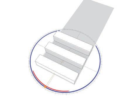
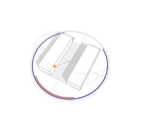
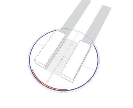
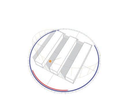
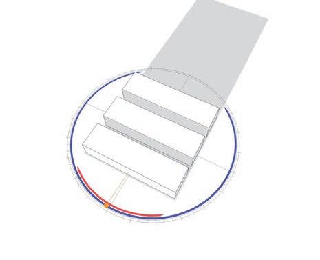
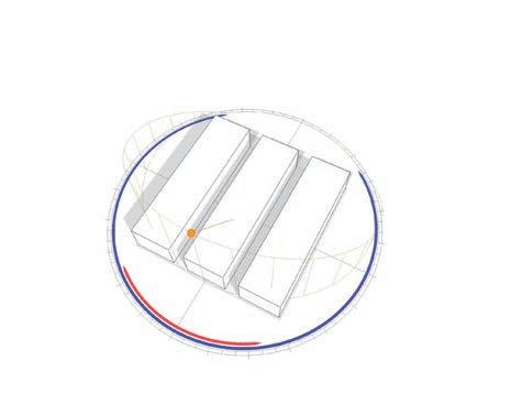
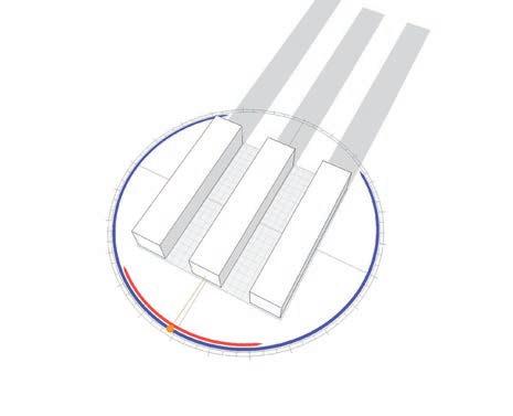
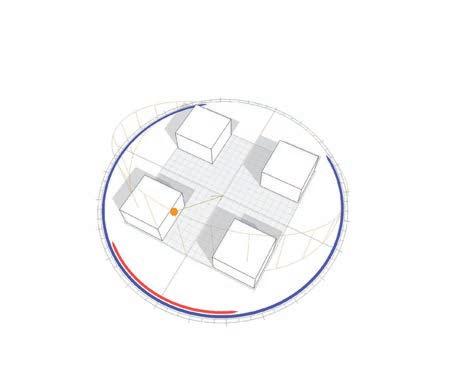
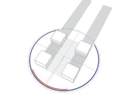

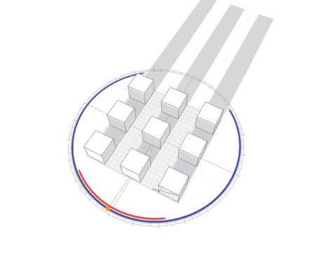
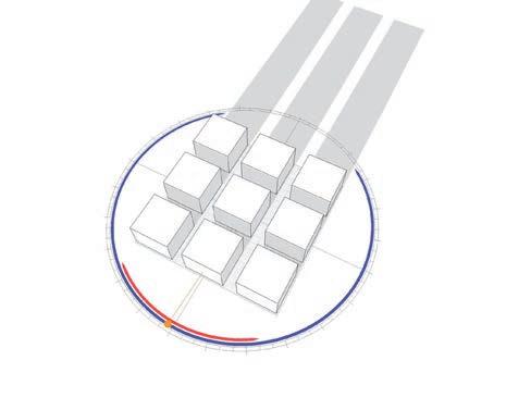
Latitude 60˚ Latitude 60˚ Latitude 60˚ Urban Canyon Ratio - 327Sun shadow studies for different latitudes
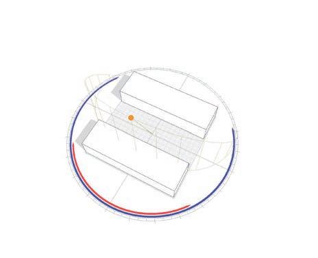
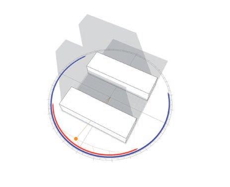
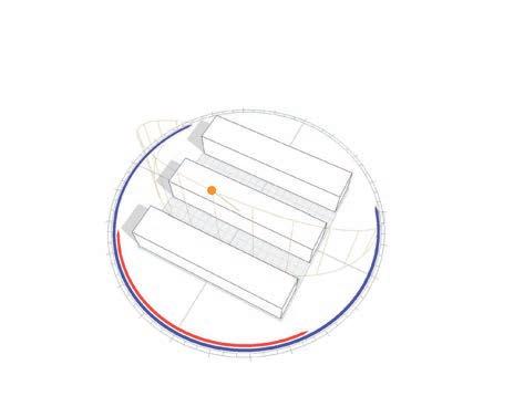
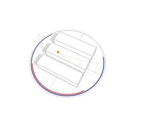
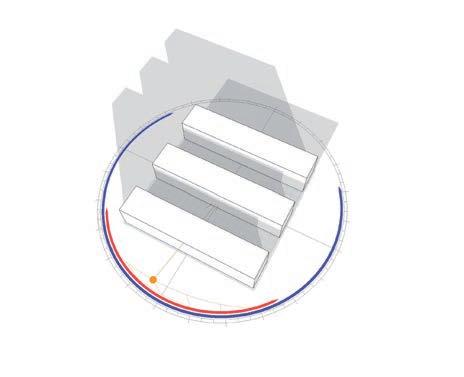
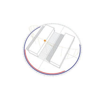
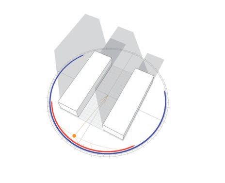
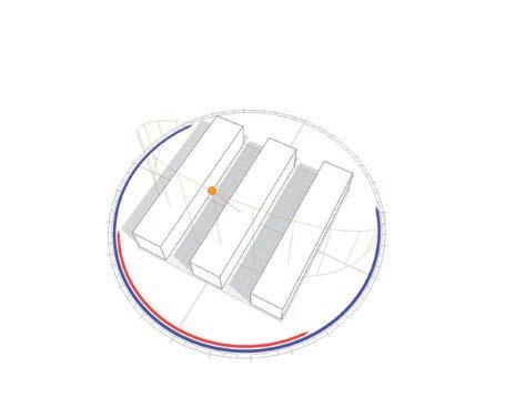
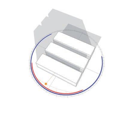
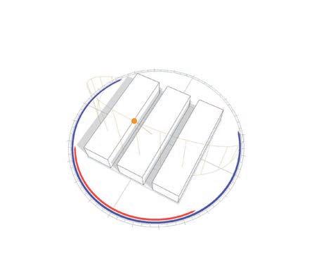
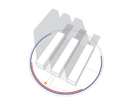
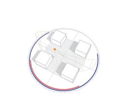
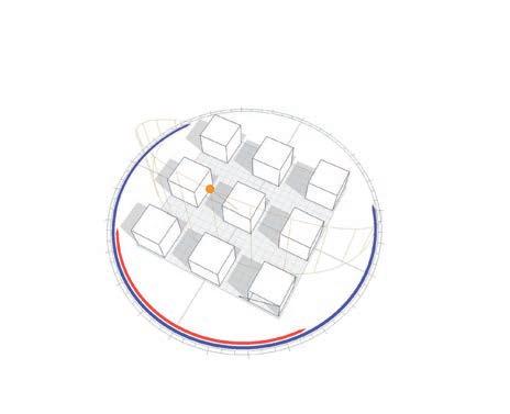
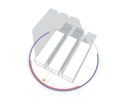
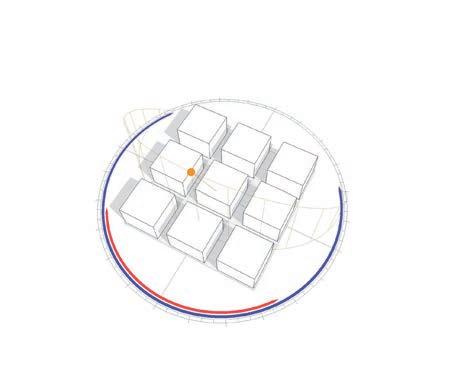
Latitude 45˚ Latitude 45˚ Latitude 45˚ Urban Canyon Ratio - 328Appendix 03
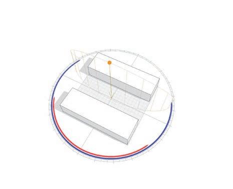
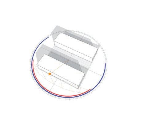

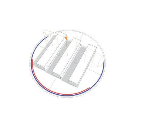
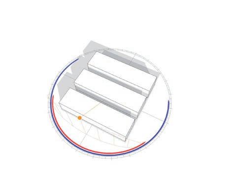
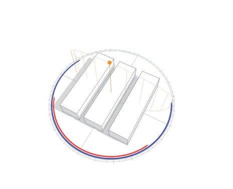
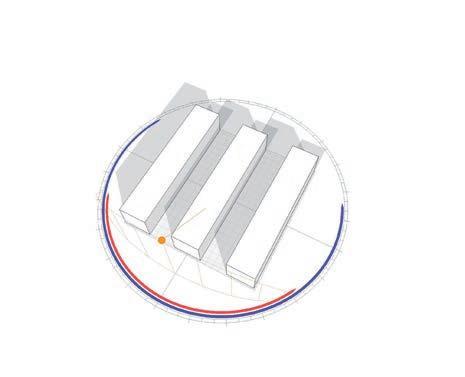
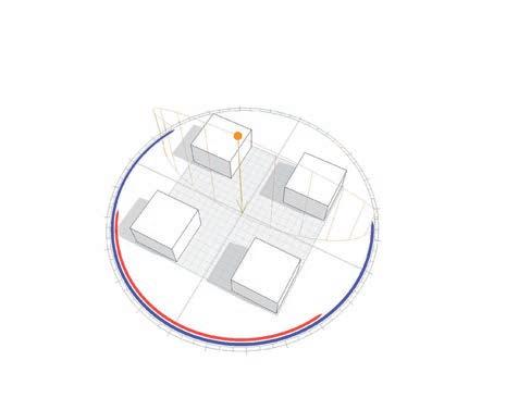
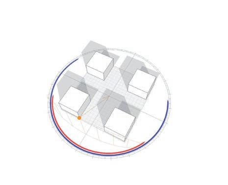

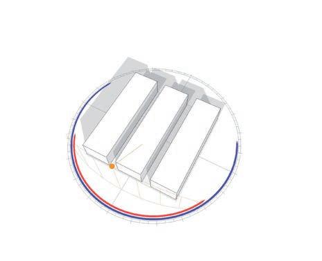
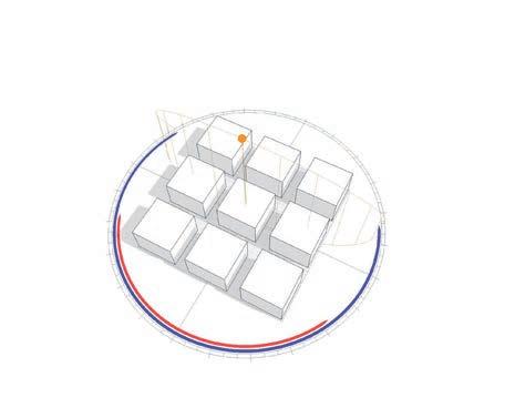
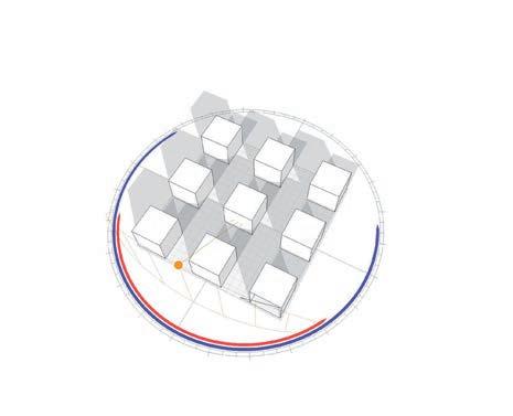
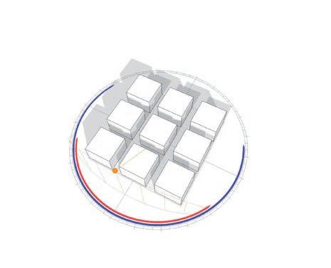
Latitude 25˚ Latitude 25˚ Latitude 25˚ Urban Canyon Ratio - 329Sun shadow studies for different latitudes
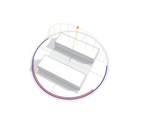
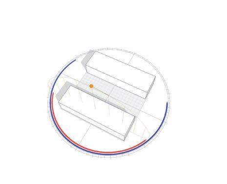
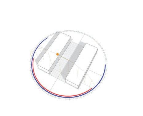
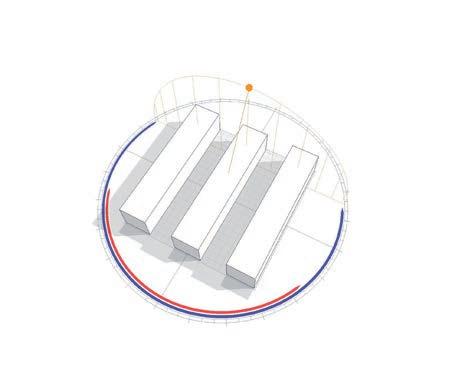
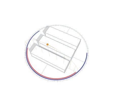
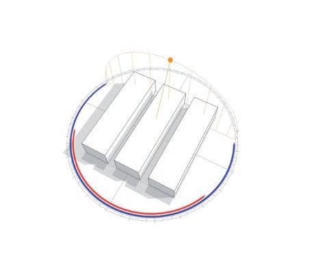
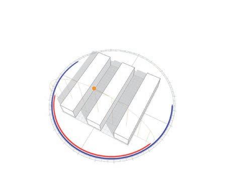
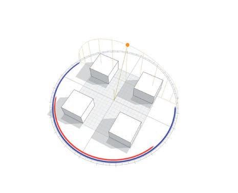
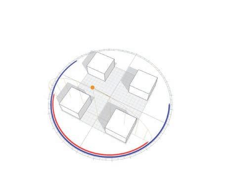
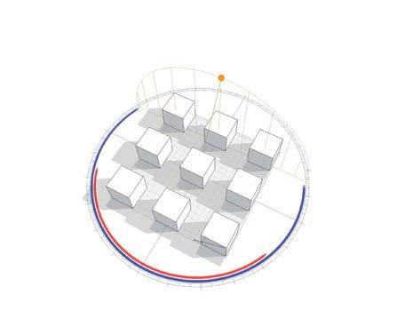
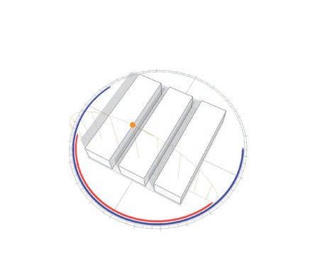
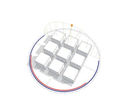
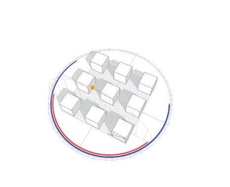
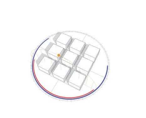
Latitude 00˚ Latitude 00˚ Latitude 00˚ Urban Canyon Ratio - 330Appendix 03
- 331Sun shadow studies for different latitudes
Appendix 04
Patch Aggregation Studies
Density: 1.02 Connectivity: 0.19 Recreation: 1.53 Fitness: 0.72
Density:
Connectivity: 0.61 Recreation: 0.95 Fitness: 0.35
Density: 1.33 Connectivity: 0.39 Recreation: 1.96 Fitness: 0.76
Density: 2.14 Connectivity: 0.36 Recreation: 0.08 Fitness: 0.31
Density: 2.20 Connectivity: 0.46 Recreation: 0.47 Fitness: 0.46 Patch
Density: 1.49 Connectivity: 0.42 Recreation: 0.84 Fitness: 2.74
Density: 1.22 Connectivity: 0.24 Recreation: 1.66 Fitness: 0.79
Density: 2.06 Connectivity: 0.29 Recreation: 0.29 Fitness: 0.33
Density: 1.30 Connectivity: 0.10 Recreation: 1.75 Fitness: 0.81 Patch
Density: 1.70 Connectivity: 0.35 Recreation: 0.62 Fitness: 3.21 Patch
Density: 2.15 Connectivity: 0.38 Recreation: 0.30 Fitness: 0.36
Density: 2.26 Connectivity: 0.29 Recreation: 0.30 Fitness: 4.78 Patch 04:
03 Density: 2.14 Connectivity: 0.38 Recreation: 0.87 Fitness: 3.53 Patch 04: Individual 04 Density: 1.49 Connectivity: 0.43 Recreation: 1.07 Fitness: 1.07 Patch 08: Individual 03 Density: 1.76 Connectivity: 0.37 Recreation: 0.85 Fitness: 8.86 Patch
04 Density: 1.40 Connectivity: 0.66 Recreation: 1.36 Fitness: 1.47 Individual
- 333Patch Aggregation Studies
Patch 01: Individual 03
Patch 01: Individual 04
1.91
Patch 05: Individual 03
Patch 05: Individual 04
Patch 02: Individual 03
02: Individual 04
Patch 06: Individual 03
Patch 06: Individual 04
Patch 03: Individual 03
03: Individual 04
07: Individual 03
Patch 07: Individual 04
Individual
08: Individual
03 Individual 04
Patch 01: Individual 05
Patch 05: Individual 05
Patch 01: Individual 06
Patch 05: Individual 06
Patch 06: Individual 06
Patch 07: Individual 05
07: Individual 06
08: Individual 06
Density: 1.58 Connectivity: 0.37 Recreation: 1.51 Fitness: 1.64
Density: 2.10 Connectivity:
Recreation:
Fitness:
0.00
0.36
0.30
Density:
Connectivity: 0.46 Recreation: 0.83 Fitness: 10.54
1.77
Density: 2.15 Connectivity: 0.31 Recreation: 0.46 Fitness: 0.40
Density: 1.51 Connectivity: 0.30 Recreation: 1.44 Fitness: 1.38
05 Density: 1.65 Connectivity: 0.00 Recreation: 0.68 Fitness: 2.34
Density: 1.63 Connectivity: 0.23 Recreation: 1.10 Fitness: 1.72
Density: 1.92 Connectivity: 0.23 Recreation: 0.00 Fitness: 0.26
Density: 1.44 Connectivity: 0.49 Recreation: 0.44 Fitness: 1.20
Density: 1.45 Connectivity: 0.46 Recreation: 0.63 Fitness: 1.36
Density: 1.42 Connectivity: 0.50 Recreation: 0.60 Fitness: 1.29
Density: 1.42 Connectivity: 0.40 Recreation: 0.00 Fitness: 1.01
Density: 1.68 Connectivity: 0.33 Recreation: 2.06 Fitness: 2.50 Patch 04: Individual 05 Density: 1.48 Connectivity: 0.38 Recreation: 2.10 Fitness: 1.13 Patch
Density: 1.87 Connectivity: 0.31 Recreation: 0.27 Fitness: 0.33 Patch
Density: 1.88 Connectivity: 0.04 Recreation: 0.57 Fitness: 0.42 Individual 05
- 334Appendix 04
Patch 02: Individual 06
Patch 02: Individual
Patch 06: Individual 05
Patch 03: Individual 06
Patch 03: Individual 05
Patch
Patch 04: Individual 06
08: Individual 05
Individual 06
Bibliography
Adolphe, L. (2000). A simplified model of urban morphology: application to an analysis of the environment performance of cities. Environment and Planning B , 28 (2), 183-200.
Ali Toudert, F. (2001). A Methodology For A Climatic Urban Design. The 18th International Conference on Passive and Low Energy Architecture, (pp. 469-474). Florianopolis.
Ali-Toudert. (2005). Dependence of Outdoor Thermal Comfort on Street Design in Hot and Dry Climate. Berichte des Meteorologischen Institutes der Universität Freiburg (15).
Ali-Toudert. (2005). Outdoor thermal comfort in the old desert city of Beni-Isguen, Algeria. Climate Research , 28, 243-256.
Ali-Toudert, F. (2007). Effects of asymmetry, Galleries, overhanging Facades and Vegetation on thermal Comfort in Urban Street Canyons. Solar Energy (81), 742-754.
Ali-Toudert, F. (2006). Effects Of Street Design On Outdoor Thermal Comfort.
Ali-Toudert, F. (2005). Numerical study on the effects of aspect ratio and orientation of an urban street canyon on outdoor thermal comfort in hot and dry climate. Building and Environment (41), 94-108.
Ali-Toudert, F. (2007). Thermal comfort in an east–west oriented street canyon in Freiburg (Germany) under hot summer conditions. Theoretical and applied Climatology (87), 223-237.
Arnfield, A. J. (1990). Street Design and Urban Canyon Solar Access. Energy and Buildings , 14, 117-131.
Arnfield, J. (2003). Two Decades of Urban Climate Research: A Review of Turbulence, Exchanges of Energy and Water, and the Urban Heat Island. International Journal of Climatology , 23, 1-26.
Berghauser Pont, M. (2010). SpaceMatrix Space, Density and Urban Form. Rotterdam: NAi Publishers.
Biller, T. &. (1983). Notes on the rise, development and destruction of a block in Friedrichstadt. Architectural Design , 53 (1/2), 20-26.
Bouyer, J. (2009). Mitigating Urban Heat Island Effect by Urban Design: Forms and Materials. Fifth Urban Research Symposium 2009.
De Schiller, S. (1998). Sustainable Urban Development; Design Guidelines for Warm Humid Cities. Urban Design International , 4, 165184.
De Schiller, S. (1995). Training Architects and Planners to Design with Urban Microclimates. Atmospheric Environment , 30 (3), 449-454. El Nahas, M. (1996). Energy saving throug urban Design - A microclimatic approach. Adelaide.
Emmanuel, R. (1995). Energy-Efficient Urban Design Guidelines For Warm-Humid Cities: Strategies for Colombo, Sri Lanka. Journal of Architectural and Planning Research , 58, 58-79.
Givoni, B. (1989). Urban Design in different Climates (Vols. WCAP-10). Los Angeles: World Meteorological Organization. Godfray, H. C. (2010). The future of the global food system. Philosphical Transactions of The Royal Society , 365, 2769-2777.
Golany, G. (1996). Urban Design Morphology and Thermal Performance. Atmospheric Environment , 30 (3), 455-465. Group, ‘2C‘. (1979). Cerda’s Barcelona. Lotus International (23), 76-94.
Grumbach, A. (1983). Paris - Rue de Rivoli. Daidalos (7), 19-23.
Huang, Y. (2008). Towards urban design guidelines from urban morphology description and climate adaptability. PLEA 2008 – 25th Conference on Passive and Low Energy Architecture. Dublin.
Jabareen, Y. R. (2006). Sustainable Urban Forms; Their Typologies, Models, and Concepts. Journal of Planning Education and Research , 26, 38-52.
Jack, H. J. (1981). Some simplified parameters to assess the energy efficiency of urban settlement configurations. Environment and Planning B , 8 (3), 333-348.
Kennedy, C. (2009). Greenhouse Gas Emissions from Global Cities. Environ. Sci. Technol. , 43, 7297-7302.
Knowles, R. (1981). Sun Rhthm Form. Cambridge, MA: MIT Press. Krier, L. (n.d.). Urban Components.
Marshall, S. (2005). Streets and Patterns. Oxon: Spon Press. Mills, G. (2006). Progress toward sustainable settlements: a role for urban climatology Theor. Appl. Climatol. , 84, 69-76.
Morello, E. (2009). Sustainable Urban Block Design through Passive Architecture A tool that uses urban geometry optimization to compute energy savings. PLEA2009 - 26th Conference on Passive and Low Energy Architecture. Quebec.
Morgan, D. (1977). Microclimates within an Urban Area. Annals of the Association of American Geographers (pp. 55-65). Taylor & Francis Ltd.
Morris, A. (1994). History of Urban Form, Before the Industrial Revolution. New York: John Wiley & Sons.
Ng, E. (2010). Designing High-Density Cities; For social & environmental sustainability. London: Earthscan.
Oke, T. R. (1987). Boundary Layer Climates (2nd Edition 1987 ed.). London: Routledge.
Oke, T. R. (2006). Initial Guidance to obtain representative Meteorological Observations at Urban Sites. Vancouver: Word Meteorological Organization. Olgyay. (1969). Design with Climate. New Jersey: Princeton University Press.
- 335 -
Oliveira Panao, M. (2008). Optimization of the urban building efficiency potential for mid-latitude climates using a genetic algorithm approach. Renewable Energy , 33, 887–896.
Oliver, P. (1997). Encyclopedia of Vernacular Architecture of the World (Vols. 1-3). Cambridge: Cambridge University Press. Rudofsky, B. (1964). Architecture without Architects. London: Academy Editions.
Salat, S. (2009). Constructing Sustainability: Ethics, Techniques or Aesthetics. Constructing Sustainability: Ethics, Techniques or Aesthetics.
Salat, S. (2007). Energy and Bioclimatic Efficiency of Urban Morphologies: A Comparative Analysis of Asian and European Cities . Conference on Sustainable Building South East Asia. Malaysia.
Salat, S. (2010). Morphological indicators for assessing the sustainability of cities.
Santamouris, M. ,. (2002). Ventilation of street canyons and its impact on passive cooling design. Universtity of Athens, Physics Department, Group Building, Environment Studies, Athens.
Sass, R. (n.d.). It’s not cool to be hot in Houston. Houston: http://www.ruf.rice.edu/~sass/UHI.html.
Siksna, A. (1998). City centre blocks and their evolution: A comparative study of eight American and Australian CBDs. Journal of Urban Design , 3 (3), 253-283.
Steemers, K. (2000). Assessing the Urban Microclimate: Introducing innovative modelling techniques. The Martin Centre for Architectural and Urban Studies.
Stewart, I. Classifying Urban Climate Field Sites by “Local Climate Zones”; The Case of Nagano, Japan. The seventh International Conference on Urban Climate. Yokohama.
Stone, B. (2006). Land use planning and surface heat island formation: a parcel based radiation flux approach. Atmospheric Envrionment , 40, 3561-3573.
UN Habitat. (2010). The state of African Cities 2010. Nairobi: UNEP.
United Nations. (2009). World Urbanization Prospects, The 2009 Revision. Department of Economic and Social Afairs. New York: Population Division.
Van Esch, M. (n.d.). Transferring Knowledge on Urban Microclimates in the Urban Planning and Design Process.
Watson, D. (1979). Energy conservation through building design. McGraw-Hill, Inc.
Whitehand, J. (1981). The urban Landscape: Historical Development and Management. London: Academic Press INC. LTD.
- 336Bibliography
