Adaptive Urban Hillscapes
Emergent Technologies and Design 2016 - 2017
A.Syed / X.Luo / D.Valdivia [M.Arch]
Y.Zhu [M.Sc]

Adaptive Urban Hillscapes
Balancing the ecological effects of anthropogenic occupation of hills
Architectural Association School of Architecture Emergent Technologies and Design 2016-17
M.Arch A.Syed / X.Luo / D.Valdivia
M.Sc Y.Zhu
| Adaptive Urban Hillscapes 4
Architectural Association School of Architecture Graduate School Programme

Programme:
Emergent Technologies and Design
Term:
Student Names:
Submission Title:
Course Tutor:
Course Title:
Submission Date:
Declaration:
04
Arshad Syed, Xiaoxiao Luo, Diego Valdivia (MArch)
Adaptive Urban Hillscapes
Michael Weinstock, George Jeronimidis, Evan Greenberg
Emergent Technologies and Design
27/01/2017
“I certify that this piece of work is entirely my/our own and that any quotation or paraphrase from the published or unpublished work of others is duly acknowledged.”
Signature of Student(s)
5 |
| Adaptive Urban Hillscapes 6
Acknowledgement
This work appeals to the innovative land-occupation, one that is synchronized with the native ecological cycles and heritage. We would like to thank all the people who in one way or another have contributed their expertise and experience to this work. When we were embarking on this project, we knew it could be challenging. Given their great support and assistance, we have managed to devote ourselves to completing this work. First and foremost, we would like to express our sincere gratitude to our course directors, Michael Weinstock and George Jeronimidis, not only for their kind and friendly supervision and support but also for their valuable guidance and assistance throughout the pursuance of this work. Their experience and assistance greatly helped us to further our knowledge, skill and understanding in the field of architecture. Many thanks also to our studio master, Evan Greenberg, and our course tutors, Manja Van De Worp, Elif Erdine and Mohammed Makki for their constant support and commitment throughout our EmTech course. We are also grateful to the jury whose valuable comments are indeed useful and inspiring. Finally, we would like to thank our families and our EmTech classmates for their support since the beginning of this course.
7 |
| Adaptive Urban Hillscapes 8
Abstract
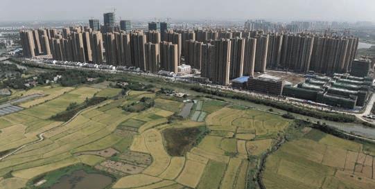
Recent studies reveal that by the year 2030, roughly 70% of the total population of China will live in cities, most likely in megacities like Beijing, Shanghai or Shenzhen. This impending phenomenon points not only to a population density and spatial issue, but also to the food and water supply affecting billions of people. While the prosperous city of Shenzhen has certainly been a migrant magnet for the past thirty years, concerns are emerging regarding identifying new supply sources to sustain city development. Yet it is worth analyzing and taking into account the amount of territory that uncontrolled urban sprawl has appropriated from green areas and arable land, as the challenge for future city planning comes now with the demand to regain food supply sources to sustain those burgeoning populations. At the same time, the predicted shortage of buildable land has become an existing problem, pushing urban growth towards unsuitable hilly terrains in a region where daily intense rainfall has been always a menace capable of triggering landslide hazards. Considering the amount of territory that urbansprawl has appropriated from hillside green areas, city planning comes today with the challenge of regaining supply sources and balancing the ecological effects of anthropogenic alteration of hill landscape Based on this scenario, this dissertation addresses the possibility of proposing an an urban system adapting its components in a synchronic way such that human activity coexists with natural phenomena, all the while taking advantage ecological forces for new sources of supply.
9 |
1.1
1.5
2.1
2.2
2.3
2.4
2.5
2.6
Research Development
| Adaptive Urban Hillscapes 10
Contents Introduction
Urban growth towards hillsides
Soil erosion and landslides
Sediment deposition
Anthropogenic Ecologies
1.2
1.3
1.4
Ambition Domain
Urbanization now - the Asian epoch
Urbanization on slope terrains
Ecological spatial patterns
Hill ecosystem
Traditional settlements and building morphologies
Rice terraces landscape systems
Slope instability
Mitigation techniques
Case of Hong Kong 2.10 Site : Shenzhen city
Conclusion Methods
Deterministic mapping
Topographical analysis 3.3 Multi-objective optimisation 3.4 Spatial quality analysis
Networks
RUSLE model
Experiment flowchart
2.7
2.8
2.9
2.11
3.1
3.2
3.5
3.6
3.7
Test patch selection 4.2 Factor map 4.3 Synthesis mapping 4.4 Slope risk analysis 4.5 Spatial pattern sampling 4.6 Data extraction 4.7 Conclusion p.12-23 p.15 p.16 p.18 p.20 p.22 p.24-83 p.26 p.30 p.32 p.36 p.38 p.44 p.50 p.58 p.64 p.74 p.82 p.78-105 p.86 p.88 p.92 p.94 p.98 p.100 p.104 p.106-155 p.108 p.116 p.122 p.134 p.138 p.152 p.154 01. 02. 03. Acknowledgement Abstract p.7 p.9 04.
4.1
Design Strategy
Design Proposal
Critical Analysis
11 |
Multi-layer approach 5.2 Attempt for synchronisation 5.3 Strategy 1 - Hydrological network 5.4 Strategy 2 - Vegetation strategy 5.5 Strategy 3 - Farming Strategy 5.6 Strategy 4 - Transport network strategy 5.7 Operative urban scales 5.8 Strategy 5 - Urban system ( cluster 1 ) 5.9 Strategy 6 - Operational public space
Strategy 7 - Building generation ( cluster 1 ) 5.11 Conclusion
5.1
5.10
6.1 Building Generation - further evaluation 6.2 Building generation - post GA evaluation 6.3 Building generation - final selection 6.4 Sections 6.5 Adaptive urban system (0.7km2) 6.6 Renders
7.1 Network analysis 7.2 Street operation and public connectivity 7.3 Building evaluation 7.4 Conclusion Appendix Bibliography p.158-207 p.158 p.162 p.164 p.172 p.174 p.178 p.180 p.182 p.196 p.200 p.206 p.207-239 p.210 p.212 p.218 p.200 p.226 p.232 p.242-251 p.243 p.246 p.248 p.250 p.226 p.254-269 p.272-275 05. 06. 07.
Introduction 01.
PRODUCED BY AN AUTODESK PRODUCED BY AN AUTODESK EDUCATIONAL PRODUCT AUTODESK EDUCATIONAL PRODUCT
AUTODESK EDUCATIONAL PRODUCT PRODUCED BY AN AUTODESK PRODUCED BY AN AUTODESK EDUCATIONAL PRODUCT
Urban growth towards hillsides
Soil erosion and landslides
Sediment deposition
Anthropogenic Ecologies
Ambition
1.1
1.2
1.3
1.4
1.5
| Adaptive Urban Hillscapes 14
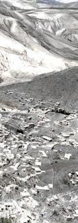
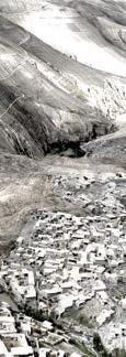
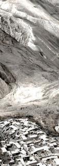
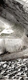
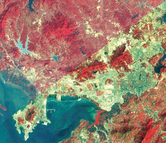
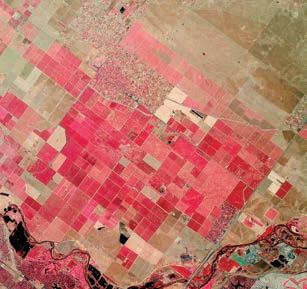
Fig. 1.1.1 - Shenzhen’s rapid urbanization spreading towards hillsides. 1988/1996 - colour infrared photo (NASA - http://svs.gsfc. nasa.gov/1060)
1.1 Urban Growth Towards Hillsides
In recent decades, the exponential growth of urban land in cities brought negative impact to the environment; economy and society (Brueckner, 2000) by planned and unplanned human occupation causing a large number of natural disaster incidents. One of the most dangerous scenarios are those involving urbanizations within or close to slope terrains. Such occupations are in permanent danger of physical damage due to landslides, which have been reported by the Center of Research on the Epidemiology of Disasters, as one of the most common threats to human life and city infrastructure. Each year landslides take thousands of victims and billions of dollars in infrastructural damage around the world (Kjekstad and Highland, 2009), and the frequency of these disasters might rise as vulnerability increases in cities where urban sprawl is the symbol of growth.
It is known that deforestation; uncontrolled usage of land and unconscious manipulation of topography on hills are among the most common trigger mechanisms of landslides as they increase surface soil exposure to erosion. After long periods of intense rainfall, erosion can easily transport big masses of soil down-slope (Parriaux, 2011), taking large numbers of unaware constructions with it. A correct understanding of hydrological flows and slope stability, together with a suitable distribution of construction following a prediction survey will help to define an efficient mitigation model in order to control future damage and loss.
15 |
Introduction
1.2 Soil Erosion and Landslides
Recently, scientists have been arguing about the benefits of natural non-accelerated soil erosion as a carbon sink process affecting the atmosphere. Their statement describes that during its process, which is the detachment, transport and deposition of soil materials by hydrological agents (Ellison, 1984), soil erosion acts as a conveyor by transporting carbon retained in plants and surface soil layers during the detachment and later submerging the carbon on the areas where sediment deposits (University of Exeter, 2007). This perception encourages the development and ambition of this proposal by taking soil erosion as a beneficial natural phenomenon that, rather than being avoided, can also be controlled at certain degree and then used as a design driver. However, soil erosion also gives way to different kind of landslides, and among these, debris flows; rotational and translational landslides are the most registered involving physical damage to urbanizations and will also be the ones considered in this research. Prolonged intense rainfall is the most common cause of soil erosion globally, while subsequent infiltration together with groundwater flows are the most common trigger factors of landslides (Johnson and Sitar, 1990). Furthermore, intense precipitation has been recently the most frequent trigger mechanism for deadliest landslides around the world (NASA, 2016).
| Adaptive Urban Hillscapes 16
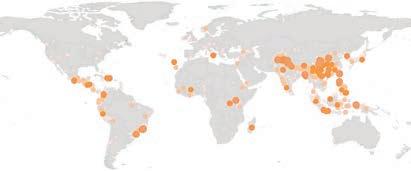
Fig. 1.2.1 Rainfall-triggered landslides globally (NASA, 2016) Redrawn
1-10 11-25 26-50 51-100 101-5000
Fig. 1.2.2 Number of fatalities associated with rainfalltriggered landslides (NASA, 2016) Redrawn
Fig. 1.2.1
Fig.
1.2.2
17 | Introduction
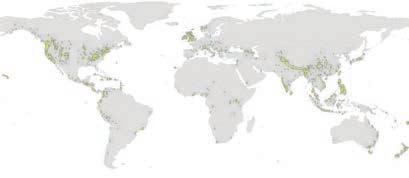
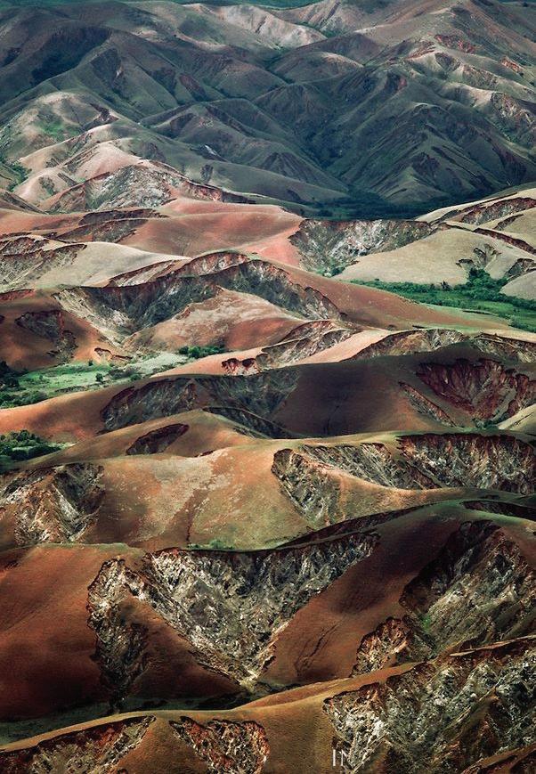
Fig 1.2.3
Severe erosion on deforested hills, Central Madagascar. (F. Lanting)
Fig 1.2.3
Bedrock
Residual Soil
Eroded Soil Deposited Soil
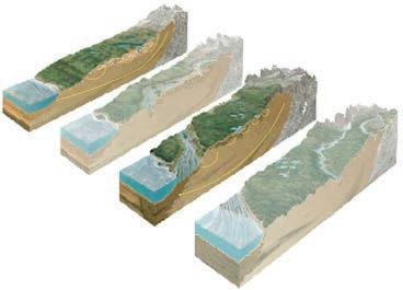
1.3 Sediment Deposition
The perception of soil erosion and landslides as a carbon sink process beneficial for the atmosphere gives a new perspective to the thesis on facing landslides acting on urbanized areas. Additionally, natural soil erosion also renews land and provides the opportunity of utilizing emerging land from depositions if these can be predicted. Anticipating erosion and predicting deposition can inform a retention and deviation strategy to allocate new land in areas where farming or public spaces are needed, and to prevent future development of the city in areas where potential risk increases.
After continuous heavy rainfall in hilly terrains, different volumes of soil are transported by hydrological agents. Thin layers of soil are removed by raindrops on sheet erosion; another scale is the removal of a large amount of soil driven by a concentrated water flow creating gullies known as gully erosion (C. Brouwer et al, 1985). Among the different mitigation techniques that will be described further in the next chapter, slope reconfiguration is probably the most fundamental when it comes to control flows. Slope angle and slope stability models will be required to retain the amount of volume of soil needed to generate new land.
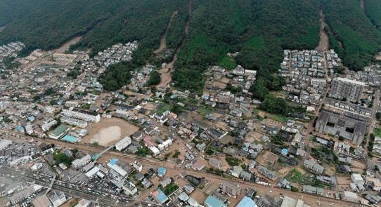
A month of heavy rainfall triggered landslides in Hiroshima. Slopes collapsed in flows of mud, rock and debris. (Reuters, 2014)
| Adaptive Urban Hillscapes 18
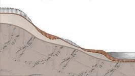
Fig. 1.3.1 Soil Erosion and Deposition in slopes. (A, Behre et al, 2007) Redrawn
Fig. 1.3.2
Fig. 1.3.1
Fig. 1.3.2
Elevation
1000 m
6 m
Debris flow paths
Landslide scars
19 |
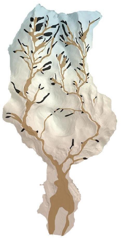
Fig. 1.3.3
FLO-2D model developed by J.S.O’Brien on1989 simulating debris flow along a DEM map. (O’Brien et al, 2011)
Introduction
Fig. 1.3.3
1.4 Anthropogenic Ecologies
Dynamic Ecosystems
The interaction between plant and animal species in different environments started to be defined as an ecosystem in the early 1900s. Their dynamic relationships, understood as exchanges of energy and matter flow are the heart of today’s ecological research, and recently, different disciplines are determined on decoding their adapted and selforganized bodies (Reed and Lister, 2014). Ecosystems are unpredictable, as it has been stated that a simple alteration in one of their agents can drive to significant changes, which sometimes are the reason why they experience growth and renewal (Bormann and Likens, 1979).
The impact of the ‘human epoch’ has produced large scale alterations to the biosphere’s ecosystem. From hunting to the clearing of land, human activities vanished several species and agricultural land, leading to big unprecedented changes in ecology, being climate the most evident. But there is more about the opportunities that are present in this global scenario. Recent studies state that the future of ecological research will benefit from focusing on novel remnant ecosystems that are found within used lands (Ellis et al, 2010).
Given those circumstances, one of the objectives of an ecological-driven design is to give importance to those forces and dynamics that are not under the control of the designer, and whose influences can reach scales larger than those expected, outside of the particular project’s immediate context (Reed and Lister, 2014). The interest of this proposal then rests on those intrinsic relationships that emerge between human induced sub-ecosystems and that can inform a unique process of city development.
"Given that novel ecosystems embedded within anthromes now cover a greater global extent than Earth’s remaining wildlands, they offer an unparalleled opportunity for conserving the species and ecosystems we value. [...] The critical challenge therefore is in maintaining, enhancing, and restoring the ecological functions of the remnant, recovering and managed novel ecosystems formed by land use and its legacies within the complex multifunctional anthropogenic landscape mosaics that are the predominant for of terrestrial ecosystems today and into the future."
- Erle C. Ellis A Taxonomy of the Human Biosphere
| Adaptive Urban Hillscapes 20
21 |
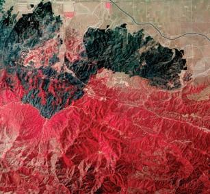
Fig. 1.4.1 Pine fire damage (Angeles National Forest) post-disaster assesment. The extent of the fire and the exposed slopes is evident, that may become deadly mudslides in winter. [color infrared photo, Cirrus-designs.com]
Fig. 1.4.2 California central valley (north of Fresno) This image shows the urban -agricultural interface in one of the most productive food growing regions in the world [color infrared photo, Cirrus-designs. com]
Fig. 1.4.2
Introduction
Fig. 1.4.1
In conditions of urban expansion towards hillsides, like in Shenzhen in southern China or any fast developing megacity with unsuitable terrain, the potential risk pertains to the unaware alteration of the hill natural ecosystem that can cause soil erosion hazards triggered by intense precipitation. On the other hand, increasing populations demand more local sustainable supply sources, which have been continuously vanishing as Shenzhen’s green areas and farmlands were depleted by exponential urban development during the past three decades. Nevertheless, an opportunity of dealing with these main problems emerges from the conception of a unique type of hill-adapted city tissue, one that is aware of the potential negotiations that connectivity between hill sub-ecosystems can provide. The complexity of such a system is found on the integration of those relationships within the networks and the build fabric that compose the city tissue, leading to an intelligent urban development and sustainable supply systems. Hence the main ambition of this research focuses on a unique dynamic urban body that reflects the operational significance of the spatial patterns emerging from anthropogenic occupancy. Therefore, the research question arises:
The following diagram (Fig. 1.5.1) explains the strategy on combining characteristics and techniques from the main research topics, together building the concepts for the system.
| Adaptive Urban Hillscapes 22
“
How to synchronically develop the components of a hill-adapted city tissue, focusing on the relationships between sub-ecosystems that can establish a complex yet fertile environment suitable for the coexistence of urban activity with the natural phenomena, all the while taking advantage of this context as new sources of supply."
1.5 Ambition
Hill Ecology
Hydrological Systems
Urban System on Slope Terrains
Vegetation
Slope Stabilization
Drainage Systems
Underground / Surface
Root systems
Terraced agriculture
Water Supply
Food Supply
Urban System
Supply System
Retention Structures
Building Morphology
Semi Public Spaces
Urban Pattern
Public Spaces
Built Fabric
Erosion/Debris flow
Sediment deposition
Sub-Ecosystems
Ecological patterns
23 | Introduction
Fig. 1.5.1 Research strategy flow chart
Fig. 1.5.1
Domain 02.
PRODUCED BY AN AUTODESK PRODUCED BY AN AUTODESK EDUCATIONAL PRODUCT AUTODESK EDUCATIONAL PRODUCT
AUTODESK EDUCATIONAL PRODUCT PRODUCED BY AN AUTODESK PRODUCED BY AN AUTODESK EDUCATIONAL PRODUCT 2.1 Urbanization now - the Asian epoch 2.2 Urbanization on slope terrains 2.3 Ecological spatial patterns 2.4 Hill ecosystem 2.5 Traditional settlements and building morphologies 2.6 Rice terraces landscape systems 2.7 Slope instability 2.8 Mitigation techniques 2.9 Case of Hong Kong 2.10 Site : Shenzhen city 2.11 Conclusion
2.1 Urbanization Now - The Asian Epoch
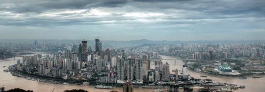
The precise demographic definition of urbanization is the increasing share of a nation’s population living in urban areas (and thus a declining share living in rural areas). In the early 1900s, the United States reached a critical point: half the country’s population had migrated into its cities, creating unprecedented ghettos and driving the high-rise metropolis. In the early 2000s, the world as a whole reached the same midpoint (54.5 percent in 2016), with squatter settlements as dense as some of the most tightly packed high-rise districts. Demographers expect this great urban in-migration to continue for three or four more decades before urban population begins to slow by mid-century. Less attention has been given to two other transitions: around 1980, the economically active population employed in industry and services exceeded that employed in the primary sector (agriculture, forestry, mining and fishing); and around 1940, the economic value generated by industry and services exceeded that generated by the primary sector. [Satterthwaite 2007] [D.Harris,2012]
The great nineteenth and early twentieth century ports and steel, textile and mining centres have lost economic importance and population (Pallagst et al. 2009); so too have some of the major manufacturing cities. The market forces shifted to Asia to realise its vast potential; when in the 1970’s China’s open market reforms and the Gulf’s oil power came into being, and in the late 1980’s India globalised its economy. These regions with modest urban areas were thrust into providing land and infrastructure to fuel the new industrial growth. Along with this came job opportunities that creates massive migration forcing urban areas to expand into rural expanse, without control in most cases. Now, more than half of the population (53 percent) of large builtup urban areas (500,000 and over) are in Asia, living in 542 of the 1,022 large urban areas worldwide. The Asian areas, particularly- the Indian subcontinent, south-east Asia and China- comprise 57 percent of the world’s large urban area population . [Demographia, 2016]
Rural-urban drift is one of the three main drivers of urbanisation, accounting for about 25 per cent of urban population growth. The other two factors are natural population increases and the reclassification of rural areas into urban ones. Two aspects of the rapid growth in the world’s urban population are the increase in the number of large cities and the historically unprecedented size of the largest cities. In the last case, the authority’s role in incessant and rapid reclassification of agricultural land for urban and industrial development has left the native dwellers stranded within a growing concrete jungle. This practice is quite common in the new megacities with special global economies, as is found in China, India or Brazil.
[Commission on Growth and Development, 2009] [D.Satterwaithe et al., 2010]
| Adaptive Urban Hillscapes 26
Fig.2.1.1 Skyline of Chonqqing, China [getty images,2016]
Rural Rural Land Drift UrbanPopulation Urban
Fig.2.1.1
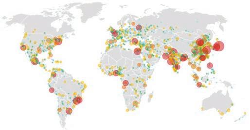
Mega city >10m (6.4%)
Large city 5-10m (4.2%)
Medium city 1-5m (11.6%)
Small city 500k-1m (5.1%)
Smallest city 300k-500k (3.6%)
Other urban <300k (23.2%)
27 |
Fig.2.1.3 World population distribution -urban & rural areas [Demographia,2016]
Fig.2.1.2 Worlds cities according to population [UN world urbanization prospects,2014]
Fig.2.1.3
Fig.2.1.4
Fig.2.1.4 World population by urban area density (habitants/km2) [Demographia,2016]
Rural 45.5% <100,000 15.1% 4,000-10,000 51.4% 10,000-20,000 18.3% 100,000-500,000 10.7% 10,000,000+ 8.2% 20,000-40,000 4.8% 40,000 & over 0.9% <Under 2,000 9.4% 2,000-4,000 15.2% 5,000,00010,000,000 3.9% 2,500,0005,000,000 5.3% 1,000,0002,500,000 6.5% 500,0001,000,000 4.7%
Domain
Fig.2.1.2
2.1.1 Urban Growth Of China

Urban / Industrial Sprawl
In the western world, suburbanization and sprawl started after World War II in many developed industrial cities. After decades of development, cities started facing lots of urban issues. This led to the idea of suburbanization, where the wealthy were able to live in relatively large spaces away from the problems of the dense inner city. Urban sprawl is a consequence of this phenomenon. Urban sprawl can refer to low-density, excessive spatial growth of cities. It is alleged that excessive urban expansion have encroached much farmland and open space. Urban sprawl is also thought to contribute to the decay of the downtown area and a number of social problems. And urban sprawl often results in overly long commute, contributing traffic congestion and air pollution. At the root of this perception is that urban sprawl is against the idea of sustainable development and many policies have been made to restrict urban sprawl in the United States.[ QI Lei et al. 2008]
Since then, population, job and commerce suburbanization has taken place, and when people took urban sprawl seriously in 1960s, the urban population proportion had already reached about 70 percent in the US. Unlike western countries, urban sprawl began in some developed cities in China only towards the end of the last century, after about two decades of urban development at an unprecedented rate. In China by 2006, the urban population proportion had reached 43.9 percent,
from 19.4 percent in 1980 (National Bureau of Statistics of China, 2007). Once the ‘open door’ policy was adopted, the new policy of changing administrative status of places was widely accepted.The official administrative status of villages to shift and become more urbanised as they were assimilated into expanding cities’ urban territories, or as the result of returning migrant workers building town-like settlements. They became ‘big villages’ and then later upgraded to ‘township’ status, again increasing the total population of towns and cities. Cities become industrial agglomerations for migrant workers without urban status, while urbanisation is treated merely as a strategy for economic building through industrialisation. [Weiwen,2008] [Segal,2008]
The process of suburbanization like the U.S. does not occur until now. In this sense, urban sprawl in China is mainly due to low-density urbanization, not excessive suburbanization like western countries. But in general, most of the Chinese megacities are tending to grow in a polycentric manner, so potentially the regional density can be kept high. But there are exceptions to such balanced development where urban expansion has encroached or converted so much farmland and open space, that Unlike the United States and other countries, farmland and other resources are much scarcer in China [ref fig.2.1.1.3]. Thus, urban sprawl is a much more dangerous signal for China.[ QI Lei et al. 2008]
| Adaptive Urban Hillscapes 28
[AD New Urban China, 2008 Huang Weiwen, the Deputy Director of the Urban and Architecture Dept. at Shenzhen Municipal Planning Bureau]
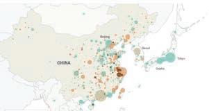
Fig.2.1.1.1 Change in population density [pewresearch.org ,2016]
Fig.2.1.1.1 Population (2010) Change in pop. density 50 million 10m 1m -25% +25% 0
29 |
Russia
Fig.2.1.1.2 Urban development in Hefei, China [theguardian.com/ gettyimages]
Canada China USA Brazil
Water resource/capita (m3) Area of farmland/capita (km2) Total Forest area (1000 km2) 1.4 2.3 0.21 1.64 1.47 30600 98500 2300 9400 43000 566 209 133 247 754
Fig.2.1.1.3 Comparison of main resources between nations of similar land area [Chou Baoxing /City Planning Review, 2007]
Fig.2.1.1.3
Domain
Fig.2.1.1.2
2.2 Urbanization on Slope Terrains
Urban Encroaching Upon Arable
The pattern of urban development thus far suggests massive encroachment upon agricultural land. However, according to a UNEP report the loss of agricultural land to the spatial expansion of urban areas is often exaggerated; one recent study suggested that only West Europe among the world’s regions has more than 1 per cent of its land area as urban In addition, a declining proportion of land used for agriculture around a city may be accompanied by more intensive production for land that remains in agriculture [Bentinck, 2000] or intensive urban agriculture on land not classified as agricultural. The availability of cultivable land close to village or town centre and cities is the main problem as urban centres will assimilate these areas and its resources, due to immoral government policies. There is an unfair competition for natural resources between industrial requirement and farming requirement.
Since the Asian region is only in its early stages of industry-oriented economy rather than on agri-forest produce economy, further urban expansion is imminent. Approximately 25 per cent of the world’s land surface is occupied by cultivated land [Cassman et al.2005]. Urban growth is more likely to reduce arable land availability if it takes place in this zone. This is a cause for concern, but more importantly the populace who are involved in agricultural practices will diminish, as the majority will be living in urban areas. [Schneider et al. 2009][ D.Satterwaithe et al., 2010].
The rapid industrialisation has taken a toll on the natural environment including water sources. According to current World Bank statistics, Chinese cities are frequently in the top 10 most polluted cities in the world and this ecological damage is causing shortage of drinking water in the major cities. The Taihu Lake pollution crisis in the Yangtse River Delta, which affected the drinking-water supply of about 2 million residents in Eastern China, and the red tides (caused by high concentrations of algae and affecting agricultural production) in the Pearl River Delta have in recent years demonstrated how severe such ecological damage can be.
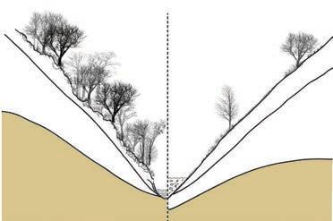
In quite a few cities, especially in south Asia and south America, the urban centre is either surrounded by hills with steep slopes or it is interspersed with such terrain. In the case of the former: the slopes are an ambiguous territory between the green cover and the city core, with varying degrees of informal occupation on the mostly unclaimed land (refer fig.2.2.1). This disorganised growth and pressure of urbanization causes reduction in the forest area, which in turn induces higher vulnerability to landslides following heavy rainfall on the region. In the case of the latter: rapid development on all fronts has forced formal transition of the slope lands to be converted for urban use. However, since they are not ideal for construction, the development is sporadic and seen as a last resort (refer fig.2.2.2). There are instances of an intense mixture of the two categories where socio economic conflicts arise. [MB.Schlee, 2015]
| Adaptive Urban Hillscapes 30
Fig.2.2.1 Factors influencing urbanization on slope terrains
Fig.2.2.2 Slope urbanization morphologies
Fig.2.2.1
Urban core Hills w/ green cover
population growth environment government policy Topography Climate Urban expansion Land reclassification Land economy Migration Factors pushing urbanization to slope terrains
Fig.2.2.2
Rapid urbanization and the associated growth of unauthorized and densely populated communities in hazardous locations, such as steep slopes, are powerful drivers in a cycle of disaster risk accumulation. Frequently, it is the most socio-economically vulnerable who inhabit landslide-prone slopes – thus increasing their exposure to landslide hazards, and often increasing the hazard itself. There is growing recognition that urban landslide disaster risk is increasing in developing countries, and that new approaches to designing and delivering landslide risk reduction measures on-the-ground are urgently needed. One such innovation would be to look at sloped terrains as having potential to give something back to the city.
The crucial trick is to find a zone which is in close enough proximity to the city, where work force and demand is ever present, and at the same time not in immediate threat of being built upon by economic forces, then it can potentially be a water reserve or serve as cultivable land that caters sustainably to the city. [mossaic.org]
Effects of Urbanisation on Slopes
Urban development on hill slopes has many potential effects on runoff processes, streamflow patterns and as a result the overall hydrology of the watershed. Urban development modifies hydrologic processes when vegetation is cleared from hillslopes, the land surface is graded and underground service systems are put in place for the buildings and roads. These changes reduce interception, infiltration, subsurface flow, evapotranspiration, stormwater storage on hillslopes, and the time required for stormwater to travel over and through a hillslope to a stream or reservoir [C.P.Konrad et al. 2002]
Consider the role of impervious surfaces in preventing water from being absorbed into the ground and promoting higher runoff during storms. All urbanised areas with hard paved surfaces like roads, pavements contribute to this.
31 |
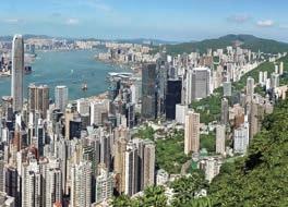
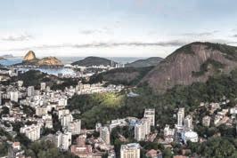
Fig.2.2.3 Rio de Janeiro - an example of a city interspersed with hills, having sporadic urbanization on the slopes. Urban sprawl of the informal favelas jostle with formal development.
Fig.2.2.4 Hong Kong - Controlled High rise development on slopes [landsd.gov.hk]
Fig.2.2.3
Fig.2.2.4
Domain
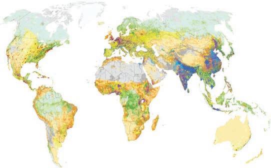
Fig. 2.3.1.1
Human influences over time.
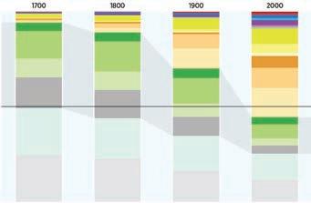
source: National Geographic, Atlas of the world, 10th Edition (2014).
2.3 Ecological Spatial Patterns
2.3.1 Anthromes
Also known as Human Biomes, Anthromes are the significant patterns that human interaction with ecosystems create globally. Anthromes are formed by global patterns of human occupation over long periods and present as ecological mosaics seen from the air. (Ellis and Ramankutty 2007) These include:
-Urbanizations
-Villages
-Croplands
-Rangelands
-Semi-natural Anthromes. (<20% of land used for crops, urban or pasture)
-Wildlands
Over the past 300 years, land use got exponentially affected by human activity expansion, driven by the industrial exploit of the earth’s energy. The evolution of agricultural and forestry techniques started to shape landscapes while rural populations migrated to urban centres, densifying cities and claiming bigger energy production. During the XVIII century, around 95% of the ice-free territories were wildlands and semi-natural anthromes, 55% of which was transformed by humans into rangelands, croplands, villages and densely settled anthromes during the following centuries.
| Adaptive Urban Hillscapes 32 Used USED Seminatural 50 % Wild
Fig. 2.3.1.1
DENSE SETTLEMENTS
Urban and other dense settlements
Urban
Densely built environments with high population
Mixed settlements
Suburbs, towns, and rural settlements, with high but fragmented populations
VILLAGES
Dense Agricultural settlements
Rice villages
Villages dominated by paddy rice
Irrigated villages
Villages dominated by irrigated crops
Rainfed villages
Villages dominated by rainfed agriculture
Pastoral villages
Villages dominated by rangeland
CROPLANDS
Lands used mainly for annual crops
Residential irrigated croplands
Irrigated croplands with substantial human populations
Residential rainfed croplands
Rainfed croplands with substantial human populations
Populated croplands
Croplands with significant human populations, a mix of irrigated and rainfed crops.
Remote croplands
Croplands without significant human populations
RANGELANDS
Lands used mainly for livestock grazing and pasture
Residential rangelands
Rangelands with substantial human populations
Populated rangelands
Rangelands with significant human populations
Remote rangelands
Rangelands without significant human populations
SEMINATURAL LANDS
Inhabitat lands for minor use for permanent agriculture and settlements
Residential woodlands
Forest regions with minor land use and substantial populations
Populated woodlands
Forest regions with minor land use and significant populations
Remote woodlands
Forest regions with minor land use and without significant populations
Inhabitated treeless and barren lands
Regions without natural tree cover having only minor land use and a range of populations.
WILDLANDS
Lands without human populations or substantial land use
Wild woodlands
Forests and savannas
Wild treeless and barren lands
Regions without natural tree cover (grasslands, shrublands, tundra, desert and barren lands).
Map of Ecological Patterns. Humans use of land affecting the global patterns of ecology all over the biosphere. source: National Geographic Atlas of the World, 10th edition (2014).
33 |
Fig. 2.3.1.2
Domain
Fig. 2.3.1.2
2.3.2 Novel Territories
Human land occupation is defined mainly as agriculture lands and urban settlements, representing 40% of the Earth’s ice-free land (Ellis et al, 2010). These activities have shaped visible spatial patterns on the planet’s surface, containing not only man-operated land but also novel ecosystems embedded within the anthromes. These territories are isolated areas of unused or less intensively managed ecosystems ‘created’ by humans, including: planted forests; woodlots; parks; abandoned lands and reserves. These novel territories tend to be designated on steep areas and less welcoming spaces (Reed and Lister, 2014).
Today, these unused territories surrounded by operated anthromes represent almost double the amount of area that wildlands currently hold, which, on the other hand, are located mostly on the cold and dry biomes of the planet (Sanderson et al, 2002). Evidence shows that high biodiversity can be found on lands used for agriculture, and even spatial patterns especially managed to enhance connectivity between anthromes to preserve habitats, can generate high levels of biodiversity on urban or village context (Ricketts, 2001). Future design’s challenge therefore is to maintain and enhance the ecological values of these remaining novel territories by incorporating them into the development of future anthropogenic landscape.
| Adaptive Urban Hillscapes 34
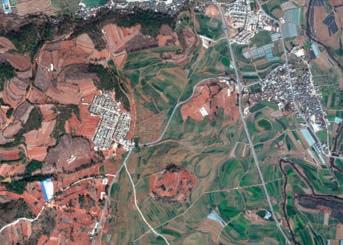
Fig. 2.3.2.1 Novel territories as forests in between farmlands in Kumming, China. source: http://www.pri. org/stories/2011-11-28/ rice-fields-asia-aboveand-below
Fig. 2.3.2.1


35 |
systems City Tissue Sub-System Rice-Terrace Sub-System Water Body Sub-System Forest Sub-system Management / Preservation Management / Preservation Management / Preservation Water / Food Supply Food Supply Water Water / Humus Water Evaporation Food Supply Domain
Fig. 2.3.2.2 Interaction relationship within Four Sub
Source: http://www. cnhp.colostate.edu/cwic/ cons/surveys.asp
2.4 Hill Ecosystems
Ground Water Exchange
Inside a hill ecosystem, the underground water can flow through different areas in response to variation of pore pressure within certain soils. The fluctuations of pressure are affected by the type of vegetation coverage or the proximity of water tables to the land surface. It is by these differences in pressure that water can return to the exterior land or water bodies, a process which is known as underground water discharge. The water recharge process, on the other hand, occurs slowly by the infiltration of water to the soil by precipitation. The characteristics that influence the recharge capacity of water bodies such as wetlands, relies on their topographic situation; soil conformation; and climatic conditions. Isolated wetlands, usually emerged from convex topographical conditions, receive precipitation and runoff water from adjacent areas in higher elevation through ground and surface water flows; while the water loss occurs through evapotranspiration, seepage to groundwater and surface runoff during intense precipitation periods. The range of isolated wetland types go from very wet to dry, in response to climatic cycles. To speed the process of discharge in water bodies, artificial seepage systems can be incorporated as the low permeability of wetlands’ underlying layers of soil limits water leakage frequency (Carter, 1997).
| Adaptive Urban Hillscapes 36
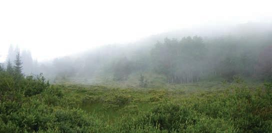
Fig. 2.4.1
A sloped dry wetland in Gilpin County, USA.
37 |
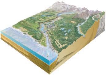
Fig. 2.4.2
Regional groundwater exchange Local groundwater exchange Domain
Groundwater and surface water interactions across the landscape. Redrawn from Winter et al. 2013.
2.5 Traditional Settlements
2.5.1 Pattern Types on Slope Terrains
Traditional settlement patterns in hilly areas, in this case studied specifically in the context of China, could be mainly categorized into three types:
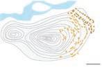
1. Settlement pattern parallel to contour:
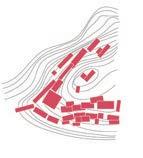
Usually the residential settlements formed in this pattern are located from the foot of the mountain to halfway up the mountain. The main means of livelihood of these village is farming, and it is very common to construct farming area around the toe of mountain. Thus this pattern has the advantage to allocate each house relatively in short distance to its corresponding paddy. e.g. Shi Bao Village, Chongqin, China
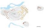
2. Settlement pattern perpendicular to contour:
This settlement pattern usually adopted by village that make living by fishing or have pier at the toe of hill. In the case of Xi Tuo Village, which located besides Yangze River, there is a main path perpendicular to contour. One of the reasions is that he village located in the valley part of mountain, has limitation from topography. Houses distributed along two sides of the main path. Each house in the village have good view of the river.
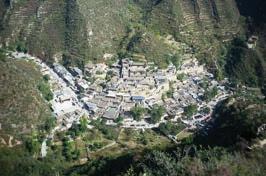
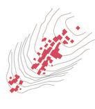
3. Settlements distributed as scattered clusters in network:
Pi An Zhai as a typical example of this particular pattern where the main means of livelihood includes collecting mountain products and hunting. Thus the village was built on the top of mountain for convenience and better protection. Small farm land integrated into villages, which help the village formed into scattered cluster in network.
| Adaptive Urban
38
Hillscapes
Village
Contour Rice paddy River Pier
e.g. Shi Bao Village, Chongqin, China
e.g. Xi Tuo Village, Chongqin, China
e.g. Pin An Zhai, Guangxi, China
Fig. 2.5.1.2
Three main types of traditional settlement pattern
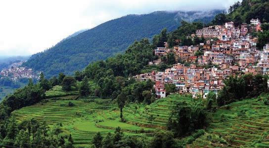
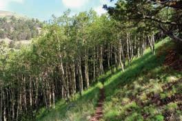
Fig.2.5.1.1
Fig.2.5.1.1 Village in hillside area
Fig. 2.5.1.2
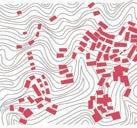
2.5.2 Settlement Formation
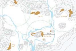
Villages in Biandan mountainous area are typical cases of settlement pattern parallel to contours, which also reveals the relationship between forest, village, paddy and water. Most of the villages are distributed at the foot of mountains, facing towards its corresponding farming area and back to mountain. Thus these villages could get protection by the mountains and have convenient access to work in field.
Forests have been preserved form the halfway to the top of hills, which could prevent landslide and nourish soil. Settlements located at the foot of mountain, thus the flat lands in the bottom of valley could be developed into paddies.
Shitou Zhai is one of the villages in Biandan mountainous area. The growth of settlement pattern of Shitou Zhai has mainly experienced four stages. At the initial stage, settlements were built on the east side, from the foot to halfway up the mountain, and grew parallel to contour. With the population growth, the village expanded from the original pattern, occupied more land at foot of mountain, and then developed following the contour. The lands at similar altitude have been covered by settlements, thus the settlements formed a circle around mountain. As population continued to grow afterwards, instead of expanded towards the top pf mountain, villagers built new settlements on the two nearby small hills, they still chose to preserve forest on the top of mountain.
39 |
Redraw from: “Construction of Ethnic Minority Settlement in Mountainous Area in GuiZhou under Survival Pressure : A Case Study of BianDan Mountainous Area“, 2015.
Fig. 2.5.2.3
Villages distribution in BianDan Mountainous Area Village
Boundary of paddy
Fig. 2.5.2.4 Growth and evolution of settlements in Shitou Zhai
1 100m N 1 100m 1 100m 1 100m Fig. 2.5.2.4 Domain
Fig. 2.5.2.3
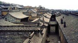
2.5.3 Traditional Building Morphologies in Hot Humid Area of South China

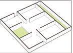
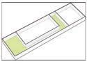
The two courtyard building morphology in Guangdong Provence is developed from traditional Chinese building type which has a courtyard in the front and in the back of the house. In order to adapt to the hot and humid weather in this area, the traditional building type developed this as a ventilation strategy. Usually the courtyard is a rectangular space which surrounded by walls or corridors. The vent between courtyard and indoor buildings are vertical openings on the building like doors and windows.
According to the ratio between width, depth and height, the generalized courtyard in this area can be classified into two type -- common courtyard and 'sky well' (tian jin). The main difference between these two type is :
1.Space Ratio: the base area for normal courtyard is bigger than 'sky well' but its height is lesser. The height of 'sky well' will more than either the width or length of its base.
2.Arrangement: Pavilion or trees are more common to be seen in a normal courtyard and water well and potted plants usually articulate a 'sky well'.
In this section, 4 traditional building types are studied for their unique morphological responses to climatic and social aspects.
| Adaptive Urban Hillscapes 40 Courtyard Name Song Minxiandafu Ci Sanyi Shushi Chenjia Ci Jiluehuang Gongci Guilin Zhai Shamian HSBC Aiqun Tower Location Floors inner courtyard 1 14.7 Width 5.8 5.8 5.16 5.16 26.7 2.5 10.2 2.22 circle, r=15.0 23.4 right trapezoid, (12.8+2.9)*19.8 9.6 Depth 2.7 3.9 3.54 4.14 14.0 14.0 12.3 2.70 5.0 4.5 Guangzhou Guangzhou Guangzhou Chaozhou Kejia Guangzhou Guangzhou Height 4.5 5.2 4.1 4.5 5.94 5.5 4.04 3.8 3.3-5.7 12.4 35.6 1 1 1 1 1 1 2 2 2 3 9 inner courtyard inner courtyard inner courtyard inner courtyard front courtyard front courtyard back courtyard back courtyard back courtyard back courtyard side courtyard
Fig.2.5.3.2 garden size in Gungdong province
Fig.2.5.3.1 sky well in Fujian common courtyard sky well (tian jin)
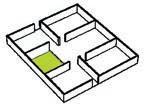
Type 1
courtyard
Due to solar radiation the temperature of the base of the courtyard and the roof of the living room will rise . The air at the bottom part of the courtyard will rise up and the cool air of the living room base will fill up the courtyard . The air at the upper part of the courtyard and corridor will flow into the living room through the top vents of the corridor. This dynamic cycle will keep running to cool down the indoor temperature. Three main factors will work on this ventilation process: ( T.Guohua, 2005)
1.
The triangular space under the roof, which is a usable space, creates a certain gathering area for hot rising air and slowly releases it outdoors from the gap between tiles (the phenomenon is more obvious in tiles which have no mortar plastering). The hot air in this triangular space is called ‘thermo cushion’, which is relatively stable and maintains a comfortable air temperature in the living room
2.
Comparing to other regions in China, the height of roof edge of buildings in Guangdong province is relatively higher, usually more than 4m. According to the principle of thermal ventilation, the edge of roof
(eaves) is the air inlet and the lower part of the living space is where the air goes out. H refers to the height between these two. The larger the H, the more effective the thermal ventilation.

3.
One of the main effects of the open corridor is to provide shading for the indoor areas and reduce the direct solar radiation that the floor might receive.
The active airflow for thermal ventilation usually only happens at the part of the living room closer to the courtyard. The higher the H is, more depth of indoor area can benefit from the active airflow. According to reference data, when H equals 4m, the depth of active airflow can be up to 2m and the wind speed experienced is around 0.4m/s.
41 |
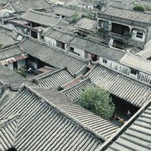
Fig.2.5.3.3 Zhenyuan Village, Guangdong
Fig.2.5.3.4 single courtyard building type
open corridor open living room slopping roof H
Slopping roof:
Height of roof edge (H):
Open corridor:
open living room open corridor front courtyard Domain
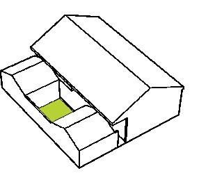
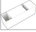
Type 2
courtyard courtyard open corridor open living room
In the previous case, the ventilation effectively occurs at the interface between the courtyard , corridor and the part of the living room closer to the corridor. In order to induce cross ventilation, an additional smaller courtyard in introduced in this typology.
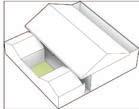
As a development of type 1, one smaller courtyard, which is called ‘tian jin’, is added into building type 2. Compared with the bigger front courtyard, due to its narrow shape, the ground of this back courtyard is shaded for most of time during summer days, which leads to a lower incident solar radiation and temperature during day time, and a slower heat dissipation during night time. This thermal difference between two courtyards triggers a thermal ventilation across the building – during daytime, the hot air in the bottom part of big courtyard rises up and the cool air in small courtyard go through the building and fills into bigger courtyard; during the night, the opposite process happens.
The difference of the solar radiation between these two courtyards is the main factor for thermal ventilation to happen, which can be translated to the height parameter of the two courtyards (Hf / Hb) and their areas.
( T.Guohua, 2005)
| Adaptive Urban Hillscapes 42
H Hb H v
Fig.2.5.3.5 Yuqiao Village, Guangdong
H
Fig.2.5.3.6 two courtyard building type
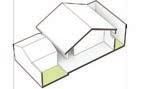
Type 3
Zhutong Wu can be considered as a multi storeyed development of type 2, where an indoor corridor is added as a ventilation tunnel.
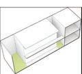
The proportion of the building shape is narrow and tall which, together with the corridor connection, helps to create a ventilation effect in the interior. During daytime the air flowing into the interior is hotter than the air in small courtyard, given the small opening and the depth of the courtyard. This brings sunlight into the house without increasing solar radiation. The cool air inside the courtyard goes down and into the indoor space, while hot air rises up until its extracted out. At night, since the outdoor air has lower temperature than indoor, the direction of air circulation is reversed, which brings cooler air into indoor space.
( T.Guohua, 2005)
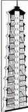
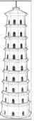
Type 4
facade openning
facade openning
central atrium
facade openning
facade openning
The wind speed generally increases with altitude, due to greater boundary friction with the earth which diminishes gradually as altitude increases. If there is a high building inside this wind field, the interaction between building and wind will add a large wind load to top part of building and create a new wind condition.
As one of the tallest structures in ancient China, the pagoda has a unique way to solve its wind condition. By building up a central atrium and alternative façade openings, most of which faces the main wind direction. Through the atrium, the wind load of pagoda can be released and with the wind going across the tower and between the floors, the inner climate can be less hot and humid. (
 T.Guohua,
2005)
43 |
courtyard courtyard open corridor open living room
Fig.2.5.3.6 Zhutong Wu building type
Domain
Fig.2.5.3.7 traditional pagoda in south China
2.6 Rice Terraces Landscape Systems
In recent years, urban farming has attracted more attention than ever. It not only proposes a way of providing food supply in city environment, also could bring sustainable benefit to citizens, such as preserve more green space and increase water retention. As mentioned in the previous section 2.1, when urban land expands into rural areas the populace involved in agriculture are forced to shift their jobs. Urban farming has the dual advantage of increasing supply close to centres of demand and also increase the number of people employed to produce for the others.
While in hillside context, the historic terraced rice paddy has been widely recognised as an intelligent farming technique on slope. When such topographical conditions exist in or near cities, there is a unique opportunity of using the slopes, which are not ideal for construction, for agricultural purposes.
The terraced rice paddy is mainly consisted of irrigation system, path system and paddy fields. It also coherently works with the forest, and the settlement, and becomes a well-functioning sustainable ecosystem.
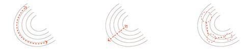
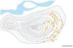
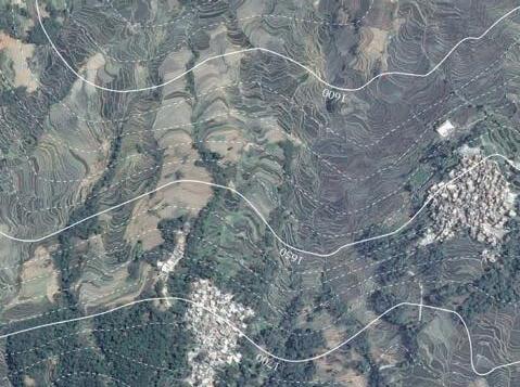
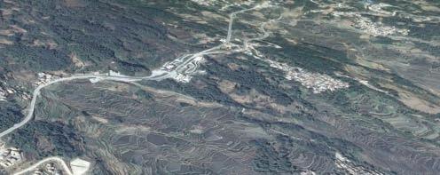
As Fig.2.4.1 shows, the forest provides water source for rice paddy and village. The rice paddy drainage system improves soil stability. The transportation system in village is integrated with the path network in rice paddy, which forms efficient route for farmer’s commute. Then the morphology and location of each paddy field is determined by slope angle and soil types. It could be seen from Fig. 2.4.2 that, the patterns of rice paddy has the the tendency of following the contour. The paddy fields become more dense at steep slopes, and they tend to be wider at gentle slopes.
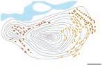
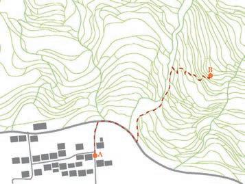
Fig. 2.4.3 presents the path system in rice paddy and how it connected to transportation network of the settlement. The roads in village could be categorized as 1st level road and 2nd level road. Paths in rice paddy also are in hierarchy, including 1st level paddy path and 2nd level paddy path. The 1st level paddy paths connect different steps of paddy in shortest distance, while the 2nd level of paddy paths set the boundary of each field. If a person intends to reach B point start from A point, the most efficient route is shown in Fig.2.4.3, which makes the best use of 1st level village road and 1 level paddy path.
| Adaptive Urban Hillscapes 44
Fig. 2.6.1
Relationship of “forest - rice paddy - village“ system
Redraw from: Qiang Wang, “Design research about Yuanyang terraced rice paddy in Yunnan Provience, China”, 2015.
FOREST SLOPE ANGLE & SOIL TYPES FOREST DRAINAGE drainage system rice paddy system water supply soil stability irrigation irrigation transportation transportation food collection pathformation precipitation morphology & location RICE PADDY DRAINAGE RICE PADDY NETWORK PADDY FIELDS VILLAGES
Fig. 2.6.1
1st level paddy path
2nd level paddy path
1st level village road
2nd level village road
Example efficient route
45 |
Fig. 2.6.3 Path system in rice paddy
Fig. 2.6.2
Fig. 2.6.2
Relationship between rice paddy patten with contours
Domain
Fig. 2.6.3
In Philippines, Cordillera Rice Terraces are on a territory of more than 20,000 square miles at an altitude of 700 to 1,500 meters above sea level in the mountains of Ifuago. About 81.77% rice terraces were constructed on slopes over 18o. The local landscape system have lasted more than 2,000 years.
The inhabitants in Ifuago have built up a landscape system which mainly consists of - Forests, 'Muyong', Terraces , river. Forests means the preserved area at high altitude location, which has the function to conserve water. The production area, including settlements and rice paddies, are usually located at lower altitude areas. Between the preserved forest and production area, productive forests have been set
up to separate these two areas, which are also called as “Muyong“ by the inhabitants.
The forests at the top of mountain absorb precipitation through crown and leaves, then store water to form stable humus-rich soil. The forest also could slow down speed of surface water flow and groundwater flow, which could irrigate rice terrace and then eventually merge into basins at the bottom of valley.
As a buffer zone between forests and production area, “Muyong“ is the main source of providing fuel, building material, food, and herbs. It minimises the impact on forests from human activities.
| Adaptive Urban Hillscapes 46
Fig. 2.6.4 Landscape system of cordillera rice terrace
Redraw from: Huijun Hou, “Reconstruction of landscape pattern on terraces based on the theory of ecological restoration and culture regression for mountain rice terraces in the Philippines Cordillera region“, 2015.
Fig. 2.6.4
Forest
Terraced rice paddy
Village FOREST
Village Village Rainwater infiltration
Village Evaporation surface water flow path groundwaterflowpath VILLAGE
MUYONG
RICE PADDY RIVER
Surface water flows
Water circulation processes for determining Farming Clusters


Precipitation
Surface/underground water flows
Forest

Farming Clusters Crops
Evapo-Transpiration
Wetland
47 |
Fig. 2.6.5
Water circulation process in terraced rice fields complex ecosystem
Domain
2.6.1 Rice Paddy Irrigation System
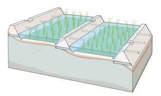
The terraced rice paddy has a system is self-irrigation, which uses the impact of gravity to let water flow from top to bottom. The rice paddy itself also has the capacity of retaining water.
The gravity based irrigation system mainly functions on two concepts: ground irrigation and underground irrigation. The ground irrigation is using surface flow; built gateways on bunds and fields channels water to control the balance between each field. The underground irrigation is using underground water flow to charge fields. Each field is connected to underground water by seepage. In rain season, rice paddy can achieve enough water from ground irrigation. While in dry season, fields rely more on underground irrigation.
Since rice paddies are ploughed over and over, the bottom clay layer of the fields have the ability to contain water as well.
The water balance equation for a paddy field can be expressed as:
WDt = WDt-1 + RAINt +WIRRt - ETAt - VTFLOt - HZFLOt -SURFLOt
RAINT ETAT WIRRT
Gravity Irrigation
Ground Irrigation
Surface flow
Underground Irrigation
Field channels
Gateways Seepage
Vertical percolation
Groundwater flow
Plough Layer 0.2-0.4 m; the clay in the bottom has ability to hold water and keep soil
2. Yellow
Layer 0.3-1.5 m; weak permeable
Illuvial Layer 0.1 m; strong permeable
3-15 m; soil moisture content 10%-20%, aquifer
< 0.1 m;
| Adaptive Urban Hillscapes 48
1.
5. C-horizon
unpermeable layer
4. Eluvial layer
layer
3.
Soil
Fig. 2.6.1.2 Irrigation system of Ziquejie Terraced paddy
Redraw from: Xu Wensheng, “Preiminary Study on Evironment Factirs Influencing Natural Gravity Irrigation in Ziquejie Terrace“, 2011
WDT SURFLOT HZFLOT VTFLOT
Fig. 2.6.1.1 The water balance equation
Fig. 2.6.1.1
Fig. 2.6.1.2
Rice Village Sub-Ecosystem
Typical rice villages are commonly located in between forests and agricultural areas, for the purpose of conservation and management of both the forest and the arable terraces. Some criteria need to be fulfilled for these villages to be located in order for them to be productive. First, distribution of dense forest in upper slope is required, then a good sun orientation for both climatic comfort and rice mill production; and thirdly, relatively flat slopes should be considered. Inside these villages, water storages are build together with bamboo channels that provide water from upper mountain flows for daily use. (Zhang, et al. 2010)
49 |
Fig.2.6.1.3 Honghen Rice Village in Hani, China. source: http://news. xinhuanet.com
Fig.2.6.1.3
Domain
- Landslide fatalities
2006(green), 2007(blue), 2008(red).
It can be seen that they occur generally along tectonically active regions. Darker shade on the world map indicates higher altitudes
2.7 Slope Instability
2.7.1 Landslides
Landslides can be defined as the movements of soil and/or rocks downwards along a slope due to the forces of gravity (Cruden and Varnes, 1996). Underneath the surface of land, internal failure occur either as curved or planar ruptures. Landslides are naturally triggered by excessive precipitation or ground shaking (USGS, 2009), and are also caused because of human disturbances, altering the natural angle of slopes in terrains where urbanization is developing. (R.Walker and B.Shiels, 2013)
| Adaptive Urban Hillscapes 50
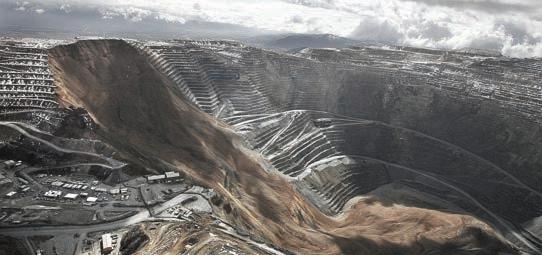
FIG 2.7.1.2
Bingham Canyon 2013 Landslide
Source: Desert News
FIG 2.7.1.1
FIG 2.7.1.1
Fig 2.7.1.2
When the surface of rupture has a curved shape (spoon-shape) and the shape of the mass movement is rotational. The area of failure known as the ‘head’ usually moves in an almost vertical direction (downwards), and occasionally tilts backward towards the scarp. Rotational landslides occur more commonly with homogeneous soils, therefore they will be found in areas with fill materials.
Translational landslides
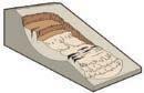
Translational landslides are one of the most common landslide types around the world. In translational landslides, the mass of soil moves out, down and outward along the surface. Usually this kind of landslides occur in not very steep slopes but can reach big distances if the rupture surface is sufficiently inclined. When the velocity of this slide increases it may disintegrate and develop into a debris flow. (Highland and Bobrowski)
Debris flows
A combination of water with mass movement such as soil, rock or organic matter. Debris flows are common in gullies and canyons, specially in volcanic areas that contain weak soils. Debris flows usually end where the slope terminates and create a triangular deposit known as debris fan which are also unstable. Commonly caused by intense rainfall or rapid snow melt that takes loose soil and rocks. (Highland and Bobrowski)
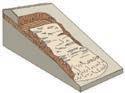
Fig. 2.7.2.4 Basic types of landslides. [Highland and Bobrowsky] <redrawn>
Domain
51 |
Fig. 2.7.2.3 Parts of a Landslide. [Highland and Bobrowsky] <Redrawn>
Fig. 2.7.2.3
Toe Surface of Rupture
Crown Head Main scarp
2.7.2 Types of Landslides
Rotational Landslides
Fig. 2.7.2.4
2.7.3 Analysis / Mechanism of Slope Stability
The phenomenon of slope instability is generally quite similar the world over, where the fundamental causes do not differ greatly with geological and geographical locations. Therefore, the methods of assessment , analysis, design and mitigation measures are mostly universal. The main difference is that in tropical areas the climate is both hot and wet which causes deep weathering of the parent rocks and the slopes are of weaker materials.
In general terms, slope failure occurs when the downward movements of material due to gravity and shear stresses exceeds the shear strength. Therefore, the factors leading to instability can generally be classified as
1. Those causing increased stress
2. Those causing a reduction in strength.
Factors causing increased stress include:
a) Increased unit weight of soil by wetting
b) Added external loads (moving loads, buildings etc)
c) Steepened slopes either by excavation or by erosion
d) Shock loads
Loss of strength may occur by
a) Vibration and earthquakes
b) Increase in moisture content addressed by hydrology management
c) Freezing and thawing action
d) Increase in pore pressure
e) Loss of cementing pressure
Aspects of Analysis
For proper design of slopes, correct soil data, groundwater regime, geology of site , analysis methods are imperative. Detailed information and analysis is required on the following aspects: topography, geology, shear strength, groundwater conditions and external loadings. [Dr.Gue Sew et al., 2000]
Topography:
Contour of the site, positions of subsurface investigation holes, layout of the development and proposed cut and fill have to correct, so that cross- sections of the slopes can be used to carry out the analysis.
Geology:
In order to predict what type of slope failure is likely to occur and where, geological conditions need to be reviewed. This includes: Soil type maps, soil data, groundwater conditions, bedrock conditions.
| Adaptive Urban Hillscapes 52
Fig 2.7.3.1
Contour map
Fig 2.7.3.1
Shear Strength:
The shear strength of a soil mass is the internal resistance per unit area that the soil mass can offer to resist failure and sliding along any plane inside it. To understand the nature of shearing resistance in order to analyse soil stability problems such as bearing capacity, slope stability, and lateral pressure on earth retaining structures, Mohr-Coulomb equation can approximate shear strength as
Tf = c + tan θ
Normal stress on failure plane
θ Friction angle of soil
c Cohesion of soil
In saturated soil, the total normal stress at a point is the sum of the effective stress ( ') and pore water pressure (u), (Dr. Das,2001 )
= ’ + u
External Loading:


Dead and live load considerations from traffic, building foundations, retaining walls etc. that have a bearing on the stability of slopes should be estimated and included in the analysis. For built structures this is valid mainly if the substructure is resting
Soil Texture map
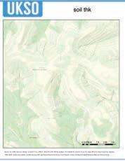
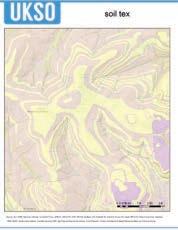
Soil Type map
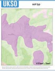
Soil depth map
[UK soil observatory]
53 |
Tf
Fig 2.7.3.2 Shear stress of soil
Fig 2.7.3.2
Fig 2.7.3.3 Examples of Geological maps:
Domain
Fig 2.7.3.3
Manmade slopes are generally less stable because in most cases it is not deposited according to the natural angle of the soil or it is not well compacted. But it is important to note that not all natural slopes are safe. It is quite common for natural slopes to fail during monsoons even when there is no landuse change like clearing of trees or development around it. For any development site, the slopes within and adjacent to it need to be evaluated. In any case, it is not advisable to disturb the natural slope and vegetation just to marginally improve its stability, unless it is unsafe. However it is simply logical not to locate buildings in areas with weak slopes or areas that could be affected by landslides [Dr.Gue Sew et al., 2000].
Factor of Safety (FOS)
The factor of safety is commonly thought of as the ratio of the maximum load or stress that a soil can sustain to the actual load or stress that is applied. Failures occurring parallel to the surface of a slope can be analysed as an infinite slope failure (Sharma et al, 1996). Slopes extending to infinity do not exist in nature. For all practical purposes any slope of great extent with soil conditions essentially same for all identical depth below the surface are known as infinite slopes.
a) Infinite slopes in cohesionless soil: To analyse failure conditions for an infinite slope of cohesionless soil, the factor of safety is defined as the ratio of soil strength to the required shear stress for equilibrium. The factor of safety against sliding is given by
Tf - Shear strength
T - Mobilised shear strength due to gravity θ - Angle of friction of the soil
- Inclined angle of the slope
b) Infinite slopes of Cohesive soil: Even in cohesive soil, the slope is stable as long as the slope angle is equal to or less than the angle of internal friction θ. If the slope angle i, is greater than , the slope can be stable only upto limited height known as critical height is given by
| Adaptive Urban Hillscapes 54
Tf tan θ
of Safety = = T tan stableslope stableslope θ θ F θ θ T T unstableslopestrengthenvelope strengthenvelope
Factor
C Hc= (tan - tan θ)cos2 i
In the free body diagram for infinite slope analysis (Fig 2.5.3.1), the Factor of Safety (for any depth less than Hc) is related to both the driving and resisting forces performing on the body. The driving force, derived from the object’s own weight, makes objects slide through a slope. The resisting force is the one composed by the friction or shear strength plus the factor of cohesion of the particular type of soil, and it’s the one opposing the driving force. The molecular cohesion between grains reinforces the material strength and hence prevents the object from sliding. The Factor of safety is given as:
In a steep slope terrain, the angle will increase, making the driving force larger while the normal and friction forces will decrease. This will be translated directly into a reduction of the Factor of Safety. The FOS for any case and type of soil is considered to be above 1.3. If the FOS is near or below 1.0, there will be high probabilities of erosion and slump to be present [Sharma et al, 1996]
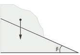
Driving force : F p = W x sin
Normal force : F N = W x cos
Resisting Force Ff + c
Factor of Safety = = Driving Force Fp
Friction force : F f = F N x : the coefficient of friction [ W x cos x ]
If the depth of the soil layer (D) were to be introduced as a parameter in infinite slopes without seepage occurring
55 |
Fig 2.7.3.4
w
Free body diagram for slope analysis
w Fp FN
W
x
+ c Factor of Safety = W x sin c tan θ Factor of Safety = +
x D x sin
cos tan
Domain
Fig 2.7.3.4
Fig 2.7.4.1
Basic
[Rex Baum, U.S. Geological Survey]
<redrawn>
2. 7. 4 Slope Reconfiguration


Excavation
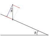
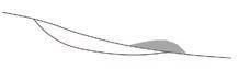
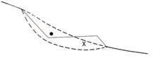
Cut and fill is a common method used to stabilize terrains with steep and shallow slopes, and basic principles should be acquired when using this methods. Removing the mass of soil from the ‘head’ part of a potential slumping area will help to reduce the driving forces and therefore improve stability. This method is more suitable in failures of rotational landslides where deep soil cuts take place, but inefficient in translational failures along planar slopes. (Highland and Bobrowsky, 2008). This practices are efficient, they increase Factor of safety by 1015% but they need to be part of a complete solution with additional modification of the land (Chatwin et al., 1994).
Diagrams 1a-b (Fig 2.5.4.1) show how altering the original centre of gravity with different criteria can affect stability due to gravity factors; diagrams 2a-b explain the criteria for mass removals in a potential landslide, by reducing resisting forces (2a) and reducing driving forces (2b); while diagrams 3a-b show the basic considerations when applying loads into the slope, increasing driving forces (3a) and increasing resisting forces (3b).
1a) Less Stable
Failure Surface
1b) More Stable
Original centre of gravity
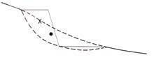
New centre of gravity
2a) Less Stable
Reduction of mass at toe, reduction of resisting forces
2b) More Stable
Reduction of mass at head, reduction of driving forces
3a) Less Stable
Load at head, increasing driving froces
3b) More Stable
Load at toe, increasing resisting froces
Fig 2.7.4.1
| Adaptive Urban Hillscapes 56
principles for excavation techniques
2. 7. 5 Hydrological Effects
Precipitation, excessive infiltration and groundwater flow are very common triggering factors for the occurrence of landslides. High levels of pore water pressure decrease the soil’s shear strength and can lead to slope failure (Iverson, 2000; Van Asch et al., 2007).
Soil Suction
When the soil is saturated, it looses its capacity of suction, which will lead to a reduction of cohesion. Cohesion is the strength within the soil that keeps particles together, hence when cohesion is reduced the overall resisting forces are reduced as well.
Seepage Force
Seepage force is created from water flows pressing on the soil particles in the direction of flow. This pressure can lead to an increase or decrease in pore water pressure, affecting the shear strength of soil [Ghiassian and Ghareh, 2008]
Pore Water Pressure
When the level of groundwater table rises, the pore-water pressure gradually rises as well. This process happens often in heavy rainfall conditions (Iverson et al., 1997). High levels of pore water pressure lead to reduction of the shear strength of the soil and destabilization of slopes. In soils with big percentages of clay, cracks and fissures can lead to big changes in pore water pressure. Reducing the volume of pores within a soil also lead to an increase in pore water pressure [Rogers and Selby, 1980; Duncan and Wright, 2005]
This also varies with soil permeability, water table, soil weathering profile. With high soil permeability, more water infiltrates the soil causing the water level in the slope to rise. Above the water table, the degree of soil saturation increases, hence the soil suction reduces (negative pore pressure). This can result in a decrease in soil strength due to suction.
Hydrological cycles in two scenarios are shown below (Fig.2.5.5.1), Undisturbed Forest and Deforested slope. Vegetation helps to control the amount of water going into and out from the soil, hence controlling landslides as a natural process by maintaining the saturation balance.
Rainwater strikes soil directly
Water runs over surface, causing flooding and run-off
Over-saturated soil
Little rainwater soaks into deep soil so the level of groundwater is depressed
Hydrological en vegetation effects on soil stability [science. jrank.org/article_images/ science.jrank.org/ deforestation-andlandscape.1] <redrawn> Domain
57 |
Saturated Rock Groundwater table Soil + Roots Evaporation/ Transpiration from trees Rainfall intercepted by trees, leaf litter or undergrowth Rainwater soaks into the soil slowly
Slow seepage from soil water
Undisturbed forest Deforested slope
Fig.2.7.5.1
Fig.2.7.5.1
Contribution of ground water to slope instability [Kwong et al.;2004]
2.8 Mitigation Techniques
2.8.1 Drainage System
Due to its ability to manage water content in soil and reducing the weight of the sliding mass, drainage systems are one of the most important contributors to control landslip. Drainage system can be either developed on surface level or subsurface.
Surface water stagnation has negative effects on agricultural productivity because oxygen deficiency and excessive carbon dioxide levels in the rootzone hamper germination and nutrient uptake, thereby reducing or eliminating crop yields. In addition, in temperate climates, wet places have a relatively low soil temperature in spring, which delays the start of the growing season and has a negative impact on crop yields. Excess water in the top soil layer also affects its workability.
[UN FAO, 2014]
Surface Drainage System
Cross slope surface drainage system
Surface drainage system is effective and economic way to prevent erosion of surface, reducing the potential for surface slumping, prevent infiltration of water into the soil and reducing ground-water pressure. The methods including site levelling and surface ditch or drain system. Subsurface drainage's objective is to improvement underground water flow aiming to reduce over saturated soils, hence reducing water pressure on potential failure surface. Runoff from both the slopes and the catchment area upslope should be cutoff, collected and lead to convenient points of discharge. For proper slope drainage, runoff should be channelled away from vulnerable slopes through the most direct route. [Dr.Gue Sew et al., 2000]
Cross Slope Drainage
Where surface runoff threatens agricultural fields in sloping lands, small cross-slope ditches can be made at their lower end, running almost along contours. Ditch spacing depend on factors such as gradient, rainfall, infiltration into the soil, hydraulic conductivity, erosion risk and agricultural practices. No general rules can be formed, but based on practises followed by Geotechnical Control Office, HongKong, a berm with horizontal drains of around 1.5m in width is recommended at every 7.5m vertical slope. Surface runoff is discharged into open collector ditches running in the direction of the natural slope to discharge into a main waterway.
Site levelling water flow path before site levelling
Pond
Soil which saturates water from pond
Site levelling water flow path after site levelling
Vegetated slope
SECTION ACROSS COLLECTOR DRAINFor long/steep slopes the channel should be stepped to reduce the velocity of flowing water
Gravel backfilled trench
Unconsolidated solid
Collector drain
Permeable bedrock max. 7.5m
Gravel backfilled trench
Low permeable bedrock
Stepped channel (for steep/long slopes)
| Adaptive Urban Hillscapes 58
Fig.2.8.1.1
Fig.2.8.1.1
Fig.2.8.1.2
Berm with cross slope drain
Berm with cross slope drain
Fig 2.8.1.3
1.5m max 7.5m
Fig.2.8.1.2
contour
surface
collector drain main drain
lines
drain
Fig.2.8.1.3
Surface ditch
Random Field Drainage
Random drains are applicable where fields have scattered isolated depressions that cannot be easily filled or graded using landforming practices. The system involves connecting one depression to another with field drains, and conveying the collected drainage waters to suitable outlets.
Subsurface Drainage System
The purpose of subsurface drainage is to lower the water table and, therefore, the water pressure to a level below that of the potential failure surfaces; to redirect adjacent groundwater sources away from the subject property and to reduce hydrostatic pressure beneath and adjacent to engineered structures. Methods or components involved in subsurface drainage include
- drain holes
- Trenches
- Horizontal Drains
- Relief Wells
- Drain Wells and Stone Columns
- Wellpoints and Deep Wells


- Drainage Galleries
Subsurface drainage with Horizontal drains
Upper forest
Filter well
Potential slide mass
Underground-water table
Failure surface
Horizontal drain pipe
Permeable bedrock
Surface drain
Slope immediately behind the crest
Drainage well
Lined Collector drain
Potential slide surface
Main subsurface drainage gallery
Horizontal drain to discharge water
59 |
Fig.2.8.1.4
Fig.2.8.1.4 Random field drainage system
Fig.2.8.1.5
Subsurface drainage system(Duncan and Christopher, 2005)
Fig.2.8.1.5
Domain
Tensile strength increased significantly with decreasing diameter of roots. (Sotkes et al. 2007)


2.8.2 Vegetation Techniques
A common and efficient way of increasing soil cohesion is the use of vegetation. Since ancient times, different methodologies have been developed for soil stabilization problems. In most cases, reinforcement of soil by the use of vegetation helps reducing shallow landslide hazards and soil erosion in slopes. (Gray and Leiser, 1982)Vegetation can be used alone or combined with other natural elements such as rocks or wood. Composites elements such as concrete or geotextiles can also be applied for reinforcement. (Strom, Nathan and Woland, 2013)
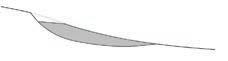
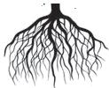
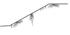
Roots
When using tree roots, mostly thick vertical roots work more efficiently in the middle area of the slope, while oblique and smaller roots help to stabilize soil at the starting and ending point of the slope (Fig.2.6.2.1). For all instances, roots should be deep enough to cross the failure plane in order to reinforce slope against landslides. The tensile strength generated by the roots in the soil is directly proportional to the dimension of its roots diameter, which makes the solution more efficient when large number of thin roots are present in the slope. (Gray and Leiser, 1982; Bischetti et al., 2005; Genet et al., 2005).
In order to determine the relationship between tensile strength for a range of species and root size, mechanical tests were done by A. Stokes et al. (2007) on small roots from three conifer and two broad-leaf species, located in different parts of France. (Fig.2.6.2.1 and Fig.2.6.2.2)
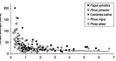
Plate roots
Grass

Small Failure plane
Large Failure plane
Tap roots
| Adaptive Urban Hillscapes 60
Slope Tensile strength (MPa) Diameter (mm)
Fig.2.8.2.2
Fagus sylvatica Pinus pinaster Castanea sativa
Pinus nigra Picea abies
Fig.2.8.2.1 [F. Danjon; D. Barker, M. Drexhage, A. Stokes, 2007] <redrawn>
Fig.2.8.2.1
Fig.2.8.2.2
15 m 0 m 5 m 10 m 20 m
Chinese Pine Vetiver grass Harland Oak
Vegetation Distribution on Different Slope Angles
<55° <45°
θ<15°
15°<θ<45°
45°<θ<55°
θ>55°
Grass hydroseeding with pit planting native species, including trees, shurbs, groundcover, ferns and climbing plants;
Grass hydroseeding with pit planting small trees(up to 3m height when mature), shurb, groundcover , fern and climbing plants
Grass hydroseeding with grounfcover and climbing plants in root tube planters
Core hole through hard surface cover for planting of groundcover and climbing plants
No particular requirement
Biodegradable erosion control mat
Tree Shrub
<35°
<45° 0
1500 MM
hydromulching system eco-bag system mulching panel Toyo-mulching system
Fig.2.8.2.4 Technical Guidelines on Landscape Treatment for Slopes, GEO Publication No. 1/2011
Biodegradable erosion control mat at shallower angle on non-biodegarable erosion control mat to suit site conditions
Non-biodegarable erosion control mat together with wire mesh, up to about 60° if ground conditions are suitable and the upslope catchment is small, thereafter hard surface cover or proprietary green surface system, where conditions permit and long-term maintenance commitments have been agreed.
Domain
61 |
Fig.2.8.2.3 vegetation design on slope (redraw from Toyo Greenland Co,. Ltd website)
Fig.2.8.2.3
Herb Grass (with deep roots) Fern
Table 2.8.2.4
Slop Gradient Possible Planting on Slope Face Example of Suitable Erosion Control Measure
Diagram 2.6.2.2 shows the vegetation distribution and soil reorganization along the slope when the angle of slopes change. The selection of planting type is heavily dependent on slope gradient.
When the entire slope is consisted of soil / colluvium / alluvium, an additional erosion control mat(usually is a wire mesh) between plants and slope surface need to be added to prevent soil from being washed away by heavy rain.
Soil Check Dams
Soil check dam is an emerging technique in soil stability technology which can collect and make sustainable use of natural deposition and prevent sediment from entering water bodies. Gully plugging using check dams, accompanied by planting between the dams to stabilize the channel, can be one of the most effective ways to conserve soil and water and rehabilitate land degraded by gullies (Guedel 2008). The whole process contains three different stages:
1. At the first stage, according to soil erosion analysis, new barriers structure are built along the debris flow path, while the existing trees around flow path can be retained and protected by a lower barrier;
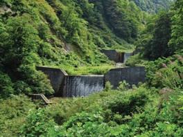
2. At the second stage, shallow deposition and water slide into concrete slab. As the deposition brought by the surface water flow is rich in organic matter, the collected volumes can be used for wetland farming or planting in this stage;
3. The third stage happens when deposition fills up the barrier structure and begins to overflow, in this stage the emergent land inside the barrier structure can be assumed temporary stable and can be used .
Controlling the height of front reinforced concrete barrier walls can provide time of usage as a new variable since different amount of volumes can be controlled before it flows into a next stage.[hkss.cedd. gov.hk][icimod.org][CWM.Yeung,2011]
| Adaptive Urban Hillscapes 62
Fig. 2.8.2.6
Soil check dam redraw from Application osf Soil Bioengineeing Measure to Man-made Slopes , D.K.P. Cheung, 2011
Fig. 2.8.2.5
Concrete Check dams along a natural water channel in Niigata, Japan
Fig. 2.8.2.6
Fig. 2.8.2.5
direction pf natural runoff back wall concrete slab inside toe wall wall top planter
Retaining existing tree
Access road
Back reinforces concrete barrier wall
Debris collection slab
Front reinforced concrete barrier wall
Land for temporary usage (farming / open green space)
Soil collected in slab and ponding (or wet land)before it’s been filled
Debris flow fills the collection slab and generates the emergent farmlands
Future soil deposition
63 |
flow
Potential debris
path Debris flow path
Fig. 2.8.2.7 Soil check dam, redraw from Application of Soil Bioengineeing Measure to Man-made Slopes , D.K.P. Cheung, 2011
Domain
Fig. 2.8.2.7
2.9 Case of Hong Kong
High Rise-High Density on Slopes
Hong Kong’s intense urbanism is the result of rapid industrialisation in the 1950’s that caused massive migration of refugees from mainland China looking for better opportunities. Urban expansion was a problem then during the colonial period and it still is, symptomatic of any island city. But instead of growing across all available land, it has carefully encroached onto the sea for high profile projects needing flat land. Secondly it has confidently accepted a high rise-high density strategy in an effort to maintain a small built footprint and a high percentage of green cover.
To date about 45% of Hong Kong lives in public housing towers, which in many cases is built on steep slopes and higher ground which has relatively lower land value. However a few informal settlements, or slums do still exist. But these informal areas house less than 1% of the population. [encounteringurbanization.com]
High Density Living
Because of its high percentage of unoccupied areas, density values at regional level are extremely high (refer fig.2.7.2). Also contributing to this, is the conscious increase in density near transport stations (refer fig.2.7.5). Slopes on the hillsides also show high density in many areas of the Eastern district and Kowloon due to the presence of many high density government housing towers.
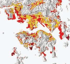
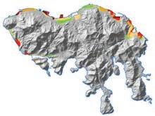
| Adaptive Urban Hillscapes 64
Fig. 2.9.1
Island of HK - Land expansion & Growth vectors
Fig 2.7.2
Fig 2.9.2
Density distribution on land elevation map (x1000 h/km2 ) [LSE cities]
2.9.2 >50 20-50 <10 <1
Fig
7.24 million 9.4 (2050) Population Density Land area Green cover Green space per capita 6990 h/km2 1100km2 2m2 9m2 (WHO standard) 70%
2.9.1 2003/6 1993/5 1994 1975 1952 1945
Fig
The high density has a significant impact on the city’s development. The high demand for land has driven Hong Kong to maximise its suitable construction land with buildings leaving a very small proportion for public open space. Most of its open space is meant for neighbourhood sports facilities and playfields. Alternate public spaces like malls, elevated pedestrian paths become areas for social interaction. Proximity to infrastructure facilities and a wide range of options for public transport (refer fig.2.7.4) encourage the population to take pedestrian journeys.

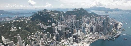
65 |
Fig. 2.9.3 Island of Hong Kong
Fig. 2.9.4 Public transport usage distribution [LSE cities]
Fig. 2.9.5
Hong Kong has very high accessibility, with over 40 per cent of its population living within 500 metres’ distance from a rail or underground station. [LSE Cities]
Fig 2.9.4
Fig 2.9.3
Fig 2.9.5
walking9.2% bus 33.5% public transport 88% metro24.1% rail 10.3% minibus 7.5% 6.6%car private bus 3.4% Population Domain
Map of reported landslides- till 2008 [http://hkss.cedd.gov.hk/]
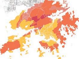
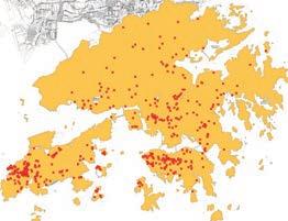
2.9.1 Slope Instability In Hong Kong
Some 60% of the land in Hong Kong comprises natural terrain, much of which is steeply sloping and mantled by. Natural hillsides are subject to progressive deterioration and the susceptible terrain is prone to raininduced landslide. The geology of HongKong is influenced heavily by subtropical weathering . Typically, superficial deposits of weak saprolitic or residual soils, or colluvial soils derived from past landslides or erosion processes overlie weathered rock of varied depth, beneath which lies fresh rock. The most common rock types include granite and volcanic tuff and rhyolite. The threshold angle for most of the slope faces with this geology lies is in the range of 25-30 degrees. [K.Y.Choi et al. 2013]
[H.N.Wong, 2007]
From the graph [2.7.xx] it can be seen that most of the landslides happen on slopes ranging from 15 to 50 degrees in HongKong. And the slopes seem to stabilise at angles greater than 50 degrees.
| Adaptive Urban Hillscapes 66
Fig.2.9.1.4 Landslides occurrence with different range of slope angle in HongKong
Fig.2.9.1.3 Slope angles of natural terrain in Hong Kong
Fig.2.9.1.1
Volcanic rock Granite Sedimentary rock Granodiorite
Fig.2.9.1.2 Geological distribution [http://hkss.cedd.gov.hk/]
Fig.2.9.1.1
60% 50% 40% 30% 20% 10% 0% 0o - 15o 15o - 50o 50o - 90o 60% 50% 40% 30% 20% 10% 0% >15o >30o Fig.2.9.1.4 Fig.2.9.1.3
Fig.2.9.1.2
2.9.2 Mitigation Measures In Hong Kong
Hong Kong has a high concentration of developments on hilly terrain in close proximity to man-made slopes and natural hillsides. Hong Kong is now renowned for its urban slope engineering and landslide risk management that enable its safe and sustainable development.
Initially Slope design and construction were based on rule of thumb, such as 55° steep for soil cut slopesand 35° steep for fill embankments. In 1977 the Geotechnical Engineering Office (GEO) was formed and the more conventional deterministic approach of slope stability analysis was adopted in slope design. Landslide prevention was primarily aimed at, and based on, achieving the required design factor of safety. In the mid-1990s- an explicit risk-based approach and strategy was introduced, in addition to the deterministic approach, for slope assessment and landslide management. The risk-based methodology embraces a holistic consideration of the likelihood of landslide and its adverse consequences. It is called Quantitative Risk Assessment (QRA) method and it aligns slope engineering and landslide mitigation with other fields that practise state-of-the-art risk management in a more
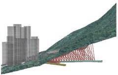
explicit manner. eg. Assessment of landslide debris mobility (Wong and Ho 1996), quantification of landslide consequence, frequency (Wong and Ho 1998), financial factors, property damage etc.
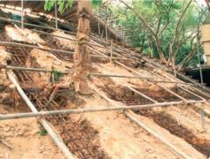
For example the residual buildings at Shatin Heights are overlooked by a 35° steep hillside that has a history of failure (Fig.2.7.2.1). In 1997, six landslides occurred on the hillside and three developed into debris flows that affected the buildings. Geotechnical assessment revealed that the landslides were rain-induced, shallow failures involving the surface layer of colluvium and completely weathered granite. Mitigation measures generally includes improvement of surface drainage and protection at the crest platform, provision of debris-resisting barriers and local slope stabilization using bio-engineering means . A general over view of such techniques is covered in the previous section.
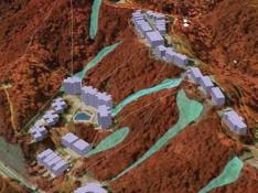
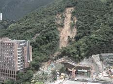
[hkss.cedd.gov.hk] [S.Parry
Sub-vertical drains
Drainage tunnels/ gallery
67 |
Fig.2.9.2.1 Landslide QRA analysis model for Shatin Heights, Hong Kong [HN.Wong, 2007]
Fig.2.9.2.2
19997 Landslide scar in Shatin Heights, Hong Kong [HN.Wong, 2007]
Fig.2.9.2.3 Scar regeneration & Slope stabilization using soil nails & grillage [HN. Wong, 2007]
Fig.2.9.2.1
Fig.2.9.2.2
Fig.2.9.2.4
Fig.2.9.2.3
et al. 2011] [H.N.Wong et al. 2007]
Fig.2.9.2.4 Po-Shan, Hong Kong sub surface drainage pipes (hkss.cedd.gov.hk)
Domain
Terrain Assessment & Building Control
A natural terrain landslide hazard study may have to be undertaken for development sites which meet the following criteria : where there is natural terrain outside the site, but within the same catchment, which is at an angular elevation of 20° or more from the site and where there is natural terrain sloping at more than 15° within 50m horizontally up slope of the site, provided that there is a credible debris flow path to the site.
A more rigorous assessment is conducted where there is natural terrain outside the site, but within the same catchment area, which is at an angular elevation of 35 degrees or more from the site and at an elevation of 50m or more above the proposed site formation level. Generally such site conditions are objectionable because they fall under ‘severe hazard’ criteria. [hkss.cedd.gov.hk]
The GEO studies the terrain as per the existing site conditions does a Quantitative Risk assessment (QRA). Once it assesses the hazard level and the Individual Risk (IR) of the proposed development, it proposes slope mitigation measures that are not necessarily the best, but which are practical, economical and come within the risk threshold. [RWM. Cheung,2011] [HN.Wong, 2007] [hkss.cedd.gov.hk]
| Adaptive Urban Hillscapes 68 35 severe hazard area >50m 20 50m
ground slope>15 ground slope<15
Fig.2.9.2.5 Development Control rules for Natural Terrain [Redraw: http://hkss.cedd. gov.hk/]
Fig.2.9.2.6 Cost effective mitigation measures based on a comprehensive QRA study [Redraw: RWM. Cheung,2011]
Planned Buildings Planned Buildings Existing Profile Raised Platform Flexible Barrier Cut Slope Cut Slope Fig.2.9.2.5 Fig.2.9.2.6
HIGH Class 3
HT > 15m and θG >27o
HT > 15m and θL >30o
6m < HT < 15m and θG >27o
6m < HT < 15m and θL >30o with HL > 3m
Class 2 LOW
HT < 6m and θL >34o with HL > 3m
Slopes, either manmade or natural, in the site or adjacent to the site, that are not in class 2 or 3
HT Total height of slope
θG Global slope angle
ORDER OF LIFE RISK
All occupied buildings
Storage buildings with dangerous goods
Open public spaces(densely used)
Roads with high traffic
Public waiting areas ( bus& train stations)
Parks, Open public spaces(lightly used)
Roads with low traffic
Unoccupied/storage buildings
The FOS values listed are not meant for natural slopes, provided that:
- The slope is undisturbed (has not been and will not be cut, stripped of vegetation, subjected to increased loading or subjected to increase infiltration by alteration of the natural drainage regime)
- A careful examination to determine there is no evidence of instability or severe surface erosion.
[HongKong GCO, 1991]
ORDER OF ECONOMIC RISK
Buildings (danger of structural damage)
Essential services and infrastructure (long term damage)
Primary distributor roads
Essential services and infrastructure
Urban trunk roads, arterial roads
Parks
Rural, Feeder, District roads
Open car parks
LIFE RISK ECONOMIC RISK >1.0 1.2 1.4 Negligible Negligible Low Low High High 1.2 1.2 1.4 1.4 1.4 1.4 Domain
Factor of Safety values
69 |
G L L HT CUT FILL
LOW
HIGH
θL Local slope angle MEDIUM
RISK CLASSIFICATION BASED ON TOPOGRAPHY
HT > 15m and 19o < θL <27o or 27o < θL <30o with HL > 3m
2.9.3 Hong Kong: Patch Analysis - Eastern District
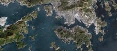
The Eastern district of Hong Kong Island is a highly dense area with commercial towers towards the coast line and more than 40 government housing towers.
In this patch, the major green cover is atop the hills, as is the case in the rest of HongKong. In addition to this, slopes which have been modified for building development have retained their forest cover. It accounts to 36 percent of the total land area in this sample. These are largely inaccessible by the public
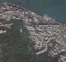
| Adaptive Urban Hillscapes 70
Patch
Land Area: 3.34 km2 Green
1.22 km2 (36%) Public Green Space: 0.15 km2 (0.45%)
Total
Cover:
Fig.2.9.3.2
Fig.2.9.3.3
Fig.2.9.3.4
Fig.2.9.3.3 Figure ground map
Fig.2.9.3.4 Green cover on the mountains and slopes
Fig.2.9.3.1 Satellite image of HongKong indicating Eastern District
Fig.2.9.3.2 Satellite image of the urban tissue sample
Fig.2.9.3.1
Public accessible open areas are very few and are predominantly in the form of playfields and sports enclosures. They account to about 4.5 percent of the land area and are evenly distributed across the built fabric. One line of the tram and metro network runs through the centre of the patch.
A test on the natural drainage of the terrain reveals some main collection channels. When compared to the existing built drain network (refer fig.2.9.3.6), the result from this test somewhat aligns with it.

71 |
0.0 52.2
Fig.2.9.3.5
Tram & metro stations
Fig.2.9.3.6
Fig.2.9.3.5 Public open/green spaces
Domain
Fig.2.9.3.6 Water runoff test with vector flow analysis
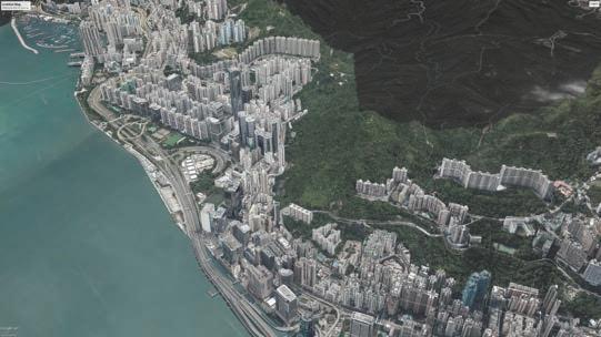
| Adaptive Urban Hillscapes 72 > > > ? #": 200 307 200 300 100
Fig.2.7.3.7
Fig.2.9.3.8
Fig.2.9.3.7
Fig.2.9.3.7
Aerial view of Eastern District, Hong Kong
Fig.2.9.3.8
Plan of the urban tissue sample [Redraw: http://www. landsd.gov.hk/mapping]
Existing built drainage channels
Slope & Built Fabric Analysis
Slope angle is analysed for every subdivided face of the natural terrain. When the building footprints are projected on this, it shows the natural condition of the site before the terrain was modified. Most of the buildings are on slopes that are stabilised. In this sample patch, it is seen that 75 percent of the buildings are constructed on gradual slope of less than 20 degrees. While 22 percent of the buildings are built on terrain that was assessed and stabilised. A small portion are built
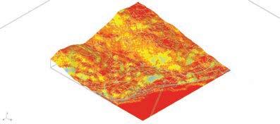
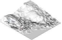
on what was hazardous steep slopes, but modified with extensive cut and fill. In one case, 30 storey tall development is built on the steepest natural slope of 51 degrees (refer Fig.2.9.3.10). The average building height is 24 storeys for this patch.
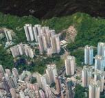
73 |
Fig.2.9.3.10
Fig.2.9.3.11
Fig.2.9.3.9
Fig.2.9.3.10 Slope angle analysis of the natural terrain
Fig.2.9.3.9 Instance of skyscrapers built on steep slopes
Fig.2.9.3.11 Building footprints projected on the natural terrain
0.0 52.2 0.0 52.2 300m 36% 58% 75% 24 (avg)68 (max) 6% 22% 2.5% 60-100m <60m ALTITUDE SLOPE ANGLE HEIGHT (storeys) 100-200m 20-35 35-52 <20 Domain
2.10 Site: Shenzhen City
2.10.1 Urban Growth In Shenzhen
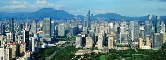
Lead by an economic development and the benefits of being located next to wealthy Hong Kong, Shenzhen has been experiencing a rapid growth in urban infrastructure since 1979. Its urban development can be categorized in three stages, each one having its own expansion cause. In the 1979-86 period, the government offered land resources to industrial development increasing the construction land from 3 km2 to 48km2. From 1987 until 2005 Shenzhen went through a period of rapid urbanization growth due to industrialization and an export driven economy. During this period, Shenzhen was following a masterplan to become one of China’s important economic zones. Because of this accelerated expansion, rural land was being abolished and urban land had risen up to 891 km2, at 16.9% annual growth of construction land. By 2005 Shenzhen reached a construction land area of 939 km2, covering half of the city’s total land area. From that year on, the government placed policies to stop urban growth and to protect farmlands, which actually reduced the construction land growth to 3.2 % by year 2014.
(J. Qian et al, 2015)
| Adaptive Urban Hillscapes 74
Fig. 2.10.1.1
Fig.2.10.1.1 Shenzhen CBD with the hills in the background [www.cbbc.org/about-us/ other/cbbc-cities/cbbccity-shenzhen/]
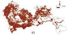
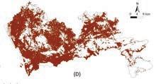
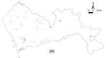
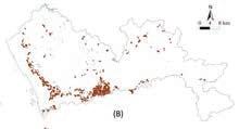
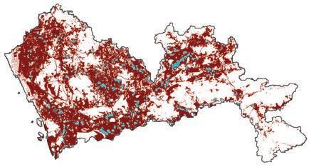
75 |
Fig. 2.10.1.2 Shenzhen’s construction land development. [J. Qian et al, 2015]
1979 2005 1986 2014
Construction land
Fig. 2.10.1.3 Shenzhen’s Urban redevelopment areas [J. Qian et al, 2015]
Construction land Urban Redevelopment Areas
Fig. 2.10.1.3
Domain
Fig. 2.10.1.2
2.10.2 Farmland Loss in Shenzhen
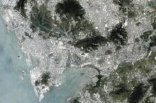
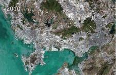
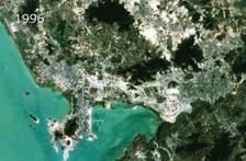
Accelerated urban expansion in Shenzhen has been vanishing farmland since the las decades, recording a total arable land loss of 51.6% from the year 1995 to 2009 (Qian et al. 2015). Although the government has recently established some measures to decrease the depletion of farmlands, Shenzhen’s economical activity will feed exponential population growth, preserving it as a menace for green areas in the city. At the same time, increasing population means more food supply needed, therefore in order to prevent high economical expenses for food imports, a rigorous plan must be held to reclaim big areas of farmland.
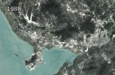
| Adaptive Urban Hillscapes 76
Fig 2.10.2.2 Change in Arable land and food production in Shenzhen (J.Shen, 2008)
Fig 2.10.2.1
Change in Grain output 132584 126461 116489 94465 81018 59138 32906 4887 4990 3700 600 60
Change in Arable land 532 ‘79 490
460 339 280 227 155 66 64 60 37 29
Satellite views of Shenzhen for the past 16 years showing farmland and green areas degradation. (http://urbanchange. eu/2010/12/14/shenzhenurbanisation/)
‘79‘80‘81‘85‘90‘91‘92‘95‘97‘00‘05‘06
‘80‘81‘85‘90‘91‘92‘95‘97‘00‘05‘06
Fig 2.10.2.2
Fig 2.10.2.1
[Shenzhen Statistic Bureau, 2015]
AREA OF SOWN FARM LAND 1980 2006 (grains) 43066 ha 305 ha YIELD OF GRAIN 1980 2006 126,461 ton 59 ton 1000 MUI (15 MUI = 1 Hectares)
[Shenzhen Statistic Bureau, 2015]
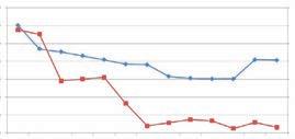
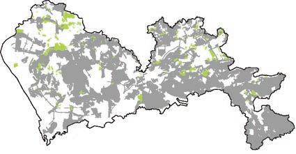
77 |
Farmlands (2008) Forest
Fig 2.10.2.3 Farmland usage in Shenzhen in 2008. (Urban Planning L&R Commision of Shenzhen, 2008)
Year 2002 2003 2004 2005 2006 2007 2008 2009 2010 2011 2012 2013 2014 Arable land (km2) 14.00 12.00 10.00 8.00 6.00 4.00 2.00 0.00 70.00 60.00 50.00 40.00 30.00 20.00 10.00 0.00 Fig
Rice Jan FebMarAprMayJunJulAugSepOctNovDec Potato Peanut Fruits
Fig 2.10.2.4 Construction occupation compared to Arable land in Shenzhen (J. Qial et al, 2015) Construction occupation of arable land (km2)
2.10.2.3 Fig 2.10.2.4
Fig. 2.10.2.5 Seasonal harvesting data in Shenzhen [source:Shenzhen Statistic Bureau, 2015]
Domain
Fig. 2.10.2.5
Shenzhen Major transport insfrastructure connecting with the rest of China(J. Zacharias et al, 2010)
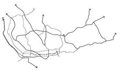
Redrawn
2.10.3 Transportation Network
Physical relief of congested areas and external communications have been the main drivers for the development of transportation network in Shenzhen city in the last couple of decades (Gao, 1995). Since the beginning of the city’s boost in urbanisation in the late 70’s, Shenzhen started to develop new residential and commercial areas around the old fishing village. This demanded planners and government to develop communication networks for diverse population targets, including the new labour class that lead Shenzhen’s densification increase.
Bao'an District Nanshan District
Futian District Luoho District
Hong Kong N.T.
| Adaptive Urban Hillscapes 78
Fig 2.10.3.1
Guangdong Province
Yantian District
Longgang District
Fig 2.10.3.1
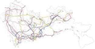

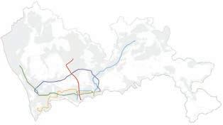
79 |
Fig 2.10.3.2
Shenzhen Metropolitan public transportOverground. (University of Southern California, 2012) Redrawn
Fig 2.10.3.4
Shenzhen Metropolitan roads. (University of Southern California, 2012) Redrawn
Fig 2.10.3.3
Shenzhen Underground lines. (University of Southern California, 2012) Redrawn
Fig 2.10.3.2
Fig 2.10.3.3
Domain
Fig 2.10.3.4
The average monthly temperature in Shenzhen
Source: Shenzhen Bureau of Meteorology
2.10.4 Climatic Conditions
Though Shenzhen is situated about a degree south of the Tropic of Cancer, due to the Siberian anticyclone, it has a warm, monsooninfluenced, humid subtropical climate. The average highest temperature is 32oC from July to August, and the lowest temperature is 13oC in January. The mean temperature difference in one day is around 6 degree.
The annual precipitation averages at around 1879,8 mm (78 in), some of which is delivered in typhoons that strike from the east during summer and early autumn. The average precipitation reaches its peak from June to August and goes down to the bottom in January. During the rain season, the daily average rainfall is from 15 to 20 mm. The rainstorms usually appears from April to September, the probability of big rainstorm occurrence along whole year is 0.03.
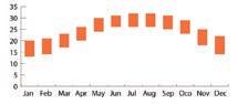
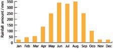
The average monthly rainfall in Shenzhen
Source: Shenzhen Bureau of Meteorology
It is suggested that, among various external factors, large amount of precipitation is one of the most important factors that caused landslides. In Shenzhen, the local precipitation is very intense and sometimes for a prolonged duration. According to statics, the relationship between rainfall and landslide is closely corresponded as seen in fig.2.10.4.5.
Fig. 2.10.4.3
Relationship between rainfall intensity and landslides occurence density, Shenzhen
Relationship between effective rainfall and landslides occurence density,, Shenzhen
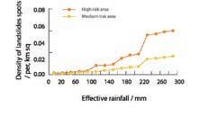
Resraw from: Xihua Gao, “Discuss on the correlations between landslides and rainfall and threshold for landslide early-warning and prediction”, 2007.
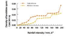
| Adaptive Urban Hillscapes 80
Fig. 2.10.4.2
13 20 14 20 17 23 20 26 24 30 26 31 26 32 26 32 25 31 23 29 18 25 14 22
Fig. 2.10.4.4
Fig. 2.10.4.1
Fig. 2.10.4.1
Fig. 2.10.4.2
Fig. 2.10.4.3
Fig. 2.10.4.4
Low
Low
Wind disaster
High Low
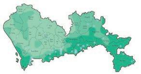
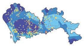
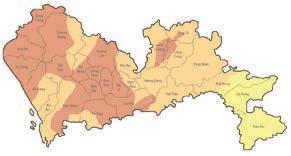
81 |
Fig. 2.10.4.5 Rainstorm disasters risk map
Fig. 2.10.4.7 Thunder disasters risk map
High
Flood Landslide
Data source: Shenzhen Bureau of Meteorology
Fig. 2.10.4.6 Wind-storm disasters risk map High
Fig. 2.10.4.5
Fig. 2.10.4.6
Domain
Fig. 2.10.4.7
2.11 Conclusion
By focusing on the recent urban development in Asia and particularly in China, it is evident that even after a couple of decades of exponential growth, there is an insatiable hunger and potential for further progress. The main issue apart from the environmental impact is that as the urban areas are expanding in size and population, the agricultural land in the region is being depleted. Because of migration, the populace involved in agriculture is also on a steep decline. According to a UN ESCAP(economic and Social commission for Asia Pacific) report of 2013, China must feed a fifth of the world’s population with about 7% of its arable land, according to the UN’s Food and Agriculture Organisation, and nearly half of that land has been “degraded” by decades of unchecked development. In terms of general availability of land for farming practices, the statistics are not as frightening. But agricultural land near urban centre is the most threatened of being converted into urban land.
In the region of interest, for this research, the Pearl River Delta was long-time important production base for rice, sugar cane and tropical fruits in China, the PRD area was once dominated by open space related to farming activities. However, farmland decreased by 3,695 sqkm. during 1990s (30% loss in 10 years); this number dropped to 925 sqkm. during 2000s(9% loss). Farmland was consistently the major source of new built-up lands in those two decades. Reflecting on the topographical conditions in major cities of the region like Shenzhen, dramatic urbanisation has left only the hillsides relatively green. But since the city is interspersed by hills, urbanisation is bound to creep up the slopes. [Shiqiang et al. 2013]
The hillsides are this ambiguous zone between the urban centre and the forest, as it is not considered prime land to build upon(refer section 2.2). This initial lack of interest may present an opportunity to develop an alternative urbanism. The question arises from this research as to whether these sloped terrains, within the city and at the periphery, have scope for sustainable dense urbanisation with a potential of being an urban supply system. This urbanism has to then adapt and maybe take advantage of any land instability event in the context. In the case of Shenzhen, it is predominantly rainfall induced erosion and debris flows.
This 'alternative' urbanism that is capable of co-existing with the ecological processes of hilly terrains, cannot follow conventional urban patterns. This is because the habitable urban settlements should function harmoniously with farmlands, forests, waterbodies. Hence, it is pertinent to study rural settlements that have such a character especially in the context of the mountainous terrain in China. The urbanization process set under the terms mentioned in this chapter demands a comprehensive design that contemplates the surrounding ecological forces, as the urban expansion is constantly shaping the boundaries of adjacent subsidiary ecosystems. Analyzing the effects of unaware landuse pattern arrangement will provide abstracted principles that can be employed in the generative process of a comprehensive land-use map and further drive detailed operation logics into the architectural outcome.
In contrast, mitigation measures require a study of state of the art engineering and bio-engineering practises prevalent today. The best examples of that is seen in HongKong, a neighbouring city to Shenzhen. Soil mechanics and knowledge about how to relate the available soil data to topographic data is important in proposing any risk analysis.
| Adaptive Urban Hillscapes 82
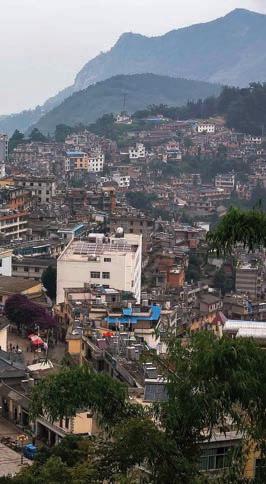
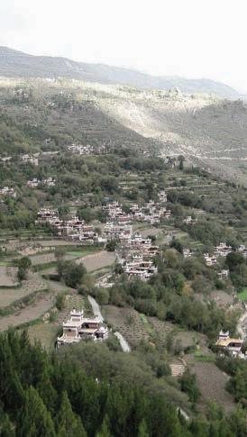
83 |
Fig 2.11.1 Xinjie village, Yunnan,China and Danba village,Tibet (Maier&Maier, 2005)
Domain
Fig 2.11.1
Methods 03.
PRODUCED BY AN AUTODESK PRODUCED BY AN AUTODESK EDUCATIONAL PRODUCT AUTODESK EDUCATIONAL PRODUCT
3.1 Deterministic mapping 3.2 Topographical analysis 3.3 Multi-objective optimisation 3.4 Spatial quality analysis 3.5 Networks 3.6 RUSLE model 3.7 Experiment flowchart AUTODESK EDUCATIONAL PRODUCT PRODUCED BY AN AUTODESK PRODUCED BY AN AUTODESK EDUCATIONAL PRODUCT
Silt:
Clay: φ=25°,T=0,04m2/h
Sand:
3.1 Deterministic Mapping
Mathematical techniques based on the concept that future behaviour can be predicted precisely from a set of data of the past behaviour. These methods ignore the existence of disturbances or external ‘shocks’ that may alter the data’s future pattern. Based on a fixed set of input data, the output always remains the same since it doesn’t take into account any uncertainties.
This method can map spatial distribution of the predicted faults based solely on 2D empirical analysis. Various Factor maps, like Landslide inventory, geology, hydrology, elevation, precipitation are required as input data. The maps are converted or broken down to polygon maps. In order to bring in contextual knowledge, variable weightage can be given to the input data based on expert evaluation. In general the inputs are reclassified and overlayed to produce final maps that show either susceptibility, hazard etc. [Van Westen, 2008]
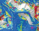
3.1.1 Physical Based Mapping
Conventionally in this approach, the factor maps are principally describing the physical characteristics of the terrain. Apart from the maps, geological and hydrological properties are required as input. The input maps can be sampled for the RGB values and those can be designated to the subdivisions of the base DEM surface. For a given set of hydrological properties, like soil wetness index and water table depth, the factor of safety can be calculated and mapped on the terrain surface. [van Westen,2008] [[A.Gunther, 2010]
Landslide inventory: Where do which landslides occur? Detailed record of where landslides of a particular type have occurred in the past.
Landslide susceptibility: Where could landslides occur? The relative spatial likelihood for the occurrence or initiation of landslide of a particular type and volume
Landslide hazard: When do what landslides occur? The probability of occurrence of a particular landslide type within a specified period of time and given area.
Landslide risk: What consequences do landslides have? Estimates the expected losses (monetary, or in number of buildings/people) due to specific landslide type within a specified period of time and given area.
Landslide density: Area covered by landslides / Area of terrain unit .(watershed)
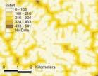
Advantages:
-Based on sound physical models
-Capable for predictive landslide analysis
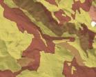
-Renders information on landslide hazard
Limitations:
-Requires high accuracy of input parameters
-Predictive models difficult to evaluate
-Complex modelling hard to perform at smaller scales
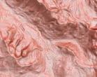
| Adaptive Urban Hillscapes 86
Fig.3.1.1.2
Fig.3.1.1.1
Fig.3.1.1.3
Fig.3.1.1.4
67 0
Fig3.1.1.1 Distance to drain channel [A.Gunther, 2010]
Fig3.1.1.2 Slope angle [A.Gunther, 2010]
Fig3.1.1.4
Overlayed susceptibility map showing the Factor of safety [A.Gunther, 2010]
Fig3.1.1.3 Soil parameter [A.Gunther, 2010]
φ=30°, T=0,4m2/h
φ=35°, T=8m2/h
FACTOR MAPS
Soil type map
Soil Data Soil depth map
Geotechnical properties
Hydological properties
Slope angle
CALCULATE FACTOR OF SAFETY

DEM
Ground water measurements
Local drain direction
Contributing areas
CALCULATE WEIGHT reclassify
Landslides Inventory Map
Factor Maps
Cross Tables
Weight Maps
W Landslide Landslide
W Soil Soil
W DEM DEM
Susceptibility Map
87 |
Fig.3.1.1.5
Fig.3.1.1.5 Landslide weighted susceptibility mapping procedure [van Westen,2008]
Methods
3.2 Topographical Analysis
The various techniques used to analyse the topography and the catchment are carried out on a computational terrain model, which is a graphical representation of the morphology of the terrain read as a continuous set of information. The surfaces or meshes at every point across their extent contain valuable information that can be
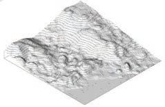
3.2.1 Digital Elevation Model (DEM)

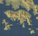
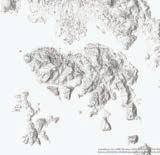
A digital elevation model (DEM) is a digital model or 3D representation of a terrain’s surface created from terrain elevation data. The elevation data is obtained from high resolution satellite imagery. In this case, Shuttle Radar Topography Mission (SRTM) data produced by NASA was used, with an accuracy of 1 arc-second or 30metres tolerance.
extracted to analyse or modify the original geometry. To understand this information the values at the infinite possible points are simplified into a limited set of values on a fixed grid of 20m x 20m. This lowering of the resolution also helps with the computational speed; and the cell size is maintained all through the thesis.
3.2.2 Slope Aspect Analysis
The slope aspect is the orientation of slope, measured clockwise in degrees from 0 to 360. It basically shows the compass direction which the slope faces. As the analysis is done on a terrain model of 20 x 20m resolution, the surface normal of every subdivided cell is calculated and projected onto the horizontal plane. The angle of the projected vector is calculated from the true north which is taken as 0 degrees.
| Adaptive Urban Hillscapes 88
North North east/ North west East/West South east/ South west South
Fig.3.2.1.1 DEM surface of HongKong Eastern district (refer 2.9.3)
Fig.3.2.2.1
Slope aspect analysis of HongKong, Eastern District
Fig.3.2.1.3 SRTM image file of HongKong
Fig.3.2.1.2 Hillshade elevation file of HongKong
Fig.3.2.1.1
Fig.3.2.1.2
Fig.3.2.1.3
Fig.3.2.2.1
N S E
3.2.3 Slope Angle Analysis

The slope angle analysis is carried out on the surface terrain model. It is calculated for every subdivided face of the surface. The more the subdivisions, better the accuracy. The following equation calculates the angle of the subdivided face to the horizontal, based on the normal and tangent vectors at the centre point of the particular cell.
3.2.4 Mapping Landslides
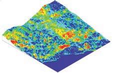
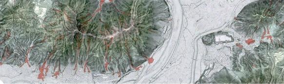
Several techniques for mapping landslides displacement have been developed over time to improve mitigation processes. From satellite light-radar measurements (Fig. 3.2.4.1) to digital elevation models, technology keeps providing more tools to track natural disasters. The accomplishment of upcoming experiments requires an appropriate understanding of the physical effects of hydrological flows on sloped terrains. Therefore, to obtain a realistic simulation of the scenario in which we are planning to work, geomorphological and precipitation data are required, since the main trigger for erosion considered in the
proposal is the intense rainfall. The topographical data is obtained using ArcGIS data together with ‘Elk’ plug-in for Grasshopper inside Rhino interface. Using the topographic model, there are two tools evaluated in this chapter that will lead a simulation of the potential erosion scenario. The first one is the cellular automaton based model ‘Caesar-Lisflood’ developed by Tom Coulthard from the University of Hull; the second will be a vector flow analysis using Kangaroo plug-in for Grasshopper.
89 |
Fig 3.2.4.1 Hiroshima landslide mapping using LIDAR measurement. (Doshida and Araiba, 2014)
Fig 3.2.4.1
<10 10-15 15-20 20-25 25-30 30-35 35-40 40-45 45-50 >50
Fig.3.2.3.1 Slope angle analysis of HongKong, Eastern District
z surface normal at the given point slope angle =(0.0 - (asin( z ) - 0.5*pi)) z Methods
Fig.3.2.3.1
3.2.5 Particle Flow Simulation
Caesar Lisflood
CAESAR (Catchment Automaton Evolutionary Slope And River) is a cellular landscape evolution model developed by Tom Coulthard (University of Hull) which allows hydrologic and sediment flows to be simulated on a given surface. The movement of sediment detachment and deposition are represented as a set of rules for a cellular automaton model, that when iterated repeatedly can simulate geomorphological movement inside the model (Coulthard et al, 2006). Topographic data needs to be inserted into the CAESAR model as a mesh of grid cells (text file), considering that smaller the cell size the higher resolution that will be obtained in the simulation. The rainfall data is represented as numerical rates for hourly precipitation in millimetres and inserted also in a format of text file.
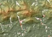
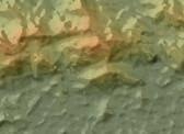
Additional values for soil roughness; grain sizes and vegetation cover are to be added inside the model for more accurate evaluation. Once the simulation starts running, initial dispersal of erosion and deposition changes the topography, which will become the starting point for the next time step (Coulthard et al, 2006). Water flows, water depth and flow velocity will be shown as polychromatic pixels overlaid on the surface image. and their values can be obtained as text files. Furthermore, the software can provide new elevation models, as in the transformation from the original topography to the one affected by erosion, allowing the user to determine the location of sediment deposition.
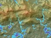
| Adaptive Urban Hillscapes 90
Current DEM Text file Erosion / Deposition Grid cells Fluvial Processes Rainfall data Hillslope Processes Elevation differences Topographic adjustment Topography Sediment Distribution Precipitation data Initial conditions: Outcome Fig 3.2.5.4
Fig 3.2.5.4 CAESAR-Lisflood: Conceptual structure adapted from Coulthard et al. (2006) Fig 3.2.5.3 Erosion - Depostion map from CAESAR-Lisflood Fig 3.2.5.2 Water depth map from CAESAR-Lisflood Fig 3.2.5.1 DEM from CAESARLisflood
Fig 3.2.5.1
Fig 3.2.5.2
Fig 3.2.5.3
A geometrical simulation of raindrop flow on a surface can also be achieved within Grasshopper and Kangaroo Physics plug-in. The surface elevation model obtained from GIS is used as the mesh to represent topography, and tracing the vector displacement of points running down the slope replicates the raindrops flow path of a strong rainfall. To build the system, a fixed grid of points over the surface is attracted vertically to it by applying a gravity force component from Kangaroo Physics. The outcome of this model will be the flow paths as curves on the surface, hence the hypothetical displacement of gullies or debris flow might be anticipated.
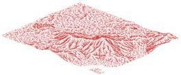
Differing from Caesar, this method is not based on a time lapse and no hydrological or soil data is considered, hence the outcome should be taken as purely physical reaction on a given surface. However, the important benefit of this method relies in the possibility of incorporating more components into the model and programme it to have different parameters. Then the model can be altered based on relationships between slope angles and predicted flows, by controlling the elevation points in order to set up a desired scenario. On the other hand, the initial simulation provided by Caesar-Lisflood can also inform future vector-flow simulations as it points specific areas where soil and water depositions can happen.
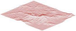
91 |
Fig 3.2.5.5 Fig 3.2.5.6 Fig 3.2.5.7 Vector Flow Simulation: Conceptual structure Fig 3.2.5.6 Result after vector flow simulation Fig 3.2.5.5 Surface points as particles Pull attractor Particles to mesh Vertical vector force Gravity Surface Elevation model Text file Topographic Reconfiguration Parametrized Particles Grid Points Vector Flow Path Curves Fig 3.2.5.7 Methods
Vector-flow Simulation
3.3 Multi-Objective Optimisation
Genetic Algorithm
The design process can get increasingly complex with multiple parameters and targets to achieve. Both the ecological analysis and the architectural design requires highly complex mathematical objectives that need to be optimised and solutions generated simultaneously.
A genetic algorithm (GA) applies concepts of emergence and evolutionary ideas of natural selection. It produces iterations that are evaluated through the definition of evolutionary goal or goals. Optimized solutions for a problem are generated using techniques like inheritance, crossbreeding,, selection and mutation. [M.Mitchell, 1996] [Doc.ic.ac.uk, 2016]
The GA is used within an associative modelling environment, with the same script that describes the parametric model. Selected parameters serve as the variable "genes" and some important measurable outputs are defined as the "objectives". The GA is used to simulate the survival
of the most optimal solution, not necessarily the fittest, over consecutive generations. Each iteration presents a point in search space or fitness landscape and a possible solution. A fitness score is assigned to each solution representing the abilities of an individual to compete in each criteria.
This generative technique is important in this thesis as it attempts at generating multiple aspects of the design in a single design stage, via multiple parameters and conflicting objectives. At a morphological level, the intention is to evolve the built form in families, based on a basic set of primitive building types. The generated forms are evaluated in isolation for their performance in environmental and spatial aspects; and more interestingly for their performance as a collective built cluster in aspects of ecological flows, networks and urban spatial conditions.
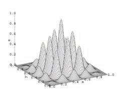
| Adaptive Urban Hillscapes 92
Script defining the analysis / geometry Variable parameters Genetic Algorithm [selective breeding] Best sub-optimal solutions Post generative evaluation FITTEST PHENOTYPE (relative) Genes Quantifiable objectives
[https://www.codeproject. com]
Fig 3.3.1 Representation of a Fitness landscape where the axes shows the various fitness
objectives.
Local maxima possible fitter solution
Fig 3.3.1
Remapping Parameters
As the parameters employed in a system are of various aspects, they will possess different numeric domains. For comparison in analysis and scoring cumulative factors, they need to be remapped into a standard domain of 0 to 1.
Various techniques are used for different kinds of remapping, as the criteria for judging the fitness will vary. For example; maximising certain objectives the higher value will not necessarily equate to a higher fitness score, therefore all parameters will be remapped such that numbers closer to 1 will mean better fitness.
Post Generative Evaluation
An additional evaluative process is proposed, once the GA is stopped. This is because, even after running several generations, the GA might not have converged at a pareto-optimal solution ie. a solution which cannot improve its overall fitness without compromising on one of the objectives. Hence, a collection of best sub-optimal solutions are evaluated for certain external criteria that was not part of the original generative process. By this process it is possible to select a reasonable solution that is assumed to be relatively fit
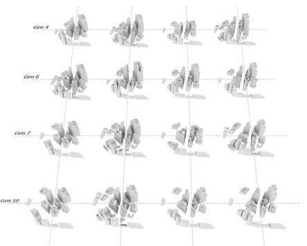
93 |
Fig 3.3.2
Example of a family of phenotypes (urban blocks) [EmTech Core studio 2 , The Great One et al. ,2016]
Methods
Fig 3.3.2
3.4 Spatial Quality Analysis
Spatial Sampling of Indigenous Settlement
This technique involves obtaining of spatial metrics from a sample settlement or settlements that have contextual similarities to the test site. These spatial metrics mentioned in this chapter (not limited to) are relevant because these indigenous settlements have evolved over time and with necessity their spaces have adapted to their local aspects of culture and occupation. This makes these indigenous settlements more sustainable environmentally and socio-culturally.
Solar Exposure
Solar exposure is one of the most vital elements when valuing spatial quality. This element is influenced by the height-width ratio (“H/W ratio”) depending on building heights and distances between them. The slope angle is another important element to be taken into account owing to the fact that the research is focusing on urbanizations in slope contexts.
The height difference between buildings in urban areas makes it difficult to calculate the H/W ratio. Nevertheless, a formula introduced by C Ratti shown in Fig. 3.4.1 presents a solution to such complexity. By adopting this formula, the optimal H/W ratios can be found corresponding to various scenarios which are built in terms of different slope degrees. Whether the slope is towards the sun (“the toward slope”) or backward the sun (“the backward slope”), is another aspect analysed in Ratti’s example.
The first experiment is set in Octopus. The genes include building heights and distances between buildings. Fitness criteria take into account building exposure, canyon exposure and canyon width. Two hundred generations have been generated, while each generation has a number of 30 populations. Later, the fittest phenotype is selected from the pool for each scenario. Results shown that in case of the 'toward slope', despite the difference in slope angles, the date indicates that to optimize sun exposure, the high-laying buildings should be higher than the low-laying ones. In contrast, in case of the backward slope, despite the difference in slope angles, the date indicates that the lowlaying buildings should be higher than the high-laying ones. In both cases (toward and backward), as the slope angle increases from 10 to 30 degree, the H/W ratio should be adjusted to decrease accordingly in order to optimize sun exposure.
In case of the 'toward slope' the H/W ratio is more than 1, whereas in the 'backward slope' the H/W ratio is less than 1. Considering the above, it is clear to state that the building on the 'backward slope' requires a relatively wider distance between buildings for better sun exposure than the one on the 'toward slope'.
Please refer to the Fig. 3.4.2 for a detailed data.
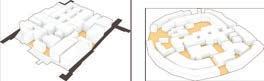
| Adaptive Urban Hillscapes 94
Height 1 Height 2 Width Slope angle P W1 W2 H1 H2 ( H / W )p = H1 + H2 2 ( W1 + W2 )
Fig. 3.4.1 Main parameters influence sun exposure
Canyon height - to - width ratio formulat:
Redraw from: C. Ratti, “Urban texture analysis with image processing techniques: winds and dispersion”, 2005
Fig. 3.4.1
Slope angle: 10deg
On the slope towards the sun
On the slope backwards the sun
Slope angle: 20deg
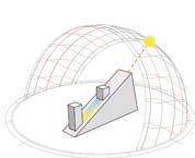
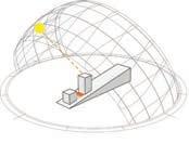
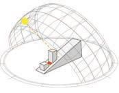
Height 1: 8 m
Height 2: 22 m
Distance: 5.2 m
Height - to - width ratio (Midpoint): 2.88
Height 1: 30 m
Height 2: 10 m
Distance: 23 m
Height - to - width ratio (Midpoint): 0.87
Slope angle: 30deg
Height 1: 10 m
Height 2: 20 m
Distance: 10 m
Height - to - width ratio (Midpoint): 1.5
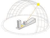
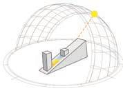
Height 1: 30 m
Height 2: 10 m
Distance: 29.5 m
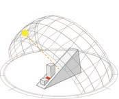
Height - to - width ratio (Midpoint): 0.68
Height 1: 11 m
Height 2: 19 m
Distance: 12 m
Height - to - width ratio (Midpoint): 1.25
Height 1: 27 m
Height 2: 13 m
Distance: 30.5 m
Height - to - width ratio (Midpoint): 0.66
95 |
Fig. 3.4.2 H/W ratio experiments in different slope scenarios
kWh / m2 1.20< 1.08 0.96 0.84 0.72 0.60 0.48 0.36 0.24 0.12 0 Methods
Fig. 3.4.2
Sky View Factor (SVF)

Sky view factor is the amount of sky visible when viewed from a base viewing plane, which could be at the ground level or any elevated terrace level. It can be imagined as an equivalent to a 'fish eye' photograph taken in a vertically upward direction from that base plane.. It is measured as the percentage of the sky that is not blocked by structures. At an urban scale, it is commonly used to judge the effect of an urban canyon. The higher the value of SVF, the quicker the urban canyon will cool. With low SVF, the canyon will retain more heat during the day, creating higher heat release during the night. Spatially, the preference of higher SVF is subjective to the context and terrain . As shown in the diagram below, SVF on a sloped terrain is naturally higher than on a flat terrain, for the same height of buildings.
Enclosure Value (EV)
Enclosure is the ratio of enclosing surfaces to the space enclosed. In the case of a public or semi public space, the facade area that surrounds is what defines the enclosure value.
This parameter describes the morphology of the convex space. A higher enclosure will mean a highly contained space disconnected from its neighbourhood, while a lower value of enclosure will denote a well connected spacce. Different cultural settings would require different enclosure values for different hierarchy of spaces. It is one of the parameters that describes the experiential aspects of the space.
Facing Sur face area
Enclosure Value = Public space area
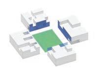

| Adaptive Urban Hillscapes 96
Example
Example
1 - 52%
1 on flat terrain - 46%
Porosity
Building porosity and public space enclosure are two methods that are contemplated in this thesis as important tools for measuring spatial and visual access from private to public or semi-public spaces; and between public spaces through buildings. This approach to urban connectivity can be employed as an environmental strategy that can improve the thermal comfort as well as the spatial quality in specific areas of the city.
The area of the openings or ‘negative’ surfaces at the building’s facades that are facing public spaces are considered in these methods as the porous surface. To calculate the amount of building porosity towards a public space, the percentage that these negative areas represent from the total façade area is considered.
Shaded Area Ratio (SAR)
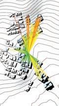
Shaded area proportion to a large extent contributes to the quality of the space. A non-shaded area may be too uncomfortable to use in hot climates and overly shaded areas will have poor lighting. The right amount of shading at the right time of the day is essential for the space to perform effectively. So this parameter is the percentage of area shaded at the period of the year when the position of the sun is at its highest, and then it can be assumed that for the rest of the year, good shading quality will be maintained. Several sun positions can be taken during the mid day period and the percentage of the building shadow on the open space is calculated
3D Isovist
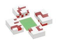
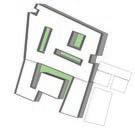
In the field of visibility analysis within urban landscapes, the Isovist is defined as a three-dimensional description of visible space from any given vantage point. This is important to understand the relation between built forms and perceived space and the relation between human activities and environment. Other studies showed that people prefer to pause and linger on in the 'inside corners' of spaces. Later 'Space syntax' focused on 'axial lines'. These lines are defined as the longest visibility lines (or ‘lines of direct movement’) in the 2D public urban space. [Morello et al.,2010] [de Smith et al.,2015]
The method proposed for this thesis is a combination of 3D viewshed and line of sight , additionally taking specific consideration of building terraces and the natural sloped terrain. The images on the right show various representations of this concept, indicating higher values for the longer lines of sight. This means that, the vantage point in consideration scores better if it has more direct line of sight to buildings that are farther away.
97 |
far near Methods
Path finding performance.
Source: https:// generativelandscapes. wordpress. com/2015/02/17/pathfinder-using-a-recursiveprocess-example-8-5/, [Accessed on 2 Mar, 2016]
3.5 Networks
3.5.1 Agent Based Path Finding
Paths exceeding a slope of 1:12 are generally inaccessible for pedestrians and therefore not likely to be used in exterior designs. A definition introduced in Grasshopper calculates the distance of possible routes between two points and consequently identify the shortest route (with a slope ratio lower than 1:12). This definition can also be applied to the design of roads and transportation networks in cities.
Taking the previous information from terraced rice paddies, transportation in the terraces is composed of different levels of paths. Main paths are the ones connecting the top and bottom of the terraced rice paddy in the most effective and efficient way, but it may have a relatively steep slope angle.
By adjusting the limit of the slope degree, the above definition can be applied to a new rice paddy in order to find the main paths. Figure 1 represents the process on how the definition works, where A is set as the start point and B, C and D are the destination. Three paths are generated based on topography.
Moreover, by introducing agent movement in the above path finding definition various alternative paths could be achieved. In this case, both start points and ends points could be random, while the moving behavior should be regulated. Besides, it is critical to set suitable fitness criteria to select optimal paths among all the generated paths.
Agents on a topographical surface [Source: https:// generativelandscapes. wordpress.com/]
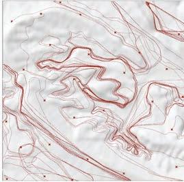
| Adaptive Urban Hillscapes 98
Fig. 3.5.1.1
A B C D A B C D A B C D
Fig. 3.5.1.1
Fig. 3.5.1.2
Fig. 3.5.1.2
3.5.2 Network Analysis
Network analysis measures can be useful predictors for a number of interesting urban phenomena. Syntactical analysis of topological relationships between the buildings, open spaces and the proposed network, based on graph theory has been proposed and revised many times over by Hillier and Hanson. The methods are mainly based on the concepts of space syntax and graph theory; and the analysis results illustrate the degree to which an edge or a node is spatially connected to the surrounding path network. [Sevtsuk et al., 2012]
The Urban Network Analysis tool [City Form lab,MIT] additionally includes buildings as nodes- with a certain weightage depending on its size or importance- to the overall graph system of edges representing paths; and nodes representing the intersection of two or more edges.
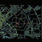
Centrality Measures
Network centrality measures are mathematical methods of quantifying the importance of each node in a graph. The Reach Centrality of a node in a graph describes the number of other nodes that are reachable at a shortest path distance within a specified network radius. Within the scope of this research, this tool can be used to identify and locate public facilities for ease of usability.
The Betweeness Centrality estimates the number of times a node lies on the shortest paths between pairs of other random nodes that are within a specified network radius. The count of the node acting as a bridge is fractional ie. if there is more than one possible shortest path, it gets distributed between different solutions. This can also be considered as a network segment having a high probability of being along various shortest paths , then this information can be utilised to locate points of interest in the urban system that might require high pedestrian volume to function effectively. [Sevtsuk et al., 2012]
Network Integration
Integration is a measure of centrality that indicates how likely it is for a space to be private or communal. The more integrated a space, the shallower it is to all other nodes in a configuration. Integration is calculated by computing the total depth of a node when the depths of all other nodes are projected on it. The street segments that require the fewest turns to reach all other streets are called 'most integrated'. Integration can also be analysed in local scale instead of the scale of the whole network, and this is useful in evaluating the generative process of the local networks .
[Nourian,2013] [Hillier..B et al., 1984]
99 |
Fig. 3.5.2.1 Indicating reach centrality [Source:Sevtsuk, 2012]
Fig. 3.5.2.2 Indicating betweeness centrality [Redrawn: Sevtsuk, 2012]
Methods
Fig. 3.5.2.3 Global network integration analysis - East manchester [EmTech Core studio 2 , The Great One et al. ,2016]
Classified soil loss map
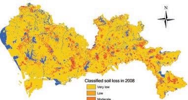
[zhang et al. 2014]
very low (<5 tonnes) low (5-25 tonnes)
moderate (25-50 tonnes)
moderate high (50-80 tonnes)
high (80-150 tonnes)
very high (>150 tonnes)
3.6 RUSLE Model
USLE: Universal Soil Loss Equation, proposed by Wischmeier and Smith (1961) and the Revised Universal Soil Loss Equation is the most common method to obtain annual soil loss in cities or urban areas, since it takes into account human induced factors (Ozcan et al, 2008). It calculates soil loss based on the product of five factors that indicate erosion risk (Meusberger et al 2010):
[ A = R x K x LS x C x P ]
Where:
A: predicted average annual soil loss [tonnes p/ hectare p/ year]
R: rainfall and runoff factor [mega joules mm p/ hectare p/ year]
K: Soil erosivity factor [tonnes p/ hectare p/ unit R]
LS: slope length and steepness factor [dimensionless]
C: cover and management factor [dimensionless]
P: conservation practices factor [dimensionless]
R; K; LS factors determine the erosion volume, while C and P factors are reduction factors with a range from 0-1. [Kumar and Kushwaha 2013]
From these five factors, the soil erosivity factor, ‘K’, represents the soil response to erosion induced by rainfall and runoff. A geological study of city of Shenzhen was carried by the University of Hong Kong (Zhang and Huang, 2014) to obtain the values for ‘K’ factor, which requires data for percentages of sand; silt; clay; and organic matter (Sharpey and Williams 1990) in the areas of study. The results are shown in fig 3.1.3.1.
Supporting this data, a previous study of Soil loss using the same method was carried by the same institution from 1996 to 2008 in Shenzhen giving the following results mapped in fig. 3.1.3.2.
The crop and management factor C depends on vegetation cover, which dissipates the kinetic energy of raindrops before they hit the soil surface. Erosion and runoff are affected by different types of vegetation cover. C equals 1 when it is subject to standard fallow conditions. As the percentage of vegetation cover approaches 100 %, the C factor value approaches the minimum.
P Conservation practice factor is defined as the ratio of soil loss from the upward and downward slope of an inclined plane where a soil preservation policy has been put in place (Park et al. 2011). Its value ranges from 0 to 1, with a lower value suggesting more effective conservation practices.
| Adaptive Urban
100
Hillscapes
Figv3.6.1
Fig.3.6.1
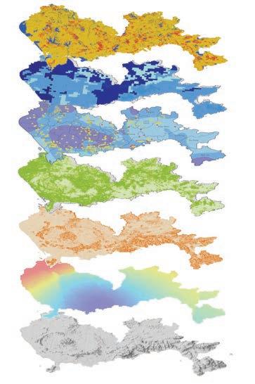
101 |
Classified soil loss K Factor Rainfall intensity C Factor LS Factor R Factor
Fig3.6.2 Overlayed USLE factor maps for Shenzhen, China
Very low Low Moderate Moderately high High Very high High: 0.376 Low: 0.117 High: 1 Low: 0 High: 7.402 Low: 0.007 High: 793.79 Low: 749.275 High Medium Low Flood Landslide Methods
Fig.3.6.2
3.6.1 Cellular Erosion Estimation
Calculation of soil loss is highly complex due to irregularities in data. In addition to such natural factors as slope, rainfall, vegetation cover, and soil characteristics, land-use changes - a direct reflection of human activities - also exert a huge influence on soil erosion. Thus in the digital experiments carried out on the test patch, it is important to evaluate the proposal for the effective soil loss, as the above mentioned factors will be altered.
Reducing the average soil loss in the test patch is one of the prime objectives, for which the land usage, block morphology and clustering is optimised.
RUSLE (Revised Universal Soil Loss equation)
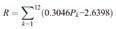
[ A = R x K x LS x C x P ]
For this thesis, the USLE equation (refer 3.7) is applied to every cell , and its sum will indicate the soil loss value for the patch in consideration. A synthesis of the product of R, K, LS, C values of every grid point will give the soil loss at that cell.
Atotal = R( Ki LSi Ci)
R Factor rainfall factor
R - rainfall and runoff factor [mega joules mm/ hectare/ year]
Pk - average monthly rainfall (mm)
R factor is constant for the central region of Shenzhen, where this test patch is located and does not reflect spatial differences. It is obtained from a detailed study by W.Zhang and Bo Huang.(W.Zhang et al. 2014)
| Adaptive Urban Hillscapes 102
LS factor Slope length & steepness is directly related to topography
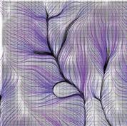
(L/22.12)m * (65.41 sin2 + 4.56 sin + 0.0065)
L is the slope length or runoff length is the slope angle m is a slope angle contingent variable (McCool. et al. 1987)
C factor is the crop and management factor, depends on vegetation cover, which is very crucial as it can be controlled by design. For tree covered areas, the tree type has to be multiplied with the ground cover type.
P Conservation practice factor, Its value ranges from 0 to 1, with a lower value suggesting more effective conservation practices.
K factor - Soil erosivity factor (UN FAO) based on the soil conditions in the test patch(refer section 4.1.2).
1.6 Slope Length (L) Main drainage channels (natural) 305.4 m Fig.3.6.1.1 Ls factor calculation method Red Soil (porous, loam) 0.18 - 0.28 Fig.6.2.4 K factor Alluvial soil (silt, sand) 0.28 - 0.42 Fig.3.6.1.1 Fig.3.6.1.2 0.001 C FACTOR P FACTOR 0.5 0.25 0.004 0 0.3 1 0.6 1 0.5 0.1 <30% cover: 0.20 30-60%: 0.07 <60% cover: 0.04 Developed areas Grasslands Forest w/ natural litter Wetlands Trees <2m Rice paddy Fig.3.6..1.2 C factor and P factor of various landuse types Fig.6.2.5 Methods
3.7. Experiment Flowchart
An organized work flow needs to be designed in order to make a contribution out of each digital analysis and avoid reiterations. It is important to recognize and understand what the outcome of each analysis will be, and to what extent a combination of data can be held to improve the accuracy of the results and proceed with the generative process.
| Adaptive Urban Hillscapes 104 C .A .E .S .A .R Topographical Analysis Vector Flow Analysis Agent Based Path Finding R.U.S.L.E Indigenous Spatial Sampling Climatic Analysis Susceptible Erosion zones Susceptible Deposition zones Slope angle Slope aspect Elevation Flow direction Accumulation Accessible gradient paths Soil loss Spatial quality metrics Solar exposure Wind direction
Fig. 3.7.1
Deterministic Mapping Rationalisation
Susceptibility map Landuse pattern
Multi-objective Optimization
Associative Modelling
Ecological strategies Urban strategies
Network Analysis
Integration Centrality Measures
105 |
Genetic Algorithm
Generative evaluation
Post
Methods
Fig. 3.7.1 Experiment flow chart
PRODUCED BY AN AUTODESK PRODUCED BY AN AUTODESK EDUCATIONAL PRODUCT AUTODESK EDUCATIONAL PRODUCT Research Development 04.
AUTODESK EDUCATIONAL PRODUCT PRODUCED BY AN AUTODESK PRODUCED BY AN AUTODESK EDUCATIONAL PRODUCT 4.1 Test patch selection 4.2 Factor map 4.3 Synthesis mapping 4.4 Slope risk analysis 4.5 Spatial pattern sampling 4.6 Data extraction 4.7 Conclusion
4.1 Test Patch Selection
4.1.1 RUSLE Based Method
Rainfall and water flow has been considered as main causes of soil erosion. Besides natural processes, human activities have recently greatly been proved as another important factor as well. Wischmeier and Smith (1961) proposed the well-known USLE model (refer sec 3.7), which has become one of the most widely used approaches to estimate soil erosion.
Soil loss could be reflected by applying formulation:
A = R * K * LS * C * P. (facing page) Thus, the higher value of indicators would lead to more serious soil loss.
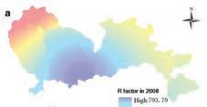
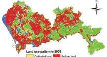
In this study, Shenzhen has been chosen as a test site. Shenzhen has a subtropical monsoon climate, which brings abundant rainfall to city. Shenzhen also features numerous mountainous areas with steep slopes. The abundant rainfall and steep slopes are aggravating factors of soil erosion. In addition to its natural characteristics, the rapid land-
use changes in the past 20 years have further aggravated its soil erosion. Given these characteristics, Shenzhen is vulnerable to severe soil erosion.
Supported by this information and considering that the proposal is based on water-induced erosion and debris flows, the site selection for the development of the design should be focused on areas of the city of Shenzhen that are susceptible to soil erosion by water forces.
A smaller test patch with comparatively higher soil erosion occurrence is selected from Shenzhen area. Figure 4.1.1.2 presents soil loss indicators of the city. Through comparing R, K, LS, C factors, it is detected that the centre mountainous area in Shenzhen has higher soil erosion possibility, which is around Meilin area. Thus the test patch is selected from this area.
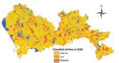
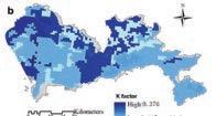
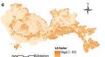
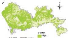
| Adaptive Urban Hillscapes 108 Land use pattern of Shenzhen (2008) Cultivated land Garden plot Wood land Pasture land Built-up land Traffic land Water body Unused land N 10 km
4.1.1.1 Land use pattern of Shenzhen (2008)
Fig.
Low: 749.275 High: 793.79 Low: 0.117 High: 0.376 Low: 0.007 High: 7.402 Low: 0 High: 1
Factor (the rainfall and runoff factor)
Factor (the predicted average annual soil loss)
Factor (the slope length and steepness factor)
Factor (the cover and management factor) Selected target patch
Zhang et al.,2015]
Classified soil loss of Shenzhen (2008) Very low Low Moderate Moderately high High
high Water body
Soil loss indicators of Shenzhen
N 10 km
Fig. 4.1.1.1
R
K
LS
C
[Source:
Fig.4.1.1.3
Very
Fig. 4.1.1.2
Fig. 4.1.1.2
4.1.2 Existing Context
Road Network
The existing road network in the chosen context mainly consists of a main road that loops around the two reservoirs in the valley and connects to an eight lane highway which leads to the city. (Fig. 4.1.2.1)
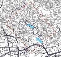
Soil Type
There are predominantly two main soil types in test patch, latosolic red soil and alluvial soil. Latosol is a name given to soils found under tropical rainforests with a relatively high content of iron and aluminium oxides (Delvaux et al., 2014) . Latosols are red or yellowish-red in colour. The red colour comes from the iron oxides in the soil. The soil generally contains a thin but very fertile layer of humus from plants and animals in the forest above, followed by an infertile second layer due to rapid leaching in the high rainfall. Alluvial soil is loose, unconsolidated soil or sediments, which has been eroded, reshaped by water in some form, and redeposited in a non-marine setting (Geology Dictionary, geology. com). Alluvium is typically made up of a variety of materials, including fine particles of silt and clay and larger particles of sand and gravel. (Fig. 4.1.2.2)
Soil Depth
The soil depth is the absolute distance to bedrock. Since actual soil layer data is unavailable, it is assumed that the soil type is homogeneous throughout the depth. In the test site location in Shenzhen, the soil depth varies from around 20-30 m in the flat terrains; 10.5 m in the valley and goes down to 6m in the higher elevations. (Fig. 4.1.2.3)
Land Use Planning

The current government land use plan for this area is mainly tree gardens and forests. A small area on the south is planned for residential use. (Fig. 4.1.2.4)
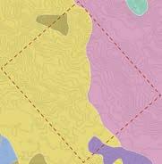
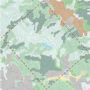
Test patch Reservoir
Main road
Test patch
Latosolic red soil
Red soil
Alluvial soil
Farm land
Yellow clayey soil Red mud
Test patch
Tree garden
Needle leaved forest
Trees green space
Broad-leaf forest Residence
Industrial land
Pond
Dry land
109 |
N
N
Fig. 4.1.2.1 Road network
Fig. 4.1.2.2 Soil type condition
Fig. 4.1.2.4 Land use
Fig. 4.1.2.3 Soil Depth [www.soilgrids.org]
54.12 m 0 m 10.5 m
Fig. 4.1.2.1
Fig. 4.1.2.2
Fig. 4.1.2.4
Research Development
Fig. 4.1.2.3
4.1.3 Patch Analysis - Xiameilin, Shenzhen
Xiameilin patch is located in Futian District of Shenzhen. In 1980s, most land in this area was farmlands and fruit plantations, but after the economic revolution, most of the farmland was removed and new dwellings, industries and infrastructure were built in this area.
The diagrams show the built areas in the region of interest. Located to the east of the mountain, over 90% of buildings are built in areas which slope angles are lower than 20 degrees. The steepest angle for building in this area is 30 degrees.
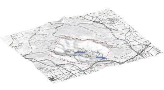
| Adaptive Urban Hillscapes 110
Existing reservoirs Main public green space Buildings Metro line Main road
Fig. 4.1.3.1
Meilinn patch, Futian district, Shenzhen
Fig. 4.1.3.2 Selected test patch in the context
Fig. 4.1.3.1
Fig. 4.1.3.2
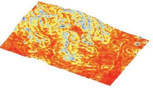
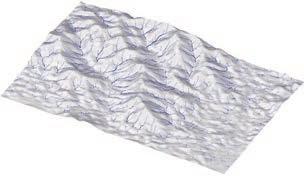
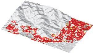
111 | 0.4° 56.5° Slope angle distribution Building location distribution Water-flow path θ<20° 20°<θ<30° θ>=30° Water-flow path
Fig. 4.1.3.3 Meilinn patch analysis
Research Development
Fig. 4.1.3.3
4.1.4 Catchment Analysis
Water Flow
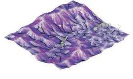
Rain water flows from the top of mountain to the foot of mountain, and eventually merges into the valley part to form the main catchments. A vector flow analysis shows the direction of flow from every grid point. From this analysis, all the main natural drainage channels can be identified. More importantly, the runoff length for every grid point can be calculated. This is the distance the surface water has to flow before it reaches a drainage channel. It is useful in RUSLE estimation of LS factor (sec 3.6) and to propose surface drainage/recharge network.
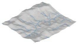
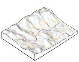
Catchment Distribution
The main water catchments are the two reservoirs in the bottom of valley. This patch can thus be considered as one watershed. Natural drainage streams are also identified, which flow into the valley and into the reservoirs.
(Fig. 4.1.4.2)
Water Accumulation
The water accumulation analysis in ArcGIS shows the area that contributes to runoff collected by each of the natural drainage streams. The results indicate that water accumulated in the bottom of valley is contributed by almost the entire area of the test patch.
This further proves that the test patch can be considered as one watershed, and any further topographical or hydrological analysis will not be affected in a major way by factors outside this patch.
(Fig. 4.1.4.3)
| Adaptive Urban Hillscapes 112
Fig. 4.1.4.2 Water catchment analysis from ArcGIS Water flow Fig. 4.1.4.3 Water accumulation analysis from ArcGIS 2 4.51 in Sq Km N Fig. 4.1.4.1 Water flow analysis
Fig. 4.1.4.1
Fig. 4.1.4.2
1.0 m Runoff Length Main drainage channels 308.0
Fig. 4.1.4.3
4.1.5 Summary of Data
Soil Data
The soil type data collected for the site in Shenzhen was about the type of top layer of the soil. The table shows all the geotechnical data extracted for an assumed textural composition under each soil type. Due to the lack of detailed soil information pertaining to the composition of the
soil ie. percentage of sand, clay, silt, loam; some informed assumptions are made and these values are followed consistently throughout this thesis,
[UN FAO.org] [geotechdata.info]
Rational Equation for Runoff Estimation
The equation to predict the volume of surface water runoff contains a coeffecient that can relate - ratio of rate of runoff to rate of rainfall and the landuse, slope and soil infiltration.
Q = 0.278 C i A
Land Use
[UN FAO.org] [www.brighthubengineering.com]
RUSLE Data for Erosion Estimation
The variables that affect the soil loss estimate the most by planning and design are C and P factors
C factor is the crop and management factor, depends on vegetation cover,
P Conservation practice factor, Its value ranges from 0 to 1, with a lower value suggesting more effective conservation practices.
LS Slope length and steepness factor for this site is calculated from the
Values shown are for slopes over 6% gradient for the following soils
Group A: Deep sand; deep loess; aggregated soils Group B: Shallow loess; sandy loam Group C: Clay loams; shallow sandy loam; soils low in organic content; soils usually high in clay
runoff length obtained by vector flow analysis shown in the facing page. R factor is constant for the central region of Shenzhen, where this test patch is located and does not reflect spatial differences. It is obtained from a detailed study by W.Zhang and Bo Huang. [W.Zhang et al. 2014]
R (MJ mm/ha/ hr/ year) = 793.79
113 |
Soil Types Red Soil - Sandy Clayey Alluvial Soil - Silty Loamy Yellow Clay -Clayey Sandy Internal Friction Angle ( degree ) 30 - 40 25 - 32 30 - 40 Grain Size ( mm ) 0.06 - 0.2 0.006 - 0.02 0.002 USLE Soil Factor ( K ) 0.04 0.1 0.6 0.18 Unit Weight ( KN/m3 ) 17 - 18.5 20.5 - 22.5 18.5 - 20 Cohesion ( KPa ) 5 - 11 20 - 22 74
Forest Meadow Farmland Residential Commercial Streets Distributed area Pasture Soil Group A 0.14 Runoff Coeffecient ( C ) 0.22 0.89 0.69 0.30 0.29 - 0.40 0.79 0.37 Soil Group B 0.18 0.18 0.89 0.7 0.37 0.34 - 0.44 0.84 0.45 Soil Group C 0.20 0.20 0.90 0.72 0.44 0.40 - 0.49 0.89 0.52
Forest w/ natural litter Land Types Trees <2m C Factor 0.001 1 0.5 0.6 <30% cover: 0.20 30-60%: 0.07;<60% cover: 0.04 1 0.25 0.3 0.04 0 0.1 0.5 P Factor Grasslands Developed areas Wetlands Rice paddy [UN FAO.org] [W.Zhang et al., 2014] Research Development
4.1.6 Land-Use Compatibility
The annual soil loss in ton per hectare can be classified into six categories, in accordance with the national soil erosion classification standard (China SL190-2007-2008).
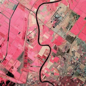
< 5 ton/ha very low
5-25 ton/ha low
25-50 ton/ha moderate
50-80 ton/ha moderately high
80-150 ton/ha high
>150 ton/ha very high
It is proposed that the land use pattern can be evaluated for neighbour compatibility while also evaluating soil loss. Many landuse types cause conflict with each other because of ecological reasons or there might be a case of imminent expansion. The relationship matrix for degrees of compatibility is shown here. Higher the number, lesser the compatibility. A minimum area of 16,000 sqm. is considered for developable land and any cluster less than that is neglected. [W.Zhang et al., 2014]
| Adaptive Urban Hillscapes 114
.6.3
Fig
Fig. 4.1.6.1 Urban Agriculture interface (Sacramento CA); understanding the influences of two diverse land-uses and the impact they have on each other. [color infrared photo, Cirrus-designs.com]
115 | Forest w/ natural litter Forest w/ natural litter Trees<2m Trees <2m Grasslands Grasslands Developed areas Developed areas Transportation Transportation Wetlands Wetlands Rice paddy Rice paddy 0 0.1 0.1 0 0.1 0.1 0.1 0.1 0.1 0.1 0.2 0.2 0.2 0.2 0.2 0.2 0.3 0.3 0 0 0 0 0 0 0 0 0 0 0 0.8 0.8 0.7 0.7 0.7 0.7 0.7 0.6 0.7 0.6 0.6 0.6 0.6 0.6 0.6 0.6 0.6 0.6 0.5 0.5
Research Development
Fig .4.1.6.2 The relationship matrix for degrees of compatibility
Elevation analysis
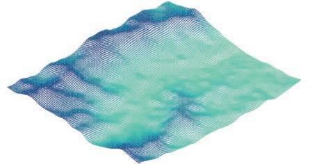
4.2 Factor Maps
4.2.1 Factor 1 - Elevation Analysis
The selected target patch is located in the central hilly area in Shenzhen. The total area of this patch is about 5.5 km2. According to the results of elevation analysis in ArcGIS, the highest altitude in this patch is 302 m (FIgure 4.2.1.1). The northern side of patch is comparatively higher than the middle and Southeast side. The whole patch looks like a valley surrounded by mountains.
Based on previous study, the traditional settlement usually occupies land from the foot of mountain to the halfway of mountain, which is for the propose of better access and farming. In this patch, the current existing urban settlements, which includes low density residential and commercial buildings, are most located in the flat area besides this patch, thus settlements in lower elevation could have closer connection and better access to city facilities.
DEM Source:
1. Open Street Map: https:// www.openstreetmap. org/#map=5/51.500/-0.100
2. USGS: http://viewer. nationalmap.gov/basic/
| Adaptive Urban Hillscapes 116
Fig. 4.2.1.1
0 m 302 m N
Fig. 4.2.1.3
4.2.2 Factor 2 - Slope Angle Analysis
Kwong suggests that, according to Hongkong’s landslide record, the slope is generally stable when the slope angle is less than 20o and greater than 50o. Since Shenzhen adjoins Hongkong and has almost similar geological conditions, it could be deduced that the slope angle from 20o to 50o is relatively unstable. [A.K.L.Kwong, 2004]
The slope angle of this target patch varies from the foot of mountain to the top of mountain, the steepest angle is 54o. While more than half of the terrain is less steep than 20o (See Figure 4.2.2.1).
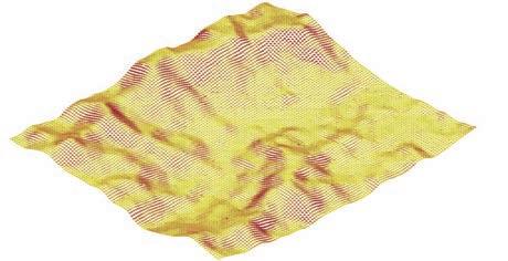
Building Morphologies, especially the foundation of buildings, would be influenced by slopes angle conditions. Refer appendix for a detailed study of external loading on slopes of varying gradients. In treating
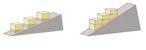
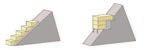
this analysis as a factor map, it is remapped in such a way that the cells with higher slope angles recieve a lower score. Although slope angles of less than 20o is preferable for building activity, in this thesis there is no explicit threshold angle considered. This is because of two reasons:
- Factor maps and their critical data are not independently important.
- Aspect of slope instability is not entirely dependent on slope angle as soil data is also a major consideration (refer sec 4.4)
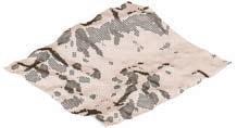
117 |
Fig. 4.2.2.3 Slope angle analysis
Over 20o Less than 20o 0o 20o 40o 10o 30o 50o
Fig. 4.2.2.1 Slope angle over and less than 20o
10o 20o 30o 40o
Fig. 4.2.2.2 The relationship of slope angles and corresponding building morphology Redraw from: Li Jiang, “The study of architectures morphology and spatial relationship in hillside area“, 2001
Fig. 4.2.2.1
Fig. 4.2.2.2
Fig. 4.2.2.3
0O 54O N Research Development
Fig. 4.2.3.1
Sun-path over test patch
Shenzhen weather file (epw) source: https://energyplus.net/ weather
4.2.3 Factor 3 - Slope Aspects Analysis
Figure 4.2.3.1 shows slope aspects analysis of the test patch. Based on Shenzhen’s location and its humid climate, more sun exposure could improve water evaporation and mitigate mildew. South, south east and south west aspects could receive comparatively more sun exposure than others.
From previous tests, it is suggested that the optimal Height/Width ratio between buildings would change according to slope aspects. To acquire optimal sun exposure in courtyard or road, on the slope towards sun, the building in front should be shorter than the buildings behind them. On the contrary, the building in the back should be shorter than building in the front if the slope is against the sun, which would lead to worse views for the users in the buildings in this case. In conclusion, blocks would have better sun exposure and views when they are on the southern slope facing the sun.
Sun radiation of canyons on different slope aspects
For that reason, the ramapped values of this factor map will be higher for cells facing south and progressively lesser as the cells orientation approaches north.
Fig. 4.2.3.3
Slope aspect analysis
N (0o)
NE/NW (450, 315o)
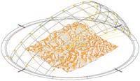
E/W (90o, 270o)
SE/SW (135o 225o)
South (180o)
| Adaptive Urban Hillscapes 118
N S W E
Latitude: 22.55
South Southeast & southwest
Fig. 4.2.3.1
Fig. 4.2.3.3
On the slope towards the sun On the slope against the sun
N
Fig. 4.2.3.2
Fig. 4.2.3.2
4.2.4 Factor 4 - Soil Depth Analysis

The soil depth is the absolute distance to bedrock. Since actual soil layer data is unavailable, it is assumed that the soil type is homogeneous throughout the depth. In the test site location in Shenzhen, the soil depth varies from around 20-30 m in the flat terrains; 10.5 m in the valley within the test site and it goes down to 6m in the higher elevations. (Fig. 4.2.4.2)
The fact that soil depth directly affects the infiltration capacity of the soil, means that higher the depth the longer it will take for the soil to be saturated and hence increasing pore pressure to lose cohesion and shear strength. With this the soil depth data is mapped onto the terrain ; the higher the depth of a cell the better its factor value and it is remapped accordingly.
119 |
Fig. 4.2.4.2 Slope aspect analysis
N
Fig. 4.2.4.2
Fig. 4.2.4.1
Soil Depth map - absolute depth to bedrock [source: www.soilgrids.org] 54.12 m 10.5 m 10.5 m
0 m
6.0
m
Fig. 4.2.4.1
Research Development
Extreme erosion Deposition
Medium risk area
4.2.5 Factor 5 - Landslide Impact Analysis
The diagram 4.2.5.1 shows the results of landslide simulation by inputting terrain and rainfall data into Caesar - Lisflood. The white area shows regions with potential for triggering soil erosion. The red area indicates possible location of heavy soil erosion, green area indicates potential deposition that formed by debris flows. Thus the direction of debris flows can be worked out by analysing areas from red to green over a contour map.
The valley area bears the most significant landslide deposition impact, while the north east slopes have large patches which lie on the debris path. The simulation results also have been translated into factor maps with remapped values that are lowest for the dark green and red areas. The images and data on the facing page show the input parameters and periodic information from the simulation on CAESAR lisflood.
risk analysis
Low risk
Medium risk (susceptible erosion zones)
High risk (susceptible deposition zones)
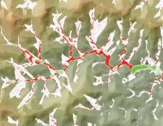
| Adaptive Urban Hillscapes 120
Fig. 4.2.5.2 Landslide
Fig.4.2.5.1 Landslide risk analysis by CAESAR-lisflood 1.9b
N
Fig. 4.2.5.2
Fig.4.2.5.1
Location: Jinhu Mountain, Futian district, Shenzhen city
Simulation period: 30 days
Peak precipitation: 98 mm/hr
Average precipitation: 4.8 mm/hr
High risk deposition
High risk erosion
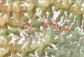
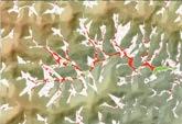
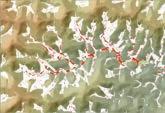
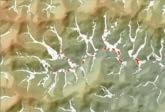
Low risk erosion
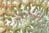
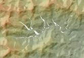
121 |
Fig 4.2.5.3
Day 1 Day 10 Day 2 Day 19 Day 3 Day 25
Research Development
Fig 4.2.5.3 CAESAR-Lisflood simulation. Erosion and Deposition risk analysis images.
4.3 Synthesis Mapping
To classify suitability for constructing urban settlements, synthesis of factor maps is adopted in this study. This is essentially a deterministic mapping method.
The main principle for synthesising factor maps is firstly divide target patch into numerous featured pieces, then assign certain value to each piece according to its performance in specific aspects. For instance, if a square could be divided into 9 pieces, named from A to I, then each piece would be evaluated from different aspects, the final value of each piece would be synthesized by all its values from these evaluated aspects.
In phase 1 of this thesis, four factors have been analysed, including elevation analysis, slope angle analysis, slope aspects analysis, and landslide impact analysis. The target patch has been divided into feature points according to terrain, then each point has been assigned a value based on its performance in different aspects. All the values have been remapped from 1 to 5, the higher the value represents better performance. Such as in the factor of slope angle analysis, the steeper slope angle has been given a smaller value ie. points in flatter locations have value closer to 5. All of the remapped values have been added up to generate a synthesised result.
Elevation: 0 - 302 m Remapped value: 5-1
Slope angle: 0o - 46o Remapped value: 5-1
Slope aspect: 0o, 450 315o, 90o 270o, 135o 225o, 180o Remapped value: 1,2,3,4,5
Landslides risk: Low, medium, high Remapped value: 5,3,1
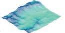
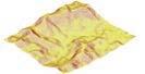
| Adaptive Urban Hillscapes 122 A1 B1 C1 D1 E1 F1 G1 H1 I1 A2 B2 C2 D2 E2 F2 G2 H2 I2 A3 B3 C3 D3 E3 F3 G3 H3 I3 A4 B4 C4 D4 E4 F4 G4 H4 I4
Fig. 4.3.2 Evaluation principle
Fig. 4.3.1 Target patch evaluation process
Fig. 4.3.1
A’ Elevation Slope angle Slope aspect Landslides impact 1 * 1 * 1 * 1 *
Fig. 4.3.2
Principle: Overlay Weightage Factor
Maps
A1 A2 A3 A4 A’ 1 * 1 * 2 * 3 * Overlay Weightage Elevation Slope angle Slope aspect Landslides impact A1 A2 A3 A4
4.3.1 Synthesis Experiment 1 (Phase 1)
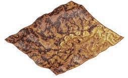
The synthesis presented in Fig 4.3.1.1 is the result of the first digital experiments from phase 1 of this thesis. Here, the four factor map values for each cell are simply added up with equal weightage or importance given to every factor. In fig 4.3.1.2 , the synthesis method involves differential weighting for each factor map. Various random combinations are tried, but relatively higher weightage is given to slope aspect map and landslide impact map; mainly because of intuition that cells with better south orientation will get a higher overall score or that cells in risk areas will get a low overall score. Thus making it easier to propose developable or inhabitable land in high scoring cells. The results of the synthesis map is broken down into five levels with the first three levels earmarked for urban development in decreasing order of density and intensity.
Limitations
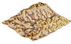
Initial experiments in developing a synthesis map from factor maps, are more intuitive than generative. A firm relationship cannot be established between the weightages of the factor maps, as the differential weighting is based only on relative importance. Furthermore, only a limited number of random combination are explored in this method. Hence, the landuse pattern is by no means directed at optimising for any evaluative criterion.
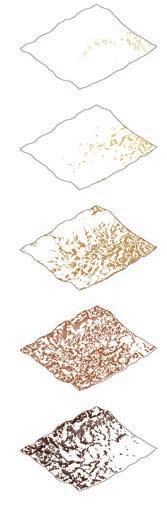
123 |
Fig. 4.3.1.1
Synthesis map of overlay weightage by 1+1+1+1
Fig. 4.3.1.2
Level 1 Level 2 Level 3 Level 4 Level 5
Synthesis map of overlay weightage by 1+1+2+3
N
Research Development
Fig. 4.3.1.2
4.3.2 Synthesis Experiment 2 - Generating a Land use Pattern
The challenge of generating an adapted urban proposal starts at the scale where the patterns of anthropogenic land use are generated. The location of the city in the hillside ecology requires to be properly distributed across the terrain, considering the situation of adjacent subsidiary ecosystems as well as their slope gradient and orientation.
Differential Weighting of Factor maps
Firstly, an additional factor of soil depth is added to the repertoire of analysed data. In this experiment to generate a synthesised landuse pattern from the factor maps, an optimisation process is employed. The aim of this process is to find the weightages that can be applied to each factor during synthesis, such that the synthesised output performs as desired in certain evaluative criteria that will directly have an influence in minimizing damage from soil erosion hazards.
The script is set up in a way that the weightages of the factor maps act as variable genes. In addition to this, a variable threshold angle is also added, that changes the vegetation and crop types according to the slope.
The primary aim of the landuse pattern is to reduce soil loss due to erosion. As discussed in sec. 3.6 , RUSLE method is most commonly used to estimate soil loss. The equation calculates soil loss for every iteration of the synthesis map, as the Crop management (C factor) and Conservation (P factor) is constantly changing with the landuse types (refer sec. 4.1.5). Each iteration is also checked for landuse compatibility, because small clusters of developable land is prone to expansion. This makes it least compatible with other productive landuse types like farmland or forests. (refer sec 4.1.6)
Maximising green cover is one way to mitigate the problem of erosion, but a land use strategy for urban development calls for other criteria to balance its ecological effects. Other criteria is to maximise the suitable land for urban development but at the same time minimise its location in risk zones. For the effective functioning of the hills ecology in maintaining pore water pressure in the soil and stabilising the steeper slopes, an additional condition is evaluated to push the heavily vegetated areas to higher elevations. With these mutually opposing criteria, the genetic algorithm can strive to give solutions with good overall performance.
| Adaptive Urban Hillscapes 124
variable genes Fitness criteria LOOP Factor map Weight 1 Initial Synthesis Map Synthesised Landuse map RUSLE estimation Minimise soil loss Maximise buildable cells Maximise avg elevation of forest Minimise buildable cells in risk zone Factor map Weight 2 Factor map Weight 3 Factor map Weight 4 Threshold angle 1 Factor map Weight 5 Threshold angle 2 Crop & Conservation factors Check for landuse compatibility Soil data Slope/Steepness factor (runoff lengths) Rainfall factor
Genes
1. Elevation map weightage (0.02-4.00)
4. Land slide risk map weightage (0.02-4.00)
Elevation: 0 - 302 m
Remapped value: 5 - 1
2. Slope angle map weightage (0.02-4.00)
5. Soil depth map weightage (0.02-4.00)
Landslides risk: Low, medium, high

Remapped value: 5, 3, 1
Slope angle: 0o - 46o
Remapped value: 5 - 1
3. Slope aspect map weightage (0.02-4.00)
Slope aspect: N, NW/NE, W/E, SW/SE, S
Remapped value: 1, 2, 3, 4, 5
Fitness Criteria
1. Maximise Buildable cells
Soil depth: 6 - 10.5 m
Remapped value: 1 - 5
6. Threshold angle for terrace & tree types (10.0 - 25.0)
3. Maximise the average elevation of Forests (Not real elevation- reference value approaching 0 is highest altitude)


Farmlands
Forests
2. Minimise Buildable cells in Erosion/Deposition zones


4. Minimise the soil loss due to erosion (by RUSLE estimation)
Urban developable land
125 |
Research Development
4.3.3 Synthesis Experiment 2 - GA Results

| Adaptive Urban Hillscapes 126 3.93 3.98 0.36 0.45 3.40 3.78 1.63 3.94 0.30 0.19 4.00 0.42 3.72 3.78 0.33 0.31 0.10 0.44 0.24 0.32 0.41 0.10 1.13 0.19 threshold angle for tree types threshold angle for tree types 11.3° 10.2° 10.1° 10.2° 10.2° 10.1° 17.3° 18.4° threshold angle for terrace types threshold angle for terrace types 23.0° 24.6° 24.6° 23.0° 24.7° 23.0° 22.7° 24.6° amount of buildable cells in risk zone (area) amount of buildable cells in risk zone 0.53 0.52 0.52 0.35 0.26 0.16 0.80 0.53 buildable cells (area) buildable cells 0.33 3.66 0.33 3.08 2.91 0.33 2.99 3.16 Objectives G49.01 G49.05 G49.02 G49.06 G49.03 G49.07 G49.04 G49.08 Objectives Weightages & Threshold angles Weightages & Threshold angles 7251 (2.9sqkm) 7323 (2.93 sqkm) 9655 (3.86 sqkm) 10417 (4.17 sqkm) 4525 (1.81 sqkm) 6298 (2.52 sqkm) 9006 (3.6 sqkm) 5350 (2.14 sqkm.) -186.63 -196.84 -200.96 -272.12 -199.35 -177.09 -253.69 -202.92 47.62 60.83 77.13 99.6 37.7 48.57 88.59 53.92 2288 (0.92 sqkm) 444 (0.18 sqkm) 2730 (1.09 sqkm) 0 540 (0.22 sqkm) 2158 (0.86 sqkm) 132 (0.05 sqkm) 516 (0.21 sqkm)
average elevation for forest area elevation map soil loss (ton/ha/yr) slope angle map slope aspect map soil depth map risk map average elevation for forest area elevation map soil loss slope angle map slope aspect map soil depth map risk map Number of Generations: 60 Solutions/Generation : 25 Solution time : 100 sec

127 | 3.40 1.69 3.36 2.18 3.93 0.17 1.65 2.75 0.15 0.26 3.74 2.19 0.33 0.15 0.03 0.16 1.01 1.16 0.43 0.57 0.26 0.35 0.57 1.13 threshold angle for tree types threshold angle for tree types 10.1° 10.2° 10.2° 17.2° 10.1° 12.6° 16.9° 17.4° threshold angle for terrace types threshold angle for terrace types 24.9° 21.7° 22.6° 22.6° 22.6° 25.0° 24.9° 22.7° amount of buildable cells in risk zone amount of buildable cells in risk zone 1.99 2.76 0.58 0.19 0.21 0.15 2.78 0.15 buildable cells buildable cells 2.88 3.95 2.97 0.98 3.74 3.04 2.71 0.29 G49.09 G49.13 G49.10 G49.14 G49.11 G49.15 G49.12 G49.16 Objectives Objectives Weightages & Threshold angles Weightages & Threshold angles 5385 (2.15 sqkm.) 5366 (2.15 sqkm.) 4325 (1.73 sqkm) 8393 (3.36 sqkm) 5358 (2.14 sqkm) 10184 (4.07 sqkm) 7822 (3.13 sqkm) 7424 (1.97 sqkm) -201.76 -245.83 -200.20 -247.94 -196.26 -284.50 -276.95 -222.48 53.91 67.68 37.24 84.44 51.9 98.6 82.87 73.53 154 (0.06 sqkm) 201 (0.08 sqkm) 340 (0.14 sqkm) 169 (0.07 sqkm) 524 (0.21 sqkm) 19 (0.01 sqkm) 145 (0.06 sqkm) 405 (0.16 sqkm) average elevation for forest area elevation map soil loss slope angle map slope aspect map soil depth map risk map average elevation for forest area elevation map soil loss slope angle map slope aspect map soil depth map risk map Research Development


| Adaptive Urban Hillscapes 128 average elevation for forest area elevation map 1.36 3.94 1.63 3.90 1.36 soil loss slope angle map 3.98 0.49 0.33 4.00 3.98 slope aspect map 0.20 0.37 1.13 0.23 0.20 threshold angle for tree types threshold angle for tree types 10.1° 10.2° 17.3° 11.2° 10.1° threshold angle for terrace types threshold angle for terrace types 24.9° 25.0° 22.6° 22.7° 24.9° amount of buildable cells in risk zone (area) amount of buildable cells in risk zone (area) soil depth map 0.19 0.04 0.28 2.80 0.13 buildable cells buildable cells risk map 2.91 3.73 3.13 0.21 2.71 Objectives Objectives Weightages & Threshold angles Weightages & Threshold angles 8114 (3.25 sqkm) 8819 (3.52 sqkm) 9422 (3.77 sqkm) 3286 (1.31 sqkm) 8201 (3.28 sqkm) -191.78 -176.69 -250.71 -211.85 -191.25 61.69 62.76 89.52 33.37 62.34 2595 (0.04 sqkm) 524 (0.21 sqkm) 220 (0.09 sqkm) 214 (0.09 sqkm) 2682 (0.07 sqkm) G49.17 G49.21 G49.18 G49.19 G49.20 average elevation for forest area elevation map soil loss slope angle map slope aspect map soil depth map risk map
4.3.4 Synthesis Experiment - Conclusion
As a summary of the generative process adopted to obtain a synthesis landuse pattern from the analysed factor maps :
- The differential weighting given to each factor map in Experiment 1 is quite arbitrary, based on intuition and relative importance. But in Experiment 2, the weightages are used to help achieve a list of goals.
- It is very difficult to establish any relation between the factor maps as to how the change of weightage of one might affect the synthesis result. This is a drawback of the approach used in Experiment 1 because there is no substantiation to the assumed 'relative importance'. However, this does not matter in Experiment 2.
- In Experiment 2, by defining the fitness criteria and allowing a larger domain for the weightage parameters, there is sufficient room for the GA to test a much larger range of solutions.
- Another crucial aspect of the process followed in Experiment 2 is that the script broadly defines the multiple goals. Which means the design intention based on intuition and ecological principles is not severely imposed on the genetic algorithm. This is seen in the GA results showing a large variation.
The designer's intuition is brought back into the GA process in selecting the fit phenotypes based on data and also the desire to have the urban developable areas embedded within the larger ecology. This is discussed in sec 2.3, as anthropogenic settlements and its relationship to other subsidiary ecosystems
The feature of avoiding the isolation in land use cells was inserted in the algorithm’s mechanism, allowing a clear definition of land use mosaics, which will eventually benefit the preservation of each subsidiary ecosystems. For example, avoiding increasing levels of urban heat island effect on surrounding green areas or farmlands by attempting bigger clusters of developable land and deleting or converting small isolated areas of urban land surrounded by green areas into green areas themselves.
Analysing the phenotypes from the genetic algorithm, it is evident that many of them showcase signs of the morphological patterns of the landslide risk map. It seems to be a dominating factor in the pattern creation. As it is taken that the safety of inhabitable areas is paramount , this is something desirable. The solution time per individual is extremely long considering that no geometry was generated at this stage. Extensive calculations involving the soil loss equation and other computational analysis of the topography could be the cause for this.
From the erosion estimation data for the 5.5 sqkm. patch, it can be seen that the soil loss, even for the fittest individuals, is in the range of 37-62 ton/hectare/yr. According to national soil erosion classification standard in China, this is moderate to moderately high. Because the competing objectives are in conflict with one another, it is impossible to achieve one best solution for soil loss.
Therefore, four marked phenotypes are taken forward in the generative process for further evaluation.
129 |
Research Development
4.3.5 Post-Synthesis Evaluation
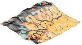
Shortlisting the individuals that reach higher values in terms of overall fitness criteria, a variated distribution of land use is observed as well as different ratios of Forests, Farmland and Constructive land in each outcome.
Following the importance of traditional production nodes located in between forested areas (‘remaining’ sub-ecosystems) (refer sec 2.6) and farmlands, the external evaluation is based on the location of potential production areas as isolated clusters of developable land located on high terrains for better irrigation and overall production management. The total farmland area and south facing farmland are also considered in the selection of the final synthesis map.
Individual 49.09 is selected considering the criteria mentioned above and also its ranking in the overall fitness value -2nd behind the fittest individual 49.05-. The challenge represented by the amount of developable area on steep terrains and the noticeable decrease of forests in the selected synthesis are also important factors considered for design purposes of this thesis.
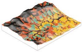
| Adaptive Urban Hillscapes 130 Farmland - % South Facing - Num of South Facing Forest Constructive - Production Area (ha) 76.6 45 % 34.5 181.6 292.9 29.2 Cells 1916 45 % 862 4541 7323 729 Farmland - % South Facing - Num of South Facing Forest Constructive - Production Area (ha) 172.9 57 % 98.6 179.7 198.6 6.8 Cells 4323 57 % 2464 4492 4965 170 49.05
49.05 49.09 49.09 [ ]
1. Number of Production nodes (isolated developable ideal for farm management)
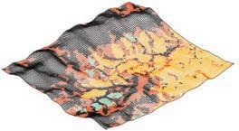
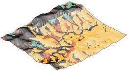


2. Total farmland area
3. Total south oriented farmland area
131 | Farmlands Evaluation Criteria
Forests Developable land Production
Water
Fig. 4.3.5.1
circulation process for determining production nodes.
Precipitation Forest Farming Clusters Crops Wetland Evapo-Transpiration Surface water flows Surface/underground water flows Farmland - % South Facing - Num of South Facing Forest Constructive - Production Area (ha) 141.3 55 % 77.7 237.4 172.6 18 Cells 3532 55 % 1943 5934 4314 450 Farmland - % South Facing - Num of South Facing Forest Constructive - Production Area (ha) 57.6 61 % 35.1 180.9 312.8 19.4 Cells 1439 61 % 878 4522 7819 485 60.13 49.10 60.13 49.10 Research Development
Fig. 4.3.5.1
4.3.6 Synthesis Map- Break Down
The selected synthesis result after the evaluation is presented in Fig 4.3.6.1. All the featured points are classified into five levels by their values. The five levels of suitability have been present by colours ranging from light yellow to black. Lighter colour represents higher value indicating better suitability for urban development and vice versa. It could be detected that the suitable locations for settlements are scattered in the patch, while most of them occupy the more flatten area and climbing from the foot of mountain to halfway of mountain. While in the bottom of valley, several dark red points indicated unsuitability for settlements, which reflect the impact of landslides.
The synthesis result has been classified into 5 levels according to suitability for settlements. Level 1 is most suitable for housing, and level 5 is most unsuitable. In level 5 the proposal is to maximise green cover with forests, which could increase soil stability and preserve water. Farm lands, specifically terraced rice paddy could be developed on the slopes of level 4 areas. Rice paddy also has the ability to conserve water and increase soil stability.
Level 1 -level 3
Level 1 to level 3 are suggested to be used for urban settlements. Based on the suitability assessment, densities of settlements are distributed differently in these three levels. Density and intensity of development is proposed to be higher in level 1 and lower in level 3.
Level 4
Comparing with level 1 to 3, level 4 is less suitable for building settlements. Level 4 cells are also scattered but importantly, they are located on steeper terrain. It is proposed to set level 4 as terraced farm land, which could take advantage of the terrain, context and soil conditions to act as food supply system to urban life and increase soil stability.
Level 5
Level 5 is the most unsuitable area for building settlements and it covers the most susceptible areas for landslide hazards. The existing condition is to be preserved as protected forests in level 5, and adjusting the vegetation types according to soil retaining ability and topography.

| Adaptive Urban Hillscapes 132
49.09 [ ]
Fig. 4.3.6.1
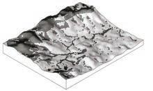
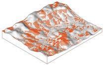
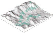
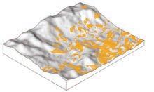
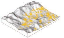
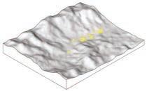


133 | Low Density Settlements Medium Density Settlements Urban Developable Land High Density Settlements Forest Farmland Level 1 Level 2 Level 3 Level 1/2/3 production cluster Level 4 Level 5 N Production Cluster Research Development
H1 Highest point in cell
H2
Lowest point in cell
HT - Slope height
4.4 Slope Risk Analysis
Topographical Risk Classification
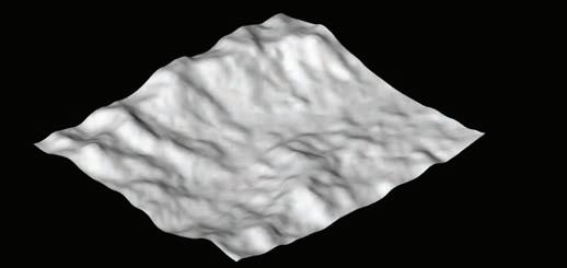
The DEM is analysed at every cell for topographical risk classification. This follows the regulation of the Geo Technical Office of Hong Kong. (refer sec. 2.9.2). The calculation is regarding only slope heights and slope angles of every cell. In order to maintain the subdivision grid of the digital model, every cell is considered to be a finite slope. Slope height is simply the elevation difference of the lowest and highest point in the slope. A combination of the two topographical parameters are used for a simple initial classification of steep slopes. This can then be used to further analyse the high risk slopes- to calculate their factor of safety, review their landuse or propose any reinforcement measures.
H1
H2
High risk slopes
Medium risk slopes
Low risk slopes
| Adaptive Urban Hillscapes 134
Fig 4.4.1
Fig 4.4.1
Fig 4.4.2
Fig 4.4.2
Factor of Safety (FOS)
The factor of safety (FOS) is calculated for each cell as a ratio between the tangents of the internal friction angle of the soil type at that particular cell and the slope angle of that cell (refer sec. 2.5.3). In addition, this equation takes into consideration the soil properties at every location, but with the theoretical condition that it is homogeneous through the entire depth. In conjunction with topographical risk analysis, a set of minimum FOS values are prescribed for every slope type (refer sec.2.9.2)
c tan θ
Factor of Safety = +
W x D x sin x cos tan
W - Unit weight of soil
The calculated FOS map is overlaid on the topographical risk map to highlight slopes that fail to attain the required FOS (image below).
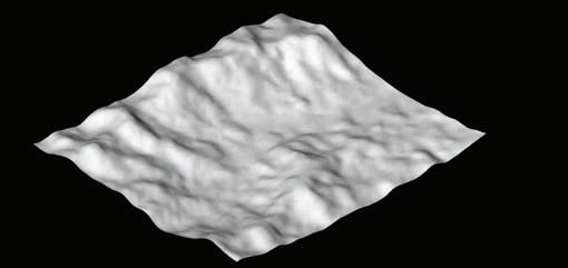
Number of cells that are below the FOS threshold: 1659 cells/13780 cells . In this test site, 12 % of the slopes can be considered weak.
c - Cohesion of soil
θ - Angle of friction of the soil
- Inclined angle of the slope
D - Soil Depth
Weak slopesSlopes below their required FOS
1659 cells
135 |
FOS High risk minimum 1.5 Medium risk minimum 1.25 Low risk minimum 1.1
RISK
Fig 4.4.3
Fig 4.4.3
Research Development
Urban development land on High risk slopes
Number of cells: 467
The analysis in the previous spread classifies the risk of each cell based on simple topographical data and the FOS calculation indicates the weak slopes. This analysis is outside of the simulation conducted in the process of attaining 'Factor map 5'- which is about extreme erosion and deposition. Reinforcing these slopes in a passive way via optimal landuse
Phenotype 49.09
By analysing the fittest phenotypes in this manner, the developable cells which are on the most risky parts of the terrain are highlighted. 6.95% of those cells are on weak slopes; 9.4% coincide with high risk slopes and 8.43% lie on medium risk slopes. These particular slopes
patterning is the first step. A major part of the slopes can be reinforced with vegetation, terracing and other natural mitigation measures; but the landuse cells with proposed urban development need to be cross examined for their slope risk and if they lie on weak slopes.
Developable land
Number of cells: 4965 cells
Urban development land on Medium risk slopes
Number of cells: 419
Urban development land on Weak slopes
Number of cells: 345
need to be given closer attention by avoiding large structures on them or by devising active reinforcement measures - structural retainment, vegetation or simply by slope reconfiguration.
| Adaptive Urban Hillscapes 136
Fig 4.4.6 Medium risk slopes
Fig 4.4.4 High risk slopes
Fig 4.4.4
Fig 4.4.6
Fig 4.4.7
Fig 4.4.7 Weak slopes
Fig 4.4.5
Fig 4.4.5
PHENOTYPE 49.09
Phenotype 49.10
As per the results of the cross examination of phenotype 49.10 from the results of the genetic algorithm; 0.25% of the developable cells lie on weak slopes; 0.15% are on high risk slopes and 6.6% lies on medium risk slopes. The fact that a large majority of the developable land is in low
risk areas is partly because of the efficacy of the optimisation process with the GA.
risk slopes
Urban development land on High risk slopes
Number of cells: 6
Developable land
Number of cells: 4314 cells
Fig
Medium risk slopes
Urban development land on Medium risk slopes
Number of cells: 287
Fig 4.4.11 Weak slopes
Urban development land on Weak slopes
Number of cells: 10
137 |
4.4.10
Fig 4.4.8 High
Fig 4.4.8
Fig 4.4.10
Fig 4.4.11
Fig 4.4.9
Fig 4.4.9
PHENOTYPE 49.10
Research Development
4.5 Spatial Pattern Sampling -indigenous settlements
The purpose of the study is to understand the pattern and hierarchy of open public and semi-public spaces that function as communal places. The primary focus will be on the relationships between these open spaces and the buildings at the block scale, super-block scale and at the scale of the entire settlement. The sample settlements are selected from south China, and they have evolved over time with necessity as they have adapted to their local aspects of culture and occupation. This makes these indigenous settlements more sustainable environmentally and socio-culturally.
As mentioned in the conclusion of the Domain chapter, the urban development on hilly terrains of a city or the fringes of a city needs to adopt an alternative approach; one which can coexist with the ecology. Settlements which have formed organically in challenging contexts are excellent precedents, which hold rich and unique spatial characteristics that are customised to their indigenous settings. The spatial aspects of the sample settlements are translated as quantifiable data that can be used in the urban design model.
The data from the tissue sampling is combined with the information of - natural flows; topographical analysis; farming process logic and the landuse pattern- in driving the generation of the new urban tissue. The spatial logics from the sample can thus be re-appropriated to suit the programmatic and topographical conditions of the test site in Shenzhen.
| Adaptive Urban Hillscapes 138
Analyse Pattern Logic Extract Spatial Data Design input Topographical Data Environmental Data Ecological Data Sample Settlement Block scale Cluster scale Spatial Pattern Hierarchy Public space areas / ratios Semi public areas / ratios Spatial quality factors Spatial quality factors Spatial Pattern Morphology Network Pattern Morphology Block Morphology Open Space Morphology
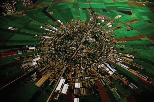
139 |
Fig.4.5.1 Moshav (co-operative village) farm at Nahalal, Israel [Yann Arthus Bertrand]
Research Development
Fig.4.5.1
4.5.1 Sample Settlement - Nuodeng Village, Yunnan, China
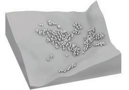
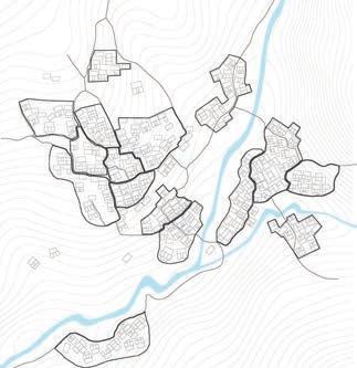
Nuodeng village, located in Yunnan district in south west China is a historic settlement which thrived with the development of trade routes during the Qing and Ming dynasties (-1911) by making salt from the abundant salt wells. Along with the development of salt industry, the social and cultural life of Nuodeng village was greatly advanced. Its reputation for cultural prosperity and talents lasted as long. Built on a steep slope above ancient salt wells, it has wel preserved centuries old residential housing made from red rammed earth. Numerous ancient buildings and cultural heritage still exist today, which combine the culture of the Central Plains and the local culture of Bai ethnic group. Ancient mansions dominate the valley, public buildings like- salt tax office, Buddhist, Confucian and Taoist temples dot the landscape, which were secularized during the Cultural Revolution.
The structures and spaces recorded the historical process in respect to the culture, economy, politics and social customs in Yunnan region for thousands of years. The inherent socio-cultural aspect of this settlement along with its indigenous adaptation to the natural context make it an interesting case study. Hence, the metrics extracted from the settlement's spatial morphology can be understood to be ingrained with social factors. (Wu Bo, 2011) (people.cn)
| Adaptive Urban Hillscapes 140 540m 600m
Area Period 0.3 km2 ¬900 AD 2199 person 10,191 /km2 5.5 - 10 m 621 Population Density Building Height No. of buildings
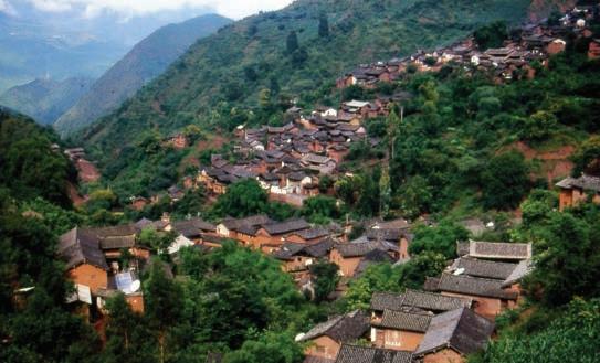
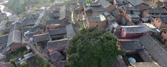
141 |
Fig.4.5.1.1 Aerial photograph showing the entire village [www.gokunming.com/]
Research Development
Fig.4.5.1.2 Aerial photograph showing the semi public spaces [www.yunnan-roads.fr/ voyage/dali/nuodeng/]
4.5.2 Open Space Hierarchy & Morphology
In order to understand the open spaces in terms of their morphology; a basic hierarchy of the operative scales of the village is established. A clear hierarchy is also seen in the social spaces themselves, with defined public open spaces with convex elements transitioning to semi public courtyards before entering private indoor spaces. The linkage between the public spaces and the semi public spaces happen via 2 types of paths.
Since the village is situated on a steep terrain, these paths are on a gradient or they are basically staircases. Hence, unlike other settlement patterns in China (eg. Hutongs) the streets are not active public spaces in themselves. Another impact that the terrain has is on the aggregation of built mass around an open space. With drop in ground level, the enclosure around the open space is always varying and this has an interesting spatial effect that is explained in more detail in the following pages. The terracing of open spaces lends the village more character, in that a space can form an informal linkage between streets at different elevations.
At a block level, the morphology of the semi-public space takes the form of a stepped courtyard; or it can be seen as the main staircase of a multi-storied apartment block. In some block types, 2 blocks at different elevations are conjoined through the stepped courtyard.
| Adaptive Urban Hillscapes 142
semi public space Private Public public space major public space
Fig. 4.5.2.1
Fig. 4.5.2.1 Plan of Nuodeng, showing degrees of public open spaces and semi-public spaces
village super-block block
Public Space Morphology

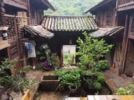
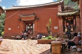
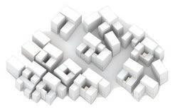
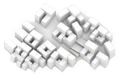
Semi Public Space Morphology
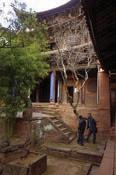
143 |
Fig. 4.5.2.2
Fig. 4.5.2.3
Fig. 4.5.2.5
Fig. 4.5.2.4
Fig. 4.5.2.2
Public space morphology in the form of terraces
Fig. 4.5.2.3 Usage of the open space in front of prominent public buildings for communal, economic activities
Fig. 4.5.2.5 Morphology of semi public spaces in the form of stepped courtyards
Block A ISOLATED BLOCK TYPE CONNECTED BLOCK TYPE Block B Research Development
Main streets (parallel to contours)
Secondary streets/ stairs (perpendicular to contours)
4.5.3 Network Patterns
A distinct hierarchy of streets is visible in the village. One that is predominantly along the contours and these are able to maintain an accessible walking gradient. These sloped paths are also comparatively wider. Small squares and public spaces open up predominantly along the primary paths
The other set of paths are basically stairs with deep treads. These secondary paths run perpendicular to the contours. The width is only 2 metres on an average. In most cases the stairs are flanked by buildings on either side. Based on Integration analysis of the overall network, it is evident that the most connected part in the centre of the village has the highest integration HH values along with higher concentration of public spaces. (Wu Bo, 2011)
| Adaptive Urban Hillscapes 144
Network Analysis Integration HH 0.05 0.13
500 m 500
Secondary Paths
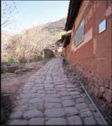
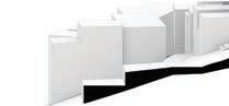


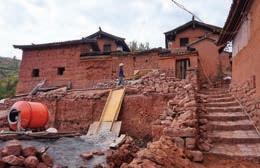


Primary Streets
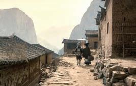
145 |
w/h = 1/3 - 1/5
w w
h
Primary Streets with access to public spaces Research Development
street aspect ratio (Wu Bo, 2011)
h
w/h = 1/2
4.5.4 Extracted Logic Design Logic
Extracted Logic Indigenous Spaces
SECONDARY SCALE OPEN SPACE: The size and morphology of open spaces within a certain scale of cluster or super block is an important aspect for the space to work
SCALE: Super Block
PRIMARY SCALE OPEN SPACE: Transition from private to public through a semi public space offers a flexibility and variety in aiding social interaction. It is essential that the transitional semi public space is embedded into the built fabric
SCALE: Village / Settlement
Analysis
- Open Space Ratio: The ratio of area of open public space to the area of the cluster
Definition of Super Block
No. & size of public space/super block
SCALE: Super Block
- Average Super Block size
- Average Public space size
Spatial Hierarchy
SCALE: Cluster
Network: Hierarchy of paths and their morphological response to the terrain is essential to having an effective connectivity.
- Gradients of different path types
- Average street aspect ratio
- Connectivity to public spaces
No. and type of paths.
Street widths
SCALE: Village & Super block SCALE: Cluster & Super block
Semi public spaces: The size and morphology of courtyard spaces within blocks in response to the terrain creates inteesting spatial effects and circulation networks.
SCALE: Block
- Open Space Ratio: The ratio of area of open semi public space to the floor area of the block
- Average Block size
- Average courtyard size
Subdivision size distribution of blocks within the super block
Size of courtyards in each block
SCALE: Block
| Adaptive Urban Hillscapes 146
semi public space public space major public space village village village village cluster cluster cluster cluster neighbourhood neighbourhood neighbourhood neighbourhood super-block super-block super-block super-block super-block super-block super-block super-block block block block block block block block block
Super Blocks are defined by division of built land by main streets and the assemblage of blocks around open public spaces. It is imperative that the different scales of the settlement are established. The range of super block areas can then be defined; and also the range of the number of blocks that constitute a super block. By comparing this to the public space in each super block or in the village as a whole, will give a fair idea of the importance and usage reach of the open spaces. The data shown below will help in setting up the operative scales of each generative cluster; and in generating the number, size and location of public spaces at a super block scale.
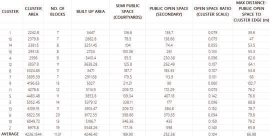
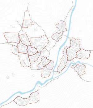
147 | 1 2 4 5 3 6 7 8 9 10 11 12 13 14 15 16
Research Development
4.5.5 Spatial Parameter Extraction
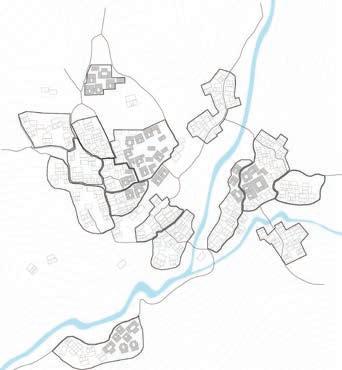


| Adaptive Urban Hillscapes 148
Sample 1
Public Space Samples
Block Type Samples
Sample 2
Sample 2
Sample 3
Sample 3
Sample 4
Sample 4
Sample 5
1 2 3 4 5
Sample 5
Sample 1
Super Block / Cluster level
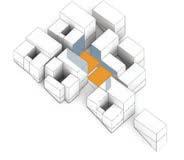
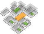
Open Space Ratio (OSR)
At a cluster level, the aspect of Open Space Ratio relates the total open space available (public & semi-public) for the net habitable area in the cluster. It is an indicator of quality of living, by the amount of population an open space should support. The average of 10.5% in this analysis is only considering well defined open pockets. Especially in a steep setting, there will be considerable unbuilt areas that also do not function as open social spaces.
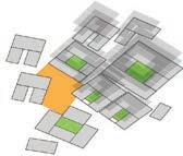
Enclosure Value (EV)
The study on EV shows that in this village of 2-3 storey courtyard houses assembled an narrow lanes, the pockets of open spaces will be fairly tightly bound by surrounding surfaces. This also indicates the intrinsic social aspect of privacy. But on sloped terrain, it is worth noting
that once the ground plane is terraced through cut and fill, the effective EV will be reduced. These aspects will be factored in the generation of the urban tissue.
149 |
Open Space area Total built up area OSR =
Average across clusters 10.5% Built up area Public Open space Open space SemiPublic Open space
Sample 1 3.05 Facing Surface area Public Space area EV =
Sample 2 1.73 Sample 3 1.76 Sample 4 3.27 Sample 5Average 2.66 3.5 Research Development
Sky View Factor (SVF)


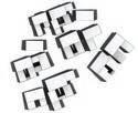


Sky view factor is calculated at the public open space at a cluster level. As the context is with a sloped terrain, it will mean that the buildings afar at higher elevations and the natural terrain itself might block the view of the sky. As this is unavoidable, only the buildings in the immediate context ie. buildings within the cluster, are considered along with the terrain.
As an experiment, SVF is calculated for the same space on flat terrain as well. It is seen that on a sloped terrain with the same built mass around, a public open space can have better visibility as the built mass' effective height reduces down the gradient. This helps in improving the spatial quality of open spaces.
Shaded Area Proportion


The proportion of shaded area of public open spaces shows that even during the hottest times of the year, an average of 29 % of the public open space is shaded. The appropriate balance of shaded to exposed areas proves vital in the usage of open spaces for social interaction.
It is commonly seen in many instances (refer fig.4.5.2.3) that vendors and hawkers set themselves up in the shaded edges of public spaces and their continual presence increases the intensity of public activity.
| Adaptive Urban Hillscapes 150
Sample 1 Sample 1 29% 21% Volume of obstructed sky dome Total volume of sky dome SVF = Avg percent of shaded area on 21 June 12:00 - 15:00
Sample 2 Sample 2 47% 5% Sample 3 Sample 3 32% 25% Sample 4 Sample 4 27% 39% Sample 5 Sample 5 Average Average 32% 29% 27.2% 55%
Sample 2 - 52%
Sample 2 on flat terrain - 46%
Sky Dome
Block Level
Open Space Ratio (OSR)


The ratio of the area of semi-public courtyard to the floor area of that block, shows the level of social significance given to communal spaces at a block level. In this village , the value of around 11% indicates the
informal nature of the space within this multi-family environment.
Shaded Area Proportion
The proportion of shaded area of semi-public courtyard spaces shows that even during the hottest times of the year, an average of 56 % is shaded. This ratio is quite balanced in these block types, which enables
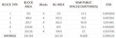
its continual usage as a social space.
Sky View Factor (SVF)

Sky view factor at the block level is taken from the stepped courtyards. A block is composed of atleast 4 buildings and each of the building heights are in the range of 2-3 storeys. In one block type, the absence of an entrance structure prevents the courtyard from being fully enclosed, which increaes its SVF drastically. Hence the SVF has an average value of 16.2 %. This differentiation of courtyard enclosures creates a specific range of experiential settings in this context.
151 |
Sample 1 Sample 1 8% 81%
Sample 2 Sample 2 5.5% 79% Sample 3 Sample 3 5% 68% Sample 4 Sample 4 40% 20% Sample 5 Sample 5 Average Average 16.2% 56% 22% 32%
Avg percent of shaded area on 21 June 12:00 - 15:00 Research Development
Topographical factors Ecological factors Environmental factors

Spatial factors

4.6 Data Extraction


The analysis illustrated in this chapter covers a wide range of factors starting from the context, that includes topography, soil, hydrology, mechanics and climatic aspects. In parallel, indigenous settlement is analysed to learn from local response to terrain, urban morphology and extract localised spatial metrics. Every analytical process needs to produce meaningful data that can be used to take the research forward. The flow chart shown here is intended to elicit the data from various sources. These sources can be both, direct data mining and analytical processes. At this stage, a hypothesis is proposed as to the manner of using the extracted data to develop further strategies. These strategies are listed here based on initial hierarchy of operative scales.

| Adaptive Urban Hillscapes 152 Evaluate Synthesis Map Context Sample Settlement Indigenous Morphology
Topography Climate Soil Data Solar Exposure Surface Flow Soil Loss
Data / Principles Design Strategies


Forests
Vegetation types
Farmlands
Crop types
Production Cluster
Harvesting hub
Easiest Path to farms
Density gradient
Urban Cluster
Density gradient
Existing Ring road junction
Risk Data
Topographical Risk Factor of Safety
Spatial Pattern
Spatial Hierarchy
Open Space Ratio
Spatial Morphology
Network Pattern

Network hierarchy
Network Morphology
Spatial Quality
Enclosure Value
Shaded area Proportion
Sky View Factor
Spatial Quality
Exposure Difference in courtyards
Fenestration pattern

Test Patch Level
Landscape Scheme
Reservoir + Wetland network
Hierarchical transport network
Operative landscapes
Cluster Subdivision

Network generation
Public Space generation
Block Subdivision

Semi
Block Morphology
153 | Input Input Input Input
Public
Low Density Mid Density High Density
Public Space generation Research Development
Space generation
Semi
4.7 Conclusion
The Research Development chapter mainly concentrates on accumulating information from data mining and analytical processes. All information regarding site, context, soil, hydrology is processed into usable maps or embedded into the base digital terrain model. This is especially important because all information is to be formatted into the same grid cells in order to effectively use it in driving the design strategies.
Site & Context
The test site selected in Shenzhen is 5.5 sqkm in area. The reason for selecting the particular quadrangle is because of the high recorded soil loss and it can be considered as a solitary watershed. This makes it sufficient to analyse the ecological aspects within the defined boundary.
Factor & Synthesis Mapping
A series of five factor maps containing topographical information, soil information and risk analysis are prepared. The data is evaluated as per the initial grid cells of 20x20m. If the cells are smaller, the analysis would be of a higher resolution and accuracy. The grid size is decided for ease of computation.
The synthesis mapping process shown in this chapter for generating a build-ability map is basically a deterministic mapping method described in sec 3.1. So, the synthesis map is directly affected by the contributing variables and there is no room for random variation. Although a GA is implemented with the aim to optimise the landuse pattern towards certain criteria, the solutions from 60 generations of 50 individuals each show a common struggle to achieve less soil loss. So 4 sub optimal results are evaluated for a set of external objectives and phenotype49.09 is selected. This selection is a combination of judging the evaluation data and also design intuition. The selected synthesis map was second ranked as per the data but it showed interesting urban cluster formation on the slopes which poses a good challenge.
This chapter finalises the major part of the landuse pattern. It is taken that the safety of built structures is paramount and hence the zones for urban development is earmarked at this stage.
Risk Analysis
By analysing the slopes for their factor of safety, the aspects of soil property, soil depth at every grid point on the terrain is used along with the topographical conditions; and this effectively indicates if the slope is weak. This information is extremely critical in informing the external loading conditions on the weak spots. As per the results of this analysis, it can be seen that 12% of the cells are on weak slopes. As for the selected landuse map, 6.95% of the developable land is on weak slopes. There are other phenotypes of the synthesis map, in which this percentage is much less, but as mentioned before, it was not selected because of design intuition. The fact that a bulk of the land suitable for urban development does not coincide with risk slopes is a validation of the optimisation process which took a combination of steep slopes, elevation, soil depth and landslide risk as parameters to synthesise an effective landuse pattern.
Spatial sampling of Indigenous Settlements
Indigenous settlements have a wealth of embedded social logics that have evolved over many generations. There is an interesting opportunity to use the extracted spatial metric from a settlement from the same region and similar context. It is to be noted that the spatial factors can reflect the climatic aspects, social practices, vocation; but nothing related to aesthetics.
| Adaptive Urban Hillscapes 154
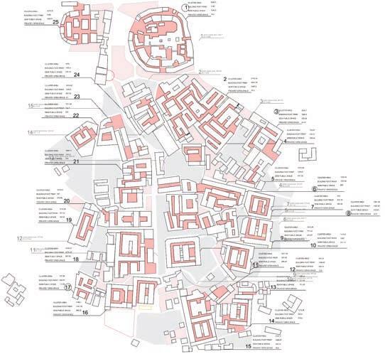
155 |
Research Development
4.7.1 Data from Huxinba village, Shaoguan, South China
Design Strategy 05.
PRODUCED BY AN AUTODESK PRODUCED BY AN AUTODESK EDUCATIONAL PRODUCT AUTODESK EDUCATIONAL PRODUCT
AUTODESK EDUCATIONAL PRODUCT PRODUCED BY AN AUTODESK PRODUCED BY AN AUTODESK EDUCATIONAL PRODUCT 5.1 Multi-layer approach 5.2 Attempt for synchronisation 5.3 Strategy 1 - Hydrological network 5.4 Strategy 2 - Vegetation strategy 5.5 Strategy 3 - Farming Strategy 5.6 Strategy 4 - Transport network strategy 5.7 Operative urban scales 5.8 Strategy 5 - Urban system ( cluster 1 ) 5.9 Strategy 6 - Operational public space 5.10 Strategy 7 - Building generation ( cluster 1 ) 5.11 Conclusion
5.1 A Multi-Layer Approach
-Initial Experiment (phase 1)
In the initial phase of this dissertation, The design strategy takes a multi-layer approach, wherein every layer is informed by the data extracted from the synthesis and factor maps developed previously. The information embedded in them mainly concernslandslide susceptibility, building density, vegetation distribution and topographical data. The diagram on the facing page indicates how the data is subdivided and translated into the various design stages.
The different aspects that constitute the design strategy can be observed as inter-dependent layers that are generated successively. The rules and logics used to generate the design layers are grounded on specific study that will be described in detail further in this chapter. Also, each process takes into consideration the results of the preceding layer.
The overall city tissue includes buildings, wetlands, functional open spaces, reservoirs and farmlands. The degree of integration is manifested by the internal hydrological mechanisms that the vegetated, water bodies and built areas contain.
| Adaptive Urban Hillscapes 158
159 | Building Densities Landslide Susceptibility Vegetation Distribution Topographic Data Slope angle Slope aspect Elevation SYNTHESIS MAP BREAKDOWN FACTOR MAPS RESERVOIR NETWORK 01. 02. 03. 04. 05. WETLAND DISTRIBUTION BUILDING MORPHOLOGY VEGETATION COVERAGE ROAD NETWORKS
Fig. 5.1.1 Multi-layer approach flow chart (phase 1)
Design Strategy
Fig. 5.1.1
5.1.1 Critical Analysis - Initial Experiment (phase 1)
The layering of various aspects of the design strategy results in a unified system that responds to the build-ability and susceptibility framework set forth in the previous chapter. By summarising the adopted methods and the techniques used to generate this unified system, it is possible to critically analyse the entire multi-layer approach.
The ordering of the design layers takes a linear process, prioritising the ecological aspects. So, the hydrological flows, drainage network and catchments are solved at the outset. The city system was developed under the same ecological conditions, and although the strategies proposed, considered the adaptation of some city components to hydrological dynamics, a lack of spatial integration was found between the layers of the built area and the surroundings. The location of plots was determined by a random omission of cells that conformed to the grid of developable land, ignoring ecological forces or supply systems, leaving behind the possibility of enhancing the operation of the urban system in such a way that human activity coexists with the environment. The urban clusters did not have any cohesive spatial or clustering logic. The determination of public space was a result of negative areas from developable land, without considering any spatial relationship between the plots or the overall built area with the public space. Connectivity, both at a local level and between clusters, is another aspect which is missing in the proposed urban fabric. The vegetation and network strategy are independent and serve as a direct response to the building and wetland distribution, without having any direct influence on them.
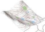
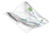
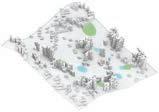
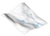
| Adaptive Urban Hillscapes 160
01. RESERVOIR NETWORK
02. WETLAND DISTRIBUTION
03. BUILDING MORPHOLOGY
04. VEGETATION COVERAGE
05. ROAD NETWORK
Fig. 5.1.1.1
Fig. 5.1.1.1
Layers of the design strategy
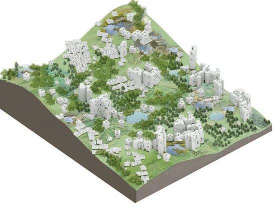
161 |
Fig.5.1.1.2 Integrated System
Design Strategy
Fig. 5.1.1.2
5.2 Attempt for Synchronisation
Subsidiary ecosystems are dynamic components of contemporary urbanization; this is the premise on which the design strategies of this dissertation are based. A synthesis map provides an approach to a safe background scenario that frames operational strategies on the site’s surface. It is at this stage that design proceeds to blur the physical boundaries between land-uses for the benefit of their integration. Hydrological, vegetation and farming strategies start the process, conserving their hierarchical background as main drivers for urbanization in the Anthropocene. These strategies are reciprocally affected and perform in response to the issues of contemporary cities on hillsides: erosion control methods complementing food and water supply systems.
Upcoming strategies relative to urban development follow the spatial directions traced by supply systems and adapt their components in response to flows that are contemplated in the hydrological strategy. Therefore, to accomplish synchronization in the design process, as the research question states, the multiple layers of the urban tissue must consider the distribution strategies of ecological components and the mechanisms of supply, facilitating the coexistence of urban activities with the natural phenomena.
To this end, the generative processes employed in certain strategies aim to produce multiple outputs simultaneously. This forces a mutually inter-dependent system at every generative stage ; and subsequent strategies take advantage of this.
| Adaptive Urban Hillscapes 162
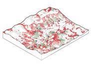
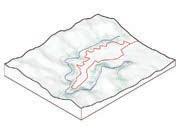
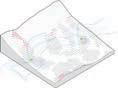
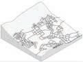
163 |
01. HYDROLOGICAL NETWORK Reservoirs Wetlands
02. VEGETATION STRATEGY Vegetation type distribution
03. FARMING STRATEGY Crop type distribution Production clusters
04. NETWORK STRATEGY Hierarchical transport network Farming trails
05. URBAN STRATEGIES
Design Strategy
Plot subdivision Local networks Building Morphology Operational Open spaces
5.3 Strategy 1 - Hydrological Network
5.3.1 Existing Hydrology
Main Reservoirs Water Supply System
In the patch, two main reservoirs are identified within the valley under topographic analysis and water flow simulation. These two main water bodies are perennial reservoirs in the existing conditions of this area of the city of Shenzhen. Although both are situated in the patch’s lower elevation zone, their elevation difference reaches approximately 25 meters , with reservoir R2 being at a lower level (Fig 5.3.1.1).
Drainage basin
The main drainage streams that form along the natural gullies are shown in Fig 5.3.1.2, pointing out the potential locations for temporary retention ponds at the intersection of these drainage streams and the contours that provide large areas with similar elevation on that specific points.
Water accumulation
This study obtains the various natural drainage channels and their hierarchy based on the contribution from subsidiary drainage basins that increase the volume of flow. The stream leading to reservoir R2 accumulates water from almost the entire test patch of 5.5 sq.km (Fig 5.3.1.4).
Retention pond network
At the numerous intersection points obtained from Fig 5.3.1.3, it is possible to calculate the accumulation volume for each pond (refer appendix). This information can inform future relationships between building density or open spaces and the volume of each pond to improve the supply proposal consistency. These ponds are meant to operate also as temporary water retention agents, controlling the water levels in the main reservoirs. (Fig 5.3.1.5)
Provided the sustained population growth that Shenzhen is subjected to, water and food supply systems need to be constantly upgraded to satisfy the upcoming population, requiring new supply sources or repotentiating existing supply mechanisms. The main water catchment agents in the city are the hills, defining why the 172 reservoirs inside the city are located within or close to the hills. Therefore, the opportunity to establish sloped areas as natural supply hubs combined with future built land arises. Currently, the area where the design is developed has two of the most important reservoirs in the district, thus the proposal integrates them to compose a water retention system that will benefit not only the supply mechanism of the city but also mitigate erosion.
| Adaptive Urban Hillscapes 164
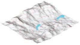
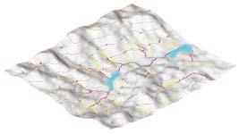
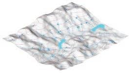
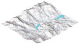
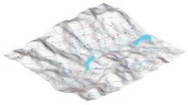
165 | 2
R2 R1 4.51 in Sq Km
Fig. 5.2.1 Main reservoirs
Fig 5.3.1.1
Fig 5.3.1.2
Fig 5.3.1.4
Fig 5.3.1.3
Fig 5.3.1.5
Fig. 5.2.2 Darinage basin
Fig. 5.2.3 Intersection with contour
Fig. 5.2.4 Water accumulation
N Design Strategy
Fig. 5.2.5 Retention pond network
5.3.2 Reservoir & Wetland Network Logic
An extreme scenario of sustained precipitation is the starting point for this research, and throughout the development, erosion prevention methods are expected to behave also as supply mechanisms. Considering heavy rainfall is the main trigger for soil erosion and landslides in this part of the country, the proposal starts by managing water retention using local reservoirs situated strategically in elevated areas in order to reduce the flow rate down to the main reservoirs. The specific location of these reservoirs responds to the proximity to main catchment streams and topographic regional curvature where the creation of ponds is more likely to occur, hence the complexity of the construction process can be reduced.
Furthermore, the hydrological strategy aims to integrate retention ponds with wetland eco-system. The relationship logic is to have the reservoirs in close proximity to these natural channels and in natural ponding locations; and the wetlands to be within a distance(variable) from the pond and also in a downstream location from urban clusters, so that it act as a natural sediment trap. It is critical to find a balance in locating both the natural features at the same time in their respective ideal areas where they can sustain themselves. Due to their interdependency, an optimisation process is adopted to generate them synchronically
| Adaptive Urban Hillscapes 166
Fig 5.3.2.1 Logic Diagram of the desired hydrology
Fig 5.3.2.1
Level 1-2-3 developed areas
Wetlands
Main natural drainage channel
Retention pond
variable genes Fitness criteria LOOP CONDITIONS Distance to main drainage channels Concave areaspossible natural ponds Retention Ponds Wetland location Maximise building cells within 200m radius Minimise the no. of reservoirs Threshold slope angle Depth of concavity Distance between pond & wetland Threshold slope angle Upstream locations from ponds Less solar exposure Elevation below avg elevation of nearest urban cluster (level 1-2-3) DEM variable genes
A curvature analysis of the natural topography indicates concave areas with a high possibility of natural ponding. This curvature map is sampled for the deepest locations and marked for evaluation in relation to the main drainage channels
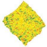
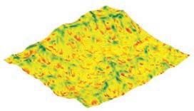

The natural reservoir locations are evaluated for the distance to its nearest major drainage channel. The distance is given as a variable range in order to computationally broaden the search.
A search radius is given as a variable to locate wetlands in the vicinity and according to the rules set. Selecting upstream locations for wetlands in the search area
pond locations close to main natural streams (variable gene)
search radius for wetland locations (variable gene)
convex possible natural pond locations upstream locations for wetlands & flow direction
Slope Aspect map
NSNW /NE SW /SE
wetland cells with less exposure building plots in higher elevation in a 200m radius
167 |
concave
Fig.5.3.2.2
Fig.5.3.2.2
Fig.5.3.2.4
Fig.5.3.2.6
Fig.5.3.2.3
Fig.5.3.2.3
Fig.5.3.2.4
Fig.5.3.2.5
Fig.5.3.2.6
Fig.5.3.2.7
Fig.5.3.2.5
Fig.5.3.2.7
Design Strategy
5.3.3 Reservoir & Wetland Network - GA Results


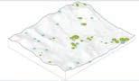
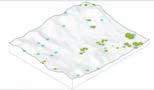
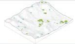
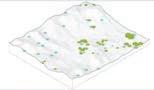

| Adaptive Urban Hillscapes 168
Buildable cells in wetland reach Buildable cells in wetland reach Buildable cells in wetland reach No. of reservoirs Number of Generations: 50 Solutions/Generation : 20 Solution time : 35 sec No. of reservoirs No. of reservoirs Objectives Objectives Objectives G20.03 fitness rank 7/60 G20.09 fitness rank 45/60 G30.06 fitness rank 27/60 G20.04 fitness rank 8/60 G30.02 fitness rank 5/60 G30.07 fitness rank 28/60 G20.07 fitness rank 44/60 G30.08 fitness rank 6/60 G30.1 fitness rank 31/60 33 27 34 34 33 36 25 28 26 5516 3215 5667 5516 5664 5722 3056 4260 3536

169 | Buildable cells in wetland reach Buildable cells in wetland reach Buildable cells in wetland reach No. of reservoirs No. of reservoirs No. of reservoirs Objectives
G44.7 fitness rank 1/60 G46.2 fitness rank 11/60 G44.20 fitness rank 2/60 G44.4 fitness rank 17/60 G46.8 fitness rank 3/60 G46.10 fitness rank 12/60 G44.16 fitness rank 9/60 G46.20 fitness rank 4/60 G46.3 fitness rank 18/60 31 32 26 34 33 26 25 35 32 5219 5050 3484 5696 5196 3366 3484 5696 4980 Design Strategy
Objectives Objectives
5.3.4 Hydrological Network -Conclusion
The image below shows the fittest phenotype from the generative process to find the ideal locations of the hydrological features viz. retention ponds and wetlands. This being a reciprocal system, the locations of the naturally occurring ponds immediately indicates the possible locations of the wetlands, based on the procedural logic described previously. Only natural ponding locations are considered because, the concavity in the terrain directs maximum surface flow towards it, as can be seen from fig.5.3.4.1.
The sustenance of wetland ecosystem is quite a challenge since the soil needs to be constantly saturated for the typical vegetative species to thrive. Hence, it cannot exist in steeper slopes where the water is easily drained away from the soil layers. In addition, it needs to avoid high solar exposure. On those grounds, some natural ponds do not have wetlands in their vicinity; even though there might be potential urban runoff from certain urban clusters. This can be considered as a limitation, because it is initially driven by the concavity in the terrain.
The genetic algorithm is run over 50 generations and the results are shown in the previous spread. It is seen that the number and position of the natural ponds is quite limiting; although the variable gene that decides the minimum depth of concavity acts as a threshold to filter out the relatively shallow concave areas. The diameter of the generated pond is proportional to the degree of concavity at that location. Research has been done to calculate the volume of water with the help of a rational equation (refer appendix), but integrating it into the script increased the solution time dramatically, so volume is not calculated. The search radius used to find possible wetland locations around the retention ponds is variable gene whose domain (100-200m) is a factor of the size of the pond. Another limitation of this process is that there is no reasonable method to re-evaluate a set of results from the GA. High end computational fluid dynamics could be used to evaluate flows and volumes, but it is not time efficient at this scale and it cannot be part of the associative modelling environment.
| Adaptive Urban Hillscapes 170
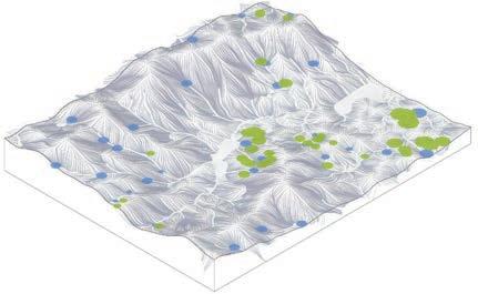
171 |
G44.7
URBAN CELLS IN WETLAND REACH (5219)
NO. OF RESERVOIRS (31)
Fig. 5.3.4.1
Design Strategy
Fig. 5.3.4.1 Retention pond & wetland network - Fittest solution
5.4 Strategy 2 - Vegetation Strategy
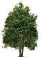


Vegetation prevents soil erosion mainly in three different ways: protecting soil surface from heavy rainfall, moistening sub-layers of soil where failure appears: and holding top soils as roots reach deep compact soils. A strategic location of tree types with different characteristics will be needed to cover the above requirements, given to the slope gradient within the test patch. One important aspect of using tree roots to avoid erosion as the root, especially tap roots, is capable of working in tensile strength to retain surface layers of soil that are exposed to erosion. Therefore, deep rooted trees will be placed in steep terrains where failure plane is deeper than in flat or less steep areas, and trees with flat and spread roots will be located in these areas.
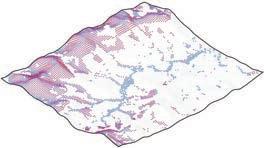
| Adaptive Urban Hillscapes 172
Wide
-
+
Distribution logic diagram Forest Slope gradient 51 1
Harland Oak 15 m 0 m 5 m 10 m 20 m
rooted trees Deep rooted trees
Steep slopes
Steep slopes
Chinese Pine Vetiver grass
Fig. 5.4.2
Tree types located in the area
Fig. 5.4.1
Slope gradient map in 5km2 patch
Fig 5.4.1
Fig 5.4.2
For the distribution, deep rooted trees for steeper slopes and shallower and wider rooted trees for lower steepness. Deep rooted shrubs can be also employed as green cover in areas where space is limited, vetiver plants (chrysopogon zizanioides) are an example of these kind of plants.


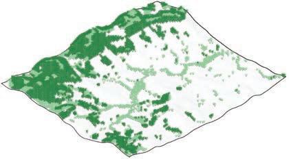
Deep rooted trees
Wide rooted trees
Deep rooted trees
Wide rooted trees
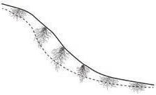
173 | Design Strategy
Failure plane
Fig. 5.4.4 Tree distribution map in 5 km2 patch
Fig. 5.4.3 Root depth function across the slope
Fig 5.4.4
Fig 5.4.3
5.5 Strategy 3 - Farming Strategy
5.5.1 Crop Distribution
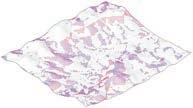
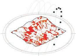
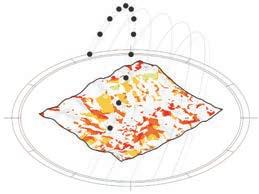
Following the synthesis map, a strategy is considered to fill the high risk areas: levels 4 and 5 assigned as forest and agricultural land respectively. This proposal is based in locating specific flora species across the hill landscape in order for them to contribute, according to their characteristics, to the integrated mitigation system for erosion and debris flow control. Differentiation is obtained by subdividing forested and agriculture areas according to the angle of steepness of the terrain where they are located, hence a threshold angle is defined for both forests and agriculture. This responds to the importance of landsteepness involving soil stability, increasing not only surface soil loss, but most important, having direct effect on two fundamental landslide drivers: subsurface failures and underground water flow.
In agriculture, rice paddies have an efficient production by naturally seeping water from underground flows, while dry crops need less amount of water seepage. Underground water discharge also reduces soil saturation, therefore, employing rice paddies in hilly terrains might help the hill ecosystem prevent risks of soil erosion by balancing the water pressure inside the soil. On the other hand, dry cop terraces have a positive effect on restraining surface water runoff after intense precipitations impact surface soils with high volumes of water, reducing the risk of having shallow debris flow that evolve into large volume of landslides. Consequently, the strategy locates rice paddies or dryarable terraces according to the steepness of the terrain in order to improve productivity and also maximize the crop area.
| Adaptive Urban Hillscapes 174 N Summer - 5 days
day from 6:00 - 18:00 Winter - 5 days
day
6:00
18:00 N Hours 60.0 57.5 55.0 52.5 50.0 47.5 45.0 Hours 50.0 45.0 40.0 35.0 25.0
Each
Each
from
-
Slope gradient on 5km 2 Slope gradient 51 1
Rice paddies
Steep
Steep crops
Steep crops + Steep crops - Exposure + Exposure Dry crops Wet crops
Terraced farming -
crops -
+
A sunlight hours analysis together with a slope gradient analysis help to differentiate the types of crops inside the 5.5 square kilometre patch. The criterion for the first analysis is based on reducing the evaporation of wet crops like rice paddies during the hottest time of the year by placing them in areas receiving less sunlight hours. Simultaneously, the criterion for the slope gradient evaluation is based on locating rice paddies on less steep areas in order to discharge underground water from higher recharge zones. On the other hand, farming through dry terraces can make good use of the steep areas where accessibility is reduced so crop production can be improved. At the same time, water runoff or soil erosion driven by heavy rainfall can be controlled to some extent by terracing the surface of steep terrains, while water seeps into the ground in each green terrace.

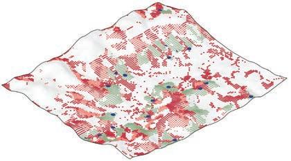
175 |
paddies
Terraced
ha Farming Cluster Harvesting hubs 35.7 % 64.3 % 3.7 % Crop area inside the patch represents 3.7 % of Shenzhen’s city total Farmland area Collective Farming Associations Hectares per associated harvest hub 11 ha 179.7 ha 16 Approximate number of harvesting hubs Total crop hectares in 5 km patch Design Strategy
Rice
115.5 ha
farming 64.2
5.5.2 Production Nodes
An internal evaluation within the clusters established as production areas takes place to define the plot that will represent the hub from which harvesting footpaths will start and converge. The principle relies on an established slope gradient for a farmer’s footpath and the maximum distance that this farmer should walk to reach a crop area. The objective is to reduce the amount of energy and time whilst maximising crop harvest. For the experiment, a maximum gradient of 1:10 and a maximum walking distance of approximately 500 meters are determined considering data extracted from a traditional farming village (Hayami & Kikuchi, 2000). This method also helps to define whether a production node is needed or not according to the range of crops that each node is able to reach, as some redundancy might be occurring in the number of crops that two or more hubs are reaching.
The initial step for this procedure is to define the hub plot by evaluating the topography surrounding each plot centroid at each production cluster (fig 5.5.2.1). The desired plot should be surrounded by a terrain that permits the largest number of possible pathways in different directions considering the maximum walking gradient that pathways should have. Once the hub is defined in each production cluster, an agent-based path finding script is employed to search for farmers’ trails that do not exceed the fixed gradient and the maximum distance.
Angle between path directions: 20 degrees
Production plots centroids
Evaluating scopes
Largest scope
Harvesting hub
Agent-path initial direction
| Adaptive Urban Hillscapes 176
Slope gradient for harvesting trails 1:10
Fig 5.5.2.1
Fig. 5.5.2.1 Harvesting hub determination and path finding method
Farmland Production Clusters Harvesting hub
Farmland Production Clusters Harvesting trails
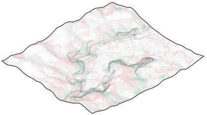
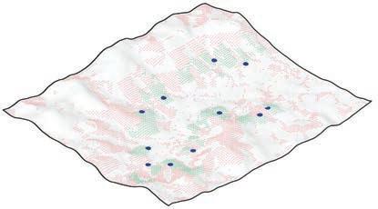
177 |
Fig. 5.5.2.3 Reached farmlands by harvest pathways.
Fig. 5.5.2.2 Harvesting hub for each production cluster
Fig 5.5.2.3
Design Strategy
Fig 5.5.2.2
5.6 Strategy 4 - Transport Network Strategy
Mountain Yinhu, the area on which the project is developed, is connected to the Shenzhen’s transport system by a ring road that goes across the valley right at the bottom of each of the developable clusters at the 5 km2 patch. Considering this ring road as the primary road, the elaboration of the subsequent trails is based on the integration between and within built clusters. Thus, an elevated road parallel to the main ring road is generated by connecting the main harvesting trails coming from harvesting hubs inside each production cluster (Fig.5.6.1), with a corresponding gradient of 1:20. These trails are the most accessible walking paths, given their gradients, for a farmer to reach the most amount of crops surrounding the production clusters. Therefore, the main road connecting the developable areas at a higher elevation will be also used for harvesting and commercial purposes as they lead directly to the harvesting hubs, where commercial activity is more likely to happen.
The criteria for network generation inside built clusters is based on improving accessibility to main public spaces and farmlands from areas with different elevations (Fig 5.6.1). So at this scale, the proposed road at higher elevation is connected to the existing ring road through vehicleaccessible roads with a 1:15 gradient that generate primary public spaces at their intersections. Additional roads parallel to the main road are proposed inside each cluster if the extents of the cluster require additional connections in different elevations. Also these parallel roads might serve as potential connections with other clusters in a future development of urbanization.
| Adaptive Urban Hillscapes 178
Contour trails
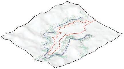
Public T. Station
Accesible paths
Harvesting hubs
Public space (Primary)
Harvesting hubs
Upper Ring Road
Ring Road
Harvesting trails
Production clusters
179 |
Fig 5.6.1
Fig. 5.6.2 Network integration logic at cluster scale.
5.6.2
To crops Gradient Connection 1:20 1:20 1:20 1:20 1:15 1:15 1:15
To
Fig. 5.6.1 Network integration at 5km2 scale Fig
To crops / other clusters
To crops
other clusters
Crops Design Strategy
5.7 Operative Urban Scales
The strategies devised till this stage are working at the "Test patch" scale of 5.5 sq.km. All the distinct clusters of levels 1,2 and 3 that represent urban developbale land are marked in the diagram on the facing page. This is obtained from the synthesised landuse map described in section 4.3.6.
Each distinct cluster is termed as "Urban Cluster"; and there are 32 such clusters in the test patch. They range from 0.015 - 0.29 sq.km in area. In order to experiment with urban strategies, a smaller "Experiment patch" of 0.7 sq.km is selected. The selection of this smaller patch is mainly to test the urban connectivity between a few clusters. There are 3 urban clusters within the selected Experiment patch, along with the presence of production nodes (farm management nodes), wetland nodes and other natural subsidiary eco-systems.
One of the primary factors that guide the urban strategies is the spatial pattern and sampled spatial metrics of the indigenous settlements. In order to effectively apply the sampled data, it is important to set the hierarchical scales for the spatial pattern adaptation.(refer sec 4.5.4)
CLUSTER<>VILLAGE An urban cluster is analogous to the scale of the entire village. The "Primary public space" data is adapted at this scale, as these open spaces are important nodes in the overall functioning of the urban cluster.
SUPER BLOCK is a group of blocks or buildings that is served by , or falls within the range of a Secondary level public space. The "Secondary public space " data is applied here and it is reciprocal in nature. In the sense that its position and reach defines the super block, and the total area of the buildings in the super block define the size of the secondary open space.
BLOCK is an individual building or multiple buildings that are connected and act as one entity. For different building types of varying densities, there may be different types of semi public space embedded into it. The data for the "Semi public space" is adapted at this scale.
| Adaptive Urban Hillscapes 180
semi public space public space (secondary) major public space (primary) village
cluster experiment patch super-block super-block block block
INDIGENOUS SETTLEMENT DATA GENERATED URBAN CLUSTER
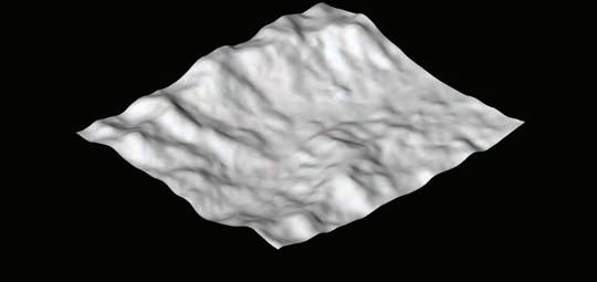
181 |
PATCH Area: 5.5 km2 No. of Clusters: 32 EXPERIMENT PATCH Area: 0.7 km2 No. of Clusters: 4
CLUSTER Area: 0.015 km2 - 0.29 km2 CLUSTER 1 Area: 0.08 km2 CLUSTER 2 Area: 0.13 km2 CLUSTER 3 Area: 0.09 km2 Design Strategy
TEST
URBAN
high risk cell
cell in cluster 1
harvesting hub
harvesting trail
5.8 Strategy 5 -Urban Systems (Cluster1)
5.8.1 Cluster Subdivision- Generative Process
Cluster subdivision strategy is focusing on building plots and the goal is to explore the possibilities of synchronously generating densified building plots, high quality of public space and functional local network with contradictory objectives. The data and spatial patterns which are sampled from indigenous village is taken into consideration in this process to maintain traditional social logic while evolving a new urban tissue.
Considering the analysis from FOS map (sec 4.4), the high risk areas are not suitable for building up, firstly the cells on weak slopes are removed from built up cells and converted into green space in next stage. For ease of computation, the process is applied to one cluster at a time.
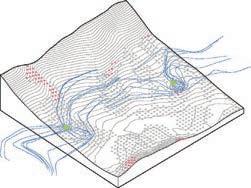
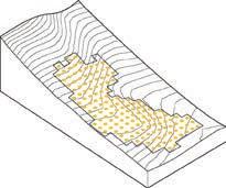
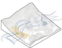
map highlighting high risk area
fig. 5.8.1.1
from 0.7 sqkm map to cluster 1 map after removal of cells in high risk area cluster 1
fig. 5.8.1.1
| Adaptive Urban Hillscapes 182
Following the farming system, cluster 1 is one of the production clusters, which has a harvesting hub and several harvesting trails can originate from it. So the first step subdivides this cluster with a randomly chosen harvesting trail, whose gradient is less than 1:20, and converts it into the first primary road. At least two primary roads need to have a good connection with each other, hence two other primary roads are chosen within a certain height difference, which is within the range of 20 to 30 meters, from the first primary road.
To connect the primary roads found in step 1, the second step is to find at least one accessible path, whose start and end points are randomly chosen along the primary road and follow the gradient which is less than 1: 15, between each two primary roads. The first hierarchy open space is located around the middle points of the paths.
To maintain a similar social logic, the population of secondary public spaces is mainly following the data extracted from the indigenous village. The service range of each secondary public space is within the range of 40 -75 meters, which is extracted from indigenous hillside village, and the amount of secondary public space is the minimum number to ensure the whole cluster covered by its service. And the area within the range of a public space is considered as a super block. The area of each public space is also calculated according to traditional open space ratio, which is in the range of 0.07 – 0.2.
Once the public open spaces are generated satisfactorily, building plots are distributed within each super block, whose size follows the density distribution of the land use map, and their collective orientations are along with contour lines. The height of each plot is also related to density.
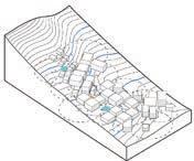
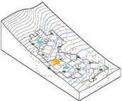
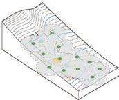
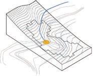
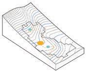
harvesting trail (primary road)
accessible path
Harvesting hub
1st hierarchy of public space secondary public space secondary public space service range
183 | Design Strategy
harvesting
harvesting hub primary road
fig. 5.8.1.2
trail
step 1. define primary roads from harvesting trail step 4. building plots generation step 4. building height generation
step 2. fine accessible path and first hierarchy public space step 3. populating the secondary public space
Input parameters and fitness critereia
Information like main harvesting hub selection, location and service range of secondary public space, size and height for each plot are fed into the block generation process as input parameters. Six objectives, are set according to different spatial function of open space, and they are set with equal weightages:
1. Maximize solar exposure in harvesting hub during winter time, which could benefit the rice drying/ milling process;
2. Minimize slope angle in first hierarchy open space to make this area as flat as possible to create more useable space for public activities;
3. Minimize average elevation for secondary public space with regard to plot elevation, which makes it possible for secondary public space
to collect water from buildings;
4. Maximise sky view factor for all public space, which increase the spatial quality for open spaces;
5. Maximise shaded area proportion for first and secondary public space to avoid uncomfortably high temperature during summer solstice;
6. Maximise built up volume.
As some of these criteria are pulling the result in opposite direction, GA process is used to generate the final result. And considering the maximum number of objectives that can be accepted by the software, the objectives of sky view factor and built up volume are remapped into one.
Fitness criteria Input parameters
1. main harvesting trail selection
2. Location and service distance for the secondary public space
Harvesting hub
1. Maximise solar exposure
2. Maximise SVF
First hierarchy public space
1. Minimize slope angle
2. Maximise SVF
3. Maximise Shaded Area Proportion
Secondary public space
1. Minimize avg elevation w.r.t building plot elevations
2. Maximise SVF
3. Maximise Shaded Area Proportion
Buildings
1. Maximise Volume
3. Plot size for each density
1. Minimize slope angle

Block scale open spaces <Maximise SVF + Volume>
4. Height for each plot
<Maximise solar exposure>
Minimize avg elevation w.r.t building plot elevations
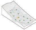
<Maximise Shaded Area Proportion>
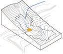
| Adaptive Urban Hillscapes 184
15 - 20 m 30 - 35 m 35 - 40 m 7 - 10.5 m 14 - 21m 28 - 35 m
variable genes
main harvesting trail selection
Fitness criteria
Maximize solar exposure in harvesting hub
variable genes
location and service distance for secondary public space
Block location cluster density
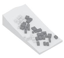
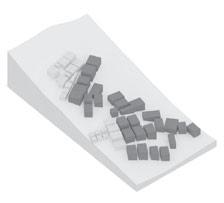
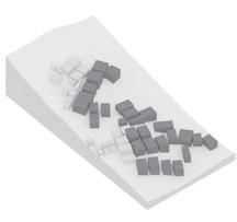
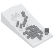
plot size
building height
5.8.2 Cluster subdivision - GA results
Number of Generations: 50
Solutions/Generation : 60
Solution time : 48 sec
Minimize maxim slope angle in first hierarchy open space
Minimize average elevation for secondary public space
Maximise sky view factor for all public space,
Maximise shaded area proportion for first and secondary public space
Maximise build up volume
Types
slope angle in 1st hierarchy openspace (r) average elevation in 2nd hierarchy open space () open space shading ratio in summer production open space exposure ration in winter
value for build-up
185 |
LOOP
volume
Objectives Fino
0.19 0.40 0.14 0.16 -269.44 -260.01 -274.81 -275.93 0.61 0.54 0.74 0.74 0.48 0.93 1.00 0.52 0.67 0.36 0.93 0.55 G49.29 G49.30 G49.31 G49.32 1 2 3 4 5 G 4929 1 2 3 4 5 G 4930 1 2 3 4 5 G 4931 1 2 3 4 5 G 4932 Design Strategy
remap
& open space SVF
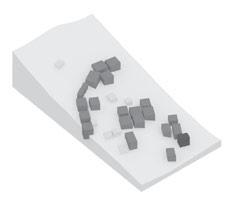
| Adaptive Urban Hillscapes 186 slope angle in 1st hierarchy openspace (r) average elevation in 2nd hierarchy open space () open space shading ratio in summer production open space exposure ration in winter remap value for build-up volume & open space SVF Objectives Fino Types slope angle in 1st hierarchy openspace (r) average elevation in 2nd hierarchy open space () open space shading ratio in summer production open space exposure ration in winter remap value for build-up volume & open space SVF Objectives Fino Types 0.15 0.12 0.15 0.19 0.18 0.11 0.10 0.12 -274.80 -257.72 -274.80 -266.70 -258.96 -271.51 -261.44 -250.51 0.76 0.31 0.76 0.58 0.71 0.53 0.49 0.41 1.00 0.68 1.00 0.45 0.59 0.88 0.65 1.00 0.63 0.89 0.46 0.65 0.55 0.63 0.89 0.73 G49.41 G49.45 G49.42 G49.46 G49.43 G49.47 G49.44 G49.48 1 2 3 4 5 G 4941 1 2 3 4 5 G 4942 1 2 3 4 5 G 4943 1 2 3 4 5 G 4944 1 2 3 4 5 G 4945 1 2 3 4 5 G 4946 1 2 3 4 5 G 4947 1 2 3 4 5 G 4948
187 | slope angle in 1st hierarchy openspace (r) average elevation in 2nd hierarchy open space () open space shading ratio in summer production open space exposure ration in winter remap value for build-up volume & open space SVF Objectives Fino Types 0.15 0.12 0.11 0.15 0.16 0.18 0.17 -268.24 -236.89 -244.93 -274.80 -270.91 -275.91 -272.72 0.81 0.55 0.72 0.76 0.72 0.80 0.63 0.70 0.70 0.93 1.00 0.53 1.00 1.00 0.47 0.67 0.97 0.65 0.41 0.55 0.30 G49.49 G49.53 G49.50 G49.54 G49.51 G49.55 G49.52 slope angle in 1st hierarchy openspace (r) average elevation in 2nd hierarchy open space () open space shading ratio in summer production open space exposure ration in winter remap value for build-up volume & open space SVF Objectives Fino Types 1 2 3 4 5 G 4949 1 2 3 4 5 G 4950 1 2 3 4 5 G 4951 1 2 3 4 5 G 4952 1 2 3 4 5 G 4953 1 2 3 4 5 G 4954 1 2 3 4 5 G 4955 Design Strategy
Cluster Sub-division - GA Fittest Phenotypes
After running 50 generations with 60 individuals in each, the top four fittest individuals are chosen. From the chosen phenotypes, the objective radar graphs show that the ranking for 5 criteria in each phenotype are not even – relatively high performance in the first 3 objectives are easily achieved in all individuals while the other two objectives show more variation. Which indicates that although we set equal weightage to each objective, the result is pulling into the first
three criteria, and maybe a differential weighting for the objectives could be a future experiment.
Since the ecological context is not taken into consideration in the block generation, the further assessment criteria aims to evaluate the influence of plots on surface water flow . In addition, network integration analysis can help in evaluating the generated local networks; and filter the best solution based on cumulative performance.
| Adaptive Urban Hillscapes 188 1 2 3 4 5 G 4932 1 2 3 4 5 G 4953 0.16 0.15 -275.93 -274.80 0.74 0.76 0.52 1.00 0.55 0.65
1. Average slope angle for 1st hierarchy open space
2. average elevation for 2nd hierarchy open space
3. summer shading ratio for all open space
4. winter exposure ratio for harvesting hub
5. remap value for open space SVF and building volume
G49.32 G49.53
189 | 1 2 3 4 5 G 4955 1 2 3 4 5 G 4956 0.18 0.11 -273.86 -272.71 0.84 0.71 0.75 0.74 0.55 0.39 G49.54 G49.55 Design Strategy
5.8.3 Cluster Sub-Division - Post GA Evaluation

Surface water flow simulation

It has been registered in previous flooding incidents, that heavy rainfall can cause severe damage to city infrastructure if water runoff destination is ignored during the urban design process. Therefore, this proposal takes into consideration the diversion of flows produced by the plot arrangement of the selected four fittest individuals from the last generation process. The objective is to measure the incidence of water flows into the public spaces that will have the function of seeping the water into the soil so that further erosion and flooding incidents can be prevented, enhancing also the soil seepage capacity of that cluster for ecological benefits that will be further discussed.
Given the different plot arrangement, the capacity that each group of public spaces has of receiving surface water flows will vary, indicating which combination would satisfy the water seepage criteria. At the same time, given the natural characteristics of the topography, some location of plots can be counterproductive in terms of avoiding water flow towards a public space or out of the cluster, and instead create areas where water can easily pond, saturating the drainage systems of the city. Therefore, another aspect to be evaluated after this simulation is the minimum number of areas where ponding can occur in each individual.
| Adaptive Urban Hillscapes 190
50.32 % of water flow incidence on public spaces 50.53 Plots Surface flows Legend Public Spaces Ponding areas Fig 5.8.3.1
Fig 5.8.3.2
4.4 % 5.9 %


191 | 50.54 50.55
Fig. 5.8.3.1 Public Spaces inside cluster
5.8 % 6.5 % Design Strategy
Fig. 5.8.3.2 Surface water flows diverted by plots inside cluster
5.8.3 Cluster Sub-Division - Post GA Evaluation
Street Network - Local Integration
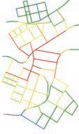
The third aspect to be considered in this post-evaluation process is the average local integration within the streets that will come from the different plot distributions. The reasonable aim is to obtain the highest average local integration value that a specific network arrangement can provide, taking into account that further adjustments can be done in upcoming stages to improve the accessibility to every plot inside the cluster, as a slope gradient analysis can create a discontinuity between streets that are accessible for vehicular or unrestricted pedestrian access.
| Adaptive Urban Hillscapes 192 Plots Surface flows Public Spaces 50.32 50.53 1.01 0.37 0.98 0.33
Fig 5.8.3.3
Fig 5.8.3.4
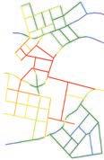
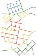
193 | 50.54 50.55 0.96 0.36 0.99 0.30
Fig. 5.8.3.3 Public space location
Design Strategy
Fig. 5.8.3.4 Street local integration
5.8.4 Cluster Subdivision Selection And Breakdown


The final selection of the plot distribution is based on determined weightages that are applied to the fitness values coming from the generative process, considering the sum of the remapped fitness values for the final selection. The final fitness values are very similar for the four individuals, since they were selected from a convergence towards a specific efficient solution found in the 50th generation of the genetic algorithm. To highlight the differentiation between the results, the criterion of surface water flows incidence on public space is given higher importance on top of local network integration and the occurrence of ponding areas inside the cluster. This process illustrates the importance of plot arrangement under extreme precipitation circumstances as the avoidance of surface erosion and flooding can be supported by a strategic diversion of rainwater flows towards green areas where water can be retained and soaked into the soil, preventing infrastructural damage.

| Adaptive Urban Hillscapes 194
50.31 1: 0.042 2: 0.917 3: 0.471 1: 0.055 2: 0.963 3: 0.508 1: 0.055 2: 0.854 3: 0.450 1: 0.061 2: 0.830 3: 0.493 50.53 50.54 50.55
Fig 5.8.4.1
Fig. 5.8.4.1
% of water flow incidence on public spaces Individual Total number of water ponding incidents Average local integration within the street network 0.67 0.66 0.63 0.64 Waterflow incidence on public spaces Number of ponding incidents Average local integration 4 2 6 8 4.4 5.9 5.8 6.5 50.31 50.53 50.54 50.55 x 3 x 1 x 2 Fitness weightage Fig 5.8.4.2
Multi-objective graphs for remapped final fitness values
Fig. 5.8.4.2
1 0.8 0.6 0.4 0.2
Real values for post evaluation process
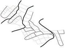
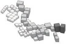
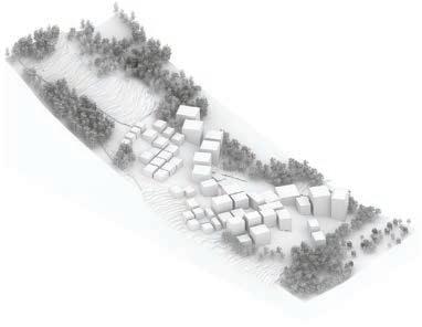
195 | Design Strategy Primary Roads High density Plots 8 - 10 4 - 8 1 - 3 1:20 Gradient Street Typology Building morphology Legend Floors > 1:8 < 1:8 Roads Medium density Recharge public spaces Stairs Low density Discharge public spaces Harvesting Hub Other public spaces Individual 50.53
Fig. 5.8.4.5 Street type differentiation
Fig. 5.8.4.4 Building density differentiation
Fig. 5.8.4.3 Plot and public space location
Fig. 5.8.4.6 Isometric view of Public spaces inside cluster 1
5.9 Strategy 6 - Operational Public Spaces

5.9.1 Ecological Operation Logic
Water exchange across hill sub-ecosystems


In hill ecosystems, balanced soil saturation is supported by a constant exchange of water taking place in the underground as water collected in high catchment areas flows downhill through different levels. This creates a sustained interaction between local areas in the hill which have the natural functions of either recharge or discharge of water to the soil according to the topographic configuration and the natural ground coverage (Carter 1996). The area occupied by the city in between forests and water body needs to maintain its water seepage capacity to avoid substantial negative effects on soil saturation values. When soil is moisturised, the surface tension between soil particles allows soil to gain cohesion, maintaining a high shear strength; whereas making soil over saturated reduces the shear strength of the soil. Developable land takes over natural green areas, reducing the ecological capability of seeping water out from the subsurface, leaving certain areas oversaturated. Hence, it is reasonable to allow open spaces behave as water conductors in order to preserve the ecological features of the site. Following this logic, the defined public spaces in between buildings will relate to this natural process of underground-water exchange depending on their location along the slope.
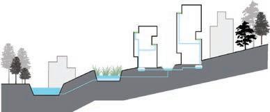
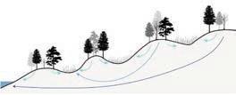
| Adaptive Urban Hillscapes 196
Local and regional recharge Local and intermediate recharge Regional flow Intermediate flow Local flow Local recharge Local recharge Local and intermediate discharge Local and regional discharge Local discharge Local discharge
Fig. 5.9.1.1
Underground water exchange across the hill ecosystem
Fig. 5.9.1.2
Building's water contribution to public space operation
Fig. 5.9.1.2
Fig 5.9.1.1
pipe wetland water
public
rain
water reservior
reservior
space
water collection tank
wetland
water collection public space


197 |
Water-discharge Urban
Water-recharge Gardens Water-recharge
Water-discharge Forest Water-recharge Water
Water-discharge
Underground waterflow Rice paddies
farming
Wetlands
parks
Underground waterflow
Fig 5.9.1.3
Fig 5.9.1.4
Fig. 5.9.1.4
Underground water exchange diagram between subsidiary ecosystems
Fig. 5.9.1.3
Design Strategy
Underground water exchange diagram between subsidiary ecosystems
5.9.2 Public Space Typology
Determining public space functions


Analysing their slope condition and location, the typology of operational public space into either mainly recharge or discharge public spaces can be established. The water flow simulation will inform the respective incidence of water flowing into certain public space compared to the rest (Fig 5.9.2.1) This data can be useful for determining the volume of vegetation required for each public space, hence informing the type of space that can be employed.
Due to the effects of gradients on underground water flows, steep areas are unsuitable for discharging water from the underground since the water table level increases in depth, preventing natural or artificial suction systems to operate; while less steep areas are appropriate for employing suction system from the underground. At the same time, water recharge spaces shaped as vegetated terraces will operate efficiently on steep zones not only to reduce water runoff but to provide the slope the capacity of seeping water to the ground.
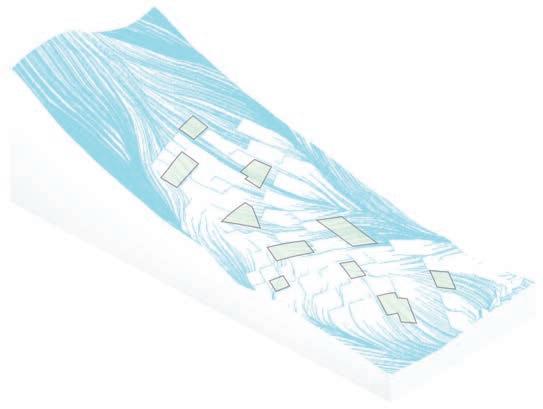
| Adaptive Urban Hillscapes 198
1 6 2 7 3 8 4 9 5 10 1 2 3 4 5 6 7 8 9 10 19.9 % 12.1 % 6.1 % 7.4 % 9.9 % 11.7 % 14.3 % 11.3 % 5.2 % 2.2 % Surface
Public Spaces
flows
Fig. 5.9.2.2
Surface water flow incidence on public spaces
Fig. 5.9.2.1
Percentage of water flow incidence on public spaces.
Fig. 5.9.2.2
Fig. 5.9.2.1
The application of certain vegetation species will help the green area to operate efficiently, as well as the opportunity to propose subsurface layers of soil filters under green areas and receive wasted water from surrounding buildings to be treated and partially purified. This strategy allows to propose parks, rain gardens or wetlands as public spaces, which at the same time can improve thermal comfort in buildings and semi public spaces through ventilation.
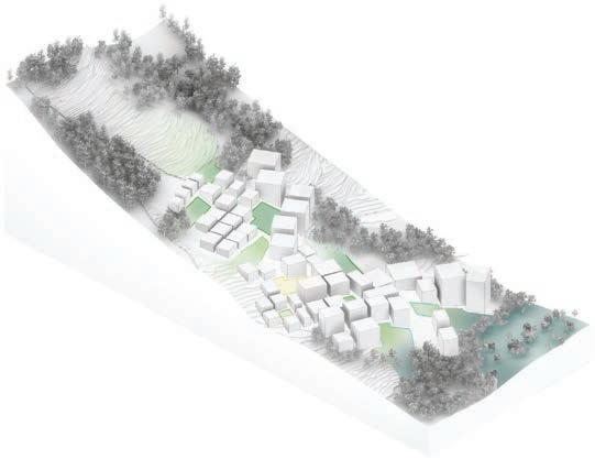
RAIN GARDEN
Area: 892.59 m2
Extremes elev. difference: 12.59 m
Slope angle: 21.95 degrees
RAIN GARDEN
Area: 526.07 m2
Extremes elev. difference: 8.8 m
Slope angle: 23.95 degrees
URBAN FARM / PLANT NURSERY
Area: 977.68 m2
Extremes elev. difference: 8.10 m
Slope angle: 14.12 degrees
PARK / MAIN RECHARGE SPACE
Area: 810.81 m2
Extremes elev. difference: 8.75 m
Slope angle: 19.72 degrees
HARVESTING HUB
Area: 1020.68 m2
Extremes elev. difference: 4.09 m
Slope angle: 5.53 degrees
PLAY GROUND
Area: 259.95 m2
Extremes elev. difference: 5.32 m
Slope angle: 13.80 degrees
RAIN GARDEN
Area: 481.89 m2
Extremes elev. difference: 2.22 m
Slope angle: 4.62 degrees
PARK / BUS STATION
Area: 2034.30 m2
Extremes elev. difference: 10.19 m
Slope angle: 16.92 degrees
WATER PARK
Area: 909.45 m2
Extremes elev. difference: 16.99 m
Slope angle: 20.44 degrees
WATER PARK
Area: 595.47 m2
Extremes elev. difference: 8.21 m
Slope angle: 17.43 degrees
Harvesting Hub
Discharge area
Recharge areas
Other public space
Wetland
199 | Design Strategy 1 2 3 4 5 6 7 8 9 10
Fig. 5.9.2.3
Fig. 5.9.2.3 Isometric view of Public spaces inside cluster 1
1 6 2 7 3 8 4 9 5 10
5.10 Strategy 7 - Building Generation (Cluster 1)
5.10.1 Morphology Development
Basic principles of the building configuration with respect to the embedded open space, is taken from the traditional building morphologies shown in chapter 2.5.3. The motive is to abstract these features for their climatic and social responses; and adapt them to a more dense scenario on a slope context.
Maintaining similar good living conditions in multi-floor buildings is one of the core principle when developing the building morphology. At the same time, considering hot and humid climate in south China, ventilation is an important aspect to be aware of. In this circumstance, the spatial pattern and spatial metrics for the semi public open space, extracted from the indigenous settlement , is used in the generative process. Plots are distributed into 3 different types according to land use map.
1. Low density building types


For low density types, with plot size is in the range of 15-20 meters, the principle is to maintain the difference in the size of the two courtyards (refer sec. 2.5.3). By doing so, ventilation is induced due to the thermal difference especially in summers.
2. Mid density building types


In mid density building types, the terraces are stagged to achieve the same spatial quality of semi-public space over multiple floors. This improves the sky view and exposure paramters to fall within the range of the sampled data. To reduce the number of overhangs over the
semi-public space, the enclosed area in the upper storeys are always less than the area of the lower storeys

| Adaptive Urban Hillscapes 200
fig.5.10.1.1
low density building type generation process
fig.5.10.1.2
mid density building type generation process
3. High density building types


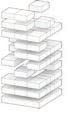
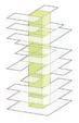
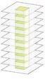

For high density building types, the orientation of the large openings in the facade ,where the semi-public space is situated, is alternated
5.10.2 Multi-objectives optimization
In order to meet the multiple spatial and environmental criteria, a GA process is involved, and based on different generation logics, 2 main variable parameters are fed into building detail generation process as input data: Number of storeys for each building and the plot subdivision.
between every floor. This parameter works in conjunction with an open central atrium to create a chimney effect and induce cross ventilation across the tower block. The area ratios between the semi public spaces and the total built up area is in the range of the extracted data.
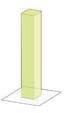
The plot is subdivided into a body plan, based on the basic plot size and the requirement of semi public spaces and the slope angle of the plot.
Input parameters
201 |
fig.5.10.1.3 high density building type generation process
low density plot low density plot mid density plot mid density plot high density plot high density plot
7 - 10.5 m (2-3 floors) 14 - 21m (4-6 floors) 28 - 35 m (6-8 floors)
1. Maximum storeys for each building
2. Courtyard location & size
Design Strategy
Objectives
Considering the spatial quality for semi-public space and buildings, 5 objectives are given to this process as fitness criteria, which are:
1. Maximize building south facing ratio, which profits by better luminous environment in the courtyards and indoor spaces;


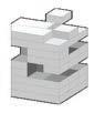
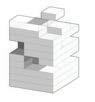

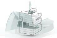
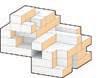
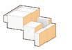
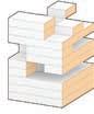
2. Maximize semi-public space sky view factor

3. Maximize semi-public shading ratio during summer solstice, which has the longest insolation duration during whole year, which could
1. South facing ratio (+)
2. Maximise Semi-public space Sky View for each building (+)
benefit the thermal comfort of the semi public spaces throughout the year.
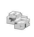


4. Maximize semi-public space solar exposure to achieve better luminous environment during winter solstice, which has the shortest insolation duration during whole year.
5. Maximize the total density for whole cluster
3. Maximize semi-public space shading ratio in summer solstice (+)
4. Maximize semi-public space exposure ratio in winter solstice (+)
5. Maximize total density for whole cluster
| Adaptive Urban Hillscapes 202
5.10.2 Building Generation - GA Results
Procedural


203 | south facing ratio total build-up volume courtyard sky view factor remap value courtyard shading ratio in summer solstice courtyard exposure ratio in winter solstice Objectives Fino Types 0.272 G49.01 G49.02 G49.03 G49.04 0.269 0.274 0.275 230052 232079 229999 227598 0.59 0.26 0.92 0.10 0.62 0.60 0.64 0.62 0.34 0.36 0.32 0.33 1 2 3 4 5 G 4901 1 2 3 4 5 G 4902 1 2 3 4 5 G 4903 1 2 3 4 5 G 4904
Number of Generations: 50 Solutions/Generation : 50 Solution time : 58 sec Fitness criteria slope angle in plots' location
generation Maximize south facing ratio Maximise Semi-public space Sky View for each building Maximize semi-public space shading ratio in summer solstice Maximize semi-public space exposure ratio in winter solstice Maximize total density for whole cluster Maximum floor for each building Courtyard location & size DEM plot subdivision repeat in floors couryard cells culled raise up along with location's slope angle variable genes LOOP Design Strategy
Building


| Adaptive Urban Hillscapes 204 south facing ratio total build-up volume courtyard sky view factor remap value courtyard shading ratio in summer solstice courtyard exposure ratio in winter solstice Objectives Fino Types G49.13 G49.14 G49.15 G49.16 0.272 0.279 0.274 0.270 230097 230826 246362 245111 0.68 0.10 0.28 0.04 0.63 0.61 0.65 0.63 0.32 0.35 0.31 0.32 1 2 3 4 5 G 4913 1 2 3 4 5 G 4914 1 2 3 4 5 G 4915 1 2 3 4 5 G 4916 south facing ratio total build-up volume courtyard sky view factor remap value courtyard shading ratio in summer solstice courtyard exposure ratio in winter solstice Objectives Fino Types 0.263 0.273 0.270 0.273 209370 231211 229971 228252 0.83 0.26 0.43 0.04 0.61 0.64 0.61 0.60 0.38 0.32 0.36 0.35 G49.17 G49.18 G49.19 G49.20 1 2 3 4 5 G 4917 1 2 3 4 5 G 4918 1 2 3 4 5 G 4919 1 2 3 4 5 G 4920


205 | south facing ratio total build-up volume courtyard sky view factor remap value courtyard shading ratio in summer solstice courtyard exposure ratio in winter solstice Objectives Fino Types 0.263 0.276 0.274 0.276 211737 243099 244682 248433 0.72 0.24 0.41 0.49 0.68 0.58 0.87 0.60 0.32 0.38 0.12 0.36 G49.29 G49.30 G49.31 G49.32 1 2 3 4 5 G 4929 1 2 3 4 5 G 4930 1 2 3 4 5 G 4931 1 2 3 4 5 G 4932 0.274 0.278 0.279 237358 252096 253430 0.97 0.22 0.53 0.65 0.67 0.64 0.31 0.28 0.32 G49.37 G49.40 G49.49 south facing ratio total build-up volume courtyard sky view factor remap value courtyard shading ratio in summer solstice courtyard exposure ratio in winter solstice Objectives Fino Types 1 2 3 4 5 G 4937 1 2 3 4 5 G 4949 1 2 3 4 5 G 4940 G49.05 0.283 235985 0.83 0.60 0.35 1 2 3 4 5 G 4905 Design Strategy
5.11 Conclusion - Design Strategies
In summation, the ambition for a synchronically strategized urban tissue is partly achieved where cohesive logics of spatial and environmental factors guide the development of the urban systems. At a macro level, the hydrological network is a reciprocal system where multiple interdependent outputs are produced. The farming strategy, has direct impact on the outcome of the macro network and consequently the urban cluster subdivisions. The inter-linking of strategies could have been worked out with greater integration.
Hydrological Network Strategy
The integrated retention pond and wetland network seek to serve multiple objectives like; reducing the flow rate along the main drainage channels down to the main reservoirs, retaining water at higher elevations for irrigation and urban distribution, acting as a natural sediment filter for urban runoff . Some retention ponds might not have the ideal conditions for the sustenance of a wetland eco-system in their proximity. Even though there might be potential for urban runoff . There is also a limitation in considering only natural ponding locations on the terrain. Considering the limitations in the computational techniques, it is worth mentioning that volume of water , which could be calculated with the rational equation, was not calculated due to dramatic increase in solution times; and there is no reasonable method to re-evaluate flows other than high end computational fluid dynamics.
Vegetation Strategy
The relevance of tree type differentiation relies on surface erosion control methods. This strategy is in fact an extension of the land-use pattern strategy set inside the 5.5 sq.km synthesis map, where the subsidiary ecosystem of forests is set to high terrains of the mountain and landslide risk zones. A tree type differentiation essentially ensures a better operation of the densely-vegetated areas in response to surface soil erosion, considering the capacity of roots to retain soil through tensile strength. A deeper study on soil characteristics as wells as the relevance of time on the body of trees could provide perhaps a more bio-technical approach to the design strategy or even lead to different outcomes of a land-use map, considering different time lapses.
Farming Strategy
To determine the harvesting trails that come out of the production clusters, a simple two-point path finding script could have been employed, with fixed origins and destinies so that accessible paths could still be generated. Nevertheless, the chosen method can offer the possibility of responding to time-lapse alterations in crop distribution, so that the destination point could be moved around different areas outside the cluster per different harvesting seasons. The agent based method explores the largest scope for destinations as it starts by selecting the area inside the production cluster that presents more possibilities for initial agent-based paths compared to other areas inside the same cluster, satisfying the gradient conditions for a pedestrianaccessible farming trail.
| Adaptive Urban
206
Hillscapes
Network Strategy
The connectivity between all the developable clusters was the main objective to determine the network arrangement. Both the existing ring road as well as the high ring road are designated to reach the isolated developable clusters in upper parts of the 5.5 sq.km patch. The options of the upper ring road on reaching isolated developable clusters are in some cases limited to certain heights where the harvesting trails are present, leaving behind the chance to reach larger areas of some of those clusters. On the other hand, the proposal involves heavy road infrastructure to be employed in areas where the main roads go across high-risk landslide areas. Vehicular transport network at the macro scale was taken as a top-down solution in benefit of public transport access to the different isolated developable clusters. At a cluster scale, the road network is disadvantaged in some cases because of the slope gradient in the terrain, creating acute angles between main roads and the accessible paths that are climbing towards other main roads in the cluster. This generates further problems during the plot generation, where the accessible paths would need to be adjusted giving space to the plot distribution.
Urban Strategies
The experiments to generate the urban patch was done considering a smaller patch area of 0.7 sq.km Ideally, it is possible to generate the entire experiment patch, consisting of three urban clusters, simultaneously with plot subdivision and building morphologies influencing each other. But the computational power needed to do geometric modifications
on 300,000 sqm. of plot area and 250-300 building forms would be immense. For computational ease, urban systems are generated one cluster at a time.
The urban generative processes shown in this chapter is split into two parts- firstly the subdivision of the cluster into super blocks ,plots, public spaces and networks ; and secondly the evolution building forms in each plot according to the density zoning. Here again, it is ideally a single process but the sheer quantity of parameters and fitness criteria for spatial and environmental aspects at a 2D and 3D level is beyond the scope of the genetic algorithm used here. A trial is attempted in the building generation GA process by remapping and combining two fitness criteria into one. So, it is possible to increase the number of objectives in this way, but it is not possible to retrieve the fitness data for the original objectives before they were remapped. These are some of the computational limitations encountered.
In summation, the ambition for a synchronically strategized urban tissue is partly achieved where cohesive logics of spatial and environmental factors guide the development of the urban systems. At a macro level, the hydrological network is a reciprocal system where multiple interdependent outputs are produced. The farming strategy, has direct impact on the outcome of the macro network and consequently the urban cluster subdivisions. The inter-linking of strategies could have been worked out with greater integration.
207 |
Design Strategy
Design Proposal 06.
PRODUCED BY AN AUTODESK PRODUCED BY AN AUTODESK EDUCATIONAL PRODUCT AUTODESK EDUCATIONAL PRODUCT
AUTODESK EDUCATIONAL PRODUCT PRODUCED BY AN AUTODESK PRODUCED BY AN AUTODESK EDUCATIONAL PRODUCT 6.1 Building Generation - further evaluation 6.2 Building generation - post GA evaluation 6.3 Building generation - final selection 6.4 Sections 6.5 Adaptive urban system (0.7km2) 6.6 Renders
6.1 Building Generation - Further Evaluation
After 50 generations which has 50 individuals in each, the top five fittest individuals are chosen. Since the generative process is split in two parts- first to define the plot subdivisions and secondly to evolve the building morphologies- the final clusters of generated buildings do not show much variation as a collective; and this is mirrored in the data as well. This is also because of the limited range in building heights
for every density type. Moreover the density zoning is decided much earlier by the landuse map, which give less opportunities for variations at this stage. As mentioned in the conclusion of the previous chapter, the urban cluster could have ideally been generated with an integraed logic where building forms could be influenced much more by their locations.
1. south facing ratio
2. total build-up volume
3. courtyard sky view factor remap value
4. courtyard shading ratio in summer solstice
5. courtyard exposure ratio in winter solstice
1. south facing ratio
2. total build-up volume
3. courtyard sky view factor remap value
4. courtyard shading ratio in summer solstice
5. courtyard exposure ratio in winter solstice
1. south facing ratio
2. total build-up volume
3. courtyard sky view factor remap value


4. courtyard shading ratio in summer solstice
5. courtyard exposure ratio in winter solstice
| Adaptive Urban Hillscapes 210 0.283 237337 0.66 0.62 0.34 1 2 3 4 5 G 4922 0.280 252200 0.59 0.65 0.31 1 2 3 4 5 G 4926 0.282 245311 0.59 0.63 0.34 1 2 3 4 5 G 4933
But there is definite variation at the level of the individual buildings, which will be evident in the further assessment of architectural qualities. The external evaluative criteria seeks to address the interface between the built form and the urban form. Methods like porosity, enclosure and visibility is used to analyse the qualitative aspects, relationships across the cluster to select the best performing phenotype and possibly propose any minor changes.
1. south facing ratio
2. total build-up volume
3. courtyard sky view factor remap value
4. courtyard shading ratio in summer solstice
5. courtyard exposure ratio in winter solstice
1. south facing ratio
2. total build-up volume
3. courtyard sky view factor remap value


4. courtyard shading ratio in summer solstice
5. courtyard exposure ratio in winter solstice
211 | 0.278 252096 0.22 0.67 0.28 0.279 253430 0.53 0.64 0.32 1 2 3 4 5 G 4949 1 2 3 4 5 G 4940
Design Proposal
6.2
Building Generation - Post GA Evaluation
6.2.1 Enclosure Value
Public Space Enclosure Value
Two aspects that can evaluate the mutual effects between public spaces and building’s spatial quality are the building’s porosity and the enclosure value of a certain public space. Visual connectivity, climatic comfort, accessibility and spatial continuity are some features that different building shape configurations can provide. In order to achieve them, the five fittest results from the building generation process are selected and analysed in terms of enclosure value and building porosity ratios for the ten public spaces inside the cluster.
The objective is to provide a better spatial connectivity and accessibility to those public spaces from and to other parts inside or outside the cluster, therefore a lower average enclosure value of the individuals is the target criterion for this evaluation. Although this feature will not guarantee direct spatial connectivity between public spaces, it contributes to a better visual connectivity from the public spaces to the exterior.
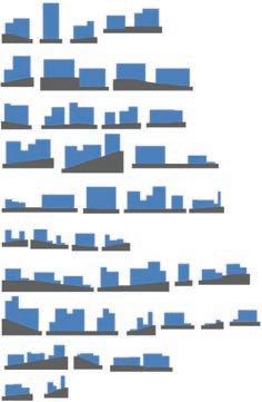
| Adaptive Urban Hillscapes 212
Public Space Unfolded elevations 10 9 8 7 6 5 4 3 2 1 Enclosure surface
Fig. 6.2.1.1
Fig. 6.2.1.1
1 2 3 4 5 6 7 8 9 10
Final selectionIndividual 49.40 unfolded elevation of public space buildings
Plots Public spaces
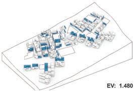
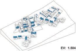

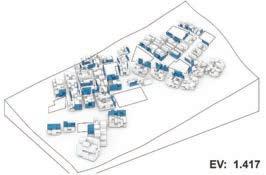
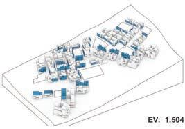
213 | 49.22 EV: 1.417 49.26 EV: 1.445 49.40 EV: 1.504 49.49 EV: 1.480 49.33 EV: 1.504
Fig. 6.2.1.2
Design Proposal
Fig. 6.2.1.2 Isometric view of Public spaces inside cluster 1
6.2.2 Building Porosity
Building porosity surrounding public spaces
Corresponding the previous evaluation: spatial continuity; accessibility and climatic comfort are features that are also under consideration in the building porosity analysis. In this method, the incidence of green areas on the semi public spaces in the buildings is predominant, as they have the potentiality to alter the thermal comfort indoors and improving the spatial quality inside buildings with a higher visual connectivity towards green areas. Additionally, spatial continuity across the cluster passing through public spaces can be aimed with a higher porosity of buildings located in between two or more public spaces. Although to support this purpose, several adjustments would need to be done in the morphology of buildings, since this property was not considered within the generative process.
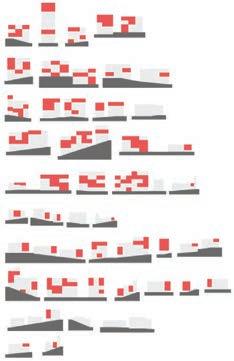
| Adaptive Urban Hillscapes 214
Unfolded Elevations Public Space 10 9 8 7 6 5 4 3 2 1 Porous surfaces Non-porous surface
Fig. 6.2.2.1
Fig. 6.2.2.1
Final selection -
1 2 3 4 5 6 7 8 9 10 Plots Public spaces
Individual 40.40 unfolded elevation of public space buildings
Positive faces Porous faces


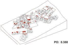
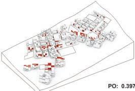
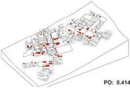
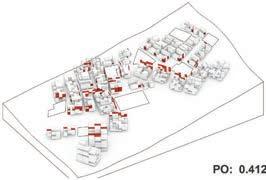
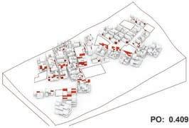
215 | 49.22 Avg Porosity value: 0.388 49.26 Avg Porosity value: 0.409 49.40 Average porosity value: 0.414 49.49 Avg porosity value: 0.412 49.33 Avg Porosity value: 0.397
Fig. 6.2.2.2
Porous
Fig. 6.2.1.2 Isometric view of Public spaces inside cluster 1
Positive faces
faces Positive faces Porous faces Positive faces Porous faces
Design Proposal
Positive faces Porous faces
6.2.3 Visibility Analysis


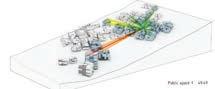
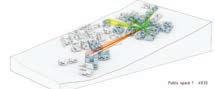
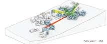
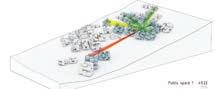
The isovists of 3 main public spaces are calculated, because better viewsheds help in place-making when navigating through the urban cluster. The expansive views from these public spaces are possible due to the basic principles of regulating the building heights according to the elevation and slope, which was set up as part of the initial script in generating the building heights. The 3D isovist representation shown here also takes into consideration the distance to obstacles.
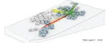
| Adaptive Urban Hillscapes 216
49.22 35% PUBLIC SPACE 1 49.26 37.5% 49.33 37% 49.40 46.5% 49.49 37.5%
1. Visibility from terraces to public space
2. 3D isovist from public spaces 1 2 3
1.
2.
10m 300m
The 5 selected phenotypes from the GA results are analysed for the aspect of visibility to and from the public spaces. The first analysis is assessing the unobstructed visual access to the public space from the building's terraces. The design intention is to promote the public open spaces, both primary and secondary, as being visually integrated with the built fabric; especially considering the hill side context. There are instances where the public space at the bottom of the cluster is visible from the buildings a the highest elevations. This is preferred in the analysis, hence the phenotype with the greater percentage of buildings having clear visual access gets a higher score in the evaluation. The representation on the right also indicates longer viewing distances with red colour rays.
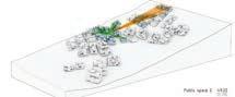
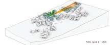
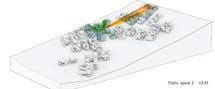
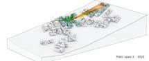
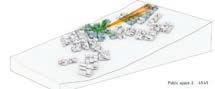
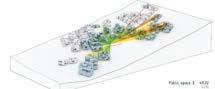


217 | PUBLIC SPACE 2 PUBLIC SPACE 3 49.22 35.7% 49.26 40% 49.33 40% 49.40 40% 49.49 42% 49.22 40% 49.22 47% 49.33 48.5% 49.40 46.5% 49.49 46.5% Design Proposal
6.3 Building Generation - Final Selection


The post-evaluation process applied to the fittest results helped to visualize the contribution of the different building details on three aspects of spatial quality in private, semi-public, and public spaces. The methods employed provide a quantifiable assessment on visual and spatial access between distant public spaces; neighbouring public spaces through buildings; from semi-public areas inside buildings to public areas; and spatial continuity of open areas across buildings. These features highlight the qualitative proficiency of the urban environment, considering that climatic comfort can also be gained with ventilation across green areas inside the city penetrating through the porous spaces of buildings. However, these qualitative criteria to approach public space continuity could have been inserted into the generation of building forms and building location, sacrificing some other cultural local principles that were prioritized in the development of the city. This friction opens the reflection of which priority should be brought into the design process and at which stage is it convenient to do so.

| Adaptive Urban Hillscapes 218
49.26 1: 0.409 2: 0.678 3: 0.411 Final fitness value: 2.73 Final fitness value: 2.78 Final fitness value: 2.68 Final fitness value: 2.70 Final fitness value: 2.59 1: 0.414 2: 0.628 3: 0.440 1: 0.397 2: 0.631 3: 0.417 1: 0.412 2: 0.647 3: 0.411 1: 0.388 2: 0.710 3: 0.369 49.40 49.33 49.49 49.22
Fig 6.3.1
Porosity values Individual Enclosure value Public space visibility 0.411 0.440 0.417 0.411 0.369 1 0.8 0.6 0.4 0.2 Porosity Value Public space visibility Enclosure value 0.678 0.628 0.631 0.647 0.710 0.409 0.414 0.397 0.412 0.388 49.26 49.40 49.33 49.49 49.22 x 2 x 1 x 3
Fig. 6.3.1
Multi-objective graphs for fitness values
Fig 6.3.2
Fig. 6.3.2
Fitness values for post evaluation process
Fitness weightage
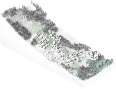
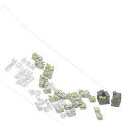
219 | Primary Roads High density8 - 10 4 - 8 1 - 3 1:20 Gradient Street Typology Building morphologyFloors > 1:8 < 1:8 Roads Medium density Stairs Low density Individual 49.40
Fig. 6.3.5 Street type differentiation
Fig. 6.3.4 Building density differentiation
Fig. 6.3.6 Isometric view of Public spaces inside cluster 1
Fig 6.3.6
Fig 6.3.5
Design Proposal
Fig 6.3.4
Recharge flows
Discharge flows
Artificial drainage
6.4 Sections

The exchange of water between adjacent subsidiary ecosystems can be displayed in this section that goes across a main recharge public space inside the urban environment and the adjacent farming subecosystem. The recharge area is designated as a park with different stages that have specific functions depending on the steepness of the terrain where they are located. A large flat area is proposed as a big rain garden that seeps large amounts of water into the soil, receiving also wasted and trapped water from the surrounding buildings in the sub-layers of soil that naturally filters and partially purifies water destined for adjacent crops. In steeper areas of this public space, dense vegetation is proposed to avoid surface erosion triggered by heavy rainfall. The rice paddies can extract underground water flows with traditional drainage systems, contributing to soil saturation balance as large volumes of water are seeped into the soil in upper areas and discharged for irrigation purposes.
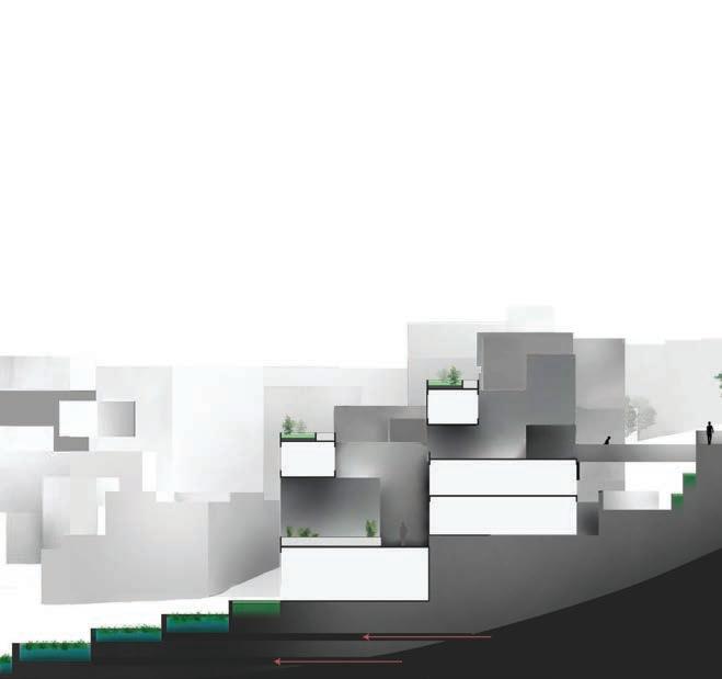
| Adaptive Urban Hillscapes 220
Medium density typology
Rice Paddies
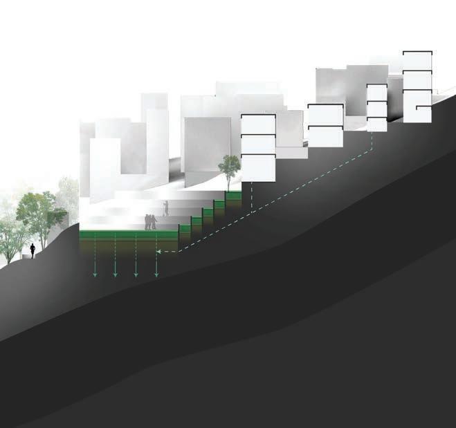
221 | Park / Recharge zone Dense vegetation Main garden Urban farming Low density typology
Surface soil
water filter
Design Proposal
Aquifer Soil
Bedrock soil
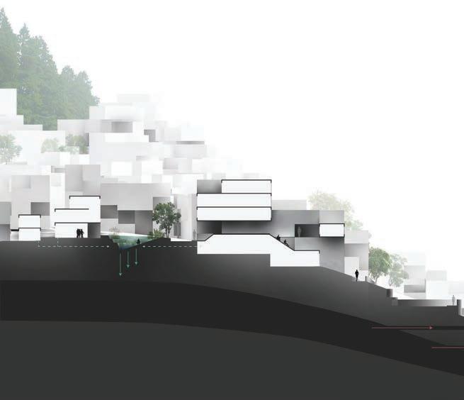
| Adaptive Urban Hillscapes 222
Medium density typology
Rain garden / Recharge zone
Forest / Main recharge subecosystem
Surface soil
Aquifer
Bedrock soil
Low density typology
Building porosity provides spatial continuity across the city, enhancing visual connectivity and public access through buildings between different public spaces. A continuous porosity along the cluster can potentially connect all the public spaces at different elevations, allowing the pedestrians to go across the different operational open spaces starting from the main recharge sub-ecosystem of forests, passing through recharge green areas, and leading to the water discharge spaces at the bottom of the cluster as they approach the wetland subecosystem. The buildings located in between water discharge areas like water parks and wetlands can have a specific modification in the ground levels to allow water flows pass through the building, bringing the chance to improve the thermal comfort of semi-public areas through crossed ventilation.
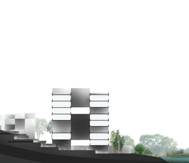
223 |
High density building
Water Park / Discharge zone
Discharge
Artificial
Design Proposal
Wetland
Recharge flows
flows
drainage
The generative process of the urban strategy locates the harvesting hub in the areas with less steep gradient inside the clusters, in such way that rice production practices can be easily enabled. As cooperative associations of farmers are targeted to share the production of the whole farmland area in the hill, the extents of their production allows to make use of low density buildings surrounding the yards to employ rice mills and any other semi-industrial or handicraft facility related to farming. The porosity of the surrounding mid-density buildings is beneficial for any kind of commercial activity, as they enclose a potential commercial place where seasonal events like farmers’ market can take place together with the mill activities. This architectural features contribute to traditional farming practices, preserving the local agriculture and providing the opportunity the generate further complementary activities adjacent to the supply system mechanism.

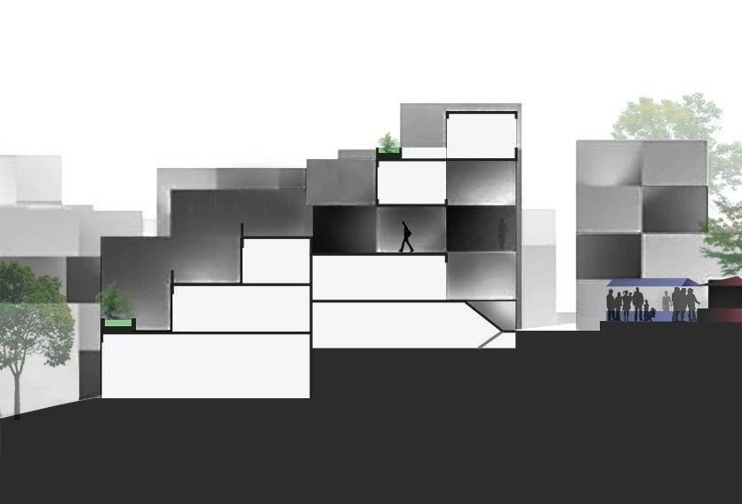
| Adaptive Urban Hillscapes 224
Road
Farmers market Medium density typology Medium density typology
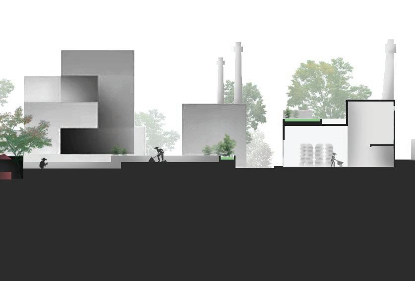
225 |
Rice mill
Drying yards
Road Design Proposal
Harvesting Hub
6.5 Adapted Urban System (0.7km2)
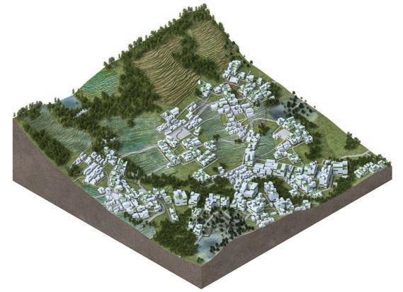
The generative procedures explained for cluster 1 in the previous chapter is repeated for the other two clusters in the experiment patch. In this step- certain opportunities, like the proximity of wetland node in cluster 2, present themselves which can be the drivers for possibly developing a new building morphology. The local networks within the clusters are worked out in the same way with the sub division of the cluster. Once the local networks are resolved, the identified primary roads are connected between the clusters at multiple levels, if necessary.
This regional network is the critical element in connecting the urban clusters that are interspersed by layers of other eco-systems, as shown in the diagram opposite. The network is analysed for additional urban proposal and this is presented in the following chapter.
| Adaptive Urban Hillscapes 226
Fig. 6.5.1
Urban tissue of 0.7 km2
Built fabric
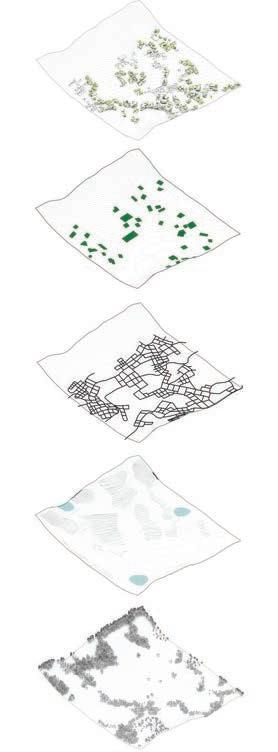
Operational public spaces
Networks
Terracing - agriculture - slope stabilisation
Forest
227 |
Fig. 6.5.2 Layers of subsidiary eco-systems
Design Proposal
6.5.1 Site Section BB
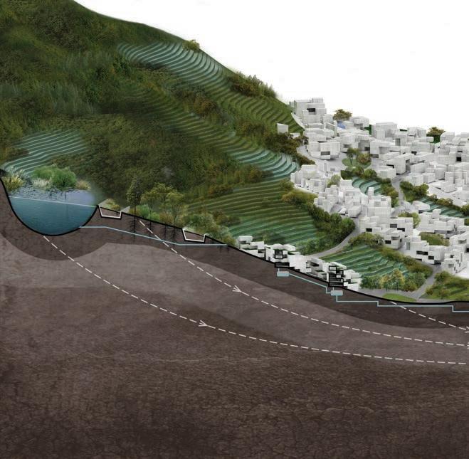
| Adaptive Urban Hillscapes 228
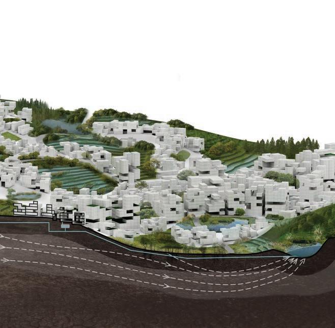
229 | B B Design Proposal
6.5.2 Site Section AA
The local interrelationships between built-up and vegetated areas is translated into the exchange of underground water flow through natural or artificial drainage systems. These mechanisms respond to the natural requirement for a balanced soil saturation condition that prevents soil loss driven by rainfall, as the drop in cohesion within sublayers of soil is prevented. Regarding this issue, the operation of public spaces emulating natural agents of underground water exchange becomes crucial. At the same time, when upcoming urban growth approach hillsides, the big impact of replacing vegetated coverage with buildings needs to be to some extent counteracted, returning the recharge properties of those specific plots. Therefore, an immediate task for the proposed morphologies is to catch water and recharge it to the
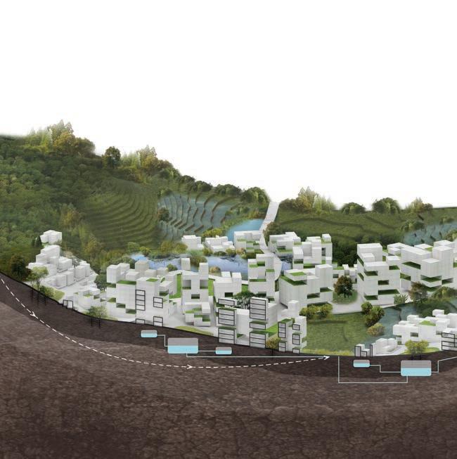
hill natural ecosystem and transfer those amounts of water into lower discharge areas.
In terms of natural supply systems, the positive impact that wetlands create on water purification is exploited by strategically locating them in between water catchment and storage zones. Whereas from the agricultural aspect, rice paddy terraces have multiple function of reducing surface erosion and discharging water from sublayers of soil while taking advantage of the terrain for food supply. The conditions that each of these spaces demand from their contiguous areas is still a task to be developed further.
| Adaptive Urban Hillscapes 230
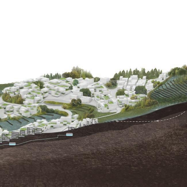
231 | A A Design Proposal
6.6 Renders
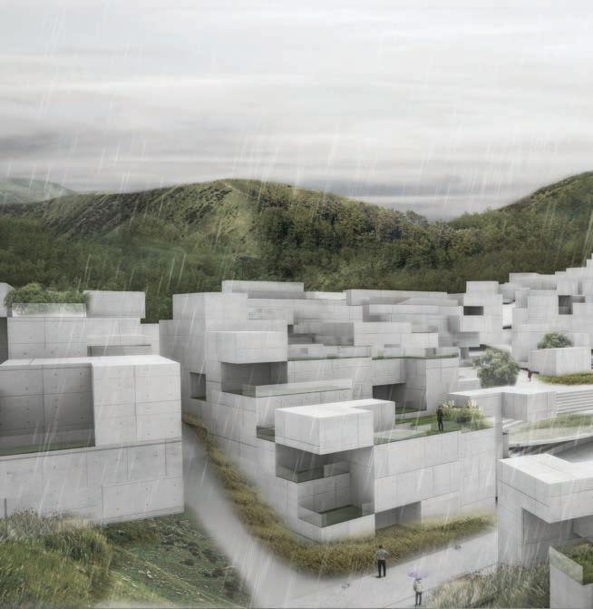
| Adaptive Urban Hillscapes 232
View 1 - Cluster 1, looking north
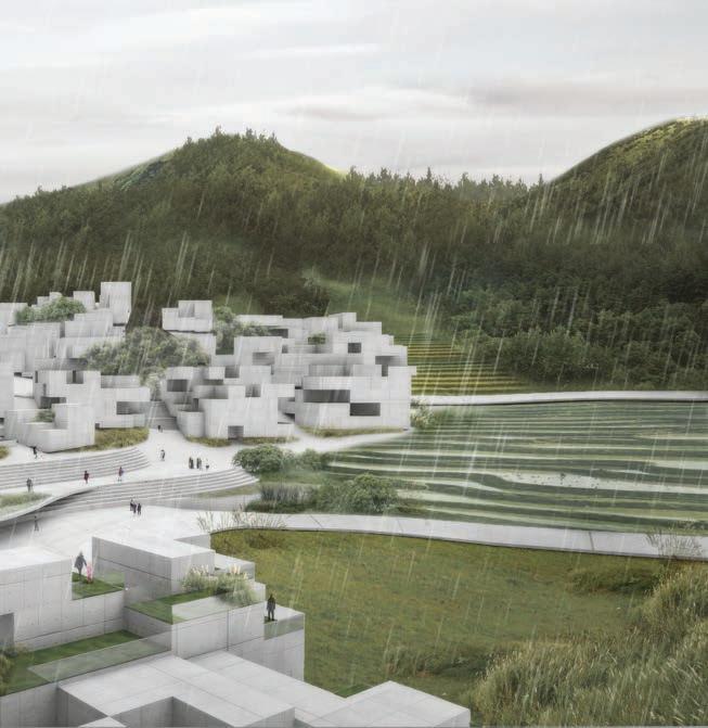
233 | Design Proposal
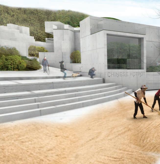
| Adaptive Urban Hillscapes 234
View 2 - Harvesting Hub
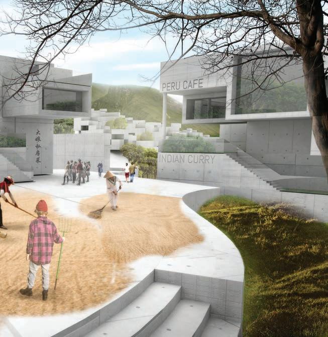
235 | Design Proposal
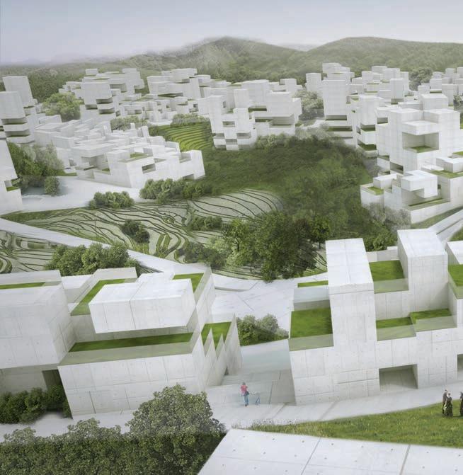
| Adaptive Urban Hillscapes 236
View 3 - From the topmost buildings in Cluster 1, looking south
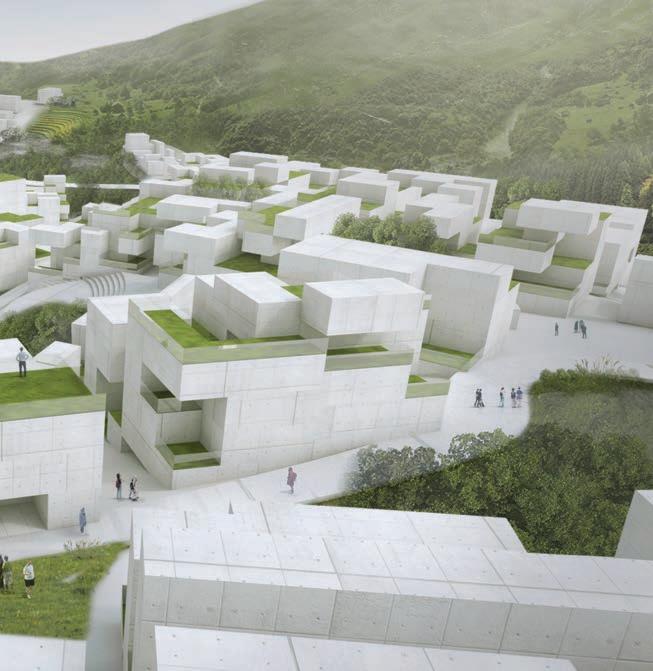
237 | Design Proposal
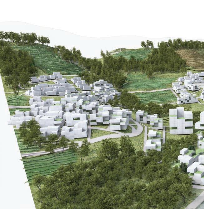
| Adaptive Urban Hillscapes 238
View 4 - From the west corner of the experiment patch
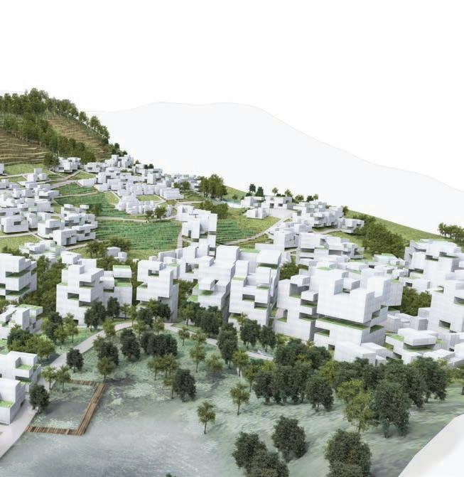
239 | Design Proposal
Critical Analysis 07.
PRODUCED BY AN AUTODESK PRODUCED BY AN AUTODESK EDUCATIONAL PRODUCT AUTODESK EDUCATIONAL PRODUCT
AUTODESK EDUCATIONAL PRODUCT PRODUCED BY AN AUTODESK PRODUCED BY AN AUTODESK EDUCATIONAL PRODUCT 7.1 Network analysis 7.2 Street operation and public connectivity 7.3 Building evaluation 7.4 Conclusion
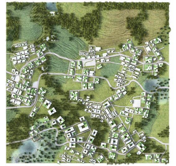
| Adaptive Urban Hillscapes 242
7.1 Network Analysis (0.7km2)
7.1.1 Commercial Amenities
The proposed network connecting the experiment patch is analysed to check the slope gradients of every network segment and it is segregated accordingly. Additional adjustments are made, such that every part of the cluster is accessed by streets and not just stairs.
Markets and shops can be proposed along busy network segments, when traversing between the three clusters in the experiment patch. A Betweeness analysis is done with every plot as the origin and two public spaces in each cluster as the destination. The most commonly used network segments along the shortest paths from every origin is indicated in the hotter colours (Fig 7.1.1.2). By cross checking these paths with the street types and the availability of building plots along them, commercial amenities can be proposed, possibly on the ground floor of the adjoining buildings.
243 |
Fig 7.1.1.1 Street types
Fig 7.1.1.1
Fig 7.1.1.2
Fig 7.1.1.2 Betweeness analysis Low
Streets with gradient > 1:8 Streets with gradient < 1:8 & Stairs High
High Low
Critical Analysis
7.1.2 Public Transport

Public transport stops are proposed solely along the main ring road in the valley (fig. 7.1.2.1), as this is the only existing connection to the other parts of the city. The macro scale network (for the 5.5 sqkm patch) is such that this ring road crosses the maximum number of urban clusters. (sec 5.6) In each cluster, public spaces that lie along the ring road are chosen and a reach analysis is done to know how many plots lie within a 400 metre network radius. This distance is taken as the 5 minute walking range on a path with mixed slope gradients (500m is considered as 5 minute walking distance on flat terrain).
Figure 7.1.2.1 shows the best option with maximum number of plots that are within a walkable network radius of 400m from the marked public transport stops. In this proposal, nine plots lie outside the required network radius. Within each cluster, it is also worth analysing the most used network segments considering the shortest route from every household to the respective public transport stop. Figure 7.1.2.2 shows the betweeness analysis and the streets represented in hotter colours can be taken the busiest segments for any further developments
| Adaptive Urban Hillscapes 244
Fig 7.1.2.1
High Low
Fig 7.1.2.2
30m400m 400m 30m
Fig 7.1.2.2 Betweeness analysis
High
Fig 7.1.2.1 Reach analysis - closest transport facility Public transport stop Ring road
Low
7.1.3 Social Amenities
This network experiment aims to locate social amenities like primary school and general health centre in a central location, closer to the maximum population within a 400 metre network radius. In this case, population count is considered more important than plot count. Based on the rule of thumb of 35 sqm. residential area per person, this patch has an estimated population of 9900 (density: 14,140/km2)
The other parameters than define the location are: - a minimum distance of 80 m between the school and health centre - school should be adjoining a designated open space that can act as a play field
- the social amenities need to be along a main road accessible by vehicles
The diagrams below show two experiments - the first one in a central location covers only 20% of the population whereas locating them at two locations as shown, can cover 81% of the population.
245 | 1 2325 habitants in 400m reach 2 5683 habitants in 400m reach BUS STOP BUS STOP BUS STOP 334m 30m
Fig 7.1.3.1
Fig 7.1.3.2
Fig 7.1.3.1 Experiment 1reach analysis for social amenities
EXPERIMENT 1 1900 / 9900 habitants in 400m network reach 334m 1900 habitants in 400m reach 50m EXPERIMENT 2 1 2325 habitants in 400m network reach 2 5683 habitants in 400m network reach 8008 habitants / 9900 habitants 1 2 Primary school Health centre 50m334m Critical Analysis
Fig 7.1.3.2 Experiment 2reach analysis for social amenities
7.2 Street Operation and Public Connectivity
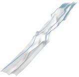
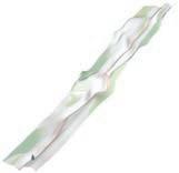
Terraced recharge streets

The selected plot distribution generates surface water flow diversions that contribute to the operation of green area seepage inside public spaces, but at the same time presents high volumes of water flowing through certain streets out of the urban cluster towards to gullies or adjacent farmlands and forests. In extreme precipitation conditions, water overload can harm land-uses that do not have a resistant drainage system operating. Moreover, the retention of water flowing across the city patch and the natural seepage down into the soil should be attempted to prevent further incidents of erosion and soil instability. Therefore, a strategy to provide certain streets the operation of retaining and draining water can be proposed by analysing which of the streets receives higher quantities of water during heavy rainfall and where is that water being diverted to.
Operational connectivity across public spaces
To enhance the public accessibility across different public spaces inside the cluster, specific connecting streets can be selected and evaluated in terms of the surface water flow incidence on them (Fig.7.2.4). The dimensions of these streets need to be considerably large so that enough green cover area can drain large amounts of water. Moreover, the diversion of surface water flow by plot orientation brings the opportunity to enhance the performance of these paths, as the generative computational process can calculate the required plot orientation for flows to be directed towards seepage streets. Providing the street network to perform both in terms of ecologic principles and urban connectivity.
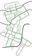
| Adaptive Urban Hillscapes 246
Public spaces Surface water flows Recharge streets Areas for recharge terraces Surface water flows Pedestrian path Main Roads 1:20 Gradient Street Typology > 1:8 < 1:8 Roads Stairs
Fig 7.2.1
Fig 7.2.2
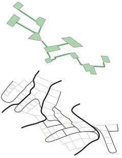
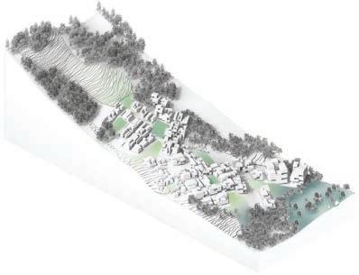
247 | Public spaces Pedestrian connectivity Primary Roads 1:20 Gradient Street Typology > 1:8 < 1:8 Roads Stairs
Fig. 7.2.4 Street type differentiation
Fig. 7.2.5
Final cluster and public space location
Fig. 7.2.3 Public connectivity trough public spaces
Fig 7.2.4
Fig 7.2.5
Critical Analysis
Fig 7.2.3
7.3 Building Evaluation
Building adaptation to adjacent ecosystems
Throughout the test patch, several group of buildings have a critical location as they are found in the boundary between two or more subsidiary ecosystems. The generative process of the city did not consider a morphological adaptation of buildings in such a way that they can have a response to these kinds of scenarios. Yet the possibility remains on evaluating environmental facts that can contribute to a design logic that takes advantage of the energy released by the variated surface covers of contrasting anthromes. For example, evapotranspiration and heat reflection are natural mechanisms of energy flow associated to different ecosystems, where the first one can be exclusively found in humid-vegetated areas and the second one in built environments. When certain buildings are found in between these natural cycles, the opportunity to apply thermal principles for ventilation into spaces can bring further variation on responsive architecture. Thermal differences on adjacent surfaces enhance natural ventilation flows that can be mapped to strategically generate uninterrupted voids across buildings; while discontinuous porosity can be counter productive in this scenario since reflected radiation will be trapped as hot air in the façade’s openings.
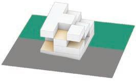
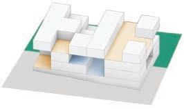
Humid / vegetated subecosystems
Dry areas
Heat reflection
Ventilation
Hot air trapped
Humid / vegetated subecosystems
Dry areas
Ventilation
Ventilation voids
Heat reflection
Dry areas
Hot air trapped
| Adaptive Urban Hillscapes 248
Fig 7.3.1
Fig. 7.3.1
Ventilation mechanisms affected by adjacent sub-ecosystems in hot humid climates
Flow diversion through plot orientation
In order to help street recharge operation, building plot shapes and their orientation can be set to divert surface water flows towards the desired areas where water can be soaked into the ground, potentially avoiding major water volumes on other vulnerable areas. Post-generation adjustments will have negligible effects since the designated process defines the plot orientation to satisfy alignment with the contour lines of the terrain, ignoring any incidence of plot orientation on flows. To apply properly this technique, it must be incorporated in the generative process itself so that other objectives are preserved and a resilient system is approached. Given the computational load that an algorithm can receive by simulating particle flow on different mesh combinations, an efficient and simple way for analysing the plots’ influence on surface flow is to simply evaluate the slope direction of the terrain where the plot curve lies (Fig7.3.2). This way an evaluation fitness criterion can be the convergence of water flows in the specific recharge streets that provide connectivity across the cluster through public spaces.
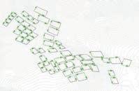
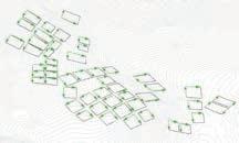
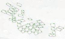
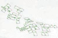
Plot curves
Predicted flow diversion
249 |
Fig. 7.3.2
Evaluation of flow diversion by plot curve orientation on slopes
Critical Analysis
Fig 7.3.2
Urban system: Opportunities for distinct approaches
An urban design provides the opportunity to bring social, ecological, and architectural features into the design through different stages. The question remains as to what is the order or sequence that should be maintained, hence setting priorities to some aspects over others. Bringing further into discussion the friction between cultural and ecological approaches that was mentioned at the end of the design strategy chapter, it can be concluded that social priorities can obstruct ecological performance of buildings if their spatial consequences are not evaluated both inside the private as well as the public areas. In qualitative terms, urban design should follow the cultural spatial patterns of a specific site, as they can foster identification between populations; but in contemporary cities, urban growth started to reach adjacent territories where different architectural responses are required to preserve the integrity of urbanization. It is at this scenario that this dissertation is situated, where the proposal encountered critical points at which certain compromises took place for the continuous development of the urban system.
Accomplishments on synchronization
A synchronical development of a contextualized urban system was achieved, taking under consideration the ecological conclusions and strategies that where set at a macro scale. The local farming practices shaped to some extent the direction of the work and evidently the socio-spatial characteristics of the local culture set the objectives of the architectural development. The rigour applied on the initial development of a 5.5 sq.km land-use map provided a solid background for an ecological-driven urban design process. High percentage of computation time was spent building an algorithm that processes the ecological principles taken from literature and displaying them in the land-use map, leading to a result that is strongly emphasizing the importance of spatial pattern arrangement in the anthropogenic landscape.
However, priorities set for the generative process of the urban tissue did not consider a responsive design towards the environmental forces of the hillsides. The ambition of the architectural development was more focused on the isolated spatial qualities of private and semi-private areas, partially ignoring the incidence that buildings can have over public spaces and the surrounding subsidiary ecosystems. A post-evaluation process tries to rescue and highlight some of the relevant features that buildings had for the benefit of public space, but those features were not set as quantifiable targets in the generative procedure, resulting in an architectural proposal that is adapted to its context more in the cultural aspect than in the ecological aspect. If features like spatial continuity were brought into the generative process, certainly a deeper exploration of ecological features could have been developed, focusing on flow-design tools to analyse in detail the effects of architectural design on environmental awareness; and bringing the opportunity to perform loops in the procedure to achieve larger variations of integrated results.
Computational Limitations
Computation plays a major part in exploring design scenarios with a wide range of factors. Although, the strategies explained in the earlier chapters takes advantage of this, there are some noticeable constraints that limit the full potential of the logics that are developed. As mentioned earlier, the urban system could have been generated for the entire 0.7 sq.km patch, consisting of 3 urban clusters, simultaneously achieving plot sub-divisions, local networks, public spaces with appropriate spatial metrics and responsive building forms. Furthermore, all of these elements could influence each other and the presence of multiple clusters and subsidiary ecosystems could present more complex opportunities with their interaction.
The flow simulations employed in this thesis is at a low resolution, and the calculation of volumes associated with this method is based on the rational equation (refer appendix). This deterministic method is also computaionally heavy, when attempted with a GA. Hence, volumes are not calculated at any stage. As previously mentioned, the only way to re-evaluate flows is using high-end CFD tools that is outside the scope of the associative modelling environment. Structural considerations are limited to assessing slope stability based on available soil data. For the purpose of architectural design in this thesis, it is attempted to establish a relationship between the load generated by a building (no. of storeys) and the shear strength of soil slopes at different inclination angles and soil conditions(bearing capacity). But such generalisations or rules of thumb for slope-load relation does not exist in engineering practice, and it is calculated on a case to case basis. (refer appendix) With increased computational power and maybe with customised genetic algorithms, the first couple of limitations can be addressed.
| Adaptive Urban Hillscapes 250
7.4 Conclusions
251 | Critical Analysis
* APPENDIX
PRODUCED BY AN AUTODESK PRODUCED BY AN AUTODESK EDUCATIONAL PRODUCT AUTODESK EDUCATIONAL PRODUCT
AUTODESK EDUCATIONAL PRODUCT PRODUCED BY AN AUTODESK PRODUCED BY AN AUTODESK EDUCATIONAL PRODUCT
Effect of Structures on Slopes
Hill slopes are unfavourable conditions for the construction of buildings, but over the years engineering methods have adapted, which has enabled massive structures to be built. Buildings transmit their loads to the slopes via their foundations. This results in the increase in shear stress, which on exceeding the shear strength of the soil causes instability of the soil slopes. (D.Raj et al., 2016)
For the purpose of architectural design in this thesis, it would be ideal to find or establish a relationship between the load generated by a building (no. of storeys) and the shear strength of soil slopes at different inclination angles and soil conditions(bearing capacity). But such generalisations or rules of thumb for slope-load relation does not exist in engineering practice. In the last few decades, every proposed building on slope is analysed on a case to case basis, by computationally calculating the critical failure plane using Limit Equilibrium Method (LEM) of slices and Finite Element Analysis(FEA). (Choudhary et al.,2009)
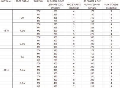
Paul and Kumar(1997) established a relation between slope failure and position of building along the slope. Failure may occur either locally or globally, which is affected significantly by the type of shallow foundation , foundation distance from the crest. Recent research by D.Raj and Singh(2016) pushes this by relating foundation load(no. of storeys of the building), slope angles, foundation location and width. They conclude that bearing capacity of the soil changes at every location on the slope with those parameters.
Foundations can be broadly categorised as Soil loading foundationsall shallow and deep foundations that transfer load to the soil layer and Pile foundations- that are embedded in the bedrock (refer fig2.5.6.3). The latter is usually isolated from the effects and affects of the soil layer. In order to analyse the influence of soil loading foundations on inclined slopes, consider Fig.2.5.6.2. For the marked locations, M1,M2,M3 at varying distances 'd' from edge and slope angles of 20 , 30 degrees; the authors solve to get the failure conditions and hence the ultimate bearing capacity. The existing methods of estimating bearing capacity ignore the slope-foundation interaction.
The results of their experiment shows Local, Global or Mixed mode failure according to the location and size of foundation at different inclination angles (Fig.2.5.6.4). Once the failure conditions are reached, they are able to estimate the degradation of the factor of safety of the slope with increasing loads. The conclusion given below shows estimated Ultimate Load Bearing capacity at every location along the slope(Mn) and distance from the slope edge(d). (D.Raj et al., 2016)
For this thesis the research can be interpreted in the following ways: Foundations at the top of a slope are most vulnerable to slope failure, where as foundations at lower parts of a slope are most stable. FOS for all slopes increases with the foundation width and its distance from slope edge. The conclusions of calculating the ultimate bearing capacity are translated into the number of storeys of building (residential).
| Adaptive Urban Hillscapes 254
LEM and FEA methods applied to calculate slope failure plane (Min Ng et al., 2014)
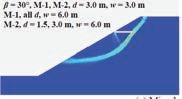
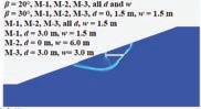
Slope geometr y and foundation locations considered for the study by D.Raj and
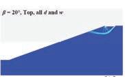

d- distance from slope edge
w- foundation width
A)Soil loading foundations -Isolated footing
B)Pile Foundation
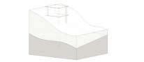
Simulation results of failure conditions for the study by D.Raj and
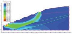
255 | Appendix
Fig 2.5.6.4
Fig 2.5.6.1
Fig 2.5.6.2
Y.Singh,2016 <redrawn>
Fig 2.5.6.4
Y.Singh,2016
Fig 2.5.6.1
Fig 2.5.6.2
M1 =20O ,30O
M2 M3 TOP d
w
A) B)
Local Failure
=20o @ TOP ; all d and w Global Failure =30o @ TOP ;all d and w
=20o @ M1,M2,M3 ; all d
=30o
@ M1,M2,M3 ; all d and w=1.5m @ M1; d=3m and w=1.5m @ M2; d=0m and w=6m @ M3; d=3m and w=3m
Mixed mode Failure
=30o @ M1,M2 ; d=3m and w=3m
=30o @ M1 ; all d and w=6m @ M2; d=1.5m,3m and w=6m
=20o @ TOP ; all d and w Local Failure
Structural Technologies
Gravity Wall
Gravity wall is a standard wall type that holds the earth mainly through its own weight as the internal leverage of the earth pressure is very high.
Context: Applicable to various small and medium-sized landslides where their thrusts are no more than 200KN/m .
Material: Mortar less, stone or concrete units
Advantages: Do not require a rigid footing in frost areas
Disadvantages: Uneconomical because the material is used only for its dead weight
Cantilever Wall
The cantilever wall (which may also extend in the other direction) uses the same earth pressure trying to topple it to stabilize itself with a second lever arm.
Context: Commonly used in sand or gravel soil. It may be used as permanent structures, but in general they are used only for temporary support.
Material: Concrete or mortared masonry (often in the shape of an inverted T) [R.F. Craig ,1997 Soil Mechanics, Sixth edition]
Advantages: Force from the earth can be used for stabilizing
Disadvantages: Instability of the retaining soil mass will cause rotation or translation of the wall.
Pile Wall
Using long pile, the wall is fixed by soil on both sides of its lower length. If the piles themselves can resist the bending forces, this wall can take high loads.
Context: Usually used in soft soils and tight spaces.
Material: Steel, vinyl or wood planks
Advantages: Less damage to the soil
Disadvantages: May be altered depending on the environment
| Adaptive Urban Hillscapes 256
Fig. 2.6.3.1
Own drawing, based on geotechnical course documents of the Technische Universität Darmstadt.
Reactive force vector Gravity Earth pressure vector Reactive force vector Reactive force vector Reactive force vector Earth pressure vector Earth pressure vector Reactive force vector Gravity
Fig. 2.6.3.1
Anchored Wall
This wall keeps itself from toppling by having cables driven into the soil or rock, fixed by expanding anchors (can be combined with other types of walls)
Context: An anchored retaining wall can be constructed in any of the aforementioned styles but also includes additional strength using cables or other stays anchored in the rock or soil behind it.
Material: Steel, vinyl or wood planks
Advantages: This method is very useful where high loads are expected, or where the wall itself has to be slender and would otherwise be too weak.
Disadvantages: Technically complex
Nailed Wall
Soil nailed walls consists of installing passive reinforcement (i.e., no post-tensioning) in existing ground by installing closely spaced steel bars or sections (i.e., nails) and placing a front face support.
Context: All soil nails within a cross section are located above the groundwater table (proven economically efficient), and can be used together with retaining wall.
Material: Steel and concrete
Advantages: Cost-effectiveness over other alternatives, much more economical than concrete gravity walls and similarly or more cost effective than ground anchor walls.
Disadvantages: Technically complex
257 | Reactive force vector Earth pressure vector Original ground surface Permanent facing Temporary facing
Fig. 2.6.3.2 Redrawn from: geotechnical course documents of the Technische Universität Darmstadt.
Appendix
Fig. 2.6.3.2
source:
Hydrological Network Study
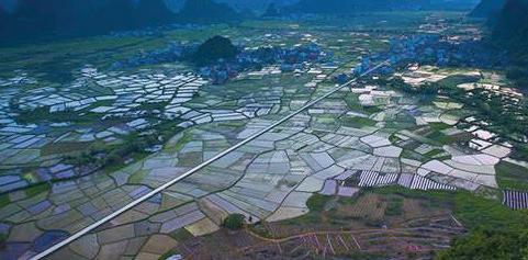
Irrigation Aqueducts
In a steep terrain rice terraces areas, Asian civilizations created unique irrigation systems to transfer accumulated water from the mountain streams into the rice terraces, by implementing canals and ditches. Main channels along high elevated contours intercept water flows from forests while secondary branch channels transfer water perpendicularly to the contour towards lower levels where the rice terraces are located. Tertiary branches could be implemented as needed. These mechanisms guaranteed sustainable utilization of water resources as the local people are involved in these practices.
| Adaptive Urban Hillscapes 258
Fig. Irrigation canal across Chinese rice paddies.
MAIN CANAL
259 |
Fig. Canal layout of irrigation system in East Laguna Bay, Phillipines. Redrawn from: A Rice Village Saga (Hayami and Kikuchi, 2000)
Lagoon
Fig. Details from the five laterals of the irrigation system rice paddies in the East Laguna Village. Data obtained from: A Rice Village Saga (Hayami and Kikuchi, 2000)
WATER SOURCE Lateral A A-2 A-1 B-1 A-1-A C-2 C-3 C-1 C-1-A D-1 E-2 E-1 A-1-A-2 A-1-B A-1-A-1 A-2-B A-2-C Lateral B Lateral C Lateral D Lateral E Lateral B 6.0 240 1 2 159 Lateral E 4.9 227 1 3 121 Lateral A 29.3 1602 9 17 1070 Lateral C 8.0 336 1 5 193 Lateral D 16.7 842 4 10 532 Average 12.98 649.4 3.2 7.4 415 Length of lateral (km) Service area (ha) Number of sub-laterals Number of villages Number of farms Appendix
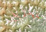
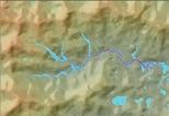

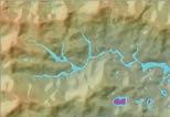
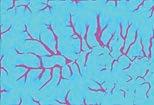
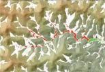
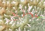
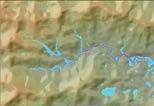
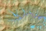
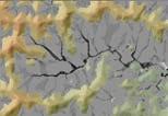
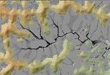
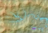
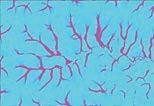
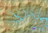
| Adaptive Urban Hillscapes 260 Flow velocity _ Day 10 Erosion depth _ Day 10 Erosion depth _ Day 19 Erosion depth _ Day 25 Flow velocity _ Day 19 Flow velocity _ Day 25 Grain size _ Day 10 Grain size _ Day 19 Grain size _ Day 25
depth _ Day 10
_ Day 19
Day 25 Water depth _ Day 19
depth _ Day 25
Water
Drainage
Drainage _
Water
Soil Erosion Simulation in CAESAR-lisflood 1.9b
Surface Runoff Estimation
Any drainage design has to be sized according to the probability of occurrence of an expected peak discharge. Discharge is calculated as volume/unit time. Surface hydrology and drainage principally depends on:
1. Slope shape;


2. Slope gradient/angle;
3. Slope length;
4. Soil Texture and permeability;
5. Depth to bedrock.
The proportion of rainfall that becomes stream flow depends on :
1. Area of drainage basin which is directly proportional to the runoff volume;
2. Topography ie. slope steepness is directly proportional to the runoff volume;
3. Soil characteristics, especially permeability and infiltraction capacity affect runoff inversely.
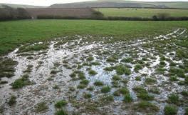
Rational Equation Method
This is a much simplified method to estimate surface discharge.
Q = 0.278 C i A
Q Peak discharge (m3/sec)
i Peak Rain intensity (mm/hr)
A Drainage basin area (Km2)
C Runoff Coeffecient (Related to soil texture, slope gradient) refer Appendix
Numerous assumptions are necessary for use of the rational formula:
(1) the rate of runoff must equal the rate of supply (rainfall excess) if train is greater than or equal to tc; (2) the maximum discharge occurs when the entire area is contributing runoff simultaneously; (4) rainfall is uniformly distributed over the basin; (5) recurrence interval of Q is the same as the frequency of occurrence of rainfall intensity I; (6) the runoff coefficient is constant between storms and during a given storm and is determined solely by basin surface conditions. The fact that climate and watershed response are variable and dynamic explain much of the error associated with the use of this method.
Total discharge for a patch with different ground surface types, at peak rainfall intensity, would be
Qtotal( m3/sec) = 0.278( Ci i A )
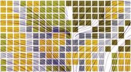
Estimated volume of discharge at peak rainfall intensity over a time period T (days)
VolumeT (m3) = 86400(Qtotal )
261 | convex parallel concave
Fig. 3.6.2
1. Built area
2. Asphaltic area
3. Gravel paving
4. Soil type 1
5. Soil type 2
Fig. 3.6.2 Example patch C (runoff coeff.) categories
Fig. 3.6.1
Slope shape types
Appendix
Fig. 3.6.1
Cluster Subdivision (cluster 1) - GA Results
angle in 1st hierarchy openspace (r)
| Adaptive Urban Hillscapes 262
slope angle in 1st hierarchy openspace (r) 0.17 0.18 0.16 0.18 -262.18 -273.86 -270.91 -254.99 0.63 0.84 0.72 0.65 0.83 0.75 0.53 1.00 0.40 0.61 0.41 0.49 average elevation in 2nd hierarchy
space () open space shading ratio in summer production open space exposure ration in winter remap value for build-up volume & open space SVF Objectives Fino Types G49.01 G49.02 G49.03 G49.04 1 2 3 4 5 G 4901 1 2 3 4 5 G 4902 1 2 3 4 5 G 4903 1 2 3 4 5 G 4904 0.16 0.20 0.16 0.19 -257.29 -255.91 -256.69 -254.78 0.43 0.50 0.45 0.43 0.98 0.83 0.84 0.70 0.93 0.67 0.44 0.95 slope
average
in summer production open space exposure ration in winter remap value for build-up volume & open space SVF Objectives Fino Types G49.05 G49.06 G49.07 G49.08 1 2 3 4 5 G 4905 1 2 3 4 5 G 4906 1 2 3 4 5 G 4907 1 2 3 4 5 G 4908
open
elevation in 2nd hierarchy open space () open space shading ratio
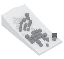

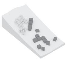
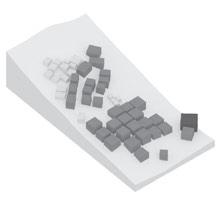
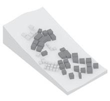
263 | 0.15 0.29 0.17 0.12 0.19 0.14 0.32 0.19 -256.47 -256.36 -268.03 -244.45 -240.12 -252.17 -251.56 -249.47 0.51 0.38 0.58 0.51 0.61 0.48 0.49 0.59 0.81 0.56 0.76 0.66 0.82 0.61 0.88 0.53 0.96 0.80 0.84 0.91 0.60 0.72 0.80 1.06 slope angle in 1st hierarchy openspace (r) average elevation in 2nd hierarchy open space () open space shading ratio in summer production open space exposure ration in winter remap value for build-up volume & open space SVF Objectives Fino Types slope angle in 1st hierarchy openspace (r) average elevation in 2nd hierarchy open space () open space shading ratio in summer production open space exposure ration in winter remap value for build-up volume & open space SVF Objectives Fino Types G49.13 G49.14 G49.11 G49.10 G49.09 G49.15 G49.12 G49.16 1 2 3 4 5 G 4909 1 2 3 4 5 G 4910 1 2 3 4 5 G 4911 1 2 3 4 5 G 4912 1 2 3 4 5 G 4913 1 2 3 4 5 G 4914 1 2 3 4 5 G 4915 1 2 3 4 5 G 4916 Appendix

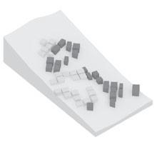
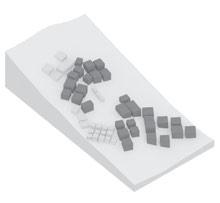

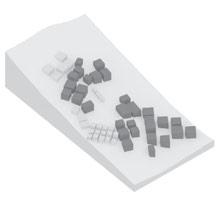
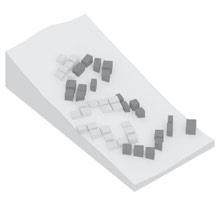
| Adaptive Urban Hillscapes 264 slope angle in 1st hierarchy openspace (r) average elevation in 2nd hierarchy open space () open space shading ratio in summer production open space exposure ration in winter remap value for build-up volume & open space SVF Objectives Fino Types slope angle in 1st hierarchy openspace (r) average elevation in 2nd hierarchy open space () open space shading ratio in summer production open space exposure ration in winter remap value for build-up volume & open space SVF Objectives Fino Types 0.18 0.32 0.18 0.15 0.12 0.12 0.17 0.15 -255.07 -259.50 -252.57 -256.91 -270.91 -247.49 -246.09 -261.63 0.64 0.51 0.51 0.53 0.34 0.43 0.56 0.25 0.95 0.53 1.00 0.54 0.49 0.95 0.59 0.46 0.64 0.90 0.66 0.92 0.86 0.74 0.39 0.42 G49.17 G49.21 G49.18 G49.22 G49.19 G49.23 G49.20 G49.24 1 2 3 4 5 G 4917 1 2 3 4 5 G 4918 1 2 3 4 5 G 4919 1 2 3 4 5 G 4920 1 2 3 4 5 G 4921 1 2 3 4 5 G 4922 1 2 3 4 5 G 4923 1 2 3 4 5 G 4924

265 | slope angle in 1st hierarchy openspace (r) average elevation in 2nd hierarchy open space () open space shading ratio in summer production open space exposure ration in winter remap value for build-up volume & open space SVF Objectives Fino Types 0.17 0.14 0.18 0.21 -262.67 -274.81 -257.74 -254.96 0.70 0.74 0.43 0.57 0.59 1.00 0.57 0.56 0.45 0.85 0.84 0.38 G49.25 G49.26 G49.27 G49.28 1 2 3 4 5 G 4925 1 2 3 4 5 G 4926 1 2 3 4 5 G 4927 1 2 3 4 5 G 4928 slope angle in 1st hierarchy openspace (r) average elevation in 2nd hierarchy open space () open space shading ratio in summer production open space exposure ration in winter remap value for build-up volume & open space SVF Objectives Fino Types 0.15 0.30 0.14 0.11 -242.57 -259.52 -255.16 -255.66 0.55 0.35 0.58 0.35 0.71 0.62 0.45 0.82 0.61 0.93 1.01 0.96 G49.33 G49.34 G49.35 G49.36 1 2 3 4 5 G 4933 1 2 3 4 5 G 4934 1 2 3 4 5 G 4935 1 2 3 4 5 G 4936 Appendix
slope angle in 1st hierarchy openspace (r) average elevation in 2nd hierarchy open space () open space shading ratio in summer production open space exposure ration in winter remap value for build-up

| Adaptive Urban Hillscapes 266 G49.37 G49.38 G49.39 G49.40
volume & open space SVF
Fino Types 0.10 0.15 0.18 0.11 -261.29 -252.20 -249.33 -258.39 0.29 0.60 0.74 0.45 0.74 0.56 0.69 1.00 0.96 0.78 0.73 0.52 1 2 3 4 5 G 4937 1 2 3 4 5 G 4938 1 2 3 4 5 G 4939 1 2 3 4 5 G 4940
Objectives
267 | Appendix
Building Generation (cluster 1) - GA Results


| Adaptive Urban Hillscapes 268
total build-up volume courtyard sky view factor remap value courtyard shading ratio in summer solstice courtyard exposure ratio in winter solstice Objectives Fino Types G49.05 G49.06 G49.07 G49.08 0.283 0.273 0.267 0.270 235985 239874 230330 227576 0.83 0.00 0.08 0.00 0.60 0.86 0.61 0.86 0.35 0.12 0.35 0.13 1 2 3 4 5 G 4905 1 2 3 4 5 G 4906 1 2 3 4 5 G 4907 1 2 3 4 5 G 4908
total build-up volume courtyard sky view factor remap value courtyard shading ratio in summer solstice courtyard exposure ratio in winter solstice Objectives Fino Types G49.09 G49.10 G49.11 G49.12 0.279 0.272 0.270 0.268 250274 229164 237054 235307 0.59 1.00 0.41 0.26 0.65 0.63 0.64 0.65 0.31 0.33 0.32 0.31 1 2 3 4 5 G 4909 1 2 3 4 5 G 4910 1 2 3 4 5 G 4911 1 2 3 4 5 G 4912
south facing ratio
south facing ratio


269 | 0.281 0.283 0.273 0.274 237293 237337 236985 226575 0.67 0.66 0.10 0.80 0.62 0.62 0.64 0.61 0.34 0.34 0.32 0.35 G49.21 G49.22 G49.23 G49.24 south facing ratio total build-up volume courtyard sky view factor remap value courtyard shading ratio in summer solstice courtyard exposure ratio in winter solstice Objectives Fino Types 1 2 3 4 5 G 4921 1 2 3 4 5 G 4922 1 2 3 4 5 G 4923 1 2 3 4 5 G 4924 south facing ratio total build-up volume courtyard sky view factor remap value courtyard shading ratio in summer solstice courtyard exposure ratio in winter solstice Objectives Fino Types 0.273 0.280 0.280 0.265 244562 252200 221631 227321 0.41 0.59 0.48 0.18 0.87 0.65 0.60 0.57 0.12 0.31 0.37 0.39 G49.25 G49.26 G49.27 G49.28 1 2 3 4 5 G 4925 1 2 3 4 5 G 4926 1 2 3 4 5 G 4927 1 2 3 4 5 G 4928 Appendix
PRODUCED BY AN AUTODESK PRODUCED BY AN AUTODESK EDUCATIONAL PRODUCT AUTODESK EDUCATIONAL PRODUCT
* BIBLIOGRAPHY
AUTODESK EDUCATIONAL PRODUCT PRODUCED BY AN AUTODESK PRODUCED BY AN AUTODESK EDUCATIONAL PRODUCT
Kjekstad, O; Highland, L. (2009) Landslides: Disaster risk reduction, chapter: Economic and Social impact of landslides
Ewing, R. (1994) Causes, characteristics, and effects of sprawl: a literature review. Environmental and Urban Issues 21(2): 1-15.
Parriaux, A. (2011) Vulnérabilité des infrastructures géotechniques au changement climatique et mesures d'adaptation selon le contexte géographique. World Road Association. Technical report.
University of Exeter. (2007) Agricultural Soil Erosion Not Contributing to Global Warming. Study Shows, Sciendaily, <https://www.sciencedaily.com/releases/2007/10/071025143317.htm> [Accessed on 15 Feb 2016].
Johnson, K., Sitar, N. (1990) Hydrologic conditions leading to debris-_ow initiation. Can., Geotech. J., Volume 27:789_801.
Ellison, W.D. (1948) Soil Erosion. Soil Science Society of America Journal, 12:479-484
Carter, V. (1996) Technical aspects of wetlands, Wetland Hydrology, Water Quality, and Associated Functions. National Water Summary on Wetland Resources, United States Geological Survey Water Supply Paper. 2425
Winter, T.C. (1976) Numerical simulation analysis of the interaction of lakes and ground water: U.S. Geological Survey Professional Paper 1001, p. 45
Winter, T.C., Harve J.W., Franke O.L., Alley W.M. (2013) Ground water and surface water a single resource, United States Geological Survey, USGS Circular 1139.
Danjon, F., Barke, D., Drexhage, M. (2008) Stokes A Using three dimensional plant root architecture in models of shallow-slope stability, Annals of Botany.
Ellison, W.D. (1948) Soil Science Society of America Journal
UN ESCAP report. (2013) Urbanization trends in Asia and the Pacific
Weiwen, H. (2008) The Deputy Director of the Urban and Architecture Department at Shenzhen Municipal Planning Bureau, AD New Urban China.
Konrad, C.P., Booth D.B. (2002) Hydrologic trends associated with urban development for selected streams in the Puget sound basin.
David, H. (2012) 100 Year forecast, Institute for the future.
Coco, L. (2015) One Chinese City’s Struggle With Water Scarcity, The Diplomat.
Wan, R.I. (1997) The impact of hill land clearance and urbanization on runoff and sediment yield of small catchments in Pulau Pinang, Malaysia. IAHS Publ. no. 245.
Michael, S., Patricia, C.A., Robert, M.B. (2009) Urbanization and Growth, Commission on growth and development.
Davi, S., Gordo, M., Cecili, T (2010) Urbanization and its implications for food and farming,
| Adaptive Urban Hillscapes 272
Bibliography
Urban sprawl: A case study of Shenzhen, China. QI Lei, LU Bin, 44th ISOCARP congress ‘08
Shiqiang, D., Peijun, S., Anton, V.R. (2013) The Relationship between Urban Sprawl and Farmland Displacement in the Pearl River Delta, China.
Wendy, W.F. (2013) An urban refuge in hong kong: transitional housing for displaced informal settlements.
Cheung, D.K.P., Li, R.P.M., Lorimer, M.J & Swann, L.H.. (2011) Application of Soil Bioengineering Measures to Man-made Slopes - A Pilot Study under the Landslip Preventive Measures (LPM) Programme.
Parry, S., Hart, J.R & Jack C.D. (2011) Science, Engineering Geology and the Landslip Preventive Measures Programme.
Ratti, C., Sabatino, S.D., Britter. D. (2005) Urban texture analysis with image processing techniques: winds and dispersion.
Miaomiao, X., Yanglin, W., Qing, C., Meichen, F., Minting Y. (2013) Assessment of landscape patterns affecting land surface temperature in different biophysical gradients in Shenzhen, China.
Li, T., Jiquan, C., Shi, X.Y., (2014) Coupled dynamics of urban landscape pattern and socioeconomic drivers in Shenzhen, China.
Guo, W, Li, S., Zhu, D. (2010) Modern geomorphological environment research during rapid urbanization in Shenzhen east coastal zone.
Wenting, Z., Bo, H., (2014) Soil erosion evaluation in a rapidly urbanizing city (Shenzhen,China) and implementation of spatial land-use optimization.
Lennartz, B. (2008) Ecological safe management of terraced rice paddy landscapes.
Kim, H.K. (2009) Estimation of irrigation return flow from paddy fields considering the soil moisture.
Mano, J., Bernd, L. (2009) Water losses through paddy bunds: Methods, experimental data, and simulation studies.
Han-Che, H. (2003) Analysis of percolation and seepage through paddy bunds.
Shih-Kai, C. (2012) Experimental study on soil erosion characteristics in flooded terraced paddy fields
Yuanyua, Z. (2010) Study on Hani Terraced Field Complex Ecosystem and its Mechanism in Climate Change Adaptation in China.
Baoshan, C. (2008) Vertical characteristics of the Hani terrace paddyfield ecosystem in Yunnan, China.
Zhao, M. (2002) A GIS-based research on the distribution of rural settlements in Yulin of northern Shaanxi.
Xu, J. (2014) The planning pattern research on mountain rural settlements in Qinba regions
Xu, J. (2015) Analysis on Village Environment and Pattern Characteristics of Tongle Village in Yunnan Province
Geotechnical Engineering Office. (2011) Technical Guidelines on Landscape Treatment for Slopes.
273 |
Bibliography
Wei, Z. (2005) A dynamic comprehensive method for landslide control.
Craig, A.J. (2011) Combined Hydrology and Slope Stability Assessment of The Olympic Region of Washington State.
Cornelia, S.B. (2011) Effect of Groundwater on Landslide Triggering.
Martire, D.D. (2012) Landslide hazard and land management in high-density urban areas of Campania region, Italy.
The Hong Kong Geotechnical Society. (2011) Landslide Risk Reduction through Works - 35 Years of Landslip Preventive Measures Programme and Beyond.
Carol, M., Zeena, F. (2014) Slope Stability Analysis - Limit Equilibrium Or The Finite Element Method?
Bert, R (2007) The Role of Fine and Coarse Roots in Shallow Slope Stability and Soil Erosion Control with a Focus on Root System Architecture: a Review.
Nenghao, Z. (2007) Physical and Mechanical Properties of Sliding Zone Soil and Mechanism of Its Action on Landslide Deformation.
Gongxian, W. (2006) Choice And Optimization Of Landslide Control Plan.
Choi, K.Y (2013) Landslide disaster prevention and mitigation through works in Hong Kong.
Kjekstad, O., Highland, L. (2009) Landslides: Disaster risk reduction, Economic and Social impact of landslides.
Ewing, R. (2009) Causes, characteristics, and effects of sprawl: a literature review’. Environmental and Urban Issues 21(2): 1-15.
Parriaux, A. (2011) Vulnérabilité des infrastructures géotechniques au changement climatique et mesures d’adaptation selon le contexte géographique. World Road Association. Technical report.
Johnson, K., Sitar, N. (1990) Hydrologic conditions leading to debris flow initiation. Volume 27:789_801.
Jianfa, S. (2008) Urban Growth and Sustainable Development in Shenzhen City 1980-2006, Department of Geography and Resource Management, The Chinese University of Hong Kong, Shatin, NT, Hong Kong.
NASA. (2016) Global Landslide Catalog Aids View From Space < https://svs.gsfc.nasa.gov/cgi-bin/details. cgi?aid=11854> [Accessed on 18 April 2016]
Sharma, B. (1984). Multinational Corporations and Industrialization in Southeast and East Asia. Contemporary Southeast Asia, 6(2), pp.159-171.
de Smith,(2015) Goodchild, Longley, Geospatial Analysis-5th Edition
Andres Sevtsuk, Michael Mekonnen ,(2012), UNA- a new tool box
Pirouz Nourian1, Samaneh Rezvani, Sevil Sariyildiz, (2013), the Netherlands, Politecnico di Milano, Italy,
| Adaptive Urban Hillscapes 274
Suleiman Wassim, Joliveau Thiery, FAVIER Eric, A New Algorithm for 3D Isovist
Eugenio Morello, Carlo Ratti, (2009), A Digital Image of the City: 3-D isovists and a tribute to Kevin Lynch
Wenting Zhang & Bo Huang, (2014), Soil erosion evaluation in a rapidly urbanizing city (Shenzhen, China) and implementation of spatial land-use optimization
Dr.Braja Das,(2001), Principles of Geotechnical Engineering
Dr.Gue See Sew, Tan Yean Chin, (2000), Hill Site Development-Planning, Design, Construction & maintenance considerations
UN FAO, (2014), Guidelines and computer programs for the planning and design of land drainage systems
Dhiraj Raj, S.M.ASCE1, Yogendra Singh, M.ASCE2, Geo-Chicago, (2016) Effect of Building Loads on the Stability of Hill Slopes
Chen Jiefang. (2014)Research on Natural Ventilation System of Traditional Village in Chaoshan Area
Lu Qi, (2008), Taditiona Village in Guangdong, China, ISBN 978-7-112-10312-6
Tang Guohua, (2005), Traditional Architecture in Hot Humid Area, Ling Nan, China, ISBN 7-112-07263-8
Zhu Xuemei, (2013), Research on the Morphology of Traditional Village and Architectural Features in Northern Guangdong, A Dissertation Submitted for the Degree of Doctor of Engineering,
Alan M.Kantrowed.Sunrisesunset :Challenging the Mythof Industrial Obsolescence
Ellis E., Ramankutty N. Frontiers in Ecology and the Environment
Reed C., Lister N. (2014) Projective Ecologies, Harvard University Graduate School of Design, ACTAR 2014
Zhang, Y., Yang, J., Dai, R., Wang, Y., Xue, D. Study on Hani Terraced Field Complex Ecosystem and its Mechanism in Climate Change Adaptation in China, College of Life and Environmental Science, Minzu University of China, Beijing 100081, China
Hayami, Y., Kikuchi, M., (2000) A Rice Village Saga, Three Decades of Green Revolution in the Philippines, International Rice Research Institute
Arnfield AJ. (2003) Two decades of urban climate research: a review of turbulence exchanges of energy and water, and the urban heat island. Int J Climatol; 23(1):1e26
275 |
Bibliography
| Bibliography
