ACKNOWLEDGEMENTS
TO OUR FAMILIES, FRIENDS AND TUTORS
009
ARBOREAL FORMATIONS
TABLE OF CONTENTS
010
INTRODUCTION
ARBOREAL FORMATIONS
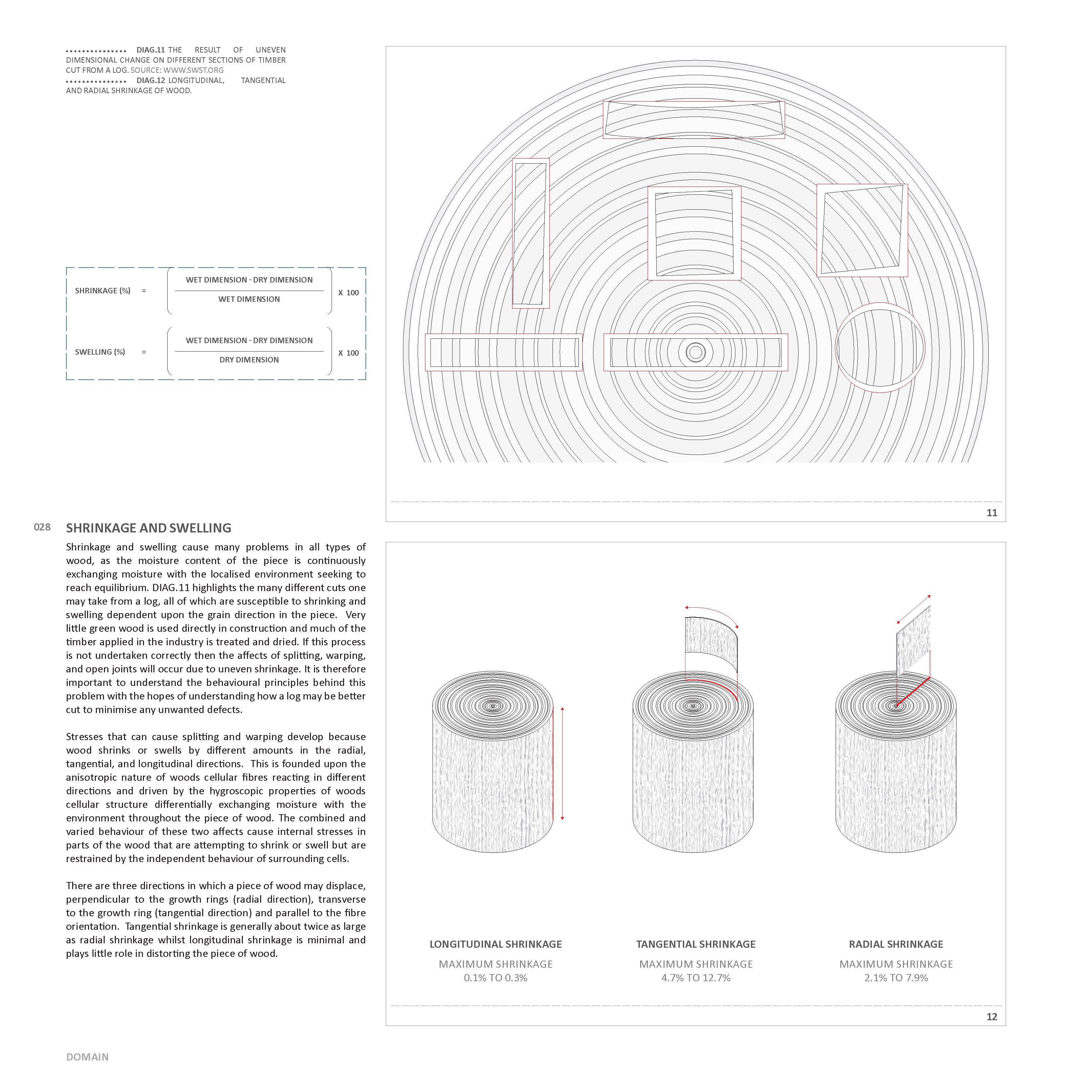
SHRINKAGE AND SWELLING
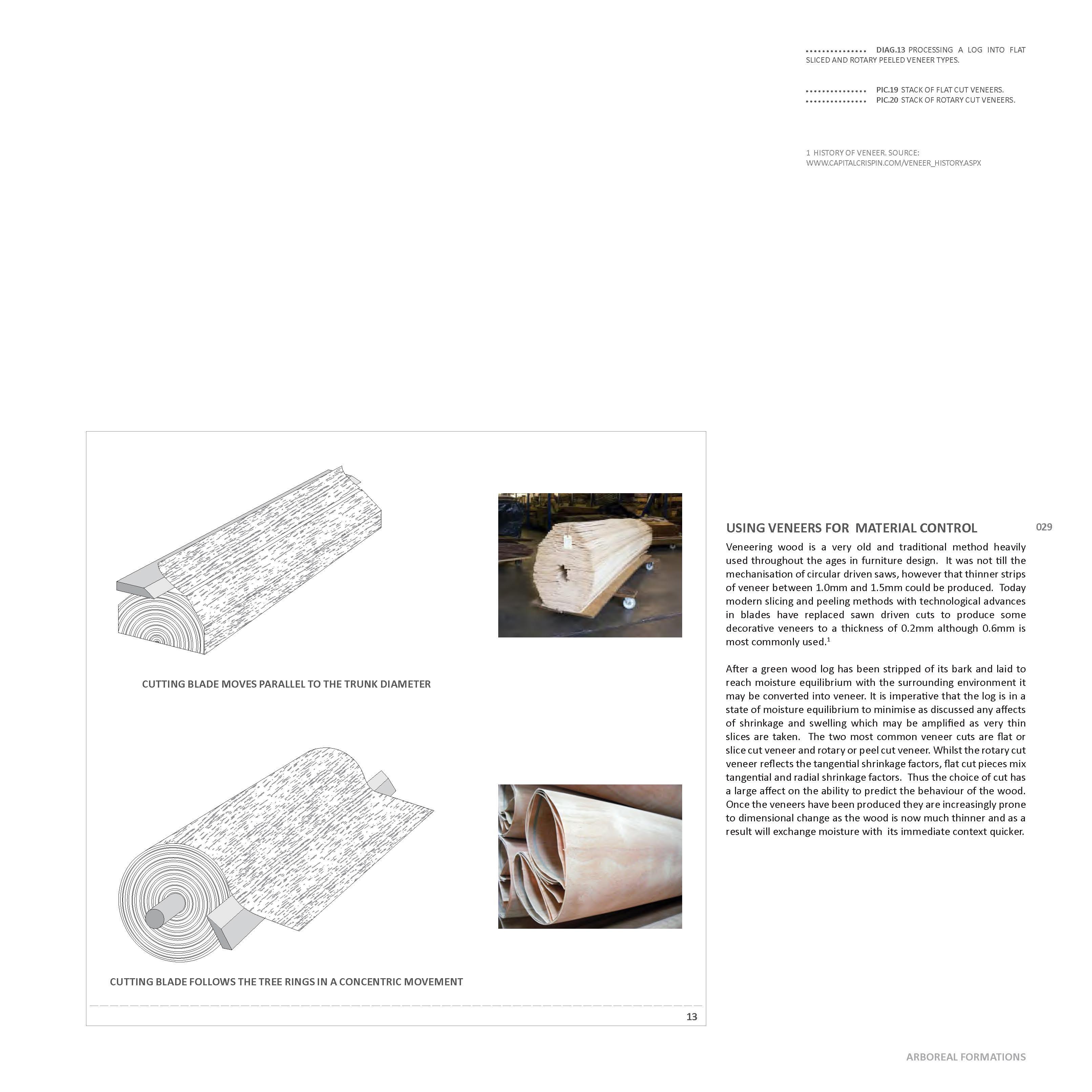
USING VENEERS FOR MATERIAL CONTROL
VARIABLE MOISTURE CONTENT BY CLIMATE
TIMBER DIMENSIONS BY LOCAL ENVIRONMENT 031
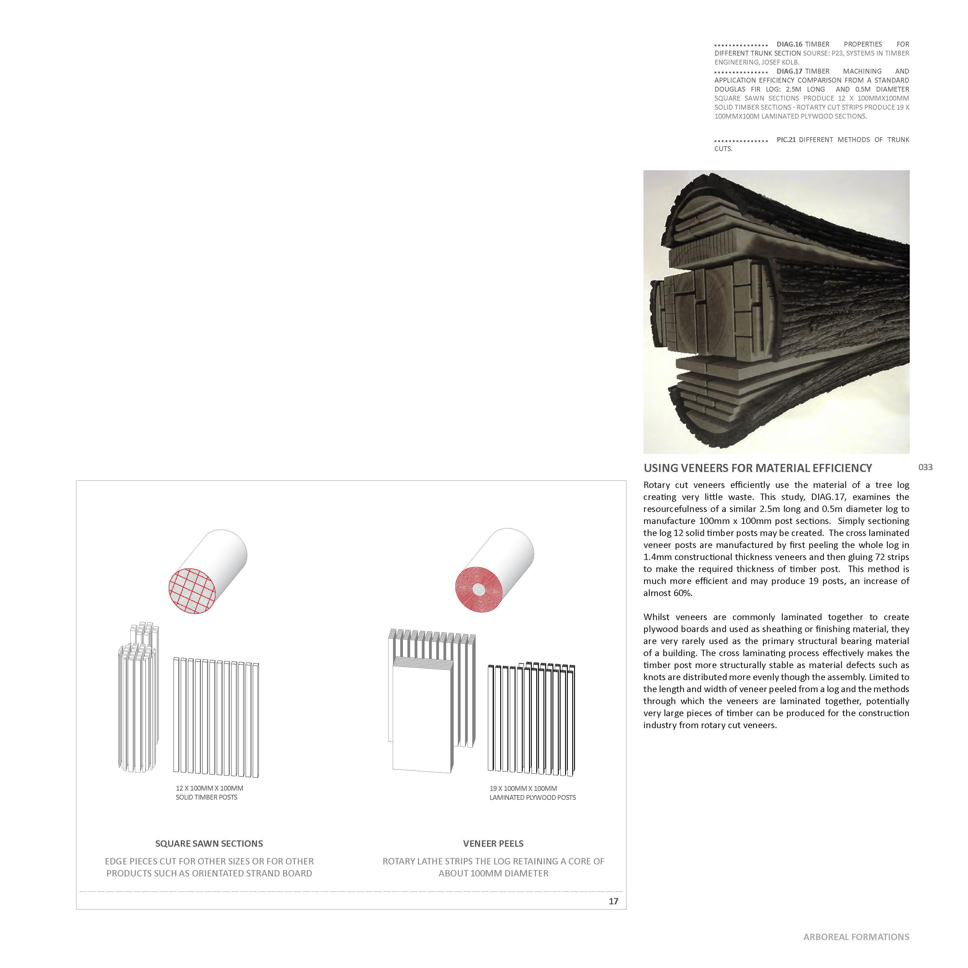
PROCESSING OF TREES TO TIMBER 0 32 USING VENEERS FOR MATERIAL EFFICIENCY
FABRICATING LARGE COMPLEX GEOMETRIES 035 GEOMETRY
STRUCTURAL PERFORMANCE
BENDING WOOD TECHNIQUES
KEYSTUDY : CHAISE LOUNGE
FABRICATION OBSERVATIONS 0 45
TIMBER APPLICATIONS SCALE 0 47
PROJECT SCALE AMBITION 0 47
MATERIAL SYSTEM AMBITION
METHODS
011 RESEARCH DEVELOPMENT 0 54 BASIC MATERIAL BEHAVIOUR PRINCIPLE 0 57 FABRICATION PRINCIPLE 0 59 GRAIN DIRECTIONALITY 0 61 FABRICATION METHOD 0 63 LAMINATION PROCEDURE 0 65 FROM PHYSICAL TO DIGITAL EXPERIMENTS 0 6 9 MATERIAL COMPONENT BEHAVIOUR 0 70 PHYSICAL EXPERIMENT PARAMETERS 071 PLATE CURVATURE:XX (/MM) 072 DIGITAL SIMULATION METHOD 073 PLATE CURVATURE:XX (/MM) 074 CALIBRATION BETWEEN WORKSPACES 075 01 WOOD SPECIES OF VENEER 077 03 THICKNESS OF VENEERS 079 04 NUMBER OF LAYERS 081 06 LENGTH OF COMPONENT 083 07 WIDTH OF COMPONENT 085 INFLUENCE OF PARAMETERS 087 EXTENDING COMPUTATIONAL DATA 089 MATERIAL COMPUTATION MATRIX 091 COMPONENT SAMPLES FROM THE MATRIX 0 93 CATOLOGUE OF MATERIAL COMPONENTS 0 95 FABRICATION DEVELOPMENT 0 96 RESEARCH DEVELOPMENT CONCLUSIONS 0 97 DESIGN DEVELOPMENT 0 98 COMPONENT ANALYSIS 1 01 KEY STUDY INTRO 1 03 KEY STUDY ANALYSIS 1 05 TIMBER IN MODERN RESIDENTIAL STRUCTURES 1 07 BUILDING SYSTEM STUDIES 1 09 STRUCTURAL SYSTEMS 1 11 BASIC GEOMETRY EXPLORATION 1 13 DEVELOPED GEOMETRY EXPLORATION 1 15 ASSOCIATIVE MODEL 1 17 GENERATIVE PARAMETERS 2D 1 21 STACKING OF GEOMETRICAL STATES 1 25 SAMPLE FLOOR PLANS 1 27 GENERATIVE PARAMETERS 3D 1 29 MORPHOLOGICAL VARIATIONS 1 31 DEFORMATION OF STRUCTURE 1 32 POTENTIALS AND LIMITATIONS 1 33 CONCLUSIONS 1 34 DESIGN PROPOSAL 1 36 PROJECT CONTEXT 1 38 MORPHOLOGICAL RESPONSE 1 41 PROGRAMMATIC STRATEGY 1 43 CONCLUSIONS 1 47 FURTHER DEVELOPMENTS 1 4 8 BIBLIOGRAPHY 1 5 0 WEBSITES 1 5 1 PICTURES 1 5 2 APPENDICIES 1 5 4
0 09 TABLE OF CONTENTS 0 10 ABSTRACT 0 14 INTRODUCTION 0 16 DOMAIN 0 18 MATERIAL DIMENSION INSTABILITIES 021 WOOD 0 22 EXPLORING WOOD 0 23 SUSTAINABLE RESOURCE 0 24
ACKNOWLEDGEMENTS
0 25
ENVIRONMENTAL IMPACT
0 26 WOOD
CELLULAR TISSUE 0 27
PRINCIPLES OF TIMBER BEHAVIOUR
A LIVING
0 28
029
0 30
0 33
0
37
0
37
0 39
0 41
0 49
0
0 52
0 52
50 METHODS
FLOWCHART
ARBOREAL FORMATIONS
012 INTRODUCTION
‘ARBOREAL’
IS DEFINED AS RELATING TO TREES.
013
ARBOREAL FORMATIONS
ABSTRACT
Arboreal Formations is a research project that investigates how specific properties of wood may be a driver for curving pieces of timber. The thesis documents an approach for generating design solutions that capitalise on the investigation and understanding of wood’s inherent properties. The work aims to create a generative process for a holistic building system implementing a methodology that prioritises materiality to enhance the relationship between material, structure and geometry.
The process investigates the calibration of physical experiments and digital simulations to define a component which may aggregate to form a system that is structurally coherent, fabrication efficient and expresses spatially dynamic morphologies. The characteristics of the component are integral to the material system and using an associative geometry is revealed in the design of a twenty storey timber residential block in New York City.
A novel fabrication technique and understanding of materiality are combined through the research to conceive a timber component that can be programmed to create a range of curvatures and be structural depending upon its thickness. The innovation presents an opportunity for new architectural spaces and forms to be created in wood.
KEYWORDS: INTEGRATED SYSTEMS, WOOD, HYGROSCOPIC BEHAVIOUR, ANISOTROPIC CHARACTERISTICS, MATERIAL COMPUTATION INFORMATION, VARIANT MORPHOLOGIES, ASSOCIATIVE MODEL
014
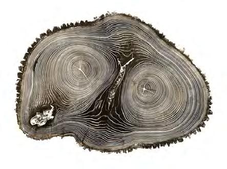
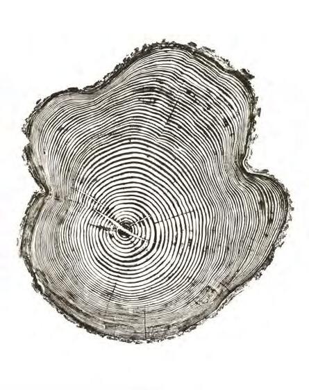
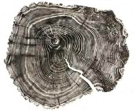
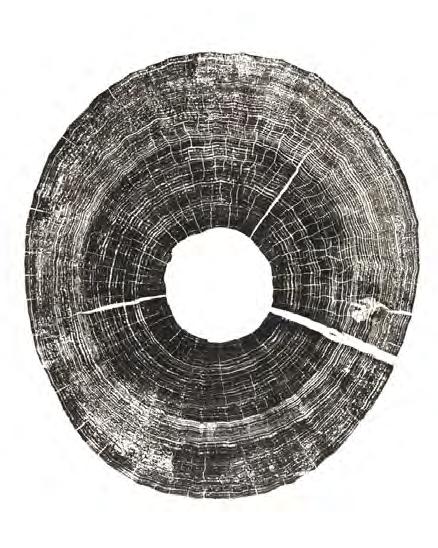
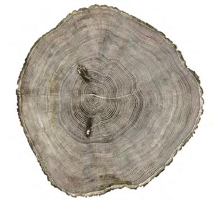
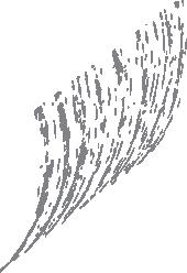
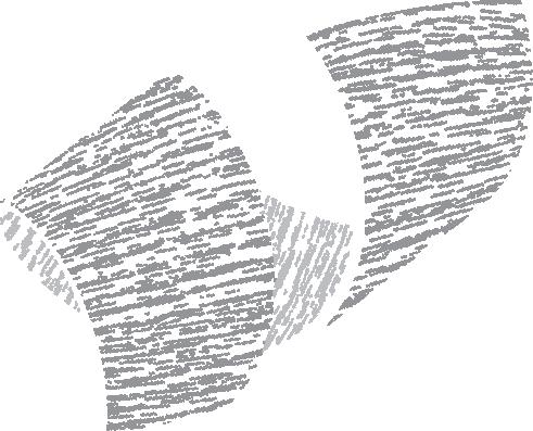
PIC.01 WOOD-CUT PRINT OF A WILLOW TREE BY BRYAN NASH GILL, 2011 PIC.02 ARBOREAL FORMATIONS. INTRODUCTION
“Arboreal Formations is a research project that investigates how specific properties of wood may be a driver for curving pieces of timber.”
015
ARBOREAL FORMATIONS
WOOD-CUT PRINT OF A WILLOW TREE BY BRYAN NASH GILL, 2011
RACHEL BEACH STACK, 2010; OIL AND ACRYLIC ON PLYWOOD, RECLAIMED LUMBER; 51 X 17 X 10 INCHES
INTRODUCTION
Nature exemplifies materiality, structure and morphology as three interwoven themes that contribute to the operation, performance and survival of an organism. Architecture often neglects the opportunity to unite these elements of design and instead separates them through a hierarchical approach that prioritises the overall project vision first. In turn this defines a process without interdependency or conviction as geometry, structure and material combine only to manifest the project outcome.
The aim of this project is to create a holistic building system, the logic of which is built upon the associated relationships of material, structure and morphology. Considering that materiality is often acknowledged last in a design process, the ambition of the work is to reverse that sequence and investigate how basic material properties can inform structure and geometry as an integrated material system.
Wood is a natural, cellular and fibrous material which when exposed to direct moisture or humidity changes is susceptible to movement. The Hygroscopic behaviour (ability to absorb moisture) and Anisotropic characteristics (direction dependent physical properties) of wood may be studied with incite to developing new fabrication techniques for the manufacture of curved pieces of timber.
The research initially explores through physical material testing the ability to predict the expanding and shrinking affects of moisture applied to thin veneer pieces of wood. This phenomenon is further investigated through fabrication processes for creating thicker elements. A principle discovery is made that when many veneer layers are differentially soaked, laminated together and left to dry, curvature and dependent upon grain direction twisting is induced into the piece. The physical experimentation is then transposed to computational simulations to run increased number of quicker tests. Focused on the curving behaviour of the component a process of calibration between physical and digital
workspaces is pursued determining which parameters influence the fabrication process and are quantifiable. This is a vital step for progressing with material information data that determines the potentials and limitations of proceeding application studies. The findings show that thinner timber elements can be fabricated with tight and more articulated curvatures and also thicker members be produced within a more limited range of curvatures.
Before the material component is applied in a material system for application at the building scale, an analysis of the component assesses its structural integrity and how it may be deployed as part of a structural system. The project considers a residential tower as the appropriate application as variations in both apartment sizes and overall massing scales may show the range of curved structural timber elements that can be achieved. A detailed knowledge of the components behaviour and structural studies suggest its suitability as both the walls and beams within a stacked arrangement. Geometrical studies investigate how the elements may then be organised to define space while reinforcing the structural logic. With the demands for controlling the relationships between material information, structural constraints and geometrical organisation strategies an associated model is employed with the use of computation code. This creates a dynamic yet controllable environment in which variables and constraints may iterate to produce different morphologies.
The model is finally tested by adjusting its input parameters to the context and criteria for the competition design proposal of a twenty storey timber residential tower in New York City. The ambition of the proposal is to showcase a systematic design approach in which rigorous material research, structural understanding and geometrical exploration integrate and enrich each other in response to the variable functional demands of residential living and site context.
The thesis research is documented through six chapters that explain the context, conception, development and application of a material system:
- Domain explains why wood and its properties deem it a prominent material for the future, why non-rectilinear geometries have benefits, the advantages of veneers and laminated fabrication techniques and the current practice for manufacturing curved pieces of timber.
- Methods set seven key aspects that the project explores in the subsequent chapters. These include physical experimentation, digital simulation, physical and digital calibration, component analysis, structural system research, geometrical system research and system evaluation.
- Research Development commences physical and digital experimentation seeking to control and calibrate between work environments the parameters which affect the curvature of a timber element and also explores the lamination process through which pieces of veneer are glued together.
- Design Development analyses the properties of the laminated veneer component and its potentials for structural application as part of a material system. Defined through a geometric associative model many components are assembled as a system which displays different morphological states and structural adaptations for functional interpretation.
- Design Proposal applies the material system within the context of a timber residential tower. Parameters of the associative model are adapted to the context of the site and the generated geometry manipulated for variable spatial living conditions.
- Further Developments draws a close to the research and suggest how additional studies could explore more aspects of the material component, material system and application.
016
PIC.03
PIC.04
INTRODUCTION
“The aim of the project is to create a holistic building system, the logic of which is built upon the associated relationships of material, structure and morphology.”
017
ARBOREAL FORMATIONS
DOMAIN
Materiality is integral to the performance and organisation of all systems whether in nature or part of the built environment. Nature is very efficient at utilising the properties of its genetic structure in response to demands placed on the system. Unlike many current design approaches form generation in nature is driven by performance with the use of minimal resources and localised material variation in composition, thickness and scale. Whilst the integration of computational tools and innovative fabrication techniques have made complex geometries more accessible to design industries, a fundamental knowledge of material behaviour is being lost.
This chapter explores how wood as one of the oldest, naturally renewable and most commonly used construction materials may be reapplied as one of the most promising materials for new innovative designs. As the living, cellular and fibrous tissue of trees, wood embodies many versatile and performative characteristics. Recent scientific explorations have found a new understanding to explain the uneven and irregular behavioural trends that wood expresses. The findings explain some uncertainties as to why wood bends, warps and twists and may be applied as new opportunities for design exploration. With the notion that wood is natural, heterogeneous and curves by nature, construction and design industries may look to embrace these properties to produce non-rectilinear geometries that are more suited to containing lateral and torsion loads and can economise on material. Current built examples have only applied the manipulation of anisotropic and hygroscopic wood properties on precedents at the scale of the pavilion or façade.
With a greater understanding of how wood performs in fire and may be protected, there are an increasing number of plans for tall timber buildings and 2012 saw the world’s tallest residential timber building realised in London. The solid laminated lumber panel system employed reflects current timber construction methods for building tall and highlights the systems restriction
to create rectilinear geometries. The system also highlights the efforts the wood industry endures to engineer timber to minimise the inherent properties of wood that makes it naturally curve. Even with advances made in fabrication technologies construction and design industries still struggle to curve timber elements with material resourcefulness and structural efficiency. The chapter closes with the project ambition seeking to embed material information at the core of design computation and fabrication to drive a more integrated process where material, geometry and structure may negotiate collectively.
018
DIAG.01
DOMAIN
POSITIONING THE PROJECT. PIC.05 WOOD-CUT PRINT OF A WILLOW TREE BY BRYAN NASH GILL, 2011
ARBOREAL FORMATIONS
FABRICATION
GEOMETRY
MATERIALITY
SCALE
STRUCTURE
SPACE
WOOD CURVE LAMINATION
HYGROSCOPY
ANISOTROPY
MID-RISE STACKING
BUILDING LATTICE FREE FLOW SHEET AGGREGATION
MIX THRESHOLDS
019 01
ARBOREAL FORMATIONS
020 DOMAIN
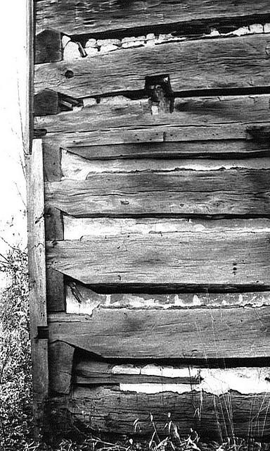
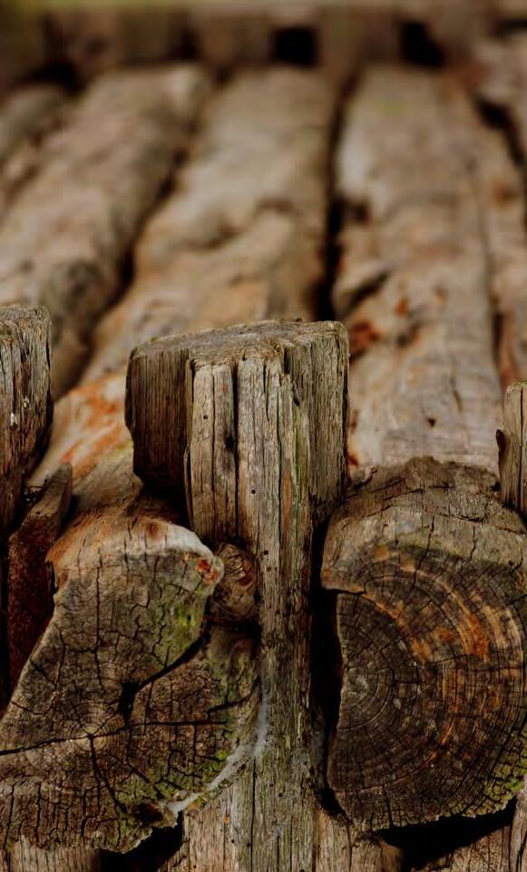
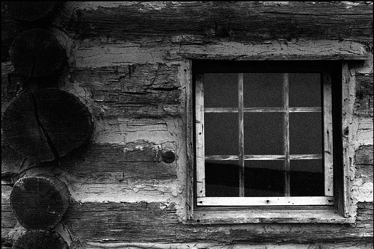
PIC.06 SERIES OF IMGES OF AGED LOG WALLS, WHERE DIMENTINAL INSTABILITY OF WOOD HAS CAUSED CRACKS AND SPLITINGS.
PIC.07 HYGROSCOPE, ACHIM MENGES AND STEFFAN REICHART AT THE CENTRE POMPIDOU IN PARIS, FRANCE.
PIC.08 HYGROSCOPE PANELS CLOSED, ACHIM MENGES AND STEFFAN REICHART AT THE CENTRE POMPIDOU IN PARIS, FRANCE.
PIC.09 HYGROSCOPE PANELS OPEN AS A REACTION TO AN INCREASE IN HUMIDITY, ACHIM MENGES AND STEFFAN REICHART AT THE CENTRE POMPIDOU IN PARIS, FRANCETO EXPOSURE TO MOISTURE.
MATERIAL DIMENSION INSTABILITIES
Throughout the life cycle of a product the dimensions of the material will fluctuate and respond to the environmental context in which it is situated. From the harvesting of raw commodities to the manufacturing and processing of the basic material to the environment in which the product is applied, the material will react to the temperature, humidity and localised pressures of its context. As the type and organisation of particles vary in different materials, the inherent behavioural qualities are also reflected through a very diverse range.
Many industries and designers understand the dimensional instability of materials to represent limitations. Whilst some systems are designed to accommodate expansion and shrinkage through joints and assembly methods, products have also been engineered to deliver stable and predictable solutions. For example plywood has developed as an alternative to solid wood because of its resistance to shrinkage, splitting, twisting, warping and improved strength. Through a cross lamination process veneers of wood are glued together with the grain of each layer alternating at right angles. The arrangement of the layers installs stability through the comprised panel with properties of the material consistent across both directions.
However through the work of material science and experimental research a more innovative approach may be envisaged for utilising dimension material limitations as design opportunities. Hygroscope, by Achim Menges in collaboration with Steffan Reichart at the Centre Pompidou in Paris PIC.07, PIC.08, PIC.09, exhibits how changing the humidity within a glass tank will influence the moisture content of wood components that morphologically respond to change shape by opening and closing. The work stands testiment to the convergence of computational design and material understanding. Uniting these two fields strives to create a more powerful medium through which material properties stand as the design generator in an integrated design process.
021
ARBOREAL FORMATIONS
1 SOURCE:P419,
022 WOOD
From primitive dwellings to ten storey timber residential towers of today, wood has been widely utilised across the globe as a dependent and versatile building material. The availability of wood, accommodation for machining, structural stability and warm characteristics have been applied to many different functions and project applications. Although a wide knowledge of techniques for fabricating wooden elements have evolved over centuries, the introduction of industrial methods of production and trends for using isotropic materials, similar properties in all directions, has diluted the craft through which wood may be explored. However designers now more than ever have new opportunities to innovate. The science of wood technology is a relatively new field of research and offers a more detailed understanding of wood behaviour.
Wood is ‘an organic material made up of lignin and cellulose, obtained from the trunks of trees, and called timber when used in construction’1. As the fundamental material of a tree, wood must support the crown leaf canopy, conduct mineral solutions throughout the tree structure from roots to leaves and store food. These structural and functional roles are fulfilled by the anatomical organisation and behaviour of a trees cell structure. Therefore wood may more specifically defined as a living fibrous cellular tissue that displays material dimensional instability through hygroscopic behaviour and anisotropic characteristics. Hygroscopy refers to a substances ability to take moisture in from the atmosphere. Anisotropy denotes the directional dependency of a materials physical characteristics. These two defining principles form the research basis from which the thesis develops.
DOMAIN
DICTIONARY OF ARCHITECTURE AND BUILDING CONSTRUCTION.
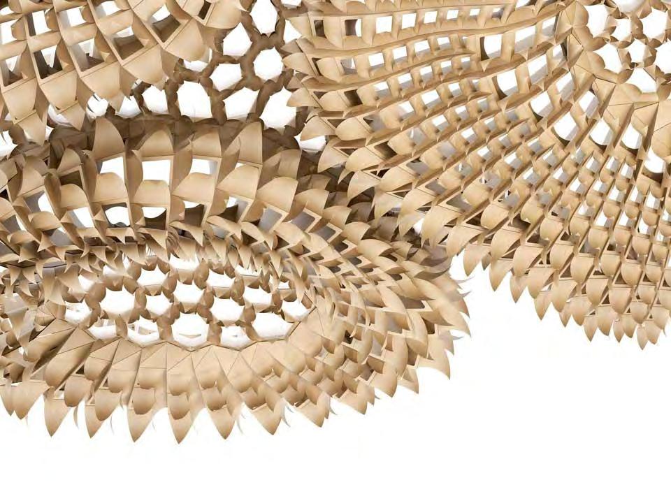
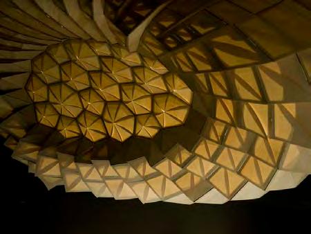
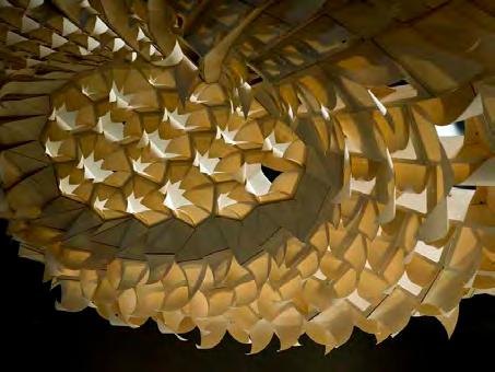
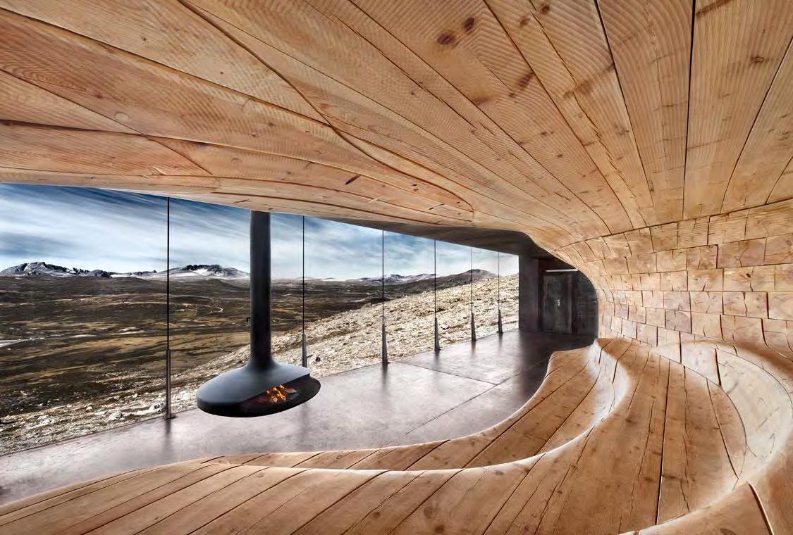
PIC.10 NORWEGIAN WILD REINDEER PAVILION BY SNØHETTA, DOVRE,NORWAY.
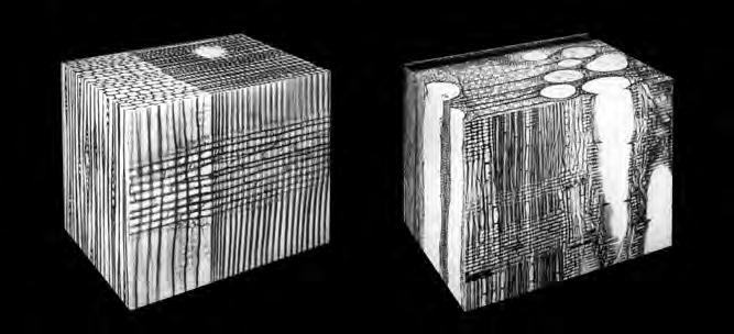
PIC.11 CELLULAR ARRANGEMENT IN A SCOTS PINE SOFTWOOD AND A EUROPEAN OAK HARDWOOD.
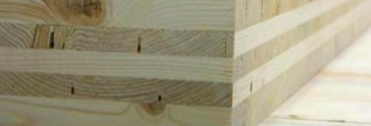
PIC.12 LENO BY METSÄ WOOD, CROSS LAMINATED TIMBER (CLT).
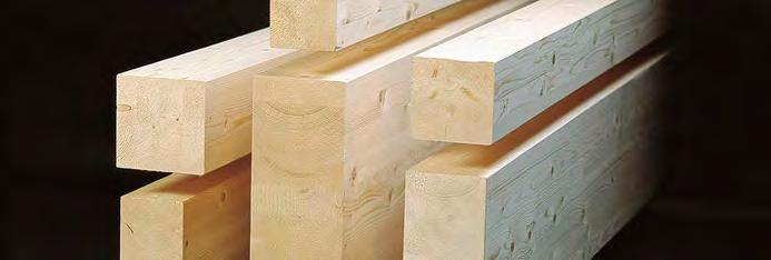
PIC.13 GLULAM BY METSÄ WOOD.
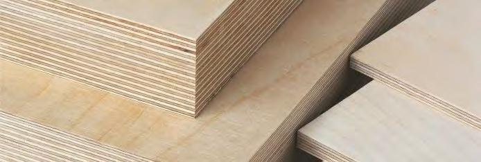
PIC.14 BIRCH PLYWOD BY METSÄ WOOD, CROSS LAMINATED VENEER (CLV).
EXPLORING WOOD
A strong demand has been made upon the building industry by designers and engineers for materials to be composed homogenously. Wood by nature however is heterogeneous with growth irregularities and anisotropic directionality. As a response to more uniform and isotropic materials such as concrete, steel and glass, many timber manufactures have focused their efforts to engineering timber based products that minimise or even eliminate the impact of hygroscopy and anisotropy such as cross laminated veneer (CLV) and cross laminated timber (CLT), PIC.12. This may seem very counter intuitive to how wood naturally behaves but as defects are evened out through the lamination of multiple layers the timber piece becomes more isotropic and properties such as its weight to strength ratio and structural performance increase.
This research questions the meaning of ‘engineered timber’ and if there is an alternative approach that embraces the hygroscopic and anisotropic natural behaviours of wood to create new types of component products for the manufacturing and construction sectors.
Timber has been heavily used in construction for its structural properties. The high tensile strength and slightly lower compressive strength properties inherent to wood make it a material well suited for many structural applications. Traditionally solid timber has been used in post and beam construction restricting the size of application achievable. Advances in CLT systems have however enabled the manufacture of larger scale building components. In both cases the timber members are well adapted to responding to a combination of tensile, compressive, shear and bending forces.
023
ARBOREAL FORMATIONS
1 IGT REPORT PUBLISHED BY BIS - DEPARTMENT FOR BUSINESS INNOVATION & SKILLS, ESTIMATING THE AMOUNT OF CO2 EMISSIONS THAT THE CONSTRUCTION INDUSTRY CAN INFLUENCE, SUPPORTING MATERIAL FOR THE LOW CARBON CONSTRUCTION,
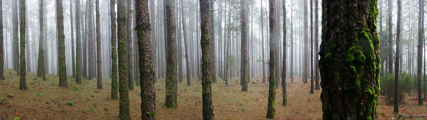
SUSTAINABLE RESOURCE
Forest covers about 30% of land worldwide with between 25,000 to 30,000 tree species. In Europe alone 190 hectares of forest cover 36% of the land area. About 600 tree species, both softwood and hardwood varieties, are traded for many different uses including building construction, furniture, paper and for fuel.
The building industry is a large contributor to global Carbon Dioxide (CO2) emissions. The UK Construction sector is responsible for almost 47% of total CO2 emissions from the UK.1 In order to minimise this footprint there are many different aspects of the building process that needs to be rethought. The processing and manufacturing of materials used in construction contributes heavily to the large carbon footprint generated by the industry. Therefore designers should be fully aware of how material choice and the means though which it was processed and will be fabricated could influence CO2 emissions.
Unlike other products that deplete the earth’s resources wood is the only major construction material that is sustainable and renewable. Trees are a growing biological tissue that converts solar energy captured by leaves into chemical energy. This process is called photosynthesis and it also uses CO2 and water releasing Oxygen as the waste product. This is a vital process that ensures other forms of life can survive. When forests are sustainably managed the impact on the environment is minimal in comparison to other materials. At the present time as the world is facing drastic climatic changes, which to large extent may have been triggered by human activity, wood appears as the material that designers and the construction industry should embrace more. Through new research and understandings of how wood can be widely applied the environment may have a more sustainable future.
024 THE FOREST MAY BE SEEN AS A CARBON OFFSETTING AGENT 0-10% 10-30% 50-70% 70-100% 30-50%
2010 02 03 DOMAIN
AUTUMN
DIAG.02 BUILDING WITH TIMBER AND FORESTING SUSTAINABLY MAY BE SEEN AS A CARBON OFFSETTING AGENT.
DIAG.03 FOREST AREA AS PERCENT OF TOTAL LAND AREA BY COUNTRY.
DIAG.04 LIFE CYCLE ASSESSMENT DOCUMENTING THE ENVIRONMENTAL IMPACT OF BUILDING MATERIALS, ASSEMBLIES AND WHOLE STRUCTURES FROM EXTRACTION OF THE RAW MATERIAL, THROUGH PROCESSING AND MANUFACTURE, ISTALLATION, OPERATION AND DISPOSAL. SOURCE:WWW.NATURALLYWOOD.COM/WHY-WOOD/ SUSTAINABLE-DESIGN
DIAG.05 EMBODIED ENERGY OF SELECTED BUILDING MATERIALS AND TOTALS IN A TYPICAL DWELLING. SOURCE:WWW.TECECO.COM/SUSTAINABILITY.EMBODIED_ ENERGY.PHP, PRODUCED BY CSIRO “THE EMBODIED ENERGY IN BUILDINGS” (WWW.DBCE.CSIRO.AU) USING DATA FROM TUCKER ET AL. (1999) AND TRELOAR (2000)
DIAG.06 STUDY APPLIED TO THREE SIMILAR FAMILY DWELLINGS CONSTRUCTED FROM DIFFERENT MATERIAL SYSTEMS TO ANALYSE THE EMBODIED AND OPERATION ENERGY USE OVER A SIXTY YEAR LIFE SPAN.
SOURCE:WWW.NATURALLYWOOD.COM/WHY-WOOD/ SUSTAINABLE-DESIGN/ENERGY
PIC.15 SUSTAINABLE FORESTING
ENVIRONMENTAL IMPACT
Life Cycle Assessments (LCA) are an internationally recognised approach to determining the environmental impacts of all building materials from individual components to complete structures through the course of their entire life. The life span of material may be considered from the harvest of the raw material through processing, transportation, installation, operation, maintenance and finally disposal or recycling. The sustainable and clean aspect of working with wood means it out performs Steel and Concrete in all LCA categories as shown in DIAG.04
Embodied energy of a material describes the total energy consumed from the acquisition of the natural resource to the final delivery of the product. The embodied energy per unit mass of material varies greatly, but this does not account for the actual quantities of material used in the construction of buildings. DIAG.05 shows that materials such as Stainless Steel and Copper have high energy contents but are used in small quantities, whereas concrete with almost the lowest embodied energy per tonne of material is consumed in large amounts.
The lower chart DIAG.06, documents part of a LCA study by the ATHENA Institute for the Canadian Wood Council. It is a comparative assessment of alternative material designs for an identical 220m2 family home. The research highlights that wood buildings do not only require less energy to construct but also to operate over time.
SOLID WASTE AIR POLLUTION INDEX GREENHOUSE GAS INDEX TOTAL ENERGY USE 800 150 12 150 ECOLOGICAL RESOURCE IMPACT USE 70 0 CONCRETE HOUSE STEEL HOUSE WOOD HOUSE PRIMARY ENERGY (GJ) INDEX VALUE X 105 INDEX VALUE X 105 INDEX VALUE X 1010 ENERGY USE(GJ X 103) EQUIVALENT CO2(KG X 104) 10,000 0 STAINLESS STEEL CONCRETE STEEL CERAMIC ALUMINIUM MASONARY FABRIC PLASTIC TIMBER PLASTER COPPER GLASS 0 EMBODIED ENERGY (GJ) 250 ONE TONNE OF MATERIAL RELATIVE AMOUNT OF MATERIAL IN A SINGLE DWELLING WOOD STEEL CONCRETE EMBODIED OPERATING SOLID WASTE AIR POLLUTION INDEX GREENHOUSE GAS INDEX TOTAL ENERGY USE 800 150 12 150 ECOLOGICAL RESOURCE IMPACT USE 70 0 CONCRETE HOUSE STEEL HOUSE WOOD HOUSE PRIMARY ENERGY (GJ) INDEX VALUE X 105 INDEX VALUE X 105 INDEX VALUE X 1010 ENERGY USE(GJ X 103) EQUIVALENT CO2(KG X 104) 10,000 0 STAINLESS STEEL CONCRETE STEEL CERAMIC ALUMINIUM MASONARY FABRIC PLASTIC TIMBER PLASTER COPPER GLASS 0 EMBODIED ENERGY (GJ) 250 ONE TONNE OF MATERIAL RELATIVE AMOUNT OF MATERIAL IN A SINGLE DWELLING WOOD STEEL CONCRETE EMBODIED OPERATING SOLID WASTE AIR POLLUTION INDEX GREENHOUSE GAS INDEX TOTAL ENERGY USE 800 150 12 150 ECOLOGICAL RESOURCE IMPACT USE 70 0 CONCRETE HOUSE STEEL HOUSE WOOD HOUSE PRIMARY ENERGY (GJ) INDEX VALUE X 105 INDEX VALUE X 105 INDEX VALUE X 1010 ENERGY USE(GJ X 103) EQUIVALENT CO2(KG X 104) 10,000 0 STAINLESS STEEL CONCRETE STEEL CERAMIC ALUMINIUM MASONARY FABRIC PLASTIC TIMBER PLASTER COPPER GLASS 0 EMBODIED ENERGY (GJ) 250 ONE TONNE OF MATERIAL RELATIVE AMOUNT OF MATERIAL IN A SINGLE DWELLING WOOD STEEL CONCRETE EMBODIED OPERATING 025
04 06 05 ARBOREAL FORMATIONS
DIAG.07 CHART SHOWING THE RELATIONSHIP BETWEEN THE MOISTURE CONTENT OF WOOD AND THE TEMPERATURE AND RELATIVE HUMIDITY OF AIR.
SOURCE:P50, TIMBER:ITS NATURE AND BEHAVIOUR
DIAG.08 CHART SHOWING AVERAGE DESORPTION ISOTHERMS IN A GIVEN TEMPERATURE RANGE.
SOURCE: P57, TIMBER:ITS NATURE AND BEHAVIOUR
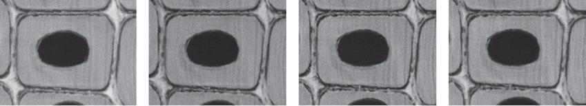
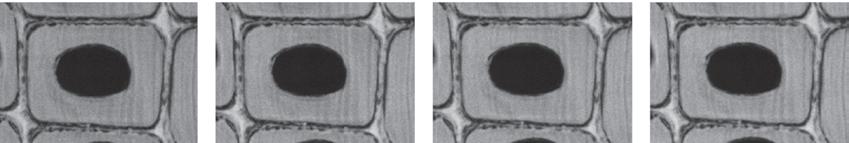
DIAG.09 MICROSCOPIC STUDIES OF CHANGES IN CELL SHAPES WITH MOISTURE CONTENT
DESORPTION. SOURCE:P29-37, SHRINKAGE OF TRACHEID CELLS WITH DESORPTION VISUALIZED BY CONFOCAL LASER SCANNING MICROSCOPY
DIAG.10 MAGNIFIED WOOD SECTION SOURCE:HTTP://WWW.SWST.ORG/TEACH/TEACH2/PROPERTIES2.PDF
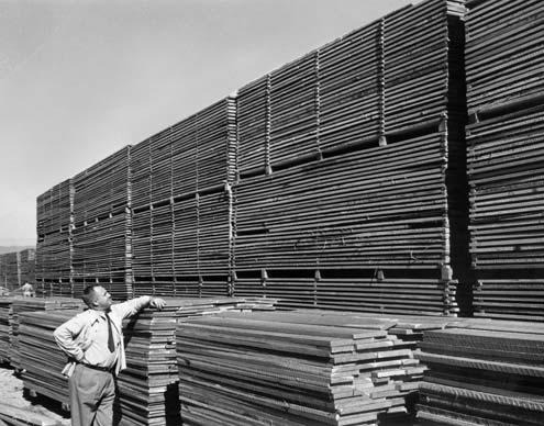
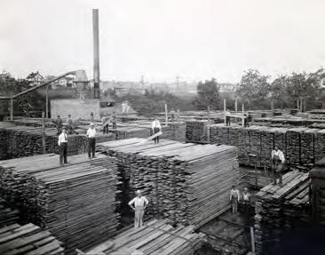
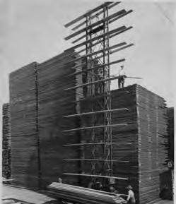
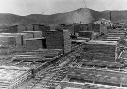
PIC.16 SERIES OF IMAGES SHOWING TIMBER STORAGE YARDS.
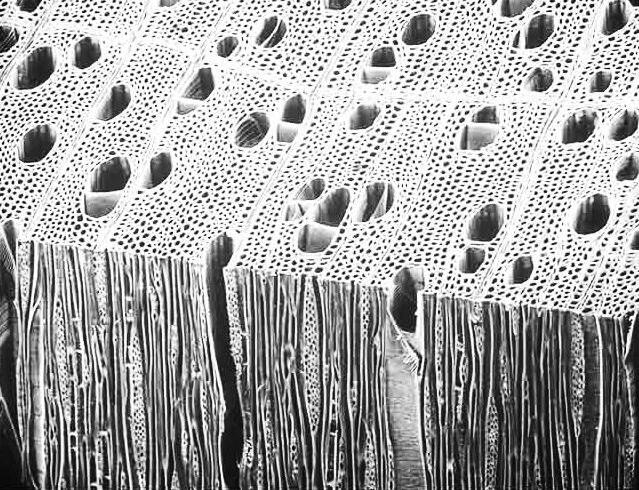
PIC.17 MICRO-IMAGE OF THE CELLULAR STRUCTURE IN A PIECE OF WOOD.
PIC.18 MICROSCOPIC STUDIES OF CHANGES IN CELL SHAPES WITH MOISTURE CONTENT DESORPTION.
1 HYGROSCOPIC DEFINITION. SOURCE: P50, TIMBER:ITS NATURE AND BEHAVIOUR.
2+3 MOVEMENT IN TIMBER. SOURCE: CHAPTER 4, TIMBER:ITS NATURE AND BEHAVIOUR.
4 P29-37, SHRINKAGE OF TRACHEID CELLS WITH DESORPTION VISUALIZED BY CONFOCAL LASER SCANNING MICROSCOPY.
026 PRINCIPLES OF TIMBER BEHAVIOUR
The forest and timber industry take great care storing green and treated wood to minimise defects such as warping or splitting that may compromise the performance of the piece. When a piece of wood is sheltered from direct sun and rain, and depending upon the relative humidity and air temperature, the piece will attain a specific moisture content. Thus a piece of wood shrinks as it loses moisture and swells as it gains moisture. The industry goes to great lengths storing timber in a controlled manner and producing products such as plywood that alternate the direction of layers to control the warping of a panel. In reaction to this principle the thesis questions whether warping as a normally undesirable but natural behaviour of wood may be controlled to produce curved pieces of timber.
The way in which wood grows and displays complex behavioural patterns is founded upon the structural arrangement and functions that the cells of wood perform as the former living biological tissue of a tree. Hygroscopy and Anisotropy are two principles that have been increasingly researched to help explain how wood behaves.
Timber is Hygroscopic meaning it will gain moisture if dry or yield moisture if too saturated until the moisture content in the wood is in balance with the water pressure vapour of the surrounding atmosphere.1 The amount of water at this point of balance is called the equilibrium moisture content (EMC) and is always below 30% for a piece of seasoned timber. When a tree is freshly felled and is therefore un-seasoned or treated, its wood is called green wood and has a much higher MC ranging from 60 to 200%. The EMC that a piece of wood achieves depends on the relative humidity and temperature of the surrounding air. The relationship between moisture content, temperature and relative humidity is shown in DIAG.07. The chart for example documents that if a cut piece of wood is placed in an environment where the temperature is 50 0C and 55% relative humidity, it will either gain or lose water until it reaches approximately 8.75% moisture content.2
CHART SHOWING THE RELATIONSHIP BETWEEN THE MOISTURE CONTENT OF WOOD AND THE TEMPERATURE AND RELATIVE HUMIDITY OF THE SURROUNDING AIR. VALUES ARE BASED ON THE DRYING OUT OF GREEN WOOD. THE TREND IS FOR EMC TO INCREASE AS RELATIVE HUMIDITY INCREASES AND TEMPERATURE INCREASES.
CHART DOCUMENTING THE AVERAGE DESORPTION ISOTHERM FOR SIX DIFFERENT SPECIES. THE CURVE SHOWS THE AVERAGE BEHAVIOUR OF THE PIECES AT 40�C AND BLUE HIGHLIGHTED AREA THE CHANGE IN BEHAVIOUR BETWEEN 15�C AND 70�C.
0 10 6 16 26 32 28 24 22 18 14 12 8 4 2 05 10 15 20 25 30 35 40 45 50 55 60 65 70 75 80 85 90 95 100 20 30 MOISTURE CONTENT OF WOOD (%) RELATIVE HUMIDITY (%) 30 20 70 90 60 50 40 10 10 5 6 7 8 9 10 11 12 13 14 15 16 17 18 19 20 20 30 4050 60 70 80 90 100 80 RELATIVE HUMIDITY (%) MOISTURE CONTENT OF WOOD (%) TEMPERATURE (˚C) 40˚C 15 C 70˚C 0 10 6 16 26 32 28 24 22 18 14 12 8 4 2 05 10 15 20 25 30 35 40 45 50 55 60 65 70 75 80 85 90 95 100 20 30 MOISTURE CONTENT OF WOOD (%) RELATIVE HUMIDITY (%) 30 20 70 90 60 50 40 10 10 5 6 7 8 9 10 11 12 13 14 15 16 17 18 19 20 20 30 4050 60 70 80 90 100 80 RELATIVE HUMIDITY (%) MOISTURE CONTENT OF WOOD (%) 40 C 15˚C 70˚C
07 08 DOMAIN
THE AMOUNT OF WATER IN WOOD EXPRESSED AS A PERCENT OF THE DRY WEIGHT IS CALLED THE “MOISTURE CONTENT” MOISTURE CONTENT IS CALCULATED WITH THE FOLLOWING FORMULA:
WEIGHT OF WATER IN WOOD
MOISTURE CONTENT (%) = WEIGHT OF TOTALLY DRY WOOD
WOOD A LIVING CELLULAR TISSUE
Water is not only found in the cells of a tree but also in the cells’ cavity walls. As soon as a tree is felled and the processing of timber pieces starts, the wood begins to negotiate moisture equilibrium with the environment. Whether the wood is dried naturally or within a kiln the water will first leave the piece from the cell cavities. This is known as free water and is not held by any forces but is comparable to water in a pipe. Free water loss has no effect on the dimensional change or structural integrity of the wood. However the amount of free water lost is considerable and the moisture content of the whole piece drops to between 30% and 27% (first stage of timber seasoning). The remaining moisture is held within the walls of each cell bonded by forces between the water and cellulose molecules. This is called bound water and the cells are at ‘fibre saturation point’ as there is no free water and the cell walls are saturated with the maximum amount of water. Moisture Content loss from this point will only be from the bound water in the cell walls. As moisture is lost and the cell walls begin to shrink they also become stronger as the microfibrils comprising the walls contract closer together. Even after a process of drying is complete, wood will continue to shrink and swell as relative humidity varies and water either leaves or enters the cell walls. The rate at which absorption and desorption takes place differs but follows an s-shaped relationship as shown in DIAG.08.3 Research undertaken in DIAG.09 highlights that the cell walls all react at uneven and irregular rates but it is the changes at the micro-cellular scale that inevitably cause timber to be dimensionally unstable.
The closely packed fibrous composition of cells in wood defines the anisotropic characteristics which informs different directional behaviours of the material depending upon the grain orientation. The strength of wood is highest and most resistant to bending when the forces are oriented parallel to the grain direction. The images show that the length of cells, the thickness of the cell walls, type of cells (early and late wood types) are all contributing factors to distinct patterns of variation which determines the directional deformations that occur in a piece of wood.
027
28.2% MC MC 14.7% 11.74% 7.20 μm 6.88 μm 9.92 μm 10.08 μm 23.0% 12.8% 18.6% 10.6% 10.97% 15.5% 8.9% A COLLABORATIVE STUDY UNDERTAKEN BY HIROKI SAKAGAMI, JUNJI MATSUMURA2 AND KAZUYUKI ODA AT KYUSHU UNIVERSITY, JAPAN STUDIED THE SHRINKAGE OF TRACHEID CELLS WITH DESORPTION THROUGH CONFOCAL LASER SCANNING MICROSCOPY. THE NEW SCANNING METHOD WAS APPLIED TO VISUALISE THE SHRINKAGE OF WOOD AT THE CELLULAR SCALE AND ITS RELATION WITH ANISOTROPIC BEHAVIOUR WITH A CHANGE IN RELATIVE HUMIDITY AND TEMPERATURE. WHILST CHANGES IN CELL SIZE ARE STILL DIFFICULT FOR THE HUMAN EYE TO VISUALISE, THE THICKNESS OF THE RADIAL WALL SHOWED NOT ONLY A CONSIDERABLE CHANGE IN THICKNESS BUT ALSO EVIDENCE OF A COMPLEX INTERACTION EXCHANGE BETWEEN CELLS AS MOISTURE IS LOST.4 09 10
BOUND WATER FREE WATER X 100 ARBOREAL FORMATIONS
VARIABLE MOISTURE CONTENT BY CLIMATE
Values for temperature and relative humidity vary depending upon the climatic conditions for different geographical locations on the Earth. DIAG.14 to the right, documents the variation between three different locations and localised changes in climate for the different months of the year. The Köppen climate classification has five different categories of classifying climates.1 London is a temperate oceanic climate, Sao Paulo a humid subtropical climate, and New York a humid continental climate. These different classifications have very different conditions and the diagram shows that moisture content will fluctuate constantly as it is directly associated to temperature and relative humidity changes throughout the month and of each day of the year.
JOHANNESBURG
SYDNEY
MOSKOW
BERLIN
ROME
INSTAMBUL
BEIJING
STOCKHOLM
VIENNA
LOS ANGELES TOKYO
SANTIAGO
BANGLADESH
SAO PAULO
MEXICO CITY
LONDON
MADRID
PARIS
JOHANNESBURG
SYDNEY
MOSKOW BERLIN
SANTIAGO
BANGLADESH
SAO PAULO
MEXICO CITY
LONDON
MADRID
PARIS
JOHANNESBURG
SYDNEY
MOSKOW
BERLIN
ROME
INSTAMBUL
BEIJING
STOCKHOLM
VIENNA
LOS ANGELES
TOKYO
LONDON SANTIAGO 21º 11º 6º 1º 94% 82% 90% 59% 24% 17% 21% 21%21% 21.5% 16.5% 14.5% 13% 11.2% 10.9% 11.3% 10.8% 10.8% 11.9% 13.8% 15.7% 17.2% 21% 22.2% 22.9% 23.5% 23.5% 21.5% 20.9% 21% 21% 11% CITIESHIGH + LOW MONTHS MOISTURE CONTENT 21º 11º 6º 1º 94% 82% 90% 59% 24% 17% 21% 20.6% 20.6% 21.2% 11.5% 10.9% 11.3% 11.2% 10.7% 10.4% 10.1% 10% 11.3% 11.4% 11.4% 12% 20.1% 19.6% 20.2% 20.8% 19.7% 20.3% 21.4% 22% 21.3% 11% TEMPERATURE HUMIDITY MOISTURE CONTENT BANGLADESH SAO PAULO
CITY
MEXICO
MADRID PARIS
NEW YORK
ROME
BEIJING STOCKHOLM VIENNA
ANGELES TOKYO NEW YORK 28º 20º 4º -3º 79% 63% 70% 57% 16% 12% 13% 13.8% 13.8%13.8% 11.5% 11.1% 10.7% 10.8% 11.2% 11.4% 11.3% 11.3% 11.2% 11.1% 11.4% 11.7% 14.3% 15.2% 15.7% 15.9% 15.4% 14.4% 14.3% 14.2% 13.5% 11% JAN FEBMARAPR MAY JUNJUL AUG SEPOCT NOV DEC JAN FEBMARAPR MAY JUNJUL AUG SEPOCT NOV DEC JAN FEBMARAPR MAY JUNJUL AUG SEPOCT NOV DEC
INSTAMBUL
LOS
030
NEW YORK
14 DOMAIN
DIAG.14 LOCATION SPECIFIC TEMPERATURE, HUMIDITY AND MOISTURE CONTENT VARIATION. SOURCE: WWW.WOODCHANGES.COM
DIAG.15 WOOD RELATIVE DIMENSIONAL CHANGE DEPENDENT ON TYPE OF SHRINKAGE FACTOR, WEATHER CONDITIONS(IN THIS CASE LOCATION) AND ANNUAL PERIOD. SOURCE: WWW.WOODCHANGES.COM
BANGLADESH
SAO PAULO MEXICO CITY
MADRID PARIS
JOHANNESBURG SYDNEY
STOCKHOLM
VIENNA
LOS ANGELES
TOKYO
SANTIAGO
BANGLADESH
SAO PAULO
MEXICO CITY
LONDON
MADRID
JOHANNESBURG
LOS ANGELES
TOKYO
NEW YORK
SANTIAGO
BANGLADESH
SAO
LONDON
MADRID
JOHANNESBURG
1 KÖPPEN–GEIGER CLIMATE CLASSIFICATION SOURCE: PEEL, M. C. AND FINLAYSON, B. L. AND MCMAHON, T. A. UPDATED WORLD MAP OF THE KÖPPEN–GEIGER CLIMATE CLASSIFICATION.
TIMBER DIMENSIONS BY LOCAL ENVIRONMENT
With the understanding that moisture content varies by climate and geographical location, if the same piece of timber is placed in different environments around the world the dimensions of the piece will change due to hygroscopic action. DIAG.15 displays the range of dimensional change as maximum swelling and minimum shrinkage for a spruce species piece of wood throughout the months of the year for London, Sao Paulo and New York. Relative to the changing temperature, humidity and moisture content by location, the dimensions of the wood will change by differing degrees of motion within the tangential and radial directions. This again suggests the importance of understanding that the way in which the tree log is cut and processed will have an impact upon the behaviour of the timber piece.
JAN FEBMARAPR MAY JUNJUL AUG SEPOCT NOV DEC month 0.8% year 2.2% month 1.5% year 4.1% month 1.5% year 2.2% month 2.9% year 3.8% month 0.8% year 2.2% month 0.7% year 1.7% JAN FEBMARAPR MAY JUNJUL AUG SEPOCT NOV DEC JAN FEBMARAPR MAY JUNJUL AUG SEPOCT NOV DEC LONDON
CITIES WOOD DIMENTIONAL CHANGE SPRUCE TANGENTIAL RADIAL TANGENTIAL RADIAL TANGENTIAL RADIAL
SANTIAGO
MOSKOW BERLIN ROME INSTAMBUL BEIJING
NEW YORK
PARIS
SYDNEY MOSKOW BERLIN ROME INSTAMBUL BEIJING STOCKHOLM
VIENNA
CITY
PAULO MEXICO
PARIS
SYDNEY
BERLIN ROME INSTAMBUL BEIJING STOCKHOLM VIENNA
ANGELES
MOSKOW
LOS
TOKYO
NEW YORK 031
15
ARBOREAL FORMATIONS
planed
032
PROCESSING OF TREES TO TIMBER
In recent times the harvesting and processing of trees to timber has been driven by the sustainable need to maximise the use of a wooden log and minimise wastage. There are many different techniques and cut methods for creating the wide range of solid timber products now available. Striving to create the most efficient use of a tree, the industry is increasingly moving away from cutting large solid wood sections which is difficult to attain without some wastage. Modern production methods include using compound sections that constitute individual segments fixed together as elements, or glulam products which glue multiple thinner solid sections of wood together.
C20,
C24 60
C20, C24,
C45 C24 80 x 100 to 120 x 200 mm 12-18 m costly straight
C20, C24, C27, C35, C45 C24 60 x 60 to 140 x 240 mm 12-18 m simple (laminations) straight planed C20, C24, C27, C35, C45 C24 60 x 100 to 140 x 240 mm 12-18 m simple (laminations) straight planed C20, C24, C27, C35, C45 C24 100 x 100 to 160 x 240 mm 12-18 m costly straight planed
GL24h, GL28k, GL28h, GL36k, GL36h
SQUARED SECTION KVH 2 PIECES 3 PIECES 4 PIECES MULTIPLE PIECES Solid structural timber, finger-jointed Solid structural timber, finger-jointed Duo® beam Trio® beam four-piece beam GL 80 x 100 to 260 x 2000 mm up to 18 m, sometimes 40 m simple (laminations) straight, curved planed STRENGTH CLASSES USE OF LOG SYSTEM SKETCH DESIGNATION TYPE USUAL STRENGTH CLASS CROSS-SECTIONS LENGTHS DRYING FORM SURFACE FINISH SOLID TIMBER COMPOUND SECTIONS GLULAM
C24, C27, C35, C45
x 80 to 240 x 300 mm up to 8 m, sometimes 12 m costly, problematic straight sawn,
C27, C35,
sawn, planed
GL24k,
C24h
16 DOMAIN
ARCHITECT
YEAR OF COMPLETION LOCATION
BUILDING TYPE
DESIGN STRUCTURE
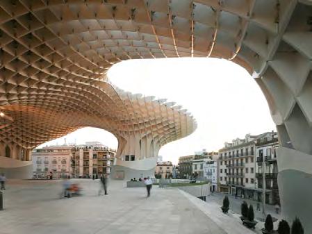
JÜRGEN MAYER-HERMANN
2011
SEVILLE, SPAIN
A MIXED USE STRUCTURE CREATES AN ELEVATED PLAZA
ROOF CANOPY APPROXIMATELY 26 M HIGH BONDED TIMBER CONSTRUCTION WITH POLYURETHANE COATING, 3000 CONNECTIONS
ARCHITECT
YEAR OF COMPLETION LOCATION
BUILDING TYPE
DESIGN STRUCTURE
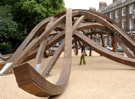
AA’S INTERMEDIATE UNIT 2, LED BY TUTORS CHARLES WALKER AND MARTIN SELF
2007
LONDON, UNITED KINGDOM
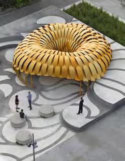
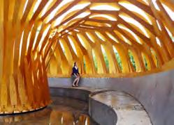
SUMMER PAVILION FOR SOCIAL GATHERING DOME LIKE PAVILION REACHING 4.3 M HIGH
A COLLECTION OF FREE FROM SOLID STRANDS OF LAMINATED TIMBER SHEETS WHICH ARE STAIGHT, SINGLE CURVED OR DOUBLE CURVED
ARCHITECT
YEAR OF COMPLETION LOCATION
BUILDING TYPE
DESIGN STRUCTURE
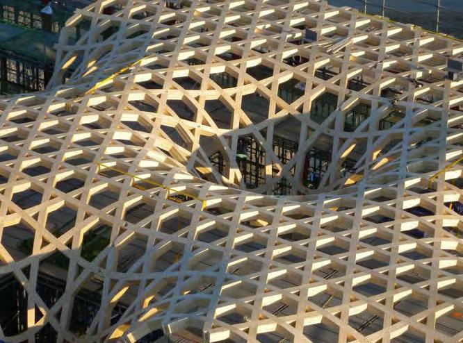
KYEONGSIK YOON (KACI INTERNATIONAL) & SHIGERU BAN ARCHITECTS
2008
YEOJU, SOUTH KOREA
A CANOPY THAT CARRIES THE ROOF OF THE FACILITY
BUILDING FOR THE GOLF CLUB
ROOF CANOPY REACHING 14 M HIGH, 21 SLENDER COLUMNS SUPPORT 32 ROOF ELEMENTS, MADE OF WOVEN TIMBER GLUELAM GIRDERS
LAMINATED TIMBER SHEETS WITH CNC CUT PROFILES LAMINATED TIMBER SHEETS WITHIN A CUSTOMISABLE JIG
SOLID TIMBER SECTION MILLED TO SHAPE
METROPOL PARASOL IS FORMED THROUGH THE CREATION OF A COMPLEX SURFACE THAT IS SECTIONED AT INTERVALS IN PERPENDICULAR CROSS DIRECTIONS. THIS GENERATES PLANAR PANELS, WHICH WHEN CNC CUT CAN BE INTERLOCKED.
BAD HAIR PAVILION ADAPTS THE LAMINATION PROCESS AS USED IN FURNITURE MANUFACTURING TO CREATE BUILDING SCALE ELEMENTS. INDIVIDUAL DOUBLY CURVED BEAMS ARE MANUFACTURED USING CUSTOM MADE JIGS AND STRAP APPLIED PRESSURE TO ENSURE COMPACT LAMINATION.
NINE BRIDGE CLUB HOUSE IS A DOUBLY CURVED SURFACE THAT IS PRECISELY DESCRIBED BY AN INTERLOCKING DOUBLY CURVED GRID SHELL. EACH BEAM IN THE GRID IS OF A DOUBLY CURVED FORM CNCMILLED FROM SOLID GLULAM BLOCKS OF TIMBER.
034
DOMAIN
DIFFERENT FABRICATION METHODS FOR EACH OF THE CHOSEN KEYSTUDIES.
PIC.22 METROPOL PARASOL
BAD HAIR PAVILION
NINE BRIDGE CLUB HOUSE
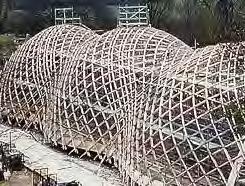
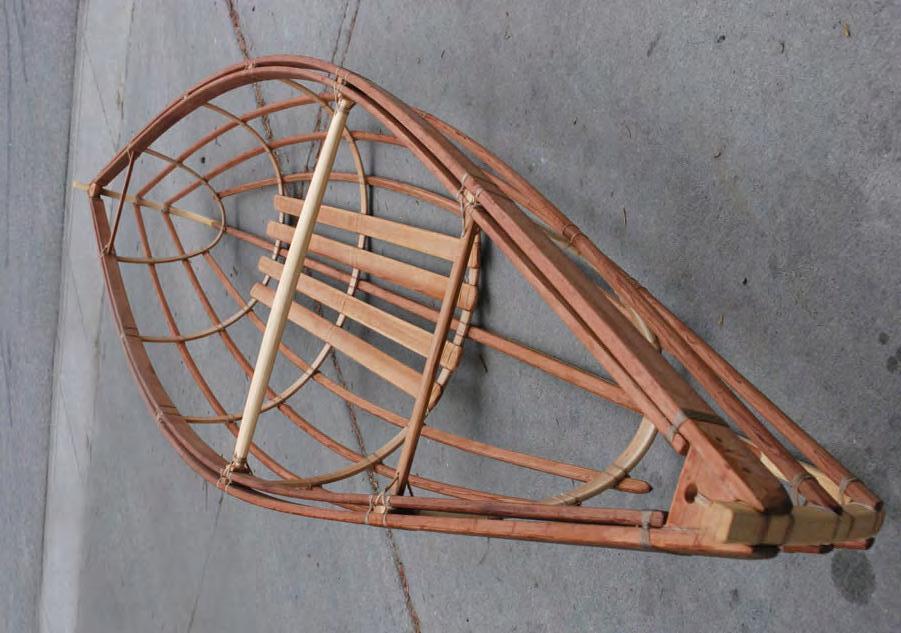
DOWNLAND GRIDSHELL
ARCHITECT
YEAR OF COMPLETION
LOCATION
BUILDING TYPE
DESIGN STRUCTURE
EDWARD CULLINAN ARCHITECTS AND BURO HAPPOLD ENGINEEERS
2002
WEALD & DOWNLAND MUSEUM, UNITED KINGDOM MUESUM AND WORKSHOP SPACES
6M HIGH TRIPLE BULB LATTICE A DOUBLE LAYERED GRIDSHELL OF OAK LATHS INITIALLY FORMED FLAT AND GRADUALLY BENT INTO SHAPE THROUGH A SYSTEM OF NODES
IN-SITU BENDING OF OAK LATHS
THE DOWNLAND GRIDSHELL UTILISES THE BENDING PROPERTIES OF GREEN OAK TO CREATE A TRIPLE BULB DOUBLY CURVED FORM. A LAYERED LATTICE OF OAK LATHS ARE INITIALLY LAID FLAT AND ELEVATED TO THE FINISHED STRUCTURE HEIGHT. UTILISING A PROP SYSTEM THE INTERLOCKING OAK STRIPS ARE GRADUALLY BENT INTO SHAPE THROUGH A NETWORK OF LOCKING NODES.
FABRICATING LARGE COMPLEX GEOMETRIES
There are relatively few examples of large scale complex geometrical structures manufactured in timber. These four examples, DIAG.18 documents some of the most expressive curving wood structures currently built. They also reveal the limitations of different wood fabrication methods by either the geometrical form created or the fabrication process used.
Metropol Parasol approximates a complex geometrical form through the employment of flat interlocking panels. None of the timber panels actually curve to create the structure. The Bad Hair Pavilion utilises some of the anisotropic properties of wood to aid the bending and twisting of individual laminate layers. However the technique is extremely labour intensive and time consuming as hot or cold presses cannot be used to clamp and apply pressure to the form. Whilst the CNC milling method used for creating the doubly curve beams in Nine Bridge Club House formulates the appearance of doubly curving wood, the manufacturing process generates much waste material and neglects the behavioural properties of wood to twist and bend. The form could have equally been created from an alternative material. The Downland Gridshell is a good example of combining wood properties and fabrication techniques. Employing the hygroscopic properties of green oak, freshly felled and containing moisture content close to 30%, the wood laths are more pliable to bending. This aids the process for pulling the lattice down into place before the moisture content of the oak equalises with the surrounding environment. Whilst holding the potential to create different doubly curved surfaces the lattice is restricted to defining single surfaces which have gradual curvature change as the solid green oak laths have bending limitations.
035
18
PIC.23
PIC.24
PIC.25
DIAG.18
ARBOREAL FORMATIONS
036 DOMAIN
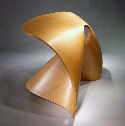
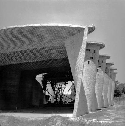
PIC.26 FORTUNE COOKIE STOOL, DESIGNED BY PO SHUN, 2008. PIC.27 CHURCH OF CHRIST THE WORKER BY ELADIO DIESTE, ATLANTIDA, URUGUAY, 1958-60.
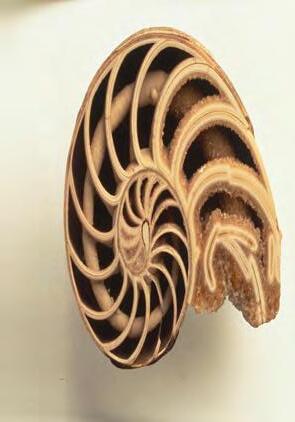
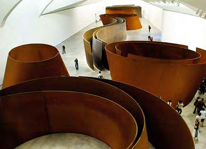
PIC.28 NAUTILUS SEA SHELL SECTION. PIC.29 “A MATTER OF TIME” BY RICHARD SERRA, OPENED JUNE 8 AT THE GUGGENHEIM MUSEUM IN BILBAO. THIS MEGA-INSTALLATION OF EIGHT BENT STEEL SCULPTURES IS CONSIDERED THE LARGEST INSTALLATION TO EVER BE HOUSED IN A MUSEUM GALLERY.
GEOMETRY
Research technologies have aided the progress of fabrication industries in recent years to make the manufacturing of complex geometries more accessible. Design trends and designers needs to explore geometrical organisations, other than those orthogonal, have created a demand for the manufacture of curved building elements. The more precise level of control achieved through digital means of fabrication has instigated the manufacture of more ergonomic, compact and detailed products and furniture. At the building scale geometry plays a vital role in determining the performance of a buildings operation functionally, structurally and environmentally. Embracing complex geometries may reveal a more responsive and exploratory framework for creating spatial models of variation and interest. A change of formulating space from rectilinear ideals towards curved geometry potentially leads to new categories of space and use.
STRUCTURAL PERFORMANCE
Geometry has a profound effect on the structural performance of all forms found in nature or manmade. Whether it is a seashell that needs to protect its occupant from the attack of predators, a chair that has to support a person sitting on it, or a wall in a building that supports not only it’s self weight but also prevents the rest of the building from collapsing, geometry plays a vital performance role.
The potential for geometrical variation within design systems may improve the structural performance and efficient use of material. Nature very rarely deploys homogenous materiality in form or composition to deliver function and performance. The building industry repeatedly increases the thickness of material in rectilinear formations to attain structural stability. However the introduction of even the smallest curved geometries would allow for more efficient structures to be built in terms of material use and performance. For example in the case of the Fortune Cookie Stool, PIC.26, inducing a curvature into the backrest helps to overcome bending moments when the load of a person is applied. Similarly, the expressive curved walls in the Church of Christ The Worker, PIC.27, integrate a geometry which is more resistant to shear forces and buckling within a relatively small structural thickness of bricks. Whilst traditionally the building industry has been opposed to more expressive geometries for reasons of cost and complexity, the advances made in geometrical exploration, material understanding and fabrication research may now make this very achievable.
037
ARBOREAL FORMATIONS
IN SITU WOOD BENDING
THIS TECHNIQUE INVOLVES DELIVERING STRAIGHT PIECES OF PLYWOOD, CUT WITH SLITS TO AID BENDING, TO A BUILDING SITE WHERE WATER IS APPLIED TO THEM. THE APPLICATION OF MOISTURE MAKES THE SHEETS MORE PLIABLE FOR INDUCING CURVATURE WHEN FORCE IS PHYSICALLY APPLIED AND THE GEOMETRY IS THEN LOCKED INTO PLACE.
STEAM WOOD BENDING
IN THIS METHOD STRIPS OF WOOD ARE PLACED IN A STEAM BOX, WHERE HEAT AND MOISTURE INFILTRATES THE WOOD. THIS MAKES THE WOOD MORE PLIABLE AND ALLOWS THE TIMBER STRIPS TO BE EASILY BENT AROUND A MOULD. STEAM BENDING IS LIMITED BY THE DEGREE OF CURVATURE THAT TIMBER ELEMENTS CAN ACHIEVE AND IS MAINLY USED IN BOAT BUILDING, FURNITURE AND MUSICAL INSTRUMENT MANUFACTURE.
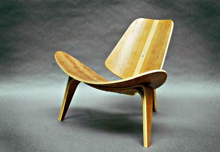
LAMINATION & PRESS BENDING
PRESSURE APPLIED LAMINATION IS A VERY COMMON TECHNIQUE FOR FABRICATING FURNITURE. THE TECHNIQUE UTILISES MULTIPLE LAYERS OF THIN VENEER LEAVES WHICH ARE LAYERED TOGETHER WITH GLUE. WHILST THE LAMINATE IS STILL WET IT IS PLACED OVER A FORMING MOULD AND AN INDUSTRIAL PRESS IS APPLIED SO THE WOOD ASSUMES THE MOULDS SHAPE. THIS TECHNIQUE IS A VERY EFFICIENT METHOD OF FABRICATION WHEN MULTIPLE COPIES OF THE SAME ITEM NEED TO BE MANUFACTURED. A HIGH NUMBER OF IDENTICAL ITEMS IS REQUIRED AS THE PRICE OF THE MOULDS AND FABRICATION SET UP CAN BE VERY HIGH.
038
DOMAIN
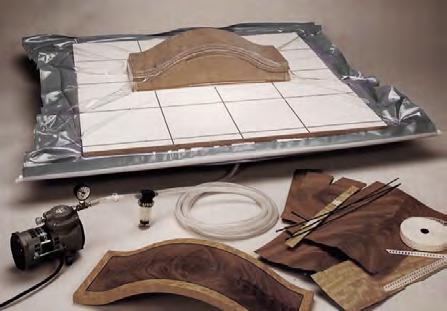
LAMINATION & VACUUM PRESSURE BENDING
VACUUM PRESSURE BENDING IS SIMILAR TO THE LAMINATION PROCESS THAT USES AN INDUSTRIAL PRESS, BUT UTILISES A VACUUM SEAL TO APPLY THE PRESSURE. VENEERS ARE PLACED IN A SEALED BAG TOGETHER WITH THE FORM MOULD. AIR IS THEN REMOVED FROM THE BAG WHICH INDUCES A FORCE BIG ENOUGH TO BEND THE VENEERS AROUND THE MOULD. THIS TECHNIQUE IS ESPECIALLY USEFUL WHEN VERY LARGE PIECES NEED TO BE LAMINATED. EXAMPLES OF 35 METER LONG FIBRE GLASS PROPELLERS ARE KNOWN TO BE LAMINATED USING THIS TECHNIQUE.
COMPOSITE MATERIAL CONSTRUCTION
UPM GRADA IS A COMPOSITE PLYWOOD MATERIAL WHICH ALLOWS CURVATURE TO BE INDUCED INTO A WOOD PANEL WITH THE APPLICATION OF HEAT AND PRESSURE. A THERMOPLASTIC FOIL IS PLACED BETWEEN CROSS BONDED ROTARY CUT BIRCH VENEER LAYERS WHEN THEY ARE MANUFACTURED AS FLAT PANELS OF PLYWOOD. TO APPLY CURVATURE TO A PANEL IT IS FIRST HEATED UP TO 130 °C. AT THIS TEMPERATURE THE FOIL MELTS ALLOWING THE VENEERS TO SLIDE. THE HOT PANEL IS THEN PLACED INTO A PRESSURE MOULD AND LEFT TO COOL DOWN.
BENDING WOOD TECHNIQUES
Wood is a material which by nature expands, shrinks and bends. Focusing on the use of veneers, there are several fabrication methods used by different industries that make use of woods hygroscopic and anisotropic properties in order to manufacture curved elements. Each method has limitations and application restrictions. Lamination is currently the most common method for fabricating single and doubly curved geometries out of timber. Whilst in-situ bending and steam bending apply post curvature to pieces or flat sheets of cross laminated veneer such as plywood, the direct lamination of veneers around a mould, allows for a much greater control of material and geometrical form. To bridge the gap between these two methods new composite plywood sheets are being developed to achieve tighter and more complex curvatures without the need for applying wet glue.
039
PIC.30
PIC.31
PIC.32
PIC.33
PIC.34
IN SITU WOOD BENDING.
STEAM WOOD BENDING.
LAMINATION AND PRESSURE
VACUUM PRESSURE BENDING.
COMPOSITE MATERIAL AND PRESS BENDING
ARBOREAL FORMATIONS
040 DOMAIN
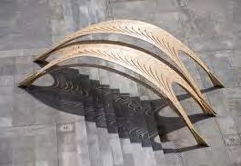
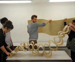
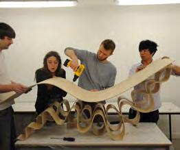
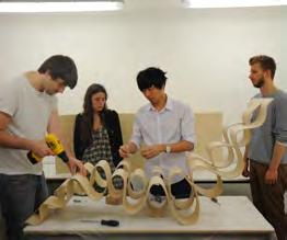
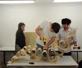
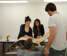
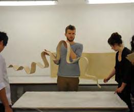
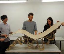
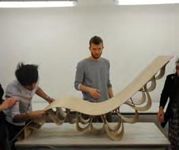
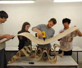
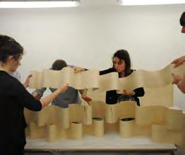
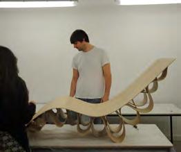
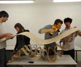
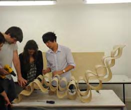
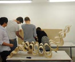
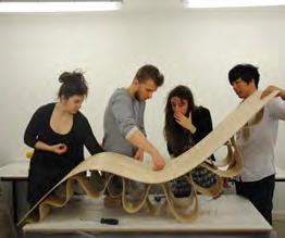
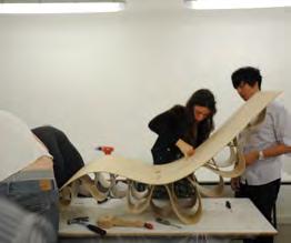
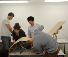
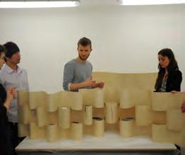
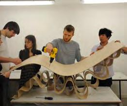
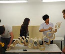
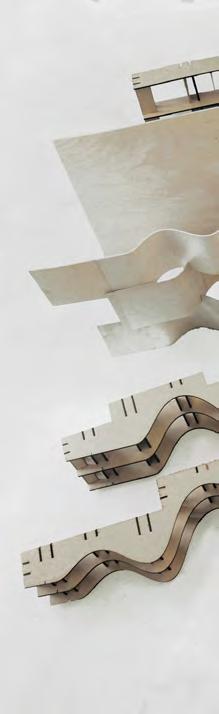
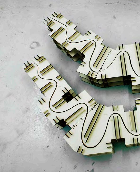
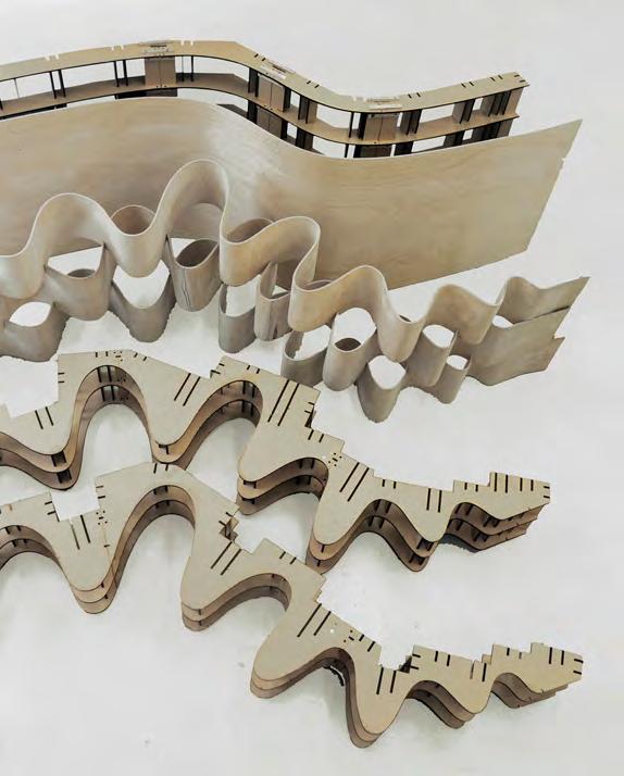
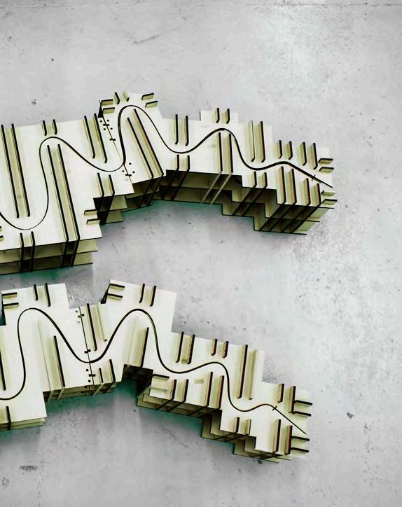
DIAG.19 ASSEMBLY LOGIC OF THE CHAISE LOUNGE.
DIAG.20 LAMINATION ELEMENTS AND FIBRE ORIENTATION OF COMPONENTS COMPRISED IN THE ASSEMBLY OF THE CHAISE LOUNGE.
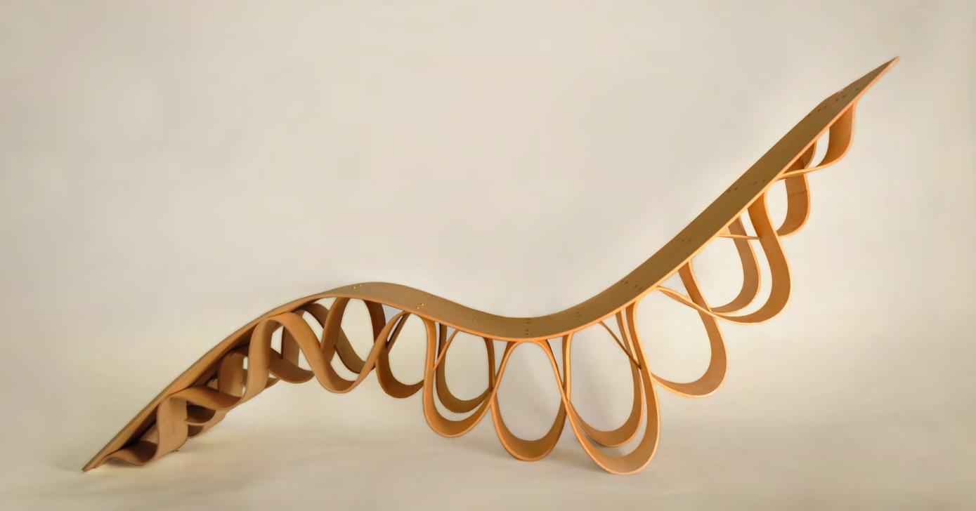
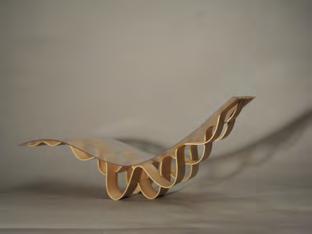
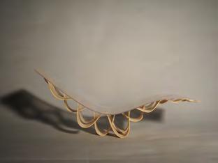
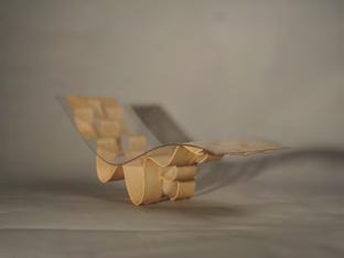
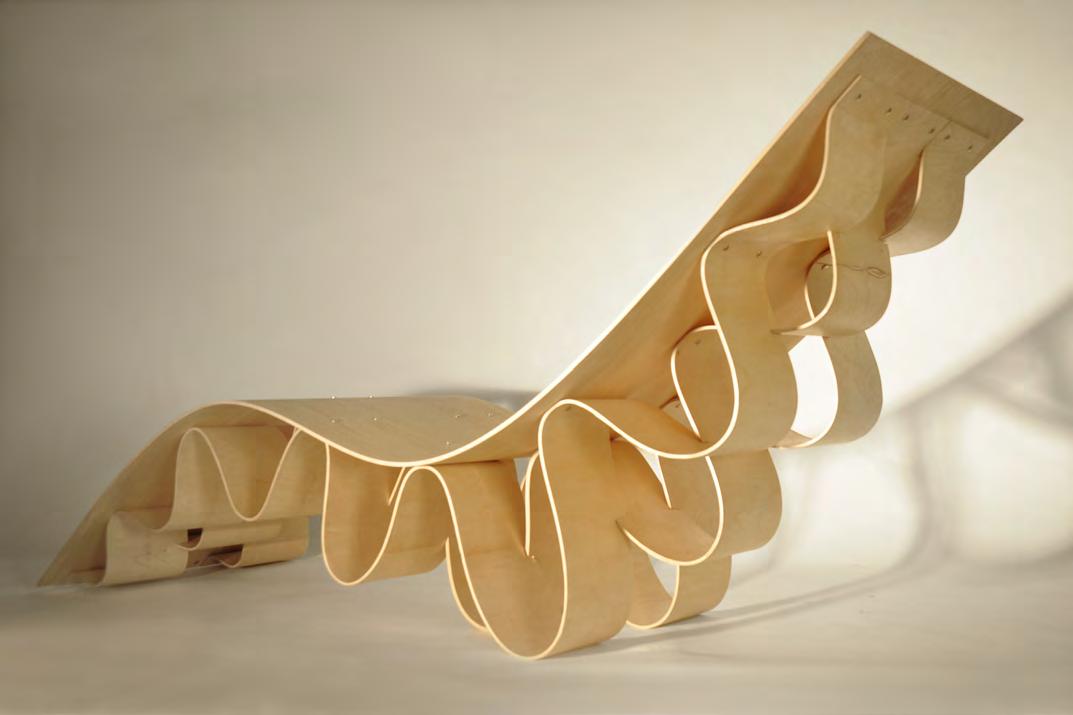
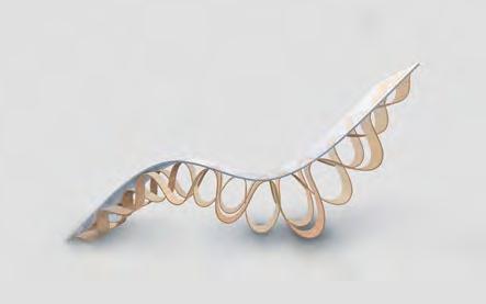
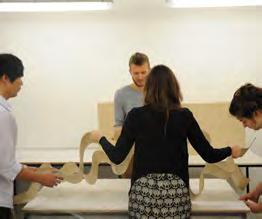
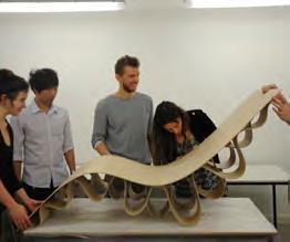
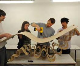
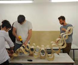
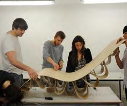
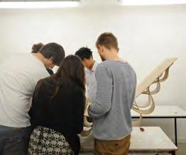
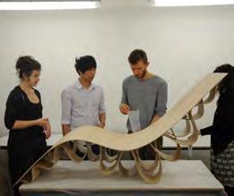
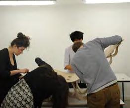
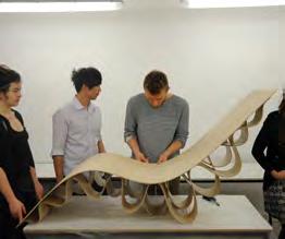
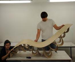
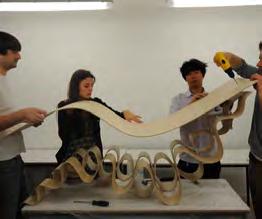
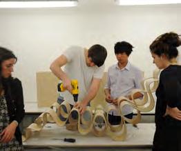
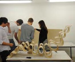
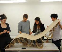
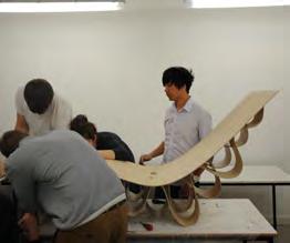
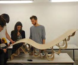
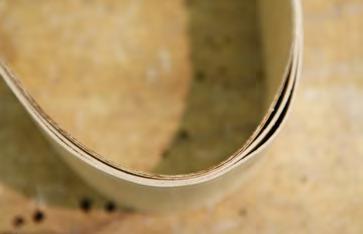
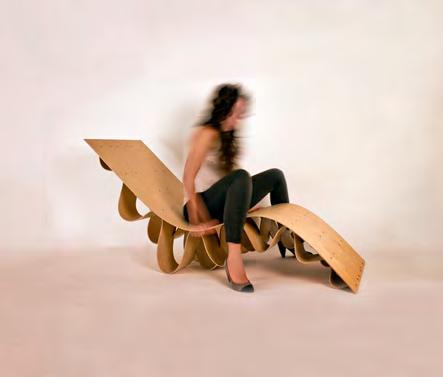
PIC.35 SERIES OF VIEWS OF THE 1:5 CHAISE LOUNGE PROTOTYPE.
PIC.36 SIDE VIEWS OF THE 1:1 CHAISE LOUNGE PROTOTYPE. LAMINATED PLYWOOD.
PIC.37 CHAISE LOUNGE CONCEPT VISUALISATION.
KEYSTUDY : CHAISE LOUNGE
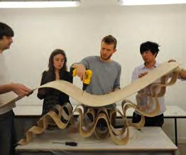
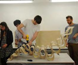
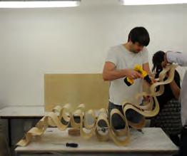
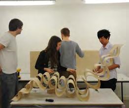
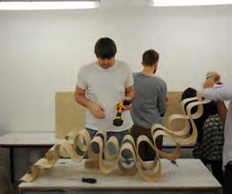
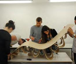
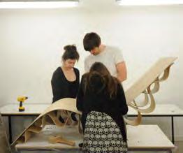
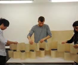
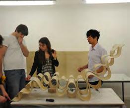
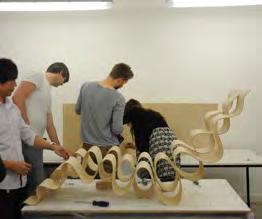
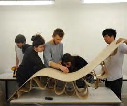
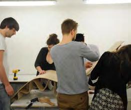
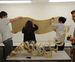
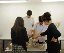
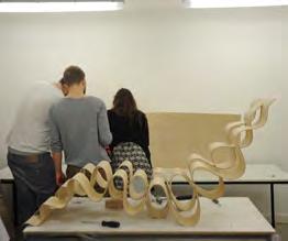
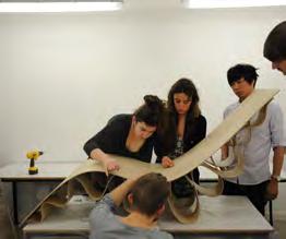
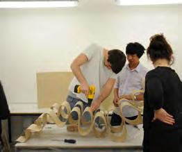
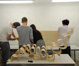
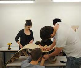
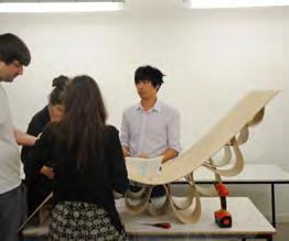
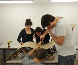
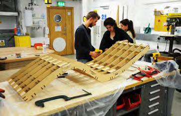
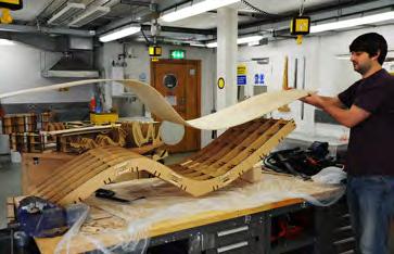
Our first experience researching and working with wood fabrication techniques was for the seating of a Pop-Up Cinema project in Gillett Square, Dalston, London. A chaise lounge wave design concept was developed to provide the user with a comfortable and embracing form on which to sit and enjoy the film. Whilst the curve of the top piece undulates to hold the user, an interlocked system of three waves distributes the users load to the ground, DIAG.19.
The chair utilised 3mm thick layers of plywood which were laminated together in different numbers of layers for the three wave components and bracing seat deck. In order to induce the required curvature into the components, three individual jigs were built. Strips of plywood were then laminated in the jigs and notches cut for the pieces to slide together. Individually each component of the system was flexible, but once the pieces were connected together, the components interlocked as one system, providing the assembly with enough strength and stiffness to assume the weight of the user.
Grain orientation of the wood played a crucial part in the fabrication process, DIAG.20. Bending strips of plywood parallel to the grain direction allowed for tighter curvatures to be achieved, but reduced the stiffness of each piece. Whilst the magnitude of the curvatures in the three wave strips was too tight to introduce alternating plywood pieces with perpendicular grain direction, the deck combined a cross lamination assembly to increase the stiffness of the plate.
041
19 20
ARBOREAL FORMATIONS
042 DOMAIN

043 ARBOREAL FORMATIONS
044 DOMAIN
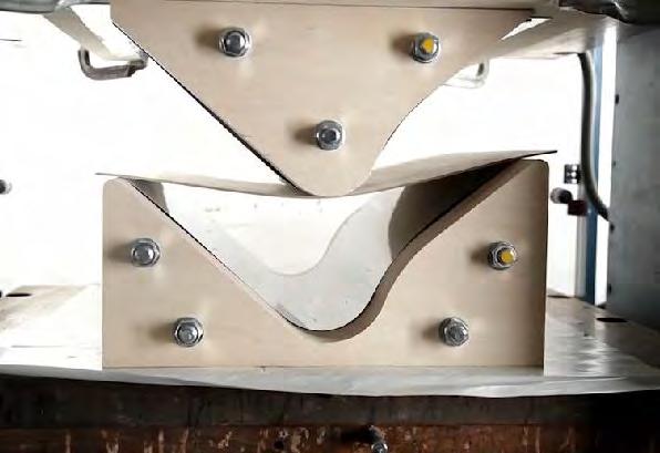
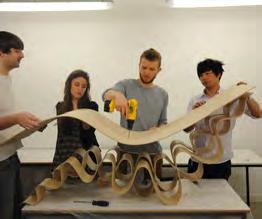
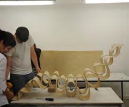
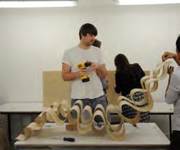
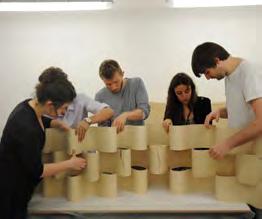
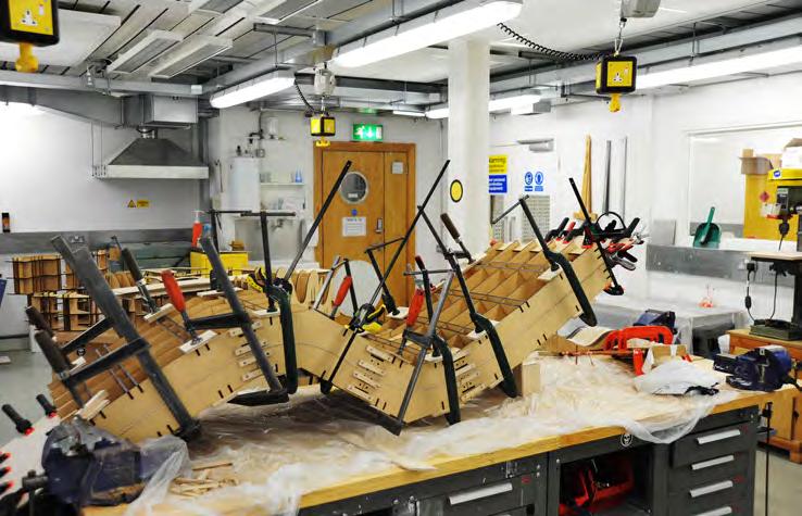
PIC.38 JIG OF THE CHAISE LOUNGE’S UPPER PART.
PIC.39 UPPER PART REMOVED FROM THE JIGS.
PIC.40 MIDDLE WAVE OF THE CHAISE LOUNGE IS REMOVED FROM THE JIG.
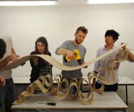
PIC.41 FINAL SIDE WAVE IS LAMINATED.
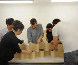
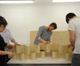
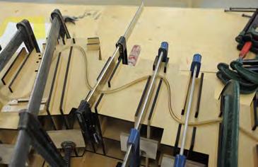
PIC.42 LAMINATION PROCEDURE
DETAILING: CLAMPING THE POSITIVE AND NEGATIVE JIG.
PIC.43 LAMINATION PROCEDURE
DETAILING: LOCAL DELAMINATION.
PIC.44 FINAL PRODUCED PARTS FOR THE CHAISE LOUNGE AND POSITIVE PART OF JIGS FOR THE WAVES.
PIC.45 BOTH PARTS OF EACH OF THE TWO JIGS NEEDED FOR THE LAMINATION OF THE WAVES.
PIC.46 REAL SCALE PROTOTYPE TESTING ON LOADING.
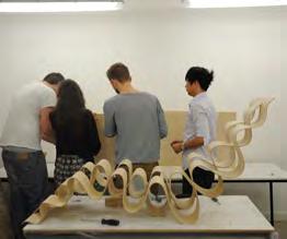
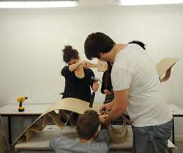
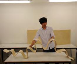
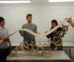
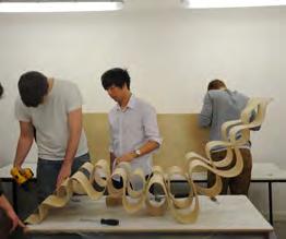
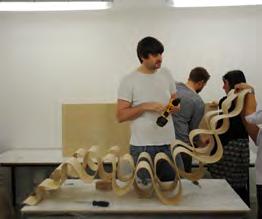
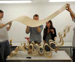
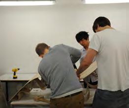
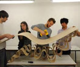
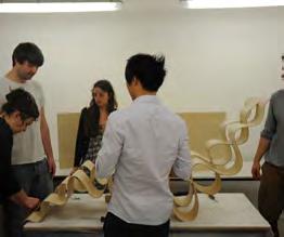
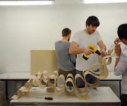
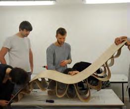
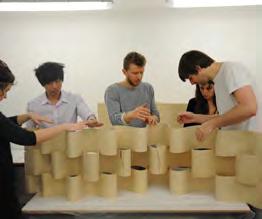
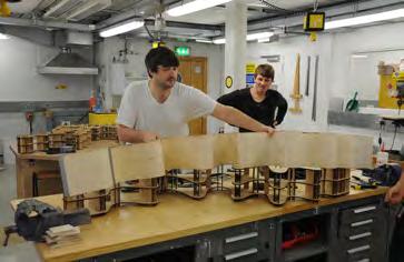
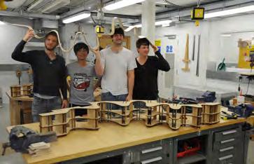
FABRICATION OBSERVATIONS
Working with wood through a hands on approach to build the chair, exposed some vital findings. Whilst we found the fabrication process to be very labour intensive and time consuming, it was easy to envisage the same procedure being adapted to the industrial scale for the manufacture of multiple copies. However the process also highlighted the difficulties in thinking this manufacturing process could be applied to large curving timber components at the building scale. The quantity of material and size of formwork required in the process combined with the power required to physically bend larger sheets of plywood would inevitably lead to an increase in costs and time. The work required to create three formworks emphasised that every time a different curvature was required another formwork would need to be machined and assembled. This was seen as a large restriction regardless of the applications scale and could only be overcome with the use of an adjustable formwork jig or exploring an alternative way of inducing curvature in laminated timber elements.
045
ARBOREAL FORMATIONS

046
APPLICATION SCALE
FURNITURE SCALE
PAVILLION SCALE
DWELLING SCALE
DOMAIN
MULTI-DWELLING SCALE
TIMBER APPLICATIONS SCALE
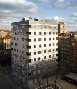
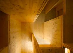
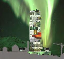
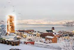
The use of laminated timber is apparent at many different scales of design. In the furniture industry there are many elegant and original solutions for bending and curving wood to make chairs and tables. There are also several examples showcasing the innovative use of laminated timber for pavilions or at the scale of a single house. The properties of wood are used here as a means to create novel morphologies and spatial conditions. Above this scale however there are very few examples of buildings that assemble to reveal different but exciting spatial conditions within the same system. Whilst there are many examples of large spanning roofs that cover single spaces there are few which accomodate different functions and uses. The tallest timber building is located in London in the borough of Hackney. This 9 storey apartment block is built from Cross Laminated Timber panels, PIC.54, organised to define apartments and rooms. There are several planned projects that aim to surpass the current record height, such as The Centre for Cultural and Innovative Interchange Between Russia and Norway in Kirkenes, Norway, PIC.55 and PIC.56, which will stand at 17 stories high. However built or planned none of these buildings explore the anisotropical properties and potentials of wood, limiting their application to standard engineered timbers and orthogonal geometries.
MULTI-FUNCTIONAL
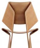
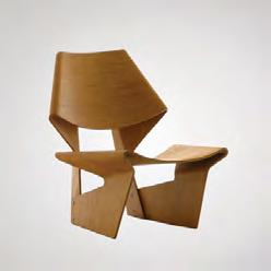
PIC.47 LOUNGE CHAIR DESIGNED BY GRETE JALK IN 1963, BEND PLYWOOD, BACK DETAIL.
PIC.48 LOUNGE CHAIR DESIGNED BY GRETE JALK IN 1963, BEND PLYWOOD.
PIC.49 TEMPORARY RESEARCH PAVILION (STUTTGART, GERMANY), DESIGNED AND FABRICATED BY INSTITUTE FOR COMPUTATIONAL DESIGN (ICD) AND THE INSTITUTE OF BUILDING STRUCTURES AND STRUCTURAL DESIGN (ITKE), TIMBER PAVILION USING 6.5 MM THIN BIRCH PLYWOOD SHEETS.
PIC.50 TEMPORARY RESEARCH PAVILION (STUTTGART, GERMANY), DESIGNED AND FABRICATED BY INSTITUTE FOR COMPUTATIONAL DESIGN (ICD) AND THE INSTITUTE OF BUILDING STRUCTURES AND STRUCTURAL DESIGN (ITKE), INTERIOR SPATIAL CONDITIONS.
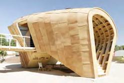
PIC.51 FABLAB HOUSE (CAMPO DEL MORO ,MADRID, SPAIN), DESIGNED AND FABRICATED BY INSTITUTE FOR ADVANCED ARCHITECTURE OF CATALONIA, THE CENTRE FOR BITS AND ATOMS AT MIT AND THE GLOBAL FAB LAB NETWORK, SELF SUFFICIENT SMALL SCALE DWELLINGMADE OF 2.5M X 12M LVL (LAMINATED VENEER LUMBER) PANELS + CURVABLE PLYWOOD.
PIC.52 FABLAB HOUSE (CAMPO DEL MORO ,MADRID, SPAIN), DESIGNED AND FABRICATED BY INSTITUTE FOR ADVANCED ARCHITECTURE OF CATALONIA, THE CENTRE FOR BITS AND ATOMS AT MIT AND THE GLOBAL FAB LAB NETWORK, SMALL SCALE STRUCTURAL PROTOTYPE.
PIC.53 THE STADTHAUS (LONDON, UK), DESIGNED BY WAUGH THISTLETON ARCHITECTS ,RESIDENTIAL NINE STOREY TIMBER STRUCTURE USING CROSS-LAMINATED TIMBER PANEL SYSTEM.
PIC.54 THE STADTHAUS (LONDON, UK), DESIGNED BY WAUGH THISTLETON ARCHITECTS, INTERIOR SPACE DURING CONSTRUCTION.
PIC.55 CENTRE FOR CULTURAL AND INNOVATIVE INTERCHANGE BETWEEN RUSSIA AND NORWAY (KIRKENES, NORWAY), DESIGNED BY REIULF RAMSTAD ARCHITECTS, 16-17 STOREY BUILDING, UNMATERIALIZED.
PIC.56 CENTRE FOR CULTURAL AND INNOVATIVE INTERCHANGE BETWEEN RUSSIA AND NORWAY (KIRKENES, NORWAY), DESIGNED BY REIULF RAMSTAD ARCHITECTS, 16-17 STOREY BUILDING, UNMATERIALIZED.
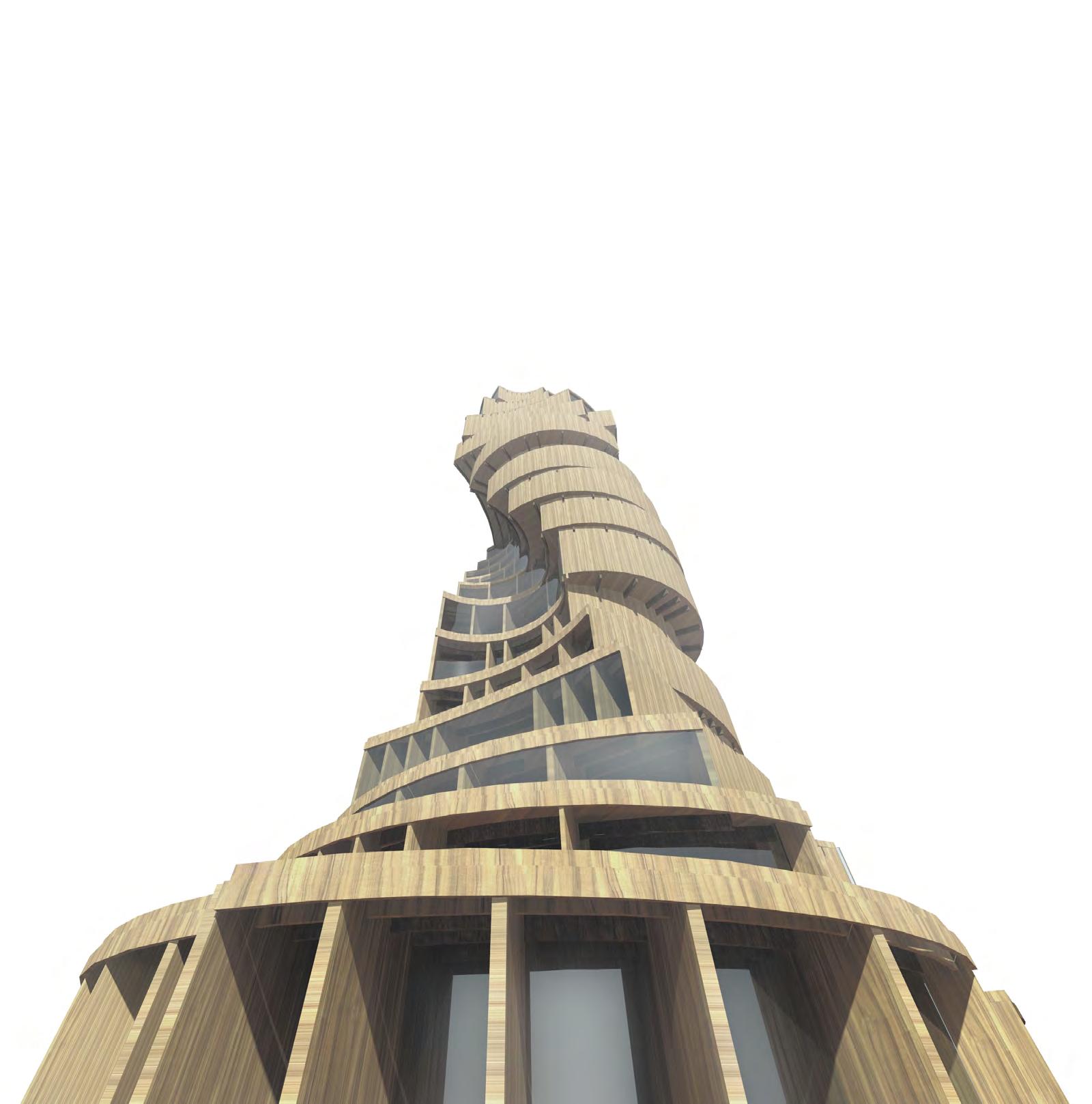
PROJECT SCALE AMBITION
The complexities of a residential programme create an ideal test bed to explore new models of inhabitation in morphologically complex environments. Our project aims to double the height of the Hackney Stadhaus. A building of 20 stories will be designed as a test model for a material system which exploits the inherent anisotropic properties of wood to curve, and depart away from orthogonal geometries. With the intent for achieving efficient structural performance and exciting spatial arrangements a building system will be created on the foundations of material component research.
047
21 DIAG.21 DIFFERENT WOODEN PROJECTS CLASSIFIED ACCORDING TO THEIR SCALE. ARBOREAL FORMATIONS
SCALE ARBOREAL FORMATIONS

048
00
G.O.
00
G.O.
450
G.O.
450
G.O.
450
G.O.
450
00
G.O.
G.O.
00
G.O.
00
450
G.O.
G.O.
450
G.O.
450
G.O.
00
G.O.
00
G.O.
00
G.O.
450
G.O.
GRAIN ORIENTATION
00 22 DOMAIN
G.O.
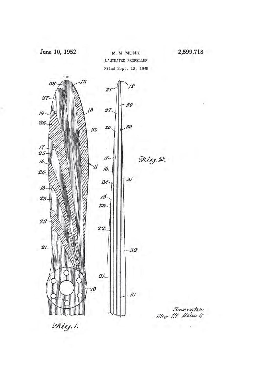
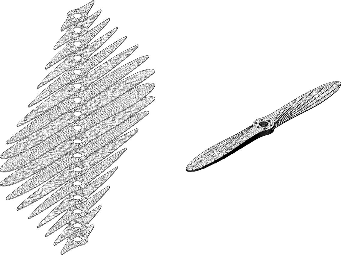
DIAG.22 MULTIPLE LAYERS OF DIFFERENT ORIENTATION ARE LAMINATED TOGETHER SHAPING THE AEREAL PROPELLAR.
PIC.57 DETAIL DRAWINGS BY M.N.NUNK, 1949.
MATERIAL SYSTEM AMBITION
In 1949 Max Munk applied his design for a new wooden propeller blade to the United States Patent Office in order to protect it. The design sought to improve the performance of the propeller and alleviate some of the stresses which flowed through other designs where the layers were laminated perpendicular to each other. He was aware that wood being a fibrous material had a greater stiffness in the direction of the fibres and the angle through which layers of wood are laminated together would affect the performance of the propeller. Through laminating twelve layers of wood with alternating layers rotated diagonally rather than at right angles to each other, a more elastic behaviour could be achieved. Thus as the thrust of the engine increased and the propeller spun faster, the organisation of the wooden layers would accommodate for a small elastic twist and allow the propeller to spin more efficiently.
The ambition of our project is to investigate a material defined architecture in which structure, spatial organisation, physical performance and fabrication are conceived as an integrated system. In a similar manner to the propellar, combining material knowledge with design application and development, the work seeks to explore how the microscopic behavioural traits of wood and fabrication methods may combine to create new curved building components.
049
ARBOREAL FORMATIONS
METHODS
Very few materials have homogenous properties that can be applied to any form and function. The methodology for the thesis research aims to utilise the dimensional instability behavioural properties of wood to program a material component that displays variation and adaption for application within the material system of a twenty story timber residential tower. The project seeks to unite the knowledge of physical material studies as a driver for computational design and performance exploration. This chapter documents the methods and steps taken to develop such an approach through seven interrelated methods of research.
- Physical Experimentation forms the basis of the project and aims to understand the behavioural trends of wood and parameters that may program a conceptual material component.
- Digital Simulation draws upon the parameters found in initial physical research as inputs for a computational simulation method that can efficiently test many different experiments.
- Physical-Digital Calibration seeks to establish and calibrate the key parameters that define the material component both as physically fabricated pieces and computationally simulated pieces.
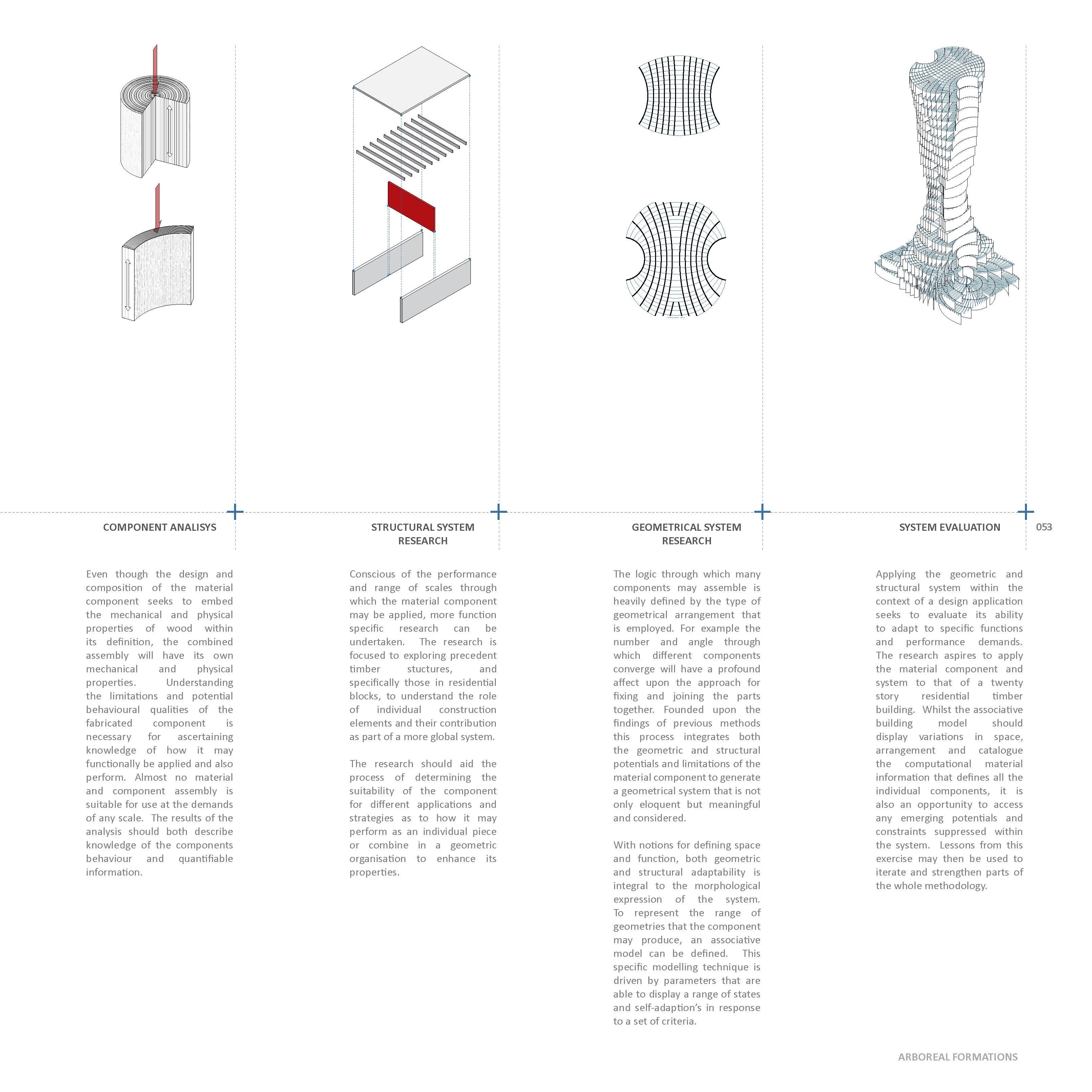
- Component Analysis aims to quantify the mechanical and physical properties of the material component and scale limitations for application.
- Structural System Research examines the context of the design application and the suitability of the material component to act as part of a structural system to meet the performance led demands.
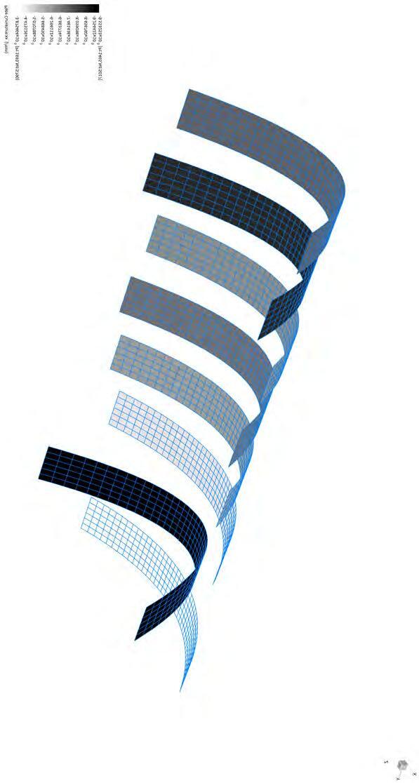
- Geometrical System Research explores the computational development of a material and structural system that displays variant morphological expressions that are adaptable to different requirements of space and function.
- System Evaluation applies the material component and system within the context of a test case project to understand the adaptability, emerging potentials and constraints of the system and how this may influence an iterated design.
METHODS
PHYSICAL EXPERIMENTS
• UNDERSTANDING BEHAVIOUR OF WOOD
• UNDERSTANDING PARAMETER OF TIMBER COMPONENTS
RESEARCH DEVELOPMENT
DIGITAL SIMULATION
• CONTROLING PARAMETERS OF TIMBER COMPONENTS
PHYSICAL - DIGITAL CALIBRATION
• SYNCHRONISATION OF PARAMETERS THAT DESCRIBES THE MATERIAL BEHAVIOUR OF THE COMPONENT IN BOTH ENVIRONMENTS
PIC.58 WOOD-CUT PRINT OF A WILLOW TREE BY BRYAN NASH GILL, 2011 050
• UNDERSTANDING MECHANICAL PROPERTIES OF THE COMPONENT
• UNDERSTANDING PHYSICAL PROPERTIES OF THE COMPONENT
• UNDERSTANDING SCALE CONSTRAINTS
DESIGN DEVELOPMENT
STRUCTURAL SYSTEM RESEARCH
• POTENTIALS OF COMPONENTS TO ACT AS PART OF STRUCTURAL SYSTEM
• EXISTING TIMBER STRUCTURES
• EXISTING STRUCTURAL SYSTEMS IN RESIDENTIAL STRUCTURES
• MORPHOLOGICAL EXPRESSION UPON THE CONSTRAINTS OF THE MATERIAL AND STRUCTURAL SYSTEM, SPATIAL ORGANISATION AND FUNCTION
DESIGN PROPOSAL
• EMERGING POTENTIALS AND CONSTRAINTS OF THE SYSTEM
• POSSIBLE APPLICATIONS OF THE SYSTEM IN THE CONTEXT OF SPECIFIC FUNCTIONS AND PERFORMANCE DEMANDS
• ADAPTATION OF GEOMETRICAL SYSTEM TO MEET TECHICAL REQUREMENTS
051
ANALISYS SYSTEM EVALUATION ARBOREAL FORMATIONS
GEOMETRICAL SYSTEM RESEARCH COMPONENT
METHODS FLOWCHART
METHODS
PHYSICAL EXPERIMENTS
Embracing the hygroscopic and anisotropic properties of wood a series of physical experiments may be undertaken to understand how moisture content, grain direction and fabrication techniques may programe laminated pieces of veneer to curve and twist. From the conception and development of different material components it is vital that the parameters used to define the pieces are quantifiable and have the potential for creating a range of results.
Commencing the research with the physical testing of wood and lamination fabrication methods seeks to prioritise these disciplines as the generative context for a more integrated design process.
DIGITAL SIMULATION
Limited by time, material and scale of physical testing, digital simulation offers a technique for efficiently pursing the experimentation of virtual timber components founded on the parameters discovered by physical experimentation.
Finite Element Analysis (FEA) software is used within the construction industry for the structural analysis and performance testing of designs. Traditionally FEA software is employed to check for the deflection of structural members when loaded and test for areas of structural failure. In the case of this research FEA is explored as a tool for simulating the behavioural nature of hygroscopic and anisotropic characteristics in pieces of laminated veneers. The objective for the exercise is to gain a closer understanding as to which parameters not only influence the curvature of laminated veneer components but may also be programmed.
PHYSICAL - DIGITAL CALIBRATION
Combining physical tests and digital simulations may focus a common set of rules from which a material component may be manufactured.
Physical testing is the only real means through which a material component can be proven in manufacture and operation. The computation of parameters which describes the design and manufacture of a material component will open a broader information resource through which different applications are able to be explored. If physical and digital experiments are successfully calibrated then a very powerful tool may be developed that is ensured to create the same material component results in both workspace environments.
052
RESEARCH DEVELOPMENT
This chapter documents the many experimental procedures that were undertaken with the aim to comprehend the complex behaviour of wood when exposed to moisture. Initial physical experiments revealed that curved strips could be created through a process of differentially soaking layers of veneer to achieve differing moisture contents, gluing and then laminating the pieces together with an elasticised clamping method.
Research Development attempts to understand which of many different parameters would affect the curvature of a veneered piece, the material component. A series of experiments were undertaken trying to explore the numerous parameters that could potentially program a component and utilise those that were quantifable to bring control over the fabrication process. The method for quantifying material information data combined parallel experiments undertaken with physical material testing and digital simulations. Successful calibration between these two fields could then be employed to form a matrix of relationships between the key influencing parameters.
054
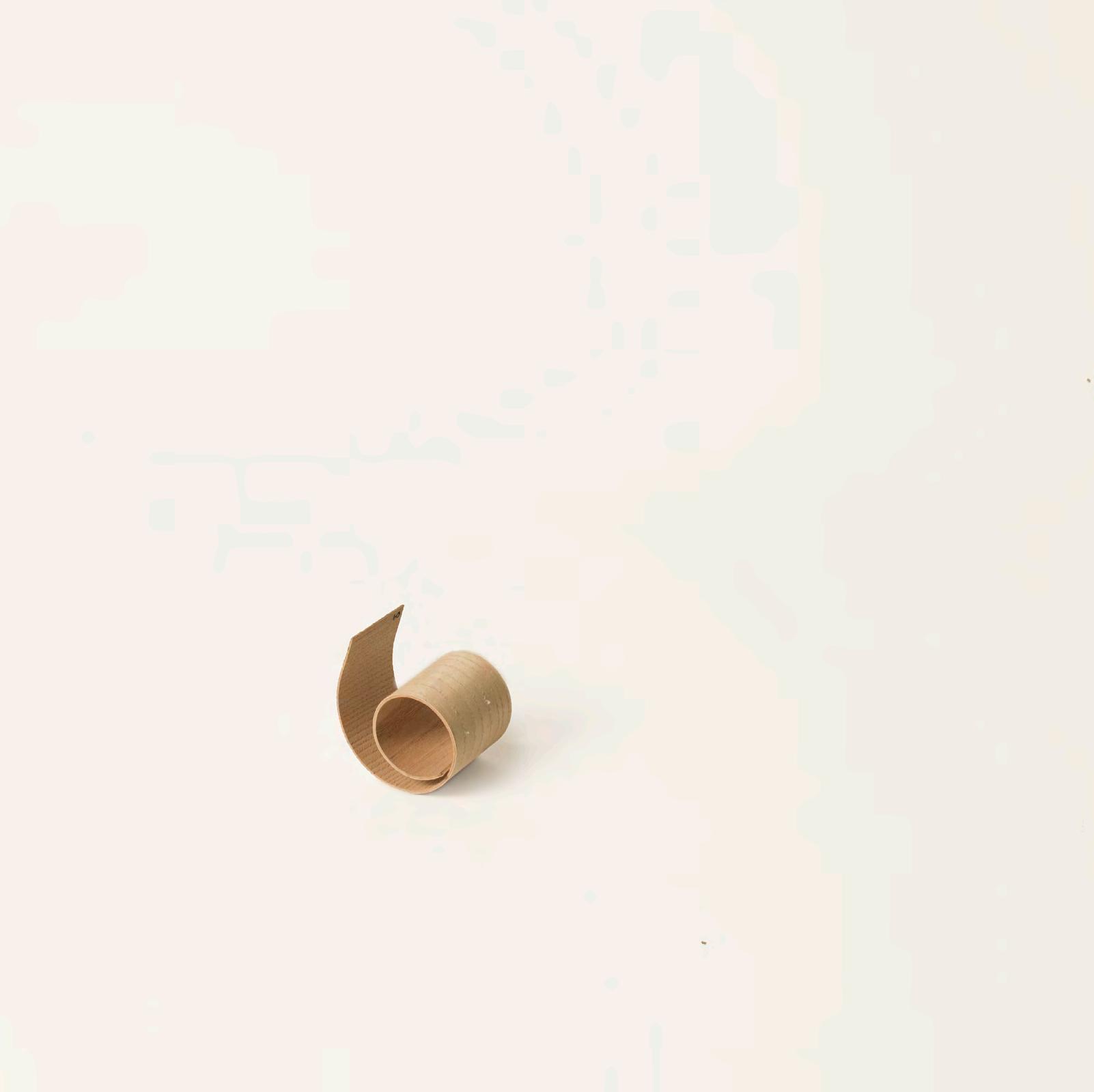
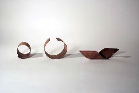
PIC.59 WOOD-CUT PRINT OF A WILLOW TREE, BY BRYAN NASH GILL, 2011. PIC.60 LAMINATED COMPONENT OF TWO
OF
RESEARCH DEVELOPMENT
LAYERS
WALNUT VENEER.
055 ARBOREAL FORMATIONS
STRIP OF ASH VENEER IS CUT TO A RECTANGULAR SHAPE OF 100 BY 100 MM AND THE MEASUREMENTS WERE RECORDED TO SEE HOW MUCH THE PIECE EXPANDS IN EACH AXIS.
THE SAMPLE IS TAKEN WITH A PREDOMINENT GRAIN DIRECTION PARALLEL TO ONE SIDE AND LITTLE VARIATION OF THE GRAIN DENSITY ALONG THE ENTIRE PIECE.
IT IS 1.4 MM THICK AND COMES OUT OF A FLAT CUT STRIP, WHICH IS IN A DRY STATE, MEANING ITS MOISTURE CONTENT IS AROUND 8% - 14% FOR THE INDOOR TEST ENVIROMENT.
THE SAMPLE PIECE IS SUBMERGED IN WATER FOR TEN MINUTES AND REMOVED.
OVER EXPOSING THE WOOD FIBRES TO MOISTURE ENSURES THE CELLS WILL REACH THEIR SATURATION LEVEL, SINCE THE PIECE WILL ABSORB AS MUCH WATER AS POSSIBLE (APPROXIMATELY 28% MOISTURE CONTENT).
AS ALREADY MENTIONED IN THE DOMAIN CHAPTER, THE WOOD EXPERIENCES NO DIMENSIONAL CHANGE BEYOND THE SATURATION LEVEL, SINCE THE REDUNDANT WATER IS KEPT IN THE CELL CAVITIES WITHOUT CAUSING FURTHER FIBRE SWELLING.
ON WITHDRAWING THE SAMPLE SHEET, MEASUREMENTS ACROSS BOTH AXIS ARE TAKEN AND RECORDED.
THE PIECE NOW MEASURES 100MM BY 105.5MM, EXPANDING MINIMALLY IN THE DIRECTION OF THE GRAIN BUT 5.50% ACROSS THE GRAIN.
AS EXPECTED, DUE TO THE ANISOTROPY OF WOOD, THE PIECE PERFORMS DIFFERENTLY IN THE TWO AXIS. AT THE SAME TIME, THE EXPANSION OF THE PIECE IS NEITHER THE RADIAL (4.90%) NOR THE TANGENTIAL AMOUNT (7.8%), AS INDICATED IN DIAG.21 FOR ASH. INSTEAD THE 5.5% VALUE ATTAINED FROM THE EXPERIMENTS WAS A BLEND OF THOSE TWO VALUES. THIS RESULT REMAINED CONSTANT FOR 3 REPEATED EXPERIMENTS BASED ON THE SAME SETUP.
(%)RADIAL SHRINKAGE (%)TANGENTIAL SHRINKAGE TANGENTIAL/ RADIAL WOOD TYPE ASH WHITE BEECH AMERICAN BIRCH YELLOW CHESTNUT AMERICAN ELM CEDAR MAPLE RED OAK RED OAK WHITE WALNUT BLACK YELLOW POPLAR CEDAR WHITE FIR WHITE PINE RED SPRUCE SITKA CEDAR WHITE 4.95.5 7.3 3.44.74 4 5.65.54.6 2.93.33.84.3 7.811.9 9.5 6.710.28.2 8.6 10.57.88.2 5.477.27.5 1.62.2 1.3 22.22.1 2.2 1.91.41.8 1.92.11.91.7 2.9 5.4 1.9 100mm expansion:~0% 100mm 100mm 105.5mm expansion:~0% 100mm 100mm 100mm 100mm 105.5mm expansion:5.5% 100mm expansion:~0%
PIECE EXPANDS
056 INITIAL STATE MOISTURE APPLIED
23 24 RESEARCH DEVELOPMENT
BEECH SPRUCE SCOTS PINE WESTERN RED CEDAR
OAK
MAHOGANY
BEECH SPRUCE SCOTS PINE WESTERN RED CEDAR
OAK
MAHOGANY
BEECH SPRUCE SCOTS PINE WESTERN RED CEDAR
OAK
MAHOGANY
BEECH SPRUCE SCOTS PINE WESTERN RED CEDAR
OAK
MAHOGANY
BEECH SPRUCE SCOTS PINE WESTERN RED CEDAR
OAK
MAHOGANY
BEECH SPRUCE SCOTS PINE WESTERN RED CEDAR
OAK
MAHOGANY
DIAG.23 BASIC PRINCIPLE OF PHYSICAL MATERIAL EXPERIMENTS. DIAG.24 EXPANSION FACTORS FOR DIFFERENT SPECIES OF WOOD SOURCE : HTTP://WWW. WOODBIN.COM.
RELATIVE DIMENSION CHANGES FOR DIFFERENT TYPES OF WOOD PLACED IN THE ENVIRONMENT OF NEW YORK SOURCE : HTTP://WWW.WOODCHANGES.COM/
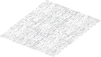
BASIC MATERIAL BEHAVIOUR PRINCIPLE
The basic principle of the physical experimentation is based on two main properties of wood : anisotropy and hygroscopy. As explained in DIAG.23, the dry ash veneer has a moisture content of around 8% - 19% when moisture equilibrium is reached with its surrounding environment.
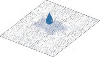
When moisture is applied to the dry piece, it starts expanding, according to the moisture absorbed. The limit for the expansion is set at the fibre saturation point, which is around 28% moisture content. This indicates that 28% of wood’s weight is the weight of the water captured in the piece and only within the cell walls of its fibres. Therefore, if the moisture applied exceeds this amount, no further expansion is noticed, since the additional water, free water, is kept in cavities between the cells.
The micro change at the cellular level, shrinking and swelling, cause noticeable dimensional changes at the global component scale. This basic principle was found to be independent of the size of the piece and same behaviour occurred for pieces of different lengths when fully saturated.
The constant shrinkage factor is also referred to as expansion factor in the context of this project, the reciprocal action of swelling. DIAG.24 documents the constant factor through which wood shrinks tangentially and radially for different species of wood. The experiment also supports the notion explained in the domain that if the veneer cut from the trunk can reflect tangential or radial shrinkage, its degree of expansion may consistently be predicted. In the physical experiments a flat cut ash veneer was unfortunately used displaying a blend of those two values.
Equally important to the cut type of the veneers is the type of wood. As shown in DIAG.25, for the given environment of New York City showing specific temperature and relative humidity variations throughout the year, different species of wood have different relative dimensional changes.
WOOD SPECIES RELATIVE DIMENTIONAL CHANGE
month 0.7% year 1.7% JAN FEBMARAPR MAY JUNJUL AUG SEPOCT NOV DEC TANGENTIAL month 0.6% year 1.3% TANGENTIAL month 0.4% year 0.9% TANGENTIAL month 0.7% year 1.7% TANGENTIAL month 0.3% year 0.7% TANGENTIAL month 0.9% year 2.1% TANGENTIAL 057
25
DIAG.25
ARBOREAL FORMATIONS
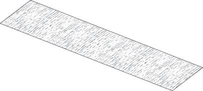
INITIAL STATE : TWO STRAIGHT LAYERS OF VENEER
TWO STRIPS OF ASH VENEER ARE CUT WITH THE GRAIN PERPENDICULAR TO THE LONG AXIS. BOTH PIECES HAVE SAME WIDTH (60MM) BUT ONE OF THEM IS CUT SHORTER THAN THE OTHER (300MM AND 283MM).
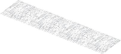
STEP.01 : MOISTURE APPLIED TO ONE LAYER
WATER IS APPLIED TO THE SHORTER PIECE AND LEFT FOR THE WOOD CELLS TO ABSORB THE MOISTURE.
GRADUALLY THE PIECE EXPANDS TO REACH ITS SATURATION POINT. EXPANSION ACROSS THE GRAIN IS MINIMAL BUT BY 5.5% PERPENDICULAR TO THE GRAIN (FOR FLAT CUT ASH VENEER).
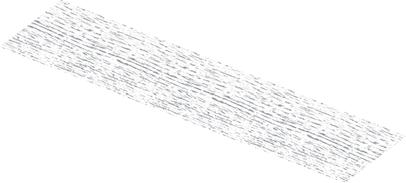
STEP.02 : WET LAYER EXPANDS
ONCE THE WET PIECE IS OF THE SAME LENGTH TO THE DRY PIECE (CALCULATED TO REACH ITS SATURATION POINT AT THAT LENGTH), PVA GLUE IS APPLIED TO THE DRY LAYER IN ORDER FOR THE TWO LAYERS TO BE LAMINATED.
STEP.03 : TWO LAYERS ARE LAMINATED TOGETHER
THE TWO PIECES ARE CLAMPED TOGETHER FOR 20 MINUTES, UNTIL PARTLY GLUED, AND THEN SET FREE TO DRY FURTHER.
STEP.04 : INNER LAYER CONTRACTS
AS THE PIECE BEGINS TO DRY, THE CELLS IN THE INNER WET LAYER LOSE MOISTURE, CAUSING IT TO SHRINK AND PULL THE OUTER LAYER INWARDS. AS A RESULT, THE PIECE BEGINS TO CURVE ALONG THE LONG AXIS.
FINAL STATE : PIECE IS CURVED
THE PIECE CONTINUES TO CURL UNTIL THE MOISTURE IN BOTH LAYERS EQUALISES WITH THE MOISTURE WITHIN ITS ENVIRONMENTAL CONTEXT.
300mm 300mm 283mm 300mm 300mm 283mm 300mm 300mm EXPANSION:5.5% 300mm 300mm 300mm 300mm 300mm 283mm 300mm 300mm 283mm 300mm 300mm EXPANSION:5.5% 300mm 300mm 300mm 058
26 RESEARCH DEVELOPMENT
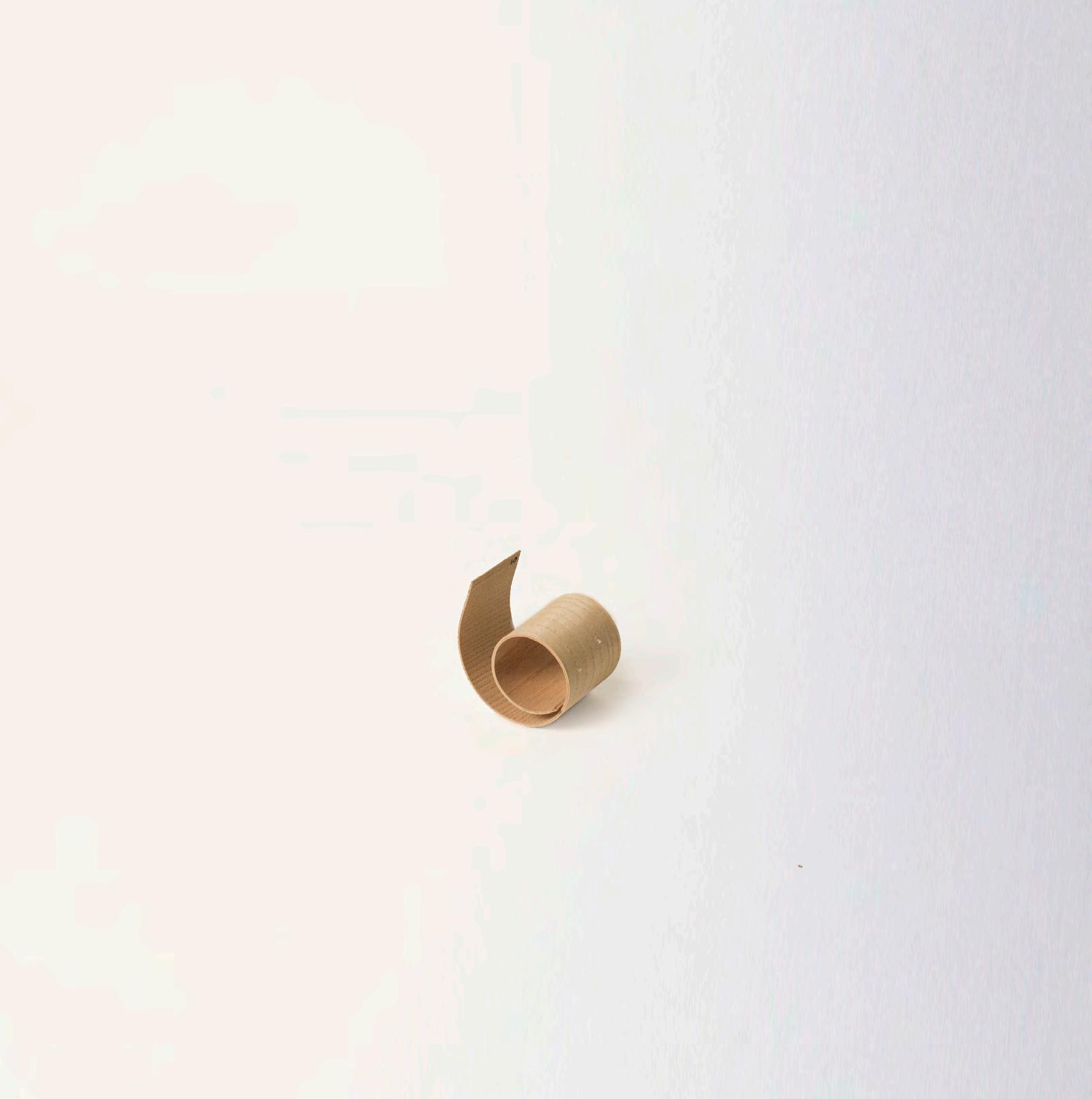
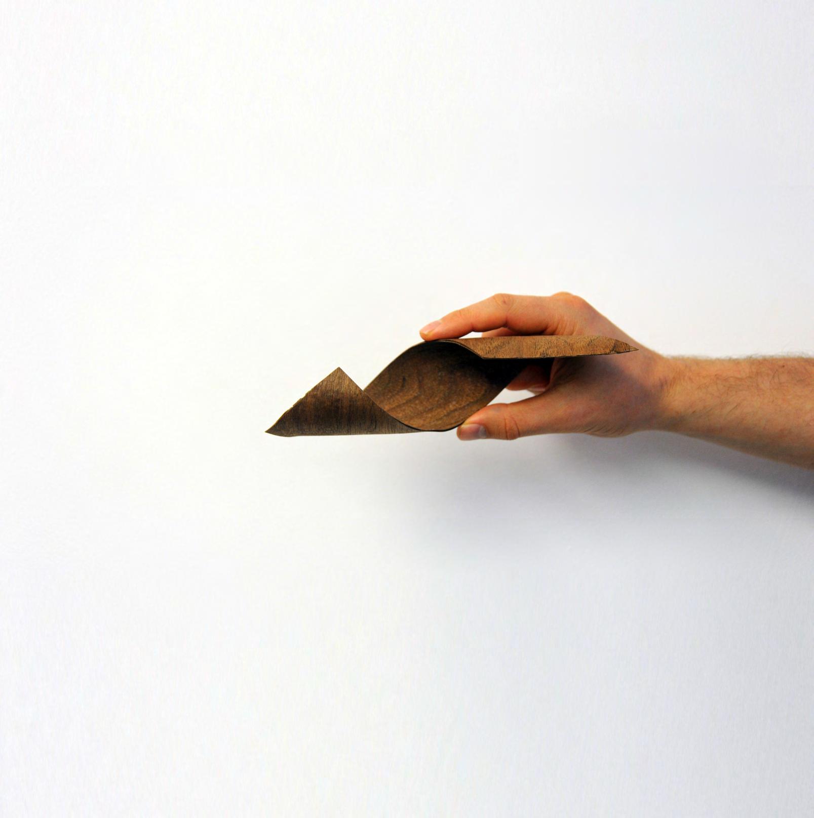
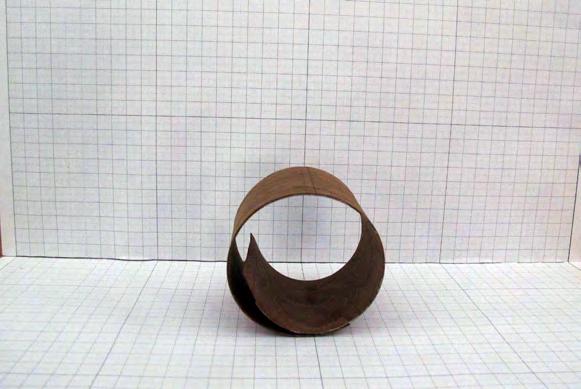
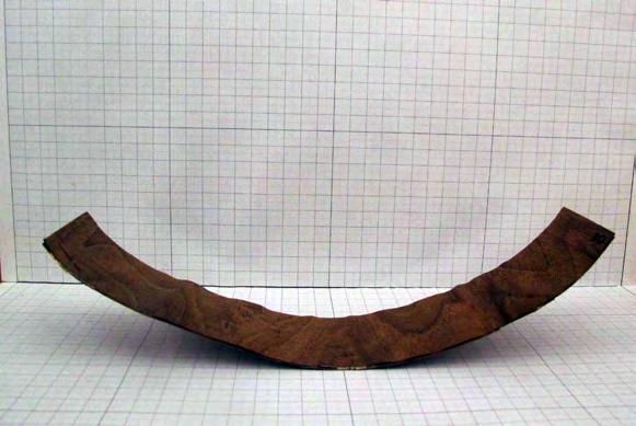
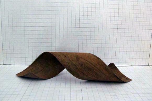
FABRICATION PRINCIPLE DIAG.26 GENERAL PRINCIPLE OF THE LAMINATION PROCEDURE BETWEEN TWO PIECES OF VENEER WITH DIFFERENT MOISTURE CONTENT. PIC.61 CURVED MATERIAL COMPONENT OF TWO LAMINATED LAYERS OF ASH, 0.6MM THICKNESS EACH.
A Bi-Metallic Strip is comprised of two fused metal layers that when heated expand at different rates. The properties of the two layers are independent but when joined together exert influence upon each other. The metal with the lower coefficient of thermal expansion is overcome by the metal with the higher coefficient and is thus on the inside as it bends.
Inspired by the Bi-Metallic Strip logic this initial experiment, DIAG.26, explores the potential of applying moisture to one layer of veneer, causing it to swell and change length, and leaving the other one dry. When the two layers are laminated together and left to dry, the layer which has been subject to the added moisture content gradually dries out, causing the wood cells to shrink. Bonded together, the drying layer contracts pulling the drier piece into curvature. In the case of the two laminated veneers, the layer that pulls the piece to curve is the one situated on the inner side of the curve rather than the outer, as in the case of the Bi-Metallic Strip.
Whilst the initial experiments showcased a promising basic fabrication principle, multiple aspects needed to be addressed in order to gain control over the overall process and the produced pieces. Effects of de-lamination could clearly be seen suggesting methods for fabrication would need great improvement. Observations for development included controlling the required moisture to reach the desired length for each layer of veneer, trialling different types of glue and advancing the quality of lamination bonding. The experiment also raised questions of what potential application could be suitable for a curved wood component.
059
ARBOREAL FORMATIONS
VENEER TYPE GRAIN ORIENTATION LAMINATION LAYERS
WALNUT BLACK G.O. 900
WALNUT BLACK G.O. 900
WALNUT BLACK G.O. 00
WALNUT BLACK G.O. 900
[L.01] 60.0 X 300.0 X 0.6 MM
[L.01] 60.0 X 310.6 X 0.6MM
[L.02] 60.0 X 300.0 X 0.6 MM
WALNUT BLACK G.O. 450
WALNUT BLACK G.O. 450
[L.01] 60.0 X 300.0 X 0.6 MM
[L.01] 60.0 X 300.9 X 0.6MM
[L.02] 60.0 X 300.0 X 0.6 MM

[L.01] 60.0 X 300.0 X 0.6 MM
[L.01] 60.0 X 300.6 X 0.6MM
[L.02] 60.0 X 300.0 X 0.6 MM
x y z x y z x y z x y z x y z x y z x y z x y z x y z x y z x y z x y z x y z x y z x y z x y z x y z x y z
STRAIGHT LAMINATION
CROSS LAMINATION
ANGLED LAMINATION 450
060
DIMENSIONS LAMINATION
TYPE
SHRINKAGE
RADIAL 5,50
5,50 TANGENTIAL 7,80 7,80 7,80 27 RESEARCH DEVELOPMENT
FACTOR
5,50
DIAG.27 USING THE SAME FABRICATION PROCESS (LAMINATION) MANIPULATING THE GRAIN ORIENTATION MAY PRODUCE DIFFERENT GEOMETRIES.
PIC.62 THREE MATERIAL COMPONENTS PRODUCED THE GRAIN ORIENTATIONS OF DIFFERENT VENEER LAYERS ( 0°, 45°, 90°)
PIC.63 SERIES OF COMPONENTS PRODUCED OUT OF THE SAME PROCESS. IN ALL CASES, GEOMETRIES WITH SIMPLE CURVATURES CAN BE PRODUCED.
GRAIN DIRECTIONALITY
The anisotropic properties of wood deduce that the grain directionality of the wood will affect how the piece may perform, in terms of deformation, bending and twisting, and structural performance. Three experiments were undertaken to document the effects of changing the orientation of the grain for two layers of Black Walnut veneer, 0.6mm thick, 300mm long and 60mm wide.
The first experiment, straight lamination, was created with the grain of both layers perpendicular to the long axis. When dried, the strip curves to complete more than a full radius. The component shows high compressive strength along its y axis, and low strength in bending on the x and z axis.
The second experiment, cross lamination, orients the grain of one layer parallel to the long axis and the other perpendicular. This caused the strip to curve less than the first one, but with a noticeable improvement in its ability of resisting bending along the x axis, whereas its loading capacity in compression along its y axis is slightly decreased.
The final experiment, angled lamination, oriented both layers through 450 degrees to the long axis and caused the strip to both bend and twist. In this case, the strip shows similar behaviour to the first experiment, though its compression strength is significantly decreased.
All the laminated pieces transformed to single curvature geometries, the first two displayed single curvature radial motion and the third twisted like a coil around a cylinder in a radial ruled surface motion. The results of manipulating grain direction within the three experiments displayed very different results and potentials for development. With the ambition to gain control over the component a decision was taken to progress the project’s research using the first experiment technique where all the veneer layers were laminated with the same grain orientation. This would allow the grain orientation variable to remain constant and the behaviour of other parameters to be studied in more detail.
DRY LAMINATED PIECE BENDING BENDING TWISTING
061
ARBOREAL FORMATIONS
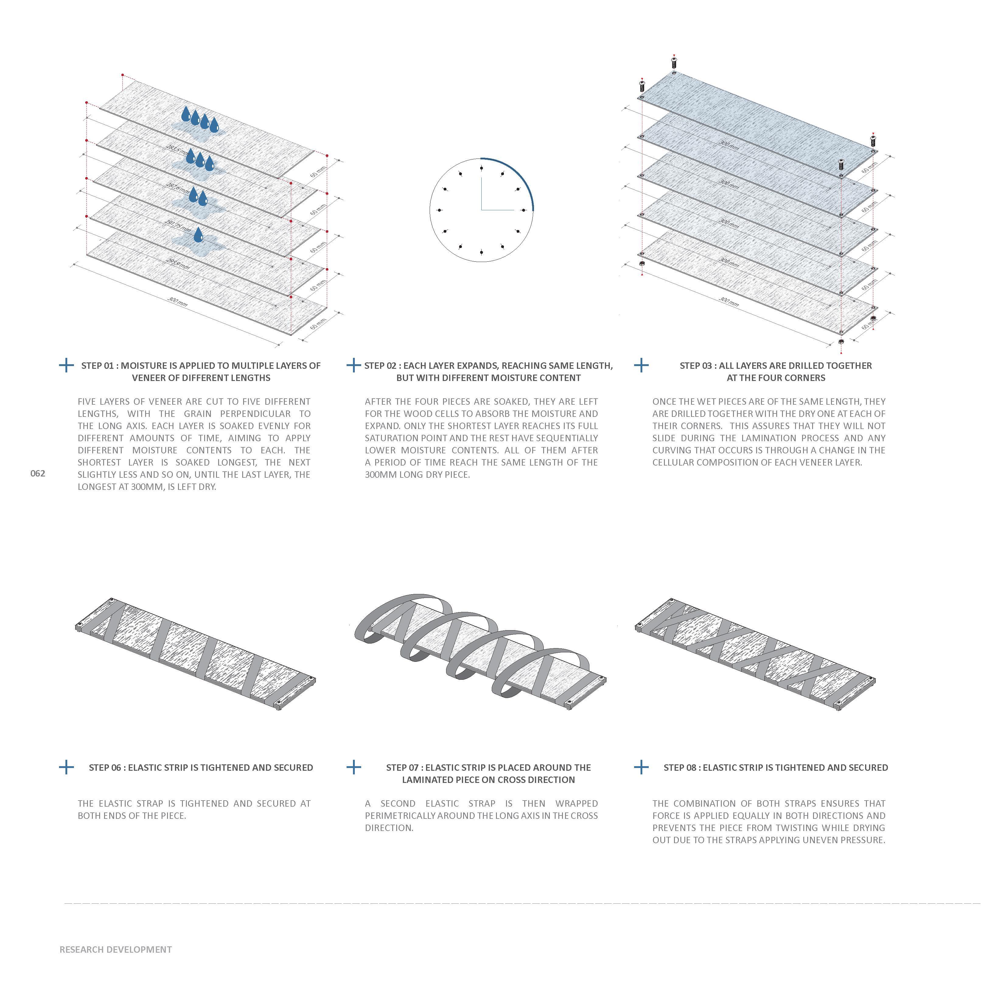
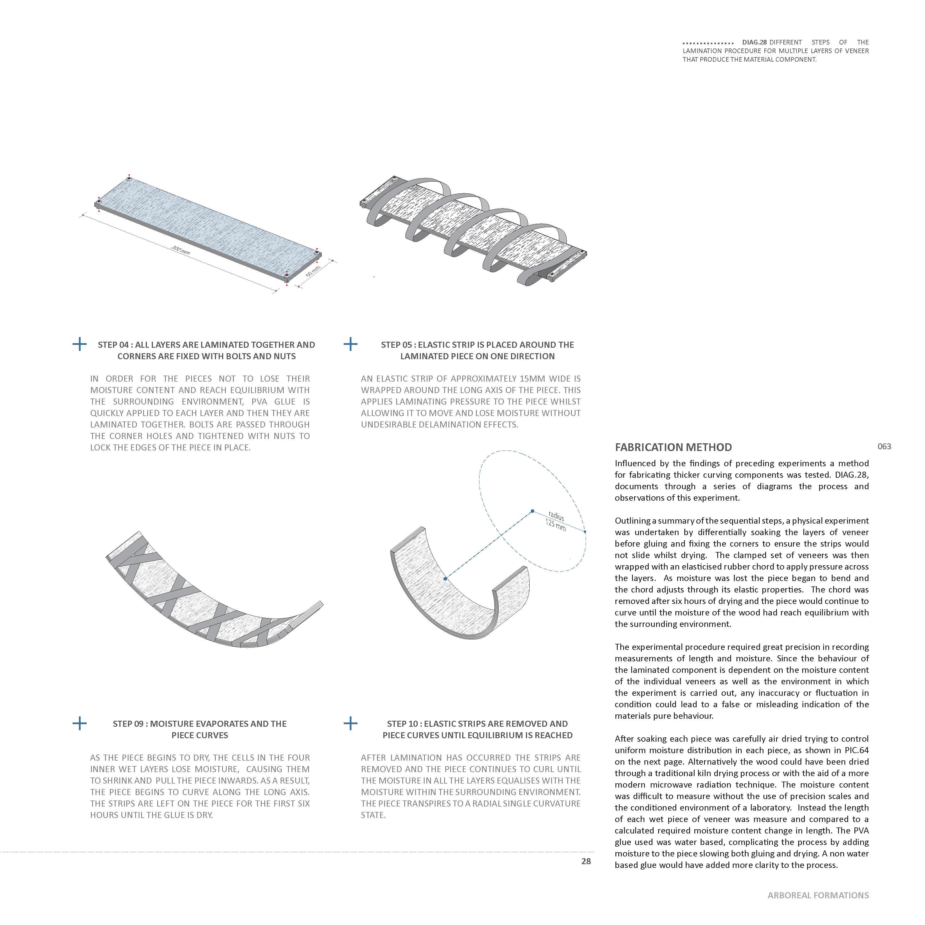
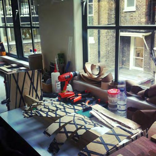
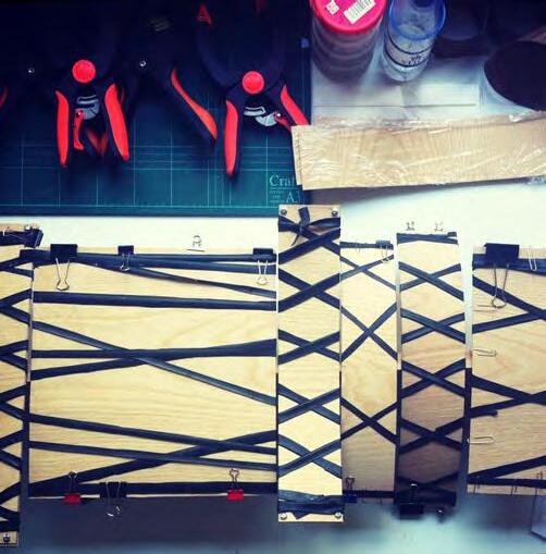
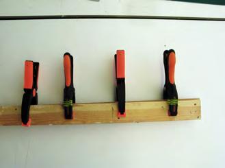
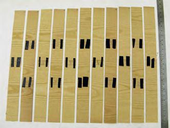
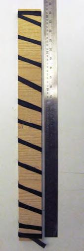
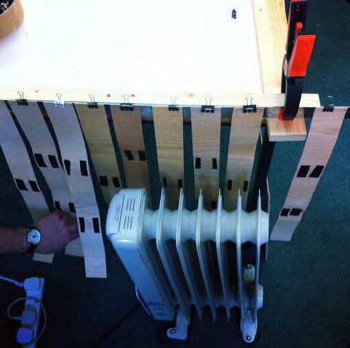
064 RESEARCH DEVELOPMENT
Tmax
DIAG.29 CURVATURE AND VENEER LAYER CALCULATIONS FOR THE PHYSICAL EXPERIMENTS.
PIC.64 FABRICATION PROCEDURE : EXPANDING, CLAMPING, CONTRACTING, DRYING. PIC.65 (NEXT PAGE) TIME FRAMES OF THE MATERIAL COMPONENT DURING THE DRYING PERIOD AS IT REACHES MOISTURE EQUILIBRIUM WITH THE ENVIRONMENT.
L - length of the inner layer
L o - length of the outer layer
R - radius of the inner arc
R o - radius of the outer arc
α - angle of the arc (in radians)
T max - maximum thicknes of the laminate
L o Li
L = R *α
L o = R o *α
L = Lo/Fexp
T max = R o - R
R = L /α
R o = L o/α
R = L o/(α*Fexp)
T max = L o/α - Lo/(α*Fexp) = = (1/α - 1/(α*Fexp)) =
= L o((α*Fexp - α)/(α2*Fexp)) =
= Lo((α*(Fexp-1))/(α2*Fexp))
T max = Lo((Fexp-1)/(α*Fexp))
L - length of the inner layer
L o - length of the outer layer
R - radius of the inner arc
R o - radius of the outer arc
α - angle of the arc (in radians)
T max - maximum thicknes of the laminate
L = R *α
L o = R o *α
L = Lo/Fexp
T max = R o - R R = L /α
R o = L o/α
R = L o/(α*Fexp)
L - length of the inner layer
T max = L o/α - Lo/(α*Fexp) = = (1/α - 1/(α*Fexp)) =
L o - length of the outer layer
R - radius of the inner arc
R o - radius of the outer arc
= L o((α*Fexp - α)/(α2*Fexp)) =
= Lo((α*(Fexp-1))/(α2*Fexp))
T max = Lo((Fexp-1)/(α*Fexp))
α - angle of the arc (in radians)
T max - maximum thicknes of the laminate
L = R *α
L o = R o *α
L = Lo/Fexp
T max = R o - R
R = L /α
R o = L o/α
R = L o/(α*Fexp)
T max = L o/α - Lo/(α*Fexp) = = (1/α - 1/(α*Fexp)) =
= L o((α*Fexp - α)/(α2*Fexp)) =
= Lo((α*(Fexp-1))/(α2*Fexp))
T max = Lo((Fexp-1)/(α*Fexp))
LAMINATION PROCEDURE
As detailed in the fabrication methodology, each physical experiment requires a number of layers, each of different length. In order to calculate and program the length of each individual veneer, a geometrical method was investigated, based on the principle that each species of wood has a known and constant tangential shrinkage Fexp. The required radius was set for the outer dry layer, which had a length Lo and then the length Li of the inner wet layer was calculated, to the maximum tangential shrinkage factor, indicating the maximum feasible expansion of the veneer strip along its long axis, where grain is oriented vertically. Based on those two limits, intermediate layers could be computed as a range between the inner and outer lengths. Additionally, through the mathematical type as indicated in DIAG.29, we could calculate the maximum thickness of the laminate piece, for a given curvature.
The results of the calculation presented a curving wood strip but with a different radius than expected. This validated that a method for geometrically setting a radius and trying to calculate the length of the inner layers could not be used, although the fabrication methodology was correct. Thus a series of experiments would need to be undertaken to search for a relationship between different parameters that affect the curvature of the laminate component.
065
Ro α Ri
L o L
Ro α Ri
29 ARBOREAL FORMATIONS
5
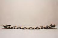
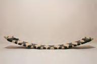
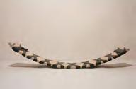
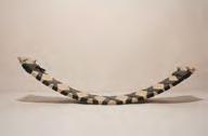
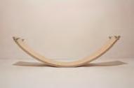

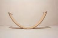
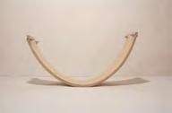
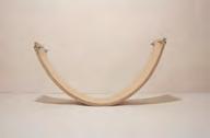
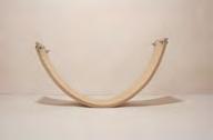
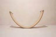
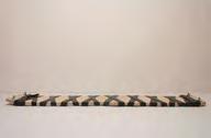
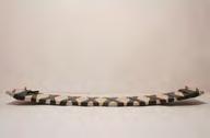
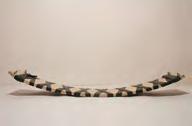
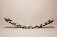
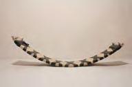
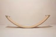
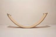
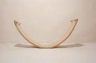
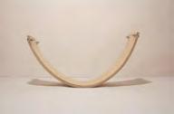

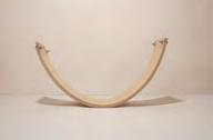

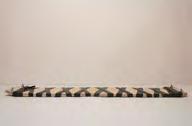
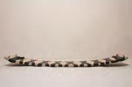
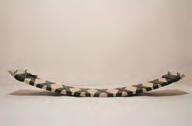
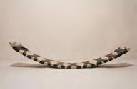
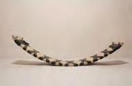
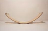

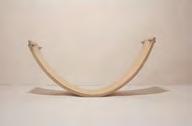
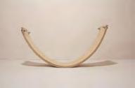
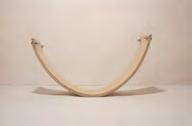
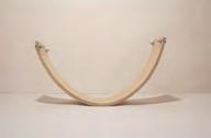
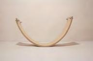
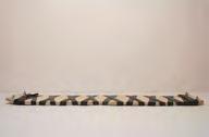
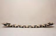
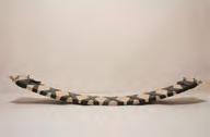
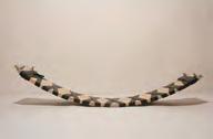
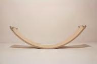

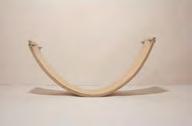
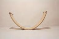

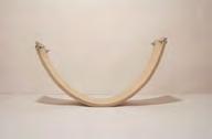

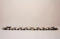
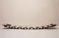
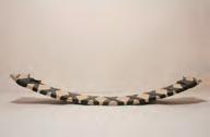
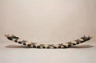
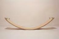
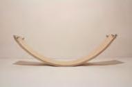
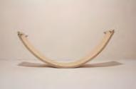
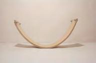
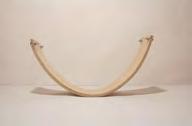
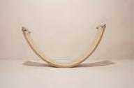
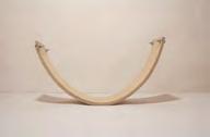
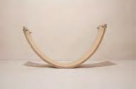
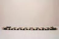
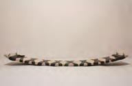
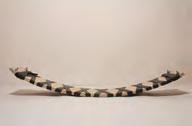
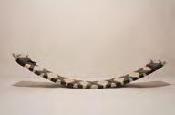
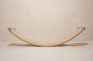
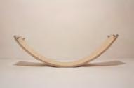
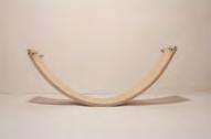
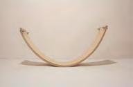
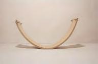
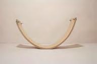
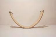
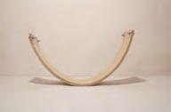
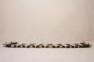
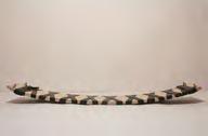
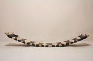
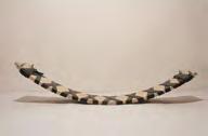
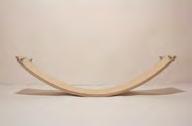
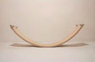
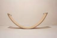
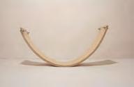
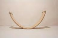
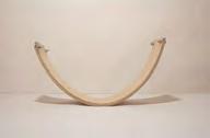
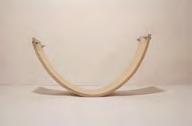
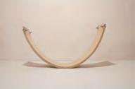
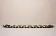
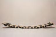
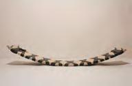
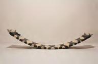
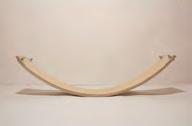
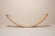
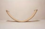
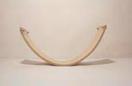
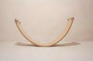
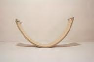
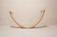
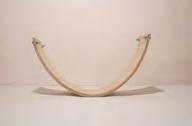
066
LAYERS OF 1.4MM BIRCH VENEER SAMPLE : 420
84 MM ELASTIC
1:00 HOUR 2:00 HOURS 3:30 HOURS 4:30 HOURS 6:00 HOURS 7:30 HOURS 9:00 HOURS 10:00 HOURS 11:30 HOURS 13:00 HOURS 12:30 HOURS 8:30 HOURS 14:00 HOURS 15:30 HOURS 5:00 HOURS
X
STRAPS REMOVED
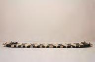
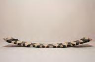
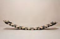
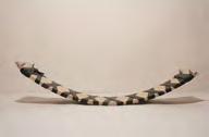
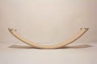
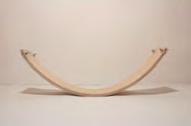
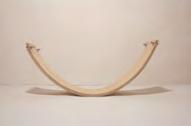
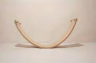
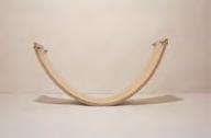
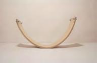
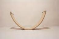
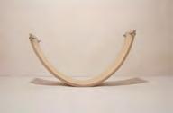

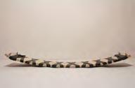
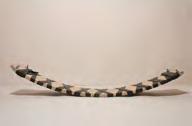
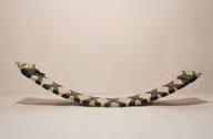
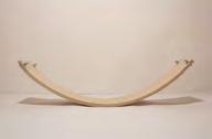
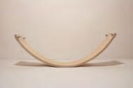
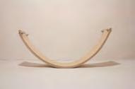
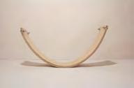
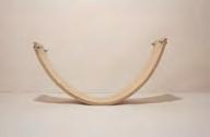
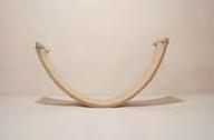
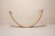
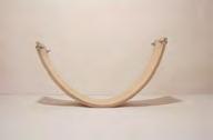
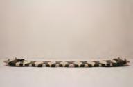
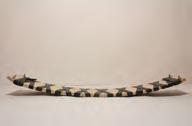
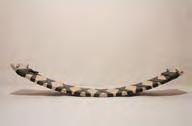
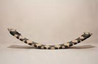
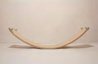
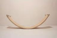

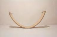
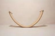
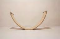
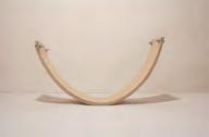
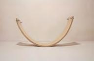

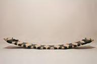
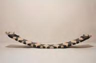
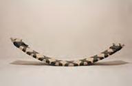
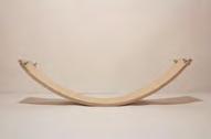
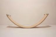
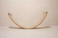
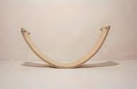
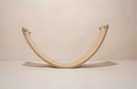

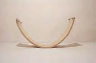
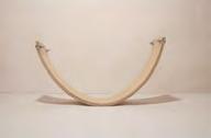
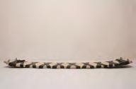
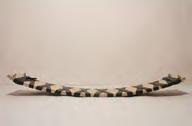
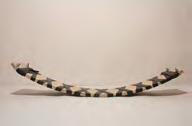
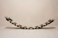
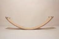
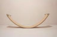

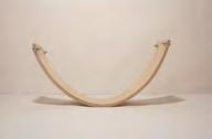
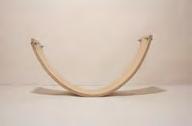
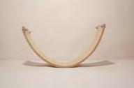
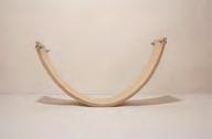
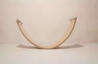
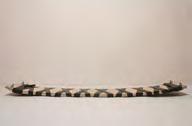
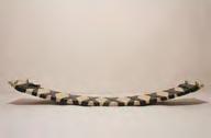
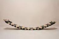
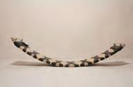
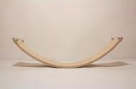
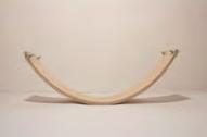
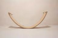
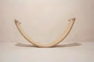
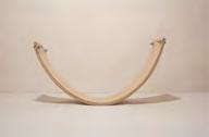
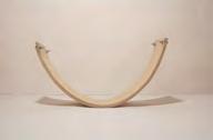

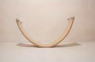
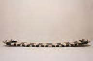
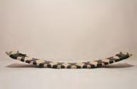
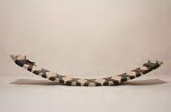
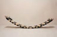
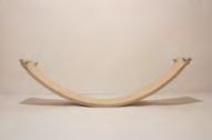
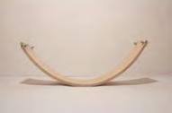
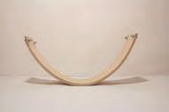
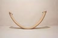

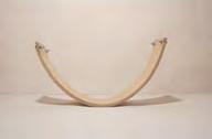
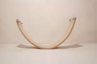
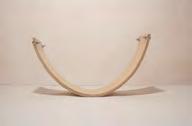
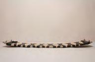
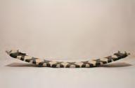
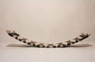
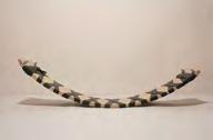
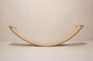
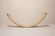
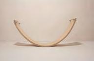
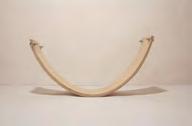
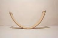
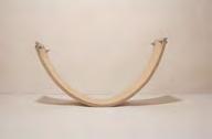
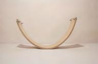
067 TIME TO REACH EQUILIBRIUM : 17H CURVATURE RADIUS : 250MM 1:30 HOURS 6:30 HOURS 7:00 HOURS 16:00 HOURS 15:00 HOURS 13:30 HOURS 11:00 HOURS 9:30 HOURS 8:00 HOURS 10:30 HOURS 12:00 HOURS 14:30 HOURS 5:30 HOURS 4:00 HOURS 2:30 HOURS 3:00 HOURS
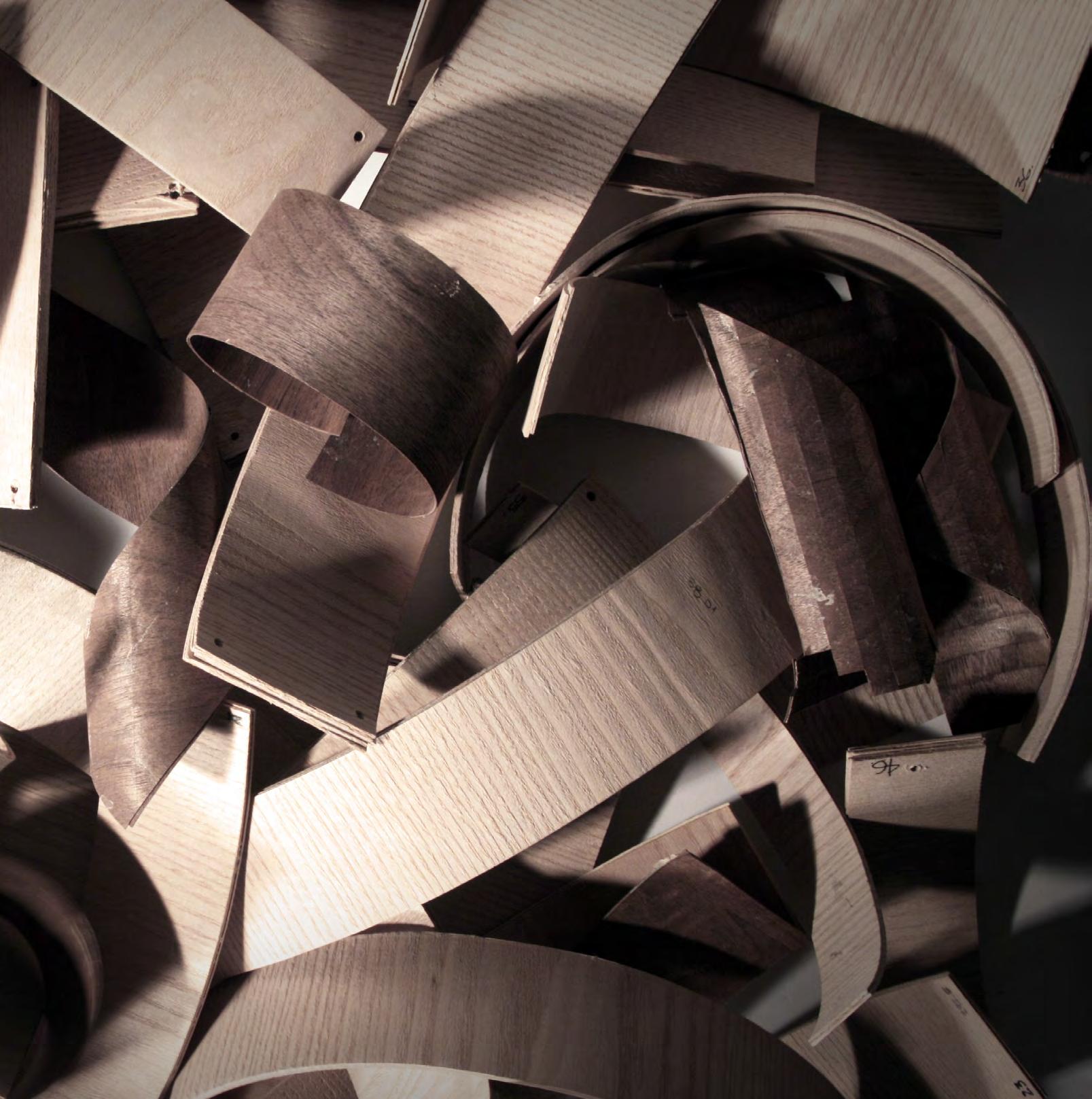
068 RESEARCH DEVELOPMENT
MATERIAL COMPONENT
PHYSICAL EXPERIMENTS
• UNDERSTANDING BEHAVIOUR OF WOOD
• UNDERSTANDING PARAMETER OF TIMBER COMPONENTS
DIGITAL SIMULATION
• CONTROLING PARAMETERS OF TIMBER COMPONENTS
PHYSICAL - DIGITAL CALIBRATION
• SYNCHRONISATION OF PARAMETERS THAT DESCRIBES THE MATERIAL
BEHAVIOUR OF THE COMPONENT IN BOTH ENVIRONMENTS
FROM PHYSICAL TO DIGITAL EXPERIMENTS
The research development intended to present a series of experiments, conducted in both physical and digital environments with the ambition for creating a controlled and quantified material component. The steps below summarise three stages of exploration.
As detailed in the methods chapter, physical material experimentation was first initiated to set the groundwork for comprehending the behaviour of wood and how through a fabrication process curved pieces of timber may be produced.
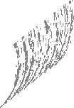
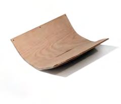
Findings from the physical experiments could then be utilised as an input for the digital simulation of the components material behaviour. In this manner, a deeper understanding and identification of specific curvature influencing parameters could be explored.
The Final stage of this parallel exploration between physical and digital workspaces is the process of calibration. With a notion that the computation workspace would allow more complex application strategies to be undertaken uniting the two working methods would ensure that computed digital components could then be physically fabricated.
x y z x y z x y z
069
SEQUENCE OF MATERIAL COMPONENT EXPLORATIONS. 30
DIAG.30
PIC.66 COLLECTION OF PHYSICAL MATERIAL EXPERIMENTS. ARBOREAL FORMATIONS
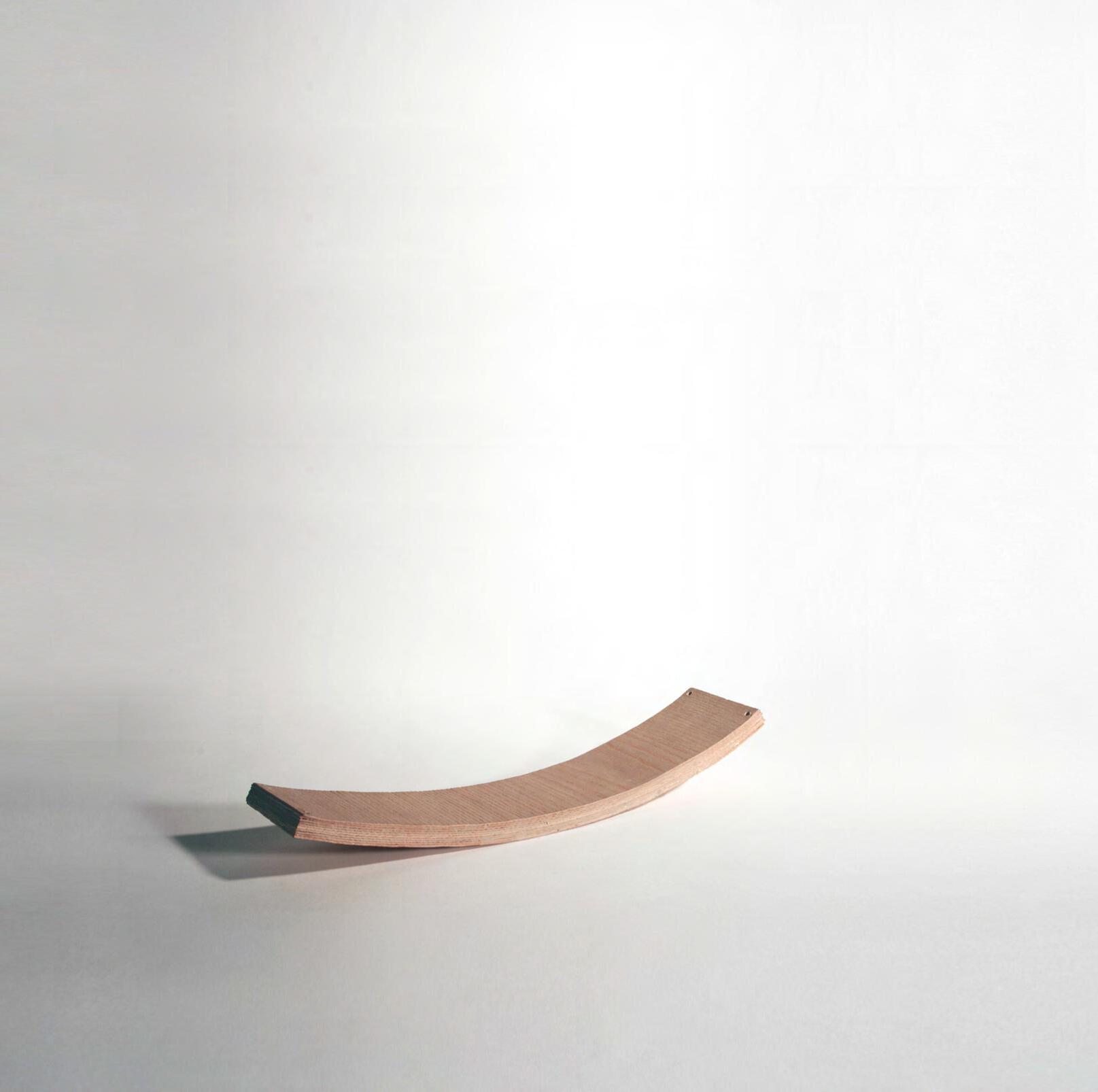
070 MATERIAL COMPONENT BEHAVIOUR 05 06 04 03 RADIALCURVATURE RESEARCH DEVELOPMENT
GRAIN ORIENTATION OF VENEER
THICKNESS OF VENEERS
NUMBER

PHYSICAL EXPERIMENT PARAMETERS
With the aim of understanding which parameters would affect the curvature of a wood strip, PIC.67, a series of physical experiments were initiated. The setup of these experiments was built on the described fabrication methodology and the failure to produce desired curvatures through a solely geometrical method for calculating the length of veneers. An alternative method was therefore required to progress the project and focused on the parameters which we thought affected the curvature of the component.
Physically working with different wood species, ash and walnut veneer, of different thicknesses, 0.6mm and 1.4mm, made us aware that both the species and thickness of each layer of veneer affected the curvature created. As anticipated the expansion factor of each layer controlled fundamentally in the fabrication process by its moisture content, also caused the component to curve in different ways. The grain orientation played a significant role in forming the produced geometry and was identified as the first influential parameter in the system but locked to ensure only single curved radial pieces were fabricated. Other variables that could affect the fabrication of the component were also assumed as variables and were thought to be related to the scale and basic dimensions, length, width and overall thickness or number of layers in the composition.
These seven outlined parameters, wood species, grain orientation, thickness of veneers, number of layers, expansion factor (shrinkage factor) of layers, length and width of component, concluded our initial physical observations and would need to be quantified and catalogued by further physical experiment investigations.
The following pages document a series of experiments investigating the affect of each individual parameter on the curvature of a laminated piece with the aim of gaining a holistic and complete apprehension of the material component’s behaviour.
071
PIC.67 MATERIAL COMPONENT OUT OF BIRCH VENEER, 10 LAYERS OF 1.4MM THICKNESS, EXPANSION FACTOR : 5.50%. WOOD SPECIES OF VENEER LENGTH OF COMPONENT 01 02 03 04 05 06 07 WIDTH OF COMPONENT EXPANSION FACTOR OF LAYERS
OF
LAYERS
ARBOREAL FORMATIONS
PRE - ANALYSIS
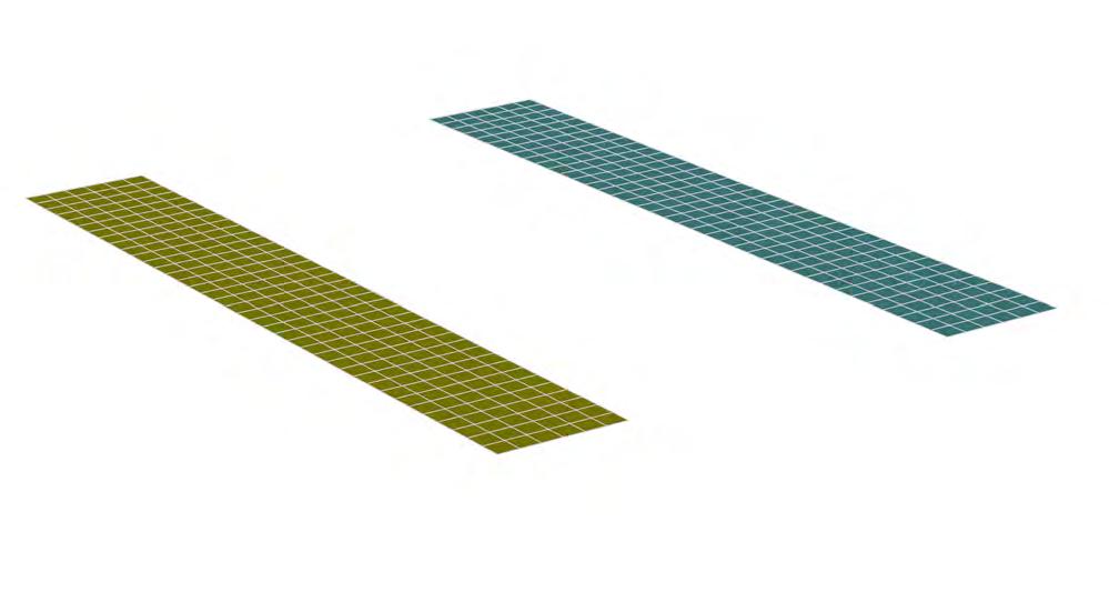
COMPONENT OF
-3.875464X10¯³ [PT:96,ND:390]
[pt:324,nd:1149]
= - 0.7039 0C
POST - ANALYSIS
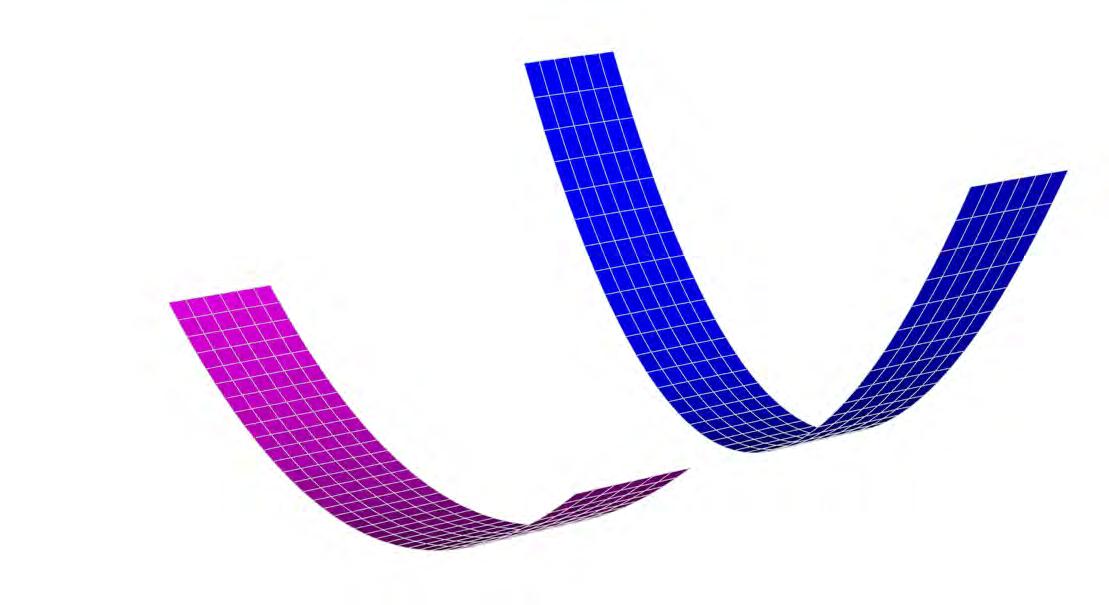
072 31
PLATE CURVATURE:XX (/MM)
DIGITAL
OAK VENEERS
ΔΤ
RADIAL
MM
DIGITAL COMPONENT
OF
MAHOGANY VENEERS
RADIAL CURVATURE PRODUCED = 104.68 MM
CURVATURE PRODUCED = 258.03
-4.473126X10¯³ -5.070788X10¯³ -5.668450X10¯³ -6.266112X10¯³ -6.863774X10¯³ -7.461436X10¯³ -8.059098X10
RESEARCH DEVELOPMENT
¯³ -8.656760X10¯³ -9.254422X10¯³ -9.553253X10¯³
0.0175 0.0075 LAY_03 0.0350 0.0150
LAY_04 0.0525 0.0225
LAY_05 0.0700 0.0300
LAY_06 0.0875 0.0375
LAY_07 0.1050 0.0450
LENGTH
INPUT DATA FOR THE FINITE ELEMENT ANALYSIS, INDICATING THE DIFFERENT PARAMETERS.
INPUT
DIGITAL SIMULATION METHOD
Digital simulation apart from simulating the material behaviour of the physical experiment, also allowed the work to continue performing experiments when sourcing the proper material or proper size was not feasible, due to time, cost, logistic etc. Additionally, when the computational set up for the digital experiment was attained, multiple experiments could be processed, saving time and material, while delivering more accurate results.
The data from the physical component tests was fed into the Finite Element Analysis (FEA) software, for both the multiple layers of veneer, example in DIAG.32, and the bonding PVA glue, DIAG.33. Next, a ΔΤ of -0.7039 0C was applied to the laminated digital component, equal to reaching equilibrium within an indoor space, simulating the physical difference in moisture content. The results as shown in the example for different wood species in DIAG.31, display the component curved and successfully simulating concurrent behaviour with that of the physical experiment. At the back of the book is an appendix in which the raw material data from all the digital FEA experiments is documented. DIAG.31 FINITE ELEMENT ANALYSIS ON TWO MATERIAL COMPONENTS OF DIFFERENT WOOD SPECIES.
EL (MPA) ET(MPA) v12
0.013 300.00 300.00 300.00 90.00˚ 90.00˚ 0.017 300.00 300.00 300.00 OAKMAHOGANY TANG.
9460.008690.00 681.12 434.50 THICKNESS 1.40mm1.40mm NO.LAYERS 7.00 7.00 LAY_01 0.0000 0.0000 LAY_02
G12(MPA) G13(MPA) G23(MPA) GRAIN ORIENTATION
EXP. (%) 10.50 4.50
mm300 mm WIDTH 60mm 60mm EL (MPA) ET(MPA) v12 G12(MPA) G13(MPA) G23(MPA) 0.300 500.00 500.00 500.00 PVA GLUE 1500.00 1500.00 THICKNESS 0.10mm 073
300
DIAG.32
DIAG.33
PVA GLUE. 32 WOOD SPECIES OF VENEER LENGTH OF COMPONENT 01 02 03 04 05 06 07 WIDTH OF COMPONENT EXPANSION FACTOR OF LAYERS NUMBER OF LAYERS GRAIN ORIENTATION OF VENEER THICKNESS OF VENEERS 33 ARBOREAL FORMATIONS
DATA FOR THE BONDING LAYER OF
DIGITAL EXPERIMENT
PLATE CURVATURE:XX (/MM)
-7.660491X10
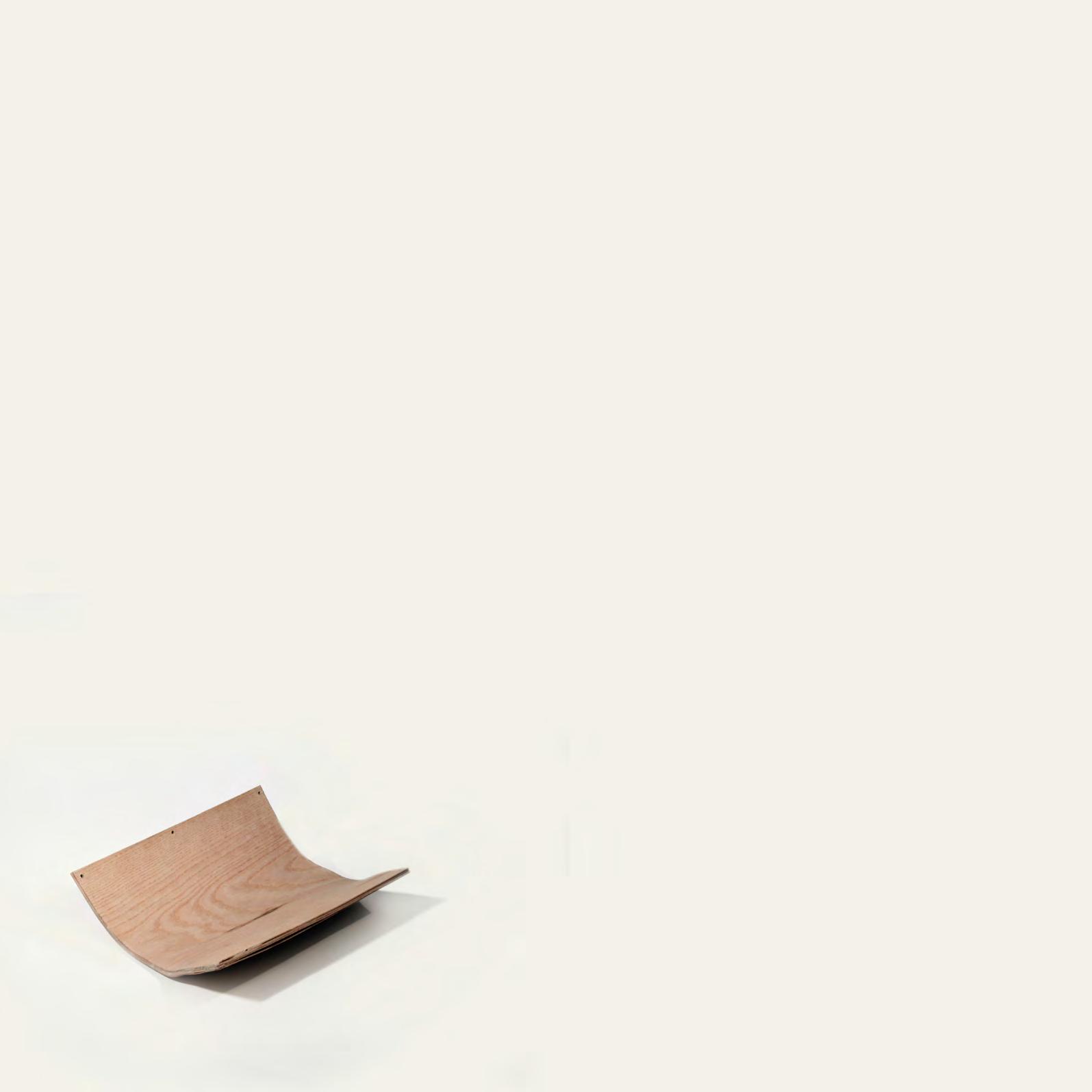
PHYSICAL EXPERIMENT
074
CROWN ASH VENEER
5
LAYERS OF 1.4MM
SHRINKAGE FACTOR : 5.50%
¯³
¯³
¯³
¯³ -7.660491X10¯³ -7.660491X10¯³ -7.660491X10¯³ -7.660491X10¯³ R
R
¯³ [PT:797,ND:2703] -7.660491X10¯³ -7.660491X10
-7.660491X10
-7.660491X10
-7.660491X10
= 155.10MM
= 130.54MM
34 RESEARCH DEVELOPMENT
-7.660491X10¯³ [pt:798,nd:2705]
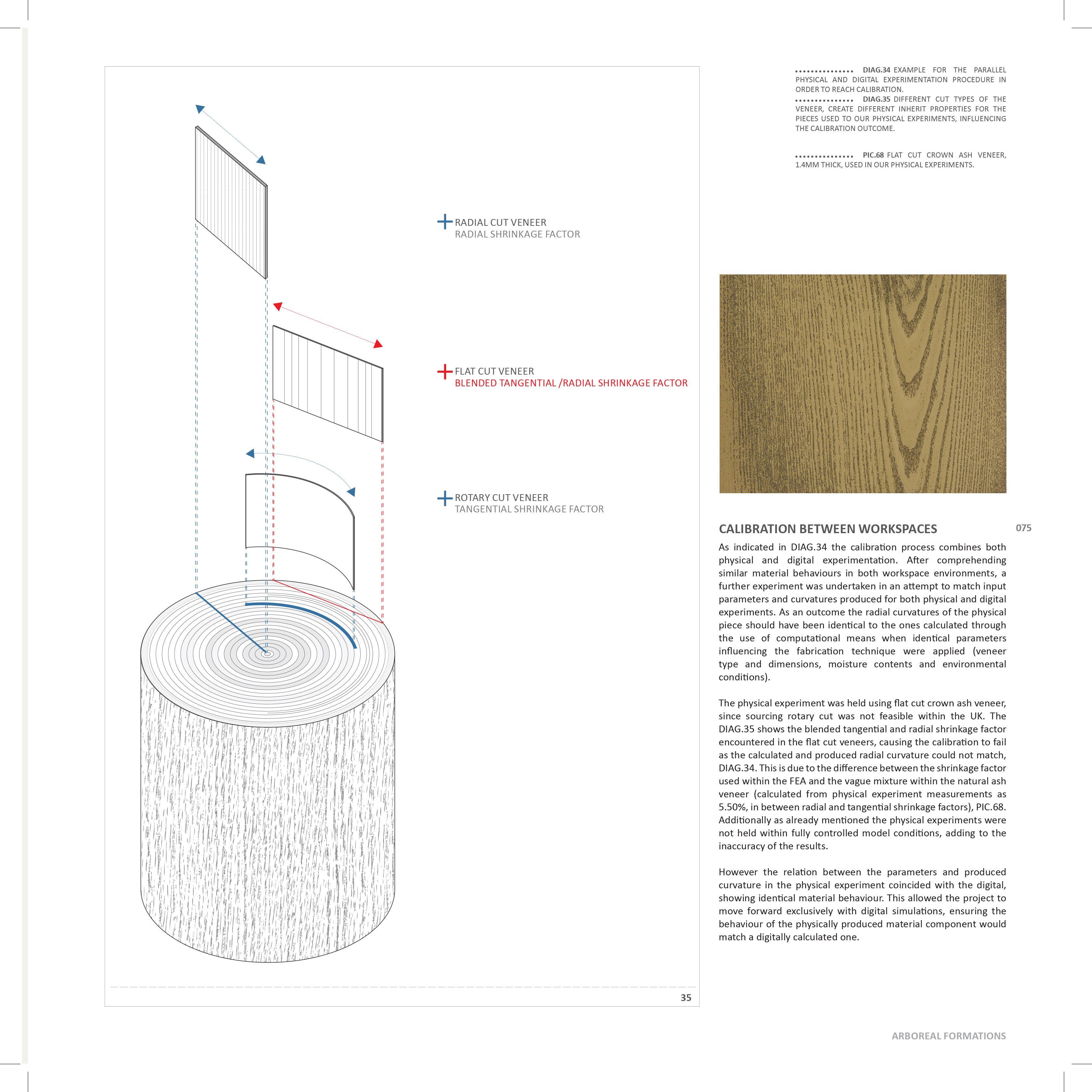

076 36 ASH WHITE BIRCH YELLOW SPRUCE SITKA WALNUT BLACK PINE WESTERN WHITE CEDAR WESTERN REDCEDAR OAK WHITE MAHOGANY AFRICAN SHRINKAGE (%) COMPRESSION (kPa) SHEAR (kPa) TENSION (kPa) RADIAL 4,90 7,30 4,30 5,50 4,10 2,50 2,40 5,60 PARALLEL 51.100 56.300 38.700 52.300 34.700 44.500 31.400 41.800 TANGENTIAL 7,80 9,50 7,50 7,80 7,4 4,50 5,00 10,50 PERPEND. 8.000 6.700 4.000 7.000 3.200 3.200 8.300 PARALLEL 13.200 13.000 7.900 9.400 7.200 10.300 6.800 12.500 PERPEND. 6.500 6.300 2.600 4.800 1.500 4.700 WOOD SPECIES DIGITAL CURVATURE VENEER TYPE 37 RESEARCH DEVELOPMENT
DIGITAL COMPONENT SIMULATION FINITE

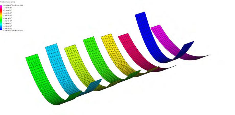
SHRINKAGE RADIAL — RADIAL SHRINKAGE IS SHRINKAGE IN THE DIRECTION FROM THE CENTER OF THE TREE TO THE PERIMETER OF THE TRUNK.
SHRINKAGE TANGENTIAL — TANGENTIAL SHRINKAGE IS SHRINKAGE DIRECTLY PERPENDICULAR TO RADIAL, PARALLEL TO GROWTH RINGS AND ROUGHLY DOUBLE IN MAGNITUDE.
COMPRESSIVE STRENGTH PARALLEL TO GRAIN—MAXIMUM STRESS SUSTAINED BY A COMPRESSION PARALLEL-TO-GRAIN SPECIMEN HAVING A RATIO OF LENGTH TO LEAST DIMENSION OF LESS THAN 11.
COMPRESSIVE STRENGTH PERPENDICULAR TO GRAIN—REPORTED AS STRESS AT PROPORTIONAL LIMIT. THERE IS NO CLEARLY DEFINED ULTIMATE STRESS FOR THIS PROPERTY.
SHEAR STRENGTH PARALLEL TO GRAIN—ABILITY TO RESIST INTERNAL SLIPPING OF ONE PART UPON ANOTHER ALONG THE GRAIN. VALUES PRESENTED ARE AVERAGE STRENGTH IN RADIAL AND TANGENTIAL SHEAR PLANES.
TENSILE STRENGTH PERPENDICULAR TO GRAIN—RESISTANCE OF WOOD TO FORCES ACTING ACROSS THE GRAIN THAT TEND TO SPLIT A MEMBER. VALUES PRESENTED ARE THE AVERAGE OF RADIAL AND TANGENTIAL OBSERVATIONS.
SOURCE : HTTP://WWW.WOODBIN.COM/CALCS/SHRINKULATOR.HTM
DIAG.36 DATA FOR PROPERTIES OF DIFFERENT WOOD SPECIES, SOURCE : HTTP://WWW.WOODBIN. COM/CALCS/SHRINKULATOR.HTM
DIAG.37 DIGITALLY PRODUCED CURVATURE FOR EACH WOOD SPECIES.
DIAG.38 CURVATURE AS FUNCTION OF COMPONENT WOOD SPECIES.
DIAG.39 FINE ELEMENT ANALYSIS FOR COMPONENTS OF DIFFERENT WOOD SPECIES.
PIC.69 DIFFERENT WOOD SPECIES OF VENEER.
01 WOOD SPECIES OF VENEER
AIM :
How do different wood species influence the produced curvature of the material component?
PROCEDURE :
Sourcing different veneer types was proved to be a difficult process, and since the initial physical experiments revealed a relation between that parameter and the produced curvature, it was decided proceeding only with the digital simulation for this experiment, trying to understand the material behaviour of different wood species.
Eight components of different wood species were digitally simulated with the use of FEA. Each set of experiments consisted of seven layers of 1.4mm thickness and different physical properties as indicated in DIAG.36, while every digital component was programmed to reach its maximum tangential shrinkage factor on the inner of the layers.
A ΔΤ = -0.7039 is then applied to the laminated pieces and after the simulation is run, the components curve differently, as shown in DIAG.39.
OUTCOME :
Each wood species has a different tangential shrinkage factor and therefore each strip displays a different radial curvature. Consequently, the selection of wood species determines the permissible range of curvatures of the material component.
For the proceeding digital experiments, white ash was picked, as one of the most easily sourced veneer types of 1.4mm thickness, displaying at the same time high tangential shrinkage factor, allowing the fabrication of tight curvatures.
DIFFERENT NUMBER RADIAL CURVATURE (MM) NUMBER OF LAYERS OF LAMINATE 290 300 310 320 330 340 350 0 2 4 6 8 10 12 WOOD SPECIES RADIAL CURVATURE (MM) 0 50 100 150 200 250 300 MAHOGANY CEDAR PINE SPRUCE ASH WALNUT BIRCH OAK 077
ASH WHITE BIRCH YELLOW SPRUCE SITKA WALNUT BLACK PINE WESTERN WHITE CEDAR WESTERN REDCEDAR OAK WHITE MAHOGANY AFRICAN
KEY FOR MATERIAL INFORMATION INPUTS
ELEMENT ANALYSIS
38 39 ARBOREAL FORMATIONS
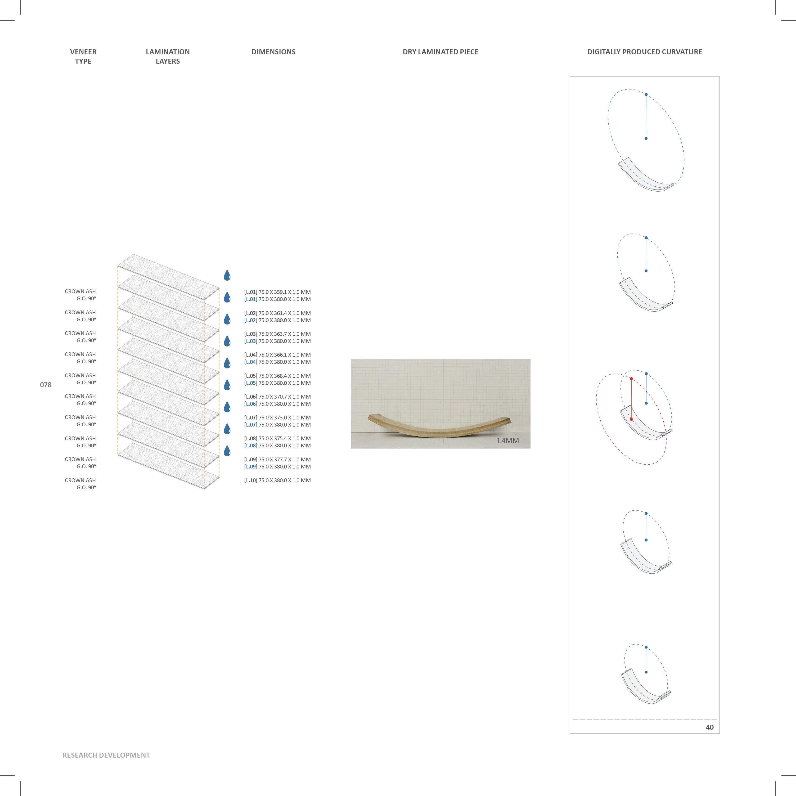
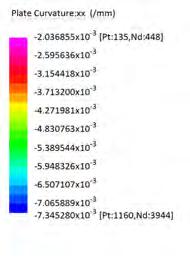
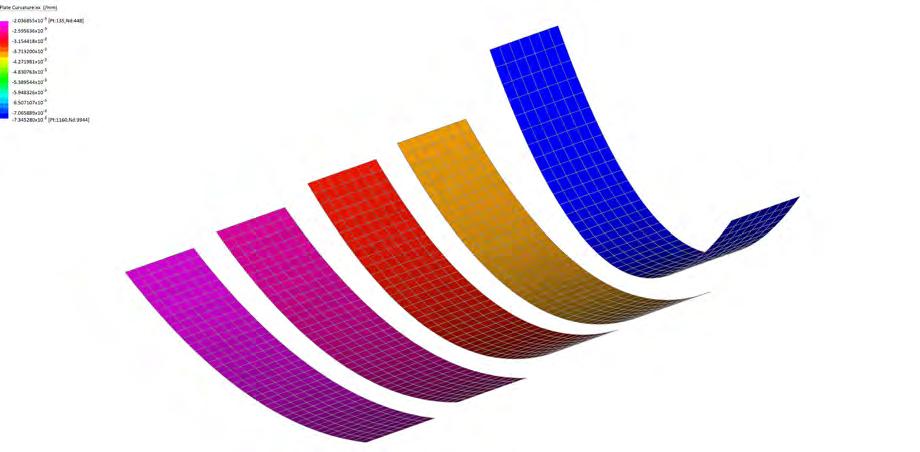
X THICKNESS OF
DIAG.40 CALLIBRATION BETWEEN PRODUCED CURVATURES OF PHYSICAL AND DIGITAL EXPERIMENTS.
DIAG.41 CURVATURE AS FUNCTION OF COMPONENT’S LAYER THICKNESS.
DIAG.42 FINE ELEMENT ANALYSIS FOR COMPONENTS OF DIFFERENT LAYER THICKNESS.
AIM :
How do different thicknesses of individual veneers influence the produced curvature of the material component?
PROCEDURE :
As in the case of the previous parameter, sourcing veneers of white ash but of different thicknesses was not feasible, and therefore, the only physical experiment conducted was limited to the thickness of 1.4mm for 10 layers of veneer.
The same setup but within the digital environment, DIAG.42, was carried out for five components of ten layers each, but of different thicknesses, 0.50mm, 1.00mm, 1.40mm (most commonly used within the building industry and called constructional veneer), 2.00mm and 2.50mm. A ΔΤ = -0.7039 is applied to the laminated pieces and after the simulation is run, the components curve differently with a function described in DIAG.41.
OUTCOME :
The thickness of the white ash veneers within the laminate influence the curvature achieved. This suggests that the thinner the individual layers are, the tighter the produced radii for a given number of layers. However an observation from physical experiments suggests difficulties in precisely controlling moisture levels in veneer under 0.6mm thick.
20x0.5mm DIFFERENT NUMBER OF DIFFERENT THICKNESS OF RADIAL CURVATURE (MM) RADIAL CURVATURE (MM) NUMBER
LAMINATE(MM) NUMBER OF LAYERS OF LAMINATE 50 100 150 200 0 2 4 6 8 10 12 100 200 300 400 500 600 700 0 20x2.5mm 20x2.0mm 20x1.4mm 20x1.0mm 079 03
41
THICKNESS OF VENEERS
42 DIGITAL COMPONENT SIMULATION FINITE ELEMENT ANALYSIS 10X2.50MM 10X0.50MM 10X1.00MM 10X1.40MM 10X2.00MM
ARBOREAL FORMATIONS
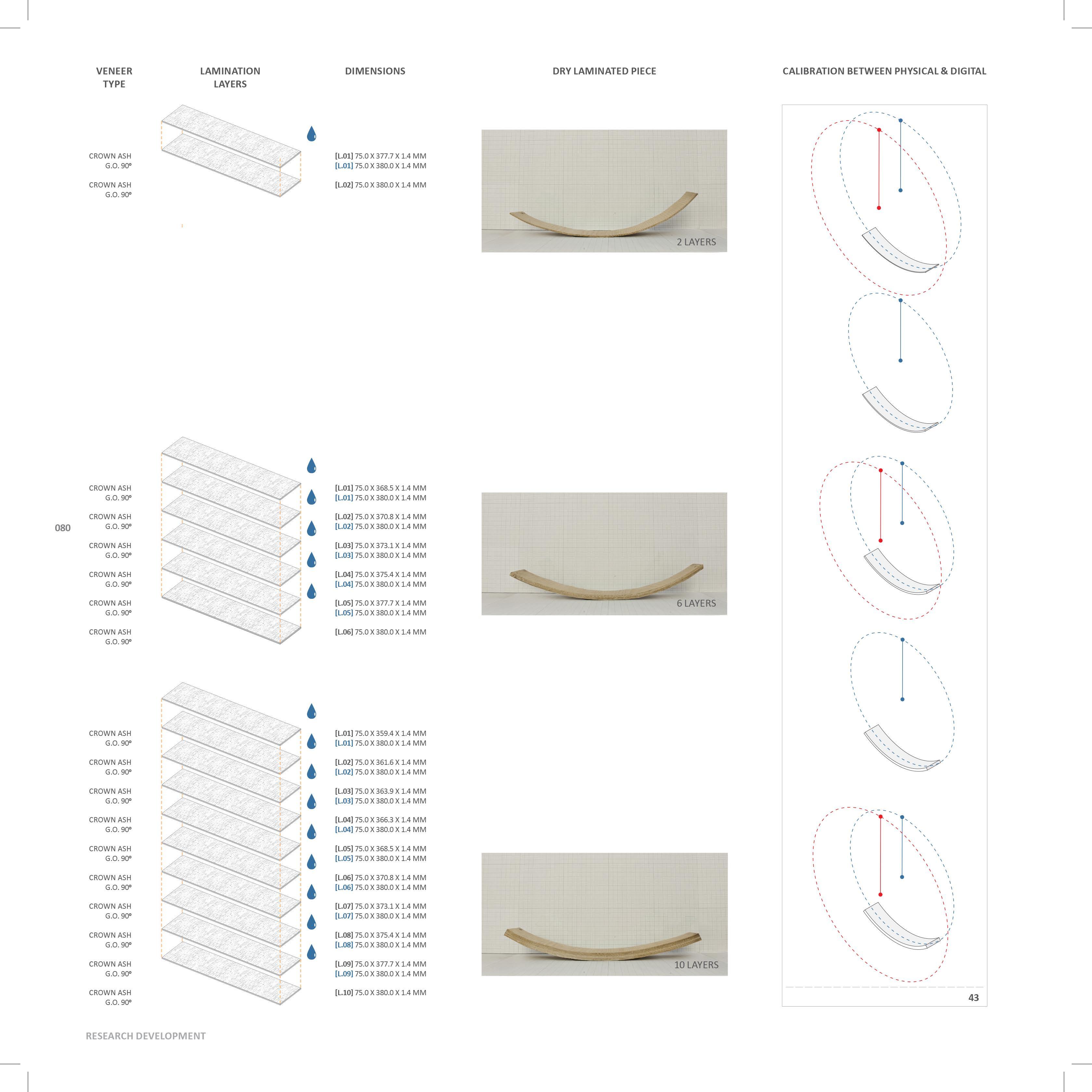

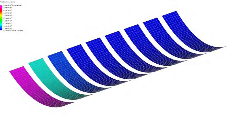
04 NUMBER OF LAYERS DIGITAL COMPONENT SIMULATION FINITE ELEMENT ANALYSIS
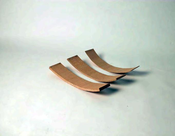
DIAG.43 CALLIBRATION BETWEEN PRODUCED CURVATURES ON PHYSICAL AND DIGITAL EXPERIMENTS.
DIAG.44 CURVATURE AS FUNCTION OF COMPONENT’S NUMBER OF LAYERS.
DIAG.45 FINITE ELEMENT ANALYSIS FOR COMPONENTS OF DIFFERENT NUMBER OF LAYERS.
X THICKNESS OF LAMINATE(MM)
PIC.70 SERIES OF PHYSICAL MATERIAL COMPONENTS OF DIFFERENT NUMBER OF LAYERS, AFTER EQUILIBRIUM IS REACHED.
PIC.71 MULTIPLE COMPONENTS WITH DIFFERENT NUMBER OF LAYERS.
AIM :
How does varying the number of layers of the component influence the produced curvature?
PROCEDURE :
Three physical experiments were carried out, for two, six and ten layers of white ash veneer of 1.4mm thickness, PIC.70. The inner layer of each component was calculated with the maximum moisture content, using the shrinkage expansion factor of 5.50% obtained from the initial experiments. The pieces after laminated and clamped were set free to reach equilibrium and showed similar curvatures.
The experiment was simulated using FEA but for a range of numbers of layers from two to ten. Those nine experiments were run for ΔΤ = -0.7039 applied on the components and revealed a linear relationship between curvature and the number of layers, DIAG.44.
OUTCOME :
When the number of the laminated layers increases, the component forms wider curvatures. Although the physical and the digital results shown in DIAG.43 did not much and the full calibration was not achievable, the physically produced curvatures are the same with the digital ones, scaled by a factor of 120%, allowing us to draw reliable conclusions on the behaviour of the piece in relation to the number of layers.
20x0.5mm WIDTH OF WOOD DIFFERENT NUMBER OF DIFFERENT THICKNESS RADIAL CURVATURE (MM) RADIAL CURVATURE (MM) NUMBER
NUMBER
OF LAMINATE RADIAL CURVATURE (MM) WIDTH X LENGTH(MM) 30x300mm 60x300mm100x300mm150x300mm300x300mm 0 20 40 60 80 50 100 150 200 250 300 0 2 4 6 8 10 12 100 200 300 400 500 600 700 0 20x2.5mm 20x2.0mm 20x1.4mm 20x1.0mm 081
OF LAYERS
44
45 2 LAYERS 3 LAYERS 4 LAYERS 5 LAYERS 6 LAYERS 7 LAYERS 8 LAYERS 9 LAYERS 10 LAYERS
ARBOREAL FORMATIONS
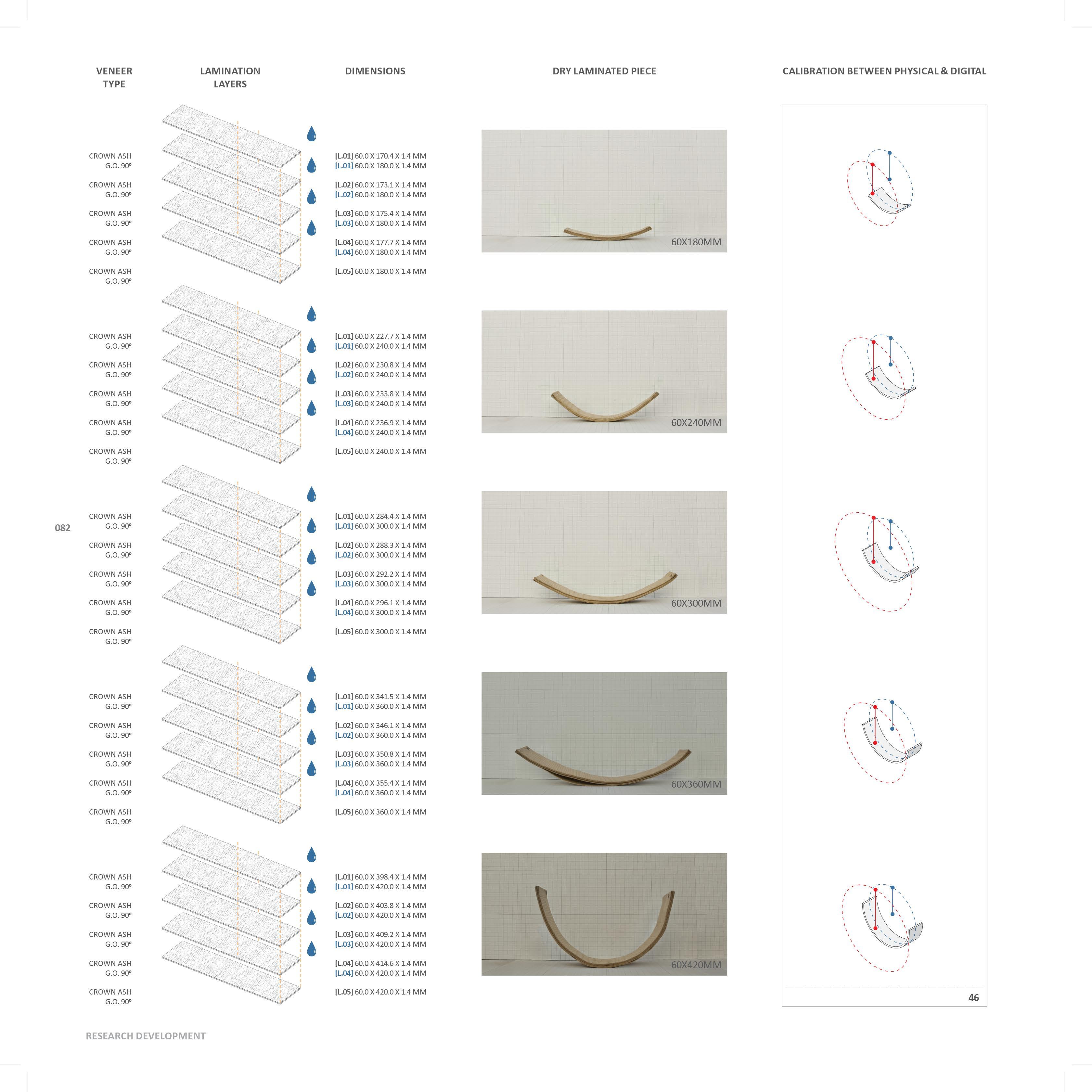

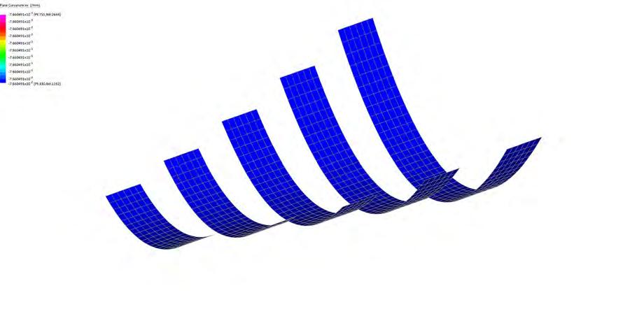
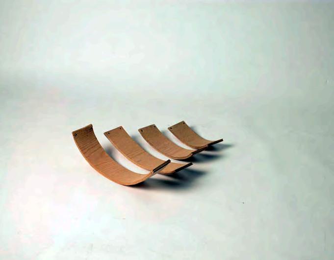
AIM :
DIAG.46 CALLIBRATION BETWEEN PRODUCED CURVATURES ON PHYSICAL AND DIGITAL EXPERIMENTS.
DIAG.47 CURVATURE AS FUNCTION OF COMPONENT’S LENGTH.
DIAG.48 FINITE ELEMENT ANALYSIS FOR COMPONENTS OF DIFFERENT LENGTH.
PIC.72 SERIES OF PHYSICAL MATERIAL COMPONENTS OF DIFFERENT LENGTHS, AFTER EQUILIBRIUM IS REACHED.
PIC.73 MULTIPLE COMPONENTS WITH DIFFERENT LENGTHS. 47
How does the length of the material component influence the produced curvature?
PROCEDURE :
Five physical experiments were carried out, with five layers of white ash veneer of 1.4mm thickness each. The components have fixed widths of 60mm but different lengths, ranging from 180mm to 420mm, PIC.72. The dried pieces show similar curvatures, apart from the piece of 380mm which curved to a tighter radii, indicating probably a mistake in the fabrication process.
In order for the physical experiments to be verified and draw conclusions regarding the influence of this parameter, the same five experiments were simulated with FEA. The data for all laminates are the same and when ΔΤ = -0.7039 is applied, the digital components curve with the exact same radii, DIAG.48.
OUTCOME :
The physical and digital experiments showcase similar material behaviours, as shown in DIAG.46, where curvatures of both procedures are overlaid and differ by a factor of 140%. Although the calibration is not achieved by matching the results, it is evident that the parameter does not influence the curvature.
20x0.5mm EXPANSION FACTOR LENGTH OF WOOD WIDTH OF WOOD DIFFERENT NUMBER OF DIFFERENT THICKNESS OF RADIAL CURVATURE (MM) RADIAL CURVATURE (MM) NUMBER
NUMBER OF LAYERS OF LAMINATE RADIAL CURVATURE (MM) RADIAL CURVATURE (MM) RADIAL CURVATURE (MM) WIDTH X LENGTH(MM) WIDTH X LENGTH(MM) 0 20 40 60 80 100 120 140 30x300mm 60x300mm100x300mm150x300mm300x300mm 60x180mm 60x240mm 60x300mm 60x360mm 60x420mm 0 20 40 60 80 100 120 140 50 100 150 200 250 300 0 2 4 6 8 10 12 100 200 300 400 500 600 700 0 0 100 200 350 20x2.5mm 20x2.0mm 20x1.4mm 20x1.0mm 0.010.020.030.040.050.060.070.080.090.1 083
X THICKNESS OF LAMINATE(MM)
06 LENGTH OF COMPONENT
48 DIGITAL COMPONENT SIMULATION FINITE ELEMENT ANALYSIS 60X180MM 60X240MM 60X300MM 60X360MM 60X420MM
ARBOREAL FORMATIONS
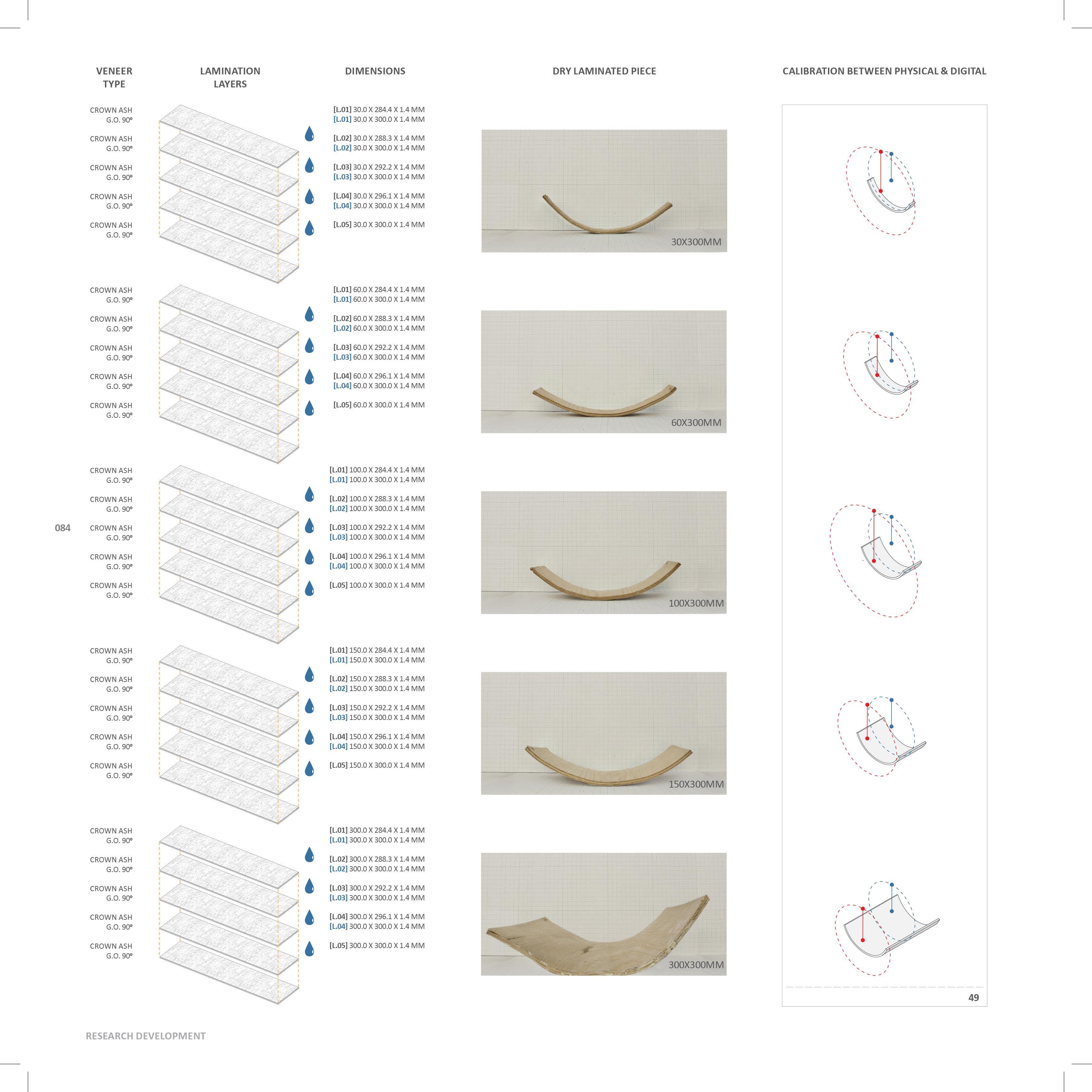

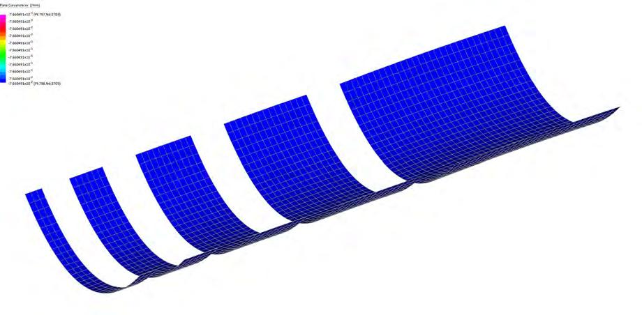
07 WIDTH OF COMPONENT DIGITAL COMPONENT SIMULATION FINITE ELEMENT ANALYSIS
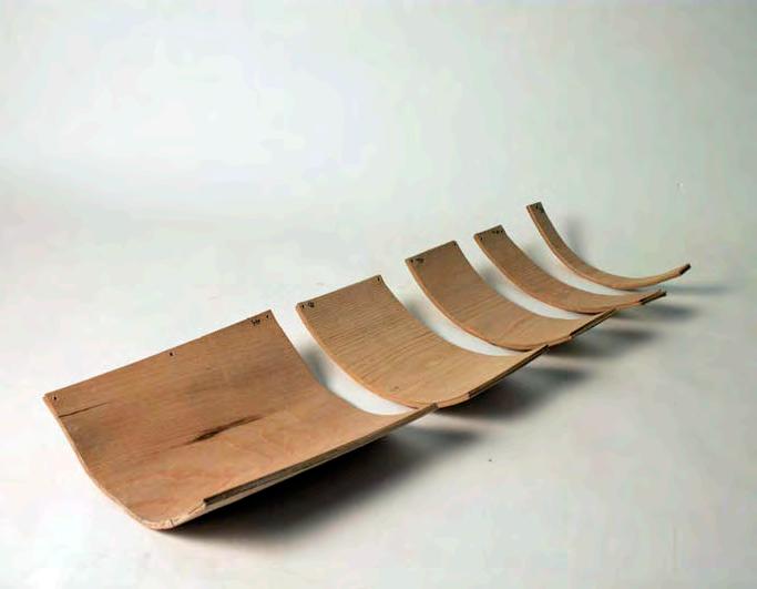
DIAG.49 CALLIBRATION BETWEEN PRODUCED CURVATURES ON PHYSICAL AND DIGITAL EXPERIMENTS.
DIAG.50 CURVATURE AS FUNCTION OF COMPONENT’S WIDTH.
DIAG.51 FINE ELEMENT ANALYSIS FOR COMPONENTS OF DIFFERENT WIDTH.
PIC.74 SERIES OF PHYSICAL MATERIAL COMPONENTS OF DIFFERENT WIDTHS, AFTER EQUILIBRIUM IS REACHED.
PIC.75 MULTIPLE COMPONENTS WITH DIFFERENT WIDTHS.
AIM :
How does the width of the material component influence the produced curvature?
PROCEDURE :
X THICKNESS OF LAMINATE(MM)
Five physical experiments were carried out, with five layers of white ash veneer of 1.4mm thickness each. The components have fixed length of 300mm but different widths, ranging from 30mm to 300mm, PIC.74. The four dried pieces, 30mm, 60mm, 150mm and 300mm wide show similar curvatures, whereas the 100mm wide piece curved in wider radii, indicating probably a mistake in the fabrication process.
In order for the physical experiments to be verified and draw conclusions regarding the influence of this parameter, the same five experiments were simulated with FEA. The data for all laminates are the same and when ΔΤ = -0.7039 is applied, the digital components curve with the exact same radii, DIAG.51.
OUTCOME :
The physical and digital experiments showcase a similar material behaviour, as shown in DIAG.49, where curvatures of both procedures are overlaid and differ by a factor of 140%. Although the calibration is not achieved by matching the results, it is evident that the parameter does not influence the curvature.
20x0.5mm LENGTH OF WOOD WIDTH OF WOOD DIFFERENT NUMBER OF DIFFERENT THICKNESS RADIAL CURVATURE (MM) RADIAL CURVATURE (MM) NUMBER
NUMBER
RADIAL CURVATURE (MM) RADIAL CURVATURE (MM) WIDTH
LENGTH(MM) WIDTH X LENGTH(MM) 0 20 40 60 80 30x300mm 60x300mm100x300mm150x300mm300x300mm 60x180mm 60x240mm 60x300mm 60x360mm 60x420mm 0 20 40 60 80 100 120 140 50 100 150 200 250 300 0 2 4 6 8 10 12 100 200 300 400 500 600 700 0 20x2.5mm 20x2.0mm 20x1.4mm 20x1.0mm
OF LAYERS OF LAMINATE
X
085
50 51 30X300MM 60X300MM 100X300MM 150X300MM 300X300MM
ARBOREAL FORMATIONS
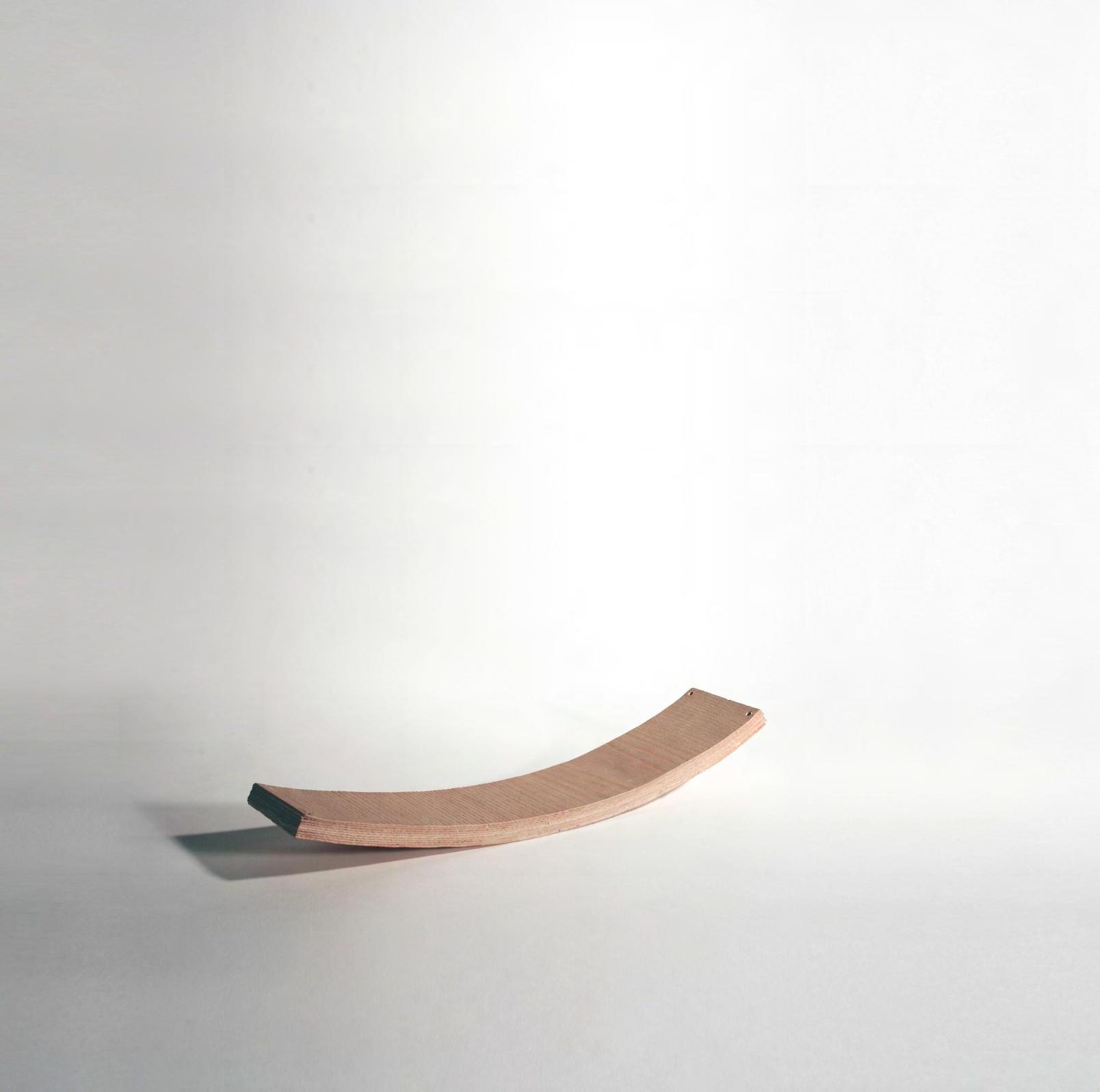
086 RADIALCURVATURE 05 06 04 03 RESEARCH DEVELOPMENT
0.010.020.030.040.050.060.070.080.090.1
FACTOR (%)

SUMMARY OF THE MATERIAL COMPONENT INFLUENCING AND NON INFLUENCIAL PARAMETERS.
PIC.76 MATERIAL COMPONENT OUT OF BIRCH VENEER, 10 LAYERS OF 1.4MM THICKNESS, SHRINKAGE FACTOR : 5.50%
INFLUENCIAL STRAIGHT LAMINATION 900
INFLUENCIAL CONSTANT VARIABLE YELLOW BIRCH THICKNESS OF VENEERS
GRAIN ORIENTATION OF VENEER
INFLUENCIAL CONSTANT VARIABLE 1.4 MM
NUMBER OF LAYERS
INFLUENCIAL VARIABLE
INFLUENCE OF PARAMETERS
The results of the five sets of experiments defined which parameters controlled the curvature of a strip and could be considered as constant or variable inputs of the material system for its further exploration.
EXPANSION FACTOR OF LAYERS
INFLUENCIAL VARIABLE
WOOD SPECIES OF VENEER LENGTH OF COMPONENT
NON INFLUENTIAL SIZE VARIABLE
The dimensions of the material component, width and length were found not to affect the curvature. Thus the width of potential pieces is only restricted by the size of the tree log. The length is restricted by the length of veneer which could be peeled from a log and therefore fairly long strips could potentially be fabricated. Focused to defining the lamination process influencing parameters, the expansion factor and the thickness of each individual layer, as well as the number of layers were proved to be influential parameters of the material components behaviour. Ultimately, the selection of wood species has very different effects on the range of curvatures produced and always operates in relation to the type of function the component will be applied to.
Width and length were defined to be size variables. The thickness and species of wood were defined to be constant variables that are function specific. The expansion factor and number of layers were defined to be curvature influencing parameters.
NON INFLUENTIAL SIZE VARIABLE
The experiments concluded that a further set of tests should be undertaken over a larger sample range exclusively within the digital environment, since the material behaviour in both workspaces was found to be true. The aim of the next set of experiments would be to test a variety of shrinkage factors for a number of strips fabricated with a different number of layers.
RADIAL CURVATURE (MM) RADIAL CURVATURE (MM) NUMBER X THICKNESS OF LAMINATE(MM) NUMBER OF LAYERS RADIAL CURVATURE (MM) RADIAL CURVATURE (MM) RADIAL CURVATURE (MM) WIDTH X LENGTH(MM) WIDTH X LENGTH(MM) 0 20 40 60 80 100 120 140 30x30060x300100x300150x300300x300 60x18060x24060x30060x36060x420 0 20 40 60 80 100 120 140 50 100 150 200 250 300 0 2 4 6 81012 200 300 400 500 600 700 100 0 20x2.5mm 20x2.0mm 20x1.4mm 20x1.0mm 20x0.5mm 0 100 200 350 400 500 600 WOOD SPECIES RADIAL CURVATURE (MM) 0 50 100 150 200 250 300 MAHOGANY CEDAR PINESPRUCE ASHWALNUT BIRCH OAK 087
SHRINKAGE
DIAG.52
52
01 02 03 04 05 06 07 WIDTH
COMPONENT
OF
ARBOREAL FORMATIONS
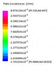
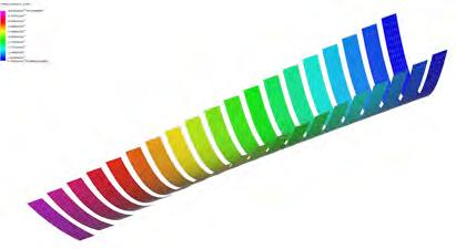
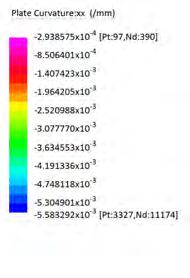
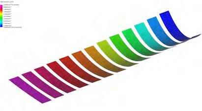

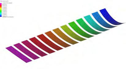

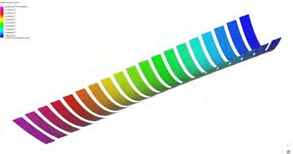


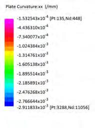
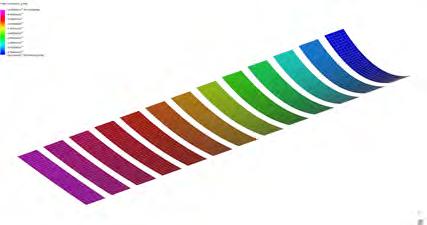
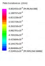
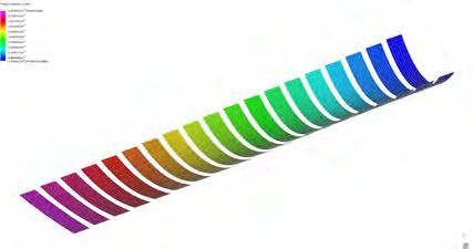

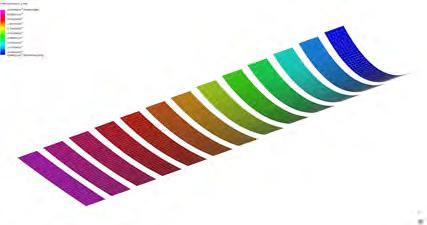

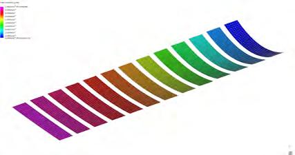
088 53 04 LAYERS 10 LAYERS 16 LAYERS 06 LAYERS 12 LAYERS 18 LAYERS 08 LAYERS 14 LAYERS 20
RESEARCH DEVELOPMENT
LAYERS
DIAG.53 FINITE ELEMENT ANALYSIS FOR COMPONENTS OF DIFFERENT NUMBER OF LAYERS AND DIFFERENT EXPANSION FACTORS PER SERIES, REVEALING THE MATERIAL BEHAVIOUR IN RELATION TO THOSE TWO INFLUENCIAL VARIABLES.
DIAG.54 COMPUTATIONAL DATA INDICATING THE DIGITAL COMPONENT’S CURVATURE IN RELATION TO EXPANSION FACTOR AND NUMBER OF LAYERS.
DIAG.55 CURVATURE AS A FUNCTION OF EXPANSION FACTOR OR NUMBER OF LAYERS.
EXTENDING COMPUTATIONAL DATA
For this set of digital experiments the size dependent and constant variables were fixed, allowing a more controlled investigation into the relationship between the expansion factor and number of layers affecting the curvature of the material component.
The digital component’s dimensions were set to 60 x 300mm, since curvature was found not to be influence by the width and length of the component. For the constant variables a yellow birch species of a 1.40mm thickness was picked as one of the most commonly used species of constructional veneer within the building industry and displaying at the same time a high tangential shrinkage factor which would potentially allow the pieces to achieve tighter curvatures.
Nine sets of digital simulations each undertaking nineteen independent shrinkage factor experiments were run measuring the produced curvature for a set of inputs, DIAG.53. With a tangential shrinkage of 9.5% a limit was set through which the wood could bend. Taken at 0.5% intervals nineteen shrinkage factors were explored through nine different thicknesses ranging from 5.6mm (four layers of 1.4mm veneer) to 28mm (twenty layers of 1.4mm veneer). As a result, a wide catalogue of computed curvatures was created, DIAG.54, enabling a more precise comprehension of the relations between tangential shrinkage factor or number of layers and radii. Curvature as a function of tangential expansion factor, showed an exponential relation, whereas curvature as function of number of layers showed a linear relation, DIAG.55.
NUMBER
NUMBER OF LAYERS (1.4 MM THICK)
OF LAYERS RADIAL CURVATURE (MM) RADIAL CURVATURE (MM) TANGENTIAL
(%) 4 6 8 10 12 14 16 18 20 BIRCH TANGENTIAL SHRINKAGE (%) 0.005 1114.44 1864.51 2629.88 3403.01 4180.50 4960.55 5742.26 6525.10 7308.76 0.010 558.89 932.25 1314.91 1701.50 2090.25 2480.27 2871.13 3262.55 3654.38 0.015 372.22 621.50 876.63 1134.34 1393.50 1653.52 1914.09 2175.03 2436.25 0.020 280.29 466.13 657.45 850.75 1045.12 1240.14 1435.56 1631.28 1827.19 0.025 223.42 372.90 525.96 680.60 836.10 992.11 1148.45 1305.02 1461.75 0.030 186.11 310.75 438.30 567.17 696.75 826.76 957.04 1087.52 1218.13 0.035 159.89 266.36 375.68 486.14 597.21 708.65 820.32 932.16 1044.11 0.040 139.93 233.06 328.72 422.70 517.10 611.49 705.89 800.28 894.68 0.045 124.07 207.17 292.20 378.11 464.50 551.17 638.03 725.01 812.08 0.050 111.64 186.45 262.98 338.36 414.02 489.69 565.35 641.02 716.69 0.055 101.53 169.50 239.07 309.36 380.05 450.96 522.02 593.19 664.43 0.060 93.06 155.38 219.15 281.96 345.00 408.05 471.10 534.14 597.19 0.065 83.47 143.42 202.29 261.77 321.58 381.58 441.71 501.93 562.21 0.070 79.77 133.18 187.84 241.67 295.70 349.73 403.77 457.80 511.84 0.075 74.44 124.30 175.32 226.87 278.70 330.70 382.82 435.01 487.25 0.080 69.78 116.53 164.36 211.47 258.76 306.05 353.34 400.63 447.92 0.085 65.69 109.68 154.69 200.18 245.91 291.80 337.78 383.83 429.93 0.090 62.04 103.58 146.10 187.97 230.00 272.04 314.07 356.10 398.13 0.095 58.78 98.13 138.41 179.11 220.03 261.08 302.22 343.43 384.67 0 1000 2000 3000 4000 5000 6000 7000 8000 5 10 15 20 25 0.005 y = 387.84x - 462.02 0.010 y = 193.87x - 230.17 0.015 y = 129.26x - 153.63 0.020 y = 96.905x - 114.65 0.025 y = 77.551x - 92.137 0.030 y = 64.629x - 76.819 0.035 y = 55.384x - 65.658 0.040 y = 47.198x - 49.281 0.045 y = 43.086x - 51.212 0.050 y = 37.833x - 39.974 0.055 y = 35.251x - 41.892 0.060 y = 31.524x - 33.281 0.065 y = 29.910x - 36.698 0.070 y = 27.017x - 28.504 0.075 y = 25.851x - 30.727 0.080 y = 23.645x - 24.978 0.085 y = 22.810x - 27.109 0.090 y = 21.016x - 22.189 0.095 y = 20.409x - 24.255 0 1000 2000 3000 4000 5000 6000 7000 8000 0.010.020.030.040.050.060.070.080.09 0.1 04 y= 36.544x-1 06 y = 32.625x-1 08 y = 28.711x-1 10 y = 24.803x-1 12 y = 20.902x-1 14 y = 17.015x-1 16 y = 13.149x-1 18 y = 9.3225x-1 20 y = 5.5553x-1 089
SHRINKAGE
54 55 ARBOREAL FORMATIONS
090 56 RESEARCH DEVELOPMENT
X=TANGENTIAL SHRINKAGE (%)
Y=THICKNESS (NO OF LAYERS)
Z= CURVATURE RADIUS (MM)
Z(X) = A1*X-1
Z(Y) = A2*Y+B
Z(X,Y) = ((1.9398*Y) - 2.3189)*X
Z= 36.544 X-1
Z= 32.625 X-1
Z= 28.711 X-1
Z= 24.803 X-1
Z= 20.902 X-1
Z= 17.015 X-1
Z= 13.149 X-1
Z= 9.3225 X-1
Z= 5.5553 X-1
COEFFICIENT= 1.9387*X - 2.3025
DIAG.56 PLOTTED RESULTS FOR CURVATURE AS A FUNCTION OF TANGENTIAL SHRINKAGE FACTOR AND CURVATURE AS FUNCTION OF NUMBER OF LAYERS, COMPOSING A 3D DATABASE.
DIAG.57 EXTENDED 3D GRAPH OF THE INFLUENCIAL PARAMETERS FOR COMPUTING THE MATERIAL COMPONENT’S CURVATURE.
DIAG.58 CHANGE OF COEFFICIENT VALUES AS A FUNCTION OF THICKNESS.
MATERIAL COMPUTATION MATRIX
Curvature against thickness and curvature against tangential shrinkage factor were measured and plotted to understand the relationship between results and compiled in a three dimensional matrix.
Since curvature is a function both of thickness and expansion factor, a general equation could have been derived. The series of data describing linear relation of curvature as a function of thickness is given by the general equation z(y) = a2*y+b, where difference of coefficient a2 is exponential between consecutive series of data. Series of data describing the exponential relation of curvature as a function of tangential shrinkage is given by the general equation z(x) = a1*x-1, where difference of coefficient a1 is linear between consecutive series of data. A linear change of coefficient a1 defining the relation between curvature and tangential shrinkage for a given thickness is shown in DIAG.58. These interrelations allowed for generalising the thickness (as the number of layers) against curvature and tangential shrinkage against curvature equations into one, plotted as the threedimensional matrix in DIAG.57. The formula allows for extending the matrix and plotting data for any input parameters without the need for testing results through experimentation. This formulated an incredibly powerful tool for programming a timber component to achieve a specific curvature from picking a thickness and using the correlative tangential shrinkage factors.
5 10 15 20 25 30 35 40 5 10 15 20 25 COEFFICIENT THICKNES
NUMBER
OF LAMINATE 0 091
=
X LAYERS
57
4 6 8 10 12 14 16 18 20
58 ARBOREAL FORMATIONS
RADIUS 17,000.00 MM
RADIUS 5,000.00 MM
RADIUS 1,000.00 MM
092 59
A01
A02
R01
R02
R03
B01
B02
C01
RESEARCH DEVELOPMENT
C02
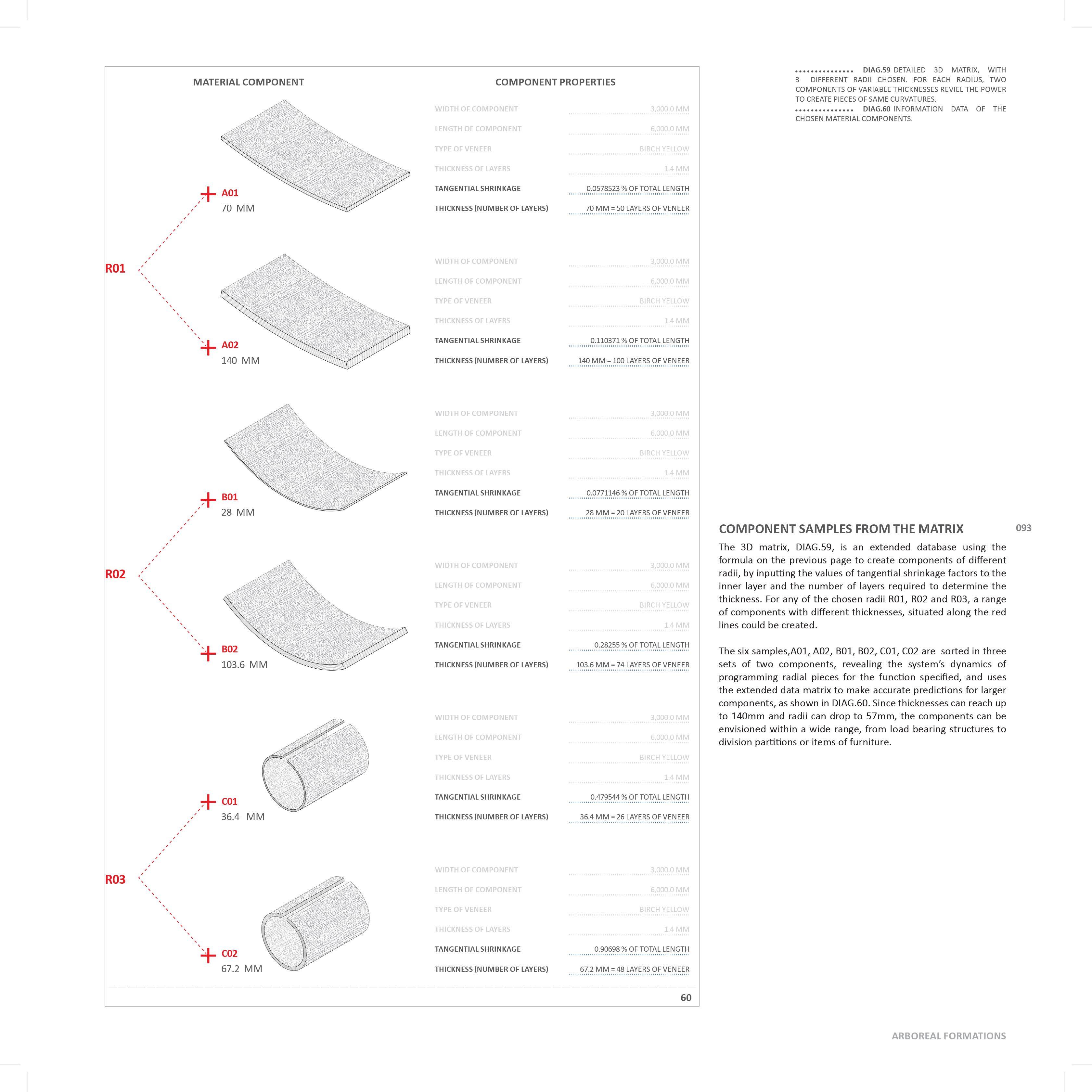
∞ 1113 556 369 277 220 183 157 137 122 110 99 91 83 78 73 68 64 61 57 ∞ 2662 1330 885 664 530 441 378 332 294 264 240 220 203 189 176 165 155 147 139 ∞ 4210 2104 1402 1051 840 700 600 527 466 418 381 350 322 299 280 262 247 233 221 ∞ 5759 2879 1918 1438 1150 958 821 722 638 573 522 479 442 410 383 359 338 319 302 ∞ 7308 3653 2434 1825 1460 1216 1043 917 811 727 663 609 562 521 486 456 429 405 384 ∞ 8857 4427 2951 2212 1770 1475 1264 1113 983 882 804 738 681 632 590 553 520 491 466 ∞ 10405 5201 3467 2600 2080 1733 1485 1308 1155 1036 945 868 801 742 693 650 612 577 547 ∞ 11954 5976 3984 2987 2390 1992 1707 1503 1328 1190 1086 997 920 853 797 747 703 663 629 ∞ 13503 6750 4500 3374 2700 2250 1928 1698 1500 1345 1227 1127 1040 964 900 844 794 749 710 ∞ 15052 7524 5016 3761 3010 2508 2150 1893 1672 1499 1368 1256 1160 1074 1003 941 885 836 792 ∞ 16600 8298 5533 4148 3320 2767 2371 2089 1844 1654 1509 1385 1279 1185 1107 1038 977 922 874 ∞ 18149 9072 6049 4536 3630 3025 2592 2284 2017 1808 1650 1515 1399 1296 1210 1135 1068 1008 955 ∞ 19698 9847 6566 4923 3940 3283 2814 2479 2189 1962 1791 1644 1519 1406 1314 1232 1159 1094 1037 ∞ 21247 10621 7082 5310 4250 3542 3035 2674 2361 2117 1932 1774 1638 1517 1417 1329 1250 1180 1119 ∞ 22795 11395 7598 5697 4560 3800 3257 2869 2534 2271 2073 1903 1758 1628 1520 1426 1341 1266 1200 0.0050.000 EXPANSIONFACTOR 5.6 THICKNESS 11.2 16.8 22.4 28.0 33.6 39.2 44.8 50,4 56.0 61.6 67.2 72.8 78.4 84.0 0.010 0.015 0.020 0.025 0.030 0.035 0.040 0.045 0.050 0.055 0.060 0.065 0.070 0.075 0.080 0.085 0.090 0.095 094 RESEARCH DEVELOPMENT
CATOLOGUE OF MATERIAL COMPONENTS
The catalogue documents 500 sample components of different thicknesses and tangential expansion factors that produce variable curvatures based on the material information matrix. All the components are 60mm wide and 300mm long of yellow birch veneer, 1.40mm thick. Among the multiple pieces, in the bottom left corner, the thinnest components show notably tighter curvatures, compared to the bottom right corner where pieces reach thicknesses of 140mm and really wide curvature revealing the bilateral restriction of curvature against thickness.
∞ 22795 11395 7598 5697 4560 3800 3257 2869 2534 2271 2073 1903 1758 1628 1520 1426 1341 1266 1200 ∞ 24344 12169 8115 6084 4870 4058 3478 3064 2706 2426 2214 2033 1878 1739 1624 1523 1433 1352 1282 ∞ 25893 12943 8631 6472 5180 4317 3700 3260 2878 2580 2355 2162 1997 1849 1727 1620 1524 1438 1363 ∞ 27442 13718 9148 6859 5490 4575 3921 3455 3051 2734 2496 2291 2117 1960 1830 1717 1615 1524 1445 ∞ 28990 14492 9664 7246 5800 4834 4142 3650 3223 2889 2637 2421 2237 2071 1934 1814 1706 1611 1527 ∞ 30539 15266 10180 7633 6110 5092 4364 3845 3395 3043 2778 2550 2356 2181 2037 1911 1798 1697 1608 ∞ 32088 16040 10697 8020 6420 5350 4585 4040 3567 3198 2919 2680 2476 2292 2141 2008 1889 1783 1690 ∞ 33637 16814 11213 8408 6730 5609 4807 4235 3740 3352 3060 2809 2595 2403 2244 2104 1980 1869 1772 ∞ 35186 17589 11730 8795 7040 5867 5028 4431 3912 3506 3201 2939 2715 2514 2347 2201 2071 1955 1853 ∞ 36734 18363 12246 9182 7349 6125 5250 4626 4084 3661 3342 3068 2835 2624 2451 2298 2163 2041 1935 ∞ 38283 19137 12762 9569 7659 6384 5471 4821 4257 3815 3483 3198 2954 2735 2554 2395 2254 2127 2017 84.0 89.6 95.2 100.8 106.4 112.0 117.6 123.2 128.8 134.4 140.0 095
DIAG.61 COMPONENT VISUALISATION OF THE 3D MATRIX INDICATING THE VARIABLE THICKNESSES AND CURVATURES THE MATERIAL SYSTEM CAN PRODUCE THROUGH THE PROGRAMMING OF DIFFERENT TANGENTIAL EXPANSION FACTORS. ARBOREAL FORMATIONS
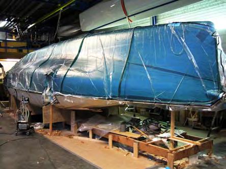
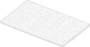
FABRICATION DEVELOPMENT
The material and digital experiments suggest that very long and thick panels may be manufactured. As the moisture content in the panels changes at the cellular scale, the individual micro material changes induce the curvature in a panel. This means that the force required to bring about curvature in the panel occurs cell by cell and does not have to overcome the force throughout the panel. Therefore it is feasible to think that the process initially explored on a 100mm x 100mm test piece of veneer could be scaled to work for much larger applications.
The length of veneer peeled from a log limits the size of panel that may be fabricated. To realise the potential of very long panels the fabrication method needs to change. One problem with using elastic straps to retain the lamination during drying is a small force in the straps needs to be overcome and affects the curvature potentially achievable.
An alternative method is to place the strip after the veneers are of the required length and glued into a vacuum sealed case, DIAG.59. Whilst the individual layers retain their moisture, removing air from the case applies pressure upon the piece and can be left for lamination to occur between the layers until glue is properly dried. Once the laminated component is removed from the case, the flat panel will begin to curve as the moisture content in the layers is lost. This approach is commonly utilised at a larger scale in the propeller and boat industries for creating laminated wind turbine blades up to 32m long and the hulls of sailing boats.
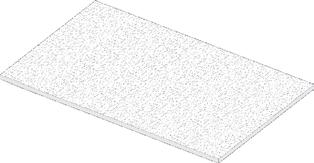
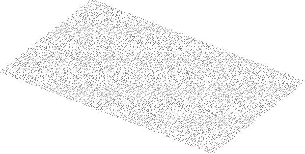
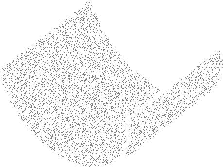
096
FABRICATION TECHNIQUE FOR THE CREATION OF LARGE TIMBER COMPONENT ELEMENT.
VACUUM PRESSURE APPLIED TO THE HULL OF A BOAT TO ENSURE EVEN LAMINATION OVER A COMPLEX SURFACE. 62 STEP.04
STEP.04
STEP.04
FINAL STATE : PIECE IS CURVED FINAL STATE : PIECE IS CURVED FINAL STATE : PIECE IS CURVED RESEARCH DEVELOPMENT
DIAG.62
PIC.77
: INNER LAYER CONTRACTS
: INNER LAYER CONTRACTS
: INNER LAYER CONTRACTS
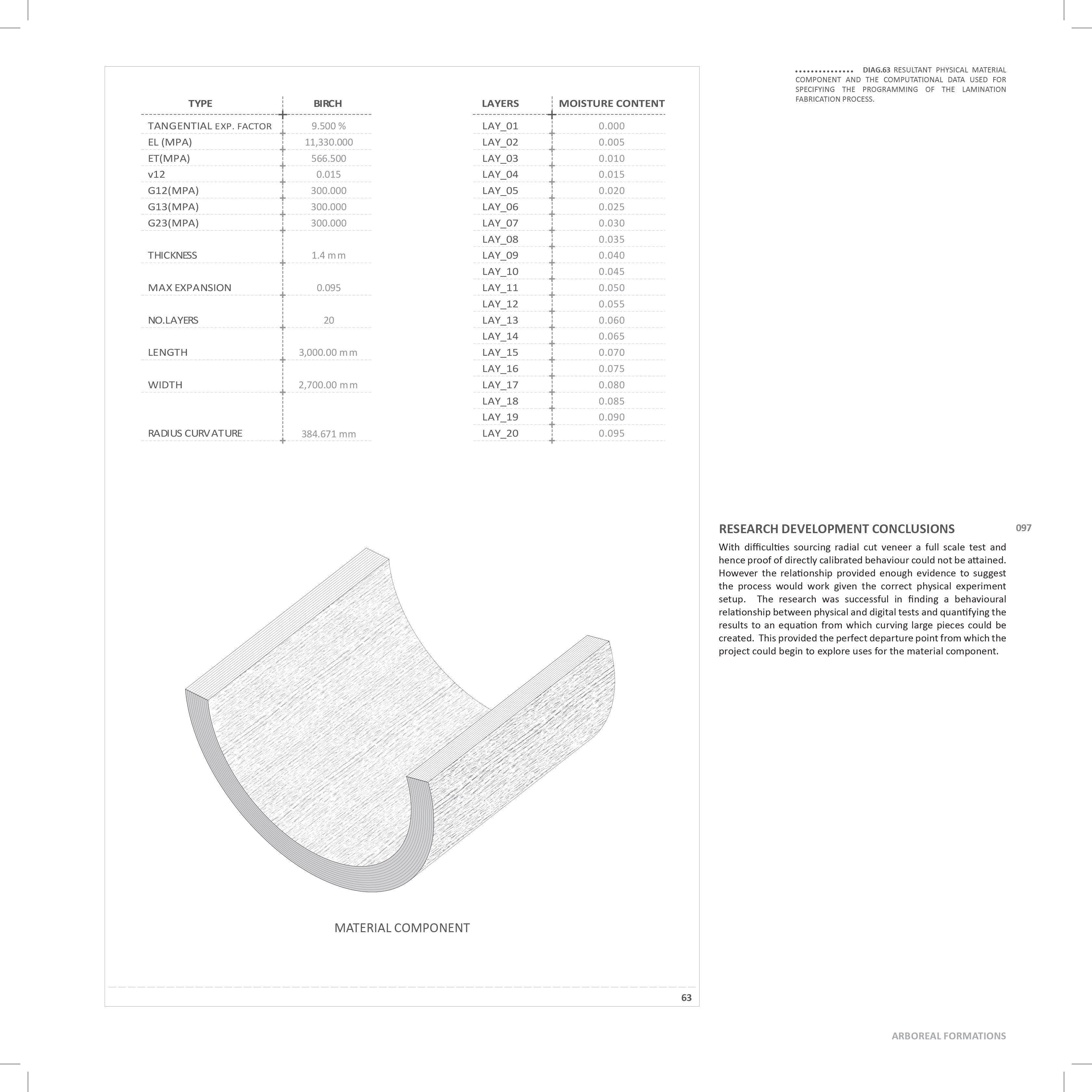
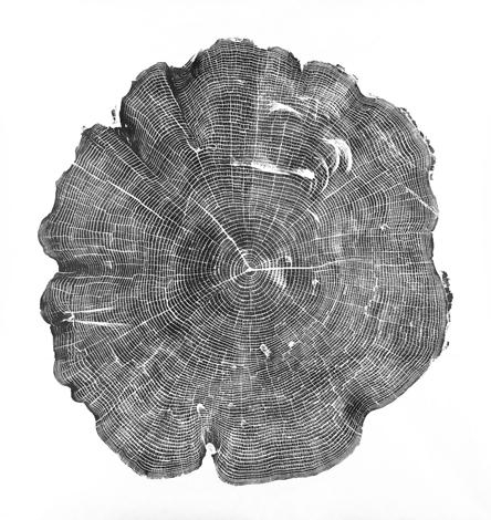
DESIGN DEVELOPMENT
Findings within the domain and material research show that the curvature of laminated timber components can be controlled in order to fabricate pieces of desired curvature and their scale is only limited by the maximum dimensions of veneer leaves from a log. This chapter of the thesis aims to apply the generation of a material system which is structurally coherent and utilises properties of the material component to further express its geometrical potentials at the architectural scale of a twenty-storey tower and use curvilinear geometry to develop new models of functional living space.
Based on early key studies of mathematical minimal surfaces preceding the main research, an interest of the thesis lies in developing systems that describe geometrical complexity through rule sets associating simple components. Geometrical complexity is not merely an aim in itself, but a mean of developing a system of integrated structural logic and dynamic architectural space of continuity and mixed thresholds, resulting in variable morphological responses. As displayed through an example of a Costa’s minimal surface, the same geometry can be described for fabrication in various ways. The photo on the top of the opposite page shows the surface approximated through interlocking planar components in opposing U and V directions. Although the resulting geometry depicts Costa’s minimal surface, logic of its fabrication does not derive from the mathematical logic given by the equation of a surface. The second photo shows the same surface, but fabrication is based on its integral geometrical logic. Interlocking UV lines are a direct physical translation of lines that describe this geometry in mathematical space. Therefore fabrication and materiality of surface is integral to its geometrical logic. The thesis takes on this path of research, focusing on developing rule sets that originate from the internal logic of a material system, to invent a formula which describes a resultant geometry.
The understanding of material system component properties is crucial to that route of investigation, thus components are analysed based on their structural and geometric capacities. These findings are then utilised to inform the structural principle for a building system. This combined with spatial ambitions for the project is employed to develop a parametric model, which associates structural logic with geometry and functional requirements. The aim is to develop a design system integrating all the project ambitions to deliver building morphologies, which in the next step of the research could be evaluated to context specific criteria.
098
DESIGN DEVELOPMENT
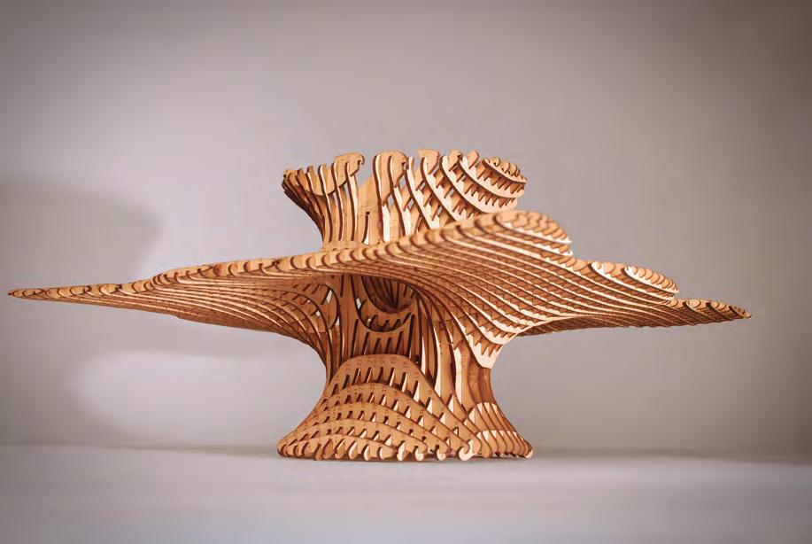
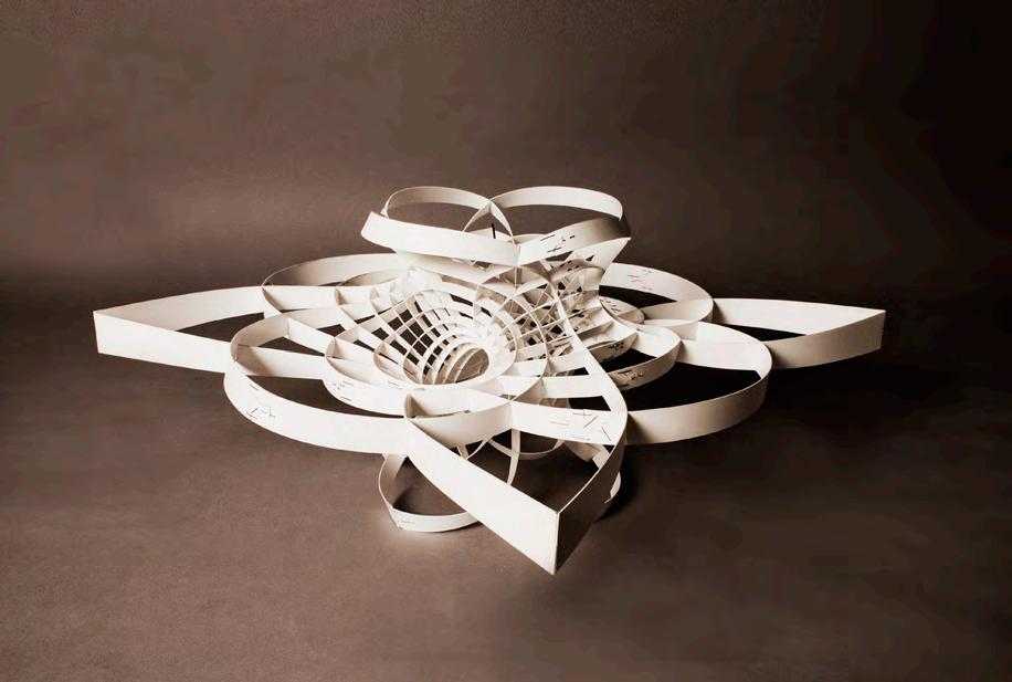
PIC.78 WOOD-CUT PRINT OF A WILLOW TREE BY BRYAN NASH GILL, 2011
PIC.79
COSTA’S MINIMAL SURFACE, MODEL FABRICATED OUT OF PLANAR INTERSECTING COMPONENTS.
PIC.80
COSTA’S MINIMAL SURFACE, MODEL FABRICATED BASED ON UV CURVES DEFINED BY THE MATHEMATICAL FORMULA OF A SURFACE.
099
ARBOREAL FORMATIONS
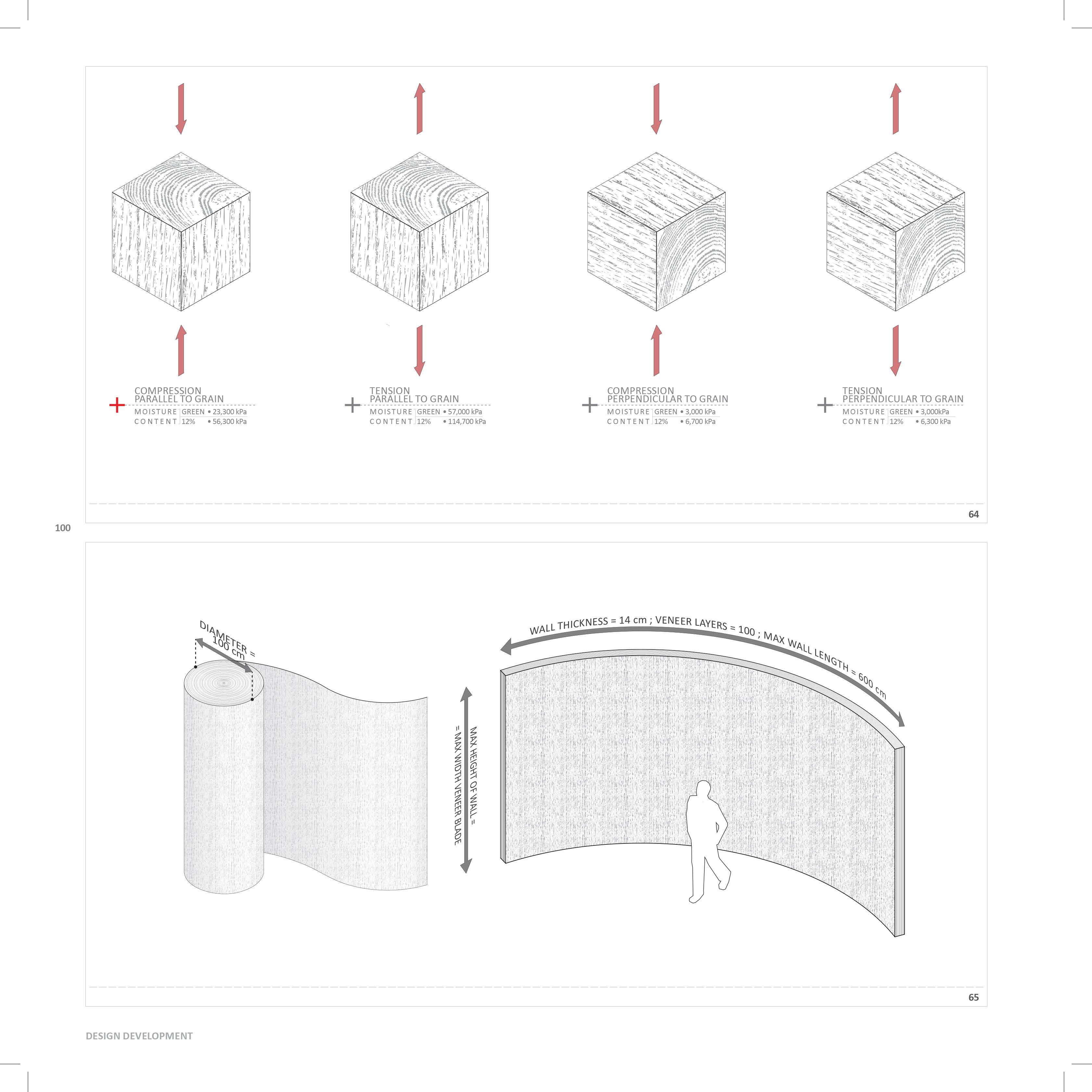
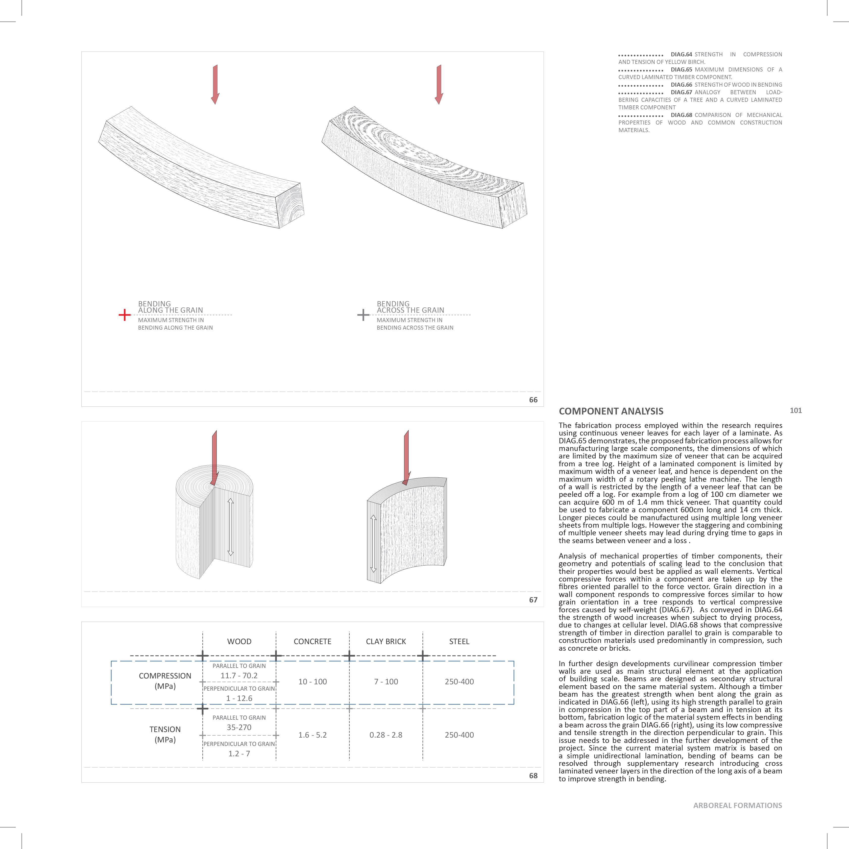
PIC.81 EXTERIOR AND INTERIOR VIEWS OF THE OKURAYAMA APARTMENTS IN TOKYO, ARCHITECT: KAZUYO SEJIMA & ASSOCIATES.
FLOOR PLANS OF THE THREE LEVELS OF THE APARTMENT BUILDING.
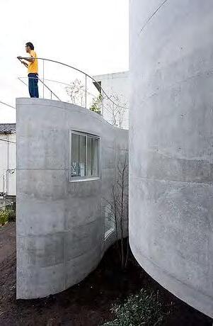
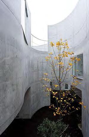
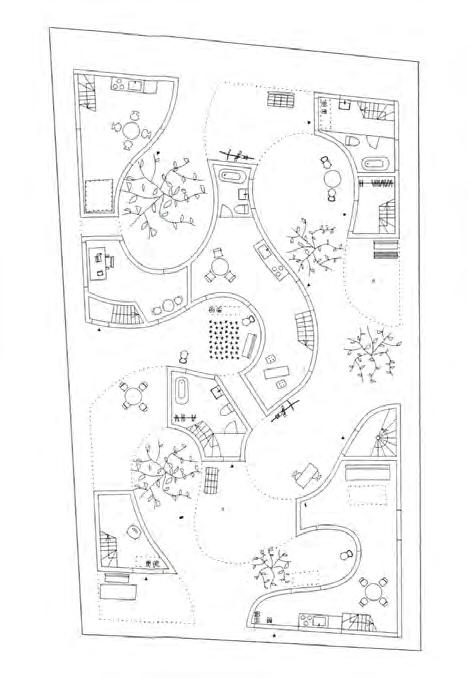
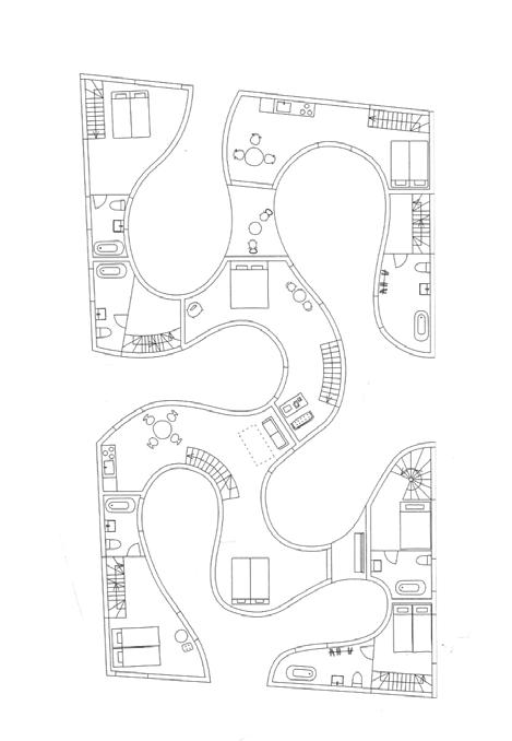
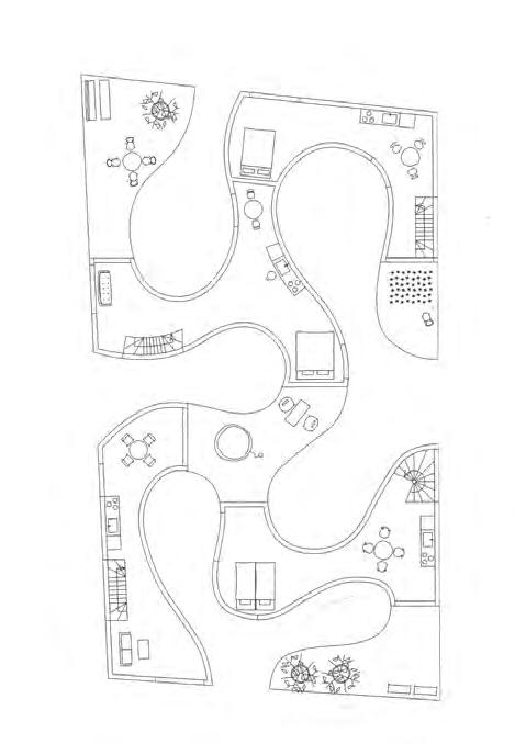
102 FLOOR PLAN LEVEL 01 FLOOR PLAN LEVEL 02 FLOOR PLAN LEVEL 03
PIC.82
DESIGN DEVELOPMENT
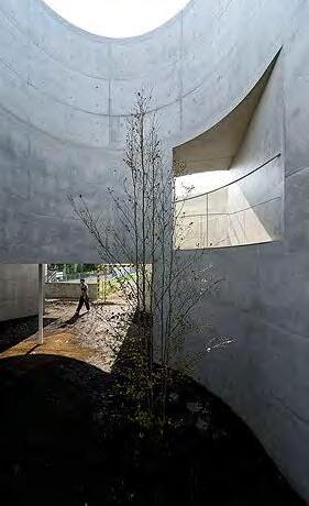
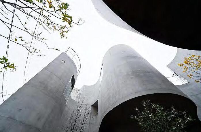
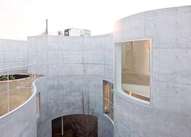
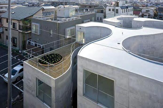
KEY STUDY INTRO
Potentials of the material system to describe geometries at a building scale were first tested on an existing building morphology. An apartment block in Okurayama designed by Kazuyo Sejima & Associates was chosen for two reasons.
First, its geometry is based on complex planar spline curvatures, which were then extruded to the height of two to three storeys. The extruded geometry creates walls displaying single curvature. Secondly, a residential function was chosen in order to learn how space based on these geometries can provide novel models of inhabitation that remain functional, as opposed to conventional residential spaces based on orthogonal plans or overly complex plans displaying chaos.
The aim of this exercise was to test the potential of the proposed timber material system that is based on radial arcs to describe more complex curved geometries.
103
ARBOREAL FORMATIONS
01A01 02A01 03A01 03A02 03A03 03A04 03A05 03A06 03A07 03A08 03A09 03A10 03A11 03A12 03A13 03A14 03A15 03A16 03A17 03B01 03B02 03B03 03B04 03B05 03C01 03C07 03C02 03C03 03C04 03C08 03C05 03C06 03C09 03C10 02A02 02A03 02A04 02A05 02A13 02A14 02A15 02A16 02A09 02A10 02A11 02A12 02A24 02A23 02A22 02A25 02A26 02A21 02A20 02A17 02A18 02A19 02C01 02C02 02C03 02C04 02C05 02B08 02B07 02B06 02B05 02B04 02B03 02B02 02B01 02A08 02A07 02A06 01B01 01C01 01D01 01D02 01D03 01E01 01F01 01F02 01F03 01F04 01F05 01F06 01F07 01E02 01D04 01D05 01C02 01C03 01B02 01B03 01B04 01B05 01B06 01B07 01B08 01B09 01B10 01B11 01B12 01B13 01B14 01A02 01A03 01A01 02A01 03A01 03A02 03A03 03A04 03A05 03A06 03A07 03A08 03A09 03A10 03A11 03A12 03A13 03A14 03A15 03A16 03A17 03B01 03B02 03B03 03B04 03B05 03C01 03C07 03C02 03C03 03C04 03C08 03C05 03C06 03C09 03C10 02A02 02A03 02A04 02A05 02A13 02A14 02A15 02A16 02A09 02A10 02A11 02A12 02A24 02A23 02A22 02A25 02A26 02A21 02A20 02A17 02A18 02A19 02C01 02C02 02C03 02C04 02C05 02B08 02B07 02B06 02B05 02B04 02B03 02B02 02B01 02A08 02A07 02A06 01B01 01C01 01D01 01D02 01D03 01E01 01F01 01F02 01F03 01F04 01F05 01F06 01F07 01E02 01D04 01D05 01C02 01C03 01B02 01B03 01B04 01B05 01B06 01B07 01B08 01B09 01B10 01B11 01B12 01B13 01B14 01A02 01A03 104 FLOOR PLAN LEVEL 01 FLOOR PLAN LEVEL 01 FLOOR PLAN LEVEL 02 FLOOR PLAN LEVEL 02 FLOOR PLAN LEVEL 03 FLOOR PLAN LEVEL 03 01A 01A 01B 01C 01C 03A 01F 01F 03C 01D 01E 03B 69 DESIGN DEVELOPMENT
1.68M
01B02
3.31M
3.37M
01B03
THICKNESS:
01C02
3.77M
THICKNESS: 0.179M SR.FACTOR: 0.050%
02A23 RADIUS: 1.57M
THICKNESS: 0.084M SR.FACTOR: 0.949%
THICKNESS: 0.106M SR.FACTOR: 0.925%
DIAG.69 ANALYSIS OF THE PERIMETRIC WALLS OF THE APARTMENT BUILDING AND THROUGH THE USE OF A GENETIC ALGORITHM APPROXIMATION OF THE CURVATURES WITH ARCS.
DIAG.70 CLASSIFICATION OF THE COMPONENTS THAT CONSIST EACH FLOOR PLAN. FIRST ATTEMPT TO APPLY THE MATERIAL COMPONENT MATRIX.
THICKNESS: 0.112M SR.FACTOR: 0.946%
THICKNESS: 0.115M SR.FACTOR: 0.933%
02A24 RADIUS: 1.76M
02C01 RADIUS: 1.76M
02A08 RADIUS: 1.97M 02A09 RADIUS: 1.86M
THICKNESS: 0.120M SR.FACTOR: 0.935%
THICKNESS: 0.120M SR.FACTOR: 0.935%
THICKNESS: 0.129M SR.FACTOR: 0.945%
THICKNESS: 0.134M SR.FACTOR: 0.932%
THICKNESS: 0.137M SR.FACTOR: 0.939%
THICKNESS: 0.151M SR.FACTOR: 0.942%
02B04 RADIUS: 2.38M 02B05 RADIUS: 2.38M
02B08 RADIUS: 2.42M 02C05 RADIUS: 2.50M
02A20 RADIUS: 2.73M
02B03 RADIUS: 3.31M
02A10 RADIUS: 3.37M
THICKNESS: 0.162M SR.FACTOR:
THICKNESS: 0.165M SR.FACTOR: 0.934%
THICKNESS: 0.171M SR.FACTOR: 0.937%
THICKNESS: 0.179M SR.FACTOR: 0.900%
THICKNESS: 0.179M SR.FACTOR: 0.742%
THICKNESS: 0.179M SR.FACTOR: 0.728%
THICKNESS: 0.179M SR.FACTOR: 0.729%
THICKNESS: 0.179M SR.FACTOR: 0.692%
THICKNESS: 0.179M SR.FACTOR: 0.654%
THICKNESS: 0.179M SR.FACTOR: 0.644%
02A19 RADIUS: 3.82M
02B01
THICKNESS: 0.179M SR.FACTOR: 0.645%
02A11 RADIUS: 3.84M
02C04 RADIUS: 4.75M
RADIUS: 4.80M
02A07 RADIUS: 5.00M
THICKNESS: 0.179M SR.FACTOR: 0.642%
THICKNESS: 0.179M SR.FACTOR: 0.518%
THICKNESS: 0.179M SR.FACTOR: 0.516%
THICKNESS: 0.179M SR.FACTOR: 0.510%
THICKNESS: 0.179M SR.FACTOR: 0.289%
THICKNESS: 0.179M SR.FACTOR: 0.472%
CURVATURE
02C03 RADIUS: 1.20M 02C02 RADIUS: 6.28M
1.86M
1.97M
02A12 RADIUS: 5.59M 02A26 RADIUS: 5.26M
THICKNESS: 0.179M SR.FACTOR: 0.466%
02B06 RADIUS: 5.56M
02B07 RADIUS: 5.84M
02A18 RADIUS: 2.00M 02A17 RADIUS: 2.20M 02A16 RADIUS: 5.20M 02A15 RADIUS: 3.82M 02A14 RADIUS: 5.96M
02A25 RADIUS: 7.27M
02A22 RADIUS: 13.26M 02A21 RADIUS: 1.61M
02A13 RADIUS: 43.74M 02A05 RADIUS: 3.37M 02A04 RADIUS: 1.68M 02A03 RADIUS: 3.77M 02A02 RADIUS: 3.55M 02A01 RADIUS: 4.73M 02B02 RADIUS: 48.21M
THICKNESS: 0.179M SR.FACTOR: 0.443%
THICKNESS: 0.179M SR.FACTOR: 0.423%
THICKNESS: 0.179M SR.FACTOR: 0.394%
THICKNESS: 0.179M SR.FACTOR: 0.338%
02A06 RADIUS: 7.81M
THICKNESS: 0.179M SR.FACTOR: 0.314%
THICKNESS: 0.179M SR.FACTOR: 0.184%
THICKNESS: 0.179M SR.FACTOR: 0.052%
THICKNESS: 0.179M SR.FACTOR: 0.050%
THICKNESS
2.38M
2.73M
3.31M
3.37M
3.77M
3.82M
KEY STUDY ANALYSIS
4.80M
5.56M
5.96M 03A10
13.46M 03C01
1.61M 03C02
In order to approximate the freeform geometry of the floor plans with the radial arcs, the spline geometry was subdivided into segments. Curvature of these segments was then evaluated through a genetic algorithm, based on its proximity to radii of radial arcs from the material system matrix. Each segment of a spline was assigned an arc, that most closely approximates its curvature, and has the biggest thickness for a given radius, DIAG.69. This process resulted in generating a catalogue of curved laminated timber wall segments shown on DIAG.70, which could be used to recreate the morphology of the Okurayama project.
7.81M
The case study demonstrated that although the geometry of the building in Okurayama delivers a novel model of spatial arrangements for residential functions and an interesting interplay between interior and exterior, there is no strong logic to how this geometry performs as an integral part of a structural system. Therefore, instead of generating an arbitrary morphology and approximating its geometry with the material system, further research focuses on using the limitations of the material system as a guideline to develop a building system based on radial geometry. This geometry should correlate with the structural logic of a building system.
01A01 RADIUS:
RADIUS:
RADIUS:
RADIUS:
4.73M 01A02
3.55M 01A03
3.77M 01B01
RADIUS:
RADIUS:
01B04
RADIUS:
01B06 RADIUS:
RADIUS:
RADIUS:
RADIUS:
RADIUS:
RADIUS:
RADIUS:
RADIUS:
RADIUS:
01C01 RADIUS:
RADIUS: 48.21M 01B05
43.74M 01B07
5.96M 01B08
3.82M 01B09
5.20M 01B10
2.20M 01B11
1.86M 01B12
1.97M 01B13
5.90M 01B14
7.81M
2.38M
RADIUS:
RADIUS:
RADIUS:
RADIUS:
01D03 RADIUS:
RADIUS:
RADIUS:
RADIUS:
RADIUS: 5.26M 01F05 RADIUS: 2.00M 01F04 RADIUS: 3.82M 01F03 RADIUS: 1.20M 01F02 RADIUS:
RADIUS:
01F06 RADIUS: 4.75M 01F07 RADIUS: 2.50M 03A07 RADIUS:
03C10 RADIUS:
03C09 RADIUS:
03C08 RADIUS:
03C07 RADIUS:
RADIUS:
03C05 RADIUS:
RADIUS:
03C03 RADIUS:
RADIUS:
RADIUS:
RADIUS:
RADIUS:
RADIUS:
RADIUS:
RADIUS:
RADIUS:
RADIUS:
03A15 RADIUS:
03A14 RADIUS:
RADIUS:
RADIUS:
RADIUS:
03A01 RADIUS:
03A02 RADIUS:
03A03 RADIUS:
03A04 RADIUS:
RADIUS:
5.56M 01C03
5.84M 01D01
3.84M 01D02
3.37M
2.20M 01D04
1.57M 01D05
1.76M 01E01
7.27M 01E02
6.28M 01F01
1.76M
5.00M
2.50M
4.75M
2.00M
2.20M 03C06
1.20M
3.82M 03C04
1.57M 03B05
5.26M 03B04
7.27M 03B03
1.76M 03B02
3.84M 03B01
5.59M 03A17
5.84M 03A16
2.38M 03A13
03A12 RADIUS: 43.74M 03A11 RADIUS:
03A09 RADIUS:
03A08 RADIUS:
03A06
1.68M
48.21M 03A05
SR.FACTOR:
SR.FACTOR:
THICKNESS:
SR.FACTOR:
THICKNESS: 0.179M SR.FACTOR: 0.742% THICKNESS:
SR.FACTOR:
THICKNESS: 0.179M
0.692% THICKNESS: 0.165M SR.FACTOR: 0.950% THICKNESS: 0.171M SR.FACTOR: 0.937% THICKNESS: 0.179M
0.338%
0.179M
0.052%
0.179M
0.728% THICKNESS: 0.179M SR.FACTOR: 0.466% THICKNESS: 0.084M SR.FACTOR: 0.948%
0.129M SR.FACTOR: 0.945% THICKNESS: 0.179M SR.FACTOR: 0.443% THICKNESS: 0.179M SR.FACTOR: 0.423% THICKNESS: 0.137M SR.FACTOR: 0.939% THICKNESS: 0.134M SR.FACTOR: 0.932% THICKNESS: 0.179M SR.FACTOR: 0.654% THICKNESS: 0.179M SR.FACTOR: 0.516% THICKNESS: 0.179M SR.FACTOR: 0.324% THICKNESS: 0.179M SR.FACTOR: 0.394% THICKNESS: 0.120M SR.FACTOR: 0.935% THICKNESS: 0.106M SR.FACTOR: 0.925% THICKNESS: 0.115M SR.FACTOR: 0.933% THICKNESS: 0.179M SR.FACTOR: 0.729% THICKNESS:
SR.FACTOR: 0.518% THICKNESS: 0.151M SR.FACTOR: 0.942% THICKNESS: 0.151M SR.FACTOR: 0.942% THICKNESS: 0.179M SR.FACTOR: 0.489% THICKNESS: 0.179M SR.FACTOR: 0.415% THICKNESS: 0.179M SR.FACTOR: 0.642% THICKNESS: 0.179M SR.FACTOR: 0.654% THICKNESS: 0.120M SR.FACTOR: 0.935% THICKNESS: 0.179M SR.FACTOR: 0.645% THICKNESS: 0.179M SR.FACTOR: 0.644% THICKNESS: 0.179M SR.FACTOR: 0.472% THICKNESS: 0.179M SR.FACTOR: 0.654% THICKNESS: 0.165M SR.FACTOR: 0.950% THICKNESS: 0.171M SR.FACTOR: 0.937% THICKNESS: 0.179M SR.FACTOR: 0.052% THICKNESS: 0.179M SR.FACTOR: 0.900% THICKNESS: 0.179M SR.FACTOR: 0.742% THICKNESS:
SR.FACTOR: 0.440% THICKNESS: 0.084M SR.FACTOR: 0.948% THICKNESS: 0.129M SR.FACTOR: 0.945% THICKNESS: 0.179M SR.FACTOR: 0.423% THICKNESS: 0.179M SR.FACTOR: 0.415% THICKNESS: 0.137M SR.FACTOR: 0.939% THICKNESS: 0.134M SR.FACTOR: 0.932% THICKNESS: 0.179M SR.FACTOR: 0.645% THICKNESS: 0.179M SR.FACTOR: 0.466% THICKNESS: 0.179M SR.FACTOR: 0.050% THICKNESS: 0.179M SR.FACTOR: 0.184% THICKNESS: 0.120M SR.FACTOR: 0.935% THICKNESS: 0.106M SR.FACTOR: 0.925% THICKNESS: 0.112M SR.FACTOR: 0.946% THICKNESS: 0.179M SR.FACTOR: 0.728% THICKNESS: 0.179M SR.FACTOR: 0.489% THICKNESS: 0.151M SR.FACTOR: 0.942% THICKNESS: 0.162M SR.FACTOR: 0.936% THICKNESS: 0.179M SR.FACTOR: 0.338% THICKNESS: 0.179M SR.FACTOR: 0.314% THICKNESS: 0.179M SR.FACTOR: 0.510% THICKNESS: 0.179M SR.FACTOR: 0.644% THICKNESS: 0.115M SR.FACTOR: 0.933% THICKNESS: 0.179M SR.FACTOR: 0.516% THICKNESS: 0.179M SR.FACTOR: 0.642% THICKNESS: 0.179M SR.FACTOR: 0.443%
0.179M
0.179M
SR.FACTOR:
SR.FACTOR:
0.936% THICKNESS: 0.165M
0.950% THICKNESS: 0.179M
0.440%
THICKNESS: 0.179M SR.FACTOR: 0.425%
105
FLOOR PLAN LEVEL 01 FLOOR PLAN LEVEL 02 FLOOR PLAN LEVEL 03 70 ARBOREAL FORMATIONS
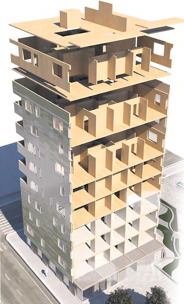
106 71 DESIGN DEVELOPMENT
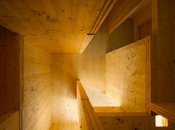
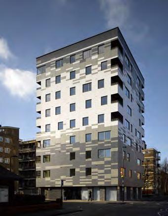
DIAG.71 SECTION AND STRUCTURAL STACKING LOGIC OF THE STADHUS, THE TALLEST RESIDENTIAL TIMBER BUILDING IN THE WORLD LOCATED IN LONDON BOROUGH OF HACKNEY. PIC.83 INTERIOR VIEW OF THE STADHUS PIC.84 EXTERIOR VIEW OF THE STADHUS
ARCHITECT: WAUGH THISTLETON ARCHITECTS
DATE OF COMPLETION: 2008
LOCATION: 24 MURRAY GROVE, HACKNEY, LONDON
BUILDING TYPE: RESIDENTIAL
DESIGN: NINE STOREY TIMBER TOWER STRUCTURE: KLH CROSS-LAMINATED TIMBER PANEL SYSTEM
1 ALL INFORMATION ABOUT CLT HAS BEEN TAKEN FROM THE ONLINE PUBLICATION: WWW.SLIDESHARE.NET/JEFFRANSON/ STADTHAUS-MURRAY-GROVE-CASE-STUDY-PRESENTATION
2 FIRE REGULATIONS. SOURCE: P124, APPROVED DOCUMENT B
TIMBER IN MODERN RESIDENTIAL STRUCTURES
Recent trends in delivering sustainable solutions in construction have drawn an increased interest on the use of timber for larger building applications. The tallest residential building at present is located in London in the borough of Hackney. Large scale crosslaminated timber panels developed by KLH were used to build a structural system of stacking walls and floors. Although the CLT (Cross-Laminated Timber)1 is of a similar scale to components and their compressive strength in the material system developed through this thesis, geometries that can be produced by CLT are always limited to rectilinear solutions. Geometrical limitations of CLT result in a structural logic similar to a honeycomb, where load-bearing walls are oriented in opposite directions leading to compartmentalisation of internal space. The use of curvilinear laminated wall components is seen as a potential for moving away from conventional space based orthogonal floor plan layouts, towards space drawn upon curvilinear geometry, characterised by mixed thresholds and continuity.
When designing a timber structure aspects of safety need to be addressed. The most critical one is fire resistance, understanding that timber buildings are prone to failure due to fire. Although solid timber is not easily ignited, it is combustible. Its combustibility can be modified through retarding chemicals. However, while exposed timber surface burns vigorously at the beginning, it soon builds up a layer of insulating charcoal. CLT has sufficient resistance to fire. For example 128 mm thick panel provides 72 minutes of fire resistance with two vertical load bearing layers remaining. The aim of this design research is to design a timber apartment building of 20 floor. A building of that function and height requires 120 minutes period of fire resistance and use of sprinkler system.2 Therefore the period of fire resistance of timber panels can be extended trough a sprinkling system and other means of fire protection. In case of fire, no damaging thermal expansions of timber structures should be credited as an advantage of this method of construction.
107
ARBOREAL FORMATIONS
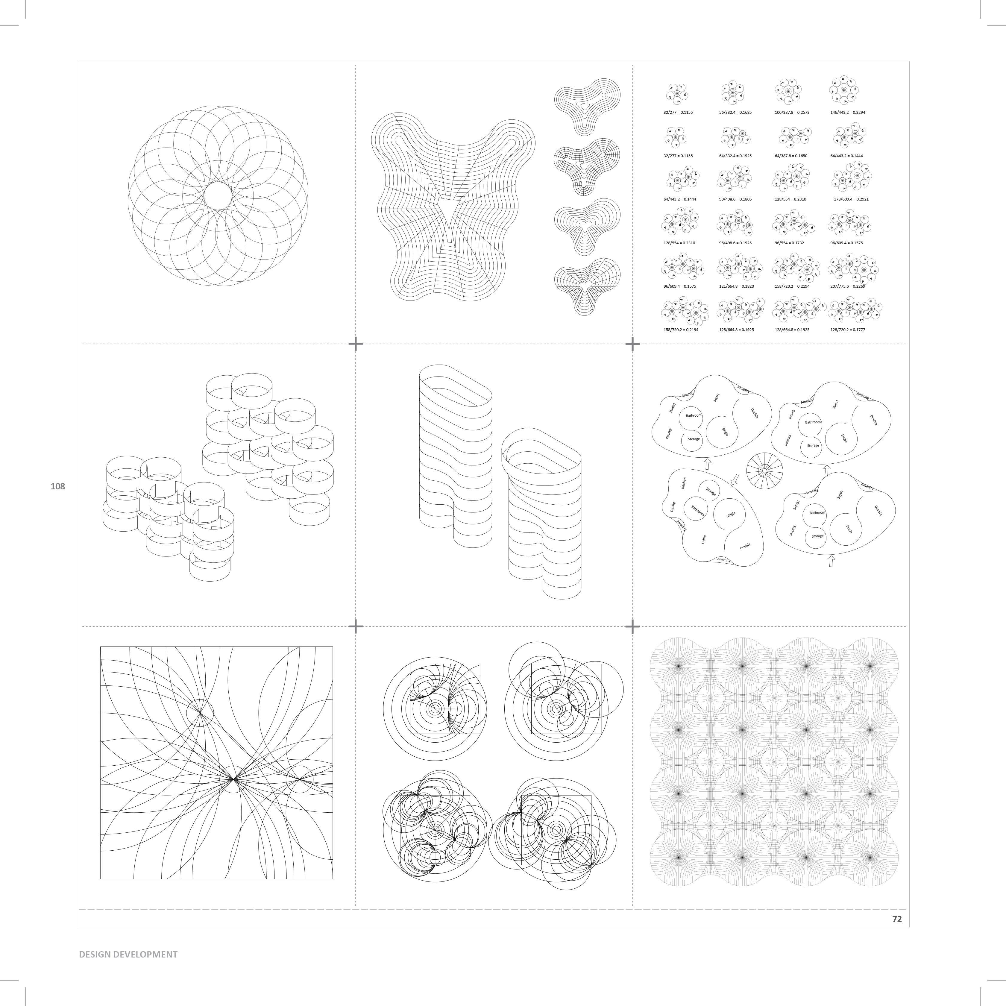
BUILDING SYSTEM STUDIES
Building upon findings from the key study of Okurayama apartments project and structural stacking logic of the Hackney residential tower the research focused on developing a structural strategy informed by geometrical and material properties of the curvilinear timber components. Several studies were undertaken with key principles as guidelines for the system:
- potential of fabricating large-scale components
- take advantage of the compressive strength of wall components
- utilise radial geometry of components as a mean for improving structural performance of a system
- introduce subdivision of space suitable for residential function
- exhibit the potential of fabricating range of curvatures from straight panels to components with tight radii
- explore variable thickness of components to function as structural, partition and furniture elements of design
- employ curved geometry to inform a novel way of approaching functional living
The set of geometrical exercises shown in DIAG.72 were undertaken and each experiment was evaluated based on criteria listed above. Several issues were common for most of the experiments. Developed systems were either too restrictive or displayed insufficient order in the geometries created. Most of the systems could potentially function within individual floors, but didn’t give notions of how these floors could be aggregated into vertical arrangements and exhibit a change of curvature ranges between floors. All the systems displayed too high level of complexity at the starting position, resulting in problems such as obscure joinery details, when multiple components met in a single node, or difficulty in gaining control of the whole system. The many problems that were encountered led to the conclusion, that existing construction systems should be analysed and complexity should emerge upon a simpler structural strategy.
109
DIAG.72 GEOMETRICAL STUDIES OF A BUILDING SYSTEM. ARBOREAL FORMATIONS
STRAIGHT WALL SYSTEM REQUIRES SHEAR WALL
WALL SYSTEM REQUIRES SHEAR WALL
WALL SYSTEM REQUIRES SHEAR WALL
WALL SYSTEM REQUIRES SHEAR WALL
WALL SYSTEM REQUIRES SHEAR WALL
WALL SYSTEM REQUIRES SHEAR WALL
WALL SYSTEM REQUIRES SHEAR WALL
WALL SYSTEM REQUIRES SHEAR WALL
110 73 74 75
STRAIGHT
STRAIGHT
STRAIGHT
STRAIGHT
STRAIGHT
STRAIGHT
DESIGN DEVELOPMENT
STRAIGHT
TIMBER WALL, BALOON SYSTEM.
SOLID PLANAR CROSSLAMINATED TIMBER WALL PANEL. DIAG.75 SOLID CURVILINEAR LAMINATED TIMBER WALL PANEL.
SHEAR WALL IN CONVENTIONAL STRUCTURAL SYSTEM AND SYSTEM BASED ON CURVILINEAR GEOMETRY WITHOUT SHEAR WALL.
STRUCTURAL SYSTEMS
Lateral forces within structural systems are always an issue that needs to be addressed by individual components in the system.
An example of the balloon system on DIAG.73 shows how the make-up of a wall component helps to overcome lateral forces in horizontal directions parallel to the surface of a wall. The inner frame of a wall needs to be stabilised with an external sheet of plywood to prevent the wall from shearing.
Flat solid walls, such as solid timber laminated panel walls, are stable in horizontal directions parallel to their surface, but are not supported at all in the horizontal direction perpendicular to the surface of a wall as shown on DIAG.74.
Curved wall components of our material system are able to overcome lateral forces in either horizontal directions both through their solid make-up and curvilinear geometry (DIAG.75).
This principle allows us to move away from the conventional structural system of walls and beams based on orthogonal geometry. As shown in DIAG.76 this system requires the introduction of shear walls (indicated with red colour) in the perpendicular direction to main structural walls, in order to ensure stability of a structure. The introduction of curvilinear walls eliminates the need for shear walls, which potentially allows the shape and subdivision of internal space to be more free and continuous whilst at the same time maintaining the robustness of a coherent structural logic.
111 DIAG.73
DIAG.74
DIAG.76
76 ARBOREAL FORMATIONS
DIAG.77 BASIC GEOMETRICAL STATES OF A STRUCTURAL SYSTEM EXHIBITING CURVATURE RANGE OF THE MATERIAL SYSTEM.
DIAG.78 SMOOTH TRANSITION OF GEOMETRY BETWEEN TWO BASIC GEOMETRICAL STATES.
ORTHOGONAL SYSTEM ORTHOGONAL SYSTEM
∞ ∞ 112
RADIAL SYSTEM 77 DESIGN DEVELOPMENT
BASIC GEOMETRY EXPLORATION
113
Upon the logic of intersecting walls and beams and the range of curvatures that are available in material system matrix, a geometry of walls and beams is described by two basic states as illustrated in DIAG.77:
- orthogonal system where walls are oriented in one direction and beams in the perpendicular direction
- radial system where walls form concentric circles and beams are oriented radially to them.
DIAG.78 shows how an orthogonal system may be smoothly manipulated through morphed distortion into a radial system. This fluent transition is important for our application, as it exhibits the full potential of the material system to produce a range of curvatures, which would find their expression in different geometrical configurations of individual floors within the building

∞ ∞ ∞ ∞ ∞ ∞ ∞ ∞ ∞ ∞
. RADIAL SYSTEM 78 ARBOREAL FORMATIONS
SMOOTH TRANSITION OF GEOMETRICAL STATES WITHIN THE STRUCTURAL SYSTEM .
ORTHOGONAL SYSTEM DIAG.79 KEY GEOMETRICAL STATES OF A STRUCTURAL MODEL BASED ON THE BASIC PRINCIPLE
∞ ∞ ∞ 114
DIAG.80
79 ORTHOGONAL SYSTEM ORTHOGONAL SYSTEM ORTHOGONAL SYSTEM DESIGN DEVELOPMENT
DEVELOPED GEOMETRY EXPLORATION
The simple logic of distortion from one geometrical state into another as introduced in DIAG.78 and may be used in order to develop more complex geometrical arrangements. A Sequence of transitional states in DIAG.80 takes the same principle of distortion and the departure state of an orthogonal system to develop a more advanced geometrical system. By warping the orthogonal state inwards the system reaches its lower extreme state (shown on the left side of chart in DIAG.80), geometry of which can be enclosed in a circle. By warping the orthogonal state outwards the system reaches it upper extreme (right side of the same chart), which is essentially described by two interconnected radial entities. Therefore in this transitional geometry system there are three key states as shown in DIAG.79.
However it needs to be mentioned that the orthogonal system is taken only as a departure point for developing a transitional geometry model and never actually exists in its pure orthogonal form. As described previously, an orthogonal structural system cannot functionally perform without the support of a shear wall. Since the aim is to design a system which uses curved geometry of main structural components to eliminate the need for shear walls, it is ensured within system that the geometrical state which is closest to the orthogonal state has always a minimum curvature induced to provide the lateral stability which is integral to the structural system.
∞ ∞ ∞ ∞ ∞ ∞ 115 RADIAL SYSTEM 80
ARBOREAL FORMATIONS
TWO RADIAL ARCS DEFINE THE SYSTEM. THESE ARCS DEPICT OUTERMOST WALLS.
TWO VECTORS ARE DRAWN AT THE ENDS OF BOTH ARCS, PERPENDICULAR TO ARCS’ CURVATURE AT THESE POINTS.
ARCS CONNECTING TWO INITIAL ARCS ARE DRAWN AT EACH END WITH A TANGENT DEFINED BY THE VECTORS IN STAGE 02.
DISTANCE BETWEEN MIDPOINTS OF THE ARCS IS SUBDIVIDED INTO EQUAL SEGMENTS OF 150 CM.
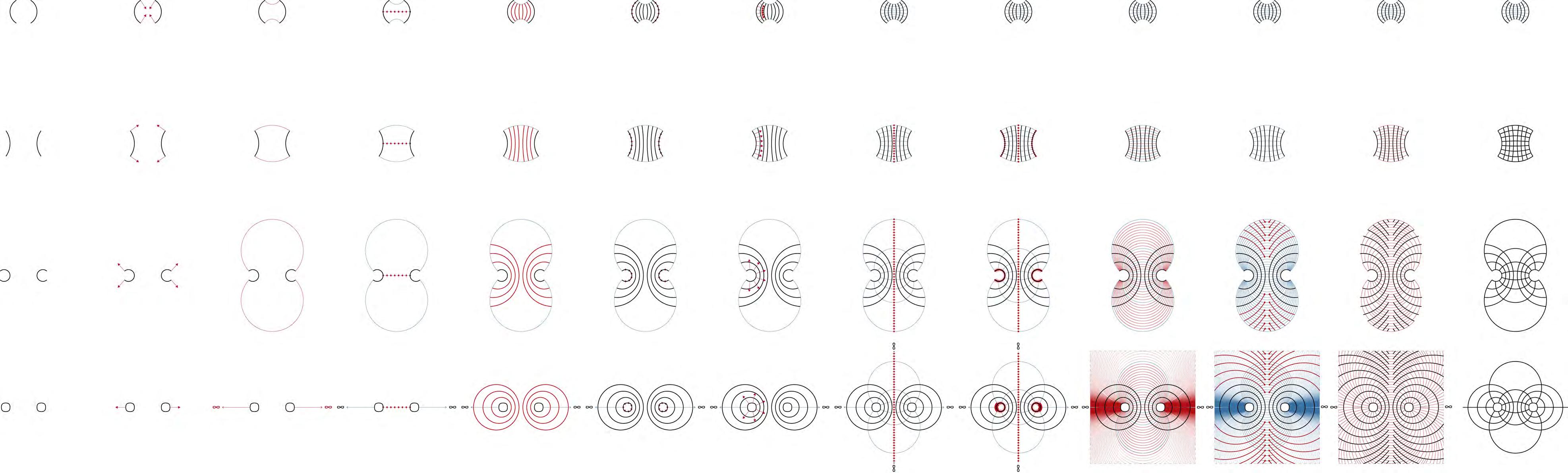
116 STAGE 01 STAGE 02 STAGE 03 STAGE 04
DESIGN DEVELOPMENT
ASSOCIATIVE MODEL
A transitional geometry system has been developed further into an associative model, that establishes interrelations between walls and beams, as the system changes from one geometrical state into another. The associative model was created through digital tools such as python scripting language and parametric modelling software.
The initial configuration of walls and beams is based on constant moduli.
Modulus for walls is 1.5 meters and delimits the maximum distance between adjacent walls. This modulus provides sufficient flexibility to the system, to be adapted for various programmatic needs required by residential functions.
Modulus for beams is 1 meter and limits the maximum distance between neighbouring beams.
The logic of the geometrical system within the associative model is based on two opposing walls that might curve inwards or outwards. From each end of both walls a new curve is constructed, going in a perpendicular direction from the wall to connect with the opposing one. This new arc describes the most outer beam. New walls are introduced between the two initial walls. Spacing between them is based on a 1.5 m modulus. Whenever distance between walls curving in opposite directions becomes more than 1.5 meters, new wall segments ate introduced. If the spacing between beams exceeds 1 meter, new beams are introduced between already existing ones. Once this phase of the scrip executes, segments of beams that are redundant are deleted. Beam segment becomes redundant whenever the distance to its neighbouring beams becomes less than 1 meter. Upon this detailed rule set, a class based scripting approach enable the geometry to be manipulated in real time.
117
81 DIAG.81 CONSTRUCTING AN ASSOCIATIVE GEOMETRIC MODEL. STAGE 05 STAGE 06 STAGE 07 ARCS DEPICTING WALLS ARE DRAWN THROUGH THE POINTS DEFINED IN STAGE 04. RADIUS OF SEQUENTIAL ARCS IS CALCULATED BY TAKING RADIUS OF A PREVIOUS ARC TO THE POWER OF 1.5. INITIAL DEFINING ARCS ARE SUBDIVIDED INTO EQUAL SEGMENTS. FROM EACH DIVIDING POINT ON ONE OF THE ARCS, VECTOR PERPENDICULAR TO CURVATURE AT GIVEN
ARBOREAL FORMATIONS
POINT IS DRAWN.
08
ARCS ARE DRAWN THROUGH DIVIDING POINTS FROM STAGE 06 AND TANGENT TO VECTORS FROM STAGE 07. THESE ARCS DEPICT BEAMS.
09
DISTANCE BETWEEN ADJACENT BEAMS IS SUBDIVIDED WHENEVER IT EXCEEDS 100 CM. DISTANCE IS SUBDIVIDED INTO SEGMENTS OF 100 CM.
10
ADDITIONAL ARCS ARE INTRODUCED THROUGH THE POINTS FROM STAGE 09. THESE ARCS DEPICT ADDITIONAL BEAMS.
11
WHENEVER DISTANCE BETWEEN ARCS DEPICTING WALLS BECOMES GREATER THAN 150 CM, ADDITIONAL WALLS ARCS ARE INTRODUCED. WALLS DESCRIBED THROUGH THEM PROVIDE EXTRA SUPPORT FOR BEAMS.
118
STAGE
STAGE
STAGE
STAGE
DESIGN DEVELOPMENT
12
WHENEVER DISTANCE BETWEEN ARCS DEPICTING BEAMS BECOMES LESS THEN 100 CM, REDUNDANT SEGMENTS ARE REMOVED.
119 82 DIAG.82 DEVELOPING AN ASSOCIATIVE GEOMETRICAL MODEL.
STAGE
ARBOREAL FORMATIONS
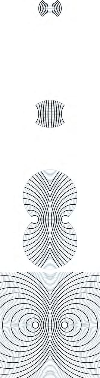
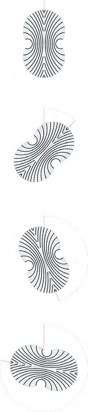
120 83 PARAMETER 01 • RANGE OF CURVATURE STATES PARAMETER 02 • SPACING BETWEEN ARCS PARAMETER 03 • LENGTH OF ARCS PARAMETER 04 • ROTATION CONSTANT 02: 8.5 PARAMETERS: 03: 17(L), 17(R) 04: 0° CONSTANT 01: 0.6 PARAMETERS: 03: 17(L), 17(R) 04: 0° CONSTANT 01: 0.6 PARAMETERS: 02: 8.5 04: 0° CONSTANT 01: 0.6 PARAMETERS: 02: 8.5 03: 17(L), 17(R) 0.1 LEFT ARC: 17 RIGHT ARC: 17 LEFT ARC: 7.8 RIGHT ARC: 7.8 LEFT ARC: 17 RIGHT ARC: 7.8 LEFT ARC: 9 RIGHT ARC: 14.4 4.5 0° 0.4 6.5 30° 0.7 8.5 60° 0.9 10.5 90° DESIGN DEVELOPMENT
(NEXT PAGE) SEQUENTIAL STEPS OF THE ASSOCIATIVE MODEL’S DIARTHROSIS.
GENERATIVE PARAMETERS 2D
The associative model is driven by a set of parameters controlling the geometry in each state. Floor plans described through these geometrical modifications can potentially respond to various programmatic and morphological requirements. The alteration of parameters might result in changes of floor area of each floor plan, number of walls or orientation.
FOLLOWING PAGE:
The matrix shows the domain of geometrical transitions within the associative model. Curvature of the walls is the only parameter displayed in its full range. The other three parameters are constant. DIAG.83 PARAMETERS OF THE ASSOCIATIVE MODEL.
121
DIAG.84
ARBOREAL FORMATIONS
STATE 01 STATE 02 STATE 03 STATE 04 STATE 05 STATE 06 STATE 07 STATE 15 STATE 16 STATE 17 STATE 18 STATE 19 STATE 20 STATE 21 STATE 29 STATE 30 STATE 31 STATE 32 STATE 33 STATE 34 STATE 35 STATE 43 STATE 44 STATE 45 STATE 46 STATE 47 STATE 48 STATE 49 STATE 57 STATE 58 STATE 59 STATE 60 STATE 61 STATE 62 STATE 63 STATE 71 STATE 72 STATE 73 STATE 74 STATE 75 STATE 76 STATE 77 STATE 85 STATE 86 STATE 87 STATE 88 STATE 89 STATE 90 STATE 91 122 DESIGN DEVELOPMENT
STATE 08 STATE 09 STATE 10 STATE 11 STATE 12 STATE 13 STATE 14 STATE 22 STATE 23 STATE 24 STATE 25 STATE 26 STATE 27 STATE 28 STATE 36 STATE 37 STATE 38 STATE 39 STATE 40 STATE 41 STATE 42 STATE 50 STATE 51 STATE 52 STATE 53 STATE 54 STATE 55 STATE 56 STATE 64 STATE 65 STATE 66 STATE 67 STATE 68 STATE 69 STATE 70 STATE 78 STATE 79 STATE 80 STATE 81 STATE 82 STATE 83 STATE 84 STATE 92 STATE 93 STATE 94 STATE 95 STATE 96 STATE 97 STATE 98 123 84 ARBOREAL FORMATIONS
85 124 STATE 38 STATE 43 STATE 48 STATE 53 STATE 58 STATE 63 STATE 68 STATE 73 STATE 78 STATE 83 STATE 88 STATE 93 STATE 98 STATE 03 STATE 08 STATE 13 STATE 18 STATE 23 STATE 28 STATE 33 DESIGN DEVELOPMENT
STACKING OF GEOMETRICAL STATES
Consecutive geometrical states defined by the associative model inform the sequence of stacked floors. Aggregation of these morphologically independent storeys defines the holistic morphology of the building. Small geometrical differences between succesive floors assures that walls and beams on one floor correlate with the walls and beams on the floor above and below it.
86 125
DIAG.85 INDEPENDENT GEOMETRICAL STATES FOR EACH FLOOR PLANS OF THE BUILDING. DIAG.86 SAMPLE BUILDING MORPHOLOGY BASED ON STACKED CONSECUTIVE GEOMETRICAL STATES. ARBOREAL FORMATIONS
U20 U22 U40U27 U40U44 U42U38 U45 U41 U21 U24 U39 U43 U36U34U32 U37 U33U35 U23 U25 U26U28 U27 U31 U29 U30 U47 U46 U49 U48 U56 U57 U01 U08 U05 U04 U02 U54 U55 U53 U52 U51 U50 U46 U47 U49 U48 U02 U01 U50 U51 U52 U53 U54 U55 U56 U57 U58 U59 U60 U61 U62 U63 U62 U61 U60 U58 U57 U56 U59 U63 U09 U05 U03U04 U06U07U08 U13 U14 U15 U16 U17 U18 U19 U17 U15 U13 U18 U16 U14 U19 U09 U10 U11 U12 U12 U11 U10 U09 U08 U07 U06 U05 U04 U03 V10 V11 V11 V10 V09 V07 V05 V03 V03 V04 V04 V09 V08 V07 V06 V05 FLOOR PLAN 01 TYPE N.APART 4523 M2 732 GFA M2 V WALLSU BEAMS FLOOR PLAN 02 TYPE N.APART 4659 M21363 GFA M2 V WALLSU BEAMS 126 87 DESIGN DEVELOPMENT
SAMPLE FLOOR PLANS
Each geometrical state informs different floor plan layouts. Sample floor plans on DIAG.88 and DIAG.87 show how different configurations created with an associative model generate different models of inhabitation.
In these examples a base geometry from the associative model was taken and modified to respond to specific functional needs. This is clearly shown in DIAG.87, where the base geometry from the upper range of the matrix generated by the associative model is significantly modified, in order to shallow the floor plan and assure proper insulation of each apartment. Different geometrical states of the associative model give only a framework for creating floorplans. They inform floorplans, but can’t be directly translated into them.
DIAG.87 shows how these base geometrical states can be modified according to needs. Apartments on the left hand side of the floor plan are more enclosed and organised around quasi-courtyards, whilst the apartments on the right hand side are open towards surroundings.
Some geometrical states are more susceptible to modifications than others. As mentioned above the geometry used to generate the floor plan on DIAG.87 provides many potentials for adaptation, whereas the base geometry of the floor plan on DIAG.88 is rather restricted and is denoted by clear bidirectional orientation.
Considering the potentials and restrictions of each geometrical state as a different floor plan layout offers a greater awareness as to how the shape and global morphology of the building may respond to context specific conditions. DIAG.87
127
V01 V02 V03 V04 V05 V06 V07 U01 U01 U02 U03 U04 U05 U06 U07 U08 U09 U10 U11 U12 U13 U14 U15 U16 U17 U18 U19 U20 U21 U22 U23 U24 U25 U26 U27 U28 U29 U30 U31 U32 U02 U03 U04 U05 U06 U07 U08 U09 U10 U11 U12 U13 U14 U15 U16 U17 U18 U19 U20 U21 U22 U23 U24 U25 U26 U27 U28 U29 U30 U31 U32 V07 V06 V05 V04 V03 V02 V01 FLOOR PLAN 01 TYPE N.APART 4523 M2 732 GFA M2 V WALLSU BEAMS FLOOR PLAN 02 TYPE N.APART 4659 M21363 GFA M2 V WALLSU BEAMS
FLOOR PLAN 01, BASED ON THE GEOMETRICAL STATE FROM THE HIGHER RANGE OF ASSOCIATIVE MODEL’S MATRIX. DIAG.88
02, BASED ON THE GEOMETRICAL STATE FROM THE MIDDLE RANGE OF ASSOCIATIVE MODEL’S MATRIX. 88 ARBOREAL FORMATIONS
FLOOR PLAN
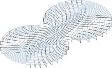
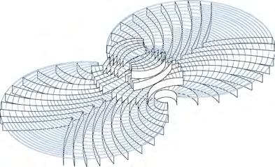
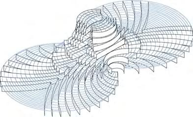
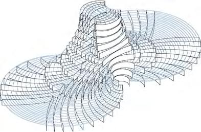
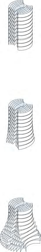
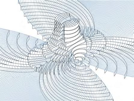
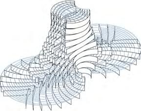
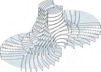


128 PARAMETER 01 • NUMBER OF FLOORS PARAMETER 02 • RANGE OF CURVATURE STATES PARAMETER 03 • SPACING BETWEEN ARCS TOP FLOOR: 0.1 GROUND FLOOR: 0.1 1 TOP FLOOR: 4.5 GROUND FLOOR: 8.5 4 TOP FLOOR: 0.1 GROUND FLOOR: 0.4 TOP FLOOR: 6.5 GROUND FLOOR: 8.5 7 TOP FLOOR: 0.1 GROUND FLOOR: 0.7 TOP FLOOR: 8.5 GROUND FLOOR: 8.5 10 TOP FLOOR: 0.1 GROUND FLOOR: 0.9 TOP FLOOR: 10.5 GROUND FLOOR: 8.5 CONSTANT 02: GROUND FLOOR: 0.84 TOP FLOOR: 0.1 PARAMETERS: 03: GROUND FLOOR: 4.5 TOP FLOOR: 4.5 04: GROUND FLOOR: 14.4(L), 14.4(R) TOP FLOOR: 14.4(L), 14.4(R) 05: GROUND FLOOR: 0° TOP FLOOR: 0° CONSTANT 01: 10 FLOORS PARAMETERS: 03: GROUND FLOOR: 4.5 TOP FLOOR: 4.5 04: GROUND FLOOR: 14.4(L), 14.4(R) TOP FLOOR: 14.4(L), 14.4(R) 05: GROUND FLOOR: 0° TOP FLOOR: 0° CONSTANT 01: 10 FLOORS PARAMETERS: 02: GROUND FLOOR: 0.75 TOP FLOOR: 0.1 04: GROUND FLOOR: 14.4(L), 14.4(R) TOP FLOOR: 14.4(L), 14.4(R) 05: GROUND FLOOR: 0° TOP FLOOR: 0° DESIGN DEVELOPMENT


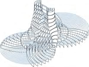
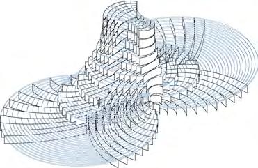
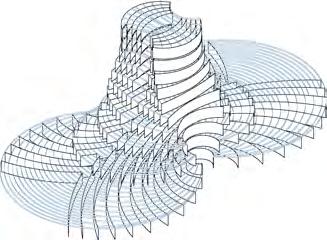
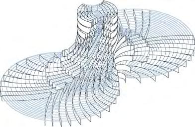
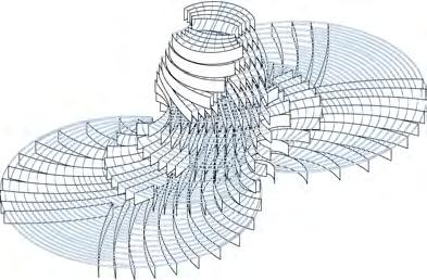
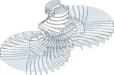
GENERATIVE PARAMETERS 3D
DIAG.89 demonstrates how parameters described in DIAG.83 vary throughout the floors of a building. Slight modifications of parameters from floor to floor results in significant changes to the global morphology. In the examples shown in DIAG.89 only one parameter is modified at a time.
129
DIAG.89 PARAMETERS OF THE ASSOCIATIVE MODEL. PARAMETER 05 • ROTATION PARAMETER 04 • LENGTH OF ARCS LEFT ARC: 17 TOP FLOOR: RIGHT ARC: 7.8 GROUND FLOOR: LEFT
RIGHT
TOP FLOOR: 0° GROUND FLOOR: 0° LEFT
17 TOP FLOOR: RIGHT ARC: 7.8 GROUND FLOOR: LEFT ARC: 7.8 RIGHT ARC: 7.8 TOP FLOOR: 30° GROUND FLOOR: 0° LEFT ARC: 17 TOP FLOOR: RIGHT ARC: 7.8 GROUND FLOOR: LEFT ARC: 17 RIGHT ARC: 7.8 TOP FLOOR: 60° GROUND FLOOR: 0° 89 LEFT ARC: 17 TOP FLOOR: RIGHT ARC: 7.8 GROUND FLOOR: LEFT ARC: 9 RIGHT ARC: 14.4 TOP FLOOR: 90° GROUND FLOOR: 0° CONSTANT 01: 10 FLOORS PARAMETERS: 02: GROUND FLOOR: 0.84 TOP FLOOR: 0.1 03: GROUND FLOOR: 4.5 TOP FLOOR: 4.5 05: GROUND FLOOR: 0° TOP FLOOR: 0° CONSTANT 01: 10 FLOORS PARAMETERS: 02: GROUND FLOOR: 0.84 TOP FLOOR: 0.1 03: GROUND FLOOR: 4.5 TOP FLOOR: 4.5 04: GROUND FLOOR: 14.4(L), 14.4(R) TOP FLOOR: 14.4(L), 14.4(R) ARBOREAL FORMATIONS
ARC: 17
ARC: 17
ARC:
01234567 8 91011121314151617181920
01234567 8 91011121314151617181920
01234567 8 91011121314151617181920
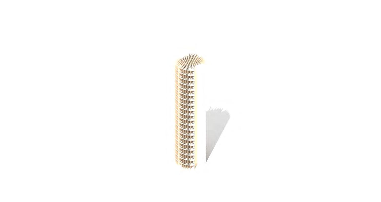
01234567 8 91011121314151617181920
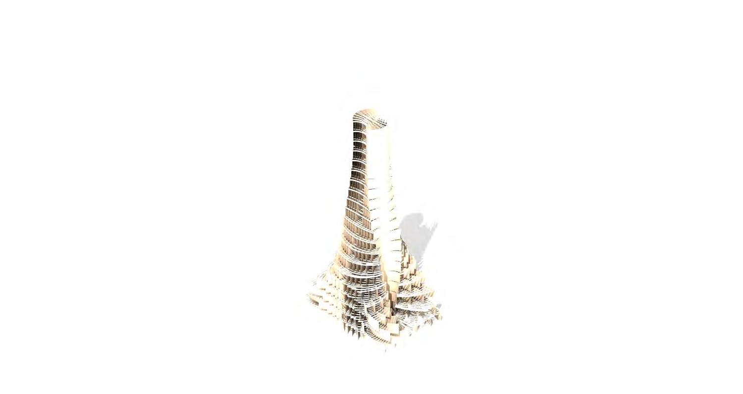
0.03
01234567 8 91011121314151617181920
01234567 8 91011121314151617181920
FLOOR LEVEL CURVATURE (FACTOR) 0.03 0.99
CURVATURE (FACTOR) 0.03 0.99
CURVATURE (FACTOR)
0.99
FLOOR LEVEL FLOOR LEVEL FLOOR LEVEL CURVATURE 0.03
CURVATURE (FACTOR) 0.03 0.99
CURVATURE (FACTOR) 0.03 0.99
FLOOR LEVEL FLOOR LEVEL 90 91 130 MORPHOLOGY 01 MORPHOLOGY 02 DESIGN DEVELOPMENT
8 91011121314151617181920
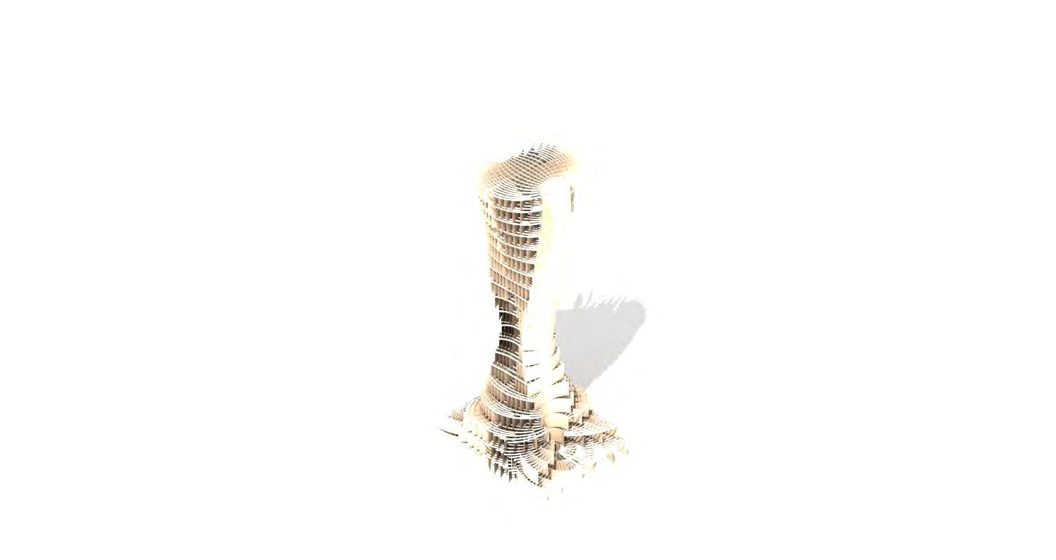
MORPHOLOGY 03
MORPHOLOGICAL VARIATIONS
Through the slight modifications of parameters affecting simultaneously all the flooplates in the height of a building, a model was generated to display different global morphologies, based on a gradient of smooth transitions between the geometries of each floor. Depending on how the parameters are changed within a range, the resulting morphologies can vary significantly. If a parameters’ range of change is not big or they are constant as displayed through example shown on DIAG.90, the resulting geometry of a building might be simple and moderate. Changing parameters to the limits of their range results in the creation of more complex geometries. The example shown in DIAG.91 embodies a linear change of parameters within the full range.
The most extreme morphologies are achieved by the nonlinear modification of parameters within full range of their domain. DIAG.92 demonstrates an example when parameters change nonlinearly throughout the range from the lower boundary of the range to the upper boundary of the domain and back to the middle range of the domain. More extreme generated morphologies result in more iconic and dynamic expressions.
CURVATURE 0.03 01234567
CURVATURE (FACTOR) 0.03 0.99 01234567
FLOOR LEVEL FLOOR LEVEL 92 131 DIAG.90 MODEL BASED ON REPETITION OF THE SAME GEOMETRICAL STATE DIAG.91 MODEL BASED ON LINEAR CHANGE OF GEOMETRICAL STATE THROUGH THE FULL RANGE. DIAG.92 MODEL BASED ON NONLINEAR CHANGE OF GEOMETRICAL STATE THROUGH THE FULL RANGE.
8 91011121314151617181920
ARBOREAL FORMATIONS
DEFORMATION OF STRUCTURE
Due to the hygroscopic and fibrous nature of timber, cells within its tissue continually change their dimensions in relation to humidity. This leads to the deformation of timber elements and internal stresses within the structure. DIAG.93 demonstrates how fabricated wall components in axis V03 and V04 of sample floor plan in DIAG.87 deform due to humidity change. Unrestricted wall components were analysed in the range of maximum humidity change between 11.2% MC and 15.9% MC in sample location in New York for a month September (DIAG.14). Displacement of a wall component was determined at 700 mm for V03 component (length:800 cm) and 150 mm for V04 component (length:400 cm). External walls are prone to biggest deformation as they are exposed to humid external environment on one side and drier internal environment on the other side. In the analysis it is assumed that walls are not weather proof and moisture can penetrate down to 20% of a wall thickness.
Deformations indicated through the analysis convey the need of restraining wall components from deformations. The bottom edge of the wall needs to be restricted by connecting it with a floor and top edge of a wall needs to be braced by beams. Both anchorages result in increased internal stresses within the structure, which need to be considered during the design process.
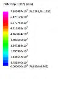
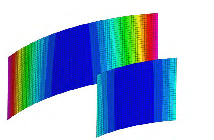
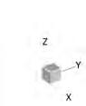
93 132 DIAG.93 DEFORMATION OF CURVED TIMBER COMPONENTS DUE TO HUMIDITY CHANGE.
V03
DESIGN DEVELOPMENT
V04
POTENTIALS AND LIMITATIONS
Resulting building morphologies feature some emerging potentials and constraints that could not be resolved directly within the associative model. As shown on DIAG.96 these emerging qualities derive from transitions within a morphology. As the form steps back, emergent external spaces may be utilised as balconies(DIAG.95). As the form steps out, geometry of the building needs to be adapted in order to ensure continuity of the structure. DIAG.94 demonstrates how walls stepping out towards the top of the building cause discontinuity in the structure, that requires the adjustment of structural components. In order to provide structural support for disjointed walls, beams and floorplates of a floor below need to be extended to these walls.
These two examples demonstrate limitations of the associative model in resolving emergent properties of the system. The associative model needs to be seen merely as a design tool and a mean of establishing interrelations between consecutive floors, creating a framework for the further development of a system.
FFL 12.00m FFL 15.00m FFL 18.00m FFL 36.00m FFL 39.00m FFL 42.00m FFL 12.00m FFL 15.00m FFL 18.00m FFL 36.00m FFL 39.00m FFL 42.00m 94 95 96 133 DIAG.94 EMERGING
DIAG.95
FORM STEPS OUTWARDS. DIAG.96
BALCONIES AS FORM STEPS BACK.
POTENTIALS AND LIMITATIONS THROUGH CHANGE IN MORPHOLOGY.
DISCONTINUITY OF STRUCTURE AS
EMERGING
ARBOREAL FORMATIONS
CONCLUSIONS
The same evaluation process applied previously for the residential project in Okurayama described in DIAG.70 was repeated for the designed building system. Wall components were analysed for their curvature as displayed in DIAG.97. To each wall component a maximum thickness for a given curvature was assigned and all components were catalogued and divided into hierarchical groups (DIAG.98).
Thickest components displaying the largest radii are mostly indicated with blue and are utilised as structural elements. Thinner wall elements within the yellow range of smaller radii are used as partition walls. Thinnest components of small radii can be used to design furniture.
The analysis demonstrates the potential of the materials system to deliver a complete building solution at each hierarchical level: from structural elements down to the furniture scale. What is more, the analysed building elements have constant curvature throughout their full length, which exploits the potential of components to be manufactured as single prefabricated elements, which could then be assembled on a site.
U47 U46 U49 U48 U02 U01 U50 U51 U52 U53 U54 U55 U56 U57 U58 U59 U60 U61 U62 U63 U62 U61 U60 U58 U57 U56 U59 U63 U05 U03U04 U06U07U08 U18 U16 U14 U19 U12 U11 U10 U09 U08 U07 U06 U05 U04 U03 V07 V05 V03 V03 V04 V04 V07 V06 V05 U01 U02 U03 U04 U05aU05b U06 U07 U08 U09 U10 U11 U14 U16 U18 U19 U20 U63a U62 U61 U60 U59a U63b U59b U58 U57 U56 U55 U54 U53 U52 U51 U50 U49 U48 P01a P01a P02 P03a P03b P04a P04a P05 Chair Chair Chair Chair Table Table Table Screen Sink U47 U46 U45 U12
134
97 MATERIAL SYSTEM COMPONENTS OF A FLOOR DESIGN DEVELOPMENT
U57 U58 U59 U60 U61 U62 U63 V04 U01 U02 U03 U04 U05aU05b U06 U07 U08 U09 U10 U11 U14 U16 U18 U19 U20 U63a U62 U61 U60 U59a U63b U59b U58 U57 U56 U55 U54 U53 U52 U51 U50 U49 V01a V01b V02a V05a V05b V06a V02b V02c V03c V04a V04b V04c V04d V04e V03b V03a U48 P01a P01a P02 P03a P03b P04a P04a P05 Chair Chair Chair Chair Table Table Table Screen Sink U47 U46 U45 U12 U01 U02 U03 U04 U05aU05b U06 U07 U08 U09 U10 U11 U14 U16 U18 U19 U20 U63a U62 U61 U60 U59a U63b U59b U58 U57 U56 U55 U54 U53 U52 U51 U50 U49 V01a V01b V02a V05a V05b V06a V02b V02c V03c V04a V04b V04c V04d V04e V03b V03a U48 P01a P01a P02 P03a P03b P04a P04a P05 Chair Chair Chair Chair Table Table Table Screen Sink U47 U46 U45 U12 U59 U60 U61 U62 U63 U01 U02 U03 U04 U05aU05b U06 U07 U08 U09 U10 U11 U14 U16 U18 U19 U20 U63a U62 U61 U60 U59a U63b U59b U58 U57 U56 U55 U54 U53 U52 U51 U50 U49 V01a V01b V02a V05a V05b V06a V02b V02c V03c V04a V04b V04c V04d V04e V03b V03a U48 P01a P01a P02 P03a P03b P04a P04a P05 Chair Chair Chair Chair Table Table Table Screen Sink U47 U46 U45 U12 U01 U02 U03 U04 U05aU05b U06 U07 U08 U09 U10 U11 U14 U16 U18 U19 U20 U63a U62 U61 U60 U59a U63b U59b U58 U57 U56 U55 U54 U53 U52 U51 U50 U49 V01a V01b V02a
U48 P01a P01a P02 P03a P03b P04a P04a P05 Chair Chair Chair Chair Table Table Table Screen Sink U47 U46 U45 U12 135 98 LOAD-BEARING WALLS LOAD-BEARING WALLS PARTITION WALLS FURNITURE
FLOOR PLAN INDICATED WITH COMPONENTS OF DIFFERENT CURVATURES. DIAG.98 CATALOGUE OF COMPONENTS WITHIN THE FLOOR. ARBOREAL FORMATIONS
V05a V05b V06a V02b V02c V03c V04a V04b V04c V04d V04e V03b V03a
DIAG.97
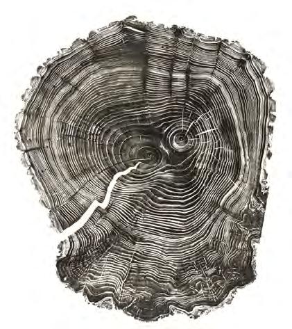
DESIGN PROPOSAL
Previous chapter discussed logic and development of the design system. This system based on the associative model can generate various morphologies upon material system logic, structural strategy and functional conditionings.
This chapter investigates how outcomes produced by the system could be evaluated based on context specific parameters.
The competition site in New York was chosen as a test field for the system. Competition calls for an innovative mid-rise timber building in Red Hook, Brooklyn with mixed use. Basic site conditions were analysed in scope of their potential to drive morphology of a building generated within the design system. Produced geometry was then modified to meet requirement for specific programmatic needs such as floor area or size of a site. Resulting building was examined in scope of reaching research aims and ambitions.
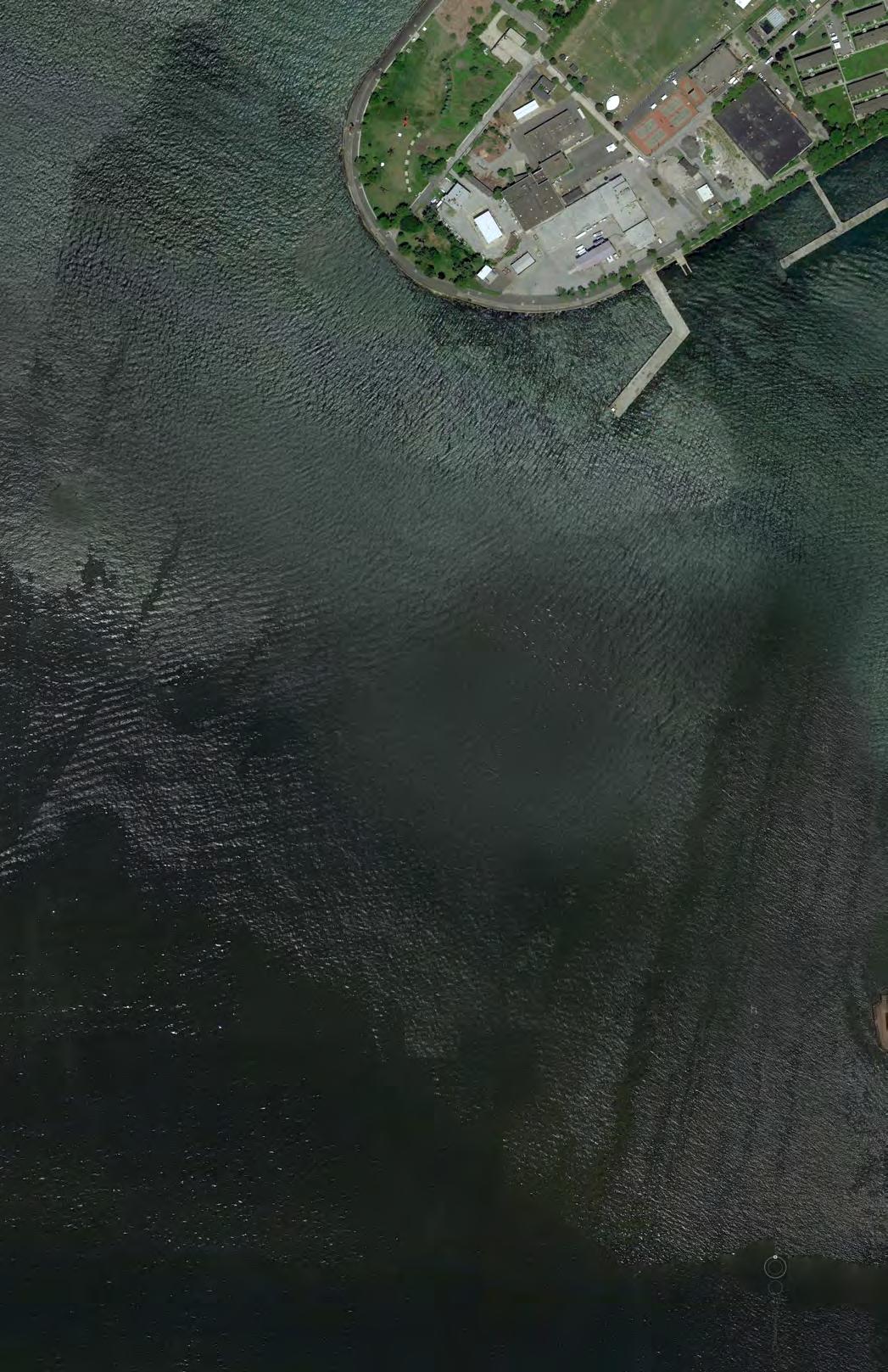
REQUIREMENTS
MID-RISE
MIXED-USE BUILDING
HOUSING UNITS
JOB TRAINING + EDUCATIONAL FACILITY
CENTRE OF WOOD TECHNOLOGY
DISTRIBUTION CENTRE
136
PIC.85 WOOD-CUT PRINT OF A WILLOW TREE BY BRYAN NASH GILL, 2011 PIC.86 RED HOOK, BROOKLYN. SOURCE: GOOGLE MAPS DESIGN PROPOSAL
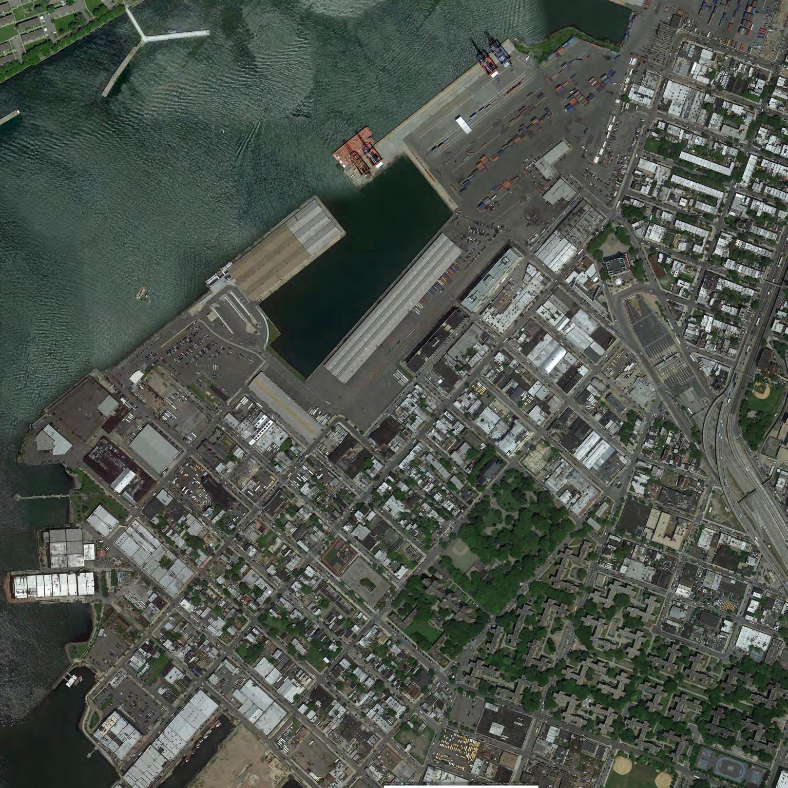
137 ARBOREAL FORMATIONS
PROJECT CONTEXT
Red Hook is the neighbourhood that is geographically cut off from much of Brooklyn, yet becomes increasingly vibrant. Project site is located at the edge of Coffey Park on the south. This provides an opportunity to create apartments oriented towards the park on the lower floors. Proximity to Manhattan on the north gives the potential of creating apartments on the top floors of the building that make use of stunning views on the panorama of the island. The site area is 2400 m2, its dimensions defined by rectangle 60 x 40 meters. Design brief draw programmatic requirements for housing units and commercial functions.
138
PIC.87 RED HOOK, BROOKLYN. SOURCE: GOOGLE MAPS DESIGN PROPOSAL
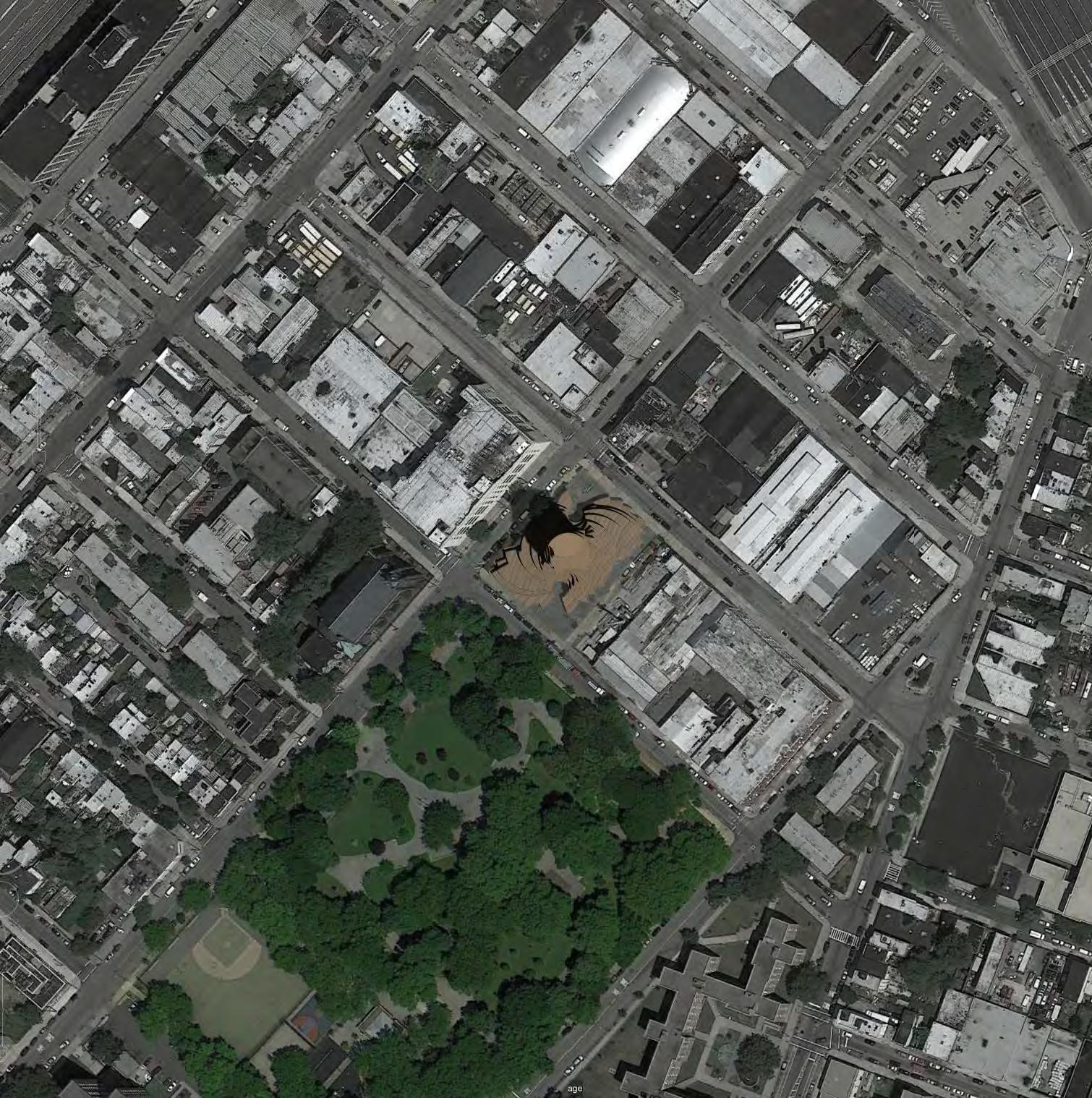
139 ARBOREAL FORMATIONS
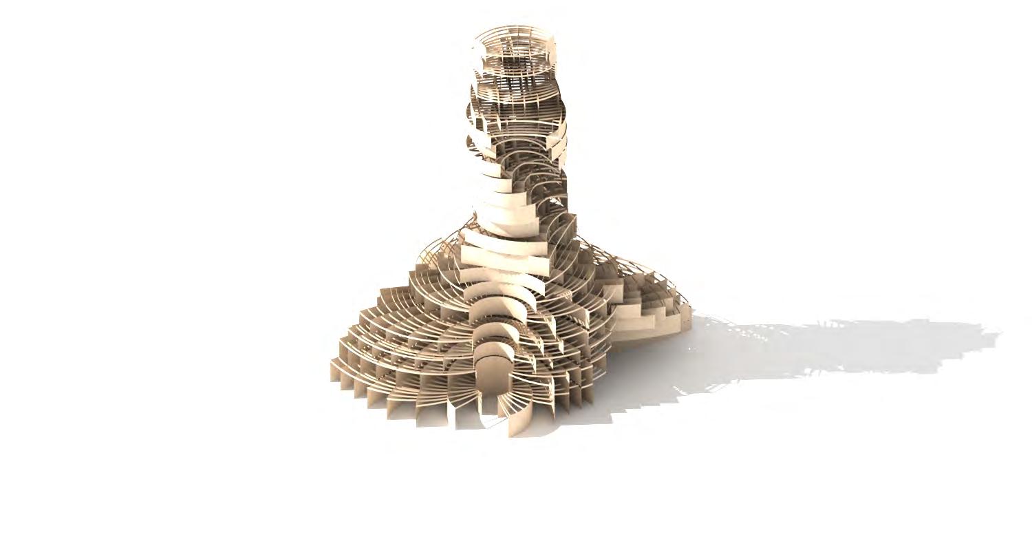
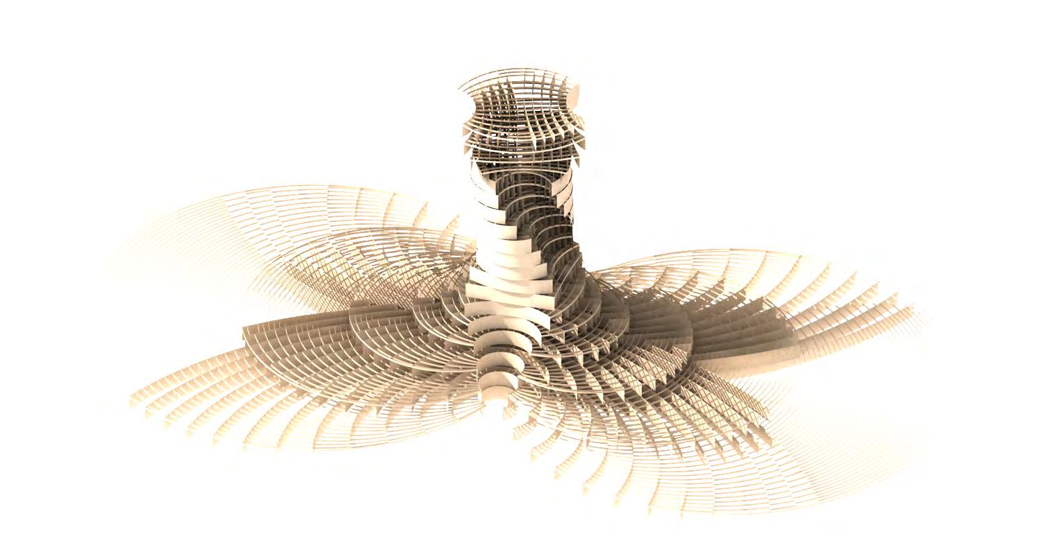
140 99 DESIGN PROPOSAL
PARAMETERS DRIVING THE MORPHOLOGY
MORPHOLOGICAL RESPONSE
Site specific conditions inform parameters of the associative model. Parameters are manipulated throughout the height as shown in DIAG.100 in order to generate smooth transition of geometrical states between floors. Shift from southern orientation towards the park on the lower floors, to northern orientation towards Manhattan on the top floors was obtained by manipulating rotation parameter. Transition from large floor plans utilised for commercial functions on bottom floors to small floor plans for residential functions on top floors was manipulated through curvature and spacing between edge arcs parameters. Openness towards park, increased exposure of facade to south to ensure proper internal lighting conditions and minimised exposure on the north to reduce heat loss, were achieved by modifying arc 01 and arc 02 length parameters. Resulting morphology shown at the bottom of DIAG.99 had to be then trimmed down to meet site restrictions of the site and requirements for floor plans. Top of DIAG.99 displays final modified building geometry. DIAG.99 GEOMETRY GENERATED THROUGH ASSOCIATIVE MODEL AFTER AND BEFORE MODIFICATION
141
100
EDGE ARCS ANGLE (DEGREES) -240 -310 � 01234567 8 91011121314151617181920 CURVATURE (FACTOR) 0.03 0.99 01234567 8 91011121314151617181920 LENGTH (M) 4m 20m 01234567 8 91011121314151617181920 LENGTH (M) 6m 30m 01234567 8 91011121314151617181920 LENGTH (M) 6m 30m 01234567 8
FLOOR LEVEL FLOOR LEVEL FLOOR LEVEL FLOOR LEVEL FLOOR LEVEL FLOOR LEVEL RADIAL 0 0.01 0.00 0.020.030.040.050.060.070.080.090.1 ROTATION 01 EDGE ARCS ANGLE (DEGREES) -240 -310 � 01234567 8 91011121314151617181920 CURVATURE (FACTOR) 0.03 0.99 01234567 8 91011121314151617181920 LENGTH (M) 4m 20m 01234567 8 91011121314151617181920 LENGTH (M) 6m 30m 01234567 8 91011121314151617181920 LENGTH (M) 6m 30m 01234567 8
FLOOR LEVEL FLOOR LEVEL FLOOR LEVEL FLOOR LEVEL FLOOR LEVEL FLOOR LEVEL 0 0.01 0.00 0.020.030.040.050.060.070.080.090.1 CURVATURE 02 EDGE ARCS ANGLE (DEGREES) -240 � -310 � 01234567 8 91011121314151617181920 CURVATURE (FACTOR) 0.03 0.99 01234567 8 91011121314151617181920 LENGTH (M) 4m 20m 01234567 8 91011121314151617181920 LENGTH (M) 6m 30m 01234567 8 91011121314151617181920 LENGTH (M) 6m 30m 01234567 8 91011121314151617181920 FLOOR LEVEL FLOOR LEVEL FLOOR LEVEL FLOOR LEVEL FLOOR LEVEL FLOOR LEVEL 0 0.01 0.00 0.020.030.040.050.060.070.080.090.1 SPACING BETWEEN EDGE ARCS 03 -240 01234567 91011121314151617181920 CURVATURE 0.99 8 (M) 4m 20m LENGTH 30m FLOOR LEVEL FLOOR LEVEL 0 0.01 0.00 0.020.030.040.050.060.070.080.090.1 ARC 01 LENGTH 04 EDGE ARCS ANGLE (DEGREES) -240 -310 � 01234567
CURVATURE (FACTOR) 0.03 0.99 01234567
LENGTH (M) 4m 20m 01234567 8
LENGTH (M) 6m 30m 01234567
LENGTH (M) 6m 30m 01234567
FLOOR LEVEL FLOOR LEVEL FLOOR LEVEL FLOOR LEVEL FLOOR LEVEL FLOOR LEVEL 0 0.01 0.00 0.020.030.040.050.060.070.080.090.1 ARC 02 LENGTH 05 ARBOREAL FORMATIONS
DIAG.100
91011121314151617181920
91011121314151617181920
8 91011121314151617181920
8 91011121314151617181920
91011121314151617181920
8 91011121314151617181920
8 91011121314151617181920
192.86 m² 189.33 m² 191.89 m² 169.73 m² 183.09 m² 188.40 m² 215.70 m² 259.01 m² 341.09 m² 472.31 m² 733.26 m² 1094.83 m² 235.00 m² 1348.67 m² 1504.35 m² 1492.67 m² 1169.87 m² 239.67 m² 139.01 m² 200.10 m² 142 TOTAL
MIXED-USE RESIDENTIAL 101 DESIGN PROPOSAL
FLOOR AREA: 10560 M2
CATALOG OF FLOORPLANS, THEIR PROGRAMMATIC DIFFERENTIATION AND SUBDIVISION INTO APARMENTS
PROGRAMMATIC DIFFERENTIATION OF THE DESIGNED TOWER BLOCK
RESIDENTIAL USES
PROGRAMMATIC STRATEGY
DIAG.101 demonstrates how sequential geometrical states generated with associative model were modified in order to meet functional requirements. of the brief. Base geometry on the ground level was trimmed down to create passage providing access to commercial functions. Diagrams of residential floor plans illustrate sample subdivisions into individual apartments.
DIAG.102 conveys how deep floor plates in the base of the building are used for mixed-use program, that does not require direct sunlight. Shallow floor plate provide access to daylight, thus are suitable for residential uses.
SHALLOW
DEEP FLOOR PLATES MIXED USE 143 102
FLOOR PLATES
DIAG.101
DIAG.102
ARBOREAL FORMATIONS
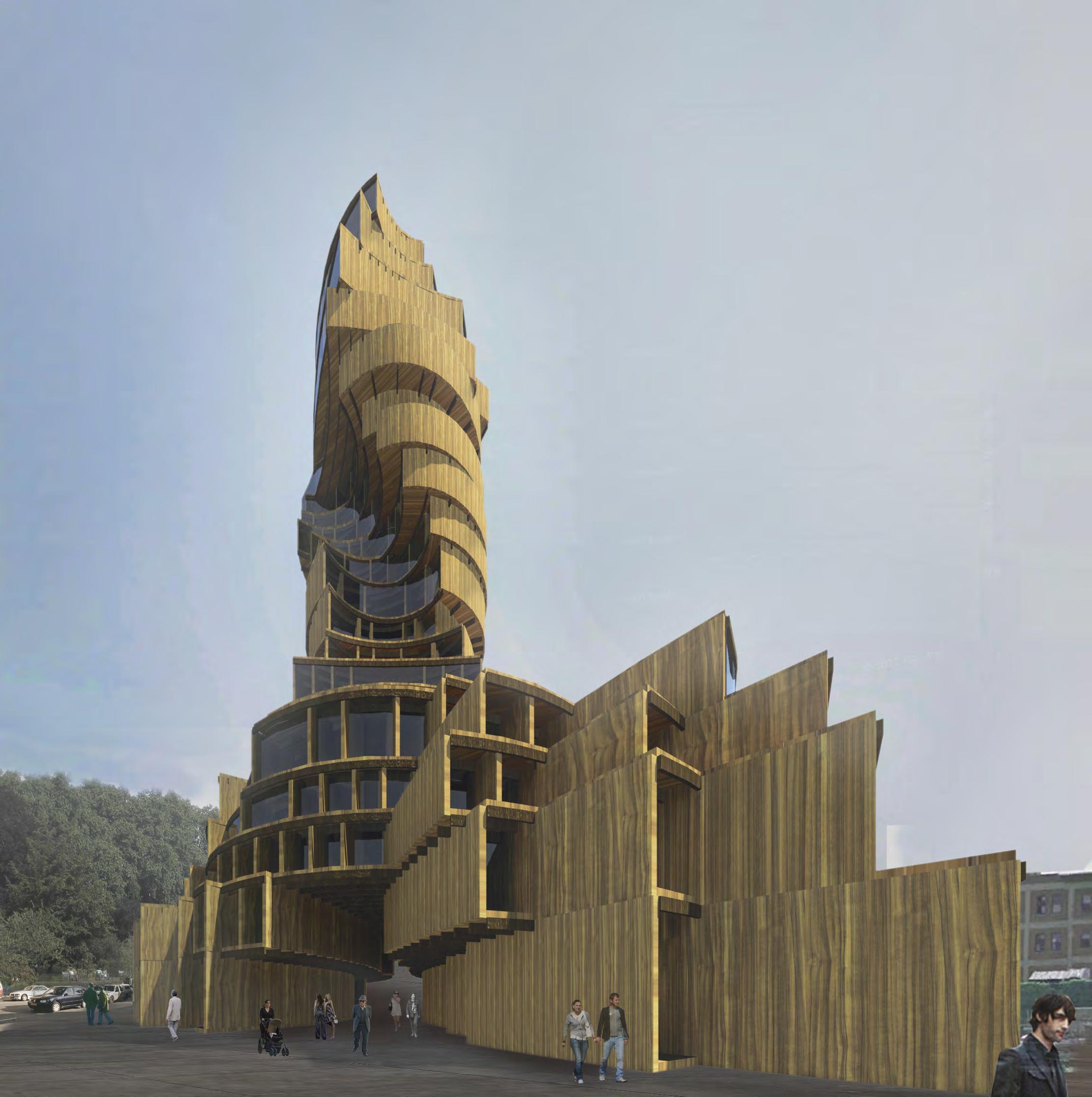
144 DESIGN PROPOSAL
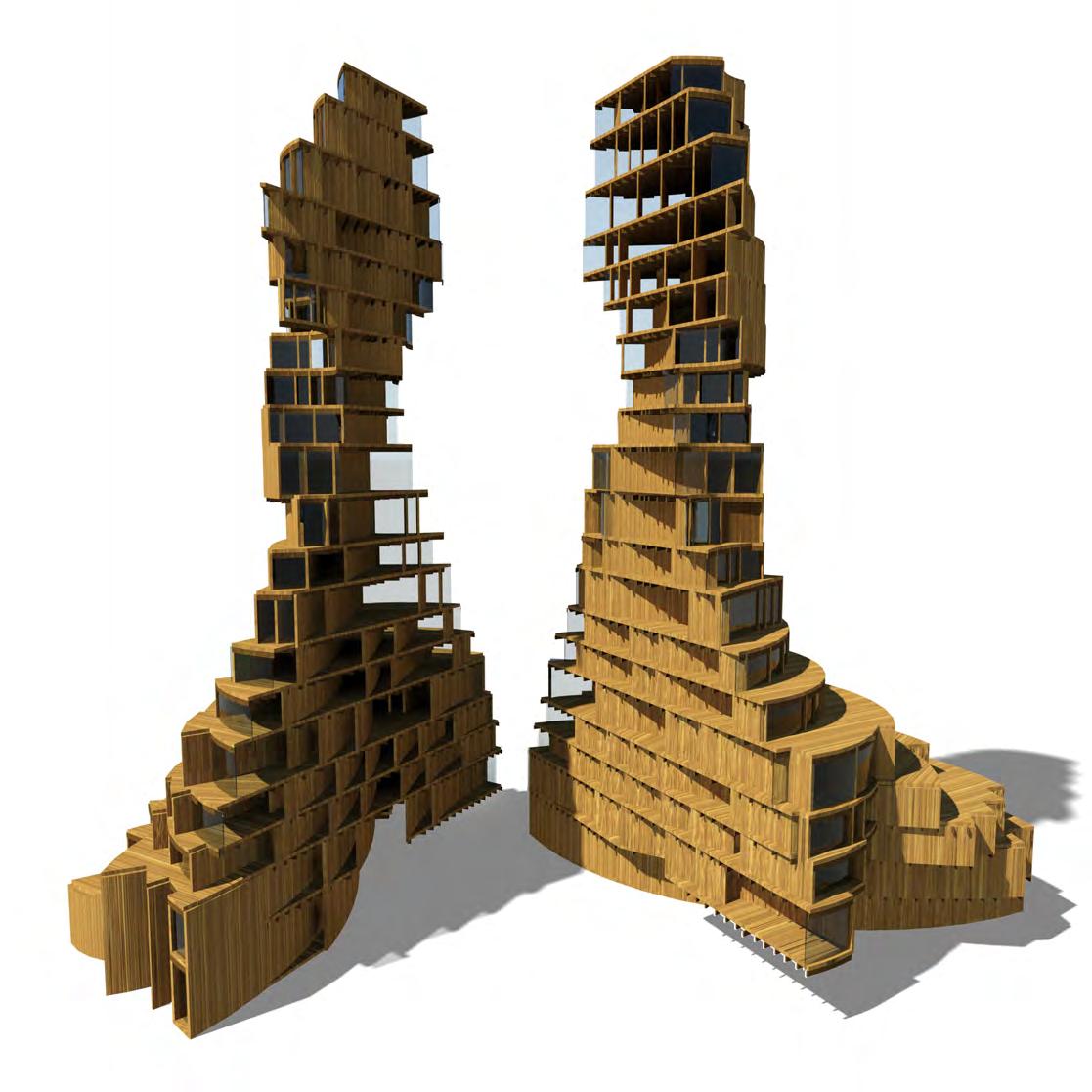
145 DIAG.103 VIEW TOWARDS COMMERCIAL
DIAG.104 SECTION
AT THE GROUND FLOOR 103 ARBOREAL FORMATIONS
PASSAGE
THROUGH COMMERCIAL PASSAGE
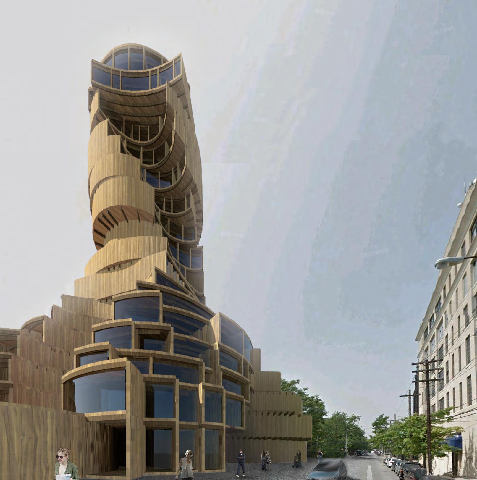
146 DESIGN PROPOSAL
CONCLUSIONS
Through the study of wood and its inherit properties, we managed to understand and control its behaviour, exploring at the same time the widely used fabrication technique of lamination combined with wood’s dimensional change due to moisture exchange. A material component could then be shaped based on simple principles, by controlling the variable parameters and at the same time its behaviour was simulated with the use of computational means. The potentials and the limitations deriving from our material component guided the geometrical explorations towards complex geometries with prominent biaxial orientation. Consequently the structural logic of our system was coupled with this idea of interlocking U and V lines in space that allow structural and at the same time spatial performance. The chosen design proposal consists an experiment for applying our building system on an environment with imposed limitations which deteriorate the multiple configurations that the system can generate. At the same time evaluation criteria, based on the specific environment, justify our design decisions, leading to a set of adequate morphologies.
147
DIAG.105 VIEW TOWARDS COFFEY PARK ARBOREAL FORMATIONS
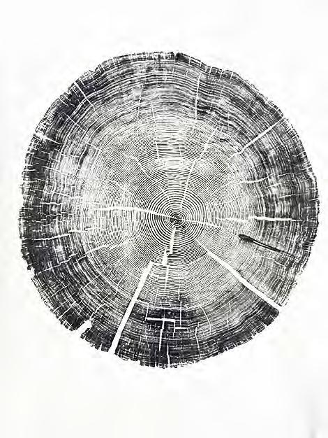
FURTHER DEVELOPMENTS
The research presented in Arboreal Formations documents an approach to generating design solutions through investigating and understanding the inherent properties of wood. With the aim of creating a generative process for a twenty storey timber residential building system, a methodology was implemented to prioritise materiality and enhance the performance relationship between material, structure and geometry.
The project conveys the potential for creating a new and exciting timber component for both industrial design and construction industries. However this research only documents the conceptual idea and initial explorations undertaken in a five month period. If further developments were to be pursued, the work may focus on three interrelated fields of the thesis work; material component, material system and application.
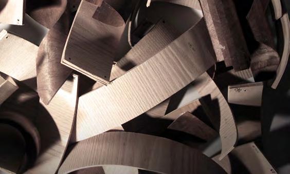
Limited by time and unsuccessfully sourcing rotary cut veneers the scale of physical material experiments was restricted. The largest scale test undertaken in Finite Element Analysis (FEA) simulated the successful bending behaviour of a component 140mm thick. The thesis would therefore be further supported by trialling the findings of the FEA on a full scale laminated piece. The test may also provide the opportunity to advance the technique of laminating the veneers together using vacuum pressure and with alternative types of glue. Live loading and pressure test could also be applied to the physical experiment to further understand the performance properties of the piece such as its strength and stiffness.
The early material investigations highlighted the potential for orienting the grain in different directions. It is a well documented fact that alternating layers perpendicular to each other will improve the strength and stability of the piece. Initial thesis findings from diagonally orientating layers suggested that the twisting forms produced was of a ruled surface nature. These tests could be further investigated both physically and digitally to understand more thoroughly the relationship and parameterisation of curvature and grain direction simultaneously. Whilst the notion of double curved timber pieces is an exciting prospect, none of our experiments suggested this may be attainable. An idea to be explored in the hope of achieving this may stitch different orientations of veneer grains together within the same layer.
148
CONCLUSIONS & FURTHER DEVELOPMENTS
MATERIAL COMPONENT
COLLECTION OF PHYSICAL MATERIAL EXPERIMENTS
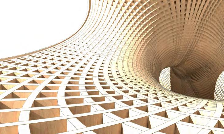
MATERIAL SYSTEM APPLICATION
The associative model employed to organise the material system offers many potentials for development. At present the model does not allocate true structural thicknesses to the elements and assumptions are made to the spacing and distance between structural members. Information data about the material components only transcribes the relationship between a specified curvature and thickness for which it may be fabricated. Introducing the structural performance of the elements in relation to thickness and curvature would help to enforce the structural potentials and limitations of the holistic material system. This work would require both the physical and computational structural testing (using FEA) of individual and aggregated assemblies of components. Gaining a more detailed understanding and quantification of the systems structural performance, the spacing between walls and beams could be further optimised to ensure the timber components are employed with efficiency and resourcefulness. The additional research may also lead to the adjustment of the geometric aggregation method as a structural hierarchy between components and the stacking of floor plates would be initiated. Applying this new associated model to a functional context would deliver a greater degree of clarity in the design solution and may also present emergent qualities of space.
The architectural application is currently used to inform the parameters of the associative model that order and define the material system. The output of this model is a pure smooth geometry which displays various states of different geometric instances and sizes. The system would benefit from the active integration of the proposed building programme to help assign building and space functionality as part of the various morphological states. This work would help define kill strategies to remove elements of the structural system with a greater notion of the desired spatial conditions and influence the overall building composition.
Buildings comprise three main elements of design; function, structure and environment. The project unites the first two of these fields but did not focus on the integration of environmental factors. Building physics and the consideration of local climatic conditions offers an opportunity to enhance a buildings performance and operation. For example the associated model might also adapt to ensure a certain amount of solar radiation or light is received on each floor plate. Building physics also encompasses the way in which building structures are sealed for reasons of moisture and thermal control. Aware that the inherent properties of wood may cause the component to move and react to moisture and thermal changes this would be a interesting lines of investigation. Although the project is very much a conceptual idea developing facade and threshold details between the juxtaposed floor plates would also deliver a greater degree of credibility for the buildings realisation.
Developed in the thesis is a material system designed for the specific functional use of a residential mid-rise tower block. Applied to other functions the material component may be employed to perform in a different manner and thus the organisation and strategy for forming the material system would change too. The range of curvatures and thickness of elements that the fabrication method may produce is a fantastic opportunity for the exploration of other design applications.
149 PIC.88
PIC.89
PIC.90
PIC.91
U02 U01 U50 U51 U52 U53 U54 U55 U56 U57 U58 U59 U60 U61 U62 U63 U62 U61 U60 U58 U56U57 U59 U63 U05 U03U04 U06U07U08 U18 U16 U14 U19 U12 U11 U10 U09 V07 V05 V03 V03 V04 V04 Chair Chair Chair Chair Table Table Table
WOOD-CUT PRINT OF A WILLOW TREE BY BRYAN NASH GILL, 2011
STRUCTURAL HIERARCHY IN THE MATERIAL SYSTEM
ABSTRACTION OF COSTA SURFACE.
ARBOREAL FORMATIONS
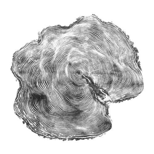
BIBLIOGRAPHY
- SALIM HIZIROGLU. DIMENSIONAL CHANGES IN WOOD. OKLAHOMA STATE UNIVERISTY.
- MAX MUNK, (1952). LAMINATED PROPELLER. UNITED STATES PATENT OFFICE.
- KIYOSI SEIKE. (1982). THE ART OF JAPANESE JOINERY. WEATHERHILL (BOSTON).
- DAVID KRETSCHMANN. (1999). ‘MECHANICAL PROPERTIES OF WOOD’, WOOD HANDBOOK: WOOD AS AN ENGINEERING MATERIAL. FOREST PRODUCTS LABORATORY FOR UNITED STATES DEPARTMENT OF AGRICULTURE (MADISON). CH 5.
- JOHN M DINWOODIE. (2000). TIMBER: IT’S NATURE AND BEHAVIOUR. E&F SPON PRESS (LONDON).
- BRUCE HOADLEY. (2000). UNDERSTANDING WOOD. 2ND EDITION. TAUNTON PRESS (NEWTOWN).
- COLIN TUDGE. (2006). THE SECRET LIFE OF TREES: HOW THEY LIVE AND WHY THEY MATTER. PENGUIN (LONDON).
- MICHAEL HENSEL, ACHIM MENGES, MICHAEL WEINSTOCK. (2006). TECHNIQUES AND TECHNOLOGIES IN MORPHOGENETIC DESIGN, ARCHITECTURAL DESIGN. WILEY (LONDON). NO 180.
- PEEL, M. C. AND FINLAYSON, B. L. AND MCMAHON, T. A. (2007). “UPDATED WORLD MAP OF THE KÖPPEN–GEIGER CLIMATE CLASSIFICATION”. HYDROL. EARTH SYST. SCI.
- SAKAGAMI.H, MATSUMURA.J, ODA.K. (2007). SHRINKAGE OF TRACHEID CELLS WITH DESORPTION VISUALIZED BY CONFOCAL LASER SCANNING MICROSCOPY. IAWA JOURNAL. VOL.28(1), PP 29-37.
- NIKOLAS DAVIES, ERKKI JOKINIEMI. (2008). DICTIONARY OF ARCHITECTURE AND BUILDING CONSTRUCTION. ARCHITECTURAL PRESS (OXFORD).
- JOSEF KOLB. (2008). SYSTEMS IN TIMBER ENGINEERING: LOADBEARING STRUCTURES AND COMPONENT LAYERS. BIRKHÄUSER GMBH (BASEL).
- ACHIM MENGES. (2009). ‘PERFORMATIVE WOOD: INTEGRAL COMPUTATIONAL DESIGN FOR TIMBER CONSTRUCTUION’, REFORM:BUILDING A BETTER TOMORROW, PROCEEDINGS OF THE 29TH CONFERENCE OF THE ASSOCIATION FOR COMPUTER AIDED DESIGN IN ARCHITECTURCE. ACADIA (CHICAGO). PP 66-74.
- ACHIM MENGES. (2010). ‘MATERIAL INFORMATION: INTEGRATING MATERIAL CHARACTERISTICS AND BEHAVIOUR IN COMPUTATIONAL DESIGN FOR PERFORMATIVE WOOD CONSTRUCTION’, LIFE IN:FORMATION : ON RESPONSIVE INFORMATION AND VARIATIONS IN ARCHITECTURE : PROCEEDINGS OF THE 30TH ANNUAL CONFERENCE OF THE ASSOCIATION FOR COMPUTER AIDED DESIGN IN ARCHITECTURE. ACADIA (NEW YORK). PP 151-157.
- ROBERT WOODBURY. (2010). ELEMENTS OF PARAMETRIC DESIGN. ROUTLEDGE (LONDON).
- (2010). FIRE SAFETY APPROVED DOCUMENT B: VOLUME 2BUILDINGS OTHER THAN DWELLING HOUSES. THE BUILDING REGULATIONS, HM GOVERNMENT.
- GEORGE LEGENDRE. (2011). ‘MATHEMATICS OF SPACE’, ARCHITECTURAL DESIGN. WILEY (LONDON). NO 212.
- ACHIM MENGES. (2012). ‘MATERIAL COMPUTATION: HIGHER INTEGRATION IN MORPHOGENETIC DESIGN’, ARCHITECTURAL DESIGN. WILEY (LONDON). NO 216.
150
PIC.92 WOOD-CUT PRINT OF A WILLOW TREE BY BRYAN NASH GILL, 2011
BIBLIOGRAPHY
WWW.NATURALLYWOOD.COM
WWW.TECECO.COM/SUSTAINABILITY.EMBODIED_ENERGY.PHP
WWW.CAPITALCRISPIN.COM
WWW.WOODCHANGES.COM
EDITION.PAGESUITE-PROFESSIONAL.CO.UK
PARAMETRICWOOD2011.WORDPRESS.COM/
WWW.ARSTECHNICA.COM
WWW.ALEXSCHREYER.NET
WWW.TREEHUGGER.COM
HTTP://PATIMG1.USPTO.GOV/.PIW?DOCID=04597715&PAGENUM =5&IDKEY=01F8803EF694&HOMEURL=HTTP://PATFT.USPTO.GOV/ NETACGI/NPH-PARSER?SECT1=PTO1%2526SECT2=HITOFF%2526D= PALL%2526P=1%2526U=%25252FNETAHTML%25252FPTO%25252F SRCHNUM.HTM%2526R=1%2526F=G%2526L=50%2526S1=4597715. PN.%2526OS=PN/4597715%2526RS=PN/4597715
PAN.CULTLAND.ORG
WWW.WORLDPANEL.COM
WWW.PLUMCREEK.COM
WWW.WOODBIN.COM
WWW.FS.FED.US/CCRC/TOPICS/URBAN-FORESTS/DOCS/ PHYSICAL%20PROPERTIES%20AND%20MOISTURE%20 RELATIONS%20OF%20WOOD.PDF
WWW.WOLFRAMALPHA.COM
WWW.FPL.FS.FED.US/DOCUMNTS/FPLGTR/FPLGTR190/ CHAPTER_05.PDF
WWW.MATBASE.COM
WWW.GLOBALWOOD.ORG
PODS.DASNR.OKSTATE.EDU
WWW.SLIDESHARE.NET
151 WEBSITES
ARBOREAL FORMATIONS
152 PICTURES
1 HT TP://WWW.GOOGLE.GR/ IMGRES?HL=EL&SA=X&RLZ=1C1AVSH_ENGR472GB473&BIW=1600 &BIH=872&TBM=ISCH&PRMD=IMVNSO&TBNID=3Z8ON5M1B2DI WM:&IMGREFURL=HTTP://WWW.DESIGNBOOM.COM/WEBLOG/ CAT/10/VIEW/21798/WOODCUT-PRINTS-BY-BRYAN-NASH-GILL. HTML&DOCID=BU_AZLZ4KQFPFM&IMGURL=HTTP://WWW. DESIGNBOOM.COM/WEBLOG/IMAGES/IMAGES_2/LEIGHA/ BSWOODCU/BSWOODC2.JPG&W=818&H=606&EI=-WKCUOAVKO3 ASGANKICAAQ&ZOOM=1&IACT=HC&VPX=506&VPY=158&DUR=35 4&HOVH=192&HOVW=260&TX=200&TY=85&SIG=103649449947388 390640&PAGE=1&TBNH=160&TBNW=211&START=0&NDSP=32&VE D=1T:429,R:2,S:0,I:76
3 HT TP://WWW.GOOGLE.GR/ IMGRES?HL=EL&SA=X&RLZ=1C1AVSH_ENGR472GB473 &BIW=1600&BIH=872&TBM=ISCH&PRMD=IMVNSO&T BNID=9Y093IC68GY8ZM:&IMGREFURL=HTTP://BLOG. GESSATO.COM/2012/06/08/WOODCUTS-BY-BRYAN-NASHGILL/WOODCUTS-BRYAN-NASH-GILL-GESSATO-GBLOG-32/&DOCID=GAWMV5MADDQS3M&IMGURL=HTTP://BLOG. GESSATO.COM/WP-CONTENT/UPLOADS/2012/06/WOODCUTSBRYAN-NASH-GILL-GESSATO-GBLOG-31.JPG&W=952&H=1200&EI=WKCUOAVKO3ASGANKICAAQ&ZOOM=1&IACT=HC&VPX=716&VP Y=128&DUR=348&HOVH=251&HOVW=200&TX=99&TY=124&SIG=1 03649449947388390640&PAGE=1&TBNH=160&TBNW=125&START= 0&NDSP=32&VED=1T:429,R:3,S:0,I:79 5 HT TP://WWW.GOOGLE.GR/ IMGRES?HL=EL&SA=X&RLZ=1C1AVSH_ENGR472GB473&BIW=1600 &BIH=872&TBM=ISCH&PRMD=IMVNSO&TBNID=HE0OE8H6H9DR DM:&IMGREFURL=HTTP://WWW.DESIGNBOOM.COM/WEBLOG/ CAT/10/VIEW/21798/WOODCUT-PRINTS-BY-BRYAN-NASH-GILL. HTML&DOCID=BU_AZLZ4KQFPFM&IMGURL=HTTP://WWW. DESIGNBOOM.COM/WEBLOG/IMAGES/IMAGES_2/LEIGHA/ BSWOODCU/BSWOODC11.JPG&W=818&H=678&EI=-WKCUOAVKO 3ASGANKICAAQ&ZOOM=1&IACT=HC&VPX=862&VPY=152&DUR=2 40&HOVH=203&HOVW=246&TX=144&TY=108&SIG=1036494499473 88390640&PAGE=1&TBNH=160&TBNW=192&START=0&NDSP=32&
VED=1T:429,R:4,S:0,I:82
6 H TTP://WWW.PHOTONOMIKON.COM/ INDEX.PHP/ILFORD-ON-CANON-F-1-MANUAL-35MM-SLR-PART-2/ HT TP://WWW.FLICKR.COM/PHOTOS/ HAWKEA/5500012569/SIZES/L/IN/PHOTOSTREAM/ HT TP://WWW.FLICKR.COM/ PHOTOS/32230793@N07/3505266067/SIZES/Z/IN/PHOTOSTREAM/ 7 HTTP://WWW.DOMUSWEB.IT/EN/DESIGN/ MULTIVERSITE/ 8
HTTP://WWW.DOMUSWEB.IT/EN/DESIGN/ MULTIVERSITE/ 9 HTTP://WWW.DOMUSWEB.IT/EN/DESIGN/ MULTIVERSITE/ 10
HTTP://WWW.DEZEEN.COM/ 11 P.6 & 8, TIMBER: ITS NATURE AND BEHAVIOUR.
12
HTTP://WWW.METSAWOOD.CO.UK
13 HTTP://WWW.METSAWOOD.CO.UK 14 HTTP://WWW.METSAWOOD.CO.UK
15 FOREST HTTP://WWW.WATCHOBS.COM/ PHOTO.HTML
16
H TTP://KIDS.BRITANNICA.COM/ COMPTONS/ART-122410/MOST-LUMBER-MUST-BE-SEASONEDOR-DRIED-BEFORE-IT-CAN
HT TP://CONTENT.LIB.WASHINGTON.EDU/ CDM4/ITEM_VIEWER.PHP?CISOROOT=/IMLSMOHAI&CISOPTR=43 77&CISOBOX=1&REC=9
HT TP://FREEPAGES.HISTORY.ROOTSWEB. ANCESTRY.COM/~MYDICKFAMILY/MILLS_OF_SOUTH_BAKER_ OREGON.HTM
HT TP://WWW.FLICKR.COM/PHOTOS/ ROANOKEPUBLICLIBRARIES/5916668214/SIZES/O/IN/ PHOTOSTREAM/
17
HTTP://THEFUNAMBULIST.NET/2012/04/20/ GUEST-WRITERS-ESSAYS-25-FIBROUS-ASSEMBLAGES-ANDBEHAVIORAL-COMPOSITES-BY-ROLAND-SNOOKS/
18 P.29-37, SHRINKAGE OF TRACHEID CELLS WITH DESORPTION VISUALIZED BY CONFOCAL LASER SCANNING MICROSCOPY.
19 HT TP://WWW.CAPITALCRISPIN.COM/ VENEER_PRODUCTION.ASPX
20 ROTARY CUT VENEER HTTP:// WWW.FORDAQ.COM/FORDAQ/SRVAUCTIONVIEW. HTML?AUCTIID=17840027
21 HT TP://WWW.GOOGLE.GR/ IMGRES?HL=EN&RLZ=1C1AVSH_ENGR472GB473&BIW=1516&BIH =905&TBM=ISCH&TBNID=ZTRVHNRENYPGUM:&IMGREFURL=HT TP://DESIGNSPIRATION.NET/IMAGE/10486262398/&IMGURL=HT TP://DESIGNSPIRATION.NET/DATA/L/585611116426_LOOGFDA3_L. JPG&W=488&H=530&EI=HX5HUPNZEOTA0QXI6IGQBA&ZOOM=1& IACT=HC&VPX=608&VPY=257&DUR=2000&HOVH=234&HOVW=215 &TX=149&TY=127&SIG=105844722297481413914&PAGE=2&TBNH=1 66&TBNW=161&START=26&NDSP=35&VED=1T:429,R:23,S:26,I:223
22 FERNANDO ALDA, DAVID FRANCK
23 HTTP://WWW.AASCHOOL.AC.UK/ 24 WWW.DESIGNTOPRODUCTION.COM/ 25 H TTP://WWW. EDWARDCULLINANARCHITECTS.COM/PROJECTS/WD 26 CREATIVE_STOOL HTTP://WWW. FURNIMAGZ.COM/FORTUNE-COOKIE-STOOL-CREATIVE-STOOLDESIGN-BY-PO-SHUN-LEONG
27 HT TP://RICHARDBUSH.WORDPRESS. COM/2010/11/20/PRODUCTION-MAKES-PERFECT/
28 HT TP://ARCH48CESQUIVEL.WORDPRESS. COM/2008/09/24/LEONARD-OF-PISA-AKA-FIBONACCI-AND-THEFIBONACCI-SEQUENCE/
29 RICHARD_SARAH HTTP://MOCOLOCO. COM/ART/ARCHIVES/001166.PHP
30 HTTP://WWW.AASCHOOL.AC.UK/
31 BOAT_FRAME HTTP://DBYNOE. BLOGSPOT.CO.UK/2010/05/NEW-LIGHTWEIGHT-CANOE.HTML
32 HTTP://WWW.OTTOWAGNER.COM
33 VACUPRRESS_COMPACT HTTP://WWW. GOOGLE.GR/IMGRES?HL=EN&RLZ=1C1AVSH_ENGR472GB473& BIW=1516&BIH=905&TBM=ISCH&TBNID=QHMAOOGWVR6UB M:&IMGREFURL=HTTP://WWW.MONSTERWOODSHOP.COM/ VACUPRESSCOMPACTSYSTEMS.ASPX&IMGURL=HTTP://WWW. MONSTERWOODSHOP.COM/IMAGES/PRODUCTS/DETAIL/ VACUPRRESS_COMPACT.JPG&W=800&H=555&EI=HMRHUJ3LMYF8 0QWO64GIAQ&ZOOM=1&IACT=HC&VPX=186&VPY=266&DUR=163 9&HOVH=186&HOVW=270&TX=106&TY=111&SIG=10584472229748 1413914&PAGE=2&TBNH=162&TBNW=201&START=24&NDSP=30& VED=1T:429,R:12,S:24,I:183 34 HTTP://WWW.UPMGRADA.COM/ 47 HT TP://WWW.DANISH-FURNITURE.COM/ EXHIBITIONS/PLYWOOD/ 48 H TTP://TOPTENPLYWOODCHAIRS. BLOGSPOT.CO.UK/2011/04/GRETE-JALK-PLYWOOD-CHAIR.HTML
49 ACHIMMENGES.NET
50 ACHIMMENGES.NET
51 IMAGE BY ADRIA GOULA
52 IMAGE BY ADRIA GOULA
53 WWW.WAUGHTHISTLETON.COM/
54 WWW.WAUGHTHISTLETON.COM/
55 H TTP://WWW.BARENTS.NO/BARENTSHOUSE.4607296-139566.HTML
56 WWW.REIULFRAMSTADARKITEKTER.NO
57 LAMINATED PROPELLER
58 TREE_RING_04
HTTP://WWW. GOOGLE.GR/IMGRES?HL=EL&SA=X&RLZ=1C1AVSH_ENGR47 2GB473&BIW=1600&BIH=872&TBM=ISCH&PRMD=IMVNSO &TBNID=GU5OH5BCUA0PJM:&IMGREFURL=HTTP://BLOG. GESSATO.COM/2012/06/08/WOODCUTS-BY-BRYAN-NASHGILL/WOODCUTS-BRYAN-NASH-GILL-GESSATO-GBLOG-22/&DOCID=CPAXAL63GZJDCM&IMGURL=HTTP://BLOG.GESSATO. COM/WP-CONTENT/UPLOADS/2012/06/WOODCUTS-BRYANNASH-GILL-GESSATO-GBLOG-21.JPG&W=814&H=1018&EI=-WKCUO AVKO3ASGANKICAAQ&ZOOM=1&IACT=HC&VPX=1355&VPY=130& DUR=357&HOVH=250&HOVW=200&TX=127&TY=123&SIG=1036494 49947388390640&PAGE=1&TBNH=160&TBNW=125&START=0&NDS P=32&VED=1T:429,R:7,S:0,I:91 59 HT TP://WWW.GOOGLE.GR/ IMGRES?HL=EL&SA=X&RLZ=1C1AVSH_ENGR472GB473&BIW= 1600&BIH=872&TBM=ISCH&PRMD=IMVNSO&TBNID=ZZCBPH QD_BTULM:&IMGREFURL=HTTP://WALLACEGARDENS.TUMBLR. COM/POST/20583531656/WOODCUT-PRINTS-BY-BRYAN-NASHGILL&DOCID=NTAFHYM46TJHUM&IMGURL=HTTP://24.MEDIA. TUMBLR.COM/TUMBLR_M1UUGZQYO11QBG4QWO4_250. JPG&W=250&H=295&EI=-WKCUOAVKO3ASGANKICAAQ&ZOOM=1 &IACT=HC&VPX=1250&VPY=280&DUR=97&HOVH=235&HOVW=20 0&TX=93&TY=126&SIG=103649449947388390640&PAGE=1&TBNH=1 57&TBNW=130&START=0&NDSP=32&VED=1T:429,R:14,S:0,I:113 69 HT TP://WWW.CAPITALCRISPIN.COM/ VENEER_PRODUCTION.ASPX
77 HUGE_VACUM HTTP://FRAMSBLOG. WORDPRESS.COM/TAG/INFUSION/
78 TREE_RING_07 HTTP://WWW. GOOGLE.GR/IMGRES?HL=EL&SA=X&RLZ=1C1AVSH_ENGR 472GB473&BIW=1600&BIH=872&TBM=ISCH&PRMD=IMV NSO&TBNID=SBKQB6SXVCVETM:&IMGREFURL=HTTP:// WWW.FORMFIFTYFIVE.COM/2011/11/BRYAN-NASH-GILLWOODCUTS/&DOCID=SPM4BXHCYH-YVM&IMGURL=HTTP://CDN. FORMFIFTYFIVE.COM/WP-CONTENT/UPLOADS/2011/11/BRYAN_ NASH_GILL_051.JPG&W=1132&H=1200&EI=-WKCUOAVKO3ASGAN KICAAQ&ZOOM=1&IACT=HC&VPX=1338&VPY=452&DUR=250&HO VH=230&HOVW=217&TX=139&TY=117&SIG=1036494499473883906 40&PAGE=1&TBNH=160&TBNW=146&START=0&NDSP=32&VED=1T :429,R:23,S:0,I:141 81 HTTP://IWAN.COM/PHOTO_OKURAYAMA_ APARTMENTS_SANAA.PHP?PLAAT=SANAA-OKURAYAMA-7962. JPG&HSIZE=&VSIZE= 82 HTTP://IWAN.COM/PHOTO_OKURAYAMA_ APARTMENTS_SANAA.PHP?PLAAT=SANAA-OKURAYAMA-7962. JPG&HSIZE=&VSIZE=
BIBLIOGRAPHY
83 WWW.WAUGHTHISTLETON.COM/
84 WWW.WAUGHTHISTLETON.COM/
85 TREE_RING_08
HTTP://WWW. GOOGLE.GR/IMGRES?HL=EL&SA=X&RLZ=1C1AVSH_ENGR47 2GB473&BIW=1600&BIH=872&TBM=ISCH&PRMD=IMVNSO& TBNID=JW3P64BMQNUTDM:&IMGREFURL=HTTP://WWW. COUNTYTIMES.COM/ARTICLES/2012/04/16/ENTERTAINMENT/ DOC4F8C3F497446D896912056.TXT%3FVIEWMODE%3DFU LLSTORY&DOCID=BQ1J6A6TW6SK4M&IMGURL=HTTP:// WWW.COUNTYTIMES.COM/CONTENT/ARTICLES/2012/04/16/ ENTERTAINMENT/DOC4F8C3F497446D8969120561. JPG&W=799&H=1000&EI=-WKCUOAVKO3ASGANKICAAQ&ZOO M=1&IACT=RC&DUR=330&SIG=103649449947388390640&PAGE =2&TBNH=155&TBNW=121&START=32&NDSP=39&VED=1T:429,R:19,S:32,I:231&TX=76&TY=61
86 MAPS.GOOGLE.COM
87 MAPS.GOOGLE.COM
88 HT TP://WWW.GOOGLE.GR/ IMGRES?HL=EL&SA=X&RLZ=1C1AVSH_ENGR472GB473& BIW=1600&BIH=872&TBM=ISCH&PRMD=IMVNSO&TBN ID=JW3P64BMQNUTDM:&IMGREFURL=HTTP://WWW. COUNTYTIMES.COM/ARTICLES/2012/04/16/ENTERTAINMENT/ DOC4F8C3F497446D896912056.TXT%3FVIEWMODE%3DFU LLSTORY&DOCID=BQ1J6A6TW6SK4M&IMGURL=HTTP:// WWW.COUNTYTIMES.COM/CONTENT/ARTICLES/2012/04/16/ ENTERTAINMENT/DOC4F8C3F497446D8969120561. JPG&W=799&H=1000&EI=-WKCUOAVKO3ASGANKICAAQ&ZOO M=1&IACT=RC&DUR=330&SIG=103649449947388390640&PAGE =2&TBNH=155&TBNW=121&START=32&NDSP=39&VED=1T:429,R:19,S:32,I:231&TX=76&TY=61
91 HT TP://WWW.GOOGLE.GR/ IMGRES?HL=EL&SA=X&RLZ=1C1AVSH_ENGR472GB473&BIW=1 600&BIH=872&TBM=ISCH&PRMD=IMVNSO&TBNID=ZLMDNRP KKL111M:&IMGREFURL=HTTP://WWW.BUSYBEINGFABULOUS. COM/INDEX.PHP/2012/06/WOODCUT-BY-BRIAN-NASH-GIL L/&DOCID=YQA3VWPHLWAADM&IMGURL=HTTP://WWW. BUSYBEINGFABULOUS.COM/WP-CONTENT/UPLOADS/2012/06/ SHOW.EASY2GALLERY-3.JPG&W=470&H=626&EI=-WKCUOAVKO3A SGANKICAAQ&ZOOM=1&IACT=RC&DUR=437&SIG=1036494499473 88390640&PAGE=2&TBNH=155&TBNW=115&START=32&NDSP=39 &VED=1T:429,R:21,S:32,I:237&TX=55&TY=59
153
ARBOREAL FORMATIONS
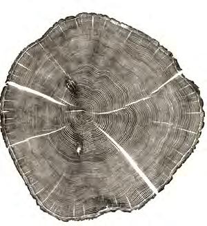
APPENDICIES
PHYSICAL EXPERIMENTS
MULTIPLE MATERIAL COMPONENTS
CHAISE LOUNGE CHAIR
FINITE ELEMENT ANALYSIS
JIG SHEETS
DIGITAL SIMULATIONS (FEA)
BASIC PARAMETERS
3D MATRIX DATA
COSTA SURFACE
FABRICATION METHOD 01
FABRICATION METHOD 02
ASSOCIATIVE GEOMETRICAL MODEL PYTHON CODE
APPENDICIES
154
PIC.93 WOOD-CUT PRINT OF A WILLOW TREE BY BRYAN NASH GILL, 2011
PHYSICAL EXPERIMENTS
MULTIPLE MATERIAL COMPONENTS
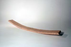
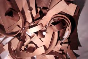
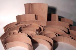
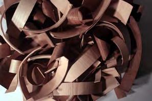
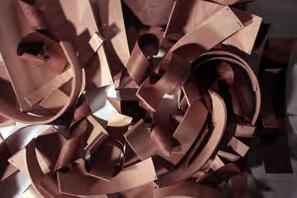
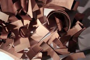
CHAISE LOUNGE CHAIR
FINITE ELEMENT ANALYSIS
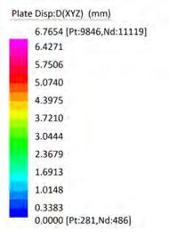
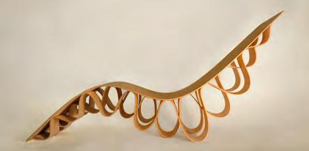
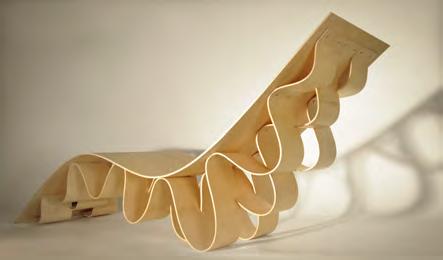
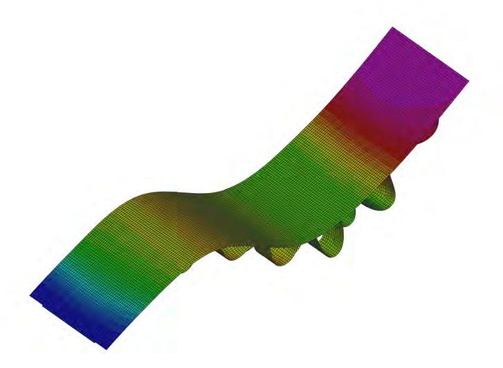
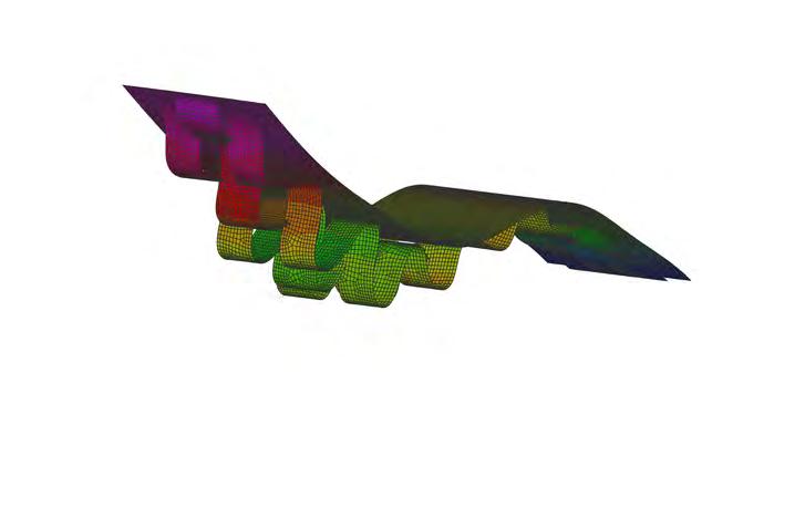

155
ARBOREAL FORMATIONS
03.B.14 03.B.04 01.A.05 03A 03B 01.B.02 01.B.01 01.B.10 01.B.12 02.B.02 03A 03B 02.B.12 03B 03A 01.B.03 03.A.07 01.A.01 01.A.04 01.B.09 03.A.12 01.A.16 02.B.05 02.B.01 01.A.14 02.B.04 01.B.07 01.B.13 01.A.10 02.A.09 01.B.09 01.A.09 03.B.02 02.A.07 01.B.09 02.A.03 02.A.10 01.B.06 02.B.03 01.A.02 03.B.05 02.A.11 02.B.08 02B 02A 01A 01B 02B 02A 01A 01B 02B 02A 01A 01B 01.B.11 01.A.03 03.A.06 03.A.03 03.B.11 03.B.07 03.A.10 03.A.08 02.B.09 01.A.13 03.B.15 03.B.08 03.A.14 03.A.13 03.B.10 03.A.0903.B.16 02.A.12 01.A.12 02.B.06 03.B.14 03.B.04 03A 03B 01.B.02 01.B.10 01.B.12 02.B.02 03A 03B 02.B.12 03B 03A 01.B.03 03.A.07 01.A.01 01.A.04 01.B.09 03.A.12 01.A.16 02.B.05 02.B.01 01.A.14 02.B.04 01.B.07 01.B.13 02.A.09 01.B.09 01.A.09 03.B.02 02.A.07 01.B.09 02.A.03 02.A.10 01.B.06 02.B.03 01.A.02 03.B.05 02.B.08 02B 02A 01A 01B 02B 02A 01A 01B 02B 02A 01A 01B 01.B.11 01.A.03 03.A.06 03.A.03 03.B.11 03.B.07 03.A.10 03.A.08 02.B.09 01.A.13 03.B.15 03.B.08 03.A.14 03.A.13 03.B.10 03.B.1603.A.09 02.A.12 03A 02B 01A 03B 03A 03B 01.B.14 01.B.16 03.A.04 03.B.01 01A 01B 03B 03A 03.A.15 03.B.06 01.A.08 02.B.10 04A 04B 04B 04A 02B 02A 01B 01A 01.B.05 01A 03B 03A 01B 01A 04A 04B 01B 04B 04A 03B 03A 01.A.07 02.A.04 01.A.11 01.B.04 02.A.08 01B 01A 02.A.05 02.B.11 02.B.07 01B 01A 02A 02B 03.B.09 03A 03B 03A 01.A.06 03B 04A 04B 02A 02B 02B 02A 02A 02B 02A 02B 04B 04A 01.A.15 03.B.03 03.A.05 01.A.12 02.B.06 03.B.14 03.B.04 01.A.05 03A 03B 01.B.02 01.B.01 01.B.12 02.B.02 03A 03B 03B 03A 01.B.03 03.A.07 01.A.01 01.A.04 01.B.09 03.A.12 01.A.16 02.B.05 02.B.01 02.B.04 01.B.07 01.A.10 02.A.09 01.B.09 01.A.09 03.B.02 02.A.07 01.B.09 02.A.03 02.A.10 01.B.06 02.B.03 03.B.05 02.A.11 02B 02A 01A 01B 02B 02A 01A 01B 02B 02A 01A 01B 01.B.11 01.A.03 03.A.06 03.A.03 03.B.11 03.B.07 03.A.10 03.A.08 02.B.09 01.A.13 03.B.15 03.B.08 03.A.14 03.A.13 03.B.10 03.B.1603.A.09 02.A.12 02A 01B 04B 01B 01A 04A 03A 03B 01.B.14 01.B.16 03.A.04 03.B.01 01A 01B 03B 03A 03.A.15 02.B.10 03.A.16 04A 04B 04B 04A 02B 02A 01B 01A 01.B.05 01A 03B 03A 01B 01A 04A 04B 01B 04B 04A 03B 03A 01.A.07 02.A.04 01.A.11 01.B.04 02.A.08 03.B.12 01B 01A 03.A.11 02.A.05 01.B.15 02.A.06 02.B.11 02.B.07 01.B.08 01B 01A 02A 02B 03.B.09 03A 03B 03A 01.A.06 03B 04A 04B 02A 02B 02B 02A 02A 02B 02A 02B 04B 04A 01.A.15 03.B.03 03.A.02 01.A.12 02.B.06 156
APPENDICIES
CHAISE LOUNGE CHAIR JIG SHEETS
03A 03B 01.B.12 02.B.02 03A 03B 02.B.12 03B 03A 01.B.03 03.A.07 01.A.01 02.B.05 02.B.01 01.A.14 02.B.04 01.B.07 01.B.13 01.A.10 02.A.09 03.B.02 02.A.07 02.A.10 01.B.06 02.B.03 01.A.02 03.B.05 02.A.11 02.B.08 03A 03B 01.B.14 01.B.16 03.A.04 03.B.01 01A 01B 03B 03A 03.A.15 03.B.06 01.A.08 02.B.10 03.A.16 04A 04B 04B 04A 02B 02A 01B 01A 01.B.05 01A 03B 03A 01B 01A 04A 04B 01B 04B 04A 03B 03A 01.A.07 02.A.04 01.A.11 01.B.04 02.A.08 03.B.12 01B 01A 03.A.11 02.A.05 01.B.15 02.A.06 02.B.11 02.B.07 01.B.08 01B 01A 02A 02B 03.B.09 03A 03B 03A 01.A.06 03B 04A 04B 02A 02B 02B 02A 02A 02B 02A 02B 04B 04A 01.A.15 03.B.03 03.A.05 03.A.02 01.A.12 02.B.06 157 ARBOREAL FORMATIONS
DIGITAL SIMULATIONS (FEA) BASIC PARAMETERS
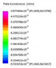
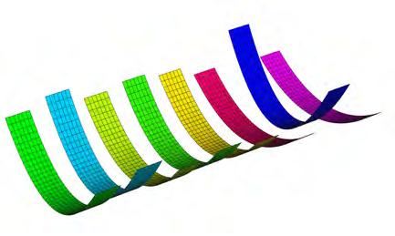
WOOD SPECIES OF VENEERS
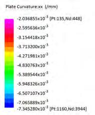

LAYER THICKNESS OF VENEERS
TYPE ASH BIRCH SPRUCE WALNUT PINE CEDAR OAK MAHOGANY TANG. EXP. (%) 7.80 9.50 7.50 7.80 7.40 5.00 10.50 4.50 EL 10890.00 11330.00 9350.00 10780.00 9020.00 7150.00 9460.00 8690.00 ET 871.20 566.50 402.05 603.68 342.76 393.25 681.12 434.50 NO.LAYERS 7.00 7.00 7.00 7.00 7.00 7.00 7.00 7.00 THICKNESS 1.4mm 1.4mm 1.4mm 1.4mm 1.4mm 1.4mm 1.4mm 1.4mm LAY_01 0.0000 0.0000 0.0000 0.0000 0.0000 0.0000 0.0000 0.0000 LAY_02 0.0130 0.0158 0.0125 0.0130 0.0123 0.0083 0.0175 0.0075 LAY_03 0.0260 0.0317 0.0250 0.0260 0.0247 0.0167 0.0350 0.0150 LAY_04 0.0390 0.0475 0.0375 0.0390 0.0370 0.0250 0.0525 0.0225 LAY_05 0.0520 0.0633 0.0500 0.0520 0.0493 0.0333 0.0700 0.0300 LAY_06 0.0650 0.0792 0.0625 0.0650 0.0617 0.0417 0.0875 0.0375 LAY_07 0.0780 0.0950 0.0750 0.0780 0.0740 0.0500 0.1050 0.0450 MAX EXPANSION 0.0780 0.0950 0.0750 0.0780 0.0740 0.0500 0.1050 0.0450 StRAND CURVATURE 7.2526 8.4348 6.3814 6.9993 6.1434 4.5622 9.5533 3.8755 RADIUS CURVATURE 137.8816 118.5558 156.7046 142.8721 162.7754 219.1927 104.6764 258.0336 EXP_01 DIFFERENT TYPES OF WOOD TYPE ASH (75X380mm)ASH (75X380mm)ASH (75X380mm)ASH (75X380mm)ASH (75X380mm) MEASURED EXP. (%) 5.50 5.50 5.50 5.50 5.50 EL 10890.00 10890.00 10890.00 10890.00 10890.00 ET 871.20 871.20 871.20 871.20 871.20 NO.LAYERS 20.00 10.00 7.00 5.00 4.00 THICKNESS 0.5mm 1.00mm 1.4mm 2.00mm 2.50mm LAY_01 0.0000 0.0000 0.0000 0.0000 0.0000 LAY_02 0.0029 0.0029 0.0029 0.0029 0.0029 LAY_03 0.0058 0.0058 0.0058 0.0058 0.0058 LAY_04 0.0087 0.0087 0.0087 0.0087 0.0087 LAY_05 0.0116 0.0116 0.0116 0.0116 0.0116 LAY_06 0.0145 0.0145 0.0145 0.0145 0.0145 LAY_07 0.0174 0.0174 0.0174 0.0174 0.0174 LAY_08 0.0203 0.0203 0.0203 0.0203 0.0203 LAY_09 0.0232 0.0232 0.0232 0.0232 0.0232 LAY_10 0.0261 0.0261 0.0261 0.0261 0.0261 LAY_11 0.0289 0.0289 0.0289 0.0289 0.0289 LAY_12 0.0318 0.0318 0.0318 0.0318 0.0318 LAY_13 0.0347 0.0347 0.0347 0.0347 0.0347 LAY_14 0.0376 0.0376 0.0376 0.0376 0.0376 LAY_15 0.0405 0.0405 0.0405 0.0405 0.0405 LAY_16 0.0434 0.0434 0.0434 0.0434 0.0434 LAY_17 0.0463 0.0463 0.0463 0.0463 0.0463 LAY_18 0.0492 0.0492 0.0492 0.0492 0.0492 LAY_19 0.0521 0.0521 0.0521 0.0521 0.0521 LAY_20 0.0550 0.0550 0.0550 0.0550 0.0550 MAX EXPANSION 0.0550 0.0550 0.0550 0.0550 0.0550 STRAND CURVATURE 7.3453 3.7908 3.3962 2.4905 2.0369 RADIUS CURVATURE 136.1418 263.7979 294.4466 401.5289 490.9530 EXP_05 DIFFERENT THICKNESS OF LAYERS OF ASH 158
APPENDICIES
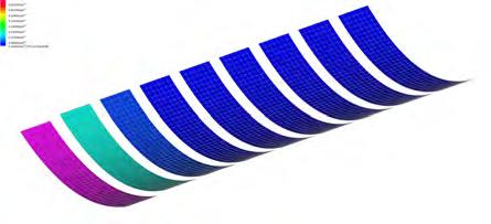
NUMBER
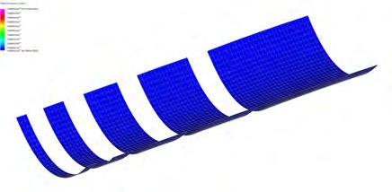
WIDTH
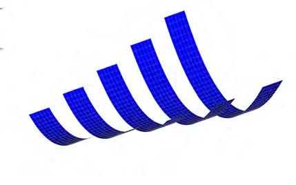
TYPE ASH (60X180mm)ASH (60X240mm)ASH (60X300mm)ASH (60x360mm)ASH (60X420mm) MEASURED EXP. (%) 5.50 5.50 5.50 5.50 5.50 EL 10890.00 10890.00 10890.00 10890.00 10890.00 ET 871.20 871.20 871.20 871.20 871.20 NO.LAYERS 5.00 5.00 5.00 5.00 5.00 THICKNESS 1.4mm 1.4mm 1.4mm 1.4mm 1.4mm LAY_01 0.0000 0.0000 0.0000 0.0000 0.0000 LAY_02 0.0138 0.0138 0.0138 0.0138 0.0138 LAY_03 0.0275 0.0275 0.0275 0.0275 0.0275 LAY_04 0.0413 0.0413 0.0413 0.0413 0.0413 LAY_05 0.0550 0.0550 0.0550 0.0550 0.0550 MAX EXPANSION 0.0550 0.0550 0.0550 0.0550 0.0550 STRAND CURVATURE 7.6605 7.6605 7.6605 7.6605 7.6605 RADIUS CURVATURE 130.5399 130.5399 130.5399 130.5399 130.5399 EXP_02 DIFFERENT LENGTHS OF ASH TYPE ASH (30X300mm)ASH (60X300mm)ASH (100X300mm)ASH (150X300mm)ASH (300X300mm) MEASURED EXP. (%) 5.50 5.50 5.50 5.50 5.50 EL 10890.00 10890.00 10890.00 10890.00 10890.00 ET 871.20 871.20 871.20 871.20 871.20 NO.LAYERS 5.00 5.00 5.00 5.00 5.00 THICKNESS 1.4mm 1.4mm 1.4mm 1.4mm 1.4mm LAY_01 0.0000 0.0000 0.0000 0.0000 0.0000 LAY_02 0.0138 0.0138 0.0138 0.0138 0.0138 LAY_03 0.0275 0.0275 0.0275 0.0275 0.0275 LAY_04 0.0413 0.0413 0.0413 0.0413 0.0413 LAY_05 0.0550 0.0550 0.0550 0.0550 0.0550 MAX EXPANSION 0.0550 0.0550 0.0550 0.0550 0.0550 STRAND CURVATURE 7.6605 7.6605 7.6605 7.6605 7.6605 RADIUS CURVATURE 130.5399 130.5399 130.5399 130.5399 130.5399 EXP_03 DIFFERENT WIDTHS OF ASH TYPE ASH (75X380mm)ASH (75X380mm)ASH (75X380mm)ASH (75X380mm)ASH (75X380mm)ASH (75X380mm)ASH (75X380mm)ASH (75X380mm)ASH (75X380mm) MEASURED EXP. (%) 5.50 5.50 5.50 5.50 5.50 5.50 5.50 5.50 5.50 EL 10890.00 10890.00 10890.00 10890.00 10890.00 10890.00 10890.00 10890.00 10890.00 ET 871.20 871.20 871.20 871.20 871.20 871.20 871.20 871.20 871.20 NO.LAYERS 2.00 3.00 4.00 5.00 6.00 7.00 8.00 9.00 10.00 THICKNESS 1.4mm 1.4mm 1.4mm 1.4mm 1.4mm 1.4mm 1.4mm 1.4mm 1.4mm LAY_01 0.0000 0.0000 0.0000 0.0000 0.0000 0.0000 0.0000 0.0000 0.0000 LAY_02 0.0061 0.0061 0.0061 0.0061 0.0061 0.0061 0.0061 0.0061 0.0061 LAY_03 0.0122 0.0122 0.0122 0.0122 0.0122 0.0122 0.0122 0.0122 LAY_04 0.0183 0.0183 0.0183 0.0183 0.0183 0.0183 0.0183 LAY_05 0.0244 0.0244 0.0244 0.0244 0.0244 0.0244 LAY_06 0.0306 0.0306 0.0306 0.0306 0.0306 LAY_07 0.0367 0.0367 0.0367 0.0367 LAY_08 0.0428 0.0428 0.0428 LAY_09 0.0489 0.0489 LAY_10 0.0550 MAX EXPANSION 0.0550 0.0550 0.0550 0.0550 0.0550 0.0550 0.0550 0.0550 0.0550 STRAND CURVATURE 2.9099 3.2875 3.3787 3.4047 3.4105 3.4093 3.4056 3.4009 3.3962 RADIUS CURVATURE 343.6577 304.1868 295.9703 293.7148 293.2084 293.3119 293.6378 294.0366 294.4466 EXP_04 DIFFERENT NO.LAYERS OF ASH 159
OF COMPONENT
LENGTH OF COMPONENT ARBOREAL FORMATIONS
OF LAYERS
DIGITAL SIMULATIONS (FEA)
NUMBER OF LAYERS (1.4 MM THICK) NUMBER OF LAYERS RADIAL CURVATURE (MM) RADIAL CURVATURE (MM) TANGENTIAL SHRINKAGE (%) 4 6 8 10 12 14 16 18 20 BIRCH TANGENTIAL SHRINKAGE (%) 0.005 1114.44 1864.51 2629.88 3403.01 4180.50 4960.55 5742.26 6525.10 7308.76 0.010 558.89 932.25 1314.91 1701.50 2090.25 2480.27 2871.13 3262.55 3654.38 0.015 372.22 621.50 876.63 1134.34 1393.50 1653.52 1914.09 2175.03 2436.25 0.020 280.29 466.13 657.45 850.75 1045.12 1240.14 1435.56 1631.28 1827.19 0.025 223.42 372.90 525.96 680.60 836.10 992.11 1148.45 1305.02 1461.75 0.030 186.11 310.75 438.30 567.17 696.75 826.76 957.04 1087.52 1218.13 0.035 159.89 266.36 375.68 486.14 597.21 708.65 820.32 932.16 1044.11 0.040 139.93 233.06 328.72 422.70 517.10 611.49 705.89 800.28 894.68 0.045 124.07 207.17 292.20 378.11 464.50 551.17 638.03 725.01 812.08 0.050 111.64 186.45 262.98 338.36 414.02 489.69 565.35 641.02 716.69 0.055 101.53 169.50 239.07 309.36 380.05 450.96 522.02 593.19 664.43 0.060 93.06 155.38 219.15 281.96 345.00 408.05 471.10 534.14 597.19 0.065 83.47 143.42 202.29 261.77 321.58 381.58 441.71 501.93 562.21 0.070 79.77 133.18 187.84 241.67 295.70 349.73 403.77 457.80 511.84 0.075 74.44 124.30 175.32 226.87 278.70 330.70 382.82 435.01 487.25 0.080 69.78 116.53 164.36 211.47 258.76 306.05 353.34 400.63 447.92 0.085 65.69 109.68 154.69 200.18 245.91 291.80 337.78 383.83 429.93 0.090 62.04 103.58 146.10 187.97 230.00 272.04 314.07 356.10 398.13 0.095 58.78 98.13 138.41 179.11 220.03 261.08 302.22 343.43 384.67 0 1000 2000 3000 4000 5000 6000 7000 8000 5 10 15 20 25 0.005 y = 387.84x 462.02 0.010 y = 193.87x 230.17 0.015 y = 129.26x 153.63 0.020 y = 96.905x 114.65 0.025 y = 77.551x 92.137 0.030 y = 64.629x 76.819 0.035 y = 55.384x 65.658 0.040 y = 47.198x 49.281 0.045 y = 43.086x 51.212 0.050 y = 37.833x 39.974 0.055 y = 35.251x 41.892 0.060 y = 31.524x 33.281 0.065 y = 29.910x 36.698 0.070 y = 27.017x 28.504 0.075 y = 25.851x 30.727 0.080 y = 23.645x 24.978 0.085 y = 22.810x 27.109 0.090 y = 21.016x 22.189 0.095 y = 20.409x 24.255 0 1000 2000 3000 4000 5000 6000 7000 8000 0.010.020.030.040.050.060.070.080.09 0.1 04 y= 36.544x-1 06 y = 32.625x-1 08 y = 28.711x-1 10 y = 24.803x-1 12 y = 20.902x-1 14 y = 17.015x-1 16 y = 13.149x-1 18 y = 9.3225x-1 20 y = 5.5553x-1 NUMBER OF LAYERS (1.4 MM THICK) NUMBER OF LAYERS RADIAL CURVATURE (MM) RADIAL CURVATURE (MM) TANGENTIAL SHRINKAGE (%) 4 6 8 10 12 14 16 18 20 BIRCH TANGENTIAL SHRINKAGE (%) 0.005 1114.44 1864.51 2629.88 3403.01 4180.50 4960.55 5742.26 6525.10 7308.76 0.010 558.89 932.25 1314.91 1701.50 2090.25 2480.27 2871.13 3262.55 3654.38 0.015 372.22 621.50 876.63 1134.34 1393.50 1653.52 1914.09 2175.03 2436.25 0.020 280.29 466.13 657.45 850.75 1045.12 1240.14 1435.56 1631.28 1827.19 0.025 223.42 372.90 525.96 680.60 836.10 992.11 1148.45 1305.02 1461.75 0.030 186.11 310.75 438.30 567.17 696.75 826.76 957.04 1087.52 1218.13 0.035 159.89 266.36 375.68 486.14 597.21 708.65 820.32 932.16 1044.11 0.040 139.93 233.06 328.72 422.70 517.10 611.49 705.89 800.28 894.68 0.045 124.07 207.17 292.20 378.11 464.50 551.17 638.03 725.01 812.08 0.050 111.64 186.45 262.98 338.36 414.02 489.69 565.35 641.02 716.69 0.055 101.53 169.50 239.07 309.36 380.05 450.96 522.02 593.19 664.43 0.060 93.06 155.38 219.15 281.96 345.00 408.05 471.10 534.14 597.19 0.065 83.47 143.42 202.29 261.77 321.58 381.58 441.71 501.93 562.21 0.070 79.77 133.18 187.84 241.67 295.70 349.73 403.77 457.80 511.84 0.075 74.44 124.30 175.32 226.87 278.70 330.70 382.82 435.01 487.25 0.080 69.78 116.53 164.36 211.47 258.76 306.05 353.34 400.63 447.92 0.085 65.69 109.68 154.69 200.18 245.91 291.80 337.78 383.83 429.93 0.090 62.04 103.58 146.10 187.97 230.00 272.04 314.07 356.10 398.13 0.095 58.78 98.13 138.41 179.11 220.03 261.08 302.22 343.43 384.67 0 1000 2000 3000 4000 5000 6000 7000 8000 5 10 15 20 25 0.005 y = 387.84x 462.02 0.010 y = 193.87x 230.17 0.015 y = 129.26x 153.63 0.020 y = 96.905x 114.65 0.025 y = 77.551x 92.137 0.030 y = 64.629x 76.819 0.035 y = 55.384x 65.658 0.040 y = 47.198x 49.281 0.045 y = 43.086x 51.212 0.050 y = 37.833x 39.974 0.055 y = 35.251x 41.892 0.060 y = 31.524x 33.281 0.065 y = 29.910x 36.698 0.070 y = 27.017x 28.504 0.075 y = 25.851x 30.727 0.080 y = 23.645x 24.978 0.085 y = 22.810x 27.109 0.090 y = 21.016x 22.189 0.095 y = 20.409x 24.255 0 1000 2000 3000 4000 5000 6000 7000 8000 0.010.020.030.040.050.060.070.080.09 0.1 04 y= 36.544x-1 06 y = 32.625x-1 08 y = 28.711x-1 10 y = 24.803x-1 12 y = 20.902x-1 14 y = 17.015x-1 16 y = 13.149x-1 18 y = 9.3225x-1 20 y = 5.5553x-1 TYPE BIRCH (60X300mm)BIRCH (60X300mm)BIRCH (60X300mm)BIRCH (60X300mm)BIRCH (60X300mm)BIRCH (60X300mm)BIRCH (60X300mm)BIRCH (60X300mm)BIRCH (60X300mm)BIRCH (60X300mm) tang exp (%) 9.50 9.50 9.50 9.50 9.50 9.50 9.50 9.50 9.50 9.50 EL 11330.00 11330.00 11330.00 11330.00 11330.00 11330.00 11330.00 11330.00 11330.00 11330.00 ET 566.50 566.50 566.50 566.50 566.50 566.50 566.50 566.50 566.50 566.50 NO.LAYERS 6.00 6.00 6.00 6.00 6.00 6.00 6.00 6.00 6.00 6.00 THICKNESS 1.4mm 1.4mm 1.4mm 1.4mm 1.4mm 1.4mm 1.4mm 1.4mm 1.4mm 1.4mm LAY_01 0.0000 0.0000 0.0000 0.0000 0.0000 0.0000 0.0000 0.0000 0.0000 0.0000 LAY_02 0.0010 0.0020 0.0030 0.0040 0.0050 0.0060 0.0070 0.0080 0.0090 0.0100 LAY_03 0.0020 0.0040 0.0060 0.0080 0.0100 0.0120 0.0140 0.0160 0.0180 0.0200 LAY_04 0.0030 0.0060 0.0090 0.0120 0.0150 0.0180 0.0210 0.0240 0.0270 0.0300 LAY_05 0.0040 0.0080 0.0120 0.0160 0.0200 0.0240 0.0280 0.0320 0.0360 0.0400 LAY_06 0.0050 0.0100 0.0150 0.0200 0.0250 0.0300 0.0350 0.0400 0.0450 0.0500 MAX EXPANSION 0.0050 0.0100 0.0150 0.0200 0.0250 0.0300 0.0350 0.0400 0.0450 0.0500 STRAND CURVATURE 0.5363 1.0727 1.6090 2.1453 2.6817 3.2180 3.7543 4.2907 4.8270 5.3634 RADIUS CURVATURE 1864.5056 932.2532 621.5017 466.1264 372.9011 310.7510 266.3579 233.0632 207.1673 186.4506 EXP_07 DIFFERENT EXP.FACTOR OF 6 LAYERS OF BI TYPE BIRCH (60X300mm)BIRCH (60X300mm)BIRCH (60X300mm)BIRCH (60X300mm)BIRCH (60X300mm)BIRCH (60X300mm)BIRCH (60X300mm)BIRCH (60X300mm)BIRCH (60X300mm)BIRCH (60X300mm) tang exp (%) 9.50 9.50 9.50 9.50 9.50 9.50 9.50 9.50 9.50 9.50 EL 11330.00 11330.00 11330.00 11330.00 11330.00 11330.00 11330.00 11330.00 11330.00 11330.00 ET 566.50 566.50 566.50 566.50 566.50 566.50 566.50 566.50 566.50 566.50 NO.LAYERS 4.00 4.00 4.00 4.00 4.00 4.00 4.00 4.00 4.00 4.00 THICKNESS 1.4mm 1.4mm 1.4mm 1.4mm 1.4mm 1.4mm 1.4mm 1.4mm 1.4mm 1.4mm LAY_01 0.0000 0.0000 0.0000 0.0000 0.0000 0.0000 0.0000 0.0000 0.0000 0.0000 LAY_02 0.0017 0.0033 0.0050 0.0067 0.0083 0.0100 0.0117 0.0133 0.0150 0.0167 LAY_03 0.0033 0.0067 0.0100 0.0133 0.0167 0.0200 0.0233 0.0267 0.0300 0.0333 LAY_04 0.0050 0.0100 0.0150 0.0200 0.0250 0.0300 0.0350 0.0400 0.0450 0.0500 MAX EXPANSION 0.0050 0.0100 0.0150 0.0200 0.0250 0.0300 0.0350 0.0400 0.0450 0.0500 STRAND CURVATURE 0.8973 1.7893 2.6866 3.5678 4.4758 5.3731 6.2543 7.1463 8.0597 8.9570 RADIUS CURVATURE 1114.4396 558.8931 372.2228 280.2882 223.4230 186.1114 159.8895 139.9334 124.0743 111.6445 EXP_06 DIFFERENT EXP.FACTOR OF 4 LAYERS OF BI 160
3D
APPENDICIES
MATRIX DATA
TYPE BIRCH (60X300mm)BIRCH (60X300mm)BIRCH (60X300mm)BIRCH (60X300mm)BIRCH (60X300mm)BIRCH (60X300mm)BIRCH (60X300mm)BIRCH (60X300mm)BIRCH (60X300mm)BIRCH (60X300mm) tang exp (%) 9.50 9.50 9.50 9.50 9.50 9.50 9.50 9.50 9.50 9.50 EL 11330.00 11330.00 11330.00 11330.00 11330.00 11330.00 11330.00 11330.00 11330.00 11330.00 ET 566.50 566.50 566.50 566.50 566.50 566.50 566.50 566.50 566.50 566.50 NO.LAYERS 12.00 12.00 12.00 12.00 12.00 12.00 12.00 12.00 12.00 12.00 THICKNESS 1.4mm 1.4mm 1.4mm 1.4mm 1.4mm 1.4mm 1.4mm 1.4mm 1.4mm 1.4mm LAY_01 0.0000 0.0000 0.0000 0.0000 0.0000 0.0000 0.0000 0.0000 0.0000 0.0000 LAY_02 0.0005 0.0009 0.0014 0.0018 0.0023 0.0027 0.0032 0.0041 0.0050 0.0059 LAY_03 0.0009 0.0018 0.0027 0.0036 0.0045 0.0055 0.0064 0.0082 0.0100 0.0118 LAY_04 0.0014 0.0027 0.0041 0.0055 0.0068 0.0082 0.0095 0.0123 0.0150 0.0177 LAY_05 0.0018 0.0036 0.0055 0.0073 0.0091 0.0109 0.0127 0.0164 0.0200 0.0236 LAY_06 0.0023 0.0045 0.0068 0.0091 0.0114 0.0136 0.0159 0.0205 0.0250 0.0295 LAY_07 0.0027 0.0055 0.0082 0.0109 0.0136 0.0164 0.0191 0.0245 0.0300 0.0355 LAY_08 0.0032 0.0064 0.0095 0.0127 0.0159 0.0191 0.0223 0.0286 0.0350 0.0414 LAY_09 0.0036 0.0073 0.0109 0.0145 0.0182 0.0218 0.0255 0.0327 0.0400 0.0473 LAY_10 0.0041 0.0082 0.0123 0.0164 0.0205 0.0245 0.0286 0.0368 0.0450 0.0532 LAY_11 0.0045 0.0091 0.0136 0.0182 0.0227 0.0273 0.0318 0.0409 0.0500 0.0591 LAY_12 0.0050 0.0100 0.0150 0.0200 0.0250 0.0300 0.0350 0.0450 0.0550 0.0650 MAX EXPANSION 0.0050 0.0100 0.0150 0.0200 0.0250 0.0300 0.0350 0.0450 0.0550 0.0650 STRAND CURVATURE 0.2392 0.4784 0.7176 0.9568 1.1960 1.4352 1.6744 2.1529 2.6313 3.1097 RADIUS CURVATURE 4180.4989 2090.2494 1393.4994 1045.1246 836.0994 696.7495 597.2142 464.4999 380.0453 321.5768 EXP_10 DIFFERENT EXP.FACTOR OF 12 LAYERS OF BIRCH TYPE BIRCH (60X300mm)BIRCH (60X300mm)BIRCH (60X300mm)BIRCH (60X300mm)BIRCH (60X300mm)BIRCH (60X300mm)BIRCH (60X300mm)BIRCH (60X300mm)BIRCH (60X300mm)BIRCH (60X300mm) tang exp (%) 9.50 9.50 9.50 9.50 9.50 9.50 9.50 9.50 9.50 9.50 EL 11330.00 11330.00 11330.00 11330.00 11330.00 11330.00 11330.00 11330.00 11330.00 11330.00 ET 566.50 566.50 566.50 566.50 566.50 566.50 566.50 566.50 566.50 566.50 NO.LAYERS 10.00 10.00 10.00 10.00 10.00 10.00 10.00 10.00 10.00 10.00 THICKNESS 1.4mm 1.4mm 1.4mm 1.4mm 1.4mm 1.4mm 1.4mm 1.4mm 1.4mm 1.4mm LAY_01 0.0000 0.0000 0.0000 0.0000 0.0000 0.0000 0.0000 0.0000 0.0000 0.0000 LAY_02 0.0006 0.0011 0.0017 0.0022 0.0028 0.0033 0.0039 0.0050 0.0061 0.0072 LAY_03 0.0011 0.0022 0.0033 0.0044 0.0056 0.0067 0.0078 0.0100 0.0122 0.0144 LAY_04 0.0017 0.0033 0.0050 0.0067 0.0083 0.0100 0.0117 0.0150 0.0183 0.0217 LAY_05 0.0022 0.0044 0.0067 0.0089 0.0111 0.0133 0.0156 0.0200 0.0244 0.0289 LAY_06 0.0028 0.0056 0.0083 0.0111 0.0139 0.0167 0.0194 0.0250 0.0306 0.0361 LAY_07 0.0033 0.0067 0.0100 0.0133 0.0167 0.0200 0.0233 0.0300 0.0367 0.0433 LAY_08 0.0039 0.0078 0.0117 0.0156 0.0194 0.0233 0.0272 0.0350 0.0428 0.0506 LAY_09 0.0044 0.0089 0.0133 0.0178 0.0222 0.0267 0.0311 0.0400 0.0489 0.0578 LAY_10 0.0050 0.0100 0.0150 0.0200 0.0250 0.0300 0.0350 0.0450 0.0550 0.0650 MAX EXPANSION 0.0050 0.0100 0.0150 0.0200 0.0250 0.0300 0.0350 0.0450 0.0550 0.0650 STRAND CURVATURE 0.2939 0.5877 0.8816 1.1754 1.4693 1.7631 2.0570 2.6447 3.2324 3.8201 RADIUS CURVATURE 3403.0100 1701.5050 1134.3368 850.7525 680.6022 567.1683 486.1444 378.1123 309.3646 261.7700 EXP_9 DIFFERENT EXP.FACTOR OF 10 LAYERS OF BIRCH TYPE BIRCH (60X300mm)BIRCH (60X300mm)BIRCH (60X300mm)BIRCH (60X300mm)BIRCH (60X300mm)BIRCH (60X300mm)BIRCH (60X300mm)BIRCH (60X300mm)BIRCH (60X300mm)BIRCH (60X300mm) tang exp (%) 9.50 9.50 9.50 9.50 9.50 9.50 9.50 9.50 9.50 9.50 EL 11330.00 11330.00 11330.00 11330.00 11330.00 11330.00 11330.00 11330.00 11330.00 11330.00 ET 566.50 566.50 566.50 566.50 566.50 566.50 566.50 566.50 566.50 566.50 NO.LAYERS 8.00 8.00 8.00 8.00 8.00 8.00 8.00 8.00 8.00 8.00 THICKNESS 1.4mm 1.4mm 1.4mm 1.4mm 1.4mm 1.4mm 1.4mm 1.4mm 1.4mm 1.4mm LAY_01 0.0000 0.0000 0.0000 0.0000 0.0000 0.0000 0.0000 0.0000 0.0000 0.0000 LAY_02 0.0007 0.0014 0.0021 0.0029 0.0036 0.0043 0.0050 0.0057 0.0064 0.0071 LAY_03 0.0014 0.0029 0.0043 0.0057 0.0071 0.0086 0.0100 0.0114 0.0129 0.0143 LAY_04 0.0021 0.0043 0.0064 0.0086 0.0107 0.0129 0.0150 0.0171 0.0193 0.0214 LAY_05 0.0029 0.0057 0.0086 0.0114 0.0143 0.0171 0.0200 0.0229 0.0257 0.0286 LAY_06 0.0036 0.0071 0.0107 0.0143 0.0179 0.0214 0.0250 0.0286 0.0321 0.0357 LAY_07 0.0043 0.0086 0.0129 0.0171 0.0214 0.0257 0.0300 0.0343 0.0386 0.0429 LAY_08 0.0050 0.0100 0.0150 0.0200 0.0250 0.0300 0.0350 0.0400 0.0450 0.0500 MAX EXPANSION 0.0050 0.0100 0.0150 0.0200 0.0250 0.0300 0.0350 0.0400 0.0450 0.0500 STRAND CURVATURE 0.3802 0.7605 1.1407 1.5210 1.9013 2.2816 2.6618 3.0421 3.4223 3.8026 RADIUS CURVATURE 2629.8834 1314.9071 876.6316 657.4510 525.9568 438.2976 375.6846 328.7247 292.1997 262.9771 EXP_08 DIFFERENT EXP.FACTOR OF 8 LAYERS OF BI 161 ARBOREAL FORMATIONS
TYPE BIRCH (60X300mm)BIRCH (60X300mm)BIRCH (60X300mm)BIRCH (60X300mm)BIRCH (60X300mm)BIRCH (60X300mm)BIRCH (60X300mm)BIRCH (60X300mm)BIRCH (60X300mm)BIRCH (60X300mm) tang exp (%) 9.50 9.50 9.50 9.50 9.50 9.50 9.50 9.50 9.50 9.50 ET 566.50 566.50 566.50 566.50 566.50 566.50 566.50 566.50 566.50 566.50 NO.LAYERS 16.00 16.00 16.00 16.00 16.00 16.00 16.00 16.00 16.00 16.00 THICKNESS 1.4mm 1.4mm 1.4mm 1.4mm 1.4mm 1.4mm 1.4mm 1.4mm 1.4mm 1.4mm LAY_01 0.0000 0.0000 0.0000 0.0000 0.0000 0.0000 0.0000 0.0000 0.0000 0.0000 LAY_02 0.0003 0.0007 0.0010 0.0013 0.0017 0.0020 0.0023 0.0030 0.0037 0.0043 LAY_03 0.0007 0.0013 0.0020 0.0027 0.0033 0.0040 0.0047 0.0060 0.0073 0.0087 LAY_04 0.0010 0.0020 0.0030 0.0040 0.0050 0.0060 0.0070 0.0090 0.0110 0.0130 LAY_05 0.0013 0.0027 0.0040 0.0053 0.0067 0.0080 0.0093 0.0120 0.0147 0.0173 LAY_06 0.0017 0.0033 0.0050 0.0067 0.0083 0.0100 0.0117 0.0150 0.0183 0.0217 LAY_07 0.0020 0.0040 0.0060 0.0080 0.0100 0.0120 0.0140 0.0180 0.0220 0.0260 LAY_08 0.0023 0.0047 0.0070 0.0093 0.0117 0.0140 0.0163 0.0210 0.0257 0.0303 LAY_09 0.0027 0.0053 0.0080 0.0107 0.0133 0.0160 0.0187 0.0240 0.0293 0.0347 LAY_10 0.0030 0.0060 0.0090 0.0120 0.0150 0.0180 0.0210 0.0270 0.0330 0.0390 LAY_11 0.0033 0.0067 0.0100 0.0133 0.0167 0.0200 0.0233 0.0300 0.0367 0.0433 LAY_12 0.0037 0.0073 0.0110 0.0147 0.0183 0.0220 0.0257 0.0330 0.0403 0.0477 LAY_13 0.0040 0.0080 0.0120 0.0160 0.0200 0.0240 0.0280 0.0360 0.0440 0.0520 LAY_14 0.0043 0.0087 0.0130 0.0173 0.0217 0.0260 0.0303 0.0390 0.0477 0.0563 LAY_15 0.0047 0.0093 0.0140 0.0187 0.0233 0.0280 0.0327 0.0420 0.0513 0.0607 LAY_16 0.0050 0.0100 0.0150 0.0200 0.0250 0.0300 0.0350 0.0450 0.0550 0.0650 MAX EXPANSION 0.0050 0.0100 0.0150 0.0200 0.0250 0.0300 0.0350 0.0450 0.0550 0.0650 STRAND CURVATURE 0.1741 0.3483 0.5224 0.6966 0.8707 1.0449 1.2190 1.5673 1.9156 2.2639 RADIUS CURVATURE 5742.2587 2871.1285 1914.0859 1435.5645 1148.4515 957.0431 820.3223 638.0285 522.0234 441.7121 EXP_12 DIFFERENT EXP.FACTOR OF 16 LAYERS OF BIRCH TYPE BIRCH (60X300mm)BIRCH (60X300mm)BIRCH (60X300mm)BIRCH (60X300mm)BIRCH (60X300mm)BIRCH (60X300mm)BIRCH (60X300mm)BIRCH (60X300mm)BIRCH (60X300mm)BIRCH (60X300mm) tang exp (%) 9.50 9.50 9.50 9.50 9.50 9.50 9.50 9.50 9.50 9.50 EL 11330.00 11330.00 11330.00 11330.00 11330.00 11330.00 11330.00 11330.00 11330.00 11330.00 ET 566.50 566.50 566.50 566.50 566.50 566.50 566.50 566.50 566.50 566.50 NO.LAYERS 14.00 14.00 14.00 14.00 14.00 14.00 14.00 14.00 14.00 14.00 THICKNESS 1.4mm 1.4mm 1.4mm 1.4mm 1.4mm 1.4mm 1.4mm 1.4mm 1.4mm 1.4mm LAY_01 0.0000 0.0000 0.0000 0.0000 0.0000 0.0000 0.0000 0.0000 0.0000 0.0000 LAY_02 0.0004 0.0008 0.0012 0.0015 0.0019 0.0023 0.0027 0.0035 0.0042 0.0050 LAY_03 0.0008 0.0015 0.0023 0.0031 0.0038 0.0046 0.0054 0.0069 0.0085 0.0100 LAY_04 0.0012 0.0023 0.0035 0.0046 0.0058 0.0069 0.0081 0.0104 0.0127 0.0150 LAY_05 0.0015 0.0031 0.0046 0.0062 0.0077 0.0092 0.0108 0.0138 0.0169 0.0200 LAY_06 0.0019 0.0038 0.0058 0.0077 0.0096 0.0115 0.0135 0.0173 0.0212 0.0250 LAY_07 0.0023 0.0046 0.0069 0.0092 0.0115 0.0138 0.0162 0.0208 0.0254 0.0300 LAY_08 0.0027 0.0054 0.0081 0.0108 0.0135 0.0162 0.0188 0.0242 0.0296 0.0350 LAY_09 0.0031 0.0062 0.0092 0.0123 0.0154 0.0185 0.0215 0.0277 0.0338 0.0400 LAY_10 0.0035 0.0069 0.0104 0.0138 0.0173 0.0208 0.0242 0.0312 0.0381 0.0450 LAY_11 0.0038 0.0077 0.0115 0.0154 0.0192 0.0231 0.0269 0.0346 0.0423 0.0500 LAY_12 0.0042 0.0085 0.0127 0.0169 0.0212 0.0254 0.0296 0.0381 0.0465 0.0550 LAY_13 0.0046 0.0092 0.0138 0.0185 0.0231 0.0277 0.0323 0.0415 0.0508 0.0600 LAY_14 0.0050 0.0100 0.0150 0.0200 0.0250 0.0300 0.0350 0.0450 0.0550 0.0650 MAX EXPANSION 0.0050 0.0100 0.0150 0.0200 0.0250 0.0300 0.0350 0.0450 0.0550 0.0650 STRAND CURVATURE 0.2016 0.4032 0.6048 0.8064 1.0080 1.2095 1.4111 1.8143 2.2175 2.6207 RADIUS CURVATURE 4960.5488 2480.2744 1653.5163 1240.1373 992.1098 826.7579 708.6499 551.1722 450.9591 381.5806 EXP_11 DIFFERENT EXP.FACTOR OF 14 LAYERS OF BIRCH 162 APPENDICIES
TYPE BIRCH (60X300mm)BIRCH (60X300mm)BIRCH (60X300mm)BIRCH (60X300mm)BIRCH (60X300mm)BIRCH (60X300mm)BIRCH (60X300mm)BIRCH (60X300mm)BIRCH (60X300mm)BIRCH (60X300mm) tang exp (%) 9.50 9.50 9.50 9.50 9.50 9.50 9.50 9.50 9.50 9.50 EL 11330.00 11330.00 11330.00 11330.00 11330.00 11330.00 11330.00 11330.00 11330.00 11330.00 ET 566.50 566.50 566.50 566.50 566.50 566.50 566.50 566.50 566.50 566.50 NO.LAYERS 18.00 18.00 18.00 18.00 18.00 18.00 18.00 18.00 18.00 18.00 THICKNESS 1.4mm 1.4mm 1.4mm 1.4mm 1.4mm 1.4mm 1.4mm 1.4mm 1.4mm 1.4mm LAY_01 0.0000 0.0000 0.0000 0.0000 0.0000 0.0000 0.0000 0.0000 0.0000 0.0000 LAY_02 0.0003 0.0006 0.0009 0.0012 0.0015 0.0018 0.0021 0.0026 0.0032 0.0038 LAY_03 0.0006 0.0012 0.0018 0.0024 0.0029 0.0035 0.0041 0.0053 0.0065 0.0076 LAY_04 0.0009 0.0018 0.0026 0.0035 0.0044 0.0053 0.0062 0.0079 0.0097 0.0115 LAY_05 0.0012 0.0024 0.0035 0.0047 0.0059 0.0071 0.0082 0.0106 0.0129 0.0153 LAY_06 0.0015 0.0029 0.0044 0.0059 0.0074 0.0088 0.0103 0.0132 0.0162 0.0191 LAY_07 0.0018 0.0035 0.0053 0.0071 0.0088 0.0106 0.0124 0.0159 0.0194 0.0229 LAY_08 0.0021 0.0041 0.0062 0.0082 0.0103 0.0124 0.0144 0.0185 0.0226 0.0268 LAY_09 0.0024 0.0047 0.0071 0.0094 0.0118 0.0141 0.0165 0.0212 0.0259 0.0306 LAY_10 0.0026 0.0053 0.0079 0.0106 0.0132 0.0159 0.0185 0.0238 0.0291 0.0344 LAY_11 0.0029 0.0059 0.0088 0.0118 0.0147 0.0176 0.0206 0.0265 0.0324 0.0382 LAY_12 0.0032 0.0065 0.0097 0.0129 0.0162 0.0194 0.0226 0.0291 0.0356 0.0421 LAY_13 0.0035 0.0071 0.0106 0.0141 0.0176 0.0212 0.0247 0.0318 0.0388 0.0459 LAY_14 0.0038 0.0076 0.0115 0.0153 0.0191 0.0229 0.0268 0.0344 0.0421 0.0497 LAY_15 0.0041 0.0082 0.0124 0.0165 0.0206 0.0247 0.0288 0.0371 0.0453 0.0535 LAY_16 0.0044 0.0088 0.0132 0.0176 0.0221 0.0265 0.0309 0.0397 0.0485 0.0574 LAY_17 0.0047 0.0094 0.0141 0.0188 0.0235 0.0282 0.0329 0.0424 0.0518 0.0612 LAY_18 0.0050 0.0100 0.0150 0.0200 0.0250 0.0300 0.0350 0.0450 0.0550 0.0650 MAX EXPANSION 0.0050 0.0100 0.0150 0.0200 0.0250 0.0300 0.0350 0.0450 0.0550 0.0650 STRAND CURVATURE 0.1533 0.3065 0.4598 0.6130 0.7663 0.9195 1.0728 1.3793 1.6858 1.9923 RADIUS CURVATURE 6525.1024 3262.5501 2175.0337 1631.2751 1305.0201 1087.5167 932.1576 725.0112 593.1909 501.9307 EXP_13 DIFFERENT EXP.FACTOR OF 18 LAYERS OF BIRCH TYPE BIRCH (60X300mm)BIRCH (60X300mm)BIRCH (60X300mm)BIRCH (60X300mm)BIRCH (60X300mm)BIRCH (60X300mm)BIRCH (60X300mm)BIRCH (60X300mm)BIRCH (60X300mm)BIRCH (60X300mm) tang exp (%) 9.50 9.50 9.50 9.50 9.50 9.50 9.50 9.50 9.50 9.50 EL 11330.00 11330.00 11330.00 11330.00 11330.00 11330.00 11330.00 11330.00 11330.00 11330.00 ET 566.50 566.50 566.50 566.50 566.50 566.50 566.50 566.50 566.50 566.50 NO.LAYERS 20.00 20.00 20.00 20.00 20.00 20.00 20.00 20.00 20.00 20.00 THICKNESS 1.4mm 1.4mm 1.4mm 1.4mm 1.4mm 1.4mm 1.4mm 1.4mm 1.4mm 1.4mm LAY_01 0.0000 0.0000 0.0000 0.0000 0.0000 0.0000 0.0000 0.0000 0.0000 0.0000 LAY_02 0.0003 0.0005 0.0008 0.0011 0.0013 0.0016 0.0018 0.0024 0.0029 0.0034 LAY_03 0.0005 0.0011 0.0016 0.0021 0.0026 0.0032 0.0037 0.0047 0.0058 0.0068 LAY_04 0.0008 0.0016 0.0024 0.0032 0.0039 0.0047 0.0055 0.0071 0.0087 0.0103 LAY_05 0.0011 0.0021 0.0032 0.0042 0.0053 0.0063 0.0074 0.0095 0.0116 0.0137 LAY_06 0.0013 0.0026 0.0039 0.0053 0.0066 0.0079 0.0092 0.0118 0.0145 0.0171 LAY_07 0.0016 0.0032 0.0047 0.0063 0.0079 0.0095 0.0111 0.0142 0.0174 0.0205 LAY_08 0.0018 0.0037 0.0055 0.0074 0.0092 0.0111 0.0129 0.0166 0.0203 0.0239 LAY_09 0.0021 0.0042 0.0063 0.0084 0.0105 0.0126 0.0147 0.0189 0.0232 0.0274 LAY_10 0.0024 0.0047 0.0071 0.0095 0.0118 0.0142 0.0166 0.0213 0.0261 0.0308 LAY_11 0.0026 0.0053 0.0079 0.0105 0.0132 0.0158 0.0184 0.0237 0.0289 0.0342 LAY_12 0.0029 0.0058 0.0087 0.0116 0.0145 0.0174 0.0203 0.0261 0.0318 0.0376 LAY_13 0.0032 0.0063 0.0095 0.0126 0.0158 0.0189 0.0221 0.0284 0.0347 0.0411 LAY_14 0.0034 0.0068 0.0103 0.0137 0.0171 0.0205 0.0239 0.0308 0.0376 0.0445 LAY_15 0.0037 0.0074 0.0111 0.0147 0.0184 0.0221 0.0258 0.0332 0.0405 0.0479 LAY_16 0.0039 0.0079 0.0118 0.0158 0.0197 0.0237 0.0276 0.0355 0.0434 0.0513 LAY_17 0.0042 0.0084 0.0126 0.0168 0.0211 0.0253 0.0295 0.0379 0.0463 0.0547 LAY_18 0.0045 0.0089 0.0134 0.0179 0.0224 0.0268 0.0313 0.0403 0.0492 0.0582 LAY_19 0.0047 0.0095 0.0142 0.0189 0.0237 0.0284 0.0332 0.0426 0.0521 0.0616 LAY_20 0.0050 0.0100 0.0150 0.0200 0.0250 0.0300 0.0350 0.0450 0.0550 0.0650 MAX EXPANSION 0.0050 0.0100 0.0150 0.0200 0.0250 0.0300 0.0350 0.0450 0.0550 0.0650 STRAND CURVATURE 0.1368 0.2736 0.4105 0.5473 0.6841 0.8209 0.9578 1.2314 1.5050 1.7787 RADIUS CURVATURE 7308.7555 3654.3764 2436.2512 1827.1882 1461.7507 1218.1256 1044.1076 812.0838 664.4320 562.2118 EXP_14 DIFFERENT EXP.FACTOR OF 20 LAYERS OF BIRCH 163 ARBOREAL FORMATIONS
COSTA SURFACE FABRICATION METHOD 01 FABRICATION METHOD 02
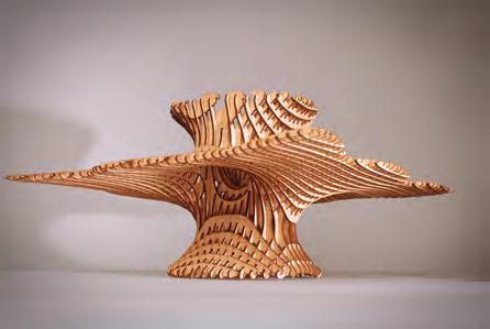
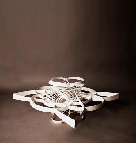
164
APPENDICIES
165 ARBOREAL FORMATIONS
ASSOCIATIVE GEOMETRICAL MODEL PYTHON CODE

166 import math import rhinoscriptsyntax as rs import sys import scriptcontext import Rhino import System
#creates defining node arcs def arc(arclen,topt,rot,check,curvature,centpt,rotG,arclen2): arclenLt=[arclen,arclen2]
UVC.Rotation=rotG arcs=[]
UVC.state=check for in range(2):
if check ==1:
angle=(360-(360*(curvature*2)))+1 rad=(arclenLt[i]/(angle/360))/(2*math.pi)
elif check ==0:
# Figure out how ‘wide’ each range is if curvature==0.5: curvature=0.501 initialrange = 1 - 0.5 angle=((360-(360*((1-curvature)*2)))/2) radmin=(arclenLt[i]/(angle/360))/(2*math.pi)
mappedrange = (arclenLt[i]/2) - radmin
# Convert the left range into a 0-1 range (float) valueScaled = float(curvature - 0.5) / float(initialrange) # Convert the 0-1 range into a value in the right range. rad= (radmin + (valueScaled * mappedrange)) d=arclenLt[i]/rad angle=(d*360)/(2*math.pi)
arc=rs.AddArc(centpt,rad,angle)
arc=rs.RotateObject(arc,centpt,((-angle/2)+rot/2)+rotG) arcmidPt=rs.DivideCurve(arc,2) vectmove=rs.VectorCreate(topt,arcmidPt[1]) rs.MoveObject(arc,vectmove) if i==0: arcs.append(arc)
vect=rs.VectorCreate(topt,centpt) vectrot=rs.VectorRotate(vect,90,(0,0,1)) if i==1: arc1=rs.MirrorObject(arc,centpt,vectrot,True) arcs.append(arc1)
UVC.tmpLt2.append(arcs) UVC.Arcs=arcs
return arcs
#subdivides node arcs and creates UV curves def arcU(arcs,arclen,check): pts=[] crvsU=[] div=arclen/1
arcCent1=rs.ArcCenterPoint(arcs[0]) arcCent2=rs.ArcCenterPoint(arcs[1]) vectCheck=rs.VectorCreate(arcCent1,arcCent2) lineCent=rs.AddLine(arcCent1,arcCent2) lineMid=rs.CurveMidPoint(lineCent) if check ==1:
arcCentPt=[] arcRad=[] for in arcs:
arcRad.append(rs.ArcRadius(i)) pts.append(rs.DivideCurve(i,div)) arcCentPt.append(rs.ArcCenterPoint(i))
arcMidLt=[] meanCrvc=[] tmpLt=[] tangLt1=[] tangLt2=[] arcAddLt=[] para1=[] para2=[] for in range (len(pts[0])): tang=rs.PlaneFromPoints(pts[0][i],arcCentPt[0],((pts[0][i][0]),(pts[0][i] [1]),((pts[0][i][2])+1))) tangLt1.append(tang) UVC.tmpLt2.append(tang)
tang2=rs.PlaneFromPoints(pts[1][i],arcCentPt[1],((pts[1][i][0]),(pts[1][i] [1]),((pts[1][i][2])+1))) tangLt2.append(tang2) vectang=rs.VectorAngle(vectCheck,tang[1])
if vectang>-0.00001 and vectang<0.00001:
arcNe=rs.AddLine(pts[0][i],pts[1][i]) arcMid=rs.CurveMidPoint(arcNe) arcMidLt.append(arcMid) tmpLt.append(arcNe) crvsU.append(arcNe)
else:
arcNe=rs.AddArcPtTanPt(pts[0][i],-tang[1],pts[1][i]) arcMid=rs.ArcMidPoint(arcNe) arcMidLt.append(arcMid) tmpLt.append(arcNe) crvsU.append(arcNe)
LtlenCh=len(pts[0]) if i>0:
arcL=rs.AddArcPtTanPt(pts[0][i-1],tangLt1[i-1][3],pts[0][i]) arcR=rs.AddArcPtTanPt(pts[1][i-1],-tangLt2[i-1][3],pts[1][i])
lineM=rs.AddLine(arcMidLt[i-1],arcMid) dist=rs.Distance(arcMid,arcMidLt[i-1]) noWall=int(dist/1)
arcLdiv=rs.DivideCurve(arcL,noWall) arcLdiv.pop() arcRdiv=rs.DivideCurve(arcR,noWall) arcRdiv.pop() arcMdiv=rs.DivideCurve(lineM,noWall) arcMdiv.pop() ltlen=len(arcLdiv)
for j in range(1,ltlen): vectN=rs.VectorCreate(arcLdiv[j],arcMdiv[j]) vectang=rs.VectorAngle(vectCheck,vectN) if vectang>-0.00001 and vectang<0.00001: stwall=rs.AddLine(arcLdiv[j],arcRdiv[j]) UVC.straightwall=stwall continue
else:
arcInt=rs.AddArc3Pt(arcLdiv[j],arcRdiv[j],arcMdiv[j]) crvsU.append(arcInt)
elif check == 0: arcCentPt=[] for in arcs: pts.append(rs.DivideCurve(i,div)) arcCentPt.append(rs.ArcCenterPoint(i)) for in range (len(pts[0])): tang=rs.PlaneFromPoints(pts[0][i],arcCentPt[0],((pts[0][i][0]),(pts[0][i] [1]),((pts[0][i][2])+1))) vectN=tang[1] vectang=rs.VectorAngle(vectCheck,vectN) if (vectang>179.99 and vectang<180.01) or (vectang>-0.01 and vectang<0.01): stwall=rs.AddLine(pts[0][i],pts[1][i]) UVC.straightwall=stwall else:
crvsU.append(rs.AddArcPtTanPt(pts[0][i],tang[1],pts[1][i]))
midlist=int(len(crvsU)/2) cnt=-1 crvsU1=[] crvsU2=[]
for i in crvsU: cnt=cnt+1 if cnt<midlist: crvsU1.append(i)
else: crvsU2.append(i) distLt=[] for j in crvsU1: testpt=rs.CurveMidPoint(j)
dist=rs.Distance(testpt,lineMid) distLt.append(dist)
distLt,crvsU1 = zip(*sorted(zip(distLt,crvsU1)))
distLt1=[] for j in crvsU2: testpt=rs.CurveMidPoint(j) dist=rs.Distance(testpt,lineMid) distLt1.append(dist)
distLt,crvsU2 = zip(*sorted(zip(distLt1,crvsU2)))
crvsU=[]
crvsU.append(crvsU1) crvsU.append(crvsU2) UVC.Ucurves=crvsU
return crvsU
def arcV(arcU,arcs,rot,check,rotG):
distofwalls=1.5 arcCentLt=[] for i in arcs: arcCent=rs.ArcMidPoint(i) arcCentLt.append(arcCent) cnt=0 crvs=[] arcsV=[] tmpArcLt=[] for j in arcs: # if curvature is less than 0.5 if check ==1: cnt=cnt+1 crvsV=[] arcsRad=rs.ArcRadius(j) arcMid=rs.ArcMidPoint(j) dist=rs.Distance(arcMid,centpt) noWalls=math.floor(dist/distofwalls) vect=rs.VectorCreate(centpt,arcMid) vect=rs.VectorUnitize(vect) for k in range (1,(int(noWalls)+2)): if k==1: nradius=arcsRad else: nradius=(arcsRad*((k)**1.2)) circ=rs.AddCircle(arcMid,nradius) if cnt ==1 and rot ==0: circ=rs.RotateObject(circ,arcMid,180+rotG) elif cnt==2 and rot ==0: circ=rs.RotateObject(circ,arcMid,0+rotG) elif cnt==1 and rot ==-90: circ=rs.RotateObject(circ,arcMid,90+rotG) elif cnt==2 and rot ==-90: circ=rs.RotateObject(circ,arcMid,-90+rotG) raddiv=rs.DivideCurve(circ,4) vectM=rs.VectorCreate(arcMid,raddiv[2]) circ=rs.MoveObject(circ,vectM) scaleWall=distofwalls*(k-1) vectSc=rs.VectorScale(vect,scaleWall) circ=rs.MoveObject(circ,vectSc) crvsV.append(circ) # if curvature is more than 0.5 elif check ==0: crvsV=[] crvsV1=[] cnt=cnt+1 arcsRad=rs.ArcRadius(j) arcMid=rs.ArcMidPoint(j) dist=rs.Distance(arcMid,centpt) noWalls=math.ceil(dist/distofwalls) vect=rs.VectorCreate(centpt,arcMid) vect=rs.VectorUnitize(vect) ltlen=int(noWalls)+1 for k in range (1,ltlen):
APPENDICIES
if k==1 or k==ltlen-1: radius=arcsRad*(k**0.4) circ=rs.AddCircle(arcMid,radius) if cnt==1 and rot ==360: circ=rs.RotateObject(circ,arcMid,0+rotG)
elif cnt==2 and rot ==360: circ=rs.RotateObject(circ,arcMid,180+rotG)
raddiv=rs.DivideCurve(circ,4) vectM=rs.VectorCreate(arcMid,raddiv[2]) circ=rs.MoveObject(circ,vectM) scaleWall=distofwalls*(k-1)
vectSc=rs.VectorScale(vect,scaleWall) circ=rs.MoveObject(circ,vectSc) crvsV.append(circ)
ltlen0=len(arcU[0]) ltlen1=len(arcU[1])
intStLt=[] intStTanLt=[] intEnLt=[] intEnTanLt=[]
for i in crvsV: divpts=rs.DivideCurve(i,4) arc=rs.AddArc3Pt(divpts[3],divpts[1],divpts[2]) intSt=rs.CurveCurveIntersection(arc,arcU[0][(ltlen0)-1]) intParaSt=rs.CurveClosestPoint(arcU[0][(ltlen0)-1],intSt[0][1]) intTanSt=rs.CurveTangent(arcU[0][(ltlen0)-1],intParaSt)
intStLt.append(intSt[0][1]) intStTanLt.append(intTanSt) intEn=rs.CurveCurveIntersection(arc,arcU[1][(ltlen1)-1]) intParaEn=rs.CurveClosestPoint(arcU[1][(ltlen0)-1],intEn[0][1])
intTanEn=rs.CurveTangent(arcU[1][(ltlen0)-1],intParaEn) intEnLt.append(intEn[0][1]) intEnTanLt.append(intTanEn) intPtOn=rs.CurveCurveIntersection(arc,arcU[0][0])
segs=ltlen-2
if cnt==1:
Arc1=rs.AddArcPtTanPt(intStLt[0],intStTanLt[0],intStLt[1]) Arc2=rs.AddArcPtTanPt(intEnLt[0],intEnTanLt[0],intEnLt[1]) StLine=rs.AddLine(rs.CurveMidPoint(crvsV[0]),rs.CurveMidPoint(crvsV[1]))
elif cnt==2:
Arc1=rs.AddArcPtTanPt(intStLt[0],-intStTanLt[0],intStLt[1]) Arc2=rs.AddArcPtTanPt(intEnLt[0],-intEnTanLt[0],intEnLt[1]) StLine=rs.AddLine(rs.CurveMidPoint(crvsV[0]),rs.CurveMidPoint(crvsV[1]))
Arc1Div=rs.DivideCurve(Arc1,segs)
Arc2Div=rs.DivideCurve(Arc2,segs) StLineDiv=rs.DivideCurve(StLine,segs) for i in range (segs): crvsV1.append(rs.AddArc3Pt(Arc1Div[i],Arc2Div[i],StLineDiv[i]))
distLt=[]
if check==0: for i in crvsV1:
testpt=rs.CurveMidPoint(i) dist=rs.Distance(testpt,arcCentLt[0]) distLt.append(dist) distLt,crvsV1 = zip(*sorted(zip(distLt,crvsV1))) for i in crvsV1: arcsV.append(i) crvs.append(crvsV1)
if check==1: for i in crvsV:
testpt=rs.CurveMidPoint(i) dist=rs.Distance(testpt,arcCentLt[0]) distLt.append(dist) distLt,crvsV = zip(*sorted(zip(distLt,crvsV))) ltlen0=len(arcU[0]) ltlen1=len(arcU[1]) for i in crvsV: intSt=rs.CurveCurveIntersection(i,arcU[0][(ltlen0)-1]) intEn=rs.CurveCurveIntersection(i,arcU[1][(ltlen1)-1]) intPtOn=rs.CurveCurveIntersection(i,arcU[0][0]) arcsV.append(rs.AddArc3Pt(intSt[0][1],intEn[0][1],intPtOn[0][1])) crvs.append(arcsV)
UVC.Vcurves=arcsV[:] UVC.Vcircles=arcsV[:] return crvs
#class to store UV curve for splitting and additional UV curves class UVCurves(): def __init__(self):
self.Arcs=[] self.ArcsRad=[] self.ArcsCent=[] self.Rotation=[] self.Vcurves=[] self.UcurvesCopy=[] self.Vcircles=[] self.VcrvRad=[] self.VcrvCent=[] self.Ucurves=[] self.UarcsSplit=[] self.UarcsSplitDead=[] self.UarcsReverse=[] self.ArcsPt=[] self.Vcrvpts=[] self.ExtraWalls=[] self.tmpLt=[] self.tmpLt2=[] self.straightwall=[] self.state=[] self.StLine=None self.CircVect=None def setCentLine(self): self.StLine=rs.AddLine(self.ArcsCent[0],self.ArcsCent[1]) self.CircVect=rs.VectorCreate(self.ArcsCent[1],self.ArcsCent[0]) def getArcRad(self): for i in self.Arcs: self.ArcsRad.append(rs.ArcRadius(i)) self.ArcsCent.append(rs.ArcCenterPoint(i)) def getVcrvRad(self): for i in self.Vcircles: self.VcrvRad.append(rs.ArcRadius(i)) self.VcrvCent.append(rs.ArcCenterPoint(i)) def intersectcurves(self): for i in self.Ucurves: tmLt1=[] UcurveLt=[] for j in i:
stpt=rs.CurveStartPoint(j) enpt=rs.CurveEndPoint(j) midpt=rs.CurveMidPoint(j)
vectcheck=rs.VectorCreate(enpt,stpt) vectang=rs.VectorAngle(vectcheck,self.CircVect) if vectang>-0.00001 and vectang<0.00001: UcurveLt.append(rs.AddLine(enpt,stpt)) else: UcurveLt.append(rs.AddArc3Pt(stpt,enpt,midpt)) tmLt2=[] divPts=[]
VcrvLen=len(self.Vcurves) for k in range(1,(VcrvLen)-1): intPt=rs.CurveCurveIntersection(j,self.Vcurves[k]) para=rs.CurveClosestPoint(j,intPt[0][1]) divPts.append(para) tmLt2=rs.SplitCurve(j,divPts) tmLt1.append(tmLt2) self.UcurvesCopy.append(UcurveLt) self.UarcsSplit.append(tmLt1) def addwalls(self): if self.state==1: rang= len(self.UarcsSplit[0]) rang2=len(self.UarcsSplit[0][0]) cnt1=-1
#cycle through the lists e1=[] Lt1=[] Lt2=[]
for i in self.UarcsSplit: cnt1=cnt1+1 cnt2=-1
Ltlen=(len(i))-1 check=-1 pc=-1 KillCounter=-1 for j in i: check=check+1
if check == Ltlen: continue else:
cnt2=cnt2+1
cnt3=-1
mid=len(j) mid=int(math.floor(mid/2))
for k in j:
#check to see the length of a split beam
tmpextwalls=[] tmpchlt=[]
cnt3=cnt3+1
if cnt3==mid: arcLen=rs.CurveLength(k)
ce=-1 if KillCounter<4: #if beam is longer than set length then create two new walls if arcLen>4.5 and cnt2!=rang: KillCounter=KillCounter+1
if self.UarcsSplit[cnt1][cnt2] == None: continue
LtlenSp=len(self.UarcsSplit[cnt1][cnt2]) SpPos=int(math.floor(LtlenSp/2))
#VLtlenSp=len(self.Vcircles) #VSpPos=int(math.floor(VLtlenSp/2))
if cnt1==0: pc=pc+1 if pc ==0: e=int(math.ceil(len(self.Vcircles)/2)) else: e=e+1 e1.append(e) if cnt1==1: pc=pc+1 e=e1[pc]
LeCircRad=self.ArcsRad[0]*((e+1)**1.2) LeCirc=rs.AddCircle(self.ArcsCent[0],LeCircRad) LeCirc=rs.RotateObject(LeCirc,(0,0,0),self.Rotation) LeCircDiv=rs.DivideCurve(LeCirc,2) LeCircVectM=rs.VectorCreate(self.ArcsCent[0],LeCircDiv[0]) LeCirc=rs.MoveObject(LeCirc,LeCircVectM) LeCircVectC=rs.VectorCreate(self.ArcsCent[1],self.ArcsCent[0]) Sca=self.ArcsRad[0]+(e*1.5)
LeCircVectU=rs.VectorUnitize(LeCircVectC) LeCircVectS=rs.VectorScale(LeCircVectU,Sca) LeCircVectM=rs.VectorCreate(LeCircVectS,self.ArcsCent[0]) LeCirc=rs.MoveObject(LeCirc,LeCircVectM) LeCircVect=rs.VectorCreate((0,0,0),self.ArcsCent[0]) LeCirc=rs.MoveObject(LeCirc,-LeCircVect) tmpextwalls.append(LeCirc) if cnt1==1: self.Vcircles.insert(SpPos,LeCirc) ch=0 tmpchlt.append(ch) self.tmpLt.append(LeCirc)
RiPos=SpPos+1 Lt1.append(RiPos)
RiCircRad=self.ArcsRad[1]*((e+1)**1.2)
RiCirc=rs.AddCircle(self.ArcsCent[1],RiCircRad) RiCirc=rs.RotateObject(RiCirc,(0,0,0),self.Rotation) RiCircDiv=rs.DivideCurve(RiCirc,2) RiCircVectM=rs.VectorCreate(self.ArcsCent[1],RiCircDiv[1]) RiCirc=rs.MoveObject(RiCirc,RiCircVectM) RiCircVectC=rs.VectorCreate(self.ArcsCent[0],self.ArcsCent[1]) Sca=self.ArcsRad[1]+(e*1.5) RiCircVectU=rs.VectorUnitize(RiCircVectC) RiCircVectS=rs.VectorScale(RiCircVectU,Sca) RiCircVectM=rs.VectorCreate(RiCircVectS,self.ArcsCent[1]) RiCirc=rs.MoveObject(RiCirc,RiCircVectM) RiCircVect=rs.VectorCreate((0,0,0),self.ArcsCent[1]) RiCirc=rs.MoveObject(RiCirc,-RiCircVect) Lt2.append(RiCirc) self.tmpLt.append(RiCirc) tmpextwalls.append(RiCirc) ch=1 tmpchlt.append(ch) if cnt1==0: self.Vcircles.insert(RiPos,RiCirc)
Ltlen=(len(tmpextwalls))-1 cnt=-1
ptArcLt=[]
#for each circle wall cycle through beams to make arcs for i in tmpextwalls:
LtLen= len(self.UarcsSplit[cnt1]) cnt=cnt+1
outline=rs.JoinCurves(self.UarcsSplit[cnt1][LtLen-1])
167
ARBOREAL FORMATIONS
ccint1=rs.CurveCurveIntersection(k,i) para=rs.CurveClosestPoint(i,ccint1[0][1]) tang=rs.CurveTangent(i,para)
UcCoLen=len(self.UcurvesCopy[cnt1])
#need the last line from each list ccint2=rs.CurveCurveIntersection(outline,i)
if ccint1==None or ccint2==None: continue
if ccint1[0][1]==ccint2[0][1]: break if round(ccint1[0][1][0],4)==round(ccint2[0][1][0],4): break
else: if cnt1==0 and tmpchlt[cnt]==0: tang=-tang elif cnt1==1 and tmpchlt[cnt]==0: tang=tang elif cnt1==0 and tmpchlt[cnt]==1: tang=tang elif cnt1==1 and tmpchlt[cnt]==1: tang=-tang
ptArc=rs.AddArcPtTanPt(ccint1[0][1],tang,ccint2[0][1]) ptArcLt.append(ptArc) self.ExtraWalls.append(ptArc)
#split beams to arcs and pass back into the original list if len(ptArcLt)>1: for m in range (cnt3,LtLen):
EvalPtLt=[] DivPt=[]
intPt1=rs.CurveCurveIntersection(self.UarcsSplit[cnt1][m] [SpPos],ptArcLt[0])
intPt2=rs.CurveCurveIntersection(self.UarcsSplit[cnt1][m] [SpPos],ptArcLt[1])
if intPt1==None or intPt2==None: continue else:
stpt=rs.CurveStartPoint(self.UarcsSplit[cnt1][m][SpPos]) mdpt=rs.CurveMidPoint(self.UarcsSplit[cnt1][m][SpPos]) enpt=rs.CurveEndPoint(self.UarcsSplit[cnt1][m][SpPos]) arc=rs.AddArc3Pt(stpt,enpt,mdpt)
EvalPtLt.append(rs.CurveClosestPoint(arc,intPt1[0][1]))
EvalPtLt.append(rs.CurveClosestPoint(arc,intPt2[0][1])) SpCrv=rs.SplitCurve(arc,EvalPtLt) SpCrv.reverse() self.UarcsSplit[cnt1][m].pop(SpPos) for i in SpCrv: self UarcsSplit[cnt1][m].insert(SpPos,i) def killbeams(self): #cycle through beams and kill any which are less than 1m apart cnt=-1
#cycle two list if self.state==1: for i in self.UarcsSplit:
Len1=len(self.UarcsSplit[0][0]) SpPos=int(math.floor(Len1/2))
cnt=cnt+1
#cycle through U lists avoiding the middle tempCnt=[] tempCntMid=[] for j in i: cnt2=-1
len2=len(j)-SpPos templt=[] templt2=[] for k in j:
cnt2=cnt2+1 if SpPos>cnt2 or cnt2>len2-1: templt.append(cnt2) else:
templt2.append(cnt2)
tempCntMid.append(templt2)
tempCnt.append(templt)
cntt=-1
Lt=len(tempCnt)
Lt1=len(tempCnt[0]) for j in range (Lt1):
if j==(Lt1): continue
else: for k in range(Lt): ind=tempCnt[k][j] if ind==Lt: continue
else: arc=self.UarcsSplit[cnt][k][ind] if arc== None: continue
else: arcMid=rs.CurveMidPoint(arc)
#check against rest of list for m in range(k,Lt): ind1=tempCnt[m][j]
archeck=self.UarcsSplit[cnt][m][ind1] if archeck == None: continue
else:
archeckMid=rs.CurveMidPoint(archeck) dist=rs.Distance(archeckMid,arcMid)
if dist== 0 or m == Lt-1: continue if dist<1:
#self.UarcsSplitDead.append(archeck) self.UarcsSplit[cnt][m][ind1]=None else: continue
Lt= len(tempCntMid) for j in range (Lt): if j==Lt: continue else:
Lt2=len(tempCntMid[j]) for k in range (Lt2): ind= tempCntMid[j][k] arc=self.UarcsSplit[cnt][j][ind] if arc ==None: continue else: arcLen=rs.CurveLength(arc) arcMid=rs.CurveMidPoint(arc) if arcLen>1.1:
for m in range (j,Lt-1): Lt3=len(tempCntMid[m]) for n in range (Lt3): ind1= tempCntMid[m][n] archeck=self.UarcsSplit[cnt][m][ind1]
if archeck ==None: continue else: archeckMid=rs.CurveMidPoint(archeck) dist=rs.Distance(arcMid,archeckMid) if dist ==0 : continue elif dist<1: self.UarcsSplit[cnt][m][ind1]=None else: continue if self.state==0: for i in self.UarcsSplit: cnt=cnt+1 #cycle through U lists avoiding the middle tempCnt=[] tempCntMid=[] Lt1=len(i) for j in range (Lt1): if j==(Lt1): continue else: Lt2=len(i[j]) for k in range(Lt2): if k==Lt2: continue else: arc=self.UarcsSplit[cnt][j][k] if arc== None: continue
else: arcMid=rs.CurveMidPoint(arc) #check against rest of list
for m in range(j,Lt1): archeck=self.UarcsSplit[cnt][m][k] if archeck == None: continue else: archeckMid=rs.CurveMidPoint(archeck) dist=rs.Distance(archeckMid,arcMid)
if dist== 0 or m == Lt1-1: continue if dist<1: self.UarcsSplit[cnt][m][k]=None else: continue
#initiate main class list UVCLT=[] for i in range (0,int(noFloors)): UVC=UVCurves() z=i*3
centpt=0,0,z #creates four nodes manipulated by footprint defCircle=rs.AddCircle(centpt,radius[i]) defCircle=rs.RotateObject(defCircle,centpt,rotG[i]) divCircles=rs.DivideCurve(defCircle,4) b=divCircles[2] #conditional statement to flip the node about the xy axis and create base geometry if curvature[i] >= 0.5: #greater than check=0 rot=360 a=arc(arclen1[i],divCircles[2],rot,check,curvature[i],centpt,rotG[i],arclen2[i]) b=arcU(a,arclen1[i],check) c=arcV(b,a,rot,check,rotG[i]) elif curvature[i] < 0.5: #smaller than check=1 rot=0 a=arc(arclen1[i],divCircles[2],rot,check,curvature[i],centpt,rotG[i],arclen2[i]) b=arcU(a,arclen1[i],check) c=arcV(b,a,rot,check,rotG[i])
UVC.getArcRad() UVC.getVcrvRad() UVC.setCentLine() UVC.intersectcurves() UVC.addwalls() #UVC.killbeams() UVCLT.append(UVC)
p=noFloors-1 b=[] c=[] d=[] e=[] f=[] for p in range(noFloors): for i in UVCLT[p].Ucurves: for j in i: b.append(j) for i in UVCLT[p].Vcurves: c.append(i)
d.append (UVCLT[p].straightwall) for i in UVCLT[p].UarcsSplit: for j in i: for k in j: d.append(k) for i in UVCLT[p].ExtraWalls: e.append(i)
for i in UVCLT[p].tmpLt2: f.append(i)
168
CREDITS
AA 169 ARBOREAL FORMATIONS
