Fibre Composite Adaptive Systems (MArch)

Fibre Composite Adaptive Systems

A manifesto into self-actuating potentials of fibre composite structures embedded with shape memory alloy actuators.

Sakthivel Ramaswamy

ARCHITECTURAL ASSOCIATION SCHOOL OF ARCHITECTURE GRADUATE SCHOOL PROGRAMMES

DISSERTATION SUBMISSION

COVER SHEET FOR COURSE SUBMISSIONS 2008-2010

Programme : Master of Architecture, Emergent Technologies and Design

Student : Sakthivel Ramaswamy

Submission Title : Fibre Composite Adaptive Systems

A manifesto into self-actuating potentials of fibre composite structures embedded with shape memory alloy actuators.

Course Tutor : Mike Weinstock

Submission Date : 16th February 2010

DECLARATION:

“I certify that this piece of work is entirely my own and that any quotation or paraphrase from the published or unpublished work of others is duly acknowledged.”

Signature of Student:

Date: 16-02-2010

Acknowledgements

I would like to thank, Mike Weinstock for his invaluable guidance and critical input. George Jeronimidis, for his immense help and encouragement, his research on biomimetics is the foundation of this project.

I would also like to thank Stelianos Dristas, for his input in evolving the geometry. Kevin Kuang and W.J.Cantwell for sharing their knowledge on fibre optic sensing, shape memory alloys and process controllers. Finally, Kostis Karatzas and Maria Mingallon, my colleagues in phase one; for generating a wonderful team spirit.

1 Jeronimidis,George‘ Biodynamics’-Emergence: Morphogenetic Design StrategiesArchitectural Design Journal edited by Michael Weinstock, Achim Menges and Michael Hensel, Academy Editions, London, Vol. 74 No 3 Issue –May/June 2004.

Abstract

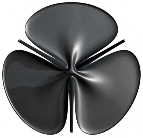
‘Thigmo-morphogenesis’ refers to the changes in shape, structure and material properties of biological organisms that are produced in response to transient changes in environmental conditions. This property can be observed in the movement of sunflowers, bone structures and sea urchins. These are all growth movements or slow adaptations to changes in specific conditions that occur due to the nature of the material: fibre composite tissue. Natural Organisms have advanced sensing devices and actuation strategies which are coherent morphomechanical systems with the ability to respond to environmental stimulus. [1]

Architectural structures endeavour to be complex organisations exhibiting highly performative capabilities. They aspire to dynamically adapt to efficient configurations by responding to multiple factors such as the user, functional requirements and the environmental conditions. Existing architectural smart systems are made of aggregated actuating components assembled and externally controlled, whose process of change is essentially different from that of Thigmo-morphogenesis. For example in a leaf, the veins account for its form, structural strength and nourishment, nevertheless they are an integral part of the sensing and the actuation function. This process of a coherent self-autonomous multi- functionality could be termed as ‘Integrated functionality’. Emulating such a Morpho-mechanical system through embedding self – actuating shape memory alloys in a fibre composite architectural envelope is the core of this research.

The proposed design application, ‘Indus Heritage Centre’ - covers the ruins of the ancient city of Lothal with a fibre composite adaptive roof structure. protecting it from environmental deterioration. The performative abilities and intelligence of the fibre composite adaptive structure springs from the integrated logics of its material behaviour, fibre organisation, topological definition and the overall morpho-mechanical strategy.

The topology is defined as a multi- layered tessellation forming a continuous surface which has differentiated structural characteristics, porosity, density, illumination, self-shading and so on. The design process and geometrical definition of the system is informed by analytical methods and environmental simulations.

Shape memory alloys embedded within the material have the potential of self-actuation with diurnal and annual variations in atmospheric temperature. They undergo significant shape change by rearranging their micro-molecular organisation, between ausentic and martensitic states, hence enabling the structure to open or close. A strategic proliferation of the shape memory alloys has facilitated continuous dynamic adaptation of the structure in order to maintain efficient micro climates within the envelope .

The argument presented in this design proposal is to explore adaptive systems which render self-organised heterogeneous micro climates through exploiting environmental energy.

Aim

Self-organisation is a process through which the internal organisation of the system adapts to the environment to promote a specific function without being controlled from outside. Biological systems have adapted and evolved over several billion years into efficient configurations which are symbiotic with the environment.

To emulate this self-organisation process by developing a fibre composite material system that could sense, actuate and hence efficiently adapt to changing environmental conditions is the primary aim of this research.

Hypothesis

Form, structure, geometry, material, and behaviour are factors which cannot be separated from one another. For example, the veins in a leaf contribute to the overall form of the leaf, its structure and geometry. At the micro scale the fibre material organisation compliments to the responsive behaviour of the leaf. Therefore, the veins display an integral coherence within the multiple functions they perform which could be termed as ‘Integrated Functionality’. Integrated Functionality occurs in nature due to multiple levels of hierarchy in the material organization.

The premise of this research is to explore the potential of self-actuating adaptive systems in order to create efficient micro-climates within an architectural envelope. Physical experiments would be performed to define a fibre composite material system with integrated sensing and actuation functions.

Fibre composites which are anisotropic and heterogeneous offer the possibility for locally varying in their material properties. Shape memory alloys which react to environmental temperature are integrated into composite material for actuation. The definition of the geometry, both locally and globally would complement the adaptive functions and hence the system would display ’Integrated Functionality’.

Figure 0.1

Images from top,

the form of hibiscus leaves,

veins of a lily pad,

pattern of a leaf,

of stomata which aid photosynthesis,

1 Domain

Fibre composites.......................................................................................................13

Fibre composites and their properties

Fibre composites in nature

Man made precedents in fibre composites

Adaptive systems.......................................................................................................23

Adaptive systems in nature

Man made precedents in adaptive systems

Smar t adaptive systems

2 Methods Material tests..............................................................................................................31

Fibre Composite embedded with Sensing + Actuation + Control

Sensing

Control

Energy

Actuation

Shape setting and heat treatment

Experiments 1 to 9

3 Design Application

I ndus Heritage Centre..............................................................................................63

Site

Context

Plan of excavated ruins

Climatic Data

Precedents

Program elements

Schematic plan of the design proposal

4 Digital Experiments

Form Finding Methods............................................................................................75

Sur face parametric definition method

Limitations of surface parametric definition method

D ynamic relaxation algorithm

Configuration of supports

Population of shells

Degree of solar exposure

Solar insolation analysis

5 Performance and Adaptability

Structural

Finite element analysis -Static structural - Principal stress vectors

Fibre organisation algorithm Environmental

Precedents

Continuous surface - Openings - Space truss

Adaptability - Fuzzy logic actuation

Actuation variables

Structural analysis with distributed components

Hierarchy of Components

Wind flow analysis - Computational fluid dynamics

Component distribution strategy

Time line of actuation

Manufacturing

Vbscript - Dynamic relaxation algorithm

Vbscript - Fibre organisation algorithm

Vbscript - Hexagon tessellation on surface

Grasshopper definition- Component geometry - suture curves

International conference in composite materials

Composite materials centre- Imperial college - London

Bibliography

Illustration credits

Glossar y

1 D omain

Fibre Composites

Composites are high performance materials that are made by combining two are more primary materials. Fibre composite materials exhibit anisotropic and heterogeneous properties, also they have a relatively high strength to weight ratio. Their physical properties vary in different magnitudes along different directions as they are composed of primary materials with dissimilar properties. Hence, fibre composites offer the possibility for locally manipulating their physical properties; such as strength and stiffness based on the direction of stresses.

This chapter is a brief summary on the physical properties of fibre composites, biological fibre composites, their organisation strategies, and an overview of the current applications of fibre composites in man made structures.

Fibre Composites and their properties

A composite is a solid material that is obtained when two or more different constituent material elements, each with their own characteristics are mixed. The resultant is a new substance whose properties are different and superior to those of the original elements, but the mixed elements retain their original characteristics. [1.1]

Fibre composites are usually a combination of two, namely reinforcement and matrix. The reinforcement is usually stronger, as well as stiffer, than the matrix. Fibre composites could be classified based on the matrix material into three major groups. Metal matrix composites, ceramic matrix composites and polymer matrix composites. The last is termed as polymer because their matrix is made up of larger molecules of the same material that makes up the reinforcement. The reinforcement or fibres are embedded in the matrix which acts as a binding substrate. Fibres could be both organic and inorganic, for example glass, carbon, aramid and polyethylene are some to mention. The reinforcement fibres are available in a variety of forms, such as continuous, chopped strand mats, woven fabrics and so on.

Finally there are numerous ways to produce fibre composite structures. It involves layering of reinforcement fibres and through the action of the matrix material the structure gets laminated on top of each another. A mould is essential for even flat surfaces. The boat building industry, which produces some of the largest fibre composite, structures are based on manual or semi automated processes. In case of smaller scale products, for example in the automotive industry, the matrix material is transferred into a closed mould with the help of partial vacuum and pressure. Resin transfer moulding and continuous lamination processes on a rolling band are processes with high precision and efficient methods for manufacturing fibre composites. [1.2]

Fibre composites display some remarkable properties, Anisotropy and Heterogeneity [Figure 1.0.a,b]

Fibre composites are heterogeneous and anisotropic material systems. The directionality of the fibre reinforcement could be manipulated to include local areas that absorb the anticipated directional load both in 2-Dimension and 3-Dimension. Unlike conventional isotropic and homogeneous materials, their properties do not predate a given application. Therefore the exact composition and properties could be tailored to meet the desired performance criteria.

Usually while designing any structure, material properties are assumed to be isotropic. On the other hand, in a composite material, large anisotropies in stiffness and strength provide new opportunities for design development. Along with the variations in strength with direction, the effect of anisotropy in stiffness with stresses under external loads should also be accounted for. The material should be designed and produced bearing in mind the way it would be loaded. Thus the process of design, material production and manufacturing could be integrated into a single operation. [1.3]

High Strength to Weight Ratio

[Figure 1.0.c,d]

Fibre composites have a very high strength to weight ratio [Table 1.0.d]. They have inherent optimization potentials, based on the choice of materials and compositions, there could be large reduction in weight and economically efficient solutions. In the case of extreme constructions their potential of nonlinear behaviour could be utilised beneficially. In artificial composite materials, the potential for controlled anisotropy offers considerable scope for integration between the process of material specification and the design.

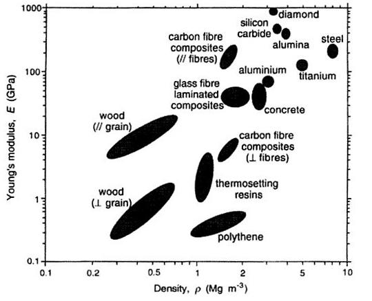
1.0.g, Young’s Modulus-Density graph in the form of areas maps for different materials.

1.1 Tsai, S.W, ‘Composite Design’, Think Composites, p.4, Daytopn, Ohio, 1988.

1.2 Bettum, Johan, ‘Skin DeepPolymer Composite materials in Architecture’, Architectural Design –Con temporary Techniques in Architecture guest edited by Ali Rahim, January-February 2002 issue, p. 72, Wiley-Academy, London, 2002.

1.3 Hull, Derek and T.W.Clyne, ‘An Introduction to Composite Materials’, Cambridge solid state science series, p. 2, Cambridge University Press, Cambridge, UK, 1996.

In considering the formulation of a composite material for a particular kind of application, it is important to consider the properties exhibited by the potential constituents. The properties of particular interest are the stiffness (Young’s Modulus), strength and toughness. Density is of great significance in many situations, since the mass of the structure may be of critical importance.

Thermal properties such as expansion and conductivity must also be considered. Composite materials are subject to temperature changes, a mismatch in the thermal expansions of the constituent’s leads to internal residual stresses. These can have a strong effect on the mechanical behaviour. This can be visualized using property maps, figure 1.0.g- This shows a plot of young’s modulus, E against density, þ. A particular material is associated with a point or a region. This is a convenient method of comparing the property combinations offered by potential matrices and reinforcements against conventional materials. [1.4]

Central to the understanding of the mechanical behaviour of a composite is the concept of load sharing between the matrix and the reinforcement. The stress may vary sharply from point to point based on the type of fibre and their directional orientation, but the proportion of the external load borne by each of the individual constituents can be gauged by volume averaging the load within them. For a simple two constituent composite under a given applied load, a certain proportion of that load will be carried by the fibre and the remainder by the matrix.

forms

Fibre composites are increasingly used in the construction industry as small components such as panels, claddings, doors, windows and so on, but they offer a wider potential for use in buildings as primary structures. A simple glass fibre reinforced panel could have structural strength exceeding that of structural steel. Fibre composite building envelopes could be visualised as monocoque or continuous thin surface configurations, rather than the conventional assembly of component parts forming primary and secondary structures. The surface could be corrugated locally at zones which require higher stiffness. It is therefore apparent that the method of form definition in case of fibre composite structures are significantly different, both geometrically and structurally compared to conventional building elements.

Recent developments in integration of CAD/CAM processes have enabled the potential of fibre composite structures to be moulded into complex free-forms. Developing large multi- axis machining tools for producing moulds directly from digital models would be cost effective to create such complex forms. Manufacturing methods could inform the design process and be integrated at an early stage of the design development. [1.5]

Mould ability into Complex

[Figure 1.0.e,f]

1.4 I bid, p.5.

1.5 Kendall, David, ‘Reinforced PlasticsBuilding the future with FRP composites’, p.3, Elsevier Ltd, 20007.

1.0.b, Fibre Organisation in Femur Bone

1.0.d, Table of strength to weight ratio,Units (kN·m/kg)

1.0.f, Ginkgo Table, Ross Lovegrove

Figure 1.0.a, Collagen nano fibres

Figure 1.0.c, White Knight Space Ship

Figure 1.0.e, PAU Mediatheque, Zaha Hadid Architects

Fibre Composites in Nature

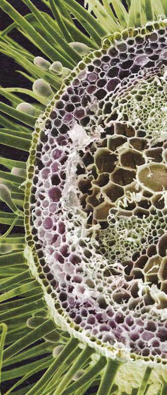
Biology makes use of remarkably few materials and nearly all loads are carried by fibrous composites. There are only four types of fibres: cellulose, collagen, chitin and silks, [Figure 1.1]. These are the basic materials of biology and they have much lower densities than most engineering materials. They are successful not so much of what they are but because the way in which they are put together. The bulk of the mechanical loads in biology are carried by these polymer fibres. The fibres are bonded together by various substances such as polysaccharrides, poly phenols and so on, sometimes in combination with minerals such as calcium carbonate (eg.mollusk shells) and hydroxyapatite (eg. bone). The organisation of fibres and the degree of interaction between them provides the means of tailoring their properties for specific requirements. For example, It is the same collagen fibre that is used in low modulus and highly extensible structures such as blood vessels, intermediate modulus tissues such as tendons and high modulus, rigid materials such as bones. [1.6]

The reason for all biological organisms being made of polymers is probably that the synthesis of long polymer chains based on carbon, oxygen, nitrogen and hydrogen makes use of readily available chemicals and can be controlled by enzymes at low temperatures. The man-made counterparts of these biological fibrous materials are high-performance fibres such as nylon, aramid and highly-oriented polyethylene. The use of fibres for making structural materials offers a great deal of scope and flexibility in design. Fibres and fibre-reinforced materials have an inherent anisotropic and heterogeneous physical and mechanical properties. If properly exploited, they can provide higher levels of optimization than what could be achieved with isotropic, homogeneous materials. Their stiffness and strength could be matched to the loads applied, not only in magnitude but also in direction.

In biology this is extremely common and happens as a result of “growth under stress”. The magnitude and direction of the loads that the organism experiences; as it develops provides the blueprint for the selective deposition of new material, where it is required and in the direction in which it is needed. The best known examples of this are the “adaptive” mechanical design of bones and trees. In bones, material can be removed from the under stressed parts and re-deposited in the highly stressed ones. While in trees a special type of wood, with different cellulose microfibril orientation and cellular structure is produced in successive annual rings when mechanical circumstances demand. Growing a structure by producing and organising fibres under the influence of the loads that it has to carry proves to be extremely efficient.

Numerous patterns of load-bearing fibre architectures are found in nature, each one of them being a specific answer to a specific set of mechanical conditions and requirements. In a sense there are no general design solutions in biology but case specific ones, governed by generic principles. In conventional engineering practices this process is replaced by stress and structural analysis which is not precise and often quite complex. In the recent years, numerical techniques based on finite elements have provided new tools to simulate the adaptive design of nature and this approach has proved to be very successful. [1.7]

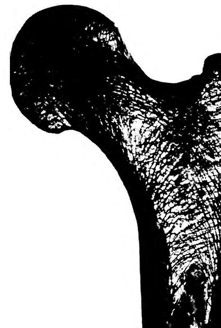
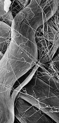
1.1 - Four basic types of fibres in nature, namely, collagen, cellulose, chitin and silks. Collagen- The fibre material composition of the human femur shows the close packing of fibres in parts which are highly stressed.

Cellulose- The section through the stem of a germanium reveals the closely packed bundles of vessels and cells. The geometrical arrangement of close packed integration produces a complex structure, strong but flexible and capable of differential movement. The large pale tubes in the centre are xylem vessels that transport water and nutrients up from the root. The five bundles of pale green vessels are phloem cells, part of the vascular system for the distribution of carbohydrates and hormones, and the smaller purple cells on the perimeter are parenchyma cells, which are thin walled and flexible and can increase and decrease in size by taking up or losing water. These changes cause deformations, which is how the plant achieves movements such as bending towards light or turning around an obstacle

1.6 Weinstock, Michael and George Jeronimidis, ‘Biodynamics’Emergence: Morphogenetic Design Strategies-Architectural Design Journal edited by Michael Hensel, Achim Menges and Michael Weinstock, Academy Editions, London, Vol. 74 No 3 Issue –May/June 2004.

1.7 Jeronimidis, George, ‘Biomimetics:Lessons From Nature For Engineering’, The 35th John Player Memorial Lecture, The Institution of Mechanical Engineers - Materials and Mechanics of Solids Group, 22 March 2000, London.

Figure 1.1

Fibre Material Hierarchies

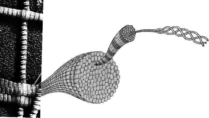
1.2 - The image above shows collagen fibres in a scanning electron microscope. The image from a transmission EM shows the characteristic “banding” pattern of individual fibrils that make up the larger anatomic fibre.

Fibres are most efficient when they carry pure tensile loads, either as structures in their own right such as ropes, cables, tendons, silk threads in spider’s webs or as reinforcement in composite materials. Being slender columns, fibres cannot carry loads in compression because of buckling, even when partially supported and laterally by the matrix in composites. In the case of polymer fibres, micro buckling at the microfibrillar level within the fibre also results in very poor compressive strengths. This problem is common to both man-made and biological composites. Since nature had no alternatives to fibres as building blocks, it had to find ways of offsetting the low efficiency of fibres in compression; in order to expand life beyond the limits of squidgy invertebrate species or aquatic environments. There are four solutions available in nature to this problem: prestress the fibres in tension so that they hardly ever experience compressive loads; introduce high modulus mineral phases intimately connected to the fibres to help carry compression; heavily cross-link the fibre network to increase lateral stability, and change the fibre orientation so that compressive loads do not act along the fibres.

Jim Gordon, says in ’ The New Science of Strong Materials and Structures’, when one is dealing with very heterogeneous fibre reinforced composite systems, the distinction between materials and structures becomes one of convenience rather than a fact. This distinction becomes even more elusive in biology because between the polymer micro molecular chains at nano metre level and the functional organ at the millimetre or metre levels there is a multiplicity of structures which represent different levels of aggregation of the load bearing materials. These hierarchical organisations are a rule rather than the exception in all biological composites. They are probably the result of growth by successive deposition of fibres and other materials. They are difficult to analyse because of their complexity but, by varying the degree of interaction

between sub elements within a hierarchical level and between levels, stiffness, strength, toughness, etc. it could be observed that they are modulated, tailored and optimised for specific requirements. This kind of integrated sub-structuring is a common theme in biology, far more subtle and extensive than in any man-made material or structure. [1.8]

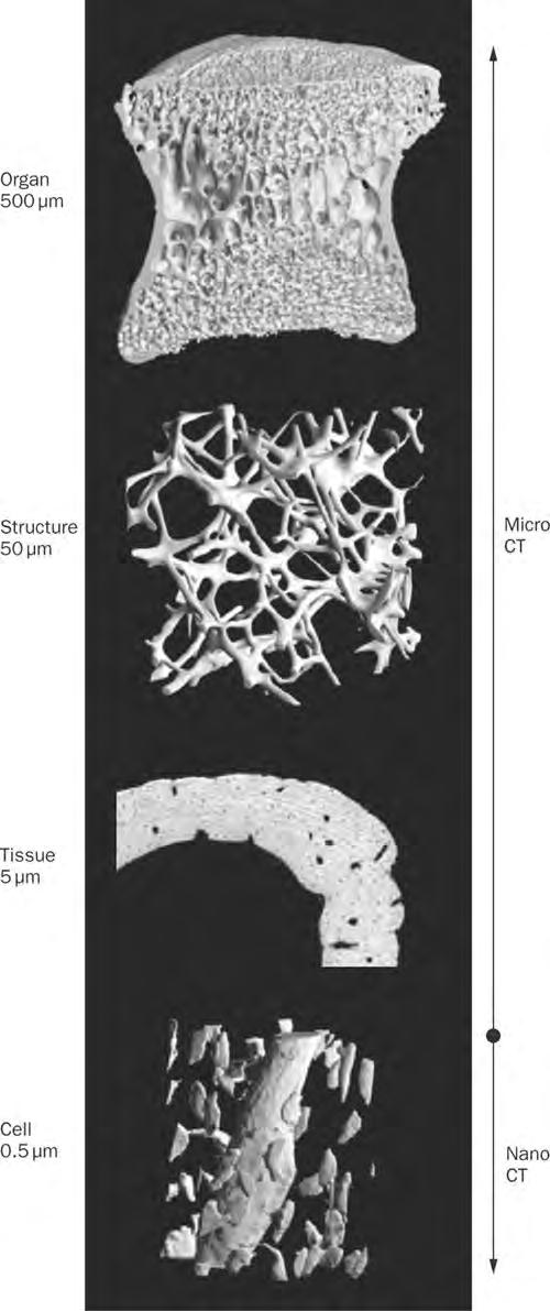
Familiar biological materials such as tendons, bones, muscles, skin and wood provide amazing arrays of hierarchies spanning in typical dimensions from 10-9 metres at the molecular level, to typically 10-3 - 10-2 at tissue level and 100 and beyond at the organ level. In trees, for example, the representative diameter of the various sub structures covers a range from 101 metres at the diameter of trunk down to 10-8 metres diameter of cellulose proto fibril; i.e. ten orders of magnitude with perhaps eight hierarchical levels: organ (trunk), tissue (wood), wood cell, laminated cell walls, individual walls, cellulose fibres, microfibrils and proto fibrils.

The figure 1.2 (right), shows the hierarchies observed in collagen fibres across various dimensional scales.

(a) Collagen fibres

(b) Collagen fibrils

(c) Collagen molecules (triple helices)

(d) α Chains

Figure 1.2

1.8 Gordon, E. Jim, ‘The New Science of Strong Materials’, p. 53, 2nd Edition, Penguin Books, London, 1976.

Growth Under Stress

Living cells have been proved to be stimulated by pressure to increase and multiply. The proof is that our skin grows thicker when we force it to hold greater loads; thus a callus is nothing else but accumulation of material driven by a sudden change in pressure. When the high pressures are reduced to their previous level, the excess in material will be removed. The material density is therefore affected by the strains to which it has been subjected, and hence the properties of the material do not only depend on the nature of the substances that constitute it but also on its history. Pressure and by extension strain are direct encouragement for growth. [1.9]

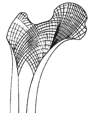
D’Arcy Thompson has extensively written about this concept, using a large number of examples present in the natural world. One of his most useful examples is the discussion held on bone constructions where he analyses the configuration of a femur bone from both the macro and the micro scales. [1.10]

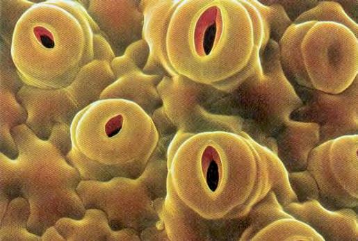
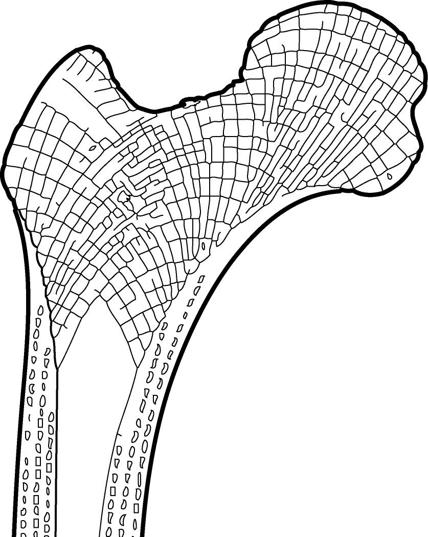
Bone tissue is a type of dense connective tissue which internal organisation consisting of a three-dimensional honeycomblike structure which allows for a variety of shapes and renders lightweight structures, yet rigid and strong enough to carry the weight load of the body, [Figure 1.3 ].

Bone is first deposited as woven bone –also known as ‘coarse fibre’- in a disorganised immature structure present in young bones and in healing injuries. Woven bone is weaker, with a small number of randomly oriented coarse collagen fibres, clearly visible by polarisation microscopy. It forms quickly and is used by the organism as a temporary structure while the final structure is being built. It is the osseous tissue which is first deposited on the calcified matrix in endochondral ossification. [ Figure 1.3]

Woven bone is rapidly replaced by lamellar bone, which is highly organised in concentric sheets. Lamellar bone –also

known as ‘mature bone’- is stronger and is characterised by the presence of collagen fibres arranged in parallel layers or sheets (lamella), forming columns parallel to each other, readily apparent when viewed by polarisation microscopy. Lamellar bone would be the final structure of the bone and it is present in both structured types of adult bone, cortical (compact) bone and cancellous (spongy or trabecular) bone. [1.12].

1.3 Fibre distribution in a femur as revealed through polarisation microscope.

1.4 Diagram showing the hierarchical organisation of fibres in the construction of bones.

1.9 Rhinelander, F.W, ‘Circulation in bone - The Biochemistry and Physiology of Bone’, Academic Press. London & New York,1972.

1.10 Hoehn, K.; Marieb, E. N, ‘Human Anatomy & Physiology’. Benjamin Cummings. San Francisco, USA, 2007.

1.11 Netter, F. H, ‘Musculoskeletal system: anatomy, physiology, and metabolic disorders’, Ciba-Geigy Corporation. New Jersey, 1987.

1.12 Derrickson, B.H, Tortora, G. J. ‘Principles of anatomy and physiology’, Wiley. New York, 2005.

Figure 1.3

Fibre Organisation Strategies

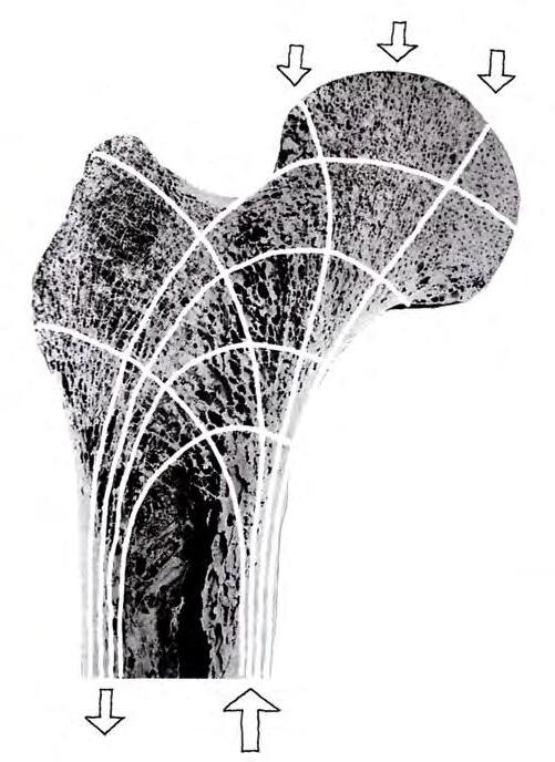
1.5 Diagram showing the arrangement of the principal lines of tension and compression in a femur. Fibre distribution in natural constructions has been proved to follow this arrangement while being continuously stimulated by the external pressures.

1.13 Thompson, D’Arcy, ‘On Growth and Form’, Cambridge University Press, UK, London, 1961.

1.14 Op. cit. Derrickson, p.15

Lamellar bone needs to be able to resist the main type of forces which will act on the bone throughout its life such as bending, torsion and compression. The first two forces require the fibres to run diagonally with different angle orientations and in opposite directions, while organising in alternating layers. In these cases cortical (compact) bone tissue is developed, forming a dense outer layer – the cortex - around the bone [Figure 1.4]. When there are compression loads –the weight of the body- cancellous (spongy or trabecular) bone tissue is developed in the interior of mature bones following the direction of functional pressure according to Wolf’s Law [Figure 1.5].

Wolff’s law is essentially the observation that bone changes its external shape and internal architecture to produce light weight structures that adapt in response to the stresses acting on it. [1.13]

The process starts with trabecular tissue being secreted and laid down fortuitously in any direction within the substance of the bone. If it lies in the direction of one of the lines of principal stress, it will be in a position of comparative equilibrium and minimal disturbance relative to the rest. However, if it is inclined obliquely to the lines of principal stress, the shearing force will tend to act upon it and since fibres are linear elements which cannot withstand shear forces, the fibre will be moved away until it coincides with a line of principal stress.

Trabecular bone tissue spreads in curving lines from the head to the hollow shaft of the femur. These linear bundles are regularly crossed by others, where each inter-crossing is as near as possible and also orthogonal; similar to how the lines of maximum compression cross the lines of maximum tension. [1.14]

The above ideas can be summarised in a single sentence: “Nature stretches the bone tissue in precisely the manner and direction in which strength is required” - D’Arcy Thompson. However, bones do not stop growing once they are formed. Bone tissue is continuously being recycled and it is capable to adapt to new loading conditions. Repeated stress, such as weight-bearing exercise or bone healing, results in the bone thickening at the points of maximum stress.

It has been hypothesised that this is a result of the piezoelectric properties of bones, which causes bones to generate small electrical potentials under stresses.

Bone structure and as a result its overall form is clearly the result of the diagram of forces acting upon it. In the macro scale , the external form we observe as continuous curved topologies, whose overall curvature is the result of the internal fibre organisation in the micro scale and further due to the internal forces acting upon the system.

Figure 1.5

M an made Precedents in Fibre Composites

Fibre composite Sails

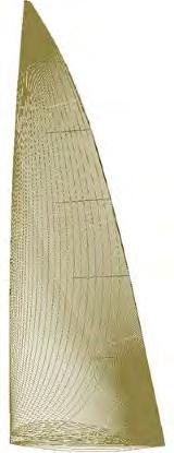
Carbon fibre and aramid fibre composites are widely used in the sail making industry owing to their high performance and durability. As sails are subjected to high wind loads, the definition of their three dimensional form and the organization of fibres along stress paths are crucial for their efficient performance. Unlike other fibre composite structures, sails exploit the anisotropic properties of the fibre composite material as their performance necessitates varying degrees of stiffness and flexibility along the surface of the sail. Contemporary sail making technologies deploy manufacturing processes that have the potential to build a unitary membrane with continuous fibres through thermo moulding process over a full-sized 3-dimensional mould. They render far greater efficiency than the traditional method of assembling panels of flat sail cloth.

The design of the sails begins with building a 3D-CAD model based on the desired ‘flying shape’. All rigging attachment points to the deck, mast size and rigging positions are defined in the 3D model. The modelled sail/rig system incorporates the mechanical properties of the rig such as moments of inertia, sail and spar area, materials stiffness and resistance to stretch. This model does not take into consideration the wind pressure or loads applied. [1.15]

Computational Fluid Dynamics (Aerodynamic Performance Analysis) is used to calculate sail efficiency and Finite Element Analysis for computing the flying sail shapes. Pressure maps are derived through CFD analysis, [Figure 1.7] which varies across the surface based on the size and shape of the sails and the conditions of the wind flow. This pressure field is then used for structural analysis. Based on the force and moments the deformations in the rig and membrane is calculated. Through several iterations the form of the sail is optimised based on pressure fields from wind flow analysis and deformation from structural analysis. The resultant optimised 3D-CAD model is taken further for manufacturing.

The manufacturing process of the sails is quite sophisticated deploying actuating moulds and numerically controlled overhead gantry for applying the structural fibres. The process is semi-automated as the laying of fibres and curing requires manual assistance. Information from the CAD model is used to form a custom mould which varies from one sail to another. The articulating mould with hydraulic actuators have been developed to assume various double curvatures based on the information retrieved from the 3D file. Hence the form of the mould is close to the actual ‘flying shape’.

A base layer of Mylar film (made from Mylar sections joined together with modest shaping to lie reasonably smoothly over the 3D surface of the mould) is draped over the mould and tensioned, a 6-axis fibre head suspended from a computer controlled overhead gantry then applies structural fibre onto the surface of the base film, precisely following the 3D curve of the mould surface. The fibre head ‘draws’ a pattern in yarn that matches anticipated loads in the sail. All structural yarns are applied under uniform tension and adhere to the surface of the film to ensure they remain in place prior to being locked by the lamination. Once the yarns are laid, a second film is positioned on top of the base film and yarn, tensioned, and then covered with a large vacuum bag that compresses the laminate at approximately 1,800 pounds per square foot. This second film contains a secondary mapping of fibres to handle incidental loads off the primary load lines. The gantry head is then removed and replaced with a carbon element heat “blanket” that cures the pressurized laminate by imparting a carefully controlled amount of heat through the laminate. This causes the laminate to conform tightly to the mould in a manner similar to a shrink-wrapping process. After forming, the sail is allowed to cure further for a period of five days prior to shipping and finishing.[1.16]

1.6 Semi-automated, manufacturing process for the laying of the structural fibres on computer numerically controlled actuating moulds.

1.7 Computational Fluid Dynamics and Finite Element Analysis are used to analyse the efficiency and to optimise the flying shape of the sails.

1.15, 1.16, Paraphrased from manufacturer’s data sheet; http://na.northsails.com

Figure 1.7

Figure 1.6

1.18 Paraphrased from Marcel Wanders web site

Automotive and Aerospace Applications

Carbon fibre composites are extensively used in aerospace and automobile applications. They are light weight and have very high strength; almost one quarter specific gravity of steel and ten times as strong as steel. This makes them the perfect material for automobile construction, space and aviation.

Carbon fibre is extensively used in the car racing industry (formula one) as they significantly reduce power/fuel consumption and are much safer. The body of the new Boeing 787 is manufactured completely out of carbon fibre, including the main wing, tail wing, fuselage etc. Carbon fibre composites are also deployed for other industrial applications such as pressure vessels windmills and so on.

Composite manufacturing is essentially an additive process, which requires heat and pressure for curing. There are several methods deployed based on the product requirements. High precision applications like aircraft hulls; wind mill blades etc. use filament winding process. Computer numerically controlled robotic arms are used for the fibre layup. In case of smaller scale applications, such as in the automotive industry, resin transfer moulding or highly skilled manual layup is deployed for achieving complex free forms. [1.17]

Carbon Chair

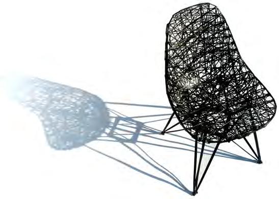
The Carbon Chair designed by Bertjan Pot and Marcel Wanders is made of epoxy drained carbon fibre tapes. The form of the chair is inspired from the plastic chair made by Charles Eames. The chair does not have any metal frames and hence its structural capacity is derived only from the fibre composite

material. The chair is extremely light weight but renders good structural strength. Though the fibre organisation on the seat looks random, it follows a systematic order which is defined by the load transfer pattern, strength and stiffness of the structure. Every point on the rim of the chair is connected to all the four points where the seat is connected to the baseframe.

The initial prototypes were made as one single piece, but for logistic reasons they were developed into individual components. The carbon chair consists of two parts: the base frame, which is coiled achieve structural strength, and the seat. The seat and the base frame are joined with hex- bolts.

The fibres are hand coiled over a single sided mould. The mould has pins attached along its periphery. Carbon fibre dipped with resin is wound around these pins in a rather regular pattern. After curing the seat is removed from the mould. The mould is made out of polystyrene and fibreglass finished to a smooth surface. The finish of the seat is smooth on one side while rough on the other, as a result of casting on a single-sided mould. [1.18]

1.17 Davies, Geoff, ‘Materials for Automobile Bodies’, Butter worth - Heinmann, Elseiver Ltd, Oxford, UK, 2003.

Figure 1.9

Figure 1.8

1.8 (left) CNC controlled filament winding for aircraft hulls.

1.8 (right) Carbon fibre automobile body parts,designed by Mercedez Benz.

1.9 Images of carbon chair by Berjan Pot and Marcel Wanders.

Adaptive systems

This chapter is a comprehensive study of adaptive systems in nature. Fibre organisation strategies in biological systems , which allow for changes in shape and material properties with respect to transient changes in the environment are investigated. The process of Stimuli-Response co-ordination, in biological organisms range from simple to complex configurations. Such configurations of sensing devices, actuators and controllers are studied, both in biology and in man-made precedents.

Adaptive Systems in Nature

Thigmo-Morphogenesis

Thigmo-morphogenesis refers to the changes in shape, structure and material properties that are produced in response to transient changes in environmental conditions. We are all familiar with the fact that many plants are capable of movement, sometimes slow as in the petals of flowers which open and close, tracking of the sun by the sunflowers, the convolutions of bindweed’s around supporting stems and snaking of roots around obstacles. These movements are sometimes visible to the eye as in the drooping of leaves when mimosa pudica is touched, while some are exceptionally rapid and too fast to be seen as in the closing of the leaves of a venus fly trap.

In all these examples, movement and force are generated by a unique interaction of materials, structures, energy sources and sensors. The material is cellulose walls of parenchyma cells, non-lignified and flexible in bending but stiff in tension. These structures are the cells themselves and they shape with the aid of a biologically active membrane that controls the passage of fluid in and out of the cells. The energy source is the chemical potential difference between the inside and the outside of the cells and the sensors are as yet unknown. These systems are essentially work as networks of interacting mini hydraulic actuators, liquid filled bags which can become turgid or flaccid, owing to their shape and mutual interaction they translate local deformations into global ones and they are also capable of generating very high stresses. Similar mechanisms can be seen in operation when leaves emerge from buds and deploy themselves to catch sunlight. Packing the maximum surface area of material in the bud and to expand it rapidly and efficiently is the result of a smart folding geometry, turgor pressure and growth. [1.19]

Morpho-Mechanical Computation

Adaptive mechanical design in biology deals with the design output arising from a set of inputs received by the evolving or growing organ or organism. The inputs can be external and internal loads, environmental changes, etc., which are superimposed on the genetic information available. The evolutionary time-scale is a long one and what we observe as a response in biological organisms is the result of all these inputs over long periods of time. This complex process of sensing and actuation could be termed as ‘MorphoMechanical Computation’. The energy input or stimulus received from the environment is transduced into electric signals by biological sensing devices. The electric signals are further processed for an appropriate responsive behaviour.

Two other aspects of ‘Morpho Mechanical Computation’ which occur over much shorter time-scales and which involve individuals as opposed to whole species, are Thigmo-morphogenesis, such as various forms of tropism, the opening and closing of stomata cells in leafs and boneremodelling. What they show is the intrinsic design flexibility due to fibres and fibre architectures. The interaction between hierarchies and the modulations between them combined with growth converges into the a specific solution required for a specific situation. In order to respond to the changes in circumstances, change in fibre orientations, modifications in structural configuration, material properties and forms both in local and global scales are altered. [1.20]

1.10 (left) Phototropism observed in Clover Plant (Syzygium aromaticum). Phototropism is directional growth in which the direction of growth is determined by the direction of the light source

1.10 (right) Heliotropism exhibited by Coriander plant (Coriandrum sativum). Leaf heliotropism is the solar tracking behaviour of plant leaves. Some plant species have leaves that orient themselves perpendicularly to the sun’s rays in the morning -Diaheliotropism, and others have those that orient themselves parallel to these rays at midday Para heliotropism.

1.19 Vincent, J.F, ‘Deployable structures in nature: potential for biomimicking’, p.1-10, Proc. Instn. Mech. Engineers, UK, 2000.

1.20 Jeronimidis, George, ‘Biomimetics - Differentiation / Integration / Emergence, Sensing – Actuation –Control’, - Lecture at the Architectural Association, London, 2009.

Figure 1.10

Configurations in Adaptive Systems

Adaptive systems in nature have an incredible StimuliResponse coordination. A change in the environment is the stimuli; the reaction of the organism to it is the response. Natural adaptive systems range from simple to complex configurations of sensing devices, actuators, controller logics and inherent energy generators. The adaptive potential is a resultant of continuous evolutionary processes to the environmental pressures under gone by the organism. Lower level organisms such as amoeba, fungi and plants display a simpler process of stimuli response co-ordination as against higher level organisms such as animals which respond to multiple stimuli.

Lower-level Organisms

In case of lower level organisms such as non-lignified plants adaptive behaviour is entirely dependent on control of turgor pressure inside the cells to achieve structural rigidity, prestressing the cellulose fibres in the cell walls at the expense of compression in the fluid.[1.21]

Higher-level Organisms

In higher level organisms, adaptive behaviour involves the synchronization of events which occur in different parts of the body, a control mechanism is located between the stimulus and the response. In multi- cellular organisms, this controller consists of two basic mechanisms by which integration is achieved, chemical regulation and nervous regulation. In chemical regulation, hormones are produced by well-defined groups of cells and are either diffused or carried by the blood to other areas of the body, where they act on target cells and influence metabolism or induce synthesis of other substances. In animals, in addition to chemical regulation, there is another integrative system called the nervous system. A nervous system can be defined as an organized group of cells, called neurons, specialized for the conduction of an impulse, an excited state from a sensory receptor through a nerve network to an actuator.[1.22]

1.22 Paraphrased from, http://www.scienceclarified.com

In single-celled organisms, adaptive behaviour is the resultant of a property of the cell fluid called irritability. In simple organisms, such as algae and fungi, a response in which the organism moves toward or away from the stimulus is called taxis. The adaptive behaviour emerges through the definition of the fibre material hierarchies in multiple scales. The energy required for actuation is also generated within the material system, In case of plants, through the process of photosynthesis and distribution of nourishment to alter the osmotic pressure and chemical disintegration in case of single celled organisms.

Organisms that possess a nervous system are capable of much more complex behaviour which allows for rapid responses to environmental stimuli. [1.9] Therefore, higher level organisms have a complex system for sensing and actuation functions. There is a multifarious integration between sensors, controllers and actuators. To maintain homeostasis, the stimulus generated from the inputs, go through filter processing which leads to decision making capabilities in higher level organisms. An equivalent to this in the manmade world are artificial neural networks which have multiple inputs processors which generate multiple outputs based on predefined rules. The energy required for actuation is again generated within the organism by the process of metabolism.

Figure 1.11

Figure 1.12

1.21 Archer, R.R, ‘Growth stresses and strains in trees’, springer Verlag, Berlin, 1986.

1.11 Diagram showing the process of Morpho-Mechanical Computation.

1.12 (left) Micrograph showing Parenchyma cells in plants which act as mini hydraulic actuators, by changing the osmotic pressure inside their cell walls.

1.12 (right) Neurons, forming neural networks in the nervous system and a neuron cell group responsive to multiple stimuli.

“ The ultimate smart structure would design itself. Imagine a bridge which accretes materials as vehicles move over it and it is blown by the wind. It detects the areas where it is over stretched and adds material until the deformation falls back within a prescribed limit… The paradigm is our own skeleton where material deposition happens in par ts which require greater strength.”[1.23]

- Adriaan Beukers and Van Hinte

M an made Precedents in Adaptive Systems

Architectural structures or building envelopes could be viewed as systems which need to self-regulate, adapt to the environmental changes and respond to natural elements such as sun, wind, rain etc. to achieve a comfortable micro climate. Environmentally responsive buildings, also called as intelligent buildings employing IBMS (Intelligent Building Management Systems) function as a collection of devices such as louvres and shades, controlled by a central computer that receives data from remote sensors and sends back instructions for activation of these mechanical systems.

On the contrary, natural systems are quite different wherein most of the sensing, decision making and reactions are entirely local and the global behaviour is the product of these local actions. This is true across all scales, from small plants to large mammals. When we run for a bus, we do not have to make any conscious decisions to accelerate our heartbeat, increase our breathing rate and volume or open our pores to regulate the higher internal temperature generated. This concept of local decision making and reacting to external conditions is termed as cybernetics.[1.24]

Noebert Wiener introduced the term ‘Cybernetics’ in 1949. The concept of cybernetics includes information theory and practice, from transmission to reception, as well as subsequent manipulation and utilization of the information to control regulatory processes of living organisms, societies, buildings and engineering situations. Information plays a decisive role in the operation of both living organisms and buildings. The emissions and transmissions which constantly emanate from infinitely many sources such as the environment are converted into information by the agents which can use them as a basis for action or inaction. Information can reach the receiver without being passed along and manipulated within; so that the system governs itself by adjusting accordingly. However,

information can also have its origin within the living organism or buildings (such as functional and spatial requirements). This feedback within a system is a special form of information in living processes which allows growth, adaptation or rather self-regulation.

Living organisms perceive information through their senses. The senses serve the organism by obtaining information about the environment, like needs for survival, namely food, safety and reproduction. The acquisition of information is partly conscious. Living organisms react to many external as well as internal signals without involving consciousness, by assimilating them unconsciously or subconsciously like the tanning of skin by deposition of melanin when exposed to sunlight does not involve the brain.[1.25]

It is this flexibility, reactive and transformational capacities of biological organisms that scientists are now seeking to replicate in materials, computers, robotics and buildings. In biomimetics, scientists look at everything from the way the brain learns through trial and error, (so that robots may do the same), to the way a fish moves through water (so the submarines can become similarly more flexible and efficient by reducing central control). This level of biomimicry takes into understanding the aspect of self-organization in biological organisms.[1.26]

There are some precedents which have endeavoured to achieve the self -organisational process observed in nature. We shall briefly discuss the system configuration of sensors, actuators, controllers and energy deployed in these precedents in relation to the higher and lower level organisms discussed in the previous section , adaptive systems in nature.

1.13 (left) Active responsive wall ‘Hyposurface’ developed by Mark Goulthorpe with motion sensors and pneumatic actuators. Diagram below shows the configuration of sensors and actuators forming a responsive system with external control and energy input.

1.13 (centre) Responsive material system ‘Cartesian Wax’ developed by Neri Oxman. Diagram below shows the configuration of sensors, actuators and energy forming an integral part of the material system.

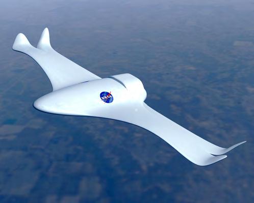
1.13 (right) Morphing smart plane, developed by NASA Dryden Flight Research Centre shows advanced concepts for the aircraft of the future. Diagram below shows the configuration of sensors , actuators, controllers and energy forming and integrated and cohesive smart adaptive system.

1.23 Beukers, Adriaan and Hinte Van‘Lightness’, p.32 , Rotterdam, 1999.

1.24 Hertel, Heinrich- ‘Biology and Technology - Form - StructureMovement’, p. 14, Reinhold, New York,1966.

1.25 Jeronimidis,George‘Biodynamics’, - Emergence: Morphogenetic Design StrategiesArchitectural Design Journal edited by Michael Hensel, Achim Menges and Michael Weinstock, Academy Editions, London, Vol. 74 No 3 Issue –May/June 2004.

1.26 Hagan, Susannah- ‘Taking Shape- A New Contract between Architecture and Nature’, p. 39 , Architectural Press, Oxford, 2001.

Hypo-Surface

‘Hypo surface’ was developed by Mark Goulthorpe of Decoi architects as an interactive installation. The responsive wall measures approximately 8 metres wide and 7 meters high. The project was a collaboration between architects, mathematicians, computer programmers and multimedia experts. The hypo surface transforms from being a flat plane into a curved plane by moving the components up and down by up to 60cm. The surface, extremely varied in its motions and highly dynamic, reacts to environmental influences. The stimuli is picked up by sensors responsive to video, sound, light, heat, movement and so on. The actuation is carried out through arrays of pneumatic pistons, which are activated in real time to the stimuli. The control system processing the information from sensors calculates and signals to each piston a precise instruction at real-time speed. The wall responds in sympathy with a clap from an observer and does not simply respond as a delayed reaction.

The surface was fractioned into small plates interconnected by rubber squids. The geometry of the curved plane (during actuation) is defined by triangular plates to enable double curvatures. [1.27]

The responsive behaviour of the hypo surface is different from the self-organisation process of adaptive systems in nature. The system consists of sensors and actuators, but the information processing or control and the energy required for the actuation of the pneumatic pistons are sourced externally.

Cartesian Wax

Cartesian wax is a material system developed by Neri Oxman. The project explores the notion of material organization as it is informed by structural and environmental performance. It is a prototype for an environmentally responsive skin and an exploration into building envelope design.[1.28]

The topology is defined as a continuous tiling system, differentiated across its entire surface area to accommodate for a range of conditions accommodating light transmission, heat flux, and structural support. The surface is thickened locally where it is structurally required to support itself, and modulates its transparency according to the light conditions of its hosting environment. Twelve tiles are assembled as a continuum comprised of multiple resin types, rigid and flexible. Each tile is designed as a structural composite representing the local performance criteria as manifested in the mixtures of resin. [1.29]

In this case the material system is predefined with sensing and actuation functions. The changes in the environmental heat flux are used to change the state of the resin from flexible to rigid and hence manipulate the transparency of the surface. The adaptive mechanism here is similar to that of lower level organisms, where the sensing, actuation and the energy required for the actuation is generated within the system. There is no information processing or decision making involved and the material responds to the changes in the environmental conditions.

Smart Plane

NASA is currently working with Boeing and the U.S. Air Force on the Active Aero-elastic Wing (AAW) F/A18 project in the quest for developing a morphing aircraft. The Aircraft of the future will employ, embedded “smart” materials and actuators that will enable aircraft wings with unprecedented levels of aerodynamic efficiencies and aircraft control.[1.30]

The smart plane would respond to the constantly varying conditions of flight, sensors will act like the “nerves” in a bird’s wing and will measure the pressure over the entire surface of the wing. The response to these measurements will direct actuators, which will function like the bird’s wing ‘muscles’. Active flow control effectors will help mitigate adverse aircraft motions when turbulent air conditions are encountered. Intelligent systems composed of these sensors, actuators, microprocessors, and adaptive controls will provide an effective ‘central nervous system’ for stimulating the structure to affect an adaptive ‘physical response’. The central nervous system will provide many advantages over current technologies. Researchers at NASA Langley Research Center are taking the lead to explore these advanced vehicle concepts and revolutionary new technologies. [1.31]

The process of morpho mechanical computation in the smart plane is similar to that of higher level organisms. There are multiple inputs from the environment such as temperature, drag coefficient, turbulence and so on; these multiple sensor inputs would be processed similar to that of the central nervous system. Then the actuation would be carried out through the actuators strategically positioned long the surface of the wing -span.

Figure

Controlled Structures

Actuator Systems

Structures

Smart Adaptive Structures

Smart Structures

Intelligent Adaptive Structures Selflearning Reactive Structures Selflearning

Smart Structures

Neural Network Systems

Smar t Adaptive Systems

All around us are living things that sense and react to the environment in sophisticated ways. As structures have become more complex and are being asked to perform ever more difficult missions, there has been an ever increasing need to build “intelligence” into them so that they can sense and react to their environment. Examples include buildings that can sense, react and survive earthquakes and spacecraft that can sense and repair damage autonomously. To perform these functions successfully a “nervous system” is required that performs in a manner analogous to those of living things sensing the environment, conveying the information to a central processing unit (the brain) and reacting appropriately. Fibre optic technology has enabled the nerves of the system to be realized. Using hair-thin glass fibres as information carriers and sensors that may be built directly into the fibres with no increase in the overall size, it is possible to create long strands of fibre sensors capable of measuring strain, pressure, temperature, and other key parameters. These sensor “strings” may then be embedded into the structural materials with no degradation in overall strength, resulting in “smart structures” with built in nervous systems. Such structures could achieve active control, where a structure senses environmentally induced structural changes and reacts in real time.[1.32]

A large scale research effort is currently underway to use advanced composite materials extensively in bridges. This research is addressing issues of corrosion, rehabilitation, and monitoring and involves new concepts and designs in bridge repair and construction. One of the most significant advances is the replacement of steel prestressed tendons with ones made of advanced composite materials. These fibre reinforced polymers are practically immune to corrosion and also lead themselves to internal monitoring by means of embedded fibre optic sensors. A structurally integrated sensing system could monitor the state of the structure, throughout its

Sensor Systems

working life. It could determine the strain, deformation, load distribution and temperature or environmental degradation experienced by the structure.

In more advanced smart structures the information provided by the built-in sensor system could be used for controlling some aspect of the structure, such as its stiffness, shape, position or orientation. These systems could be called adaptive (or reactive) smart structures to distinguish them from the simpler passive smart structures. A more appropriate term for structures that only sense their state might be “Sensory Structures”. Smart structures might eventually be developed that will be capable of adaptive learning and these could be termed “Intelligent Structures”. Indeed, if we consider the confluence of the four fields- structures, sensor systems, actuator control systems, and neural network systems- we can appreciate that there is the potential for a broad class of structures such as, Controlled Structures, Self-learning Reactive Structures, Smart Structures and Self-learning Smart Structures. Therefore smart structures open up a new panorama for biomimetic systems.

As Eric Udd says, “This era would see the marriage of fibre optic technology and artificial intelligence with material science and structural engineering. Major structures constructed in this period would be constructed with built-in optical neurosystems and active actuation control that would make them more like living entities than the inanimate edifices we are familiar with today. To carry this biological paradigm one step further, it may even be possible to contemplate future structures that have the capacity for limited self-repair. Indeed, if we think of the new frontiers for engineering as being in space or underwater, self-diagnosis, self-control, and self- healing may not be so much esoteric as vital”. [1.33]

1.14 Diagram showing Smart adaptive systems possible by the confluence of four disciplines: materials and structures, sensing systems, actuator control systems, and adaptive learning neural networks.

1.27 Burr y, M, ‘Between Surface and Substance’, Architectural Design, March-April 2003 issue, pp 8-19, WileyAcademy, London, 2003.

1.28 Reference from Oxman’s blog http://www.materialecology .com

1.29 Reference from http://www.contructioninvivo.com

1.30 h ttp://www.strangemilitary. com/content/item/10443.html

1.31 h ttp://www.nasa. gov/centers/langley/news/fact sheets/21stcentury.html

1.32 ,1.33 Udd, Eric, ‘Fiber Optic Smart Structures’, p.172-240 , John Wiley and sons London,1995.

Figure 1.14

2 Methods

Material Tests

This section elaborates on the concepts of sensing, actuation, energy, control and the material experiments performed. The aim of the experiments is to develop a fibre composite material system which has an integrated potential of sensing, actuation and control functions.

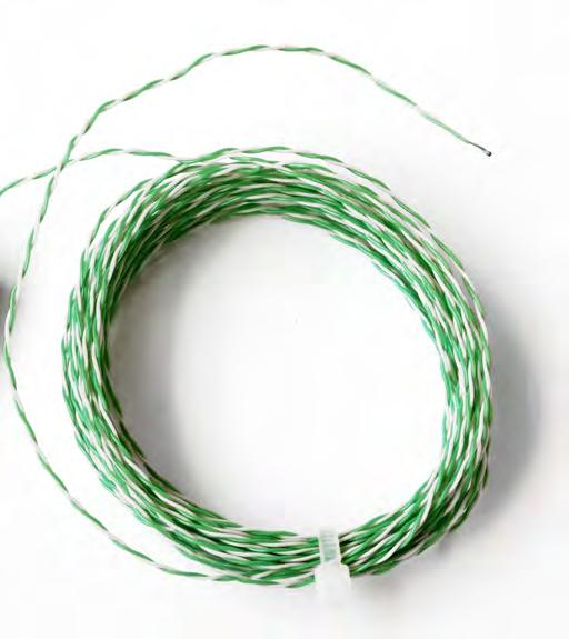
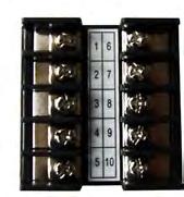
Fibre optic sensors are considered for the sensing functions (while thermocouples and strain gauges are used in the experiments)and Shape Memory alloys are used as actuators. Process controllers are used to sense both temperature and strain which inform the actuators.

Fibre Composites embedded with Sensing + Actuation + Control

Material Configuration

The main aim of the material tests was to develop a fibre composite material system that has embedded sensing, actuation and control functions. The energy used for the actuation is supplied through a heat source which forms the part of the experimental setup. Nevertheless, the hypothesis is that atmospheric temperature would be used as the heat source to supply the necessary energy for actuation. The diurnal variation in the atmospheric temperature could be efficiently used to manipulate the adaptive potential of the smart material system. A smart behaviour would emerge from a coherent functioning of changes in temperature, morphological definition and actuation logics. Further chapters would elaborate on the morphological definition, local definition of the geometry which controls opening and closing and a graphical mapping of actuation against annual variation in atmospheric temperature.

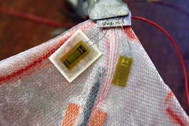
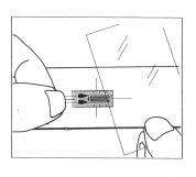
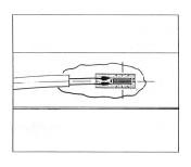
The base fibre composite used is a glass fibre mat reinforced with epoxy resin. It is essentially a sandwich structure with shape memory alloy actuators embedded [Figure2.1]. Fibre optics is proposed as sensors for sensing functions, owing to their advantages of sensing multiple parameters such as temperature, strain and humidity. Also fibre optics being thin fibres could be seamlessly integrated in to the fibre composite material. However, due to the lack of laboratorial facilities, fibre optic sensors were substituted with strain gauges and thermocouples. Strain gauges are used to sense the strain applied on the structure and thermocouples are used sense the temperature of the shape memory alloys. Process controllers are used to monitor the strain induced in the structure and real time monitoring of the temperature variation in the shape memory alloys, to regulate and trigger

the heating. The heat source used for the supply of energy is in the form of silicon heating patches attached to the shape memory alloys integrated within the sandwich construction. The figure 2.1 on the right shows the process of building the fibre composite structure by embedding all the above mentioned sensors, controllers, actuators and energy source.

Setup of the experiment

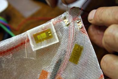
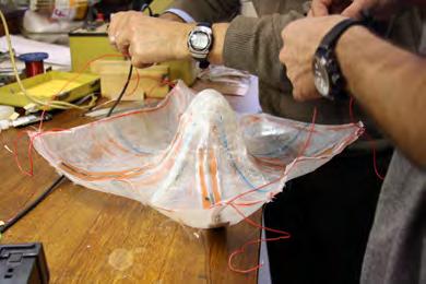
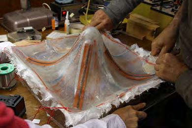
A simple shell with double curvature was formed on a mould by applying epoxy resin over the glass fibre mat. The shape memory alloys ribbons and the silicon heating patches were sandwiched between two layers of glass fibre mats. The strain gauges were attached onto the surface of the shell. The system [Figure 2.2] is setup such that, when the shell receives any strain, a signal is sent out by the strain gauges to the strain gauge processing unit, this unit in turn coverts the strain into a small voltage ranging between 0-2 volts. Once the single input controller receives the signal through this voltage, it triggers the main controller which regulates the heat supplied through the silicon heating patches. The main controller receives the variation in temperature in real time and terminates the heat supply when it reaches the actuation temperature. This forms one cycle of actuation and the process repeats when the structure senses another strain.

Before getting to the detailed description and the results of the experiment it is essential to briefly summarise the properties and processes involved for the deployment of sensors, actuators, controllers and energy sources.

2.1 Diagram showing the material configuration and the process of laying up the fibre composite sandwich structure embedded

2.2 (above) Diagram shows the change in shape expected after actuation.

2.2 (below) Diagram shows the experimental setup connected to the controllers and heat sources.

with SMAs.

Fibre composite

Glass fibre Mat

Epoxy Resin

Fibre Optics

Thermocouples

Strain Gauges Shape Memory Alloys

1/16

Controller

Strain

Embedded shape memory alloys After

Thermocouples

Strain gauges

Figure 2.1

Sensing

Fibre Optic Sensors

Fibre optic cables [Figure 2.3, left] are very common in the communications industry; they also have wide applications as sensors. Fibre optics can be used to measure strain, temperature and humidity based on the properties of light which get transmitted through them. The receptive ability is achieved by designing the fibre optic cable to be sensitive to a specific parameter. The light pulse sent through the cable is received by a processing unit. The resultant light pulse is then analysed to determine the amount of strain or temperature being measured. Fibre optic sensors can be classified based on the modulation and demodulation process. A sensor can be called an intensity, phase or a frequency sensor. Detection of frequency in optics calls for interferometric techniques, the latter is also termed as an interferometric sensor. Intensity or incoherent sensors are simple in construction, while coherent detection (interferometric) sensors are more complex in design but offer better sensitivity and resolution. [2.1]

Current applications of fibre optic sensors are largely in the manufacturing or cure monitoring of composites. Nondestructive evaluation could be costly and time consuming. If sensors are directly integrated into composite materials as a form a sensor network, it will help monitor the internal state of the composite structural members and reduce any uncertainity regarding the status of the material. Such integrated sensors can generate quantitative data which will indicate the state of the curing and later on for health monitoring. Fourier Transform Infrared (FTIR), ultrasonic measurements and fluorescence spectroscopy are some of the known methods used in cure sensing. The cure state is monitored on the basis of refractive index changes, while health monitoring is achieved using Fabry-Perot Interferometric (FPI) techniques. [2.2]

Thermocouples

A thermocouple is a junction between two different metals that produces a voltage relative to a temperature difference. Thermocouples are widely used temperature sensors [Figure 2.3, middle] and they can also be used to convert heat into electric power. Any circuit made of dissimilar metals will produce a temperature-related potential.[2.3] Thermocouples are made of specific alloys for measurement of temperature, which in combination have a predictable and repeatable relationship of temperature and voltage. Thermocouples are standardized against a reference temperature of 0oC; practical instruments use electronic methods of coldjunction compensation to adjust for varying temperature at the instrument terminals. Electronic instruments can also compensate for the varying characteristics of the thermocouple, and hence improve the precision and accuracy of measurements. [2.4]

Strain Gauges

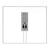
A strain gauge is a resistance-based sensor to measure strain in an object. Strain is defined as the change in length of a component divided by the length of a component. It consists of a long thin “wire” of metal foil that is wrapped back and forth across a grid, called a matrix. The matrix is attached to a thin flexible backing material with an adhesive. The strain gauge is bonded to an object for evaluation. The strain exerted in the object is also exerted on the strain gauges, and the wire that makes up the matrix stretches or compresses.[2.5]

Strain gauges are available in a variety of sizes and configurations, depending on the material and geometry of the part to be tested and the expected strain levels.

2.3 (left) Fibre optic cables transmitting light through total internal reflection.

2.3 (middle) Thermocouple

2.3 (right) Strain gauge, Half- bridge configuration.

2.4 (left) Strain gauge processing unit

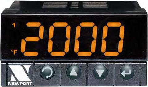
2.4 (middle) Temperature, Process, & Strain Meter & PID Controller.

2.4 (right) 1/16 DIN Temperature/Process Controller with Fuzzy Logic.

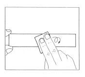
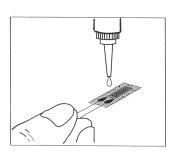
2.5 Process of Installation of a strain gauge onto the structure.

2.1 Udd, Eric, ‘Fibre Optic Smart Structures’, p.13, Wiley, Blackwell, London, 1995.

2.2 ibid. p.18

2.3 Pollock, Daniel.D, ‘Thermocouples, theory and properties’, CRC Press,1991.

2.4 Reference from, http://www.temperatures.com/tcshtml

2.5 Bentley.P. John, ‘Principles of measurement systems’, Pearson Education, 2005.

2.6 Lipták .G. Béla, ‘Instrument Engineers’ Handbook: Process control and optimization’, CRC Press, 2006.

2.7 Window.A. L. , ‘Strain gauge technology’, Springer, 1992.

Half- Bridge strain gauge circuit

Strain Gauges (stressed)

Figure 2.3

Control

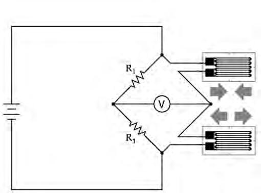
A strain gauge is a resistive sensor. A voltage is passed through the wire, and any variation in resistance is calculated based on a measured voltage. If the part is compressed, the wire that makes up the strain gauge matrix is compressed, and its cross-section area increases. This reduces the resistance of the wire. If the part is stretched, the wire that makes up the strain gauge matrix is compressed, and its cross-sectional area decreases. This increases the resistance of the gauge. In these terms, if tensile strain is considered positive, then resistance is proportional to strain. The measured voltage is converted to strain using a circuit called a Wheatstone’s Bridge.[2.6]

Temperature Compensation: Active-Dummy Method - The active-dummy [Figure 2.3, right] method uses a 2-gauge system where an active gauge, is bonded to the measuring object [Figure 2.5] and a dummy gauge, is bonded to a dummy block which is free from the stress of the measuring object but under the same temperature condition as that affecting the measuring object.

The dummy block should be made of the same material as the measuring object. As shown in Figure 2.3 (right), the two gauges are connected to adjacent sides of the bridge. Since the measuring object and the dummy block are under the same temperature condition, thermally-induced elongation or contraction is the same on both of them. Thus, both gauges bear the same thermally-induced strain, which is compensated to let the output be zero because these gauges are connected to adjacent sides. [2.7]

Strain Processing unit

The strain gauges attached on the surface of the model senses strain. Further, a signal is sent to the strain processing unit [Figure 2.4, left]. When the signal arrives at the unit it is read, measured and translated accordingly to a voltage output of about 0-2 Volts. One of the crucial procedures for setting up the experiment, is the calibration of the processing unit. There are a series of parameters that need to be set with very high accuracy, which include the zero-curvature of the gauges, the relation between the μ strains sensed and the voltage output, in relation to the exact gauge factor and so on.

Single Input Controllers

There are two controllers used in the experiment, namely Temperature, Process, Strain Meter & PID Controller [A] [Figure 2.4, middle] and 1/16 DIN Temperature/Process Controller with Fuzzy Logic[B], [Figure 2.4, right].

The Voltage from the processing unit acts as an input for the single input controller [A]. When a value higher than the programmed tolerance - 0.1 is received , the controller turns on/off the actuation circuit that activates the controller [B]. This is done by passing the live wire of the actuation circuit, through this controller. The single input controller [B] essentially controls the heating of the SMA strips, This controller has two inputs one the real time temperature (x) of the SMA sensed by thermocouples and a set value of temperature (y) which triggers turn on/off the heating patches. The set value (y) is the actuation temperature of the SMA (65 oC). When the real time value (x) reaches the set value (y), there is complete shape change and therefore the heat supply is turned off.

Figure 2.4

Actuation Energy

Silicon Heating Strips

Energy is essential to carry out any kind of actuation process. Since the actuators used in the experiment are shape-memory alloys, the energy required to raise/lower the temperature could be direct or indirect.

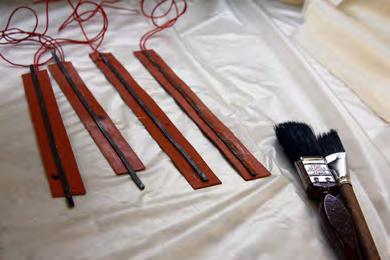
In case of direct energy, the temperature of the SMAs are raised by a heating source. This method was adopted in the experiments through silicon heating patches [Figure2.5, left] which are thin and easy to integrate within a composite structure. The heating strips are attached to the SMAs and connected in series, which is controlled by the temperature process controller.

Alternatively, other methods to supply indirect energy for heating could be considered. For example, passing electrical current through the alloys would consequently heat them and enable shape change. The necessary electrical current could be generated indigenously within the adaptive system. Piezoelectricity and laser energy are possible methods of investigation.

Piezoelectricity is the ability of some materials (notably crystals and certain ceramics, including bone) to generate an electric potential in response to applied mechanical stress. The reversal of this effect is called the inverse piezoelectric effect, i.e. the same materials undergo dimensional change under the influence of an electric field. [2.8, 2.9]

There is a lot of research around laser energy carried out on fibre optic cables. This could be an interesting option, since laser energy could heat the SMAs just by placing the fibre optic cable over them. [2.10]

Shape Memory Alloys / Effect

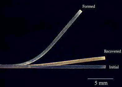
Shape Memory Alloys are a group of metallic materials that demonstrate shape memory effect. Shape memory effect is the ability of the material to remember the shape it had upon a certain characteristic temperature, even though it was severely deformed at a lower temperature (below the characteristic). The material, after being deformed at the lower temperature, recovers its original shape on being heated to the characteristic temperature. There has been a considerable interest in the recent years in developing shape memory alloy actuators because of their advantages in producing large plastic deformations, high force-to-weight ratio and low driving voltages.

A specially manufactured alloy of nickel and titanium, called Nitinol [NiTi], is one of the many that can generate significant force upon changing shape. SMA’s being bio compatible makes them good candidates for medical applications. SMA actuators have also found applications in robotics, vibration control and active control of space structures due to their ability to generate high forces. However, the main disadvantage of an SMA actuator is the nonlinear response of the strain to input current. SMAs demonstrate a hysteresis characteristic as a result of which their control is imprecise.

[2.11]

Phases of SMA

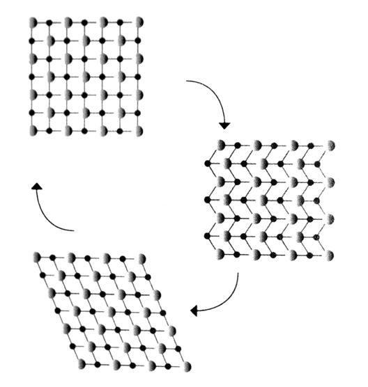
Nitinol [NiTi] shape memory alloys can exist in three different crystal structures or phases called martensite, stress-induced martensite and austenite [Figure2.6, left] . At low temperature, the alloy exists as martensite, which is weak, soft and more

2.5 (left) Silicon heating strips, light weight, thin, flexible (2.5W/in2 ) with operating temperature up to 232oC.

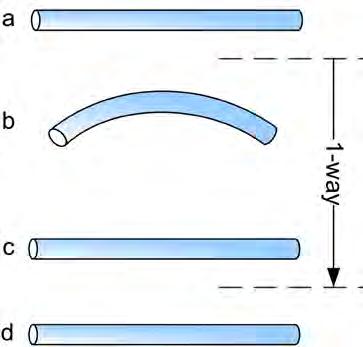
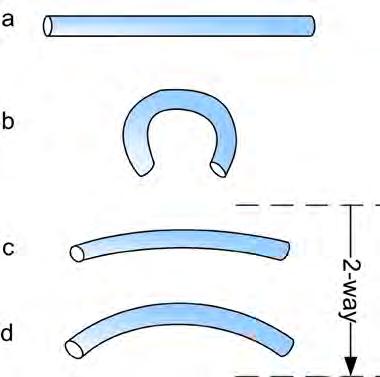
2.5 (middle) , (right) - One and Two Way shape memory effect. A shape memory alloy is an alloy that “remembers” its shape, and can be returned to that shape after being deformed, by applying heat. SMAs have the highest known force/weight ratio among actuators. The figure shows the two types, one way shape memory alloy and two way shape memory alloy.

2.6 (left) Microscopic, Inter molecular arrangement when the SMA undergoes solid phase change between Austenite, Martensite phases with respect to change in temperature.

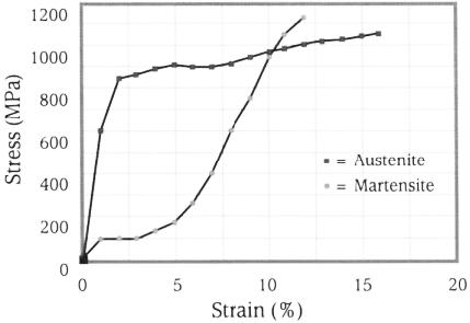
2.7 Table of mechanical properties in both austentite and martensite phases compared against stainless steel.

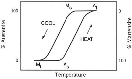
2.8 (above) Graph showing the phase change of SMA with respect to time.

2.8 (below) Graph comparing the stress strain curves of both the states of SMA.

2.8 Heywang, Walter, Karl Lubitz and Wolfram Wersing, ‘Piezoelectricity’, Springer, 2008.

2.9 Yang, Jiashi, ‘An Introduction to the Theory of Piezoelectricity’, Springer, 2005.

2.10 Wadhawan, K.Vinod, ‘Smart Structures: Blurring the Distinction Between the Living and the Nonliving’, OUP Oxford, 2007

Figure 2.5

Lowest and highest values have been compiled from picked references (Buehler l. 1967, Funakubo 1987, Breme et al. 1998,

Melton, K. N, ‘Ni-Ti Based Shape Memory Alloys’, - Engineering Aspects of Shape Memory Alloys, pp. 28 – 34, edited by T. W Duerig et al., Butterworth , London, 1990.

2.12 Smith,S. A, ‘Shape Setting Nitinol’, - Proceedings of the Materials and Processes for Medical Devices Conference, pp 266 – 270. edited by S. Shrivastava, ASM International, Sept., 2003.

2.13 Okamoto. Y, ‘Reversible Changes in Yield Stress and Transformation Temperature of a NiTi Alloy by Alternate Heat Treatments’, pp 517 – 520. Script Metallurgica, Vol.22, 1988.

deformable. Stress - induced martensite or super elastic NiTi is highly elastic (rubber-like) and is present at a temperature that is slightly above its transformation temperatures. The austenite is the stronger, higher temperature phase present in NiTi. Most of the physical properties of austenite and martensite, vary during phase transformations. Based on Harrison, the properties that change during transformation include Young’s Modulus, resistance, heat capacity, latent heat of transformation and thermal conductivity. [2.11]

One-Way Shape Memory Effect

A specific temperature is related to a martensitic phase transition. The terms ‘austenite’ and ‘martensite’ are used in a generic sense for the higher-temperature phase and the lower-temperature phase, respectively. The shape memory effect arises primarily due to the accommodative molecular reorientation of the austenitic and the martensitic phases.

Super elasticity is the ability of a material to be able to undergo large but recoverable strains, provided the deformation is carried out in a characteristic range of temperatures. This property is an example of a purely field-induced phase transition (at a fixed temperature). When the deforming stress is applied at a temperature (within the characteristic temperature range) at which it is in the austenitic phase, the stress sends the material to the martensitic phase, with an accompanying large deformation. When the stress is removed, the material recovers its shape because it reverts back to the austenitic phase. [2.12]

A typical shape-memory cycle runs as follows, assuming that the material is in the martensitic phase at room temperature. It is first heated towards the temperature of the martensite-

austenite phase transition. Since this is typically a case of firstorder phase transition, there is a range of temperatures in which the martensitic and the austenitic phase coexist. There is thus a temperature at which the austenitic phase starts forming. Further increase of temperature converts more and more of the martensitic phase to the austenitic phase. Finally at a certain temperature, the transition is complete.

At the end of the cooling down process, the SMAs usually does not recover its original plastically deformed shape. Since the shape is remembered only on heating and not also on cooling-down to the martensitic phase, this is called one-way shape memory effect. [Figure 2.5, middle]

Two-Way Shape Memory Effect

If the alloy remembers its shape, in both the austenitic and the martensitic phases, it exhibits two-way shape memory effect. [Figure 2.5, right]

To obtain this behaviour, a specimen has to be trained. A variety of training protocols have been experimented. Most of them amount to creating a network of dislocations in the specimen. These dislocations have an associated strain field, and that martensitic configuration develops on cooling to the other phase for which the overall strain energy is the least. This can happen repeatedly across the heating and cooling cycles.

Training procedures include: repetition of the one-way SMA cycle, constrained cycling across the phase transition, thermal cycling at constant applied stress and super elastic cycling. [2.13]

martensite (de twinned)

martensite (twinned)

Figure 2.6

Figure 2.7

Figure 2.8

2.11

Shape Setting and Heat Treatment Process

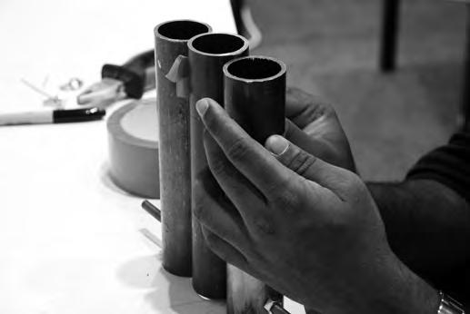
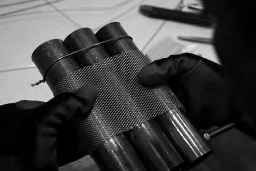
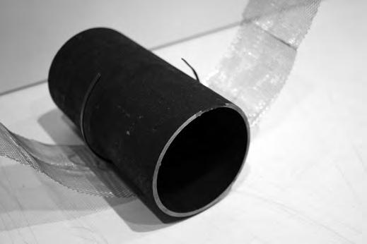
Shape setting process is essential to induce shape memory effect in Nitinol - shape memory alloys. The actuator element designed for a particular purpose generally requires the setting of a custom shape. Shape setting process is similar in all forms of Nitinol, such as, wire, ribbon, strip, sheet, tubing or bar. Shape setting is accomplished by constraining the Nitinol element on a mandrel or a fixture of the desired shape and applying an appropriate heat treatment. The heat treatment methods used to set shapes in both shape memory and super elastic forms of Nitinol are similar. [2.14]

Nitinol produced by the mill is normally finished by cold working to achieve dimensional control and enhance surface quality. Cold working suppresses the shape memory response of these alloys. It also raises the strength and decreases the ductility. However, cold work does not raise the stiffness of the material. Heat treating after cold working diminishes the effects of cold working and restores the shape memory response of these alloys. Therefore, in order to optimise the physical and mechanical properties of a Nitinol product and achieve shape memory or super elasticity, the material is cold worked and heat treated. [2.15]

The heat treatment parameters chosen to set both the shape and the properties of the actuator element are critical, and usually need to be determined experimentally. In general, temperatures as low as 400 oC and times as short as 1-2 minutes can set the shape, but generally one uses a temperature closer to 500 oC and a time period of 5 minutes. Rapid cooling of some form is preferred via a water quench or rapid air cool. Higher heat treatment times and temperatures will increase the actuation temperature of the SMA and often gives a sharper thermal response. There is also an accompanying decrease in abilityof the actuator to resist permanent deformation. [2.16]

The initial experiments were setup with the aim of understanding the process of shape setting in Nitinol. Two kinds of shape memory alloys were used to setup these experiments, a ribbon of dimensions 1.2 (thick) X 4.6 (wide) X 270 mm (long) with actuation temperature 65 °C [Figure 2.9] and a wire of .05 mm dia X 1000mm (long) with actuation temperature 35 °C. [Figure 2.10]

The Nitinol ribbon and wires were trained by rolling them around metal pipes and maintaining them in position while they were placed in an oven. In case, of this particular experiment, the oven was heated up to 500°C and the temperature was maintained for 5 minutes [Figure 2.11].

The SMAs were subsequently removed from the oven and immediately immersed in cold water, whilst maintaining the imposed bend shape throughout the cooling procedure.

When the setup was removed from the oven the ribbon had opened up, but had a considerable curvature forming an arc which was then mechanically flattened. The ribbon was attached to a clip on one end, against a grid to observe the change in curvature. The SMA ribbon was heated up to the actuation temperature of 65 °C with a hot air gun.

It was observed that the SMA ribbon had regained the exact same curvature of the set shape. It was apparent that the SMA ribbon was much softer and easily deformable at room temperature but got stiffer and hardened when heated.

2.9 Preparation for shape setting of the Nitinol wire wound around three metal pipes of 40mm diameter.

2.10 (left) , (middle) Preparation for shape setting of the Nitinol ribbon wound around a metal pipes of 80mm diameter.

2.10 (right) The opened up Nitinol ribbon after the shape setting/ heat treatment process from the kiln.

2.11 Kiln used for the shape setting/ heat treatment process.

2.14 Smith,S. A, ‘Shape Setting Nitinol’, - Proceedings of the Materials and Processes for Medical Devices Conference, pp 266 – 270. edited by S. Shrivastava, ASM International, Sept., 2003.

2.15 Brailovski .V, ‘Optimization of Postdeformation Annealing Heat treatment for NiTi Shape Memory Alloys’, in SMST 2000, Proceeding of the International Conference on Shape Memory and Super elastic Technologies, pp 33 – 42 , Edited by Russell Pelton, April, 2000.

2.16 Melton, K. N, ‘Ni-Ti Based Shape Memory Alloys’, - Engineering Aspects of Shape Memory Alloys, pp. 28 – 34, edited by T. W Duerig et al., Butterworth , London, 1990.

Figure 2.9

Figure 2.10

Actuation Experiments 1 & 2

Experiment 1

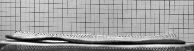
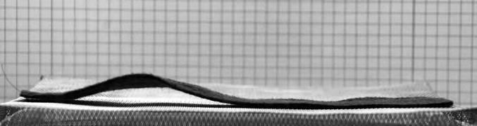
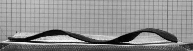
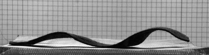
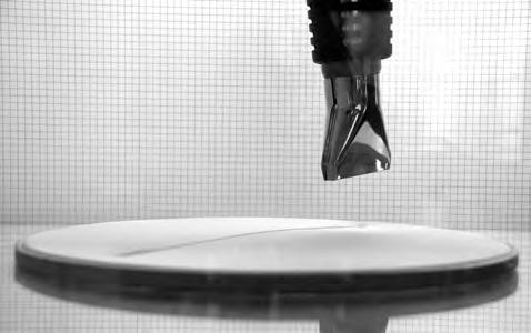
The first experiment was a simple testing of the actuation. The SMA wires were stitched onto a piece of felt to give a better visual result of the shape change. The felt was heated with the hot air gun. The result [Figure2.12] was as expected, with the SMA taking the ‘memorised’ shape quite quickly.

Experiment 2

The second experiment was to introduce a surface element and test the shape change in relation to tha. Therefore the SMA ribbon was placed under a thin tensioned fabric. The fabric was attached on a circular frame and the heating of the SMA was carried out with a hot air gun. The surface [Figure2.13] followed the curvature change of the alloy as expected.

Due to the high temperature the SMA fabric started burning and finally tore it apart. At this point, the factor of temperature resistant materials arouse. Any material used in the same system as the SMAs, should be able to resist temperatures as high as 65 oC. The aim is to implement the alloys in a fibre composite. Most of the polymers, have working temperatures higher than the actuation temperatures of the SMAs.

Figure 2.11

Figure 2.12

Figure 2.13

Actuation Experiment 3

Cantilevered Support

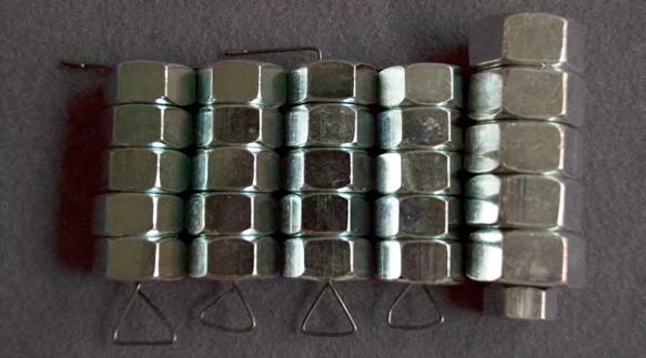
These set of experiments were focused on extrapolating the Force to Weight ratio and Force-Time graph. It was observed that the SMA ribbon of 9 gm in a cantilevered position could lift loads up to 114 gm. As observed in the graph the phase change happened in a short interval. The test was carried out in sequential increments by adding a 56 gm weights. The restoring capacity of the initial degree of curvature reduced when the loads were increased. [Figure 2.16, above]

Simply Supported

The load carrying capacity of the SMA ribbon improved significantly when the strip was simply supported.

The ribbon of 9 gm could lift a load of 883 gm, almost 100 times it self-weight. [Figure 2.17, below]

This indicates that when the SMAs are embedded within a fibre composite elastomer, they would have the ability to induce high stresses on the flexible surface; enabling it to redistribute the stresses and re-organise the components. The test was carried out in sequential increments by adding weights. The restoring capacity of the initial curvature of the strip reduced to a greater degree with the increase in weights. The ultimate load of 883 gm did not allow the ribbon to take any curvature and it barely managed to get back to a straight line. The retrieval of the original shape (martensitic state) happens quicker when the loads are increased. The change in shape during phase change from austenite to martensitic state is more gradual, while the other way around is much faster. The simply supported SMA ribbon displays a much higher force to weight ratio as there are two constraint points and the lifting distance is reduced to half.

The results of this series of experiments were carefully mapped into graphs and analysed. One of the surprising outcomes -besides the impressive force to weight ratio of the ribbon- was the time required for the actuation to take place. For example, the 9 grams SMA ribbon needed 18 seconds to lift 850 grams of weights. As shown in the graphs [Figure 2.15], the time needed for the weights to touch the ground was 85 seconds and another 35 for the full rest position.

Simply Supported

Cantilevered

Figure 2.14 Weights used for the Force-Strength-Time-experiments

Figure 2.16, 2.17 Sequential photos of Actuation Experiment 3 Cantilevered and Simply Supported.

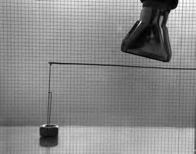
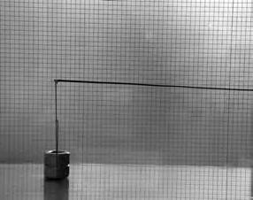
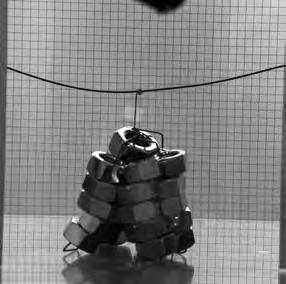
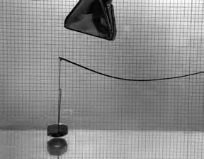
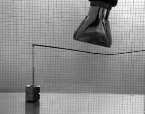
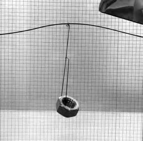
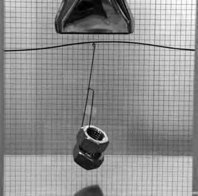
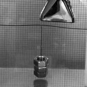
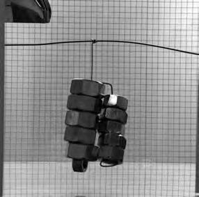
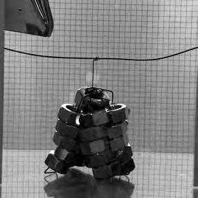
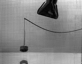
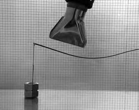
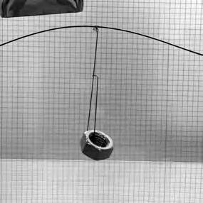
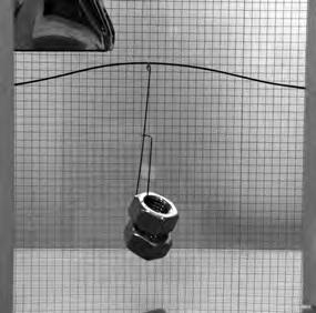
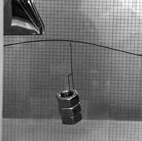
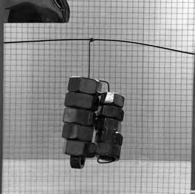
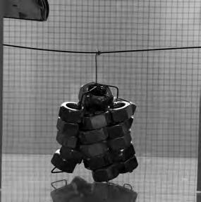
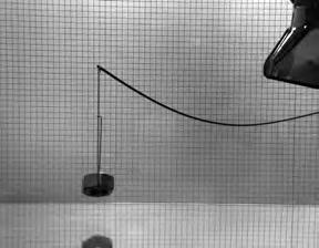
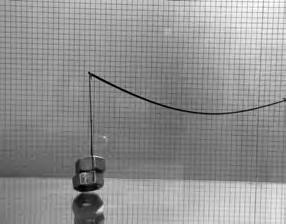
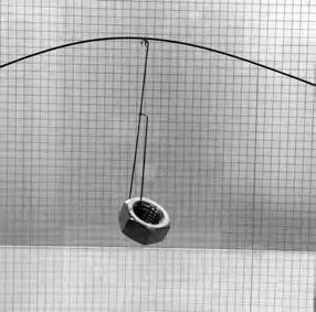
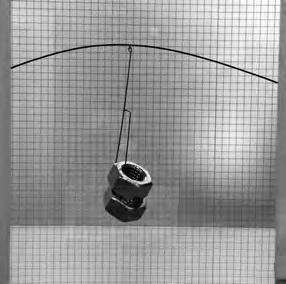
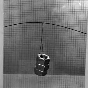
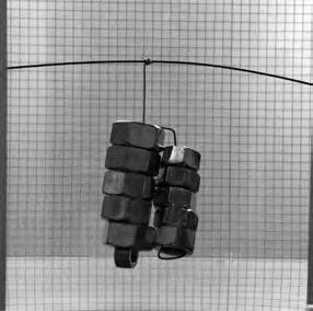
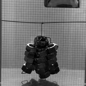
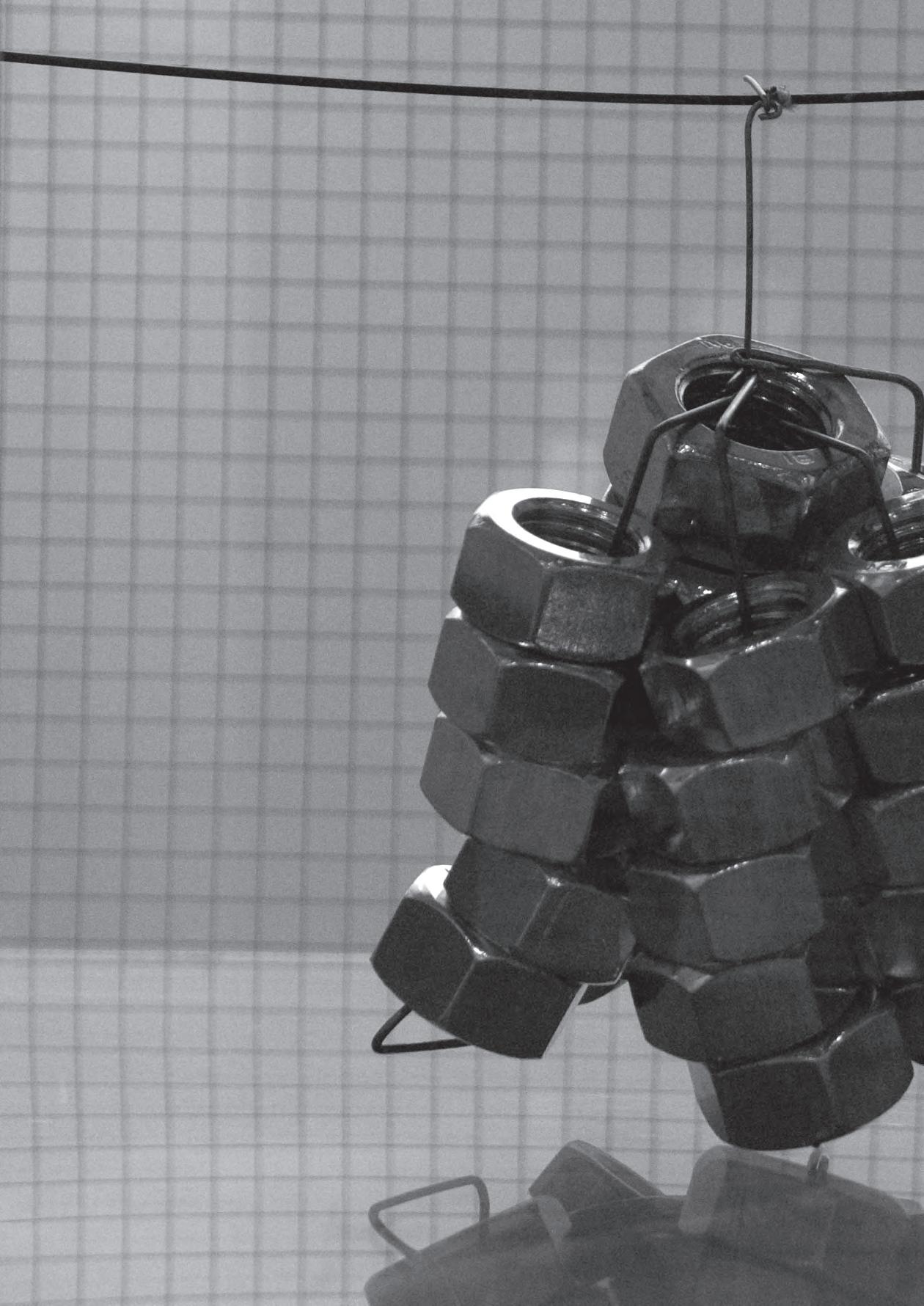
The Nitinol ribbon of 9 gm could lift a load of 883 gm, almost 100 times it self-weight.

Actuation Experiment 4

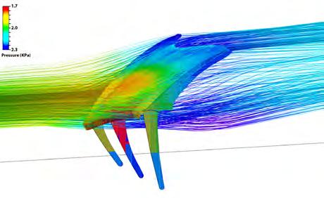
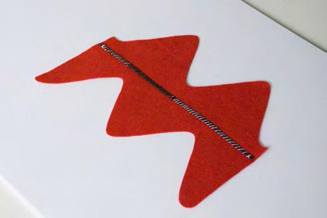
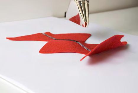
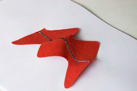
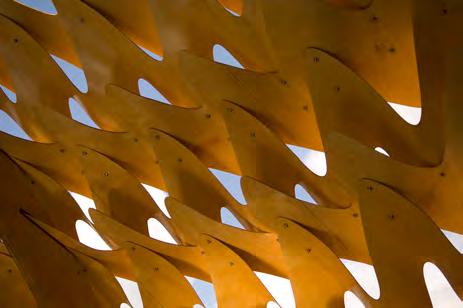
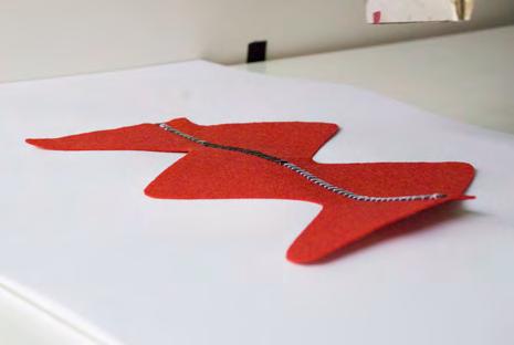
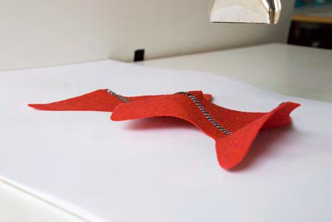
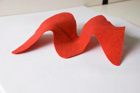
Actuated Canopy

The morphology of the Emtech canopy constructed at the Architectural Association was finalized after several environmental simulations. The structure was optimised by strategically negotiating between these parameters, such as reducing wind loads, maximizing exposure to sun and still providing a covered shelter for the rain.

A smart fibre composite adaptive system could allow the strip morphology of the canopy to dynamically re-organise, open and close based on current environmental conditions. Such a dynamic response would enable the structure to evaluate

the parameters and prioritize the shape change. For example, close it when there is a strong wind, tilt it to drain off the rain water or shrink the coverage and allow more sunlight.

The second cycle of shape setting was done to suit the strip morphology of the canopy. The images above [Figure 2.18] shows the process of actuation and changes in the curvature of the strip morphology.

Figure 2.18

2.18 (top left) Computational Fluid Dynamic windfow analysis of the canopy.

2.18 (top right) Close-up of the strip morphology of the canopy on site.

2.18 (below) Sequential photos of the actuation experiment .

Actuation Experiment 5

Actuated Openings

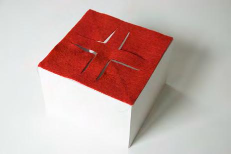
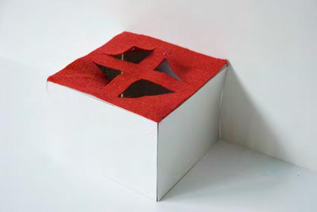
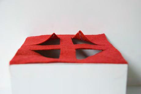
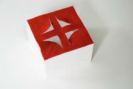
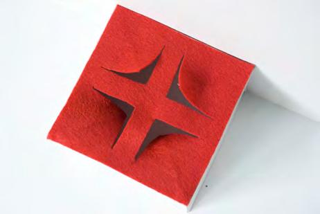
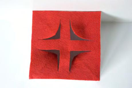
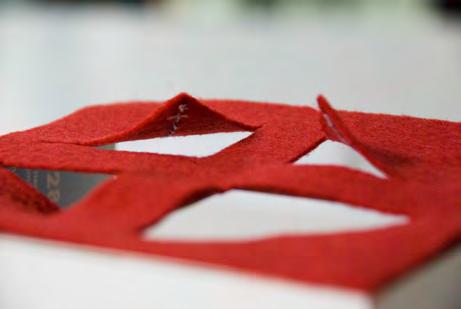
The previous set experiments were focused on shape change or changes in the curvature on a surface. This experimental setup was made to explore openings on a surface.

In this experiment, thin Nitinol wires were used. The SMA wires were cut and bundled together forming arcs. The openings on the surface was defined as four squares, free on two edges to open and close. A bundle of three wires were woven to the felt along the diagonal of each square to create the openings.

The SMA wires were placed in such as way that the arching direction achieved during actuation is towards the inside in

two squares and the opposite in the other two. As observed in the image above [Figure 2.19] the hot air gun was place beneath the surface to actuate the openings. As they were heated the SMA wires reached the actuation temperature forming arched openings. Hence the surface opens up on both directions on the inside and the outside.

Figure 2.19

2.19 Sequential photos of the actuations (openings) experiment.

Actuation + Control Experiment 5

In this experiment the element of control was introduced into the system. The same SMA ribbon that was used for the actuated canopy experiment was attached to a silicon heating patch. As the patches were designed to work at 110 Volts, two of them had to be connected in series in order to reach the 220 Volts of the power supply. One end of the patche was connected to a power supply, while the other to a controller. A thermocouple was also used to measure the temperature on the SMA.

The controller has a single input (temperature of the thermocouple) and one output (turn on/off the heating patches). A set temperature was configured to the controller

- which is the actuation temperature 65 oC. By turning the system on, the controller registers the process temperature from the thermocouple and until value is lesser than the set value (65), the heating is on. When the temperature reaches the set value, full shape change occurs and the system stops heating.

This experiment helped in understanding the establishment of controlled actuation. The temperature of the alloys reached from room temperature to 65 oC in less than 15 seconds. The accuracy of temperature control was precise, temperature measurement was efficient and the controller could respond accurately to slight difference in values.

System Configuration

Actuation

1 SMA Ribbon Silicon Heating Patches Control

Thermocouple (Temperature)

Single Input Control Unit

(Temperature Set Value

Temperature Process Value)

Figure 2.20

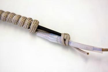
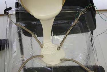
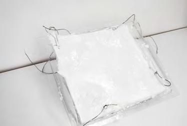
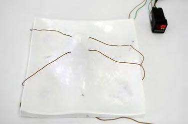
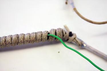
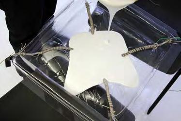
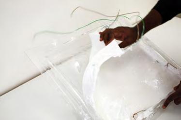
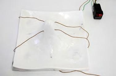
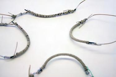
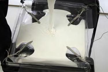
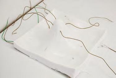
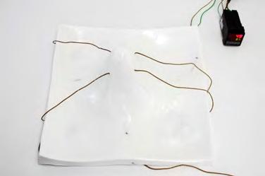
System Configuration

Actuation

4 SMA Ribbons

Rope Heaters

Control

Thermocouple (Temperature)

Single Input Control Unit

(Temperature Set Value

Temperature Process Value)

Actuation + Control Experiment 6

The next step of the material experiments, was the integration of more SMAs into a model. A silicon rubber model was made and while casting, the SMAs were embedded within. The alloys were wrapped with rope heaters and one of them was connected to a thermocouple. [Figure 2.21]

The process of the experiment is similar to the previous one, the main difference was rope heaters were used instead of silicon heating patches and four alloys instead of one.

The shape change results were not as expected. Only a small degree of shape change could be observed [Figure 2.21, bottom right] mainly due to two reasons. First of all, the

material used for the model - silicon rubber - was inappropriate since it was very flexible and had no stiffness. Besides this, the placement of the SMAs inside the model was not designed properly. The alloys were orientated more towards the side instead of the upper-lower part of the rubber and at the same time they had no support due to the high flexibility of the surrounding material.

Revising this experiment, was the first step to design and set-up towards the final fibre composite model. Positioning of the alloys was rethought and also the rope heaters were discarded because of their thickness (more than 1cm), which would be difficult to integrate into a thin composite material.

Rope heater wrapped around the SMA ribbon

Thermocouple attached on the SMA

4 SMAs connected in series (after actuation)

Figure 2.21

Sensing + Control Experiment 7

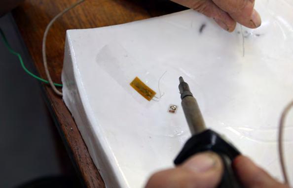
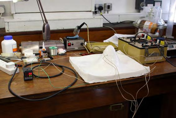
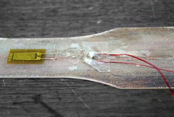
The actuation and control system was well tested in all the previous experiments, now the challenge was to establish and efficient sensing system for strain.

In theory, the system uses fibre optics for all the sensing functions. Fibre optics technology is widely spread and applications of fibre optic sensors have been established for years. There is currently a lot of research on simultaneous sensing of multiple parameters and the results are very promising. So, even though the technology required is already out there, it has not been possible to locate a fibre optics processing unit for use in the experiments. Owing to this reason strain gauges were opted for sensing strain.

Although the previous silicon rubber model [Experiment 6] was not functional, the sensing circuit was experimented on it. Consecutively , a separate piece of fibre reinforced polyester strip proved to be much more efficient.

After calibrating the strain gauges processing unit and completing all the necessary wiring, the gauges were attached onto the two models and tested successfully. The final step was to link it to the actuation circuit to test actuation

System Configuration

Sensing

Thermocouple (Temperature)

Strain Gauges (Strain)

Control

Single Input Control Unit

(Temperature Set Value

Temperature Process Value)

Strain Gauges Processing Unit

Strain gauge attached on the rubber model

Testing the actuation circuit

Testing the sensing on a polyester piece

Calibrating the processing unit

Figure 2.22

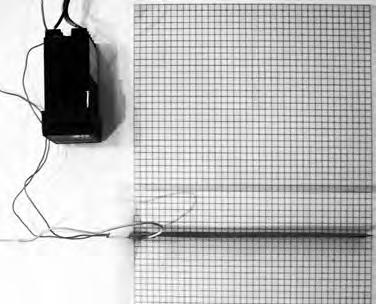
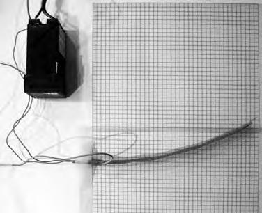
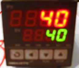
1.39 Results of the curvature change calibration

Curvature Calibration Experiment 8

Calibration of the curvature change of the SMA was crucial to accomplish, before getting on with the final model in which the alloys would be embedded in glass fibre mat and epoxy resin matrix.

The amount of curvature change in every step of the temperature variation had to be measured, so that the shape change could be controlled. This would help determine the thickness and the expected shape change in the fibre composite model. A simple experiment was setup [Figure 2.23] with the temperature controller, thermocouple and the SMA ribbon that would be embedded in the fibre composite model.

The results, as shown in the table display a slightly different behaviour than the description given by the manufacturer’s document. The shape change observed was more linear than expected and started at 38 oC. A complete shape change was observed between the range of 58-60 oC and not at 65 oC, which was the prescribed actuation temperature of the alloy.

Figure

Measurement of curvature change

Figure 2.23

Actuation + Sensing + Control + Energy Final Experiment 9

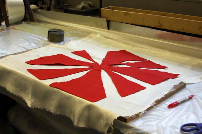
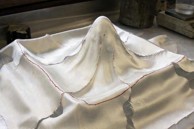
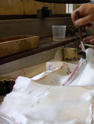
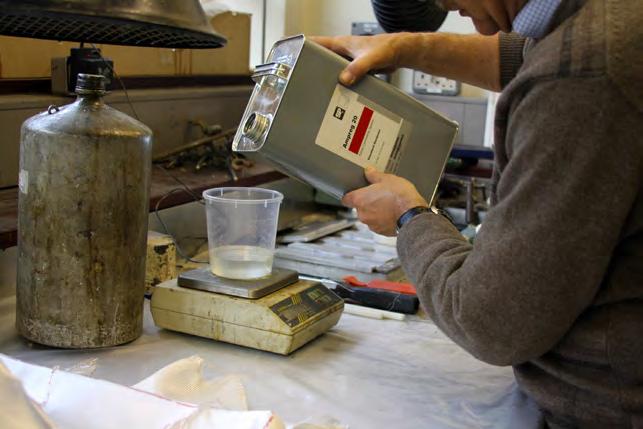
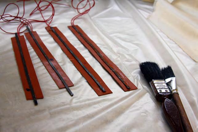
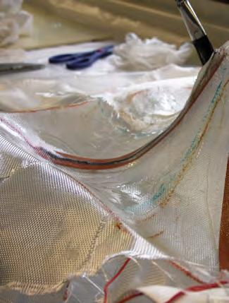
The base material used in the Final Model was glass fibre reinforced epoxy resin. It was designed as a sandwich structure with four embedded SMA ribbons attached onto silicon heating patches and strain gauges fixed on the surface. A thermocouple was used to measure real time (process) temperature of the alloys.

After the curing of the model in the oven for approximately one hour, it was removed and un-moulded. The curing process was done carefully by controlling the temperature of the oven, because if it reached over 35 oC the SMAs would start actuating. That would consequently cause a shape change and the model would deform before it could be cured. Due

to this, the curing time was longer than usual. Ideally resin models are cured in much higher temperatures around 90 oC.

After the removal of the model from the mould, all the essential wiring was configured and the actuation circuit was tested successfully. The next step was to set up and testing of the sensing.

Using a soldering device, all the wires were prepared and a first test was performed on another piece of resin. Then the two gauges were connected. The active one was attached on the surface of the model with a resin glue and the dummy gauge on a piece of stiff thermoplastic. [ Figure2.25]

Cutting pattern of the glass fibre mat

Glass fibre mat placed on the mould

The SMAs attached on the heating patches

Measuring the resin needed for the model

Un-moulding the model

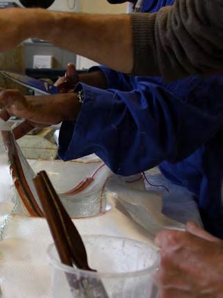
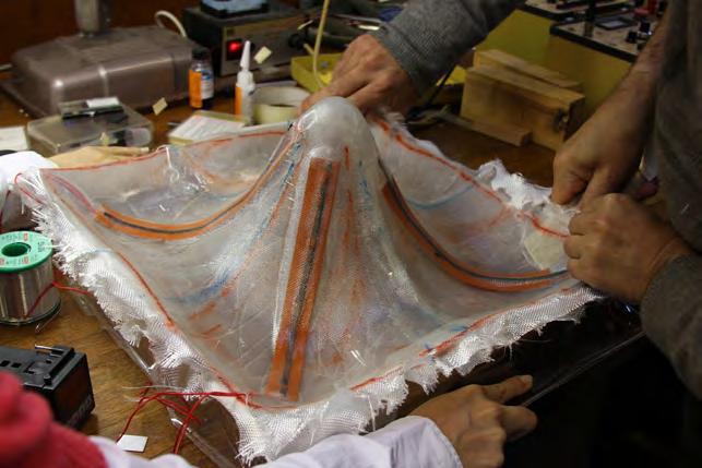
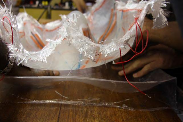
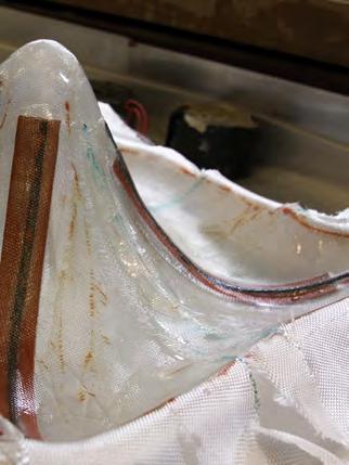
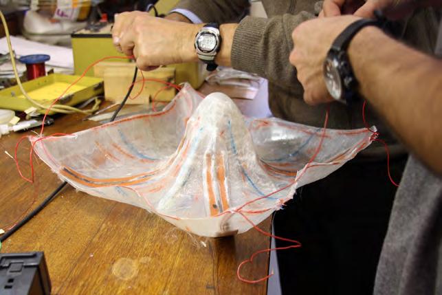
System Configuration

• Sensing

Strain Gauges (Strain) Thermocouple (Temperature)

• Actuation

4 SMA Ribbons

• Control Single Input Control Unit ( Temperature Set Value Temperature Process Value)

Strain Sensing Control Unit ( Voltage Input)

Strain Gauges Processing Unit

• Energy Silicon Heating Patches

Fixing the wires for the actuation circuit

Connecting the heating patches in series

Un-moulding the model

Applying the second layer

Applying resin

Figure 2.24

Actuation + Sensing + Control + Energy Final Experiment 9

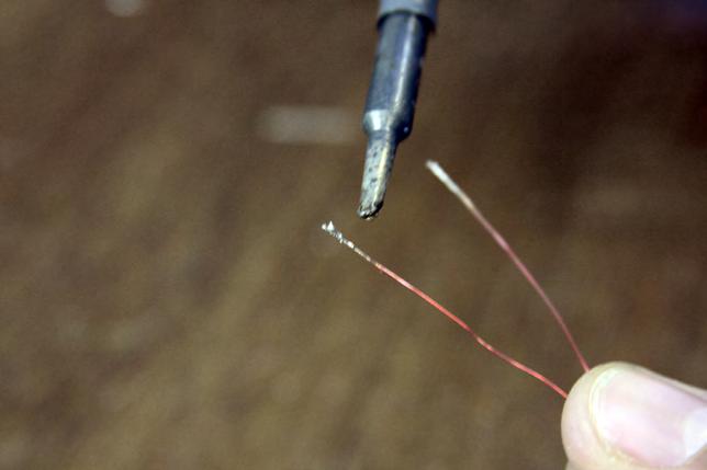
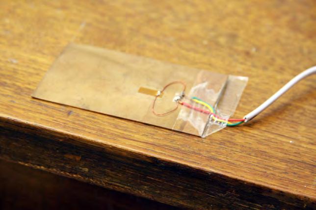
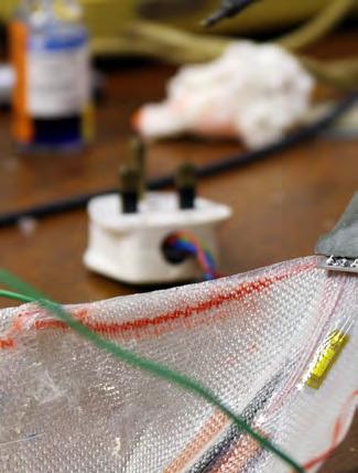
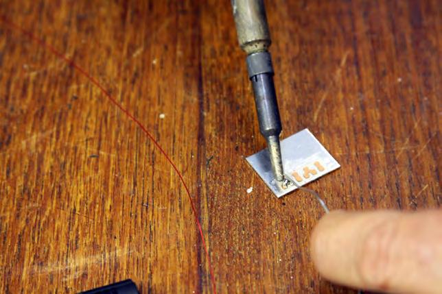
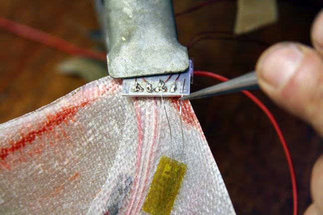
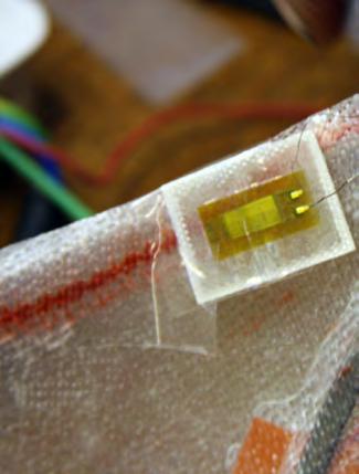
The strain gauges were attached to the bottom of the surface, in order to sense the strain occurring due to vertical external loads on the surface. The configuration used for the strain gauges was Wheat stone’s half-bridge. There are two gauges used , one active and one dummy- in order to achieve temperature compensation.

The active is fixed directly on the surface of the model and the dummy, on a piece of stiff thermoplastic, so that it doesn’t get any curvature change when the model gets deformed. The use of the dummy gauge was crucial, because the active one was placed very close to the SMA, with the raise in temperature of the active gauge might render faulty results.

When a strain is sensed by the gauge, a signal is sent to the processing unit. When the signal arrives at the unit it is read, measured and translated into a voltage output ranging between 0-2 Volts.

The Voltage from the processing unit acts as the input for the single input controller. When a value higher than the programmed tolerance (0.1) is received , the controller turns on/ off the actuation circuit that follows. This is done by passing the live wire of the actuation circuit, through the controller.

The final step is connecting the actuation process controller into the system. This controller has two inputs. The set value

Soldering the edges of the strain gauge wire

Testing the processing unit by using a trial piece

Connecting the gauges to the wires

Soldering

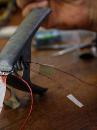
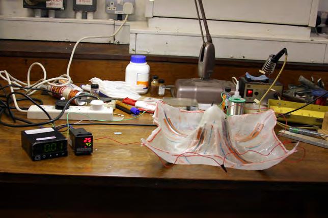
and the process value of the temperature on the SMAs. When it is switched on by the previous controller, it starts heating the alloys by turning on the heating patches, which are connected in series. The heating process stops, when the process temperature becomes equal to the set temperature of the system. This means that the actuation temperature of the SMAs has been reached and as a result, there would be a complete shape change.

The final step was to connect both the sensing and actuation circuits and test the functioning of the whole system. As shown in figure 1.41, the shape change happened as expected and both the sensing and actuation were calibrated properly.

Finally, the setup of the final model was configured for repeatability of the experiment. The experiment was performed several times to obtain precise measurements and evalute the results. The illustrations in the following three pages show the experimental setup and the results achieved. [ Figure 2.26, 2.27,2.28 ]

Sequential photos of the actuation circuit testing

Attaching the dummy gauge

Attaching the strain gauge

Figure 2.25

Strain Gauges

Model

Strain Gauges Processing Unit

Figure

Thermocouple

Strain Gauges Processing Unit

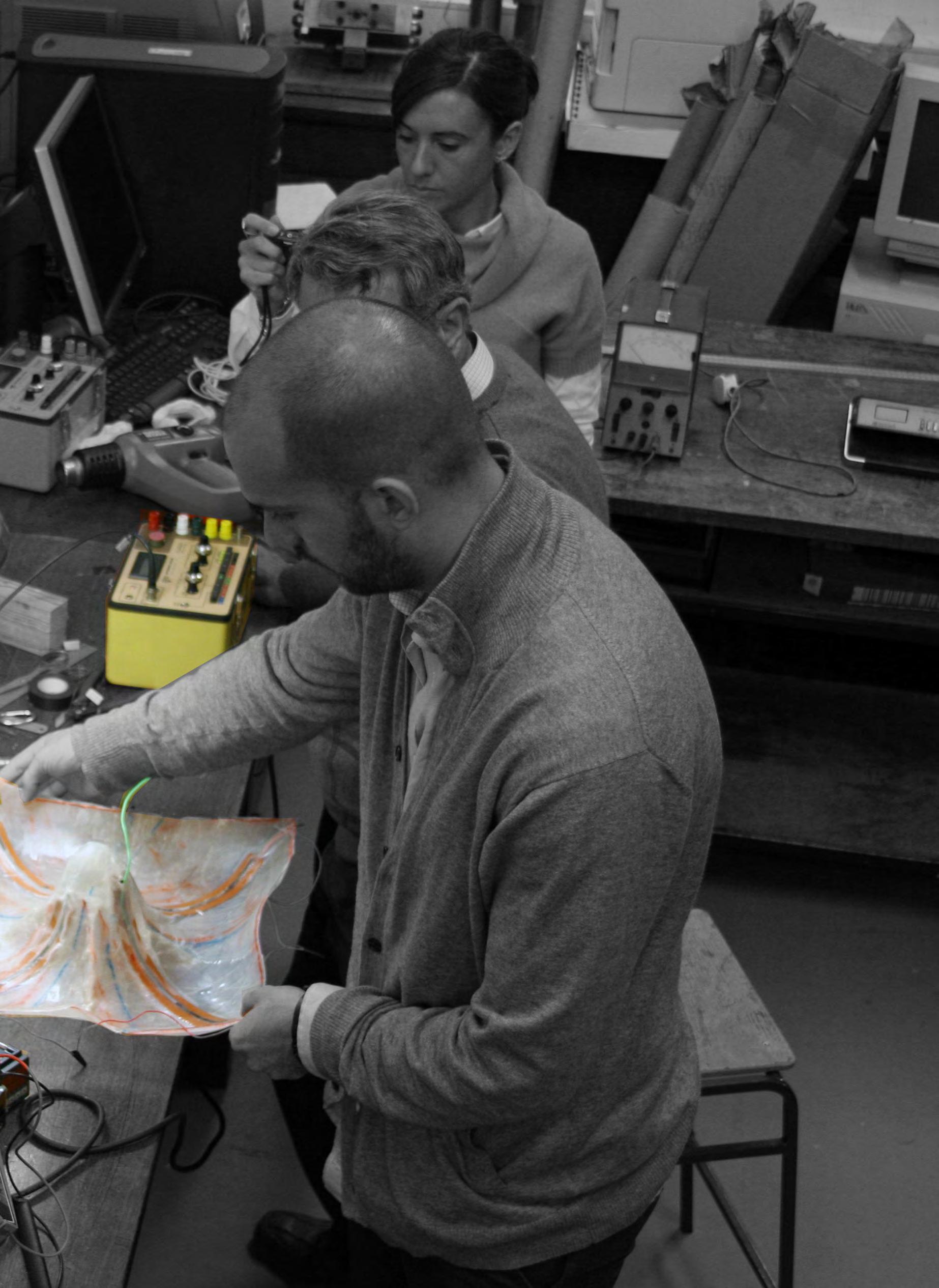
As the signal from the strain gauges arrives at the processing unit, it is read, measured and translated accordingly into a voltage output. ranging between 0-2 Volts.

Single Input Controller

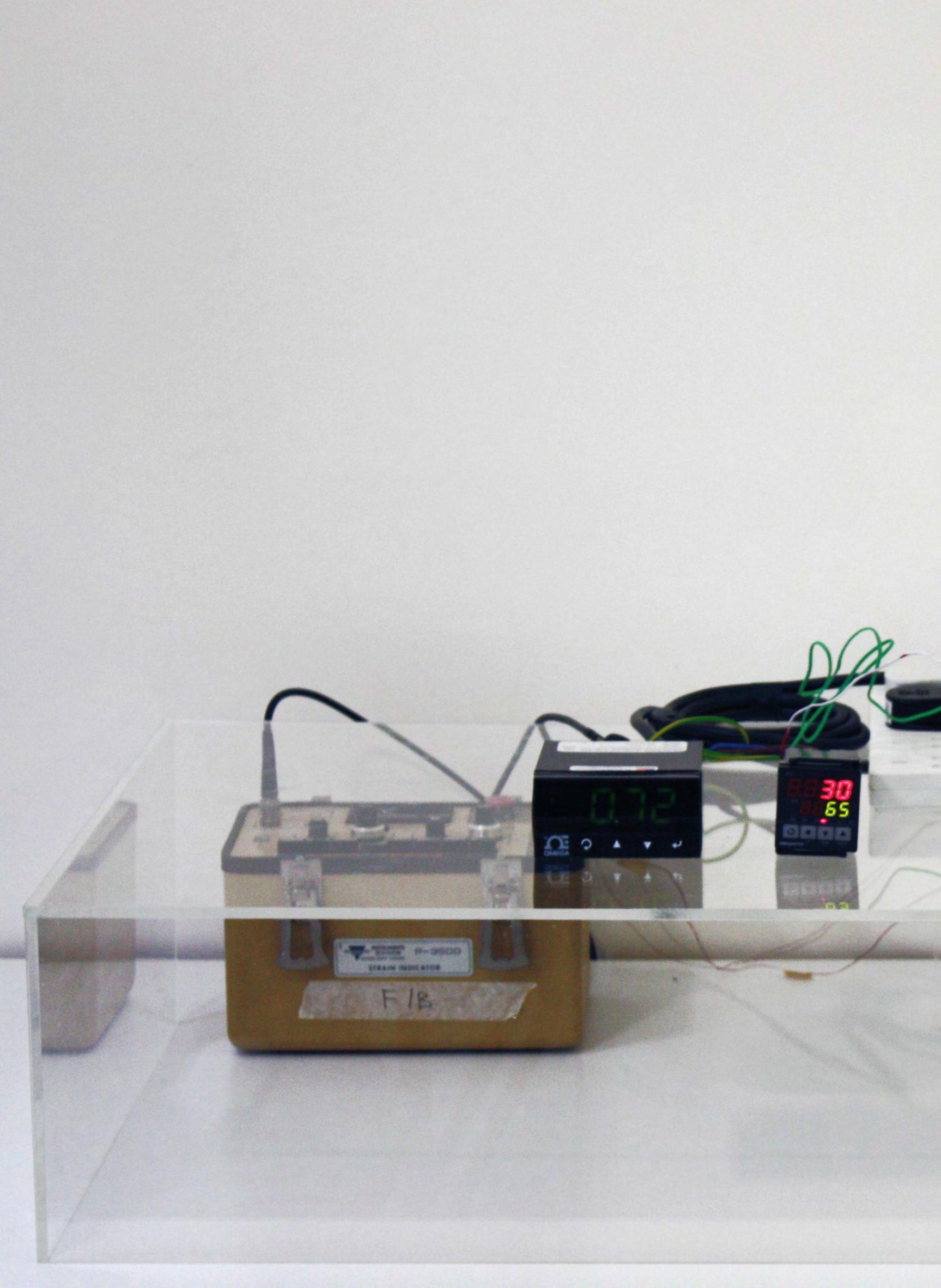
The Voltage from the processing unit acts as an input for the controller. When a value higher than the programmed tolerance (0.1) is received , the controller turns on/ off the actuation circuit.

Actuation Temperature Controller

This controller has two inputs. The set value and the process value of the temperature on the SMAs. When it is switched on by the previous controller, it starts heating the alloys by turning on the heating patches, which are connected in series. The heating process stops, when the process temperature becomes equal to the set temperature of the system.

Figure

Figure 2.28 Superimposed Collage of

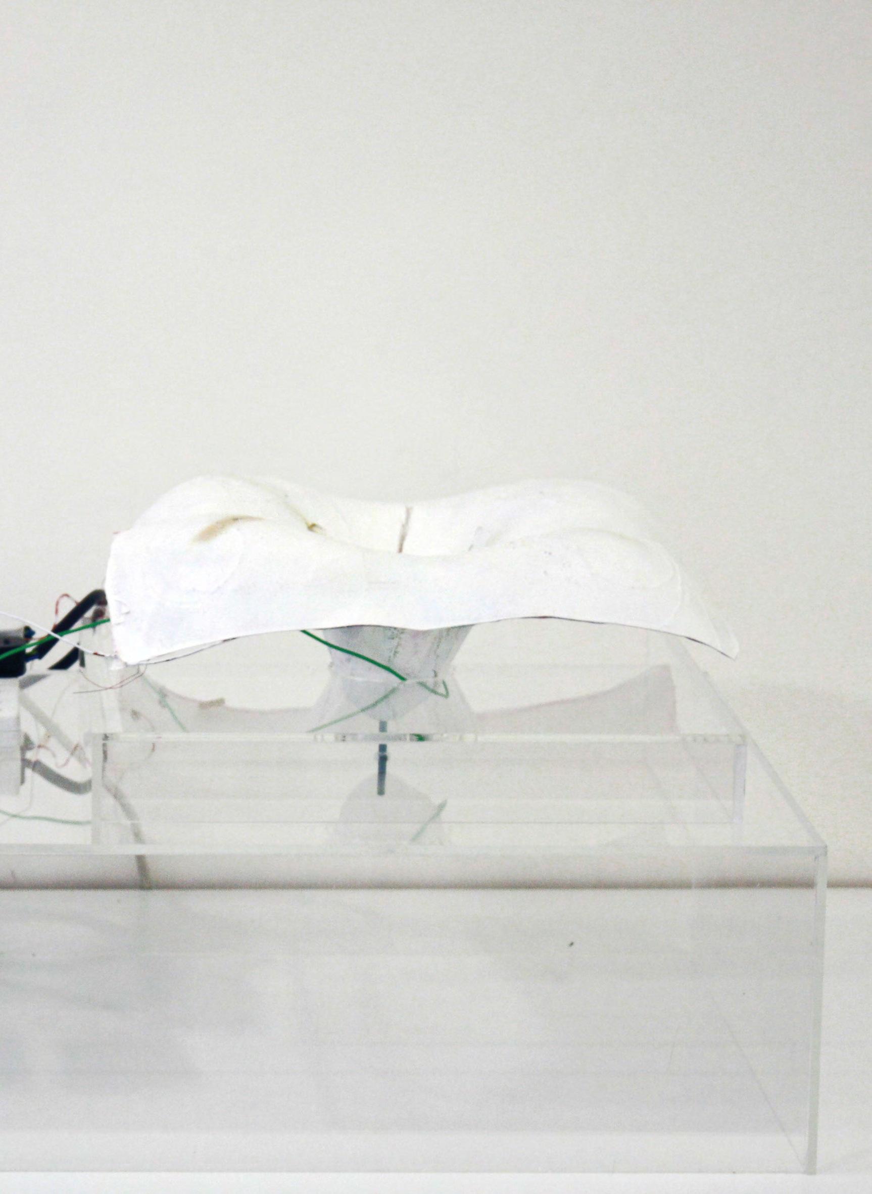
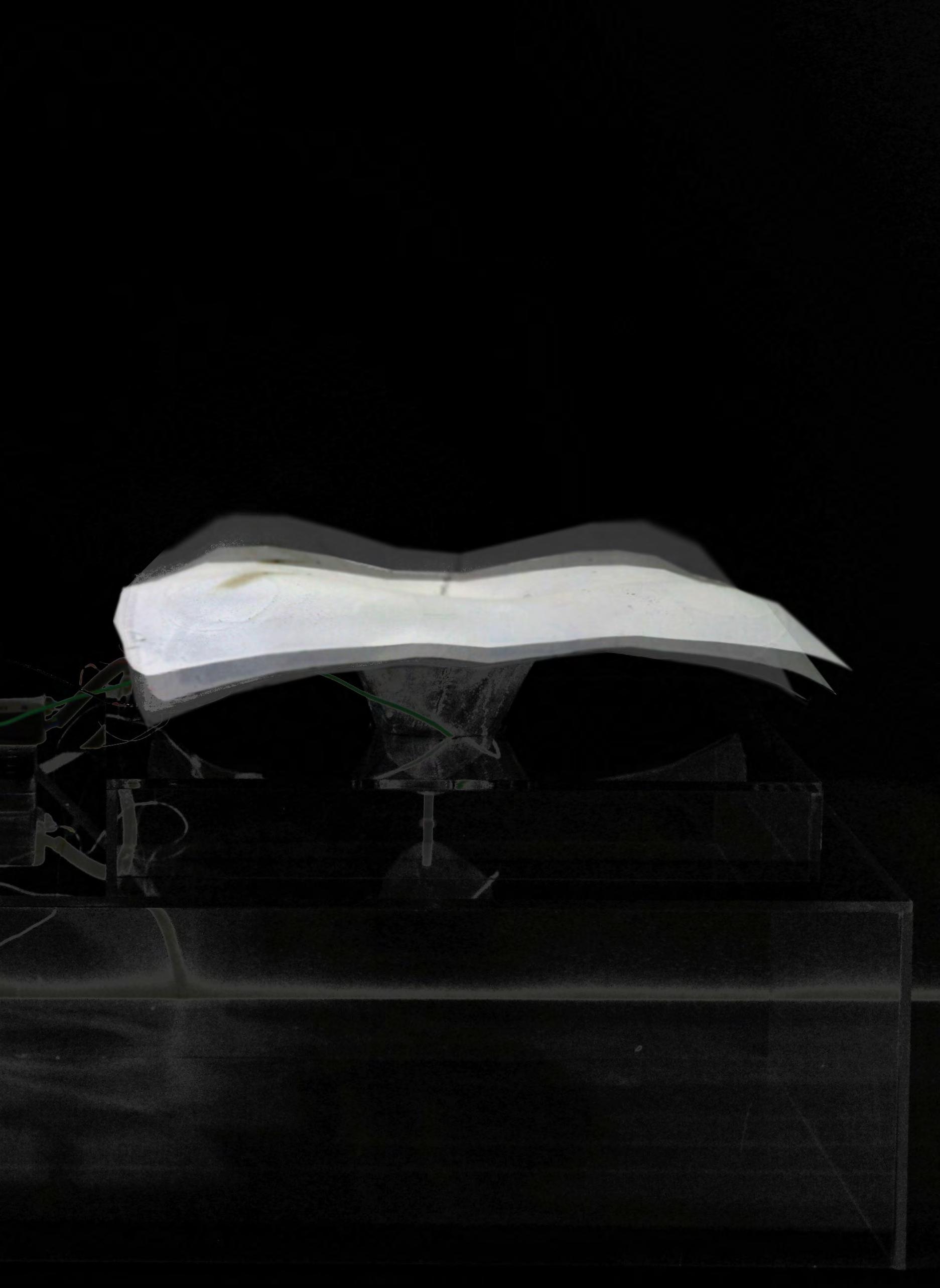
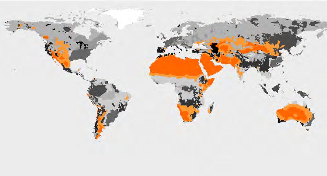
• Annual variation in temp. : 11- 42 °C

• Diurnal variation in temp. : 10-15 °C

• Relative Humidity: 30%- 50%

Critical Reflections and Self-Actuation potential of the system

The Final Experiment 9 - Fibre Composite Adaptive System was successful in terms of its functionality and performance. The hypothesis was proven and established through the physical experiments, i.e; to built an adaptive system that could sense , actuate and also control the flow of information through basic decision making.

A critical detail of the fibre composite model was its stiffness. It is essential to determine the scale of the structure in relation to the actuation function. One was able to understand the importance of the ratio of curvature change against the stiffness of the composite. In the case of the final experiment the stiffness of the model was very high as against the size of the alloys and the maximum curvature they could render.

Also, one of the issues of the sensing-actuation cycle was the delay in response time of the SMAs. This occurred due to the connectivity of the heating patches (in series) and the heat transfer loss from the silicon heating patches to the alloys. Using heating patches of 220V instead of the 110V in series, would lead to faster heating of the alloys and hence a quicker shape change in the model.

Self- Actuation

On an Architectural scale, the aim is to induce actuation not through an external heat/energy source, but by taking advantage of the environmental variation in temperature. Therefore, enabling the self-actuation potential of the shape memory alloys; with out the deployment of any external energy source.

Hot and dry climatic zones [ highlighted in Figure 2.29 ] which have a considerable diurnal variation in temperature would be the most appropriate to exploit the environmental energy for the efficient functioning of the adaptive system Commercially available SMAs are based on a range of actuation temperatures. The temperature of actuation ranges between 30 to 95 °C [ Figure 2.30 ]. The type of alloys used

throughout the experiments were a of value 65 °C. While, alloys with an actuation temperature of 35°C could actuate with the changes in atmospheric temperature.

For instance, in hot and dry climatic zones the variation in average atmospheric temperature would be between 22°C to 44°C in the summer months. Therefore, the surface temperature of the shape memory alloys could easily reach the actuation temperature of 35°C.

Information Processing and Decision Making

Self-Actuation potential of any structure invariably necessitates integrating decision making abilities, intelligent/smart behaviour into the adaptive system, i.e, to adapt appropriately to the changing environmental conditions. Morphological definition of the structure plays a key role in adaptation and has to be coherent with the actuation logic.

All emergent systems in nature have developed such a decision making and intelligent behaviour through evolutionary process. Responsiveness, on a short term and adaptability on a long term is established through their genetic information. In nature the genotype comprises of a genetic constitution of an individual organism, while phenotype is the characteristics of that individual organism resulting from the interactions between the genotype and the environment. The adaptive properties of natural forms stem from the generative processes that work upon successive versions (generations) of the genome. This genome is the compact data that is transformed into the biomass of increasing complexity through generations.[2.17]

The material tests and experiments conducted, establishes the premise for the architectural application of the fibre composite adaptive system proposed in the following chapters. The proposal would focus on taking advantage of the self-actuation potential of the system with reference to context specific climatic data. The site would be in the northwestern part of India, a hot dry climatic zone.[Figure2.29]

2.17 Weinstock, Michael, ‘Morphogenesis and the Mathematics of Emergence’, Emergence: Morphogenetic Design Strategies, p.-1017, Architectural Design Journal edited by Michael Hensel, Achim Menges and Michael Weinstock, Academy Editions, London,Vol. 74 No3, Issue- May/June 2004.

Figure2.29

Figure2.30 Actuation temperatures of commercially available shape memory alloys.

Alloy N

Alloy S

Alloy C

Alloy B

Alloy M

Alloy H

Flexinol Wire

Superelastic Alloy

Superelastic Alloy

Superelastic Alloy

Actuator Alloy

Actuator Alloy

Actuator Alloy

Actuator high fatigue

Superelastic standard alloy, 'colder' than alloy S (Af ca. -15° C)

Superelastic standard alloy, 'softer' than alloy N (Af ca. 0° C)

Cr-doped superelastic alloy, 'stiffer' than alloy S and N

Body temperature alloy (Af ca. 35° C)

Actuator Alloy with intermediate transformation temperatures (Af ca. 65° C)

High temperature actuator alloy (Af ca. 95° C)

Especially optimized actuator wire with high fatigue resistance (Af ca. 100° C)

3 D esign Application

Indus Heritage Centre

Ruins of Ancient city of Lothal

A museum for archaeological ruins, demands large span structures with minimal vertical supports. It is crucial where the structure touches the ground. The potentials of the fibre composite continuous surface could be utilised to achieve such a differentiated structure.

‘Lothal’- is one of the most prominent cities of the ancient Indus valley civilization which existed 4400 years ago. It is one of most important archaeological sites in the world from that era. Since its excavation in 1952 to 1961 the archaeological site has been a victim to harsh environmental conditions, causing irreversible deterioration. An adaptive structure covering the site would be ideal to protect it from the harsh environmental conditions and maintaining stable micro climatic conditions. The Indus Heritage Centre would house museum galleries, conservation laboratories and research facilities.

Site

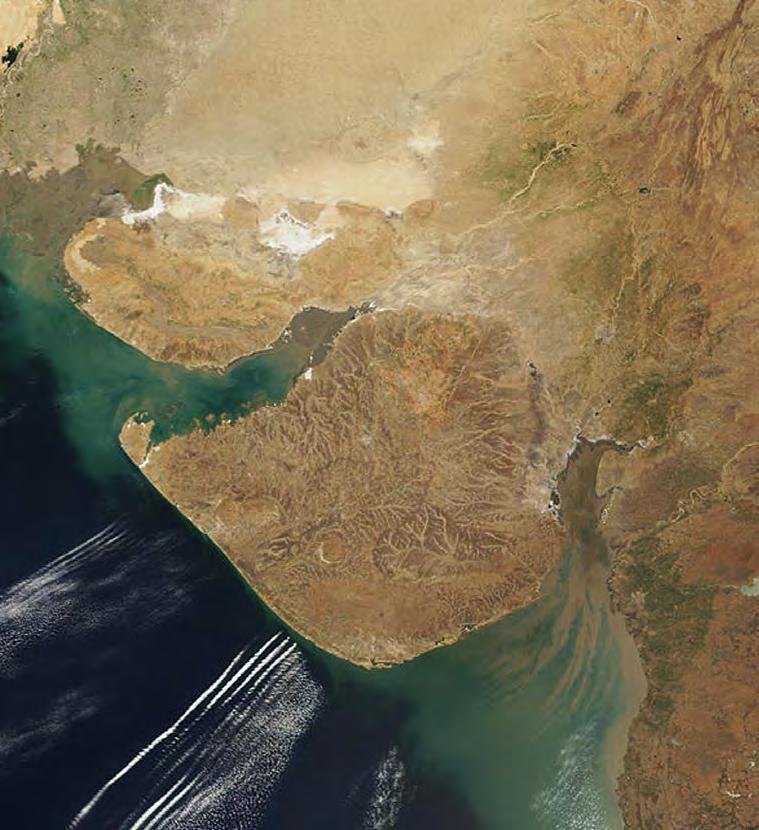
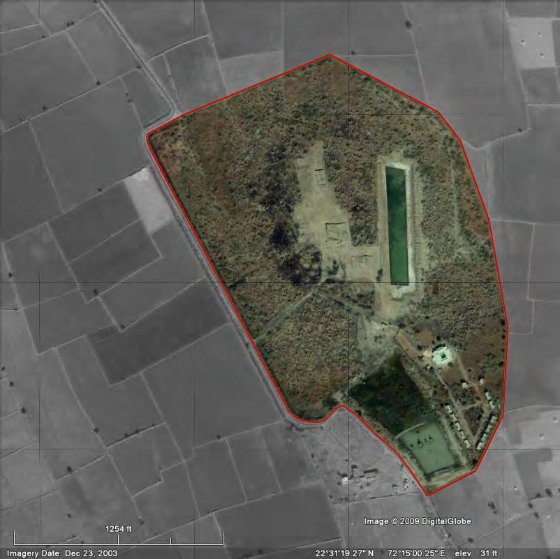
‘Lothal’- is located in the North western part of India in the state of Gujarat, about 85 km southwest of Ahmedabad. The ancient city developed on the left bank of river Bhogawa near the estuary where the river meets the Arabian Sea. With the changing coastline, now the ruins is situated 23km away from the coast from Gulf of Kambhat and 12m above mean sea level.

Lothal is one of the most prominent cities of the ancient Indus valley civilization which existed 4400 years ago. The site is approximately 400 X 800 meters covering an area of 26.5 hectares. It is one of the most important archaeological sites from that era.

Lothal’s dock, the world’s earliest known, connected the city to an ancient course of the Sabarmati river on the trade route between Harappan cities in Sindh and the peninsula of Saurashtra. It was a vital and thriving trade centre in ancient times reaching the far corners of West Asia and Africa.

Lothal’s people were responsible for the earliest-known portrayals of realism in art and sculpture, telling some of the most well-known fables of today. Its scientists used a shell compass and divided the horizon and sky into 8–12 whole parts, possibly pioneering the study of stars and advanced navigation—2000 years before the Greeks. [3.1]

Arabian sea

Gulf of Khambhat Gujarat

INDIA

Lothal

Figure 3.2 Location I Latitude: 22° 31’17’’N I Longitude: 72 ° 14’ 58’’E

Figure 3.1 Satellite image showing locations of ancient Harappan cities

3.1 Sir Wheeler, R.E.M, ‘The Indus Civilization(supplement to the Cambridge History of India), (Secon Revised Edition.), Cambridge, England, 1960.

Context

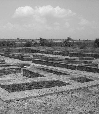
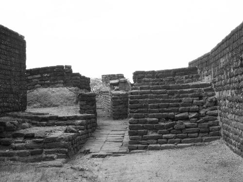
Archaeological sites are usually large in size. Once the excavation is completed, the relics are obtained and the site is reburied to protect it from weathering.

An on site museum with a super structure covering the ruins would protect it from weathering. Research could be undertaken by experts on site, while allowing ‘public exhibition’ and ‘preservation’ to be carried out simultaneously. ‘Floating walkways’- which do not touch the ground, could be developed to view the ruins from above. Digital simulations could be projected on the actual site to enable the visitors to visualise a reconstructed model of the ruins. Therefore, site protection, archaeological research and public exhibition could

happen simultaneously. This would bring about a user experience which is culturally unique and informed by scientific facts.

The museum housed within the adaptive roof structure would display the artefacts excavated. The museum would have galleries on conjectural ideas of the ancient Harappan town of Lothal. Artefacts such as beads, terra-cotta ornaments, replicas of seal and sealings, shell and ivory objects, copper and bronze objects, tools, potteries and objects recovered from burials and ritual objects yielded from excavations would be exhibited. The museum would also house a library and a publication counter.

Citadel Lower town

Artefacts and Seals

Figure 3.3

Plan of Excavated Ruins

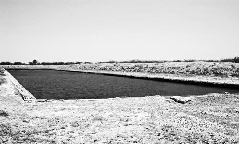
The most dominant structure of Lothal is its dockyard, spanning an area 37 meters from east to west and nearly 22 meters from north to south. It is one of the pioneering works of maritime dating 5000 years back. Ships would have entered in the northern end of the dock through an inlet channel connecting to the estuary during high tides. The lock gates could be closed to raise the water level for floatation. An inlet channel from the tank allowed excess water to escape.[3.2]

Warehouse of Lothal was located on a plinth of about 3.5 meters. The whole town was situated on a patch of high ground. A wall was erected to encircle the town, and a platform was built where goods were stored.

Citadel, near the warehouse is also on a high plinth. The upper town or acropolis spans 128 by 61 meters and has extensive drainage systems. [3.3]

Lower town contains commercial and residential areas. The arterial streets running from north to south were flanked by shops, merchant dwellings and artisan’s workshops. Streets running from east to west led to the residential areas with lanes allowing access to individual dwellings. The bead factories, situated at the conjecture of residential and commercial areas, comprised the main industry of the Harappans. The factory comprises of rooms, which includes worker’s quarters, warehouses and guard rooms, surrounding a courtyard.

Lower town Citadel Ware house Dock

Bead Factory Cemetery

Citadel Dock

Figure 3.5

Figure 3.4

3.2 Rao, S.R, ‘A Persian Gulf Seal from Lothal’, Antiquity, Vol. 37 pp. 96-99 and Plates 9,10,11,Cambridge, England, 1963.

3.3 Possehl. L .Gregory, ’The Indus Civilization’, - A Contemporary Perspective, pp.80-85, Rowman and Littlefield Publishers. Inc. , Oxford, UK, 2002.

Climatic Data

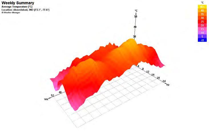
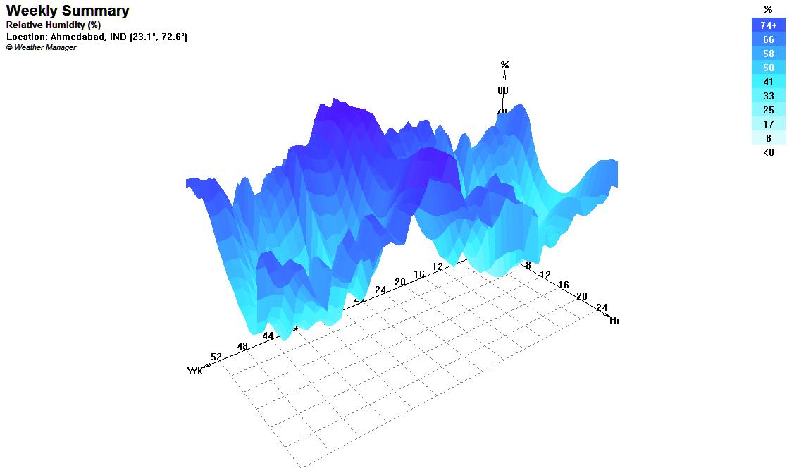
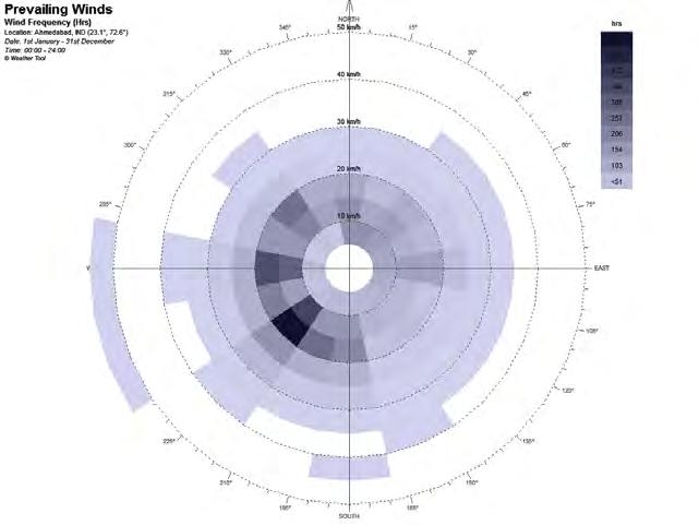
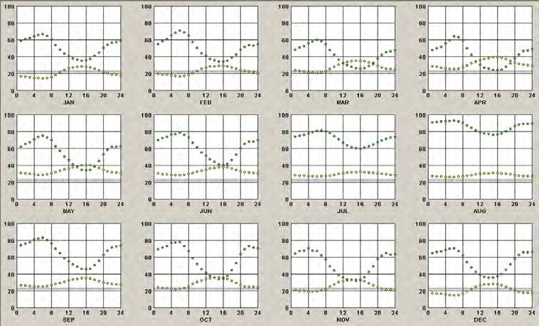
Lothal experiences ‘Semi-Arid climate’, with high air temperatures.[ Figure 3.6] It receives intense direct solar radiation of 4.4 to 7.3kWh/m2 , (daily global radiation). The diurnal variation is temperature ranges between (12 to15oC). The annual average mean sky luminance is about 25,500 lx. [3.4]

Due to the proximity to the coast of Arabian sea, it experiences fairly high humid and dry months.[ Figure 3.7] The months of June-August receive the maximum rainfall the rest of the year almost remains dry.

The site located about 25 Kms from the coast,alongthe south western direction experiences fairly good wind velocities

ranging between 3.2- 5m/s on an annual average. Almost all year round the year the predominant wind direction is from the south west. [ Figure 3.8 ]

The annual temperature, humidity graph [Figure 3.9] shows that the maximum summer temperature reaches 42oC and the maximum winter temperature reaches 32oC. This is well with in the range of the actuation temperature of shape memory alloys 35oC. Therefore the site would be ideal to deploy the adaptive structure which could close when the temperature rises above 35oC and remain open for temperatures below that value.

Figure 3.8 Prevailing wind direction: South West

Figure 3.6 Diurnal variation in temperature: 12-15 oC

Figure 3.7 Average Relative Humidity: 60%

Figure 3.9 Annual graph of Temperature I Humidity I Comfort zone

3.4 Weather Data source : ISHRAE, Indian Society of Heating, Refrigerating and Air Conditioning Engineers.

Precedents I New Acropolis Museum I Athens

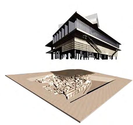
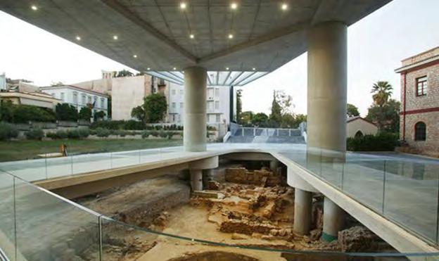
A museum over archaeological ruins should be rather sensitive to the ground conditions to protect the key elements in the ruins. The New Acropolis museum over the ruins of Marikygianni in Athens deploys a Reinforced cement concrete structure. The main galleries and museum activities are raised on pilotis or a highly dense concrete column grid.

The grid grows denser at the base[Figure 3.12] of the structure owing to seismic requirements. This kind concrete column grid’s intervention on the existing ruins causes irreversible loss of some parts of the ruins; also the observer is no more able to perceive the ruins as an autonomous entity as it is always read in juxtaposition against the new structure. An intercession of

this nature has to be essentially avoided. [Figure 3.11]

The architect’s statement is rather an oxymoronic, ‘The base of the museum floats on pilotis over the existing archeological excavations, protecting and consecrating the site with a network of columns’. [Figure 3.10] It is rather indispensable to explore the possibilities of a structural system that could span large areas.[3.5]

Concrete column grid

Archaeological site of Makrygianni

Figure 3.11 View from ruins level

Figure 3.12 View from entrance ramp

Figure 3.10

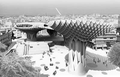
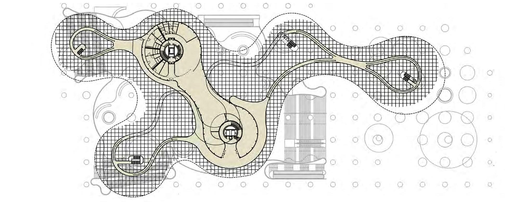
3.6 Referred from Project booklet Metropol Parasol,’ Redevelopment of plaza,de le Incarnacion, Seville,Spain. http://holcimfoundation.org/Portals/1/ docs/ES_booklet.pdf

Precedents I Meteropol Parasol I Seville

The Metropol Parasol is a large scale urban development project built over the archaeological ruins of Seville. The scheme with its large mushroom like structures protects the archaeological site consecutively providing a farmers market, an elevated plaza, cafes and restaurants underneath and within the parasols, as well as a panoramic terrace. The structure manufactured from laminated wood with intersecting crate morphology. [3.6]

The parasols grow out of the archaeological excavation site. The columns become prominent points of access to the museum below as well as to the plaza and panorama deck above. One of the significant features of the structure is

the spanning of the columns, the column centre to centre distance ranges from 100-120m. The structure stands in the middle of a square which is approximately 415 X 200m.

The archaeological remain inform the negotiation of the positioning of the 6 columns/ vertical circulation. The structure is porous allowing the efficient natural ventilation in the square and reducing the penetration of harsh sun light. The structure proves efficient programmatically, structurally and also environmentally.

Laminated wood structure Archaeological Ruins

Figure 3.13 Section

Figure 3.15 Plan approx. ground coverage 415 X 200 m

Figure 3.14 Aerial view

Precedents I Emperor Qin’s Terracotta Warriors Museum I Xian

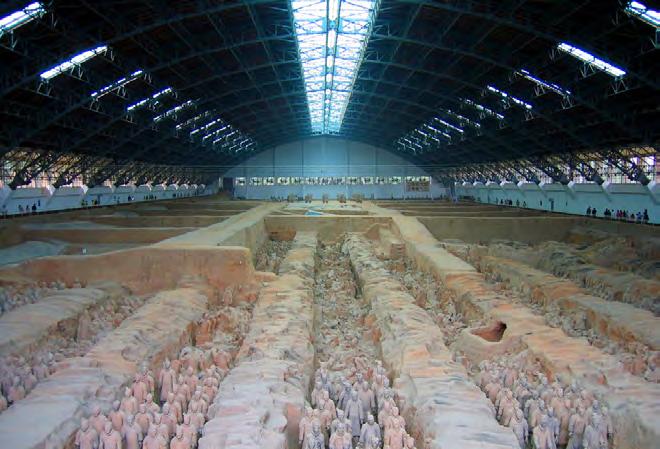
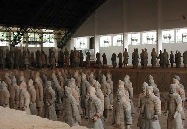
The Emperor Qin Shi Huang’s terracotta warrior’s museum in the Xian province of China covers the archaeological ruins of the Qin Dynasty. The ruins consist of long trenches which have a complete replicas in terracotta of the emperor’s army. The structure covers an area of 75 X 225m. The roof structure is rather conventional, similar to any industrial structure which covers a large span. The arch truss is made of tubular steel components in two parts with a joint at the centre.[3.7]

The structure has a sequential array of these arch trusses connected by purlins which run along the entire length. There are visitor walkways along longitudinal direction on both sides with some intermediate passages connecting them.

These walkways allow the visitor to observe the process of archaeological preservation, as each the conservation of the sculpture is carried out on site. Though the structure does not intervene with the archaeological ruins, the lighting within the structure is inefficient. The structure being completely covered necessitates mehanical means for maintaining stable micro climatic conditions.

3.7 Referred from,

http://www.chinaculture.org/gb/en_ museum/2003-09/24/content_30784. htm

http://www.chinamuseums.com/ qinshihuangt.htm

Steel truss structure (Spanning 75 X 225m)

Archaeological Ruins

Figure 3.16 Section

Figure 3.18 Interior view

Figure 3.17 Interior view

Enclosed space - public

Enclosed space with private access

Semi open space - public

Exhibition space.

Museum shop, Book Shop.

Temporary exhibition gallery.

Restaurant and cafe.

Floating walkways for viewing the ruins of the ancient city.

Entrance and Information centre.

Program Elements

The Indus Heritage Centre would cater to the requirements of public visitors and the scholarly community to provide scientifically derived information on one of the earliest urban societies. The Centre would be involved in supporting research, conservation, training and education, the program elements are based on these functions.

The program elements are divided based on the type of spaces required, namely, enclosed space for public, enclosed spaces with private access, semi- open space for the public, miscellaneous spaces and services.

Spaces such as permanent galleries, library and auditorium require large areas and a controlled environment to protect the artefacts. While cafes, restaurants and other supporting activities could be positioned on semi- open areas with transient but comfortable micro climates. 1-2 million visitors are expected to visit the centre annually.

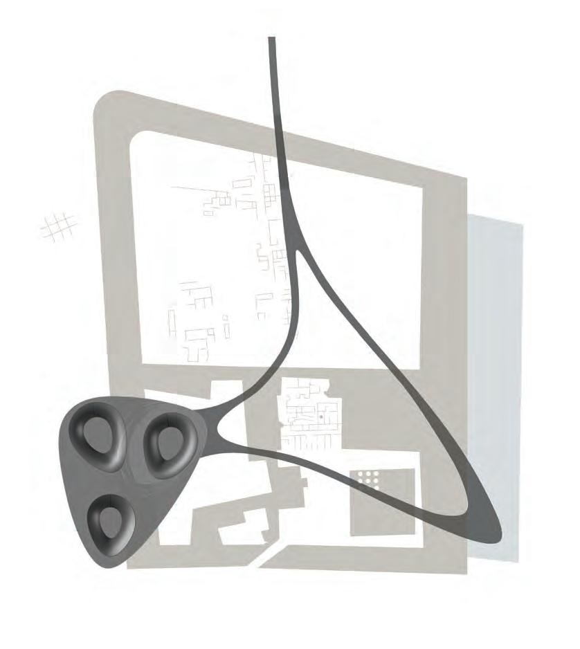
Fibre Composite Adaptive roof structure

Micro climatic control

Rainwater harvesting

Sub structure

Permanent Exhibition space

Temporary exhibition gallery

Auditorium

Library and archives centre

Museum shop, Book Shop

Restaurant and cafe

Research and conservation centre

Administration office

Restoration laboratory and Storage

Walkways

Floating walkways for viewing and Decks Craft demonstration zone

Schematic Plan of the Design Proposal

The plan shows the conceptual layout of the design proposal for the Indus heritage centre over the archaeological ruins of Lothal. There are three key elements in the design proposal.

1. The most important one being the adaptive roof that would cover about three quarter of the ruins. The roof structure would span an area of about 300 X 175 meters covering an area of approx. 52500 Sq.m. The structure would be made of fibre composite embedded with sensing and actuation technology, which could enable the adaptive potential of the structure.

The adaptive structure would perform two key functions. Firstly, to maintain comfortable microclimate within the structure. The actuators would control the openings by increasing or reducing, solar penetration and air ventilation with respect to the change in environmental conditions. The second function of the roof would be to act as a rainwater harvesting device. The area being in the hot and dry climatic zone, receives heavy rainfall only for one month in a year. Therefore the harvested rainwater could be used for the museum requirements.

2. The substructure, within the fibre composite adaptive roof would house all the museum activities. The morphology of the substructure is defined in such a way to accommodate all the three kinds of spaces discussed earlier, namely enclosed (public), enclosed (private) and semi-enclosed spaces.

As observed in the diagram there are three large envelopes which would accommodate the permanent gallery, library and auditorium which require complete enclosure. Activities such as administrative office, storage and conservation centre would be placed on a lower level of these envelope, enclosed with private access. The cafes, restaurants and shops would be in a semi open elevated plaza, interconnecting the enclosed spaces.

3. Floating walkways, are elevated ramps and path ways which would allow the visitor to meander and observe the ruins from above. The walkway runs parallel to the main city road of the ruins running north-south. Also the walkway, connects the main features of the ruins, such as the ancient dockyard and the citadel framed in the centre. Alternatively the visitor can choose to directly enter the museum galleries.

4 D igital Experiments

Form Finding Methods

Digital Form generation experiments were focused on developing a geometric/parametric rational for deriving a continuous shell geometry. Two methods of form finding have been elaborated, parametric definition and dynamic relaxation algorithm. The final global form was derived through the dynamic relaxation method which has an integral logic of minimal surfaces. Solar insolation analysis was performed for selecting a particular global form which would receive minimal solar gain. This base shell geometry would be further analysed through finite element analysis(structural) to organise the fibre based on principal stress paths..

Figure

Sur face Parametric Definition Method

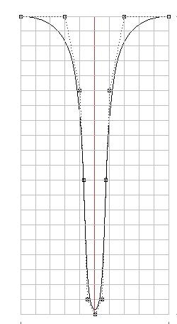
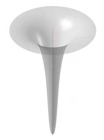
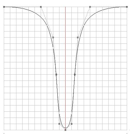
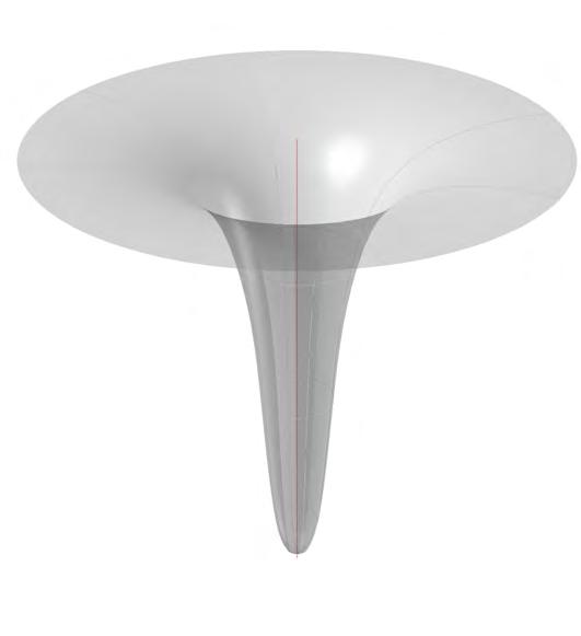
The architectural ambition is to develop a continuous fibre composite shell structure, covering three quarter of the archaeological site. [Figure 4.1] The geometry of the double curved shell would be defined, in such way that it touches the ground only at minimal points without affecting the existing ruins. Further, the aim is to enable the adaptive potential of the shell, through creating openings that have the ability to actuate; controlling sunlight penetration and air ventilation.

Through defining the parameters of the curves that generate the surface, various proportional relationships could be achieved in the forms generated. [ Figure 4.3 ] The continuous surface is essentially made of two types of components,

the vertical cone like surfaces and the horizontal double curved surfaces. This method of distinguishing the surface geometry into horizontal and vertical elements was mainly based on considering braiding as a manufacturing process for the vertical surfaces. As braiding happens over a revolving mandrel, this technique would allow for geometries developed by revolution along a single axis, also the forms could be asymmetrical along the centre axis. The constrain with braiding techniques is that there cannot be cross sectional variations with the exception of tapering geometries to enable the release of the mandrel.

The curve that generates the vertical cone like surfaces was

Figure 4.3

Shows mathematically the different forms of fish due to different growth rates, On Growth and Form,

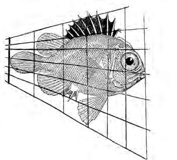
Rotational Symmetry

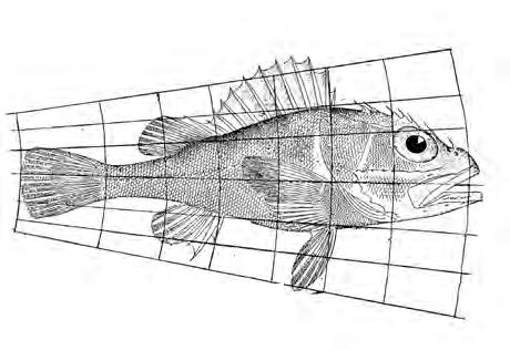
Asymmetry about one plane

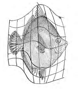
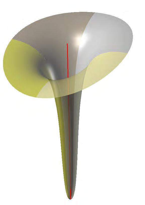
Asymmetry about two planes

defined with eleven control points on a regular square grid. This square grid could then be distorted to achieve different proportional relationships,––– much like the diagrams made by D’arcy Thompson.[ Figure 4.2 ] The column surface is generated by the defining curve through revolution along the centre axis. The diagram on the left shows two different columns having different proportions generated by the parametric curve. An assembly of these forms would render only a planar horizontal roof.

The vertical column surfaces could be asymmetrically defined to fit single curvature and double curvature roof planes. The figure 4.4 ( centre and right ) shows two different columns

which are asymmetrical along one plane and two planes. An assembly of the columns which are asymmetrical along one plane would generate a single curved surface; asymmetrical columns along two planes would generate a double curved surfaces. [ Figure 4.5, 4.6, 4.7 ]

Figure 4.2

D.W.Thompson.

Figure 4.4

symmetry - Planar surface

Limitations of Parametric Definition Method.

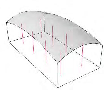
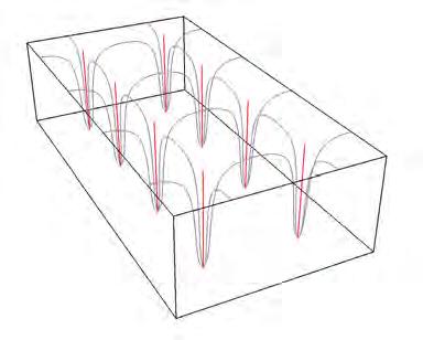
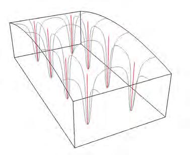
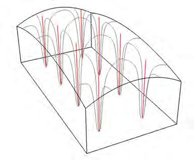
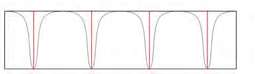
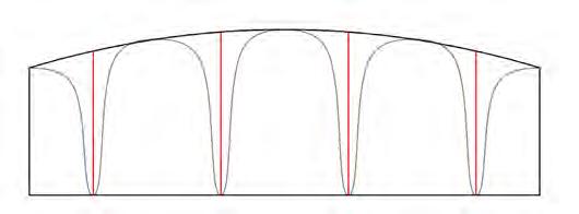
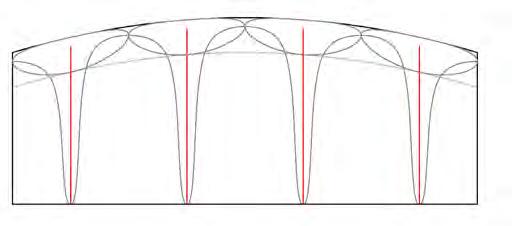
The parametric definition method has certain inherent limitations. Since the geometry of each component is manipulated and built manually, achieving differentiation in the proliferation of columns becomes complex. The radius of curvature varies sharply along the surface.

This method of building the geometry does not integrate any structural logic, consequentially performing (structural) finite element analysis of the surface becomes rather complicated. Nevertheless, the manufacturing logic would still remain the same, with the assembly of vertical components and horizontal components. [ Figure 4.5, 4.6, 4.7 ]

A logic of maintaining constant radius of curvature within the surface geometry as in the case of minimal surfaces would integrate the structural logic within the system. Differentiations could be achieved in the placement of columns and the spanning zones.

For this reason dynamic relaxation, a digital method to simulate formation minimal surfaces has been used. A custom algorithm was written to define the parameters and numerically determine the resultant geometry. The algorithm is further elaborated in the following section, Dynamic Relaxation Algorithm.

Rotational

Asymmetry about one plane - Single curvature surface

Asymmetry about two planes -Double curvature surface

Figure

Figure

Figure 4.7

D ynamic Relaxation Algorithm

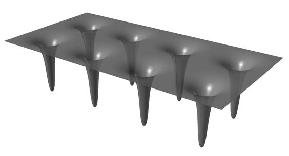
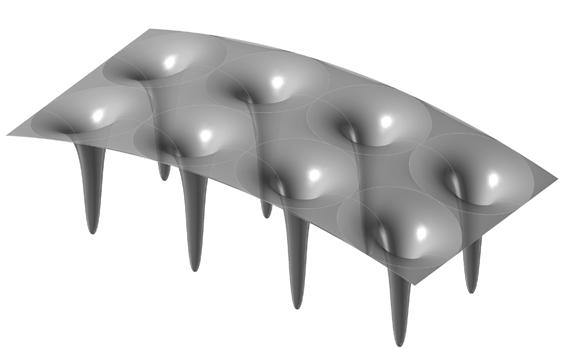
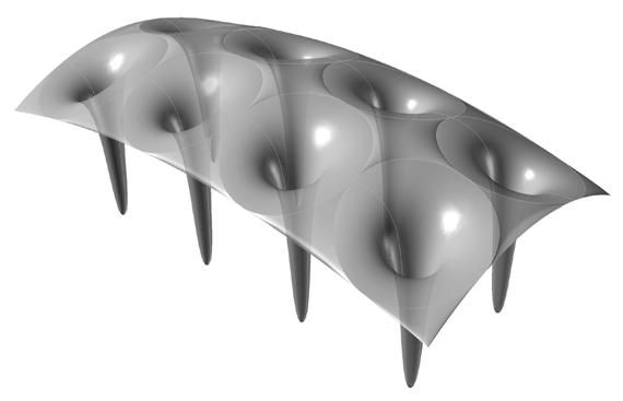
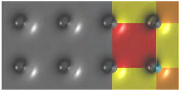
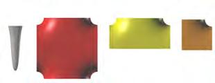
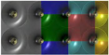
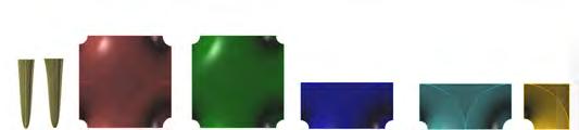
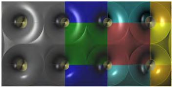
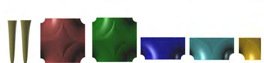
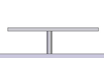
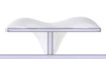
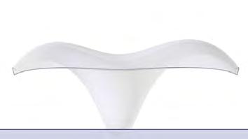
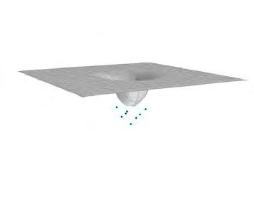
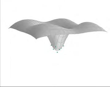
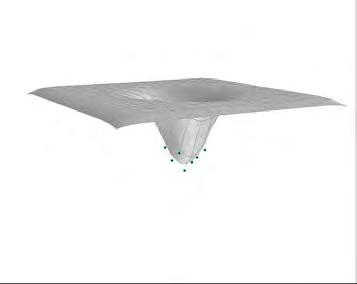
As observed in the figure 4.8 the goal is to substitute the role of a conventional roof-column structure with a thin double curved surface. The shell structure would perform the roles of both a column, in transferring loads to the ground while, acting as a spanning element to cover the site. The shell structure by virtue of its double curvature would render a certain degree of stiffness to the system, which could be further enhanced by providing structural depth. The definition of the surface geometry was carried out through digital form finding.

Visual Basic Scripting

The images above show the typological process of digital form finding through the ‘Dynamic Relaxation Algorithm’, written in visual basic to generate the global morphology. [Figure 4.9 ]

which could digitally simulate the working logic of a physical hanging chain model. The aim is to find geometrical forms in which all forces are in equilibrium. In the past this was done through physical models, using hanging chains and weights or through soap films, which have the property to form find a minimal surface. The dynamic relaxation method is based on discretization the continuum under consideration by lumping the mass at nodes and defining the relationship between nodes in terms of stiffness. The system oscillates about the equilibrium position under the influence of loads. An iterative process is followed by simulating a pseudo-dynamic process in time, with iterations based on an update of the geometry.

[ 4.1]

There are several parameters which influence the form finding process. The system is defined as a set of particles and springs. The mass of the particle and the stiffness of the springs is defined for each object. The algorithm mainly uses

Figure 4.8

Figure 4.9 Form Finding through Dynamic Relaxation

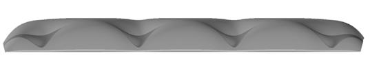
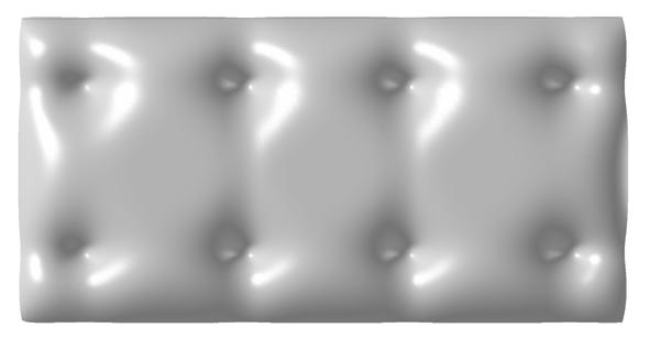
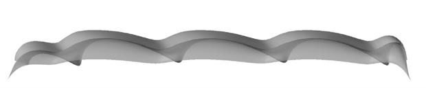
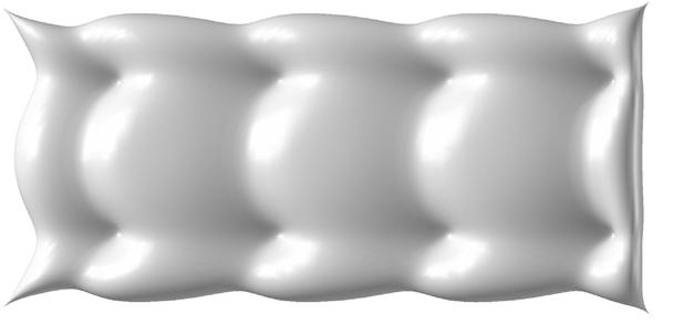
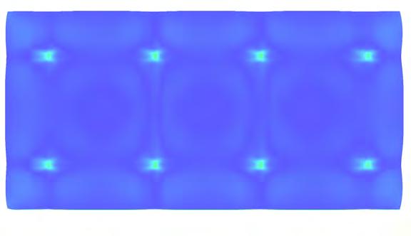
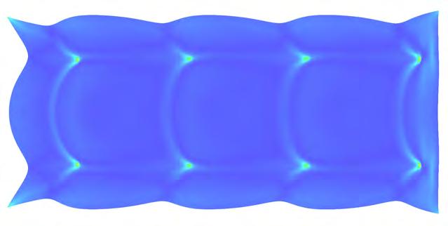
two equations, Newton’s second law of motion (F=m*a) and Hooke’s law (F=-f*x). Gravity , time / no. of iterations , initial position of the particles , drag coefficient are some of the important parameters defined to perform the calculations and derive the resultant geometry.

By varying each of these parameters a wide variety of forms could be generated. Apart from the mass of the particle, an external force could be defined to act on the particle to constrain points to the ground. The definition of external forces result in the column like structures within the surface.

The process starts with a flat surface located at the height of what would have been a simple roof. Vertical loads are applied around the perimeter of a fictitious central column, responsible for transferring the loads to the ground. The rest of the parameters of the system are input in the algorithm. At a particular instance during simulation the points/particles

defining the surface start oscillating. A few minutes later, an equilibrium status is found and the overall form is defined. [Figure 4.9]

The curvature of the roof surface depends of the applied external loads. By changing the magnitude and direction of the external force vector the orientation of the column structure could be manipulated. This enables the possibility of maximising or minimizing the surface area of solar exposure. The resultant geometry could be chosen based on the solar exposure criteria. [Figure 4.10,]

It can also be observed from the mean curvature analysis that the curvature remains constant through out the surface as in minimal surfaces. [Figure 4.11]

Figure 4.10 External forces applied at 90o (above) and 30o (below)

Figure 4.11 Mean curvature analysis

Configuration of Supports

The diagram above shows the schematic configuration of supports for the shell structure. The touch down zones are marked as hatched areas, these zones are either outside the boundary wall of the ruins or at zones which have minimum structures of the archaeological ruins. [ Figure 4.12 ]

The column structures are placed at a distance of 80 metres apart from each other. It can be observed that there are only three columns within the ruins. The columns are placed in such a way that they form a triangulated network. This would provide for greater stability and not less than three principal paths/arches to transfer the loads vertically.

The shell also has continuous edges supports on three sides as highlighted in the diagram. The free edge on the north would form a large arch as a result of dynamic relaxation.

During dynamic relaxation, external forces would be placed at the position of the red dots to create the column structures, While the particles forming the edges would be defined with zero mass, constraining the edges to the ground plane.

80m radius

Shell Touch down zones

Edges supports

Figure 4.12

Population of Shells

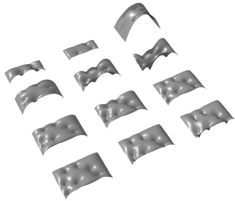
The diagram above shows various shell forms derived through manipulating the parameters of the dynamic relaxation algorithm. [ Figure 4.13 ]

Row A - When a greater mass was defined for the particles, they started accelerating faster resulting in forms that were very high and without a distinct column definition.

Row B - Lesser stiffness in springs, resulted in shell forms which were almost like a piece of fabric . It was crucial to perform several iterations to define the most appropriate stiffness factor to achieve a height not exceeding 50 meters and similarity in all the column forms.

Row C - Once the appropriate stiffness was determined, variations in the magnitude of the external loads were iterated. All the shells in row c have external loads applied at 90o the relaxation surface.

Row D - The final parameter to be defined in these set of iterations was the direction of the external force. The diagram shows three different orientations with 90o, 45o and 60o

Figure 4.13 Surfaces generated by varying the parameters of dynamic relaxation algorithm.

A - Mass of the particles

B - Stiffness of the springs

C- Magnitude of the external forces

D- Direction of the external forces

Degree of solar exposure

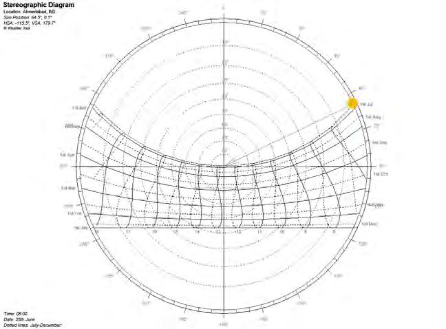
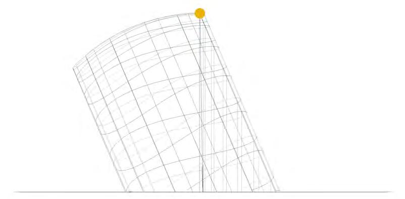
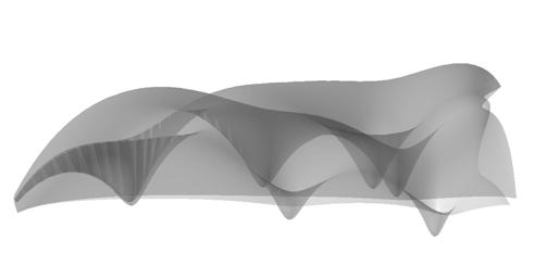
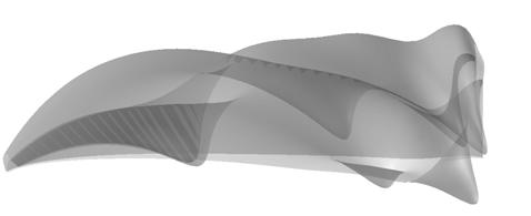
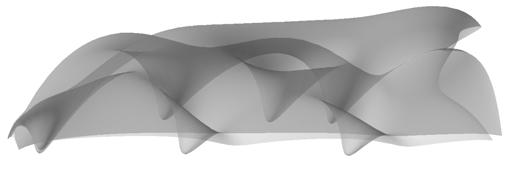
Once the right parameters were determined for dynamic relaxation to the render the appropriate height and stiffness for the shell, the next step was to select the fittest shell form from this population. The degree of solar exposure is an important fitness criteria that influences the selection process.

In hot and dry climatic zones, the aim is to reduce the degree of solar exposure and minimize the solar gain. The site being located in the northern hemisphere experiences a southern tilt on its sun path [ Figure 4.14]

During the summer months of April-September the solar azimuth angle is almost perpendicular to the ground plane, particularly between 10am to 2pm. During the winter

months between October- February the solar azimuth angle is far swallower.

The shell surface covering a large area could be assumed almost as a horizontal plane on a global scale. Reducing the solar exposure and achieving self shading could be enhanced only through exaggerating the geometry of the column structures, by tilting the orientation against the direction of sun path [Figure 4.15, right] This would considerably reduce the solar gain, also some parts of the structure could self shade. The other two options , with vertical orientation and orientation towards the sun path proved inefficient in minimizing solar gain. [ Figure 4.15, left and centre]

Figure 4.15 Vertical Orientation

Figure 4.14 Annual Sun Path Diagram

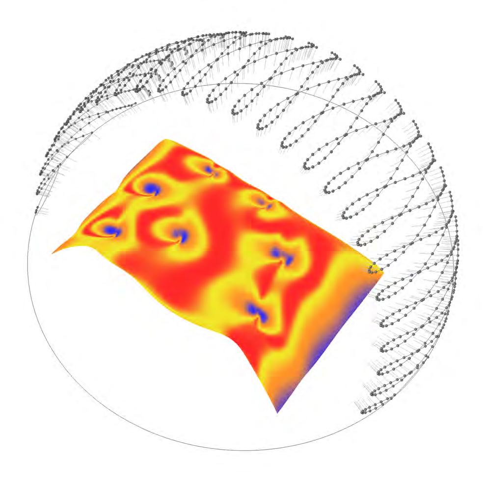
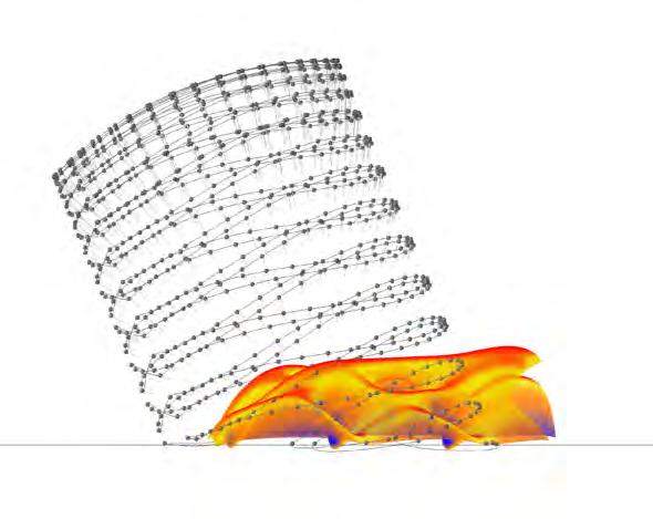
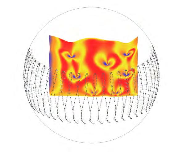
Time period: Annual (1st Jan to 31st Dec) Longitude: 72o 13’ Latitude: 22o 31’ Platform: Rhino Grasshopper

- The Solar Position algorithm is based on National Oceanic and Atmospheric Administration’s Solar Position Calculator http://www.srrb.noaa.gov/highlights/sunrise/azel.html

- Calculation of solar irradiance is in general based on algorithm by University of Oregon Solar Radiation Monitoring Laboratory http://solardat.uoregon.edu/SolarPositionCalculator.html

Solar Insolation Analysis

Solar insolation is the amount of electromagnetic energy or the amount of solar radiation incident on the surface of the earth. Solar insolation analysis is the study of incident solar radiation impacting the structure. Incident solar radiationinsolation refers to the wide spectrum of radiant energy from the Sun which strikes an object or surface. This includes both a direct component from the Sun and a diffused component from the visible sky.

The objective of the analysis is to determine the amount of radiation received on the surface of the structure being analysed. The outputs generated from the analysis are graphical and tabular representations of the amount of radiation (Watt-hours) received by the structure in a given period of time. [ 4.2]

The analysis was performed on the shell surface for an annual time period from the 1st January to the 31st March. It was observed that the zones with shallow curvature receive maximum radiation.

The base of the column structure which has a sharp change in curvature receives the minimum solar radiation. Also, due to the tilt in the orientation of the columns, they begin to self shade. Grasshopper platform was used to perform the solar insolation analysis.

Figure 4.16 Solar Insolation Analysis

Figure 4.17

Figure 4. 18

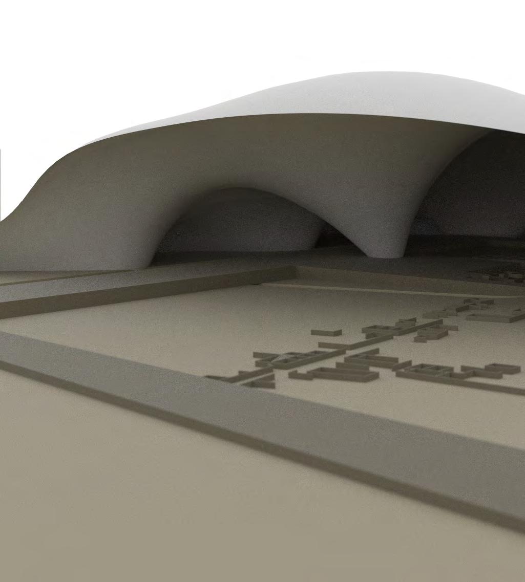
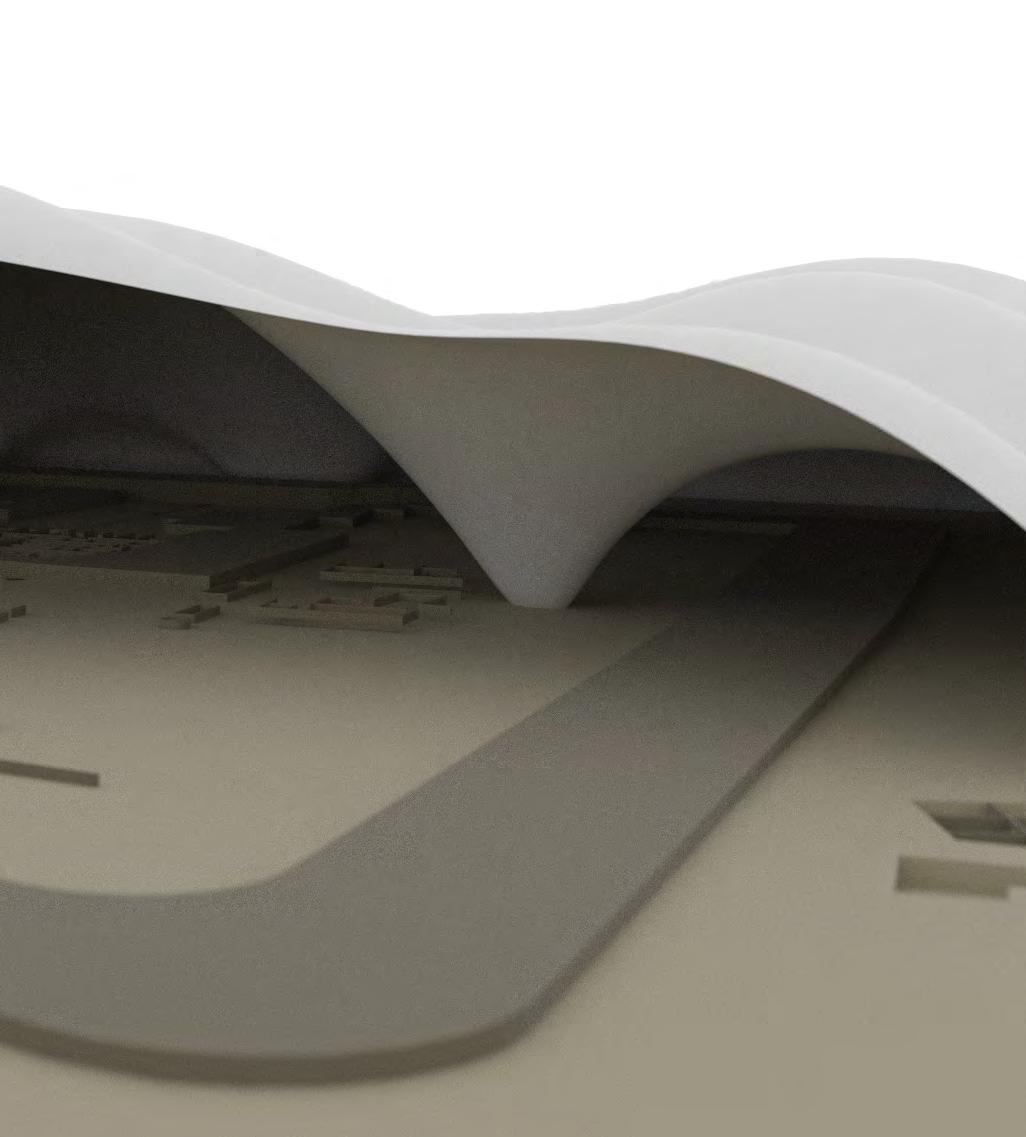Figure 4.19 Base morphology of the shell structure

5 Performance and Adaptability

Structural Performance

A fibre organisation strategy was employed to achieve efficient structural performance of the fibre composite shell, which was formulated on the basis of interactions between material and forces. In natural constructions, material is being continuously removed from places where it is not required and deposited where it can contribute to maintain the structural integrity of the structure. This concept was summarised by D’Arcy Thompson as “Growth under stresses”. Such a differentiated distribution process of fibres emerges through sensing the patterns of loading, or stresses constantly received by the natural organism.

This process of stress analysis forming the data set for fibre organisation results in optimal material usage and great structural efficiency. Finite element analysis was used to derive the principal stresses by simulating loading conditions. The data set was further used to organise the fibres in different hierarchical levels. An algorithm was written in visual basic to simulate these natural process in the digital environment- ‘Fibre Organisation Algorithm’.

maximum, middle and minimum principal vectors. The last three correspond to the angle sequence required to produce a coorsystem whose x,y and z-axis are the direcmaximum, middle and minimum principal respectively. This Euler angle sequence is

Finite Element Analysis - Principal Stress Vectors

θxy,θyz,θzx and orients the principal coordinate relative to the global system. obtain the components of the principal Cartesian coordinates, it was necessary to Euler rotation matrixes.

these values were conveniently stored in an vbscript and the design platform Rhino.

Fibre directionality and Fibre density are important factors that influences the strength of fibre composites. Fibre directionality accounts for the orientation of the internal loads that would need to be withstood by the material: ‘force travelling paths’. While fibre Density responds to the variable magnitude, being denser where there is a concentration of higher loads which need to travel through.

These fibre organisation mechanisms act at the micro level, but are also responsible for the overall form. Smooth or sharp curvatures in the overall form (macro scale) are the result of the fibre organisation in the micro level. In the micro level, fibres are oriented following the direction of the lines of principal pressure which by extension are the lines of principal strain, also known as principal stresses. In other words, the direction of the fibres responds to the direction of the internal forces present in the material. Also in the micro level, fibre density is increased or decreased according to the scalar value of the forces locally. There would be areas where there is a concentration of load and thus, a higher density of fibres will be supplied. In contrast, material should be saved in areas where loads are lower.

This process of fibre distribution was simulated digitally through an algorithm written to fit the specifications. The process started by form finding - dynamic relaxation (elaborated in the previous chapter) to determine the overall form, for which the optimum fibre organisation would be subsequently found.

Finite element analysis was performed to obtain the principal stress vectors. The design process continues with the static structural analysis of the shell surface in ANSYS which focuses on extracting the stress values at each point of the surface and in particular the principal stresses vectors. The data given

by ANSYS requires certain manipulation before it can be used to distribute and orient the fibres. At this point, it would be necessary to explain in detail how stresses are defined and why the principal stresses are particularly interesting for the development of the fibre organisation algorithm.

Stresses are not uniformly distributed over a cross section of a material body, [ Figure 5.2,5.3] and consequently it is necessary to define the stress not at a given area but at a specific point in the body. The stress at any point in a continuous shell surface is defined by a second order tensor known as the Cauchy stress tensor:

The Cauchy stress tensor can be rotated into another coordinate system such that only normal stresses remain and all shear stresses are zero. The three normal stresses that remain are called the principal stresses: σ1 – maximum, σ2 –middle and σ3 – minimum. [Figure 5.1]

The data exported from ANSYS is organised in six columns. The first three correspond to the modules of the maximum, middle and minimum principal stresses vectors. The last three correspond to the Euler angle sequence required to produce a coordinate system whose x,y and z-axis are the directions of maximum, middle and minimum principal stresses, respectively. This Euler angle sequence is θxy,θyz,θzx and orients the principal coordinate system relative to the global system.

In order to obtain the components of the principal vectors in Cartesian coordinates, it was necessary to use the Euler rotation matrixes. Once these values were conveniently stored in an excel file, the distribution of the fibres is made with the aid of vbscript on the design platform Rhino.

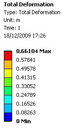
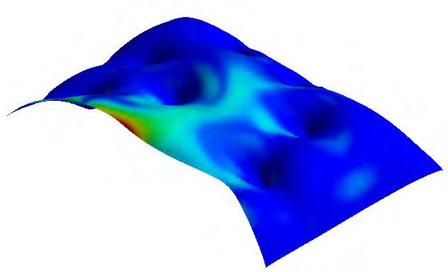
Thickness of the shell: 20cm

Loads: Self load & Pressure: 10Kpa

Supports : Fixed Supports at column base and three edges

Platform: Ansys

Material: Carbon fibre (Kevlar in epoxy resin)

Young’s Modulus: 75 Gpa

Poisson’s Ratio: 0.34

Thermal expansion Coefficient: 4 strain/K

Density: 1.4 g/cc

Figure 5.2 Finite Element Analysis - Static Structural

Figure 5.3 Finite Element Analysis - Plan and front elevation.

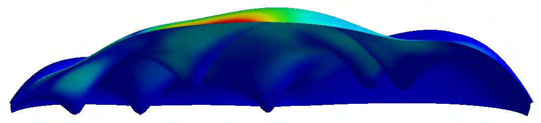
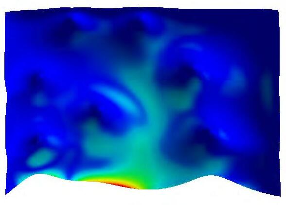
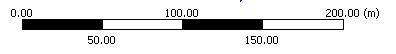
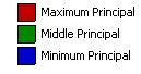
Figure 5.4 Image extracted from the FEM model developed in Ansys for the post-analysis of the form found geometry, to obtain the magnitude and direction of the principal stresses.

Figure 5.5 Data set of principal stress vectors extracted from Ansys FEM static structural analysis

Fibre Organisation Algorithm

The Fibre organisation algorithm digitally simulates the growth of the fibres. In bones, fibres are distributed following the direction of the lines of principal pressure whose equivalent in structural engineering are the principal stresses [5.1]. The principal stresses are obtained by rotating the ‘Cauchy stress tensor’ - originally oriented in Cartesian coordinates- into such a coordinate system that shear stresses are zero and only normal stresses remain.

Shearing forces are those which produce ‘angular distortion’ or in other words, it is a force that tends to cause particles to slide over one another. While shearing stresses can by no means be suppressed, the danger of rupture under shearing stress is lessened the more we arrange the fibres along the lines of principal stresses since there is no shearing stress along or perpendicular to these lines.

The shearing stress is greatest in the ‘neutral zone’, where neither tension nor compression are manifested; the neutral zone is defined by the line which cuts at equal angles of 45 degrees the orthogonally intersecting lines of pressure and tension. Therefore, laying the fibres along the lines of principal stress will diminish the adverse effects of the shearing forces and will contribute to minimising the amount of fibre material utilised. [Figure 5. 6]

The algorithm would start by asking the user to select a ‘surface’. It then continues by importing the data from the Excel file where the direction of the vector principals were

stored. Before the fibres can be laid, the algorithm needs to sort out the lists of points by direction and magnitude. Fibres are then laid by ‘linking’ points with similar directions of the principal stresses. The higher the stress value the greater the number of fibres that would be accumulated. [Figure 5. 8]

The result is a compendium of fibres wrapped around the periphery of the column structure, modelled through form finding to simulate a conventional vertical support. Fibres curve and cross orthogonally with one another, exactly following the lines of principal stresses extracted from the FEM analysis. They distribute around the cylindrical trunk, becoming denser the closer than they are towards the end of the support. In contrast, fibres spread out across the extension of the roof and fading around at the corners. [ Figure 5.7 ]

The idea was to generate a design where the distribution of fibres together with the overall form could create a single continuous surface featuring different degrees of flexibility. The spanning zones would be more flexible in comparison to the area surrounding the vertical support. This would be essential in order to integrate actuation components within the system. (elaborated in the following section, environmental performance). The spanning zones being more flexible were intended to have intense actuation, involving apertures and closures of actuating components. In contrast, the area around the column requires higher densities and thus, actuation had to be restricted to the minimum in this zone.

Figure 5.6 Diagram illustrating the rules used to construct the algorithm for distributing the fibres on the shell surface

5.1 Reyner Banham, ‘The Machine Aesthetic’, The Architectural Review, Vol. 447, No. 700, 1955.

illustrating the design concept

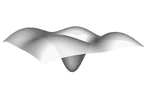
Finding

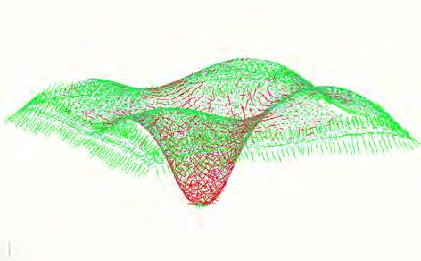
Element Analysis

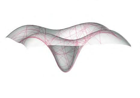
Distribution

Relaxation Algorithm

Stress Vectors

Organisation Algorithm

Figure 5.8 Diagram outlining the logic and information flow in the fibre organisation algorithm

Figure 5.7 Diagram

Fibre Organisation Algorithm

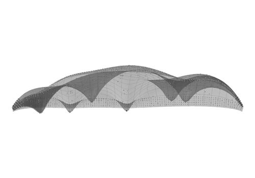
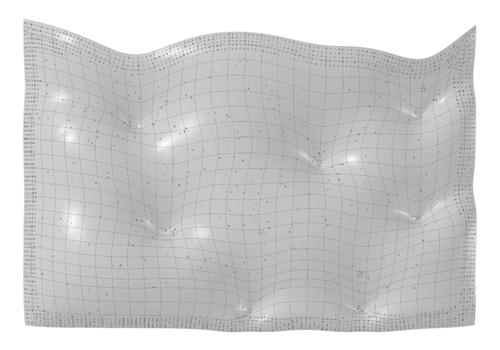
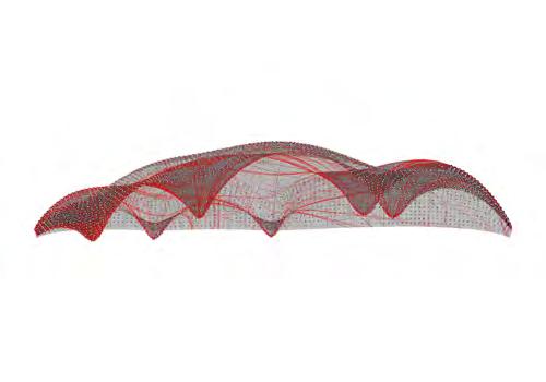
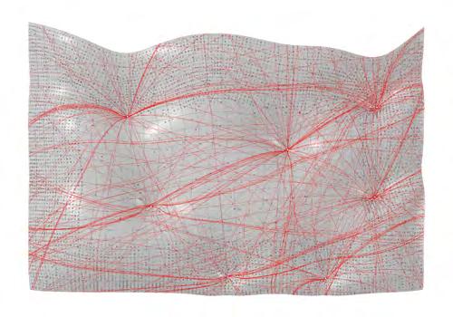
The images above show the digital simulation process of fibre growth. The shell surface geometry modelled through digital form finding is used to distribute the fibres. The principal stress values obtained in Ansys, were exported into an Excel file. Once these preparations were finished the algorithm starts running. [ Figure 5.7].

Traditionally, fibre layout in a composite is made with fibre mats where shearing effects are dealt with by allocating a higher number of fibres in many directions. The logic is to increase the fibre density. In this methodology, a greater amount of material is employed. For cases where the dimensions of the final product are considerably small this may still be worthwhile, since laying fibre mats is a relatively quick and easy process with computer numerically controlled automation.

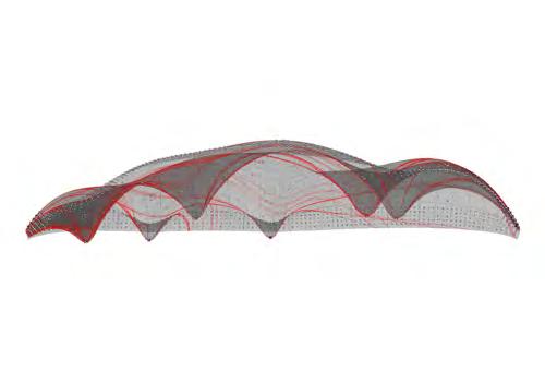
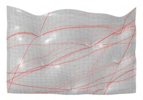
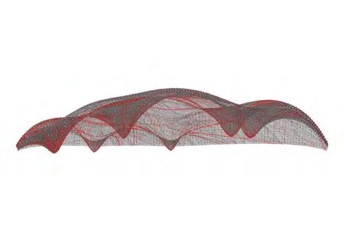
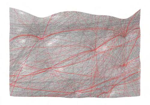
=However, for large scale applications it is essential to ensure that the amount of material used is optimised. Laying the fibres along the lines of principal stress minimises the amount of fibres required, but increases the cost towards manufacturing. Currently, this method is only used in the sail making industry, as discussed in the earlier chapters.

In this case a combination of macro and micro fibres are deployed along the direction of principal stresses. Structural and reinforcing fibres have been organised in two levels: macro and micro. In the macro level fibres are laid following the lines of principal stresses. Micro fibres consist of thin fibrils, whose principal orientation will coincide with the direction of the nearest macro fibre. The micro fibres will act as a reinforcement to bind the polymer material.

Figure 5.7 Process of ‘Fibre distribution algorithm’ written in visual basic to distribute the fibres in the direction of the principal stresses.

Nodes of principal stresses

Macro fibres connecting nodes with similar magnitude and direction

Populating fibres to increase fibre density

Second set of nodes

Macro fibres are placed were values exceed the yield of the polymer

Increasing fibre density, where the values exceed the yield strength of the fibres

Micro fibres , to reinforce the polymer

Macro and Micro fibres Fibres

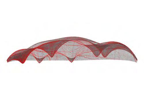
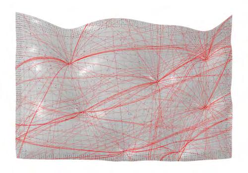
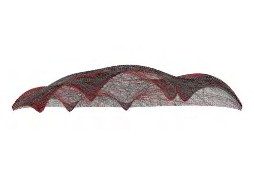
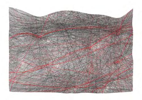
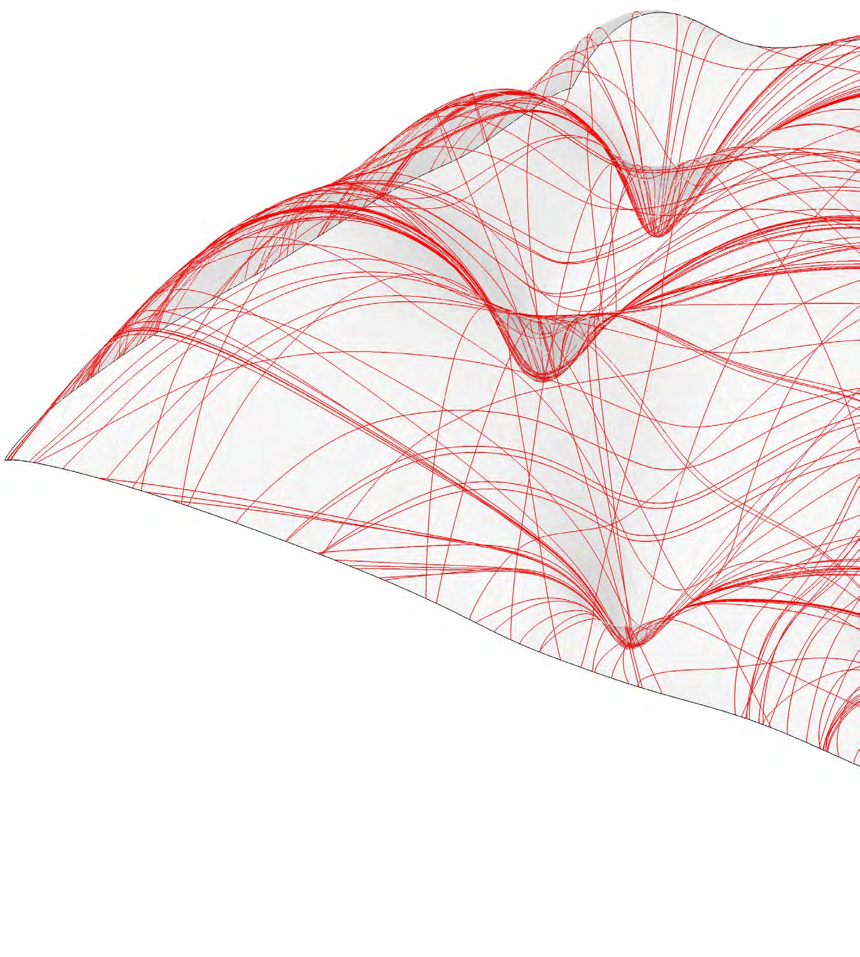
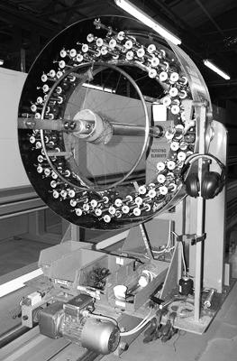
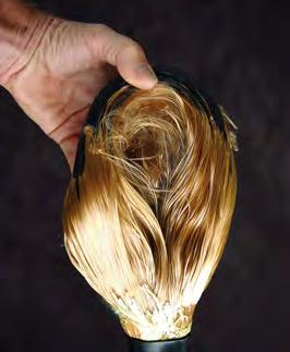
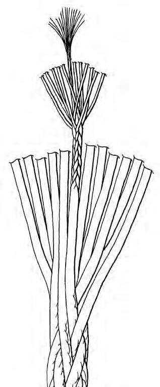
The Macro fibre bundles of approx. dimension 80mm would be made from Kevlar (Aramid), a manmade organic polymer produced by spinning a solid fibre from a liquid chemical blend. They have high strength and low density that result in very high specific strength.

Continuous winding process, also known as the sling process is used for braiding of the fibre bundles. The bundles would be braided in a hierarchical pattern to achieve equal tension in all the micro bundles.

Figure 5.9

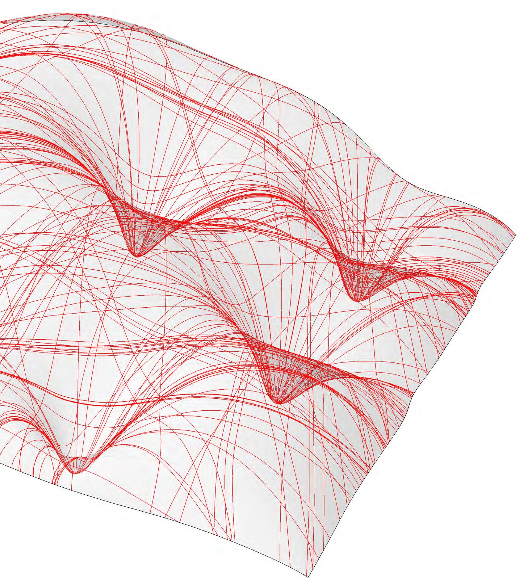Figure 5.8 Organisation of Macro fibres along the direction of principal stresses

20mm

Figure 5.9 Organisation of Micro fibres along the direction of principal stresses

5 Performance and Adaptability

Environmental Performance

Vernacular tradition of using screen walls or ‘Jalis’ have proven to be efficient micro-climate control devices. These screen walls, moderate the transition between the inside and the outside, creating low energy - passive solutions to manage the extremes in hot dry climates. Nevertheless, creating such fenestrations would weaken the structural strength of the shell geometry. The fenestrations were defined in such a way that it could enhance the structural performance, at the same time integrate the functions of a screen wall in cutting out the harsh sunlight, yet keeping the interior of the envelope well ventilated.

Actuation has been integrated in the openings to enable the potential of adaptability. The adaptation logic is based on the variations in the atmospheric temperature, both diurnally and annually. The shape memory alloys embedded within the material can sense these temperature changes and efficiently adapt. The definition of geometry is crucial to enable the intelligent behaviour of the system.

This chapter elaborates on the definition of the local geometry (openings-fenestration) , their intelligent behaviour in response to solar radiation and wind flow. Also, the local geometry greatly contributes in enhancing the structural performance of the system

Precedents - Jali - Screen walls

‘Jali’ , derived from ja-a-li, in Gujarati; is the term for a perforated stone or latticed screen, usually with an ornamental pattern constructed through the use of calligraphy and geometry. [5.2] Such screens are highly efficient in low-energy and passive micro-climatic control, as against other mechanical means of modulating interior environment. These highly articulated surfaces create porous heterogenous spaces of energetic exchange. The jali, screen wall enables ventilation, provides shading and modulates the luminous environment within the interior space. The filigree designs create a dramatic display of light and shadow creating virtual spaces within the enclosure.

Screen walls create comfortable inhabitable spaces, whose external boundaries are rather vague, adjustable and relatively irregular. Such elements create a performative synthesis of the delineating material threshold and the environmental gradient. [5.3]

The attempt in the design proposal is to explore a morphology beyond a simple flat-screen application into a layered envelope. Parametric associative modelling would be employed to inform the design of a highly performative and porous envelope.

The layering of the envelope with variations in porosity would create a variety of micro climates. Surface articulation, orientation and layered spatial arrangements are the key factors to be manipulated to create heterogeneous spaces which are comfortable, in contrast to the homogenous interiors modulated through mechanical means. [5.3]

Such a differentiated envelope would create passive environmental modulation based on the dynamics of energy exchange. The design process would be informed by analytical methods such as solar insolation, simulations of wind flow, structural performance and so on. The results of the analysis would act as critical design parameters that inform the design rather than post-rationalisation and post optimization.

5.2 Thapar, Binda, ‘Introduction to Indian Architecture, p. 81, Periplus Editions, Singapore, 2004.

5.3 Hensel, Michael, ‘Performance Oriented Design-Precursors and Potentials’, -Versatility and Vicissitude, p.48, Architectural Design Journal, Wiley, MarchApril 2008.

Figure 5.10 Sidi_Saiyyad_Ni_Jaali, Ahmedabad, India

Figure 5.11 Interiors of Humanyun’s Tomb, India

Precedents - Erwin Hauer- Continua

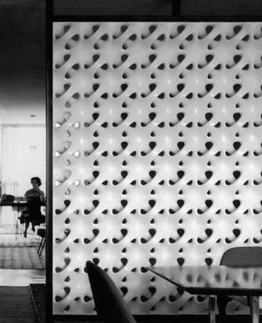
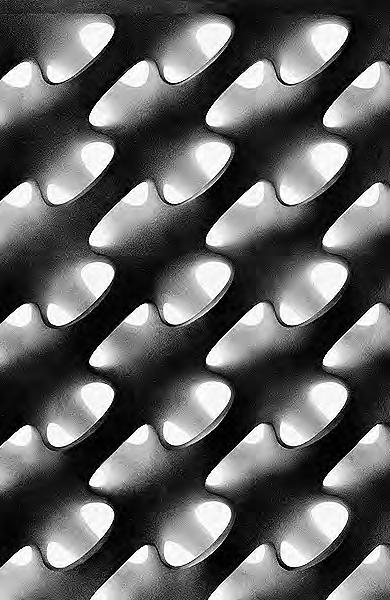
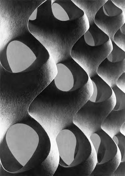
One of the predominant contemporary versions of the jali screen walls are the sculptural experiments of the Austrian sculptor Erwin Hauer. Erwin Hauer explored infinite continuous surfaces in the 1950s. His research started with the study of mathematically defined surfaces such as the Möbius strip, Klein bottle which led to his inclusion within the movement known as ‘modular constructivism’: a style of sculpture based on carefully structured modules which allow for intricate and in some cases infinite patterns of repetition. These are used to create limitless, basically planar, screenlike formations which can also be employed to produce multidimensional structures [5.4].

The development of these topologies involves an extensive study of their mathematical formulation and the combinational possibilities of curvilinear and fluidly shaped modules, which are capable of creating a seamless, quasiorganic unity that can be either rounded and self-enclosed, or open and potentially infinite. In an article published in Architecture Week (4th August 2004), Hauer explains that “continuity and potential infinity have been at the very centre of my sculpture from early on.”

Hauer’s research is quite extensive and covers many different

aspects that range from the start of the conceptual design to the fabrication of these modules. However, the part of his work, which is of interest is the way these topologies are conceived and the algorithmic rules that generate the system; how a thin surface turns into a tissue-like webbing pattern interconnecting convex and concave surface curvatures –saddle surfaces- and thus, allowing for smooth self-combination in multiple dimensions.

The result is an interwoven of continuous surface-like geometries in different layers which ultimately form a space truss. A set of thin surfaces prone to buckling is therefore transformed into a robust structure by means of altering its topological definition; a compendium of interwoven surfaces defines now a continuous space truss capable of withstanding a wider range of loading conditions.

In addition to their structural efficiency , these geometries have an aesthetic potential of creating differential light qualities within the architectural envelope. Complex patterns, with apertures transmitting and filtering light, while rendering smooth indirect light and gradient patterns of shadows [5.4.

Figure 5.12 Installation in showroom of Knoll Internacional de Mexico, Mexico City

Figure 5.13 Screen walls- 8-inch module cast hydro stone.

Continuous Surface - Openings - Space Truss

Having studied the topologies developed by Erwin Hauer the focus was on developing a variation based on hexagonal grids rather than orthogonal. The entire geometrical definition could be illustrated based on the logic used to construct it. [Figure 5.14 ]:

1. The first level consists of two hexagonal grids shown in two levels: top and bottom. The origin of one of the grids is offset with respect to the other one; the appearance when looking at the plan view is that the vertexes of the hexagons in one grid coincides with the centre of the hexagons in the other one [Figure 5.14 (1)].

2. These grids are then linked to each other with two set of ‘tripods’. The first set goes from the top grid to the bottom one and vice versa for the second set of tripods. For the first set of tripods –top to bottom-, the top vertex is located at the centre of the top grid hexagons while its three legs are resting on the perimeter vertexes of the bottom grid hexagons. The same logic is followed by the bottom to top set of tripods [Figure5.14 (2)].

3. These tripods hold the control points defining the ‘suture curves’. The entire topology of these curves is based on the spatial arrangement of the tripods and their geometrical association with the hexagonal grids [Figure 5.14 (3)].

4. Removing the auxiliary grids will help visualising how the suture curves construct the space-frame [Figure 5.14 (4)]. This effect is emphasised and the local geometry is finally displayed by means of lofting between these curves [Figure 5.15]. The result is a space truss out of a thin layer of fibrous material.

This kind of a geometrical definition not only integrates the opening with in a continuous surface geometry, but also enhances the structural performance of the system. Usually, Fibre composite structures are characterised for achieving high ultimate strength values which lead to the production of extremely thin surface- like geometries. These are very useful for the development of shell structures where all the external loads travel across the surface and thus, there are no out-ofplane forces to be considered, or these can be neglected. For those cases where out-of-plane effects cannot be neglected, reduced thicknesses would not contribute to transferring the loads and thus, the strategy needs to be re accessed.

Instead of increasing the surface thickness –which will lead to a bulkier design- a more efficient strategy for dealing with this problem is to carefully re configure the geometry. The aim is to generate ‘structural depth’ in the out-of-plane dimension; in other words, the material would be re-distributed away from the hypothetical ‘neutral axis’ originally positioned half way through the surface thickness. This arrangement can easily be achieved through the space truss configuration of the continuous surface geometry. [ Figure 5.15 ]

Varying the height of the suture curves, would result in stiffer differentiated areas which ultimately contribute to the structure integrity of the system. The image on the following page [ Figure 5.16 ] shows, openings integrated in a double curve shell. Consequentially, the spanning areas achieve greater stiffness by virtue of the space truss configuration of the geometry.

(3)

(4)

Figure 5.14 Construction of the multilayered continuous surface, integrating openings

Figure 5.15 Connectivity between the layers, forming a surface space truss.

Figure 5.16

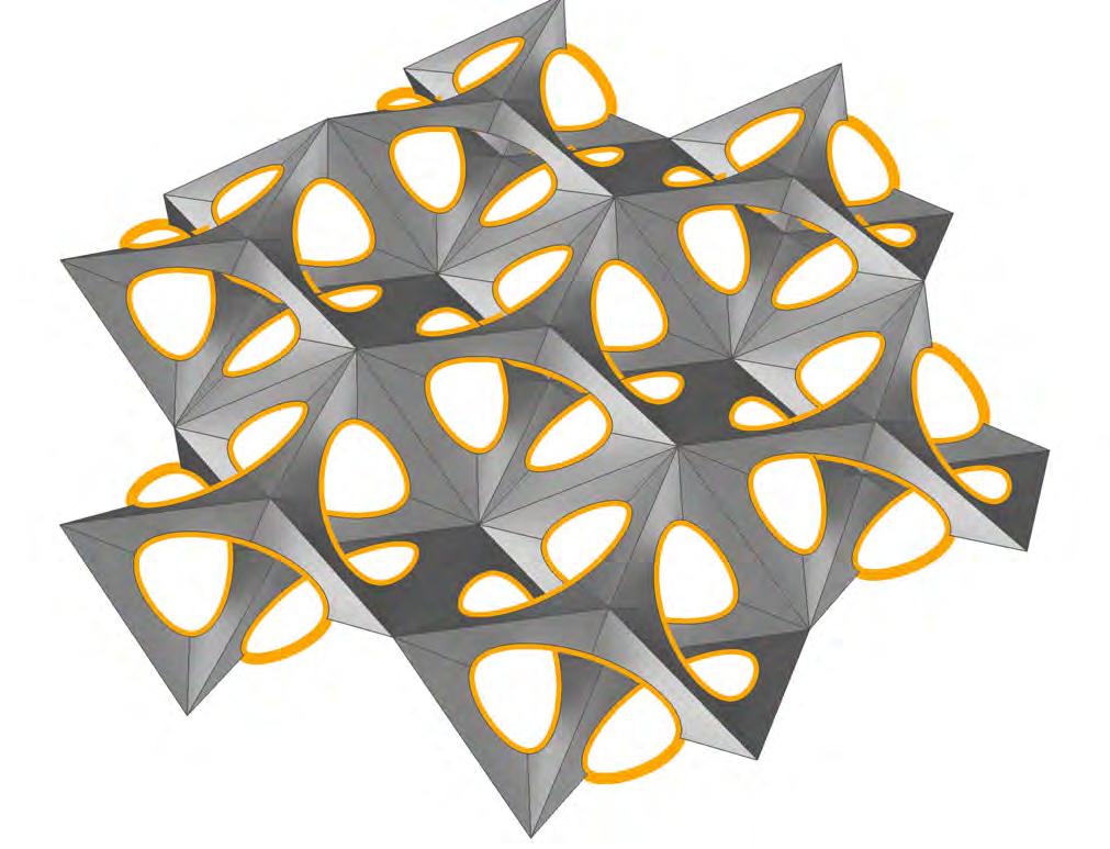
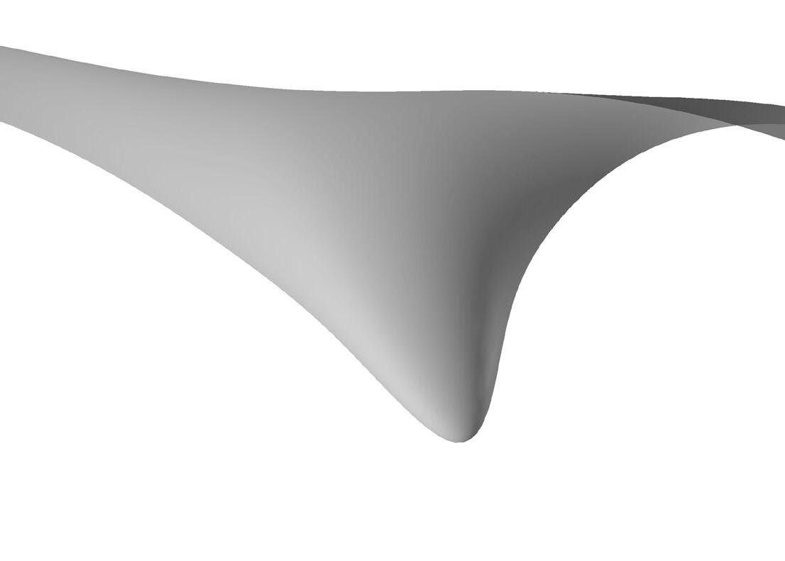
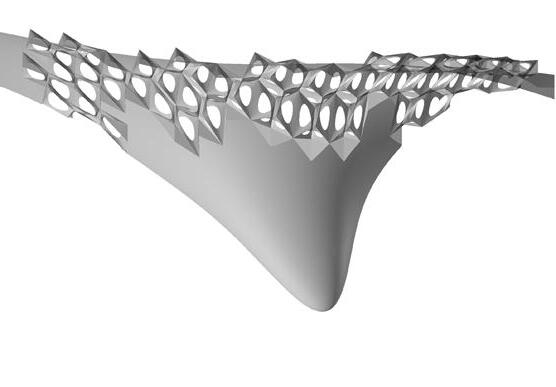
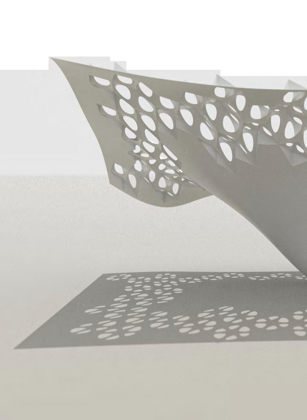
Figure 5.17 The geometry has been exploited with the ambition to fully embrace the benefits offered by the fibre composite material. One of the main contributions of fibre composite materials is the possibility of achieving extremely thin surface geometries. However, from the structural point of view the thin surface geometries can be quite controversial since they might lead to ‘early’ structural failure, i.e. collapse of the structure occurs before the ultimate strength of the material is reached. For example, under compressive loads thin surface geometries might lead to buckling depending on how and where are the external loads applied. Therefore, a smart geometrical configuration by integrating the opening and consequentially the space truss logic allows a ‘surface-like’ geometry to become stiffer where and when required.

Hence the geometry is approached from two different scales: local and global. Locally at the level of a single cell or opening as the smallest unit within the material system. The proliferation of these single cell would respond to very specific rules which govern the fusion of the local and global geometries and the environmental performance of the fibre composite adaptive system.

Adaptability - Fuzzy Logic Actuation

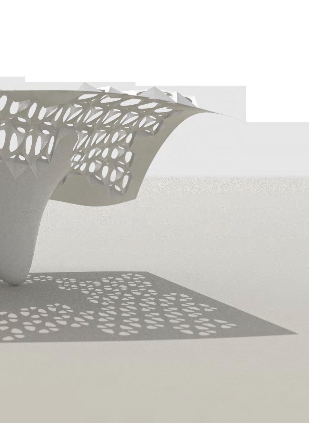
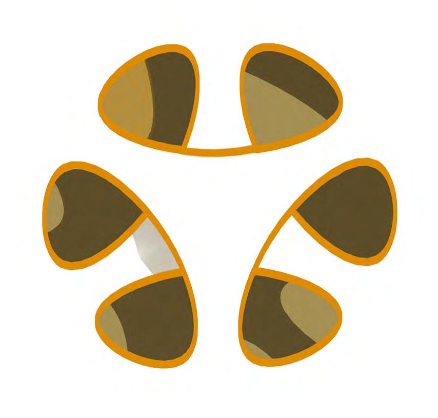
Unlike the static screens cast in concrete by Erwin Hauer, the proposed fibre composite adaptive system is characterised by its dynamism and capacity of adaptation to external stimulus. The shape memory alloy actuators are embedded along the suture curves, in the fibre composite material system as shown in figure 5.18 (left). The adaptive roof is capable of sensing stimuli and actuating appropriately. The actuation process occurs by means of shape change from one initial state to another, which rather than being instantaneous, happens gradually through time. [Figure 5.19] The SMA actuators display a characteristic logic known as ‘fuzzy logic’.

The fuzzy logic is a form of multi- valued logic derived from fuzzy set theory to deal with reasoning that is approximate rather than precise. In contrast to binary sets having binary logic - also known as crisp logic- the fuzzy logic variables may have a membership value of not only 0 or 1; instead they can range -inclusively- between 0 and 1. [Figure 5.18, right].

Most of the electrical devices that we use nowadays are conceived using this logic, as it is the case of the controllers used in the experiments (refer chapter two experiment 9). Fuzzy controllers consist of an input stage, a processing stage, and an output stage. The input stage maps the sensor or other inputs, such as switches –‘on-off’ inputs- to the appropriate membership functions and truth values. The processing stage invokes each appropriate rule and generates a result for each; these are logic rules in the form of ‘if-then’ statements, where the ‘if’ part is called ‘antecedent’ and the ‘then’ part is called the ‘consequent’. As part of the processing stage each rule and result are combined and these data is then used in the output stage which converts the results back into a specific control output value.

The most common shape of membership functions is triangular, although trapezoidal and bell curves are also used. In our case, the actuation curve approximates to a trapezoid where any corners have been smoothened up. The changes in shape from one to another occur through a gradual variation

governed by the functioning rules imposed by the sensing and controlling devices. In case of the final design proposal the sensing , actuation and decision making functions are performed by the shape memory alloy themselves in coherence with the geometrical definition and relative to the changes in the atmospheric temperature.

Fuzzy logic is therefore associated with the concept of gradual adaptation. The combination of both, synthesises how this novel material system could enhance the ‘spacetruss’ configuration. [Figure 5.19]

However, the ‘adaptation’ of the system should be carefully structured into different fields of action or would be referred to as ‘actuation variables’. [Figure 5.20] These constitute the set of parameters that can be altered within the adaptive system in order to adapt to novel situations. For this particular case, these have been set to be as follows:

• Size of openings which would regulate the light and air transferred through,

• O verall cur vature which allows the material system to adapt to doubly curved surfaces if necessary,

• and finally, the height of the undulating pattern which from the structural point of view must be seen as the structural depth of the space-truss.

Although these three actuation variables will be discussed in detail later on, it is worth introducing here how these are actually achieved. After a rigorous investigation of the geometry it was ascertained that the edge curves of the interwoven surfaces were the true controllers of the system. Altering these curves or the points that control them would incur into altering the global system geometry. Therefore it was decided to strategically locate the actuators along these ‘suture curves’ establishing the negotiation logic in the proposed fibre composite adaptive system.

At a point in time represented by the orange line there is a range of values rather than absolute values. ‘0’ and ‘1’ and are the extremes of the different intervals.

Figure 5.18 Integration of actuators into the shell surface

Continuous surface geometry, highlighting the location of the integrated shape memory alloy actuators along the suture curves.

SMA Actuators

5.19 Location of ‘suture curves’ control points. Top (below) and isometric (above) views.

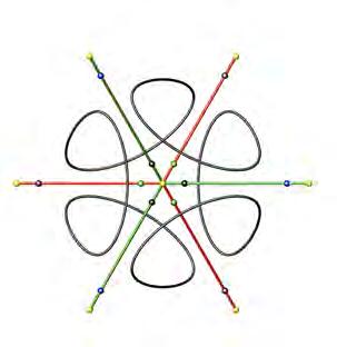
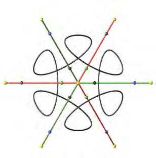
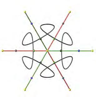
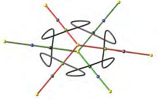
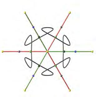
Opening

Suture Curves

Variables Curvature

Grid Distortion

Grids Spacing

Figure

Figure 5.20 Diagram of actuation variables

Openings

Actuation Variables

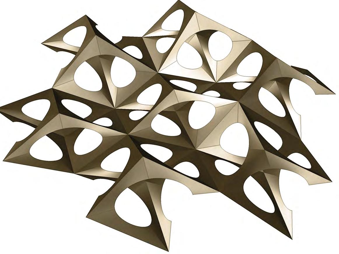
This section elaborates on the geometrical definition of the actuation variables. The suture curves, the edges of the openings control the adaptive potential of the system. An associative parametric model was developed to digitally simulate the behaviour of the adaptive system. The model was been set up in Grasshopper and in Rhinoceros platform.

Varying the size of the openings will result in increasing or decreasing the amount of solar penetration and air transferred. The geometrical definition of the suture curves allows for such variation by simply altering the position of the control points along the tripods defining each cell. These consist of two tripods one going from the top to bottom grid (red lines) and a second one from bottom to top grid (green line). [Figure 5.23]

In total there are eighteen control points, of which twelve share their location in space and are positioned closer to the perimeter of the cell; the other six points left are located near the centre of the cell. Each tripod leg hosts two points which are spaced out along its length –one closer to the top end and the other one closer to the bottom end. Moving the control points along the legs of the tripods results in altering the curvature of the suture curve, hence reducing or increasing the size of the openings.

However, in order to avoid unrealistic curvature changes, the

movement of these points had to be studied in detail and a specific set of rules were established.

The control points are grouped in four sets of three points. The first set has been highlighted in purple in figure 5.23. The second, third and fourth sets are shown in black, green and blue respectively [Figure 5.23]. The movement of the red set is coupled with the movement of the blue set and thus, when the height is reduced the red set of points travel downwards along the tripods while the blue set is travelling upwards. The same rule is applied to the black and green sets of points.

When the height is reduced the horizontal spacing of the legs increases – tripod expands- and vice versa –tripod contractswhen the height is increased. [Figure 5.25]

Therefore the suture curves are the ultimate controllers of the geometry, by manipulating the openings the height in between the two layers could be increased or decreased. Also when a set of cells actuate in tandem the overall curvature of the shell surface would vary, provided there is enough flexibility in the embedded fibre composite material.[Figure 5.24]

Figure 5.23 Control points along the tripods. These have been extracted from the digital model created to simulate the adaptive abilities of the material system developed.

Figure 5.21 View of set of cells before actuation

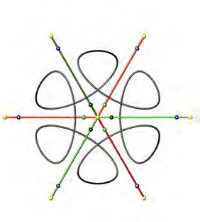
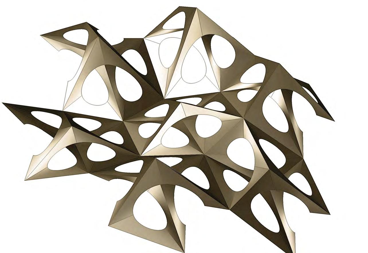
Suture Curves

Curvature

Figure 5.22 View of a set of cell in the process of closing

Figure 5.24 Change in overall curvature

Figure 5.25 Change in height - structural depth, between the two layers

Figure 5.26 Detail showing the actuation, opening and closing in a single component.

Figure 5.27 View of a portion of the adaptive roof structure responding to variations in atmospheric temperature to control the degree of solar penetration and wind flow.

Figure 5.28

Images of Stereo lithography model representing the form before actuation

Figure 5.29

Images of Stereo lithography model representing the form after actuation

Struc tural analysis with distributed components

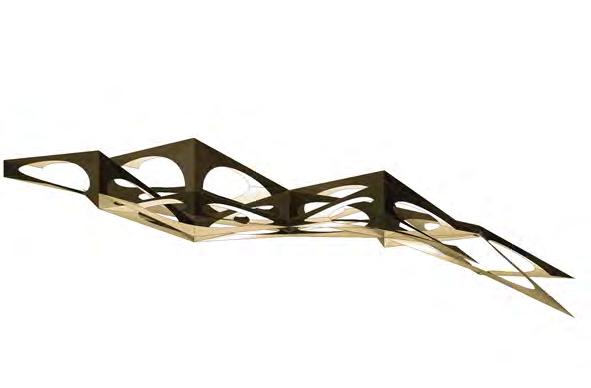
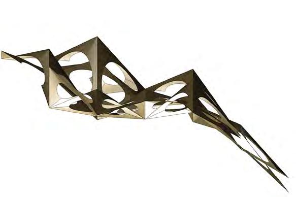
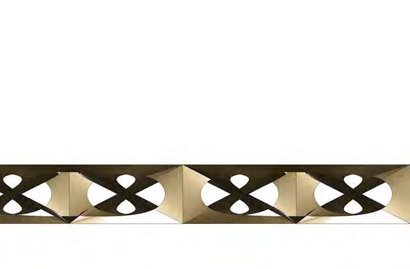
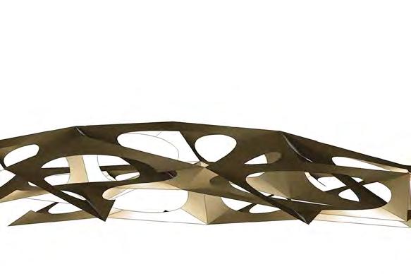
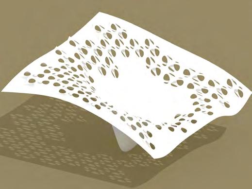
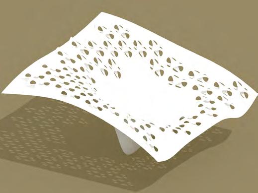
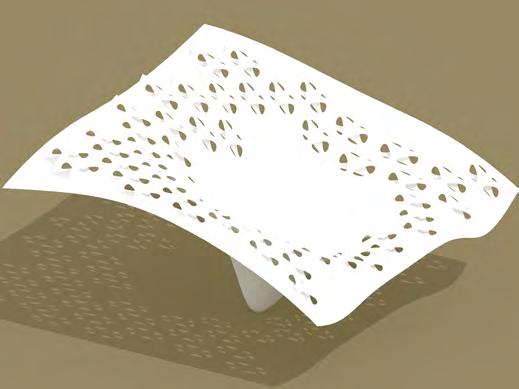
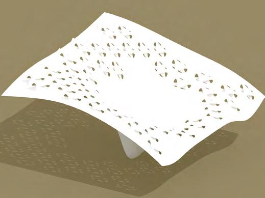
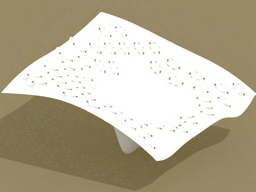
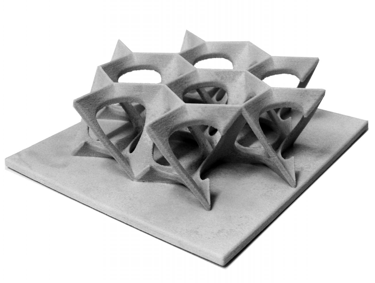
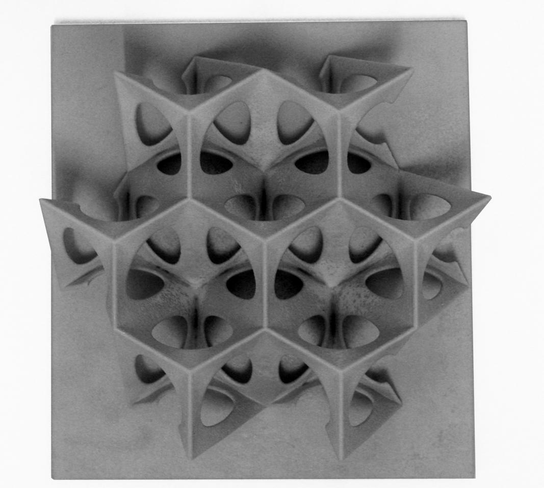
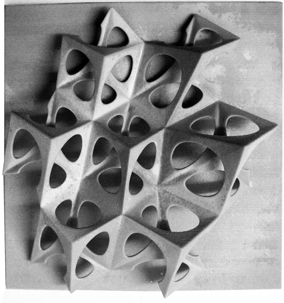
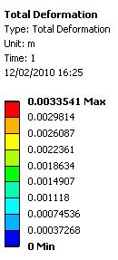
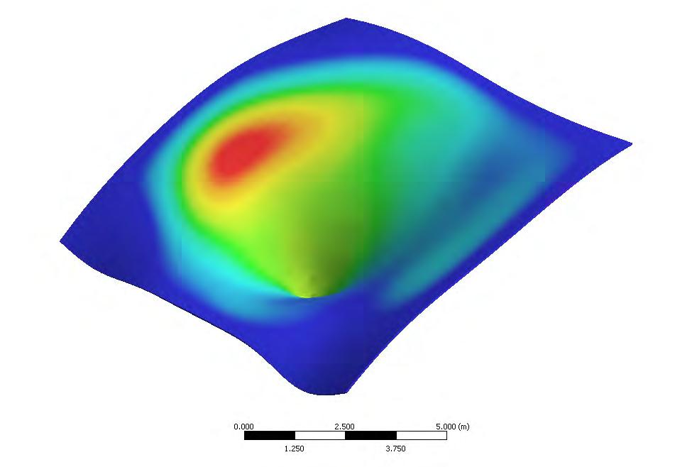
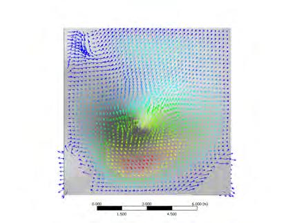
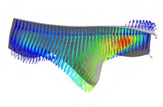
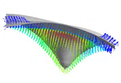
To ascertain the structural performance of the space truss configuration a comparative structural analysis was performed on a thin double curved shell and the shell with components distributed on it. The aim was to extrapolate the structural performance of the shell with distributed components to inform the distribution strategy. Due to computational limitation only a portion of the shell was considered for the analysis rather than the complete shell.

Material simulated was kevlar fibres in epoxy resin. Thickness of the shell was maintained to 50mm in both the cases. A fixed support was defined at the base of the shell , also the four

edges of the shell were assigned as fixed supports. The loads acting on the structure was given a 5 Kilo pascals including self load.

The results were quite interesting, the simple shell showed very minute deformations, as it can be observed in the figur5.30. While the space truss configuration had nil deformation. Therefore, for sure the space truss configuration is stiffer than the thin shell. Nevertheless, since there is minute deformation the thickness of the shell can be reduced even further than 50mm.

Figure 5.30 Static structural analysis of thin double curved shell

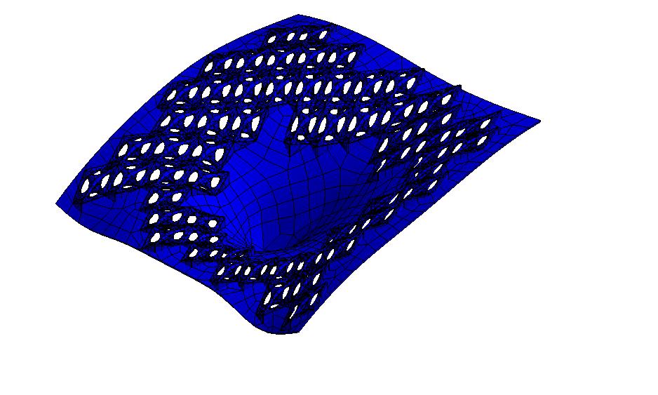
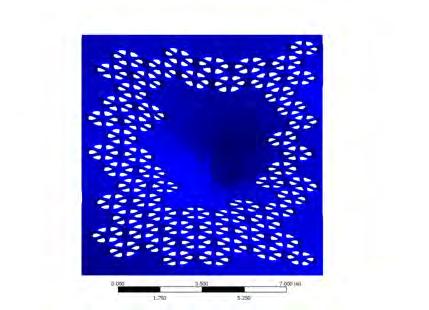
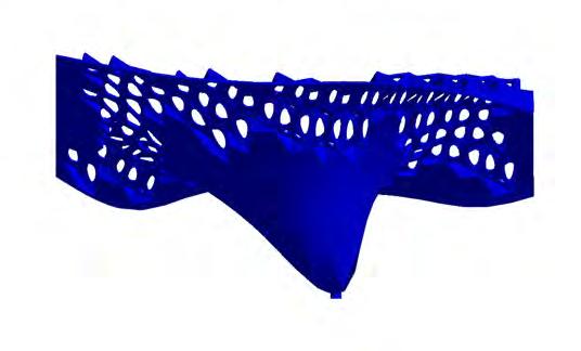
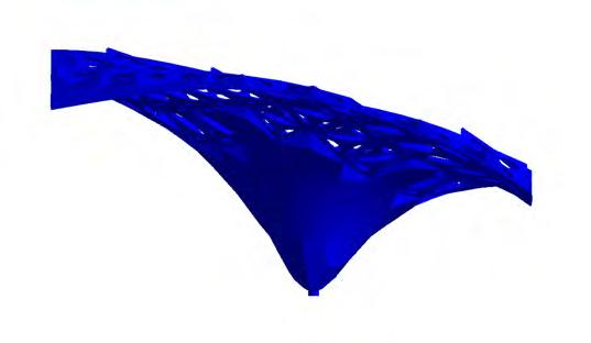
Thickness of the shell: 5cm

Loads: Self load & Pressure: 5Kpa

Supports : Fixed Supports at column base and four edges

Platform: Ansys

Material: Carbon fibre (Kevlar in epoxy resin)

Young’s Modulus: 75 Gpa

Poisson’s Ratio: 0.34

Thermal expansion Coefficient: 4 strain/K

Density: 1.4 g/cc

Figure

Type A _ Structural

Type B _Actuators

H

ierarchy of Components

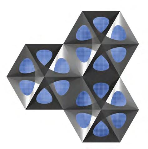
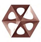
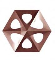
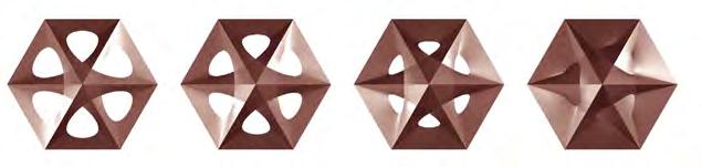
The actuating component has multiple performative potentials, both structurally and environmentally. One of the drawbacks of the component is the coupled parameters during actuation. When the openings are increased or decreased the height as well as the overall curvature of the shell surface changes. In case of a large scale application, such coupling of parameters have to be avoided for better performance of the system. The openings may close to protect the interior from harsh sunlight but it still needs to perform the role of air ventilation and maintain the structural integrity of the system. Owing to this reason, it is essential to establish a hierarchy within the adaptive system.

As in the case of collagen fibres in animals, which are arranged in a hierarchy, with fibres are various scales performing a specific function and maintaining the coherence within the adaptive system (refer section fibres composites in nature). Likewise establishing a hierarchy within the components through scales and material properties would allow it to perform a specific function more efficiently.

The components are categorised in three hierarchies; type A, type B and type C.

Type A, components perform the role of structural enhancement within the system. They have an edge length of 1.5 meters. These components are rigid, adding stiffness to the structure. By virtue of their geometry, they act similar to a space truss spanning large areas efficiently. These

components are fixed edge to edge by means of ultrasonic welding. The openings in these components are closed by a translucent thermoplastic welded along the suture curve. The type A components do not have any actuation potential as they would be manufactured with kevlar fibres cured in epoxy resin, a very stiff and strong material.

Type B, components are the actuating components, they have shape memory alloys embedded along the suture curve edges. They have an edge length of one meter, placed at a distance of 30 cm apart from each other. This would enable the fibres to be laid along the intermediate spaces. The material makeup should be flexible , hence a elastomeric matrix resin would be used to enable the opening and closing of the suture curve actuators.[Figure 5.33]

Type C, components would perform the role of air ventilation within the system. These would act as fenestrations that would enhance the wind flow and air transfer within the envelope. These are also stiff components made of kevlar fibres cured in epoxy resin.

As observed in the fibrous structure of cactus [Figure5.35], fibres laid in between the components would form a hexagon pattern [Figure 5.34] providing greater strength and stiffness to the structure. The placement of the components need to be carefully negotiated with the fibre organisation of the material system.

5.32

Type C_Ventilation

Figure 5.33 Multiple states of actuation in Type B component

Figure

Figure 5.35 Image of the fibrous structure present in a Cactus.

Figure 5.34 Fibre organisation with components

Figure 5.36 Macro fibre running along the shell surface

Wind flow Analysis - Computational Fluid Dynamics

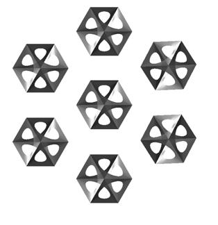
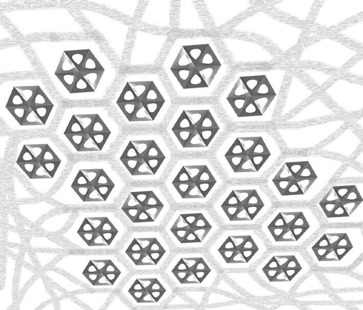
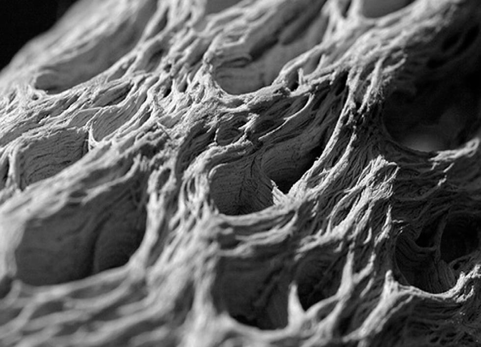
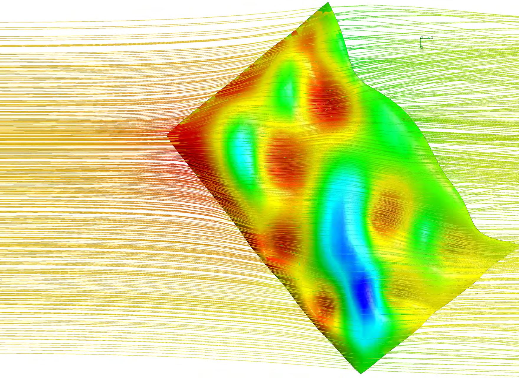
A strategic distribution of the components on the shell surface would render an efficient environmental performance, with each type of component performing a specific function. The process of component distribution is informed by several analytical methods. Solar Insolation analysis and static structural analysis were elaborated in the previous chapters, It is crucial to perform a wind flow (CFD) analysis to position the ventilation elements on the shell geometry to enhance the wind flow within the envelope.

Bernoulli’s principle states that, for an in viscid flow, an increase in the speed of the fluid occurs simultaneously with a decrease in pressure or a decrease in the fluid’s potential energy. [5.5] Bernoulli’s principle can be derived from the principle of conservation of energy. This states that in a steady flow the sum of all forms of mechanical energy in a fluid along a streamline is the same at all points on that streamline. This requires that the sum of kinetic energy and potential energy remain constant.

Fluid particles are subject only to pressure and their own weight. If a fluid is flowing horizontally and along a section

of a streamline, where the speed increases it can only be because the fluid on that section has moved from a region of higher pressure to a region of lower pressure; and if its speed decreases, it can only be because it has moved from a region of lower pressure to a region of higher pressure. Consequently, within a fluid flowing horizontally, the highest speed occurs where the pressure is lowest, and the lowest speed occurs where the pressure is highest.[ 5.6 ]

Based on this principle, the high pressure and low pressures zones were identified on the shell surface geometry through computational fluid dynamic simulation. Throughout the year, Lothal experiences predominant winds from the southwest direction. To accelerate the wind flow within the envelope, openings would be created on the high pressure and low pressure zones. The number of type C components would be larger in the high pressure zones and lesser in the low pressure zones to enable laminar flow within the envelope. [ Figure 5.37 ]

As observed in figure 5.357 the zones marked in red are high pressure zones, There are two kinds of high pressure zones,

5.5 Pitman, L. J. Clancy, ‘ Aerodynamics’ - Journal of Fluid Mechanics , chapter 3, Cambridge University press, 1976.

5.6 Streeter, V.L., Fluid Mechanics, E, McGraw–Hill Inc. , New York, 1966.

5.7 Tsui, Eugene- Evolutionary Architecture-Nature as a Basis For Design, John Wiley and sons, New York, 1999, pp.90,91.

High pressure zones, due to turbulence within the column structures.

High pressure caused due to form drag and frictional drag in the wind flow.

Low pressure caused due to swallow curvature and reduced form drag.

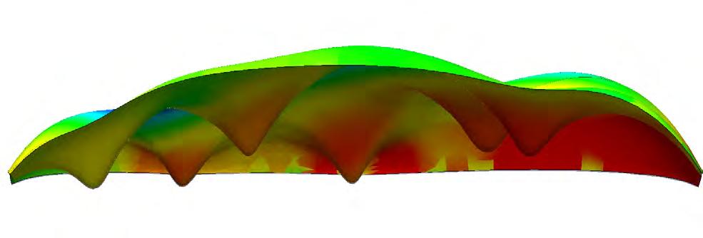
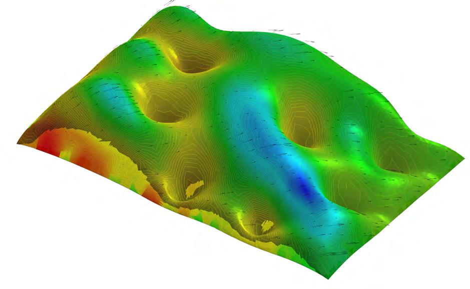
Prevailing Wind Direction : South west Wind velocity: 18m/s

Units: Pascals

Platform of simulation: Solid Works

one along the southwest corner created due to form drag and frictional drag. Form drag is induced as a resultant of the sharp curvature against the wind flow direction, this causes a frictional flow. The second type of high pressure occurs within the column structure owing to their funnel shaped form. The funnel shaped form creates turbulence resulting in high pressure. The zones marked in blue indicated low pressure zones. The curvature of the shell is swallower in relation to the wind flow, causing low pressure in these areas.

A strategy to position the type C ventilation components could be learnt from the prairie dog tunnels. The have mastered the manipulation of wind flow in their burrows to create a comfortable micro climatic situation. The “mounds” and “volcanoes” that mark the entrances and exits of prairie dog burrows serve to direct a current of air through the burrow for ventilation, in accordance with the Bernoulli’s principle. Of

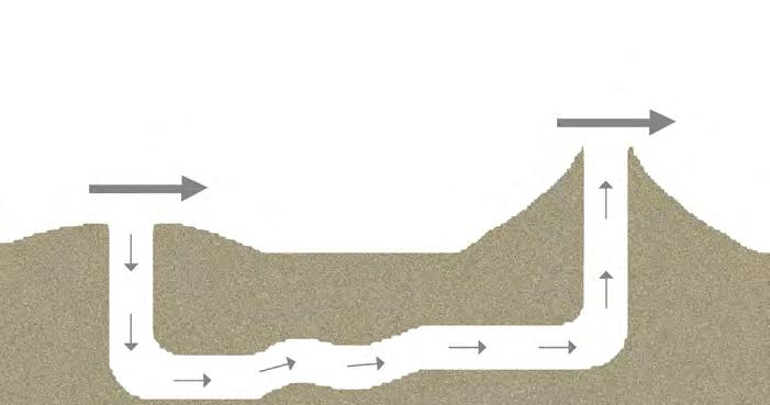
the two entrances of a burrow one is taller than the other, thus the air that flows over the taller mound moves faster (or at a greater velocity) because it has to travel a longer distance. This creates a difference in pressure as the air that travels faster has lower pressure. This slight pressure difference causes the air to flow through the burrow as shown in figure5.40. Thus, the burrow is ventilated as the air flows faster over the volcano and is sucked into the burrow as if into a vacuum, seeking the low pressure area to exit.

The raised entrance system produces a complete change of air within 10 minutes with even the slightest breeze of 18 inches per second. This system of ventilation enables the comfort condition for the survival of prairie dogs. The importance of the wind ventilating the burrow may explain why prairie dogs prefer the mostly treeless wind swept parts of the prairie. [5.7 ]

Figure 5.39 Isometric view showing wind flow vectors and high-low pressure zones

Figure 5.38 Front elevation, the column structures receive high pressure due to turbulence.

Legend and Details of the analysis

Figure 5.40 Bernoulli’s Principle in the Prairie dog tunnels.

Component Distribution Strategy

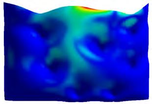
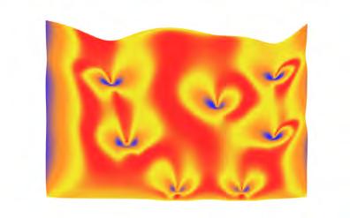
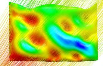
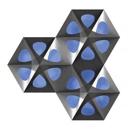
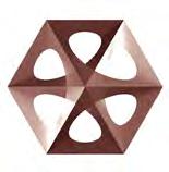
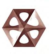
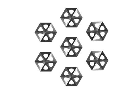
The efficiency in environmental performance of the adaptive structure covering the ruins, largely depends on the strategic distribution of the three types of components [Figure 5.43, 5.44] Analytical methods - environmental simulations were carried out in the digital environment to inform the design process. Like emergent systems in nature, a hierarchy in fitness criteria was established. Structural integrity was given prime importance, hence the highest ranking. Consecutively the control of solar penetration and wind flow were given second and third orders respectively. [Figure 5.41]

Based on the structural analysis performed (figure 5.41,a) zones with maximum deformation was identified. By placing the type A structural components at these zones, the shell would achieve better stiffness and eliminate any deformations from occurring.

The zones which receive the maximum in solar radiation was identified through solar insolation analysis (figure 5.41,b). The main aim was to reduce the solar gain in the summer months when the temperature reaches far beyond comfort levels, at the same time the solar gain has to increase during the winter months. The type B, actuator components were deployed on the zones with maximum solar gain to control the openings to increase or decrease the solar gain. As observed in the figure 5.43, in areas which have both structurally weak zones and receive maximum solar gain; the type A components

were retained and type B components were deleted. As the fitness ranking of structural performance is higher than solar control.

The type C components were placed in zones which experience significant high pressures and low pressures (figure 5.41,c).Placing the components in this contrasting spectrum would enable the air flow to accelerate within the envelope. As elaborated in the previous section, this would contribute in reducing the interior temperature in the summer months. The ancient dock yard positioned in the eastern end of the site, would contribute to a certain degree of evaporative cooling.

Thermal stack effect, diurnal variation in temperature, thermal mass of the shell and the structures within the ruins could be used efficiently in conjunction with the airflow pattern to improve the microclimate. Time lag between the absorption and radiation of heat (in the thermal mass) and the exchange of hot air and cold air between the day time and night time respectively could be staggered to exploit the environmental energy.

The process of actuation in the type B components are further elaborated to understand their contribution in the environmental performance and maintaining comfortable micro climate within the architectural envelope.

Type A

Type B

Type C

Figure 5.43 Plan showing the

Figure 5.44 Aerial view showing the distribution of components

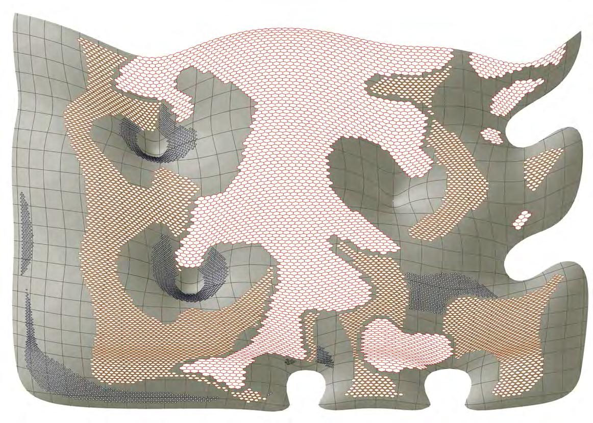
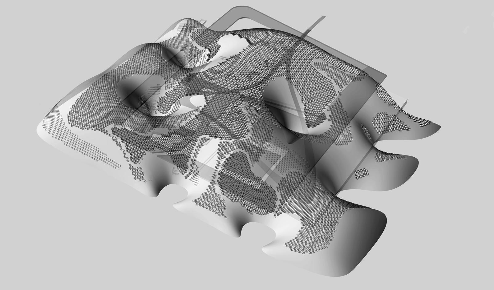
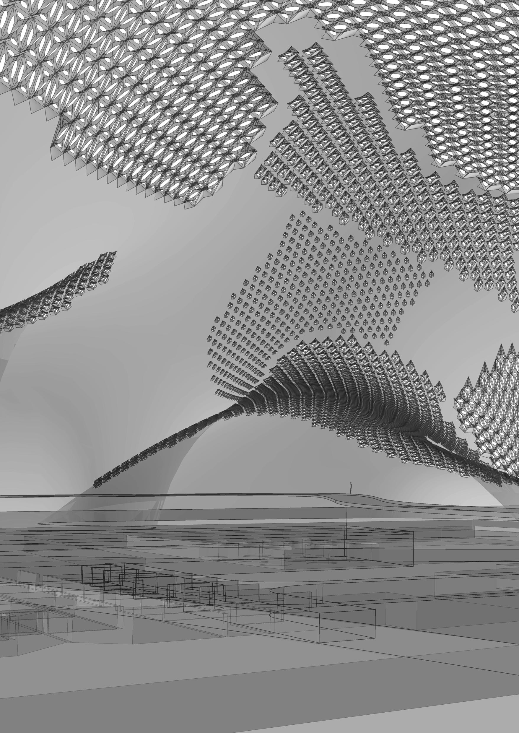
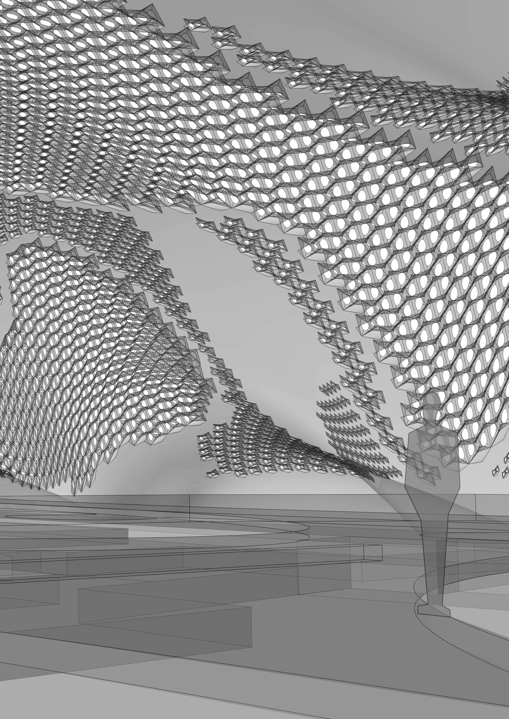Figure 5.45 Interior view showing the distribution of

Time line of Actuation

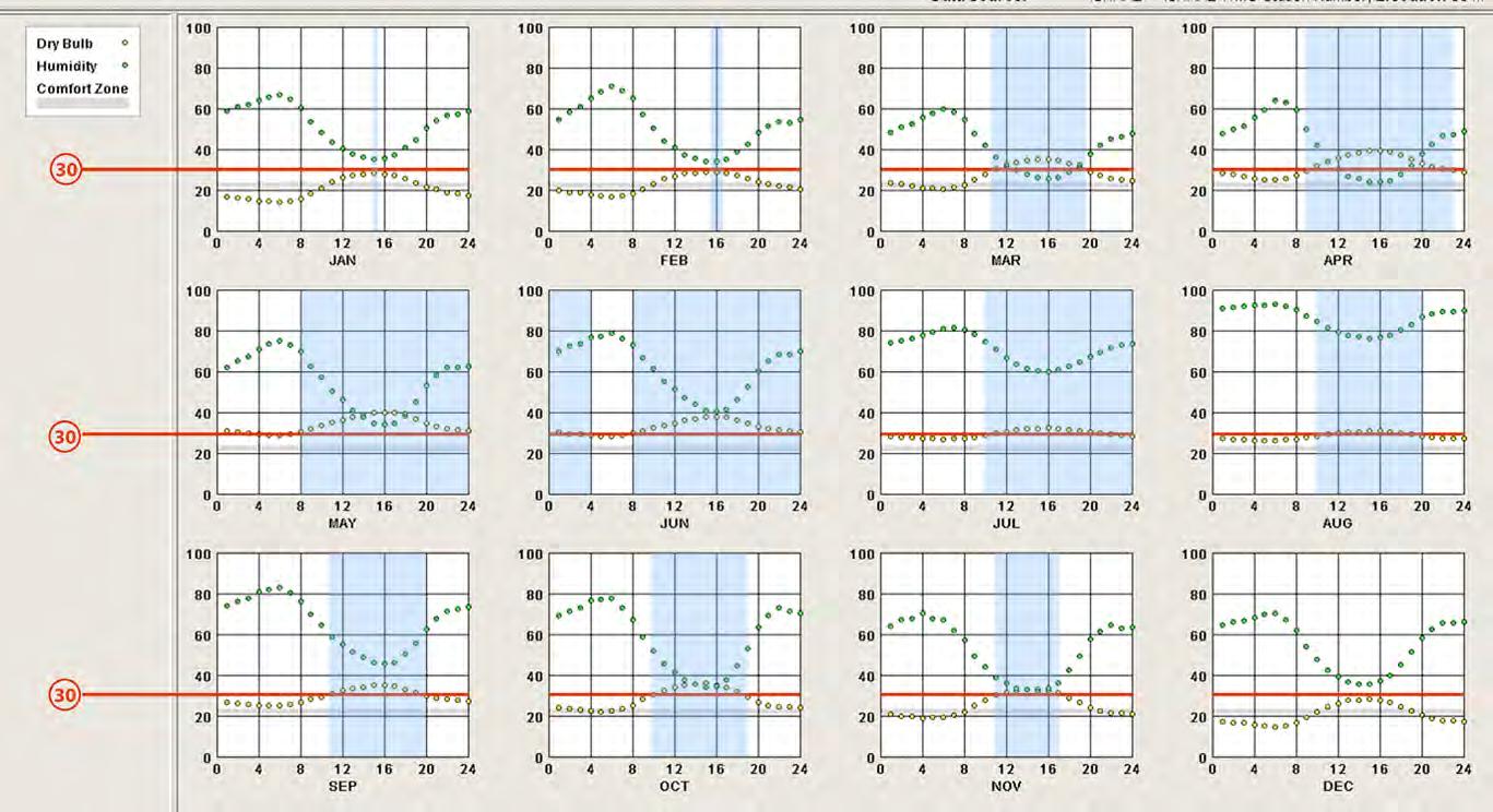
The Smartness of the fibre composite adaptive system relies on the geometrical definition of the components in the local scale. The Annual-hourly temperature humidity graph shows that in the extreme summer months (May and June) the temperature ranges between 30-40oC and in the extreme winter months the temperature remain below 30oC (December and January). This seasonal variation in temperature ranges in ideal top reverse the behaviour of the shape memory alloy to maximise solar gain in winters and minimise solar gain in winters.

The highlighted areas in the graph (shown in blue) are the time ranges when the shape memory alloy would actuate. The actuation shape setting would be done in a way, that the component geometry closes on reaching the actuation temperature of 30oC. It can be observed that the type B actuators would remain closed almost through 80% in the month of June and remain open 100% in the month of December.[ Figure 5.46]

The comfort zone being in the range of 22-24oC, the actuating adaptive structure would render a multitude of heterogenous micro climatic conditions. This kind of a heterogeneity in microclimate of an architectural envelope is in contrast with the homogenous interior environmental condition created through mechanical air conditioning. Though they resultant micro climatic environment in predictable in the case of

mechanical conditioning, the draw back is the irreversible carbon footprint created. Also a great deal of energy loss in maintaining homogeneity which is more a preference rather than a requirement.

The argument presented in this design proposal is the exploration of heterogeneous micro climates which have the potential of exploiting environmental energy and consequentially reducing the ecological footprint.

In the vernacular tradition the use of environmental energy was mastered through the building elements such as the Jali screen walls. The topological definition of the global form in the vernacular tradition was not a superimposition, but an indigenous development of efficient forms as a resultant of the climatic context.

Such a performative strategy has been reinterpreted in the context of smart fibre composite materials. Shape memory alloys which change shape with atmospheric temperature, define the component geometry. While a bottom up process, such as dynamic relaxation (catenary logic) was employed to define the global geometry. The resultant Fibre composite adaptive system has an inherent potential of exploiting the environmental energy at the same time a new morphological definition dictated by the structural and environmental performance of the adaptive system.

Figure 5.46 Annual-Hourly, Temperature Humidity Graph showing

6 Manufacturing Methods

Techniques

This section elaborates of the techniques proposed of the manufacturing of the fibre composite adaptive structure. There are two key issues to be dealt with in the process of manufacturing, one is maintaining the fibre continuity of the macro fibres and the second is the multi- layered casting of the defined components.

Fibre composite manufacturing in the proposed scale of the adaptive roof structure has little or no precursors. Existing references in large scale applications of fibre composites range from windmills, aerospace and the sail making industries.

Existing References

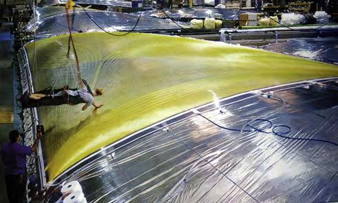
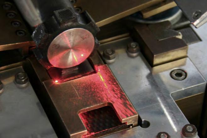
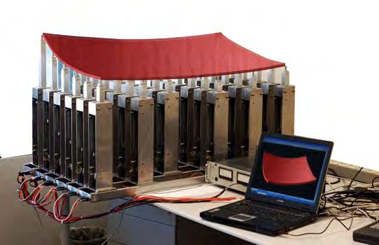
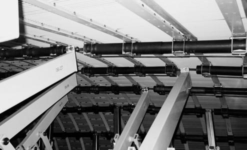
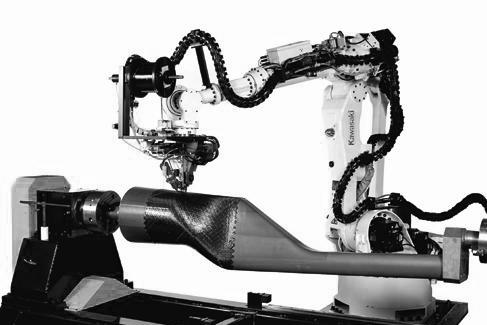
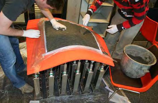
Fibre composites have a wide range of properties which could be manipulated based on the application and the scale of the product. Hence, there are a multitude of manufacturing methods, with each one very specific to its application.

Fibre composite structures in the scale of the design proposal illustrated has little or no precursors. This is largely due to the high cost of carbon fibres, nevertheless with carbon fibre composites becoming more common in a lot of smaller scale products and auto motives, they economic viability is rapidly increasing..

3DL Sail Technology

In conventional sail making, cut patterns are stitched or glued together to produce the optimum shape. In 3DL, the sails are moulded in the optimum flying shape and so eliminate cutting and joining. This produces sails that are up to 20% lighter than conventional equivalents. They are also stronger and seamless. 3DL sail technology, employed in manufacturing a single cast piece of fibre composite sail has a lot of similarities to the design proposal for the adaptive roof structure. 3DCAD models of the sails are tested for their performance with the aid of computational fluid dynamic simulations, once the stress patterns are derived from the CFD analysis their global shape undergoes an optimization process to derive the most suitable flying shape of the sail.

The manufacturing methods in 3D sails comprises of a ro-

bust automated system of moulds for forming the double curve surface and a semi automated process for fibre layup. The 3DL process combines the benefits of composite laminating with filament winding. The three-dimensional sheet geometries are formed over computer-guided moulds The figure 6.2 shows the underside of the CNC automated mould which could render the essential variation in the double curvatures required. Figure 6.1 shows the semi- automated fibre layup process carried out by programming the overhead gantry crane to move along the direction of the fibres and laying the fibres manually. The fibre reinforcement (aramid and carbon) are laid down individually along predetermined lines of stress. They are sandwiched between thin sheets of polyethylene therephthalata (PET) coated with a specially developed adhesive. Locally, computer numerically controlled robotic arms are used for fibre laying, which is a completely automated process.

Ultrasonic Welding

Ultrasonic welding is an established technology for welding fibre composite sheets and panels. Depending on the material composition, an appropriate welding process is employed to deliver bonding strength equivalent to that of the parent material. The existing technology of ultrasonic welding is used for thin fibre composite sheets (3-10mm). . The welding process happens through stationary machines to join seams (like a sewing machine).Nevertheless ultrasonic

Figure 6.4 Filament winding

Figure 6.1 3DL Sail making technology

Figure 6.3 Ultrasonic Welding

Figure 6.2 Automated mould

Figure 6.5 Adjustable mould

Figure 6.6 Concrete casting on adjustable mould

Fibres Continuity

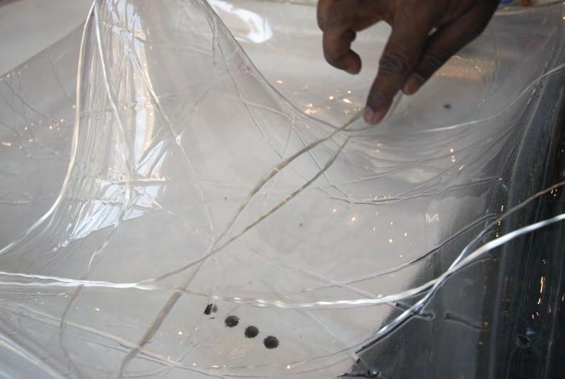
Multiple- layer casting

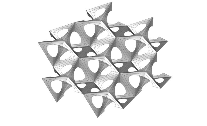
welding machines have the option of being customised for a free robotic arm version or an automated system which moves along a track.

The logistic feasibility of manufacturing the fibre composite shell measuring approx. 300m X 175m demands an assembly of parts. The global form could be manufactured as components, panels of size not larger than 10m X10m could and assembled on site. Ultrasonic welding could be employed to weld the seams during on site assembly.

CNC Adjustable mould

Casting double curved panels in fibre composite material demands manufacturing several moulds with a unique geometry based on the form for each panel. This can prove to be extremely ineffective economically. Also, the moulds would be employed on sacrificial basis wasting material.

A CNC controlled adjustable mould could be extremely efficient to achieve a multitude of double curvatures. As observed in figure 6.5 a grid of telescopic members could be used to define the double curvature. The panel geometry of the 3D - CAD could be directly input into the actuating data set of the mould to the take the exact same form. Further the fibre composite could be formed over this actuated mould.

Key Issues in Manufacturing

There are two main issues in the manufacturing process of the fibre composite adaptive roof. One is maintaining the fibre continuity of the macro fibres, which account for the structural strength. Second, is fibre composite casting in multiple layers as it occurs in the component geometry.

To overcome the above mentioned issues a sequential process would be adopted during manufacturing. The site having sensitive ground conditions, due to the ruins, elaborate form work in the construction process has to be essentially avoided. Therefore the components and panels are precast off site and the assembly would be carried out on site.

The initial sequence is to assemble the double curved panels on site through ultrasonic welding. This primary layer would be made of 0-90o Kevlar fibre mat cured in epoxy resin. This primary layer would act as the form work for laying up the macro fibres. After laying up of the macro fibres, a second layer of resin curing would be carried out.

The sequence of manufacturing is elaborated further in the following section.

Figure 6.7 Fibre continuity being quintessential to protect the integrity and stability of the structure,

Figure 6.8 The continuous surface being woven in multiple layers poses challenging problems for developing a manufacturing process.

M anufacturing Sequence- Stage One

The Stage one in the manufacturing process is the casting of the fibre composite panels (off site). The geometry of the shell has a uniform radius of curvature throughout its surface, as it was derived through a minimal surface logic. It could be observed from the Gaussian curvature analysis [ Figure 6.9] that the shell is synclastic at the base of the columns and has swallow double curvatures over rest of the areas. Synclastic surfaces are double curve geometries which have both their principal curvatures pointing towards the same direction. (bowl shaped).

An computer numerically controlled adjustable mould could be employed to cast the panels forming the shell. An bed size of 10 X 10m could be deployed. Based on the bed size, the geometry is split into panels of less than 10 X 10m. The panels are named alpha numerically in relation to their row and column. [ Figure 6.10]

An adjustable mould has been developed by Daan RietbergenIn, research fellow at the university of TU Delft. [Figure 6.11] The results of the experiments has established a novel method of fabricating double curved glass and double curved ECC- concrete panels. The system employs an telescopic actuators placed on a rectangular grid arrayed. The data for actuation is derived from the geometry built in a 3D CAD software. Therefore, the 3D modelling platform and the computer aided manufacturing (CAM) platforms are directly

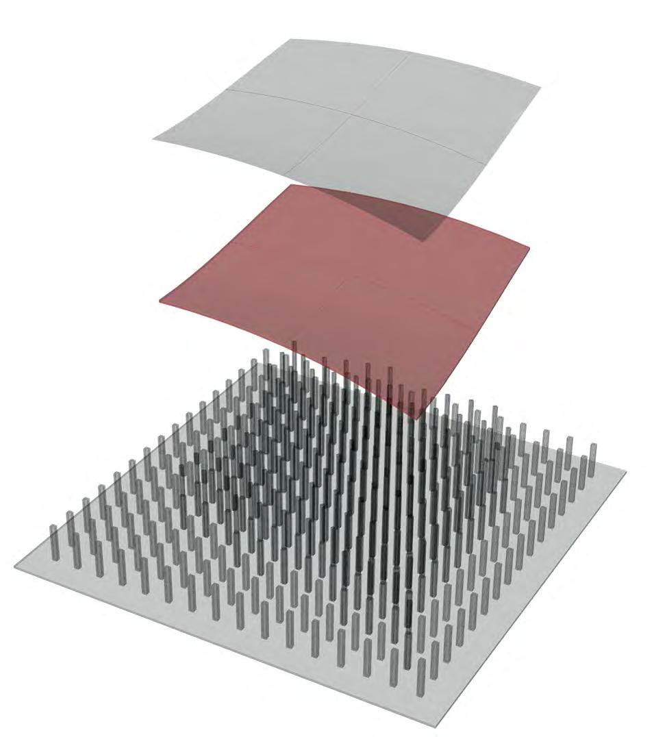
connected. This method has been developed for limiting costs in the production of double curved panels.

By adopting this technique, the base layer for assembly on site could be fabricated. The base layer would act as a form work for further laying of macro fibres. The base layer would be cast from kevlar fibre mat and cured in epoxy resin. [Figure 6.12]

There are several advantages of casting the panel off site, the fibre laying and the curing process could happens in controlled environments. This would make the forming process quicker and easier on site assembly.

Figure 6.9 Gaussian curvature analysis

Figure 6.10 Panel Nomenclature

Figure 6.12 Casting of fibre composite panels for the base layer

CNC Adjustable Mould

Base Layer

Fibre composite mat and resin layup

Figure 6.11 Forming Glass panels on an adjustable mould

M anufacturing Sequence - Stage Two

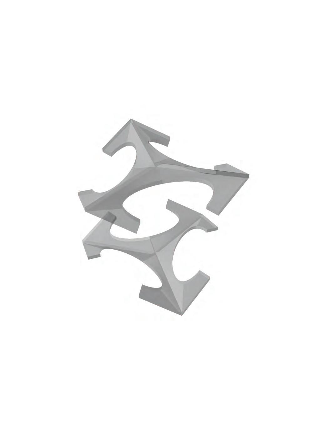
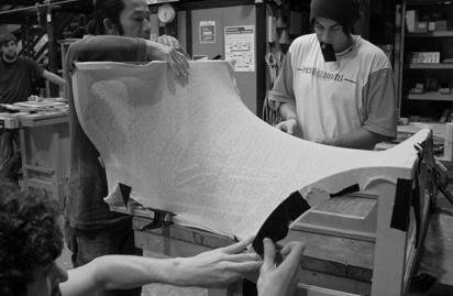
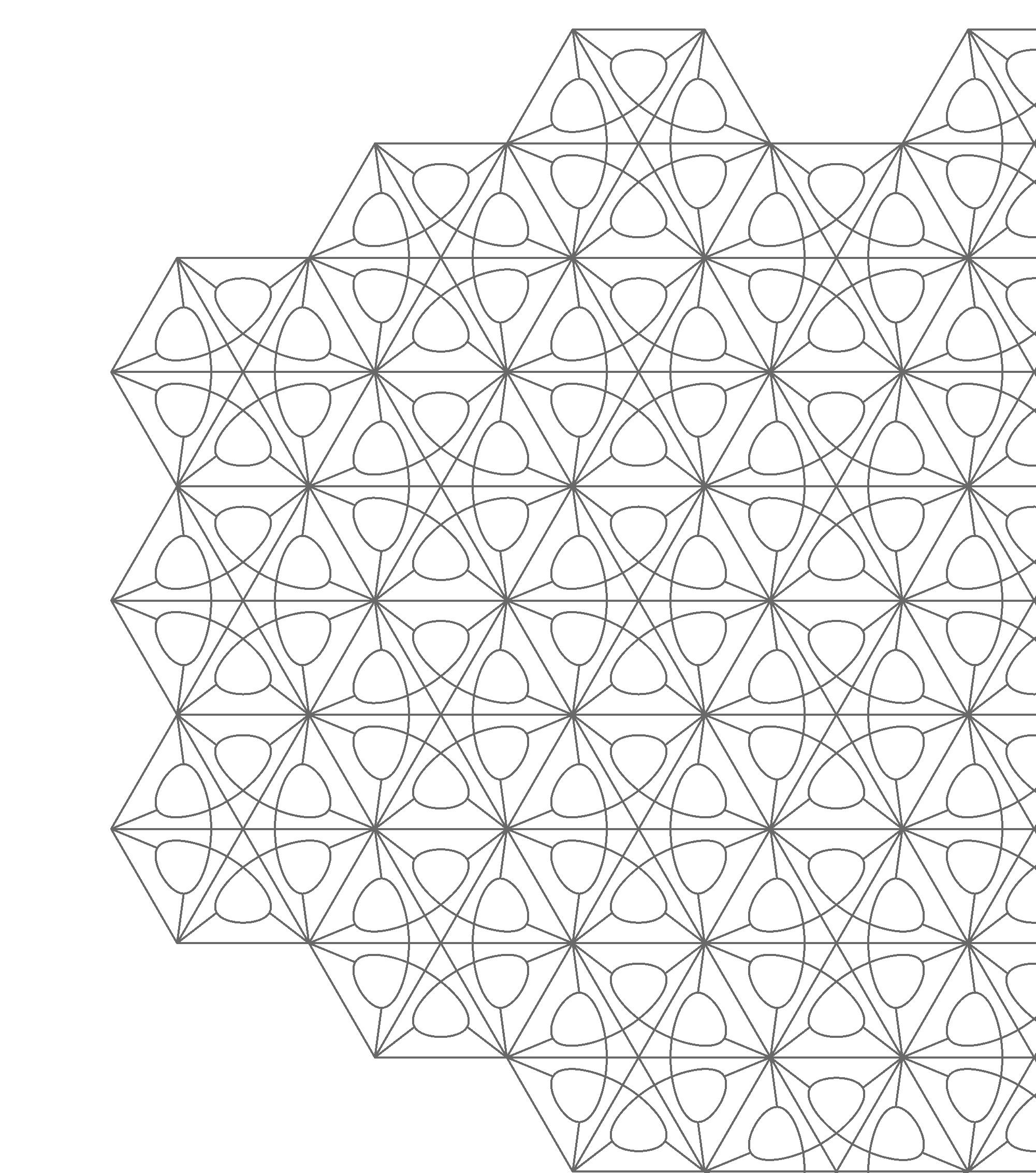
The stage two in the manufacturing process would be casting the components. The component’s geometry is defined as a continuous surface interwoven in between two layers. This could be rather difficult to manage during the casting process.

As observed in figure 6.13 the component’s geometry is split horizontally forming two panels. These panels could then be cast on a positive or convex mould. The split parts of a single component display a rotational mirror symmetry, ie, the both parts are identical. [ Figure 6.13]

The identical panels would be welded along the seams to form a complete single component. Further, assembly of component to component would happen through joining the edges as shown in figure 6.15. with the aid of ultrasonic welding.

Hexagonal components, proliferated on a double curved surface are not identical to each other. Nevertheless, since the scale of the component is relatively small compared to the global scale the geometric variations are minor, to the degree of manipulating tolerances. This variation in dimensional tolerances could be achieved through a fabric form work stretched along rims forming the edges of the components.

Figure 6.14 shows the process of fabric form work , constructed for a student workshop at the Architectural Association.

A similar method with adjustable rims could be deployed for fabricating the components. Three adjustable rim form works need to be constructed for the three types of components, namely A,B and C.

Ultrasonic Welding along seams

Figure 6.13 Assembly of identical components in double layer

Figure 6.15 Multilayer casting of components and assembly procedure

Figure 6.14 Fabric forming

On site Assembly Sequence - Stage Three

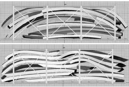
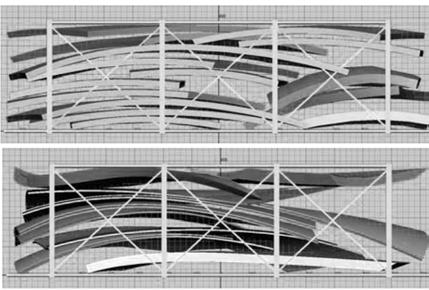
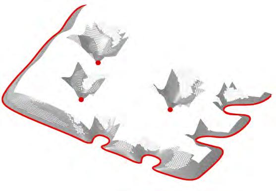
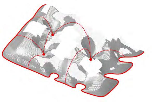
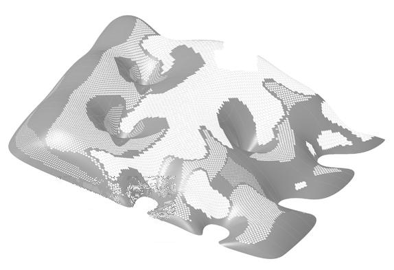
The stage three of the manufacturing process involves on site assembly. The precast panels and components would be transported to the site in batches. The dimensions of the panels and components are maintained within transportable dimensions, this greatly solves logistic issues. The figure 6.17 shows the transportation logic adopted in the Yitzhak Rabin Center project made of GRP panels. The panels are stacked based on their degree of curvature.

On site assembly would start with the base layer. The base layer is formed in order to eliminate the requirement for a dense form work. It is essential to avoid very dense supports which could possibly damage the ruins.

During the process of construction, it is crucial to maintain structural stability of the system. Therefore a strategic assembly logic is quintessential.

As illustrated in the diagrams in figure 6.16 the assembly of panels would begin from the base of the columns and along the peripheral edges of the shell. In order to avoid any eccentric loads due to cantilevering while assembly, intermediate arches would be formed from the base of the columns to the edge of the periphery. Further, intermediate spaces are filled with panels. This forms the base layer excluding the components.

The components are further assembled, resulting in the global form of the structure. The structural macro fibres could then be laid along the interstitial spaces between the three types of components. Finally, a second layer of epoxy resin would be applied and cure processed on site.

Column base and edge

Connections to the edge and intermediate connections

Components at the free edge

Figure 6.17 Transportation of panels (Rabin Center)

Figure 5.14 View from the ancient dock yard

Figure 5.14 Aerial view

Figure 5.14 Approach to exhibition galleries

Figure 5.14 View from walkways

7 Conclusion

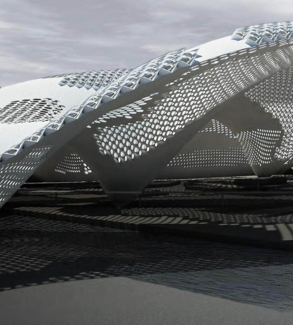
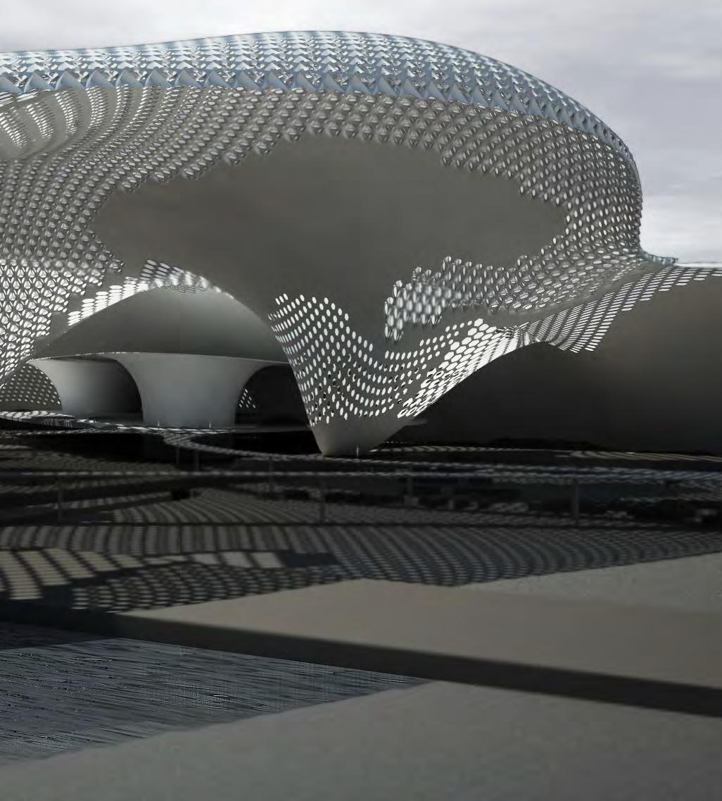
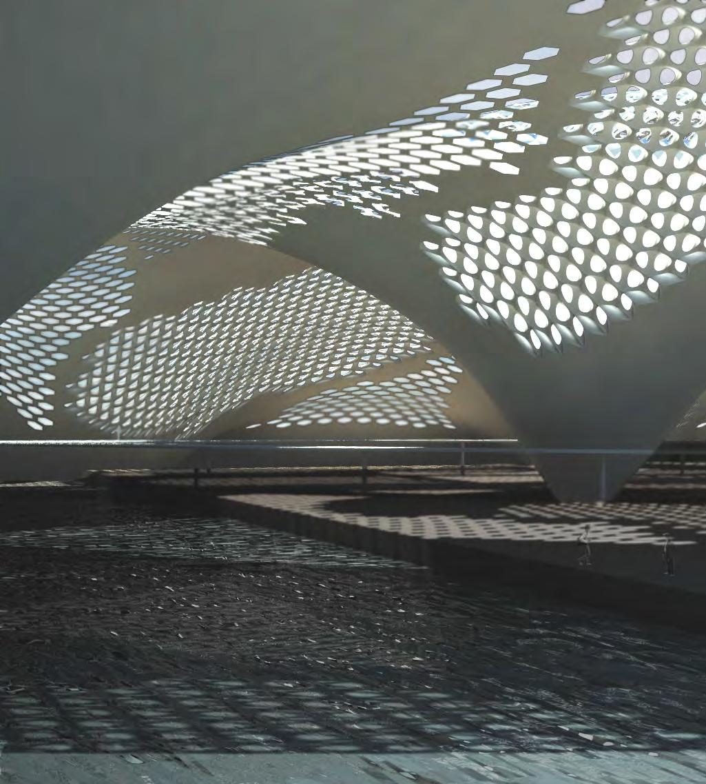
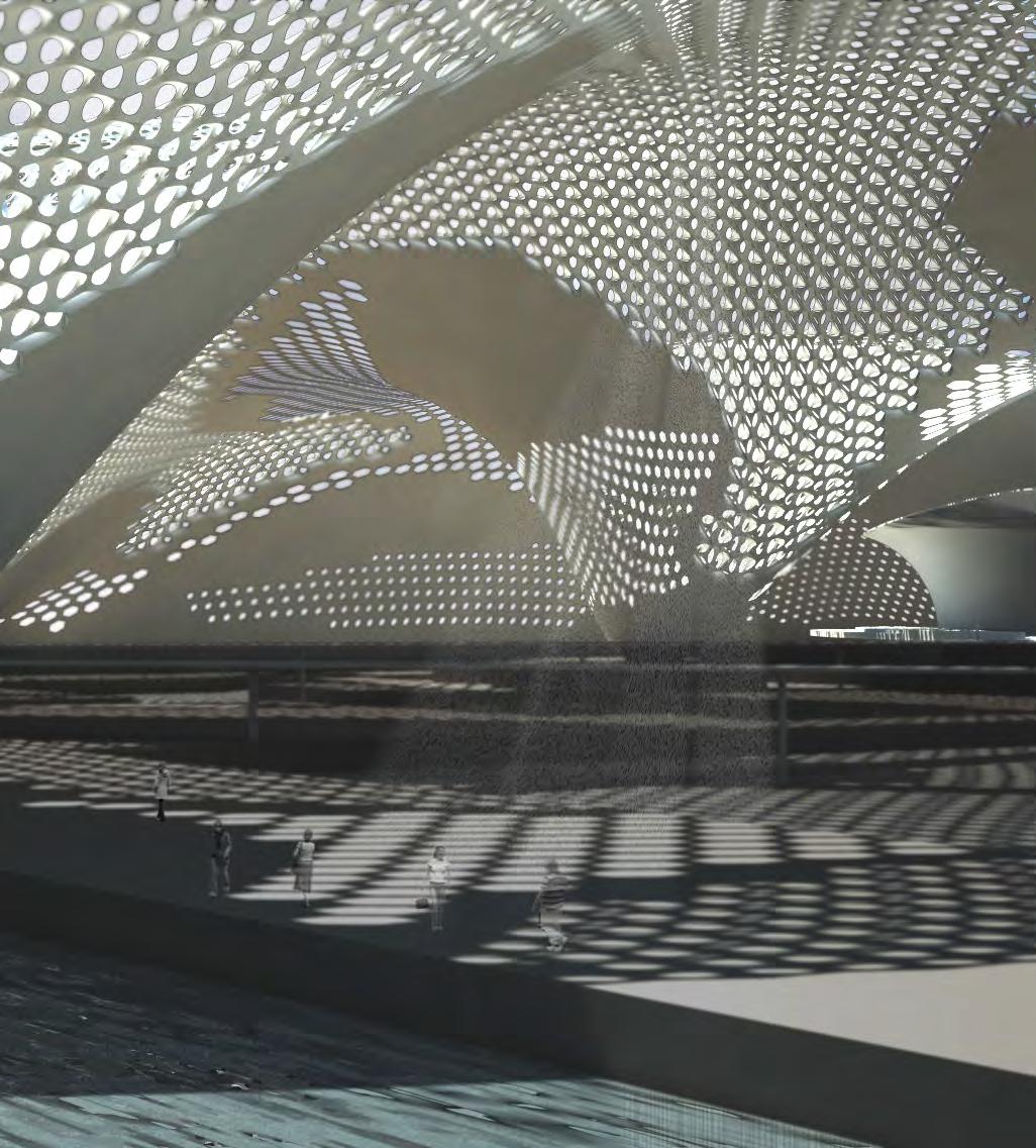
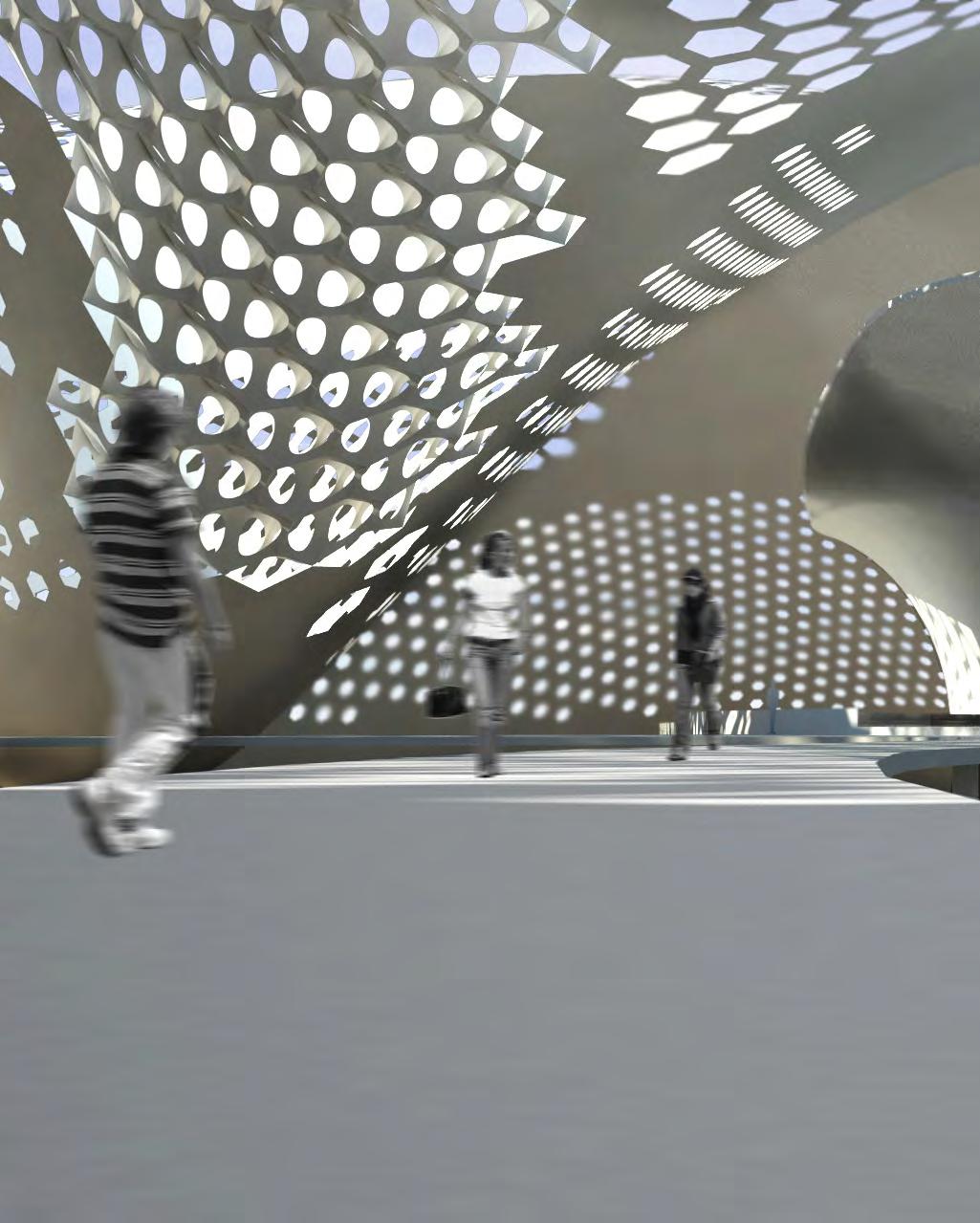
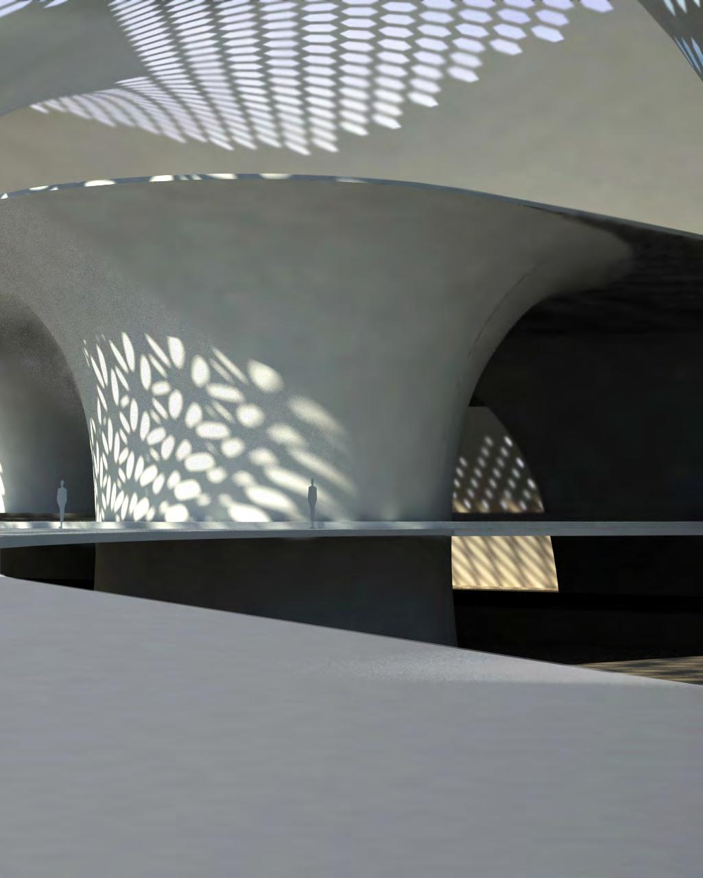
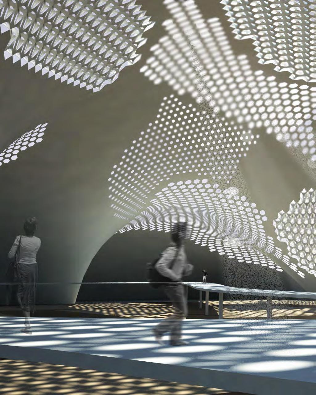
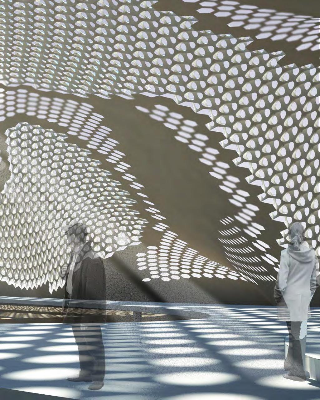
The proposed fibre composite adaptive system displays, ‘Integrated Functionality’, the factors such as form, structure, geometry and behaviour form a cohesive synergetic whole which complement one another. Biological organisms display emergent properties as they are organised in complex assemblies over several hierarchical scales. The design proposal, a fibre composite adaptive roof structure covering the ruins of the ancient city of Lothal, possesses multiple organisational scales that have different assembly logics at each scale which augment to their behaviour and performative abilities. Hence the system displays emergent behaviour which is not a mere sum of the parts but larger.

In hierarchical scalar levels the level one is the definition of the shape at the molecular level of the shape memory alloy actuators. Shape memory alloys have the ability to alter between their bi-stable states of equilibrium, the inherent- martensite state and the shape set-austenite phases. The level two is at the composite material level, embedded with shape memory alloys for actuating the opening and closing of the envelope. The level three is the component scale, defined as a continuous interwoven space truss which modulates the illumination and the wind flow, consequentially rendering better structural performance in spanning. The level four is that of the global shell form, which exploits the anisotropic and heterogeneous properties of the fibre composite material through varying fibre organisation density and orientation. The synergy between the assembly

logics in all the four scales results in a system which has the potential to adapt and self-organize efficiently to the transient changes in the environment.

The argument presented in this research is to explore the potential of self-actuating adaptive systems which could render efficient micro climates by utilizing environmental energy. The resultant micro climates within the architectural envelope would be heterogeneous, in contrast to homogeneous interior environments controlled through mechanical means. Although the proposal is context specific, informed by the climatic data and digital environmental simulations, the adaptive system has the potential for deployment in several environmental contexts. The definition of geometry could be altered to create openings to maximize the solar gain in cold climates in contrast to the closing logic presented here for a hot dry climate.

The further direction in this research would be to test the operational efficiency of the adaptive system. The technology of embedding shape memory alloys within a fibre composite material is still at its infancy in many fields of application, for example the aerospace and aviation industries. Nonetheless, the experiments performed at a smaller scale showed promising results. The next stage in the development of the research would be to build a full scale working prototype, to test the operational potential of the adaptive system and evolve the manufacturing logics.

8 A ppendix

Dynamic Relaxation Algorithm- Visual Basic Script

Option Explicit

Call Main() Sub Main()

Dim nx,ny,mx,my

Dim nprt,prts(),i,iy,ix

Dim x,y,z

Dim p,v,a,m,o

‘’-- block screen (for speed)

rhino.enableredraw False

‘’{{{-- SYSTEM SETUP --------------------

‘’-- define grid size

Rhino.MessageBeep 2

Rhino.MessageBox “STEP 1: DEFINE THE GRID SIZE”,0, “ALGORITHM INITIAL PARAMETERS”

nx=Rhino.IntegerBox (“Define grid size - X axis”, 10, “GRID SIZE”)

ny=Rhino.IntegerBox (“Define grid size - Y axis”, 10, “GRID SIZE”)

mx = nx-1

my ny-1

‘’---------------------------------------

‘’-- define points/particles/nodes

nprt = nx * ny

Dim gridcount(1),pgrid()

gridcount(0)=nx

gridcount(1)=ny

i 0

for iy 0 to my

for

z 0

‘’-- particle properties: position, velocity, acceleration, mass, graphic p = array( x, y, z )

v array( 0.0, 0.0, 0.0 )

a = array( 0.0, 0.0, 0.0 )

m 1.0

o = rhino.addpoint( p ) ReDim Preserve prts(i) prts( i ) = array( p, v, a, m, o )

‘’--prepare array for printing a surface from control points in the grid

‘’--prepare the array prts into pgrid which contains only the initial position of the points

ReDim Preserve pgrid(i) pgrid(i)=prts(i)(0)

i i + 1

Next

Next

rhino.enableredraw True

‘’--print Grid as a NURBS SURFACE from Control points, KnotU, KnotV, degree of surface and weights at each point

Dim gridsurface

Dim arrDegree

arrDegree=array(3,3)

Dim arrKnotU(),KnotUcount

‘number of elements in arrKnotU arrPointCount(0) + arrDegree(0) - 1

KnotUcount=gridcount(0)+arrDegree(0)-1

For i=0 To KnotUcount-1

ReDim Preserve arrKnotU(i)

arrKnotU(i)= (gridcount(0)/(KnotUcount))*i

Next

Dim arrKnotV(),KnotVcount

‘number of elements in arrKnotV arrPointCount(0) + arrDegree(0) - 1

KnotVcount=gridcount(1)+arrDegree(1)-1

For i=0 To KnotVcount-1

ReDim Preserve arrKnotV(i)

arrKnotV(i)= (gridcount(1)/(KnotUcount))*i

Next

‘Set up weights for each control point of the surface

‘At this moment all points are set up with equal weight (min value = 1)

Dim arrWeights()

For i=0 To ubound(pgrid)

ReDim Preserve arrWeights(i)

arrWeights(i)=1

Next

‘’-- define fixed points --> zero mass Dim fixed_points,j,ii

Rhino.MessageBeep 2 Rhino.MessageBox “STEP 2: SELECT FIXED POINTS (SUPPORTS)”,0, “ALGORITHM INITIAL PARAMETERS” fixed_points=Rhino.GetObjects (“SELECT FIXED POINTS”,1)

For j=0 To ubound(fixed_points) For ii=0 To nprt-1 If prts(ii)(4)=fixed_points(j)Then prts(ii)(3)=0.0 arrWeights(ii)=1 Rhino.ObjectColor fixed_points(j), RGB(255,0,0) End If Next Next

rhino.enableredraw False ‘’-- particle property mnemonic Dim PRT_P,PRT_V,PRT_A,PRT_M,PRT_O

PRT_P 0 ‘’ position

PRT_V = 1 ‘’ velocity

PRT_A 2 ‘’ acceleration/force

PRT_M = 3 ‘’ mass

PRT_O 4 ‘’ point object

‘ for num_of_fixed 0 to 5 ‘ prts( int( rnd * mx ) + int( rnd * my ) * nx )( PRT_M ) 0.0 ‘ next

Dim ia,ib,ic,id Dim k,l,d ‘’--get stiffness Rhino.MessageBeep 2 Rhino.MessageBox “STEP 3: DEFINE THE STIFFNESS OF THE MATERIAL - E (GPa)”,0, “ALGORITHM INITIAL PARAMETERS” Rhino.RealBox “E (GPa)”,3.1,”ALGORITHM INITIAL PARAMETERS”

k=5

‘’--get damping ratio Rhino.MessageBeep 2 Rhino.MessageBox “STEP 4: DEFINE THE DAMPING RATIO OF THE SYSTEM - d (no units)”,0, “ALGORITHM INITIAL PARAMETERS” d=Rhino.RealBox (“d (no units)”,0.5,”ALGORITHM INITIAL PARAMETERS”)

‘’-- define edges/springs/lines Dim nedg,edgs() nedg ny * mx + nx * my

i 0 for iy = 1 to my for ix 1 to mx

‘’-- get global offset from local offset in particle grid

‘’-- the following is to draw the lines in the grid: ‘’-- starting from a point, back, then in diagonal and then above ia ( ix - 0 ) + ( iy - 0 ) * nx ‘’-- current ib = ( ix - 1 ) + ( iy - 0 ) * nx ‘’-- before ic ( ix - 1 ) + ( iy - 1 ) * nx ‘’-- diagonal id = ( ix - 0 ) + ( iy - 1 ) * nx ‘’-- above

‘k 2.00 ‘’-- stiffness l 1.00 ‘’-- rest length

‘d 0.50 ‘’-- damping

‘’--with the following an ‘L’ is drawn ‘’-- current->before ‘CheckLayer “Lines”,1,1,1 o = rhino.addline( prts( ia ) ( PRT_P ), prts( ib )( PRT_P ) ) ReDim Preserve edgs(i) edgs( i ) = array( ia, ib, k, l, d, o ) i i + 1

‘’-- current->above o = rhino.addline( prts( id ) ( PRT_P ), prts( ia )( PRT_P ) ) REdim preserve edgs(i) edgs( i ) array( id, ia, k, l, d, o ) i i + 1 ‘’draw first column (it was left by the code above)

‘’-- handle first column

If( ix = 1 ) Then o = rhino.addline(

prts( ib )( PRT_P ), prts( ic )( PRT_P ) ) REdim preserve edgs(i) edgs( i ) array( ib, ic, k, l, d, o )

i i + 1 end if ‘’draw first row (it was left by the code above)

‘’-- handle first row

If( iy = 1 ) Then o = rhino.addline( prts( ic )( PRT_P ), prts( id )( PRT_P ) ) REdim preserve edgs(i)

edgs( i ) array( ic, id, k, l, d, o ) i = i + 1

Next

Next

‘’-- spring property mnemonic

Dim EDG_s,EDG_E,EDG_K,EDG_L,EDG_D,EDG_O

EDG_S = 0 ‘’-- start

EDG_E 1 ‘’-- end

EDG_K = 2 ‘’-- stiffness

EDG_L 3 ‘’-- rest length

EDG_D 4 ‘’-- damping

EDG_O 5 ‘’-- line object

‘’{{{-- OBTAIN THE REST OF THE INITIAL PARAMETERS PRIOR TO START SIMULATION

Dim iteration,iterations

Dim iedg, edg,si,ei,sp,ep

Dim u,f,s,sf,ef,iprt

Dim g

Dim delta

Dim ext_f_vector(),ext_f_vector_x,ext_f_ vector_y,ext_f_vector_z,ext_f_values(),ext_f_number

‘Get iterations

Rhino.MessageBeep 2

Rhino.MessageBox “STEP 5: DEFINE MAX NUMBER OF ITERATIONS”,0,”INITIAL PARAMETERS”

iterations=Rhino.RealBox (“iterations”,1000,”ALGORITHM INITIAL PARAMETERS”)

‘Get gravity value

‘Rhino.MessageBeep 2

‘Rhino.MessageBox “STEP 6: DEFINE ACCELERATION OF GRAVITYLow value for slow variation”,0,”ALGORITHM INITIAL PARAMETERS” ‘g=Rhino.RealBox (“GRAVITY”,0.005,”ALGORITHM INITIAL PARAMETERS”)

g=0.005

‘’Get External forces (Point of application, direction and value)

‘How many forces to be applied (ONE BY DEFAULT)

Rhino.MessageBeep 2

Rhino.MessageBox “STEP 8: NUMBER OF EXTERNAL FORCES TO BE APPLIED”,0,”INITIAL PARAMETERS”

ext_f_number=Rhino.IntegerBox (“NUMBER OF FORCES”,1,”ALGORITHM INITIAL PARAMETERS”)

For i=0 To 7

ReDim Preserve ext_f_vector(i)

ext_f_vector(i)=array(0,0,-1)

ReDim Preserve ext_f_values(i) ext_f_values(i)=0.7 Next

rhino.enableredraw True

Dim ext_f_points,ext_f_indexes()

Rhino.MessageBeep 2

Rhino.MessageBox “STEP 10: SELECT POINTS WHERE FORCE IS APPLIED”,0, “INITIAL PARAMETERS”

ext_f_points=Rhino.GetObjects (“SELECT POINTS”,1)

For j=0 To ubound(ext_f_points)

For ii=0 To nprt-1

If prts(ii)(4)=ext_f_points(j)Then

ReDim Preserve ext_f_indexes(j) ext_f_indexes(j)=ii Rhino.ObjectColor ext_f_points(j), RGB(255,0,0)

End If Next

Next

Dim points_start()

For iprt=0 To nprt-1

ReDim Preserve points_start(iprt)

points_start(iprt)=prts(iprt)(PRT_O) Next

Rhino.AddLayer “Points”, RGB(0, 0, 255)

Rhino.ObjectLayer points_start, “Points” Rhino.LayerVisible “Points”, False

gridsurface=Rhino.AddNurbsSurface (gridcount, pgrid, arrKnotU, arrKnotV, arrDegree, arrWeights) rhino.enableredraw False

‘’{{{-- SIMULATION

For iteration 0 To iterations

‘’-- reset forces/accelerations

‘’-- all the grid points to have starting acceleration of 0,0,0 at the start of each iteration

for iprt 0 to nprt - 1

prts( iprt )( PRT_A )( VECTOR_X ) 0.0

prts( iprt )( PRT_A )( VECTOR_Y ) 0.0

prts( iprt )( PRT_A )( VECTOR_Z ) = 0.0 next

‘’COMPUTE

‘’--

‘’--

for iedg = 0 to nedg - 1

‘’-- select edge

edg edgs( iedg )

si edg( EDG_S ) ‘’-- index of start particle

ei edg( EDG_E ) ‘’-- index of end particle

sp prts( si ) ‘’-- particle at start of spring

ep = prts( ei ) ‘’-- particle at end of spring

‘’-- spring position and velocity differences

u vector_create( ep( PRT_P ), sp( PRT_P ) ) ‘’-- displacement (used for force) v vector_create( ep( PRT_V ), sp( PRT_V ) ) ‘’-- relative motion (used for damping)

‘’-- particle distance -> displacement ‘’-- lo --> length at rest l vector_length( u )

‘’-- spring law F k * ( Lf -lo ) --> lo length at rest and Lf length when compressed ‘’-- formula is usually F= -k * x --> in this case the (-) sign comes from (Lf- lo) assuming Lf < lo f = edg( EDG_K ) * ( l - edg( EDG_L ) )

‘’-- damping (force against motion/ velocity between particle hence dot/l)

‘’-- damping - c * v ; in our case c = d (constant) and v is the velocity ‘’-- the dot product is u . v = ¦u¦*¦v¦*cos (tita)

‘’-- if tita 90, then u v 0

‘’-- if tita = 0 (parallel displacement and velocity) then u . v = ¦u¦*¦v¦ and then

‘’-- ( u v) / l (¦u¦ *

¦v¦ )/ ¦u¦ --> damping force d c * v

d edg( EDG_D ) * ( vector_dot( u, v ) / l )

‘’-- sum spring force s = f + d

‘’-- start/end particle force vectors (they are opposite!)

sf vector_rescale( u, -s ) ef vector_rescale( u, s )

‘’-- accumulate forces

prts( si )( PRT_A ) = vector_

add( prts( si )( PRT_A ), sf ) prts( ei )( PRT_A ) = vector_

add( prts( ei )( PRT_A ), ef ) next

‘’-- compute gravity force ‘’--

g 0.5 ‘’ acceleration of gravity

For iprt 0 To nprt - 1

‘’-- gravity force ( F m * g )

f = vector_new( 0.0, 0.0, ((g) * prts( iprt )( PRT_M )) )

‘’-- accumulate forces

prts( iprt )( PRT_A ) vector_ add( prts( iprt )( PRT_A ), f )

Next ‘ ‘’----------------------------------

‘’-- compute external forces

‘’-- external forces defined as a vector by the user ‘’’’’number of forces ‘’’’’direction (x,y,z) components -- unit vector ‘’’’’value (KN)

For i 0 To ubound(ext_f_indexes)

iprt=ext_f_indexes(i)

For ii = 0 To ubound(ext_f_vector)

f = array(ext_f_vector(ii) (0)*ext_f_values(ii),ext_f_vector(ii)(1)*ext_f_ values(ii),ext_f_vector(ii)(2)*ext_f_values(ii))

‘’-- accumulate forces

prts( iprt )( PRT_A ) vector_add( prts( iprt )( PRT_A ), f ) arrWeights(iprt)=1 Next

Next

‘’-- compute viscous drag (aka friction)

‘’- d 1.2 ‘’ drag coefficient

for iprt 0 to nprt - 1

‘’-- drag force ( F - d * v ) force = agaist a fraction of velocity

f vector_scale( prts( iprt )( PRT_V ), -d )

‘’-- accumulate forces

prts( iprt )( PRT_A ) vector_

add( prts( iprt )( PRT_A ), f ) next

‘’-- draw forces

‘ for iprt = 0 to nprt - 1

‘ p prts( iprt )( PRT_P )

‘ f = prts( iprt )( PRT_A )

‘ l rhino.addline( p, vector_add( p, f ) ) ‘ if( not isnull( l ) ) then call rhino.objectcolor( l, vbred ) ‘ next

‘’-- integrate positions using an euler solver

‘’-- this induces errors for large time steps! ‘’--

Dim dt

dt = 0.01 ‘’-- time step

for iprt = 0 to nprt - 1

‘’-- position ( p_new = p_old + dp/dt = p_old + v )

v vector_scale( prts( iprt )( PRT_V ), dt )

prts( iprt )( PRT_P ) vector_ add( prts( iprt )( PRT_P ), v )

‘’-- velocity ( v_new = v_ old + dv/dt v_old + a v_old + f / m )

if( prts( iprt )( PRT_M ) <> 0 ) then

a vector_scale( prts( iprt )( PRT_A ), dt / prts( iprt )( PRT_M ) ) else

a vector_new( 0.0, 0.0,

0.0 ) ‘’-- zero mass -> zero acceleration/force end if

prts( iprt )( PRT_V ) = vector_ add( prts( iprt )( PRT_V ), a ) next

‘’-- some safety rules against explosions

or pseudo inelastic collision

ie don’t allow particles outside a maximum volume

Dim xmin,ymin,zmin Dim xmax,ymax,zmax Dim reset

‘delta u or v (at least) ‘’-- a bounding cube size delta=nx

xmin -delta: xmax delta

ymin -delta: ymax delta

zmin -delta: zmax delta

Rhino.AddLayer “Lines”, RGB(225, 100, 20)

Rhino.LayerVisible “Lines”, False

for iprt 0 to nprt - 1

‘’-- on explosion reset velocity reset = false

‘’-- xmin < position.x < xmax

if( prts( iprt )( PRT_P )( VERTEX_X ) < xmin ) then

prts( iprt )( PRT_P )( VERTEX_X ) xmin reset = true

elseif( prts( iprt )( PRT_P )( VERTEX_X ) > xmax ) then

prts( iprt )( PRT_P )( VERTEX_X ) xmax reset = true end if

‘’-- ymin < position.y < ymax

if( prts( iprt )( PRT_P )( VERTEX_Y ) < ymin ) then

prts( iprt )( PRT_P )( VERTEX_Y ) ymin reset = true

elseif( prts( iprt )( PRT_P )( VERTEX_Y ) > ymax ) then

prts( iprt )( PRT_P )( VERTEX_Y ) ymax reset = true end if

‘’-- zmin < position.z < zmax

‘if( prts( iprt )( PRT_P )( VERTEX_Z ) < zmin ) then

‘prts( iprt )( PRT_P )( VERTEX_Z ) zmin ‘reset = true

‘elseif( prts( iprt )( PRT_P )( VERTEX_Z ) > zmax ) then

‘prts( iprt )( PRT_P )( VERTEX_Z ) zmax ‘reset = True ‘end if

‘’-- exploded! if( reset ) then

prts( iprt )( PRT_V )( VERTEX_X ) 0.0

prts( iprt )( PRT_V )( VERTEX_Y ) 0.0

prts( iprt )( PRT_V )( VERTEX_Z ) 0.0 end if next

rhino.pointcoordinates

prts( iprt )( PRT_O ), prts( iprt)( PRT_P ) ReDim Preserve newpgrid(iprt) newpgrid(iprt)=prts(iprt)(PRT_P) Next

‘’--delete previous grid surface and redraw it with new coordinates rhino.deleteobject gridsurface gridsurface=Rhino.AddNurbsSurface (gridcount, newpgrid, arrKnotU, arrKnotV, arrDegree, arrWeights)

‘’-- update edges (delete and redraw) For iedg 0 To nedg - 1 rhino.deleteobject edgs( iedg )( EDG_O ) si edgs( iedg )( EDG_S ) ei = edgs( iedg )( EDG_E ) sp = prts( si ) ep = prts( ei )

edgs( iedg )( EDG_O ) = rhino.addline( sp( PRT_P ), ep( PRT_P ) ) Rhino.ObjectLayer edgs( iedg )( EDG_O ), “Lines” Next

‘’-- ok show! rhino.enableredraw True

End If Next

‘’-- unblock screen rhino.enableredraw True

Rhino.AddLayer “Supports”, RGB(255, 0, 0) Rhino.AddLayer “Forces”, RGB(0, 255,0)

For i=0 To ubound(fixed_points) Rhino.ObjectLayer fixed_points(i), “Supports” Next

For i=0 To ubound(ext_f_points) Rhino.ObjectLayer ext_f_points(i), “Forces” Next

Rhino.AddLayer “Grid Surface”, RGB(255, 255, 255) Rhino.ObjectLayer gridsurface, “Grid Surface” Rhino.LayerVisible “Grid Surface”, True

Dim pointsA(),pointsB() Dim i1,i2 Dim half_limit half_limit=((ubound(newpgrid)+1)/2)-1

For i1=0 To half_limit ReDim Preserve pointsA(i1) pointsA(i1)=newpgrid(i1) Next Dim counter counter=-1

For i2=half_limit+1 To ubound(newpgrid) counter=counter+1 ReDim Preserve pointsB(i2) pointsB(counter)=newpgrid(i2) Next

Dim i3, geodesics()

‘ Rhino.AddLayer “Geodescis”, RGB(255, 255, 255) CheckLayer “Geodesics”,1,1,1

For i3=0 To ubound(pointsA) Redim preserve geodesics(i3) geodesics(i3)=Rhino.ShortPath (gridsurface, pointsA(i3),pointsB(i3)) Rhino.UnselectAllObjects Rhino.SelectObject gridsurface Rhino.SelectObject CStr(geodesics(i3)) Rhino.Command “_ExtendCrvOnSrf” Rhino.UnselectAllObjects Next CheckLayer “Grid Surface”, 1,1,1 Rhino.LayerVisible “Geodesics”, False ‘ Rhino.ObjectLayer geodesics, “Geodesics”

End Sub

‘’ Functions from STYLIANOS DRITSAS LIBRARY

Function vector_dot(va,vb)

Dim VECTOR_X:VECTOR_X=0

Dim VECTOR_Y:VECTOR_Y=1 Dim VECTOR_Z:VECTOR_Z=2

If( iteration Mod 10 0 ) Then

‘’-- graphics time! rhino.enableredraw False

‘’-- update particles and control points of grid(just update)

for iprt 0 to nprt - 1

vector_dot=(va( VECTOR_X )*vb( VECTOR_X ))+(va( VECTOR_Y ) * vb( VECTOR_Y ))+(va( VECTOR_Z )* vb( VECTOR_Z ))

End Function

Function vector_new( x, y, z )

vector_new vertex_new( x, y, z )

End Function

Function vector_create( va, vb )

vector_create vector_new(vb( VECTOR_X ) - va( VECTOR_X ),vb( VECTOR_Y ) - va( VECTOR_Y ),vb( VECTOR_Z ) - va( VECTOR_Z ))

End Function

Function vector_length( vector ) vector_length sqr(vector( VECTOR_X ) * vector( VECTOR_X ) +vector( VECTOR_Y ) * vector( VECTOR_Y ) + vector( VECTOR_Z ) * vector( VECTOR_Z ))

End Function

Function vector_add( va, vb )

vector_add = vector_new(va( VECTOR_X ) + vb( VECTOR_X ), va( VECTOR_Y ) + vb( VECTOR_Y ),va( VECTOR_Z ) + vb( VECTOR_Z ))

End Function

Function vector_scale( vector, factor )

vector_scale vector_new(vector( VECTOR_X ) * factor,vector( VECTOR_Y ) * factor,vector( VECTOR_Z ) * factor)

End Function

Function vector_rescale( vector, length )

Dim length_: length_ vector_length( vector )

If( length_ = 0.0 ) Then

vector_rescale vector_new( 0.0, 0.0, 0.0 ) Else

vector_rescale vector_new(length * vector( VECTOR_X ) / length_,length * vector( VECTOR_Y ) / length_,length * vector( VECTOR_Z ) / length_)

End If

End Function

Function vector_dot( va, vb )

vector_dot = va( VECTOR_X ) * vb( VECTOR_X ) +va( VECTOR_Y ) * vb( VECTOR_Y ) +va( VECTOR_Z ) * vb( VECTOR_Z )

End Function

‘’ My own functions

Sub CheckLayer(ByVal layername,ByVal red,ByVal green,ByVal blue)

If Rhino.IsLayer(layername) Then Rhino.CurrentLayer (layername)

Rhino.LayerColor layername,RGB(255*red,255*green,255*blue) Else Rhino.AddLayer (layername)

Rhino.CurrentLayer(layername) Rhino.LayerColor layername,RGB(255*red,255*green,255*blue)

End If

End Sub Sub UnCheckLayer(ByVal layername)

If Rhino.IsLayer(layername) Then If Rhino.LayerVisible(layername) True Then Rhino.LayerVisible layername, False

End If

End If

End Sub

Fibre

Option Explicit

Call Main() Sub Main()

Dim surface1,surface2,i

surface1=rhino.getobject(“Select first surface”,8)

surface2=rhino.getobject(“Select second surface”,8)

Dim stension_points(),stension(),stension_vector()

Dim syield_fibres,syield_polymer

Dim smaxyield_polymer(),smaxyield_fibres()

‘Dim scale_factor,thickness

Dim n()

‘Enter properties of the material: polymer and fibres

syield_polymer=Rhino.RealBox (“Specify syield polymer (MPa): “,59, “Yield Stress - Polymer”)

syield_polymer=(syield_polymer)*10^(6) syield_fibres=Rhino.RealBox (“Specify syield fibres (MPa): “,90, “Yield Stress - Fibres”)

syield_fibres=(syield_fibres)*10^(6)

‘Enter scale factor and thickness ‘scale_factor=Rhino.RealBox (“Density of fibres at max tension points: “,0.01, “FIBRES DENSITY”)

‘thickness=Rhino.RealBox (“Specify max thickness at max tension points: “,2.0, “THICKNESS MAIN VEINS”)

Dim aPoints(),s1Values(),s1Vector(),s2Val ues(),s2Vector(),s3Values(),s3Vector()

Dim smaxyield_fpoints(),smaxyield_f_tension_vector()

Dim smaxtension_check_points_sorted,smaxtension_check_vector_sorted

Dim smaxyield_fibres_check_points_sorted,smaxyield_fibres_ check_vector_sorted,smaxyield_fibres_check_values_sorted

Dim Max_fibre_yield_s,Min_polymer_yield_s,Max_fibre_s,Min_fibre_yield_s

ImportFromExcel 2,2,aPoints,s1Values,s1Vec tor,s2Values,s2Vector,s3Values,s3Vector

create_list 3,n

get_tension_fibres aPoints,s1Values,s1Vector,s2Values,s2Vector,s3V alues,s3Vector,syield_polymer,stension,stension_points,stension_vector

get_tension_fibres_yield stension_ points,stension,stension_vector,syield_fibres,smaxyield_ fibres,smaxyield_fpoints,smaxyield_f_tension_vector

max_min stension,Max_fibre_yield_s,Min_polymer_yield_s max_min smaxyield_fibres,Max_fibre_s,Min_fibre_yield_s

For i=0 To ubound(n)

check_stress surface1,surface2,Max_fibre_yield_s,Min_ polymer_yield_s,n,i,syield_fibres,stension,stension_points,stension_ vector,smaxtension_check_points_sorted,smaxtension_check_vector_sorted

check_stress_populate surface1,surface2,Max_fibre_s,Min_fibre_ yield_s,n,i,syield_fibres,smaxyield_fibres,smaxyield_fpoints,smaxyield_f_ tension_vector,smaxyield_fibres_check_points_sorted,smaxyield_ fibres_check_vector_sorted,smaxyield_fibres_check_values_sorted

Next

CheckLayer “Edge Surface”,1,1,1 Rhino.DuplicateEdgeCurves surface1

If (surface2 <> vbNull) Then Rhino.DuplicateEdgeCurves surface2

End If

Rhino.LayerVisible “Surface”, False Rhino.LayerVisible “Supports”, False Rhino.LayerVisible “Fibres”, False Rhino.LayerVisible “Points”, False

End Sub

Sub ImportFromExcel(ByVal startrow,ByVal startcolumn,ByRef aPoints(),ByRef s1Values(),ByRef s1Vector(),ByRef s2Values(),ByRef s2Vector(),ByRef s3Values(),ByRef s3Vector())

‘Define constant for the maximum number of rows in the Excel file ---’Do not change this value’’ Const xlDown = -4121

‘Define new variables for extracting data from Excel file Dim oExcel, oSheet, nRow, nRowCount, sFileName ‘Get the name of the file to import

sFileName = Rhino.OpenFileName(“Select File”,”Excel Files (*.xls)|*.xls||”)

If IsNull(sFileName) Then Exit Sub ‘Launch Excel and open the specified file

Set oExcel CreateObject(“Excel.Application”)

oExcel.Workbooks.Open(sFileName)

‘Set the active worksheet

Set oSheet oExcel.ActiveSheet

‘Count the number of rows that need to be processed nRowCount oSheet.Range(“a”&CStr(startrow), oSheet. Range(“a”&CStr(startrow)).End(xlDown)).Rows.Count If (nRowCount 0 ) Then

Rhino.Print “No data range found in file.”

Exit Sub

ElseIf (nRowCount < 2 ) Then Rhino.Print “Not enough points to create curve.”

End If

Exit Sub

‘Re-dimension the resulting array of points accordingly

‘Process all rows Rhino.Print “Importing data...”

‘Define the variables for the data to be imported from Excel Dim s1,s1x,s1y,s1z,x,y,z,s2,s2x,s2y,s2z,s3,s3x,s3y,s3z

‘These are the arrays where the node coordinates, the s1 tension values and vectors will be stored

‘ Read the values from columns, starting with “startcolumn” defined by the user ‘ Read the values from the rows, starting from “startrow” defined by the user

For nRow startrow To nRowCount+startrow-1 ‘Get coordinates of the nodes x=oSheet.Cells(nRow,startcolumn).Value y=oSheet.Cells(nRow,startcolumn+1).Value z=oSheet.Cells(nRow,startcolumn+2).Value

‘Get the value of the s1 principal stress s1 oSheet.Cells(nRow, startcolumn+6).Value

‘Get the vector of s1 principal stress s1x oSheet.Cells(nRow, startcolumn+19).Value s1y = oSheet.Cells(nRow, startcolumn+20).Value s1z oSheet.Cells(nRow, startcolumn+21).Value

‘Store values in arrays ReDim Preserve aPoints(nRow-startrow) aPoints(nRow-startrow)=array(x,y,z) ReDim Preserve s1Values(nRow-startrow) s1Values(nRow-startrow)=s1 ReDim Preserve s1vector(nRow-startrow) s1vector(nRow-startrow)=Array(s1x,s1y,s1z)

‘Get the value of the s2 principal stress s2 oSheet.Cells(nRow, startcolumn+5).Value ‘Get the vector of s2 principal stress s2x oSheet.Cells(nRow, startcolumn+16).Value s2y oSheet.Cells(nRow, startcolumn+17).Value s2z oSheet.Cells(nRow, startcolumn+18).Value

‘Store values in arrays ReDim Preserve s2Values(nRow-startrow) s2Values(nRow-startrow)=s2 ReDim Preserve s2vector(nRow-startrow)

s2vector(nRow-startrow)=Array(s2x,s2y,s2z)

‘Get the value of the s3 principal stress

s3 = oSheet.Cells(nRow, startcolumn+4).Value

‘Get the vector of s3 principal stress s3x = oSheet.Cells(nRow, startcolumn+13).Value s3y oSheet.Cells(nRow, startcolumn+14).Value s3z = oSheet.Cells(nRow, startcolumn+15).Value

‘Store values in arrays

ReDim Preserve s3Values(nRow-startrow) s3Values(nRow-startrow)=s3 ReDim Preserve s3vector(nRow-startrow)

s3vector(nRow-startrow)=Array(s3x,s3y,s3z) Next

‘Close Excel and disassociate object variables

oExcel.Quit

Set oSheet Nothing

Set oExcel Nothing

CheckLayer “Points”,1,1,1 rhino.addpoints aPoints

End Sub

Sub max_min(ByVal stension(),ByRef Maxs,ByRef Mins)

‘Find out maximum And minimum principal tension stresses Dim stension_sorted stension_sorted=Rhino.SortNumbers (stension) Mins=stension_sorted(0) Maxs=stension_sorted(ubound(stension))

End Sub

Sub CheckLayer(ByVal layername,ByVal red,ByVal green,ByVal blue)

If Rhino.IsLayer(layername) Then Rhino.CurrentLayer (layername) Rhino.LayerColor layername ,RGB(255*red,255*green,255*blue)

Else

Rhino.AddLayer (layername) Rhino.CurrentLayer(layername)

Rhino.LayerColor layername ,RGB(255*red,255*green,255*blue)

End If End Sub

Sub UnCheckLayer(ByVal layername)

If Rhino.IsLayer(layername) Then If Rhino.LayerVisible(layername) True Then Rhino.LayerVisible layername, False

End If

End If

End Sub

Sub get_tension_fibres(ByVal aPoints(),ByVal s1Values(),ByVal s1Vector(),ByVal s2Values(),ByVal s2Vector(),ByVal s3Values(),ByVal s3Vector(),ByVal syield_ polymer,ByRef stension(),ByRef stension_points(),ByRef stension_vector())

‘Counters (auxilliar)

Dim i,j,l

‘Define variables for examinating the s1yield of the fibres and the polymer and storing the values

j=-1

For i=0 To ubound(s1Values)

If s1Values(i)>s2Values(i) And s1Values(i)>s2Values(i) And s1values(i)>0 And (abs(s1Values(i))>syield_polymer) Then j=j+1

ReDim Preserve stension(j)

stension(j)=s1Values(i) ‘s1tension stores values of principal stress s1 if in tension

ReDim Preserve stension_points(j)

stension_points(j)=aPoints(i) ‘s1tension_points stores the 3D points that register a negative value of s1, i.e. are in tension

ReDim Preserve stension_vector(j)

stension_vector(j)=Rhino.VectorUnitize(Rhino. VectorCreate(s1Vector(i), stension_points(j)))

‘s1tension_vector stores the 3D vector of the principal stress s1, which will be afterwards used to draw the fibres

End If

Next

For i=0 To ubound(s2Values)

If s2Values(i)>s1Values(i) And s2Values(i)>s3Values(i) And s2values(i)>0 And (abs(s2Values(i))>syield_polymer) Then j=j+1

ReDim Preserve stension(j)

stension(j)=s2Values(i) ‘s1tension stores values of principal stress s1 if in tension

ReDim Preserve stension_points(j)

stension_points(j)=aPoints(i) ‘s1tension_points stores the 3D points that register a negative value of s1, i.e. are in tension ReDim Preserve stension_vector(j) stension_vector(j)=Rhino.VectorUnitize(Rhino. VectorCreate(s2Vector(i), stension_points(j))) ‘s1tension_vector stores the 3D vector of the principal stress s1, which will be afterwards used to draw the fibres End If Next

For i=0 To ubound(s3Values)

If s3Values(i)>s1Values(i) And s3Values(i)>s2Values(i) And s3values(i)>0 And (abs(s3Values(i))>syield_polymer) Then j=j+1

ReDim Preserve stension(j) stension(j)=s3Values(i) ‘s1tension stores values of principal stress s1 if in tension ReDim Preserve stension_points(j) stension_points(j)=aPoints(i) ‘s1tension_points stores the 3D points that register a negative value of s1, i.e. are in tension ReDim Preserve stension_vector(j) stension_vector(j)=Rhino.VectorUnitize(Rhino. VectorCreate(s3Vector(i), stension_points(j))) ‘s1tension_vector stores the 3D vector of the principal stress s1, which will be afterwards used to draw the fibres End If

Next

End Sub

Sub get_tension_fibres_yield(ByVal stension_points(),ByVal stension(),ByVal stension_vector(),ByVal syield_fibres,ByRef smaxyield_fibres(),ByRef smaxyield_fpoints(),ByRef smaxyield_f_tension_vector()) ‘Counters (auxilliar) Dim i,l

l=-1

For i=0 To ubound(stension) ‘Store the fibres that are over the syield of the fibres,i.e. more fibres would be required at these positions If abs(stension(i))>syield_fibres Then l=l+1

ReDim Preserve smaxyield_fibres(l) smaxyield_fibres(l)=stension(i) ‘s1yield_fibres stores values of principal stress s1 if syield of the fibre is exceeded

ReDim Preserve smaxyield_fpoints(l) smaxyield_fpoints(l)=stension_points(i) ‘s1yield_fibres stores values of principal stress s1 if syield of the fibre is exceeded ReDim Preserve smaxyield_f_tension_vector(l) smaxyield_f_tension_vector(l)=Rhino.VectorUnitize(Rhino. VectorCreate(stension_vector(i), smaxyield_fpoints(l))) ‘s1yield_fibres stores values of principal stress s1 if syield of the fibre is exceeded

End If

Next

End Sub

Sub create_list(ByVal m,ByRef n()) dim i For i=0 To m-1 ReDim Preserve n(i)

n(i)=i+1

Next

End Sub

Sub check_stress(ByVal surface1,ByVal surface2,ByVal Maxs,ByVal Mins,ByVal n(),ByVal t,ByVal syield_fibres,ByVal smaxyield_fibres(),ByVal smaxyield_ fpoints(),ByVal smaxyield_f_tension_vector(),ByRef smaxyield_fibres_ check_points_sorted(),ByRef smaxyield_fibres_check_vector_sorted()) Dim spart,up_bound,k,low_bound,j,i Dim smaxyield_fibres_check_points(),smaxyield_ fibres_check_vector(),bigarray spart=(Maxs-Mins)/(ubound(n)) up_bound=Maxs j=-1 For k=0 To ubound(n) low_bound=Maxs-n(k)*spart For i=0 To ubound(smaxyield_fpoints) If (abs(low_bound)<abs(smaxyield_fibres(i))) And (abs(smaxyield_fibres(i))<=abs(up_bound)) Then j=j+1 ReDim Preserve smaxyield_fibres_check_points(j) smaxyield_fibres_ check_points(j)=smaxyield_fpoints(i) ReDim Preserve smaxyield_fibres_check_vector(j) smaxyield_fibres_check_ vector(j)=smaxyield_f_tension_vector(i) End If Next up_bound=low_bound Next

Dim smaxyield_fibres_check_vector_s()

bigarray=array(smaxyield_fibres_check_ points,smaxyield_fibres_check_vector) smaxyield_fibres_check_points_sorted=Rhino. SortPoints(smaxyield_fibres_check_points)

For i=0 To ubound(smaxyield_fibres_check_points)

For j=0 To ubound(smaxyield_fibres_check_vector) If bigarray(0)(i)(0)=smaxyield_fibres_check_ points(j)(0)And bigarray(0)(i)(1)=smaxyield_fibres_check_points(i)(1) And bigarray(0)(i)(2)=smaxyield_fibres_check_points(i)(2) Then ReDim Preserve smaxyield_fibres_check_vector_s(i) smaxyield_fibres_check_ vector_s(i)=smaxyield_fibres_check_vector(j) End If Next

Next

smaxyield_fibres_check_vector_sorted=smaxyield_fibres_check_vector_s

‘Draw fibres at points where the tensile stress exceeds the syield of the polymer, following the stresses path, ‘’’’’’’’’’’i.e. the points With similar tensile stresses Or within a range. This range Is determined by ‘m’ ‘This function will also increase the density of the fibres depending on how much tension over the syield of the fibre is felt at that point draw_tension_fibres_stresses_path surface1,surface2,smaxyield_ fibres_check_points_sorted,smaxyield_fibres_check_vector_sorted

End Sub

Sub check_stress_populate(ByVal surface1,ByVal surface2,ByVal Maxs,ByVal Mins,ByVal n(),ByVal t,ByVal syield_fibres,ByVal smaxyield_ fibres(),ByVal smaxyield_fpoints(),ByVal smaxyield_f_tension_vector(),ByRef smaxyield_fibres_check_points_sorted(),ByRef smaxyield_fibres_check_ vector_sorted(),ByRef smaxyield_fibres_check_values_sorted())

Dim spart,up_bound,k,low_bound,j,i Dim smaxyield_fibres_check_points(),s1yield_fibres_ check_vector(),s1yield_fibres_check_values(),bigarray spart=(Maxs-Mins)/(ubound(n)) up_bound=Maxs j=-1 For k=0 To ubound(n) low_bound=Maxs-n(k)*spart For i=0 To ubound(smaxyield_fpoints) If (abs(low_bound)<abs(smaxyield_fibres(i))) And (abs(smaxyield_fibres(i))<=abs(up_bound)) Then j=j+1 ReDim Preserve smaxyield_fibres_check_points(j) smaxyield_fibres_ check_points(j)=smaxyield_fpoints(i) ReDim Preserve smaxyield_fibres_check_vector(j) smaxyield_fibres_check_ vector(j)=smaxyield_f_tension_vector(i) ReDim Preserve smaxyield_fibres_check_values(j) smaxyield_fibres_ check_values(j)=smaxyield_fibres(i) End If Next up_bound=low_bound Next

Dim smaxyield_fibres_check_vector_s(),smaxyield_fibres_check_values_s() bigarray=array(smaxyield_fibres_check_ points,smaxyield_fibres_check_vector) smaxyield_fibres_check_points_sorted=Rhino. SortPoints(smaxyield_fibres_check_points)

For i=0 To ubound(smaxyield_fibres_check_points) For j=0 To ubound(smaxyield_fibres_check_vector) If bigarray(0)(i)(0)=smaxyield_fibres_check_ points(j)(0)And bigarray(0)(i)(1)=smaxyield_fibres_check_points(i)(1) And bigarray(0)(i)(2)=smaxyield_fibres_check_points(i)(2) Then ReDim Preserve smaxyield_fibres_check_vector_s(i) smaxyield_fibres_check_ vector_s(i)=smaxyield_fibres_check_vector(j) ReDim Preserve smaxyield_fibres_check_values_s(i) smaxyield_fibres_check_ values_s(i)=smaxyield_fibres_check_values(j) End If Next Next

smaxyield_fibres_check_vector_sorted=smaxyield_fibres_check_vector_s smaxyield_fibres_check_values_sorted=smaxyield_fibres_check_values_s

‘Draw fibres at points where the tensile stress exceeds the syield of the polymer, following the stresses path,

the points With similar tensile stresses Or within a range. This range Is determined by ‘m’

‘This function will also increase the density of the fibres depending on how much tension over the syield of the fibre is felt at that point

populate_tension_fibres_stresses_path surface1,surface2,smaxyield_ fibres_check_values_sorted,syield_fibres,smaxyield_fibres_check_ points_sorted,smaxyield_fibres_check_vector_sorted

End Sub

Sub draw_tension_fibres_stresses_path(ByVal surface1,ByVal surface2,ByVal smaxyield_fibres_check_points_sorted(),ByVal smaxyield_fibres_check_vector_sorted())

Dim arrpoints(),pointsrf1,pointsrf11,pointsrf2,points rf22,crvonsrf,crvonsrf1,initial_point1,initial_point2 Dim i

‘Draw the fibres where the value there is tension and it is over the syield of the polymer For i=0 To ubound(smaxyield_fibres_check_vector_sorted)

CheckLayer “Fibres”,1,1,1 ReDim Preserve arrpoints(i) arrpoints(i)=Rhino.VectorAdd (smaxyield_fibres_check_ points_sorted(i), smaxyield_fibres_check_vector_sorted(i)) initial_point1=Rhino.EvaluateSurface(surface1, array(0.0142803, 0.00878829))

If (surface2 <> vbNull) Then initial_point2=Rhino. EvaluateSurface(surface2, array(0,0.029335)) End If

If IsArray(initial_point1) And IsArray(arrpoints(i))Then pointsrf1=Rhino.PullPoints (su rface1,array(arrpoints(i),initial_point1)) pointsrf11=Rhino.PullPoints(surface1,arra y(smaxyield_fibres_check_points_sorted(i),initial_point1)) If VarType(Rhino.AddInterpCrvOnSrf (sur face1,array(pointsrf11(0),pointsrf1(0))))=vbString Then crvonsrf=Rhino.AddInterpCrvOnSrf (surfa ce1,array(pointsrf11(0),pointsrf1(0))) Rhino.UnselectAllObjects Rhino.SelectObject surface1 Rhino.SelectObject CStr(crvonsrf) Rhino.Command “_ExtendCrvOnSrf” Rhino.UnselectAllObjects CheckLayer “Macrofibres”,1,1,1 Rhino.SelectObject CStr(crvonsrf) Rhino.Command “_Pipe 0.001 0.001 enter” rhino.DeleteObject(crvonsrf) Rhino.UnselectAllObjects End If End If

If (surface2 <> vbNull) And IsArray(initial_ point2) And IsArray(arrpoints(i))Then pointsrf2=Rhino.PullPoints (su rface2,array(arrpoints(i),initial_point2)) pointsrf22=Rhino.PullPoints (surface2,array(smaxyield_ fibres_check_points_sorted(i),initial_point2)) If VarType(Rhino.AddInterpCrvOnSrf (surf ace2,array(pointsrf22(0),pointsrf2(0)))) vbString Then crvonsrf=Rhino.AddInterpCrvOnSrf (surfa ce2,array(pointsrf22(0),pointsrf2(0))) Rhino.UnselectAllObjects Rhino.SelectObject surface2 Rhino.SelectObject CStr(crvonsrf) Rhino.Command “_ExtendCrvOnSrf” Rhino.UnselectAllObjects CheckLayer “Macrofibres”,1,1,1 Rhino.SelectObject CStr(crvonsrf) Rhino.Command “_Pipe 0.001 0.001 enter” rhino.DeleteObject(crvonsrf) Rhino.UnselectAllObjects End If End If Next End Sub

Sub populate_tension_fibres_stresses_path(ByVal surface1,ByVal surface2,ByVal smaxyield_fibres(),ByVal syield_fibres(),ByVal smaxyield_fpoints(),ByVal smaxyield_f_tension_vector())

‘Now only where syield of the fibres is exceeded, a higher number of fibres is allocated.

‘The number of fibres is proportional to how much the syield of the fibres is exceeded.

Dim smaxyield_f_arrpoints(),i

Dim number_fibres,start_point,end_point,n,initial_point1,initial_point2 Dim pointsrf1,pointsrf11,pointsrf2,point srf22,crvonsrf1,crvonsrf2,crvonsrf3 Dim difference,pipe

For i=0 To ubound(smaxyield_f_tension_vector)

If abs(smaxyield_fibres(i))>syield_fibres Then CheckLayer “Fibres”,1,1,1 ReDim Preserve smaxyield_f_arrpoints(i) smaxyield_f_arrpoints(i)=Rhino.VectorAdd (smaxyield_fpoints(i), smaxyield_f_tension_vector(i)) initial_point1=Rhino. EvaluateSurface(surface1, array(0.0142803, 0.00878829)) If (surface2 <> vbNull)Then initial_point2=Rhino. EvaluateSurface(surface2, array(0,0.029335))

End If

If IsArray(initial_point1) And IsArray(smaxyield_f_arrpoints(i))Then pointsrf1=Rhino.PullPoints (surface1,array(smaxyield_f_arrpoints(i),initial_point1)) pointsrf11=Rhino.PullPoints(s urface1,array(smaxyield_fpoints(i),initial_point1)) If VarType(Rhino.AddInterpCrvOnSrf (su rface1,array(pointsrf11(0),pointsrf1(0)))) vbString Then crvonsrf1=Rhino. AddInterpCrvOnSrf (surface1,array(pointsrf11(0),pointsrf1(0))) Rhino.UnselectAllObjects Rhino.SelectObject surface1 Rhino.SelectObject CStr(crvonsrf1) Rhino.Command “_ExtendCrvOnSrf” Rhino.UnselectAllObjects crvonsrf2=rhino.firstobject()

CheckLayer “Extra-Macrofibres”,1,1,1 Rhino.SelectObject CStr(crvonsrf2) Rhino.Command “_Pipe 0.005 0.005 enter” Rhino.UnselectAllObjects pipe=rhino.firstobject()

‘Now increase the number of fibres where the tensile stress exceeds the syield of the fibres ‘The new fibres created are offset from the original one on the surface to make them ‘visible’ to the user ‘The idea is to easily visualize the areas where the main veins are to be located difference=int(smaxyield_fibres(i)-syield_fibres) If difference<syield_fibres Then number_fibres=0 ‘so that it only generates an extra fibre ElseIf difference>syield_fibres Then number_fibres=1 ‘so that the total of extra fibres is 2 End If

For n=0 To number_fibres start_point=Rhino.CurveStartPoint(crvonsrf2) end_point=array(start_ point(0)+rnd*0.01,start_point(1)+rnd*0.01,start_point(2)+0.01) crvonsrf3=Rhino. CopyObject (pipe, start_point,end_point) Next End If End If

If (surface2 <> vbNull) And IsArray(initial_ point2) And IsArray(smaxyield_f_arrpoints(i))Then pointsrf2=Rhino.PullPoints (surface2,array(smaxyield_f_arrpoints(i),initial_point2)) pointsrf22=Rhino.PullPoints (surface2,array(smaxyield_fpoints(i),initial_point2)) If VarType(Rhino.AddInterpCrvOnSrf (su rface2,array(pointsrf22(0),pointsrf2(0)))) vbString Then crvonsrf1=Rhino. AddInterpCrvOnSrf (surface2,array(pointsrf22(0),pointsrf2(0))) Rhino.UnselectAllObjects Rhino.SelectObject surface2 Rhino.SelectObject CStr(crvonsrf1) Rhino.Command “_ExtendCrvOnSrf” Rhino.UnselectAllObjects crvonsrf2=rhino.firstobject() CheckLayer “Extra-Macrofibres”,1,1,1 Rhino.SelectObject CStr(crvonsrf2) Rhino.Command “_Pipe 0.005 0.005 enter” Rhino.UnselectAllObjects pipe=rhino.firstobject()

‘Now increase the number of fibres where the tensile stress exceeds the syield of the fibres ‘The new fibres created are offset from the original one on the surface to make them ‘visible’ to the user ‘The idea is to easily visualize the areas where the main veins are to be located difference=int(smaxyield_fibres(i)-syield_fibres) If difference<syield_fibres Then number_fibres=0

‘so that it only generates an extra fibre ElseIf difference>syield_fibres Then number_fibres=1

‘so that the total of extra fibres is 2 End If For n=0 To number_fibres start_ point=Rhino.CurveStartPoint(crvonsrf2) end_point=array(start_ point(0)+rnd*0.01,start_point(1)+rnd*0.01,start_point(2)+0.01) crvonsrf3=Rhino. CopyObject (pipe, start_point,end_point) Next End If End If End If Next End Sub

Hexagon Tessellation on Surface - Visual Basic Script

Option Explicit ‘Script written by <insert name>

‘Script copyrighted by <insert company name>

‘Script version Tuesday, 08 December 2009 18:04:00

Call HexOnSurf()

Sub HexOnSurf()

‘Rhino.Command “_SelAll Delete”

‘Get Surface

Dim strObject,arrDomU, arrDomV

strObject Rhino.GetObject (“Select Surface”, 8, True)

If IsNull(strObject) Then Exit Sub

arrDomU

Rhino.SurfaceDomain(strObject, 0)

arrDomV = Rhino.SurfaceDomain(strObject, 1)

Dim u,v,t

Dim stp : stp Pi/3

Dim Hex_uCount : Hex_uCount 25

Dim Hex_vCount : Hex_vCount 25

Dim off_int : off_int 0.25

Dim hex_off : hex_off = 1

Dim hex,cir

Dim uLength : uLength Hex_uCount*(3*Cos(stp))+Cos(stp)

Dim vLength : vLength Hex_vCount*(2*Sin(stp))+Sin(stp)

Dim dUspacing : dUspacing (arrDomU(1)-arrDomU(0))/(uLength)

Dim dVspacing : dVspacing (arrDomV(1)-arrDomV(0))/(vLength)

Call Rhino.EnableRedraw(False)

For v = 0 To Hex_vCount-1

For u 0 To Hex_uCount-1

hex = DrawHex (strObject,u,v, stp,dUspacing,dVspacing,hex_off,off_int)

Next

Next

Call Rhino.EnableRedraw(True) End Sub

Function DrawHex (ByVal strObject,ByVal u,ByVal v,ByVal stp,ByVal dU,ByVal dV, ByVal hex_off, ByVal off_int)

Dim t

Dim c1,c2

Dim x,y,z

Dim Pi : Pi Rhino.Pi

Dim arrPointsN,arrPointsO

Dim arrParam,arr3DPts

For t 0 To 2*Pi Step stp

x u+u*Cos(stp)+2*Cos(stp)+(Cos(t)*hex_off)

y (2*v*Sin(stp))+(Sin(stp)*(0)^(u Mod 2))+Sin(stp)+(Sin(t)*hex_off)

z off_int

arrParam = Array((x*dU),(y*dV))

arr3DPts Rhino.EvaluateSurface(strObject, arrParam)

‘Offset Curve

Dim arrNormal,crvScale

Dim arrNormalOffset,arrOffsetPts

arrNormal = Rhino.SurfaceCurvature(strObject, arrParam)

‘crvScale (arrNormal(2)* z)- z arrNormalOffset = Rhino.VectorScale(arrNormal(1),1*z) arrOffsetPts Rhino.VectorAdd(arr3DPts, arrNormalOffset)

arrPointsN AddPtToArray(arrPointsN, arr3DPts)

arrPointsO AddPtToArray(arrPointsO,arrOffsetPts)

Next

c1=Rhino.AddPolyline (arrPointsN)

c2=Rhino.AddPolyline(arrPointsO) Rhino.AddLoftSrf Array(C1,C2)

DrawHex=arrPointsN End Function

Function AddPtToArray (arrPoints, arrPt)

If IsArray(arrPoints) Then ReDim Preserve arrPoints( UBound(arrPoints) + 1 ) Else

ReDim arrPoints(0)

End If

arrPoints(UBound(arrPoints))= arrPt

AddPtToArray arrPoints End Function

Component Geometry (suture curves) - Grasshopper Definition

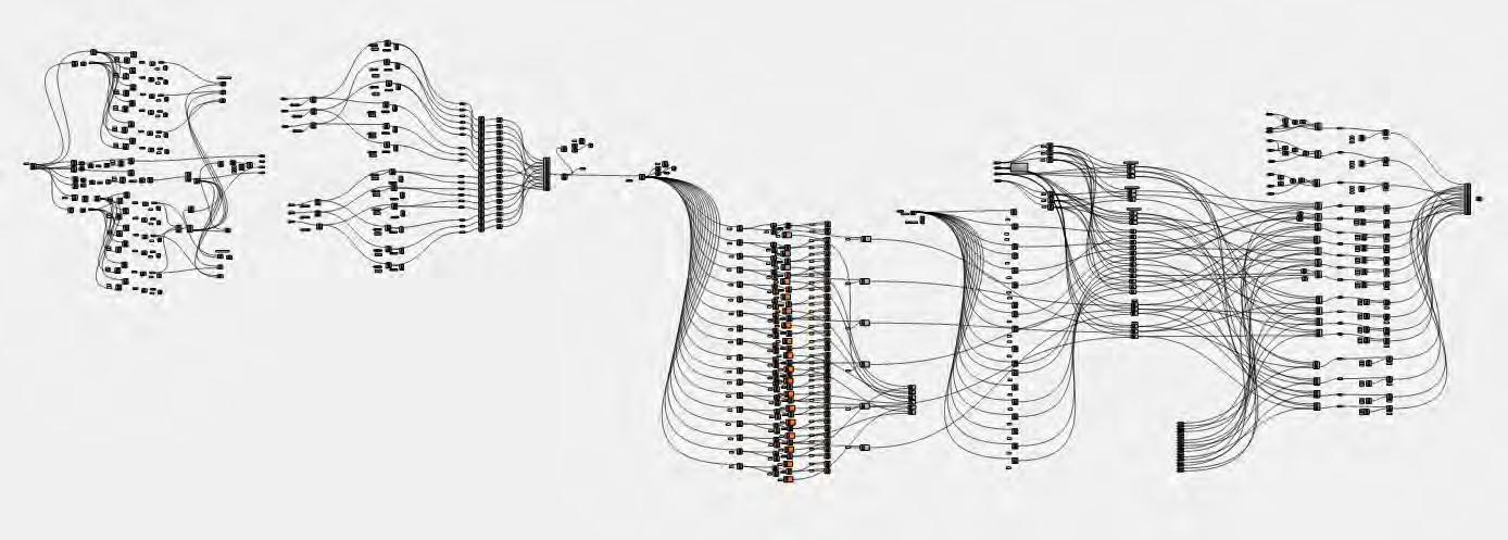
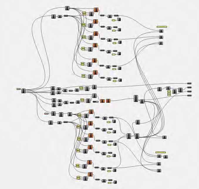
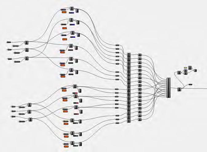
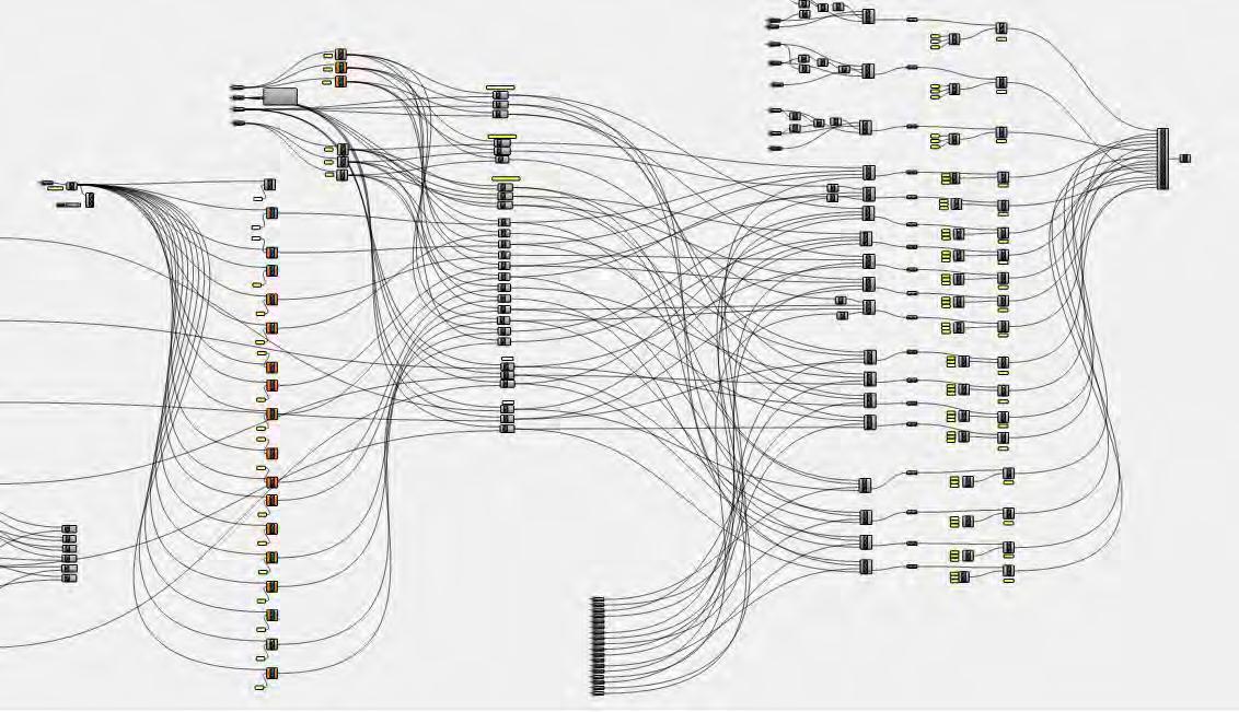
Participation in the International Conference of Composite Materials in Edinburgh, proved to be very helpful in the progress of the research. It gave a wider perspective on current applications of fibre composites, and the status of research all over the world. Specifically in the field of smart composites, adaptive smart systems and fibre optic technology.

It was informative in dealing with critical issues of designing and building a material system that integrates sensing and actuation. This kind of material research is still in the development phase in several fields including aeropace and the aviation industry.

Another very important aspect of the visit, was the fact that it created an opportunity to discuss the project with professors and researchers from varied and different backgrounds. Their feedback was crucial for the looking at the research critically and and revising certain experiments performed.

International Conference in Composite Materials

Themes Covered in the Conference

Industry Focused

A1. Advanced Composite Materials in Construction

A2. Aerospace Applications

A3. Automotive Applications and Recycling

A4. Marine Composites

A5. Offshore Applications

A6. Other Applications

A7. Wind Turbine Applications

Applications

B1. Biomedical Applications

B2. Composite Pressure Vessels

B3. Composites for Fuel Cells and Alternative Energy

B4. Electronic Composites

B5. Multi-functional Composites

B6. Sandwich Structures

B7. Smart Composites and Applications

B8. Structural Health Monitoring

B9. Thermal Applications and Heat Transfer

Manufacturing

C1. Composites Forming

C2. Flow Processes in Composite Materials

C3. Manufacturing Technologies

C4. Residual Stresses and Processing

Materials

D1. 3D Textiles and Composites

D2. Biomimetic Composites

D3. Carbon/Carbon Composites

D4. Ceramic Matrix Composites

D5. Fibre-metal Laminates and Hybrid Composites

D6. High Performance Fibres

D7. Interphases and Interfaces

D8. Metal Matrix Composites

D9. Natural Fibre Composites

D10. New Resins and their Performance

D11. Textile Composites

D12. Thermoplastic Matrix Composites

Nanocomposites

E1. Carbon Nanotube Composites

E2. Modelling and Analysis of Nanocomposites

E3. Multifunctional Nanocomposites

E4. Nanoclay/Nanosilicate Composites

E5. Nano-structured Surfaces and Coatings

E6. Polymer Nanocomposites for Structural Applications

E7. Processing of Nanocomposites

Behaviour

F1. Aging, Moisture and Viscoelastic Properties

F2. Analysis for Flight Certification of Composite Structure

F3. Buckling and Postbuckling Behaviour of Laminated

Shell Structures

F4. Composites in Fire

F5. Composites Testing and Model Identification

F6. Damage Mechanics and Multiscale Modelling

F7. Damage Tolerance and Impact

F8. Deformation and Fracture of Composites

F9. Delamination

F10. Dynamic Failure and Blast

F11. Energy Absorbtion and Crashworthiness

F12. Failure Criteria for Design

F13. Fatigue of Composites

F14. Full Field Measurement Methods

F15. Interlaminar Reinforcement

F16. Joining of Advanced Composites

F17. Mechanics of Short Fibre Composites

F18. Micromechanics/Nanomechanics

F19. NDE

F20. Probabilistic Analysis and Reliability

F21. Repair

F22. Structural Analysis and Optimisation

F23. Sustainable Green Composites

F24. Wear

Composites Materials Centre

In the intial phase of the project, a visit to the Composite Materials Centre of the Department of Aeronautics at Imperial College gave a clear understanding of several processes involved in manufacturing fibre composites. The equipments involved, manufacturing and testing methods were understood in detail.

To gain knowledge about existing methods of fabricating and testing composite materials was crucial to develop the physical experiments further.

The facilities, testing devices and processes observed are as follows:

Unidirectional Prepreg Epoxy Carbon Fibre Hand Lay Up Vacuum (Used after hand lay up to remove air between layers of prepreg) - 0/0/0/90 are the directions of the fibre of each of the 4 individual layers

Cured quasi-isotropic carbon fibre specimen

Stitched woven quasi-isotropic carbon fibre fabric

Autoclave

Strain gauded carbon fibre specimens

Ultrasonics as (NDE) Non Destructive Evaluation of Carbon Fibre Specimens for defects

C-scan examples from ultrasonics

Cured unidirectional carbon fibre specimen with 60% volume fraction

Bibliography

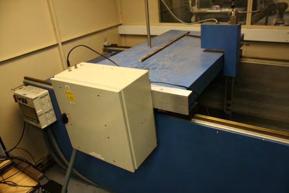
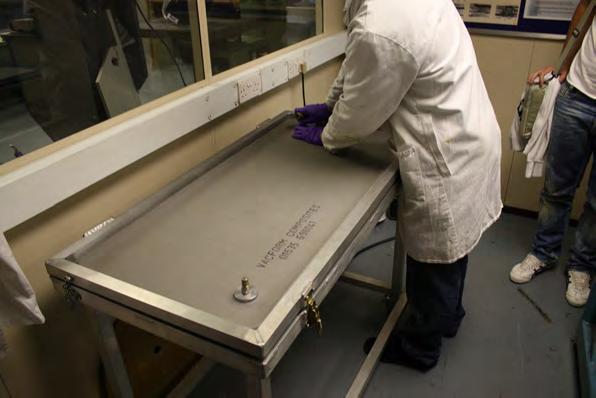
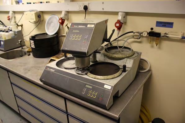
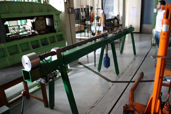
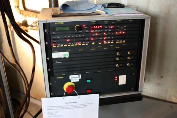
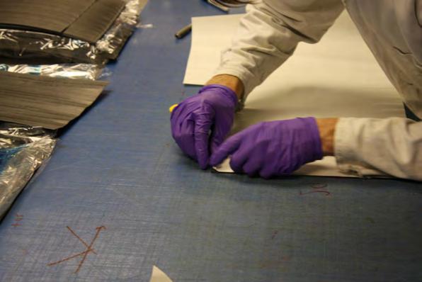
Books

Archer, R.R, ‘Growth stresses and strains in trees’, springer Verlag, Berlin, 1986.

Bentley, P. John, ‘Principles of measurement systems’, Pearson Education, 2005.

Beukers, Adriaan and Hinte Van- ‘Lightness’, p.32 , Rotterdam, 1999.

Davies, Geoff, ‘Materials for Automobile Bodies’, Butter worth - Heinmann, Elseiver Ltd, Oxford, UK, 2003.

Derrickson, B.H and Tortora, G. J, ‘Principles of anatomy and physiology’, Wiley. New York, 2005.

Gordon, E. Jim, ‘The New Science of Strong Materials’, p. 53, 2nd Edition, Penguin Books, London, 1976.

Hagan, Susannah- ‘Taking Shape- A New Contract between Architecture and Nature’, p. 39 , Architectural Press, Oxford, 2001.

Hauer, Erwin , ‘Continua--Architectural Screens and Walls’, Princeton Architectural Press, New York, 2004.

Hertel, Heinrich, ‘Biology and Technology- Form- Structure –Movement’, p. 14, Reinhold, New York,1966.

Heywang, Walter, Karl Lubitz and Wolfram Wersing, ‘Piezoelectricity’, Springer, 2008.

Hoehn, K. and Marieb, E. N, ‘Human Anatomy & Physiology’. Benjamin Cummings. San Francisco, USA, 2007.

Hull, Derek and T.W.Clyne, ‘An Introduction to Composite Materials’, Cambridge solid state science series, p. 2, Cambridge University Press, Cambridge, UK, 1996. Kendall, David, ‘Reinforced Plastics - Building the future with FRP composites’, p.3, Elsevier Ltd, 2007.

Lewis, W.J, ‘Tension Structures’, Form and Behaviour, London, Telford, 2003.

Lipták .G. Béla, ‘Instrument Engineers’ Handbook: Process control and optimization’, CRC Press, 2006.

Melton, K. N , ‘Ni-Ti Based Shape Memory Alloys’, - Engineering Aspects of Shape Memory Alloys, pp. 28 – 34, edited by T. W Duerig et al., Butterworth , London, 1990.

Netter, F. H, ‘Musculoskeletal system: anatomy, physiology, and metabolic disorders’, Ciba-Geigy Corporation. New Jersey, 1987.

Okamoto, Y , ‘Reversible Changes in Yield Stress and Transformation Temperature of a NiTI Alloy by Alternate Heat Treatments’, pp 517 – 520. Script Metallurgica, Vol.22, 1988. Pitman, L. J. Clancy, ‘ Aerodynamics’ - Journal of Fluid Mechanics , chapter 3, Cambridge University press, 1976.

Pollock, Daniel.D , ‘Thermocouples, theory and properties’, CRC Press,1991.

Possehl. L .Gregory , ’The Indus Civilization’, - A Contemporary Perspective, pp.80-85, Rowman and Littlefield Publishers. Inc. , Oxford, UK, 2002.

Rao, S.R , ‘A Persian Gulf Seal from Lothal’, Antiquity, Vol. 37 pp. 96-99 and Plates 9,10,11,Cambridge, England, 1963.

Reyner Banham, ‘The Machine Aesthetic’, The Architectural Review, Vol. 447, No. 700, 1955.

Rhinelander, F.W , ‘Circulation in bone - The Biochemistry and Physiology of Bone’, Academic Press. London & New York,1972.

Streeter, V.L, Fluid Mechanics, E, McGraw–Hill Inc. , New York, 1966.

Thapar, Binda , ‘Introduction to Indian Architecture, p. 81, Periplus Editions, Singapore, 2004.

Thompson, D’Arcy, ‘On Growth and Form’, Cambridge University Press, London, 1961.

Tsai, S.W , ‘Composite Design’, Think Composites, p.4, Daytopn, Ohio, 1988.

Tsui, Eugene, ‘ Evolutionary Architecture-Nature as a Basis For Design’, pp.90,91, John Wiley and sons, New York, 1999.

Udd, Eric , ‘Fiber Optic Smart Structures’, p.172-240, John Wiley and sons London,1995.

Vincent, J.F , ‘Deployable structures in nature: potential for biomimicking’, p.1-10, Proc. Institute of Mechanical Engineers, UK, 2000.

Wadhawan, K.Vinod, ‘Smart Structures: Blurring the Distinction between the Living and the Nonliving’, OUP Oxford, 2007.

Window.A. L., ‘Strain gauge technology’, Springer, 1992.

Wheeler, R.E.M , ‘The Indus Civilization’, (supplement to the Cambridge History of India), (Second Revised Edition.), Cambridge, England, 1960.

Yang, Jiashi , ‘An Introduction to the Theory of Piezoelectricity’, Springer, London, 2005.

Periodicals

Bettum, Johan, ‘Skin Deep’ - Polymer Composite materials in Architecture, Contemporary Techniques in Architecture, Architectural Design, p.72, Wiley-Academy, London, January-February 2002.

Burry, M, ‘Between Surface and Substance’, Architectural Design, March-April 2003 issue, pp 8-19, Wiley-Academy, London, 2003.

Jeronimidis, George ,‘Biodynamics’, - Emergence: Morphogenetic Design Strategies-Architectural Design, Academy Editions, London, 2004.

Weinstock, Michael, ‘Morphogenesis and the Mathematics of Emergence’, Emergence: Morphogenetic Design Strategies, p.-10-17, Architectural Design, Academy Editions, London, May/June 2004.

Hensel, Michael , ‘Performance Oriented Design - Precursors and Potentials’, - Versatility and Vicissitude, p.48, Architectural Design, Wiley, March-April 2008.

Seminars and Lectures

Brailovski .V, ‘Optimization of Post-deformation Annealing Heat treatment for NiTi Shape Memory Alloys’, in SMST 2000, Proceedings of the International Conference on Shape Memory and Superelastic Technologies, pp 33 – 42 , Edited by Russell Pelton, April, 2000.

Jeronimidis, George, ‘Biomimetics:Lessons From Nature For Engineering’, The 35th John Player Memorial Lecture, The Institution of Mechanical Engineers - Materials and Mechanics of Solids Group, 22 March 2000, London.

Jeronimidis, George, ‘Biomimetics - Differentiation / Integration / Emergence, Sensing – Actuation –Control’, - Lecture at the Architectural Association, London, 2009. Smith, S. A , ‘Shape Setting Nitinol’, - Proceedings of the Materials and Processes for Medical Devices Conference, pp 266 – 270. edited by S. Shrivastava, ASM International, Sept., 2003.

Websites

http://leedanalysis.com/location.php (accessed on 10th February 2010)

http://www.chinaculture.org/gb/en_museum/2003-09/24/content_30784.htm (accessed on 16th Sep 2009)

http://www.marcelwanders.nl (accessed on 23rd August 2009)

http://www.materialecology .com (accessed on 25th August 2009)

http://www.contructioninvivo.com (accessed on 25th August 2009)

http://www.strangemilitary.com/content/item/10443.html (accessed on 13th August 2009)

http://www.nasa.gov/centers/langley/news/factsheets/21stcentury.html (accessed on 13th August 2009)

http://www.scienceclarified.com (accessed on 13th August 2009)

http://holcimfoundation.org/Portals/1/docs/ES_booklet.pdf (accessed on 12th January 2010)

http://www.temperatures.com/tcshtml (accessed on 6th October 2009)

http://www.tschumi.com/ (accessed on 5th January 2010)

http://na.northsails.com (accessed on 19th October 2009)

http://www.chinamuseums.com/qinshihuangt.htm (accessed on 23rd August 2009)

Illustration Credits

1.a -http://cybele.bu.edu/index/leaf.jpg (accessed on May4th 2006)

1.b-http://www.buffalogardens.com/historical/Crystal_Palaces/body_crystal_palaces.html (accessed on May4th 2006)

1.c -http://www.mjausson.com/2003/img/walk24Jun03/14gunnera_dt.jpg (accessed on May 4th 2006)

1.d - http://universe-review.ca/I10-22a-stomata.jpg (accessed on May 4th 2006)

Chapter 1

1.0.a http://www3.interscience.wiley.com/(accessed on Sep 4th 2009)

1.0.b Drew, Philip- Frei Otto – Form and Structure, Granada, London,1976 ,p. 22

1.0.c http://www.virgingalactic.com/(accessed on Dec 14th 2009)

1.0.d Gordon, E. Jim, ‘The New Science of Strong Materials’, p. 53, 2nd Edition, Penguin Books, London, 1976. 1.0.e http://www.theverymany.net/labels/zaha%20hadid.html(accessed on Dec 1st 2009)

1.0.f http://www.rosslovegrove.com/(accessed on Dec 1st 2009)

1.0.g Hull, Derek and T.W.Clyne, ‘An Introduction to Composite Materials’, Cambridge solid state science series, p. 2, Cambridge University Press, Cambridge, UK, 1996. 1.1a - Emergence: Morphogenetic Design Strategies- Architectural Design,Academy Editions, London, Vol. 74 No 3 Issue May/June 2004, p.4 1.1 b - Drew, Philip- Frei Otto – Form and Structure, Granada, London,1976 ,p. 22 1.1c -http://nanotechweb.org/articles/news/1/11/5/1/0611102 (accessed on Jun 12th 2009)

1.1 d- http://upload.wikimedia.org/wikipedia/commons/a/ab/Spider_web_with_dew_drops04.jpg(accessed on Jun 12th 2009)

1.2a- http://education.vetmed.vt.edu/Curriculum/VM8054/Labs/Lab5/Lab5.htm(accessed on July 18th 2009)

1.2 b- http://www.bio.miami.edu/~cmallery/150/physiol/physiology.htm(accessed on July 25th 2009)

1.3.a http://commons.wikimedia.org/wiki/File:Caput_femoris_cortex_medulla.jpg (accessed on Sep 19th 2009)

1.3.b http://www.scienceclarified.com/Ro-Sp/Skeletal-System.html (accessed on Sep 18th 2009)

1.4 http://www.jcestnik.com/?p=139 1.a -http://cybele.bu.edu/index/leaf.jpg (accessed on May4th 2006)

1.5 http://www.feppd.org/ICB-Dent/campus/biomechanics_in_dentistry/ldv_data/mech/basic_bone.htm(accessed on Dec 29th 2009)

1.6, 1.7 http://na.northsails.com/(accessed on Jun 17th 2009)

1.8.a http://www.mmsonline.com/uploadedimages/Publications/MMS/Articles/Internal/Viper%20machine%20%202.jpg (accessed on April 15th 2009)

1.8.b http://www.cardesignonline.com/production/materials/carbon-fiber.php (accessed on Oct 3rd 2009)

1.9.a,b,c http://www.marcelwanders.nl/wanders/pages/seaters-carbonchair_1_3_grouppage.shtml(accessed on Oct 3rd 2009)

1.10 http://www.flickr.com/groups/nikon_d300_users/discuss/72157609158588988/(accessed on Oct 3rd 2009)

1.11, 1.12.a Images obtained from the lecture presented by George Jeronimidis at the Architectural Association, 2009 1.12.b - http://skitterbot.com/blog/?cat=49 (accessed on Oct 11th 2009)

1.13.a Between Surface and Substance, Architectural Design, March-April 2003 issue, pp 8-19, Wiley-Academy, London, 2003

1.13.b http://www.materialecology .com (accessed on June 14th 2009)

1.13.c http://www.nasa.gov/centers/langley/news/factsheets/21stcentury.html (accessed on June 14th 2009)

1.14 Fiber Optic Smart Structures, John Wiley and sons, 1995, p.172

Chapter 2

2.3.a http://www.teamfibre.co.uk/images/blue_fibre.jpg

2.3.b http://www.weldotherm.com/products_consumables_thermocouple_wire.asp

2.3.c http://www.allaboutcircuits.com/vol_1/chpt_9/7.html

2.4 .b,c http://www.omega.co.uk/shop/

2.5 http://www.omega.co.uk/shop/

2.5.b,c http://www.answers.com/topic/shape-memory

2.6, 2.7, 2.8 Melton, K. N, ‘Ni-Ti Based Shape Memory Alloys’, - Engineering Aspects of Shape Memory Alloys, pp. 28 – 34, Butterworth , London, 1990. 2.29 http://blog.knowledge-journal.com/archives/63/introducing-your-climate

Chapter 3

3.1 http://visibleearth.nasa.gov/

3.2 Courtesy Google earth

3.3 http://www.globalheritagefund.org/where/uk_indus.html

3.4 redrawn from Rao, S.R, ‘A Persian Gulf Seal from Lothal’, Antiquity, Vol. 37 pp. 96-99 and Plates 9,10,11,Cambridge, England, 1963. 3.10,3.11,3.12 http://www.arcspace.com/architects/Tschumi/ 3.13,3.14, 3.15 redrawn from Project booklet Metropol Parasol,’ Redevelopment of plaza,de le Incarnacion, Seville,Spain. 3.16 Extrapolated drawing, source: http://www.chinamuseums.com/qinshihuangt.htm (accessed on 23rd August 2009)

Chapter 4

4.2 The Science Book, Cassel and co, London, 2001, p.422

Chapter 5

5.35 Tsui, Eugene- Evolutionary Architecture- Nature As a Basis for Design, John Wiley and sons, New York, 1999, p.92

5.40.a http://www.flickr.com/photos/47923322@N00/606453026/ 5.40.b http://riverdeep.net/current/2002/02/020402_animalscience.jhtml (accessed on July 3rd 2006)

Chapter 6

6.1,6.2 http://na.northsails.com/

6.3 http://www.nucleus-gmbh.com/english/products/ultrasonic-welding/rotosonic-v4e-i.html

6.4 http://www.rvatr.com/research/projects/silver.htm

6.5,6.6, 6.11http://www.glassfiles.com/library/21/article1332.htm

6.14 http://www.shinegashira.com/archives/154

6.17 http://www.hollandcomposites.nl/referenties/12/Yitzhak-Rabin-Centre-Tel-Aviv/

Glossary

Af-Temperature:

Temperature, above which the phase transformation from Martensite to Austenite is fully completed during heating of the alloy.

Actuator:

Device made out of a shape memory alloy, which is able to provide a significant amount of mechanical work due to the occurance of the phase transformation during heating. Actuation force and displacement are functions of the actuator geometry and design.

Apeak- or Ap-Temperature:

Temperature, at which the phase transformation from Martensite to Austenite shows the maximum of heat flow during heating. The alloy needs a certain amount of energy (heat flow) to initiate the phase transformation and to move the phase boundary through the alloy. The maximum is a value which can be accurately measured in a DSC equipment, whereas the As-and Af-temperature measurements are sometimes lacking reproduceability.

As-Temperature:

Temperature, at which the phase transformation from Martensite to Austenite is initiated during heating of the alloy.

Austenite:

Crystallographic description of the high temperature phase of a shape memory alloy, which starts to form during heating of the low temperature phase Martensite when the As-temperature is passed. The formation of Austenite is completed above the Aftemperature.

Biocompatibility:

General expression for the suitability of a material for use in the human body and in the endogenous fluids. For NiTinol, a multitude of clinical studies and long clinical history have shown that the biocompatibility is excellent, especially in terms of cytocompatibility, haemocompatibility, genocompatibility, and corrosion performance. The most current studies report that the overall biocompatibility of NiTi alloys is comparable to stainless

steel and Titanium alloys. In some applications, such as stents, recent studies suggest that the biocompatibility of NiTi alloys may be even superior to stainless steel.

DSC (Differential Scanning Calorimetry):

Calorimetric method for the characterization of a shape memory alloy with respect to its transformation temperatures. The DSC measures the specific heat flow, which changes constantly during the phase transformation. The overall accuracy and the ease of usage of the DSC equipment together with the high reproduceability makes it the most suitable method for alloy characterization. The main disadvantage of the DSC is the fact, that material deformation and external load cannot be simulated with this measurement.

Hysteresis:

a) thermal hysteresis:

The thermal hysteresis means generally the difference between the Apeak- and the Mpeak-temperatures. The hysteresis appears during passing of the transformation temperatures and is affected by a number of parameters (alloy composition, thermomechanical treatment, external load, etc.).

b) mechanical hysteresis:

The mechanical hysteresis appears during loading and unloading of a shape memory component in its high temperature phase above Af. The NiTinol component shows a large amount of strain during loading, which recovers during unloading. The necessary force to initiate the transformation during loading is higher as the released force during unloading.

Martensite:

Crystallographic description of the low temperature phase of a shape memory alloy, which starts to form during cooling of the high temperature phase Austenite when the Ms-temperature is passed. The formation of Martensite is completed below the Mf-temperature. But the Martensite can also be induced during loading of the Austenite above Mf. This is related to a large amount of recoverable strain and is called ‚Superelasticity‘.

NiTiNOL:

Common trade name for the commercially most important family of shape memory alloys (NiTi alloys).

One way effect (or thermal shape memory):

The one way effect occurs in a shape memory alloy, which has been deformed below its lower transformation temperature Ms. The obvious deformation is called pseudoplastic because the alloy recovers shape during subsequent heating into its austenitic high temperature phase. During this shape change the shape memory alloy is capable of providing a significant amount of work output and can be used as an actuator. The subsequent cooling in to the austenitic phase is normally not subject to a reverse shape change, as long as there is no external stress during Austenite - Martensite transformation.

Phase transformation (here: martensitic phase transformation):

Physical mechanism, which is the metallurgical basis of the shape memory effect. The term martensitic phase transformation describes the formation of Martensite during cooling OR during loading with an external stress of the austenitic high temperature phase.

R-Phase:

Phase, which appears under certain conditions in for instance NiTinol alloys and which is still considered as being a ‚premartensitic‘. The R-phase is related to some anomalies of certain functional properties. The R-phase transformation shows a very narrow thermal hysteresis, but at the same time a very small amount of work output.

Superelasticity:

Sometimes compared to a rubber-like deformability of shape memory alloys, which occurs during application of an external stress on the austenitic high temperature phase above Af. Thus, the superelastic effect is related to about 8% of recoverable elastic stress, for which temperature changes are not necessary. The superelasticity occurs basically in the same alloys as the thermal shape memory (one way effect).

Thermomechanical treatment:

Treatment of a shape memory alloy consisting out of a combination between colk working steps and annealing processes. The purpose of the thermomechanical treatment is the adjusting of a number of functional properties, like e.g. the phase transformation temperatures. Usually the annealing of the component or the semi-finished shape is the last step of the fabrication process.

Transformation temperatures:

Temperature values, at which start and finish of the phase transformation can be measured (Ms-, Mf-, As-, Af-temperature).

Two way effect:

Special form of the thermal shape memory effect, in which not just the heating but also the cooling of the shape memory element are subject to shape changes. This effect is induced either by a special thermomechanical treatment (‚Training‘) or through external stresses during cooling. For design and industrial application of actuators this latter option is highly preferred for as multi-tude of reasons.