Slender multistress driven structures

Slender multistress driven structures

guillem baraut

mattia gambardella

EMERGENT TECHNOLOGIES AND DESIGN. 2005-2006

ABSTRACT

The combination of multiple design criteria is usually complex to manage. The aim of this study is to develop a methodology that combines both structural and spatial performance from the first steps of the design process.

Some methods like topology optimization and minimal paths algorithm are mixed with physical form finding experiments, and with theoretical concepts such as biomimetics and existing cutting edge manufacturing techniques. The same principles are considered in both global and local scales.

Slenderness and stress driven materialisation are the basic concepts that will lead the developed methodology.

The final result is a combination of all these techniques in a complex software network that includes Matlab codes, Generative Components scripts, Rhino files and Excel spread sheets that are used to exchange data from one program to another.

The results of this methodology are then evaluated and compared in order to establish a criteria of fitness for the solutions that the user achieve.

guillem baraut

mattia gambardella

tutors:

mike weinstock

michael hensel

achim menges

martin hemberg slender

01. INTRODUCTION

guillem baraut

mattia gambardella

tutors: mike weinstock

michael hensel

achim menges

martin hemberg

guillem baraut

mattia gambardella

tutors:

INTRODUCTION

Slender structures, like suspension bridges, use primarily tension to carry both the design loads and their own weight and are generally optimal in that the primary structural elements are not subject to buckling. The need to avoid long compressive spans is critical in determining the optimal form of such structures.

Natural systems also use prestressing and as much elements in tension as possible as an strategy to avoid buckling stability problems. All those natural systems are using fibers as a material system for being the cheapest way to introduce tensile structural members in terms of manufacturing time and energy.

All natural systems are the results of thousands of generations of an evolutionary system. This long process has been optimising the performance of every single element. Genetic algorithms are the most powerful tools that have been developed that can reproduce this processes of optimization, but they are difficult to implement, and need a very powerful machine. Instead of that, there are similar processes but far more simple that can produce satisfactory results.

Actual design methodologies doesn’t consider any optimization process because are time consuming and need experts in many fields. The way the majority of design practices work is to create a team that exchanges a lot of information between them, but there is no one person that controls every single aspect of that.

This complex work system can be improved if the proper tools are being used. The more expertise work in a team, the more important is the good exchange of information.

mike weinstock

michael hensel

achim menges

martin hemberg

slender multi stress driven structures

02. AIMS AND SCOPE OF THE RESEARCH

guillem baraut

mattia gambardella

tutors: mike weinstock

michael hensel

achim menges

martin hemberg

slender multi stress driven structures

guillem baraut

mattia gambardella

A IM AND SCOPE OF THE RESEARCH

The aim of our research is to define a design methodology that combines the stress driven form finding with a fiber distribution in structures to create a framework that includes both physical and digital form finding tools. Within this framework we will be able to process all the environmental information including external loads to design an optimized structure.

The structural evaluation will be embedded in the design process since it integrates the structure optimization. This optimization will be considered from several points of view such as shape, size and topological optimization.

Another criteria that will be used in this design methodology is the circulation of people within the structure. Other spatial criteria will be then negotiating with the structural performance.

For these purposes some digital tools will be developed to allow the user to have a good level of control over all these criteria.

At the end these tools will be tested. The results will be compared within themselves and with existing structures, and several evaluation criteria will be set and analysed.

tutors: mike weinstock

michael hensel

achim menges

martin hemberg slender multi stress driven structures

The following Diagram introduces the different fields of research that have been involved during the development of the topic.

Each section describe an overviewed research field: the final design result lies in between the overlapping area of those fields of interest.

It is meant, in fact, as a non linear product of different influences, each one having it contribution in defining the final result.

TECHNIQUES

CNC CUT foam form

Glass Fibers Resin Matrix

guillem baraut

mattia gambardella

tutors: mike weinstock

michael hensel

achim menges

martin hemberg

METHODS

Emergence

Biomimetics

Minimum road network

Structural Optimization

Final Outcome

TOOLS

Physical form finding

Minimum road network

Nested catenaries analysis

Digital tools

Structural Optimization

Parametric design

METHODOLOGY FLOW CHART

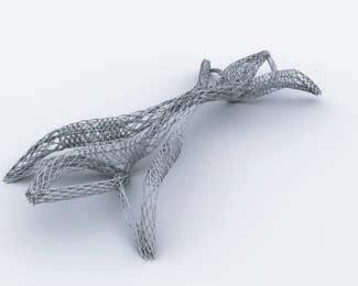
The diagram below illustrates the research path undertook in studying the topic in observation. The tools for investigations are both coming from physical and digital experiments.

The cross influence amongst those experiments led at the end to the final design.

GLOBAL SCALE

DIGITAL TOOLS

PHYSICAL EXPERIMENT

LOCAL SCALE

guillem baraut

mattia gambardella

DIGITAL TOOLS

MANUFACTURING TECHNIQUES

tutors: mike weinstock

michael hensel

achim menges

martin hemberg

03. HYPOTHESIS

guillem baraut

mattia gambardella

tutors: mike weinstock

michael hensel

achim menges

martin hemberg

slender multi stress driven structures

guillem baraut

mattia gambardella

tutors:

HYPOTHESIS

Slender lightweight structures could be achieved with optimal distribution of fibers in a system which topology has been defined through an automatic process of optimization.

From both architectural and engineering point of view lightweight long span structures will be studied in two scales of operation:

- Macroscale based in the overall shape of the structure (metres)

- Microscale based in heterogeneity and anisotropic distribution of fibers considering directionality and density (centimetres)

Both scales of operation can be defined by stress driven form finding processes.

mike weinstock

michael hensel

achim menges

martin hemberg slender

04. BIOMIMETIC PRINCIPLES

guillem baraut

mattia gambardella

tutors: mike weinstock

michael hensel

achim menges

martin hemberg

slender multi stress driven structures

BIOMIMETHICS

Natural structures are smart structures par excellence as they are the result of a continuous process of optimization over millennia.

The field of biomimetics is at the intersection of biology and engineering and is dedicated to understanding strategies with which nature builds its structures and determining the extent to which some design principles may be incorporated in the design of mane-made structures.

Characteristic of the natural structures

1. Multifunctionality

2. Hierarchical Organization as Basis for structural integrity

A study of natural materials/structures such as tendon, bone, wood, and shells reveals that a living organism builds the material and develops its architecture starting at levels well below that of the living cells.

Tendon, for example, which serves as a link between muscle and bone, has an extremely intricate and complex structure, with six discreet level of hierarchical organization.

Thus in natural systems, a judicious combination of elements, materials and components of differing strength in the same structure leads to acceptable and adequate hybrid systems whose properties are tailored for their specific usage. The variety of such designs is made possible by the hierarchical interaction between material and structure.

This integrated approach seems to be one of the design rules and the key strategy with which nature achieves that elusive but enviable objective of balancing strength and stiffness without sacrificing toughness.

guillem baraut

mattia gambardella

tutors: mike weinstock

michael hensel

achim menges

martin hemberg

Fig.1 Fiber arrangement in natural systems

guillem baraut

mattia gambardella

tutors: mike weinstock

michael hensel

achim menges

martin hemberg

Fiber DISTRIBUTION

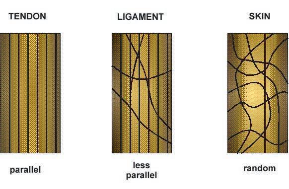
Anisotropy and heterogeneity are the strategies of optimization for the amount of material needed in all the natural structures. Anisotropy refers to differentiation in direction, when fibers follow the stress paths of the structure. Heterogeneity appears when density of fibers in every location in space is differentiated in order to maximize the structural performance.

For this dissertation we considered the fiber distribution in several scales:

- Microscale: several manufacturing techniques will allow us to distribute fibers where are necessary and in the density, direction and layers that are needed.

- Macroscale: the structural shape is determinant in this scale. Fibers will follow the axis of the structural elements.

What concerns fiber distribution in structural optimization is approached from several points of view:

- Shape: fibers have high load-bearing capacity with very small transverse area. Distribution will be in hollow structures to avoid local buckling problems.

- Topology: directionality of fibers is defined by the stress path and will force us to define several different topological distributions, like the ones that are in figure 2 and 3.

- Density: distribution of fibers where concentrations of stresses occurs like in bones, see figure 4.

Long span structures will be approached by studying shape optimization (macroscale), introduce the material system in the analysis considering fibers, and within this material system studying fiber distribution optimization (microscale).

Fiber distribution

Figure 1. Wood bundles

Figure 2. Fibres distribution in natural fibrous systems

FUNCTIONAL INTEGRATION AND DESIGN

One might define a good engineer as someone who is capable of extracting maximum performance at minimum cost from the he materials he has available and achieve a design that is “fit for purpose”.

This has been a recurrent theme in engineering courses since the subject became academically acceptable as discipline and, together with creativity, they are the yardsticks by which we judge success or failure.

All too often, the problem is not with the aims but with the methods we use to achieve them. I refer in particular to the fact that our traditional approach to design has been severely limited by the labels that we often attach to ourselves, or that others have seen fit to identify us with: engineer (mechanical, structural, civil, materials, medical, aeronautical, transport, electrical, electronic, software…).

In the same way as in nature the boundary between materials and structures is blurred, the study of biological systems to understand those aspects of design that might be useful for our purposes requires an integration of all the disciplines above.

The main reason for this is that biological structures are often multifunctional, in the sense that they often perform more than one task. If we do not understand what the various functions are, and how they are controlled and integrated, it will be difficult to extract any useful lesson.

It would be difficult to argue that multifunctionality is a route to optimization. The recently emerging disciplines of smart materials and structures are at the forefront of scientific and technical developments in that direction and in doing so they have stimulated a renewed interest in biology and biomimetics.

STRUCTURAL OPTIMIzATION

In this respect there is nothing special about biological systems other than the fact that the solutions it has arrived at are the logical conclusion of the problems with fibers mentioned earlier. There are rules which govern the efficiency of materials in a structural context and the answers we observe in nature appear to follow them, probably better than we do ourselves. If fibers are good in tension and bad in compression (and hence in bending), use them in tension either by pre-stressing them or by stabilizing them laterally using ceramic materials of high modulus or extensive cross-linking with suitable matrices. All these tricks are used in biology.

Many animals with flexible skins (worms, sharks, tunicates) use hydrostatic skeletons where the pre-stressing of fibers in tension is balanced by compression in a fluid (mostly water and hence not expensive).

Similarly, non lignified plants are entirely dependent on control of turgor pressure inside the cells to achieve structural rigidity, pre-stressing the cellulose fibers in the cell walls (typically up to 200 MPa) at the expense of compression in the fluid.

In bones, mineralization of the collagen with hydroxyapatite increases the modulus of the collagen-mineral composite 5 fibers and hence their buckling resistance; what is particularly interesting in this system is that the collagen micro fibrils have all the chemistry needed for mineralization already there, but the mineral is deposited only when needed.

Biomimetic Principles

Maximum performance from fibrous structures, exploiting to the limit anisotropy and heterogeneity (hierarchical assemblies).

AIMS OF BIOMIMETIC DESIGN

DIFFERENTIATION AT THE “MATERIAL” LEVEL

Anisotropy

Heterogeneity

Hierarchies

guillem baraut

mattia gambardella

tutors: mike weinstock

michael hensel

achim menges

martin hemberg

Fig.1 Sectionof a tree trunk showing fiber continuity and orientation in the intersection with a new branch

ADAPTABILITY

A good example of the ability of the living organism is to adapt to the stress conditions encountered.

Living bone continually undergoes a process of reshaping which remodel and reaccomodates the micro-structure according to the changing of the load conditions.

Cycling strain histories are found more effective than steady strain histories in inducing higher remodelling rates.

Fiber reinforced Composites

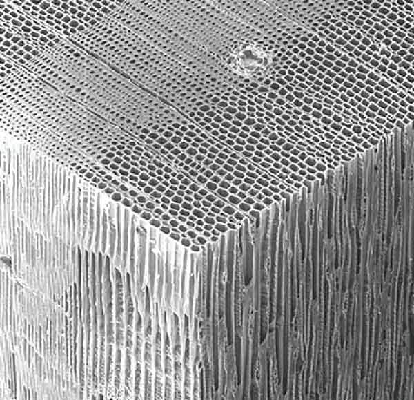
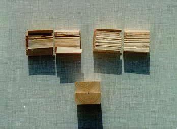
Wood is a natural composite that exhibits a remarkable combination of strength, stiffness, and toughness.

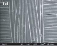
Wood has a cellular composite structure in which it is possible to identify four levels of organization: molecular, fibrillar, cellular, and macroscopic (Jeronimidis). A wood cell is essentially an hollow tube of about 30 micron diameter with a multi layered wall (Fig.2).

The important point in the wood load bearing capability is that the energy absorption mechanism depends on the arrangement of fibers in the cell walls.

This understanding led to a promising man made counterpart composite of fiber reinforced materials.

guillem baraut

mattia gambardella

tutors: mike weinstock

michael hensel

achim menges

martin hemberg

Fig.1 Wood cells alignment

Fig.2 Hierarchical structure in wood

Fig.3 Wood sections showing cells orientation

PATH SYSTEM - TRAFFIC NETWORKS

Minimum path networks

Minimum path network are distances (path or road systems) with the lowest total route length in the connection o several individual points.

The interest in this domain is to study the minimum paths system for pedestrians circulation in a connecting infrastructure such as a pedestrian bridge.

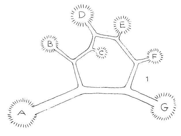
The traffic flows connecting the locations shown in the right picture,have a particular network by which the total expenditure for traffic is at a minimum. This is therefore an optimal structure from the point of view of Traffic engineering.

The minimum road system is then a particular configuration in which the points are interrelated where the sum of all roads is at the minimum.

The first aim is then to define a relation between the ultimate design shape and a minimized path: in order to do so we used a method (supported by both physical and digital experiments) to determine a connecting system for any point constellation having the minimum sum length.

Frei Otto was a pioneer in exploring the potentialities of the physical experiments used to form-find solutions confirmed then by rigorous analysis.

The picture to the right shows the difference existing in connecting a cloud of points with two different solutions:

- Direct network system (is obtained by connecting the points with straight lines in all possible connecting pos sibilities)

- Minimum road network (obtained by collapsing the line one on the other and decreasing therefore the total length of the connections)

On air photographs old way nets in rural area look like minimal nets.

The plan for the foundation of the new city Toulouse - Le Mirail corresponds in most of its parts the geometry of minimal network.

The principle of accessibility is characterized by the differentiation in side walks and road ways.

The net of side walks is spanned between points of accessibility but supplies the area in its whole length.

The abstraction of these traffic system into nets between points does not apply without reservation.

The proof of a minimal net length in fact should be put, however, in relation to a number of city planning factors, such quantitative detail of the traffic, the distribution of exploitation.

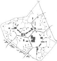
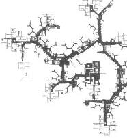
Fig.1/2 Thread Experiments of path optimization

guillem baraut

mattia gambardella

tutors: mike weinstock

michael hensel achim menges

martin hemberg

Fig.3/4 plan for the foundation o Toulouse - Le Mirail

05. PHYSICAL EXPERIMENTS

guillem baraut

mattia gambardella

tutors: mike weinstock

michael hensel

achim menges

martin hemberg

05.01 WOOL THREADS

guillem baraut

mattia gambardella

tutors: mike weinstock

michael hensel

achim menges

martin hemberg slender

EXPERIMENT 05.01 WOOL THREADS

In 1964 Frei Otto founded the Institute of Lightweight Structures at the University of Stuttgart.

Here Otto and his team undertook extensive research into natural forms and processes, generating and inspiring optimum structures. As well as shell structures, lightweight or optimum structures include membrane structures, cable-net, geodesic domes, inflatable and air supported structures, and lattice or reticulated shell structures such as the grid shell. Otto explored several pioneering experiments in form-finding optimal structural configuration.

AIM

The problem is to develop a method which is suitable to determine a connecting system for any plane point constellation having the minimum sum length.

The reorganization of the wet threads, due to the capillar water tension, follows the shortest and less energy consumption (stress consumption) configuration that the physical conditions permit.

In that sense, those experiments are useful in finding, in an empirical way, a suitable configuration in networks of transportation and traffic.

Real systems, such as of supply, traffic or communication can be simulated in this way.

The method is suitable both for planar and dimensional systems.

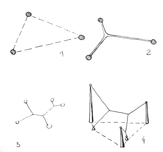
The minimum path network linking three points (fig.1) with each other is not a triangle, but a star-shaped system. In the case of traffic systems in the form of a minimum path networks, pedestrian walkaways, roads, rail paths, the land required, the material expenditure and labour costs are reduced to the minimum.

guillem baraut

mattia gambardella

martin hemberg

tutors: mike weinstock

michael hensel

achim menges

Fig.1. Minimum network between three pointsFig.2. Minimum network between several points

Fig.3. Result of wool threads experiments

EXPERIMENT 05.01 WOOL THREADS

The physical experiment carried on with the wool threads aim at exploring the following topics:

- Minimum network

- branching ratio

Experiment Protocol:

Wool treads are connected from the starting points to the ending points according to the specific experiment settings (number of connecting threads)

- 1 starting point connecting 3 points

- 2 starting points connecting 3 points

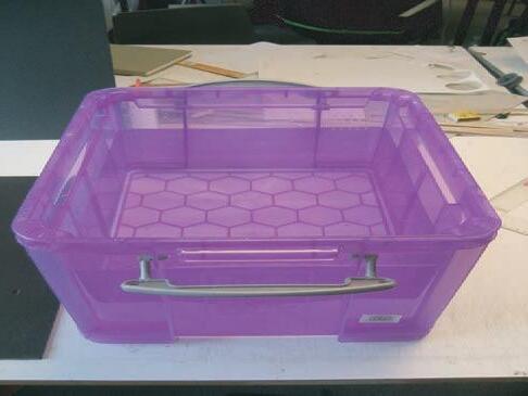
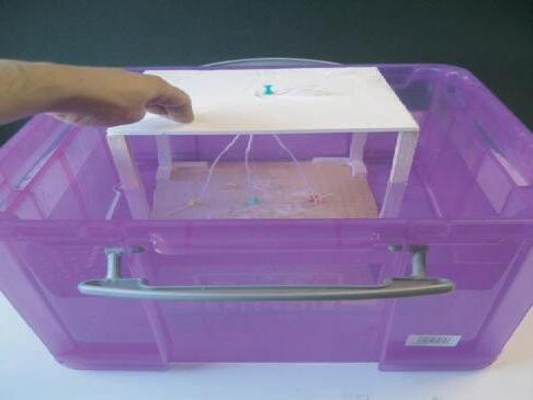
Experiment Protocol

guillem baraut

mattia gambardella

tutors: mike weinstock

michael hensel

achim menges

martin hemberg

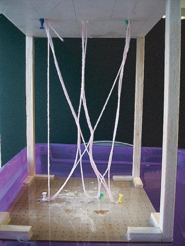
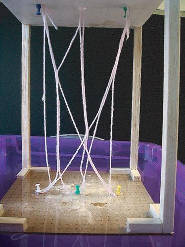
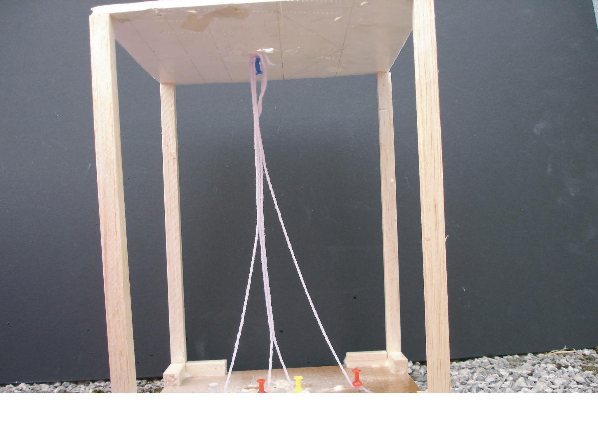
The test was overviewing the possible combinations existing in the set-up made of three thread connected to other three.

The more encountered configuration is the one listed as n.4/5.

That is due to the proximity of the wool thread in the central section of the experiment set.

guillem baraut

mattia gambardella

tutors: mike weinstock

michael hensel

achim menges

martin hemberg

This is the previous experiment but rendered in a different way to highlight the optimized configuration obtained in each case.

It seems that in many of the tested cases the configuration obtained presents similarities in shape and in the total length of the found minimized path.

guillem baraut

mattia gambardella

tutors: mike weinstock

michael hensel

achim menges

martin hemberg

2 threads

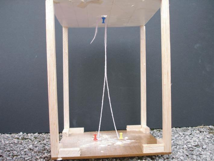
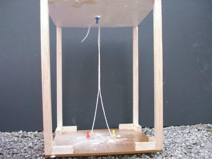
The following experiments were used in studying the branching ratio and the configuration of each minimum network.

By considering a basic set of connections, it was possible to abstract some information (length of branching, branching ratio) to be exported in the definition of the matlab problem as active area where run the topology optimized routine.

guillem baraut

mattia gambardella

tutors: mike weinstock

michael hensel

achim menges

martin hemberg

Variable considered:

- total length of thread (h)

- distance amongst starting points (d)

- distance between branching points (b1, b2)

Example n.1

h= 30 cm

d = 5 cm

b1= 14 cm

b2= 16 cm

branching height ratio 1/2 h

Example n.2

h= 30 cm

d = 5 cm

b1= 17 cm

b2= 13 cm

branching height ratio 1/3 h

Example n.3

h= 30 cm

d = 5 cm

b1= 12 cm

b2= 18 cm

branching height ratio 1/2 h

Example n.4

h= 30 cm

d = 5 cm

b1= 16 cm

b2= 14 cm

branching high ratio 1/3 h

3 threads

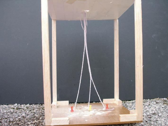
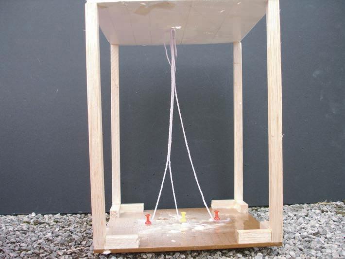
Variable considered:

- total length of thread (h)

- distance amongst starting points (d)

- distance between branching points (b1, b2,b3)

Example n.1

h= 30 cm

d1 = 3 cm

d2 = 3 cm

b1= 9 cm

b2= 10 cm

b2= 11 cm

branching height ratio 1/3 h

Example n.2

h= 30 cm

d1 = 3 cm

d2 = 3 cm

b1= 7 cm

b2= 10 cm

b2= 13 cm

branching height ratio 1/3.5 h

Example n.3

h= 30 cm

d1 = 3 cm

d2 = 3 cm

b1= 10 cm

b2= 11 cm

b2= 9 cm

branching height ratio 1/3 h

Example n.4

h= 30 cm

d1 = 3 cm

d2 = 3 cm

b1= 8 cm

b2= 10 cm

b2= 12 cm

branching height ratio 1/3.5 h

guillem baraut

mattia gambardella

tutors: mike weinstock

michael hensel achim menges

martin hemberg slender

4 threads

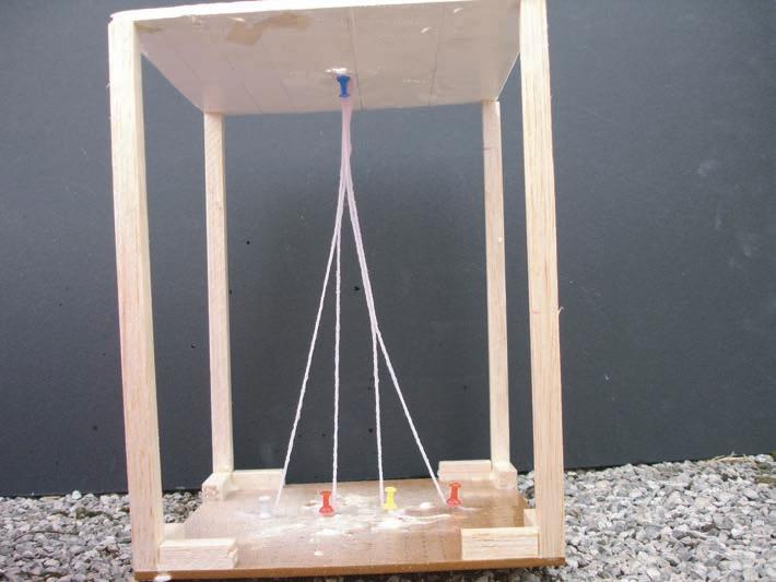
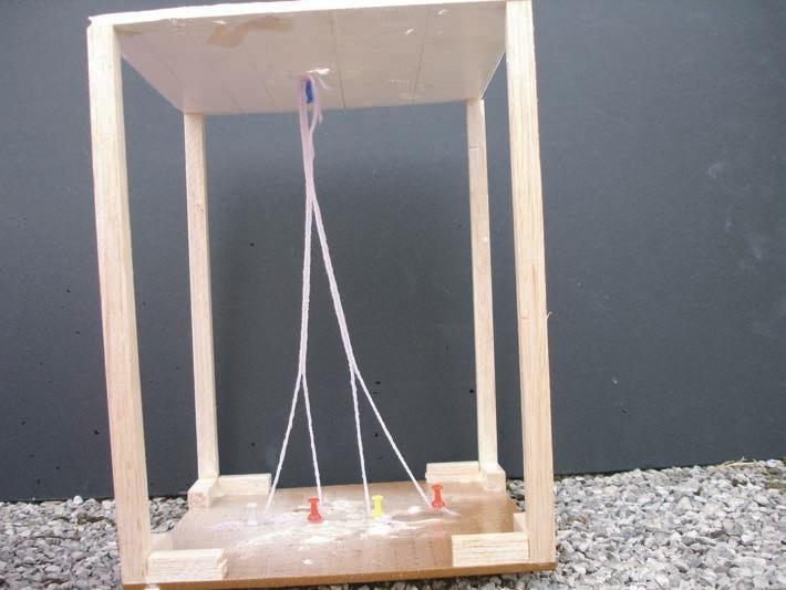
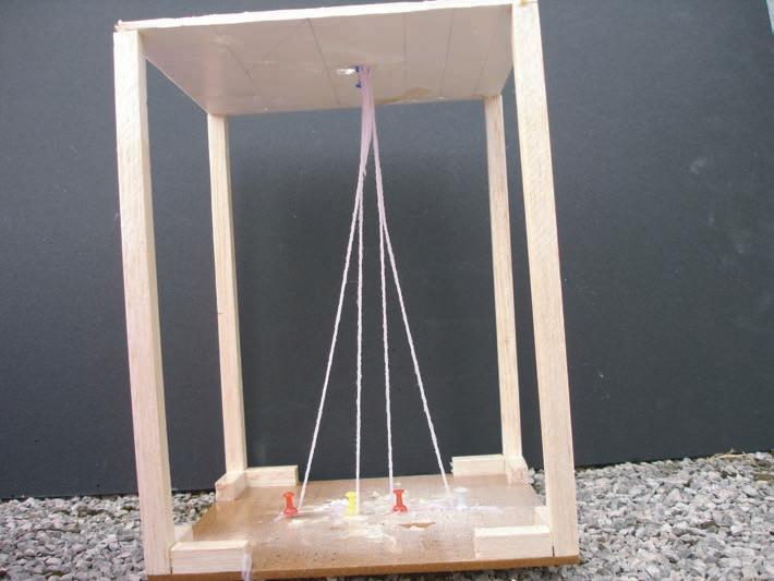
Variable considered:

- total length of thread (h)

- distance amongst starting points (d)

- distance between branching points (b1, b2,b3, b4)

Example n.1

h= 30 cm

d1 = 3 cm

d2 = 3 cm

d2 = 3 cm

b1= 7 cm

b2= 3 cm

b3= 9 cm

b4= 11 cm

branching height ratio 1/4.5 h

Example n.2

h= 30 cm

d1 = 3 cm

d2 = 3 cm

d2 = 3 cm

b1= 7 cm

b2= 14 cm

b3= 9 cm

b4= //

branching height ratio 1/3 h

Example n.3

h= 30 cm

d1 = 3 cm

d2 = 2 cm

d2 = 3 cm

b1= 7 cm

b2= 2 cm

b3= 21 cm

b4= //

branching height ratio 1/3.5 h

Example n.4

h= 30 cm

d1 = 3 cm

d2 = 2 cm

d2 = 3 cm

b1= 10 cm

b2= 8 cm

b3= 9 cm

b4= 3 cm

branching height ratio 1/4 h

guillem baraut

mattia gambardella

tutors: mike weinstock

michael hensel

achim menges

martin hemberg slender

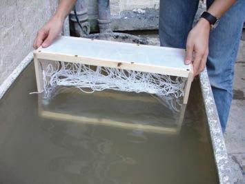
Figures 2a, 2d

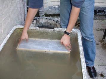
Figures 2b, 2e

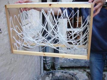
Figures 2c, 2f

EXPERIMENT 05.01

WOOL THREADS

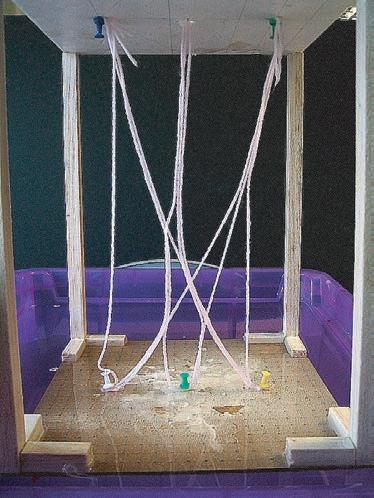
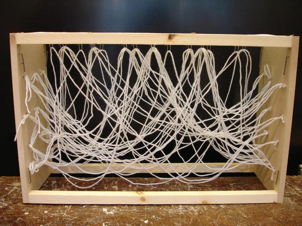
The aim of this experiment is to explore a net system created by wool threads sank in water, in order to have a tension based structure organized near a minimum path equilibrium. This set of experiments was first developed by Frei Otto.

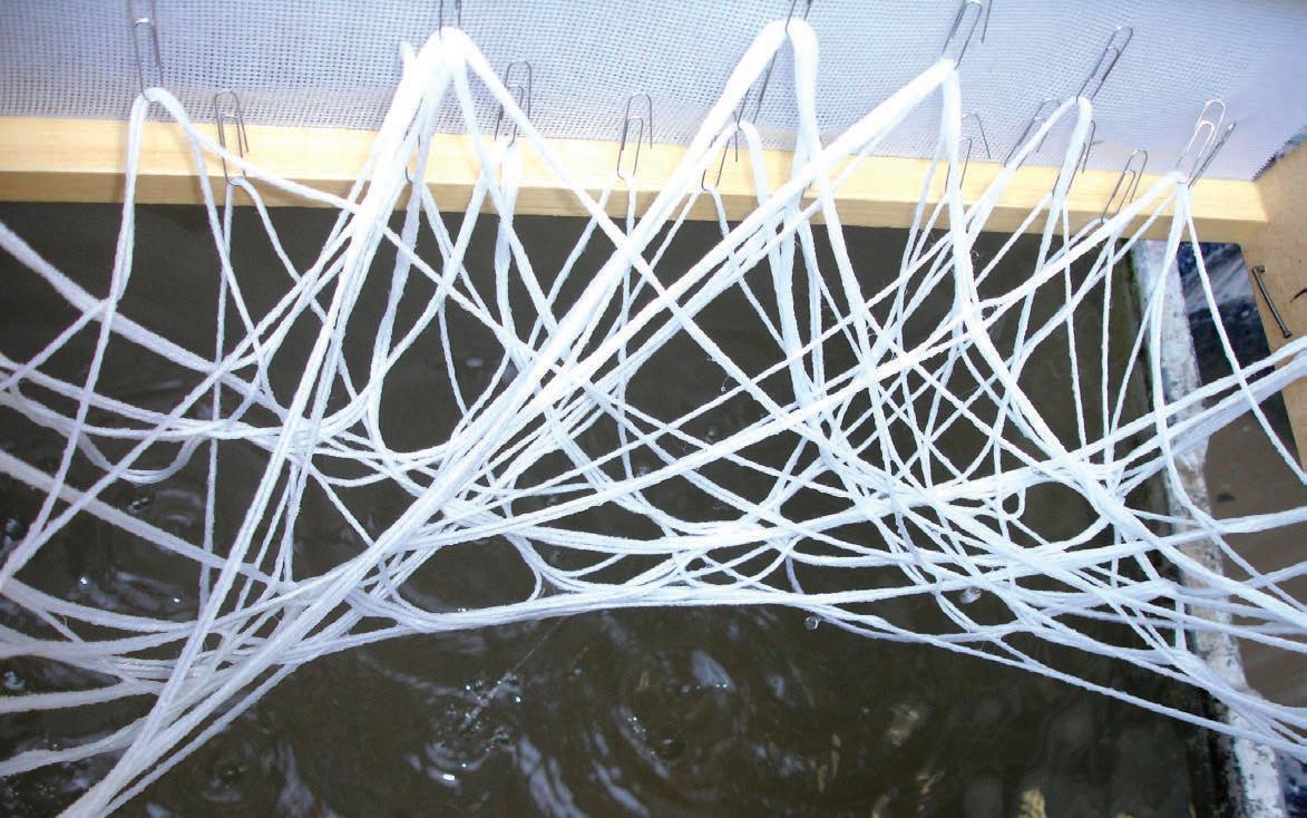
As it is shown in figure 1 the wool threads are attached in several points of a frame, creating a complex network with lots of intersections.

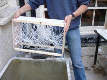
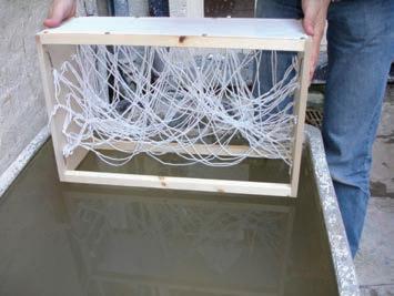
When the whole box is dipped into water as shown in figures 2a to 2f, the water goes into the wool threads and due to the surface tension the threads are attached one to each other. This physical phenomena creates a network of threads with some groups of them, with the characteristic that all of them are loaded in tension but not in compression. That makes the threads adopt an equilibrium shape that is near minimal paths, depending on the loose left in every single thread.

RESULTS

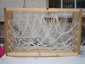
Two different sort of results can be seen in figures 3 and 4. In the first one a system of nested catenaries are defined by the network of threads, due to the weight of water absorbed by them. The high level of complexity achieved by this experiment is going to be reproduced in the digital realm, following the rules of minimal path branching. The final topology of the system that is defined by the connectivity between threads, is going to be achieved through an algorithm based in structural optimization and minimal path.

The second set of results that is shown in figure 4 consists in another configuration of the same system, where the box has been turned 90 degrees, so the gravity is informing the threads in another direction. This case can be interpreted from an engineering point of view as a structure with a continuous load on the upper deck, where all the structural elements are working in compression. The physical model is just loaded in tension because of the water weight and the nature of the threads.

guillem baraut

mattia gambardella

weinstock

Figure 1

Figure 3

Figure 4

05.02 JOINT Fiber DISTRIBUTION

guillem baraut

mattia gambardella

tutors: mike weinstock

michael hensel

achim menges

martin hemberg slender

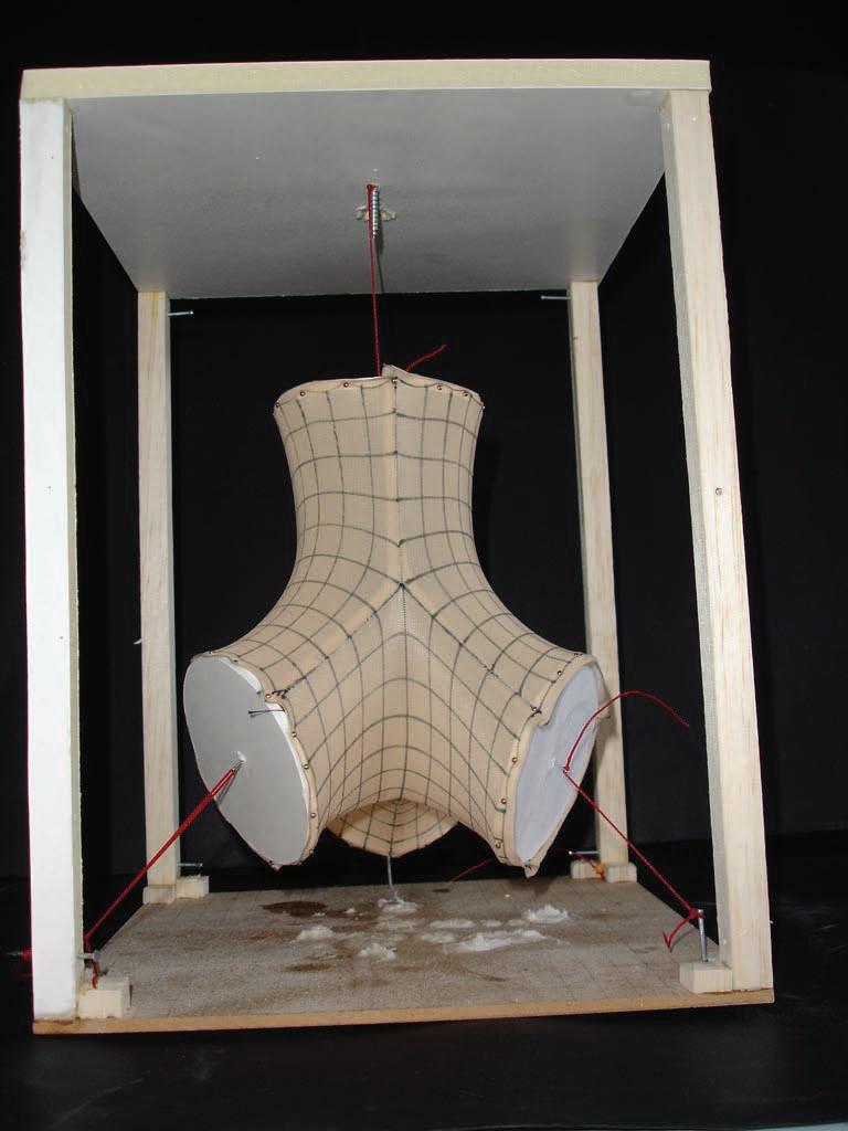
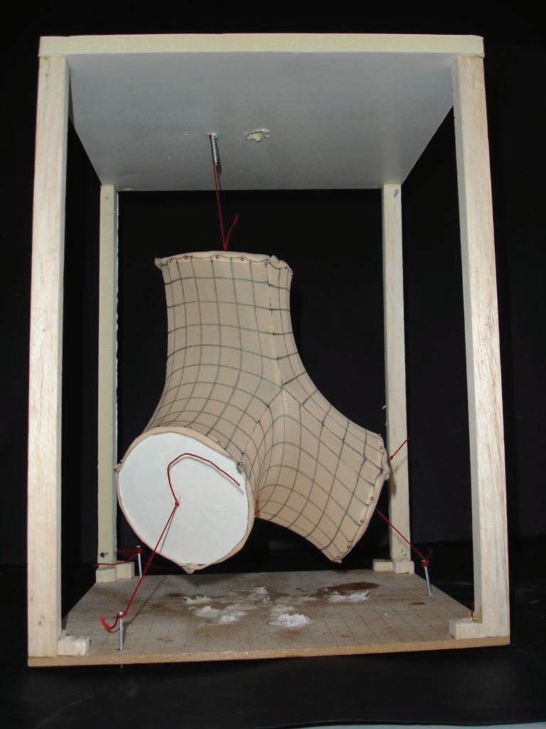
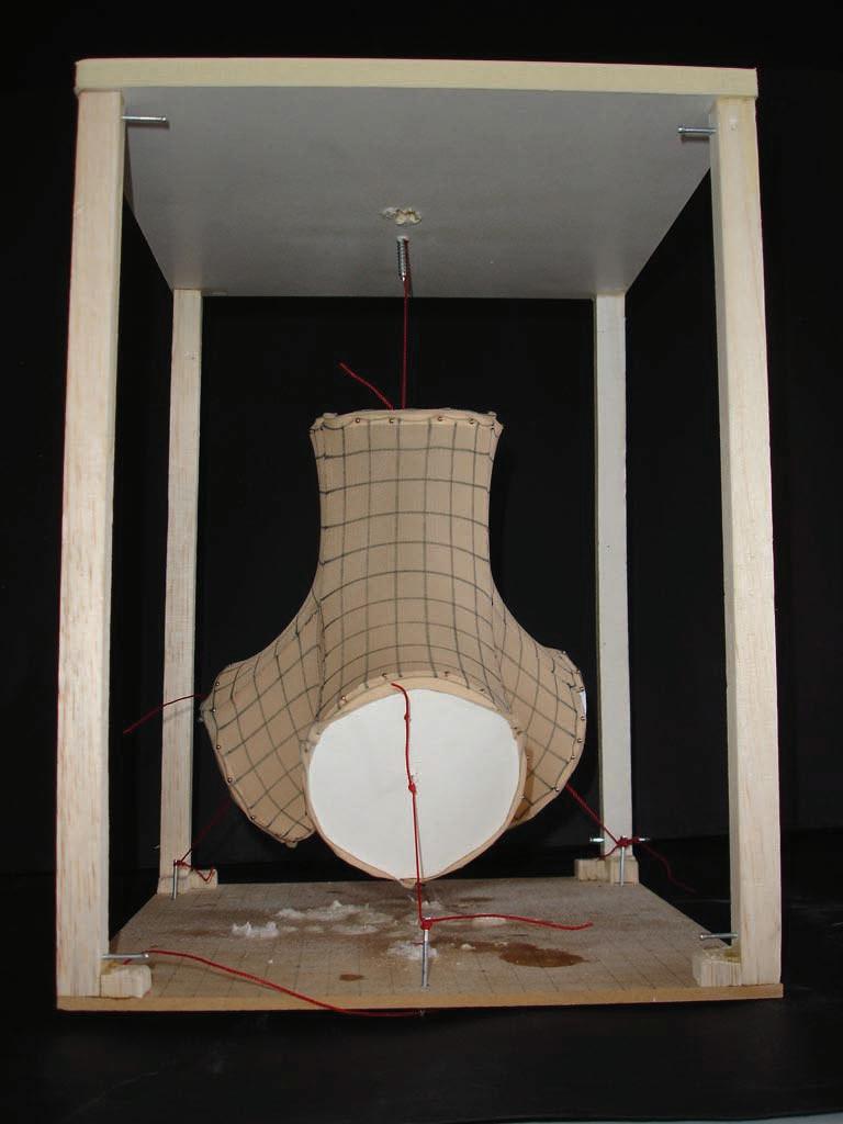
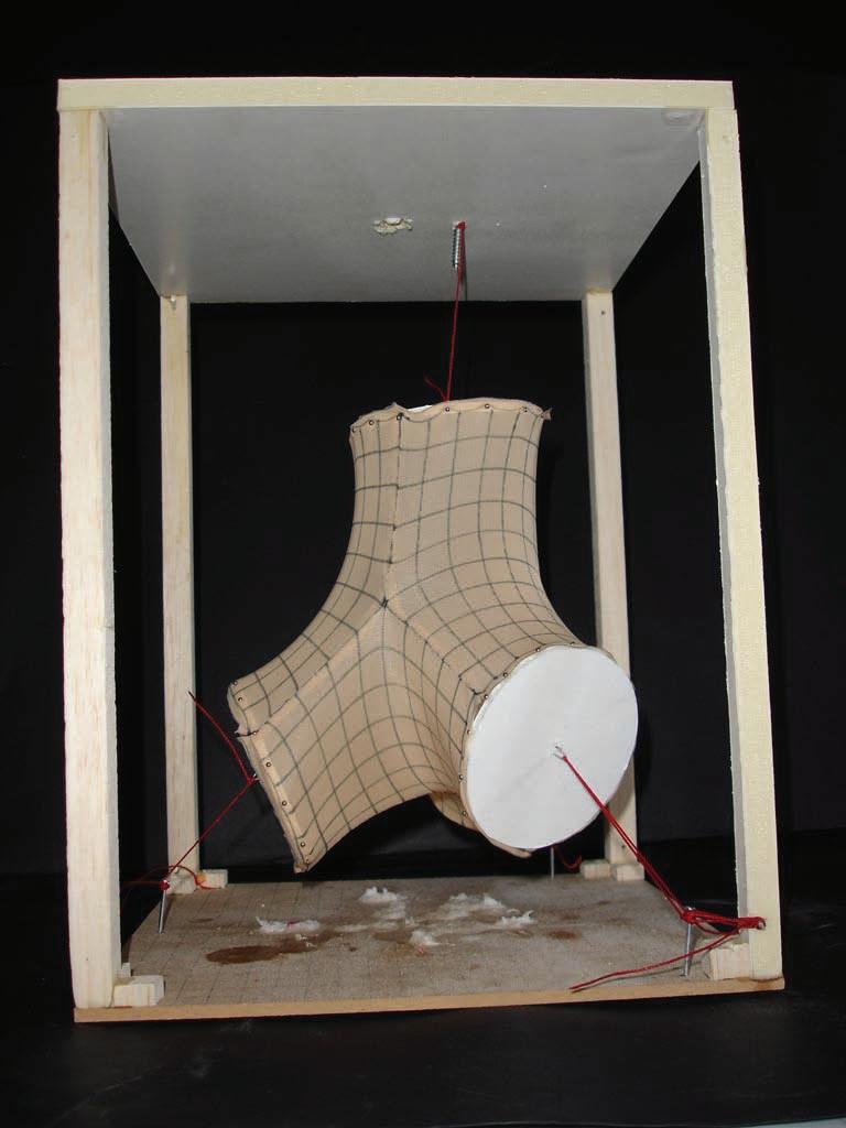
EXPERIMENT 05.02

JOINT Fiber DISTRIBUTION

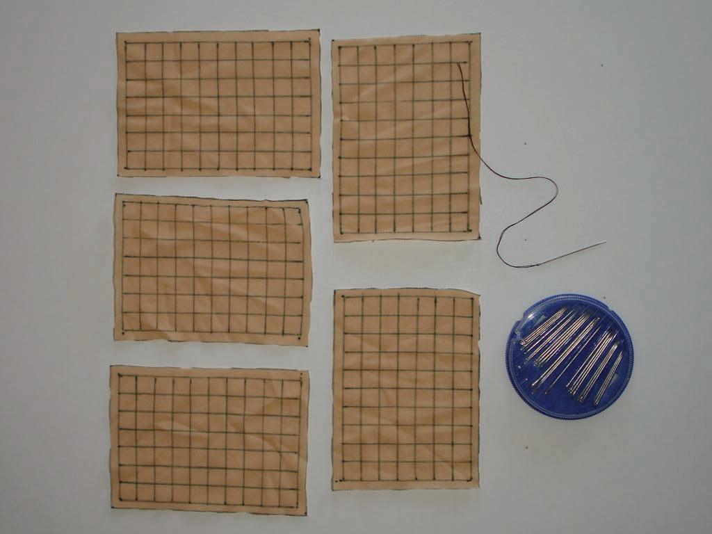
The aim of this experiment is to study the optimal distribution of properly oriented fibers in a joint formed by 4 beams with a circle like shape profile.

The optimal fiber distribution is studied by creating a minimal surface that join the 4 circular profiles. This minimal surface is called P-Shwarz minimal surface. Some elastic lycra patches with a grid drawn on them were joined together to form this joint.

The grid is oriented in the way that there is always an axis of it that is tangent joining the direction of one beam with another one. The edges of the patches coincide in one central point between three beams, where the fiber can be distributed like the previous observation or continue to the forth one following the transverse direction of the next patch.

It’s shown in the lycra density the zones that has been stretched more than the others. This zones determine the main directionality of the fibers, or the predominant orientation in this minimal surface.

tutors: mike weinstock

michael hensel

achim menges

guillem baraut

mattia gambardella

05.03 TOPOLOGY OPTIMIzATION. LYCRA

guillem baraut

mattia gambardella

tutors: mike weinstock

michael hensel

achim menges

martin hemberg slender

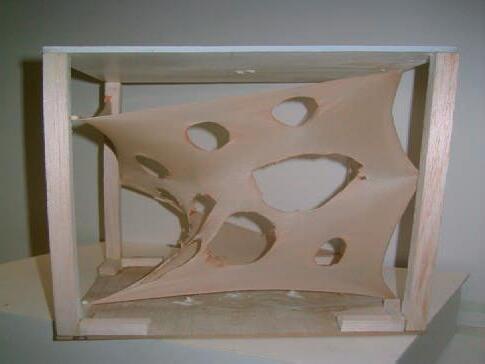
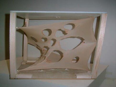
EXPERIMENT 05.03

TOPOLOGY OPTIMI z ATION.LYCRA

Materials used:

1 Lycra fabric

1 Frame box

1 Lighter

pins Introduction:

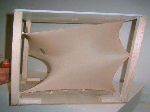
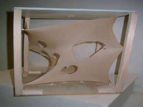
The test aims in understanding how to carry topological optimization through physical form finding.

Most topology optimization problems use objective functions like compliance: one way to optimize the structure topologically is to reduce the amount of material without affecting the structural and shape properties. By creating progressively of holes into the fabric we reduce the amount of necessary lycra tissue to maintain the overall shape.

guillem baraut

mattia gambardella

tutors: mike weinstock michael hensel achim menges martin hemberg

05.04 TOPOLOGY OPTIMIzATION. NUTS

guillem baraut

mattia gambardella

tutors: mike weinstock

michael hensel

achim menges

martin hemberg

EXPERIMENT 05.04

TOPOLOGY OPTIMI z ATION. NUTS

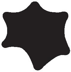
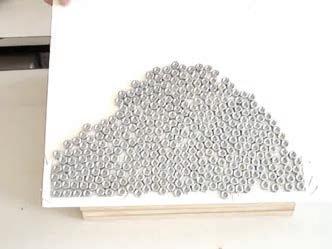
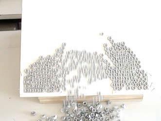
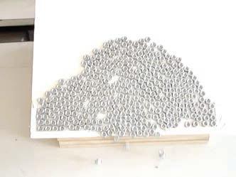
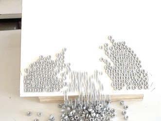
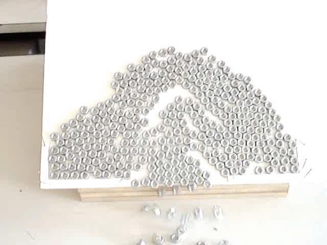
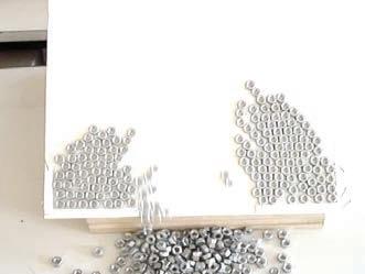
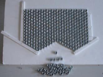
The aim of this experiment is to study the self topology optimization combined with self organization of a group of steel nuts placed on an inclined plane.

The nuts are affected by their own weight due to the inclination of the plane, and their movement is restricted by certain boundary conditions that can stop and support them. The contact between the nuts affect them in the way that they can be interconnected because of the hexagonal shape giving them certain friction, and in the way that the upper nuts increase the load applied on the lower ones.

The most interesting aspect of this experiment is that the topology optimization of the system is controlled by the self weight of the elements and the contact between themselves. The digital models that have been

guillem baraut

mattia gambardella

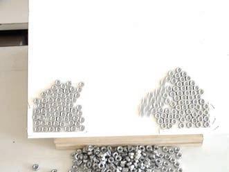
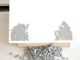
studied are always affected by external loads but not the self weight. This consideration is very important when studying long span structures, where the self weight can be more than half of the total amount of loads.

RESULTS

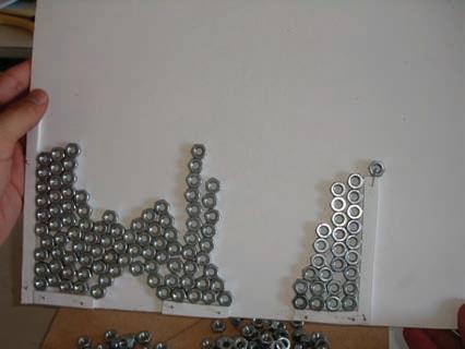
This images are a series of frames taken from a video where a total collapse of the system is seen. This is one of the first experiments done with this system and the results can be considered as non successful. But there is one aspect in one intermediate step where the system stood for almost a second sustained by an arch that is close to a catenary curve.

The initial structure and organization of the nuts as well as the way they are compacted are two fundamental variables of this experiments.

tutors: mike weinstock

michael hensel

achim menges

martin hemberg

EXPERIMENT 05.04

TOPOLOGY OPTIMI z ATION WITH EVEN ORG ANI z ATION

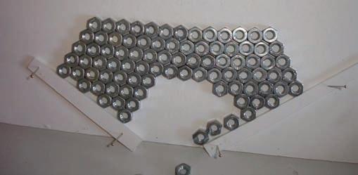
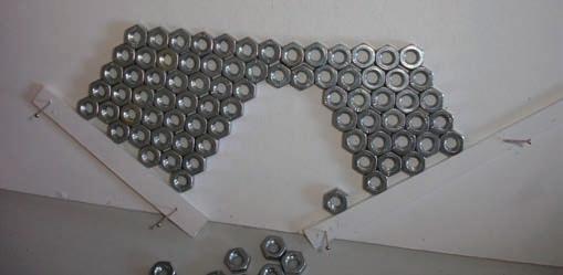
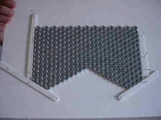
These two experiments are based on the same procedure of the last one, but with the difference that the initial distribution of nuts is following a regular pattern.

Two regular patterns are examined, considering one of the sides of the hexagonal nuts vertical and horizontal respectively. The nuts are located on an inclined plane where two inclined boundaries with a gate or space in between act

as a support of the system.

The results are shown in the figures below.

RESULTS

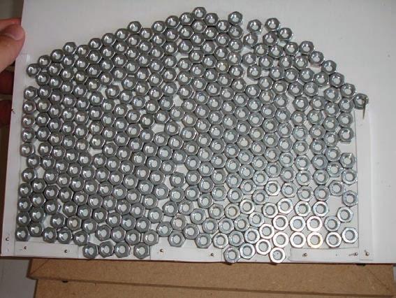
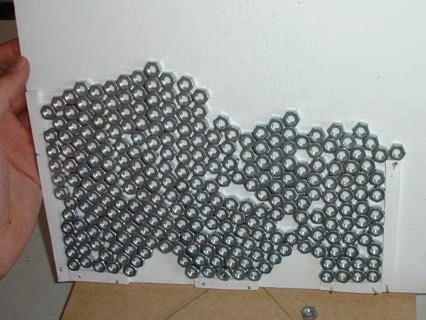
Both experiments resulted in a stable final configuration. The inclined boundaries gave to the system a certain lateral compression that made the final stage more stable.

The gap obtained on the gate of the boundaries have linear edges and is following the direction where the nuts are more close one to each other.

In the first experiment these lines are inclined 60, 0 and -60 degrees, while on the second one are 30 and -30 degrees, as shown with the red lines in figures 1 and 2.

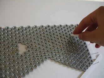
In the second experiment we started to add some holes removing the nuts following the same pattern found while the experiment was taking place. Those holes were stable when the boundaries were following the same inclination as the arch.

guillem baraut

mattia gambardella

tutors: mike weinstock

michael hensel

achim menges

martin hemberg

Figure 1

Figure 2

EXPERIMENT 5.1

EXPERIMENT 5.2

EXPERIMENT 05.04

TOPOLOGY OPTIMI z ATION

guillem baraut

mattia gambardella

tutors: mike weinstock

michael hensel

achim menges

martin hemberg

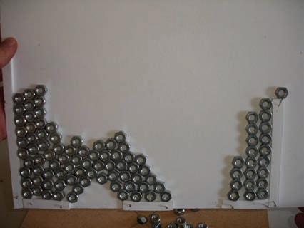
The last experiment of this series with nuts consisted in a plane with several little holes, with random initial distribution of nuts.

As considered in the results of the first one, in this case the nuts were compacted before opening the holes, in order to achieve a more stable nut-structure.

The dimension of the hole was also reduced in order to avoid a general fail of the whole system.

RESULTS

The system achieved for some seconds a stable figure with two little arches, but at the end one of them failed. As seen in the images below, the arches followed an even distribution of nuts like in previous examples, and the one that failed is the one that differed more of this configuration, at the right hand of the image.

05.05 NESTED CATENARIES

guillem baraut

mattia gambardella

tutors: mike weinstock

michael hensel

achim menges

martin hemberg slender

EXPERIMENT 05

In order to define the overall geometry of the final structure, the span length and the height of it will be controlled by several attractors and repellors. These affections will be informed by form-finding experiments based on nested catenaries.

Some experiments with catenaries in both 2D and 3D have been carried out. All the experiments have a common characteristic that is its simplicity, in order to understand the physical behaviour of the system, to facilitate its implementation into the digital model.

Experiments preparation

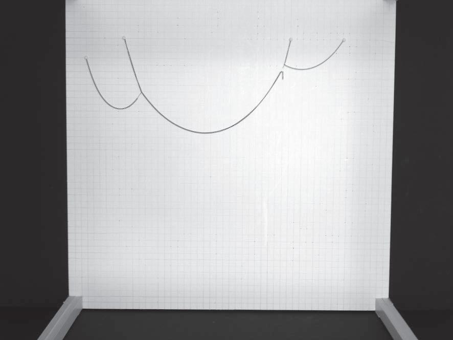
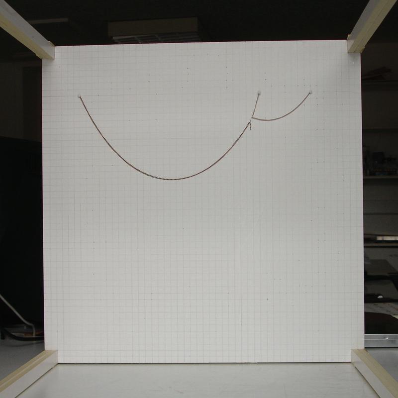
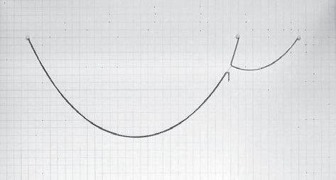
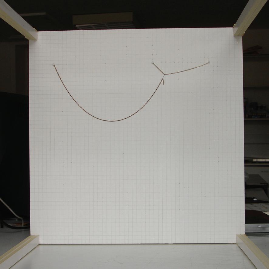
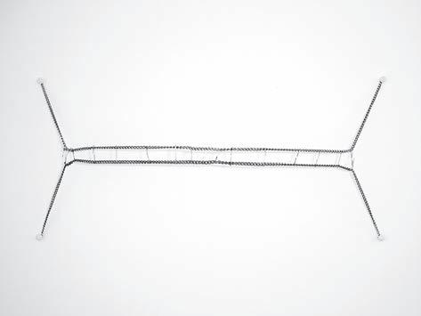
The physical experiments started creating the simplest set of nested catenaries possible. A larger chain is attached to two shorter chains, all made of the same steel and with the same transverse section, as seen in figure 2. The chains are hanged with pins on a cardboard panel with guidelines every 1.0 cm, as can be seen in figures 1a to 1d. These guidelines will be the basis for the variation of the experiments, since some geometric parameters will be modified.

In the following pages all the experiments carried out are developed, explained and analysed.

guillem baraut

mattia gambardella

tutors: mike weinstock

michael hensel

achim menges

martin hemberg slender

Figure 1a. Experiment 10.1

Figure 1b. Experiment 10.2

Figure 1c. Experiment 10.3

Figure 1d. Experiment 10.4

Figure 2. Experiment preparation

EXPERIMENT 05 CATENARIES 05.1

The first experiment consists in three chains hanged at the same height, like it is shown in the first figure. The two shortest chains are in the physical experiment the same chain, and the longest one is attached to this one with a staple.

The variable of these several states of the experiment is the point of attachment between the two chains, that determines the lengths S2 and S3 represented in figure 3. Because of being part of the same chain the total length S2 + S3 remains constant.

The length of the longest chain (S1) is constant, measuring 37.5cm. The same with the position of attachment on the cardboard frame, L and L1, which are measuring 28.0 and 8.0 cm respectively. This is represented in figure 3.

The proportion between S2 and S3 has been varied and the results are shown in the picture in figure 2. These results are analysed in the following pages.

Figure 1. Picture of the cardboard frame used for the experiments

Figure 3. Representational scheme of the chains and the variables that are analysed

guillem baraut

mattia gambardella

tutors: mike weinstock

michael hensel

achim menges

martin hemberg

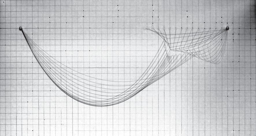
Figure 2. Superimposed pictures of the several states analysed in this experiment

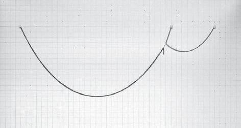
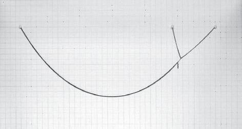
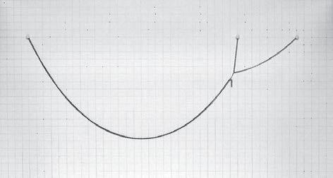
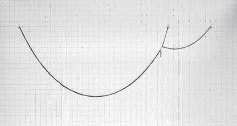
Figure 2. Superimposed view of all the results

guillem baraut

mattia gambardella

tutors: mike weinstock

michael hensel

achim menges

Figures 1a (top left) to 1h (bottom right). Several stages of this physical experiment and values of the lengths S2 and S3

martin hemberg slender

ANALYSIS OF THE RESULTS

In figure 1 there are highlighted the first and last catenaries in red and the one with maximum height in blue. As it can be seen the maximum height corresponds to an intermediate curve with an S2 value approximately the half of S3. In other words the maximum height of this case is when the longest chain is attached at the first 1/3rd of the shortest one. The values of these lengths are highlighted in table 1.

The orange line represents the possible position of the junction point of the two catenaries. The point that is tangent to a vertical line is the attachment for which the longest catenary S1 have minimum width. This curve is highlighted in green, and corresponds to a width of 27.0 cm according to table 1.

If the z value of the attachment point was invariant, the shorter width and the maximum height should be the same curve because the length S1 is constant. Due to the fact that this is changing to provide structural stability these two curves are much different (blue and green curves).

These two relations will be implemented in the GC model in form of the gravity force of the repellors that will be placed in the space. Colour legend

guillem baraut

mattia gambardella

tutors: mike weinstock

michael hensel

achim menges

martin hemberg

Figure 1. Analysis of the results: picture of the superimposed catenaries highlighting the most characteristic ones

Table 1. Values of the lengths of the catenaries S1, S2 and S3, and height and width of the longest one (S1)

EXPERIMENT 05 CATENARIES 05.2

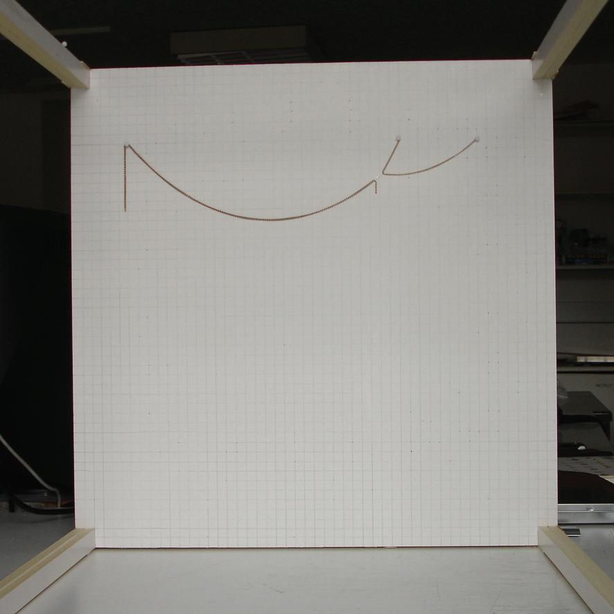
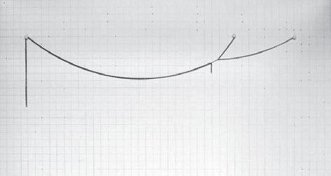
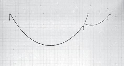
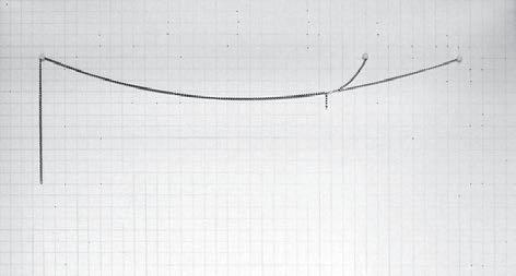
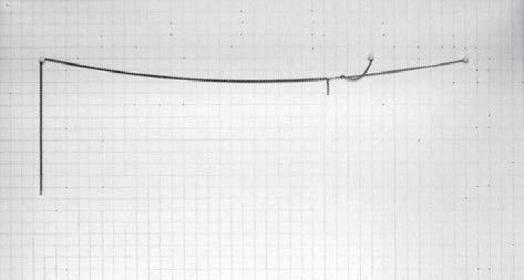
This experiment consists in the same three chains hanged at the same height, like it is shown in the first figure, in a similar configuration that the first experiment.

The variable of these several states of this experiment is the length of the longest chain, that will vary to the maximum of 37.5 cm. This variation of length is done at the left end of the chain.

The position of the attachments to the cardboard are invariant, as well as the attachment between the two chains. In this case the lengths S2 and S3 take the values

S2 = 4.0 cm

S3 = 10.7 cm

Like in the previous experiment the position of attachment on the cardboard frame, L and L1, are measuring 32.0 and 8.0 cm respectively. This is represented in figure 3.

The length S1 has been varied several times and the results are shown in the picture in figure 2. These results are analysed in the following pages.

Figure 1. Picture of the cardboard frame used for the experiments

Figure 3. Representational scheme of the chains and the variables that are analysed

guillem baraut

mattia gambardella

tutors: mike weinstock

michael hensel

achim menges

martin hemberg

Figure 2. Superimposed pictures of the several states analysed in this experiment

guillem baraut

mattia gambardella

Figures 1a (top left) to 1g (bottom right). Several stages of this physical experiment and values of the length S1 and height h

tutors: mike weinstock

michael hensel

achim menges

martin hemberg

Figure 2. Superimposed view of all the results

ANALYSIS OF THE RESULTS

In figure 1 there are highlighted the first and last catenaries in red and the one with tangency continuity between S1 and S3 in blue. The two curves in red have the curves S2 and S3 in opposite sides, while in the bottom one S2 is above the tangent at the end point of S1, and S3 is below this tangent, in the top red curve S2 is below the tangent to S1 and S3 is above.

The blue curve is approximately where S1, S2 and S3 have the same tangent at the end point of S1. This happens for a value of S1 = 35.0 cm.

The orange line represents the possible position of the junction point of the two catenaries. The point that is tangent to a vertical line is the attachment for which the longest catenary S1 have minimum width. According to the table 1 this point is the last one, that means that probably until the catenary is horizontal this width will be decreasing.

Colour legend

guillem baraut

mattia gambardella

First and last positions. S1 min and max

Tangency between S1, S2 and S3

Path of the end point of catenary S1

tutors: mike weinstock

michael hensel

achim menges

martin hemberg

slender multi stress driven structures

Figure 1. Analysis of the results: picture of the superimposed catenaries highlighting the most characteristic ones

Table 1. Values of the lengths of the catenaries S1, S2 and S3, and height of the longest one (S1)

EXPERIMENT 05 CATENARIES 05.3

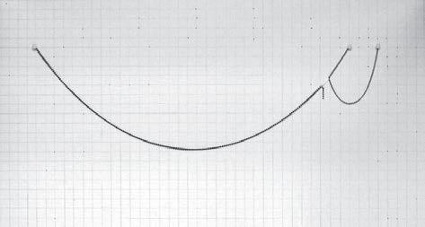
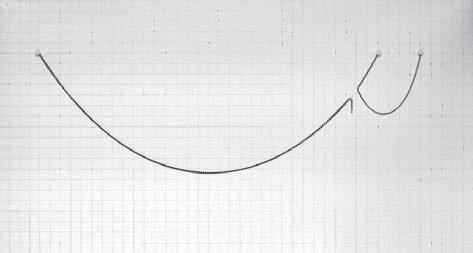
This experiment consists in the same three chains hanged at the same height, like it is shown in the first figure, in a similar configuration that the other experiments.

The variable of these several states of this experiment is the horizontal distance between the attachment points of the chains. The total distance is invariant but the central point moves from 1.0 to 14.5 cm.

The lengths of the chains will remain constant with values:

S1 = 37.5 cm

S2 = 4.0 cm

S3 = 14.7 cm

guillem baraut

mattia gambardella

tutors: mike weinstock

michael hensel

achim menges

martin

The distance between the left and right pins is constant being:

L + L1 = 36.0 cm

These values and the varying variables are represented in figure 3.

The results of varying the ratio between L and L1 are shown in the picture in figure 2, and analysed in the following pages.

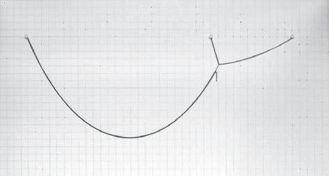
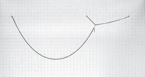
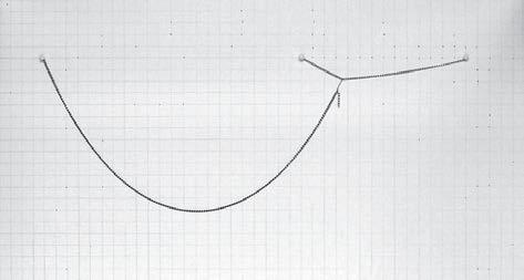
Figure 1. Picture of the cardboard frame used for the experiments

Figure 3. Representational scheme of the chains and the variables that are analysed

Figure 2. Superimposed pictures of the several states analysed in this experiment

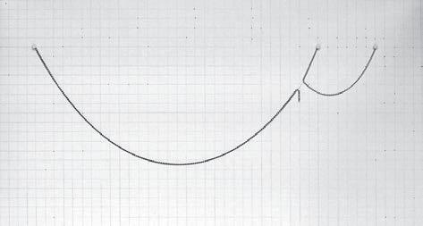
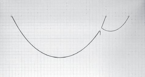
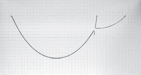
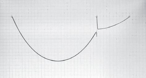
ANALYSIS OF THE RESULTS

In figure 1 there are highlighted the first and last catenaries in red and the one with maximum height in blue. As it can be seen the maximum height corresponds to an intermediate curve with a distance between pins

L = 26.0 cm

L1 = 10.0 cm

The values of these lengths are in table 1, with the height and width values of every curve. The ratio between these two distances is

L1/L = 10.0/26.0 = 38.5 %

which is very close to the ratio between the two chain lengths

(S2+S3)/S1 = 14.7/37.5 = 39.2 %

The orange line represents the possible position of the junction point of the two catenaries.

This relation will also be implemented in the GC model in form of the gravity force of the repellors that will be placed in the space. Colour

guillem baraut

mattia gambardella

tutors: mike weinstock

michael hensel achim menges

martin hemberg

slender multi stress driven structures

Figure 1. Analysis of the results: picture of the superimposed catenaries highlighting the most characteristic ones

Table 1. Values of the lengths L and L1, and height (h) and width (w) of the longest catenary (S1)

EXPERIMENT 05 CATENARIES 05.4

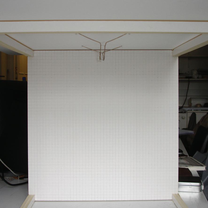
For this experiment the aim is to observe the relations between several catenaries when they are branching in 3D.

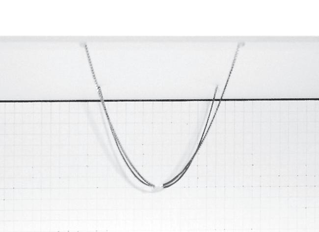
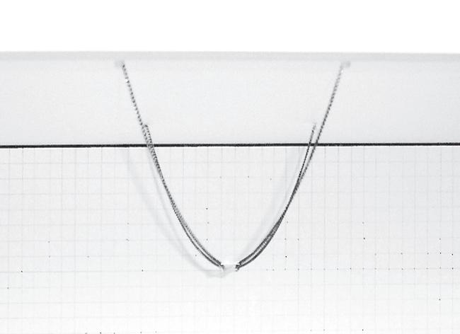
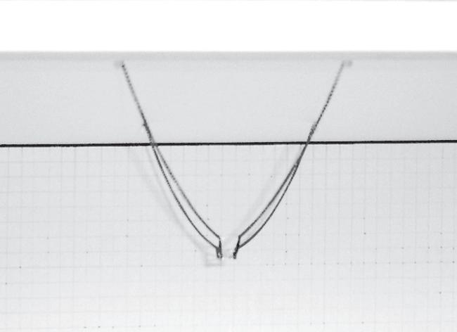
Two chains with the same length are hanged from a piece of cardboard. The attachment points are placed in the corners of a rectangle that measures 12.0 per 26.0 cm. The length of the chains is 35.0 cm.

The set of experiments carried out with this material consists in attaching the chains in the center of them, and in a certain length. This length is the experiment variable that is called S1.

The range of values for S1 is from 0.0cm to 22.0 cm, and the values measured is the height of the resulting system.

In figure 1 there is a picture of the experiment set up, while the results are represented in an overlapping of pictures in figure 2. These results are analysed in the following pages. The next 2 pages are the pictures of the system with the different values taken for S1, and in the third there is the analysis of the results.

Figure 1. Picture of the cardboard frame used for the experiments

The variables considered for this experiment are represented in a schematic way in figure 3, where there are also specified the values for the fixed variables. B

guillem baraut

mattia gambardella

tutors: mike weinstock

michael hensel

achim menges

Figure 2. Superimposed pictures of the several states analysed in this experiment

martin hemberg slender

Figure 3. Representational scheme of the chains and the variables that are analysed L

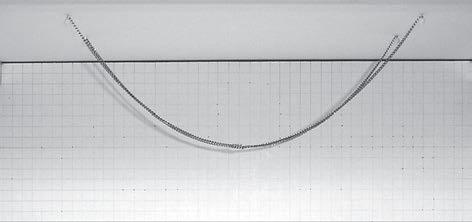
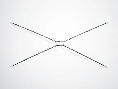
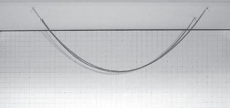
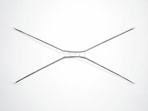
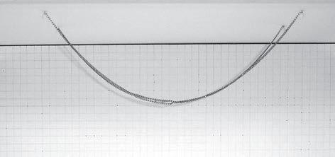
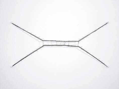
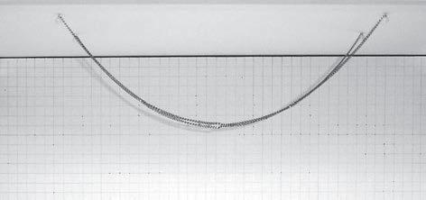
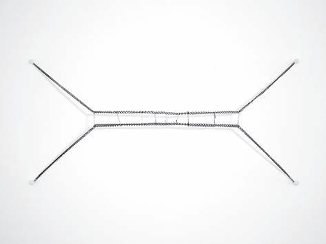
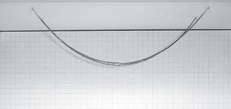
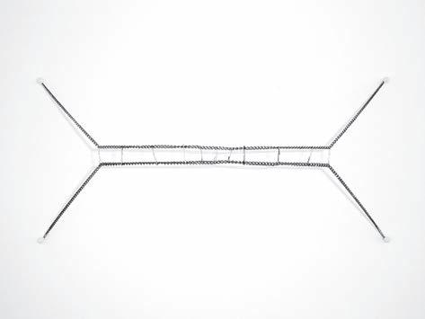
Figure 2e. Plan S1 = 12.0 cmFigure 1f. Elevation

Figure 2f. Plan

guillem baraut

mattia gambardella

tutors: mike weinstock

michael hensel

achim menges

martin hemberg

Figure 1a. Elevation Figure 2a. Plan S1 = 0.0 cmFigure 1b. Elevation Figure 2b. Plan S1

Figure 1e. Elevation

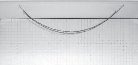
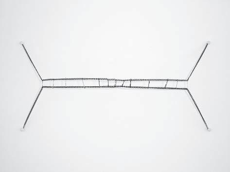
S1 = 0.0 cm

Figure 1.a Front view

S1 = 2.0 cm

Figure 1.b Front view

S1 = 4.0 cm

Figure 1.c Front view

S1 = 8.0 cm

Figure 1.d Front view

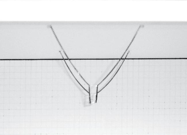
S1 = 12.0 cm

Figure 1.e Front view

S1 = 16.0 cm

Figure 1.f Front view

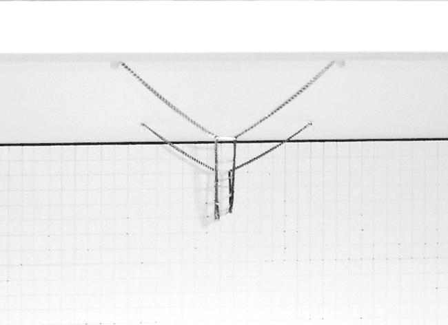
S1 = 20.0 cm

Figure 1.g Front view

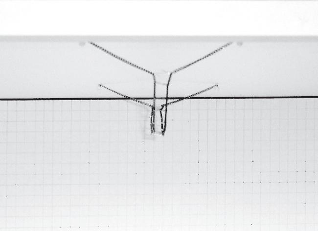
S1 = 22.0 cm

Figure 1.h Front view

guillem baraut

mattia gambardella

tutors: mike weinstock

michael hensel

achim menges

martin hemberg slender

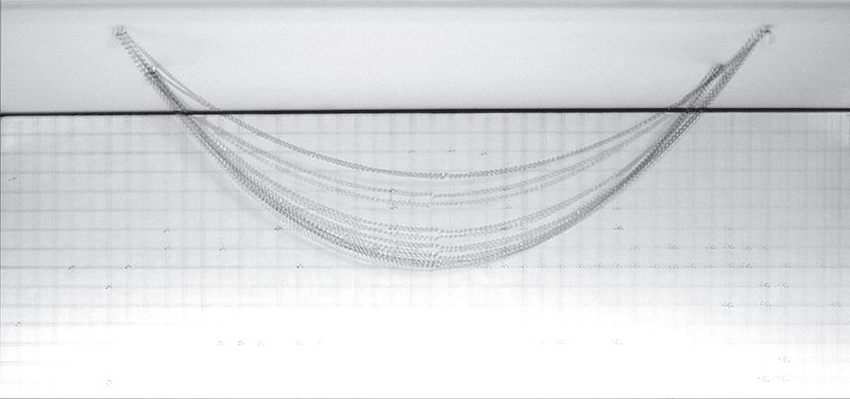
ANALYSIS OF THE RESULTS

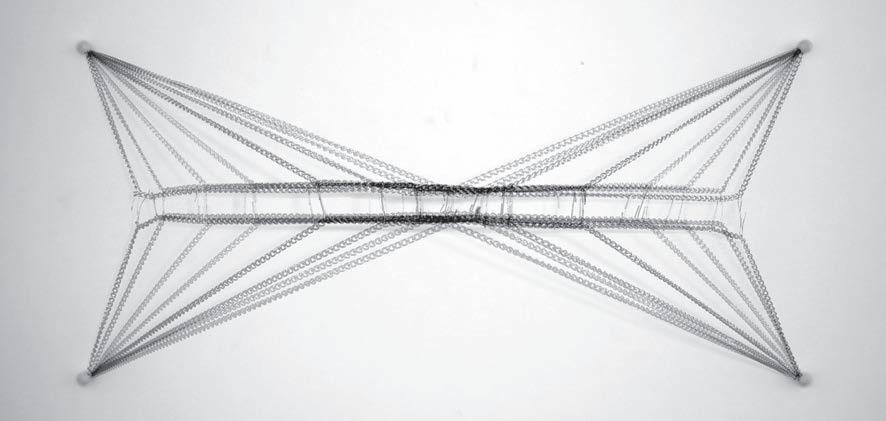
The first characteristic that can be observed in these pictures is that in the elevation view (figure 1a) there is a continuous catenary curve with apparently tangency continuity, while in the front view there is a clear vertex in the connection point. The chain can be thus considered as two different catenaries connected in this vertex, that share a continuous elevation.

In the plan projection (figure 1c) all the curves are lines that means that all the catenaries in this 3D distribution are really located in vertical planes.

In terms of dimensions this will not be used for informing the gravity attraction of attractors and repellors, but for defining the geometric relations between the several curves of the final system.

The continuity in elevation will be considered for working in longitudinal way of the final design with just the projection of the whole system of catenaries. This projection can contain all the different types of branching that are studied in the previous experiments.

Figure 1a Elevation (top left)

Figure 1b Front view (top right)

Figure 1c Plan (left)

guillem baraut

mattia gambardella

tutors: mike weinstock

michael hensel

achim menges

martin

There are 2 different catenaries in plan, but they have perfect continuity in elevation

The branching possibilities of a nested catenaries system can be forced to have a certain continuity in elevation, that means a path without pronounced vertexs can be defined in 3D.

This qualitative abstraction of this experiment will be used when designing the catenaries system of the final configuration, and also considered in the tangency continuity between them.

06. DIGITAL EXPERIMENTS

guillem baraut

mattia gambardella

tutors: mike weinstock

michael hensel

achim menges

martin hemberg

06.01 TOPOLOGY OPTIMIzATION

guillem baraut

mattia gambardella

tutors: mike weinstock

michael hensel

achim menges

martin hemberg

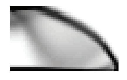
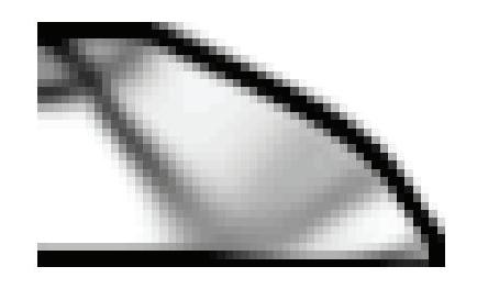
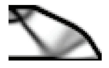
TOPOLOGY OPTIMIzATION

The topology optimization method solves the problem of distributing a given amount of material in a design domain subject to load and boundary conditions, such that the stiffness of the structure is maximized.

This method gained popularity and is being applied to many different fields of design. The aim of this digital experiment is to use the method for complex structural design. This method can improve design cost and quality.

The start point of this experiment is the article ‘A 99 line topology optimization code written in Matlab’, by O. Sigmund (Department of Solid Mechanics, Technical University of Denmark).

In figure 1 there is an example of the results of this code for a cantilever fixed at the left of the image and a punctual vertical load at the bottom right.

The code written in Matlab has been adapted for our purposes in terms of inputs and the way we treat the results, how we export the information to other software, and how we change the parameters according to either the results of other software or even the Matlab results. At the end the 99 line code turned into a 320 lines code, including options for exporting data to excel, text files, generative components, or even command script files for Rhino with the options of lines in 3D and triangulated meshes in 2D and 3D.

guillem baraut

mattia gambardella

tutors: mike weinstock michael hensel achim menges martin hemberg

Figure 1. Example of the Matlab code applied to a cantilever fixed at the left of the image and a punctual vertical load at the bottom right.

TOPOLOGY OPTIMIzATION. MATLAB CODE

The code by O. Sigmund is based in the ‘power-law’ approach, also called SIMP approach (Solid Isotropic Material with Penalization). Material properties are assumed constant within each element used to discretize the design domain and the variables are the element relative densities.

This code will be later used as an initial step in the design process. In these first steps there is no structure, material or object defined, and that’s why we can assume these considerations of a solid isotropic material. Later on in the design methodology real materials with manufacturing constraints will be introduced, and the design will be adapted to that.

In that code the design domain is assumed to be rectangular and discretized by square finite elements. The topology optimization problem based on the power law approach, where the objective is to minimize compliance, is written as:

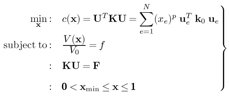
where U and F are the global displacement and force vectors, respectively, K is the global stiffness matrix, ue and k e are the element displacement vector and stiffness matrix, respectively, x is the vector of design variables, xmin is a vector of minimum relative densities (non-zero to avoid singularity), N (= nelx×nely) is the number of elements used to discretize the design domain, p is the penalization power (typically p = 3), V (x) and V0 is the material volume and design domain volume, respectively and f (volfrac) is the prescribed volume fraction.

The main program is called from the Matlab prompt by the line:

top(nelx,nely,volfrac,penal,rmin)

where nelx and nely are the number of elements in the horizontal and vertical directions, respectively, volfrac is the volume fraction, penal is the penalization power and rmin is the

filter size (divided by element size). Other variables as well as boundary conditions are defined in the Matlab code itself and can be edited if needed.

We added the variables

jpg,rhino,gc,minx

where jpg, rhino, and gc are integer variables that can take the values 0 or 1. When the variable is 1 the code will generate an output in images created for a gif file (jpg), a command script for rhino to generate splines, surfaces or lines depending on the code that we wrote (rhino), or a text file for generative components (gc). Finally, minx is a variable for filtering the data that is exported to rhino.

In figure 1 there is an example with the domain of optimization with load and boundary conditions (top), intermediate and final results from the Matlab code (center), and results exported to Rhino (bottom). When the variable minx = 0 all the data from Matlab is exported, and as can be seen in figure 1 at the bottom, the white areas in Matlab are also represented with lines in Rhinoceros. The variable minx can be any number between 0 and 1, and is the minimum volume density (x in Matlab code) that is exported.

In appendix 1 there is the final Matlab code that was used for linking with Generative Components and Rhinoceros.

guillem baraut

mattia gambardella

tutors:

mike weinstock

michael hensel

achim menges

martin hemberg slender

Figure 1. Domain of optimization with load and boundary conditions (top), intermediate and final results from the Matlab code (center), and results exported to Rhino (bottom)

06.02 MINIMIzING PATHS SYSTEMS

guillem baraut

mattia gambardella

tutors: mike weinstock

michael hensel

achim menges

martin hemberg slender

guillem baraut

mattia gambardella

michael hensel

achim menges

martin hemberg

M INIMAL P ATH

A spacial performance considering the minimal distance for connecting different points is the driving design input for planning spatial relationship between elements.

The structure then focuses on solving problems related to the minimum path of connecting points.

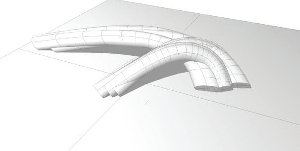
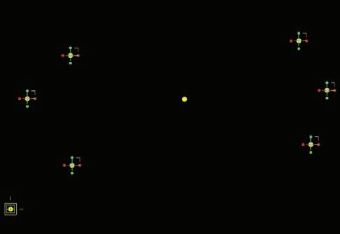
From a cloud of points is it possible to define a “centroid”; The centroid of a triangle is the point of intersection of its medians (the lines joining each vertex with the midpoint of the opposite side).

The centroid divides each of the medians in the ratio 2:1.

tutors: mike weinstock

guillem baraut

mattia gambardella

tutors: mike weinstock

michael hensel

achim menges

martin hemberg slender

Fig.1 Rendered images of first digital minimal path outcomes and their com bination with topology optimization

guillem baraut

mattia gambardella

tutors: mike weinstock

michael hensel

achim menges

martin hemberg

MINIMAL PATH

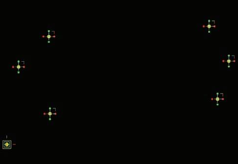
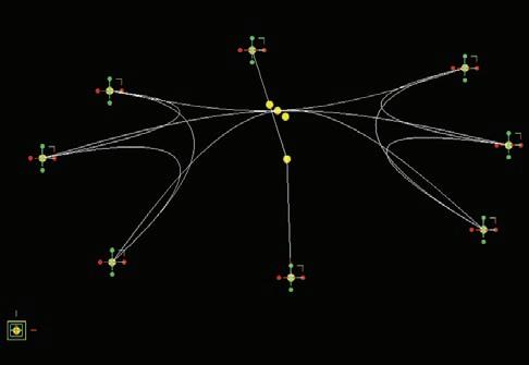
The next set of digital experiments are exploring several ways of defining the minimal paths from an origin to an end point, using some attractors and repellors to determine the area of the flow, but without fixing it.

The flow paths can be classified in these classes:

- Vector field: when the flow is going from known origin and end points and is affected by the environment (other attractors and repellors)

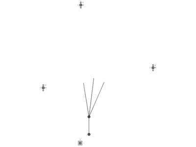
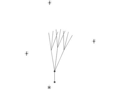
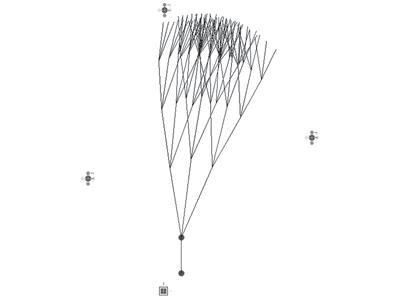
- L-system: The flow is originated in a certain point and certain direction, and is affected by the environment (other attractors and repellors). This flow is going to a broader space in each iteration in order to search the final point. This search is defined according the Lindenmayer system rules, dividing the flow in branches.

The combination of both systems can give us a mixed flow between searching and browsing in the space in order to join the origin point with the final one. This end point can be either an attractor, creating a more hierarchical or searching flow paths, or a simple point, making the flow more random-like, or more similar to browsing.

In between these points there will be placed other attractors creating interest for some points in the space, and repellors, creating the necessary voids. These voids will determine the spans for the structure and the spaces where the structure cannot be placed.

In figure 1 there is a diagram to represent these possibilities

Figure 1. Diagram for the several possibilities of the minimal path flow definition

guillem baraut

mattia gambardella

Figure 1. Points to be connected

MINIMAL PATH. PARAMETRIC SOFTWARE

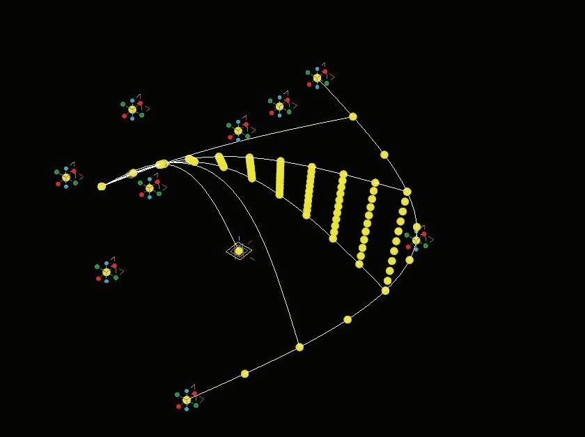
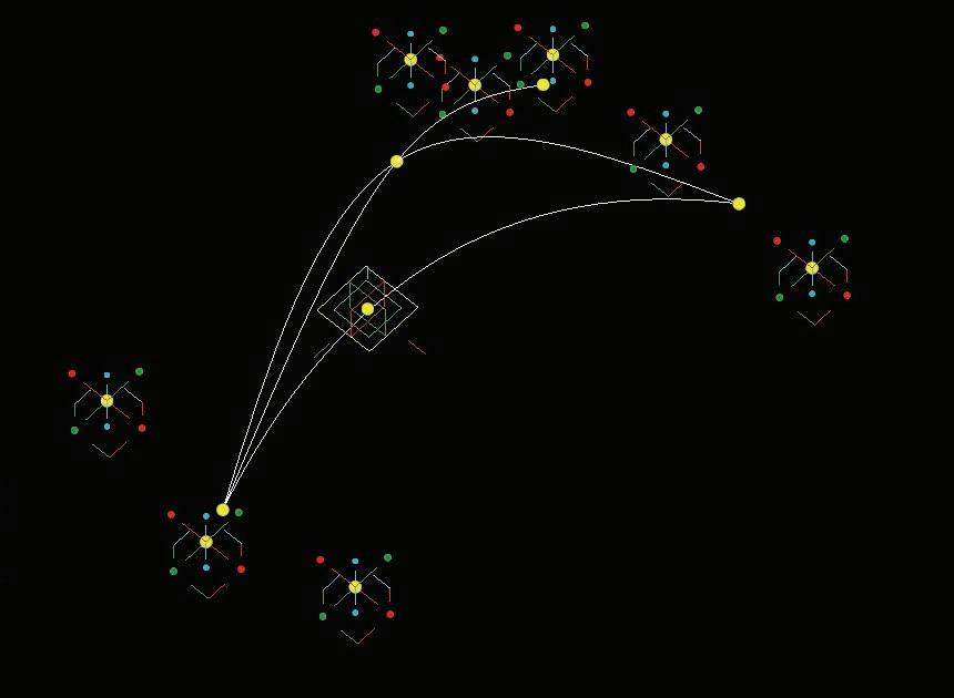
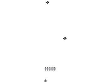
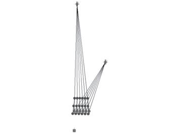
In this exercise we explore the capabilities of a parametric software to generate several paths of connections between points. In this case six points are placed in the space (fig. 1), and they will be connected with BSplines curves through their centroid (fig. 2).

Figure 2. The centroid of these points is calculated by Generative Components. The connection between the centroid and the other points is a way to find a minimal path.

Figure 3. An attractor (up) and a repellor (down) are inserted. The attractor pulls the centroid towards it through a line (in this case at the mid point of the line), and the repellor pulls it in the direction of the line that connects it with the centroid, in an hyperbolic rate.

The mid point of the three closest yellow ones is the final centroid to be used for the BSpline curves

tutors: mike weinstock

michael hensel

achim menges

martin hemberg

The centroid later on is affected by an attractor and a repellor (fig. 3) that generate two new centroids. At the end the final curves will be defined through or by the new centroid located in between the two new points generated in the previous step (fig. 4)

Figure 4. The points are connected from left to right through the centroid, and between the groups on the left and right using this centroid as a pole.

guillem baraut

mattia gambardella

Figure 1. Points to be connected. The start point at the bottom of the image is an array of points that will be the origin of the vector field

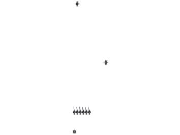
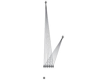
Figure 2. The end point (attractor) and the repellor (at the right hand side of the image) are joined to the start point by an array of lines. These are the directions of attraction and repulsion

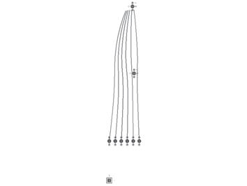
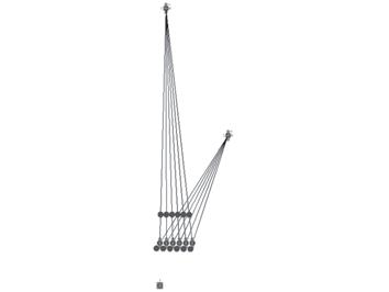
Figure 3. The attracted and repelled points are placed on the lines

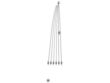
Figure 4. The final point that will define the vector field is the centroid of the points inserted in the last step.

tutors: mike weinstock

michael hensel

achim menges

MINIMAL PATH GUIDED BY A VECTOR FIELD

Once the start and end points are defined we experimented with two ways of joining them. In this first exercise a vector field is created reproducing flow lines from the start points to the end point, affected by a repellor and attracted by the end point.

Figures 1 to 8 explain the process followed to create this vector field represented by the flow lines.

Figure 5. Final vectors from the initial point to the centroids previously found. This vector definition is saved as a new feature in Generative Components. From this step the feature can be reproduced as a component in the space, affected by the previous vectors (start point of the vector will be the end point of the previous), the attractor and the repellor.

Figure 6. The feature is inserted several times creating these flow lines from the start point to the end point

Figure 7. The gravity variable of the attractor is changed, as it is increased, the flow lines become more similar to a straight line.

Figure 8. The repellor placed under the flow lines will give us the chance to create 3D flow lines in the space, creating the voids necessaries for the final long span structure.

martin hemberg slender

guillem baraut

mattia gambardella

Figure 1. At the bottom of the image there is the tree-like flow lines that are attracted by the endpoint (top) and another attractor (right) and a repellor (left). The length and direction of the new searching branches are just defined by the combination of the gravity of the attractors and repellor

Figure 2. This tree like shape is saved as a new feature and reproduced at the end of each new branch in order to continue the search of the end point

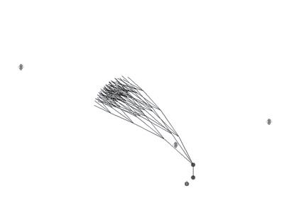
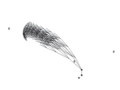
Figure 3. The attraction of the two points make it difficult to find the end point

MINIMAL PATH GUIDED BY AN L-SYSTEM

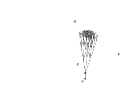
This experiment is similar to the previous one, but the way the vector field is created is completely opposite. In this case the flow is an almost random expansion of the vector field, that reproduce a non hierarchical flow lines going from the start point to the direction of the end point without knowing where it is placed. The way this is created is by an L-system that expands the flow lines attracted by the end point, and affected by other inputs as other attractors or repellors.

Figure 5. The end point is moved even more far away and the flow follows it

Figure 6. The L-sys flow paths are reproduced some more times to try to reach the end point

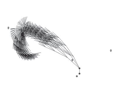
Figure 4. The final point is moved in the space to study its influence. The more far it is moved the stronger its attraction is

tutors:

mike weinstock

michael hensel

achim menges

martin hemberg

Figure 7. The gravity variable of the other attractor is increased making the flow invert its direction towards it and leaving the end point .

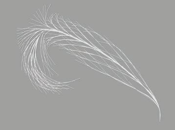
Figure 8. Rendered image of the flow once its filtered to the most probable flow paths. This probability is defined according to the length from the origin to the end of the spline, and the distance of this end point and the final point or attractor.

FINAL MINIMAL PATH ALGORITHM

The final algorithm will combine all the methods previously explained. Before defining how the minimizing path algorithm works there are some considerations that have to be explained.

The minimizing path algorithm will run on a 3D surface that has been defined according to the catenaries system physical experiments. The experiments relate the proportions between lengths, heights and widths of the catenaries, as well as the angles that they form when connected. All these data is translated into attractors and repellors within the Generative Components model.

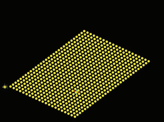
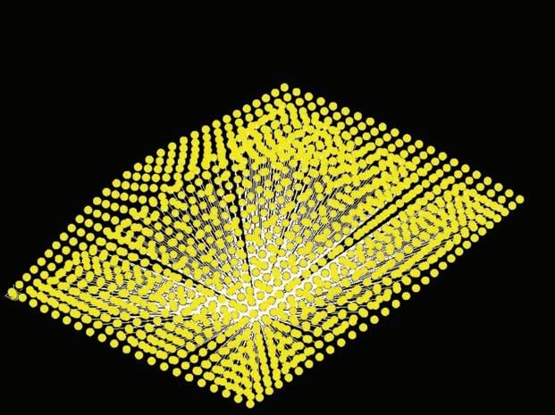
In figures 1 and 2 there is the formation process of this 3D surface from an array of points with the same dimension as the topology optimization frame. The dimension is given by the number of finite elements used in Matlab, that is directly translated into number of points in GC. This array of points is then affected by the attractors and repellors according to the catenaries experiment.

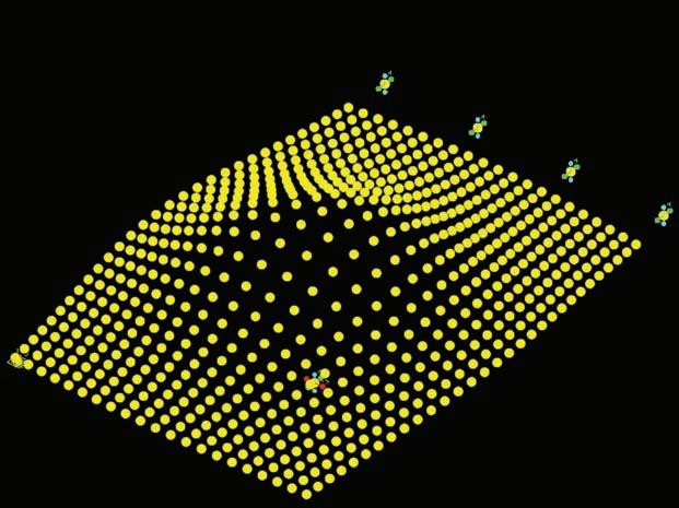
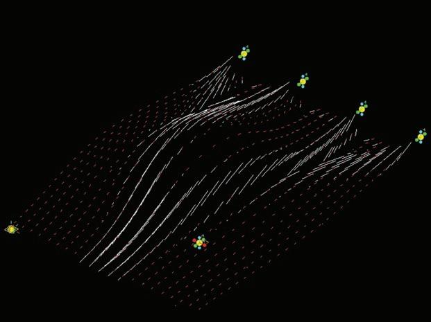
The start and end points of the structure, or in other words, the supports of the structure are added into the model as attractor points, like the yellow points that are added in figure 3.

With this system composed by attractors and repellors and the 3D point grid a vector field is mapped. This vector field is made of lines that have a direction guided by the start and end points of the structure added in the previous step. The length of these lines is defined according to the stiffness of each element resulting of the topology optimization in Matlab. An example of this vector field is represented in figure 4.

guillem baraut

mattia gambardella

tutors: mike weinstock

michael hensel

achim menges

martin hemberg slender

Figure 1. Array of points in GC with the same number of rows and columns as the Matlab frame

Figure 2. Array of points affected by attractors and repellors. These attractors and repellors are affecting the catenaries system that defines the final 3D surface

Figure 3. Final array with end points of the structure. These end points are attractors for the structure.

Figure 4. Vector field on the array with the direction pointing to the end points (which are attractors) and with length of the vector according to Matlab results

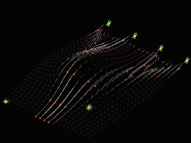
On the vector field there are mapped the last attractors that will guide the minimizing paths algorithm. The red points that are added in figure 1 correspond to the maximum stiffness of the elements in the topology optimization results, and are defined from the vector field that has been created in previous steps. These points will finally be the guide for the minimizing path algorithm.

Figures 2, 3 and 4 show the result of this algorithm for 2, 10 and 50 iterations.

The solver for this minimizing path works with the following scheme:

- Choose a start point from the start points of the structure (in the example in figures 1 to 4 there are 4 start points and 4 end points)

- Look for the closest matlab attractor (red points), considering the 3D distance on the surface.

- Read the direction of the vector field in that point, and according to the intensity and direction of the vector in that point look for the next closest attractor. This step internally considers the L-system algorithm to look for the next closest point

- Repeat the process until an end point is reached

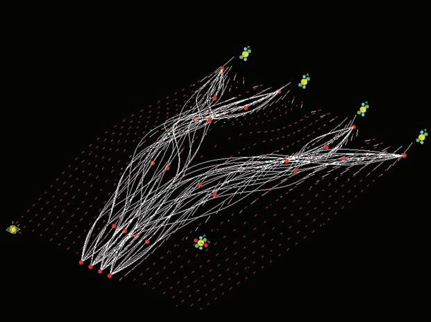
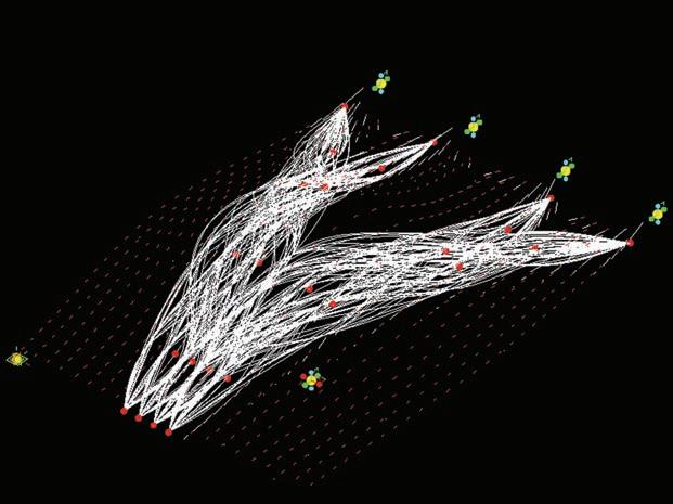
- Repeat the whole process for the next start point until another end point is reached.

- Repeat the process until the number of iterations that the user asked for is reached.

At the end a sorting algorithm is run and the shortest paths that connect all the start points with all the end points are selected and sent to either the next iteration in Matlab, or to the last Generative Components script to materialise the paths into fiber structures.

guillem baraut

mattia gambardella

tutors: mike weinstock

michael hensel

achim menges

martin hemberg slender

Figure 1. The red points are the points with maximum stress in the results from Matlab.

Figure 2. First 2 iterations of the minimizing path algorithm. These paths are guided by the vector field and also with two groups of attractors: the end points (4 yellow points on the right) and the Matlab points (red points)

Figure 3. Results after 10 iterations. The solution is being refined for every iteration

Figure 4. Results after 50 iterations. When the algorithm stops there is another one that will choose the shortest path system within the results and will map it again into the Matlab routine

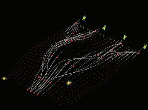
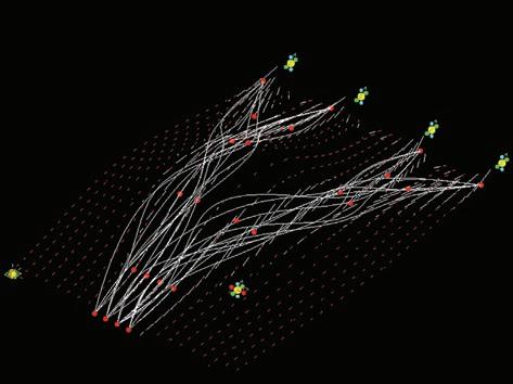
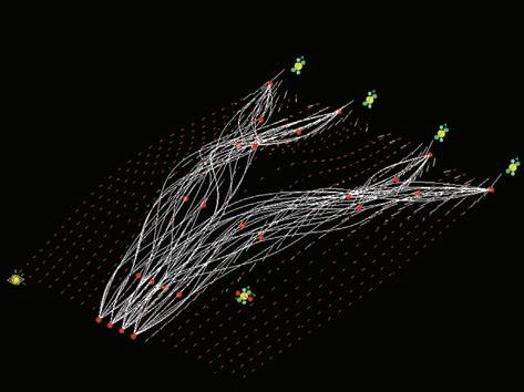
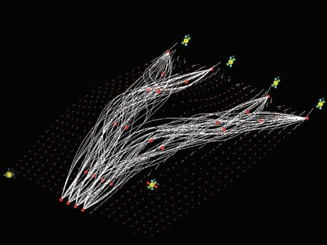
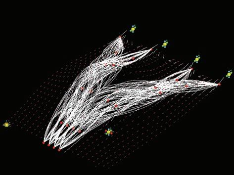
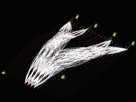
These figures 1a to 1g are the solutions for several number if iterations for the minimizing paths algorithm. At the chapter Evaluation criteria there is a comparison of the solutions depending on this number of iterations, and an evaluation of how good are the solutions according to this parameter.

guillem baraut

mattia gambardella

tutors: mike weinstock

michael hensel

achim menges

martin hemberg slender

Figure 1a Vector field from topology optimization

Figure 1b Minimal path n = 5

Figure 1c Minimal path n = 10

Figure 1d Minimal path n = 20

Figure 1e Minimal path n = 50

Figure 1f Minimal path n = 100

Figure 1g Minimal path n = 200

07. MANUFACTURING TECHNIQUES

guillem baraut

mattia gambardella

tutors: mike weinstock

michael hensel

achim menges

martin hemberg

slender multi stress driven structures

A DVANCEMENTS IN T ECHNOLOGY FOR C ONTROLL ING F IBER O RIENTATION IN C OMPOSITE P ARTS

The performance of a composite part is primarily determined by the orientation of fibers in the plies.

Designers wishing to exploit the full potential of composite materials, while avoiding manufacturing problems and part failures, must define and control fiber orientation. Anticipating true fiber orientation for a single ply is seldom intuitive, and predicting the behaviour of an entire laminate made of tens or hundreds of plies is nearly impossible.

Traditionally, verifying the design of a composite part has required repetitive, expensive physical prototyping and testing. The part design could be refined only through lengthy trial and error involving costly redesigns and additional prototyping. Engineers, hampered by time constraints and unable to predict true fiber orientation, often resorted to over-designing composite parts, which added weight and cost to the product.

Now designers are getting faster and more reliable feedback about the producibility and behaviour of composite parts by using specialized software that is fully integrated into the engineer’s CAD environment. Such software enhances the CAD model by adding features to it that are specific to composites, such as zones, plies, cores, and rosettes.

The software provides a configurable library of composite materials specifications, as well as the ability to define the surface, boundary, thickness, and orientation of plies. It also simulates material drapability for different composite manufacturing processes, displaying areas of problematic or unacceptable material deformation and fiber deviation. Designers can export data representing true fiber orientations to other tools such as finite element analysis (FEA) software so the ultimate performance of the part can be more accurately predicted and design revisions can be quickly made. Employing the CAD model as a single upstream information source for composite design ensures the closest possible match between the specifications and the manufactured part.

Due to their outstanding specific properties (strength and stiffness versus density ratios), composite materials are increasingly used in diverse industrial sectors as automobile, rail, ship and aeronautics industry, building, leisure and sports, ..., and the characteristics of those materials are generally:

high degree of anisotropy

low secondary strength;

sensitivity to stress concentration;

huge amount of data and results

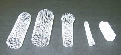
guillem baraut

mattia gambardella

tutors: mike weinstock michael hensel achim menges martin hemberg

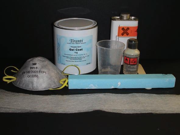
MATERIALS

- Glass fiber tissue

- Gel coat

- Catalyst

- Foam

- Kitchen foil

- Mask

- Plastic glass and wood stick

- Acetone

guillem baraut

mattia gambardella

GLASS FiberS LAY OUT PROCESS

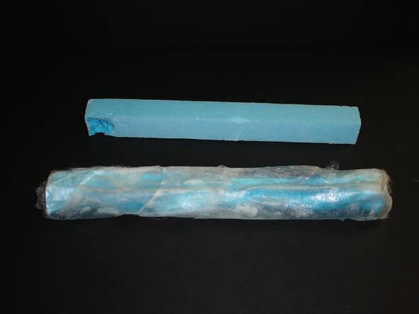
The aim of this experiment was the study of the process of laying out of glass fibers on several forms. The first one consisted in using a piece of foam that works as a form for the final structure.

If successful, this experiment will open us the door of a technique to create the future models consisting in CNC milled pieces of foam where the fibers will be laid out.

In this experiment no orientation of fibers is considered.

PROCEDURE

The cut foam is covered with kitchen plastic foil to protect the foam to be melted by the resin. In the glass the gel coat and catalyser are mixed. The fibers are laid out on the piece of foam and with the wood stick the resin fix the fibers in the final position.

The model is left hanged in the air to be hardened.

RESULTS

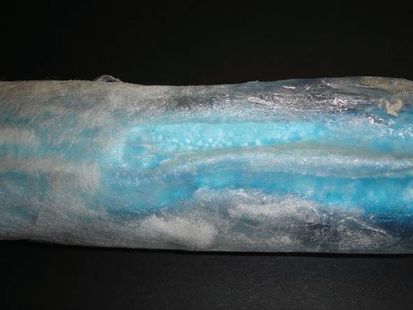
As seen in figures 2, 3 and 4 even with the kitchen foil the resin melted part of the foam. This effect made the fibers to loose its final shape into a fabric-like shape.

Another effect seen in this experiment is that not the whole amount of fibers have enough resin, probably because of the effect of the melted foam.

For further experiments with CNC milled foam a better protection against the resin has to be found.

tutors: mike weinstock

michael hensel

achim menges

martin hemberg

Figure 1

Figure 4

Figure 3

Figure 2

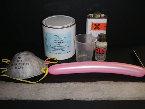
MATERIALS Figure 1

- Glass fiber tissue

- Gel coat

- Catalyst

- Balloon

- Kitchen foil

- Mask

- Plastic glass and wood stick

- Acetone

guillem baraut

mattia gambardella

GLASS FiberS LAY OUT PROCESS

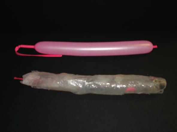
The aim of this experiment was the study of the process of laying out of glass fibers on several forms. The first one consisted in using a balloon (pneumatic scaffold) that works as a form for the final structure.

If successful, this experiment will be a proposal technique to create the future models consisting in inflatable forms where the fibers will be laid out.

In this experiment no orientation of fibers is considered.

PROCEDURE

The balloon is covered with kitchen plastic foil to protect the foam to be melted by the resin. In the glass the gel coat and catalyser are mixed. The fibers are laid out on the piece and with the wood stick the resin fix the fibers in the final position.

The model is left hanged in the air to be hardened.

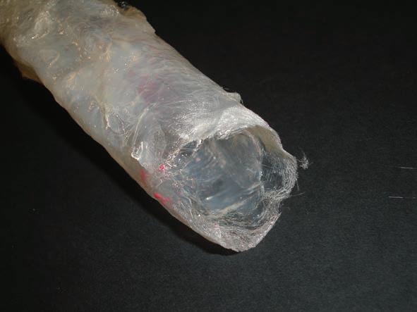
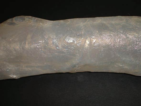
RESULTS

As seen in figures 2, 3 and 4 even with the kitchen foil the resin melted part of the foam. Due to the highly esothermic reaction of the hardening resin some of the balloons got easily ripped.

For further experiment we have to consider the heat resistance of the pneumatic scaffold.

tutors: mike weinstock

michael hensel

achim menges

martin hemberg

Figure 4

Figure 3

Figure 2

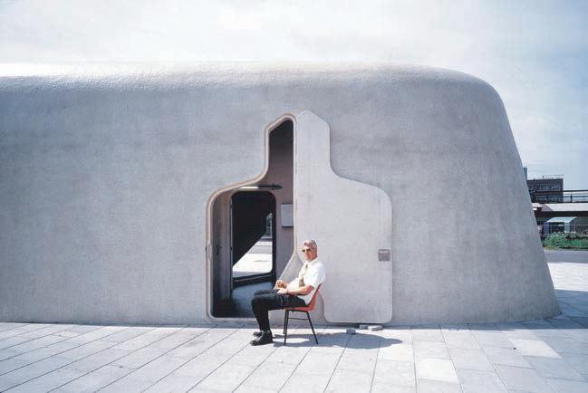
michael

achim menges

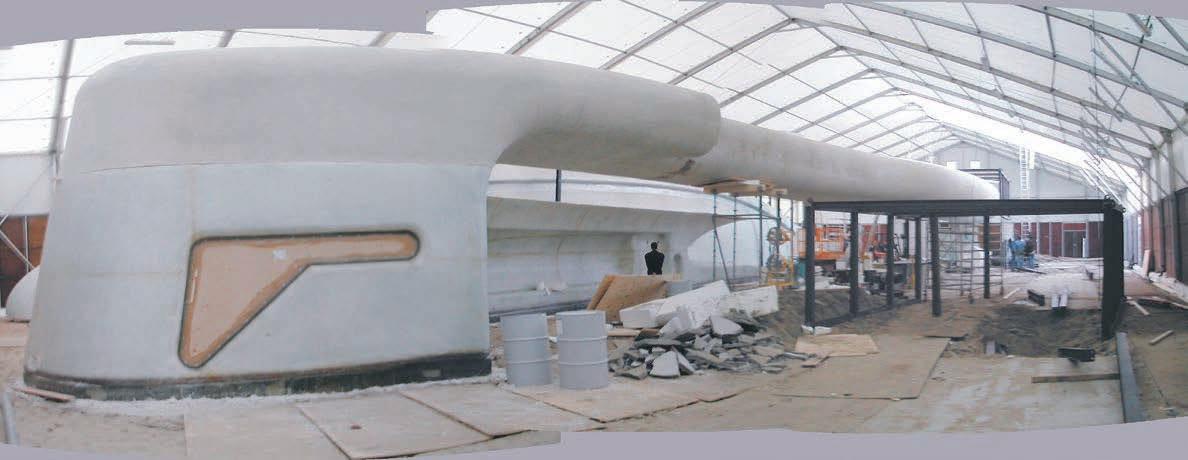
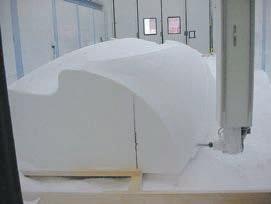
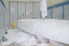
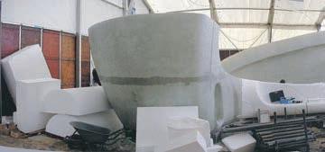
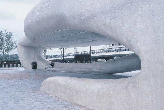
This bus stop won an ar+d prize from the Architectural Review, and is the world’s biggest structure built entirely from synthetic materials: factory-cut polystyrene foam with a polyester skin. It is the terminus of several bus routes in Hoofddorp, forming an oval roundabout in front of the edge-of-town hospital.

guillem baraut

tutors: mike weinstock

hensel

Section of bench (scale: 1/20)

NIO architecten Hoofddorp Bus Station , the Netherlands 2003

NIO Architecten 2003

YITZHAK RABIN CENTER / Tel Aviv

Material composition roofs :

Sandwich with a core material of non-combustible PIR foam and a stressed skin of glass fibre reinforced polyester.

The sandwich has an integrated web of inserts and ribs.

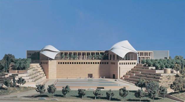
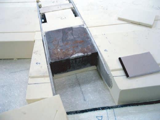
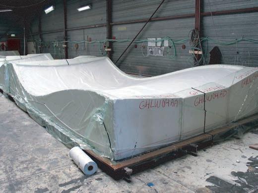
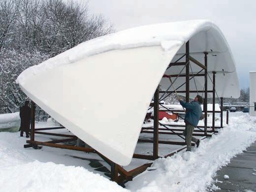
The international tendering procedure for the roofs with the accompanying steel construction and glass facades was won, due to an innovative concept, by Octatube, the design & build company of professor Mick Eekhout, and an project syndicate of co-makers. As the roofs were approached as free spanning shells a lightweight construction could be proposed and developed. For the shells a glassfiber reinforced composite material is used, combined with a production technique known from aircraft and yachting industries.

Transportation of pieces

guillem baraut

mattia gambardella

tutors: mike weinstock

michael hensel

achim menges

martin hemberg

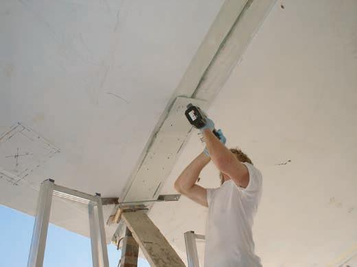
Closing the seams between the GRP roof segments with glued and bolted high-density glass fibre plates.

Left, a marking of the position of a steel 'insert' that will be connected to a 'wing connector'

slender multi stress driven structures

Machined polystyrene mould for a GRP roof segment

Machined polystyrene mould for a GRP roof segment The core of the GRP segments: polyurethane blocks and an 'insert' in order to connect the roofs to the columns

Test assembly in the Netherlands of the upper Library wing segments on a temporary steel frame

RACE SAILING MANUFACTURING TECHNIQUES

As racing sail materials continues to improve, so does cruising sail fabric.

New weaving techniques allow hybrid weaving with exceptional warp strength. Newer composite materials are stronger, lighter, and more durable.

Lightweight and low stretch sails benefit the cruising sailor by filling sooner in light winds, contributing to less heeling and pitching moment when set, using less space when stowed and holding their designed shape over a greater wind range.

Improving the sail material was seen as a real advantage over the other syndicates. Lighter weight aloft would translate into improved righting moment and reduced pitching. Sails that don’t stretch translate more air force to the boat, need fewer adjustments, hold their shape and don’t require recutting as often.

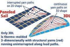
The last technologies in racing sail manufacturing techniques considers as well unitary membrane on full-sized 3-dimensional molds.

The structural yarns are laid on the mold in the precise 3-dimensional space they will occupy when flying, and run in continuous paths across the sail with no seams to distort or interfere with load transition.

The molds are scanned by lasers to verify shape within imperceptible tolerances. The laminate is then thermo-formed on the mold in a manner similar to a shrink-wrap process. The sail produced at th end is a precise flying shape the sail designer created.

guillem baraut

mattia

tutors: mike weinstock

michael hensel

achim menges

martin hemberg

gambardella

Fig.2 Diagram illustrating two different options existing in laying out fiber yarn on sails (North Sails source)

Fig.1 Images of the layout process of fiber yarns on racing sail

O RESUND B RIDGE - C ONSTRUCTION P HASES

ASSEMBLY STRATEGIES

PROJECT OVERVIEW

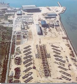
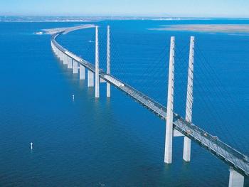
In 1991 the Denmark and Swedish governments agreed to build a bridge to connect the two countries across Oresund. Later that year the two parliaments ratified the agreement and scheduled the design to be completed by 1994. The 16 km long Oresund link between Sweden and Denmark is now complete.

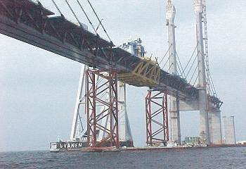
The Oresund Bridge is the world’s longest single bridge carrying both road and railway traffic. In the design full advantage was taken of repetition by composing the major part of the bridge of identical spans. The high bridge with its record-breaking cable-stayed span of 490m is designed to harmonize both structurally and aesthetically with the approach bridges. In the construction phase the on-site activities were completed in just 2 1/2 years due to an extensive use of prefabrication and erection of large units.

Twenty-seven bridge spans form the 3,739-m long eastern approach bridge. Of these, 24 are 140 m long and 4 are 120 m long. The western approach bridge is 3,014 m long, comprising eighteen 140-m spans and four 120-m spans. The bridge’s curved shape is the result of gradual changes in the angles at the joints between the bridge spans. These are located at the piers.

51 bridge piers support the approach bridges, placed in dredged pits some 15 m below sea level. Protective islands surround the anchor piers on either side of the pylons.

tutors: mike weinstock

michael hensel

achim menges

martin hemberg

A viaduct on the artificial island diverts the motorway traffic from the upper deck of the bridge to its new location next to the railway. The viaduct is a 560 m long concrete structure, cast in situ in 30 m sections.

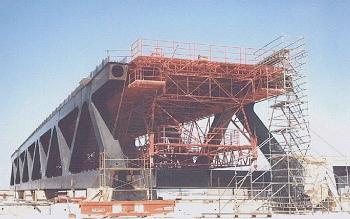
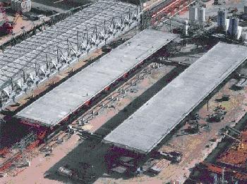
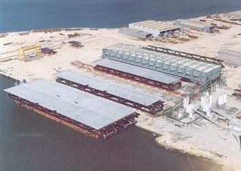
Final dimensions of each span were 25 meters x 140 meters, with a final total weight for the 49 spans of 245,000 Tons.

The transportation was performed in 25 shipments (every 21 days) with 2 spans per shipment weighting each span approximately 5,000 tons.

08. SELECTED METHODS

guillem baraut

mattia gambardella

tutors: mike weinstock

michael hensel

achim menges

martin hemberg

slender multi stress driven structures

DIGITAL EXPERIMENTS

MANUFACTURING TECHNIQUES

FINAL DESIGN STRATEGY

Once revised and analysed all the experiments carried out in both physical and digital realms, a final design strategy is developed. All these experiments and case studies are summarized in figure 1.

Just the most successful physical experiments and digital tools will be used for that purpose. In this case the wool threads and the catenaries experiments are the ones that are chosen in order to inform the digital tools, that are the topology optimization code in Matlab, the minimizing paths system algorithm in Generative components, and the Finite Elements Analysis software Ansys for both structural analysis and 3D topology optimization.

In the local scale the experiments chosen are the foam as a form for laying out the fibers, and the lycra knot to study how to lay out fibers in complex geometries.

In the last stage the manufacturing techniques that are considered are the racing boats sails, for the laying out of fibers just where they are needed, the CNC cut foam that will be the form where the fibers will be laid out, and the casting of the biggest pieces possible in a factory and special transportation to the site. For the microscale we choose using single fibers or textile fibers with a main direction, but not the pultrusion techniques.

At the next page there is the same figure with this relations highlighted in red.

guillem baraut

Figure 1. Summary of the physical and digital experiments carried out, with the study of the manufacturing techniques.

mattia gambardella

tutors: mike weinstock

michael hensel

achim menges

martin hemberg

PHYSICAL EXPERIMENTS. FORM FINDING

MACROSCALE

MICROSCALE

DIGITAL EXPERIMENTS

MANUFACTURING TECHNIQUES

Figure 1. Diagram of the state of the study with the relation between the physical experiments that are considered successful to continue with, the digital experiments, and the manufacturing techniques that will be used to develop the methodology. The main path of the study process is the development of the digital tools, and they are informed by both physical experiments and manufacturing techniques.

guillem baraut

mattia gambardella

tutors: mike weinstock

michael hensel

achim menges

martin hemberg slender

09. METHODOLOGY PROCESS SET-UP

guillem baraut

mattia gambardella

tutors: mike weinstock

michael hensel

achim menges

martin hemberg

slender multi stress driven structures

USING NETWORK-FLOW TECHNIQUES TO SOLVE AN OPTIMIzATION PROBLEM

Structures can be considered as objects capable of transferring forces over distances.

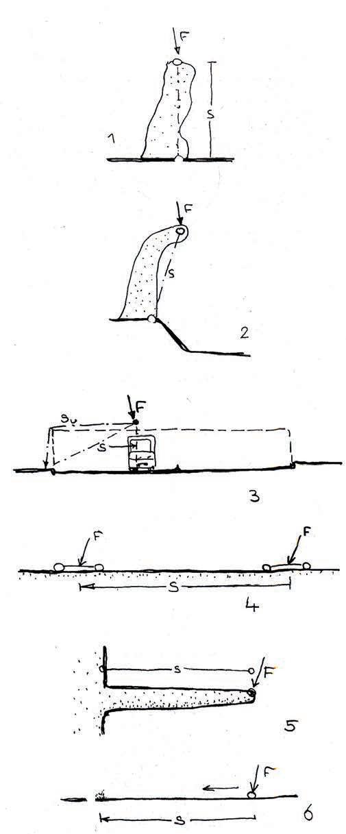
In the simplest case (fig.1) a force acting in any direction on a single point is transferred by a material object of a random shape to a solid surface.

The distance s is the “force path”. It is the distance along which the force is transported.

PROVIDED NO OTHER CONDITIONS EXIST, THE FORCE PATH IS ALWAYS THE SHORTEST DISTANCE OVER WHICH THE FORCE IS TRANSPORTED TO A STABLE LOCATION.

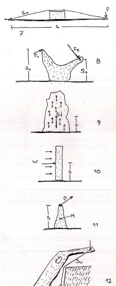
The force path is determined by the forces applied and the distances over which they are transmitted.

When several forces act on an object, the force path is the sum of all product of simultaneously acting forces.

guillem baraut

mattia gambardella

tutors: mike weinstock

michael hensel

achim menges

martin hemberg

Fig.1 Matlab optimized stress path example

Fig.2/3 Load cases diagrams

The use of the matlab routine as a mapping tool was providing some new potentialities within the design process.

Given its flexibility we could set different scenarios that could consider as much accesses to the bridge as needed.

What the routine does is to change the stiffness of the field elements to have an even (and optimized) distribution of stresses along the structure. The program then tend to optimize the path of the densities in such a way to redistribute evenly the stresses.

This could have to kind of outcomes:

- one is strictly related to the structural performance of the designed artefact

- secondly, the use of optimizing paths is related to the concept of minimal path for the people flow (fig.1) The routine in fact is going to find the easiest and shortest way to distribute stresses evenly.

In the first run the routine is providing the spatial configuration that would respond to the following variables:

- number of access to the bridge

- distance in-between the accesses

- starting hight of the access

- flow dimension (fig.1)

guillem baraut

mattia gambardella

tutors: mike weinstock

michael hensel

achim menges

martin hemberg

The Matlab code is built up as a standard topology optimization code. The main program is called from the Matlab prompt by the line top(nelx,nely,volfrac,penal,rm in) where nelx and nely are the number of elements in the horizontal and vertical directions, respectively, volfrac is the volume fraction, penal is the penalization power and rmin is the filter size (divided by element size).

Other variables as well as boundary conditions are defined in the Matlab code itself and can be edited if needed. For each iteration in the topology optimization loop, the code generates a picture of the current density distribution. U and F are the global displacement and force vectors, respectively, K is the global stiffness matrix, ue and ke are the element displacement vector and stiffness matrix, respectively, x is the vector of design variables, xmin is a vector of minimum relative densities (non-zero to avoid singularity), N (= nelx×nely) is the number of elements used to discretize the design domain, p is the penalization power (typically p = 3), V (x) and V0 is the material volume and design domain volume, respectively and f (volfrac) is the prescribed volume fraction.

Fig.1 Bees Movement flow

Figure 1. First steps of the digital design process, starting with the topology optimization algorithm in Matlab, and implementing the minimal path criteria in Generative Components

PROCESS SET UP

This design methodology combines structural topology optimization in a routine in Matlab with a minimizing path system algorithm implemented in Generative Components. The first script in Matlab is, in the first go, informed by the wool threads physical experiment in terms of initial branches and position of the branching points. The first run the routine is providing the first spatial configuration.

A pedestrian bridge is developed in order to explain how this methodology works. This bridge will respond to the following variables:

- Number of access to the bridge

- Accesses spatial position

- Flow dimension

The program tend to optimize the distribution of the stiffness in such a way to redistribute evenly the stresses. The use of the Mathlab routine as a mapping tool provides new potentialities within the design process.

When having the first results from the topology optimization they are mapped as a vector field in GC in order to provide the initial configuration for the minimum road algorithm. This vector field is mapped on a 3D surface defined according to the catenaries physical experiments and the first topology optimization in elevation in 2D.

Those mapped points from the topology optimization will represent the digital areas in which run the path length optimization algorithm.

A spline tracing algorithm is run amongst those points: in several iterations the starting and ending points of each side are connected between them by a family of curves.

Figure 1 shows the first two iterations of this process for an example that links 1 to 4 points.

guillem baraut

mattia gambardella

tutors: mike weinstock

michael hensel

achim menges

martin hemberg

Figure 1a. Initial topology optimization in a plan view, for a bridge that links 3 points at the top with 3 more at the bottom.

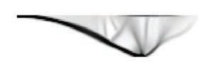
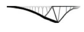
Figure 1b. Initial topology optimization in elevation for the same bridge. The figure just show half of the elevation.

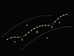
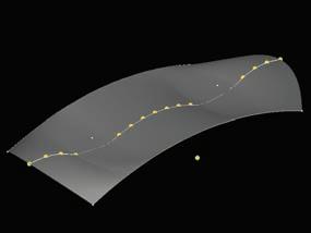
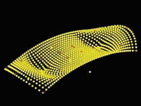
Figure 2. Parametric model that starts with information from the catenaries physical experiments creating a 3D surface, then the information from Matlab is mapped and at the end the minimizing paths algorithm runs, exporting the results into Matlab again.

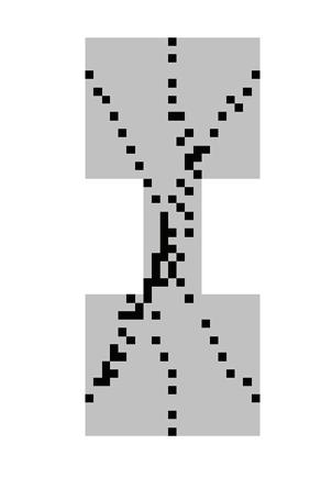
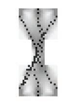
Figure 3. The topology optimization code runs again considering the information coming from the minimizing paths algorithm.

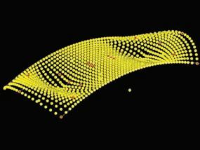
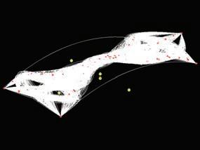
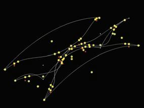
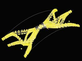
Figure 4. The same procedure continue until a successful result is achieved. At the end the las two images show the selected shortest paths used to run another parametric model. This model defines the material distribution on this paths

Amongst those lines (potential minimum path) just few are picked by the computer as the shortest solution to that specific connection problem.

Once the Path is optimized through the script, the points composing its shape are exported again into Matlab to run for the second time the topology optimzation script.

This process can be run automatically several times until the designer found that the requirements are successfully achieved.

The figure 1 on the left show the initial topology optimizations in plan and elevation for a bridge that is linking 3 and 3 points. This information is then mapped into a Generative Components parametric model. The first images in figure 2 show how some repellors and attractors informed by the catenaries physical experiments define a 3D surface. The results from Matlab are mapped on this surface, and then the minimizing path algorithm start running.

The shorter paths from the last image of figure 2 are then imported again into Matlab (figure 3) in order to run again the topology optimization algorithm, affected by this new information.

The process continue until the user consider that a successful solution is achieved. In Figure 4 there are the final steps of the methodology consisting in getting the shortest paths of the minimizing algorithm, and running another script that defines the material distribution on this structure.

guillem baraut

mattia gambardella

tutors:

mike weinstock

michael hensel

achim menges

martin hemberg

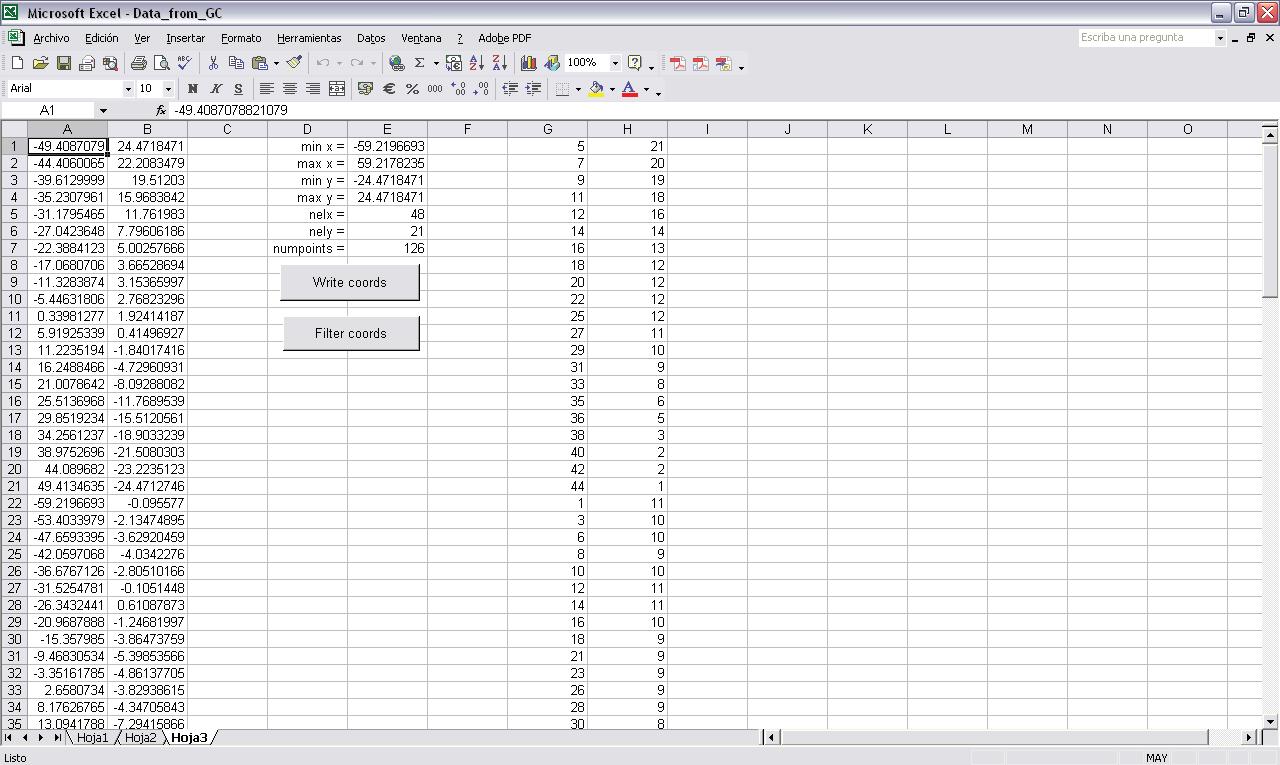
The excel spreadsheet in figure 1 shows in columns A and B the x,y and z coordinates of the points that forms the minimal path in the 3D space.

The button ‘Filter coords’ is a macro in excel that gets the coordinates from the sheets ‘Hoja1’ and ‘Hoja2’ that are written by GC, and filter all the non numerical data into columns A and B, that are x and y coordinates.

The cells in column E and F are the minimum and maximum x and y coordinates, the number of elements ‘nelx’ and ‘nely’ that will be in the domain in Matlab, and the last value is the number of points coming from GC.

All those data is then used by the second macro ‘Write coords’ that translate the coordinates x and y from the first column into a finite domain defined by ‘nelx’ and ‘nely’, with integer coordinates within this domain.

The columns G and H are then directly read by Matlab from this excel spreadsheet.

A similar exchange excel file is used in order to translate the data from Matlab into GC.

guillem baraut

mattia gambardella

tutors: mike weinstock

michael hensel

achim menges

martin hemberg slender

Figure 1. Excel spreadsheet used to translate the points from Generative Components to Matlab

DESIGN PROCESS

In order to summarize the design process there is the diagram in figure 1. The design process is defined by a digital tool that is working following this scheme:

i. Start with topology optimization in Matlab that is informed by physical experiments (wool threads).

ii. Export structure 2D and map a 3D surface created in GC. This surface is developed according to the results of the catenaries experiments. Run the minimal path algorithm and export the results to Matlab.

iii. & iv. Run the topology optimization and minimal path in GC iteratively until finding the result that the user is looking for.

v. On the final geometry we develop a parametric model that maps the material on the paths according to the stress vector field of the optimized structure

It is interesting to highlight that there exists a crossed relation between the physical experiments and digital tools that are related to minimal path and structural performance.

In that sense the topology optimization code, a structural performance based software, is informed from the beginning by the wool threads experiments, that are directly related to minimal path.

The same happens with the Generative Components models, that basically consist in a minimizing path algorithm that is informed by the catenaries physical experiments, directly related to structural performance. DIGITAL

guillem baraut

mattia gambardella

tutors: mike weinstock

michael hensel

achim menges

martin hemberg slender

Figure 1. Design process flow chart

10. STRESS DRIVEN MATERIAL DISTRIBUTION PROCESS

guillem baraut

mattia gambardella

tutors: mike weinstock

michael hensel

achim menges

martin hemberg

slender multi stress driven structures

DEVELOPMENT OF A STRUCTURAL COMPONENT

Bridge piece

Bending Moment

Shear

Total strengths on this bridge piece

The surface created between the link of Matlab and Generative Components is the guide that will define the final shape of the structure, but will not be neither the final structure nor the ultimate design.

This surface has been designed with a clear structural criteria with the topology optimization algorithm, but it is still missing a material criteria, dead and live loads, and manufacturing techniques. For these reasons a structural component is designed considering all the missing information, in order to be proliferated at the same time as being differentiated along this surface.

Structural criteria

Figure 1 shows a general structure where a small intermediate piece is separated from the whole, and is analysed with all the constraints and loads acting on it.

There is an external load q acting on a length ds, shear and axial stresses and a bending moment, if it is analysed as a 2D piece. The axial force is actually being considered in the first part of this design process with the topology optimization algorithm in Matlab.

In order to study the structural behaviour of this component a preliminary analysis in 2D is going to be done in Matlab. It will be considered as a cantilever with a fixed side, and the same loads that could be acting on it.

Model of the bridge piece implemented in Matlab

Figure 1. Scheme of the strengths and loads acting in a piece of a structure. The last diagram is an example about how to represent it in the algorithm for Matlab.

guillem baraut

mattia gambardella

tutors:

mike weinstock

michael hensel

achim menges

martin hemberg

TOPOLOGY OPTIMIzATION ANALYSIS

Table 1. Results of 2D topology optimization for several values of moment and shear represented by the tensions a and b, according to figure 1. #it.c is the number of iterations needed for convergence of the model in Finite Elements Analysis and the topology optimization algorithm in Matlab.

MV M a - a V b

Figure 1. Representation of the forces and momentus considered in Matlab for the topology optimization

nelx = nely = volfrac = penal = rmin = 30 20 0.25 3.0 1.5

The cantilever that has been presented is analysed with the topology optimization algorithm, according to several values of the shear and the bending moment.

The external load q acting in such a short length of the structure is considered negligible in terms of this analysis, and for that reason is translated as a single vertical force on each end of the piece. That is translated in Matlab as an increased shear force.

The axial force is also not considered as a variable because of the design of the overall geometry, that has been done according to a catenary based shape. The changes in this force will be small enough, compared to the variability of shear and bending moment.

For those reasons just two variables are considered in this analysis. The table 1 shows the results for several values of bending moment and shear. The variable considered are the tension a and b defined in Figure 1, and the Matlab parametres are shown in Table 2.

As can be seen in this tables the main characteristics of the cases with high bending moment and low shear are a big upper and lower cord, while the cases with higher shear have a clear crossing braces.

guillem baraut

mattia gambardella

tutors:

mike weinstock

michael hensel

achim menges

martin hemberg

Table 2. Common values used for the Matlab algorithm

Vd b = 1.0

These results are compared with a grid of trusses that studied Frei Otto, of which a picture of a study model can be seen in figure 1.

Vd b = 2.0

Vd b = 4.0

Vd b = 8.0

#it.c = 64

#it.c = 104

#it.c = 137

#it.c = 91

#it.c = 177

#it.c = 33

#it.c = 54

#it.c = 57

#it.c = 185

#it.c = 177

#it.c = 33

#it.c = 38

#it.c = 149

#it.c = 367

#it.c = 177

#it.c = 32

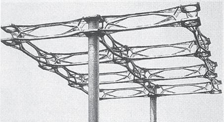
i.ii.iii.

i. Center of span: big moment but no shear equivalent to a = 20.0; b = 1.0

ii. 1/3 of the length: no moment with some shear equivalent to a = 1.0; b = 2.0

iii. support face: big moment with big shear equivalent to a = 20.0; b = 4.0

This model clearly shows the differentiation of several parts of a continuous truss that is supported by circular columns. There are some parts that are mainly working with a high bending moment and low shear (figure 1.i), parts with some shear and no bending moment (figure 1.ii), and some other with both high bending moment and shear (figure 1.iii).

As can be seen in those pictures there is an important similarity with the results obtained in these several experiments carried out with the topology optimization algorithm.

guillem baraut

mattia gambardella

tutors:

mike weinstock

michael hensel

achim menges

martin hemberg

Figure 1. Frei Otto study model of a support grid. In every cross of the trusses there is a circular hole for a support. Just two supports are modelled.

Table 1. Results of 2D topology optimization for several values of moment and shear.

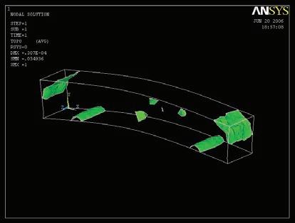
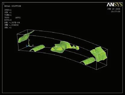
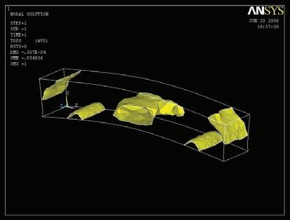
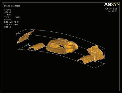
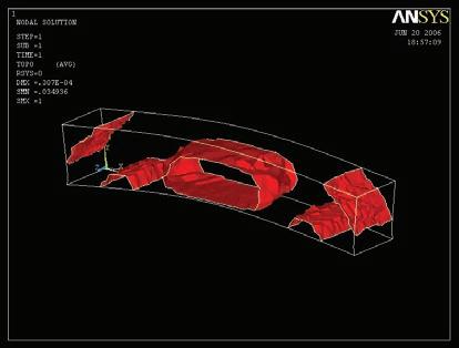
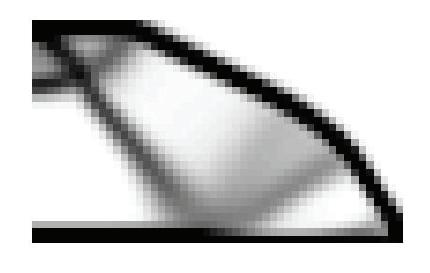
TOPOLOGY OPTIMIzATION IN ANSYS (3D)

In order to continue the development of the component in 3D, some topology optimization experiments are done in Ansys, a professional Finite Elements Analysis software with a topology optimization module.

In figure 1 there are the results of this analysis for a single span beam with a square section. The different colors are according to several material densities. These densities are analog to the grayscale of the elements in the results from the topology optimization analysis in Matlab.

In figure 2 there are some shots of the elevation of the optimization process carried out in Matlab for the same beam, and the same boundary and loading conditions.

guillem baraut

mattia gambardella

tutors: mike weinstock

michael hensel

achim menges

martin hemberg

Figure 1. Surfaces of several material density obtained through a topology optimization process carried out in Ansys, for a single span beam with square section and a uniform and continuous load.

Figure 2. Several stages of the topology optimization of a single span beam in Matlab.

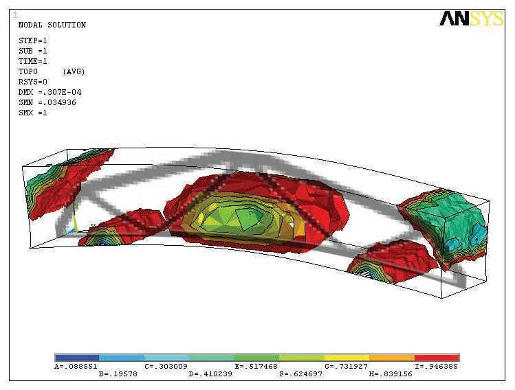
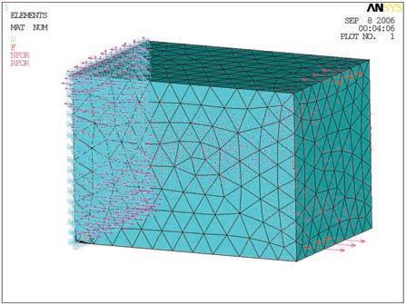
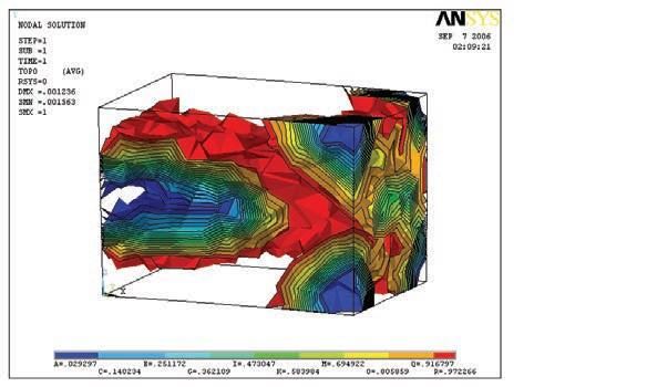
FROM 2D TO 3D

The same cases that have been analysed in Matlab in 2D, are translated to simple 3D models, and imported into Ansys. A first run of the topology optimization algorithm in Ansys shows the similarities with the results in Matlab.

The same load cases are applied and equivalent materials and dimensions are used.

The advantages that Ansys provides is the third dimension, that can be used not only for the geometry, but also to take in consideration other loads that are applied to the real structure, such as wind, torsion, etc.

In figures 1 and 2 the similarities between the results of the two programs can be seen.

In order to continue the definition of the distribution of material Ansys is used to define the stress vector field on the structure that is been previously defined.

guillem baraut

mattia gambardella

tutors: mike weinstock

michael hensel

achim menges

martin hemberg

Figure 1. Comparison of the results from Matlab and Ansys, for a single span beam with initial square section

Figure 2. Comparison of the results from Matlab and Ansys, for the component design

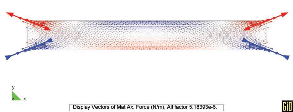
Figure 1. Comparison of the results from Matlab and Ansys, for a single span beam with initial square section

STRESS VECTOR FIELD

In Figure 2 there is the same beam in elevation as in figure 1, but in that case with a representation of the principal stresses vector field.

The direction of principal stress is the one for which there is no shear stress. The two or three principal stresses (in a surface or in a volume) are always perpendicular. With this consideration the fiber material can be placed with the direction of the stresses. In that case the material can be working at 100% of its capacity, because it will not be any redundant material in any direction.

From this study we conclude that the best solution for the definition of the final design is to drive the position and direction of the material according to the principal stresses vector field. This vector field will be defined through a process of optimization in 3D with Ansys.

In Figure 3 there is the same two dimensional example of the single span beam with the main direction of the stresses highlighted in red.

The figure shows how the angle a is varying from 45º when the shear is maximum and with a low bending moment, to around 30º at the left side when there is maximum negative bending moment and maximum shear. At the centre of the beam, with no shear and with maximum bending moment the angle turns to 0º.

Figure 2. Vector field of principal stresses on the same beam as above

guillem baraut

mattia gambardella

tutors:

mike weinstock

michael hensel

achim menges

martin hemberg

Figure 3. Vector field of principal stresses with the main stresses directions highlighted

These results are almost the same that were defined by the topology optimization carried out previously, and that can be seen at the tables of the previous pages.

Figure 1. Final result of the methodology in the global scale. The paths are defined through the topology optimization and the minimal path algorithms.

TRANSLATION FROM VECTOR FIELD TO GC

The Finite Elements Analysis method can take a long time for a big structure, and the process of transferring the vector field data to Generative Components can be even slower.

In order to avoid that, the way the fibers are defined in Generative Components is according to the vector field principles, but without calculating it for every single piece of the structure.

The way for doing that is translating the angle a from the vector field to every position along the structure.

In figure 1 there is one path highlighted. As it was seen in the previous page, the angle can vary depending on the distance of the supports, or the position along the structure. For that reason the way we define the angle is according to the T value along the curve of the path, that has been defined trough the Macroscale process.

In Generative Components the process to do that is:

- Generate some points on the curve according to the T value

- The distance or spacing from one point to the other is directly related to the angle of the vector field (figure 2)

- Generate splines around the ellipses with a regular pattern of crossings. According to the distance between the ellipses these crosses will occur with a more pronounced angle, or they will be almost horizontal (figure 3). The longer the spacing is, the more horizontal the splines will be.

Figure 2. On the path highlighted in figure 1 some ellipses are placed with different T value, with a spacing s defined in relation to the angle of the principal stresses in the vector field.

Figure 3. Splines around the ellipses. Through a variation of the spacing between the ellipses the angle between the splines changes. This relation allows to reproduce the principal stresses vector field. s s s s s a a s s s

guillem baraut

mattia gambardella

tutors:

mike weinstock

michael hensel

achim menges

martin hemberg

At the end, as it is shown in figure 3, the pattern of the splines crossing around the ellipses is according to the stress vector field.

The dimensions of the ellipses are defined according to manufacturing and spatial requirements.

The image below show an example of a typical three span bridge with a stress driven orientation of the fibers.

Figure 4. Three span bridge after locating fibers on it

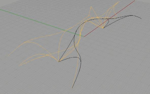
Figure 1. Splines

a

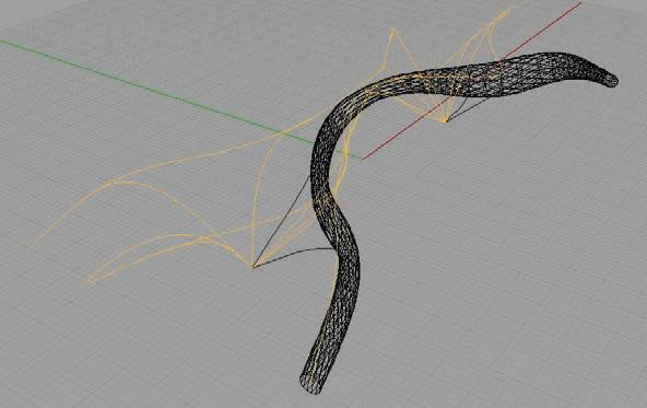
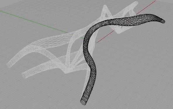
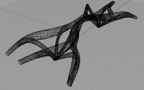
In the first drawing there is an

representation of the relation previously explained between spacing and angle

the splines. In the following drawings there is a view of the results from Generative Components: generation of the paths, definition of ellipses according to the principal stresses vector field, proliferation of the splines around the path curve, and repetition of the process for all the paths.

function (arrPoints, arrPoints2, cs)

{ int n,ne,nl,np,nsp,ind,incr; double B,x,y,z; DPoint3d points = {};

ind = 0; incr = 0;

nsp = 4; //number of splines

ne = arrPoints2.Count; //number of ellipses per spline

np = arrPoints[0].Count; //number of points per ellipse

nl = 2*np; //number of final lines for each //spline

for (value i = 0; i < nsp; ++i) //for each spline

{ for (value j = 0; j < nl; ++j) //generate nl lines

{ //ind = ToInt(Random(0,np+1));

//incr = ToInt(Random(0,5)-2);

ind = j; if (j<np)

{ incr = 1;

} else

{ incr = -1;

} for (value k = 0; k < ne; ++k) //for each ellipse

{ n = i; if (i == 3)

{ n = 5; }

x =arrPoints[n*ne+k][(ind+incr)%np].X;

y =arrPoints[n*ne+k][(ind+incr)%np].Y;

z =arrPoints[n*ne+k][(ind+incr)%np].Z;

points[k] = new DPoint3d(x,y,z);

//incr = incr + ToInt(Random(0,5)-2); if (j<np)

{ incr = incr + 1; } else { incr = incr - 1; } }

B = CreateChildFeature(“BsplineCurve”, this);

B.ByPointsOnCurveAsDPoint3ds(cs, points); } } }

Figure 2. Script in Generative Components for splines generation

guillem baraut

mattia gambardella

tutors: mike weinstock

michael hensel

achim menges

martin hemberg

proliferation around

path.

schematic

of

guillem baraut

mattia gambardella

tutors: mike weinstock

michael hensel

achim menges

martin hemberg

Figure 1. Rendered image of a possible distribution of the material along the paths resulting from the developed methodology in the global scale

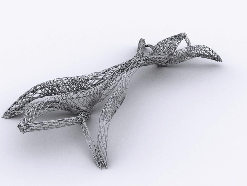
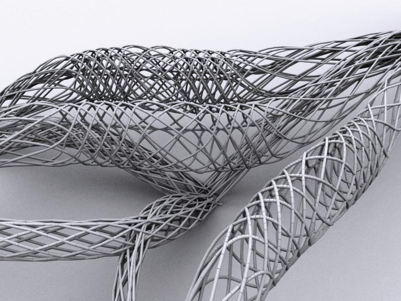
guillem baraut

mattia gambardella

tutors: mike weinstock

michael hensel

achim menges

martin hemberg slender

Figure 1. Rendered image of a possible distribution of the material along the paths resulting from the developed methodology in the global scale

MANUFACTURING PROCESS CONSIDERATIONS

The diagrams I to VII explain the manufacturing concepts that are embedded in the digital design process. They represent a typical section of a solution obtained by the global scale methodology that has been ex-

plained in previous chapters. In the last stage of this methodology the manufacturing techniques that are proposed informs the model. This process consists in using a conventional internal form with standardized dimensions (h and b), where the CNC cut foam pieces are attached. The CNC capabilities are consid-

ered in order to define minimal dimensions for the fibers positions and size, and the number of pieces that are placed in each section.

When the fibers are laid out on the CNC cut foam, the internal form is removed from the inside. The foam pieces then can be moved into the

space that is left, and at the end the final structure is ready to be transported and placed on site.

I. Section of a generic minimal path and topology optimization algorithms results

II. Minimal conventional forms dimensions

IV. Final 3D volume model to be sent to production h b

III. CNC milling capabilities, axis numbers, angles and dimensions

V. Foam volumes are cut according to the forms dimensions

guillem baraut

mattia gambardella

VI. The cuts are done in a way that they can be moved into the form space once it is removed

VII. The foam pieces are CNC milled in a conventional 3 or 5 axis machine. The original foam pieces can be defined by standardized dimensions

DIGITAL PROCESS

During the design phase the digital methodology is informed by the existing manufacturing capabilities like forms dimensions (h, b) and milling caps dimensions (d). These measurements will be considered at the final steps of the definition of the fiber layout process in the Generative Components scripts.

tutors:

mike weinstock

michael hensel

achim menges

martin hemberg slender

MANUFACTURING

The manufacturing process consists in cutting the CNC foam blocks, they are put on a conventional form box, the fibers are laid out, the form is removed from the inside and the foam pieces are moved into the form space and removed from the inside.

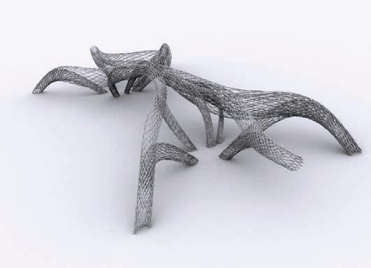
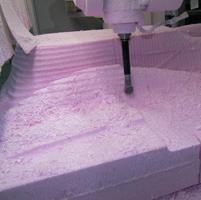
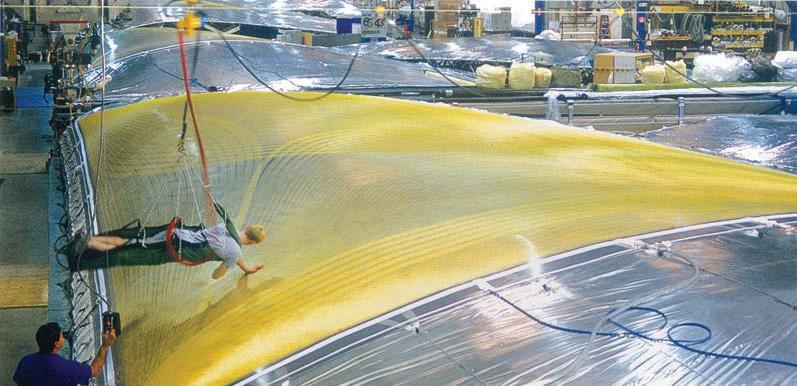
3a.

Figure 2b. Bottom. As an example of this technique this image show how aramid fibers are laid on a form, following the stress patterns.

MANUFACTURING PROCESS

In order to summarize the manufacturing process figures 1 to 3 shows the main steps.

The methodology explained defines the 3D model until the CNC pieces to be cut. These pieces are then sent to manufacturing as figure 1 shows.

guillem baraut

mattia gambardella

After being cut the foam pieces are assembled together in a factory on a conventional form and scaffolding.

On these pieces the glass fibers are laid out with resin. The fibers follows the traces that the CNC milling machine drew on the foam. These

traces are digitally defined according to the principal stresses vector field. Figure 2 shows this process with a real example, the manufacturing of sails for racing boats.

On the factory the structure is built in pieces as big as they are able to

tutors: mike weinstock

michael hensel

achim menges

martin hemberg

Figure 3b. Bottom. Example of a bridge construction. The Oresund Bridge (Denmark, Sweden) was built in 140m spans in Cadiz (Spain), including road pavements rails and lighting, and shipped to the site. On site it was assembled with the supports and the rest of the structure.

transport on site. These pieces are then shipped on site and assembled together. The limits of this technique are even more than hundred metres, as can be seen in figure 3 with the Oresund bridge example.

Figure 1a. Top. CNC cut foam attached to a conventional form

Figure 1b. Bottom. An example of the technique is the bus stop by NIO Architecten in Hoofddorp.

Figure 2a. Top. Lay out of fiberglass on the foam, following the principal stresses vector field that is already defined on the foam during the CNC milling. The structure is fabricated in parts as big as possible, to be transported and assembled on site.

Figure

Top. Assembly of the fabricated parts on site.

11. TEST MODELS

guillem baraut

mattia gambardella

tutors: mike weinstock

michael hensel

achim menges

martin hemberg

slender multi stress driven structures

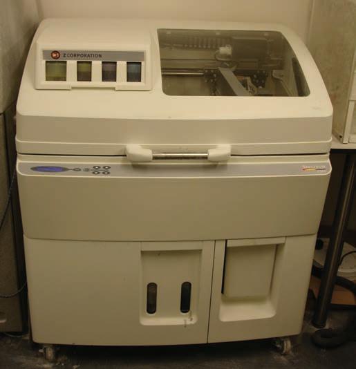
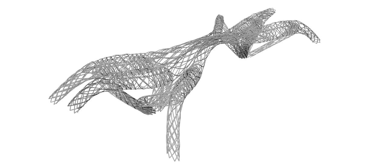
RAPID PROTOTYPE MODEL

Directly from Generative Components software, the model is sent to Rhinoceros to check naked edges on the surfaces, and then can be sent to manufacturing.

In that case a Rapid Prototyping model has been done with this technique. The printer that has been used is the model zPrinter 310 Plus made by the company z Corporation, located at the Royal College of Arts in London.

The capabilities of this machine are:

- Build Speed: 2 - 4 layers per minute

- Build Size: 8” x 10” x 8” (203 x 254 x 203 mm)

- Layer Thickness: User selectable at the time of printing; 0.0035”-0.008” (.089-.203 mm)

- Material Options: High performance composite, snap-fit, elastomeric, direct casting, investment casting

The system software accepts all common file formats like STL, VRML and PLY as input.

Figure 1 shows a general view of the machine, and in figure 2 there is the vacuum cleaner for the finished models, used to remove the unused powder. Figure 3 is a rendered image of the model that has been printed. In the next page there are some images of the finished model.

This structure is a pedestrian bridge measuring 60m long at the central span, and 30m each one of the six legs on each side. The model is printed at 1/400 scale.

guillem baraut

mattia gambardella

tutors: mike weinstock

michael hensel

achim menges

martin hemberg

Figure 1. Rapid prototyping machine from z corporation, at Royal College of Arts (London)

Figure 2. Vacuum cleaner machine for RP models, at Royal College of Arts (London)

Figure 3. Rendered image of the model that has been sent to the rapid prototyping machine. The dimensions of the fibers lines had to be increased because of the capabilities of the machine.

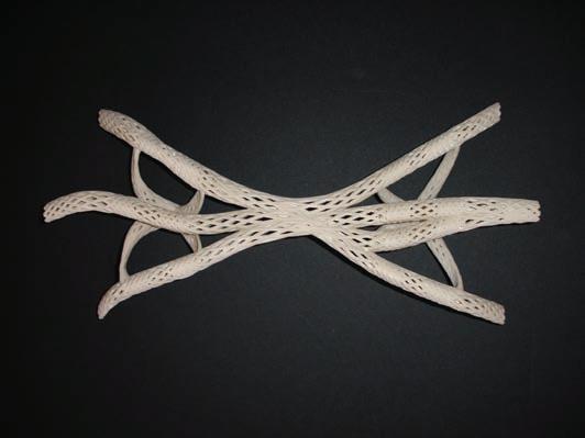
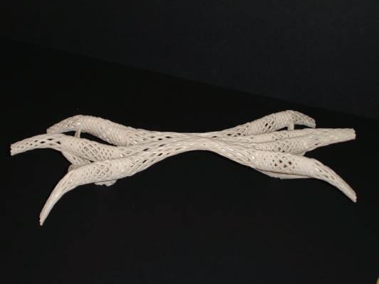
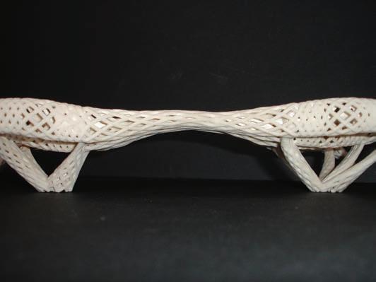
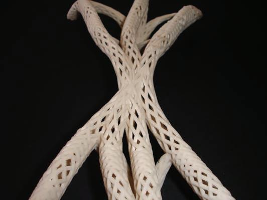
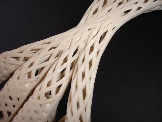
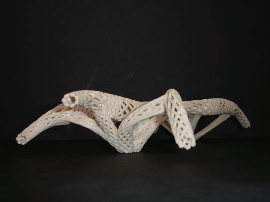
RAPID PROTOTYPE MODEL

In these images there are some views of the final model that has been printed. Because of the size of the model and the capabilities of the technique in producing thin elements, the thickness of the pipes had to be increased to 2mm of diameter. That makes the model a bit more solid than the image on the previous page.

With this model we tested the speed of post processing and manufacturing of the developed methodology. The model printed at 1/400 scale shows several defects that we had in the last scripts when placing the fibers in a regular pattern.

At the top right image there is one of the fiber paths that is always horizontal along all the paths. This was then corrected at the generative components scripts. The problem was a simple indexing mistake in one of the scripts.

guillem baraut

mattia gambardella

tutors: mike weinstock

michael hensel

achim menges

martin hemberg slender

Figure 1. Several views of the Rapid prototype model

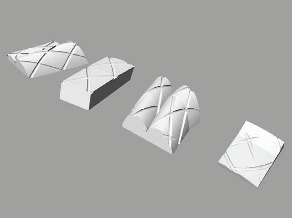
FiberGLASS ON A CNC CUT FOAM

The aim of this model is to test the proposed manufacturing technique, consisting in cutting a foam form in a CNC milling machine, assembling the pieces, laying out the fibers and removing the form from the inside.

Figure 1 shows a rendered image of the digital model that has been sent to the machine. This model is a piece of one of the solutions generated using this design methodology.

The CNC milling machine that has been used is a 2 axis machine located at the Architectural Association School of Architecture, in London.

The procedure for the building of the model is the following:

- Cutting the foam with the CNC milling machine

- Assembling the pieces with needles

- Painting a coat of water based resin separator (Scopas parting agent), in order to avoid the resin to stick on the foam

- Laying out the fibers on the foam following the traces defined in the digital model, and cut by the CNC milling machine

- Leave the resin to harden and remove the needles from the foam, and the foam pieces from the glass fiber model.

guillem baraut

mattia gambardella

tutors: mike weinstock

michael hensel

achim menges

martin hemberg slender

Figures 1a and 1b. Rendered image of the mould for the model that is going to be produced

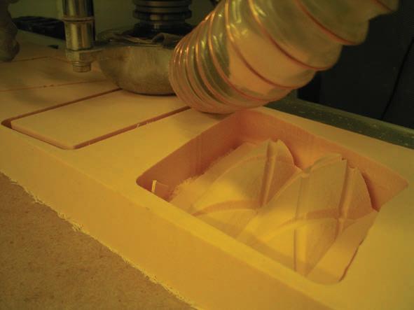
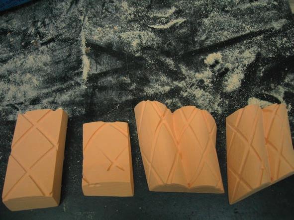
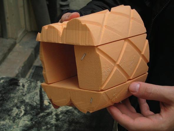
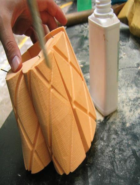
FiberGLASS ON A CNC CUT FOAM

The images in figure 1a to 1f show the manufacturing process of the form where to lay out the fibers.

The first one in top left is the CNC milling machine when working on the board, producing the four pieces for the form. The next one to the bottom is the final result from this machine and the third one at the bottom shows the for pieces separated from the board. These pieces had to be sanded before assembled because of some edge problems. In a bigger scale this shouldn’t be a problem.

On the right column there is the assembling process with some needles that attach the four pieces together, and the last two images show the form being painted with the parting agent.

guillem baraut

mattia gambardella

tutors: mike weinstock

michael hensel

achim menges

martin hemberg

Figures 1a and 1f. Production of the mould in a CNC 2 axis milling machine, cutting the pieces from the original foam board, assembling them and painting with the parting agent.

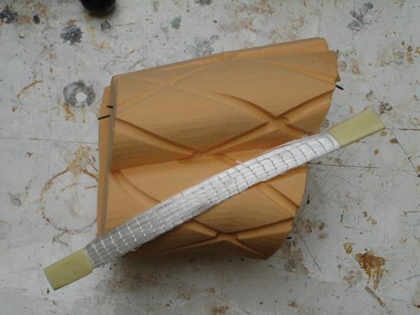
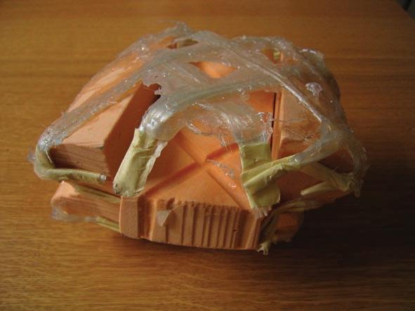
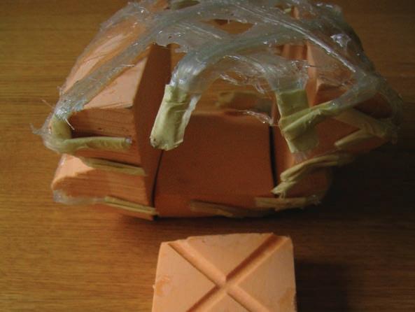
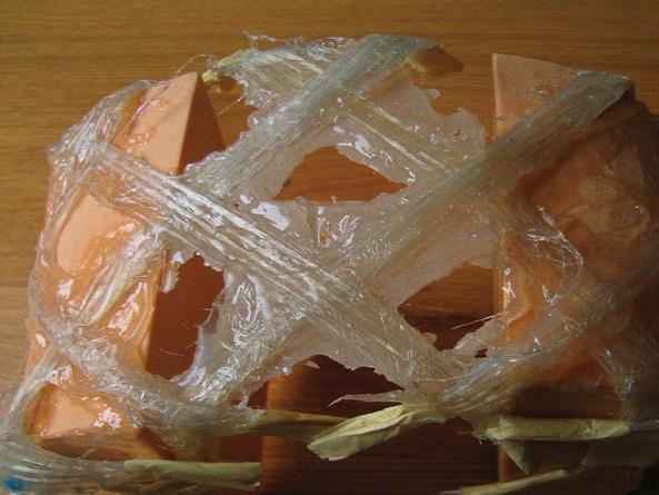
FiberGLASS ON A CNC CUT FOAM

Once the parting agent is dried the fiber glass can be laid out on the foam with polyester resin. In the first image in figure 1 there is all the material needed:

- Fiber glass oriented 99% in one direction

- Polyester resin

- Acetone

- Catalyser

- Masking tape

- Mask, wood sticks, pins and a brush

The fibers are cut and attached with masking tape at the ends, then they are painted with the resin and attached to the foam with the pins.

Once the resin has hardened the pins can be removed, and then also the needles that attach the foam pieces together are taken out.

The foam can be separated from the glass fibers and then removed from the inside, and the model can be finally sanded as the final finishing.

guillem baraut

mattia gambardella

tutors: mike weinstock

michael hensel

achim menges

martin hemberg

Figure 1. Images of the fiber glass laying out procedure.

12. EVALUATION CRITERIA

guillem baraut

mattia gambardella

tutors: mike weinstock

michael hensel

achim menges

martin hemberg

slender multi stress driven structures

COMPARATIVE EVALUATION CRITERIA

At that stage of the research the design outcome is tested to verify how, by altering the internal variables, is it possible to obtain a different result.

The two selected evaluation criteria refers to:

- Spatial performance

The intention of which is to study the effectiveness of the formal configuration in solving a specific connection problem

- Structural performance

The intention of which is to test the changing of the structural behaviour as the layout of the fibers is arranged differently

In the first case the result was tested according to the criteria of the minimum road network.

In the second, the model was run into a FEA program to perform the structural elastic analysis of the dead load and the live load in different conditions of the fibers layout.

guillem baraut

mattia gambardella

tutors: mike weinstock

michael hensel

achim menges

martin hemberg

Spatial Evaluation

Structural evaluation

METHODOLOGY VARIABLES

The process that has been developed depends on multiple variables. We classify the variables of our system in three main categories, and for each of them several subcategories. These are:

- Project Set-up (With the subcategories geometry and environment)

- Structural Optimization Algorithm (Topology, Nested catenaries system, fibers distribution)

- Paths System Optimization Algorithm (Branching, Paths system length optimization)

These parameters are controlled by the user and defined according to the site characteristics and the project purposes. The scale of affection of a change on the value of any of these variables is also classified in three categories:

- Global

- Regional

- Local

In the next page there is a table with all the variables and parameters that can be modified, and also the scale of affection of each of them in a qualitative classification.

The boundaries of every scale of affection are certainly diffuse and one cannot define a perfect border for them. In some cases a variation in a variable value may clearly affect in a very well defined scale, but that’s not the usual case.

EVALUATION TESTS

For the evaluation of the results of this methodology we carried out several tests. In order to focus on the performance of the system the tests are mainly studying the structural and spatial behaviour of several results.

These tests are based on changing some of the variables that the user is able to control, and compare the results between them and with external references.

All the tests will be carried out within an example composed by a bridge that is connecting 6 points, grouped in 3 points at each side of the longest span. The material used is conventional glass fiber and the flow of people is the same for each branch.

There are 3 repellors just below the main central span, and 2 attractors that will form the central supports.

The considered loads are just dead and live gravitational loads with a uniform distribution along the paths.

STRUCTURAL EVALUATION

The structural evaluations is done in two tests. The first one is based on structural slenderness, and the second one on structural analysis with a professional Finite Elements Analysis software (Ansys).

The structural slenderness is studied according to Frei Otto results in his experiments with the Institute for lightweight Structures. The results are compared to his evaluation of existing structures with the variables structural slenderness and Load bearing capacity.

For the structural behaviour three models were tested in Ansys with different variations. The variables that were changed in order to compare the results are the fibers distribution (regular or irregular) and the structural connectivity. Both changes are local changes with global and regional affection

This last variable means that two paths that are crossing can be connected in terms of circulation of people, but can be absolutely independent in terms of structure. The structural connectivity will lead us back to the biomimetic concepts of redundancy in natural structures. The paths will have exactly the same amount of material, but adding some more connections will change their structural behaviour.

To summarize the changes that will be done are:

- Fibers distribution: local variable

- Affection: Regional and local scale (in this case the separation between regional and global is really diffuse when we consider the structural analysis)

- Fibers paths connection: local variable

- Affection: Global, regional and local scale

SPATIAL EVALUATION

For the spatial evaluation test we focus on the Minimum path system algorithm, where the number of minimizing algorithm iterations is changed.

Several solutions are run and the results will be compared.

- Number of iterations: global variable

- Affection: global scale

guillem baraut mattia gambardella

tutors: mike weinstock michael hensel achim menges

martin hemberg

EMERGENT TECHNOLOGIES AND DESIGN. 2005-2006

VARIABLES

PROJECT SET UP

GEOMETRY

- NUMBER OF CONNECTIONS

- DIMENSIONS

- FLOW BETWEEN CONNECTIONS

ENVIRONMENT

- ATTRACTORS (Points of interest, Structure supports)

- REPELLORS (Topography, water)

S TRUCTURAL OPTIMI z ATION Algorithms

T OPOLOGY OPTIMI z ATION

- NUMBER OF ELEMENTS

- LOADS

- BOUNDARY CONDITIONS

- VOLUME FRACTION

- PENALI z ATION POWER

- FILTER SI z E

NESTED CATENARIES SYSTEM

- NUMBER OF CHAINS

- LENGTHS OF CHAINS

- CHAIN’S ENDPOINTS POSITION

- NUMBER OF CONNECTIONS BETWEEN CHAINS

- POSITION OF THE CONNECTIONS

FiberS DISTRIBUTION

- NUMBER OF WRAPPING SPLINES

- ANGLE VARIATION

- TRANSVERSE SECTION SI z E

- CONNECTIVITY BETWEEN Fiber ELEMENTS

- MATERIAL PROPERTIES

PATH OPTIMI z ATION Algorithms

BRANCHING VARIABLES

- BRANCH LENGTH

- ANGLE BETWEEN BRANCHES

P ATHS LENGTH OPTIMI z ATION

- NUMBER OF ITERATIONS

- NUMBER OF CONNECTIONS BETWEEN PATHS

- WEIGHTS PER BRANCH FLOW

SCALE OF AFFECTION

- HIGH INFLUENCE

- MEDIUM INFLUENCE

- IRRELEVANT INFLUENCE

guillem baraut

mattia gambardella

tutors: mike weinstock

michael hensel

achim menges

martin hemberg

12.01 SPATIAL EVALUATION

guillem baraut

mattia gambardella

tutors: mike weinstock

michael hensel

achim menges

martin hemberg

slender multi stress driven structures

For evaluating the spatial performance of the bridge it was decided to compare three different models determined form a different number of iteration.

The three types have the same input in terms of connection points, their spatial location.

The iteration was run for 10, 70, 150 times.

From a solution where the spline algorithm was traced with a different iteration (10, 70, 150), the program was able to pick, amongst that group of lines, the shortest solution, the most responding one, to that level of iteration.

10 ITERATIONS

70 ITERATIONS

150 ITERATIONS

guillem baraut

mattia gambardella

The spacial performance includes as well a multiple number of spatial conditions:

- The connection points, in fact, can have different height on not lie in the same plane

- The number of connecting points can be up to two elements with endless configurations

tutors: mike weinstock

michael hensel

achim menges

martin hemberg

A comparison was then draw between the DIRECT NETWORK

TOTAL LENGTH (orange dotted line) and the MINIMUM NETWORK LENGTH (green line) provided by the routine per each iteration case.

In the first case (10 iterations) the efficiency of the found system reached a performance level of 48 % on the overall comparison.

As the number of iteration goes higher, we can notice an increasing shortening in the total length of the found path and therefore a bettering in the performance.

The third solution, in fact, shows the fittest solution to that circulation problem: we can easily state that, as the number of iteration increases, for that specific connection case, the solution tents to converge toward the shortest one.

guillem baraut

mattia gambardella

tutors: mike weinstock

michael hensel

achim menges

martin

guillem baraut

mattia gambardella

12.02 STRUCTURAL EVALUATION Slenderness criteria

tutors: mike weinstock

michael hensel

achim menges

martin hemberg

slender multi stress driven structures

SLENDERNESS CRITERIA

The classical definition of slenderness describes the ratio of an object’s height to its width, but it’s independent of load. Frei Otto defined a new type of slenderness that considers this:

where l is the slenderness of the structure, and s is the distance of transfer of the force F .

This load is considered as a two dimensional value, being the load applied in a certain area. The distance s is a one dimensional value, thus Frei Otto defined the slenderness with the square root of the force, and the resultant slenderness is non dependent of the absolute dimensions. This means that as happens with the geometrical slenderness, the slenderness of a structure will be the same for the structure itself, and for the model of this structure.

In order to measure the load bearing capacity of a structure Frei Otto introduced the variable Tra as:

Tra = F·s

In the widest sense Tra is a measure for the ability of an object to transfer forces. Because of it is not always possible to define a clear value of Tra , Frei Otto introduced the concepts of ‘maximum Tra’, ‘deformation Tra’, ‘dead load Tra’, ‘live load Tra’, etc. He used this variable to classify structural forms, and to compare the efficiency of different systems by means of numerical values.

Neither slenderness nor Tra provide any information about the crucial criterion for lightweight construction, that can be a reference to the mass of this construction. For that reason he defined a new variable called BIC:

Figure 1 on the next page illustrates the relation BIC- l for several bridges that were calculated in the Institute for Lightweight Structures. Because of the large differences between the values the diagram is done with logarithmic scales.

All these variables and the diagram will be used later on to compare the results of the whole process explained in this dissertation with real existing structures.

For this example, that is shown in figure 1 these variables take the following values:

This variable is a characteristic of lightweight structure since defines a relationship between a structure’s mass m and its ability to transfer loads Tra into its supports.

guillem baraut

mattia gambardella

tutors:

mike weinstock

michael hensel

achim menges

martin hemberg

This values are calculated exporting the lengths and other data directly from Generative Components to Microsoft Excel. The Excel Spreadsheet is added at the end of this book in appendix 2.

Figure 1. Rendered image of the bridge analysed, and for which the structural slenderness has been calculated

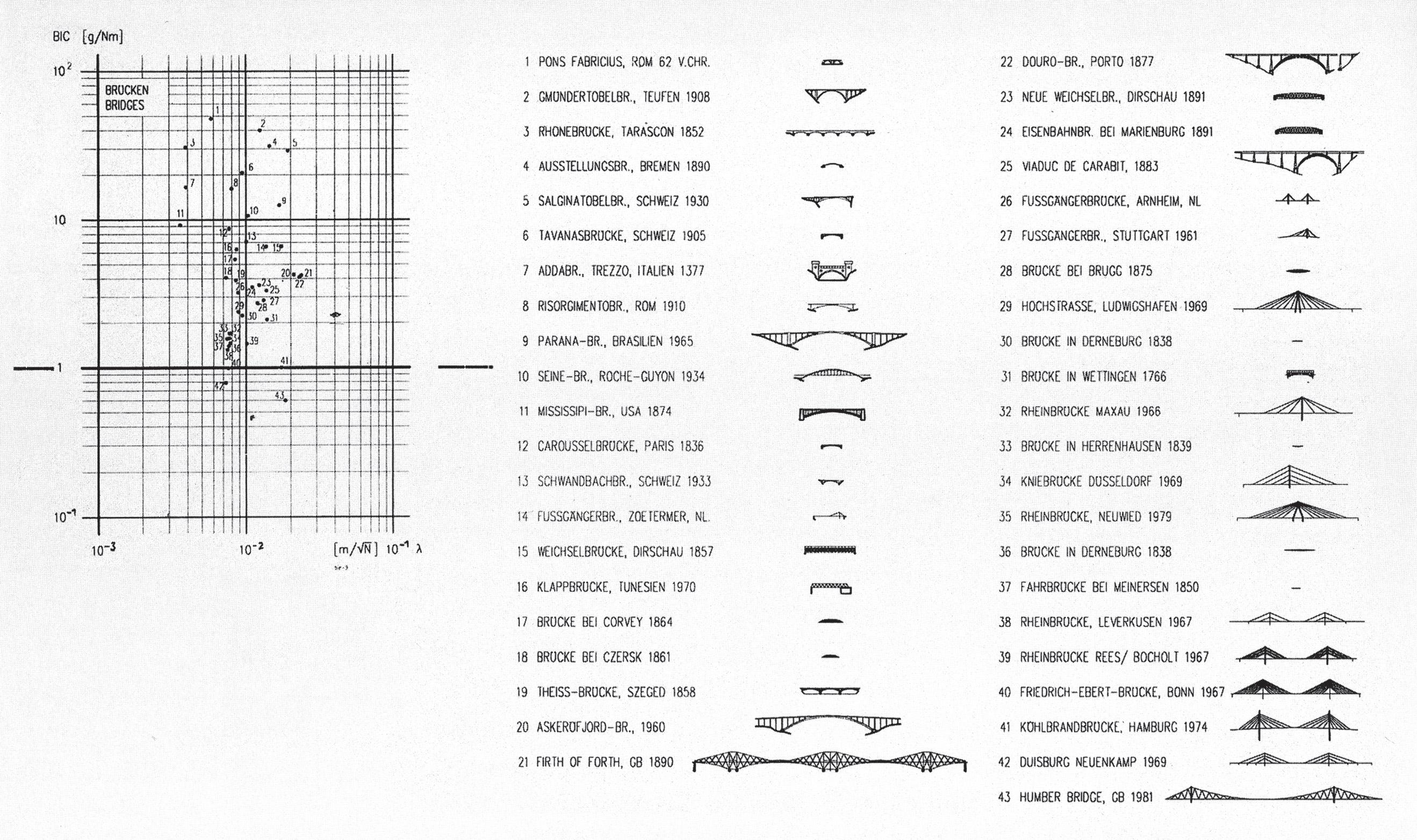
The results are calculated according to the values:

guillem baraut

mattia gambardella

tutors: mike weinstock

michael hensel

achim menges

martin hemberg

From the chart of the Institute for Lightweight Structures we see that the final design coincides with some of the first cable stayed bridges of the 60’s.

This is still a bit far away form the most slender suspended bridges, but this was one of the first results of the method. Adjusting some parametres this result can be improved.

slender multi stress driven structures

Figure 1. BIC- l diagram for some major bridge constructions (Institute for lightweight structures)

guillem baraut

mattia gambardella

12.03 STRUCTURAL EVALUATION Elastic Analysis

tutors: mike weinstock

michael hensel

achim menges

martin hemberg

slender multi stress driven structures

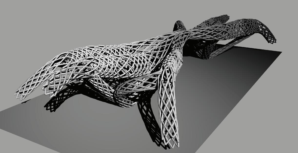
STRUCTURAL ANALYSIS

The structural performance evaluation consists in an elastic static analysis using a professional finite elements analysis software, Ansys.

The results are used in order to define the dimensions of the structural elements. In other words, the amount of fibers that are necessary for every strand are defined.

Three cases are analysed and compared, for which of them some variables are changed. The variables are mainly the distribution of fibers (regular or irregular), and the structural connectivity when a cross occurs between two paths. This cross can just be in terms of circulation but the structure can still be completely detached, or completely connected.

In figures 1 and 2 there are two simple examples of a regular distribution of fibers in the first one, and an irregular in the second image. The irregular distribution means that the fibers don’t follow a regular pattern, but they still follow the angles defined by the vector field.

In the following pages there is the comparison between three cases:

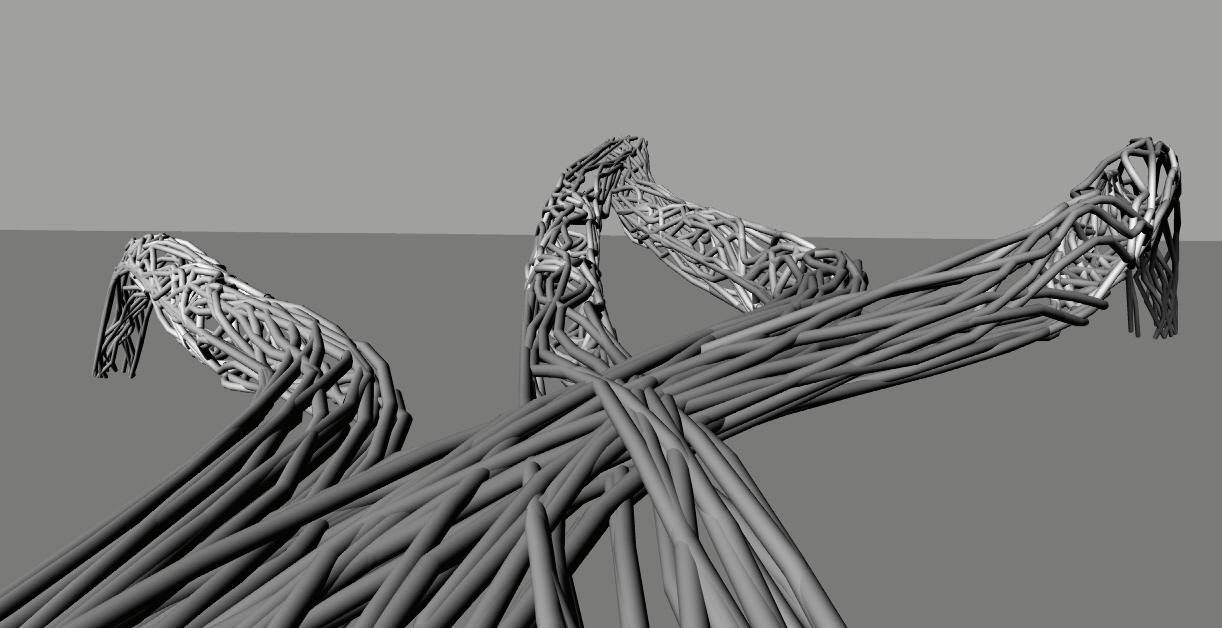
guillem

mattia

tutors: mike weinstock

michael hensel

achim menges

martin hemberg

1. Even distribution of fibers without structural connection between the several paths

2. Irregular distribution of fibers with structural connection between the several paths

3. Even distribution of fibers with structural connection between the several paths

In all the analysis we will see that the third one is always the best solution. For all cases the amount of material that is used is exactly the same, the same profiles and transverse sections for every fiber path.

baraut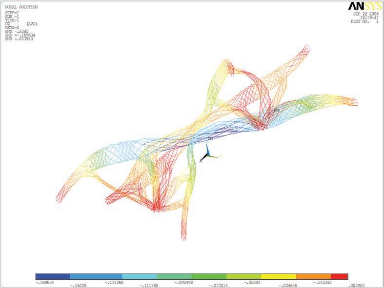

gambardella

Figure 1. Example of a solution of the developed methodology where the fibers are distributed following a regular pattern

Figure 2. Example of a solution of the developed methodology where the fibers are distributed following an irregular pattern

Case 1. Regular distribution of fibers without structural connection between paths. This figure shows the vertical displacement with the nodal solution of the Finite Elements Analysis.

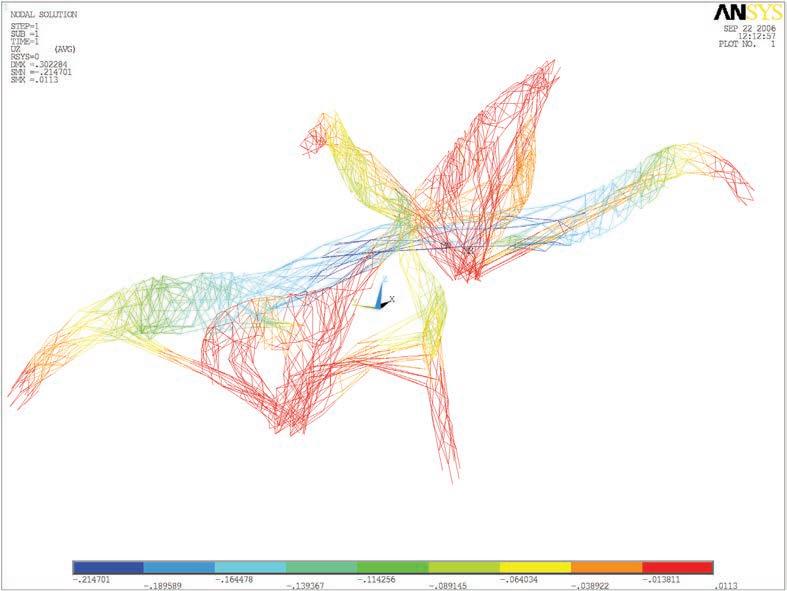
Case 2. Irregular distribution of fibers with structural connection between paths. This figure shows the vertical displacement with the nodal solution of the Finite Elements Analysis.

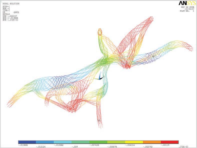
Case 3. Regular distribution of fibers with structural connection between paths. This figure shows the vertical displacement with the nodal solution of the Finite Elements Analysis.

MAXIMUM VERTICAL DISPLACEMENT

CASE dv (m)

1 -0.169

2 -0.215

3 -0.014

ANALYSIS OF THE RESULTS

The maximum vertical displacement occurs in the first two cases at the center of the longest span, while for the third case this is in one of the shortest ones. The value is reduced by ten at the last case. This structural connectivity can be related to the biomimetic principles explained at the first chapters of this study. The redundancy in the structure can be achieved with exactly the same amount of material, it is a matter of how connected are the fibers. This is a clear example of how this extra connectivity, a local change, can improve a lot the global behaviour of the system.

guillem baraut

mattia gambardella

tutors: mike weinstock

michael hensel

achim menges

martin hemberg

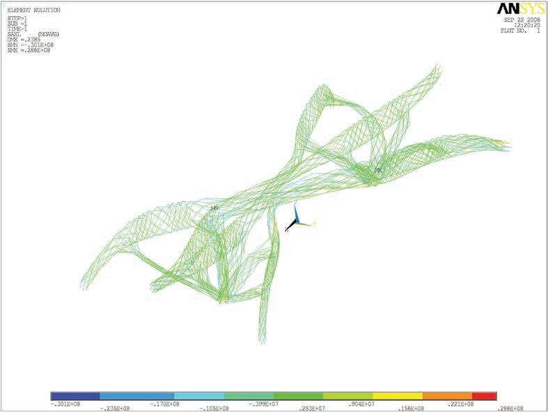
Case 1. Regular distribution of fibers without structural connection between paths. This figure shows the axial force in each element.

Case 2. Irregular distribution of fibers with structural connection between paths. This figure shows the axial force in each element.

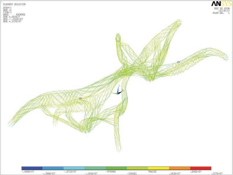
Case 3. Regular distribution of fibers with structural connection between paths. This figure shows the axial force in each element.

MAXIMUM AXIAL FORCE

2

3

MINIMUM AXIAL FORCE CASE

1

2

3

ANALYSIS OF THE RESULTS

The same behaviour can be observed when comparing the axial forces on each element. On the third case the maximum compression and tension forces are reduced by ten.

The structural behaviour is then gaining benefits from the redundancy in connectivity in both maximum stresses and maximum deflection.

guillem baraut

mattia gambardella

tutors: mike weinstock

michael hensel

achim menges

martin hemberg slender

13. FURTHER RESEARCH

guillem baraut

mattia gambardella

tutors: mike weinstock

michael hensel

achim menges

martin hemberg

slender multi stress driven structures

guillem baraut

mattia gambardella

tutors: mike weinstock

michael hensel

achim menges

martin hemberg

FURTHER RESEARCH

Some new lines of research have been open.

In terms of architectural/engineering applications some new research can be done in:

01. Embedding environmental analysis in the methodology

02. Considering special dynamic and wind load cases for longer spans

03. Use the same methodology in 2d and 3d in order to apply it on other structures.

slender multi stress driven structures

14. CONCLUSIONS

guillem baraut

mattia gambardella

tutors: mike weinstock

michael hensel

achim menges

martin hemberg

slender multi stress driven structures

guillem baraut

mattia gambardella

tutors: mike weinstock

michael hensel

achim menges

martin hemberg

CONCLUSIONS

The ultimate design is responding to both the requirements criteria:

01. Spacial performance (minimal road network)

02. Structural performance (Slenderness criteria)

03 The reiterative process helps in finding the most suitable solution to each specific project case.

04. Material anisotropy is improved by controlling the fiber layout – therefore the structural performance increases.

05. The researched anisotropy increases the structural performance in the ultimate design, where a stress driven distribution of fibers can improve the load bearing capabilities.

06. Moreover, the methodological approach illustrated in this work opens to a wide variety of possible configurations due to the flexibility of the digital tools.

15. BIBLIOGRAPHY

guillem baraut

mattia gambardella

tutors: mike weinstock

michael hensel

achim menges

martin hemberg

slender multi stress driven structures

EMERGENT

BIBLIOGRAPHY

[1] DYNAMIC LOADING AND DESIGN OF STRUCTURES

A.J. Kappos (Ed)

Spon Press, 2002

ISBN 0 – 419 – 22930 – 2

[2] TEXTILE COMPOSITES AND INFLATABLE STRUCTURES

INTERNATIONAL CONFERENCE ON ADVANCES IN COMPUTATIONAL MULTI BODY DYNAMICS

E. Oñate (Ed), B. Kröplin (Ed)

Springer, 2005

ISBN 1 – 4020 – 3316 – 8

[3] THE HANDBOOK OF ADVANCED MATERIALS

ENABLING NEW DESIGNS

James K. Wessel (Ed)

Wiley Interscience, 2004

ISBN 0 – 471 – 45475 – 3

[4] ACTIVE MATERIALS AND ADAPTIVE STRUCTURES

PROCEEDINGS OF THE ADPA/AIAA/ASME/SPIE CONFERENCE ON ACTIVE MATERIALS AND ADAPTIVE STRUCTURES

Gareth J. Knowles (Ed)

IOP Publishing Ltd, 1992

ISBN 0 – 7503 – 0191 – 0

[5] COMPUTER AIDED OPTIMUM DESIGN OF STRUCTURES VIII

S. Hernández, C.A. Brebbia, M.E.M. El-Sayed (Ed)

WIT Press, 2003

ISBN 1 – 85312 – 972 – 0

[6] MECHANICS OF LAMINATED COMPOSITE PLATES AND SHELLS THEORY AND ANALYSIS

J.N. Reddy

CRC Press, 2004 (2nd Edition)

ISBN 0 – 8493 – 1592 – 1

[7] MECHANICS OF COMPOSITE STRUCTURES

László P. Kóllar, George S. Springer

Cambridge University Press, 2002

ISBN 0 – 521 – 80165 – 6

[8] FUNDAMENTALS OF Fiber REINFORCED COMPOSITE MATERIALS

A.R. Bunsell, J. Renard

IOP Publishing Ltd, 2005

ISBN 0 – 7503 – 0689 – 0

guillem baraut

mattia gambardella

tutors: mike weinstock

michael hensel

achim menges

martin hemberg

[9] ANALYSIS OF COMPOSITE STRUCTURES

Christian Decolon

Kogan Page Science, 2004

(1st Edition Hermes Science Publications, 2000)

ISBN 1 – 9039 – 9662 – 7

[10] THE MANUFACTURING TECHNOLOGY OF CONTINOUS GLASS FiberS

K.L. Loewenstein

Elsevier, 1993 (3rd Edition)

ISBN 0 – 444 – 89346 – 6

[11] PROCEEDINGS OF THE SEVENTH INTERNATIONAL CONFERENCE ON COMPUTATIONAL STRUCTURES TECHNOLOGY

B.H.V. Topping, C.A. Mota Soares (Ed)

Civil-Comp Press, 2004

ISBN 0-948749-93-8 (book)

ISBN 0-948749-94-6 (CD-ROM)

ISBN 0-948749-95-4 (combined set)

[12] PROGRAMMING THE FINITE ELEMENT METHOD

I.M. Smith, D.V. Griffiths

Wiley, 2004 (4th Edition)

ISBN 0 – 470 – 84970 – 3

[13] COMPUTATIONAL TOPOLOGY OPTIMIzATION IN CONTINUUM MECHANICS

T. Borrvall

Department of Mechanical Engineering, Linköpings Universitet

ISBN 91-7373-310-5

[14] AD. CONTEMPORARY TECHNIQUES IN ARCHITECTURE CREATING SYNTHESIS PARTNERS

K. Shea, A. Rahim (Ed)

Wiley Academy, 2002

ISBN 0 – 470 – 84320 – 9

[15] PERFORMANCE-BASED OPTIMIzATION OF STRUCTURES

THEORY AND APPLICATIONS

Qing Quan Liang

Spon Press, 2005

ISBN 0 – 415 – 33594 – 9

[16] TEXTILE COMPOSITES AND INFLATABLE STRUCTURES II SECOND INTERNATIONAL CONFERENCE ON TEXTILE COMPOSITES AND INFLATABLE STRUCTURES

E. Oñate (Ed), B. Kröplin (Ed)

Cimne, 2005

ISBN 84 – 95999 – 83 – 8

[17] DESIGN IN NATURE

LEARNING FROM TREES

C. Mattheck

Springer, 1998

ISBN 3 – 540 – 62937 – 8

[18] SWARM INTELLIGENCE

FROM NATURAL TO ARTIFICIAL SYSTEMS

E. Bonabeau, M. Dorigo, G. Theraulaz

Oxford University Press, 1999

ISBN 0 – 19 – 513159 – 2

[19] DIGITAL DESIGN AND MANUFACTURING

CAD/CAM APPLICATIONS IN ARCHITECTURE AND DESIGN

D. Schodek, M. Bechthold, K. Griggs, K. Martin Kao, M. Steinberg

John Wiley & Sons, 2005

ISBN 0 – 471 – 45636 – 5

[20] EXTREME TEXTILES

Matilda Mc Quaid

Thames & Hudson, 2005

[21] IL 1, Minimalnet

Institut für Leichtbau Entwerfen und Konstruieren, Stuttgart,1969

[22] IL 22, Form-force-mass 2

Institut für Leichtbau Entwerfen und Konstruieren, Stuttgart, 1988

[23] IL 23, Form-force-mass 3

Institut für Leichtbau Entwerfen und Konstruieren, Stuttgart,1992

[24] IL 24,Form-force-mass 4-Lightweight principles

Institut für Leichtbau Entwerfen und Konstruieren, Stuttgart,1991

[25] IL 25,Form-force-mass 5-Experiments

Institut für Leichtbau Entwerfen und Konstruieren, Stuttgart,1990

guillem baraut

mattia gambardella

tutors: mike weinstock

michael hensel

achim menges

martin hemberg

16. ACKNOWLEDGEMENTS

guillem baraut

mattia gambardella

tutors: mike weinstock

michael hensel

achim menges

martin hemberg

slender multi stress driven structures

We would like to thank all the people that in some way helped us to develop this dissertation, from our tutors

. Mike Weinstock

. Michael Hensel

. Achim Menges

to our families and friends that supported us, and also

. Martin Hemberg (Imperial College, AA)

. Nikolaos Stathopoulos (Buro Happold, AA)

. George Jeronimidis (University of Reading)

. Chris Williams (University of Bath)

. Julien Vincent (University of Bath)

. Eugenio Oñate (Universitat Politècnica de Catalunya)

. Robert Aish (Bentley)

guillem baraut

mattia gambardella

tutors: mike weinstock

michael hensel

achim menges

and Ceril for his coffee, Pavel for his criticism, RCA for the RP model, and all other EmTech students for this year.

Guillem Baraut would like to thank “la Caixa” and The British Council for their economic support

martin hemberg slender

17. APPENDICES

guillem baraut

mattia gambardella

tutors: mike weinstock

michael hensel

achim menges

martin hemberg

slender multi stress driven structures

EMERGENT

APPENDIX 1

Final Matlab code used for topology optimization

%%%% A 99 LINE TOPOLOGY OPTIMIZATION CODE BY OLE SIGMUND, JANUARY 2000 %%%

%%%% CODE MODIFIED FOR INCREASED SPEED, September 2002, BY OLE SIGMUND %%%

%%%% CODE MODIFIED, May 2006, BY GUILLEM BARAUT & MATTIA GAMBARDELLA %%%

function top_07(nelx,nely,volfrac,penal,rmin,jpg,rhino,gc,minx);

% INITIALIZE

x(1:nely,1:nelx) = volfrac;

%x = unifrnd(0.2,1,nely,nelx);

%strexcel = ‘c:\Documents and Settings\Guillem Baraut\Mis documentos\Data_ from_GC.xls’;

%numpoints = 37;

%points = load(‘c:\Documents and Settings\Guillem Baraut\Mis documentos\Data from GC.txt’);

%numpoints = points(1,1);

%for i =1:numpoints

% xblack = int8(xlsread(strexcel, 3, strcat(‘J’,int2str(i))));

% yblack = int8(xlsread(strexcel, 3, strcat(‘K’,int2str(i))));

% yblack = points(i+1,1)

% xblack = points(i+1,2)

% x(yblack,xblack) = 1;

%end

% PASSIVE ELEMENTS. RECTANGLES 1/3 CENTRAL BOTH SIDES for ely = 1:nely for elx = 1:nelx if ely>10/9*nely/nelx*elx+6/5*nely

% if and(and(ely>1/3*nely+1,ely<2/3*nely),or(elx<1/3*nelx+1,elx>2/ 3*nelx))

passive(ely,elx) = 1; x(ely,elx) = 0.001; else

passive(ely,elx) = 0; end end end loop = 0; change = 1.;

% Added by Guillem Baraut % Mattia Gambardella %colormap(jet); imagesc(-x+0.5); axis equal; axis tight; axis off;pause(1e6); colormap(gray); imagesc(-x); axis equal; axis tight; axis off;pause(1e-6);

% Print results in jpg files if jpg == 1 nam=’c:\Documents and Settings\Guillem Baraut\Mis documentos\frm_’; filename=strcat(nam,’000’); saveas(gcf,filename, ‘jpg’);

end if rhino == 1

guillem baraut

mattia gambardella

tutors: mike weinstock

michael hensel

achim menges

martin

fid = fopen(‘x3.txt’,’w’); end

% Print results in a file

% START ITERATION while change > 0.01 loop = loop + 1; xold = x;

% FE-ANALYSIS [U]=FE(nelx,nely,x,penal);

% OBJECTIVE FUNCTION AND SENSITIVITY ANALYSIS [KE] = lk; c = 0.; for ely = 1:nely for elx = 1:nelx n1 = (nely+1)*(elx-1)+ely; n2 = (nely+1)* elx +ely; Ue = U([2*n1-1;2*n1; 2*n2-1;2*n2; 2*n2+1;2*n2+2; 2*n1+1;2*n1+2],1); c = c + x(ely,elx)^penal*Ue’*KE*Ue; dc(ely,elx) = -penal*x(ely,elx)^(penal-1)*Ue’*KE*Ue; end end

% FILTERING OF SENSITIVITIES [dc] = check(nelx,nely,rmin,x,dc);

% DESIGN UPDATE BY THE OPTIMALITY CRITERIA METHOD [x] = OC(nelx,nely,x,passive,volfrac,dc); %[x] = OC(nelx,nely,x,volfrac,dc);

% PRINT RESULTS

change = max(max(abs(x-xold))); disp([‘ It.: ‘ sprintf(‘%4i’,loop) ‘ Obj.: ‘ sprintf(‘%10.4f’,c) ... ‘ Vol.: ‘ sprintf(‘%6.3f’,sum(sum(x))/(nelx*nely)) ... ‘ ch.: ‘ sprintf(‘%6.3f’,change )])

% PLOT DENSITIES

%colormap(jet); imagesc(-x+0.5); axis equal; axis tight; axis off;pause(1e6); colormap(gray); imagesc(-x); axis equal; axis tight; axis off;pause(1e-6);

% PRINT JPG IMAGES

if jpg == 1 if loop < 10

filename=strcat(nam,’00’,int2str(loop)); end if and(mod(loop,2)==0,and(loop > 9,loop < 100))

filename=strcat(nam,’0’,int2str(loop)); end

if and(mod(loop,5)==0,loop > 99)

filename=strcat(nam,int2str(loop));

end saveas(gcf,filename, ‘jpg’); end

% PRINT FILE FOR RHINO x2.txt if rhino == 1 if loop == 140 for i=1:nelx for j=1:nely if x(j,i)>minx if i<nelx if x(j,i+1)>minx

fprintf(fid,’_Line ‘);

fprintf(fid,’%s’,strcat(int2str(i),’,’,int2str(j),’ ,’,num2str(10*x(j,i),’%6.2f’)));

fprintf(fid,’ ‘);

fprintf(fid,’%s’,strcat(int2str(i+1),’,’,int2str(j) ,’,’,num2str(10*x(j,i+1),’%6.2f’)));

fprintf(fid,’ ‘);

end end if j<nely if x(j+1,i)>minx

fprintf(fid,’_Line ‘);

fprintf(fid,’%s’,strcat(int2str(i),’,’,int2str(j),’ ,’,num2str(10*x(j,i),’%6.2f’)));

fprintf(fid,’ ‘);

fprintf(fid,’%s’,strcat(int2str(i),’,’,int2str(j+1) ,’,’,num2str(10*x(j+1,i),’%6.2f’)));

fprintf(fid,’ ‘); end end end end end

fclose(fid); end end end if rhino ==1

fclose(fid); end

% PRINT FILE FOR gc Data_to_GC.xls if gc ==1

strExcelWrite = ‘c:\Documents and Settings\Guillem Baraut\Mis documentos\Data_to_GC.xls’;

xlswrite(strExcelWrite, nelx, ‘Hoja1’, ‘B1’);

xlswrite(strExcelWrite, nely, ‘Hoja1’, ‘B2’);

xlswrite(strExcelWrite, x, ‘Hoja1’, ‘A3’);

[xmax]=VectMax(nelx,nely,x);

xlswrite(strExcelWrite, sort(xmax(:,:,2),2), ‘Hoja2’, ‘A1’); end

%%%%%%%%%%%%%%%%%%%%%%%%%%%%%%%%%%%%%%%%%%%%%%

% THE END %

%%%%%%%%%%%%%%%%%%%%%%%%%%%%%%%%%%%%%%%%%%%%%%

%%%%%%%%%% OPTIMALITY CRITERIA UPDATE %%%%%%%%%%%%%%%%%%%%%%%%%%%%%%%%%%%%%% function [xnew]=OC(nelx,nely,x,passive,volfrac,dc)

%function [xnew]=OC(nelx,nely,x,volfrac,dc)

l1 = 0; l2 = 100000; move = 0.2; while (l2-l1 > 1e-4)

lmid = 0.5*(l2+l1);

xnew = max(0.001,max(x-move,min(1.,min(x+move,x.*sqrt(-dc./lmid))))); xnew(find(passive)) = 0.001; if sum(sum(xnew)) - volfrac*nelx*nely > 0; l1 = lmid; else

l2 = lmid; end end

%%%%%%%%%% MESH-INDEPENDENCY FILTER %%%%%%%%%%%%%%%%%%%%%%%%%%%%%%%%%%%%%%%%

function [dcn]=check(nelx,nely,rmin,x,dc)

dcn=zeros(nely,nelx); for i = 1:nelx for j = 1:nely sum=0.0; for k = max(i-floor(rmin),1):min(i+floor(rmin),nelx) for l = max(j-floor(rmin),1):min(j+floor(rmin),nely)

fac = rmin-sqrt((i-k)^2+(j-l)^2);

sum = sum+max(0,fac);

dcn(j,i) = dcn(j,i) + max(0,fac)*x(l,k)*dc(l,k); end end

dcn(j,i) = dcn(j,i)/(x(j,i)*sum); end end

%%%%%%%%%% FE-ANALYSIS %%%%%%%%%%%%%%%%%%%%%%%%%%%%%%%%%%%%%%%%%%%%%%%%%%%%% function [U]=FE(nelx,nely,x,penal) [KE] = lk();

K = sparse(2*(nelx+1)*(nely+1), 2*(nelx+1)*(nely+1));

F = sparse(2*(nely+1)*(nelx+1),1); U = zeros(2*(nely+1)*(nelx+1),1); for elx = 1:nelx

for ely = 1:nely

n1 = (nely+1)*(elx-1)+ely;

n2 = (nely+1)* elx +ely; edof = [2*n1-1; 2*n1; 2*n2-1; 2*n2; 2*n2+1; 2*n2+2; 2*n1+1; 2*n1+2];

K(edof,edof) = K(edof,edof) + x(ely,elx)^penal*KE;

end end

guillem baraut

mattia gambardella

tutors: mike weinstock

michael hensel

achim menges

martin hemberg

EMERGENT TECHNOLOGIES AND DESIGN. 2005-2006

% DEFINE LOADS AND SUPPORTS (HALF MBB-BEAM)

%F(2,1)=-1;

%F([2*(nely+1)*10+2:2*(nely+1):2*(nely+1)*(nelx+1-10)+2],1) = -1;

%F([2*(nely+1)*round(nelx/6)+2:2*(nely+1):2*(nely+1)*(nelx+1)],1) = -5;

%F([2*(nely+1):2*(nely+1):2*(nely+1)*(nelx+1)],1) = -1;

%Uniform load top

F([2:2*(nely+1):2*(nely+1)*(nelx+1)],1) = -1;

%F([2*(nely+1)*nelx+2:2:2*(nely+1)*(nelx+1)],1) = -1;

%for i = 2*(nely+1)*nelx+1:2:2*(nely+1)*(nelx+1)

% F(i,1) = -1 + 2/(2*(nely+1))*(i - (2*(nely+1)*nelx+1));

%end

%F(2*(nely+1)*(nelx+1),1) = -1;

% 4 forces bottom

%F([2*(nely+1):2*(nely+1)*round((nelx+1)/3.1):2*(nely+1)*(nelx+1)],1) = -1;

% 4 forces top

%F([2:2*(nely+1)*round((nelx+1)/3.1):2*(nely+1)*(nelx+1)],1) = 1;

% 3 forces bottom

%F([2*(nely+1):2*(nely+1)*round((nelx+1)/2.1):2*(nely+1)*(nelx+1)],1) = -1;

% 3 forces top

%F([2:2*(nely+1)*round((nelx+1)/2.1):2*(nely+1)*(nelx+1)],1) = 1;

%3 forces top, 3 forces bottom

%F(2*(nely+1),1)=-1;

%F(2*(nely+1)*round((nelx+1)/2),1)=-1;

%F(2*(nely+1)*round((nelx+1)/2+1),1)=-1;

%F(2*(nely+1)*(nelx+1),1)=-1;

%F(2,1)=1;

%F(2*(nely+1)*round((nelx+1)/2)+2,1)=1;

%F(2*(nely+1)*round((nelx+1)/2+1)+2,1)=1;

%F(2*(nely+1)*(nelx+1)-2*(nely+1)+2,1)=1;

%Symmetry conditions at vertical right hand side edge and pin support at 1/9 of the length at the bottom

%fixeddofs = union([2*(nely+1)*nelx+1:2:2*(nely+1)*(nelx+1)],(round(1/ 9*nelx)+1)*2*(nely+1));

%Symmetry conditions at vertical left hand side edge and pin support at 5/7 of the length at the bottom

fixeddofs = union([1:2:1/3*2*(nely+1)],union((round(7/ 10*nelx))*2*(nely+1),(round(7/10*nelx))*2*(nely+1)-1));

%fixeddofs = ([2*(nely+1)*round((nelx+1)*0.45)+2:2*(nely+1):2*(nely+1)*roun d((nelx+1)*0.55)+2]);

%fixeddofs = union([round(2*(nely+1)*(4.49/9*(nelx+1)+4.4/9)): round(2*(nely+1)*(4.49/9*(nelx+1)+4.6/9))],...

% [round(2*(nely+1)*(4.51/9*(nelx+1)+4.4/9)):round(2*(nely+1)*(4.51/ 9*(nelx+1)+4.6/9))]);

%fixeddofs = union([2*(nely+1)*(nelx)-2:(nely+1)*(nelx)+2],union(... % [(nely+1)*(nelx+1)-2:(nely+1)*(nelx+1)+2],[(nely+1)*(nelx+2)-2:(nely+1) *(nelx+2)+2]));

%fixeddofs = union([1:2:2*(nely+1)],[2*(nelx+1)*(nely+1)]);

%fixeddofs = [round(4/5*2*(nely+1)):2*(nely+1)];

%fixeddofs = ([2:2*(nely+1):2*(nelx+1)*(nely+1)]);

%fixeddofs = union([2*(nely+1):2*(nely+1):round(2*(nelx+1)*(nely+1))],[2*(n ely+1)-1:2*(nely+1):round(2*(nelx+1)*(nely+1))]);

%fixeddofs = union([(nely+1):2*(nely+1)],[2*(nelx+1)*(nely+1)-2*(nely+1): ...

% 2*(nelx+1)*(nely+1)]);

%fixeddofs = union([1:2*(nely+1)],[2*(nelx+1)*(nely+1)-...

% 2*(nely+1):2*(nelx+1)*(nely+1)]);

%fixeddofs = union([1:4],[2*(nelx+1)*(nely+1)-2*(nely+1):2*(nelx+1)*...

% (nely+1)-2*(nely+1)+3]);

%fixeddofs = union([1:2:2*(nely+1)],union([2*(nely+1)*(nelx+1)-... % 3:2*(nely+1)*(nelx+1)],[2*(nely+1)*(nelx)-3:2*(nely+1)*(nelx)]));

%fixeddofs = union([1:2:2*(nely+1)],union([2*(nely+1)*(nelx-30)-...

% 3:2*(nely+1)*(nelx-30)],[2*(nely+1)*(nelx-29)-3:2*(nely+1)*(nelx29)]));

%fixeddofs = union([2*(nely+1)-3:2*(nely+1)],[(2*(nely+1)*(nelx+1)/5-3):...

% (2*(nely+1)*(nelx+1)/5)]);

alldofs = [1:2*(nely+1)*(nelx+1)];

freedofs = setdiff(alldofs,fixeddofs);

% SOLVING

U(freedofs,:) = K(freedofs,freedofs) \ F(freedofs,:);

U(fixeddofs,:)= 0;

%%%%%%%%%% ELEMENT STIFFNESS MATRIX %%%%%%%%%%%%%%%%%%%%%%%%%%%%%%%%%%%%%%%%

function [KE]=lk

E = 1.;

nu = 0.3;

k=[ 1/2-nu/6 1/8+nu/8 -1/4-nu/12 -1/8+3*nu/8 ... -1/4+nu/12 -1/8-nu/8 nu/6 1/8-3*nu/8];

KE = E/(1-nu^2)*[ k(1) k(2) k(3) k(4) k(5) k(6) k(7) k(8)

k(2) k(1) k(8) k(7) k(6) k(5) k(4) k(3)

k(3) k(8) k(1) k(6) k(7) k(4) k(5) k(2)

k(4) k(7) k(6) k(1) k(8) k(3) k(2) k(5)

k(5) k(6) k(7) k(8) k(1) k(2) k(3) k(4)

k(6) k(5) k(4) k(3) k(2) k(1) k(8) k(7) k(7) k(4) k(5) k(2) k(3) k(8) k(1) k(6) k(8) k(3) k(2) k(5) k(4) k(7) k(6) k(1)];

%

%%%%%%%%%% MAXIMUM 3 POINTS IN 8 ROWS %%%%%%%%%%%%%%%%%%%%%%%%%%%%%%%%%%%%%% function [xmax]=VectMax(nelx,nely,x) [xmx,indxmax] = sort(x,2,’descend’); for j = 1:8 % Eight rows in x array if j > 1 ely = round(1/7*nely*(j-1)); % Row number ely of x array else ely = 1; end for i = 1:3 % Three points in each row

xmax(j,i,1)=xmx(ely,i);

xmax(j,i,2)=indxmax(ely,i)-1; end end

guillem baraut

mattia gambardella

tutors: mike weinstock

michael hensel

achim menges

martin hemberg

slender multi stress driven structures

EMERGENT TECHNOLOGIES AND DESIGN. 2005-2006

%%%%%%%%%%%%%%%%%%%%%%%%%%%%%%%%%%%%%%%%%%%%%%%%%%%%%%%%%%%%%%%%%%%%%%%%%%%%

% This Matlab code was written by Ole Sigmund, Department of Solid % % Mechanics, Technical University of Denmark, DK-2800 Lyngby, Denmark. %

% Please sent your comments to the author: sigmund@fam.dtu.dk %

% %

% The code is intended for educational purposes and theoretical details % % are discussed in the paper

%

% “A 99 line topology optimization code written in Matlab” % % by Ole Sigmund (2001), Structural and Multidisciplinary Optimization, %

% Vol 21, pp. 120--127.

% %

%

% The code as well as a postscript version of the paper can be % % downloaded from the web-site: http://www.topopt.dtu.dk %

% % % Disclaimer: %

% The author reserves all rights but does not guaranty that the code is % % free from errors. Furthermore, he shall not be liable in any event %

% caused by the use of the program.

%%%%%%%%%%%%%%%%%%%%%%%%%%%%%%%%%%%%%%%%%%%%%%%%%%%%%%%%%%%%%%%%%%%%%%%%%%%%

%

guillem baraut

mattia gambardella

tutors: mike weinstock

michael hensel

achim menges

martin hemberg slender multi stress driven structures

APPENDIX 2

Excel Spread Sheet used to calculate the structural slenderness for comparison with Frei Otto criteria in the evaluation chapter.

tutors: mike weinstock michael hensel achim menges martin hemberg slender multi stress driven structures

guillem baraut

mattia gambardella

tutors: mike weinstock

michael hensel

achim menges

martin hemberg

slender multi stress driven structures