Urban Metabolic Growth
4
Mohammed Makki
Pavlos Schizas
I would like to thank,
George Jeronomides for his support and encouragement throughout the project, and for continuously helping with finding solutions and alternatives to the several challenges that were faced. Toni Kotnik for his valuable input and uninterrupted support with the scripts that were developed throughout the dissertation, as well as his aid and advice throughout the final leg of the dissertation.
Mike Weinstock for his unceasing and relentless guidance throughout the entirety of the dissertation. His patience and persistence in ensuring that I work to the very limits of my capabilities constantly pushed me into working harder and reaching further throughout the length of the dissertation. Therefore it is to Mike Weinstock that I give most gratitude for helping achieve and finalize this dissertation.
Asma Ahli for being the supportive friend that I called for in my times of need. Her kind words of encouragement and heartening motivation throughout the length of the project are endlessly treasured and immeasurably cherished. To her, I will always be in debt.
My Father, Tarek Makki. He taught me the importance of patience and logical conclusions of everyday life. His heartfelt morale-boosting support and continuous interest in my work has given me the courage and boldness that I most strived for. It is only through his priceless life lessons that I was able to persevere throughout the length of this course and achieve the best of my abilities. He is the prime example of what I wish to achieve and who I strive to be in my life.
My Mother, Haya Makki. She was the person who knew that I was troubled and stressed without me having to call. Although she lived continents away throughout this course, she unfailingly ensured that I never lacked her love, affection, tenderness and warmth. At the times throughout the course where I was only breaths away from giving up, it is to her that I say ‘thankyou’ for making sure that I remained tenacious in my persistence to reach the very maximum of my capabilities.
Mohammed Makki
Acknowledgments
Many thanks to
Mike Weinstock for his constant support and essential guidance throughout the entire period of the dissertation. His precious assistance was the catalyst for achieving progress and acquiring knowledge and experience from this collaboration.
George Jeronimides for his beneficial advice and willingness to help us with any challenge arisen during the entire time. Toni Kotnik for his contribution to resolve many puzzles, especially with computational issues.
My parents, Akis and Zena Schizas, for their enormous psychological support and great endeavor to encourage me with my work during the stressful times. They have been extremely caring during my entire work and have never hesitated to sacrifice anything in order to help me.
Finally, special thanks to my siblings Nicos, Michalis and Christiana Schizas, to my friends from EmTech, as well as my friends Andreas Poullaides and Andri Shalou for being continuously encouraging and supportive during our discussions.
Pavlos Schizas
5
6 Table of Contents Abstract ...................................................................... 9 1. Domain ...................................................................... 11 1.1 Introduction ...................................................................... 13 1.2 Planned Cities ...................................................................... 14 Brasilia ...................................................................... 15 Milton Keynes ...................................................................... 18 Abuja ...................................................................... 20 Chandigarh ...................................................................... 22 1.3 Evolving Cities ...................................................................... 25 Nicosia ...................................................................... 26 Istanbul ...................................................................... 32 1.4 Mono/poly-centric Cities ...................................................................... 37 Houston ...................................................................... 41 Tokyo ...................................................................... 45 1.5 Densities ...................................................................... 49 Los Angeles ...................................................................... 52 Shanghai ...................................................................... 53 1.6 Conclusions ...................................................................... 55 2. Methods ...................................................................... 57 2.1 Introduction ...................................................................... 59 2.2 Space Syntax ...................................................................... 60 2.3 City Engine ...................................................................... 66 2.4 L-systems ...................................................................... 70 2.5 Conclusions ...................................................................... 73
7 3. Experiments ...................................................................... 75 3.1 Introduction ...................................................................... 77 3.2 Path Expariments ...................................................................... 78 3.3 Blocks Experiments ...................................................................... 82 3.4 Conclusions ...................................................................... 93 4. Design ...................................................................... 95 4.1 Introduction ...................................................................... 97 4.2 China ...................................................................... 98 4.3 Australia ...................................................................... 114 4.4 Water Resources ...................................................................... 125 4.5 Agriculture ...................................................................... 128 4.6 Renewable Energy ...................................................................... 134 4.7 Urban Blocks ...................................................................... 137 4.8 Paths ...................................................................... 143 4.9 I ntegration ...................................................................... 148 4.10 energy Demands ...................................................................... 150 4.11 Detailed Patch ...................................................................... 160 4.12 Conclusions ...................................................................... 165 5. Conclusions ...................................................................... 166 6. Further Research ...................................................................... 168 Appendix ...................................................................... 171 Bibliography ...................................................................... 190
8
Abstract
Metabolic systems have been extensively studied within a biological context throughout history; however it is only recently that metabolic systems have been researched and related to different fields. The contribution that a metabolic system - as a model – has on urban development is to ensure that the flow of energy is continuous throughout the system, where all the components that make up the system are interdependent on one another. In other words, the backbone of the city heavily relies on allocating the natural resources that will sustain it from the onset. In modern day planning, there is a lack of consciousness in considering the availability of these natural resources and their significance in dictating the urban development and growth. Ancient cities on the other hand do not seem to have the flaws that modern day cities have; these “evolving” cities grew with respect to functionality and the location of resources. Despite the many paradigms that ancient/evolving cities offer, modern day planners seem to overlook these examples. This project aims to design two scenarios of metabolic urban development placed in two regions with different extreme climatic conditions, using planned cities and evolved cities as case studies to help govern the different elements that make up the cities fabric. Different tools and methodologies will also be utilized to help achieve two different scenarios that are based on the same metabolic model.
9
10
Domain
To understand what defines a city as a successful one, one must first understand the different components that comprise a city and how they are implemented in both planned cities, as well as evolving cities.
11
1.
12
1.1 Introduction
The broadest question one might ask is ‘what makes a successful city?’ The answer to this question is so complex that there actually isn’t an answer. There are so many factors that affect the growth of a city; to try to find the optimal solution for all the problems a city could face is next to impossible. The most efficient way to begin understanding the success of cities is to simply carry out case studies on different cities, in different climates, developed at different times under different political conditions. Although the actual planning of cities did not begin until 200 years ago, there are two main categories for cities; evolved or planned. Both these categories have their share of advantages and disadvantages; however, one system might be more advantageous than the other.
The effects of polycentricism within a city will also be analyzed to further understand how they affect the growth of a city, and whether polycentricism has an effect on the efficiency of a city with respects
to density and infrastructure. There is a heavy correlation between polycentricism and the density of a city, whether one is a by product of the other is yet to be analyzed, however, one can predict that there must be a particular balance of the population density within the city for the proper growth of the city. Other than a correlation between the city’s density with its centrality, there is an even larger correlation between the city’s density and the energy efficiency levels that it performs at.
All the different elements that will be researched must not be isolated from one another. There are many relationships between the different areas of research, the way they these systems operate are mostly interrelated, and at times interdependent on one another. This will help put together a clearer image of what factors make a city a unsuccessful one.
13
1.2 Planned cities
A planned city is designed as a final master plan that is implemented in a specific site. With a predicted population count, growth period and development scenario, planned cities are designed and implemented as a top down method rather than a bottom up one.
14
Fig.1.21a-d
a: The two main intersecting axes on which the whole design concept is based. b: The horizontal axis shapes a curve now and the boundaries are engraved according to the natural landscape. c: Initiating the zoning process starts to configure the final morphology of the plan. d: Around the main artery other peripheral streets are added as a secondary circulation system.
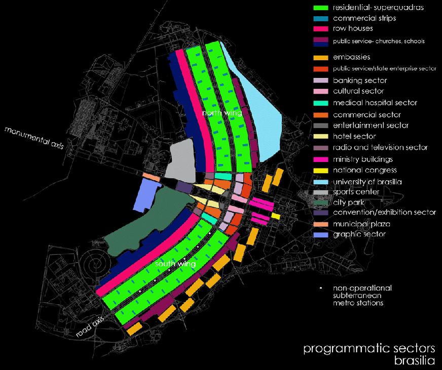
Fig.1.22
The map shows the distribution of functions in the planning process. It is clear that there is no mix of uses in the zones; the zones retain a cohesive character.
Brasilia planning strategies
Brasilia was planned by Lucio Costa in the middle of the 20th century, after the government assigned the project to him. The Brazilian government decided to relocate the capital city from the coast to the Midwestern interior of the country; a decision made in order to encourage population growth to the internal parts of Brazil.
The following steps describe the way the city has evolved and formed the present pattern, out of the initially born idea:
1. The first engraving was drawn as a simple gesture of someone marking their position; with two axes intersecting at a 90 degree angle shaping a simple cross [Fig.1.21a].
2. The main engravings are slightly deformed in order to serve the topographic demands of the area, the drainage inclination and coastline. Thus, the natural boundaries are created and describe an equilateral triangle. The horizontal main axis has now turned into a curve, in order to maximise the length of the following development [Fig.1.21b].
3. The main curved axis has been turned into an artery of fast crossing circulation and bulks of the residential districts have been placed along its length. Additional side lanes were added on the sides of the axis for local circulation [Fig.1.21c,d].
4. The transverse axis, with its monumental assertiveness, facilitates the civic and administrative centres, the cultural, entertainment and sporting centres, the municipal administration facilities, the barracks, the storage and supply zones, the sites for small local industries and the railway station along its length. Banking and commercial districts were placed on the intersection of the two main axes [Fig.1.22].
5. The main roads intersect between one another in several levels in height, creating parking spaces for private vehicles. This entails the coherence of the roads along their length and the lack of connectivity on many junction points, hence transit flows smoothly. There is a very small number of traffic lights in the whole street network. However, traffic jams are usual at certain points.
15
Fig.1a
Fig.1c
Fig.1d
Fig.1b
6. The dominant pattern so far is a clover look-alike one, shaped by the two main monumental axes. An additional independent road system was established for vehicular traffic. This secondary system is comprised by nodes and intersections with perpendicular roads; however, it does not cross the main axes system at any point, apart from the sports district [Fig.1.21c,d].
7. The pedestrian network was established in both central and residential areas in reference to the automotive traffic system; separately but not completely isolated from the cars.
8. One of the outstanding particularities of this project was the innovation of interactive levels on the free space development. A three-dimensional configuration was created between public spaces, such as a square, pedestrian network and buildings, following the local topographical characteristics. The idea was to integrate the ancient oriental terrace technique into the modern planning.
9. Green lanes were designed symmetrically along the monumental axis, constituting the city’s lungs.
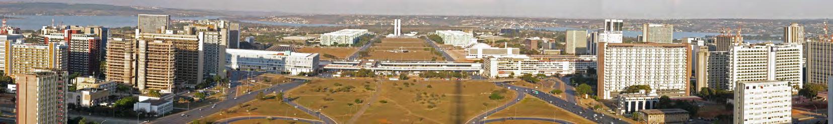
10. The sectors individually form an “autonomous plastic unit within the whole” (B.Areal). The particular way of planning entails homogeneity throughout the spatial organisation of the city; this homogeneity provides a noble scale locally, however in particular points the feeling of monumentality is predominant [Fig.1.23], [Fig.1.24].
11. The main block organisation is based on a continuous sequence of large blocks settled left and right along the residential axes, combined with the green area configuration; in this way the blocks appear to be on a second plane but simultaneously merged into the scenery. The blocks consist of uniform-height residential units – about six-floor buildings – raised on pillars and with the pedestrian network being separated from the automobile traffic.

Fig.1.23
The long coherent main axes of the city planning are transformed into huge monumental paths crossing the building blocks.
Fig.1.24
With the development of Brasilia during the Modernist years, many architectural expressions have been contemplated by the architects of that time. The city has some focal points that can be considered as communal spaces and landmarks and they manifest the monumental character of the city.
16
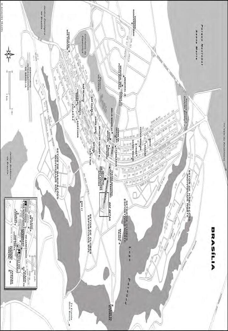
Fig.1.25
General plan of the city and its expansions. It is obvious that although the city was built to reside only 500.000 people, eventually the growth occurred unpredictably fast thus the city was expanded to the land around the planed part.
Areas that were uncontrollably expanded outside the borders of the planned city.
The initial area of the city that was planned to accommodate 500.000 people.
12. The blocks near the highways cost more than the ones in the inner areas; however, the social segregation was prevented by an act of mixing together people from different social classes in several sets of blocks. Moreover, many other factors improve the social neutralisation, such as the differences in densities of occupation, space allocation and material used for construction of the units.
13. For the preservation of the landscape value, there was no building activity along the lakefront.
The main issue concerning the city today is its sharp growth rate; a growth that exceeds every initial speculation at the planning phase. In
1960 the population of the city was just 140,000 residents and within ten years it has risen up to 537,000. The latest research shows that in 2000 the population reached 2,000,000 people, a sharply increased number compared to the initial plans according to which it was anticipated to facilitate only 500,000 people.
Finally, the city as a whole provides differentiation in its components, however homogeneity to its overall form. Beneath its comfort, efficiency and functionality, the city has limited boundaries in terms of growth [Fig.1.25]. Its limits are strongly engraved and defined by the topography and architectural inputs of a modernistic concept.
17
N 01 km
Brasilia
Milton Keynes the initial plan
The initial design phase of Milton Keynes began in 1967, mainly by The firm of Llewelyn Davies, Weeks, Forestier-Walker and Bor, several contractors and sub contractors as well as North American transport engineers were also involved (the renowned association of Milton Keynes to Los Angeles may be attributed to these engineers). The main feature regarding the design of Milton Keynes is the fact that it was designed to accommodate the car rather than the pedestrian. Although the pedestrian was not completely overlooked, as the design of Milton Keynes progressed, the pedestrian (and consequently, the pedestrians’ needs) faded further into the background. The plan of the city was designed as a grid of roads, distanced 1000 metres apart [Fig.1.26]. The initial aim of the design was to distribute the different zones throughout the city with the intent of creating several smaller hubs rather than a main city centre. However, in all the different design variations, a predominant feature was inevitable, which was a main shopping centre. This was due to two main reasons; firstly, in order to attract strong retailers, a main hub with an agglomeration of retailers was essential; secondly, the design board believed that a main centre
was imperative for the “image” of the city. Thus, the decision to build a main shopping centre was finally made, which inescapably created the city centre of Milton Keynes, and so, the designers’ initial goal of creating several equal hubs was eradicated.
A distinct city centre did not eliminate retail outlets from being constructed throughout the rest of the city; on the contrary, retail outlets were very cleverly placed alongside the roads, taking advantage of passing by commuters - whether vehicle or pedestrian. This raises the question of what will happen to the “left over” spaces? In other words, when a 1 kilometre by 1 kilometre grid of roads is constructed, and retail outlets are placed alongside the roads themselves, that leaves the centre of each 1 kilometre by 1 kilometre ‘superblock’ relatively empty [Fig.1.27]. The first logical use of these spaces would be landscaped areas, such as public parks or gardens, however the potential problems with these spaces is that they are somewhat distant from the main roads, and therefore may be very easily transformed into an attraction for crime.
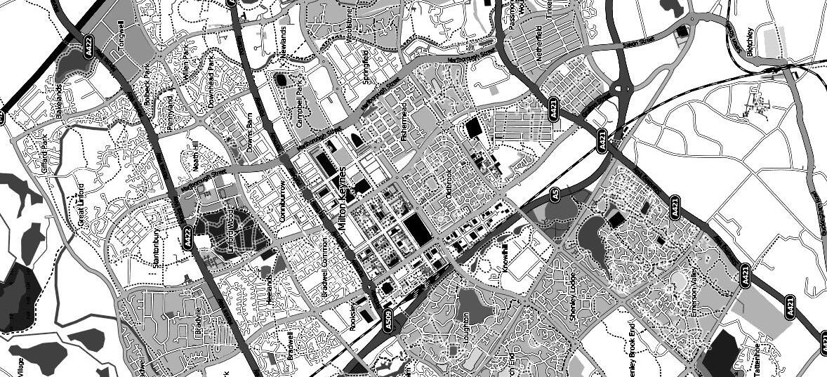
Fig.1.26
Aerial view of the street network of Milton Keynes. Although the grid system is not completely linear, one can clearly identify the 1000 metre by 1000 metre ‘superblocks’.
18
Fig.1.27
Graphic representation of the preliminary design of the intended built up area against the design that was actually constructed by the developers. The two images on the left show represent the planners original goal of positioning the built up area alongside the main roads; however, the two images on the left which the developers adapted clearly show the built up area position in the centers of each ‘superblock’ leaving the sides of the road empty.
the implemented plan
All of the intentions, aims and goals stated above were the designers’. As mentioned, design began in 1967; three years later in 1970, the final designs were handed over to the developers for implementation. This was a crucial point for the design of Milton Keynes, because it was at this time where several major changes in the designs were carried out (mainly by the developers). Michael Edwards (member of the design team) blames (in part) the developers’ changes to the designs on the way the designs were handed over from one team to the other. The designs were drawn up in a way where there were many open-ended questions without enough extreme assertions. This gave the developers the feasibility to take control and change whatever they pleased. The major “amendment” was to change the original intention of placing retail outlets alongside the main roads to clustering them in the centre of the 1 kilometre by 1 kilometre lots. This instantly reduced the possibilities of these outlets to be seen by commuters, as well as dramatically changed the appearance of the main roads. This consequently forced the building units to be built within the lots as well.
For this reason, each main ‘superblock’ was given to a developer for design and construction. The main negative implication of this is that without precise development regulation laws, the identity of the city can be very easily lost due to different developments being designed by different developers.
The eagerness for the development board to construct the main shopping centre created an unpredictable result. Although the shopping centre was a very successful one, attracting people from all over the city, as well as from other cities, it automatically obliterated any chance of smaller retail outlets to be built throughout the city. In other words, the possibility of creating several hubs throughout Milton Keynes (regardless of the size of these hubs) was absolutely abolished. One might suggest that the solution to all these problems would have been a stricter initial plan, one that forced the developers to follow it by the letter. As will be seen in the case of Abuja, this method of implementation also yields negative results.
19
Abuja
a precipitate masterplan
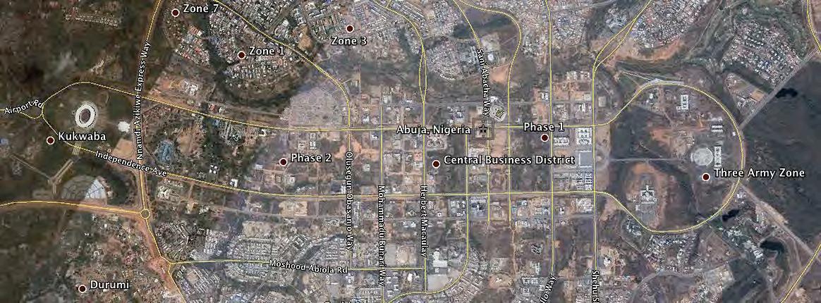
Before beginning the analysis of the city plan of Abuja, it is crucial to state that the main reason the proposal of Abuja was put forward was due to the failure of Nigeria’s original capital city, Lagos. Alongside severe congestion and poor drainage, Lagos was succumbing to a substantial amount of population pressure (Daramola, Aina, 2004); According to the Lagos state government, the population of Lagos has reached 17 million, and the United Nations organisation predicts that Lagos will be the third largest mega city by 2015 (2009). This pushed the Nigerian government to create a new federal capital, Abuja. The Philadelphia based firm, ‘Wallace, Roberts and Todd,’ alongside the Japanese architect Kenzo Tange were commissioned to plan the new city. The planning of Abuja was informed by Le Corbusier’s proposed ‘City of Tomorrow’ design (Daramola, Aina, 2004). In a quick overview, the plan of Abuja is a simple grid laid onto the topography; the topography itself did not direct the layout of the street network, nor did it affect the different zone allocations throughout the city.
One of the main characteristics of Abuja was the zoning policies
that were applied. Superblocks were extensively used to advocate these policies. Governmental offices were clustered together in one part of the city, while the residential areas were concentrated at the opposite side of the city [Fig.1.28]. The advantage of clustering the governmental buildings in superblocks that are within the same vicinity of one another is simply convenience; in other words, there is faster transit between one governmental building to the other, consequently promoting better communication between governmental offices. However, the disadvantage of this segregation far outweighs the advantages; to separate the residential zones from the governmental superblocks in such a manner automatically triggers class stratification (Alayande, 2006). The ramifications of this stratification have an almost everlasting effect on the future of the city. Akin Mabogunje, One of the original surveyors of the Abuja site, stated that “The original planners had attempted to avoid what has happened in places like Brasilia… Brasilia’s planners didn’t provide for the lodgings of the service population, massive shanty towns developed around the capital city
Fig.1.28
Aerial view of Abuja, to the right of the main ‘artery,’ is the three arms zone, next to that is the centre where the agglomeration of governmental buildings have been developed. The residential zones are placed in the areas of Wuse and the area of Garki.
20
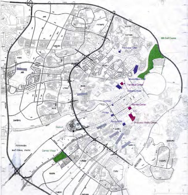
Fig.1.29 (left)
Masterplan of Abuja and its expansion from the initial plan. The overall form of street and block organisation is a system of a distorted grid laid on the topography. The streets form the grid and the blocks fill the voids between the streets, which are then subdivided into smaller systems of loops (neighborhoods).
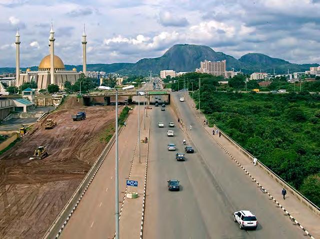
Fig.1.210 (right)
The main landmark of the city is the central Mosque. It is obvious that because the city was precipitately planned there are some areas with two contradicting situations: very well organised parts of built and open spaces against untouched and unorganised ones. These two situations are within a very small distance from each other.
Unfortunately, no sooner had the Abuja plan been completed than politicians attempted to hurry the move, disrupting the smooth development of the city” thus creating the very same shantytowns they wanted to avoid (Zacks, 2001) [Fig.1.29]. This hastened approach that the government accommodated has not only caused the development of these shanty towns/slums, it has also disrupted the main system established by the commissioned firm for infrastructural development. This infrastructural development system was based on the logic of phasing. There were six phases in general, in other words, the infrastructure would be developed and constructed in phases to allow for a smoother transition between one phase and the other (Alayande, 2006) [Fig.1.210]. In order for this phasing of the infrastructure to succeed, timing is of grave significance. Due to the government’s impatience, these shanty towns developed in areas of Abuja where the corresponding infrastructural phase has not yet begun, therefore a town with very poor infrastructure is constructed, and without prior notice, characteristics from the city of Lagos begin to emerge in the outskirts of Abuja.
One of the major flaws with Milton Keynes was implementation. The developers had enough freedom to change initial design concepts set out in the plan. In Abuja on the other hand, the developers of the city plan made sure to completely implement the master plan. However, It must be stated that there were changes made to the original plan, such as the transformation of parkways to land development, and the almost complete eradication of open space (Daramola, Aina, 2004). Nevertheless, the global implementation of the master plan was being adhered to with complete disregard to the current situation of the city. In order to blindly submit to the master plan, the developers have demolished any shantytowns that are hindering the implementation of the plan.
The major criticism in the design of Abuja was the idealistic approach of trying to predict how many people the city would accommodate. The first phase of the development of Abuja was planned for a population of 200,000 people, however in reality, that figure exceeded 1 million. This pattern of “predicting” how many people a city is able to accommodate has been repeated extensively in the design phase of many cities, yet
21
Chandigarh
an orthogonal grid amongst the hills
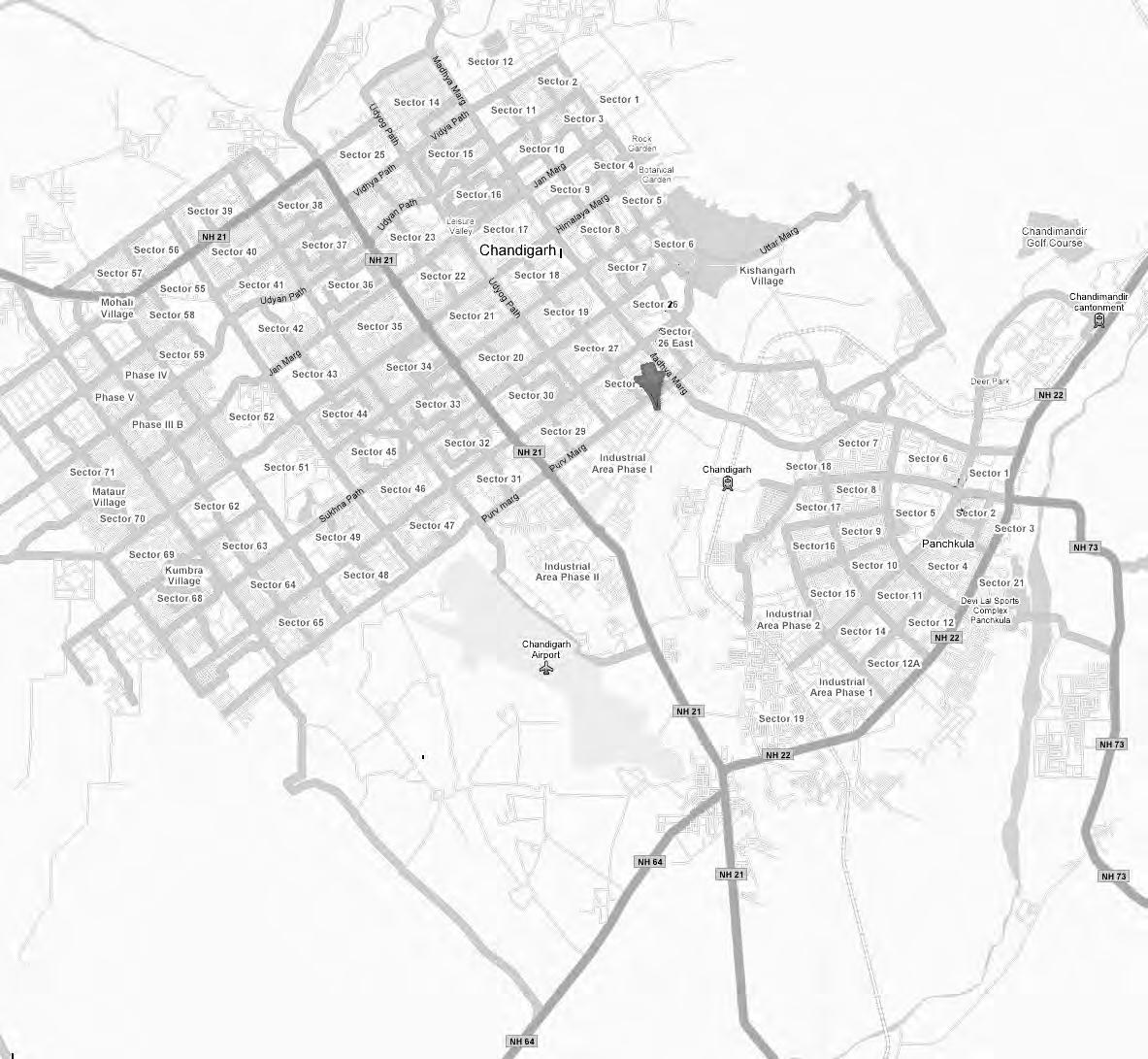
The city of Chandigarh – India is developed between two main rivers, one on the northwest and the other on the southeast [Fig.1.211]. The master plan, as well as many of the architectural projects of the city, was created by Le Corbusier in 1951, after India’s loss of Punjabi capital, Lahore. The city was made mainly to replace the might of Lahore that was lost to Pakistan in 1947.
Chandigarh was considered to represent the new expectations of the people and ideologies of its fight for independence and hence, it was designed to be an aesthetic paradigm and most of all, a social utopia. Le Corbusier’s attempt was to divide the city by function, like most of the master plans applied for cities during the Modernism period. According to the planning, the city obtained a distinctive character given from Le Corbusier, where a well-organised matrix was created out of a generic “neighbourhood unit”, which collaborates with the hierarchical circulation pattern of the seven Vs (United Nations Copyright, 2009).
The main roads V3 define a strictly rectangular grid, which encloses the neighbourhood units or sectors [Fig.1.212]. The sectors begin from one to seventy, with the lowest numbers closer to the mountains. Each sector has an introverted character; it is a self-sufficient unit which is connected to the adjacent ones via secondary roads (V4). Apart from the residential units, within every sector there are schools, shops and other essential services. The roads are designed to channel traffic away from homes.
The residential areas comprise most of the city; however there are some individual building designs by Le Corbusier that belong to the “special” part of the city. These are the “Capitol Park”, the City Centre, the Cultural Complex, the Government Museum, the Art Gallery and the College of Art. The last one includes Le Corbusier’s Gandhi Bhavan, a centre that is completely dedicated to the study of the works of the legacy of Mohandas K. Gandhi.
Fig.1.211
The city pattern is almost absolutely symmetrical with a layer of green zone interfering between the road axes. The rivers and hills surrounding the grid network define the city’s natural boundaries.
Fig.1.212
The strict rectangular grid prescribes the network morphology and the block organisation. The homogeneity of the plan leads to the method of setting a number of each block in order to identify them.
22
2 km 0 01 02 03 04 05 06 07 08 09 10 11 12 14 15 16 17 18 19 27 28 26 25 20 21 22 23 24 29 30 31 32 33 34 35 36 37 38 39 40 41 42 43 44 45 46 47 Green belt Sector number 01
2 3 4 5 6 9 8 7 10 11 12 26 14 15 16 17 18 19 27 28 25 24 23 22 21 20 30 29 38 37 36 35 34 33 32 31 40 41 42 43 44 45 46 47 39 55 54 53 52 51 50 49 48 56 58 59 60 61 62 63 64 65 57
Fig.1.213 (left)
The natural boundaries - rivers, green areas and hills - are visible, as well as the main vehicle arteries and some essential attractions of the city.
The main particularity of Chandigarh is its topographical setting; it is spread over a plain surrounded by the foothills of the Himalayas. The correlation between the hills and the two main streams define the natural edges of the city [Fig.1.213]. The green valley that is spread in the middle of the plain in an organic form which constitutes the city’s lungs. This was the only implemented urban project of Le Corbusier and one can conclude that he managed to stimulate the uniqueness of the social and topological characteristics of the designed city. Similar approaches, based on similar principles of a Modernistic philosophy can be seen in other cities around the world, such as Brasilia – Brazil.
However, it will be examined whether this design method of a clear “functionality” approach is the optimum for urban planning.
One can conclude that the rectangular grid system, comprised by loops, prevents the congestion effect that is sometimes noticed in treeform structures, thus the potential of many vehicles tending to follow common routes at the same time. On the other hand, rectangular grids maximise the material use for their construction, turning the system non-suitable for material optimisation techniques.
23
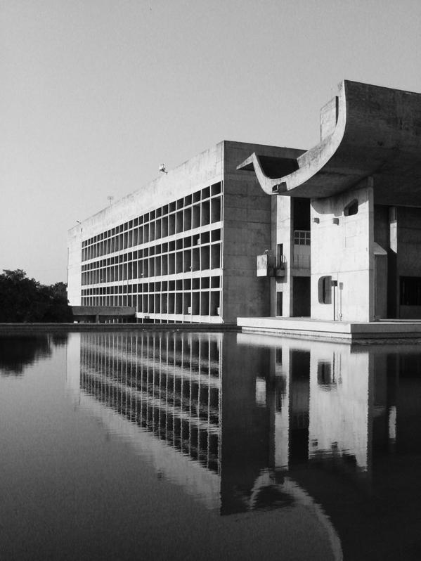
Fig.1.214 (right)
“The Palace of the Assembly” building - Le Corbusier, 1953.
conclusions
The main fault of planned cities is the planners’ perception that factors such as population count, growth rate and how the final plan will be implemented and developed are factors that can be controlled and predicted. In all the case studies examined, these predictions are consistently incorrect. Whether it was the population count of Brasilia, the growth rate of Abuja, or the implementation of the plan of Milton Keynes, the planners predicted a scenario that was far from the scenario that actually occurred. The gridded plan has developed into a design methodology that appeared to be implemented globally, regardless of topography, culture or climate. Whether it was in Milton Keynes, Chandigarh or Houston, the gridded plan seems to be resultant from a plan designed to accommodate the car and not the pedestrian.
24
1.3 Evolving cities
An evolving city has constantly changed and readjusted itself to accommodate the society that has resided within it. The city’s position was established mainly based on the natural resources available in the area, and has grown based on the functional needs of the population.
25
First occupations - Ledra
BC Coastal kingdoms were important
Paphos became the capital
timeline of nicosia
history Nicosia
The history of Nicosia begins about 4500 years ago, during the Bronze Age, when the city emerged out of wholesale settlements of local people in the area. Initially, when Cyprus was divided into kingdoms 3000 years ago, Nicosia – named as Kingdom of Ledra at the time –was a less powerful and prosperous kingdom than most of the coastal ones, thus it remained under the political rule of its neighbours. Until the Roman years, approximately 1980 years ago, Nicosia was just a small town. However, almost 2000 years later it managed to exploit its natural resources and geographical location, in the centre of the island, when it experienced a development boost. The significance of Nicosia peaked when during the years the city was developing more and more, while other areas ceased to exist.
Nicosia became the capital city of Cyprus since the 10th century A.D., when there was a movement of population from the coastal areas towards the inner part of the island. Between the 12th and 15th centuries the city was developed into a western medieval metropolis (Hadjichristos Christos, 2005).
Nicosia became the capital again Frankish period (Lusignan)
First fortification of the city
Construction of a second wall to defend from the Ottomans
Fig.1.31 (bottom left)
During the mediaeval period the main city was mostly concentrated inside the wall area. The three main arteries at that time (marked with red colour on the diagram) were used mostly for trading purpose with the other cities. Later on, more network paths were created in a rather disorganised pattern linking more areas between them. These patterns have the river on the west side as a starting point developing towards the east.
26
Bronze Age 2500 BC City-kingdoms
1050
Hellenistic period 310
Roman period 30 AD Byzantine period 330 AD Arabs invasion 647 AD 310 AD
1191
Venetian
1489
BC
AD
period
AD
Ottoman occupation 1571 AD British rule 1878 AD Independence of Cyprus 1960 AD Turkish invasion 1974 AD
Green Line
Paphos gate
Kyrenia gate
Towards
01/41/3 2/3 1 km N River Pediaeos
Famagusta gate
Towards Famagusta Towards Paphos
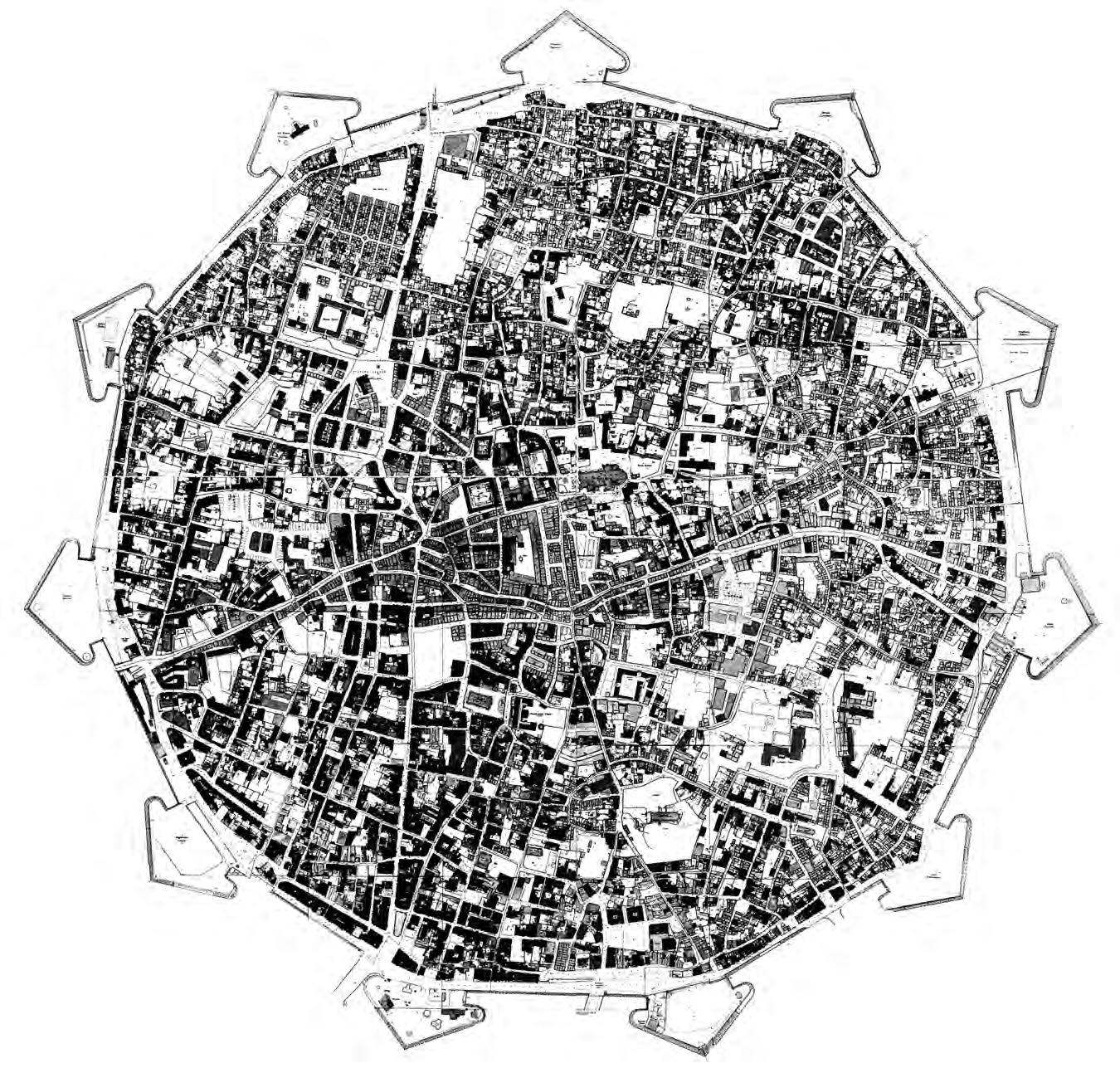
Kyrenia
Plan of the city wall. The engraving of the wall is very dominant in the plan due to the moat that the area is surrounded with. The occupation and street network within the wall is denser and more indistinct than the planning outside the wall area.
27
Fig.1.32
and growth
The following two centuries the city was under the Venetian rule, when it remained the capital city of the island. The Venetians built the city’s circumferential wall for protection from the Ottoman attacks; its plan is a circular shaped wall enclosing the whole city at the time. There are eleven ridges around the wall used as bastions in the old times [Fig.1.32], and now constitute a major particularity of the city
The wall is the most eminent sample of the city’s heritage. Prior to the Venetian dominion, the Franks had built another wall around the city, which its traces have almost disappeared through the time. Due to the multiple cultures that influenced the country in the past, the current pattern of the city – and most of the Cypriot cities – is a product of a complex urban configuration that has emerged out of consecutive layers of urban development throughout the history.
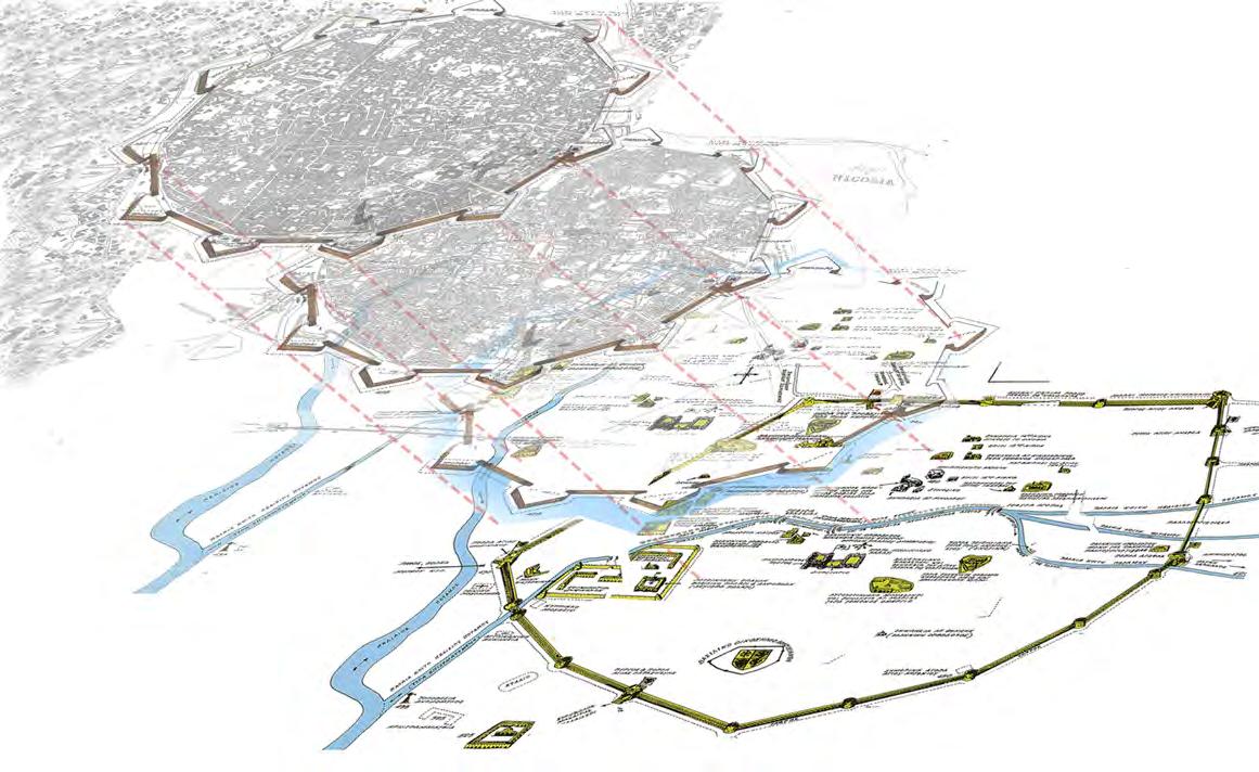
The current pattern of Nicosia demonstrates the development of the city in the last century against the historical part of the city that is inside
the wall, with the shape of the wall clearly eminent on the city plan, while the surrounding moat still remains intact. The cinquecento shape of the walls is contradictive to the irregular shape of the mediaeval pattern of the rest of the urban fabric. At the time, the walls had only three entry points; each one was facing a different direction and they were all connected to three of the main coastal cities of the island, Kyrenia, Paphos and Famagusta. Three main paths connected each entrance to another city, in a tri-radial arrangement [Fig.1.31]. During the ancient and medieval years, where trade was one of the critical wealth resources, the main road connections were built in a way to link the city with other cities that were near the sea, where the import and export of goods was taking place via the ports. Thus, apart from the three main paths, which were branching out from the Venetian wall, a new main axis was created; a north-to-south path linking the city with the port of Limassol. Therefore, at the time commercial activity was mostly concentrated along these axes, the north-to-south and eastto-west.
Fig.1.33
Several stages of the Nicosia’s growth during the time of the beginning till the end of the 20th century. The occupations are shown with the black colour and the network with the gray colour. The sharp sprawl of population outside the area of the walls is evident, especially comparing the proportion of the occupied areas during the 1981 against the ones fifty years before.
28
1932 1945 1958 1968 1981
plan
Fig.1.34
Diagram showing the palimpsest of old Nicosia: layers of patterns that formed the city during the years of the Frankish and Venetian periods. The first attempt for the city’s fortification was made by the Franks during their rule on the island, which is shown on the bottom of the four layers. With the construction of the second wall by the Venetians, the first pattern of the city was formed within the wall, when it became denser right before the expansion of the city outside the wall.
During the 19th century, when the island was under the British rule, the colonial administrative offices moved outside the wall area. This triggered the sprawl of the population to expand outside the district of the walls [Fig.1.33]. The axis from north to south was enhanced with more commercial activity during these years. This triggered a dramatic residential development outside the city wall that attracted people from the suburban areas moving into the wider region of Nicosia, leading to the diversion of social classes of the people living in the city. During the period of the British rule the manifestation of the first signs of urban intervention by automobiles led to the widening of the main arteries of the city, as well as the opening of new gates around the wall in order to create more linking paths from the inner area of the wall to the outer. Moreover, the introduction of a system based on vehicles was followed by the transformation of the north-to-south axis into the first motorway construction on the island. In the following years after the World War II, the intensive urbanisation led to the rapid urban development in the areas around the historic core and hence to the broader sprawl of the
urban fabric through a centrifugal movement of the population. The development occurred mainly along the main arteries around the city (Pattichi Elina, 2007). The building activity is characterised by two-floor buildings of small scale, whose configuration is perfectly interrelated to the one inside the wall.
The Turkish forces occupied the northern side of the island in 1974 and since then it is divided into two parts. There is a constant boundary dividing the two parts extended from the east to the west, called the “Green Line”, which constitutes the buffer zone between the two governments. The bipolar development is the main issue that occupies the urban planners, as the division maintains a complete individuality between the two parts. Thirty years ago this stimulated a sharp growth in the south part of the island, mainly due to the fact that 40% of the population at the time had suddenly transferred to that part. Most of the refugees were concentrated to the peripheral area of the capital.
29
The refugee housing was located mainly according to government land availability and not according to urban planning criteria. The sudden movement of these people triggered a steep urban growth, which takes place outwards away from the city core until today; however this happens mainly to the south part of the city, thus the radial growth forms a semi-circular shape with the northern part still remaining underdeveloped.
To his document (Hadjichristos Christos, 2005), Christos Hadjichristos, professor at the University of Cyprus, mentions that during the radial growth of both the north and south sides of the city, “the private sector turned to the suburbs which have become the centres of population and employment growth, diminishing further the sense of centrality and unity”. The centrifugal direction of the urban development occurred rapidly with an uncontrolled rate of growth, leading to the lack of urban density and public space organisation, which are crucial for the configuration of a good city with urban reference points and a
qualitative relation between the surroundings and the people. Thus, each one of the two governments of each side – the Greek-Cypriot and Turkish-Cypriot – produce different local plans for their territory leading to the discontinuity and extreme variety of the urban fabric.
The current conditions describe the city as a fast-track, vehicle based urban arrangement. In essence, after the years of British rule in the island, the private vehicle was the dominant medium of transportation; hence, until today, people’s movements inside the city are simply focused on the starting and ending points, with the intermediate route being unimportant to the observer’s view. One of the main reasons behind this situation is the homogeneity in the morphology, scale and quality of the urban fabric, especially in the areas that were developed after the period of the British rule. Furthermore, since the bulge in the automobile use, the circulation inside the city has been chiefly achieved by the use of private vehicles, due to the dispersed city pattern and the underdeveloped public transportation system.
Fig.1.35-1.36
The north part of the city (left) has been partially developed, with some areas still resembling the image of the city during the years of the war; mostly shown by the abandoned buildings that are intact since their demolition from the bombs. The south part (right) has now the characteristics of a vastly developing city that is being sprawling more and more. The old buildings have obtained new usages thus steadily becoming integrated with the whole.
30
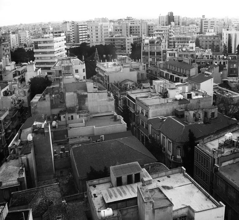
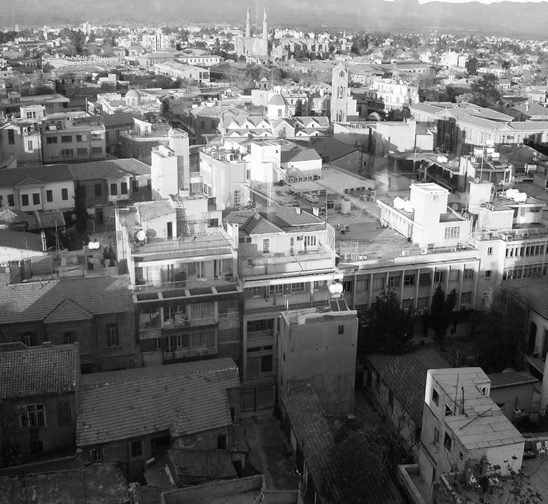
Fig.1.37
Arial view of the central area of Nicosia, during the 1960s. Before the sudden growth, the city’s expansion was mainly concentrated within the walls, with a few areas being organised around the walls.
From a pedestrian’s view it is very interesting to observe the difference between the two parts; the north part is partially developed and most of the buildings and streets are untouched, whereas the south part has developed rapidly and radially around the core since the division [Fig.1.35-1.36]. The main concern is that the decentralisation of the city growth will lead to a possible degradation. Currently there is a selected plan for the revitalisation of the city core that is destined to be implemented after a potential enosis of the two parts in the future. It is called the “Strategy for Urban Heritage-based Regeneration” (Hadjichristos Christos, 2005), which suggests the establishment of cultural touristic and educational units inside the core, aiming at a further stimulation of commercial and residential activities in the area. Moreover, the vision of this plan focuses on turning the walled city into a sustainable development resource that will constitute a centre of attraction for the residents. The circulation is estimated to form a series of concentric rings surrounding the historic core of the wall area, with the main existing arteries cutting axially through the rings and converging into the historic core. The plan also envisages of a city comprised of – apart from the prime central area inside the wall – multifunctional peripheral centres that will constitute additional functionally sustainable attraction points for the outlying regions.
31
32
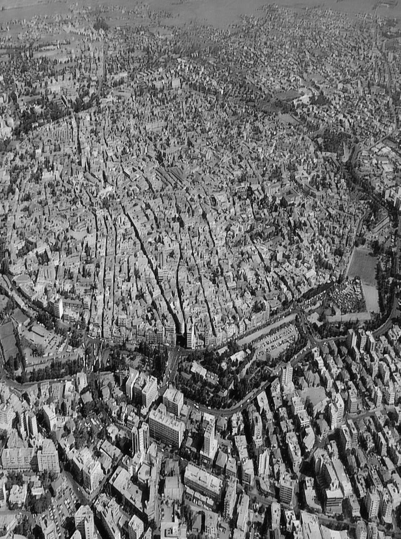
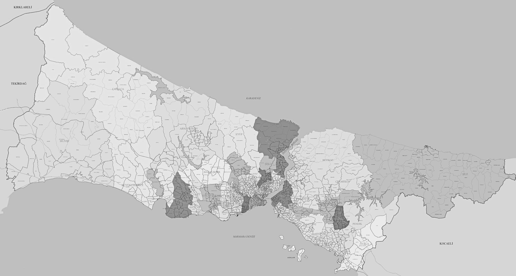
Fig.1.38 (left page)
The vast expansion of Istanbul during the modern years, compared to its initial territory. It is remarkable that the city has attracted so many people who live outside the central area. Like every big city, Istanbul’s centre has high cost on living expenses, therefore most of the people who could not afford a place in the centre have been living outside the city’s area, creating suburbs of vast areas. For a daily worker who lives in the suburbs, it can take him up to three hours drive by car to get to the centre.
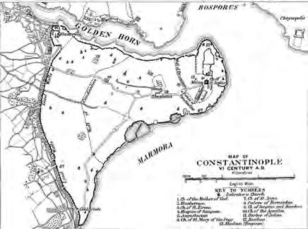
Fig.1.39 (right)
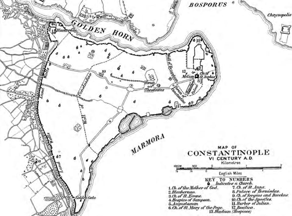
An impression of Constantinople in the 6th century. The ‘borders’ to the city are very prominantly shown by the sea walls, that border constantinople around the sea, and theTheodesian walls, that close off Constantinople from the rest of the land. In a light dotted line is the Wall of Constantine which was construced about 100 years before the Theodesian walls. The main ‘Mese’ that cuts through Constantinople is clearly visible. Along the Mese are open spaces, which are the forums. These forums served as the focal points for the layout of the rest of the street network.
Istanbul
the city’s evolution
The capital city of three different historic eras, that when combined together have spanned well over 2000 years, is the city of Istanbul.
The Megarians (Greeks) were the first to actually establish a major settlement in Istanbul about 2600 years ago. However, thousands of years before the Megarians, there existed settlements in Istanbul belonging to the Neolithics, the Chalcolithics and Phoenicians. Nonetheless, it was the Megarians that established the beginnings of the city of Byzantium (Governorship of Istanbul).
An important characteristic of evolved cities is that the new is built onto the old, it is very rarely the case in evolved cities that a city is completely demolished to begin construction of a new one (unless the city was demolished due to natural causes such as fires or earthquakes). Therefore, Ottoman Istanbul was built atop Byzantine Istanbul, which
was built atop Roman Istanbul. It was during the period of Constantine in the Roman period that the street networks’ main skeleton was laid out. The most dominant remains of Roman street network that still exists to this day is the main ‘Mese’ (main road) and a secondary road connected to it forming a Y shape (Kubat, 1999). This remnant of the Roman Empire is an example of the linearity in which the Romans laid out their streets. Using Forums as focal points, the main roads in the Roman Empire created long visual linearity to these forums, lined with colonnades and grand arches, these main roads were also used as parade routes for imperial ceremonies (Kubat, 1999) [Fig.1.39]. Open spaces in the Roman Empire were as important as the building themselves, hence the attention that was given to these forums within the city.
33
timeline of istanbul
Stone Age
6500 BC
Neolithic Settlement
Copper Age
5500 BC
Chalcolithic Artifacts
Thracian Port of Lygos
1200 BC
1000 BC
Phoenecians Port of Chalcedon
Megarians
685 BC
Settle in Chalcedon
Megarians
660 BC
Byzantium is Established
513 BC
405 BC istanbul fortification history
When compared to the Ottoman Muslim city, there are immense differences between Roman Istanbul and Ottoman Istanbul. The most interesting feature of this change was that one was not completely eradicated for the other; on the contrary, Roman Istanbul served as the ‘canvas’ that Ottoman Istanbul was constructed upon. The main difference between Roman and Ottoman cities was privacy. Mainly due to Islamic traditions, the Ottomans made a clear distinction between the public, the private and the semi-private. Therefore based on this logic, all of the open spaces of the Roman period, such as forums, were built upon. Yet, that did not eliminate the notion of social gathering, instead the forums were simply replaced with interiors of great mosques and their connected buildings (better known as Kulliyes). These Kulliyes did not create a completely new urban space; alternatively, they simply created an urban space within a preexisting urban space (Kuban, 1996). The most noticeable attribute of the Ottoman street network is its Organic layout. Compared with Romans’ linear Mese, the Ottoman religious buildings have an absence of any right-angled reference to
the main roads, while the streets recurrently changed their widths consequently creating cul-de-sacs throughout the city (Kubat 1999).
In modern days, the use of the cul-de-sac is frowned upon, because it is simply understood as a dead end street; however, in Ottoman Istanbul, the cul-de-sac was the principle tool to differentiate the public from the private. The cul-de-sac was not a dead end road; it was a semi-private space that connected several houses with one another. Kubat describes Ottoman Istanbul as a “’molecular’ city, composed of functional elements linked to each other by irregular veins” (1999). In this case, the ‘Mahalle’ or the urban quarter is the molecule, which can be broken down further into ‘cells’ that are the cul-de-sac.
As the Ottoman era began to break down, and the Tanzimat reform attained control, the westernized street network was introduced, the grid. Although the Roman street networks were famous for their linearity, they were not a grid; they were generated through a series of focal points and visual continuity.
34 600 BC Byzantinium Walls 330 AD Constantinan Walls 330 AD Sea Walls 408 AD
Theodesian Walls
Persians Control Byzantium
Control Byzantium
Spartians
Romans
population increase during the time
Control Constantinople, declared Capital of Ottomans
Modern Turkey Tanzimat reforms begin
AD
today’s expansion
On the other hand, as the Tanzimat came to power, the cities urban layout was transformed. Modern Turkish planners accommodated Western gridded, ‘rational’ street networks, over the ‘irrational’ street networks of the past. As the 20th century got underway, Istanbul’s organic layout was replaced with a gridiron street network support by an ordered traffic system (Kubat, 1999). The previously narrow Ottoman streets were widened, the heights of the building facades were increased and cul-de-sacs were altered into thoroughfares. The main flaw with this gridded street network was that it lacked any homogeneity with respects to the organization of buildings and spaces.
Although there are great differences between the street networks of the Roman, Ottoman and Modern Turkish eras, each period had its advantages and disadvantages. However, one might notice that the city experienced a shortage of cohesion during modern times; this may be attributed to the introduction of the gridded street network; however, that does necessarily mean that there is a flaw with the gridded network, the flaw lies with supposing that the gridded network is a global network, that complies to any urban fabric it is applied to.
35 40,000 330 550,000 530 300,000 715 400,000 950 150,000 1200 36,000 1453 80,000 1481 600,000 1566 874,000 1885 1,000,000 1900 1,470,000 1960 2,133,000 1970 5,475,000 1985 6,630,000 1990 8,803,000 2000 11,372,000 2007
Antigers Control Byzantium
BC Romans Byxantium is Attached to Rome 74 BC
318
Byzantium Re
Con-
330 AD Romans Constantinopolis Capital
Rome 400 AD Crusadors Control Constantinople 1204 AD Byzantions Control Constantinople 1261 AD Ottomans
named to
stantinopolis
of
1453 AD
1839
conclusions
Unlike planned cities, evolving cities were established as a bottom up system that developed based on function, population and need. In the early periods of evolving cities, natural resources were the main attraction to why a city was founded in a particular area rather than another. The layout of the paths within the city were developed based on the functions of different areas throughout, such as the focal points in Istanbul that determined the layout of the main paths. The street network of the city was also heavily influenced by the topography. It must be noted that an evolving city des not stop growing, in almost all walled cities, the city developed well beyond its walls; this is clearly visible in both Nicosia and Istanbul. However, the city constantly altered and reworked its plan to better fit whatever period or culture the city was sustaining.
36
1.4 Mono/poly-centric cities
Centrality within a city is crucial in determining different aspects that range from the success rates of different businesses, the probabilities and effects of congestion, and the importance of transportation within the city.
37
Monocentric model:
1 main centre
9 Transit paths
Polycentric model:
10 different centres
45 Transit paths
monocentric and polycentric models
Monocentric cities have developed through street and public transport networks, whereas polycentric cities emerged from the accelerated boost of automobile use. In monocentric cities the central business district is shaped by radial transport networks that link the surrounding suburbs with the centre. The central activity is purely commercial [Fig.1.41]. The specific structure offers a great advantage of exploitation of the radial networks in public transportation. However, there are serious ramifications concerning the sustainability of transit in the city, as there are long-distance routes appearing due to the separation of residential and employment land uses and there are increased transits within the city that increase the congestion in certain points.
The development of the cities had a drift after the automobile was introduced in people’s lives; the peripheral urban ring had gained increased accessibility due to the motorway networks. Initially as the cities were growing they were facing many issues such as rising land costs, long routes for people travelling to their work, frequent
congestions on certain points, decreased access to open space and the countryside, increased need for costly investments in new infrastructure, increased pollution that induced health problems and increase of moral degeneracy and crime. As adaptive organisms, cities started developing multiple secondary cores with concentrated activity within the metropolitan area, referred to as “subcentres” or “satellite cities” that will be examined later on. Consequently, the urban core was steadily decentralised; new economic activity areas had emerged that constituted supplementary attraction poles for the city. The particular type of urban forms is described as polycentric cities. The environmental impact of the sharp economic growth and great mobility that were followed by the polycentric pattern was tremendous. Most of the transit type is car-based and the distances are long; this entails frequent car use, high fuel emissions and more energy required.
Fig.1.41
The mapping of the monocentric and polycentric transit patterns is shown to the diagrams below: in the monocentric model nine residential sectors are linked directly to one centre through nine transit paths. In the polycentric model nine secondary centres are added to each of the residential sectors, apart from the main one. Every centre is linked to the main one and to all the other centres thus creating 45 different transit paths. These diagrams represent a generic pattern of cities; monocentric cities do not strictly follow the diagrammatic way but manifest more deviated paths due to other parameters that define the pattern. Accordingly, in the polycentric model the amount of links between the centres are more than the one in real cities, as many of them are merely unnecessary.
38
Fig.1.42
The map shows the plan of the “European Ecocity”. The European Union envisages that in the future all european regions with multiple centres will organise into collaborative economic clusters that will form sustainable networks of access, mobility and green infrastructure [Ref.2].
P >= 5.000.000
P: 2.000.000 - 5.000.000
P: 750.000 - 2.000.000
P <750.000
New global integration zones
the european polycentric plan
However, many arguments have risen concerning the environmental implications of the polycentric cities, as these arguments assert that these cities can easily readjust their pattern in such a way that polycentricity can lead to positive results. For instance, a policy of “concentrated dispersion” can be applied (Smith A. Duncan), which means that a lot of decentralised high-density activities settle around significant public transportation nodes. This policy can also be applied in cases where monocentric cities can constitute smaller parts of a larger polycentric network of different urban arrangements. Such a theory has been addressed by many European cities [Fig.1.42], planning to follow the implementation of a large-scaled “polycentric sustainable urban network” (Crossley David, 2007).
The urban centres of monocentric and polycentric cities have a direct relation with the business and public service activities of the cities. There are two types of centres in polycentric cities, as mentioned above: the subcentres and satellite cities. Subcentres are concentrations of employment or commercial services constructed within the continuously built up area, however they are distinct from the central business district. Satellite cities are new developments or major expansions to existing settlements that are separated from the main metropolitan core by belts or rural land.
39
the effects of polycentric cities
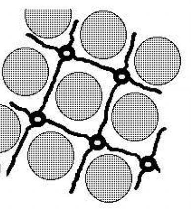
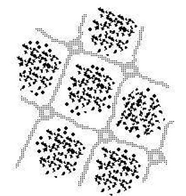
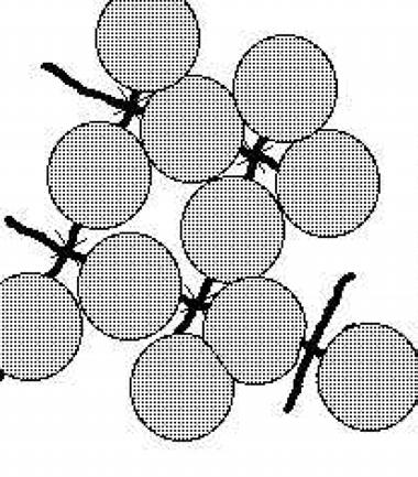
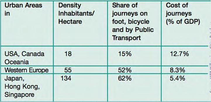
In 1944 Patrick Abercrombie designed the most influential plan of decentralisation, “The greater London plan” (Sorensen André, 2001). In order to solve the issues of pollution and congestion, he proposed a “green belt” that would be ringed around London, thus forcing people to move to new and expanded towns outside the “green belt”. This plan entailed that London would remain a sprawled city but it would expand outside its boundaries. However, it has been noticed that cities with a high density consume lower rates of gasoline [Table.1.44]. Cycling and walking become a viable option for many trips, hence reducing the amount of automobile use. Moreover, higher density forms allow a more efficient operation of public transport systems. One clever strategy would be the development of nodes with concentrated mixed use that would satisfy most of the needs within the local areas, hence reducing the necessity for trips to the city centre. Furthermore, the nodes would be connected to each other and to the main city centre by public transportation; this allows high levels of mobility yet reducing the overall automobile usage.
The largest part of Houston has been built on a forest land and along the gulf coastal plain. The flatness of the area’s terrain favoured the expanded sprawl of the city that has a vast impact on the today’s city pattern.
After the car use was initiated in 1920 the growth pattern of Houston had been steeply uplifted, when after the World War II the growth took a different direction. Until the early 1970s the city pattern was still unidentified and obscure in terms of its urban character. The great differences of the ways the city evolved through the time led to a situation of uneven qualities in the city pattern. Until the 1940s the atmosphere was characterised by a confined, homogeneous urban development with the network pattern been engraved following a regular grid system. At the time the network pattern of the city was mainly transitoriented (Smith A. Duncan) with the basic arteries serving the traffic towards and outwards one central area.
Fig.1.43
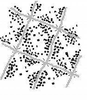
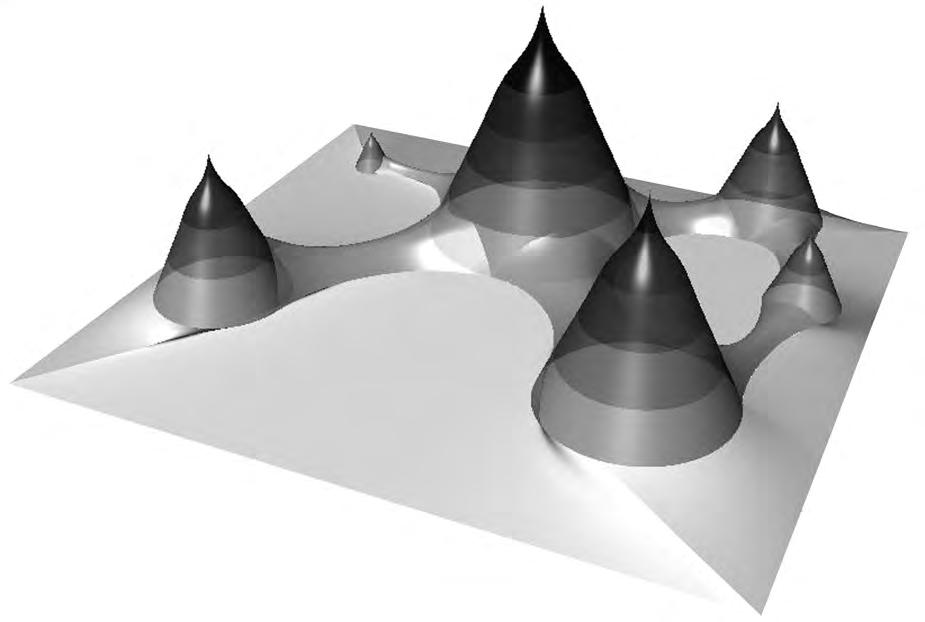
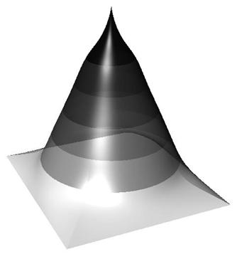
Digital models simulating the centrality character of monocentric and polycentric cities. The monocentric model shows a uniform quality; the density grows as the distance to the centre decreases. The polycentric model reveals the hierarchical arrangement of the several centres of a city. The peripheral area around each centre is partly integrated with the peripheral area of the other one.
Table.1.44
In dense urban patterns most of the transit is accomplished by public transport. This reduces the costs for transportation. For instance, in Manhattan 82% of the residents travel to work either by public transit, bicycles or on foot [Ref.3,urban data].
40
Fig.1.45
A system of concentric circular arteries that are crossed by axial main arteries that converge to the main centre of the city is the basic transit system of Houston. It is very beneficial for polycentric urban patterns. Specifically the concentric circles are useful for the circumferential circulation between the areas around the centre and the perpendicular roads for direct transit in and outside the centre.

Central Area Area close to the centre
Area far from the centre
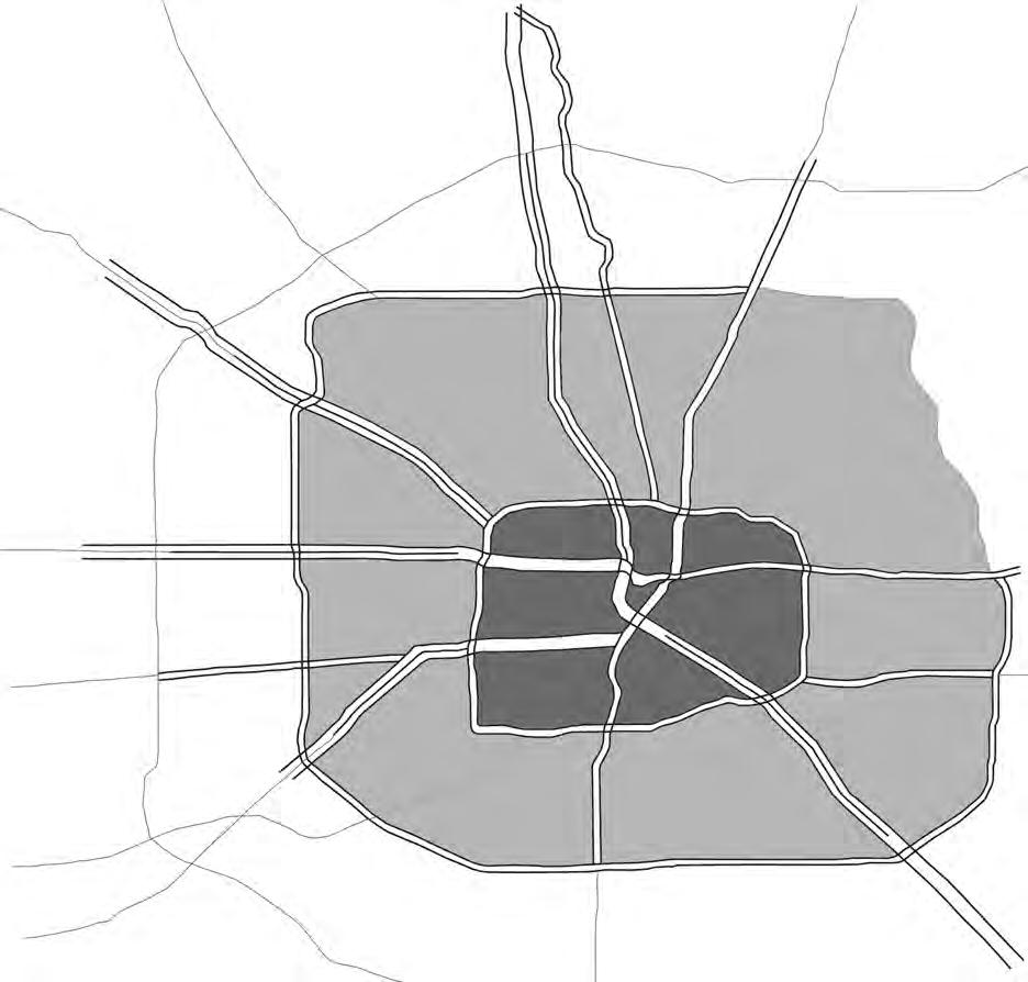
The [Fig.1.45] shows that the main road type of network resembles a tree pattern with the rest of the secondary street patterns form a loop system enclosing the neighbourhoods. The typology of this pattern describes a suburbs-surrounding-a-single-core model, which is almost entirely based on building more roads further and further from the “core”.
On the other hand later on, until the late 1970s, the city evolved in a rapid rate, sprawling over large areas and merging with the suburban region, thus increasing the heterogeneity of spatial occupation. Right after the beginning of the 1940s a new plan was introduced, which involved a proposal of a new system of main roads forming concentric rings around the centric area, leading to the discongestion of the primary main arteries and hence to the redistribution of the vehicle accumulation in certain areas of the road network.
41
houston
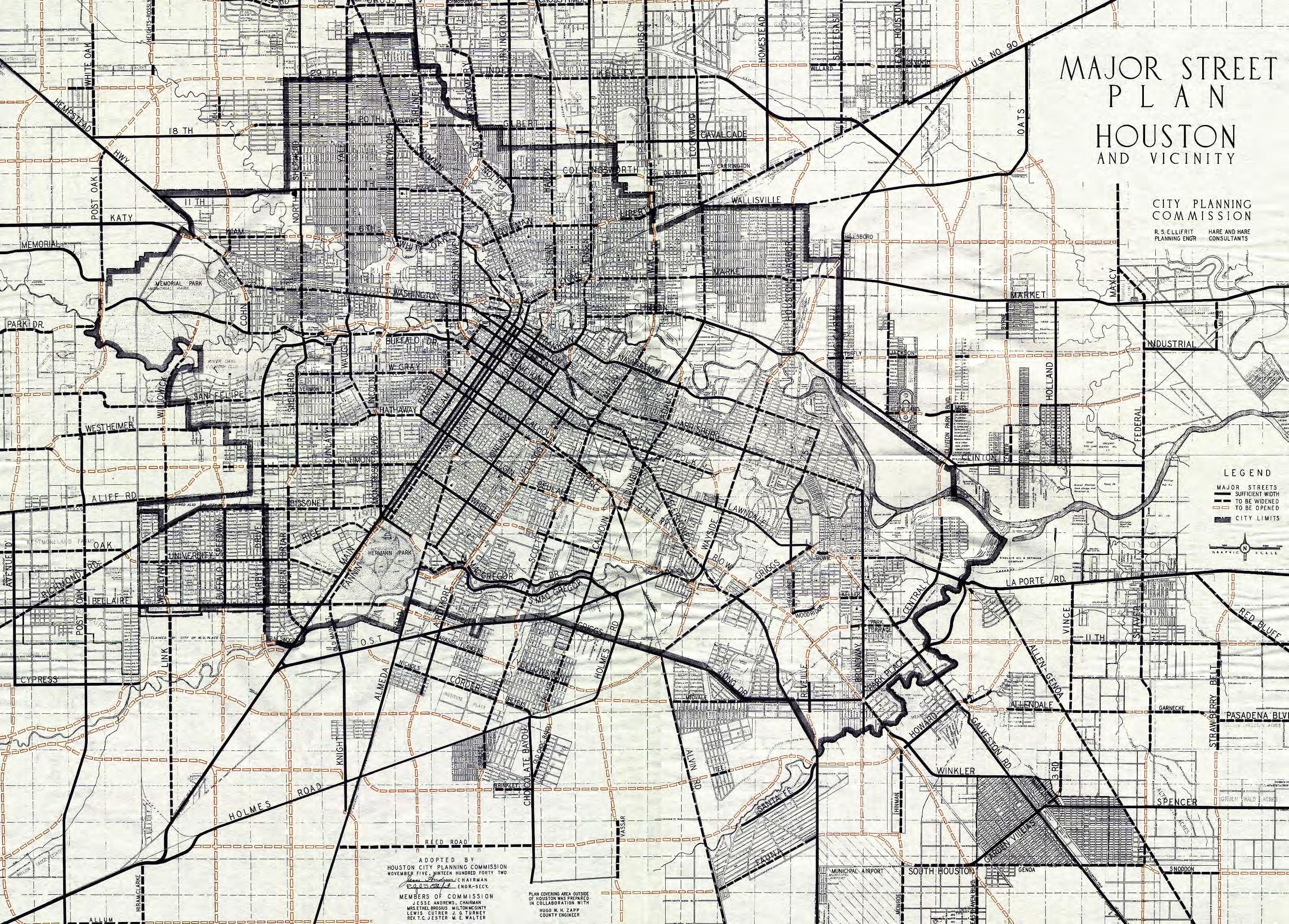
Fig.1.46 (left page)
The rapid sprawl and the merging with the suburban region during the 1970s was the basis for the polycentric character of the current city pattern. The main centre is the red circle enclosed in the road loop and around it there are some of the emerged sub-centres of the city.
Since then the city keeps evolving in an extreme density; nowadays Houston is characterised by three main definitions: Palimpsest, Pluralism and Polynucleation (Papademetriou C. Peter, 1990). The city has evolved in a way that the street patterns form a radial arrangement of several concentric rings, with the areas in between comprised by a social mosaic of a great diversity in social classes. The massive congeries of population concentrated in the city led to the composition of new, decentralised areas, which they gradually became autonomous individual cores [Fig.1.46]. The aim of the city’s evolution was the development of these cores into small individually sustained towns, which would be surrounded by green areas and connected to each other by a transit system. Many European cities are planning to follow the same plan right now; of the polycentric sustainable city
Houston is characterised by a torrid climate, flat terrain, great distances and lack of apparent order (Fox Stephen, 1990). In fact, Houston is the largest city in the U.S. without any zoning code, as
it has been rejected for public planning by the habitants four times between 1929 and 1962. The main problems derive from the lack of organisation and responsibility on behalf of the government. All the public spaces in the city were produced after many prodding actions that involved donations. The architectural morphology expresses an array of typological and generic intentions rather than a conscious specific architectural plan. Therefore, the historical elements are now disused and disconnected to the contemporary tissue.
The city has been traversing through the time by adapting to its emergent behaviours; something inevitable for most of the polycentric cities. As Stephen Fox mentions in his document (Fox Stephen, 1990), Houston’s most attractive characteristics are openness, energy and optimism; these terms had been the reason why the mess of the city is also the source of its scandal and charm.
43

44
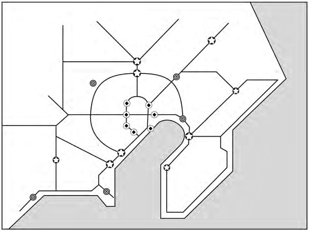
Fig.1.47
Central Tokyo rail system and main stations in 1930. The private rail lines travel from all around the country to a few main stations, consequently creating the spontaneous development of the sub-centers in Shinjuku, Shibuya and Ikebukuro. Although these three developments are considered as sub-centers, there proximity to the main centre (around Tokyo station), does not eliminate their possibility of being integrated within the main centre.
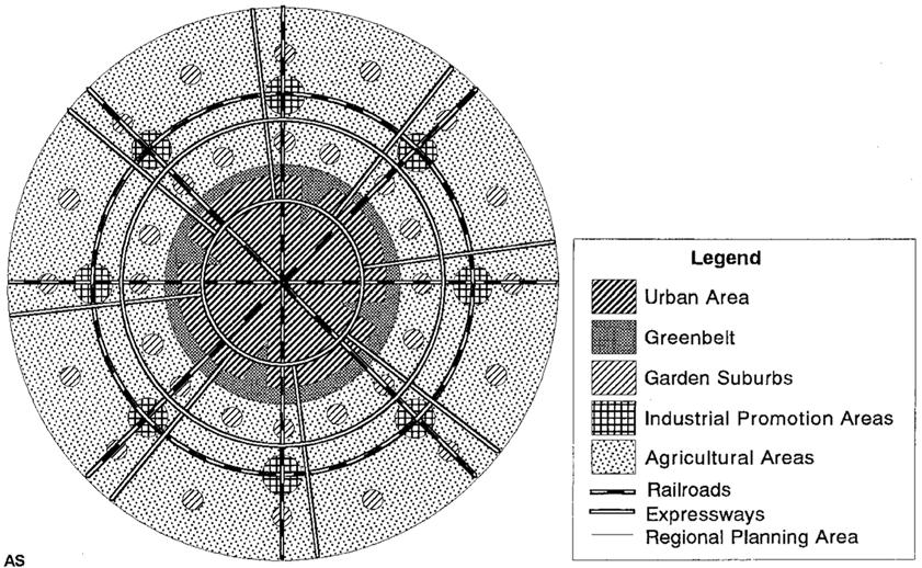
Fig.1.48
Kanto region metropolitan structure plan, 1940. This plan was very similar to Ebenezer Howard’s ‘Social City’ scheme. The organization of this plan may be idealistic in its formal distribution, however it does restrict urban growth within the urban area, and promote urban development out of the city.
Throughout the 1900’s, the Japanese government was under heavy strain to control the increasing population of the city of Tokyo. The rapid growth of Tokyo’s population was caused by two main factors. The first was due to the First World War’s sudden industrialization that enabled the growth of the streetcar and rail systems [Fig.1.47].
This enabled the workforce to travel long distance to and from the city. The second factor that affected rapid population growth was the Kanto earthquake in 1923 that destroyed 60% of the city. The massive destruction resulting from the earthquake promoted the rapid population of suburban districts (Sorensen, 2001). The government’s priority after the earthquake was the reconstruction of Imperial capital [Fig.1.48]; therefore all other districts were put second on the government’s agenda of reconstruction. However, that did not preclude the main sub-centres of Shibuya, Shinjuku and Ikebukuro to develop (Sorensen, 2001). This unprompted development of these three main sub-centres was mainly
SubcentresandSatelliteCities
CentralTokyorailsystemandmainstationsin1930.
due to the second factor mentioned above. The establishment of these sub-centres was crucial for the government’s future plans of relieving the main centre of Tokyo from elevated population density.
linesinitiallyeachhadtheirownterminusinthecentralpartofthecity,at Shimbashi,Ueno,andIidabashirespectively(seeFigure1).Justbeforetheturn ofthecenturytheYamanotelooplinewasbuilttothewestofthethenbuiltup areasothatfreighttrains,particularlythosecarryingsilk,Japan’smaininternationalexport,fromcentralHonshutotheportatYokohama,couldrun straightthroughtotheportwithoutunloadinginthecity.Inthe nalphaseof theTokyoCityImprovementProjectcompletedin1919,theloopwasjoinedon theeastsidebymakingaconnectionthroughtheurbancorefromUenoto ShimbashiandTokyoStationwascompletedin1915toserveasthenewcentral station.Thebuildingofthenewcentralstationsolidi edthestatusofthe MarunouchitoGinzaareaasthecapital’sCBD.Inthe1920sanewtrainservice, thenowfamousYamanoteLine,wasestablishedtocircletheloop.Thisstructure creatednaturalgrowthpointsattheintersectionsofthemainradialswiththe peripheralloop.
Tokyo’s Central area was established on account of the National Railway System being radially centred on Tokyo. This centrality also added to the population density of the city. in the case of Tokyo, the public transport system heavily influenced the sites of new sub-centre as well as the hierarchy of the importance from one sub-centre to the other. As a result of the high influx of commuters travelling back and forth from the city, the main interchanges were set upon the three subcentres that developed on account of the Kanto earthquake. Owing to the large amount people interchanging at these stations, entertainment as well as restaurants quickly developed transforming these districts into major sub-centres (Honjo, 1978).
Asecondfactorcontributingtotheestablishmentofthesubcentreswasthe purchaseoftheprivatelybuiltTokyostreetcarsystemin1911bytheTokyo municipalgovernment.Thestreetcarsystembythistimeformedacomprehen-
45
13
Figure1.
tokyo
SubcentresandSatelliteCities
Figure3. The rstcapitalregionimprovementplanof1958,andtheFourthNCRDP of1986.
In Peter Abercrombie’s Greater London Plan, he proposed that the best solution for London’s overcrowded population was decentralization. Therefore to instigate this notion of decentralization, a ‘Greenbelt’ would be wrapped around the city to restrain any urban development within the city, and therefore force the development of urban towns or satellite cities outside of this ‘Greenbelt’ (Cherry, 1988). In order for this concept to be successful, one must understand what the predicted results are. In this case, they are one of two:
1. Create towns outside the main city, where residents must still commute to the city for work. In this case, a public transport system is essential to transfer commuter to and from the city.
2. Create towns outside the main city that are self-sufficient. In other words, the residents do not have to travel to the city anymore; everything they need is within the satellite town/city they are in.
Figure3. The rstcapitalregionimprovementplanof1958,andtheFourthNCRDP of1986.
One of the first plans drawn up to attempt to restrain the urban development of Tokyo did not greatly differ from Ebenezer Howard’s ‘Social City’ scheme (Howard, 1898,1985) [Fig.1.48]. This plan was later developed into the first plan in a series of four plans to constrain Tokyo’s urban growth. In 1958, a plan was drawn up, which was influenced by both Howard and Abercrombie, to wrap the existing built up area of Tokyo with a ‘Greenbelt’ and induce the growth of satellite cities around Tokyo. However, due to government bureaucracy that is too complex to get into, the ‘Greenbelt’ plan was never implemented. Instead, the fourth plan finalized in 1986, which replaced the ‘Greenbelt’ with suburban developments, was the one that was implemented (Sorensen, 2001) [Fig. 1.49,1.410].
Fig.1.49
The first plan of 1958, the green belt clearly rings around the then existing built up area, restricting any more urban development within the main central area, thus instigating the development of satellite cities away from the main city.
Fig.1.410
The fourth and final plan of 1986. The greenbelt has been replaced with suburban development area; satellite cities that were in the original plan of 1958 pertained their position. Analysis of this map leads one to conclude that urban development will add to the population of Tokyo rather than relieving it.
46
17
Fig.1.411
Third long term plan for the Tokyo metropolis. The close proximity of the sub-centres to one another makes it seem that there integration with one another is inevitable. One may look at this plan and understand Takashi Onishi’s argument.

Tsuchiura
Omiya
Urawa Kashiwa
Tokorozawa
Ikebukuro
Shinjuku
Shibuya
Osaki
Yokohama/Minato Mirai
Ueno/Asakusa
Kinshicho/Kameldo
Coastal Subcentre
Kisarazu


As a result of the congested centre, a plan was drawn up in 1970 to transfigure an overcrowded city into a ‘multi-polar structure [Fig.1.411].’
A plan called the ‘Third Long Term Plan’ was drawn up to develop four new sub-centres that would be considered as ‘business core cities,’ these sub-centres would generate employment opportunities, relieving population growth away from the main centre (Japan National Land Agency, 1987). This plan further strengthened the transformation of the Kanto plain into an expansive built up area, where growth points that should have originally been satellite cities, are now sub-centres adding to the continuously growing number of sub-centres within the metropolis area.
The original plan in 1968 seemed like the most efficient plan to restrict urban growth within Tokyo; the elimination of the ‘Greenbelt’ and the continuous development of sub-centres have created negative results with respect to the original intention to constrain Tokyo’s population growth. Takashi Onishi (1994) argues that so many sub-centres are simply adding to the overall congestion of the city. The sudden growth of several main sub-centres around the centre will in due time, become engulfed within the main centre and act as one large Central Business District; by doing so, any original plan of relieving Tokyo from overcrowded population will never be fulfilled (Tanaki, 1990).
47
Kumagaya
Chiba
Narita
Funabashi
Kawasaki
Yokosuka
City
Principal Cities Business Subcentres
Odawara Atsugi
Subcentres
conclusions
Unlike planned cities, evolving cities were established as a bottom The advantages that polycentric cities have over monocentric ones are plentiful, however they mostly revolve around functionality. Setting aside the problems of congestion and growth in monocentric cities, issues such as the decline of businesses throughout the city are ones that hinder both growth, as well as the economy of the city. It is crucial to note that polycentric cities are categorized into wither sub-centres or satellite cities. The example of Tokyo indicates that although the intention of its sub-centres was to create multiple centres that were both dependant and independent, they failed in fulfilling their task of creating different partially self-sustaining centres. If Tokyo had implemented its green belt plan, the green belt would have physically hindered the growth of the different centres, and so would have been a successful scenario.
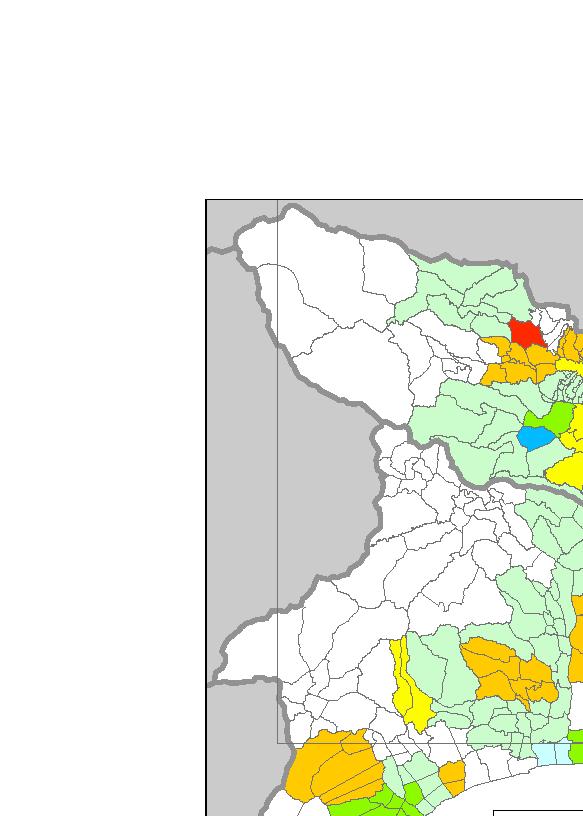
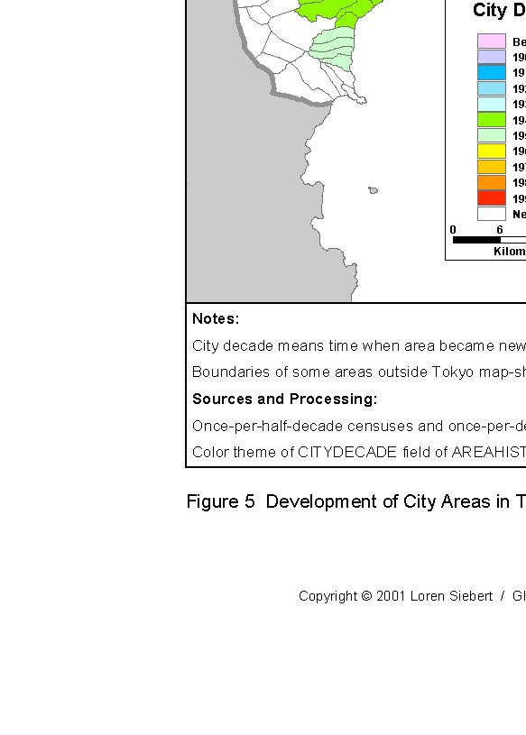
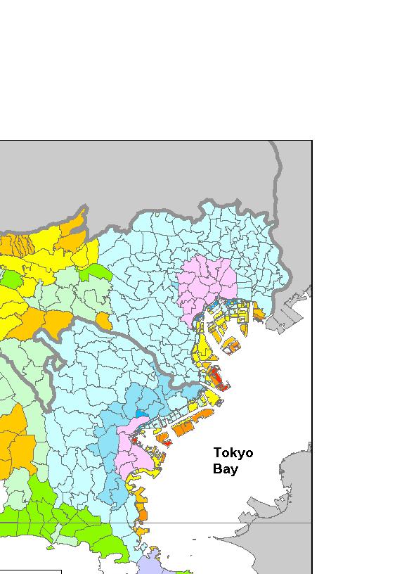
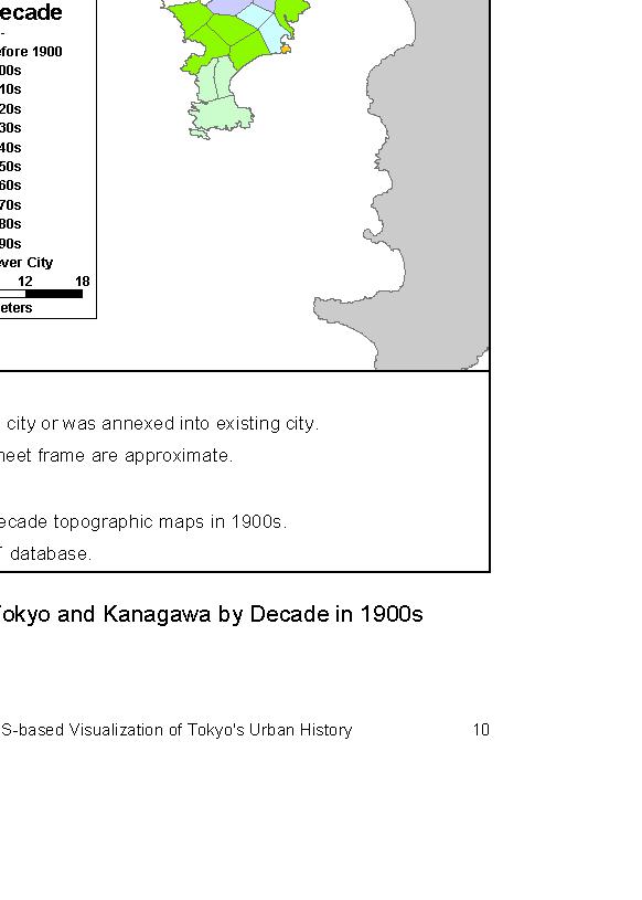
Fig.1.412
Development of city areas in Tokyo. The map clarifies the growth of Tokyo by representing the different phases in time where towns have grew into cities. The map shows how many towns developed into cities at around the same time, indicating a simultaneous growth of different sub-centres.
48
1.5 Densities
Although the density of a city plays an important role in determining the probabilities of congestion, growth and consumption, it also plays a pivotal role in the energy efficiency of the city’s fabric.
49
population densities
Apart from the fact that master plans have been applied under defined rules, they have been adjusted to some pre-existing conditions. Hence, the final scale and density of each city differs according to the respective parameters.
Population density is being estimated by the number of people per unit area – usually per square kilometre. It is often compared to the overall occupied area of the respective territory measured. Comparing some of the metropolises of the world between them, very interesting conclusions would be extracted [Fig.1.51a-d]. After a research
conducted by Newman and Kenwothy (1989) measuring the population densities of several cities around the world, they concluded that there are many correlations between aggregate population density and private vehicle use. Nevertheless, this correlation is not the only factor that contributes to the variations in urban form. Although high density encourages mixed land uses and many public transport access points, thus a more sustainable function of the city, there are more factors that control the final pattern of urban fabrics; these can be for instance economic factors such as income and fiscal policy.
Fig.1.51a-d
The diagram shows the population densities of four metropolises of the world that differ significantly between each other in terms of density; Shanghai, Tokyo, Los Angeles and London. Los Angeles is the most sprawled city between the four, whereas Shanghai is the densest one of all.
50 21,740 inhabitants per km2 12,630 inhabitants per km2 3,050 inhabitants per km2 11,536 inhabitants per km2
shanghai tokyo los angeles
20 km 20 km 20 km 20 km
london
Fig.1a Fig.1b
Fig.1c
Fig.1d
Table.1.52
The table shows the first 44 cities in the world with the biggest density; Density is defined as the ratio between the overall population to the land area of the city. The two first cities both belong to India. Mumbai is the densest city in the world and outweighs the second one, Kolkata.
City Country Population Land area km2 Density people/km2
The [Table.1.52] shows the population density of the biggest cities in the world, from the densest one to the sparse. Mumbai – India is the most condensed city in the world, with the biggest ratio of people living within its total area. The second one is also an Indian city, Kolkata. Comparing Mumbai, which has 14,350,000 people living within an area of 484 sq. Km and London with 8,278,000 people in a 1,623 sq. Km area, one can imagine the dramatic difference of the morphological or functional character of the two cities.
51
1 Mumbai India 14,350,000 484 29,650 2 Kolkata India 12,700,000 531 23,900 3 Karachi Pakistan9,800,000 518 18,900 4 Lagos Nigeria13,400,000 738 18,150 5 Shenzhen China 8,000,000 466 17,150 6 Seoul/Incheo n South Korea17,500,0001,049 16,700 7 Taipei Taiwan 5,700,000 376 15,200 8 Chennai India 5,950,000 414 14,350 9 Bogota Colombia7,000,000 518 13,500 10 Shanghai China 10,000,000 746 13,400 11 Lima Peru 7,000,000 596 11,750 12 Beijing China 8,614,000 748 11,500 13 Delhi India 14,300,0001,295 11,050 14 Kinshasa Congo 5,000,000 469 10,650 15 Manila Philippines14,750,0001,399 10,550 16 Tehran Iran 7,250,000 686 10,550 17 Jakarta Indonesia14,250,0001,360 10,500 18 Tianjin China 4,750,000 453 10,500 19 Bangalore India 5,400,000 534 10,100 20 Ho Chi Minh City Vietnam 4,900,000 518 9,450 21 Cairo Egypt 12,200,0001,295 9,400 22 Baghdad Iraq 5,500,000 596 9,250 23 Shenyang China 4,200,000 453 9,250 24 Hyderabad India 5,300,000 583 9,100 25 Sao Paulo Brazil 17,700,0001,968 9,000 26 St Petersburg Russia 5,300,000 622 8,550 27 Mexico City Mexico17,400,0002,072 8,400 28 Santiago Chile 5,425,000 648 8,400 29 Singapore Singapore4,000,000 479 8,350 30 Lahore Pakistan5,100,000 622 8,200 31 Recife Brazil 3,025,000 376 8,050 32 Istanbul Turkey 9,000,0001,166 7,700 33 Dalian China 2,750,000 389 7,100 34 Khartoum Sudan 4,000,000 583 6,850 35 Rio de Janeiro Brazil 10,800,0001,580 6,850 36 Monterey Mexico 3,200,000 479 6,700 37 Bangkok Thailand6,500,0001,010 6,450 38 Osaka/Kobe/ Kyoto Japan 16,425,0002,564 6,400 39 Guadalajara Mexico 3,500,000 596 5,900 40 Athens Greece 3,685,000 684 5,400 41 Ankara Turkey 3,100,000 583 5,300 42 Madrid Spain 4,900,000 945 5,200 43 London UK 8,278,0001,623 5,100 44 Tel Aviv Israel 2,300,000 453 5,050 45 Sapporo Japan 2,075,000 414 5,000 46 Buenos Aires Argentina11,200,0002,266 4,950 47 Moscow Russia 10,500,0002,150 4,900 48 Barcelona Spain 3,900,000 803 4,850
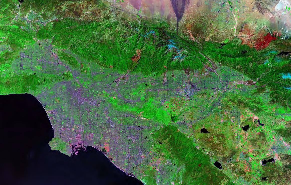
los angeles
According to the figures, Los Angeles covers a larger surface area compared to Shanghai, however, the population of Los Angeles living within one square kilometre is approximately one seventh of the Shanghai’s one. The images [Fig.1.53,1.55] show the difference of the centrality character between the two cities; Los Angeles central area is condensed with middle-height buildings whereas Shanghai’s centre covers a much larger area with high buildings of imposing character
The sectional diagrams [Fig.1.53,1.55] show the way the two cities form the skyline. The diagrams compare the measurements of each city’s development; i.e. for Los Angeles it can be concluded that there is a large extended area – which is mostly occupied by residential function – with relatively low-height buildings and a condensed centre with significantly higher buildings, however not as high as the taller buildings that exist in most of the American Metropolises. The main reason for this homogeneity in section derives from infrastructureal reasons, i.e. the fact that the area is seismically active and that its topographical feature is described by a plane surrounded by mountains.
Fig.1.53 (top)
The differentiation in density of the Los angeles urban tissue can be seen in the satellite image; the purple colour represents the built environment whereas the empty land is shown by the green colour. However, there are not highly dense areas according to the intensity of the purple colour.
3,050 inhabitants per km2
Fig.1.54 (bottom)
The central areas within the city of Los Angeles are easily recognisable because of the sharp increase of buildings’ height in those areas, compared to the rest of the urban fabric. Most of the populated areas are spread on flat terrain, where the areas that are near the hills have lower densities.
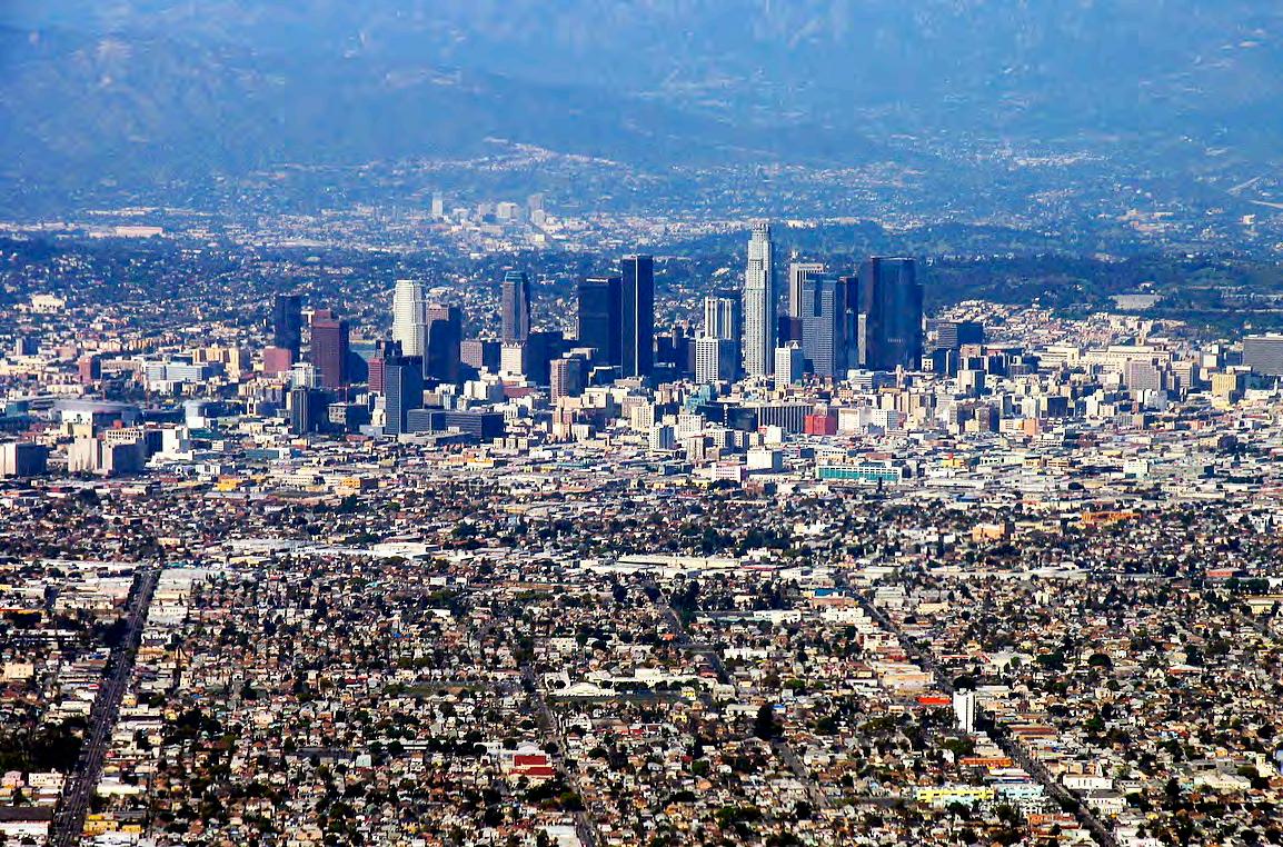
52
20
km
Fig.1.55 (top)
The intensive purple colour shows that Shanghai is a highly dense city. Most of the population is concentrated into the main core and the transition from the core to the surrounding area is abrupt.
Fig.1.56 (bottom)
Shanghai’s skyline is homogeneous throughout the city; a combination of high-rise buildings and open space forms the urban pattern, whose edges can be easily recognisable as the buildings are interrupted by the surrounding rural areas.
20 km
21,740 inhabitants per km2
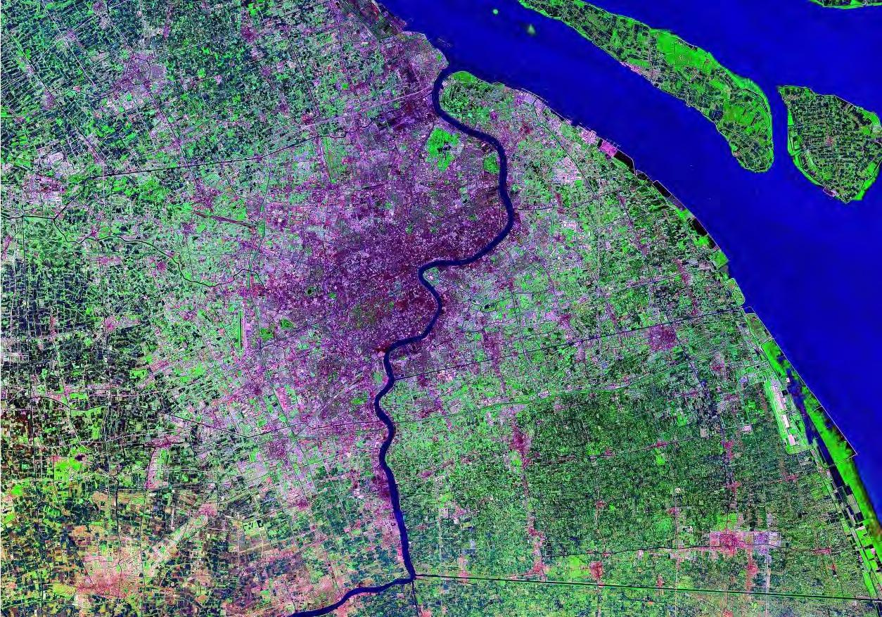
shanghaiShanghai on the other hand is comprised by 18 individual districts that form the city’s jurisdiction; this fact entails that there is a system of multiple centres scattered between the districts, thus appointing the polycentric character of the city. The city’s development was initiated along the river and then was further expanded mainly on the west, as the east side was occupied by agricultural activities.
The density factor of the city has a remarkable impact on the environmental conditions; due to the fact that Shanghai belongs to a warm climate zone, the high density contributes to the entrapment of warm air within the built environment, thus the temperature is frequently increased in particular points. However, highly dense cities prove to be more efficient in terms of fuel emissions, as the distances are smaller and the car use is lower (Avila, 2009).
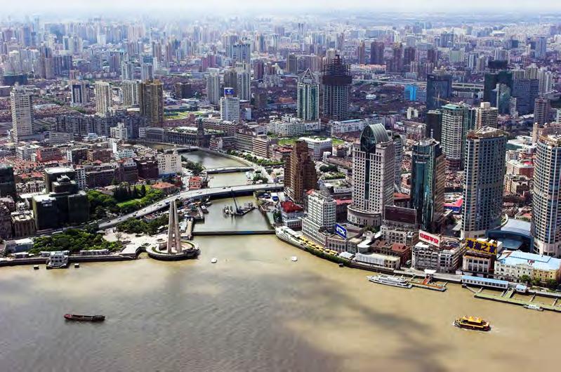
53
conclusions
One might consider a dense city to be one that has high CO2 emission rates and thereby the most harmful to the environment. This is not the case; a dense city encourages the use of public transport, consequently reducing the need for vehicular transportation. Also, a dense city creates shorter distances between people’s homes and the places they work, encouraging both walking and cycling amongst the population; all these factors contribute to lower emissions. However, this does not mean that the denser the city is the better it will perform, there must be an optimal density level that is advantageous to all parts of the city.
54
1.6 Conclusions
The planned city heavily relies on predictability. The planners must predict how many people will populate the city, they must predict the simultaneous growth of different sub-centers, and they must also predict in what manner the developers will implement the original plans. However, throughout almost all the four examples of planned cities, no single planner was able to predict the expected population of the city. Brasilia was predicted for 500,000 people, however that figure grew to 2 million, which pushed the city limits outside the boundaries of the topography it was originally intended for. When creating a planned city, the planner must also control the speed by which the city grows. In the example of Milton Keynes, the simple fact that one shopping center grew faster than the rest had a vast negative effect on the city. Retailers that were spread throughout the city could not sustain themselves, and consequently, a monocentric city was established. The analyses of these four cities lead to a straightforward and vital conclusion; there is not any one street network that can be considered uniform and/or global enough to be applied to any site regardless of topography or climate. The modern consensus is that the gridded street network has become the most efficient one; this is completely false. The single advantage of gridded networks is lack of congestion, because there are several routes to any destination, congestion is very rarely an issue; the disadvantage of this is that there are many streets that are very rarely used, hence neighborhoods are left ‘forgotten.’ It is within these neighborhoods that crime is at its peak.
Evolved cities on the other hand are much more culturally rich and have a much more functional street network that is topographically based. Nonetheless, it is difficult to come to a conclusion that is completely preferential towards evolved cities, for the simple fact that evolved cities have become so culturally vibrant because of the different cultures that have settled in them. Each culture had a unique identity and set of requirements, therefore it’s the overlapping of the different cultural set-
tlements that have given evolved cities the identity they have. Thus, to simulate an evolved city seems unpractical; to try and replicate a system that has evolved through several millennia is impossible. The logical solution seems to be an optimal balance between planned cities and evolved ones, in other words, ‘”planning” a “evolving” city.’
The monocentric module produces patterns with centres that have limited accessibility and capacity of land-uses. In essence monocentric patterns have almost equal economic or other functional conditions in areas that have equivalent distances from the centre. Therefore, there is a good control of the several qualities of land-use within a city. On the other hand, due to the fact that there is one core in monocentric cities, the commuters usually cover long distances within the city. Furthermore, pedestrian and traffic congestion is caused on certain nodes or admittances to the city centre, due to the main circulation taking place from the peripheral area towards one main core.
In polycentric patterns policies such as the “concentrated dispersion” are implemented, meaning that there is a high-density concentration of clustering decentralized activities around public transport nodes. Hence, there is an optimized distribution of functions in the urban fabric with a greater integration between living and working environments within small areas of the city. Consequently, polycentric cities can be comprised by several sustainable centres that contribute to the reduction of congestion problems and negative environmental impact. Although the polycentric pattern seems highly beneficial as a paradigm, many of today’s polycentric cities fail to maintain those benefits. The land-uses are distributed arbitrarily; the business cores could be well organised but the people corresponding to those centres are usually sprawled around to other cores, thus sharpening the effect of traffic congestions and long distance routes.
55
56
Methods
There are many tools that are currently researched that prove beneficial for both development and analysis of urban development. Each tool excels in a particular field, thus encouraging the use of multiple tools simultaneously.
57
2.
58
2.1 Introduction
Designing a city entails many premises, which can only partly control its form and growth. The planning is not a static situation; it should summarize the characteristics of each phase of the city’s growth. Nowadays, the tools that contribute to digital urban simulations are limited compared to the components that comprise the city. The following chapter includes parts of three large subjects that prescribe ways of simulating, analyzing and producing digital urban systems. These tools are Space Syntax, which are useful for analyzing the network systems within the urban environment, City Engine is a computational tool for creating digital simulations of urban patterns (either existing or fictional) and finally, L-Systems and fractals that are formed out of mathematical matrices that infuse sequential steps of developing path networks.
Although throughout this chapter, these three tools will be analyzed separately, they are heavily related with one another, and so will be the case in the following chapters. To fully understand and examine the tools at hand, one must analyze them in isolation from one another so that when they are integrated, each tool carries out its task in benefiting the system as a whole. It is crucial to note that there isn’t one tool that will be able to carry out all the simulation and experiments required; the level of complexity desired will be achieved through an integration of several smaller tools that work together for a more complex whole.
59
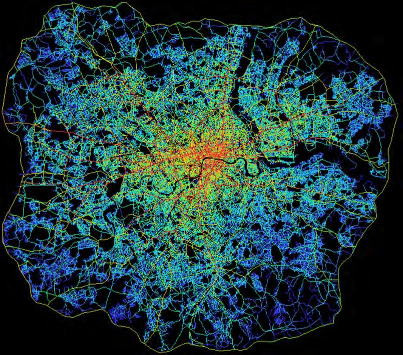
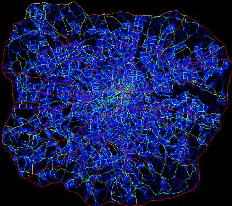
2.2 Space syntax
theory
The study is mainly focused on two fields that comprise space: the architecture, which is defined by the geometry, and the topology, which represents a certain pattern of connections. Consequently, Space Syntax uses the software tools in order to collect a set of relative distance measurements and therefore to analyse the spatial design configurations – the physical arrangement and organisation of spaces. Moreover, its main attribute is the study of the correlation between the spatial layout and people’s movements.
Analysing the space configurations, Space Syntax uses a set of definitions that provide the reader with the tools to understand the process of analysis. These definitions are:
- Relative distance: It can be the distance from one point to anywhere, within a certain radius defined a priori, either by distance, time etc. By adding new points on an existing street layout, this entails that all the relative distances will change, as the new point will constitute part of the choice measure.
- Integration [Fig.2.21a]: The relative distance is being assessed and it defines the degree of agglomeration and reachability effect. These two definitions, agglomeration and reachability effect, are primarily influenced by other types of parameters, such as the geographic location and design layout.
- Choice Measure [Fig.2.21b]: A point is set as a reference, then the amount of paths that overlap in order to get to that point from all the other places is being measured. In essence, choice measure defines the amount of flow on each path for reaching the reference point.
Fig.2.21a
Integration map of London greater area. The map is a representation of the spatial agglomeration and reachibility of the London’s street network. The paths that are coloured with red are the most beneficial in terms of agglomeration; this entails that the red paths are the ones that have short relative distance to all the others, whereas the blue ones are the ones that are far away from most of the paths of the city.
Fig.2.21b
Choice map of London greater area. The map shows the different hierarchical levels of the segments of the London’s street network. The red paths are the ones that have maximum accessibility within the city, the green paths are second in hierarchy and they distribute the movement flow to the red paths. The dark blue paths are the ones that have the least flow of all the others.
60
Fig.2.22a-c (top)
In general, a grid with smaller central blocks and larger peripheral ones [Fig.2a] has a lower mean metric distance from every point to all the others than a regular grid [Fig.2b].
The mean distance of a grid with larger blocks in the centre [Fig.2c] is higher than the regular grid. This formal fact is reflected everywhere in cities. Therefore, city centres, with their need for inner-accessibility and commercial transaction, need to have smaller block structures than the residential areas that surround them [Ref.11].
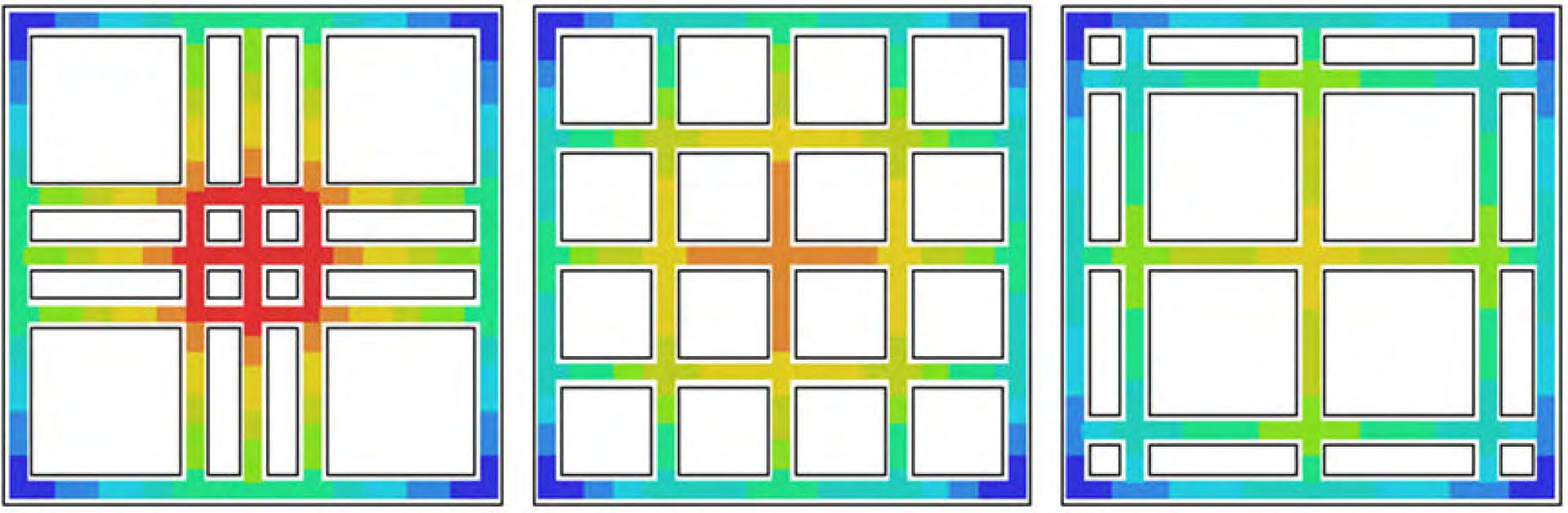
Fig.2.23 (bottom)
The area of Waterloo station and Embankment in London analysed by Space syntax: the coloured lines follow the axial map, which is created by straight lines from a point to its furthest visible point. The lines are next coloured according to their connectivity; the red colour represents the axes with high accessibility of pedestrian movement and as the colour changes to blue the accessibility is reduced.
Fig.2.22a
Cell count: 305
Mean to all distances: 2.69
Fig.2.22b
Cell count: 305
Mean to all distances: 2.79
Fig.2.22c
Cell count: 305
Mean to all distances: 3.02
- Radius: It is the specification of the relative distance from one place to everywhere. It is a limit for a relative distance measure in order to narrow down the capacity of distance possibilities.
Three different logics of spacing between the components of a grid that compose a notional urban street layout have been examined by the Space Syntax in terms of the relative geometric distance [Fig.2.22a-c].
The red colour indicates the nearest places to everywhere (central) in terms of relative distance, whereas the blue colour shows the places furthest away to everywhere (edges).
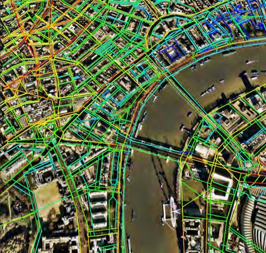
61
centre spatial forms
Every city region’s wealth is located and essentially generated in their urban centres. London is a rare example of a centre of population that was expanded in the largest range, compared to other cities in the world, before people start using cars in a massive percentage. London is a polycentric city, with two internationally identified centres (Knightsbridge and West End), ten metropolitan centres, 30 major centres, about 150 district centres and over 1,300 neighbourhood centres (Castle, Leah, 2009).
In general, centres constitute the attraction poles of the cities for people living either near or far from them; they facilitate the sharing of many public services, production facilities and markets, they are places of import – export. In the case of London, the wealthiest live in the most desirable areas and thus London contributes positively to the economy of the United Kingdom.
Space Syntax has made a lot of research on the centre’s spatial form. Some of the potential spatial configurations are shown [Fig.2.24a-d].
The continuous and pervasive centres [Fig.2.24a] have blurred edges and more coherent and pervasive to the centre. They provide a great alteration of qualitative experience and local market. The central zone of London follows the same form. Online centres [Fig.2.24b] are located on main traffic arteries. Their location is optimal in terms of accessibility to transportation facilities and merge with the local market. In London this is the most typical form of centre. Offline –online centres [Fig.2.24c] are located just off main traffic arteries, but still on linear streets. They are well embedded in the local market and constitute significant transportation interfaces. Offline pod centres [Fig.2.24d] occur where the previous condition is at its extreme phase, meaning that they are isolated from main arteries. Sometimes they offer great transportation and design experience, though they are not embedded in the local market.
Fig.2.24a
The continuous and pervasive centres are more coherent while heading towards the centre.
Fig.2.24b
The online centres are located on main arteries and people can experience both fast and low modes of transportation.
Fig.2.24c
The offline - online centres are located on secondary arteries.
Fig.2.24d
The offline pod centres can be shopping malls or big box retail parks.
62
Fig.2.24a
Fig.2.24c
Fig.2.24b
Fig.2.24d
Fig.2.25
The expansion of the city was driven mainly by two forces: the centrifugal radial growth outwards the centre and the linear growth along two axes as the arrows show.
Fig.2.26
The unplanned settlements around the centre have an introvert character. However, locally, they retain a very good connectivity and function.
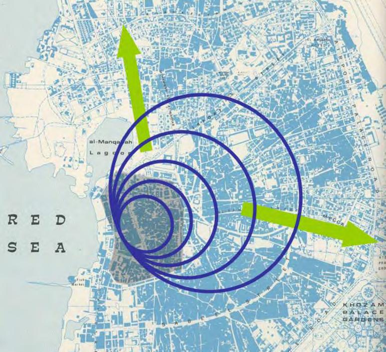
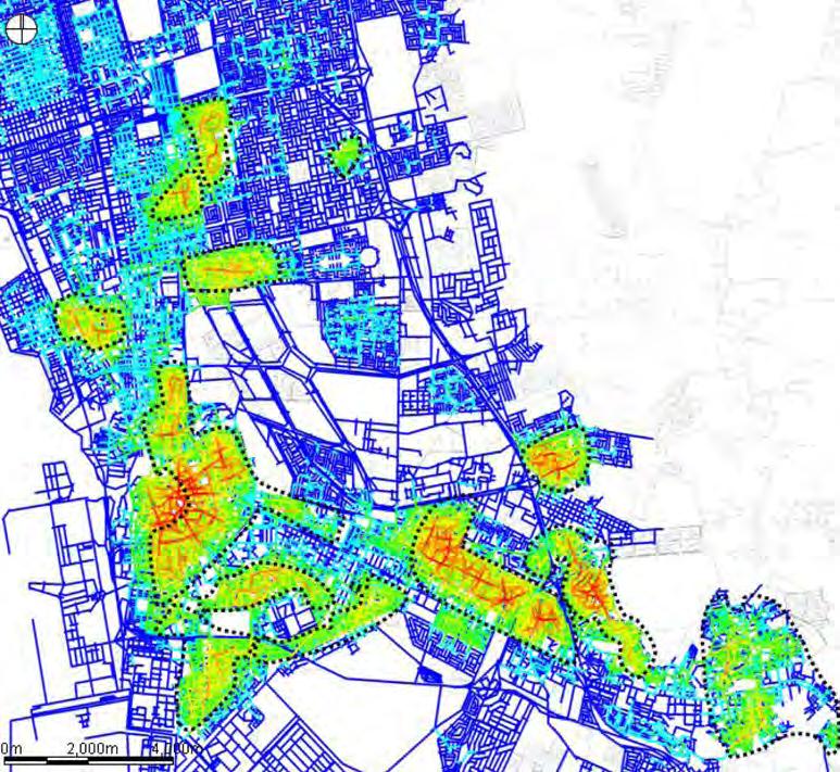
The historic city of Jeddah has been approached by Space Syntax as a multi-scale problem that should be resolved efficiently. For that, they identify the city as a self-organising system from which the global form, network patterns, land use patterns and density distribution would emerge.
The particular project of Jeddah was mainly focused on a solution that had to face a high degree of unplanned situations. In essence, Space Syntax followed four steps:
1. Build a model of the site and its context.
2. Test the model against current movement flows and land use patterns.
3. Using the model in order to test out designs by inserting them into the model and re-running the analysis.
4. Suggest new ideas from the analysis.
Therefore, the method was applied to solve the spatial connection problems in several points that interrupted the sequential flow to the centre of Jeddah. Another goal was to examine the way that land use factors can be related to the spatial issues.
The historic centre of Jeddah is the oldest part of the city and represents the core of development for the entire city. It is the threshold for the movements to the main port, thus it links the entire movements from the land to the sea and vice-versa. The city’s today configuration comprises of the historic core surrounded by prime developable land and dense unplanned settlements. Through the growth period of the city, two main forces were driving the expansion; radial growth around the historic core and linear growth along the two main axes [Fig.2.25].
63
jeddah
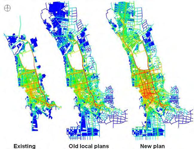
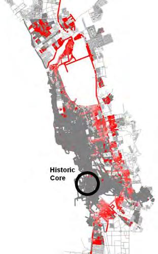
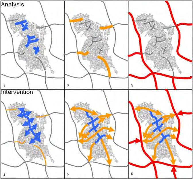
The unplanned settlements have an introvert character, though their internal structure is very strong [Fig.2.26]; it is comprised by a mix of land uses. Therefore, the historical centre of Jeddah remains relatively isolated with its structure being segregated from its surroundings. As the development of Jeddah has mainly confined to the north and east sides [Fig.2.27a,b], the current situation shows one main axis of circulation and some lateral ones with less vehicle access. In that manner, the urban integration that each street segment gains is unequally distributed, with most of the gains occurring away from the historical centre [Fig.2.28]. After several analytical diagrams, Space Syntax considered that the right tool for the regeneration of the centre was not to re-design it but to reconnect it. Consequently, two main tasks were addressed; to re-integrate the unplanned settlements into the urban and social environment of the centre and to develop some significant adjacent units (i.e. the harbour and the old airport).
With the old airport acting as an infrastructural barrier to the north-east
side of the centre, the radial growth was conciliated. However, the car use had uplifted after the outset of the growth. There were many ring roads developed during the growth, which they crossed through the dense unplanned areas that were increasing in capacity to the southeast side of the city and constituted another barrier for the growth.
The project proposal has a strong technique, which started as followed: the existing local structures of the surrounding settlements were analysed and next improved in order to achieve a continuous connectivity with the network of the next hierarchical level [Fig.2.29]. The same process was followed for linking those with the global network system. During this process, any streets that can be extended into main arteries were identified and thus transformed into main axes that would link the surrounding areas directly to the centre, while many lateral streets would be used as a secondary network that would connect the unplanned areas between them [Fig.2.210].
Fig.2.27a-c
[6a,b] The analysis shows that the integrated area (the paths with red colour) is concentrated outside the city’s central core, which has a very small accessibility. This outcome derives as a part of the old plan of the city, meaning that city planning is not followed by the right criteria. [6c] The new proposal by Space Syntax suggests of a system of relinking the centre with the new developments via car-use and pedestrian bridges, thus forming an integrated network for the city.
Fig.2.28
The red coloured areas are the well-integrated ones and the grey areas are disembodied from the rest of the urban fabric. The degree of the isolation of the historic centre is dramatically noticeable.
Fig.2.29
A method that Space Syntax developed for the project trying to re-integrate the unconnected settlements while preserving internal structures. There is a hierarchical way of connecting paths, each time to a different scale; from the more local towards the global.
64
Fig.6a-c
Fig.7
Fig.8
Fig.2.210
The diagram shows the main routes with the red colour, the intermediate routes with the deep orange colour, the deep yellow coloured roads are primary streets of local districts and finally, the light yellow coloured paths are the secondary local routes.
Fig.2.211
The proposed transportation system: the purple nodes are significant points of access to the transportation means, the red lines are segments of the primary transportation network, the red dashed lines are secondary segments of the network, the deep blue coloured zone is the area of pedestrian priority and the light blue zone is the area of both pedestrian and bus circulation.
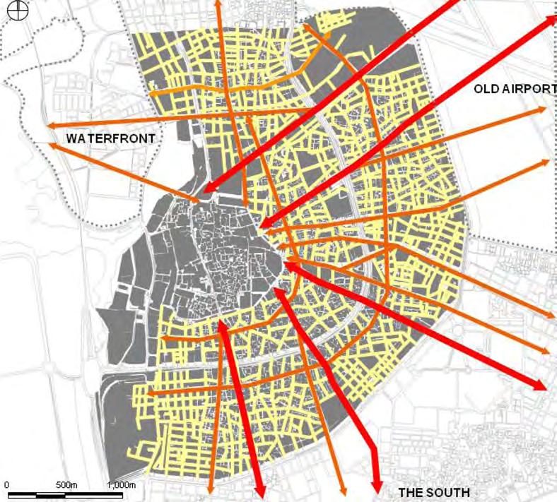
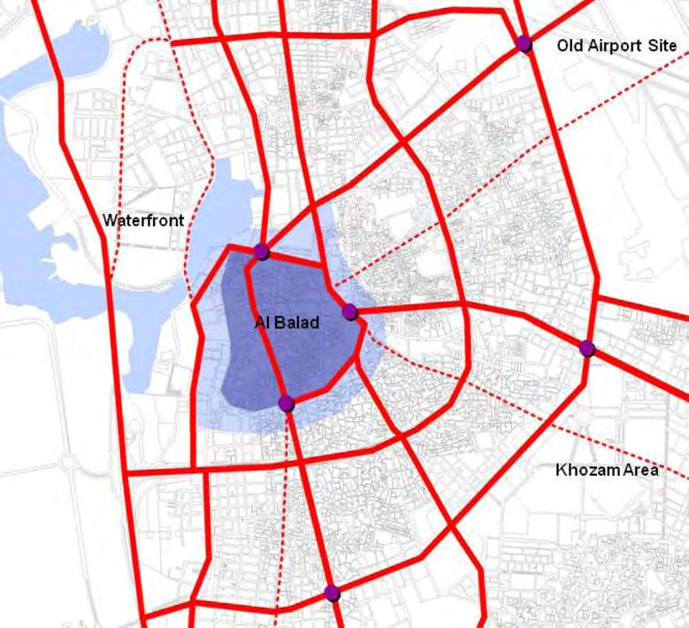
conclusions
The proposal consists of a study for a reconfiguration of land uses and spaces between the blocks. Moreover, a new public transportation system was proposed in order to enhance the new street network [Fig.2.211].
Finally, the proposal aims at the re-integration of the entire centre of Jeddah, which can be achieved not only by improving the central area but also by the combination with a careful planning of the wider area of the city. According to the plan, many more street axes were created in order to bring the structure of the city back to the centre as well as to integrate the unplanned settlements.
Space syntax is a tool that covers a wide range of ways that form spatial patterns in relation to the human behaviour; it deals with movements on foot, on cycles and in vehicles. The scale of the analysis being conducted varies from big cities to small-scale buildings. The Space syntax team deals with many factors in order to extract the information needed; for instance, they produce simulation of people with high accuracy with the help of agent-based systems, of analyses which contain measurements that are extracted from experiments that have been conducted for months and of virtual observations done on site. With the help of high-technological analytical tools, Space syntax provides the medium that informs the design about the qualities and values of the space.
65
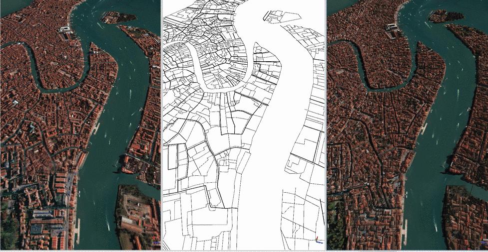
2.3 City Engine
generating urban forms
Procedural: City Engine is a software that can run rapid simulations of cities with the use of very basic and few user defined parameters. The process of simulating a city in City Engine can be broken down into three main steps:
1. Create the street network
2. Create the lots/blocks
3. Generate the buildings
Within each of the above steps are a series of parameters that the user can control to simulate a city based on the users preference. Such parameters include the number of streets, global pattern of the street network – organic, radial or raster, lot size, relationship of one lot to its neighbour, heights of buildings, shapes of buildings and so on.
City Engine also includes a script editor to allow further control over particular parameters and/or variables. A very useful characteristic
that City Engine retains is its import function. Street networks can be created in other software such as AutoCAD or Rhino and imported into City Engine as DXF files [Fig2.31]. All the different parameters listed above are applicable to the imported street network, as well as the added possibility of further manipulating the network after it has been imported. The user can also import existing street networks from existing cities through the open source website openstreetmap.org and apply the different parameters to them.
Another feature of City Engine is ‘Shape Grammars.’ The use of ‘shape grammars’ is well integrated between City Engine and any .obj file created by 3D software. This gives the user additional control over the required shapes of the buildings that will be created. In other words, building forms can be created in a program such as Rhino or Maya, and exported to City Engine where they would be used as a ‘blueprint’ for the extruded buildings [Fig.2.32]. The same method can be applied to the shapes of streets and sidewalks.
Fig.2.31
An example of City Engine’s ability to import street networks of existing cities and simulate a digital rendition of the city. The image on the left is an aerial view of Venice, the middle image is the imported street network, and the image on the right is the simulated city from City Engine.
66
Fig.2.32
Different examples of street network patterns that can be created with city engine’s parameters. Starting from the top image, the pattern is a combination of radial and raster streets. The one beneath that is a combination of raster main streets with organic minor streets. The next one is a combination of organic main streets with raster minor ones. The final image combines radially patterned main streets with raster minor ones.
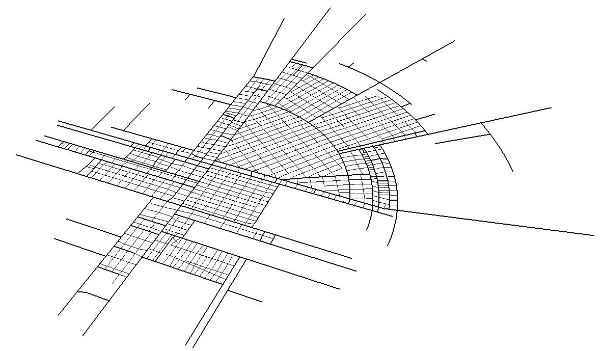
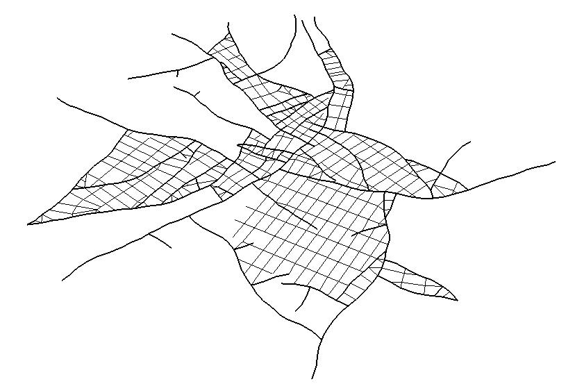
Although all the above characteristics may seem very luring at first, one quickly notices the lack of crucial attributes from this software. The first and most important one is the inability of scripting street networks. The script editor is limited to controlling the extrusions, yet seems to lack the operations that would allow the user scripting control over street networks. One may argue that street networks may be scripted
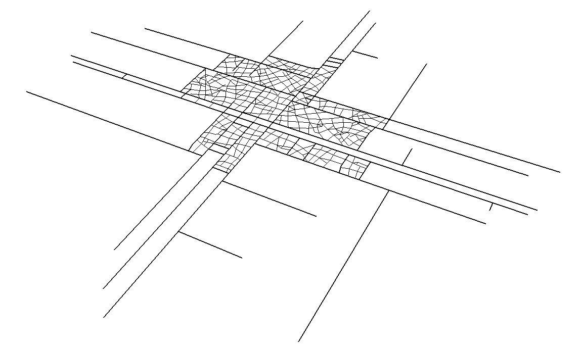
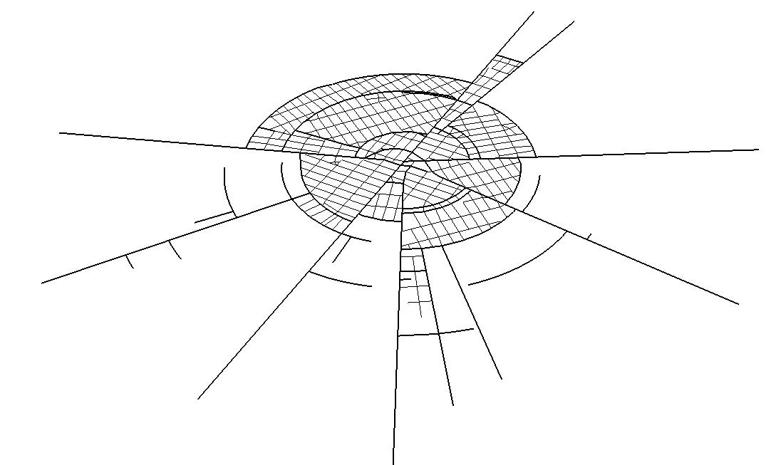
in parallel software and imported into City Engine, and although that may sound reasonable at first, it still means that the street network is initially created, and the lots are applied to it. Hence preventing the possibility of integrating the street network with extruded lots, i.e. the possibility of integrating the infrastructure with the built up area is remote.
67
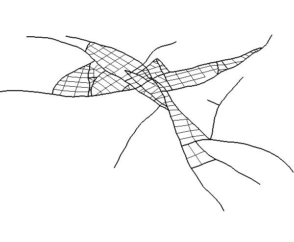
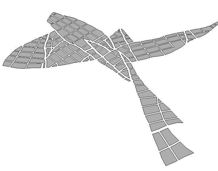
Fig.2.33
The different phases of simulating a city in City Engine. The first image is creating the street networks, these were created parametrically through the City Engine functions. The streets were then used to create lots. Initially, the lots are created by interpolating the intersection of the streets, however in the third image, the lots can be further subdivided into smaller lots, which are finally used to extrude buildings (right page). The lots do not have to be subdivided for building extrusion. The disadvantage of subdividing the lots is that there is not a specific way to parametrically introduce streets between the subdivided lots, they must be introduced manually.
Another feature that is absent from City Engine is a quantitative evaluation of a cities density. This is related to both feedback and generation. Once the user simulated a city, there is no function that would give the user a quantitative feedback on the density of the simulated city [Fig.2.33]. The only reference to the density of the city is visual. Furthermore, the user does not have the capability to control size of the city based on a particular desired density. There are options of subdividing lots into smaller ones, however the user cannot generate the size of the lot based on a predefined quantitative density.
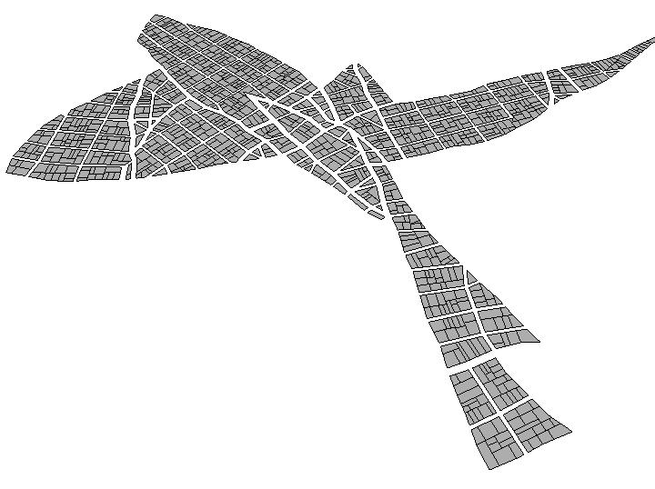
68
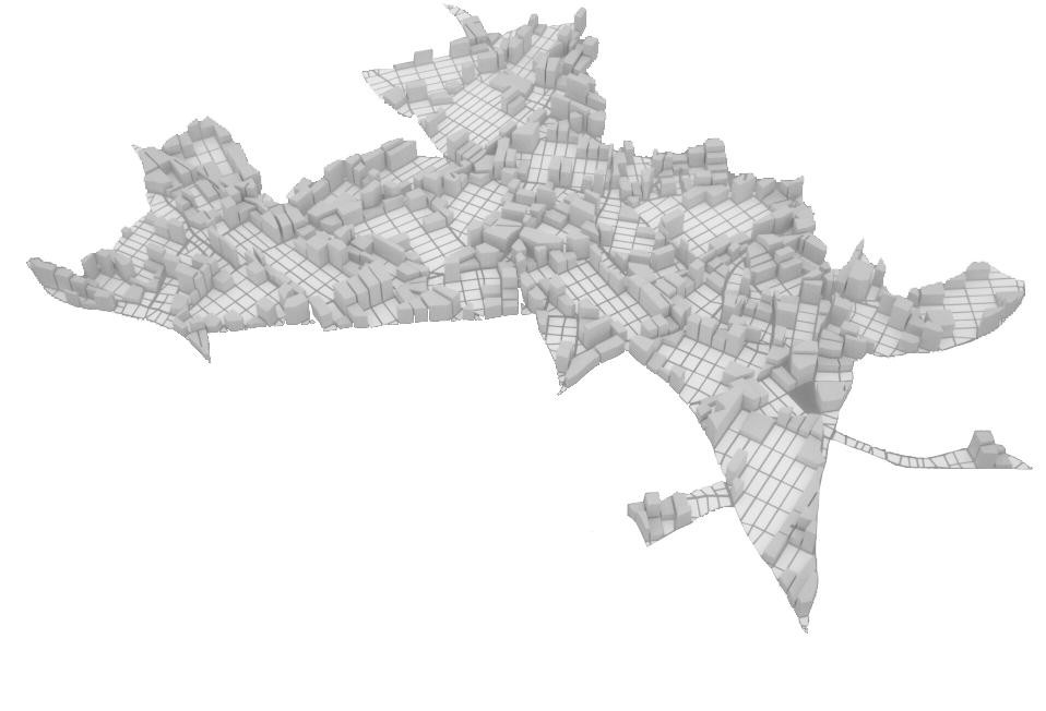
conclusions
In the case of City Engine, the advantages outweigh the disadvantages. The software is an extraordinarily strong tool for city simulation and will prove extremely beneficial as the design experiments commence. However, one cannot neglect the attributes that the software has; on the contrary, other solutions/paths must be conceived to fill in the gaps left behind. It might be necessary that several software are used simultaneously to supplement each others limits.
69
initiator
generator
Figure1.1:Constructionofthesnowflakecurve
2.4 L-systems
fractals
Lindenmayer systems - or L-systems - were devised by Aristid Lindenmayer in 1968 as a mathematical theory of plant development (Prusinkiewicz, Lindenmayer, 1991). L-systems have evolved a great deal since then; combined with digital tools, the most modern use of L-systems has become plant modelling. However, alongside plant modelling, another vital application for L-systems is Fractal generation (Ochoa, 1998). The main concept of L-systems is rewriting. In general, rewriting is the method to describe a complex geometry by successively replacing parts of that object with simpler ones. The most well known example of rewriting is Von Koch’s ‘snowflake curve’ [Fig.2.34]. Put simply, one begins with an initiator and a generator, these two shapes are not bound by any restrictions, neither are they limited to be open shapes or closed ones. The first step is to replace each side of the initiator shape with the generator shape. In the next generation/
WhiletheKochconstructionrecursivelyreplacesopenpolygons,rewritingsystemsthatoperateonotherobjectshavealsobeeninvestigated. Forexample,Wolfram[160,161]studiedpatternsgeneratedbyrewritingelementsofrectangulararrays.Asimilararray-rewritingmechanismisthecornerstoneofConway’spopular gameoflife [49,50].An importantbodyofresearchhasbeendevotedtovariousgraph-rewriting systems[14,33,34].
iteration, each side of the resultant shape from step one is replaced with the same generator shape. One can repeat this process infinitely; the only obstacle would be that the more generations that are run, a stronger computer would be required to run the rewriting system. The most basic form of L-systems is called DOL-systems. The most straight forward example of a DOL-system is given by Prusinkiewicz and Lindenmayer (1991): a → ab b → a
Themostextensivelystudiedandthebestunderstoodrewritingsys- Grammars temsoperateoncharacterstrings.Thefirstformaldefinitionofsucha systemwasgivenatthebeginningofthiscenturybyThue[128],but awideinterestinstringrewritingwasspawnedinthelate1950sby Chomsky’sworkonformalgrammars[13].Heappliedtheconceptof rewritingtodescribethesyntacticfeaturesofnaturallanguages.A fewyearslaterBackusandNaurintroducedarewriting-basednotation inordertoprovideaformaldefinitionoftheprogramminglanguage ALGOL-60[5,103].TheequivalenceoftheBackus-Naurform(BNF) andthecontext-freeclassofChomskygrammarswassoonrecognized
The above rules contain two letters, or strings, a and b. Each letter contains a rewriting rule. a is to be replaced with ab b is to be replaced with a
Fig.2.34
Von Koch’s snowflake curve. A simple initiator combined with a simple generatorhave the power to create complex forms with only a few iterations.
70
a b ab aba abaab abaababa
2 Chapter1.GraphicalmodelingusingL-systems
[52],andaperiodoffascinationwithsyntax,grammarsandtheirappli-
Fig.2.35
An example of a typical turtle string, although the string seems long and complex, the form that is generated is very basic.
Fig.2.36
Several examples of different turtle strings applied to the same initiator. In this case, the initiator is a simple square. The examples below are all in their fourth generation. The distance ‘ d is halved with each successive generation.
To begin the rewriting process, an axiom (a distinguished string) is required. Let us consider the string b as the axiom. Therefore, according to the rules, the first step is to replace the string b with a The second generation/iteration replaces the string a created by the first step with the string ab. The resulting string so far is ab. The third generation replaces a with ab and b with a, resulting with the string aba, the fourth generation yields the string abaab, and the generation after that yields the string abaababa, and so on.
Rewriting strings using the above method is limited to creating simple geometries. To model more complex geometries of plants, an advanced graphical interpretation of L-systems is needed. For instance, how can one draw the Koch snowflake using an L-system? This is where turtle interpretation is introduced. In the previous example, we had two initial strings, a and b. Instead, the basic forms of turtle interpretation is based on a string containing the symbols ‘F’, ‘+’, and ‘-‘. Each symbol has a defined function:
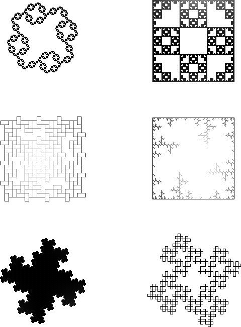
Chapter1.GraphicalmodelingusingL-systems
Chapter1.GraphicalmodelingusingL-systems
Chapter1.GraphicalmodelingusingL-systems
Figure1.9:AsequenceofKochcurvesobtainedbysuccessivemodification oftheproductionsuccessor
F = move forward with one step + = Turn left - = Turn right
The two main variables with the above function are the distance ‘d ’ by which the ‘turtle’ moves forward, and the angle ‘δ ‘ by which the ‘turtle’ turns right or left.
The following example demonstrates how one can use these three functions to create a string that will generate a particular form. In this case, ‘d ‘ is 1, and ‘δ ‘ is 90 degrees [Fig. 2.35].
Figure1.9:AsequenceofKochcurvesobtainedbysuccessivemodification oftheproductionsuccessor
Therefore, if we used the same principals of ‘initiators’ and ‘generators’, but instead of using geometries we use strings, an almost infinite number of shapes can be created. The following examples are different generator strings applied to the same initiator string [Fig.2.36].
Figure1.9:AsequenceofKochcurvesobtainedbysuccessivemodification oftheproductionsuccessor
Figure1.9:AsequenceofKochcurvesobtainedbysuccessivemodification oftheproductionsuccessor
71 FFF-F-F+F+FF+F-F-FFF-FFFF-F+F-FFF
10
10
conclusionsAlthough the examples given by this method of branching system may seem very planar, there are many possibilities to accommodate different topographies. Once strings begin to be developed in relation to street networks, this method of branching system that is based on initiators and generators is very useful begin generating street networks. The possibility of integrating turtle strings to develop fractals is another area that opens up another set of interesting possibilities of generating street networks.
72
2.5 Conclusions
The chapter was focused on the study of the current tools that are used for simulating, analysing and evaluating the urban space. Systems like Space Syntax provide essential methods for understanding and interpreting the urban space so that in future attempts of designs all the crucial points would be taken into consideration. City Engine, as a purely urban-design tool, has many limitations for further innovation in an architectural context. However, it is a successful tool for simulations of urban forms as it combines design of standard forms with a significant part of parametric input.
Nevertheless, these tools have their limitations; for instance, the capacity of ecological extend is not clearly identified through the process. Furthermore, the analytical tools provided approach urban forms within a certain, fixed boundary, without adapting to any type of growth and evolution within or outside the city. In this way, eventually the methods produce representations of steady situations without capturing time. The datum on which the tool functions is twodimensional, hence it does not include the entire context of the space samples unless if it was applied on several layers in height.
Space syntax is a tool that covers a wide range of ways that form spatial patterns in relation to the human behaviour; it deals with movements on foot, on cycles and in vehicles. The scale of the analysis being conducted varies from big cities to small-scale buildings. The Space syntax team deals with many factors in order to extract the information needed; for instance, they produce simulation of people with high accuracy with the help of agent-based systems, of analyses which contain measurements that are extracted from experiments that have been conducted for months and of virtual observations done on site. With the help of high-technological analytical tools, Space syntax provides the medium that informs the design about the qualities and values of the space.
In the case of City Engine, the advantages outweigh the disadvantages. The software is an extraordinarily strong tool for city simulation and will prove extremely beneficial as the design experiments commence. However, one cannot neglect the attributes that the software has; on the contrary, other solutions/paths must be conceived to fill in the gaps left behind. It might be necessary that several software are used simultaneously to supplement each others limits.
73
74
Experiments
Analysis of blocks and paths and the methodology used in generating them must first begin with a set of experiments that will identify the possibilities, as well as the setbacks, of these two systems.
75
3.
76
3.1 Introduction
Following up from the methods that were analyzed in the previous chapter, the two categories that will be further analysed and experimented are the development of paths, and the development of the blocks. Up until now, the paths have been analyzed planarly, with simple initiators and strings. However, introducing fractals and combining them with L-system opens a new set of possibilities of street networks. However, a condition that will heavily inform the street networks is topography, therefore, the street paths must break away from their planar forms, and explore three dimensional possibilities. The main difficulty that will arise will be to allow both the topography and the street paths to ‘communicate’ with one another rather than simply become layered pieces of information that are placed on top of each other.
The second leg of the experiments will focus on the different methods used to generate blocks, and explore all the different factors that would inform the shapes of the blocks. The optimization method will rely on an emergent process that will focus on creating several generations of blocks, where each generation is more optimal than the one preceding it. However, the block will not be considered as an independent entity, on the contrary, the relationship between the block and the ‘superblock’, as well as the relationship between the superblock to the global urban fabric is crucial to take into account, ensuring that the urban fabric works as an interrelated entity rather than an accumulation of isolated elements. For all the experiments that are carried out, the ‘site’ or ‘topography’ are arbitrary, what will be explored is the effect of the terrain (regardless of the form of the terrain) on the development of both the paths and the blocks.
77
3.2 Paths experiments
planar configurations
Following up on the initial experiments carried out in chapter 2, a new generator string is developed that reads as follows:
FF-F--F-F
d = 1/3
δ = 90 degrees
Once this generation string is applied to a simple initiator, in this case a square, a pattern emerges that is beginning to exhibit similarities with actual street networks. In this case, characteristics such as hierarchy between the streets and development of spaces within the network are the most dominant. In this particular example, the generator string is much more interesting than the initiator. Therefore, in order to break away from this simple square initiator, the generator must be applied to different initiators that show some characteristics of asymmetry and growth. Retaining the 90-degree angle brings forth characteristics that are similar to street networks [Fig.3.21]. Since this is a DOL-system, the string has a tendency to simulate a tree, therefore if an angle other
than 90 was used, street network characteristics are instantly lost. However, this only applies to the generator, what has been discovered was that as long as the generator string retained angles of between 80 and 100 degrees, street characteristics are achieved, the initiator on the other hand has the freedom to contain any particular angle required. By doing so, the global form is changed, while the local network retains characteristics similar to actual street networks. The examples on the following page introduce a more complex initiator, with a slightly different generator. The top example contains the following strings:
Initiator = FYYFXY
Generator = FFF+FY+F
The bottom example contains the following strings:
Initiator = FYYFXFXF+FF-FXF
Generator = FFF+FY+F
78
Fig.3.21: Fractal experiments
79 Generator Initiator Generator Initiator
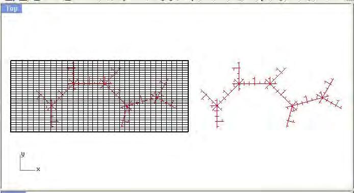
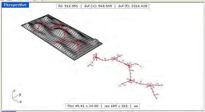
fractals on a terrain
So far, all of the Fractals/DOL-systems have been planar. All of the generators and initiators have acted only on the x-y plane. However, as discussed in chapter one, a street network must conform to the topography it is laid upon. In order to introduce the new ‘z’ dimension [Fig.3.22], one must incorporate it within the script. For tree simulation, introducing a third dimension is quite simple, because the result is visually similar to a plant. However, when the ‘z’ dimension is applied to the street network, it has the tendency to do the exact same thing, simulate a plant. Therefore the result does not pertain any characteristics that are similar to street networks. Regardless of what angle is used in the generator/initiator, as soon as the ‘z’ axis is introduced, the street network suddenly transforms into a plant simulation. A temporary solution for this obstacle (the permanent
solution would be to fix the script) is to use the project function. This is where the generated street network is projected onto a particular topography. The flaw in this method is its similarity to previous methods of slapping a gridded network on any particular topography. The street network must change with respects to the topography, in other words, the topography must inform the network when, where and with what intensity to skew. Therefore, a solution to this problem would be to initially generate the street network based on the topography it will lay on; one may understand this as using the topography as a blueprint to generate the most suitable network for that particular topography. Once the network is generated, it is then projected onto the topography and should thus complement it.
Fig.3.22
Plan, elevation and perspective views of a fractal/DOL-system generated street network projected onto a arbitrary topography. When compared with the street network generated by introducing the ‘z’ axis in the script, this solution is much more visually successful; however, in order to make it compliment the topography it will lay on, it must be generated based on the topography itself.
80
conclusions
The possibilities and variations that arise from initigrating initiator and generator strings are many, however, the main driving force that will determine both the layout and global forms of the paths will be the topography. In modern planning, the streets are developed planarly at first, where the left over spaces between the streets are then allocated for building lots. However, in cases such as in Istanbul, and the ancient cities of Egypt, the lots were initially located rather than the streets, this lead for the paths to be generated between as a result of the lots. This method of development of street networks proves to be the most efficient, as well as the most functional.
81
energy efficiency of blocks 3.3 Blocks experiments
The first set of experiment is focused on the configuration of the blocks and the relational parameters between each other on a local level within a certain area of the urban fabric. Prior to the actual experimentation of the urban blocks, the research introduces some references to urban sustainable environmental studies; this information constitutes certain criteria that are part of the design algorithm, on which the logic of growth is based.
Initially some of the basic ways of adapting passive systems into the algorithm are being explored; airflow, sun radiation exposure and daylight acquisition are some of the factors that could possibly be taken into consideration. In cities the wind flow is slower to the level of the streets compared to the countryside, as the building volumes act as obstacles that slow down the speed of the wind. This would entail
that the smaller the distance between the blocks the slower the wind flows. However in these cases turbulence might be created, especially when the buildings exceed certain heights or if the streets are very narrow and surrounded by tall buildings they could act as wind tunnels that contribute to the acceleration of the wind speed. Moreover, the airflow, as well as most of the environmental parameters, is directly interrelated to the urban morphology. Simos Yannas, director of the Environment and Energy Studies Programme of the Architectural Association, mentions in his document “Urban Climatology and Design” that “the way air moves in towns is a function of the geometry of the urban tissue” (Yannas, 2002). The resistance to the air flow decreases where the streets are almost parallel to the direction of the wind and where the streets are wider.
Fig.3.31a-c
The urban pattern can be formed in a relational way between the paths and the buildings. Here the three figures show a way of adjusting the heights of the buildings or the distances between them according to their orientation towards the sun. The planner can define then, whether the shadowed area is the desired result or not and exploit the properties of the respective environment into the design.
82
D S H D S H D S H
Fig.3.311a
Fig.3.31b
Fig.3.31c
Fig.3.32
Section of the building complex in Nuremberg - Germany by the architect Joachim Eble. The shorter building faces the south and the taller one the north. Thus the short building does not overshadow the tall one but also allows the sunlight to enter the internal courtyard between them. The courtyard behaves as a space that captures a desired degree of heat in the winter, when during the summer the space can be used as an area with increased ventilation for cooling, using the appropriate methods.
Fig.3.33
Internal aspect of the indoor atrium. Through design solutions of gaining natural light, air treatment, building materials and surface treatment, the architect aims at the accomplishment of comfortable indoor conditions for the visitors.
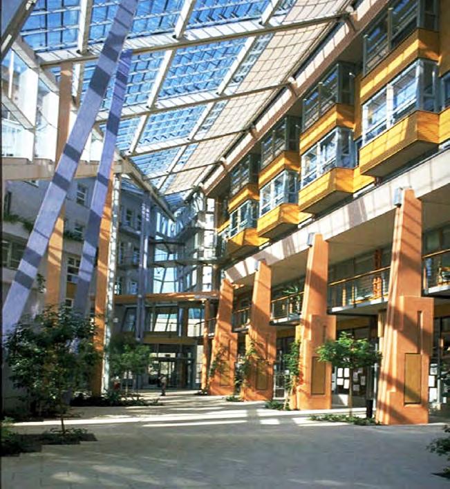
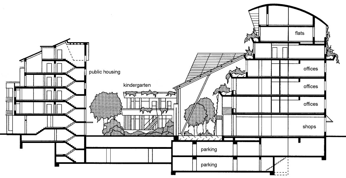
As mentioned earlier the urban morphology’s role is fundamental to the impact of the various environmental parameters that influence the performance of the city. The morphological characteristics of the urban tissue have a direct influence on the microclimatic conditions on a local scale, creating an interrelation between every block to the other and hence defining the macroclimatic state of the urban tissue on a global scale. The surface area exposed to sun radiation is a factor that contributes to the heating conditions of the area around the blocks through the gained solar energy. It can be adjusted according to some relational measurements, such as the ratio between the height of the buildings to the distance between them and the orientation of the buildings in relation to the heating requirements of each one individually [Fig.3.31a-c].
The research appeals to some examples that refer to the block’s behaviour to the climatic conditions of the urban fabric. In the document “Sustainable Urban Block Design through Passive Architecture” [Ref.2] the block of internal courtyards is taken as an optimised solution for a larger surface exposed to the sun radiation. The internal courtyard configuration resembles an older method of building, which has been re-adapted by many German architects in order to introduce an ecological design method with low energy consumption in the contemporary architecture (e.g. the mixed-use and socially balanced building complex – by architect Joachim Eble – Nuremberg, Germany) [Fig.3.32-3.33]. Through a set of tests and experiments, the argument arose is that considerable savings on energy consumptions can be achieved by simply disposing the building volumes in a different way (Morello, 2009).
83
- Energy consumption is influenced by the directionality between the blocks and the energy source. For instance, a rotation of 45 degrees is more beneficial in terms of energy gains as the solar exposure is more homogeneous.
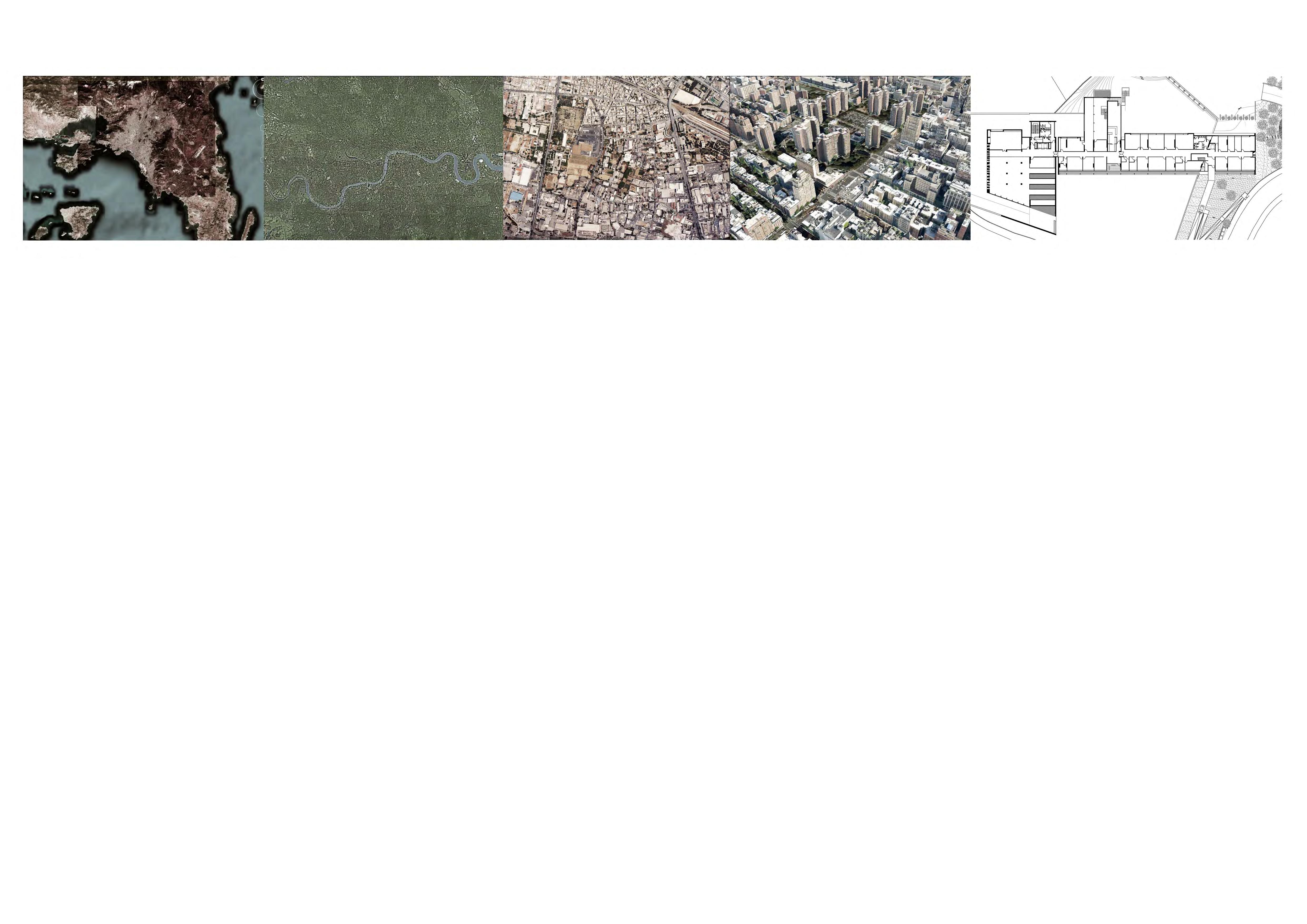
Fig.3.34
Different scales of urban morphology (from left to right): [a] urban region - the peripheral area around the settlement with the city itself, [b] the city - the various geographical characteristics constitute special morphological elements, [c] neighbourhood urban fabric - factors such as density are critical tools for defining local morphologies in the city, [d] city blocks - the ratios between built-unbuilt areas and movement networks produce different outcomes, [e] buildings - the individual elements within a block [Ref.3].
Fig.3.35
Three different samples of the urban fabric in Paris that show different urban morphology and consequently energy consumption. The modernist module is not suitable at all for the reduction of energy consumption; the surface area of the open space is much bigger than the built volume and the distribution of the built volume inside the block is not optimal for saving energy.
18-19th C
Traditional courtyard (0.21 GJ/year/m2):
- Very high building density
- High FAR and high block density
- Bad solar admittance
1918-1980
Modernist fabric (0.36 GJ/year/m2):
- High solar admittance, bad shape factor
- Very low building density, FAR and block density
On the larger scales it has not been identified yet the relation between the density and energy (Lorch, 2009), as cities are complex systems of a combination of built volumes and empty spaces. However, the CSTB Urban Morphology Laboratory has proved that the appropriate morphological characteristics of the urban fabric can reduce energy consumption and carbon emissions by a factor of two; a significantly reduced proportion (Lorch, 2009). There have been studies about certain historical areas in Paris – a traditional urban tissue sample, a modernistic one and the contemporary [Fig.3.35] – which they have been measured for their energy consumption for heating needs. [Fig.3.35] shows that the modernistic example is way inefficient in terms of heat conservation, whereas the contemporary and traditional ones consume much less energy on heating needs than the modernistic one. The reason is the ratio between the building volumes to the distances between them – density – and the materials. Density is a significant factor that influences the exposure of building’s surfaces to sun radiation that contributes to the heating, as well as the speed of the wind, which increases the natural cooling.
1980-2000
Contemporary courtyard (0.20 GJ/year/m2):
- Medium building density
- Medium block density
85
The shape factor, defined as the ratio between the total external surface area of the building to the volume: C = ∑ Aext / V2/3
The bigger the C the more energy consumption occurs. However, by minimising the C does not entail better effects, because then the surface exposed to the sun is reduced and perhaps the energy gains are inadequate for natural heating. The opposite happens when natural cooling is required; desiring a bigger C, the surface area of the building is more exposed to the sun radiation. Thus, an optimum ratio is needed for both cases.
The building density usually varies at a large range within the urban fabric. In order to examine the possibilities of solar energy gains,
Arunava Sarkar’s work of “Low Energy Urban Block” (Sarkar, 2009) is focused on configuring an urban block through a general guidance that potentially could be used for other cases as well. The “solar envelope” is defined as “the maximum limits of a three-dimensional buildable volume on a given site that does not obstruct more than any predefined hours of solar access onto adjacent sites and buildings”. Therefore, through a combination of applying the azimuth angles of solar radiation (winter – summer, am – pm) of a certain geographical position and the method of slicing, a given volume is partially sliced thus creating a polyhedral prism [Fig.3.36].
Fig.3.36
Two volumes are generated by the azimuth angles: the north-to -south that is generated from the annual limits (top) and the eastto-west that is generated by daily limits. On the right there is the final volume which is generated by the integration of the previous ones.
86
Winter Summer S N S N AM PM W E W E methods of solar exposure
Fig.3.37
The image on the left shows a standard block form that its geometry is based on criteria that do not enhance solar exploitation. The middle image is a perspective model of the proposed block form after applying the method of “slicing” the top parts of the buildings following the angles of the solar radiation. The model on the right is a section of the block showing the relation between the angles and the shape of the building’s facade.
However, the form of the solar envelope should not derive exclusively from one factor but be a product of many variables that involve both urban planning and architecture. These parameters could define the position, orientation, dimensions of urban blocks, which would next define the surface exposed to the sun through sections.
The solar envelope can be generated by two methods: the descriptive method and performance method. The descriptive method relies on the placing of several vertical planes that are generated by solar angles following the solar azimuth and altitude angles within a certain period of time. The performance method mainly involves the decision
of the planner to determine the form that would contribute to a desired exposure to the sun. In the document “Low energy Urban Block” (Sarkar, 2009) Arunava Sarkar suggests a descriptive/performance method by E. Shaviv; an example of the combination of the ones above implemented in Tel-Aviv. The sun angles of the most critical hours of the day of specific locations are engraved in a diagram. These inclined lines are being placed on the section of a specific site. According to the desired condition, the building’s height and distance between them, as well as the distribution of open spaces, streets and building volumes are defined [Fig.3.37].
87
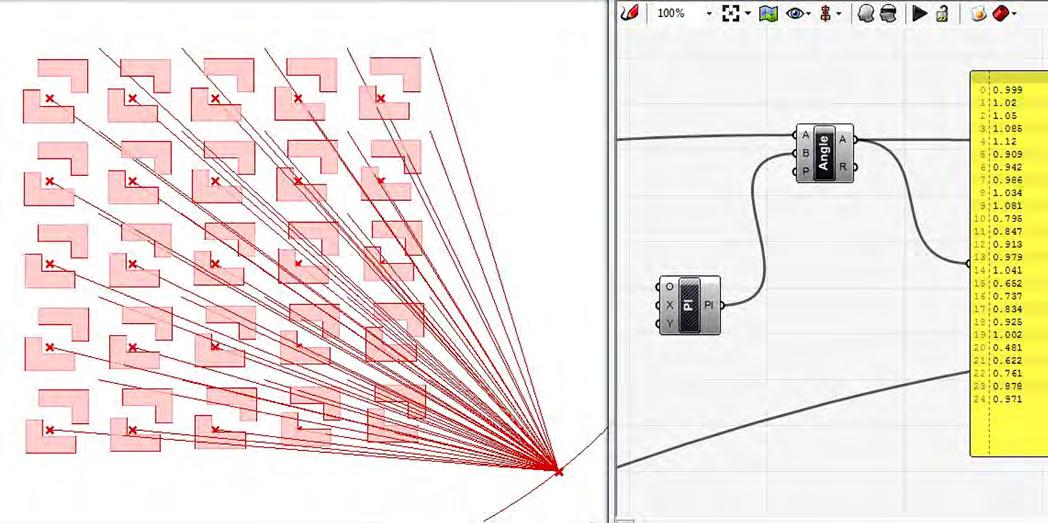
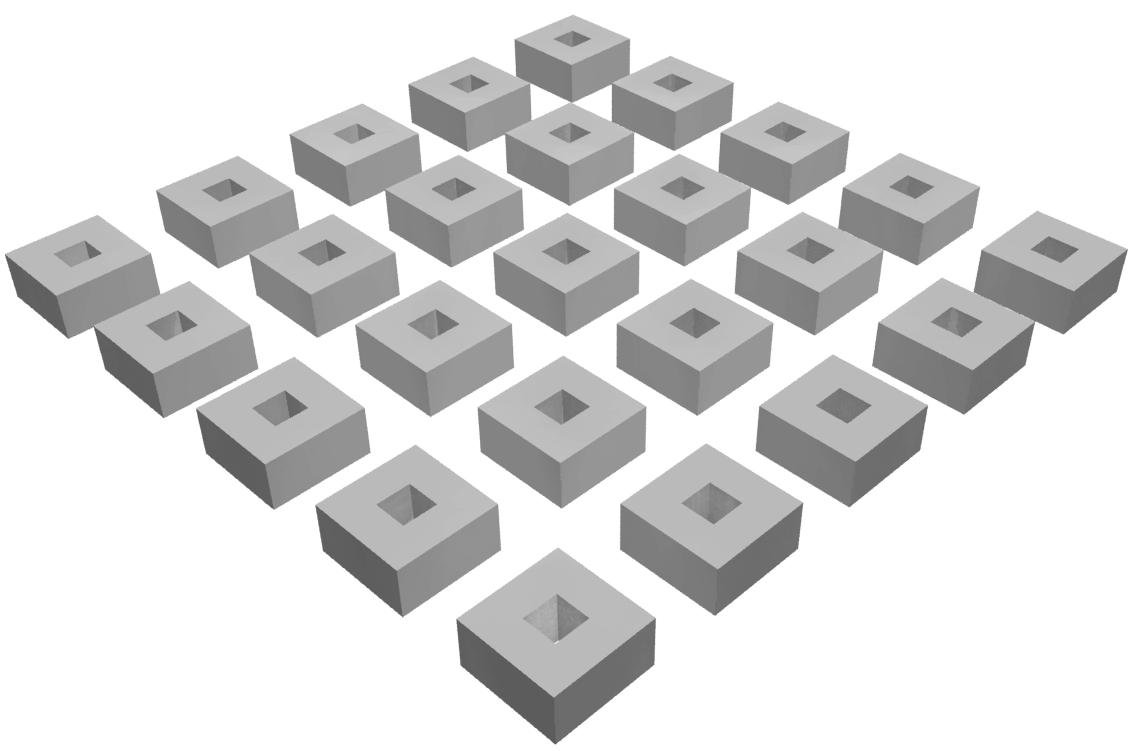
Fig.3.38
The experiments begins with the configuration shown in the image: 25 similarly formed blocks with equivalent distances between each other. The reason for the homogeneity is to observe the degree of differentiation that would be created eventually, as well as the adequacy of the parameters as the input.
The experiment aims to examine various parameters that affect the size, shape, position and other properties of the urban blocks. The setup is a set of 25 blocks (in rows of 5x5) with initially the same size, shape, height and distance between each other [Fig.3.38]. A system is being developed according to which every block corresponds to a specific point in space that represents a potential direction of the sunlight. Then the reference point is joined to every base point of each block and the grasshopper script measures the angles between every of those lines and the plane (0,0,0). The different angles are next transferred to a scale factor defining different heights of the respective blocks [Fig.3.39]. Defining these angles as parameters for manipulating the morphological properties of the blocks would rationalise the system: the blocks that are further away are the ones that are blocked by those that are in front, thus receiving less sunlight. Therefore, the blocks at the back should be the tallest ones compared
experiment 1
to the others in the front row. The blocks at the back have smaller angle, hence the system should work reversely; i.e. the last block at the back should grow taller than the block in front that has a bigger angle. Moreover, the same logic is applied to the definition of the distances between each block to the other. Therefore, the blocks at the back are taller and more dispersed than the ones at the front that receive more sunlight. It is crucial to mention that each block is comprised by two L-shaped volumes, which their heights and distances vary between the two of them within a block.
There are multiple tests of the experiment with the reference point placed in four different positions along an inclined arch in space. Then the differences between heights and distances are identified for these cases [Fig.3.310a,b].
Fig.3.39
Plan view of the arrangement of the blocks. There are 25 lines joining the reference point with every block. The end-point of every line represents the bottomleft corner point of each block before their displacement and scaling. Due to the differentiation between the angles of each line with the plane (0,0,0) the buildings are displaced with different distances between them, thus enhancing variation among them and simultaneously allowing the sun radiation to reach surfaces that had been shadowed before.
88
Fig.3.310a,b
The population of blocks is tested in two different cases; with the reference point’s position changed at each case. When the reference point is lower it means all the angles become smaller, hence the height of the buildings and the distances between them as well. However, the differences are very small between the two cases, while the ratio between those measurements remains constant.
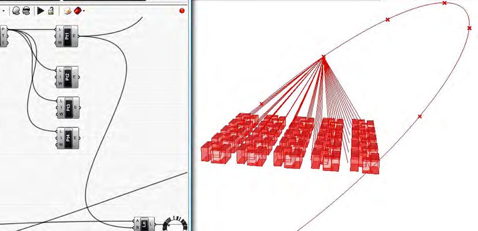
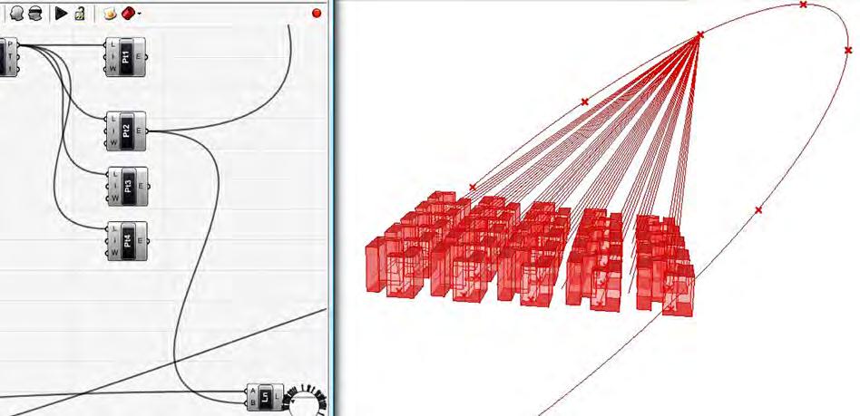
The different position of the reference point does not induce dramatic differences to the system. The logic is the same: each block is slightly taller to its neighbour and the distance between each block to its neighbour is slightly bigger. When the reference point is at a relatively low position – meaning that the value of its Z is smaller – then the differentiation in height and distance is almost inconsiderable. On the other hand, as the point moves higher in space the differentiation gets greater and greater. If the reference point starts moving on plan view then the variables are almost not affected at all, unless if the point moves to a position that very steep angles are created (i.e. on top of the block in the middle of the grid). Then the relation between heights
and distances of each block changes considerably and the results are far away from reality; the buildings of the blocks become extremely tall and the distances between them are vast.
In general it is being considered that the above method of defining a specific point on space and measuring the angles of each block to that point does not have an essential implementation of the height and distance variation. Furthermore, although the desired type of differentiation is achieved, the method does not produce accurate results of heights and distances.
89
A second experiment is being developed reconsidering the whole structure. Nine blocks are placed in rows of 3 by 3. The block in the middle is taken as the reference block. Its top point is joined with the base point of each other block [Fig.3.311]. The blocks start growing in height according to the angle of their base point and the reference point (RP). Prior to the extrusion of each block, the potential direction of the sunlight should be taken into consideration in order to direct the results of the angles to the desired heights. Through this method the experiment takes two directions: first, the height of the building volumes is adjusted and second, a new criterion is introduced; the amount of area surface exposed to sun radiation, which is a method of changing the distances between the blocks [Fig3.311]. Therefore, a first step of differentiation appears out of two different criteria.
Consequently, after one loop of the process ends, another block is taken as the reference one and other new blocks with different distances
experiment 2
and heights emerge. The method reveals a strongly emergent result; however there should be more parameters (mainly architectural) as the input for the future design method. Moreover, the particular method concerns simple extrusion of rectangular shaped elements, which resembles a conventional way of designing. The attempt for the next step is to apply analogous methods of emergent behaviours in a way of introducing more complex methods, starting from the assemblage of the block itself.
As the current experiment considers the block as an abstract rectangular volume, the setup is strictly symmetrical and it does not take into account the orientation of the blocks against the sun. Such a result is not desired as during the expansion of the blocks a stronger differentiation should emerge.
Fig.3.311 (left to right)
On the left the image shows the plan view of the initial setup with the reference point in the middle joined with the base points of each block for measuring the angles next. The second images shows the change of heights according to the angles. In the third image the surface area of the volumes exposed to solar radiation is measured and compared to the shadowed one. The last image on the right shows how the distances between the blocks affect the solar gains by increasing the surface area exposed to the sun.
90 a b RP RP a b RP a b RP Surface exposed to the sun Shadowed surface Reference block Passive block
Fig.3.312 (top left)
Each block is formed by the assemblage of individual volumes together. The Grasshopper tool defines the shadows of each volume to the others within a block; they are shown with the highlighted areas of red colour.
Fig.3.313 (top right)
The sample of the Grasshopper script shows one of the volumes which create shadows on the adjacent ones.
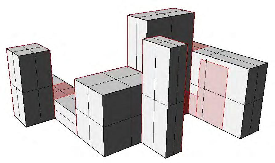
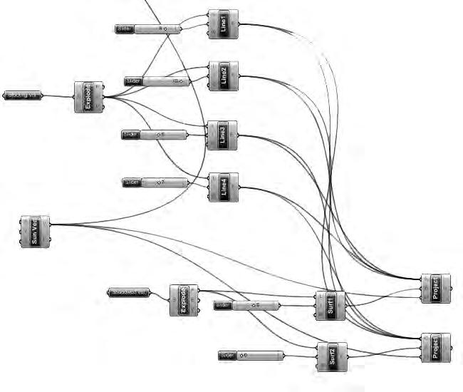
experiment 3
Taking the conclusions of the last experiment into consideration, it is assumed that the blocks are not conventional uniform rectangular volumes, but they are comprised by the combination of different volumetric forms assembled together [Fig.3.312]. The small exercise attempts to define a specific parameter in order to give a specific value to each block, therefore they can be next ranked into different categories. In essence, this experiment is the precursor of a genetic algorithm, which could possibly develop a process of repeating steps with the combination of receiving feedback and finally organise the urban tissue.
The experiment is based on the evaluation of the blocks according to a criterion, which will then define which elements perform better or not against it. For the moment the criterion is not yet set; however it is defined that it will be directly related to the amount of solar energy that each block gains from the solar radiation that hits its surfaces. Therefore, the block which is exposed to the sun most than the others
fits the criterion that will be set. With the help of the Grasshopper software, a simple script is developed, according to which a potential direction of the sun is set and hits each block independently [Fig.3.313]. The Grasshopper tool defines the outline of each volume and projects the respective shadow on the adjacent volumes that are influenced, based on a vector that represents the sun direction [Fig.3.312]. The volumes that comprise the block create self-shadowing between each other, reducing the area of exposure to the sun. This way it is very easy to measure the surface area that gains solar energy and the area that is shadowed accordingly.
It has been noticed that depending on the volumes’ configuration within a block the amount of surface exposed to the sun varies. Moreover, the amount of surface exposed to the sun changes dramatically when the block is rotated on the horizontal plane.
91
conclusionAccording to the examples that have been studied earlier, an efficient model of urban block in terms of capturing or releasing energy has the following characteristics:
- its shape is optimised in order to achieve or avoid energy gains accordingly - the arrangement of volumes around an atrium; it is a transition space between the outdoor and indoor spaces, a qualitative space of vegetation that contributes to the improvement of the microclimate conditions and a method of air supply and heat exchange between the spaces.
- the external surface of the structure are insulated - the green roofs provide longevity to the buildings.
Therefore, the aim is to maintain many of the properties to the following design process, depending on the desired conditions.
92
3.4 Conclusions
The experiments carried out are extremely useful for the next chapter, where the design scenarios will begin. Although the experiments are based on arbitrary terrains, they give an insight to what difficulties or issues might be faced once the actual terrain is introduced. The main difficulty with the paths is to integrate it with the topography, and ensure that the ‘gridded plan’ is not repeated where the street networks are simply applied on the terrain, without taking into consideration the effects that the terrain would have on the development of the street networks. The blocks on the other hand have been analyzed with respect to the effects of sunlight on their morphology, however, once the design scenarios are introduced, sunlight on its own will not be sufficient in developing and optimizing the blocks into forms that comply with the different demands of a city. Topography will have a large effect on the blocks, however it will not necessarily raise difficulties once implemented, on the contrary, the topography might further benefit performance of the blocks with respect to the region climatic conditions.
The possibilities and variations that arise from initigrating initiator and generator strings are many, however, the main driving force that will determine both the layout and global forms of the paths will be the topography. In modern planning, the streets are developed planarly at first, where the left over spaces between the streets are then allocated for building lots. However, in cases such as in Istanbul, and the ancient cities of Egypt, the lots were initially located rather than the streets, this lead for the paths to be generated between as a result of the lots. This method of development of street networks proves to be the most efficient, as well as the most functional.
According to the examples that have been studied earlier, an efficient model of urban block in terms of capturing or releasing energy has the following characteristics:
- its shape is optimised in order to achieve or avoid energy gains accordingly
- the arrangement of volumes around an atrium; it is a transition space between the outdoor and indoor spaces, a qualitative space of vegetation that contributes to the improvement of the microclimate conditions and a method of air supply and heat exchange between the spaces.
- the external surface of the structure are insulated
- the green roofs provide longevity to the buildings.
Therefore, the aim is to maintain many of the properties to the following design process, depending on the desired conditions.
93
94
Design
To fully understand the potential of a metabolic system with respect to urban development, urban metabolic growth will be implemented onto two different scenarios to convey the different outcomes that are achieved on account of the regional conditions.
95
4.
96
4.1 Introduction
Metabolic systems have been extensively studied in biology, however it is only recently that metabolic systems have been related with different fields. To fully understand the effects of a metabolic system on urban growth, one must first understand what are the advantages of metabolic systems in general, and how one can use them as a model for other fields. To have a more advantageous understanding of the effects of applying the metabolic system within urban development, two different scenarios will be chosen. However, it is crucial to ensure that the scenarios chosen are complete opposites, with respect to both the climatic conditions, as well as the average energy consumption of that particular region.
The researched carried out throughout the dissertation so far will all heavily inform the direction that the scenarios will be developed. For instance, both planned cities as well as evolved cities contain
examples of what is advantageous to the urban fabric, and what’s not. The effects of densities and centrality all contribute to the overall efficiency of the city. The tools that were researched will be of great benefit to develop the design; one thing to consider however is that there is no single tool that will develop everything, in order to fulfil the different objectives and aims set out, several tools have to work in conjunction with one another. Although the experiments carried out were with respect to an arbitrary terrain, they gave an example of the different effects the terrain will have on the experiments, thus giving an insight into what might be expected once the terrain of the actual scenarios are introduced.
97
China population
China is the most populated country in the world with 1.24 billion people in 1998 (Samuelsson, 1998). Today its population reaches almost 1.33 billion (ISTA, 2007), from which the 90 percent of it lives in 15 percent of the total land area. Specifically, most of the population is concentrated on the east and south-east coastline, whereas the inland is under-populated [Fig.4.22]. Therefore, the big cities of the coastline are over-populated and highly dense while immense areas in the rest of the country remain unexploited.
Shanghai’s inhabitants reach the 17.4 million and Beijing almost 15 million. There are eleven cities in China that their population exceeds the 2 million. The area of focus is located in the province of Ningxia, southern to the borders with Inner Mongolia, on the banks of Yellow River.

98
4.2
Fig.4.21
Fig.4.22
The map shows the population distribution in China, as well as the population accumulation in big urban centres. The sharp differentiation between the coastal areas and the inland in terms of population density is visible on the map. There are six hierarchical categories of ranking the cities within the country, according to their population density. The biggest cities are Beijing, Shanghai and Tientsin, with over 3 million people and they are all in the eastern part of the country. Despite the many attempts of the government to move population towards the inner part of the country, Chinese inhabitants remain concentrated on the east part. The vast empty lands and cold climate give the impression of areas that cannot be easily occupied.
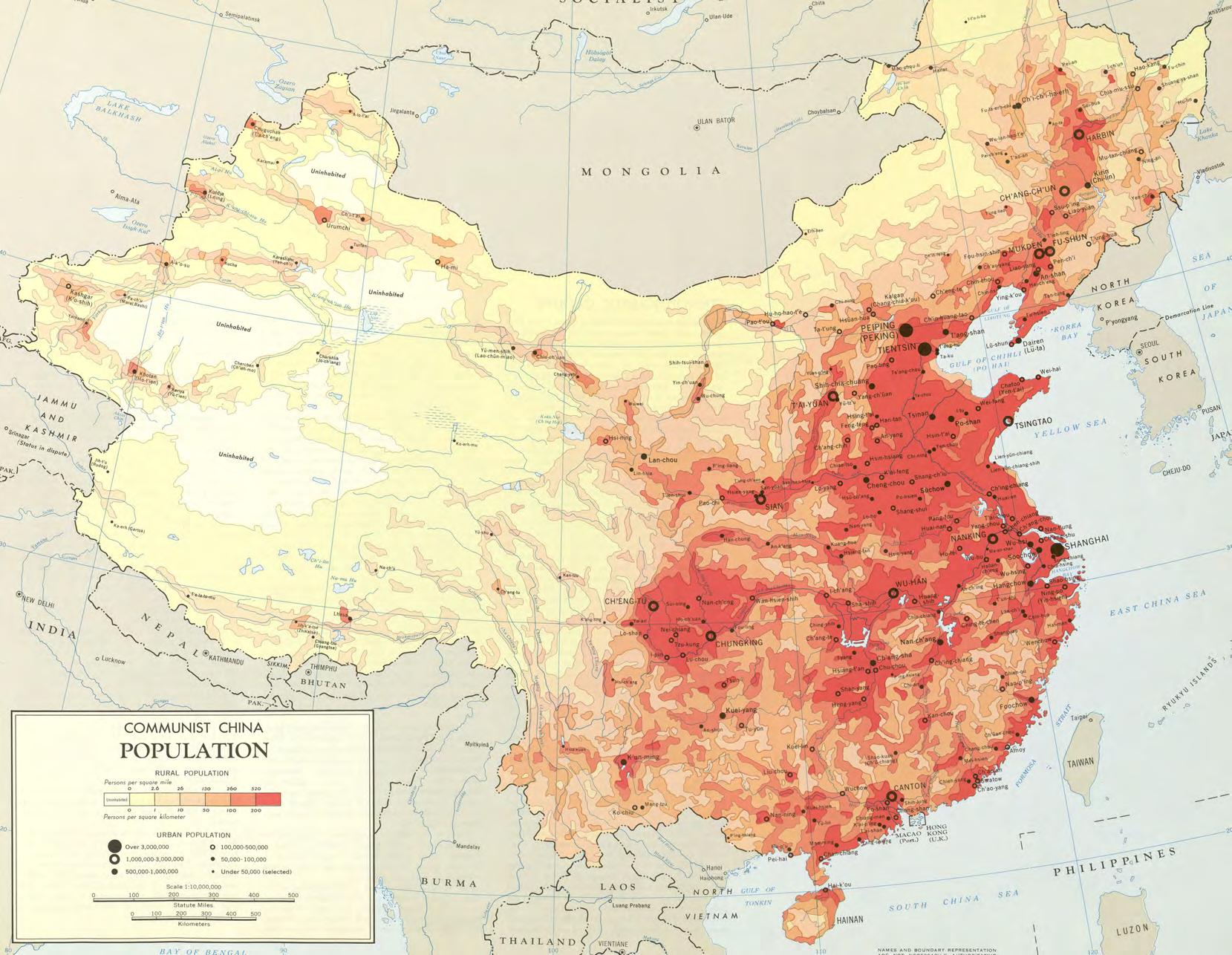
99
temperature
Cold temperatures dominate in the north part of China during the months December to March. In the area of the site the average temperature during January is -10oC [Fig.4.25]. The winter is considerably long and carries long periods of thin snow that covers the sand land and mountains. Summer ranges from May to August, with relatively low summer temperatures due to the high altitude of the area. During July the average temperature is 22oC and the rainfall is slightly increased compared to the winter [Fig.4.26]. In general days with sunshine dominate throughout the year.

100
Fig.4.23
Fig.4.24
The west part of China around the Himalayas, as well as the north-est part of the country, have extremely low annual temperatures. The area with the warmest average temperature is the southern part of China. The difference between these two areas of extreme temperatures is remarkable.
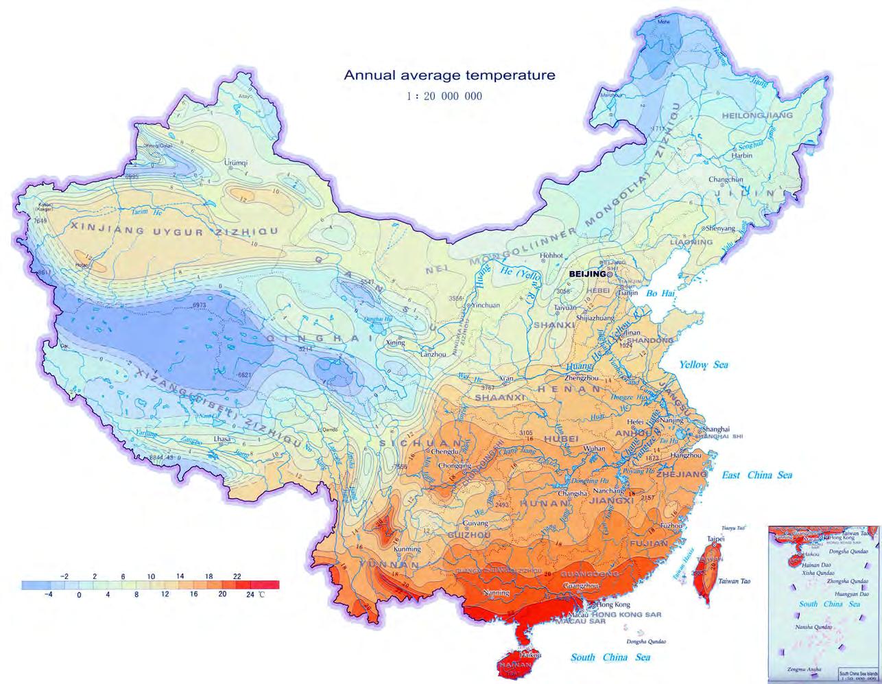
101
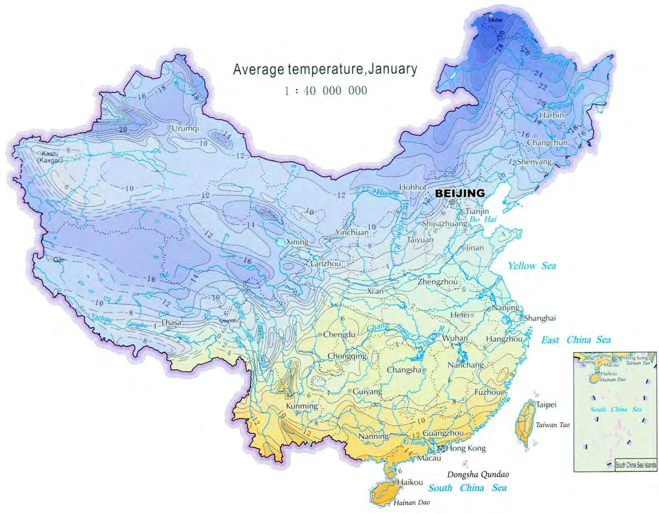
Fig.4.25
During January most of the country’s temperatures are relatively low, except from the south-east areas. The average temperature can reach the -30oC on the very north. The area of Ningxia experiences average temperatures of -8oC to -12oC .
102
Fig.4.26
Summers are warm around the country, apart from the west part. The highest average temperature in July is around 28oC and the area of Ningxia, although being on the north part of China and on very high altitude (13002000 metres above sea level), is not far from the average; its temperatures vary from 22oC to 24oC.
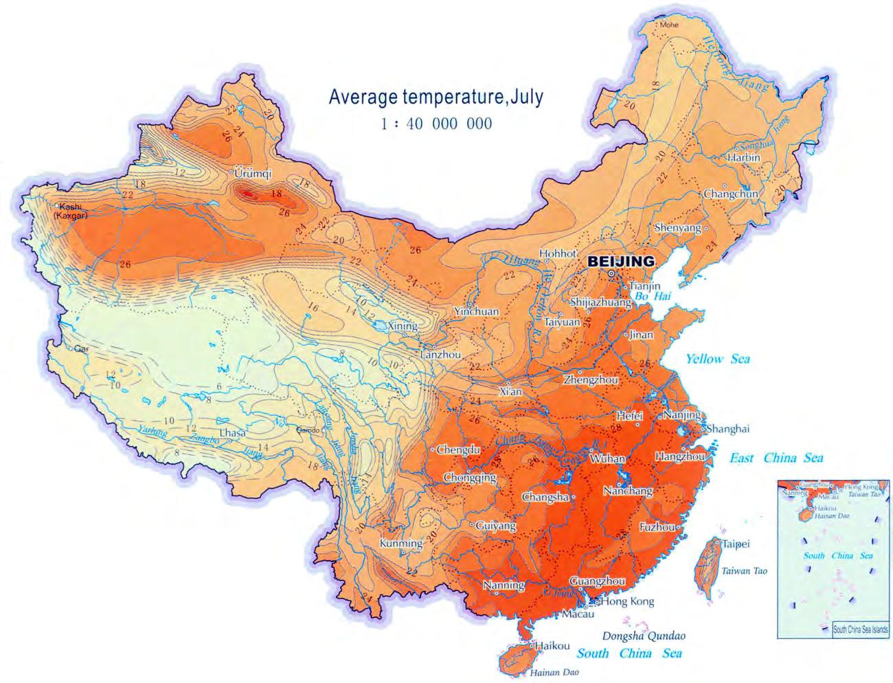
103

precipitation
A large area on the north part of China is covered by desert, whereas in the south and especially south-west there is a high annual rainfall. This vast incongruity from extremely dry to highly humid environment within the country is getting bigger as the global climatic change is increasing throughout the years. In 2003 the government decided to implement the South-North diversion plan, aiming to divert water towards north from three different locations. The project has been postponed for economical reasons, leaving the project in doubt whether it is implementable or not.
The location of the site belongs to the zone of which its annual precipitation ranges from 100 to 250 millimetres [Fig.4.28]. It is of extreme importance that the site is not far from areas with higher precipitation levels, as well as significantly close to severely dry ones. During the last 40 years, the wider area of North China Plain suffers from overuse of surface water resources and excessive exploitation of groundwater (Changming). This is a consequence of the dramatic
changes over the last decades, such as the rapid development of the existing cities and industries and the expansion of the farmland areas; these factors led to the increase of water demand in many sectors. Scientists talk about essential measurements for an ecologically oriented water management as the only way of water saving and sustainability (Changming); the goal is to provide capability and infrastructure to these areas. The site is located next to the Yellow river, on which most of the North China agriculture is currently relied. It is anticipated that within the next 30 years the Yellow river will probably run dry.
104
Fig.4.27
Fig.4.28
The figure maps the areas of China into zones of annual precipitation values in millimetres. The site is located on the verge between a very dry area, with annual rainfall ranged between 100 to 250 millimetres, and an area of slightly higher humidity with values between 500 and 750 millimetres. In some locations the chart of the monthly precipitation throughout the year is shown. In areas of northeastern China it is obvious that the highest precipitation occurs at the beginning of the autumn period, with a significantly higher frequency than the winter period. In south-east of the country the rainfall is frequent throughout the year; during the summer period the frequency is slightly higher than the rest of the periods.
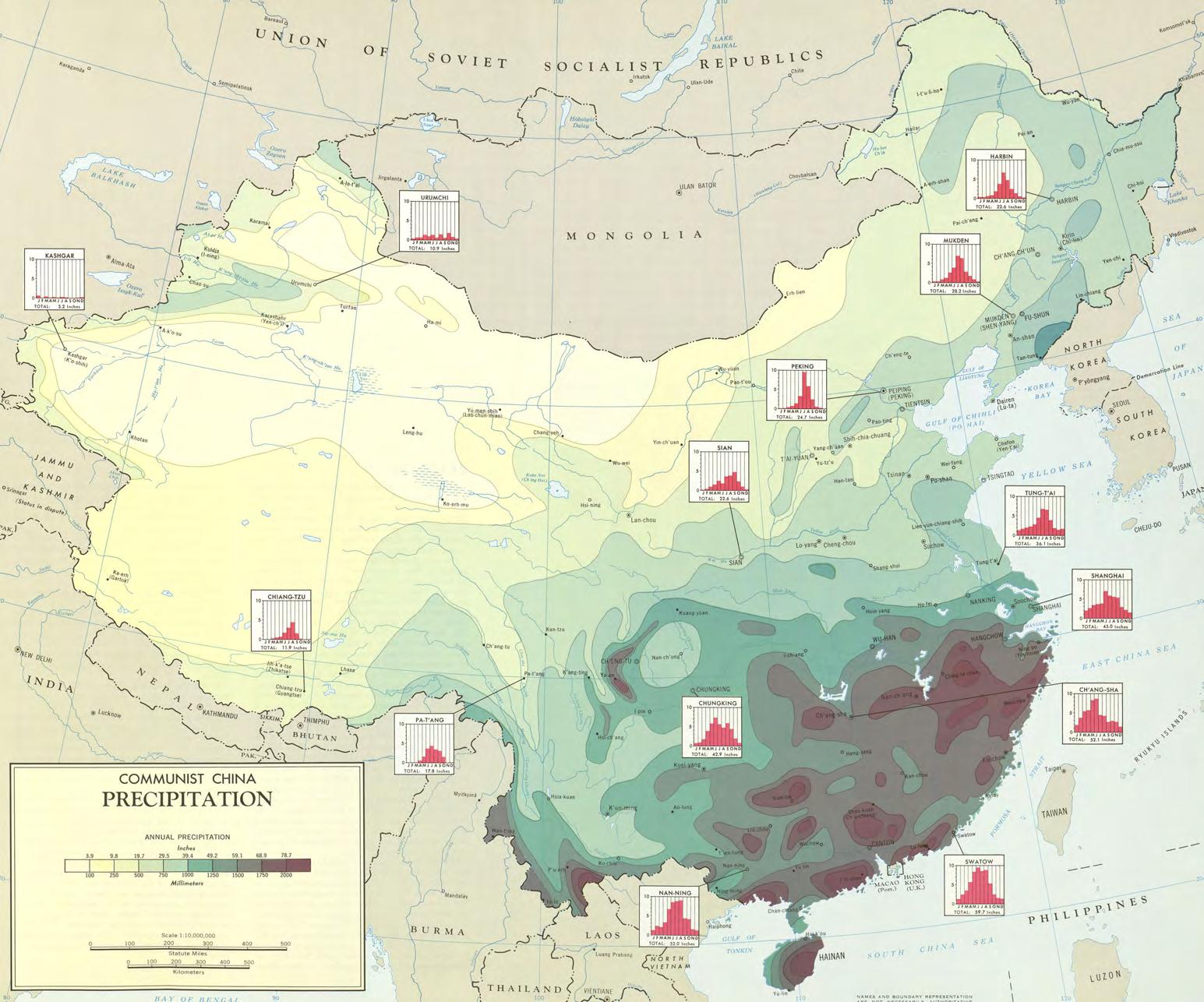
105


Fig.4.29 (left)
The general texture and morphology of the landscape is manifested in the image. The landscape around the area of Ningxia, especially along the Yellow river, is formed by rocky hills covered by a thin layer of sand.
Fig.4.210 (right)
The coexistence of vast arid lands and agricultural activities nearby conveys a spectacular sense of antithesis in terms of the natural landscape. The agriculture is organised in a linear form along the Yellow river and the water supply is currently completely dependent on the river, however its significance is essential as it is used as a linear vegetation zone of inhibiting desertification from the north.
soil and vegetation
The wider region of the central area of North China is mostly surrounded by steppe; semi-desert areas with low vegetation. The vegetation in North China has been examined by a team of the Chiba University (QiJing), where it was concluded that from the potential vegetation that would naturally flourish, only 43% currently exists. The main reasons for the significant reduction of vegetation is the last century’s massive deforestation, the replacement of meadow by farmlands, with the combination of the climatic change; especially the increase of drought in the area.
The soil of the central north area of China is mostly Halpic Xerosols, Arenosols, Unidentified and Calcic Xerosols and Lithosols. Xerosols are types of dry sandy soil, Arenosols are coarse loamy sandy soils and Lithosols are soils with high quantities of rocky soil. Generally, the soils that cover the area are characterised as loess soils. Loess soils
contain high portions of nitrogen, potassium and phosphorus and they retain water effectively, thus they are productive despite the region’s seasonally dry climate [Fig.4.29].
The site is located on the verge between highly arid land and extensive areas of agricultural activity [Fig.4.210]. The area is often exposed to sandstorms, especially during the end of April, which they mostly flow from the west to east and they last approximately for two weeks. The site area is surrounded by mountains on the north and north-west side, which they contribute to the inhibition of the strong wind flow from the west. The altitude of the area varies from 1300 metres to 2000 metres above sea level.
106
Fig.4.211
The major types of soils are mapped according to the areas with the most dominant type distribution. Most of the west part of China is rocky and arid in contrast to the east and southeast parts where the soil is offered for crop cultivation and rich vegetation.
Soil map of the people’s republic of China
(Revised version 1990 based on the FAO Unesco soil map of the world)
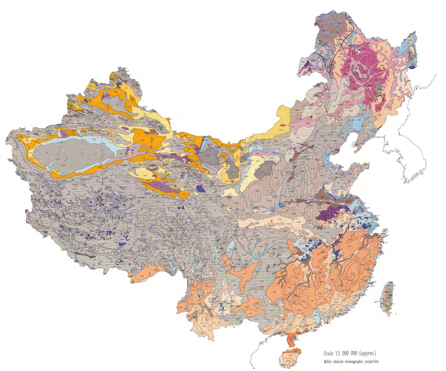
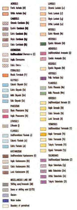
107

agricultureChina is the world’s leading producer of rice (34% of the world’s rice production), with 200.5 m tons in 1999. However, 90% of the rice is produced in the south part, mainly because of the water demands. Wheat is being cultivated throughout the whole country region [Fig.4.213]. In 1999 the production was 114.4 m tons. Its production is mainly located in North China Plain and Yangtze valley as the water demand for its cultivation is low. Corn cultivation mainly develops in Southwest China, but also some areas in the North. Drought-tolerant millet, as well as kaoliang, are species that flourish mostly in the northern and north-eastern part of China, whereas in the south of the Yellow river there is production of sweet potatoes. White potato production is concentrated in cooler areas, i.e. north of the Great Wall. Cotton flourishes along the middle and lower reaches of Yangtze
River and on the plains of Yellow and Huai Rivers. Sugar production dominates mostly in the south part, but 19% of the total production is based on the north and north-east China.
China has the largest irrigated land in the world; in 1950 there were 15.3 million hectares of irrigated land, which was rapidly increased and in 1998 it reached the 52.5 million hectares. Agricultural yields are expected to decrease for all major cereal crops in all major regions of production of the world, once the global average temperature increases beyond 3oC. For some crops the yield could decrease by over 20% at low latitudes, where the impact will be greatest.
108
Fig.4.212
Fig.4.213
The area of interest is mapped as a relatively low agricultural activity one. However, there are many types of crops cultivated in the area including kaoliang, corn, potatoes, oats, cotton and buckwheat for winter wheatmillet, which exists mostly on the south part of Ningxia, and sesame seed, buckwheat-millet, oats, linseed, kaoliang, hempseed and rapeseed for spring wheat, which is spread mostly on the north and north-east parts of Ningxia.
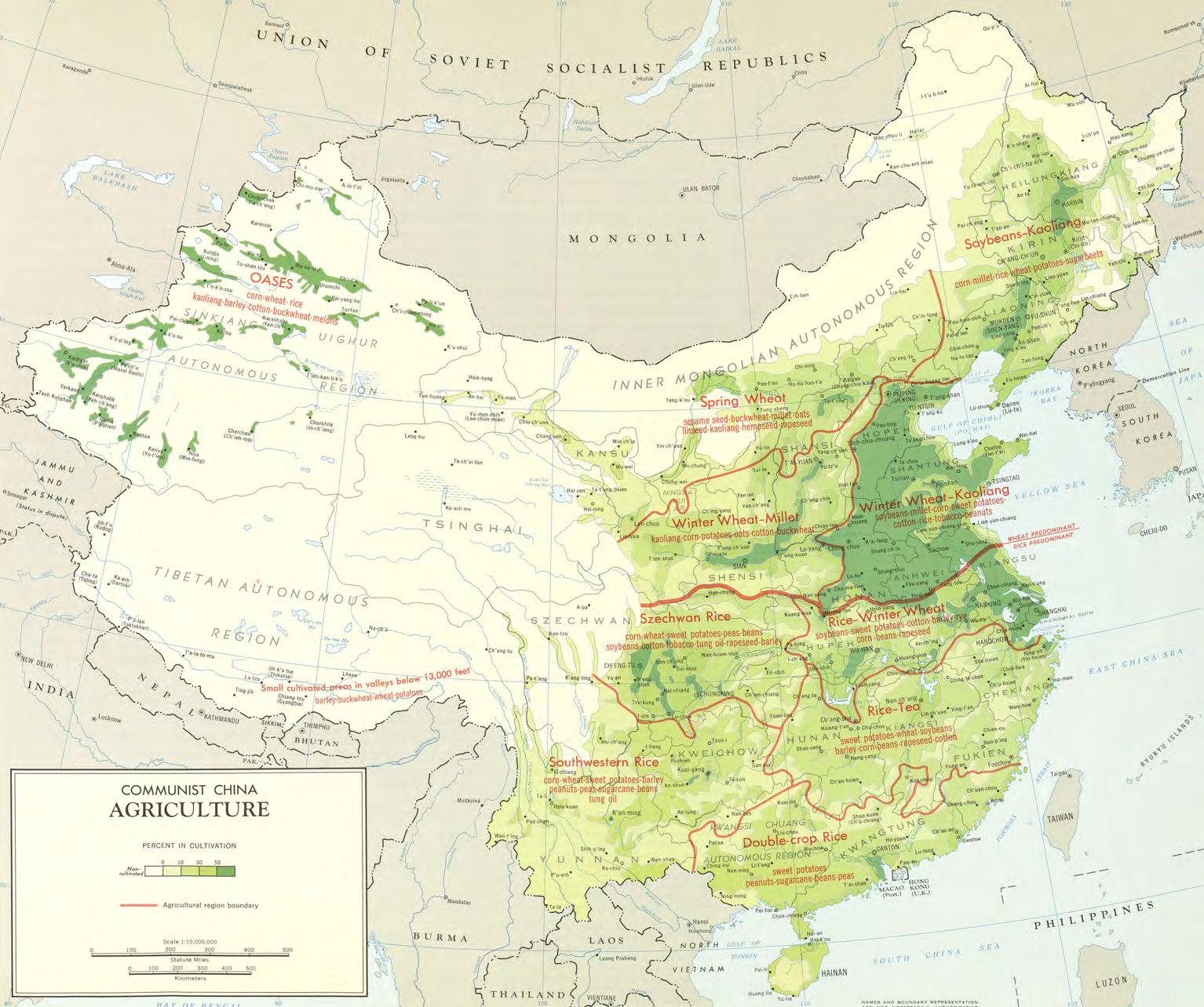
109

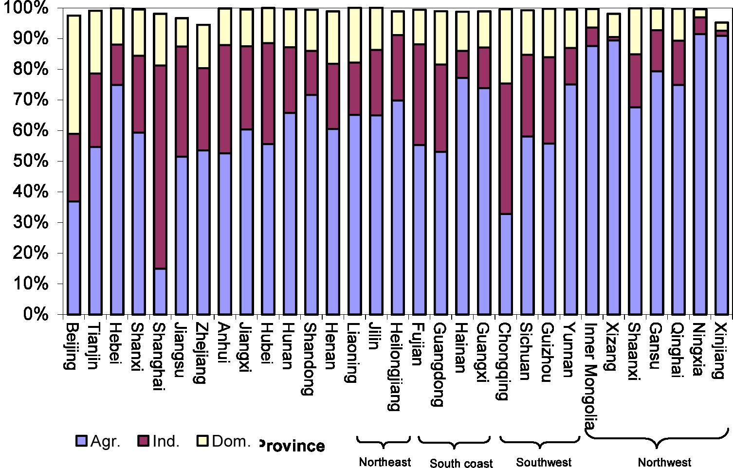
water and energy consumption
Two of the most crucial issues concerning China today are energy and water resources. Water is scarce especially on the north and northwest parts of the country. There is a large amount of annual water deficit in the whole region of China, estimated around 40 billion cubic meters (Fredrich, 2007). During the last decades, water allocation has been shifting from traditional agricultural irrigation to larger shares for industrial and domestic uses. However, agriculture remains the major field of water consumption: from 97% it dropped to 69% during the last 50 years, when industrial and domestic uses increased from 2% to 21% and 1% to 10% respectively (Guan).
In most of the areas the proportion of water use for agricultural development exceeds the 50% of their total water consumption, except from Shanghai, Beijing and Chongqing (Zhou, 2005). In the province of Ningxia the proportion of water used for agricultural activities in comparison to the total water consumption reaches the 90%, with only 10% remaining for industrial and domestic use [Table.4.215].
Agricultural use covers the farmland irrigation, forestry, animal husbandry and fishery. One of the major reasons of inefficiency in water distribution, especially through long-distance networks, is the leakage in irrigation systems. Hence, local water resources are more preferable for safety and economic reasons. Moreover, in the review of the Philosophical Transactions of the Royal Society (Jing , 2005) an important question arises; whether it is worth it or not to develop water transferring systems from the south part of China to the north or exploring new resources locally for water sustainability. In essence, the researchers worry that with such a mega-infrastructural network, the environmental impact will be more catastrophic than using local resources.
Table.4.215: Provincial share of water use by agricultural, industrial and domestic sectors respectively.
The table indicates that in the northwestern provinces, such as Xinjiang, Ningxia, Qinghai, Tibet and Inner Mongolia, agriculture has the highest share of water use, which is over 85%. A high share of water is also distributed to agriculture in the two areas of the south coast, Guangxi and Hainan, as well as in the provinces of Hebei and Shandong in the North China Plain. In the provinces where the big cities belong to there is a lower share of water for agriculture.
110
Fig.4.214
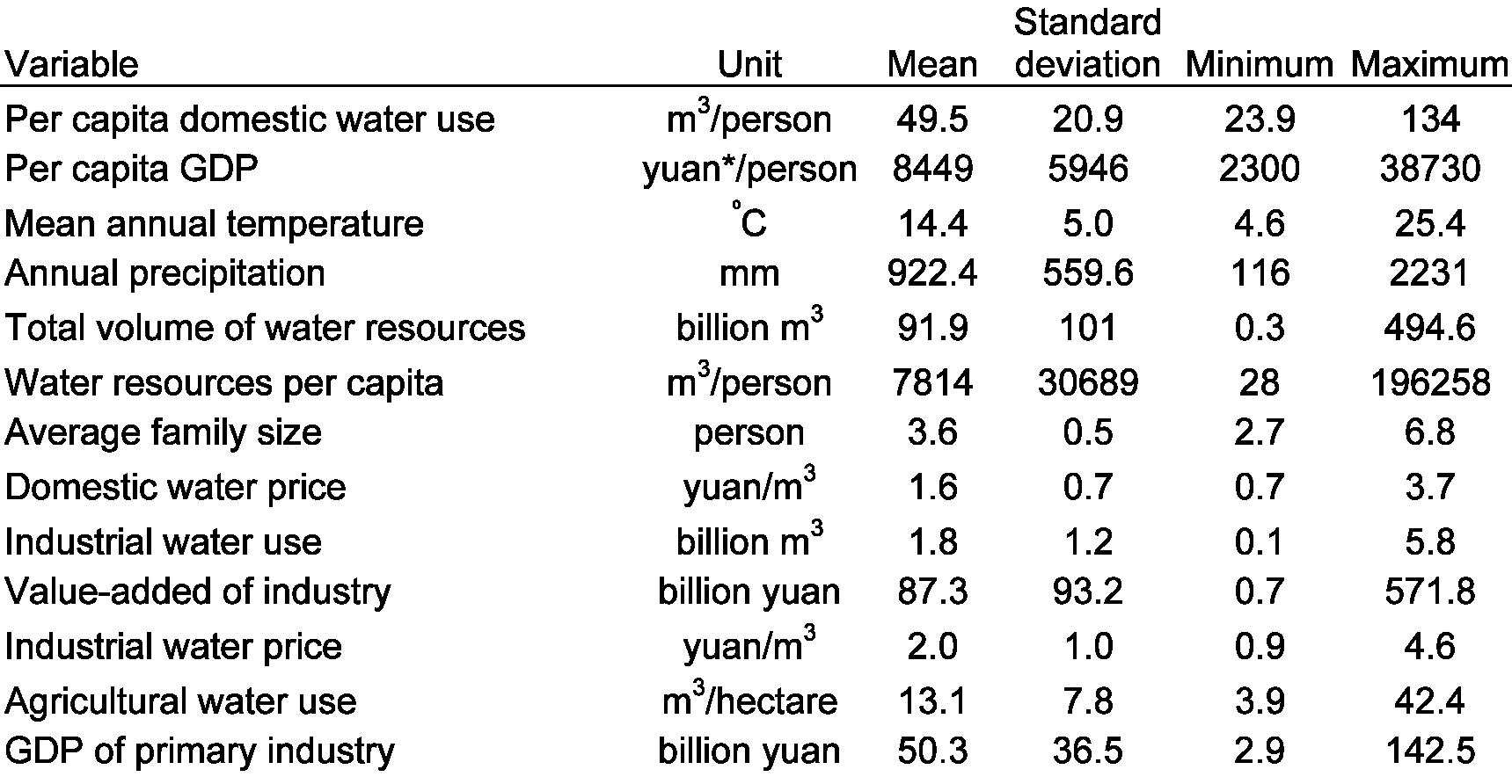
Table.4.216: Variables of China’s main energy sources
The variables are shown as their mean, minimum and maximum values, as well as the standard deviation number (negative or positive).
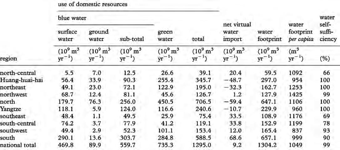
Table.4.217: Water footprint by region in 1999
Water footprint can be described as the water needed for sustaining a certain area of activities, such as agriculture, domestic use, industrial e.t.c. The table shows the water footprint per person for each of China’s regions in 1999.
Water consumption varies significantly from region to region. The average annual domestic water use in Shanxi province is around 26 cubic metres per capita, whereas in Shanghai is 107 cubic metres per capita. In 2003 the estimated overall annual water consumption in China was approximately 408 cubic metres per capita. Studies have revealed that during the period of 1997 to 2003 the mean water consumption per capita in China was around 50 cubic metres per person, or 50 Kilo-litres per person, however varying from 23.9 to 134 cubic metres per person according to the area [Table.4.216]. In the same study the features show that the mean agricultural water consumption was 13.1 cubic metres per hectare with standard deviation up to 7.8 cubic metres per hectare. It has been estimated that the water footprint per capita in the area of North-central China in 1999 was around 60 billion cubic metres [Table.4.217], one of the lowest values compared to the rest of the country.
Food production seems to derive from more various sectors than in
the past, mostly due to China’s sharp economic growth of the last decades, which led to the improvement of lifestyle in the people’s daily needs. This automatically led to the re-configuration of the economic resources, which for instance, have shifted from agricultural activities to industrial uses. Therefore, the energy consumption in the country in general had shifted towards more commercial energy sources, such as electricity for domestic devices, coal, oil products e.t.c. In 1975 the government allowed small local coalmines to be developed in order to reduce the domestic energy demands (Guan). After the economic development of the country, many new energy sources emerged. The statistics of 1999 show that the average annual energy use per capita in urban areas is 3.5GJ and in rural is 11.7GJ. The overall average annual energy use is 8.2GJ per person. The annual average energy use per household is 10.9GJ in urban areas, 51.9GJ in rural and the overall is 30.2GJ.
111

climate change
A research conducted, based on a regional climate change model which was developed by the United Kingdom Hadley Centre of Climate Prediction and Research, attempts to simulate the climate in China and next develop climate change scenarios for the country (Guan). According to research results, by the end of the 21st century the temperature in China will rise by 3-4oC. The phenomenon of higher temperatures will trigger the increase of rainfall and its intensity all over the country, however distributed unevenly from one area to the other, thus having a tremendous impact on climate-sensitive sectors such as agriculture.
Finally, the research concludes to a potential scenario that would prevent the massive distortion in the agricultural productivity rate of the country; as the climatic changes are inevitable, adaptation is
the key. Some strategies of implementation include improvements in the agricultural substructure (i.e. irrigation and drainage systems), developments in the water saving technology such as the irrigation systems, developments of advanced technological instruments in order to improve the protection of crops, forests, livestock and fisheries from droughts, pests and climate variability, recovery of grassland to avoid further desertification and finally assessments on the carrying capacity of water resources based on the climatic change and water supply.
112
Fig.4.218
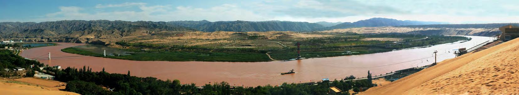


113
Fig.4.219
Fig.4.220
Fig.4.221
Fig.4.222
Fig4.223

4.3 Australia population
Australia’s current population reaches the 22 million people (Australian Bureau of Statistics, 2009). The population that is concentrated in the coastal areas around the country over-exceeds the population of the inland areas and this chasm increases throughout the years [Fig.4.32]. The average population density is around 2.4 people per square kilometre. The highest population densities dominate in the south-east part of the country, mostly in the wider areas of Brisbane, Sydney, Canberra, Melbourne and Adelaide.
During the last couple of years the population growth in the big cities was extremely rapid; Perth and Darwin were the most fast-growing cities with a growth rate of 2.8 percent during 2007-8. The location of interest is near the lake Argyle, an artificial reservoir in the north-west area of Australia in the East Kimberly region, around 500 kilometres south-west from the city of Darwin. The altitude ranges from 100 to 400 metres above sea level.
1 dot = 1000 people
The population distribution is mostly concentrated to the east coastal areas, the southwest and the very northern ones, where the land in the inner part of the country is almost uninhabited.
114
Perth
Adelaide
Melbourne
Hobart
Canberra
Sydney
Brisbane
Fig.4.31
Fig.4.32
Fig.4.33: Mean minimum temperatures for the year 20082009
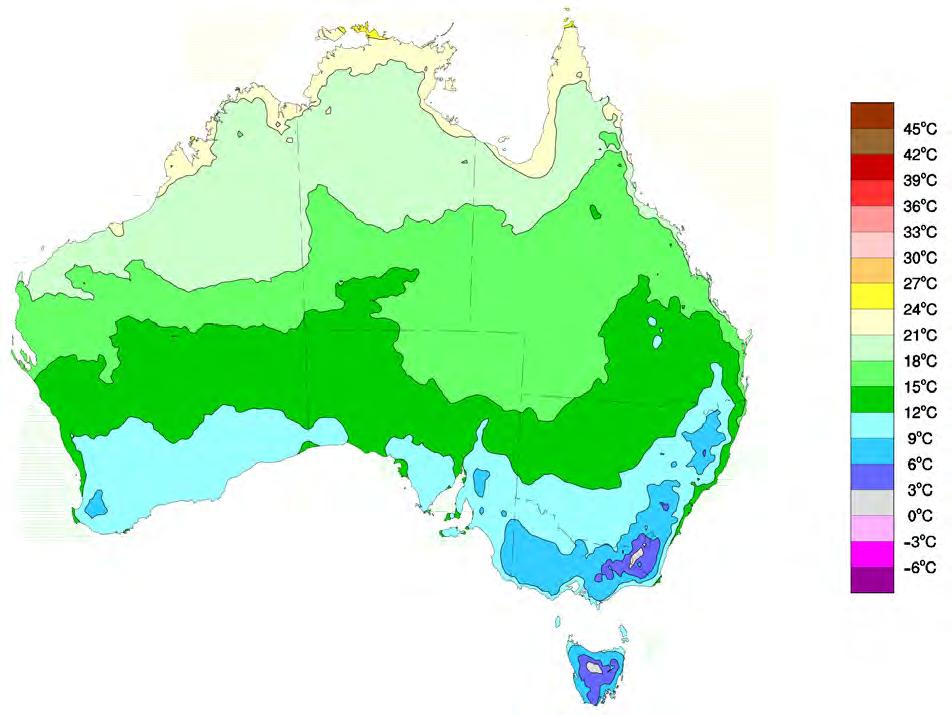
Fig.4.33
Temperatures in Australia change gradually from warmer to colder from north to south. However, there are not extremely cold areas, as the areas with the lowest mean temperatures are the south ones and they do not drop lower than 0oC.
Fig.4.34
The areas in the south part of Australia do not rise sharply throughout the year, they fluctuate with deviation of approximately 3oC to 4oC up or down. On the north the temperatures fluctuate with higher intensity, with approximately 15oC of maximum deviation.
Fig.4.34: Mean maximum temperatures for the year 20082009
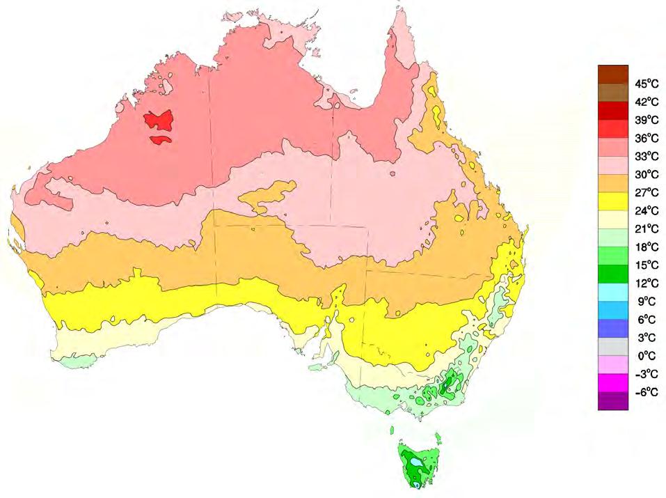
temperature
A large area of the inland is covered by deserts where the climate is dry and extremely hot in the summer period. So far this was a reason for avoiding any kind of development in those areas. A wide range of various climates dominate in Australia, with tropical and sub-tropical on the north and east parts respectively, equatorial climate on the north peninsulas of the country, grassland existing around the inner areas that are mostly deserts and finally, temperate climate characterises the coastal areas on the south-east and south-west. The site is located in a hot arid climatic region, with an average temperature of 36 to 39oC during January and 24 to 27oC during July (Australian Government, 2009) [Fig.4.33,4.34].
115
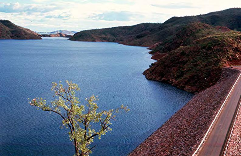
precipitation
The area of the site has average annual precipitation of 600 to 800 millimetres. The coastal areas, especially on the north, east, southeast and south-west parts of Australia, are highly humid. On the other hand moving inwards the main land the mean rainfall decreases dramatically, with the central part of the country being the driest area of the country with zero to 200 millimetres of mean annual rainfall. The reservoir Argyle currently storages 84.35 percent of its total water capacity, a surprisingly high amount of water preservation considering the hot and dry weather of the area. However, due to the rapid global climatic change and the sharp rise of temperature that is anticipated for the next couple of decades, the water storage in the dam is very likely to reduce dramatically as a result of its large exposed surface area that increases the chance of evaporation.

116
Fig.4.35
Fig.4.36
Fig.4.37
High precipitation levels occur mostly around the coastal areas. The transition between the areas of high annual rainfall to the dry ones is extremely sharp. There are two extreme conditions within the Australia region: the very humid areas with very high levels of rainfall and the very dry ones. Considering the fact that Australia is one of the most water-consuming countries in the world, it is remarkable to see that the area of the land with very low rainfall outweighs the area of land with high rainfall.
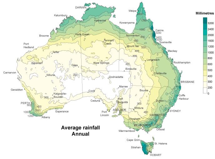
117
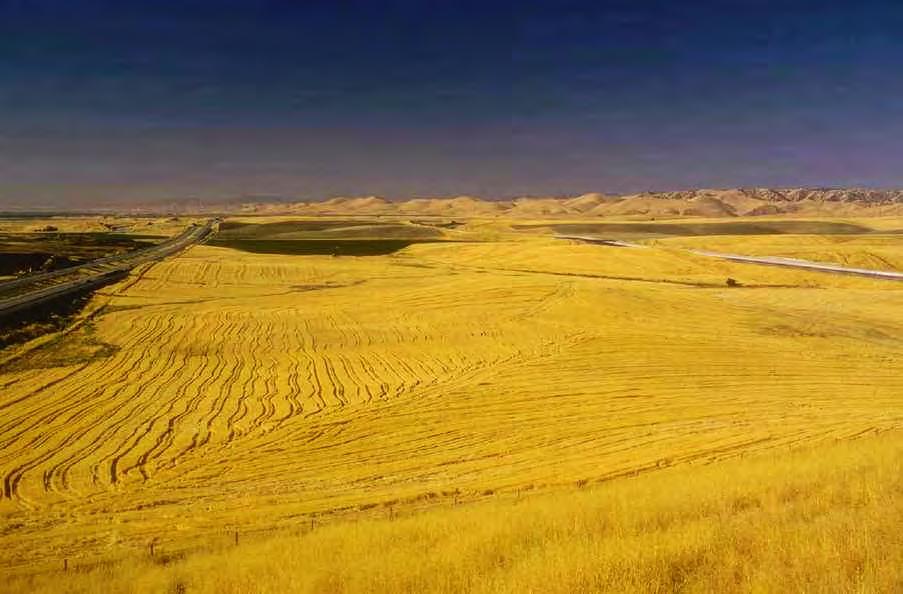
agriculture
Western Australia is divided into five different agricultural zones: the Rangelands region, Northern Agricultural, Central Agricultural, South West Agricultural and Southern Agricultural regions. The major agricultural activities in the Northern Agricultural region, where the site is located, are forestry plantations, commercial seed production, field crops and horticultural crop production. The seed production includes the cultivation of sorghum, sunflower seed, cotton wheat, as well as rice mainly on the northern part where the climate is more humid. Mangoes, bananas, melons, pumpkin and citrus constitute the basic horticultural crops.
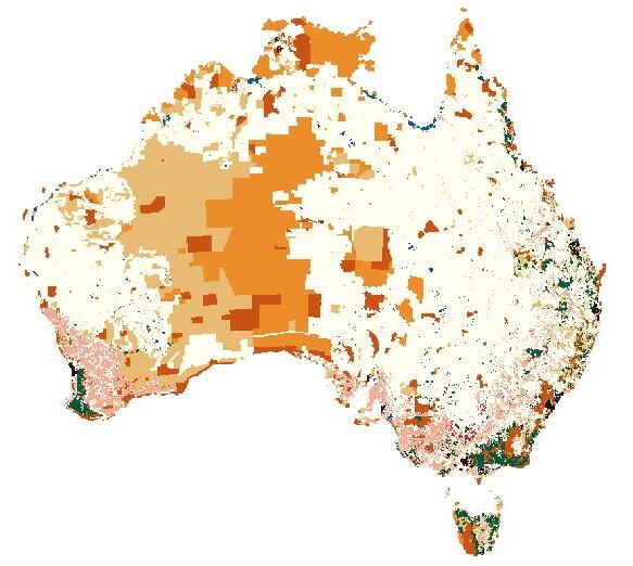
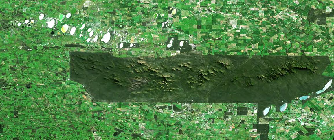
118 Source: 1996/97 Land Use of Australia Summary and 1996/97 Land Use of Australia, Version 2, National Land and Water Resources Audit The data set was derived and compiled by the Bureau of Rural Sciences. Land uses were derived using data from the 1997 and 1999 Collaborative Australian Protected Areas Database (Environment Australia), TOPO-250K Version 1 (AUSLIG), the National Forest Inventory 1997 tenure and forest data, Normalised Difference Vegetation Index images (Environment Australia) and AgStats 1996/97 (Australian Bureau of Statistics). Control sites provided by state and territory agencies: NSW Agriculture, Victorian Dept of Natural Resources and Environment, Queensland Dept of Natural Resources and Mines, Primary Industries and Resources SA, Agriculture Western Australia, Tasmanian Dept of Primary Industries, Water and Environment, Northern Territory Dept of Lands, Planning and Environment.
Fig.4.38
Fig.4.39
Fig.4.310
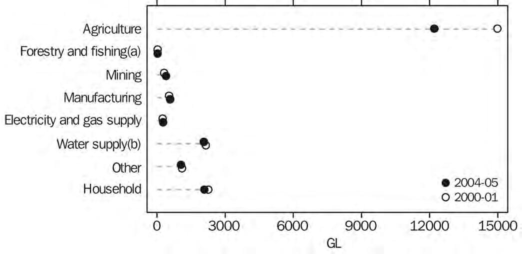
Table.4.311: Water consumption in Australia for 2000-1 and 2004-5
There is a vast amount of water distributed for agricultural activities compared to forestry and fishing or mining. However, the quantity of water given to agriculture had a significant redundancy during the last few years, when other factors such as industry and commercial have been rapidly developed.
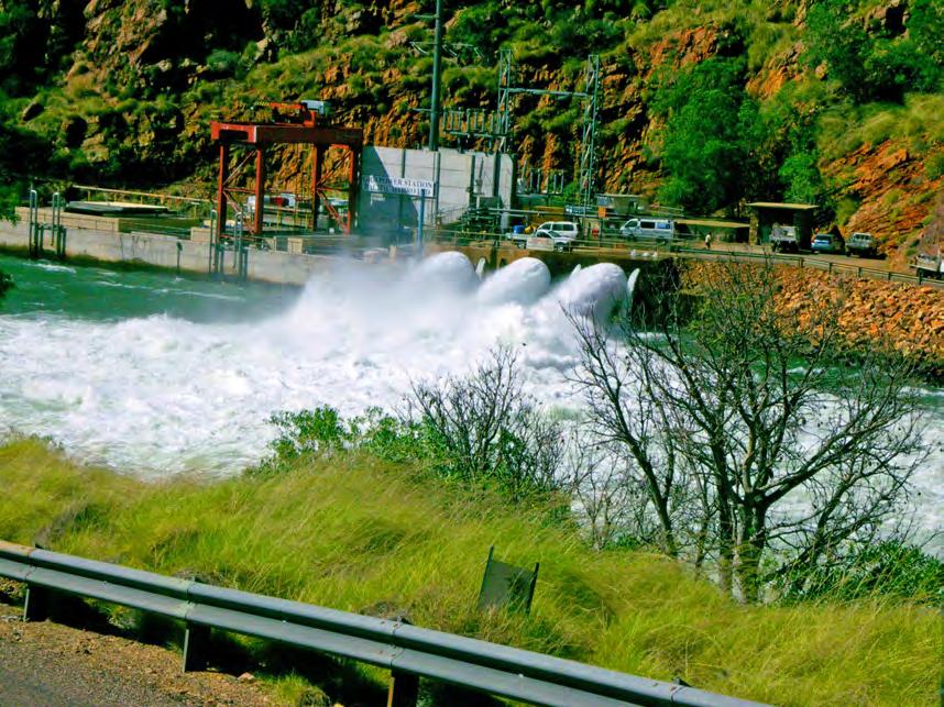
water and energy consumption
Most of water consumption in Australia is distributed to agricultural activities; during the years 2004-2005 the amount of water use was around 12 thousand Giga-litres, three thousand Giga-litres less than in 2000-2001 [Table.4.311]. The domestic use occupies approximately 2.5 thousand Giga-litres of water consumption (Australian Government, 2004). Considering the capacity of the Lake Argyle, which is almost 6 thousand Giga-litres, it is remarkable the fact that the second largest artificial dam in Australia holds almost half of the amount of water that is used for the country’s agriculture per year.
According to the United Nations Development Programme (Australian Government, 2004) the USA hold the first position of average daily water use per capita in the world, with the amount of almost 570 litres
per day, followed by Australia with almost 490 litres per day. On the other hand, China holds a considerably small amount of people’s daily water consumption; around 80 litres per person per day [Table.4.313]. Within the Australian regions, West Australia is the first with the largest amount of annual water consumption per capita; in 2000-1 the consumption reached the 200 Kilo-litres per person but in 20045 it was reduced to 185 Kilo-litres per capita. Victoria holds the last position with just around 80 Kilo-litres per capita [Table.4.314].
119
Fig.4.312
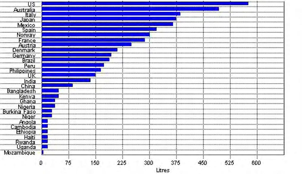
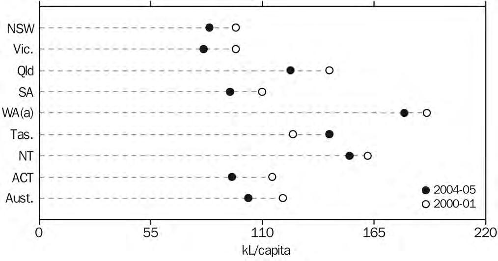
Table.4.313: Average water use per person per day
The USA hold the first position of the most waterconsuming country in the world in terms of daily water consumption per person. Australia is the second most consuming country with around 500 Litres per person per day. A Chinese person consumes approximately 420 Litres less than an Australian person for the daily needs.
Table.4.314: Household water consumption per capita for 2000-1 and 2004-5
The area of West Australia is the most consuming one in both years and Victoria (south-central) is the least consuming one. The Victoria district is mostly covered by deserts and currently there are not any big water resources - neither natural nor artificial. On the other hand, although West Australia has big arid areas as well, it has the second biggest reservoir of Australia, Lake Argyle, which can sustain the urban and rural areas around.
120
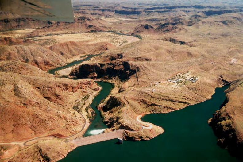

climate change
It has been stated that since the middle of the 20th century the temperatures in Australia had been risen by about 1oC, causing extreme weather phenomena, such as increase of rainfall in the tropical areas and simultaneously decrease in the eastern and south-east parts of the country, where the climate was already dry. Moreover, the frequency of heat-waves had been increased whereas the number of cold days had shown a sharp decline (Australian Government, 2010). This entails the increase of evaporation of the existing water resources and sprawl of deserts around the country, thus increasing the humidity in the atmosphere. The climate change is a phenomenon affecting the entire world, with some countries being affected in more extreme ways than others. Meteorologists are trying to ring the bell for the Australian government, warning the authorities that drastic measures should be taken immediately for improving the resources management of the country.
121
Fig.4.315
Fig.4.316
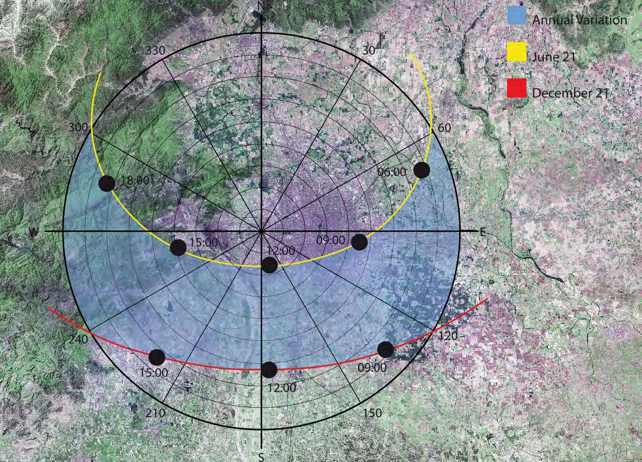
solar azimuth
During the summer period the sunlight in North China lasts longer than the winter period and the direction of the sun varies from southeast to south-west during the day [Fig.4.317]. Although the climate is cold, most of the days are sunny throughout the year. In Australia the sun is dominant throughout the year, but the temperatures are much higher compared to North China, which introduces issues such as evaporation of the exposed water resources. The sun path in Australia is completely different from North China, as the former is on the northern hemisphere while the latter is on the southern. Hence, in Australia the direction of the sun is from north-east during the morning moving towards the north-west along the day [Fig.4.318].
Another important difference between the two locations is the seasonal situation throughout the year, also due to their different latitude; one being on the northern and the other to the southern hemisphere respectively. Winters in North China fall during the months of December to March and are incredibly cold, where in West Australia they hold the months of June until the end of August (Williams, 2005). The opposite applies for the summers.
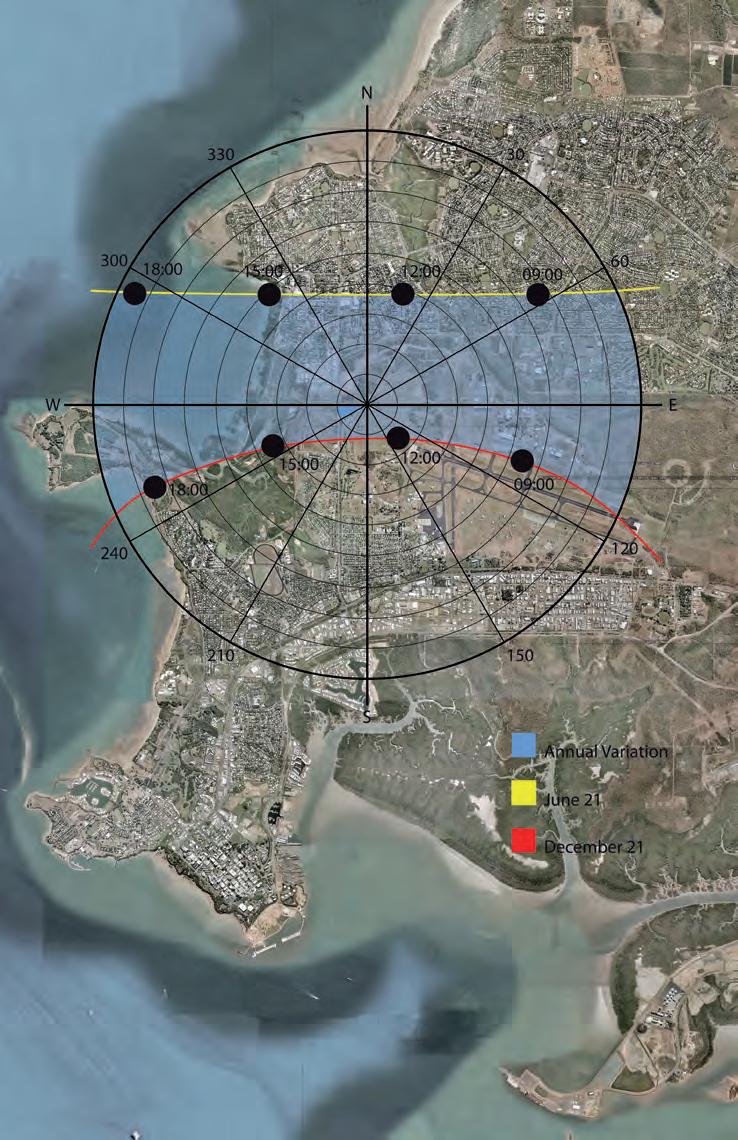
Fig.4.317 (top left)
Solar angles of Beijing - China, Azimuth and Elevation angles.
Fig.4.318 (right)
Solar angles of Darwin - Australia, Azimuth and Elevation angles.
122
conclusions
In China the annual water consumption ranges from region to region, from 26 Kilo-litres to 107 Kilo-litres per person. The big cities hold the largest amounts of water consumption, with Shanghai being the most water-consuming city within China. In Ningxia the consumption is relatively low, reaching the 50 Kilo-litres per person per year. Compared to Australia, China consumes much less water every year, especially on the north part of the country. For instance, the least waterconsuming region of Australia, Victoria, has an annual consumption of three times more than the least water-consuming region of China. Moreover, Shanghai region, whose annual consumption is around 107 Kilo-litres per person, use almost half of the water that is consumed in the West Australia region. Finally, according to Table.2, the average daily water consumption per person in China is the 1/6 of the consumption in Australia. This is a tremendous difference between the two areas, entailing that for these two countries, the management of the local energy resources would be directly related to people’s habits concerning the water consumption.
123
resources
water agriculture
solar energy
blocks paths
topography
solar energy
topography
Metabolic Diagram
superblock
hierarchies
focal points patch
block volume transit pedestrian vehicular interaction with irrigation network
integration paths - blocks readjusting blocks readjusting streets
124
4.4 Water resources reservoirs
Water Resources
Referring back to the metabolic diagram, the first resource to be developed is the water resource. The positions of the reservoirs will allocate the paths for the irrigation system, which will in turn allocate the agricultural fields. The amount of water will also determine the quantity of agriculture that can be grown, as well as the population that can be sustained.
The ‘particle simulation’ tool in “Maya” served a very beneficial role in establishing the most viable locations for the reservoirs to be developed. In other words, a ‘rain simulation’ test was carried out on the topography, where particles were emitted at given intervals throughout the terrain. Based on the natural catchment area of the topography, the particles generally accumulated within valleys throughout the site; however, it was clear that some reservoirs collected more particles than others due to a larger catchment area. Although there were several reservoir locations that began to emerge as a result of the particle simulation, not all of these locations were suitable. The variable that one must not neglect to consider is the transport of water from the reservoir to other locations. Many examples of both natural and artificial reservoirs throughout the world heavily rely on the use of pumps to transport the water out of the reservoir; therefore, to spare
the need for any energy demanding pumps, the topography proves to be advantageous in allowing gravity to transport water out of the reservoirs. Therefore, the position of the reservoir will determine the location that the irrigation system will be distributed, consequently leading to the abstract positioning of the cities general footprint. Thus, in order to take advantage of the topography’s role in transporting water, the reservoir locations determined by the particle simulation are narrowed down to sites that are relatively high on the terrain.
Conclusions
The particle simulation tool proved to be a beneficial instrument to abstractly locate the positions of the reservoirs throughout the terrain. Although some reservoirs will hold different volumes of water than other reservoirs, the population of each patch will be sustained by the reservoir belonging to it. The volume of water will be distributed appropriately among the patch at a ratio of 1:5:2, ‘1’ being for household consumption, ‘5’ for agricultural use and ‘2’ for the other industries. The amount of water consumed will depend on the trends of water consumption of the region, however the same 1:5:2 ratio will be implemented for both scenarios.
125
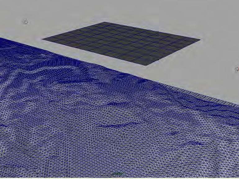
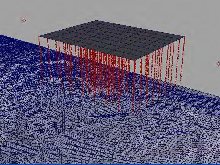
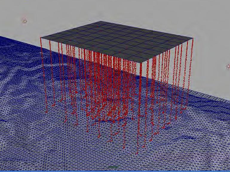

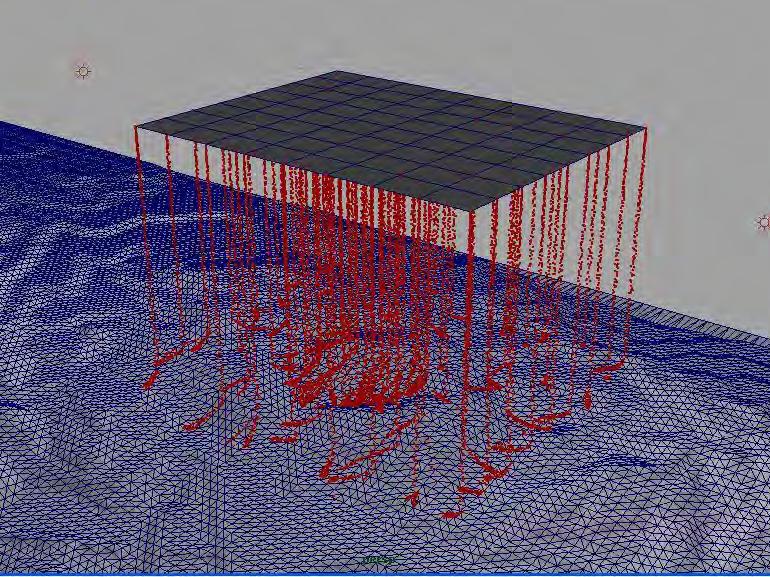
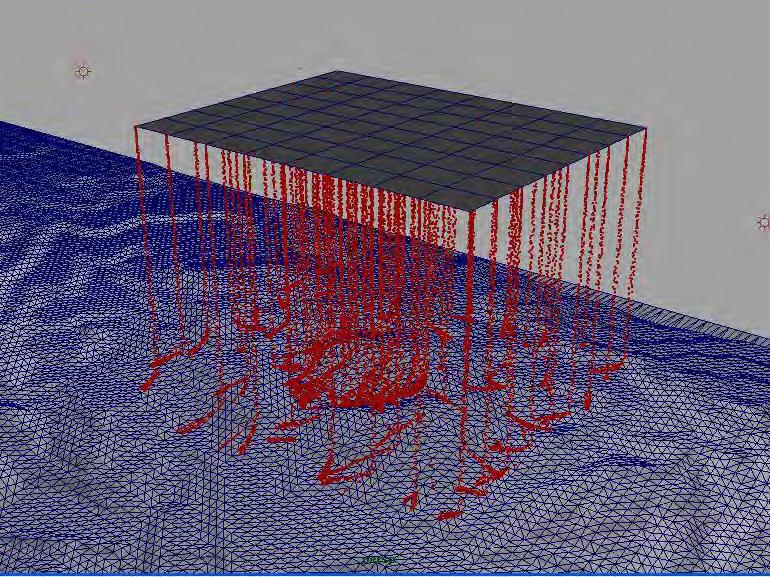
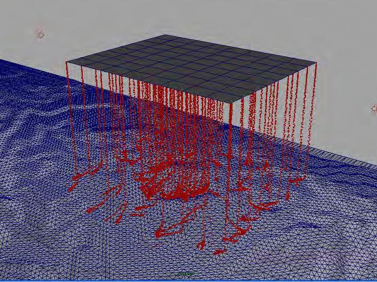
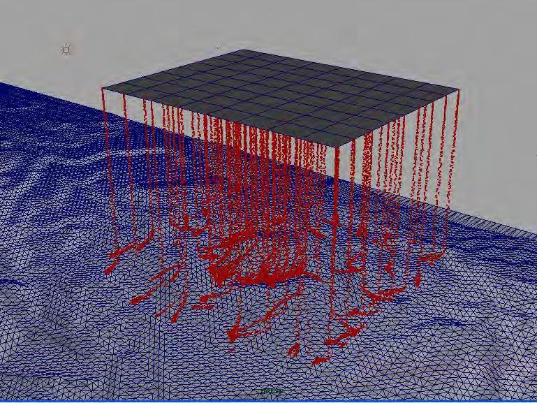
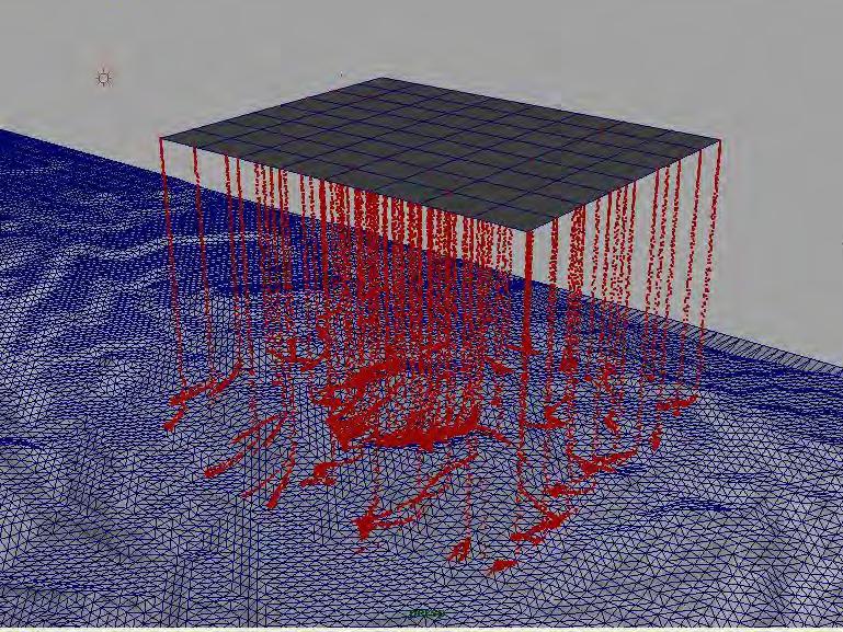
Fig.4.41a-i
The Maya particle simulation tool was very helpful for identifying the deep valleys on the terrain of the two scenarios. Therefore, according to the intensity of accumulation of the particles, it was easy to define the areas that could potentially serve water storage facilities. The locations of the potential reservoirs were chosen according to three criteria: being the deepest valleys, being close to the existing resources but at the same time not being dependent on them and finally being on a higher altitude than the potential city development.
126
Fig.4.41a
Fig.4.41b
Fig.4.41c
Fig.4.41d
Fig.4.41e
Fig.4.41f
Fig.4.41g
Fig.4.41h
Fig.4.41i
127
4.5 Agriculture water distribution
Agriculture:
Out of all industries, the agriculture industry is the most water consuming. Within any country, the amount of water consumed by agriculture is approximately 63%, while household water consumption is 13%. The remaining 24% is consumed by other industries, which include supplying energy to the city, and therefore must not be overlooked (These numbers are more or less the same throughout the world; there are cases where these percentages change, however throughout the dissertation, these percentages will be taken as the norm).
To determine the relative amount of water needed for both agriculture and household consumption, a ratio is created to specify how much water can be consumed. Based on the percentages given, the ratio is:
1 : 5 : 2
For example, for every litre of water given to household consumption, 5 litres must be given to agriculture, and 2 litres must be given to all the other industries. Since we are mainly focusing on agriculture and household consumption, all the other industries are grouped into one category. This ratio will be used to regulate the distribution of water in both the China scenario, and the Australia scenario. The difference in water consumption between both scenarios will be particular to the water consumption numbers available in each region.
128
Fig.4.51-4.54
Irrigation systems based on sprinklers. Each sprinkling unit covers a large area of crop section around it, thus the whole crop land can be sustained with only a few sprinkling units. However, the system is not suitable for areas with high temperatures, as most of the water is wasted by evaporation.

Fig.4.55-4.56
Centre pivot irrigation systems: they are used mostly in hot arid areas, as they are more efficient on preventing evaporation. As they are set on a system of rotating arms, the outcome is an array of circular patches of vegetation contradicting to the arid area around them.

irrigation systems
The main irrigation systems used are the sprinkler system, centre pivot system and the drip system. All systems differ in their advantages and disadvantages, yet some excel over the others.
Sprinkler systems [Fig. 4.51-4.54]:
The simplest of irrigation systems is the sprinkler system. It is simply composed of a sprinkler placed on the ground and sprays water in the air with a given radius to supply water to the plants around it. The main issue with this method of irrigation is efficiency; it is the least efficient of all irrigation systems because of the water loss due to evaporation and wind drift. One also cannot regulate the amount of water spouted from the sprinkler to suit the needs of plants with different water demands; the amount of water dispersed is generally equal. Sprinkler systems are usually used on small fields and commonly supply water to grass or more generally, herbaceous plants.
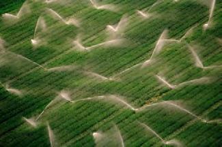

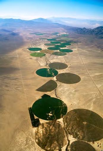
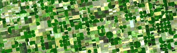
Centre pivot systems [Fig.4.55-4.56]:
Centre pivot irrigation is a system that is more widely used exclusively for agricultural irrigation, where sprinklers are placed on a rotating arm at given intervals. This method typically creates circular crop fields. Although centre pivot systems use sprinklers, they are much more efficient in how the water is distributed among the crops. The first difference between the two systems is that in centre pivot systems, the sprinklers are placed downwards facing the crops, hence spouting water directly onto the crops. In normal sprinkler systems on the other hand, the sprinklers are placed upwards and spurt water in the air. To further enhance the efficiency of water use, the rotating arm rotates only a few feet above the crops, thus minimizing any water loss due to evaporation or wind drift. The disadvantage of centre pivot irrigation is linearity; due to the linearity of the rotating arm, this system can only be used on flat fields, and proves to be unsuitable for inclined terrains.
129
Fig.4.51
Fig.4.52
Fig.4.53
Fig.4.54
Fig.4.55
Fig.4.56
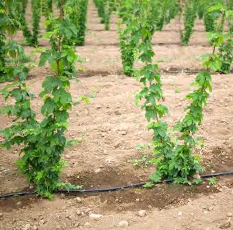

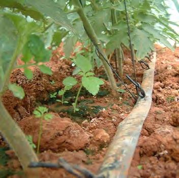
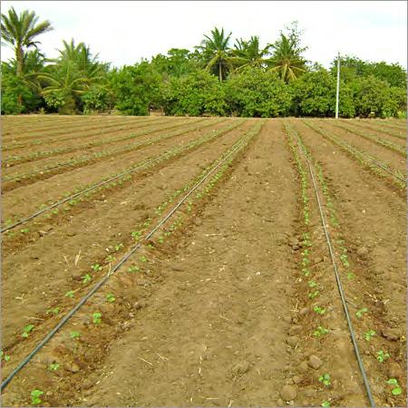
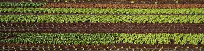
Drip irrigation systems are the most efficient out of all three [Fig.4.574.512]. A technique is used where water is dripped to the roots of each individual plant. The system simply consists of a perforated hose that transfers water from a main water source and drips out the water along its perforations. The main mechanical elements used for this system are to pump the water out of the water source and through the pipes, however, if the gradient of the terrain can be used so that gravity replaces the task of pumps, then the need for these mechanical elements becomes obsolete. Unlike centre pivot irrigation, there is no need to level out the field for the system to be used, drip systems can easily accommodate inclined terrains as well as serve advantageous for irregular shaped fields. The main complication that arises from drip systems is the potential for the perforations along the hose to clog up; however, proper inspection along with proper maintenance should avert this problem.
As a result of the systems’ water efficiency, and its ability to accommodate different terrains, drip system irrigation will be used as
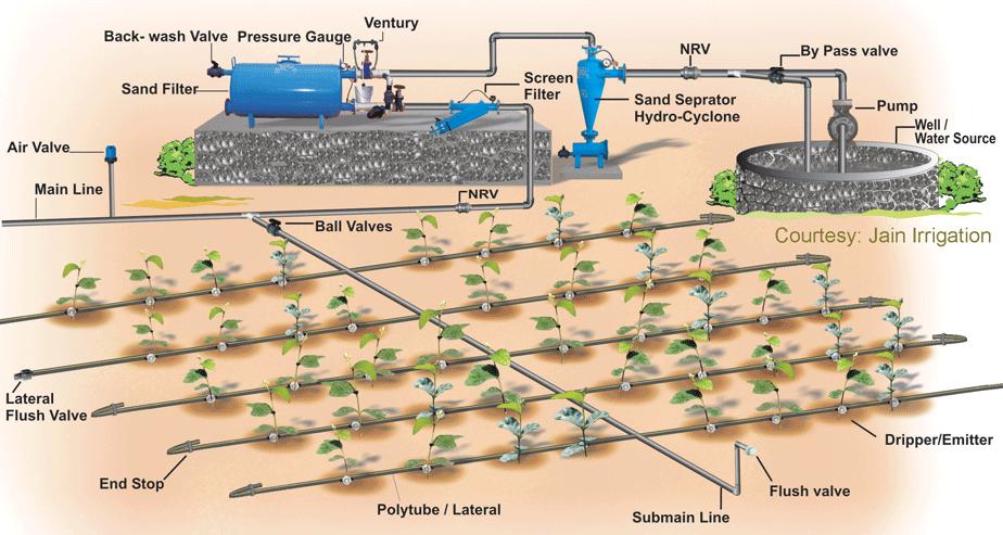
Fig.4.57-4.511
Drip irrigation systems: are mostly suitable for areas that face evaporation issues, as the water distribution is controlled and steady. However, these systems cannot cover a large span, thus the pattern created by the vegetation is linear, following the irrigation lines.
Fig.4.512
Diagram of a dripping irrigation system: the pump distributes the water to the filters and next it flows through the pipes, which they are organised in arrangements of branching systems.
130
the irrigation method for both scenarios.
Fig.4.57
Fig.4.58
Fig.4.59
Fig.4.510
Fig.4.511
Fig.4.512
Fig.4.513-4.516 (page.132)
Images of the four steps followed in order to define the irrigation lines for the first scenario, China. In each additional image the next level of hierarchy of the irrigation branches is added.
application
The same particle simulation tool that was used to locate the reservoirs was also used to determine the irrigation lines [Fig.1,5]. In this case however, the tool had an added script that tracked the path of the particle with a line.
The irrigation system is categorized under several hierarchies. The first hierarchy is the main irrigation line that spans between two reservoirs [Fig.2,4]. This line is manually derived with one simple rule – the line ends at a lower contour then from where it began. Therefore to take complete advantage of the terrain, the main line is generated from both reservoirs and meet at the midpoint between the two reservoirs. Once this first hierarchy is derived, it is divided into a particular number of segments, this number is based on the number of branches the main line will have. The amount of branches the main line will have will be informed by the crop types (the space required for the crops to grow), but more importantly by the amount of water available for the agriculture industry. Once the amount of branches has been
determined, the particle simulation tool is introduced.
Each division point along the main line is used as an emitter point to emit a single particle on the terrain. Once the particle is emitted, the script draws a line that follows the path the particle took on the terrain. This line is transformed into the second hierarchy in the irrigation system [Fig.3,7]. The particle defined a path from the main irrigation line that travelled downwards along the terrain. This is crucial to ensure that all irrigation lines are travelling from a higher contour line to a lower one. Once the secondary lines are established, they are divided into a particular amount of segments that will generate the next hierarchy in the irrigation system [Fig.4,8]. Once again, the most important rule is to ensure that line travels from a high contour point to a lower one. The diameter of each hierarchy of pipes is based on Murray’s law, where each subsequent hierarchies diameter determines the diameter of the hierarchy preceding it.
131

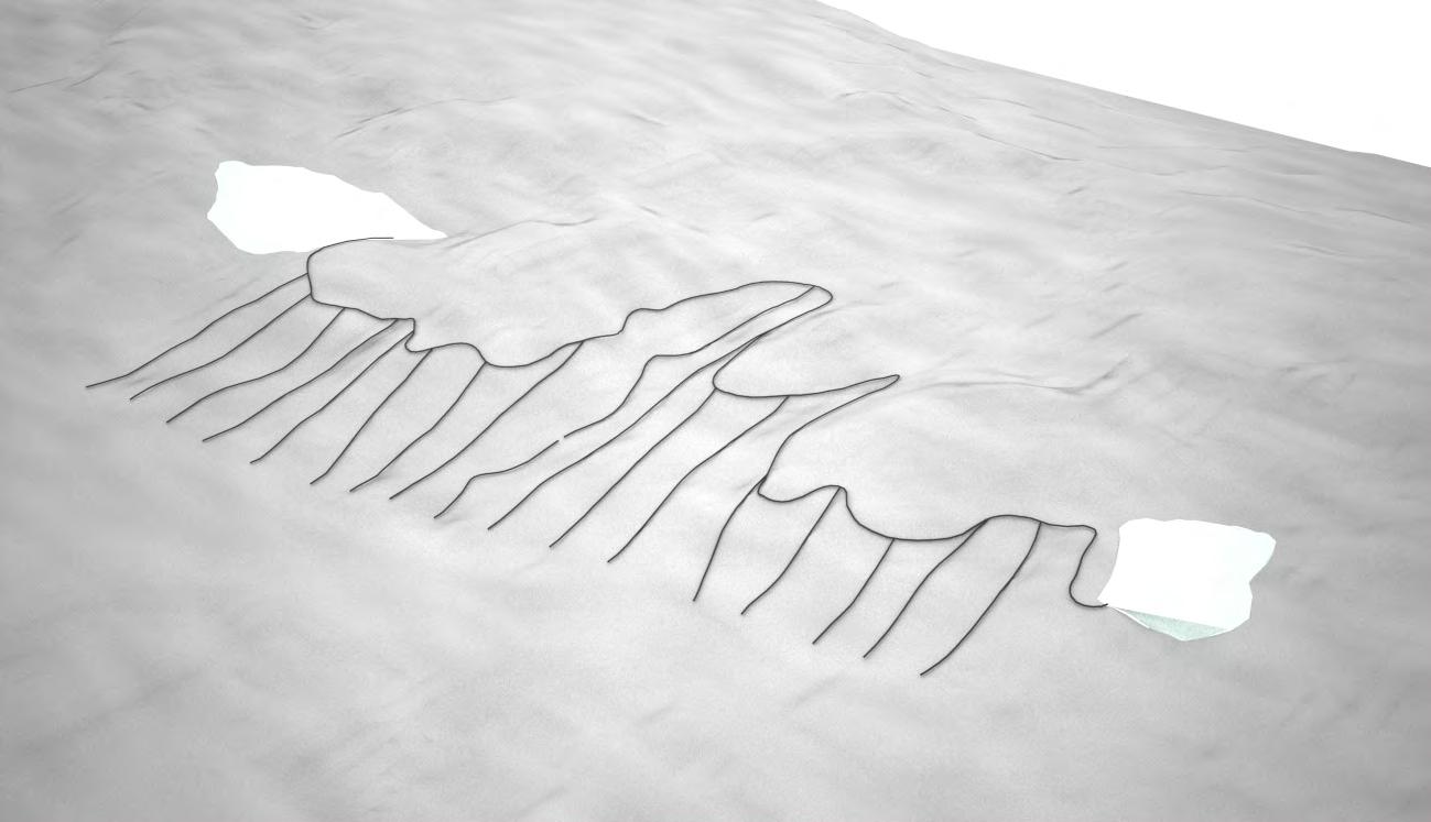

132
Fig.4.513
Fig.4.514
Fig.4.515
Fig.4.516
Integration
Drip irrigation was originated in the 1880’s by researchers in Afghanistan. They were researching the possibilities of integrating the irrigation system with the drainage system. This complies with our initial objective of integrating systems with one another rather than continuing the norm of separating infrastructure from the other systems throughout the city. Therefore, the irrigation lines will be used to transfer water not only to the agricultural fields, but the lines will extend to transfer water throughout the city for consumption. This method of integration allows the irrigation system to directly inform the general footprint of the city, which will be the basis for the placement of the blocks.
Conclusions
Out of the different irrigation methods, the most suitable and appropriate method that best fits the terrain is the drip irrigation system. As well as being the most water efficient of all irrigation systems, it is the system that takes the most advantage of the terrain. Whilst laying out the irrigation system, the only ‘rule’ to be followed is that the irrigation line starts at a higher contour and ends at a lower one, ensuring that gravity is the method in which water will be transported from the reservoirs to the agricultural fields and finally throughout the city as a whole.
133
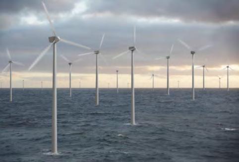

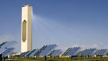
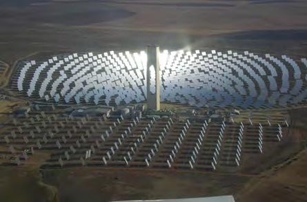
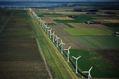
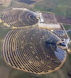
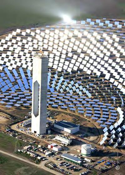
4.6 Renewable energy methods
Renewable energy has become a more sought after industry due to the effects of climate change, and more precisely our dependency on fossil fuels. Although there is a large shift towards generating renewable energy, most of the world’s energy is being produced by fossil fuels such as coal, oil and natural gasses. The setback with this type of energy is that it is not renewable, and it is running out. Unlike water resources, there are alternatives to fossil fuels; these alternatives mainly depend on nature. Renewable energy resources are generated by simply harnessing the earth’s natural sources such as the sun, wind, water or geothermal sources. There are many different methods of harnessing these sources, some of which are described below:
Wind turbines [Fig.4.61-4.63]:
Wind turbines utilize and convert kinetic energy created by wind into either mechanical energy (wind mills) or electrical energy (wind turbines). These turbines are placed in areas that have strong winds
such as coasts. Wind turbines are also used as an alternative to solar power in areas that lack long hours of sunlight.
Heat furnaces [Fig.4.64-4.67]:
Heat furnaces combine solar, water and wind sources in the same system. This method consists of solar panels (a combination of photovoltaics and mirrors) that reflect solar energy from the sun towards the top of a tower that is placed in the centre of the panels. Pipes with running water are placed at the top of the tower. The process is as follows; the solar panels reflect solar energy towards the tower, where it begins to heat the water and allow it to evaporate. The steam that is given off by the evaporating water is passed through a series of turbines, which in turn creates electricity. The biggest example of a heat furnace is in Seville, Spain.
Fig.4.61-4.63 (left)
Examples of wind turbines; they are placed in areas with high wind speed and no obstructions around them. During the last decade this system has been one of the most widely implemented all around the world, especially in the Mediterranean countries and northern Europe.
Fig.4.64-4.67 (right)
Heat furnaces consist of solar panels that rotate accordingly in order to concentrate the sun rays to a water heating unit. The heated water creates electricity. In the areas with heat furnaces there is strong rays of sunlight created by the reflection of the sun and sometimes they cannot be reachable by people. During the last couple of years the system has been used mostly in Spain.
134
Fig.4.61
Fig.4.62
Fig.4.64
Fig.4.65
Fig.4.63
Fig.4.66
Fig.4.67
Fig.4.68-4.613
Applications of photovoltaic panels; their inclination and distance between them is set in a way to avoid any self-shadowing. Over the last couple of years the system has been upgraded to become more efficient on energy production. Thus, with the same amount of panels more energy is produced compared to a few years ago.
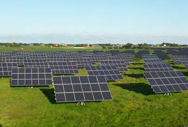
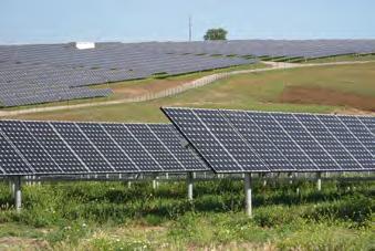


Photovoltaic panels [Fig.4.68-4.613]:
The most familiar of all methods are photovoltaics, which simply transfer solar energy from the sun into electrical energy. The most appropriate locations for this method of renewable energy are regions with long hours of sunlight; however, climates that are too hot reduce the efficiency of the photovoltaics. The demand on photovoltaic panels has made rapid advances in its industry. The high demands have also reduced their cost, however, one of the main disadvantages of photovoltaics is still their price.
Although these different methods are exceedingly useful in there ability to generate renewable energy, each method excels in a particular climate. There are differences between the efficiency levels of each system, however with the rapid advances in technology, the efficiency numbers are rising at an accelerated pace.
135
Fig.4.68
Fig.4.69
Fig.4.610
Fig.4.611
Fig.4.612
Fig.4.613
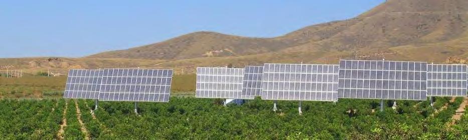
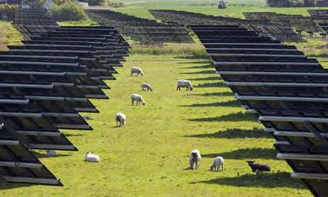
Area of solar panels
Area of the city
integration
The latest “eco-friendly, zero-carbon” city that is currently being developed is ‘Masdar City’ in Abu Dhabi, UAE. Masdar city currently holds the largest photovoltaic power plant in the Middle East. Whilst there is a motive to integrate solar panels within building facades, the main source for the energy created comes from a solar power plant that is placed outside the city’s borders in an isolated patch of land [Fig.4.616]. Although it seems that the earth has an adequate amount of land to spare, it was once perceived that the earth had an adequate amount of water to spare, it was also once perceived that the earth had an adequate amount of fossil fuels to spare. What might seem like an adequate amount now, might not be the case in the near future; therefore an integration of these power plants (regardless of the type of renewable energy generated) within the city is crucial. Throughout different regions in the world from Germany, all the way to Canada, solar plants are merged with agricultural farms, allowing multiple uses
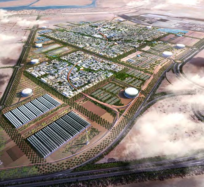
for the same land by two industries that predominantly require vast amounts of land each. It is this integration that we find most critical and thus will apply in both the China scenario, as well as the Australia scenario [Fig.4.614-4.615]
Conclusions
Choosing which method of renewable energy to be used will heavily rely on the climatic conditions of the region. Solar panels might prove to be useful for one region, while is disadvantageous for another. The crucial factor to consider is the integration and multiple uses of the land. Whether it was photovoltaics, solar furnaces or windmills, they must be integrated within the city rather than be isolated outside the city borders. The most suitable integration would be with the agricultural land, where both industries take advantage of the open land, whilst efficiently serving their own purpose.
Fig.4.614-4.615 (top, bottom left)
The images show the way the agriculture and the solar panels are incorporated together; thus there is a significant space saving. Moreover, this is beneficial in terms of saving energy, as the source (solar panels) are very close to the several systems that need energy, hence the transfer of energy occurs within a small distance. However, due to the shadowing effect created by the panels, the agriculture might be affected.
Fig.4.616 (bottom right)
Arial view of Masdar city, showing that the solar energy source is an individual system separated from the city.
136
4.7 Urban blocks introduction
One of the basic components of the urban environment is the blocks; they are organised by an accumulative way around urban attractions. In order to observe the urban expansion usually people talk about the expansion of the blocks, even though the paths might have already extended outside the main area of the city.
The organisation of the urban space is directly relied to the blocks, which they constitute the element of internal space, visual link between several points within a city, the density of the area and generally the main body of the city. Without the blocks the street network would be an ambiguous system, without any specific character or attribute. Urban blocks give the urban space the heterogeneity and differentiation needed for a qualitative experience within the urban environment. Furthermore, they distinguish the private, semi-private and public
spaces between them.
Urban planning has been so far following the sequence of firstly defining the street patterns of a planning city and the urban blocks afterwards. In this dissertation the order is reversed with the blocks first appearing in the city, with their organisation being informed by the topographical and environmental features of the area, then the street network and finally, the pattern emerges from the interaction between the two systems together. Eventually, the blocks will diverge from their initial form and configuration, creating a range of differentiated urban spaces. As in nature every living organism is formed by the cells as their main component and the growth occurs by the cell expansion; accordingly the main cells of the city are the blocks.
137

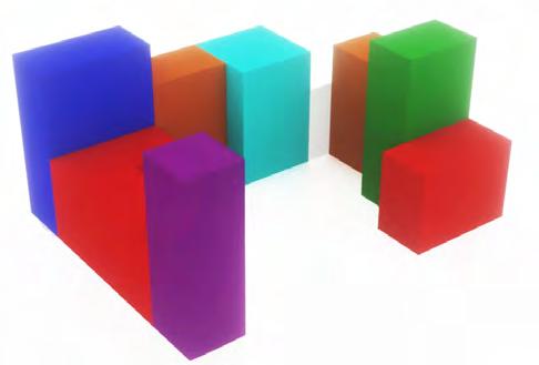
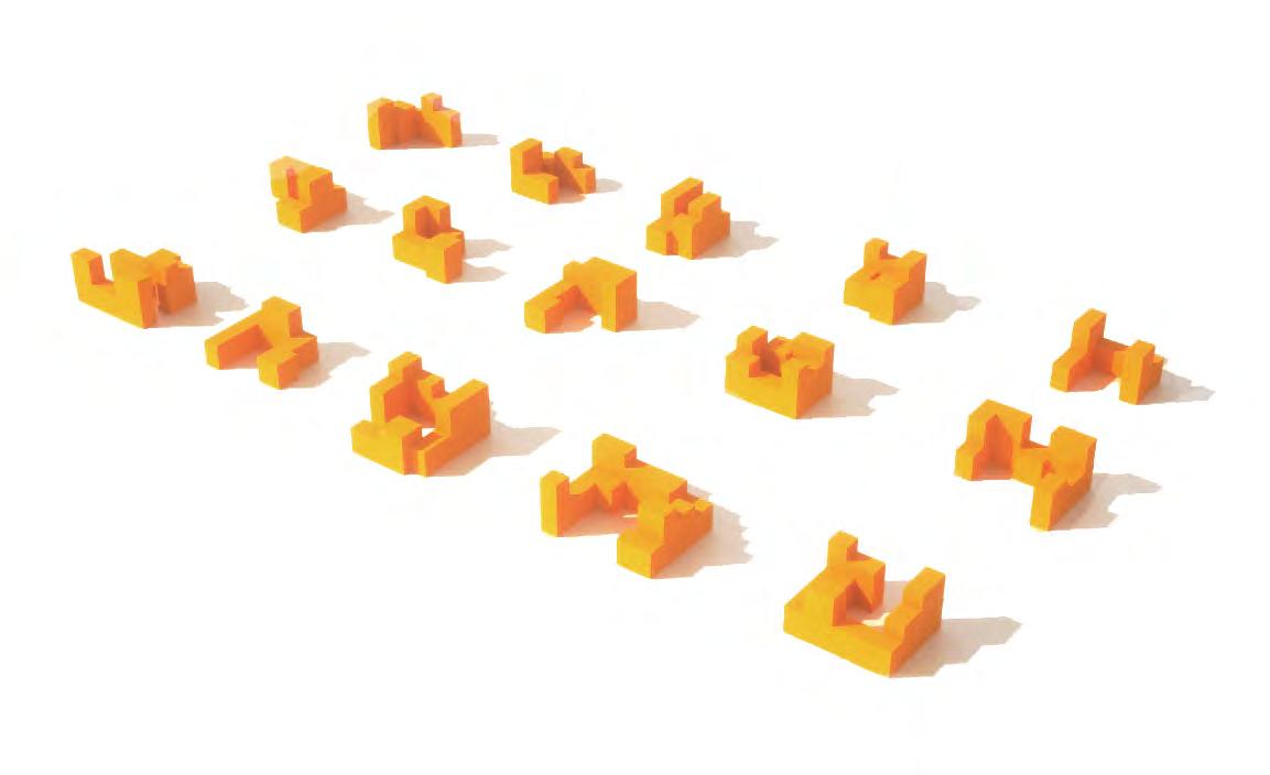
Fig.4.71 (top left)
A set of 8 volumes are first colour-coded and combined together to create variations of urban blocks. The colours were set simply on the initial stage; they help for distinguishing the volumes between them during their assembly.
Fig.4.72 (bottom left)
One of the assembled blocks, containing 7 of the colour-coded volumes. Sometimes a volume can be used more than once within a block.
Fig.4.73 (right)
The first populations consists of 15 individual blocks, assembeld by the volumes following the model of the volumes’ organisation around internal courtyards.
emergence
Comparing the results from the three samples of the Paris current urban tissue, it can be concluded that the organisation of the building volume surrounding relatively small open spaces can be proved an ideal model for reducing energy loss of the buildings. The small space that is enclosed within the block could be a great opportunity for use of vegetation, as well as a method of channelling, diffusing or blocking the wind flow, depending on the desired microclimatic conditions. Therefore, the initial point of the block organisation resembles the model of the prime example of an energy efficient block (Chapter 3 –Methods of Research), which could be used as a tool of modularity in the further development of the urban blocks. An evolutionary process based on genetic algorithms is used for the generation and next the expansion of the urban blocks. The steps include small, rational steps to generate sets of urban blocks, which are part of a constantly
developing method of readjustments with the interaction of the other systems of the city. Finally, some of them start to merge and evolve into urban clusters that hold the properties of the urban complexity
Population 1
The first population of blocks is created with the assembly of eight different primitive volumes [Fig.4.71]. Different combinations of the volumes create many variations of block morphologies, however all of them are always organised around an inner open space and approximately occupying similar surface area [Fig.4.72-4.73]. The open spaces refer to the widely known urban block technique of inner courtyards, which constitute valuable spaces of private or semi-private activities.
138
Fig.4.74
The blocks of the first population are changed in order to fit better the criteria in a different way in each scenario accordingly. The method is inspired by a similar method of slicing studied in Chapter 3 (“Blocks experiments” - Methods of solar exposure)
Scenario 1 (top):
Part of the shadowed volume was sliced and added to the area that is exposed to the sun.
Scenario 2 (bottom):
A small amount of volume is added to the shadowed part, thus retaining the same surface exposed to sun while the total volume is increased.
Fig.4.75 (top right)
The figure shows two blocks, one of each scenario and the effect of shadows created on their volumes, according to a specific position of the sun. According to the fitness criterion that was set, each block’s fitness performance changes when the block is rotated but not when it moves.
Fig.4: Optimisation techniques
Fig.4.76 (bottom right)
Snapshot from the grasshopper file which shows the way each volume affects the other within a block. The fitness performance of a block not only depends on its overall configuration, i.e. how much space is left for the courtyard, how much total volume is added e.t.c., but also depends on the way of distribution of the volumes; for instance if most of the tall volumes are placed forward to face the sun they will create large shadowed areas on the rest of them.
Population 2
Fitness criterion: Surface exposed to sun Total Volume
The climatic conditions for each case scenario are considerably different, thus the evaluation criterion should differ between the two sites. Choosing the relation between the blocks and the direction of the prevailing sun, the first population is modified in order to adapt to the respective environment. Particularly, in the first scenario, China, the solar radiation absorbed by the surfaces of the buildings within a block is significantly desired. On the other hand, in the second scenario, Australia, the self-shadowing effect between the buildings within the block is extremely crucial for the thermal comfort of the residents. Therefore, the volumes of the blocks in both scenarios are reformed with the method of slicing such as: in the first scenario, a part of the shadowed volume is sliced and repositioned in a new area that is exposed to the sun radiation and thus exposing more surface are to the sun, whereas in the second scenario more volume is added to the self-shadowed areas [Fig.4.74]. Finally, two different populations are created by the modification of the first population by the two methods of optimisation, in order to be site-specific.
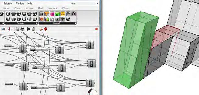
The evaluation criterion is based on the amount of energy that each block gains from the sun [Fig.4.75]. Therefore, the criterion for each block is set as the ratio between the sum of the surface area that is exposed to the sun divided by the total volume of the block. With the help of the Grasshopper tool, a script has been developed which is directly informed by the sun azimuth and altitude angles of the prevailing sun direction for each scenario independently, and hence the outline of the shadow of each volume is marked on the other volumes of the blocks [Fig.4.76]. The evaluation method is applied on both populations, with the difference that in the first scenario the fittest elements have bigger values of the ratio, contrarily to the second scenario where the fittest ones have the smallest value. The nine fittest elements from both populations are next selected in order to form the first superblock for each scenario individually.
139
Fig.5,6: Evaluation criterion
Fig.4.77a: Scenario 1
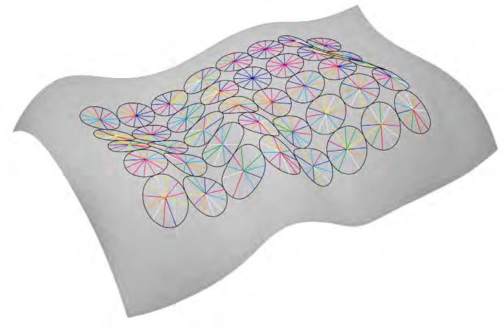
In both scenarios the volumes of the two populations, since placed on site, begin to readjust their height – always related to one another –according to the local morphology of the ground at each local position. In the first scenario, the optimum position is on a hill facing the sun, where each volume exposes more surface to the sun due to the height differentiation between them [Fig.4.77a]. Self-shadowing occurs less in this case. On the contrary, in the second scenario hills that face the same direction with the sun are preferable as the self-shadowing of the volumes is increased [Fig.4.77b].
Due to the particularity of the topography in both scenarios, a method of the blocks’ adjustment to the terrain was implemented; based on
Fig.4.77b: Scenario 2
< G < 0.55
< G < 0.60 0.60 < G < 0.65
0.65 < G < 0.70
a script, a grid of points is projected on the surface of the area that accommodates the blocks. Each point constitutes the centre point of a circle that belongs to the surface of the terrain. Twelve different lines, which connect each centre point with the periphery of the respective circle, subdivide each circle in twelve parts. Each line follows the local curvature value of the surface and can be described as the tangent of the local position. Hence, each line contains the same gradient value with the surface at its specific position. The values are categorised into a table, in which ten different groups of gradient results are represented by a specific colour [Fig.4.78]. Therefore, the colour of each line represents a range of specific gradient values that define the steepness at each location on the terrain.
Fig.4.77a,b
The topography is directly related to the performance of the blocks in the respective fitness criterion for each scenario: since the volumes move down in order to accommodate topography, the area of the surfaces that are exposed to the sun is changed, either increasing the fitness performance or decreasing it.
Fig.4.78
A small part of the terrain shows the way that the gradient is defined on many points along its surface. The colour-coding table indicates the gradient values of each line on the terrain. This method will then feed the blocks’ algorithm; it is very helpful for identifying quickly the direction where the blocks will be next orientated to.
140
0 < G < 0.05 0.05 < G < 0.10 0.10 < G < 0.15 0.15 < G < 0.20 0.20 < G < 0.25 0.25 < G < 0.30 0.30 < G < 0.35 0.35 < G < 0.40 0.40
G < 0.45 0.45
0.50
<
< G < 0.50
0.55
Fig.4.78: Colour-coding the Gradient values (G)
Gradient
Fig.4.79a,b
The nine blocks are placed on the topography in equal distances from each other, facing towards a common direction.
Fig.4.710a,b
All the blocks are orientated, based on the pivot point defined by the gradient script, towards the direction of the steepest inclination of the topography; this direction is directly given from the gradient script.
Fig.4.711a,b
After their evaluation, If the value of some blocks is lower than a standard one, these blocks are displaced. In the first scenario the blocks move further away from the adjacent ones in order to avoid self-shadowing and capture more solar energy. In the second scenario on the other hand the blocks move closer to the adjacent ones for achieving self-shadowing and reduce overheating of the blocks’ surface.
Fig.4.712a,b
Another evaluation process is followed, according to which any block that has a fitness value lower than a certain limit it is next eliminated. This way the setup starts to create open spaces and provide variation of building density within the city.
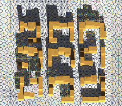
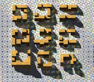
Superblock
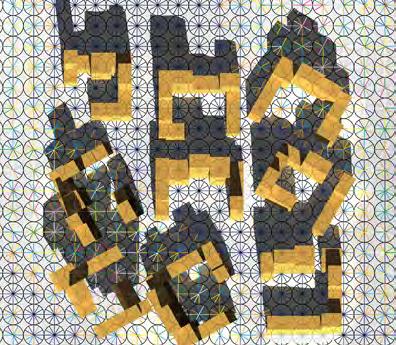
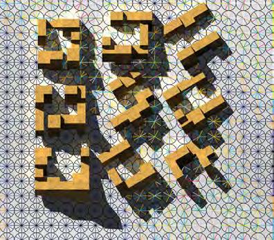
A superblock is defined as the set of nine blocks, arrayed in three columns and three rows of blocks. Therefore, the first nine fittest individuals are taken from the two populations of blocks of each scenario. The first superblock is placed on site, with each block taking its position by the use of one of the points of the gradient map, defined as the pivot point of the block [Fig.4.79a,b]. Each block is next oriented towards the direction of the steepest terrain on the local position; in plan view the block is rotated around the pivot point [Fig.4.710a,b].
Population 3
Each block is next re-evaluated according to the same fitness criterion; however the evaluation process considers the location and the relation of all the blocks between them. For instance, the algorithm not only takes into account the shadows of each volume on its adjacent ones within a block, but also measures the shadowed areas that occur from the adjacent blocks around. In essence, the evaluation is informed
by the actual solar azimuth angles of the specific area and returns the representative values. As mentioned earlier, in the first scenario the fittest blocks are the ones with the highest ratios of surface area exposed to the sun to the total volume, whereas in the second scenario the opposite is applied [Table].
For the first scenario, the blocks whose fitness value is below a certain threshold are hereupon slightly displaced from their initial position, to any direction where possible in plan view, to increase their surface area exposed to the sun [Fig.4.711a]. Consequently, in the second case the blocks whose fitness value is above a specific value are the ones being displaced from their position, however moving closer to the other blocks in order to achieve self-shadowing [Fig.4.711b]. The blocks are next re-evaluated in both cases and finally, if a block is predicated that it does not fulfil the fitness criteria it is next eliminated [Fig.4.712a,b].
141
Fig.9a
Fig.9b
Fig.10a
Fig.10b
Fig.11a
Fig.11b
Fig.12a
Fig.12b


The expansion of the cities is based on the aforementioned algorithmic process. Although the algorithm is comprised by a set of many logical steps, there are numerous issues that were not addressed in the process, which they constitute significant factors for a city’s development. These factors are crucial for creating differentiations to the several urban areas, therefore giving qualitative value to the urban space. Hence, some additional rules were applied during the expansions of the cities for both scenarios, such as the formation of large open spaces that could be next considered as “focal points”, or the use of natural obstructions, i.e. rivers, lakes, steep hills, in order to deviate the current direction of the expansion. Conversely, the use of attractions drives the expansion towards points of interest, such as flat terrains, areas of fertile soil or points that are close to natural resources.


The urban block is the most basic component of the city, although it might come in different shapes and sizes, it still remains the dominant ‘cell type’ of any city. Therefore the method that the block is created is crucial. Applying an emergent process proved most beneficial in ensuring that the blocks created are developed and optimised into energy efficient ones that are site specific. The interaction between the block and the one next to it, as well as the interaction between the block and the superblock is important in guaranteeing that the urban blocks are not isolated from one another, consequently ensuring that the urban fabric is made of components that correlate with one another rather than be completely isolated from each other.
Fig.4.713a-d
The evolutionary process with the combination of additional rules form many possible versions of the growth model. The images show one example, where the blocks are adjusted according to the rules, creating various spatial configurations at the same time. The future “focal points” are visible, which they constitute open urban spaces. In the first scenario these spaces are exposed to the sun and provide thermal comfort to the city’s inhabitants.
142
Fig.4.713a
Fig.4.713b
Fig.4.713c
Fig.4.713d conclusions
Fig.4.81
In Istanbul the focal points were the main body of the street network structure; according to their position the main arteries were established during the history. The secondary and tertiary streets were linking intermediate points with the primary ones.
Fig.4.82
In ancient Egypt the initiator for the street network structure were the main arteries: three almost parallel primary streets were established parallel to natural elements (e.g. rivers) and between them a system of different hierarchical divisions of secondary and tertiary streets was developed. This system, between the main arteries, seems homogeneous without any points of particular significance.
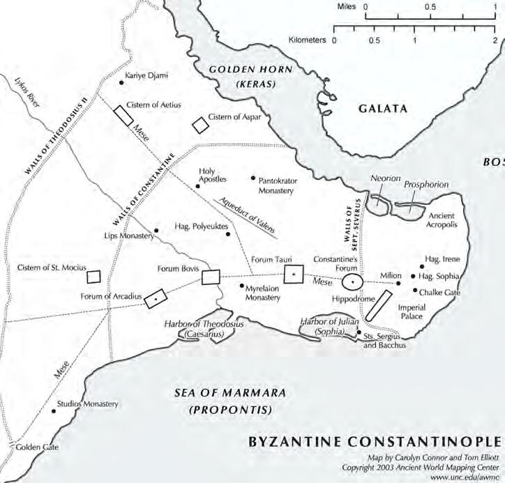
4.8 Paths models of street networks
The dimensions of the cities in both scenarios are greatly informed by the fact that the city is designed to accommodate the pedestrian rather than the car. Therefore, walking distances were a crucial element in determining the paths distances and positions relative to one another. Another element that informed the development of the paths was the gradient of the terrain; nevertheless, the effect of the gradient on the paths is visible more in particular paths than in others. This will be discussed in further detail in the next part of this subchapter.
Istanbul:
In Istanbul, the Romans laid out their paths with respect to particular focal points. These focal points served as ‘attractor points’ for the main paths in the city [Fig.4.81]. Although the functions of the focal points have changed throughout Istanbul’s history, (from open forums during the Roman period to Mosques and inner courtyards during the Ottoman period), the main paths that connected to them also survived Istanbul’s different eras. From these primary paths, secondary and
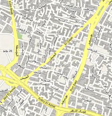
tertiary paths connected different parts of the city; the topography was the “blueprint” that the development of the secondary and tertiary paths was based on.
Ancient Egypt:
Cities in ancient Egypt give a prime example of how the main ‘arterioles’ (primary paths) of the city were connected to one another through an intricate branching network of secondary and tertiary paths [Fig.4.82]. Rather than the contemporary method of planning, where the paths of the city are initially designed, and the ‘left over’ spaces that arise are allocated for building lots, in the ancient Egyptian city, lots were defined and divided between the main arterioles consequently creating paths that divided the lots from one another. Some of areas of Egypt still show this method of planning. These two examples will be used as models to generate the paths for both scenarios.
143
hierarchies
The paths in both scenarios are categorized into four main hierarchies. The first and main hierarchy is generated primarily based on the gradient of the terrain [Fig.3a]. Using the global footprint of the city (defined by the irrigation lines and blocks) as a blueprint, the main arterioles follow the lowest gradient throughout each patch. The path with the lowest gradient is defined by the gradient script that was used to position the blocks on the terrain. This primary path creates a loop around the patch, and is the only path that is used by vehicular transport, however it is also shared by public transport, which in this case is a light rail system. It is through this main arteriole that patches will connect to one another, as well as connect to external areas outside the city.
As the blocks were laid out across the topography, focal points were created [Fig.4.83b]; these focal points are either open spaces or a group of blocks. Using Istanbul city as a model, the secondary paths were generated and connected these focal points with one another, however unlike Istanbul where the main paths connect the focal points, in this case it is the secondary paths that connect the focal points [Fig.4.83c]. This second hierarchy of paths is assigned for the use of public transport, a tram system, and pedestrian use. The primary and secondary paths developed so far emulate the main arterioles found in the ancient Egyptian city, and thus will be connected to one
another through a branching network of tertiary and quaternary paths [Fig.4.83d].
As the tertiary and quaternary paths connect the primary and secondary paths with one another, they also connect the different parts of the city to the primary and secondary paths. As mentioned in the previous subchapter, as well as distributing water to the agricultural fields, the irrigation lines extend to provide water to the different parts of the city, however to avoid the development of two different systems, one for water supply and one for transport, the system for water supply shares the same tertiary and quaternary path system. This sets about informing how the tertiary and quaternary will connect to the different blocks throughout the city, ensuring that each block is connected by a path, and consequently confirms water supply for each block. The tertiary and quaternary paths are assigned for pedestrian use only. Therefore, any point throughout the tertiary and quaternary paths must not be more than 400 metres from any public transport system. This number is based on the walking distances in Islamic cities that ensure that every point throughout the city is no more than 400 meters away from a mosque. The fact that the city must accommodate the pedestrian rather than the car greatly reduces CO2 emissions, ensuing easy and quick access to the different parts throughout the city.
Fig.4.83a-d (right)
The series of the four different hierarchies that form the path system. The concept combines the two aforementioned paradigms, Istanbul and Egypt, in order to create an efficient system that takes into account the functionality of each hierarchy of paths as well as the desired connectivity between the urban spaces.
144

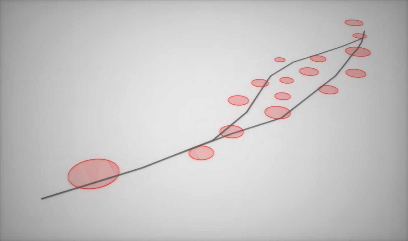
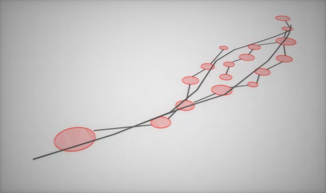
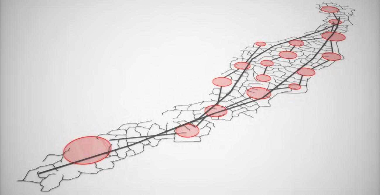
145
Fig.4.83a
Fig.4.83b
Fig.4.83c
Fig.4.83d
paths
paths
multiple paths created - selection based on shortest route and lowest gradient
multiple paths created - selection based on shortest route and lowest gradient
To guarantee that all paths that are generated are below a particular gradient, thus avoiding paths with steep angles, a script was developed that created a path from any two points on the terrain; however, rather than simply determining the shortest route from one point to the other, the path with lowest gradient is calculated. Seeing that there may be several routes from one point to the other, several paths are generated, and the route with the shortest path is selected (the script automatically ensures that the lowest gradient is chosen).
Conclusions
As shown in the Ancient cities of Egypt, as well as throughout the history of Istanbul, paths were developed based on the positions of the blocks, and so, the street networks in both scenarios follow the same methodology. The paths connect focal points as well as the
main arteries with one another. Topography plays an extensive role in determining the exact layout of the path, regardless of hierarchy. The essential element to take into account is the fact that the paths are laid out and developed to accommodate the pedestrian and not the car. Therefore the dimensions of the overall patch as well as the distances between the different path hierarchies must succumb to the pedestrian rather than the car.
Fig.4.84a,b
After the primary streets were defined, the secondary ones were created in order to link the primary ones with specific points, marked with the red dots. These points acted as attractor points in the script, driving the secondary paths towards them. There were several possible paths branching out from the primary one. The one with the shortest route from the primary path to the attractor point was the one selected, while the rest were eliminated. This way it was easy to define the points of the branching streets.
146
Fig.4.84a
Fig.4.84b
gradient
Script
Option Explicit ‘Script written by <Mohammed Makki_Pavlos Schizas>
Call Main() Sub Main()
Dim origin,plane,planar,move,border,segments,pt,line,segment,line1, Dim angle,k,l,q
Dim color,line2,threshhold,i,shortest,j
Dim endpt,distance,centre,centrepoint,segpts,surface,gradient,anglepoints()
threshhold = 500
origin=rhino.getpoint (“pick origin”) endpt = rhino.GetPoint (“pick”) surface = rhino.GetObject (“pick surface”,8)
Rhino.EnableRedraw False
For j = 0 To 100 pt = rhino.AddPoint (origin) plane = rhino.MovePlane (rhino.ViewCPlane(“Top”),origin) planar = rhino.Addplanesurface (plane,20,20) move = rhino.SurfaceAreaCentroid (planar) rhino.MoveObject planar,move(0),origin rhino.MoveObject planar,array(0,0,500) border= rhino.duplicatesurfaceborder (planar) segpts = rhino.DivideCurve (border(0),32) segments = rhino.projectpointtosurface (segpts, surface, array(0,0,-1))
Rhino.DeleteObject planar Rhino.DeleteObject border(0)
q=0
ReDim anglepoints(0) For k=0 To ubound(segments)
gradient=abs(origin(2)-segments(k)(2))/sqr((origin(1)-segments(k)(1))^2+(origin(0)-segments(k)(0))^2)
If Not (gradient < 0) And gradient < 0.3 Then
ReDim Preserve anglepoints(q) anglepoints(q)=segments(k) q=q+1
End If Next
For i = 0 To ubound(anglepoints)
line1 = array(origin,endpt) line2 = array(origin,anglepoints(i)) angle = rhino.angle2 (line1,line2)
If angle(0) < threshhold Then threshhold = angle(0) shortest=i
End If Next
rhino.addline origin,anglepoints(shortest) origin=anglepoints(shortest) distance = rhino.distance (origin,endpt)
If distance < 10 Then Exit Sub End If Next
Rhino.EnableRedraw True End Sub
147
4.9 Integration
interaction between streets and blocks
The integration of the street network and the block organisation is a step which entails the direct and constant interaction between the two systems; the streets re-inform the orientation, displacement, or even the elimination of the blocks and the particularities of each block necessitate the reconfiguration of the adjacent streets. An algorithmic method is developed in order to prioritise the adjustments between streets and blocks. Firstly, the blocks of the prototype populations of both scenarios are categorised into either penetrable or impenetrable blocks by streets [Fig.4.91a,b].
Every street crosses the block with a particular way, hence there are three cases where the blocks interact in three different ways with the streets:
- If the block is impenetrable and a street crosses it then the block is moved towards any empty spaces around until it does not block any street any more [Fig.4.92a].
- If the block is impenetrable and a street crosses it but there is not enough space for it to move, then the block is deleted [Fig.4.92b].
- If the block is penetrable and a street crosses it from a different direction that the block requires, then the block is rotated in such a way that it does not block the street anymore [Fig.4.92c].
With a similar logic the streets can readjust in order to avoid potential obstacles created by the blocks. There are some blocks that are organised in a way that when a street enters it, the exit point is on one of the sides of the block instead of being opposite the entrance point. These blocks are called semi-penetrable. In these cases:
- If the block is semi-penetrable and a street crosses it all the way through, then the street creates a detour around the part of the block that cannot be crossed [Fig.4.92d].
Fig.4.91a,b
Two samples of 36 and 27 blocks from scenarios 1 and 2 respectively are ranked according to three categories: the penetrable, impenetrable and semi-penetrable blocks. Penetrable are the blocks that have two open edges, one opposite the other. Impenetrable are the ones that have only one entering point and cannot be crossed through by a street. Semi-penetrable are the ones that have two open edges in two perpendicular edges.
148
Fig.4.91a
Fig.4.91b
Fig.4.92a-d
The figures show four different possibilities of the interaction between the streets and the blocks. According to the four rule, the blocks or the streets are readjusted in each case.
Case 1
If the block is impenetrable ---> move block
Case 1
If the block is impenetrable and cannot move ---> delete block
Case 1
If the block is penetrable ---> rotate block
Case 1
If the block is semi-penetrable ---> readjust streets
149
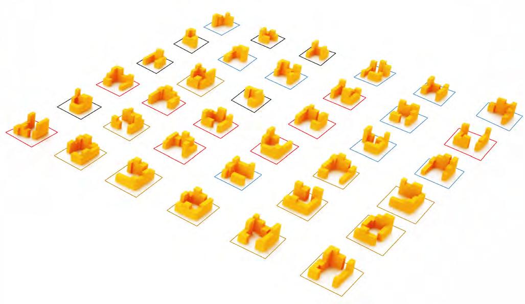
4.10 Energy demands categories
The process is iterated for the first four superblocks, thus having an array of 36 differently configured blocks in both cases, which constitute a new prototype population. The expansion of the blocks in each case is a repetitive process according to which in every step a new superblock is created by a sample of nine of the 36 blocks of the prototype population accordingly. It is essential that these blocks will not remain as they are; eventually their size, position and form will be modified according to new parameters introduced afterwards. Eventually, their growth is terminated when they reach the density of a patch that is estimated to be the desired one, depending on the available resources that can sustain the specific patch [Fig.4.101,4.102].
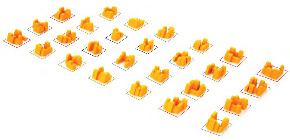

Fig.4.101
A sample of 36 blocks from the first scenario is isolated and ranked according to the four categories set for energy demands. The blocks are distributed to each category according to their total volume.
Fig.4.102
The same classification process was followed for the second scenario, with a sample of 27 blocks.
150
Diagram.4.103
The three main hierarchies of the blocks, according to the way they are organised within the city: the patch is a set of around 80 superblocks, the superblock consists of 9 blocks and the last element is the block itself. All the categories of energy demand are classified from high to the lowest.
superblock patch
high energy demand
medium energy demand
low energy demand
high energy demand
medium energy demand
low energy demand
lowest energy demand
block
high energy demand
medium energy demand
low energy demand
lowest energy demand
hierarchies
Through the process of expansion of the superblocks along the topography some additional rules are introduced, which create variations in the density and organisation of the blocks. Three types of hierarchies are introduced in order to organise the urban space with the qualitative properties of the mix of uses within the city and to avoid the crucial disadvantage of the Modernistic cities, which were completely function-dependent.
Initially, the patch is categorised globally into three types of zones: the areas that raise high necessity of additional energy for their function, the areas of medium energy demand and the ones with low energy demand. Thereafter, the prototype population is sub-categorised to the blocks with the highest, medium, lower and the lowest energy demand. This essentially entails that the superblocks, which form the energy-related zones of the patch, are defined as high-energy or lower-energy ones accordingly, depending on the way of the blocks’ distribution within the superblock. For instance, if a superblock
contains many blocks of low-energy demand and less ones of highenergy demand, then the superblock is considered to be in the zone of low energy demand. Consequently, the superblocks that belong to the high-energy demand zones contain a larger proportion of highenergy demand blocks. The third step of hierarchy is the sub-division of the block itself into volumetric areas of different energy necessity properties [Diagram.4.103]. Therefore, every block is tagged with the respective energy demand, according to the proportion of the energy demand volumes within the particular block.
The necessity of energy is defined by a distributional method of three steps, each one related to each hierarchical level. Firstly, the patch is divided into three energy demanding zones; each zone is represented by a different colour, yellow for the lowest, blue for the middle and red for the highest energy demand zones. The proportion of each zone within a patch is defined by a percentage taken as the potential landuse of the respective zone.
151
According to the features of recently developed urban projects, the distribution of land-use is divided into three main categories; around 70% of uses entail lowest energy needs, 20% of uses translated into heist energy needs and 10% of uses with middle energy needs.
Nevertheless, the method seemed more rational if it is created by a bottom-up sequence, which is next tested whether it fulfils the above scheme. The four categories of energy demand within the superblocks are created as followed [Fig.4.104]:
- Low energy demand (LED): It is estimated that there is a particular surface area that corresponds to each person in the city, according to the land-use. In this category, the value of 50 square metres per person is set, assuming that the building use could be potentially interpreted into residential activity. Taking a sample of 300,000 people, which is a number that the two cities will initially reach after the first four patches are developed, the estimated total area that corresponds to this amount of people, is 15,000,000 square metres. Turning this space into volume by multiplying with 3.5 metres, the respective volume per person equals to 52,500,000 cubic metres. The energy demand of each category is directly related to the amount of building volume within its blocks. This category, the low energy demand one, requires that the volume of each block should be approximate to the value of 25,000 cubic metres. Therefore, the total amount of blocks of this category is 2100 for all four patches.
- High energy demand (HED): The required area of space is 15 square metres per person, assuming that the land use refers to office, hospitals and hotel use. Only 65% of the total population is taken into account, which is 195,000 people, as the potential use accommodates part of the overall population. These people occupy 2,925,000 square metres space area, namely 10,237,500 cubic metres of building volume. The desired volume of each block in this category, the high energy demand one, equals to 60,000 cubic metres, hence the total amount of blocks is 220
- Medium energy demand (MED): As the specific energy demand category would be possibly translated into marketing use, each person corresponds to 10 square metres. The total area of use within the four patches is 3,000,000 square metres, which are equivalent to 10,500,000 cubic metres of building volume. Since the necessary volume within each block is 40,000 cubic metres, the total amount of the medium energy demand blocks is 263
- Lowest energy demand (LSED): The specific category refers to service uses, such as schools, libraries, police stations e.t.c. It is estimated that every one or two superblocks should contain one block of this category and the energy demand required is the lowest. Therefore, the total amount of the lowest energy demand blocks is approximately 200 for the four patches.
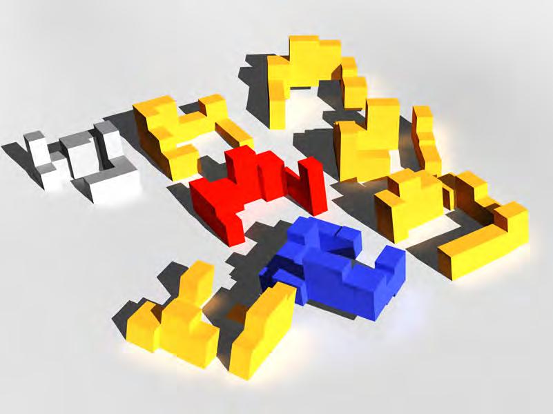

Fig.4.104
An example of a superblock which contains a large amount of low energy demand blocks (yellow colour). There are only 8 blocks, as one of them was eliminated during the evolutionary process of the blocks’ organisation.
Fig.4.105
The subdivision of each block into the four energy demand categories is based on the estimated percentages of the blocks of each superblock’s category. This subdivision occurs in a multilevel field within the block, thus creating variations of potential land uses at different levels in height.
152
Lowest energy demand Low energy demand Medium energy demand High energy demand


As mentioned earlier, a patch is divided into three categories, the high, medium and low energy demand categories. Taking the overall volume from the respective three categories above, the proportion of each category within a patch can be found. Specifically the first category, which corresponds to the low energy demand one, takes 72% of the expansion of a patch. Consequently, the second category, meaning the high energy demand one, occupies 13% of the patch and finally, the third category, i.e. the medium energy demand one, occupies the 15%.
The four energy demand categories are applied to the second hierarchical level, the superblocks, with similar proportions. As each superblock is comprised by nine blocks, the four categories are organised as the figures show below:
- Low energy demand superblock [Fig.4.106a]:
1 block of the lowest energy demand
6 blocks of low energy demand
1 block of medium energy demand
1 block of high energy demand
- Medium energy demand superblock [Fig.4.106b]:
1 block of the lowest energy demand
2 blocks of low energy demand
5 blocks of medium energy demand
1 block of high energy demand
- High energy demand superblock [Fig.4.106c]:
1 block of the lowest energy demand
3 blocks of low energy demand
1 block of medium energy demand
4 block of high energy demand
153
Fig.4.106a
Fig.4.106b
Fig.4.106c
Finally, focusing on the third hierarchical level, the block is subdivided into three energy demand zones with similar proportions as above. The volumes that form the block are grouped into the three zones according to the specific energy need for the respective use. Consequently, a second re-organisation of the blocks between them would reconfigure the proportion of the volume distribution amongst the blocks, while retaining the proportions that are already set for the previous hierarchical categories. Therefore, referring to the previous calculations:
LSED = 200 blocks
LED = 2100 blocks
MED = 263 blocks
HED = 220 blocks
Reconfiguring the energy distribution:
LSED = 150 LSED + 25 LED + 13 MED + 12 HED
LED = 25 LSED + 2017 LED + 30 MED + 28 HED
MED = 12 LSED + 30 LED + 200 MED + 21 HED
HED = 12 LSED + 28 LED + 20 MED + 160 HED
The three categories, the low, medium and high energy demand volumes, are organised as followed [Fig.4.105]:
- Lowest energy demand blocks:
75% Lowest energy demand volume
12.5% Low energy demand volume
6.5% Medium energy demand volume
6% High energy demand volume
- Low energy demand blocks:
1.2% Lowest energy demand volume
96% Low energy demand volume
1.5% Medium energy demand volume
1.3% High energy demand volume
- Medium energy demand blocks:
4.6% Lowest energy demand volume
11.4% Low energy demand volume
76% Medium energy demand volume
8% High energy demand volume
- High energy demand blocks:
5.5% Lowest energy demand volume
12.7% Low energy demand volume
9.1% Medium energy demand volume
72.7% High energy demand volume
The process entails the mix of use throughout all the hierarchical levels of the urban space, however in different proportions according to the respective energy demand zone. Moreover, the several demanding categories are distributed in different heights within the blocks, thus creating an interesting alternation of nonuniform usages in the buildings, enhancing the whole notion of mix of use.
Conclusions
In the previous case studies of planned cities, monozoning has resulted in segregation between the classes, as well as isolation of different parts of the city from the main central district. Therefore, an integration of the different zones in all hierarchies (patch, superblock, block) is vital. Unlike the conventional method of zoning, where the urban fabric is categorized into commercial, residential and business, the zoning in both scenarios is categorized by energy demand; high, medium and low. Although a block might have a dominant energy demand, the different energy demand zones are integrated within that block, as is the case through the city as a whole.
Fig.4.107
The subdivision of a patch into the three energy demand zones, the low, medium and high ones.
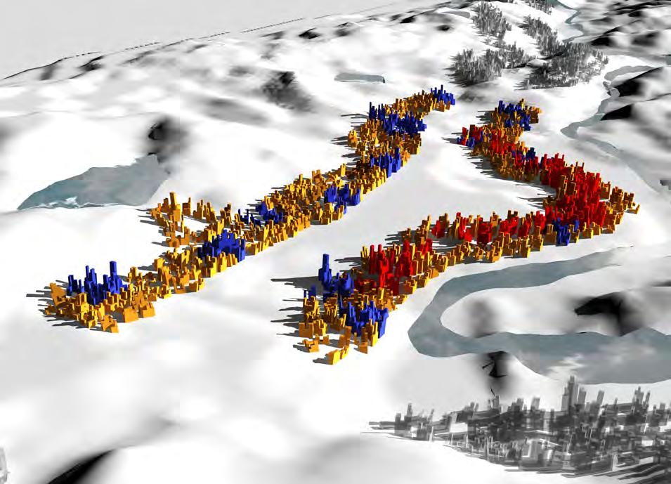
154
resources
water
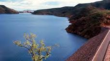
agriculture

solar energy
blocks paths
topography
solar energy
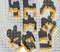


Metabolic Diagram
hierarchies
topography
focal points patch
superblock block volume transit pedestrian vehicular interaction with irrigation network
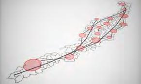
integration paths - blocks readjusting blocks readjusting streets
155
multiple paths created selection based on shortest route and lowest gradient paths
Fig.4.108: Potential growth model for the city of Scenario 1.
The figure shows four patches that have been expanded following a similar model: the reservoirs being on the north and on areas of high elevation, a zone of agriculture below them organised in a linear manner, a strip of the estimated urban tissue, another zone of agriculture followed by the second strip of urban tissue and finally, one more strip of agriculture on the southern part that reaches the river. It is suggested that at a potential growth the model will be developed linearly along the river. This creates in a way a large-scale zone of vegetation that has the possibility to inhibit desertification from the north.
156 1km
1km
Fig.4.109: Potential growth model for the city of Scenario 2. The way of development of the city in Scenario 2 is as followed: first the reservoirs are located on the mountains, north-west from the lake Argyle. The first settlements are organised around these reservoirs, expanding towards the lake. Another patch is developed right next to the lake, to which the rest of the city’s expansion converges. Initially, the urban patches are partly sustained from the existing lake, until they reach a point that can be self-sustained.
157
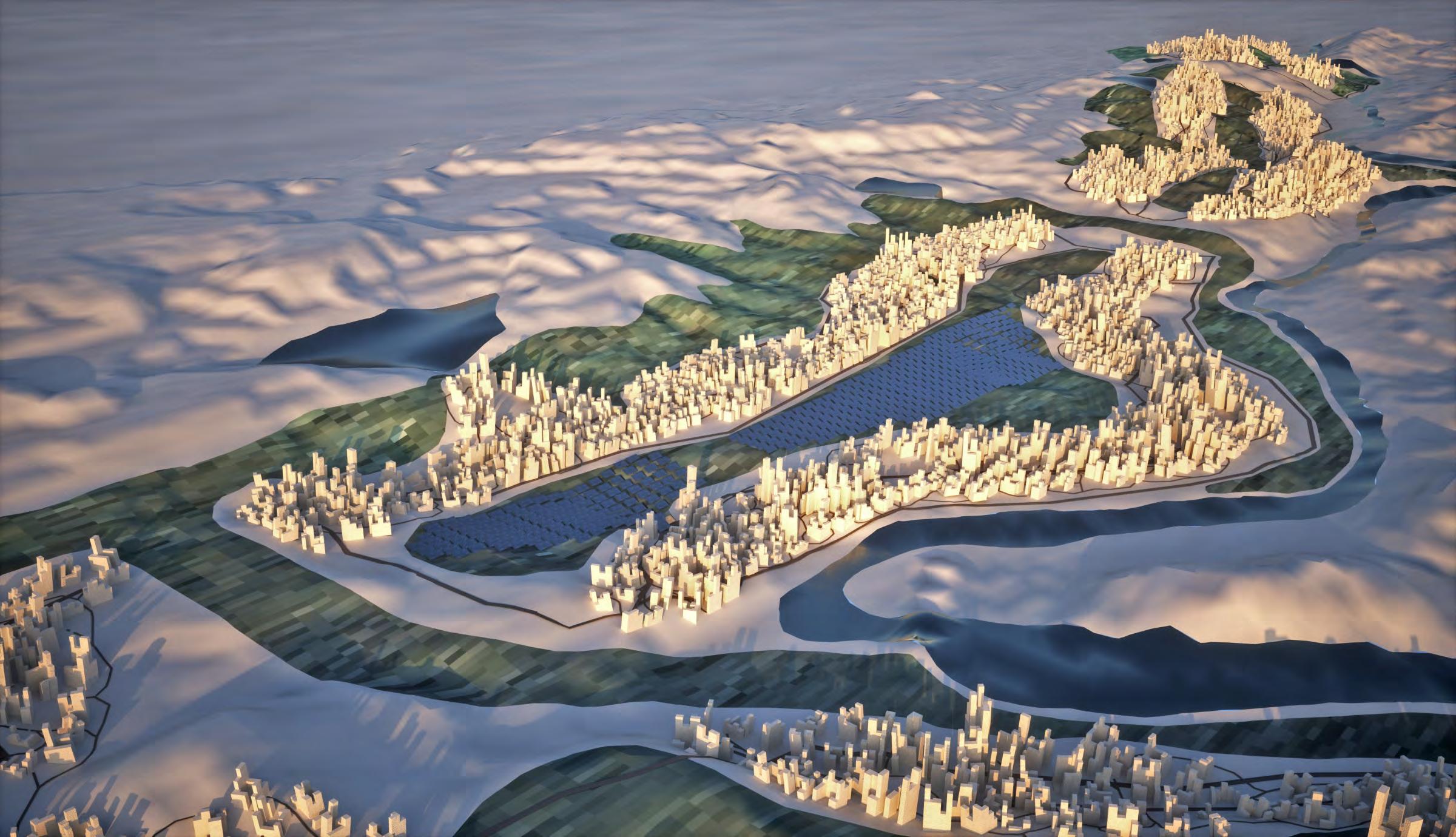
158
Fig.4.1010: Perspective view of the city, Scenario 1.
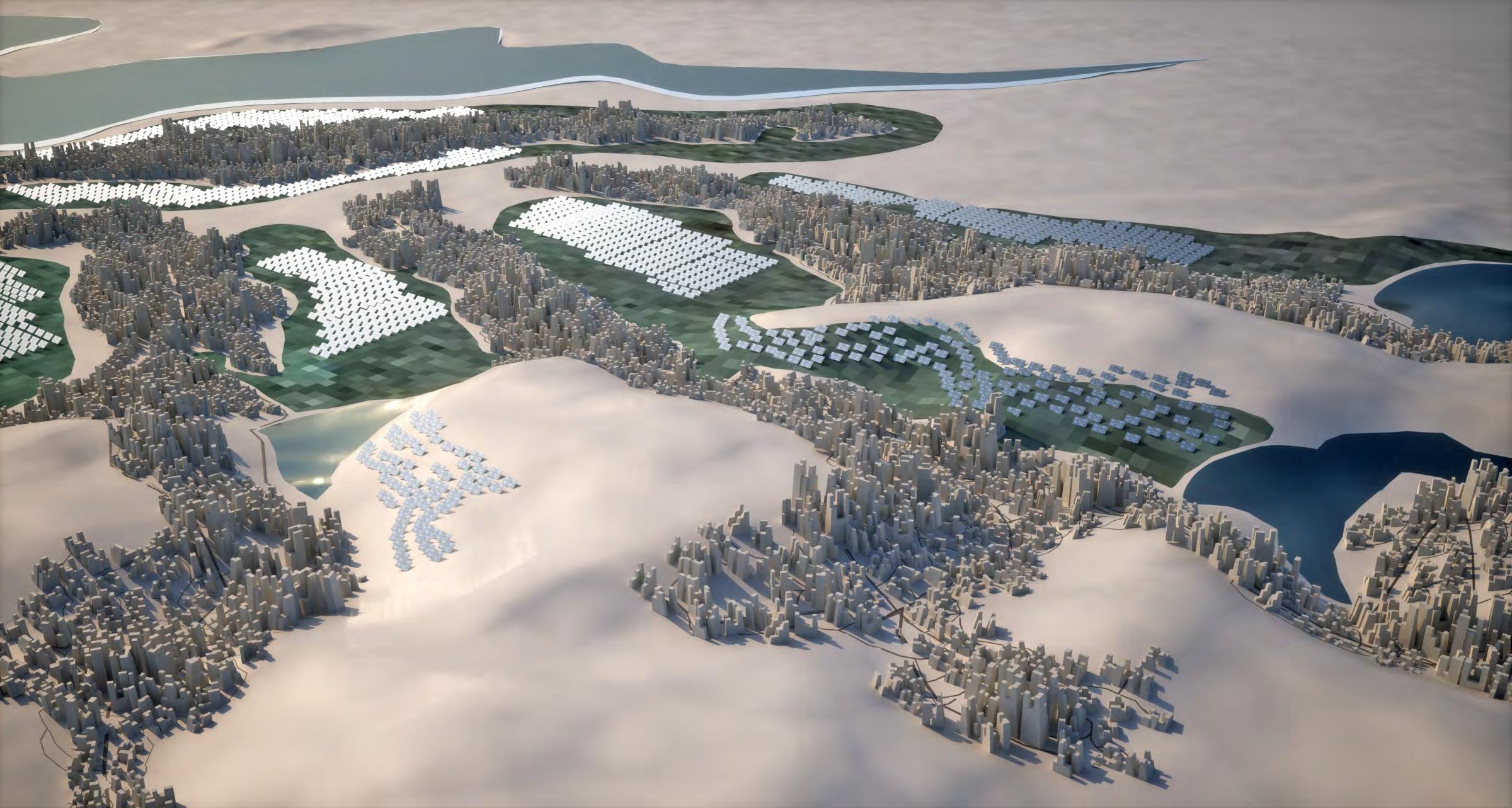
159
Fig.4.1011: Perspective view of the city, Scenario 2.
4.11 Detailed patch
Apart from the interaction with the paths, the blocks also start readjusting according to the energy demands. From all the examples of urban forms that have been brought up so far, especially the ones for evolving cities, it has been concluded that one of the cities’ characteristics is that they constantly readjust to time. The aim is to induce the same logic in the algorithm of the developing blocks. Particularly, in the case where the blocks require high energy demands, the total volume is increased accordingly. Therefore, there are many levels of height differentiation between the blocks, which are organised as follows: The blocks with the lowest and low energy demands do not change in terms of their building volume, however their volume distribution is altered and further re-configured for creating bigger variations. The medium energy demand blocks become higher by adding volume in the same amount as the existing one. Accordingly the high energy demand blocks become taller than the medium ones, as they grow vertically with an increase of volume of three times more than the existing volume. It is essential that the volume that is added to those
blocks is organised in different ways from one block to another, thus leaving the opportunity open for other factors to define these organisations, simply by local behaviours, i.e. behaviours affected by cultural decisions of the people who will inhabit the place. Even though that there are much more factors that amplify the readjustments and emergent behaviours within the city, they have bwween considered for further development.
The volume added to the blocks is organised in a way that the levels where people circulate around the city are incorporated with the built environment. Due to the hilly topography, the datum is offered for creating an interplay between streets and blocks, where people walk on the ground and suddenly the ground becomes the top of the buildings and then ground again [Fig.4.111], or where some volumes link buildings between them and the streets pass underneath them. In essence, the aim is to emphasize the complexity of the urban form.
Fig.4.111
Section of a small part of the city in the second scenario. The sketch shows that while people walk through the urban space, they experience different relations between paths and blocks: sometimes the movements occur on a higher level than the surrounding buildings, sometimes the paths cross underneath them or in some cases paths and blocks are on the same level. Through this method, there is an attempt to address the different qualities within the urban space and the dialogue between the built environment and networks.
160
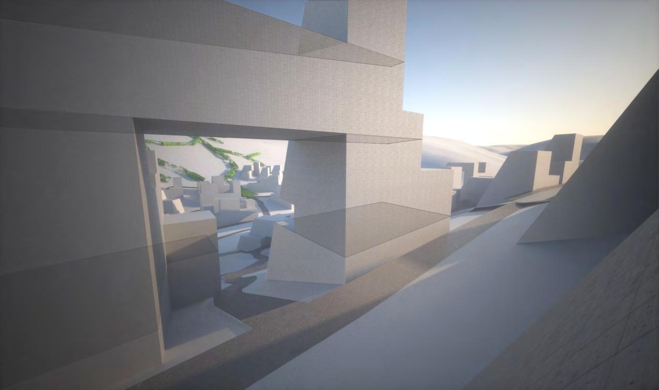
161
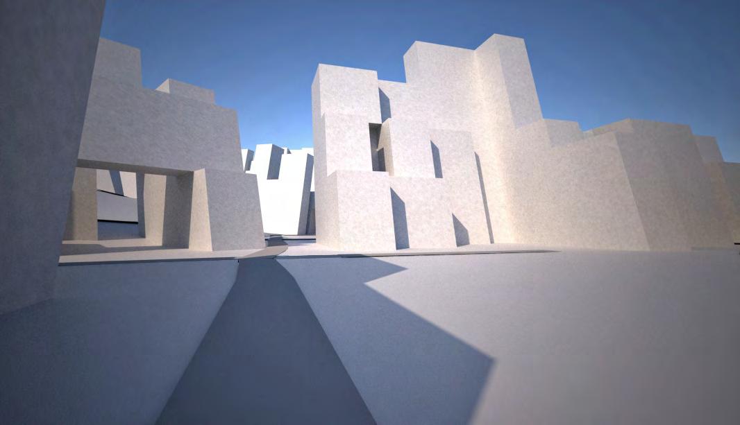
162
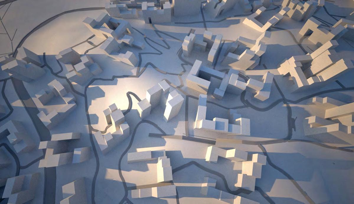
163
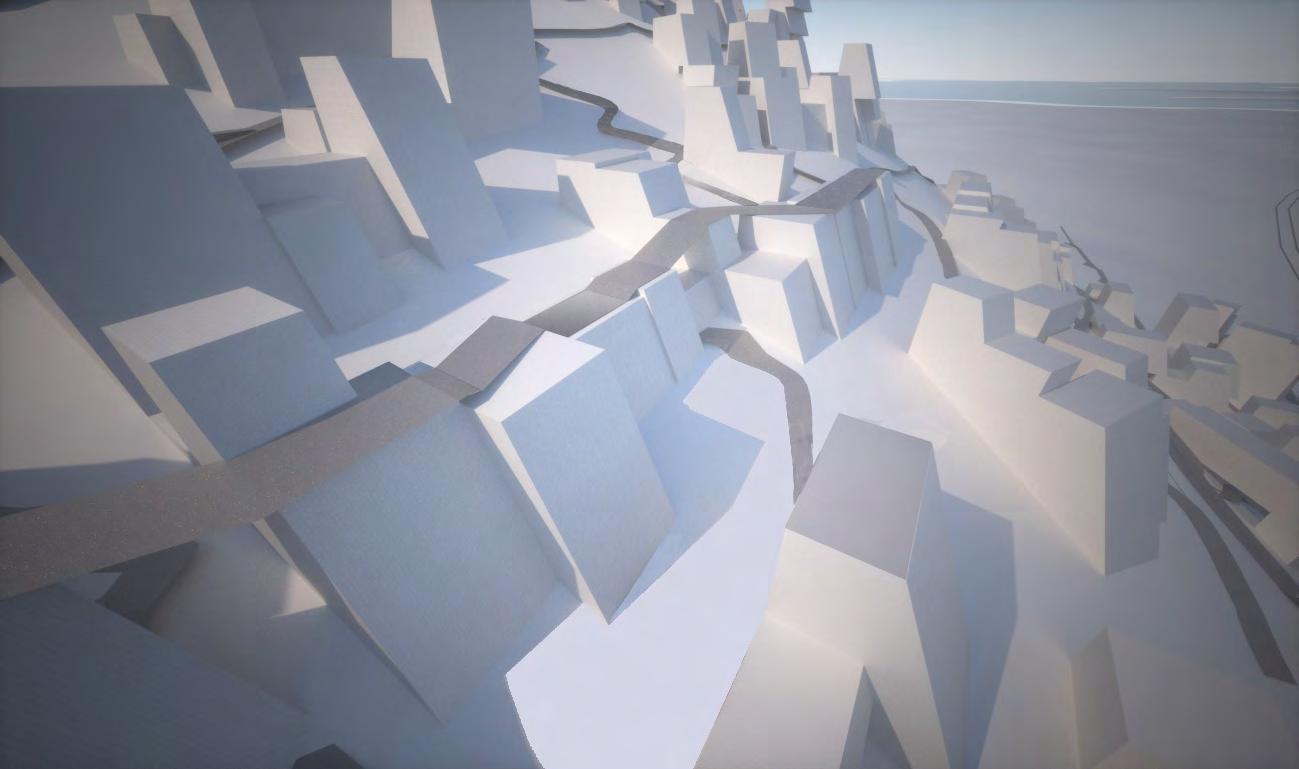

164
In China the annual water consumption ranges from region to region, from 26 Kilo-litres to 107 Kilo-litres per person. The big cities hold the largest amounts of water consumption, with Shanghai being the most water-consuming city within China. In Ningxia the consumption is relatively low, reaching the 50 Kilo-litres per person per year. Compared to Australia, China consumes much less water every year, especially on the north part of the country. For instance, the least water-consuming region of Australia, Victoria, has an annual consumption of three times more than the least water-consuming region of China. Moreover, Shanghai region, whose annual consumption is around 107 Kilo-litres per person, use almost half of the water that is consumed in the West Australia region. Finally, according to Table.2, the average daily water consumption per person in China is the 1/6 of the consumption in Australia. This is a tremendous difference between the two areas, entailing that for these two countries, the management of the local energy resources would be directly related to people’s habits concerning the water consumption.
The particle simulation tool proved to be a beneficial instrument to abstractly locate the positions of the reservoirs throughout the terrain. Although some reservoirs will hold different volumes of water than other reservoirs, the population of each patch will be sustained by the reservoir belonging to it. The volume of water will be distributed appropriately among the patch at a ratio of 1:5:2, ‘1’ being for household consumption, ‘5’ for agricultural use and ‘2’ for the other industries. The amount of water consumed will depend on the trends of water consumption of the region, however the same 1:5:2 ratio will be implemented for both scenarios.
Out of the different irrigation methods, the most suitable and appropriate method that best fits the terrain is the drip irrigation system. As well as being the most water efficient of all irrigation systems, it is the system that takes the most advantage of the terrain. Whilst laying out the irrigation system, the only ‘rule’ to be followed is that the irrigation line starts at a higher contour and ends at a lower one, ensuring that gravity is the method in which water will be transported from the reservoirs to the agricultural fields and finally throughout the city as a whole.
Choosing which method of renewable energy to be used will heavily rely on the climatic conditions of the region. Solar panels might prove to be useful for one region, while is disadvantageous for another. The crucial factor to consider is the integration and multiple uses of the land. Whether it was photovoltaics, solar furnaces or windmills, they must be integrated within the city rather than be isolated outside the city borders. The most suitable integration would be with the agricultural land, where both industries take advantage of the open land, whilst efficiently serving their own purpose.
4.12 Conclusions
The different aspects of the metabolic diagram all work together for the comprehensive performance of the city. The method by which water reservoirs are created, alongside the layout of the irrigation lines and the integration of the solar panels all work together in ensuring that the flow of energy throughout the system is the most efficient. The interdependence of all the different elements of the system on one another creates multiple uses of a single function (such as the agriculture, and renewable energy sharing the same land) further substantiating the advantages of using a metabolic system as model for urban development. The constant readjustments that take place between the blocks and the street networks begin to emulate the examples of how an evolving city continuously readjusts itself over a time. It is crucial to state that the significance given to the global morphology of the city is equal to that of the local scale of the detailed patch. Once the city begins to develop from the detailed patch, new areas of possibilities begin to emerge, such as introducing the third dimension to the street network, and thus further emphasizing the integration between the street network and the blocks.
The urban block is the most basic component of the city, although it might come in different shapes and sizes, it still remains the dominant ‘cell type’ of any city. Therefore the method that the block is created is crucial. Applying an emergent process proved most beneficial in ensuring that the blocks created are developed and optimised into energy efficient ones that are site specific. The interaction between the block and the one next to it, as well as the interaction between the block and the superblock is important in guaranteeing that the urban blocks are not isolated from one another, consequently ensuring that the urban fabric is made of components that correlate with one another rather than be completely isolated from each other.
As shown in the Ancient cities of Egypt, as well as throughout the history of Istanbul, paths were developed based on the positions of the blocks, and so, the street networks in both scenarios follow the same methodology. The paths connect focal points as well as the main arteries with one another. Topography plays an extensive role in determining the exact layout of the path, regardless of hierarchy. The essential element to take into account is the fact that the paths are laid out and developed to accommodate the pedestrian and not the car. Therefore the dimensions of the overall patch as well as the distances between the different path hierarchies must succumb to the pedestrian rather than the car.
In the previous case studies of planned cities, monozoning has resulted in segregation between the classes, as well as isolation of different parts of the city from the main central district. Therefore, an integration of the different zones in all hierarchies (patch, superblock, block) is vital. Unlike the conventional method of zoning, where the urban fabric is categorized into commercial, residential and business, the zoning in both scenarios is categorized by energy demand; high, medium and low. Although a block might have a dominant energy demand, the different energy demand zones are integrated within that block, as is the case through the city as a whole.
165
Conclusions 5.
The differences between planned cities and evolved cities are many. Although each type of city has its advantages and disadvantages, planned cities are overcome with disadvantages that go against the objectives they aim to achieve. In the planning process of Milton Keynes, the city was a polycentric one that accommodate the pedestrian as much as it did the car, however the end product was a monocentric city that revolved solely around vehicular transportation.
The reason Abuja was planned was to try to create a city that was a successful financial and economic capital to Nigeria, one that ensured that the problems that arose in Lagos would not be repeated. However, before Abuja’s plan was fully implemented, shantytowns developed and hindered the growth of Abuja; the problem that was originally aimed to avert forced itself into the plan of the city. There are many examples of how the planners’ initial objectives were never achieved
in the actual development of the master plan. Even though evolving cities have their share of disadvantages, they seem to have a solution to the problems that modern day planners are facing; the solution is not to try and predict what the future of the city will reach in terms of population and growth. Evolving cities are considered as growth models that grow over time, constantly readjusting to accommodate the functional needs of the population residing within the city.
In both scenarios, evolving cities were used as examples of growth models, while planned cities served as a constant reminder of what not to deviate towards, which in this case is to try and predict the future of the city. Thus, both scenarios were based on the growth models that are most apparent in evolving cities, however, the metabolic diagram was the main driving force in the development of both scenarios.
166
The metabolic approach relies on a system that comprises of several components that are interdependent on one another, however simultaneously, the system as a whole is interdependent on the flow of energy throughout itself as well as the storage of energy within the system. Therefore, ‘energy’ is the keyword that defines many different aspects within both scenarios. Although water resources, agricultural land, and renewable energy all fall under the umbrella of ‘energy’, they are categorized into different hierarchies of importance. The volume of water collected defines the amount of agricultural land that can be maintained whilst taking into account the number of households that can be sustained. The ratio of 1:5:2 is the most vital in determining the allocation of the water resources through out each patch, ensuring that each ‘industry’ is fed with an adequate amount of water, food and renewable energy. Therefore, the amount of water collected will determine the growth of the city, however, rather than predicting the expected population, a density ratio is set up which will inform the growth of the patch; in both scenarios, the density ratio is 10,000 people per square kilometre. This ratio is implemented uniformly throughout the patch in both scenarios, however, that is only the first step; the next step is to study the possibilities of having the overall density ratio of the patch to be 10,000 people per square kilometre, yet having different parts of the patch with different density ratios.
In both the China and the Australia scenarios, there are many similarities; this is because the rules that are being implemented are at their initial stages. The algorithms that create the blocks, or the paths will develop into more site specific algorithms which will consequently differentiate each scenario based on the climatic conditions of its region. However, the challenge that arises as a consequence of this is that the because the rules are greatly informed by the topographical conditions, a site that consists of flat terrains add another level of complexity in ensuring that the patches are specific to the site itself, rather than developing into yet another ‘gridded plan’ that is implemented on any site and in any climatic condition. Although the two scenarios chosen were set in two different extreme climatic conditions, the rules applied were successful in both scenarios, however, the global morphology of each scenario differed to accommodate the climatic demands of each region.
It is crucial to note that the scenarios presented are not final plans that will be implemented, on the contrary, they retain the evolving city’s example of the growth model, thus, both scenarios are examples of growth models that will develop over time based on the cultural and functional needs of their respected regions.
167
Further research
The scenarios carried out and developed throughout the dissertation are experiments that will serve as a basis for further areas of exploration. These areas of further research will serve as a starting point for the next phase of urban metabolic growth.
The first and most significant area of further research is establishing the growth model. As mentioned, both scenarios are not examples of master plans, but of growth models. Therefore, it is crucial to resolve how the city grows and over what period of time. To comply with any metabolic system, the city must experience simultaneous growth of its different patches rather than sequential growth. Although each patch grows at more or less the same rate, the size of each patch will be informed by the amount of water collected in its respected reservoir. Although one scenario has a linear global morphology, while the other one experiences a more radial morphology, this should not hinder the simultaneous growth of the patches within each scenario. It is crucial to visually represent the stages of growth of each scenario with respect to time. In order to comply with the models of evolving cities,
the growth models of both scenarios are not fixed; on the contrary, they only direct the growth of the global morphology. However on the local scale, the patch may readjust itself as it is growing to accommodate the functional needs of the population of that region.
Both scenarios are similar in their morphologies; the reason for this is that cultural context has still not been considered within the rules and algorithms that generate the scenarios. However, the cultural context of a particular region plays a pivotal role in influencing the local conditions of the patch, as well as differentiating the emergent blocks that are created between scenarios; this is achieved by simply introducing rules that comply with cultural context within the algorithms. One must be aware not repeat the mistakes of modern day planners, where the initial objectives are defied by the implementation process. In other words, although cultural context is integrated within the rules and algorithms, they must also comply with the initial objectives of creating a system that is energy efficient throughout all hierarchies of the patch, the superblock and the block.
168
6.
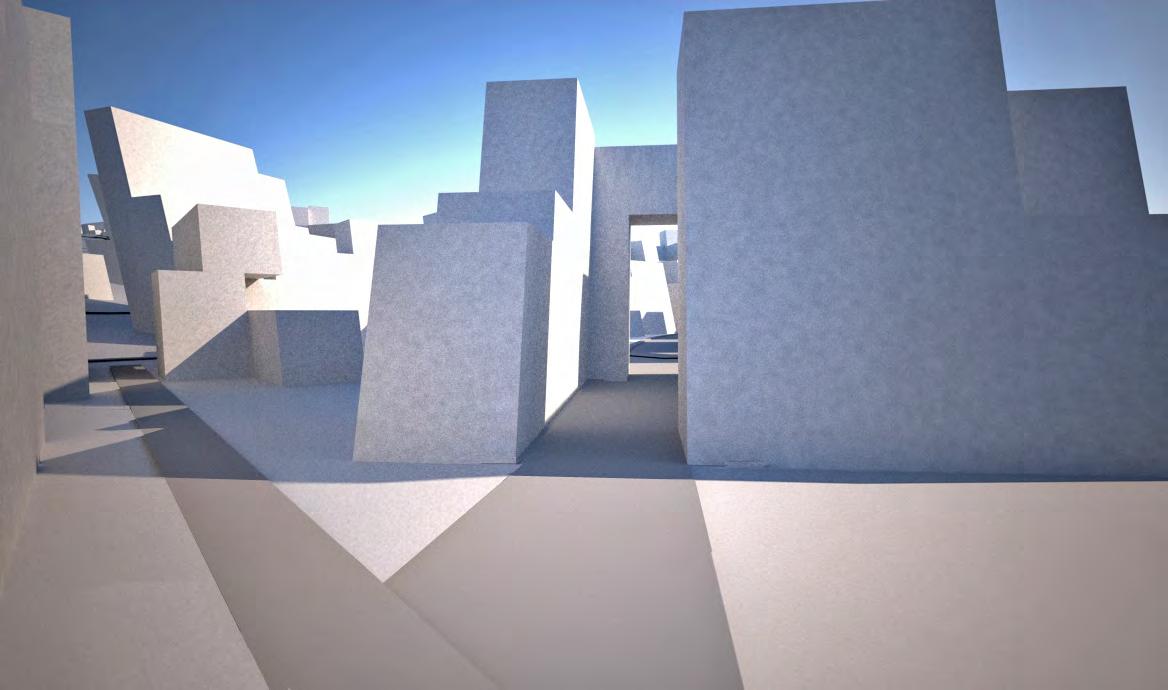
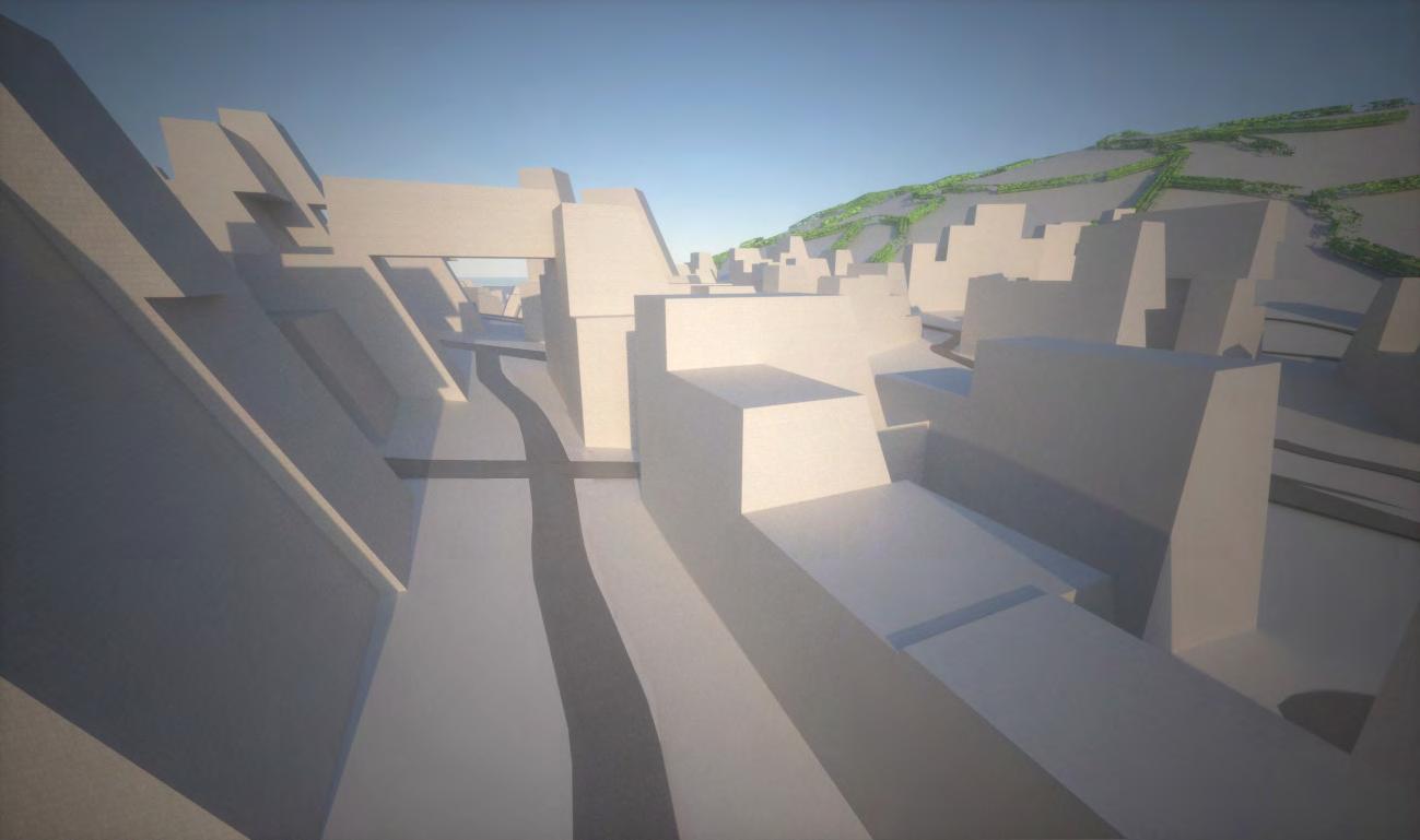
A significant setback that reservoirs throughout the world are dealing with is water evaporation. Lake Argyle loses 25 percent of its water annually to evaporation. The volume capacity of Lake Argyle is approximately 5800 Gigalitres, therefore, the reservoir loses 1450 Gigalitres of water annually. Although initially water evaporation might seem like an insignificant issue, the amount of water lost from one reservoir, can sustain an entire city. In both scenarios, the dependency on the water collected through the reservoirs is vital; therefore methods must be developed in preventing water evaporation. However, one must ensure to continue the metabolic system throughout all aspects of the city, thus the solution to this problem must be one that complies with the metabolic system. For example, rather than simply covering the reservoir with a tertiary element that is a complete ‘alien’ to the entire system, a solution can be to construct the city itself over the reservoir, hence using an element that is already within the system to solve the problem of water evaporation.
Another area of research that follows on from water evaporation is
the issue of waste management. Although it is acknowledged that both scenarios are not completely self sustaining examples, one must ensure that components of a city such as agriculture are as important as the waste created from the agricultural industry, and so, where is the waste disposed? Are there possibilities of using the waste created from the different parts of the city and recycling it into elements that can be beneficial to other parts of the city? The issue of waste management grows considerably when combined with the solution of covering the reservoir with the city itself. One cannot spoil the water that is used to sustain the different industries within the city.
These areas of further research are all crucial in ensuring that urban metabolic growth does not simply generate a city. Any system will have issues that must be resolved, however what is vital is that the solutions comply with the initial principles of the system, and do not defy the primary goals and objectives assigned at the outset of the project.
169
170
171
Appendix
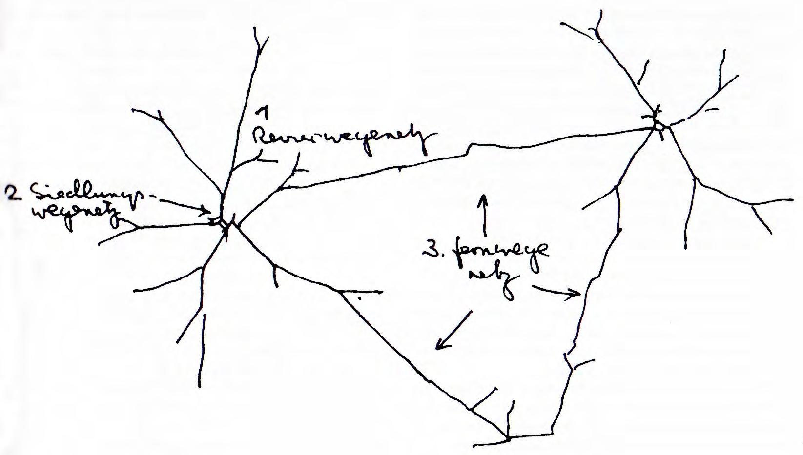
Path systems paths in nature
For living organisms in order to communicate, they need to have connections. “Transport paths connect the occupied territories. Neither the occupations nor the transport paths have to be material” (Menges, 2009). When living organisms migrate, they leave traces, permanent or not, that form path systems. As soon as they are etched on the earth surface, they are being used by multiple other organisms. When the process is repeated, the overall pattern is a grid network formed out of paths.
Paths systems exist in almost every domain of nature, but without always serving a certain purpose. Rivers carry water from higher levels to lower ones through a path system, lightning is a path system of transporting electrons. Sliding rocks, slipping snowflakes etc often follow the most direct way to climb down. Furthermore, the formation of cracks on clay is a documentation of movement, a path network (Menges, 2009).
Path systems can be found in numerous ways in living nature. One is the fluid transport systems of all animals, micro-organisms and plants. These functional systems mostly follow the form of branching structures. In plants these systems are simpler than in animals, as they constitute common paths for all the transporting functions (fluids, nutrients, energy). For the animals different layers of paths are responsible for particular functions and the transporting elements are numerous (blood, energy, chemical substances, nutrients, air etc).
Every living organism has the ability to be transported from one territory to another. The methods of achieving the transportation vary between the species, but the configuration of their paths created during this process is very common. Plants can release seeds or pollen, which can be transferred to another location with the help of the wind, birds, or insects. Animals change their location constantly in order to be able to survive, leaving traces that form path systems – known as game passes, ant or mouse runs (Menges, 2009).
Fig.1
Path systems of fieldmice. The system mainly concerns the path produced for finding food sources.
172
Fig.2
Path systems of fieldmice. The system mainly concerns the path produced for finding food sources.
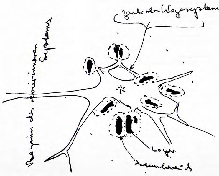
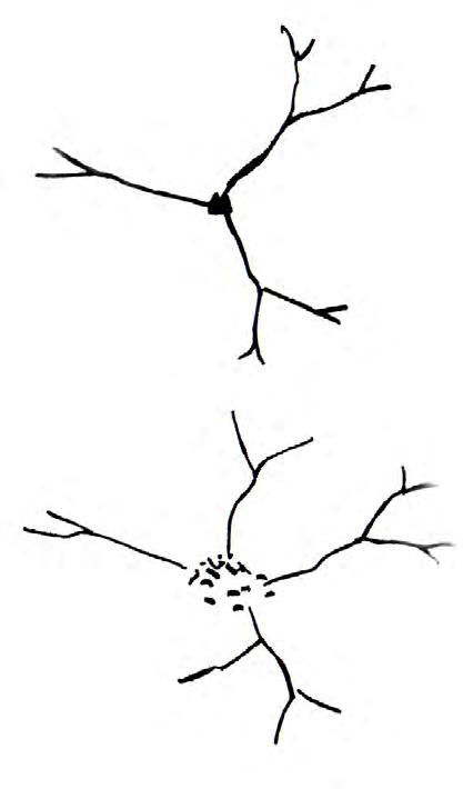
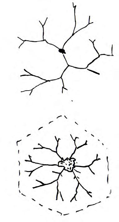
The traces that are created by eating, mostly by species such as larvae, caterpillars or snails, constitute path systems, as well as systems of surface occupation. One of the most dominant path system in nature is the spider-web, a medium that spider uses for most of its functions. It is easy for someone to descry the path that the spider took in order to spin its web.
The early humans managed to survive by collecting food or water, by inadvertently forming path systems in an emerging way. These path systems reveal a certain amount of intelligence, since their structure is adjusted for minimising the energy expense for the collection of sufficient supplies.
There are three different types of path systems recognised in the
primordial humans:
Territory path network: It constitutes an open branching system and expands within a territory, from the centre of it towards the edges. It could be helpful for the local foraging actions of humans.
Settlement path network: It concerns individual areas that tend to shift closer to one another. Therefore, the path system converges in one central area.
Long-distance path network: It is intended for the collection or production of food. It connects settlements and it is used for interregional migrations. It is not set whether the branching system or direct path network is dominant; it depends on the intensity of communication between the linked centres. All three systems differ in scale; however their morphology is merely alike: they are branching systems with forking areas.
173
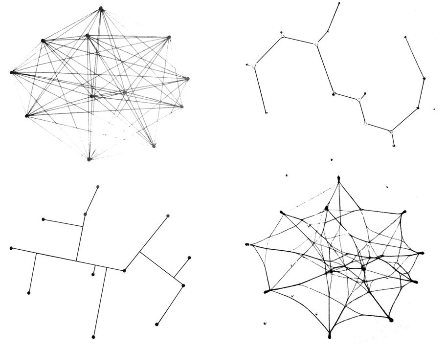
categoriesThere are many types of path systems in general. Assuming that we have several occupied points and we need to connect them between them, the first way is to link them by straight lines. This method is called the “direct path system”. Another way is by the minimal path system, which constitutes the shortest way of connecting several points between them. In essence, in a comparison of the overall length of the paths that connect all the points between them, the sum should be the minimum. The intermediate state between the two path systems above is the minimised detour networks, which are formed under the influence of more than one parameter. Finally, the generative net is another way of connection, where through a sequential process, the shortest way is created between two points every time. These ways are then connected to each other, intersecting on new points. In the last three cases new points are introduced on the junctions of the path systems, which they constitute emergent occupation points.
Direct Path system
At every setup of points, either on a plane or in space, when the connection between two of them is a straight line then we have direct paths. There are no path forks, ramifications or detours [Fig.3a]. Some of the applications of direct path systems occur in energy-transport cases, e.g. when a frame transports the forces of a high building into the ground by the shortest route. In addition, the traces of aeroplane or boat routes simulate direct path systems (Menges, 2009).
Minimal Path system
In the case of connecting two points, the minimal and direct paths are the same: a straight line. When more than two points are involved, the minimal path network is comprised by detours and forks. The main characteristic is that the total length of the whole path system is the minimum one of all the other methods of path systems [Fig.3b].
Fig.3a-d
Direct paths, minimal paths, generative paths and minimised detours are shown respectively.
174
Fig.3a
Fig.3b
Fig.3c
Fig.3d
Fig.4a,b
Examples of applications of generative path systems.
Fig.5a
Applications of minimised detour systems in branching structures.
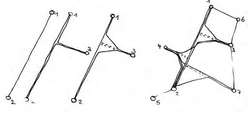
Fig.5b,c
Results of experiments of minimised detours with the thread and water apparatus.
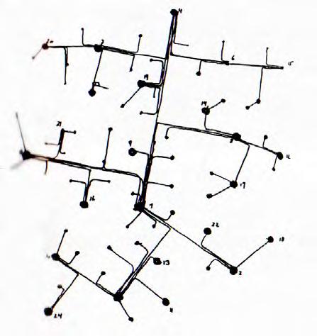
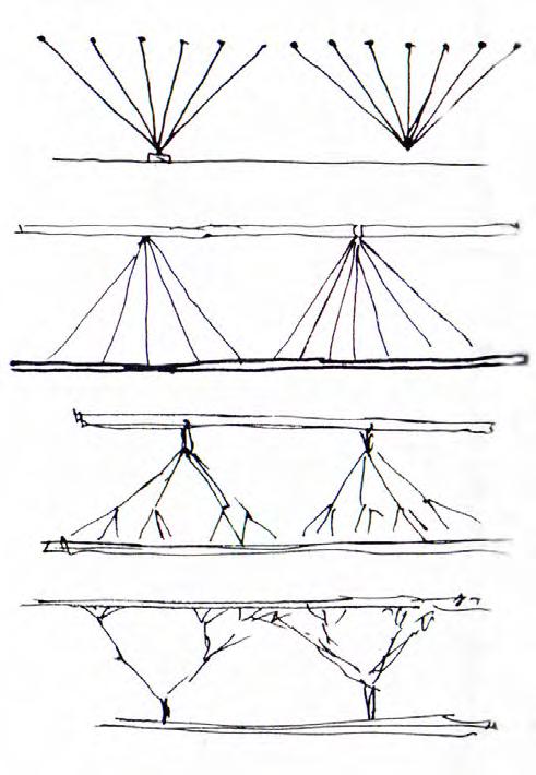
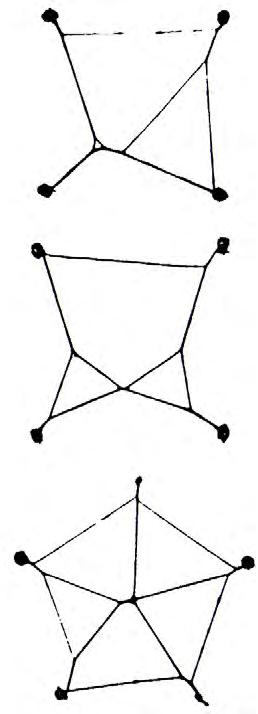
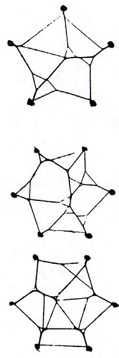
Generative Path system
It is the path system created in a sequential way of connecting emerging points with the rest of the network, by the minimum possible length. Usually every new path forms a right angle with the path that is connected to (forming T-junctions), unless if the new point is far away from the existing path in an almost parallel way. Then the new point is connected directly to the nearest existing point [Fig.3c]. This method is suitable for distinguishing the “age” of the network, because the morphology of the generative path systems reveals the previous steps of the process.
Minimised Detour system
It is the intermediate state between direct path and minimal path systems [Fig.3d]. This system can be useful for energy optimisation
techniques, where the minimal way is not the desired result, because it could be not useful to other inputs and the direct way is not sufficient enough for minimising the distances. For instance, it can be useful for optimising structures, such as space frames, as the shortest way of transporting the loads into the ground.
Applications that exist within the concept of minimised detour systems are bridge constructions, branching supports for large-spanned spaces, or road designing systems. In nature is almost impossible to find examples of direct or minimal paths. On the contrary, most of the applications of energy optimisation techniques in nature are minimised detour systems; ant colonies, rivers, the organisms’ respiratory system and lightning are some of the examples.
175
Fig.4b
Fig.5a
Fig.5b
Fig.5c
Fig.4a
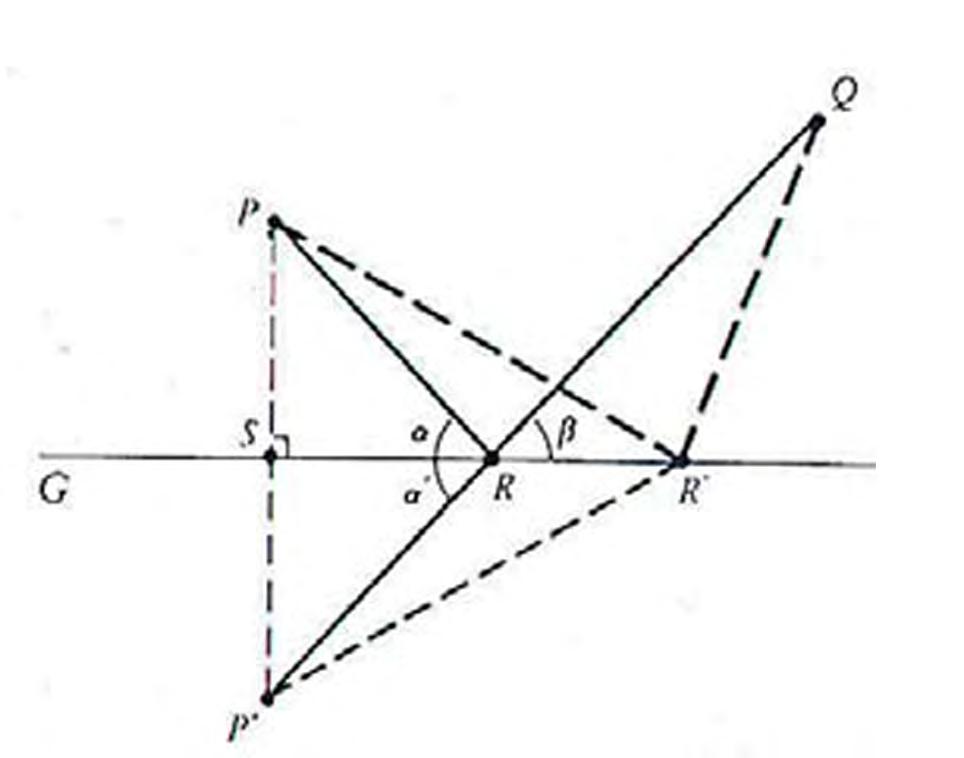
minimal path systems
The initial approach on solving the minimal path problem has been attempted by mathematicians at the times of ancient Greece. They tried to determine the shortest way of connecting several points of a common plane between them. One of the first investigators of minimal path systems was Alexandrian Heron, who stated that the light must always follow the shortest path. He managed to find a way to achieve the minimal path that joins two points P and Q, passing through a third point R located on a curve. According to his investigation, in order to create the minimal path two lines must be drawn, PR and RQ in a way that the angle of incidence is equal to the angle of reflection [Fig.6] (Hildebrand, 1996).
Another mathematician who had dealt with minimal paths was Jakob Steiner. According to his theory, three cities A, B and C are to be connected with the least possible total length of the path that would join
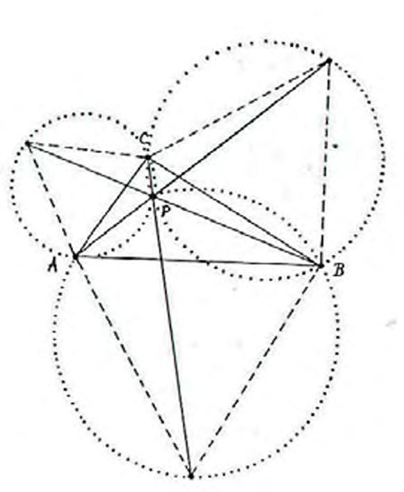
them. He concluded that for any three points A, B and C, which they form a triangle with all its angles less than 120 degrees, there is a P point, called Fermat point, which is joined with all three points by three lines, AP, BP and CP. The total length of these lines is the minimum (Hildebrand, 1996).
Finding the P point
The three points A, B and C form a triangle whose angles do not exceed the 120 degrees. From each side of the triangle three equilateral ones are created, using the length of each side respectively. Each point A, B and C are connected to the vertex of their opposite triangle, creating three new lines that cross through the initial triangle. The point where all the three lines converge is the P point. Furthermore, if three circles are created, each one around every equilateral triangle, the point where these circles intersect is the P point [Fig.7].
Fig.6
Alexandrian Heron’s diagram of minimal path route between three points. The point R is the intermediate point between the two initial ones, P and Q.
Fig.7
The two ways of finding the P point within a triangle:
1. From the equilateral triangles created by the edges of the triangle, each vertex is joined with the opposite one by a line. Their intersection is the P point.
2. Each equilateral triangle is enclosed by the circle that crosses through their vertices. The intersection of these three circles is the P point.
176
Fig.8
Soap film model experiment. The apparatus consists of two horizontal planes joined by three nails. Between them the soap creates soap film surfaces whose edges describe the minimal path between the three points.
Fig.9
Between four points there are two different possibilities of path configurations that occur at the soap film experiment.
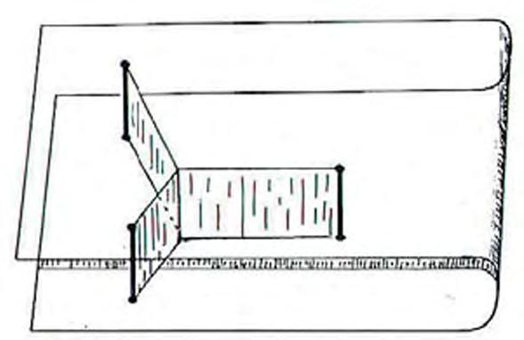
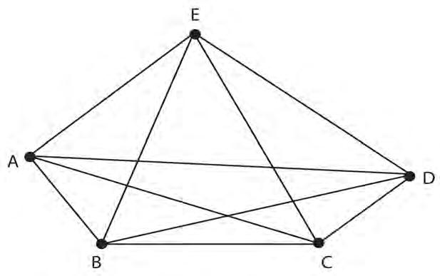
Fig.10a,b
The road connection example: Comparison between the direct path and minimal path solutions of connecting several points between them.
Contrarily to the Steiner’s theory, when more points are involved there is not only one solution for the production of the minimal path. Many experiments have been conducted for achieving minimal path systems by the Institute of Lightweight Structures, mostly by using soap bubbles. The simplest form of experiment was an apparatus comprised by two glass planes parallel to each other and connected by nails. The model was immersed in a soap solution, where between three nails three soap films were created, perpendicular to the planes [Fig.8]. In an experiment with four nails, two different types of configurations of the soap films were observed [Fig.9]. Consequently, by adding more points the system becomes increasingly more complex with many possible configurations.
Minimal networks are open systems without any closed units. Every junction forms an angle of 120 degrees. In nature it is almost impossible to find exact minimal path systems. However, there are ways to
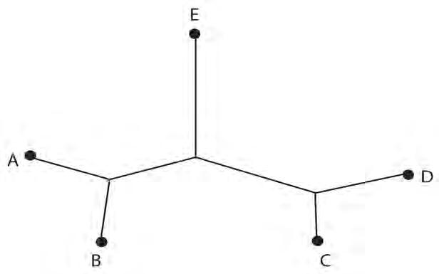
create closed minimal path systems. For example, three points are connected by a hexagonal minimal path system and one side of the hexagon is open. By closing the shape it might add a one sixth of the total length but the effectiveness is doubled.
Minimal path systems are of great importance in terms of traffic flow study, road connections, nodes, or the effects of topology and distance. An example of road connection is the one created by Klaus Bach and Berthold Burkhardt, where they firstly modelled a direct path system connecting five points, A to E and they observed that the system was comprised by 20 roads, 11 closed loops and five crossings. Then they created the minimal path system for the same five points where they observed seven partial roads and no loops at all [Fig.10a-b]. There is a significant reduction of the paths, their length and eventually the cost of their construction.
177
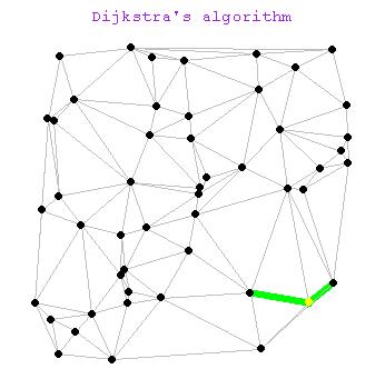
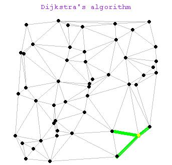
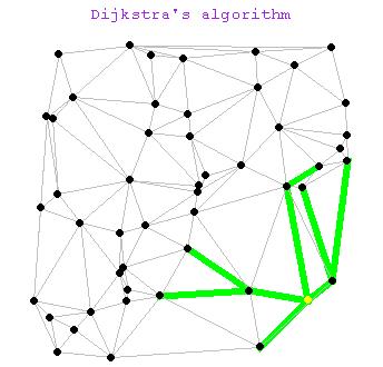
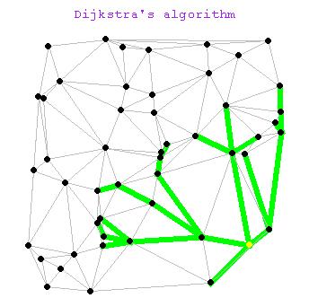
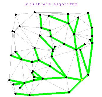
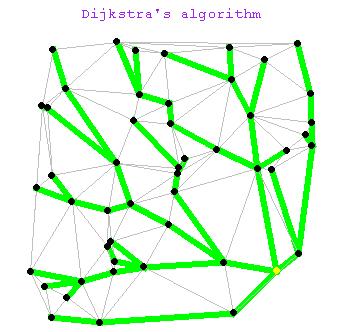
Due to the complexity of the minimal path systems concerning occasions where many points are involved, mathematicians had tried to solve the particular problems with the help of algorithms. These algorithms aim at the minimization of the overall distance that connects several predefined points on a plane.
Dijkstra’s Algorithm
In 1959 a Dutch computer scientist, named Edsger Dijkstra, created a graph search algorithm that solved the single-source shortest path problem for a graph with non-negative edge path costs, outputting a shortest path tree. According to the algorithm, the first action is the measurement of all the distances between the points. In essence, it initially maps a potential direct path system between the points. Then it documents all the distance measurements hierarchically, starting from the smallest one. The first step is to display the shortest distance between two points of the system. Consequently, it keeps following the same process from the already displayed points by choosing the
next shortest distance every time. The algorithm ends when all the points are connected through a path [Fig.11a-g]. The same process could be simulated as followed: we create a knotted web of strings, with each knot corresponding to a node, and the strings corresponding to the edges of the web: the length of each string is proportional to the weight of each edge. Then we compress the web into a small pile without making any knots or tangles in it. We grab the starting knot and pull straight up. As new knots start to come up with the original, we can measure the straight up-down distance to these knots: this must be the shortest distance from the starting node to the destination one. The acts of “pulling up” and “measuring” must be abstracted for the computer, but the general idea of the algorithm is the same: you have two sets, one of knots that are on the table, and another of knots that are in the air. Every step of the algorithm, we take the closest knot from the table and pull it into the air, and mark it with its length. If any knots are left on the table when finished, they are marked with the distance infinity.
Dijkstra’s algorithm.
178
a b d c e f g
algorithms
Fig.11a-g
Fig.12a-g Kruskal’s algorithm.
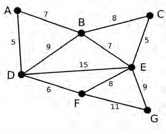
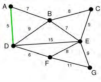
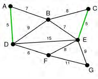
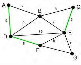
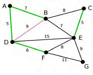
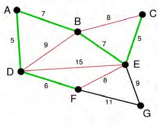
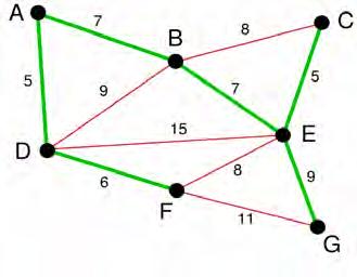
Kruskal’s Algorithm
Kruskal’s algorithm is an algorithm in graph theory that finds a minimum spanning tree for a connected weighted graph. If the graph is not connected, then it finds a minimum spanning forest (a minimum spanning tree for each connected component). This algorithm first appeared in 1956, and was written by Joseph Kruskal.
In a setup of points on a plane, there are several predefined direct lines that connect the points. The algorithm firstly chooses the shortest line as the initial path. Then it sequentially highlights the next shortest path, even if it is away from the initial one. Next the process is followed by a killing tactic; if the algorithm finds a line that connects two points that are already connected to a third, common point, the line between them will be cancelled out [Fig.12]. The algorithm ends when all the points are included in the minimum spanning tree that was created.
179
a b d c e f g
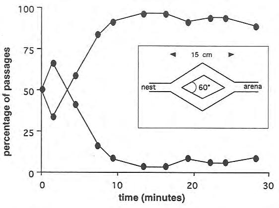
minimised detour systems
In nature one of the examples of a minimised detour system is the foraging behaviour of ants. The local interaction of individual ants sequentially leads to the emergent macro-behaviour of the colony. The low levels of intelligence of an individual ant are contradictive to the high sophistication of the whole colony. The foraging process is an example of the way the “intelligent” ant colony finds the way to collect as much food as possible by spending the least energy. It is in a way, a natural application of a minimised detour system, acting through an emergent mechanism of swarm intelligence.
During their foraging process, every individual ant leaves trails by releasing a substance called “pheromone”. The word derives from the Greek word “φέρω” (phero) – which means “to carry” – and the word hormone. The foraging ants follow the pheromone of the previous ants afterwards. When an ant follows another ant to reach the food source, or when it follows the pheromone, the process is called “recruitment”. When ants follow exclusively chemical trails they constitute a mass
recruitment. The path selection of the foraging ants is based on selforganisation. “The emerging structures in the case of foraging ants include spatiotemporally organised networks of pheromone trails” (Bonabeau, 1999). The particular behaviour of ants has been studied through an experiment with Argentine ants “Linepithema humile”. A brief description of the experiment shows the preferable route that the ants follow during their forage. A food source is placed away from the nest, with a bridge comprised of two individual branches connecting the nest and the food source. The branches A and B have equal lengths and no pheromone at all, thus they have the same probabilities ob being selected by the ants. Initiating the experiment, a few more ants walk on the branch A for inconsequential reasons. This causes more pheromone traces left on the branch A and therefore the result shows that the number of ants that chose branch A was significantly larger than of the ants that chose branch B [Diagram.13], (Bonabeau, 1999).
Diagram.13
The diagram shows the percentage of all passages per unit time on each of the two branches as a function of time: one of the branches is eventually used most of the time. The fact that the winning branch was not favoured by the initial fluctuations indicates that these fluctuations were not strong enough to promote exploitation of the other branch. The inset is a schematic representation of the experiment setup [Ref.5].
180
Fig.14
Experimental setup and drawings of the selection of the short branches by a colony of “Linepithema humile” respectively four and eight minutes after the bridge was placed [Ref.5].
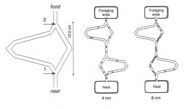
In a repetition of the experiment with one branch longer than the other, a critical behaviour was unexpectedly observed. The most preferable path is the one with the shortest length, but why? The first ants initiate the foraging process with those that chose the short branch reaching the food source before the others and consequently, they return to their nest much earlier than the ants that followed the long route. Therefore, when other ants initiate their course to the food source, they find double amount of pheromone on the short path, as the ants that chose that path before have already returned to the nest; they passed twice from the same branch, once towards the food and once when they came back. From that moment, almost every ant that initiates its forage will in turn follow the shortest path towards the food source [Fig.14]. After several experiments, it has been noticed that the ratio between the long path and the short one is proportional to the number of ants that would choose the short path instead of the long one.
During the forage it is difficult to maintain well preserved trails of pheromone on a longer trail, thus the result leads to a situation that cannot be described as completely optimal. In nature there are other factors that may influence the results of this food seeking process. There are cases where ants have to perform their foraging activity in a specific site of area for protective reasons. Even if the specific route is not the optimum one, it is beneficial to the colony to follow it instead of jeopardising its safety. Through a series of experiments, it has been discovered that the Argentine ants could solve the minimal spanning tree problem, which is a system with varied solutions of interconnected vertices in a hierarchical way.
181
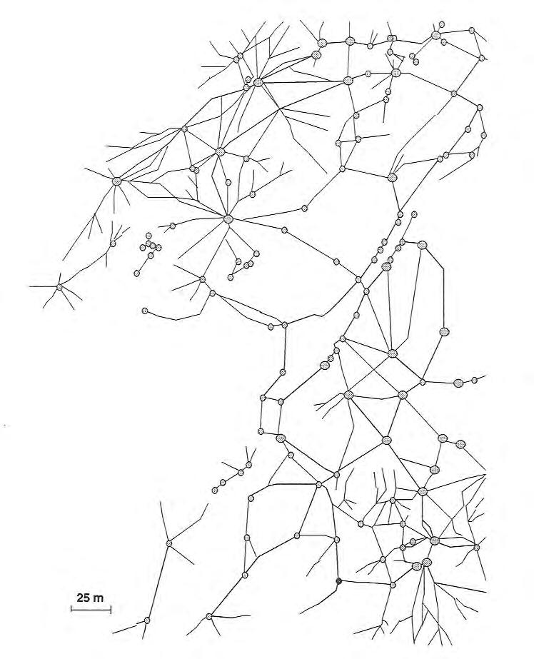
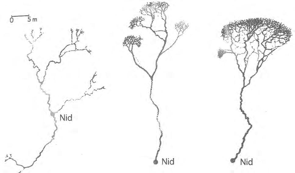
The apparatus of the experiments is a system of three or four nests connected between them. There have been experimentations of cutting out one or two of the bridges that connected the nests or putting them back in order to document the behaviour of ants. The paths indeed formed a minimal spanning tree, exclusively relied on the chemical cue behaviour of the ants. On the contrary, visual cues were merely inessential to the ants’ choices of route. The particular example of interconnected nests mirrors the actual colony formation, which can be formed by huge networks of connected nests, which form settlements in million possible configurations, even in a span of hundred of meters [Fig.15].
The environment where the forage takes place is the main factor that influences the final pattern of the path the ants form during the process. For instance, in a different distribution of food sources, the morphology of the final pattern would be different in each case [Fig.16].
Finally, it is speculated that, according to these patterns, the ants foraging process can be considered as a description of optimal “distribution networks”. The key point is in essence the fact that ant colonies can collect big quantities of food by spending small amounts of energy
expense, or likewise, minimise the energy expense for a given quantity of food sources.
Through the study of the “intelligent” solution of the ant colonies to find the shortest way to a desired source, due to the emergent result of the individual ants’ actions, the first application of an ant colony algorithm was develop for a path optimisation problem. The algorithm is called the “Travelling salesman problem” (TSP), which has performance very similar to the foraging process of ant colonies. The main concept of the algorithm is to keep the idea of the reinforcement of trails in order to provide great accuracy to the results, based on the positive feedback logic.
Ant based algorithms have been applied to several combinatorial problems, such as the quadratic assignment problem, graph colouring, job-shop scheduling, sequential ordering, and vehicle routing (Bonabeau, 1999). There is a parallelism between ant-based optimisation algorithms and other optimisation algorithms inspired by nature, such as evolutionary computation and neural nets.
Fig.15
Network of interconnected nests of a super-colony of “Formica lugubris” [Ref.5]. Fig.16
Foraging patterns of three army ant species. The environment is the main factor that defines the morphological configuration of the foraging pattern. According to the way the food is spread, the path system can be spread out with a sparsely branching way, or contrarily, we can observe areas with accumulative concentration of ants [Ref.5].
182
183
Master planning history
The idea of the master plan starts from the last century as a method of “mastering” the city character, when cities started to manifest an emergent behaviour, which was interpreted as an “uncontrolled” rate of growth. Suggesting that the form and the development of a city should be predicted, master planning seemed to come after the city components that it was supposed to improve.
There can be seen four prevailing principles in the initial idea of master planning:
1. The same method is applied to every case. This leads to the repetition of the same model in different geographical, climatic, economic and social conditions.
2. The attention was mostly given to the protection of public good. Eventually the private sector had to follow the plan, without developing any progress.
3. The general principle of master planning is a top-down logic, which determines the regional guidelines first and then continues inwards to define the local margins.
4. Any kind of evolution or progress was to happen within the outline boundaries set by the plan.
In terms of history, master planning has been used in order to represent a scheme that could be replicated in different scales in other places. At the time, the main issues were mobility, expansion and ways of improving appearance. Eugene Henard, a French architect, during his research for solutions to the circulation pattern of Paris, he studied the predominantly radial traffic strategies of major cities [Fig.1a-d] (Busquets, 2006). However, during the years most of the planned cities started to manifest unpredictable behaviours. In their attempt to rationalise this situation, many scientists failed to predict the emergent conditions of urbanisation and therefore improve them.
Fig.1a-d
Anticipating the problems of infrastructurural congestion, Eugene Henard studied the predominantly radial, or the ring traffic strategies of major cities in order to search out solutions to the circulation pattern of Paris along its radial arteries [Ref.5].
184
berlin paris london moscow
Fig.2a,b
The figure 2a (left) shows the mix use of functions in the historical cities; this contributed to the minimization of the distances. In the figure 2b (right) the sprawl and expansion of the functions occurring in the modern cities is shown.
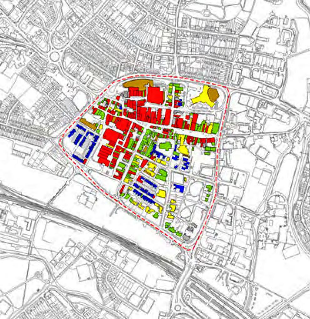

Catering
Others
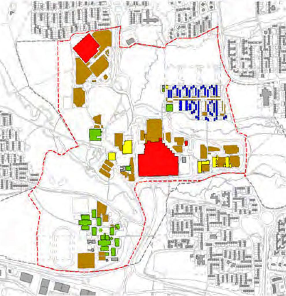
Nowadays master plans are being used by cities in order to reclassify their spaces; for optimising the locations for economic development, or improvement of the residential areas and invention of new methods of applying services in order to reduce the big differentiation of incomes. Most of the cases involve master planning for adaptability to unpredicted and changing conditions. However, this does not predicate that everything can be solved. Sometimes adaptability means lack of speculation and abuse (Busquets, 2006).
The prevailing rules that a master plan follows could be:
1. Thorough study of the existing conditions before planning. Particularly, the environmental and ecological factors are being given most of the attention.
2. A research about the current formal and morphological situation of cities and the new contents they introduce.
3. A deep look into the system of mobility, prioritising the positions of transportation, private vehicles and pedestrians.
4. The understanding of the polycentric character of most of the cities in terms of functionality improvement.
There is another major difference between the historical planned cities and the modern ones, in terms of functional distribution; in the historical cities [Fig.2a] there are mixed land uses condensed into a certain area, hence the journey lengths are minimised, whereas in the modern cities [Fig.2b] the functions are divided by zones making the mobility use more essential. This is something that has a great impact in regards to sustainability issues that will be examined in a following chapter.
185
Commercial Residential Services Transport
Gradient
script
Option Explicit ‘Script written by <insert name> ‘Script copyrighted by <insert company name> ‘Script version Monday, November 30, 2009 11:47:47 AM
‘...............Mohammed Makki ................... Pavlos Schizas
Call Main()
Sub Main()
Dim pts,x,y
Dim points
Dim plane
Dim circle,circle1
Dim segmentpoints,segmentpoint,lines,segments,segment
Dim surface
Dim curves
Dim projectedpoints
Dim centre
Dim results
Dim segpts
Dim projcirc
Dim segpt,coor,coor2
Dim centrepoints
Dim text
Dim newpoints(),arrpts
Dim i,j,gradient
Dim top,plane2,angle
Dim color1,color2,color3,color4,color5,color6,color7,color8
Dim color9,color10,color11,color12,color13,color14,color15
Dim line
surface = rhino.GetObject (“pick surface”,8) arrpts = rhino.GetObjects (“pick points”,1)
color1 = RGB(0,0,127) ‘Dark blue color2 = RGB(0,0,255) ‘Blue color3 = RGB(255,127,0) ‘Orange color4 = RGB(0,255,255) ‘Turquoise color5 = RGB(255,255,0) ‘Yellow color6 = RGB(255,255,255) ‘White color7 = RGB(0,255,0) ‘Green color8 = RGB(191,191,255) ‘Lavender color9 = RGB(255,0,255) ‘Magenta color10 = RGB(0,127,0) ‘Dark Green color11 = RGB(255,0,0) ‘Red color12 = RGB(155,48,255) ‘Purple color13 = RGB(63,0,0) ‘Dark Red color14 = RGB(139,139,0) ‘Golden Yellow color15 = RGB(255,255,255) ‘Black
Rhino.enableredraw False
186
For i=0 To ubound(arrpts)
pts=arrpts(i)
ReDim Preserve newpoints(i)
newpoints(i)=rhino.PointCoordinates(pts) plane = rhino.MovePlane (rhino.ViewCPlane(“Top”),newpoints(i)) circle = rhino.AddCircle (plane,7.5) projcirc = Rhino.ProjectCurveToSurface (circle,surface,array(0,0,1)) centre = Rhino.ProjectPointToSurface(newpoints(i), Surface, Array(0,0,1)) plane2 = rhino.MovePlane (rhino.ViewCPlane(“Top”),centre(0)) segments = rhino.DivideCurve (projcirc(0), 12) segmentpoints = rhino.addpoints (segments) centrepoints = rhino.AddPoints (centre) coor = Rhino.PointCoordinates (centrepoints(0)) coor2 = rhino.PointCoordinates (segmentpoints(0))
‘’rhino.Print coor(2)
text = rhino.addtext (coor(2), plane2,0.5) ‘’rhino.addtext coor2(2),segments(i),0.5 rhino.ObjectLayer pts, “layer01”
‘’segpts = rhino.projectpointtosurface (segmentpoints, surface, array(0,0,-1))
‘’rhino.addpoints segmentpoints For Each segment In segments
gradient = abs(centre(0)(2)-segment(2))/sqr((centre(0 (1)-segment(1))^2+(centre(0)(0)-segment(0))^2) line = rhino.addline (centre(0),segment)
If gradient > 0 Or gradient = 0 And gradient < 0.05 Then rhino.objectcolor line,color1
End If
If gradient>0.05 Or gradient = 0.05 And gradient<0.1 Then rhino.objectcolor line,color2
End If
If gradient>0.1 Or gradient = 0.1 And gradient<0.15 Then rhino.ObjectColor line,color3
End If
If gradient>0.15 Or gradient = 0.15 And gradient<0.2 Then rhino.ObjectColor line,color4
End If
If gradient>0.2 Or gradient = 0.2 And gradient<0.25 Then rhino.ObjectColor line,color5
End If
If gradient>0.25 Or gradient = 0.25 And gradient<0.3 Then rhino.ObjectColor line,color6
End If
If gradient>0.3 Or gradient = 0.3 And gradient<0.35 Then rhino.ObjectColor line,color7
End If
If gradient>0.35 Or gradient = 0.35 And gradient<0.4 Then rhino.ObjectColor line,color8
End If
If gradient>0.4 Or gradient = 0.4 And gradient <0.45 Then rhino.ObjectColor line,color9
End If
If gradient>0.45 Or gradient = 0.45 And gradient<0.5 Then rhino.objectcolor line,color1 0
End If
If gradient>0.5 Or gradient = 0.5 And gradient<0.55 Then rhino.objectcolor line,color11
End If
If gradient>0.55 Or gradient = 0.55 And gradient<0.6 Then rhino.ObjectColor line,color12
End If
If gradient>0.6 Or gradient = 0.6 And gradient<0.65 Then rhino.ObjectColor line,color13
End If
If gradient>0.65 Or gradient = 0.65 And gradient<0.7 Then rhino.ObjectColor line,color14
End If
If gradient>0.7 Or gradient = 0.7 And gradient<0.75 Then rhino.ObjectColor line,color15
End If
End If
If gradient>1.15 Or gradient = 1.15 And gradient<1.2 Then rhino.ObjectColor line,color15 ‘ End If
Rhino.EnableRedraw True
187
Next Next
End Sub
Fig.1a,b (right page) The metabolic components of the two urban experiments are shown separately in different levels in both scenarios. Their order (from bottom to top) represents the order according to which each sector will be developed: first the water resources, then agriculture and solar energy, while the blocks and paths will follow, depending on the available resources.
Patch analysis metabolic components
188
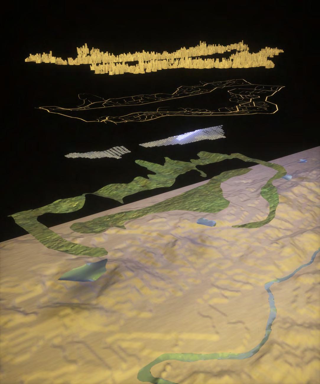

189
Bibliography
Alayande, James F., 2006. Abuja: Readings in city planning. Booksurge Llc
Australian Bureau of Statistics. 2009. Population clock. [Online] Available at: http://www.abs.gov.au/ausstats/abs%40.nsf/94713ad445ff1425ca25682000192af2/1647509ef7e25faaca2568a900154b63?OpenDocument [Accessed 13 December 2009]
Australian government: Bureau of meteorology. 2010. Climate change. [Online] Available at: http://www.bom.gov.au/climate/change/ [Accessed 13 December 2009]
B. Areal Augusto Cesar . 1957. The History of Brasilia - The Pilot Plan as presented by Lucio Costa in 1957. Available at: http://www.infobrasilia. com.br/pilot_plan.htm
[Accessed 15 December 2009]
Benmansour Fethallah, D. Cohen Laurent. “Fast Object Segmentation by growing Minimal Paths from a Single Point on 2D or 3D Images”. LLC 2008. Springer Science and Business Media.
Blog of Article Reviews into Climate Change and China. “Possible Adaptation Decisions from investigating the impacts of future climate change on food and water supply in China”. Posted by JNH202. April 2008. http://chinaenvhistcw.blogspot.com/2008/04/possible-adaptation-decisions-from.html
Bonabeau, E. Dorigo, M. Theraulaz. Guy., 1999. Swarm intelligence – From Natural to Artificial Systems. Oxford University Press, New York.
Busquets Joan, Correa Felipe. “Cities X Lines – A New Lens for the Urbanistic Project”. 2006. Harvard University – Graduate School of Design.
Castle Helen, Leach Neil. “Digital Cities” – Architectural Design magazine. July/August 2009. London.
Changming Liu (Beijing Institute of Geography and Natural Resources, CAS, China), Changyuan Tang & Yasuo Sakura (Graduate School of Science and Technology, Chiba University, Japan). “Water Resources Development and Problems in North China Plain”)
Cherry, G.E., 1988. Cities and Plans. London: Edward Arnold.
Howard, E., 1898, 1985. Garden Cities of Tomorrow. Rhosgoch, Wales: Attic Books. Onishi, T., 1994. A capacity approach for sustainable urban development: an empirical study, Regional Studies, 28(1), pp.39–51.
Cody Sacha. “Shanghai’s Development Zones”. China Briefing. April 2003.
190
Crossley David. “Green Cities, Garden Cities: A New Paradigm for Healthy, Livable Communities”. September 2008. Woodland Heights.
Crossley David. “Interview with Rod Rice, Part II. The Polycentric city”. Houston Tomorrow – An institute of Research, Education and Discussion. March 2007.
http://www.houstontomorrow.org/livability/story/Interview-with-Rod-Rice-Part-II-The-Polycentric-City/.
Encyclopedia of the Nations. 2010. Australia-population. [Online] Available at: http://www.nationsencyclopedia.com/economies/Asia-and-the-Pacific/Australia-POPULATION.html [Accessed 13 December 2009]
Figueiredo Lucas, Amorim Luiz. “Decoding the Urban grid: Cities are neither trees nor perfect grids”. Bartlett School of Graduate studies – UCL, London.
Fox Stephen. Hadly Nancy (editor). “Houston: architectural Guide”. 1990. The American Institute of Architects/Houston.
Getis, Arthur. “What is GIS?” – “Essays on Geography and GIS”. ESRI. 2008.
Governorship of Istanbul. 2010. Hello to Istanbul. [Online] Available at: http://english.istanbul.gov.tr/Default.aspx?pid=292 [Accessed 30 September 2009].
Guan Dabo, Hubacek Klaus. “Lifestyle Changes and its Influences on Energy and Water Consumption in China”. Leeds Institute of Environment (LIfE) – School of the Environment – University of Leeds
Hadjichristos Christos. “Nicosia: Its Space and d-Visions”. 2005. University of Cyprus – Nicosia.
Hildebrand S. and Tromba A. “The Parsimonious Universe: Shape and Form in the Natural World”. 1996. New York: Springer.
Honjo, M., 1978. Trends in development planning in Japan, in: F. Lo & K. Salih Growth Pole Strategy and Regional Development Policy: Asian Experience and Alternative Approaches. Oxford: Pergamon Press and UNCRD.
Jing Ma, Arjen Y. Hoekstra, Hao Wang. “Virtual virsus Real Water Transfers within China”. Review. Philosophical Transactions of the Royal Society. October 2005.
191
Kahrl Fredrich, Roland-Holst David. “Water Policy not known” (2008) 1-16: “China’s water – energy nexus”. Energy and Resources Group and Department of Agricultural & Resource Economics, University of California at Berkeley. August 2007.
Kubat, A.S., 1999. The morphological history of Istanbul. Urban Morphology, 3(1), pp.28-41.
Kuban, Dogan., 1996. Istanbul: An urban history: Byzanton, Constantinopolis, Istanbul. Economic and social history foundation of Turkey.
Lagos State Government. 2009. Population. [Online] Available at: http://www.lagosstate.gov.ng/index.php?page=subpage&spid=12&mnu=null [Accessed 27 September 2009].
Lynch Kevin. “The image of the City”. The MIT Press. USA.
Menges Axel. “Feri Otto – Occupying and Connecting. Thoughts on Territories and Spheres of Influence with Particular Reference to Human Settlement”. 2009. Stuttgart/London.
Metropolis Magazine. 2001. Capital Idea: Can Nigeria live up to the democratic ideals inherent in its new capital city’s design? [Online] Available at: http://www.metropolismag.com/html/content_0701/ob/ob01.html [Accessed 27 September 2009].
Morello Eugenio, Gori Virginia, Balocco Carla, Ratti Carlo. “Sustainable Urban Block Design through Passive Architecture – A tool that uses urban geometry optimization to compute energy savings”. PLEA2009 – 26th Conference on Passive and Low Energy Architecture, Quebec City, Canada, June 2009.
Lorch Richard (editor). “Building Research and Information – International Research, Development, Demonstration and Innovation” – “Special Issue: Research on Building Stocks”. Volume 37, Numbers 5-6. UK, September – November 2009.
National Institute of Informatics – Scholarly and Academic Information Navigator. “Energy Consumption in Residential House and Emissions Inventory of GHGs, Air Pollutants in China”. 2005-2009. http://ci.nii.ac.jp/naid/110006345696/en/
Ochoa, G., 1998. An introduction to Lindenmayer systems, [Online] Available at: http://www.biologie.uni-hamburg.de/b-online/e28_3/lsys.html
[Accessed 13 October 2009]
Papademetriou C. Peter. Hadly Nancy (editor). “Houston: architectural Guide”. 1990. The American Institute of Architects/Houston.
192
Pattichi Elina. “From the traditional typology of the market to the mall – The contemporary example of Nicosia ”. National Technical University of Athens Archive – Lecture. June 2007
Prof. Hillier Bill. Presentation: “Using Space Syntax to regenerate the historic centre of Jeddah”. University College London. July 2008.
Prusinkiewicz, P. Lindenmayer, A., 2004. The algorithmic beauty of plants. New York: Springer-Verlag.
Qi-Jing Liu, Akihiko Kondoh, Nobuo Takeuchi. “Study on the potential vegetation of North-East China by Biogeoclimatic Classification”. Centre for Environmental Remote Sensing Research, Chiba University.
Samuelsson Marcus, Söderström Olle. “Water Scarcity in China – The role of price / A minor field study” (C-Tesis). UMEA School of Business and Economics – Department of Economics. Autumn 1998.
Sarkar Arunava. “Low energy Urban Block: Morphology and planning guidelines”. PDF. 45th ISOCARP Congress 2009.
Sorenson, A., 2001. Subcentres and satellite cities: Tokyo’s 20th century experience of planned polycentricism. International planning studies, 6(1), pp.9-32.
Smith A. Duncan – PHD student. “Polycentricity and Sustainable Development: a Real Estate Approach to Analysing Urban Form and Function in Greater London”. University College London.
Stonor Tim. Presentation: “Creating Sustainable Places – spatial layout and pervasive centrality”. University College London. November 2008.
Tanaka, T., 1990. The analysis of the relationship between recent trends of office accumulation in Tokyo and floor-area control, Collected Papers of the Japanese City Planning Association Nihon Toshi Keikaku Gakkai Ronbun Shu, 25, pp.439– 444.
“The largest cities in the world by land area, population and density”. City Mayors Statistics. January 2007. http://www.citymayors.com/statistics/largest-cities-density-125.html.
United Nations Copyright (UNESCO/ World Heritage Centre). 2009. Urban and Architectural work of Le Corbusier in Chandigarh. Available at: http://whc.unesco.org/en/tentativelists/5082/ [Accessed 17 December 2009]
Water Corporation. 2010. Statewide dam storage. [Online] Available at: http://www.watercorporation.com.au/D/dams_storagedetail.cfm?id=2224. [Accessed 13 December 2009]
193
Western Australia 2009 Crop Travel. 2009. United States Department of Agriculture – Foreign Agricultural Service. Commodity Intelligence Report.
Williams, J,. 2005. Answers: When do the seasons begin. USA Today. [Online] Available at: http://www.usatoday.com/weather/resources/askjack/2003-12-21-answers-seasons_x.htm [Accessed 15 December 2009]
Yannas Simos. “Urban Climatology and Design”. Environment and Energy Studies Programme – Architectural Association. London – October 2002.
Yenen, Z., 1996. A world city on water: urban development of Istanbul and transformation of townscape. NED Architecture and Planning journal, pp.1-13.
Zhou Yuan, Tol S. J. Richard. “Water Use in China’s Domestic, Industrial and Agricultural Sectors: An Empirical Analysis”. Hamburg University and Centre for Marine and Atmospheric Science – Research Unit Sustainability and Global Change. June 2005.
194
List of illustrations
Figures 2.21 - 2.211 Leach, N., 2009. Digital cities AD: Architectural Design. John Wiley and sons
Figures 2.34 - 2.36 Ochoa, G., 1998. An introduction to Lindenmayer systems, [Online] Available at: http://www.biologie.uni-hamburg.de/b-online/e28_3/lsys.html [Accessed 13 October 2009]
Figures 3.32, 3.33 Gunter Lohnert, Dr. D1 PRISMA
Figure 3.35 Lorch Richard (editor). “Building Research and Information – International Research, Development, Demonstration and Innovation” – “Special Issue: Research on Building Stocks”. Volume 37, Numbers 5-6. UK, September – November 2009.
Figures 3.36, 3.37 Sarkar Arunava. “Low energy Urban Block: Morphology and planning guidelines”. PDF. 45th ISOCARP Congress 2009.
Figures 4.22, 4.28, 4.213 http://images.google.co.uk/imgres?imgurl=http://www.lib.utexas.edu/maps/middle_east_and_asia/china_map_folio/ txu-oclc-588534-54932-10-67-map.jpg&imgrefurl=http://www.lib.utexas.edu/maps/middle_east_and_asia/china_ map_folio/&usg=__OPSjFjpOa6OAyIxKpkIzJkPQM5M=&h=3483&w=4158&sz=2550&hl=en&start=25&sig2=beC9vjCA-GJ4AiOddsvsw&um=1&tbnid=mxcNpRaNSkbLeM:&tbnh=126&tbnw=150&prev=/images%3Fq%3Dchina%2 Bpopulation%2Bdensity%2Bmap%26ndsp%3D21%26hl%3Den%26client%3Dfirefox-a%26rls%3Dorg.mozilla:en-GB: official%26sa%3DN%26start%3D21%26um%3D1&ei=8xUES_OgMZL2-AaXx8nKCg
The University of Texas at Austin – University of Texas Libraries – Perry-Castaneta Library, Map collection – Communist China: Population map
Figures 4.24 - 4.26 http://images.google.co.uk/imgres?imgurl=http://www.chinatouristmaps.com/assets/images/chinamaps/chinatemperature.jpg&imgrefurl=http://www.chinatouristmaps.com/china-maps/climate/china-average-temperature. html&usg=__GL3IWL9wG1F-7kwvqZvxt2fVE2E=&h=997&w=1300&sz=340&hl=en&start=1&um=1&tbnid=c9_Ljqd GpHW6YM:&tbnh=115&tbnw=150&prev=/images%3Fq%3Dchina%2Baverage%2Btemperature%2Bmap%26hl%3De n%26client%3Dfirefox-a%26rls%3Dorg.mozilla:en-GB:official%26sa%3DN%26um%3D1 China Tourist Maps: China Climate Map – Annual Average Temperature.
Figures 4.215 - 4.217 Zhou Yuan, Tol S. J. Richard. “Water Use in China’s Domestic, Industrial and Agricultural Sectors: An Empirical Analysis”.
Hamburg University and Centre for Marine and Atmospheric Science – Research Unit Sustainability and Global Change. June 2005.
195
Figures 4.33, 4.34, 4.37, 4.39 Australian government: Bureau of meteorology. 2010. Climate change. [Online] Available at: http://www.bom.gov.au/ climate/change/ [Accessed 13 December 2009]
Figure 4.311, 4.314 Australian Bureau of Statistics: National Water Commission. 2004-05.
Figure 4.313 www.data360.org/dsg_list.aspx
196
197
