
NET.SIM digital simulation of tension-active cable nets for design investigation of material behaviours on structure and spatial arrangement
Architectural Association Emergent Technologies and Design Masters of Architecture Dissertation 2007-2008
ring ring
Sean Ahlquist
Moritz Fleischmann
Tutors: Michael Hensel
Achim Menges
Michael Weinstock
OUTLINE
ABSTRACT
1 PRECEDENTS & PRIMARY RESEARCH
1.1 Precedents
1.1.1 Physical Form-Finding
1.1.2 Computational Form-Finding Engineering-Based Software for Form-Finding Software Using Spring-Based Solvers
1.1.3 Articulation of Computational Form through Fate Map
1.1.4 Cable Nets as Space-Making Devices
1.2 Computational Networks
1.2.1 Network and Geometric Topology
1.2.2 Spring-Based Particles Systems
1.2.3 Springs in Processing Hooke’s Law
1.2.4 Cylindrical Net Topology
2 EXPERIMENTS & DEVELOPMENT
2.1 Embedded Fabrication
2.1.1 Cylindrical Transformations
2.1.2 Mapping of Computational Cylindrical Net
2.1.3 Data Mining for Fabrication through Node ID
2.1.4 Spatial Articulation of Net
2.1.5 Evaluating Cable Net Installation
2.2 Topologically Defined Net Components
2.2.1 Component Systems for Form-Found Structures
2.2.2 Subdivision Algorithm for Cellular Framework
2.2.3 Single Cell Net Parameters
2.2.4 Multiplication and Association of Net Components Hierarchies and Meta-Spring
2.2.5 Evaluating Cab le Net Installation
2.3Threshold Conditions
2.3.1 Comparing Actual Density and Perceived Density
2.3.2 Computational Threshold Analysis
2.3.3 Extended Vector-Based Analyses
3 APPLICATION & OUTLOOK
3.1 Contextual Inputs
3.1.1 In-Situ: Turbine Hall of Tate Modern
3.1.2 Comparison to Marsyas Installation
3.2 Conclusion
3.2.1 Elemental Processes
3.2.2 Architectural Emergence
3.2.3 Embedded Feedback
3.3 Outlook
4 REFERENCES
5 APPENDIX
3.3.1 Translations to Material and Fabrication
5.1 Apendix A: Rhino Scripts
5.2 Apendix B: Processing Scripts
5.3 Work Map
5.4 DVD
NET.SIM digital simulation of tension-active cable nets for design investigation of material behaviours on structure and spatial arrangement
ABSTRACT
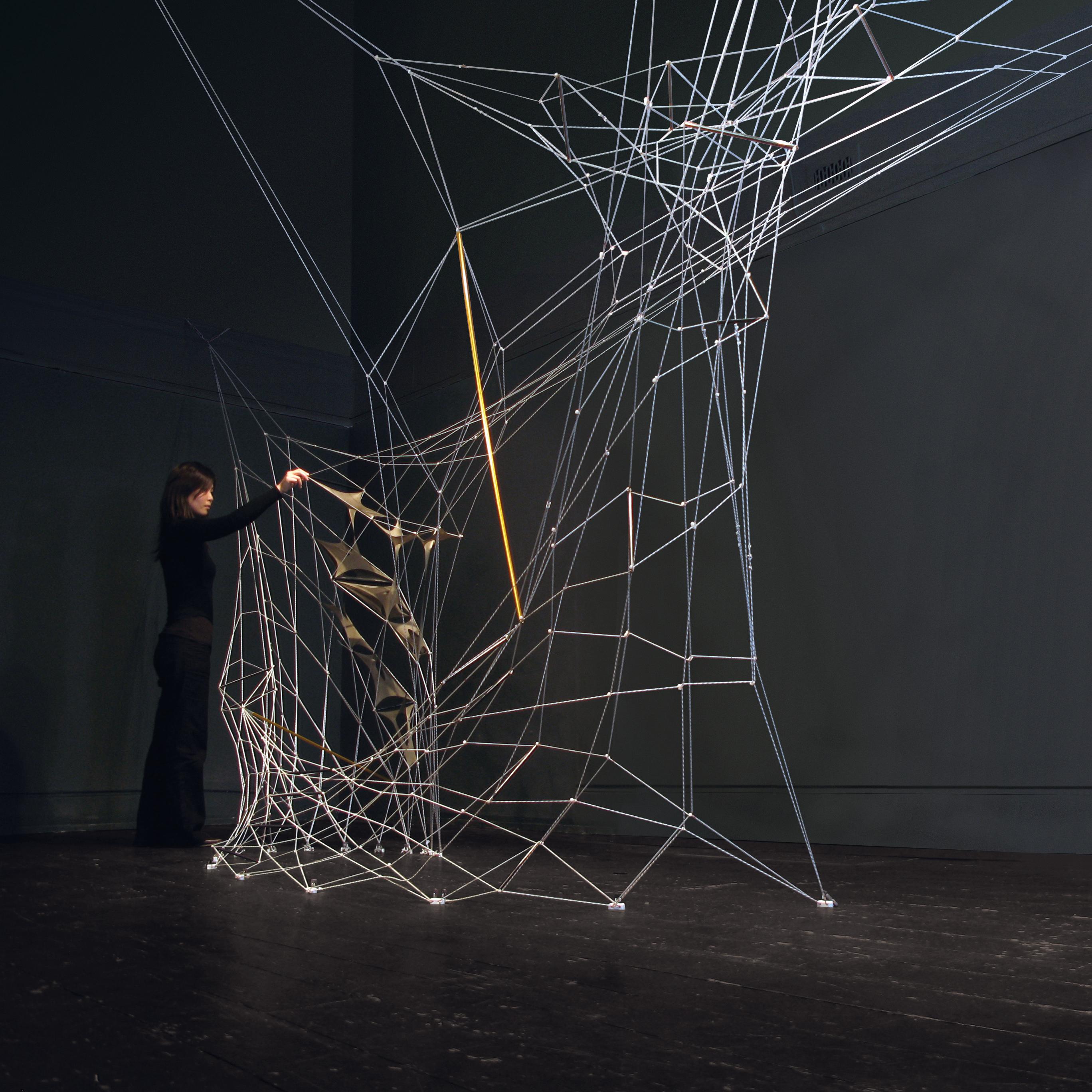
Tension active systems are compelling architectural structures having an intimate connection between structural performance and the arrangement of material. The direct flow of structural forces through the material makes these systems attractive and unique from an aesthetic point of view, but they are a challenge to develop from a design and an engineering perspective. Traditional methods for solving such structural systems rely on both analog modeling techniques and the use of highly advanced engineering software. The complexity and laborious nature of both processes presents a challenge for iterating through design variations. To experiment with the space-making capabilities of tension active systems, it is necessary to design methods that can actively couple the digital simulation with the analog methods for building the physical structure. What we propose is a designer-authored process that digitally simulates the behaviors of tension active systems using simple geometric components related to material and structural performance, activated and varied through elemental techniques of scripting. The logics for manufacturing and assembly are to be embedded in the digital generation of form. The intention is to transform what is a highly engineered system into an architectural system where investigation is as much about the determination of space and environment as it is about the arrangement of structure and material.
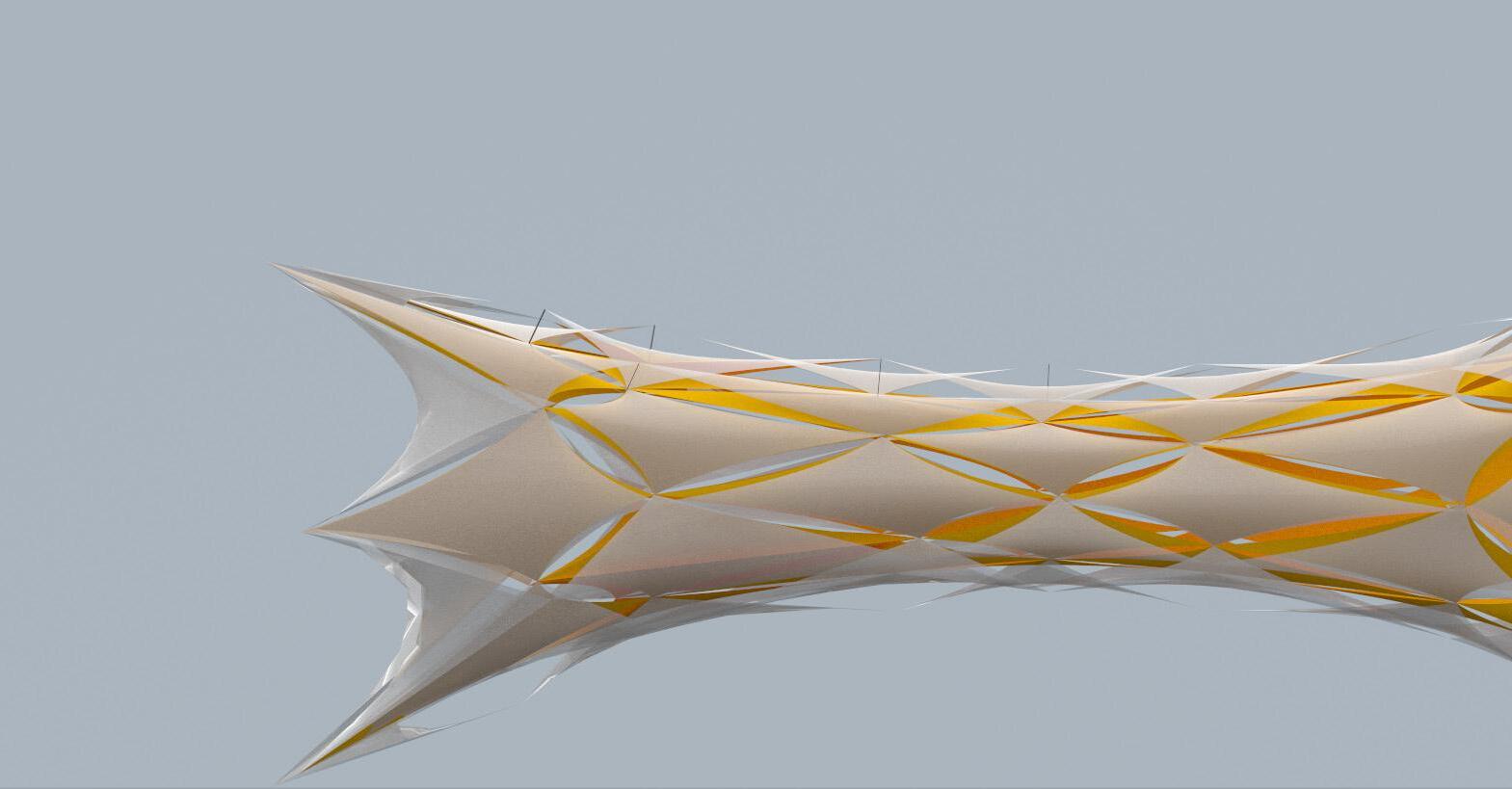
1 Computationally form-found structure. Branched, volumetric structure formed with 4 topologically cylindrical net components.
1 PRECEDENTS & PRIMARY RESEARCH
1.1 Precedents
1.1.1 Physical Form-Finding
1.1.2 Computational Form-Finding Engineering-Based Software for Form-Finding Software Using Spring-Based Solvers
1.1.3 Articulation of Computational Form through Fate Map
1.1.4 Cable Nets as Space-Making Devices
1.2 Computational Networks
1.2.1 Network and Geometric Topology
1.2.2 Spring-Based Particles Systems
1.2.3 Springs in Processing Hooke’s Law
1.2.4 Cylindrical Net Topology
1.1 Precedents
A common method for digital design generation is to separate the shaping of form from the application of a structural strategy. While this process allows for freedom in form and space experimentation, it often leads to problems when coordinating a structural system with the forms that have been established. In comparison, with tension active systems the overall form and position of materials are driven directly by the flow of forces through the system. This presents a certain degree of efficiency in the relation of material to structure and enclosure of space. The lightness of these structures in relation to the amount of force that they can withstand is attractive. It presents an opportunity to directly link design generation with the material and structural strategy. But, the complexity of this type of structural system poses a challenge for the architects, particularly those who wish to explore non-standard spatial and material organizations.
1.1-1
Computational spring-based model built in Processing, describing the elements of a kinetic structure and whether they are acting in tension or compression. Simulation by Sam Joyce, Bath University of the Heatherwick Studio Rolling Bridge project.
Defining architecture in a digital environment is a matter of manipulating geometries. Geometries without structural or material constraints have a vast solution space. The first step for narrowing the solution space is in defining the most basic geometric element and charging it with properties (constraints) based on physical behavior. The next step is addressing the network by establishing a solver for the behavior of the whole system (aggregation of geometric units). In the case of simulating cable nets, a simple digital element that can simulate flow of forces is a computational spring which follows Hooke’s Law of elasticity. This is represented by a simple unit of geometry (a line), yet dynamic and extensible in that it can be realized as an element under tension force or compression force, with direct implications into material definition. Solving the network happens through the method of dynamic relaxation, iterative steps for finding the balance of force flow through the system.
To fold this into a system for iterative design and structural behavior simulation, there has to be variability and accessibility within the system. The mathematics and programming for computational spring systems and dynamic relaxation are advanced, but their processing load is quite light. The number of variables for a single spring is limited but can be connected to material properties such as elasticity. The organization of a network of springs, though, is completely flexible and independent of the individual spring properties. Accessing variables of individual springs
and defining the protocol for connectivity of the network are straightforward and done through basic scripting.
This mode of realizing extensibility through simple material units and techniques for transformation fits with the process of biological growth. Examining these methods aid in understanding the need for simple design mechanisms to generate high degrees of variation and specification in form. Activating all of the options for spring parameters and network association provides for vast arrays of forms, each of which are structurally valid. But, considering this tool as a system for exploration, validity could be expanded to consider forces of arrangement, function, atmosphere, and other spatial characteristics. These particular traits would be realized through a well-managed catalog of elements and variables.
1.1.1 Physical Form-Finding
The study of cable net structures falls into the more general category of form-finding, structural systems where material and structure have very strong interdependencies. Form-finding, in contemporary methods, is done through two sets of procedures: physical simulation with scale models, and digital simulation through advanced engineering software. These two modes are often not directly related, and both, independently have impedances to a quick, iterative design-oriented process. The resolution and optimization of material to structure is often the singular mode of
intention for both of these processes.
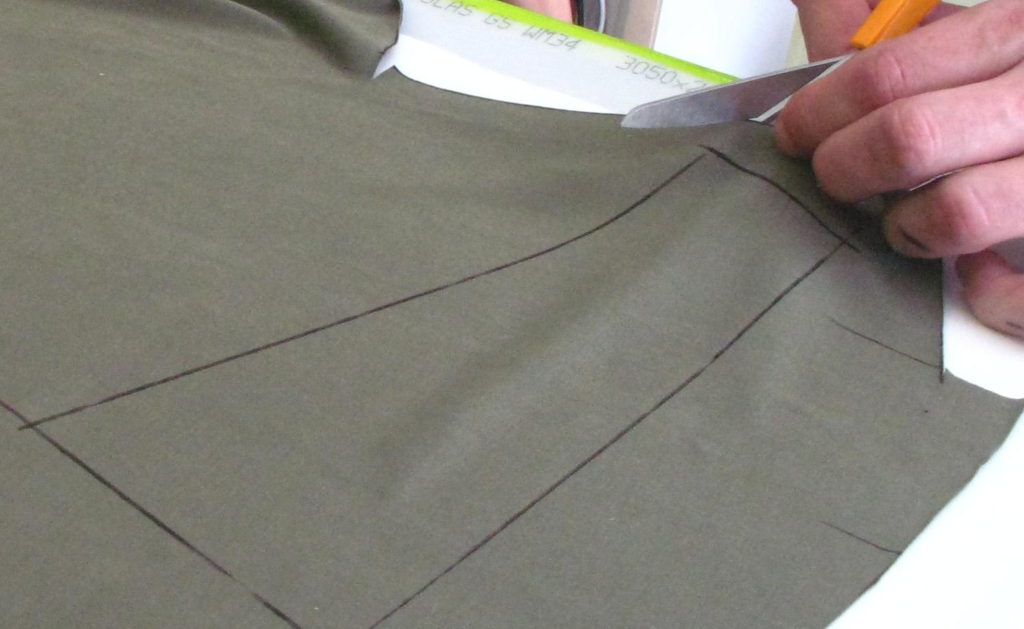
Physical modeling as the method for designing with form-finding structures is done at a particular scale where there can be a connection between the materials in the scale model and the materials to be used in construction. This often means models are built at a scale as close to 1:1 as possible. Where the flow of force is dependent on the properties of the material, “scaling” the performance of the model to full-scale means there has to be a link in material make-up between the different scales. There is a translational process not only in size but in material properties, structure, and performance of the overall system. This transition if often not easily accomplished. Factors of material and structure can scale at different rates when moving up in size.
To study the analog model, understanding the transitions in scale, means an almost scientific examination of its behavior, purely within the scope of structural performance and how the materials can withstand those forces. This knowledge and method is outside of the realm of the architect as a designer. To understand the behavior of the system, the entire system has to be constructed. This is embedded in the nature of structures based on form-finding. Structure and material are interdependent; therefore all material parts play a role in the shaping of form. Where the architect wants to investigate various possibilities of the effects of the structure on physical environment and its influences on inhabitation, changes to parts of the system
are inevitably necessary. This means a cost in the physical adjustment of the scale models, and the re-analysis of the relation of material and structure for the entire system. Iterative design changes are a challenge in this mode of design investigation. When basing process and analysis on physical modeling methods, the transition to information for construction is cumbersome as well. It means another layer of incredibly precise examination to determine dimensions for material and methods of assembly.
1.1-2
Tension-active
1.1-3
Proposal
1.1-4
1.1.2 Computational Form-Finding
The process of developing form-found tensionactive structures is highly technical and exhaustive. The primary methods are through either analogue modelling and analysis techniques or in specialised engineering software. The breadth of knowledge necessary to utilise these methods and their highly prescriptive nature are impediments to a design process investigating variation in form of this structural type and its potential for non-standard spatial and environmental conditions. The development of computational spring algorithms has provided an avenue for efficient studies of tension active structures. Accomplished through a programming language such as Processing, the design environment is also accessible and variable. Tracking through examples of spring systems generating hybrid tension/compression structures, a design process can be formed with elemental means of geometry and programming, making possible iterative investigations of complex tension-active systems.
Engineering-Based Software
Digital simulation alleviates some of the issues around translation in terms of physical forces and information for construction. But, the accessibility of these programs, such as Forten 3000, from a design point of view is limited, and the use does still demand expertise in the structuring of tensile systems. RhinoMembrane, by TSI, is a plug-in for Rhino that simulates tensile membrane
structures, and attempts at bridging the gap between design and engineering for tension-active systems. In testing the software, though, there is still a limitation to design investigation. Because of the demanding setup and the prescription of certain elements to their part in the form-finding process, defining edge cables and pre-stress for instance, being able to control and vary the system is difficult. Also, this works with a “black box” algorithm meaning the computation and mathematics at play are not being fully exposed to the designer therefore not utilized in the design investigation process. These engineering-based software packages and plug-ins do not offer a light or low-resolution analysis within the architects grasp to provide intuition in form-making that can later be fully examined.
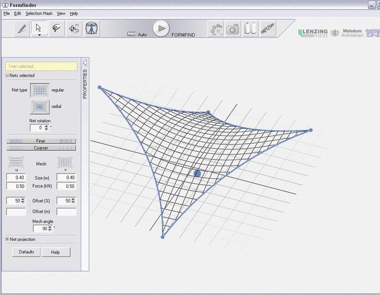
Relatively new packages have emerged that are oriented towards architects, where it is considered that the architect is more interested in design than technical specification and analytical feedback. To provide design accessibility, though, these softwares have to minimize the range of geometric options, while still demanding a specification of elements during the setup of the design. For the Formfinder software, the base geometric components to start with either a “regular” or “radial” mesh description. These particularly topologies will have limits to the type of geometries that can be produced. The software also only deals with “open” surfaces (sheets). The Rhino Membrane plug-in does allow a large range of meshes as the initial input. The geometries are
“relaxed” based on rules for defining a surface with equilibrium tension. But, the relxation solver highly depends on the specification of the “edges” of the membrane. The edges define where the rest of the geometry will relax towards. What this means is that the definition of the edge gives a strong indication of what the general position of the relaxed geometry will be. It minimizes the concept of form-finding, and leaves design to the configuration of the edges and the strength to which the hold the shape when tension forces run through the geometry. This is a challenging parameter to control when there is no understanding of the exchange between initial shape, edge definition, and relaxed geometry.
1.1-6
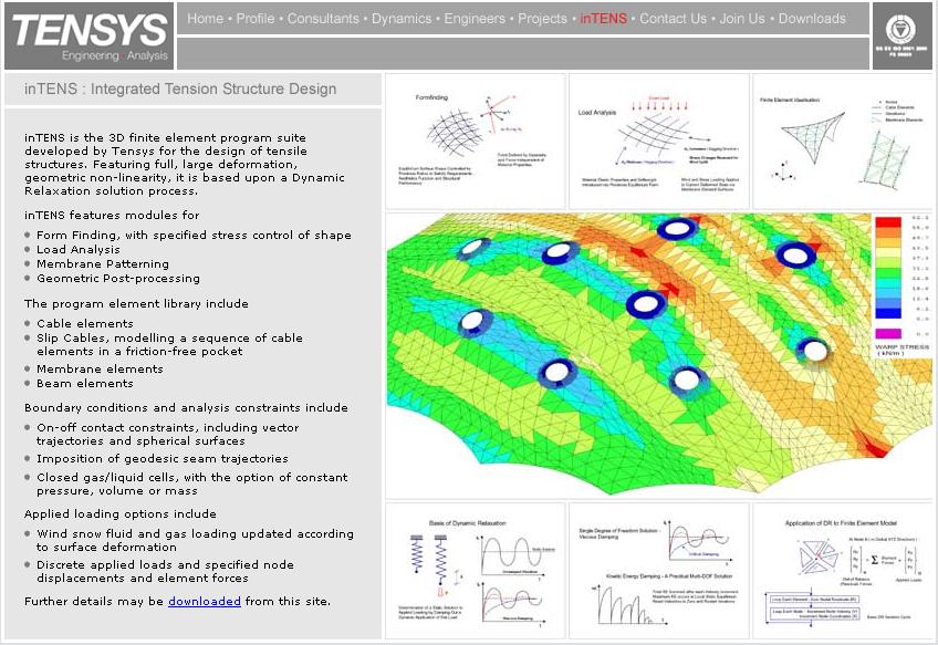
inTens software by Tensys. Finite element analysis is integrated in the program for creating tensionactive structures.
1.1-7
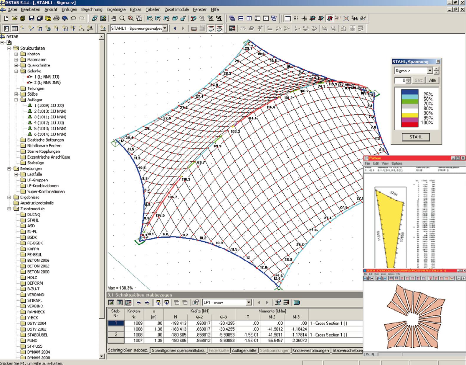
RSTAB software connected to Easy membrane design software, by Dlubal. Together, the software packages can produce models, provide analysis, and produce data for fabrication.
1.1-8 Formfinder software. The software is defined as a sketching tool of membrane design for architects.
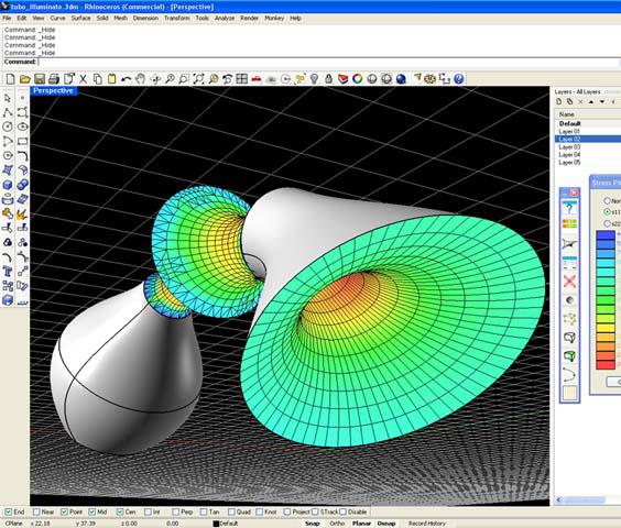
1.1-9 Rhino Membrane plug-in by TSI for Rhino3d. Finite element analysis is included in this plug-in that relaxes any mesh to a stressed (tension) surface.
Software Using Spring-Based Solvers
Various experiments in developing digital algorithms mimicking form-finding methods have led to the creation of an efficient computational method for simulating tension-active systems based on springs. In 2004, Prof. Ochsendorf and Simon Greenwold, through a workshop at MIT, conducted digital form-finding experiments based on Gaudi’s analog form-finding experiments with catenaries. One product of this workshop was an algorithm built for the Processing language based on the physics of springs. Axel Kilian, as a part of his PhD research at MIT, utilized this algorithm to digitally form-find linear catenaries. He extended the application to solve for tensile surfaces by using a network of springs. Springs are a part of a computational physics model where their force, generally, is connected to the distance at which the two ends of the spring sit apart from each other. Hooke’s Law specifies the amount of force through the degree of difference between a spring’s actual length and its rest length. A spring-based computational system serves as an efficient solver for tension-active systems. The particular system by Greenwold is placed within the programming environment of Processing (a Java based language) allowing it be lightweight, flexible, and openly accessible.
Spring systems become effective design experimentation tools when they are computationally efficient and openly accessible. Visually, responsiveness is necessary to understand the relation-
ship between the outcomes emerging from the process and the input parameters. Accessibility is necessary from a programming standpoint, so that the algorithms necessary to run the system can be developed and controlled by the designers themselves. A design system developed by Soda shows how a complex structure can be understood and refined visually through interactive engagement and immediate feedback. Sodaconstructor is a web-based construction kit for spring systems, developed through an interest in dynamic systems where behaviour could arise through the feedback between the user and the computational rules of the system.1 What emerges is an understanding of how particles and springs interact in the context of gravity and movement. What this poses for a design paradigm is that spring systems can be very lightweight computationally allowing for configurations to be developed, varied and reconfigured while structural forces are solved instantaneously.
Connecting the dynamic nature of spring systems and the affects of mapping particular associations of springs is expressed in a model that describes the Rolling Bridge by Heatherwick Studio. By configuring the truss network with springs, the simulation, written in Processing, is able to describe tension and compression forces, and the switching in between. The experiment seeks to understand the physical behaviour of the constructed bridge through the conceptual nature of the computationally based spring system. This offers interesting possibilities in describing valid structures through a computational component that has specific
structural properties but not absolute material properties.
The simulation of the Rolling Bridge offers a different approach from the Sodaplay website in that it is not interface driven. Both are based on computational springs, but the Rolling Bridge simulation is defined and controlled within the script. For the designer of the script, it offered the best option for establishing the structural concept (computational springs with a dynamic relaxation solver), testing it through a very specific concept and understanding all the inter-relationships between parameters.
1.1-10
CarefulSlug by Soda from Sodaplay. com. Web environment allows for the construction of tensioncompression structures that undergo influence of gravity and friction. Underlying solver is based on computational springs developed in Java.
1.1-11
Structure developed in SW3D (sw3d. net). Using the Sodaconstructor library, SW3d, created by Marcello Falco, expands the functionality into three dimensions creating an environment where kinetic structures can be interactively generated and edited.
1.1-12
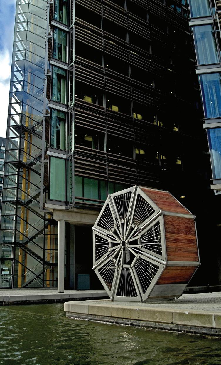
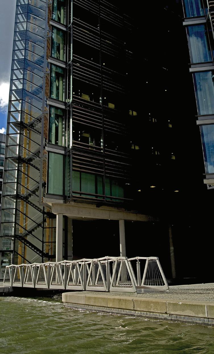
Heatherwick Studio, Rolling Bridge, Paddington Basin, London, 2004. The kinetic steel-framed bridge transforms through the hydraulic expansion and contraction of various struts in the truss-like structure.

1.1-13
Sam Joyce, Rolling Bridge simulation, School of Architecture and Civil Engineering, University of Bath, 2008. The program simulates the physical behaviour of the Rolling Bridge, comparing the abstracted physics of the spring system with the actual performance in the bridge
1.1-14
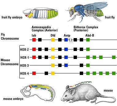
Description of the shared homebox genes between a fruit fly and a mouse.
1.1-15
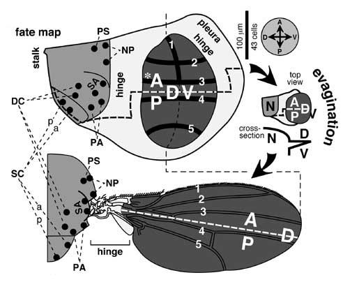
Fate map for the development of the fruit fly wing. Diagram A depicts the layout of genes. Diagram B shows the related morphological development.
1.1-16
Initial layout of particles with double-array ordering system.
1.1-17
Fate map describes the specification of geometry (springs) and association (various connection types between particles).
1.1-18
Morphological description of fate map described in Figure 1.16.
1.1-19
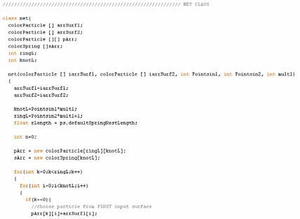
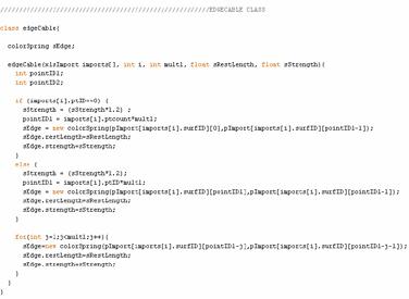
Samples of the toolkit (scripted functions in Processing) which develop and specify form. Most functions simply address the ordering system in various waysassociating particles within a single network of springs and/or across two networks of springs. Additional variables such as spring-strength provide for further specification and adaptation of form.
precedents
1.1.3 Articulation of Computational Form through Fate Map
1.1.3 Articulation of Computational Form through Fate Map
Michael Hensel hypothesizes about a computational process “extending the concept of the material system by embedding material characteristics, geometric behavior, manufacturing constraints and assembly logics.”1 This is the goal of a computational design process for cable net structures. An examination of the field of evolutionary biological development offers models for how integration of a high number of components and functions can be realized through simple, repetitive means.
Evolutionary Developmental Biology explains growth and development through the following: modularity, repetition, switching, and geography.2 The interconnection of these is what gives the process its robustness and extensibility. The functioning of the homeobox presents clear processes for how variation can be generated with the same set of tools.
Moving through the stages of development, the challenge is how to track and control variation from the initial setup through to the final form. Abstracting processes described in evolutionary developmental biology provide the logic for proceeding through the steps of geometric form development. In defining the base geometric unit, extensibility is primary. Embryological development works with several primary materials to realise multiple structural types (both tension and compression systems). Instead of prescrib-
ing multiple context-independent components, a single unit should be able to develop into various material types.
The fate map, a representation technique for tracking cell development, is a helpful concept in managing form specification in complex systems. The control of articulation can only be gained when the initial setup can be connected to the final form. In the spring-based system, the network arrangement is akin to the fate map, the particle being equivalent to the cell. A logical ordering system for the components of the map allows for easy determination of where particular articulations in form occur, in what contexts, and which transformation functions are applied.
1 Hensel, M and Menges, A, Inclusive
Performance: Efficiency versus Effectiveness, Versatility and Vicissitude: Performance in MorphoEcological Design, 2008, Volume 78 No 2, 54-63.
2 Carroll, S, Endless Forms Most Beautiful: The new Science of Evo-Devo and the Making of the Animal Kingdom. London, Orion Books Ltd, Phoenix, 2007.
1_precedents
Architects have the ability to alter our perception of a space (environment) through the use of physical material.
Often the relation between the geometry and the material is not immediate. Especially in the current state of fabrication a lot of materials are “standardized”. Not only in performance, but also dimension, geometry and size. Shape and material property are highly determined by industry standards and fabrication methods. These are treated as an additional layer. Sometimes this choice is based on certain material characteristics (transparency etc.) or a specific performance criteria (high isolation, high strength etc.). In rare cases does the material choice feed back into the actual geometry a significant degree. “Structural Analysis” operates as a re-dimensioning process (widen beam, thicken floor plate, re-dimension column) altering a very limited set of input parameters (thickness, width etc.) of the initial, individual element. The agglomeration of these elements make up the “architecture”. A current trend is the design of Information systems that help managing the vast amount of elements (BIM), but the process becomes very elaborate and problem of detached geometry and structure remain. This ultimately leads to a very limited way in which we, as architects, allow ourselves to manipulate an individual’s perception of a certain space.
Tensioned nets are one example of a basic material system. Their shape is determined, by the forces acting upon the whole structure and each element
used within the net contributes to this behavior. The physical process in which a net takes shape under the application of external forces is usually referred to as form finding.
Not only is this process interesting for architects to look at, because of the fact that the resulting form / net geometry has a certain degree of validity or inherent truth, which other models that are not based on form finding methods lack.
A fascinating aspect of these design investigation systems is the amount of inputs needed to re-define the shape of the model. Moving one anchor point of a net to another location in space can have significant repercussions on the form. This means, that the architect / designer can actually explore different shapes, of the same validity (regarding the distribution of physical forces) with very little effort. At least in a model.
But the model has to be able to account for these alterations intended by the designer. A certain material’s elasticity might prevent one from exploring a certain configuration of anchor point locations. The only intervention left for the designer in this case (besides disregarding the idea) is to either change material (with more elasticity) or add material. Both options result in the rebuilding of the net (model), which is a time-consuming procedure. Something that we experienced during our first form finding investigations of tensionactive nets during EmTech’s core studio in the fall of 2008.
Without being specialists in the construction and
dimensioning of nets we were able to observe during this important period of time of our studies, that all nets have certain similarities. Their tendency to take shape into what would mathematically be described as a minimal surface was particularly interesting, as this was a property inherent to the material system, but never “intended” by us, the designers.
It was our interest to expose the drivers / actuators for these common properties amongst nets and membranes in order to explore net configurations that would expand the vocabulary of spatial perception of these architectures thus far.
In order to use nets as space-making devices we focused on net topologies that are not very common and rarely used for projects at an architectural scale. Usually architects and engineers investigate the use of planar net topologies. These nets are, by nature, “flat”. Their inherent capability to circumscribe a space is limited. These planar nets have multiple boundaries (equivalent to “sides” of a polygon in geometry) and are mostly used to define form-active roof structures - which is logical, if the underlying topology is understood.
By “closing” the net in 1 dimension, or in simpler terms, by transforming the planar topology into a cylindrical one, the boundary conditions are reduced to only 2. Furthermore a directional of the net is generated that was previously not present. Whereas the planar nets (objects) allow the spectator (subject) to define his position in relation to the object (“I am under / above the net”), the cylindri-
cal net topology generates spatial conditions that can be described as being “inside” of the net. This new characteristic led to a search for ways of emphasizing or alleviating degrees of enclosure enforced by a cylindrical tension active net system.
In order to pursue this exploration of spatial effects of cylindrical nets on their environment it was necessary to develop a digital form finding method. Embedded into this method needed to be information about structure, performance and characteristic of each element augmenting the system. Implementing a method for accessing all data for fabrication was necessary, as our intention as architects was not to develop hypothetical computational mesh geometries, but actual physical architecture manifested through a digital method of form finding.
A lightweight vector-based analysis tool simulating the perception of a net’s density from different points of views was developed. By measuring degrees of enclosure of cylindrical nets this analysis tool aims at a computational method for defining a net’s space-making capacities as well as its potential to serve as a protective shield against external forces (simulated through vectors) such as sun, rain or wind.
1.10
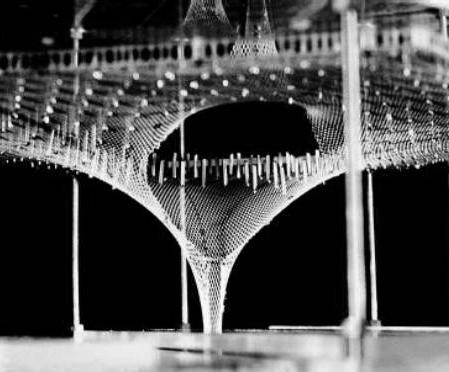
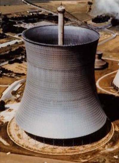
cable-net structure for a cooling tower for Balcke in Germany built in 1972. Consulting by Schlaich engineers. 142 meters in diameter, 181 meters pylon height.
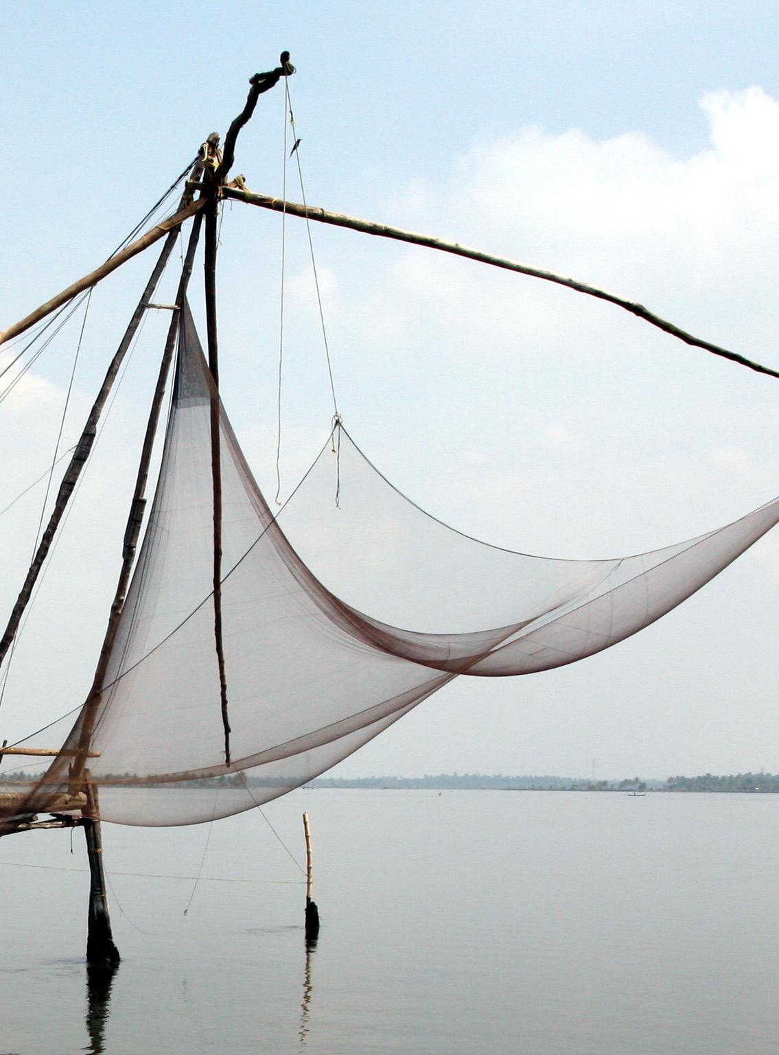
1.11 fishing net in China. an example of a net with a medium mesh size.
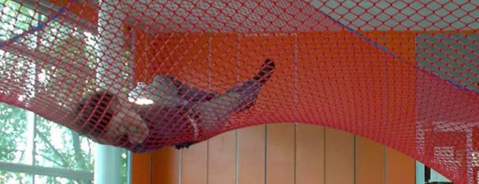
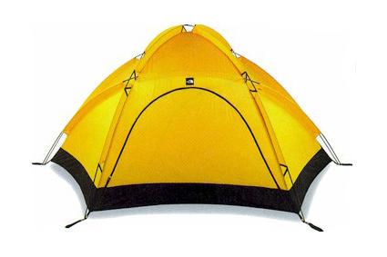
1.12 membranes can be considered very tight nets. As tension-active elements they are used for tents to protect against wind, rain and sun.
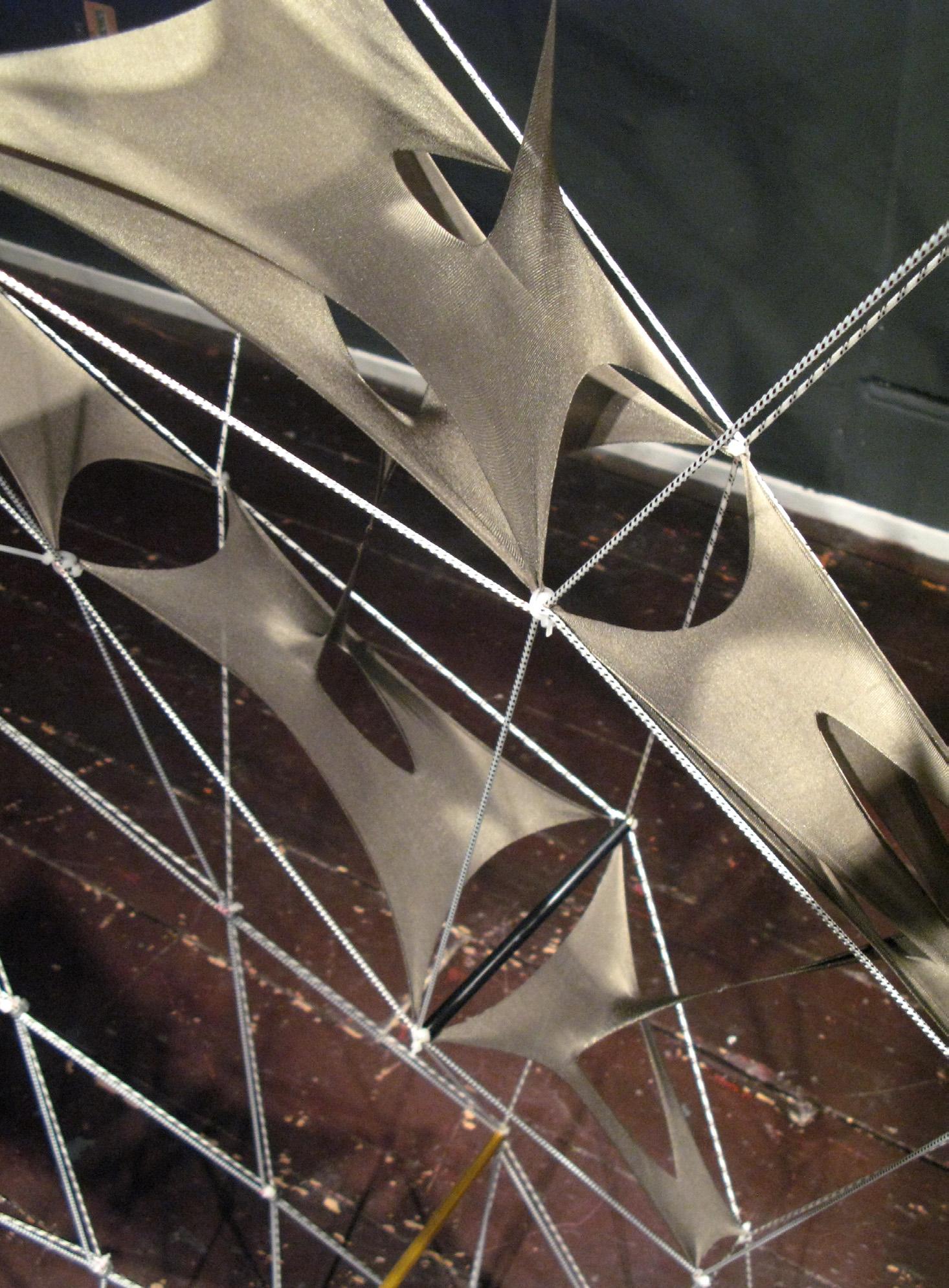
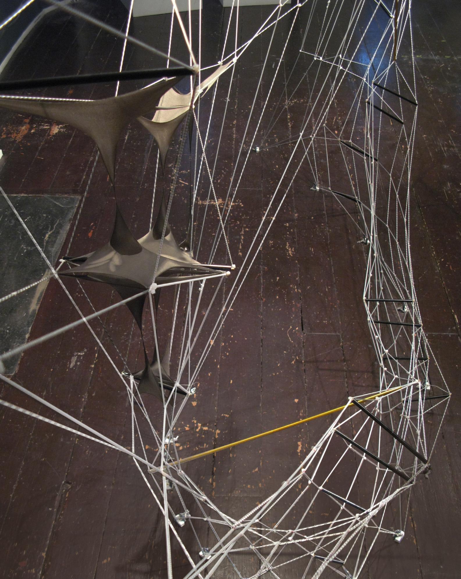
1.13
net installation at the Johann Wolfgang von Goethe University of Frankfurt by Hannes Schewertfeger. 90 squaremeter area.
A spring-based particle system simulates the tension and compression within a network of connected springs. The overall connectivity between the elements forms the net-topology. In order to simulate multiple net configurations quickly a method derived from the investigations in evo-devo was developed.
Every computational net is built through a logic map (2-dimensional array), which determines potential size & density of the net through its dimensions.
In processing Springs are inserted based on the logic map, that determines Particle-to-Particle relations, connectivity and the overall net topology.
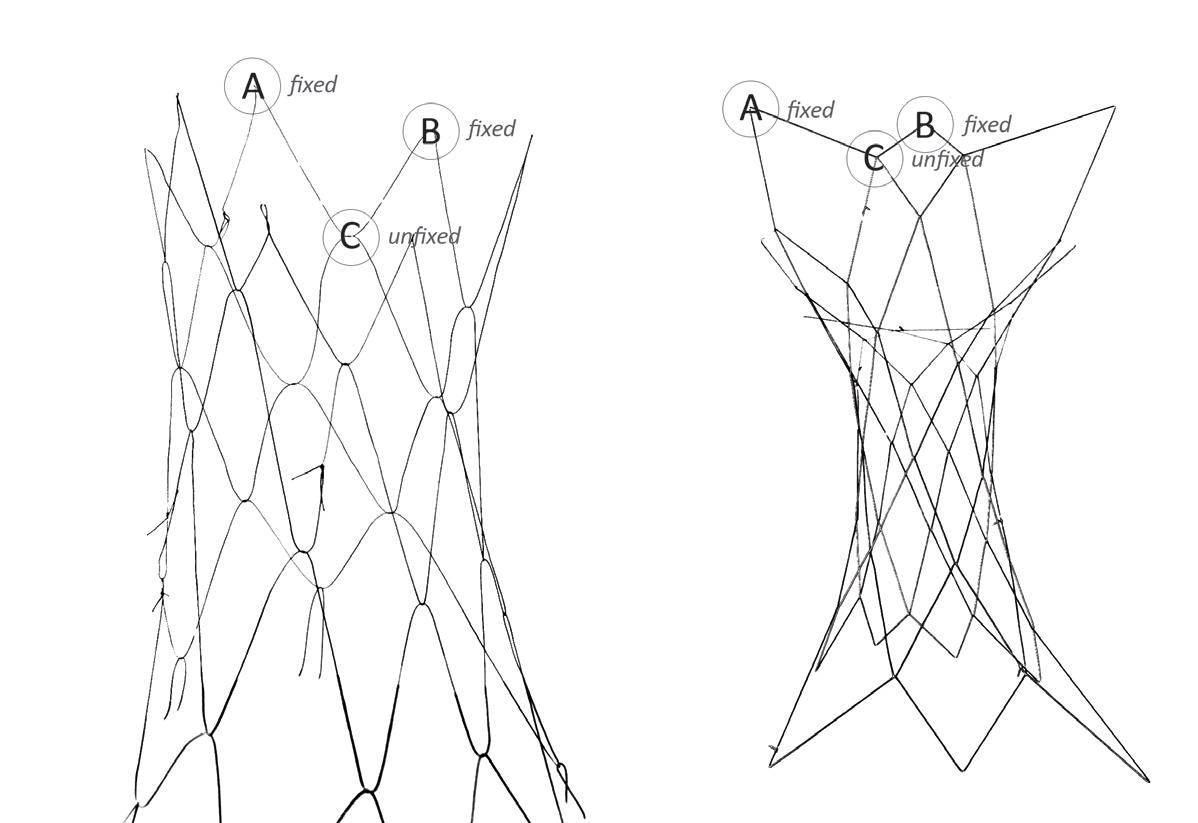
Switches are accessed to fix or unfix the boudaries of the nets. The combined use of these switches and the logic map allows to simultate multiple net variations easily and quickly, while the method of how they were constructed maintains absoluetly transparent and accessible (see chapter 2.1. embedded fabrication). In the process of dynamic relaxation the predetermined network topology takes shape through the simulation of the forces within the system.
1.2.1. Network and Geometric Topology
The mapping of nodes describing pathways for communication and data transfer is the basic definition of network topology, where nodes are considered as devices constituting a computer network.
Examples of base network topologies are shown in Figure 1.2-2. This is a useful description for how a particular pattern (or a systematic hybrid of multiple patterns) for the association of nodes can be constructed to form an interconnected continuous network. It is also important to clarify that network topology does not consider position. It refers only to the strategy for arrangement of the devices that are engaged in the network environment. This explains the difference between a logical topology (of associations) and physical geometry (of position).
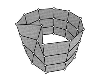
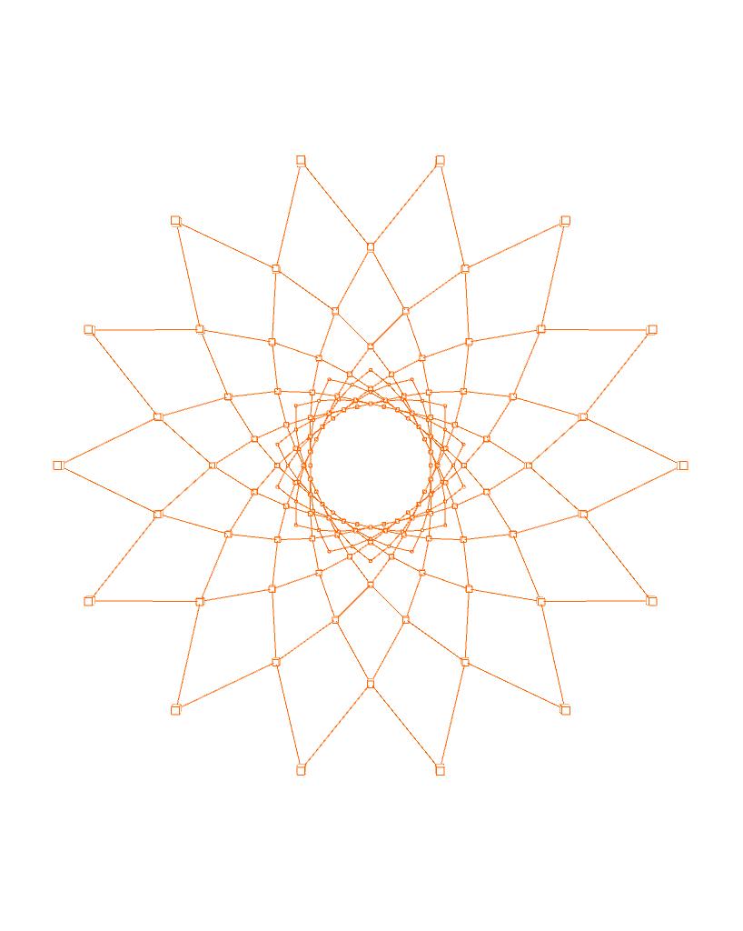
Geometric topologies have limits to the types of geometries that they can construct. The repercussions are examined here both in terms of geometry performance and in connection to its potential for the definition of the boundaries of architectural space. In the cable net experiment, selecting the logic akin to the “ring” topology, when transformed into 3 dimensions, means for a continuous surface that can define various degrees of bounded space.
The appropriateness of the “ring” topology is evident when compared to other network topology types. It makes sense that the “line” topology expands to an open surface defined by 4 edges, where the “ring” topology easily transforms to a 1-dimensional continuous surface, bounded by 2 edges. (Figure 1.2-4) It would seem that forming space through a series of open surfaces involves more effort, physically and computationally. Surfaces are either transformed to define a continuous boundary (with subsequent geometric issues as mentioned earlier) or coupled with multiple surfaces to eventually have a clear delineation of space. The other topologies, cylindrical and torus based, more quickly and clearly begin to define the boundaries and orientation of a particular space (Figure 1.2-4), and all with a single strategy.
1.2.2 Spring-Based Particle Systems
Particle systems are simple physics models that only deal with point-masses and forces. That means that - as opposed to rigid-body models - objects in particle systems do not occupy any volume. Their behaviour is quite simple, but powerful. (Figure 1.2-8)
Particles
A particle is an object with a location and a mass. It is acted upon by any number of forces. The greater a particle’s mass, the more is required to accelerate it.
A particle’s location in space is determined by the forces acting on it, unless the particle’s position is declared as “fixed”. This boolean value indicates whether a particle’s position is being controlled manually or by the forces in the system. A fixed particle can be attached to a single point in space, or the mouse, or may be moved simply by (re-) setting its position. Often a whole system of particles will be attached to a single fixed particle and will move with it. In order to be a solvable system from a structual point of view the particle system needs to contain fixed particles. Springs Springs are forces that exist between 2 particles. The force enacted by the spring pulls or pushes the 2 particles together or apart with a force proportional to the distance of their separation. A spring’s performance is defined by the variables of rest length, spring strength, and damping.
Rest length is considered to be the length of a spring at which it no longer pulls or pushes. The strength of a spring determines how hard it pulls / pushes when it is stretched / compressed. The amount of Damping controls the energy absorbed by the spring as it bounces (dynamic relaxation) Damping is necessary in order to prevent the spring from oscillating for too long.
Hooke’s Law
Hooke’s Law is a solver for the forces in computational springs. It determines the forces on two particles connected by a spring. If the spring’s current length during the process of dynamic relaxation is greater than its Rest length then the force of the spring acts to pull the two particles together. If the spring length is less than the rest length, then the force acts to repel the two particles. Both of these forces act along the vector defined by the two particles. The force on a particle “a” due to particle “b” is given by:
Where ks is the spring’s strength, kd is the damping constant and r is the Rest length.
To solve the accumulation of vector forces such as in a network of interconnected springs, the RK Solver or Euler Solver is typically used.
1.2.3 Springs in Processing
For the “Form-Finding and Structural Optimization: Gaudi Workshop” at the MIT in 2004 conducted by Prof. Ochsendorf, Simon Greenwold developed a Particle System written in the Processing - a Java-based computer programming language
This programming language, which is available for free download at www.processing.org, has gained a high degree of popularity far beyind the initially targeted community of artists. The software is used by engineers (for example: Chris Williams) and by
architects at workshops like Smart Geometry. Axel Killian, who took part in MIT’s workshop, provided the particle system library for processing and helped in getting started with the first particle systems.
When using the Particle System, the initial setup is developed through the creation of an array of particles. Each particle carries values for mass and position, where force can acts to negotiate the particle’s final position. Force, in this case, comes from a linear network of springs. The position of a particle can be calculated through the simple equation of force (f) = mass*acceleration, where f is the vector sum of all forces.
The step of enacting external forces and resolving the internal flow of forces drives the final positioning of the particles. With the spring system, this happens through the combination of the spring solver and the resulting computational process of dynamic relaxation. Dynamic relaxation is the current standard for realizing the equilibrium state of tension active systems through iterative steps of vector oscillation. It is important to see the distinction between the physical topology defined through dynamic relaxation and the user-defined network topology defined through the 2-dimensional array of particles: the logic map.
Network Topologies
Examples of logical network topologies depicting various patterns for connecting network devices. Logical topology describes association not spatial position.
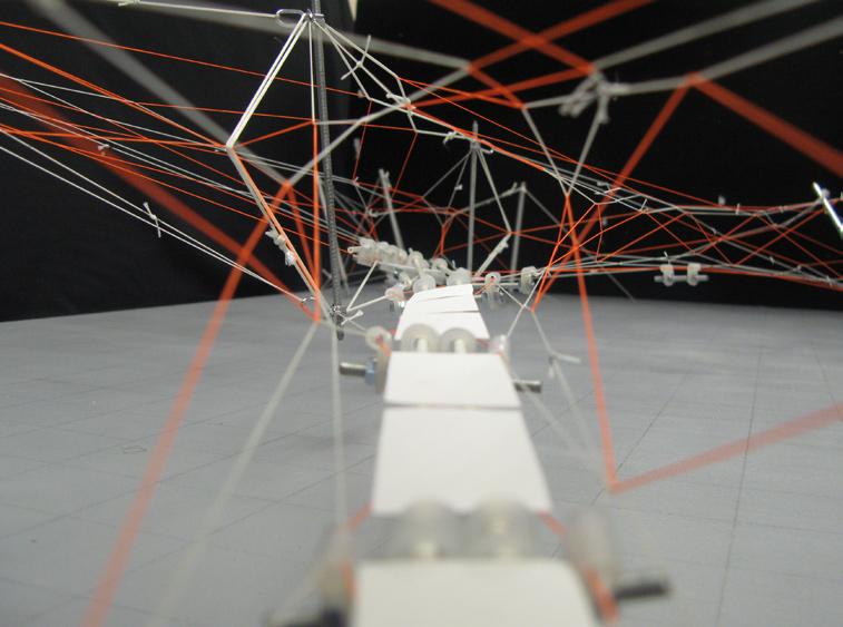
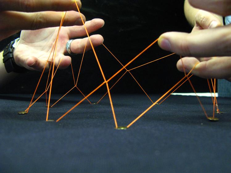
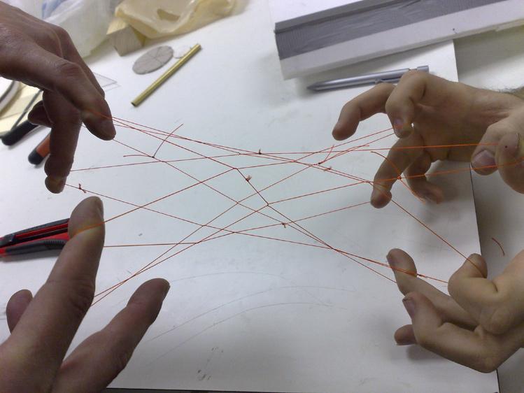
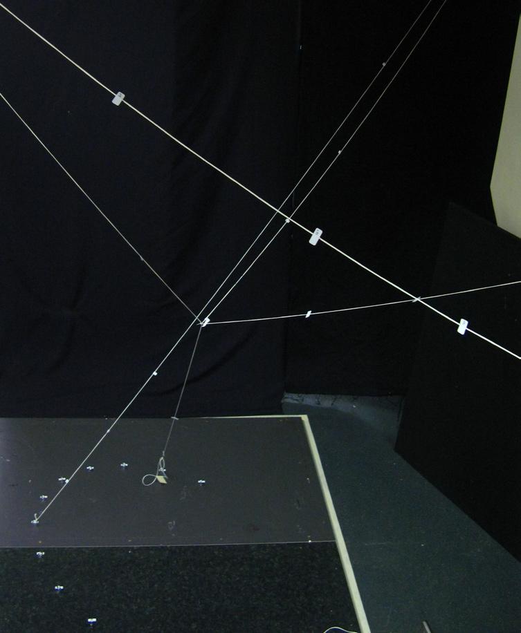
1.2-3 various physical prototypes of cylindrical nets were built. The development of a spatial network topology is shown through a series of physical modeling experiments with tensioned net structures. With the intention of forming a system that when translated into its physical topology arranges surface, structure, and space, this model is an example of a typical “formfinding” process. The interesting aspect is in the link between the inherent geometric logic of the initial loop, as a closed “ring” (bottom left), and the spatial form constructed when activated into a physical topology (top middle). This connection between material and space in the most rudimentary components of the design system is a primary necessity in the design process that solves for integrated conditions of surface, space, and structure.

1.2-4
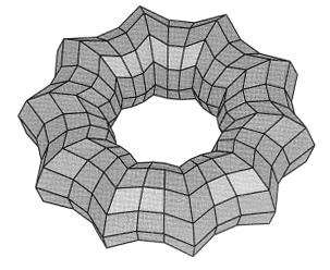
Geometric Topologies by increasing in topological dimensionality (curves have 1-dimension, usually described by the parameter “t”, surfaces are 2-dimensional, UV-space) of a network of nodes as shown on the vertical axis, different geometries can be formed. By closing their open ends, respectively edges, higher degrees of enclosure can be achieved. In 3-dimensional geometry the sphere / torus have the highest degree of enclosure. Based on experiments with cylindrical nets, a topology that introduces directionality and a certain degree of enclosure to the planar topology by very simple means (closing 1 edge) was chosen as a component for the construction of different net morphologies.
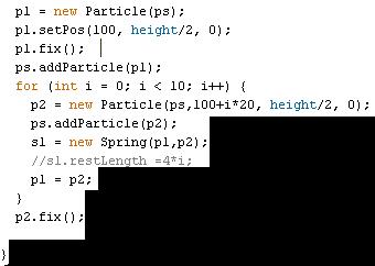
1.2-5 programming a computational chain through the linear connection of multiple (10) particles in a singular (1D) “for”-loop a chain between particles is formed. By inserting computational springs between the particles, the behavior of a physical chain can be simulated (in real-time). One end of the chain (p2) is fixed to a specific location in Cartesian Space whereas the other end of the chain is controlled via a particle that is directly connected to the user’s mouse position (ScreenX, ScreenY). The visual result of this small script displayed here is shown in
1.2-8
Computational Chain Model

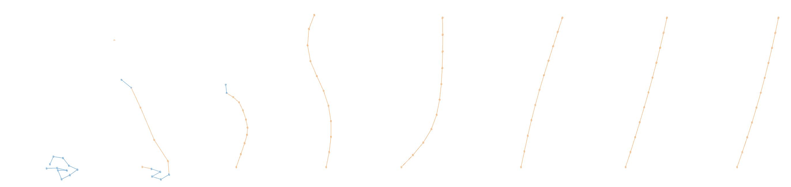
Dynamic Relaxation of Spring system in Processing. A linear network of springs connects 10 particles. The last particle’s position in the chain, is controlled via the position of the user’s mouse in the processing interface (dashed circle). The first particle is fixed (orange circle). Dynamic Relaxation resolves system to equilibrium state of forces. The system is able to track which spring is in tension (blue) or compression (orange) within the system. With increasing distance between the fixed particles, the springs increase their tension force.
1.2-9
particle system diagram besides rest Length, a spring has 2 other parameters: strength and damping. Particles, the other important part of a Particle system besides forces, can be fixed to a specific location in space (XYZ), but in computationally simulated nets, most particles negotiate their position through the forces acting upon them. In order to simulate the behavior of tension-active systems, only Particles and Springs are necessary - even though a Particle System consists of more parameters. Boolean values equal “switches” of a “fate map” in biological models in function.
particle system
F
1.2-7
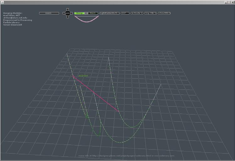
CADENARY software
A software programmed and developed by Axel Killian at the MIT during a workshop for digital formfinding experiments based on Gaudi’s hanging chain models. The software was written in processing and utilizes Simon Greenwold’s particle System written for this workshop. The software focusses on real-time user interaction through an interface for the digital simulation of linear and planar networks of hanging chains. It can be downloaded and explorer at www.designexplorer.net/
1.2-10
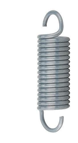
Hooke’s Law
a law in physics which calculates the forces within a spring.
The 2 most important stages in which an active spring can be observed, are shown in this diagram: tension and compression. If a spring is stretched beyond its rest Length, it will act as a tension element (top / orange). If the spring is forced into a length below its rest Length, it acts as an compression element. The mass of the particles connected to each end of the spring cause it to oscillate past its rest Length until a final position / length is determined with regards to all other forces in the network (computational form finding).
1.2-11 logic map
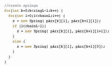
The logic map is a 2-dimensional array in processing. 2-dimensional arrays are a very common programming device and can be seen as simple ordering systems. Technically they are most efficiently generated through the use of a double “for-loop” in the script, where the outer “for”-loop determines the “height” of the logic map (even though it is a nongeometric , topological map) and the inner “for”-loop controls the width” of the logic map. The logic map can be used for multiple purposes and the method of generating it is common to all the experiments undertaken as a part of the research - not only in this chapter, but throughout the entire dissertation.
In this basic example, the logic map is used to create particles and assign them a unique ID based on their location on the logic map (top diagram). Furthermore, the map is used to determine which particles are fixed particles (middle diagram - orange particles are fixed). In this case, Particles at the bottom (i=0) and top (i=4) of the logic map are, through a simple “IF”-statement, declared as “fixed” parts of the net. In a third and last step, springs are inserted into the logic map. The method in which particles are connected via springs needs to be determined once and is then automatically repeated throughout the net (like most things with a “for”-loop). The particles a at the sides of the 2-dimensional array, were connected back to the beginning in order to build a cylindrical as opposed to planar net. Computationally , all these events take place in 1 double “for”-loop.
A 2-dimensional cylinder is difficult to draw (1.2-11 - bottom) and can be easier understood as a 3-dimensional geometry (see next figure).
1.2-12
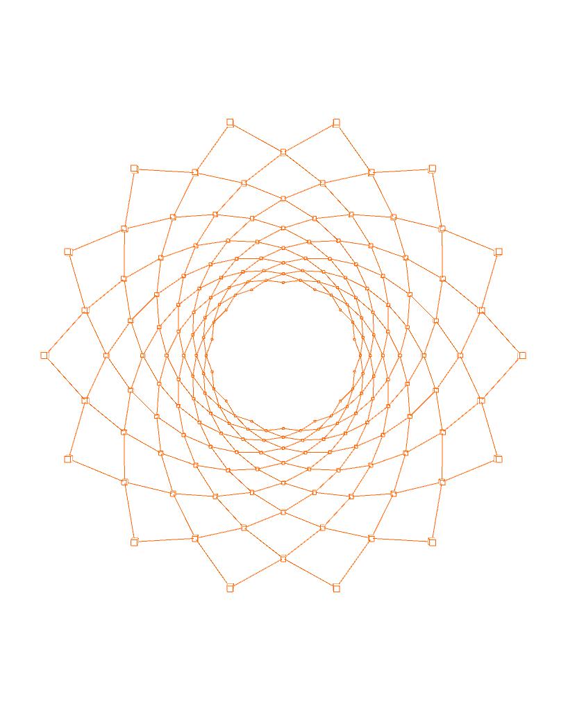
Shows the geometrical output of the combined inputs of the logic map in diagram 1.2-11 . The additional information as opposed to the logic map is, that every particle has been assigned to a specific XYZ-location in space. At this point it could be anywhere, but for purposes of readability we created a “cylindrical mesh”. Highlighted is the edge condition of the logic map
1.2-13 topological symbols are used to identify the underlying topology of a cylindrical net geometry, because it becomes more and more difficult to identify the inherent topology of a net, once the process of dynamic relaxation has started. In this case, all the characteristics of the net (size, connectivity, edge connectivity) built through the logic map in 1.211 are maintained
particles & ID
particles & ID
Spatial Networks
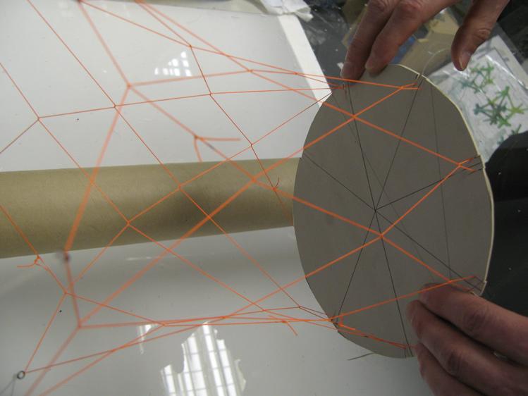
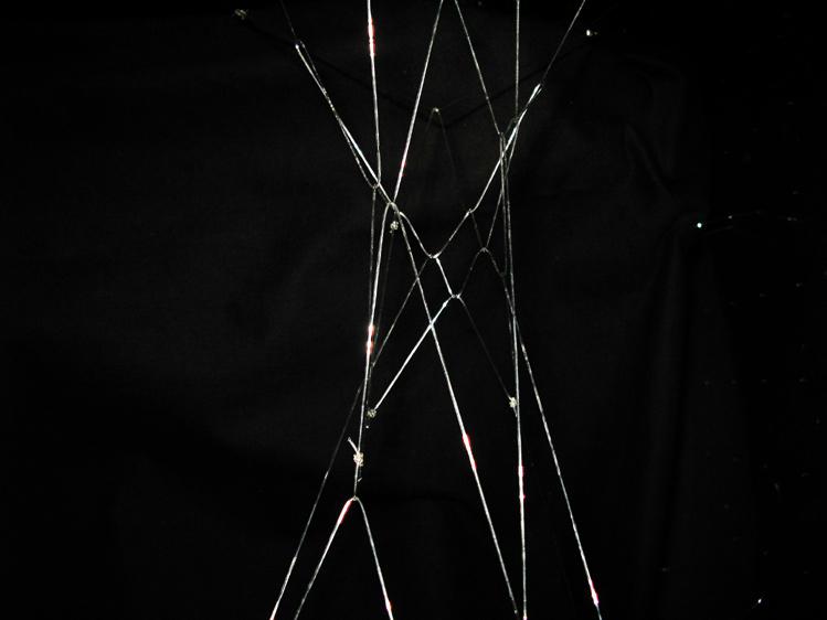
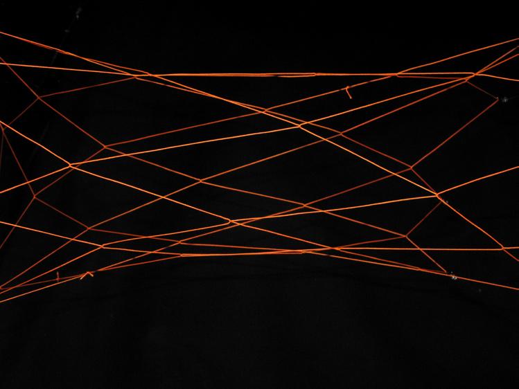
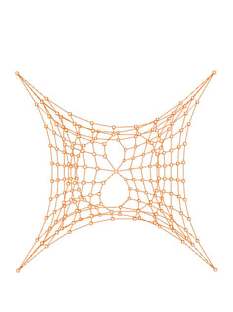
This initial experiment is based on physical experiments undertaken with cylindrical nets. A cylindrical network topology has a certain potential for enclosing and orienting space where the geometric units that construct the network have a direct correlation with a material strategy. The development of a spatial network topology is shown through a series of physical modeling experiments with tensioned net structures (figure 1.2-16) , preceding the design of the Cable Net Installation in the next chapter. With the intention of forming a system that when translated into its physical topology arranges surface, structure, and space, the “ring” network topology is translated into a 3-dimensional network. In figure 1.2-16, the system is defined by 5 closed loops, where each loop is 30 cm in perimeter and each pair of loops are interwined 5 times. This experiment delineates clearly the translation from a simple network topology into a physical topology. The loop dimension and number of “intertwinings” describes the variables for the system. This model is an example of a typical “form-finding” process. But, the interesting aspect is in the link between the inherent geometric logic of the initial loop, as a closed “ring”, and the spatial form constructed when activated into a physical topology.This connection between material and space in the most rudimentary components of the design system is a primary necessity in the design process that solves for integrated conditions of surface, space, and structure.
1.2-16
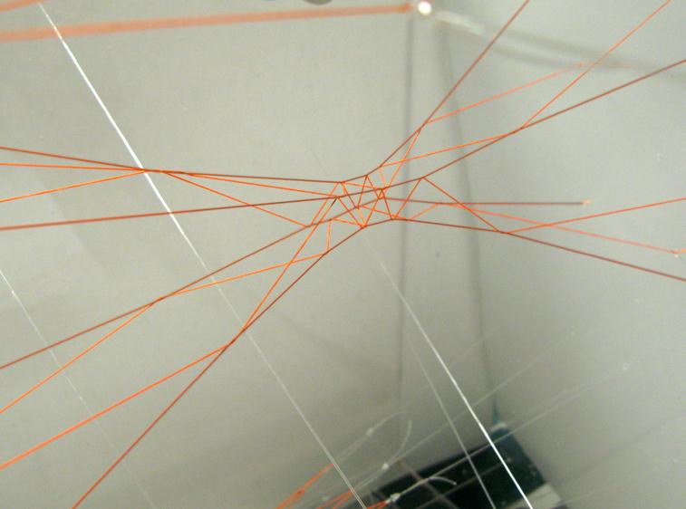
formfinding cylindrical nets

In this physical experiment, the Initial network topology is transformed into a tensioned net structure.When tension is added, the location of the nodes is determined and also descriptive of the flow of forces through the entire array of loops. Computationally-based Spatial Networks
1.2-14
net geometry
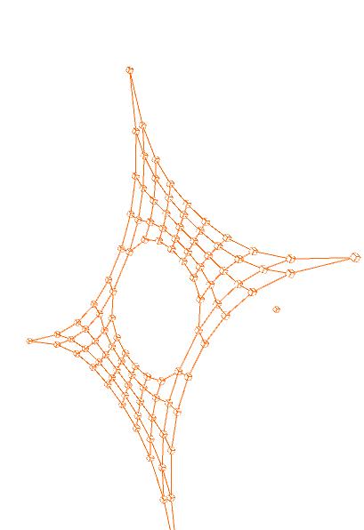
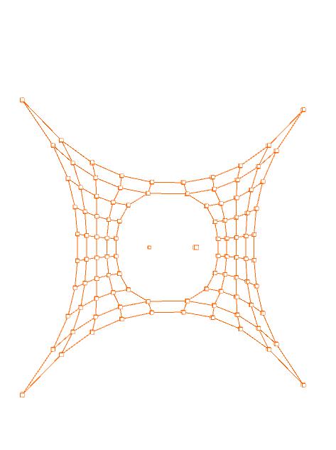
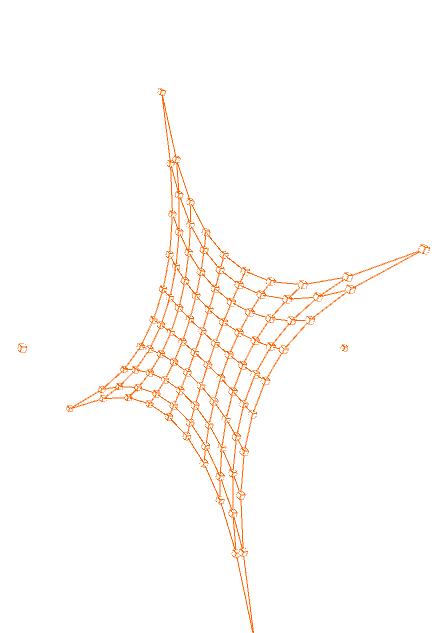
the depicted cylinder uses a larger logic map, but maintains all characteristics desribed previously. The image shown is comparable to 1.2-12, with the significant difference, that the lines draw in 1.2-12 for diagrammatic reasons are now substituted by actual, computational springs. The images shows the cylindrical net at frame 0 of the dynamic relaxation process from the out- and inside.
1.2-15
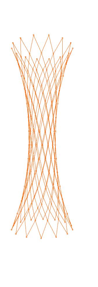
net morphology at frame 1000 the springs have shaped the net into its final form. Geometry is altered / Form is found. Both through the application of forces implied by springs, that shape the now tension-active system.
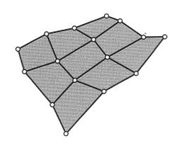
1.2-17 logic map for planar net
Through a simple alteration of the logic map, a different type of net can be simulated. In this case a planar net with 4 fixed particles at its corners and a slightly different way of building the network of springs through particle associations (bottom): The springs are now running from left to right and top to bottom (of the map). This has repercussions on the behavior of the net, which, if simulated with a high density (in this case “9”) resembles that of a membrane. The chosen network is more closely related to the Weft and Warp of a membrane (different structural behavior in different directions, because of weaving manufacturing process).
1.2.4 Cylindrical Net Toplogy
These first sets of experiments were conducted in order to intially understand how computational springs are effective solvers for the simulation of physical forces. Beyond that. the main interest was that of connecting these simple elements into larger networks to simulate the behaviour of physical, cylindrical nets. By utilizing a two-dimensional array of particles as a logic map for building the topological network of springs, a simple underlying method was achieved. This model could be accessed at later stages of the design of cylindrical nets (see chapter 2.1.”embedded fabrication”).
Understanding how the topological associations between particles, through the connectivity defined in the logic map, affect the overall geometry in the process of dynamic relaxation to simulate the behaviour of physical nets made the rebuilding of physical prototypes for every new investigation redundant.
Spatial Networks
These first physical experiments use a cylindrical network topology. The nets resulting from these topological conditions have a certain potential for enclosing and orienting space where the geometric units that construct the network have a direct correlation with a material strategy
The development of a spatial network topology is shown through a series of physical modeling
experiments with tensioned net structures, preceding the design of the Cable Net Installation. With the intention of forming a system that when translated into its physical topology arranges surface, structure, and space, the “ring” is translated into a 3-dimensional, cylindrical network. This model is an example of a typical “form-finding” process. The interesting aspect is in the link between the inherent geometric logic of the initial loop, as a closed “ring”, and the spatial form constructed when activated into a physical topology.This connection between material and space in the most rudimentary components of the design system is a primary necessity in the process that solves for integrated conditions of surface, space, and structure.
Computationally-based Spatial Networks
Other types of systems can be engaged working with the same directness, responding to inputs of space, material and structure. Considering fabric (membrane) materials as a part of the cylindrical net morphologies provides for further definition and articulation of space, while also working reflexively with the structure of the system.
It is through these types of tools and the understanding of their underlying logics through which we intend to realize architectures of multiple, specific, and interrelated concerns of material and space.
Surfaces, Boundaries, and Continuity
In the Cable Net Installationshown in the next chapter, the main characteristic of architectural space is one of continuity. Continuity, as we choose to further characterize it, is that of a series of spaces that are both interconnected yet distinct described by the most minimal means of material and structure.
The purpose for these initial experiments is the establishment of parameters in the computational system (the geometric topology, the springs, the material, the structure, and the fabrication) that allow a simulation of physical behaviour of cylindrical nets.
This is achieved by validating the computationally generated (logic map) nets through comparisons to physical prototypes. Valdation is not achieved through the simulation of highly specific (structural) conditions, but through the observation and modelling of the behaviour of these tension active systems.
Once the capabilities are understood, the computational process can be expanded to test and evolve relationships that include these more specific characteristics of space. It could be argued that in the design possibilities of this type of material system, examination in built form is necessary to evolve the method, the pressures on the system, and the outcome.
1.2-18 membrane component
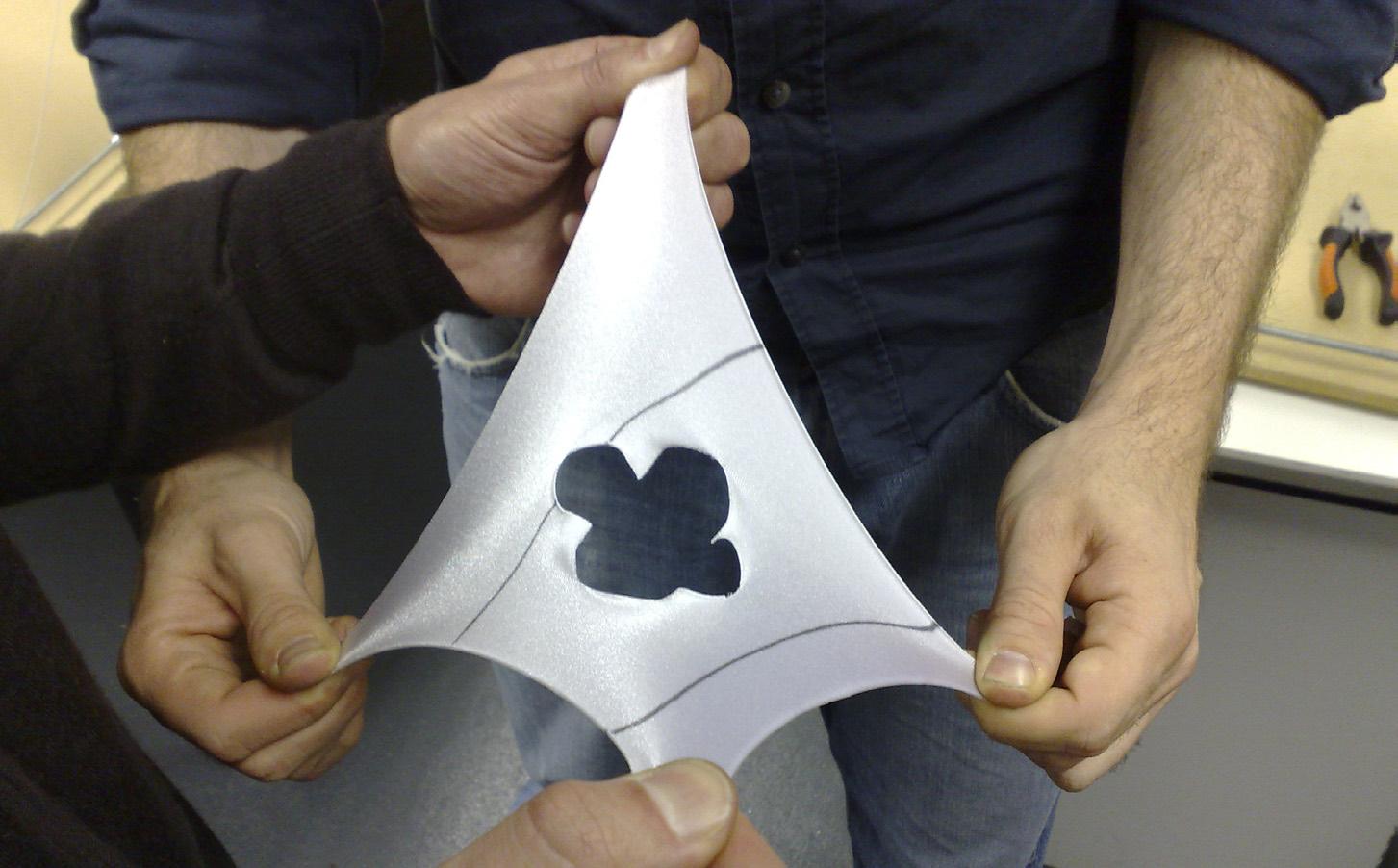
Based on physical experiments with membranes a component consisting of 2 minimal-hole membranes rotated by 180 degrees was developed. The comprehension of the mechanisms at work led to the development of a similar computational net component.
1.2-19 computational planar net (type1, type 2 & type6) by accessing the logic map, a catalogue of 6 different palar net components was developed. Even though never used, these elements show the potential of understanding the logic map as a device for building, accessing and altering net geomentries.
1.2-20 logic map of type 6 by deleting / not generating particles in specific locations, interesting spacial conditions, such as minimal holes can be achieved / articulated.
1.2-21 meta nets understanding the potential for the articulation of space through the use of different net topologies is a important challenge for the designer. Shown is a cylindrical meta-net, with planar components, that feed back into the shape of the architecture.
2 EXPERIMENTS AND DEVELOPMENT
2.1 Embedded Fabrication
2.1.1 Cylindrical Transformations
2.1.2 Mapping of Computational Cylindrical Net
2.1.3 Data Mining for Fabrication through Node ID
2.1.4 Spatial Articulation of Net
2.1.5 Evaluating Cable Net Installation
2.2 Topologically Defined Net Components
2.2.1 Component Systems for Form-Found Structures
2.2.2 Subdivision Algorithm for Cellular Framework
2.2.3 Single Cell Net Parameters
2.2.4 Multiplication and Association of Net Components
2.3Threshold Conditions
2.3.1 Comparing Actual Density and Perceived Density
2.3.2 Computational Threshold Anaylsis
2.3.3 Extended Vector-Based Analyses
2.1 Embedded Fabrication
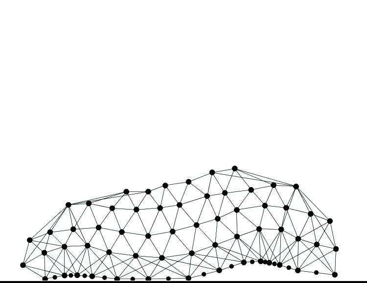
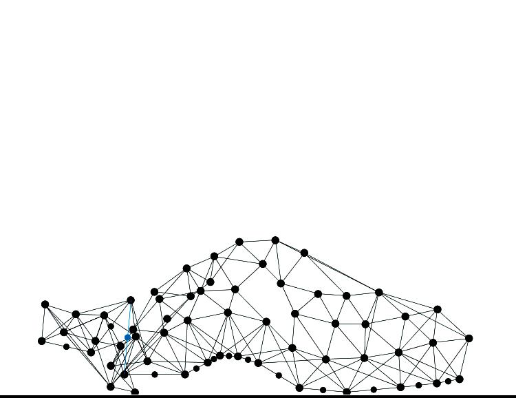
The Cylindrical Net Morphologies cable-net installation is an experiment in synthesizing processes of digital simulation and fabrication into a design system allowing for experimenting with associations between material arrangement and spatial effects.
Considering the computational system in a more direct application to architecture, the questions of material and assembly arise. The spring, once relaxed into a state of force equilibrium, has implications for the type of material that it may represent in the constructed form. Being in tension or compression has obvious influences on material specification. The fate map planning of the system provides the opportunity to link between initial setup, materiality and fabrication. In the Cylindrical Net Morphologies installation at the Architectural Association, the method of inscribing a logical identification system to the particles in the spring system allowed for ease in fabrication. Re-tracking through the network meant re-accessing the identification system through different looping protocols. The iterative for-loop mechanism was the fundamental programming method to accomplish this degree of control and production.
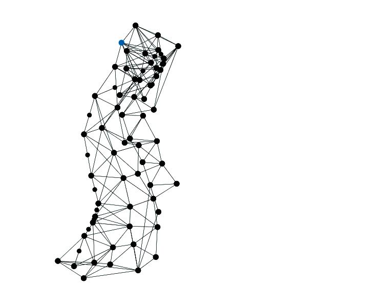
2.1-1
Computational model of form-found net with mapping of nodes and associations for use in fabrication
The Cylindrical Net Morphology is defined by the user-generated network topology consisting of computational springs where form is generated through finding an equilibrium of tension forces. The network topology is based on the 1D continuous surface (“ring” network) method of association. Embedded in this strategy is a comprehensible logic for manufacturing and assembly of any form that the system produces. Part of the potential for the network topology is to realize a specific architecture of multiple spaces defined by a single continuous boundary. Prior to all particles positions being realized, there is the opportunity to embed certain surface performance characteristics, beginning to narrow the solution space.
2.1.1 Cylindrical Transformations
The initial experiments focus on establishing the list of parameters available in the system using symmetry to test the process. Considering the context of the exhibition space, the symmetrical arrangement is transformed into an involuting cylinder through the variation of two basic functions. (Figure 9) The circular array of anchor points undergoes an anisotropic transformation into an elliptical array. It is then varied and tested to determine which end-nodes of the system attach to points along this elliptical array. This function drives the basic involution of the cylinder when an end-node from one end is transformed to the other end. The variable of switching nodes from being fixed (anchored in physical terms) to un-fixed is tested in various locations. This investigates the ranges of density in the resulting mesh and the number of anchor points to the existing exhibition space. Attachments points for the net are minimized in the ceiling and evenly distributed in the floor.
2.1.2 Mapping of Computational Cylindrical Net
One of the simplest components of the design system is the double array assignment identifying each particle. The double array is created through a simple nested for-loop. Each step of assembling (defining the network topology), refining, and extracting information from the particle array simply means re-accessing the double array. The identification for each node remains constant through every transformation of the form. The methodology (the for-loop) remains constant as does the data inserted into the for-loop (the double array values for each particle/node). The ability to address different issues and manipulate
form generation in various ways is simply through the shift in how the for-loops move through the double array. These varied methods are described in Figures 12 and 13. It is a quite sophisticated capability in controlling, localizing, and accurately locating transformation, but accomplished through simple for-loop mechanisms.
The ease of fabrication is in the direct relationship of the initial components of the computational system to the parts of the physically constructed form. The particle is the identifier of a node in space, the point at which the springs connect. The spring, in the relaxed model, defines a physical distance between the nodes. Fabrication is a matter of coordinating this information and qualifying it to the characteristics of the material being used for construction. This logic is universal in the system. No matter what the formal outcome is the method for sorting through the nodes/particles for fabrication is the same for each result.
2.1.3 Data Mining for Fabrication through Node ID
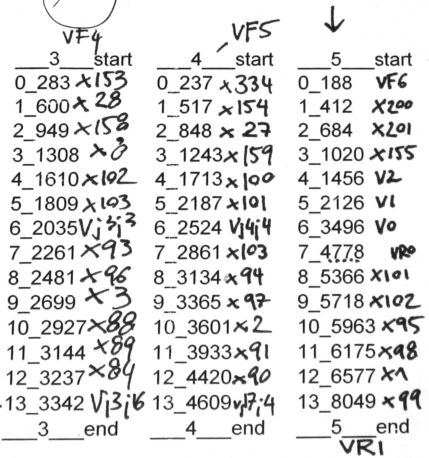
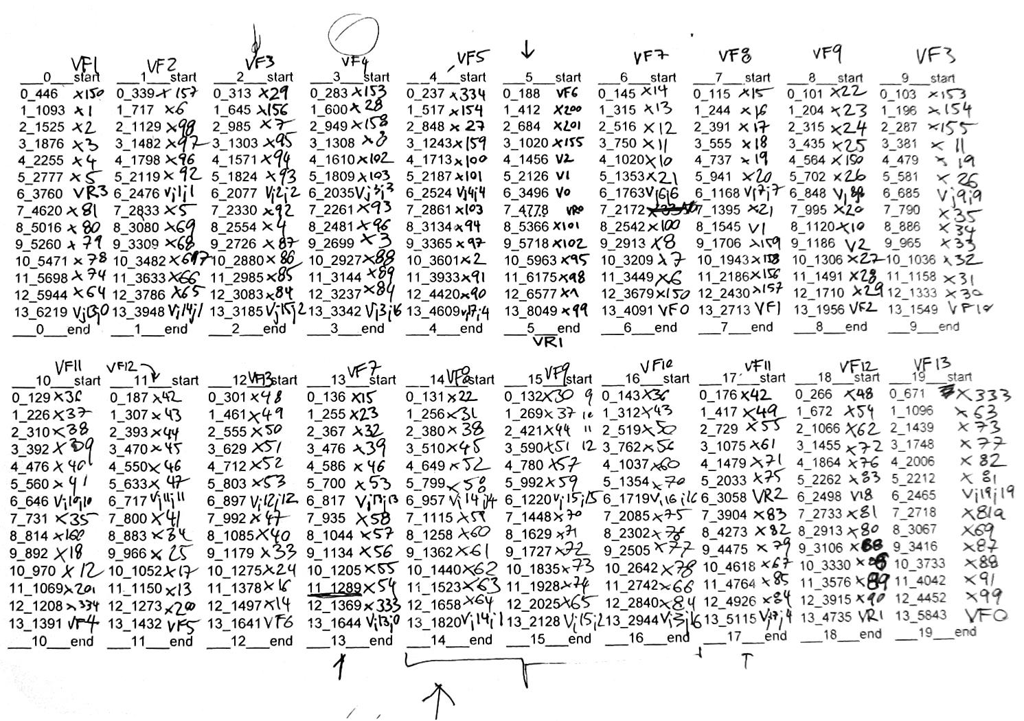
The node identification is the most valuable information of the entire system. This is generated in the very first step of the process, where each node is defined by a unique double array value. The next step is in understanding the sequence of connecting the nodes. Rather than translating one spring to one length of material (in this case, 2.5mm diameter string is used), an array of springs is connected (Figure 3.5) so each net is broken down into only 20 individual lengths of material. The connection sequence for nodes is shown in Figure 3.XX. For construction, tags are generated to locate the nodes along the lengths of line and indicate which lines connect at each particular node. (Figure 3.XX) This data is then further filtered to define the specific distances between nodes and the overall lengths of the lines for construction. In calculation, the stretch of the 2.5 mm diameter string is considered and the distances between nodes are adjusted to respect material as opposed to their finite locations in digital space.
2.1.4 Spatial Articulation of Net
The “ring” topology eludes to certain types of geometries, in a rudimentary way: the cylinder. The cylinder is of particular interest because it describes a boundary and a directionality. In a form-finding process, this spatial capability can
be taken further to investigate directionality while simultaneously arranging structure. This combination of organizing space simultaneously with structure is intended to carry into the articulation of the Cylindrical Net Morphology installation.
A membrane component which combines tensionactive surfaces with an internal compression element serves to articulate the flow of view and space between the 2 surfaces of the net installation (Figure 2.1-33). Using the net surfaces for anchor points of the component, it becomes a lower-hierarchy element within the whole system. Though, visually, it becomes more apparent and registers the space between the two nets more distinctly.
Compression elements exist in the computational model to push the surfaces of the net apart in certain regions. In construction, they also serve as a device for post-tensioning. Computationally, the compression element is a spring whose actual length is shorter than its defined rest length. The nature of the force, tension or compression, can only be realized in the dynamic relaxation process, when all the spring forces are acting against eachother. This introduces another scenario where situations of both structure and space are solved simultaneously in this computational form-finding process.
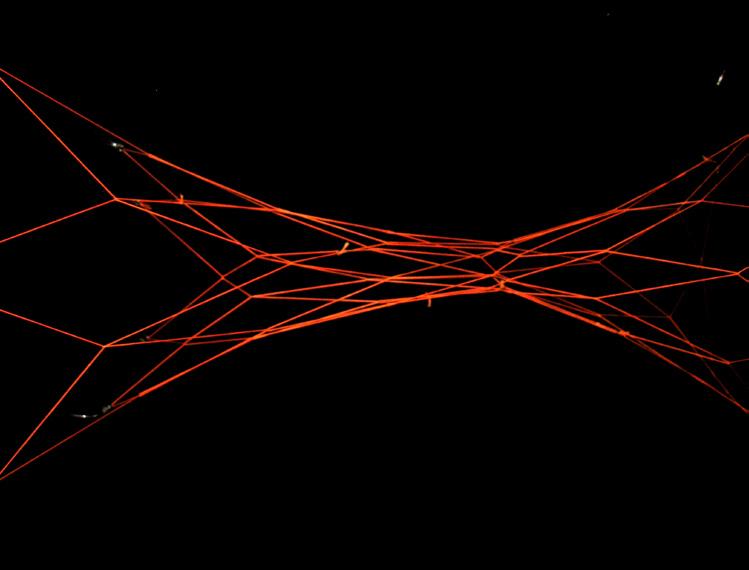
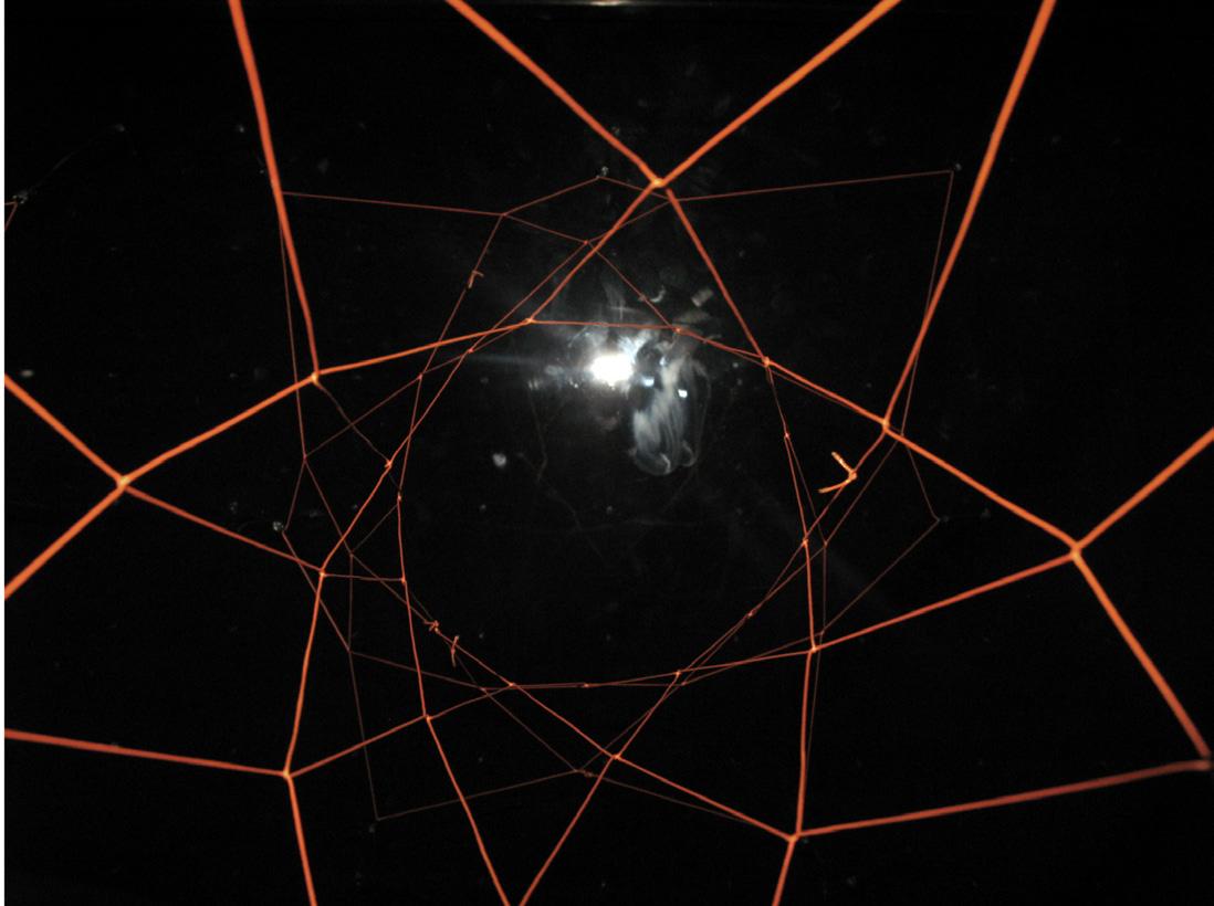
Cylindrical Net Morphologies
cable-net installation for AA
Project Review Exhibition, spring 2008. the tensioned net, compression elements and membrane components for this installation were developed through the computational spring system in Processing. a cylindrical network topology of springs was transformed to produce the complex physical arrangement. the installation was built in the Studio 2 space at Bedford Square, june 2008.
2.1-3 transformation from symmetry. the initial spring model is based on a pair of circular arrays of anchor points. to adapt to the studio space for the installation, the two sets of anchor points are scaled eccentrically.
2.1-4 the transformation to the final net arrangement for fabrication utilizes 3 variables. 1- the anchor points are scaled assymetrically, 2-various edge particles in the net are unfixed, and 3- one fixed particle is relocated from its native location along the bottom array of points to a location along the top array. the red line indicates the relocation of a fixed particle from it original location to that on the upper boundary.
2.1-5 initial design for experiment of translating digitally form-found model in Processing to physical construction. the design was extracted as linework from Processing into Rhino.
2.1-6 manual placement of node tags. nodes were identified in the digital model at the intersections between individual springs. the IDs were done manually, so there is no clear convention nor a specific pattern in the naming.
2.1-7 length measurements from Processing. the distances between particles (meaning the length of springs) was calculated digitally and compiled directly into an Excel spreadsheet. the lengths were compiled in a way to create continuous lengths of material. the translation was 14 individual computational springs = 1 length of string with individual lengths measured along that line.
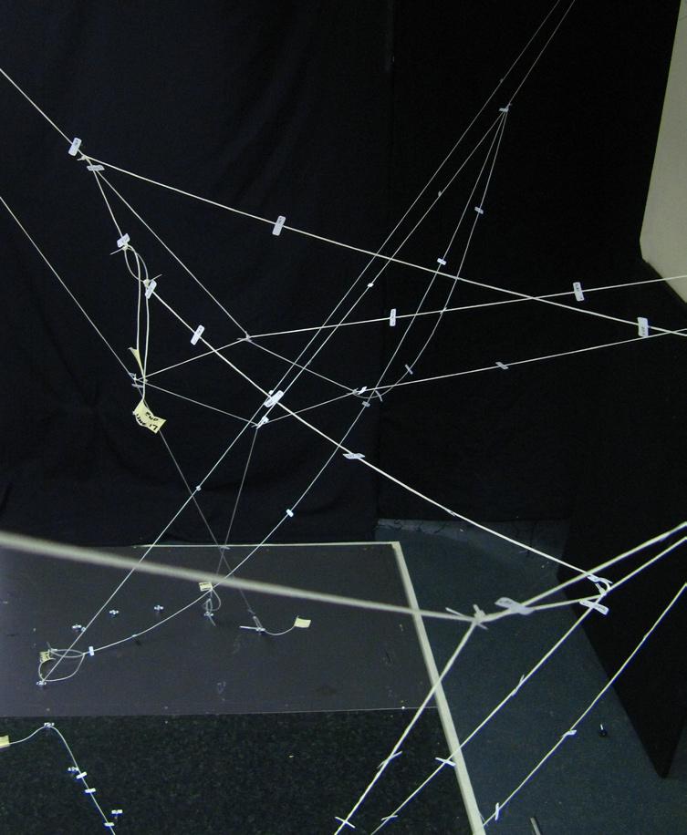
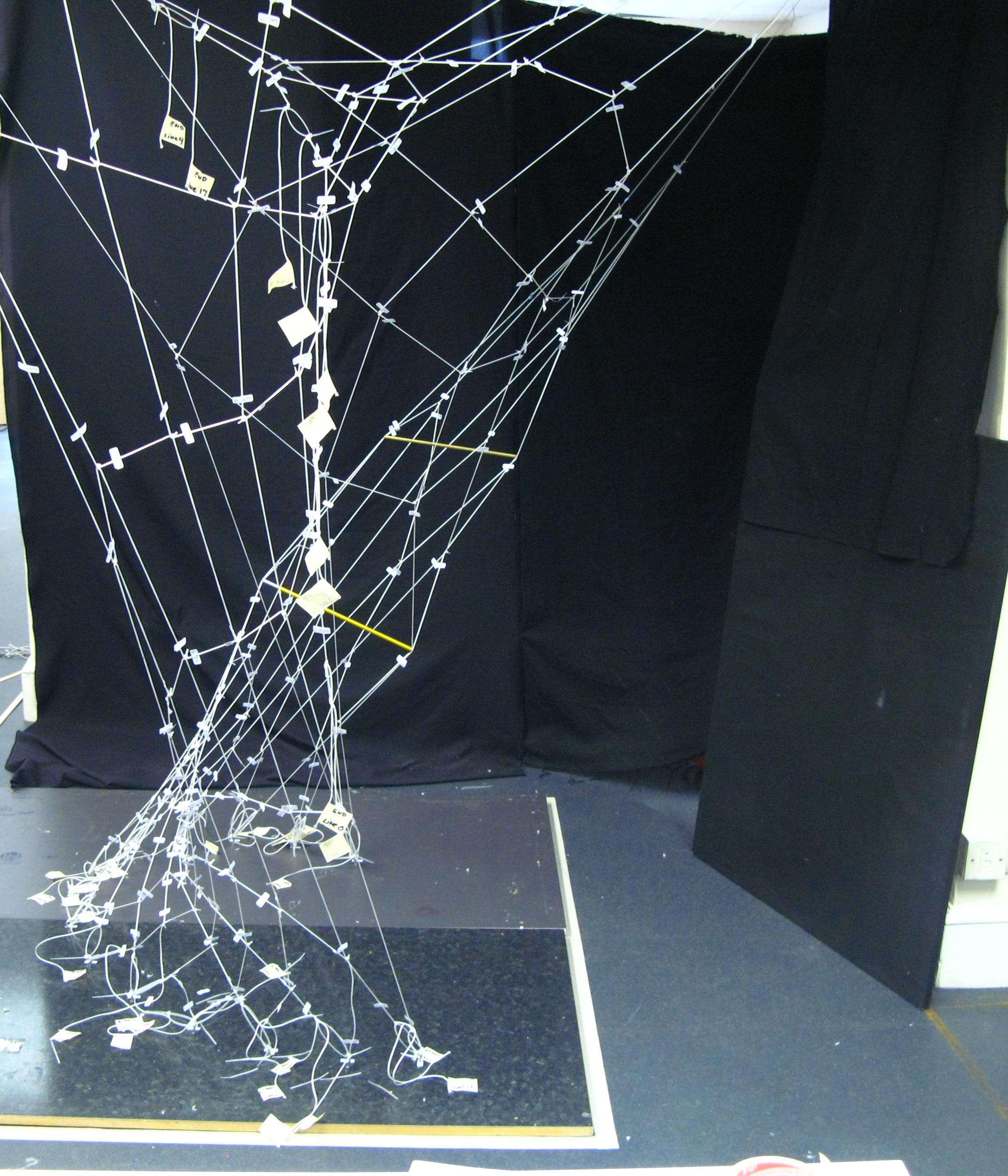
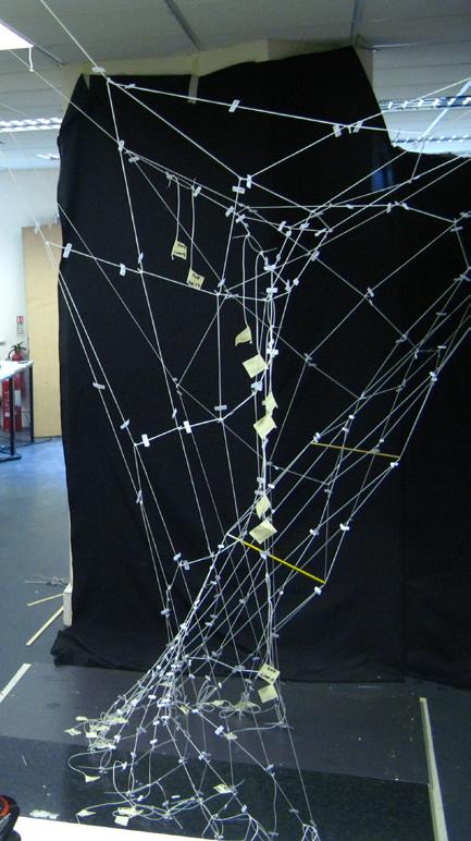
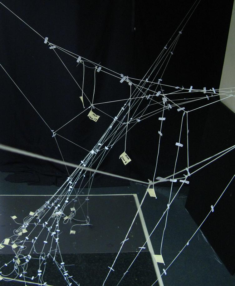
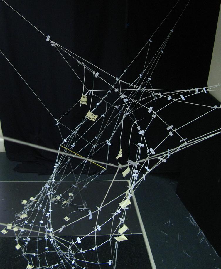
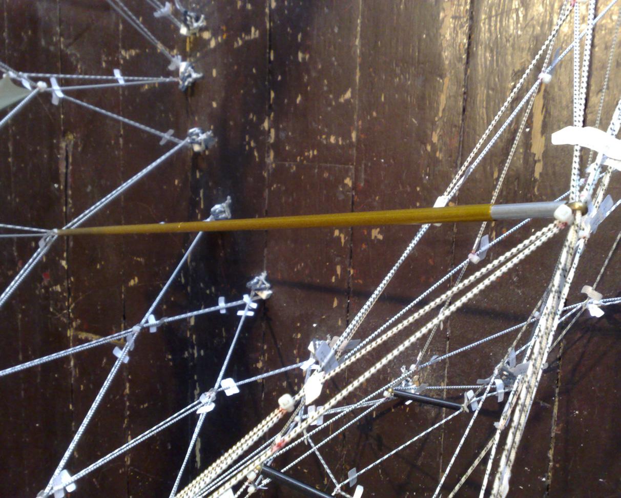
2.1-8 and 2.1-11 full-scale mockup for design of tensioned net installation. this mockup tests the translation from computational data and the method for assembling the cable net. the white tags are the node identifiers. the larger tags identify the start or end of the major line elements. gold elements compression elements. inserted into the net testing their affect for post-tension and spatial articulation.
2.1-9
sequencing of fabrication. lines were installed and locked together, using cable ties, where they crossed per the information in the digital model. one node ID exists on 2 lines. this indicates the crossing point and where the two seperate lines would become locked together. the only positional information (x,y,z coordinates) that was necessary was for the anchor points on the floor and ceiling of the space.
2.1-10
compression elements were installed into the net after it was fully assembled. these acted as devices to add tension to the system and see how local posttension would effect the overall arrangement. these elements also allowed to spatially articulate the net - expanding certain areas by pushing apart the surfaces of the net. the compression element were aluminum tent poles with a diameter of 8mm. in future experiments, the simulation of compression elements was added as a capability of the computational process.


2.1-12 and 2.1-12a unique double array values. simple particle map which describes the unique ID for each particle. the ID is created through a simple , logical double for-loop in Processing.
2.1-13 and 2.1-13a installing of springs, connecting all particles. this is an example of how the double array ID method becomes useful. for inserting the network of springs, it is a simple computational method of stepping incrementally through the list of particles.
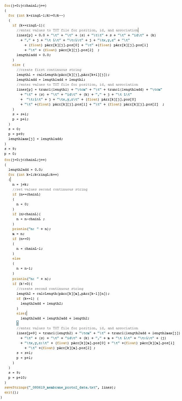
2.1-14 and 2.1-14a moving through node network for fabrication. while we want to track the springs in the network, we want to move through it in a fashion that connects springs across the entire network. for fabrication, as opposed to translating one spring into a single length of material. this method assembles multiple springs, accumulating the length and association data, and creating longer, but fewer continuous lengths of material. the computational method for extracting this information is more complex. though, the complexity is primarily due to tracking across the ends of the computational boundary. the incrementing has to be adjusted when hitting the maximum boundary of the array - setting is back to zero 0 to then continue incrementing upwards.

2.1-15
final design of cable net for installation. the orange line highlights multiple springs to be connected for fabrication as a single length of material. each spring length is tabulated and logged into the associated node information. nodes and the static spring model is reconstructed through a script in Rhino. this version of the net is designed for installation in the AA Studio 2 space.
2.1-16
ID tag for specific node/particle. the ID for the tag originates from the double-array value assigned to the particle during the initial creation of the array of particles and spring network.
2.1-17
particle map for computational net. the hilighted springs describe the movement through the double-array of particles to describe the a single continuous line for fabrication. this method is embedded in the computational process in Processing. because it describes a movement through the topological particle map, any geometry can be analyzed in this same manner., and thus fabricated as well.
A2_id6,20 L14:L20
A2_id6,20
L14:L20
L14:L20
A2_id6,20
L14:L20
2.1-18
description of complete net with all node IDs. the installation consists of 2 nets (net A and net B, as shown in excel data Figure 3.19). They grey and orange lines depict the 2 different nets. At moments, they are pushed apart by springs acting in compression in the computational model.
2.1-19 sample of excel data extracted from computational model.
a distance in computational model from current particle to the previous particle
cummulative distance for physical string material. value is reduced by 10% to account for material stretch
c net A or net B
d node number alond current line and unique ID for current node
e other line which crosses at current node
f current line
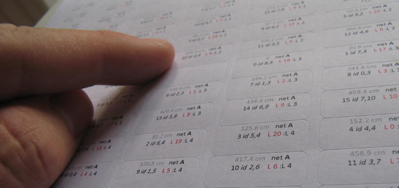
2.1-20 list of Excel sheet printed for fabrication. these “mappings” laid out all the lengths and node locations for the strings to fabricate the entire net. for net A and net B, there were a total of 8 sheets necessary to build the entire installation.
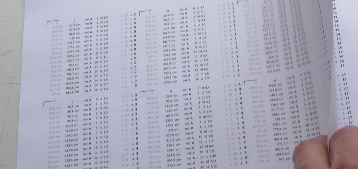
2.1-21 printed tags. from the Excel file, tags were printed to be affixed to the strings. this allows for the physical node to be seen in space. data on the tag would indicate which lines should cross at any given node.
2.1-22 sample of Excel spreadsheet showing the data for construction of 2 seperate lines. data is extracted directly out of the Processing model.
b
1 : 1/30/2009 : _080625_membrane_proto4_data_pArr1_stretch10_formatted.xls
: _080625_membrane_proto4_data_pArr1_stretch10_formatted.xls
2.1-23 digital layout of lines for fabrication of net. the values above and below the line represent that actual distance computationally (below) and the adjusted distance reduced to consider stretch in the string material used for fabrication. the reducing the lengths, this insured that we would be construction a tensioned net without adding further tensioning mechanisms.
2.1-24 detail of one of the lines for fabrication. the ‘x’ indicates an anchored point for that end of the line.
2.1-25 measuring and location of nodes on string material. the material is 2.5mm nylon string.
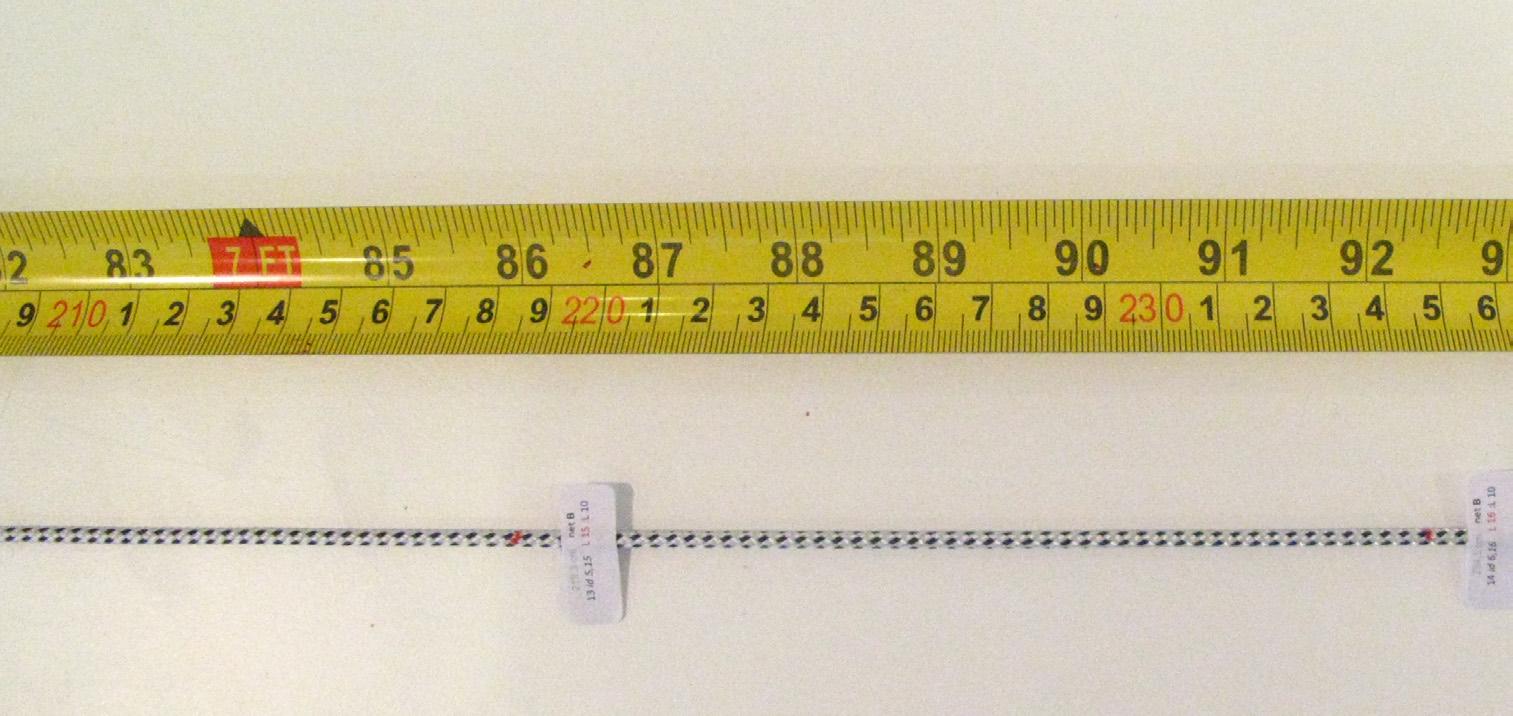
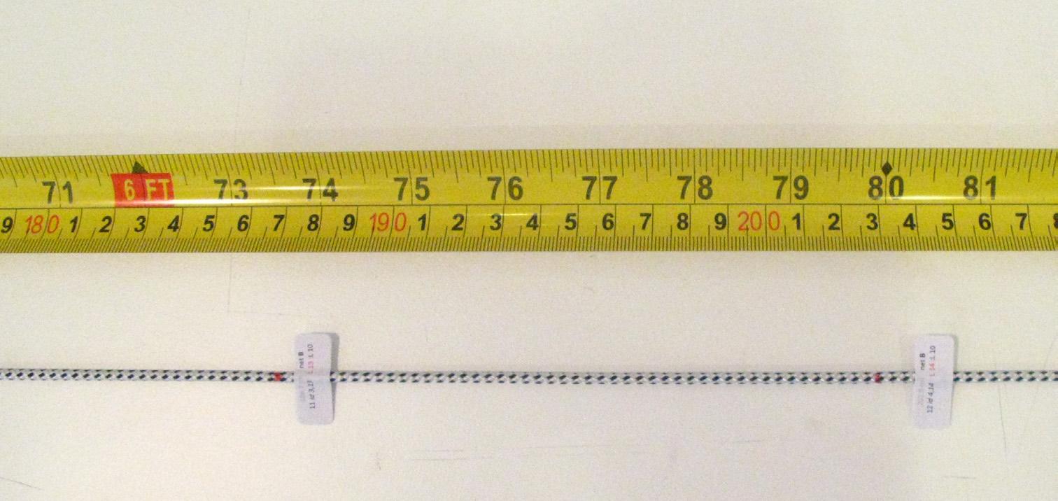
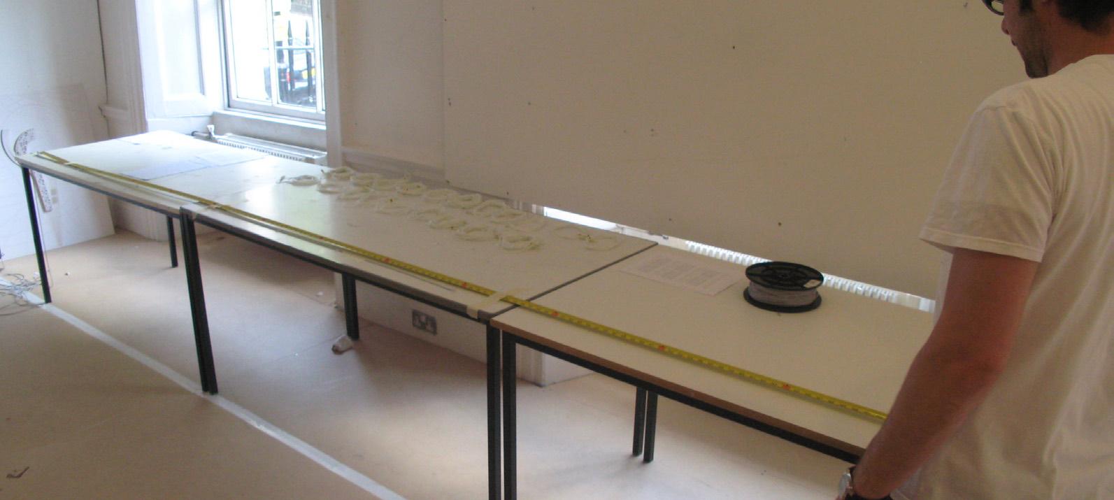
2.1-26 setup for measuring overall line length and location nodes along line.
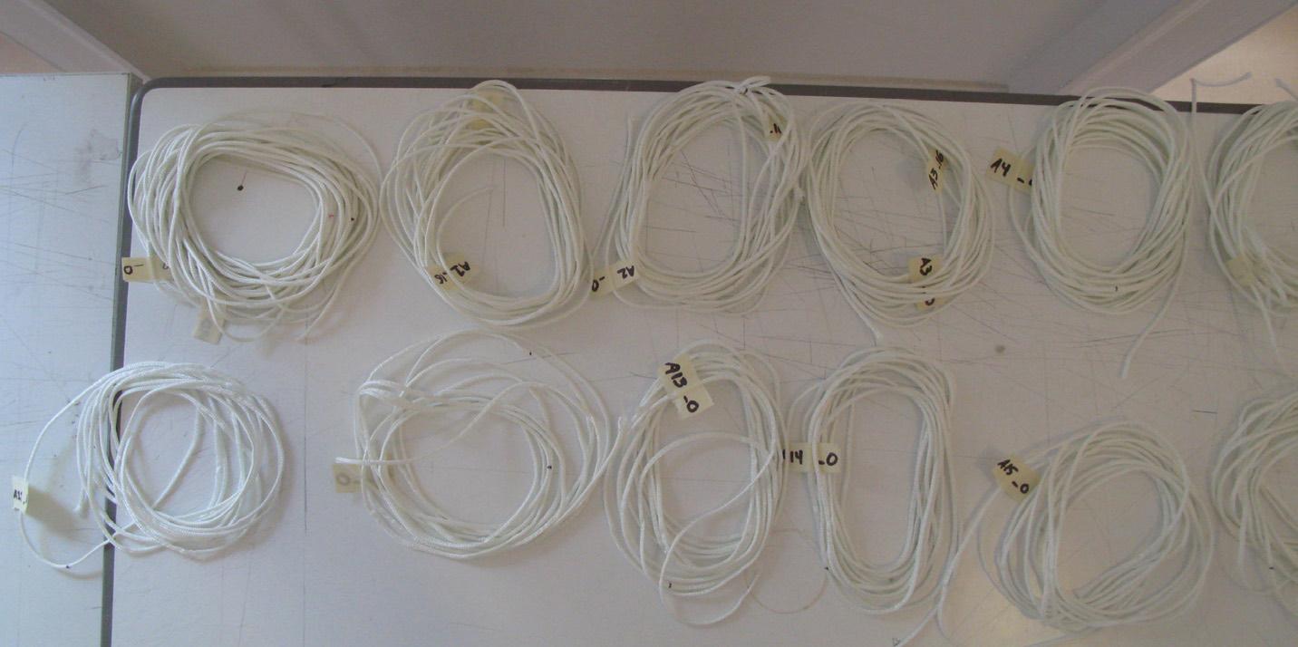
2.1-27 series of strings measured and tagged with node locations.
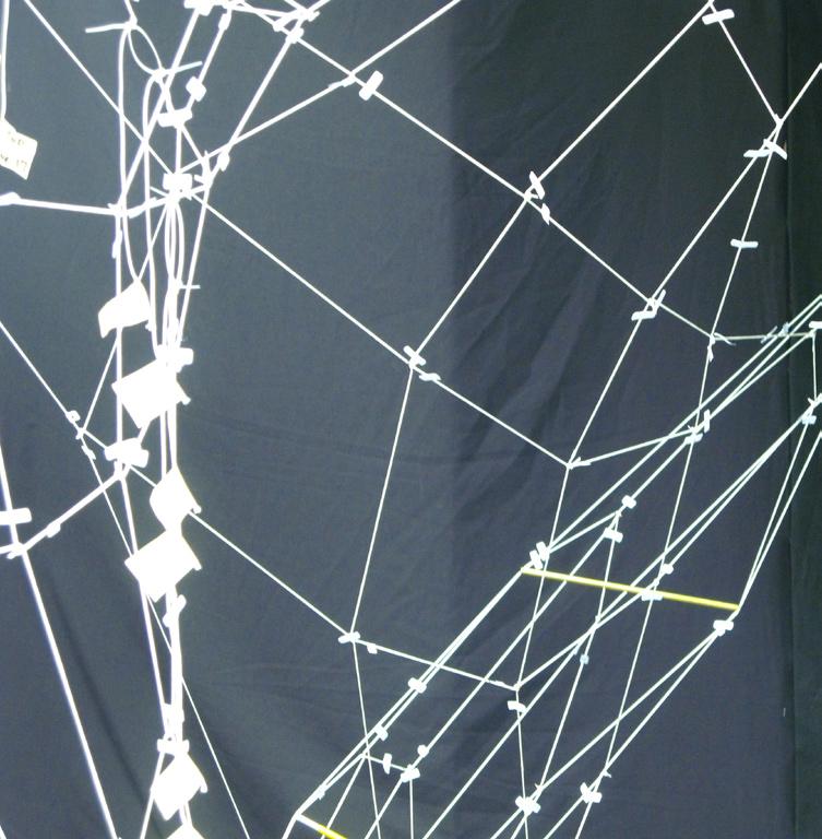
2.1-28 node and ID tags in completed installation. the node is fixed with a cable tie, connecting the two lines that cross at this particular node. the node is “form-found” through the procedure of locking the two lines together (line 19 and line 17 in the photo). the node is not determined through the input of a coordinate (x,y,z) position. the arrangement of the net is derived through the connecting of the nodes - by tracking common node IDs across different lines, and locking them together.
2.1-29 anchors for the ceiling. the extension bolts allowed for some degree of post tension in the installation.

2.1-30 node at which 2 nets are locked together. an 8-way node is generated when the nodes of nets A and B are locked together.
2.1-31 nodes for nets A and B. the two different string patterns signify the difference between net A and net B. this distinction is also noted on the tags.
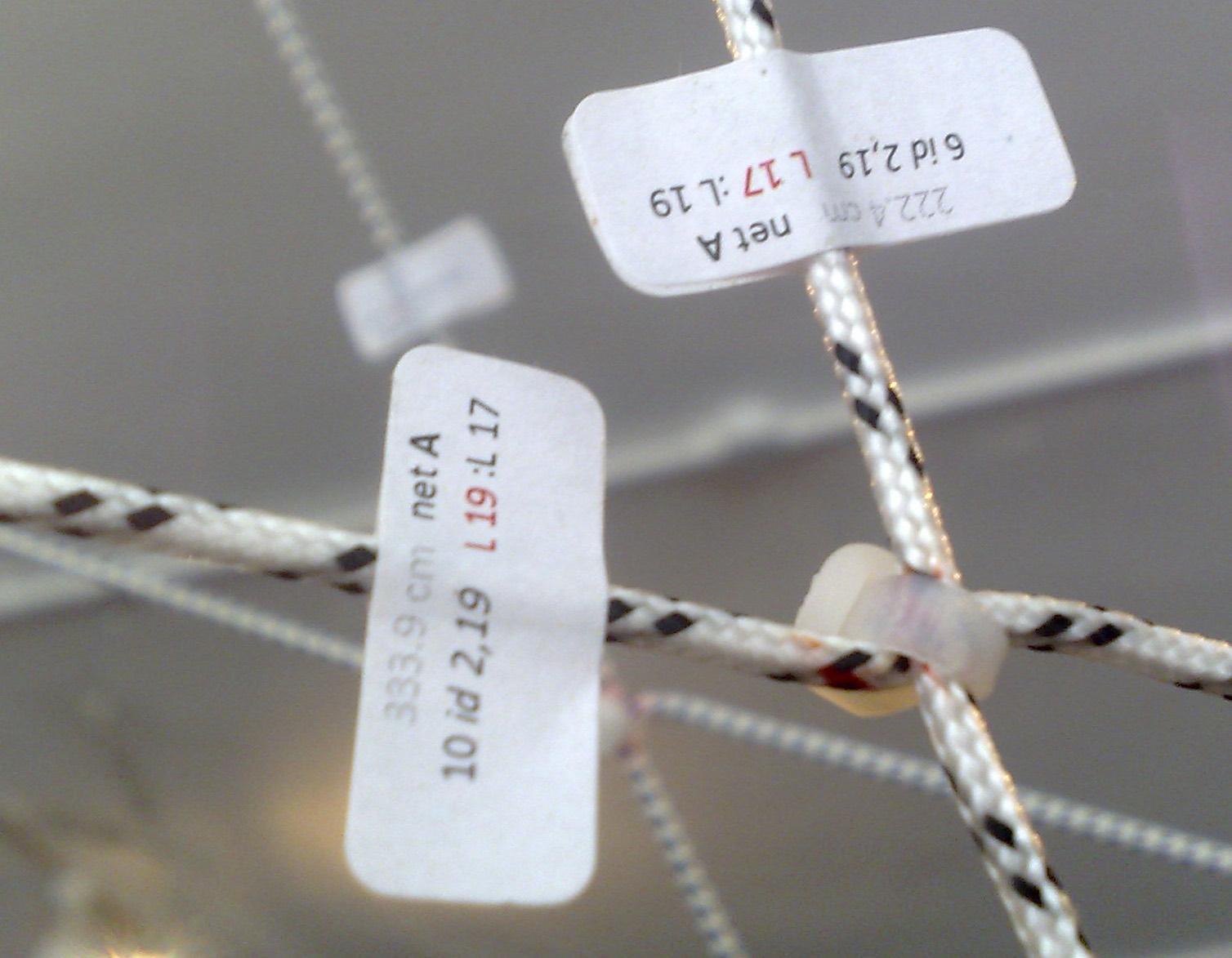
2.1-28 node and ID tags in completed installation. the node is fixed with a cable tie, connecting the two lines that cross at this particular node. the node is “form-found” through the procedure of locking the two lines together (line 19 and line 17 in the photo). the node is not determined through the input of a coordinate (x,y,z) position. the arrangement of the net is derived through the connecting of the nodes - by tracking common node IDs across different lines, and locking them together.
2.1-29
comupational compression member. the function for generating compression elements exists within the dynamic relaxation process in Processing. a compression element is a spring that exterts a pushing force (its actual length is shorter than it rest length). in this scenario the size and amount of force is parametric to the distance between neighboring particles. therefore, the size of the compression member has to be solved during the dynamic relaxation process. the spring incrementally expands and gains strength to eventually meet the criteria set for it - in this case, a length that equals 1/2 the distance between 2 neighboring particles.
2.1-30 connection element for compression member. at certain nodes an additional spring element was introduced to simulate a compression member and push the nets apart in certain places. this pin is located at those nodes and anchors the insertion of an aluminum rod.
2.1-31
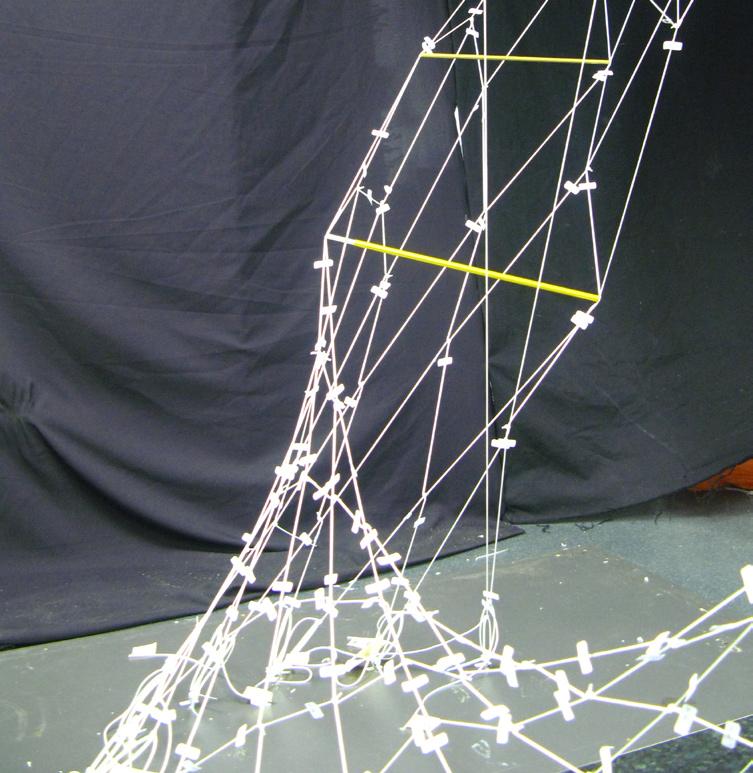
compression members in installation. the compression members provide secondary, local post-tensioning for the net. they also articulate the spatial characteristics of the overall structure. as the installation is created of two nets (one inside the other), there are moments where the nets are pushed apart from eachother by the compression members, creating gaps between the two surfaces.
2.1-32
compression member spanning across networks. there are also instances where a compression element (signified by the gold rods) spans across the entire installation. at each end they connect to both nets A and B, spanning across the entire interior of the installation. these act primarily as devices for expanding the gross spatial characteristics of the net. they add a minimal amount of posttensioning.
if (length(local) < distance * 0.5) then { springRestLength(local) = springRestLength(local) * 1.5; springStrength(local) = springStrength(local) * 1.5; }
2.1-33
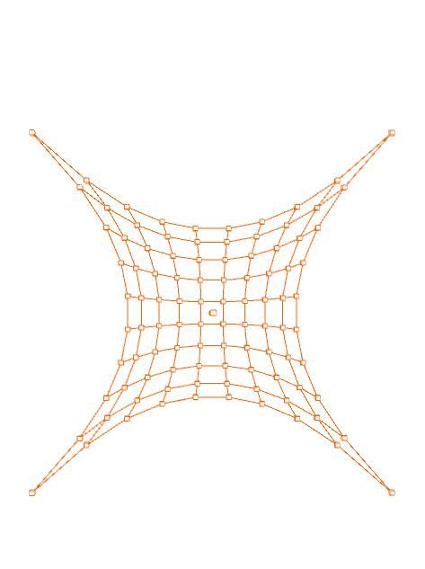
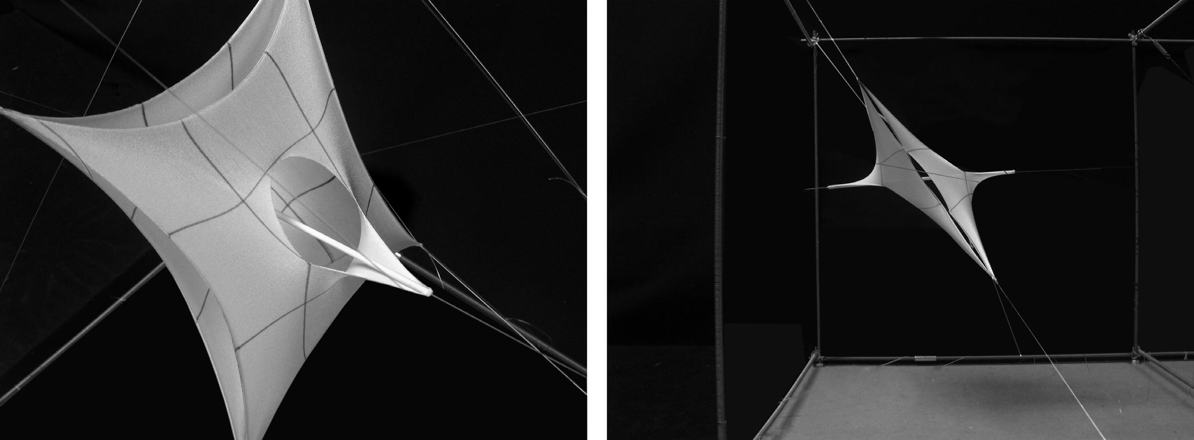
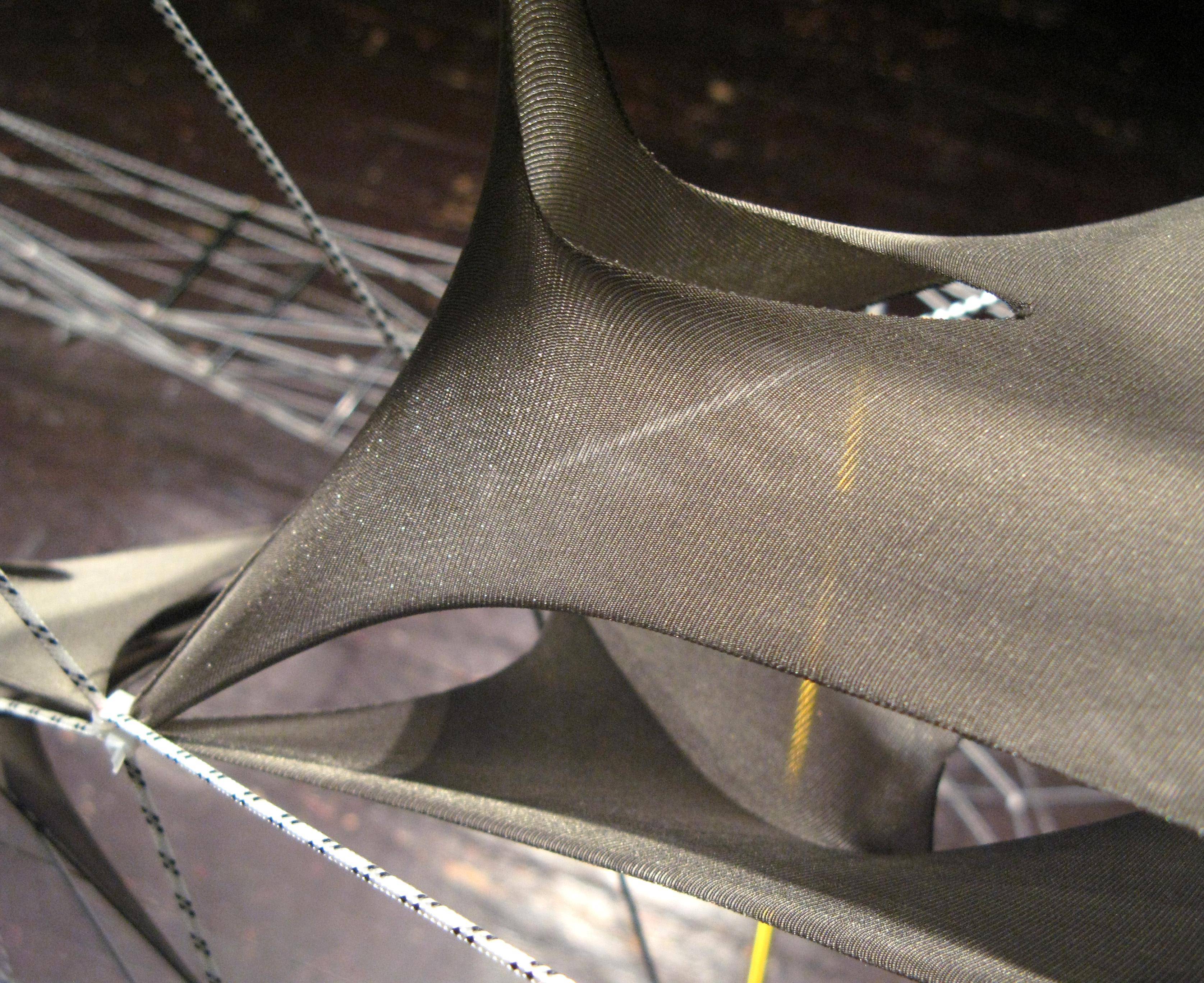
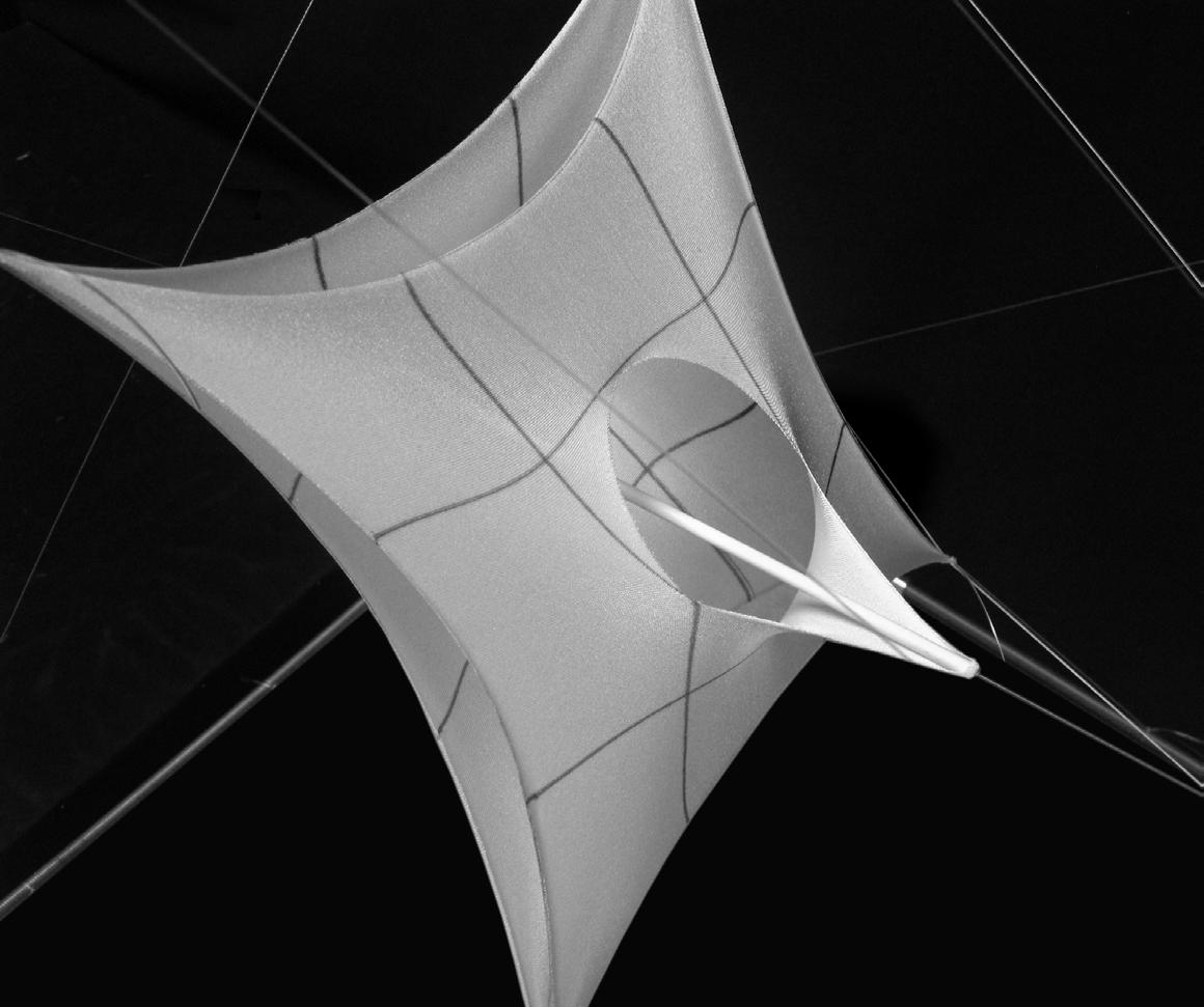
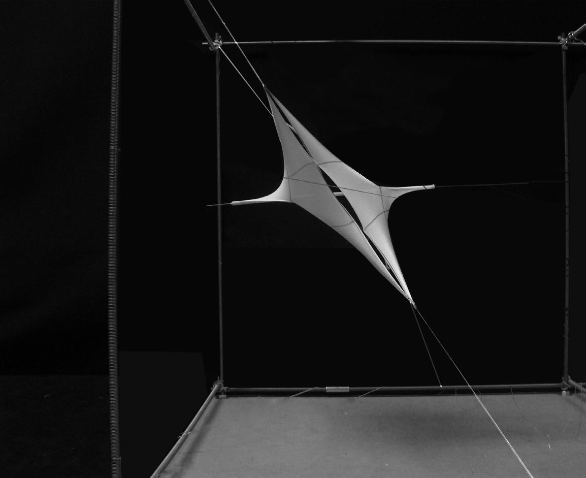
experiment with tension and compression active component. the membrane is anchored (via strings) at 4 corners with an internal compression element. when tension is activated in the component, the compression element finds it position and simultaneously opens up minimal holes on both membranes surfaces.
2.1-34 membrane component installed into net. membrane components were added to the net after it was completely installed. they did little to affect the overall tensioning. they acted primiarily as visual devices emphasizing the gap between net A and B.
2.1-35 computational membrane component. this component was simulated computationally, though it was not utilized for the fabrication of the installation. it was not clearly understood how to translate the computational geometry to a physicall material.
2.1-36
mambrane fabrication. the caluclations, sizing, and fabrication for the membrane components were all done manually.
2.1-37 array of membrane components. the compression element is not present in the membrane component for the installation. the connection of the minimal holes between components provided the same effect spatially.

38
embedded fabrication
ITERATION.05
chain.count:
ring.count:
rest.length
x.parameter
20 12 5.0 (pow(i,2.6)*r*sin(a)*0.006)+60-0.8*i (pow(i,2.0))*(r*(cos(a))*0.01)
The most interesting result from the experiment is that the digital process is transformed from structural simulation to a design simulation with embedded structural and material constraints. In engineering software packages dedicated to cable net structures, the setup demands high specificity of material and positional details. In this environment where demands are many and mostly related to predetermined material and structural matters, the ability to connect variables with design intent is quite minimal. The ability to perform multiple iterations can be even more difficult.
ITERATION.01
chain.count:
ring.count:
rest.length
x.parameter
y.parameter
20 8 5.0 (pow(i,2)*r*sin(a)*0.006)+60-0.8*i (pow(i,2))*(r*(cos(a))*0.01)
ITERATION.02
chain.count:
ring.count:
rest.length
x.parameter
y.parameter
20 20 1.0 (pow(i,1.7)*r*sin(a)*0.006)+60-0.8*i (pow(i,1.7))*(r*(cos(a))*0.01)
FRONT TOP SIDEITERATION.05
chain.count:
ring.count:
rest.length
x.parameter
20 12 5.0 (pow(i,2.6)*r*sin(a)*0.006)+60-0.8*i (pow(i,2.0))*(r*(cos(a))*0.01)
2.1-39
ITERATION.01
chain.count:
ring.count:
rest.length
x.parameter
y.parameter
20 8 5.0 (pow(i,2)*r*sin(a)*0.006)+60-0.8*i (pow(i,2))*(r*(cos(a))*0.01)
ITERATION.02
chain.count:
ring.count:
rest.length
x.parameter
y.parameter
20 20 1.0 (pow(i,1.7)*r*sin(a)*0.006)+60-0.8*i (pow(i,1.7))*(r*(cos(a))*0.01)
ITERATION.03
chain.count:
ring.count:
rest.length
x.parameter
y.parameter
30 20 5.0 (pow(i,1.1)*r*sin(a)*0.006)+60-0.8*i (pow(i,2))*(r*(cos(a))*0.01)
ITERATION.04
chain.count:
ring.count: rest.length x.parameter y.parameter
24 6 5.0 (pow(i,2.6)*r*sin(a)*0.006)+60-0.8*i (pow(i,2.0))*(r*(cos(a))*0.01)
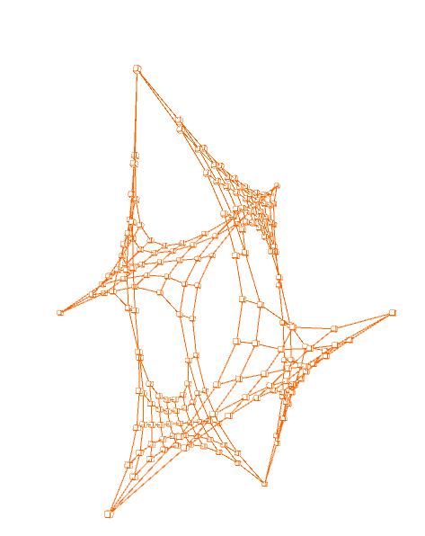
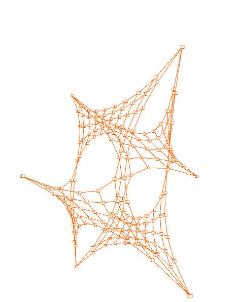
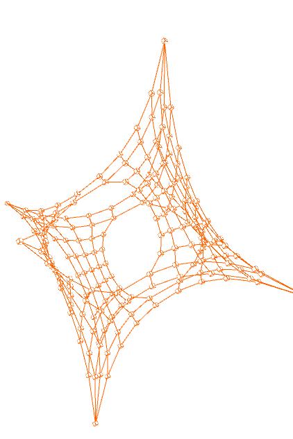
2.1-38 and 2.1-39 examples of design variation from the same computational process that generated the Cylindrical Net Morphologies installation. these examples utilize only a minimal set of variables to produce very different formal outcomes. each design, though, has the same topological strategy, and can therefore be fabricate in the same manner and with the same ease as the Net installation. the design would be in the scale of the network. as the chain.count (num. of particles in the lateral direction) and ring.count (num. of particles in the longitudinal direction) increase, the number of elements to be fabricated will also increase.
ITERATION.05
chain.count:
ring.count:
rest.length
x.parameter
y.parameter
20 12 5.0 (pow(i,2.6)*r*sin(a)*0.006)+60-0.8*i (pow(i,2.0))*(r*(cos(a))*0.01)
ITERATION.06
chain.count:
ring.count:
rest.length x.parameter y.parameter
40 12 7.0 (pow(i,2)*r*sin(a)*0.006)+60-0.8*i (pow(i,1.6))*(r*(cos(a))*0.01)
FRONT TOP SIDEExamining visually the installation, it is apparent in how the density of the mesh (frequency of lines and nodes within a certain sized area) plays a part in comprehending the shape of the net and its possible implications as a threshold. A regularized pattern, one which has a certain frequency of repetition, aids in reading the continuity of the surface and thus reading the form. With this installation, the pattern is more typically irregular as the two nets connect and disconnect, and the compression element push the patterns of the two nets out of sync. This is an interesting aspect in being able to produce and fabricate, in a heavily methodical way, such irregularity. But, there is also an interest in producing readable forms; ones
which can serve as thresholds or boundaries to clearly defined areas of space.
Figure 3.41 begins to show how the cylindrical net can form boundaries to shape areas other than typical centralized cylinder form. In the design, this is generated through the involution of the cylindrical form (see Figure 3.4). These types of spaces, generated from the cylindrical topology are compelling. Further experiments will focus on how to locate such conditions, and how these conditions can control or indicate certain types of movement through spaces defined by these cylindrical net morphologies
2.1-40 regularity in pattern. the mesh is organized in a way that present a relatively regular pattern. the membranes accentuate the pattern. these 2 conditions, the pattern and the membranes, help to more clearly define the shape of the overall form.
2.1-41 bounded area. the involuted cylinder, from this perspective, begins to define a bounded area. the membranes serve to enhance the clarity of reading this bounded space.
2.1-42 movements indicated by different net arrangements. net densities can begin to elicit certain types of movements through the nets.
2.2 Topologically Defined Net Components
As the Cylindrical Net Morphologies installation worked with a pair of layered cylinders, this experiment focuses on how to construct and associate a series of interconnected cylinders. With the installation, the two nets were relatively autonomous. They connected at moments, but the moments were more about pattern than they were about following a particular reasoning and design / structural strategy for why they should connect or disconnect at particular moments.
When beginning to associate multiple nets, the question of hierarchy arises. There is a need to address it at the computational level: how to control and easily access a growing number of elements, arrays and variables. It is also vital to address hierarchy at the level of structure and material. A spring’s location within the net may determine its hierarchy (a standard spring within the field of a cylinder or a spring that represents an edge cable, for example). These are the focal issues for this experiment. The challenge of controlling density as a factor that describes the visual readability of a net and its form is also an underlying factor in driving the capabilities of a system that generates multiple inter-connected nets.
To accomplish these varied criteria, the intention is to continue to work with the topology of the spring networks, as opposed to discreet geometry. This is to allow for maintaining an extensibility in the types of geometry that can be derived from the spring networks. The meaning of the topologically defined component is that of a component that is mainly described through numbers (of particles and springs) and hierarchy (particle or spring at the edge of the network, shared between networks or within a network).
With digital simulation of tension-active structures, there is often a limitation in the topology of the components. Prior to realizing the geometric form, the base topology is defined. This is most evident in physical form-finding methods and is, therefore, typically transferred into computational form-finding methods. The base topology has significant ramifications on the types and range of geometries that can be created when tension forces are applied. By looking for extensibility at the level of “base topology”, the types of geometries that can be solved for becomes increasingly vast. Ultimately, this means that the process of generating nets is not the governor of form. Rather, other external design criteria can be determinants to the validity of form.
2.2.1 Component Systems for Form-Found Structures
With understanding architecture through the assembly of components comes the recognition of hierarchies between these components. Two primary hierarchies are that of the framework (or the “grid” - the overall framework for the structure) and what could be called the infill (the system that occupies the cells established by the grid). In a typical architectural process, computationally, the framework would be the UV parameters of a surface, and the infill would be a series of geometric components, of which contain a similar or dis-similar topology.
Looking at the hierarchical structure for components in a physical form-finding process, we can identify how these hierarchies become regularized, and subsequently limiting to the range of geometric deformations that can be achieved. It may be of a particular design aesthetic to maintain a minimal amount of variation from one component to the next. But, ideally, this should be born of the design intentions, not of a limitation in the design process itself.
In Frei Otto’s studies for the Stuttgart Main Railway Station (see Figure 2.2-3), we see a 6-sided framework and then a component that consists of a network of 6-sided polygons. The topology for the component aids in flexibility to find forms that have an equilibrium tension state. Because of the limitation in stretch of physical materials, it is necessary to use this particular topology to have an opportunity to pursue some degree of variation in form between components, albeit a minimal amount.
2.2.2 Subdivision Algorithm for Cellular Framework
Pursuing the extensibility of the Cylindrical Net as a component, the creation of the framework is driven by a computational method that is extensible as well. The extensibility focuses primarily on producing a topologically varied cellular pattern. In this case, topologically varied means the cells can be described with a varied number of nodes.
In contrast to the Cutty Sark Pavilion (see Figure 2.2-6) where all of the cells of the framework were hexagonal, the method for creating frameworks for the Cylindrical Net component produces cells with varied numbers of sides.
The cellular network is generated through a subdivision algorithm that was created in RhinoScript for this experiment. The system utilizes a slicing method to subdivide larger volumes in a manner that distributes a range of volumes, considering scale, adjacencies, and orientation. It provides an opportunity to consider condition that the Net system cannot. In this case, number of elements, size of elements, and which elements are neighbors to others.
The idea of neighbors is what intimately connects the two methods. A volume that has been subdivided creates two volumes with a new set of shared edges. The Net components look to utilize these shared edges to expand the network creating larger continuous surfaces.
2.2.3 Single Cell Net Parameters
When a Net component occupies a cell, it mainly reads the corner point and a directional orientation. Computationally, this is the data that is processed out of a script in Rhino: arrays of corner points (see Figure 2.2-14a). The Net component is installed in Processing, where 3 hierarchies are established: anchor spring, edge spring, and net spring. The anchor springs connect to corner points (provided by the cellular framework), the edge springs connect the boundaries of the net back to the anchor springs, and, finally, the net springs establish the cylindrical geometry.
Density is an important variable at this scale of the system. A Net that simply traces the corner points is quite open and does not clearly describe or insinuate at the cylindrical, directional form (see Figure 2.2-15). In Processing, a variable has been set to multiply the number of particles at the boundaries
of the Net component, to introduce more springs and introduce more density. These new particles are captured by the edge springs and included in the construction of the Net component.
2.2.4 Multiplication and Association of Net Components
Beyond the rules for the Net component in relation to a single cell, there is another set of rules when the Net components are installed into a multicellular framework. The main factors that influence the net creation have to do with neighboringconditions at which one cell neighbors another. Two main types of neighboring are analyzed. First, the condition where a corner point from two cells share the exact same position. In the Net component, it means that the particles at that position are “stitched” together, and unfixed from that location. Second, if an edge from two cells is completely coincident, then the edge particles between two nets are “stitched” and unfixed. Generally, a shared condition in the framework means that the nets will connect with each other and expand the continuity in the spring network. The interest is in blurring the “component” nature of the system and allowing these rules for association to drive emergent characteristics for spatial orientation (direction) and definition of boundary (surface).
2.2-2
Computational model consists of 4 interconnected Net components (front view). the orange lines designate springs that act as edge cables. they occur at the open edges of each component. this is not a prescribed condition. it occurs when the association between all of the nets is determined.
CUTTY SARK TEMPORARY PAVILION
2.2-3 physical form-finding models, Frei Otto, Stuttgart Railway Station. the topology of the component is hexagonal providing for enhanced flexibility (compared to a quad topology) in finding an equilibrium tension in the form.
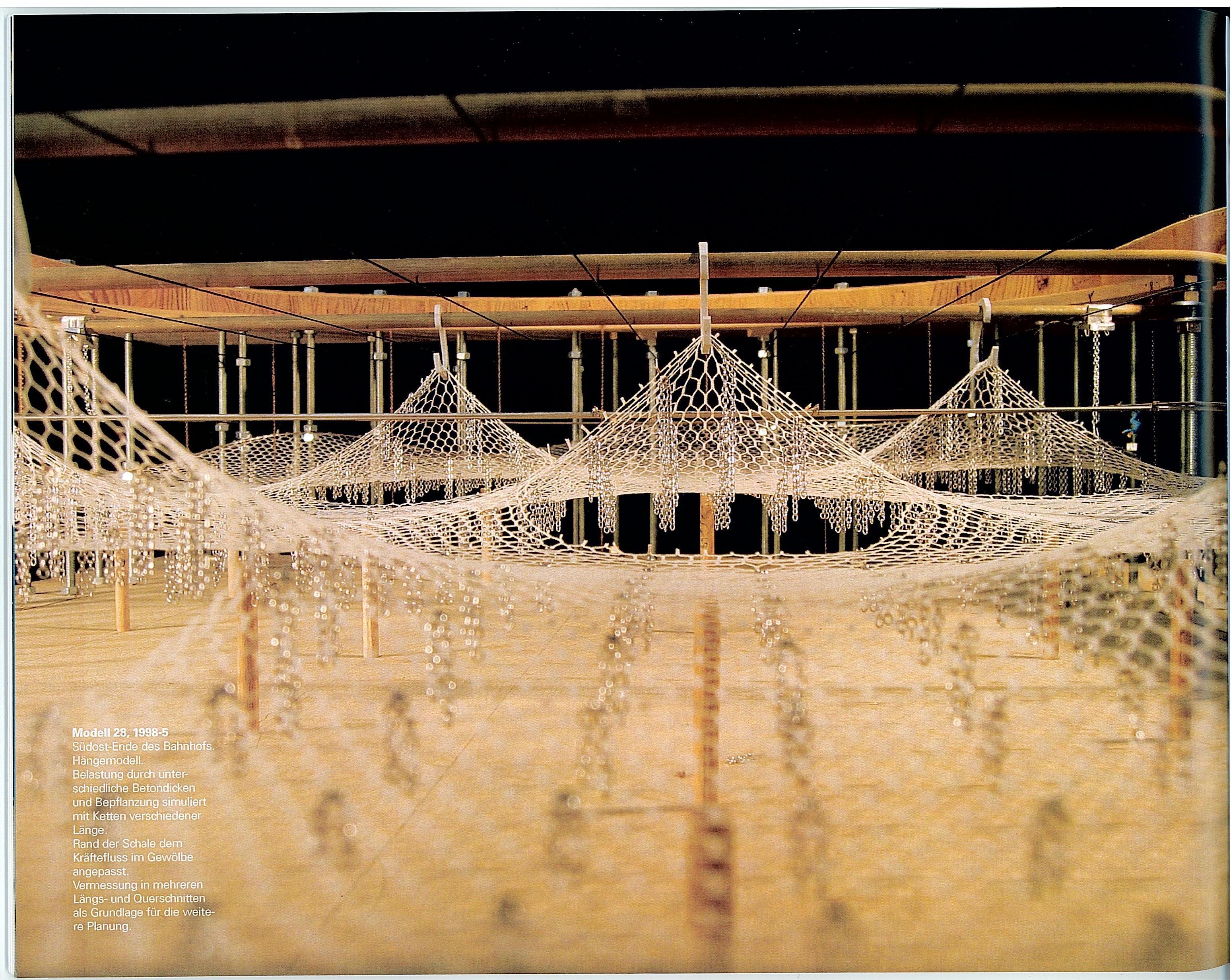
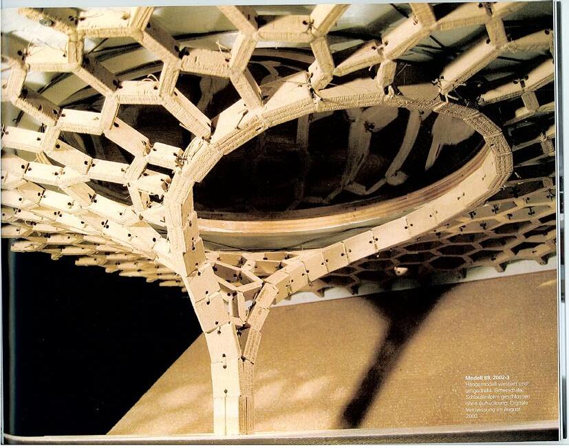
2.2-4 & 2.2-5 component array into larger framework. the hexagonal topology exist at the upper-level hierarchy as the framework for the individual column/roof components
2.2-6 component roof system for Cutty Sark Pavilion, by youmeheshe architects, 2007. the hexagonal framework is infilled with a membrane component. the hexagonal framework varies slightly between cells, while each component varies geometrically, though topologically similar.
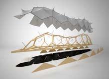
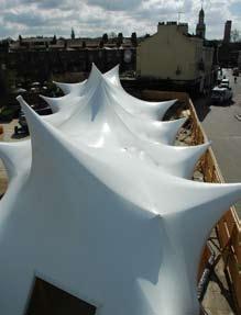
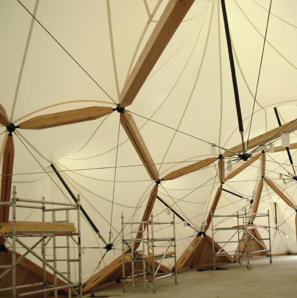
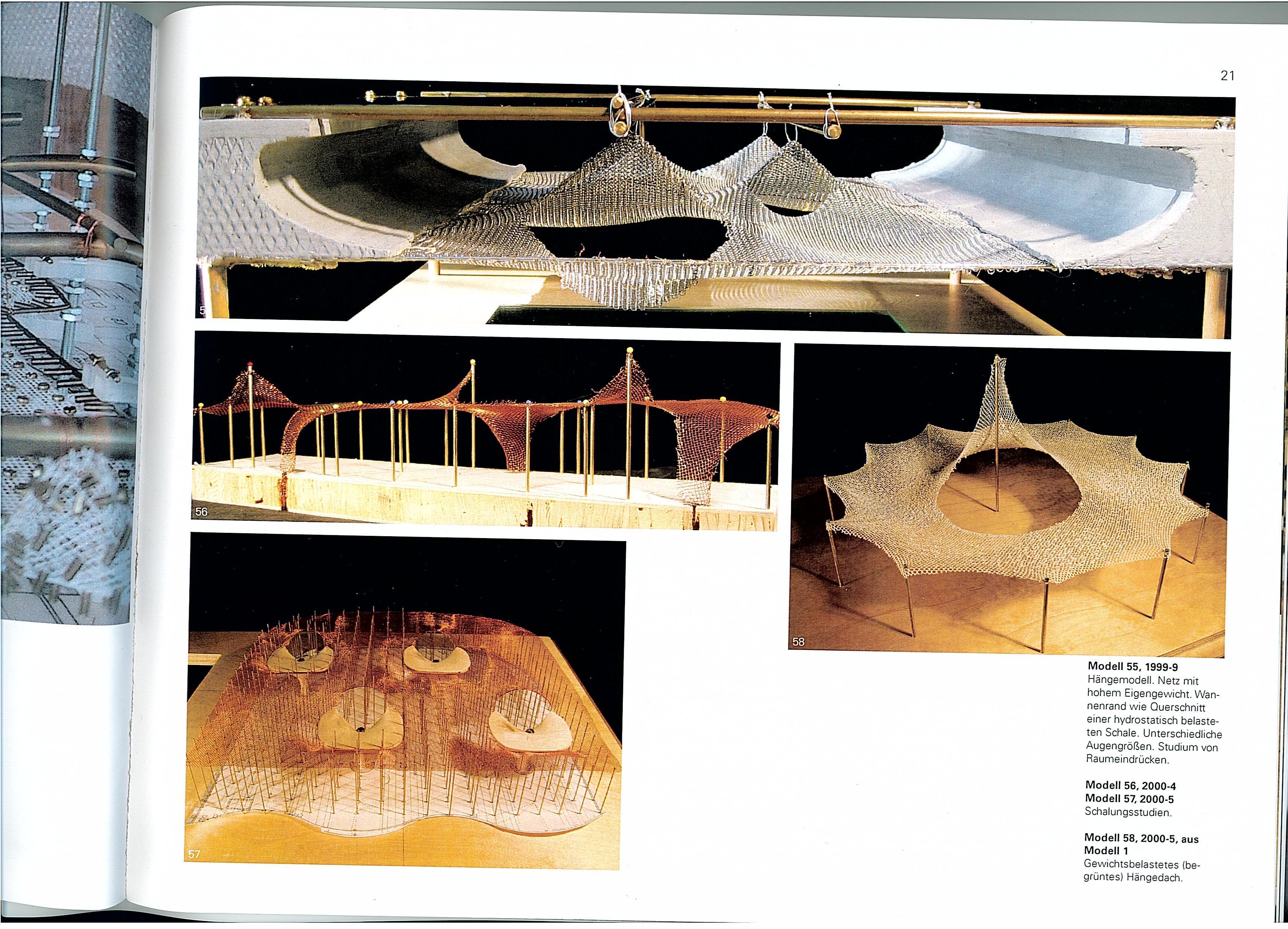
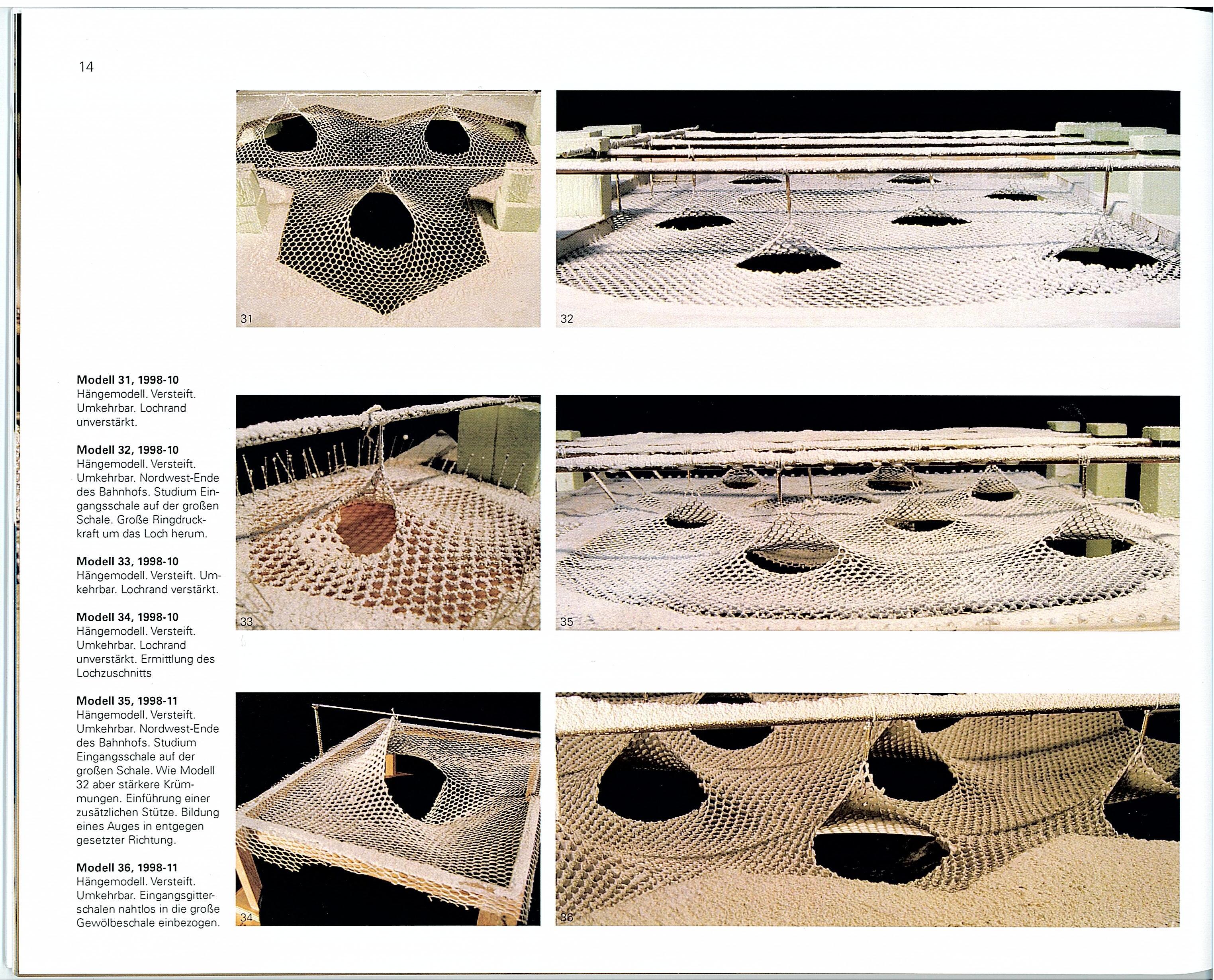
Cutty Sark Pavilion
Whilst the Cutty Sark conservation and structural works are being carried out, the Pavilion will maintain the publics interest in the ship with an exhibition and the opportunity to view the on going works. The Pavilion design has been generated with the aid of a highly sophisticated cad package enabling the form to be produced using the most economic use of material and structure.
2.2-3 2.2-4 2.2-6 2.2-5
CUTTY SARK TEMPORARY PAVILION
Cutty Sark Pavilion
Client:
Cutty
Status: completed
Value: £0.5m
2.2.1 Component Systems for Form-Found Structures topological components
66
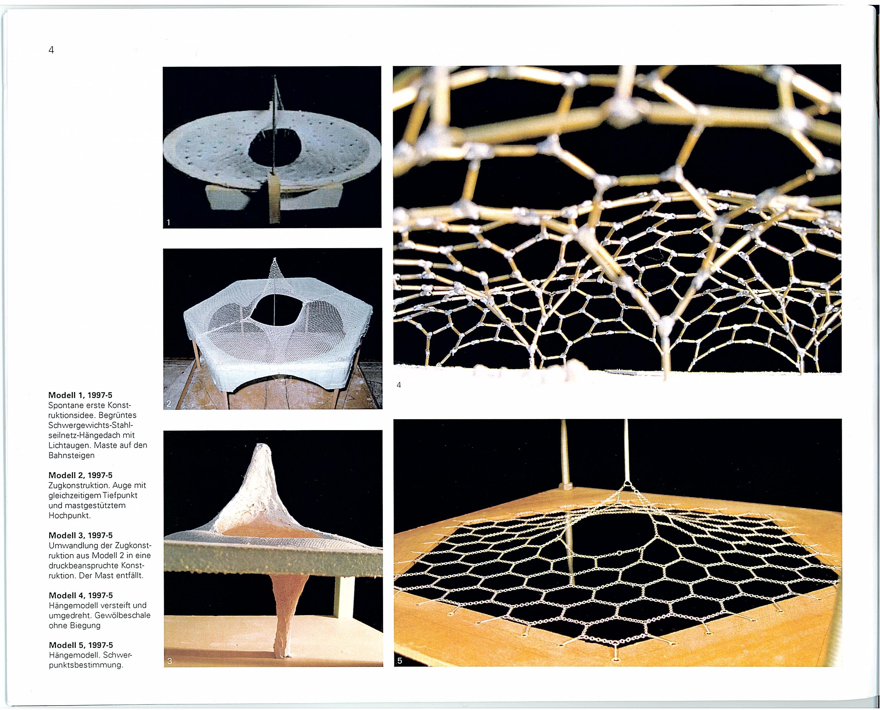
2.2-8 inputs for spatial subdivision algorithm. the algorithm works to utilize a minimal number of variables but produce high degrees of variation in the forms that are generated. inputs 1,2 & 3 allow for a classification of the volumes that are generated. input 4 determines the range of variation for the geometric transformation function, a rotate and slice function. input 5 determines the envelope which will be subdivided.
2.2-9
output from the spatial subdivision algorithm. the algorithm generates the color coded volume sets with the primary criteria of adjacency and size. as the system steps through the priorities (defined by input 3) volumes get more and more distributed. volumes get continually subdivided to meet the particular volume size requirement defined through input 2.
2.2-10
overall assembly of volumes. in this instance, the dark grey coded volumes are set as void space, therefore removed from the final model. the subdivision algorithm produces packed assemblies of volumetric spaces with differing degrees of articulation.
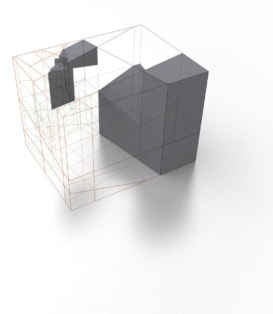

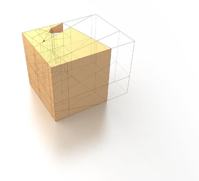

2.2-11
volumes as frameworks for Net component. the Net component does, primarily, two things with the framework. first, one volume means the insertion of one component. the number of subdivisions therefore has an indicator for how many components and material will be generated from the particular model. second, the neighboring of volumes is interpreted as a series of associations between neighboring nets. they do not simply affix to corner points of the volumes. shared point and edges define connections between nets and begin to generate large networks and more complex spatial arrangements. additionally, the net component only requires 2 (of the 6 or more) surfaces from each volume as an input. this allows for the variable of directionality. the top-bottom surfaces can be utilized creating a vertical oriented net, or the front-back surfaces can be used to generate a horizontally oriented net, etc.
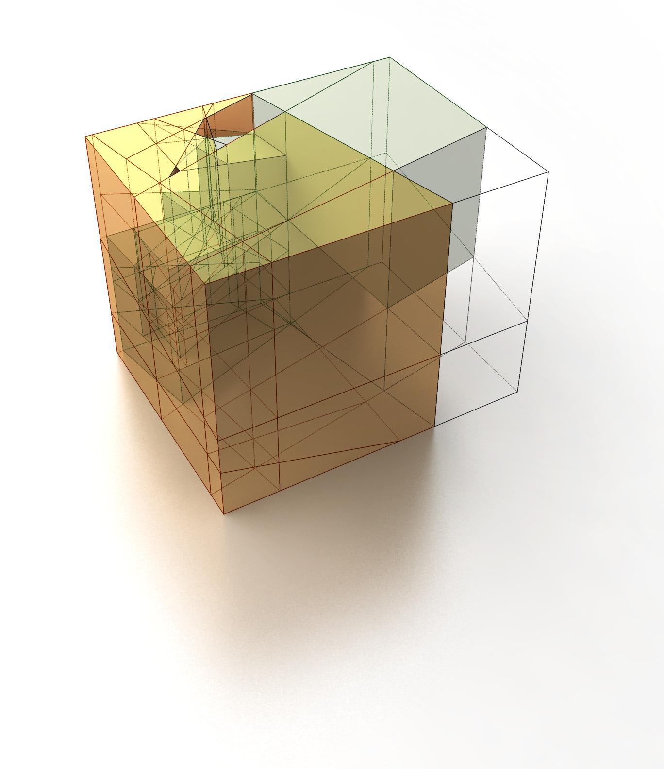
2.2-12
outline for the spatial subdivision algorithm. the color coding defines the input for how many classifications of volumes there should be, the amount for each classification, and the priority. these are percentages to divide the given volume with. the number values determine the offset values for the slicing mechanism that splits of the volumes. the random seed allows for these values to be reproduced if a desired form is generated.
the slicing mechanism is a recursive action that selects each face of a volume and uses it to subdivide the volume itself. the acts until all of the faces have been utilized.
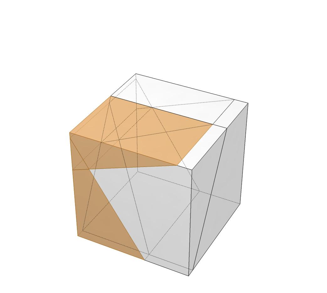
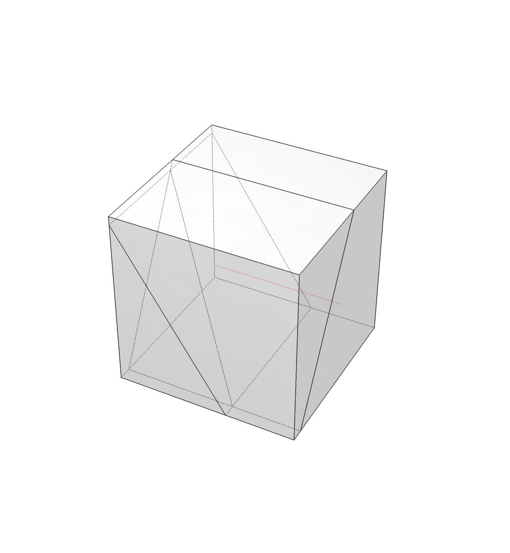
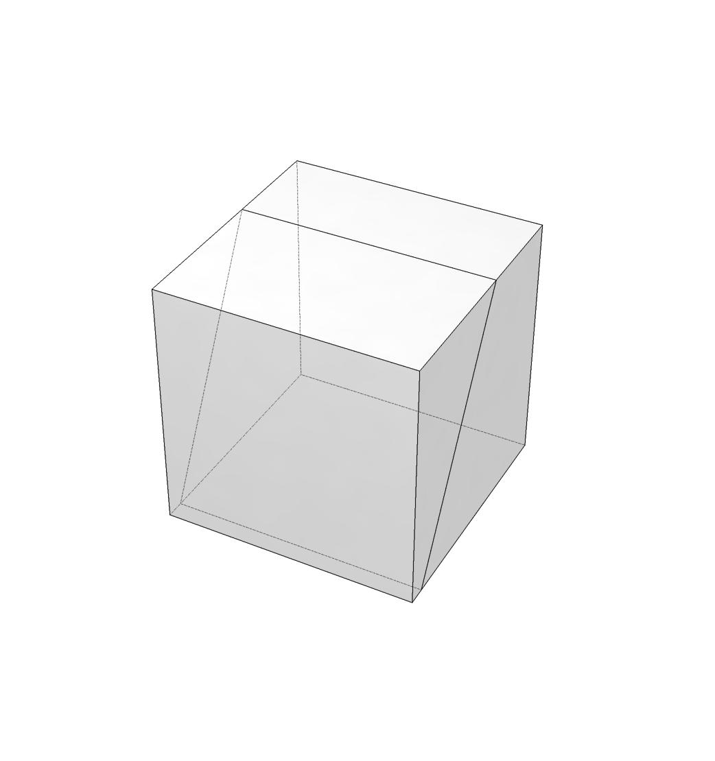
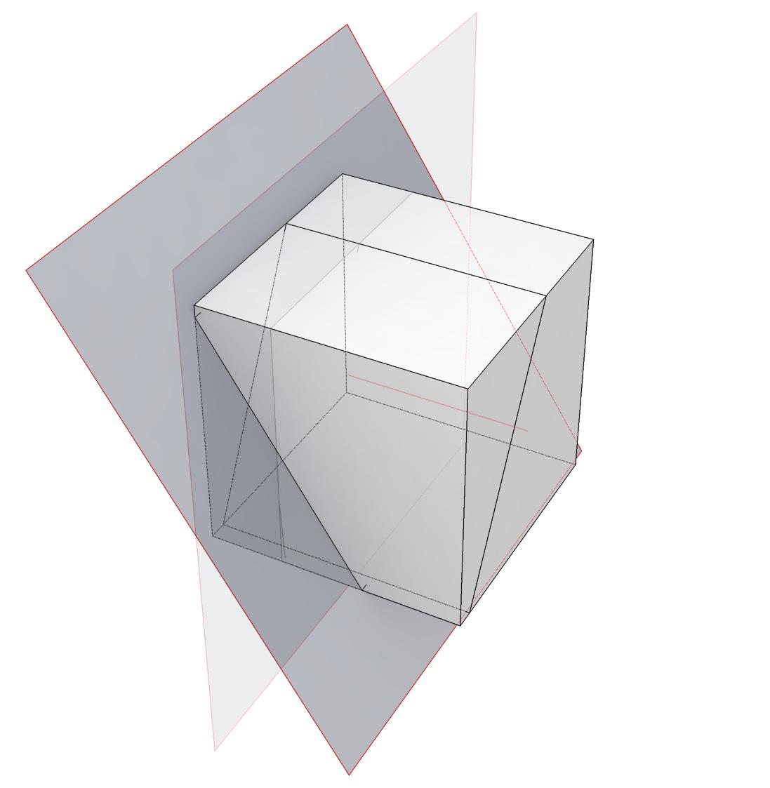
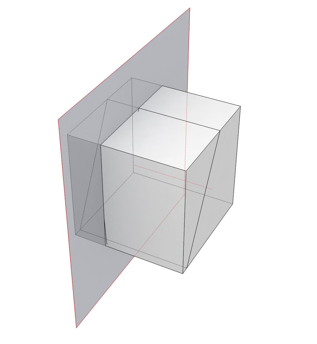
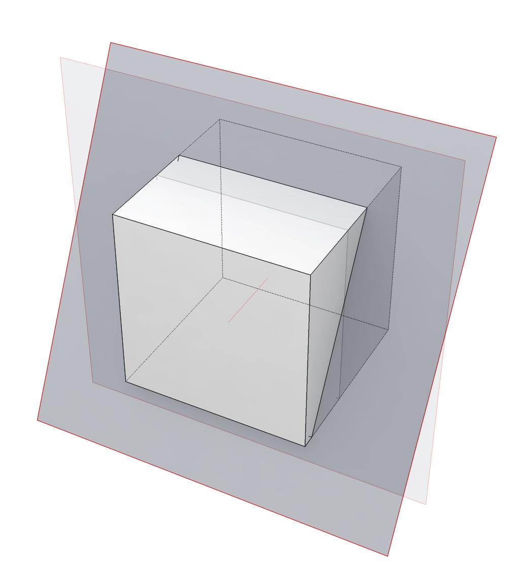
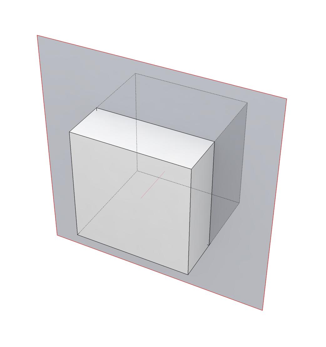
it then begins to fill the new volumes with the color coding (starting with the first). - fitting the biggest amount into the biggest volumes. if volume and colored classification amounts do not match (a volume is too big given the amount indicated in the coding diagram), then the subdivision routine runs again to define a better sized volume. the nearest volume is selected and utilized as the “envelope” for subdivision.
2.2-13
map describing the distribution and amounts of color coded volumes. this map provides a clear layout for how the slicing mechanism has broken up the initial volume. for the net component, it provides information for number of volumes produced, sizes and their location vertically within the entire model.
2.2-14
2.2-14 two surfaces define framework for a single Net component. the algorithm samples 2 opposing surfaces from a single volume. the corner points are transferred into corner particles and become the anchors for the net component.
2.2-14a data transferred to Net component. from the script in Rhino, the locations and sequence of the corner points are tabulated. as a text file, this is transferred into processing and the Net component is installed.
2.2-15 installation of rudimentary Net component into framework. in this instance, there is a direct relationship between the number of corner points and the density of the mesh in the net. the density is quite minimal and this represents that standard hierarchy between framework and infill component.
2.2-15a map depicting the direct relationship between the framework and the elements of the Net component.
2.2-15
2.2-16 density multiplier variable for the net component. in Processing, the density multiplier takes the corner point count and multiplies it to create a higher number of particles and thus springs. this creates a control for the visual density of the net, and it ability to more or less clearly define a boundary. in this instance, the new particles are dispersed evenly along each edge and fixed in place. these locations are calculated in the processing script, and assigned to the particles.
2.2-16a added hierarchy between corner points and net. in this example, there is a new array of particles along the edge of the framework. the information from these particles is passed into the Net component, where the particles at the boundary of the Net are parented to these new edge particles.
2.2-17 increasing the density multiplier variable. the scaling of the density is parametric in the script. this simple switch of the multiplier to a higher value will expand the array of particles and spring and produce a higher density mesh.
2.2-18 locating elements within the arrays of particles. to derive the locations for each particles (in terms of the equal disbursement of the particles along the edges), it needs to be known where an edge particle sits in relation to its next corner particle. with the mod function, we can derive this information, while also understanding how far away we are from the next corner particle. since the mod can return that remainder, that information can be used to locate the particle in context of the corner particles. this is a very lightweight method for dispersing the new edge particles. but, ultimately, this method was too hard to utilize for connecting edge particles between nets. since this single edge particle array captures the corner particles, the intermediate particles, and has an association with the net boundary particles, filtering through these to isolate certain sets of particles within the array was too difficult to do with the mod function as developed.
2.2.3 Single Cell Net Parameters topological components
corner points: 4
density multiplier (dMult): 6
corner points: 4
density multiplier (dMult): 20
2.2-17
0,0
PARTICLE, unfixed PARTICLE, fixed CORNER PARTICLE, fixed CORNER POINT [surface,point]
i (of particle count) in relation to corner particle: cornerPoints[(i - (i mod dMult))/dMult]
i (of Particle count) when AT corner particle: cornerPoints[i/dMult] where i mod dMult = 0
i: incrementing value for the boundary particles cornerPoints: array of corner point from framework dMult: density multiplier variable in Processing mod: modulo
2.2-19 hierarchy of particles and springs. as stated previously, locating and controlling a single array of particles mathematically for separate tasks was too difficult. to alleviate this problem, a set of hierarchically different particles is created. starting with the lowest level is the net particle (part of the cylindrical net component), at the next level is the edge particle (defining a series of edge springs which connect the boundaries of the net component), and at the top level is the corner particle (associated with the corner point of the framework).
2.2-19a
expanded hierarchy seen in particle map. by instituting different levels of hierarchy, connection methods between springs and variables such as spring strength can be more easily controlled. as seen in Figure 2.2-19, the edge springs (orange) are stronger than the net springs (black).
2.2-20
expanded top level hierarchy: the meta particle / spring. instead of affixing directly to the corner points of the framework, a meta system is introduced to mediate between the framework and the Net component. this defines the highest level of the spring network: a series of springs that connect from the framework corners to the corner particles of the Net component.
2.2-20a particle map which includes meta particles and springs. the spring existing between the corner point of the framework and the corner particle allows for articulation of the overall net forms. it can be strengthened (and shortened) computationally so that the net shapes more tightly to the framework. this set of springs can also act as a device for posttensioning when translated to a series of anchoring cables in physical construction.
2.2-20b
layers of different arrays and associations. the meta particles absorb the location information defined by the corner points. the corner particles are then parented to the meta particles. the edge particles utilize the density multiplier to determine how many are generated between each corner particle. the boundary net particles are parented to both corner particles and edges particles.
2.2.3 Single Cell Net Parameters topological components
2.2-19
2.2-20
NET PARTICLE, unfixed
PARTICLE, fixed NET PARTICLE parented to EDGE PARTICLE, unfixed NET PARTICLE parented to CORNER PARTICLE, fixed
PARTICLE parented to CORNER PARTICLE, unfixed
2.2-21 framework of two neighboring cells. the larger frame from the previous examples has been split into 2 sub-frames. from that split arises two sets of shared edges and points. the information for these coincident geometries is logged into an Excel sheet (see Figure 2.221a). the conditions that are noted are points that sit in the same location and edges that start and end in the same locations.
2.2-21a coincident points when a pair of coincident points are located, the connection is tabulated in the Excel sheet and both particles fixed option is set to false coincident edges at a coincident edge the, start and end points are noted along with the information for the coincident points at each end of the edge. the direction of the edge is important to note as it can vary. in some cases, the edges may move in opposite directions (as shown in Figure 2.2-21). but, in other conditions, the edges may run in the same direction. there is no indicator within this Excel sheet as to how the particles and spring respond to this edge condition. the repercussions are handled in Processing as the edge condition relates to the edge particles - which are generated only in Processing (driven by the density multiplier variable)
2.2-22
Net component in multi-cell framework. the coincident edge association from the Excel sheet drives the edge particles to be connected with “stitch” springs (red dashed). with coincident points, the corner particles are “stitched”. this creates a continuously connected edge.
2.2-22a particle map for net in multi-cell framework. at the coincident points, the corner particles are set to unfixed, and stitched together. along the coincident edge, the edge particles are all stitched together.
2.2-23 expanding the continuous spring network. when the new “stitch” springs are set to be strong and short, the two edges of the two Net components are stitched tightly together and resemble a larger single continuous spring network.
2.2-24 combination of edge and stitched springs in 3-cell framework. the system exhibits conditions where the Net components are neatly stitched together along some edges while open on other edgesbeing captured by a series of edge springs.
2.2-24a particle map describes interconnections between nets of 3 cells. along the center seam of the framework, there exists coincident points but no coincident edges. the coincident edges only occur between the second and third cell.
looking at the particle map more generally, there is a growing complexity in representing the model in this method. this map is constructed manually. the set of rules driving this relationship are relatively simple, but as the number of components arises the only way to compile this data is through computation.
2.2-25 varying directionality of net components. the framework for the Net components is derived from a subdivided volumetric model. from each volume only 2 surfaces are selected. in the previous examples, the top and bottom surfaces have been selected from each volumetric cell. in this iteration, cell 3 is defined by two side surfaces. this significantly shifts the definition of the coincident edge condition and remaps the edge springs.
2.2-26 orientation of each cell. the yellow cell (cell 3 as shown in Figure 2.225) has been switched from utilizing the top and bottom surfaces of the volume to the side surfaces.
2.2-27
2.2-27
perspective views of Cylindrical Net component in cellular framework from Figure 2.2-25. the meta-springs (brown lines) have been further utilized and varied in their strength parameters for this model. this does not disturb the overall mapping and association between the Net components. rather, it helps to deform the gross morphology of the entire network of springs.
Realizing Spatial Properties
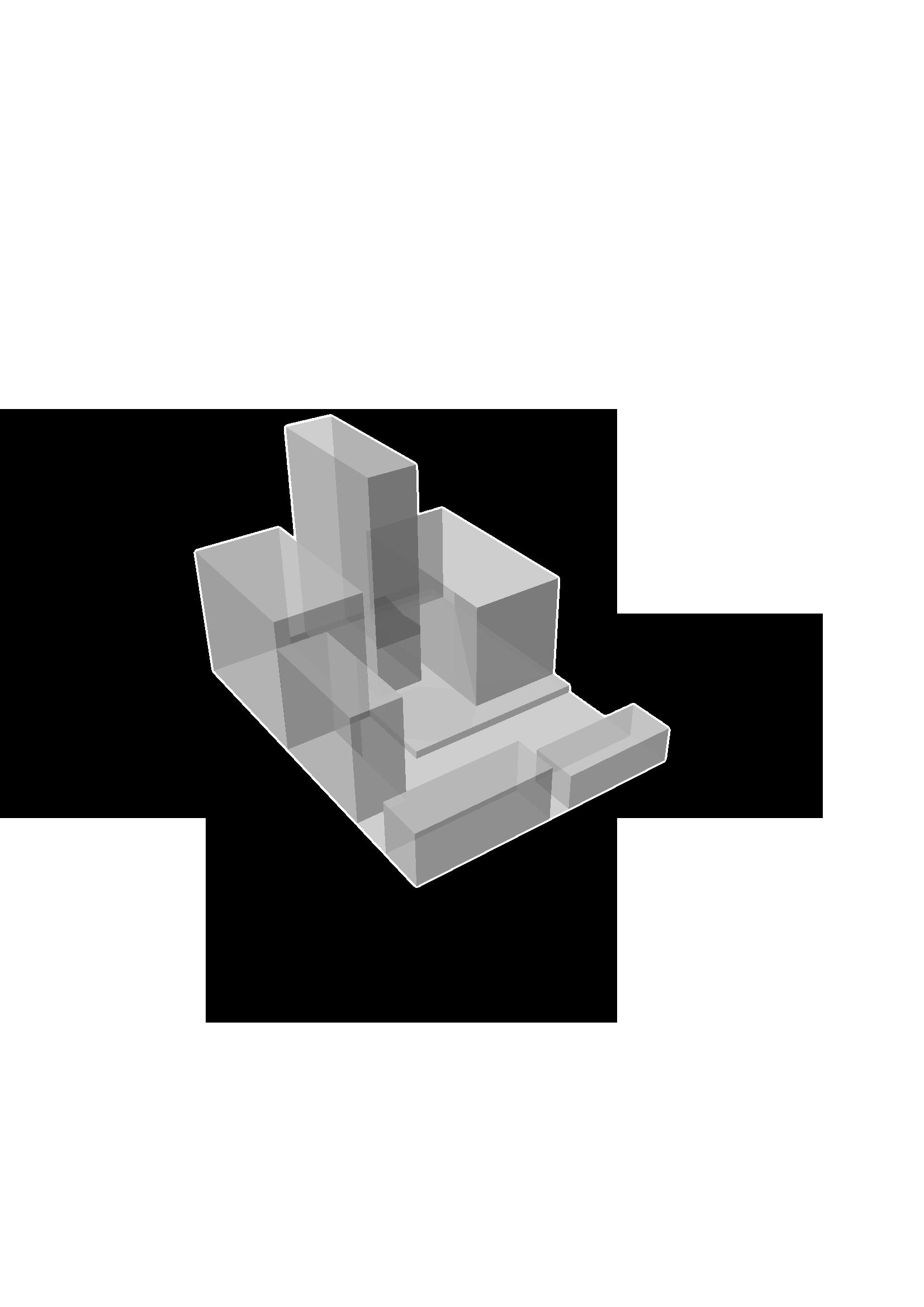
Working with larger assemblies of nets, the possibilities for spatial complexity becomes apparent. In the design shown here, the entire network exhibits a 3-way branching behavior. This is not utilized as a direct control for circulation or boundary of space. But, if you start to consider other types of pathways that may influence the movement or gathering of people, then this type of material spatial organizing be an alternative mechanism for arrangement and experience of architectural space.
The branching phenomena in this example emerges through the “hub” of associated frames (see Figure 2.2-30). It is not directly coded in the script as a “branching” function. It merely emerges because of a certain arrangement and accumulation of coincident points and edges. This poses an interesting condition for how the framework relates to the final net form. The central “hub”
because each element has a coincident condition of some sort provides no information for position in the final form. It only drives association between the nets. Thus, in Figure 2.2-28, the central hub is floating with no physical connections to it.
Recognizing this relation in the process helps to qualify some of the geometric definition in the cellular framework mechanism of the system, and the subdivision algorithm that drives it. There are 3 main conditions that arise: frames that associate with the context and create fixed anchor points, frames which only define association between neighboring nets, and frames that are a hybrid of both - association and location.
This design begins to expose more the meta-spring aspect of the system. Here, it expands beyond that as a device for connecting to anchor points. It becomes a larger network of springs which aids in controlling the overall form of the net.
2.2-28 assembly of nets in a particular context and scale. the net is arranged where density and clearly defined apertures are used to connect various directionalbased user-oriented experiences. this could have to do with environmental conditions such as view, movement, and exposure to light. a uniqueness of this type of material assembly is the porous nature from all perspectives as a cable net while from particular locations different apertures and silhouettes visually emerge.
2.2-29 outline of context in which net is installed.
2.2-30 net associations defined by cellular framework. the central hub defines the type of associations between the 4 nets. in this case, it defines a branching condition. since each aspect of each frame (point or edge) has a coincident condition, then this set of frames only defines association, not position.
2.2-31 overall network of springs is defined through 4 Net components. the 4 components are stitched together to generate a 3-way branching structure. the meta-springs (yellow) act to expand the volume of space at the branching node. with spring networks, typically, the further the springs are from the anchor points, the more compressed the cross-section becomes. the meta-springs make a more direct connection back to the anchors points adding force in expanding the cross-section at the central moment of the net.
2.2-32 front elevation of net, scale 1:500.
2.2-32 plan view of net, scale 1:500.
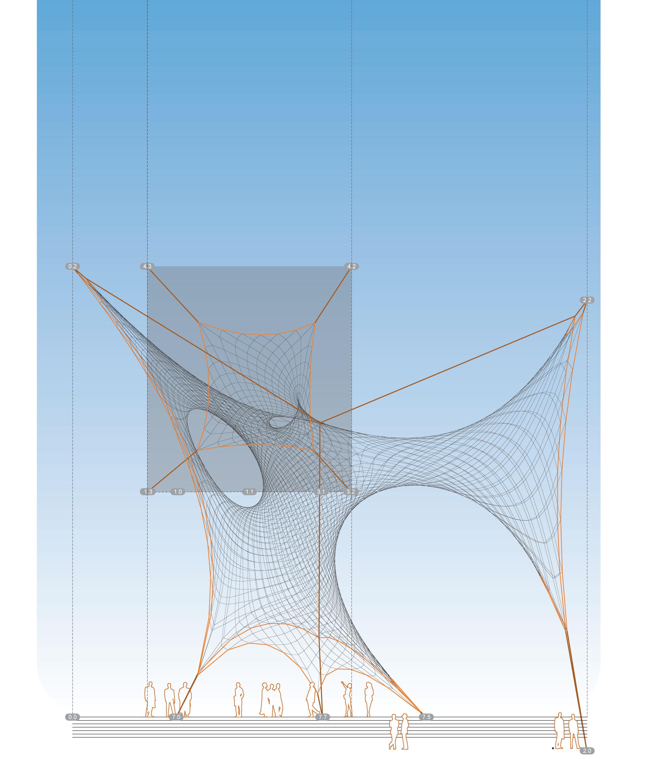
2.3_Threshold Conditions
Perceived density is different than actual density. In order to measure actual net densities from specific view points, it is not sufficient to access the logic map. Physical or even perceived proximity of nodes cannot be extracted from the topological associations.
Denser locations of nodes, formed either through multiple, overlapping nets, varied net density (weft & warp) or perspective distorsion are material thresholds that alter the perception of space. Tracking, analyzing and locating these proximities embeds visual perception as a criteria into the process of computational net formations.
2.3-1
Net Density Analysis analysis and display of iradius filter determing number of “neighbors” within each particular region.
Physical (cable-)nets vary in sizes and meshdensities. The larger the meshes of a net are, the less knots are defining its shape. The geometry formed by the net under the influence of structural forces is what the architect wants to investigate and utilize. “Utilization” in this context extends beyond the performance as a shelter against certain external pressures such as wind, light, rain.
As the form is found naturally and with the space defined through it, the focus can shift from a structural analysis towards an investigation into how this architecture is or might be able to alter the way a user / visitor / inhabitant perceives the space defined by it.
This intimate connection between well-informed form (fabrication process, flow of forces) and its influence on local environment is very intriguing. Environment can be a certain climatic condition (temperture-zones created, exposure to wind, openings for rain) but can also be seen as a spatial condition. Of course the theory of what space is has be going on for centuries and it would be out of proportion of this thesis to give an overview of even some of these in a meaningful way.
Instead of discussing the notion of space in general, we want to focus on nets as “spacemaking devices” and how, through the parameters set up and described in the previous chapters, methods for informing (existing) spaces through the insertion of nets can be formulated, accessed and utilized.
Ultimately it is about understanding architecture as a material system, capable of altering a person’s perception of space while synchronizing structure, forces and form.
2.3.1 Comparing Actual and Perceived Density
Computational and physical nets have similar properties, if analyzed visually. Their geometry is vector-based; there is no inherent surface geometry (even though nets describe the shapes of mathematical minimal surfaces). Vectors intersect and connect at nodes to form a larger networka mesh. In computational terms the description ends here. There is no meta-system defined for a mesh-geometry in today’s 3D software 1 But Frei Otto and his Team describe “meshes” as a subset of larger “nets” in his Institute’s book IL ??- NETS AND NATURE”.2 This description would equal what is computationally described as a “mesh-face”.
The important common criteria of both - computational and physical nets (we will refer to nets as opposed to meshes from now on, to describe the network of springs in the computer ) is that they take the shape of “minimal surfaces” (zero degree mean curvature), but as they are meshes as opposed to surfaces they do have a high “visual
porosity” - depending on their scale. This “Visual porosity” can be measured through a Net’s density.
As “net density” we understand the density at which a net appears on the screen (projected onto a 2D plane). This density is highly dependant on a node’s distance to the next. A computationally simulated membrane for example has a very high “net density” and a long chain has a very low “net density” value. Of course there is no example of when a node-to-node distance is actually small enough in order to be categorized as “dense” and this will have to be evaluated from case to case and maybe some field studies. Our interest was the effect that node-proximities would potentially be able to trigger and how we would be able to access this information through the methods defined previously. One obvious effect, that can be observed without any detailed knowledge of nets from a structural point of view is that, the denser a net is, the more visible it is to the spectator and the more likely it is to affect its environment . A membrane is more sufficient for blocking sunlight, than a rope.
As the nets in the previous chapter are oriented into multiple directions, it is more difficult to categorize them and their potential to influence their environment.
In order to be able to show a nets potential to act as a space making device, a method for describing their density was developed in processing. But not like in the Chapter 2.1, Node-densities can not be accessed through the logic map. This results from the fact that a spectator is able to tell, which part of a net appears denser than others, but this is not necessarily based upon a higher density / connectivity defined in the logic map. Sometimes it is just the front and back of a net overlapping, that causes it to “give the impression” of being dense. This erases all “logical” neighbourhood information and in order to be able to simulate this perceived density a new ordering system has to be constructed.
A net’s “perceived density” can be based on a meshes actual density (high number of particles and springs), but must not (multi-layered effects of nets) and the computational analysis tool for identifying these areas will have to be able to recognize both conditions..
2.3.2 Computational Threshold Analysis
In order to simulate the way we perceive a 3-dimensional net from a certain point of view in XYZ-coordinate space we need to project the location of all its particles to a plane (similar to what a 3D program does - it produces 2D images of 3D objects). This process “erases” all established node-to-node relationships of the logic map. The flattened image of the net needs a new ordering
system, not based on topological relationship, but physical proximity.
In a lightweight analysis tool, written in processing, each particle of a net simulation looks for its nearest neighbours. “Nearest neighbours” is a critical term, because it indicates that there are neighbours that are not “near”. This definition of “relevant proximity” is necessary because otherwise the tool would consider all particles except itself as neighbours, making the analysis redundant (each particle would have the same number of neighbouring particles). “Nearest” in our case is parametrically described through a circle, circumscribing each particle at a fixed radius (radius = 50cm, but this can easily be changed). If there are any particles within this range on the plane of the projected net particle , the particle is highlighted with a circle, that grows in size as the number of particles found increases. Additionally it changes its colorvalue from (RGB 0/0/0 - White) to (RGB 255/0/0 - Red) accordingly.
2.3-2
3D SITUATION
A 3-dimensional net is perceived as a 2 dimensional image. The net appears denser than it is. This effect, resulting from the projection can be simulated in processing.
2.3-3
2D IMAGE
The image of the net as the spectator sees it.
2.3-4 a-c
vdensity analysis during dynamic relaxation process because processing is a programming language initially designed for 2D-graphics, it was possible to implement the projection of the nets onto a plane efficiently. The red areas display regions of higher density with regards to the camera perspective (the camera uses a parallel projection, which results in a undistorted view). As the springs negotiate the nets final form, the areas of density shift and the net’s densities increase towards the structure’s center and the emerging minimal holes. At each frame of the animation each particle ‘s distance to its closest 3 particles (neighbours) is measured and recorded. This value feeds into the coloration and size of the circles and allow the computer to recognize zones of high density.

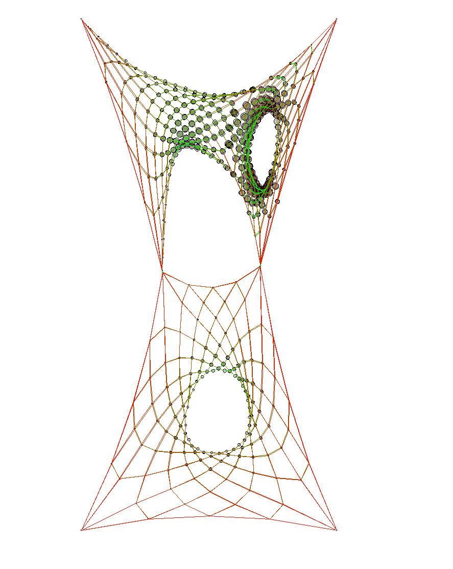
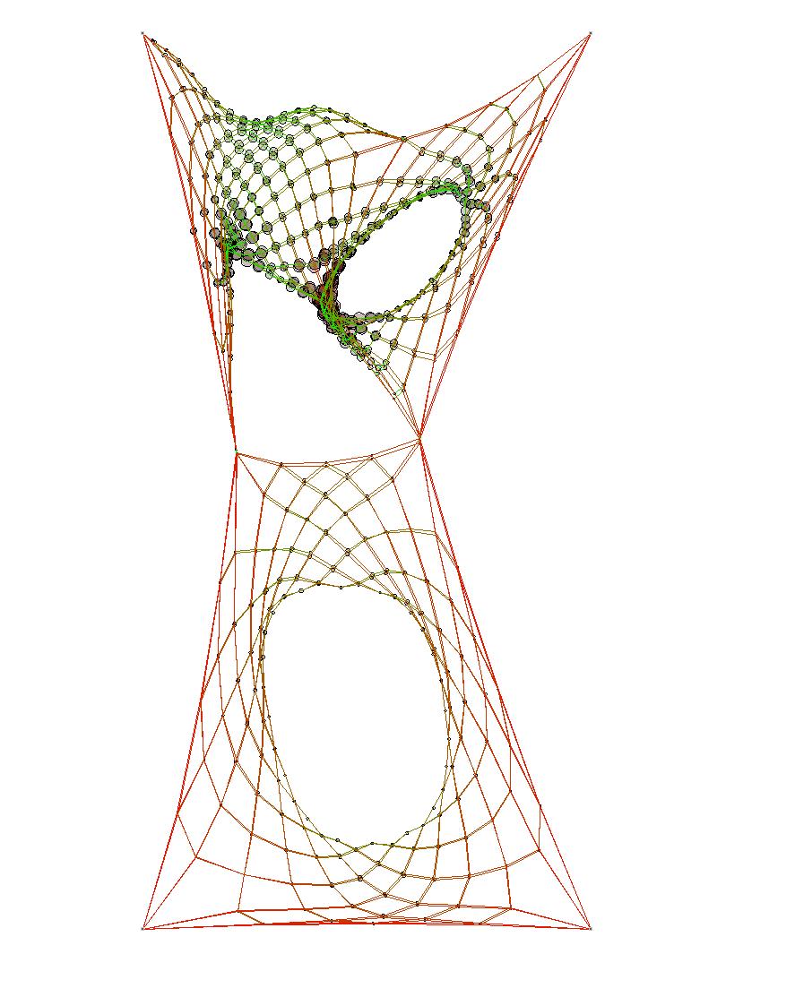
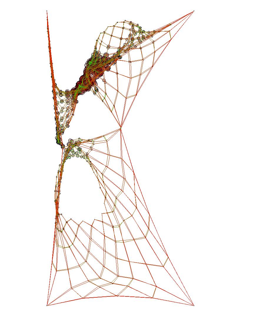
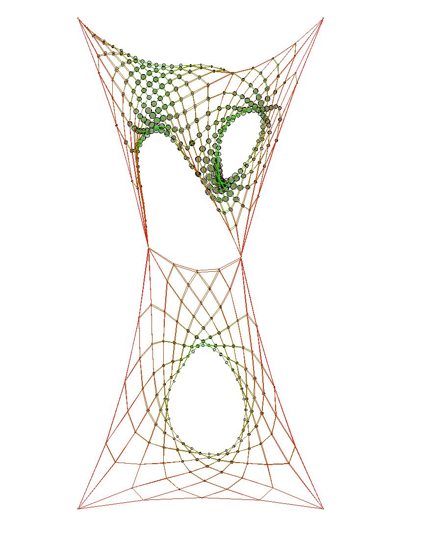
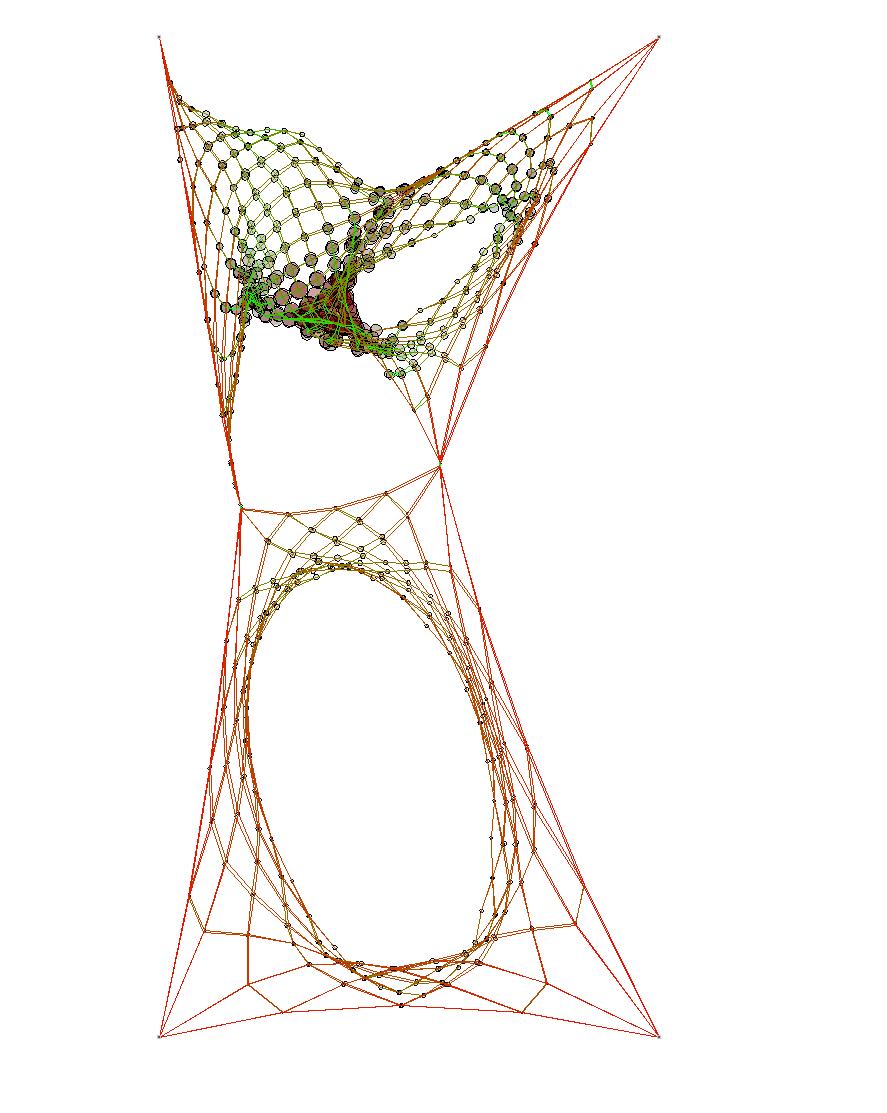
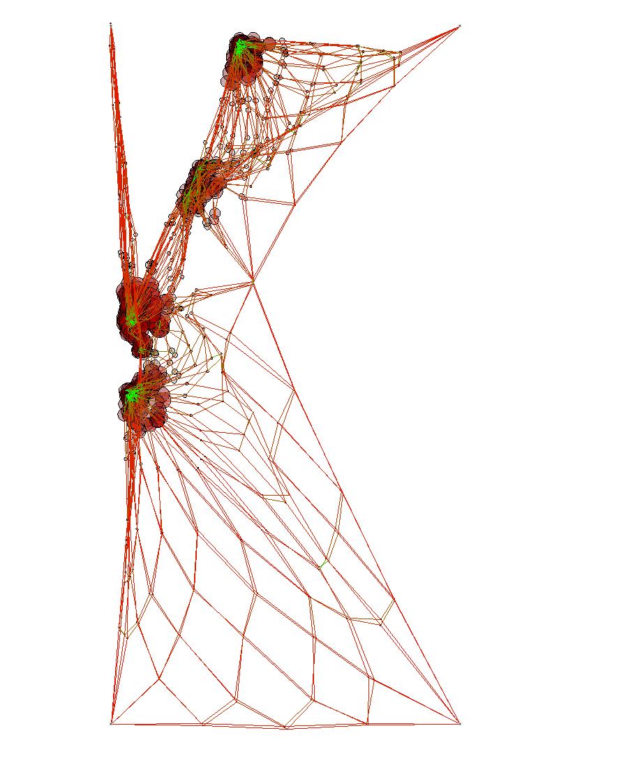
PROCESS
PROCESSING
//IMPORT (importXLS CLASS)
import a net from Rhino through Ecel and build network of springs.
# of neighbours (3) closest 3 particles
// EVALUATE determine the 3 closest neighbours within a given radius (iradius = 50 cm). Determine the amount of particles within that range (neighbours).
current
2.3-5 input geometry even though the process happens in realtime and during dynamic relaxation, the analysis of net densities of a relaxed net are described here, as their result is related to the final shape of the net.
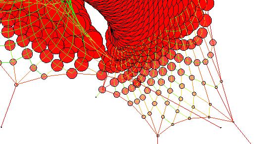
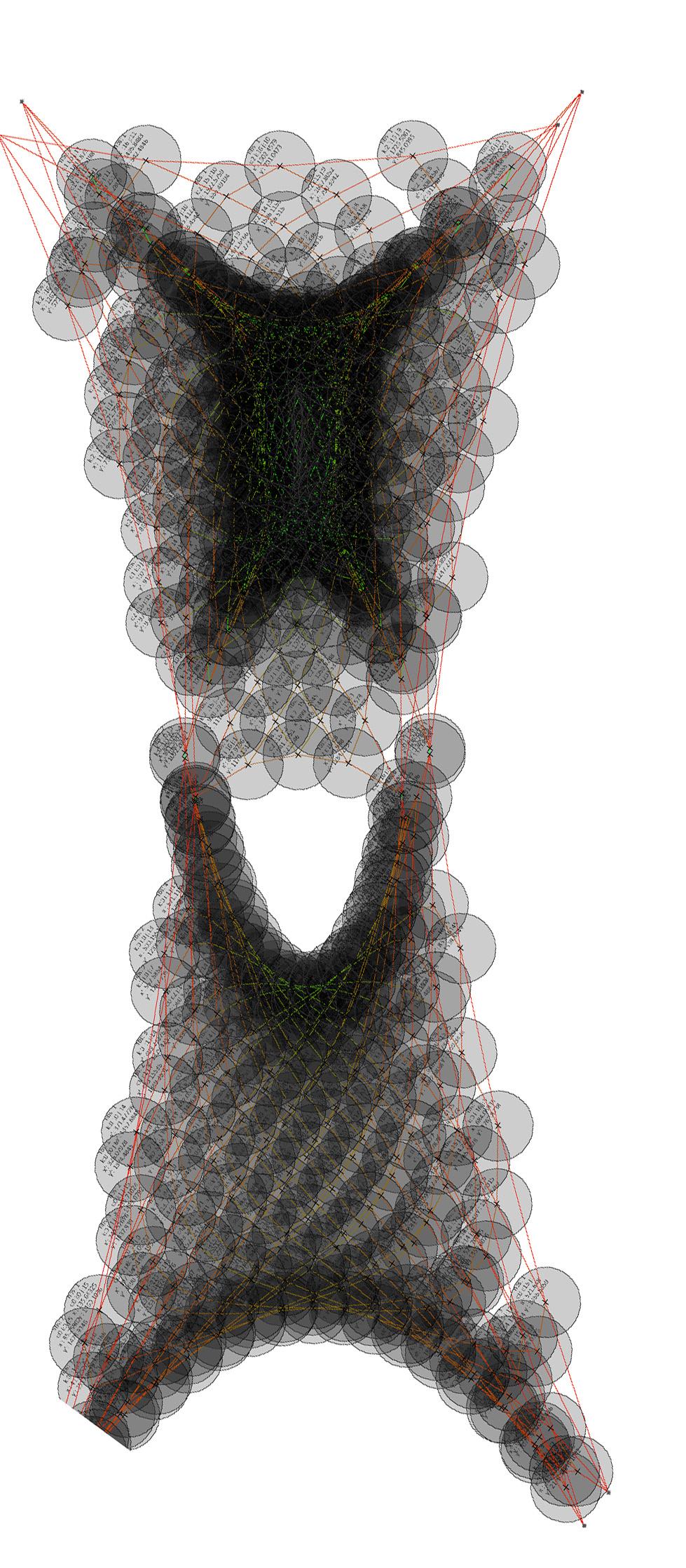
2.3-6 analysis / identifiying neighbours each particle p is projected onto a 2-dimensional plane and the looks for neighbours within a previously defined radis (iradius = 50cm).
a) single particle
b) situation close-up
c) entire net
2.3-7 evaluation / visualizing data depending on the number of “neighbours” within iradiuis, a “local density” is measured. A circle is drawn around each particle in the next step. This time not with a constant radius, but with a radius dependant on the amout of neighbours determined previously. The more particles there are within the boundaries of iradius, the bigger and more red the resulting circle will be.
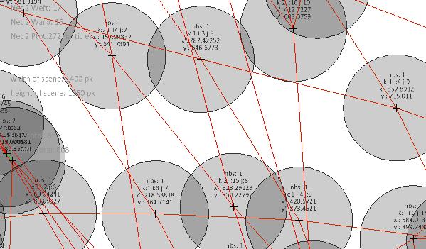
// INPUT
# of neighbours (3) closest 3 particles
//VISUALIZE (NBC2 CLASS)
draw a circle, base its RED value on the # of neighbours &assign a radius that equals the distance to the 3rd closest particle.
<- if this line is commented out, the analysis is not displayed (for fixed particles)
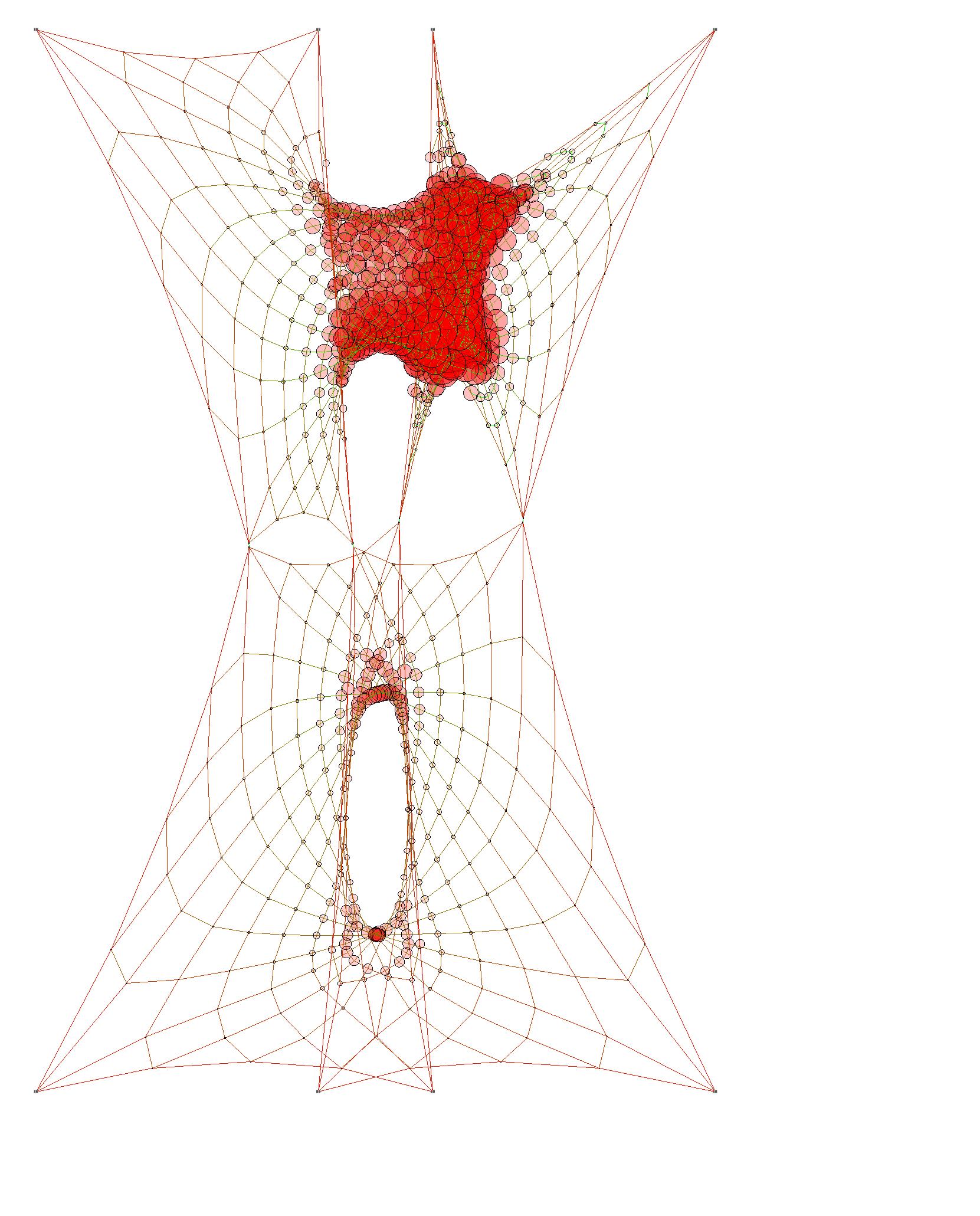
<- if this line is commented out, the analysis is not displayed (dor unfixed particles)

simulation and analysis
2.3-8 A particlereal-time
Looking “behind the scenes” of the density analysis tool. This code explains the extension to Simon Greenswold’s library in order to enable particles to “see”, “count” and “measure the distance to” their closest neighbouring particles.
See the chapter “conlusion” fore a detailed map of the workflow. comments next to each step explain each step of the script.
2.3-10 analyzed net the net is analyzed and the results are visualized immediatly.
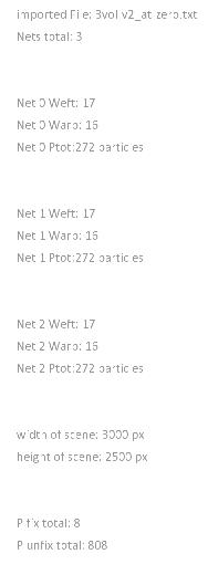
4
the resulting circle
2.3-9 inside a particle (class) the nbc2 (short for neighbourClass version 2) is the core of the density analysis.
Within this class, which is packaged into each particle, neighbours are determined, distances are measured and visual analysis tools (circles of different colors and sizes) are applied.
See the chapter “conlusion” fore a detailed map of the workflow. comments next to each step explain each step of the script.
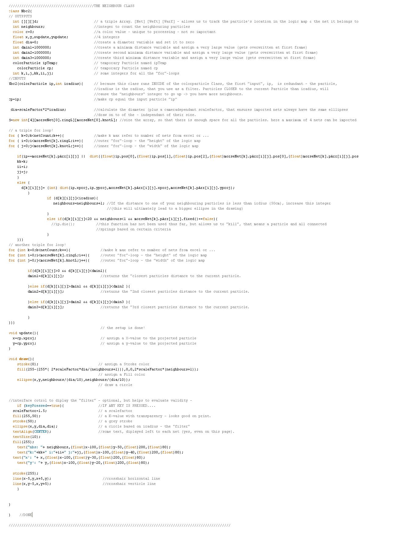
2.3-11 net installation as this analysis tool works across all scales and from all angles, it is possible to perform the analysis on other, context specfic nets, too. in this case a large nte consisting of 4 net components is observed from 3 angles. This drawing shows the side elevation view.
2.3-12 threshold analysis red areas are zones of high mesh density. In these regions, the threshold defined by the net is higher than at remote locations (anchorpoints for example)
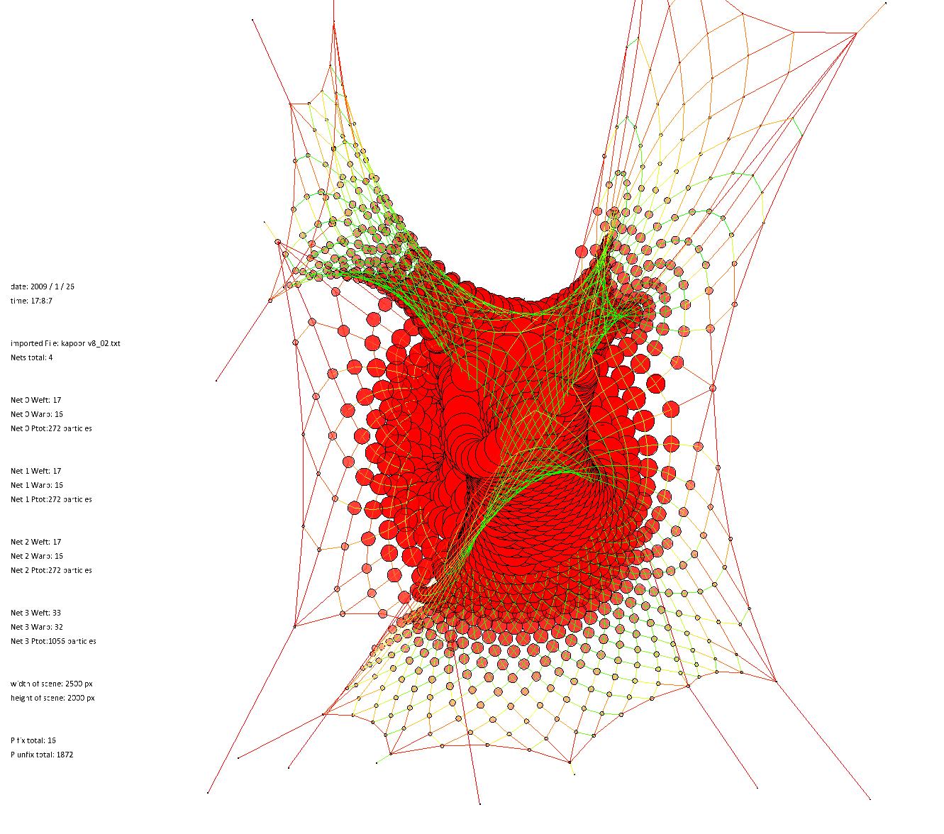
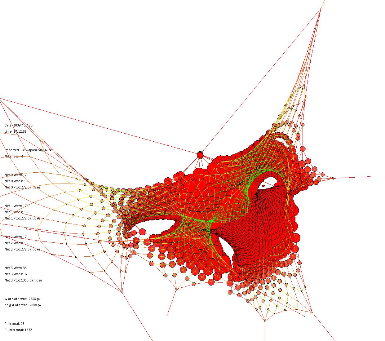
a) performed from the top from this anle, the structure diplays some openings, that would enable light to enter.
b) performed from the side net appears completely closed from this anlgle.
c) performed from the front clearly readable minimal hole condition in the net .
2.3.3 Extended Vector-Based Analysis
The ability to simulate the location of nodes through particle systems in processing computationally provides certain capabilities to alter a nets apearance / performance in certain regions, based on external pressures. The Vector-based threshold analysis promises to be an extensible tool for multiple purposes. As the net is projected onto a plane and re-evaluated based on the criteria of node-proximity in real-time during dynamic relaxation we are now able to make certain predictions about how the net will perform in ceratin regions. If, for exaple, a first “point of view” is defined at eyelevel, 10m away from the net, the net density from ground level (+- 0) to average roomheight (app. + 240cm) can be analized and regions of higher density will be less likely to be penetrated by a user’s movement, because it will appear to ba a wall-like condition of the net. As the individual moves towards the, his point-of-view changes and so does the analysis of the perceived net density. This simple program would,through the extended simulation of “decision making” be able to serve as a tool for defining “pathways” through the structure. Another example would work in the same manner, but the POV (point of view) could be considered as the sun’s path. As the sun changes its position throughout the day, the net appears denser or less dense.
Through simple alteration of the net configuration (mesh density defined in the logic map through the amount of particles, adding multiple nets in
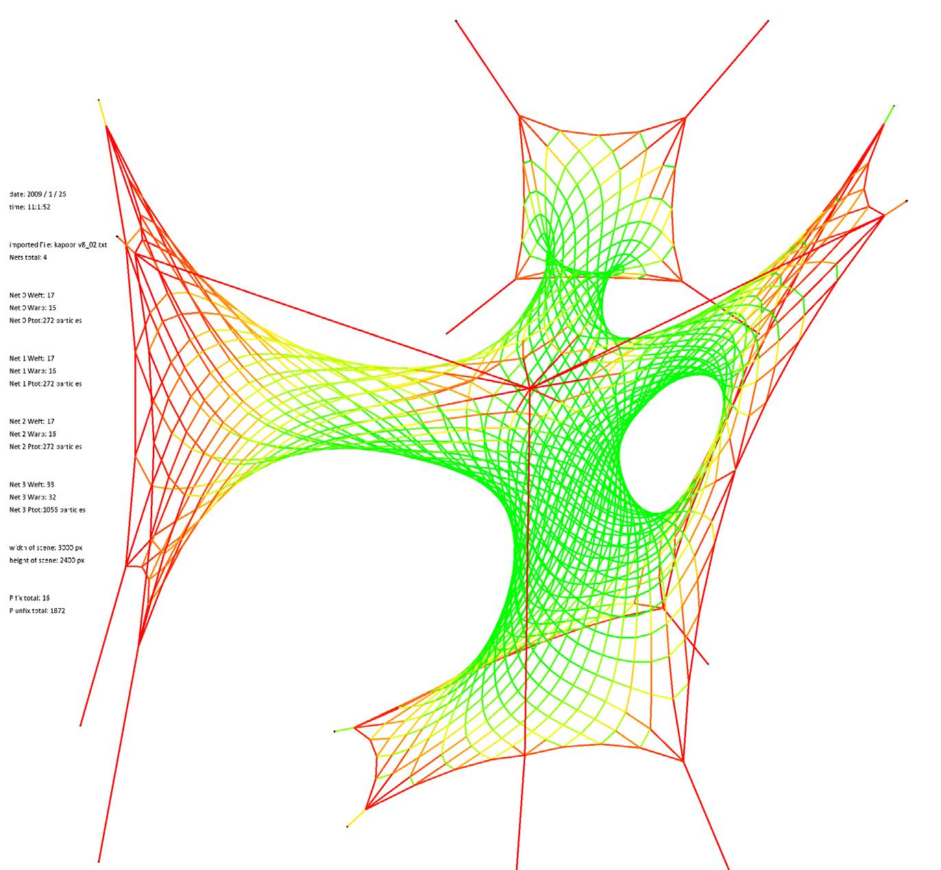
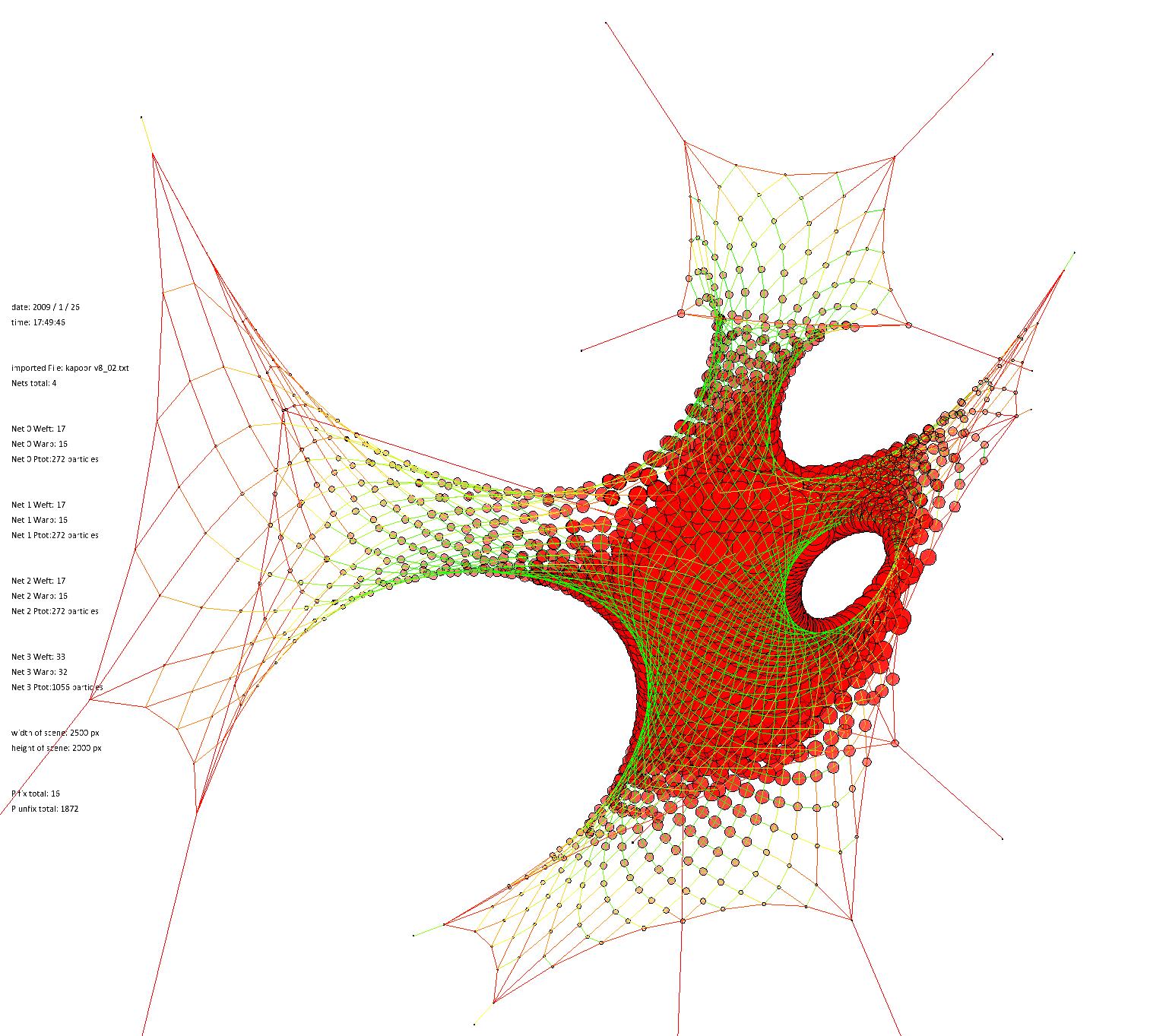
the same location, varying spring rest Lengths, location of fixed particle position, adding dense subnets, similar to membranes....) it is possible to enhance the performance of a net with regards to the amount of threshold it defines which in the next step has multiple repercussions on how sunlight pentetrates it or a person recognizes its shape.
By setting up multiple criteria (for example ability to move through and “shading”- high density of net from the sun’s current POV) and defining the parameters which can be altered, a perfect framework for a net-evolution based on a genetic algorithm has been set up.
2.3-13
2.3-13
structural analysis based on the deviation of a springs actual length to its restLength, the ditribution of forces can be visualized as well. Thiss happens at the same time as the density analysis.
2.3-14 paths
depending on a nets ground condition, certain patterns of movement can be allowed. Through the option of fixing and unfixing particles this movement can be altered, accelerated, slowed down.
This intervention, though, occurs only on the ground plane. In 2D.
The net density is a tool that allows a 2D-analysis of a 3-dimensional system of net components. Because of the object-based nature of the scripts it is possible to now examine and expose the parameters contributing to specific net conditions and re-parametrize them. These interventions could be undertaken to further define a visual threshold from different angles, in order to prevent rain from entering from the top, wind from passing through from a side and still maintain enough porosity in the structure to allow movement or emphasize paths and views.
3 APPLICATION & OUTLOOK
3.1 Contextual Inputs
3.1-2
The Turbine Hall at the Tate Modern was chosen as a specific context to insert a tensioned net structure. This allows for a comparison to the tensile structure design by Anish Kapoor and ARUP, Marsyas, installed into the Tate Modern in 2002.
While the Marsyas installation is a membrane structure and the Cylindrical Net Morphologies are cable-nets, there are still possible comparisons from a design process point of view, and through analyzing manufacturing methodologies.
The artist of Marsyas portrays the installation as one of such great scale that it cannot be understood or documented from one particular view. Kapoor contends that the plan cannot be visually understood through any experience of viewing or walking around the structure.
With the Cylindrical Net Morphologies, there is this same characteristic of not being able to ascertain the true shape of the form. But, the interesting condition is because of its porosity as a net, you can view all elements that make up the structure from each perspective, but you still cannot determine exactly the movement of the surfaces and the overall assembly.
3.1-1
Cylindrical Net Morphologies installation design for context of Tate Modern Turbine Hall.
3.1-2
tensioned membrane installation by Anish Kapoor and ARUP, titled Marsyas, in the Tate Modern Turbine Hall, 2002.

From a design standpoint, the installation proposal looks to vary the description of view, boundary and aperture through the inherent capabilities of the cable-net structure. Porosity can be defined through ranges of densities in the net pattern. Larger densities degrade the appearance of a continuous net, invoking the view through it to become more primary. Where the network becomes highly dense, the surface of the net itself becomes more prominent. There is also the function of the holes that emerge in various forms within the entire network of cylindrical net components. They are directional (in that they contain a certain depth to them) so that they can be read only from certain positions. An effort was exerted to try to position these holes so that they may offer connections for view, movement, and
light. This analysis is not fully explored, though, in this design model.
To position the certain effects, the arrangement of cells, and the controlling of the meta-springs it utilized. The meta-springs are varied in degrees of connection and their strength, so that they may reposition larger areas of the net (see Figure 3.3-7). The resulting edge springs and Cylindrical Net components are a consequence of the associations between cellular frameworks and the stronger meta-springs.
The meta-springs also aid in articulating the form where a minimal number of anchor points are possible.
3.1-3 Cylindrical Net Morphologies design proposal for Tate Modern Turbine Hall. north elevation, scale 1:5000.
3.1-4 section looking east, scale 1:5000.
3.1-5 floor plan scale 1:5000.
3.1-6 cellular framework for installation built of cells with topologies ranging from 4-sided to 8-sided.
3.1-7 meta-springs and edge springs extracted from dynamically-relaxed model.
This arrangement of springs is generated from 8 Cylindrical Net components. The directionality and degrees of association are highly varied. The image at right shows the type of apertures (holes) that emerge from various direct inputs and indirect hierarchical relationships. The orientation of the framework (up-down or left-right, for instance) will establish a fairly clear direction for the Cylindrical Net component. The directionality of one of the branched apertures (see Figure 3.1-9) shows how the feature of component directionality can be more intuitively controlled. Here, an aperture is generated to create a view connection to one of the protruding boxes on the upper level.
Between components, emergent properties are revealed as associations generate secondary
cylinders (between 2 stitched Net components), and holes (multiple cylinders attached at corner, but not along all edges).
These can be understood as emergent properties where they are not discreetly scripted into the assembly of the nets. Also, their properties arise through the interlinking of points and edges: the most basic elements of the process. There are not separate components, or separately programmed functions to deal with different scenarios of association. The overall effects are driven by the analysis of points and edges and their degrees of coincidence. More complex effects arise as the number of elements increase and the types of associations expand. For instance, when more than two points and/or edges are coincident a branching type
3.1-10
3.1-9
3.1-8 view from bridge looking towards entry.
3.1-9 view from bridge towards protruding box on upper level.
3.1-10 directionality for framework, roughly indicating the directional orientation of the Net component.
arrangement can occur. As shown in Figure 3.1-8, apertures can emerge through the definition of a surface (within a single cylindrical component) and also through a series of connected edge springs (the open boundaries of the multiple neighboring components).
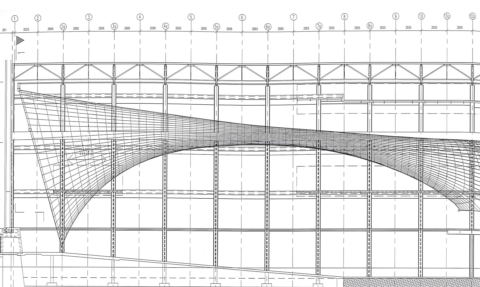
The main topic for discussion when comparing the two designs and their respective methods revolves around the functionality of the design process to produce a certain level of valid and valuable results.
For Arup, they focused on developing a quick design process that could simulate tension-active structures. We they developed was a similar spring-based computational process.1 But, to consider fabrication they only saw their model as static geometry and exported that information to Tensys, to regenerate as a tensile structure and extract information for membrane material patterns. In general terms, Tensys created cutting patterns by taking strips from their models and “shrinking” it to respect material elasticity and
tension force. This same strategy was utilized for the Installation at the AA, though for a cablenet structure. In simulating similar details to the Marsyas, a different approach was taken from that of Arup’s design process. Where the ring hovers above bridge to add a pulling force, our system utilizes meta-springs to capture internal portions of the net and tie them back to the anchor points. This allows for a higher level of articulation and essentially creates the impression of an anchor points where there is none.
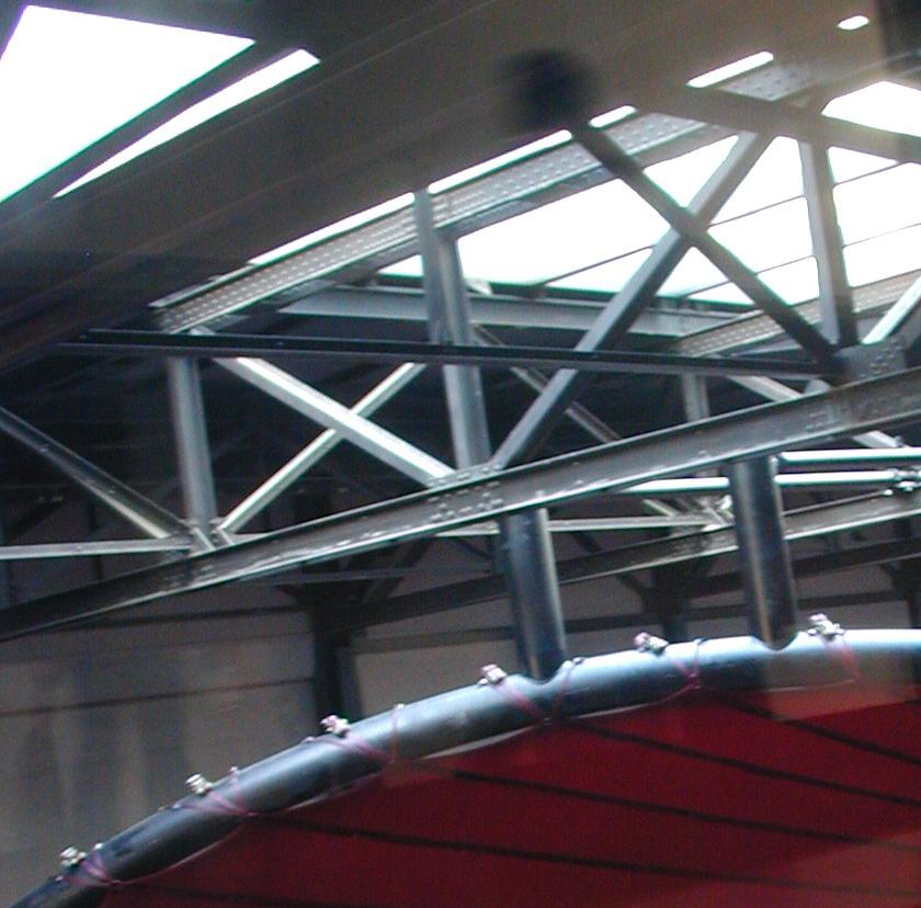
The method for utilizing downward force could be simulated with the particle system driving the Cylindrical Net components. By enabling and controlling the variables of particle mass and environment gravity, a pulling force, through the
particles, could be simulated. Arup used sand in the large ring to balance the structure and provide proper force. The mass values for particles could be connected to such a method for physical construction.
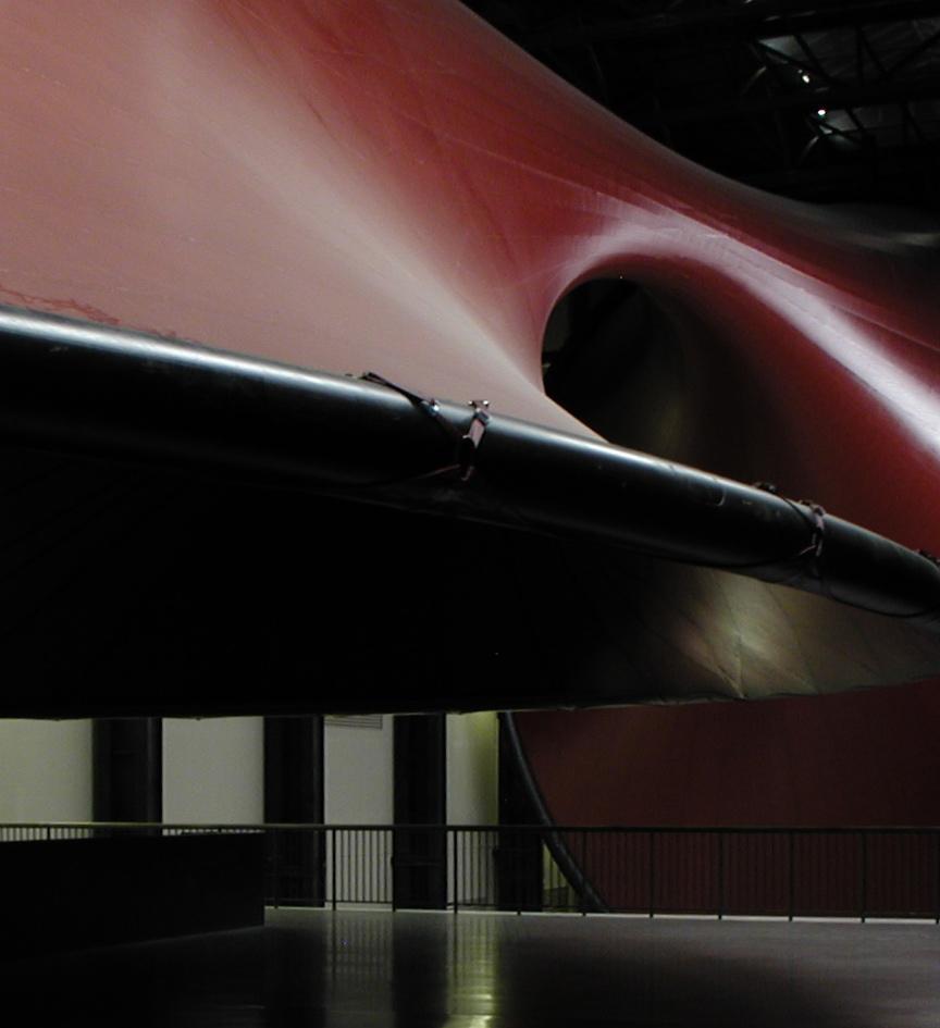
When viewing the design approach and intentions, there is no telling whether the process or the idea produced the simple 3 pronged branch structure for the Marsyas installation. But, with the Cylindrical Net components, a higher level of complexity can be achieved and with embedded indicators for structure and construction through the meta-springs, the edges springs, the analysis for force, and the logic for fabrication.
1 Engineering Marsys at Tate Modern, The ARUP Journal, 01/20/2003.
3.1-11 weighted compression rings adding downward force for the tensioning of the overall membrane structure (left). direct connection of another compression ring to the structure of the Tate (right).
3.1-12 use of meta-springs to aid in structuring and articulation of the overall cable-net form.
3.1-13 activating of mass and gravity would allow for simulation of downward force, akin to the horizontal ring in the Marsyas installation.
3.1-14 to simulate a compression ring, the spring’s capability to exert compression force could be utilized.
3.1-15 detail elevation of Marsyas.
3.1-16 detail elevation of Cylindrical Net Morphologies design.
3.2 Conclusion
First looking at the Cylindrical Net Installation for the AA, the experiment intended to take a physical phenoma (form-found cable net), translate it to a computational simulation, and convert that back to a digitally-informed but manually-constructed object. This scope would typically produce what would be called a “material system”: a set of associated materials that are constrainted by parameters for material and manufacturing, where shape is formed under the pressure of structural forces.
What was of particular interest with the AA Installation was the nature in which the cable net described different boundaries of space within its relatively small footprint. Some areas were more clearly, visually apparent (see Figure 2.1-41), while other were only vaguely described because of the overlapping of open nature of the cable net’s mesh. Expanding the previously stated definition of “material system”, the last stages of research focused on considering the net’s affect on space as a built-in criteria within the computational process.
3.2-1
various Net components isolated from the overall spring network generated for the design of the Tate Modern installation (see Chapter 3.1.1)
SPATIAL SUBDIVISION

define number of cells select envelope-volume 001 subdivide envelope-volume 001 based on number of cells save

CREATE
This map explains the individual steps, that make up the entire process of the computational formfinding process. The extraction of data for fabrication is for purposes of readability not repeated, as it is explained in detail in chapter2.1 “embedded fabrication”.
Rhino generates the geometry (points) that serves as the framework for the dynamic relaxation. These points are created through the extraction from surface corner points, that are part of a larger volume-geometry. These Poly-surface geometries are generated through a “Spatial Subdivision” algorithm. The points provided, can be fixed in order to represent beams and other anchor point conditions. This data is written directly into Excel via a VBscript-function.
Excel serves as a data converter. But not only is the data gathered and restructured in Excel. Through comparison of coordinates, coincident points are located, tagged and additional information is added, that gets transferred into Processing.
Processing logic map is built based on the information provided by Excel. The net components necessary to connect between the point sets provided by the “spacial subdivision algorithm” in Rhino are created. Into each net, the edge cables are inserted and serve because of their higher spring strengths as a meta - structure for the nets. In a last step multiple nets are connected together and to the anchor points by very strong springs. Through the repetition and simple rules of connectivity a large network of springs with different hierarchies is constructed.
This network can be analyzed with lightweight tools directly built into the particle and spring classes. The neighbor class identifies neighboring particles and visualizes high net densities, that potentially turn the net into a space-making device. Inside of each spring is a colorcoding algorithm that is used and can be accessed at any time to visualize the distribution of tensile and compression forces within the entire architecture of cylindrical net components. conclusion
surface 01
.pde
point01
point02
point03
(...) multiplier
surface 02
point01
point02
point03
(...) multiplier
xlsImport (*.xls) class { } net class
{ }
import excel data by row
create corner particles create edge particles
create net particles create net springs
edgeCable class { }
create edge springs based on multiplier value
edgeStitch class { }
create stitch springs
Particle class
setup Particle Object
location (X,Y,Z)
fix (true / false) mass (int)
draw Particle Object
neighbours class { }
setup neighbours
project particle to Cplane count particles within iradius (nbs) measure distance to 3 closest particles
draw neighbours Object
set fill to R-value based on neighbours within iradius (nbs) draw circle with radius based on 3rd closest particle
colorSpring class { }
setup Spring Object
restLength (double) strength (double) damping (double)
draw Spring Object
measure spring‘s current length ( d ) set strokeColor to value based on current length ( d )
3.2-5 3.2-6
The previous graph speaks of the elemental steps which develop the computational spring networks. The functions are built of simple scritping mechanisms (for-loops and if-statements) and organized into classes and functions. The simplicity of each scripted element allows it to be extensible and applicable to a various range of inputs and produce a vast array of geometries. This connection from the simple yet extensible processes to the ouput is what begins to generate emergent conditions in the architecture that is being produced.
The example that most descsribes this is the occurence of a branched condition. With the computational process being built of elemental methods it is not explicitly encoded for a branched condition to occur. But, as the script works fundamentally with points and edges - certain associations end up producing various branched conditions (a 2-way branch (at left) and a 3-way branch (above)).
These occurences are architectural, as they shape a volume and estabish a direction of movement. Driven by the computational spring, there are indications for material type and calculations for stresses. The assembly sequence is still mapped into each Cylindrical Net component since they maintain there internal IDs and network topologies.
A general defintion of an emergent condition is a situation that is borne of local interactions
which produce some sort of discernable macrobehavior.1 The compuational process for the Net works primarily at the lowest, most local level of the system: the point (the particle), the edge, and the spring. The spring can only connect two particles. It, therefore, can only negotiate at the local level. The macro-behavior that arises is that of a larger continous network generating various threshold conditions.
Though there are macro-behaviors that can be understood from the Cylindrical Morphologies, there is an interesting characteristic to where the entire assembly cannot always be visually understood. Because of conditions of overlap and varying densities in the mesh, the description of the overall structure is not always readily attainable. It is possible, though, that this adds experience and user-defined perspective as a part of the emergent behavior of the overall system. Through various movements of the user, a new (or different) understanding of the macro-behavior becomes apparent.
3.2-2 diagram of framework and frame associations. the arrangement generates a spring network that exhibits a branching volumetric structure.
3.2-3 spring network exhibiting a branching structure.
3.2-4 exploded diagram of individual Cylindrical Net components.
3.2-5 exploded diagram of individual components from proposal for Tate Modern installation (see Chapter 3.1.1).
3.2-6 floor plan with colored Cylindrical Net components.
Simulation is typically seen as an engineer’s tool for analysing the structural phenomena in particular material arrangements. This removes it from the realm of design investigation. When material and structural properties can be embedded into simple components of an accessible digital process, then iterative design experimentation can be engaged. An example of this has been discovered in the use of springs within the Processing programming environment. Once structural behaviour and manufacturing logics have been invested into the process, the system is able to pursue the relationship between material arrangement and its effects on space, organisation and environment. Behaviour can be expanded beyond technical and engineering realms encompassing particularities of architectural space.
(http://twenty1f.com/high-techlow-tech-exhibition/)
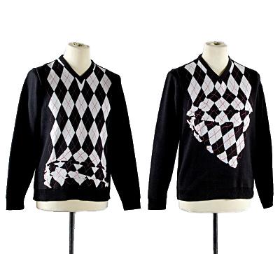 3.3-1
Argyle pullover (2001/2). Luna Maurer / Roel Wouters. Acryl. Machine braided. image: Luna Maurer.
3.3-1
Argyle pullover (2001/2). Luna Maurer / Roel Wouters. Acryl. Machine braided. image: Luna Maurer.
The translation from computation to fabrication is an on-going avenue for research. It is particularly critical with tension-active structures where force is “live” and an embedded feature in the design process. With the Marsyas example, ARUP chose to utilize a form-finding software to generate a static geometry, though presumably built of minimal surfaces. With the AA Installation, it was chosen to build a tensioned net, though the tension had a different dynamic from that of the computational model. The computational model used springs of all similar rest lengths. The physical structure used strings of different lengths (though measured to a shorter distance than what the digital model indicated, to automatically incite tension in the structure). This version, computationally, would mean that each spring would have a different rest length.
These types of comparisons are important to continue to experiment with, setting up computational models and testing results with constructed models. When moving up in scale, these issues become even more critical, placing more scrutiny on the nodes (connections) as well as the strings.

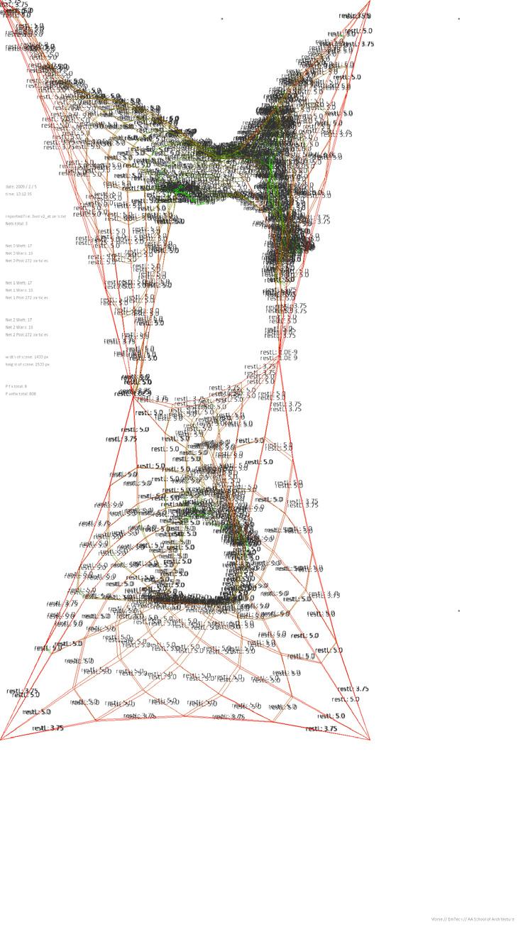
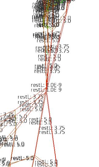
3.3-2
The rest lengths of each spring can be accessed and changed at any time during the process of dynamic relaxation.
Because every spring (of the same type) has the same rest length spring is stretched to a different degree. The resulting actual length indicates the distribution of forces throughout the entire structure. The areas of high tension are colored red.
3.3-3
Two lines of code are enough to change the force distribution from one second to another, while maintaining the structural integrity of the tension active system. The code is executed at frame 100 of the process of dynamic relaxation and every 20th frame after that. It checks, if a spring is stretched “too much” (beyond twice its rest length, in this case) and resets the rest length to three quarters of the actual, measured distance. This keeps the spring in tension and unifies the distribution of force. In the physical world, the different rest length values would equate to different material lengths (which can be grouped to larger sets of strings for manageability, as shown in the AA exhibition), whereas the model shown in 3.32 represents a model made out of very elastic material - but of the same rest Length.
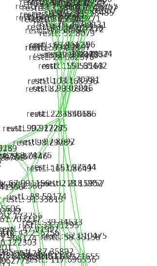
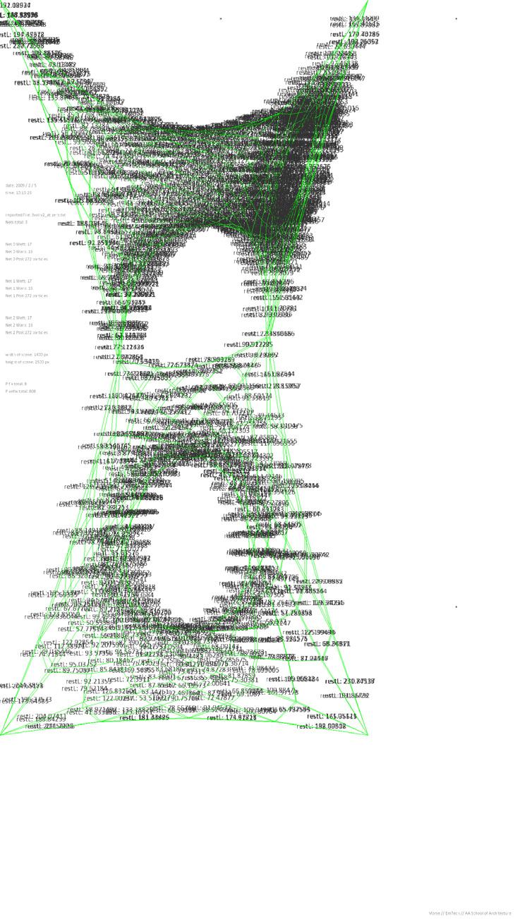
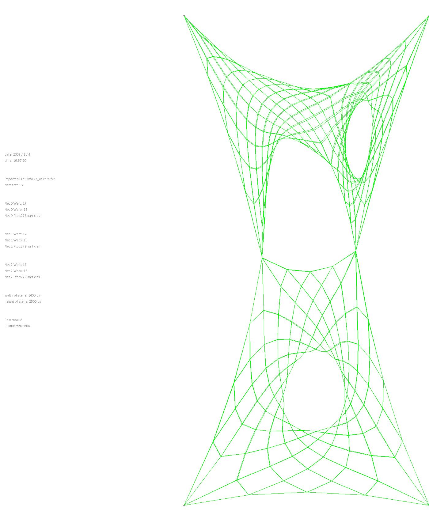
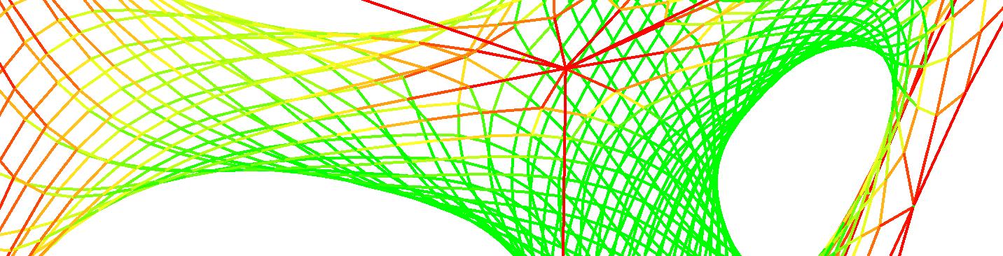
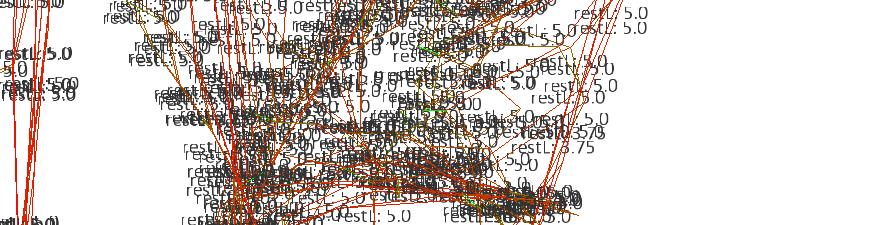
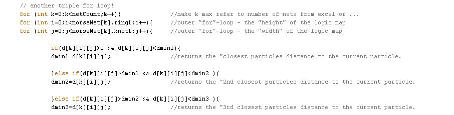
3.3-4

the transparency of the digital form finding process allows all information related to structure and geometry to be accessed at all times. The computational spring is the one element in the current models, that drive the process of dynamic relaxation. The next interesting steps would include a validation of the process by the use of elastic material in another, larger physical prototype (3.3-5). In a next step, as larger structures would have to be tested, stronger materials would have to be used, utilizing the individual rest length function described on the previous page (3.3-6). It is necessary to expand the view from the singular element to larger networks and the way in which they are fabricated. Fishing nets are such examples Usually they do consist of similar mesh sizes (3.3-7). The automation of weaving and braiding through industrial machines (3.3-8) potentially enables the realization of nets with differing mesh sizes as shown by Evan Greenberg in his EmTech dissertation (MSc 2008).
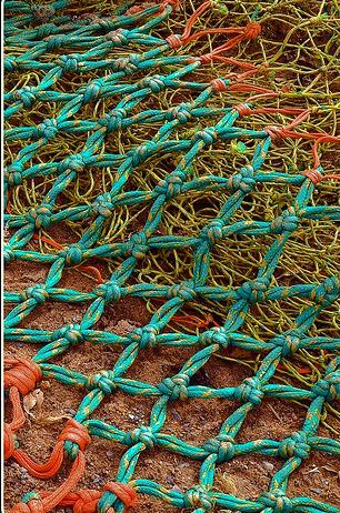
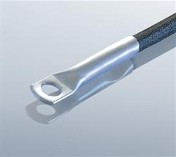
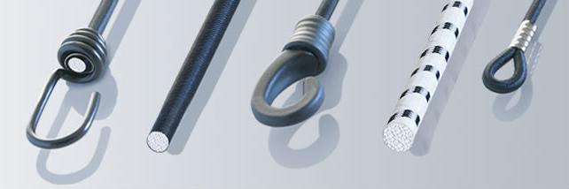
4 REFERENCES
Hensel, M and Menges, A, Inclusive Performance: Efficiency versus Effectiveness, Versatility and Vicissitude: Performance in Morpho-Ecological Design, 2008, Volume 78 No 2, 54-63.
Carroll, S, Endless Forms Most Beautiful: The new Science of Evo-Devo and the Making of the Animal Kingdom. London, Orion Books Ltd, Phoenix, 2007.
Medhi, D and Ramasamy, K, Network Routing: Algorithms, Protocols, and Architectures, Morgan Kaufmann Publishers, San Francisco, 2007.
Dye, M, McDonald, R and Rufi, A, Network Fundamentals, CCNA Exploration Companion Guide, Cisco Press, 2007.
Rutten, D, RhinoScript for Rhinoceros 4.0, Robert McNeel & Associates, Seattle, 2007.
Pottman, H, Aspel, A, Hofer, M, Kilian, A, Bentley, D, Architectural Geometry, Bentley Institute Press, Exton, 2007.
Greenwold, S, Form-Finding and Structural Optimization: Gaudi Workshop. MIT, Cambridge, 2004.
Wills, T, DForms: Concept by Toni Wills, http://local.wasp.uwa.edu.au/~pbourke/surfaces_curves/dform/ [01-04-08]
Turner, J, The Tinkerer’s Accomplice: How Design Emerges from Life Itself, Harvard University Press, Boston, 2007.
Johnson, S, Emergence: The Connected Lives of Ants, Brains, Cities, and Software, Penguin Books, London, 2001.
Frazer, J, Themes VII: An Evolutionary Architecture, AA Publications, London, 1995.
Evans, R, Figures, Doors & Passages, Translations from Drawing to Building and Other Essays, Architectural Association Publications, London, 2003.
Holland, J, Emergence: From Chaos to Order, Oxford University Press, Oxford, 2000.
Berlinski, D, The Advent of the Algorithm, Harcourt, Florida,2001.
Leach, N, Turnbull, D, Williams, C, Digital Tectonics, Wiley Academy, West Sussex, 2004.
Hight, C, Architectural Principles in the Age of Cybernetics, Routledge, 2008.
Kemp, M, Seen/Unseen, Oxford University Press, Oxford, 2006.
Hensel, M, Menges, A, Weinstock, M, Techniques and Technologies in Morphogenetic Design, 2006, Volume 76 No 2.
Hensel, M, Menges, A, Weinstock, M, Emergence: Morphogenetic Design Strategies, 2004, Volume 74 No 3
Bedau, M, Emergence: Contemporary Readings in Philosophy and Science, The MIT Press, Cambridge, 2008.
Otto, F, Netze in Natur und Technik - Nets in Nature and Technique. IL 8, Stuttgart: Institut für Leichte Flächentragwerke, 1976.
Reas, C, Fry, B, Processing: A Programming Handbook for Visual Designers and Artists, The MIT Press, Cambridge, 2007.
Yoshida, N, A+U Special Issue: Cecil Balmond, May 2006, Volume 2006:10.
5 APPENDIX
Option Explicit
'Script written by Sean Ahlquist
'Script copyrighted by morse
'Script version Friday, November 21, 2008 5:49:21 PM
''/////create excel file
Dim objXL , objXLSheet
''Dim xlRight = -4152
Set objXL = CreateObject ( "Excel.Application" )
objXL . Visible = True
objXL WorkBooks Add
objXL Columns Select
objXL Columns ColumnWidth 7
objXL Selection HorizontalAlignment =- 4152
objXL UserControl = True
Set objXLSheet = objXL . ActiveWorkbook . WorkSheets ( 1 )
Call idCornerPoints ()
Sub idCornerPoints ()
Dim boundarySurfs
boundarySurfs = rhino . GetObjects ( "select TOP and BOTTOM surfaces (in PAIRS)" , 8 )
If IsNull ( boundarySurfs ) Then Exit Sub
If ( ubound ( boundarysurfs )+ 1 ) Mod ( 2 )<> 0 Then rhino print "even numbered set of surfaces required exiting routine"
Exit Sub
End If
Dim i , j , k , kk , m , pairCount , ptListCount , cp (), edges , tempPt0 , tempPt1 , edges0 , edges1 , ptCount , edgeCountVaries , ptDirection , vectorBaseLine
Dim textDot ptListCount = 0 pairCount = 0
For m 0 To ( ubound ( boundarySurfs )+ 1 )/ 2 - 1
''/////determine the MAX value of corner points rhino . EnableRedraw False edges0 = rhino DuplicateEdgeCurves ( boundarySurfs ( m * 2 ))
edges1 rhino DuplicateEdgeCurves ( boundarySurfs (( m * 2 )+ 1 ))
If ubound ( edges0 ) > ubound ( edges1 ) Then rhino Print ( "point count varies" )
ptCount = ubound ( edges0 )
edgeCountVaries = True
ElseIf ubound ( edges0 ) ubound ( edges1 ) Then rhino Print ( "point count EQUAL" )
ptCount = ubound ( edges0 )
edgeCountVaries = False
Else
rhino Print ( "point count varies" )
ptCount ubound ( edges1 )
edgeCountVaries True
End If
rhino Print "max number of cPts: " & ptCount + 1
rhino . DeleteObjects edges0
rhino DeleteObjects edges1
rhino EnableRedraw True
For k = pairCount To pairCount + 1
edges rhino DuplicateEdgeCurves ( boundarySurfs ( k ))
rhino print "ubound edges: " & ubound ( edges )
If edgeCountVaries = True And ubound ( edges ) < ptCount Then rhino Print "edge count varies between two surfaces"
If k = pairCount Then
kk = pairCount + 1
Else
kk pairCount
End If
''/////rebuild edge for surface that has less corner points
edges = rebuildEdges ( boundarySurfs ( k ), boundarySurfs ( kk ))
rhino print "ubound edges (rebuilt): " & ubound ( edges )
End If
''////create first two corner pts based on edges(0)
If k = pairCount Then
ReDim Preserve cPt ( 1 )
cPt ( 0 ) rhino EvaluateCurve ( edges ( 0 ), rhino CurveDomain ( edges ( 0 ))( 0 ))
cPt ( 1 ) = rhino EvaluateCurve ( edges ( 0 ), rhino CurveDomain ( edges ( 0 ))( 1 ))
vectorBaseLine = array ( cPt ( 0 ), cPt ( 1 ))
''////create first two corner pts based on edges(0)
If k = pairCount Then
ReDim Preserve cPt ( 1 )
cPt ( 0 ) = rhino . EvaluateCurve ( edges ( 0 ), rhino . CurveDomain ( edges ( 0 ))( 0 ))
cPt ( 1 ) rhino EvaluateCurve ( edges ( 0 ), rhino CurveDomain ( edges ( 0 ))( 1 ))
vectorBaseLine = array ( cPt ( 0 ), cPt ( 1 ))
Else
ReDim Preserve cPt ( 1 )
cPt ( 0 ) rhino EvaluateCurve ( edges ( 0 ), rhino CurveDomain ( edges ( 0 ))( 0 ))
cPt ( 1 ) = rhino EvaluateCurve ( edges ( 0 ), rhino CurveDomain ( edges ( 0 ))( 1 ))
''///determine the proper cPt0 as compared to other string of points
''/////compare angle to determine clock-wise or counterclockwise
'' ptDirection = setDirection(edges,vectorBaseLine)
'' ReDim Preserve cPt(1)
'' cPt(0) = ptDirection(0)
'' cPt(1) ptDirection(1)
End If
Call rhino AddPoint ( cPt ( 0 ))
textDot = rhino . AddTextDot ( k & ".0" , cPt ( 0 ))
Call rhino ObjectColor ( textDot , RGB ( 45 , 45 , 45 ))
Call rhino AddPoint ( cPt ( 1 ))
textDot rhino AddTextDot ( k & ".1" , cPt ( 1 ))
Call rhino ObjectColor ( textDot , RGB ( 45 , 45 , 45 ))
Dim xpt1 , xpt2
rhino print "ubound edges: " & ubound ( edges )
For i 2 To ubound ( edges )
''/////identify proper J value AND whether it is
CurveDomain (0) or (1) for next line in the chain
''/////means one end aligns with previous cPt AND opposite end of J line does NOT match up with the 2nd previous cPt For j 1 To ubound ( edges )
tempPt0 = rhino EvaluateCurve ( edges ( j ), rhino CurveDomain ( edges ( j ))( 0 ))
tempPt1 = rhino EvaluateCurve ( edges ( j ), rhino
CurveDomain ( edges ( j ))( 1 ))
If Round ( tempPt0 ( 0 ), 1 ) = Round ( cPt ( i - 1 )( 0 ), 1 ) And Round ( tempPt0 ( 1 ), 1 ) = Round ( cPt ( i - 1 )( 1 ), 1 ) And Round ( tempPt0 ( 2 ), 0 ) =
Round ( cPt ( i - 1 )( 2 ), 0 ) Then
If Round ( tempPt1 ( 0 ), 1 ) <> Round ( cPt ( i - 2 )( 0 ), 1 )
Or Round ( tempPt1 ( 1 ), 1 ) <> Round ( cPt ( i - 2 )( 1 ), 1 ) Or Round ( tempPt1 ( 2 ), 1 ) <> Round ( cPt ( i - 2 )( 2 ), 1 ) Then
ReDim Preserve cPt ( i )
cPt ( i ) = rhino . EvaluateCurve ( edges ( j ), rhino .
CurveDomain ( edges ( j ))( 1 ))
End If
ElseIf Round ( tempPt1 ( 0 ), 1 ) Round ( cPt ( i - 1 )( 0 ), 1 )
And Round ( tempPt1 ( 1 ), 1 ) Round ( cPt ( i - 1 )( 1 ), 1 ) And Round ( tempPt1 ( 2 ), 1 )
Round ( cPt ( i - 1 )( 2 ), 1 ) And tempPt0 ( 0 ) <> cPt ( i - 2 )( 0 ) And tempPt0 ( 1 ) <> cPt ( i - 2 )( 1 ) And tempPt0 ( 2 ) <> cPt ( i - 2 )( 2 ) Then
ReDim Preserve cPt ( i )
cPt ( i ) = rhino EvaluateCurve ( edges ( j ), rhino
CurveDomain ( edges ( j ))( 0 ))
Else rhino Print "didnt work"
End If
Next rhino Print "i: " & ( i ) & " j: " & j
Call rhino AddPoint ( cPt ( i ))
textDot = rhino AddTextDot ( k & "." & i , cPt ( i ))
Call rhino ObjectColor ( textDot , RGB ( 45 , 45 , 45 ))
Next
Call pointDataExcel ( cPt , k , ptListCount )
Call rhino DeleteObjects ( edges )
ptListCount = ptListCount + ubound ( cPt ) + 1
Next pairCount pairCount + 2 Next
Function rebuildEdges ( ByVal bSrfLess , ByVal bSrfMore )
''break up lines until you have the right number of corner points
Dim i , j , k , edg0 , edg1 , newCount , maxCount , dom0 , dom1 , tmpEdg0 , tmpEdg1 , arrEdg0 ()
edg0 = rhino DuplicateEdgeCurves ( bSrfLess )
edg1 = rhino . DuplicateEdgeCurves ( bSrfMore )
newCount ubound ( edg0 )
maxCount ubound ( edg1 )
Do While newCount < maxCount rhino . Print "remake edges"
''/////compare edgelengths - subdivide the long ones
For i 0 To newCount
If rhino CurveLength ( edg0 ( i )) > rhino CurveLength ( edg1 ( i ))*.
5 Then
''//split the line into 2 pieces
rhino . SelectObject edg0 ( i )
rhino Command "-reparameterize 0 100"
rhino UnselectAllObjects
dom0 rhino CurveDomain ( edg0 ( i ))( 0 )
dom1 = rhino CurveDomain ( edg0 ( i ))( 1 )
tmpEdg0 = rhino AddLine ( rhino CurveStartPoint ( edg0 ( i )), rhino . EvaluateCurve ( edg0 ( i ),( dom1 - dom0 )*. 5 ))
tmpEdg1 = rhino AddLine ( rhino EvaluateCurve ( edg0 ( i ),( dom1 - dom0 )*. 5 ), rhino CurveEndPoint ( edg0 ( i )))
''//reassemble all edges
ReDim Preserve arrEdg0 ( i + 1 )
arrEdg0 ( i ) = tmpEdg0
arrEdg0 ( i + 1 ) = tmpEdg1
k = i + 2
For j = ( i + 1 ) To ubound ( edg0 )
ReDim Preserve arrEdg0 ( k )
arrEdg0 ( k ) edg0 ( j )
k = k + 1
Next Exit For
Else
Next
ReDim Preserve arrEdg0 ( i ) arrEdg0 ( i ) edg0 ( i )
End If
newCount = ubound ( arrEdg0 ) edg0 arrEdg0
Loop rebuildEdges = arrEdg0
'rhino.DeleteObjects(array(tmpEdg0,tmpEdg1))
'rhino.DeleteObjects edg0
rhino DeleteObjects edg1
rhino Print "new edges done, new count: " & ubound ( arrEdg0 )+ 1
End Function
Function
setDirection ( ByVal edges , ByVal vBaseLine )
Dim vectorPtBase , vectorPt0 , vectorPt1 , vector1a , vector1b , vectorLine0 , vectorLine1 , cPt0 , cPt1
vectorPtBase = rhino AddPoint ( vBaseLine ( 0 ))
vectorPt0 rhino AddPoint ( vBaseLine ( 0 ))
vectorPt1 rhino AddPoint ( vBaseLine ( 0 ))
vector1a = rhino VectorCreate ( rhino CurveStartPoint ( edges ( 0 )), rhino
CurveEndPoint ( edges ( 0 )))
vector1b rhino VectorCreate ( rhino CurveEndPoint ( edges ( 0 )), rhino
CurveStartPoint ( edges ( 0 )))
Call rhino MoveObject ( vectorPt0 , vector1a )
Call rhino . MoveObject ( vectorPt1 , vector1b )
vectorLine0 = array ( rhino PointCoordinates ( vectorPtBase ), rhino
PointCoordinates ( vectorPt0 ))
vectorLine1 array ( rhino PointCoordinates ( vectorPtBase ), rhino
PointCoordinates ( vectorPt1 ))
( edges ( )))
Call rhino MoveObject ( vectorPt0 , vector1a )
Call rhino . MoveObject ( vectorPt1 , vector1b )
vectorLine0 = array ( rhino PointCoordinates ( vectorPtBase ), rhino PointCoordinates ( vectorPt0 )) vectorLine1 array ( rhino PointCoordinates ( vectorPtBase ), rhino PointCoordinates ( vectorPt1 ))
If rhino . Angle2 ( vBaseLine , vectorLine0 )( 0 ) > rhino . Angle2 ( vBaseLine , vectorLine1 )( 0 ) Then
cPt0 rhino EvaluateCurve ( edges ( 0 ), rhino CurveDomain ( edges ( 0 ))( 0 ))
cPt1 = rhino EvaluateCurve ( edges ( 0 ), rhino CurveDomain ( edges ( 0 ))( 1 ))
Else
cPt0 = rhino EvaluateCurve ( edges ( 0 ), rhino CurveDomain ( edges ( 0 ))( 1 ))
cPt1 rhino EvaluateCurve ( edges ( 0 ), rhino CurveDomain ( edges ( 0 ))( 0 ))
End If
setDirection = array ( cPt0 , cPt1 )
End Function
Function pointDataExcel ( ByVal ptArr , ByVal surfNum , ByVal ptSetCount )
Dim i , j , k , m
m = 1
k 1
For i = 0 To ubound ( ptArr ) 'cells(row,column) objXL . Cells (( i + ptSetCount ) + 1 , 1 ). Value = i ''point
i + ptSetCount ) + 1 , 12 ). NumberFormat = "@" ''
shared edge ID'ed objXL Cells (( i + ptSetCount ) + 1 , 13 ). NumberFormat = "0" ''
excel line determining other point on THIS surface that defines edge
objXL Cells (( i + ptSetCount ) + 1 , 14 ). NumberFormat = "0" ''
excel line determining FIRST point on OTHER surface that defines edge
objXL Cells (( i + ptSetCount ) + 1 , 15 ). NumberFormat "0" ''
excel line determining SECOND point on OTHER surface that defines edge
objXL Cells (( i + ptSetCount ) + 1 , 16 ). NumberFormat = "0.0" '' multiplier for stiffness of anchor cable at this point
If i = 0 Then
objXL Cells (( i + ptSetCount ) + 1 , 9 ). Value ubound ( ptArr ) +
1 ''number of points in set
End If
Next
'''/////test for fixed or unfixed and identify relationships for shared points
For i = 1 To uBound ( ptArr ) + ptSetCount +
For
'''/////test for shared edges - where 2 points of one surface define an edge that is exactely shared with an edge of another surface
''in this case, k is the last point in the array, and m is the ZERO point of the array
If objXL Cells (( objXL Cells ( k , 11 ). value ), 7 ) objXL Cells (( objXL Cells ( m , 11 ). value ), 7 ) And objXL Cells ( k , 11 ). value > 0 And objXL Cells ( m , 11 ). value > 0 Then
objXL Cells ( m , 12 ). Value = "edge" 'this is the LEADING pt for this edge
objXL Cells ( m , 13 ). Value = k
objXL Cells ( m , 14 ). Value = objXL Cells ( m , 11 ). Value
objXL Cells ( m , 15 ). Value objXL Cells ( k , 11 ). Value
If objXL Cells ( objXL Cells ( m , 11 ). Value , 1 ) 0 Or
objXL Cells ( objXL Cells ( m , 11 ). Value , 1 )> objXL Cells ( objXL Cells ( k , 11 ).
Value , 1 ) Then
objXL Cells ( objXL Cells ( m , 11 ). Value , 12 )= "edge" ' this is the LEADING pt for the OTHER edge
Else
objXL Cells ( objXL Cells ( k , 11 ). Value , 12 )= "edge" ' this is the LEADING pt for the OTHER edge
End If
End If
ElseIf objXL . Cells ( k , 10 ). Value = "point" And objXL . Cells ( k + 1 , 10 ). Value = "point" And objXL Cells ( k , 11 ). Value > 0 And objXL Cells ( k + 1 , 11 ).
Value > 0 Then
objXL Cells ( objXL Cells ( k , 11 ). value , 7 ) objXL Cells ( objXL Cells ( k + 1 , 11 ). value , 7 ) Then
If
objXL Cells ( k + 1 , 12 ). Value = "edge" 'this is the LEADING pt for this edge
objXL . Cells ( k + 1 , 13 ). Value = k
objXL Cells ( k + 1 , 14 ). Value = objXL Cells ( k + 1 , 11 ).
Value
objXL Cells ( k + 1 , 15 ). Value objXL Cells ( k , 11 ). Value
If objXL Cells ( objXL Cells ( k , 11 ). Value , 1 ) = 0 And objXL Cells ( objXL Cells ( k + 1 , 11 ). Value , 1 ) > objXL Cells ( objXL Cells ( k , 11 ). Value , 1 )+ 1 Then
''if one point is the ZERO point, and the other is the MAX ARRAY point the ZERO point is the leading point
objXL Cells ( objXL Cells ( k , 11 ). Value , 12 )= "edge" ' this is the LEADING pt for the OTHER edge
ElseIf objXL Cells ( objXL Cells ( k , 11 ). Value , 1 )> objXL Cells ( objXL . Cells ( k + 1 , 11 ). Value , 1 ) Then
objXL Cells ( objXL Cells ( k , 11 ). Value , 12 )= "edge" ' this is the LEADING pt for the OTHER edge
Else
objXL Cells ( objXL Cells ( k + 1 , 11 ). Value , 12 )= "edge"
'this is the LEADING pt for the OTHER edge
End If
End If
If objXL Cells ( objXL Cells ( k + 1 , 11 ). Value , 11 ). Value > 0 Then
''this means that the k+1 point is shared by TWO other points
If objXL Cells ( objXL Cells ( objXL Cells ( k + 1 , 11 ). Value , 11 ). Value , 7 ). Value = objXL . Cells ( objXL . Cells ( k , 11 ). Value , 7 ). Value Then
'' and it Is a part of a shared edge
objXL Cells ( k + 1 , 12 ). Value "edge" 'this is the LEADING pt for this edge
objXL Cells ( k + 1 , 13 ). Value = k
objXL Cells ( k + 1 , 14 ). Value = objXL Cells ( objXL
Cells ( k + 1 , 11 ). Value , 11 ). Value
objXL
Value = 0 And objXL . Cells ( objXL . Cells ( k + 1 , 14 ). Value , 1 ) > objXL . Cells ( objXL Cells ( k + 1 , 15 ). Value , 1 ). Value + 1 Then
''if one point is the ZERO point, and the other is the MAX ARRAY point the ZERO point is the leading point
objXL Cells ( objXL Cells ( k + 1 , 15 ). Value , 12 )= "
edge" 'this is the LEADING pt for the OTHER edge
ElseIf objXL . Cells ( objXL . Cells ( k + 1 , 15 ). Value , 1 )>
objXL Cells ( objXL Cells ( k + 1 , 14 ). Value , 1 ) And objXL Cells ( objXL Cells ( k + 1 , 14 ). Value , 1 ). Value <> 0 Then
objXL Cells ( objXL Cells ( k + 1 , 15 ). Value , 12 )= "
edge" 'this is the LEADING pt for the OTHER edge
ElseIf objXL Cells ( objXL Cells ( k + 1 , 14 ). Value , 1 ).
Value 0 And objXL Cells ( objXL Cells ( k + 1 , 15 ). Value , 1 ) > objXL Cells ( objXL Cells ( k + 1 , 14 ). Value , 1 ). Value + 1 Then
objXL Cells ( objXL Cells ( k + 1 , 14 ). Value , 12 )= "
edge" 'this is the LEADING pt for the OTHER edge
ElseIf objXL . Cells ( objXL . Cells ( k + 1 , 14 ). Value , 1 )=
objXL Cells ( objXL Cells ( k + 1 , 15 ). Value , 1 ) + 1 Then
objXL Cells ( objXL Cells ( k + 1 , 15 ). Value , 12 )= " edge" 'this is the LEADING pt for the OTHER edge
End If End If End If
If objXL Cells ( objXL Cells ( k , 11 ). Value , 11 ). Value > 0 Then ''this means that the k point is shared by TWO other points
If objXL Cells ( objXL Cells ( objXL Cells ( k , 11 ). Value , 11 ). Value , 7 ). Value = objXL . Cells ( objXL . Cells ( k + 1 , 11 ). Value , 7 ). Value Then '' and it Is a part of a shared edge
objXL Cells ( k + 1 , 12 ). Value "edge" 'this is the LEADING pt for this edge
objXL Cells ( k + 1 , 13 ). Value = k
objXL Cells ( k + 1 , 14 ). Value = objXL Cells ( k + 1 , 11 ).
Value
objXL Cells ( k + 1 , 15 ). Value = objXL Cells ( objXL Cells ( k , 11 ). Value , 11 ). Value
If objXL Cells ( objXL Cells ( k + 1 , 15 ). Value , 1 ).
Value 0 And objXL Cells ( objXL Cells ( k + 1 , 14 ). Value , 1 ) > objXL Cells ( objXL Cells ( k + 1 , 15 ). Value , 1 ). Value + 1 Then
''if one point is the ZERO point, and the other is the MAX ARRAY point the ZERO point is the leading point
objXL Cells ( objXL Cells ( k + 1 , 15 ). Value , 12 )= "
edge" 'this is the LEADING pt for the OTHER edge
ElseIf objXL Cells ( objXL Cells ( k + 1 , 15 ). Value , 1 )>
objXL Cells ( objXL Cells ( k + 1 , 14 ). Value , 1 ) And objXL Cells ( objXL Cells ( k + 1 , 14 ). Value , 1 ). Value <> 0 Then
objXL . Cells ( objXL . Cells ( k + 1 , 15 ). Value , 12 )= "
edge" 'this is the LEADING pt for the OTHER edge
ElseIf objXL Cells ( objXL Cells ( k + 1 , 14 ). Value , 1 ).
Value 0 And objXL Cells ( objXL Cells ( k + 1 , 15 ). Value , 1 ) > objXL Cells (
objXL Cells ( k + 1 , 14 ). Value , 1 ). Value + 1 Then
objXL Cells ( objXL Cells ( k + 1 , 14 ). Value , 12 )= "
edge" 'this is the LEADING pt for the OTHER edge
ElseIf objXL Cells ( objXL Cells ( k + 1 , 14 ). Value , 1 )=
objXL Cells ( objXL Cells ( k + 1 , 15 ). Value , 1 ) + 1 Then
objXL Cells ( objXL Cells ( k + 1 , 14 ). Value , 12 )= "
edge" 'this is the LEADING pt for the OTHER edge
End If
End If
End If
End If
k = k + 1
Next
m = k Loop
End Function
Option Explicit
'Script written by <insert name>
'Script copyrighted by <insert company name>
'Script version Sunday, November 09, 2008 2:27:21 PM
Call Main ()
Sub Main ()
Dim progLines
progLines rhino GetObjects ( "select program lines in order" )
If IsNull ( progLines ) Then Exit Sub
Call varyProgInput ( progLines )
End Sub Function varyProgInput ( ByVal progElements )
Dim tempUnits , eNumTotal , arrStart , pUnit (), rList , newProgElements (),
tempElement
Dim i , j , k
eNumTotal - 1 k 0
'determine number of total UNITS and rebuild as individual 100cm lines
For i = 0 To ubound ( progElements )
tempUnits = rhino CurveLength ( progElements ( i ))/ 100
For j 0 To tempUnits - 1
eNumTotal eNumTotal + 1
ReDim Preserve pUnit ( eNumTotal )
arrStart = array ( rhino CurveStartPoint ( progElements ( 0 ))( 0 ), rhino . CurveStartPoint ( progElements ( 0 ))( 1 ) + 100 , rhino . CurveStartPoint ( progElements ( 0 ))( 2 ))
pUnit ( eNumTotal ) rhino AddLine ( arrStart , array ( rhino CurveStartPoint ( progElements ( 0 ))( 0 ) + 100 , rhino CurveStartPoint ( progElements ( 0 ))( 1 ) + 100 , rhino CurveStartPoint ( progElements ( 0 ))( 2 )))
rhino ObjectColor pUnit ( eNumTotal ), rhino ObjectColor ( progElements ( i ))
rhino ObjectPrintColor pUnit ( eNumTotal ), rhino ObjectColor ( progElements ( i ))
rhino ObjectPrintWidth pUnit ( eNumTotal ), 1.00 Next Next
'generate RANDOMLY ORDERED LIST of numbers rList randomList ( pUnit )
'develop UNIQUE ORDER for program UNITS For i = 0 To ubound ( pUnit ) Call rhino . MoveObject ( pUnit ( rList ( i )), array ( 0 , 0 , 0 ), array ( i * 100 , 0 , 0 )) Next
'join NEIGHBORING UNITS of same program type
For i = 1 To ubound ( pUnit ) If i = 1 Then
If rhino . ObjectColor ( pUnit ( rList ( i ))) = rhino . ObjectColor ( pUnit ( rList ( i - 1 ))) Then
ReDim Preserve newProgElements ( k )
newProgElements ( k ) rhino AddLine ( rhino CurveStartPoint (
pUnit ( rList ( i - 1 ))), rhino CurveEndPoint ( pUnit ( rList ( i ))))
rhino
ObjectColor newProgElements ( k ), rhino ObjectColor ( pUnit ( rList ( i )))
rhino ObjectPrintColor newProgElements ( k ), rhino
ObjectColor ( pUnit ( rList ( i )))
rhino ObjectPrintWidth newProgElements ( k ), 2.00
k = k + 1
Else ReDim Preserve newProgElements ( k )
newProgElements ( k ) = rhino AddLine ( rhino CurveStartPoint ( pUnit ( rList ( i - 1 ))), rhino CurveEndPoint ( pUnit ( rList ( i - 1 ))))
rhino ObjectColor newProgElements ( k ), rhino ObjectColor (
pUnit ( rList ( i - 1 )))
rhino ObjectPrintColor newProgElements ( k ), rhino
ObjectColor ( pUnit ( rList ( i - 1 )))
rhino ObjectPrintWidth newProgElements ( k ), 2.00
k =
k + 1
ReDim Preserve newProgElements ( k )
newProgElements ( k ) rhino AddLine ( rhino CurveStartPoint (
pUnit ( rList ( i ))), rhino CurveEndPoint ( pUnit ( rList ( i ))))
rhino ObjectColor newProgElements ( k ), rhino ObjectColor (
pUnit ( rList ( i )))
rhino ObjectPrintColor newProgElements ( k ), rhino
ObjectColor ( pUnit ( rList ( i )))
rhino ObjectPrintWidth newProgElements ( k ), 2.00
k = k + 1
If rhino ObjectColor ( pUnit ( rList ( i ))) rhino ObjectColor ( newProgElements ( k - 1 )) Then tempElement = rhino AddLine ( rhino CurveStartPoint ( newProgElements ( k - 1 )), rhino . CurveEndPoint ( pUnit ( rList ( i )))) rhino DeleteObject newProgElements ( k - 1 ) newProgElements ( k - 1 ) tempElement
rhino ObjectColor newProgElements ( k - 1 ), rhino ObjectColor ( pUnit ( rList ( i ))) rhino ObjectPrintColor newProgElements ( k - 1 ), rhino
ObjectColor ( pUnit ( rList ( i )))
rhino ObjectPrintWidth newProgElements ( k - 1 ), 2.00
Else
ReDim Preserve newProgElements ( k )
newProgElements ( k ) = rhino AddLine ( rhino CurveStartPoint ( pUnit ( rList ( i ))), rhino CurveEndPoint ( pUnit ( rList ( i )))) rhino . ObjectColor newProgElements ( k ), rhino . ObjectColor ( pUnit ( rList ( i ))) rhino ObjectPrintColor newProgElements ( k ), rhino
ObjectColor ( pUnit ( rList ( i )))
rhino ObjectPrintWidth newProgElements ( k ), 2.00 k = k + 1 End If End If
Next
rhino DeleteObjects pUnit
rhino . Print "number of program Elements: " & ubound ( newProgElements )+ 1
rhino MoveObjects newProgElements , array ( 0 , 0 , 0 ), array ( 0 , 100 , 0 )
randomList ( ByVal pointList )
i , j , tempNum , numList (), randSeed i = 0
. Print "bound" & ubound ( pointlist )
= CInt ( Rnd * 1000 )
tempNum = numlist ( j - 1 ) Then rhino Print i & "_" & ( tempnum & "_repeat" )
"x"
For
ReDim Preserve numlist ( i ) numlist ( i )= tempnum
If
tempNum = "x" Then
rhino Print i & "_" & tempnum
i + 1 End If
ReDim Preserve numList ( i ) numlist ( i )= tempnum
Print i & "_" & tempnum
If Loop rhino Print "_______seed: " & randSeed
Option Explicit
'Script written by Morse
'Script copyrighted by Morse
'Script version Wednesday, April 30, 2008 11:59:03 AM
Call deployProgram () Sub deployProgram ()
'//////////inputs - bldgEnvelope and programAmount
Dim buildingEnvelope
buildingEnvelope rhino GetObject ( "select building envelope" , 16 , True )
If IsNull ( buildingEnvelope ) Then Exit Sub
Dim popStartNum popStartNum rhino GetInteger ( "start number for population" , 0 , 0 , 20 )
If IsNull ( popStartNum ) Then Exit Sub
Dim popCount popCount = rhino . GetInteger ( "maximum count in population" , 10 , 1 , 100 )
If IsNull ( popCount ) Then Exit Sub popCount ( popCount - 1 )
Dim popArray popArray = rhino GetString ( "generate population array?" , "y" )
If poparray = "y" Then
Dim popBranch popBranch rhino GetString ( "population branch" )
End If
Dim randRotMin
randRotMin = rhino GetInteger ( "amount of rotation variation, min" , 0 , 0 , 45 )
Dim randRotMax randRotMax = rhino GetInteger ( "amount of rotation variation, max" , 30 , 0 , 90 )
If randRotMin > randRotMax Then rhino Print "please set MAX value lower than MIN value"
Exit Sub
End If
Dim progOrig , progAmount , progAllVolume , progPercents , progLines progOrig = rhino . GetObjects ( "select lines to describe program amounts" , 4 ,, True )
If IsNull ( progOrig ) Then Exit Sub
progAllVolume = rhino SurfaceVolume ( buildingEnvelope )( 0 )
'' progPercents = programPercents(progLines) - dealt with later becasue generating new progLines for each individual
If rhino CapPlanarHoles ( buildingEnvelope ) True Then 'cap the main envelope if necessary Call rhino CapPlanarHoles ( buildingEnvelope )
End If
Dim popOffsetDist
popOffsetDist = popOffset ( buildingEnvelope , progOrig )
Dim baseEnvelope (), selectEnvelope , subdEnvelope , progEnvelope (), reducedEnvelope (), nearEnvelope , progColor , progGraphLine (), programGraphAvg (), xVal , yVal , xVal2 , yValOrg , yValTotal , yValAvg
Dim randRotVals (), randOffsetVals (), rotValsText (), crvStartX , crvStartY , textHeight
Dim g , h , i , j , k , m , n , o , p , q , r , s
For j = popStartNum To popCount
'//////////initiate original envelope
ReDim Preserve baseEnvelope ( 0 )
baseEnvelope ( 0 ) rhino CopyObject ( buildingEnvelope )
If popArray "y" Then
rhino MoveObject baseEnvelope ( 0 ), array ( 0 , 0 , 0 ), array (( j + 1 )*
popOffsetDist , 0 , 0 )
End If
rhino Print "initiating individual: " & j
'//////////generate array of random values and display as text
textHeight 20
crvStartX = ( rhino CurveStartPoint ( progOrig ( 0 ))( 0 ))
crvStartY = ( rhino CurveStartPoint ( progOrig ( 0 ))( 1 ))
Rnd (( j + 44 )*- 1 )
Randomize ( j * 3 +( j ^ 2 ))
rhino AddText "random seed: " & j * 3 +( j ^ 2 ), array ( crvStartX + ( j +
1 )* popOffsetDist , crvStartY -( textHeight * 2 ), 0 ), textHeight
rhino AddText "rotation min: " & randRotMin , array ( crvStartX + (
j + 1 )* popOffsetDist , crvStartY -( textHeight * 4 ), 0 ), textHeight
rhino . AddText "rotation max: " & randRotMax , array ( crvStartX + (
j + 1 )* popOffsetDist + ( textHeight * 10 ), crvStartY -( textHeight * 4 ), 0 ),
textHeight
rhino AddText "rotation values: " , array ( crvStartX + ( j + 1 )*
popOffsetDist , crvStartY -( textHeight * 6 ), 0 ), textHeight
For g = 0 To 9
ReDim Preserve randRotVals ( g )
randRotVals ( g ) = CInt (( randRotMax - randRotMin ) * Rnd +
randRotMin )
rhino AddText randRotVals ( g ), array ( crvStartX + ( j + 1 )*
popOffsetDist + ( textHeight * 10 ) + (( g +. 02 )*( textHeight * 2 )), crvStartY -( textHeight * 6 ), 0 ), textHeight
Next
rhino AddText "offset multiplier values: " , array ( crvStartX + ( j +
1 )* popOffsetDist , crvStartY -( textHeight * 8 ), 0 ), textHeight
For h 0 To 4
ReDim Preserve randOffsetVals ( h )
randOffsetVals ( h ) = CInt ( Round ( Rnd (), 2 )* 100 )*. 01
rhino . AddText randOffsetVals ( h ), array ( crvStartX + ( j + 1 )*
popOffsetDist + ( textHeight * 14 ) + (( h + 0.2 )*( textHeight * 3.5 )), crvStartY -(
textHeight * 8 ), 0 ), textHeight
Next
'////////generate unique progLines input for each individual progLines = varyProgInput ( progOrig )
rhino MoveObjects progLines , array ( 0 , 0 , 0 ), array (( j + 1 )* popOffsetDist , 0 , 0 )
progPercents programPercents ( progLines )
For i = 0 To ubound ( progPercents )
progAmount = ( progPercents ( i )) * progAllVolume
rhino Print "initial program amount: " & progAmount & " overall volume: " & progAllVolume
progColor = rhino ObjectColor ( progLines ( i ))
ReDim Preserve progEnvelope ( 0 )
progEnvelope ( 0 ) = Empty m 0
'//////////begin recursion to deploy Program - initial step
Do While IsEmpty ( progEnvelope ( 0 )) = True
If IsEmpty ( progEnvelope ( 0 )) = True And ubound ( baseEnvelope ) = 0 Then 'this signifies first step in process where subdivision and determining volume is priority
rhino Print "^^^^^^initial step in process: subdivide volume"
subdEnvelope = subdivideEnvelope ( baseEnvelope ( 0 ), randRotVals , randOffsetVals )
For k 0 To ubound ( subdEnvelope ) 'redefine baseEnvelope
ReDim Preserve baseEnvelope ( k )
baseEnvelope ( k ) = subdEnvelope ( k ) Next
For k = 0 To ubound ( subdEnvelope ) 'redefine baseEnvelope
ReDim Preserve baseEnvelope ( k ) baseEnvelope ( k ) subdEnvelope ( k ) Next
End If
If IsEmpty ( progEnvelope ( 0 )) True And ubound ( baseEnvelope ) >
0 Then 'no program has been assigned yet
rhino Print "^^^^^^first step in process: selecting volume"
rhino Print "@_@_@_ubound for baseEnv: " & ubound ( baseEnvelope )
selectEnvelope determineVolume ( baseEnvelope , progAmount ) 'only moment at which selectEnvelope is used to determine fit volume
rhino . ObjectColor baseEnvelope ( selectEnvelope ), progColor 'assign program
xVal rhino CurveStartPoint ( progLines ( i ))( 0 ) 'create program graph line
yVal = rhino CurveStartPoint ( progLines ( i ))( 1 ) + rhino
SurfaceVolumeCentroid ( baseEnvelope ( selectEnvelope ))( 0 )( 2 )
xVal2 = xVal + (( rhino SurfaceVolume ( baseEnvelope ( selectEnvelope ))( 0 )/( progPercents ( i ) * progAllVolume )) * rhino
CurveLength ( progLines ( i )))
yValTotal rhino SurfaceVolumeCentroid ( baseEnvelope ( selectEnvelope ))( 0 )( 2 )
ReDim Preserve progGraphLine ( m )
progGraphLine ( m ) = rhino AddLine ( array ( xVal , yVal , 0 ), array ( xVal2 , yVal , 0 ))
rhino ObjectColor progGraphLine ( m ), progColor
ReDim Preserve progGraphAvg ( i )
progGraphAvg ( i ) = rhino AddLine ( array ( xVal , yVal , 0 ), array ( xVal + rhino . CurveLength ( progLines ( i )), yVal , 0 ))
rhino ObjectColor progGraphAvg ( i ), progColor
ReDim Preserve progEnvelope ( m ) 'create program
collection
progEnvelope ( m ) baseEnvelope ( selectEnvelope )
progAmount = progAmount - rhino SurfaceVolume ( progEnvelope ( m ))( 0 ) 'reduce program amount
rhino Print "~~~~~item: " & i & "step: " & m & "program
total: " & (( progPercents ( i )) * progAllVolume )
rhino Print "~~~~~item: " & i & "step: " & m & "program
deployed: " & rhino SurfaceVolume ( progEnvelope ( m ))( 0 )
rhino Print "~~~~~item: " & i & "step: " & m & "program
remaining: " & progAmount
rhino Print "~~~~~item: " & i & "step: " & m & "program
cutoff: " & (( progPercents ( i )) * progAllVolume ) * 0.05 m m + 1
rhino Print "&&&&&baseEnvelope ubound before: " & ubound ( baseEnvelope )
o 0
For n 0 To ubound ( baseEnvelope ) 'reduce baseEnvelope set, removing the bit that has been programmed If n <> selectEnvelope Then ReDim Preserve reducedEnvelope ( o ) reducedEnvelope ( o ) = baseEnvelope ( n ) o o + 1
End If
Next
For r = 0 To ubound ( reducedEnvelope ) 'redefine baseEnvelope and re-run the process ReDim Preserve baseEnvelope ( r ) baseEnvelope ( r ) reducedEnvelope ( r )
Next
rhino Print "&&&&&baseEnvelope ubound AFTER: " & ubound ( baseEnvelope )
End If
'//////////recursive steps to deploy program
Do While progAmount > (( progPercents ( i )) * progAllVolume ) * 0.05
nearEnvelope determineNearest ( baseEnvelope , progEnvelope , progAmount , progPercents ( i ) * progAllVolume ) 'find nearest envelope
nearEnvelope = determineNearest ( baseEnvelope , progEnvelope , progAmount , progPercents ( i ) * progAllVolume ) 'find nearest envelope
If rhino SurfaceVolume ( baseEnvelope ( nearEnvelope ))( 0 ) > progAmount Then 'this means that volume is too big to fit program
rhino . Print "^^^^^^second step in process: nearest volume is not proper size. need to subdivide"
rhino Print "$$$$near envelope to subdivide: " & nearEnvelope & " volume: " & rhino SurfaceVolume ( baseEnvelope ( nearEnvelope ))( 0 )
rhino Print "#^#^#^#baseEnv before subdivision: " & ubound ( baseEnvelope )
subdEnvelope = subdivideEnvelope ( baseEnvelope ( nearEnvelope ), randRotVals , randOffsetVals )
rhino Print "_*_*_*_* ubound right after subdivide
for subdEnvelope: " & ubound ( subdEnvelope )
rhino Print "X*X*X*X*X ubound for baseEnvelope ( including nearest): " & ubound ( baseEnvelope )
o 0
If ubound ( baseEnvelope ) 0 Then
For n = 0 To ubound ( subdenvelope ) ReDim Preserve baseEnvelope ( n ) baseEnvelope ( n ) = subdEnvelope ( n )
Next
rhino Print ":P:P:P:P:P: baseEnv was zero, new ubound is: " & ubound ( baseEnvelope ) Else
For n = 0 To ubound ( baseEnvelope ) 'reduce baseEnvelope set, removing the bit that has been subdivided If n <> nearEnvelope Then
ReDim Preserve reducedEnvelope ( o ) reducedEnvelope ( o ) baseEnvelope ( n ) o = o + 1
End If
Next
rhino Print "+|+|||++|+|+|+|ubound for baseEnv after nearest is removed: " & ubound ( reducedEnvelope )
For q 0 To ubound ( reducedEnvelope ) 'redefine baseEnvelope
ReDim Preserve baseEnvelope ( q ) baseEnvelope ( q ) = reducedEnvelope ( q )
Next
rhino Print "+}+}+}+}+}+ubound for recreated baseEnv: " & ubound ( baseEnvelope )
For k = 0 To ubound ( subdEnvelope ) 'add subd blocks on the end of baseEnvelope ReDim Preserve baseEnvelope ( k + ubound ( reducedEnvelope ) + 1 )
= subdEnvelope ( k )
baseEnvelope ( k + ubound ( reducedEnvelope ) + 1 )
Next End If
rhino Print "=================ubound for baseEnvelope (including subd): " & ubound ( baseEnvelope )
Else 'assign program, reduce set, reduce program rhino Print "^^^^^^second step in process: assign program to nearest volume" rhino ObjectColor baseEnvelope ( nearEnvelope ), progColor 'assign program
xVal rhino CurveEndPoint ( progGraphLine ( m - 1 ))( 0 ) ' create program graph line
yVal = rhino CurveStartPoint ( progLines ( i ))( 1 ) + rhino . SurfaceVolumeCentroid ( baseEnvelope ( nearEnvelope ))( 0 )( 2 )
xVal2 = xVal + (( rhino SurfaceVolume ( baseEnvelope ( nearEnvelope ))( 0 )/( progPercents ( i ) * progAllVolume )) * rhino CurveLength ( progLines ( i )))
ReDim Preserve progGraphLine ( m )
progGraphLine ( m ) = rhino AddLine ( array ( xVal , yVal , 0 ), array ( xVal2 , yVal , 0 ))
rhino ObjectColor progGraphLine ( m ), progColor
yValTotal = yValTotal + rhino SurfaceVolumeCentroid ( baseEnvelope ( nearEnvelope ))( 0 )( 2 )
yValAvg ( yValTotal / ( m + 1 )) + rhino
CurveStartPoint ( progLines ( i ))( 1 )
rhino Print "(((((local Z value for " & m + 1 & " " & rhino . SurfaceVolumeCentroid ( baseEnvelope ( nearEnvelope ))( 0 )( 2 ) & " y value: " & yVal & " total: " & yValTotal & " avg: " & yValAvg
rhino DeleteObject progGraphAvg ( i )
progGraphAvg ( i ) rhino AddLine ( array ( rhino
CurveStartPoint ( progLines ( i ))( 0 ), yValAvg , 0 ), array ( rhino CurveEndPoint ( progLines ( i ))( 0 ), yValAvg , 0 ))
rhino ObjectColor progGraphAvg ( i ), progColor
ReDim Preserve progEnvelope ( m ) 'add to program
( progLines ( ))( ) rhino . Print "(((((local Z value for " & m + 1 & " " & rhino SurfaceVolumeCentroid ( baseEnvelope ( nearEnvelope ))( 0 )( 2 ) & " y
value: " & yVal & " total: " & yValTotal & " avg: " & yValAvg
rhino DeleteObject progGraphAvg ( i )
progGraphAvg ( i ) = rhino AddLine ( array ( rhino
CurveStartPoint ( progLines ( i ))( 0 ), yValAvg , 0 ), array ( rhino CurveEndPoint ( progLines ( i ))( 0 ), yValAvg , 0 ))
rhino ObjectColor progGraphAvg ( i ), progColor
ReDim Preserve progEnvelope ( m ) 'add to program collection
progEnvelope ( m ) = baseEnvelope ( nearEnvelope )
progAmount = progAmount - rhino . SurfaceVolume ( progEnvelope ( m ))( 0 ) 'reduce program amount
rhino Print "~~~~~item: " & i & "step: " & m & "
program total: " & (( progPercents ( i )) * progAllVolume )
rhino Print "~~~~~item: " & i & "step: " & m & " program deployed: " & rhino SurfaceVolume ( progEnvelope ( m ))( 0 )
rhino . Print "~~~~~item: " & i & "step: " & m & " program remaining: " & progAmount
rhino Print "~~~~~item: " & i & "step: " & m & " program cutoff: " & (( progPercents ( i )) * progAllVolume ) * 0.05
m = m + 1
o = 0
For n = 0 To ubound ( baseEnvelope ) 'reduce baseEnvelope set, removing the bit that has been programmed If n <> nearEnvelope Then
ReDim Preserve reducedEnvelope ( o ) reducedEnvelope ( o ) = baseEnvelope ( n ) o = o + 1
End If
Next
For q 0 To ubound ( reducedEnvelope ) 'redefine baseEnvelope and re-run the process
ReDim Preserve baseEnvelope ( q ) baseEnvelope ( q ) = reducedEnvelope ( q )
Next
rhino print "++++ubound for reducedEnvelope: " & ubound ( baseEnvelope )
End If Loop Loop
rhino Print "~~~~~item: " & i & "program total: " & (( progPercents ( i )) * progAllVolume )
rhino . Print "~~~~~item: " & i & "program remaining: " & progAmount rhino Print "~~~~~item: " & i & "program cutoff: " & (( progPercents ( i )) * progAllVolume ) * 0.05
Next
If ubound ( baseEnvelope ) > 0 Or ubound ( baseEnvelope ) = 0 Then
For s 0 To ubound ( baseEnvelope ) 'change color of remaining boxes to white rhino ObjectColor baseEnvelope ( s ), RGB ( 255 , 255 , 255 )
Sub Function programPercents ( ByVal progLns ) Dim i , j , progPrcnts (), progAll progAll = 0
For j 0 To ubound ( progLns ) progAll = progAll + rhino CurveLength ( progLns ( j ))
rhino Print "curvelength: " & rhino CurveLength ( progLns ( j )) Next
rhino Print "program length: " & progAll
For i = 0 To ubound ( progLns )
ReDim Preserve progPrcnts ( i ) progPrcnts ( i ) = rhino . CurveLength ( progLns ( i ))/ progAll
rhino Print "program part: " & i & " percent: " & progPrcnts ( i )
* 100 & "%"
programPercents = progPrcnts
determineVolume ( ByVal baseEnv , ByVal progAmnt )
volDifference , selectEnv , tempVol , tempDist , minDist , nearestEnvelope , n , o , p
Function determineVolume ( ByVal baseEnv , ByVal progAmnt )
Dim volDifference , selectEnv , tempVol , tempDist , minDist , nearestEnvelope , n , o , p p = 0
minDist 500000000 volDifference 500000000 For n = 0 To ubound ( baseEnv )
If IsNull ( rhino SurfaceVolumeCentroid ( baseEnv ( n ))) Then rhino Print " R%R%R%R% during nearest, null volume is: " & n rhino CopyObject baseEnv ( n ), array ( 0 , 0 , 0 ), array ( 30 , 0 , 0 ) End If
rhino Print ",z,z,z,z,z determine volume step: " & n & " " & rhino SurfaceVolume ( baseEnv ( n ))( 0 )
tempVol rhino SurfaceVolume ( baseEnv ( n ))( 0 ) 'type mismatch!! 'rhino.Print "envelope: " & n & ", tempVol: " & tempVol & ", difference: " & progAmnt - tempVol
If volDifference > ( progAmnt - tempVol ) And ( progAmnt - tempVol ) > 0 Then volDifference progAmnt - tempVol selectEnv n End If
Next determineVolume = selectEnv
rhino print "selectEnvelope: " & selectEnv End Function
Function determineNearest ( ByVal baseEnv , ByVal progEnv , ByVal progCurrent , ByVal progTotal )
Dim tempDist , nearestEnv , minDist , p , q , r , xVal , yVal , zVal minDist = 500000000 xVal = 0 yVal = 0 zVal 0
rhino Print "``````during nearest search, ubound for program: " & ubound ( progEnv )
rhino . Print "~~~~~~during nearest search, ubound for baseEnv: " & ubound ( baseEnv )
If ubound ( progEnv ) 0 And progCurrent progTotal Then
For p 0 To Ubound ( baseEnv ) tempDist = rhino Distance ( rhino SurfaceVolumeCentroid ( baseEnv ( p ))( 0 ), rhino SurfaceVolumeCentroid ( progEnv ( 0 ))( 0 )) 'type
mismatch
If minDist > tempDist Then minDist tempDist nearestEnv p
End If Next
Else
For q = 0 To ubound ( progEnv ) 'find centroid of multiple program envelopes
xVal rhino SurfaceVolumeCentroid ( progEnv ( q ))( 0 )( 0 ) + xVal
yVal = rhino SurfaceVolumeCentroid ( progEnv ( q ))( 0 )( 1 ) + yVal
zVal = rhino SurfaceVolumeCentroid ( progEnv ( q ))( 0 )( 2 ) + zVal
Next
For r = 0 To Ubound ( baseEnv )
'rhino.Print "****object: " & r & " " & baseEnv(r)
'rhino.Print ",,,,,step in finding nearest: " & r
If IsNull ( rhino SurfaceVolumeCentroid ( baseEnv ( r ))) Then rhino . Print "________________________________________&*&* &* during nearest, null volume is: " & r
'rhino.CopyObject baseEnv(r),array(0,0,0),array(30,0,0)
Else
tempDist = rhino Distance ( rhino SurfaceVolumeCentroid ( baseEnv ( r ))( 0 ), array ( xVal /( ubound ( progEnv )+ 1 ), yVal /( ubound ( progEnv )+ 1 ), zVal /( ubound ( progEnv )+ 1 )))
'type mismatch in previous step, happens right after subdiv., reducedEnv has fallen to ZERO, but more prog needs to be filled
If minDist > tempDist Then minDist = tempDist nearestEnv = r
tempDist = rhino Distance ( rhino SurfaceVolumeCentroid ( baseEnv ( r ))( 0 ), array ( xVal /( ubound ( progEnv )+ 1 ), yVal /( ubound ( progEnv )+ 1 ), zVal /( ubound ( progEnv )+ 1 ))) 'type mismatch in previous step, happens right after subdiv., reducedEnv has fallen to ZERO, but more prog needs to be filled If minDist > tempDist Then minDist = tempDist nearestEnv = r
determineNearest = nearestEnv rhino . Print "><><><new nearest envelope: " & determineNearest
Function Function subdivideEnvelope ( ByVal baseEnv , ByVal rotVals , ByVal offsetMultVals )
Dim macroCap macroCap "-_Cap"
macroShrinkTrim macroShrinkTrim = "-_ShrinkTrimmedSrf"
Dim cutSurfs , cutSurfDomU , cutSurfDomV , centerPt , tempPt , tempPtx , tempPty , xVector , yVector , offsetSurfs (), splitBaseEnv , baseEnvTmp , subEnvelope (), firstSplitEnv , fixEnv
cutSurfs rhino ExplodePolysurfaces ( baseEnv , False ) centerPt = rhino SurfaceVolumeCentroid ( baseEnv )
For i = 0 To UBound ( cutSurfs )
rhino SelectObject cutsurfs ( i ) 'in later generations, the trimming from earlier subdividing causes errors in finding the centroid of the surface rhino Command macroShrinkTrim
rhino . UnselectAllObjects
cutSurfDomU rhino SurfaceDomain ( cutSurfs ( i ), 0 ) 'locate centroid of surface. when used with centerPt, it creates vector for offseting the surface. this method does NOT work universally
cutSurfDomV = rhino SurfaceDomain ( cutSurfs ( i ), 1 )
tempPt = rhino . EvaluateSurface ( cutSurfs ( i ), array ( cutSurfDomU ( 1 )( Abs (( cutSurfDomU ( 1 )- cutSurfDomU ( 0 ))*. 5 )), cutSurfDomV ( 1 ) - ( Abs (( cutSurfDomV ( 1 )- cutSurfDomV ( 0 ))*. 5 )))) rhino AddPoint tempPt
tempPtX = rhino EvaluateSurface ( cutSurfs ( i ), array ( cutSurfDomU ( 0 ) , cutSurfDomV ( 1 ) - ( Abs (( cutSurfDomV ( 1 )- cutSurfDomV ( 0 ))*. 5 ))))
tempPtY = rhino . EvaluateSurface ( cutSurfs ( i ), array ( cutSurfDomU ( 1 )
-( Abs (( cutSurfDomU ( 1 )- cutSurfDomU ( 0 ))*. 5 )), cutSurfDomV ( 0 ))) xVector rhino VectorCreate ( tempPt , tempPtX ) yVector rhino VectorCreate ( tempPt , tempPtY )
ReDim Preserve offsetSurfs ( i ) 'create splitter surface, locate within envelope using random offsetSurfs ( i ) = rhino ScaleObject ( cutSurfs ( i ), tempPt , array ( 4. 0 , 4.0 , 4.0 ))
rhino RotateObject offsetSurfs ( i ), tempPt , rotVals ( n ), yVector
If n = Ubound ( rotVals ) Then 'step to next rotation value - if the last value in the array was used then reset back to the first value n = 0
Else n n + 1
End If
rhino . MoveObject offsetSurfs ( i ), tempPt , array ( tempPt ( 0 ) + (
offsetMultVals ( p ) * ( 2 * ( centerPt ( 0 )( 0 ) - tempPt ( 0 )))), tempPt ( 1 ) + (
offsetMultVals ( p ) * ( 2 * ( centerPt ( 0 )( 1 ) - tempPt ( 1 )))), tempPt ( 2 ) + (
offsetMultVals ( p ) * ( 2 * ( centerPt ( 0 )( 2 ) - tempPt ( 2 )))))
If p = Ubound ( offsetMultVals ) Then 'step to next multiplier value - if the last value in the array was used then reset back to the first value p 0
If p Ubound ( offsetMultVals ) Then 'step to next multiplier value - if the last value in the array was used then reset back to the first value p
m = 0 'this is an independent counter for collecting the split elements - see line 76-82
If i 0 Or IsNull ( firstSplitEnv ) True Then 'begin slicing. first 'if' test is necessary because you are starting with a string. after first slice, baseEnvelope is always an array
rhino Print "___i: " & i
baseEnvTmp = rhino CopyObject ( baseEnv )
firstSplitEnv rhino SplitBrep ( baseEnvTmp , offsetSurfs ( i ), False ) 'string required
If IsNull ( firstSplitEnv ) = True Then rhino . DeleteObject baseEnvTmp 'rhino.DeleteObject firstSplitEnv 'sometimes this is a string, sometimes it is an array
Else
rhino ObjectColor firstSplitEnv ( 0 ), RGB ( 255 -(( i * 3 )+( k * 3 )), 255 -(( i * 2 )+( k * 3 )), 255 -(( i * 3 )+( k * 3 ))) 'type mismatch
rhino ObjectColor firstSplitEnv ( 1 ), RGB ( 255 -(( i * 3 )+( k * 3 )), 255 -(( i * 2 )+( k * 3 )), 255 -(( i * 3 )+( k * 3 )))
rhino SelectObject firstSplitEnv ( 0 ) rhino Command macroShrinkTrim rhino Command macroCap 'only way to cap the solids is to call the command outside the script rhino UnselectAllObjects rhino . SelectObject firstSplitEnv ( 1 ) rhino Command macroShrinkTrim
rhino Command macroCap rhino UnselectAllObjects
Call rhino CapPlanarHoles ( firstSplitEnv ( 0 )) Call rhino CapPlanarHoles ( firstSplitEnv ( 1 )) rhino . DeleteObject baseEnvTmp baseEnvTmp = firstSplitEnv
End If
Else
For k = 0 To Ubound ( baseEnvTmp ) 'type mismatch for ubound rhino . Print "___i: " & i
splitBaseEnv rhino SplitBrep ( baseEnvTmp ( k ), offsetSurfs ( i ), False )
If IsNull ( splitBaseEnv ) Then 'check if envelope and surface intersect ReDim Preserve subEnvelope ( m ) 'put block back into envelope array for cutting in the next round subEnvelope ( m ) baseEnvTmp ( k ) m = m + 1
Else
If ubound ( splitBaseEnv )> 1 Then ' ****** POTENTIAL PROBLEM - when slicing through area that produces more than 2 seperate entities rhino print "..............after splitting more than two object were generated: " & ubound ( splitBaseEnv )
'Dim getsomething
''
'getsomething rhino.GetObject( "stopping script")
End If
rhino SelectObject splitBaseEnv ( 0 )
rhino Command macroCap
rhino UnselectAllObjects
Call rhino CapPlanarHoles ( splitBaseEnv ( 0 ))
rhino . SelectObject splitBaseEnv ( 1 )
rhino Command macroCap
rhino UnselectAllObjects
Call rhino CapPlanarHoles ( splitBaseEnv ( 1 ))
'If IsNull(rhino.SurfaceVolume(splitBaseEnv(0))) Then 'fixEnv = rebuildEdges(splitBaseEnv(0))
'splitBaseEnv(0) fixEnv 'rhino.Print
splitBaseEnv(0))(0)
rhino UnselectAllObjects
Call rhino CapPlanarHoles ( splitBaseEnv ( 1 ))
'If IsNull(rhino.SurfaceVolume(splitBaseEnv(0))) Then 'fixEnv = rebuildEdges(splitBaseEnv(0))
'splitBaseEnv(0) fixEnv
'rhino.Print "!O!O!O!O!O!O!O!O!O!O!O!O!O!O!O!O!O!O!O! envelope edges were rebuilt, confirm volume:" & rhino.SurfaceVolume( splitBaseEnv(0))(0)
' End If
' If IsNull(rhino.SurfaceVolume(splitBaseEnv(1))) Then
'fixEnv rebuildEdges(splitBaseEnv(1))
'splitBaseEnv(1) = fixEnv
' rhino.Print "!O!O!O!O!O!O!O!O!O!O!O!O!O!O!O!O!O! O!O!envelope edges were rebuilt, confirm volume:" & rhino.SurfaceVolume( splitBaseEnv(1))(0)
' End If
rhino ObjectColor splitBaseEnv ( 0 ), RGB ( 255 -(( i * 3 )+( k *
3 )), 255 -(( i * 2 )+( k * 3 )), 255 -(( i * 3 )+( k * 3 )))
rhino . ObjectColor splitBaseEnv ( 1 ), RGB ( 255 -(( i * 3 )+( k *
3 )), 255 -(( i * 2 )+( k * 3 )), 255 -(( i * 3 )+( k * 3 )))
ReDim Preserve subEnvelope ( m + 1 ) 'distribute 2 split volumes into larger array
subEnvelope ( m ) splitBaseEnv ( 0 ) subEnvelope ( m + 1 ) = splitBaseEnv ( 1 )
'rhino.Print ":::sub_" & Ubound(subEnvelope) rhino DeleteObject baseEnvTmp ( k ) m m + 2
End If
Next baseEnvTmp = subEnvelope 'establish new baseEnvelope to split using next 'i' split surface
End If
Next rhino DeleteObjects offsetSurfs
For q = 0 To Ubound ( subEnvelope )
If IsNull ( rhino . SurfaceVolume ( subEnvelope ( q ))) Then 'fixEnv = rebuildEdges(splitBaseEnv(0)) 'splitBaseEnv(0) fixEnv
rhino Print "!O!O!O!O!O!O!O!O!O!O!O!O!O!O!O!O!O!O!O!envelope edges were rebuilt, confirm volume: " & q
End If
Next
subdivideEnvelope subEnvelope
rhino Print "##### ubound right after subdivision function: " & ubound ( subEnvelope ) & " " & ubound ( subdivideEnvelope )
rhino . DeleteObject baseEnv
End Function
Function rebuildEdges ( ByVal envelope )
Dim macroRebuildEdges macroRebuildEdges = "-_RebuildEdges .00001"
Dim macroCap macroCap "-_Cap"
Dim macroJoin macroJoin = "-_Join"
Call rhino CapPlanarHoles ( envelope )
Dim tempSurfs , newEnv tempSurfs = rhino ExplodePolysurfaces ( envelope , True )
'rhino.CopyObjects tempsurfs,array(0,0,0),array(40,0,0)
rhino SelectObjects tempSurfs
rhino Command macroRebuildEdges
'rhino.Command macroJoin
rhino UnselectAllObjects
newEnv = rhino JoinSurfaces ( tempSurfs , True )
'rhino.DeleteObjects tempSurfs
'Call rhino.CapPlanarHoles(newEnv)
If isnull ( newEnv ) Then rhino Print " NULL"
End If rhino . Print "|?|?|?|?new repaired volume: " & newEnv
'rhino.SelectObject newEnv
'rhino.Command macroCap
'rhino.UnselectAllObjects
'Call rhino.CapPlanarHoles(newEnv)
rebuildEdges = newEnv
End Function
Function popOffset ( ByVal env , ByVal lines )
Dim dist , i , boundbox dist = 0
For i 0 To ubound ( lines ) dist dist + rhino CurveLength ( lines ( i ))
Next
boundbox = rhino . BoundingBox ( env )
dist = dist + rhino Distance ( boundbox ( 0 ), boundbox ( 1 ))
dist dist * 2 dist ( CLng ( dist * 0.01 )) * 100
popOffset = dist
rhino Print "££££££££ offset distance: " & popOffset
End Function
Function varyProgInput ( ByVal progElements )
Dim tempUnits , eNumTotal , arrStart , pUnit (), rList , newProgElements () , tempElement
Dim i , j , k
eNumTotal - 1 k = 0
'determine number of total UNITS and rebuild as individual 100cm lines
For i 0 To ubound ( progElements )
tempUnits rhino CurveLength ( progElements ( i ))/ 100
For j = 0 To tempUnits - 1
eNumTotal = eNumTotal + 1
ReDim Preserve pUnit ( eNumTotal )
arrStart = array ( rhino CurveStartPoint ( progElements ( 0 ))( 0 ), rhino CurveStartPoint ( progElements ( 0 ))( 1 ), rhino CurveStartPoint ( progElements ( 0 ))( 2 ))
pUnit ( eNumTotal ) = rhino AddLine ( arrStart , array ( rhino
CurveStartPoint ( progElements ( 0 ))( 0 ) + 100 , rhino CurveStartPoint ( progElements ( 0 ))( 1 ), rhino . CurveStartPoint ( progElements ( 0 ))( 2 )))
rhino ObjectColor pUnit ( eNumTotal ), rhino ObjectColor ( progElements ( i ))
rhino ObjectPrintColor pUnit ( eNumTotal ), rhino ObjectColor ( progElements ( i ))
rhino . ObjectPrintWidth pUnit ( eNumTotal ), 1.00 Next Next
'generate RANDOMLY
If rhino ObjectColor ( pUnit ( rList ( i ))) = rhino
ReDim Preserve newProgElements ( k )
newProgElements ( k ) rhino AddLine ( rhino CurveStartPoint ( pUnit ( rList ( i - 1 ))), rhino CurveEndPoint ( pUnit ( rList ( i ))))
rhino . ObjectColor newProgElements ( k ), rhino . ObjectColor (
pUnit ( rList ( i )))
rhino
ObjectPrintColor newProgElements ( k ), rhino
ObjectColor ( pUnit ( rList ( i )))
rhino
Else
ObjectPrintWidth newProgElements ( k ), 2.00
k = k + 1
ReDim Preserve newProgElements ( k )
newProgElements ( k ) = rhino AddLine ( rhino CurveStartPoint (
pUnit ( rList ( i - 1 ))), rhino CurveEndPoint ( pUnit ( rList ( i - 1 ))))
rhino
ObjectColor newProgElements ( k ), rhino ObjectColor ( pUnit ( rList ( i - 1 )))
rhino ObjectPrintColor newProgElements ( k ), rhino
ObjectColor ( pUnit ( rList ( i - 1 )))
rhino
ObjectPrintWidth newProgElements ( k ), 2.00
k k + 1
ReDim Preserve newProgElements ( k )
newProgElements ( k ) = rhino AddLine ( rhino CurveStartPoint (
pUnit ( rList ( i ))), rhino CurveEndPoint ( pUnit ( rList ( i ))))
rhino . ObjectColor newProgElements ( k ), rhino . ObjectColor ( pUnit ( rList ( i )))
rhino
ObjectPrintColor newProgElements ( k ), rhino
ObjectColor ( pUnit ( rList ( i )))
rhino
ObjectPrintWidth newProgElements ( k ), 2.00
k = k + 1
End If Else
If rhino ObjectColor ( pUnit ( rList ( i ))) rhino ObjectColor ( newProgElements ( k - 1 )) Then tempElement = rhino AddLine ( rhino CurveStartPoint ( newProgElements ( k - 1 )), rhino . CurveEndPoint ( pUnit ( rList ( i ))))
rhino DeleteObject newProgElements ( k - 1 )
newProgElements ( k - 1 ) tempElement rhino ObjectColor newProgElements ( k - 1 ), rhino ObjectColor ( pUnit ( rList ( i ))) rhino ObjectPrintColor newProgElements ( k - 1 ), rhino
ObjectColor ( pUnit ( rList ( i )))
rhino ObjectPrintWidth newProgElements ( k - 1 ), 2.00
Else ReDim Preserve newProgElements ( k ) newProgElements ( k ) = rhino AddLine ( rhino CurveStartPoint ( pUnit ( rList ( i ))), rhino . CurveEndPoint ( pUnit ( rList ( i ))))
rhino ObjectColor newProgElements ( k ), rhino ObjectColor ( pUnit ( rList ( i )))
rhino ObjectPrintColor newProgElements ( k ), rhino
ObjectColor ( pUnit ( rList ( i )))
rhino ObjectPrintWidth newProgElements ( k ), 2.00
k = k + 1
End If
End If
Next
rhino DeleteObjects pUnit
rhino . Print "number of program Elements: " & ubound ( newProgElements )+
1
varyProgInput newProgElements
End Function
Function randomList ( ByVal pointList )
Dim i , j , tempNum , numList (), randSeed
i = 0
rhino Print "bound" & ubound ( pointlist )
randSeed = CInt ( Rnd * 1000 )
Rnd ( 23 *- 1 )
Randomize ( randSeed )
Do While i < ( Ubound ( pointList ) + 1 )
tempNum Int (( ubound ( pointList ) - 0 + 1 ) * Rnd + 0 )
If i > 0 Then
For j = 1 To i
If tempNum = numlist ( j - 1 ) Then
rhino . Print i & "_" & ( tempnum & "_repeat" )
tempNum = "x" Exit For Else
ReDim Preserve numlist ( i )
Preserve numList ( i )
( i )= tempnum
5.2 Processing Scripts
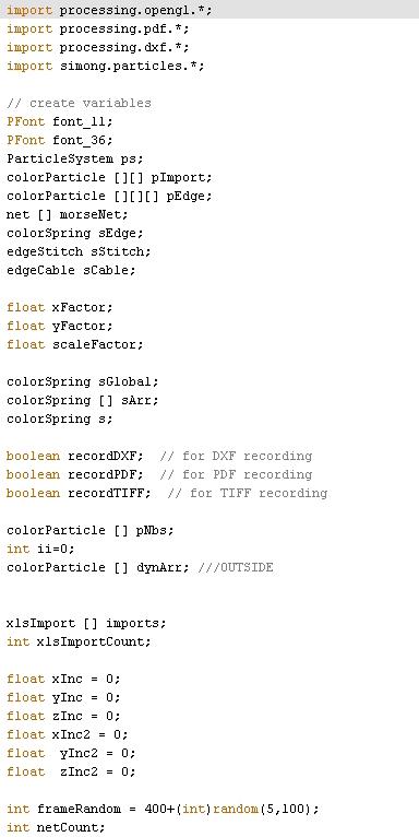
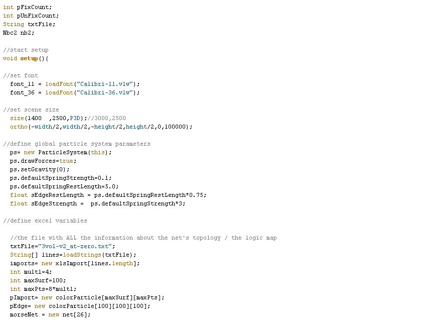
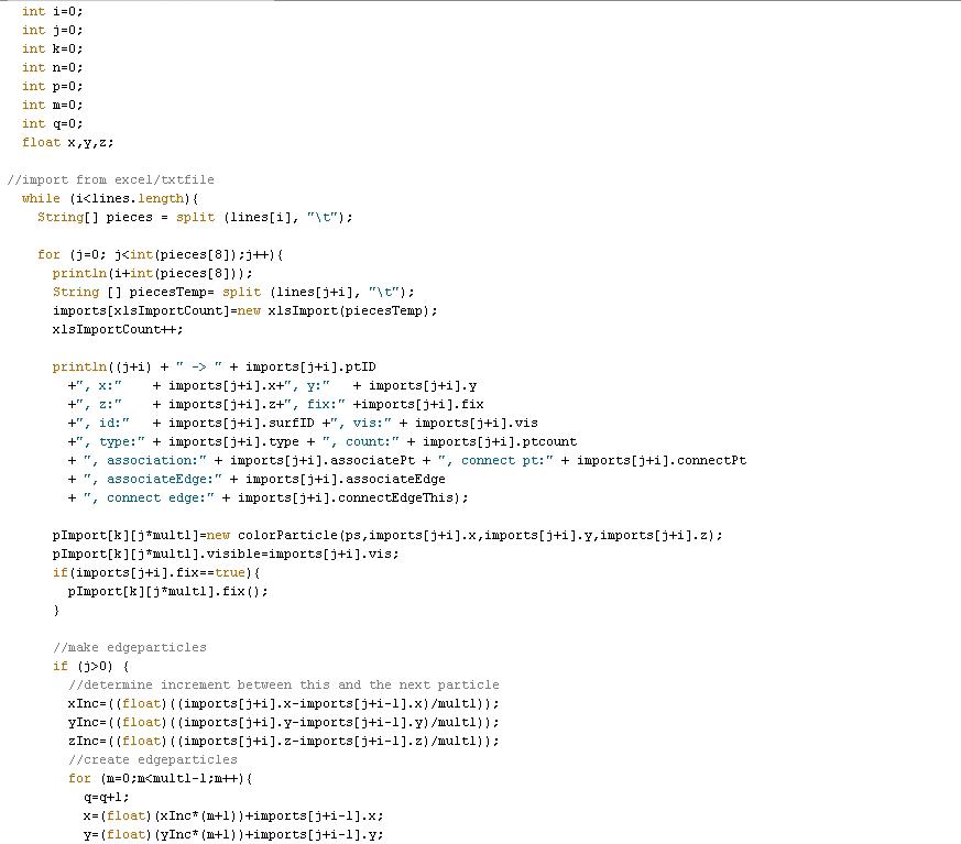
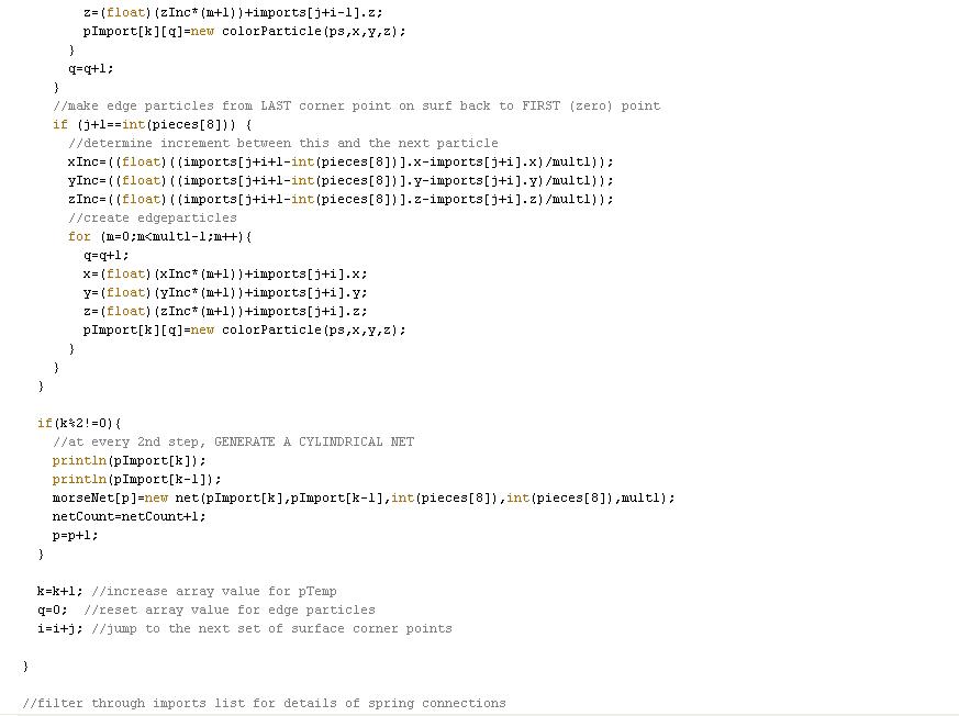
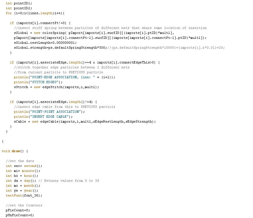


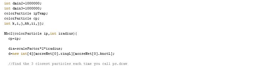
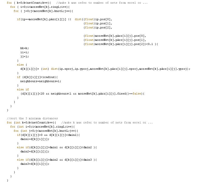

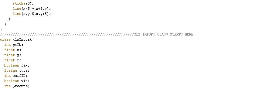
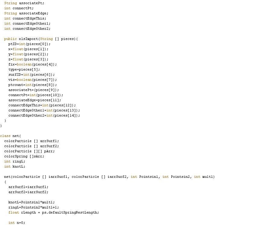
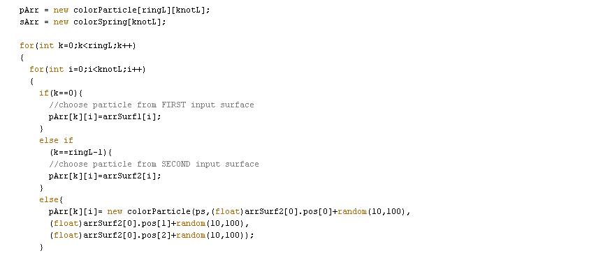
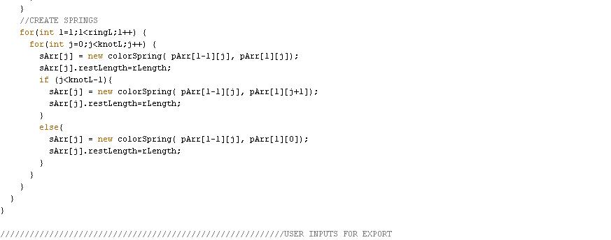
5.3 Work Map
ABSTRACT
1 PRECEDENTS & PRIMARY RESEARCH
1.1 Precedents
1.1.1 Physical Form-Finding
1.1.2 Computational Form-Finding Engineering-Based Software for Form-Finding Software Using Spring-Based Solvers
1.1.3 Articulation of Computational Form through Fate Map
1.1.4 Cable Nets as Space-Making Devices
1.2 Computational Networks
1.2.1 Network and Geometric Topology
1.2.2 Spring-Based Particles Systems
1.2.3 Springs in Processing Hooke’s Law
1.2.4 Cylindrical Net Topology
2 EXPERIMENTS & DEVELOPMENT
2.1 Embedded Fabrication
2.1.1 Cylindrical Transformations
2.1.2 Mapping of Computational Cylindrical Net
2.1.3 Data Mining for Fabrication through Node ID
2.1.4 Spatial Articulation of Net
2.1.5 Evaluating Cable Net Installation
2.2 Topologically Defined Net Components
2.2.1 Component Systems for Form-Found Structures
2.2.2 Subdivision Algorithm for Cellular Framework
2.2.3 Single Cell Net Parameters
2.2.4 Multiplication and Association of Net Components Hierarchies and Meta-Spring
2.2.5 Evaluating Cab le Net Installation
2.3Threshold Conditions
2.3.1 Comparing Actual Density and Perceived Density
2.3.2 Computational Threshold Analysis
2.3.3 Extended Vector-Based Analyses
3 APPLICATION & OUTLOOK
3.1 Contextual Inputs
3.1.1 In-Situ: Turbine Hall of Tate Modern
3.1.2 Comparison to Marsyas Installation
3.2 Conclusion
3.2.1 Elemental Processes
3.2.2 Architectural Emergence
3.2.3 Embedded Feedback
3.3 Outlook
3.3.1 Translations to Material and Fabrication
3.3.2 Parametric Dimensioning of Nodes and Vectors
Sean Ahlquist
Moritz Fleischmann