Jheny Nieto Ropero
Architectural Association School of Architecture
Emergent Technologies and Design Master/ Feb 2010
Tutors: Michael Weinstock, George Jerodimus and Toni Konik
London, UK
jhenyni@googlemail.com
T I M B E R C O M P O S I T E C O N T I N U O U S S U R F A C E S shell system
ACKNOWLEDGMENTS
I thank my tutor Michael Weinstock for helping me in structuring my thousands ideas and for his wise advise on the way of this project.
I am deeply grateful to George Jerodimus who have reinforced this research and my own knowledge with his great dedication and involucration in the project.
I own a big thank to my friends and family for constantly supporting my work all the time.
Finally, I am thankful to Emtech as it has opened my mind in discovering parallel interests to architecture that I know one day will become real constructions.
Jheny Nieto Ropero Architectural Association School of Architecture Emergent Design and Technologies Master London, UK jhenyni@googlemail.com
In this project, the aim is the experimentation and further development of a new composite material made out of plywood, fiber glass and resin. It proposes a fabrication logic to design large continuous double skin, self structural and performative surfaces.
The project introduces a step forward in the manipulation of plywood panels, pre-stressing them in a form finding process to achieve curvatures; thus, developing large structures. Through a reinforcing construction process necessity of big mandrels is avoided. Digital simulations and physical experiments were implemented in the research in order to achieve real possible geometries, to reduce weight and to simplify the structure.
THE OBSESSION WITH A SURFACE
The project gets the interest of producing one continuous surface based on the material behavior just as Dieste explored deeply in his research where he recognized that the surface offered a realm formal exploration that in turn, could solve structural problems.
The surface is the result of environmental, structural and architectural necessities. Its efficiency responds to the optimization process. Therefore form and expression, fabrication and structural efficiency led the development of a new language of building. The optimization process determines the final shape. The shells are the material with certain thickness, but the shape is still more fundamental as it contains the space and the quality of itself.
1.5
2.4
2.5
2.6
3.1.
3.2.1
LOAD CAPACITY IN INDIVIDUAL STRIPS pag 52
3.2.2 EVALUATION OF TORSION pag 56
3.2.3 LINEAR BUCKLING ANALYSIS COMPARISON ONE THE STRIP WITH DIFFERENT MATERIALS pag 60
3.3.1 PHYSICAL BUCKLING MODES IN A SHEET OF PLYWOOD pag 62
3.3.2 DIGITAL BUCKLING MODES IN A SHEET OF PLYWOOD pag 64
3.4.1. DIGITAL SIMULATIONS OF STITICHING BUCKLING AND BENDING PLYWOOD. pag 68
3.4.2. PHYSICAL SIMULATIONS OF STITCHING BUCKLING AND BENDING PLYWOODREINFORCING PROCES S pag 70
3.5.1. DEVELOPABLE SURFACES pag 72
3.5.2. DEVELOPABLE SURFACES pag 73
3.6.1. PHYSICAL BENDING OF PLYWOOD pag 74
3.6.2. SIMULATION OF A RESTRICTED SURFACE pag 76
3.7. SET TING THE LOGIC FOR MY THEORETHICAL SHELLS IN TIMBER COMPOSITES pag 78
3.8. CURVATURE ANALYSIS pag 80
3.9. PANELIZATION pag 82
3.10. EVALUATION AND RANKING pag 86
CHAPTER 1 MATERIAL PROPERTIES AND MANUFACTURING TECHNIQUES pag 6
TIMBER COMPOSITES pag 8 1.2 WOOD PROPERTIES pag 10
CURVED TIMBER SURFACES pag 10 MANUFACTURING pag 10 THE HALLIVAND MOSQUITO pag 14
COMPOSITES PROPERTIES
16 MANUFACTURING
16
1.1
1.3
1.4
pag
pag
TIMBER COMPOSITES PROPERTIES
25 CHAPTER 2 CASE STUDIES - Current Methods and Techniques implemented for composites and timber) pag 28
ALSOP POD - ONE pag 30 2.2 ALSOP POD -TWO - PECHAM LIBRARY pag 32
DEVELOPMENT
FIBERGLASS REINFORCED VENEER PRODUCTS pag 34
pag
2.1
2.3
OF
35
3D VENEER DEVELOPED BY REHOLZ pag
STRUCTURALLY DEFORMED PLYWOOD IN FURNITURE pag 36
FABRICATION TECHNIQUES FOR SHELLS pag 38 ELADIO DIESTE RAFAEL GUASTAVINO TECHNIQUES CHAPTER 3 EXPERIMENTS pag 40
CANOPY pag 42
TESTING
CHAPTER
4.1 FABRICATION
4.2
4.3.1
4.3.2
4.4
5.1
5.2
DEVELOPMENT pag 90
4 DESIGN
PROCESS pag 92
96
DIGITAL PROCESS - T H E S Y S T E M pag
102
DIGITAL PROCESS TO PRODUCE ONE SHELL pag
104
ALTERNATIVE REINFORCE PROCESS pag
CHAPTER 5 DESIGN pag 109
THE VOIDS EFFECT - LIGHT IN THE SURFACE
SYSTEM APPLICATION 1 - SAN ANDRES pag 110 DEPLOYMENT SCENARIO - PASEO pag 112 CHANGING FUNCTION - ORIENTATION - STABILITY pag 115
APPLICATION
pag 116
PROCES
pag 118
pag 123 STRUCTURAL SIMULATIONS pag 124 CONCLUSIONS – FURTHER DEVELOPMENTS pag 136 REFERENCES pag 138 B OOKS ARTICLES WEB SITES ENDNOTES pag 140 APPENDIX pag 143 A . TWISTING CONCRETE MAEDA WORKSHOP pag 144 B. LOGICAL DESIGN WORKSHOP - Summer DLAB pag 146 C. GRASSHOPPER DEFINITIONS AND SCRIPTINGS pag 148 ACKNOWLEDMENTS pag 152 DISCLAIMER
SYSTEM
2 - LETICIA -AMAZONAS RIVER
DESIGN
S
PERFORMANCE

CHAPTER ONE - MATERIAL PROPERTIES AND MANUFACTURING TECHNIQUES
1.1 TIMBER COMPOSITES
Ancient composites, such as straw reinforced clay; structures of wood, hide bone sinew and horn, have been used and implemented according to necessity. The combination of different materials usually improves quality and the disadvantages of the individual disappear.
Composites combine high stiffness and strength with low density, their composition allows new designs such as the shape of the wings of airplanes with regard to air speed. Their capacity to display complex shapes sounds attractive for different fields like aerospace, the sports industry and civil engineers and designers, and in the past years in architecture.
The idea of turbo-fan engines, where flying faster is linked to flight at higher altitudes due to the low air density (lower friction) and where the resistance to moving mass could decrease, was one of the first reasons to implement fiber reinforced polymers. The transport systems started looking into reducing the resistance per unit weight as it changes according to the friction in water or air. The history of the aircraft is important in demonstrating the improvements in shape and material. Jack Northrop created in the late 40’s the flying wing, which blends the fuselage and the wing approaching an enclosed cross-section, which reduces fuel consumption, take off-weight, empty weight propulsion, and increases the aerodynamic efficiency.
The end properties of a composite part produced from these different materials is not only a function of the individual properties of the resin matrix and fiber (and in sandwich structures, the core as well), but is also a function of the way in which the materials themselves are designed into the part and also the way in which they are processed.
8 MATERIAL PROPERTIES AND MANUFACTURING TECHNIQUES
Geometries in architecture have been evolving parallel to the materials. For instance, shells have been explored in thin concrete skins as well as in glass reinforced polymers resulting in different space qualities and fabrication constraints. Grid shells have passed from steel beams to bamboo structures and tensile and membrane structures have passed from temporary to permanent.
The textile industry has explored in-depth the different fibers and different patterns while composite engineers have just started to explore these ideas. Typically, with a common hand lay-up process as widely used in the boat-building industry, a limit for Fiber Volume Fraction is approximately 30-40%. With the higher quality, more sophistication and precise processes used in the aerospace industry, Fiber Volume Fractions approaching 70% can be successfully obtained.
Architecture is a field that broadly has influenced societies and countries in several aspects, from art to economy. Evolving architecture means evolving other disciplines and vice versa and since primitive constructions in adobe or straw, man has been looking into techniques to build their own habitats. In this sense new materials have evolved demonstrating the intelligence in obtaining certain performance or requirements. Science keeps looking for “smart materials” that can offer multi-functionality at all scales.
The aim of this first chapter is to understand the properties of timber and fiber composites and their existent manufactured forms, which will be used in the timber composite as the proposal material.
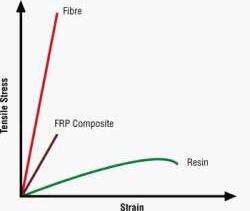
The elasticity of fiber-glass allows the wood to be more elastic, increasing the yield stress of the final material. The composite allows a greater structural capacity, while leaving a thin material, in addition to the fact that the matrix (fiber glass) allows the adherence between plywood and resin.
9 MATERIAL PROPERTIES AND MANUFACTURING TECHNIQUES
1.2 WOOD PROPERTIES
The chemical and anatomical properties of wood define its technical qualities. This is the most anisotropy material, which means its characteristics depend on directionality. Along the grain, wood has one hundred times greater tensile strength and four times greater compressive strength than at the right angles to the grain. Its load capacities are higher than concrete structures, having the advantage of low dead weight. For example, wood’s strength and hardness will be different for the same sample if measured in different orientation. Cellulose, which is a high molecular weight polysaccharide, is the main constituent of wood and is directly responsible for stiffness and strength. Lignin is a heavily cross-linked phenolic resin which is very brittle. Wood is stronger in tension than in compression and has a breaking stress of about 100 to 140 MPa. “The compressive strength of wood is about a third of its tensile strength. The difference is attributed to local buckling of the cell walls under compression followed by a macroscopic crease” (Dinwoodie, J. M. 2000).
1.3 CURVED TIMBER SURFACES
In the bending of wood or other elastic materials it is usual to assume that transverse plane sections remain plane and normal to the longitudinal fiber. The end sections initially square with the faces of the piece remain square during the process of bending. In the bent state, the lengths of the convex and concave faces are no longer equal, as they were when originally cut. The difference in these lengths on the concave faces to shorten, and induced tensile stresses causing fibers on the convex face to stretch. (fig. 1.3.1)
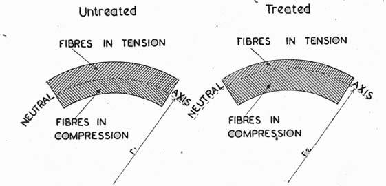
fig. 1.3.1
Common timbers cannot be bent in their natural state to small curvatures without fracturing, or retaining its elastic properties to cause them to spring back to approximate their original shape on removal of bending forces. However, some timbers when are subjected to heat in the presence of moisture, such as steaming or boiling, become semi-plastic. Therefore its compressibility is increased and comparatively small compressive stresses are capable of producing a very appreciable strain without fracturing the material.
MANUFACTURING
Bending has a long history that goes from small devices made out of wood through proper steel machines that bend several pieces at the same time. The methods have improved along with the machines.
Solid bending requires soft treatments such as steaming, which, in order to render plasticity, and compression, provides heat and moisture. Studies have proven that if wood contains 25-30 percent moisture it is suitable to bend. The method most commonly used to obtain this condition is to subject the timber to saturated steam at atmospheric pressure in a steam chest. Other methods such as immersing the wood in heated wet sand or heating the appropriate portions in a naked gas flame shape the wood into the desired curvature without the application of moisture. What is remarkable is that the fibers from the compressed side of a bent piece show compression failures, shrinkage and expansions in the longitudinal direction (fig. 1.3.1).
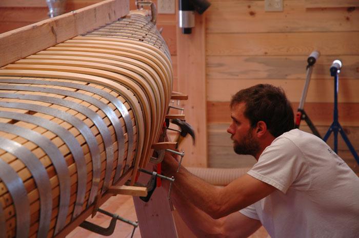
Hand bending can be applied to some devices, but the bending will be performed manually. Cold bending refers to bending in untreated timber, in its natural or dried states such as in the curved planking of boats, which sometimes are cold, bent and secured to the ribs. Hot bending will vary the radius of curvatures according to the type of wood, but in general will be use for bends of smaller radius. For making steamed but unsupported material some of the following methods can be utilized: a. Clamp the piece to the suitable curve. b. Force the piece to a prepared wooden or metal curved and sequentially clamps it into to the right position (figure 1.3.3). Wood is very prone to fracture when subjected to tensile stress.
10 MATERIAL PROPERTIES AND MANUFACTURING TECHNIQUES

S/R = 0.02 Cold bending
S/R = 0.08 Hot bending
11 MATERIAL PROPERTIES AND MANUFACTURING TECHNIQUES
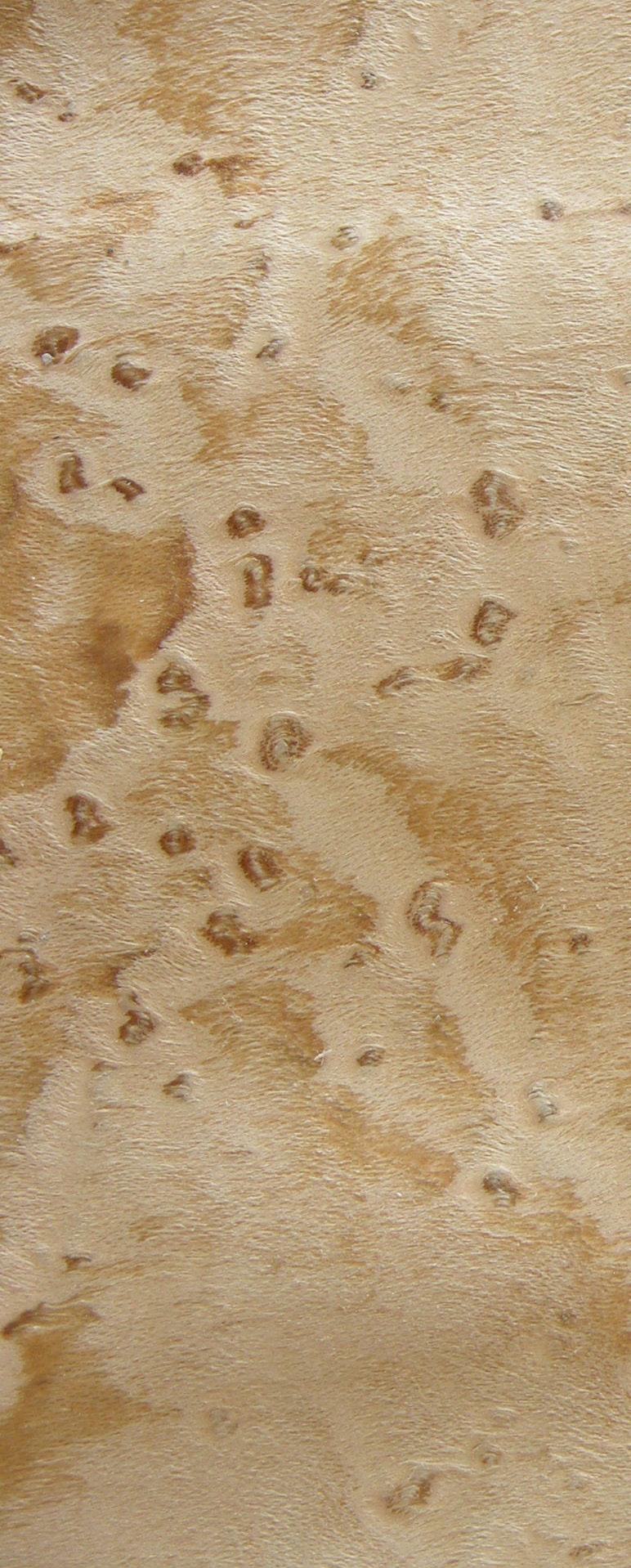
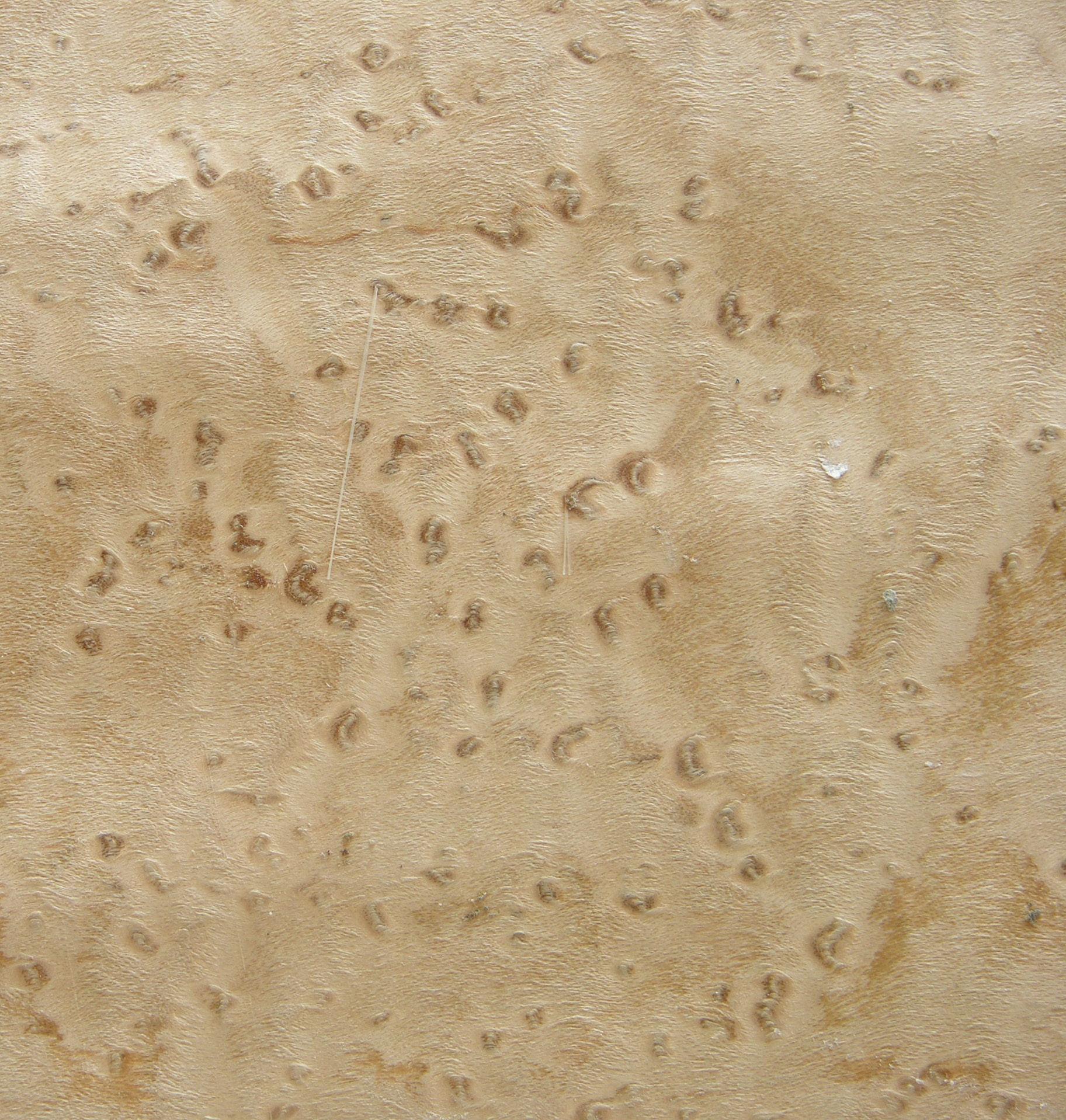
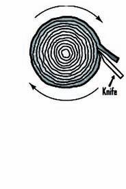
fig 1.3.0 Tree section
fig. 1.3.1 Fibers in tension and Compression
fig. 1.3.2 The steaming box
fig. 1.3.3 Clamping the piece into a metal curved piece
fig. 1.3.4 Clamping the piece into a metal curved piece
fig. 1.3.2
fig. 1.3.3
fig. 1.3.4
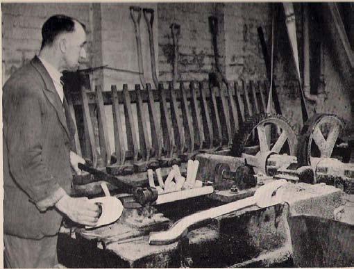
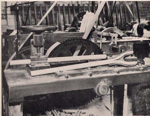
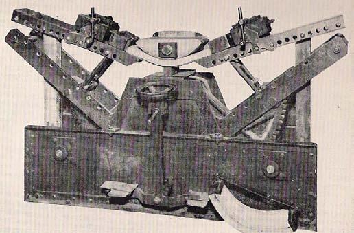
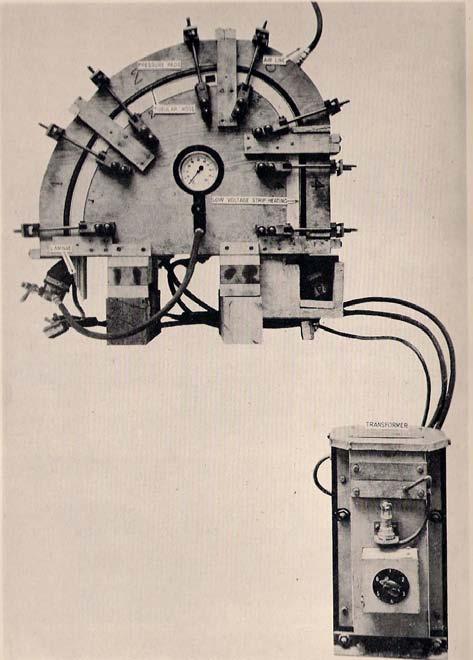
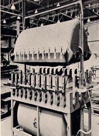
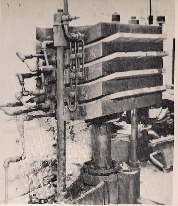
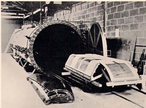
fig. 1.3.5 Spade handle bending machine
fig. 1.3.6 Bending machine for making split type spade handles
fig. 1.3.7 Lever arm bending machine operated by a rack and pinion mechanism
fig. 1.3.8 Air-inflated tubular hose and low voltage strip-heating used in the production of laminated bends
fig. 1.3.9 Pressure moulding bag
fig. 1.3.10 Hydraulic press and steam heated cauls
fig. 1.3.11 Laminated bending by the autoclave process (rubber bag re moved)
fig. 1.3.12 A commercial machine employed for production of laminated bends by the continuous strip method
MATERIAL PROPERTIES AND MANUFACTURING TECHNIQUES
fig. 1.3.5
fig. 1.3.6
fig. 1.3.7
fig. 1.3.8
fig. 1.3.10
fig. 1.3.11
fig. 1.3.12
fig. 1.3.9
The evolution of machines for bending is marvelous and of course its capacities to bend several pieces at the same time, plus the possibility to apply greater forces (fig. 1.3.8).
Laminated bending was introduced in timbers as pieces could be bent by cold or hot systems; however they will tend to resume their original shape upon removal of the bending forces. To avoid this, the pieces need to be secured to a rigid framework or secured to one another in a concentric manner that wouldn’t allow them to move. Laminate should be dried to a moisture content of less than 20 percent before they can be considered in a stage fit for gluing. They may be in the form of sawed, sliced or rotary cut veneers or plywood.
The following new methods were introduced to press and laminate: the metal tension band, the fluid pressure, the flexible rubber hose and metal strap, the inflated rubber bag and female mold, the deflated rubber bag. These methods are outdated and require a mold to shape the timber into a specific curvature and thickness.
Engineered timbers are composite constructions of wood and high strength adhesive. Wood particles, strands or veneers are locked into a laminated structure, which is dimensionally stable and durable. These materials are used in a variety of combinations to produce lightweight structures, engineered to precise requirements.
Some theoretical considerations suggest engineering timbers utilize the high strength and stability of laminated wood. The visual and mechanical properties are affected by the type of wood, adhesive and method of production. Laminated strand lumber (LSL), oriented strand board (OSB), medium density fiberboard (MDF), plywood and I-beams. It is possible to produce flame retardant and water resistant grades.
The basic element for composite wood products may be the fiber, as it is in paper, but it can also be larger wood particles composed of many fibers and varying in size and geometry. Properties of such material can be changed by combining, reorganizing, or stratifying these
elements.
Plywood was invented in the 1850s as a combination of three or more layers of wood. Cheap and easily accessible, it has been an important medium for experimentation by modernist designers from the 1920s onward.
Many important examples of modernist furniture were made of plywood. Cheaper and more easily accessible than aluminium or steel, plywood was a key material for early 20th century designers such as Gerrit Rietveld, Marcel Breuer and Alvar Aalto, as well as midcentury modernists like Charles and Ray Eames, and contemporary figures including Jasper Morrison.
Plywood consists of at least three layers or veneers of wood which have been plied together with the grain running crosswise to add strength and resilience. The earliest examples of plywood furniture date back to the 18th century, but it was not until the 1850s that it was put into commercial production by John Henry Belter, a German émigré to the US. Furniture progressed as new fabrication techniques evolved. The case studies in the second chapter will show some of this evolution at both small and large scales.
13 MATERIAL PROPERTIES AND MANUFACTURING TECHNIQUES
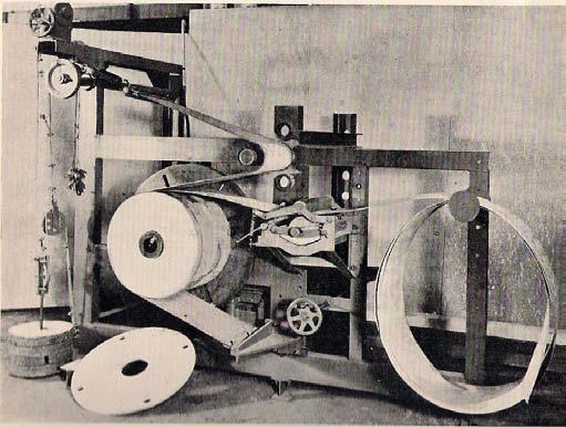
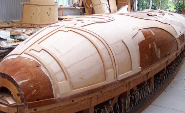
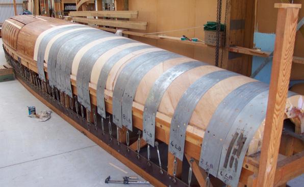
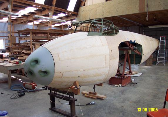
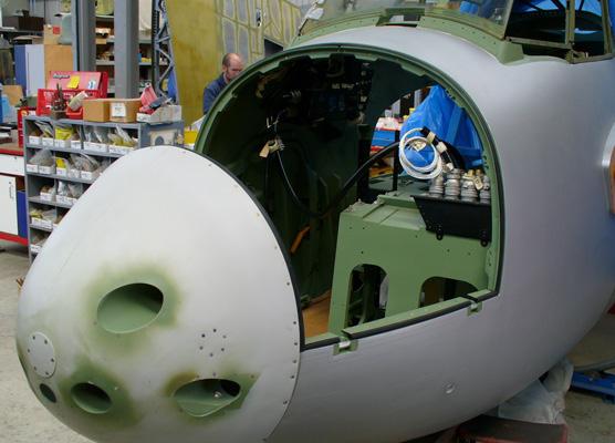
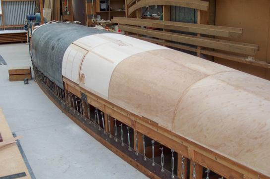
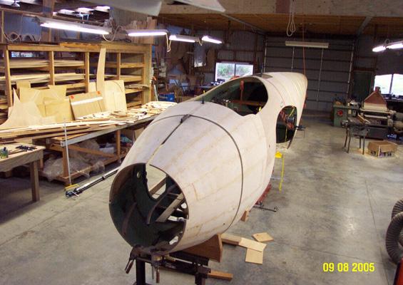
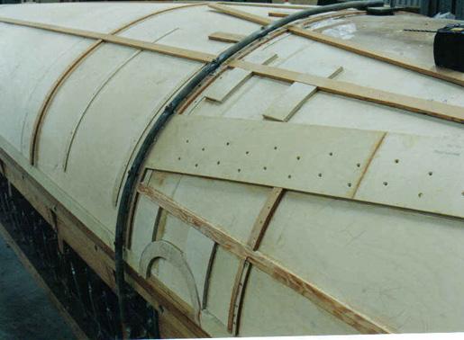
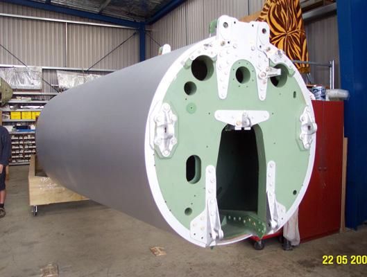
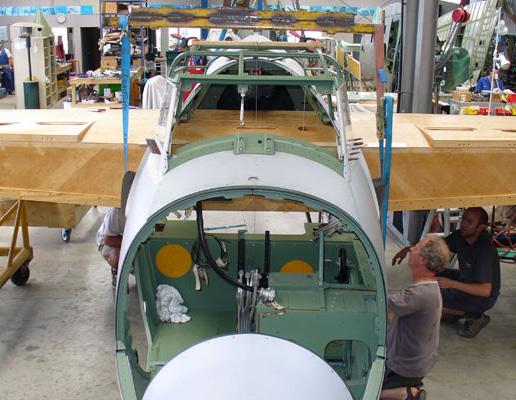
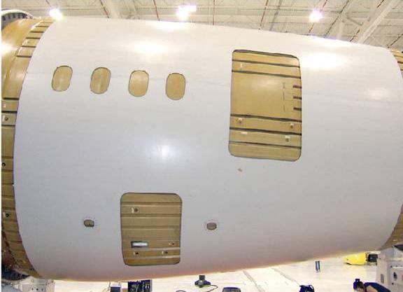
THE HALLIVAND MOSQUITO
After the machines already had the control of the bending one of the bigger tasks was to pass from small scale to large scale . The timber has been used as molds for different materials, from traditional concrete structures that require it to frame the liquid to mold structures for airplanes.
“The Havilland Mosquito was a lightweight, fast British combat aircraft made mainly of wood using advanced construction methods. The fundamental considerations in the design was that the aircraft be as clean and aerodynamic as possible, that it get into the production phase as short a period of time as possible and that it be capable of being produced by as many firms as needed to meet mission requirements.”.
Crew: 2
Length: 44 ft 6 in
Wingspan: 54 ft 2 in
Height: 17 ft 5 in
Wing area: 454 ft²
Empty weight: 14,300 lb
Powerplant: 2× Rolls-Royce Merlin 76/77
Maximum speed: 361 knots
Range: 1,300 nm with weapons load
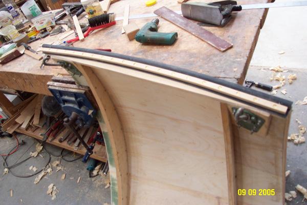
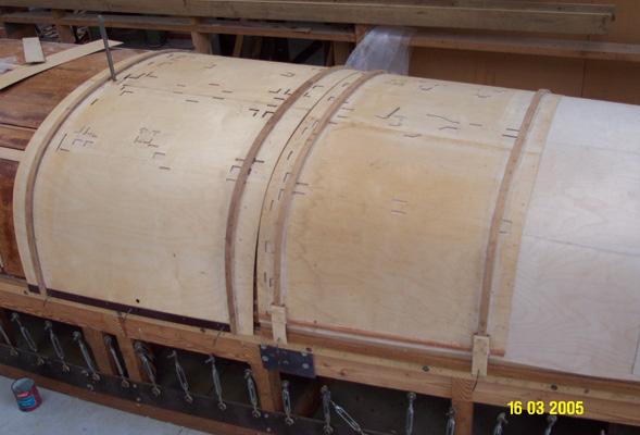
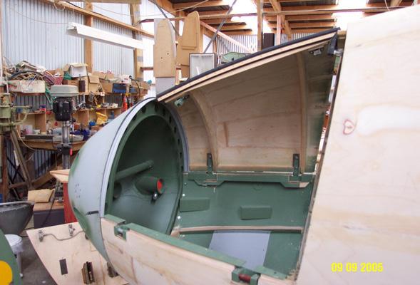
Pictures on the right correspond to the construction done in 2005 by The Fighter Factory.
fig. 1.3.13 Fuselage shell half construction
fig. 1.3.14 Fuselage shell half construction
fig. 1.3.15 Fuselage shell half construction
fig. 1.3.16 Fuselage with steel bands
fig. 1.3.17 Browning door, fitting catches
fig. 1.3.18 Browning doors Port open
fig. 1.3.19 Fuselage on assembly jig 2
fig. 1.3.20 Joining shell halves
fig. 1.3.21 Rear bulkhead with fittings
fig. 1.3.22 Nose browning doors off KA114
fig. 1.3.23 Port mould fitting interskin members
fig. 1.3.24 Fuse to wing front on 12 07
Source: http://www.fighterfactory.com/restoration/dehavilland-mosquito-aircraft.php
14 MATERIAL PROPERTIES AND MANUFACTURING TECHNIQUES
15 MATERIAL PROPERTIES AND MANUFACTURING TECHNIQUES
fig. 1.3.13
fig. 1.3.16
fig. 1.3.19
fig. 1.3.22
fig. 1.3.14
fig. 1.3.17
fig. 1.3.20
fig. 1.3.23v
fig. 1.3.15
fig. 1.3.18
fig. 1.3.21
fig. 1.3.24
1.4 COMPOSITES PROPERTIES
A fiber-reinforced polymer (FRP) composite is a combination of fibers within a matrix of a plastic or resin material. The fibers bring the strength to the composite, the matrix binds the fibers together, transfers the loads between them and the rest of the structure, and protects the fibers from the environment. Fibers are usually: glass (GRP), carbon, aramid (Kevlar or Twaron), and natural fibers.
The matrices are divided in two groups of polymers:
Thermosets are resins cured by heat or chemical reaction (polyesters, vinyl-esters, epoxies, phenolics).
Thermoplastics melt to form highly viscous liquids at elevated temperatures (200C and 300C) but solidify to glassy or crystalline substances as they cool. They can be softened again by reheating polyamides (nylon), thermoplastic polyesters (eg PET) polypropylene.
MANUFACTURING
Well manufactured composites structures display higher stiffness and strength as better resistance to fatigue and environmental degradation, and when big impacts on the structure occur the composite perform with a better energy absorption such as in formula cars. The manner of combining fibers and matrix into a composite material depends on the fiber/resin combination and on the scale and geometry of the structure to be manufactured. There are seven main methods for FRP. This study will present all of them briefly and focus on the molding methods.
Pultrusion tightly packed tow of fibers, impregnated with catalyzed resin, are pulled through a shaped die to form highly aligned.
Due to the high fiber content and the high degree of fiber alignment resulting from the tensile force used to pull the fiber bundle through the die, extremely good mechanical properties can be obtained
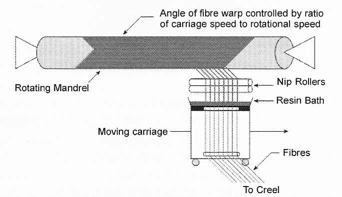
Filament Winding
Cylindrical symmetric structures can be made by winding fibers or tapes soaked into with precatalysed resin onto expendable or removable mandrels. After the resin has hardened, the mandrel (mold) is removed and if the size permits, the product may be post-cured at an elevated temperature. Uniformity is definitely one of the advantages of this method.
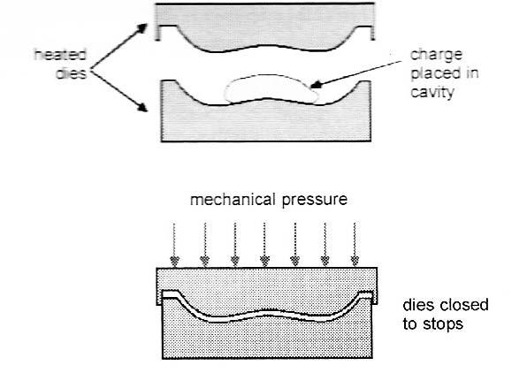
Compression and transfer molding SMC and DMC
If the fibers are short (1 cm or 2cm) a dough-molding compound (DMC) is created, known as bulk molding compound (BMC). When fibers are longer (5cm to 10cm) a pliable sheet molding compound (SMC) is produced. DMCs are produced by blending together the good combinations of resin, chopped fibers, fillers and pigments, and moldings aids in an industrial blender (or mixer) to form a thick doughy paste. These compounds can be fabricated to their final shape by compression molding - squeezing into shape between heated, shaped dies.
16 MATERIAL PROPERTIES AND MANUFACTURING TECHNIQUES
fig. 1.4.1
1.4.2 fig. 1.4.3
fig.
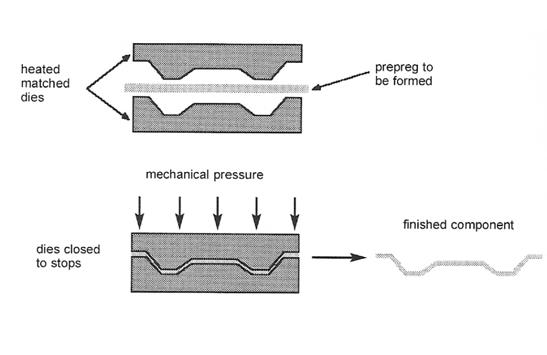
Matched-die molding and autoclaving
Hot-pressing sheets of pre-impregnated fibers or cloth between flat or shaped platens. Or by pressure autoclaving to consolidate a stack of prepreg sheets against a heated, shaped die. Double curvatures can be made by woven reinforcements.
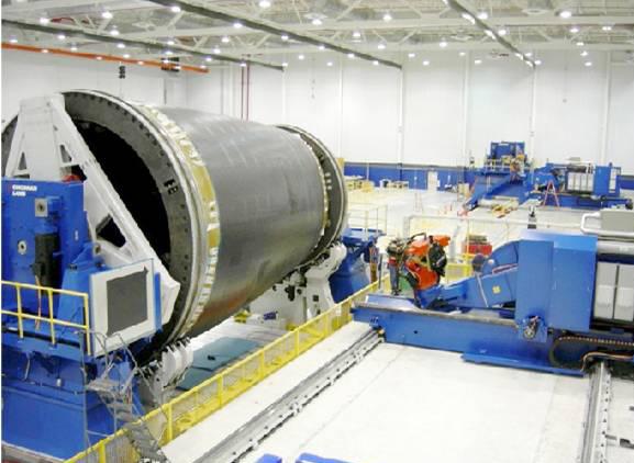
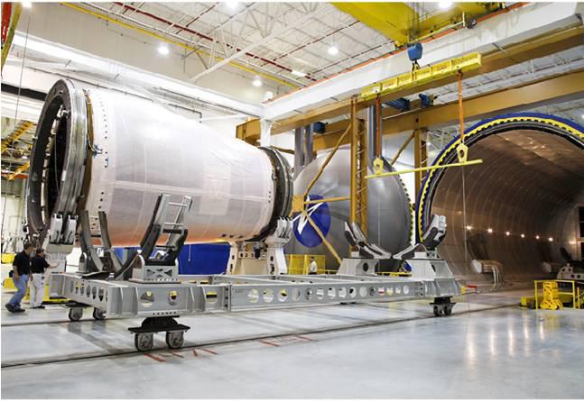
A mold of a section of the fuselage is wrapped with carbon-fiber tape using a robotic tape-laying machine. The tape-wrapped mold is then placed into a large pressurized oven called an autoclave, where the composite is cured through a process of head and pressure. (Over 300C of temperature and pressures over 90psi).
After curing in the autoclave, the fuselage is separated from the fuselage mold. Openings are cut out if necessary.
In autoclaves moldings, a single shape surface is used and consolidated and the pre-preg stack is achieved under heat and pressure in a chamber, which can be both evacuated to remove excess air and pressurized to compact the pre-preg and drive out excess resin.
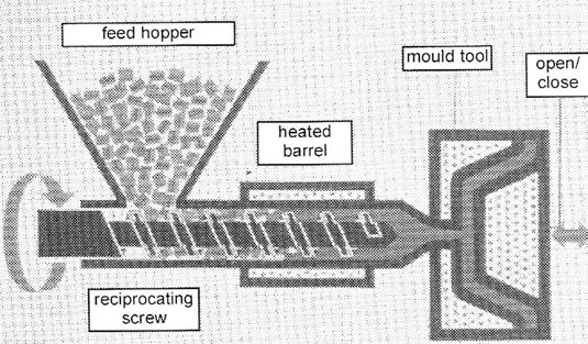
Injection- molding of reinforced thermoplastics
Thermoplastics-based materials such as Nylon, are made by the injection molding of granules of material, in which the chopped fibers and matrix have been pre-compounded. It is often used for repetitive manufacturing and the dyes and presses are very expensive.
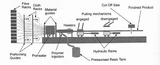
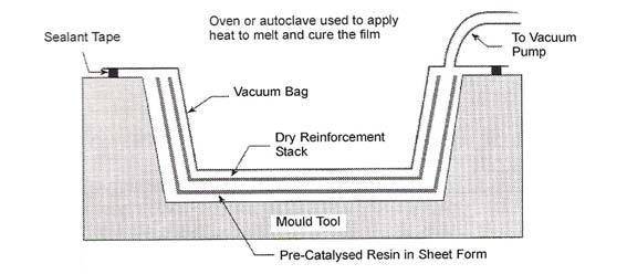
Continuous sheet production
Continuous sheet production chopped strand mat or chopped strands are impregnated with resin and sandwiched between two layers of film on a moving belt. The sandwich passes through guides that form the corrugated or other desired profile as it enters a long oven section in which curing takes place.

fig. 1.4.1 Pultrusion method
fig. 1.4.2 Filament Winding
fig. 1.4.3 Compression and transfer molding SMC and DMC
fig. 1.4.4 Matched-die molding and autoclaving
fig. 1.4.5 Autoclaving
fig. 1.4.6 Injection molding of granules of material
fig. 1.4.7 Continuous sheet production
Source. Ann ALderson. 2002. Fibre-reinforced polymer composited in construction. London, CIRIA.
MATERIAL PROPERTIES AND MANUFACTURING TECHNIQUES
17
fig. 1.4.4
fig. 1.4.5
fig. 1.4.6
fig. 1.4.7
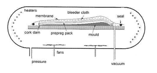
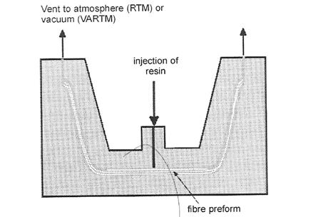
Resin-transfer molding (RTM) and vacuum- assisted resin-transfer molding (VARTM)
RTM is a low-pressure process, the equipment is not as expensive and the dies can be made from metal sheets, electro-formed nickel, cast or machined aluminium alloys, or even GRP. It produces high-quality mouldings of complex shape at much lower cost. Pre-catalysed is pumped under low pressure into a fiber pre-form in a heated space. Thick components containing foamed polymer cores can also be produced this way.
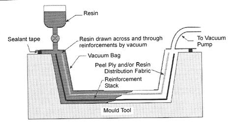
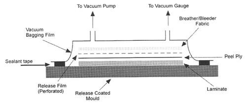
In Resin-infusion a pre-arranged fiber pack is laid against a single-sided shaped die and covered with a flexible sheet. The space is evacuated and atmospheric pressure consolidates the fiber pack, where pre-catalyzed resin is then bled into the fibers to form the desired component.
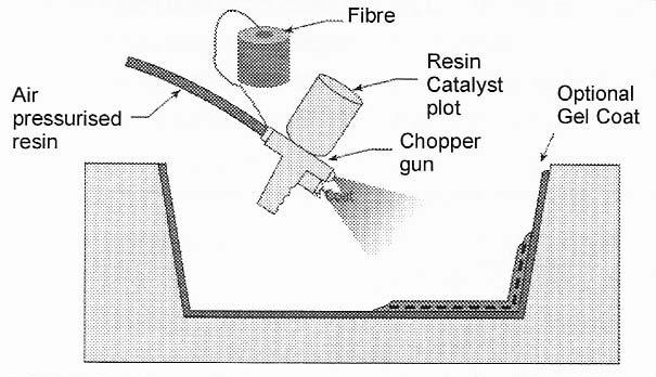
Open-mould processes: contact molding by hand layup or spray-up.
Composites reinforced with chopped-strand mat (CSM) or woven cloth are often laid up by hand methods, especially for irregularly shaped structures. A shaped former is coated with gel-coat and the required shape and thickness are then built up by rolling on layer upon layer of resin-impregnated cloth or mat. After the final flow coat, the structure is cured by the heat. The same process can be alternatively done by spraying short fiber bundles through a gun. The distribution and quality depends on the operators.
18 MATERIAL PROPERTIES AND MANUFACTURING TECHNIQUES
1.4.9
fig.
1.4.8 fig.
CASE STUDIES 19
fig. 1.4.10
fig. 1.4.11
fig. 1.4.12
fig. 1.4.8 Vacuum assisted resin molding (VARTM) Resin transfer molding (RTM)
fig. 1.4.9 Open mold process: hand-up and spray-up
fig. 1.4.10 Autoclave
fig. 1.4.11 Autoclave
fig. 1.4.12 Autoclave
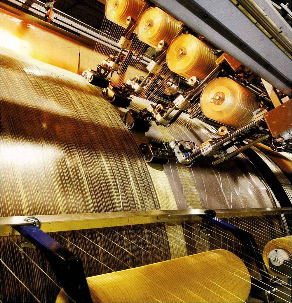
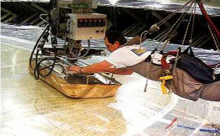
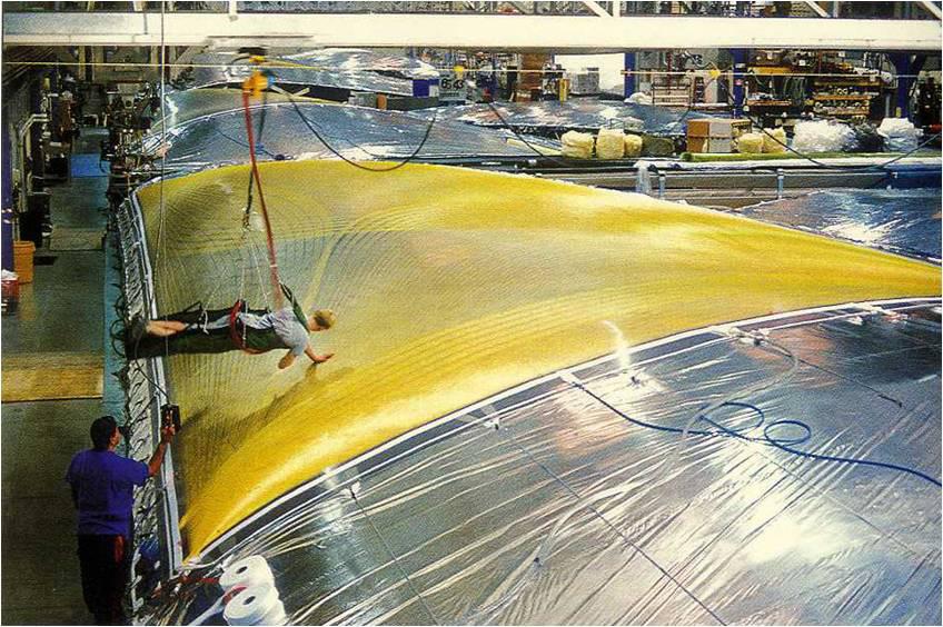
3d thermal laminating
This technology is used to make ultra lightweight, seamless 3D sails. The fiber reinforcement is continuous over the entire surface of the sail, replacing traditional methods of cutting and gluing.
The process combines the benefits of composite laminating with filament winding. The 3D sheet geometries are formed over computer guided molds. The fiber reinforcements are laid down individually along pre-determined lines of stress.
They are sandwiched between thin sheets of polyethylene terephthaalte (PET) coated with a specially developed adhesive. Since the demand increased, 3D rotary laminating (3DR) was developed as a method of continuous production. Instead of the large 3D molds, 3DR is carried out on a single rotating drum.
The shape of the drum is manipulated as the sail is constructed over it.
1. The process starts with the digital design according to each specific sail boat.
There are a range of sizes from 10-500 sqm.
2. The PET film is laid across the mold and pulled tight with tensioning straps.
3. The 6-axis computer controlled gantry lays down the strands of carbon fiber (fig.1.4.13). Finally an operator checks for mistakes (fig.1.4.15). The PET and fiber are vacuum bagged and held under pressure.
A technician then moves over the sail applying heat to thermally form the composite over the mold surface (fig.1.4.14).
Due to the factors described above, there is a very large range of mechanical properties that can be achieved with composite materials. Even when considering one fiber type on its own, the composite properties can vary by a factor of 10 with the range of fiber contents and orientations that are commonly achieved.
The comparisons that follow therefore show a range of mechanical properties for the composite materials. The lowest properties for each material are associated with simple manufacturing processes and material forms (e.g. spray lay-up glass fiber), and the higher properties are associated with higher technology manufacture (e.g. autoclave molding of unidirectional glass fiber pre-preg), such that are found in the aerospace industry.
fig. 1.4.15 fig. 1.4.14
1.4.13
fig.
FIBRE CONTENT ORIENTATION FIBRE LENGTH APPLICATIONS MANUFACTURING PROCESS
CONTROL
Vf(%) (%) L(mm)
0 short fibers Small detailed parts Thermosets
Lcrt<L<10 Housing and brackets Thermoplastics Injection moulding
pressing
25 discontinous fibers beams and shell injection moulding
10<L<100 structures (S)RIM Resin infusion
car body parts pressing
BMC/SMC GMT
40 100 endless fibers large plate and laminating L->& shell structures
aerospace tapelaying
packaging/ filament winding pressure vessels
ship building/ civil engineering resin infusion
small plate and shell structures pressing aerospace
diagram forming
70 profile beams pultrusion
civil engineering
fig. 1.4.13 The 6-axis computer controlled gantry lays down the strands of carbon fiber
fig. 1.4.14 A technician then moves over the sail applying heat
fig. 1.4.15 Operator checks for mistakes
fig. 1.4.16 Fiber manufacturing specifications (from Flying LightnessPromises for structural elegance)
fig. 1.4.16
CASE STUDIES 21
Corrosion Resistance
FIBER GLAS S WITH RESIN
Superior resistance to a broad range of chemicals. Unaffected by moisture or immersion in water if ends are properly sealed.
Surfacing veil and UV additives create excellent weatherability
Insect Resistance
Unaffected by insects.
Strength
Stiffness
Electrical Conductivity
Pultruded fiberglass is stronger, and has higher flexural strength than timber. Ultimate flexural strength (Fu) LW = 30,000 psi, CW = 10,000 psi.
Pultruded fiberglass is approximately 1-1/2 times as rigid as wood. Modulus of elasticity LW = 2.5 x 10⁶ psi, CW = .8 x 106 psi.
Non-conductive - high dielectric capability
Weight Specific gravity = 1.7
Pultruded fiberglass has significantly higher strength-to-weight ratio.
Finishing & Color Pigments added to the resin provide color throughout the part. Special colors available. Composite design can be customized for required finishes.
Cost
Lower maintenance, longer product life often equals lower overall costs.
Anisotropy Isotropic when it is bounded with the resin
TIMBER
Can warp, rot and decay from exposure to moisture, water and chemicals.
Coatings or preservatives required to increase corrosion or rot resistance can create hazardous waste and/or high maintenance.
Susceptible to insect attack (marine borers, termites, etc.). Coatings to increase resistance to insects can be environmentally hazardous.
Extreme fiber bending = up to 2800 psi.* Compression parallel to grain = up to 1800 psi.*
Modulus of elasticity = up to 1.8 x 10⁶ psi.*
Timber can be conductive when it is wet.
Specific gravity = .51 (oven dried).*
Must be primed and painted for colors. To maintain color, repainting may be required.
Lower initial cost.
Is the anisotropy material by excellence.
fig. 1.4.17
22 MATERIAL PROPERTIES AND MANUFACTURING TECHNIQUES
CHARACTERISTIC S
WOOD 1. Anisotropic
2. Moisture
3. Electrical conductivity
4. Weight
5. Strength
6 Stiffness
GLASS 1. Isotropic REINFORCED
2. Unstiff and Unstrog across the axxis GLASS 3. Stiff and Strong (tension and compression) along the axis
RESIN 1. Bond
2. Adherence
3. Good longevity
4. Fair UV resistance
5. Good resistance to water
Bending one direction
Prestressed the fibers
fig. 1.4.17 Comparison chart fiber glass with resin and timber fig. 1.4.18 The manipulation of individual materials in the manufacturing steps.
Timing in the application
23 MATERIAL PROPERTIES AND MANUFACTURING TECHNIQUES
ALTERATED CHARACTERISTICS POS SIBLE SEQUENCE STEPS TO TAKE IN MANUFACTURING
+
STEP 1 STEP 2 STEP 3 STEP 3 STEP 1 STEP 2
fig. 1.4.18
1.5 TIMBER COMPOSITES PROPERTIES
Young modulus (E) is a measure of the stiffness of an isotropic elastic material.
Young’s modulus is the ratio of stress, which has units of pressure, to strain, which is dimensionless; therefore Young’s modulus itself has units of pressure. MPa or N/ mm2.
Wood being an anisotropic material requires a minimum of 2 values of Young modulus: one along the grain (E1 ) and the other perpendicular to it (E2).
Glass fiber is a matrix molded by the resin or vice versa, according to the density of the GF more or less resin is required. The ratio of glass fiber or resin is measure in the Volume fraction. In general, since the mechanical properties of fibers are much higher than those of resins, the higher the fiber volume fraction, the higher the mechanical properties of the resultant composite will be.
Young module Glass Fibre Ef= 70000 N/mm2
Young module Resin E r = 1500 N/mm2
Volume fraction Glass Fibre Vf
Volume fraction Resin V r
E2 =1000 N/mm2 E1 = 10000 N/mm2 lay 1 thickness (t)=0.5 mm lay 2 0.5 mm t=0.5 mm lay 3 0.5 mm t=0.5 mm
A sheet of plywood of 1.5mm (3 veneer layers of 0.5mm each one) is required to analyze the elasticity separately.
= E
+ E r
r = 70000*0.5 + 1500 *0.5 = 35000 + 750 = 35750 N/mm2
= E r
= 70000 * 0.4 + 1500 *0.6 = 28000 + 900 = 28900 N/mm2
E2 = E r E1 = 1/2 *28900 = 14450 N/mm2 E2 = 1/2 *28900 = 14450 N/mm2
= 70000 * 0.3 + 1500 *0.7 = 21000 + 1050 = 22050 N/mm2
= E r
= 1/3 * 22050 = 7000 N/mm2
24 MATERIAL PROPERTIES AND MANUFACTURING TECHNIQUES
(E lay1)1
+ (E lay2)1 *t2 + (E lay3)1 *t3 E1 plywood = -------------------------------------------------------------------------t1 + t2 + t3
(E lay2)1
= --------------------------------------------------------------------------
=
(10000
= ------------------------
10500 = ---------
6500 = ----------------1.5 A B C Volume fraction (V) 0.5 V= 0.4 V= 0.3 E1
*t1
2 (E lay1)1 *t1 +
*t2
1.5mm 2(10000*0.5) + (1000) * 0.5
------------------------------------------------------------1.5mm
+ 500)
1.5
1.5 2(1000*0.5) + (10000) * 0.5 E2plywood= 1.5mm
f*Vf
*V
E2
E1
E1
E2
Erandom composite
Young modulus’s Yield Stress (N/mm2) (N/mm2) glass fiber unidirectional 35750 80000 glass fiber orthogonal 28900 40000 glass fiber random 7000 20000
(main direction horizontal) Ex
(main direction vertical) Ex

The weight of plywood depends on the number of veneer on it and on the amount of glue 3 pounds per square foot per inch of thickness.
¼ inch 0.71 pounds per square foot
3/8 inch 1.06 pounds per square foot
½ inch 1.42 pounds per square foot
5/8 inch 1.77 pounds per square foot
¾ inch 2.13 pounds per square foot
25 MATERIAL PROPERTIES AND MANUFACTURING TECHNIQUES
4000 plywood
4000
7000 resin 1500 Ey Ex Ex Ey
plywood
7000 Ey
Ey
fig. 1.5.1
fig. 1.5.1 Comparison chart Young modulus and Yiel Stress
1.6 CONCLUSIONS
The common advantages of fiber composites are as follows: Time saving, durability, repair, lightweight, blast/fire, low maintenance, thermal insulation, high strength and dimensional stability; in addition to appearance and design flexibility.
The structural efficiency of the fibers varies according to manufacturing, fiber orientation and density. Fiberglass can be tailored to meet the specifications by building up layers oriented with stress while removing unnecessary material from areas with little stress. The timber composite, being quasi-isotropic could be assumed to be as strong in the x-y directions.
The uniformity in strength of composite panel. One of the big advantages of composites is that buckling is avoided, which is one of the main reason to be used in airplanes.
The curvature is directly related to the wood treatment and of course to the fiber state, which can make wood more or less flexible. The ratio of thickness and curvature are directly related.
26 MATERIAL PROPERTIES AND MANUFACTURING TECHNIQUES
27 MATERIAL PROPERTIES AND MANUFACTURING TECHNIQUES
THIN LIGHT SHELL STRUCTURES
The optimization of a shell structure, “monocoque shells” refers to optimization of geometry and therefore to reduction of weight.
Thin shell structures are lightweight constructions, which usually are assembled into large surfaces. Some examples are in airplanes, boat hulls, and roof structures. The shell structure has curvature as opposed to plate’s structures which are flat. Where a flat plate acts similar to a beam with bending and shear stresses, shells are analogous to a cable, which resists loads through tensile stresses. Therefore, the ideal thin shell must be capable of developing both tension and compression.
For instance the grid shell derives its strength from its double curvature, just as a fabric.
Fiber Reinforced Polymer (FRP) and Glass reinforced Polymer (GRP) initial architectural applications were focused in on pieces or parts of the building such as windows, and roofs. Nowadays there are a few examples at a bigger scale compared to the FRP applications but not as many as expected considering that one laminate of glass fiber reinforced is stronger than one laminate of steel. In some cases FRP has been used to produce self-supporting large structures such as curved domes for mosques, which would be
difficult and more expensive to build in conventional materials.
The geometric optimization is being an important task to reduce weight and eliminate a secondary structure, and it can be implemented in the efficient drainage strategy as well.
It is important to understand that most efficient FRP structures are fundamentally different in both geometric and structural form to conventional building structures. Therefore it is necessary to change the methodology of building design to enable FRP to provide more efficient solutions than currently available with conventional building materials.
The reduction of supporting structures for larger spans is one of the most challenging aspects of FRP, the material reduces assembly issues and filtrations. As will be shown in this chapter, complex surfaces have been made usually by plywood molds just adjusting the size of the sheets to be laid out.
Some interesting alternatives for the complements of these types of projects have been worked on by Frei Otto, particularly on the foundations of shell structures.
CHAPTER TWO - CASE STUDIES (Current Methods and Techniques implemented for composites and timber)
This is one of the meeting room pods designed by Alsop architects; it is located at the Victoria House courtyard, Bloomsbury Square, London.
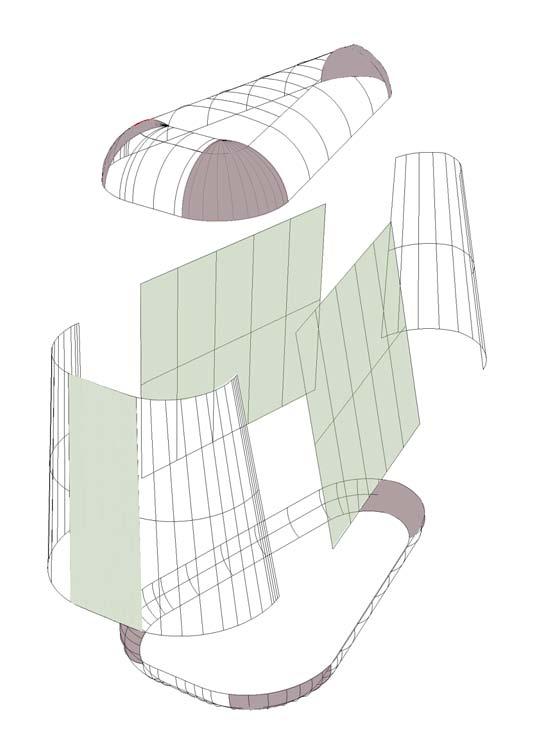
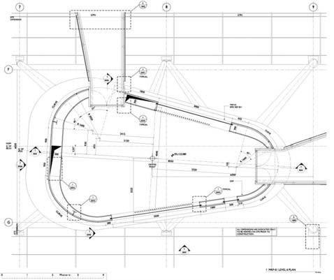
This project, developed from 2000 to 2003, had the task of locating the meeting rooms inside the covered courtyard of the building. As some other projects done by Alsop, GRP was the chosen material to create the entire surface. During the design and manufacturing stage the geometry was simplified to straight lines and arches at the corners. The section could be simplified in radius curves (arch) of 1.30m at the top corners and radius curves of 3m at the bottom corners, this rationalization had the goal to work with regular lines and avoid splines curves which are more difficult to achieve in real materials(fig. 2.1.3)
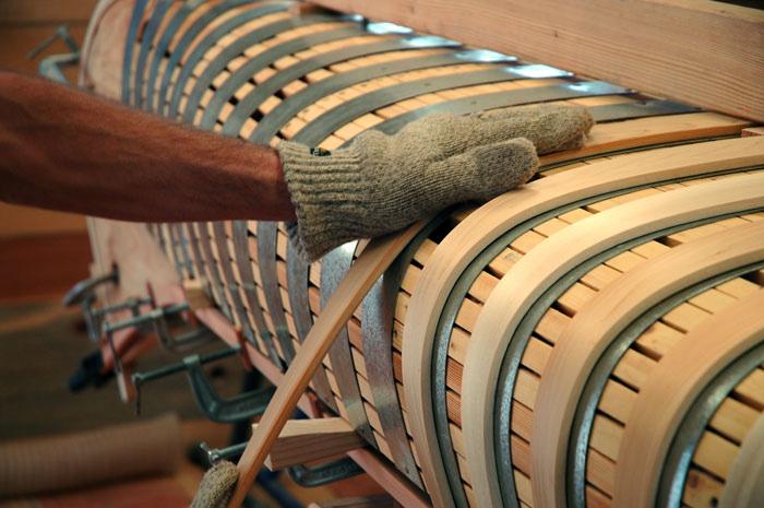
A set of ribs were made in MDF with the curvature that GRP pieces required, they were placed every 0.50cm (fig. 2.1.5) and subsequently some wood beams were placed in between to make enough support for the plywood (fig. 2.1.6). The strips of plywood [6] of approximately 0.40m were cut and laid out with the grain along its large dimension though directionality looked for adaptation to the curves at the corners (fig. 2.1.7). The glass fiber reinforced plastic was laid up with mats of random direction. The pod was built in 6 pieces which were assembled inside the building. The top two pieces didn’t require any additional structure, as it was selfstructural and didn’t have to bear extra load, contrary to the two intermediate, which had some metallic columns to support the mezzanine (fig. 2.1.10).
The complexity in the curvatures of the shell can be simplified into single curvature at the vertical corners, double curvatures at the 6 extreme corners and planar surfaces in the rest of the surface. As is expected, the plywood mold crosses the curves according to its bending possibilities.
CASE STUDIES 30
corners - double curve surface curved in one direction planar surface 2.1 ALSOP POD - ONE fig. 2.1.1
fig. 2,.1.2
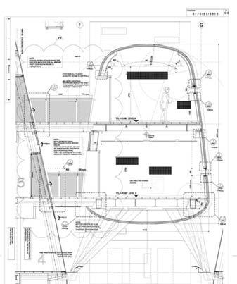
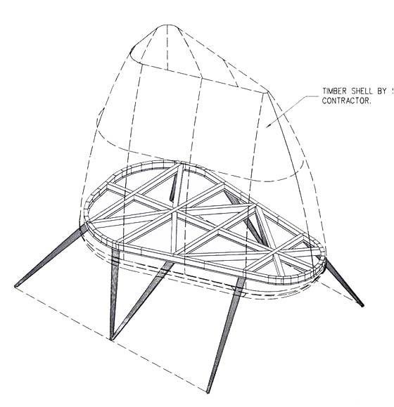
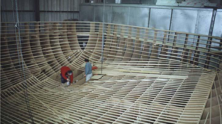
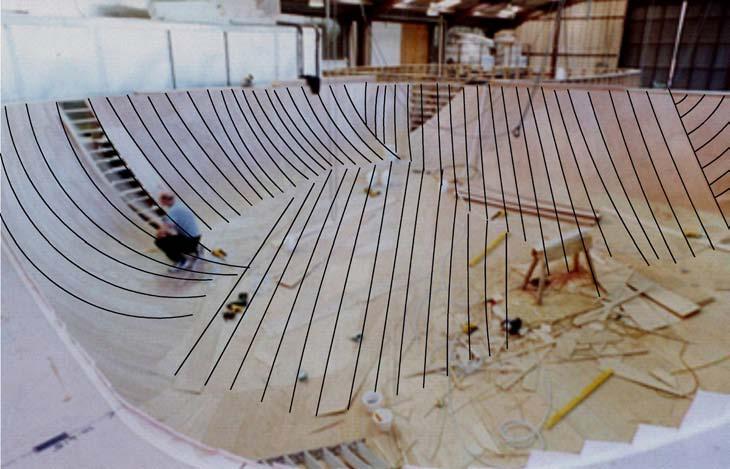
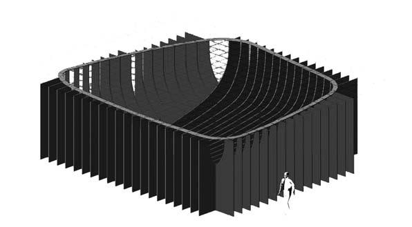
fig. 2.1.1 Geometry abstraction
fig. 2.1.2 Top view
fig. 2.1.3 Transversal section
fig. 2.1.4 Geometry abstraction
fig. 2.1.5 MDF ribs
fig. 2.1.6 Wood beams placed in between MDF
fig. 2.1.7 Plywood strips
fig. 2.1.8 Temporary assembly of 4 pieces
fig. 2.1.9 Pod placement through the ceiling
fig. 2.1.10 Metallic mezzanine structure
fig. 2.1.11 GRP pod at the courtyard Victoria Housebury
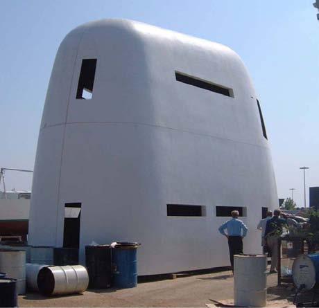
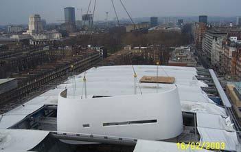
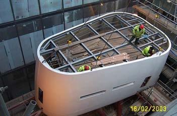
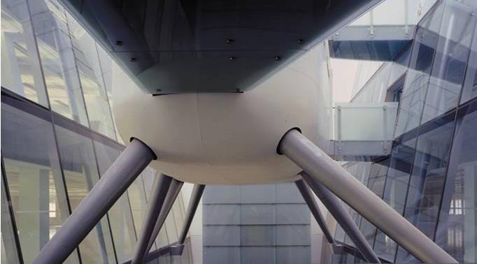 fig. 2.1.3
fig. 2.1.5
fig. 2.1.4
fig. 2.1.6
fig. 2.1.7
fig. 2.1.8
fig. 2.1.11
fig. 2.1.10
fig. 2.1.9
fig. 2.1.3
fig. 2.1.5
fig. 2.1.4
fig. 2.1.6
fig. 2.1.7
fig. 2.1.8
fig. 2.1.11
fig. 2.1.10
fig. 2.1.9
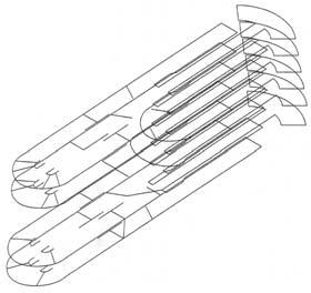
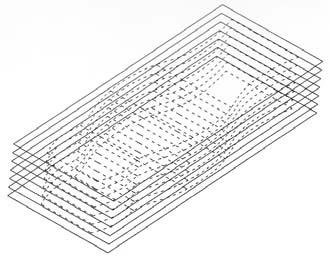
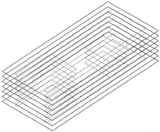
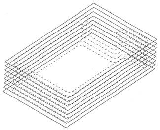
Three “organic” reading rooms located inside the new Peckham Library were created using shell forms from curved timber ribs with structural plywood inner and outer skins. These structures were designed by Alsop architects.
Drawing the objects was an important task for the team as the accurate definition of the geometry would allow unrolling the flat plywood sheets.
The timber ribs were set as a frame in a stand up structure. The initial idea was to create a smooth surface that was going to be covered with leather. The laminates (LVL laminated veneer lumber) were stapled to the ribs. Subsequently the pieces of 0.40 x 0.60m were laid out over the timber structure adopting small curvatures. The skin was placed on both sides, inside and outside, to encourage stress skin action. The pods have a very thin 3mm layer of the same timber tiles stapled to the frame. The pods have an insulating material inside.
The smooth curvature through the surface plus the decision of having short dimension laminates allowed the project to succeed.
CASE STUDIES 32
corners - maximum double curve surface
average doubly curve surface
2.2 ALSOP POD -TWO - PECHAM LIBRARY
fig. 2.2.1
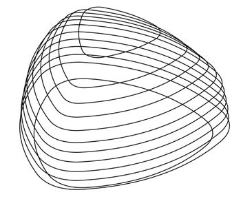
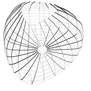
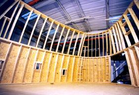
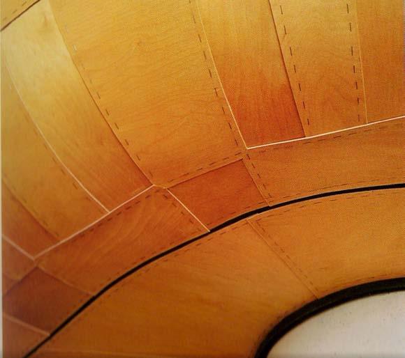
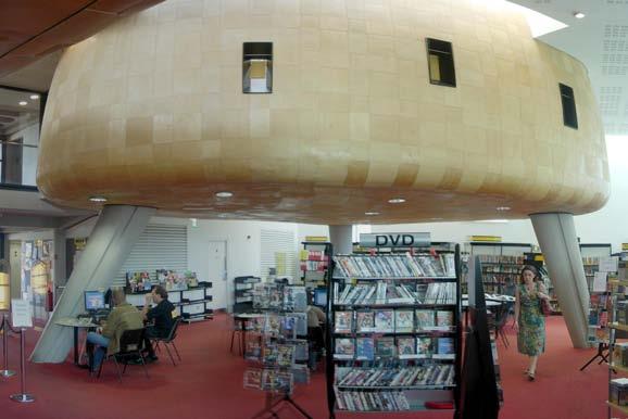
fig. 2.2.1 Geometry abstraction
fig. 2.2.2 Definition of the pod geometry
fig. 2.2.3 TImber ribs as the frame
fig. 2.2.4 Staple of LVL to the ribs
fig. 2.2.5 Interior of Peckam Library
fig. 2.2.6 Interior of Peckam Library
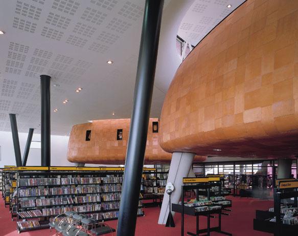 fig. 2.2.2
fig. 2.2.3
fig. 2.2.4
fig. 2.2.5
fig. 2.2.6
fig. 2.2.2
fig. 2.2.3
fig. 2.2.4
fig. 2.2.5
fig. 2.2.6
Material preparation
Wood veneer : About 1.2mm–1.6mm
Resins: UF and PF
Reinforcement: Chopped Strand Mat (CSM 200)
Binders: Polyester resin (PE)
Source: Development Of Fiberglass Reinforced Veneer Products article
2.3 DEVELOPMENT OF FIBERGLASS REINFORCED VENEER PRODUCTS
The Forest Research Institute Malaysia (FRIM) carried out research looking for an alternative timber product, as timber has a large demand in architectural applications but is becoming gradually more expensive. This study presents an alternative product to minimize the usage of timber while still retaining the timber qualities. It aims to produce a thin, light and yet strong panel.
The limited timber resources in Malaysia has affected the supply of veneer that caters to the panel and furniture industry. Because of this the less popular or lesser-known species, as well as incorporating oil palm and coconut veneer as cores in plywood are used.
Methods
Board configuration
Flat fiberglass reinforced veneer panel (6 and 7 layers) were developed based on two design configurations: 1. CSM placed at the center of the panel between the veneers
Panel A: Veneer + CSM + Veneer
CSM : Three layers
Resin: UF (PA1) and PF (PA2)
2. CSM reinforced after the second and fourth layer respectively of the panel.
Panel B : Veneer + CSM + Veneer + CSM + Veneer ‘
CSM : Two layers
Resin: UF (PB1)
3. Control : Same configuration without CSM
Contact angle and formaldehyde test
“The veneer and panel were tested to determine the contact angle. This is done by determining the wetability of the veneer and the panel using contact angle calculation on the samples selected. The FRIM’s in-house method of testing and evaluation is used.ii) The panels were also sent for formaldehyde emission test based on JAS standard. Other parameters such as press time, temperature and veneer thickness were also considered and determined during the preliminary study. The optimum option was selected for subsequent panel production” (H. Hamdan)
Result and Evaluation
In this study, the veneers were arranged following the orientation of plywood. This orientation was preferred because the panel produced using the laminated veneer lumber (LVL) method tends to warp and be dimensionally unstable when thin layers are required. Contact angle is the mean value of contact angle of
the veneer was 80o before it gets penetrated after 2 to 4 seconds. Although the contact angle of the panels was about 82o, it took more that one minute before it penetrated. This shows that the latter is more difficult to be penetrated by the liquid adhesive which indicates that the board is dimensionally stable.
*Formaldehyde emission analysis. The panel was tested to determine the level of formaldehyde emission released by using the JAS standard for plywood. The panel tested was PA1 and PB1 using UF supplied by a collaborating agency. The result showed that it only achieved F** level. 47
In order to allow the Japanese market to use it for interiors, the panel should meet the F**** standard requirement. The classification obtained for panels in this study would qualify for exterior usage only. However, for interior usage, it is recommended that a certain percentage of catcher® be added into the resin to minimize the emission of formaldehyde, thus meeting the standard requirement. Physical and mechanical properties. Generally, the panels were quite heavy compared with the control. It is interesting to note that in panel PA1 and PA2, the MOE and MOR were much higher lengthwise than widthwise. For resins used, the panel PA2 that used PF had much higher physical and mechanical properties. For panel PB1 where the configuration of CSM was at 2 alternate layers, it is interesting to note that the mechanical properties were almost similar in both lengthwise and widthwise directions. This shows that the composite has become quasi-orthotropic (x-y) in nature. When the panels were tested for its mechanical strength, the veneer used in the panel prevented the panel from showing a ductile type failure characteristic that is often seen with fiberglass.
Conclusion
Generally, the fiberglass reinforced veneer panel shows great potential in being developed and utilized by the industry. The uniformity in strength of the panel at both x-y direction shows that it is more stable to be used as membrane for wider area. The results from this study are now being employed in the making of fiberglass reinforced molded products. The superior strength of this engineered composite panel product suggests that buildings can now be designed by incorporating this thin panel. In addition, this product contributes to less construction site waste because it can be ordered to specification. The thin and lightweight material also has potential for use in the development of some furniture designs.
CASE STUDIES 34
2.4
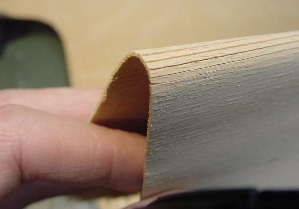
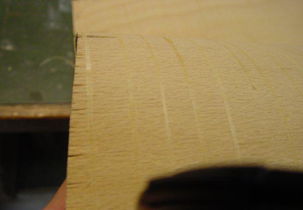
3D VENEER DEVELOPED BY REHOLZ
The 3D veneer is produced by the company Reholz especially for furniture (chairs weight could be 1.880g). The veneer is sliced (from the backside, not completely through) and “cracked” towards the upper/outside surface (fig. 2.4.1). This makes the slicing much less visible. The “individual sticks” are held together from the backside with glue-strings going in perpendicular direction.
The slices blend seaming less together after pressing the veneer together. The sliced veneer works similar to a textile and this is what allows the entire structure to get doubly curved (fig. 2.4.2). The individual sticks can slide a little according to each other; this is what the whole trick is about. Pressing tools are used to make the plywood with cold, glued layers with different directionalities.
With this technique the material thickness is reduced and high stiffness and strength is achieved due to the superposition of veneer in different directions. For prototypes die, stamp and sometimes a forming ring is necessary. For serial production pressing made of aluminium, heated (2- oder 3- parts, that means swage, stamp and if necessary a forming ring).
Glue for plywood manufacturing: Hot gluing: Kaurit 390 powder + hardener 70 + extender Bonit. cold gluing: Kaurit 234 (100 T) + hardener 30 (10 T) + extender Bonit (20T)
Processing: The surface layer does not required it to be moisten or glued and is the last process step to the veneer package. The 3D veneer should not be positioned back side together, in other words, the glue stripes of 3D-veneer shouldn’t be added together in the first join under the surface veneer.
Specifications: Amount of glue is approx. 130 g/m². Open time of the layer before last: 10…15 Min. depending on the climate.
Press temperature: approx. 100°C. press pressure spec.: approx. 2,5 Mpa (it´s a precondition for successful mechanical treatment).
Processing of the 3D-veneer with wood moisture approx. u=8%.
Mechanical treatment of 3D-plywood molding:
Clamping of the moldings without vibrations (especially for thin moldings important) of the pieces with holohedral vacuum, which have reached to the edges of the molding, is necessary. The best way is milling in parallel feed with an end mill, 90° to the surface of the molding
1,15 mm ± 0,05 mm size: length: max. 1300 (2100)mm witdth: max. 980 mm
Surface layer: Beech-rotary cut knife cut veneers (Beech, Am. Walnut, Euro Walnut, Am.White Oak, Euro Oak, Black Cherry, Euro Cherry, Vinterioveneers and others)
Inside layer: Beech rotary cut Ilomba/Kapokier rotary cut
Source: REHOLZ® GmbH. 2009
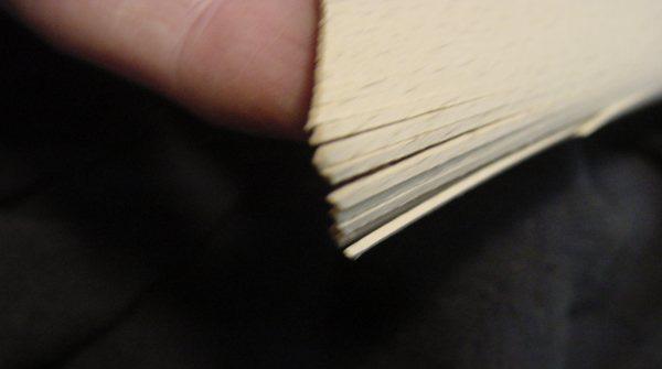
fig. 2.4.1 Sliced veneer fig. 2.4.2 Glue lines on the back fig. 2.4.4 The individual sticks slide a little according to each other
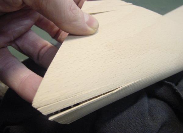 fig. 2.4.1
fig. 2.4.2
fig. 2.4.4
fig. 2.4.1
fig. 2.4.2
fig. 2.4.4
1859-2002
2.5 STRUCTURALLY DEFORMED PLYWOOD IN FURNITURE
The next list shows the evolution of technique through designed chairs:
Bent, massive Chair, Thonet, 1859
Bent plywood Seat, AAlto, 1932
Slightly Molded ArmChair, Eames, 1945
Bent Chair, Prouve, 1950
Slightly Moled Chair, Jacobsen, 1950
Twisted plywood Chair, Gehry, 1990
Multiple Bent 2D plywood chair, Claesson, 2001
Molded
GERMAN WORKSHOPS
3d Plywood chair, Karpf, 2002
Plywood furniture construction
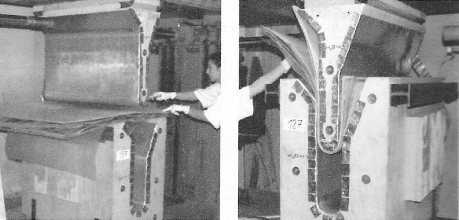
Lounge Chair, Charles and ray Eames, 1941
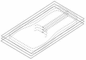
After a series of experiments, the Eames made a prototype chair seat produced by a laborious method of gluing together and heat bonding thin plies in a plaster formwork, located at the base of the machine. An inflatable machine membrane, enclosed in the wooden box, covered the layers of wood. After the device was securely bolted together, the membrane was inflated with a bicycle pump to keep the wood plies pressed against a plaster form. During the four to six hours molding process, heating elements embedded in the plaster form cured the glue. Air was pumped into the membrane regularly to maintain the required level of pressure. Heating elements embedded in the plaster form cured the glue. Air was pumped into the membrane regularly to maintain the required level of pressure. Once the glue had set, the pressure was released and the formed seat was removed from the mold. The edges were trimmed with hand say to the desired finished shape and hand sanded.
This first Bent Ply product for furniture application was made from three rather thick veneers, with all the grains laid out in the same direction. Where the radius was too small, so that bending would have broken veneers, cuts were introduced into the initial veneers. The here with separated parts of the sample where than later re-
joined with bolts to stiffen the overall structure.”
Used wood material : Veneer
Number of Plies: 3
Thickness of Plies: 003mm
Thickness of Composite (plywood): 009mm
Grain Direction: Parallel
Deformation Mode: Molded
Pre-treatment: Structural Edge cut veneers
Joints:
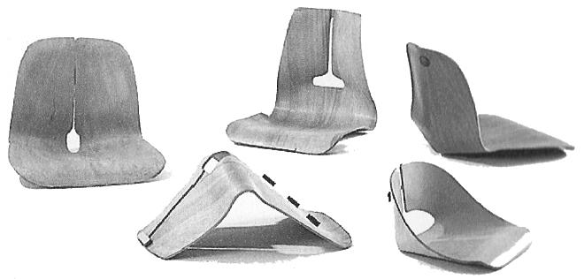
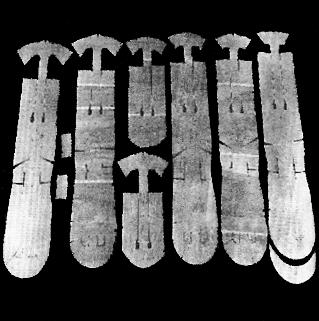
Leg Splint, Charles and Ray Eames, 1941
The famous Eames leg-splints were made from a relatively large number of very thin veneers, which all were pre-cut to size and therefore had to be laid upon each other very carefully before molding. These pre-cut forms match the load bearing character of the splint, in highly stressed parts the number of veneers increased; in others the number is reduced. Small bending radius were achieved by bending two, previously cut and separate edges towards each other and later joining them. The result offered a complex form with partly tight curvatures, structurally (by number of veneer in cross section) specifically designed according to its loading.
Used wood material: Veneer
Number of Plies: 6
Thickness of Plies: 001mm
Thickness of Composite (plywood): 006mm
Grain Direction: Perpendicular
Deformation Mode: Molded
Pre-treatment: Entirely pre-cut veneers
Joints: Glued
http://www.loc.gov/exhibits/Eames/Furniture.html
CASE STUDIES 36
fig. 2.5.1
82us chair, Peter Karpf, 2002
This example employs abilities of high pressure molded plywood, which results in extreme structural performance. A plywood sheet is molded into a three dimensional shape with small curvatures and complex shell shapes and then cur and finished by hand. The chair, made out of this one single bolded plywood piece, takes advantage of the tensions appearing during the molding process- the upper plies get tensioned, while the lower plies in cross section get jolted, so that the performance is quiet similar to pre-tensioned concrete, where two parts with different load bearing characters complement each other , this shell principles allows a coherent and non-joints chair uniquely made form plywood.
Used wood material: Plywood
Number of Plies: 7
Thickness of Plies: 000,8mm
Thickness of Composite (plywood): 005,6mm
Grain Direction: Perpendicular
Deformation Mode: Molded
Pre-treatment: None
Joints: None
fig. 2.5.1 Lounge Chair
fig. 2.5.2 Leg Splint
fig. 2.5.3 Mold for Wave Desk
fig. 2.5.4 Cut pattern on veneers for Lounge Chair
fig. 2.5.5 Cut pattern on veneers for Leg Splint
fig. 2.5.6 Cut pattern on veneers for 82us
fig. 2.5.7 Cut pattern on veneers Plywood Chair 50642
fig. 2.5.8 Cut pattern on veneers for Wave Desk
Plywood Chair 50642, Erich Menzel, German Workshops
Hellerau, 1950
Used wood material: Veneer
Number of Plies: 8
Thickness of Plies: 001mm
Thickness of Composite (plywood): 008mm
Grain Direction: Parallel
Deformation Mode: Bent
Pre-treatment: -
Joints: Glued
Source: “Mythos Hellrau” /Exhibition catalogue , Deutsche Werkstatten, 2002
Wave Desk, Eric Pfeiffer, 2002
This wave desk is still made from numerous veneers, which get stacked and then pressed into a mold. The pressed sample is then automatically cut, sanded and finished, so that the usual work distribution of industrial production, followed by a manufactured finish is inverted.
Used wood material: Veneer
Number of Plies: 8
Thickness of Plies: 001mm
Thickness of Composite (plywood): 008mm
Grain Direction: Perpendicular
Deformation Mode: Molded/Bent
Pre-treatment: None
Joints: Glued
Source “Bent Plky, Ngo, Pefeiffer, Princeton architectural, press, new york, 2003)
CASE STUDIES
fig. 2.5.3
fig. 2.5.2
fig. 2.5.4
fig. 2.5.5
fig. 2.5.6
2.5.7
fig.
2.5.8
fig.
2.6 FABRICATION TECHNIQUES FOR SHELLS ELADIO DIESTE
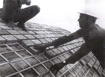
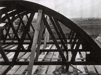
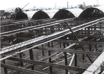
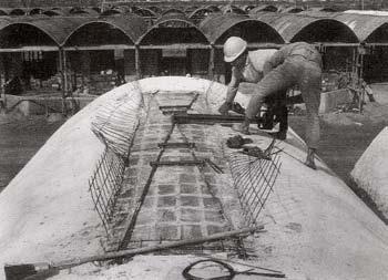
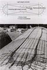
Eladio Dieste is an Uruguayan engineer who developed the technique of reinforced masonry vaults, technique that has genuinely provided advances in the use of brick in complex geometries and its construction process. The first technique refers to self-weighted vaults, which are always catenaries curves, the most efficient structural form. The vaults are pre-stressed to take bending forces and thus act like beams. What the main interest is for this research is the ingenuity of combining the aesthetic and the structural capacity to its maximum in the surface. For instance, in the storage of the Massaro there are groups of vaults supported in distant columns, having 16.5 m cantilevers. The vaults are also perforated for light in middle areas but also overlap to have indirect light.
The second vault type used by Dieste solves the problem of buckling in the Gaussian vaults through the shape, giving strength in the center of this span with the changing S-section. “The simple catenary curve of a reinforced self-supporting vault allowed it to perform as a beam” (Nordenson, G. 2008). Dieste’s work is outstanding architecturally and in engineering as he combines through one surface the concepts of proportion, space, light, surface, texture, structure and rapid construction.

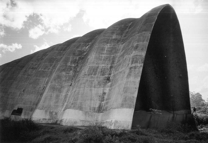
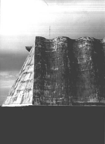
fig. 2.6.1 Wood strips nailed to formwork to position the bricks
fig. 2.6.2 Small self-carrying vaults
fig. 2.6.3 Timber trusses for the formwork
fig. 2.6.4 Pre-stressing the looped steel rods with a manual jack
fig. 2.6.5 Looped pre-stressing steel, absorbs negative bending moments
fig. 2.6.6 S-shape on Gaussian vaults
fig. 2.6.7 Corrugation effect on a sheet paper
fig. 2.6.8
fig. 2.6.9 Cadyl Horizontal Silo
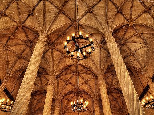
fig. 2.6.10 Lonja de la Seda de Valencia, 15th century
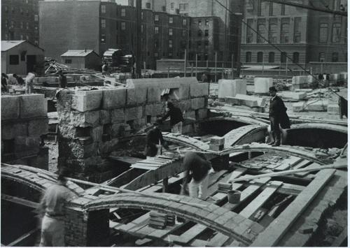
fig. 2.6.11 The method of timbrel vault
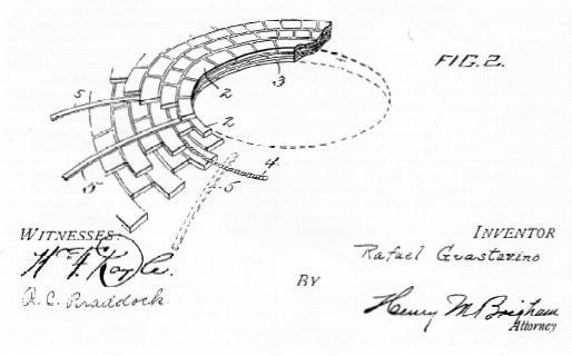
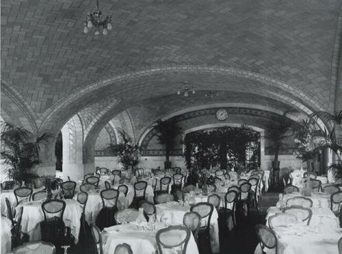
fig. 2.6.12 Oyster Bar in Grand Central Terminal
fig. 2.6.13 Adhesion of several layers of overlap ping tiles
CASE STUDIES 38
EXTERIOR INTERIOR
fig. 2.6.1
fig. 2.6.2
fig. 2.6.3
fig. 2.6.6
fig. 2.6.8 fig. 2.6.9 fig. 2.6.4 fig. 2.6.5
fig. 2.6.7
RAFAEL GUASTAVINO TECHNIQUES
The Catalan vaulting system is a masonry technique perfected in Catalonia, Spain. Rafael Guastavino took it to United States where the system was used in many large scale buildings. This technique as this research proposes, does not require formwork and is capable of spanning large open spaces and constructing robust, self-supporting arches and architectural vaults.
The Catalan system is effective at covering large areas gracefully and economically. The key of the system is a fast-setting mortar on two edges of a tile, which allows it to hold itself after being tapped into place. Once the first course is laid, the second course of single tiles is progressed, breaking the joints of the previous layer with rich Portland cement mortar. After the second course is set, the worker can stand on the tile ring and lean to progress erecting the first course of the second row. The process continues until the dome is closed at the apex. One of the most remarkable aspects of Guastavino’s vaults is that they hold their own weight the day after the tiles are set. Due to this inherent selfsupporting nature of the construction, the vaults can be built without centering and scaffolding – unless it is necessary to elevate the workers.
CASE STUDIES
fig. 2.6.12
fig. 2.6.13
fig. 2.6.10
fig. 2.6.11
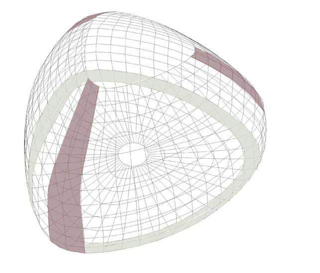
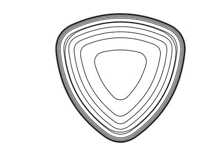
A wide range of fabrication techniques were explored in the next chapter in order to achieve different geometries in wood and plywood and to keep the resulting curvatures on the final shape. Some experiments have focused their efforts in transferring the geometry from physical to digital experiments, in order to provide precision and viability in the fabrication. The research looks for different methodologies in the simulation of the plywood deformed geometries using Rhino*, Rhinoscript*, Grasshopper* and Strand7*. The material behavior of the composite is understood through the simulations, as well as the structural capabilities.
* Rhino is 3D design software
* RhinoScript is a scripting language based on Microsoft’s VBScript language
* Grasshopper is a graphical algorithm editor tightly integrated with Rhino’s * 3-D modeling tools * Strand7 is a Finite Element
CAD Digital DESIGN GEOMETRY CAM Machine DESIGN PROCESS GEOMETRYMaterial capacity
System
Analysis (FEA) Software
DESIGN PROCESS
Geometry
FABRICATION METHOD (no mould)
-Theoretical shells - Form finding for panels (buckling method)
- Panelization - Form finding on the assemblies (stitching)
- Light filters
System to create shells
- Reinforcing construction method
CHAPTER THREE - EXPERIIMENTS
Plywood + Fiber glass + Resin
design process
CFD Analysis wind rain
Structure
Parametric model
geometry
fabrication
Bending material CNC milling
Construction Sequence
EXPERIMENTS 42
3.1. CANOPY
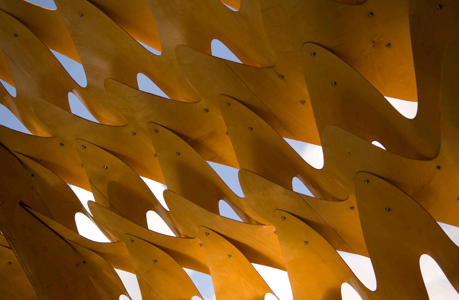
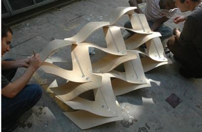
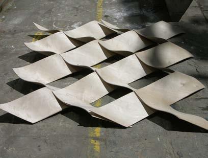
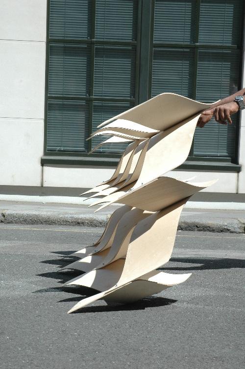
fig. 3.1.0 Close capture of the overlaping
fig. 3.1.1 Options for matching the strips
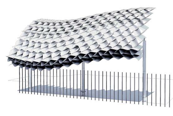
fig. 3.1.2 Inclination of assembly for drainage
fig. 3.1.3 Fin section
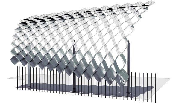
fig. 3.1.4 Variation in the openings by Grasshopper definition
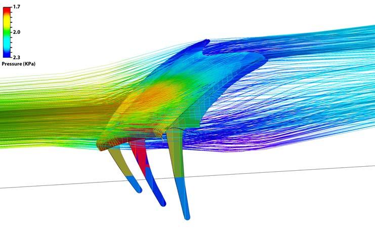
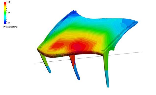
fig. 3.1.5 CFD (Computational Fluid Dynamics) analysis
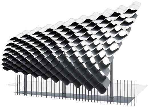
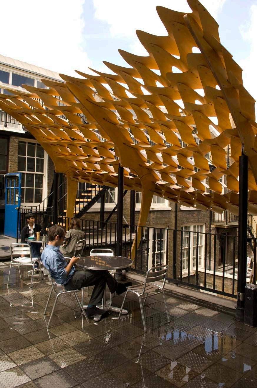
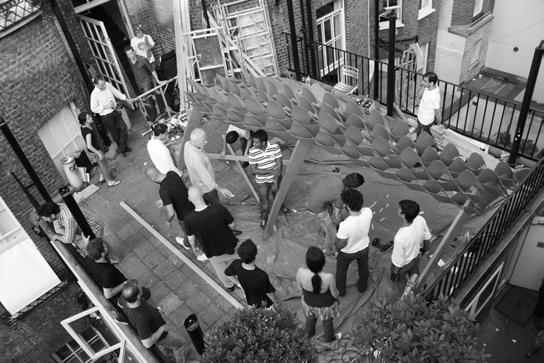
Design and Fabrication of “EmTech” Canopy at the Architectural Association
The Canopy project was developed by the master course Emergent Technologies and Design 2008-2009, and consultant from Buro Happold Engineers for the structural design.
The project utilized the timber composite as a result of previous experiments run in Core Studio at the beginning of the year. These initial explorations of the material are presented on the experiment 2.1.
Design process
The design had to respond to wind conditions, drainage facility and structure capacity at the AA terrace. After deciding the wood as the main material and corrugated strips as the strategy for the overall form, the goal was to stand up the canopy making the strips work as struts when transferring the load to the ground. Sadly the wood wasn’t enough to create the 3D struts required (Figure XX). Plus, due to its thickness and overall geometry it would continuously creating fatigued moments which were not appropriate to the only three columns available to transfer loads to the beam located within the terrace floor.
In the initial prototypes steel struts were placed as compression elements in between the strips, however, one of the final decisions before starting the fabrication stage was to remove them and as a solution transfer loads to the existent rounded columns and to guaranty the stability of the structure through high wind channels. The struts were eliminated and three fins were placed to support the canopy.
EXPERIMENTS 44
fig. 3.1.4
fig. 3.1.1 by Jheny Nieto
fig. 3.1.2 by Jheny Nieto
fig. 3.1.3
Structure
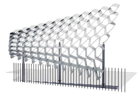
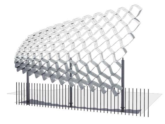
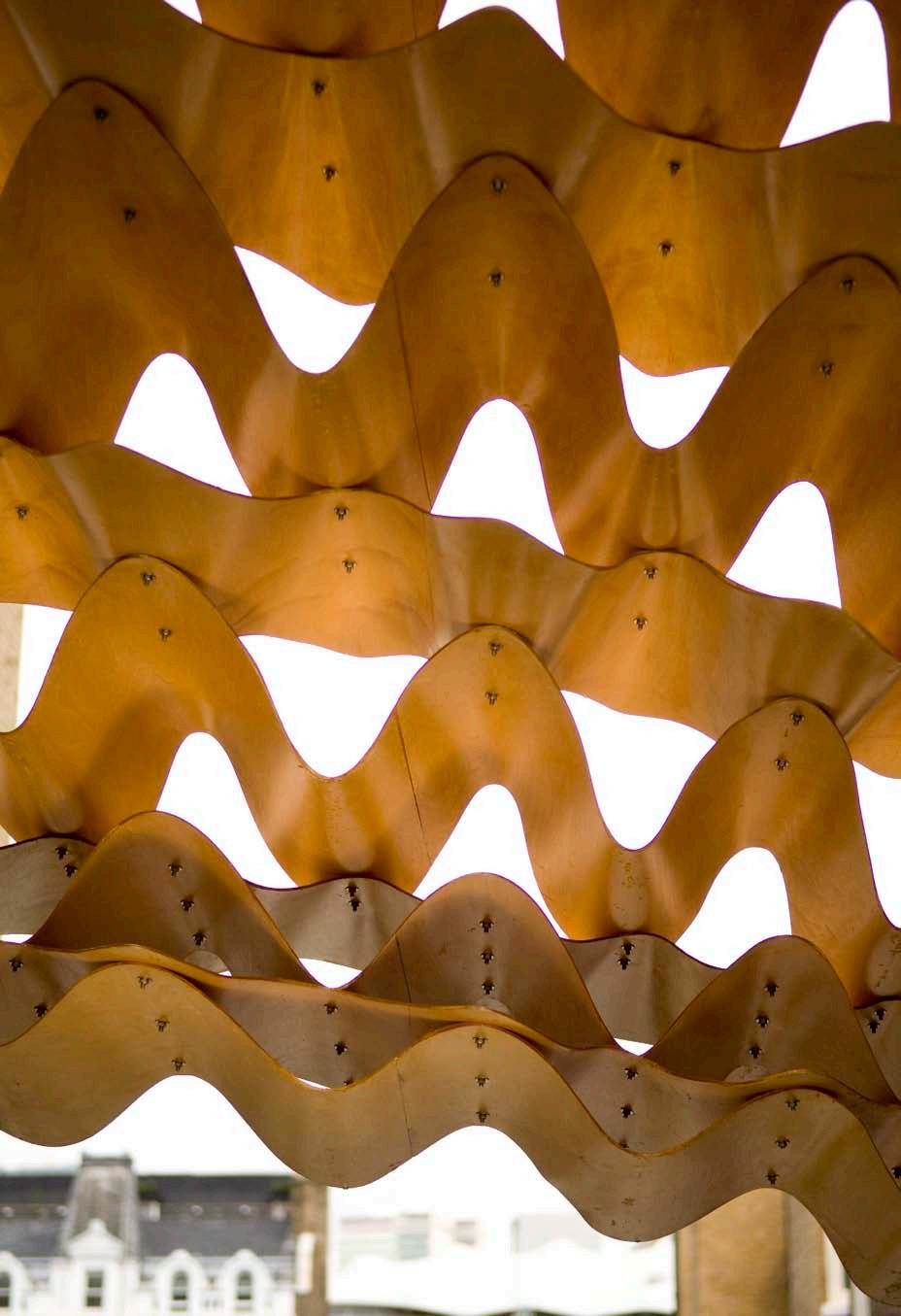
The curved morphology distributes vertical loads laterally. The component made use of the elastic bendable properties of plywood.
The corrugation
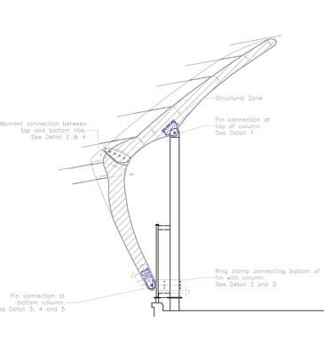
The fins - The structure has a total of three fins -one per column; each fin consists of three layers of plywood: 12mm in the outer layers and 18mm for the inner one. Plywood sheets with these thicknesses are only provided in 1.2 x 2.4m rectangular panels. This required each fin to be divided further into two parts: top and bottom. The upper fin is connected to the top plate of the existing columns through a pin connection (20mm dia.). The existing column plate is reinforced with a steel flitch plate screwed to the inner layer. The lower fin connects to the existing columns at the bottom using a ring clamp around the columns.
Wind and drainage
The wind is channeled through but the shape of the component creates local turbulence that separates the airflow from the rain. Rainwater is channeled down in the direction of the drainage points defined by the slope of the overall surface. A flow analysis of the final structure was necessary to determine how big the voids should be to help to reduce the wind pressure indicated in the specifications.
Variation
An associative digital model was developed so that it can input the changes and readapt to specific structural requirements. Transferring this associative model to the real structure was one of the major challenges as plywood had certain constraints in the bending according to the curvature required.
EXPERIMENTS 45
fig. 3.1.5
EXPERIMENTS 46
fig. 3.1.6
EXPERIMENTS
Fig. 3.1.6 Canopy at AA terrace
Fig. 3.1.7 Variation of voids height. Plan utilized in construction
fig. 3.1.7
Option Explicit‘Script written by <insert name>‘Script copyrighted by <insert company name>‘Script version Friday, February 27, 2009 10:59:26 PMCall Main()Sub Main() Dim strCurve Dim blnCreate Dim arrPts, arrPoint Dim l Dim strtext1, strtext2, strtext3, strtext4 ‘l = blnSegments strCurve = Rhino.GetObject (“select curve to cut”,7) If isnull(strcurve) Then Exit Sub ‘points = Rhino.Getobjects (“select holes ‘points’...to drill”,1) l = Rhino.GetInteger (“number of segments”,750) arrPts = Rhino.DivideCurve (strCurve, l, 1) ‘1 it’s because it’ s boolean function Dim m , strfilter, strfilename, strpoint, objFSO, objStream strfilter= “*.txt” strfilename=rhino.SaveFileName(“points file”,”strfilter”,”c:\ Works”,”file”,”nc”) Set objFSO = CreateObject(“Scripting. FileSystemObject”) Set objStream = objFSO.CreateText File(strFileName) ‘’ starting part of the file Dim stt0 : stt0 = “G90” Dim stt1 : stt1 = “M90” Dim stt2 : stt2 = “G71” Dim stt3 : stt3 = “M25” Dim stt4 : stt4 = “G75” Dim stt5 : stt5 = “G00 T06 (T6 - Drill 6mm)” Dim stt6 : stt6 = “G97 S16000” Dim stt7 : stt7 = “G00 Z-15.” Dim stt8 : stt8 = “ “ objStream.WriteLine(stt0) objStream.WriteLine(stt1) objStream.WriteLine(stt2) objStream.WriteLine(stt3) objStream.WriteLine(stt4) objStream.WriteLine(stt8) objStream. WriteLine(stt5) objStream.WriteLine(stt6) objStream. WriteLine(stt8) objStream.WriteLine(stt7) objStream. WriteLine(stt8) ‘Dim temppt ‘’ generating points ‘For m = 0 To Ubound (points) Step 1 ‘temppt = rhino.pointcoordinat es(points(m)) ‘strpoint = (“G00” & “ X” & temppt(0) & “ “ & “Y” & temppt(1)) strtext1 = “M12” strtext2 = “G83 R-12. Z.5 Q30. F33.333” strtext3 = “M22” strtext4 = “ “ objStream. WriteLine(strPoint) objStream.WriteLine(strtext1) objStream. WriteLine(strtext2) objStream.WriteLine(strtext3) objStream. WriteLine(strtext4) ‘Next ‘’ generating curves.....starting part Dim str0 : str0 = “ “ Dim str1 : str1 = “Z-15.” Dim str2 : str2 = “G00 T21 (T21 - 9.52 mm Compression)” Dim str3 : str3 = “G97 S18000” Dim str4 : str4 = “G00 Z-6.” objStream. WriteLine(str0) objStream.WriteLine(str1) objStream. WriteLine(str2) objStream.WriteLine(str3) objStream. WriteLine(str4) Dim str5 : str5 = “M12” ‘’ generating curves For m = 0 To Ubound (arrPts) Step 1 If m=0 Then strpoint= (“G00”&” X”&arrPts (m) (0)&” “&”Y”&arrPts (m) (1)) objStream.WriteLine(strPoint) objStream.WriteLine(str5) End If If m<>0 Then strpoint= (“G01”&” X”&arrPts (m) (0)&” “&”Y”&arrPts (m) (1)&” “ & “Z.1 F166.667”) objStream. WriteLine(strPoint)End If Next ‘’ last bit Dim sq1 : sq1=”G00 Z-6.” Dim sq2 : sq2=”M22” Dim sq3 : sq3=”G00 Z-15.” Dim sq4 : sq4=”M22” Dim sq5 : sq5=”(End)” Dim sq6 : sq6=”G00 X2440 Y1220 Z-200” Dim sq7 : sq7=”M02” objStream.WriteLine(sq1) objStream.WriteLine(sq2) objStream.WriteLine(sq3) objStream.WriteLine(sq4) objStream. WriteLine(sq5) objStream.WriteLine(sq6) objStream. WriteLine(sq7) objStream.CloseEnd Sub
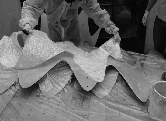
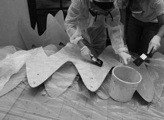
Fabrication
Before beginning the construction, the flat pieces were nested in Rhino files so that the top and bottom lines of the waves were along the grain to facilitate the manual bending process(fig. 3.1.8).
General construction Sequence
Phase 01: CNC milling of sheets (fig. 3.1.9). fig. 3.1.9
Phase 02: Sealing process on the outer side of the cut pieces plywood
Phase 03: Lamination of strips
Phase 04: Sealing the other side of the assembled strips /sanding of the borders
Phase 05: Assembly of the top and bottom fins
Phase 06: Placement of the 5m long strips from top to bottom
Phase 07: Rotation of the complete fin and strips structure to its final position and fixing of bolted joint at lower part of column
Phase 08: Lifting and securing of fins and boltconnection at top of column
Different tests were done at the beginning of the lamination process to decide the assembly method. Finally, the overlapping method was selected and the forming of a single strip a total of twelve pieces where required (six top and six bottom).
CNC milling
200 sheets of 1.5 mm thickness plywood were necessary to fabricate the 14 strips constituting the new canopy(fig. 3.1.11). Each sheet measured 1525x1525 mm. The bed of CNC machine used was 1220 mm width and thus, we had to re- cut the plywood sheets to 1525x1220 mm. A script was written in order to work with the Multi-CAM software used by the CNC where two drillers were used, 6mm for the cutting of the edges and 9mm for the cutting of holes for future bolting (fig. 3.1.9, fig. 3.1.10)
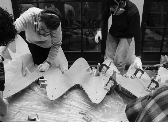
The jig
The precision of the entire canopy relied on fabricating the strips as precise as possible (fig. 3.1.14). In addition to the curvature of the individual waves, each strip was also curved overall. The curvature of the waves was governed by the height and length of each wave. In order to achieve the global curvature on each strip, a curved jig was carefully designed and built. The lamination process takes place on the jig. The process is a continuous iteration of the next steps: laminating, clamping, and bolting (fig. 3.1.15, fig. 3.1.16)
EXPERIMENTS 48
plywood main grain direction
fig. 3.1.8
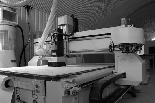
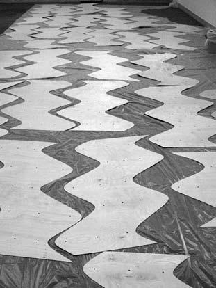
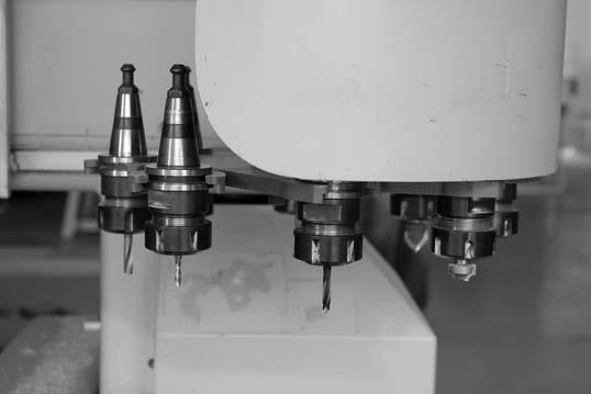
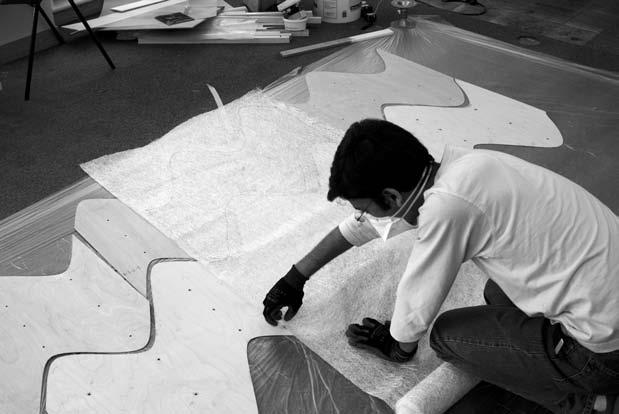
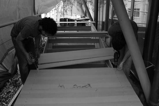
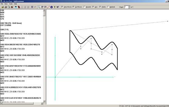
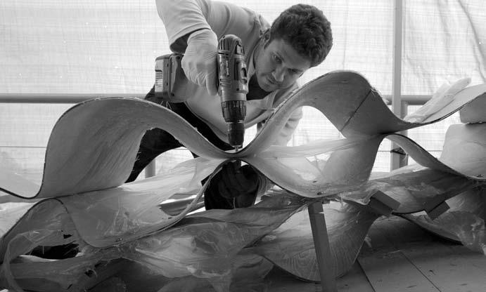
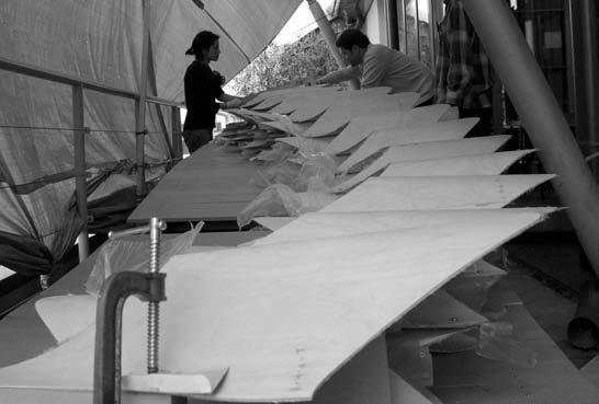
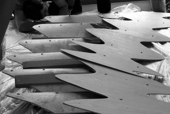
fig. 3.1.8 Rhino file
fig. 3.1.9 CNC milling machine
fig. 3.1.10 G-Code in Multicam software
fig. 3.1.11 Cut sheets of plywood
fig. 3.1.12 Cutting fiber glass pieces
fig. 3.1.13 Bolting strips
fig. 3.1.14 Jig under construction
fig. 3.1.15 Third strip curing
EXPERIMENTS
fig. 3.10
fig. 3.1.9
fig. 3.1.11
fig. 3.1.13
fig. 3.1.14
fig. 3.1.15
fig. 3.1.12
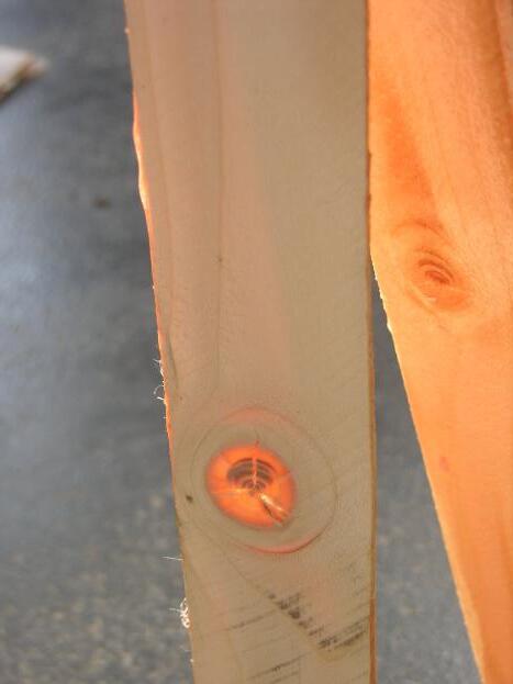
Lamination - Clamping Process - Bolting
Significant knowledge was gained in the process of transferring the material capabilities into grasshopper model as parameters and of course vice versa. A ratio between strip height to the zigzag shape (from top view) was establish to allow the plywood get its bending without creating so much perpendicular force to the grain.
Each strip is laminated with fiber glass and resin in a sandwich and directly curved, bolted and held in position with clamps for at least one hour until the resin is dry. Subsequent strips are constructed on top of the previous, securing the relative position of the two strips with bolts (fig. 3.1.17 ).
Sealing
The plywood is varnished before and after the lamination in order to protect the wood from humidity. Assembly - Placement of the 5m long strips from top to bottom
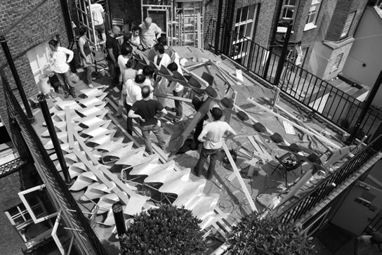
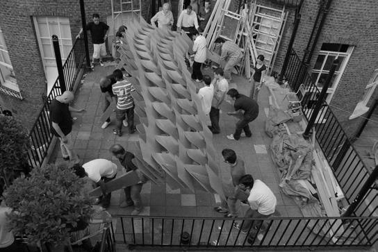
The assembly of the entire canopy was done by groups of strips in situ.
Rotation of the complete fins and strips
The fins were disposed on the terrace in order to assemble the groups of strips to the slots previously cut on them. In order to test the lifting process some attempts of the rotation of the fins were done with only one group of strips on it. Afterwards, the entire lower fins are positioned on the outer side of the balustrade, while only a small section of the upper fins goes over the terrace fencing. The connection between the top and bottom fins was first thought to be pinned similarly to the one at the top of the column. However, providing a momentary connection at this position helped with distributing the vertical load in between (fig. 3.1.18)
EXPERIMENTS
fig. 3.1.16
3.1.16 Close capture of voids differentiation
3.1.17 Laminating-Clamping-Bolting Process
3.1.18 Fixing the group of strip to fins
EXPERIMENTS
fig. 3.1.17
fig. 3.1.18
fig.
fig.
fig.
3.2.1
Having as a hypothesis that torsion pre-stress the wood fibers and avoids the buckling of each piece in order to support more load. The experiments were run with the expectation that the fiber glass with resin increases the properties of the wood and allow the performance of a light structure bearing larger loads.
The next 4 processes were taken in order to run the physical experiments, a torsion machine was built and a testing loading machine
LOAD CAPACITY IN INDIVIDUAL STRIPS
TP Torsion Process
When the torsion is given on the central axis the pieces that had 90degrees of torsion remained at 45 degrees of torsion, this is called spring back which is the property of the materials to change back. In this case, according to the original torsion and according to the ratio of the reinforcement process.
When the torsion is not given on the central axis it remains at 90 degrees as the pre-stress is not that high. The pieces get a predetermined trend to bend towards the displaced axis.
RP Reinforced Process
The reinforced process was initially done with different parameters in order to determine the output of each procedure. Resin on one side of the wood, fiber glass perpendicular to the wood fibers + resin, fiber glass parallel to the wood fibers+ resin, fiber glass around the knots + resin.
A priori to disassembling from the torsion machine the pieces were subjected to dry less than 23 degrees.
TE Testing Experiments
As the piece of wood has been in torsion and apriori reinforced, each one was tested under an increasing load in the same direction of the wood fibers.
The tests showed that a thin piece of wood under certain procedures can support considerable loads and confirm the knots as the weak area of any piece of wood.
AL Assembly Logic
The variation in the torsion degree gave a change of direction to the assemblies which are remarkably efficient for geometries to avoid buckling; this means the “triangle” form increases the inertia on the structure (fig. 3.2.1.9)
The results
Timber is a material with big variation on its internal structure. Each piece can display a different behavior according to its growth conditions; the reinforced material can give continuity to the wood fibers through glass fibers around the knots.
The pieces had a potential in carrying loads along the fibers and the torsion increase the section of the piece keeping it light (thickness of 3mm) but strength. The torsion is like a virtual bounding box. In testing, the results showed the reinforced pieces has a tendency to lose the torsion and start bending when the load applied is over 20 kg.
EXPERIMENTS 52
TESTING
fig. 3.2.1.1
BENDING
TP TORSION PROCESS
TP TORSION PROCESS
before after
before after
RP REINFORCED PROCESS
RP REINFORCED PROCESS
RESIN
RESIN
TE TESTING EXPERIMENTS
TE TESTING EXPERIMENTS
UNRETURNABLE
UNRETURNABLE
BENDING
BENDING
RESIN + FIBRES
RESIN + FIBRES
PERPENDICULAR 1 LAYER
PERPENDICULAR 1 LAYER
RANDOM 3 LAYERS
RANDOM 3 LAYERS
RANDOM 5 LAYERS
RANDOM 5 LAYERS
AROUND KNOTS
AROUND KNOTS
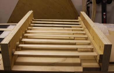
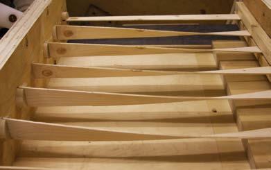
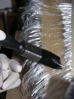
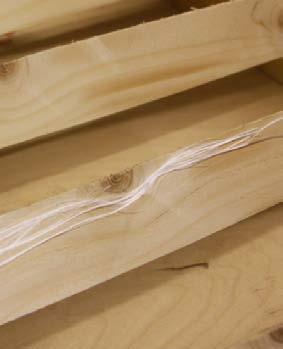
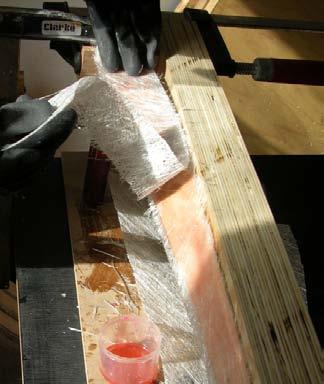
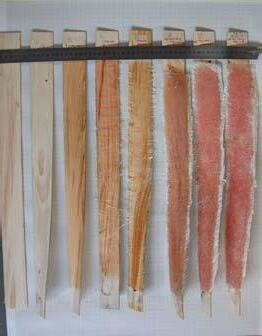
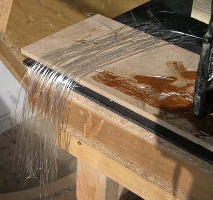
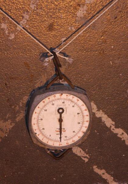
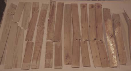
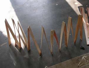
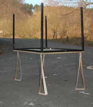
fig. 3.2.1.1 Knot in strip wood
fig. 3.2.1.2 Torsion machine
fig. 3.2.1.3 Reinforced strip with fiber glass-one direction
fig. 3.2.1.4 Reinforced strip with 3 layer of fiber glass - random direction
fig. 3.2.1.5 Reinforced strip with fiber glass around the knot
fig. 3.2.1.6 Twisted pieces reinforced
fig. 3.2.1.7 Cracked pieces under load
fig. 3.2.1.8 Assembly of twsted pieces
fig. 3.2.1.9 Test aproximately 50kg on strips without displacing from its original position
EXPERIMENTS P3 P4 P5 P6 P7 P8 P9 P10 P3 P2 P1 P5 P6 P7 P11 P12 P13 P14 P15 P16 P17 P18 P19
AL ASSEMBLY LOGIC A1 A2 A3 A4 A5 A6 FLEXIBLE RIGID
COMPLEX STRUCTURE
CRACK LOOSE OF TORSION
90
120 90
45
amounts from allowed
AL ASSEMBLY LOGIC A1 A2 A3 A4 A5 A6 FLEXIBLE RIGID
COMPLEX STRUCTURE
CRACK LOOSE OF TORSION
BENDING
90
120 90
45
3.2.1.4
3.2.1.7 fig 3.2.1.8
fig 3.2.1.2 fig
fig
fig 3.2.1.3 fig 3.2.1.5 fig 3.2.1.6
TORSION PROCESS
REINFORCEMENT PROCESS
fpa=fibers paralell
fpe=fibers perpendicular fr= fibers random
fk=fibers around knots
lay=layers of fiber
TEST EXPERIMENTS
s1= side 1
s2= side2 s1/s2
EXPERIMENTS 54 P 1 P 2 P 3 P 4 P 5 P 6 P 7 P 8 P 9 P 10 P 11 P 12 P 13 P 14 P 15 P 16 l= length 0.60m 0.60m 0.60m 0.60m 0.60m 0.60m 0.60m 0.60m 0.60m 0.60m 0.60m 0.60m 0.60m 0.60m 0.60m 0.60m w = width 0.05m 0.05m 0.05m 0.05m 0.05m 0.05m 0.05m 0.05m 0.05m 0.05m 0.05m 0.05m 0.05m 0.05m 0.05m 0.05m t= thickness 0.005m 0.003m 0.003m 0.003m 0.003m 0.003m 0.005m 0.003m 0.003m 0.003m 0.003m 0.003m 0.003m 0.003m 0.003m 0.003m
knots 0 1 1 0 1 1
to=torsion (axxis) 0 0 0 60 60 60 60 60 60 60 30 30 60 60 60 60
k=
resin r=10ml r=10ml r=10ml r=40ml r=40ml r=40ml r=10ml r=10ml r=20ml r=20ml r=10ml r=10ml r=10ml r=10ml
r=
fpe= low density fpe= high density fr= 3 lay fr= 3 lay fr= 5 lay fr=1 lay fr=1 lay
fracture moment 5kg 5kg 4kg 3.7kg 6.5kg 4kg 5kg 8kg 10kg 13kg bend=bending moment 20kg 20kg 5kg 20kg 20 kg
fra=
J1 J1 90 90 90 90 J2 A1 individually A2 two-stand bythemselves A3 two- vertical A4 two- overlap A5 four- perpendicullar to each other A6 three- create a triangule to get a column with a seccion area
fig. 3.2.1.11
fig. 3.2.1.10
0.60m 0.60m 0.60m 0.90m 0.60m
0.05m 0.05m 0.05m 0.05m 0.05m
0.003m 0.003m 0.003m 0.003m 0.003m 1 0 1 1 0
fig. 3.2.1.10 Chart of parameters and craking results
fig. 3.2.1.11 Alternatives of assemblies
fig. 3.2.1.12 Stable Pair pieces assemblies
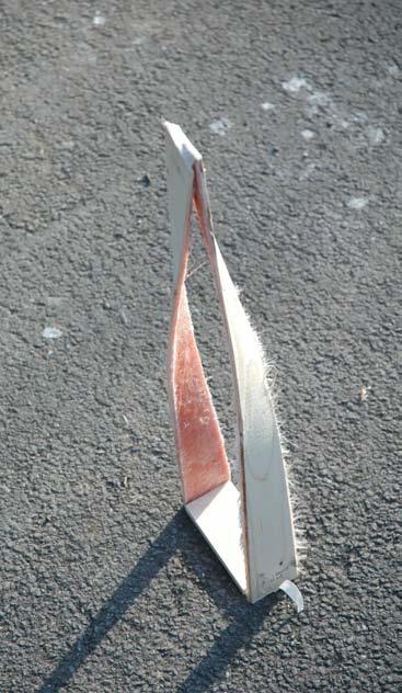
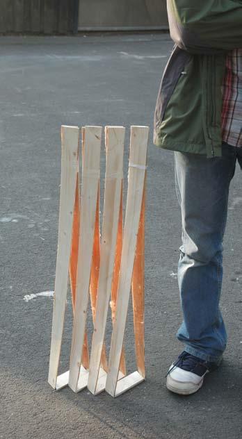
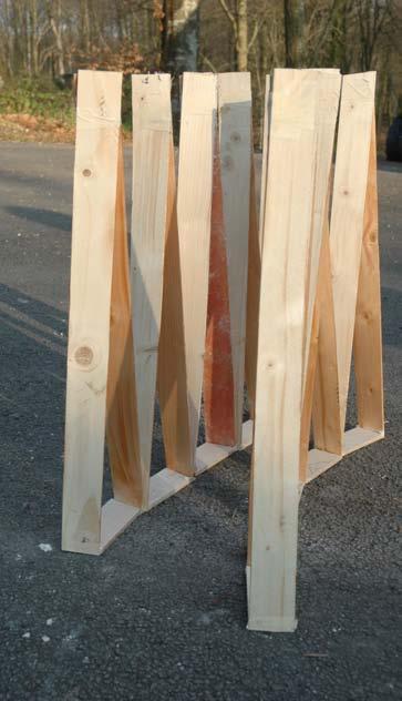
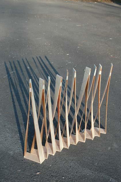
EXPERIMENTS 55
17 P
P
18 P 19 P 31-39 P 21-29
60
45
fk=high
dens fr=1 lay
18kg 18kg 7kg
60 60 45
r=10ml r=10ml r=8ml
den fk=high
fk=
fig. 3.2.1.12
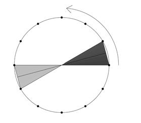
As a further exploration of the experiments done in Hooke Park, a Grasshopper logic* was developed to observe the advantages of controlling torsion individually and rotation in the overall form.
Two boundaries were defined and subsequently divided into equal segments; one line was located into each division point at the center and perpendicular to the boundary curve. As the number of segments from top and bottom are the same, the lines from the top are lofted with their correspondent lines at the bottom to create the strips. The torsion of each strip can be controlled by rotating the top lines, each on its own axis center.
Based on the strips density and torsion, visibility and transparency can be tested by changing the parameters.
These patterns are shown in the wall display. If this geometrical digital test could be done in phys ical experiments again, the torsion as it was studied in previous experiments added stiffness to each piece and in this case to the entire wall expects the geometry driven by the boundaries curves would define the strength in the total structure.
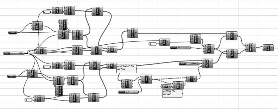
[See appendix]
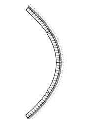
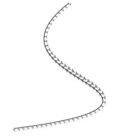
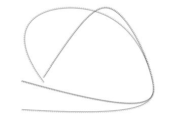
EXPERIMENTS 56
Boundary 1 Boundary 2 Torsion Division bottom line top line 30o 60o 90o 120o 150o 180o 0o top view top view 3.2.2 EVALUATION OF TORSION
top view
*Grasshopper logic is a graphical algorithm editor which works as a plug-in for Rhino.
fig. 3.2.2.1
Boundary 1
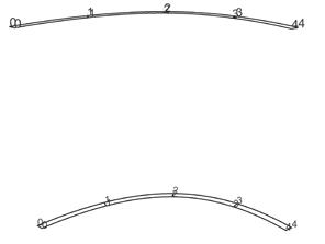
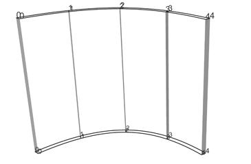
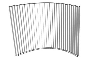
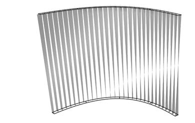
Boundary 1
Boundary 2
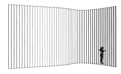
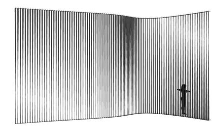
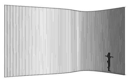
Boundary 1
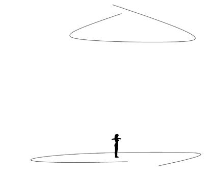
Boundary 2
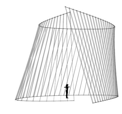
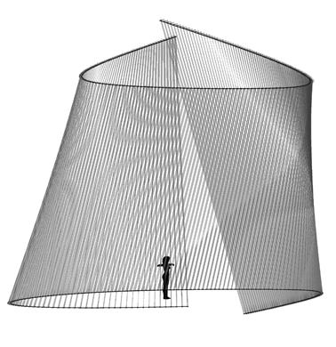
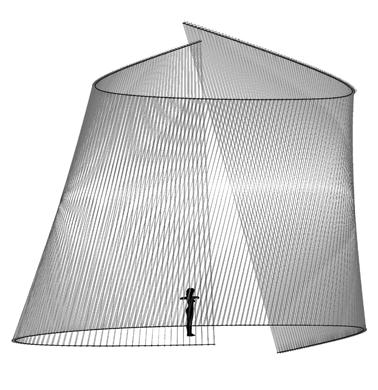
EXPERIMENTS Div =5 Torsion =0 Div =30 Torsion=0
Div =30 Torsion=30 Div =100 Torsion=0 Div =100 Torsion=90 Div =50 Torsion=0 Div =200 Torsion=90 Div =200 Torsion=210 Div =50 Torsion=0
Boundary 2
fig. 3.2.2.2
fig. 3.2,2,1 Top view torsion angles in one strip
fig. 3.2.2.2 Visual effects by changing torsion and density on strips
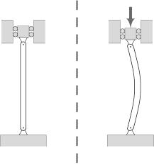
EXPERIMENTS 58
fig. 3.2.2.3
In engineering, buckling is defined as “a failure mode characterized by a sudden failure of a structural member subjected to high compressive stresses. This mode of failure is also described as failure due to elastic instability. Mathematical analysis of buckling makes use of an axial load eccentricity that introduces a moment, which does not form part of the primary forces to which the member is subjected.”(Wikipedia)
In order to obtain stabled buckles the form needs to be working according to the material, reason why for instance composites which have high yield stress values are known and utilized to avoid buckling in wing aircrafts.
However, buckling will be utilized on this research as a manufacturing process thus, it won’t be consider a failure as in the Timber Composite the load will be transfer through the GRP material.
The graphs below show why the buckling modes on the plywood do not affect or decrease the plywood capabilities as they are still in the elasticity region.
Besides it will be seen in this chapter that the plywood won’t bear load when working on the final structure but it is important to state that the followings procedures won’t make the plywood weaker as the buckling modes stay in the elasticity region.
The load capacity of a material is determined by the Young Modulus, the Inertia area and the length of itself. The project will combine the three factors in order to increase structural capabilities on the final structure.
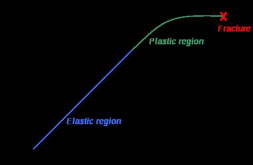
EXPERIMENTS 59
2. (F)
2.
(D) Deformation (F) Force 1. 1. 2. (F) Failure (D) Deformation (D) Deformation THE CONCEPT OF BUCKLI NG
F =
L =
E =
I
inertia E I L2 MAX LOAD=
1. Buckling-mode plywood
Spring back timber composite
fig. 3.2.2.5
force acting on the tip of the beam
length of the beam (span)
modulus of elasticity
= area moment of
fig. 3.2.2.4 fig. 3.2.2.3 Buckling setup fig. 3.2.2.4 Elasticity - Plasticity regions fig. 3.2.2.5 Spring back within elasticity region
These sets of digital simulations were done in pieces with the same dimensions as the previous physical strips experiments (3mm, 50mm, and 600mm). The purpose was to test load capacity in strips of the same size but with different material composition.
The simulations were run into Strand7* where the wood properties and the Glass Fiber composite properties were set. Linear Static Analysis was run previous to the Linear Buckling Analysis. First at all, the strip was meshed in a set of 6*60 nodes. The 6 nodes at the bottom boundary were fixed in translational (x,y,z) and rotational, the 6 nodes at the top were fixed in translational (x,y) and rotational. This set was in order to constraint the strip from displacing from its own central axis.
By applying 100N on the top boundary the Linear Buckling Analysis would give us several modes which are the result of increasing the load not gradually, but removing the load and applying it again; the last buckling mode is usually when the piece lose its own axis, and this is the reason why it shows a twisting piece. Observing the buckling modes of the four strips we could easily deduce they display the same pattern even when the bearing load is different from one to another.
Two main evaluations were deduced from these simulations. The strip 2 and 3 have very similar load capacity through the first 6 buckling modes, however the strip 3 (wood, fiber glass and resin) took more than the double of the force. Therefore, thickness is an important parameter to take into account at the time of defining a proportion of one or another material. Definitely the pre-twisted piece (strip 4) could take more than double of the force by replacing one laminate of wood for one laminate of GRP.
* Strand7 is a Finite Element Analysis (FEA) Software
EXPERIMENTS 60
3.2.3 LINEAR BUCKLING ANALYSIS COMPARISON ONE THE STRIP WITH DIFFERENT MATERIALS fig. 3.2.3.1 Results chart of buckling modes fig. 3.2.3.2 Linear Buckling Analysis
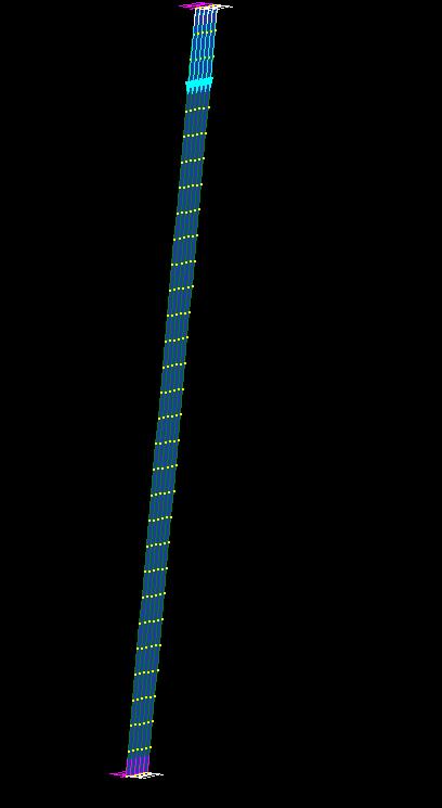
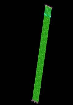
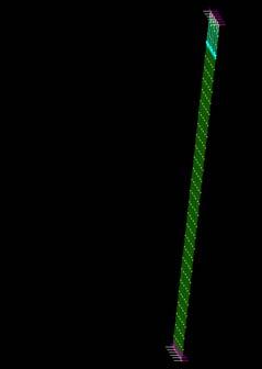
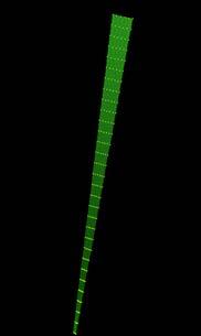


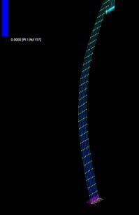
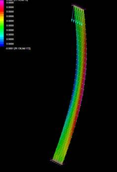
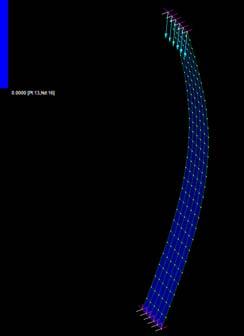
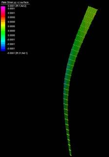
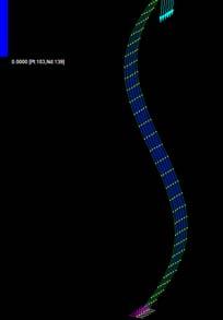
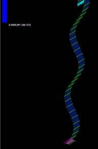
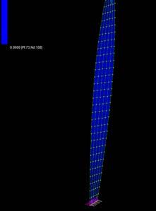
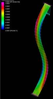
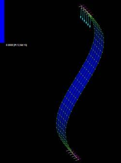
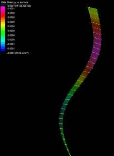
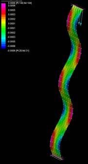
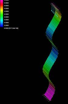
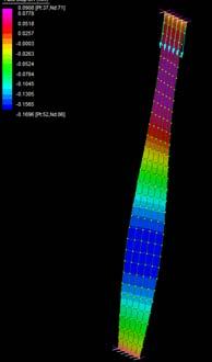
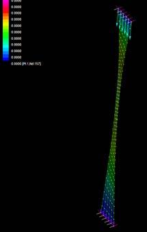
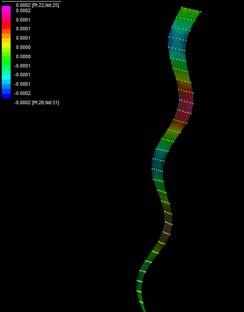
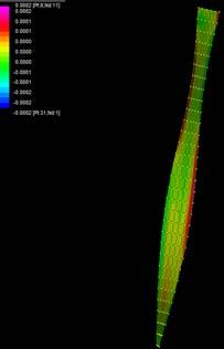
EXPERIMENTS laminate 1 laminate 2 total geometry mode (Newton) thickness wood fiber - resin wood fiber -resin 1 2 3 4 5 6 7 8 9 10 strip 1 3mm 3mm 0.51 2.1 4.6 8.2 12.9 18 strip 2 3mm 3mm 6mm 13.7 14.7 33 58.9 92.4 133 182 238 274 strip 3 3mm 3mm 6mm 4.11 16.5 27 66 103 144 strip 4 3mm 3mm 6mm pre-twist 15 16 36 63 99 143 194 254 278 295 strip 1 mode 1 mode 2 mode 5 mode 6 18N strip 2 mode 1 mode 2 mode 5 mode 6 274N strip 3 mode 1 mode 2 mode 5 mode 6 strip 4 mode 1 mode 2 mode 6 mode 10 295N fig. 3.2.3.2 fig. 3.2.3.1
3.3.1 PHYSICAL BUCKLING MODES IN A SHEET OF PLYWOOD
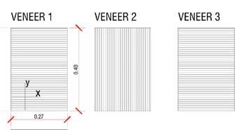
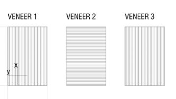
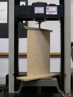
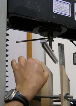
3.3.1.1 Grain direction of veneers
Outer layers horizontal grain direction
fig. 3.3.1.2 Outer layers vertical grain direction
Fixing the top boundary
fig. 3.3.1.3 Loading machine
fig. 3.3.1.4 Constraint machine
fig. 3.3.1.5 Horizontal grain direction-constraints
fig. 3.3.1.6 Vertical grain direction-constraints
fig. 3.3.1.7 Horizontal grain direction-constraints
fig. 3.3.1.8 Vertical grain direction-constraints
fig. 3.3.1.9 Horizontal grain direction-constraints
fig. 3.3.1.10 Adjustment of the experiment
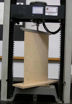
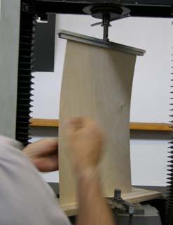
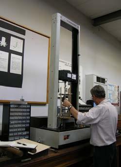
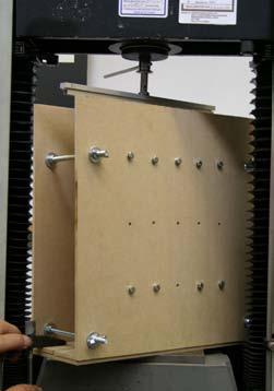
The next experiments were run at University of Reading, pre-stressing the plywood in a form finding process to obtain extreme curvatures. The exploration of these experiments looks towards deformations on the plywood as well as the implementation of a robotic machine that can produce and control the curvatures in the plywood piece by constraining some areas of the surface.
The set
As it is already shown in previous experiments when applying load on the border of any piece (boundary), precision is required. As it is so sensitive, the horizontal displacement of the boundary or the none even force application could result in significant none acquires results. Therefore, the plywood piece was fixed at the top boundary and at the bottom and the force was applied for every sample buckling individually. The forces were checked on the computer as well as the z-displacement.
The results
Sample 1 has the outer veneers with horizontal grain direction which makes the piece bend quickly taking only 20N before breaking the piece. Sample 2 has the outer veneers with vertical grain direction which makes the piece take more than 4 times the load than the Sample1. This situation leaving the surface free of constraints, while holding the Samples at the center the comparison was 40N to 400N.
Same set of constraints were set for Samples 3 and 4, 5 and 6 respectively and with large differences between the horizontal grain plywood to the vertical. By digital experiments and the experience with the material buckles, forms are predictable at certain points, what is not predictable is which side of the plywood will deform, as it can be either side. By constraining only one side of the surface the robot tells the surface (gives a clue) which side will buckle. The constraints can reduce or increment the load that one piece requires to get certain deformation and this is where the control of the machine happens on the surface.
The machine could be used in a manufacturing technique to reinforce plywood as the surface area can be free (none having a pressing mold at any side). Ideally the constraints can be adjusted, the load could be applied and therefore the buckling would appear. As this process happens the constraints could be removed and the reinforcement process could take place with any
EXPERIMENTS 62 1 2
20N 130N PLywood
Top and bottom boundaries Fixed x,y translational x,y,z rotational Fixed x,y,z translational x,y,z rotational
0.015m 0.27m 0.40m
fig. 3.3.1.1
fig. 3.3.1.2
fig. 3.3.1.3
fig. 3.3.1.4
fig.
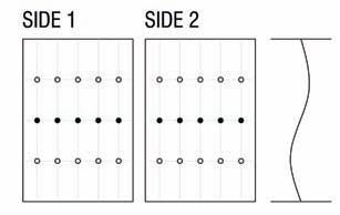
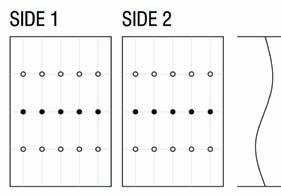
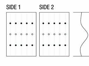
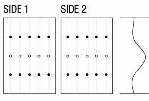
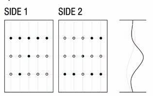
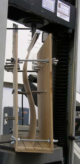
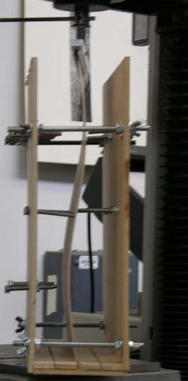
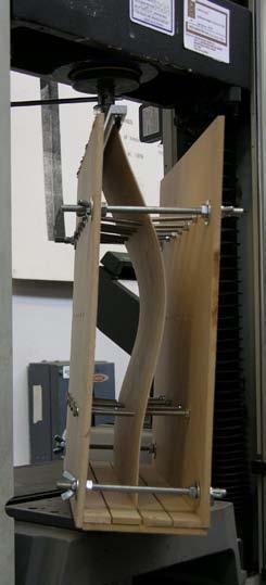
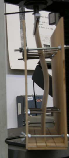
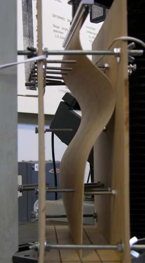
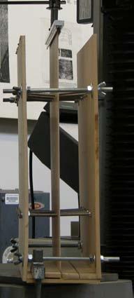
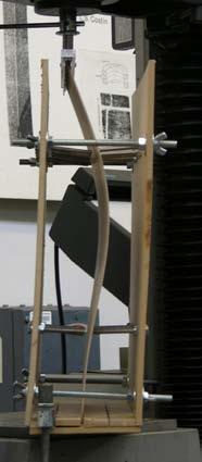
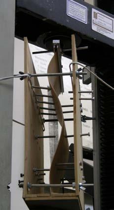
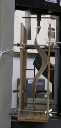
of the placing fiber methods already studied (most likely spraying the chopped fiber glass).
Another interesting method to develop would be to make the constraints in pneumatic system and probably controlled by Arduino program, which can establish the connection between the physical robot and the software.
EXPERIMENTS 3 4 5 6 48N 480N 75N 450N 7 140N
fig. 3.3.1.5
fig. 3.3.1.6 fig. 3.3.1.7 fig. 3.3.1.8 fig. 3.3.1.9
fig. 3.3.1.10
The next experiments were run into Strand7* in 4 sample sets changing the orientation of the rectangular sheet (1mx2m) and changing the grain orientation. First Static Analysis was run and then Linear Buckling Analysis.
Please take into account that the results are showing color patterns of the displacement in z, in this case z is the axis perpendicular to the plate. As in previous experiments the top and bottom boundaries were fixed and aligned vertically. Next, an initial vertical force of 100N is applied on the pieces on the top boundary so 12 buckling modes are displayed in analysis before the piece could break. Each mode adds the load incrementally in small ratios.
The color pattern displayed in each captured has individual correspondence to its highest and lowest displacement, and to its buckling mode. Usually as the plywood are flat sheets and have anisotropic behavior, several areas that have the appearance of double curve, are actually ruled surfaces. However, some extreme buckling modes obtain double curvature by the tension (concave side) and compression (convex side) in very small scale.
The last experiment, took one already buckled mode and force under the same conditions was applied. The result is the increment of bending in the areas already buckled. This specific experiment opens a wide range of possibilities to manipulate the curvatures to its extreme deviations from the original flat sheet.
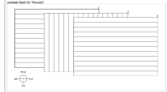
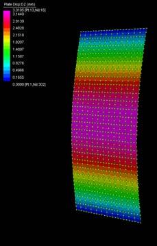
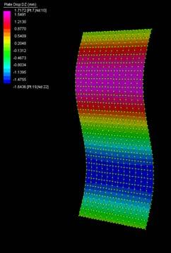
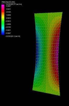
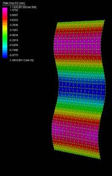
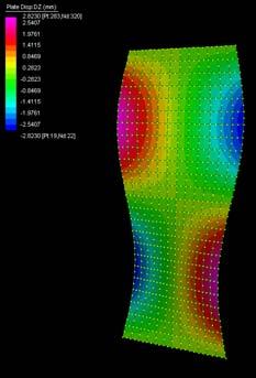
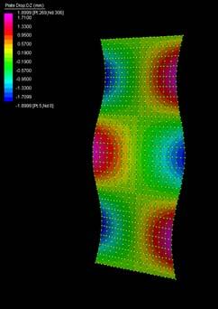
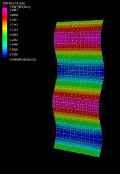
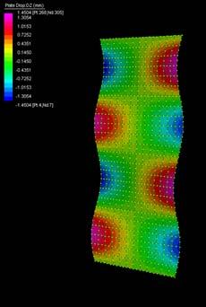
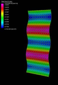
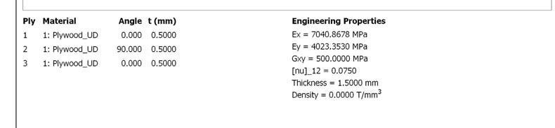
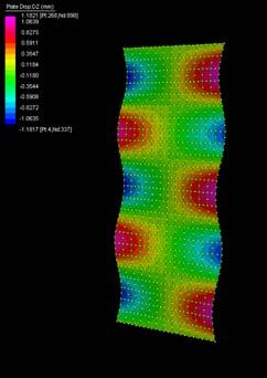
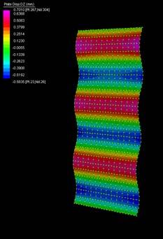
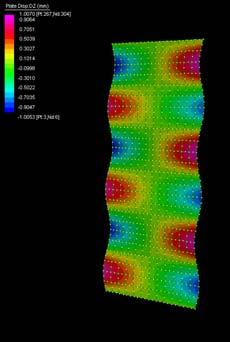
Linear Buckling Analysis 1A
Fixed x,y translational x,y,z rotational Fixed x,y,z translational x,y,z rotational 3.3.2 DIGITAL BUCKLING MODES IN A SHEET OF PLYWOOD mode 1 mode 2 mode 3 mode 4 mode 5 mode 6 mode 7 mode 8 mode 9 mode 10 mode 11 mode 12
3.3.2.1
The buckling modes have a scale visual factor of 5%
fig.
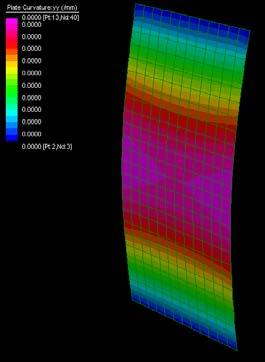
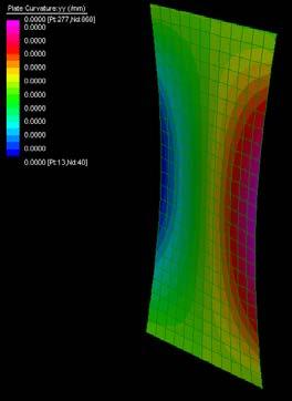
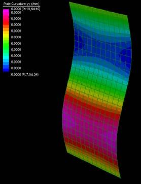
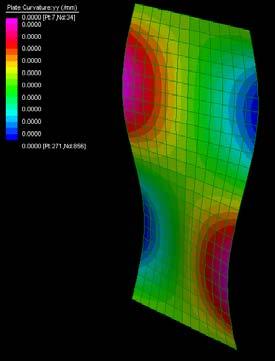
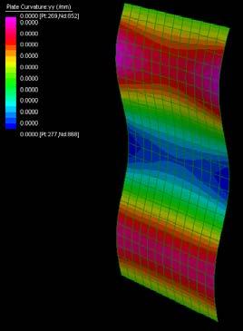
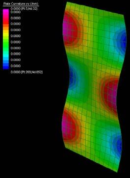
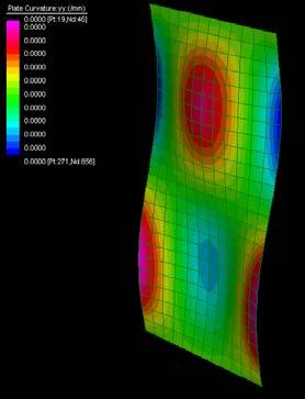
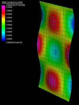
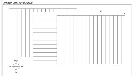
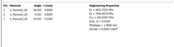
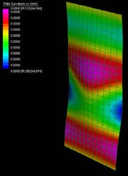
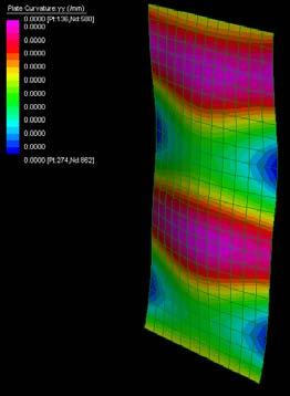
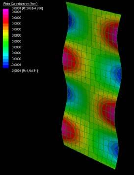
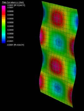
EXPERIMENTS 65 Linear Buckling Analysis 1A mode 1 mode 2 mode 3 mode 4 mode 5 mode 6 mode 7 mode 8 mode 9 mode 10 mode 11 mode 12
fig. 3.3.2.1 Linear Buckling Analysis on plywood of 1m X 2m outer veneer layers with horizonal grain direction
fig. 3.3.2.2 Linear Buckling Analysis on plywood of 1m X 2m outer veneer layers with vertical grain direction
fig. 3.3.2.2
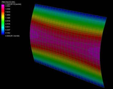
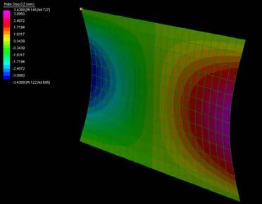
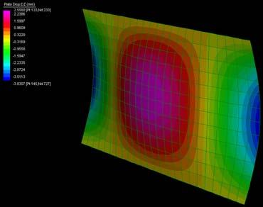
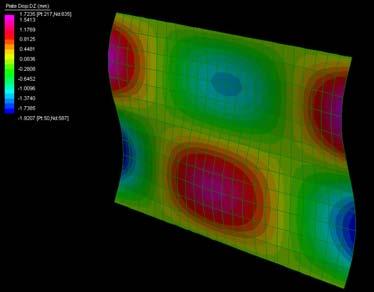
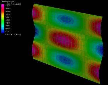
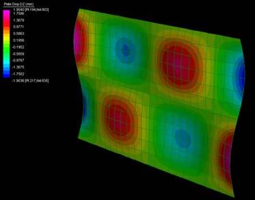
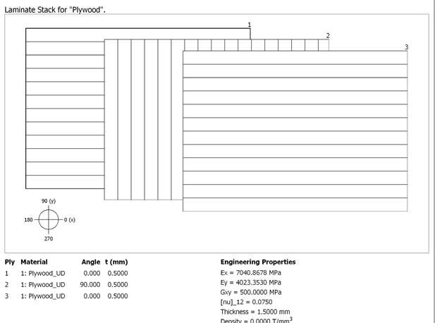
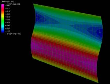
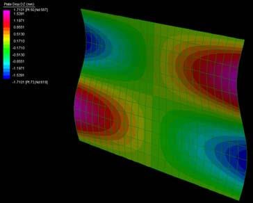
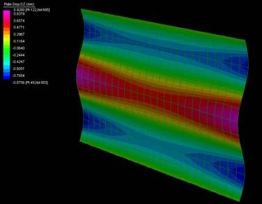
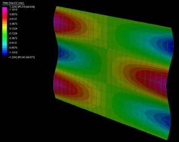
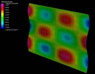
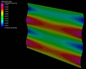
EXPERIMENTS DIGITAL BUCKLING MODES IN A SHEET OF PLYWOOD
2A mode 1 mode 2 mode 3 mode 4 mode 5 mode 6 mode 7 mode 8 mode 9 mode 10 mode 11 mode 12
Linear Buckling Analysis
3.3.2.3
fig.
3.3.2.3 Linear Buckling Analysis on plywood of 2m X 1m outer veneer layers with horizonal grain direction
fig. 3.3.2.4 Linear Buckling Analysis on plywood of 2m X 1m outer veneer layers with vertical grain direction
Linear Buckling Analysis 2B
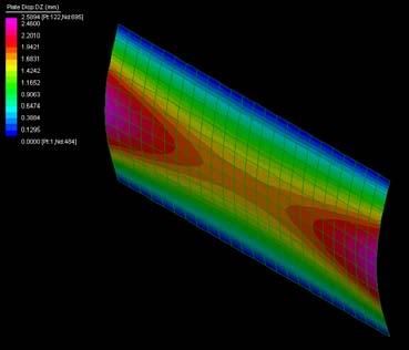
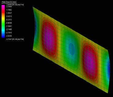
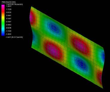
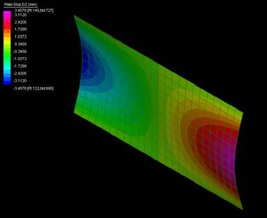
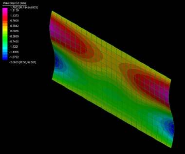
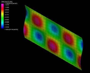
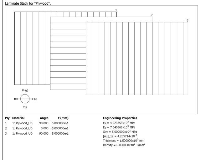
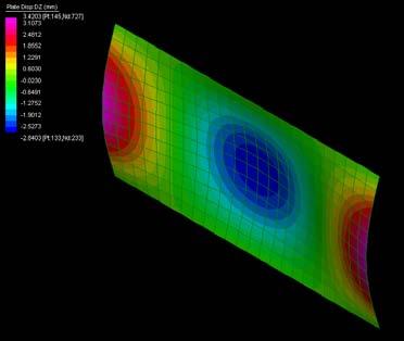
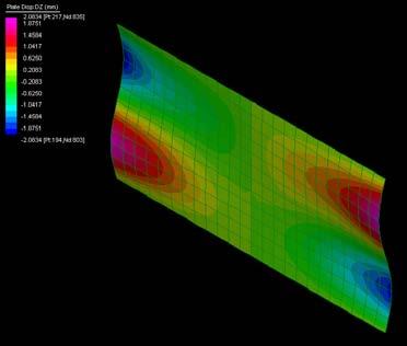
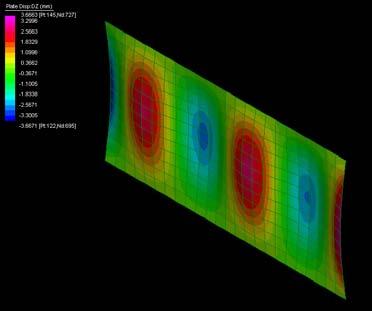
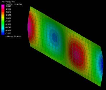
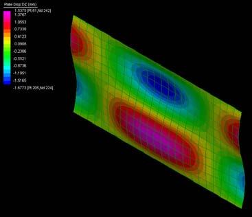
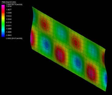
mode 1 mode 2 mode 3 mode 4 mode 5 mode 6 mode 7 mode 8 mode 9 mode 10 mode 11 mode 12
fig. 3.3.2.4
fig.
These experiments were carried out run into Strand7* in different samples simulating the lateral stitching of plywood sheets. The experiments were set matching the edges in two alternatives. First, having two similar edges and second, having two opposite edges.
The initial panels were taken from previous buckled panels in experiment 3.3.2. The surfaces were mesh in Rhino with high definition and improved in Strand7 to have better results. To simulate the stitching, springs where placed on the nodes located at the edges and, by controlling the axial, torsion, and stiffness factor as well as thermal contraction factor. After setting the parameter Linear Static Analysis were run on the models. By adjusting the edges with the stitching gaps can stay in between according to the future design requirements. The figure 3.4.1.2 show the experiments simulating the behavior of the plywood when stitching two buckled panels of plywood.
As in previous experiments the timber is simulate it in the program through laminates of veneer, for the timber composite one laminated of fiber glass and resin is added to the surfaces with its material specifications, thickness as well as the size and directionality.
The figure 3.4.1.3 show the panels stitched when already having the fiber glass with resin on the surface. These last displays a very stable sheet comparing to the panels of only plywood.
The stitching seems to work well under the calibrated parameters, however the limits on pulling are displaced on the surface when stress patterns are high (red) on the simulations.
3.4.1. DIGITAL SIMULATIONS OF STITCHING BUCKLING AND
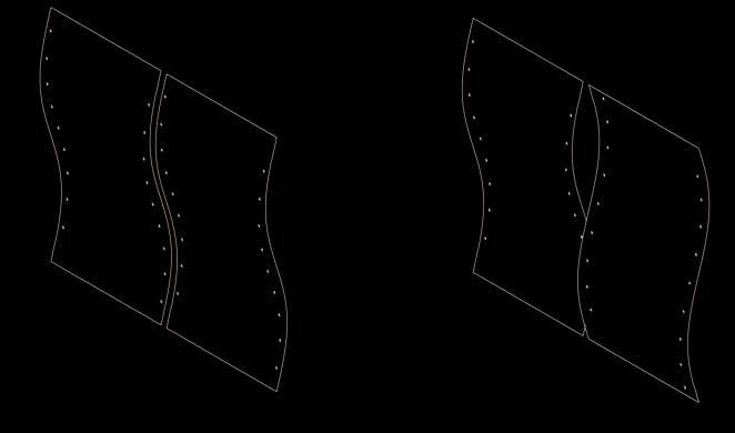
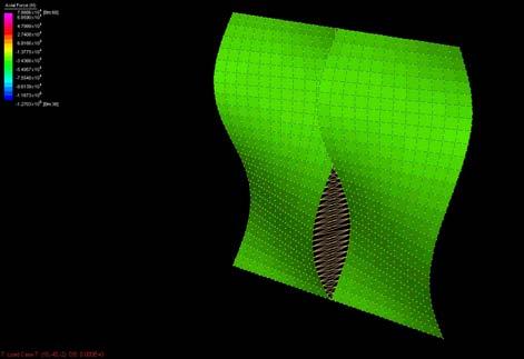
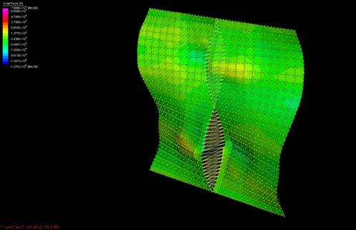
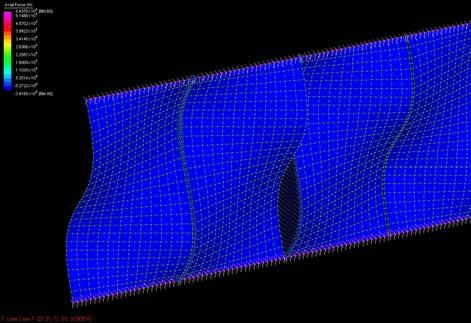
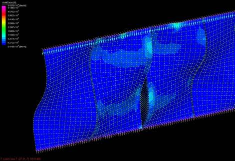

fig. 3.4.1.1 Front view - timber composite stitching simulation fig. 3.4.1.2 Stitching simulation on buckled plywood panels fig. 3.4.1.3 Stitching simulation on timber composites panels
BENDING PLYWOOD.

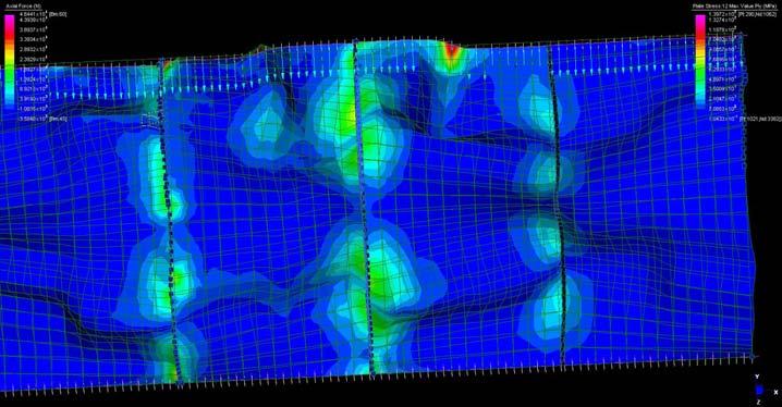
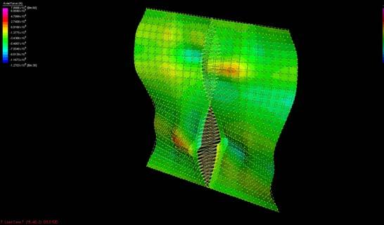
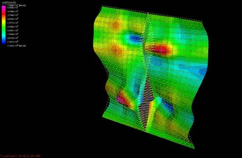
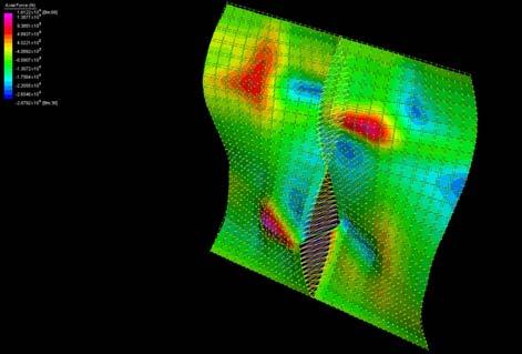
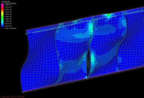
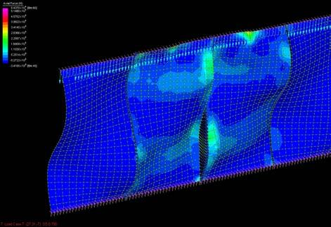
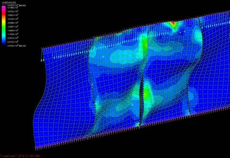
Stitching specifications:
Beam property : Spring Damper
Stiffness : Axial 1.0000X10³ N/mm
Lateral 1.0000X10³ N/mm
Torsion 1.0000X10³ N.mm/rad
fig. 3.4.1.3
fig. 3.4.1.2
fig. 3.4.1.1
Damping : Spring Mass 0.0000x 100 Thermal Expansion 2.5000x10⁻² Damping Ratio 0.0000 x 100
Viscous
The next experiments were done in order to observe more closely the steps that should be taken to achieve a continuous surface, and also to observe the effects of the stitching in physical experiments.
The set
The load machine was installed horizontally to be able to apply the resin horizontally and let it dry properly for the experiment. Likewise, the constraint machine was set horizontally and the load was applied in this case by pulling the threads as indicated on the images. When applying the load the threads pull the piece 1 which pulls the first boundary to obtain the buckling modes on the plywood.
The procedure
The first two flat sheet panels of 30x40cm were buckled at the same time when applying the 10kg load (fig. 3.4.2.6), the deformation was adjusted through the constraints established previous with the machine. Secondly, the resin was applied on the surface without covering the areas of the holes as indicated in figure 3.4.2.7, this in order to stitch the two panels while the bounding material is still not cured; the aplication of fiber glass and resin is done as indicated on figures 3.4.2.8 and 3.4.2.9. The third step consisted in buckling with a load of 10kg the next two pair panels and to reinforce and stitch as with the first pair. The fourth step was to adjust the already unified pair of panels; in this case it was done by placing only fiber glass and resin.
Observe figures 3.4.2.4 and 3.4.7; the surface was tightened along the edges except on the area of the voids.
The stitching has several advantages on the system as it adjusts the surfaces to have continuity between the panels. Should be stated now that the stitching won’t be a weak area in the timber composite as the fiber glass with resin would have a thickness of approximate 4 centimeters, plus this will be the material that will take the structural capabilities and not the plywood which is only working structurally through its geometry. The second important conclusion is that the stitching process varies its capabilities according to the stage of the composite’s cure.
3.4.2. PHYSICAL SIMULATIONS OF STITCHING BUCKLING AND BENDING PLYWOOD - REINFORCING PROCESS
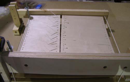
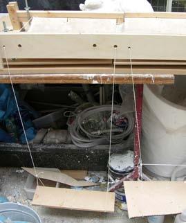
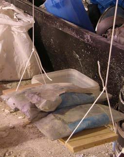
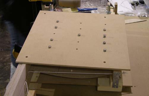
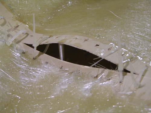
3.4.2.1 Set up for first panel pair with holes at the edges
fig. 3.4.2.2 Loading system
fig. 3.4.2.3 Constraint machine
fig. 3.4.2.4 Close up of a void
fig. 3.4.2.5 Screws in the constraint machine
fig. 3.4.2.6 Flat panel pair with untighted stitching
fig. 3.4.2.7 Buckled panels with resin
fig. 3.4.2.8 Fiber glass mat + resin
fig. 3.4.2.9 Fiber glass mat + resin
fig. 3.4.2.10 Stitching
fig. 3.4.2.11 Application of Fiber glass mat + resin on the edge
fig. 3.4.2.12 Assembly of the 2 pairs (gap with only fiber glass.
fig. 3.4.2.1
fig. 3.4.2.2
fig. 3.4.2.3
fig. 3.4.2.4
fig. 3.4.2.5
fig.
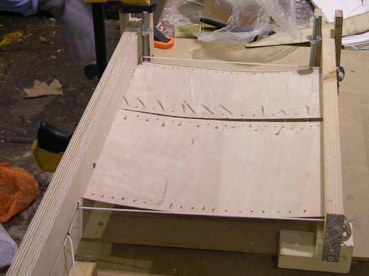
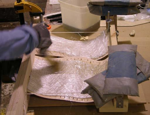
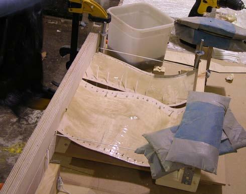
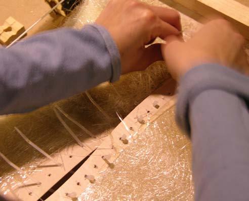
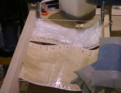
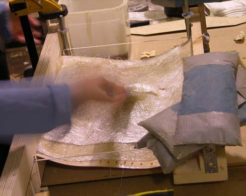
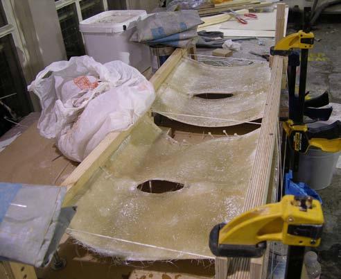
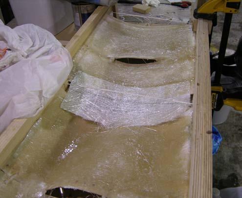
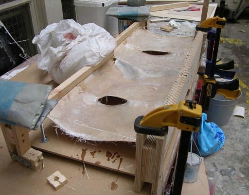
the process allows voids for ventilation and transparencies, see chapter 4
fig. 3.4.2.6
fig. 3.4.2.9
fig. 3.4.2.10
fig.
3.4.2.11
fig. 3.4.2.12
fig. 3.4.2.7
fig. 3.4.2.8
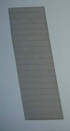
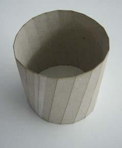
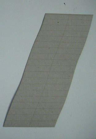
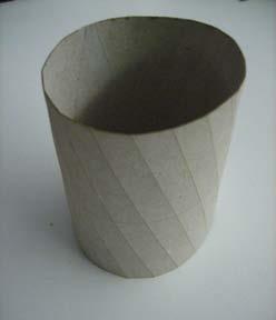
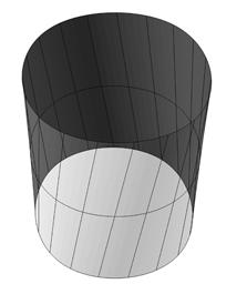
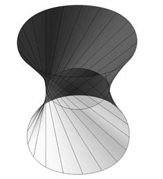
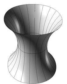
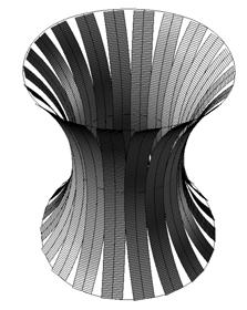
Rotational Surfaces (surfaces of revolution)
Are generated by rotating a curve C about and axis A. Translational surface
Are generated by translating the profile curve K along the path curve L.
Ruled surfaces.
Cylinders, cones, one-sheet hyperboloids, and hyperbolic paraboloids. “Ruled surfaces that consists of all tangents of a spatial curve are developable surfaces. Together cylinders and cones, these surfaces have the important property that they can be unfolded into the plane without stretching or tearing”.
The two digital models were set in the following order in a grasshopper definition:
1. One circle at the top and one circle at the bottom were subdivided in same amount of points. Subsequently, the top points were connected to the bottom points with straight lines, the lines were lofted and by shifting the correspondence between the top and bottom points in one point the loft surface became a rotational hyperboloid surface.
2. On the second model the same procedure was done, just the points were shifted by 5 points.
3. On the third model one smaller circle was added in between the top and bottom circles. Again the circles were subdivided into same number of points; in this case one curve was drawn tracing every three correspondence numbers and sequentially the curves were lofted to create the surface. The result was an undevelopable surface as it is completely hyperbolic.
4. On the fourth model the curves drawn interpolating the top, middle and bottom points were the path to run the script to create developable strips.
The exercise allows clarifying the reason for not having the same result in the physical as in the digital experiments.
Even though the surface area from the digital experiment is the same as the surface area in the physical cardboard model, the material in the digital experiment is assumed as a stretchable; contrary to the physical experiment where the cardboard is restrained to have curvature in vertical and horizontal directions.
fig. 3.5.1.1 Laser cut surface 1 fig. 3.5.1.2 Laser cut surface 2 fig. 3.5.1.3 Digital files for surfaces
fig. 3.5.1.4 Top view Digital surfaces
fig. 3.5.2.1 Physical non-matching model
fig. 3.5.2.2 Laser cut file
fig. 3.5.2.3 Curvature graph on isocurves
EXPERIMENTS 3.5.1.
SURFACES
DEVELOPABLE
1 2 3 4 5 6 18 1 2 3 4 5 6 1 2 3 4 5 6 18 1 2 3 4 5 6 7 8 9 18 fig. 3.5.1.1 fig. 3.5.1.3 fig. 3.5.1.4
3.5.1.2
fig.
The set
The fabrication method consisted of subdividing the entire shell in a set of developable strips, and cutting them off from a plywood sheet on the laser cut. In order to achieve the curvature direction required along the surface, each strip had to be split into three parts, according to where the curvature flips its direction from inside to outside. The isocurves drew on Rhino were scored on the plywood on the concave side, in addition a series of holes were cut close to the edge of each strip in order to stitch the pieces together.
Though the density of the isocurves on the arcs was of a high accuracy level, when scoring them (lines cut half the way through the plywood) they segmented the real material and constrained it when bending the arcs; especially at the top where the shell assumes extreme curvature. In this way, the arcs could bend independent from each other but not match at the extreme curvature.
The pieces should match and be stitched together to assemble the shell. The unsuccessfulness in this exercise relied on the score done with the laser cutter and also on the location of the points where G0 continuity happens wasn’t precise.
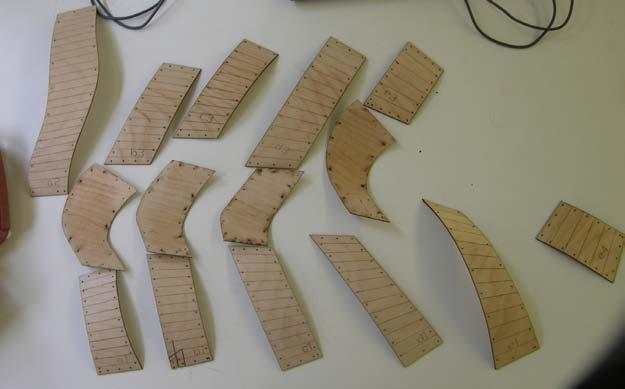
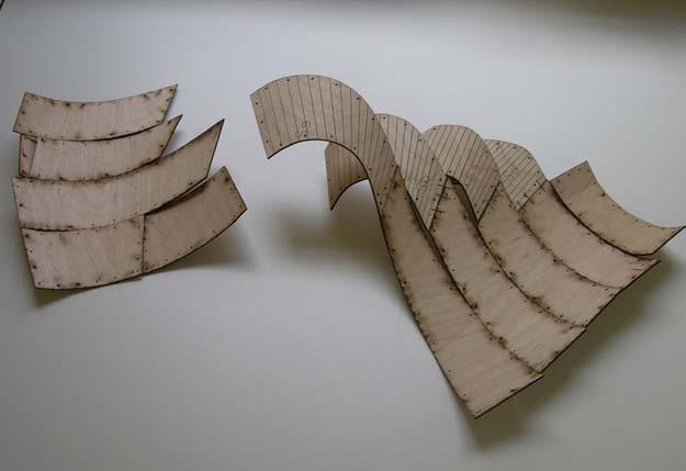
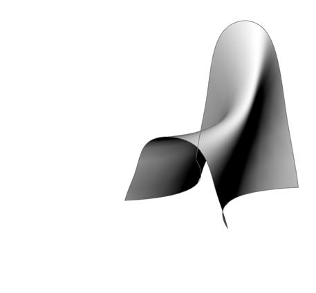
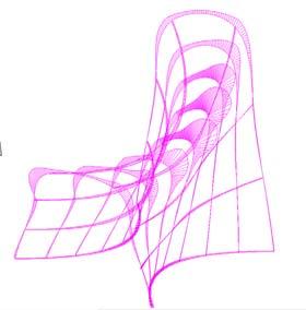
EXPERIMENTS
G0 a1 e3 b3 b2 c2 c3 e1 e4 a2 d1 b1 c1 e2 d2 d3 3.5.2. DEVELOPABLE SURFACES
fig. 3.5.2.1
fig. 3.5.2.2
fig. 3.5.2.3
PHYSICAL BENDING OF PLYWOOD
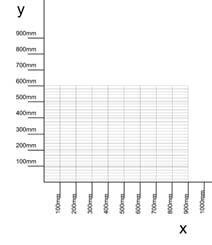
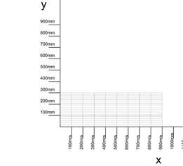
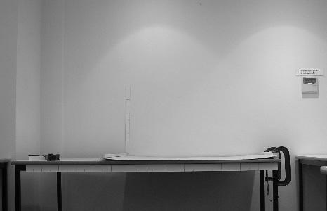
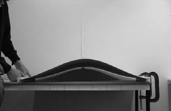
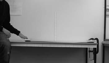
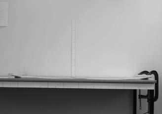
The sheets of plywood were individually set in between two boundaries, one fixed and the opposite free. The sheets were bent manually by pushing the free boundary.
The results are predictable as the curve achieved by the plywood is according to its length. What is remarkable is that the proportion of the sheet is relative to the force required to bend it. The grain of the fibers in the sheets are disposed parallel to the boundary where the force is applied, therefore the fibers are easier to open and bending occurs. Strips 90x30cm of plywood are easier to bend than rectangles of 90x60cm, while rectangles are easier than squares of 90x90cm. The results show the piece of 60 x 30cm was easier to bend than the 60x60cm. The larger is the surface, the easier to bend.
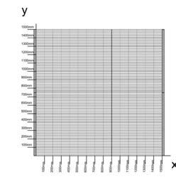
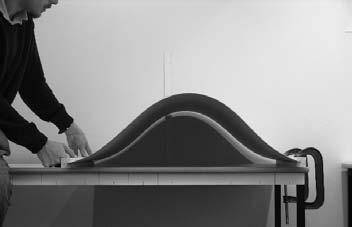

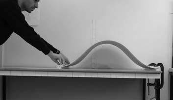
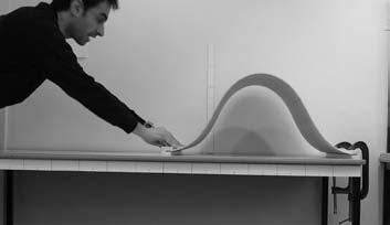

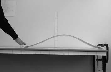
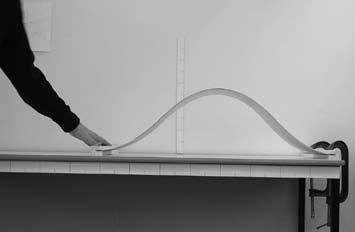

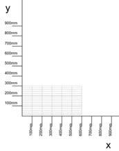
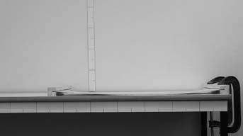
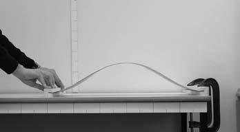

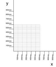


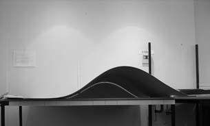
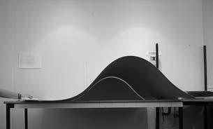
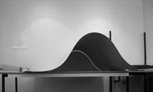

EXPERIMENTS 74
90 80 70 60 50 40 30 20 10 cms 90 80 70 60 50 40 30 20 10 cms 90 80 70 60 50 40 30 20 10 cms 80 70 60 50 40 30 20 10 cms 90 80 70 60 50 40 30 20 10 cms
3.6.1.
1.
90X90CM 2. 90X60CM
3.
90X30CM 4. 60X30CM 6. 150X150CM
5. 60X60CM
fig. 3.6.1.1 Manual bending tested on sheets with different proportions
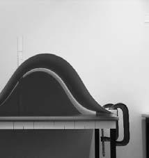
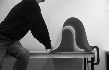
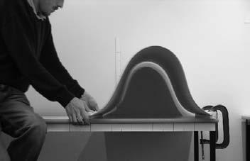
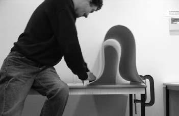
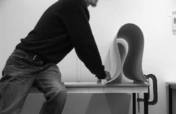
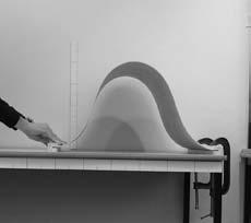
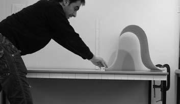
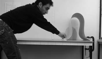
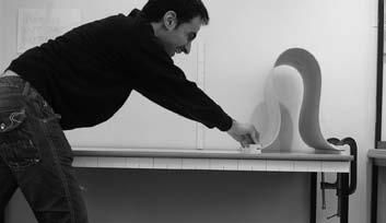
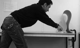
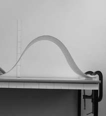
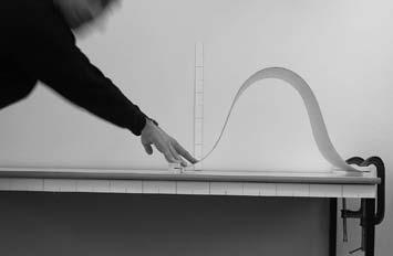
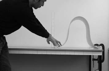
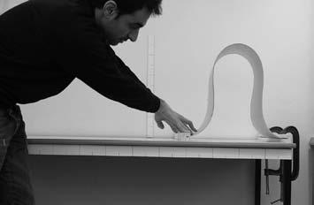
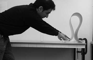
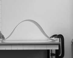
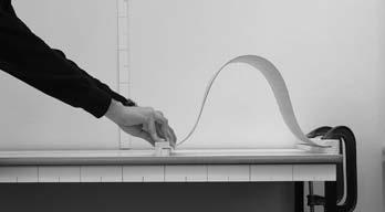
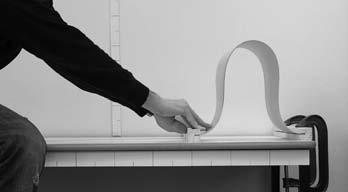
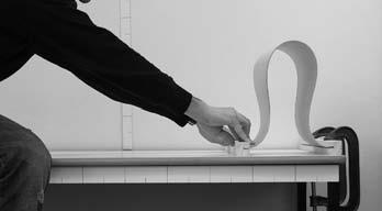
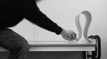

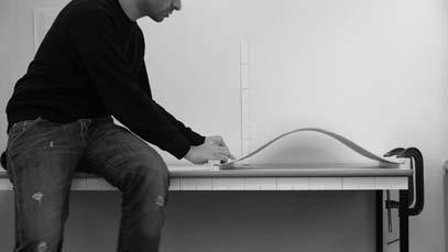
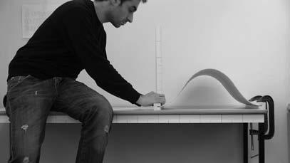
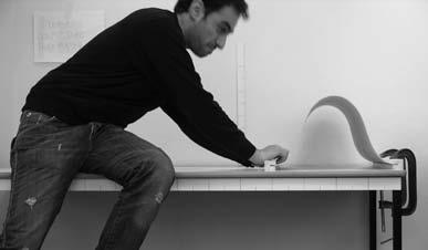
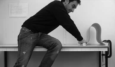
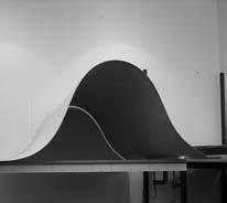
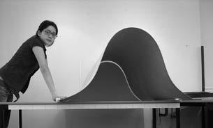
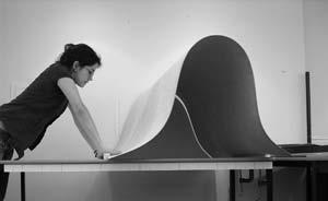
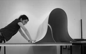
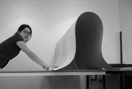
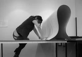
EXPERIMENTS cms fig. 3.6.1.1
The theoretical morphospace is a contribution to the analysis of form. It is the tool that documents the range of actual structures that are theoretically possible. Theoretical morphospace exist only because of the advance of computers , and initially it had two purposes:
1. to build it with less parameters. 2. to create all possible forms that nature can create.
Theoretical morphospaces spirals and shells accretionary Growth systems. The best way to explain the morphospace as David M. Raup has done it and how George R. McGhee has explained in his book is through the “Cube”; a set of parameters which can be defined into dimensions. It means three parameters define three dimensions. However, two parameters can be compared between them, it means two dimensions, and it still will produce a set of theoretical forms. It is important to understand that axis and ratios are the domain of growth. Measures are not enough to constraint the growth, which ratios can take relations of one to another.
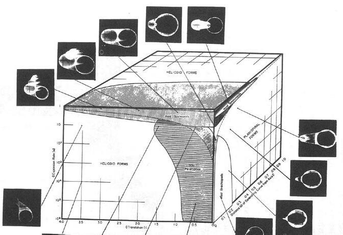
Having this short but acquire reference of the Theoretical Morphospace on the left, a new task was employed for the next steps.
This research attempts to create a fabrication and design system to create the shells with the timber composite material. The exercise looks for a set of rules that can establish the three dimensions that will define regions where the shell can exist, these regions are geometrical definitions taken from digital and physical experiments:
1. Plywood possible curvatures.
Thickness
Grain direction
Ratio (proportion of the sheet)
2. Manufacturing possible geometries during the manufacturing process.
Sequence in the pres-stress of wood/ fiber glass application/ resin application/ Assembly
3. Shell Stability
Thickness
Self-weight
Transcendental questions for this research start taking place for the next set of experiments and for the entire project. How to transfer the possible geometries of one sheet of (LVL) into digital. In architecture the traditional design process attempt to define a form and then panelize it into pieces. This exercise is showing the contrary process, the panel from the beginning has some dimensions (length and surface area) which define a none elastic material.
The process is as important as the tools.
What is seemingly an easy question is actually what tackles the precision of transferring the material behavior of a flat sheet of plywood into a digital set. How to draw and bend a plywood sheet in a software.
The following processes are non successful in obtaining a complete control of the geometry, but give good feedback. One of the challenges of this dissertation is to
transfer the material possible geometries into a digital geometrical set:
Option A. Simulate a ratio of lengths through grasshopper definition. The curve on the graph has three points a, b, c. The Grasshopper attempts to, by pulling the point a in y coordinates pull the point b in x coordinates, of course in a ratio that the length remains the same.
Option B. Mathematical surfaces do not have material properties, the surfaces are stretchable and do not correspond to the bending of a non-stretchable material such as wood. In the example on the right the surface is defined by the equation, and by changing parameter a the surface gets deformation but without controlling the surface are.
Option C. Define a mesh with dimensions of plywood and set a particle system on it, with points (mass) and strings (stiffness, rest length and damping). In order to simulate the bending moments, 2 sets of parameters with different specifications were established on the strings. To create some strings working in tension and the others in compression the differentiation is establish by changing the rest length from its original value (0.5= compression, 2= tensions).
Option D. Take a sheet of plywood, draw a grid of points on it, using the Digitizer trace the points in order to have them in Rhino. Subsequently create a data base of possible curvatures and set the possible double curvatures in plywood.
It is clear that mathematical surfaces work in u and v coordinates, but what is in between those coordinates is the material or the surface area. If the surface area does not change when displacing some points from the surface it means the material is non elastic, while if it changes the “virtual” material it is stretchable. This is an important point to highlight as plywood or veneers are non stretchable materials and so the simulations that change lengths or surface areas are non precise for the purpose of the dissertation. This is the reason why the best option is to use Strand7 as the materials behavior can be acquired and simulated.
fig. 3.6.2.1 Raup’s W-D-T Theorethical morphospace [1966] known as “the Cube”
fig. 3.6.2.1 Rhino loft surface. Pulling control points
fig. 3.6.2.2 Simulation of bending a line with grasshopper
fig. 3.6.2.3 Mathematical surface controlled by grasshopper definition
x2/a2 + y2/b2
fig. 3.6.2.4 Relaxation plug-in for Rhino
3.6.2. SIMULATION OF A RESTRICTED SURFACE
fig. 3.6.2.0
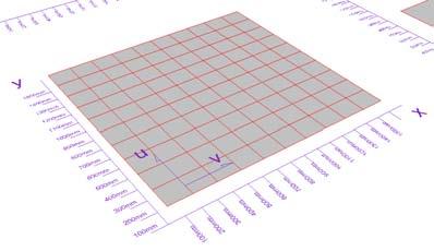
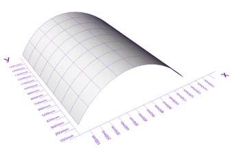
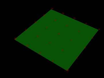
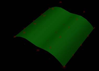
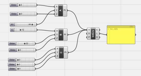
curve’s length

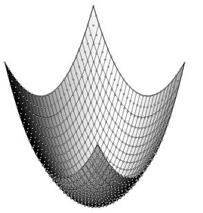
C
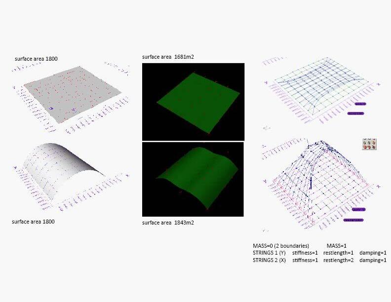
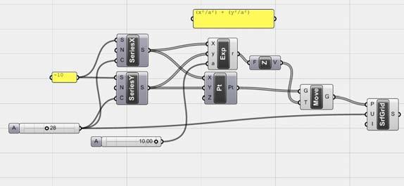
mass=0 (2 boundaries) mass=1
string 1 (y) stiffness=1 restlength=1 damping=1
string 2(x) stiffness=1 restlength=2 damping=1
EXPERIMENTS 77
a b c a b c a b c
OPTION A
grasshopper
a value
OPTION
fig. 3.6.2.1
fig. 3.6.2.2
fig. 3.6.2.3
fig. 3.6.2.4
The theoretical morphospace is a contribution to the analysis of form. It is the tool that documents the range of actual structures that are theoretically possible. Theoretical morphospace exist only because of the advance of computers , and initially it had two purposes: 1. to build it with less parameters. 2. to create all possible forms that nature can create.
Theoretical morphospaces spirals and shells accretionary Growth systems. The best way to explain the morphospace as David M. Raup has done it and how George R. McGhee has explained in his book is through the “Cube”; a set of parameters which can be defined into dimensions. It means three parameters define three dimensions. However, two parameters can be compared between them, it means two dimensions, and it still will produce a set of theoretical forms. It is important to understand that axis and ratios are the domain of growth. Measures are not enough to constraint the growth, which ratios can take relations of one to another.
3.7. SETTING THE LOGIC FOR MY THEORETHICAL SHELLS IN TIMBER COMPOSITES
boundary1 boundary1 axxis span
A theoretical set of shells was set according to general parameters generic shells geometry require. Three parameters; two boundaries, a central axis and its height; can change without hierarchy in the creation of one single object. (fig 3.7.1)
Subsequently, a selection system was established in order to get the fittest objects to be fabricated and the fittest objects into occupancy efficiently.
The shells presented on the right are evaluated according to geometry, usage and fabrication on the page 87.
variation of the span
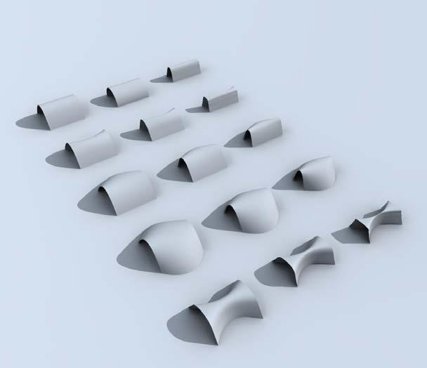
AXXISHEIGHT
B1B2 straight curved Fixed Inclined Gradient BOUNDARY
(Z)
fig. 3.7.1
fig. 3.7.2
fig. 3.7.1 Parameters chart
fig. 3.7.2 Set of possible shell forms according to chart (it could be extend it)
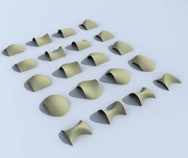
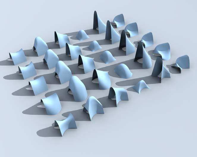
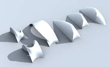

EXPERIMENTS variation height variation axis variation span - height-axis a b c bZ=aZ+(cY*2) parabola bZ=aZ+cY
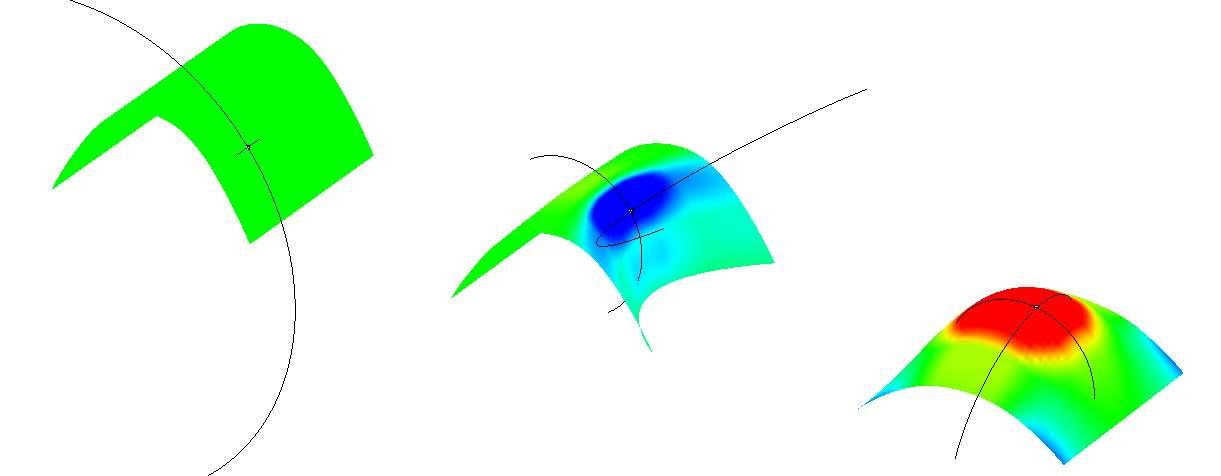
To understand the complexity of surfaces and its repercussions on panelization and fabrication, a deep curvature analysis was run on the shells created on the previous experiments.
Curve curvature “is easy to grasp intuitively. You simply fit a circle to short piece of curve as best as you can, this is called an osculating circle and the radius and center of this circle tell you all you need to know about the local curvature” (Rutten, D. 2007).
The points indicated on the curve have certain curvature associated with them. In fact, the curvature is the inverse of the radius, and the direction of the vectors is an indication of the curved plane.
(K ) curvature = R 0 0 If both are zero the surface is planar 0 non-zero 0 (Cylindrical surface) + + + spherical (synclastic) surface - red + - - hyperbolic(anticlastic) surface- green
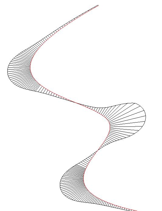
By finding all possible normal curvatures it can be seen that the surface is flatter in one direction and more bent in another. These are the principal curvatures of the surface which are totally independent from the u and v directions which not necessarily are perpendicular within them, although, principal curvatures come in pairs (minimum and maximum). As the progression of the principal curvatures direction across the surface is not very smooth, as shown clearly on the drawing at the right, the curvature analysis is run through the Gaussian and Mean curvatures.
Gaussian curvature maximum principal curvature (Kmax) minimum principal curvature(Kmin)
Kgaussian = Kmin * Kmax
Kmean = Kmin + Kmax
Though the surface with zero Gaussian curvatures can be unrolled into a flat sheet and any surface with a negative can be made by stretching an elastic cloth. Coming back to the relation between geometry and material, the maximum principal curves that run across the surface are driven by the fiber directionality, thus these principal curvatures on the surface define the plywood bending directionally.
Mean Curvature
“A surface with zero mean curvature is not merely anticlastic; it is a minimal or zero-energy surface. It is the natural shape of soap film with equal atmospheric pressure on both sides, these surfaces are extremely important for tensile architecture, as they spread stress equally across the surface resulting in structurally strong geometry”(Rutten, D. 2007).
The next page shows single curvature happening on the shells that span from side to side controlling the straight boundaries and axis, resulting in a complete 0 Gaussian curvature surface. Double curvatures occur when the boundaries or the axis becomes curvy like in the figures 8.2 and 8.3”, synclastic areas indicated in blue in the figure 8.2, and hyperboloid anticlastic surfaces indicated in red in figure 8.3.
fig. 3.8.1 Single curvature
fig. 3.8.2 Anticlastic surface
fig. 3.8.3 Synclastic surface
fig. 3.8.4 Curvature graph
fig. 3.8.5 Auto-range in Rhino
fig. 3.8.6 Approximation to the maximum double curvature on the panel for the plywood with this buckling surface deformation method
fig. 3.8.7 Puling control points to decrease gaussian
EXPERIMENTS 80
---------------------2
1
fig 8.1 Gaussian curvature analysis 8.2 Gaussian curvature analysis 8.3 Gaussian curvature analysis
3.8. CURVATURE ANALYSIS
fig. 3.8.1
fig. 3.8.2
fig. 3.8.3
fig. 3.8.4
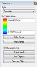
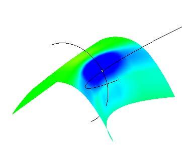
To understand how Rhino defines the areas of Gaussian curvature, it is important to note that it works within ranges. The auto range in figures 9.3 and 9.4 determines a range within 0.0009057426 and -0.0009057426, the max range option establishes a range between 0.0006432333 and -0.0075795315. Thus, manually different ranges can be set to establish tolerances between the digital and physical experiments. The digital simulations done previously in Strand7 with the sheet plywood panels were taken into Rhino as surfaces and analyzed with Gaussian curvature. The maximum double curvature extracted from this catalogue was 0.0008, a very small value, but still shows what the research has shown since the beginning; when bending a surface of wood or plywood, on one side the fibers tense and on the other side the fibers get compressed, meaning the length of the surfaces change and not only ruled surfaces are achieved but also double curvatures, nevertheless at a micro level scale.
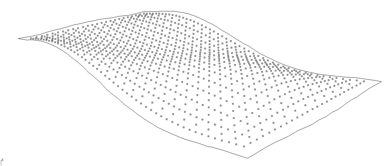
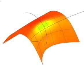
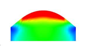
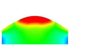

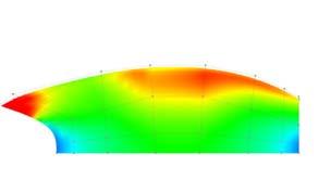
EXPERIMENTS
fig. 3.8.5
fig. 3.8.6
fig. 3.8.7
Looking for Developable surfaces
The same shell can have positive, negative and 0 curvature along the surface. Thus, in order to decrease the areas with positive or negatives trying to achieve a 0 Gaussian, the surfaces that can be unrolled and in this specific research surfaces could come out of plywood. The figure 3.9.4 show how to optimize the surface decreasing positive curvature. By simply pulling the control points of the surface curvature can change locally.
Defining the surface
For the next exercise, different ways of defining the surfaces were attempted in Rhino and Grasshopper:
1. Extracting the points from the surfaces in the figure 3.9.3 it is seen that the areas with 0 Gaussian curvature in green and the positive curvature require less definition than the blue areas. In the first line the surfaces are defined with 10 divisions in u and v direction while in the third line the surface is defined with 10 divisions in both directions. In both cases in the blue areas the isocurves get closer, almost shrunk.
Isoparametric curve (isocurve) is a curve of constant u- or v-value on a surface. Rhino uses isocurves and surface edge curves to visualize the shape of a NURBS surface.
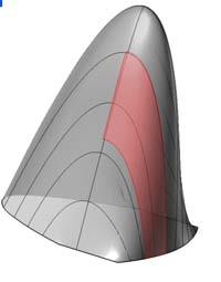
2. In order to read the curvature locally on the surface the following Grasshopper definition was created: the surface was split into 25 u and 25 v divisions locating 767 points on it. Thus, by evaluating the surface at those points the list of Gaussian curvatures was extracted. Having this list, the specific areas with double curvature were read and selected by an additional definition to the grasshopper. The exercise has the potential of extracting areas within the surface to subdivide them or in general change them according to the project necessities (fig 3.9.2) [see appendix].
3. The second exercise was looking for the most efficient developable surface tracing the principal curvatures on the surface, by mapping the two principal curvatures on the surface at one initial point and following the direction of one of those, plotting a second point and iterating the previous step, the curve was drawn on the surface until reaching the opposite edge. Several lines were drawn on the surface and cut in order to create large developable surfaces that could reduce the amount of panels and assemblies. Even though the exercise would result in the best option to optimize the surface, the cutting pattern on the surface won’t allow standardization of the system to be implemented in other shells (fig 3.9.5, 3.9.6 next page).
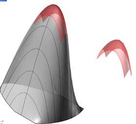
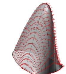
EXPERIMENTS 82
1 -23.739 2 -2.156 3 -0.185 4 -0.03 5 -0.007 6 -0.002 7 -0.001 8 0 9 0 10 0 11 -6.00E-06 12 0 13 -3.00E-06 14 0 15 0 16 0 3.9. PANELIZATION
fig 3.9.1
fig 3.9.2
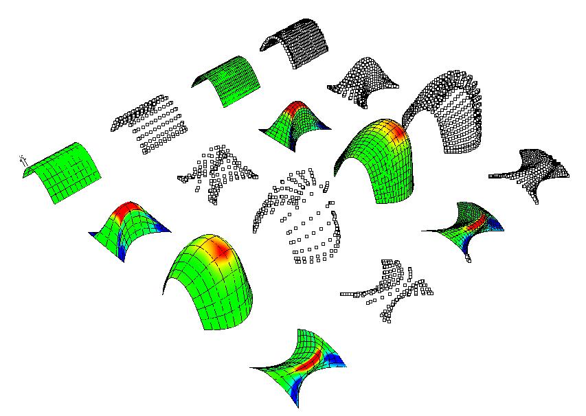
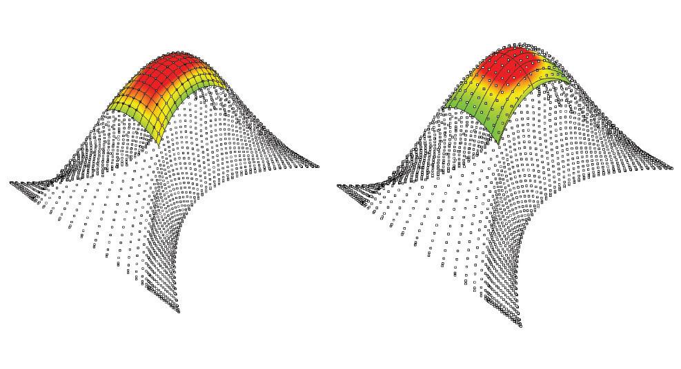
fig. 3.9.1Extraction of a surface
fig 3.9.2 Curvature values at points
fig 3.9.3 Different definitions of the surface
fig 3.9.4 Decreasing Positive Gaussian curvature analysis
EXPERIMENTS 83
fig 3.9.3
fig 3.9.4
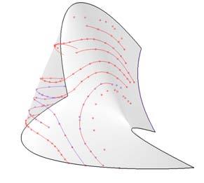
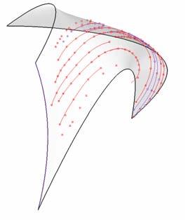
4. In general, literature describes 0 Gaussian curvature as surfaces that can be unrollable, however these green areas cannot be unrolled in one sheet, though the second attempt on figures 3.9.9 and 3.9.10 was subdiving the surface with different definitions according to the curvature, on the first line the areas with positive, negative and 0 curvature were extracted and subdivide until finding developable panels. Hyperboloid areas require extreme definition in strips, which is almost like defining a surface from a repetition of lines. However, for the final experiments the small panelization won’t be efficient for the system.
Developable panels that come from these subdivisions do not have right angles and always have different sizes according the definition of the surface.
5. The last attempt subdivides the surface running a RhinoScript, the script subdivides the surface along u and v values with isocurves, and then evaluates the subdivided panels according to Mean or Gaussian curvature. In this case the Gaussian Values used was 10, as the value extracted from the panel analysis is too low and would result in a extreme subdivided surface.
(fig 9.9.7, fig 9.9.8) [see appendix].
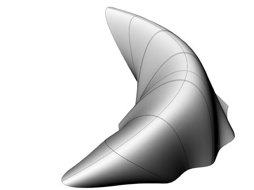
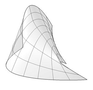
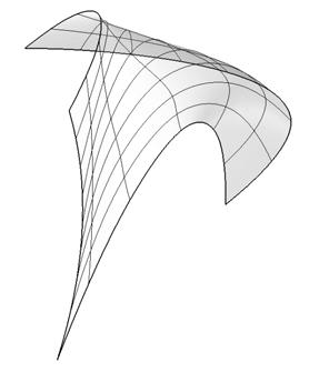
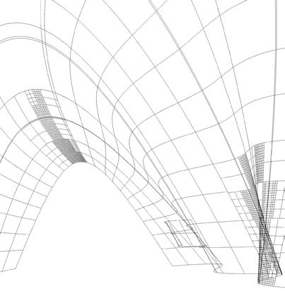
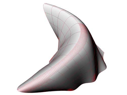
EXPERIMENTS 84
fig 3.9.5
fig 3.9.6
fig 3.9.8
fig 3.9.7
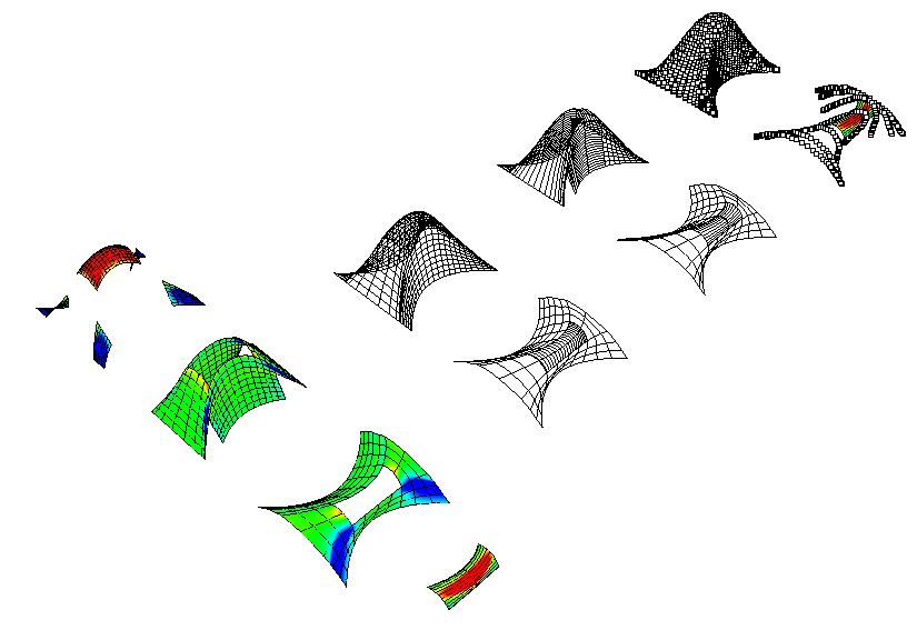
fig 3.9.5 Principal curvatures
fig 3.9.6 Isocurves
fig 3.9.7 Panelization with Rhinoscript
fig 3.9.8 Panelization with Rhinoscript
fig 3.9.9 Spliting of the surfaces according to curvature
fig 3.9.10 Unrollable panels
flat panels(top view)
EXPERIMENTS 85
fig 3.9.9
fig 3.9.10
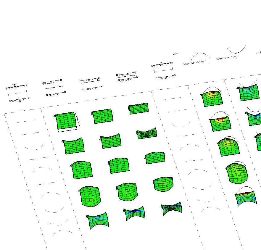
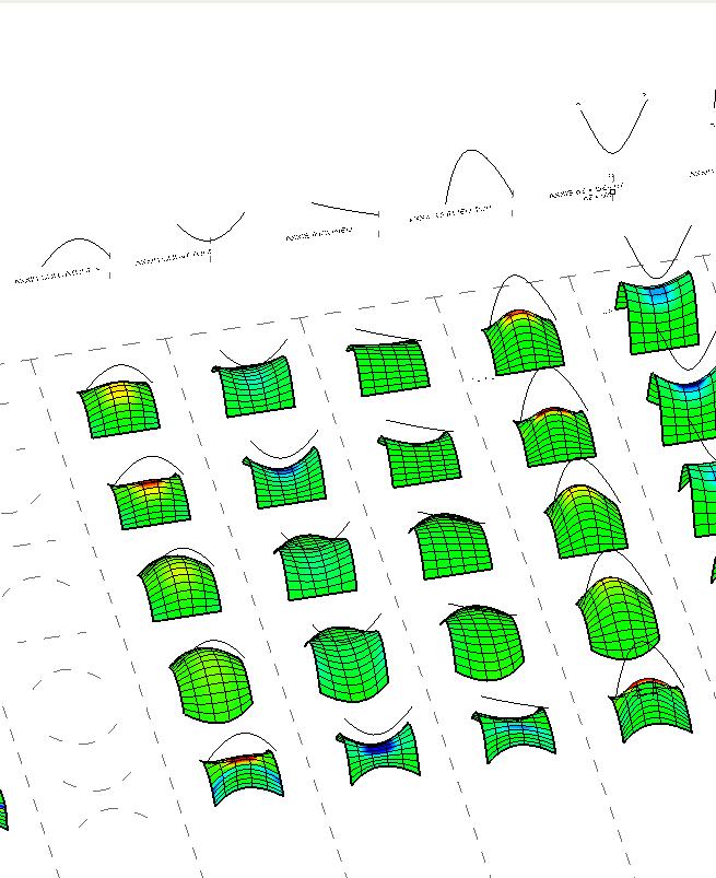
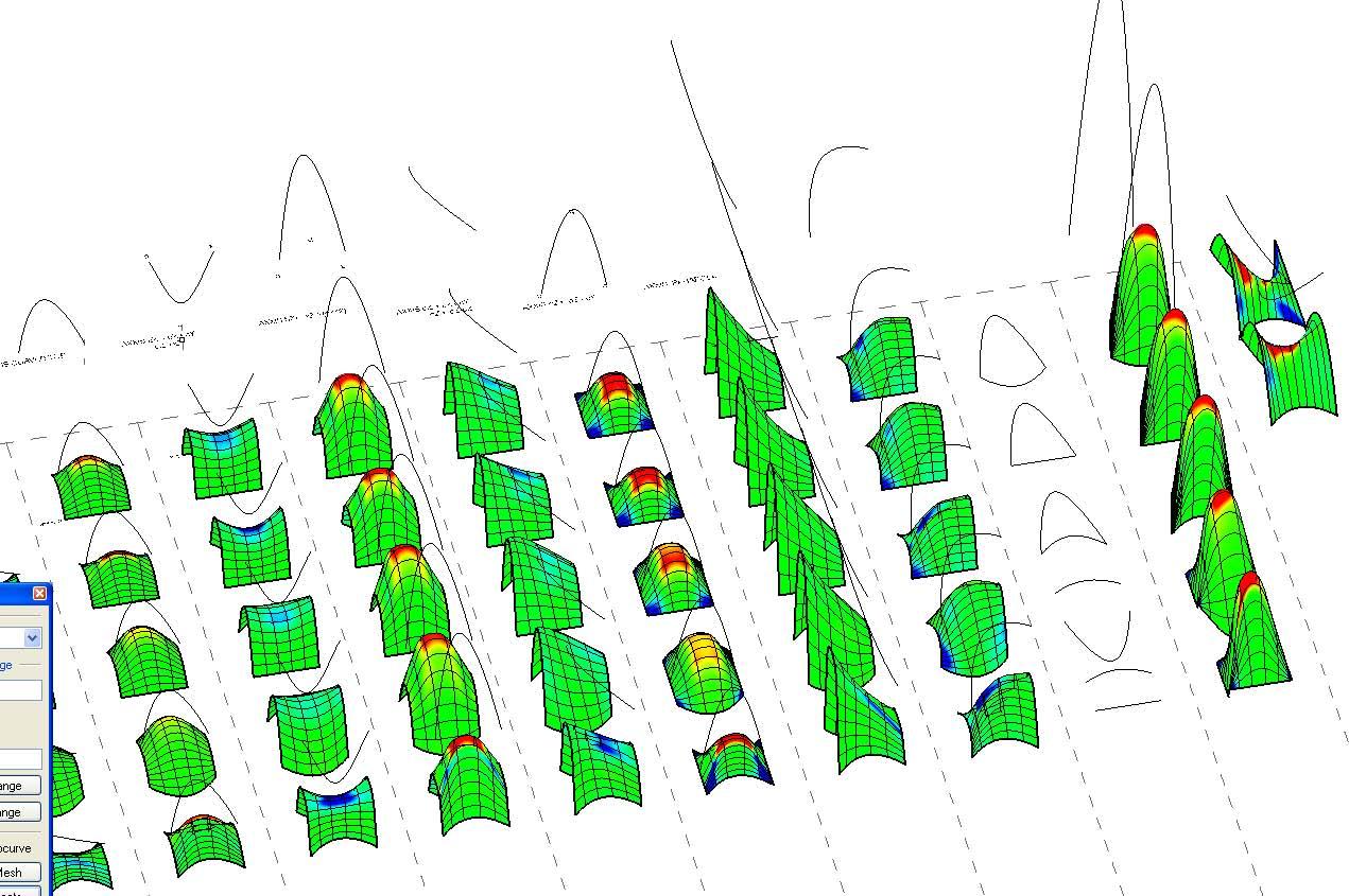
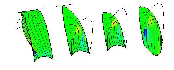
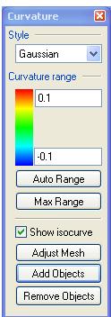
extreme + curvature ( 5%) large
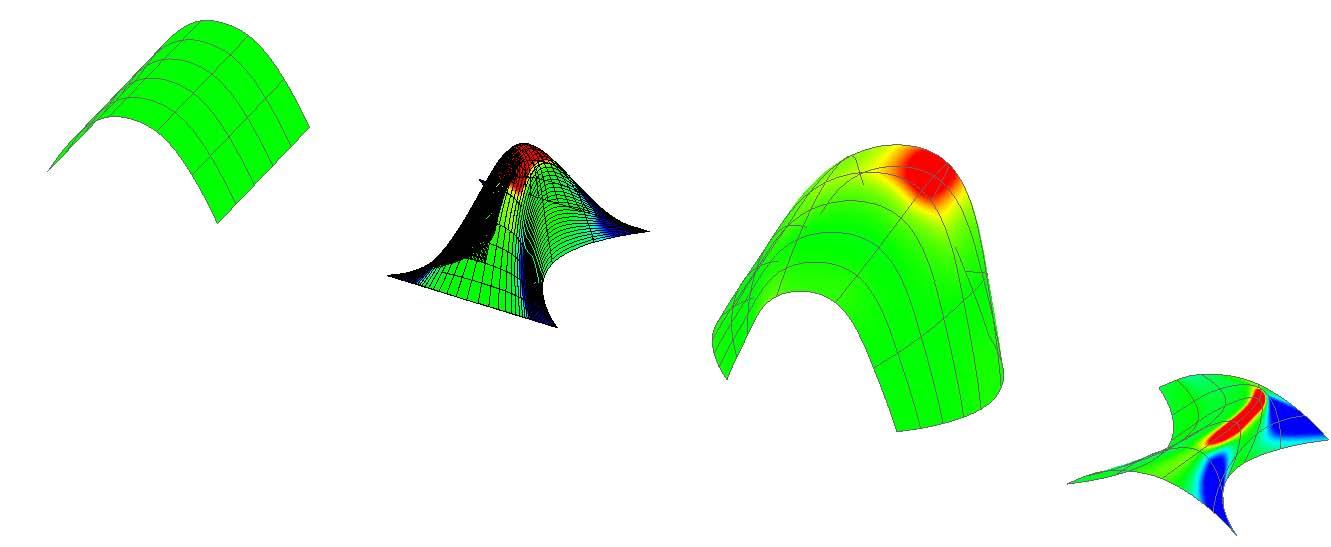
extreme – curvature( 20%)
EXPERIMENTS
3.10. EVALUATION AND RANKING
fig 3.10.1
even
fig 3.10.2
ranges
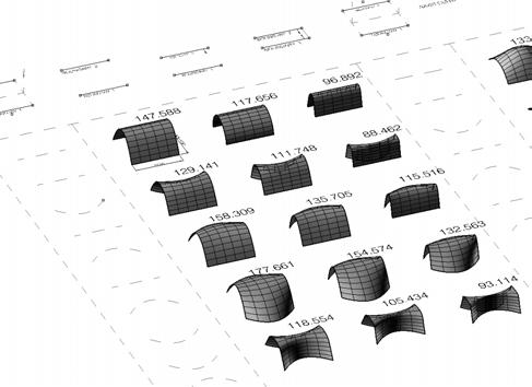
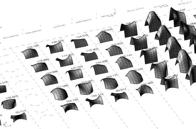
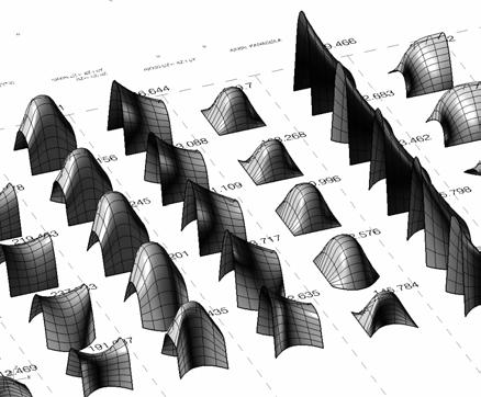
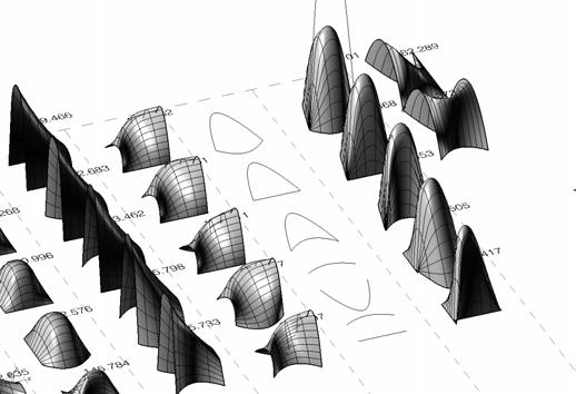
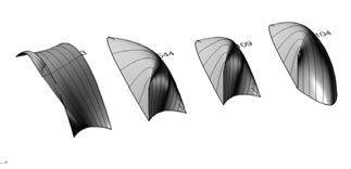
The mean curvature analysis on left page was done in Rhino, the selected surfaces were extracted for having the minimum range of differentiated curvature, the largest ranges, and the highest percentage in positive and highest percentage in negative curvature. The areas of the surfaces with 0 mean curvature are the surfaces easier to fabricate and they can be ruled and subdivided into panels that can be developed, while the + curvature are hyperboloid curvatures that would require different logic.
The Surface Area and the Floor Surface Area (coverage area by the shell) values were extracted for all shells. The evaluation selected the extreme ratios. As a conclusion for the next steps, the shells with Minimum ratio SA = FSA are most optimum for the fabrication, as they will cover more space plus will have less weight from the surface.
Of course combining the two rankings, the chosen shells would be the fittest to fabricate.
[see appendix]
fig 3.10.1 Gaussian curvature analysis
fig 3.10.2 Ranking of extreme ratio of curvatures according to Gaussian analysis
fig 3.10.3 Surface area and Floor Surface area of each shell
fig 3.10.4 Ranking of extreme ratio Surface Area and Floor
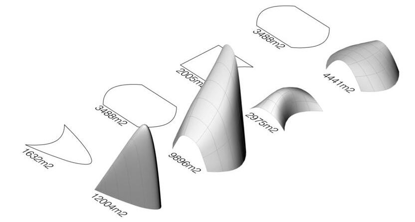
EXPERIMENTS 87 fig 3.10.3
fig 3.10.4
Worst ratio SA/FSA
Maximum SA/FSA
Best ratio SA - FSA
Minimun SA/FSA
Floor surface area (FSA)
Surface area (SA)
By embedding the material integrity and fabrication logic in the design process, the system can generate shells that require no secondary structure as the surface performs both structurally and architecturally. Thus, the timber composite surface enhances structural capacities allowing the system to span with lightweight material.
As can be seen on the right graph, if the geometry and the material are working with similar purposes, the structures can be stiffer and stronger without increasing the weight. The simulations run on Strand7 were more successful than the other attempts as they work with scale, proportion and material properties.
The curvature analysis defines where a surface has single or double curvature. Nonetheless, the process of analysis has to be reverted in the next chapter in order to produce a system of shells that work within the limits of plywood and the limits of the fabrication technique proposed.
The process presents important advantages in local reinforcement and in the assembly process due to the high stiffness and strength with low density of the composite.
EXPERIMENTS 88
CONCLUSIONS
FLEXURAL PROPERTIES OF SOLID LAMINATES & SANDWICH PANELS
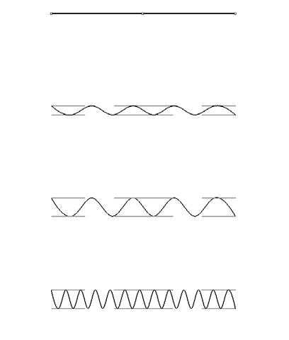
MATERIAL LOGIC
fig 3.11.1 Graph - increasing the thickness will not increase proportionally the weight, while indeed it will increase stiffness and strength
EXPERIMENTS 89
GEOMETRY - STRUCTURAL- FABRICATION
37 9.25 1.06 7 3.5 1.03 1.00 1.00 1.00 0 5 10 15 20 25 30 35 40 StiffnessStrengthWeight Solid laminate thickness t Sandwich panel thickness 2t Sandwich panel thickness 4t plywood 1.5mm plywood 1.5 + plywood 1.5mm plywood 1.5mm + plywood 1.5mm + fiber glass + fiber glass + resin 1.5mm resin 4.5mm
A system to fabricate shells with timber composite material with low-technologies. After having done the geometry and curvature analysis plus the physical test of translating the digital geometry into the physical material, it was found that the most efficient way to panelize the large surface is through strips, “horizontal” along u direction and vertical along v direction. The design development shows some fabrication processes explored, plus some alternatives of the system for specific architecture requirements; the purpose is to embed some architecture qualities such as light, and ventilation conditions through the optimum fabrication process chosen.
While establishing the system, the design is exploring some alternatives as well as recognizing constraints, in this way it establishes the rules and analysis evaluation to achieve structural and architectural capabilities from the surfaces.
CHAPTER FOUR - DESIGN DEVELOPMENT
The general process to achieve the shell is described on the diagram 4.1.1. It shows the alternatives the research has explored picking some of them, and moving forward on the next steps.
The digital (grasshopper) adjustment of the architecture, the physical experiments and the simulations done during the process are taking place at different stages of the diagram. However, in order to have clarity of the fabrication process they will be display in a linear way.
The deformation and reinforcement process have as premise to stabilize gradually the surface, from the pair of panels buckled, to the arches, to the entire surface.
1. Plywood panels. The plywood panels are cut according to the geometry defined on the digital process with holes on the edges.
- The cut pattern & Thickness. From the physical experiments was clear that thickness make changes on the corrugation as well as the grain direction, however extreme curvatures can be displayed easier due to the cut pattern. By the variation from rectangular to irregular edges when applying the force on the top boundaries, the edges behave dramatically different, from 20 cm maximum to 2mm.
- The size of the panel and fiber directionality. It is an extensive digital process to simulate the buckling and bending of each panel to achieve the corrugated surface. As a result, on large pieces the bending occurs easily but also in vertical rectangular pieces with fibers in the plywood perpendicular to the boundary where the force is applied. The proportion makes a wide difference according to the panel.
2. Applying the Load. The panels are disposed in arcs (fig. 4.1.2), and the load is applied by pairs of panels to obtain buckles (fig 4.1.1).
3. The fiber-glass and resin is spray-up on the pair of panels to stabilize them.
4. The pair of panels is stitched on its common edges.
5. The next pair of panels is buckled. Step 2, 3 and 4 are iterated every time the pair of panels is stable.
6. The pairs of panels are stitched on its common boundary defining adjustability to allow voids or transparencies.
7. The fiber-glass and resin is spray-up on the pairs of panels to stabilize them.
8. The process of buckling, stitching and reinforcing continues along the arch (fig 4.1.2).
1. PLYWOOD PANELS
2. APPLYING LOAD BY PAIRS
3. GRP ON THE FIRST PAIR (LAYER 1 ) To stabilize
4. STITCHING THE FIRST PAIR
5. ITERATION
6. STITCHINGADJUSTING THE TWO PAIRS
ITERATION 4.1. FABRICATION PROCESS
7. GRP ON THE THE TWO PAIRS (LAYER 2)
fig 4.1.1 Fabrication process until arch assembly
Size panels-Cut pattern Thickness
Similar Edge Opposite edges
unidirectional ortho random
spray - up fiber glass and resin
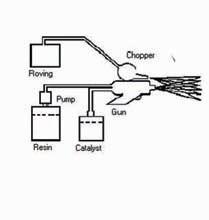
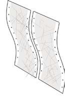
Loose Tight
assembly without transparency in between transparency in between
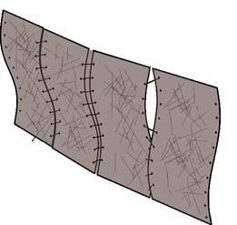
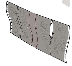
Fiber directionality
DESIGN DEVELOPMENT 93
a b a b a b
F
On the fig 4.1.2 the diagram shows the process to create one arch, therefore the process showed in the previous page takes place in the creation of every arch.
After all arches are created on the ground the tilt-up process takes place. Thus, the sequence has to be studied according to the stability of the shell. In fig 4.1.3 the arcs located on the center are assemble first as the other 6 are working in cantilever on both sides.
9. One layer of fiber-glass and resin is applied on the first four arches assembled.
10. The assembly of the other two groups takes place on the ground and then the entire surface is assembled. Another possibility is to tilt-up arch by arch from these last ones; however, it would depend on the weight of the arches, though the big assembled parts can be moved by a few men. At the end the shell has to be reinforced with another continuous layer of GRP on top of the total surface
An alternative procedure to reduce operations on site would be to produce the buckled stabilized (reinforced) pair panels in the industry and take them to the site as pre-fabricated. This would eliminate the necessity of having the loading machine on site; instead this procedure could take place in an interior area. Nonetheless, the reinforcing process for the arches as well as for the entire structure would have to take place on site.
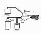 A. Flat panels
B. Load machine applying force on first two panels
C. Reinforced Resin+Fiber Glass the entire arch
D. Stitching first two panels
E. Move the Load machine next panels
A. Flat panels
B. Load machine applying force on first two panels
C. Reinforced Resin+Fiber Glass the entire arch
D. Stitching first two panels
E. Move the Load machine next panels
F F
F. Reinforced the entire arch
4.1.2
F. Iteration of steps B, C, D, E
fig
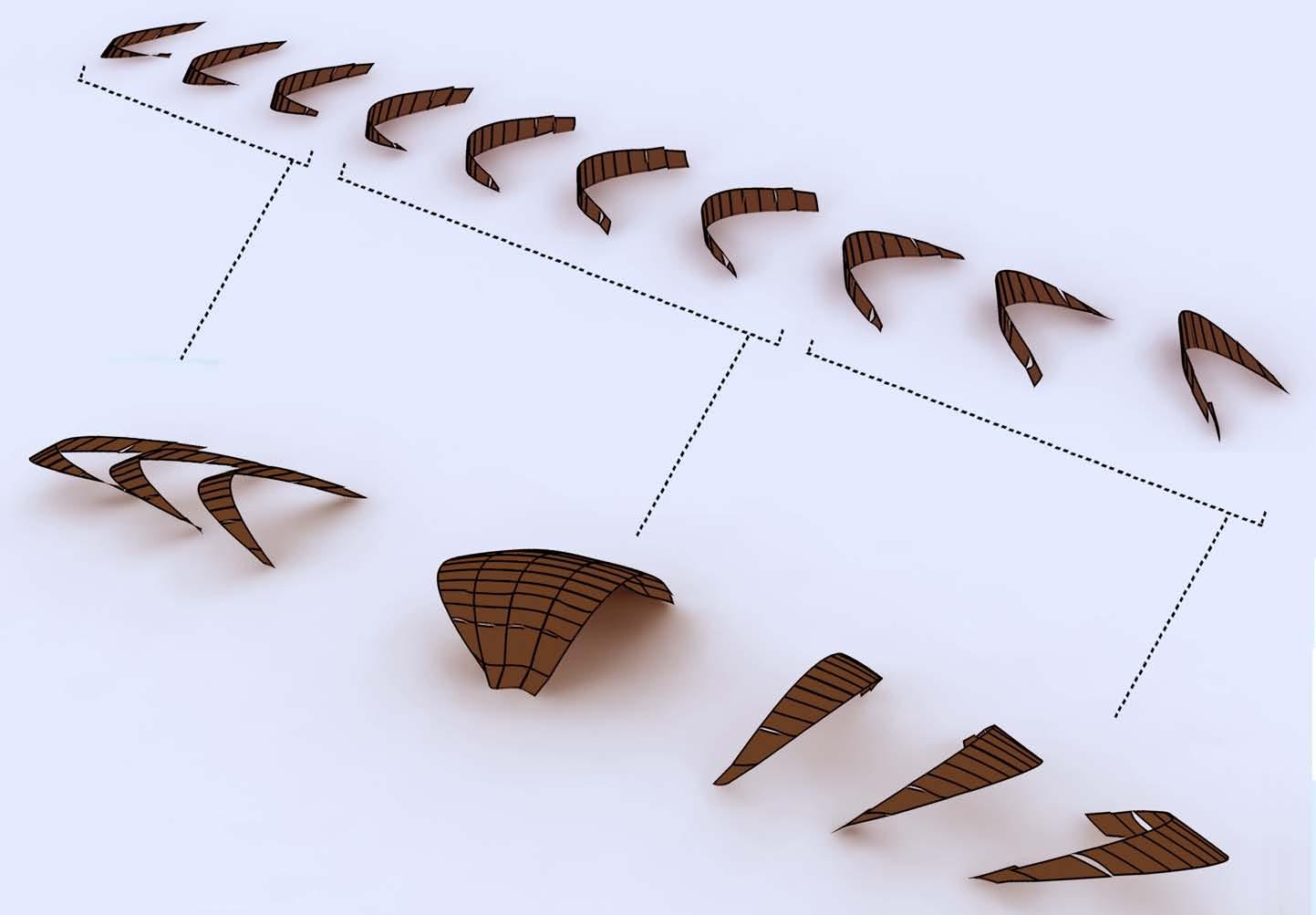
DESIGN DEVELOPMENT
fig 4.1.3
fig 4.1.2 Facrication of one arch in situ
fig 4.1.3 All arches on the ground
fig 4.1.4 Tilt-up of the arches. Requires on last reinforcement
fig 4.1.3
LOCATE THE BOUNDARIES
REQUIREMENTS
GENERAL POSSIBLE SURFACES
ANALYSIS ON GLOBAL SURFACE
REQUIREMENTS 2
- Span
- Height
- Aproximated covered areas
- Curvature analysis
- Corrugation
- Light Condition
- Ventilation
CORRUGATION ON SURFACE
PANELIZATION
ANALYSIS ON LOCAL PANELS
CUSTOMIZE BUCKLING STRAND
ANALYSIS ON GLOBAL SURFACE
- Curvature analysis
- Structural
- Force required for each panel
- Structural
- Wind
- Sun
- Filtering light
- Refraction on surface
4.2.1 General digital process - Data connection between programs
[ rhino ]
[ grasshopper - rhino ]
[ rhino ]
[ grasshopper - rhino ]
[ rhinoscript ]
[ rhino ]
[Strand7 - Excel - rhino ]
[Strand7, AnsysCFD, Grasshopper, 3dmax]
DESIGN DEVELOPMENT 96
iteration 4.2 DIGITAL PROCESS - T H E S Y S T E M
fig
The digital process on the left page follows the result of the digital and physical explorations, the physical experiments of buckling were recorded in a data base which performs as a catalogue in continues progress. Previous to fabrication, any shell should go through this process in order to guaranty the feasibility of fabricating it, of course within the limits of the system. Let’s follow the process:
Minimum of two lines of support are required plus three or more specifics heights along the axis according to the function. Public areas require minimum height of 3.5 meters while private areas require a minimum of 2.5m. The surface area shouldn’t exceed the proportion of 2:1 SA: FSA. Combining these two factors some shells pass to the next process of global curvature evaluation where a maximum of Gaussian curvature was 0.006.
Consecutively, the surface is evaluated according to sun light conditions in the specific location and to sun light interior filters. Having firstly, the filters of light along the entire surface and secondly, only along certain areas within the space. The light filters are specifically related to the ventilation voids, as the light filters can be voids or just translucency areas.
Once the requirements of the surface are set, the subdivision takes place: u is divided it into segments of approximate 2 meters, and v is divided into segments of approximately 1 meter. This is in order to make the most efficient panelization: bigger panels with fewer assemblies and less arches; but also to afford better the corrugation required on each panel, splitting the surface on the less curved areas. Basically the system splits the curved surface in curvy panels, and extracts the corners of each panel to create a flat panel.
This size of panel is an approximation to the size of sheet plywood that will be required. Afterwards, the analysis of curvature is run on the panels according to the maximum factors of tolerance establishes on previous experiments. Now the corrugation is viable and the corrugated panels are unrolled into flat sheets, which will be the cutting pattern of the plywood. These flat pieces are disposed along the curves on the ground with the same inclination as if the panels were going to be flat (4.1.2 F).
The resulting panels are taken into Rhino as .dxf
surfaces and assembled in the predefined arcs. Then the arches are taken into Strand again to simulate the stitching step. Once this procedure is done with all the arches, they are taken into Rhino again to assemble the entire shell and one more time take it into Rhino to simulate the stitching.
The digital process related to the fabrication system is a back and forward process which has as main purpose look for optimization previous to the construction time.
THE OBSESSION WITH A SURFACE
The project gets the interest of producing one continuous surface based on the material behavior just as Dieste explored deeply in his research where he recognized that the surface offered a realm formal exploration that in turn, could solve structural problems. The surface is the result of environmental, structural and architectural necessities. Its efficiency responds to the optimization process. Therefore form and expression, fabrication and structural efficiency led the development of a new language of building. The optimization process determines the final shape. The shells are the material with certain thickness, but the shape is still more fundamental as it contains the space and the quality of itself.
DESIGN DEVELOPMENT 97
h p1 p2 p3 = 10
p2 p3 = 10 p1=0
p2 = 10 p1 p3 =0
p1 p3 = 10 p2 =0
p1 p2 p3
h
h
p1 p2 p B1 B2
h
corrugation B2 corrugation B1 B2 corrugation B1 B2
Requirements 1 Requirements 2 Height Points on axxis
fig 4.2.2 Alternatives on the digita process
Panelization
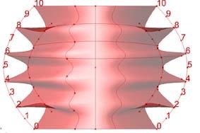
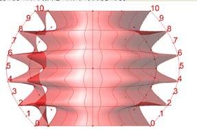
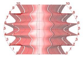
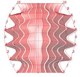
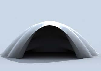
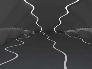
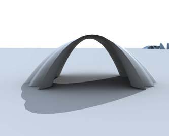
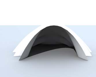
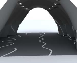
DESIGN DEVELOPMENT
4 filters 1 filters 0 filters u = 10 v = 10 u = 10 v = 10 u = 4 v = 10 open closed open closed u = 10 v = 8 u = 10 v = 15
= 10 v = 10 u = 10 v = 5 u = 10 v = 1 8 filters u = 9 v = 10
Analysis on global surface flat panels filters dark- bright filters in close and open space filters of light filters of light
u
pattern of panels pattern of filters
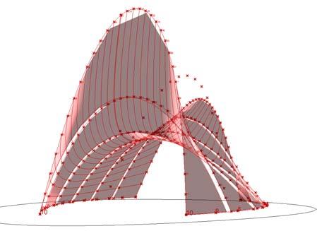
matching arches with void in between
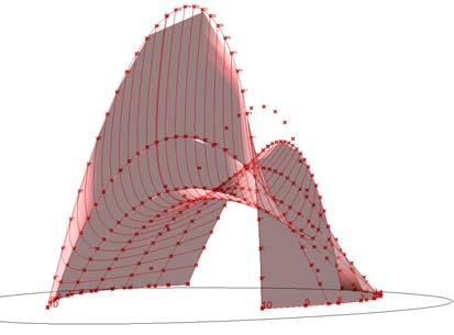
matching arches edges
4.2.3 changes on the arches through grasshopper definition [see appendix]
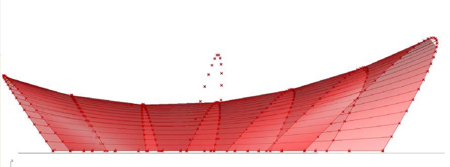
fabrication method by arches - change the light filter
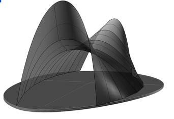
matching arches
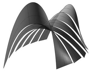
void in between 7cm - it will be reinforced with GRP
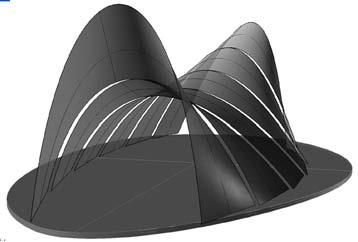
void in between 5cm - it will be reinforced with GRP
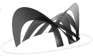
crossing arches - voids will be reinforced with GRP
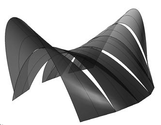
crossing arches - the space will be reinforced with GRP
DESIGN DEVELOPMENT
fig
The openings along the surface deploy the alternative of having cross ventilation in the shells that have close sides, the big opening is positioned towards the wind coming direction and small openings are done in the upper part of the surface.
The system, presented in the previous and present page shows the variation of steps it can achieved by changing the parameters. The system can always expand according to environmental or space quality requirements; however, it will present some contraints due to fabrication.
1 PERSON
1 telephone cabine
1 Toilet
1 bedroom Magazine stand 10 PERSONS
shop Café internet Public toilets Bike Parking place Meeting room A house
DESIGN DEVELOPMENT 101
PUBLIC BUILDING Church Library Auditorium Restaurants
ventilation usage determines span
Flower
fig 4.2.4 The shells working at different scales
big opening facing the prevailing wind directionvoids on the surface to produce cross ventilation

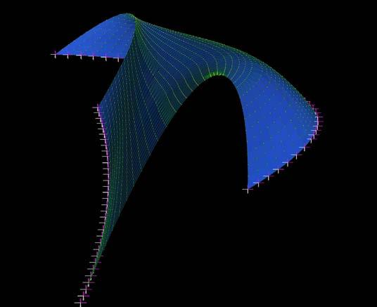
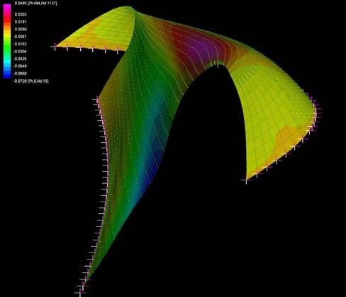
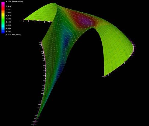
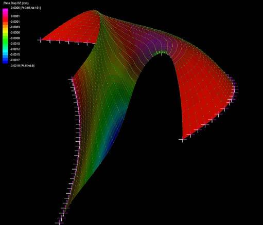
4.3.1 DIGITAL PROCESS TO PRODUCE ONE SHELL
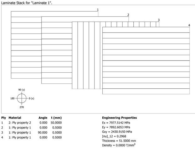
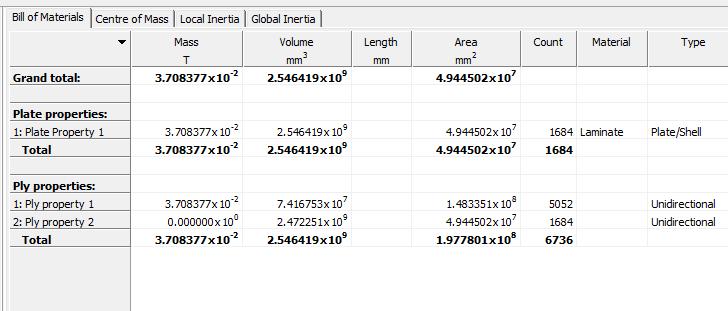
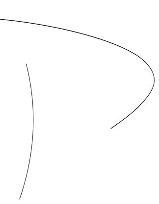 A. 3d model fixed boundaries to the ground, surface meshed
B. Linear Static Analysis composite 1cm
C. Linear Static Analysis composite 5cm
D. Linear Static Analysis composite 7cm
fig 4.3.1.1
fig
A. 3d model fixed boundaries to the ground, surface meshed
B. Linear Static Analysis composite 1cm
C. Linear Static Analysis composite 5cm
D. Linear Static Analysis composite 7cm
fig 4.3.1.1
fig
4.3.1.2
On this first surface the entire digital process of shell’s production was tested. The process was initiated setting two curves as boundaries that will be attach to the ground, plus defining the axis with the correct height. The first attempt to panelize the surface was through the isocurves in u and v direction, the curves going in v direction will become straight segments (fig
4.3.1.4 ) and the curves going in u direction will assume the curvature. Taking advantage of the fabrication method of obtaining buckle sheets, the corrugation was exaggerated along u direction. The colors on figures
4.3.1.3 and 4.3.1.4 refer to the particular reinforcement quantity that needs to be applied on each pair throughout the fabrication. This initial attempt proposes to fabricate the shell from bottom to top in rows in a fabrication logic number.
The figures below show different stages in the manufacture of the fiber composite panel with incremental material being added in the laminate.
On the left side the figures from top to bottom display the Linear Static Analysis run in the shell increasing the thickness of the composite. The displacements are minimums, the 5cm centimeter thickness shell can stand; however, the thickness can still be less and the longest free edges are trend to wobbled, therefore some extra reinforcement would be required on these areas.
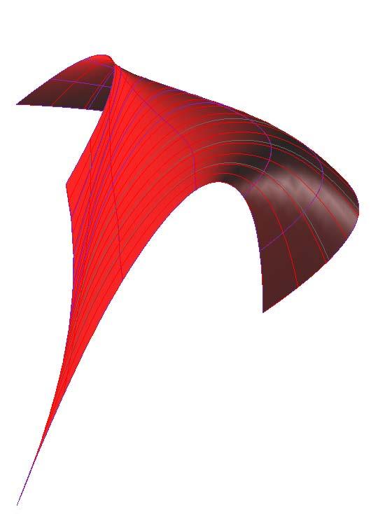
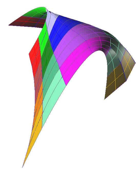
fig 4.3.1.1 Linear Static Analysis on the shell
fig 4.3.1.2 Specification for the Timber Composite in Strand7
fig 4.3.1.3 Reinforcement chart per panels
fig 4.3.1.4 Subdivision of the surface
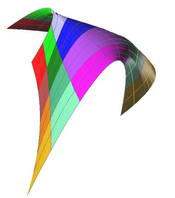
DESIGN DEVELOPMENT 103
U V fiber glass +resin STABILIZATION RING 2 ‐REINFORCEMENT STABILIZATION RING 3 ‐REINFORCEMENT fiber glass +resinthickness thickness BUCKLING IN PAIRSASSEMBLY ‐VERTICAL STITCHING ply 1 ply 2 ply 3 ply 4 ply 5 from boun plywood 1A BAB AB 1‐AB1‐CD 1C DCD CD 1‐CD1‐EF 1E FEF EF 1‐EF1‐GH 1G HGH GH TOTAL RING 1 2A BAB AB 2‐AB2‐CD 2C DCD CD 2‐CD2‐EF 2E FEF EF 2‐EF2‐GH 2G HGH GH TOTAL RING 2 3A BAB AB 3‐AB3‐CD 3C DCD CD 3‐CD3‐EF 3E FEF EF 3‐EF3‐GH 3G HGH GH TOTAL RING 3 REINFORCEMENT IN PAIRS ASSEMBLY ‐VERTICAL STITICHING STABILIZATION RING 1 ‐REINFORCEMENT RINGS PLYWOOD PANELS fiber glass +resin fiber glass +resin thickness thickness
fig 4.3.1.3
fig 4.3.1.4
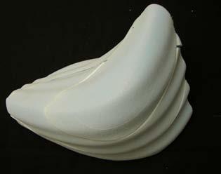
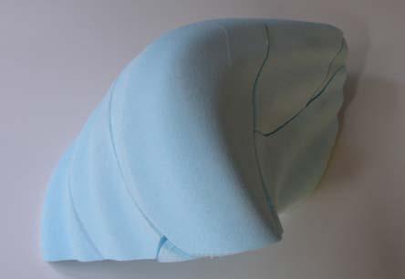
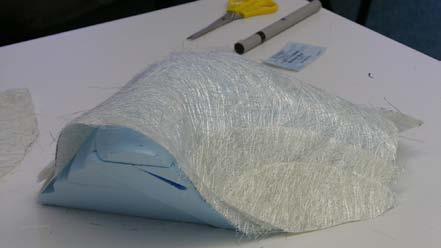
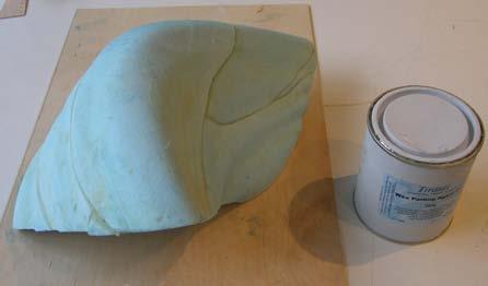
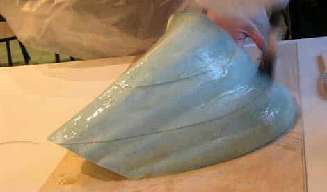
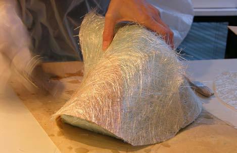
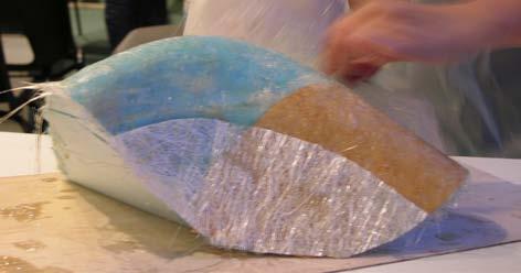
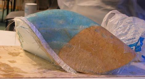
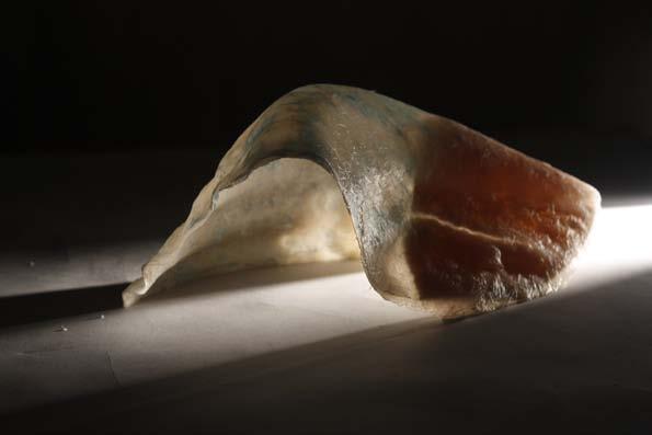
4.3.2 ALTERNATIVE REINFORCE PROCESS
The mold was milled into four pieces out of low density foam followed by its assembling, in order to create the big shell. When the foam shell is assembled the fiber glass light mat pieces are cut: one big layer that covers the entire surface, one that covers the first and second line and a third just covering the bottom as seen in figure H.
The shell accumulates more material on the most vulnerable areas. Thus, the bottom area has more reinforcing material than the rest of the surface. The borders of the shell that will be in cantilever are also reinforced to avoid wobbling on the shell.
A. Low density foam milling mold pieces fitted in 30X40 cm.
B. Fiber glass chopped light mat cut
C. The surface is cover with wax
D. One veneer sheet is place on the surface
E. First of fiber glass with polyester resin
F. Second layer of fiber glass mat (first row)
G. Reinforcing the edges
H. FInal model with translucent effect
4.3.2.2 Rhino file of the 4 pieces for CNC milling machine
4.3.2.4 Alternative reinforcing process in horizontal strips
A G F E B C D H
fig 4.3.2.1 Modelling Process
fig
fig 4.3.2.3 Shell with variated thickness
fig
fig 4.3.2.1
fig 4.3.2.2
The figures below show different stages in the manufacturing of the fiber composite panel with material being incrementally added in the process.
The fact that the panels are laid on courses allows the shells to have stability as the accumulation of material will be higher at the bottom than at the top, therefore, different thickness along the surface.
This procedure of fabrication has some similar advantages as the Guastavino techniques presented in the second chapter. However, the fabrication of the temporary arches would present disadvantages over other techniques and the corrugation along v direction according to the fabrication of the courses will decrease the structural capacity of the shell. If is possible to imagine, it is actually helping the surface to fold by its own weight. This evaluation is taken forward for the next steps in the design development.
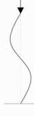
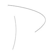
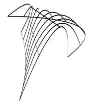
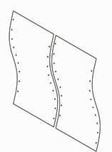
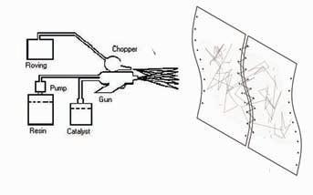
1. Ancher points -Set the boundaries
ring 1
ring 2
ring 3
ring 3
ring 2
ring 1
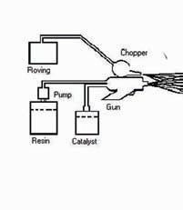
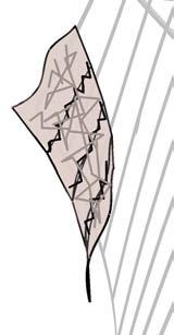
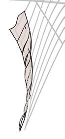
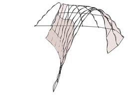
2. Temporary arches places
3. Cutted flat plywood sheets
4. Buckle 2 panels at the time - holes on the edges of plywood - loose stitiching [iterate for every 2 new panels]
- Apply fiberglass +resin / tight the stitching
5. Step 3
6. Assemble 4 panels / tight the stitching
7. Fiber glass +resin - 4 panels
8. Reinforce Ring 1 (stabilize the ring)
9. Ring 2 : Iterate steps 3 to 7 placing on the arches
10. Reinforce Ring 1 and 2 at the same time (stabilize the ring)
11. Ring 3: Iterate steps 3 to 7 placing on arches
12. Reinforce Ring 1 , 2, 3 at the same time (stabilize the ring)
DESIGN DEVELOPMENT 105
fig 4.3.2.3 fig 4.3.2.4
4.4 THE VOIDS EFFECT - LIGHT IN THE SURFACE
The high contrast between the interior and the exterior is the result of the global form. In long shells the central area has more intimacy due to less luminosity while the access areas (public) are brighter.
The surfaces work during day time with natural filters of light from outside to inside and, during night time work as lamps when the interior is illuminated (fig 5.2.21).
The fabrication has an intrinsic relation with the spatial final quality; the matching edges from individual panels drive the light filters on the surface. This also happens when the arches previously seen in 4.3 vary their regular direction, the pattern created by the light lines radically changed.
The size of the resulting voids between plywood sheets can change very little but will display big differences in the reflection on the panels.
The GRP has translucency and the voids can be covered for only light filtration and no water. Due to the small thickness of the plywood, the surface can have certain effect when the light focus is placed close to the surface (fig 5.3.2, fig 5.3.3).
In addition the holes also have nice effect filtering the light.
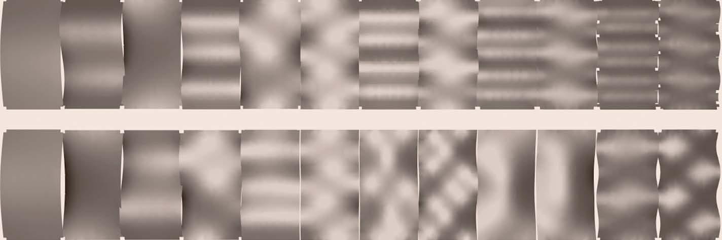
fig 5.3.1 Light effect through the voids on buckled panels from experiement 3.3.2
fig 5.3.2 Light effect from the plywood side. Close spotlight - translucency on the plywood.
fig 5.3.3 Light effect from the GRP side. Close spotlight - translucency on the plywood.
fig 5.3.4 Light effect from the GRP side. Far spotlight - translucency on the ply wood.
fig 5.3.5 Light effect from the plywood side. Far spotlight - translucency on the plywood
DESIGN DEVELOPMENT 106
fig 5.3.1
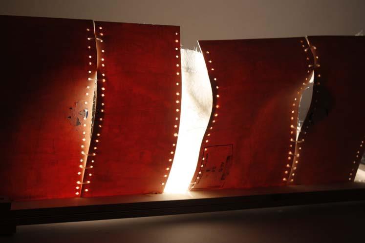
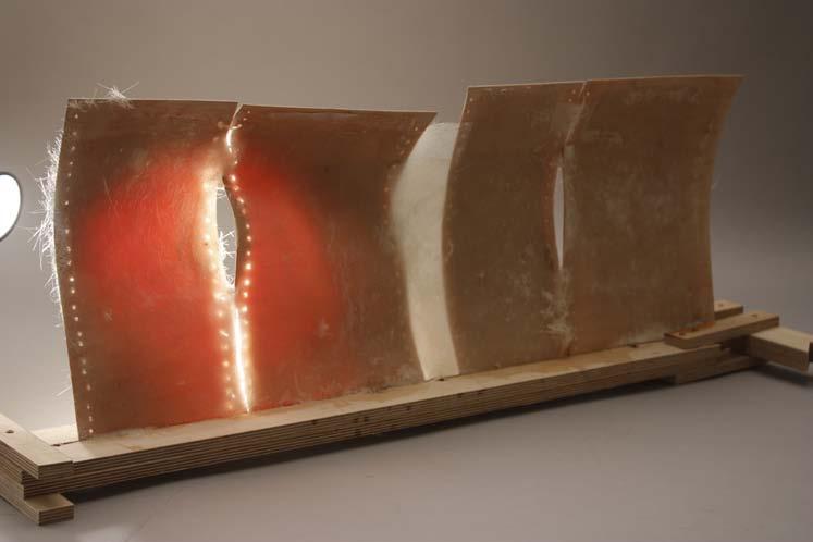
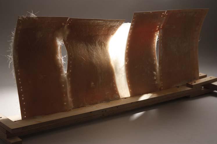
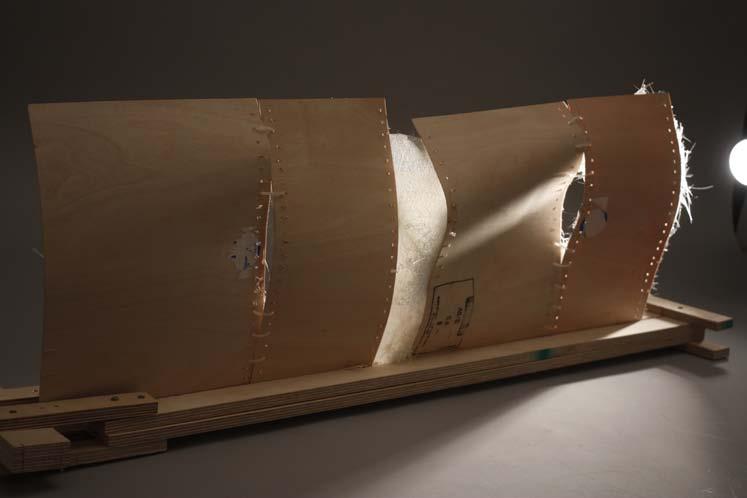
DESIGN DEVELOPMENT
fig 5.3.2
fig 5.3.4
fig 5.3.3
fig 5.3.5
CHAPTER FIVE - DESIGN
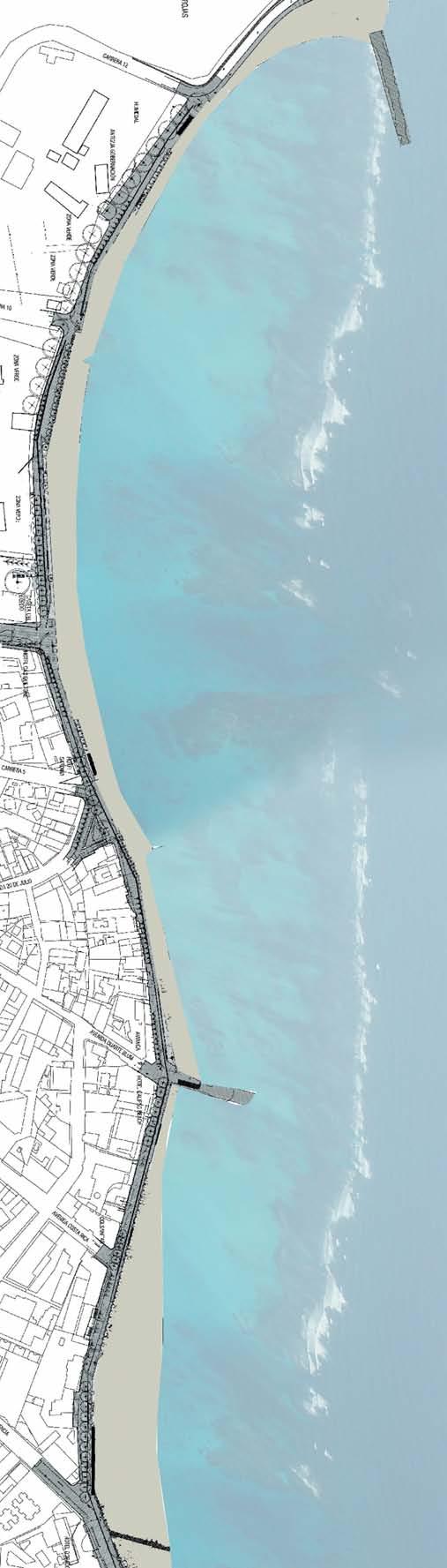

Latitude -4.2
Longitude -69.9
Time zone -5
Humidity 83%
F
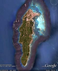
82
Location 1 Location 2 Location 3
fig 5.1.1
fig 5.1.2
N
fig 5.1.3
The next two places are possible locations for the application of the system. One of the advantages is to create a family of similar differentiated shells with large covered surfaces that require no mold. The system can be adjustable to small or big different architectural requirements.
The first explored location for the application of the system was in San Andres Island along the coast where an intervention took place in 2005. The pedestrian “Paseo” of 1.5km transformed the street for cars into a pedestrian way for tourists and natives to enjoy the beach as well as the view. It is proposed to concentrate the activities on the three points of the path located on the left plan, the beginning, close to the center and, at the end where it connects with another public space project. At these three points the shells will act as public enclosures with multiple functions.
The shells initially respond to the specific location, generally spanning from one side to its opposite and liberating the view towards the sea. The sun analysis informs the general rotation of the boundaries in order to achieve maximum shadow throughout the year. Besides according to lightweight properties inherent on each shell they can rotate. As indicated on figure 5.1.4 the design takes into account the possibility to rotate ensuring the shell won’t interrupt any of the public furniture and still allow a new configuration.
DESIGN 111
5.1 SYSTEM APPLICATION 1 - SAN ANDRES
fig 5.1.1 Top view Paseo Peatonal- Locations 1,2, 3
fig 5.1.2 Aereal view in 2007
fig 5.1.3 San Andres Island - Colombia
SCENARIO 1 - December 21
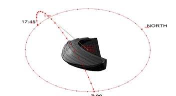
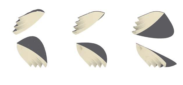
Shadow analysis
SCENARIO 2 - June 21
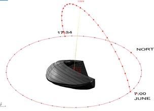
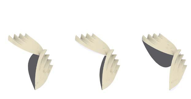
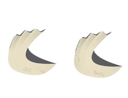
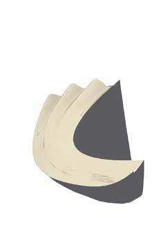
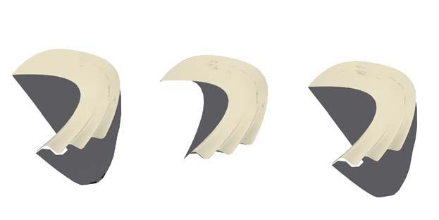
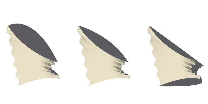
[see appendix] fig 5.1.4. Possibilities of rotation along z-axis according to shadow analysis and approximation of shells weight. fig 5.1.5 Section of the assembly
DESIGN 112 DEPLOYMENT SCENARIOS - PASEO
Weight
Surface area 291m2 Location
Location
Surface area
Surface area 59m2 each
885kg
1 Location 2
3
110m2
December 21 10:00 am December 21 12:00 am December 21 16:00 pm December 21 10:00 am December 21 12:00 am December 21 16:00 pm June 21 10:00 am June 21 12:00 am June 21 16:00 pm June 21 10:00 am June 21 12:00 am June 21 16:00 pm December 21 10:00 am December 21 12:00 am December 21 16:00 pm
SCENARIO 3 - Summer Festival - December
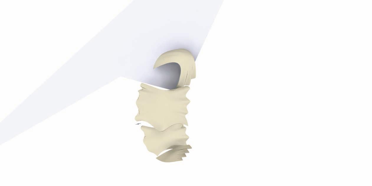
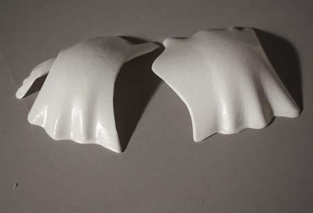
Location 1
Surface area
a. 142m2
b. 262m2
c. 151m2
d. 59m2
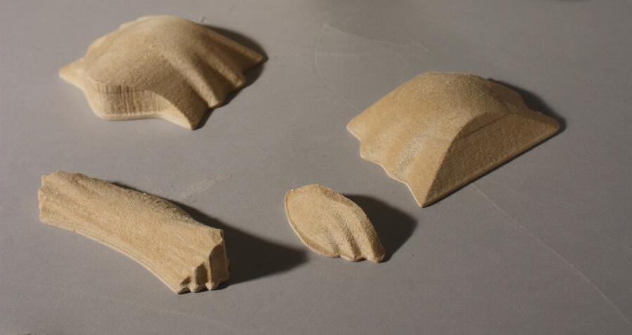
On the first column the shells are located according to December sun light exposure, on the second column the shells with less than 800kg are rotated on the z axis from its initial position to a more convenient, according to sun exposure in June. On the third column some alternatives were proposed to assemble the shells to configure bigger spaces, moving them from the other locations along the coast or bringing totally new shells. These bigger spaces can be utilized for big festivals that the Island received.

Approx weight 15 per m2
AVENIDADUARTEBLUM
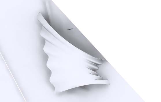
free area to rotate the shell (boundaries always within this range)
DESIGN 113
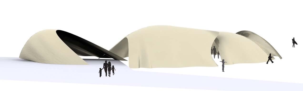

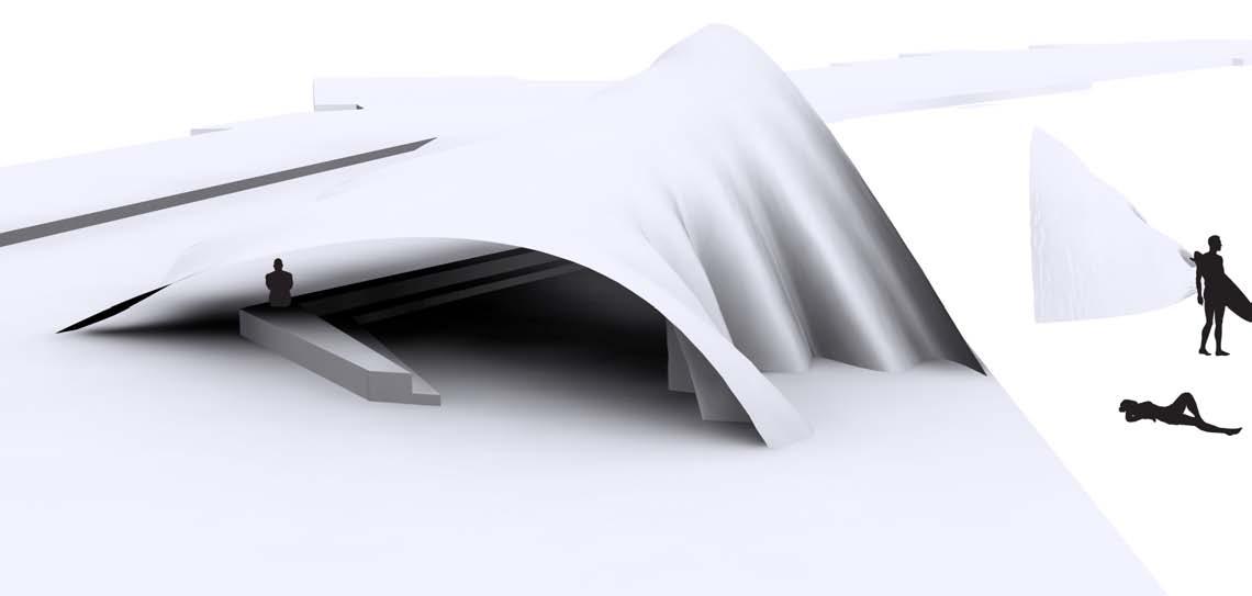
DESIGN 114 fig 5.1.6
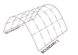
ROTATION ALONG X AND Y AXIS
Lightweight shells could be carried by man-power, and repositioned on different locations. This leads to the possibility of changing not only environmental conditions, but also functions in the same structure.
The rotation can happen along z-axis but also along the x and y axis’. The shell has to be designed according to the functions it needs to perform; therefore its stability is embedded in the possible rotations. On figure 5.1.7 the boundaries define the rotation. The first figure is supported on B1 and B2 and defines a covered area, the second is supported on the surface that can become a sitting area and the third is supported on B4. Therefore the surface can become a covered area in cantilever as in figure 5.1.10. As proposed in the system proposal, the design can create a second layer in certain areas, either to reinforce the surface or to create some “pockets” (fig 5.1.8,fig 5.1.9). The purpose of these pockets is to locate sand bags that can work as the foundations of the shell; hence the location of the pockets has to be established from the design phase. When the shell is situated on the desired position, the sand bags are placed in the pockets. When the surface rotates the location of the sand bags change as well.
fig 5.1.7 3d rotational surfaces
fig 5.1.8 Initial position for fabrication
fig 5.1.9 Pockets for sand bags - stability
fig 5.1.10 Rotated surface
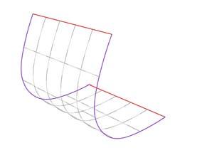
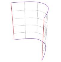
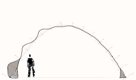
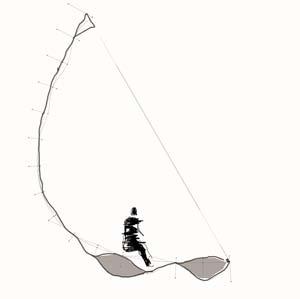
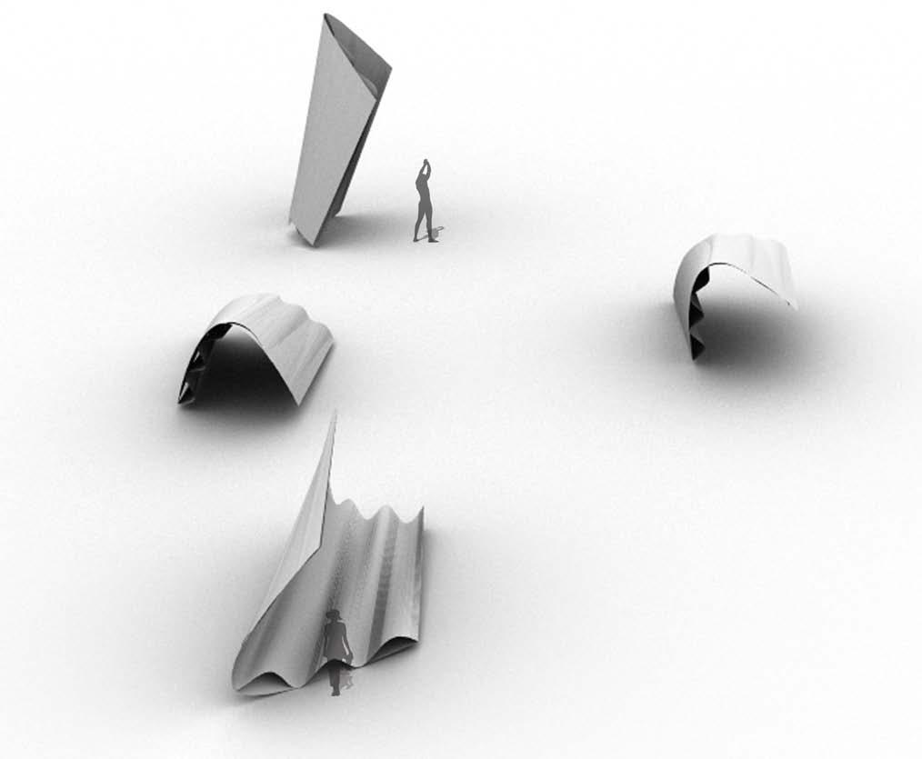
DESIGN 115 BOUNDARY 3 BOUNDARY 4 BOUNDARY 3 BOUNDARY 4 BOUNDARY 1 BOUNDARY 2 BOUNDARY1 BOUNDARY 3 Surface area 50m2 Weight 750kg Aprox. thickness 4cm BOUNDARY
- ORIENTATION - STABILITY
4 CHANGING FUNCTION
fig 5.1.6 View of the shells on site
fig 5.1.7
fig 5.1.8
fig 5.1.9
fig 5.1.10
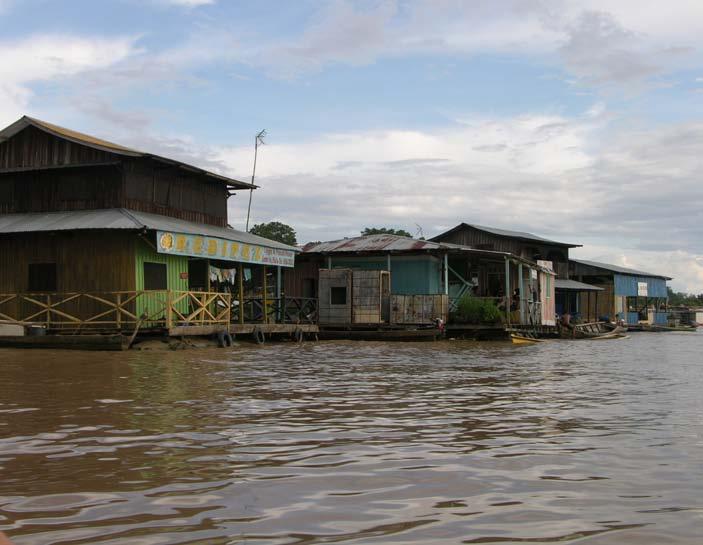

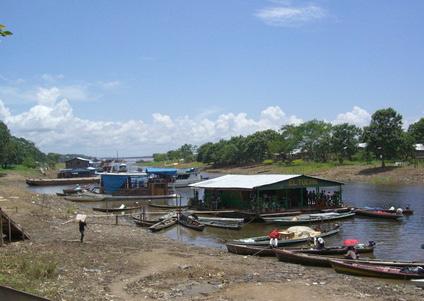
Latitude 4.09
Temperature
°C
°F).
Longitude 69.57 Time zone -5
27
(80.6
fig
fig
fig 5.2.4
fig 5.2.1 Border of the river
5.2.2 Borders of the rive
5.2.3 Actual floating houses on platforms
Amazonas River - Leticia - Colombia
fig 5.2.1 by Jheny Nieto
fig 5.2.3
fig 5.2.2 by Jheny Nieto
The second location explored as a potential application of the system was Leticia Port. The city located in southern Colombia on the borders of the Amazon River. Nowadays, Leticia is connected to other important locations by the river, having its own boat dock based on floating platforms with houses that work as boat stops.
The four platforms indicated on figure 5.2.4 are the beginning of what in the future should be the development of the border of the river, as it is the most important transport system for passengers and shipping points for tropical fish of the aquarium trade. Each shell is located on one platform and belongs to the same small company. The system attempts to solve shells with similar surfaces and coverage; meaning small variations according to specific requirements and differentiation according to each platform.
This chapter focuses on solving the entire process in one shell. Architecturally, the shell solves the interior space based on the central lineal circulation that cross the platform and separate the activities for passengers at the interior. This circulation is connected with a peripherical circulation for boarding around the shell.
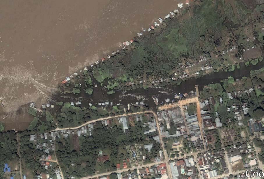
DESIGN
5.2 SYSTEM APPLICATION 2 - LETICIA -AMAZONAS RIVER
N
fig 5.2.4
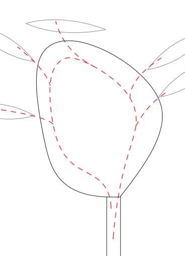
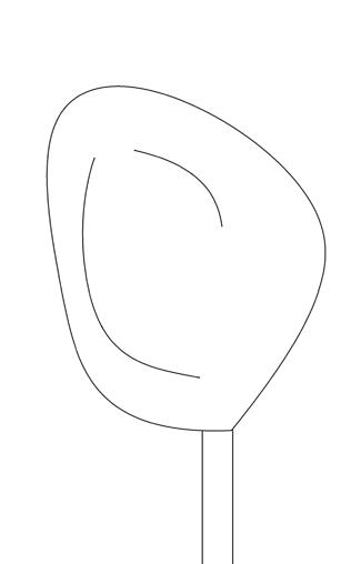
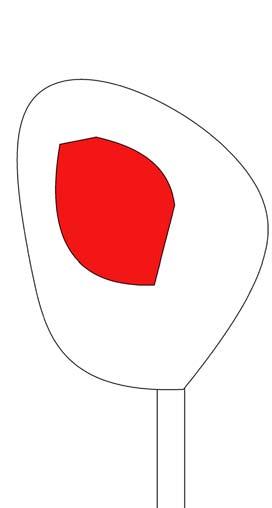
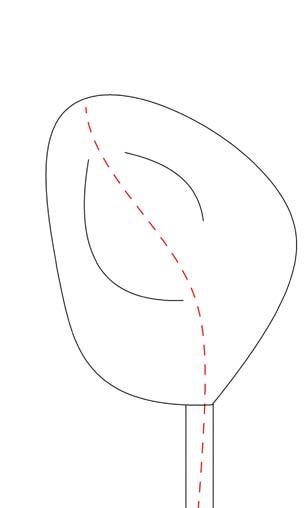
DESIGN 118 8m 15m platform peripherical circulation boarding areas technical boats entrance waiting tickets- info cafeteria boundaries covered area circulation architecture requirements length along the edges transversal lines for arches corrugation along
direction straight lines along v - 6th arch
5.2.5 Design generation process of the surface
v
fig
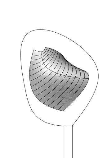
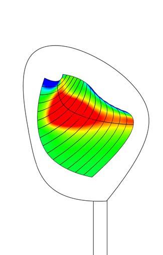
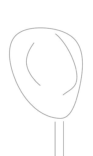
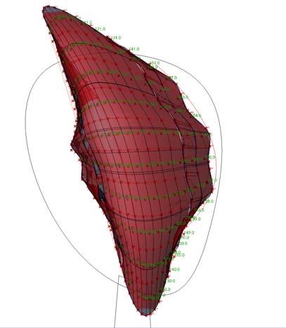
10 arches 158 panels 158 panels
DESIGN 119 surface gaussian
adjustment
boundaries
curvature analysis
of
and platform
height ventilation filters of light sitting
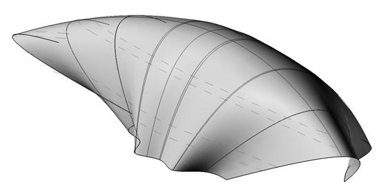
Location of the openings required from the smooth shell
arch1
arch2
arch3
arch4arch5
arch6arch7arch8arch9
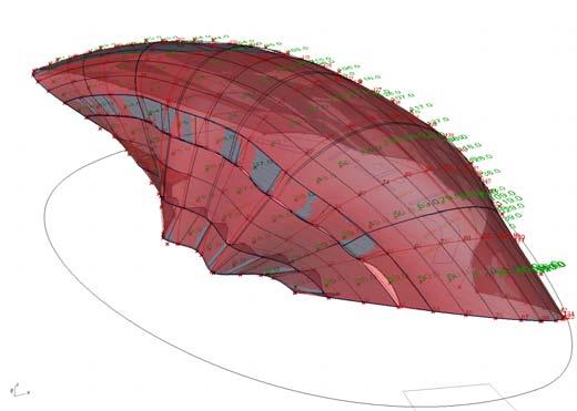
arch10
Corrugated shell to achieve with openings [see appendix]
The digital process of refining the geometry and the architecture according to the convenient filtrations of light and wind rely on one structure. However, during the process of setting the individual force that the panels require individually, there is a tolerance factor and the surface assumes small differentiations. Of course, it is expected to have another adjustment of the surface within tolerances when the shell is constructed on site. This, due to the plywood properties as well as the stitching qualities explained in the experiments chapter.
One of the big qualities of this fabrication system is to create shells that go beyond “monocoque” structures, as in some scenarios they don’t reach the spherical surface. Structurally, any arch tends to open, reason why the corrugations go along its perpendicular direction.
The span varies from 4.5 meters to 8.5; two cantilevers: 7.6 m and 6.3 m and height between 3.3 and 5.2 meters. Surface area 220m2, floor surface area 105m2.
The fabrication process allows having cantilevers without framework, by having organized the sequence to tilt up the arches as explained in chapter 4.
DESIGN 120
fig 5.2.6
fig 5.2.6 Digital adjustment of the surface fig 5.2.7 Digital corrugated panels to achieve with th ebuckling study on each panel
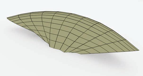
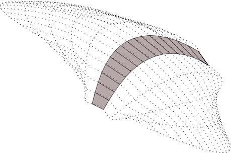
DESIGN 121 1 2 3 4 5 6 7 8 9 10 11 12 13 14 15 16
Flat panels on arch 6 to assemble
Flat panels on the shell fig
5.2.7 Flat cut panels
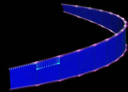
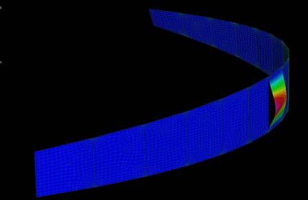


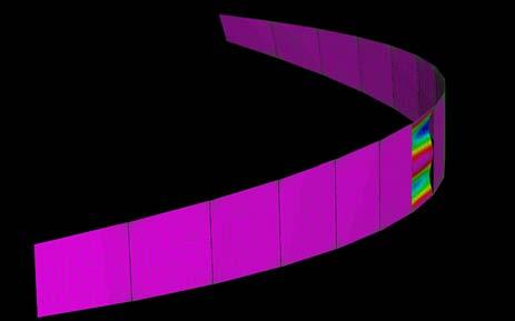
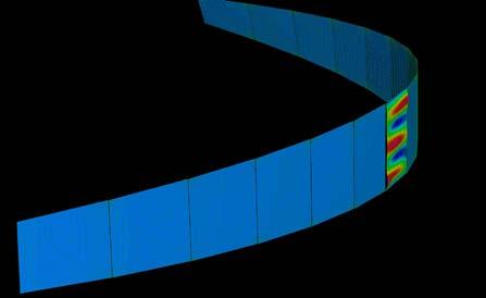
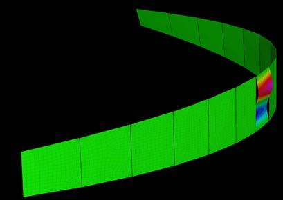
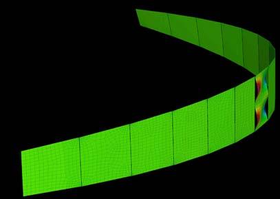
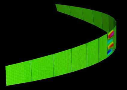
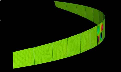
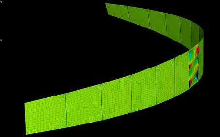
Taking the 6th arch from the previous page: The buckling simulation takes place on each panel from the arch. The flat panels set on the ground creating the arch, subsequently the force need to be apply along the direction of the panel (each panel has a small different inclination, they are not vertical). Once the force is apply and the Linear Static and Buckling Analysis are run the buckling modes are obtained.
The designer needs to pick the buckling mode more suitable or similar to the required corrugation from desired design on each panel (fig 5.2.6). A bigger set of possibilities can be obtained on the panels by constraining some nodes on the surface as in experiment 3.3.1.
Surface performance
Sun Analysis
Due to the equatorial location the sun angles in the Leticia are quite high, the sun position is almost perpendicular to the earth year long
CFD
For the flow speed parameters: Normal Speed: 5m/s = 18km/h THe prevailing wind direction is north (wind runs across the river)
Mode 1 Mode 2 Mode 3 Mode 4 Mode 5 Mode 6 Mode 7 Mode 8 Zoom in Mode 3 fig 5.2.8 fig 5.2.8 Linear Buckling Anaylisis on panel fig 5.2.9 Radiation on the surface - Shadow Analysis fig 5.2.10 CFD Analysis on the surface
Flat panels constraint on top and bottom boundaries Force on top
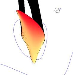

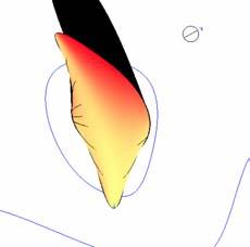
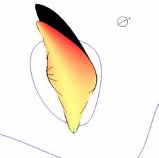
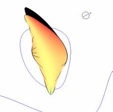
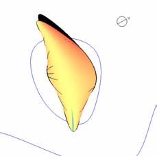
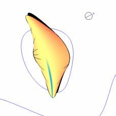
7:00am 8:00am 9:00am 10:00am 11:00am 12:00pm 7:00am 8:00am 9:00am 10:00am 11:00am 12:00pm
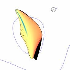
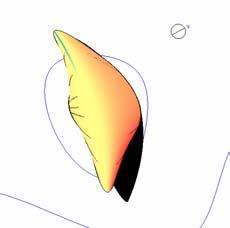
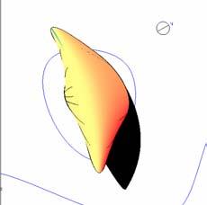
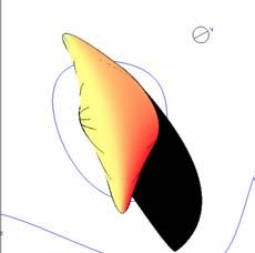
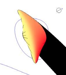
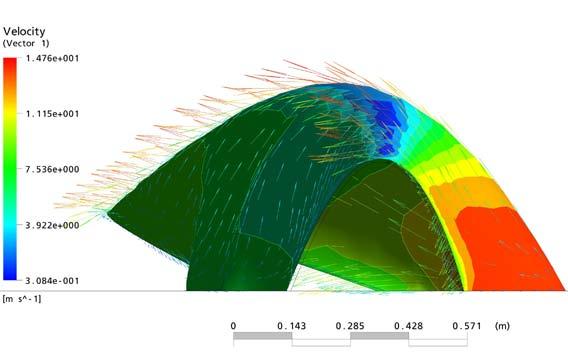
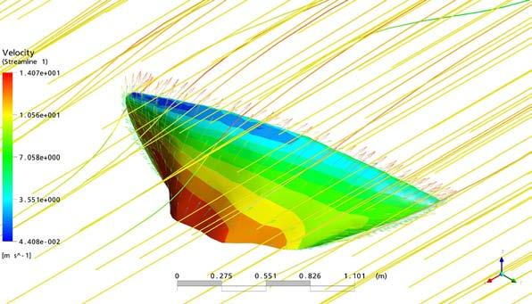
DESIGN
fig 5.2.9
December
fig 5.2.10
21
The structural analysis run on the shell demonstrates that the surface can have a total thickness of 5cm and still take wind load and self-weight.
The surface was meshed in Strand7 as the Finite Element method requires. Several simulations were run changing the thickness of the GRP while the plywood thickness is constant 1.5cm.
The material specifications are shown in the next page. As in previous experiments the Timber Composite was defined though plies that are laminated in Strand7 options.
Observe in the image the fiber glass + resin layer was changed to achieve the smaller thickness with less displacement. Nonetheless, the simulations suggest the reinforcement should happen locally; thus, the thickness varies within the surface according to local the stresses.
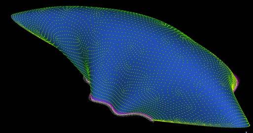
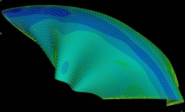
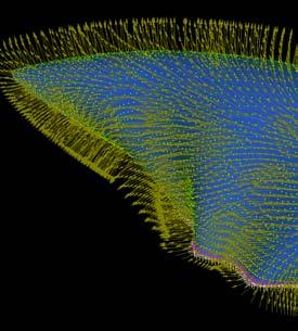
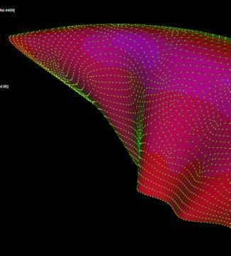
 Meshed shell
Fixed nodes to the ground
Load Case 2
Meshed shell
Fixed nodes to the ground
Load Case 2
Load Case 1 Global Self-weight Load Case 2 Normal W ind Load -0.5Mpa Global Self-weight
Static Analysis Load Case 2 plywood thickness 1.5cm fiber glass +resin 1.0 cm max displacement 42mm Linear Static Analysis Load Case 1 plywood thickness 1.5cm fiber glass +resin 1.0 cm
Linear
fig 5.2.11
fig 5.2.11 Structural Analysis variating the thickness
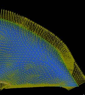
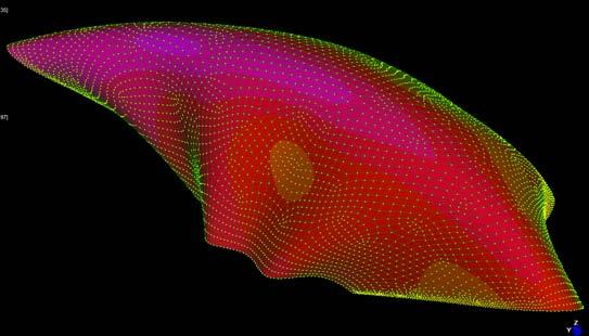
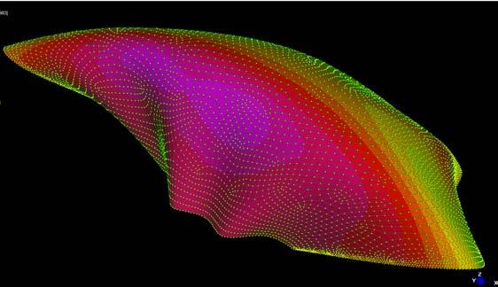
Linear Static Analysis
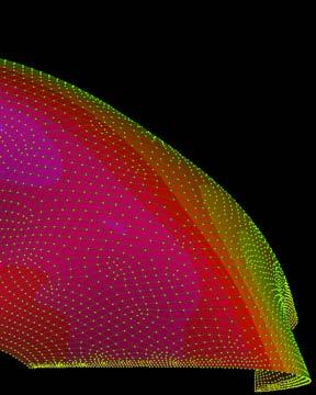
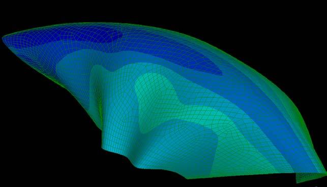
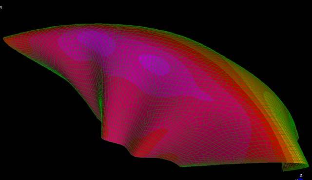
Linear Static Analysis
Load Case 2

plywood
fiber glass
max
thickness 1.5cm
+resin 2.0 cm
displacement 24mm Linear Static Analysis
plywood thickness 1.5cm fiber glass +resin 2.0 cm
Load Case 1
plywood thickness
fiber glass +resin
cm max
Static Analysis
Case 1 plywood thickness 1.5cm fiber glass +resin 3.5 cm
Load Case 2
1.5cm
3.5
displacement 11mm Linear
Load
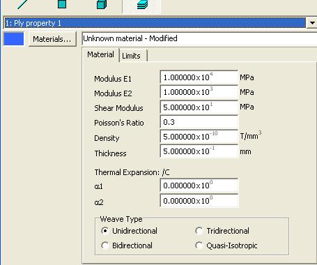
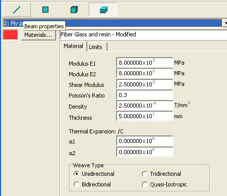
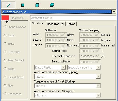
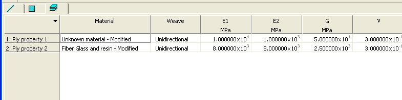
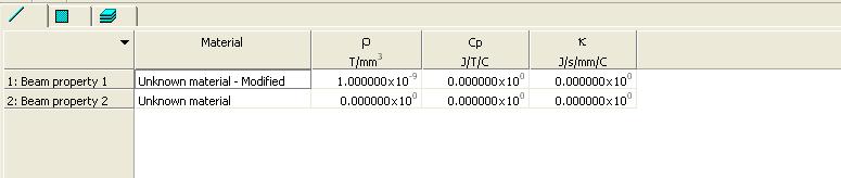
After buckling the plywood sheets on strand on each arch as shown in page 122, all buckled panels are assemble in Rhino and then taken into h where the stitching has to be done carefully joining the nodes at the edges of each panel (red lines on the image). Linear Static Analysis followed by Linear Buckling Analysis is run mesh. fig 5.2.12

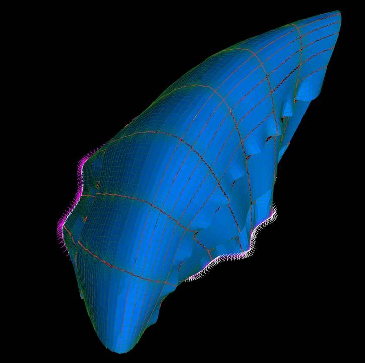
Meshed shell surface, panels stitiched in between them
Fixed boundaries to the ground
Material
Material
Stitching
fig 5.2.12 fig 5.2.13 one veneer 3.5
Properties fig 5.2.13
Properties fig 5.2.14
simulation in Strand7
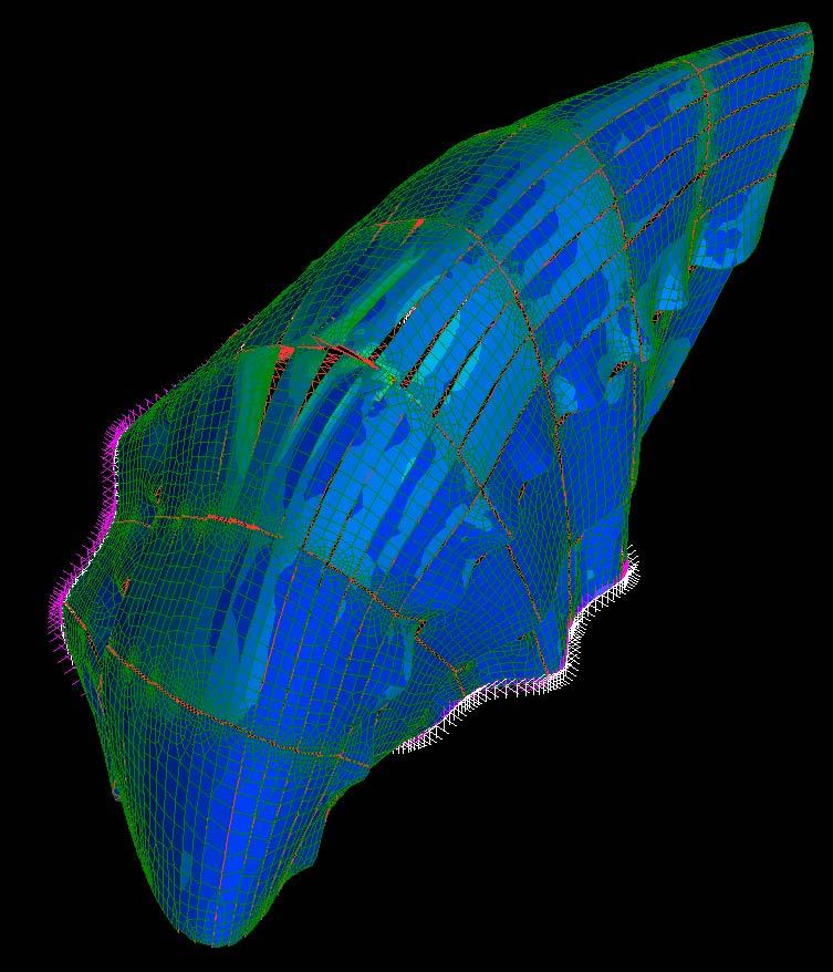
Linear Buckling Analysis Mode 2 1.33985
Panels stitched on the shell plywood thickness 1.5cm fiber glass +resin 3.5cm
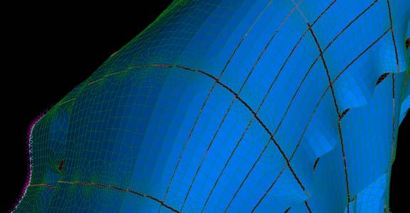
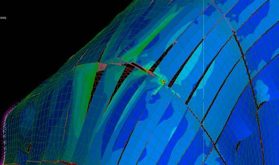
Stitching specifications:
Beam property : Spring Damper
Stiffness : Axial 1.0000X10³ N/mm Lateral 1.0000X10³ N/mm Torsion 1.0000X10³ N.mm/rad
: Spring Mass 0.0000x 100 Thermal Expansion 2.5000x10⁻² Damping Ratio 0.0000 x 100 fig 5.2.14
Viscous Damping
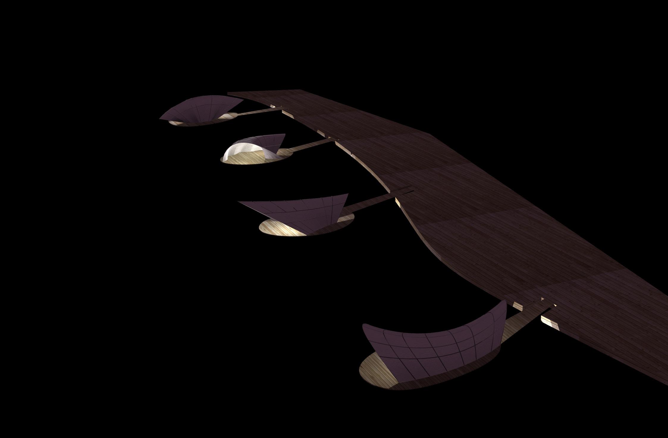
DESIGN
fig
5.2.16
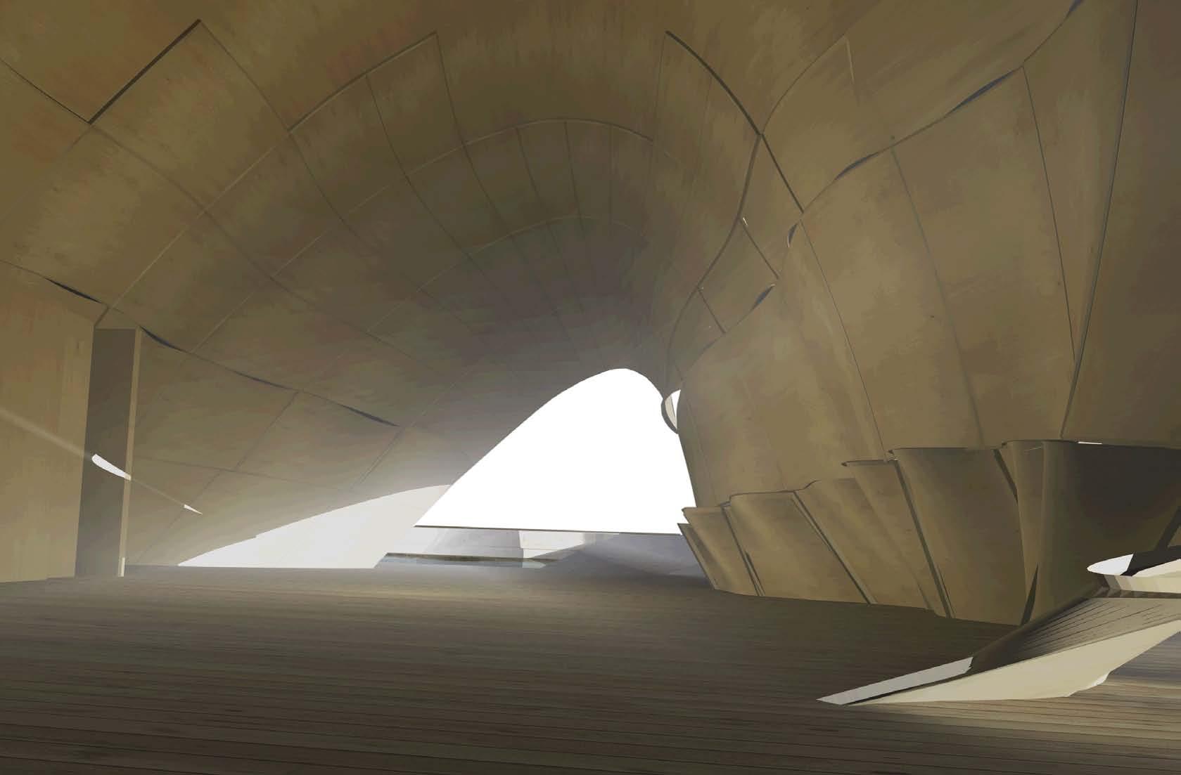
DESIGN
fig 5.2.15 Interior view - plywood side
fig 5.2.16 Aereal view - Boat dock (shells on platforms)
fig 5.2.15
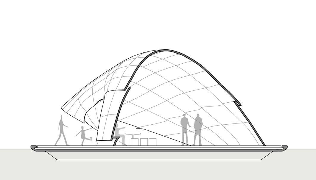
The span: varies from 4.5 to 8.5m
Two cantilevers: 7.6 m and 6.3 m
Height: between 3.3 and 5.2 m.
Surface area: 220m2
Floor surface area: 105m2.
Thickness of plywood 1.5mm GRP 3.5mm
DESIGN 130
Section A fig 5.2.18 Section B fig 5.2.19 Top view
fig 5.2.17
fig 5.2.17
thickness of entire timber composite 5mm
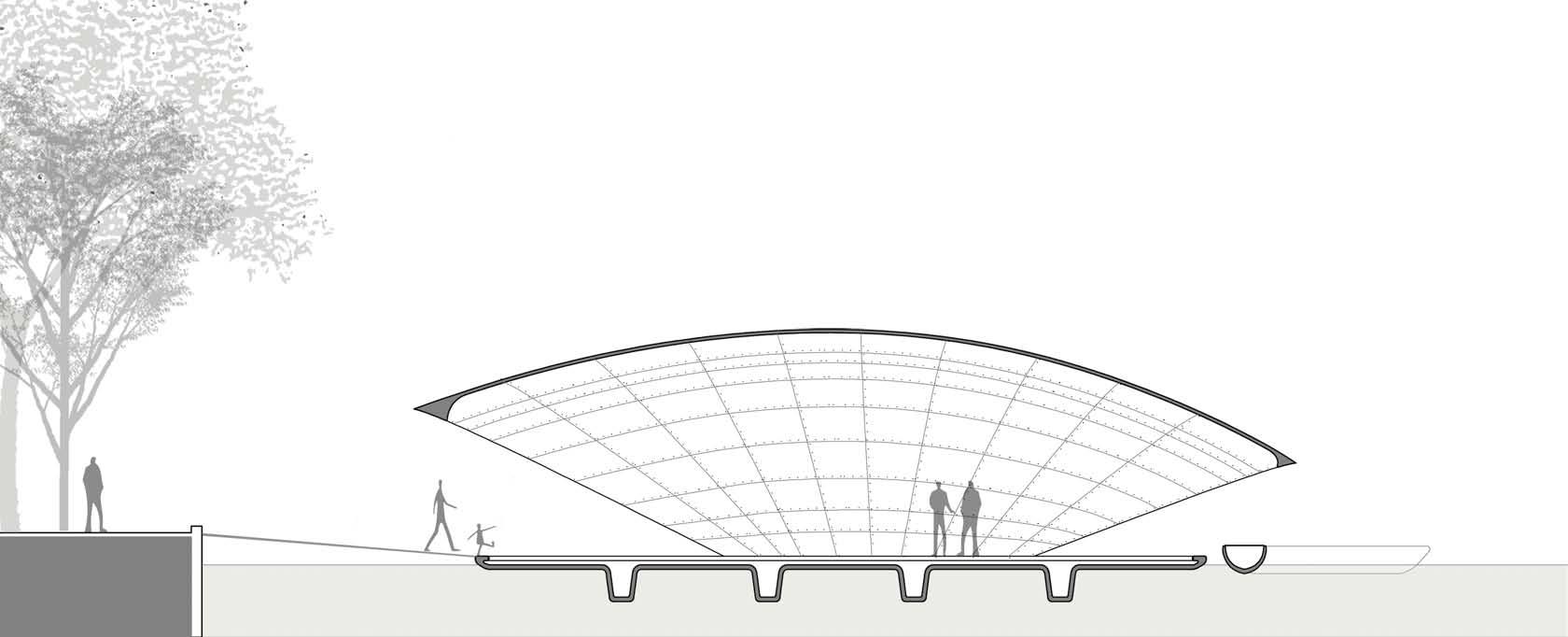
ventilation
local reinforcement at edges platform (above-wood) platform (below-GRP)
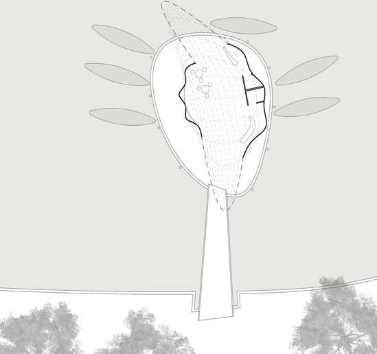
DESIGN
fig 5.2.18
fig 5.2.19
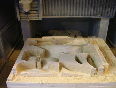
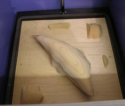
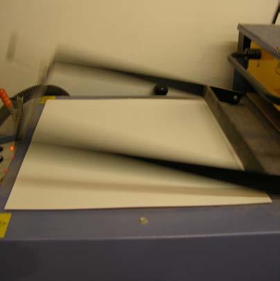
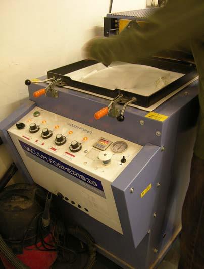
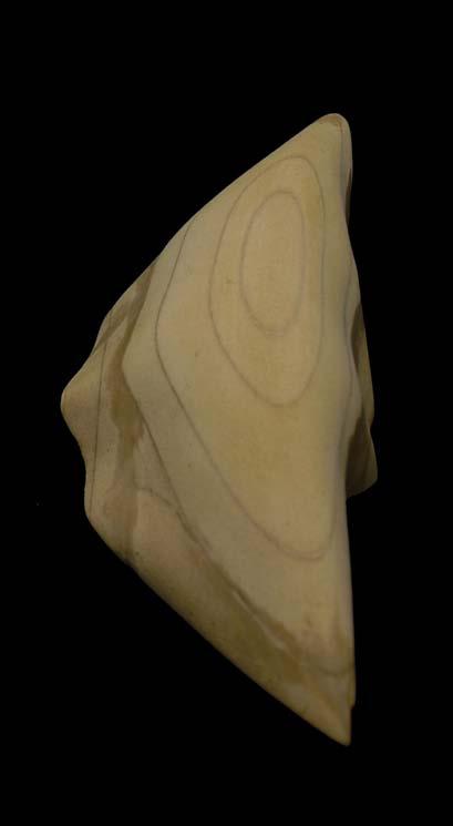
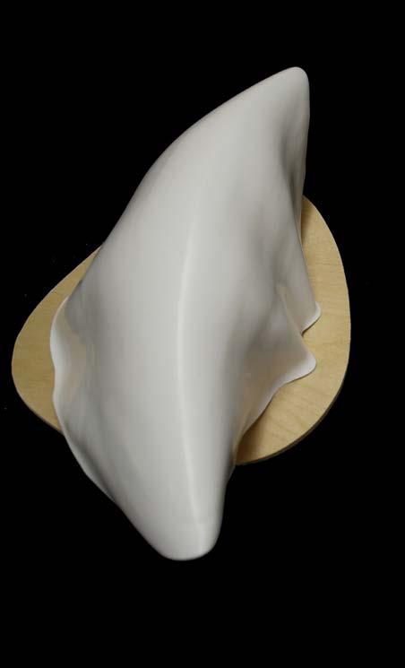

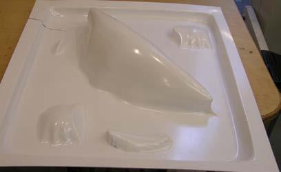
DESIGN 132
fig 5.2.20
A. CNC milled on MDFs of 40cmx50cm
B. CNC molds inside vacuum
C. Polythene plastic
D. Vacuum machine
fig 5.2.20 Brown model = MDF model cut on CNC milling machine
D E C B A
White model = polythene plastic piece vacuumed on the CNC mold
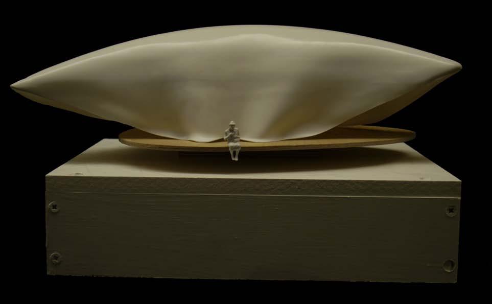
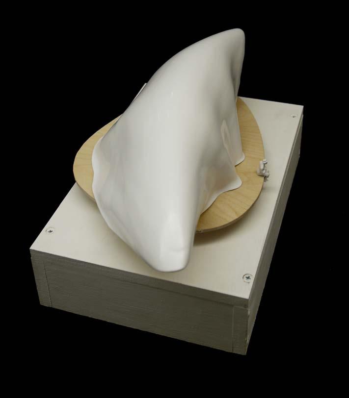

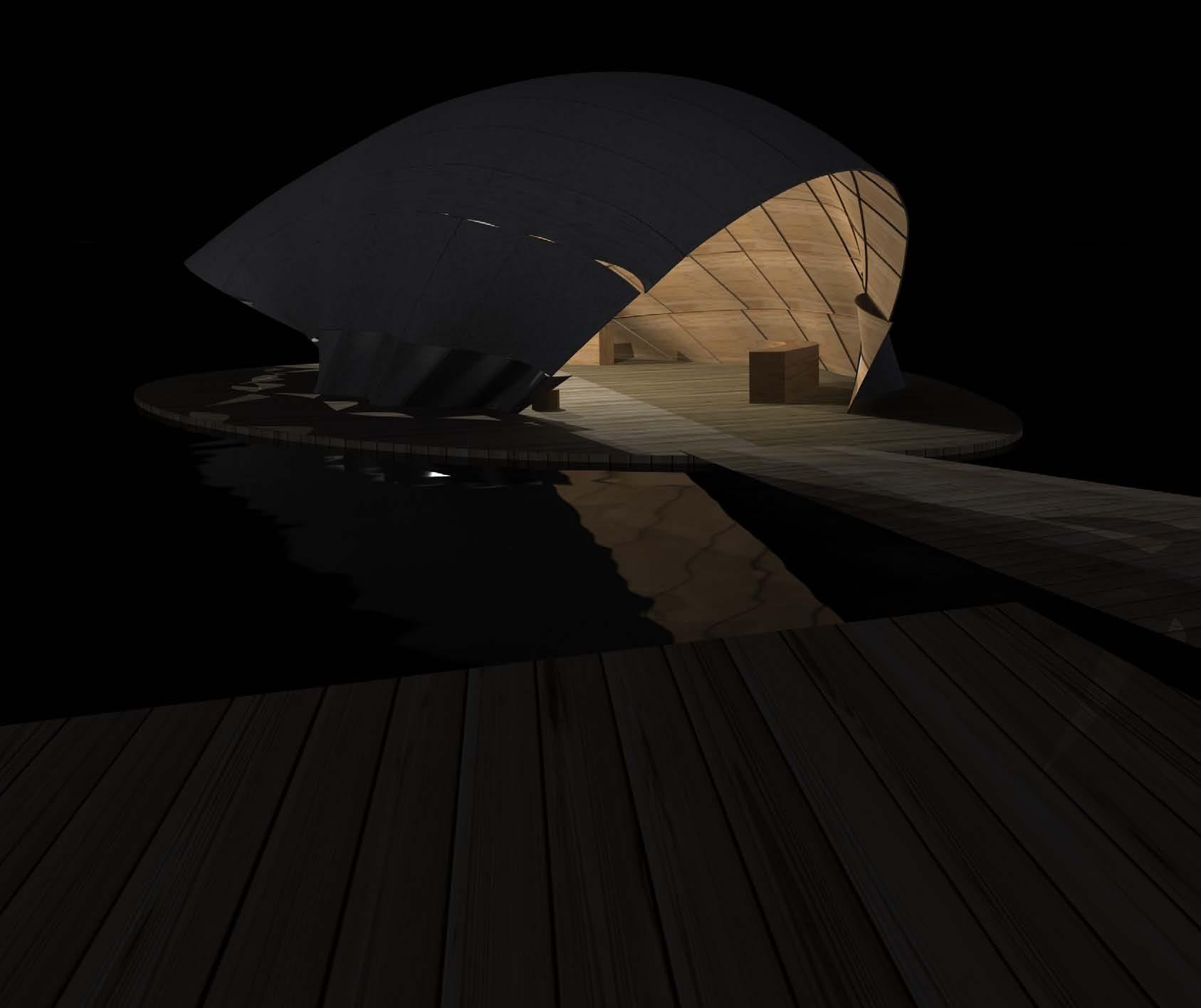

OPTIMIZATION
The proposed design process embeds the main aspects of a traditional architecture design process, which solves form and function and later on solves materiality and fabrication . The interesting part is when all these aspects run through an optimization process and loop into itself to select and generate again possibilities that result in feasible design to production.
JOINTS
Generally, the joints represent a big issue in any architectural design project as in its solution the project can expand or shrink. In this research the stitching strategy works accurate as the assemblies are not working structurally. The thickness of the plywood 1.5mm doesn’t perform in transferring the loads, is the GRP side that works on bearing loads with its own thickness, and the plywood is definitely working structurally only through the geometry that is producing which at the end creates thickness that exponentially helps the structure. This is very similar to a truss that increases the section of a beam without increasing the material and the weight. If the simple stitching procedure could be industrialized large surfaces could be fabricated and the sheets of plywood could be seen as a large fabric with certain complex geometry.
THE SOFTWARE (CAD)
Programs such as Strand7 or Ansys (Finite Element Method) are extremely useful in order to run infinite simulations of structures, but also to simulate material behavior. Nonetheless, in this project as the main goal was related to the link between Computing Aid Manufacturing (CAM )and Computing Aid design (CAD), the physical experiments took an important place on the research. It can be seen that by setting the basic parameters such as the Young modulus, density, fiber directionality and Poisson Ratio… among others, the material behavior can be simulated on the computer. The plywood is a predictable material, and this aspect allows customization on its manipulation. The customization refers to the control of the machine or to its variation on the operation hence, the specific
effects required by the architecture are achievable through the machine. This control is easily achievable with GCODE that can make the connection between the computer and the machines. Nonetheless every material and customization would require big efforts in performing itself, thus if designers keep working in this field, the design could be take more advantages from the machines.
DOUBLE SKIN
The research has shown the potential of having one surface in a composite with two skin sides. Multi functionality can happen within spaces but also within one material. In general cladding surfaces are duplicated to supply the necessities of outside and inside, plus having intermediate structure to support both. The outer layer protects the inner layer while the inner layer produce the space quality and light refraction. Wood is considered a gentle material for spaces, interior or exterior. The fabrication process allows effortlessly the system to switch the reinforcing side, thus, the outer layer can be wood, and the inner GRP. In this case the shells can be located potentially inside other building leaving the wood exposed.
TIMBER COMPOSITES - MATERIAL SYSTEM - NO MOLD
This research triggered small ranges of differentiation that can change significantly the space qualities. Thus, small openings on large surfaces are the result of the material behavior studies and definitely can perform more sensitive architecture. Nonetheless, the richness in the space shouldn’t necessary represent complexity in the fabrication. Certainly, the research has shown one alternative in the fabrication of large structures without mold, an interesting topic for new researches.
CONCLUSIONS 136
CONCLUSIONS
SYSTEM CONSTRAINTS AND ADVANTAGES
If for instance in the shell proposed in chapter 5 for Leticia, the span increases more than 15 meters keeping the same height of approximately 3.5m, the surface area would be incremented from 220m2 to 350 m2, and the thickness will have to be incremented to approximately to 10cm: therefore the weight will reach approximately 5000 kg. (The weight per m2 is calculated to be no more than 15kg per square meter with a thickness of 4cm).
A shell with this specifications wouldn’t be feasible in this specific fabrication system and with the timber composite material. As it was set at the beginning of this research the volume ratio depends on the resin and immediately on the fiber glass that can hold the amount of resin, the weight as a result of all the mentioned parameters is a constraint to the system to expand into larger surfaces, however is also the possibility to move one entire structure without much effort.
FURTHER POSSIBILITIES OF THE MANUFACTURING
The proposed system to create shells without mold has a big potential that could be explored in other materials such as concrete, plaster, earth…
It is also possible that the pre-stressed plywood panels could be a framework for prefabricated concrete pieces, thus, two different faces could be achieved for the same piece. In addition, a good sealing method on the plywood would allow reutilizing them several times, just like when creating scaffolding to build walls.
The potential of mixing different materials will be a constant in future researches, the usage of only natural materials that follow the same logic would be interesting to develop, thus, polyester resin, which at the moment is the more affordable in price but still toxic bounding material instead, could be exchanged by Bio-resin or another bounding material. In addition the fiber glass could be exchanged by natural fibers. In consequence, the new composite could be completely natural and economic . Definitely this is just the beginning of what science and architecture will perform in the next environmental needed days.
CONCLUSIONS 137
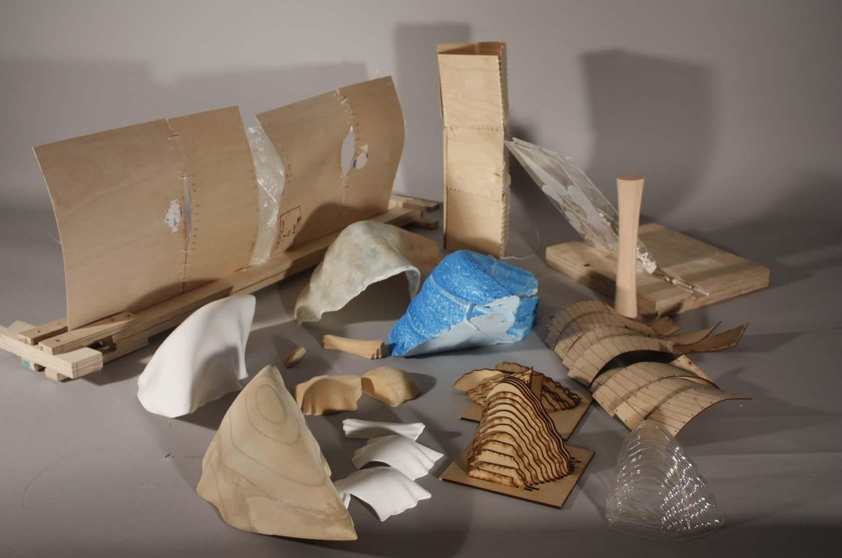
REFERENCES
REFERENCES
BOOKS
W. C. Stevens, M. A, A. M. I. Mech. E., and N Turner. 1948. Solid and Laminated wood bending. London, Forest Products Research Laboratory.
Ann ALderson. 2002. Fibre-reinforced polymer composited in construction. London, CIRIA.
Beukers, Addrian & Van Hinte, Ed, 2005. Flying LightnessPromises for structural elegance. Rotterdam: 010 Publishers.
Fibre composite aircraft-capability and safety. Published by Australian Transport Safety Bureau. ATSB Transport safety investigation Report. Aviation research and Analysis Report -AR-2007-021 Final
Barnett J. R. and Jeronimidis G. Eds. 2003. Wood Quality and its Biological Basis. Oxford: Blackwell CRC Press. ISBN 0-8493-2819-5
Bodig J. and Jayne B. A. 1993. Mechanics of Wood and Wood Composites. Krieger Publ.
Dinwoodie J. M. 2000. Timber: Its Nature and Behaviour. 2nd Edition. London: E&FN Spon.
Harris J. M. 1989. Spiral Grain and Wave Phenomena in Wood Formation. Berlin: Springer (Springer Series in Wood Science).
Rutten. D. 2007. RhinoScript for Rhinoceros 4.0. Robert McNeel & Associates. London.
Pottman, H,Aspel,A, Hofer, M, Kilian,A, Bentley, D, 2007. Architectural Geometry, Bentley Institute Press, Exton.
GR McGhee , 1999. Theoretical Morphology: The Concept and Its Applications (Critical Moments and Perspectives in Earth History and Paleobiology)
D’Arcy Wentworth Thompson and John Tyler Bonner, 2005. Growth and Form. London
Nordenson, Guy. 2008. Seven structural engineers : the Felix Candela lectures, New York
Anderson, Stanford. 2004. Eladio Dieste : innovation in structural art. Princeton Architectural Press
Objectile Fast-wood : a Brouillon Project Patrick Beauce + Bernard CAcheSpringerWienNewYork
ARTICLES
Ramage M.2004. 4.666 The Construction of Building Pottmann, P., Liu, Y., Wallner,J., Bobenko,A., Wang,W . 2007. Geometry of muti-layer freeforms structure for architecture.
Chin-Jen, C. Mechanical behavior of fiberglass reinforced timber joints
H. Hamdan, U. M. K. Anwar, S. Abd. Hamid, S. Mohd. Jani,M. K. Mohamad Omar, W. S. Hashim, P. Mohd. Fauzi & A. Khairul. Development Of Fiberglass Reinforced Veneer Products
Forest Research Institute Malaysia (FRIM), 52109 Kepong, Selangor Darul Ehsan (Project No. 03-03-10SF0034)
REHOLZ® GmbH. 2009. Advantages of using 3D-veneer. Recommendation for lacquering of products made of 3D-veneer. Product information
WEBSITES
http://www.wealddown.co.uk/buildings http://delta7sports.com by mike http://www.isotruss.org by mike http://www.loc.gov/exhibits/Eames/Furniture.html http://www.infinitidesign.it/eng/loop3dwood.php http://www.reholz.de/ http://www.loc.gov/exhibits/eames/furniture.html http://hivemodern.com/pages/products.php?cid=156 http://www.fighterfactory.com/restoration/dehavillandmosquito-aircraft.php
ENDNOTES 1. 3. 2
fig. 1.3.1 Fibers in tension and Compression.
Source: W. C. Stevens, M. A, A. M. I. Mech. E., and N Turner. 1948.
fig. 1.3.2 The steaming box.
fig. 1.3.3 Clamping the piece into a metal curved piece
fig. 1.3.4 Clamping the piece into a metal curved piece.
Source: http://images.google.co.uk/
fig. 1.3.5 Spade handle bending machine
fig. 1.3.6 Bending machine for making split type spade handles
fig. 1.3.7 Lever arm bending machine operated by a rack and pinion mechanism
fig. 1.3.8 Air-inflated tubular hose and low voltage stripheating used in the production of laminated bends
Pressure moulding bag
fig. 1.3.9 Pressure moulding bag
fig. 1.3.10 Hydraulic press and steam heated cauls
fig. 1.3.11 Laminated bending by the autoclave process (rubber bag removed)
fig. 1.3.12 A commercial machine employed for production of laminated bends by the continuous strip method.
Source: Stevens, M. A, A. M. I. Mech. E., and N Turner. 1948.
fig. 1.3.13 Fuselage shell half construction
fig. 1.3.14 Fuselage shell half construction
fig. 1.3.15 Fuselage shell half construction
fig. 1.3.16 Fuselage with steel bands
fig. 1.3.17 Browning door, fitting catches
fig. 1.3.18 Browning doors Port open
fig. 1.3.19 Fuselage on assembly jig 2
fig. 1.3.20 Joining shell halves
fig. 1.3.21 Rear bulkhead with fittings.jpg
fig. 1.3.22 Nose browning doors off KA114.jpg
fig. 1.3.23 Port mould fitting interskin members.jpg
fig. 1.3.24 Fuse to wing front on 12 07.jpg
Source: http://www.fighterfactory.com/restoration/ dehavilland-mosquito-aircraft.php
fig. 1.4.1 Pultrusion method
fig. 1.4.2 Filament Winding
fig. 1.4.3 Compression and transfer molding SMC and DMC
fig. 1.4.4 Matched-die molding and autoclaving
fig. 1.4.5 Autoclaving
fig. 1.4.6 Injection molding of granules of material
fig. 1.4.7 Continuous sheet production
fig. 1.4.8 Vacuum assisted resin molding (VARTM)
Resin transfer molding (RTM)
fig. 1.4.9 Open mold process: hand-up and spray-up
Source: Ann ALderson.2002.
fig. 1.4.10 Autoclave
fig. 1.4.11 Autoclave
fig. 1.4.12 Autoclave
Source: Emtech presentation
fig. 1.4.13 The 6-axis computer controlled gantry lays down the strands of carbon fiber
fig. 1.4.14 A technician then moves over the sail applying heat
fig. 1.4.15 Operator checks for mistakes
Source: Emtech presentation
fig. 1.4.16 Fiber manufacturing specifications (from Lightness and Flyingness)
Source: Beukers, Addrian & Van Hinte, Ed, 2005.
fig. 2.1.2 Top view
fig. 2.1.3 Transversal section
fig. 2.1.4 Geometry abstraction
fig. 2.1.5 MDF ribs
fig. 2.1.6 Wood beams placed in between MDF
fig. 2.1.7 Plywood strips
fig. 2.1.8 Temporary assembly of 4 pieces
fig. 2.1.9 Pod placement through the ceiling
fig. 2.1.10 Metallic mezzanine structure
fig. 2.1.11 GRP pod at the courtyard Victoria Housebury
Source: Alsop architects
fig. 2.2.2 Definition of the pod geometry
fig. 2.2.3 TImber ribs as the frame
fig. 2.2.4 Staple of LVL to the ribs
fig. 2.2.5 Interior of Peckam Library
fig. 2.2.6 Interior of Peckam Library
Source: http://www.alsoparchitects.com
REFERENCES
chapter
fig. 2.5.1
Source: http://www.loc.gov/exhibits/Eames/Furniture. html
fig. 2.5.2
Source: “Mythos Hellrau” /Exhibition catalogue , Deutsche Werkstatten, 2002
fig. 2.5.3
Source “Bent Plky, Ngo, Pefeiffer, Princeton architectural, press, new york, 2003)
fig. 2.4.1 Sliced veneer
fig. 2.4.2 Glue lines on the back
fig. 2.4.4 The individual sticks slide a little according to each other
Source: REHOLZ® GmbH. 2009
fig. 2.6.1 Wood strips nailed to formwork to position the bricks
fig. 2.6.2 Small self-carrying vaults
fig. 2.6.3 Timber trusses for the formwork
fig. 2.6.4 Pre-stressing the looped steel rods with a manual jack
fig. 2.6.5 Looped pre-stressing steel, absorbs negative bending moments
fig. 2.6.6 S-shape on Gaussian vaults
fig. 2.6.7 Corrugation effect on a sheet paper
fig. 2.6.8
fig. 2.6.9 Cadyl Horizontal Silo
Source: Nordenson, Guy. 2008.
fig. 2.6.10 Lonja de la Seda de Valencia, 15th century
fig. 2.6.11 The method of timbrel vault
Source: http://images.google.co.uk/ imgres?imgurl=http://krisdedecker.typepad.com/photos
fig. 2.6.12 Oyster Bar in Grand Central Terminal fig. 2.6.13 Adhesion of several layers of overlap ping tiles
Source: http://www.lowtechmagazine.com/ images/2008/11/10/guastavino_2.gif
fig. 3.1.0 Close capture of the overlapping Photograph taken by Sue Bar
fig. 3.1.3 Fin section
fig. 3.1.4 Variation in the openings by Grasshopper definition
fig. 3.1.5 CFD (Computational Fluid Dynamics) analysis
Production from the Emtech Class
Fig. 3.1.6 Canopy at AA terrace Photograph taken by Sue Bar
fig. 3.1.16 Close capture of voids differentiation Photograph taken by Sue Bar
fig. 3.2.1.1, fig. 3.2.1.7 Experiments carried out with Kun Kun Chan fig. 3.2.2.3 Buckling setup. http://wikipedia.com fig. 3.2.2.4 Elasticity - Plasticity regions. http:// wikipedia.com
REFERENCES
APPENDIX
This workshop was possible thanks to the generous support of the Maeda corporation. Twisting concrete Maeda workshop is the exploration of minimal surfaces made in a thin concrete layer working in compression with the implementation of chopped fiber-glass working in tension.
Prof Shin egashira organized this intensive workshop, where the constrains of working with minimal surfaces of fabric and plaster were explored. These, once being stretched into bended pipe frames and solidified, would become a static mould for glass fibre-reinforced concrete structures.
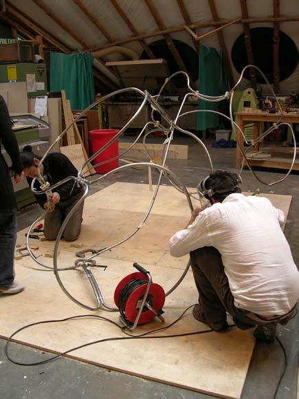
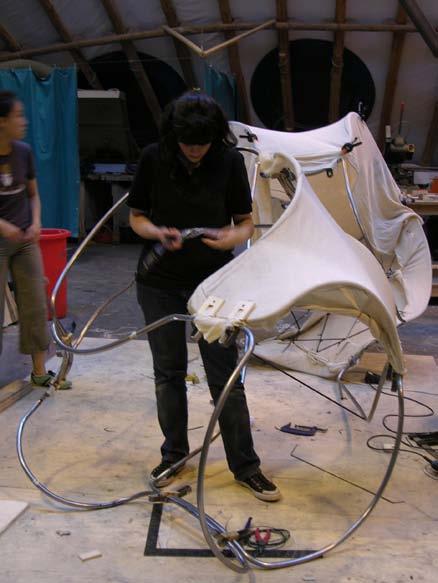
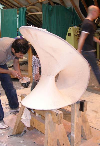
APPENDIX 144
Pipe as a mould
Tense the fabric to the pipes (minimal surface). Application of plaster on side 1 of the fabric.
A TWISTING CONCRETE MAEDA WORKSHOP
fig A.1 The process in different
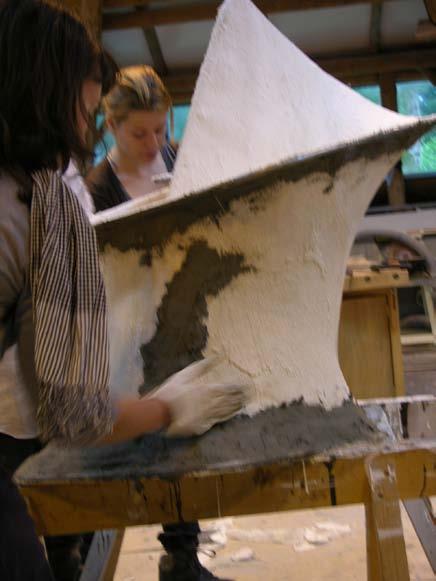
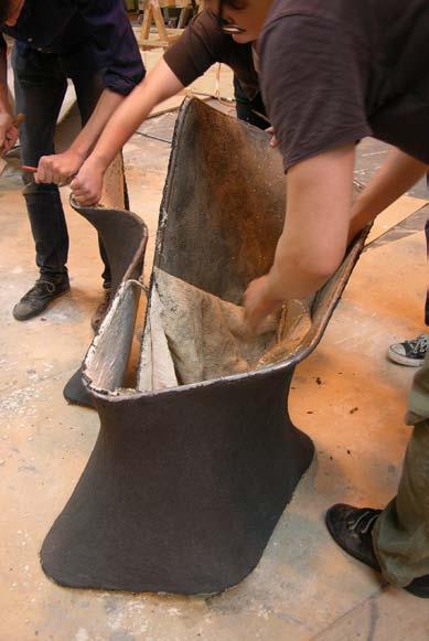
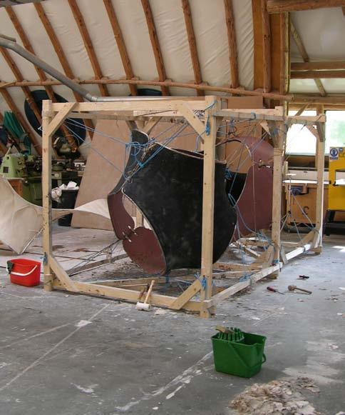
APPENDIX 145
Fabric as a mould - Twisting concrete Maeda Workshop(Shin E.)
The pipes as a mould to hold the shape is kept on the final product
Application of the concrete on the side 2 of the fabric. Remove the fabric.
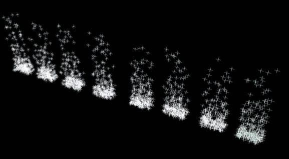
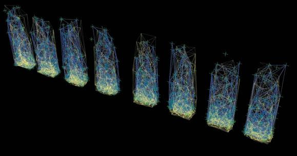
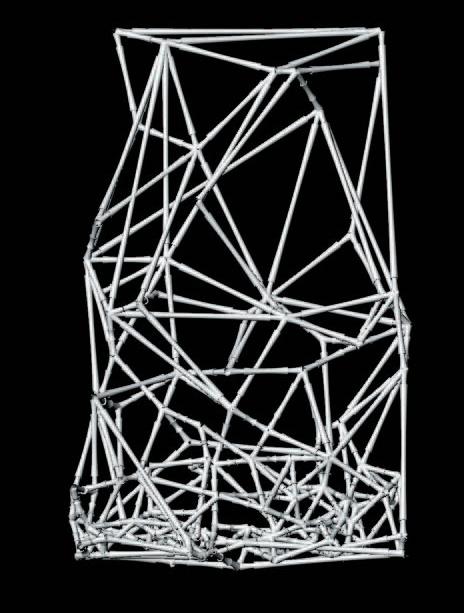
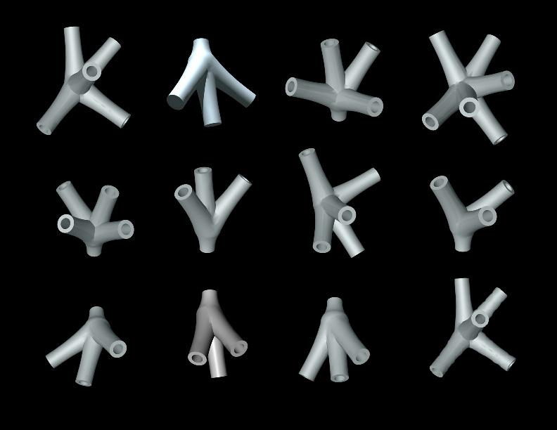
B LOGICAL DESIGN WORKSHOP
The Architectural Association, School of ArchitectureLondon, UK
Tutors: Chikara Inamura & Shajay Bhooshan
In collaboration with Luz Jadal Leon, Fernando Z. and Ricardo Sosa
Objective:
To design a canopy using computational design production tools.
Description:
Dlab is an integration of software-based environments to prototyped production. The brief for the unit was to learn basic Maya 2009 Particles system and Catia with basic Script on it to perform fabrication methods for joints on the structure that was proposed by each team. The technology available at AA was part of the constraints on the fabrication (laser cutting, CNC-milling, 3D printing).
In collaboration with Jadal Leon, Fernando Z., Ricardo Sosa
The initial concept was developed in MAYA by using particles and Mel Scripting. The particles were dropped in a box and their positions where controlled with gravity, density air, and bouncing values. As a result there was a denser agglomeration near the bottom. Using Mel Scripting we connected the nearest particles with straight lines. The lines were later taken into CATIA as INPUT to develop a joint and connection system with scripts previously designed. As a result a parametric constraint model able to interconnect multiple models of points was developed. To conclude , the surfaces of the box that habited the particles was subdivided using a Voronoid RHinoScript; using the particles that touched surfaces to generated the geometry.
Scripting in Katia
Since the project explores the non-standardization of the joints, the scripting in Catia was the most essential part. With the scripts developed the intelligent joint could adapt to multiple situations. The production of 2 or 200 joints would require no extra effort and modifications could be made automatically.
fig B.1 Maya MelScript of particles
fig B.2 Stiffness in the structure
fig B.3 None-standard joints
fig B.4 Stl joint- CNC milling bone
fig B.5 Stl model
fig B.6 Assembly process
fig B.7 Canopy in cantiliver
- Summer DLAB
fig B.1
fig B.2
fig B.3
The joint
Every particle corresponds to a joint and every line corresponds to a “bone”. The joint is a sphere located in every point with a cylinder going along the line that connects to another point. The joints can be reached by multiple lines.
The bones are loft surfaces of different diameters circles placed on the center and at 8cm from the tips, one bone per line.
The models
The joint was created on the 3d printing machine in order to make it compact and hollowed. The STL (Stereolythography) file was done in Rhino. The bones were done in the CNC milling machine, in high density foam; the 3d model was sliced into two parts, thus the cylindrical form could be cut by the drill and then the two half parts could be join and create one compact piece.
For the entire structure another STL model was done, which had a minimum of 3 mm thickness on the connections.

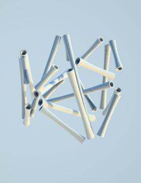
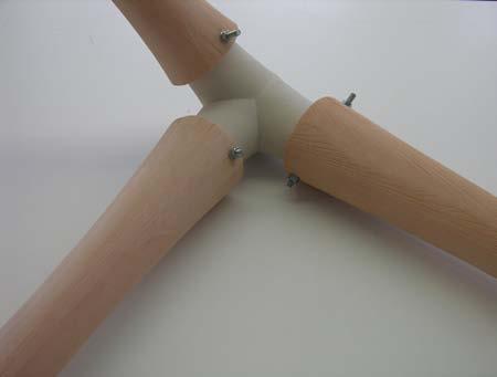
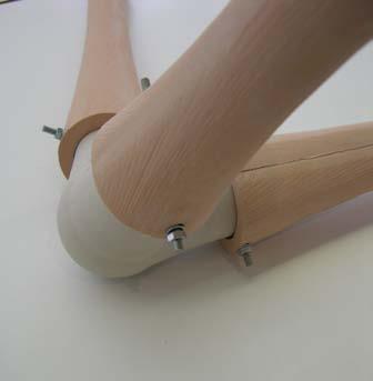
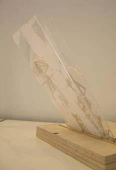

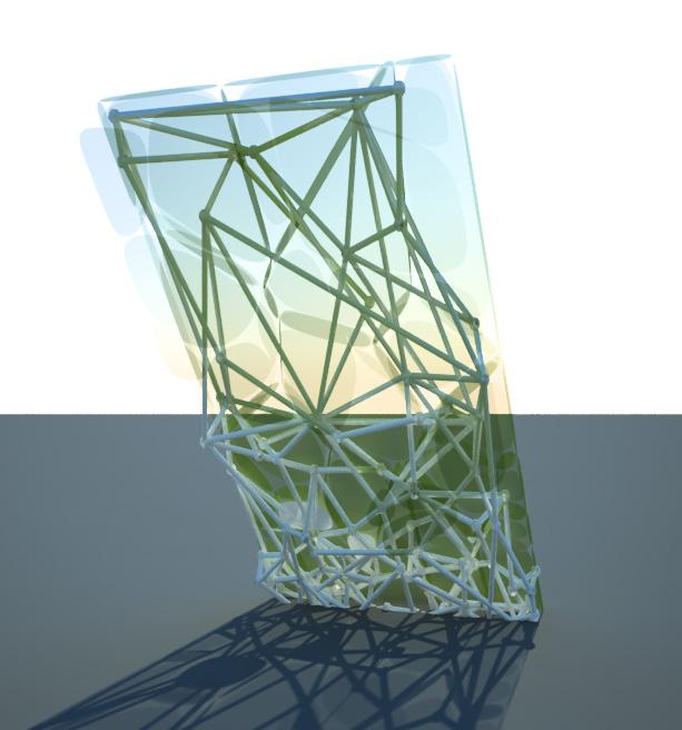
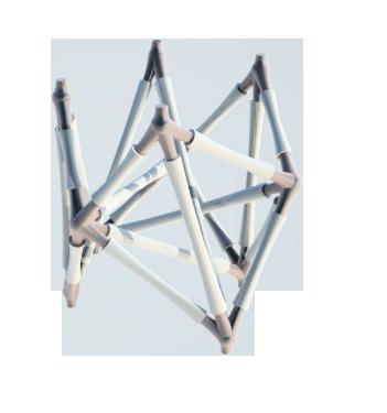
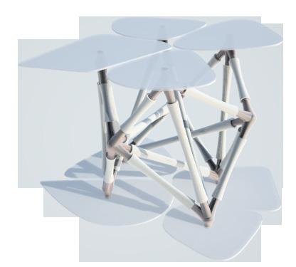
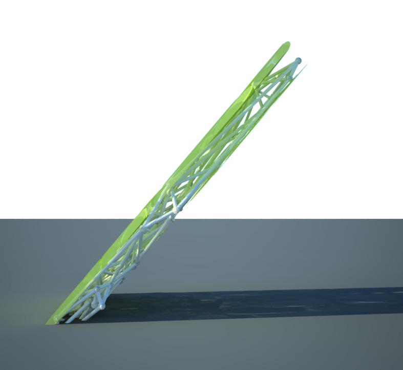
APPENDIX
fig B.7
fig B.6
fig B.5
fig B.4
‘ recursively subdivide surface based on curvature
‘ author: robert stuart-smith | 2008 | www.kokkugia.com
Call Main()
Sub Main()
Dim strSrf
‘get surface strSrf = Rhino.GetObject(“pick a surface”,8)
Rhino.EnableRedraw False
‘call function to subdivide PanelizeSurface strSrf, 10,5
Rhino.EnableRedraw True
End Sub
Function PanelizeSurface(strSrf, intSubD,intGen) ‘declare variables
Dim arrCrvs, arrCrvPts, arrPara
Dim i,j,n, arrCrvsU, arrCrvsV, arrSrfs()
‘conditional statement to stop subdividing infinitely ‘(as we will Call the Function recursively) If intGen > 0 Then
‘resize arrays for storing curves in both directions of surface; u & v directions
ReDim arrCrvsU(intSubD)
ReDim arrCrvsV(intSubD)
‘extract edge curves arrCrvs = Rhino.DuplicateEdgeCurves(strSrf)
‘do for 2 curves one in both directions of surface:
For i = 0 To 1
‘divide curveby number of points (using variable subD) arrCrvPts = Rhino.DivideCurve(arrCrvs(i), intSubD, False,True)
For j = 0 To UBound(arrCrvPts)
‘extract isocurves using points in the array above arrPara = Rhino.SurfaceClosestPoint(strSrf, arrCrvPts(j))
‘use case statement to seperate isocurves into their direction (u or v) and store in u or v array
Select Case i
Case 0
ExtractIsoCurve(strSrf, arrPara,1) Case 1
ExtractIsoCurve(strSrf, arrPara, 0)
End Select Next Next
‘loop through curves to create surfaces n = 0
For i = 0 To UBound(arrCrvsU) -1
For j = 0 To UBound(arrCrvsV) -1
arrCrvsU(j) = Rhino.
arrCrvsV(j) = Rhino.
C GRASSHOPPER DEFINITIONS
ReDim Preserve arrSrf(n) arrSrf(n) = Rhino.AddEdgeSrf(Array(arrCrvsU(i)(0),arrCrvsV(j) (0), arrCrvsU(i+1)(0),arrCrvsV(j+1)(0))) n = n + 1
Next
Next
‘delete the original surface Rhino.DeleteObject strSrf
Dim arrPt, arrCurvature,dblMCurvature ‘loop through created panels
For i = 0 To UBound(arrSrf)
‘get surface centre point arrPt = Rhino.SurfaceAreaCentroid(arrSrf(i))
‘get surface parameter at the ctr point arrPara = Rhino.SurfaceClosestPoint(arrSrf(i),arrPt(0))
‘get the surface curvature at the surface parameter position
arrCurvature = Rhino.SurfaceCurvature(arrSrf(i),arrPara)
‘size up and simplify curvature result for legibility dblMCurvature = Abs(arrCurvature(7)*1000)
‘colour surface based on mean curvature
Rhino.ObjectColor arrSrf(i), RGB(dblMCurvature*2, 0, dblMCurvature)
‘based on curvature choose to subdivide further or not - ie. recursively call this function
Option Explicit
‘RhinoScript Workshop ‘University of Arts & Design ‘Chelsea, London, 2008
‘Session 2: construct developable normal surface along curve
Call DevelopableSurface()
Sub DevelopableSurface()
‘input: curve and length of ruling
Dim strCurveID
Dim dblScale strCurveID = Rhino.GetObject(“Pick base curve for ruling”,4,False,True)
If IsNull(strCurveID) Then Exit Sub dblScale = Rhino.GetReal(“Length of ruling: “,10)
If IsNull(dblScale) Then Exit Sub
Call GenerateRuling(strCurveID,dblScale)
End Sub
Function GenerateRuling (ByVal CurveID, ByVal Scale)
‘--- initialization of array of lines
Dim arrDomain arrDomain = Rhino.CurveDomain(CurveID)
Dim maxSize maxSize = CInt((arrDomain(1)-arrDomain(0))*10)
Dim allLines() ‘--- variables
Dim arrData,arrTangent,arrNormal,arrBinormal
Dim arrStart,arrEnd1,arrEnd2
Dim newLine
Dim i
Dim numberLine
‘--- calculate lines of ruling numberLine=0
For i = arrDomain(0) To arrDomain(1) Step 0.1
If i > arrDomain(0) Then i = i-0.001 arrData = Rhino.CurveCurvature(CurveID,i) If Not IsNull(arrData) Then arrTangent = arrData(1) arrNormal = Rhino.VectorSubtract(arrData(2),arrData(0)) arrBinormal = Rhino.VectorCrossProduct(arrTangent,arrNormal) arrBinormal = Rhino.VectorUnitize(arrBinormal) arrBinormal = Rhino.VectorScale(arrBinormal,Scale) arrStart = arrData(0) arrEnd1 = Rhino.PointAdd(arrStart,arrBinormal) arrBinormal = Rhino.VectorScale(arrBinormal,-1) arrEnd2 = Rhino.PointAdd(arrStart,arrBinormal) newLine = Rhino.AddLine(arrEnd1,arrEnd2)
If Not IsNull(newLine) Then ReDim Preserve allLines(numberLine) allLines(numberLine) = newLine numberLine = numberLine+1
End If End If Next
‘--- generate loft and group ruling If numberLine > 1 Then Rhino.AddLoftSrf(allLines)
End If End Function page 72
GenerateRuling = Rhino.AddObjectsToGroup(allLines,Rhino.AddGroup())
APPENDIX 148 page 84
/ SCRIPTS
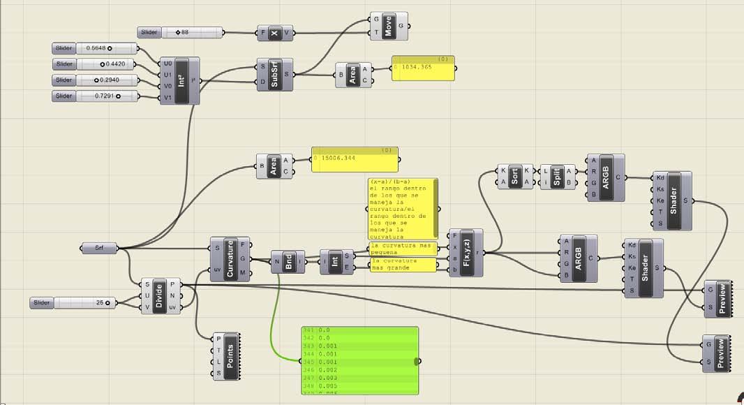
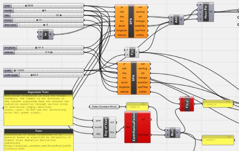
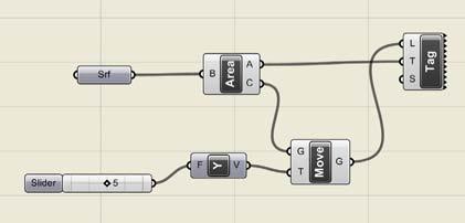
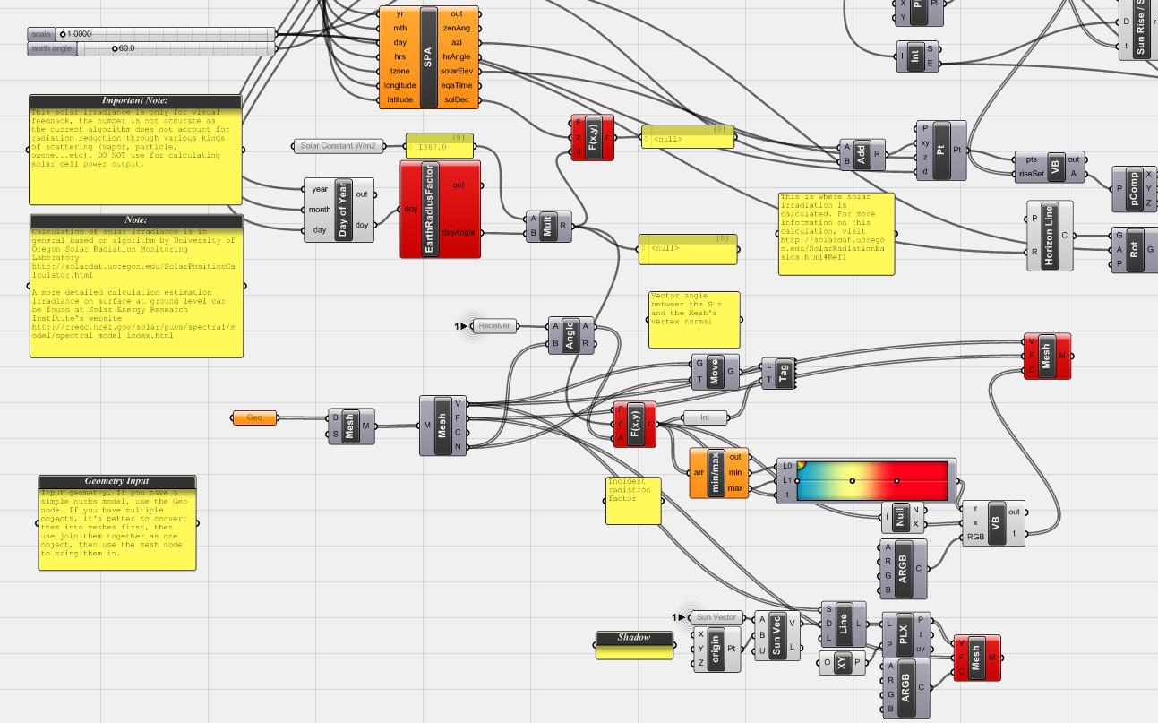
APPENDIX 149
page 112 from http// tedngai.net.experiments.htlm
page 82 by Jheny Nieto
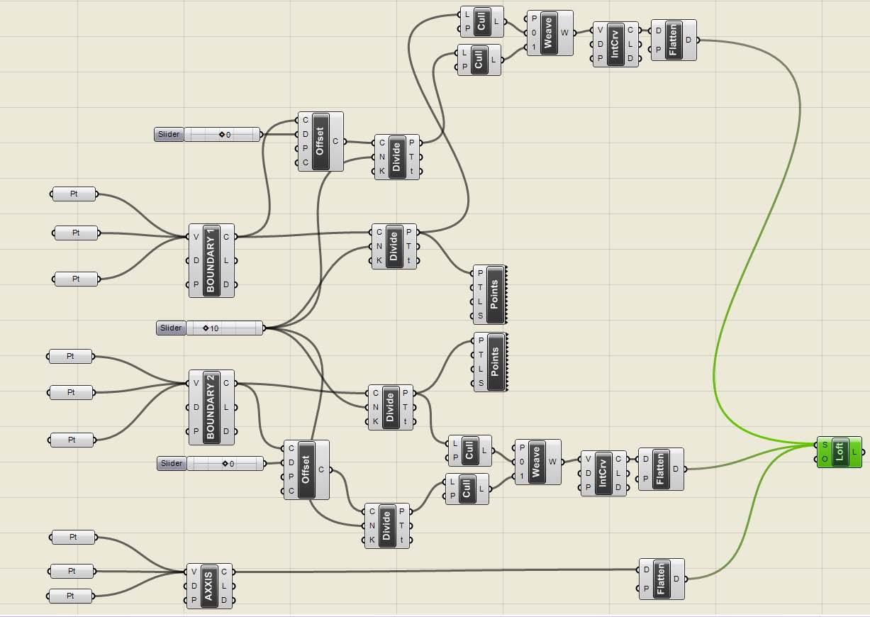
page 120
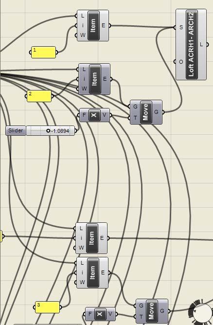
page 100
grasshopper definitions by Jheny Nieto
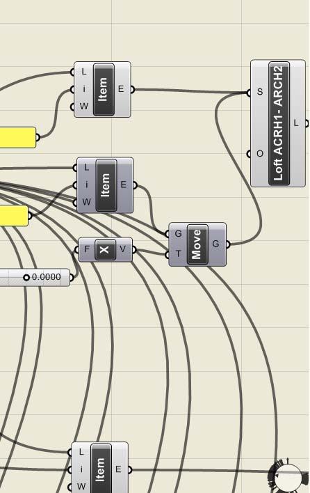
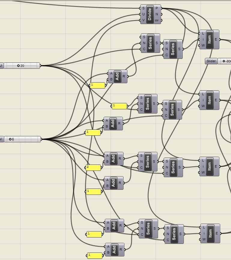
page 121
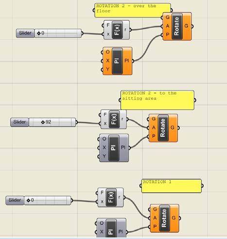
rotation of the surface along different axis

Boundary 1
Boundary 2 Division page 72
APPENDIX
shell
corrugation
All
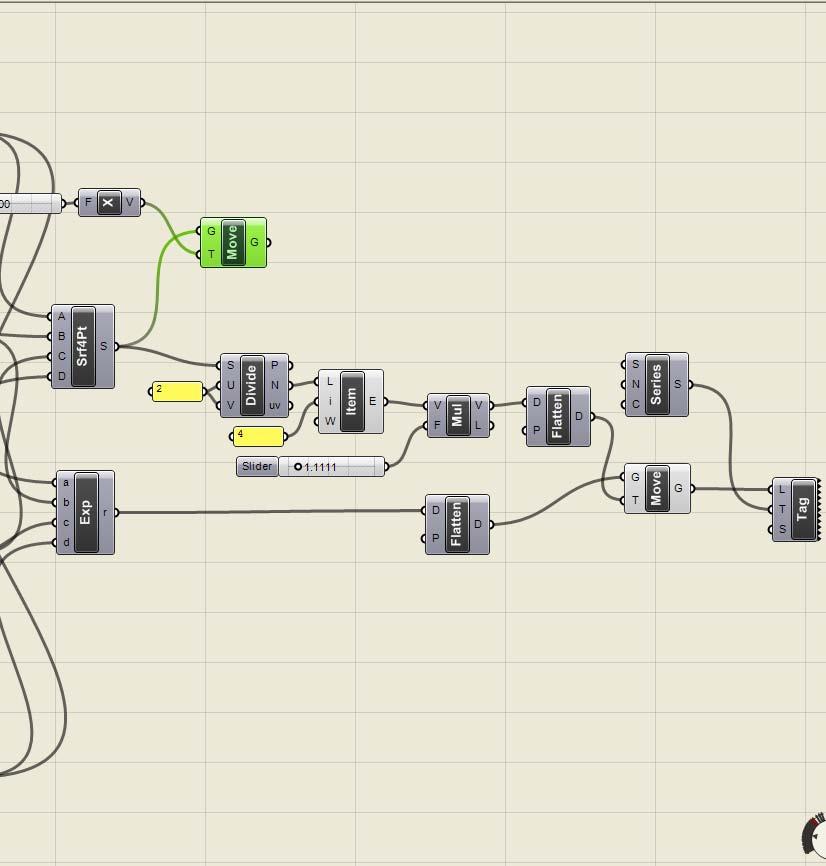
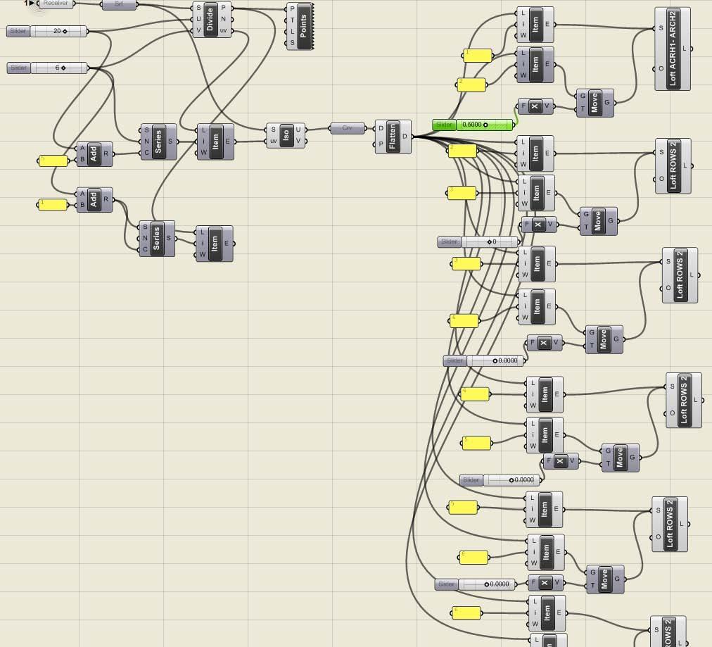
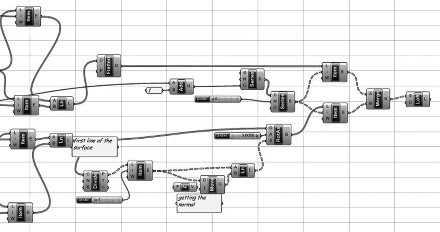
control of the voids along the surface
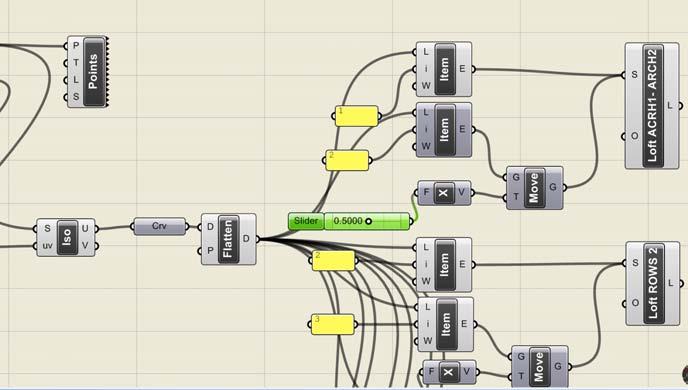
close-up of the voids control
APPENDIX 151
shell in flat panels
page 120
Torsion
