3.6 Model Specification

technologies, extent of usage of adopted technologies, perception of processing and fabrication technologies and constraints limiting adoption of GAPs. The ratings of perception were: Agree =3, Not sure =2 and Disagree =1. Objective IV was realized through the use of before and after analysis while objectives V was achieved through the use of Logit model.

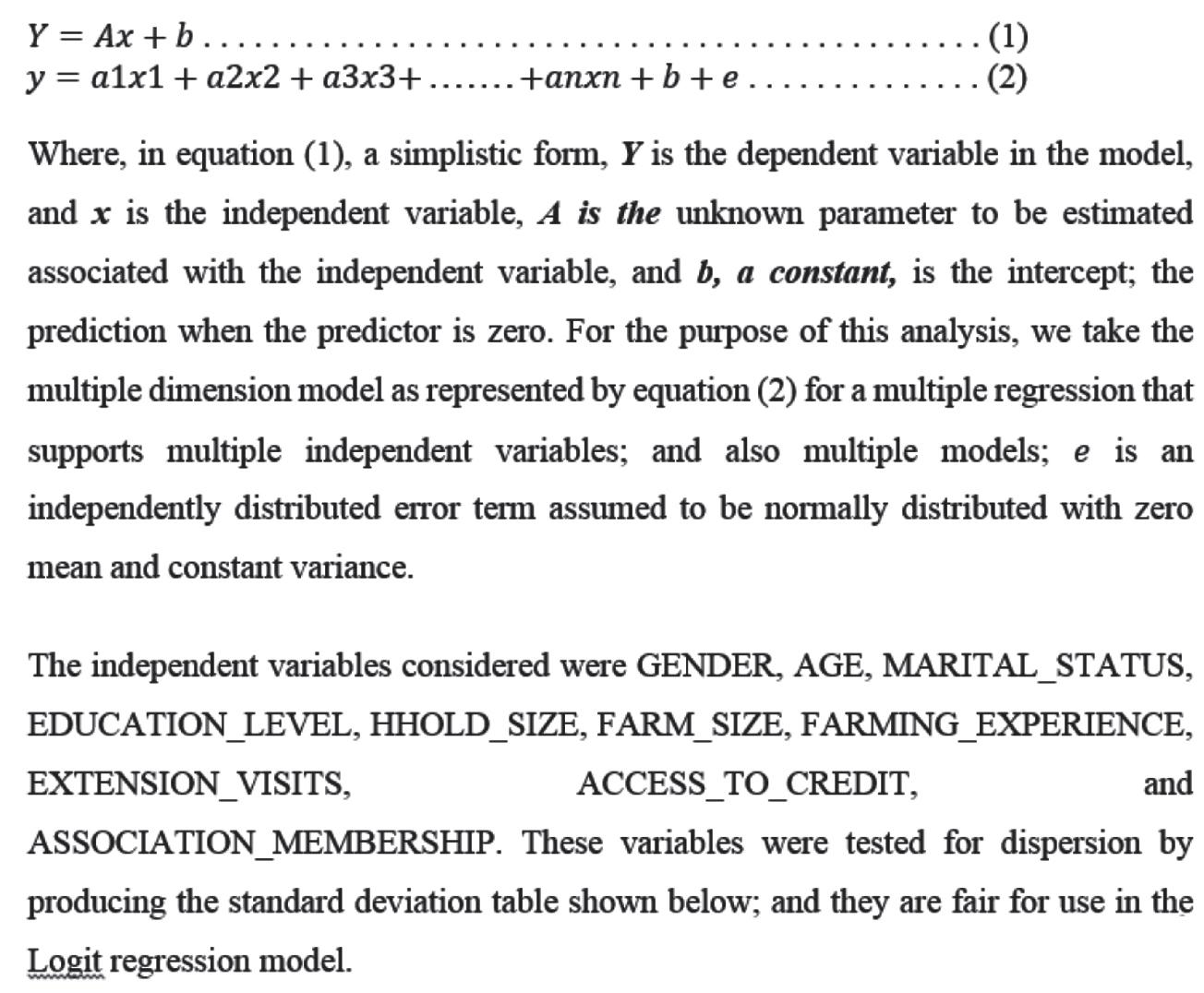
3.6 Model Specification Logit model was used to ascertain the factors influencing the adoption of good agronomic practices (GAP) among ATASP-1 farmers. The model is specified as follows

Standard Deviation

Statistics

e n d e r G E A G S i z e F a r m M a r i t a l S t a t u s E d u c a t i o n e h o l d H o u s S i z e i o n E x t e n s i s i t V t o s c c e s A r e d i t C o c i a t i o n s s A M e m b e r s h i p

N Valid 96 96 96 96 96 96 96 96 96

Missing 0 0 0 0 0 0 0 0 0

0.307 0.435 5.08714 0.375 1.615 7.758 0.175 0.503 0.144Std. Deviation

Logistic Regression Analysis Logit and Probit analysis produce similar results. In this case, Logistic Regression Analysis, also called Logit model, was used to ascertain the factors influencing the adoption of Good Agronomic Practices amongst ATASP-1 farmers (Objective ix). The adoption or non-adoption response is captured with a binary variable, coded 0 for not adopted; and 1 for adopted. In this analysis, GAP_ADOPTED is the dependent variable. Gender and Marital Status variables are dichotomous, Age has been recoded into 3 groups (coded 1, 2, 3). Education is coded 1 to 6; while Household Size and Farm Size was treated as continuous.

. . . . . . . . . . . . . . (2)

The Binary Logisitic regression analysis which is accepted as robust against multivariate normality and better suitable for small sample size data than Probit model; and has similar output with Probit was used for the regression analysis. This study has a total sample of less than 100; precisely 96 for farmers. The coefficients of the model equation are as shown in the output table below. The dependent nominal variable is GAP_ADOTION (Not Adopted = 1; Adopted =2); and the covariates are GENDER, AGE, EDUCATION, HOUSEHOLD_SIZE, FARM_SIZE, EXTENSION_VISITS, ACESS_TO_CREDIT, and ASSOCIATN_MBR

GENDER B S.E. Wald df Sig. 0.982 0.962 1.04 1 0.308

AGE

-2.18 0.812 7.201 1 0.007 EDUCATION -0.877 0.252 12.105 1 0.001 HHOLD _ SIZE 0.08 0.049 2.636 1 0.104 FARM _ SIZE -0.056 0.051 1.231 1 0.267 ENTENTN _ VISITED 0.199 1.73 0.013 1 0.908 CREDIT _ ACCESS 1.226 0.584 4.409 1 0.036 ASSOCIATN _ MBR 1.235 1.659 0.554 1 0.457 Constant 2.136 4.758 0.202 1 0.654

2The first observation made on the output was the pseudo R , the -2Log likelihood improvement, the minimization criteria used in SPSS. It was observed that the

2 2Nagelkerke's R is 0.583 which indicates that the model is good. Cox and Snell's R in the

thnth root (with this data set, 96 of the -2Log likelihood improvement). This can be interpreted as a 41.2% probability that the event of the covariates influencing the dependent variable (GAP Adoption), is explained by the Logit model. The classification result is at 80.2% which is good. The output table above shows the variables in the model equation and the coefficients. It generates the regression function:

. . . . . . . (3) This table also shows the test of significance for each of the coefficients in the Logistic

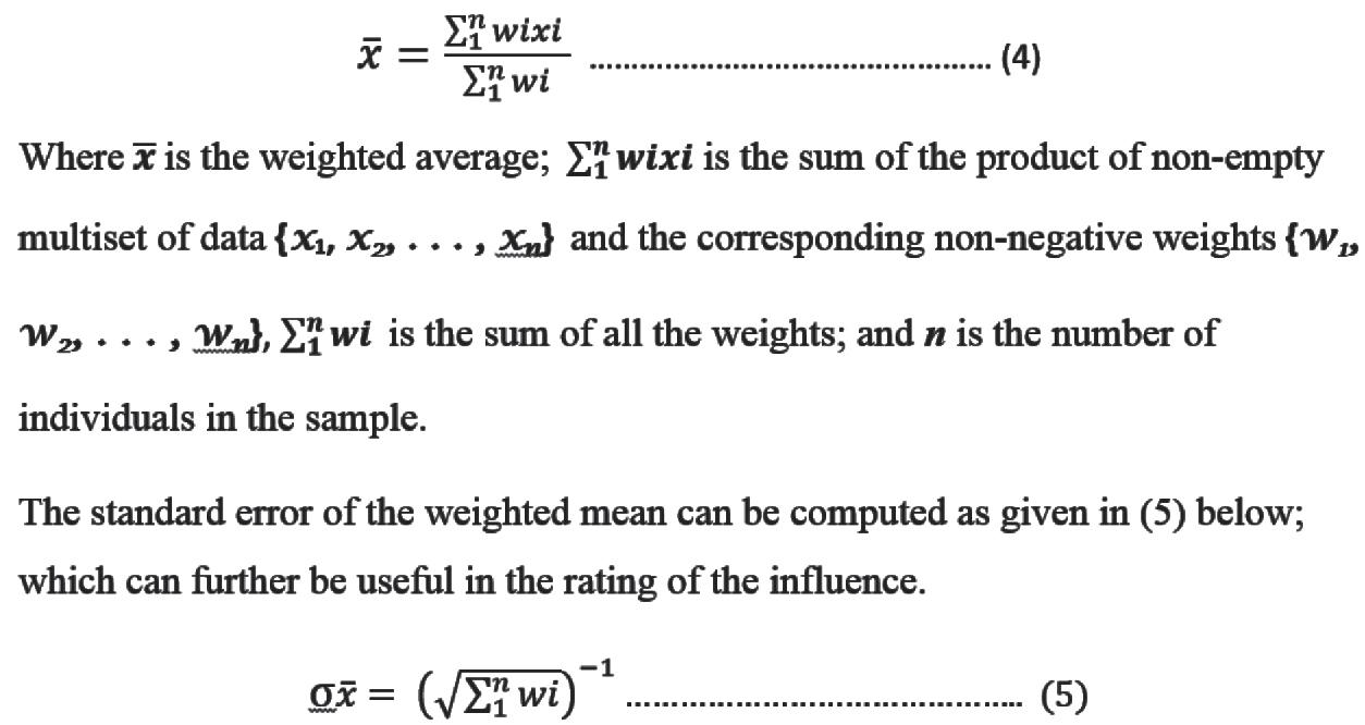
2 regression model. Wald statistics (basically t or chi-square distributed with df = 1) has been used here instead of t-test because of the sample size for which the t-values may not be valid. As observed, AGE and EDUCATION are the most significant respectively at 7.2 and 12.1; while CREDT_ACCESS, HHOLD_SIZE, FARM_SIZE and GENDER are respectively at 4.4, 2.6, 1.2 and 1.04. However, as can be observed from the regression function (3) above, the other variables each exercises some influence, positive or negative at varying magnitudes as the dependent variable scales in step of 1. All these are non-zero influence in the model; which counts. Weighted Average: Weighted average was also used in the analysis where found useful in obtaining a more accurate look at the set of data than the normal average; weighted average computation was used where doing so could improve the interpretation of how the mean of a subset in a dataset influenced others in the entire set. The general formula for calculating the weighted average is given in (4) below.