References

We now want to analyze whether the bubble we have just described can be obtained in equilibrium. Tirole (1985) derives two conditions under which rational bubbles may emerge in equilibrium: (i) arbitrage and (ii) rationality.

Equation (3.1) is the arbitrage condition. It means that investors will not purchase the bubble unless the return on the bubble is higher (or equal) than the alternative investment option. In our model, the alternative to investing in the bubble is the storage technology, which has a return equal to π. Equation (3.2) is the rationality condition. It means that the price of the bubble is constrained by the amount of money in the economy. In the most optimistic case, in which all young agents choose to put their endowment in the bubble, the total amount of money that they would put together would be eLt. Equation (3.2) means that the price of the bubble cannot be higher than this quantity. In other words, we want to avoid situations in which Bt > eLt. How could the price of the piece of paper be higher than eLt? As we said, if all young agents purchase the bubble, the price is eLt. The price of the asset could be above eLt if investors from another model (or Planet) were purchasing the asset. This is why we label this inequality, the rationality condition. In other words, we cannot justify the emergence of a bubble with an asset price appreciation that requires a demand higher than the total amount of money in the economy.

It is convenient to rewrite Eqs. (3.1) and (3.2) using per capita terms. Denoting bt ≡ Bt /Lt, these conditions become,

Equation (3.3) describes the evolution of the bubble for any given initial bubble. For example, if we start with an initial bubble equal to b0 < e, the size of the bubble next period will be b1 = 1+π 1+n b0. As the reader can see, the bubble will be growing over time if π > n, and it will shrink over time if π < n. Which is the equilibrium size of the bubble? Before answering this question, let us introduce the notion of steady-state equilibrium. We say that b∗ is the steady-state equilibrium if bt+1 = bt = b∗ . Intuitively, if the size of the bubble is b∗, the bubble will no longer move

Bt+1 /Bt ≥ 1 + π , (3.1)

eLt ≥ Bt . (3.2)

bt+1 = 1+π

1+n

bt ifbt ≤ e 1+π 1+n , ∞ bt ifbt = e (3.3)

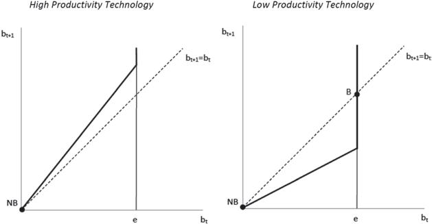
Fig. 3.1 A model of rational bubbles. Notes The lines are described in the main text. The left-hand side represents the asset price bubble dynamics when the storage technology is very productive (i.e., π > n). The right-hand side represents the case in which the storage technology has a low productivity (i.e., π < n)

and it will remain at this point forever. We are now ready to solve this dynamic problem heuristically with the help of Fig. 3.1.

Figure 3.1 represents the steady-state equilibrium for the two relevant cases: (i) high productivity storage technology (π > n) and (ii) low productivity storage technology (π < n). Let us start with the high productivity storage technology case (left-hand side fgure). The dotted line is the 45-degree line and represents the equation bt+1 = bt. The bold straight line is Eq. (3.3). Note that the slope of this line is higher than one because π > n. Finally, the vertical line represents the equation bt = e. Graphically, the steady-state equilibrium is the intersection between the 45-degree line and the bold straight line. In the intersection point, the bubble would stay there forever. Note that the only intersection is at zero. That is, the only steady-state equilibrium is bNB = 0. The economic intuition behind this result is the following. The bubble needs to grow, at least, at the same rate as the productivity of the storage technology to be an interesting investment option for the investor. Given that the storage technology is very productive, it means that the bubble needs to growth at a rate higher than n! Since young agents are rational, they understand that this cannot happen because it would require that, at some point, the demand for the asset were higher than the total endowment of the

economy. In other words, at some point, the economy would be hitting the rationality constraint (bt ≤ e). Therefore, when the storage technology is very productive, there can be no bubbles in equilibrium.

We now consider the case in which the storage technology has a low productivity (i.e., π <n). This case is depicted in the right-hand side of Fig. 3.1. By comparing the two fgures, we see that we have the same lines as before but the bold straight line, which has a different slope. Indeed, the slope of the bold straight line is now lower than one. Interestingly, this line intersects with the 45-degree line in two points. Thus, we have two steady-state equilibria: (i) fundamental equilibrium (bNB = 0) and (ii) bubble equilibrium (bB = e). Which equilibrium is better for the economy? In the fundamental equilibrium, young agents decide not to purchase the piece of paper and they put all their savings into the storage technology. In this case, their old-age consumption will be cNB = (1 + π )e. In contrast, in the bubble equilibrium, the agents put all their endowment into the bubble. In this case, the consumption is driven by the growth of the bubble, which is (1+n). Therefore, consumption in the bubbly equilibrium is cB = (1 + n)e. Note that consumption is higher with the bubble (i.e., cB > cNB because n> π).

To summarize, in this model, if the storage technology is very productive, bubbles cannot arise in equilibrium. In contrast, bubbles may emerge in the economy when the storage technology has low productivity. In addition, in this case, the economy is better off with the bubble than without the bubble. Our interpretation is that the bubble emerges because young agents need a better store of value than the storage technology. In other words, there exists a shortage of assets that bubbles solve by adding assets into the economy.

The reader may have noticed a determinacy problem with this model. When the storage technology has low productivity, there are two possible equilibria. How do we know which equilibrium will be played? There is a large literature in game theory that analyzes this multiplicity problem. For the purpose of this book, we just assume that there exists a device that helps agents to coordinate into one equilibrium (bubble or no bubble). In particular, we consider the following sunspot equilibrium. Imagine that young agents look at the sky before deciding whether to put their endowment into the storage technology or to purchase the piece of paper. We assume that if they see a sunny sky, they purchase the piece of paper. In contrast, if they see a cloudy sky, they put all their endowment in the storage technology. Note that this device is enough to