4.3 An Application: The US Housing Bubble

in (steady-state) equilibrium (Eq. 3.8). If we apply this condition to a fnancially developed economy, Eq. (3.8) becomes

Is this condition satisfed if the country is fnancially developed? The answer depends on the depreciation rate of houses. If the depreciation rate is small, the supply of assets will be high and condition (4.9) will not be satisfed. In contrast, if the depreciation rate is very large, the supply of assets will be small and condition (4.9) will be satisfed. As we have seen in the previous chapter, rational bubbles may emerge in equilibrium when the supply of assets is small. In other words, if we have a high δ, the model is like the standard Samuelson model we discussed above.

From now on, we assume that the depreciation rate is small. To be precise, we assume that δ < δ∗, where δ∗ is implicitly defned by aU (1) = dU (δ∗ , 1). As we have discussed, this assumption implies that there is no shortage of assets in the fnancially developed country. In other words, rational bubbles cannot emerge in the fnancially developed country if it remains in autarky.

We are now ready to analyze the effect of letting the fnancially developed country trade with the fnancially underdeveloped country. In the absence of rational bubbles, the free trade equilibrium can be described by the following capital market clearing condition.

The left-hand side of Eq. (4.10) is the world demand of assets in the economy (i.e., the sum of the demand of assets in country U, AU, and the demand of assets in country C, AC). Analogously, the right-hand side of the equation is the world supply of assets. There exists a unique equilibrium interest rate that clears the world capital market.4 In other words, given this interest rate, the world supply of assets equals the world demand of assets.

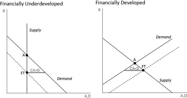
Figure 4.2 represents the capital market of the fnancially underdeveloped economy (left-hand side) and the capital market of the fnancially

B = AU − DU = a U (1) − dU (δ , 1) > 0. (4.9)

AU + AC = DU + DC . (4.10)

4 It can be shown that the fundamental (or non-bubble) equilibrium is unique under mild conditions. See Basco (2014) for the exact condition. Basically, it can be shown that the supply of assets (D) monotonically decreases with the interest rate. Similarly, the demand of assets (A) increases with the interest rate provided that the index of the quality of fnancial institutions of country C, Ɵ, is low enough.

Fig. 4.2 Globalization and housing bubbles. Notes Bond market for a fnancially underdeveloped country (left-hand side) and a fnancially developed country (right-hand side). Point A represents the autarky equilibrium. Point FT represents the trade equilibrium. CA is the current account of the country. Equations discussed in the text

developed economy (right-hand side). Let us frst review the autarky equilibrium in both countries. The autarky equilibrium (without bubbles) is when the domestic supply of assets equals the domestic demand of assets (represented by point A in both fgures). Note that, for the fnancially underdeveloped economy, point A is not the only autarky equilibrium. As we discussed in Chapter 3, rational bubbles could potentially emerge in autarky because there is a shortage of assets when R = 1. Graphically, we would have the same multiple equilibria as the ones represented in Fig. 3.2. In contrast, if we look at the right-hand side of Fig. 4.2, we can see that the only autarky equilibrium in the fnancially developed economy is point A. That is, rational bubbles cannot emerge in this country in autarky. The reason is that we have assumed that the depreciation rate is small enough so that there is no shortage of assets in equilibrium. Graphically, given the small depreciation rate, the supply of assets is larger than the demand of assets when R = 1 (the horizontal axis in Fig. 4.2).

The free trade equilibrium is represented in point FT of Fig. 4.2. Note that at this interest rate, the total supply of assets is equal to the total demand of assets. In other words, given this interest rate, the world current account is zero (i.e., CAU + CAC = 0). Which is the direction of capital fows? To answer this question, we just need to compute the current account in each country at the equilibrium interest rate. Remember that the current account is defned as the difference between the national demand and national supply of assets (i.e., CAi = Ai −Di). Note that for the fnancially developed economy, at the equilibrium interest rate, the supply of domestic assets is higher than the domestic demand (i.e., AU < DU). This implies that the current account of the fnancially developed economy is negative. In other words, the fnancially developed economy receives capital infows. This can be seen in the dotted line, which represents the total demand of assets (the domestic demand plus the extra demand coming from the fnancially underdeveloped economy). By defnition, we obtain the opposite result for the fnancially underdeveloped economy. At the equilibrium interest rate, the domestic demand of assets is higher than the domestic supply of assets (i.e., AC > DC). Thus, the fnancially underdeveloped economy runs a current account surplus.

The intuition for this trade equilibrium is the following. The middle-aged agents of the fnancially underdeveloped economy want to save to consume when they will be old, but their country does not generate enough assets to match this demand. Indeed, the only way that middle-aged agents have to save is to lend their money to young agents. However, since their fnancial institutions are not very well developed, the amount of collateralized debt that their country is able to generate is too low. Therefore, when the fnancially underdeveloped economy can trade with the fnancially developed economy, middle-aged agents of the fnancially underdeveloped country are no longer constrained by their domestic fnancial institutions but they will purchase assets originated in the fnancially developed economy.

To better understand the implications of the model, let us label the fnancially developed economy United States and the fnancially underdeveloped economy China. It is reasonable to assume that fnancial institutions are more developed in the United States than in China. The model predicts that if China opens up to trade with the United States, the United States will run a current account defcit and China a current account surplus. This is what actually happened to the current account of

the United States and China. From the IMF World Economic Outlook Database, we see that in 2000, the current account (over GDP) was 1.7% in China and −3.9% in the United States. By 2006, these numbers were 8.4% for China and −5.8% for the United States. To have a better sense of the magnitude of these changes, we compare the current account of both countries in US dollars. The difference in the current account between China and the United States increased from 423,883 billion in 2000 to 1,037,896 billion in 2006. This large increase in the difference between the current account of (mostly) China and the United States was labeled as “global imbalances” (a term coined by Bernanke 2005). The economic intuition behind this model is basically the same as the savings glut hypothesis of Bernanke. When China opened up to trade, the world demand for assets increased and capital fowed towards the US, which satisfed this demand of assets. This resulted in a decline in the global interest rates and created an increasing current account defcit in the US. Caballero et al. (2008) develop a similar model (without housing) to explain how shocks that reduce the aggregate supply of assets will generate a permanent current account defcit in the region with “better” assets.

Once we have understood the trade equilibrium without bubbles, we want to analyze whether rational bubbles may emerge in this trade equilibrium. Remember that if the fnancially developed economy remains in autarky, rational bubbles cannot arise. Does this conclusion change when it opens up to trade with a fnancially underdeveloped economy? To answer this question, we need to apply the condition for the existence of bubbles to the free trade case. It is straightforward to check that Eq. (4.9) becomes,

B = AWorld (1) − DWorld (1)> 0, (4.11)

where AWorld (1) = aU (1) + aC θ C

, 1 and DWorld (1) = dU (δ , 1) + dC θ C

5 . Equation (4.11) means that rational bubbles can emerge in the free trade equilibrium if there is a world shortage of assets when R = 1. Remember that we need the shortage of assets at R = 1 because the rational bubble can only grow at the rate of the population rate, which we have assumed to be zero.

5 In our setup, the depreciation rate, δ, would also affect the demand of assets of the fnancially constrained agents, aC, but we ignore this effect for simplicity (see Basco 2014 for more details).

Mathematically, we can fnd a threshold of the level of fnancial institutions below which bubbles can emerge in equilibrium. In particular, rational bubbles can appear when θ C <θ ∗∗, where θ ∗∗ is implicitly defned by aU (1) + aC (θ ∗∗ , 1) = dU (δ , 1) + dC (θ ∗∗). That is, bubbles can emerge when the index of the quality of fnancial institutions in the fnancially underdeveloped economy is low. Note that the location of the bubble is not determined in the model. This is the same indeterminacy problem we discussed above regarding the asset where the bubble is attached to. That is, in our model, the bubble could equally emerge in the fnancially developed and the fnancially underdeveloped economy. However, we assume that if the bubble can emerge in the fnancially developed economy, it will emerge in this economy. One rationalization of this assumption is that bubbles in fnancially developed economies are perceived as safer for investors. In any event, our model implies that when the fnancially developed economy opens up to trade, it can experience rational bubble episodes. It is important to emphasize that rational bubbles could not emerge in this country in autarky.

Intuitively, the fnancially underdeveloped economy has a need for extra assets (AC > DC). If this extra demand for assets is not compensated for an extra supply of assets in the fnancially developed economy (DU > AU), there will be a shortage of assets at the world level. Remember that once there is a shortage of assets, rational bubbles can emerge in equilibrium. If we look at the case represented in Fig. 4.2, the fnancially developed economy was able to generate more assets in the trade equilibrium without bubbles (DU,FT > DU,A) as a response to the increase in the demand of assets. Notice that, in this case, this additional supply was enough to avoid a shortage of assets. However, if the extra demand of assets was very large, the fnancially developed economy would not be able to generate enough assets and there will be a shortage of assets. Graphically, at some point, the dotted line on the right-hand side of Fig. 4.2 (the total demand of assets in the fnancially developed economy) would cross the supply of assets below one. In this case, note that the total demand of assets would be higher than the supply of assets at R = 1 (the horizontal axis). In other words, there would be a bubble equilibrium in which the total supply of assets (including the bubble) is equal to the demand of assets.

After understating the case for two countries, let us analyze the effect of an increase in globalization. To perform this exercise, we consider that

the world economy consists of one fnancially developed country (country U) and a mass one of fnancially underdeveloped countries indexed by i. We assume that these fnancially underdeveloped economies are identical (i.e., θ i = θ C for all i) except for the fact that only a fraction τ of these countries can trade with the fnancially developed country. We interpret τ as an index of fnancial globalization. That is, as τ increases, more fnancially underdeveloped economies become part of the international capital market.

We can now study how the increase in fnancial globalization affects the likelihood of having rational bubbles in the fnancially developed economy. As an aside, note that rational bubbles can always emerge in the countries that are fnancial underdeveloped and do not participate in the international capital market (this was the case we discussed in Chapter 3 and it is summarized in Fig. 3.2). In any event, the condition for the emergence of rational bubbles in the fnancially developed economy becomes,

Note that this condition depends on the level of fnancial globalization (τ). When the fnancially developed economy does not trade with fnancially underdeveloped economies, τ = 0, it is as if the country were in autarky. In this case, Eq. (4.12) becomes Eq. (4.9). On the other extreme, if all fnancially underdeveloped economies participate in the international capital market, τ = 1, Eq. (4.12) becomes Eq. (4.11). Thus, we already know the answer to the question on how fnancial globalization affects the likelihood of experiencing rational bubble episodes. Indeed, as we discussed above, rational bubbles cannot emerge in the fnancially developed economy in autarky. In other words, when τ = 0, there will be no rational bubbles in the fnancially developed economy. In contrast, we have seen that when τ = 1, rational bubbles can emerge provided that θ C <θ ∗∗ . Therefore, if we assume that θ C <θ ∗∗, we can conclude that the probability that the fnancially developed economy experiences a rational bubble increases with the fnancial globalization. That is, there will a threshold τ∗ such that, if τ < τ∗, bubbles cannot emerge. In contrast, if τ > τ∗, bubbles can appear in equilibrium. Note that this threshold is implicitly defned by B(τ∗) = 0 in Eq. (4.12). In words, when the level of fnancial globalization is τ∗, the size of the bubble is zero.

B(τ) = AU (1) + τ AC (1) − DU (1) + τ DC (1) > 0. (4.12)