6.2 Macroprudential Regulation

CHAPTER 6

Regulating Housing Bubbles

Abstract In this fnal chapter, we explain how regulation could mitigate the emergence of credit and housing bubbles. We start with a discussion on the origin of the recent credit boom. Then, we use the Spanish mortgage bubble to describe how macroprudential tools would have affected the lending behavior of banks. Finally, we discuss how the recent fnancial crisis has changed the consensus on the determinants of potential vulnerabilities of countries.

Keywords Housing bubble · Financial crisis · Mortgage · Macroprudential tools · LTV

6.1 wHAt HAve we leArnt from pAst episodes? We have arrived at the end of our journey through the origins and economic consequences of housing bubbles. As we have seen in the last chapter, the crash of housing bubbles has large economic costs. Thus, it seems reasonable to ask what could be done to mitigate the emergence of bubbles. There exists a large academic literature that relates the probability of having fnancial crises to excessive credit (see, for example, Jordà et al. 2013). Moreover, we have discussed that asset price bubbles are funded by credit. Therefore, it is important to understand the causes of credit growth.

© The Author(s) 2018 S. Basco, Housing Bubbles, https://doi.org/10.1007/978-3-030-00587-0_6 85

As in all markets, the equilibrium amount of credit is determined by the supply and demand of credit. For example, credit could increase because households feel that they will become richer in the future and, thus, they want to borrow today to smooth consumption. This is the standard argument for why young agents should be borrowing and middle-aged agents should be saving for retirement. Another demand-driven explanation is expected house price appreciation. That is, households may want to participate in the housing bubble and apply for a mortgage. We already saw in Chapter 5 that this effect was empirically relevant. Finally, it could also be the case that households are borrowing because the banks are expanding their supply. That is, imagine that banks are obtaining money at a lower interest rate than before and, thus, they are happy to fund more investment projects than before. Which of the three explanations was driving the recent mortgage credit boom in the developed economies?

This question has sparked a huge academic debate in the United States. Mian and Suf (2009) represents the frst attempt to answer this question. They proceed as follows. First, they rank municipalities according to the share of subprime borrowers.1 Then, they compare the increase in credit growth with this ranking of municipalities. If credit growth was higher in municipalities with more subprime borrowers, this is a signal that supply was driving the credit boom. The reason is that credit would be growing more in riskier municipalities. They fnd that this is indeed the case. They also provide evidence against the demand hypothesis. They document that in these municipalities income was falling. Moreover, they show that this supply effect also applies in housing supply elastic municipalities (where there was no housing bubble). Thus, Mian and Suf (2009) conclude that the credit boom was supply driven because credit increased more in riskier municipalities, which also experienced lower income growth. This established narrative has been recently challenged. Adelino et al. (2016) argue that the credit boom in the United States was driven by demand. Their argument follows from directly comparing the evolution of mortgage debt of households with different income levels. That is, whereas Mian and Suf (2009) focus

1 Mian and Suf (2009) defne a borrower as subprime if the credit score is below 660. Credit scores are used in the United States to determine the probability of default of the borrower. Borrowers with a score above 660 were considered (in 1996, which is the year used in their work) lower-risk borrowers.

on comparing municipalities, Adelino et al. (2016) compare households. The main fnding of Adelino et al. (2016) is that borrowing was not concentrated among poor and subprime borrowers, but mortgage debt increased in all income levels. Their fndings are consistent with the view that the increase in mortgage demand, through rising house prices, explains the credit boom in the United States. To summarize, from this debate, there is a general consensus that increasing house prices explains the mortgage debt boom. However, it is not clear if beyond the increase in house prices, an increase in supply affected debt growth. From a policy perspective, it is important to know whether credit supply had a signifcant effect on mortgage debt growth. That is, if we conclude that all the increase in debt is driven by house price expectations, the policy response should be focused on managing the expectations of households. In contrast, if it was the supply, policymakers should better control how fnancial institutions provide this credit. Basco and Lopez-Rodriguez (2018) contribute to this debate by analyzing the boom-bust of mortgage debt in Spain.

The Spanish credit bubble in the mid-2000s was very large by international standards. For example, credit growth reached annual rates of 25%. In comparison, the peak in the United States was 10%. The increase in mortgage debt (mostly) explains the credit growth. Mortgage debt even surpassed the 100% of GDP in 2008. Thus, along the same lines as in the studies on the US debt, they focus on the evolution of mortgage credit. The empirical strategy in Basco and Lopez-Rodriguez (2018) to identify the driver of debt growth is based on an exogenous supply shock to the Spanish banking system. The supply shock was the statement of BNP Paribas the 9th of August of 2007.2 In this statement, BNP Paribas announced that, due to problems in US subprime mortgage market, it was freezing two funds. Why was it a supply shock for Spanish banks? It is well established that Spanish banks participated in international securitization markets to obtain funds (see discussion on Basco and LopezRodriguez 2018). After the statement of BNP Paribas, the securitization markets froze and this represented a liquidity shock for Spanish banks. It is also important to emphasize that the Spanish economy was still growing at the time of the announcement. Indeed, real GDP growth at the

2 The statement of BNP Paribas can be found in the next link https://group.bnpparibas/en/press-release/bnp-paribas-investment-partners-temporaly-suspends-calculation-net-asset-funds-parvest-dynamic-abs-bnp-paribas-abs-euribor-bnp-paribas-abs-eonia.

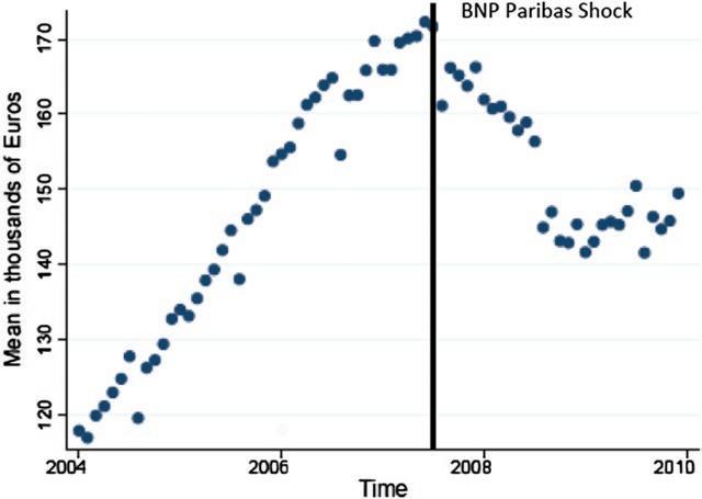
Fig. 6.1 Credit bubble—average mortgage in Spain. Notes Each point represents the monthly average mortgage in Spain. The vertical line is August 2007 (the month of the BNP shock). The interest reader is refereed to Basco and Lopez-Rodriguez (2018)

end of 2007 was 3%. Thus, we can argue that the announcement of BNP Paribas represented a supply but not a demand shock. Figure 6.1 reports suggestive evidence on the aggregate effect of this shock. It represents the monthly evolution of the average mortgage in Spain between 2004 and 2010. Note that it has an inverse-U shape with the peak in August 2007 (the BNP Paribas announcement). During the boom, it increased from around 120 to 170 thousand euros. The rising trend suddenly stopped in August 2007 and the average mortgage declined up to 140 during 2008.

The idea in Basco and Lopez-Rodriguez (2018) is the following: If the mortgage credit boom was driven by supply, aggregate credit growth should fall after the BNP shock. In addition, the change in credit growth should be higher in municipalities with higher credit risk. Note that this exercise is similar, in spirit, to Mian and Suf (2009). However, by using the BNP shock, they can directly compare the relative fall in mortgage

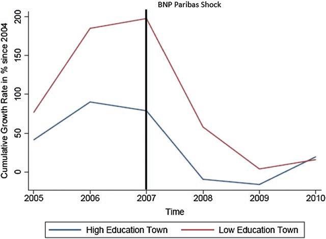
Fig. 6.2 Residential mortgage credit in Spain-high and low education towns. Notes The blue (red) line represents the cumulative growth rate of residential mortgage credit in high (low) education municipalities. Low (high) education municipalities are municipalities in the top (bottom) quartile of the of share of population with basic education distribution. The vertical line is 2007 (the year of the BNP shock). See Basco and Lopez-Rodriguez (2018) for further information

debt due to the supply shock. As a measure of credit risk, Basco and Lopez-Rodriguez use the share of the population with (at most) basic education. One advantage of this measure with respect to using credit scores is that it does not depend on previous credit activity. Moreover, it seems a more fundamental predictor of credit and income risk. For example, the data show that people with basic education are more likely to become unemployed in recessions. Figure 6.2 reports the evolution of residential mortgage credit between low-educated (red line) and high-educated (blue line) municipalities. First, note that during the boom period, the increase in credit growth was much larger in low education municipalities. This is consistent with the fnding of Mian and