7 Hydraulic analysis

Hydraulic modelling consists of understanding the physical properties of the flood water such as depth and velocity. This can be completed in various ways including:

- One-dimensional (1D) modelling, which consists of representing a creek or river with flood information provided at regular interval cross-sections along a stream as well as pipe systems and drainage networks

- Two-dimensional (2D) modelling, which consists of representing a floodplain as a grid with flood information provided at each cell of the grid allowing the model to define flowpaths

- Two-dimensional modelling, which can be completed as a combination of 1D and 2D models.

7.1 Model selection

TUFLOW HPC has been used for hydraulic modelling in this study to simulate flood behaviour across the study area. TUFLOW is a robust and widely accepted unsteady-state flood simulation software with combined 1Dand 2D capabilities. The use of a TUFLOWmodel allows integrated investigation of local overland flow flooding, mainstream creek flooding, foreshore flooding and tidal influences, and the inclusion of storm-water drainage infrastructure.

The GIS data layers and control files used to drive the model can be easily modified for use in the optionsassessment, including modelling the impact of mitigation measures, or assessment of development applications. MHL flood modelling processes follow guidance provided in ARR 2019.

The dynamically linked 1D/2D model requires a number of GIS data layers to represent the study area. These include:

• 1D Domain

- Pits and headwalls GIS layer;

- Pipe network GIS layer;

- Culverts GIS layer;

• 2D Domain

- 2D grid / digital elevation model (DEM);

- Topographic modifications and break lines (e.g. to incorporate channel crosssections);

- Materials layer (specifies surface roughness and infiltration);

- Rainfall on the grid;

- Layered flow constrictions layer for 2D bridges; and

- Initial water level polygons

7.2 Model setup

The following considerations were required to set up the TUFLOW model.

7.2.1 Model extent and grid size

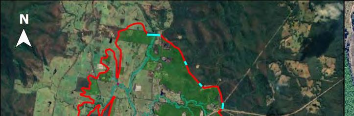
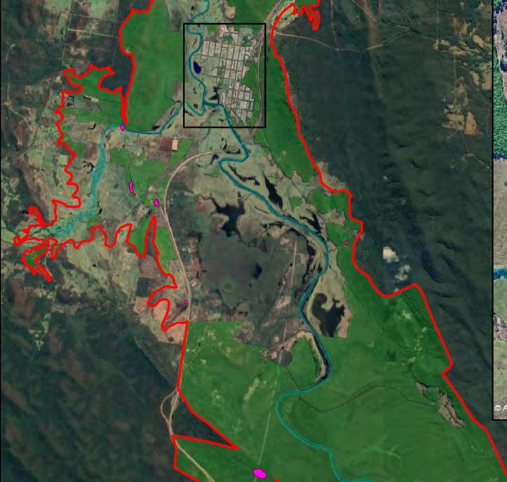
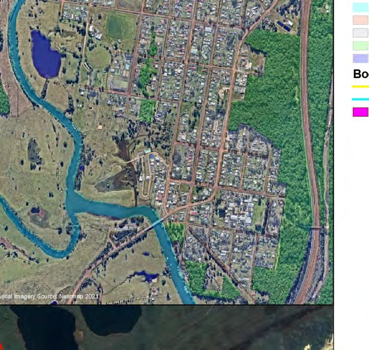
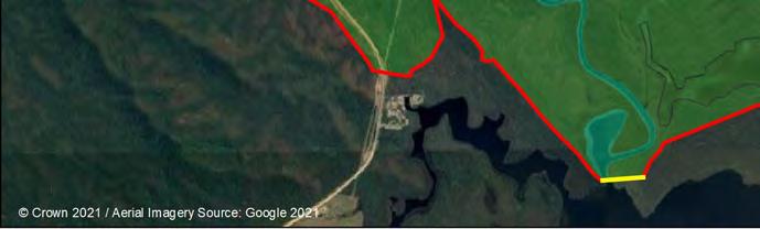
Testing of various model extents showed that the TUFLOW model was significantly impacted by the representation of the storage area within the floodplain. For this reason, the TUFLOW model was therefore set up to cover the majority of the floodplain area below approximately 10 m AHD. This covers an area of approximately 89 km2 between Bombah Broadwater and approximately 5 km upstream of Bulahdelah. Given the area of this model, the Quadtree capability of TUFLOW was adopted to represent the catchment. This capability allows the use of multiple cell sizes in the model to increase resolution in areas of interest by halving the cell size a number of times. The grid definition adopted for the TUFLOW model is presented in Figure 7.1

.

A grid cell size of 3.0 m by 3.0 m was found to be suitable to represent flooding within the township of Bulahdelah and was also applied to represent embankment structures such as elevated roads (blue extent in Figure 7.1) The Quadtree capability was then used to transition to a 6 m cell size in the floodplain where rural properties are located and along the main river (yellow extent in Figure 7.1), and to 12 m for the rest ofthe catchment that ismainly composed of large vegetated areas (red extent in Figure 7.1).

The sub-grid sampling (SGS) capability of the TUFLOW model was also set to 1 m (i.e. the resolution of the available DEM). The SGS allows the use of sub-grid-scale elevation data to enhance the hydraulic accuracyof the model (byproviding an improved representation of flows in and out of each cell and the definition of the volume within each cell) while keeping reasonable run times.

This variable size grid complemented by the activation of the SGS allows an appropriate representation of the features of the local urban catchment while keeping the run time reasonable. Initial timesteps of 1.5 second for the 2D model and 0.75 second for the 1D model have been adopted as these are the recommended values for a 3 m cell size (being the smallest cell size in the model) TUFLOW HPC uses an adaptive timestep approach to maintain stability and would vary this original value as required.

7.2.2 Modelling approach

MHL applied the following modelling approach to the development of a detailed, calibrated and reliable 2D/1D TUFLOW hydraulic model for the study area:

• Extent of the study area and 2D hydraulic model was determined based on the available elevation data

• Direct rainfall method was adopted over the 2D model extent and upstream catchments were represented as inflows calculated using WBNM

• Stormwater infrastructure: All pits, pipes, culverts and bridges were modelled as described in Section 7.2.6

• Blockages: The blockage applied to the pits and pipes system has been established by following the method described in the blockage assessment form provided in ARR 2019 and ARR Project 11: Blockage of Hydraulic Structures

• Hydraulic roughness: a materials layer was delineated from Council’s cadastre, zoning and aerial photography along with site observations. Initial material categories and associated depth-varying Manning’s roughness coefficients were established for the present study

• Fences: given significant uncertainty and variation in fence type, hydraulic behaviour and permanency throughout the study area, and a lack of verification of hydraulic modelling capabilities to represent them, MHL did not specifically model fences. Rather a ‘lumped’ hydraulic roughness approach was adopted

• Thorough model calibration, validation, verification by alternative methods and quality assurance checks.

7.2.3 Hydraulic roughness

Hydraulic roughness coefficients (Manning’s n) are used to represent the resistance to flow of different surface materials. Hydraulic roughness has a major influence on flow behaviour and is one of the primary parameters in hydraulic model calibration.

Spatial variation in hydraulic roughness is represented in TUFLOW by delineating the catchment into zones of similar hydraulic properties. The hydraulic roughness zones adopted in this study have been delineated based on consideration of Council LEP zoning, cadastral data and aerial photography. Factors affecting resistance to flow were of primary importance including surface material, vegetation type and density, and the presence and density of flow obstructions such as buildings, fences and gross pollutant traps (GPTs). Manning’s ‘n’ values assigned to each zone were determined based on aerial imagery, with reference to standard values recommended by Chow (1959). As resistance to flow due to surface and form roughness varies with depth (e.g. Chow 1959, Institution of Engineers Australia 1987), variable depth-dependent hydraulic roughness values have been adopted for this study to consider the typical sizes of vegetation/obstruction (i.e. typical grass or brush height) Once obstruction is underwater, roughness reduces. Figure 7.2 and Table 7.1 summarise the Manning’s n values used in the hydraulic model. The creek/river roughness used for the TUFLOW model was increased to consider the deep pools present along the river with large variations in invert level from -2 to -11 m AHD at regular intervals along the river channel.

N.B.: The Manning’s n value is changing with depth and for example, for Open Space, the Manning’s n value is 0.075 up to a depth of 0.1m and then transition to a smaller Manning’s n of 0.04 at a depth of 0.5 m or more.

7.2.4 Boundary conditions

Key boundary conditions are illustrated in Figure 7.2 and further details are provided below.

Inflows

The simulated hydrographs produced by the WBNM model for the wider catchment upstream of the TUFLOW model were input at key locations at the upstream end of the TUFLOW model as shown in Figure 7.2

Moreover, within the TUFLOW domain, the direct rainfall approach was applied to the model using the design events identified and defined in the hydrological analysis (Section 6).

Downstream boundary condition

The water level as recorded at the Bombah Point water level gauge was applied as downstream boundary condition for the calibration and validation runs.

The Bombah Point gauge data was analysed to determine appropriate downstream water levels for the design events.

Table 7.2 summarises the peak water levels in Bombah Broadwater based on the annual maximum series (AMS) probability estimation of the water levels at the Bombah Point gauge and as extracted from the 2015 Lower Myall River and Myall Lakes Flood Study It is noted that the period of record is only 20 years at the Bombah Point gauge and the analysis can be influenced by large flood events. For example, the March 2021 level at Bombah Point was much larger than the other values recorded since the installation of the AMS analysis gauge back in July 2001 and this may skew the results of the AMS results over such a short record period. The AMS analysis was therefore completed with and without this event

Table 7.2 Peak design levels at Bombah Point at Bombah Point gauge / in Bombah by:

* Annual Maximum Series based on 20 years of data only

** Value was interpolated based on other values provided in flood study

Based on this comparison, the 2015 study values were adopted as tailwater for this study for the following reasons:

• The 2015 study values are based on modelled levels rather than raw data analysis and noting that higher levels within the lake would be subject to the topography and increasing volume of the lakes which the AMS does not accurately consider; and

• The AMS was only completed over a 20-year period of record allowing the data to potentially be skewed by large events with return period larger than 20 years that occurred over this period.

Based on the historical water level and rainfall data measured at Bulahdelah and Bombah Point, it was noted that the flooding of Bulahdelah and Bombah Point are not independent and are likely to coincide as the Myall River catchment contributes to a significant portion of the catchment leading to Bombah Broadwater. Therefore, coinciding AEPs have been assumed for Bombah Broadwater and the Myall River (i.e. a 1% AEP design flood event for Bulahdelah was associated with a 1% AEP water level at Bombah Broadwater).

However, further analysis was completed on the timing of the peak of flooding at the Bulahdelah and Bombah Point gauges. It was found that the peak level at Bombah Point typically occurs several hours after the peak at Bulahdelah. This was considered when developing the tailwater level behaviour for each flood event.

To estimate a tailwater behaviour for the model, the following process was followed:

• the volume of the lake at 0.1 m intervals was estimated up to 3 m AHD, as well as at 4 m and 5 m AHD, based on the topographic (LiDAR) data to create a simplified “bucket” model of the lake with an outflow from the lake that was estimated based on these volumes and the recession rate observed during the largest event on record at Bombah Point (i.e. March 2021).

• The inflows calculated in the WBNM model were then inputted in this model (assuming a typical initial water level of 0.5 m AHD for design events) to determine a general shape for the rising limb of Bombah Point based on the Bulahdelah inflows.

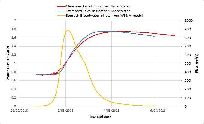
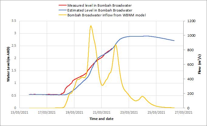
• This general shape of the rising limb was then scaled to peak at the appropriate level at Bombah Point foreach design event (e.g. peakof 2.38 m AHD for a 1%AEP flood event). This approach was applied to the March 2013 and March 2021 calibration/validation events and the results are provided in Figure 7.3 While the full timing is not an exact match, it appears to follow a relatively similar trend, and this was considered acceptable for the purpose of defining a tailwater level at the downstream end of the TUFLOW model. This is particularly true given the relatively small influence of the tailwater level on the peak water level at Bulahdelah as discussed in Section 9.1. Therefore, this approach was applied to define the tailwater for the longer critical duration associated with the flooding of the river. The peak Bombah Broadwater values were directly used as a constant value for the shorter critical duration associated with the flooding of the township.

7.2.5 Blockage

Bridges and culverts are structures that allow water to flow under roads, railways or other obstruction from one side to the other. These structures can be affected by various blockage mechanisms, resulting in increased flood levels, changes to stream flow patterns, changes to erosion and deposition patterns in channels, and physical damage to the structures. Blockage of these structures is discussed in ARR 2019.

This ARR 2019 blockage procedure presented in the Blockage Assessment Form was followed. Cross-drainage structures were identified from Council GIS and included the pedestrian footbridge across Frys Creek.

Each cross drainage was assigned a “High”, “Medium” or “Low” rating for the following ARR 2019 attributes:

• Debris availability – this rating was based on aerial imagery to assess the upstream catchment and the availability of debris

• Debris mobility – this rating was defined using contours based on steepness of the source area and proximity of source area to streams.

• Debris transportability – based on stream dimension in comparison to potential debris as well as stream shape.

• Debris length L10 : ARR 2019 defines this value as:

- the average length of the longest 10% of the debris reaching the site and should preferably be estimated from sampling of typical debris loads. However, if such data is not available, it should be determined from an inspection of debris on the floor of the source area, with due allowance for snagging and reduction in size during transportation to the structure.

- In an urban area the variety of available debris can be considerable with an equal variability in L10. In the absence of a record of past debris accumulated at the structure, an L10 of at least 1.5 m should be considered as many urban debris sources produce material of at least this length such as palings, stored timber, sulo bins and shopping trolleys.

- A value of 1.5 m has been adopted for L10 for all blockage structures in the model. Based on the above approach, the majority of cross-structures have opening lower than the selected L10 and have a design blockage varying between 25% and 100% depending on the AEP ofthe event. The pedestrian bridge west of Rose Street and the culvert under David Street have a larger opening and the blockage would vary between 10% and 20% depending on the AEP of the event.

Regarding all other pits and pipes that were not identified as cross drainage structure, a 50% design blockage was adopted. This value was developed based on the design blockages described in Table 7.1 of ARR Project 11 – Blockage of Hydraulic Structures Stage 2.

7.2.6 Structures

In accordance with the available structures data and topographic data the following structures were included in the hydraulic model:

• Nan Syron Bridge was modelled at 1D elements

• The edge of the Bulahdelah Bypass bridge was modelled as a form loss into the 2D model while the centre of the bridge above the 1D river was not included as the deck level was well above the PMF level.

• Battles Bridge, Frys Creek Bridge and three doubled bridges along Pacific Highway were modelled as 2D elements

• Markwell Back Road Bridge and Wootton Way Bridge were modelled as 1D elements.

• The Crawford River weir was modelled in 2D based on LiDAR levels.

• All pipes and culverts within the study area were modelled as 1D elements.

Figure 7.4 illustrates the pipe network, culverts and bridges included in the hydraulic model.

7.2.7 Creeks and river representation

Following the site inspection, the upstream creeks appeared to be relatively shallow. Some information on depthsand historical cross-sectionswere made available and used to represent the various creeks and rivers. The following assumptions were made in the model:

• Several historical cross-sections of the Myall River were provided as PDF drawings from the Myall River Flood Study in May 1990 and a few cross-sections were also available from the 1991 Bulahdelah Flood Appraisal report. The various cross-sections were used to represent most of the Myall River channel between Bombah Broadwater and Bulahdelah as a 1D model.

• The upstream sections of the various creeks and the upstream end of the Myall River were assumed to be approximately 0.5 m deep and the lowest point observed from the LiDAR data was lowered by 0.5 m assuming a V-shape of the channel from the bank to the invert level.

• No cross-section of Frys Creek was available. However, an invert level was available at regular intervals along the creek (Public Works, 1994), and this level was assumed along the creek, and a V-shape channel was assumed in the upstream creeks.

• The Crawford River channel was reported to be in the order of 3 m deep (NSW Fisheries Office of Conservation, 2003). Therefore, the invert level was set at -2.5 m AHD at the upstream end of the model deepening to -2.7 m AHD at the junction with the Myall River. Based on aerial photograph and LiDAR data, the deep centre of the channel was assumed to be approximately 12 m wide and then transition to the existing bank level where LiDAR becomes representative (i.e. where no water is present).

• Some minor channels leading to ponding areas along the river were also adjusted to remove anomalies in the LiDAR data where blockage of the channels was indicated.

• The DEM at the downstream end of the Myall River, where an anabranch is located, was adjusted to include some local storage assuming a transition from -5 to -6 m AHD depths along the Myall River to a depth of -2 m AHD within the anabranch.

• The ground elevation of the caravan park directly north of the Nan Syron Bridge was updated based on the survey data collected during the project team site visit discussed in Section 4.8.3