Past Global Changes Horizons Vol #2 by PAGES

VOLUME 2 ∙ JUNE 2022

W A R M

W O R L D S

Picture the past

Change the future

Migrations pp 8 – 11

Warm climates in the deep past pp 18 – 21

Stalagmite memories of ancient rainfall pp 46 – 50

TABLE OF CONTENTS 3

Editorial – What can we learn from past warm worlds for our future?

Can climate change humankind? This may have happened 450,000 years ago during a long climate-temperate period

Migrations

Rapid drying of large, deep lakes in the karst mountains of the Lacandon Forest, southern Mexico

Will the Amazon survive a warmer world?

Warm climates in the deep past

Ti(c)k to(c)k: Into the geologic clock

Past global warming in the Basin of Mexico

What can algae tell us about Antarctic sea ice 130,000 years ago? And what does it mean for the future?

A gut-wrenching climate archive: What the stomach content of an Antarctic bird can tell us about past climate

Better forecasts of sea-ice change? Melt puddles and melt models

The story of interglacial permafrost unraveled in frozen caves

Stalagmite memories of ancient rainfall

The mystery of the shells at the river bank

From a secret cold war project to the future of the ice sheet

Antarctic foxes

The science behind the comic: Ice-core records as clues to past changes

Back to the future? Climate clues from past warm periods

Glossary

Meet the authors and illustrators

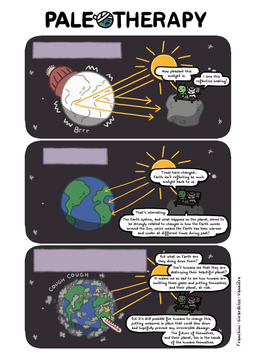
Paleotherapy

Cover Quentin Girardclos Editors Boris Vannière, Nathaelle Bouttes, Graciela Gil-Romera, Emilie Capron and Sarah Eggleston

doi.org/10.22498/pages.horiz.2.3

EDITORIAL

DEAR READERS, We hope you enjoyed the first issue of PAGES Horizons in 2021. It has already been more than a year since that issue came out, and a lot has happened since then. Global change is ongoing! The Intergovernmental Panel for Climate Change (IPCC) published three new reports on the mechanisms, impacts, and mitigation of climate change, but the COVID-19 pandemic and global conflicts captured most of the governments’ attention. In the meantime, although the global CO2 emissions in the atmosphere decreased during the lockdowns around the world in 2020 and 2021, this trend has now reversed, pre-pandemic emission levels have already been exceeded, and evidence of accelerated global change has continued to accumulate. At the beginning of 2022, humanity transgressed the planetary boundary for freshwater – our current consumption for agriculture, livestock, industry and all human activities in general is drawing on the essential stock of plants and animals on Earth, creating a risk for all living beings. In May 2022, the World Meteorological Organization issued a warning that there is a 50% probability that the 1.5°C (2.7°F) threshold for global average temperature, set in the Paris Agreement that was adopted by 196 parties at COP 21 on December 2015, would be surpassed at least once within the next five years. Even if the temperature does not exceed this threshold every coming year, even a one-year increase will likely have strong consequences for most ecosystems and people across the globe, particularly in the form of climate-related extreme events such as intense heat waves, megafires, or extensive flooding. Even if greenhouse gas* emissions in the atmosphere are reduced in the coming decades to keep global warming below 2°C (3.6°F), and countries pursue efforts to limit it to about 1.5°C (2.7°F), the lessons that we have learned from paleoclimatological and paleoenvironmental research tell us that the impacts of this global warming will continue beyond 2100. We will feel the effects for many centuries because of long-term feedbacks related to ice-sheet volume loss, which will lead to global sea-level rise, ocean circulation changes, and changes in the carbon cycle. One of the main messages we hear from most governments, and many stakeholders, is that ecosystems will adapt, that we need to adapt, that we can adapt, that

we know that humanity has always been able to adapt, because we are still thriving as a species today! For the IPCC, adaptation is “the process of adjustment to actual or expected climate and its effects”. It is true that plants, animals, and societies have already faced major climatic and environmental changes. However, those past crises did not occur without loss. The current climate change does not threaten the survival of our species, at least not in the next 100 years. But the IPCC also questions the ability of the most vulnerable populations to cope with additional warming beyond the current ~1.2°C (~2.2°F). At the local and regional levels, there are great disparities in terms of possible “adaptation” to climate hazards and the extreme climate events likely to come. Some regions of the world will be more affected than others by increased frequency of droughts and floods, sea-level rise, loss of sea ice* and biodiversity, and human migration. This is the first time ecosystems and humanity have faced such a significant climatic and environmental crisis. The causes and nature of this crisis, as well as the magnitude and speed at which it is occurring, are unprecedented in the history of the Earth, and we cannot be certain that all species will be able to adapt, or that all societies will be able to adapt. Future generations will inherit a planet very different from today’s, and how it has been in the past. This second Horizons issue highlights warm periods that occurred on Earth in the past, and their causes and mechanisms, as well as some of the effects of warming during the past on some of the key components of the Earth system such as polar ice sheets*, sea ice, vegetation, and humans. Focusing on the topic “warm worlds”, we aim to put the current global warming into perspective. Exploring climate dynamics during warm intervals in the Earth’s history provides a unique opportunity to test what the notion of adaptation may involve, outside the limited present-day observation range, and across timescales that fit with climatic and environmental processes. Seventeen illustrated contributions, such as photo reports, comics, and interviews, provide different pictures of the past that show the exceptional nature of the current global warming. This demonstrates the urgency of restraining future levels of CO2 emissions to avoid climate warming that might no longer be reversible. This new collection of articles illustrates how we can picture the Earth in the past and learn from this history in order to change our future. Boris Vannière, Nathaelle Bouttes, Graciela Gil-Romera, Emilie Capron and Sarah Eggleston

PAGES HORIZONS • VOLUME 2 • 2022

doi.org/10.22498/pages.horiz.2.4

Can climate change humankind?

This may have happened 450,000 years ago during a long climate-temperate period Marie-Hélène Moncel; illustrations: Quentin Girardclos

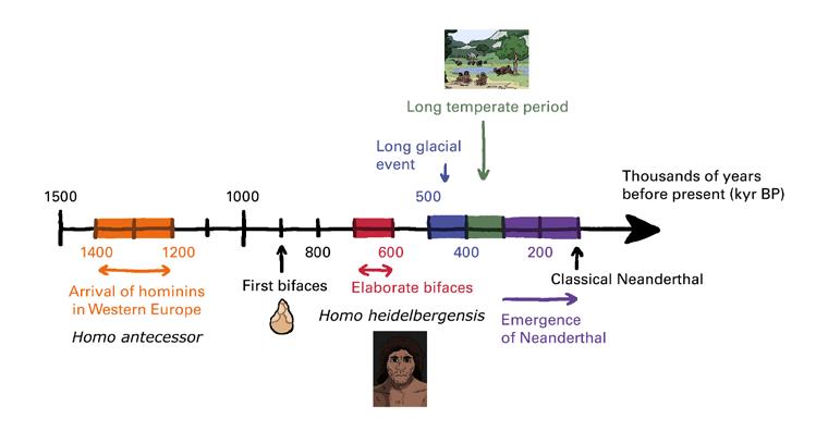
450,000 years ago, a long period of temperate climate (relatively warm in comparison to the current one) took place and lasted about 50,000 years. During this time interval, major changes in the anatomy of hominins occurred, with the appearance of Neanderthal. Hominins living in Europe developed stone tools and hunting methods among other cultural adaptations. Their population probably doubled in size, and they occupied larger territories. This long temperate period, also known as Marine Isotope Stage 11, appears to have been a time where innovative behaviors (such as stone tools) flourished and promoted expansion of populations across Europe. The impacts of climate on human culture is currently a very hot topic, and understanding how our ancestors adapted their culture in response to climatic variability is highly relevant to how we evaluate our own ability to adapt to present-day climate change. Figure 1. Timeline of the prehistory of Europe. The dates are approximate, due to uncertainties in the dating methods that were used. Information about the climate is provided above, in particular the long temperate period of 450-400 thousand years ago. Below: some key dates related to hominin evolution, including first bifaces, large pointed tools made on two faces, indicating new hominin ability in making stone tools.

PAGES HORIZONS • VOLUME 2 • 2022

Beginning of human presence in Europe The earliest traces of humans in Europe are often compared to those observed in the African archaeological records, where tools have been found and dated to 3.3 million years ago. In Europe, the earliest tools have been dated to around 1.4–1.2 million years ago (Fig. 1). Because humans migrating from Africa to Europe would have brought tools (or at least the knowledge of how to create tools!) with them, it is likely that small groups of hominins entered Europe from the Near East at this time, when the climate was temperate and humid. These groups mainly stayed in southern Europe, but there are indications of occupations at higher latitudes, for example in southern England, earlier than 900,000 years ago, when continental conditions were milder and allowing hominins to survive and thrive in this area. This part of England has never been covered by ice sheets*, even during glacial events* when ice sheets in other parts of the world were larger and thicker than today, and some traces of early humans have been preserved. Paleoanthropologists have assigned the name of Homo antecessor to these first Europeans.

Human fossils from this period are, however, very rare, with only some teeth and fragments of bones recovered from archaeological sites. Nevertheless, remains of stone tools that they abandoned provide evidence that they once inhabited these areas. More than 1 million years ago, these hominins used blocks and pebbles of various stones from which they removed cutting stone fragments to cut the meat from the carcasses of large herbivores, such as elephants, that were present at that time in Europe. These elephants were adapted to the European climate, both in the southern and northern latitudes (Fig. 2). Hominins ate the meat of animals that died naturally, or that were killed by large carnivores such as saber-toothed tigers.

Figure 3. Flint bifaces dated to 700,000 years ago from the French site of la Noira (central France) and made by Homo heidelbergensis (photo by M.-H. Moncel; drawings by A. Theodoropoulou).

Figure 2. Elephas antiquus, one of the largest elephant species living in Europe at the time of Homo heidelbergensis. Its height at withers (the ridge between the shoulder blades) was on average 4 m (13 ft), compared to the hominin who was ~1.60 m (~5 ft 3 in) in height.

Appearance of new tools Around 700,000 years ago, hominins’ toolkit evolved to include more complex tools such as bifaces, large pointed tools made on two faces (Fig. 3). These new tools were either introduced in Europe by newly arrived groups of hominins named Homo heidelbergensis (Fig. 4), or they were developed by Homo antecessor. These new hominins seem to have been more adapted to temperate and cold climatic conditions in terms of anatomy and behavior, because artifacts indicating their presence have been found at archeological sites both in southern and northwestern Europe. For instance, some of the hominins lived in the Somme Valley in northern France around 670,000 years ago, when the climate was colder, with open vegetation Figure 4. Reconstitution that supported herds of Homo heidelbergensis, of large mammals. living in Europe.

PAGES HORIZONS • VOLUME 2 • 2022

However, there is no evidence of fire, though the hominins had probably found alternative solutions to survive during winters (for example, clothes from animal skins and habitats protected against cold wind by screens made of animal leather). Europe, however, was possibly not continuously populated during this period. As the European climate changed over time with alternating periods of cold and temperate conditions, the vegetation and fauna also changed accordingly. This variability could have led to successive depopulations, or extinctions, of small hominin groups, with subsequent recolonizations when the climate was more favorable and temperate, similar to the present-day. This was the case until approximately 450,000 years ago when large, thick ice sheets covered a large part of northern Europe during a long glacial event, which reduced the land area available for hominins to live on. This glacial event of about 100,000 years is considered to have recorded profound changes in human occupation of Europe because afterwards we can observe across Europe new stone tools and new methods to make these tools, increase of herbivore hunting and ability to replicate/make fire.

Towards Neanderthal Following the glacial event 450,000-350,000 years ago, a 50,000-year-long interglacial* is recorded in ice-core climate records. From then on, the numbers of traces of hominins, and archaeological sites, increased in Europe. However, this increased

number is not due to better site preservation. Rather, populations grew in size due to improved environmental conditions that favored such a demographic expansion (Fig. 5). New behaviors, such as an improved ability to control fire, aided this population increase and allowed groups to expand once again into northern latitudes, such as northern France and southern England. More controlled use of fire allowed them to cook meat and protect themselves against large carnivores. Scientists associate these new behaviors with the evolution of the Neanderthal species. Neanderthals were our close relatives. Anthropological analyses of these more numerous human fossils (since populations were larger) show that the Neanderthal anatomical features (such as certain properties of the skull, body size, and robustness of the skeleton) emerged in European populations between 450,000 and 400,000 years ago among local human groups of Homo heidelbergensis. During this interglacial period, anatomical evolution took place at a rapid pace, even though genetic data show that the process actually started hundreds of millennia earlier, around 600,000 years ago. The severe glaciation dated at around 450,000 years ago is considered to represent a major crisis for hominins, explaining the profound populational changes that followed, not only with respect to anatomy but also for cultural behaviors. In addition to fully mastering fire and occupying northern territories, these hominins also planned more and more hunting of large herbivores, while scavenging of carcasses decreased (Fig. 6).

Figure 5. View of a life scene of a group of Homo heidelbergensis, some making stone tools and others cutting meat from a carcass. The landscape is typical of the habitat of early humans who co-existed with herds of large herbivores during periods of temperate climate.

PAGES HORIZONS • VOLUME 2 • 2022

Figure 6. Hunting scene of a cervid (deer) by Homo heidelbergensis. The deer is stuck in a swamp, enabling the prehistoric humans to hunt it.

Large tools like bifaces became less common, and hominins began to produce smaller stone tools produced with complex methods and long successions of gestures (Fig. 7). Similar behaviors are observed between human groups living within the same regions, indicating that there were regional traditions. This 50,000-year-long interglacial period, which followed a harsh glacial period, would have been beneficial to hominin occupation in Europe. Vegetation during this temperate period led to higher biomass availability (quantity of animals and plants

available) with forests and meadows providing a habitat and food for various herbivores. This large number of animals across Europe allowed human groups to be more mobile and, thus, expand demographically. It was easier for human groups to occupy larger areas of Europe and exchange innovations, such as stone tool technology. Neanderthal anatomy stabilized around 100,000 years ago, and their populations expanded across Europe until the arrival of Modern Humans (Homo sapiens) in Europe around 40,000 years ago. The reasons underlying these behavioral changes at 450,000–400,000 years ago have yet to be identified in detail, and identifying the factors and understanding these processes is the aim of the Neandroots project, which brings together the expertise of numerous European scientists from various disciplines. Questions on how populations of the past adapted to changes in climate mirror the challenges we face today, even if the societies are completely different.. However, understanding how hominins found solutions by changing how they interacted with plants and animals to overcome environmental change, may serve as a proof-of-concept for studies of human– environment interactions today. About half a million years ago, very small groups of hominins adapted to climatic changes that were happening much more slowly compared to today, by moving to favorable territories or modifying their survival strategies and stone tool technologies. Today, however, climatic conditions are changing very quickly – will we be able to adapt?

Figure 7. Flint tools dated to 450,000 years ago from the French site of la Noira (center of France) and made by the ancestors of the Neanderthals (scale: 5 cm = 1.5 in) (photo credit: M-H. Moncel).

PAGES HORIZONS • VOLUME 2 • 2022

doi.org/10.22498/pages.horiz.2.8

ff uff hu huff h

WHO’S THERE ?!

HALT!

A LT H d i a Is OOT ! H S l l ’ I or

BY MARCO PALOMBELLI & PETER GITAU

H A LT in the n ame o f t he L AW!

PAGES HORIZONS • VOLUME 2 • 2022

! G N G! A B BAN

You’re back! Finally!!

A AA

what are you?

H! AHH

I’m a fossilized skull! Don’t you remember? You've been digging here for months!

I’ve never been here before...

Really? aren’t you one of the paleontologists?

Pity, they were uncovering a pretty sweet part of our origins... Our origins?

I can’t see - I don’t have eyes! No, they took a plane and left...

Imagine the Plio-Pleistocene* and our beloved Rift Valley filled with large lakes that separated the very first few groups of hominids.

...I’m leaving too. My village has been taken back by the desert - there’s nothing there for me anymore...

Yes, the origins of hominids!

See all these lines in the rock? They tell the story of a particular kind of lake you can find only here, on the Rift Valleys: the “amplifier lakes”.

Large forests allowed their populations to grow a lot before splitting into smaller groups moving nothward or southward to richer areas. PAGES HORIZONS • VOLUME 2 • 2022

As time went by, the inclination of the Earth's axis rotated and climate shifted.

For a transitional period of about 2500 years, the lakes receded and so did the forests, facilitating migrations both eastward-westward and northward-southward. Migrations fostered by a harsher environment.

Populations shrank and became more isolated as migrations were rendered either very arduous or impossible. The end of that transition gave way to a dry period where the now-dry valley and much harsher environment forced populations into small patches of forests.

But the orientation of Earth's axis kept rotating, slowly shifting the climate and moving the cycle back to a new wet phase.

These wet-dry periods happened multiple times in the past, separating and differentiating our ancestors more and more, until we, modern humans, came into being. 10

PAGES HORIZONS • VOLUME 2 • 2022

But, hey, cheer up!

Admittedly, a lot of fellow hominids went extinct during this process...

Nowadays you can take one of those “planes” to escape your harsh land, just like the archeologists!

yeah... I wish!

But I can’t. If someone like me loses their home to the desert, they have no right to ask for asylum in another country.

So I have to try to cross the border unseen.

That’s rough!

And here I thought only dead things got stuck in one place long enough to become fossils!

Good luck! May the chains of history and politics be less cumbersome than those of the climate!

END PAGES HORIZONS • VOLUME 2 • 2022

doi.org/10.22498/pages.horiz.2.12

Rapid dr ying o f l a r g e, deep lakes in the karst mountains of the

Lacandon

F o r e s t,

southern Mexico Liseth Pérez and Matthias Bücker

Imagine you live right next to a large lake and all of a sudden this lake disappears within only a couple of weeks!

The mountains of the Lacandon Forest, southern Mexico, host several karst lakes of different sizes, such as Lakes Tzibaná (foreground) and Metzabok (background). (Photo credit: Geotem)

PAGES HORIZONS • VOLUME 2 • 2022

In July 2019, this happened to the Lacandones, indigenous Maya communities living in the Lacandon Forest, a remote rainforest in southern Mexico. The Lacandon Forest does not only give the local Maya communities a home, but is one of the world’s most important biodiversity hotspots. This means that there is an incredible variety of animals and plants inhabiting the rainforest. Moreover, the Lacandon Forest also hosts many small and large lakes, many of which are connected by underground conduits. Both the lakes and the conduits originate from the dissolution of the carbonate rock constituting the subsurface in this area. This type of landscape is known as karst. Karst lakes Nahá, Metzabok and Tzibaná, which are some of the largest and deepest in the Lacandon Forest, have a high water quality, which implies that toxic substances and pollutants in the water are absent. Therefore, the lakes are exceptional natural resources for the native Mayan inhabitants as they provide them with water and fish, and attract tourists – as well as scientists. As aquatic ecosystems, the karst lakes of the area are complex and highly dynamic.

Water levels in Lakes Metzabok and Tzibaná declined dramatically within a two-week period in July 2019. Lake Metzabok dried completely (photo credit: Johannes Hoppenbrock).

Our team has been monitoring the lakes of the Lacandon Forest since 2013 to track environmental variables such as water temperature, conductivity, acidity, and dissolved oxygen. We have also studied how aquatic animals and plants evolve over time. To get an idea of what happens in the caves and underground conduits below our feet, we have also used geophysical methods on the lakes, which helped us to create images of the layers and structures in the subsurface. In July 2019, when the local Lacandones observed that water levels in Lake Tzibaná declined dramatically by about 30 m and Lake Metzabok dried up completely, we organized emergency field work. We expected this sudden drying to have profound environmental impacts and to cause a loss of aquatic biodiversity and genetic diversity, which we wanted to document and describe. During a two-week field study in October 2019, we evaluated the

hydrological and ecological effects of the sudden drying, using a variety of methods. We collected and analyzed samples of water, surface sediment and short sediment cores (a tube of mud) from what remained of the water bodies. At Lake Metzabok, we observed the beginning of the transition from an aquatic (water-based) to a terrestrial (land-based) habitat. Grasses and spiders rapidly colonized cracks in the dry sediment and the lakebeds that were now above water. The profound water decline exposed delta sediments in the southern part of Lake Tzibaná where the Nahá River enters. A delta refers to a landform created by build-up of sediment, when rivers enter a slower-moving water body, such as lakes. We studied the exposed delta deposits and short sediment cores from remnant waters to infer the recent environmental history of the lake, and to find out whether such rapid lake desiccation events had happened before or might eventually happen again in the future. PAGES HORIZONS • VOLUME 2 • 2022

e Nahá since 2013. We have been monitoring Lak variables and collect We measure environmental for analysis in the s ple water and sediment sam ). tem Geo it: laboratory (photo cred

Lacandones are native Maya inhabitants, most of whom live in remote are as of the karst mountains of Chiapas, Mexic o (photo credit: Liseth Pérez).

Single fish were sometimes observed in the few remnant waters of Lake Metzabok (photo credit: Daniel Ochoa).

Using geophysical methods based on the measurement of electric and magnetic fields, we can create images of the sediment layers covering the lake bottom. (photo credit: Liseth Pérez).

Live microscopic aquatic organisms reacting sensitively to environmental change were in identified and counted in our field laboratory Nahá (photo credit: Liseth Pérez). 14

PAGES HORIZONS • VOLUME 2 • 2022

Short sediment cores and delta deposits were retrieved from Lake Tzibaná to infer the past environmental history and to identify episodes of previous lake level chan ge

d by some The desiccation event was exploite nized the colo dly terrestrial species. Plants rapi oa). Och iel Dan it: cred exposed lake bed (photo

(photo credit: Liseth Pér ez).

en the We used geophysical methods to scre floor. lake ut d-o drie sediment layers on the rates ope ents stud ters mas Here, one of our ll sma very s ster regi ch whi ice, dev a seismic to ilar sim ks vibrations of the ground and wor er). Bück thias Mat it: an ultrasonic device (photo cred

Lower lake levels of Lake Tzibaná allowed us to sample and analyze the delta sediments deposited during the past ~100 0 years (photo credit: Liseth

Pérez).

Acknowledgements: Many thanks to M.A. Guerra, R. Martínez-Abarca, M. Bonilla, P. Echeverría-Galindo, T. Lauke, F. Charqueño-Celis, J. Massaferro, K. Rubio, B. Moguel, M. García, C. Pita de la Paz, S. Rodríguez, W. Morales, A. Correa-Metrio, D. Ochoa, A. Flores Orozco, M. Brenner and J. Hoppenbrock. Related publications:

tion event that occurred Our team studied the sudden desicca est. This extraordinary in 2019 in lakes of the Lacandon For interdisciplinary studies event highlights the need for future environmental and social to understand the past and future s (photo credit: Daniel Ochoa). lake e impacts of such changes in thes

Bücker M et al. (2021) Solid Earth 12: 439-461 Charqueño Celis NF et al. (2020) J Limnol 79: 82-91 Díaz KA et al. (2017) Holocene 27: 1308-1317 Echeverría Galindo PG et al. (2019) Rev Biol Trop 67: 1037-1058 Hoppenbrock J et al. (2021) Sensors 21: 8053 PAGES HORIZONS • VOLUME 2 • 2022

doi.org/10.22498/pages.horiz.2.16

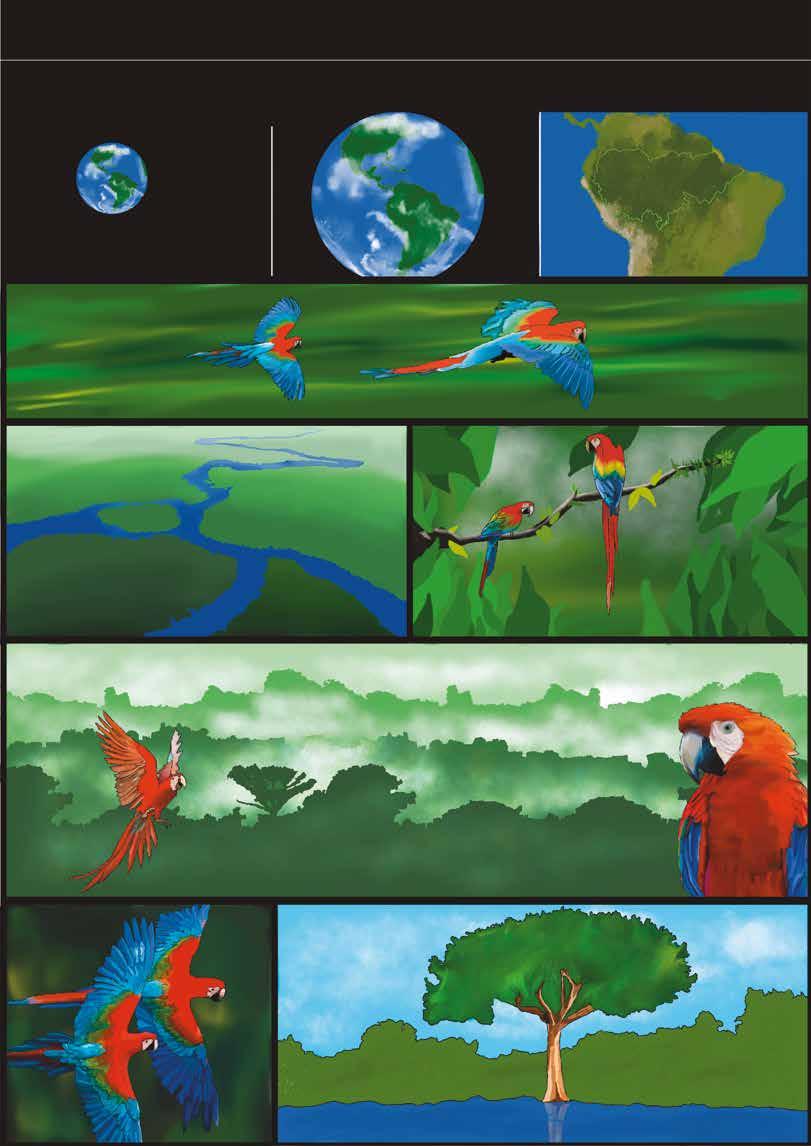
Will the Amazon survive a warmer world? Amanda Gerotto, Marcos de Luca and Renata Hanae Nagai It took Earth 3 billion years to build the largest tropical forest in the world: the Amazon rainforest. The forest takes up carbon from the atmosphere,

trees have a difficult time surviving when the climatic conditions – such as temperature and rainfall – are very different.

helping the global climatic system to cope with the human-induced excess carbon dioxide and slowing down global warming. However, like all living organisms,

So if we keep warming up the planet, will the Amazon survive?”

Area: 6,740,000 km² (2,300,000 mi) about 7% of Earth’s surface!

Come along, little one! Today is your first big flight! Let me show you our home!

Wow! It’s really huge!

What are these white clouds, Mommy?

Yes it is! The forest and its rivers are not only huge, they are the homes of over 3 million species.

Rivers with wings, Mommy? Now come, I want to show you something...

PAGES HORIZONS • VOLUME 2 • 2022

In addition to their role in climate, Amazonian trees tell stories of a climate-changeresistant past.

These are the flying rivers on their way to the south.

No, darling. We call them that because they carry moisture through the atmosphere, providing water to southeastern South America.

Pliocene* (2.6–5.0 million years ago) 3°C

Today

5°F today

Millions of years ago, ancient Amazon tree lineages survived temperatures up to 2-3°C (4-5°F) higher than we have today.

Future (100-year projection) 3°C

However, we are living in a changing world, where the temperature is increasing rapidly around the world, and humans are affecting the Amazon more than ever before.

5°F today

The temperature increase that is predicted for 100 years in the future, if the planet continues to warm, is similar to the difference between today and the Pliocene. Back then, the Amazon was able to survive the heat… but our world is very different now!

We can look into the past to answer your question, my darling. For example, when plants burn, the charcoal left behind tell us a story. That story tells us that over the last 370,000 years, fire was rare. So if the trees survived, will our species survive too, Mommy?

Fires have become more and more common in the last decades.

Is there still time to change this, mommy?

Nowadays, even our homes are being burned – it’s not just the increase in temperature that impacts the Amazon.

Large areas of our forest have been cleared, making it less effective in our fight against climate change. Deforestation affects the flow of flying rivers, decreasing the rainfall over South America, and the forest’s ability to absorb CO2.

The past tells us that the Amazon Forest has recovered from a warmer world, but if the deforestation and fires don’t stop in the next 10-15 years, the Amazon Forest may not survive.

doi.org/10.22498/pages.horiz.2.18

Gilles Ramstein; Illustrations: Cirenia Arias Baldrich The warming of our planet is quickly However, for most of our geological becoming an existential concern. history, the Earth experienced The burning of fossil fuels (coal, gas, warmer climates associated with and petroleum), produces a rapid higher levels of CO2 and higher sea increase in the atmospheric concenlevels compared to those of today. tration of carbon dioxide (CO2), which Interestingly, they can be compared is a greenhouse gas*. The impact that to those that planet Earth will experihuman activity has on the warming of ence in the near future. our planet is undeniable and leads to unprecedented climate changes. Figure 1 Timeline of the Phanerozoic era (last 542 million years). Myr BP = million years before present.

PAGES HORIZONS • VOLUME 2 • 2022

We are warming our planet at an alarming rate and in a very unusual context. Today, we have two large ice sheets*: Greenland and Antarctica. Over geological time, the existence of ice sheets was very rare. To better understand this, let’s look at what has been happening on the scale of millions of years and put it into the context of our planet’s climate history. To explore the conditions of the deep past, i.e. before the Quaternary* (2.5 million years), we use data from solar insolation, tectonics, and atmospheric CO2 concentration reconstructions as input for climate models. There is a diverse range of climate models, which vary in complexity, but all aim to compute the spatial variation of temperature and precipitation.

Traveling back into the deep past The Phanerozoic era corresponds to the last 542 million years (Fig. 1) and begins with the explosion of life in the Cambrian. During this era, several glaciations are recorded, for example during the Ordovician or Permo-Carboniferous. Exceptional periods of glaciation occurred during the Jurassic and Cretaceous. The last massive glaciation took place 300 million years ago, when large continental land masses were located around the South pole (Fig. 2a). The atmospheric concentration of CO2 was low enough to allow for the formation of an ice sheet. However, for most of Earth's history, there were no ice sheets. A well-known example is the time of the dinosaurs, which appeared 250 million years ago and disappeared 65 million years ago (Fig. 1): 185 million years largely without ice sheets (Fig. 2b). Until 34 million years ago, there were no ice sheets, barring some rare, exceptional events. There are two possible explanations for this: either there was no continent at the poles or sub-polar locations where it is was cold enough for ice to have formed; or that the climate was warm enough, with a high atmospheric concentration of greenhouse gases, leading to the rapid melting of winter snowfall during summertime.

The crucial role of paleogeography There are specific periods, for example the Cenomanian (100 million years ago), for which the temperature distribution is more uniform (Fig. 3). Compared to today, the thermal gradient from equator to pole (i.e. the difference between the average temperatures at high and low latitudes in each hemisphere) was much flatter, with much higher temperatures at the poles. Moreover, tropical and subtropical plants could be

Figure 2 Paleogeography for three different periods: (A) the Permo-Carboniferous, which was the last period of long and extensive glaciation, dating from 320 million to 270 million years ago; (B) the ice-free Cenomanian (Cretaceous), 100 million years ago; (C) the Paleocene, 65 million years ago.

found at very high latitudes, and temperature differences between summer and winter were reduced. All these characteristics describe a very different climate to that of today: much more uniform across space and time. About 65 million years ago, the continents were separated into several landmasses (Fig. 2c). The continent of Antarctica was already in a polar location. However, no ice sheet existed at that time because the atmospheric CO2 content was very high: about 1500 ppm compared with 416 ppm today (2021) and about 280 ppm before industrialization during the 19th century. The absence of an ice sheet was due to the melting of winter snow instead of its accumulation year after year, which would allow an ice sheet to form. The sea level was then much higher than today. PAGES HORIZONS • VOLUME 2 • 2022

Overheating a warm climate Scientists have highlighted exceptional warming events, which occurred during some of the already warm periods throughout climate history. The most spectacular one, the Paleocene-Eocene Thermal Maximum, happened about 56 million years ago at the frontier between the geological periods known as the Paleocene and Eocene (Fig. 1), when a drastic atmospheric CO2 change, with pCO2 more than eight times higher than pre-industrial* levels (Fig. 4), destabilized the already warm climate. This warmer climate event lasted about 200,000 years, and is sometimes depicted as a parallel to our current global warming period because it corresponds to a big, sharp and fast modification in the carbon cycle, with a major impact on the temperature of the Earth. There are several key differences between this period and today: First, the Paleocene-Eocene Thermal Maximum took place in a warmer world than today with higher CO2 atmospheric concentration: about 1,200 ppm com-

pared to around 420 ppm today. It is interesting to note that by 2100 we might also reach very high pCO2 values. But as there was no ice sheet before the Paleocene-Eocene Thermal Maximum, there was no risk of major sea-level rise at that time. These comparisons make it a fascinating period to study. Second, the speed of change was at least 10 times slower than the recent and ongoing human-driven CO2 and temperature increases. Third, the tectonics of the Earth during the Eocene also played a major role in the global climate: changing mountains, ocean bathymetry, and seaways, which were different to those of today. For instance, this period corresponds to the large uplift of Tibetan Plateau due to collision between Indian and Asian plates. Some important seaways were closed, such as the Drake passage, but others were opened, e.g. the Central American seaway.

A gradual cooling from the Eocene to the end of the Pliocene* From the Eocene until the Pliocene-Quaternary transition (2.52 million years ago), atmospheric CO2 concentration decreased to about 300 ppm, while temperatures also gradually decreased (Fig. 4). This cooling took more than 40 million years, which gives us a timescale of the Earth's climate processes. Despite the cooling, the climate remained warmer than the last interglacial periods of the Quaternary, including the present one.

Figure 3 Schematic of the temperature from the equator to the poles during (A) the Cenomanian (mid-Cretaceous) and (B) the present-day periods. The difference between the equator and pole temperatures (gradient) is low at the Cenomanian and high at the present. 20

PAGES HORIZONS • VOLUME 2 • 2022

The climate of the midPliocene Warm Period (~3 million years ago) has been simulated in great detail by climate models (see Capron and Bouttes p. 68). These simulations were carried out in the context of 3 million years ago; different models were compared. The models were then either validated/ invalidated by comparing the climate reconstruction to existing data. Climate models

have found a global temperature rise of 2–3°C warmer than preindustrial temperatures. Indeed, the paleogeography of this period is comparable to ours. The most prominent difference is that the sea level was 10–25 m (30–80 ft) higher. This can be explained by an important reduction of the Greenland and West Antarctica ice sheets, as well as loss of ice from areas along the margin of the East Antarctic Ice Sheet. This situation is perfectly consistent with the idea that, with a high value of pCO2 over a long timescale, the most vulnerable ice sheets (Greenland and the western part of Antarctica) can melt entirely. This would represent an equivalent sea-level rise of approximately 10–12 m (33–39 ft). However, as helpful as it is to compare such models, it is also important to take into account the differences. The most significant difference is that the present warming of our planet is not in equilibrium. When the world is warming, the ice sheets and deep ocean need thousands of years to reach equilibrium. The ice sheets and oceans are not in equilibrium with the climate because of inertia effects, which mean that they are several thousands of years slower in reaction compared to surface climate warming, which can occur over hundreds of years.

A few more possible insights from past climate simulations? For all the warm climate periods described above – the Cenomanian, Eocene, and Pliocene – climate models tend to underestimate the temperatures reconstructed for high latitudes. Climate models often fail to capture the flat profile of the thermal gradient from equator to pole, shown in Figure 3. This problem was first discovered in the 1980s with simpler climate models, but even today with much more sophisticated models, the problems persist.

Figure 4 Indirect CO2 reconstructions for the last 70 million years based on the Earth’s Cenozoic CO2 from different paleoclimate indicators as seen in Beering and Royer (2011), https://doi.org/10.1038/ngeo1186

Over the next century, the climate of the high latitudes will change drastically as the ice sheet progressively melts and the sea ice* shrinks, or disappears. In turn, this will lead to major changes in the climate of the lower latitudes. It is difficult to predict what impact the melting ice sheets will have on the global climate. Nor do we know how the atmosphere and the oceans, which redistribute heat from the warm equator to the cold poles, will respond. This issue is crucial for a better understanding of our future climate, and will certainly be a focus for a new generation of researchers. And the fascinating deep past remains one of the best ways to address the question! PAGES HORIZONS • VOLUME 2 • 2022

doi.org/10.22498/pages.horiz.2.22

Jose Dominick Guballa, Deborah Tangunan, richard jason antonio & Jesse Jose Nogot

You might have seen THESE videos squeezed in a minute.

What’s in a Facebook or an Instagram story? Or in a Tiktok video?

What about the Earth’s entire history in a minute?

Complete memories and stories all TOLD in a very short time!

A blink of an eye lasts about 1/3 of a second, or 0.55% of a minute. If Earth’s age is crammed in one minute, a blink of an eye…

…is about 25.3 MILLION Earth Years! Earth scientists work on These timesCALES, way beyond human history! And within a blink of an eye…

ah wo

Then, ARE YOU READY TO TRAVEL BACK TO ANY TIME IN THE Earth's past? yes, it will be millions of years back! Way, way back!

PAGES HORIZONS • VOLUME 2 • 2022

…countless volcanoes erupted! even the Arctic froze and thawed mANY Times! Curious to check THIS out and get caught in the geologic clock?

HUH!?!

REAdy or not, here we go!!

the water is very warm!

AAA

A Ah

...and yes, THE phone is still working!

!!!

WOAh?! wait! is this really happening? where are you taking me? am i in the ocean?

BACK TO the middle miocene* climatic optimum?

n c arbo pheric Atmos e: 450 ppm id x dio

Hmmm, looks like the atmospheric carbon dioxide is similar to the present day levels (450 parts per million), yet it became much warmer than the present?! that's why scientists are very curious about it! woah! THIS PART OF THE OCEAN is about 7oc warmer than the present day! that’s why the water feels SO warm!

look, over there, whales! these marine mammals started to become abundant and diverse during this time. and so are the fish, which also seem to be loving the warm water. wait! something’s floating in the water! can you see it? we should turn the phone’s camera on and try the augmented reality app so we can see what they are!

This coccolithophore group, the tiny Reticulofenestra, is abundant during the middle miocene climatic optimum.

2000 x

Organism: COCCOLITHOPHO RE S - single -celled pho tosynthetic algae wit h shells made up of calciu m carbonate Genus: Ret iculofe nestra Siz e: whole shells (coccospheres) are as small as dust par ticles, about 5-10 microm eters

Scientists say that they can tolerate a wide range of temperatures, so they were doing fine while other coccolithophores WEre not surviving! This makes them the main group of coccolithophores during this time! In fact, their relatives today are the most abundant coccolithophore group and can survive almost anywhere! Talk about being persistent!

PAGES HORIZONS • VOLUME 2 • 2022

Oh? the phone’s camera is on again?!

oh no! is my time running out? wait!!

NOOO!!

I want to know more! A piece of the puzzle is still missing!

being sucked up by the wormhole, she can see the whole west side of north america from above. a large volcanic event is happening in the northwest united states!

this eruption, the columbia river basalts, could have released huge amounts of gases into the atmosphere! the increase of these gases, like carbon dioxide, may have resulted in high temperatures during thE MIDdle MIOCENE CLIMATIC OPTIMUM. but this could be just one of the many factors... interesting!

woah! that was amazing! never thought i could travel back to 16 million years in less than a minute! the geologic clock sure knows how to warp!

TO BE CONTINUED...

PAGES HORIZONS • VOLUME 2 • 2022

doi.org/10.22498/pages.horiz.2.25

g n i m r a w l a Past glob o c i x e M f o n i s in the Ba -Martínez, arcía, Antonio Flores -G no za Lo o rr co So barca, Rodrigo Martínez-A ballero o and Margarita Ca er rr ue G aeg rt O riz Beat

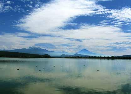
Figure 1. Left: Location of the Basin of Mexico. The dashed line shows the annual mean position of the Intertropical Convergence Zone.

Lake Chalco as a time machine Mexico City is located in the Basin of Mexico (Fig. 1). Rivers extending from the highlands produced a system of lakes: Zumpango, Xaltocan, Texcoco, Xochimilco and Chalco. However, the lakes were drained in later

Right: Photograph of Lake Chalco as seen from the west. Behind the lake you can see the Iztaccihuatl (left) and Popocatepetl (right) volcanoes (photo by Socorro Lozano). Photo by Peter Fawcett

Mexico City is one of the largest cities in the world: more than 20 million people inhabit the city and its metropolitan area. The constant growth in population since 1960, when there were only around 5 million inhabitants, has led to increases in demand for drinking water, the size of the urban area, and the emission of greenhouse gases* into the atmosphere. Consequently, and coupled with global climate warming, the city's meteorological records show that the annual average temperature has risen 1.6°C (2.9ºF) since 1880. The outcomes are already discernible today, e.g. through the extinction of “Ayoloco” in 2018, an iconic glacier located in the Iztaccihuatl volcano, and one of the few in Mexico.

Although the current speed of global warming is the highest that it has ever been over the course of human history, increases in global temperature have occurred in the past on longer timescales. Various paleoclimatic records on both hemispheres have preserved evidence of a warm period that occurred about 125 thousand years ago and known as the Last Interglacial.* During the Last Interglacial, global temperature increased by 0.5°C with respect to the pre-industrial* value. In Central America and southwestern North America, it is known that forest communities and precipitation changed dramatically during this period. Yet for Central Mexico, the Last Interglacial has been little studied. Because the Last Interglacial represents one of the most recent warm periods in the Earth’s history, understanding the regional environmental changes undergone during its establishment are key in anticipating possible future scenarios for Mexico City.

PAGES HORIZONS • VOLUME 2 • 2022

centuries and only small remnants of water are preserved. Lake Chalco, southeast of the Mexico Basin, is a high-altitude tropical water body (about 2200 meters or 7200 ft above sea level) located on the northern edge of the American tropics. Lake Chalco acts as a sediment trap where all the particles produced outside and inside the lake are deposited. The region is influenced heavily by the climate: in particular, the amount of rain is promoted by the location of the Intertropical Convergence Zone, a band of clouds encircling Earth near the Equator that provides humidity during the summer to Central Mexico. The Intertropical Convergence Zone has changed its average position during the last few million years, causing fluctuations in past rain amounts. In 2008, sediment cores were drilled to a depth of 122 m (400 ft) southeast of Lake Chalco. Subsequent studies showed that the sediments in the core include clays rich in plant remains such as roots, leaves, and wood (organic matter), minerals, fossils such as micro-crustaceans (ostracods) or microalgae (diatoms), carbonate layers, and volcanic ash. The age of the sediments was obtained by dating tiny pieces of wood and pollen found at specific depths within the sediments. Based on these data, it was estimated that the Lake Chalco sedimentary record covers the last 140 thousand years: the oldest (that is, the deepest) of these sediments are older than the Last Interglacial!

Reconstructing the Last Interglacial The analysis of geochemistry in Chalco’s sediments, as well as the study of microscopic algae (diatoms), pollen from surrounding vegetation, and carbonized particles produced during natural fires (Fig. 2), has provided paleoenvironmental information all the way back to the glacial* period preceding the Last Interglacial (125 thousand years ago).

PAGES HORIZONS • VOLUME 2 • 2022

Figure 2. Some of the indicators found in Lake Chalco sediments and used during the environmental reconstruction.

Figure 3. Image of sediments deposited during the Penultimate Glacial Period* in Lake Chalco.

At the end of the Penultimate Glacial Period*, mountain glaciers were lowered by about 1000 m compared to today. The reconstructions suggest that Lake Chalco was a deep, nutrient-rich lake filled with freshwater. Seasons were well defined, as witnessed by the presence of thin and bright sediment layers composed of diatoms (Fig. 3). Also, this was a wet period with high freshwater flowing from the rivers into the lake. The vegetation was composed of large grassland areas. This type of vegetation results in little plant matter to burn, which is why fires were not as frequent (Fig. 4).

Figure 4. Reconstruction of the landscape in Lake Chalco during the Penultimate Glacial (130 thousand years ago), the Last Interglacial (125 thousand years ago) and the current state.

During the Last Interglacial, the scenario changed dramatically when compared to the preceding glacial period. Lake Chalco became a shallow, alkaline lake characterized by high evaporation. Riverine runoff decreased due to low humidity in the region. Grasslands still dominated the vegetation; however, forest communities and fire activity increased (Fig. 4). There is no way to measure paleotemperature in this region directly yet, but it is possible that the increase in temperature may have been larger than the current warming. The decrease in precipitation during the Last Interglacial has been associated with the southward migration of the Intertropical Convergence Zone towards the Southern Hemisphere in response to changes in the Earth’s orbit. The Lake Chalco drilling provides the first record in Mexico that allows us to understand the climate and environmental changes during this past warm period. The study of the sediments of Lake Chalco, one of the oldest lakes in Mexico, will continue providing key information on future climatic scenarios for Mexico City. Open questions remain, such as the speed of change and the resilience of ecosystems to warming. These are critical uncertainties for the urban and rural communities that face them.

PAGES HORIZONS • VOLUME 2 • 2022

doi.org/10.22498/pages.horiz.2.28

ic t c r a t n A t u o b a s u What ca n algae tell t a h w d n A ? o g a s r a e y sea ice 130,000 ? e r u t u f e h t r o f n a e does it m Matthew Chadwick and Claire S. Allen

The Last Interglacial* is a time period that occurred between 130,000 and 116,000 years ago, and was a time when Antarctic temperatures were similar to what is predicted for 2100. The Last Interglacial, therefore, represents an excellent case study to investigate the response of the sensitive components of the Earth system, for instance, the polar ice sheets* (ice on the land which has formed from snowfall) and the seaice* cover (ice on the sea which has formed from freezing seawater), to a warmer-than-today polar climate.

PAGES HORIZONS • VOLUME 2 • 2022

Present-day Antarctic winter sea ice covers an area of 18,000,000 km2, nearly twice the size of the USA, and is highly reflective compared to the surface of the ocean. White surfaces (like sea ice) reflect solar energy whereas dark surfaces (like the ocean) absorb solar energy. Therefore, the less sea ice there is, the more solar energy the Earth absorbs and the warmer it gets. Sea ice provides a platform that multiple species of penguins and seals rely upon for resting and breeding. Sea ice is also a surface for microscopic algae to grow on, and, during the yearly melt of winter sea ice, nutrients and meltwater are released, helping to promote large algal blooms in the Southern (or Antarctic) Ocean. Therefore, understanding how Antarctic sea ice responded to warming air and ocean temperatures during the Last Interglacial is important for predicting how it will respond to current global warming, and thereby estimating how much Antarctic sea ice will be lost by 2100, and the domino effect of that loss in reflectivity.

vertical sl ice looked (a n io ct se s os cr ic at arctica Fig ure 1: Schem hern Ocea n near Ant species ut So e th of ) de si e atom at from th preference for th e di ell as a l ta en nm ro vi en e th as w showin g ag ila rio psis cylindrus, neath the Fr d an a rt cu is ps rio Frag ila om be g a sedi m ent core fr in ct lle co ip sh ch ar se re ed ge. present-day sea-ice

To find out how Antarctic sea ice changed during the Last Interglacial, and what caused those changes, we look at the sediments deposited on the ocean floor. Silica (glass) “skeletons” of diatoms, a type of photosynthesizing micro-algae (5-300 µ m in size, or about the thickness of a sheet of paper) are preserved in these sediments.

There are only a few ways of reconstructing past sea ice, and diatoms preserved in marine sediments are the most robust and commonly used. Numerous species of diatoms live in the Southern Ocean today, each with their own specific environmental preferences; therefore, the changing abundances of these different species in ocean floor sediments can be used to reconstruct past environmental changes. Here, the focus is on just two diatom groups, and what they can tell us about changes in Antarctic sea ice during the Last Interglacial.

The first of these diatom groups is the combined abundance of Fragilariopsis curta and Fragilariopsis cylindrus (FCC), which is associated with Antarctic winter sea ice (Fig. 1). A higher percentage of diatom skeletons from the FCC group in ocean floor sediments indicates the presence of winter sea ice above that location, and a decreased abundance indicates the retreat of the winter sea-ice edge further south than that location. The second diatom group is the Eucampia antarctica, which is associated with the iceberg flux over a location (Fig. 1). High abundances of Eucampia in ocean floor sediments indicate a large number of icebergs over that location.

PAGES HORIZONS • VOLUME 2 • 2022

uca m pia) across E d n a C C (F ps ou gr in nces of two diatom eir Last Interg lacial ab un da nces da un ab ic at m he e th re Figu re 2: Sc e periods alon gs id sa n d yea rs ago. T he sedi m ent co nt. m ti al ci la rg te in d ou ex te gl acia l a n een 132 a n d 120 th th e present-day winter sea-ice tw be d te si po de t d n ica a sedi m en lative to Antarct re n ow sh is on ti loca

In order to investigate how the abundances of these two groups of diatoms changed during the Last Interglacial, we take a cylinder of ocean floor sediments, known as a sediment core. This core was collected by a research ship (Fig. 1) and is made up of a combination of particles originating from continents, such as dust blown from deserts or pieces of rock eroded and transported by icebergs, and biological particles, which have settled down from the surface ocean. The material in this core accumulated over hundreds of thousands of years, and we can select the sediments that were deposited during our time interval of choice, in this case between 132,000 and 120,000 years ago (Fig. 2), to investigate changes in diatom abundances both just before and during the start of the Last Interglacial. 30

PAGES HORIZONS • VOLUME 2 • 2022

Results from the studied marine sediment core suggest a decrease in the FCC abundance (blue in the zoom-in graph covering the interval

132,000–120,000 years ago in Fig. 2) to a minimum at 130,000 years ago before an increase to a relative maximum at around 126,000 years ago. The FCC abundance is then largely the same for the entire time between 125,000 and 120,000 years ago. In parallel, the Eucampia abundance (purple in the zoom-in graph covering the interval 132,000–120,000 years ago in Fig. 2) is low between 132,000 and 128,000 years ago before increasing at the same time as the increase in FCC abundance. The Eucampia abundance is then largely the same for the whole 126,000 to 120,000 thousand years ago time period. While these changes in FCC and Eucampia abundances are significant for understanding the dynamics of sea ice and icebergs during the Last Interglacial, they are relatively small changes on the scale of a full glacial-interglacial* cycle, as shown by the schematic abundances represented on the left in Figure 2.

As the Earth warmed during the Last Interglacial, much of the sea ice surrounding Antarctica melted, causing the sea-ice edge to move closer to the continent, shown by the decrease in FCC abundance at 130,000 years ago. This retreat allowed the less reflective ocean to absorb more solar energy and warm even further. The warm ocean helped drive a large release of icebergs from the Antarctic ice sheets, as shown by the increase in Eucampia abundance at 126,000 years ago, causing a substantial reduction in the size of the Antarctic ice sheets. As the icebergs travelled across the ocean, they would have melted and released cold and fresh water into the surface of the ocean, causing a large rise in global sea levels. The cold, fresh surface waters can also freeze more easily; therefore, the large number of icebergs helps cause the slight re-expansion of sea ice, as shown by the FCC abundance increase 126,000 years ago.

Still, the changes in FCC abundances indicate a retreat of the winter sea-ice edge past the location of this core during the Last Interglacial to a minimum sea-ice extent around 130,000 years ago before a slight re-expansion of Antarctic winter sea-ice extent at 126,000 years ago. The Eucampia abundances indicate that this small expansion of winter sea-ice extent occurs at the same time as a large increase in the amount of icebergs passing over this core location. Taken together, these two diatom groups help elucidate some of the responses of Antarctic sea ice to warming ocean and air temperatures.

From these two diatom groups we can see how both Antarctic sea-ice cover and the Antarctic ice sheets were sensitive to warmer polar temperatures during the Last Interglacial, with substantial reductions in the extent of both compared to the present day. The slight re-expansion of Last Interglacial sea ice indicated by the FCC abundances (Fig. 2) was still reduced relative to the present-day sea-ice extent, and it is clear that if Antarctic temperatures reach or exceed the 2100 predictions (1.5 to 3oC, or 2.7 to 5.4oF, warmer than the present-day) this warming will be accompanied by a loss in both Antarctic sea ice and ice sheets.

PAGES HORIZONS • VOLUME 2 • 2022

doi.org/10.22498/pages.horiz.2.32

A gut-wrenching climate archive: What the stomach content of an Antarctic bird can tell us about past climate Thale Damm-Johnsen and Ellie Honan Picture a vast white, frozen desert reaching as far as the eye can see. It is summer and the sun is out, but the icy wind blowing towards you still makes your nose numb and your eyelashes freeze. In the far distance you see a mountain range protruding from the endless white, like spikes poking holes in a blanket. Out of the corner of your eye you see something moving across the sky towards the mountains: a white bird, about the size of a pigeon, that almost completely blends in with its surroundings. It gives out a faint cry, as if to say hello, and gracefully disappears into the white. You are standing on the Antarctic Ice Sheet*: a huge mass of tiny ice crystals, sustained by the cold temperatures to form one gigantic mass of ice. The bird you got a glimpse of was a snow petrel, one of the few birds that live and thrive in the Antarctic all year round (see Fig. 1 and 2). The snow petrel was heading home to its nest among the crevices of Antarctica’s nunataks, the exposed rock surfaces that protrude above the ice sheet (see Fig. 2, 3, and 4). Every austral summer (December–February), the snow petrels return from the ocean to incubate and raise their chicks. f a pigeon. out the size o ab is l re et p snow Figure 1. The

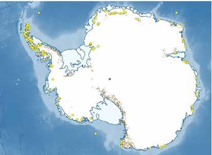
w petrel cations of sno lo a; ic ct ar nt Figure 2. A yellow dots. presented by ach-oil colonies are re here the stom w to ts in o p llected. The arrow gure 8 was co Fi in d ye la p is deposit d

Snow petrel chicks hatch as small balls of grey fluff, reliant on their parents for food and occasional warmth during the first months of their life (see Fig. 5). The warmth is truly only occasional, as the parents regularly leave the chicks for several days at a time to find food at sea. However, despite their winsome appearance, the chicks are anything but defenseless. 32

PAGES HORIZONS • VOLUME 2 • 2022

ice. ing up out of the inland Figure 3. Nunataks stick untains. mo e an nd Ro r Sø nan in the Photo taken by Ellie Ho

dripping st, covered by ne its in l re et ow p Figure 4. A sn eposit. d il o stomach

home and breeding ground of small organisms called sea-ice* algae. During spring, the ice melts and the algae are released into the water where they become a vital meal for krill, a small crustacean about the size of your little finger. The krill form the base of the food chain for the larger organisms in the Southern Ocean, from the tiniest fish, to birds like the snow petrel, and true giants like the blue whale.

But let’s back up a second. What makes a bird like the snow petrel want to live in the hostile cold of Antarctica in the first place? The answer doesn’t lie in the ice sheet itself, but in the waters just offshore (see Fig. 6). The annual cycle of freezing ocean water in winter (when the temperature drops to –2 degrees Celsius or 28 degrees Fahrenheit) and melting of the sea ice in summer forms the foundation of one of the most fertile waters on the planet. In winter, tiny holes in the sea ice serve as the ball of fluff. ick: i.e. a grey ch l re et p w o Figure 5. A sn PAGES HORIZONS • VOLUME 2 • 2022

nests on ute from their m m co ls re et wp photo shows Figure 6. Sno for food. This nt hu to e ic a e se t covering land out to th e big ice shee th f o e g ed e at th snow petrels e begins. here the sea ic w a, ic Antarct

The snow petrel feeds at the edge of the sea ice and in rare openings within the sea-ice pack; they live primarily off of fish and krill that are found in the upper meters of the water column. These nutrient-rich foods serve as the snow petrels’ main energy source needed for them to be able to grow and survive in the extreme cold throughout the year. During the summer, they convert the fatrich fish and krill to an oil that they store in a small organ located just above their stomach. The organ is linked to the stomach, but storing the oil in this organ instead of the 34

PAGES HORIZONS • VOLUME 2 • 2022

stomach allows them to hold onto all the energy and fat from their prey. They are thereby able to save the bright orange oil, allowing the snow petrel parents to provide their chick with the nutrients they need to grow. When the snow petrels return to the nest, they can regurgitate this oil easily into the chick’s beak. However, don’t be fooled by the innocent expression of the snow petrel! If a predatory bird (like a skua) or an unfortunate researcher gets too close, the snow petrels will defend themselves in a particularly smelly way: they spit with impressive force at the intruder. But unlike us (and llamas), they

ls can protect old snow petre d an g un yo g stomach oil. Figure 7. Both by regurgitatin s ua sk ig b m o themselves fr

don’t use saliva: instead, they spit their stomach oils (see Fig. 7). Beside smelling strongly of half-digested seafood, the stomach oil clings to the feathers of the attacker. A coating of oil makes the predator’s feathers less waterproof, affecting its ability to keep itself warm and weighing the bird down as it becomes waterlogged. In Antarctica, a lack of insulation and the inability to fly can mean death for oily birds. Luckily for science, some of this stomach oil never makes it onto the intruder but lands in the vicinity of the bird’s nest, settling among the rocks of the crevices where they nest. As snow petrels return to the same nest site year after year, the stomach contents slowly but steadily solidify and accumulate into greybrown layers that we call stomach-oil deposits (see Fig. 8). The largest one found so far by humans is 90 cm thick—just imagine the generations of snow petrels needed to make this deposit! The freezing, desert-like climate of Antarctica helps to preserve these stomach-oil deposits, which record the signal of the snow petrels’ diet through time. The bottom layer of the deposits is the oldest and gets younger upwards, either gradually or in leaps, depending on how often the snow petrels returned to this exact nesting spot. Antarctic climate scientistic have dated some of these deposits to be almost 60,000 years old! We know that climate has changed quite a lot over the past 60,000 years, so we bring these deposits all the way back from Antarctica and into the lab to perform a chemical analysis on the

dy posit back in the lab rea Figure 8. Stomach oil de ee thr in ed ch oil deposit is slic for analysis. The stoma er stratigraphy. sections to reveal the inn

deposit. This allows us to study how the snow petrel diet might have changed in response to changing climate through the time the deposit was accumulating. Performing this analysis on samples from the deposits is an intricate process, with many steps necessary before scientists can read the signal from the stomach oils. However, the reward is high, as we can detect tiny chemical fossils known as biomarkers that give us a direct indication of what the birds ate. The biomarkers are invisible to the naked eye, and specific to different organisms. You and I, the apple you had for lunch, and the fish that swim in the sea all have different biomarkers. Which biomarkers are found in an organism is partly dependent on the environment the organism lives in. For example, the temperature, the amount of rain, and whether it lives in water or on land all affect the type of biomarkers that we find. But the biomarker content is also dependent on what an organism consumes. Therefore, you can expect your own PAGES HORIZONS • VOLUME 2 • 2022

contain Figure 9. Fish and krill

of biomarkers. different distributions

biomarker content to be affected by the apple you ate, and that your biomarker content would change if you ate a piece of bread instead. The same principle applies to the snow petrel. Based on modern observations, the birds have a dominant diet of either krill or fish, depending on how close to the shores of Antarctica they collect their food (see Fig. 9). Close to Antarctica, the ocean gets shallower, and the sea surface temperatures are colder. Even in summer the surface of the ocean is below zero degrees Celsius (32ºF), and the ocean is shielded from the atmosphere by a layer of sea ice. As snow petrels cannot penetrate the sea ice to feed, they must travel offshore to where there is less dense sea ice and the ocean surface is exposed (see Fig. 10). This means that how far out the summer sea ice stretches from the Antarctic coast affects where food is available for the snow petrel. However, as the petrels are restricted to breeding on land, if the seaice edge is too long a commute during the period where adult snow petrels are taking care of their chicks, it is thought that they may 36

PAGES HORIZONS • VOLUME 2 • 2022

snow a ice is close to shore, Figure 10. When the se . sea-ice edge petrels feed along the

take advantage of openings within the sea ice, called polynyas. Polynyas situated close to the coast are usually formed by winds blowing over the land toward the ocean that push the newly formed

petrels’ stomach oils. Therefore, the stomach-oil deposits give us indirect insight into how the seaice extent has evolved parallel to a changing climate, and how sea ice and climate affected the diet of the snow petrels.

d, it is a ice edge is far from lan Figure 11. When the se n the sea ice feed in openings withi hypothesized that they r. when winds are stronge that form during winter

sea ice further away from the coast, leaving the surface ocean and the fish and krill living there exposed for the snow petrels to feed on (Fig. 11). This affects both their diet and the environment where the snow petrels feed, thus affecting the biomarkers of the snow

Sea ice is a difficult environment to measure and model, so we still have lots to learn about how it reacts to climate change. Records of the past, like the stomachoil deposit, will provide a new perspective on an aspect of the climate system that we know very little about. This knowledge can further be used to improve our best guess for how climate may change in the future, which we sorely need if we want to decipher how our climate will react to enhanced CO2 emissions. However, as no one has looked into these deposits in a systematic way before, we are not yet completely sure what we are going to find—but that’s the thrill about being a climate scientist, entering the unknown!

Back on the white ice you stare into the endless white horizon. You can't see it, but in the far distance is the ocean, partly covered by a shifting blanket of ice. The wind howls around you, but inside your hood and thick snow suit it's warm and cozy. Another faint cry floats through the wind, and you look up to see the white silhouette of a snow petrel soaring over the sky above you. Perhaps it has delivered its fat-rich stomach contents to its chicks, assuring the survival of the next generation, and is on its way out for new rations. The nature of these tenacious birds, who fly hundreds of kilometers across the ice in order to access their food and raise their chicks, is extraordinary on its own, and can perhaps help us climate scientists solve the still mysterious climate puzzle of how the southern polar regions will react to climate change. Acknowledgements: This article is a part of a wider project at Durham University funded by the ERC (grant No. 864637) and the Leverhulme Trust. Snow petrel photos were taken by Johan Bondi, in a snow petrel colony close to the Norwegian Antarctic station Troll.

PAGES HORIZONS • VOLUME 2 • 2022

doi.org/10.22498/pages.horiz.2.38

Better forecasts of sea-ice change? Melt puddles and melt models Louise Sime, Irene Malmierca, Rachel Diamond and David Schroeder

Several reasons make it essential to have good forecasts of future sea-ice* area in the Arctic. Arctic sea ice is linked to extreme weather events across Europe, America, and the far East, from intense droughts to “snowmaggedon” winters. Evidence suggests that changing sea ice will have repercussions on patterns of extreme weather over the coming decades. Ongoing sea-ice change will also determine the range over which Arctic animals thrive. Whilst a few species will benefit from future ice loss, like the orca, which is extending its range into the new open water areas in the Arctic, loss hurts other top predators, particularly the iconic polar bear. Ongoing sea-ice change will determine the range over which each Arctic animal thrives. Over the last forty years, Arctic sea ice has declined rapidly (Fig. 1). This is a key part of the climate change picture. To predict how climate will evolve

Arctic sea-ice minimum extent 4.72 million km2 16 September 2021

Yellow

in the future, scientists use “global climate models”: sophisticated computer models that can simulate conditions everywhere on the planet. These models mostly do a good job at representing the climate correctly. However, while there is variation between individual model results, most models don’t quite predict the amount of sea-ice decline that we know is actually happening. This is a problem for politicians, scientists, and engineers, because it limits confidence in the forecasts from climate models. Human actions over the coming years, particularly total carbon emissions, will make a real difference to the extent of these changes in the Arctic and beyond. However, we would also like to have more confidence in our climate model-based forecasts of sea-ice change to understand how our climate-related actions will affect Arctic sea ice. Recent model results suggest that if we continue to emit carbon dioxide at our current level, the Arctic Ocean could be free of sea ice during summer within twenty years – or as late as in eighty years. If we do not know when it will occur, it is difficult for Arctic communities and governments to plan for the consequences line 1981, avg. min. of a sea ice-free summer in future.

Figure 1a of sea ice on Whole Arctic view when the ice 16 September 2021, yearly miniits appeared to reach is date, the extent mum extent. On th illion square m of the ice was 4.72 square miles). on kilometers (1.82 milli sualization Studio tific Vi Credit: NASA’s Scien

PAGES HORIZONS • VOLUME 2 • 2022

This means that it is crucial for climate scientists to test the equations that shape the model calculations, by studying how well models represent past sea-ice changes when the climate was warm and sea ice was reduced. To address this problem, we investigated the physics and causes of sea-ice change, concentrating on Arctic changes during the most recent warm past climate period: the Last Interglacial*– from 130,000 to 115,000 years ago. The Arctic was about 4OC (7OF) warmer than today during the Last Interglacial. This is known thanks to many valuable records of past air temperature, especially from pollen recovered from lake bottoms and peat cores. The focus on this warm period, and on how sea ice reacted, gives insight on how the Arctic will respond to future warming. It also allows us to check our climate models against measured Last Interglacial temperatures and sea-ice changes so we can find out if they do a good job of forecasting how sea ice changes during warm climates. Figure 1b Regional view of Arctic sea ice in early summer, with extensive melt ponds. Credit: Don Perovich

Ice cores are a great source to know about past climate conditions. One item of interest in Greenland ice cores is the ratio of water isotopes*: versions of water with more or less neutrons. It is easier for versions with less neutrons to evaporate from the open sea surface, and inversely. Depending on the sort of isotopes we find and in what quantity, we can estimate how close or how far the sea ice was from Greenland at different times during the past, and we can say with high certainty that the amount of sea ice in summer was much lower during the Last Interglacial than today. The latest climate models reveal one of the key reasons there was so little Last Interglacial summer ice: puddles of melted ice. Today, in spring and early summer, shallow puddles of water form on the surface of the ice. These puddles, or “melt ponds”, determine how much sunshine is absorbed by the ice and how much is reflected back into space (Fig. 2).

Figure 2 How melt ponds work: in early spring (April-May), most energy from the sun (gold arrow) is reflected by the reflective sea ice so very little heat (red arrow) is passed through to the sea. If a darker meltpond forms on the ice, it absorbs heat that warms the surrounding sea ice and the sea below, melting more of the sea ice above and around. This kicks off a positive feedback process through the rest of spring and into the summer: now that the sea ice is thinner, solar warmth can pass more easily through the melt pond and into the sea ice and sea, so the sea ice thins even more, and so on.

Figure 1c Close up view of Arctic sea ice in early summer, with melt ponds. Credit: Don Perovich

PAGES HORIZONS • VOLUME 2 • 2022

This says two important things. Firstly, the Arctic was probably ice-free in summer. Secondly, we can use this new model to check how well climate models do during warm climates with little or no Arctic sea ice left.

During the Last Interglacial, there was much more intense springtime sunshine than now. This created many melt ponds, which absorbed a lot of this extra sunshine and completely melted the sea ice. This exposed the ocean surface, which absorbed even more sunshine and heated up, explaining how the Last Interglacial Arctic was 4OC (7OF) warmer in summer than today. Unlike older models, the UK’s new weather and climate forecast model has melt ponds built in. And also unlike older models, this new model simulated a fully ice-free Last Interglacial Arctic in summer. We know we can likely trust this result because we found a very close match between the model’s simulated temperatures, and those inferred from Last Interglacial summer pollen, which suggests the model represented well the most important Last Interglacial climate processes (Fig. 3).

Studying sea ice during the Last Figure 3 Interglacial was technically and scienThe temperature data from pollen and from the model match! tifically challenging. We continue to work on it to The x- and y-axes represent the modeled and actual temperature gain better insight into what happened and why. increases that occurred during the Last Interglacial in degrees Celsius. There is a better correlation for the new model results, In particular, we want to understand whether and they are closer to the other models – from all climate modeling groups compared to the older model, theoretical best fit line. around the world – show the same response to Last Interglacial changes. If they show a similar response, this tells us about the reliability of our models. Already, by uncovering this Arctic sea-ice Related publications: change during this period, and crucially finding out Diamond R et al. (2021) Cryosphere 15: 5099-5114 why it became ice-free, we have helped politicians, Guarino MV et al. (2020) Nat Clim Chang 10: 928-932 scientists, and engineers have greater confidence in Malmierca Vallet I et al. (2018) Quat Sci Rev 198: 1-14 model forecasts of our future.

PAGES HORIZONS • VOLUME 2 • 2022

doi.org/10.22498/pages.horiz.2.41

THE STORY OF INTERGLACIAL PERMAFROST UNRAVELED IN FROZEN CAVES Stuart Umbo, Franziska Lechleitner and Sebastian Breitenbach

What is permafrost, and why should we care? Over 10% of the Earth’s land is covered in permanently frozen ground, called permafrost (Fig. 1). As humans cause the planet to warm up through climate change, permafrost will begin to thaw. What happens to it will have tremendous repercussions both locally and around the world. Permafrost forms when the ground temperature drops below zero degrees Celsius (32 degrees Fahrenheit), freezing the water within. If temperatures the following summer aren’t warm enough to thaw the ground, it stays frozen all year. When this continues for two or more years… Voilà! You have permafrost. Most of the permafrost that exists today formed during the last ice age*, around 20,000 years ago, when the Earth was much colder. Ancient organic matter, like dead and decaying plants and animals, has remained frozen inside until the present day. Now, as humans cause our planet to warm, we’re measuring permafrost thaw accelerating, especially at its most southern edges. As it does so, the frozen organic matter starts to break down to carbon dioxide and methane (Fig. 2). This has the potential to release vast quantities of greenhouse gases* into the atmosphere and accelerate climate change. Scientists are worried that large-scale thawing of permafrost could release greenhouse gases into the atmosphere. This will cause further warming and increase the rate of permafrost thaw, creating what we call a positive feedback loop. This makes permafrost a tipping element—a key component of our climate which, once pushed into a new state, could cause irreversible changes to the climate system.

northern

Tibet, and Figure 1 Permafrost is widespread in Siberia, Canada, ia. This map Siber in caves China. We study the Lenskaya and Botovskaya e the North Pole. abov from down ng looki Earth shows a view of the

PAGES HORIZONS • VOLUME 2 • 2022

g past n i s u s t s scie*nti redict future e r a w o H s to p ost? l a i c a l g r e int ermafr p n i s e g chan f the arm periods o ls, w to k o lo s st Scienti rglacia , known as inte Earth’s history ow permafrost might h to understand n-caused climate a m u respond to h ture. fu change in the s h ha Ear t d e h all e so, t s o r r i o d s, c ar e r a e e . We t on y mp milli nd war ectively d in pas 2 t s s a e p a a s g d p e l r o an t ur e w ial s r t he s ch gh c Ove d throu nterglac rost ha empera , we i e af lt dl y st cycl ls* and perm he globa day. Sa rmafro a w i o c e o t p ,t n e in g l a n g at h whe er than eck the ewher or i , k s l o lo cia warm and ch d som ehavi r gla inte r to, or in time , we nee afrost b nd such la te simi go back ectly. So nt perm ay. We fi arbona e r c t i d i ’ can itions d to anc odern alcium s c m c o n d c l u e s a to t h e f o r m o f s . h d c e m i e wh r e s er v s, in t h l e o t he e e p are s in cav n as sp w e c o a n k pl osit s dep

Speleothems com e in many forms— for example, you may have alre ady heard about st alagmites! They form over th ousands (sometim es even millions!) of years when calcium carb onate precipitates from drip water. It’s the same process that sometimes ca uses chalky deposit s (limescale) to build up on your shower and hot w ater pipes.

To find suitable speleothems, we travel to remote corners of Siberia and explore kilometers of caves, many of which have never been explored before.

ace in take pl w as n e t f o s lo ns peditio mperatures a ice roads x e r u O to te , when urn rivers in ves. winter t ca ) e F ° h t to (- 40 travel - 40 °C o t s u l ow that al 42

PAGES HORIZONS • VOLUME 2 • 2022

Whereve rw and drin e stop, we make a fi k Sometim tea because it's s re o cold.. es we eve n make a sauna !

ditions of the cave like We also monitor environmental con centration. This can help us temperature, drip rates, and CO2 con ironmental parameters (like understand the impact of specific env , or cave ventilation) on temperature, drip rate, water chemistry . speleothem composition as they grow

What do speleothems tell us about permafrost stability? Speleothems grow when water drips into a cave through the ground above. If permafrost is present above the cave, water remains frozen, and speleothems stop growing. This can give us information about where and when permafrost thawed during past interglacials.

Figure 2

il, In temperate so k microbes brea matter, c ni ga or down nhouse releasing gree * rost gases . Permaf s so freezes microbe to they ’re unable ganic break down or ng it in matter, trappi en for the ground, oft ars. thousands of ye rost When permaf s thaws, microbe wn do star t breaking c ni fossilized orga ing material, releas of huge amounts ses. greenhouse ga

PAGES HORIZONS • VOLUME 2 • 2022

Figure 3

discontinuous d end of glaciations, At the beginning an cave, stopping spesome sections of the in s rm fo st ro af rm pe allowing water to ile thawing in others, wh , th ow gr em th leo the timing of ground ms can tell us about he ot rele Sp e. at ltr infi rm when calcium ca . Cr yo-carbonates fo ing aw ple th lti d mu an g lin ing ez mp fre ter. Sa out of (re-)freezing wa s te ta ipi . ec aw pr th te st na ro bo permaf tablish the speed of caves, we can also es

B 44

p water enters the rmafrost thaws and dri pe , ial lac erg int rm wa a , the soil deepens, During w. With a warmer climate gro to ms the leo spe ing a speleothem as it cave, allow ses chemical changes in cau is Th s. urn ret on conditions! Looking and vegetati uct past environmental str on rec to use can we 00 years ago) can grows that afrost thawed (e.g. 125,0 rm pe en wh als erv int at past warm in the future. permafrost might thaw help us predict if/when

”.

es ls the cave “hibernat C Duringstglasucia stops r te wa , rrounds the cave Permafro accumulates inside. flowing, and ice often

Understanding the conditions under which permafrost thaws n ical compositio m e ch e th t a k s as to We can loo to give us clue ditions m e th o le e sp of a l con environmenta the timing and als. ci of past intergla

Speleothems can be dated accurately using a technique called radiometric dating. This allows us to determine when permafrost was absent from above the cave. As speleothems grow they incorporate tiny amounts of radioactive uranium isotopes.* These decay over thousands of years. As they decay, the concentration of uranium within the speleothem decreases. Uranium decays into thorium and lead, increasing the concentration of these “decay products” over time. By measuring the ratio of uranium to thorium or lead, we can determine when the speleothem formed. This tells us when permafrost around the cave started to thaw.

Atoms come in heavy and light forms that we call isotopes. The different isotopes within a speleothem give us further clues as to the environmental conditions—how warm or wet it was, for example— when permafrost thawed. We hunt for tiny bubbles of water trapped in the speleothem as it grows. The number of heavy oxygen isotopes found in the water changes with the precipitation conditions when it was trapped. The concentration of noble gases dissolved in the water depends on temperature. So, we can measure them and estimate the temperature of the water when it was trapped. We can combine this by looking at the way that carbon and oxygen are bonded together within the speleothem. This changes as the cave warms and cools. So, we can use it to estimate the temperature at which speleothems formed—even if that’s millions of years ago! We can measure many other speleothem properties to learn about the past. As speleothems form, tiny traces of chemicals are deposited in the calcium carbonate. Their quantities change with environmental conditions like rainfall, vegetation, and even the number of wildfires! We can measure these in the lab to build up a detailed picture of environmental conditions when the speleothem formed.

opic nd isot ines a l a c i he chem ems on mach asure t We me on of speleoth s. er iti compos ss spectromet a m d e call

R adiometric dati in ultra-clean ng is conducted labs. We hav e to wear space-age bu nny suits, so we don’t contaminate our speleothem samples!

In this way we can infer the timing and environmental conditions of permafrost thaw at different locations. This allows us to reconstruct permafrost shifts in response to warming and helps us predict what might happen to permafrost as anthropogenic warming continues in the future. PAGES HORIZONS • VOLUME 2 • 2022

doi.org/10.22498/pages.horiz.2.46

WRITTEN BY ALENA KIMBROUGH ILLUSTRATED BY DANIEL A. BECKER

There once was a girl who grew up in the mountains, spending summers digging for dinosaur bones and happily hunting for cave crystals. As she grew older, she learned about the oceans getting too warm and too harsh for corals and plankton to survive in.

Fires and droughts were becoming more frequent and storms unpredictable all around the warming planet.

Winters in the mountains weren't like they used to be. She wondered what this meant, as the familiar was starting to become unfamiliar. How much will the world change?

How much has it changed in the past?

So, she became a scientist and returned to the mountains and caves to try to understand the changes happening around the world.

PAGES HORIZONS • VOLUME 2 • 2022

In search of answers, our scientist went to Sulawesi, an Indonesian island near the Equator.

Sulawesi is surrounded by some of the warmest ocean water on the planet and sits in the path of the Australasian Monsoon*, which brings critical rainfall to southeast Asia, Indonesia, and Australia. The collision of warm water, the Monsoon, and other large weather systems, produces huge amounts of energy and transports heat around the Earth.

to prepare for the effects of future climate change, our Scientist wants to learn what this Monsoon was like during PAST warm periods.

Luckily, there are ancient rocks with coded memories that can tell us about their past.

monsoon rain carries a message in each water droplet.

those droplets trickle through soil and rock into caves. the water then drips...

d r o a p f t e r d r o p layer upon layer...

And forms a stalagmite.

Our Scientist carefully collects these unique climate archives to decode and analyze at the laboratory.

Using Uranium-Thorium dating, we know that stalagmites can be over 500,000 years old. This makes it possible to learn how the Monsoon changed as the Earth swung between extremely cold and warm periods, known as Glacial-Interglacial cycles.

PAGES HORIZONS • VOLUME 2 • 2022

To isolate brief snapshots of time, tiny samples are carefully drilled out along the central line of growth. These fine powders contain a chemical imprint of the water droplets that fed the stalagmite.

Our scientist uses very sensitive instruments to extract this chemical information.

2 1

The stalagmite powders are dissolved in phosphoric acid and become CO2 gas.

Powerful magnets in the mass spectrometer are then used to accelerate the CO2 gas around a curve, causing the molecules to separate into smaller parts.

As the elemental components zip through the magnet, they fan out according to weight (number of neutrons) and slam into a collection wall at the other end of the mass spectrometer.

O x y g e n

O18 O16 C13

C a r b o n

C12

By measuring the smattering of elements, the information stored in layers of the stalagmite can be pieced together into a climate record. Oxygen isotopes* tell us about changes in past rainfall. Carbon isotopes tell us about past vegetation above the cave.

240,000 years old

310,000 years old

230,000

wetter

years old

d18O

(Oxygen Isotopes)

180,000 drier

years old

youngeR (top)

older (bottom)

5,000 years old

40,000 years old

By analyzing the oxygen isotopes of many stalagmites that grew at different times in the past, our scientist can combine them to form one long rainfall record.

PAGES HORIZONS • VOLUME 2 • 2022

The stalagmites tell us that Sulawesi’s monsoon experienced huge changes in the past that coincided with Earth’s cold (glacial) and warm (interglacial) periods.

During each ancient warm period, the Monsoon was strong and behaved much as it does today, delivering lots of rainfall to Sulawesi.

InterGlacial period

Glacial period

(wetter)

(drier)

(Land masses exposed due to low sea level)

In between each warm phase is a long cold glacial period. The Monsoon was much weaker and Sulawesi was much drier than it is today.

this consitent pattern of dry and wet cycles gives us important information about how extreme the monsoon can be... but sulawEsi stumps our scientist with a new mystery.

there is an important section of history missing from the stalagmite record. This is the most recent warm period, known as Marine Isotope Stage 5e. It occurred ~130,000 years ago, when earth had slightly warmer temperatures and sea levels were probably about 9 meters (30 feet) higher than today.

Wetter

d18O

(Oxygen Isotopes)

drier 0 kyr BP 40 kyr BP 130 kyr BP

330

230 kyr BP

kyr BP

(kyr BP = thousand years ago) present

past

PAGES HORIZONS • VOLUME 2 • 2022

Understanding how the monsoon behaved during this past warm period will help us to better prepare for the warmer future that is expected if we continue on our current trajectory. This is especially important if the missing section of the record (where no stalagmite growth has yet been found) was caused by a major interruption to the climate system.

Using these amazing time-capsules, Alongside records from other parts of the world, our scientist is determined to solve the mystery of sulawesi’s missing warm period.

This story of our scientist reminds us to be curious and ask questions. The natural world has a lot to say.

We are eternally grateful to the Australian Research Council for past and current funding (e.g. ARCDP180103762). There is a large research team behind this work and we acknowledge the enormous contributions from Mike Gagan, Gavin Dunbar, and Claire Krause. We are indebted to Baharudin (of Konservasi Sumber Daya Alam), our colleagues at the Research Center for Geotechnology, Indonesian Institute of Sciences (LIPI), and the staff of Bantimurung-Bulusaraung National Park (with special thanks to Syaiful Fajrin). We thank Hamdi Rifai for field assistance and translating the comic into Bahasa Indonesia. 50

PAGES HORIZONS • VOLUME 2 • 2022

doi.org/10.22498/pages.horiz.2.51

THE MYSTERY OF THE SHELLS IN THE RIVER BANK Angélica Ballesteros-Prada

i, nice to meet you! My name is Magnita. A few days ago, I was taking a walk along Samborombón Bay. It’s a beautiful place in Argentina (Fig. 1), there are many canals and rivers that empty into the Atlantic Ocean. When I was walking, I looked at the river bank, and something surprised me. In the sediment, I could see a line of marine shells. Wow! That was surprising because I wasn’t anywhere near the sea! I wondered: how did these shells get here? Do you know what could have happened? I had no idea.

When I got back home, I talked about this with my friend Maria. She’s a biologist, and she studies what Samborombón Bay was like in the past. She explained to me that Samborombón Bay is a great place to study the climate and the environment of the Quaternary* (period of time from about 2.5 million years ago to the present). The evolution of the bay is related to variations in sea level, particularly between 11,650 and 7,000 years before present (BP), a time period called the early Holocene.

Figure 1. The location of Samborombón Bay (red circle), where I saw a line of marine shells ( ) and a picture of these.

“It’s okay, don’t worry – I’ll explain everything.” Microfossils are small organisms that can live in the sediment or in the water (Fig. 2). They are smaller than a pinhead, so you can’t see them without magnification: you need a microscope. The most important thing is that these organisms are difficult to decompose, which means they can be preserved in the sediment for hundreds, even thousands, of years!

She told me about microfossils, too: how she uses them to do environmental reconstructions of the past, and how microfossils could help me solve this riddle. I had never heard about microfossils before – have you?

Figure 2. Look! In a few grams of sand, there are many microfossils, but these are so tiny that you need a microscope to see them.

Figure 3. Pictures of different microfossils taken with a scanning electron microscope. The smallest microfossils are called nanofossils, and charophytes are some of the biggest.

PAGES HORIZONS • VOLUME 2 • 2022

Around the world, there are many kinds of microfossils, for example, coccolithophores, radiolaria, foraminifera (for short, scientists often called these “forams”), ostracods, testate amoebae, and charophytes (Fig. 3). In this case, Maria told me about the forams and ostracods. (WOW! Difficult names to remember.) We can use these microfossils to reconstruct the environment of the past because we can find them in the present, and we know where they live. Today, forams usually prefer to live in salty waters, such as the sea, or between the open ocean and the mouth of a river (salt marsh or estuary), but different types of forams live in different places. As for the ostracods, they prefer to live in freshwater, such as in lagoons, while some also live in brackish water (a mix between freshwater and seawater) and marine environments. To understand this, we can see how the foraminifera and ostracods are distributed throughout the estuarine marsh (Fig. 4). This is a place with a wide range of salinity (a measure of the amount of salt dissolved in the water). The saltiest area of a salt marsh is shallow seawater: this is an area between the coast and the open sea and is permanently covered with water. There, we can find forams such as Buccella and ostracods such as Coquimba.

Low and high marshes are located in the middle section. This is a coastal area and is divided into zones, which are usually at different elevations. This controls how often the different zones are flooded. This area is dominated by plants that can tolerate water with high salinity. Low salt marshes with marine influence are flooded daily but have no river or stream flowing through. Low-growing plant species can be found in this zone. Low salt marshes with freshwater influence are frequently flooded and have fewer plant species. The water in this area is a mix of freshwater, from rivers, and seawater. Ammonia and Elphidium species can tolerate low-to-medium salinity water, such as low marshes and tidal flats. However, Ammonia is more abundant in low salt marshes with freshwater influence, and Elphidium is more abundant in low salt marshes with marine influence. High salt marshes are rarely flooded – only during periods of extreme high tide and storms, and has many tall plant species. Jadammina can only live in the sediment below bodies of water with low salinity, so it prefers to live in high-to-middle marsh sediments. Limnocythere can generally live in freshwater environments like lagoons. Figure 4. Foraminifera and ostracod distribution through the estuarine marsh. The black lines represent where the different organisms live.

This was fascinating, but I still didn’t understand how we could use all of this information to actually reconstruct the past climate. Maria gave me some clues. Okay. Do you want to help us? Don’t worry – it’s gonna be easy.

PAGES HORIZONS • VOLUME 2 • 2022

1. We take a sample of sediment at different points in the river bank: A, B, C, and D. The sample at the base of the wall (A) is the oldest of all the samples, and the sample at the top of the wall (D) is the youngest (Fig. 5). 2. We wash the sample through a sieve, dry it, and put it on the counting tray (Fig. 5).

Figure 5. In this picture you can see the place where we take the samples and Mariel, who also studies the past of Samborombón Bay. Here we’re washing the samples, and Maria is looking at the samples through the microscope.

Now we need you! 3. Find 10 microfossils in each counting tray (samples A, B, C, and D). 4. Count and classify the different microfossils in each sample according to the images.

5. Use the information from step 4 to find the type of environment corresponding to each sample. Use the following table and match each sample from the wall of the river to its environment.

PAGES HORIZONS • VOLUME 2 • 2022

Good Job! What do you think happened at Samborombón bay? A. This place was a desert in the past. B. Seawater flooded this place in the past. C. These sea animals moved to the sea from the river because this place was better for them. Okay. I’ll tell you a little bit more about the Samborombón Bay history. The Earth went through periods where the climate alternated between warm and cold. The cold, dry, and dusty periods with large ice sheets* are called glacial periods or ice ages*, and warmer periods with smaller ice sheets are called interglacial periods1.

These climate changes affected marine and continental environments. For example, the temperature variation influenced global sea level. During glacial periods, the low temperature allowed large ice sheets to grow, and as water was stored on the continent in the form of snow and ice, sea level decreased. On the other hand, during interglacial periods with smaller ice sheets, sea level was higher. The most recent glacial period occurred between about 120,000 and 11,500 years BP, and the Last Glacial

PAGES HORIZONS • VOLUME 2 • 2022

Maximum occurred about 20,000 years BP. During the Last Glacial Maximum, global sea level was 120–135 m (390–440 ft) lower than at present, with large ice sheets in North America and Eurasia (Fig. 6). Big mammals lived during this period, like mammoths, giant ground sloths, saber tooth tigers, glyptodonts, and others (these remind me of a movie…). Figure 6. A comparison between summer ice coverage from 18,000 years before the present and recent observations (modified from ref. 1).

Approximately 19,000 years BP2, the ice sheets and glaciers began to melt. This event affected the coastline in different places of the world, such as Samborombón Bay. Between 6000 and 5500 years BP, sea level reached a maximum here. Sea level was about 4 m (13 ft) higher than present sea level and covered the bay (marine transgression); then the sea retreated to the current position (marine regression).

Figure 7. Evolution model of the Bahía Samborombón central. You can see when the sea level rose and covered the bay, and also when it retreated to the current position.

At our site, to ~10 km (~6 mi) from the line coast (Fig. 7): (A) First, between ~6700 and 6500 years BP (a period of ~200 years), the area around the bay was a low-energy salt marsh. Then, (B) between ~6500 and ~6220 years BP (~280 years), seawater covered the bay and transformed this place into a shallow marine environment. (C) Between ~5200 and 4150 years BP, the regressive sea-level phase began, and this place transformed into a salt marsh again, but with more rivers and freshwater influence. However, this is not a normal regression; this is forced regression that is the result of other factors different to glaciation and deglaciation events. For example, in Samboronbón Bay, the rivers moved a lot of sediment, and it was deposited on the coast, this contribution of sediments causes the sea to recede and the continental area to advance3. (D) Recently this region turned back into a high marsh near a freshwater canal. This means that sea-level rise in Samborombón Bay was due to deglaciation events, but local factors also influenced in decreasing sea level, such as contribution of sediment.

Wow! This is amazing! I never thought that this area could have been in the ocean. Now I understand what happened in the past with the sea level when it was warmer. I think that we can use this information to understand how the recent global warming can affect changes in the environment and, in particular, sea level. Do you know what your city was like in the past? At some point, it may have been in the ocean, a desert, or even covered by a glacier.

Related publications: 1. NCEI (2021) Glacial-Interglacial Cycles | National Centers for Environmental Information (NCEI) formerly known as National Climatic Data Center (NCDC). ncei.noaa. gov/sites/default/files/2021-11/1%20Glacial-Interglacial%20Cycles-Final-OCT%202021.pdf. Accessed: 20 Nov 2021 2. Mendelova M et al. (2017) Cuadernos de investigación geográfica 43: 719-750 3. Luengo MS et al. (2021) Quat Int 602: 4-14

PAGES HORIZONS • VOLUME 2 • 2022

doi.org/10.22498/pages.horiz.2.56

T C E J O R P R A W D L O C T E R C E FROM A S T E E H S E C I E H T F O E R U T U F E H T TO You’re about to embark on a journey to Camp Century, a nuclear-powered U.S. Army base built in 1959 and 1960. It was a grid of thousands of feet of snow tunnels dug into the Greenland Ice Sheet*. You might feel like you’re watching an old James Bond movie or even entering a science fiction novel, right?! Yet, the science born out of this military adventure is anything but fiction. Recently, alarming secrets about the potential future of the Greenland Ice Sheet have come to light from sediment at the bottom of an ice core collected beneath the base. 56

PAGES HORIZONS • VOLUME 2 • 2022

w: Story and intervie Paul Bierman Andrew Christ and

the location and showing estern Greenl hw rt no of p 1965). oric ma credit: Clark Figure 1: Hist rcle) (image ury (yello w ci nt Ce mp Ca of

During the Cold War in the 1950s, the threat of Soviet attack over the Arctic Ocean led to a military build-up in the far north by the U.S. and its NATO allies. In northwestern Greenland, the Danish government allowed the U.S. to construct Thule Air Base in 1951. The airbase hosted sensitive radar and a runway long enough for strategic bombers; Thule could house up to 10,000 people. With Thule as a base, the U.S. military began to explore the arctic using motorized convoys and airsupported expeditions. In 1953, they built the first camps in the ice, known as Sites I and II; these were radar installations disguised as weather stations. The bases were metal tubes under the snow filled with insulated barracks and they worked – 18 soldiers lived at 25°C (77°F) while the winds howled above them.

trench that will inings of a sno w Figure 3: The beg ght 1986). Wri : dit (im age cre soon be deepened

A few years later, the Army began hauling men, construction materials, and machines across the ice sheet to build a different type of base. They went big and used native materials, snow, and ice for construction. First came Camp Fistclench, nearly 300 km (200 mi) from the edge of the ice sheet. Trenches were dug out of the snow by Swiss Peter Plows that once cleared deep snow from passes in the Alps. Then, the trenches were roofed with wood and metal arches and snow blown on top – it quickly sintered to form a hard, camouflaged roof.

Figure 2: Aerial view of the heavy swing transporting supplies to Camp Century from Camp Tuto (image credit: Wright 1986).

excavating s Peter Plow ). Figure 4: Swis n et al. 2014 se el Ni credit: trench (image

air was almost invisible Figure 5: Camp Century from the (image credit: Leighty 1963).

The proof of concept worked, and soon the same engineers designed Camp Century, named after the planned distance along the ice road, 100 miles (160 km). But nature didn’t cooperate, and the right site, one flat enough to build the camp in the dry snow zone, was actually 138 miles (222 km) from the edge of the ice sheet. Men, materials, and fuel moved to Camp Century across the ice in heavy swings, tractors pulling sleds including heated living quarters and mess halls. The swings moved at about the speed people could walk, and took three days to reach Camp Century from Thule.

ark 1965). ge credit: Cl ed trench (ima sh ni fi a g in Figure 6: Roof

PAGES HORIZONS • VOLUME 2 • 2022

: cam p (im age credit 's view of the the Figure 7: An artist ne, Geographic Magazi Scheel, National R.C. Magis, E.M. . 95) w/2 sho ms/ y.o meka.net/ite https://campcentur

Between 1961 and 1963, Camp Century was powered by a small nuclear reactor and housed over 100 soldiers, scientists, and engineers, all of whom lived in heated, insulated, prefabricated buildings within the tunnels cut into the snow (Fig. 7). Camp Century was a chilly place to walk around since the interior temperature was kept well below freezing, which was necessary to keep the snow tunnels intact! Camp Century was highly visible to the public and used as a Cold War propaganda tool in the U.S. The army welcomed coverage from media outlets including National Geographic, Popular Science, and international newspapers (Fig. 8). To optimize military operations in the challenging and harsh Arctic environment, the U.S. Army needed scientists to study the ice and snow itself. It's also possible that the U.S. had a more insidious motive: a secret mission called Project Ice Worm that sought to hide nuclear weapons and move them by rail inside the Greenland Ice Sheet — away from prying Soviet eyes. However, this project was never fully realized — not even close, although a short section of railway was built in one of Campy Century’s tunnels.

to portant enough Century was im Figure 8: Camp or! col l ce in ful of Popular Scien make the cover

PAGES HORIZONS • VOLUME 2 • 2022

In the meantime, snow and ice scientists went to Camp Century. Their purpose was to study the properties of ice and snow, drill into the ice sheet, and learn more about Earth’s climate history preserved in the ice and snow. Swiss scientist Henri Bader convinced the U.S. military they needed to understand the fundamental properties of snow and ice in order to operate at the poles. Bader had other motives as well: by 1950 he suspected that ice cores drilled in glaciers and ice sheets would recover the annual layers of snowfall that would preserve important records of climate and atmospheric composition. Chester Langway, a young American scientist, was brought by Bader to Greenland in 1956 and began collecting shallow ice cores (a few hundred meters, or up to 1000 ft) from other military outposts on the ice sheet and developing methods for measuring important variables on the ice samples.

In 1960, with funding from the recently established U.S. National Science Foundation, Chester Langway and chief drilling engineer B. Lyle Hansen set out on the most ambitious ice-core drilling project yet (Fig. 1, 9–11). Coring at Camp Century was first done using a thermal drill, but this was largely unsuccessful. In the last year, a mechanical drill was repurposed from the oil fields and worked like a charm. The project ended on 4 July 1966 when the borehole, over 1300 meters (4200 ft) long, reached the bottom of the ice sheet and kept going into the sediment below. The cores were stored in the U.S. from then until they were sent to Copenhagen in the early 1990s and vanished; some were only rediscovered by Danish scientists in 2019. The hypotheses of these early climate scientists proved to be correct, and the data retrieved from the samples exceeded all expectations.

p Century drill Figure 9: The Cam dit: C. Langway, cre age (im trench Engineers). U.S. Army Corps of

vered at the bottom of the Figure 11: The sediment reco ). credit: Fountain et al. 1981 ge Camp Century ice core (ima

Camp Century ice Figure 10: A piece of the (image credit: hole the of core comes out s of Engineers). C. Lang way, U.S. Army Corp

PAGES HORIZONS • VOLUME 2 • 2022

t at Camp Century based n of the Greenland Ice Shee Figure 12: A visualizatio alization Studio). Visu ic credit: NASA's Scientif on ice radar data (image

The Camp Century ice core recovered a climate record extending through the entire Holocene (0–11,700 years ago), through the last ice age* (11,700–115,000 years ago) and included part of the last interglacial* period. It was an engineering feat that has yet to be repeated because the drilling engineers retrieved the thickest (~3.5 m or 11.5 ft) subglacial sedimentary sequence recovered from Greenland (Fig. 11).

Even before the ice core was collected, the U.S. Army realized that storing nuclear weapons inside the ice sheet was a bad idea. The weight of the annual snowfall began to collapse the ice tunnels and crush building structures from above while the flowing ice was deforming and compressing the ice tunnels (Fig. 13). The army abandoned Camp Century in 1966, but the ice-core project proved to be a boon for the nascent field of climate science. Now, over half a century later, scientists are still learning from this invaluable climate record.

it: F.J. Leskovitz). r abandonm ent (image cred Figure 13: Camp Century afte

PAGES HORIZONS • VOLUME 2 • 2022

INTERVIEW PAGES scientists interviewed Andrew Christ and Paul Bierman, two geologists studying how glaciers and climate change have altered landscapes in the polar regions through time. They are both based at the Gund Institute for Environment and the Rubenstein School of Environment and Natural Resources at the University of Vermont, USA. In Figure 14, Drew and Paul are processing sediment from under the ice at Camp Century. Andrew and Paul recently led a study based on samples of sediment taken from below 1.4 km (0.9 mi) of ice at Camp Century (Fig. 15, 16) that had been forgotten in a freezer in Denmark for decades! They told us how they found ancient twigs and leaves in those samples that hold lessons about climate change and information about the potential fate of the Greenland Ice Sheet.

in the laboratory t) and Drew Christ working Figure 14: Paul Bier man (lef on). (image credit: L. Williams

The Camp Century ice core was drilled in the 1960s; how is it that some of the material had not been used until your recent study?

Figure 15: Drew Christ showing a Camp Century soil sample (image credit: K. Kasic).

While the 1.4 km-long (0.9 mi-long) ice core revealed Earth’s climate history of the past ~100,000 years in fantastic detail, the very bottom of the ice core – about 17 m (56 ft) of sediment-rich ice and 3.5 m (11 ft) of frozen sediment from beneath the ice sheet (Fig. 11) – had not been studied as intensively. By the mid-1990s, the most interesting samples from Camp Century had been sent to Denmark, and more recent polar ice-core drilling projects were keeping scientists busy. Back then, the samples were transferred from the ice-core storage facility in Buffalo, NY, USA, to the ice-core repository in Copenhagen, Denmark. But the boxes were left unopened, and eventually scientists thought that the samples of sediments from the bottom of the Camp Century ice core had simply been lost. What a happy surprise when Jørgen-Peder Steffensen, the curator of the Danish ice-core storage facility, found the Camp Century ice and sediment inside some glass jars in a freezer a few years ago!

deepest frozen Figure 16: A portion of the d be an coul that Camp Century sediment as 2.5-3.0 old as soil st afro perm ancient credit: D. Christ). million years old (image

PAGES HORIZONS • VOLUME 2 • 2022

What sort of analyses did you do on the basal sediment samples? While we were sorting the Camp Century sediment samples from 10 cm (4 in) below the bottom of the ice sheet into different grain sizes (Fig. 17), we noticed some black specks floating in the rinse water. We looked at them under the microscope and were shocked to discover fossil remains of freeze-dried tundra vegetation! We were looking at delicate leaves, stems, and twigs from an ancient ecosystem preserved beneath 1.4 km (0.9 mi) of ice (Fig. 18). This was incredibly surprising to us because glaciers typically erode and pulverize the landscape; yet, these delicate plants had remained intact. We knew immediately that our discovery of the frozen plants was significant because they provided evidence that the ice sheet had melted and a tundra ecosystem emerged in northwestern Greenland in the past.

Figure 17: Basal sediment from Camp Century core (image credit: D. Christ).

We were excited to perform more analyses on those samples to learn more, and for that we worked with a large team of international scientists from several disciplines (see the green box at the end of this paper). For instance, so-called “luminescence” measurements were used to identify when the last time the sediment was exposed to sunlight when the ice sheet had melted away. In order to collect luminescence measurements on the sediment, people cutting the core worked in a -20°C (-4°F) freezer using only photography darkroom lights (Fig. 19). Molecular indicators were studied to determine if any information about past ecosystems was preserved in the sediment.

Figure 18: Twigs and leaves from Camp Century soil sediments (image credit: D. Christ, D. Peteet).

What did you learn from your analyses? We learned that the sediment from the bottom of the Camp Century ice core captures snapshots of times in the geologic past when the ice sheet had melted away and the tundra ecosystems emerged in northwestern Greenland. We found plant fossils and organic molecules from ancient tundra ecosystems when northwestern Greenland was ice-free: once in the Early Pleistocene, as long as 2.5-3 million years ago, and another time in the last million years. Similar results from measurements in bedrock in central Greenland suggests that much of the ice sheet melted and re-formed at least once during the past million years. Figure 19: Andrew Christ working in a -20°C

PAGES HORIZONS • VOLUME 2 • 2022

(-4°F) freezer (image credit: D. Christ).

Why did the Greenland Ice Sheet melt, and when did it happen? First, it is important to note that many questions remain difficult to answer because it is challenging to determine exactly when and how much of the ice sheet melted in the past. Most soils and sediment deposits that could tell us when and where the ice sheet was present or absent in the past are difficult to access and analyze, because the thick ice sheet on Greenland today is covering them. Information inferred from sediments deposited on the seafloor around Greenland suggest that the ice sheet may have been smaller during several warm interglacial periods over the last million years or so, but we cannot know the size of the ice sheet at those times. One possible reason that portions (maybe even large portions) of the ice sheet melted, was the long duration of interglacial warmth in the polar regions. In particular, there was an interglacial period about 400,000 years ago that was very long compared to the other ones, lasting about 29,000 years (most last fewer than 15,000 years). The long duration of warm temperatures may have led

to extensive melting and retreat of the ice sheet. Paleoclimate archives, both globally and offshore of Greenland, suggest that the Greenland Ice Sheet was smaller during this time, forests inhabited southern Greenland, and global sea level was 6 to 13 m (20–43 ft) higher than it is today. But we do not have evidence from a climate archive on the Greenland landmass – yet – to directly determine how much smaller the ice sheet was then.

How does Camp Century look today, and how did it look back when there was no ice? Today in northwest Greenland you have to imagine a very flat and white landscape. At Camp Century, the thickness of the ice sheet is about 1.4 km (0.9 mi) and the remnant of the base is currently buried under 65 m (210 ft) of snow and ice (Fig. 20)! But back in the geologic past when it was deglaciated, the landscape was mountainous, and probably dotted with small ponds and lakes that hosted a treeless, tundra ecosystem, where the subsoil was permanently frozen (Fig. 21).

Figure 20: Camp Century today (image credit: GEUS).

Figure 21: What northwestern Greenland possibly looked like during ice-free periods (image credit: J. Brown).

PAGES HORIZONS • VOLUME 2 • 2022

Figure 22: Ice-free Greenland landscape (image credit: J. Brown).

Why does your study matter in the context of current and future climate change? The melting of the northwestern Greenland Ice Sheet within the past million years is important because this region is among the most vulnerable sectors of the ice sheet to climate warming. When we first found the freeze-dried plants in this frozen sediment, we realized how different Greenland must have been for a tundra ecosystem to emerge in a place currently covered by 1.4 km-thick (0.9 mi-thick) ice. A warmer Arctic with a smaller, or even non-existent, Greenland Ice Sheet could also result in the emergence of tundra and forest ecosystems in areas presently covered by ice. Such ecosystem shifts would result in more climate impacts because it would change how much solar radiation is reflected back into space, and how carbon is removed from the atmosphere by vegetation (Normand et al. 2013).

PAGES HORIZONS • VOLUME 2 • 2022

Within the last 30 years, ice-mass loss from Greenland was greatest in northwestern and southeastern Greenland (Smith et al. 2020). As these sectors of the ice sheet continue to melt now and into the future, they will contribute a lion’s share of Greenland’s addition to sea-level rise. It is a warning that melting even the margins of the Greenland Ice Sheet would have immense consequences for sea-level rise in the coming centuries. Understanding the stability of these areas of the ice sheet in the past can provide critical information about how much ice we could expect to melt in the future. But all of these changes in the geologic past happened without any human influence. Humans are rapidly altering the climate system by burning fossil fuels and raising atmospheric CO2 concentrations far above levels observed over the last 800,000 years (Past Interglacials Working Group of PAGES 2016).

Figure 23: Camp Century subglacial sediment project: collaboration home institutions (image credit: N. Bouttes).

A “text-book” example of international and multi-disciplinary collaborative science There is less sediment from the bottom of ice cores from Greenland or Antarctica than there are moon rocks that have been brought back to Earth! As such, this project could not have functioned without strong collaborations. In order to perform as many analyses as possible on a relatively small amount of material, Andrew and Paul are working closely with an international team of scientists from a wide range of disciplines.

Meeting in person at first in 2019, they determined which analyses to carry out and developed protocols for how to process and distribute sediment samples to the different labs involved across the USA and the EU (map above). As the global pandemic hit, all interactions had to move online. The team continued to communicate regularly by email, to present new results in online meetings, and to submit abstracts to scientific conferences as a team. We were successfully awarded a U.S. National Science Foundation grant in 2021 to analyze the entire archive of frozen sediment from the bottom of the Camp Century ice core; the grant will last through 2023.

References Nielsen KH et al. (2014) Sci Cult 23: 443-464 Clark EF (1965) Technical Report 174: Camp Century: Evolution of concept and history of design, construction,

Normand S et al. (2013) Philos Trans R Soc Lond B Biol

and performance. U.S. Army: Cold regions research and

Sci 368: 20210479

engineering laboratory, 69 pp Past Interglacial Working Group of PAGES (2016) Rev Fountain J et al. (1981) J Glaciol 27: 193-197

Geophys 54: 162-219

Leighty RD (1963) Special Report 56: Pictorial

Smith B et al. (2020) Science 368: 1239-1242

performance study of Camp Century (1960-1962). U.S. Army: Cold regions research and engineering laboratory, 20 pp

Wright EA (1986) CRREL's First 25 Years 1961-1986. U.S. Army: Cold regions research and engineering laboratory, 67 pp

PAGES HORIZONS • VOLUME 2 • 2022

doi.org/10.22498/pages.horiz.2.66

ANTARCTIC FOXES SCIENTISTS ARE DRILLING DEEP INTO THE ICE SHEET* LOOKING FOR ICE THAT'S MORE THAN A MILLION YEARS OLD.

LITTLE DOME C

WHY DO WE COME HERE? IT'S MUCH TOO COLD!

IN ANTARCTICA WE CAN FIND VERY OLD ICE!

BUT I DON'T WANT TO DIG UP ICE, EVEN IF IT'S A BILLION YEARS OLD! I'M ALREADY COLD ENOUGH!

ANALYSIS OF THE GAS IN THE BUBBLES HAS SHOWN THAT ATMOSHERIC CO 2 CONTENT AND TEMPERATURE ON EARTH ARE STRONGLY CORRELATED.

THIS WAY, SCIENTISTS CAN RECONSTRUCT THE CLIMATE OF THE PAST, IN PARTICULAR, CHANGES IN AIR COMPOSITION AND THE TEMPERATURE THROUGH TIME.

BRR... THERE ARE LITTLE BUBBLES IN IT – IS IT FROZEN SPARKLING WATER?

CO 2 TEMPERATURE

ICE CORE CO 2 AND TEMPERATURE EVOLUTION ARE CORRELATED!

AND TODAY, IF WE DON'T DO ANYTHING ABOUT CO 2 EMISSIONS, GLOBAL WARMING COULD BE VERY HARMFUL TO HUMANS AND ECOSYSTEMS AROUND THE WORLD.

DRAWINGS: @FOXES IN LOVE – TEXT: ALEXV 66

PAGES HORIZONS • VOLUME 2 • 2022

BUT THEN WHY DON'T WE DO SOMETHING?

doi.org/10.22498/pages.horiz.2.67

THE SCIENCE BEHIND THE COMIC: ICE-CORE RECORDS AS CLUES TO PAST CHANGES Nathaelle Bouttes and Emilie Capron

Why do scientists go to Antarctica? Since the 1950s, scientists have been collecting ice from ice sheets*, because it provides clues of past climate changes. Let’s see how. When snow falls on the top of an ice sheet, it buries older snow that fell in the previous years, decades, and even centuries. Slowly but surely, the weight of the newer snow causes the snow deeper down to become more compact and transform into ice. Then the ice flows very slowly towards the bottom and the margins of the ice sheet (Fig. 1). 1000 km

Annual layers 2021 2020 2019 ...

1 km snow fall

ice core

accumulation Iceberg

thinning

flow

Ice cores are full of surprises: not only are they made of ice, but they also contain air bubbles (Fig. 2)! As thedoi.org/10.22498/pages.horiz.2.66 surface snow is buried and compressed into ice, a small amount of air from the atmosphere is trapped in bubbles. By analyzing this gas, scientists can reconstruct the past composition of atmospheric gases. In particular, Antarctic ice cores provide a unique record of the past atmospheric concentrations of greenhouse gases* such as carbon dioxide (CO2). At the beginning of the 21st century, a large multinational European ice-core drilling project named EPICA (European Project for Ice Coring in Antarctica) measured the changes in Antarctic surface temperature and atmospheric CO2 concentrations reaching as far back as 800,000 years (Fig. 1 in Capron and Bouttes p. 68). The records showed a very tight link between the changes of temperature and atmospheric CO2 concentrations through time. During warm periods, the atmospheric CO2 concentrations were high, and when it got colder (such as during the last ice age*), the atmospheric CO2 concentrations were lower. Those records also show that the CO2 concentration in the atmosphere today is higher than at any point during the past 800,000 years.

layers go ice sheet: the to the is drilled in an p to re e co th e at ic An ow rmed sn Figure 1. m the newly fo the bottom. back in time fro r due to ice flowing) ice at inne oldest (and th

Because of seasonal changes in the atmosphere and the amount of snowfall over the course of a year, scientists can detect different layers of ice in the ice sheet. While the deeper layers are being compacted and thinned, more snow deposits at the surface, leading to the formation of more layers of ice through time. Each layer of snow records information about the climate and the environment at the time it was deposited at the surface, and such information is preserved within the ice (see Christ and Bierman p. 56). This means that the ice becomes older and older the deeper you go into the ice sheet. By drilling ice cores into an ice sheet using a specialized drill, scientists are able to collect this ice and study those old ice layers. They can analyze many different chemicals, including gases, that are trapped in the ice, and also make physical measurements such as the temperature. These measurements allow them to reconstruct the climate of the past, including changes in local surface temperature (see Christ and Bierman p. 56).

lished piece h a thin and po looking throug eet. Tiny air bubbles are is n ro ap C sh Figure 2. Emilie Greenland ice atmosphere at the time drilled in the of an ice core ose the composition of the pp Kipfstuhl). cl Se visible; they en ed in the ice (image credit: pp the air was tra

These analyses help climate scientists to better understand the links between climate and CO2, and how to improve numerical models used to simulate future changes. In the context of current and future climate change, past climate data from ice sheets are essential to better understand how our climate system works.

PAGES HORIZONS • VOLUME 2 • 2022

doi.org/10.22498/pages.horiz.2.68

BACK TO THE FUTURE? CLIMATE CLUES FROM PAST WARM PERIODS Emilie Capron and Nathaelle Bouttes; illustrations: Cirenia Arias Baldrich

Figure 1. Icebergs from Jakobshavn Glacier. Past warm intervals provide case studies in which we can, for example, assess whether the Greenland Ice Sheet was significantly smaller – this could have caused global sea level to rise by up to 7 m (23 ft)! (Greenland; photo credit: E. Capron).

Interglacials* are warm periods in the past that can provide key information about changes in the climate. These periods are particularly useful in getting a better idea of what we should expect in the future. And just why is this? About 50 warm time intervals, referred to as interglacials, punctuated the Quaternary* (the last 2.6 million years). The one we are living today started about 12 thousand years before present (kyr BP) and is called the Holocene (Fig. 2). Each interglacial lasted between about 5 to 27 kyr. Interglacials are characterized by a relatively small amount of ice on the continents in the Northern Hemisphere. During the last four interglacials, the (air) temperature in Antarctica was either similar to, or warmer than, the temperature during the early 1800s (prior to the Industrial Revolution). Interglacials alternate with glacial periods*, also known as ice ages, during which ice sheets* in the Northern Hemisphere grew to cover large areas of Europe and North America (Fig. 2). 68

PAGES HORIZONS • VOLUME 2 • 2022

The transition from a cold glacial to a warm interglacial is called a deglaciation; this corresponds to a period of significant global sea-level rise and ice-sheet melting. Deglaciations are the largest global climate changes that happened during the Quaternary. To give you an idea of their amplitude and speed, during the Last Deglaciation, temperatures at the surface of the Earth rose by about ~4°C (~7°F) in 10 kyr, while global sea level increased by about 120 m, or almost 400 ft (Fig. 2). Past interglacials: natural experiments of warm climate Past interglacials represent a series of natural experiments to understand how the climate system reacts to what we refer to as “boundary conditions”. The main boundary conditions defining global climate during the Quaternary are: (1) the amount of incoming sunlight, and where on the Earth’s surface this sunlight is directed (orbital forcings; see Box 1); (2) the concentrations of greenhouse gases*, such as carbon dioxide (CO2) and methane (CH4) in the atmosphere; and (3) the continental ice-sheet volume, which influences global sea level and sunlight reflection (also called “albedo”; see Franchini et al. p. 80).

The onset and course of each interglacial is associated with a unique combination of orbital forcing (the tilt of the Earth, for example) and atmospheric concentrations of greenhouse gases. Because both of these factors affect the size and location of the ice sheets, the ice sheets varied from interglacial to interglacial. Such differences in the boundary conditions from one interglacial to another had effects on the climate during each period. Scientists can learn about these past differences in climate by studying samples from “natural archives” such as polar ice or sediments taken from the deep sea (Box 2). These records of paleoclimate reveal large variations between the different climatic parameters (temperature, ice sheets, etc.) during interglacials. Furthermore, the intensity of these parameters, the order in which changes occurred, and the lengths of the interglacial vary from one interglacial to another (Fig. 2). For example, in some interglacials, the temperature reached its maximum early in the period, and soon after the ice sheets began to melt. In other cases, the maximum

temperature wasn’t reached until the end of the interglacial; this was the case, for example, around 400 kyr BP, during an interglacial that scientists call Marine Isotope Stage 11, or MIS 11. Interestingly, the temperature records from the ice core drilled in Antarctica at EPICA Dome Concordia (see Vauthier and Foxes in Love p. 66) suggest that Antarctica warmed during some of the past interglacials to a similar extent to what is projected to happen over the coming 78 years by climate simulations (Fig. 2). Past interglacials are not strict analogs for future warming: interglacial polar warming results from changes in the Earth’s orbit (Box 1), while future warming is driven by anthropogenic CO2 emissions from fossil fuels. Still, interglacials are a unique opportunity to assess with data, the effect of warmer-than-pre-industrial* climate on critical parts of the Earth, such as ocean circulation, ice sheets, and sea level.

Box 1: Orbital parameters: how the position of the Earth relative to the Sun controls the amount of sunlight reaching its surface Slow changes in the tilt of the Earth’s axis and shape of the Earth’s orbit around the sun affect the climate by modifying the total amount of sunlight reaching its Earth. To refer to this physical process that affects the Earth’s climate, scientists commonly refer to the “orbital forcing”. This forcing is made up three main orbital parameters (Fig. B1): Eccentricity quantifies the deviation of Earth's orbital path from the shape of a circle. Changes in the shape of the Earth’s orbit are important as it affects the amount of solar radiation received by Earth, and it varies on a cycle of about 100 kyr. Obliquity represents the angle between the Earth's axis and the perpendicular axis to the orbital plan. It doesn’t change much: this angle ranges from 22.1 to 24.5 degrees with a periodicity of ~41 kyr. The obliquity impacts the distribution of solar energy input, which is important for the formation of ice sheets.

Precession describes the motion of the axis of rotation of the Earth. Indeed, the Earth’s axis of rotation does not point towards a fixed direction through time. Instead, as Earth rotates, it wobbles slightly upon its axis, like a slightly off-center spinning toy top with a periodicity of about 19 to 23 kyr. Changes in precession impact the distribution of solar energy on the planet’s surface. About a century ago, the Serbian scientist Milutin Milankovitch hypothesized that over millennia the collective effects of changes in Earth’s position relative to the Sun are a strong driver of Earth’s climate. In particular, he proposed that changes in the amount of summer insolation in the high latitudes of the Northern Hemisphere (Fig. 2) are responsible for triggering the beginning and end of glacial periods. Indeed, summer insolation in the Northern Hemisphere high latitudes drives the summer temperatures in this region, which in turn, control the growth or melting of continental ice sheets. For example, persistently low summer insolation in northern high latitudes over thousands of years may prevent winter snow from melting in the summer, thus allowing for the accumulation of perennial snow and the slow growth of an ice sheet, which can lead to an ice age.

Figure B1. Schematic of the three orbital parameters which change the amount and distribution of energy from the sun (insolation) that reaches the Earth’s surface. PAGES HORIZONS • VOLUME 2 • 2022

Figure 2. Air temperature changes (°C) in Antarctica compared to the present; summer insolation at 65°N (W/m2); and atmospheric CO2 concentration (ppm) over the past 800 kyr. The temperature and CO2 concentration information are from measurements on the ice and the trapped air in the deep ice core drilled at EPICA Dome Concordia in Antarctica. The time is shown in thousands of years before present (kyr BP). The future temperature is estimated in the 6th IPCC assessment report using CO2 concentrations from two “Shared Socio-Economic Pathways” (SSP*) as inputs. The future temperature in the high-CO2 case comes from the SSP5-8.5 scenario, and the temperature in the low-CO2 case is from the SSP1-2.6 scenario.

The Last Interglacial* as a case study To illustrate how can we use past interglacials to infer clues about our future, let’s focus on the Last Interglacial, which occurred just before the last ice age, about 125 kyr BP (Fig. 2). During the Last Interglacial, global climate was about 0.8°C (1.5°F) warmer than during the pre-industrial period, meaning that the temperature was close to what it is today. However, records of sea-surface

temperature measured on marine sediment cores located near the polar regions, and air temperature from polar ice cores (Box 2) suggest that temperatures during the Last Interglacial were a lot higher on Greenland and Antarctica – at least 3°C (5°F) higher than today. The warmer-than-pre-industrial climate during the Last Interglacial was due to the Earth’s orbital configuration at the time, which caused more direct sunlight over the Northern

Figure 3. Comparison of the present-day with two past interglacial periods occurring at ~125 (Last Interglacial) and ~400 (MIS 11) kyr BP in terms of global air temperature, atmospheric CO2 concentration, and maximum global sea level. The light blue shading indicates uncertainty in the maximum global sea level. The uncertainty range covers the published estimates that are based on different lines of evidence. Adapted from Dutton et al. (2015).

PAGES HORIZONS • VOLUME 2 • 2022

Hemisphere during summer – the warmth was not due to higher atmospheric greenhouse gas concentrations, which were relatively similar to pre-industrial values. However, climate projections suggest that such high-latitude warming may be reached before the end of our century. In addition, paleoscientists who study sea-level changes have suggested that global mean sea level during this period was 6–9 m (20–30 ft) higher than today, because some of the ice on Greenland and Antarctica melted (Fig. 3). All this makes the Last Interglacial a time period at the forefront of paleoclimatic research,

and that’s why you will find several other articles in this issue (Sime et al. p. 38; Chadwick and Allen p. 28; Martínez-Abarca et al. p. 25) about this time interval! A lot of work has been done on the Last Interglacial period as part of an international project comparing data from climate archives (Box 2) and climate models from different research groups that can simulate past climates based on changing boundary conditions (Box 3). Figure 4 shows comparisons between two different numerical climate models, and between the models and the available data (Box 4). In particular, the comparison is made

Box 2: Scientists’ tools for studying past interglacials: natural climate archives Scientists have many different ways of collecting data about the climate in the past. The different types of materials that they sample, known as natural climate archives, contain substances or features (also referred to as environmental tracers) that can be analyzed using a variety of methods. The records can be interpreted to provide qualitative, and sometimes quantitative, information about climate. For example, the presence of certain species can provide evidence that the climate was warmer, or cooler, than today at a given time and place. In some cases, natural archives can even be used to tell what the absolute temperature (with an attached uncertainty) was, at a given time and place. Figure B2 shows three commonly-used natural archives used to study past interglacials and the main environmental information they provide. Ice cores drilled in polar regions are vertical cylinders of ice about 10 cm (4 in) in diameter that are drilled out of an ice sheet (see Christ and Bierman p. 56); they can be up to several kilometers (miles) long. Such cores contain information about past air temperature above the ice sheet, and many other aspects of the environment, including the concentrations of gases that were in the atmosphere at some time during the past, when they were trapped in tiny air bubbles (see Bouttes and Capron p. 67).

Marine cores are drilled at the bottom of the ocean seafloor. These cores are collected in the “mud” present at the bottom of the ocean seafloor. Their diameter may vary between 6 and 12 cm (2–5 in). They are composed of sediments, a combination of terrigenous particles of various origin (e.g. atmospheric dust, riverine material) and composition, and remains of biological organisms that lived in the surface or deep ocean. They provide information about changes in the ocean (e.g. sea temperature and salinity, intensity of the oceanic circulation) and the nearby continents (e.g. vegetation, precipitation). Speleothems are found in caves where limestone is present, and are formed when calcium carbonate precipitates out from drip water (see Kimbrough and Becker p. 46). They give us information about the climate and environment just outside the cave (e.g. hydrological cycle, vegetation, temperature). Studies of past climate are by no means limited to these archives– a wide range of other records also provides insights into past changes, such as lake sediments (see Martínez-Abarca et al. p. 25) and peatlands (accumulation of partially decayed vegetation or organic matter).

Figure B2. Schematic of three climatic archives, where they are extracted in the Earth system, and some of the main climate information they convey. PAGES HORIZONS • VOLUME 2 • 2022

Figure 4. Temperature difference at the ocean surface between the Last Interglacial (at 125 kyr BP) and the pre-industrial period from model simulations (background color) and data (colored dots). Although the two models shown here do not simulate

for sea-surface temperature, which can be simulated by climate models and also estimated by measuring samples from marine sediment cores. The comparison suggests that both models are able to represent warmer than today conditions in the North Atlantic during the Last Interglacial, such as also seen in the reconstructed data (Fig. 4). The similarity between the models’ estimations of past temperature and the data from the marine sediments gives us confidence. It also assures us that these models are likely to provide accurate estimates of climate change in the future. However, differences are also observed in the exact amplitude of the warmth between each model and the data, and between the two models. Differences between the data and the model may result from the fact that even the most complicated models are simplifications of what really happens on Earth, so they may not include some processes that could be important for the climate, such as changes in vegetation on land, or the amount and location of sea ice*. Overall, the comparison tells us that the models are on the right track to reproduce the last interglacial climate, but there’s still plenty of work for the next generation of climate scientists, such as figuring out how to model more processes and improving our understanding of others. Another remarkable interglacial: MIS 11 MIS 11, an interglacial that occurred about 400 kyr BP, stands out in paleoclimatic records as it was particularly long, lasting about 27 kyr (Fig. 1). During this period, prolonged warmth was observed in many locations across the globe. In particular, the polar regions warmed significantly, which was likely responsible for melting of ice on Greenland and Antarctica, leading to a global sea level of 6 to 13 m (20–43 ft) higher than today (Fig. 3; see

PAGES HORIZONS • VOLUME 2 • 2022

exactly the same pattern, both suggest that the Last Interglacial was a few degrees warmer than the pre-industrial period (i.e. this temperature difference is positive almost everywhere). Adapted from Capron et al. (2014).

also Christ and Bierman p. 56). Unfortunately, because MIS 11 is so far back in time, not as many samples are available from this period compared to the Last Interglacial, and it is more difficult to precisely determine the age of those samples. On top of that, there aren’t as many models that have been used to estimate what the climate was like during MIS 11. All of these factors make it challenging to compare data and models in order to better understand the magnitude and the drivers of such enhanced warmth, but scientists are currently working hard towards this goal! We expect that within the next decade, this past warm period will provide new valuable insights into which processes on Earth are most important for the climate and, in particular, what changes we should expect due to prolonged global warming. Take-home messages • Interglacials are past warm periods that can provide key information about the processes that cause climate changes and are particularly useful to understand the impacts of warming in the future. Some interglacials were warmer than the present, such as the Last Interglacial (125 kyr BP) and MIS 11 (400 kyr BP). Global sea level during these periods was higher compared to today. • One of the best ways to learn more about which processes are important for climate change is by comparing output from models, which simulate these processes, with data from the past. • Studying past interglacials can help us to better estimate global and regional temperature changes, and how these are linked to changes in the polar ice sheets, ocean circulation, and radiative forcing under different types of warm climates.

Box 3: Scientists’ tools for studying past interglacials: Earth system models To investigate which processes could explain the changes that are seen in their data, scientists try to represent the natural physical laws in climate models. Climate models are computer programs with many (often tens of thousands!) lines of code, including numerous equations describing the exchange and transport of energy and water in the main Earth components: atmosphere, ocean, land, and ice. The first models were developed in the 1950s; one of the early pioneers in this field was Syukuro Manabe, one of the winners of the 2021 Nobel prize in physics. Early climate models were very simple, with a focus on the atmospheric component of the climate system. Many features have been added since then, such as the ocean, sea ice, terrestrial biosphere, and the carbon cycle, to name only a few. Computers are powerful, but even today, it can take weeks or even months for climate models to run. This is because the equations in the models must be solved numerically everywhere around the world and over a long period of time. To make this work manageable, modelers divide the Earth’s surface into small pieces called grid cells (Fig. B3). The equations are then solved for each grid cell. Not everything is computed by the model: modelers prescribe some parameters that

are not affected by processes within the Earth system; for example, the insolation from the Sun (which depends on the relative position of the Earth and Sun; see Box 1). Modelers also often prescribe greenhouse gas concentrations such as carbon dioxide (CO2), methane (CH4) and nitrous oxide (N2O): for past simulations it is still difficult to model these accurately. For the future, we use a range of socio-economic scenarios to estimate concentrations of greenhouse gases. Given this input, the models then compute the values of variables in each grid cell over a given time; for example, 1000 years. Some simple models can run on a normal computer and are very fast, taking only minutes to run 1000 years. Complex models such as those used for future predictions often run on thousands of processors, and can only compute a few simulated years in a full day of processing. Once the simulation is finished, the outputs of the model, typically temperature and precipitation, can be compared to climate information reconstructed from natural archives (Box 3).

Fig. B3. Schematic representation of the main steps in running a climate model. PAGES HORIZONS • VOLUME 2 • 2022

Box 4: Model–data comparison and model intercomparison Over the recent decades, scientists studying natural archives and those running climate models have started to work together closely. In particular, the modeling of interglacials and the comparison of model results with paleodata are key to (1) test hypotheses about climate processes using physicsbased models and (2) evaluate how well climate models simulate warm climates, which is important because these models are also used to predict the climate in the future. Also, there is not just one climate model in the world, but many of them: in many cases, scientists in different countries have developed and use different models. The climate models generally have some features in common, such as the main fundamental equations. Yet different choices have been made by the modeling teams; for example, regarding processes that are not well understood yet, such as clouds.

Figure B4. Schematic of model-intercomparison and model-data comparison applied to the Last Interglacial period. The data shown (dots) in the figure represent sea-surface temperature reconstructions from marine sediment cores located in the North Atlantic Ocean at 125 kyr BP.

References Capron E et al. (2014) Quat Sci Rev 103: 116-133 Dutton A et al. (2015) Science 349: aaa4019

PAGES HORIZONS • VOLUME 2 • 2022

To compare all the model results with the same conditions, i.e. the same forcings (or boundary conditions), scientists have organized themselves in working groups called model intercomparison projects. One of them is dedicated to past climates: the Paleoclimate Modelling Intercomparison Project (PMIP). In these comparisons each model is run using the same values, for example of insolation (orbital parameters), greenhouse gas concentrations, and sometimes the extent of the ice sheets. The model results can then be compared among themselves to understand the similarities or differences, and against observational data, to evaluate if they accurately represent known past changes. When model results differ from observational data, researchers can study these differences to understand why, and to improve the climate models by changing or adding equations in the code (Fig. B4). To do this, researchers focus on time periods for which we have numerous data from the natural archives, such as the Holocene and the Last Interglacial.

doi.org/10.22498/pages.horiz.2.75

GLOSSARY A greenhouse gas is a gas that warms the atmosphere due to its capacity to interact with infrared radiation emitted by the Earth. The main greenhouse gases on Earth are currently water (H2O), carbon dioxide (CO2), methane (CH4) and nitrous oxide (N2O). CO2 concentration in the atmosphere is measured in parts per million (ppm); a concentration of 400 ppm means that there are 400 g of CO2 for every 1,000,000 g of (all) gases in the atmosphere. SSP stands for Shared Socioeconomics Pathways. The SSP scenarios are a series of scenarios of greenhouse gas emissions (such as carbon dioxide and methane) which depend on future human activities (Fig. 1). These emission scenarios are used as inputs for climate simulations with numerical models. To span a large range of possible emissions due to different societal choices, scientists/economists have defined several scenarios of human emissions, based on several scenarios of human societies’ evolution. Climate models are then run with these different scenarios to evaluate the impact of different societal choices on future changes of temperature, sea level, etc.

The pre-industrial period is the time around 1850, before the main industrialization that is associated with large greenhouse gas emissions in the atmosphere. Ice sheets correspond to ice sitting on a continent (and not on the ocean; Fig. 2). Ice sheets are often very high, reaching a few kilometers. If an ice sheet melts, the water goes into the ocean and results in global sea-level increase. Today, the two main ice sheets on Earth are the Greenland Ice Sheet (in the Northern Hemisphere) and the Antarctic Ice Sheet (Southern Hemisphere). If they were to melt entirely, the global seal level would increase by around 7 m (23 ft) from the Greenland ice sheet, and around 60 m (200 ft) from the Antarctic ice. During glacial periods, additional ice sheets grew on both the American and Eurasian continents. Due to this additional ice on these continents, the global sea level was ~120 m (400 ft) lower. Contrary to ice sheets, sea ice floats on water. While an ice sheet is formed from snow falling onto land, sea ice comes from freezing seawater. Sea ice is also much thinner – only a few meters (feet) thick. When sea ice melts, it does not cause any change in sea level because this type of ice floats on the ocean. Today, you can find a lot of sea ice in the Arctic ocean in the Northern Hemisphere, and in the Southern Ocean around Antarctica in the Southern Hemisphere.

Figure 1. Scenarios of atmospheric CO2 concentration evolution.

Times:

Time is referred to in thousands of years before present (kyr BP), or million years before present (Myr BP). The reference for the present is the year 1950, which corresponds to a time when many nuclear tests were done, and is easily seen in environmental records. The Pliocene is the period from 5.3 to 2.6 Myr BP. The Plio-pleistocene ranges from 12 to 5.3 Myr BP. The Miocene is the period from 23 to 5.3 Myr BP. The Quaternary corresponds to the last 2.6 million years. A glacial/ice age is a relatively cold period of the Quaternary with large ice sheets. An interglacial is a relatively warm period of the Quaternary with small ice sheets. The penultimate glacial period is the cold period (glacial) that took place at ~130 kyr BP. The Last Interglacial is the last warm period (interglacial) before the current one at around 130 to 115 kyr BP. The Last Glacial Maximum is the last cold period (glacial) at ~21 kyr BP.

Figure 2. Ice sheet and sea ice. Isotopes are atoms that have the same number of protons, but a different number of neutrons. For example, the most common oxygen isotope has 16 neutrons (16O), but some isotopes have 17 (17O), or 18 neutrons (18O). This means that while they have very similar physical and chemical properties, they have a different mass (the more neutrons, the heavier). This mass difference leads to slight differences in some reactions, such as during phase changes. For example, when water from the ocean evaporates, the heavier oxygen isotope with 18 neutrons remains in the ocean more than the lighter isotope with 16 neutrons, which will be relatively more abundant in clouds (Fig. 3). Hence the relative proportion of these two isotopes is different in the ocean and in clouds. Often, the heavier isotope reacts less quickly. This property is used in analysis to infer climatic or environmental information. The most used isotopes in climate studies are the oxygen and PAGES HORIZONS • VOLUME 2 • 2022

carbon isotopes (12C, 13C and 14C). In addition, some isotopes, such as 14C, are unstable and decay radioactively. This is used to determine how old a substance containing carbon is.

When the air rises above the continent, the water vapor in the air condensates, resulting in a lot of rain and clouds on land. During winter (Fig. 4b), the land cools more than the ocean, and the winds descend over land and rise over the ocean. The rain (and clouds) thus remain over the ocean, and there is very little rain on land. a) Summer water condensates: it rains warm air rises

air loads with water warm continent

cold ocean

b) Winter water condensates: it rains cold and dry air

Figure 3. Schematic of isotopic fractionation during evaporation and precipitation.

warm air rises

A monsoon is a seasonal change of winds due to the oceanland temperature contrast, resulting in drastic changes in rain. In summer (Fig. 4a), land warms faster than the ocean, so that the winds rise above the continent (where it is warm and the air becomes lighter) and fall over the ocean. The winds blow from the ocean, where the air is very humid, to the land.

cold continent

warm ocean

Figure 4. Schematic of the monsoon.

ACKNOWLEDGMENTS The editors extend their sincere gratitude to Flavio Anselmetti, William Banks, Miguel Bartolomé, Juan Bernal Wormull, Estelle Camizuli, Nathan Chellman, Tiphaine Claveau, Xavier Crosta, Anne-Katrine Faber, Jerome Fort, Penélope GonzálezSampériz, Aline Govin, Alan Haywood, Sergio Henrique Faria,

PAGES International Project Office Hochschulstrasse 4, CH-3012 Bern, Switzerland Series Editors Sarah Eggleston, Boris Vannière, Graciela Gil-Romera, Marie-France Loutre Series Editors Nathaelle Bouttes, Emilie Capron Text Editing Leigh Martens Winiger, Chené van Rensburg Layout Sarah Eggleston Design sujata.design recycled paper by 76 Printed PAGESon HORIZONS • VOLUME 2 • 2022 Läderach AG, Bern, Switzerland

Iván Hernández Almeida, David Hutchinson, Pierre Jacquet, Amy McGuire, Encarni Montoya, Ana Moreno, Peter Neff, Marion Papanian, Graham Rush, and Christoph Spoetl for lending their expertise in reviewing the articles in this issue.

Telephone +41 31 684 56 11 Email pages@pages.unibe.ch Website pastglobalchanges.org Twitter @PAGES_IPO Facebook PastGlobalChanges Find out more about PAGES Horizons at pastglobalchanges.org/products/pages-horizons Parent program PAGES is a Global Research Project of Future Earth. Supporters The PAGES International Project Office and its publications are supported by the Swiss Academy of Sciences (SCNAT), the Chinese Academy of Sciences (CAS), and the University of Bern, Switzerland.

MEET THE AUTHORS AND ILLUSTRATORS Marie-Hélène Moncel CNRS, National Museum of Natural History, Paris, France marie-helene.moncel@mnhn.fr I am a specialist of hominin behaviors, in particular technology and land-use patterns, from the earliest occupations in Europe to Neanderthal occupations. Can climate change humankind? (p. 4)

Quentin Girardclos quentingirardclos@gmail.com, @quentin.girardclos As an illustrator in Strasbourg, France, I write and draw stories for comic books. I also work with scientists to illustrate presentations or articles. Cover; Can climate change humankind? (p. 4); Paleotherapy (p. 80)

Marco Palombelli ink.mpalo@gmail.com, @ilcorvoblu, @ilcorvoblu I'm a comic artist/biologist using my expertise in both fields to weave stories about people, other animals, and the wonderful planet they inhabit. Migrations (p. 8)

Peter Gitau Alliance Sorbonne Université, France, and National Museums of Kenya, Nairobi, Kenya ngashpeter@gmail.com, @peterngangaG I am an ecologist who travels back in time to find out how aquatic ecosystems respond to human- and climate-driven changes. Migrations (p. 8)

Liseth Pérez Technische Universität Braunschweig, Germany l.perez@tu-braunschweig.de, @LisPere18539244, @lisi_perez_biogeo I am a biologist. My research focuses on the long-term history of tropical lakes, and how they respond to recent climate and human influences. Rapid drying of large, deep lakes in the karst mountains of the Lacandon Forest, southern Mexico (p. 12)

Matthias Bücker Technische Universität Braunschweig, Germany m.buecker@tu-bs.de As an applied geophysicist, I create images of subsurface electrical conductivity to learn about materials and structures without drilling a single borehole. Rapid drying of large, deep lakes in the karst mountains of the Lacandon Forest, southern Mexico (p. 12)

Amanda Gerotto University of São Paulo, Brazil gerottoamanda@gmail.com I investigate Earth's past climate from clues preserved in marine sediments and I love sharing and communicating science. Will the Amazon survive a warmer world? (p. 16)

Marcos de Luca Curso do Dalton, São Paulo, Brazil lucademarcos@gmail.com, @marcos.de.luca I'm a painter, a musician, and a drawing teacher, working mostly with kids. I like to paint almostextinct animals, both on the streets and digitally. Will the Amazon survive a warmer world? (p. 16)

Renata Hanae Nagai renatanagai@ufpr.br, @labpaleo2 I am an ocean scientist studying marine sediments chemistry and microfossils to reconstruct ocean and climate connections through time. Will the Amazon survive a warmer world? (p. 16)

Gilles Ramstein LSCE/IPSL, Gif-sur-Yvette, France gilles.ramstein@lsce.ipsl.fr I am a climate modeler who is passionate about climate change over many time periods, from millions of years in the past to the future. Warm climates in the deep past (p. 18)

José Dominick Guballa University of Toronto, Canada doms.guballa@mail.utoronto.ca I am a micropaleontologist interested in fossils of very small, plant-like ocean plankton called coccolithophores. Ti(c)k to(c)k: Into the geologic clock (p. 22)

Deborah Tangunan Cardiff University, UK TangunanD@cardiff.ac.uk I am a micropaleontologist studying fossil remains of microscopic marine algae called coccolithophores, and an occasional illustrator and digital artist. Ti(c)k to(c)k: Into the geologic clock (p. 22)

Richard Jason Antonio University of Bremen, Germany rantonio@uni-bremen.de I am a geologist specializing in igneous petrology and geochemistry, who studies rocks to understand the geologic evolution and history of an area. Ti(c)k to(c)k: Into the geologic clock (p. 22)

Jesse José Nogot Saskatchewan, Canada jjosenogot@gmail.com I am a freelance graphic artist and illustrator, always eager to learn new things to create and play with. I enjoy collaborating with scientists in transforming their research into visual illustrations. Ti(c)k to(c)k: Into the geologic clock (p. 22) PAGES HORIZONS • VOLUME 2 • 2022

Rodrigo Martínez-Abarca Technische Universität Braunschweig, Germany l.martinez-abarca@tu-braunschweig.de, @Rodrigo37708943 I am a paleolimnologist and sedimentologist. I describe and analyze lacustrine sedimentary records. Some of them cover up to the last 140 thousand years in Mexico. Past global warming in the Basin of Mexico (p. 25)

Socorro Lozano-García National Autonomous University of Mexico, Mexico City, Mexico mslozano@unam.mx, @MexiDrillChalco My main research interests are vegetation history, palynology, fire history, and human impact during the Quaternary in neotropical areas, using sediments from ancient lakes. Past global warming in the Basin of Mexico (p. 25)

Antonio Flores-Martínez National Polytechnic Institute, Mexico antonio.mtzhm@gmail.com I am a high-school student. I have been interested in painting since I was a child. I would like to study graphic design or engineering at university. Past global warming in the Basin of Mexico (p. 25)

Beatriz Ortega-Guerrero National Autonomous University of Mexico, Mexico City, Mexico bortega@igeofisica.unam.mx I am a geoscientist who analyzes the magnetic minerals in lake sediments to study environmental changes on several timescales. Past global warming in the Basin of Mexico (p. 25)

Margarita Caballero National Autonomous University of Mexico, Mexico City, Mexico maga@igeofisica.unam.mx, @LabPaleolimno I study modern ecology of diatoms in Mexican lakes and carry out paleolimnological and paleoclimatic reconstructions for the Late Pleistocene and Holocene using these microalgae. Past global warming in the Basin of Mexico (p. 25)

Matthew Chadwick British Antarctic Survey, Cambridge, UK chaddersm@gmail.com I am a paleoceanographer who uses intricate tiny marine fossils (diatoms) to reconstruct the climate of the past. What can algae tell us about Antarctic sea ice 130,000 years ago? (p. 28)

Claire S. Allen British Antarctic Survey, Cambridge, UK csall@bas.ac.uk I use the fossils of microscopic algae (diatoms) preserved in marine sediment and ice cores to reconstruct environmental changes in the Southern Ocean and Antarctica. What can algae tell us about Antarctic sea ice 130,000 years ago? (p. 28)

Thale Damm-Johnsen Durham University, UK thale.damm-johnsen@durham.ac.uk, @ThaleDammJ I am a paleoclimatologist who loves to look thousands of years back in time, through stomach oil deposits, to unravel how the Antarctic Ocean behaved in the past. A gut-wrenching climate archive (p. 32)

Eleanor (Ellie) Maedhbh Honan Durham University and British Antarctic Survey, Cambridge, UK eleanor.m.honan@durham.ac.uk, @EllieOnTheRocks I am a PhD researcher studying how modern snow petrels interact with the sea-ice environment through analysis of tracking data and diet. A gut-wrenching climate archive (p. 32)

Louise Sime British Antarctic Survey, Cambridge, UK lsim@bas.ac.uk Climate modeling gets me out of bed in the morning. Comparing ice-core and other past climate measurements to my model data is endless fun. Better forecasts of sea ice change? (p. 38)

Irene Malmeirca British Antarctic Survey, Cambridge, UK irealm37@bas.ac.uk I am interested in using climate models to develop a better understanding of the changes in the ice sheet, sea ice, and climate over the last 800,000 years. Better forecasts of sea ice change? (p. 38)

Rachel Diamond University of Cambridge, UK and British Antarctic Survey, Cambridge, UK radiam24@bas.ac.uk I simulate what the Arctic looked like thousands of years ago, which helps us work out how the environment will change in future. Better forecasts of sea ice change? (p. 38)

David Schroeder Reading University, UK d.schroeder@reading.ac.uk I am a sea-ice modeler improving the sea ice component of a climate model by implementing new physical processes. Better forecasts of sea ice change? (p. 38)

Stuart Umbo Northumbria University, UK stuart.umbo@northumbria.ac.uk, @umbostuart, isoperm.net I develop new ways to recreate the temperature, thousands, sometimes millions of years in the past. I love traveling to remote places for my job. The story of interglacial permafrost unraveled in frozen caves (p. 41)

PAGES HORIZONS • VOLUME 2 • 2022

Franziska Lechleitner University of Bern, Switzerland franziska.lechleitner@unibe.ch, @DrFranziskaAnna I am a geochemist and cave lover – I use stalagmites to understand how climate and environmental conditions changed in the past. The story of interglacial permafrost unraveled in frozen caves (p. 41)

Sebastian Breitenbach Northumbria University, UK sebastian.breitenbach@northumbria.ac.uk, @SFMBreitenbach I am a speleo-affine paleoclimatologist with focus on carbonate geochemistry. My work focuses on environmental changes on the continents, especially Siberia and Central Asia. The story of interglacial permafrost unraveled in frozen caves (p. 41)

Alena Kimbrough University of Wollongong, Australia akimbrough@uow.edu.au I am a paleoclimatologist who studies ancient tropical climate. My research takes me deep into caves to learn the wonderful secrets stored in stalagmites. Stalagmite memories of ancient rainfall (p. 46)

Daniel A. Becker invisible.ink.studio@gmail.com, @invisible.ink.studio I've been working as an illustrator in Australia since 2015. You can find more of my work at invisibleinkstudio.com. Stalagmite memories of ancient rainfall (p. 46)

Angélica Ballesteros-Prada INIBIOMA-CONICET and Museo Paleontológico, Bariloche, Argentina amballesterosprada@comahue-conicet.gob.ar, @magnitabp I'm a biologist; I study the past environment using tiny fossils. I love to play games, and I think that that's an excellent strategy to talk about science. The mystery of the shells at the river bank (p. 51)

Andrew Christ University of Vermont, Burlington, VT, USA Andrew.Christ@uvm.edu, @drewchrist_geo, @campcentury.fossilsunderice I'm a glacial geomorphologist studying the evolution of the Antarctic and Greenland ice sheets over the last several million years by applying cosmogenic nuclides to a variety of climate archives. From a secret cold war project to the future of the ice sheet (p. 56)

Paul Bierman University of Vermont, Burlington, VT, USA pbierman@uvm.edu I focus on the Greenland Ice Sheet, direct the NSF/ UVM Community Cosmogenic Facility, and am completing a book on the history of arctic science in the 1950s and 1960s and what it tells us about the future, “When the Ice is Gone”, North, 2023. From a secret cold war project to the future of the ice sheet (p. 56)

Alex Vauthier University of Franche-Comté, France alex.vauthier@edu.univ-fcomte.fr I am a student in archaeology. I basically dig... but I also like to create little stories. Antarctic Foxes (p. 66)

Foxes in Love @foxes_in_love This is a simple comic about simple foxes. They may not know much, but they know what love is. Antarctic Foxes (p. 66)

Vincent Franchini University of Franche-Comté, France vincent.franchini@edu.univ-fcomte.fr, @franchini_vincent I am a student in art history and archeology at the University of Besançon. I hope to continue with a master's on the Morvan massif. Paleotherapy (p. 80)

Cirenia Arias Baldrich cireniasketches@gmail.com, @CireniaSketches, @CireniaSketches I am a scientist and freelance illustrator in love with science communication. I help others to communicate their work using the power of images. Illustrations

Boris Vannière CNRS, Besançon, France, and University of Bern, Switzerland boris.vanniere@univ-fcomte.fr I'm fascinated by wildfire history and human– environment interactions since prehistoric times, across the world but especially in the Mediterranean. Editor; Paleotherapy (p. 80)

Nathaelle Bouttes LSCE/IPSL, Gif-sur-Yvette, France nathaelle.bouttes@lsce.ipsl.fr I’m a climate modeler working on carbon-cycle changes. I also love to translate research ideas into simple schematics whenever possible! Editor; Ice-core records as clues to past changes (p. 67); Climate clues from past warm periods (p.68); Glossary (p. 75)

Graciela Gil-Romera CSIC, Zaragoza, Spain graciela.gil@ipe.csic.es I'm a time-traveler who investigates how ecosystems coped with change in the past. I try to translate that knowledge to the present so we can have a better future. Editor

Emilie Capron Institut des Géosciences de l'Environnement, Grenoble, France emilie.capron@univ-grenoble-alpes.fr I reconstruct past climate and environmental changes using geochemical tracers measured in deep ice cores drilled in Greenland and Antarctica. Editor; Ice-core records as clues to past changes (p. 67); Climate clues from past warm periods (p.68); Glossary (p. 75)

Sarah Eggleston Past Global Changes, Bern, Switzerland sarah.eggleston@pages.unibe.ch I'm an ice-core scientist, mathematician, and science officer at PAGES, where I assist paleoresearchers from a wide range of fields with their work. Editor PAGES HORIZONS • VOLUME 2 • 2022

doi.org/10.22498/pages.horiz.2.80

Millions of years ago, there were times when the Earth was covered in ice...

At other times in Earth's past, there was no ice at all.

Today, humans are releasing so many greenhouse gases* into the atmosphere, and at an alarming rate, by burning fossil fuels, cutting down forests, farming livestock... All these gases trap heat and are warming the Earth considerably!

PAGES HORIZONS • VOLUME 2 • 2022

Past Global Changes Horizons Vol #2

Articles inside

The mystery of the shells at the river bank

From a secret cold war project to the future of the ice sheet

Back to the future? Climate clues from past warm periods

Meet the authors and illustrators

Paleotherapy

Better forecasts of sea-ice change? Melt puddles and melt models

Can climate change humankind? This may have happened 450,000 years ago during a long climate-temperate period

Warm climates in the deep past

What can algae tell us about Antarctic sea ice 130,000 years ago? And what does it mean for the future?

Migrations

Editorial – What can we learn from past warm worlds for our future?

Will the Amazon survive a warmer world?

Past global warming in the Basin of Mexico

A gut-wrenching climate archive: What the stomach content of an Antarctic bird can tell us about past climate