32 minute read
LESSON 8: MANAGING WORKSHEETS
8
LESSON SKILL MATRIX
Advertisement
Skills
Organizing Worksheets
Exam Objective
Copy and move a worksheet Rename a worksheet Change worksheet order Change worksheet tab color Hide or unhide worksheets Add a worksheet to an existing workbook
Using Zoom and Freeze to Change the Onscreen View
Change magnification by using zoom tools Change window views Finding and Replacing Data Search for data within a workbook Replace data
Objective Number
1.1.4 1.3.2 1.3.3 1.3.1 1.4.1 1.1.3
1.4.7 1.4.5
1.2.1 2.1.1
SOFTWARE ORIENTATION
Worksheet Management
Think of an Excel workbook as a collection of the types of things you have previously recorded on paper and stored in a folder that was then filed in a cabinet. A workbook does not have to include the contents of the entire cabinet, just the records that pertain to one subject. Business transactions that take place during a period of time, such as a specific week or month, might make up a workbook.
You can divide a workbook into sheets to subcategorize transactions into days, such as the records for a spa. Another option is to have each sheet represent a certain sales department. Excel can also be used for many other purposes besides keeping track of business accounts.
In this lesson, you become familiar with how you can manipulate worksheets within a workbook the way you might reorganize the contents of a folder in your desk drawer. You find the commands for this lesson in the Cells group and Editing group, which are both located on the Home tab (Figure 8-1).
Figure 8-1
Commands to organize worksheets
Insert or delete worksheets
New sheet button Move or copy worksheets Hide and unhide worksheets
ORGANIZING WORKSHEETS
When you create a new Excel workbook, by default, it has one blank worksheet. You might need only one, though you can easily add more when you need multiple worksheets that pertain to the same topic. There’s no practical limit to how many worksheets a workbook can contain. The order of worksheets in a workbook is determined by the sequence of tabs along the bottom of the Excel window. You use these tabs to switch between worksheets in the window. In this way, you can arrange worksheets in a sensible order that helps you find them easier and keep related content grouped together.
Copying a Worksheet There’s a clear difference between copying the contents of a worksheet into another worksheet and copying worksheets in their entirety. This objective covers the latter task, and one big reason you’d want to do this is to create a new worksheet that’s identical in style and format to an existing one, so you can enter new data. Imagine a kind of ledger form that you publish for yourself, one sheet at a time. You might need to delete some or all of the copied data in the newly produced worksheet, depending on how much data you’ve already entered and how much of it also applies to the new worksheet. Copying a worksheet duplicates everything, including formatting, data, and formulas.
STEP BY STEP Copy a Worksheet
GET READY. LAUNCH Excel 2016.
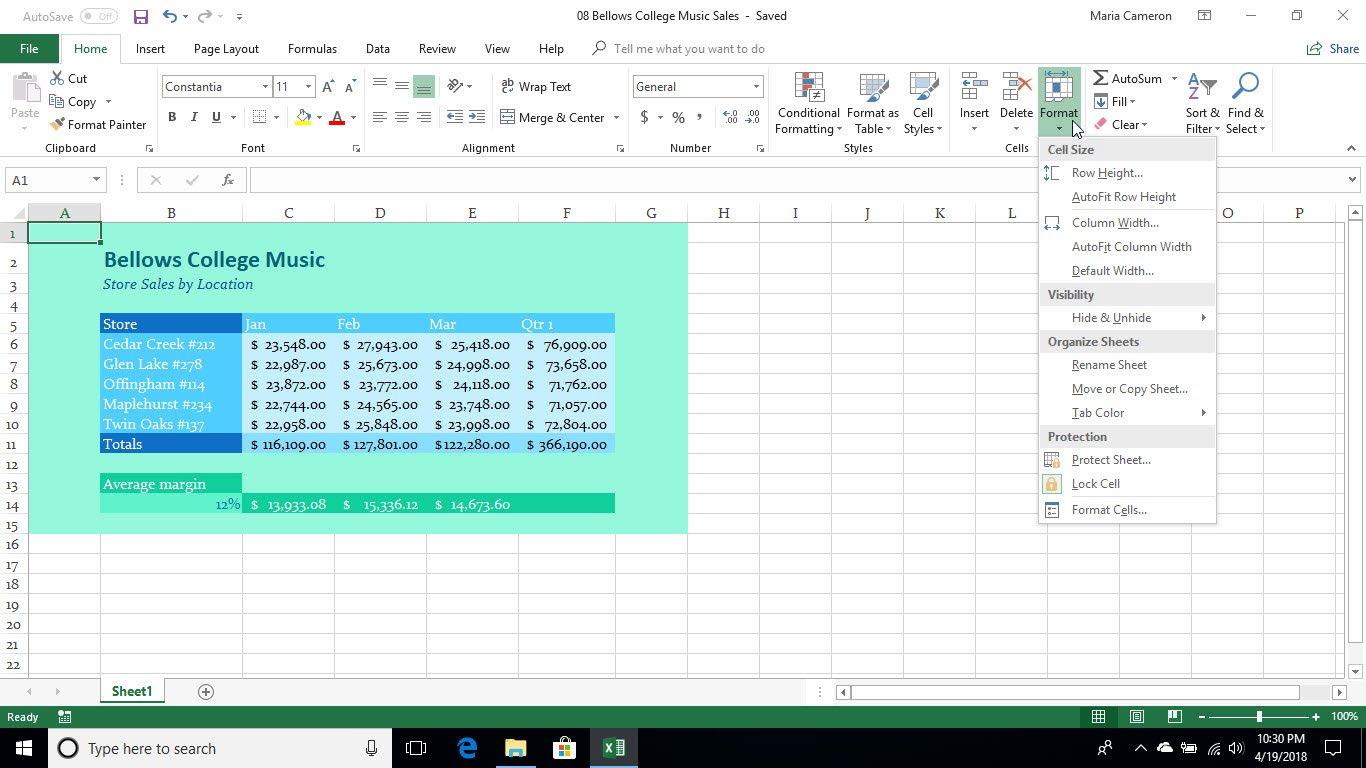
1. OPEN the 08 Spa Services workbook from the data files for this lesson. 2. SAVE the workbook as 08 Spa Services Week of 2-20 Solution in the lesson folder on your flash drive. 3. With the Monday worksheet active, click the Home tab, and in the Cells group, click
Format. 4. Click Move or Copy Sheet. The Move or Copy dialog box opens. Here, the Before sheet list shows the current sequence of worksheets in the workbook even if there’s only one.
The selected item represents the place you want to put the copied sheet in front of.
Figure 8-2
The Move or Copy dialog box
Figure 8-3
The updated Spa Services worksheet 5. In the Before sheet list, select (move to end). Next, select the Create a copy check box, as shown in Figure 8-2, and then click OK. A copy of the Monday worksheet is inserted at the end of the sequence, to the right of Lookup. The new worksheet is given the default name Monday (2).
6. Click the Monday worksheet tab. Next, click and hold the Monday tab and then press and hold Ctrl. The pointer changes from an arrow to a paper with a plus sign in it. 7. Drag the pointer to the right until the down arrow just above the tabs bar points to the divider to the right of Monday (2). Release the mouse button and Ctrl key. A new worksheet is created, with its tab located just to the right of where the down arrow was pointing. Its name is Monday (3). 8. With Monday (3) active, click cell B2 and type the date 2/21/2017. 9. Select cells B4:H9. 10. Beginning in cell B4, type the following data, skipping over cells without an “x” or a number (Figure 8-3):
Sarah 351 x x 0.5
Erin 295 x x x x 1
Catherine 114 x
Gail 90 x x x 1
Adriana 205 x x x x 1
Renata 34 x
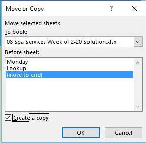
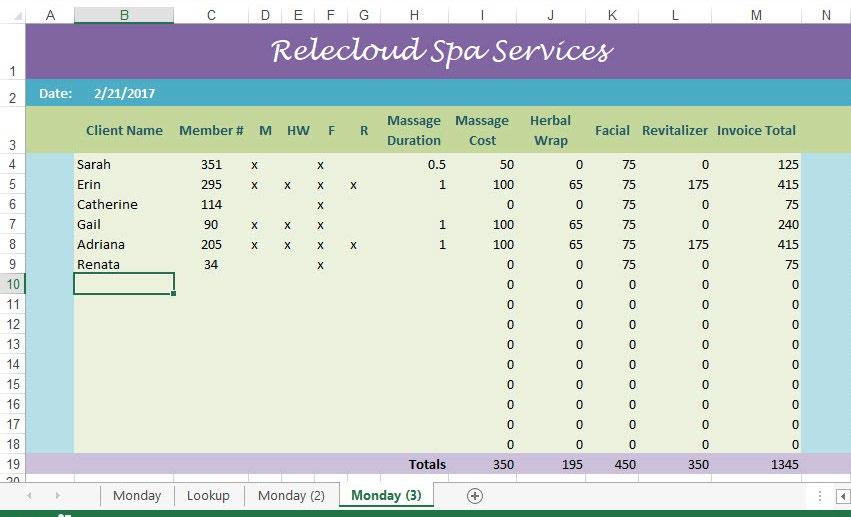
Figure 8-4
Copying a worksheet using the mouse PAUSE. LEAVE the workbook open to use in the next exercise.
When you need a new worksheet that has the styles, formatting, and formulas that work well in an existing worksheet, it’s easy to just copy the existing one and place it where it needs to go in the workbook. When it’s convenient, you should copy the existing one before you add data to it, but that’s not always possible. Your copied worksheet contains a duplicate of whatever data the existing one contains, but you can easily delete just the data without removing the formatting and formulas you wanted to copy in the first place.
In the preceding exercise, you used two methods to copy a worksheet. Excel gives each copied sheet a name, though probably just a temporary one with the name of the copied sheet followed by a number in parentheses, such as Monday (3). Selecting the Move or Copy Sheet command from the Format menu shows you a dialog box with all your options.
The second method is more of a shortcut, where you hold the pointer down over the worksheet tab while pressing Ctrl, and move the copied sheet to its new location. Figure 8-4 shows how the mouse pointer helps you by signaling to you symbolically that you’re copying a worksheet. You can use whichever method you prefer.
Worksheet copying mouse pointer
Renaming a Worksheet Excel gives a newly inserted or copied worksheet a temporary name, such as Sheet2, Sheet3, or Monday (2), as in the example. In the example, obviously we don’t want multiple Mondays, and the day for which you just entered transactions happens to be Tuesday.
STEP BY STEP Rename a Worksheet
GET READY. USE the 08 Spa Services Week of 2-20 Solution workbook that is open from the previous exercise. 1. Double-click the Monday (3) worksheet tab to select its name. 2. Type Tuesday and then press Enter. The new name appears on the tab. 3. Repeat this process for the Monday (2) worksheet tab, renaming it Wednesday. 4. With the Wednesday worksheet active, select cell B2 and type the date 2/22/2017. 5. Select cells B4:H11. 6. Beginning in cell B4, enter the following data, skipping over cells without an “x” or a number (Figure 8-5):
Rebecca 210 x Annie 44 x x x 1.5 Allison 191 x x x x 1 Michel 221 x x x 1 Julia 118 x x Yolanda 21 x x x x 1 Gwenael 306 x x x 1 Dorena P. 6 x x x x 1
Figure 8-5
The updated Wednesday worksheet

7. SAVE the workbook.
PAUSE. LEAVE the workbook open to use in the next exercise.
Repositioning the Worksheets in a Workbook If you were to hand a manila file folder full of key documents to your boss, the sequence of papers in that folder would be important. Your boss might be the type of person who reads the folder’s contents from top to bottom or in chronological order. The same principle applies to organizing worksheets in a workbook—place worksheets in chronological order, if applicable. If the workbook includes a Summary worksheet, it should typically be placed at the beginning of the sequence.
STEP BY STEP Reposition the Worksheets in a Workbook
GET READY. USE the 08 Spa Services Week of 2-20 Solution workbook that is open from the previous exercise. 1. Click the Tuesday worksheet tab. On the Home tab, in the Cells group, click Format. 2. Click Move or Copy Sheet. The Move or Copy dialog box opens. 3. To make sure Tuesday appears before Wednesday, in the Before sheet list, click
Wednesday and then click OK. 4. Click and hold the Lookup worksheet tab. The pointer changes from an arrow to a paper without a plus sign. 5. Drag the pointer to the right until the down arrow just above the tabs bar points to the divider to the right of Wednesday. Release the mouse button. The Lookup worksheet is repositioned at the end of the sequence, and nothing inside the worksheet itself is changed. 6. Click the Monday worksheet tab. 7. Select cells B4:H7. 8. Beginning in cell B4, enter the following data, skipping over cells without an “x” or a number:
Barbara Z. 15 x x x x 1 Rebecca 210 x x 1 Elly 301 x x Jennifer 213 x x x x 1
PAUSE. LEAVE the workbook open to use in the next exercise.
Take Note The worksheet displayed when you first open a workbook is whichever sheet was active when you last saved the workbook, regardless of where that sheet falls in the tab order.
Changing the Color of a Worksheet Tab In Excel, the “tabs” that denote the names of worksheets in a workbook don’t quite look like tabs in the real world. One feature that tabs have in the real world, especially when you use them to divide paperwork into folders, is color. If your business already uses color coding to denote categories of documents you’d find in the file cabinet or if you just need a splash of color to help you better distinguish worksheets from one another in a workbook, you can apply a color to each worksheet’s tab.
STEP BY STEP Change the Color of a Worksheet Tab
GET READY. USE the 08 Spa Services Week of 2-20 Solution workbook that is open from the previous exercise. 1. Right-click the Monday worksheet tab. 2. In the shortcut menu, click Tab Color. 3. In the popup menu, under Standard Colors, click Red. Excel applies a light red gradient to the Monday worksheet tab. 4. Click the Tuesday worksheet tab. Notice the Monday worksheet tab is now the bold red color you chose. Excel applies only the gradient tint to the tab for the active worksheet to make it stand out above the others. 5. Repeat the color selection process for the Tuesday and Wednesday worksheet tabs, choosing Orange and Yellow, respectively. 6. Click the Lookup worksheet tab. Your tabs bar should now appear as shown in
Figure 8-6.
Figure 8-6
Different colors applied to worksheet tabs
7. SAVE the workbook.
PAUSE. LEAVE the workbook open to use in the next exercise.
Take Note When you copy a worksheet whose tab has been given a color, that color is copied to the new worksheet along with its contents and formatting.
Hiding and Unhiding Worksheets Not every element of data in a workbook needs to be visible to every user. For example, many workbooks contain lookup tables and other auxiliary data. This type of data might need to be updated from time to time, but it doesn’t need to display to everyone using the workbook. For this reason, you can hide a worksheet and unhide it to work with it again. Hiding a worksheet does not make it confidential, because all worksheets are easy to unhide. Hiding simply gets stuff out of your way just as filing something away in a desk drawer keeps it out of sight.
STEP BY STEP Hide and Unhide a Worksheet
GET READY. USE the 08 Spa Services Week of 2-20 Solution workbook that is open from the previous exercise. 1. With the Lookup worksheet tab active, on the Home tab, in the Cells group, click
Format. 2. Click Hide & Unhide and then click Hide Sheet. The Lookup worksheet is no longer visible. 3. Click Format, click Hide & Unhide, and then click Unhide Sheet. The Unhide dialog box opens. 4. Make sure Lookup is selected in the Unhide sheet list and then click OK. The Lookup worksheet reappears and is active. 5. In the Lookup worksheet, select cell B3. 6. Type 70 and then press Enter. 7. Right-click the Lookup worksheet tab, and click Hide. The Lookup worksheet disappears again, although the change you made to one price is reflected in the other sheets that refer to it. 8. SAVE the workbook.
PAUSE. LEAVE the workbook open to use in the next exercise.
Take Note When a workbook contains hidden worksheets, the Unhide Sheet command is enabled in the Format > Hide & Unhide menu, and the Unhide command is enabled in the shortcut menu when you right-click any tab.
To hide several worksheets at the same time, display the first sheet you want to hide, hold down Ctrl and then click the tab for each additional sheet you want to hide. Then, right-click any of these tabs and click Hide in the shortcut menu. However, you can unhide only one worksheet at a time. You can right-click any visible tab and click Unhide to bring up the Unhide dialog box with the Unhide sheet list, where you choose a worksheet to make visible.
Inserting a New Worksheet into a Workbook In Excel, a new workbook contains only one worksheet. For most everyday tasks, you’ll be surprised how often you need more than one worksheet. You could keep adding worksheets forever, though in practice, you’ll find it easier to keep the number down to a handful. If your tasks become so complex that you need dozens of worksheets at a time, you might consider dividing sheets among multiple workbooks. Excel recognizes cell references that cross workbook boundaries, so your workbooks are not limited to worksheets that relate just to one another.
Figure 8-7
The Insert menu GET READY. USE the 08 Spa Services Week of 2-20 Solution workbook that is open from the previous exercise. 1. Click the Wednesday tab. 2. On the Home tab, in the Cells group, click the Insert drop-down arrow (Figure 8-7).
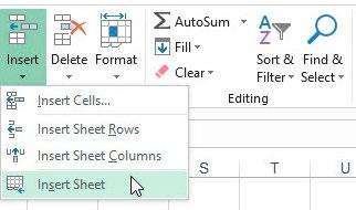
3. Click Insert Sheet. A new, blank worksheet is created, and its tab is inserted before the tab of the active sheet (Wednesday). Excel gives it a temporary name, beginning with
Sheet followed by a number. 4. Move the new worksheet to the end of the tab sequence. 5. Rename the new worksheet Survey. 6. Click the Wednesday worksheet tab again. 7. Click the New sheet (+) button to the right of the worksheet tabs. Another new worksheet is created with a temporary name, and this time, its tab is inserted after
Wednesday. 8. Rename this new worksheet Totals. 9. SAVE the workbook.
PAUSE. LEAVE the workbook open to use in the next exercise.
Deleting a Worksheet from a Workbook Removing a worksheet from a workbook is a simple process, at least up front. Any problems will likely come later, if you have to reconcile formulas that might have referred to data on the deleted sheet. Be certain the contents of a worksheet you’re about to delete are not referred to or required by any element inside another worksheet.
STEP BY STEP Delete a Worksheet from a Workbook
GET READY. USE the 08 Spa Services Week of 2-20 Solution workbook that is open from the previous exercise. 1. Click the Totals worksheet tab. 2. On the Home tab, in the Cells group, click the Delete drop-down arrow. 3. Click Delete Sheet. The Totals worksheet is removed and its tab disappears. 4. Right-click the Survey tab, and click Delete. The Survey worksheet is removed and its tab disappears. 5. SAVE the workbook.
PAUSE. LEAVE the workbook open to use in the next exercise.
Take Note Although Excel offers a reliable way to undo many of the things you do to workbooks by accident (press Ctrl+Z to step back over mistakes you made, for instance), you cannot undo the deletion of a worksheet from a workbook. To protect yourself against losing hours of work, save your workbook often and maintain backup copies. That way, if you do accidentally delete a worksheet, you can at least recover an older version from a saved file.
WORKING WITH MULTIPLE WORKSHEETS
One benefit of having multiple worksheets in a workbook that are based on the same form is that whenever data appears in the same cell or cells in each one, you can select them all, make changes to that data once, and have it reflected on all the sheets simultaneously. Excel doesn’t know in advance which worksheets look alike, or mostly alike, so you have to select them yourself first in order to group them. You know Excel has grouped sheets together when the word Group appears after the filename in the title bar. When Group is displayed, everything you type into one sheet in the group, or certain changes you make to one sheet in the group, is replicated to all the others in the group. To resume working with each worksheet individually, you need to ungroup the worksheets first.
You can view portions of several worksheets in a workbook simultaneously. This is handy when you need to make comparisons between the data that appears on these sheets. You don’t have to close one window and open the other, go back and forth, and rely on your memory to fill in the details of what isn’t displayed. In this exercise, you group a handful of worksheets together in preparation to make changes that affect all of them, and you arrange them onscreen to compare contents.
STEP BY STEP Work with Multiple Worksheets in a Workbook
Figure 8-8
Reformatted worksheet GET READY. USE the 08 Spa Services Week of 2-20 Solution workbook that is open from the previous exercise. 1. SAVE the workbook as 08 Spa Services Week of 2-20 Solution 2 in the lesson folder on your flash drive. 2. Right-click any worksheet’s tab and click Select All Sheets. The title bar now reads Spa
Services Week of 2-20 Solution 2 – Group. All visible worksheets are included in this group, whereas hidden worksheets are excluded. Although all the worksheets’ tabs are now boldface, the active worksheet name remains highlighted in green. 3. Select cells I4:M19. 4. On the Home tab, in the Number group, click Accounting Number Format. The cell formats for the range switch to a currency style where the dollar sign is aligned left, and the value is aligned right with two decimal places. Column K (Facial) is too narrow for its contents, so its values currently read #####. 5. Adjust the width of column K to fit its contents. 6. Select column M. 7. In the Font group, click Bold. All cells in column M are now boldfaced. Press
Ctrl+Home. 8. Click the tab for a worksheet other than the current worksheet. The worksheets are now ungrouped, but the changes you made to the previous sheet are reflected in all three worksheets, as demonstrated by the reformatted Tuesday worksheet in Figure 8-8.
9. Select the Monday worksheet. 10. Click the View tab, and then in the Window group, click New Window. A new Excel window opens, also containing the Monday worksheet. 11. With the new window active, select the Tuesday worksheet. 12. Click the View tab and click New Window again. Another window opens. 13. With this new window active, select the Wednesday worksheet. 14. Click the View tab, and then in the Window group, click Arrange All. The Arrange
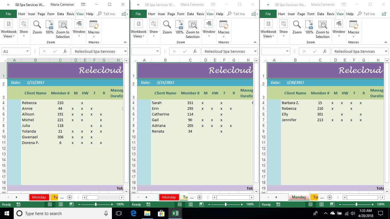
Windows dialog box opens. 15. In the dialog box, click Vertical and then click OK. Excel rearranges your three windows to appear as shown in Figure 8-9.
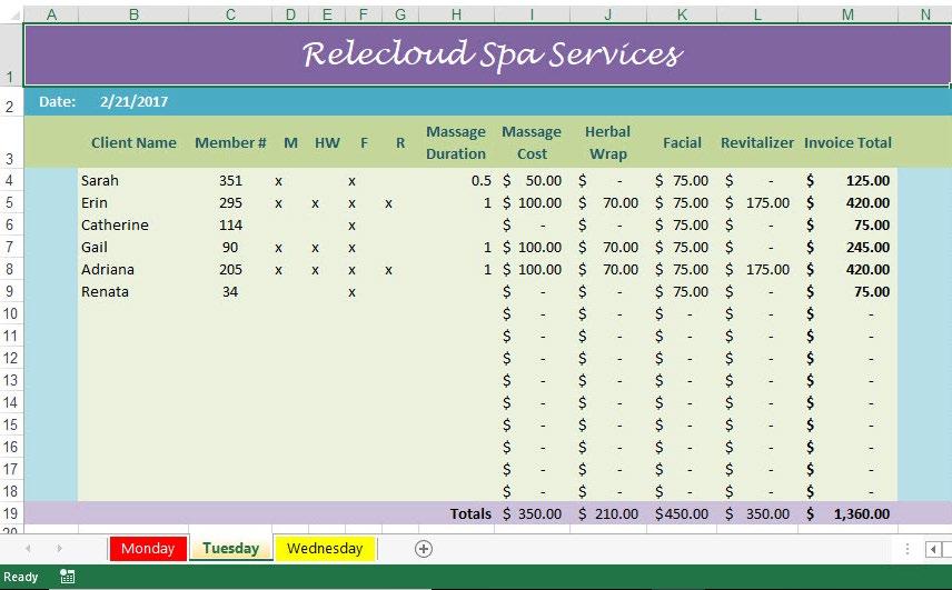
Figure 8-9
Vertically tiled worksheets
PAUSE. LEAVE the workbook open to use in the next exercise.
Suppose you grouped several worksheets together, as you learned previously. When you try to copy or cut data from any one worksheet in a group, Excel assumes you’re trying to extract that data from the entire group. So when you try to paste that data into a single, ungrouped worksheet— perhaps in another workbook—you can’t. The reason is because Excel expects the area to which you’re pasting data to be the same size as the cut or copied data, which in this case comes from multiple sheets. Now, if you try to paste into a group of worksheets that’s the same number as the cut or copied area comes from, you can complete the operation.
Take Note When there is too little space for all the visible worksheet tabs to appear in the tabs bar, as is the case in Figure 8-9, left and right scroll arrows appear next to one another in the lower-left corner of each window. Use these arrows to slide the tabs area left and right until you find the tab you’re looking for.
USING ZOOM AND FREEZE TO CHANGE THE ONSCREEN VIEW
Most of the time, Microsoft Windows tries to render the contents of a document such as an Excel worksheet at relatively the same size as it would appear if you printed it onto a piece of paper from your printer. That approximate size is what Excel calls “100%.” So, 50% magnification equals roughly half the size that your worksheet would appear if printed, whereas 200% equals twice the size. You can adjust or zoom this display magnification at any time to make contents easier for you to read, or to fit more contents onto the screen at one time, without impacting the size of the worksheet when you print it. When you save the workbook, Excel saves the magnification of each of its worksheets.
You’re familiar with a pane of glass on the window of your home. In some Windows applications, including Excel, a pane is a portion of a divided window. Many worksheets include one or more rows of cells as column labels. When you add a large amount of data to a worksheet, you can lose sight of these labels when you scroll down the worksheet. Excel gives you a way to freeze portions of a worksheet onscreen so that when you do scroll down, or even when you change magnification, you don’t lose track of which elements the labels refer to.
STEP BY STEP Use Zoom and Freeze to Change the Onscreen View
GET READY. USE the 08 Spa Services Week of 2-20 Solution 2 workbook that is open from the previous exercise. 1. Maximize the window displaying the Monday worksheet. 2. SAVE the workbook as 08 Spa Services Week of 2-20 Solution 3 in the lesson folder on your flash drive. 3. Select cell B4. 4. To increase magnification, click and hold the zoom control in the lower-right corner and drag the Zoom slider to the right (Figure 8-10). The maximum zoom is 400%. Notice the window zooms in on the selected cell.
Figure 8-10
Maximum zoom on a worksheet
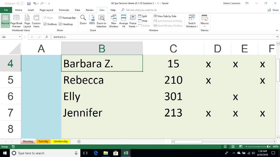
Figure 8-11
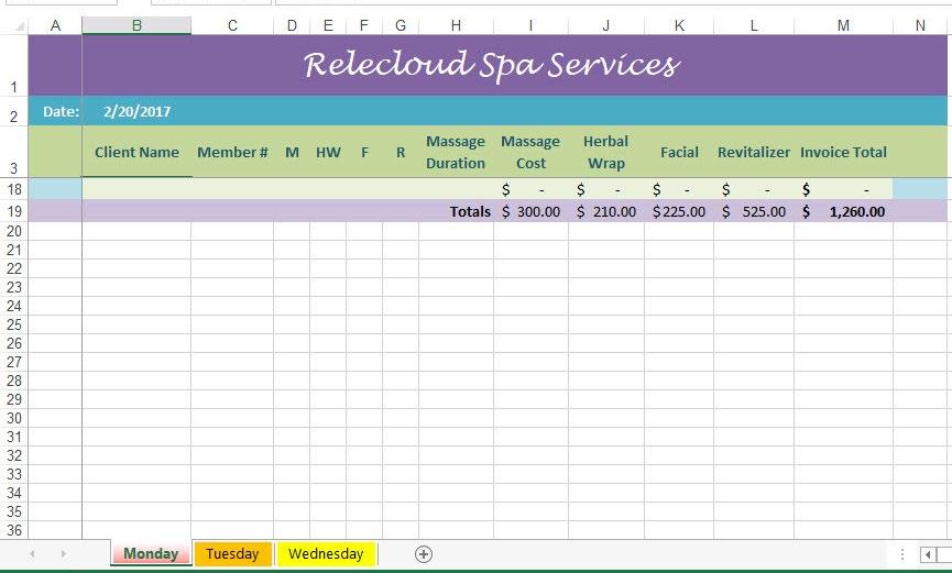
Worksheet with frozen panes 5. Click the View tab, and in the Zoom group, click 100%. The worksheet returns to standard magnification. Press Ctrl+Home to display the top of the worksheet again. 6. Select cell B4 again. On the View tab, in the Window group, click Freeze Panes and then click Freeze Panes in the menu. Cells above and to the left of the selected cell (B4) are now frozen in place for scrolling. 7. Scroll down so that row 19 comes close to the labels in row 3. Notice that rows 1 through 3 remain in place (Figure 8-11).
Vertical freeze line Horizontal freeze line
8. Press Ctrl+Home to scroll the worksheet to the top. On the View tab, in the Window group, click Freeze Panes and then click Unfreeze Panes. The thin lines denoting the frozen borders of the worksheet disappear.
PAUSE. LEAVE the workbook open to use in the next exercise.
If you’re accustomed to using the wheel of your mouse to scroll up and down, you can use the same wheel while holding down the Ctrl key to zoom in (up) and out (down) of a worksheet.
FINDING AND REPLACING DATA
If you’ve used a word processor before, such as Microsoft Word, then you’ve probably used the Find command, which locates a passage of text. And if you’ve written a letter or a memo, maybe you’ve used Find and Replace to change the spelling of a word throughout a document. Excel has a Find command and a Replace command that work similarly, only they navigate through cells instead of paragraphs.
Locating Data with the Find Command With Excel, you can use the Find command to search for text you’ve entered as data, such as a person’s name, as well as values that happen to be the results of formulas. That’s important, because if you’re certain that $10,000 comes up in a cell someplace but you’ve never typed those digits into the system directly, you can still find it, even if it’s the result of a formula.
Take Note The Find command does not match contents in a hidden worksheet.
STEP BY STEP Locate Data with the Find Command
Figure 8-12
Using the Find and Replace dialog box GET READY. USE the 08 Spa Services Week of 2-20 Solution 3 workbook that is open from the previous exercise. 1. Select the Monday worksheet. Select cell B4. 2. Click the Home tab, and then in the Editing group, click Find & Select. Click Find. The
Find and Replace dialog box opens. 3. In the dialog box, click Options. The dialog box expands. 4. Click the Within drop-down arrow, and in the drop-down list, click Workbook. 5. Click the Look in drop-down arrow, and in the drop-down list, click Values. 6. Click the Find what text box, delete any contents that might appear there, and type
Annie. Click Find Next. The workbook window moves to the Wednesday worksheet, and automatically selects Annie in cell B5. Meanwhile, the dialog box remains open, as shown in Figure 8-12.

Figure 8-13
The Find and Replace dialog box after using Find All 7. Double-click the Find what text box, press Delete, and then type Becca. Click Find
Next. Excel highlights cell B4, whose contents include “becca” within the cell entry, and in a non-matching case. 8. Select cell B5. 9. In the Find and Replace dialog box, click Match case and then click Find Next. This time, Excel reports the text can’t be found, because it’s looking for the name Becca that begins with a capital “B.” Click OK to dismiss the message. 10. Double-click the Find what text box, press Delete, and then type 420. Click Find All. The dialog box shows a detailed report listing all the cells in the workbook that contain the value 420. In this case, it points to all the locations where customers paid “the works” for all the services together. You can use the scroll bars or drag the lower-right corner of the dialog box to display all the data, as shown in Figure 8-13.
11. Click the first item in the list whose Sheet entry is marked Tuesday. Excel displays the
Tuesday worksheet and selects cell M5, which contains an entry for $420.00. 12. Click Close to dismiss the dialog box. 13. CLOSE two of the open workbook windows. Maximize the remaining window, if necessary. SAVE the workbook.
PAUSE. LEAVE the workbook open to use in the next exercise.

Troubleshooting When you choose the Match entire cell contents option in the Find and Replace dialog box, Excel skips over cells whose contents do not match the text in the Find what box in their entirety. For instance, in this case a search for “Dorena” would skip the cell containing “Dorena P.” if the Match entire cell contents option is checked.
Replacing Data with the Replace Command The functions for finding and for replacing text are located in the same dialog box, even though Excel gives you two ways to bring it up. You might have already noticed the Find tab at the top of the Find and Replace dialog box. The Replace tab is next to it. The Replace command differs from Find only in one important respect—it adds a text box for the contents you intend to insert in place of any matches Excel finds. This way, if you misspell a name throughout a workbook, you can correct it once and have that correction be reflected everywhere.
GET READY. USE the 08 Spa Services Week of 2-20 Solution 3 workbook that is open from the previous exercise. 1. Select the Wednesday worksheet. Select cell B4. 2. On the Home tab, in the Editing group, click Find & Select. Click Replace in the menu.
The Find and Replace dialog box opens. 3. Make sure the dialog box is expanded and that Workbook is the selected option for
Within. 4. If the Find what text box shows the contents of the previous search, then double-click the text box and press Delete to erase its contents. 5. Click in the Find what text box and type Michel. 6. Click in the Replace with text box and type Michele. The dialog box should now appear as shown in Figure 8-14.
Figure 8-14
The Find and Replace dialog box with the Replace tab displayed

7. Click Replace All. Excel searches for all instances of Michel and adds an “e” to the name (correcting this client’s spelling) and then notifies you when the job is done.
Excel makes one replacement. 8. Click OK and then click Close. 9. SAVE the 08 Spa Services Week of 2-20 Solution 3 workbook and then CLOSE the workbook.
STOP. CLOSE Excel.
Troubleshooting Use Replace All only when you are certain you need to replace every instance of a passage of text or an item of data. There will be times when you need to replace only some instances but not all of them.
Knowledge Assessment
Multiple Choice
Select the best response for the following statements.
1. Which of the following procedures is not a way to delete one or more worksheets from a workbook? a. Right-click a worksheet tab and click Delete. b. Press Ctrl+A to select all cells in the worksheet and then press Delete. c. Click the Delete drop-down arrow on the Home tab and click Delete Sheet. d. Select a group of worksheets, right-click the group, and click Delete. 2. Which of the following statements about hidden and unhidden worksheets is correct? a. Unhidden worksheets cannot contain formulas that refer to hidden worksheets. b. When you click Find All, the Find and Replace dialog box will show matched contents within hidden worksheets as well as unhidden ones. c. A hidden worksheet cannot be inadvertently deleted. d. Excel creates a minimized window for each hidden worksheet. 3. Which of the following statements describes a reason as to why you would need to copy a worksheet within a workbook? a. It’s the easiest way to make a backup before making changes. b. It lets you reuse formats and formulas in a new sheet. c. It helps Excel learn where your data ranges are located. d. You should keep one worksheet hidden in case of an error. 4. To zoom out of the worksheet and display twice the amount of worksheet data for any given area of the screen, which of the following Zoom settings should you choose? a. 200% b. 120% c. 75% d. 50% 5. Which of the following statements describes how to change the color of a worksheet tab? a. On the Page Layout tab, in the Themes group, select Colors. b. Right-click the tab and select Tab Color. c. Use the Fill Color tool on the Home tab. d. You cannot change the color of a worksheet tab. 6. Which of the following steps is a method for hiding a single worksheet in a multi-sheet workbook? a. On the View tab, in the Window group, click Hide. b. Select the visible area of the worksheet. c. Right-click the worksheet’s tab and click Hide. d. Enter the name of the worksheet in the Hide dialog box. 7. Which of the following steps is not a method for inserting a worksheet into a workbook? a. Click the New sheet (+) button to the right of the worksheet tabs. b. On the Home tab, click Insert and then click Insert Sheet. c. On the Insert tab, click Worksheet. d. Right-click a worksheet tab and click Insert, then click Worksheet and click OK. 8. In order for you to freeze the first column of a worksheet into a frozen pane: a. All data in the column must be visible. b. The first row of the column must be non-blank. c. Duplicate worksheets must also be able to have their first columns frozen. d. You can click Freeze First Column in the Freeze Panes menu.
Projects
9. When you create a copy of an existing worksheet named August, Excel gives that worksheet which of the following names? a. September b. August (2) c. Sheet2 d. July 10. When you click the New sheet (+) button on the tabs bar, where is a worksheet always inserted? a. At the beginning of the tabs sequence b. Before the active worksheet c. After the active worksheet d. At the end of the tabs sequence
Project 8-1: Copying and Modifying a Worksheet
You are performing accounting tasks for a chain of sheet music and collectable CD stores. In this project, you will rename a worksheet, use the Name Box to select a cell range, and copy an existing Quarter 1 worksheet that you modify to enter Quarter 2 sales.
GET READY. LAUNCH Excel.
1. OPEN the 08 Bellows College Music Sales workbook from the data files for this lesson. 2. SAVE the workbook as 08 Bellows College Music Sales Solution in the lesson folder of your flash drive. Maximize the window, if necessary. 3. On the Home tab, in the Cells group, click Format. Click Rename Sheet. 4. Type Q1 and then press Enter. 5. Click Format again and then click Move or Copy Sheet. 6. In the Move or Copy dialog box, click (move to end), click Create a copy, and then click
OK. 7. Rename the Q1 (2) sheet as Q2. 8. In the Q2 worksheet, select cell C5. 9. Delete the text Jan and replace it with Apr. 10. Use AutoFill to change the next two months’ column headings, and then in cell F5, change Qtr 1 to Qtr 2. 11. Click the Name Box and then enter the cell reference C6:E10. Press Enter and then press Delete. 12. For the months in the second quarter, enter the following values:
$22,748.00 $21,984.00 $20,194.00 $22,648.00 $21,068.00 $21,698.00 $24,971.00 $23,498.00 $23,011.00 $23,400.00 $24,681.00 $23,497.00 $21,037.00 $20,960.00 $19,684.00
13. If necessary, adjust column widths so that the entries are legible.
PAUSE. SAVE and CLOSE the workbook. LEAVE Excel open for the next project.
Project 8-2: Renaming Worksheets, Unhiding a Worksheet, and Arranging Windows
You’re helping a photo development kiosk at a local office supplies store to keep track of the extra sales its employees have to produce in order to keep a development shop open in the digital camera era. In this project, you will rename worksheets, unhide a hidden form worksheet, arrange windows onscreen, and make changes.
GET READY. LAUNCH Excel if it is not already open. 1. OPEN the 08 Photo Weekly Product Tracker workbook from the data files for this lesson. 2. SAVE the workbook as 08 Photo Weekly Product Tracker Solution in the lesson folder on your flash drive. 3. Click the Sheet1 worksheet tab. 4. On the Home tab, in the Cells group, click Format. In the menu, click Rename Sheet. 5. In the worksheet tab for Sheet1, type Kelly (the first name of the sales associate in cell
A7) and then press Enter. 6. Repeat this process for the sales associates in Sheet2 and Sheet3. 7. On the Home tab, in the Cells group, click Format. In the menu, click Hide & Unhide, and click Unhide Sheet. 8. In the Unhide dialog box, select Form and click OK. 9. With the Form sheet active, click Format again and then click Move or Copy Sheet. 10. In the Move or Copy dialog box, in the Before sheet list, click Form. Click Create a copy.
Click OK. 11. Click cell A6. Type the name Sanjay Jacob. 12. Edit cell B4 to reflect the date shown in the other worksheets. 13. Rename the Form (2) worksheet Sanjay. 14. Right-click the Form tab. Click Hide. 15. In the Sanjay worksheet, select cells B8:H12 and type the following values for each of the days shown in the following table, skipping blank cells as indicated:
Sunday Monday Tuesday Wednesday Thursday Friday Saturday 2 3 4 2 10 1 2 6 4 2
400 3 4 75 150
200 2 1 2
16. Select the Kelly worksheet. 17. Click the View tab, and then in the Window group, click New Window. 18. In the new window, select the Erik worksheet. 19. Again, on the View tab, in the Window group, click New Window. 20. In the new window, select the Janet worksheet. 21. Once again, on the View tab, in the Window group, click New Window. 22. In this new window, select the Sanjay worksheet. 23. In the Sanjay worksheet, on the View tab, in the Window group, click Arrange All. 24. In the Arrange Windows dialog box, click Tiled. Click Windows of active workbook.
Click OK. 25. SAVE the 08 Photo Weekly Product Tracker Solution workbook and then CLOSE all four workbook windows.
STOP. CLOSE Excel.


