Semi-airborne electromagnetic exploration using a scalar magnetometer suspended below a multicopter

Michael Becken1*, Philipp O. Kotowski1, Jörg Schmalzl1, Gregory Symons2 and Klaus Braunch3 demonstrate the use of an optically pumped magnetometer (OPM) suspended below an UAV to measure scalar EM responses.

Abstract Semi-airborne electromagnetic (EM) techniques offer the opportunity to combine lightweight airborne receivers mounted on unmanned aerial vehicles (UAV) with high-moment transmitters on the ground. Owing to their low flying speed, UAVs facilitate recordings of low-frequency signals, which is beneficial for the exploration of deeply seated mineral deposits or other geological targets. However, noise from the electrical components of the aircraft as well as motional noise pose limits on the signal-to-noise ratio at far offsets from the transmitter. Here, we demonstrate the use of an optically pumped magnetometer (OPM) suspended below an UAV to measure scalar EM responses in the frequency range from 1-256 Hz that is nearly unaffected by motional noise. The responses can be identified with the component of the EM signal in the direction of the geomagnetic field, and they can be inverted into resistivity using available software solutions. We illustrate the technique using field data from the Hope deposit, Namibia. Two-dimensional inversion models image the mineralization zone with remarkable resolution from the surface to about 300 m depth, in good agreement with results from previous exploration. This field example suggests that the method is efficient for exploring conductive mineral deposits at depths of several hundred meters.

Introduction There is a strongly increasing demand for efficient geophysical exploration technologies that can directly or indirectly characterize deeply seated mineral deposits (e.g., Ali et al., 2017). Among the geophysical exploration methods, airborne electromagnetics (AEM) is a widely used method to delineate non-magnetic ore bodies. AEM is, however, limited in depth penetration and relies in most cases on one-dimensional interpretations or simplified plate-models.

An approach to increase exploration depths is the semi-airborne EM method. Semi-airborne EM uses ground-based transmitters to induce eddy currents in the conductive subsurface and measures the induced EM field using a passive airborne receiver (e.g., Seigel, 1979; Elliot, 1996; Mogi, 1998; Smirnova et al. 2019; 2020; Becken et al., 2020). The recorded secondary fields can be converted into the electrical resistivity distribution of the subsurface by means of two-dimensional (2D) or three-dimensional (3D) inversion (e.g., Smirnova et al., 2019; 2020). As with other airborne EM methods, semi-airborne EM is primarily sensitive to conductive anomalies embedded within resistive background and is thus suited to detect interconnected conductive phases such as massive sulphide deposits.

Because semi-airborne EM systems only need to tow a passive receiver in the air, this approach is also ideally suited for lightweight unmanned aerial vehicles (UAVs; e.g. Stoll et al., 2019). In a recent contribution, Kotowski et al. (2021) successfully demonstrated the efficiency of a UAV-based system for semi-airborne EM application. Here, miniaturized induction coil sensors were utilized to measure the vector components of the induced EM field at frequencies above 30 Hz. The test survey was carried out in a sedimentary environment near Merfeld, NW-Germany, employed 1-2 km-long grounded electric dipoles, achieved a total airborne coverage of about 10 km2 and imaged the top of a highly saline aquifer at 100-300 m depth.

In this contribution, we describe a realization of the semi-airborne EM method to a mineral exploration target. In contrast to Kotowski et al. (2021), we employed an optically pumped magnetometer (OPM) suspended below a multicopter. The OPM is a Geometrics MagArrow magnetometer specifically designed for UAV applications. It measures the scalar total magnetic intensity (TMI) at a rate of 1000 Hz with a bandwidth of 400 Hz.

An OPM has two important advantages compared to induction coil sensors. Firstly, the OPM has no lower sensitivity limit on the frequency and is thus useful for deep exploration objectives. Secondly, scalar magnetometers are not susceptible to motional noise, which is the dominant noise in airborne EM data at low frequencies. Considering a UAV as a carrier, low flight speeds can be realized, which enable good spatial resolution at low frequencies, i.e., the low flying speeds reduce the spatial averaging length in data processing, which is inherent to the analysis of data obtained with moving platforms.

1 Institute of Geophysics | 2 Gregory Symons Geophysics | 3 terratec Geophysical Services * Corresponding author, E-mail: michael.becken@uni-muenster.de DOI: 10.3997/1365-2397.fb2022064

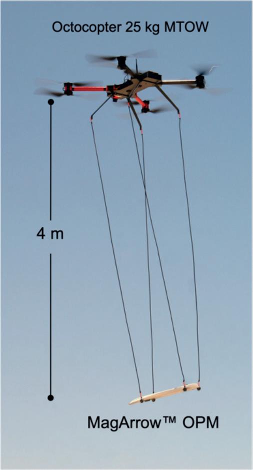
Figure 1 The employed UAV is an octocopter developed by MGT/Arealis, Germany. It has a maximum take-off weight of 25 kg. The MagArrow bird has been suspended 4 m below the UAV; it integrates two miniaturized OPMs, a compass, GPS and a MEMS inertial measurement unit; the total weight of the bird is 1 kg. Flight endurance in this setup is about 40 min.

Conceptually, the use of scalar magnetometers for EM applications has been proposed by Avdeev et al. (1997) in the context of deep crustal sounding and by Cattach et al. (1993) in the context of deep mineral exploration and is thus well established. In combination with the availability of cheap and flexible multi-copter UAV and modern lightweight TMI sensors, this approach may become more widely applicable for practitioners due to its relative ease of use and efficiency.

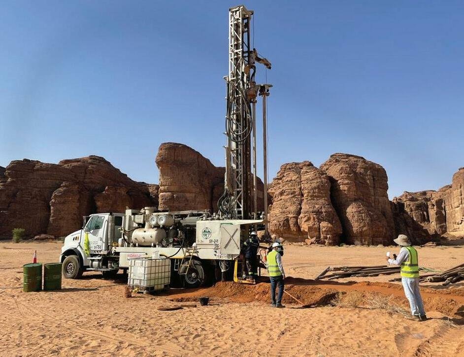
A test has been performed at a well-known but unexploited massive sulphide deposit in Namibia. The Hope ore body is located in west-central Namibia and associated with the Matchless amphibolite belt (Killick, 2000). Previous ground and airborne geophysical surveying, including various EM techniques, and extensive drilling has identified a conductive horse-shoe-shaped Cu-Zn ore body that extends in the East-West direction by at least 3 km and which is plunging from a surface outcrop to at least 400 m depth. It is thus a suitable target to test for the detection capabilities of a UAV-based semi-airborne EM system.

In this paper, we describe the principles of the semi-airborne EM approach using a scalar magnetometer, illustrate the method with 1D and 2D synthetic examples, and describe and discuss the data and models obtained for the Hope deposit, Namibia.

Methods Semi-airborne electromagnetics There are significant differences between semi-airborne EM and AEM methods. As opposed to AEM systems that rely on transmitter loops towed by the aircraft, semi-airborne EM can utilize both inductively coupled loops or galvanically coupled electric dipole transmitters on the ground. The geometry of eddy currents in the ground and their spatial decay away from a grounded dipole transmitter is substantially different than for currents induced with a loop transmitter. Consequently, the sensitivity pattern to subsurface structures as well as the footprint of a single transmitter are different for the two transmitter types. For instance, eddy currents below loop transmitters are primarily horizontal circular current loops and thus sense layered conductors with good resolution, whereas with extended grounded transmitters, current concentrations within laterally extended conductors oriented parallel to the transmitter spread can be efficiently excited.

Depth penetration of EM fields generally depends on both frequency of the signal and distance between transmitter and receiver. Using fixed transmitter-receiver geometries as in AEM, the depth penetration is controlled by frequency (or decay time) only. In semi-airborne EM applications, multiple spatially separated transmitters with overlapping footprints (operated sequentially and with flight-lines overlapping by 50% or more) are combined to yield multiple transmitter-receiver geometries for each receiver point. In this way, semi-airborne EM takes advantage of both frequency and geometry variations. In summary, combining broad-band signals with both short and large offsets in a semi-airborne EM arrangement provides good spatial coverage in combination with good depth resolution. The resulting maximum exploration depths can exceed those of classical AEM systems, and the method can yield better spatial coverage than that of pure ground operations.

The computational load for numerical 2D or 3D simulations or inversions scales either with the number of receivers or transmitters. In AEM, the number of transmitter and receiver locations is identical and typically in the order of several thousands; therefore, full 3D inversion remains a tremendous computational task and is not included in standard workflows. Since semi-airborne EM uses only a small number of transmitters (say, below ten transmitter locations), full 3D inversion becomes tractable (e.g., Smirnova et al., 2019). In this work, we use 2D inversion, but forthcoming analyses will employ full 3D inversion.

Generally, semi-airborne EM data can be interpreted in time or in frequency domain. We use a frequency domain approach that relates the recorded field component to the transmitter current at the excited frequencies (Becken et al., 2020). We record both the current waveform and the received fields with GPS-synchronized data loggers and transform the time series to spectral domain for statistical processing. Both 50% and 100% duty cycles are feasible as the source signal. In practice, we use a 100% duty cycle rectangular current waveform and evaluate the responses at the fundamental frequency and all recorded harmonics. Typically, harmonics are binned to about seven estimation frequencies per decade, and about three frequency decades can be evaluated for a good transmitter waveform with short current turn-off and tune-on times.

Scalar EM responses The dominant source of noise in airborne EM is motional noise, which is due to rotations of the sensitive axes of vector magnetometers within the geomagnetic main field (e.g., Becken et al., 2020). In turn, scalar magnetometers, such as OPM, yield the rotationally invariant TMI. Therefore, rotations of a scalar magnetometer have a negligible effect on data quality unless the optical sensor axis enters the dead zone, a sensor orientation where no meaningful signal is provided. This makes these sensors in principle very well suited for airborne EM applications. Here, we use the Geometrics MagArrow system, a Cs-magnetometer

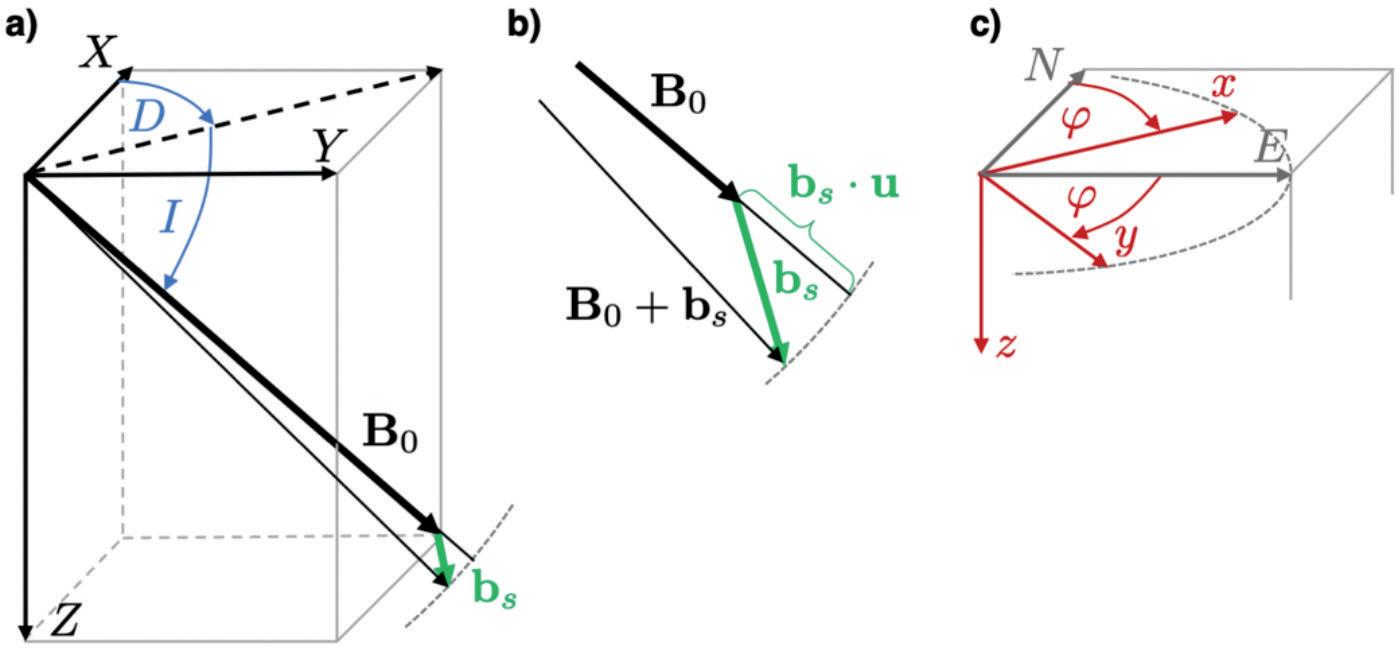
Figure 2 Coordinate frames. a) Geomagnetic main field vector B0 = (X,Y,Z)T with declination D and inclination I, defined in a geographic frame. The EM signal vector bS superposes on the main field but leaves its direction nearly unchanged. b) Zoom into panel a. The magnitude of the vector sum | B0 + bS | is approximated by its projection onto the direction of the main field, B0 + bS · u. c) Clockwise rotation of the modelling or measurement frame by an angle φ out of the geographic frame.

that has been miniaturized for UAV operations (c.f. Figure 1). The MagArrow offers a bandwidth of about 400 Hz and a noise level of and it is an excellent compromise between sensor specifications and payload.

The use of a scalar magnetometer for EM applications is based on the principle that the recorded time-varying scalar magnetic flux, which we denote as bS(t) , can be identified with the component of the EM signal vector bS(t) projected in the direction u(D, I) of the geomagnetic main field, B0 = B0u , where D and I are the local declination and inclination. The projection is valid under the assumption that the strength of the main field is much larger than the EM signal, which is generally true. It means that the component bS is oblique and has a well-defined direction u (cf. Figures 2a,b; see also Avdeev et al, 1997; Yang and Oldenburg, 2015).

Any signal measured with a scalar magnetometer can thus be conceived as a linear combination of the three vector components in geographic coordinates and depends on the local declination and inclination. For example, at high latitudes and near-vertical inclinations bS is close to the vertical component, whereas at equatorial latitudes (near-horizontal inclinations) bS approaches the geomagnetic northward horizontal component (i.e., the direction of declination). This also implies that at equatorial latitudes, the method is weakly sensitive to conductivity anomalies elongated in the direction of declination, because the induced excess currents are associated with anomalous magnetic fluxes polarized in the perpendicular direction. No such limitations are obvious at higher latitudes.

As with conventional vector magnetic observations, we process the TMI time series into frequency domain response functions. The final data are the complex-valued transfer functions ϐS(ω), estimated statistically from the linear relation

BS(ω) = ϐS(ω) I(ω)

where BS(ω) and I(ω) are spectral estimates of the recorded (scalar component of) magnetic flux density and the transmitted current.

Validation using field data To validate the UAV semi-airborne EM setup with a scalar magnetometer, a test measurement was carried out at the Merfeld site, NW Germany. At the test site, previous UAV-based semi-airborne EM measurements using induction coil magnetometers are available for comparison (Kotowski et al., 2021). Scalar responses were obtained for a single grounded electric dipole transmitter of about 2.3 km length; the transmitter was a Metronix 22 kW TXM22. A 100% duty cycle rectangular waveform with a fundamental frequency of 1 Hz and a current of ±15A was injected.

Firstly, the MagArrow was flown at a height of ~40 m above a ground station equipped with a Metronix SHFT02e induction coil triple attached to a Metronix ADU08e data logger. From the recorded time series, amplitude and phase response functions were derived in frequency domain from both the scalar MagArrow readings during the overflight and the vector induction coil readings on the ground (cf. Figure 3a). The scalar responses were truncated at frequencies above 400 Hz, and the vector responses were truncated below 32 Hz. In the overlapping band between 32 Hz and 400 Hz, both sensors are sensitive.

To facilitate a comparison, the induction coil response estimates (coloured symbols in Figure 3a) were rotated horizontally in the direction of the local declination and vertically into the direction of the local inclination. Then, the component of the rotated data that is aligned with the direction of declination and inclination (open black symbols) corresponds to the component recorded with the scalar magnetometer (solid black symbols).

We observed a discrepancy in time stamps between the two time-series. This is likely to be due to different GPS boards and filters in the two data loggers, and due to different internal time handling. However, repeated runs showed that the delay was constant. We estimated the delay to be –3.746 ms by matching the time series and the phase responses and applied a corresponding frequency-dependent correction factor to the scalar response. We also observed a slight offset in amplitudes between the two systems; this can however be explained with the altitude difference between the airborne MagArrow and the ground-based SHFT02e sensor.

In Figure 3b, we show a comparison between the scalar responses (solid black symbols) and the induction coil responses projected in the direction of the local geomagnetic field (open black symbols) at a frequency of 32 Hz. The time correction factor determined from the ground station overflight was applied to the scalar responses. It is seen that at offsets greater than 1000 m (or amplitudes less that 10–2 nT/A), the induction coil response exhibits scatter whereas the OPM data still decays smoothly, suggesting better signal-to-noise ratio at this frequency. The

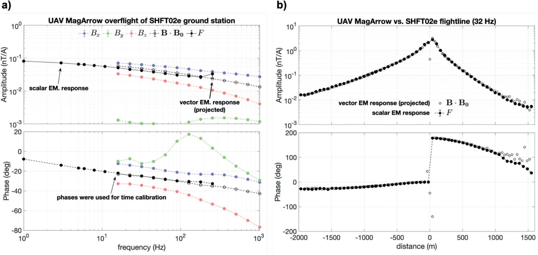
Figure 3 Comparison of scalar and vector UAV semi-airborne EM response functions. a) Results from an overflight of the MagArrow over a ground station equipped with SHFT02e induction coils. Solid black symbols show response estimates obtained from the scalar data; coloured symbols show responses for vector components, and open black symbols are estimated from vector responses by rotation into the declination and inclination directions. b) Comparison of scalar and rotated vector responses along a coincident flight line. See text for details.

Figure 4 1D test model. a) Synthetic measurement geometry. Red line depicts a 2km-long horizontal electric dipole (HED) transmitter; filled circles sketch the locations of 5km-long flightlines centred at the transmitter. The geometry is rotated by φ = 68° eastward from geographic north. b) Parameters of the layered Earth model.

results of the comparison strongly suggest that both setups yield consistent data.

Synthetic model study 1D layered Earth responses In this work, we use the 2D modelling and inversion software Mare2DEM (Key, 2016). Generally, modelling (or measurement) frames must not be aligned with the geographic frame. Particularly in 2D scenarios, the modelling frame should be aligned with the geoelectric strike direction.

Let us therefore assume that the modelling (or local measurement) coordinate system is horizontally rotated out of geographic north by an angle φ (c.f. Figure 2c). Because the scalar component bS is invariant with respect to coordinate transformations, the projection on the main field direction in the φ-rotated frame is obtained by substituting the declination D with D – φ. Given the local declination and inclination of a measurement area, and a φ-rotated modelling coordinate frame, it is thus simple to model the field component recorded by a scalar magnetometer with any existing modelling tools that can predict the EM field in cartesian components. Mare2DEM can readily account for arbitrary receiver rotations. We thus take the rotated receiver z-axis to align with the main field direction (in the modelling frame) and take this component as the observed component (see also Figure 2 for coordinate axes directions).

To test the approach and to verify the 2D code, we first compare the synthetic responses obtained with Mare2DEM for a layered half-space model with the modelling result using our own 1D modelling code, which is based on a quasi-analytical solution expressed as Hankel transforms of wavenumber components (e.g., Streich and Becken, 2011). Figure 4a depicts the hypothetic survey geometry and Figure 4b shows the layered resistivity model used in this exercise. The modelled transmitter is a 2km-long grounded electric dipole aligned with the x-axis, and responses are simulated along two parallel, 5km-long flight-lines aligned with the y-axis. The layered Earth model is composed of a shallow layer of moderate resistivities (50 Ωm) and a 100m-thick conductive layer (5 Ωm) at 500 m depth, embedded within a resistive background (500 Ωm). For the modelling, we used D = –13°28' and I = –64°51’, and a modelling frame rotated clockwise by φ = 68° (see inset in Figure 4a), mimicking the field data reported later in this paper.

Figure 5 displays a comparison of simulated response functions along both flightlines and for three different frequencies (1 Hz, 10 Hz, 100 Hz) using the 1D modelling code and the 2D

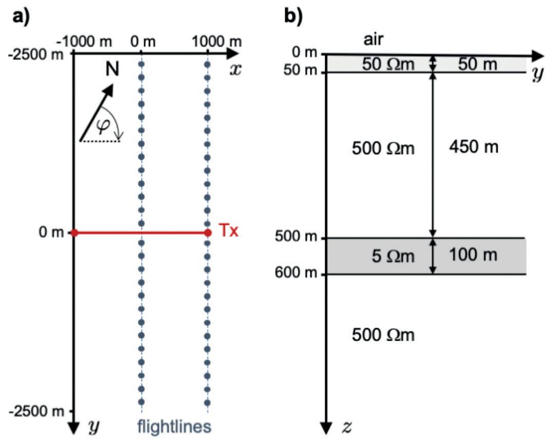
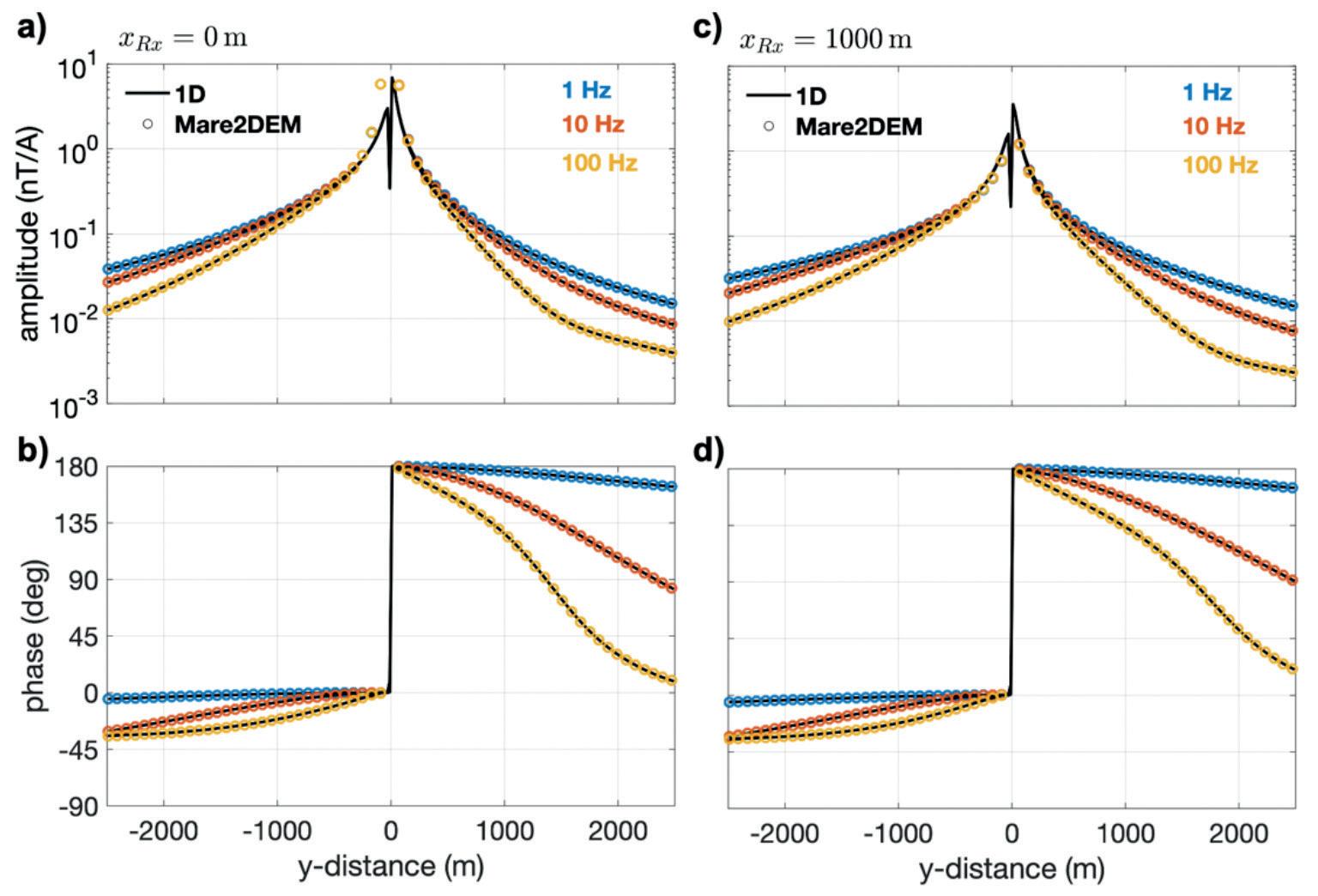
Figure 5 Comparison of 1D model responses of the scalar transfer function B s(ω) for a flightline across the centre of the transmitter (panels a, b) and across one pole of the transmitter (panels c, d). We depict the responses in terms of amplitude (a, c) and phase (b, d) and for frequencies of 1 Hz (blue), 10 Hz (red) and 100 Hz (yellow), respectively; black solid lines show the results using a 1D quasi-analytical solution and coloured open dots depict the results of the 2D modelling code Mare2DEM from Key (2016).

Figure 6 2D synthetic inversion test. a) Noisecontaminated scalar amplitude and b) Phase responses (symbols) simulated for a synthetic model, and responses of the inversion model (solid lines) for four transmitters Tx0-3 for a frequency of 8 Hz. c) Inversion model, with the true model parameters superimposed. The inversion achieved a normalized r.m.s. misfit of 1.0. The main features of the true model can be recovered.

Mare2DEM code. Both codes show matching results, suggesting good numerical accuracy and correct treatment of coordinate rotations. Discrepancies are evident near the transmitter and are due to numerical inaccuracies in the 2D solution. Therefore, for inversion, we exclude data within ±300 m from the transmitter. Note also that the responses are not symmetrical with respect to the transmitter. This is a consequence of the mixing of the vertical and horizontal components that determine the oblique component in the direction of the main field.

2D synthetic inversion test We also tested the capability of the method to resolve elongated conductive zones at depth with a synthetic model study. We constructed a 2D synthetic model that contains a horizontal conductive tube (infinitely extended in the x-direction) at 400 m below surface embedded within a resistive background. To increase model complexity, we added a layered background structure including a thin conductive overburden (Figure 6c).

The model mimics the situation at the Hope deposit, Namibia. We employed realistic transmitter-receiver geometries and included topography. Four transmitters were modelled; they are oriented in the x-direction, 2 km in length and separated in the y-direction by approximately 1 km; flightlines are oriented in the y-direction. Forward modelling was carried out to predict the scalar responses in the frequency range from 1 Hz to 256 Hz along a flightline approximately across the centres of all four transmitters (denoted as the line 6) and for the local declination and inclination valid at the Hope site (D = –13°28', I = –64°51'). Like the 1D modelling example, the geometry is rotated by φ = 68° east from geographic north, i.e., the x-axis is aligned with the ENE direction, and the y-axis is in the SES direction. The simulated synthetic data were contaminated with Gaussian noise corresponding to 10% in amplitude and a corresponding phase error of 3°.

These data were used as the observed data and inverted into a 2D resistivity structure. Both the forward modelling and the inversion employed Mare2DEM; it is however important to state that the model parameterization and the finite element modelling mesh were different for the forward modelling and the inversion. To parameterize the inversion model domain, we used quadrilaterals with minimal side-lengths of 25 m, expanding geometrically in height with depth. The quadrilaterals are deformable to match

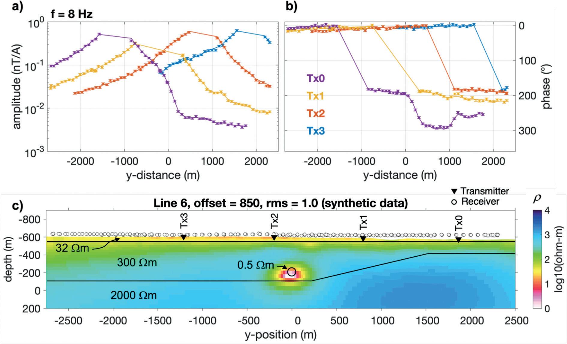
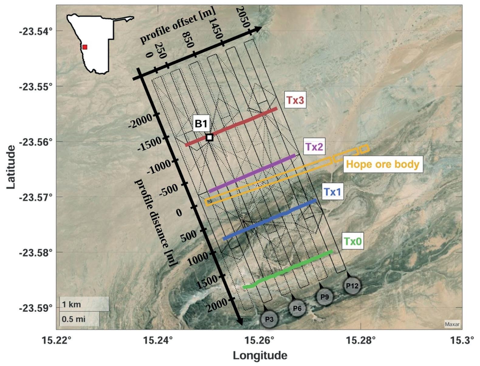
Figure 7 Site map. Transmitter dipoles are depicted as bold coloured lines (2 km length); flightlines are shown as black lines. The Hope ore body (yellow outline) crops out at the surface in the west (Gossan) and plunges eastward to about 400 m depth below surface at an offset of 2 km. Dark amphibolite rocks of the Matchless Amphibolite Belt (MAB) are seen to the south of the Hope mineralization with a flat plan to the north consisting of overburden (conductive) and resistive underlying schists and granite.

the topography. The finite element mesh refines the model parameterization further to accurately represent the field equations numerically. The inversion model is heavily overparameterized and smoothing regularization (Occam scheme) is used to constrain the model. The Occam scheme consists of two phases; the first phase reduces the misfit down to a target misfit, which was set to 1.0, and the second phases reduce the model roughness while maintaining the target misfit. The starting model was a homogenous half-space of 300 Ωm. The inversion converged to a normalized root mean square value (r.m.s) of 1.0 within 19 iterations, including the last three iterations of the smoothing phase that minimizes model roughness; a r.m.s. misfit of 1 indicates that the data are fitted to within the data errors.

In Figure 6, we display the noise-contaminated synthetic data (symbols in Figures 6a,b) and the responses of the inversion model (solid lines) for an exemplary frequency of 8 Hz and for all four transmitters; Figure 6c shows the final inversion model with the true model superimposed. It is seen that the conductive anomaly at a profile distance of 0 m is well recovered at the correct horizontal position and depth; moreover, the inversion introduced the shallow conductive surface layer which is also contained in the true model. The test was repeated with the anomaly placed at different depth levels, from 300–800 m; in all cases the inversion recovered a conductive anomaly, but the horizontal and vertical position and the extent of the anomaly becomes less constrained with increasing depth (not shown).

Application to the Hope Copper Deposit, Namibia Brief geological and geophysical overview of the Hope Copper Deposit The Hope Copper Deposit is situated approximately 120 km south of Swakopmund on the northern side of regional syncline, a few kilometres from its western closure (Schnieder, 1992) as seen in Figure 7. The syncline is made up of dark amphibolite units which are part of the Matchless Amphibolite Belt (MAB) surrounded by quartz biotite schist (QBS). To the north of the Hope deposit the open plane is covered by shallow overburden overlying QBS and, further to the north, Donkerhuk Granite (DG). The Hope deposit consists of massive sulphide accompanied by a magnetite quartzite. From a geophysical point of view the country rocks (amphibolite, QBS and DG) are highly resistive (>1000 Ωm) as is the magnetite quartzite making up the Hope mineralization, while the sulphide is typically massive and consists of chalcopyrite and pyrite, and it is conductive (0.01–1 Ωm). The Hope deposit consists essentially of a deformed syn-formal ribbon plunging shallowly ((10-15) degrees) to the east and has been followed down-plunge for a distance of 4-6 km and down to a depth of 500-600 m.

Geophysical data existing prior to the semi-airborne EM data described in this paper consists of Large Loop TDEM, which detected the ore body down to a vertical depth of 300 m, ground magnetics which clearly images the magnetite quartzite portion of the mineralized body and audio-magnetotellurics (AMT), which detects the mineralization to a depth of 500-600 m. A recent TDEM helicopter-borne survey was completed over the deposit, the results of which are still being analysed.

The measurement area is located remotely from any anthropogenic noise sources and has a very low ambient EM noise level, originating mostly from natural sources which have a signal level well below of . Therefore, limits on the data quality are due to sensor noise, noise due to motion (which plays a minor role using a scalar magnetometer) and noise emissions from the aircraft.

Data acquisition and response functions A total of four grounded electric dipole transmitters of 2 km length each were deployed in parallel to the ENE extended Hope ore body (cf. Figure 7). Transmitters Tx0 and Tx1 are in the SSE of the target formation, and Tx2 and Tx3 are in the NNW. To power the dipole, a Zonge GGT10 9 kW transmitter was employed and amperages of 5-8 A could be realized. The GGT10

is a reliable time-domain transmitter and provides clean signal with short ramp times, as required for broadband applications. We used a 100% rectangular waveform with a fundamental frequency of 1 Hz. The current output was monitored with current clamps attached to a GPS-synchronized ADU08e data logger.

In total, about 220 line-km (black lines in Figure 7) were completed with the MagArrow in the UAV-based semi-airborne EM configuration. All flightlines were repeated with the three-component SHFT02e induction coil sensor; the induction coil data will be reported in a forthcoming contribution. The total flight area spans 5 km × 2 km and the flight line separation is 200 m. Explicit tie lines were not flown but oblique transfer flights provide control about the repeatability of measurements at cross-over points with regular flight lines. The cruising speed was constant at 7 m/s throughout all flights, and the flight-height was about 30 m above terrain.

Because flight endurance is limited by the battery power to about 40 minutes with the operated setup and because visual line of sight must be maintained, the survey area was subdivided into a total of 12 patches of 1250 × 600 m lengths in the NEN and ENE directions, respectively. Data were acquired consecutively in these patches. Individual take-off and landing points were considered to minimize transfer time. The six central subareas were covered for all four transmitters, whereas the three northernmost and three southernmost patches were omitted for the southernmost and northernmost transmitters Tx0 and Tx3, respectively. In this way, we achieve substantial overlap of flight areas for the separate transmitters.

Data processing yielded response function estimates in the frequency range from 1 to 256 Hz with a logarithmically equidistant frequency distribution (2 estimates per octave). For this purpose, harmonics were binned into half-octave intervals and processed together; the estimate is then attributed to a centered frequency within each bin. Estimates were obtained for a total of 15 frequencies.

Figure 8 displays representative amplitude and phase response functions for three different frequencies (1 Hz, 11 Hz and 90.5 Hz) along a single flight line (line 6) and for transmitter Tx3. The profile distance refers to the distance from the gossan at the surface outcrop of the Hope ore body (cf. Figure 7, positive y-distances are towards the south). The depicted flightline has an offset of about 850 m from the gossan in the x-direction (towards the east), i.e. it is centrally located in the surveyed area. As described above, data have been merged from independent line segments acquired during separate flights. This data set also served as the template for the synthetic 2D inversion study presented in a previous section.

It can be noted from the spatial decay away from the transmitter and from the observed phase behaviour that inductive effects become more evident with increasing frequency, as expected. An important anomalous behaviour is observed at low frequencies (e.g., 1 Hz and 11 Hz) in the distance range from 0 m to 500 m, where the amplitude response drops, and where the phase exhibits a strong increase. This effect cannot be observed at the highest frequencies shown (90 Hz). Hence, the data clearly indicate buried anomalous conductance at depth and at profile

Figure 8 Transfer function determined from MagArrow data along line 6, about 850 m to the east of the gossan (cf. map in Figure 7). Three frequencies are shown. Profile distance refers to the gossan; north is at negative distances. The transmitter location and the location of the Hope ore body are indicated.

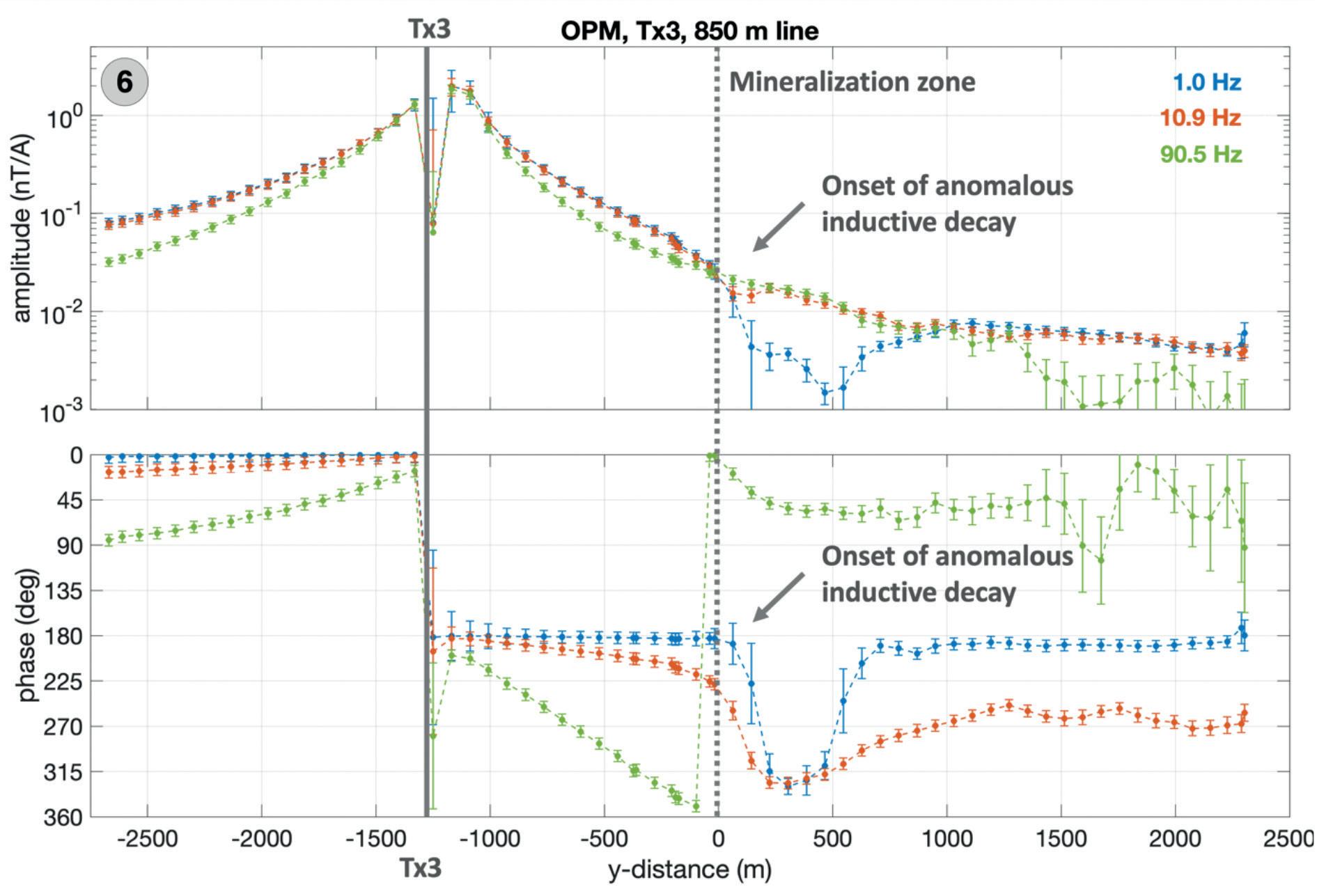
distances corresponding to the ore body location. At increasing distances, the inductive response becomes less pronounced again; the low-frequency data at 1 Hz exhibit nearly in-phase fields at profile distances greater than 1000 m, thus approach the DC limit.

2D Inversion results For the 2D inversion, we used the same inversion procedure as for the synthetic model discussed above. Error floors of 10% on the amplitude and 3° on the phase data were imposed to down-weight subsets of data that are affiliated with overly small statistical error estimates to balance the data fit across all observations. The inversion started at a normalized r.m.s. of 10 for most profiles and converged to the target misfit of 1.1 exhibiting a very good data fit.

Figure 9a and b depict the amplitude and phase responses at an exemplary frequency of 8 Hz (symbols) and the model responses (solid lines). Colours decode the corresponding active transmitters. Figure 8c shows the final inversion model. The most prominent feature in the model is a conductive anomaly (red-to-white colours) at a profile distance of ~0 m and a depth of ~200 m below surface. Estimated resistivities of this anomaly are in the range between 2 Ωm and 10 Ωm (100-500 mS/m). within a diameter of ~100 m. This anomaly can be identified with the Hope ore body, which is known to be buried at about 200 m at the profile crossover location. The estimated resistivity range is within the typical range of volcanogenic massive sulphide deposits, although at the upper limit.

The inversion images a conductive overburden of undulating thickness, which is locally interrupted by resistive features (blue structure in Figure 9c); some can be identified with geological structures. For instance, resistivities exceeding 1000 Ωm at the surface in the vicinity to transmitter Tx1 are likely to be associated with amphibolite (dark colours in the satellite image in Figure 7). Furthermore, a trough-like structure is imaged to the south, which matches the extent of the folded rock units of the amphibolite belt (cf. Figure 7). These observations further increase confidence in the inversion result.

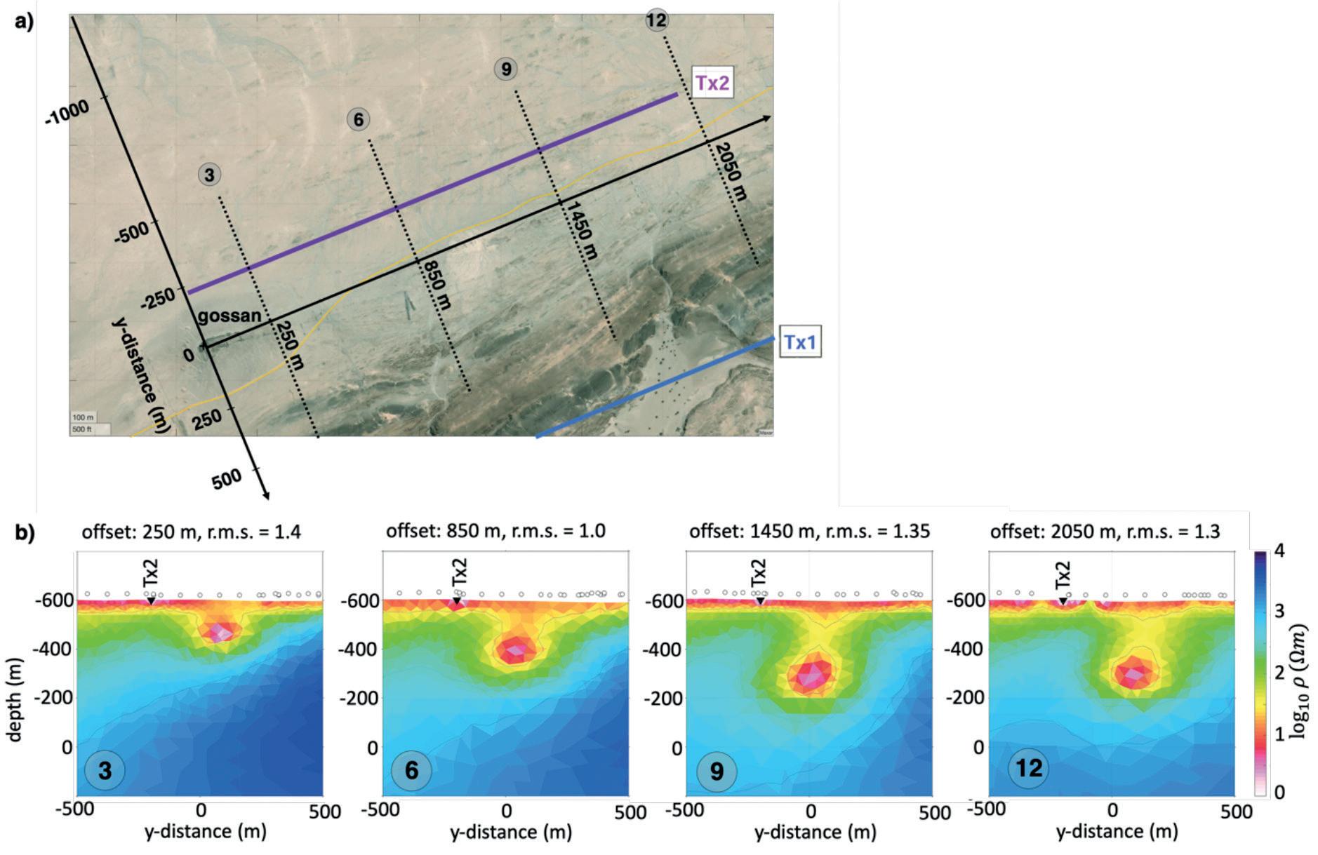
The major focus of the study was to test for the ability to image the Hope ore body from the near-surface at the gossan down-plunge to 400 m depth to the east. We conducted independent 2D inversions along different flightlines, following the procedure described above. Results, shown in Figure 10, are based on data from transmitters Tx1 and Tx2 only; for clarity, we show the central section across the Hope ore body only (the models have the same lateral extent as the model shown in Figure 9).

Figure 10 displays an enlargement of the site map and presents cut-outs into independent inversion models along four parallel flightlines (lines 3, 6, 9, 12 at offsets of 250 m, 850 m, 1450 m and 2050 m, respectively). The resistivity sections consistently image the conductive feature at profile position 0 m plunging eastward to depths of approximately 200 m, 250 m, 300 m, and 300 m, respectively. These results illustrate that the Hope body is imaged well as a conductive anomaly at the expected location and depth, although the easternmost profile appears to place it a bit too shallow in comparison with the available prior information from drilling and ground geophysics.

Conclusion We employed a multicopter UAV in combination with a lightweight scalar magnetometer with a bandwidth of 400 Hz to measure time variations of the TMI in a semi-airborne EM configuration. A total flight area of 5 km x 2 km was covered with a total of 220 km flightlines. Flights were conducted sequentially for four separate horizontal electric dipole transmitters of 2 km length each. As the source current, a 1 Hz rectangular waveform with amperages of 5-8 A was injected. With this setup, transfer functions were derived in the frequency range from 1-256 Hz and inverted into 2D resistivity.

The test survey supports the following main conclusions. Firstly, field operations with the employed 25 kg MTOW multi-copter, the lightweight MagArrow sensor and the medium-sized Zonge GGT10 transmitter, turned out to be highly efficient and reliable. Secondly, because the TMI readings are essentially free of motional noise, high data quality could be obtained within the frequency range from 1-256 Hz and within a footprint of ±2.5 km from each transmitter. Thirdly, despite the limited bandwidth, this dataset imaged subsurface structures with unexpected resolution. Consequently, it could be demonstrated that the configuration can acquire high-quality data at frequencies as low as 1 Hz, considerably lower than in helicopter-borne applications and likely very beneficial for the exploration of deep targets.

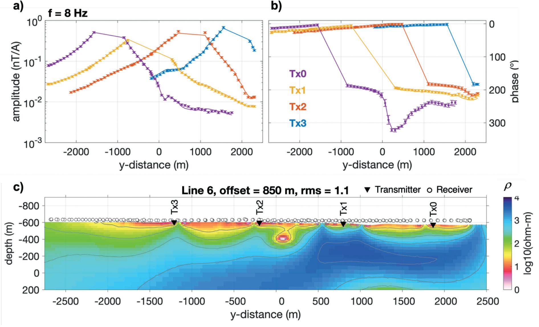
Figure 9 2D inversion along line 6. a) Amplitude and b) phase responses for all four transmitters estimated at 8 Hz (symbols) and corresponding model responses (solid lines). c) Final 2D resistivity model. The inversion achieved a r.m.s misfit of 1.1. The model images the Hope ore body as a conductive feature at the y-distance of 0 m and a depth of 200 m below surface.

Figure 10 2D inversion model sections. a) Detail map, showing the modelling coordinate system and the location of vertical sections in panel b; flightlines are labelled as 3, 6, 9 and 12. b) Zoom into selected 2D resistivity models along selected flightlines across the Hope ore body. A conductive body tracks the Hope mineralization from a depth of approximately 100 m below surface at offset 250 m to a depth of 300 m below surface at offset 2050 m, a distance of 1800 m along plunge. Note that the plunge angle appears to shallow between offsets 1450 m and 2050 m agreeing with existing drill results.

The handling of scalar EM response functions requires some geometrical considerations, as the response is the component in the direction of the local geomagnetic main field. 1D and 2D modelling studies have validated the method. Limitations on the applicability must be expected at low latitudes in regions with low inclinations of the geomagnetic main field.

The test site is a massive sulphide deposit in Namibia, which provided ideal geological as well as environmental conditions to perform a UAV measurement, such as good electrical contrasts, minor topography, and low ambient EM noise. Compared to more densely populated countries, the ambient noise at Hope is negligible. However, note that the signal strength generated with a controlled source can to some extent be adopted to local noise conditions.

The estimated resistivity models image the Hope ore body to 300 m depth, with remarkable coincidence with prior knowledge from ground EM measurements and from drilling. These results suggest that the method is a promising technique for imaging buried conductors at several hundred metres depth. Further measurements to the east along strike are planned to determine if the semi-airborne EM method could detect the mineralization to a depth of 500-600 m or more. The Hope mineralization is as far as is known open ended along plunge.

Acknowledgements This work is part of the DESMEX II (deep electromagnetic sounding for mineral exploration) project, which is funded by the Federal Ministry of Education and Research (BMBF) of Germany under grant no. 0133R13. Permissions and support to survey over the Hope Copper Deposit has been kindly provided by Bezant Resources PLC (https://www.bezantresources.com/). We are grateful for the support from the DESMEX working group and for the cooperation throughout the course of the collaborative DESMEX and DESMEX II projects.

References

Ali, S.H., Giurco, D., Arndt, N., Nickless, E., Brown, G., Demetriades, A.,

Durrheim, R., Enriquez, M.A., Kinnaird, J., Littleboy, A., Meinert,

L.D., Oberhänsli, R., Salem, J., Schodde, R., Schneider, G., Vidal, O. and Yakovleva, N. [2017]. Mineral supply for sustainable development requires resource governance. Nature 543, 367-372. https://doi. org/10.1038/nature21359 Avdeev, D.B., Kuvshinov, A.V. and Pankratov, O.V. [1997]. Tectonic process monitoring by variations of the geomagnetic field absolute intensity. Ann. Geophys. 40(2). Becken, M., Nittinger, C.G., Smirnova, M., Steuer, A., Martin, T., Petersen, H., Meyer, U., Mörbe, W., Yogeshwar, P., Tezkan, B., Matzander,

U., Friedrichs, B., Rochlitz, R., Günther, T., Schiffler, M. and Stolz,

R. [2020]. DESMEX: A novel system development for semi-airborne electromagnetic exploration. Geophysics, 85, E253-E267, doi: 10.1190/geo2019- 0336.1. Cattach, M.K., Lee, S.J., Stanley, J.M. and Boyd, G.W. [1993]. Sub-Audio Magnetics (SAM) — A High Resolution Technique for Simultaneously Mapping Electrical and Magnetic Properties1. Exploration

Geophysics, 24(3-4), 387-399. Elliott, P. [1998]. The Principles and Practice of FLAIRTEM, Exploration

Geophysics, 29:1-2, 58-59, DOI: 10.1071/EG998058 Key, K. [2016]. MARE2DEM: a 2-D inversion code for controlled-source electromagnetic and magnetotelluric data, Geophysical Journal

International, 207(1), 571-588, https://doi.org/10.1093/gji/ggw290.

Killick, A.M. [2000]. The Matchless Belt and associated sulphide mineral deposits, Damara Orogen, Namibia. Communs geol. Surv. Namibia, 12, 79-87 Kotowski, P.O., Becken, M., Thiede, A., Schmidt, V., Schmalzl, J., Ueding, S. and Klingen, S. [2022]. Evaluation of a Semi-Airborne Electromagnetic Survey Based on a Multicopter Aircraft System. Geosciences, 12, 26. https://doi.org/10.3390/geosciences12010026 Mogi, T., Tanaka, Y., Kusunoki, K., Morikawa, T. and Jomori, N. [1998].

Development of grounded electrical source airborne transient EM (GREATEM). Explor. Geophys., 29, 61-64. Schnieder, G.I.C. and Seeger, K.G. [1992]. Copper, 2.3-135- 2.3-137. IN:

The Mineral Resources of Namibia. Geol. Surv. Namibia, Windhoek. Seigel, H.O. [1979]. An overview of mining geophysics, in: Hood, P.J.,

Ed., Geophysics and geochemistry in the search for metallic ores.

Geol. Surv. Canada Econ. Geol. Report 31, 7-23. Smirnova, M.V., Becken, M., Nittinger, C., Yogeshwar, P., Mörbe, W.,

Rochlitz, R., Steuer, A., Costabel, S. and Smirnov, M.Y. [2019].

DESMEX Working Group. A novel semiairborne frequency-domain controlled-source electromagnetic system: Three-dimensional inversion of semiairborne data from the flight experiment over an ancient mining area near Schleiz, Germany. Geophysics, 84, E281–E292. http://dx.doi.org/10.1190/geo2018-0659.1 Smirnova, M., Juhojuntti, N., Becken, M., Smirnov, M., and the

DESMEX WG, [2020]. Exploring Kiruna Iron Ore fields with largescale, semi-airborne, controlled-source electromagnetics. First

Break, 38(1), 35-40. https://doi.org/10.3997/1365-2397.fb2020070 Steuer, S., Smirnova, M., Becken, M., Schiffler, M., Günther, T., Rochlitz,

R., Yogeshwar, P., Mörbe, W., Siemon, B., Costabel, S., Preugschat,

B., Ibs-von Seht, M., Zampa, L.S. and Müller, F. [2020]. Comparison of novel semi-airborne electromagnetic data with multi-scale geophysical, petrophysical and geological data from Schleiz, Germany,

J. Appl. Geophys., 182, 104172. Stoll, J., Noellenburg, R., Kordes, T., Becken, M., Tezkan, B., Yogeshwar,

P., Bergers, R. and Matzander, U. [2019]. Semi-Airborne Electromagnetics Using A Multicopter. In: Proceedings of the GEM-2019

Workshop, Xi’an, China. Streich, R. and Becken, M. [2011]. Sensitivity of controlled-source electromagnetic fields in planarly layered media. Geophys. J. Int., 187, 705-728. Yang D. and Oldenburg D.W. [2018]. 3D inversion of total magnetic intensity data for time-domain EM at the Lalor massive sulphide deposit. Exploration Geophysics, 48(2): 110-123.

ADVERTISEMENT