
12 minute read
Simulation in a world of trouble: part two


In the second of two installments, Ralph H. Weiland and Nathan A. Hatcher, Optimized Gas Treating Inc., explore case studies to show how simulation is used in troubleshooting.


Simulation tools are used extensively in a wide range of activities from plant design, unit revamps, and troubleshooting, to plant optimisation and unit monitoring. Confi dence and trust in a simulator are usually gained by running simulations against measured plant-performance data. But what happens when measurement and simulation do not align? Is it possible to learn anything from such experiences?
This is the second of a two-part series of case studies to illustrate examples of how simulation is used in troubleshooting (part one of this article was published in the May 2021 issue of Hydrocarbon Engineering).1 The two further cases discussed here were each initiated by disparity between simulation and plant data too large to be attributed to just modelling and measurement errors. The examples are cases attributed to poor temperature control and to a problem with the model itself. Each case compares simulation results with measured performance metrics, and each one uses a combination of data and simulation to logically deduce a diagnosis and resolve the issue.


Case study 1
A Middle Eastern ammonia plant was experiencing very erratic operation of its CO2 removal system with CO2 concentrations in the treated gas ranging from 10 to 10 000 ppmv in a seemingly random fashion. The unit was using piperazine-promoted MDEA solvent with a split fl ow design. Figure 1 shows a process fl ow diagram (PFD) of the bulk removal and polishing absorbers which were packed with RVT Hifl ow® Rings #50 – 5 and #25 – 5, respectively. The unpredictable nature of the product gas CO2 content threw the rest of the process into chaos and demanded a rapid resolution.
Speculation about the cause of the instability included the possibility of foaming, tower fl ooding, and hysteresis in control elements such as fl ow control valves. However, pressure drop measurements gave no indication of any hydraulic anomalies, and solvent fl owrates showed completely steady behaviour at least to within the measuring ability of instrumentation. Ultimately, recourse was had to simulation.
The absorption system, sectioned off from the rest of the CO2 removal process, was set up in the ProTreat simulator using the actual tower diameters, bed depths and type, and size of packing contained in each of the two beds in each column. Temperatures, pressures and fl owrates of all inlet streams were set at the nominal values at which the plant was known to be operating. It had been observed that the problem was less severe during winter months and on colder nights during the summer, and it was known that the fi n-fan coolers on the semi-lean amine stream were operating at their limit for current production rates. In fact, the licensors of the process technology had originally recommended that the semi-lean amine temperature be kept below 70°C, whereas under hot ambient conditions the temperature of this stream was sometimes as high as 75 or even 80°C. It was implausible that temperature variations of a few degrees could cause CO2 in the treated gas to escalate to 10 000 ppmv; nevertheless, a simulation study of sensitivity to operating parameters was done. Figure 2 summarises the results.
A temperature of 74°C produces synthesis gas below 1000 ppmv CO2 and one quarter of a degree cooler drops the CO2 level by a factor of 10. Semi-lean temperature only 2°C higher elevates the treated gas to almost 10 000 ppm. The simulations indicate that 74°C is a critical temperature whose

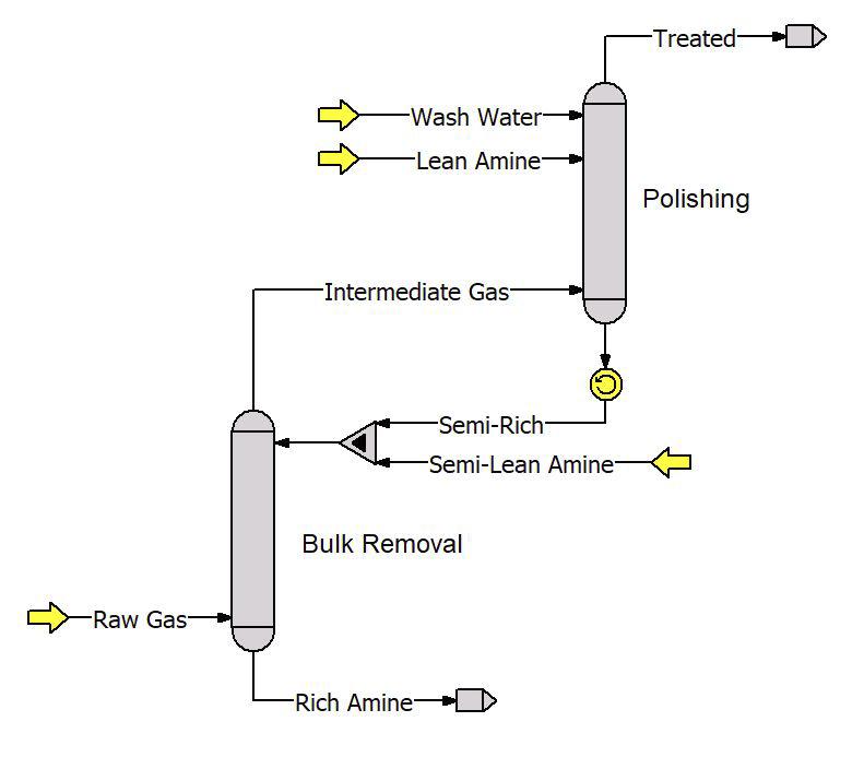
Figure 1. PFD of the ammonia plant’s CO2 absorption system.
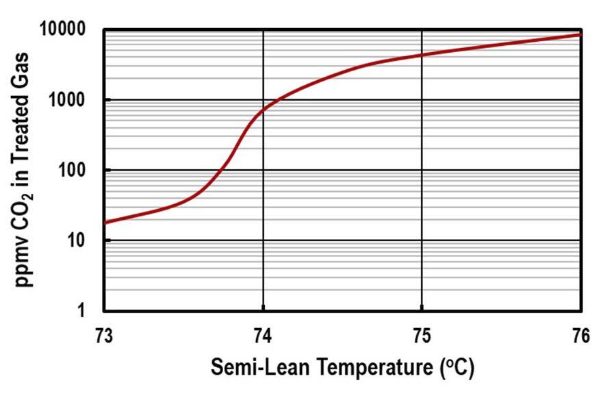
Figure 2. Treating sensitivity to semi-lean temperature.
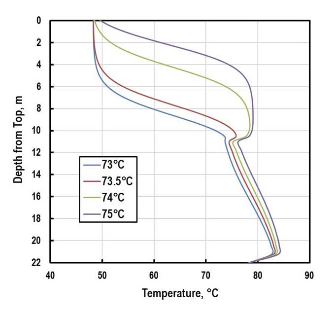
Figure 3. Response of polishing column to semi-lean temperature vicinity shows extreme sensitivity. The problem reveals itself in the polishing column but its cause is in the bulk column. The maximum possible net loading of solvent in the bulk column depends on temperature, and this goes down as temperature goes up. Any CO2 not removed in the bulk column spills over into the polisher and must be removed there; however, the polisher also has CO2 capacity limits. At 73°C, the approach to equilibrium loading at the rich end of the polisher is 80% and the lean solvent loading controls treating. But at 74˚C the rich solvent loading is at 98% of equilibrium, so now it is the rich solvent loading that controls treating. The bulk removal column is so close to capacity that only a 1°C change in semi-lean temperature throws the polisher from lean-end to rich-end control.
Figure 3 illustrates the extreme sensitivity of the polishing column to any increase in demand on the bulk column’s performance. It should be noted that this is an optimally designed set of columns and each one in the pair is balanced against the other. Therefore, near the critical temperature of 74°C, even a slight increase in semi-lean temperature translates into a decrease in the maximum possible net loading. The bulk column simply does not have the capacity to function properly with a lower net loading, so the excess CO2 necessarily has to spill over into the polisher. However, it is also at its limit, meaning that there is no choice but for the excess to pass through and leave the polisher as an off-specifi cation product gas.
For completeness, the plant’s sensitivity to fully-lean and semi-lean solvent fl owrates and CO2 loadings were also assessed, and in the vicinity of 74°C, small fl uctuations in these variables also cause marked changes in treated gas CO2 content. Around 74°C, both columns are near their capacity for holding CO2 and the whole system is in a delicate balance. This is one of the risks of operating a process plant near its stability limits.
Case study 2
The fi nal case relates to the simulation of packed absorbers in the CO2 removal units of two LNG plants. In one plant, the absorber contained a 250-size structured packing and in the other it contained 50 mm random packing. Both were performing more or less according to design with treated gas at just below 1 ppmv CO2 and a temperature bulge of just under 85°C in one case and at 8 ppmv CO2 and 75°C in the other. The purpose of the ProTreat® simulations was to validate the simulator against known performance data. The operators of both plants use thermal imaging and scanning extensively in troubleshooting and monitoring of the units.
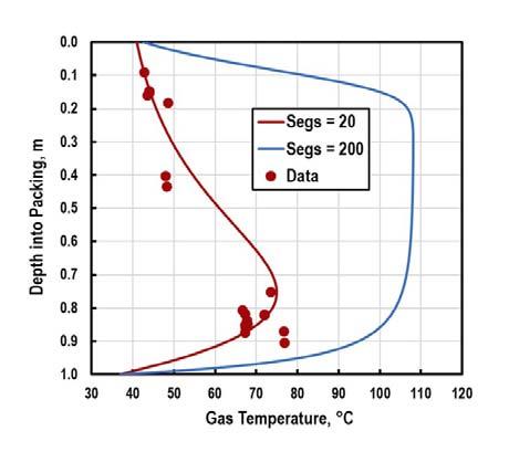
Trayed columns are naturally discretised by the actual trays they contain. However, because packed columns are continuous contacting devices, they must be discretised somewhat artifi cially for simulation because simulators are digital, not analogue, and must deal with continuous variables by discretising them. Figure 4 shows the effect of discretisation on the simulated temperature profi les for the two columns.
Comparing with the measured data, discretisation of Columns A and B into 37 and 20 segments, respectively, gives a very satisfactory comparison between model and data. It is important to note that the data are column skin temperatures. Depending on ambient temperature and wind speed, these
may be several degrees cooler than might be measured inside the towers. These degrees of segmentation appear to represent the behaviour of these absorbers quite well. Segmentation (or the height of segments) is related quantitatively to: The total depth of packing in the column. The packing size.
The ProTreat simulator automatically defaults to the correct segment size based on heuristics developed from comparisons against a wide range of unit performance data from numerous columns containing a variety of both random and structured packings. But what does segmentation really represent?
A column described by a single segment is essentially equivalent to a well-mixed vessel. One with a very large number of segments has both phases in plug fl ow. Real packed columns operate somewhere between these extremes. As Figure 4 shows, ProTreat simulation with 200 segments produces a very broad fl at bulge of high temperature which returns to known end conditions only very close to the top and bottom of the columns. The heat being carried by the gas and liquid in plug fl ow would have little or no opportunity to disperse across the column like it would with longitudinal mixing of vapour with vapour and liquid with liquid. Without axial mixing, the two phases would retain all of their heat, simply carrying it up and down the column. As a result, the full heat of reaction would heat both phases to the maximum extent possible.
A simulator that produces temperature profi les like the blue lines in Figure 4 is using incorrect parameter values, which invalidates the results because it disregards the fact that there is signifi cant axial mixing in real packed columns. Based on thinking along lines parallel to numerical integration for the area under a curve, at one time OGT advised using fi ne enough segmentation to obtain results that gradually became stable against ever fi ner segmentation. This was bad advice
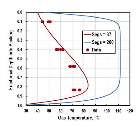
Figure 4. Simulated vs measured temperatures in two LNG absorbers (Column A – left, and Column B – right).

COMPLETE PROCESS LINES FOR THE SULPHUR INDUSTRY

SBS STEEL BELT SYSTEMS is your reliable partner for continuous process plants and
SBS STEEL BELT SYSTEMS S.r.l
SBS will be a bronze sponsor of the next Sulphur + Sulphuric Acid 2021 Virtual Conference and Exhibition

based on faulty thinking. The development team went through a thorough review of all the elements in the rate model including detailed assessment of vessel heat-loss expectations, packed-bed heat transfer and mass-transfer correlations for packing, reaction kinetics, and vapour-liquid equilibrium. The analysis was conducted based on feedback from several customers, and it led to the conclusion that ever fi ner segmentation corresponded with perfect plug fl ow of both phases; whereas real packed columns exhibit signifi cant axial dispersion that is masked and eventually negated by ever-fi ner segmentation.
An interesting conclusion is that without axial mixing, LNG absorbers would have to be operated quite differently – it is mixing that keeps temperatures within acceptable limits. Axial mixing or dispersion is critical to the success of gas treating with large heat effects. Without axial mixing it would be very diffi cult to keep temperatures low enough to avoid serious solvent degradation and to allow the desired treating to be achieved with reasonable solvent fl ow rates. On the other side of the axial mixing coin, maldistribution of either phase will lead to greater axial mixing, poorer performance and cooler temperature curves. Measured temperatures that fall too much below simulation are indicative of maldistribution or packing that has been poorly installed or that has lost some of its integrity, perhaps leaving large voids in the bed. Axial dispersion can also take place in trayed columns. OGT has recently extended axial dispersion considerations to the separation performance of trays by allowing for specifi able levels of weeping and entrainment from each tray in a column.
Summary
Without simulation, a defect can hide and go uncorrected for a long time. What is worse, using a less-than-rigorous simulator with buried tuning parameters can lead to some fruitless and costly adjustments to operating conditions, hardware replacements, misdiagnosis of the true problem, or the resigned acceptance of reduced processing rates and lost revenue.
Troubleshooting is not always as straightforward as in some of the examples here, but it can be made a lot easier when a reliable simulator is used to assess the validity of measured data. It is almost always important in assessing lean loadings to account for the HSS concentrations, simply because HSS levels can account for the lean loading value itself. In treating to low residual acid gas levels, HSSs can determine the treat actually achieved. If the simulation tool is reliable, it is almost always possible to pinpoint the cause(s) of poor performance because a reliable simulator tells what the plant as-specifi ed should be doing. It is up to the engineer to use the simulator thoughtfully to understand why expectations are not being met.
Reference
1. WEILAND, R.H. and HATCHER, N.A., ‘Simulation in a world of trouble: part one’, Hydrocarbon Engineering, (May 2021), pp. 44 - 46.
Your Specialist for PRESSURE RELIEF SOLUTIONS
Consulting. Engineering. Products. Service. T +49 2961 7405-0 T +1 704 716 7022