Saimm 202403 Mar

The Southern African Institute of Mining and Metallurgy

OFFICE BEARERS AND COUNCIL FOR THE 2023/2024 SESSION

Honorary President

Nolitha Fakude

President, Minerals Council South Africa

Honorary Vice Presidents

Gwede Mantashe

Minister of Mineral Resources and Energy, South Africa

Ebrahim Patel

Minister of Trade, Industry and Competition, South Africa

Blade Nzimande

Minister of Higher Education, Science and Technology, South Africa

President

W.C. Joughin

President Elect

E. Matinde

Senior Vice President

G.R. Lane

Junior Vice President

T.M. Mmola

Incoming Junior Vice President

M.H. Solomon

Immediate Past President

Z. Botha

Honorary Treasurer

E. Matinde

Ordinary Members on Council

W. Broodryk M.C. Munroe

Z. Fakhraei S. Naik

R.M.S. Falcon (by invitation) G. Njowa

B. Genc

S.J. Ntsoelengoe

K.M. Letsoalo S.M. Rupprecht

S.B. Madolo

A.T. van Zyl

F.T. Manyanga E.J. Walls

K. Mosebi

Co-opted Council Members

M.A. Mello

Past Presidents Serving on Council

N.A. Barcza C. Musingwini

R.D. Beck S. Ndlovu

J.R. Dixon J.L. Porter

V.G. Duke M.H. Rogers

I.J. Geldenhuys D.A.J. Ross-Watt

R.T. Jones G.L. Smith

A.S. Macfarlane W.H. van Niekerk

G.R. Lane – TP Mining Chairperson

Z. Botha – TP Metallurgy Chairperson

K.W. Banda – YPC Chairperson

S. Nyoni – YPC Vice Chairperson

Branch Chairpersons

Botswana Vacant

DRC Not active

Johannesburg N. Rampersad

Limpopo S. Zulu

Namibia Vacant

Northern Cape I. Tlhapi

North West I. Tshabalala

Pretoria Vacant

Western Cape A.B. Nesbitt

Zambia J.P.C. Mutambo (Interim Chairperson)

Zimbabwe Vacant

Zululand C.W. Mienie

PAST PRESIDENTS

*Deceased

* W. Bettel (1894–1895)

* A.F. Crosse (1895–1896)

* W.R. Feldtmann (1896–1897)

* C. Butters (1897–1898)

* J. Loevy (1898–1899)

* J.R. Williams (1899–1903)

* S.H. Pearce (1903–1904)

* W.A. Caldecott (1904–1905)

* W. Cullen (1905–1906)

* E.H. Johnson (1906–1907)

* J. Yates (1907–1908)

* R.G. Bevington (1908–1909)

* A. McA. Johnston (1909–1910)

* J. Moir (1910–1911)

* C.B. Saner (1911–1912)

* W.R. Dowling (1912–1913)

* A. Richardson (1913–1914)

* G.H. Stanley (1914–1915)

* J.E. Thomas (1915–1916)

* J.A. Wilkinson (1916–1917)

* G. Hildick-Smith (1917–1918)

* H.S. Meyer (1918–1919)

* J. Gray (1919–1920)

* J. Chilton (1920–1921)

* F. Wartenweiler (1921–1922)

* G.A. Watermeyer (1922–1923)

* F.W. Watson (1923–1924)

* C.J. Gray (1924–1925)

* H.A. White (1925–1926)

* H.R. Adam (1926–1927)

* Sir Robert Kotze (1927–1928)

* J.A. Woodburn (1928–1929)

* H. Pirow (1929–1930)

* J. Henderson (1930–1931)

* A. King (1931–1932)

* V. Nimmo-Dewar (1932–1933)

* P.N. Lategan (1933–1934)

* E.C. Ranson (1934–1935)

* R.A. Flugge-De-Smidt (1935–1936)

* T.K. Prentice (1936–1937)

* R.S.G. Stokes (1937–1938)

* P.E. Hall (1938–1939)

* E.H.A. Joseph (1939–1940)

* J.H. Dobson (1940–1941)

* Theo Meyer (1941–1942)

* John V. Muller (1942–1943)

* C. Biccard Jeppe (1943–1944)

* P.J. Louis Bok (1944–1945)

* J.T. McIntyre (1945–1946)

* M. Falcon (1946–1947)

* A. Clemens (1947–1948)

* F.G. Hill (1948–1949)

* O.A.E. Jackson (1949–1950)

* W.E. Gooday (1950–1951)

* C.J. Irving (1951–1952)

* D.D. Stitt (1952–1953)

* M.C.G. Meyer (1953–1954)

* L.A. Bushell (1954–1955)

* H. Britten (1955–1956)

* Wm. Bleloch (1956–1957)

* H. Simon (1957–1958)

* M. Barcza (1958–1959)

* R.J. Adamson (1959–1960)

* W.S. Findlay (1960–1961)

* D.G. Maxwell (1961–1962)

* J. de V. Lambrechts (1962–1963)

* J.F. Reid (1963–1964)

* D.M. Jamieson (1964–1965)

* H.E. Cross (1965–1966)

* D. Gordon Jones (1966–1967)

* P. Lambooy (1967–1968)

* R.C.J. Goode (1968–1969)

* J.K.E. Douglas (1969–1970)

* V.C. Robinson (1970–1971)

* D.D. Howat (1971–1972)

* J.P. Hugo (1972–1973)

* P.W.J. van Rensburg (1973–1974)

* R.P. Plewman (1974–1975)

* R.E. Robinson (1975–1976)

* M.D.G. Salamon (1976–1977)

* P.A. Von Wielligh (1977–1978)

* M.G. Atmore (1978–1979)

* D.A. Viljoen (1979–1980)

* P.R. Jochens (1980–1981)

* G.Y. Nisbet (1981–1982)

A.N. Brown (1982–1983)

* R.P. King (1983–1984)

J.D. Austin (1984–1985)

* H.E. James (1985–1986)

H. Wagner (1986–1987)

* B.C. Alberts (1987–1988)

* C.E. Fivaz (1988–1989)

* O.K.H. Steffen (1989–1990)

* H.G. Mosenthal (1990–1991)

R.D. Beck (1991–1992)

* J.P. Hoffman (1992–1993)

* H. Scott-Russell (1993–1994)

J.A. Cruise (1994–1995)

D.A.J. Ross-Watt (1995–1996)

N.A. Barcza (1996–1997)

* R.P. Mohring (1997–1998)

J.R. Dixon (1998–1999)

M.H. Rogers (1999–2000)

L.A. Cramer (2000–2001)

* A.A.B. Douglas (2001–2002)

S.J. Ramokgopa (2002-2003)

T.R. Stacey (2003–2004)

F.M.G. Egerton (2004–2005)

W.H. van Niekerk (2005–2006)

R.P.H. Willis (2006–2007)

R.G.B. Pickering (2007–2008)

A.M. Garbers-Craig (2008–2009)

J.C. Ngoma (2009–2010)

G.V.R. Landman (2010–2011)

J.N. van der Merwe (2011–2012)

G.L. Smith (2012–2013)

M. Dworzanowski (2013–2014)

J.L. Porter (2014–2015)

R.T. Jones (2015–2016)

C. Musingwini (2016–2017)

S. Ndlovu (2017–2018)

A.S. Macfarlane (2018–2019)

M.I. Mthenjane (2019–2020)

V.G. Duke (2020–2021)

I.J. Geldenhuys (2021–2022)

Z. Botha (2022-2023)

Editorial Board

S.O. Bada

R.D. Beck

P.den Hoed

I.M. Dikgwatlhe

B.Genc

R Hassanalizadeh

R.T. Jones

W.C. Joughin

A.J. Kinghorn

D.E.P. Klenam

J.Lake

H.M. Lodewijks

D.F. Malan

C.Musingwini

S. Ndlovu

P.N. Neingo

S.S. Nyoni

M.Phasha

P.Pistorius

P.Radcliffe

N.Rampersad

Q.G. Reynolds

I.Robinson

S.M. Rupprecht

K.C. Sole

T.R. Stacey

D.Vogt

F.Uahengo

International Advisory Board members

R.Dimitrakopolous R.Mitra

A.J.S. Spearing

E.Topal

D.Tudor

Editor /Chairperson of the Editorial Board

R.M.S. Falcon

Typeset and Published by

The Southern African Institute of Mining and Metallurgy PostNet Suite #212 Private Bag X31 Saxonwold, 2132

E-mail: journal@saimm.co.za

Journal Comment: The relentless march of Moore’s law by Q.G. Reynolds iv

President’sCorner:SANCOTandSAIMM byW.C.Joughin

NEWS OF INTEREST

THE INSTITUTE, AS A BODY, IS NOT RESPONSIBLE FOR THE STATEMENTS AND OPINIONS ADVANCED IN ANY OF ITS PUBLICATIONS.

Copyright© 2024 by The Southern African Institute of Mining and Metallurgy. All rights reserved. Multiple copying of the contents of this publication or parts thereof without permission is in breach of copyright, but permission is hereby given for the copying of titles and abstracts of papers and names of authors. Permission to copy illustrations and short extracts from the text of individual contributions is usually given upon written application to the Institute, provided that the source (and where appropriate, the copyright) is acknowledged. Apart from any fair dealing for the purposes of review or criticism under The Copyright Act no. 98, 1978, Section 12, of the Republic of South Africa, a single copy of an article may be supplied by a library for the purposes of research or private study. No part of this publication may be reproduced, stored in a retrieval system, or transmitted in any form or by any means without the prior permission of the publishers. Multiple copying of the contents of the publication without permission is always illegal. U.S. Copyright Law applicable to users In the U.S.A. The appearance of the statement of copyright at the bottom of the first page of an article appearing in this journal indicates that the copyright holder consents to the making of copies of the article for personal or internal use. This consent is given on condition that the copier pays the stated fee for each copy of a paper beyond that permitted by Section 107 or 108 of the U.S. Copyright Law. The fee is to be paid through the Copyright Clearance Center, Inc., Operations Center, P.O. Box 765, Schenectady, New York 12301, U.S.A. This consent does not extend to other kinds of copying, such as copying for general distribution, for advertising or promotional purposes, for creating new collective works, or for resale.

Honorary Legal Advisers

M H Attorneys

Auditors

Genesis Chartered Accountants

Secretaries

Advertising Representative

Barbara Spence

Avenue Advertising

The Southern African Institute of Mining and Metallurgy 7th Floor, Rosebank Towers, 19 Biermann Avenue, Rosebank, 2196

PostNet Suite #212, Private Bag X31, Saxonwold, 2132 E-mail: journal@saimm.co.za

Telephone (011) 463-7940 . E-mail: barbara@avenue.co.za

ISSN 2225-6253 (print) . ISSN 2411-9717 (online)

Printed by Camera Press, Johannesburg Directory

COMPUTATIONAL MODELLING PAPERS

A finite-element method model for a ferromanganese and silicomanganese pilot furnace by M. Sparta and V.K. Risinggård

A finite-element-method model of a pilot furnace for the production of manganese alloys was developed. The model is a multiphysics model that can be used to study both quasi-steady states and transient states in time-dependent simulations. It can simulate production of both ferromanganese and silicomanganese alloys and provides furnace runs, temperature profiles, current paths, energy balances, and alloy and slag production rates and compositions.

A pragmatical physics-based model for predicting ladle lifetime by S.T. Johansen, B.T. Løvfall, and T. Rodriguez Duran

This paper outlines the development of a physics-based model for lining erosion in steel ladles. The model predicts the temperature evolution in the liquid slag, steel, refractory bricks, and outer steel shell of the ladle. The mass and heat transfer coefficients are modelled and wall shear velocities are obtained from CFD simulations. The model is capable of reproducing both thermal and erosion evolution. It is fast and has been tested successfully in a ‘semi-online’ application.

Pragmatism in industrial modelling: An application to ladle lifetime in the steel industry by S.T. Johansen, B.T. Løvfall, T. Rodriguez Duran, and J. Zoric

A methodology for building pragmatic physics-based models is here adapted to predict the erosion of ladle linings in the steel industry. The adopted work flow for the development, challenges faced, and some model results are presented. Combining or extending the model using machine learning and cognition-related methods is discussed.

Prediction of burden distribution and electrical resistance in submerged arc furnaces using discrete element method modelling by S.J. Baumgartner, Q.G. Reynolds, and G. Akdogan ..................................................................

A computational model for studying segregation and the corresponding electrical behaviour of the burden in a submerged arc furnace used in the production of ferrochrome is presented. Built on the discrete element method, this model illustrates how the consumption of materials is affected by changes in electrode length, reductant fraction, reductant sizing, and reductant density during the formation of a reductant bed. The resistance algorithm can generate quantitative estimates of the electrode-to-electrode and electrode-to-bath electrical conduction conditions.

Numerical simulation of the electromagnetic field in the secondary cooling zone of arc-shaped slabs by B. Yang and Y. Ren .............................................................................................

The magnetic field characteristics due to electromagnetic stirring in the secondary cooling zone of a continuous casting slab are numerically determined using Maxwell’s equations. This paper examines the distribution of magnetic induction intensity and electromagnetic force in relation to the magnetic field. Results indicate that the direction of the electromagnetic force is the same when the electromagnetic stirrers at the 30° and 60° positions are powered in the same way, otherwise, the direction is opposite.

Incompressible versus compressible fluid flow models: A case study on furnace tap-hole lancing by M.W. Erwee, Q.G. Reynolds, and J.H. Zietsman

Pyrometallurgical furnaces represent complex multiphase systems that challenge direct industrial research. In this work, a multiphase fluid flow model was used to investigate bulk flow dynamics, with a focus on the effects of the lancing process on the inside of the furnace immediately behind the tap-hole. Incompressible and compressible multiphase fluid solvers were used and their performance compared. There were negligible disparities in bulk fluid flow behaviour between the solvers, indicating that solver selection might be less consequential for certain aspects of oxygen lancing.

A mathematical mould model for transient infiltration and lubrication behaviour of slag in a steel continuous casting process by M-H. Cao, B. Yu1, C. Zhou, and X-Z. Zhang

In a continuous steel casting process, the transient infiltration and lubrication behaviour of slag is important for the quality of the billet. A two-dimensional coupled mathematical mould model was established and the accuracy of the model verified by comparing the calculated slag consumption with plant measurements. Results showed that the liquid slag is consumed from the middle and late period of positive strip time. Increasing the positive pressure of the slag channel was found to be conducive to lubrication.

Near real-time interpolative algorithm for modelling air quality in underground mines by K.W. Brown Requist, E. Lutz, and M. Momayez .....................................................................

For the real-time monitoring of airborne contamination distributions, we propose a spatial Computational Fluid Dynamics (CFD) interpolation methos that can estimate the distribution of airborne contaminants in near-real time in US underground mines. This method outperforms other methods and provides spatial interpolation with a Euclidean distance. By providing contamination distribution information to operators, this method and its derivatives stand to outperform current atmospheric monitoring systems.

85

93

139

147

Journal Comment

TCopper Cobalt

The relentless march of Moore’s law

his special edition of the Journal showcases recent work in metallurgical applications of computational modelling. But what exactly is computational modelling? Historically this would have included any science or engineering problem that required a computer to solve numerical approximations of the governing equations. Computers were typically large, expensive pieces of equipment, and the problems solved were limited by the available power of the machine – early applications included chemical thermodynamics, numerical heat and mass transfer, and simple problems in fluid flow.

However, in modern times we have computing pervading our lives to an ever-increasing degree, and we are starting to catch more unusual fish in our computational modelling nets. Driven by sustained exponential growth in computer power over more than six decades (your wristwatch today has more capability than was available to the entire Apollo space programme), methods such as computational fluid dynamics have been enhanced beyond all recognition and are now capable of modelling realistic engineering problems with multiphase flow and free surface interfaces, coupled heat transfer, electromagnetic fields, and others. Tools like massively-parallel GPU accelerators are also breathing new life into old methods like discrete element modelling, giving us unprecedented insight into particulate flow problems.

Alongside the rapid growth in capability and performance of traditional computational modelling tools, the role of such models in the knowledge industry has also evolved. From being able to give an isolated (and usually not very accurate) result, they are now routinely used to study the general behaviour of systems across wide ranges of their parameter spaces. Such models are also increasingly viewed as intermediate analysis and interpretation tools for building intuition rather than producing the ‘final answer’, and they generate one thing that is in short supply in metallurgical processes – data. And since data feeds the physics-informed or data-driven reduced order models which power the ongoing revolution in artificial intelligence, computational modelling will remain a useful piece of the puzzle for a long time to come.

Q.G. Reynolds Pyrometallurgy Division, Mintek Chemical Engineering Department, Stellenbosch University

President’s Corner

ISANCOT and SAIMM

n February, I had the pleasure of participating in two notable events organized by the SAIMM and SANCOT: the Herrenknecht Seminar, which focused on ‘New Developments in Mechanized Tunnelling and Shaft Sinking for the Civil and Mining Industries’ held in Johannesburg, and the SANCOT-ITA Workshop that delved into ‘Technical and Legal Aspects of Underground Construction, Operational and Mine Accident and Fire Risk’ in Cape Town.

Many of you might already know that SANCOT (South African National Council on Tunnelling) has been operating as a special interest group within the SAIMM since 2003. https://www.saimm.co.za/about-saimm/saimmcommittees/south-african-national-council-on-tunnelling-sancot

However, SANCOT’s roots extend much further back. Established in 1973, SANCOT became a founding member nation of the International Tunnelling Association and Underground Space Association (ITA) just a year later, in 1974. https://www.saimm.co.za/ news/313-sancot-and-the-international-tunnelling-association-ita

Today, the ITA is an international non-governmental, non-profit organization with 79 member nations, incorporating both corporate and individual members. The organization is dedicated to promoting the use of underground spaces for the public good, the environment, and sustainable development. It also supports progress in the planning, design, construction, maintenance, and safety of tunnels and underground spaces. The partnership between SANCOT and the SAIMM is reciprocal, with the SAIMM Secretariat providing valuable administrative services and event management.

The primary focus of SANCOT and ITA lies in the realm of civil underground infrastructure, yet the parallels with tunnels and large excavations in mines are quite evident. The civil engineering sector’s experience with the latest underground technologies is a rich source of knowledge. In particular, the area of mechanized tunnelling and boring has seen remarkable progress within civil engineering applications. Tunnel boring machines (TBMs) have become instrumental in the safe and rapid development of long tunnels for road and rail transport, water and sewage transfer, and many other applications. Historically, TBMs have seen limited use in mining; however, the industry is now considering the adoption of newer, compact, and more versatile TBMs.

A good example is Master Drilling’s recent initiative to develop an exploration decline at Anglo American Platinum’s Mogalakwena mine, employing its Mobile Tunnel Borer (MTB).

The MTB is a horizontal cutting machine that incorporates a full-face cutter head with disc cutters, a concept borrowed from traditional TBMs. This innovative machine is designed for functionality in both inclines and declines and is capable of navigating around corners in access tunnels with a diameter of 5.5 m. It has front and tail shields to temporarily support the rock, protecting operators and the specialized equipment. The integrated bolter rig can install a pattern of 1.8 m long resin rebar bolts. Ground conditions are better with less support, due to the circular tunnel profile and absence of blast damage.

https://sanire.co.za/documents/symposium-presentations/symposium-2022/day-1/ session-2/882-support-design-for-two-tunnels-at-anglo-platinum-mogalakwena-sandslootexploration-28-july-2022/file

https://im-mining.com/2021/08/31/master-drillings-mobile-tunnel-borer-heads-anglosmogalakwena-mine/

President’s Corner (continued)

In mining operations, raise boring is a common technique used for excavating vertical shafts and orepasses. However, its application is limited to scenarios where the rock mass is stable and competent throughout the entire length of the excavation because support can only be installed once boring is completed. Addressing this limitation, manufacturers of TBMs have engineered shaft boring machines that have the dual capability of boring while concurrently installing the necessary support. Construction of orepass and ventilation raises could also be carried out with boxhole boring machines (BBRs) to create a pilot hole and boxhole backreaming machines (BBMs) to enlarge to the final diameter. A lining can be installed concurrently during the back reaming process to provide early support in challenging ground conditions.

At the Herrenknecht seminar, the talks covered a range of topics, including selection criteria for TBMs in varying rock mass conditions, innovative technologies for the excavation of vertical shafts, BBR and BBM technology, TBMs for the development of spiral ramps and horizontal infrastructure, pipe laying technology and its potential application in mining, and reef boring trials for narrow tabular orebodies. Reference projects were included where this new technology has been applied. An informative discussion panel on ‘Innovation in Mechanized Excavation’ provided some additional insights.

Mechanized tunnelling machines represent a significant advancement, yet broader adoption will take time. Adaptions will be necessary to tailor these machines for specific mining purposes. They demand a substantial initial investment and skilled personnel for operation and maintenance. However, these costs could be balanced by enhanced safety measures, accelerated development, and earlier access to reef. Mechanized boring of narrow tabular reefs is intriguing, since it will be much safer, and potentially more productive, but it will take even longer to develop the new mining methods that utilize this equipment.

At the SANCOT-ITA workshop, a variety of engaging presentations were delivered, addressing an array of subjects, including the state of technology for mechanized shaft and tunnel development in hard rock, fire safety in underground facilities, lessons learnt from a challenging rescue after a tunnel collapse, transferring essential skills from the tunnelling industry to the mining industry, contract management, and geotechnical aspects.

The next SANCOT Symposium will take place during October 2024, and I look forward to seeing you there.

W.C. Joughin President, SAIMM

Affiliation:

1NORCE Norwegian Research Centre AS, Universitetsveien 19, NO-4630 Kristiansand S, Norway.

Correspondence to:

V.K. Risinggård

Email: veri@norceresearch.no

Dates:

Received: 14 Feb. 2023

Revised: 25 Jul. 2023

Accepted: 10 Aug. 2023

Published: March 2024

How to cite:

Sparta, M. and Risinggård, V.K. 2024

A finite-element method model for a ferromanganese and silicomanganese pilot furnace.

Journal of the Southern African Institute of Mining and Metallurgy, vol. 124, no. 3. pp. 85–92

DOI ID: http://dx.doi.org/10.17159/24119717/2737/2024

A finite-element method model for a ferromanganese and silicomanganese pilot furnace

by M. Sparta1 and V.K. Risinggård1

Synopsis

We report on the development of a finite-element method model for a pilot furnace for the production of manganese alloys. The model is a multiphysics model that addresses material flow, electrical conditions, heat transfer, and physical and chemical transformations. It is capable of studying both quasi-steady and transient states in time-dependent simulations. The model includes common charge materials and fluxes and can simulate production of both ferromanganese and silicomanganese alloys with acid and basic slags, as well as changing charge compositions. The model output provides access to the material distribution in the furnace during furnace runs, temperature profiles, current paths, energy balances, and alloy and slag production rates and compositions.

Keywords

modelling, finite-element method, pilot furnace, manganese alloys.

Introduction

Ferromanganese (FeMn) and silicomanganese (SiMn) are manganese alloys produced by carbothermic reduction of manganese oxides and quartz in a submerged-arc furnace (Olsen, Tangstad, and Lindstad, 2007). In order to gain insight into the process, a pilot-scale furnace has been developed and run at the Norwegian University of Science and Technology. The furnace is used to investigate the electrical operation, effect of raw materials, coke bed formation, and more (Tangstad et al., 2001, 2017; Monsen, Tangstad, and Midtgaard, 2004; Monsen et al., 2007; Eidem et al., 2010; Ringdalen and Tangstad, 2013).

To complement the experimental work, we have developed a comprehensive model for a pilot-scale silicomanganese furnace that takes into account the material flow, process chemistry, and electrical and thermal conditions of the furnace (Sparta et al., 2021). The original model assumed a simplified charge consisting of pure carbon and silicon and manganese oxides, giving total of seven condensed species [MnO(s), MnO(l), Mn(l), SiO2(s), SiO2(l), Si(l), and C(s)], as well as CO(g). In this contribution we report on the expansion of the model to address both ferromanganese and silicomanganese alloys in the presence of fluxes and spectator oxides. The original model has been expanded to a total of 18 species by including Fe2O3(s), Fe(s), Fe(l), CaO(s), CaO(l), MgO(s), MgO(l), Al2O3(s), Al2O3(l). and CO2(g).

Model description

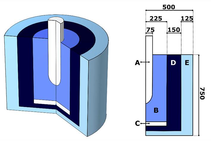
This iteration of the model (FeSiMn) builds on the previous SiMn model described in Sparta et al. (2021). This section provides a brief overview of the original model, with particular emphasis on modifications and amendments introduced in the current version. The model is implemented using the finite-element method (FEM) in COMSOL Multiphysics (COMSOL Inc., 2022). FEM provides an accurate representation of curved surfaces and natural handling of gradient boundary conditions (Zienkiewicz and Morgan, 2006) and the multiphysics capability of the software platform is fully exploited. However, the same implementation could be achieved with other methods for representing and evaluating partial differential equations. The cylindrical symmetry of the experimental equipment is exploited to reduce the computational cost of the model by using the two-dimensional axisymmetric interface. The furnace geometry is shown in Figure 1. For the purposes of the FEM model, the furnace consists of five domains: The top and bottom electrodes (A, C) are made of solid graphite, and are responsible for carrying the electric current into and out of the charge mix (B). The charge consists of manganese ore, quartz, coke, and fluxes. The charge and

A finite-element method model for a ferromanganese and silicomanganese pilot furnace

the electrodes are contained in two structural and insulating layers made from alumina refractory bricks (D) and silica sand (E).

The dependent variables of the FEM model are: the electrical potential in the electrodes and the charge (A, B, and C); the temperature (all domains); the velocity fields of the solids, slag, and alloy phases (B); and the concentrations of all solid and liquid species (B). Furthermore, the model tracks all the material inputs and outputs for the solid, liquid, and gas phases.

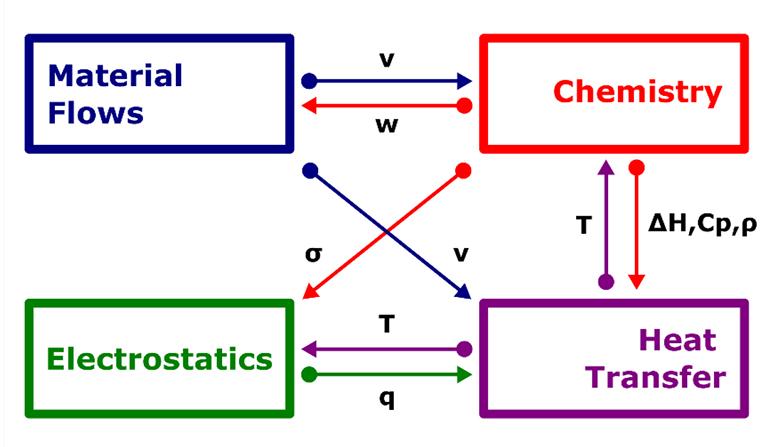
Figure 2 indicates the major couplings and interactions in the multiphysics representation. Briefly, the mixing and distribution of the chemical species is determined by the advection velocities (v). The physical and chemical transformations in turn determine the void fraction (w), which drives the material flow. The local concentrations of the charge species determine the bulk material properties such as the conductivity (σ), density (ρ), and heat capacity (Cp), which in turn determine the current distribution and ohmic heat generation (q). The local temperature (T) influences the electrical conditions through the temperature dependency of the conductivity (σ), as well as the chemistry through the reactions and transformations that absorb and release heat (ΔH).

Physical and chemical transformations

For each chemical species, the model solves an advection-diffusion equation:

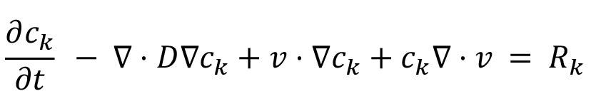
Here, ck is the concentration of the chemical species k, v is the velocity component of the species (described in the next section), D is the diffusion constant for the species, and Rk is its local rate of generation. The reaction rate for each species is calculated as the sum of the rates of all the reactions that the species participates in.

Kinetics and enthalpies of major reactions

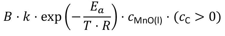
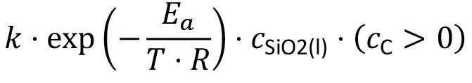
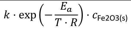
The current iteration of the model includes ten physical and chemical transformations. Reactions (1)–(5) below were already present in the previous version and include the melting of MnO(s) and SiO2(s) (reactions 1 and 2), carbothermic reduction of MnO(l) and SiO2(l) (reactions 3 and 4), and the Mn–Si exchange reaction (reaction 5). The current version also includes the solid-state reduction of iron oxide by CO gas (reaction 6), the melting of metallic iron (reaction 7), and the dissolution of fluxes and inert oxides in the slag phase (reactions 8–10).

The reduction reactions are assumed to follow first-order rate laws (Table I) with an Arrhenius-type temperature dependence. The activation energies are set to 200 and 250 kJ/mol for MnO and SiO2, respectively (Canaguier and Tangstad, 2020), and 60 kJ/ mol for Fe2O3 (Ostrovski et al., 2002).

Table I

Figure 1—Visualization of the furnace proportions and its 2D axisymmetric representation. A: top electrode; B: charge; C: bottom electrode; D: alumina refractory; E: silica sand. Dimensions are given in millimetres

Figure 2—Modules and interactions. The functionality of the model can be understood in terms of four modules: material flows, chemistry, electrostatics, and heat transfer (adapted from Sparta et al. (2021)

A finite-element method model for a ferromanganese and silicomanganese pilot furnace

We note that from an energy balance perspective, the contributions from reactions 3 and 4 account for more than 90% of the total enthalpy of reactions. Kinetic prefactors have been selected to match average results from experimental runs on the pilot furnace.

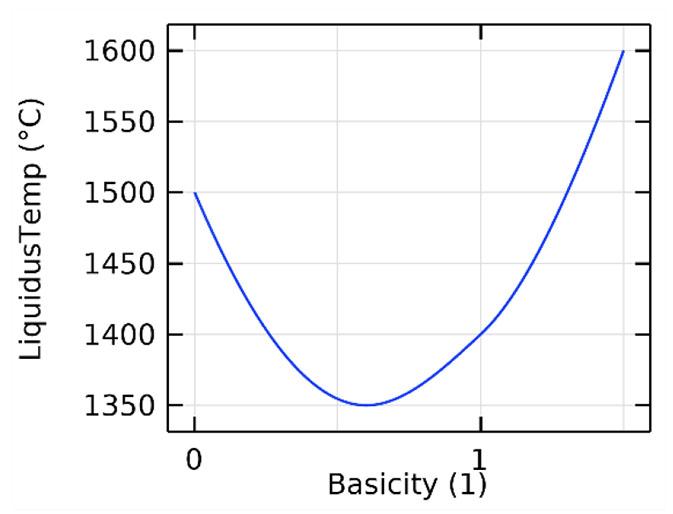
Furthermore, the model is making use of the concept of basicity. In this work basicity refers to the ratio (CaO+MgO)/(SiO2+ Al2O3) calculated on a mass basis for the tapped slag.(Olsen, Tangstad, and Lindstad, 2007) The basicity affects the following properties of the model.

➤ Slag liquidus temperature. The temperature at which the oxides melt into the slag phase depends on the basicity of the system (Liao, et al., 2023). The liquidus temperature profile as a function of the basicity of the slags used in this work is shown in Figure 3.

➤ Slag fluidity. High-basicity slags are less viscous (Tangstad et al., 2021). This is pragmatically included in the model by increasing the velocity at which the slag trickles through the charge by up to 30% as a function of the basicity of the slags.

➤ Slag reactivity. The MnO activity increases in basic slags (Tangstad et al., 2021). This effect is implemented in the model by increasing the rate constants of reactions 3 and 5 by up to 50% in high-basicity slags (B factor in Table I).

Note that these are pragmatic and effective dependencies on the basicity, which can be further improved by using more accurate estimations or coupling with more advanced methods

Material flows

The model takes three different approaches to calculating the advection velocity v, depending on whether the species in question is in the solid, liquid, or gas phase.

Advection-diffusion equations are used for tracking all the species in the condensed phases. For the solid phases, an advection velocity field for the flow of granular material is calculated using the dissipative Coulomb model. This model is based on the NavierStokes equations for incompressible flow:

Here, v → is the granular velocity, p is the pressure, ρ is the medium density, and η is the medium viscosity. The local density of the effective medium is calculated from the composition of the charge or coke bed as ρ = ∑kχk ρk, where ρk is the density of species k and χk is its volume fraction (Artoni, et al., 2008). The flow is driven by the formation of voids in the lower part of the furnace as the solid material t reacts to form liquid metal and slag. The liquid

material subsequently trickles down through the granular coke bed. For the liquid phases, precomputed velocity templates are used in the advection-diffusion equations. The slag velocity is dependent on the basicity, as described in the previous section, whereas the alloy velocity is taken to be independent of the alloy composition.

The gas flow is not addressed in the current version of the model. The fluxes of CO and CO2 escaping at the top of the furnace are calculated as integrals over the gas-producing reactions in the charge.

Electrostatics

The direct current (DC) approximation is used to determine the electrostatic properties of the system. This approximation is satisfactory for small furnaces with a power factor close to unity (Eidem et al., 2010; Halvorsen, Olsen, and Fromreide, 2016; Fromreide et al., 2021).

In the case of power distribution in industrial-scale furnaces, DC simulations and linear combination of DC solutions can be used as a fair approximation to a full AC description.(Halvorsen, Olsen, and Fromreide, 2016; Tesfahunegn et al., 2020; Fromreide et al., 2021) The electrostatic potential V is obtained by solving the Poission equation

[14]

in domains A, B, and C in Figure 1. The electric field E → and the current density J → are obtained from the electrostatic potential by the constitutive relationships E → =−V and J → =σE → . A constant power of 150 kW (Tangstad et al., 2001, 2017; Monsen, Tangstad, and Midtgaard, 2004; Monsen et al., 2007; Eidem, Tangstad, and Bakken, 2009; Eidem et al., 2010) is maintained by adding a global constraint to the system. The conductivity of the electrodes is constant and set to 80 kS/m (Haynes, Lide, and Bruno, 2017), whereas the conductivity of the charge depends on the local composition. The bulk conductivity of the charge is calculated as the sum of the conductivities of each component weighted by volume fraction,

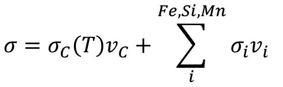
[15]

The material conductivities for the reduced species [Fe(s,l), Si(l), Mn(l)] are set to 10 kS/m. The material conductivity for carbon is dependent on temperature, increasing linearly from 10 to 400 S/m in the range 800–1600°C, with the extreme values acting as cut-offs for lower and higher temperatures (Surup et al., 2020). The oxides do not contribute to the conductivity.

Heat transfer

The local temperature is determined by solving the heat equation: [16]

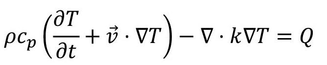
Here, T is temperature, ρ is the medium density, cp is the medium heat capacity, v → is the advection velocity, k is the thermal condutivity, and Q is the local heating

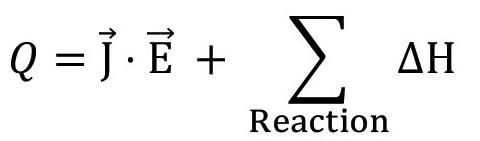
[17]

comprising the resistive term (J → is the current density, E → is the electric field), and total enthalpy of reactions. In the charge, the local density and heat capacity are calculated from the local charge composition based on a weighted average, similar to that used for the electrical conductivity in Equation [15] . The thermal

Figure 3—Effect of basicity. The liquidus temperature decreases for higher basicity

A finite-element method model for a ferromanganese and silicomanganese pilot furnace

conductivity is taken to be independent of the charge composition but takes into account radiative heat transport in pores and voids. A model similar to the one described by Schotte (1960) is used, but with an additional contribution from heat conduction through the particle contact points added in series with the radiative contribution. The particle thermal conductivity is taken to be 30 W/m·K (the value compensates for the lack of the convective effects of the CO/CO2 counterflow), the contact point effective thermal conductivity is taken to be 2 W/m·K, the particle diameter is set to 30 mm, and the emissivity to 0.9. This results in a thermal diffusivity that is somewhat higher than experimentally measured bulk thermal diffusivities for common manganese ores (Ksiazek et al., 2013), which is to be expected given the contribution from the higher conductivity carbon material.

Simulation modes

The FEM model solves for the time evolution of the system. Tapping and charging occur in a continuous way. Liquid species that reach the level of the bottom electrodes are removed from the simulation and accounted as tapped flow. A constant charge level is maintained by continually adding an amount of charge corresponding to the volume of material consumed in the hearth of the furnace. The composition of the incoming charge is specified by the user, and can be set to be:

➤ Constant for the duration of the simulation. This mode can be used, for example, to simulate a start-up stage when the internal temperature is increasing, or during over-coking or under-coking (periods in which the charge contains more or less carbon than needed).

➤ Switching from an initial to a final set of concentrations at a prescribed time. For example, this can be used to study a transient state. In the examples below, this mode will be used to investigate what happens when the charge switches from a composition rich in iron and acid oxides to a silicomanganese one rich in basic oxides.

For a suitable amount of carbon in the charge mix, the constant charge mode will eventually reach a quasi-steady state. The depth of the coke bed in this steady state depends on the carbon balance of the charge. Insufficient carbon coverage will lead to a shallow coke bed and excessive slag production. Excessive amounts of carbon will give rise to an ever-deepening coke bed that eventually fills the furnace.

To more closely simulate industrial operation, an additional control is implemented for the carbon content in the charge mix. For either mode, the amount of carbon in the mass flux that is added to the system can be adaptive, meaning that the amount added matches the amount of carbon consumed in the reactions and escaping as CO/CO2. This simulates the ideal situation, in which an exact carbon coverage is maintained. If the initial conditions are relatively close to the equilibrated solution, adaptive coking leads to a quasi-steady state solution determined by the input power and relative ratios of the metal oxides in the charge. Adaptive coking will be demonstrated in the second simulation example below.

Simulation examples

Quasi-steady state

The first simulation presented aims at reaching a steady state. For this example, the input power is set to 150 kW and the charge composition is as specified in Table II.

Table II

Composition of the charge for a 20 kg batch

Species

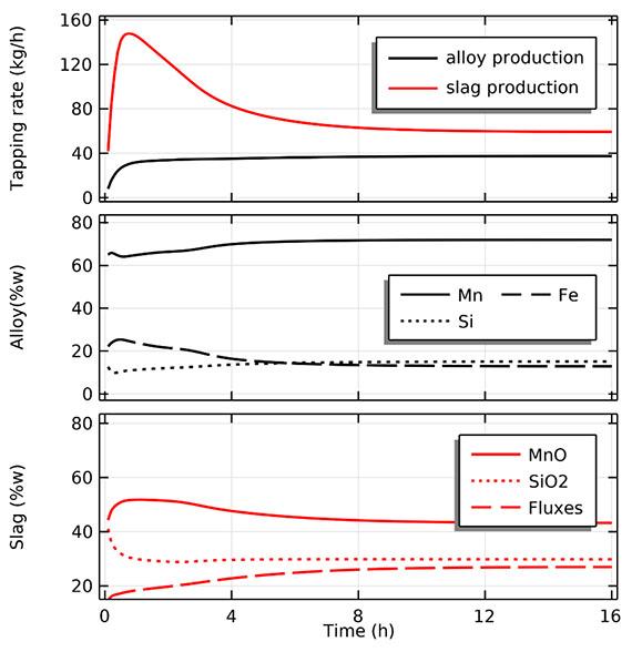
The initial condition is a homogenous charge at 800°C with the composition specified in Table II. The production profiles of slag and alloy and their compositions are reported in Figure 4. In the early stage the furnace is cold, and most of the oxides dissolve in the slag phase and leave the system without reacting any further. This means that, in the early stage of the run, the furnace is fed with an excess of carbon that accumulates in a coke bed between the electrodes. As the furnace warms up and enough energy is available, the slag percolating through the carbon-rich zone undergoes carbothermic reduction and the carbon consumption increases until a balance is reached.

After 16 hours, the furnace reaches a quasi-steady state with an alloy and slag production of approximately 38 and 59 kg/h, respectively. Considering this hourly production and the input power of 150 kW, the energy consumption is 3.9 kWh/kg of alloy, a value in line with experimental values (Monsen, Tangstad, and Midtgaard, 2004; Monsen et al., 2007; Eidem, Tangstad, and Bakken, 2009; Eidem et al., 2010).

Regarding the composition of the tapped material, the alloy has a relatively high iron content in the early stages of the run as the direct gas-solid reduction of iron oxide starts occurring at relatively low temperatures. As the system reaches equilibrium

Figure 4—Top: Production rates of alloy and slag (kg/h) during a 16hour simulation run. Centre: Composition of the alloy (wt%). Bottom: Composition of the slag

A finite-element method model for a ferromanganese and silicomanganese pilot furnace

the iron content stabilizes and the alloy has a final composition of 72 wt% Mn, 15% Si, and 13% Fe. For the charge mix used in this simulation, the the slag at equilibrium contains 43 wt% MnO, 30% SiO2, and 27% fluxes. As can be seen in Figure 4, this simulation run demonstrates that the model can reach a stable state with a carbon consumption matching the incoming charge, provided that reasonable values for the energy input and charge recipe are supplied.

Figure 5 shows the conditions in the furnace at the end of the simulation. Directly below the top electrode one finds the hot zone, with temperatures exceeding 2000°C (left panel). The entire coke bed has a temperature exceeding 1400°C. The coke bed can be visualized by plotting the volume fraction of carbon in the furnace (middle panel). The boundary of the coke bed is located between the 1600 and 1800°C isotherms. The divergence of the velocity of the granular material is shown in the right panel. The divergence divv → is calculated as divv → = . v →. The negative divergence indicates that granular material is converging on the interface between the charge and the coke bed. In other words, in this region solid material is consumed by melting and by chemical reactions.

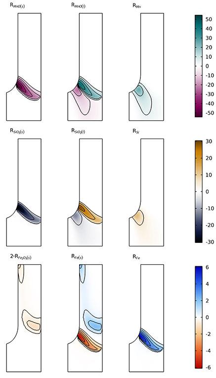
The species distribution for the triad MnO(s), MnO(l), and Mn(l) is shown in Figure 6. MnO(s) is the only species present during the descent of the charge from the top of the furnace to the top of the coke bed. MnO(l) forms when the charge has passed the 1600°C isotherm, and Mn(l) forms by carbothermic reduction of MnO(l) in the coke bed.

Owing to the relatively fast percolation of the slag, although the charge contains 30 wt% MnO, the liquid MnO never exceeds approximately 0.6 wt%. The rate of carbothermic reduction of MnO increases with temperature, leading to the profile seen for Mn(l). The distribution of Si-containing species follows the same pattern. Results from the excavation of the pilot furnace are in line with the simulations, i.e. MnO is scarce in the column directly below the electrode and is mostly found in the periphery of the furnace, and Si is mostly concentrated directly below the top electrode (Tangstad et al., 2001).

The profiles for the iron species are markedly different to those for manganese and silicon, as shown in Figure 7. Iron oxides are reduced in the solid state by the CO(g) passing upward through the solid charge. The charge in the proximity of the electrode is warmer (see Figure 5), consequently unreacted Fe2O3 can be found deeper in the furnace at the periphery than at the centre. Solid metallic iron exists between the 800 and 1800°C isotherms above the top of the coke bed. The iron starts to melt as it reaches the top of the coke bed and enters the liquid alloy phase. It should be noted that the kinetics of the solid-gas reaction ultimately depend on the CO diffusion in the solid particles – this in turn depends on the porosity and size of the particles. These dependencies are not explored in the model.

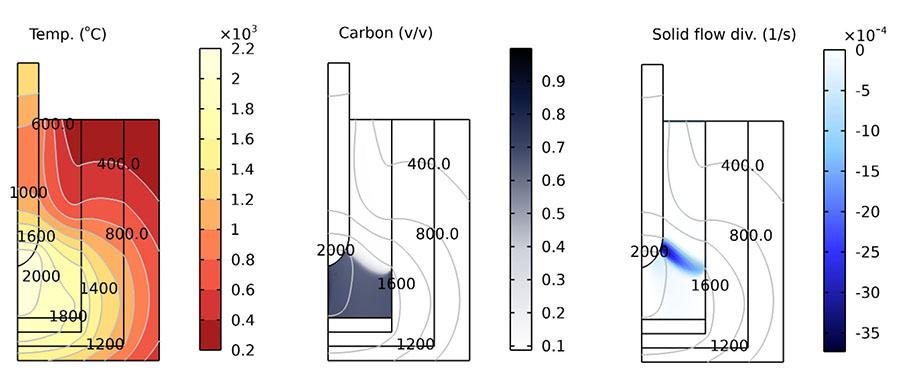
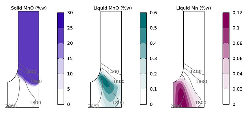
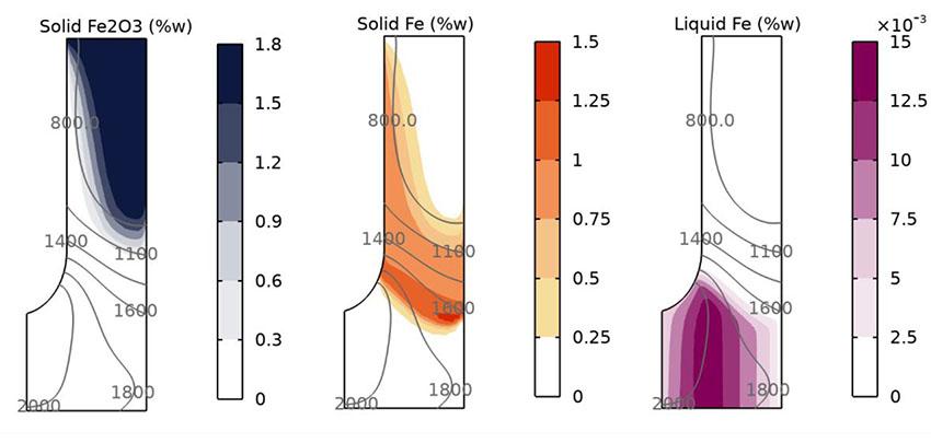
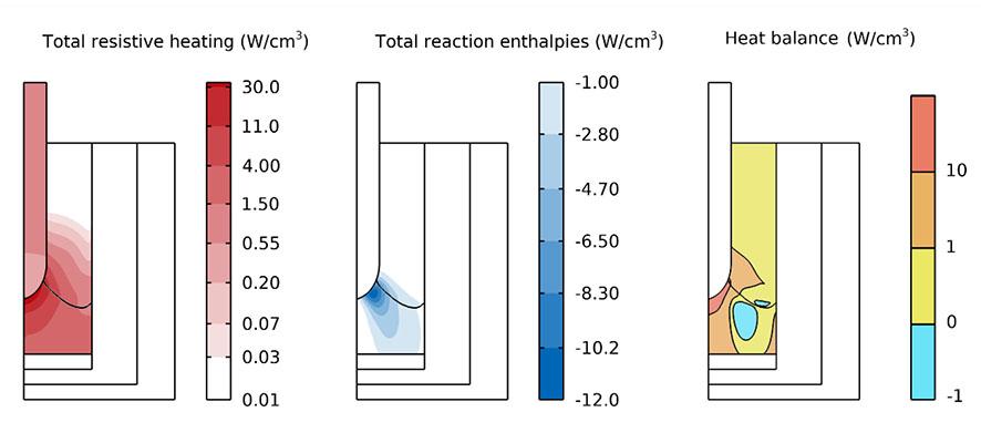
Figure 8 depicts the heat balance of the system. The left panel shows the distribution of ohmic heat generated by the applied electrical current. The boundary of the coke bed (marking where carbon content exceed 50 wt%) is shown with a black line for convenience. One notices that, because of the DC approximation, there is no accumulation of current at the surface of the electrode (skin effect), and the heat generated in the electrode is distributed homogenously. In the charge, the current paths with the least resistance pass through the tip of the top electrode and spread out in the coke bed to reach the flat bottom electrode, hence the heat generation in the charge is concentrated near the tip of the top electrode. The resistance of the coke bed varies between 3 and 4 mΩ·m as a function of position, in close agreement with experimental estimates (Eidem, Tangstad, and Bakken, 2009). The total resistance of the furnace is about 10 mΩ, similar to values from experimental runs in this pilot furnace (Ringdalen and Tangstad, 2013).

The central panel in Figure 8 shows the sum of the reaction enthalpies. Overall, the reactions are endothermic, and most of the thermal energy consumed by the reactions is used in the coke bed near the tip of the top electrode. The endothermic contributions from reactions 3 and 4 (the carbothermic reduction of silicon

Figure 5—Left: Temperature distribution (°C) at the end of the simulation. Centre: Carbon concentration (v/v) confirms the formation of a coke bed. Right: Divergence of the solid flow (1/s). All panels show isothermal contours (°C)

Figure 6—MnO(s), MnO(l), and Mn(l) distribution in the charge domain (wt%). Isothermal contours (°C)

Figure 7—Fe2O3(s), Fe(s), and Fe(l) distributions in the charge domain (wt%). Isothermal contours (°C)

Figure 8—Total resistive heating (left), reaction enthalpies (centre), and heat balance (right) in W/cm3. The black line in the charge marks the boundary of the coke bed

A finite-element method model for a ferromanganese and silicomanganese pilot furnace

and manganese oxides) are the dominating terms. This correlates well with the species distribution (Figure 6) and temperature distribution (Figure 5): liquid oxides that flow the hot region near the tip of the electrode react readily and trickle downward as alloy droplets. Conversely, closer to the periphery the lower temperature results in a less efficient conversion of the slag. The total heat balance (right panel) is obtained by combining the ohmic heating with the reaction enthalpies. Here it can be seen that the resistive heating produces excess heat to maintain the reactions in the region near the electrode. Excess heat is also produced at the furnace periphery. The mid-section of the coke bed is the only region with a negative heat balance. However, note that as the simulation has reached a quasi-steady state, the system is in thermal equilibrium. All the excess heat produced in the core of the furnace and at the furnace periphery is used to either (1) compensate the deficit in the middle of the coke bed, (2) heat the incoming charge, or (3) compensate the heat loss at the furnace surface.

Finally, in Figure 9 the production and consumption of nine major species is show as the rates of reaction (mol/m3s).

Examination of the figure confirms that the dissolution of the species and the reduction reactions occur in different zones.

Transient state

The second simulation aims at studying the conditions in the furnace when changing the charge recipe from a composition rich in iron and acidic oxides (Table II) to a silicomanganese charge rich in basic oxides (Table III). The initial condition corresponds to the quasi-steady state reached at the end of the simulation presented in the previous section. The simulation spans 6 hours and at t =1 h the charge switches from the initial recipe to the final composition. Furthermore, an adaptive carbon coverage is used, meaning that the incoming flux of carbon matches the amount consumed by the carbothermic reduction reactions.

The evolution of the product in the 6-hour run is shown in Figure 10. Although the composition of the charge changes at t = 1 h, (marked in the plot by a blue vertical dashed line), the composition of the products tapped at the bottom of the furnace remains constant up to about t = 1.8 h, since the new charge has to descend and reach the core of the furnace before impacting the system. Once this occurs, the furnace transitions into a new regime within 1–2 hours. Production of both alloy and slag decreases, and the iron content in the alloy drops. The final composition of the alloy is approximately 80 wt% manganese and 20 wt% silicon. The silicon content in the alloy is comparable to experimental runs in this furnace (Ringdalen and Tangstad, 2013) and in line with that of industrial alloys (Olsen, Tangstad, and Lindstad, 2007). The content of fluxes in the slag remains quite constant (28 wt%). The content of

Table III

Composition of the charge for a 20 kg batch: /transient state

Species

aCarbon content varies with consumption in the core.

9—Production and consumption of nine major species

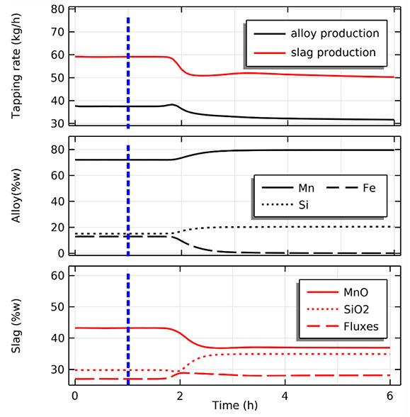
Figure 10—Top: Production of alloy and slug (kg/h) during a 6-hour simulation run with switching of the charge composition after 1 h (blue vertical dashed line). Centre: Composition of the alloy (wt%). Bottom: Composition of the slag

SiO2 increases to 35 wt% and, as expected, the MnO content of the slag decreases with increasing basicity, ending up at 37 wt%.

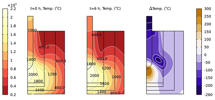
It is interesting to study the different temperature distributions in the furnace at the two quasi-steady states, as shown in Figure 11. One can observe three major differences.

1. The top part of the electrode is much colder; this is a direct effect of the lower conductivity of the charge due to the lack

Figure

(mol/m3s)

A finite-element method model for a ferromanganese and silicomanganese pilot furnace

of ferrous material. The total resistance of the systems is therefore increased, and hence a lower current is needed to reach 150 kW of power.

2. A much higher temperature is found at the tip of the top electrode. This is because although the total current is lower, current accumulates at the tip of the top electrode and increases the power density in that area.

3. The charge in the middle of the furnace is significantly colder, owing to the reduced amount of heat in the area (see point 2) and less heat being transported away from the core. The latter phenomenon is partly due to the higher activity of MnO in the basic slag and a higher reactivity near the hot zone.

Interestingly, the furnace at the beginning of the simulation would appear warmer than at the end, whereas the situation is reversed in the core.

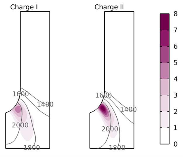
In conclusion, the final quasi-steady state shows larger temperature gradients in the charge approaching the coke bed. This, and the higher activity of MnO in the basic slag, effectively reduces the reaction volume and places it closer to the tip of the electrode, as shown in Figure 12. Despite this pronounced peak in th Mn production rate, the total Mn production is greater for charge I (27 kg/h) than for charge II (25.1 kg/h).

Summary

We have expanded our previous model of a pilot-scale silicomanganese furnace to allow for the study of the ferromanganese process and to investigate the effect of different fluxes.

In total, the movement of 18 chemical species is tracked: two species in the gas phase – CO(g) and CO2(g) – and 16 in the condensed phases – MnO(s), MnO(l), Mn(l), SiO2(s), SiO₂(l), Si(l), C(s), Fe2O3(s), Fe(s), Fe(l), CaO(s), CaO(l), MgO(s), MgO(l), Al2O3(s), and Al2O3(l).

The model uses the quaternary basicity ratio (CaO+MgO)/ (SiO2+ Al2O3) calculated on a mass basis, to encode experimental observations into the controlling equations for the material flows, process chemistry, and electrical and thermal conditions in the furnace.

As for the previous iteration, the model predictions of process parameters such as slag and alloy production rates and compositions are in agreement with experimental values (Ringdalen and Solheim, 2018). In addition, the model complements the information from experiments with insights like the internal temperature distribution and the concentrations of different chemical species in the hearth during the production run.

Acknowledgements

The support from SFI-Metal production (project no. 237738), a Norwegian Centre for Research-Based Innovation, is acknowledged.

Credits

MS: Conceptualization, Methodology, Investigation, WritingOriginal draft preparation. VKR: Methodology, Validation, WritingReviewing and Editing.

References

Artoni, R., Santomaso, A., and Canu, P. 2008. A dissipative Coulomb model for dense granular flows. AIP Conference Proceedings, vol. 1027. p. 941. https://doi. org/10/c53425

Canaguier, V. and Tangstad, M. 2020. Kinetics of slag reduction in silicomanganese production. Metallurgical and Materials Transactions B, vol. 51, no. 3. pp. 953–962. https://doi.org/10.1007/s11663-020-01801-3 COMSOL Inc. 2022 COMSOL multiphysics. https://www.comsol.com/

Eidem, P.A., Tangstad, M., and Bakken, J.A. 2009. Electrical conditions of a coke bed in SiMn production. Canadian Metallurgical Quarterly, vol. 48. p. 355. https://doi.org/10/ghcz4s

Eidem, P.A., Tangstad, M., Bakken, J.A., and Ishak, R. 2010. Influence of coke particle size on the electrical resistivity of coke beds. Proceeding of the Twelfth International Ferroalloys Congress, INFACON XII, Helsinki, Finland. Outotec Oyj, Finland. pp. 349-358. https://www.pyrometallurgy.co.za/InfaconXII/349Eidem.pdf

Fromreide, M., Gómez, D., Halvorsen, S.A., Herland, E.V., and Salgado, P. 2021. Reduced 2D/1D mathematical models for analyzing inductive effects in submerged arc furnaces. Applied Mathematical Modelling, vol. 98. pp. 59–70. https://doi.org/10.1016/j.apm.2021.04.034

Halvorsen, S.A., Olsen, H.A.H., and Fromreide, M. 2016. An efficient simulation method for current and power distribution in 3-phase electrical smelting furnaces. IFAC-PapersOnLine, vol. 49, no. 20. pp. 167–172. https://doi.org/10/ gf9hgp

Figure 11—Temperature at the beginning (left, FeMn acid charge) and end of the 6-hour simulation (centre, SiMn basic charge), and temperature difference between the two states (right)

Figure 12—Production of Mn (g/cm3 h) at the beginning and end of the simulation

A finite-element method model for a ferromanganese and silicomanganese pilot furnace

Haynes, W.M., Lide, D.R., and Bruno, T.J. 2017. CRC Handbook of Chemistry and Physics. 97th edn. CRC Press.

Ksiazek, M., Manik, T., Tangstad, M., and Ringdalen, E. 2013. The thermal diffusivity of raw materials for ferromanganese production. Proceeding of the Thirteenth International Ferroalloys Congress, INFACON XIII, Almaty, Kazakhstan, pp. 127-136. https://www.pyrometallurgy.co.za/InfaconXIII/0127Ksiazek.pdf

Liao, J., Qing, G., and Zhao, B. 2023. Phase equilibrium studies in the CaO–SiO2–Al2O3–MgO system with MgO/CaO ratio of 0.2. Metallurgical and Materials Transactions B, vol. 54, no. 2. pp. 793–806. https://doi.org/10.1007/s11663-02302726-3

Monsen, B., Tangstad, M., and Midtgaard, H. 2004. Use of charcoal in silicomanganese production. Proceeding of the Tenth International Ferroalloys Congress, INFACON X, Cape Town, South Africa. pp. 392–404. https://www. pyrometallurgy.co.za/InfaconX/009.pdf

Monsen, B., Tangstad, M., Solheim, I., Syvertsen, M., Ishak, R., and Midtgaard, H. 2007. Charcoal for manganese alloy production. Proceeding of the Eleventh International Ferroalloys Congress, INFACON XI, New Delhi, India, pp. 297-310. https://www.pyrometallurgy.co.za/InfaconXI/297-Monsen.pdf

Olsen, S.E., Tangstad, M., and Lindstad, T. 2007. Production of Manganese Ferroalloys. Tapir Akademisk Forlag, Trondheim, Norway. Ostrovski, O., Olsen, S.E., Tangstad, M., and Yastreboff, M. 2002. Kinetic modelling of MnO reduction from manganese ore. Canadian Metallurgical Quarterly, vol. 41, no. 3. pp. 309–318. https://doi.org/10.1179/ cmq.2002.41.3.309

Ringdalen, E. and Solheim, I. 2018. Study of SiMn process in a pilot furnace. Proceeding of the Fifteenth International Ferroalloys Congress, INFACON XV, Cape Town, South Africa. Southern African Institute of Mining and Metallurgy, Johannesburg.

Ringdalen, E. and Tangstad, M. 2013. Study of SiMn production in pilot scale experiments – comparing Carajas sinter and Assmang ore. Proceeding of

the Thirteenth International Ferroalloys Congress, INFACON XIII, Almaty, Kazakhstan. pp. 195-205. https://www.pyrometallurgy.co.za/InfaconXIII/0195Ringdalen.pdf

Schotte, W. 1960. Thermal conductivity of packed beds. AIChE Journal, vol. 6. p. 63. https://doi.org/10/b3dgz9

Sparta, M., Risinggård, V.K., Einarsrud, K.E., and Halvorsen, S.A. 2021. An overall furnace model for the silicomanganese process. Journal of the Minerals, Metals & Materials Society, vol. 73, no. 9. pp. 2672–2681. https://doi. org/10.1007/s11837-021-04791-y

Surup, G.R., Pedersen, T.A., Chaldien, A., Beukes, J.P., and Tangstad, M. 2020. Electrical resistivity of carbonaceous bed material at high temperature. Processes, vol. 8, no. 8. p. 933. https://doi.org/10.3390/pr8080933

Tangstad, M., Bublik, S., Haghdani, S., Einarsrud, K.E., and Tang, K. 2021. Slag properties in the primary production process of Mn-ferroalloys. Metallurgical and Materials Transactions B, vol. 52, no. 6. pp. 3688–3707. https://doi. org/10.1007/s11663-021-02347-8

Tangstad, M., Heiland, B., Olsen, S.E., and Tronstad, R. 2001. SiMn production in a 150 kVA pilot scale furnace. Proceeding of the Ninth International Ferroalloys Congress, INFACON IX, Quebec City, Canada. pp. 401-406. https:// www.pyro.co.za/InfaconIX/401-Tangstad.pdf

Tangstad, M., Ringdalen, E., Manilla, E., and Davila, D. 2017. Pilot scale production of manganese ferroalloys using heat-treated Mn-nodules. Journal of the Minerals, Metals & Materials Society, vol. 69. p. 358. https://doi.org/10/ f9pvxj

Tesfahunegn, Y.A., Magnusson, T., Tangstad, M., and Saevarsdottir, G. 2020. Comparative study of AC and DC solvers based on current and power distributions in a submerged arc furnace. Metallurgical and Materials Transactions B, vol, 51. pp. 510–518.

Zienkiewicz, O.C. and Morgan, K. 2006. Finite Elements and Approximation. Dover, Mineola, NY. u

The Southern African Institute of Mining and Metallurgy (SAIMM) would like to extend our congratulations to SRK on reaching this incredible milestone.

We are honoured to be associated with SRK and grateful for the continued support and collaboration with SAIMM throughout the years. Your expertise and insights have enriched our Institute. Your support has been instrumental in fostering a culture of excellence and innovation within the industry.

Dr. Oskar Steffen, co-founder of SRK and winner of the prestigious Brigadier Stokes Memorial Award in 1995 provided outstanding leadership to the SAIMM and the industry during his term as President in 1989/1990. Today, under the guidance and leadership of William Joughin, the current SAIMM President, we continue to reap the benefits of the legacy of excellence and innovation.

As you celebrate this momentous occasion, we applaud SRK for your outstanding contributions to the minerals industry and we thank you for your continued support to SAIMM and the broader minerals industry. Congratulations

Journal of the Southern African Institute of Mining and Metallurgy

Affiliation:

1SINTEF, Norway.

Correspondence to: S.T. Johansen

Email:

Stein.T.Johansen@sintef.no

Dates:

Received: 13 Mar. 2023

Revised: 17 Jul. 2023

Accepted: 27 Sep. 2023

Published: March 2024

How to cite:

Johansen, S.T., Løvfall, B.T., and Rodriguez Duran, T. 2024

A pragmatical physics-based model for predicting ladle lifetime.

Journal of the Southern African Institute of Mining and Metallurgy, vol. 124, no. 3. pp. 93–110

DOI ID:

http://dx.doi.org/10.17159/24119717/2680/2024

A pragmatical physics-based model for predicting ladle lifetime

by S.T. Johansen1, B.T. Løvfall1, and T. Rodriguez Duran1

Synopsis

In this paper we develop a physics-based model for lining erosion in steel ladles. The model predicts the temperature evolution in the liquid slag, steel, refractory bricks, and outer steel shell of the ladle. The flow of slag and steel is due to forced convection induced by inert gas injection, vacuum treatment (extreme bubble expansion), natural convection, and waves caused by the gas stirring. The lining erosion takes place by dissolution of refractory elements into the steel or slag. The mass and heat transfer coefficients inside the ladle during gas stirring are modelled based on wall functions which take the distribution of wall shear velocities as a critical input. The wall shear velocities are obtained from computational fluid dynamics (CFD) simulations for a sample of scenarios, spanning out the operational space, and a model is developed using curve fitting. The model is capable of reproducing both thermal and erosion evolution well. Deviations between model predictions and industrial data are discussed. The model is fast and has been tested successfully in a ‘semi-online’ application. The model source code is available to the public at [https://github.com/SINTEF/refractorywear].

Keywords refractory lining erosion, steel ladle, modelling.

Introduction

In the steel industry ladles are frequently used to keep, process, or transport steel. Ladles are designed to typically hold metal masses ranging from 80 to 300 t (Figure 1). The melt typically consists of hightemperature liquid steel and some slag, which when interacting with the inner wall of the ladle will harm the wall integrity and cause significant wear. In order to reduce the wear, temperature-resistant and chemically resistant refractory bricks are applied to build an inner barrier, typically three layers of wear bricks (inner lining) which should last for a long time in contact with the liquid steel, and at the same time protect the ladle from showing hot areas. In this paper we address the inner lining erosion of a ladle utilized in secondary metallurgy (SM) at a Sidenor plant. Sidenor is the largest manufacturer of special steel

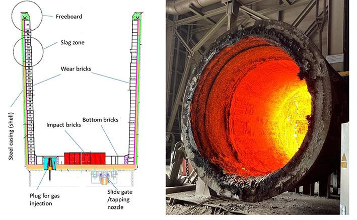
Freeboard

Slag zone

Wear bricks

Bottom bricks

Figure 1 Left: Cross-section of a typical steel ladle, with wear refractory bricks, permanent lining (between wear bricks and steel casing), steel casing, bottom bricks, bottom plug for bottom gas blowing, and slide gate for transfer into casting tundish. Right: Hot ladle that has been in use and is waiting for the next heat. Maximum steel capacity is around 150

A pragmatical physics-based model for predicting ladle lifetime

long product in Spain, and is an important supplier of calibrated products in Europe.

During SM many processes may be going on. The SM ladles have a porous plug installed at the bottom. Gas (Ar or N2) is injected through the plug to induce liquid steel stirring. The rising flow of the liquid steel promotes the transfer of inclusions from the steel to the slag, and homogenizes the temperature and chemical composition.

The main objective of SM is to obtain the correct chemical composition and appropriate temperature for the casting process. In addition, there are several important processes which must be complete during SM, for example the removal of inclusions and gases. In order to attain these objectives, Sidenor has a SM mill consisting of two ladle furnaces (LFs) and a vacuum degasser (VD). Each of the LFs has three electrodes for heating the slag, steel, and ferro-additions. The ladle contains steel and slag for the whole production process, from EAF tapping to the completion of the casting process. The liquid steel in the ladle has a temperature of around 1700 K, and is covered with slag. The slag, which helps to remove impurities from the steel and prevents contact between the steel and atmosphere, has lower density than steel. The slag consists basically of lime and oxides. Slag conditioning can be improved during SM by adding slag-formers such as lime and fluorspar. In order to handle the liquid steel and slag at such high temperature, the ladle is built with a strong outer steel shell lined inside is with layers of insulating refractory ceramic materials. The most important properties of the refractory lining are:

➤ Ability to withstand high temperatures

➤ Favourable thermal properties

➤ High resistance to erosion by liquid steel and slag.

The inner layer of refractory bricks, which is in contact with the liquid steel, is eroded by the interaction with the hot metal and the slag. Each heat erodes the refractory bricks, and after several heats, they are so eroded that it is not safe to continue using the ladle. The refractory is visually checked after each heat and depending on its state, it may be used for another heat, put aside for repair, or demolished. In case of repair, the upper bricks of the ladle, which are more eroded due to chemical attack by the slag, are replaced and the ladle is put back into production. Later, based on continuing visual inspection, the ladle may be deemed ready for demolition. In this case, the entire inner lining is removed and the ladle relined with new bricks.

One important goal for Sidenor is to reduce refractory costs by identifying new methods for extending the refractory life. One of the key points is to increase the number of heats without compromising safety. Another important issue is to better understand the mechanism of refractory erosion, in order to improve working practices and so increase ladle lifetime.

Motivation

The main goal of this investigation is to develop a model whose results, in conjunction with operator experience, can indicate whether the ladle can be safely used for another heat. The model should incorporate both historical and current production data. In addition, the model should provide information about the major factors that contribute to ladle refractory erosion and indicate practises that could be adopted to extend refractory life.

Previous work on ladle lining erosion

Several studies have been published dealing with properties of refractory bricks (Mahato, Pratihar, and Behera, 2014; Wang, Glaser, and Sichen, 2015), advising on improvements to produce

high-quality bricks. A more general review of MgO-C refractories was given by Kundu and Sarkar (2021). The corrosion-erosion mechanisms have been studied in a few papers (Kasimagwa, Brabie, and Jönsson, 2014; Jansson, 2008; Mattila, Vatanen, and Harkki, 2002; Huang et al., 2013; LMM Group, 2020; Zhu et al., 2018). In the opinion of these authors, the most thorough approach was that of Zhu et al. (2018). Bai et al. (2022) investigated the impact of slag penetration into MgO-C bricks.

In order to predict refractory erosion, temperature, fluid composition, and mass transfer mechanisms must be considered. The heat balance has been studied in some specialized works (Çamdali and Tunç, 2006; Glaser, Görnerup, and Sichen, 2011; Zimmer et al., 2008; Duan et al., 2018; Zhang et al., 2009). The effect of slag composition has been studied in multiple works (Bai et al., 2022; Jansson, 2008; Kasimagwa, Brabie, and Jönsson, 2014; Mattila, Vatanen, and Harkki, 2002; Sarkar, Nash, and Sohn, 2020; Sheshukov et al., 2016; Zhu et al., 2018). A critical step in developing prediction models is the local mass transfer between the lining and slag/metal. This has to date been treated by semiempirical models Bai et al., (2022); Sarkar, Nash, and Sohn, 2020; Wang et al., 2022). Wang et al., (2022) applied 3D computational fluid dynamics (CFD) and their predictions seemed to agree with observations. However, they did not report the diffusivities used in their model, and the underlying erosion-corrosion models were empirical and tuned to the data. It was found that these tuning factors would depend on the operating conditions.

In industry, refractory wear is known to be a result of (i) thermal stresses, resulting in thermal spalling, (ii) dissolution of the refractory bricks into the slag/metal, and (iii) dissolution of the binder materials into the slag/metal. Moreover, mechanical stresses imposed on the refractory during cleaning operations will impact on erosion and lifetime. Phenomena such as spalling due to hydration of the bricks are also involved (Wanhao Refractory, 2023).

The impact of thermal stresses will be most severe at the bottom of the ladle when hot steel meets colder refractory. As the velocity of the metal at the moment of impact is high, this is where the maximum thermal stresses are expected. The colder the ladle wall is when it meets hot steel at high speed, the greater the risk of crack formation.

It must be noted that the time between heats has a significant effect on thermal spalling. The temperature distribution in the ladle refractory wall at the time of filling is an important parameter that can be predicted using the model to be presented. However, the addition of a heating burner at the ladle waiting station is not included for now. Instead, we simulate a reduced waiting time to mimic the effects of using a burner to maintain refractory temperature.

The pragmatism-based approach to a model for ladle lining erosion

In previous publications, the authors defined a methodology ‘Pragmatism in industrial modelling’ (Johansen and Ringdalen, 2018; Johansen et al., 2017; Zoric et al., 2015), which is especially suited for developing fast and sufficiently accurate industrial models. In a twin paper (Johansen et al., 2023) the authors have outlined the methodology that was applied in this work and the learnings that may be exploited in future projects. Here the details of the physics-based model are explained.

The objective of the model is to be able to advise or support operators in assessing if it is safe to use the ladle for another heat. In such an application, the erosion state of the refractory must be updated from heat to heat and a simulation for a subsequent

A pragmatical physics-based model for predicting ladle lifetime

virtual heat performed. The virtual heat should contain as much information as possible about the next heat. The result of such a simulation and visual or optical inspection of the lining would then lay the foundation for the final assessment.

Model simplifications and assumptions

The pragmatic model must be fast as we wish to simulate a transient ladle operation, lasting about two hours, in less than a minute. This is critical as we wish to simulate all ladle operations within a year in a few hours in order for the results to be applied directly in production, to carry out tuning, or perform a parameter sensitivity analysis.

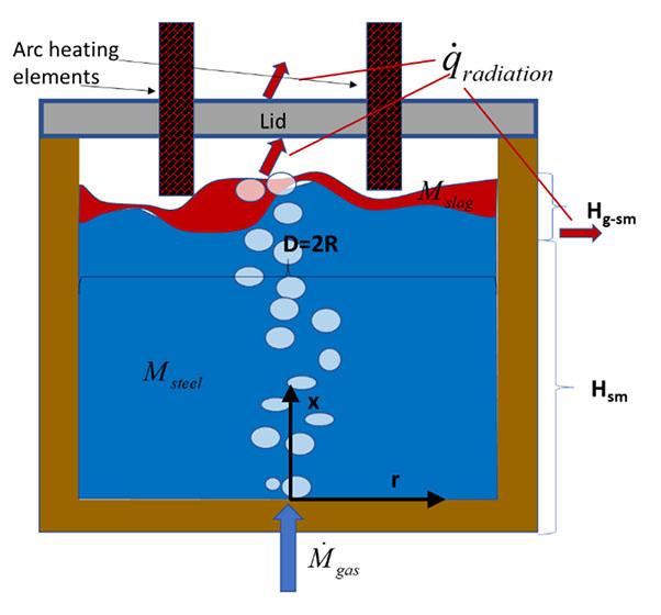
Figure 2 gives some ideas about the phenomena involved. The heating elements (electrodes) can be submerged in the slag, or work from above. They produce electric arcs that heat the liquid steel. The flow of the slag and liquid steel is not only a function of the gas flow rate applied for blowing, but is also influenced by several factors such as the mass of steel and slag, vacuum pressure, and the thermophysical properties of the fluids.

The ladles are 3D objects, but due to speed requirements some overall model simplifications were done:

i. The model is 2D (cylinder-symmetrical) with the porous bottom plug placed in the centre. As a consequence, we assume that the gas/steel/slag flows can be regarded as rotationally symmetric

ii. The stirring gas is inert (only provides mixing)

iii. In the sidewalls only the radial heat balance is included

iv. In the bottom only vertical heat balance is included

v. The solubility of MgO in the slag and of C in the steel are assumed constant

vi. The metal and the slag phases are stratified and are assumed to be internally perfectly mixed. The phases exchange mass and energy with each other and the refractory

vii. Above the slag energy is exchanged by radiation only viii. Refractory erosion due to thermomechanical stresses is not considered.

Volumes and mass balances

As the model will compute situations with different amounts of steel and slag in the ladle, we have to take into account all these possible situations. The total volume of the slag and metal is represented by

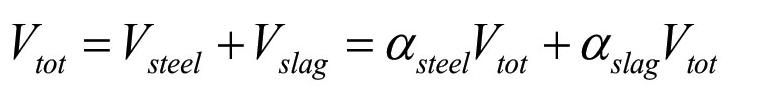
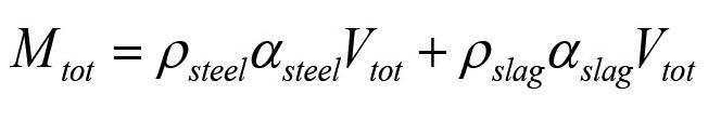
Accordingly, the mass of liquids inside the ladle is:

In our first approach, we neglect the volumes of the protruding impact element at the bottom and the volumes modified by eroded bricks. In this case, the metal-slag interface is positioned at height

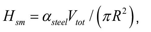
and the thickness of the slag layer is:

The mass balance for the ladle must also be respected. That is, for the slag

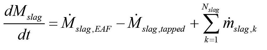
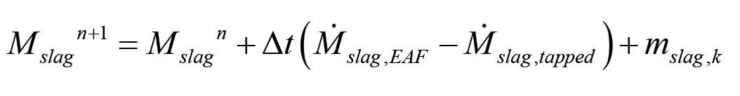
Here M . slag,EAF and Msteel,EAF are the transient mass flow rates of slag and steel coming into the ladle during tapping from the EAF. m . slag,k is the mass flow rate of added slag former of type k Typically a slag former of type k, total mass mslag,k, can be assumed to be added during one numerical time step, between time tn and tn+1, such that

For the metal we have:

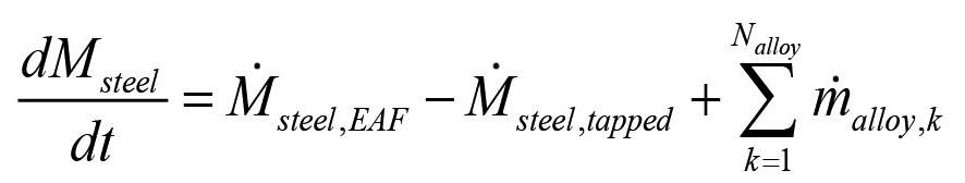
M . slag,tapped and M . steel,tapped are the transient mass flow rates of slag and steel tapped out of the ladle. Similarly, m . alloy,k is the mass flow rate of added alloy of type k. As for the slag, an alloy of type k, total mass malloy,k, can be assumed to be added during one numerical time step between tn and tn+1, such that

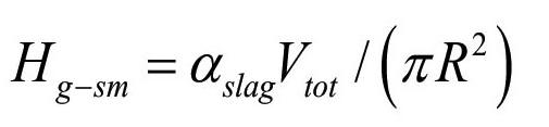
Based on Equations [5]–[8], the phase densities, the purge gas fractions present in each phase, and corrections for the eroded ladle radius, we can compute the transient interface position for the metal and slag. This is critical input to the thermal and erosion models.

Thermal models

A quasi-2D thermal model for the complete refractory lining and outer steel shell is outlined in Appendix A. Thermal modelling. Both the sidewall and the bottom are included. The model is referred to as quasi2-D as vertical heat transport between horizontal brick layers is assumed to be insignificant compared to heat exchange with metal, slag, and radiation and is ignored. The steel shell exchanges energy with the surroundings while the wetted inner refractory layer exchanges energy with the liquid steel and slag. Nonwetted refractory elements are exchanging energy with the top slag-metal surface, and internally, both by radiation. Enthalpy-based conservation models for steel and slag are developed, as detailed in Appendix A. In general, appropriate boundary conditions are developed and outlined in the appendixes.

Figure 2 Idealized, simplified ladle, showing slag (red), metal (blue), gas bubbles, heating elements, and refractory (brown)

A pragmatical physics-based model for predicting ladle lifetime

Discrete equations for the slag and metal energy

The coupled discrete equations for slag and metal enthalpy (see Equations [64] and [66], Appendix A) can be solved analytically, provided the inner refractory wall temperatures are known. First, we need to establish the relationship between temperatures and enthalpies. This is elaborated in Appendix C. Temperature-enthalpy relationships. As seen from Appendix D. Discrete equations for the slag-metal heat balance, explicit expressions for the slag and metal enthalpies are given by Equation [92]. Temperatures are then computed by Equations [75] and [77].

Erosion model

The erosion is primarily a result of dissolution and mass transfer from the refractory into the metal and slag. The erosion mechanism considered is mass loss of refractory to the liquid by dissolution. In addition, we have mass losses due to thermal stresses. These may be addressed in a machine learning model, which may exploit the predicted difference between refractory temperature and that of the incoming steel temperature.

Refractory loss in the steel wetted region

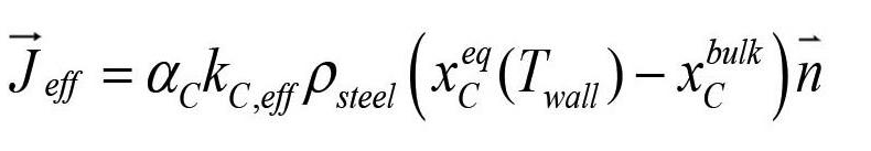
During periods of considerable agitation of the metal and slag (bubble-driven convection, natural convection, electromagnetic stirring) the carbon binder of the MgO-C refractory may be dissolved into the steel. The mass flux of carbon into the steel is locally given by: [9]

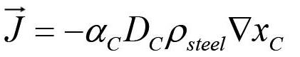
Here aC is the volume fraction of the refractory that is occupied by carbon, DC is the diffusivity of carbon in steel, and xC is the mass fraction of carbon in the steel.

By introducing the concept of a mass transfer coefficient, we may write Equation [9] as

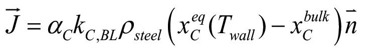
Here kC,BL is the mass transfer coefficient for the liquid side boundary layer and xC eq (Twall) is the solubility of C in the steel

[10]

with its actual composition, and where Twall is the temperature at the inner ladle wall. The temperature is controlled by the steel temperature and the temperature in the refractory brick. As the thermal conductivities of the liquid steel and the wear refractory are of the same order of magnitude (see Table I), the wall temperature will depend on both steel and refractory temperature.

For forced convection we may use the mass transfer coefficient suggested by Scalo, Piomelli, and, Boegman (2012) and Shaw and Hanratty (1977), stating that the mass transfer coefficient for Schmidt number Sc > 20 can be approximated by

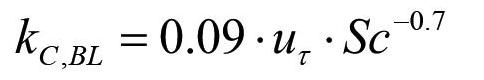
Values for the shear velocities typically range from zero to 0.1 m/s.

[11]

From Equations [10] and [11] we learn that erosion of the steelwetted ladle wall will increase with increasing gas-stirring flow rate, and temperature (increased C solubility and diffusivity, decreased viscosity).

Mass transfer resistance at the interface between MgO-C and steel

At the inner surface of the MgO-C bricks the C in the C-continuous domains (graphite and carbon contributions from binder) (Zhang, Marriott, and Lee, 2001) will dissolve into the steel while MgO may be considered as inert. A schematic is provided in Figure 3. As the carbon (from carbon-dominated areas) is dissolved into the steel, the average transport length s pore will stabilize at around a typical MgO particle radius. If the MgO particles are small the convection inside the pore space can be neglected. In this case the transport in the pore space may be represented by pure diffusion. In that case we can write:

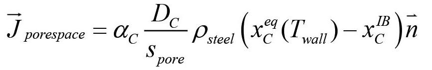
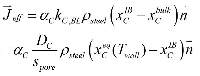
Here xCIB is the mass fraction of C at the wall, defined at the outer surface made up if the MgO particles protrude out of the C matrix. In this case the mass flows through the inner and outer layers must match, giving:

Physical properties. Here T is temperature in °C and Xc is mass fraction of carbon dissolved in the steel

‒ r 0.835(T – 273.15) +

(–83.2 + 8.35 . 10–3 (T – 27315))

: Ceotto, (2013)

‒Cp:1

1https://www.setaram.com/application-notes/an372-heat-capacity-of-a-steel-betwwen-50c-and-1550c-liquid-state/

Table I

A pragmatical physics-based model for predicting ladle lifetime

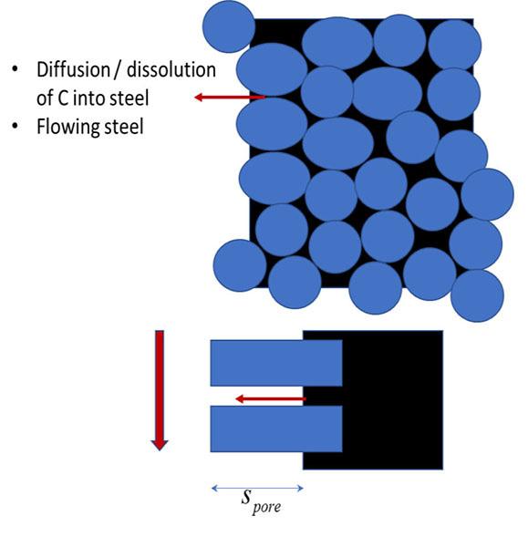
Figure 3 (Above) MgO particle in a C matrix. The flow of liquid steel is shown on the LHS. (Below): Illustration of C that must diffuse through channels between MgO grains to reach the inner side of the flow boundary layer. The vertical arrow indicates the steel flow. Horizontal arrow indicates diffusion flux

[13]

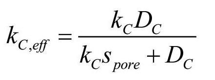
and where the mass transfer coefficient is given by [14]

The effective mass transport of C from the MgO-C brick to the steel is then [15]

Refractory loss in the slag-wetted region

The slag is collected in a relatively thin layer at the surface of the molten bath . Due to the bubble plume, caused by the stirring gas, the slag will be pushed towards the refractory wall. As the bubble plume is asymmetrical, the slag thickness close to the refractory wall will vary along the ladle perimeter. We neglect these complexities and assume complete radial symmetry. The thickness dslag of the slag layer that contacts the refractory can be estimated by:

[16]

The slag layer will move vertically, driven by waves generated by the bubble plume, as illustrated in Figure 4. The slag layer has thickness dslag and wave amplitude awave.

The mass transfer from the wall to the slag layer can be analysed by assuming a developing boundary layer. According to Schlichting (1979) the mass transfer along a developing boundary layer can be expressed as

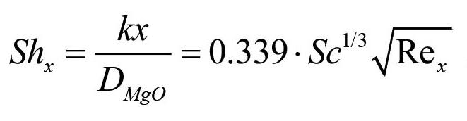
The explicit mass transfer coefficient is now: [19]

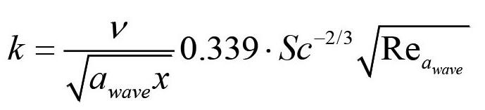
By averaging the mass transfer coefficient k in Equation [19] over the thickness of the slag layer we obtain [20]

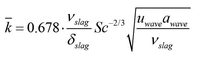
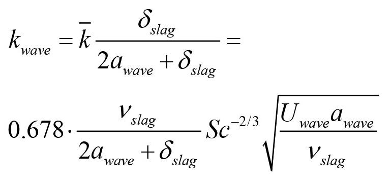
The wave velocity uwave is now estimated by Equation [108] (Appendix E), and the swept distance (amplitude) awave can be represented by lw in Equation [107]. It is possible to represent the distribution of mass transfer by a probability distribution. However, as a first approximation we assume that the wave-induced mass transfer applies to a region that extends over the thickness of the slag layer and a region that extends awave both above and below the slag layer. In this case we may estimate the mass transport to the slag to be given over height 2 awave, + dslag, and where the average mass transfer coefficient for this layer is [21]

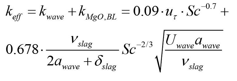
In addition to the explicit wave contribution to mass transfer, the impact of the bubble-driven flow (slag version of Equation [11]) must be added:

Overall refractory loss model

We will track both the MgO and C components of the refractory. We may note that bottom erosion is not included in the model for now. The bottom is included due to its impact on the thermal balance (heat storage).

[17]

where k is the mass transfer coefficient and x is the distance along the developing boundary layer.

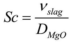
DMgO is the diffusivity of MgO into the slag, and is related to the Schmidt number by

[22]

Figure 4 Schematic of the slag layer, close to the refractory, moving vertically with wave amplitude awave

A pragmatical physics-based model for predicting ladle lifetime

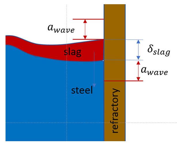
It is assumed that when C is dissolved from the bricks in the steel region a corresponding amount of MgO is released and will end up in the slag. It is also assumed that the density of the bricks is related to C and the corresponding MgO volume fractions (aC, aMgO) and phase densities (rC, rMgO) by [23]

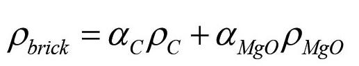
where aC + aMgO = 1. The MgO mass loss, MMgO, from a brick element during time dt, eroding a slice of thickness l, is

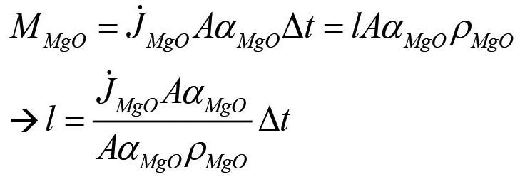
Here A is the total area, and AaMgO is the partial area where MgO is contacting slag.

The corresponding loss of C due to loss of MgO is then

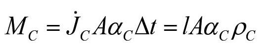
[24]

Here aC is the volume fraction of carbon in the brick, while (1−aC) is the MgO fraction. a* i,slag is the wave-enhanced slag fraction, being in contact with the lining. As a first approach for a* i,slag we use a* i,slag = 0.25ai-1,slag + 0.5ai,slag + 0.25ai-1,slag.

The left-hand terms are split and the effect of total mass change entered into the models. In the case of the slag we have:

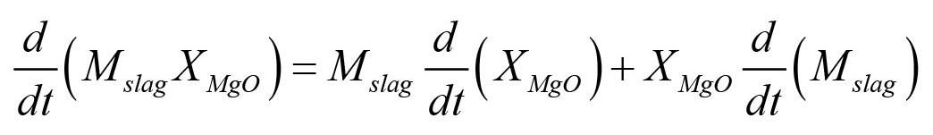
where the mass balance was given by Equation [5]. According to these equations we may write Equation [30] as

[25]

From Equations [24] and [25] we find that in the slag region the carbon flux out of the refractory wall is given by

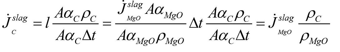
[26]

According to Equation [26] the volume flows of the carbon and steel are equal. However, the surface areas are different due to the actual volume fractions. The mass flow of carbon, per unit surface area, to the liquid in the slag region is then

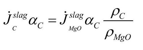
Similarly, the loss of MgO in the steel region due to carbon dissolution is

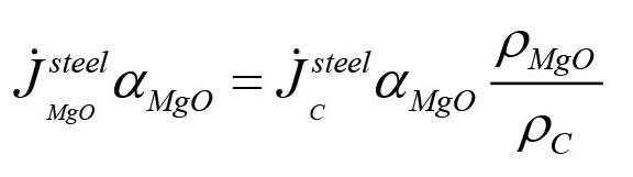
Carbon balance

[27]

where it is assumed that there is no MgO in the slag tapped from the EAF.

Similarly, the mass balance for carbon becomes

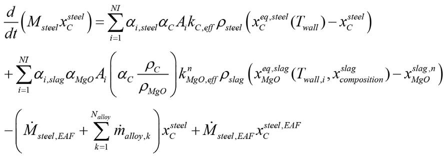
The solubility of MgO in the slag is given as (see acknowledgements) by

[28]

The carbon is lost from the refractory by two mechanisms, depending on whether we are consodering the steel-wetted or slagwetted zone.

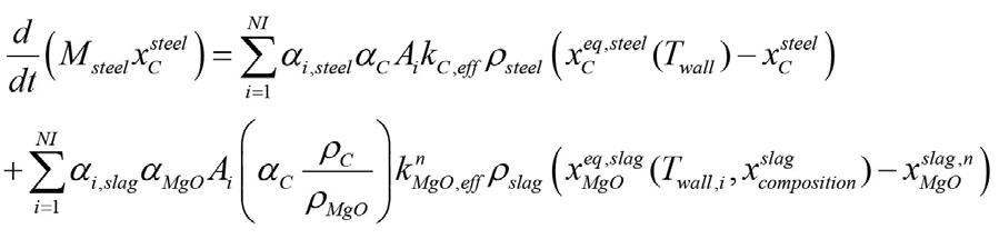
[29]

The summation is over all the vertical refractory bricks. Here ai,steel is the local steel fraction (which varies with height in the ladle) and aC is the carbon fraction in the refractory brick. Ai = 2pRDxi is the local wall area.

MgO balance

The MgO is lost from the refractory in a similar way to the two mechanisms above.

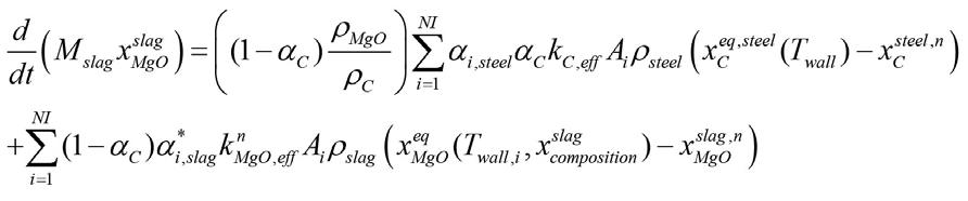
[30]

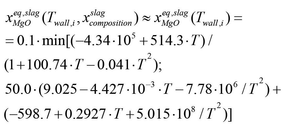
Here T is the temperature in degees Celcius. As the slag composition is not known we use a temperature dependency which is approximate for 50 wt%CaO, 10 wt%SiO2, 2.5% FeO, and the balance Al2O3

Developing sub-models – a multi-scale approach

In the present approach we used CFD simulations (Johansen and Boysan, 1988) to obtain the shear stresses along the wall of the ladle. Based on a set of CFD simulations a fitted curve of the vertical shear stress distribution was provided as input for the both the thermal and erosion models (see Appendix B. Wall shear stress model). We did not include the effects of the slag. Using dynamic simulations with slag present more details could be added, and based on curve fitting or lookup tables, the data could be plugged into the model. This would have improved the accuracy.

FACT SAGE calculations were performed for the solubility of MgO in the slag (see Acknowledgements). At the present time it was not possible to use this detailed information as we have no information of the composition of the slag arriving at the ladle from the EAF. Based on this it was possible to close the model equations and realize the models.

[31]

[32]

[33]

[34]

A pragmatical physics-based model for predicting ladle lifetime

Software

The model was coded in python 3, using libraries numpy, pandas, math, pickle, and scipy, and we used matplotlib and vtk for plotting and visualization. The basic version of the model is available on github.com, at https://github.com/SINTEF/refractorywear

The model is licensed under the open source MIT license (https://opensource.org/licenses/MIT).

Tuning the model

Tables I-III lists the physical and thermodynamic data that was used.

Unfortunately, detailed geometrical data and process data cannot be given due to company confidentiality. In order to apply the model to single heats, operational data from Sidenor was read. The static data included steel mass, time with steel in the ladle, temperature of the steel before leaving the EAF, and cyclic data for vacuum pressure, heating power, measured steel temperatures, gas flow rates, and mass and composition of additions, all versus time. The simulation was initiated at the time when the ladle was filled with liquid steel from the EAF and run for 2 hours. Once the casting process is finished, the ladle is considered to be empty, but still losing heat.

As there is no data on the initial slag mass or composition, it was not possible to incorporate changes in slag composition in the model. The initial slag mass was therefore assumed to be always 500 kg. Another consequence was that we had to assume constant solubilities of C in steel and MgO fraction in the slag. As a result, the solubility of MgO in the slag depends only on temperature (see Equation [34]. Furthermore, all additions were assumed to contribute to the slag. This is acceptable if the alloy additions are of same order of, or smaller than, the pure slag contribution. However, for special steels, addition levels are significant and the model should be updated such that additions are transferred to the metal.

Different additions have different thermodynamic properties, such as melting temperature and melting enthalpy. As this information was largely unknown, we used the same melting temperature and heat of melting for all additions.

Table II

Solubilities

Carbon solubility in steel: x C eq (Twall) 0.1 eq,slag

MgO solubility in slag: xMgO (Twall) See Equation [34]

Table III

Tuning parameters

First, we tuned the steel temperature as a good thermal prediction was a prerequisite for the erosion model. At the beginning of each heat it was found that the initial temperature in many cases was a leftover from the previous heat. We therefore decided to use the temperature measured in the EAF, decreasing this by 50 K due to heat loss during tapping. For heats where the initial temperature was unavailable or resulted in large temperature residuals, the initial temperature was corrected in an iterative manner until the residual for average relative temperature was below 20 K. The residual was computed from all measured values except the first, which was not reliable. In both Figure 5 and Figure 6 we see successful simulations, showing zero-order residuals of 5 K and 3 K, respectively. The first-order residuals (RMSE) are similarly 7 K and 5 K. In both cases the initial temperature was optimized, but for heat 206217 the ‘measured’ initial steel temperature was quite close to the optimized initial temperature. To obtain these results, the thermal efficiency of the heater was reduced to 85% and the thermal conductivity of the refractory bricks and insulation was increased significantly (see Tables I and III).

In the second step, the erosion model was tuned. We decided to work with constant solubilities of C in steel (soluble mass fraction was set to 0.1), while the MgO solubility in the slag is based on a fixed slag composition and only varies with temperature (see Table II). As we decided to keep the solubility of C in the steel constant, the only tuning that was possible is the pore diffusion length s pore (see Equation [12] and Figure 3).

This tuning was done as follows:

i) Start with simulating the preheating of the ladle

ii) Look up the heat ID, then read operational data for the heat and simulate temperature and erosion

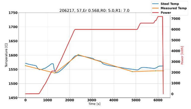
and

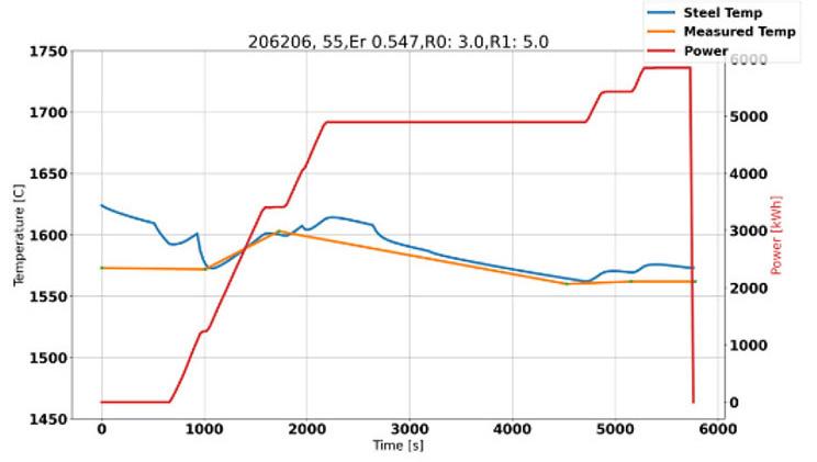
6 Predicted

Figure 5 Predicted steel temperature evolution, measured temperatures,

energy added to the ladle ‘"Power’) for ladle 5, heat 206217

Figure

A pragmatical physics-based model for predicting ladle lifetime

iii) Based on the erosion data, reduce the radial cell sizes for the three inner bricks (wear bricks)

iv) Account for the thermal history of the ladle until next heat

v) Repeat step (ii) for the next use of the specific ladle (next heat in campaign, and where the campaign number is unique for the wear lining, from relining until demolition), and then accumulate the erosion of the bricks

vi) If the ladle was taken out for repair of some bricks, the repaired bricks are also repaired in the model. After repair the temperature is again initialized

vii) Repeat step (v) until the ladle is taken out for lining demolition. At this time the predicted erosion profiles are saved and compared to data from the demolition.

In the demolition data, the ladle is segmented in two halves, where ‘Left’ is close to the porous plug while ‘Right’ is away from the plug. In addition, the brick with the most erosion in each half is registered. In this way, a maximum erosion is recorded and the average value for each brick row is not known. However, the 2D model can only be compared with the average of the two and should have some underprediction due to the above observation. For the selected tuning factor s pore we see that the prediction in Figure 7 is good, both qualitatively and quantitatively. The shape of the erosion in the steel region, below the slag line, is typical for all ladles and campaigns. We note that for bricks 36−40 the erosion level is quite high. This is above the liquid steel level and is a result of metal splashing, causing thermomechanical cracking, and disintegration due to the vacuum treatment (Jansson, 2008). In Figure 8 we see the prediction from a campaign where the erosion in the steel section (bricks 10−25) is underpredicted. Note that in this case, brick numbers below 9 were not measured. The underprediction could be a result of the different steel qualities treated in this specific campaign, or because for some reason the variation along the perimeter, at each brick layer, is larger than usual. As we have no data on the erosion from heat to heat, we cannot tell if this happened during specific heats in the campaign. Another interesting feature, seen in both Figure 7 and Figure 8, is the pronounced dip of erosion around brick 16 and 17. This may be a result of the addition of alloying materials when the ladle is approximately 1/3 full. Alloying elements and slag may stick to the colder wall long enough to protect the lining somewhat.

Model performance against Sidenor operational data

The model was run with all available Sidenor data for 2019. The

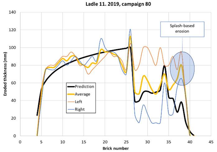
production campaigns that started in 2018, or ended in 2020, were omitted from the current data-set as those campaigns were not complete. Altogether, we analysed 5216 heats, involving 11 different ladles and 61 campaigns. Averaged erosion over bricks 5-25 is compared in Figure 9. An outlier (ladle 8, campaign 76), marked A, is seen, where the details were already shown in Figure 8. We compare the average erosion per heat in Figure 10, as distributed over the number of heats in each campaign. The model predicts a variation of ±12%, while the data has a variation of ±18%. The outlier A from Figure 9 is clearly seen.

Figures 7 and 8 show a peak in erosion close to the surface of the steel where the slag is located (around brick 35). The steel mass in the ladle varies from heat to heat, but in cases when the reported mass is low this may be due to operation challenges during casting. Therefore, the minimum steel mass is set to 110 t. This introduces another uncertainty in the predictions. Now, it may seem that the erosion does not change much from heat to heat, as indicated from

Figure 7 Comparison of predicted versus measured eroded thickness for ladle 11, campaign 80, 2019

Figure 8 Comparison of predicted versus measured eroded thickness for ladle 8, campaign 76, 2019

Figure 9 Comparison between measured and predicted erosion thickness at time of demolition of wear lining. Symbols represent different ladle numbers. Outlier A is marked

A pragmatical physics-based model for predicting ladle lifetime

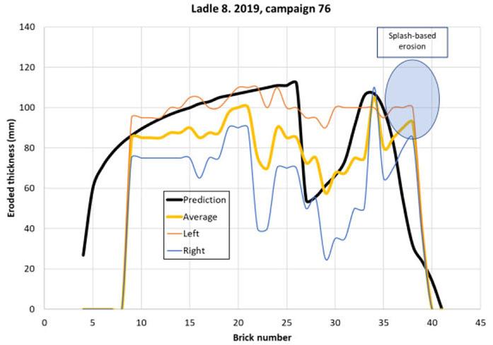
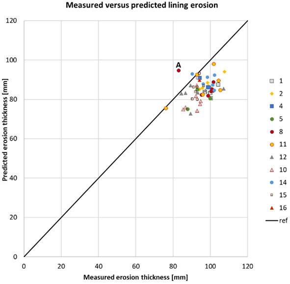
Figure 10. We see in Figure 11 that the predictions show significant difference in amount eroded, and erosion pattern, from heat to heat. Around brick 25 (steel-wetted region) the erosion for use number 17 is around twice as high as for use 69. This difference is mainly due to temperature, time with vacuum, gas flow rates, and operational times. However, when averaged over a complete campaign, these variations are significantly reduced.

Discussion

The model predicts a smooth increase in erosion rate from the bottom towards the slag. This is in very good agreement with some of the measured erosion profiles. Figure 7 shows one example. This is a result of the bubble-driven flow, enhanced by vacuum, the transport processes in the brick (represented by s_pore, or s pore), and in the flow boundary layer, as well as the solubility of carbon in the steel. We used an artificially high value for the saturated carbon mass fraction (XCeq = 0.1). However, similar results to those shown here may be obtained by another combination of s pore and XCeq

We see above that the model performs quite well. At the same time, there is room for improvements. The most obvious improvements are:

i) Modelling of the slag composition and adding the solubility of MgO in the slag as a function of composition. However, this requires knowledge of the composition of the slag tapped from the EAF.

ii) Separating additions into slag formers and alloying elements, and updating the enthalpy-temperature relationships to represent the true compositions of slag and metal.

iii) Empirical slag temperature is needed to calibrate and validate the slag temperature predictions.

iv) Including the solubility of carbon in the steel. Data for the steel composition is available but the carbon solubility for different compositions must also be available.

Some features seen in the data, such as shown in Figure 12, cannot be reproduced by the model. The very high observed erosion

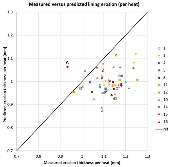
rates close to the bottom cannot be explained with the available information about the operation. It is possible that gas purging was done with a very low steel level and containing slag. Such issues can be regarded as abnormal operations. Other possibilities are excessive mass loss during ladle cleaning, or that the lining brick quality was not consistent for a period.

Conclusions and recommendations

The presented model predicts the evolution of lining erosion fairly well. Much better agreement between model and data is hard to obtain due to uncertainties in operational data, physical data, and measurements. The model is primarily predicting lining erosion based on hydrodynamics and solution of lining elements in steel and slag. The contribution from thermomechanical cracking (thermal spalling) of the lining is not included in the model. However, the model predicts lining temperatures at the time metal is tapped into the ladle. This information can in the future be used to assess thermomechanical brick degradation. As this effect was not included, the model was tuned to predict less erosion than what is observed. Similarly, the lining degradation above the melt, which is particularly pronounced during vacuum treatment, was not included in the model. However, a hole in the lining this far up on the ladle wall has far less serious consequences than holes deep below the steel surface.

Figure 10 Comparison between ‘per heat averaged’ measured and predicted erosion thickness at time of demolition of wear lining. Symbols represent different ladle numbers. Outlier A is marked

Figure 11 Predicted eroded fraction of wear lining versus brick number for four heats that are part of campaign 71. Graphs are labelled by ladle use number of the campaign. The symbols mark each brick, where a brick corresponds to a grid cell

Figure 12 Comparison of erosion profiles for ladle 5, campaign 69, 2019

A pragmatical physics-based model for predicting ladle lifetime

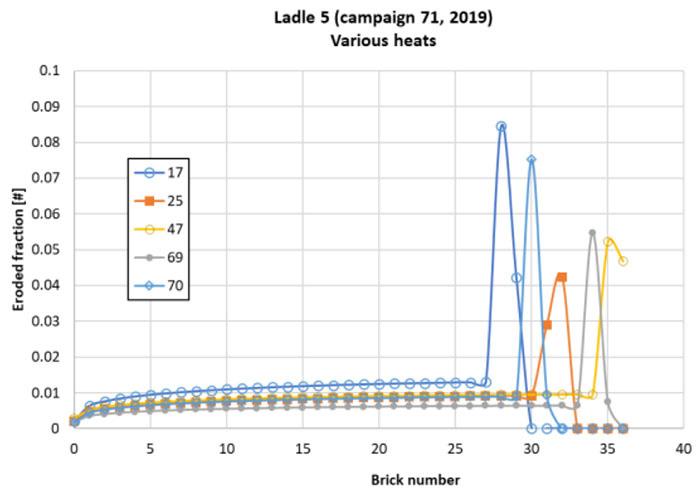
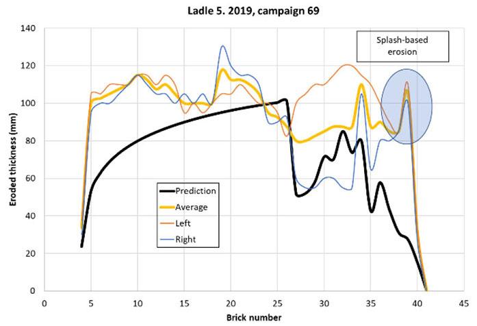
Model predictions, as we have presented, will provide important support for the ladle operator when deciding if the ladle can be used for another heat. The model shows how the variation in steel level between heats impacts erosion. If all the heats were run with the same volume of steel this would have an adverse impact on lining lifetime. On the other hand, the refractory life may be extended by running scheduled amounts of steel in the heats. When the operator is unsure about the ladle conditions, and based on previous experience from running the model, the model prediction will help the operator to make an appropriate decision.

Finally, it must be acknowledged that the heart of the model is based on complex multiphase 2D CFD simulations that provided critical information about the distribution of shear stresses, and resulted in distributed heat transfer and mass transfer coefficients.

The source code is available from https://github.com/SINTEF/ refractorywear

Acknowledgements

We thank Dr Kai Tang, SINTEF Industry, for his assistance with the FactSage calculations of MgO solubility in slag. The simplified MgO solubility versus temperature was based on this work.

This research was funded by the H2020 COGNITWIN project, which has received funding from the European Union’s Horizon 2020 research and innovation programme under grant agreement No. 870130.

CRediT author statement

STJ: Conceptualization, methodology, writing - original draft preparation; BTL: Software, data curation, validation, visualization, writing - reviewing and editing; TRD: Resources, investigation, writing- reviewing and editing.

References

Ashrafian, A. and Johansen, S.T. 2007. Wall boundary conditions for rough walls. Progress in Computational Fluid Dynamics, vol. 7, no. 2. pp. 230–236. https:// doi.org/10.1504/PCFD.2007.013015

Bai, R., Liu, S., Mao, F., Zhang, Y., Yang, X., and He, Z. 2022. Wetting and corrosion behavior between magnesia–carbon refractory and converter slags with different MgO contents. Journalof Iron and Steel Research International, vol. 29. pp. 1073–1079. https://doi.org/10.1007/s42243-021-00695-y

Çamdali, Ü. and Tunç, M. 2006. Steady state heat transfer of ladle furnace during steel production process. Journal of Iron and Steel Research International, vol. 13. pp. 18–20. https://doi.org/10.1016/S1006-706X(06)60054-X

Ceotto, D. 2013. Thermal diffusivity, viscosity and prandtl number for molten iron and low carbon steel. High Temperature, vol. 51, no. 1. pp. 131–134. https://doi. org/10.1134/S0018151X13010045

Churchill, S.W. and Chu, H.H.S. 1975. Correlating equations for laminar and turbulent free convection from a vertical plate. International Journalof Heat and Mass Transfer, vol. 18. pp. 1323–1329.

Cloete, S.W.P. 2008. A mathematical modelling study of fluid flow and mixing in gas stirred ladles. MSc thesis). Stellenbosch University, South Africa.

Duan, H., Zhang, L., Thomas, B.G., and Conejo, A.N. 2018. Fluid flow, dissolution, and mixing phenomena in argon-stirred steel ladles. Metallurgical and and Materials Transactions B, vol. 49. pp. 2722–2743. https://doi. org/10.1007/s11663-018-1350-4

Ede, A.J. 1967. Advances in free convection. Advances in Heat Transfer. Hartnett, J.P. and Irvine, T.F. (eds). Elsevier. pp. 1–64. https://doi.org/10.1016/S00652717(08)70272-7

Glaser, B., Görnerup, M., and Sichen, D. 2011. Fluid flow and heat transfer in the ladle during teeming. Steel Research International, vol. 82. pp. 827–835. https:// doi.org/10.1002/srin.201000270

Goodman, S. 1957. Radiant-heat transfer between nongray parallel plates. Journal of Research of the National Bureau of Standards, vol. 58, no. 1. pp. 37–40. https:// doi.org/10.6028/jres.058.006

Hiratsuka, A., Tsujino, R., Sasaki, Y., Nishihara, K., and Iguchi, M. 2007. Prediction of the period of swirl motion appearing in gas injection processes at high temperatures. Journal of High Temperature Society, vol. 33. pp. 169–172. https://doi.org/10.7791/jhts.33.169

Huang, A., Gu, H., Zhang, M., Wang, N., Wang, T., and Zou, Y. 2013. Mathematical modeling on erosion characteristics of refining ladle lining with application of purging plug. Metallurgical and Materiaks Transactions B, vol. 44. pp. 744–749. https://doi.org/10.1007/s11663-013-9805-0

Huang, A., Harmuth, H., Doletschek, M., Vollmann, S., and Feng, X. 2015. Toward CFD modeling of slag entrainment in gas stirred ladles. Steel Research International, vol. 86. pp. 1447–1454. https://doi.org/10.1002/srin.201400373

Jansson, S. 2008. A study on the influence of steel, slag or gas on refractory reactions. Doctoral thesis, Department of Material Science and Engineering, Royal Institute of Technology, Stockholm. http://www.diva-portal.org/smash/ get/diva2:13829/FULLTEXT01.pdf

Johansen, S.T. and Boysan, F. 1988. Fluid dynamics in bubble stirred ladles: Part II. Mathematical modeling. Metallurgical Transactions B, vol. 19. pp. 755–764.

Johansen, S.T., Løvfall, B.T., Rodriguez Duran, T., and Zoric, J. 2024. Pragmatism in industrial modelling: An application to ladle lifetime in the steel industry. Journal of the Southern African Institute of Mining and Metallurgy, vol. 124, no. 3. pp. 111–122.

Johansen, S.T. and Ringdalen, E. 2018. Reduced metal loss to slag in HC FeCr production - by redesign based on mathematical modelling. Proceedings of Furnace Tapping 2018, Kruger National Park, South Africa, 14−17 October 2018. Steenkamp, J.D. and Cowey, A. (eds). Symposium Series S98. Southern African Institute of Mining and Metallurgy, Johannesburg. pp. 29–38.

Johansen, S.T., Meese, E.A., Zoric, J., Islam, A., and Martins, D.W. 2017. On pragmatism in industrial modeling Part III: Application to operational drilling. Progress in Applied CFD, CFD2017. Proceedings of the 12th International Conference on Computational Fluid Dynamics in the Oil & Gas, Metallurgical and Process Industries. SINTEF Academic Press, Trondheim, Norway. http:// hdl.handle.net/11250/2465068

Kasimagwa, I., Brabie, V., and Jönsson, P.G. 2014. Slag corrosion of MgO–C refractories during secondary steel refining. Ironmaking & Steelmaking, vol. 41. pp. 121–131. https://doi.org/10.1179/1743281213Y.0000000110

Kundu, R. and Sarkar, R. 2021. MgO-C refractories: A detailed review of these irreplaceable refractories in steelmaking. International Ceramic Review, vol. 70. pp. 46–55. https://doi.org/10.1007/s42411-021-0457-9

LMM Group. 2020. Erosion mechanism of magnesia-carbon brick in ladle in slag. https://www.lmmgroupcn.com/erosion-mechanism-of-magnesia-carbon-brickin-ladle-in-slag/ [accessed 30 November 2022].

Mahato, S., Pratihar, S.K., and Behera, S.K. 2014. Fabrication and properties of MgO–C refractories improved with expanded graphite. Ceramics International, vol. 40. pp. 16535–16542. https://doi.org/10.1016/j.ceramint.2014.08.007

Mattila, R.A., Vatanen, J.P., and Harkki, J.J. 2002. Chemical wearing mechanism of refractory materials in a steel ladle slag line. Scandinavian Journal of Metallurgy, vol. 31. pp. 241–245. https://doi.org/10.1034/j.16000692.2002.00531.x

Sarkar, R., Nash, B.P., and Sohn, H.Y. 2020. Interaction of magnesia-carbon refractory with metallic iron under flash ironmaking conditions. Journal of the European Ceramic Society, vol. 40. pp. 529–541. https://doi.org/10.1016/j. jeurceramsoc.2019.09.019

Scalo, C., Piomelli, U., and Boegman, L. 2012. High-Schmidt-number mass transport mechanisms from a turbulent flow to absorbing sediments. Physics of Fluids, vol. 24. 085103. https://doi.org/10.1063/1.4739064

Schlichting, H. 1979. Boundary Layer Theory. 7th edn. McGraw-Hill, New York. Shaw, D.A. and Hanratty, T.J. 1977. Influence of Schmidt number on the fluctuations of turbulent mass transfer to a wall. AIChE Journal, vol. 23. pp. 160–169. https://doi.org/10.1002/aic.690230204

The Journal of the Southern African Institute of Mining and Metallurgy

A pragmatical physics-based model for predicting ladle lifetime

Sheshukov, O.Yu., Nekrasov, I.V., Mikheenkov, M.A., Egiazar’yan, D.K., Ovchinnikova, L.A., Kashcheev, I.D., Zemlyanoi, K.G., and Kamenskikh, V.A. 2016. Effect of refining slag phase composition on ladle furnace unit lining life 1. Refractories and Industrial Ceramics, vol. 57. pp. 109–116. https://doi. org/10.1007/s11148-016-9937-2

Sidenor. Not dated. https://www.sidenor.com/en/[accessed 28 August 2023).

Wikipedia. 2022. View factor.https://en.wikipedia.org/wiki/View_factor

Wang, H., Glaser, B., and Sichen, D. 2015. Improvement of resistance of MgObased refractory to slag penetration by in situ spinel formation. Metallurgical and Materials Transactions B, vol. 46. pp. 749–757. https://doi.org/10.1007/ s11663-014-0277-7

Wang, Q., Jia, S., Qi, F., Li, G., Li, Y., Wang, T., and He, Z. 2020. A CFD study on refractory wear in RH degassing process. ISIJ International, vol. 60. pp. 1938–1947. https://doi.org/10.2355/isijinternational.ISIJINT-2019-768

Wang, Q., Liu, C., Pan, L., He, Z., Li, G., and Wang, Q. 2022. Numerical understanding on refractory flow-induced erosion and reaction-induced corrosion patterns in ladle refining process. Metallurgical and Materials Transactions B, vol. 53. pp. 1617–1630. https://doi.org/10.1007/s11663-02202471-z

Wanhao Refractory. 2023. 4 effective measures to improve the life of ladle. https://www.linkedin.com/pulse/4-effective-measures-improve-life-ladlesujiao-zhao-agyfe?trk=article-ssr-frontend-pulse_more-articles_relatedcontent-card [accessed 13 February 2023].

Warner, C.Y. and Arpaci, V.S. 1968. An experimental investigation of turbulent natural convection in air at low pressure along a vertical heated flat plate. International Journal of Heat and Mass Transfer, vol. 11. pp. 397–406. https:// doi.org/10.1016/0017-9310(68)90084-7

Zhang, S., Marriott, N.J., and Lee, W.E. 2001. Thermochemistry and microstructures of MgO–C refractories containing various antioxidants. Journal of the European Ceramic Society, vol. 21. pp. 1037–1047. https://doi. org/10.1016/S0955-2219(00)00308-3

Zhang, S.F., Wen, L.Y., Bai, C.G., Chen, D.F., and Long, Z.J. 2009. Analyses on 3-D gas flow and heat transfer in ladle furnace lid. Applied Mathematical Modelling, vol. 33. pp. 2646–2662. https://doi.org/10.1016/j.apm.2008.08.003

Zhu, L., Jia, Y., Liu, Z., Zhang, C., Wang, X., and Xiao, P. 2018. Mass-transfer model for steel, slag, and inclusions during ladle-furnace refining. High Temperature Materials and Processes, vol. 37. pp. 665–674. https://doi. org/10.1515/htmp-2017-0011

Zimmer, A., Lima, Á.N.C., Trommer, R.M., Bragança, S.R., and Bergmann, C.P. 2008. Heat transfer in steelmaking ladle. Journal of Iron and Steel Research International, vol. 15. pp. 11–14. https://doi.org/10.1016/S1006706X(08)60117-X

Zoric, J., Busch, A., Meese, E.A., Khatibi, M., Time, R.W., Johansen, S.T., and Rabenjafimanantsoa, H.A. 2015. On pragmatism in industrial modeling - Part II: Workflows and associated data and metadata. Proceedings of the 11th International Conference on CFD in the Minerals and Process Industries, Melbourne, Australia, 7-9 December 2015. Solnordal, C.B., Liovic, P., Delaney, G.W., Cummins, S.J., Schwarz, M.P. and Witt, P.J. (eds). 7 pp. http://www.cfd. com.au/cfd_conf15/PDFs/032JOH.pdf

Zoric, J., Johansen, S.T, Einarsrud, K.E., and Solheim, A. 2015. On pragmatism in industrial modeling. Progress in Applied CFD; Selected Papers from 10th International Conference on Computational Fluid Dynamics in the Oil & Gas, Metallurgical and Process Industries. Volume 1.Sintef Academis Press, Trondheim, Norway. pp. 9–24.

Nomenclature

A area [m2]

p pressure [Pa], or [bar]

V volume [m3]

M mass [kg]

D diffusivity [m2/s]

k mass transfer coefficient [m/s]

J mass flux [kg/m2s]

Nu Nusselt number

Gr Grashof number

Pr Prandtl number

Ra Rayleigh number

m . alloy mass flow of additions to the ladle during alloying and refining [kg/s]

M mass flow [kg/s]

Sc Schmidt number

s pore pore diffusion length [m], also denoted s_pore, with ref. to Figure 3

ut wall shear velocity [m/s]

Uwave wave-induced velocity [m/s] (Equation [108])

a volume fraction

dslag slag layer thickness [m]

awave wave amplitude [m]

b thermal expansion factor [1/K]

e thermal emissivity [#]

r specific density [kg/m3]

m fluid viscosity [kg/ms]

v fluid kinematic viscosity [m2/s]

l thermal conductivity [W/mK]

s Stefan-Boltzmann coefficient (5.67e-8 W /m2K4)

tw wall shear stress [Pa]

Dh specific heat of melting [kJ/kg]

Dt numerical time step [s]

DT change in temperature between two time steps: DT = Tn+1—Tn

Dx, Dy grid spacings in axial and radial directions [m]

Ψ expression given by Equation [58]

Cp specific heat capacity [J/kg K]

h specific enthalpy [kJ/kg]

h heat transfer coefficient [W/m2K]

H height or distance [m]

Hsteel total enthalpy of steel [kJ]

Hslag total enthalpy of slag [kJ]

r radial position [m]

R ladle inner radius [m]

T temperature [K]

x mass fraction, subscripts representing carbon (C) or MgO

Q gas volume flow rate [normal l/min]

q . heat flux [W/m2]

Q heat flow [W]

Superscripts

eq thermodynamic equilibrium

EAF electric arc furnace

EXT external

IB inner boundary layer

Appendix A. Thermal modelling

Ladle sidewall energy model

The ladle sidewall is built with a number of radial layers, as shown in Figure 13. Next, we let the numerical grid, as seen in the figure, represent each vertical layer of wear bricks, and stack multiple layers on top of each other to represent the entire sidewall of the ladle. The colours in Figure 13 represent different properties of the materials. The bottom part of the refractory is built of a stack of discs, which also may be represented by Figure 13, but now rotated 90o clockwise.

A pragmatical physics-based model for predicting ladle lifetime

In this manner, the numerical grid for the ladle wall and casing temperature will consist of a single one-dimensional grid (here 7 cells) for the bottom and N one-dimensional grids for the vertical wall (N × 7 cells). For the horizontal and radial heat balance we have

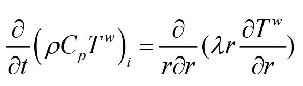
Equation [35] is discretized for each layer according to

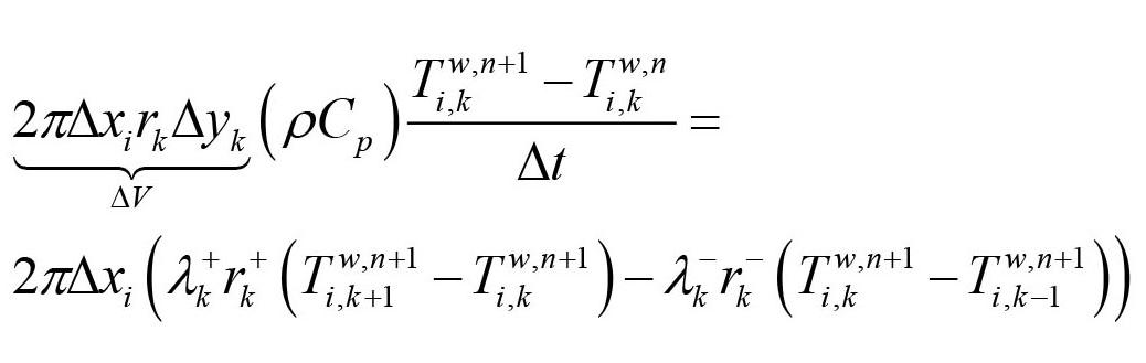
[35]

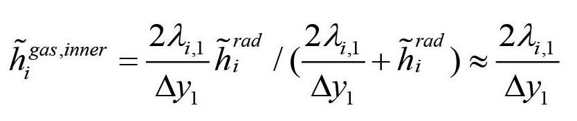
where the external temperature is given by TEXT. The radiation heat transfer coefficient is given by

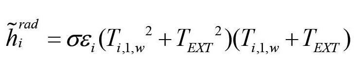
and where the wall temperature is further approximated by the temperature in the near wall cell at the previous time step:

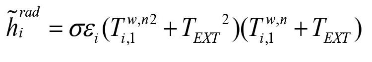
For the outer wall at yNJ = y7 (steel casing) we have:

Superscripts + and – represent the value at the positive and negative sides of the cell face. Dxi is the vertical height of the grid cell at level i cell while rk is the radial position index for the cell. We use harmonic averages for the cell face thermal conductivities and l –k+1 and lk + [37]

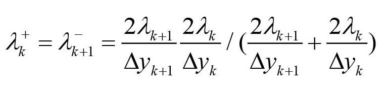
where rk is defined according to Figure 13: [38]

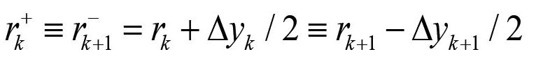
In the cell contacting the hot liquid steel and slag (k = 1) we have [39]

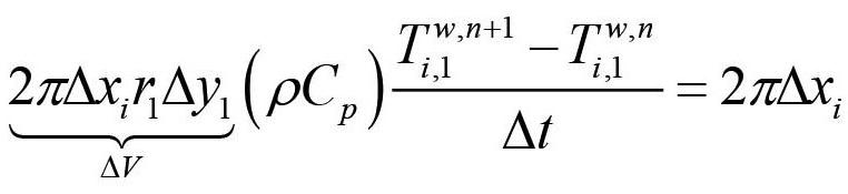
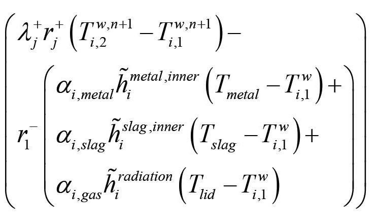
In Equation [39] ai,metal, ai,slag, and ai,gas are the local volume fractions of the phases contacting the element Dxi at a given time.

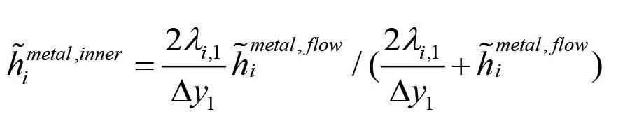
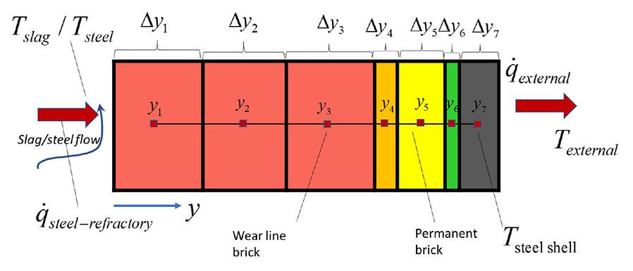
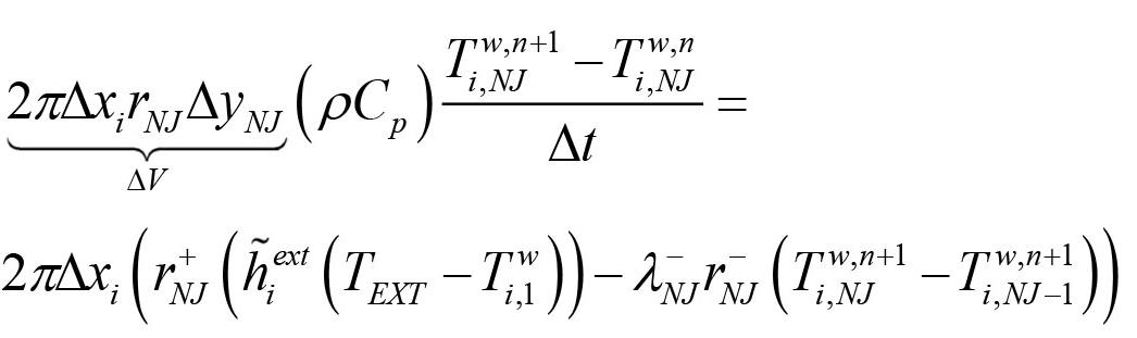
Here the external heat transfer coefficient is estimated by the sum of natural convection and radiation. The convective external heat transfer coefficient hNC is given by Equation [104] using the properties for air. The dimension used in the convective model should be the half height of the ladle standing straight up. The effective external heat transfer coefficient is then

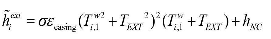
When the ladle is located inside a cabinet, within a compartment with external walls, the effective heat emissivity in Equation [46] can be multiplied by a factor of 0.5.

It should be noted that the external heat transfer coefficients must be adjusted to the situation the ladle experiences (melt refining, transport to casting station, casting, transport to waiting station, waiting). If the external heat transfer conditions varies between the different events, this must be handled in an appropriate manner such that we can tune the model to get a realistic thermal history for the ladle.

Ladle bottom energy model

The model for the bottom energy is completely analogous to that described above, but now with the discrete equation

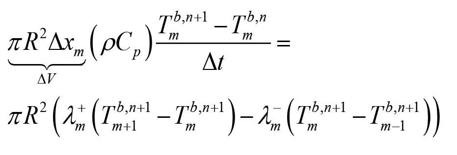
Here R is the inner radius of the ladle. For the element close to the liquid steel (we assume that steel flows into the bottom at time = 0.0 s) we have:

Figure 13 Element of the refractory where the transient thermal heat balance is addressed

A pragmatical physics-based model for predicting ladle lifetime

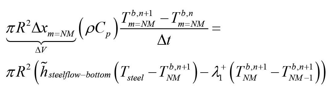
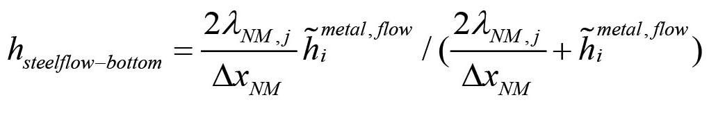
For the bottom element (steel shell) we have:

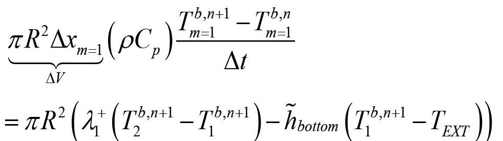
where we estimate

Radiation - Wall temperatures and heat transfer above the slag/metal

Above the liquid phase the refractory will only see the top lid, the other parts of the wall, and the metal surface. We will assume that the top lid is adiabatic, such that no energy is drained out through the lid. We now have to assess radiation transfer between different inner wear bricks and the top surface of the slag/metal. The radiative flux from a surface with emissivity ep and temperature Tp is given by

The radiation heat flow from surface elements A1 to A2 is given by (Wikipedia, 2022)

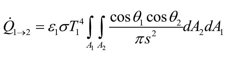
The geometrical configuration is seen in Figure 14.

The radiation heat flow from A2 to A1 is then

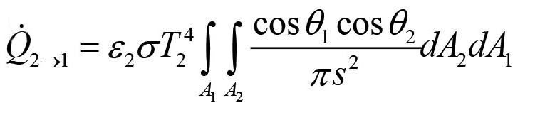
The heat flow between the two surfaces A1 and A2 can be given by (Goodman, 1957):

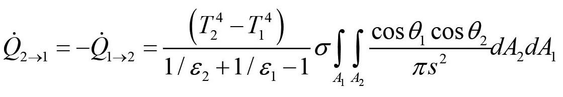
Based on Equations [52]−[55], the surface normal vectors n1 and n2, and the vector connecting area elements dA1 and dA2, all radiation heat flows can be computed. These are Qw,m→slag-metal (from brick number m to slag-metal interface), Qw,m→ceiling (from brick number m to ceiling), and Qslag-metal→ceiling (from slag-metal interface to ceiling). The direct radiation between bricks is ignored. The radiation from the slag-metal interface must respect that the slag only covers a fraction aslag of the total free surface area. Hence, the radiation temperature T4 slag-metal is replaced by: [56]

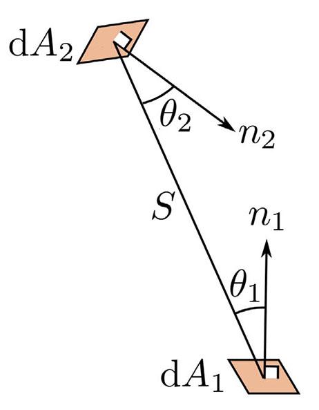
Figure 14 Geometrical arrangement for radiation exchange between areas and (Wikipedia, 2022)

It is further assumed that the ceiling (ladle lid) is adiabatic and that the slag and metal are well mixed. However, for the refractory bricks the thermal conduction heat flux into the inner wall surface brick and the net radiation flux must balance. The surface temperature of the wall bricks is then given as

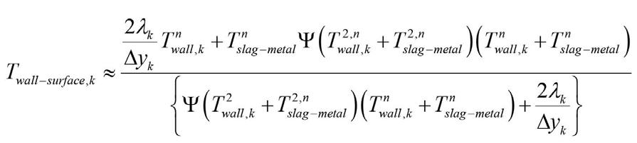
[57]

This illustrates the fact that it is surface temperature that communicates radiation and not volume-averaged temperature for the computational cell.

The factor Ψ is given by

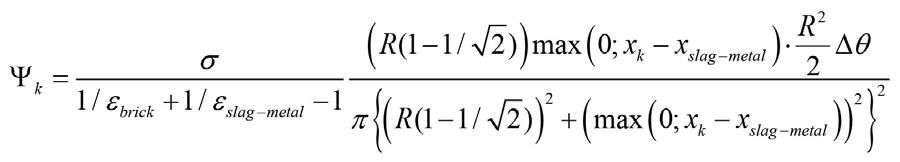
where R2 2 Dq is the horizontal area element (per radian) which exchanges radiation between slag/metal and bricks.

[58]

The heat flows may be converted to heat transfer coefficient by rewriting Equation [55] as

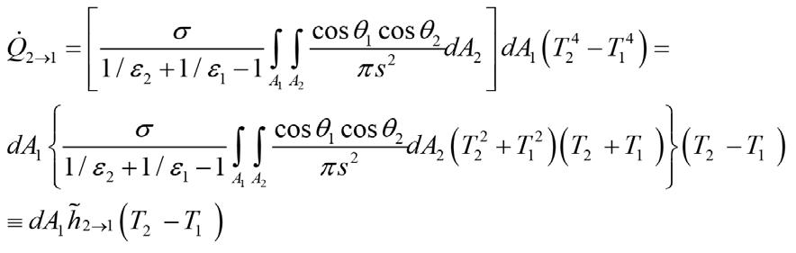
[59]

where h2→1 is the heat transfer coefficient expressed by the bracketed terms in Equation [59] above.

As the lid is adiabatic we have the following condition to fulfil:

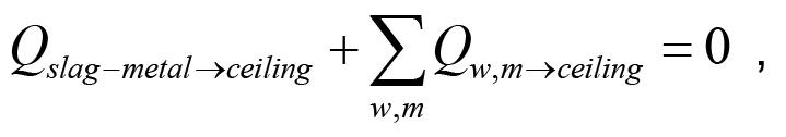
From Equation [60] we compute the ceiling temperature.

Effective heat transfer coefficient

[60]

The effective heat transfer coefficient hliq in the liquid steel and slag may now be estimated based on three different contributions:

1. The wave induced contribution hwave, elaborated in Appendix F. Wave-induced heat transfer 2. The heat transfer due to bubble stirring hstirring, elaborated in Appendix G. Inner wall heat transfer coefficients due to forced convection by bubble stirring

3. The heat transfer due to natural convection hNC, elaborated in Appendix E. Pure natural and effective convection heat transfer':

Heat balance for the slag

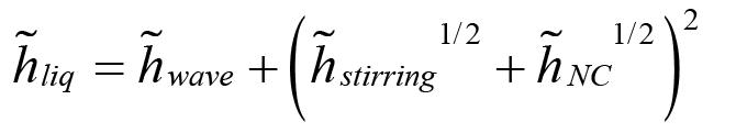
[61]

Due to the melting of additives (slag formers, refining additions, alloying elements) we have selected to represent the energy by the specific enthalpy h.

First, we give the slag enthalpy by a simplified relationship:

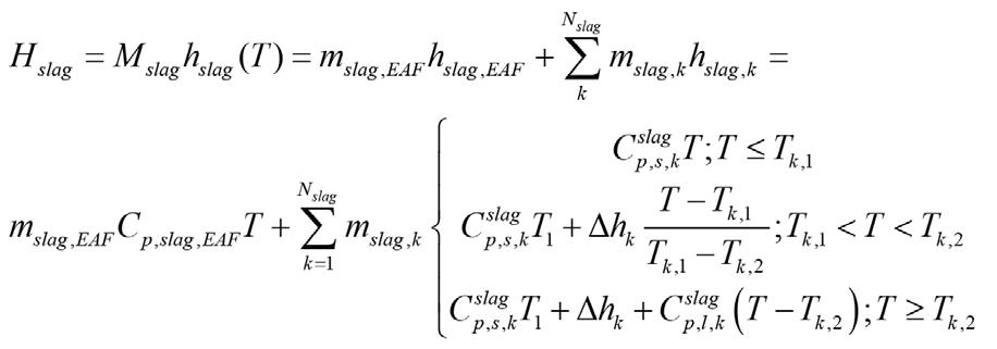
[62]

A pragmatical physics-based model for predicting ladle lifetime

Here the enthalpy for the solids is represented by Cp,sT, and for the liquids by Cp,sT1 + Dh+Cp,l (T-T2), where Cp,l is the liquid heat capacity and Dh is the latent heat of fusion. The temperatures T1 and T2 are the temperatures at which the phase transition (melting) starts and is completed, respectively.

The heat balance for the slag is then

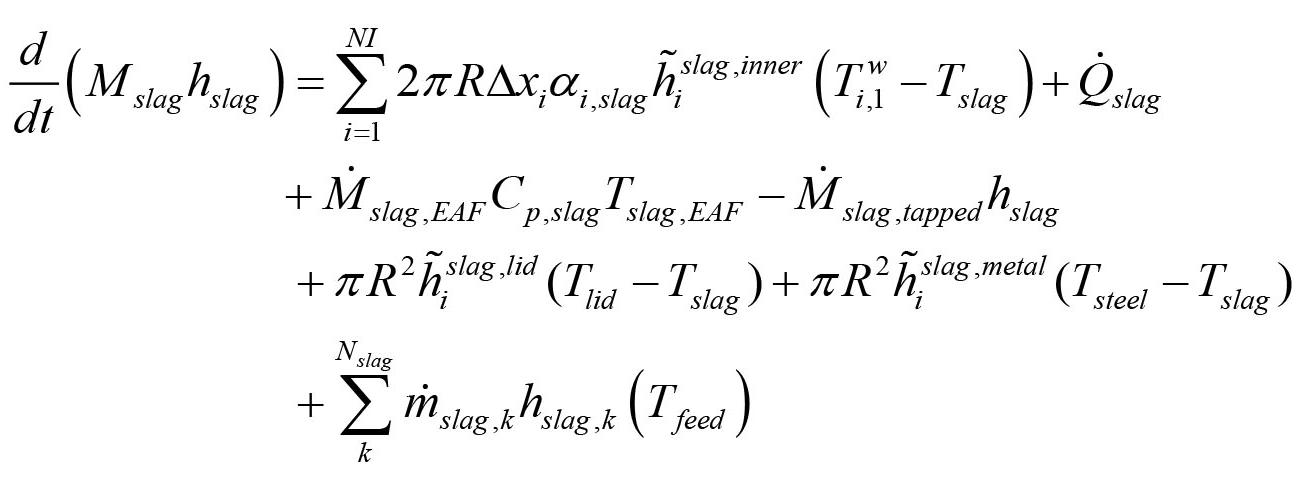
[63]

Here ai,slag is the slag fraction contacting brick number i and varies with time. Tfeed is the temperature of the materials at the time of feeding, typically less than 100°C. M . slag,EAF is the time-dependent mass flow of slag from the EAF. h ~ i slag,lid is the heat transfer coefficient for slag surface – top lid heat exchange, and h ~ i slag,metal is the area-averaged heat transfer coefficient between the metal and slag. Q slag is the heating power supplied to the slag [W/kg]. All these quantities are in general varying with time.

By subsituting the mass balance (Equation [5]) into Equation [63] we obtain:

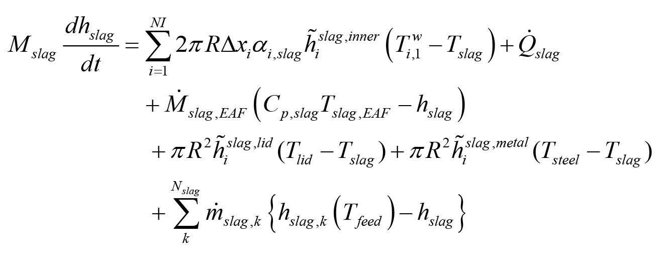
[64]

We may note that Equation [64] indicates that the slag components, fed at low temperature Tfeed, will lower the enthalpy of the slag as hslag,k (Tfeed) — hslag < 0.

Heat balance for the metal

As for the slag, the metal enthalpy Hsteel can be expressed by the specific enthalpy hsteel:

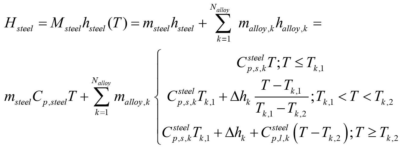
[65]

Similarly, for the metal (steel) we have

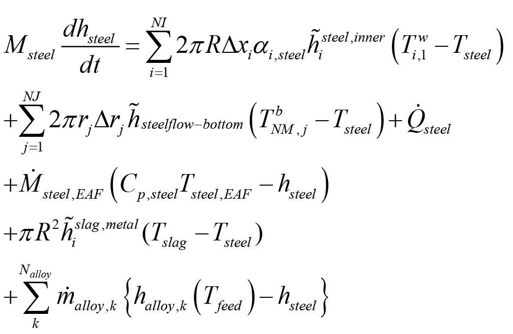
[66]

assumed that the bottom heat transfer is zero before steel is received in the ladle.

ai,steel is the metal fraction contacting brick number i and varies with time. M . steel,EAF is the time-dependent mass flow of steel from the EAF. hsteelflow-bottom is the heat transfer coefficient for metalbottom refractory heat exchange, and h ~ i slag,metal is the area-averaged heat transfer coefficient between metal and slag. Q steel is the heating power supplied directly to the steel [W/kg]. Again, these quantities are in general varying with time.

The heat source and Q . slag are related to the total power Q . tot supplied by the heating electrodes. Q tot is the power logged at the plant. The heat entering the slag and metal will be lower. We introduce an overall heating efficiency heff [0,1] and a heat distribution coefficient hslag, such that

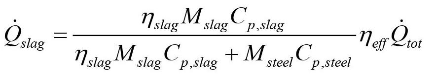
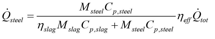
The first right-hand-side sum represents the heat transfer along the vertical ladle wall, while the second summation term represents the heat transfer between steel and the bottom refractory. It is

[67]

[68]

The coefficient hslag = 1.0 indicates that slag and metal increase in temperature at the same rate. If hslag = 2.0 the slag temperature increases twice as fast as that of the steel. If hslag = 0.5 the slag temperature increases at half the rate of the steel. The introduction of the coefficient hslag allows a more controlled way to distribute heat between the steel and slag.

Solution for the wall energy equations

Based on previous temperatures the radiation flows and fluxes are computed (Equations [52]−[57]). For the radial wall elements the discrete equations [36], [39] and [47] can be written as

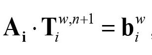
Here bi w will contain reference to previous slag and metal temperatures, radiation fluxes, and external temperatures. The solution is obtained by inverting the NJ × NJ (here 7 × 7) matrix Ai: [70]

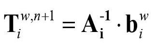
We notice that while the ladle is in steady operation (no filling or tapping) the matrix Ai is fixed. In this case the new wall temperatures are obtained by only updating bi w , which depends on values from previous time step, and then repeating the matrixvector operation in Equation [70]. This allows very fast solution of wall temperatures.

The bottom part of the wall is solved in the same manner.

Appendix B. Wall shear stress model

The steady-state flow in the ladle was simulated (Johansen and Boysan, 1988) for the different (500, 600, 800, and 1200 Nl/ min) argon gas flow rates, using a typical steel mass (130 t) and ladle geometry from Sidenor. In addition, the simulations were performed for both atmospheric pressure and 0.003 bar above the melt. The simulated wall stresses were expressed by fitting functions and the effect of pressure was handled by a linear fit between the atmospheric and near-vacuum pressures.

Denote P as pressure in atmospheres (P = 1 bar = 1e5 Pa) , and we have volume flow of argon Q in normal litres per minute (nl/ min), relative heigh x = X/H

Wall stress data for low pressure (P = 0.003 bar):

A pragmatical physics-based model for predicting ladle lifetime

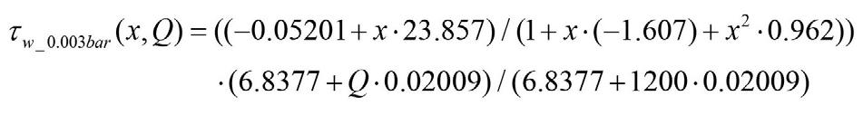
Wall stress data for normal pressure (P = 1.000 bar):

From the two fits above the wall stress distribution, including operating pressure, becomes

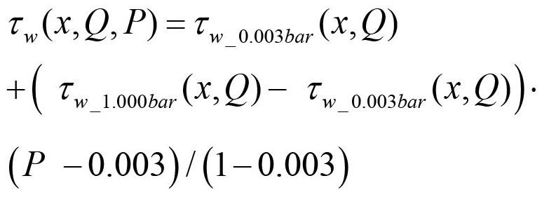
Equation [71] is simply the new model. The result is shown in Figure 15.

Wall shear velocity ut now becomes

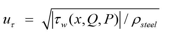
Appendix C. Temperature-enthalpy relationships

As we use both enthalpy and temperature, we establish some critical relationships.

In the case of the steel, we can find the temperature from the enthalpy by a Taylor expansion of the enthalpy function:

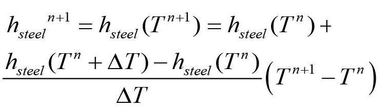
According to Equation [73] the temperature is

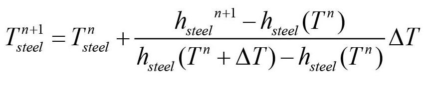
As we wish to replace the temperatures of the slag and metal with enthalpies, we carry out the following reorganizations:

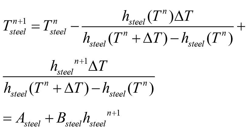
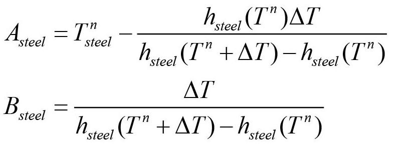
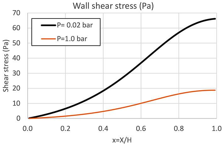
15

Similarly, for the slag we obtain:

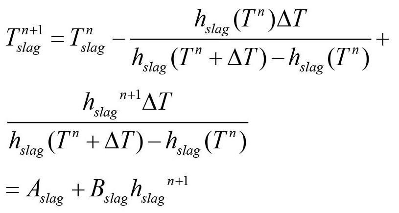
where we have

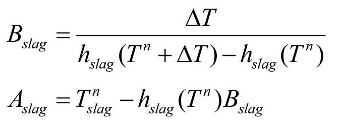
Based on Equations [73]−[78] we can produce coupled enthalpy equations for the metal-slag-refractory system.

Appendix D. Discrete equations for the slag-metal heat balance

Fluid temperatures

We can now write discrete equations for the slag and steel temperature. We use implicit treatment of the right-hand-side enthalpies. The slag heat balance, given by Equation [64] now reads [79]

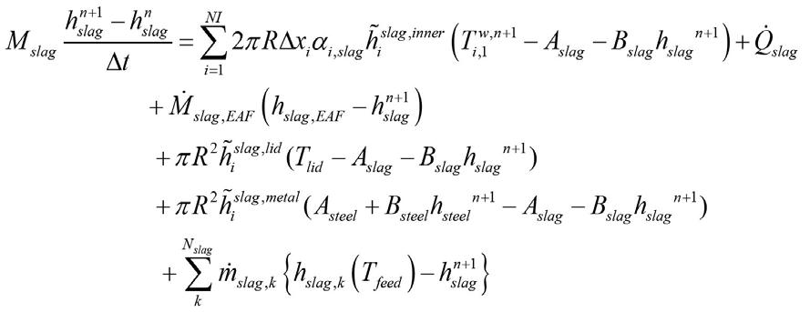
while for the metal (steel) heat balance we have

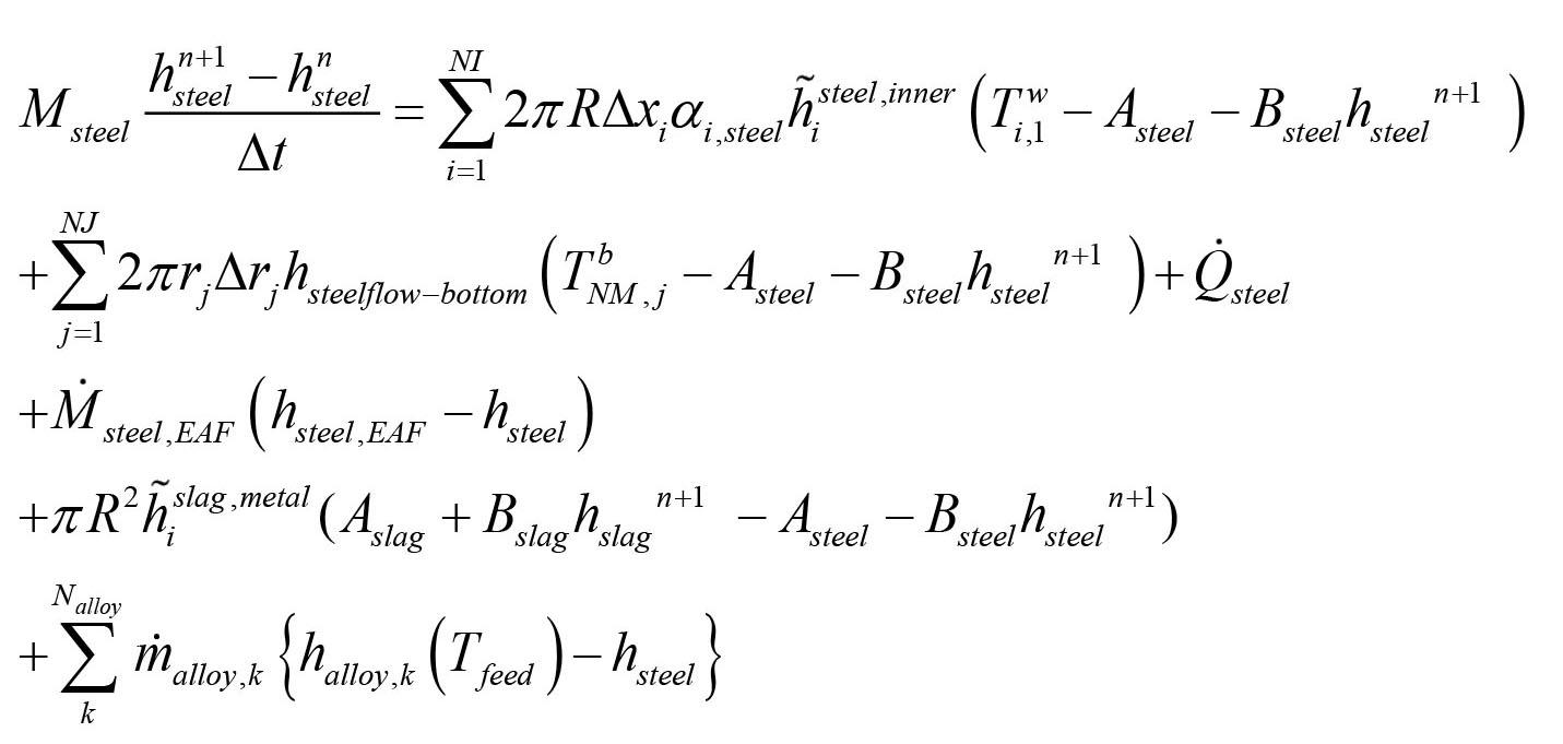
The discrete equation for the slag can be written in a simplified form:

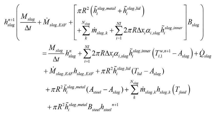
We simplify Equation [81] as

where

[80]

Figure

The distribution of shear stress (Equation [71], plotted for two absolute pressures above the melt

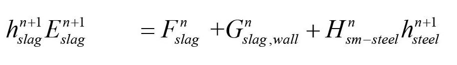
A pragmatical physics-based model for predicting ladle lifetime

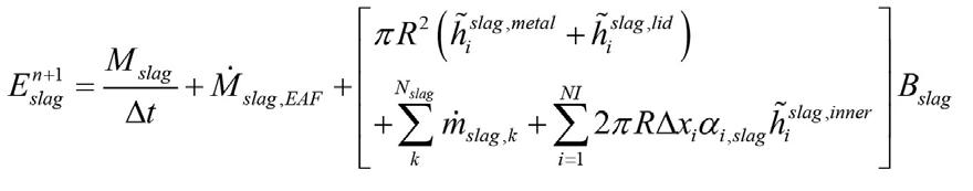
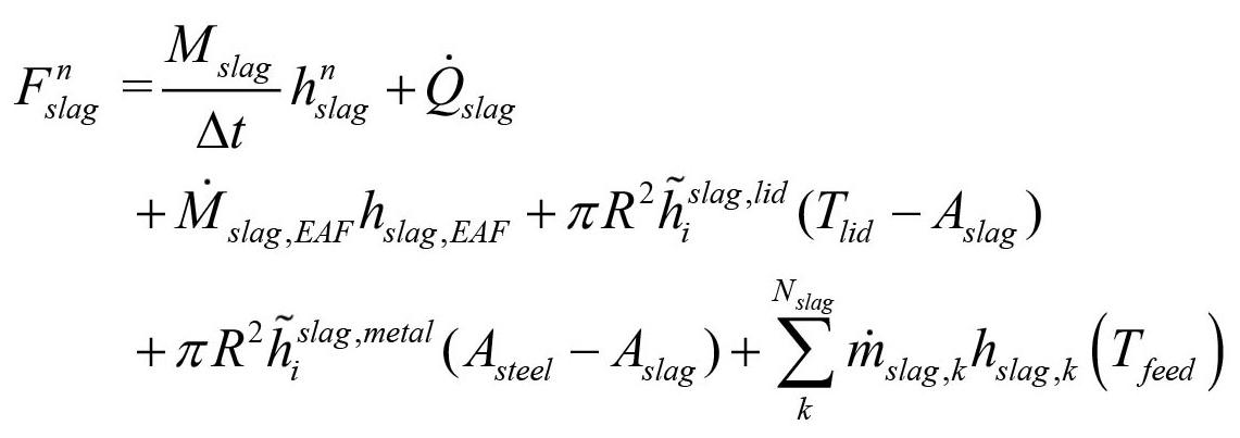
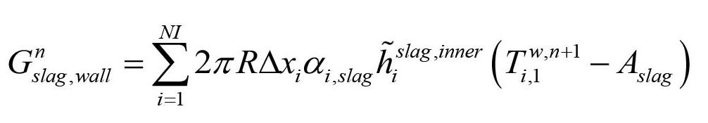
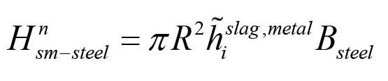
We have here treated the internal wall temperature in an explicit manner in order to be able to separate the set of equations and allow fast computations. The coefficients represented by Equations [83]− [86] have to be updated for every time step.

For the steel phase we may, based on Equation [80], write

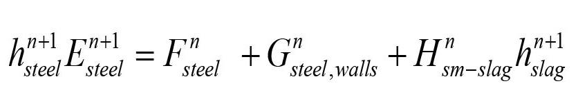
where

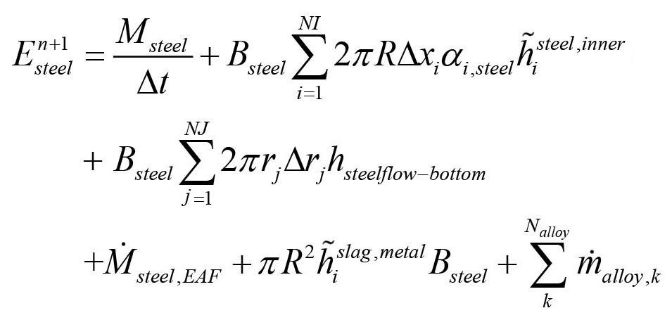
and

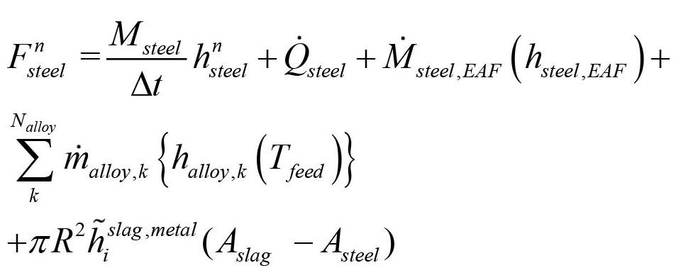
and

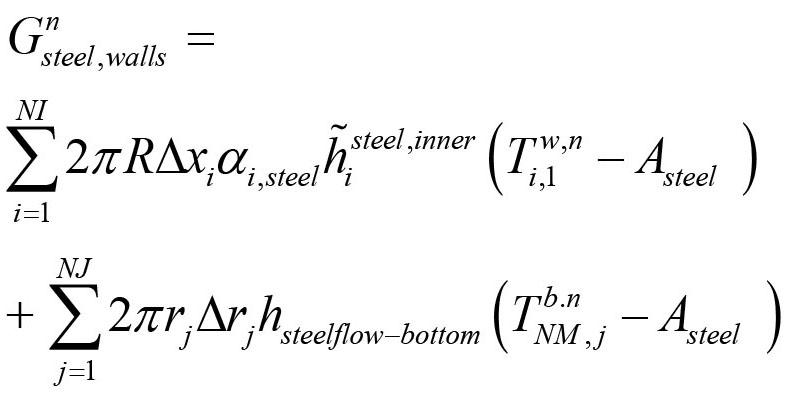
and where

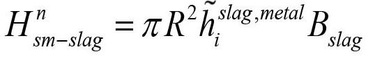
The solution for Equations [82] and [87] is trivial, giving:

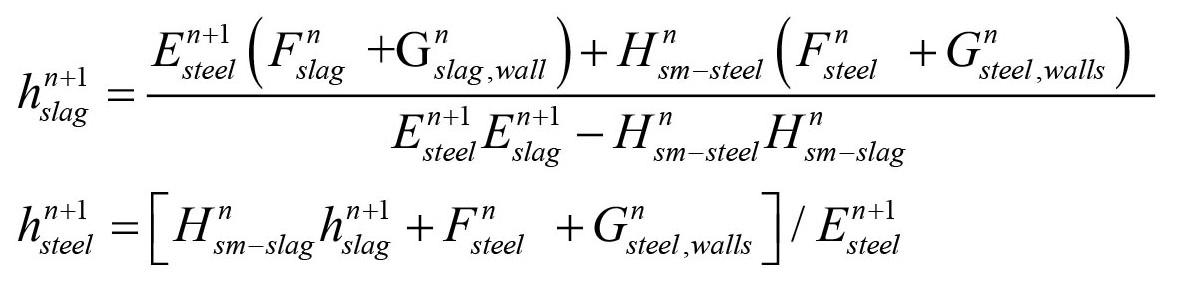
The calculations of temperatures from the enthalpies are given by Equations [75]−[78].

Appendix E. Pure natural and effective convection heat transfer

According to Ede (1967) the heat transfer due to pure natural convection can be estimated by:

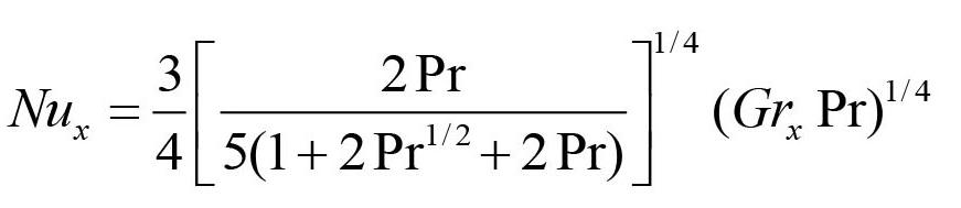
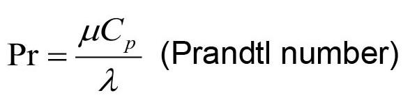
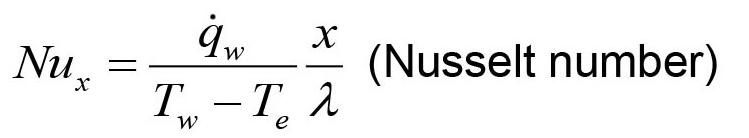
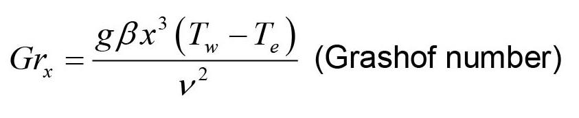
An average distance x may be estimated by the liquid height Hsteel, giving x3= 1 4 Hsteel3 , and

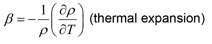
The Churchill-Thelen correlation (Churchill and Chu, 1975) gives:

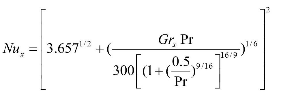
The latter correlation is fine for turbulence controlled natural convection. However, for Ra = GrxPr smaller than 1010 the model given by Equation [93] is very good. We therefore propose a mixture of the two models with a transition at Ra = GrxPr = 2 1010

The assembled model then becomes:

and the Rayleigh number is

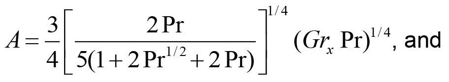
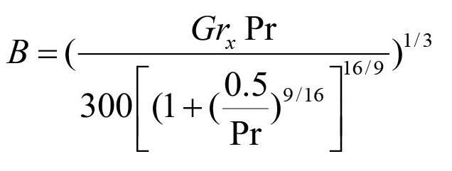
See Figure 16 for comparison with the base correlations.

The heat transfer coefficient due to natural convection is now:

A pragmatical physics-based model for predicting ladle lifetime

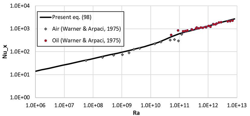
Figure 16

The performance of the suggested natural convection heat transfer

Nusselt number Nux, Equation [99], plotted against Rayleigh number Ra.

Data from Warner and Arpaci (1968) is included

Effective heat transfer coefficient

The effective heat transfer coefficient in the liquid steel and slag may now be estimated from

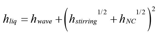
Appendix F. Wave-induced heat transfer

The bubble plume impinging on the surface will produce waves at the interface (Cloete, 2008). An empirical correlation for the wave period Ts was produced by Hiratsuka et al. (2007)

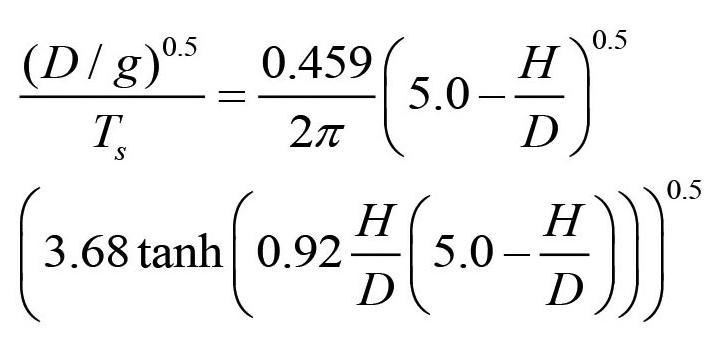
where D is ladle diameter and H is liquid height. The length swept by the wave is lw, where

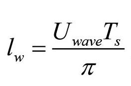
The wave velocity is here based on the turbulent velocities near the wfree surface. From 2D CFD simulations we have curve-fitted the computed turbulent velocities as:

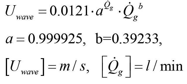
According to Equation [108] the wave velocities Uwave will range between 0.13 and 0.18 m/s for gas flow rates ranging between 500 and 1200 l/min.

According to Blasius : [109]

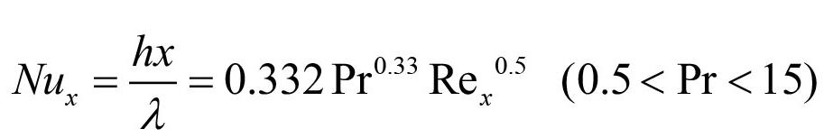
Over the distance lw /2 and average velocity u = 2Uwave p , the averaged heat transfer coefficient hwave* is: [110]

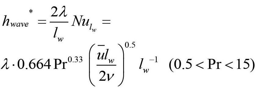
The wave-induced added heat transfer will apply to a region close to the surface. Due to the small thickness of the slag layer, it is proposed that the wave-induced heat transfer applies only to the metal, given by the following relationship: [111]

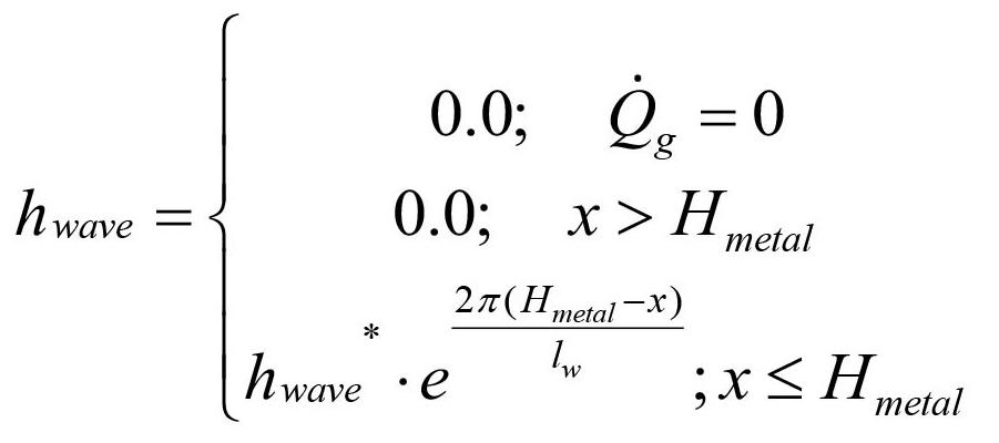
Appendix G. Inner wall heat transfer coefficients due to forced convection by bubble stirring

The heat transfer coefficients due to forced convection can be obtained from the definition of the dimensionless flow temperature T+ :

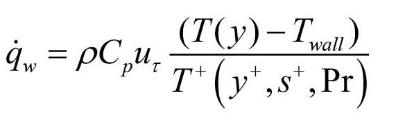
[112]

Here qw is the wall heat flux, ut is the wall shear velocity, defined by ut = √tw r , y+ = yut/v is the non-dimensional wall distance, and s+ = sut/v is the non-dimensional wall roughness.

The resulting heat transfer coefficient then becomes

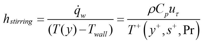
[113]

Using a wall function model (Ashrafian and Johansen, 2007) the T+ function can be evaluated at a typical bulk fluid wall distance y+ = 1000, and for a given hydrodynamic roughness height s+ = s ut/v), where v is the kinematic viscosity of the steel. u

[114]

[105]

[106]

[107]

[108]

SAMCODES App

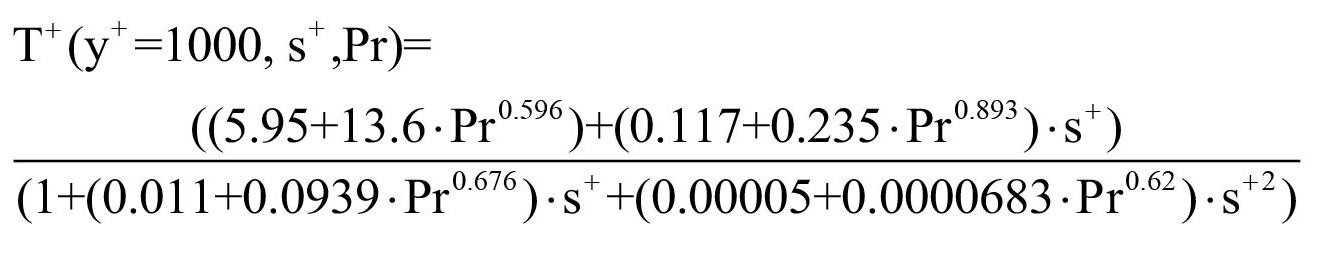
 Development of the App is still ongoing for an improved interface and compatibility with iOS Look out for more quizzes focusing on various SAMCODES topics

 SAMCODES App is available for download on the Google Play store and instructions for downloading iOS version available here: https://www.samcode.co.za/news/229-samcodes-app

Training programmes

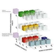
The UNFC workshop was held on 20 February 2024 by GSSA with over 100 attendees. The workshop covered various topics including an update on the AMREC Code and the draft UNFC and CRIRSCO bridging document, to be finalized in April 2024. The workshop recording is on the GSSA YouTube channel and can be accessed via the link below: 2024 United Nations Framework Classification (youtube.com)

AMREC is the African Mineral Resource Classification and Management System that is based on the UNFC’s EFG axis, as opposed to Mineral Resource and Mineral Reserves. The focus of AMREC is the African Mining Vision and the Sustainable Development Goals It is used by governments and NGOs to identify and track mineral inventory, and is not particularly relevant to public reporting for stock exchanges.

Committee updates

Continuation of incorporation of ESG factors into SAMCODES and recommendations for additions into SAMREC Table 1 and SAMVAL

Liaison with IMVAL for planning of conferences and alignment

SAMOG Code updates continued and will be finalized this year

Updates to SAMESG Guideline 2.0 and ESG definitions guide

Updates to the Industrial Minerals guidelines are underway

SAMCODES ESG Working Group activities

The ESG Working Group is finalizing work on incorporating ESG recommendations into the SAMCODES. A feedback session on ESG matters will be hosted later this year after consultations.

International liaison

The CRIRSCO AGM will be held in Vancouver, Canada in mid-October 2024. Immediately thereafter a Mineral Resource and Reserve conference will be hosted by CIM, also in Vancouver. CRIRSCO is also busy with CRIRSCO template updates as the CRIRSCO definitions have been approved

JSE Readers Panel

Two new reviewers were ratified, each of whom have over 35 years’ industry experience in Competent Persons reporting

Affiliation:

1SINTEF, Norway.

Correspondence to: S.T. Johansen

Email:

Stein.T.Johansen@sintef.no

Dates:

Received: 13 Mar. 2023

Revised: 31 Oct. 2023

Accepted: 2 Nov. 2023

Published: March 2024

How to cite:

Johansen, S.T., Løvfall, B.T., Rodriguez Duran, T., and Zoric, J. 2024

Pragmatism in industrial modelling: An application to ladle lifetime in the steel industry.

Journal of the Southern African Institute of Mining and Metallurgy, vol. 124, no. 3. pp. 111–122

DOI ID:

http://dx.doi.org/10.17159/24119717/2681/2024

Pragmatism in industrial modelling: An application to ladle lifetime in the steel industry

by S.T. Johansen1, B.T. Løvfall1, T. Rodriguez Duran1, and J. Zoric1

Synopsis

A methodology for building pragmatic physics-based models is here adapted to predict the erosion of ladle linings in the steel industry, in order to support operators when deciding whether the lining can be used safely for another heat. A defective lining may allow 140 t of molten steel to spill, with disastrous consequences for workers and plant. The adopted work flow for the development, challenges faced, and some model results are presented. One key learning outcome is that model development should allow time for maturing the process understanding, as well as for many iterations by ‘questions-responses and actions’ at various stages in the model development. Good interaction between the development team and industry case owner is an important success factor. Combining or extending the model with the use of machine learning and cognition-related methods, such as knowledge graphs and self-adaptive algorithms, is discussed.

Keywords pragmatism, physics-based model, ladle lining, steelmaking.

Introduction

Many industrial processes involve complex physical and chemical systems. In addition, the observability (Wikipedia, 2022a) may be very poor and accordingly process control becomes difficult. In hightemperature processes, including the metallurgical industry, we find many representative cases. One example is aluminium reduction cells (the Hall-Héroult process), where the alumina concentration in the cell is measured by manual sampling once a day at a fixed location. This is the most important control parameter for a cell. Another example is from the ferro-alloy industry, where electric furnaces may have an installed power of around 40 MW. Due to the high temperatures of the charge (up to 2000°C: Jayakumari and Henning, 2020) there are no sensors capable of monitoring the interior state of the furnace. Sensors may be available in specific cases, but these are generally extremely expensive to purchase and maintain. Physics-based models can provide an alternative method for predicting the internal states of the process, if based on a realistic set of assumptions and simplifications. The amount of data in these types of processes is limited, and some of the data may have significant issues as a result of operational challenges. The operations are not automated, and sometimes fast decisions must be made without time to check if the change in operation impacts the data collection. In response to these challenges we have been developing a generic methodology (Johansen et al., 2017; Johansen and Ringdalen, 2018; Zoric et al., 2015a, 2015b), termed ‘pragmatism in industrial modelling’, for the development of industry-applicable physics-based models.

Earlier work on pragmatism (Johansen et al., 2017; Zoric et al., 2015a, 2015b) addressed solutions to various industrial tasks and problems. Here the best approaches were proposed and discussed, by assuming no limitations in human expertise and resources. A generic scheme for our pragmatic development approach is shown in Figure 1.

The use of the pragmatic modelling paradigm is aimed at handling the complexity of a hybrid modelling approach (a combination of data-based and physics-based modelling techniques in the same work flow) by:

1. Structuring the exchange of data and information between sub-models (often at different levels of abstraction)

2. Structuring the modelling and analytic work flows

3. Providing good interfaces to include some machine learning (ML) or artificial intelligence (AI) prediction tools (also in cases where the analytical or computational physics models are more tightly integrated with AI/ML tools)

4. Connecting these various tools to the relevant decision support tools and processes.

Pragmatism in industrial modelling: An application to ladle lifetime in the steel industry

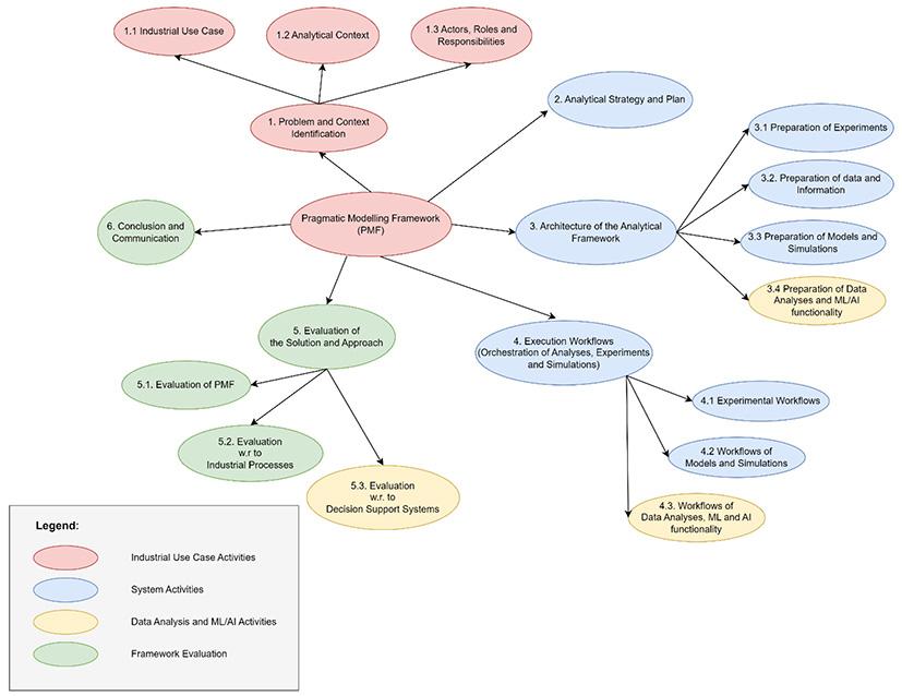
The inclusion of modelling and simulation frameworks in industrial processes and decision support systems requires significant structure and standardization, which we hope to contribute to by this work.

Pragmatic modelling starts always with a given industrial application, by defining an industrial use case (i.e. problem to solve) (Wikipedia, 2022b). The pragmatic model is the simplest model that can give fast and sufficiently accurate answers. There could be a short step from a pragmatic model to online process control and operation support tools. A pragmatic model starts with the simplest possible model that has a value for the user. The main steps of the pragmatic work flow are shown in Figure 1:

1. Problem and context identification

2. Analytical strategy and plan

3. Architecture of the analytical framework

4. Execution (coordination of analyses, simulations, and experiments)

5. Evaluation of the solution

6. Conclusion and communication.

A key element in this work is the appointment of the system architects team (Zoric et al., 2015a, 2015b; Wikipedia, 2022c; 2022d), as the capabilities of this team will be a critical factor for a successful outcome of the work.

The methodology, which the system architects team has to orchestrate, is not limited to any specific techniques (steps 2-4), and the palette of tools may contain elements that involve mathematical methods, such as statistical methods, singular value decomposition (Wikipedia, 2022e), and reduced order methods (Wikipedia, 2022f) as well as numerical continuum physics, numerical particle physics, and molecular and quantum mechanics. In practice the system architects team will learn to apply and orchestrate the methods that are at hand for the development team (methods applicable to the reality of the industrial process, and related decision support systems and routines), and AI should already be included in the

abovementioned methods. The pragmatism-based methodology will use available sensor data and assess the validity of the data. However, development of new sensors, even if critical, is not dealt with by the methodology.

In this paper we aim to present a simplified pragmatism-based approach for the development of a prediction model for steel ladle refractory erosion and lifespan. A particular challenge is that the total development team is small (2–3 people) and multiple trade-offs must be made to develop a useful model in a limited time.

Context of the COGNITWIN project

This work, as a part of the Horizon 2020 project (COGNITWIN, 2022), is aiming at accelerating the digital transformation and introducing Industry 4.0 to the European process industries. The project is focused on six industrial pilots, ranging from aluminium, silicon, and steel production to engineering. Here we address the pilot for the Sidenor1 steel company, where we analyse how to increase the ladle refractory lifespan, and how the digital twin concept can contribute.

Sidenor ladle case description

Steel production in the melting shop process is based on three main steps. The first involves the production of liquid steel by smelting iron ore in a blast furnace (BF) or melting scrap in an electric arc furnace (EAF) or induction furnace. The second step – secondary metallurgy (SM) – is necessary for refining the liquid steel, and the last one solidifies the steel during ingot or continuous casting processes.

Typically, a ladle can contain from tens to hundreds of tons of liquid steel (Figure 2). Most ladles have a porous plug at the bottom. Gas (Ar of N) is injected through the plug to stir the liquid steel.

1https://www.sidenor.com/en/

Figure 1—Proposed work flow for a pragmatism-based development (Zoric et al., 2015b). Arrows indicate sub-use cases and related activities that have to be realized

Pragmatism in industrial modelling: An application to ladle lifetime in the steel industry

Freeboard

Slag zone

Wear bricks

Bottom bricks

Impact bricks

Steel casing (shell) Plug for gas injecdtion Slide gate/ tapping nozzle

The bubble driven upward flow of the liquid steel promotes the transfer of inclusions from the steel to the slag and homogenizes the temperature and chemical composition.

The main objective of SM is to obtain the correct chemical composition and to ensure an appropriate temperature for the casting process. In addition, there are several important tasks which must be complete during SM, for example removal of inclusion and gases. In order to reach these objectives, Sidenor has a SM mill consisting of two ladle furnaces (LFs) and a vacuum degasser (VD). Each LF has three electrodes for heating the slag, steel, and ferro-additions. The ladle contains liquid steel and slag for all the production process, from the EAF to the end of the casting process. The liquid steel has a temperature of around 1850 K in the ladle and it is covered with slag, which prevents contact between the liquid steel and the atmosphere. The slag has a lower density than steel and consists mainly of lime and various oxides. Slag conditioning can be improved during SM by adding slag-formers.

In order to handle the liquid steel and slag at such high temperature, the ladle is constructed with a strong outer steel shell, the inside of which is lined with layers of insulating (refractory) materials. The refractory consists of ceramics and its most important properties are:

i. Ability to withstand high temperatures

ii. Favourable thermal properties

iii. High resistance to erosion by molten steel and slag,

The inner layer of refractory bricks, which are in contact with the liquid steel, and slag, is progressively eroded by each heat, and after several heats the erosion is such that it is not safe to use the ladle for another heat. The refractory is visually inspected after each heat and depending on its state, the ladle may be used again, or put aside for repair or demolition. In case of repair, the upper bricks, which are more eroded, will be replaced and the ladle is returned to production. Later, based on continuing visual inspection, the ladle may be deemed ready for demolition. In this case the entire inner lining is replaced.

One important goal for Sidenor is to reduce the refractory costs by identifying new methods for extending the refractory life. One of the key aims is to use the same ladle for more heats without compromising safety, but another important issue is to better better understand the mechanism that underlies refractory erosion and avoid as much as possible the working practices that shorten the usable life of the lining.

Target for the pragmatic model development

The main goal of our pragmatic modelling approach is to develop a model from which the results can help decide whether the ladle can be safely used again without repair or relining. The model should incorporate both historical and current production data. The model should increases the knowledge of the operators, and could also contribute to related digital twins in semantic and cognitive aspects. In addition, the model should provide information about which parameters contribute the most to ladle refractory erosion, and what precautions can be taken to extend refractory life.

Physics-based pragmatic model

We now investigate the recommended work flow for the development of the abovementioned pragmatic model. The generic work flow could be applied to the development of any physics-based models. A particular ambition with this work is to develop a hybrid model that can base predictions on any combinations of direct use of data, indirect use of data, and the physics-based model. However, for the physics-based model the data is crucial for tuning the model. The justification of tuning is that we are dealing with an extremely complex process, containing multiple levels of uncertainty. As part of the overall complexity many aspects of critical physical data are unknown or have changed due to ageing.

It was decided to frame the model as PPBM (pragmatism in physics-based modelling). Referring to the pragmatism steps 1–6 above, we first set out to establish the development team, comprising mainly two developers. This step is preparatory, and the team was selected based on experience and skills. In addition, the contributions from the industry were crucial for understanding the case and providing relevant data.

The following text describes the PPBM development in six steps, as illustrated in Figure 1.

Pragmatism step 1: Problem and context identification

Step 1 aims at describing accurately the purpose of the model and the quantitative output data the model shall produce, including time constraints and accuracy requirements. To facilitate this step we employ the user experiences described from the perspective of ladle operators at Sidenor. The main user, who is expected to benefit from the model results, places the model in the industrial perspective and defines its role and contribution to the industry process. We discuss our experiences in solving the challenges met during that

Figure 2 – Left: Schematic of a typical steel ladle, showing wear refractory bricks, permanent lining (between wear bricks and steel casing), steel casing, bottom bricks, bottom plug for gas blowing, and tap-hole (nozzle) with slide gate. Right: Hot ladle waiting for the next heat. Maximum steel capacity is around 150 t

Pragmatism in industrial modelling: An application to ladle lifetime in the steel industry

collaboration, which we experienced as very demanding. The actors and entities participating in the overall case work flow are shown in Figure 3. The step (1) Definition Accepted should have been finished at latest after 6 months. However, the problem definition and context were continuously challenged without any formal requests to change the definition. In addition to developing the physics-based model the objective included developing the model in such a way that it can be used in different hybrid approaches, combining data and physics-based models. The hybrid approach, involving using data to calibrate the model, is included here, while development of models that explore the combination of the physicsbased model and all additional available data is outside the scope of this development. However, continuous interaction between the ML team (MLT) and the physics-based team had to be ensured. Important decision gates during the model development process are illustrated in Table I.

User story

The main output of this phase, the user story, can be summarized as a model of the SM that can predict the average refractory loss for a given use of the ladle, and the accumulated loss over the lifespan of the ladle. The expected input paramesters are the amounts of steel, slag, and additives held in the ladle. Predictions of the temperature of the steel, slag, and refractory wall are important determinants

of refractory loss. We therefore need the temperature in the steel as hot steel is added to the ladle. To account for heating during SM we need the electrical power that is input as a function of time. In addition, we need the time history of applied inert gas and the vacuum pressure above the melt. The model must be able to take the entire history of the ladle (since the last relining) into account when the simulations are run. The state of the refractory wall from the previous heat, in terms of temperatures and erosion, must be input to the next use of the ladle (next heat). It should be possible to continue the simulation when new data is available.

Pragmatism step 2: Analytical strategy and plan

This part of the development included overall model design, resulting in a specification document. This document was very detailed, but still only a signpost towards the implementation. Instead of writing a specific implementation report the code included necessary comments and the original specification was updated when changes were made. As regards the functionalities (how to use the model) no specific documentation was completed apart from short text files to explain the scripts.

The ladle and refractory, with bottom porous plug and tap-hole, is three-dimensional. To develop a fast model that can simulate the refractory behaviour over weeks in real time, using a full 3D model, and with the available time and resources, was deemed infeasible.

Figure

Pragmatism in industrial modelling: An application to ladle lifetime in the steel industry

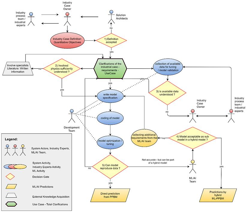
Table I

Decision gates in model development (see also Figure 3)

Decision gate Outcome Resulting procedure scenario

1. Case definition accepted Yes Now a physics-based model can be created No Ask industry case owner for more information

Comment

2. Involved physics Yes Implementation can start Implementation can start as soon as each sub-model has sufficiently understood? reached a proper understanding and is well-specified No Involve specialists and relevant literature. The industry case owner can be helpful at this stage

3. Available data understood? Yes The model can be run

No Go back to the decision gate 2

4. Model acceptable as a sub- Yes

Sub-model can now be used in a hybrid model model in a hybrid model? No Go back to the decision gate 3

5. Model can reproduce the data? Yes

Model finished No

The model can be run as long as the provided data has the right structure. Proper data is only required for decision gate 4 and 5

This could be due to data not being understood, assumptions in the physics being wrong or the case definition not being properly understood

Go back to the decision gates 2 and 3 If tuning model parameters is not sufficient to reproduce the data, both the data and the physics should be reviewed.

However, many of the ladle‘s features can be represented in a simplified 2D model. It was therefor decided to move on with a 2D model.

The model simplifications are listed below.

➤ During part of the ladle operation the ladle is inside a ladle furnace (SM mill) with electrodes (for Ohmic heating) immersed in the slag. The electrodes have a heating efficiency (tuning coefficient) and dynamic effects of heat storage in the electrodes are neglected. However, it was subsequently learned that the electrodes do not contact the slag or metal, but supply heat via arcs between electrode tip and slag/metal. The arcs radiate towards the refractory bricks placed above the level of liquid steel and slag. This radiation may be excessive in some cases.

➤ The additions to the ladle will need time to melt and mix. It is assumed that the melting and mixing processes are instantaneous. As a result, the model will predict an immediate temperature drop when additions are made to the melt, while in reality this cooling effect will manifest over several minutes.

➤ Vertical heat conduction between the bricks and inside the steel casing is neglected.

➤ Steel and slag temperatures are represented by mass averages.

➤ When hot steel is teemed into a colder ladle thermal cracking will occur, increasing with increasing temperature difference. These effects are very hard to model in detail and are proposed to be dealt with as a hybrid extension of the model.

➤ Excessive erosion of refractory above the slag/metal level is due to the extremely high temperature of the electrode arcs, together with irregular splashing of hot metal during vacuum treatment. These erosion phenomena, taking place above the average melt surface, are not included in the model.

Effects which are dealt with are dynamic temperatures in the side and bottom refractory bricks, insulation layer, and steel shell. When stirring gas is injected 2D CFD simulations were performed to compute the distribution of wall shear stresses. In Figure 4 we see an example from a 2D simulation of the gas-driven flow in the ladle containing both steel and slag. The maximum velocity is around 0.9 m/s, using a typical gas flow rate that has been used by Sidenor. The broken lines show trajectories of gas bubbles released from the

bottom plug. The methods used here are Lagrangian representation of the bubbles, which expand due to the lower hydrostatic pressure and vacuum above the melt interface. The slag motion is represented by the volume of fluid technique (Wikipedia, 2023).

Based on a set of these CFD simulations the wall shear stress as function of gas flow rate and relative height could be extracted and used as input for heat- and mass-transfer models. Based on visual observations from video taken at the plant at a late stage of the project, it was found that application of the vacuum, together with gas stirring, led to a violent agitation in the steel close to the surface. This observation resulted in recalculations with CFD to account for gas expansion due to the local steel pressure. The result was much higher shear stresses close to the surface when vacuum was applied. New fitting functions for the wall shear stress as result of relative height, gas flow rate, and pressure above the steel were created and implemented in the model. It is noticed that when other team members visited the plant earlier in the project, the consequences of vacuum treatment on gas stirring was not realized and brought forward to the system architects team.

Figure 4—CFD simulation of gas-driven flow in the ladle. Regions coloured blue and red (at the top) represent volume fractions of steel and slag, respectively

Pragmatism in industrial modelling: An application to ladle lifetime in the steel industry

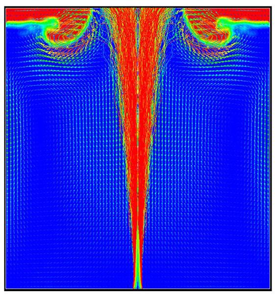
It was assumed that the slag behaved like a moving ‘lid’, floating on top of the liquid steel. The modelled wave agitation of the slag, caused by the gas stirring, provided an added local mass transfer rate for refractory dissolution into the slag. The assumption of the slag behaving as a lid should later be relaxed. This will, however, require more complex and time-consuming CFD work. This would improve the model in the slag-metal transition region.

Sub-models for refractory dissolution and erosion of the steel-wetted refractory, as well as dissolution into the slag, where it is present, had to be developed. Data for solubility of refractory binder in the steel, and for refractory solubility into the slag, was obtained from the literature and from thermodynamic equilibrium software (FactSage). The energy equations for slag and steel were written in terms of enthalpy, allowing for any relationship between temperature, composition, and enthalpy. This is important when dealing with cold additions to hot slag and steel.

Pragmatism step 3: Architecture of the analytical framework

Step 3, the architecture of the analytical framework, incorporated the designs of both the experiments, data structures and related analyses, and model and simulation entities in greater detail. After this step the development team should be ready for coordination of the experiments, analyses, models, and simulations and data/ information exchange among them. Of course, this phase is usually carried in several iterations, usually starting with the proof-ofconcept model (simplest possible representative model), which gradually approaches the final result, i.e. the framework ready for execution of the work flows (step 4).

The architecture of the model was created in phases. In the first phase, a simplified proof-of-concept model was quickly implemented (as a monolithic approach) to see how the specification was holding up, and if more input was required. This proved valuable, as several issues were handled early. Python was chosen for building the model.

Once the basic model was working satisfactorily, the implementation was redesigned as a set of modules with welldefined interfaces to give the required flexibility in future applications of the model. We needed a model that could keep its state and be flexible enough to enable changes without major rewrites. The model itself was implemented as a single class, which proved valuable as we had to do several rewrites to accommodate unforeseen changes. The use of the model was set up as a series of input scripts, executing runs for the LadleModel object, and with different purposes. For instance, (i) running a single case, (ii) tuning the model with a set of parameters based on one or many cases, and (iii) running entire campaigns from first use till demolition.

The data was originally given as column-based data files (MS Excel and csv). In order to efficiently utilize the data, we had to pre-process it to fit our needs. For instance, the time-dependent data was given as large chunks containing multiple heats. These were split into one file for each heat. Later, the data was uploaded to a database (InfluxDB)2, and the data reading had to be changed to accompany two different sources. With hindsight it would have made sense to use a database in the first place. The output of the model was handled as a mix of plots, output to screen and the results saved to file. For the data from a database, the results were written back to the database.

framework is quite generic and several other, standard database solutions could also be used).

Description of model implementation

The physics-based model developed here is implemented in Python as a single class. This enables a complete state of the model to be saved to disk and continued at a later stage. This is important as the final version will model several different steel ladles in parallel. Each heat-run of the ladle that should be simulated depends on the previous modelled state. As the simulation time is specified to be significantly shorter than one hour (seconds in reality), while each lade is used two or three times a day, we need to be able to start and stop the simulation easily.

The main ladle model depends on several stateless sub-models, all described in Johansen, Løvfall, and Rodriguez Duran (2023).

The model is reliant on both static and transient data from the plant. The data can be retrieved either from an InfluxDB database or from files on disk. Either way, data retrieval is relatively timeconsuming, and is therefore done only when necessary, and the required data is stored inside the object and used when needed. When a new heat-run is simulated, a new set of data must be loaded, and the previous data-set is overwritten. Since the data will be loaded several times for the same object, it is loaded independently from the model initialization.

Depending on the model scenario, the same model with the same data could be run several times. For instance, the time from when casting is finished to when the ladle is filled with steel again is modelled as an empty ladle. This is done before the model is run again, but this time the full model and data is used. This way of using the model requires the possibility of resetting parts of the ladle state between the different runs. The temperature in the ladle wall, for instance, should not be reset, but parmeters like the amount of steel and simulation time should be reset.

The actual simulation of a specific heat for a of the steel ladle is carried out with constant time-steps. First, a preparatory step is done, where the amount of steel and slag in the ladle is determined, the heat added to the ladle during the time-step is calculated, and the gas flow rate and pressure are extracted from the data. In addition, the fraction of steel and slag for each cell is determined, and the mass lost from the refractory during the time-step is calculated.

Next, the new temperature in the steel and the slag is solved for. With this given, the temperature in the wall and the bottom layer is calculated. Once the model is solved, time-dependent data is stored inside the object before the next time-step is carried out.

The mass loss (erosion) of the wall is calculated, and accumulated for each time-step, but the wall is eroded only at the end of each heat. Due to the different modes that the model is run in, the actual wall erosion is controlled from the outside as an explicit call to erode the wall. This is done to ensure that the temporary runs to create the correct wall temperatures do not affect the wall thickness.

The model should always be used with an external script that sets up a given scenario to be run. How the scenario is set up has a large impact on the results.

After a ladle is re-lined, it is used many times (40–50) before parts of the refractory are replaced. The ladle is then used until the entire lining needs to be replaced. Between each use of the ladle, the wall is not allowed to cool down (if the waiting time is too long

Data was originally provided as csv files. At a later stage, data was loaded into InfluxDB. Doing this at a much earlier stage could have saved time. The database was chosen by external parties and was not a design choice for the pragmatic model (the modelling 2https://www.influxdata.com/

Pragmatism in industrial modelling: An application to ladle lifetime in the steel industry

the refractory is heated with burners, although this is not included in the model), thus the state of the refractory wall at the end of one heat and the waiting time until it is used again are both important for the next simulation. All must be taken into account when a simulation is run. This is done by allowing the user to control the model from the outside.

When a ladle object is created, no data is read into the object, therefore running the model at this stage would fail. This avoids having several ways to set the data, and enables the same object to be used for consecutive heats without copying results.

To show how this can be done, we will go through a couple of different scenarios.

First of all, it is important to be able to run a single heat independently, and to reproduce the results quickly. This way of running will not take the history of the ladle into account properly, and we need a way to estimate a realistic initial state for the refractory wall.

First we have a method to set the initial wall temperature (so as not to start from a totally unrealistic state, which would require a long simulation time to obtain a realistic result). This method will yield a linear temperature profile between the inner and outermost bricks. After reading the relevant production data into the case, we can run the case for a given amount of time to heat up the refractory to a realistic temperature. From the time that casting is finished to the next heat, the ladle will stand idle and the refractory will cool significantly. To account for this, we can run the model without steel and slag for a given time. The model will not be able to solve all the equations properly, and so a flag is set, telling the model that the simulation is run with an empty ladle. The ladle state is now ready to run the actual simulation. Due to the different modes described above we have an additional method to actually erode the ladle wall at the end of the simulation. This is to make sure that the temporary simulations are not changing the refractory thickness.

A more realistic scenario is to simulate an entire lifespan of a ladle. This can be done in much of the same way as described above. For the first heat, the recipe will be identical, while for the subsequent heats we can use the results of the previous heats as the initial state of the refractory. In this case we can also take into account the actual time between successive heats, as the waiting time between heats is recorded. This is now used to calculate how long the ladle is empty. Sometimes the waiting time is so long that a burner has to be used to keep the refractory wall warm. This is not simulated, and therefore we ignore waiting times longer than three hours.

We had an additional challenge; the initial temperature of the steel in the ladle was unknown. The temperature of the the EAF was available, but we found that this is not always representative of the starting state. To compensate for the unknown steel temperature, we iterate to find the initial temperature that results in the smallest difference between the calculated steel temperature and the measured temperature.

Pragmatism step 4: Execution

Step 4 coordinates work flows of experiments, models, and simulations and executes related data analyses. Ideally it should be possible, without any framework changes, to repeat the exercises and include them as an integral part of the industrial process. However, usually analyses in the evaluation step (step 5 in Figure 1) require repeating steps 3–4 until the framework reaches the quality needed for support of the industrial process.

The model exemplifies hybrid modelling, where we exploit both static data and dynamic data. Static data includes ladle materials,

geometry, last temperature before it is filled with metal, time for repair of the refractory, and total number of heats before full relining of the ladle. At both relining and demolition (full relining) the erosion profile in the ladle was mapped. Dynamic data includes gas purging, vacuum evolution, heater power, steel temperatures (probe-based), alloy and slag-forming additions, time of tapping, and idle time until next heat.

The output data from the process is the measured steel temperatures and the data for relining and demolition. The number of heats before relining and demolition depends on the operator's visual assessments. The erosion profiles are maximum values and must be compared with the predictions, which are ensemble averages.

The execution step was found to be far from linear as it must involve multiple iterations. Based on initial execution of the model, using available input data, several issues regarding poor representation of data were found. As we see from Figure 3, decision point 5, when the model fails to reproduce data, we backtrack and update the model specification. This process was repeated many times throughout the project.

A good example of industrial data not always reflecting what might be expected is the steel temperature data reported by Sidenor. The logging system reports a new temperature every second, but from the data we could see that the temperature was constant for a long time, and then suddenly jumped. We quickly confirmed with the industrial partner that the logging system would repeat the last temperature value entered until there was a new value. In practice the temperature was measured at irregular intervals during the heats. We compensated for this by making a linear interpolation between the measured points. The temperature series is used to compare the calculated values with the measured, but is not used as input to the model, with one exception. The first temperature point was used as a starting value for the steel temperature in the ladle.

As the model improved, and we started running more cases, we realized that the first temperature sometimes seems inaccurate. For instance, we found cases where the temperature increased without any energy being added. Further investigation revealed that the first temperature ‘measured’ for a heat was the last temperature from the previous heat. We thus had no value for the critical starting temperature in the ladle. Temperature measurements from the EAF proved unsuitable for use as a starting value. We then decided that the best way forward was to iterate on the steel temperature by using the EAF temperature as a starting value, and minimize R0 (see Equation [2]) to a given tolerance, chosen to be 10 K.

To improve the model, we defined a set of tuning parameters. We then simulated the erosion state and temperature of the ladle continuously over many heats, until the maximum erosion of the refractory was 75%. This can be compared with the dynamic measured steel temperature in each heat, as well as the number of heats that was run until repair was necessary.

Another critical input for the numerical model is the amount of steel in the ladle. This is given in the data, but we found that sometimes the results from the numerical model gave a poor match with the data, and the reported amount of steel seemed either too high (more steel than the ladle can hold) or very low. By going through the steps of pragmatic modelling, we found out that the reported amount of steel in the ladle was what was cast, and not a direct measurement. Casting issues occasionally result in a cast being aborted. This will result in the reported steel weight being less than that actually used in the refining. The remaining steel will then end up being registered to one (or several) later heats. There

Pragmatism in industrial modelling: An application to ladle lifetime in the steel industry

is no way for the numerical model to compensate directly for these errors, as was done for the steel temperature. To avoid over-large discrepancies, we limit the minimum and maximum amounts of steel added to the ladle.

Tuning parameters that were selected were (i) refractory conductivity, (ii) melting heat for each addition, (iii) heat transfer coefficients (external, external emissivity, metal-wall, slag-wall, metal-slag, and slag, refractory and lid emissivity), (iv) electrode energy efficiency, and (v) carbon diffusion length in wear bricks. Here only the latter deals purely with erosion.

During testing of the model, it was found that the erosion state of the refractory and the evolution of temperature were closely coupled. In Figures 5 and 6 we see that the steel temperature is higher for a relatively uneroded refractory than for an eroded one. This is a result of a lower heat capacity in the eroded refractory. As expected, it was found that when the refractory was cold at the time of filling, the steel temperature is lower and more heating power is needed.

Temperature tuning was done in two steps, using a preliminary and approximate erosion model. As we found that the initial measured temperature in the data was not relevant, we also needed a strategy for obtaining a relevant initial temperature for the steel. Fortunately, we had measured temperatures from the EAF that could be used, when available. A temperature drop due to transfer of the steel had to be assumed.

Tuning step (a)

RMS residual for temperature was defined as

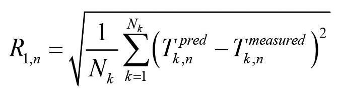
Here n expresses a campaign number and Nk (k = 1, .., Nk) is

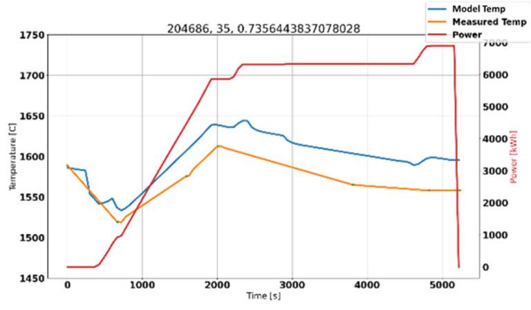
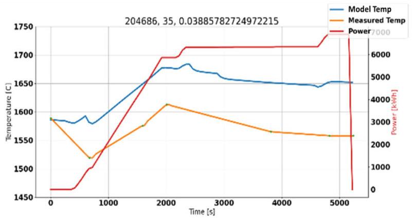
the number of temperature measurements in one heat. Now, if the initial steel temperature is incorrect that will drive a large residual R1,n. However, this problem is picked up by the residual R0,n defined as

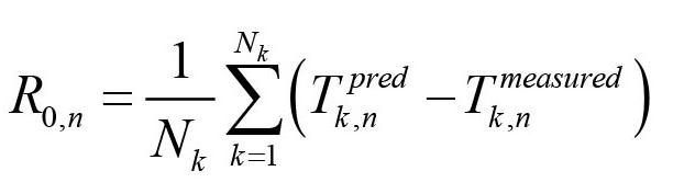
If the predictions are perfect we have, due to incorrect initial temperature for the steel, that Tk,nprep - Tk,nmeasured = DTinitial, resulting in R0,n = DTinitial, and R1,n = |DTinitial|. On the other hand, if the temperature levels of both simulation and data are identical, we have, R0,n = 0.0, and

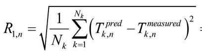
0. Accordingly, we used as the overall residual to minimize: [3]

Tuning step (b)

Here we correct the initial temperatures in order to obtain the correct steel temperatures for the simulation of refractory erosion. Based on step (a) the initial temperatures are corrected for all cases where |R0,n| > 10 K.

Note that in both steps (a) and (b) the erosion is predicted based on preliminary tuning. As the refractory is eroded this will also impact the thermal dynamics of the system.

Tuning step (c)

Now we tune the erosion part of the model. We have data on when a decision was taken to repair the refractory and when it was demolished.

We do not have a model for degradation due to thermal shock, and this element is for now not considered. As thermal shock is most important at the bottom of the ladle, while chemical erosion is most pronounced at the slag line, this omission may not be critical for the usability of the model. Accordingly, we tune the erosion part of the model to match the observed number of uses until repair.

Repair is deemed necessary when the maximum erosion is greater than 75% for the three inner bricks.

We have here a new residual, Θrepair,n to minimize.

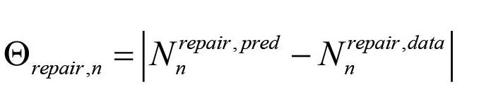
Here N represents the number of heats and n is the campaign number.

Tuning step (d)

When we can reproduce the times of repair well, we move on to reproduce the number of heats before demolition. In a ladle repair the bricks above a given level are repaired, while those below are not repaired. This must also be considered for the tuning. Optimally, we should find that tuning of the demolition is not required. However, it is possible for a repair to change the properties of the refractory in a way that necessitates some tuning of the models to handle the evolution of erosion after repair.

In this case it was eventually found that no tuning behind step (c) was necessary. The model could reproduce the demolition data very satisfactorily.

Figure 5—Evolution of predicted and measured steel temperature for a 73.6% eroded refractory. Heater power is also shown

Figure 6—Evolution of predicted and measured steel temperature for an almost fresh (3.9% eroded) refractory. Heater power is also shown

Pragmatism in industrial modelling: An application to ladle lifetime in the steel industry

Pragmatism step 5: Evaluation of the solution

The outcome of the development is twofold. We have a model that can deliver certain prediction results. In addition, we have a numerical code that can be utilized as an element in multiple applications such as cognitive digital twins and other applications for asset management and optimization.

The quality of the solution is in this case exemplified by a comparison between prediction and measurements at the time of demolition, for all ladles and ladle campaigns operated by Sidenor in 2019. The result is shown in Figure 7. The averages are carried out over bricks 7–35, referring to Figure 8. It must be noted that the measurements have picked the bricks which are most eroded at each level. In Figure 8 we see typical measured and predicted erosion profiles. The measured values are a result of the ladle being sectioned in two halves, and where the most eroded bricks for each half are measured. As a result, the model should predict lower values than what is observed. This is also the case as seen in Figure 7. We further see from Figure 8 that high erosion is found above brick 35, labelled ‘splash-based erosion’. This erosion is a result of thermal shock due to intermittent splashing of steel during vacuum

treatment, combined with low-pressure chemical decomposition (Jansson, 2008) of the MgOC bricks, neither of which are accounted for in the model.

It is fair to ask whether the model can support the operators in allowing more uses of the refractory before demolition. Based on the result in Figure 7 it seems that the answer is yes. The model shows a good comparison between measured demolition data and what is predicted. All campaigns with predicted erosion thickness below 80 mm could be safely extended with more heats. If the model predicts that erosion is not excessive but the operator is uncertain, this could result in one more heat. We have seen that some heats may involve as much as three times or more erosion than average heats. This knowledge would also be useful for the operator's assessment.

Pragmatism step 6: Conclusion and communication

The conclusions are presented in the final section of this paper. Communication is done internally within the team and with the industry partner. The present paper is an important part of the communication, together with a technical paper (Johansen, Løvfall,

Figure 7—Comparison between measured and predicted average eroded thickness for all Sidenor ladles in 2019. Colour codes represent different ladle numbers

Figure 8—Comparison between measured and predicted erosion profiles, at time of demolition of lining, for Sidenor ladle 1, campaign 79, 2019

Pragmatism in industrial modelling: An application to ladle lifetime in the steel industry

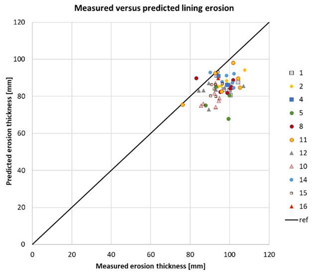
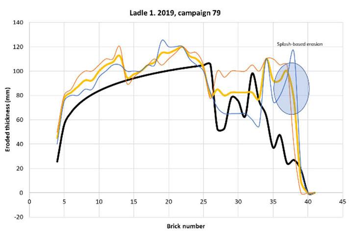
and Rodriguez Duran, 2024) that outlines the details of the physicsbased simulation model.

Observations and learning outcomes

The steps in the pragmatism work flow of the presented use case had to be adjusted due to limited time and resources. As seen from Figure 3, multiple feedback loops had to be implemented in the work flow. This was critical to continuously improve the understanding of the ladle process, the data, and the physics involved. The work was done with an absolute minimum team. Such a small team is typical for many industrial developments. The learning outcomes from this work may therefore be useful in future developments.

➤ The overall development would have been faster if the data had been organized in a database (such as TimescaleDB3 or InfluxDB) at the outset. This would have allowed for a more generic pre-processing and presentation of data and saved significant time at later stages in the project. However, the initial development would have taken more time.

➤ The code should be modularized as early as possible. This makes the code more versatile to use (testing, tuning, prediction) and easier to develop and later extend. As our model could be accessed as one object, specific scripts could be deployed according to need at any stage of the development.

➤ The implementation programming language should be chosen to allow agile and rapid application developments, with performance a secondary concern until the model structure has settled down. The Python programming language is a good example of this.

➤ It is very difficult to design a model architecture for the start of the project when so many changes and iterations are needed. It is then expected that several redesigns of the code are required. The initial design should be simple, but effective.

➤ Need for maturing time: The duration of the work should be sufficiently long to allow better understanding of (a) the case, (b) the data, and (c) the underlying physics. When the model is applied and does not fit with the data this most often pushes the understanding to a higher level.

➤ More iterations needed than expected: This is linked to maturing time. For the increased maturing time to make a difference, more iterations in the work flow is a must.

➤ It was found that data for model tuning was scarce, even if the amount of input data was significant. Data for temperature validation for the slag was not available, as was the case for refractory temperature below the steel surface. The only information available was the state of the refractory before repair (typically after more than 40 heats) and at the time of demolition. The erosion difference between heats is only obtained from our model predictions. The model predicts a one-dimensional erosion profile while the data shows variation in erosion along the perimeter of the ladle. The details of this variation have been recorded recently. Unfortunately, this information is too late to be processed in the COGNITWIN project. This information is critical for a more quantitative assessment of the stochastic variations in erosion, which is beyond the capabilities of the current model. Processing this information to assess the variability in erosion at different levels above the ladle bottom would be of help in interpreting the model predictions in terms of maximum erosion at different levels in the ladle.

➤ Industrial data is not always what it seems to be for outsiders. Data documentation might sometimes rely on in-house knowledge that is not transparent for outsiders. Thus is it important to question all data that could not be explained. The data in itself might not be wrong, but the interpretation could be.

One could ask, why not go for a pure ML approach here? This has been attempted but was found challenging as the amount of output data is very limited. Such an approach was, however, explored by Mutsam et al. (2019) and they obtained acceptable agreement between data, applying both a linear regression model and a deep learning neural network model. As part of preprocessing of their data they removed outliers (unexpected high erosion spots). The difference between our and these approaches is that we have physical mechanisms that we can touch and manipulate and, when tuned to data, this allows us to work outside the data window. This cannot be done safely with models relying only on interpolating data.

After being tuned to data, the physics-based model is already a hybrid digital twin. A natural next step is to explore the deviation between the model’s predictions and the results obtained by various alternative ML methods. This could help to single out missing mechanisms, as well as the degree of randomness in the data (from causes we have not recognized or measured).

A final aspect is the introduction of cognition into this task. This may happen through various mechanisms, such as:

i. The operators use the model actively and build experience on how the model predictions and visual observations relate. This will increase trust in the model in cases where the operator has doubts as to whether to proceed with another heat.

ii. The model predictions, together with operations data, may be presented to the operators as knowledge graphs4. This may offers additional support to the operators (Albagli-Kim and Beimel, 2022).

iii. Self-adaptive algorithms, by learning from data, may continuously improve the model.

The pragmatic modelling approach comprises two equally important phases: development and exploitation (including use of the models and data in the overall decision support systems and processes). Both phases require a small, but dedicated, team of experts (not necessarily more than 2–3 persons). Their engagement should start with the framework development and continue with the exploitation of models and produced results/ data. They should also exploit the potential of the framework and the continually produced data for further process optimization and improvement. This requires continuity of the team and availability of the financial resources for a longer period. Without dedicated strategic management support, the value of the work be significantly reduced, if not lost.

There should be a plan for internal training and model adaptation in case the model development is outsourced.

Conclusions

The pragmatism in industrial modelling methodology was applied and extended to the development of a model for ladle refractory lifespan prediction. The major contributions to the methodology were as follows.

3https://www.timescale.com/ 4https://en.wikipedia.org/wiki/Knowledge_graph

Pragmatism in industrial modelling: An application to ladle lifetime in the steel industry

i) Processes in the metallurgical industry are complex in many dimensions. Operational data will entail many challenges and sometimes the data does not express what it seemingly is supposed to express. Therefore, it is critical that the solution architects have some experience with this type of industry to enable good communication with the industry experts.

ii) Developing a model based on a slim team (a core team of two scientists) should be extended in time, allowing multiple iterations in the development process. Allocating large funding resources to be utilized over a short time would be costly and would produces less valuable results.

iii) A well-defined tuning strategy was implemented. However, exact tuning was not possible as data relevant for operation is monitored, but not data that would be useful for model tuning and validation. As a result, only approximate tuning was possible. Tuning should ensure that all qualitative variations in the data are accommodated. In this case the model can be used in a semi-quantitative manner, where model predictions, visual inspections of the ladle refractory, and operator experience together inform the decision whether the lining should be demolished or not.

Acknowlegements

The work described in this paper was funded by the H2020 project COGNITWIN (grant number 870130). We thank the COGNITWIN consortium partners who were involved into the Sidenor pilot discussions.

CRediT author statement

STJ: Conceptualization, Methodology, Writing - Original draft preparation; BTL: Conceptualization, Methodology, WritingOriginal draft preparation; TRD: Resources, Investigation, WritingReviewing and Editing; JZ: Conceptualization, Methodology, Writing - Original draft preparation

Nome-nclature

AI Artificial intelligence

BF Blast furnace

EAF Electric arc furnace

Campaign The campaign, is given an ID number, and for given ladle number, starts with the first use with new lining, and ends with the demolition of the lining.

LF Ladle furnace

ML Machine learning

MLT Machine learning team

SM Secondary metallurgy

Tn,k Temperature [K]

Θn Residual, defined by Equation [3]

VD Vacuum degasser

References

Albagli-Kim, S. and Beimel, D. 2022. Knowledge graph-based framework for decision making process with limited interaction. Mathematics, vol. 10. 3981. https://doi.org/10.3390/math10213981

COGNITWIN/ 2022. COGNITWIN - Cognitive plants through proactive selflearning hybrid digital twins. https://www.sintef.no/projectweb/cognitwin/ (accessed 1 September 2022).

Jansson, S. 2008. A study on the influence of steel, slag or gas on refractory reactions. Materialvetenskap, Materials Science and Engineering, Kungliga Tekniska högskolan, Stockholm.

Jayakumari, S. and Henning, P. 2020. Role of silicon carbide (SiC) in silicon/ ferro silicon (Si/FeSi) process. NTNU TekNat. https://www.ntnu.no/blogger/ teknat/en/2020/12/15/role-of-silicon-carbide-sic-in-silicon-ferro-silicon-si-fesiprocess/ (accessed 24.October 2023).

Johansen, S.T., Meese, E.A., Zoric, J., Islam, A., and Martins, D. 2017. On pragmatism in industrial modeling Part iii: Application to operational drilling. Progress in Applied CFD – CFD2017 Proceedings of the 12th International Conference on Computational Fluid Dynamics in the Oil & Gas, Metallurgical and Process Industries. SINTEF, Trondheim, Norway.

Johansen, S.T., Løvfall, B.T., and Rodriguez Duran, T. 2024. A pragmatical physics-based model for predicting ladle lifetime. Journal of the Southern African Institute of Mining and Metallurgy, vol. 124, no. 3. pp. 93–110.

Johansen, S.T. and Ringdalen, E. 2018. Reduced metal loss to slag in HC FeCr production - by redesign based on mathematical modelling. Proceedings of Furnace Tapping 2018, Kruger National Park, 14–17 October 2018. Steenkamp, J.D. and Cowey, A. (eds). Symposium Series S98. Southern African Institute of Mining and Metallurgy, Johannesburg. pp. 29–38.

Mutsam, A., Gantner, G., Viertauer, G., Winkler, N., Grimm, F., Pernkopf, A., Ratz, A., and Lammer, W. 2019. Refractory condition monitoring and lifetime prognosis for RH degasser. AISTech2019: Proceedings of the Iron and Steel Technology Conference. AIST, Warrendale, PA. pp. 1081–1090. https://doi. org/10.33313/377/111

Wikipedia. 2023. Volume of fluid method`. https://en.wikipedia.org/wiki/Volume_ of_fluid_method

Wikipedia. 2022a. Observability. https://en.wikipedia.org/w/index. php?title=Observability&oldid=1107687392 (accessed 1 September 2022).

Wikipedia. 2022b. Use case https://en.wikipedia.org/w/index.php?title=Use_ case&oldid=1106419225 (accessed 1 September 2022).

Wikipedia. 2022c. Systems architect. https://en.wikipedia.org/w/index. php?title=Systems_architect&oldid=1090682953 (accessed 1 September 2022).

Wikipedia. 2022d. Systems architecture. https://en.wikipedia.org/w/index. php?title=Systems_architecture&oldid=1076684041 (accessed 1 September 2022).

Wikipedia. 2022e. Singular value decomposition. https://en.wikipedia.org/w/index. php?title=Singular_value_decomposition&oldid=1103873662 (accessed 1 September 2022).

Wikipedia. 2022f. Model order reduction. https://en.wikipedia.org/w/index. php?title=Model_order_reduction&oldid=1107700833 (accessed 1 September 2022).

Zoric, J., Busch, A., Meese, E.A., Khatibi, M., Time, R.W., Johansen, S.T., and Rabenjafimanantsoa, H.A. 2015a. On Pragmatism in industrial modeling - Part II: Workflows and associated data and metadata. Proceedings of the 11th International Conference on CFD in the Minerals and Process Industries. CSIRO Publishing, Melbourne. p. 7. http://www.cfd.com.au/cfd_conf15/PDFs/032JOH. pdf

Zoric, J., Johansen, S.T., Einarsrud, K.E., and Solheim, A. 2015b. On pragmatism in industrial modeling. Proceedings of the 10th International Conference on CFD in the Minerals and Process Industries, vol. 1. SINTEF Academic Press, Trondhein, Norway. pp. 9–24. u

Pragmatism in industrial modelling: An application to ladle lifetime in the steel industry

2ND BATTERY MATERIALS CONFERENCE 2024

5 AUGUST 2024 - WORKSHOP

6 -7 AUGUST 2024 - CONFERENCE

8 AUGUST 2024 - TECHNICAL VISIT THE ARENA, EMNOTWENI CASINO, MBOMBELA, MPUMALANGA

The intensified search over the past decade for alternatives to fossil fuels as sources of energy, has led to the development of a number of renewable energy technologies. A major issue with renewable energy sources is its intermittency which requires energy storage. This requirement has led to an exponential growth in the demand for batteries and research into battery technologies. The largest application by far has been in transportation, followed by the balancing of electrical distribution grids.

Of the raw materials required for battery manufacture, metals such as cobalt, manganese, vanadium and to a lesser extent nickel are concentrated in southern Africa. The supply of lithium, on the other hand, is mainly concentrated in Australia, Chile and Argentina with only Zimbabwe boasting significant resources in Africa. These activities have created both opportunities and challenges. Opportunities such as new value chains for the associated raw materials, with several production companies with battery-material metals in their plant feedstocks undertaking research towards producing battery-grade products. Challenges such as the means for recycling these batteries once they reach the end of their (first) life.

The aim of this conference is to provide the opportunity for thought leaders in the global battery value chain to exchange ideas on recent developments in the fields of:

• Materials and high-purity intermediates for battery components

– Novel battery chemistries

• Flow-battery electrolytes

• Processes for the recycling of batteries

• Market outlook and legislative implications

– New projects and entrepreneurship in the battery industry

• Related case studies.

An even sharper focus can be provided by addressing the following questions and hypotheses:

• Will future battery developments and applications in southern Africa centre more around bulk energy storage by drawing on regional metal resources and addressing local bulk energy shortages?

• Will lithium-ion batteries continue to dominate most battery applications, with other battery technologies serving only niche applications?

• What (exactly) are the criteria and specifications for battery materials, intermediates and electrolytes required to achieve the envisaged performance and life of the batteries?

– What impact will South Africa’s electrical supply issues have on the local motor manufacturing industry and the market for EVs?

Affiliation:

1Samancor Chrome, Dikwena Chrome, South Africa.

2Mintek, South Africa.

3Stellenbosch University, South Africa.

Correspondence to:

S.J. Baumgartner

Email: shana.baumgartner@samancorcr.com

Dates:

Received: 18 Aug. 2023

Revised: 15 Jan. 2024

Accepted: 22 Jan. 2024

Published: March 2024

How to cite:

Baumgartner, S.J., Reynolds, Q.G., and Akdogan, G. 2024

Prediction of burden distribution and electrical resistance in submerged arc furnaces using discrete element method modelling.

Journal of the Southern African Institute of Mining and Metallurgy, vol. 124, no. 3. pp. 123–132

DOI ID:

http://dx.doi.org/10.17159/24119717/3042/2024

ORCID:

G. Akdogan

http://orcid.org/0000-0003-1780-4075

Prediction of burden distribution and electrical resistance in submerged arc furnaces using discrete element method modelling

by S.J. Baumgartner1,3, Q.G. Reynolds2,3, and G. Akdogan3

Synopsis

A computational model of a submerged arc furnace (SAF) used in the production of ferrochrome is presented. The model‘s intended use is to investigate the extent to which intrinsic and extrinsic properties of the raw materials affect burden distribution and electrical resistance within the furnace. The model is built on the discrete element method and calculates the mechanical interactions of particle distributions resulting from the flow motion of typical raw materials used in the smelting of chromium ore. This model excludes the effects of thermodynamics, furnace chemistry, and heat transfer. It illustrates how the consumption of materials (chromite pellets, flux, and reductant) is affected by changes in electrode length, reductant fractions, and reductant sizing and density during the formation of a reductant bed. The resistance calculation algorithm developed by Mintek was applied to construct networks developed from particle contacts, which can quantitatively generate estimates of the electrode-to-electrode and electrode-to-bath electrical conduction conditions.

Keywords submerged arc furnace, resistance, ferrochrome, segregation.

Introduction

Ferrochrome is an essential source of elemental chromium for the production of stainless steel, to which it imparts increased corrosion resistance, hardness, and toughness. South Africa is a primary producer of ferrochrome and possesses 72–80% of the world’s total chromite ore reserves (Beukes, Dawson, and van Zyl, 2010). The industry contributes approximately R42 billion in GDP per annum and employs over 200 000 people directly or indirectly (Africa Mining IQ, 2019). Recently, the ferrochrome industry has been placed under severe strain due to increasing electricity tariffs and a decaying electrical infrastructure that poses a threat to the sustainability of high-energy processes.

Researchers such as Kajiwara, Jimbo, and Sakai, (2006) and Shi et al. (2016) have studied burden distribution in blast furnaces used in the steel industry and developed prediction models that have been used in the understanding and optimization of blast furnace operations. However, these models failed to consider the influence of raw material properties on the charge, which would influence in the burden distribution due to the changes in the properties of the raw materials used (Mio et al., 2020). In addition, Mio et al. (2020) included the specifications of the equipment used to dictate burden behaviour and developed these models using discrete element modelling (DEM). The study by Mio et al. (2020) investigates the influence of particle segregation during the charge flow within a blast furnace. The authors found that DEM can analyse in detail the behaviour of the charge particles, and can inform researchers on the behaviour of the charge layers and time series changes that would be impossible to observe via traditional experimental methods. In addition, the use of DEM in blast furnace studies clarifies control mechanisms and the influence of design operations on the process (Mio et al., 2020). Mio et al. acknowledge the influence of material properties on the dynamics of segregation and advise that these findings from studies be compared against actual process phenomena.

Considering the similarities in burden flow between blast furnace and SAF operations, along with the lack of studies specifically conducted on SAFs for ferrochrome production regarding material flow and resulting segregation, it was decided to investigate the behaviour of the burden using DEM modelling. Mio et al. (2020) effectively contrasted DEM simulations with real blast furnace performance and subsequently implemented their findings in real blast furnace operations. In addition, the DEM simulations were conducted to analyse the behaviour of the burden in a ferrochrome furnace. This study also considered the electrical behaviour of the burden, taking into account various properties of the raw materials.

Prediction of burden distribution and electrical resistance in submerged arc furnaces

Model description

DEM governing equations and force models

Both the translational and rotational motion of granular particles can be defined by Newton’s second law of motion in combination with the force-displacement correlation at the points of contact between particles (Wei et al., 2019; Zhao et al., 2015). An appropriate time step of 1 x 10-4 seconds was adopted for the simulations. The time step depends on the damping coefficient, particle mass, and normal stiffness and is defined by Equation [1]:

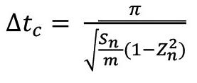
where ∆tc is the critical time step (s), Sn is the normal stiffness (N/m), m represents the mass of the particle (kg), and Zn is a dimensionless coefficient.

Software implementation

LIGGGHTS-PUBLIC® (CFDEMresearch GmbH, 2022), which is available as an open-source computational software package, was used as the modelling tool for the present work. Reynolds et al (2021) describe the model as based on the time-step of soft sphere algorithms and it can introduce a broad range of friction and collision force models. An advantage of using LIGGGHTS-PUBLIC® is that the software allows flexibility in the application thereof and the implementation of other models as subcomponents.

To perform the electrical resistance calculations based on the particle assemblies resulting from the DEM modelling, Python (Python Software, 2022) was used to process the electrical contact network algorithm. The construction and manipulation methodology was implemented using the Network X package (Network X, 2022). The SciPy package (SciPy, 2022) was used to optimize and increase the efficiency of the matrix algorithm of the linear system, and to speed up the resistance calculation, parallel computing was exploited through the mpi4py Python library (mpi4py, 2021).

The use of the resistance calculation algorithm

The methodology employed in this study, to determine the resistance of the cases , is proprietary to Mintek and is known as the resistance calculation algorithm (RCA) (Reynolds et al., 2021).

Utilizing the RCA, the resistance between the three electrodes and the surrounding burden is estimated. At each time step, DEM simulations yield the particle assemblies, which are defined as the coordinates of the individual particles within the array and the number of distinct surfaces that some of the particles make contact with.

The algorithm takes into account pairings of particles that are in mutual contact within the given system. In the current study, the collection of paired particles was arranged to exclude any interaction with nonconductive particles, including flux and pellets (sintered and pelletized chromite concentrate). The remaining sets of particle pairings in the contact network are utilized to graphically construct a contact network by constituting nodes as edges on the graph. The resistance network between a pair of electrodes and conductive and nonconductive particles is depicted conceptually in Figure 1.

Thereafter, the graphed data is analysed for connections and contacts between the cathode and anode surfaces, and where there are legitimate relationships, the data is processed to determine the resistance network. The resistance network is structurally identical

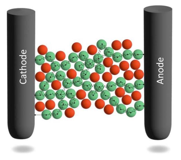
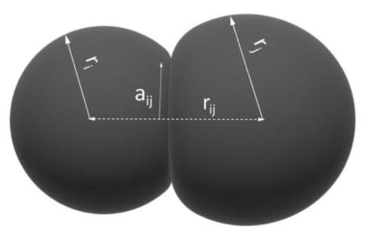
to the graph generated for the contact networks; however, in this case each edge is represented by the electrical resistance of each pair of particles. Thereafter, Kirchoff’s Circuit laws are used to convert the resistance network into a matrix equation containing the voltage of each particle node, which is finally solved using linear algebra methodology.

When particles touch each other, they have a shared surface, which allows for the calculation of the electrical resistance between the pairs of particles. This is accomplished by integrating the combination throughout the entirety of the particle pair's volume, starting at the centre of each particle and extending to the point where they make contact. Figure 2 depicts the concept by showing the geometric configuration of spherical particles i and j. Each particle has a radius of ri and rj, respectively, and separation is defined as rij < ri + rj. aij represents the shared radius between the two particle.

The current density vectors are assumed to be parallel to the axis where all the points are in contact between the particle pair, thus the net resistance Ωij between the particle centres is defined by Equation [2] below. The normal force is implicitly accounted for by the rij; however, the normal force contributing to the interparticle resistance is not accounted for in the equation.

Here the electrical conductivities of the two particles, i and j, are represented by σi (S/m) and σj (S/m), respectively (Reynolds et al., 2021).

Two electrical burden conduction models were used to determine the inter-electrode resistances of the SAF DEM model simulation outcomes for various model situations. One model examines the direct conduction between electrodes, as depicted in Figure 3a. The other model analyses conduction from the electrode through the molten phases, slag, and alloy, and then back to the neighbouring electrode, bypassing the burden, as shown in

Figure 1—Visualization of the resistance network between conductive particles (green spheres) and nonconductive particles (red spheres)

Figure 2—Contact relationship between two particles

Prediction of burden distribution and electrical resistance in submerged arc furnaces

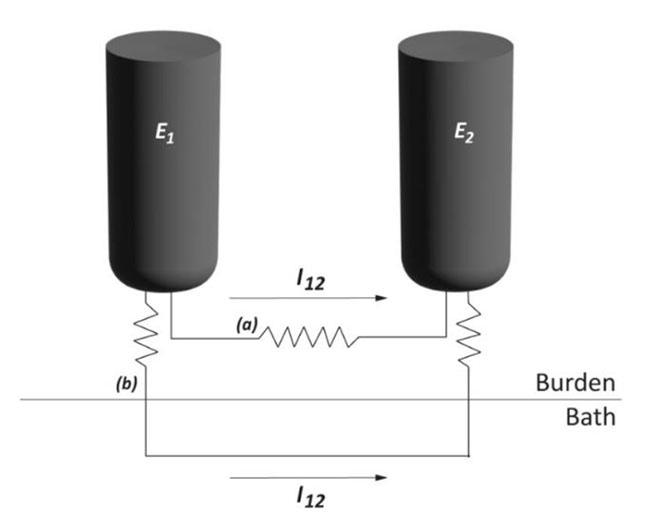
Figure 3b. To measure the resistance of the two models, the electrode surfaces were designated as the cathode, while any other surface was selected as the anode within the resistance calculation algorithm (Reynolds et al., 2021).

Particle consumption model

The particle consumption region in the DEM simulation can be found in one of three areas in the furnace: directly below the electrode tip, in the intermediate zone between the charge and the liquid phase (consisting of slag and alloy), or in the molten slag phase. Figure 4 depicts this configuration.

Using the information given:

(1) Indicates the region where particles are consumed below the electrode tip.

(2) the area within the furnace where partial slag consumption occurs, situated in the intermediate region.

(3) Illustrates the entire area of consumption, encompassing the entirety of the molten phase, including slag and alloy phases.

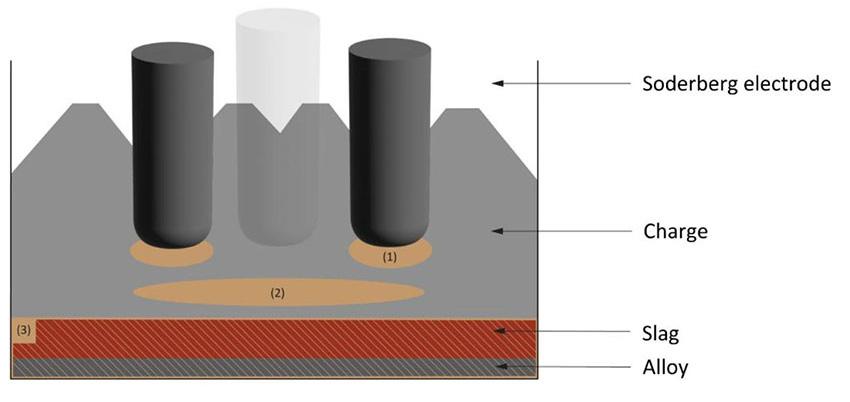
A comparative analysis was conducted to identify the best realistic consumption scenario that closely mimics the typical behaviour found in an industrial furnace. This investigation entailed assessing the resistances between electrode and electrode, as well as between the electrode and bath, for all three scenarios. Furthermore, the study examined the rates of consumption and their corresponding patterns for these three scenarios to determine the conditions that are most likely to imitate the consumption patterns of raw materials within a SAF, with a specific emphasis on the flow of burden. The model that best matches the observed furnace consumption behaviour was chosen based on the comparative results acquired during the post-processing of the data.

The post-processing results of the DEM electrode resistances for the three cases of the particle consumption zones are shown in Figure 5, where the electrode-to-electrode resistance through the burden and the electrode resistance through the molten bath,are shown.

The cumulative duration of all simulations (the total runtime) was 2000 seconds, during which the initial conditions reached a pseudo-steady dynamic state (or in cases 1 and 2, a state of fluctuating stability). Table I provides a thorough analysis of the average resistance results for every model and occurrence throughout the pseudo-steady dynamic state.

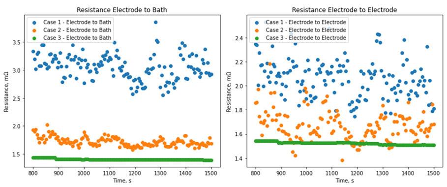
I Average resistance results for the different consumption zones

* (1)– (3) refers to Figure 4 above

Table

Figure 3—Illustration of the different inter-electrode conduction models, (a) electrode-to-electrode (b) electrode-bath-electrode

Figure 4—Illustrations of the different consumption cases

Figure 5—Resistance comparisons of the different particle consumption zones

Prediction of burden distribution and electrical resistance in submerged arc furnaces

If the model had considered the resistances related to the slag and metal, the results would have indicated that the conduction model between the electrodes was mostly affected by conduction through the molten bath. In this situation, the resistance value would have been significantly reduced in comparison to the conduction model, as the current flows from one electrode to another through the burden (Reynolds et al., 2021). However, in the present study the conduction caused by the slag and metal is ignored. The main objective of this research is to examine the material segregation and resistance that may be completely attributed to the burden. The expected result of the inter-electrode conduction for both models is anticipated to be similar. This is grounded on the consistency of the material composition across the entire model, along with the measurements of the distance between the electrode tip and the molten bath (1.50 m) and the electrode pitch radius (2.25 m). The most closely related results for this condition are found in the case of a complete slag consumption zone (case 3), where the resistances from electrode to electrode via the burden and through the molten bath are measured at 1.52 mΩ and 1.40 mΩ, respectively.

To eliminate the inclusion of material thermodynamics and heat transmission, it is beneficial to utilize a technique that effectively accommodates the consumption zone, hence ensuring the validity of the present study.

Results and discussion

Base case model

The geometry of the generic model was based on the design parameters of a common mid-sized industrial SAF used in South Africa, which are summarized in Table II.

The electrical conductivity of the reductant was derived from studies by Surup et al. (2020) and Nhiwatiwa and Cromarty (2021). Consult Table III for the particle properties and parameters, which include the calibrated parameters.

Figure 6 is a graphical depiction of the simulation model's geometry, illustrating the arrangement of the charge chutes and electrode layout.

Figure 7 provides a 360 deg view of the base case furnace DEM model profile. An essential element in the model is the placement of the electrode tip, which presents challenges in the SAF environment due to the several variables that impact the electrical performance of the electrodes and the alignment of the tip with the metal heel. The variables being considered encompass characteristics such as burden resistance, slag composition, and tapping cycles, along with other pertinent parameters. Various endeavours have been made to employ data and methodologies, such as electrode hydraulic pressure, data analysis, modelling, and acoustics, to precisely ascertain the length and positioning of the electrode tip. Nevertheless, this endeavour is additionally impeded by numerous

Base case model geometric parameters

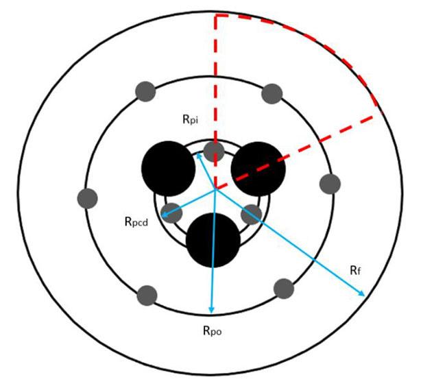
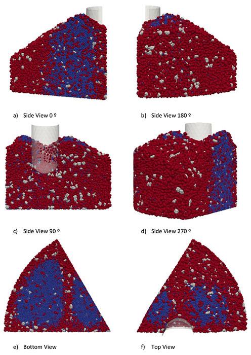
external and internal factors, as well as complex interactions involving mechanical, electrical, and chemical components.

Yoneka et al., (1981) investigated the reduction burden of ferroalloys and highlighted the significance of maintaining an ideal position for the electrode tip, particularly in larger furnaces. They state that the electrode tip has a crucial function in controlling and improving furnace operations. Hence, it was imperative in this study to determine the optimal parameters for the baseline scenario, which could then be compared to the actual furnace values of a system that conforms to design criteria. The electrode tip position was evaluated by utilizing operational expertise and employing the information from design specifications provided in confidential documentation. The electrode tip height, as measured from the metal heel, was determined to be 1.5 m.

In its initial state the model volume is empty, and it is gradually filled with particles introduced through the charge chutes. The total number of particles introduced into the DEM simulation ranged between 180 000 and 200 000. These particles enter the furnace and are then continuously generated, with the rate of supply being directly proportional to the rate at which the burden is consumed. The models were simulated for a duration of 650 seconds

Table II

Figure 6—Simulation geometry of the base case model

Figure 7—Particle assembly of the base case shown at different angles (blue = pellets; red = reductant; grey = flux)

Prediction of burden distribution and electrical resistance in submerged arc furnaces

Table III

Base case material properties

Coefficient of pellet-anthracite static friction, μs

D (mm)a

Young's Modulus, G (GPa)c Actual

Young's Modulus, G (MPa) DEM

aValues obtained from plant data

bAverage value calculated from Bukowska et al.,2022

cValue extrapolated from Cong et al., 2023

dValue cited from Gustafsson., 2012

eValue cited from Wei et al., 2019

fValue cited from Moncada et al., 2022

gValue cited from Mena-Negrete et al., 2022

hValue cited from Barrios et al., 2013

iValue cited from Wei et al., 2019

until stable pseudo-steady dynamic conditions were achieved. Similarly, Reynolds et al. (2021) assumed that the electrodes exhibit symmetry. To make the computational model feasible, the size of the region was scaled down by a factor of 5.

A summary of material properties determined and used in the base case model is given in Table III.

Effect of electrode length on model behaviour

A pivotal control mechanism in ferrochrome SAF furnaces and one that efficiencies depend upon is the electrode positions. In industrial ferrochrome furnaces, the electrode position is controlled by automation and relates to the electrodes' secondary current and resistance. Therefore, studying and understanding the impact that electrode tip position relative to the metal heel has on the burden structure and the electrical behaviour is of importance to improve electrode control on an industrial scale to increase alloy throughput, provide consistent and even power distribution, and allow for

consistent and stable electrode penetration to maintain optimum metallurgical conditions for improved smelting. DEM simulations were run where the electrode tip position relative to the metal heel was varied between static positions ranging between 500–2900 mm, while keeping all other parameters in the model constant as per the base case model in Tables II and III. The comparison simulations are provided in Figure 8.

A notable observation is the consistent distribution and separation of the burden with electrode tip positions 700 mm and 2700 mm from the heel. While the position of the electrode may vary, the composition of the raw materials remains constant. This is because the characteristics of the raw materials remain consistent regardless of the electrode tip position. Although the degree to which this regularity in the burden distribution is visually apparent (Figure 8) may be limited, a more precise demonstration of this consistency has been conducted. This involved directly calculating the mass fractions of the reductant and FeCr pellets at different

Prediction of burden distribution and electrical resistance in submerged arc furnaces

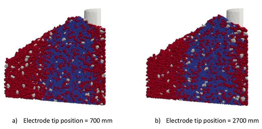
positions within the simulated areas. The resulting quantitative data is visually presented in a two-dimensional format in Figure 9, providing a more precise representation of the level of consistency. The red circles in the figure indicate the positions of the electrodes and the feed ports. The representation consists of a composite of all the planes through the burden .

Figure 10 demonstrates a clear trend: as the electrode tip* location increases, the resistance also increases. The connection between 1250 and 1900 mm demonstrates a variance in the trend, as seen in Figures 10 and 11. However, it may be argued that the values within this range are in the expected range of resistance values. The anomaly is most likely caused by approximations made in the model, leading to numerical noise. Specifically, there may be a disproportionality between the compact model, designed for computing efficiency, and the effects of physical contact regions.

Effect of change in reductant fractions on model behaviour

To investigate the impact of varying reductant concentrations on the flow characteristics and electrical resistance in different scenarios, simulations were conducted with reductant fractions ranging from 10% to 40% of the total mass. All other parameters were held constant, aligning with the base case model, as outlined in Tables II and III.

The fraction range chosen to simulate the reductant fractions was purely for experimentation purposes to observe and study the behaviour of resistance of the reductant contribution in a comprehensive manner.

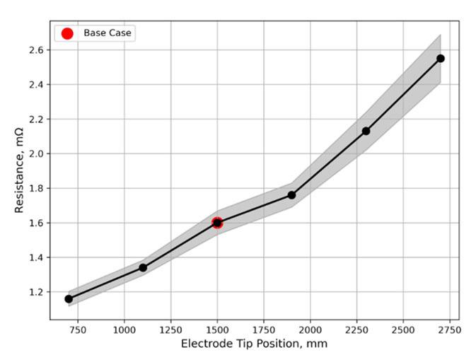
Visualizations of the particle assemblies for reductant fractions of –50% and +50% are shown in Figure 12. An increase in the reductant fractions leads to the formation of a larger reductant bed, which will result in better contact with the electrodes, and it reduces the occurrence of the reductant depleted pockets.

The changes in the burden structure are indicated by the resistance calculation results. With a richer reductant bed, the resistance is reduced as shown in Figures 13 and 14.

Another interesting observation is the large range in which the resistance of the furnace charge can fall when the reductant mass fraction is set between 15% and 20%. This is most likely attributable to a more randomized and discontinuous stable reductant bed.

Effect of change in reductant sizing on model behaviour

The effect of reductant particle size on the bed resistance is summarized in Figures 15 and 16. There is a notable correlation between electrical resistance and the sizing of reductant particles, with an increase in reductant size resulting in a decrease in furnace resistance.

Visualizations of the particle assembly are shown in Figure 17 for a sizing ranging from –25% to +25% of the base case reductant

Figure 9—Reductant and pellet mass fractions at (a) electrode tip position at 700 mm and (b) electrode tip position at 2700 mm

Figure 10 — Total furnace resistance as a function of electrode tip position (mm)

Figure 8—Model simulations of the electrode tip position at a) 700 mm b) 2700 mm relative to the metal heel

Prediction of burden distribution and electrical resistance in submerged arc furnaces

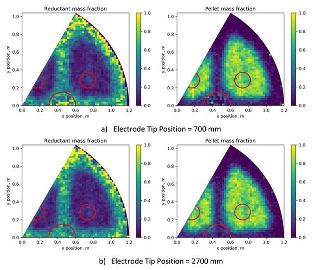
size of 30 mm (base case = 1). A reduction in the reductant sizing results in a more even distribution of reductant particles with distinct pellet voids interrupting the continuous electrical paths between the reductant particles, thereby imparting a high resistance to the bed. Comparing the case with +25% larger reductant sizing,

segregation of the reductant particles towards the contours of the electrodes and the delta region between the electrodes (the area to the left of the visualizations) is dominant and the electrical paths formed between the reductant particles between the electrodes and across the bed are concentrated, leading to a lower bed resistance.

Figure 11—Total resistance as a function of simulation time for different electrode tip positions

Figure 12—Model simulations of the two cases of reductant fraction

Figure 13 – Total furnace resistance as a function of reductant fractions

Figure 14—Total resistance as a function of simulation time for different reduction fractions

Prediction of burden distribution and electrical resistance in submerged arc furnaces

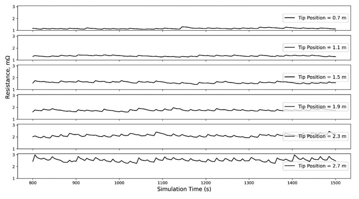
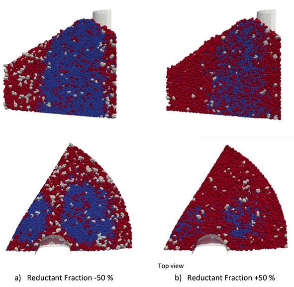
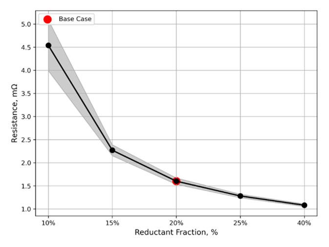
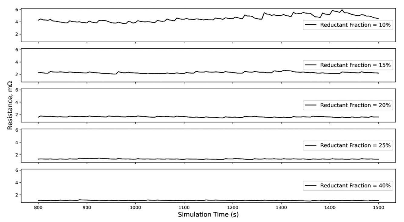
The above observation is significant for industrial furnace operations as the reductant sizing is a parameter that can be manipulated to suit the required resistance of a reductant bed for optimum efficiencies.

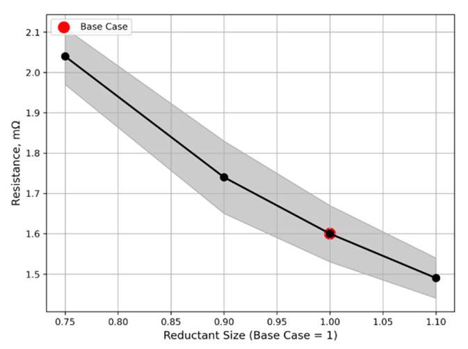
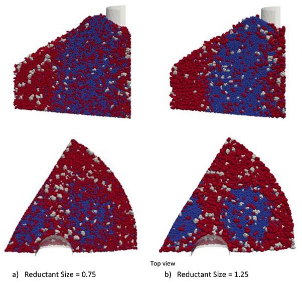
Effect of change in reductant

density on model behaviour

An investigation was conducted to examine the influence of density on the segregation of particles and the resulting resistance.

The findings indicate a significant correlation between density and resistance, with resistance values ranging from 0.90 mΩ to 2.67 mΩ with increasing density. This suggests that changes in reductant density have a impact on furnace resistance, as illustrated in Figure 18.

The observed phenomenon can be ascribed to the extent of segregation, which intensifies with increasing density. as reductant particles of lower density tend to aggregate prominently on the surface of the furnace simulation, as illustrated in Figure 19c. Concurrently, it is noteworthy that particles of lower density contribute to a more uniform dispersion of particles close to the electrode and beneath it, as depicted in Figure 19a. In contrast, reductant particles of higher density form a less concentrated zone, leading to a greater degree of segregation among FeCr pellets, as evident in Figure 19d. Specifically, higher-density reductant particles exhibit increased concentration, featuring well-defined voids amid FeCr pellets and flux particles, as portrayed in Figure 19b.

These findings align with the conclusions drawn by Gray and Ancey (2015), whose investigations revealed a prevalence of regions rich in the lowest density particles near the free surface, with a notably limited presence of particles from other species.

Figure 15 – Total resistance as a function of simulation time for different reductant sizings

Figure 16—Computational visualizations of furnace burden at different reductant sizes

Figure 17—Computational visualizations of furnace burden at different reductant sizes

Figure 18—Comparison of resistance changes with change in reductant density

Prediction of burden distribution and electrical resistance in submerged arc furnaces

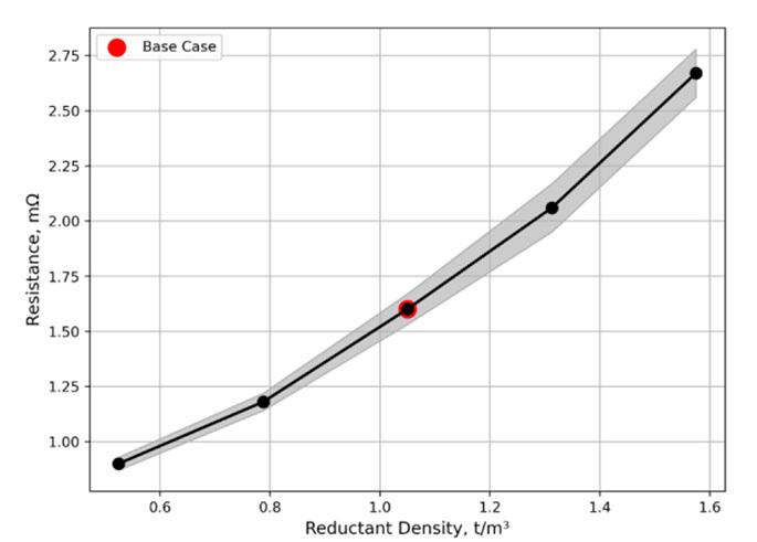
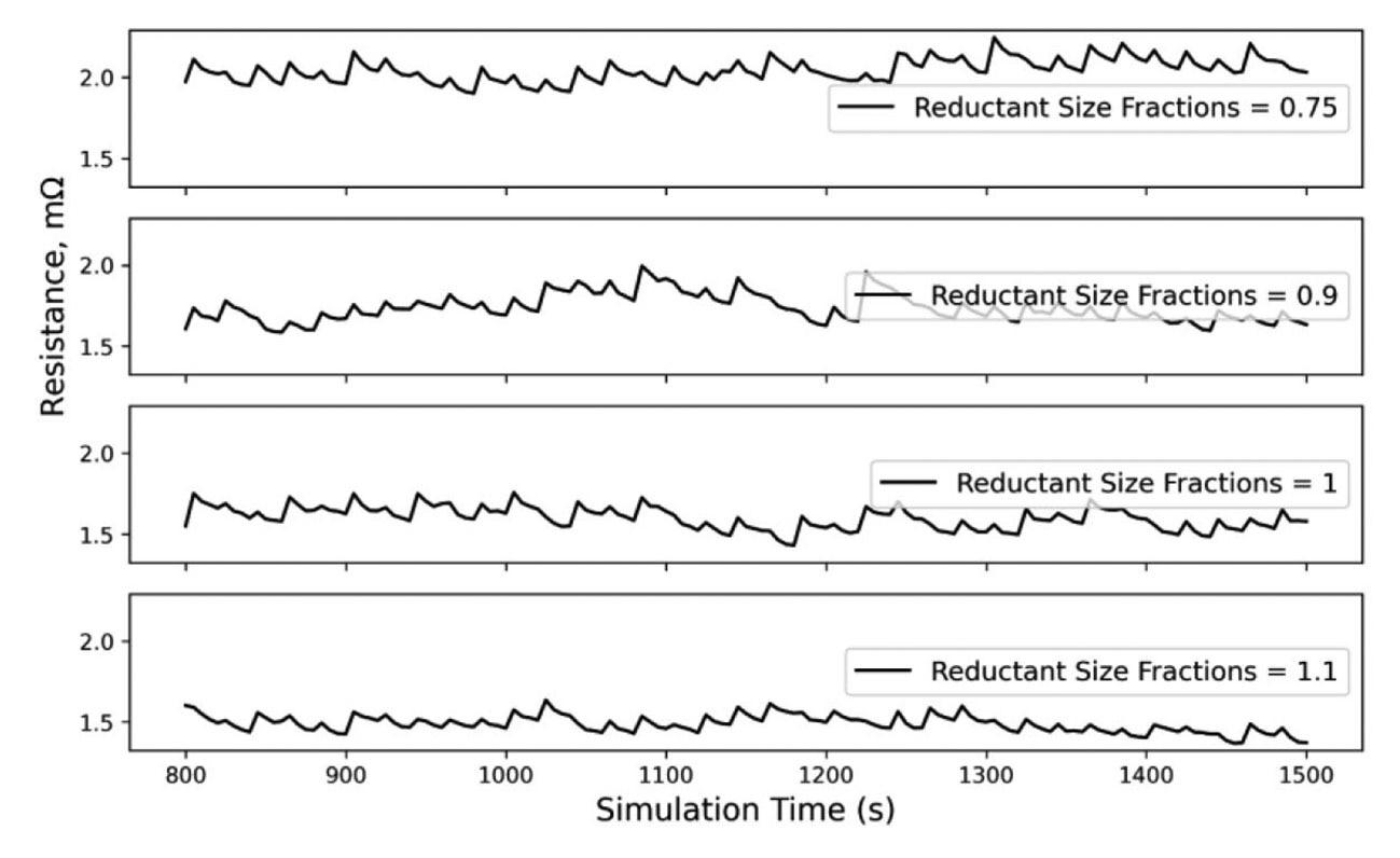
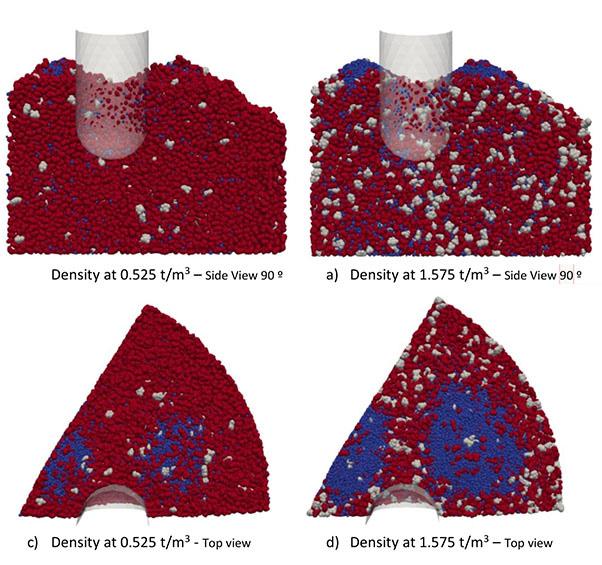
A discernible trend emerges towards the base, wherein the concentration of the lightest species decreases, while that of the highest-density particles undergoes a corresponding increase – a correlation congruent with the empirical observations made in the present study.

Conclusion

This study aimed to develop models for understanding solid particle flow behaviour in a submerged arc furnace, with a focus on establishing relationships between material properties and electrical resistance. The discrete element method (DEM) was employed for investigating furnace burden properties, with accurate results dependent on appropriate parameter values. Calibration involved direct measurements, cold flow experiments, and bulk calibration methodology, using the angle of repose as a primary foundation. Following the establishment of key parameters, a scaled-down DEM model was developed to simulate a submerged arc furnace (SAF) used for smelting ferrochrome (FeCr) ores. This model acts as a foundational reference for conducting parametric studies. The study revealed a complex correlation between electrical properties and raw material attributes, establishing a clear relationship between reductant size and furnace resistance. A 27% increase in resistance was observed with an increase in sizing, aligning with prior research findings. Altering the reductant charge fraction led to a 76% change in resistance. The study also explored the impact of particle morphologies on segregation and resistance, aligning with prior observations. Increased reductant density resulted in a 66% resistance increase.

Future work

The current research will be enhanced by investigating several factors. Firstly, the effects of intrinsic material properties, such as Young's modulus, the coefficient of friction, and the restitution coefficient, will be examined. Secondly, the study will explore the impact of furnace geometry. This includes analysing the pitch circle diameter, electrode diameter, and furnace diameter. These aspects will be evaluated for their influence on particle segregation in SAFs and their subsequent impact on electrical resistance relationships.

Acknowledgements

This paper is published by permission of Mintek and Samancor

Chrome Ltd. The authors acknowledge the Centre for High Performance Computing (CHPC), South Africa, for providing computational resources.

The authors would like to thank the following institutions, companies, and individuals for their contributions and support:

➤ Samancor Chrome for providing the authors with operational data

➤ Stefan Swanepoel and Markus Erwee from Samancor Chrome for their technical guidance and support.

References

Adema, A., Yang, Y., and Boom, R. 2009. Coupled DEM-CFD modeling of the ironmaking blast furnace. Proceedings of the Seventh International Conference on CFD in the Minerals and Process Industries, CSIRO, Melbourne, Australia, 9-11 December 2009. 6 pp. https://www.cfd.com.au/cfd_conf09/PDFs/138ADE. pdf

Africa Mining IQ. 2019. Chrome mining in South Africa. https://www.projectsiq. co.za/chrome-mining-in-south-africa.htm [accessed 22 February 2020], Amberger, S., Freidl, M., Goniva, C., Pirker, S., and Kloss, C. 2012. Approximation of objects by spheres for multisphere simulations in DEM. Proceedings of the European Congress on Computational Methods in Applied Sciences and Engineering, Vienna, 10-14 September. Vienna University of Technology.

Barrios, G.K.P., De Carvalho, R.M., Kwade, A., and Tavares, L.M. 2013. Contact parameter estimation for DEM simulation of iron ore pellet handling. Powder Technology, no. 248. pp. 84–93. https://doi.org/10.1016/j.powtec.2013.01.063

Baumgartner, S.J., Reynolds, Q.G., Bergmann, C., Akdogan, G., and Coetzee, C.J. 2022. Toward discrete element modelling of material flow in submerged arc furnaces. Proceedings of APCOM 2021. pp. 205–214.

BenSaïda, A. 2023. Shapiro-Wilk and Shapiro-Francia normality tests. MATLAB Central File Exchange. https://it.mathworks.com/matlabcentral/ fileexchange/13964-shapiro-wilk-and-shapiro-francia-normalitytests?tab=reviews [accessed 10 November 2023].

Beukes, J.P., Dawson, N.F., and van Zyl, P.G. 2010. Theoretical and practical aspects of Cr(VI) in the South African ferrochrome industry. Journal of the Southern African Institute of Mining and Metallurgy, vol. 110, no. 12. pp. 743–750.

Blender Software. 2023. OpenCV. https://www.blender.org/ [accessed 15 August 2023].

Bukowska, M., Kasza, P., Moska, R., and Jureczka, J. 2022. The Young’s Modulus and Poisson’s Ratio of hard coals in laboratory tests. Energies, vol. 15. p. 2477. https://doi.org/10.3390/en15072477

CFDEMresearch GmbH. 2022. LIGGGHTS open source discrete element particle simulation code. https://www.cfdem.com/liggghts-open-source-discreteelement-method-particle-simulation-code [accessed 30 January 2023].

Chakrabarty, A., Basu, S., Nag, S., Ghosh, U., and Patra, M. 2021. Model study of centre coke charging in blast furnace through DEM simulations. ISIJ International, vol. 61. pp. 782–791. https://doi.org/10.2355/isijinternational. ISIJINT-2020-498

Coaplen, J., Stronge, W.J., and Ravani, B. 2004. Work equivalent composite coefficient of restitution. International Journal of Impact Engineering, vol. 30, no. 6. pp. 581–591. https://doi.org/10.1016/j.ijimpeng.2003.10.038

Coetzee, C.J. 2016. Calibration of the discrete element method. Powder Technology, no. 297. pp. 50–70. https://doi.org/10.1016/j.powtec.2016.04.003

Cong, R., Yang, R., Li, G., Huang, Z., Gong, Y., Jing, M., and Lu, M. 2023. Geomechanical properties of thinly interbedded rocks based on micro- and macro-scale measurements. Rock Mechanics and Rock Engineering, vol. 56. pp. 1–19. https://doi.org/10.1007/s00603-023-03360-w

Dhainaut, M. 2004. Simulation of the electric field in a submerged arc furnace. Proceedings of INFACON X, Cape Town, South Africa, 1-4 February 2004. pp. 605–613. https://www.pyrometallurgy.co.za/InfaconX/079.pdf

Dijs, H.M. 1979. A laboratory investigation of reducing agents for use in the electric smelting industry. National Institute for Metallurgy, Randburg, South Africa. idem, P.A. 2008. Electrical resistivity of coke beds. Doctoral thesis, Norwegian University ofScience and Technology. http://ntnu.diva-portal.org/smash/get/ diva2:132857/FULLTEXT01

Eidem, P.A., Tangstad, M., and Bakken, J.A. 2007. Measurement of material resistivity and contact resistance of metallurgical coke. Proceedings of INFACON XI: Innovations in the Ferroalloys Industry, New Delhi, India, 18-21 February 2007. Indian Ferro Alloy Producers’ Association. pp. 561–571.

Figure 19—Computational visualizations of furnace burden at a low and high reductant density

Prediction of burden distribution and electrical resistance in submerged arc furnaces

Eidem, P.A., Tangstad, M., and Bakken, J.A. 2008. Determination of electrical resistivity of dry coke beds. Metallurgical and Materials Transactions B, vol. 39. pp. 7–15. https://doi.org/10.1007/s11663-007-9105-7

Eidem, P.A., Runde, M., Tangstad, M., Bakken, J.A., Zhou, Z.Y., and Yu, A.B. 2009. Effect of contact resistance on bulk resistivity of dry coke beds. Metallurgical and Materials Transactions B, vol. 40. pp. 388–396. doi: 10.1007/ s11663-009-9235-1

Eidem, P.A., Tangstad, M., Bakken, J.A., and Ishak, R. 2010. Influence of coke particle size on the electrical resistivity of coke beds. INFACON XII: Proceedings of the Twelfth International Ferroalloys Congress, Helsinki, Finland, 6-9 June 2010. Outotek Oyj. pp. 349–358.

Gray, J. and Ancey, C. 2015. Particle-size and -density segregation in granular freesurface flows. Journal of Fluid Mechanics, no. 779. pp. 622–668. doi: 10.1017/ jfm.2015.438

Gustafsson, G. 2012. Mechanical characterization and modelling of iron ore pellets. PhD dissertation, Luleå Tekniska Universitet. https://urn.kb.se/ resolve?urn=urn:nbn:se:ltu:diva-17284

Al-Hashemi, H.M.B. and Al-Amoudi, O.S.B. 2018. A review on the angle of repose of granular materials. Powder Technology, vol. 330. pp. 397–417. https://doi. org/10.1016/j.powtec.2018.02.003

Hockaday, S.A.C. and Bisaka, K. 2010. Some aspects of the production of ferrochrome in pilot AC arc furnaces at Mintek. INFACON XII: Proceedings of the Twelfth International Ferroalloys Congress, Helsinki, Finland, 6-9 June 2010. Outotek Oyj. pp. 367–376.

Jingchun, L. 2001. Discussion of ideal smelting model of submerged-arc furnace. Infacon IX: Proceedings of the Ninth International Ferroalloys Congress, Quebec City, Canada, 3-6 June 2001. The Ferroalloys Association, Wahington, DC. pp. 121–130.

Kajiwara, T., Jimbo, T., and Sakai, T. 2006. Development of a simulation model for burden distribution at blast furnace top. Transactions ISIJ, vol. 23. pp. 1045–1052.

Kapure, G., Kari, C., Mohan Rao, M., and Raju, K.S. 2007. Use of chemical energy in submerged arc furnace to produce ferrochrome: prospects and limitations. Proceedings of INFACON XI: Innovations in the Ferroalloys Industry, New Delhi, India, 18-21 February 2007. Indian Ferro Alloy Producers’ Association. pp. 165–170.

Krogerus, H., Lintumaa, T., and Jokinen, P. 2006. Laboratory investigations of the electrical resistivity of cokes and smelting charge for optimizing operation in large ferrochrome furnaces. Proceesings of Southern African Pyrometallurgy 2006. Jones, R.T. (ed.). South African Institute of Mining and Metallurgy, Johannesburg. pp. 309–328.

Mena-Negrete, J., Valdiviezo-Mijangos, O.C., Nicolás-López, R., and Coconi-Morales, E. 2022. Characterization of elastic moduli with anisotropic rock physics templates considering mineralogy, fluid, porosity, and porestructure: A case study in Volve field, North Sea. Journal of Applied Geophysics, vol. 206. 104815. doi: 10.22201/igeof.00167169p.2021.60.4.2118

Mitra, T. and Saxén, H. 2015. Discrete element simulation of charging and mixed layer formation in the ironmaking blast furnace. Computational Particle Mechanics, vol. 3. https://doi.org/10.1007/s40571-015-0084-1

Mio, H. and Narita, Y. 2018. Simulation of particle behavior in charging process of blast furnace by discrete element method. Nippon Steel & Sumitomo Metal Technical Report no. 120. December 2018. https://www.nipponsteel.com/en/ tech/report/nssmc/pdf/120-11.pdf

Mio, H., Narita, Y., Nakano, K., and Nomura, S. 2020. Validation of the burden distribution of the 1/3-scale of a blast furnace simulated by the discrete element method. Processes, vol. 8, no. 1. https://doi.org/10.3390/pr8010006

Moncada, M., Betancourt, F., Rodriguez, C., and Toledo, P. 2022. Effect of particle shape on parameter calibration for a discrete element model for mining applications. Minerals, vol, 13, no. 1. 40. https://doi.org/10.3390/min13010040 mpi4py. 2022. Python bindings for MPI. https://pypi.org/project/mpi4py/ [accessed 15 January 2023].

Ndiaye, B.C., Gao, Z., Fall, M., and Zhang, Y. 2021. Effect of the rolling friction on the heap formation of dry and wet coarse discs. Applied Sciences, vol. 11. 6043. https://doi.org/10.3390/app11136043

NetworkX. 2022. NetworkX: Network analysis in Python. https://networkx.org/ [accessed 15 January 2023].

Nhiwatiwa, J. and Cromarty, R. 2022. Evaluation of Coke Resistivity for the Manganese Alloy Market. Materials, vol. 15. 2897. https://doi.org/10.3390/ ma15082897

Olsen, S.E., Tangstad, M., and Lindstad, T. 2007. Production of Manganese Ferroalloys. Tapir Academic Press, Trondheim, Norway.

OpenCV Python. 2023. OpenCV. http://opencv-python · PyPI [accessed 15 August 2023]

PyMeshlab. 2023. OpenCV. https://www.meshlab.net/ [accessed 15 August 2023]

Python Software Foundation. 2022. Python. https://www.python.org/ [accessed 15 January 2023].

Reynolds, Q., Baumgartner, S., Erwee, M., Swanepoel, S., Geldehuys, I., and Akdogan, G. 2021. Computational modelling of electrical conduction in ferroalloy furnace burdens. INFACON XVI: Proceedings of the 16th International Ferro-Alloys Congres, Trondheim, Norway, 27-29 September 2021. http://dx.doi.org/10.2139/ssrn.3926638

Reynolds, Q.G. and Bisaka, K. 2013. Computational modelling of submergedarc furnace burden behaviour. Infacon XIII: Proceedings of the Thirteenth International Ferroalloys Congress, Almaty, Kazakhstan, 9-12 June 2013. https:// www.pyrometallurgy.co.za/InfaconXIII/0821-Reynolds.pdf

Ringdalen, E., Rocha, M., Ramos Neto, J., and Malvik, T. 2013. The high carbon ferrochromium process, reduction mechanisms. SINTEF Materials and Chemistry, Trondheim, Norway.

Sakia, R. 1992. The box-cox transformation technique: A review. The Statistician, vol. 41. doi: 10.2307/2348250

Scikit Image. 2023. Scikit: Image processing in Python. http://scikit-image [accessed 15 August 2023].

SciPy. 2022. SciPy. https://www.scipy.org/ [accessed 15 January 2023].

Shi, P.Y., Zhou, P., Fu, D., and Zhou, C.Q. 2016. Mathematical model for burden distribution in blast furnace. Ironmaking & Steelmaking, vol. 43. pp. 74–81. doi: 10.1016/j.apm.2015.02.054

Sithole, N.A., Rambuda, N., Steenkamp, J.D., Hayman, D.A., and Hockaday, C. 2018. Silicomanganese production at Mogale Alloys. Journal of the Southern African Institute of Mining and Metallurgy, vol. 118, no. 11. pp. 1205–1216. http://www.scielo.org.za/scielo.php?script=sci_ arttext&pid=S2225-62532018001100013&lng=en&nrm=iso

Surup, G.R., Pedersen, T.A., Chaldien, A., Beukes, J.P., and Tangstad, M. 2020. Electrical resistivity of carbonaceous bed material at high temperature. Processes, vol. 8. 933. https://doi.org/10.3390/pr8080933

Tripathi, A., Kumar, V., Agarwal, A., Tripathi, A., Basu, S., Chakrabarty, A., and Nag, S. 2021. Quantitative DEM simulation of pellet and sinter particles using rolling friction estimated from image analysis. Powder Technology, vol. 380. pp. 288–302. doi: 10.1016/j.powtec.2020.11.024

Wei, H., Tang, X., Ge, Y., Li, M., Saxen, H., and Yu, Y. 2019. Numerical and experimental studies of the effect of iron ore particle shape on repose angle and porosity of a heap. Powder Technology, vol 353. pp. 526–534.

Wensrich, C.M. and Katterfeld, A. 2012. Rolling friction as a technique for modelling particle shape in DEM. Powder Technology, vol. 217. pp. 409–417. https://doi.org/10.1016/j.powtec.2011.10.057.

Wójcik, A., Klapa, P., Mitka, B., and Sladek, J. 2018. The use of the photogrammetric method for measurement of the repose angle of granular materials. Measurement, vol. 115. pp. 19–26.

Wolf, P.R., DeWitt, B.A., and Wilkinson, B.E. 2014. Elements of Photogrammetry with Applications in GIS. 4th edn. McGraw-Hill Education, New York. https:// www.accessengineeringlibrary.com/content/book/9780071761123.

Yamagishi, K., Endo, K., and Saga, J. 1974. A comprehensive analysis of the furnace interior for high-carbon ferrochromium. Infacon I: Proceedings of the First International Congress on Ferro-Alloys, Johannesburg, South Africa, 22-26 April 1974. https://www.pyro.co.za/InfaconI/143-Yamagishi.pdf

Yoneka, S., Harada, K., Kojima, K., and Nakagawa, K. 1981. Considerations of electric furnace dimension& dynamic operation based on research. Journal francais de l'électrothermie, vol. 1. pp. 2 9–34.

Yu, Y. and Saxén, H. 2012. Effect of DEM parameters on the simulated inter-particle percolation of pellets into coke during burden descent in the blast furnace. ISIJ International, vol. 52. pp. 788–796.

Yu, Y. 2013. The experimental and discrete element simulation studies of bell-less charging system on blast furnace. PhD thesis, Abo Akademi University, Finland.

Zhao, T., Dai, F., Xu, N.W., Liu, Y., and Xu, Y. 2015. A composite particle model for non-spherical particles in DEM simulations. Granuar Matter, vol. 17. pp. 763–774.

Zheng, C., Yao, Q., Li, X., Hudson-Edwards, K., Shan, C., Shang, X., and Li, Y. 2022. Experimental investigation of mechanical characteristics of coal samples at different drying temperatures. Drying Technology, vol. 40, no. 16. https:// www.tandfonline.com/doi/abs/10.1080/07373937.2022.2060999Zhou, Z.Y., Yu, A.B., Ng, C., Standish, N., and Xie, Z. 2006. Determination of contact forces in ball mills. Powder Technology, vol. 167. pp. 69–78. u

The Journal of the Southern African Institute of Mining and

Affiliation:

1School of Materials and Metallurgy, University of Science and Technology Liaoning, China.

2State Key Laboratory of Metal Material for Marine Equipment and Application, China.

Correspondence to:

Y. Ren

B. Yang

Email: yang583766560@163.com

Dates:

Received: 16 Jan. 2024

Accepted: 25 Feb. 2024

Published: March 2024

How to cite:

Yang, B and Ren, Y. 2024

Numerical simulation of the electromagnetic field in the secondary cooling zone of arc-shaped slabs. Journal of the Southern African Institute of Mining and Metallurgy, vol. 124, no. 3. pp. 133–138

DOI ID:

http://dx.doi.org/10.17159/24119717/3252/2024

Numerical simulation of the electromagnetic field in the secondary cooling zone of arcshaped slabs

by B. Yang1,2 and Y. Ren2

Synopsis

The magnetic field characteristics due to electromagnetic stirring in the secondary cooling zone of an extra-thick slab during continuous casting are numerically determined using Maxwell's equations, with particular emphasis on the distribution of magnetic induction intensity and electromagnetic force, as well as the influence of process parameters on the magnetic field. The orientation of the electromagnetic force is the same when the electromagnetic stirrers at the 30° and 60° posistions of the arc-shaped slab are powered in the same direction; otherwise, the orientation is opposite. The magnetic induction at the centre of the section of the stirrer's central axis at the 30° positio, as well as the current, frequency, and fitting formulae, are as follows: B = {0.075I.(1/A)-0.3} mT and B = {-1.75f.(1/Hz)+22} mT. The electromagnetic force and current fitting formula at the central point of the B-B section is F = {0.03168I2.(1/A2)-03.762I.(1/A)+326.7} N/m3, and the fitting formula of electromagnetic force and frequency at the centre point is divided into two segments. The first takes the form of a parabola: = {-21((f-4.3).(1/Hz)2)+970} N/m3, and the second segment is negative linear: F = {-1.65f (1/Hz)+51.5} N/m3.

Keywords: electromagnetic stirring, fitting formula, electromagnetic force, magnetic field.

Introduction

Industrial experience demonstrates that the appropriate use of electromagnetic stirring in the continuous casting process can effectively improve the internal structure and surface quality of the slab (Trindade et al., 2011; Kiu, 2010). Extensive research has been carried out on electromagnetic stirring (An et al., 2019; Wang et al., 2022; Trindade et al., 2017), and various types of electromagnetic stirring devices have been widely used in industry. Practical research shows (Lei et al., 2018; Sivesson, Hallen, and Widell, 1998; Javurek et al., 2008) that electromagnetic stirring can change the growth direction of columnar crystals and even break them down, allowing the microstructure to be transformed into equiaxed crystals, thus achieving grain refinement, increasing equiaxed crystal ratio, and reducing slab centre segregation Jiang and Zhu, 2015; Limoges, and Beitelman, 1997; Beitelman, 1990.

During continuous casting, wide and thick slabs are prone to difficulties such as problematic pouring, cracking, segregation, breakout, and looseness. Because the primary shell is liquid, it is prone to bonding defects between the primary shell and the crystallizer wall. Therefore, understanding the molten steel flow, heat transmission, and slab shell expansion is critical.

The majority of numerical simulations of electromagnetic stirring in the secondary cooling zone of continuous casting focus on the production process of conventional slabs (260–320 mm), with few reports in the literature on extra-thick slabs (above 360 mm). As a result, electromagnetic stirring technology research and development in the secondary cooling zone of extra-thick continuous-cast is slabs in its early stages. Electromagnetic stirring is utilized in the secondary cooling zone of continuous cast extra-thick slab to control the flow, heat transfer, mass transfer, and solidification of the molten steel. Mechanism difficulties require further investigation. In the light of this, this study proposes cutting-edge basic research on steel for time engineering applications (extra-thick slabs) and includes in-depth research on the electromagnetic characteristics of the secondary cooling zone, based on existing work.

This work employs ANSYS CFX software (Version 11.0, ANSYS, Pittsburgh, PA, USA, 2008) (Lei et al., 2018; Zhang et al., 2018) to perform numerical simulation on the secondary cooling zone, and focuses on the electromagnetic field in the extra-thick slab in detail. The changes in magnetic induction intensity and electromagnetic force under different current intensities and frequencies, as well as different energization processes, are investigated, providing vital reference for actual steel mill operation.

Numerical simulation of the electromagnetic field in the secondary cooling zone of arc-shaped slabs

Magnetic field model

Geometry and mesh model

Figure 1 depicts the slab's dimensions and mesh model. The slab dimensions are 360 mm (thickness) × 2050 mm (width), and the inner arc diameter is 10 m, the iron core diameter is 240 mm, and the length is 2050 mm. The electromagnetic stirring mechanisms are situated at 30° and 60° with respect to the slab.

Magnetic field model parameters

The construction of the electromagnetic stirrer is critical. It has a direct impact on the working efficiency of electromagnetic stirring and is even related to the question of whether molten steel can be stirred at all. As a result, an explanation of the structure of the electromagnetic stirrer is essential.

The essential simulation parameters of the magnetic field can be determined using mathematical modelling-- and the structural properties of the electromagnetic stirrer, as indicated in Table I.

A three-phase travelling wave magnetic field is used in this paper. Figure 2 depicts the method of feeding current to the electromagnetic stirrer coil using two different power supply modes A and B.

Mathematical model

Assumptions

When researching magnetic field laws, it is critical to develop acceptable assumptions. The following assumptions can be made for the purpose of modelling the magnetic field in ANSYS.

➤ Molten steel is a conducting liquid that is incompressible.

➤ All the physical properties of molten steel are scalar constants.

➤ The slow flow of molten steel has little effect on the electromagnetic field. The wavelength of low-frequency electromagnetic waves at 10 Hz is extremely long (about 30 000 km, or roughly the diameter of the Earth). Therefore, in everyday practical applications (such as interior

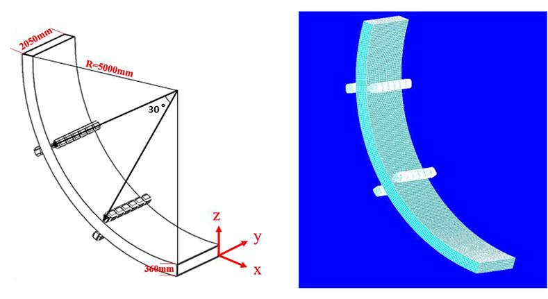
Table I

Magnetic field simulation parameter

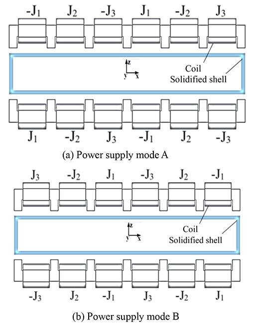
environments, within electrical equipment, etc.), such electromagnetic waves can be considered quasi-static -fields (Yang et al., 2019).

Magnetic field governing equations

Based on the above assumptions, the governing equations of the slab magnetic field are (Yang et al., 2019).

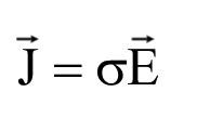
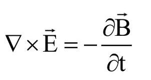
where H is the magnetic field intensity (A/m), E is the electric field intensity (V/m), B is the magnetic flux density (T); s is the electrical conductivity (S/m), D is the electric flux density (C/m), t is the time (s), and Re is the real part

Boundary conditions and numerical solution

The slab area is placed within the air domain, which has a spherical shape and can effectively surround the magnetic field lines created by the coil in the air domain. The slab is grid-based on a uniform hexahedral mesh, the coil and iron core are grid-based on a nonuniform hexahedral mesh, and the air domain is grid-based on a nonuniform tetrahedral/hexahedral mesh. The calculating domain contains 390 000 elements in total according to the traditional calculation of the number of elements (Yang et al., 2022).

The time-averaged- electromagnetic force is calculated by:

Figure 1—Geometric model and mesh model

Figure 2—Current supply modes to the electromagnetic stirrer coil

Numerical simulation of the electromagnetic field in the secondary cooling zone of arc-shaped slabs

The magnetic induction intensity in the calculation domain is initially zero, the electromagnetic induction intensity is zero at infinity, the magnetic field is concentrated near the electromagnetic stirrer, and the phase angle difference between adjacent coils is 120°. Outside the air domain, the magnetic field line-parallel boundary condition is utilized since the magnetic field lines are closed.

The ANSYS Emag software package solves Maxwell's equations to perform a harmonic calculation of the 3D distribution of the electromagnetic field in the calculation domain.

Results and analysis

Figure 3 depicts views of the magnetic field geometric model to help clarify the problem. The A-A section represents the slab's centre symmetry plane in the y-axis direction; the B-B and C-C sections are sections of the electromagnetic stirrer's central axis at the 30° and 60° positions, respectively.

Magnetic field model validation

Figure 4 indicates that the simulated magnetic induction values correlate well with the measured values. The magnetic induction intensity on the centreline shows two peaks, the highest at 1.65 m and 41.6 mT, and the other at 0.36 m and 40.4 mT. The difference between the measured and simulated values at 0.62 m is 8.1 mT, whereas the difference between the other observed and simulated values is less than 3.5 mT. Because the calculation error is within the acceptable range, the numerical simulation results are trustworthy. The errors in numerical calculations and experimental values are primarily due to the experimental environment, numerical assumptions and model restrictions, experimental operating abilities, and calculation methods.

Magnetic flux density distribution

The difference in energization method directly determines the difference in magnetic field distribution. The magnetic field distributions of the B-B section and the C-C section are the same if the electrification mode of two pairs of stirring rollers is mode A or mode B (Figure 2); if the two pairs of stirring rollers are electrified in opposing ways , the distributions of the B-B and C-C section are opposite, as seen in Figures 5 and 6.

Figures 5 and 6 demonstrate that the maximum magnetic induction strength in the two sections is 20 mT, and the profile for each section is trimodal, with the peak at the horizontal centre being higher than the peaks at the left and right ends. As a result, the magnetic field on the strand's surface is stronger than that in the centre because the strand's surface is closer to the electromagnetic stirrer.

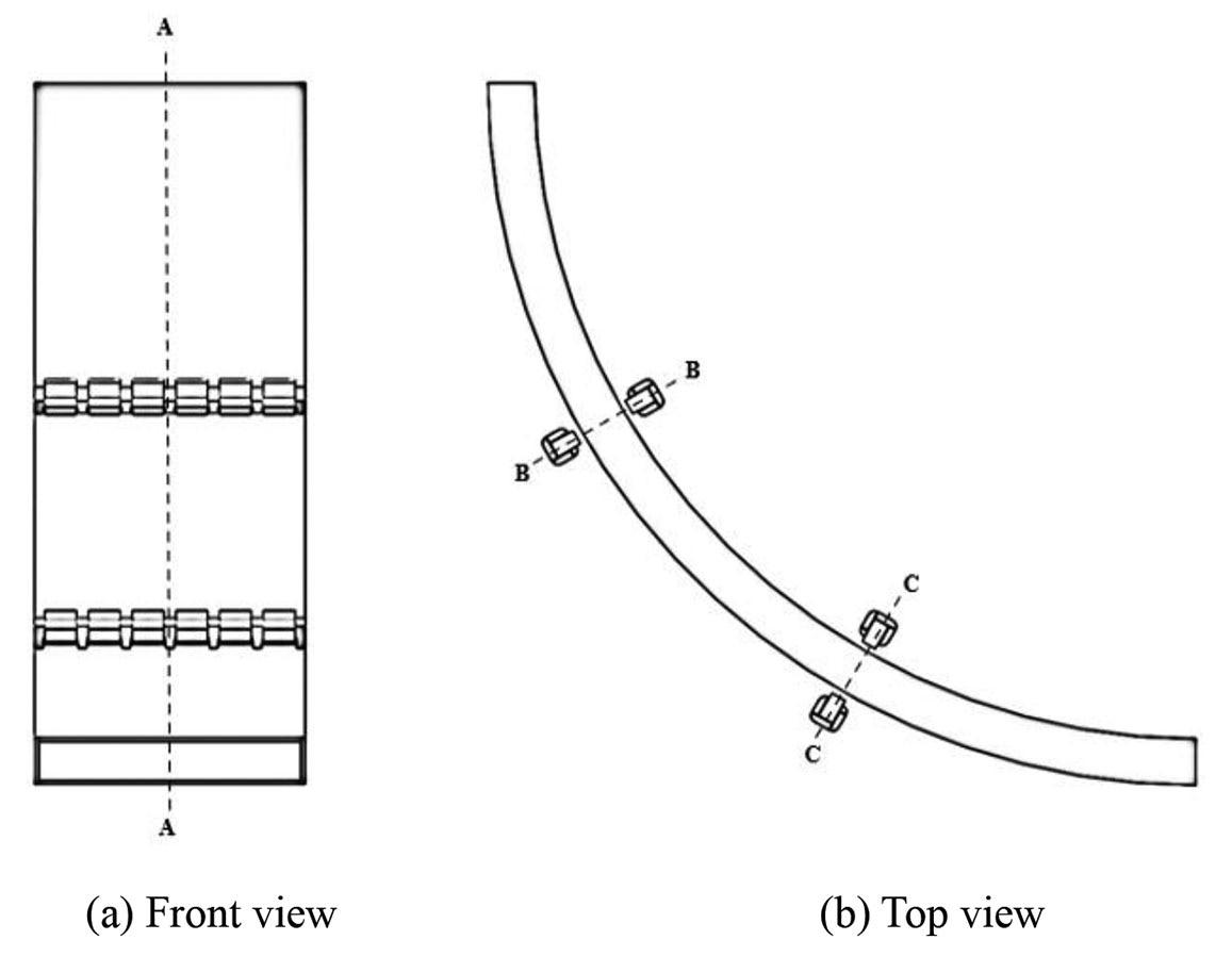
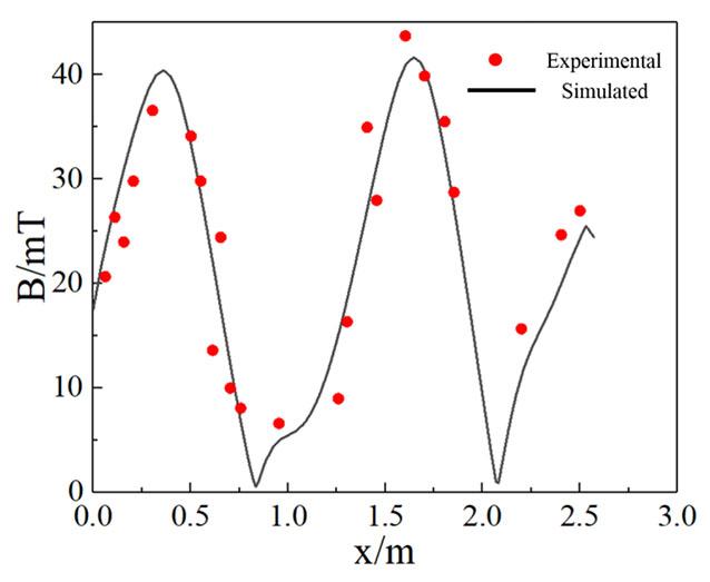
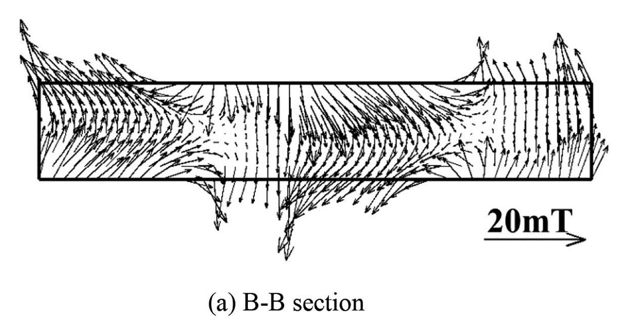
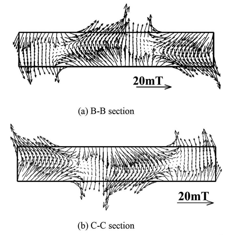
Figure 7 depicts the electromagnetic force distribution in the B-B section and C-C sections when the linear coil of the stirring roll is electrified at the 30° and 60° positions of the slab. The two sets of electromagnetic stirrers are in mode 1. The electromagnetic force is axisymmetrically distributed, with each section's electromagnetic force obliquely pointing to the central axis, and aligned along the same direction from left to right, with a value of roughly 1000 N/m3

Figure 8 shows slab distribution of electromagnetic force at the electromagnetic stirring device, where the electromagnetic stirring device is located at 30° and 60° of the slab. The electromagnetic forces of the B-B section and the C-C section are both axisymmetrically distributed, and the directions of the electromagnetic forces of the respective sections point obliquely. The central axis and orientation of the two portions are opposed, and the value is approximately 1000 N/m3. In general, when the

Figure 3—Views of the magnetic field geometry model

Figure 4—The measured values and numerical simulation results for the electromagnetic field in the second cold zone (Zhang et al., 2018)

Figure 5—Magnetic field distribution when the coils are energized in the same direction

Figure 6—Magnetic field distribution when the coils are energized in opposing directions

Numerical simulation of the electromagnetic field in the secondary cooling zone of arc-shaped slabs

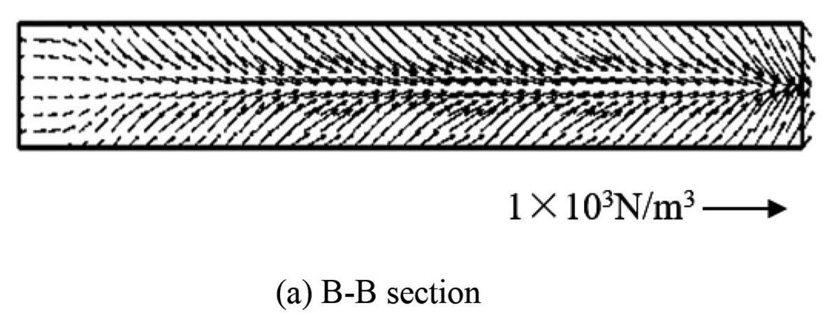
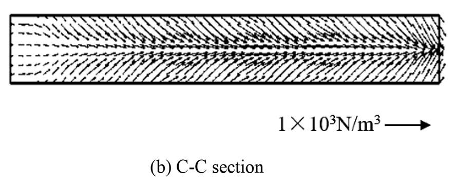
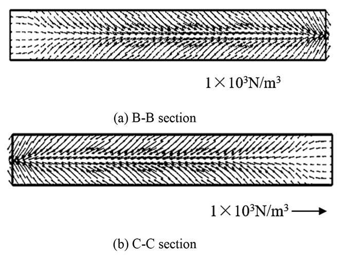
amplitude of the current is the same but the method of energizing the coils differs, the magnitude of the electromagnetic force is the same but the direction is reversed.

The electromagnetic force distribution of the two pairs of stirring rollers when not in operation is depicted in Figure 9. The electromagnetic force directions are the same when the same energization method is employed; when opposiing energization methods are utilized, the electromagnetic force directions of the two pairs of stirring rollers are opposed. The electromagnetic force has a maximum value of 1000 N/m3, which will not affect the stability of the cast.

The influence of frequency and current on the magnetic field

Figure 10 depicts the magnetic flux density distribution along the centreline of the B-B section. The magnetic flix density has a trimodal distribution across the breadth of the slab, with the middle peak the highest. The magnetic flux density gradually increases with increasing current, but the magnetic field distribution remains constant. The left peak appears at 0.1 m, the centre peak at 1.0 m, and the right peak at 1.8 m.

Figure 11 depicts the effect of current on the magnetic flux density at the centre point of the B-B section. An increase in the current from 150 A to 250 A causes the magnetic flux density to increases from 10.9 mT to 18.4 mT. In other words, for every 1 A increase in current, the magnetic flux density rises by 0.075 mT.

The relationship is described by Equation [6]: [6]

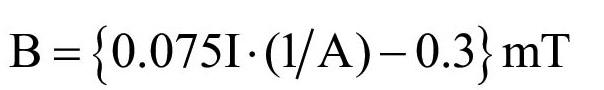
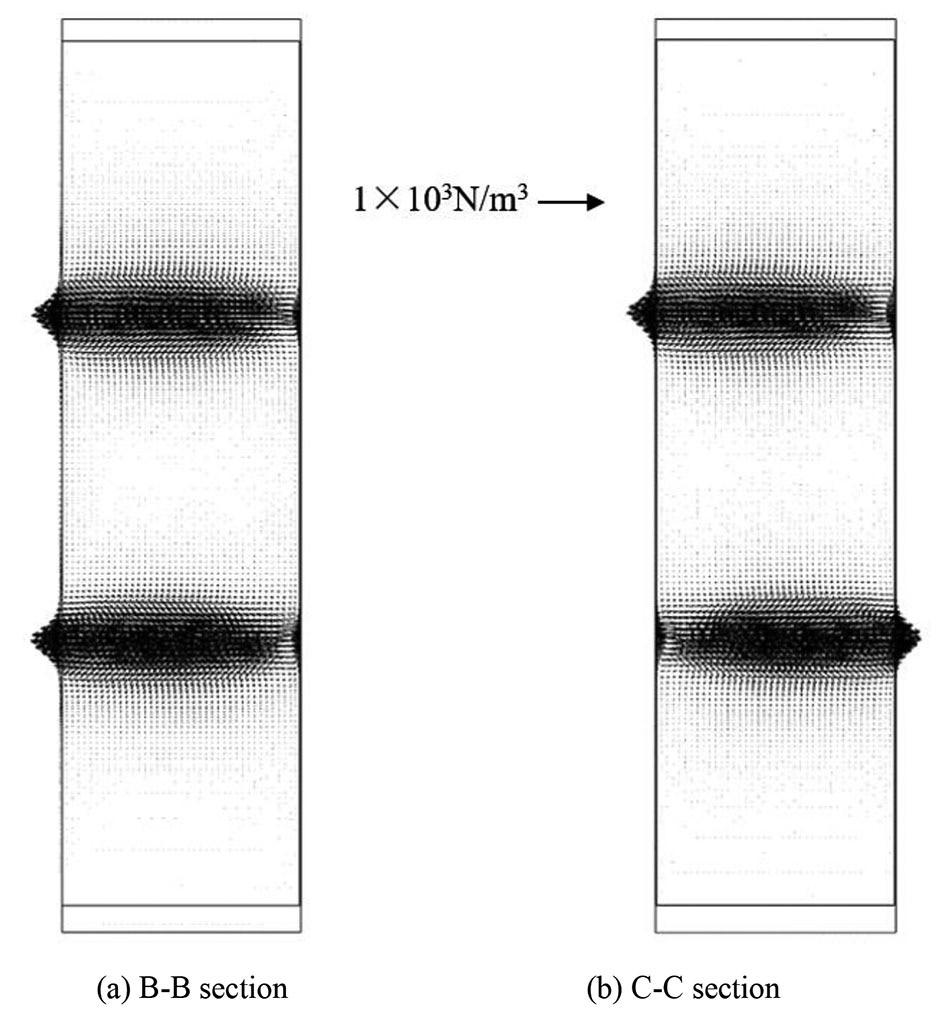
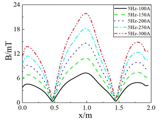
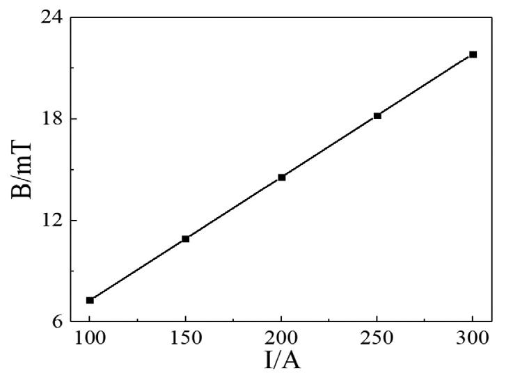
Figure 12 depicts the effect of current frequency - on the flux density distribution along the B-B section centreline. In contrast to the effect of current, the distribution curve varies with frequency. With increasing frequency, the two minima in the distribution shift to the left, with the minimum value on the right undergoing a larger shift.

Figure 13 depicts the effect of frequency on magnetic induction at the central point of the B-B section. The flux density drops from

Figure 7—Electromagnetic force distribution when the coils are energized in the same direction

Figure 8—Electromagnetic force distribution when the coils are energized in opposing directions

Figure 9—Distribution of electromagnetic force

Figure 10—Influence of current on the magnetic flux density of the B-B section centreline

Figure 11—The effect of current on the magnetic flux density at the centre point of the B-B section

Numerical simulation of the electromagnetic field in the secondary cooling zone of arc-shaped slabs

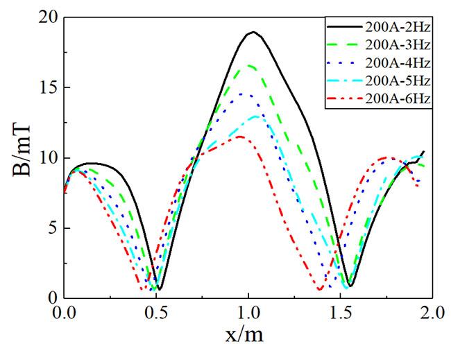
Figure12—Variation of magnetic flux density on the B-B section centreline at different frequencies

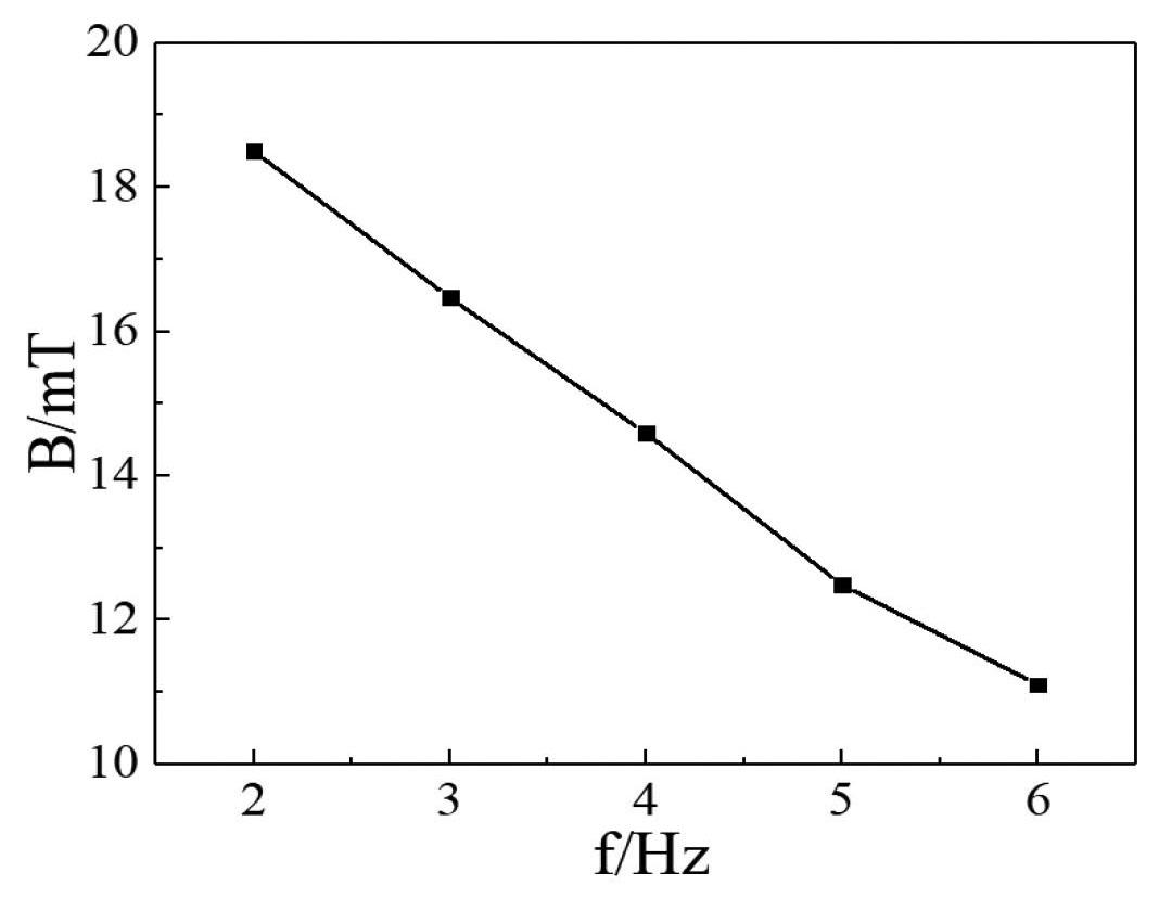
13—Variation

18.5 mT to 11.5 mT as the current frequency increases from 2 Hz to 6 Hz. That is, the flux reduces by 1.75 mT for every 1 Hz rise in frequency.

The relationship is given by:

Figure 14 depicts the distribution of electromagnetic force along the B-B section centreline. The electromagnetic force steadily increases as the energizing current is increased, but the distribution law of the electromagnetic force remains the same; the closer to the centre, the greater the change in magnitude of the electromagnetic force.

The effect of current on electromagnetic force at the central point of the B-B section is depicted in Figure 15. As the current is increased from 150 A to 250 A, the electromagnetic force at the centre point increases from 480 N/m3 to 1380 N/m3. The electromagnetic force is proportional to the square of the current:

Figures 16 and 17 depict the variation of the electromagnetic force at the centre line and centre point of the B-B section with increasing frequency=. Figure 17 shows that the electromagnetic force at the cross-section's centre increases first and then diminishes. This is because the electromagnetic force is determined by both the induced current and the flux density. The current increases as the frequency increases, but the flux density drops. The figure shows that the electromagnetic force reaches its maximum at a current frequency of 4 Hz.

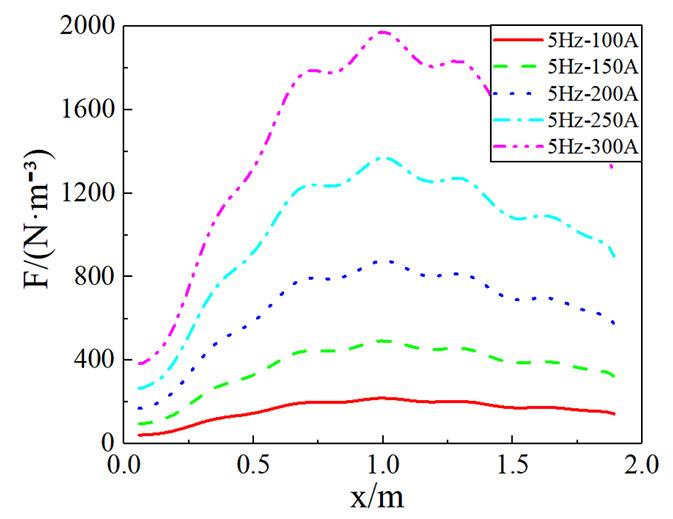
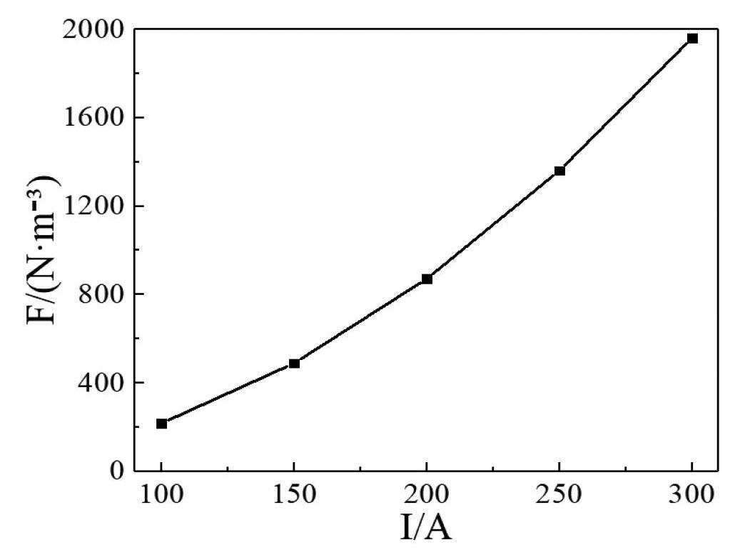
15—The effect of current on the electromagnetic force at the centre

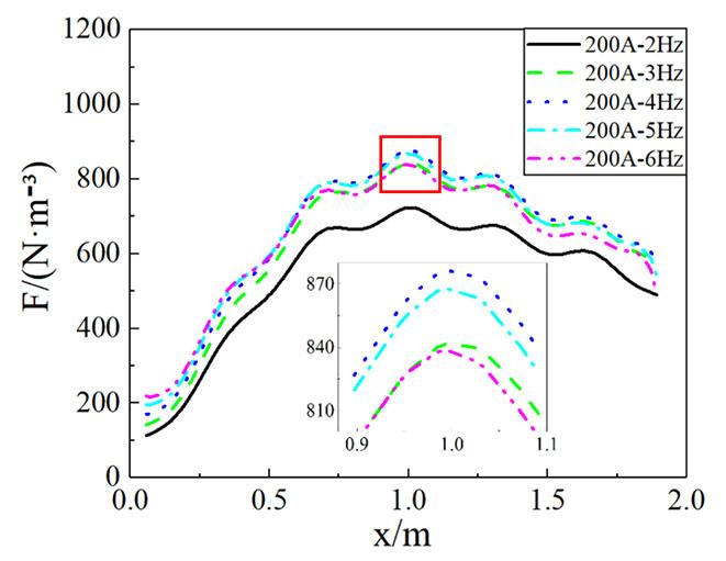
16—The effect of frequency on the electromagnetic force of the

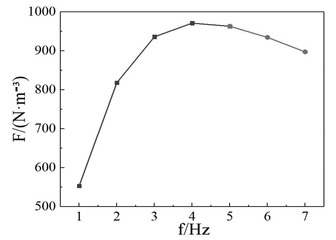
17—The effect of frequency on the electromagnetic force at the centre point of the B-B section

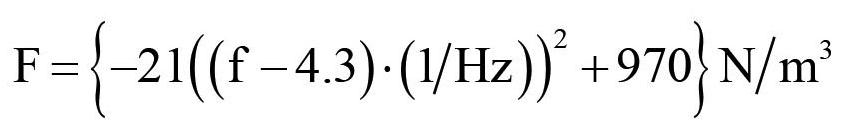
At the central point of the B-B section, the curve of electromagnetic force and frequency consists of two parts. [9]

Figure

of the magnetic flux density at the center point on the B-B section at different frequencies

Figure 14—The effect of current on the electromagnetic force along the centreline of the B-B section

Figure

point of the B-B section

Figure

centreline of the B-B section

Figure

Numerical simulation of the electromagnetic field in the secondary cooling zone of arc-shaped slabs

The second segment follows a linear expression (5 Hz to 7 Hz): [10]

Conclusions

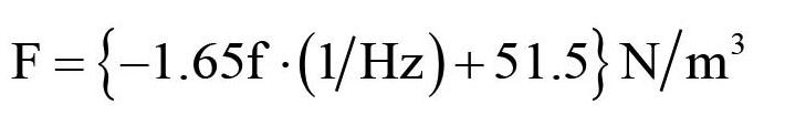
ANSYS simulations were used to model the magnetic field characteristics under electromagnetic stirring in the secondary cooling zone of a continuous caster, and the effects of changes in current and frequency in the magnetic flux intensity and electromagnetic force distribution studied. The main conclusions are as follows.

➤ The magnetic flux intensity in the B-B and C-C sections (sections of the stirrer's central axis at positions of 30° and 60°, respectively) exhibits a trimodal distribution, with a large (20 mT) central peak and a smaller peak on each side. The electromagnetic forces in the B-B and C-C sections are axisymmetrically distributed, with a maximum value of 1000 N/m3

➤ The direction of the electromagnetic force is the same at the 30° and 60° positions of the arc-shaped slab when the power supply method is the same. When opposed energization methods are utilized, the electromagnetic forces generated have opposite polarities.

➤ As the energizing current increases, so does the magnetic induction. The magnetic induction at the centre point of the B-B section increases with increasing current frequency.

➤ The electromagnetic force increases with increasing current. Withincreasing frequency, the electromagnetic force at the centre point of the B-B section first increases, reaching a maximum at 4 Hz, and then declines.

➤ The relationships between magnetic flux density, current, and frequency at the centre of the B-B section are

B = {0.075I.(1/A)-0.3}mT

B = {-1.75f (1/Hz)+22}mT.

➤ The electromagnetic force and current at the central point of the B-B section are related by:

F = {0.03168I2 (1/A2)03.762I (1/A)+326.7}N/m3. With increasing frequency the electromagnetic force at this point at first increases following a parabolic relationship:

F = {-21((f-4.3) (1/Hz)2)+970}N/m3 and then decreases in a linear fashion at frequencies above 5 Hz:a

F = {-1.65f (1/Hz)+51.5}N/m3

Conflict of interest

The authors declare that there is no conflict of interest.

Acknowledgement

We thank the University of Science Technology of Liaoning United Fund (HGSKL-USTLN(2022)07), National Natural Science

Foundation of China(Grant NO.NSFC52074151) the Education Department Project of Liaoning Province(Grant NO.2020LNJC03), and the Department of Science & Technology of Liaoning Province(Grant NO.2022JH2/101300079) for financial support of the current work.

References

An, H.H., Bao, Y.P., Wang, M., and Yang, Q. 2019. Electromagnetic torque detecting for optimization of in-mould electromagnetic stirring in the billet and bloom continuous casting. Ironmaking & Steelmaking, vol. 46. pp. 845–854.

Beitelman, L. 1990. Effect of mold EMS design on billet casting productivity and product quality. Canadian Metallurgical Quarterly, vol. 38, no. 5. pp. 301–309.

Javurek, M., Barna, M., Gittler, P., Rockenschaub, K., and Lechner, M 2008. Flow modelling in continuous casting of round bloom strands with electromagnetic stirring. Steel Research International, vol. 79. https://doi. org/10.1002/srin.200806174

Jiang, D.B. and Zhu, M.Y. 2015. Flow and solidification in billet continuous casting machine with dual electromagnetic stirrings of mold and the final solidification. Steel Research International, vol. 86. https://doi.org/10.1002/srin.201400281

Lei., H., Jiang, J.M., Yang, B., Zhao, Y., Zhang, H.W., Wang, W.X., and Dong, G.W. 2018. Mathematical model for collision-coalescence among inclusions in the bloom continuous caster with M-EMS. Metallurgical and Materials Transactions B, vol. 49. doi: 10.1007/s11663-018-1186-y

Limoges, J. and Beitelman, L. 1997. Continuous casting of carbon and alloy billets with in-mold dual-coil electromagnetic stirring system. Iron and Steelmaking, vol. 24, no. 11. pp. 49–57.

Liu, C.T. 2010. Refined model development and performance assessment of a linear induction-type electromagnetic stirrer. IEEE Transactions on Magnetics, vol. 46. p. 3724.

Sivesson, P., Hallen, G., and Widell, B. 1998. Improvement of inner quality of continuously cast billets using electromagnetic stirring and thermal soft reduction. Ironmaking & Steelmaking, vol. 25. pp. 239–246.

Trindade, L.B., Nadalon, J.E.A., Contini, A.C., and Barroso, R,C. 2017. Modeling of solidification in continuous casting round billet with mold electromagnetic stirring (M-EMS). Steel Research International, vol. 88. https:// doi.org/10.1002/srin.2016003191600319

Trindade, L.B., Vilela, A.C.F., Filho, A.F.F., Vilhena, M.T.M.B., and Soares, R.B. 2011. Numerical model of electromagnetic stirring for continuous casting billets. IEEE Transactions on Magnetics, vol. 38. p. 3658.

Wang, T., Wang, E.G., Delannoy, Y., Fautrelle, Y., and Budenkova, O. 2022. Effect of vertical electromagnetic stirring on solute distribution in billet continuous casting process. Journal of Iron and Steel Research International, vol. 29. pp. 132–143.

Yang, B., Lei, H., Bi, Q., Jiang, J.M., Zhang, H.W., Zhao, Y., and Zhou, J.A. 2019. Electromagnetic conditions in a tundish with channel type induction heating. Steel Research Internationsl, vol. 89. https://doi.org/10.1002/srin.201800145

Yang, B., Liao, X.W., Liu, K., Zhao, C.L. and Han, P. 2022. Numerical simulation of residence time distribution (RTD) in tundish with channel type induction heating. JOM, vol. 74, no. 5. pp. 2129–2138.

Zhang, K., Chen, S.F., Yang, B., Liu, T.y., Zhao, Y., and Lei. H. 2018. Study on arrangement of S-EMS rollers in secondary cooling zone of slab continuous casting machine. Journal of University of Science and Technology Liaoning, vol. 41. pp. 335–340+350. u

Affiliation:

1University of Pretoria, Pretoria, South Africa.

2Samancor Chrome Ltd, Sandton, South Africa.

3Mintek, Randburg, South Africa.

4Stellenbosch University, Stellenbosch, South Africa.

5Ex Mente Ltd, Pretoria, South Africa.

Correspondence to:

M.W. Erwee

Email: markus.erwee@gmail.com

Dates:

Received: 15 Feb. 2024

Revised: 25 Feb. 2024

Accepted: 25 Feb. 2024

Published: March 2024

How to cite:

Erwee, M.W., Reynolds, Q.G., and Zietsman, J.H. 2024

Incompressible versus compressible fluid flow models: A case study on furnace tap-hole lancing.

Journal of the Southern African Institute of Mining and Metallurgy, vol. 124, no. 3. pp. 139–146

DOI ID: http://dx.doi.org/10.17159/24119717/3292/2024

Incompressible versus compressible fluid flow models: A case study on furnace tap-hole lancing

by M.W. Erwee1,2, Q.G. Reynolds3,4, and J.H. Zietsman1,5

Synopsis

Pyrometallurgical furnaces, essential for metal extraction, operate at temperatures exceeding 1600°C and represent complex multiphase systems that challenge direct industrial research. Multiphysics models play a key role in shedding light on their intricate behaviours, supporting the refinement of design and operational strategies. Integral to the operation are the tap-holes, which facilitate the removal of molten products and are routinely opened by lancing, a process comparable to the use of a cutting torch, where high temperatures result from oxygen reacting with an iron lance. When the lance pierces the clay, oxygen gas enters the furnace, which could influence the behaviour of the molten material inside.

In this work, a multiphase fluid flow model was used to investigate bulk flow dynamics, with a focus on the effects of the lancing process on the inside of the furnace, immediately behind the tap-hole. Incompressible and compressible multiphase fluid solvers were used and compared with respect their performance – the intention was to assess whether using a compressible solver would yield a different solution to the incompressible one. It was concluded that there are negligible disparities in bulk fluid flow behaviour between the solvers for the case studies examined, indicating that solver selection might be less consequential for certain aspects of oxygen lancing.

Keywords tap-hole, lancing, modelling, multiphase fluid flow.

Introduction

Background

High temperature processing of ores to produce metals, alloys, mattes, and slags is carried out in pyrometallurgical furnaces. The furnaces vary significantly in design, but all have one aspect in common: material needs to be removed from the vessel at certain stages of the production process. In most cases, the molten material is removed through a tap-hole.

DC open bath furnaces are used for the production of ferrochrome, titanium slag, ferronickel, and steel (Jones, 2014). Raw material is usually charged continuously into DC furnaces, with a direct current electric arc acting as an intense, focused heat source. The energy intensity of the process is such that the melting and reactions occur rapidly compared to other furnace heating methods. The molten slag and alloy accumulate inside the furnace and are tapped at regular intervals.

An example of a DC furnace is shown in Figure 1a.

A furnace tap-hole undergoes periodic closing and opening. Closing is achieved by sealing the tap-hole with refractory clay which expands and hardens, creating a plug to block material flow.

To tap the furnace, this refractory plug is removed. This can be achieved mechanically, thermally, or through a combination of both. Mechanical removal involves drilling into the hardened plug, while thermal removal melts the material away using an oxygen lance.

Oxygen lancing is used only when absolutely necessary, for example, in blast furnace ironmaking and ilmenite smelting (Nelson and Hundermark, 2016; Mgenge, and Steenkamp, 2014), while in other processes such as ferrochrome production, a combination of drilling and oxygen lancing for each tap is commonplace (Nelson and Hundermark, 2016; Lindstad, 2018). In a platinum and Ni smelter industry survey, it was found that about 36% of these furnaces employ lancing as the primary means of opening the tap-hole (Nolet, 2014). In some platinum smelters, it is common for slag and matte tap-holes to be opened using oxygen lancing almost exclusively (van Beek et al., 2014).

Lancing furnace tap-holes is an aggressive process and, if not done with care, can result in significant damage to the refractory lining and tap-hole of a furnace, in addition to potentially harming the furnace operator. An example of an expert furnace tapper lancing a tap-hole is shown in Figure 1b.

Incompressible versus compressible fluid flow models: A case study on furnace tap-hole lancing

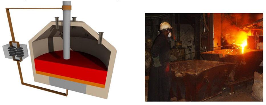
The lances used for opening the tap-hole are made of carbon steel tubes with varying diameters. Lance designs vary, but operate in the same way. Pure oxygen is charged through the tube at high flow rates (approximately 100-600 Nm3/h)(Trefimet, 20171). The tip of the lance is ignited by using a spark or flame. The burning of the lance is due to the continuous oxidation of iron in the steel tube with the release of intense, focused heat at the tip. This heat is used to melt the hardened clay inside the tap-hole.

Not all the oxygen is consumed by the burning of the lance, with up to two thirds bypassing through the tip of the lance (Morales, Morales, and Nunes, 2018).

DC furnaces can be sensitive to operate and care is required to maintain and run them effectively. Compared to, for example, submerged arc furnaces (SAFs), bulk reaction dynamics in DC furnaces is rapid, i.e. changes in process parameters often manifest within a very short time and as such continuous monitoring as well as the prevention of process disturbances are essential (Geldenhuis, 2017).

Recently, the authors conducted a series of studies (Erwee, Reynolds, and Zietsman, 2016, 2023; Erwee et al., 2019) to investigate the impact of lancing furnace tap-holes using multiphase fluid flow and thermochemical modelling. The focus of these studies was specifically on the case in which oxygen bypasses the lance tip and comes into contact with the molten process material. Limited literature exists on this topic, because the problem cannot be directly studied in a furnace; yet, evidence of damage is often observed in the tap-hole region when furnaces are down for maintenance.

Modelling offers an alternative way of unpacking the problem, but does pose its own challenges due to the complex nature thereof.

Impetus for and scope of this study

The authors have studied the possible effects of lancing from different angles (Erwee, Reynolds, and Zietsman, 2016, 2023; Erwee et al., 2019), specifically for open-bath smelting processes such as DC ferrochrome smelting, trying to establish the best framework to answer two main questions:

➤ How would short bursts of oxygen from the lance influence the molten process material? Some subquestions that come to mind:

– Is the slag-alloy interface disturbed in any significant way? (this work)

– Would upset conditions in a furnace be exacerbated by lancing? (future work).

➤ Can modelling offer some insight as to what extent the process could be influenced?

– Could one use the results from modelling to better quantify the effect of lancing? (this work)

– Could the results from the modelling work be used with other models (e.g. thermochemical models) to better understand refractory wear? (future work).

In previous studies (Erwee, Reynolds, and Zietsman, 2016, 2023; Erwee et al., 2019), the authors mainly used an incompressible multiphase fluid flow solver in the OpenFOAM open source platform. The choice of solver and approach is explained in previous work, but it was necessary to do a sub-study in which a compressible solver was used to capture any potential flaws in the assumptions made in the incompressible solver.

The reason for testing a compressible solver is the fact that unlike alloys and slags in furnaces, gases such as oxygen, which would enter through the lance, are compressible.

Many compressible-flow solvers are available in commercial and open source CFD tools; however, finding accurate values for material properties with temperature can prove to be a problem in pyrometallurgy, which means that the effort required to achieve sufficiently accurate models increases. The question the authors had was how much this would change any of the possible answers when compared to the incompressible case?

In this paper, the focus is specifically on a case where the alloy tap-hole is lanced while slag is still present in the furnace (see Figure 2).

Governing equations,

modelling framework, and

1Note, in this case, the unit quoted, Nm³/h, is the flow rate at standard conditions of temperature and pressure (273.15 K and 101.325 kPa).

The governing equations for the multiphase fluid flow problem were solved using the open-source framework OpenFOAM®v2212 (OpenFOAM, 2024), using two standard solvers: an incompressible multiphase solver, multiphaseInterFoam, and the compressible version of the solver, compressibleMultiphaseInterFoam. To track the interfaces between the phases, the volume of fluid method is used (Hirt and Nichols, 1981).

solvers

Figure 1 DC furnace operations (a) A 3D cutaway of a DC furnace showing the slag (red phase on top) and alloy (orange phase on the bottom) beneath a graphite electrode (courtesy of Q.G. Reynolds, Mintek, 2024) (b) A furnace operator lancing the furnce tap-hole on a 200 kVA DC furnace at Mintek. (Photograph: I.J. Geldenhuys, Mintek, 2004)

Incompressible versus compressible fluid flow models: A case study on furnace tap-hole lancing

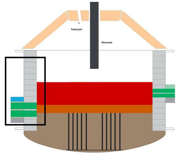
For both solvers, the equations for the conservation of momentum and mass are solved:

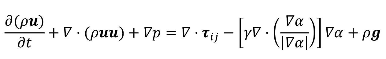
where ρ is the density of the fluid, u is the velocity, p is the pressure, τij the viscous shear tensor, and α the phase fraction of each phase (gas, slag, and alloy).

The pressure term, p, refers to the static pressure minus the quasi-hydrostatic2 pressure, ρgh. In the incompressible solver, an arbitrary reference value can be chosen for p, while in the compressible solver, this value is calculated from the equation of state.

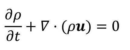
and:

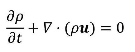
where:

The bulk density and viscosity of each cell are scaled linearly by the volume fraction of each phase that occupies the cell.

In the case of the incompressible solver, the density of each phase is assumed to be constant, which simplifies the aforementioned equations.

Although most alloys and slags are considered incompressible fluids, gases such as oxygen and carbon monoxide are considered compressible, and the density of these gases is a function of both pressure and temperature (via an equation of state chosen by a user). In the compressible version of the solver, the effects of temperature on the density of each phase can be accounted for by solving an additional energy equation (see Equation [5]). There is a compressible component added to the incompressible component in the pressure equation in compressibleMultiphaseInterFoam (not shown here).

where T is the temperature, αeff represents the effective thermal diffusivity, and K is a representation of the flow kinetic energy. In both solvers, the assumption is made that viscosity and interfacial tension are constant. In reality, there would be changes in these values as a function of temperature, composition, presence of surfactants, etc. However, values for these two parameters also come with a degree of uncertainty, since they are difficult to measure. The sensitivity of bulk flow in and around the tap-hole region to these parameters is a topic for future study.

Computational domain, meshing strategy, and computing resources used

Computational domain

The area of interest in this case study is the alloy tap-hole area of the furnace (see black box3 in Figure 2). An enlarged version of this area in three dimensions is shown in Figure 3. The domain is a 1/6th wedge of a furnace with a diameter of 12 m, the same as in a previous study (Erwee, Reynolds, and Zietsman, 2023).

Meshing strategy

The computational domain is quite large. To fully resolve flow, quite a fine mesh is required, typically a maximum element size of 2.5 mm was specified in the final mesh used. However, meshing the entire domain at that resolution would be computationally expensive. To overcome this problem, a preliminary simulation was performed on a coarse mesh, followed by refinement in the areas where flow was dominant. This approach has proven to be successful in the past (Reynolds et al., 2019; Erwee, Reynolds, and Zietsman, 2023). Although adaptive mesh refinement could be implemented, it could be more computationally expensive. Coarse meshes were typically in the order of 500 000 elements, with finer meshes at 3.2 million elements. An example of a coarse and a fine mesh is shown in Figures 4a and 4b, respectively. Meshes were generated using cfMesh (cfMesh, 2022).

Note that the visualizations shown in the figures are a slice through the middle of the three-dimensional domain (a plane in the y-direction).

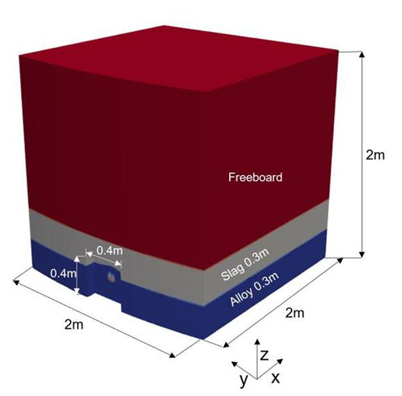
2Quasi-hydrostatic pressure refers to the pressure exerted by either the slag or alloy phase. For more information see https://www.openfoam.com/documentation/ guides/latest/doc/guide-applications-solvers-variable-transform-p-rgh.html 3Note that the refractory assembly below the alloy phase and the tap-hole on the outside, along with the refractory assembly is not part of the domain here.

Figure 2 DC furnace with slag (red) and alloy (orange) present. The black box on the left is the area of focus in this study (drawing adapted from Geldenhuys, 2013)

Feed port

Electrode

Anode pins

Figure 3 Computational domain used in this study

Incompressible versus compressible fluid flow models: A case study on furnace tap-hole lancing

Computing resources

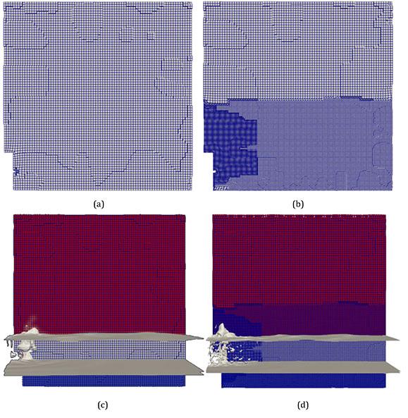
To simulate 5 seconds of real time4 in a reasonable amount of time, it was necessary to use parallel computing resources. Computations were done at the NICIS Centre for High Performance Computing in Cape Town on 10 computing nodes, each equipped with Intel Xeon processors (2.6 GHz, 24 cores) and 128 GB RAM. The simulations took between 25 and 72 hours to complete. Post-processing was performed in ParaView version 5.11.0 (Hansen, and Johnson, 2005; Ayachit, 2015; Kitware, 2024) on a desktop computer equipped with a Ryzen 9 5950X CPU, 64GB RAM, and a NVidia GTX 4070 graphics card. It is interesting to note that, on average, the compressible solver did not take a significant amount of extra time over the incompressible one for simulations (often less than 20% more computing hours were required).

Basis for comparison and model assumptions

Basis for comparison

To test the idea that a compressible solver would yield a different result from an incompressible one for this particular problem, three case studies were performed. At the same time, a second idea was tested, i.e. the sensitivity of the compressible solver to a difference in gas inlet temperature was also performed.

Simulations were performed for a case where lancing is done in the alloy tap-hole, but some slag is still present in the furnace5 The authors concede that when conditions change significantly this assumption would need to be checked again. However, there are only a few typical configurations for this particular problem in an industrial environment.

Three cases were considered:

➤ Incompressible case 0, where parameters were fixed as per Table I

➤ Compressible case 1, where the values for the parameters were the same as in case 0, but an energy equation is solved. This case was considered to see whether there would be a different result from case 0

➤ Compressible case 2, where there is a 200K difference between the gas temperature at the inlet and the molten phases (alloy and slag) at the beginning of the simulation. This was to test the sensitivity of the solution in case 1 to temperature.

To compare solutions against each other, each field that was solved for and was common in each of the solvers was compared over 5 seconds of real-time simulated. Solutions were compared along each principal direction from the lance tip:

➤ In the x-direction: gas travelling from the tip of the lance towards the centre of the furnace

➤ In the y-direction: from the tip of the lance to each side of the domain, i.e. gas travelling along the wall of the furnace

➤ In the z-direction: gas travelling upwards through the slag to the freeboard of the furnace.

The following parameters are plotted for comparison:

➤ The time-averaged density (both as a visualization of a plane through the middle of the domain as well as a plot of the density in each direction). Since density and pressure are coupled, it is necessary to see whether any significant changes in density are observed

➤ The time-averaged pressure at the lance tip and away from it (as per first item)

➤ The time-averaged kinetic energy, i.e. 1 2 r|U|2, which serves to check whether there is any significant changes in energy dynamics between simulations.

Model inputs and assumptions

For all simulations, the gas inlet velocity was set at 20 m/s, which is based on the diameter of the lance and the estimated flow rate of the gas bypassing the tip of the lance. Baseline values (incompressible case) for density, viscosity, and interfacial tension were taken from a ferrochrome system as documented in a previous publication (Erwee, Reynolds, and Zietsm, 2023. The Pr numbers6 for slag, alloy and gas were taken from Nelson and Hundermark (2016). Pr numbers are used in the compressible solver, together with the heat capacity, CP, for calculations related to the thermal diffusivity used in the energy equation (see Table I for details).

The importance of accurate materials properties should not be underestimated (Lopis et al., 2022), especially since these properties are difficult to obtain in pyrometallurgical systems. The authors wish to explicitly acknowledge that this will require further study; the effects of property variability are not part of the scope of this paper.

Case study results and discussion

Background to case study

The results of the OpenFOAM simulations were processed in ParaView for 5 seconds of real time using the temporal statistics filter. This filter computes simple statistics such as the average, standard deviation, minimum, and maximum values of all the different fields over time.

In all plots given, the results are presented in the order: incompressible case 0, compressible case 1 (injected gas at same initial temperature as other phases), and then compressible case 2 (a 200K difference between the gas and alloy/slag temperature at the start of the simulation).

4A typical short burst of oxygen during penetration of the lance into the molten material.

5In practice, slag is usually tapped first; however, under certain conditions it can be necessary to open the alloy tap-hole for several reasons.

6Pr = CPµ/k where k is thermal conductivity.

Figure 4 (a) Coarse mesh for initial solution. (b) Fine mesh used in simulation. (c) Typical result (coarse mesh). (d) Typical result (fine mesh)

Incompressible versus compressible fluid flow models: A case study on furnace tap-hole lancing

Table I

Model inputs

Time-averaged density

A visual inspection of the density averaged over time provides a quick view of how each phase (gas, alloy, and slag) changes, on average, over the course of the simulation. Because the densities of the three phases are so distinctly different, the visualization is a reasonable representation of each phase fraction at the same time. In Figure 5, all three cases produce a very similar result. As the gas enters the alloy melt, it loses momentum in the direction of the lance and moves through both the alloy and the slag phasez, which is what one would expect due to the large density differences between the gas and the liquid phases.

To study the differences in a more quantitative manner, the plots were compared in the three main directions from the lance

tip. Gas does not penetrate deep into the melt, and most of the gas is concentrated at the tip of the lance. Interestingly, it can be seen that in the small region in front of the lance tip, the mixture has a density close to that of a gas-slag mixture (specifically see Figure 6c), i.e. the alloy is displaced and a slag-gas mixture circulates around the lance tip.

The most apparent differences, despite being small, are between the two compressible cases in the area in front of the lance tip. The difference in temperature of the gas and alloy results in a slightly different density between the cases. This is most noticeable in the z-direction, the main direction of gas flow. The incompressible solver solution falls between the two compressible solutions on average. In the x- and y-directions, there is virtually just alloy with variations in density only apparent to about a 0.1 m from the lance

Figure 5 Time-averaged density fields for the three cases. From left to right: incompressible case, compressible case (same initial temperature for all phases), compressible case (lower initial gas temperature). Gas = red, slag = grey, alloy = blue

Incompressible versus compressible fluid flow models: A case study on furnace tap-hole lancing

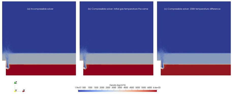
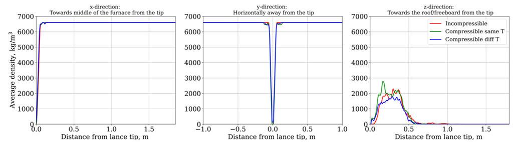
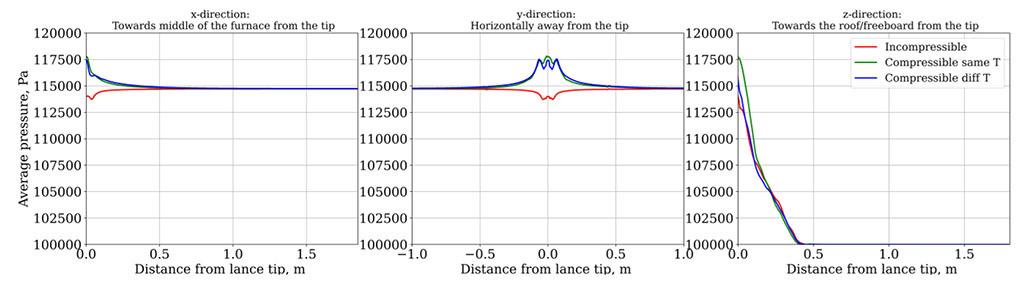
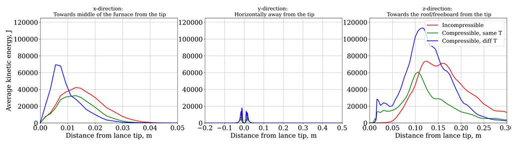
tip in these directions. The ‘feet’ on the two compressible cases can possibly be explained by the fact that close to the tip of the lance, the density is reflective of a mixture of gas and alloy.

Time-averaged pressure

Plots of the average pressure follow much the same pattern as density. There is very little difference between the solutions (see Figure 7) close to the tip of the lance. In the case of the - and y-directions, pressure profiles converge to the pressure exerted by mostly the liquid alloy. Closer to the tip of the lance, the pressure profiles change somewhat due to the presence of gas. There is a distinct difference between the incompressible case and the two compressible ones in terms of the profile close to the lance tip. When post-processing the results for the compressible cases, it was observed that, within the first few time-steps (up to about 0.2 seconds), there is an initial spike in pressure, reflective of the temperature dependence of density and pressure in these calculations. The result is that the maximum pressure for the

compressible cases (approx. 350 000 Pa) skews the average values used for the plot. When considering the effect that this has on the bulk fluid flow behaviour in the system, this difference becomes insignificant.

Time-averaged kinetic energy

When comparing the kinetic energy, the difference between the incompressible case which shares the same initial conditions as the compressible solver is also not noticeable, and the difference between the two compressible cases shows the effect of the difference in temperature more prominently (see Figure 8) in the z-direction.

Estimated change in interfacial area

An estimate of the interfacial area between the slag and the alloy, as well as between the slag and the gas, was made over 5 seconds in real time. Such a calculation can be useful when, for example, mass transfer rates are of interest.

Figure 6 Effect of gas flow on time-averaged density in different directions from the lance tip

(a)

(b)

(c)

Figure 7 Effect of gas flow on time-averaged pressure in different directions from the lance tip

(a)

(b)

(c)

Figure 8 Effect of gas flow on time-averaged kinetic energy in different directions from the lance tip

(a)

(b)

(c)

Incompressible versus compressible fluid flow models: A case study on furnace tap-hole lancing

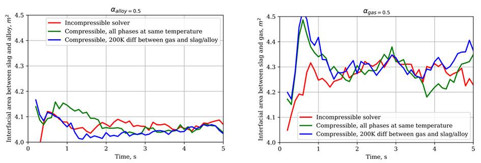
When comparing the incompressible case with the compressible case, the difference in the interfacial area looks large, but on average there is a 5% difference between the two solutions; the difference is simply exaggerated by the small range on the y-axis. Within the confines of an engineering estimate, this should not have a more significant impact on any design calculations. The same applies in this case to the difference in solutions between the two compressible cases. Note that the curves are less smooth due to the fact that the results for the simulation were only written out to files in 0.1 second intervals.

Conclusions and Recommendations

To consider the effect of the compressibility of gas when lancing into molten alloy in a full open bath furnace, and at the same time test how large the impact of a different gas inlet temperature would be, three case studies were performed using OpenFOAM as the calculation platform.

It was found that, for the properties of the same materials, there was no significant difference between the use of an incompressible fluid flow solver (multiphaseInterFoam) and its compressible counterpart (compressibleMultiPhaseInterFoam). Overall, both solutions are robust enough to capture the bulk flow dynamics in the particular cases considered and, as in the case of any simulation, depend on the quality of the inputs, especially materials properties. Despite the added complexity of the compressible solver, computational time was not as expensive as initially thought.

For the conditions assumed in the simulations, it was found that the interface between slag and alloy is disturbed in such a way that alloy can be displaced by a slag-gas mixture in front of the area where lancing occurs. A marginal shift in the overall interfacial area is also observed, concentrated at the tip of the lance.

Minor differences are apparent when there is a temperature difference between the gas at the tip of the lance entering the melt and the liquid phases, which was expected. When considering any future cases, it can be important to account for this, along with other materials properties, when studying the lancing problem in more detail.

Further studies will consider a more comprehensive parameter space search, especially changing the phase into which is lancing is done, different initial gas temperatures, as well as bath levels and depth of penetration of the lance, to double-check when a more complex solution is required.

Acknowledgements

This paper is published by permission of Mintek. The authors also thank the Centre for High Performance Computing (CHPC), which is part of the National Integrated Cyber Infrastructure System (NICIS), for making computing resources available for this research project.

References

Ayachit, U. 2015. The ParaView Guide: Updated for ParaView Version 4.3. Full color version. Edited by Lisa Avila. Kitware Inc., Clifton Park, NY.: Kitware Inc. ISBN: 978-1-930934-30-6.

cfMesh. 2022. https://cfmesh.com/

Erwee, M.W., Reynolds, Q.G., and Zietsman, J.H. 2016. Comparison of 2D and 3D computational multiphase fluid flow models of oxygen lancing of pyrometallurgical furnace tap-holes.'Journal of Metals, vol. 68, no. 6. pp. 1556–1562. http://link.springer.com/10.1007/s11837-0161873-6

Erwee, M.W., Reynolds, Q.G., and Zietsman, J.H. 2023. The effect of oxygen lancing into a furnace alloy tap-hole: A computational case study for an openbath furnace. Journal of Metals, vol. 75, no. 1. pp. 248–253. https://link.springer. com/10.1007/s11837-022-05571-y

Erwee, M.W., Reynolds, Q.G., Zietsman, J.H., and Bezuidenhout, P.J.A. 2019. Multiphase flow modelling of lancing of furnace tap-holes: validation of multiphase flow simulated in OpenFOAM®. Journal of the Southern African Institute of Mining and Metallurgy, vol. 119, no. 6. https://www.saimm.co.za/ Journal/v119n06p551.pdf.

Geldenhuys, I.J. 2013. Aspects of DC chromite smelting at Mintek – An overview. Proceedings of the Thirteenth International Ferroalloys Congress, Almaty, Kazakhstan, 9-12 June. pp. 31–47. https://www.pyrometallurgy. co.za/InfaconXIII/0031-Geldenhuys.pdfhttps://www.pyrometallurgy.co.za/ InfaconXIII/0031Geldenhuys.pdf

Geldenhuys, I.J. 2017. The exact art and subtle science of DC smelting: Practical perspectives on the hot zone. Journal of Metals, vol. 69, no. 2. pp. 343–350. http://link.springer.com/10.1007/s11837-016-2171-z.

Hansen, C.D. and Johnson, C.R. (eds.) 2005. The Visualization Handbook. Elsevier-Butterworth Heinemann, Amsterdam, Boston.

Hirt, C.W. and Nichols, B.D 1981. Volume of fluid (VOF) method for the dynamics of free boundaries. Journal of Computational Physics, vol. 39, no. 1. pp. 201–225. https://linkinghub.elsevier.com/retrieve/ pii/0021999181901455

Jones, R.T. 2014. DC arc furnaces — Past, present, and future. Celebrating the Megascale. Mackey, P.J., Grimsey, E.J., Jones, R.T., and Brooks, G.A. (eds). Springer, Cham. International Publishing. ISBN: 978-3-319-48591-1, 978-3-

(a)

(b)

Figure 9 (a) Estimated interfacial area between gas and alloy. (b) Estimated interfacial area between slag and gas

Incompressible versus compressible fluid flow models: A case study on furnace tap-hole lancing

319-48234-. pp. 129–139. doi: 10.1007/978-3-319-48234-7_10

KitWare. 2024. ParaView. https://www.paraview.org/. [accessed 4 February 2024]

Lindstad, L.H. 2018. More hearthealth-friendly materials for the tapping area. Proceedings of the SAIMM Furnace Tapping Conference, Kruger National Park, South Africa, 15-16 October. pp. 95–100. http://www.saimm.co.za/ Conferences/FurnaceTapping2018/095-Lindstad.pdf

Lopis, A.S., Erwee, M.W., Reynolds, Q.G., Glasser, L., Venter, G.A., Malaka, L., Hilane, V.S., and Zietsman, J.H. 2022. Physical properties of molten slags: Thermodynamics, transport, and other properties obtained using molecular dynamics, empirical correlations, databases, and neural networks. Proceedings of the THANOS International Conference 2022, vol. 1. pp. 45–62. https://www. researchgate.net/publication/369419739

Mgenge, S.G. and Steenkamp, J.D. 2014. Furnace tapping practice at Tronox Namakwa Sands. Proceedings of the SAIMM Furnace Tapping Conference, Muldersdrift, South Africa, 27-29 May. pp. 137–146. https://www.saimm.co.za/ Conferences/FurnaceTapping/137-Mgenge.pdf

Morales, D., Morales, C., and Nunes, S. 2018. Tap-hole opening: advances and improvements. Proceedings of the SAIMM Furnace Tapping Conference, Kruger National Park, South Africa, 15-16 October. pp. 231–250. Available at: http:// www.saimm.co.za/Conferences/FurnaceTapping2018/231-Morales.pdf

Nelson, L.R. and Hundermark, R.J. 2016. The tap-hole - key to furnace performance. Journal of the Southern African Institute of Mining and Metallurgy, vol. 116, no. 5. pp. 465–490. https://www.saimm.co.za/Journal/v116n05p465. pdf

Nolet, I. 2014. Tapping of PGM-Ni mattes: an industry survey. Proceedings of the SAIMM Furnace Tapping Conference, Muldersdrift, South Africa, 27-29 May. pp. 223–232. http://www.scielo.org.za/pdf/jsaimm/v116n1/08.pdf

OpenFOAM. 2024. www.openfoam.com. [accessed 22 January, 2024].

Reynolds, Q.G., Olsen, J.E., Erwee, M.W., and Oxtoby, O.F. 2019. Phase effects in tap-hole flow - a computational modelling study. Journal of the Southern African Institute of Mining and Metallurgy, vol. 119, no. 6. pp. 527–536. http://ref.scielo.org/qw2gjk

Trefimet. 2017. Trefimet Ceroxi Lance Technical Sheet, May. Padre Hurtado, Chile.

Van Beek, W.S.B., Goff, T.J., Nel, P.E., and Rex, E. 2014. An overview of the design, operation, and maintenance practices relating to tap-hole management on a PGM smelting furnace. Proceedings of the SAIMM Furnace Tapping Conference, Muldersdrift, South Africa, 27-29 May. pp. 113–128. http://www.scielo.org.za/ pdf/jsaimm/v116n1/11.pdf u

Mintek @ 90 Conference

Gearing the Industry for a Sustainable Mineral Future

In celebration of 90 years of excellence in mineral innovation, Mintek proudly presents the Mintek@90 conference, taking place on 11-12 November 2024 at the prestigious Sandton Convention Centre.

This event is a unique opportunity for industry leaders, experts, and enthusiasts to come together and shape the future of the mineral sector.

The conference aims to foster collaboration and address pivotal areas of development within the industry, including Energy, Critical Minerals, Emerging Technologies, Unlocking Resources, Advanced Materials, Environmental considerations, Social Responsibility, Governance, and Human Capital Development for the Future Mining Industry.

REGISTRATION FEES

Early Bird Registration: R4000. The early bird registration is valid until 31 August 2024 Registration: R5000

ECSA Validated CPD Activity, Credits = 0.1 points for every hour attended.

For more information on this milestone event, whether as an exhibitor or an attendee, visit www.mintek.co.za or www.saimm.co.za.

Affiliation:

1National Engineering Research Centre for Equipment and Technology of Cold Rolled Strip, Yanshan University, Qinhuangdao, China.

2Ocean College, Hebei Agricultural University, Hebei, China.

Correspondence to: X-Z. Zhang

Email: zhangxzh@ysu.edu.cn

Dates:

Received: 12 Oct. 2023

Revised: 16 Feb. 2024

Accepted: 29 Feb. 2024

Published: March 2024

How to cite:

Cao, M-H., Yu, B., Zhou, C., and Zhang, X-Z. 2024

A mathematical mould model for transient infiltration and lubrication behaviour of slag in a steel continuous casting process.

Journal of the Southern African Institute of Mining and Metallurgy, vol. 124, no. 3. pp. 147–152

DOI ID:

http://dx.doi.org/10.17159/24119717/3158/2024

A mathematical mould model for transient infiltration and lubrication behaviour of slag in a steel continuous casting process

by M-H. Cao1, B. Yu1, C. Zhou2, and X-Z. Zhang1

Synopsis

The transient infiltration and lubrication behaviour of slag during continuous casting of steel is important for billet quality. A two-dimensional coupled mathematical mould model was developed to investigate these phenomena. The accuracy of the model was verified by comparing the calculated slag consumption with measurements by the plant. The results show that the liquid slag is consumed from the middle and late period of positive strip time to the next early period of positive strip time, including the entire negative strip time. The maximum downward infiltration velocity and positive pressure in the slag channel is at the middle of the negative strip time. Increasing the positive pressure of the slag channel is conducive to lubrication. The shear stresses acting on the shell surface and at the mould side were determined by the lubrication slag consumption and total slag consumption, respectively, and gradually decreased with increasing slag consumption. The negative strip time was lengthened to increase the slag consumption and prolong the time near the maximum downward shear stress, so as to be conducive to the demould.

Keywords lubrication, slag consumption, slag infiltration, shear stress, continuous casting.

Introduction

Most of the world's steel is produced by the continuous casting process, in which molten steel is continuously injected into a water-cooled mould. The molten steel solidifies along the mould wall, and the semi-finished billet is continuously pulled from the lower part of the mould (Youming, Yeming, and Kuangdi, 2022). Billets with diverse sizes, shapes, and qualities are produced. Continuous casting has the advantages of high quality products and cost efficiency (Louhenkilpi, 2014).

The slag plays an important role in continuous casting by providing effective heat insulation (Yang et al., 2020) and lubrication (Zhang et al., 2018; Yan et al., 2019), preventing secondary oxidation of molten steel and improving heat transfer within the mould. Liquid slag infiltrates from the slag pool into the gap between the shell and mould wall, forming a slag film that is conducive to lubrication and prevents the shell from sticking to the mould wall.

The behaviour of slag in the continuous casting process has been the subject of numerous studies. A semi-empirical model was proposed by Shin et.al. (2006) to predict slag consumption based on plant measurements, but a description of transient slag consumption was omitted. The phenomenon of slag infiltration and initial shell solidification in the meniscus was characterized though an integrated model (Ramirez-Lopez et al., 2010; Ramirez-Lopez, Lee, and Mills, 2010). The total slag consumption near the meniscus was calculated, but the result was slightly higher than that shown from plant data. Jonayat and Thomas (2014) studied the effects of casting parameters on slag consumption by a computational model of the meniscus region; however, the meniscus shape was prefixed and the solidified shell was not considered. Yang, Meng and Zhu (2014, 2018) described the transient pressure variation of liquid slag in the channel using a cold model, and analysed the impact of casting speed on liquid slag consumption by means of a two-dimensional coupling model. The impact of the modification ratio (α) of non-sinusoidal oscillation on slag lubrication was investigated by Yan et al., (2019) but the model only took into account the liquid slag consumption. Zhang et al. (2019a, 2019b, 2021) investigated the infiltration of slag, and compared the effects of different casting parameters on total slag consumption. Slag infiltration at the corner of the mould was described by Ji et al. (2023) through a three-dimensional mathematical model. However, there was little information considered regarding the evolution of lubrication consumption of liquid slag and friction. Understanding the infiltration and lubrication behaviour of slag was found conducive to smoothly demolding of the shell from the mould and improving lubrication between the slab and the mould.

A mathematical mould model for transient infiltration and lubrication behaviour of slag

In the current work we established a coupled model to investigate the transient infiltration and lubrication behaviour of slag. The accuracy of the model was verified by comparing the calculated slag consumption with measurements by the plant. The transient variation in infiltration velocity of slag in the slag channel, pressure in the slag channel, thickness of the liquid and solid slag layers, shell surface temperature, heat flux of the copper plate, total slag consumption, lubrication consumption, the shear stress of the liquid slag on the shell surface, and shear stress at the mould wall were monitored at 300 mm below the meniscus. The transient infiltration of slag and slag lubrication were analysed, providing a theoretical basis for controlling the slag consumption and shear stress, thereby enhancing the lubrication effect of the slag and improving the surface quality of billets.

Description

Assumptions

The assumptions were proposed based on describing the industrial production of continuous cast slab through numerical simulation calculation:

➤ Due to the symmetry of the flow and temperature fields in the mould, half of the mould was used as the calculation domain.

➤ Molten steel is an incompressible Newtonian fluid.

➤ The impact of mould taper on flow and heat transfer were not taken into consideration, and the dimensional change of casting slabs caused by solidification cooling shrinkage was ignored.

➤ The solid-liquid phase was considered a porous medium during solidification.

Model description

The mould model included the submerged entry nozzle (SEN), copper plate, and fluid domain (steel-slag-air), as shown in Figure 1a. The steel surface was covered with slag and air, each with a thickness of 50 mm. ICEM was used to build the mesh. The total amount of mesh elements was 168 962, and the area near the fluidsolid interface was subjected to mesh refinement with a minimum mesh size of 50 μm (Figure 1b).

Fluid flow, heat transfer, and solidification during the continuous casting process were included in the model. ANSYS Fluent 19.2 was employed to solve the Navier-Stokes equations. The volume of fluid method (VOF) was used to calculate the phase fractions. The interface was tracked by continuous surface forces (CFS). The k-ε model was utilized to solve turbulent flow. The solidification of fluid was solved by using the solidification model.

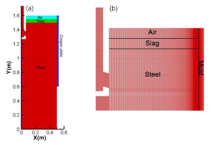
The boundary settings are shown in Figure 2. The boundary of the upper surface was set as a free surface with a temperature of 300 K. The boundary of the mould outlet was set to outflow, resulting in a fully developed flow at this boundary. The interface between the fluid and solid was defined as a coupled wall, the fluidmould interface was coupled in terms of velocity and heat flux, and oscillated with the mould. The walls of the SEN and top and bottom walls of the mould were set as insulated due to the negligible heat flux across these walls in the real process. A symmetric boundary condition was applied for the plane of symmetry. The boundary of the SEN inlet was set to velocity inlet, where the inlet velocity (Vin) was determined by the mass balance as shown in Equation [1], and the inlet temperature was 1830 K. The cold wall of the copper plate was set as a convection boundary with the water temperature 305 K and the heat transfer coefficient (hc) as per the empirical determination by Xiang. Xia, and Wu (2023) of 28 000 W/m2K, correlating to a water flow rate of 10 m/s. Similarly, the wall of the secondary cooling zone was set as a convection boundary with the water spray temperature 300 K and heat transfer coefficient (hs) 2000 W/m2K correlating to a specific water flow in the secondary cooling zone of 1.03 L/kg as determined by Zang et al. (2019). The oscillation mode of the mould was sinusoidal. The velocity and displacement expressions of mould oscillation are illustrated in Equations [1]–[3]. A dynamic mesh was employed to achieve the oscillation of the mould.

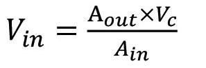
where Vc is the casting speed (m/min), Ain the inlet area (m2), and Aout the outlet area (m2). [2]

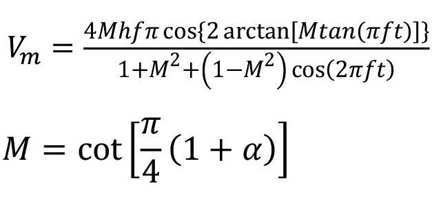
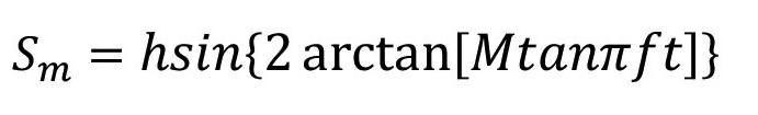
where Vm is the mould velocity (m/s), h the oscillation amplitude of the mould (m), f the oscillation frequency (Hz), α the modification ratio (sinusoidal mode when α was zero), and Sm mould displacement (m).

[1]

Figure 1—(a) Schemes of model , (b) mesh

Figure 2—Boundary of the model

A mathematical mould model for transient infiltration and lubrication behaviour of slag

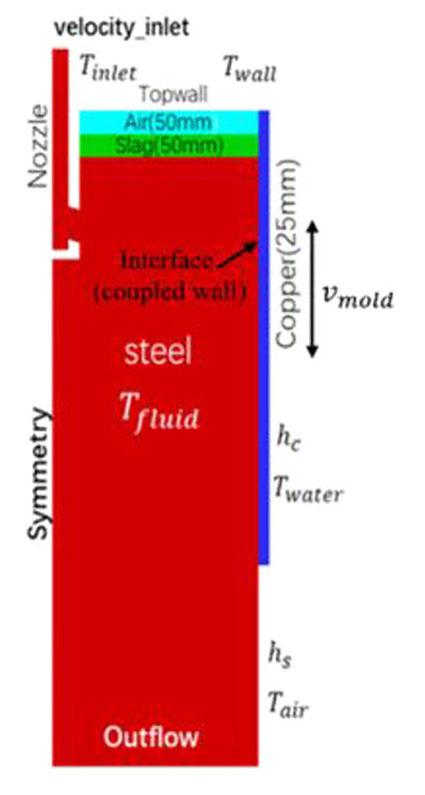
The break temperature of the slag was utilized to distinguish the liquid and solid phases since the formation of the first solids in the liquid slag is related to the break temperature (Kölbl, and Harmuth, 2019). The time step of the solution was 0.0001 seconds, and the results were calculated for more than a month of casting. The detailed governing equation, casting parameters, model parameters, and material properties are described elsewhere (Cao et al., 2023).

Validation of slag consumption

The model was validated in Cao et al. (2023) by comparing the oscillation marks with plant measurements and the pitch of oscillation marks with the theoretical values, respectively. In addition, the 17 cases in Table I were simulated, and the slag consumption was calculated during one cycle after the calculation was stable. The slag consumptions were compared with the plant measurements (Shin et al., 2006). Figure 3a shows that the calculated slag consumption was in good agreement with the plant measurements. The slag consumption decreased with increasing casting speed (Figure 3b), which is consistent with observations by Shin et al. (2006)

Based on the above, the depth of the oscillation mark and the slag consumption were compared with the plant measurements. The two-dimensional model showed good accuracy and robustness, and hence could be used to study the lubrication behaviour of slag.

Table I

Results and discussion

Under the mould oscillation for f = 174 cpm, h = 2.9 mm, α = 0 with Vc=1.4 m/min, the specific variables at 300 mm below the meniscus were tracked to investigate the transient infiltration of slag and slag lubrication. The velocity and displacement of mould oscillation are presented in Figure 4, where the time period when the downward oscillation velocity exceeds the pulling speed is negative strip time (tn), and the rest period the positive strip time (tp).

Figure 3—(a) Validation of predicted slag consumption per oscillation cycle with measurements taken at different positive strip times, (b) effect of casting speed* on slag consumption in each oscillation cycle

Figure 4—Oscillation velocity and displacement

A mathematical mould model for transient infiltration and lubrication behaviour of slag

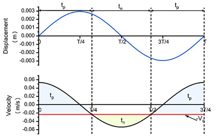
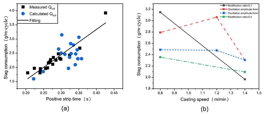
Infiltration velocity of slag and pressure in slag channel

The transient downward infiltration velocity of slag in the slag channel is shown in Figure 5. During the early and late stages of tp, the slag flowed upward owing to the upward oscillation of the mould. During the tn, the downward infiltration of the slag was accelerated due to the increase in the downward oscillation velocity of the mould, reaching a maximum of 0.032 m/s at the middle stage, followed by a gradual decrease in infiltration velocity. The infiltration velocity of slag was determined by the velocity and position of mould oscillation.

The variation of the pressure in the slag channel in a cycle is illustrated in Figure 6. The pressure varied between the maximum positive and negative pressures. The slag channel experienced negative pressure during the early and late stages of tp, with a maximum value of 12 167.55 Pa. However, the slag channel experienced positive pressure during the tn, reaching a maximum value of 24 671.961 Pa at the middle of the tn. The pressure in the slag passage was affected by mould oscillation and the movement of the slag rim (Cao et al., 2023).

The variation of slag pressure exerted an influence on the meniscus and the initial shell, resulting in periodic deformations (i.e. oscillation marks). Increasing the negative pressure of the slag channel was conducive to enhancing the effect of liquid slag infiltration in the slag channel, and improving the lubrication effect. Increasing the positive pressure of the slag channel was conducive to forced demoulding and preventing breakout. However, an increase in both maximum positive and negative pressures resulted in an increasing pressure difference within the slag channel, exacerbating meniscus fluctuations and initial shell deformations, which is not conducive to improving the surface quality of slabs. Therefore, it was crucial to control these parameters.

Thickness of slag film

The surface temperature of the shell and heat flux of the copper plate are shown in Figure 7. The heat flux was within 1.83 to 3.44 MW/m2, and the surface temperature of the shell was within the range1487.20 to 1524.13 K. The maximum temperature and minimum heat flux appeared near the tn. The higher the surface temperature of the shell, the faster the slag melting rate, resulting in a thicker liquid slag layer, which is conducive to lubrication. The greater the heat flux, the thicker the solid slag layer, which is not conducive to the solidification of liquid steel into a shell.

The transient variation in thickness of solid and liquid slag layers is exhibited in Figure 8. The thickness variation of the solid

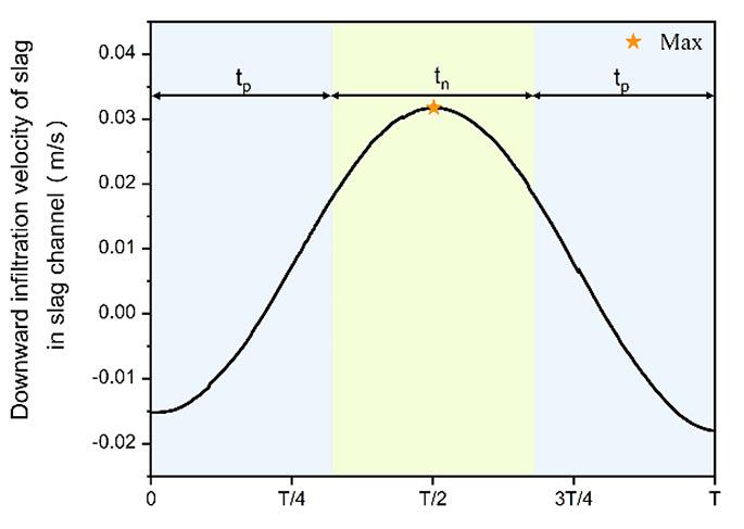
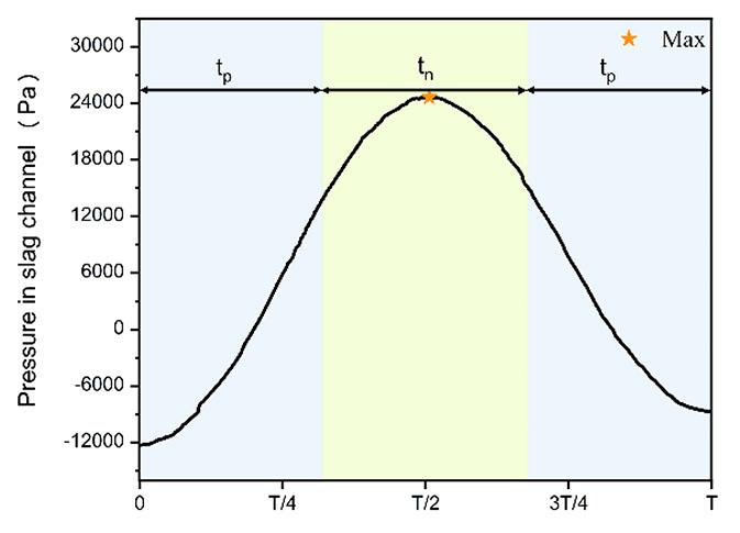
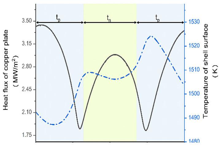
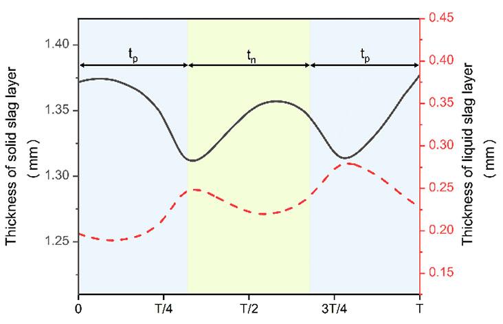
slag layer was inversely related to that of the liquid slag layer, and the thicknesses were 1.31 to 1.37 mm and 0.19 to 0.28 mm, respectively. At the middle of the tn, the the liquid layer affected by fast flowing slag became thinner and the solid layer became thicker. The maintenance of a thick and uniform liquid slag film, while ensuring a thin solid slag film, was crucial in order to prevent breakout.

Slag consumption

The slag film could prevent the shell sticking to the mould wall, which contained the liquid and solid layers. The liquid slag layer could help the shell to demould smoothly. The slag consumption was an important index for evaluating the lubrication performance of the slag. The slag consumed in the total slag film was considered as total slag consumption (Qt, kg/s), while the slag consumed in the liquid slag film was considered as lubrication consumption

Figure 5—Infiltration velocity of slag in slag channel

Figure 6—Variation of pressure in channel

Figure 7—Surface temperature of the shell and heat flux of the copper plate

Figure 8—Transient variation in thickness of solid and liquid slag layers

A mathematical mould model for transient infiltration and lubrication behaviour of slag

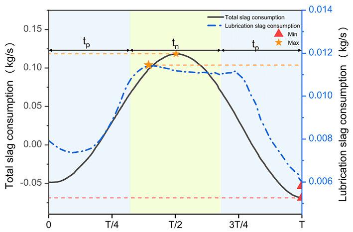
(Qlub, kg/s). Transient lubrication consumption and total slag consumption are presented in Figure 9, where the minus sign indicates upward movement of slag

The slag consumption tended to increase during the tn.The variation of Qt and Qlub was similar, with average values of 0.03 and 0.009 kg/s, respectively. The liquid slag was pumped into the slag channel under positive pressure. The maximum Qt and Qlub were observed near the middle of tn, with values of 0.118 and 0.011 kg/s, respectively.

The mechanism of liquid slag consumption was elucidated according to the above slag consumption, the flow and pressure of slag in the slag channel, and the variation of slag film thickness. The liquid slag flowed upward due to the upward movement of the mould during the early stage of tp; the inertial effect weakened and the lubrication consumption increased with the decrease in upward oscillation velocity of the mould. As the upward velocity of the mould decreased to zero and the mould began to oscillate downward, the downward flow of liquid slag was facilitated by the inertial effect of the mould and liquid slag continued to be consumed, reaching the maximum value of 0.0115 kg/s at the initial stage of tn. After that, although the liquid slag infiltrated into the slag channel under the action of the increased positive pressure and slag infiltration velocity, the decrease in thickness of the liquid slag film led to a decrease in lubrication consumption. The lubrication consumption decreased to 0.0111 kg/s at the middle of tn. Later, the lubrication consumption began to increase with the increase in thickness of the liquid slag film. With the upward oscillation of the mould, the slag consumption decreased due to the weakening of the suction and the inertial effect of the mould. The lubrication consumption was minimum at –0.0061 kg/s at the end of tp. Liquid slag was consumed from the middle and late period of tp to the next early period of tp, including the entire tn

Shear stress

Shear stress acting on the shell surface (τs/l) and at the mould side (τs/l), Pa) were important parameters which characterized the slag lubrication and the interaction between the mould wall and shell, and the surface quality of the shell and productivity of continuous casting were directly affected. Hence, τs/l and τmold were calculated according to Equations [4] and [5] (Meng and Thomas, 2003), respectively:

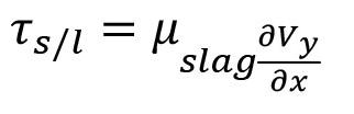
where: μslag is the viscosity of the slag(Pa∙s), Vy is the vertical velocity of the slag (m/s), ∂x the thickness of the liquid slag layer (m), σy the axial stress in the solid slag layer, ds the thickness of the solid slag layer (mm), and ν the Poisson's ratio of the slag (0.17 in the current study).

The upward shear stress on the shell surface (τs/l) and shear stress at the mould side (τmould) are plotted in Figure 10. The variations in τs/l and τmold were inversely related to the variations in Qlub and Qt, respectively. The τs/l was within 29.62 to 209.75 Pa, τmould was within 18.55 to 19.54 kPa, and the maximum occurred when the mould was near the equilibrium position during the tp. During the tn, the τs/l decreased with the increase in slag consumption, reaching the minimum at the middle of tn, and subsequently increased with a decrease in slag consumption. The τmould fluctuated around the minimum value of 18.55 kPa due to the fluctuation in lubrication slag consumption. The shear stress depended on the velocity gradient of the slag, slag viscosity, and the thickness of the solid and liquid slag films. Adequate slag consumption could reduce shear stress, avoid breakout, and be conductive to demould.

Conclusions

A two-dimensional coupled mathematical model was employed to study the infiltration and lubrication behaviour of the slag during continuous casting of steel. The infiltration velocity of slag and the pressure in the slag channel, the thickness of the liquid and solid slag layers, the total slag consumption, the lubrication slag consumption, and the shear stress of the liquid slag on the shell surface and at the mould wall were investigated. The conclusions can be summarized as follows.

➤ The mould oscillation led to periodic variations in the pressure and infiltration velocity in the slag channel. During the early and late stages of positive strip time (tp), the slag flowed upward and the slag channel pressure was maximum negative pressure. At the middle of the negative strip time (tn), infiltration velocity and the slag channel pressure reached maximum downward infiltration velocity and maximum positive pressure, respectively.

➤ The thickness variation of the solid slag layer was inversely related to that of the liquid slag layer, and was determined by the cooling strength and surface temperature of the shell. At the middle of the tn, the thickness of the liquid layer with fast flowing slag became thinner and the solid layer became thicker.

➤ The variations of Qlub and Qt were similar. Slag consumption tended to increase during the tn, and the peak values for Qt

Figure 9—Total slag consumption, lubrication slag consumption, and average slag consumption during the tn and tp

Figure 10—Upward shear stress of the liquid slag on the surface of the shell and shear stress at the moold side

A mathematical mould model for transient infiltration and lubrication behaviour of slag

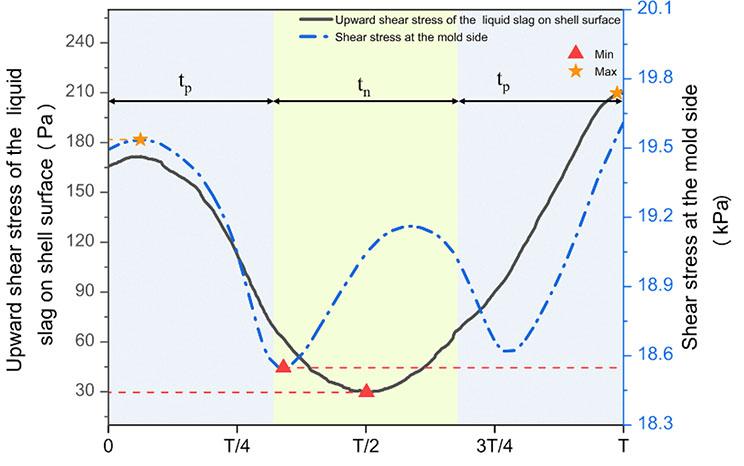
and Qlub were observed near the middle of tn. The liquid slag was consumed from the middle and late period of tp to the next early period of tp, including the entire tn

➤ The τs/l and τmould were determined by Qlub and Qt, respectively, and gradually decreased with increasing slag consumption. The maximum τs/l and τmould occurred when the mould was near the equilibrium position during the tp. The minimum τs/l and τmould occurred during the tn

Acknowledgements

This study was funded by Hebei Province Natural Science Fund (grant number E2020203128) and Hebei Education Department Higher Education Science and Technology Program (grant number ZD2021106).

Conflicts of Interest: The authors declare that they have no conflict of interest.

Data availability: The data that supports the findings of this study is available on request from the corresponding author.

References

Cao, M., Liu, Y., Yu, B., Zhou, C., and Zhang, X-Z. 2023. Modeling study on the initial solidification and formation of oscillation marks in continuous casting mold. Transactions of the Indian Institute of Metals, vol. 77. pp. 51–60. https:// doi.org/10.1007/s12666-023-03040-x

Ji, J., Cui, Y., Zhang, X., Wang, Q., He, S., and Wang, Q. 2023. 3D coupled model on dynamic initial solidification and slag infiltration at the corner of slab continuous casting mold. Steel Research International, vol. 92. pp. 21–27. https://doi.org/https://doi.org/10.1002/srin.202100101

Jonayat, A.S.M. and Thomas, B.G. 2014. Transient thermo-fluid model of meniscus behavior and slag consumption in steel continuous casting. Metallurgical and Materials Transactions B, vol. 45. pp. 1842–1864. https://doi.org/10.1007/ s11663-014-0097-9

Kölbl, N. and Harmuth, H. 2019. Automated break temperature determination of mould slags for the coninuous casting of steel based on temperature-dependent viscosity data. Ironmaking & Steelmaking, vol. 47. p. 899. https:doi.org/10.1080/ 03019233.2019.1639028

Louhenkilpi, S. 2014. Continuous casting of steel. Treatise on Process Metallurgy Seetharaman, S. (ed.). Elsevier, Boston. Chapter 1.8.

Meng, Y. and Thomas, B.G. 2003. Modeling transient slag-layer phenomena in the shell/mold gap in continuous casting of steel. Metallurgical and Materials Transactions B, vol. 34. pp. 707–725. https://doi.org/10.1007/s11663-003-0041-x

Ramirez-Lopez, P., Lee, P., and Mills, K. 2010. Explicit modelling of slag infiltration and shell formation during mould oscillation in continuous casting. ISIJ International, vol. 50. pp. 425–434. https://doi.org/10.2355/ isijinternational.50.425

Ramirez-Lopez, P., Lee, P., Mills, K., and Santillana, B. 2010. A new approach for modelling slag infiltration and solidification in a continuous casting mould. ISIJ Intermational, vol. 50. p. 1797. https://doi.org/10.2355/ isijinternational.50.1797

Shin, H.J., Kim, S.H., Thomas, B.G., Lee, G-G., Park, J-M., and Sengupta, J. 2006. Measurement and prediction of lubrication, powder consumption, and oscillation mark profiles in ultra-low carbon steel slabs. ISIJ International, vol. 46. p. 1635. https://doi.org/10.2355/isijinternational.46.1635

Xiang, H.L., Xia, F., and Wu, G. 2023. Development and application of heat flux model of high casting speed billet mould. Continuous Casting, vol. 42. p, 21. https://www.chinamet.cn/Jweb_lz/EN/abstract/abstract154583.shtml

Yan, X., Jia, B., Wang, Q., He, S., and Wang, Q. 2019. Mold nonsinusoidal oscillation mode and its effect on slag infiltration for lubrication and initial shell growth during steel continuous casting. Metals, vol. 9. p. 418. https://doi. org/10.3390/met9040418

Yang, J., Chen, D., Long, M., and Guan, H. 2020. An approach for modelling slag infiltration and heat transfer in continuous casting mold for high Mn–high Al steel. Metals, vol. 10. p. 51. https://doi.org/10.3390/met10010051

Yang, J., Meng, X., and Zhu, M. 2014. Experimental study on mold flux lubrication for continuous casting. Steel Research. Internstional, vol. 85. p. 710. https://doi.org/10.1002/srin.201300232

Yang, J., Meng, X., and Zhu, M. 2018. Transient thermo-fluid and solidification behaviors in continuous casting mold: Oscillation behaviors. ISIJ International, vol. 58. p. 2071. https://doi.org/10.2355/isijinternational.ISIJINT-2018-169

Youming, W., Yeming, W., and Kuangdi, X. 2022. Continuous casting and continuous rolling. ECPH Encyclopedia of Mining and Metallurgy. Xu, K. (ed.). Springer Nature, Singapore.

Zhang, S., Wang, Q., He, S., and Wang, Q. 2018. Study of the mechanism of liquid slag infiltration for lubrication in slab continuous casting. Metallurgical and Materials Transactions B, vol. 49. pp. 2038–2049. https://doi.org/10.1007/ s11663-018-1267-y

Zhang, X., Chen, W., Scheller, P.R., Ren, Y., and Zhang, L. 2019a. Mathematical modeling of initial solidification and slag infiltration at the meniscus of slab continuous casting mold. JOM, vol. 71. p. 78. https://doi.org/10.1007/s11837018-3177-5

Zhang, X., Dan, Z., Chen, W., Zhang, L., and Wang, Q. 2021. Mathematical modeling on slag consumption and lubrication in a slab continuous casting mold. Metallurgical and Materials Transactions B, vol. 52. pp. 322–338. https:// doi.org/10.1007/s11663-020-02022-4

Zhang, X., Chen, W., Ren, Y., and Zhang, L. 2019b. Mathematical modeling on the influence of casting parameters on initial solidification at t meniscus of slab continuous casting. Metallurgical and Materials Transactions B. vol. 50. pp. 1444–1460. https://doi.org/10.1007/s11663-019-01570-8 u

Affiliation:

1Department of Mining and Geological Engineering, University of Arizona, Tucson, Arizona, USA.

Correspondence to:

K.W. Brown Requist

Email: katebrown@arizona.edu

Dates:

Received: 20 Feb. 2023

Accepted: 22 Mar. 2024

Published: March 2024

How to cite:

Brown Requist, K.W., Lutz, E., and Momayez, M. 2024

Near real-time interpolative algorithm for modelling air quality in underground mines.

Journal of the Southern African Institute of Mining and Metallurgy, vol. 124, no. 3. pp. 153–162

DOI ID:

http://dx.doi.org/10.17159/24119717/2638/2024

ORCID:

K.W. Brown Requist http://orcid.org/0000-0002-5408-5340

Near real-time interpolative algorithm for modelling air quality in underground mines

by K.W. Brown Requist1, E. Lutz1, and M. Momayez1

Synopsis

As real-time air quality monitoring becomes more prevalent in US underground mines, it is important to provide the highest data reliability with the fewest possible sensors. Real-time sensors remain costly, and these costs are not exclusively financial; the time required to install, calibrate, and maintain real-time sensors poses a large barrier to widespread implementation. Current atmospheric monitoring systems typically rely on displaying point-specific values. This requires operators to infer real-time airborne contamination distributions. Monitoring and control software utilizing mine ventilation network (MVN) solvers has been implemented in limited cases because of their ability to simulate ventilation systems quickly, but these solvers use a one-dimensional representation of the mine, limiting spatial resolution of estimated distributions. Computational fluid dynamics (CFD) has likewise been considered as a means to improve spatial resolution, but processing times prevent its use as a basis for monitoring and control. For the real-time monitoring of airborne contamination distributions, we propose a spatial interpolation method that can estimate the distribution of airborne contaminants in near-real time. This method provides a middle ground between fast processing times and increased spatial resolution. With the use of a pathfinding algorithm and optimization through absolute percentage error minimization, this method outperforms spatial interpolation with a Euclidean distance. By providing contamination distribution information to operators, this method and its derivatives stand to outperform current atmospheric monitoring systems.

Keywords real-time monitoring, occupational exposure, carbon monoxide, underground mining, mine gases, coal dust.

Introduction

Air quality has long been a concern in underground mines. From the understanding of the role coal dust exposure plays in life-long human health outcomes (Wang and Christiani, 2000; Rogan, 1970; Kissell and Colinet, 1900) to the recent increased concern regarding crystalline silica exposure (Wang and Christiani, 2000; Ziskind, Jones, and Weill, 1976; Holman, 1947), the mining industry has been acutely aware of the importance of a healthy air mixture in underground working areas. The 2006 MINER Act, stemming from the Sago Mine disaster on 2 January 2006, required the US Mine Safety and Health Administration (MSHA) to expand its policies for environmental monitoring in underground mines (United States, 2006). This legislation laid the pathway for a final ruling in 2008, which required underground coal mines to monitor carbon monoxide with sensors that automatically alert and record values and required the training of individuals managing these sensors (US Mine Safety and Health Administration, 2008). Since this ruling, the data from these federally mandated sensors has been extensively warehoused, with minimal further use. Current atmospheric monitoring systems (AMSs) provide methods to display sensor values overlain on a mine plan as in Figure 1, or individual graphs of sensor values over time, but critical information available to these systems is not leveraged.

Sensor networks are costly to install and maintain. These costs are not exclusively monetary, particularly considering federal requirements for routine maintenance. In the USA, underground mines using realtime sensors as part of an AMS must visually inspect the sensors daily, bump test the sensors weekly, and calibrate them monthly (US 30 CFR 75.351). The time spent in calibration and maintenance results in a loss in productivity. Current movements to expand the monitoring and control of ventilation systems have been hindered by the operational and capital costs associated with the monitoring of airborne contamination. The total cost to establish a wireless sensor network can quickly increase with increasing safety ratings, sensor capability, wireless functions, and naturally, the number of sensors. Real-time sensing of airborne particulate matter has proven particularly challenging, with purchase prices for diesel particulate matter (DPM) and dust sensors in the tens of thousands of US dollars (Shriwas and Pritchard, 2020; Halterman,

Near real-time interpolative algorithm for modelling air quality in underground mines

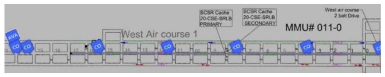
Sousan, and Peters, 2018). Alternatively, wireless electrochemical carbon monoxide sensors are available commercially starting at US$105, but notably these do not meet intrinsically safe requirements for coal mines (Estrada et al., 2019). With the high costs associated with adding more sensors to a mine‘s AMS, operations opt to use the minimum number of sensors necessary to meet regulatory requirements. In 2018, the largest AMS in the USA consisted of 300 sensors, a notable outlier from the industry average of 38 (Rowland, Harties, and Yuan, 2018).

The cost and time associated with expanding air quality monitoring capabilities in underground mines poses as significant barrier to improved ventilation system monitoring and control. Current AMSs have wide-ranging utility as early warning systems for mine fires in underground coal mines, but offer no currently accepted method to infer the distribution of gases between sensors (Shriwas and Pritchard, 2020). This lack of data ultimately limits the functionality of the AMS; gas distribution data is virtually inaccessible to AMS operators because of the location-specific nature of sensor data.

In general, the issue of estimating distributions between known sensor locations is a solver problem. Methods for estimation are wide-ranging, including deterministic methods like nearestneighbour and polygonal interpolation and inverse distance weighting, and stochastic methods like ordinary kriging, Bayesian maximum entropy, and sequential Gaussian simulation (Lam, 1983). All of these methods are well documented for the spatial interpolation of distributions between known data-points, but no method has been implemented in any commercially available AMS. This is in part due to current practices with representations of underground ventilation systems and difficulties associated with creating robust statistical relationships between locations that account for changes in mine geometry.

Various solutions and improvements to modern AMSs have been suggested in the literature. Mine ventilation network (MVN) solvers have long been the backbone of modern ventilation system design. MVN software has shown promising results for real-time monitoring and control of mine ventilation conditions. In the late 1990s and early 2000s, a real-time monitoring and control project was started at the Waste Isolation Pilot Plant (WIPP) in New Mexico. This project focused on the use of WIPPVENT, a specially designed MVN software for the WIPP monitoring infrastructure. The WIPP employed pressure and velocity sensors to monitor the flow of air through the mine but (critically) did not include any implementation of air contamination monitoring (Shriwas and Pritchard, 2020; McDaniel and Wallace, 1997; Ruckman and Prosser, 2010). Further implementations of real-time monitoring and control using MVN software have not included air contamination monitoring as a key variable in the assessment or ventilation system control (Gillies et al., 2004; Wu and Gillies 2007). Importantly, MVN software relies on a one-dimensional network approach. This allows for fast simulation of the ventilation network, making it an ideal candidate for the monitoring and

control of air flow within a mine (Sereshki, Saffari, and Elahi, 2016). As a consequence of the one-dimensional approach, variation of contamination estimated using MVN software is only available on the mine entry scale. Because mine entries are represented as vertices of a directional graph, it is not possible to estimate the distribution of airborne contamination within the entry itself. Instead, calculated concentrations apply uniformly as the mean concentration for the entire entry. This poses a similar problem to that seen with traditional AMS systems; the level of data resolution is lower than is useful for the holistic monitoring of contamination within a ventilation system.

Computational fluid dynamics (CFD) has likewise been proposed as a method for improving understanding of contamination distributions in underground mines. CFD can return models with extremely high spatial resolution, but critically struggle with sensitivity to the size of grid used in the simulation and the time required to converge on a stable solution (Mora et al., 2002; Xiang, Wei, and Haibo., 2017). Additionally, CFD cannot model the entire mine with an appropriate grid size in a reasonable time-frame. This, then, requires the creation of several disjointed CFD models in order to simulate the entire mining environment, leading to problems in appropriately modelling boundary and initial conditions for the ventilation system, impacting the accuracy of CFD results compared to experimental observation of mine conditions (Yuan, Zhou, and Smith, 2016). While the spatial resolution of CFD methods is highly desirable for AMSs, the time required to converge on a solution makes these methods unsuitable for real-time monitoring of contamination distributions.

Because current AMSs have no commonly accepted method for the estimation of gas distribution between installed sensors, it is difficult to establish a mine-wide view of airborne contamination. This is especially vital for monitoring and control. While MVN software has shown promise for the monitoring and control of air flow in underground mines, its implementations for contaminants is still problematic. Furthermore, MVN software relies on a onedimensional network representation of the ventilation system. This means that contamination distributions within mine entries are wholly inaccessible to AMS operators who may choose to use a MVN-based monitoring system in the future. CFD eliminates the issues of resolution, but does so at the expense of calculation time, making it currently unfit for use in real-time monitoring systems.

To improve on current AMSs, a real-time monitoring method should be capable of increasing data resolution by providing estimates of contaminant distribution between sensors. Additionally, the method should be able to run in practically real-time with one-minute temporal resolution. Because of the interrelated nature of airborne contamination from location to location in a mine ventilation system, the use of spatial interpolation of sensed data is a promising avenue to provide a more holistic approach to atmospheric monitoring in underground mines without the need for installation of more sensors.

Figure 1 Strata gas monitoring user interface. Sensor locations are overlain in blue over the plan drawing of the mine

Near real-time interpolative algorithm for modelling air quality in underground mines

The real-time estimation of gas distribution in underground mines is limited by the use of a MVN approach. While such approaches are extremely capable of resolving contamination distributions, the lack of spatial resolution makes it difficult to determine the extent of hazardous air conditions, especially within mine entries. We propose a framework for the near real-time spatial interpolation of this data, known as the Near Real-Time Interpolative Measurement (NeaRTIMe) Algorithm. With the use of a pathfinding algorithm, NeaRTIMe attempts to better preserve the effect of air flow in the interpolation of data, which is not feasible with other methods of spatial interpolation. Traditional spatial interpolation methods rely on a Euclidean distance between points as the relevant distance metric. With the use of a pathfinding algorithm, it is possible to encode the interpolation method with a mine’s geometry. This allows for distance metrics to be used based on the distance of travel within the mine, rather than assuming constant reduction in concentration through various media like air, rock, and stoppings. By constraining movement to mine entries and measuring the effective distance from entry to entry, this provides an improved confidence in the interpolated contaminant distribution. The pathfinding algorithm runs in pre-processing, allowing for real-time interpolation with minimal computational delays. To further decrease error in the interpolated estimate of contaminant distribution, an optimal power coefficient is determined by minimizing the absolute percentage error as calculated by leave-one-out cross-validation. The use of interpolative modelling methods for atmospheric monitoring in underground mines will allow for time-dependent determination of the source of contamination, enable predictive analysis of contamination behaviour within the mine and provide an avenue for indirect exposure assessment for miners. From data collection to visualization, NeaRTIMe is able to provide site-wide interpolations in under one minute.

Methods

NeaRTIMe is a spatial interpolation algorithm that leverages inverse distance weighting and the A* search algorithm for pathfinding to create an interpolation that respects the geometry of the underground excavation (Hart, Nilsson, and Raphael, 1968). Because this is a spatial interpolation method, the primary information required to arrive at an estimation is the distance between the sensor and the location where airborne contamination is to be estimated. To construct these distance values, information about the mine’s geometry and orientation is needed.

The pathfinding algorithm used to calculate distances for spatial weighting of the sensor data requires a set of interior mine points, as well as a set of barriers. This set of barriers comprises air-rock boundaries and air-stopping boundaries. Air-stopping boundaries are generally defined as boundaries between air and non-rock, effectively solid items, such as sealed drifts or crosscuts, or wellsealed doors. Because these boundaries are found in all mines, spatial interpolation of environmental air quality must consider these unique interactions.

In order to to move away from proposed one-dimensional MVN approaches to monitoring, the one-dimensional network model must be updated to a framework that supports higher spatial resolution within mine entries. Concepts like an adjacency matrix are not a feasible option, because adjacency matrices are one-dimensional graphs mapped to a matrix (Ponstein, 1966). This retains the overall one-dimensional nature seen in MVN solvers. The use of a mesh structure like those used in CFD simulations, on the other hand, sacrifices processing time for the sake of spatial resolution. Using an intermediate format would allow for improved spatial resolution without an extreme increase in processing time, making it better suited for real-time atmospheric monitoring. The mine layout must therefore be converted to a rasterized or bitmap image. This image can be created through a variety of methods, the majority of which lie outside the scope of this paper. The method we elected to apply for a two-dimensional air quality analysis in a US underground coal mine utilized AutoCAD 2023 to import a CAD drawing of a section of mine beltway, as shown in Figure 2.

From this imported CAD drawing, pillar, stopping, and excavation boundaries are extracted, yielding a set of distinct lines that may then be converted into points in AutoCAD, as shown in Figure 3. These boundaries can then be overlain with an array of points, creating a network of evenly spaced points within the excavation, not inclusive of points inside pillars or beyond the excavation boundaries, as in Figure 4. The array of points as overlain with AutoCAD represents the mine entries through which air can travel.

These internal points and boundaries are then exported to .csv files, where they are processed in the Julia programming language to create a bitmap image of the mine (Bezanson et al., 2017). This is achieved by rounding the imported point values to the nearest interval. The interval elected for application here is 152 cm (5 feet).

While the goal of NeaRTIMe is to improve the spatial resolution of airborne contamination distribution estimations, it is impractical to use a small scale. Rather, it is better to scale the study area to minimize the number of estimations NeaRTIMe must perform while still providing improved spatial resolution. Scaling the study

Figure 2 CAD drawing of the area of study in an underground coal mine

Near real-time interpolative algorithm for modelling air quality in underground mines

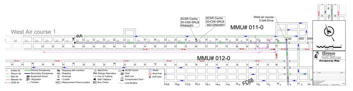
Figure 3—Air-rock and air-stopping boundaries must be extracted prior to input to the pathfinding algorithm. The red line indicates the interpolation boundary (outermost walls) within the coal mine and the blue lines indicate the air-rock or air-stopping interfaces

Figure 4—Internal points (airways) in the study area. Note discontinuities in some regions due to stoppings

area is beneficial for two reasons. Primarily, this yields a steep reduction in processing time both in pre-processing of distances used in spatial interpolation and processing of sensor data for spatial interpolation. Additionally, it reduces unnecessary artificial precision. Because individual sensors within an AMS have their own precisions (often 0.1–10 ppm for most gas detection), precision exceeding this threshold is unnecessary and provides a somewhat inaccurate picture of conditions between sensors (Afshar-Mohajer et al., 2017). Scaling the area seeks to minimize this creation of artificial precision.

The calculation of distance values for spatial interpolation entails a unique challenge not encountered in most spatial interpolation use cases. Because air quality is the topic of concern, interpolation must focus on distances between points where air flows. This means that standard distance calculations, such as Euclidean distance calculations, as in Equation [1], do not suffice:

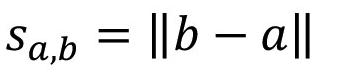
where a and b are two vectors representing two n-dimensional points in space and ||b a|| is the L2-norm (Euclidean norm)

Instead, the A* algorithm can be applied. The A* algorithm is a best-first search algorithm and operates as an extension of Dijkstra’s algorithm ,with the use of a heuristic to generate the shortest path between two points while respecting any boundaries between two points (Hart, Nilsson, and Raphael, 1968).

This application of the A* algorithm is especially advantageous; because the A* algorithm calculates a shortest path with respect to any boundaries, it is possible to calculate the shortest path through air between any two points in an underground mine. The use of the A* algorithm ensures that interpolation respects the natural flow of air in the mine, and prevents the interpolation from calculating distances through rock, doors, or stoppings that would otherwise cause an erroneous result.

The A* algorithm seks to minimize the distance between points within a path with the use of a cost function and a heuristic function. Following from Equation [1], the cost function is

considered here as the Euclidean distance between the current position and the next position:

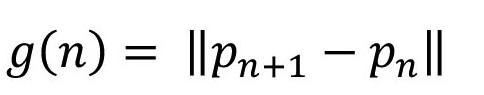
[2]

This is effectively the distance moved in one step from the current position to a neighbouring position. Likewise, the heuristic function is governed by the distance between the current position and the goal position: [3]

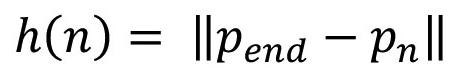
Following Equations [2] and [3], the A* algorithm iteratively creates a path such that:

[4]

The length of this path can then be obtained from the number of members in the set of points describing the optimal path. The A* algorithm in this application does not generate a continuous distance, as Euclidean distance calculations do in Equations [1], [2], and [3]. Instead, it counts the number of locations visited along the rasterized path between two locations. This discrete value generated works well for spatial interpolation over the rasterized mine layout. It is important to note that Euclidean distances and A* distances are not inherently interchangeable. The underlying scales of the metrics are different. This means that visual inspection of values attached to a colour scale can show differences in values, but direct comparison of numbers is not a helpful means of determining differences.

As shown in Figures 5 and 6, the average A* distance values tend to bleed horizontally in the centre of the excavation. This spread of average values is noticeably different from the Euclidean distance, which cannot account for stoppings on either side of the centre drift.

While the visual difference between the two distance metrics is small, the use of A* distances in interpolation with NeaRTIMe provides a meaningful reduction in estimation error. By better accounting for the mine’s geometry, spatial relationships between

Near real-time interpolative algorithm for modelling air quality in underground mines

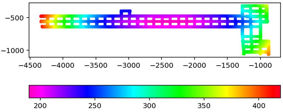
locations within the mine’s ventilation system are more realistically preserved than is possible with a Euclidean distance, which may draw its lines through rock or stoppings. This effect is slightly more visible when displaying the minimum distances to sensors within the mine (Figures 7 and 8). The A* distances tend to have curving, subcircular contours, whereas the Euclidean distances tend to preserve horizontal and vertical contours more, due to the orientation of the excavation and placement of sensors.

Spatial interpolation across the underground mine is achieved by inverse distance weighting, which uses the distance from a set of known values to a target (i.e., the output of the A* algorithm) (Shepard, 1968). Inverse distance weighting is predicated on the assumption that values from a known point generally decay with increasing distance from that point. This decay can be generalized as:

where d is the distance between a known-value location xi and the location to be interpolated, x, and p is the power coefficient describing the rate of decay.

The power coefficient, p, increases the rate of decay for p>0, as shown by graphing the equation f(x) = 1 xp with various power coefficients, as in Figure 9.

The value at a point then follows from Equation [5]:

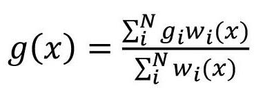
where gi is the value at a known location.

Although a power coefficient of p=2 is commonplace in the application of inverse distance weighting for resource geostatistics, an optimal power coefficient can be determined and used via leave-one-out cross-validation (Babak and Deutsch, 2009). This is advantageous, as various environmental variables may cause nonuniform rates of decay within the mine. These variables can include changes in air flow, changes in temperature and pressure, and individual differences in gas properties.

Optimization of the power coefficient is achieved by minimizing the absolute percentage error as calculated by leave-one-out crossvalidation. Error for the interpolated is calculated as:

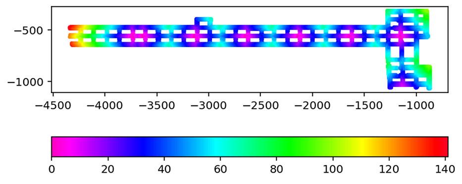
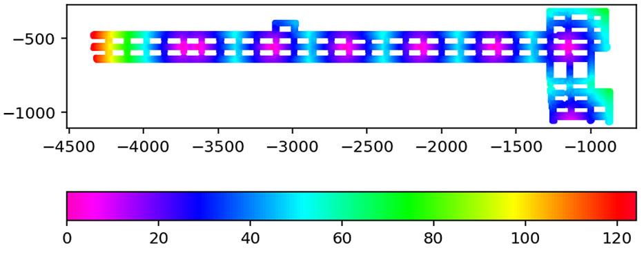
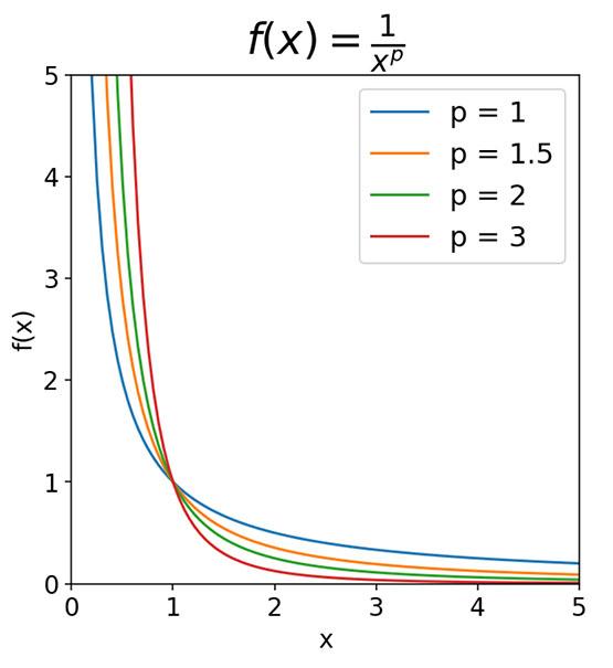
9—Inverse power functions for various values of p. Distance-based decay increases (f(x) decreases) as the power coefficient increases

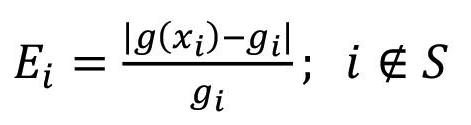
where g(xi) is the calculated value at the known location, gi is the measured value at the known location, and S is the set of all sensor values except those removed for error calculation. This error function does not account for sensors reporting zero; these values are assumed to be at the limit of detection for the sensor, often 0.05–1 ppm, depending on the contaminant (Afshar-Mohajer et al., 2017). Because absolute percentage error is extremely sensitive to differences between true and estimated values when the true value is small, care must be taken to avoid dividing by zero. Using the limit of detection of the sensor can prevent this error. In further implementations, it may be more appropriate to minimize the mean-squared error (MSE) or root-mean standard error (RMSE) to optimize the power coefficient. While MSE and RMSE would be helpful metrics to compare interpolation models where the input data remains constant, comparing various models across changing mine conditions and input concentrations is more difficult, because MSE and RMSE are not directly comparable metrics when the input data changes over multiple successive interpolations. Because of this, we have elected to use absolute percentage error as the current error metric while continuing to compare various interpolation approaches with varying input data.

The error can be calculated with the optimal power coefficient to provide the estimated error for the entire model. This error is minimized to find the optimal power coefficient, as in Equation [8]: [8]

[7]

Figure 5—Average A* distance from all sensors to all points. Horizontal and vertical axes represent rotated mine coordinates in metres

Figure 6—Average Euclidean distance from all sensors to all points. Horizontal and vertical axes represent rotated mine coordinates in metres

Figure 7 A* distances to nearest sensor for all points

Figure 8 Euclidean distances to nearest sensor for all points

Figure

Near real-time interpolative algorithm for modelling air quality in underground mines

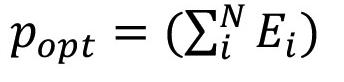
While leave-one-out cross-validation for optimization would be unfit for an interpolation using two or three sensors, underground AMSs generally have an average of 38 sensors, providing an opportunity to better reduce estimated error for the model (Rowland, Harties, and Yuan, 2018).

Results and discussion

Considering a set of concurrent AMS alerts from a portion of an underground room-and-pillar coal mine in Utah, it is possible to use NeaRTIMe to estimate the distribution of carbon monoxide in a portion of the mine, especially in areas between sensors. While the alerts presented here are concurrent, adoption of the NeaRTIMe method would require a departure from the current industry practice of alerting at specific concentrations above the mine’s background carbon monoxide concentration. Instead, NeaRTIMe would base interpolation estimates for any sensors above the limit of detection. For commercially available carbon monoxide sensors, this is generally 0.5–1 ppm (Afshar-Mohajer et al., 2017).

Most AMSs display a a visualization output similar to that in Figure 1. Sensor locations are overlain on a mine plan, with popups displaying on the system interface when a sensor in the AMS signals an alert. This yields, at best, a nearest-neighbour assumption of realtime air mixtures available to the AMS operator, most likely without respect to air-barrier interfaces, as in Figure 10. While nearestneighbour interpolation is possible based on A* distance outputs, this yields no appreciable difference in the resulting visualization and still fails to paint an in-depth picture of most probable air quality conditions.

Because nearest-neighbour interpolation is based on the nearest sensor value, lines of demarcation are strikingly apparent between each sensor’s radius of influence. Additionally, there is no input of data from other sensors when a point lies entirely constrained by one sensor’s radius of influence. This yields a visualization that assumes discrete changes in values from one radius of influence to another, which is naturally not the case when considering the constantly evolving nature of potentially hazardous air mixtures in an underground mine. Interpolation of the sensor data utilizing the A* algorithm, as in Figure 11, creates a much smoother visualization, with minimal demarcation between sensor domains in the study area. This method of interpolation can still be improved. The average error is relatively high, but by adjusting the power coefficient, the interpolation can be optimized to reduce the average error and create a more realistic visualization of air quality conditions.

With a power coefficient of p = 2, the average percentage error of the interpolation is 30.2%. By increasing the power coefficient incrementally to reduce the percentage error, an optimized power coefficient of p = 5 is obtained. Because of the nature of

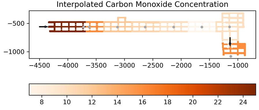
the tip of the leftmost arrow. Axes represent rotated mine coordinates in metres

Figure 11—Interpolated carbon monoxide concentration utilizing A*-informed inverse distance weighting with p=2 and an average error of 30.2%. Air flow direction is indicared with black arrows, and sensor locations are denoted in grey. A continuous miner is located at the tip of the leftmost arrow. Axes represent rotated mine coordinates in metres

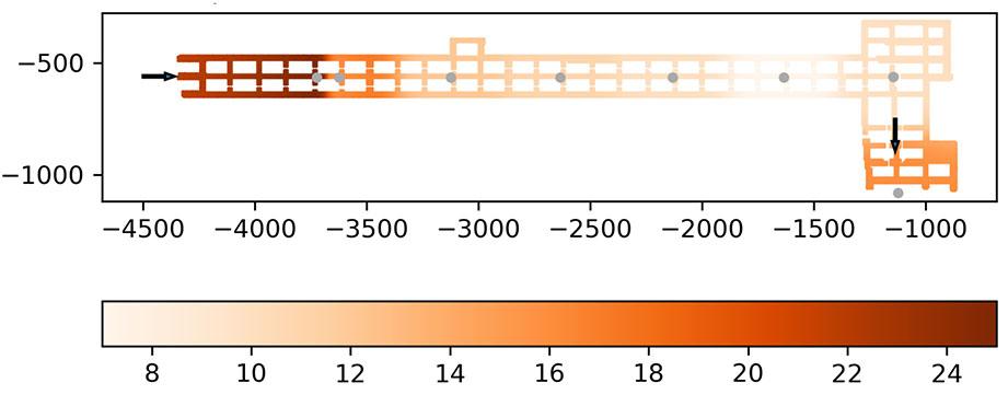
Figure 12—Interpolated carbon monoxide concentration utilizing A*-informed inverse distance weighting with p = 5 and an average error of 27.3%. Air flow direction is indicated with black arrows, and sensor locations are denoted in grey. A continuous miner is located at the tip of the leftmost arrow. Axes represent rotated mine coordinates in metres

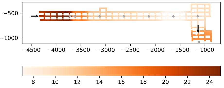
Figure 13—Interpolated carbon monoxide concentration utilizing Euclidean-based inverse distance weighting with p = 2 and an average error of 31.5%. Air flow direction is indicated with black arrows, and sensor locations are denoted in grey. A continuous miner is located at the tip of the leftmost arrow

optimization via error minimization, power coefficients could range between p = 2 and p = 100 with 0.5-step increments. Upon optimizing the interpolation with p = 5, average percentage error reduces by 9.7%. This yields an interpolation as in Figure 12. Demarcation between sensor domains is noticeable, as in a nearest-neighbour interpolation, but is significantly less prominent. Optimization of this interpolation seeks to equally constrain all sensors; sensors that are further away from an interpolated point have less effect on the resulting value at p = 5 than p = 2. This constraint offers a decrease in error, as well as a better-informed interpolation.

This is most prominent when considering the interpolations in Figures 11 and 12, where the left side of the figure is interpolated to be significantly lower in value in Figure 11 than in Figure 12. At p = 2, the lower sensor value on the right side of the figure has a higher influence on point values than when p = 5, creating artificially depressed values on the left side of the interpolation. Further still, error reduction is visible when considering a linear interpolation, as in Figure 13, compared to an A*-informed interpolation. With an estimated error of 31.5%, NeaRTIMe can achieve a total percentage error reduction of 13.3%. This error reduction is crucial to return a contamination distribution that is as close to real-time mine conditions as possible. As discussed in relation to Figure 9, the

Figure 10—Interpolated carbon monoxide concentration utilizing Euclidean distance-informed nearest-neighbour interpolation. Air flow direction is indicated with black arrows, and sensor locations are denoted in grey. A continuous miner is located at

Near real-time interpolative algorithm for modelling air quality in underground mines

power coefficient is related to the rate of decay of concentration from a known location to an unknown location. By optimizing the power coefficient, this assumed rate of decay can be more precisely controlled. This allows for reduced percentage error in the interpolated model as the model begins to reflect the spatial relationships between sensors more accurately. In other words, while a power coefficient of p = 2 may be treated as a default, changing the power coefficient to minimize percentage error will better capture the physical conditions within the mine and return a model with lower error and higher confidence.

Figures 11, 12, and 13 provide views of different interpolation methods based on a set of concurrent AMS alerts from an active underground coal mine. By extension, the preferred model should return the lowest percentage error as calculated by leave-oneout cross-validation. The optimized interpolated model (Figure 12) is the model that most closely matches the experimental conditions experienced in the mine during the AMS alert period. Obviously, different mines with different equipment operations, mine geometries, and ventilation systems would return different distributions stemming from different input data, with different optimized power coefficients. Further development and verification of the NeaRTIMe method and related approaches is under way to improve model resolution and certainty. Based on inverse distance weighting, NeaRTIMe presumes that the main factor influencing the distribution of airborne contamination is the interaction between a ventilation system and mine geometry in the form of a distance metric. While normal inverse distance weighting typically uses a Euclidean or linear distance, accounting for mine geometry can reduce error in the model. Furthermore, by optimizing the power coefficient, the spatial relationships between input data and estimated values can be more faithfully utilized in interpolation.

An additional aspect of this optimization method is that it permits a greater understanding of the effects of dilution and exhausting. While the figures presented consider a single point in time, air mixtures in underground mines are extremely dynamic. As fresh air enters the excavation at the active face, the resulting contaminated air is exhausted along the beltway. The effects of dilution and exhausting are visible in the right side of both figures, where carbon monoxide remains high as the bulk of the contaminant is exhausted further down the beltway. An additional region of relatively high carbon monoxide is visible on the left side of the figures, which will eventually undergo the same dilution and exhausting processes as the previous bulk of contamination. This raises the point that dilution as a mechanism is only responsible for the location-specific reduction of contaminant concentration. This mechanism does not govern the removal of contamination, but instead describes how contamination in a single area will reduce as fresh air is added. This fresh air does not remain in the same location, so the bulk of the contamination still requires exhausting to physically remove it from the working area. More succinctly, concentration values are reduced at the sensor via dilution (the inclusion of fresh air) but exhausting (the entire or almost-entire replacement of contaminated air with fresh air) remains the physical means of removal of contaminants across the whole excavation.

As a method designed to operate with higher combined spatial and temporal resolution than currently available methods, NeaRTIMe is well suited to visualize the kinematic behaviour of airborne contamination in underground mines. Minute-overminute, estimations of contamination distribution can be calculated using NeaRTIMe. These estimations can then be plotted and made available for replay by AMS operators. The operator is able to review critical alarm events in a holistic, spatial-visual way rather

than relying on a time-stamped record of alerts or a graph for a single sensor. By including the visualization aspect with improved combined spatial and temporal resolution, AMS operators will be afforded a more comprehensive understanding of contamination dynamics within the underground mine than is currently available from AMSs.

The A* pathfinding algorithm is vital for NeaRTIMe’s ability to return estimates with higher confidence than other airborne contamination models using inverse distance weighting. While spatial statistical methods like those used in geostatistical resource estimation generally consider relationships along straight lines (Euclidean distances), the use of pathfinding algorithms like Dijkstra’s algorithm has been well-documented for cases where spatial relationships vary through a region (Boisvert and Deutsch, 2008; Boisvert, Manchuk, and Deutsch, 2009). The same logic can be applied to the estimation of airborne contamination. Spatial relationships, when considering straight lines drawn through rock and stoppings, fail to properly capture spatial autocorrelation of airborne contamination, increasing the error in the interpolated model, as shown in Figure 13. Instead, the A* algorithm calculates spatial relationships with respect to open mine entries. By preventing the calculation of distances in media separate from mine air, like rock and stoppings, spatial relationships can account for mine geometry and better preserve the effects of air flow in the interpolation.

The A* search algorithm is vital for the spatial interpolation of airborne contamination distributions using NeaRTIMe. Inverse distance weighting requires some distance metric as an indicator of the impact that a known value at a known location has on an estimation location. Because of its ability to resolve paths within airways, rather than requiring that distances be measured through rock and stoppings, the A* algorithm provides an improvement in estimation confidence. Previous methods for spatial interpolation in air typically have used a Euclidean distance for interpolation above ground (Vicedo-Cabrera et al., 2013; Sahu and Mardia, 2005). However, due to the comparatively complex nature of a ventilation system, alternative distance metrics are required. the use of preprocessing for A* distances is highly advantageous; processing of distances with a scale of 152 cm (5 feet) across a study area of approximately 1200 × 300 m requires 7 minutes of processing time when using the Julia programming language. For real-time reporting, this delay is too large to provide a reasonable picture of air quality throughout the study area. Additionally, because of the computational and time complexity of the A* search algorithm, programming languages that utilize just-in-time (JIT) compilers tend to see a sizeable acceleration during A* calculation. This is best evidenced in the use of Julia and Python (Van Rossum and Drake, 2009). Python, being an interpreted language, required an estimated 150 or more days to calculate the A* distances for the same data-set processed in Julia, which uses a JIT compiler.

With pre-processed distances, updates to the geometry only need to be made when the study area has changed significantly. This means that updates to a NeaRTIMe-based AMS would only need to be made as frequently as they currently are with other AMS systems. After the pre-processing of distances, interpolation and optimization, and visualization require approximately 45 seconds in Python to complete, allowing for almost real-time air quality monitoring on a 45-second delay. With optimization, interpolation, and visualization in Julia, we anticipate a moderate reduction in this delay, albeit not as dramatic as the change seen in pre-processing of A* distances.

Near real-time interpolative algorithm for modelling air quality in underground mines

Current mine ventilation system design programs offer methods for the theoretical modelling of contamination but have limited capabilities for real-time monitoring across the mine footprint (Shriwas and Pritchard, 2020). This is due in part to several factors. One of the largest barriers to real-time analysis is the method used for calculation of these systems. Because MVN software prioritizes calculations for the movement of air, a graph-network approach is used. This is evidenced in the work flow of such programs: discrete sections of the mine are initialized and then connected to other discrete sections to form an (effectively) closed system. These discrete sections are assumed to have uniform properties, such as excavation dimensions, surface roughness, temperature, and humidity. This is an inherent feature of the MVN approach to ventilation system design and monitoring. Because MVN approaches require a one-dimensional representation of the space, there is no means to increase spatial resolution of gas distributions beyond current capabilities. While the one-dimensional approach permits faster simulation, the assumptions of constant conditions within a mine entry limits its ability to provide the clearest possible picture of mine ventilation conditions.

These assumptions create an environment not optimized for the use of experimental or real-time data, because such conditions are constantly changing throughout the discrete sections. For similar reasons, the use of an adjacency matrix to represent the space will not improve the spatial resolution of any model. Because adjacency matrices are one-dimensional directed or indirect graphs mapped to a matrix, the same assumptions must be made – that ventilation conditions within the mine entry remain constant across the entry (Ponstein, 1996; Sereshki, Saffari, and Elahi, 2016). With a rasterized approach like that used by NeaRTIMe, large volumes of discrete points can be individually interpolated, rather than interpolating values at the intersections of the mine excavation and within mine entries. Crucially, this interpolation can provide higher spatial resolution than that available using MVN approaches for contamination monitoring and control, without the extreme processing times required to converge on a solution provided by a CDF simulation. Instead, NeaRTIMe provides an intermediate method for estimation between MVN and CDF methods, while still operating with a time resolution that permits quick action from the AMS operator in the case of a hazardous change in the mine atmosphere.

NeaRTIMe is currently limited by a number of factors. Because NeaRTIMe only considers the location of the value to be estimated and the input sensing data, the resulting interpolation cannot account for additional transport variables, such as temperature and humidity. While NeaRTIMe does not currently consider exogeneous data, expanded sensing capabilities across the mine or additional methods for interpolation may be utilized to create a sound, well-informed modelling method. The application of a multiple input, single output model may positively contribute to a reduction in estimated error for NeaRTIMe or its derivative methods, providing a stable understanding of typical variances encountered in the measurement of additional input variables. Additionally, NeaRTIMe is fundamentally incapable of true real-time sensing. This is limited by the sensing frequency of installed sensors as well as the processing delay time. This delay time can be highly variable from computer to computer, although advances in multithreading may help to reduce this delay at increasing mine scales and higher resolutions.

Conclusion

Real-time carbon monoxide monitoring is rapidly becoming a

standard in underground coal mining, and underground metal mines are beginning to adapt this technology for the detection of other contaminants, such as respirable silica. Despite the volume of data available to create meaningful understandings of real-time air mixtures, this data has largely been neglected. Spatial interpolation methods, such as nearest-neighbour interpolation and inverse distance weighting, are powerful tools for creating well-informed snapshots of air quality, with minimal processing delays. Further optimization of the power coefficient used in inverse distance weighting allows AMSs to display more usable data with more confidence than is currently available.

Although required by law, these sensor networks are extremely expensive to operate and maintain. This cost is not only financial – the sensors require scheduled calibration and maintenance that quickly becomes time-intensive with respect to the total number of sensors in the mine requiring servicing. Thus, it is imperative to obtain a comprehensive understanding of air quality conditions within the mine with the fewest sensors possible. Current AMSs cannot achieve this without the incorporation of additional sensors, as the methods used to visualize air quality display only the data at the sensor location. Spatial interpolation seeks to improve data visualization, as well as provide an estimate of values with low error across the mine.

Further work is warranted in the modelling of air quality in underground mines. Most notably, steps should be taken to reduce the estimated error in these models. Likewise, the inclusion of other validation metrics like RMSE and MSE will provide valuable insights into interpolation performance. Inverse distance weighting, by nature, cannot identify minima and maxima that lie outside of the input data. This means that all modelled values within the interpolation are constrained between the minimum and maximum values reported by sensors. In its current state, NeaRTIMe is limited by its interpolation method. With the use of stochastic methods such as ordinary kriging and cokriging, rather than deterministic methods like nearest-neighbour and inverse distance weighting, NeaRTIMe would permit the inclusion of exogenous factors like air velocity, humidity, and temperature (Pan et al., 1993). The combination of these variables in an interpolation model would most likely have a significant impact on estimation error while also returning a distribution of the estimate rather than a point estimate.Ordinary kriging has shown promise for the real-time monitoring of underground gas distributions, with the added benefit of improved quantification of uncertainty for each estimate rather than the estimated distribution as a whole. Work is ongoing to develop a pathfinding algorithm that will account for the flow of air within the mine, which should improve the quality of estimates with NeaRTIMe. The addition of other exogeneous factors will be vital to improved monitoring because of their impact on the fate and transport behaviours of airborne contaminants. Additionally, further work is required to reduce the total delay from data collection to visualization. Methods for error and delay reduction would also provide opportunities for the analysis of fate and transport mechanisms within the mine, allowing AMS operators and ventilation-on-demand systems to detect and mitigate potentially harmful conditions.

The NeaRTIMe algorithm seeks to lay a framework for air quality monitoring and modelling utilizing interpolative methods to create a realistic representation of real-time air quality across an entire mine. Leave-one-out cross-validation allows for the optimization of the power coefficient for interpolation, minimizing the percentage error of the interpolation. With the use of the A* pathfinding algorithm to inform inverse distance weighting,

Near real-time interpolative algorithm for modelling air quality in underground mines

air-rock boundaries can be respected while performing spatial interpolation. Although this pathfinding process is computationally intensive, the use of the Julia programming language in conjunction with pre-processing of distances prior to data collection, interpolation and optimization, and visualization reduces delays to below one minute from data collection to visualization. NeaRTIMe provides a simple numerical approach to the modelling of air quality data with few inputs. While this method cannot account for minima or maxima in the data between sensors, the use of optimization as a means of error reduction stands to provide a more reliable estimate of local airborne contamination distribution based on location-specific air quality monitoring data. As air quality continues to be a major concern in underground mines, the methods used for daily and real-time monitoring should be mathematically and computationally feasible to increase the amount of actionable data available to AMS operators.

Acknowledgements

Research reported in this publication was supported by the National Institute of Occupational Safety and Health (NIOSH) under award number U60OH012351.

The data-set utilized was provided by Bronco Energy’s Emery underground coal mine in Emery, Utah, USA. We would like to express special thanks to the Emery mine and its health and safety and technical services teams for their aid in the development of NeaRTIMe with the use of their data.

CRediT Author Statement

Author 1: Conceptualization, Methodology, Software, Validation, Writing – Original draft preparation. Author 2: Resources, Supervision, Writing – Review & Editing, Funding Acquisition. Author 3: Supervision, Writing – Review & Editing, Funding Acquisition.

References

Afshar-Mohajer, N., Zuidema, C., Sousan, S., Hallett, L., Tatum, M., Rule, A.M., Thomas, G., Peters, T., and Koehler, K. 2017. Evaluation of low-cost electrochemical sensors for environmental monitoring of ozone, nitrogen dioxide and carbon monoxide. Journal of Occupational and Environmental Hygiene, vol. 15, no. 2. pp. 87−98. https://doi.org/10.1080/15459624.2017.138 8918

Babak, O. and Deutsch, C.V. 2009. Statistical approach to inverse distance interpolation. Stochastic Environmental Research and Risk Assessment, vol. 23. pp. 543-553. https://doi.org/10.1007/s00477-008-0226-6

Bezanson, J., Edelman, A., Karpinski, S., and Shah, V.B. 2017. Julia: A fresh approach to numerical computing. Society for Industrial and Applied Mathematics Review, vol. 59, no. 1. pp. 65−98. https://doi.org/10.1137/141000671

Boisvert, J.B. and Deutsch, C.V. 2008. Kriging in the presence of LVA using Dijkstra’s algorithm. Centre for Computational Geostatistics, University of Alberta. https://www.ccgalberta.com/ccgresources/report10/2008-110_lva_ kriging_dijkstra.pdf

Boisvert, J.B., Manchuk, J.G., and Deutsch, C.V. 2009. Kriging in the presence of locally varying anisotropy using non-Euclidean distances. Mathematical Geosciences, vol. 41. pp. 585−601. http://doi.org/10.1007/s11004-009-9229-1

Estrada, E., Moreno, M., Martin, K., Meyer, Á. L., Rodrigo, P. M., and Gutiérrez, S. 2019. Low cost CO detector integrated with IoT. Proceedings of the 2019 Institute of Electrical and Electronics Engineers International Conference on Engineering Veracrus (ICEV), Institute of Electrical and Electronics Engineers, Boca del Rio, Mexico. http://doi.org/10.1109/ICEV.2019.8920567

Gillies, A.D.S, Wu, H.W., Tuffs, N., and Sartor, T. 2004. Development of a real time airflow monitoring and control system. Proceedings of the 10th US/North American Mine Ventilation Symposium. Ganguli, R. and Bandopadhyay, S. (eds), Taylor and Francis, London. pp. 145−155.

Halterman, A., Sousan, S., and Peters, T.M. 2018. Comparison of respirable mass concentrations measured by a personal dust monitor and a personal DataRAM to gravimetric standards. Annals of Work Exposures and Health, vol. 62, no. 1. pp. 62−71. http:/doi.org/10.1093/annweh/wxx083

Hart, P.E., Nilsson, N.J., and Raphael, B. 1968. A formal basis for the heuristic determination of minimum cost paths. Institute of Electrical and Electronics

Engineers Transactions on Systems Science and Cybernetics, vol. 4, no. 2. pp. 100−107. https://doi.org/10.1109/TSSC.1968.300136

Holmann, T. 1947. Historical relationship of mining, silicosis, and rock removal. British Journal of Industrial Medicine, vol. 4, no. 1. pp. 1−29. http://dx.doi. org/10.1136/oem.4.1.1

Kissell, F.N. and Colinet, J.F. 1900. Control Of Respirable Dust-Lung Diseases of Miners. https://stacks.cdc.gov/view/cdc/8625

Lam, N.S.N. 1983. Spatial interpolation methods: A review. American Cartographer, vol. 10, no. 2. pp. 129−150. https://doi.org/10.1559.152304083783914958

McDaniel, K.H. and Wallace, K.G. 1997. Realtime mine ventilation simulation. US Office of Scientific and Technical Information. http://doi. org/10.2172/515492

Mora, L., Gadgil, A.J., Wurtz, E., and Inard, C. 2002. Comparing zonal and CFD model predictions of indoor airflows under mixed convection conditions to experimental data. Proceedings of the 3rd European Conference on Energy Performance and Indoor Climate in Buildings. https://www.aivc.org/sites/ default/files/members_area/medias/pdf/Conf/2002/118_060%20Mora.pdf

Pan, G., Gaard, D., Moss, K., and Heiner, T. 1993. A comparison between cokriging and ordinary kriging: Case study with a polymetallic deposit. Mathematical Geology, vol. 25. pp. 377−398. https://doi.org/10.1007/ BF00901424

Ponstein, J. 1966. Self-avoiding paths and the adjacency matrix of a graph. SIAM Journal on Applied Mathematics, vol. 14, no. 3. pp. 600−609.

Rogan, J. 1970. Coalworkers’ pneumoconiosis: A review. Journal of Occupational Medicine, vol. 12, no. 8. pp. 321−324. http://www.jstor.org/stable/45001381

Rowland, J.H., Harties, S.P., and Yuan, L. 2018. A survey of atmospheric monitoring systems in U.S. underground coal mines. Mining Engineering, vol. 70, no. 2. pp. 37−40. http:/doi.org/10.19150/me.8058

Ruckman, R. and Prosser, B. 2010. Integrating ventilation monitoring sensor data with ventilation computer simulation software at the Waste Isolation Pilot Plant facility. Proceedings of the 13th US/North American Mine Ventilation Symposium Hardcastle, S. and McKinnon, D.L. (eds) MIRARCO, Sudbury, ON. pp. 237−242.

Sahu, S.K. and Mardia, K.V. 2005. A Bayesian kriged Kalman model for short-term forecasting of air pollution levels. Journal of the Royal Statistical Society, vol. 54, no. 1. pp. 223−244. doi: 10.1111/j.1467-9876.2005.00480

Sereshki, F., Saffari, A., and Elahi, E. 2016. Comparison of mathematical approximation methods for mine ventilation network analysis. International Journal of Mining Science, vol. 2, no. 1. pp. 1−14.

Shepard, D. 1968. A two-dimensional interpolation function for irregularly-spaced data. Proceedings of the 1968 23rd Association for Computing Machinery. Association for Computing Machinery, New York. pp. 517−524. https://doi. org/10.1145/800186.810616

Shriwas, M. and Pritchard, C. 2020. Ventilation monitoring and control in mines. Mining, Metallurgy & Exploration, vol. 37. pp. 1015−1021. http://doi. org/10.1007/s42461-020-00231-8

Trolex. 2022. Strata. https://trolex.com/product/strata [accessed 4 February 2023]. US Mine Safety and Health Administration. 2008. Flame-Resistant Conveyor Belt, Fire Prevention and Detection, and Use of Air From the Belt Entry. 73 F.R. 80579, to be codified at 30 C.F.R parts 6, 14, 18, 48 and 75.

United States 30th Code of Federal Regulations 75.351. Atmospheric Monitoring Systems. https://www.ecfr.gov/current/title-30/chapter-I/ subchapter-O/part-75/subpart-D/section-75.351

United States. 2006. Mine Improvement and New Emergency Response Act of 2006. 109 P.L. 236, 120 Stat. 493. Enacted S2803.

Van Rossum, G. and Drake, F.L. 2009. Python 3 reference Manual. CreateSpace, Scotts Valley, CA.

Vicedo-Cabrera, A., Biggeri, A., Grisotto, L., Barbone, F., and Catelan, D. 2013. A Bayesian kriging model for estimating residential exposure to air pollution of children living in a high-risk area in Italy. Geospatial Health, vol. 8, no. 1. pp. 87−95. doi: 10.4081/gh.2013.57

Wang, X.R. and Christiani, D.C. 2000. Respiratory Symptoms and functional status in workers exposed to silica, asbestos, and coal mine dusts. Journal of Occupational and Environmental Medicine, vol. 42, no. 11. pp. 1076−1084. http://www.jstor.org/stable44995772

Wu, H.W. and Gillies, A.D.S. 2005. Real-time airflow monitoring and control within the mine production system. Proceedings of the 8th International Mine Ventilation Congress. Gillies, A.D.S. (ed.). Australasian Institute of Mining and Metallurgy, Melbourne. pp. 383−389.

Xiang, Z., Wei, Y., and Haibo, H. 2017. Computational grid dependency in CFD simulation for heat transfer. Proceedings of the 8th International Conference on Mechanical and Aerospace. doi: 10.1109/ICMAE.2017.8038641

Yuan, L., Zhou, L., and Smith, A.C. 2016. Modeling carbon monoxide spread in underground mine fires. Applied Thermal Engineering, vol. 100. pp. 1319−1326. https://doi.org/10.1016/j.applthermaleng.2016.03.007

Ziskind, M., Jones, R.N., and Weill, H. 1976. Silicosis. American Review of Respiratory Disease, vol. 113, no. 13. pp. 643−665. https://doi.org/10.1164/ arrd.1976.113.5.643 u

Near real-time interpolative algorithm for modelling air quality in underground mines

SRK’s 50 years of innovative contributions to mining, SAIMM

This year marks 50 years of SRK Consulting’s contribution to the mining industry, with the company’s professionals and leaders making valuable input over many decades to the SAIMM itself.

Formed in 1974 by Oskar Steffen, Andy Robertson and Hendrik Kirsten – and initially named Steffen Robertson & Kirsten – the company took the unusual step of offering mining houses a service that would generally have been conducted in-house. Indeed, said SRK Consulting (South Africa) Andrew van Zyl, mining companies tended to internally employ all the skills they needed to run their operations.

“SRK’s founders believed that there was a gap for specialist consulting – initially in geotechnical services and tailings design,” said Van Zyl. “History certainly proved them correct.”

Today, SRK Consulting comprises a global network of around 1700 engineers and scientists in a range of engineering fields as well as natural and social sciences. According to Tim McGurk, group CEO of SRK Global, the company is celebrating its golden anniversary year under the theme of ‘Innovation in Focus’.

“Innovation was a key driver in the company’s founding and our people continue to build on that legacy,” said McGurk. “Because the projects we undertake with our clients are becoming increasingly complex, it is inevitable that we renew our commitment to innovation in our work, as we reflect on our past and future.”

This year, he said, SRK will continue to innovate both with technology and with its approach to tailoring services to meet clients' needs for sustainable solutions.

“For example, we have consultants harnessing machine learning to support exploration projects, and others using objectoriented programming to optimize field data interpretation and visualization,” he explained. “We are also developing tools for understanding the impact of hydrology and climate change on surface water.”

Later this year, SRK’s consultants from across the company will gather in Cardiff, United Kingdom, for the company’s fourth global innovation workshop. These events encourage thought leaders to step outside the box and stimulate creativity by breaking away from traditional workspaces.

According to Tracey Drew, principal consultant and head of data services at SRK Australia, the company recognises that innovation thrives on the exchange of ideas – and advocates for an open environment where experts can apply a collective approach to problem-solving.

“These internal workshops serve as a meeting point for SRK’s engineers and scientists to share their ideas with like-minded creators,” said Drew. “They gather insights they otherwise might not have had and explore novel solutions to some of the mining industry’s most complex challenges.”

SRK’s 50 years of valuable contributions to the SAIMM is demonstrated by the active role that its staff have always played the SAIMM’s activities and leadership. Current SAIMM president William Joughin is the fourth incumbent of this position to hail from SRK. The first of the four was SRK co-founder Oskar Steffen, who held the post in 1989, followed by Roger Dixon in 1998 and Dick Stacey in 2003.

The SAIMM has also honoured three SRK chairmen with its coveted Brigadier Stokes award: Steffen in 1995, Stacey in 2008 and Dixon in 2020. SRK professionals continue to be active participants in many of the SAIMM’s committees and events.

Speaking at an SRK 50th anniversary celebration in Cape Town recently, SRK global chairman Alejo Sfriso highlighted how important the company’s culture and ethos was in fostering innovation. SRK’s flat, employee-owned business model empowers its employees and partners.

“We attract bright people by inviting them to build their own practices within our company," he said. “Innovation is an outcome of this approach, not a top-down business plan. Financial results and staff growth are also outcomes. Even new service offerings are not planned, but result from our people's awareness of market opportunities, which they naturally pursue following their individual interests.”

Andrew Van Zyl Managing Director

SRK Consulting

NATIONAL & INTERNATIONAL ACTIVITIES

12-13 March 2024 — GMG Kiruna Forum | Tomorrow’s Mining: Innovating to Improve the Way We Mine

Contact: Camielah Jardine

Tel: 011 538-0237

E-mail: camielah@saimm.co.za

Website: https://gmggroup.org/gmg-kiruna-forumtomorrows-mining-innovating-to-improve-the-way-wemine/

19-25 April 2024 — World Tunnel Congress 2024 Shenzhen, China

Website: https://www.wtc2024.cn/

24-25 April 2024 — Drilling and Blasting Online Short Course 2024

Contact: Camielah Jardine

Tel: 011 538-0237

E-mail: camielah@saimm.co.za

Website: http://www.saimm.co.za

20-23 May 2024 — The 11TH World Conference of Sampling and Blending 2024 Hybrid Conference

Misty Hills Conference Centre, Johannesburg, South Africa

Contact: Camielah Jardine

Tel: 011 538-0237

E-mail: camielah@saimm.co.za

Website: http://www.saimm.co.za

27-31 May 2024 — Nickel-Cobalt-Copper LithiumBattery Technology-REE 2024 Conference and Exhibition Perth, Australia

Website: https://www.altamet.com.au/conferences/alta2024/

11-13 June 2024 — 15TH International Conference on Industrial Applications of Computational Fluid Dynamics

Trondhedim, Norway

E-mail: Jan.E.Olsen@sintef.no

Website: https://www.sintef.no/projectweb/cfd2024/

18-20 June 2024 — Southern African Rare Earths 2ND International Conference 2024 Swakopmund Hotel and Entertainment Centre, Swakopmund, Namibia

Contact: Camielah Jardine

Tel: 011 538-0237

E-mail: camielah@saimm.co.za

Website: http://www.saimm.co.za

3-5 July 2024 — 5TH School on Manganese Ferroalloy Production

Decarbonization of the Manganese Ferroalloy Industry Boardwalk ICC, Gqeberha, Eastern Cape, South Africa

Contact: Gugu Charlie

Tel: 011 538-0238

E-mail: gugu@saimm.co.za

Website: http://www.saimm.co.za

5-8 August 2024 — 2nd Battery Materials Conference 2024

The Arena, Emnotweni Casino, Mbombela, Mpumalanga

Contact: Camielah Jardine

Tel: 011 538-0237

E-mail: camielah@saimm.co.za

Website: http://www.saimm.co.za

1-3 September 2024 — Hydrometallurgy Conference 2024

Hydrometallurgy for the Future Hazendal Wine Estate, Stellenbosch, Western Cape, South Africa

Contact: Camielah Jardine

Tel: 011 538-0237

E-mail: camielah@saimm.co.za

Website: http://www.saimm.co.za

5-6 September 2024 — Mine Planning and Design

Colloquium 2024

Electra Mining Nasrec, Johannesburg, South Africa

Contact: Camielah Jardine

Tel: 011 538-0237

E-mail: camielah@saimm.co.za

Website: http://www.saimm.co.za

18-21 September 2024 — Infacon XVII 2024

17TH International Ferro-Alloys Congress Beijing, China

Website: https://www.infacon17. net/?sid=2178&mid=577&v=108

16-17 October 2024 — ESGS Conference 2024

ESG in the minerals industry challenges and opportunities

Focus Rooms, Modderfontein, Johannesburg, South Africa

Contact: Camielah Jardine

Tel: 011 538-0237

E-mail: camielah@saimm.co.za

Website: http://www.saimm.co.za

28-29 October 2024 — SANCOT Symposium 2024

Lesotho Highlands, Lesotho

Contact: Gugu Charlie

Tel: 011 538-0238

E-mail: gugu@saimm.co.za

Website: http://www.saimm.co.za

11-12 November 2024 — Mintek@90 Conference 2024

Sandton Convention Centre, South Africa

Contact: Camielah Jardine

Tel: 011 538-0237

E-mail: camielah@saimm.co.za

Website: http://www.saimm.co.za

Company affiliates

The following organizations have been admitted to the Institute as Company Affiliates

3M South Africa (Pty) Limited

A and B Global Mining (Pty) Ltd

acQuire Technology Solutions

AECOM SA (Pty) Ltd

AEL Mining Services Limited

African Pegmatite (Pty) Ltd

Air Liquide (Pty) Ltd

Alexander Proudfoot Africa (Pty) Ltd

Allied Furnace Consultants

AMEC Foster Wheeler

AMIRA International Africa (Pty) Ltd

ANDRITZ Delkor(Pty) Ltd

Anglo Operations Proprietary Limited

Anglogold Ashanti Ltd

Anton Paar Southern Africa (Pty) Ltd

Arcus Gibb (Pty) Ltd

ASPASA

Aurecon South Africa (Pty) Ltd

Aveng Engineering

Aveng Mining Shafts and Underground

Axiom Chemlab Supplies (Pty) Ltd

Axis House Pty Ltd

Bafokeng Rasimone Platinum Mine

Barloworld Equipment -Mining

BASF Holdings SA (Pty) Ltd

BCL Limited

Becker Mining (Pty) Ltd

BedRock Mining Support Pty Ltd

BHP Billiton Energy Coal SA Ltd

Blue Cube Systems (Pty) Ltd

Bluhm Burton Engineering Pty Ltd

Bond Equipment (Pty) Ltd

Bouygues Travaux Publics

Caledonia Mining South Africa Plc

Castle Lead Works

CDM Group

CGG Services SA

Coalmin Process Technologies CC

Concor Opencast Mining

Concor Technicrete

Council for Geoscience Library

CRONIMET Mining Processing

SA Pty Ltd

CSIR Natural Resources and the Environment (NRE)

Data Mine SA

DDP Specialty Products South Africa (Pty) Ltd

Digby Wells and Associates

DRA Mineral Projects (Pty) Ltd

DTP Mining - Bouygues Construction

Duraset

EHL Consulting Engineers (Pty) Ltd

Elbroc Mining Products (Pty) Ltd

eThekwini Municipality

Ex Mente Technologies (Pty) Ltd

Expectra 2004 (Pty) Ltd

Exxaro Coal (Pty) Ltd

Exxaro Resources Limited

Filtaquip (Pty) Ltd

FLSmidth Minerals (Pty) Ltd

Fluor Daniel SA (Pty) Ltd

Franki Africa (Pty) Ltd-JHB

Fraser Alexander (Pty) Ltd

G H H Mining Machines (Pty) Ltd

Geobrugg Southern Africa (Pty) Ltd

Glencore

Gravitas Minerals (Pty) Ltd

Hall Core Drilling (Pty) Ltd

Hatch (Pty) Ltd

Herrenknecht AG

HPE Hydro Power Equipment (Pty) Ltd

Huawei Technologies Africa (Pty) Ltd

Immersive Technologies

IMS Engineering (Pty) Ltd

Ingwenya Mineral Processing (Pty) Ltd

Ivanhoe Mines SA

Kudumane Manganese Resources

Leica Geosystems (Pty) Ltd

Loesche South Africa (Pty) Ltd

Longyear South Africa (Pty) Ltd

Lull Storm Trading (Pty) Ltd

Maccaferri SA (Pty) Ltd

Magnetech (Pty) Ltd

Magotteaux (Pty) Ltd

Malvern Panalytical (Pty) Ltd

Maptek (Pty) Ltd

Maxam Dantex (Pty) Ltd

MCC Contracts (Pty) Ltd

MD Mineral Technologies SA (Pty) Ltd

MDM Technical Africa (Pty) Ltd

Metalock Engineering RSA (Pty)Ltd

Metorex Limited

Metso Minerals (South Africa) Pty Ltd

Micromine Africa (Pty) Ltd

MineARC South Africa (Pty) Ltd

Minerals Council of South Africa

Minerals Operations Executive (Pty) Ltd

MineRP Holding (Pty) Ltd

Mining Projections Concepts

Mintek

MIP Process Technologies (Pty) Limited

MLB Investment CC

Modular Mining Systems Africa (Pty) Ltd

MSA Group (Pty) Ltd

Multotec (Pty) Ltd

Murray and Roberts Cementation

Nalco Africa (Pty) Ltd

Namakwa Sands(Pty) Ltd

Ncamiso Trading (Pty) Ltd

Northam Platinum Ltd - Zondereinde

Opermin Operational Excellence

OPTRON (Pty) Ltd

Paterson & Cooke Consulting

Engineers (Pty) Ltd

Perkinelmer

Polysius a Division of Thyssenkrupp

Industrial Sol

Precious Metals Refiners

Rams Mining Technologies

Rand Refinery Limited

Redpath Mining (South Africa) (Pty) Ltd

Rocbolt Technologies

Rosond (Pty) Ltd

Royal Bafokeng Platinum

Roytec Global (Pty) Ltd

RungePincockMinarco Limited

Rustenburg Platinum Mines Limited

Salene Mining (Pty) Ltd

Sandvik Mining and Construction

Delmas (Pty) Ltd

Sandvik Mining and Construction

RSA(Pty) Ltd

SANIRE

Schauenburg (Pty) Ltd

Sebilo Resources (Pty) Ltd

Senet (Pty) Ltd

Senmin International (Pty) Ltd

SISA Inspection (Pty) Ltd

Smec South Africa

Sound Mining Solution (Pty) Ltd

SRK Consulting SA (Pty) Ltd

Time Mining and Processing (Pty) Ltd

Timrite Pty Ltd

Tomra (Pty) Ltd

Trace Element Analysis Laboratory

Traka Africa (Pty) Ltd

Trans-Caledon Tunnel Authority

Administarator

Ukwazi Mining Solutions (Pty) Ltd

Umgeni Water

Webber Wentzel

Weir Minerals Africa

Welding Alloys South Africa

Worley

5TH SCHOOL ON MANGANESE FERROALLOY PRODUCTION

THEME: DECARBONIZATION OF THE MANGANESE FERROALLOY INDUSTRY

3-4 JULY 2024 - CONFERENCE

5 JULY 2024 - TECHNICAL VISIT

Venue: Boardwalk ICC, Gqeberha, Eastern Cape, South Africa

The energy-intensive industry of manganese (Mn) ferroalloy production is one of the largest producers of direct carbon emissions. The demand for ferromanganese alloy, an additive of steel, follows the demand for steel and continues to increase. This means Mn ore and the production of Mn ferroalloys form an integral part in a future energy sector based on renewable energy technologies. Major structural features of wind turbines, solar panels, and energy storage devices are all made of steel components.

The current industrial practices and state-of-the-art in Mn ferroalloy production are heavily dependent on the use of fossil-based carbon. The 5th SAIMM school on Mn ferroalloy production thus aims to bring together industry and research in order to support smelters and foster collaborations between researchers towards adopting the transition of decarbonizing the ferroalloy industry. The conversation around the topic will shed light on some of the fundamentals and industrial integration of the various decarbonization strategies.

OBJECTIVE

• To create a platform to discuss the environmental impact of carbon emissions from the production of Mn ferroalloys.

• To provide the opportunity for industrialists and researchers to exchange views on the decarbonization of the Mn ferroalloy industry.

• To further enhance collaborations between parties.

TARGET AUDIENCE

• Local and international delegates from the Mn ferroalloy industry or those who support them.

• Existing and potential future industry role players.

• Engineering companies.

• Research/academic institutions.

• Companies providing funding for new Mn projects.

TOPICS

• Commercial production processes and overview of Mn production in South Africa and Europe, including potential new projects.

• Process fundamentals on thermodynamics, slag fundamentals, and reaction kinetics based on various decarbonization strategies.

• CO2 reduction programs in the industry, CO2 capture and energy recovery, Bio-carbon, H2 and, solar energy.

Contact:

Gugu Charlie, Conferences and Events Coordinator

E-mail: gugu@saimm.co.za | Tel: +27 11 538-0238 Web: www.saimm.co.za

Validated CPD Activity, Credits = 0.1 points per hour attended.

ESG IN THE MINERALS INDUSTRY CHALLENGES AND OPPORTUNITIES

DATE: 16-17 OCTOBER 2024

VENUE: JOHANNESBURG

BACKGROUND

Environmental, Social, and Governance (ESG) considerations have become increasingly important in the business world, as it contributes to long-term sustainability and responsible corporate behaviour.

In the minerals industry, ESG considerations are particularly important due to the sector’s significant environmental and social impacts. Mining operations involve land use, energy and water consumption, and waste generation, which have lasting effects on ecosystems. Additionally, the industry faces challenges related to labour practices, community engagement, and the impact on indigenous populations.

An ESG-driven strategy is not only a responsible approach to business but also a strategic imperative for long-term success. It can contribute to risk mitigation, enhances reputation, attracts capital, and fosters innovation, making it a competitive advantage in today’s business landscape. In the mining industry, ESG considerations are crucial for addressing environmental and social challenges and ensuring the industry’s sustainable development.

The role of the Southern African Institute of Mining and Metallurgy (SAIMM) in the promotion of ESG is based on the premise that sustainability, and the contribution of the mining and minerals industry to society, is dependent on the professional and ethical conduct of minerals industry professionals – our members.

On this basis, the purpose and focus of this conference is to influence professional behaviour, and foster industry dialogue on sustainability and responsible mining through Environmental, Social, Governance, and Sustainability-related matters.

We invite you to share your knowledge and experience with an audience of like-minded individuals to inspire growth and change.

Camielah Jardine: Head of Conferences and Events

ECSA Validated CPD Activity, Credits = 0.1 points per hour attended.