VOLUME 122 NO. 7 JULY 2022


Blade
President Elect Z. Botha Senior Vice President W.C. Joughin Junior Vice President E. Matinde Incoming Junior Vice President G.R. Lane Immediate Past President V.G. Duke Honorary Treasurer W.C. Joughin
*
Mining Chairperson Z.
Chairperson
Vice Chairperson Branch Chairpersons Johannesburg
Council South Africa
* A. McA. Johnston (1909–1910) * J. Moir (1910–1911) * C.B. Saner (1911–1912) * W.R. Dowling (1912–1913) * A. Richardson (1913–1914) * G.H. Stanley (1914–1915) * J.E. Thomas (1915–1916) * J.A. Wilkinson (1916–1917) * G. Hildick-Smith (1917–1918) * H.S. Meyer (1918–1919) * J. Gray (1919–1920) * J. Chilton (1920–1921) * F. Wartenweiler (1921–1922) * G.A. Watermeyer (1922–1923) * F.W. Watson (1923–1924) * C.J. Gray (1924–1925) * H.A. White (1925–1926) * H.R. Adam (1926–1927) * Sir Robert Kotze (1927–1928) * J.A. Woodburn (1928–1929) * H. Pirow (1929–1930) * J. Henderson (1930–1931) * A. King (1931–1932) * V. Nimmo-Dewar (1932–1933) * P.N. Lategan (1933–1934) E.C. Ranson (1934–1935) R.A. ***********************(1935–1936)Flugge-De-SmidtT.K.Prentice(1936–1937)R.S.G.Stokes(1937–1938)P.E.Hall(1938–1939)E.H.A.Joseph(1939–1940)J.H.Dobson(1940–1941)TheoMeyer(1941–1942)JohnV.Muller(1942–1943)C.BiccardJeppe(1943–1944)P.J.LouisBok(1944–1945)J.T.McIntyre(1945–1946)M.Falcon(1946–1947)A.Clemens(1947–1948)F.G.Hill(1948–1949)O.A.E.Jackson(1949–1950)W.E.Gooday(1950–1951)C.J.Irving(1951–1952)D.D.Stitt(1952–1953)M.C.G.Meyer(1953–1954)L.A.Bushell(1954–1955)H.Britten(1955–1956)Wm.Bleloch(1956–1957)H.Simon(1957–1958)M.Barcza(1958–1959) Lambrechts (1962–1963) * J.F. Reid (1963–1964) * D.M. Jamieson (1964–1965) * H.E. Cross (1965–1966) * D. Gordon Jones (1966–1967)
Namibia
The Southern African Institute of Mining and Metallurgy OFFICE BEARERS AND COUNCIL FOR THE 2020/2021 SESSION Honorary President Nolitha President,FakudeMinerals
*
* P. Lambooy (1967–1968) * R.C.J. Goode (1968–1969) * J.K.E. Douglas (1969–1970) * V.C. Robinson (1970–1971) * D.D. Howat (1971–1972) * J.P. Hugo (1972–1973) * P.W.J. van Rensburg *(1973–1974)R.P.Plewman (1974–1975) * R.E. Robinson (1975–1976) * M.D.G. Salamon (1976–1977) * P.A. Von Wielligh (1977–1978) * M.G. Atmore (1978–1979) * D.A. Viljoen (1979–1980) * P.R. Jochens (1980–1981) * G.Y. Nisbet (1981–1982) A.N. Brown (1982–1983) * R.P. King (1983–1984) J.D. Austin (1984–1985) * H.E. James (1985–1986) H. Wagner (1986–1987) * B.C. Alberts (1987–1988) * C.E. Fivaz (1988–1989) * O.K.H. Steffen (1989–1990) * H.G. Mosenthal (1990–1991) R.D. Beck (1991–1992) * J.P. Hoffman (1992–1993) * H. Scott-Russell (1993–1994) J.A. Cruise (1994–1995) D.A.J. Ross-Watt (1995–1996) N.A. Barcza (1996–1997) * R.P. Mohring (1997–1998) J.R. Dixon (1998–1999) M.H. Rogers (1999–2000) L.A. Cramer (2000–2001) * A.A.B. Douglas (2001–2002) S.J. Ramokgopa (2002-2003) T.R. Stacey (2003–2004) F.M.G. Egerton (2004–2005) W.H. van Niekerk (2005–2006) R.P.H. Willis (2006–2007) R.G.B. Pickering (2007–2008) A.M. Garbers-Craig (2008–2009) J.C. Ngoma (2009–2010) G.V.R. Landman (2010–2011) J.N. van der Merwe (2011–2012) G.L. Smith (2012–2013) M. Dworzanowski (2013–2014) J.L. Porter (2014–2015) R.T. Jones (2015–2016) C. Musingwini (2016–2017) S. Ndlovu (2017–2018) A.S. Macfarlane (2018–2019) M.I. Mthenjane (2019–2020) V.G. Duke (2020–2021)
Honorary Vice Presidents
Mans Pretoria Vacant Western
PAST PRESIDENTS
* J.R. Williams (1899–1903) * S.H. Pearce (1903–1904) * W.A. Caldecott (1904–1905) * W. Cullen (1905–1906) * E.H. Johnson (1906–1907) * J. Yates (1907–1908) * R.G. Bevington (1908–1909)
Gwede MinisterMantasheofMineral Resources, South Africa Ebrahim Patel Minister of Trade, Industry and Competition, South Africa MinisterNzimandeofHigher Education, Science and Technology, South Africa President I.J. Geldenhuys
Metallurgy Chairperson
Ordinary Members on Council
* C. Butters (1897–1898) * J. Loevy (1898–1899)
*Deceased Honorary Legal Advisers M H Attorneys Auditors Genesis Chartered Accountants Secretaries The Southern African Institute of Mining and Metallurgy 7th Floor, Rosebank Towers, 15 Biermann Avenue, Rosebank, 2196 PostNet Suite #212, Private Bag X31, Saxonwold, 2132 E-mail: journal@saimm.co.za
Z. Fakhraei S.J. Ntsoelengoe B. Genc S.M. Rupprecht K.M. Letsoalo A.J.S. Spearing S.B. Madolo M.H. Solomon F.T. Manyanga S.J. Tose T.M. Mmola A.T. van Zyl G. Njowa E.J. Walls Co-opted to Members M. M.I.Azizvan der Bank Past Presidents Serving on Council N.A. Barcza S. Ndlovu R.D. Beck J.L. Porter J.R. Dixon S.J. Ramokgopa R.T. Jones M.H. Rogers A.S. Macfarlane D.A.J. Ross-Watt M.I. Mthenjane G.L. Smith C. Musingwini W.H. van Niekerk G.R. Lane–TPC Botha–TPC A.T. Chinhava–YPC M.A. Mello––YPC D.F. Jensen N.M. Namate Northern Cape Jaco Cape A.B. Nesbitt Zimbabwe C.P. Sadomba Zululand C.W. Mienie
Zambia Vacant
* W. Bettel (1894–1895) * A.F. Crosse (1895–1896) * W.R. Feldtmann (1896–1897)
* R.J. Adamson (1959–1960) * W.S. Findlay (1960–1961) * D.G. Maxwell (1961–1962) * J. de V.
VOLUME
STUDENT PAPERS
President’s Corner: You cannot step into the same river twice by I.J. Geldenhuys v-vi Effect of electrode flux composition on impact toughness of austenitic stainless-steel weld metal by G. Lubbe, P.G.H. Pistorius, and D.S. Konadu 323 The aim of this investigation was to determine whether the composition of a shielded-metal arcwelding electrode coating affected the low-temperature impact toughness of austenitic stainless-steel weld metal. Three commonly available potassium–rutile E308L electrodes were used. Analysis of the electrode coatings showed very similar chemistry and basicity. Significant differences in the inclusion contents of the weld metal were observed. Regression analysis confirmed that the inclusion content had a significant effect on the impact toughness at all temperatures.
Contents Journal Comment: The Potential of the Young by P. Pistorius .
Ferritic stainless steel is used to fabricate automotive exhaust systems using a ferritic weld metal. In this study, the Ti content of ferritic stainless steel weld metal was changed by using a Ti-free (Type 436) and a Ti-containing (441) ferritic stainless steel as base metals. The metal-cored welding consumable contained 0.4% Ti. Gas–tungsten arc welding and gas–metal arc welding processes were compared. The fraction of equiaxed grains was sensitive to the Ti content, but not to the welding process.
THE INSTITUTE, AS A BODY, IS NOT RESPONSIBLE FOR THE STATEMENTS AND OPINIONS ADVANCED IN ANY OF ITS PUBLICATIONS. Copyright© 2022 by The Southern African Institute of Mining and Metallurgy. All rights reserved. Multiple copying of the contents of this publication or parts thereof without permission is in breach of copyright, but permission is hereby given for the copying of titles and abstracts of papers and names of authors. Permission to copy illustrations and short extracts from the text of individual contributions is usually given upon written application to the Institute, provided that the source (and where appropriate, the copyright) is acknowledged. Apart from any fair dealing for the purposes of review or criticism under The Copyright Act no. 98, 1978, Section 12, of the Republic of South Africa, a single copy of an article may be supplied by a library for the purposes of research or private study. No part of this publication may be reproduced, stored in a retrieval system, or transmitted in any form or by any means without the prior permission of the publishers. Multiple copying of the contents of the publication without permission is always illegal. U.S. Copyright Law applicable to users In the U.S.A. The appearance of the statement of copyright at the bottom of the first page of an article appearing in this journal indicates that the copyright holder consents to the making of copies of the article for personal or internal use. This consent is given on condition that the copier pays the stated fee for each copy of a paper beyond that permitted by Section 107 or 108 of the U.S. Copyright Law. The fee is to be paid through the Copyright Clearance Center, Inc., Operations Center, P.O. Box 765, Schenectady, New York 12301, U.S.A. This consent does not extend to other kinds of copying, such as copying for general distribution, for advertising or promotional purposes, for creating new collective works, or for resale. 122 NO. 7 JULY 2022
. . . . . . . . . . . . . . . . . . . . . . . . . . . . . . . . . . . . . . . . . . . . . . . iv
▶ ii JULY 2022 VOLUME 122 The Journal of the Southern African Institute of Mining and Metallurgy Editorial Board S.O. Bada R.D. Beck P. den Hoed I.M. Dikgwatlhe R. Dimitrakopolous* M. Dworzanowski* L. Falcon B. *InternationalD.F.D.L.D.E.T.R.A.J.S.K.C.S.M.I.Q.G.N.P.P.M.S.S.M.P.N.S.C.H.R.D.F.H.M.D.E.P.A.J.W.C.R.T.GencJonesJoughinKinghornKlenamLodewijksMalanMitra*MöllerMusingwiniNdlovuNeingoNicol*NyoniPhashaPistoriusRadcliffeRampersadReynoldsRobinsonRupprechtSoleSpearing*StaceyTopal*Tudor*UahengoVogt*Advisory Board members Editor /Chairman of the Editorial Board R.M.S. Falcon Typeset and Published by The Southern African Institute of Mining and Metallurgy PostNet Suite #212 Private Bag X31 Saxonwold, 2132 E-mail: journal@saimm.co.za Printed by Camera Press, Johannesburg Advertising Representative Barbara Spence Avenue E-mail:TelephoneAdvertising(011)463-7940barbara@avenue.co.za ISSN 2225-6253 (print) ISSN 2411-9717 (online) Directory of Open Access Journals
Effect of titanium content on solidification structure of ferritic stainless steel gas–tungsten and gas–metal arc welds by L.S. Linda and P.G.H Pistorius 331
. . . . . . . . . . . . . . . . . . . . . . .


Optimizing cut-off grade considering grade estimation uncertainty – A case study of Witwatersrand gold-producing areas by C.C. Birch 337
In this study, estimated block values are compared to those determined after mining has occurred. Data from four mines shows that uncertainty follows a Laplace distribution and that there is no single solution regarding adjusting the cut-off grade away from the breakeven grade. However, adjusting the cut-off grade downwards is noted when optimising the profit considering grade uncertainties. This type of adjustment could open significant mining areas and extend the life of a mine. Quality control in tailings resource exploration at Havelock Mine, Eswatini by S. Gan, L. Birrell, D. Robbertze, B. Zhao, E. van Niekerk, and L. Ncubi
Probability of failure and factor of safety in the design of interramp angles in a large open iron ore mine by V.F. Navarro Torres, R. Dockendorff, J.M. Girao Sotomayor, C. Castro, and A. Silva 363 This paper shows the importance of performing probabilistic analyses in open pits especially for mine planning. This can produce more efficient ore extraction and meet the acceptability criteria for safety in mine slopes. Three-dimensional stability analyses and probabilistic analyses were performed from which it was possible to plot the probability of failure for the future pit in each lithology. IRA recommendations were made for two scenarios. The results show that probabilistic evaluation is an important tool for establishing alert mechanisms in slopes that may be termed stable. A review of readiness assessments for mining projects by H. Mulder and M.C. Bekker 377
The increasing demand for Rare Earth Elements (REE) has made REE production methods important but little has been published on the economics of the beneficiation process. In this study, various methods were evaluated economically based on the data of the Mountain Pass (MP) facility. It was found that the flotation method was more profitable, with larger NPV and IRR values, and a lower payback period.
Modelling and analysis of a hydraulic support prop under impact load by G.D. Zhai and X. Yang 397
Implementation of good policies and working protocol is critical for decision-making in mining projects as is well demonstrated for the tailings storage facilities of Havelock Mine. Different statistical tools were applied to analyse the assay results of samples. The outcome proves that quality control in the Havelock Mine is aligning to best practice guidelines in the industry. The resource estimation indicates that the tailings material of Havelock Mine could become a significant source of magnesium to the global market.
The Journal of the Southern African Institute of Mining and Metallurgy VOLUME 122 JULY 2022 iii ◀
Costs and benefits of fit-for-purpose sampling solutions by T. Bruce and R.C.A. Minnitt 413 Mining operations are generally reluctant to install high-cost sampling systems due to the time and costs involved. A less than perfect or fit for purpose sampling solution may be acceptable, provided the magnitude of sampling errors is understood and the assay results interpreted accordingly. Practical examples of benefits of fit for purpose sampling solutions at sampling facilities around the world are provided.
Economic analysis of rare earth element processing methods for Mountain Pass ore by T. Uysal 407
PROFESSIONAL TECHNICAL AND SCIENTIFIC PAPERS
347
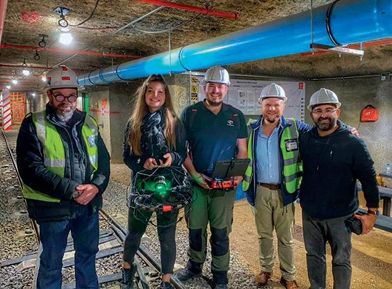
The objective of this paper is to describe the research followed in creating a generalised, readiness assessment tool for mining projects. The outcome of this process is a weighted readiness assessment tool the main benefits of which are that it will guide decision-makers and project managers through the definition phases of the project and improve the likelihood of project success. A review of remote-sensing unmanned aerial vehicles in the mining industry by M. Loots, S. Grobbelaar, and E. van der Lingen 387
.........................................
This review identifies possible improvement and innovation opportunities for the use of unmanned aerial vehicles. Fifteen applications were identified with exploration found to be the majority of the applications. From the eight remote sensing techniques identified, photogrammetry was the one most often used. Future studies could aim to include empirical data on the latest UAV applications used in the mining industry.
The prop is the most important part of the hydraulic support. When the hydraulic support is impacted by the roof, its prop is prone to extrusion deformation, expansion and even burst. The stress of doubly telescopic prop of hydraulic support under impact load was studied. The results of the finite element analysis show that the stress of the middle hydraulic cylinder is much greater than that of the bottom hydraulic cylinder under impact load. This can provide reference for prop design.
▶ iv JULY 2022 VOLUME 122 The Journal of the Southern African Institute of Mining and Metallurgy
The Potential of the YoungJournalComment
The present Student Edition had me wondering where the careers of our students showcasing their work here will take them. How many will return to their respective topics discussed in this edition during their careers, and in what way? What other reunions might our students encounter with previous assignments and experiences they embarked on as their careers progress? These reunions between the past and the present could be unexpected and intriguing. I remembered a few examples from my own career. My first job, in the mid-eighties, was in a now-defunct heavy foundry that produced mining equipment, such as winders, ball mills, crushers, and a range of dragline components. One of the flagship product lines was winders for the gold and platinum mining industry. Recently, 35 years after leaving the foundry, I helped to evaluate one of those winders. I immediately recognized the imprints from the mould assembly and the indifferent surface finish inherent to the Portland cement-based sand system used in that foundry. The winder did not show any evidence of cracking and was probably good for another three of four decades of service. That the component was completely overdesigned will probably stand the owner in good stead. It is almost counterintuitive, but the scarcity of sophisticated finite-element analyses techniques when this winder was designed will help to ensure a long service life. Some years ago, I took a group of third-year students on a visit to a power station that was still under construction. We were shown around by the commissioning personnel. It was to me, probably more than to the students, a fascinating visit, with the boilers in various states of construction. We looked down on a low-pressure turbine that was shipped from the supplier as a complete unit and had been lowered into position a few days before our visit. While looking at the casing, I realized that I remembered the patternmaker’s drawings for this component. There was an incident, many decades ago, when a skip filled with chills (small steel inserts used to affect the solidification front) dropped its load through the pattern, destroying months of patternmakers’ work. I recently helped a mechanical engineer to review the repair procedures for a very large type-316L stainless-steel tank. On working through the documentation, I discovered that the tank was fabricated by a company in Gauteng that I had visited when I started to expand the scope of welding-related activities in the Department of Materials Science and Metallurgical Engineering at the University of Pretoria. The founder and owner of the fabrication company had a very clear and useful perspective on the role that a young engineer should play in such companies: essentially, a young engineer should not spend too much time in the office, get onto the shop floor, and get some holes in his or her overalls. As far as I know, the company has disappeared, but the stainless-steel tank was still in good condition, and it was well worth repairing the few small defects that had developed in over twenty years’ service. It would be unwise to speculate what circuitous routes the careers of the students represented in these ten papers will follow. The world, Southern Africa, and the mining and metallurgical industries are rapidly evolving, and in this dynamic environment, it is unlikely that most of these papers present first steps in a highly specialized career in the respective fields of knowledge for these students. Rather, it is likely that some of these students will again be acquainted with their work in a roundabout way, possibly similarly to what I have encountered. From a different perspective, the students’ papers also embody and demonstrate two important skills, namely the ability to absorb and apply new knowledge and the ability to communicate it. These durable skills are only developed when the quality of investigative work and quality of presentation of the results (in this case, as a journal paper) are high. Finally, it is worthwhile to stay somewhat humble, and remember that some students may take the material that they are taught much further than their professors can ever anticipate. P. Pistorius University of Pretoria, South Africa
This volume is similar to previous Student Editions in that it covers a range of diverse topics, from the determination of project readiness in a mining house to the welding behaviour of ferritic stainless steels used to fabricate automotive exhaust systems. There is also significant diversity in the experimental techniques used, and the application of probability calculations is particularly noteworthy in several papers. All this illustrates the breadth, depth, and vitality of the next generation starting to contribute to the activities of the various SAIMM technical communities represented by this Journal. It is worthwhile to remember that these papers have been through the same review process as other papers submitted to the Journal.


You cannot step into the same river twice
No man indeed steps in the same river twice. The waves are different. The sand has shifted. Even if you step in, step out, and step right back in, you will still be entering a different body of water the second time. But there’s another aspect of this that is also true. Before each entry, you’ve also changed. You have new lessons learned, new relationships, and new aspects of your worldview. Not only did the river change. You did too. It means that the same actions that you take may not lead to the same result whenOverrepeated.thepast year, I have had the privilege to work with many incredibly inspiring individuals who offer their time and energy to the SAIMM through various activities. The volunteers who tirelessly, and often with very little support, manage to arrange technical events that embody the motto of the SAIMM. Leaders in their fields who carve out time to work on committees for the greater good of the mining and metallurgical industries have humbled me on many occasions with their unwavering commitment. I’ve written about volunteerism before. The SAIMM wholly relies on the knowledge, experience, and time of professionals to create this river. I’ve always loved the Heraclitus quote. It reminds me to be present and attentive, to live in the moment because everything around us is always in a state of flux. And even if we can easily see the ever-changing world around us, we often overlook how we are part of this continuous flux of change. One may of course think of this as an individual, the proverbial ‘no man’, that always undergoes inevitable change just as the river is always changing. It is also true of the SAIMM. As an Institute we also cannot step into the same river twice. I am reminded of this as my year as SAIMM President is rapidly coming to an end with July being the financial year-end and the Annual General Meeting (AGM) due in August when a new President will step into the river.The SAIMM, through tradition and organization, follows a relatively structured annual programme. So, in apparent contrast to everything always being in a state of flux, there is also a force that unifies everything, a force that cycles through the seasons. We can stand on the banks of the river of life and observe the surface or we can become part of the future by going with and becoming part of the flow of changes. We must accept and embrace change before we can influence it, or more accurately before letting ourselves influence it. My involvement in the SAIMM can be directly linked to a very specific individual who inspired me to commit time and supported me throughout my journey which culminated this past year in being privileged to lead this wonderful Institute. There have been many others along the way, but I can pinpoint the person who helped me step into the river. I have heard similar stories from others who are active in the SAIMM and who can trace back their involvement to a single mentor or colleague who pushed them, someone who issued a call to arms to them. It is a reminder to us all to be aware of how we came to be a volunteer. What inspired you to be involved? Who helped you along the way to be who you are in the SAIMM?
President’sCorner
‘No man ever steps in the same river twice, for it’s not the same river and he’s not the same man’ Heraclitus (Greek philosopher)
The Journal of the Southern African Institute of Mining and Metallurgy VOLUME 122 JULY 2022 v ◀

Sometimes inspiration is passive awareness, but most often it is enlightened awareness which requires activity. Enlightenment is what engages new members and allows them to grow and develop into the next generation of SAIMM leaders. We all need to actively be the message to people. Mentorship in its simplest form is to ensure that there is someone to follow in your path. No matter who you are, or where you volunteer, identify a few people in your sphere of influence and introduce them to the SAIMM, always remembering that it is not just a onceoff. Don’t give up. Remember that part of the journey is to step into the river but that the experience is different for everyone.
▶ vi JULY 2022 VOLUME 122 The Journal of the Southern African Institute of Mining and Metallurgy
If you are reading this and think to yourself, I want to get involved, I urge you to step into the river. Rivers flow for thousands of kilometres and nourish the land along the way. The land becomes richer because of the river flowing by it. We can do the same by making a positive impact on the people we come across every day through our actions and contributions. Rivers never flow in a straight line they crisscross the landscape and find the best path to reach their destination. Similarly, as professionals, we also need to be prepared to navigate through life’s challenges and stay the course until we reach our goals. I believe this is where the SAIMM can play a vital role in professional and personal development.
And remember: ‘If you cannot see where you are going, ask someone who has been there before. ’ (J. Loren Norris – international leadership speaker) I.J. Geldenhuys President, SAIMM President’s Corner (Continued)
During the past year I have been inspired by and filled with immense gratitude towards the many, many willing volunteers that organize branches, the (often solo) organizing chairpersons of technical events, and the leadership and active members of interest groups and key committees. And I also want us to take a moment before stepping into the river of the new year to express this gratitude to those who are helping to maintain the flow of the SAIMM river. Thank you!
Affiliation: 1Department of Materials Science and Metallurgical Engineering, University of Pretoria, Pretoria, South Africa.
323The Journal of the Southern African Institute of Mining and Metallurgy VOLUME 122 JULY 2022
TheSynopsisaimof this investigation was to determine whether the composition of a shielded-metal arc-welding electrode coating affected the low-temperature impact toughness of austenitic stainless-steel weld metal. It is generally accepted that increases in the δ-ferrite and nitrogen contents result in a decrease in toughness at low temperatures. Weld metal from electrodes with a basic coating also generally exhibit better toughness than those from rutile (acidic) electrodes. An increase in basicity was expected to decrease the number and size of inclusions, which in turn provides a tougher weld metal. Three commonly available potassium–rutile E308L electrodes were used, complying with the E308L-16 and E308L-17 specifications. Analysis of the electrode coatings showed very similar chemistry and basicity.
*Paper written on project work carried out in partial fulfilment of BEng (Metallurgical Engineering) degree
Significant differences in the inclusion contents of the weld metals were observed: the E308L-17 weld metal had a lower inclusion content (1.4% by volume) than the E308L-16 weld metal (3.7%). The former had higher impact toughness at all temperatures, despite a slightly higher nitrogen content. Regression analysis confirmed that the inclusion content had a significant effect on the impact toughness at all Shielded-metalKeywordstemperatures.
2Department of Materials Science and Engineering, University of Ghana, Accra, Ghana Correspondence to: P.G.H. Pistorius Email: pieter.pistorius@up.ac.za Dates: Received: 28 Oct. 2021 Revised: 12 Apr. 2022 Accepted: 12 Apr. 2022 Published: July 2022 How to cite: Lubbe, G., Pistorius, P.G.H., and Konadu, D.S. 2022 Effect of electrode flux composition on impact toughness of austenitic stainless-steel weld metal. Journal of the Southern African Institute of Mining and Metallurgy, vol. 122, no. 7, pp. 323–330 DOI 8157https://orcid.org/0000-0001-6582-P.G.H.ORCID9717/1879/2022http://dx.doi.org/10.17159/2411-ID::Pistorius
Effect of electrode flux composition on impact toughness of austenitic stainless-steel weld metal by G. Lubbe1, P.G.H. Pistorius1, and D.S. Konadu1,2
arc welding, inclusions, flux composition, austenitic stainless steel, ferrite number. Introduction Austenitic stainless steels are face-centred cubic Fe-Cr-Ni alloys that are widely used at low temperatures (among many other applications) due to the absence of a ductile-to-brittle transition, which is present in steels with a ferritic body-centred cubic structure (Hertzberg, 1995). Many austenitic stainless steel weld metals contain some δ-ferrite. Predictions of the amount of δ-ferrite (often expressed in terms of the ferrite number, FN) and the primary solidification mode can be made using the WRC-1992 diagram (Kotecki and Siewert, 1992). By calculating the chromium equivalent, which is the combined contributions of Cr, Mo, and Nb to ferrite formation, and the nickel equivalent, which is the combined contributions of Ni, C, N, and Cu to austenite stabilization, a prediction of FN can be made (Kotecki and Siewert, 1992). Electrode manufacturers typically guarantee a FN between 4 and 10, which indicates that the primary solidification mode will be ferritic. This decreases the probability of solidification cracking (Szumachowski and Reid, 1978). Factors that affect the impact toughness of austenitic stainless steel at lower temperatures have been extensively explored (Kamiya, Kumagai, and Kikuchi, 1992; Lee and Dew-Hughes, 1982; Read et al., 1980; Reed and Horiuchi, 1982; Szumachowski and Reid, 1978). One of the most critical factors affecting the toughness of austenitic stainless steel at low temperatures is the content and morphology of the δ-ferrite (Kamiya, Kumagai, and Kikuchi, 1992; Szumachowski and Reid, 1978). At higher impact testing temperatures, about 10% δ-ferrite resulted in the best impact toughness; however, at a testing temperature of −196°C, the presence of any δ-ferrite reduced the impact toughness (Lee and DewHughes, 1982). The effect of δ-ferrite on the impact toughness of austenitic stainless steel has been rationalized by classifying its morphology as globular, vermicular, or lacy. The presence of vermicular ferrite lowers impact toughness at lower temperatures to a greater extent than the other two forms, an effect attributed to vermicular δ-ferrite being parallel to the [100] plane, which is the preferential plane for cleavage fracture. Globular ferrite shows little to no brittle fracture because of low stress concentrations. Lacy ferrite shows little brittle fracture due to a Kurdjumov–Sachs relationship between the ferrite and

The flux was assayed by X-ray fluorescence and its basicity calculated using Equation [1]. Full-size Charpy impact test specimens were machined so that the notch was at the centreline of the butt weld and were tested according to the ASTM E229815 standard at a range of temperatures from room temperature to -196°C. The FN was determined according to AWS A4.2-98, using a Fischer MP3B Feritscope (Lippold and Kotecki, 2005). FN measurements were done on the top surface of the weld bead after light grinding. Ten FN measurements were performed on every weld bead. The weld metal chemical composition was determined on a cross-section of the welded joint by means of optical emission spectroscopy (OES). During OES analysis, care was taken to sample the weld beads, but not the base metal. The inclusion contents of the weld metals were measured in four different areas. Polished unetched sections of each weld bead were taken and nine micrographs of each sample were analysed at 100× magnification. The area fraction and sizes of the inclusions were measured using ImageJ optical analysis software. The microstructure was revealed by etching using 100 g/L oxalic acid. Additionally, polished sections of the weld metal were etched with standard aqua regia with a hydrochloric acid: nitric acid ratio of 3:1. Charpy impact fracture surfaces generated at −196°C and 20°C were examined by scanning electron microscopy.
Experimental procedure
Table I Extracts from manufacturers’ data-sheets for the electrodes used in this study
The Journal of the Southern African Institute of Mining and Metallurgy austenite phases. The most likely ferrite structure is vermicular, due to the low expected FN (Kamiya, Kumagai, and Kikuchi, 1992). A certain minimum amount of δ-ferrite is necessary to prevent solidification cracking in weld metal by ensuring the solidification of primary ferrite. Consequently, the weld metal becomes the critical part of a welded joint in low-temperature applications. Industrial focus concerning austenitic stainless steel applications at low temperatures is therefore mainly on the δ-ferrite content; other factors, such as the flux composition of the electrode coating or inclusion content of the weld metal, are paid little attention (Szumachowski and Reid, 1979).
A BI value of less than unity indicates an acidic flux, between unity and 1.2 is neutral, and above 1.2 is classified as basic (Entrekin, 1979). Researchers have noted that electrodes with a basic composition result in a weld metal with a higher impact toughness than that of rutile electrodes. For example, a linear regression model was used to predict that a basic electrode tested at −196°C would have 0.07 mm greater lateral expansion than weld metal of the same composition deposited with rutile electrodes. The associated difference in impact toughness was about 5 J (Szumachowski and Reid, 1978). From the AWS specification governing austenitic stainless steel electrodes (AWS SFA-5.4, 2006), the suffix (-15, -16, or -17) refer to the usability of an electrode with a specific coating. The -15 electrode (not available in South Africa at the time of this investigation) has a basic coating and can be used using a direct current electrode-positive (DCEP) polarity in all positions. The coatings for -16 electrodes contain readily ionizable elements (potassium is mentioned specifically in the specification); these electrodes can be used with either DCEP or alternating current (AC) in all positions. The coating of the -17 electrodes was modified by replacing some of the titanium-rich oxides in the -16 coating with silica. Similar to -16 electrodes, -17 electrodes can be used in all positions, with DCEP or AC. In older versions of the AWS SFA-5.4 specification, -16 and -17 electrodes were classified as -16. The change in usability of the -17 electrodes, associated with a slower freezing slag, necessitated separation of the -16 and -17 electrode types. The specification does not define differences in chemical composition of either the electrode coating or of the weldThedeposit.aimof this investigation was to determine the effect of the inclusion content from varying flux compositions on the lowtemperature impact toughness of austenitic stainless-steel weld metal, using commonly available electrodes.
Effect of electrode flux composition on impact toughness of austenitic stainless-steel weld metal
Fluxes for shielded-metal arc-welding processes can be classified as rutile, basic-rutile, or basic. Constituents such as SiO2, Al2O3, and TiO2 that are present in acidic fluxes are oxide networkformers and generally increase the size and number of oxide inclusions in the weld metal compared with basic and neutral fluxes. Basic fluxes contain constituents such as CaO and MgO, which break the networks created by silica (Entrekin, 1979). The basicity index (BI) is calculated in terms of the mass percentages of the various components: [1]
AISI 304L austenitic stainless-steel plates, 200 mm long × 150 mm wide × 15 mm thick, were used to fabricate butt welds with double bevel edges with an included angle of 60°. The root opening was 3 mm, which is typical practice. A Lincoln Electric S350 power supply was used. A multipass weld was deposited in a horizontal flat welding position. The welding current varied between 100 and 140 A, closely following the limits set by the electrode manufacturers. The heat input and, as a consequence, the weld bead size was reasonably constant for the different weld beads in a specific weld bead, and between different butt welds.
324 JULY 2022 VOLUME 122
Electrode A B C Electrode type E308L-16 E308L-16 E308L-17 FN 4-10 3-10 3-10 Impact toughness (J) 20°C 67 70 70 -50°C 48 -60°C 38 49 -196°C 36
E308L electrodes with a diameter of 4 mm from three different suppliers were used. Electrodes A and B were of E308L-16 type and electrode C was E308L-17; the electrode type was as stated by the electrode manufacturer. Extracts from the data-sheets for these electrodes and comparisons of the important parameters are given in Table I. From the data supplied by the electrode manufacturers, electrode C was expected to produce a weld deposit with slightly higher impact toughness.
Results The flux composition and basicity index of the three electrodes are given in Table II. The BI values were similar and less than unity, indicating that all three had acidic coatings (Entrekin, 1979). It is likely that the behaviour of an electrode with a specific coating does not depend only on the basicity index but also on the constituents of the electrode coating and possibly the presence of trace elements in the electrode coating. In addition, comparison
Table II Flux compositions (mass%) obtained by XRF Element Reported as
Electrode
Electrode
E308L-16 E308L-16 E308L-17 C C 1.42 1.19 1.23 S S 0.028 0.026 0.016 Mn MnO 1.34 1.71 1.72 P P₂O₅ 0.15 0.095 0.11 Si SiO₂ 24.8 21.8 20.5 Cr Cr₂O₃ 0.78 0.96 0.72 Ni NiO 0.07 0.71 0.15 Cu CuO ≤ 0.01 ≤ 0.01 ≤ 0.01 Al Al₂O₃ 5.17 4.34 4.17 V V₂O₅ ≤ 0.005 ≤ 0.005 ≤ 0.005 Ti TiO₂ 47.1 50.8 53.0 Co CoO 0.047 0.058 0.056 Ca CaO 9.09 7.10 8.15 Mg MgO ≤ 0.005 0.064 0.23 Fe FeO 6.38 7.32 6.07 K K₂O 3.06 2.97 3.28 BI 0.31 0.30 0.32 Table III Weld metal chemical compositions (mass%) from the three electrodes. The FN, as predicted from the chemical composition, is also Elementgiven Specification Sample Minimum Maximum Electrode A Electrode B Electrode C C 0.03 0.019 0.021 0.021 Mn 2.0 0.66 0.76 0.75 S 0.03 0.010 ≤ 0.005 ≤ 0.005 P 0.045 0.033 0.023 0.018 Si 0.75 0.72 0.84 0.71 Cr 18 20 18.9 20.4 19.3 Mo 0.13 0.03 0.08 Ni 8 12 9.64 9.68 9.84 Cu 0.14 0.06 0.04 Al ≤ 0.005 ≤ 0.005 ≤ 0.005 V 0.068 0.059 0.060 Nb ≤ 0.005 0.012 0.012 Ti 0.007 0.010 0.009 Co 0.12 0.058 0.036 N 0.0661 0.0598 0.0810 Creq 19.03 20.44 19.39 Nieq 11.99 11.93 12.61 Predicted FN 5 11 5
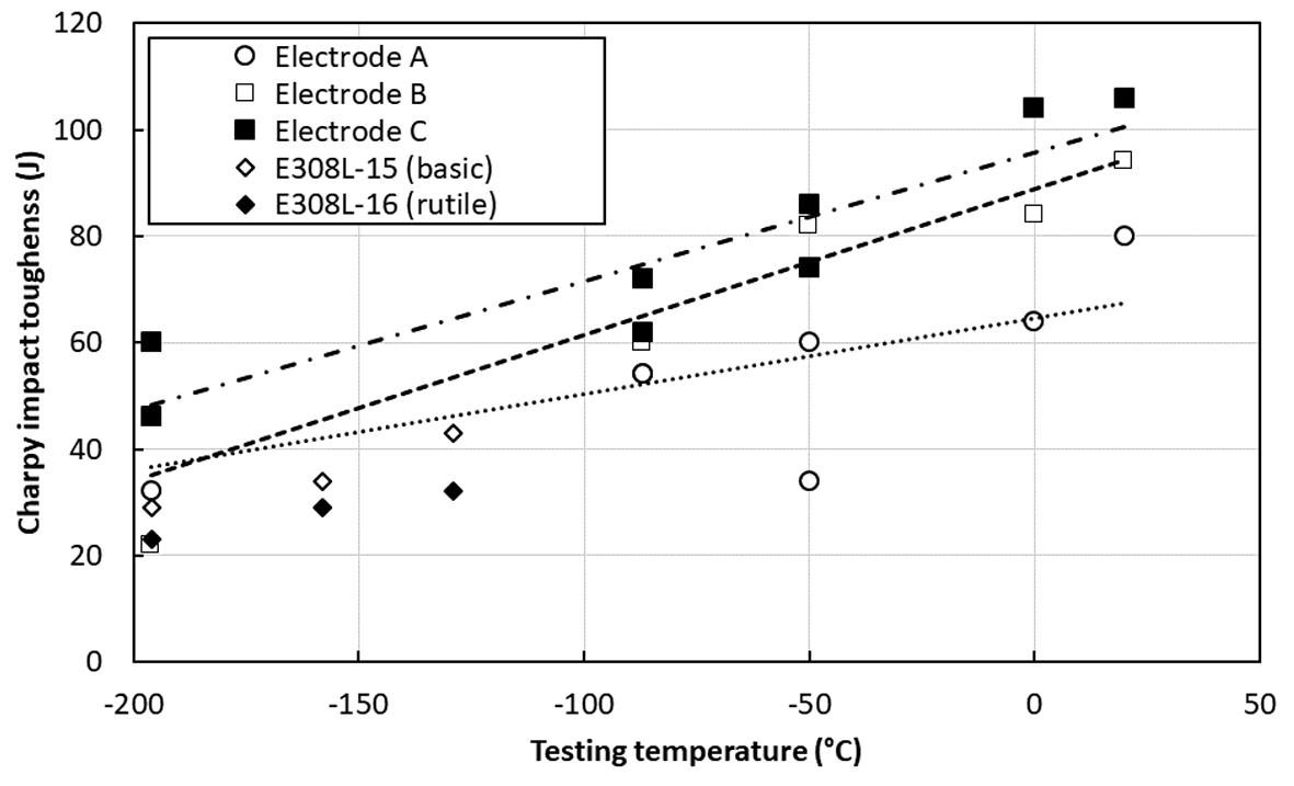
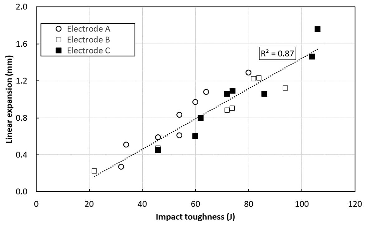
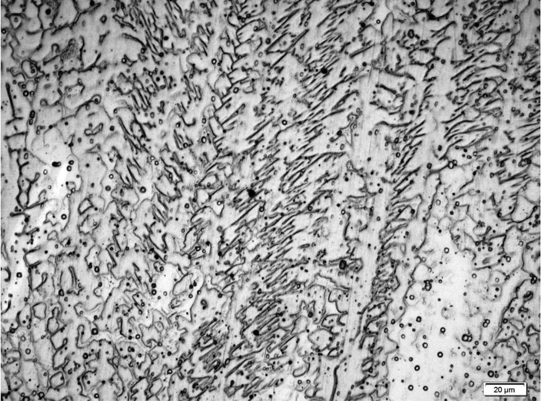
Table III gives the weld metal chemistry and predicted ferrite content (expressed as FN) of the three weld deposits. The weld metal from electrode B contained 0.84%Si, above the specified limit of 0.75%, and 20.4% Cr, marginally above the specified limit of 20%.Table IV summarizes the most important results. Electrodes A and C showed similar weld metal FN values, at 5.2 and 4.9, respectively; that from electrode B had a significantly higher FN of 9.4. The predicted solidification mode in all three cases was primary ferrite solidification, which is associated with low risk of solidification cracking (Szumachowski and Reid, 1978). The inclusion contents from electrodes A and B were similar, at 3.8% and 3.7%, respectively. Electrode C resulted in a weld deposit with a much lower inclusion content of 1.4%. The impact toughness at −196°C in relation to that at ambient temperature (R0/Rt) was lowest for electrode B, which had the highest FN. With increasing impact testing temperature, the average impact toughness values generally increased for all electrodes. With the exception of −196°C, all testing temperatures showed a gradual impact toughness increment from electrode A to electrode C. The exception was a high value of 39 J for electrode A, which decreased to 34 J for electrode B and then increased to 53 J for electrode C. Lateral expansion (LE) measurements showed similar trends to the average impact toughness values. Figure 1 shows the results of the impact tests at different temperatures as well as those of Szumachowski and Reid 1979). The latter reported lower impact toughness than this investigation, but did show higher impact toughness at all temperatures for the basic electrodes (E308L-15) compared with the rutile electrodes (E308L-16). The results of this investigation showed higher impact toughness values for these low-basicity rutile electrodes than previously published. Significant differences in impact toughness between the three electrodes were also observed. Weld metal from electrode C had the highest impact toughness value at all tested temperatures. Lateral expansion of every Charpy impact test specimen, plotted as a function of impact energy, confirmed the consistency of the impact test results (Figure 2). Figure 3 shows a typical weld metal microstructure. All three weld deposits showed a microstructure containing δ-ferrite with vermicular structure, which is associated with lower impact toughness values (Kamiya, Kumagai, and Kikuchi, 1992). Electrode A Electrode B C type
Effect of electrode flux composition on impact toughness of austenitic stainless-steel weld metal of the flux composition of electrode C (the only -17 electrode in this study) showed a lower SiO2 and a higher TiO2 content than electrodes A and B (which were -16 electrodes), contrary to the description in the relevant specification (AWS SFA-5.4, 2006). The reasons for this discrepancy between the flux composition and the stated electrode type were not clear, but could be related to a difference in usability, as determined by the electrode manufacturer, and not to the SiO2 and TiO2 content.
325The Journal of the Southern African Institute of Mining and Metallurgy VOLUME 122 JULY 2022
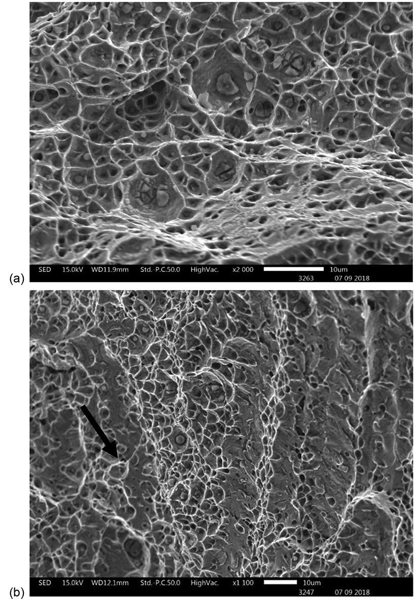
Effect of electrode flux composition on impact toughness of austenitic stainless-steel weld metal 326 JULY 2022 VOLUME 122 The Journal of the Southern African Institute of Mining and Metallurgy Figure 4 shows fracture surfaces of the impact toughness coupons tested at −196°C. The fracture surfaces displayed microvoids consistent with ductile fracture; limited cleavage fracture was observed. Typical of weld metal, inclusions were visible on all fracture surfaces. Many large broken inclusions were visible on the fracture surface of the weld metal from electrode A (Figure 4a). Figure 5 shows the particle size distribution of the inclusions as a fraction of the inclusion content in the steel. Although the Table IV Summary of results: actual ferrite number, volume fraction inclusions, impact energy (IE), and lateral expansion (LE) at a range of test temperatures, and change in impact toughness from 20°C to −196°C, expressed as R0/Rt (R0 – impact toughness at −196°C; Rt – impact toughness at 20°C) Electrode A Electrode B Electrode C Measured FN 5.2 ± 0.6 9.4 ± 1.5 - 4.9 ± 0.4 Volume fraction inclusions (%) 3.8 3.7 1.4 Testing temperature (°C) IE (J) LE (mm) IE (J) LE (mm) IE (J) LE (mm) -196 32 0.27 46 0.47 46 0.45 -196 46 0.59 22 0.22 60 0.60 -87 54 0.61 72 0.88 72 1.06 -87 54 0.83 60 0.60 62 0.80 -50 34 0.51 74 0.90 86 1.06 -50 60 0.97 82 1.22 74 1.09 0 64 1.08 84 1.23 104 1.46 20 80 1.29 94 1.12 106 1.76 R₀/RT 0.49 0.36 0.50 Figure 1—Comparison of measured impact toughness of three weld metals with published results for basic and rutile weld deposits (Szumachowski and Reid, 1978)Figure 2—Lateral expansion as a function of impact energy, as a check on the consistency of the impact test results
Broken inclusions were particularly prominent in the fracture surface of weld metal from Electrode A, which consistently exhibited the lowest impact toughness (Figure 1). The most likely explanation of this effect is that an inclusion acts as an initiation site for micro-void decohesion, as evidenced by the enlarged ‘cup’-type structures surrounding broken inclusions (Figure 4a). This indicates that an increase in inclusion content will decrease the energy required to fracture the steel and is supported by the impact results of electrodes A and B (Table IV and Figure 1), which clearly indicate that an increase in the inclusion content decreased the impact toughness of the weld metal. From Table IV, for one percentage of inclusions added to the weld metal, the impact toughness should decrease by 8.54 J. For the same increase in inclusion content, the lateral expansion should decrease by 0.091 mm. The statistical significance of these results is quantified by the P-values for the effect of inclusion content on the impact toughness (0.00036) and on the lateral expansion (0.02). A P-value below 0.05 is deemed to indicate a statistically significant effect. In contrast, the P-value for the effect of δ-ferrite content (quantified with FN) on the lateral expansion was 0.98, indicating that the FN had no statistically significant effect on the lateral expansion. The P-value for the effect of FN on the impact energy was 0.042, only marginally below 0.05. In contrast to results of previous work, the high FN of the weld metal from electrode C did not result in a significant reduction in impact toughness at lower temperatures; this was one of the surprising observations of this study. The observation that, at low testing temperatures, any δ-ferrite in the weld metal will Figure 3—Weld metal microstructure of electrode C. Original magnification 500×
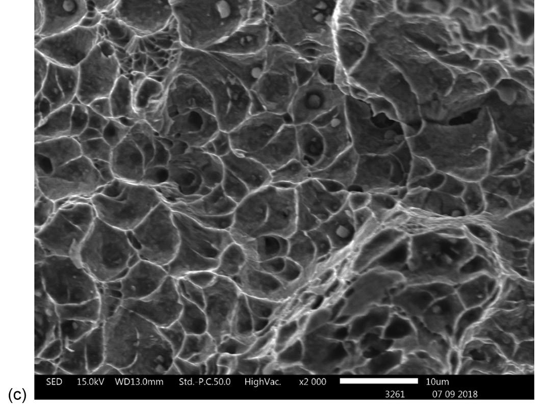
weld metal from electrode C contained fewer inclusions, there were larger particles relative to the weld metal from the other two electrodes, which had very similar particle size distributions. For electrodes A and B, the distribution of inclusion size peaked at 1 μm; for electrode C, the peak inclusion size was 3.5 μm. The total inclusion content for electrode C was lower, but this weld metal contained, on average, larger inclusions. Linear regressions of the impact energy and lateral expansion results were carried out with respect to FN, the inclusion content, and temperature as variables, as given by Equation [2]: [2] where X is either the lateral expansion (mm) or impact energy (J), A is the intercept, and A1 to A 3 are the coefficients of the indicated variables. The results are set out in Table V. Correlation coefficient R2 values of 0.85 and 0.86 were obtained for the linear regressions of the impact energy and lateral expansion, respectively.
Effect of electrode flux composition on impact toughness of austenitic stainless-steel weld metal
Discussion The results showed that the weld metal produced with electrode C had fewer inclusions and higher impact toughness at all temperatures than those of electrodes A and B. As stated, the flux basicity of this electrode was 0.32. The weld metal of electrode C had an inclusion content of 1.4%, compared with electrodes A and B with basicities of 0.31 and 0.30 which resulted in an inclusion content of about 3.78% and 3.74% , respectively. Because the flux basicities were so similar, it could not be assessed, based on this result, whether the basicity affected the inclusion content. For electrode B, the high inclusion content may be associated with the high Si content in the weld metal, as a higher Si content in the weld metal may be the result of less deoxidation of the weld metal.
327The Journal of the Southern African Institute of Mining and Metallurgy VOLUME 122 JULY 2022
For the same reason, the lower weld metal Si content and the low inclusion content of electrode C may be associated. The chemical composition of individual inclusions was not determined; such work presents a useful avenue for further study. The chemical composition of inclusions may help to explain the differences in the inclusion size that could not be explained using the current results. The large number of inclusions visible on the fracture surfaces of the scanning electron micrographs supports the hypothesis that the inclusion content affects impact toughness.
328 JULY 2022 VOLUME 122 The Journal of the Southern
4—Fracture
Effect of electrode flux composition on impact toughness of austenitic stainless-steel weld metal African
Institute of Mining and Metallurgy
Figure surfaces of weld metal Charpy impact specimens tested at −196°C, showing fracture inclusions. (a) Electrode A (measured impact tough ness: 32 J); (b) electrode B (measured impact toughness: 46 J); (c) electrode C (measured impact toughness 46 J)
Effect of electrode flux composition on impact toughness of austenitic stainless-steel weld metal Southern African Mining Metallurgy result in a reduction in impact toughness (Lee and Dew-Hughes, 1982) may provide an explanation for the high impact toughness of weld metal from electrode C at low temperatures. All three weld metals contained significant amounts of δ-ferrite (as quantified in terms of the FN), and differences in impact toughness for the three weld metals evaluated in this study were primarily related to the inclusion content.
The support of the Southern African Institute of Welding and Columbus Stainless is gratefully acknowledged.
➤ The weld metal from electrode C, which had a lower inclusion content (1.4%), had a higher impact toughness at all temperatures than the weld metals deposited from electrodes A and B, which had inclusion contents of about 3.8%.
Conclusions Three electrodes were examined to determine whether the composition of a shielded-metal arc-welding electrode coating affected the low-temperature impact toughness of austenitic stainless steel weld metal. The following conclusions were drawn from the results.
➤ The electrode coatings of electrodes A, B, and C were all acidic and showed very little difference in chemical composition or basicity.
➤ The ferrite content had no statistically significant effect on lateral expansion. Linear expansion was sensitive to the testing temperature and inclusion content.
VOLUME 122 JULY 2022
➤ The impact energy was, as expected, sensitive to the inclusion content and testing temperature. That an increase in the amount of δ-ferrite resulted in slightly higher impact toughness was unexpected.
References AWS SFA-5.4/SFA-5.4M:2006. Specification for stainless steel electrodes for shielded metal arc welding. American Welding Society, Miami, FL. EnTrekin Jr, C.H. 1979. The influence of flux basicity on weld-metal microstructure. Metallography, vol. 12, no. 4. pp. 295–312. HerTzberg, R.W. 1995. Transition temperature approach to fracture control. Deformation and Fracture Mechanics of Engineering Materials. Wiley Hoboken, NJ. pp. 375–401. Kamiya, O., Kumagai, K., and Kikuchi, Y. 1992. Effects of delta ferrite morphology on low-temperature fracture toughness of austenitic stainless steel. Quarterly Journal of the Japan Welding Society, vol. 9, no. 4. pp. 525–531. KoTecki, D.J. and SiewerT, T.A. 1992. WRC-1992 constitution diagram for stainless steel weld metals: a modification of the WRC-1988 diagram. Welding Journal, vol. 71, no. 5. pp. 171–178. Lee, K. and Dew-Hughes, D. 1982. The effect of delta-ferrite upon the low temperature mechanical properties of centrifugally cast stainless steels. Austenitic Steels at Low Temperatures. Horiuchi, T. and Reed, R.P. (eds). Springer Science & Business Media. pp. 221–242. LinnerT, G.E. 1994. Transfer of elements between SAW flux/slag and weld metal. Welding Metallurgy, Carbon and Alloy Steels, vol. 1. American Welding Society. pp. Lippold,759–761.J.C.and KoTecki, D.J. 2005. Welding Metallurgy and Weldability of Stainless Steels. Wiley Hoboken, NJ. Read, D.T., McHenry, H.I., STeinmeyer, P., and Thomas Jr, R.D. 1980. Metallurgical factors affecting the toughness of 316 L SMA weldments at cryogenic temperatures. Welding Journal, vol. 59, no. 4. pp. 104s–113s. Reed, R. and Horiuchi, T. 1982. Austenitic Stainless Steel at Low Temperatures Plenum Press, New York. Saxena, A., Kumaraswamy, A., Reddy, G., and Madhu, V. 2018. Influence of welding consumables on tensile and impact properties of multi-pass SMAW Armox 500T steel joints vis-a-vis base metal. Defence Technology, vol. 14, no. 3. pp. Szumachowski,188–195.E. and Reid, H. 1978. Cryogenic toughness of SMA austenitic stainless steel weld metals: Part l - Role of ferrite. Welding Journal, vol. 57, no. 11. pp. Szumachowski,325s–333s.E.andReid, H. 1979. Cryogenic toughness of SMA austenitic stainless steel weld metals: Part ll - Role of nitrogen. Welding Journal, vol. 58, no. 2. pp. 34s–44s. u Figure 5—Inclusion size distributions in weld metal regression results Coefficient Lateral expansion Impact energy Value Standard error P value Value Standard error P-value A (intercept) 1.52 0.12 7.01 × 10⁻¹¹ 95.3 6.56 9.85 × 10⁻¹² A₁ (inclusion content) -0.091 0.035 0.02 −8.54 1.97 0.00036 A₂ (FN) 0.00038 0.019 0.98 2.31 1.06 0.042 A₃ (temperature) 0.0043 0.00042 3.42 × 10⁻⁹ 0.23 0.02 1.08 × 10⁻⁸
Institute of
➤ The nitrogen content, in the range encountered in this study, did not affect the impact toughness or lateral expansion.
Table V Linear
and
329The Journal of the
Acknowledgements
KSB South Africa, manufactures our globally recognised pump solutions locally to the most stringent international and local quality standards. Our innovative solutions provide for the most demanding and corrosive slurry applications with superior abrasion resistance.
Wear Resistant, High PerformanceGlobal Quality Mining Pumps.
At KSB South Africa, we manufacture and service your slurry systems. We work with you one on one to find the best solution for your slurry and process pumping applications. Partner with KSB to help you meet your production goals. One team - one goal.
KSB Pumps and Valves (Pty) Ltd • www.ksb.com/en-za • Your Level 1 B-BBEE Partner
KSB South Africa is based in Johannesburg with modern manufacturing and sales facilities. With Sales & Service facilities in Southern Africa, West, Central and East Africa. KSB is represented throughout the whole country.
KSB MINING Kseb...


Affiliation: 1Department of Materials Science and Metallurgical Engineering, University of Pretoria, Pretoria, South Africa
Ferritic stainless steels, often alloyed with Ti, Nb, Mo, or some combination of these elements, are used to fabricate automotive exhaust systems. The fabrication process involves manufacturing longitudinally welded tubes that are often subsequently plastically deformed. For this reason, the welded joint must have adequate ductility. Given the cyclic nature of the temperature of an exhaust system and the high peak temperatures encountered, the weld metal is usually ferritic to avoid dissimilar thermal expansion, which is inherent in the use of an austenitic welding consumable. Ferritic weld metal is inherently less ductile than an austenitic material, so it is more difficult to achieve adequate ductility. One precondition for ferritic weld metal with adequate ductility is a solidification structure that is dominated by equiaxed grains (Villafuerte, Pardo, and Kerr, 1990). The solidification of ferritic stainless steel weld metal starts by epitaxial solidification, i.e., growth of unmelted grains (in the high-temperature heat-affected zone) into the weld pool, resulting in large columnar grains. Under specific conditions, equiaxed grains may form closer to the centre line of the weld pool (Lippold, 2014). The columnar–equiaxed transition (CET) is sensitive to, among other parameters, the Ti content of the weld metal. Villafuerte, Pardo, and Kerr (1990) reported autogenous gas–tungsten arc welding (GTAW) beads on five Type 409 ferritic stainless steels (with about 11% Cr). The welding speed was varied from 3 to 14 mm/s. The fraction of equiaxed grains in the weld metal was measured on the top surface of the weld. A low welding speed resulted in a low fraction of equiaxed grains. Once the Ti content exceeded a threshold value of about 0.18%, the fraction of equiaxed grains increased with a higher Ti content. Metallographic evidence of the role of Ti-containing particles in nucleating equiaxed grains was presented. Villafuerte, Kerr, and David (1995) confirmed the role of TiN
*Paper written on project work carried out in partial fulfilment of BEng (Metallurgical Engineering) degree FerriticSynopsisstainless steel is utilized to fabricate automotive exhaust systems using a ferritic weld metal. Ductility of the weld metal is higher if its microstructure contains a significant proportion of equiaxed grains. The formation of equiaxed (rather than columnar) grains is favoured by a higher titanium weld metal content. In this study, the Ti content of ferritic stainless steel weld metal was changed by using Tifree (Type 436) and Ti-containing (441) ferritic stainless steel as base metals. The metal-cored welding consumable contained 0.4% Ti. Gas–tungsten arc welding and gas–metal arc welding processes were compared. The weld metal Ti content ranged from zero to 0.5% Ti, as determined from scanning electron microscopy supplemented by inductively coupled plasma optical emission spectroscopy. Cross-sections of the weld beads were subjected to point counting (to estimate the fraction of equiaxed grains) and image analysis (to estimate the average grain size). Point counting proved to be more reliable. The fraction of equiaxed grains was sensitive to the Ti content, but not to the welding process. Below 0.4% Ti, the fraction of equiaxed grains gradually increased with an increase in the weld metal Ti content; above 0.4% Ti, the fraction of equiaxed grains rapidly increased with increasing Ti content. The transition in behaviour at 0.4% Ti corresponded to a Ti content at which Ti-rich precipitates became stable at the estimated liquidus temperature of the weld metal.
Dates: Received: 13 Dec. 2021 Accepted: 23 Feb. 2022 Published: July 2022 How to cite: Linda, L.S. and Pistorius, P.G.H. 2022 Effect of titanium content on solidification structure of ferritic stainless steel gas–tungsten and gas–metal arc welds. Journal of the Southern African Institute of Mining and Metallurgy, vol. 122, no. 7, pp. 331–336 DOI 8157https://orcid.org/0000-0001-6582-P.G.H.ORCID9717/1944/2022http://dx.doi.org/10.17159/2411-ID::Pistorius
Effect of titanium content on solidification structure of ferritic stainless steel gas–tungsten and gas–metal arc welds by L.S. Linda*1 and P.G.H Pistorius1
ferriticKeywordsstainless
Correspondence to: P.G.H. Pistorius Email: pieter.pistorius@up.ac.za
331The Journal of the Southern African Institute of Mining and Metallurgy VOLUME 122 JULY 2022
steel, fusion welding, solidification structure, columnar-to-equiaxed transition, Introductiontitanium.
Typical of industrial practice, the wire feed was pulsed. A constant current programme was used (program 375 on the Lincoln Electric S350 Power Wave welding power supply). For the GMAW, the wire feed speed, welding current, and welding speed were varied to achieve full penetration welds, using pulsed-spray transfer with an Ar–2% O2 shielding gas. For both processes, pure Ar backing gas was used. The welding parameters for both processes are noted in Table II. Wide ranges of welding speeds and currents were used. Given the objective to achieve full-penetration welded joints on thin sheet, the heat input was low and did not vary significantly.
Samples were sectioned transverse to the weld, hot mounted, ground, polished to a 1 μm finish, and etched using Villella’s reagent (1 g picric acid, 5 ml hydrochloric acid, and 100 ml ethanol). Energy-dispersive X-ray spectroscopy scanning microscopy (SEM–EDS, JEOL JSM-IT300, Japan, equipped with Aztec software) was employed to determine the chemical composition of the base and weld metals. In addition, several welds were removed by sectioning and submitted for analysis using inductively coupled plasma optical emission spectroscopy (ICP–OES).Thefraction of equiaxed grains in the weld metal was determined by two techniques: manual point counting and image analysis. A monotone image of the grain boundaries of each Table I
Characterization of weld metal
Two ferritic stainless steel base metals were used: Grade 436 (a Mo-containing steel with no intentional Ti addition) and Grade 441 (with nominally 0.2% Ti). Compositions are shown in Table I. A metal-cored welding consumable with a nominal Ti content of 0.4% was used. The plate thickness was 1.5 mm (Grade 436) or 1.2 mm (Grade 441). The base metal was cut into strips with a width of 50 mm and wiped down with alcohol to remove oil, dust, and other surface impurities before welding. Two welding processes were used: GTAW and GMAW. For the GTAW, two welds were autogenous (without filler wire); for the rest of the GTAW beads the metal-cored filler wire was used with a range of welding currents and wire feed speeds. Pure argon was used as the shielding gas. The welding speed was approximately 5 mm/s.
Experimental procedure
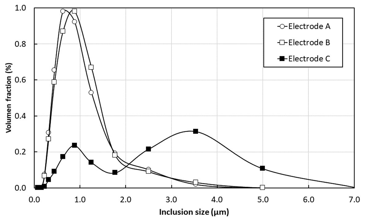
Effect of titanium content on solidification structure of ferritic stainless steel gas the Southern African Institute of Mining and Metallurgy particles in nucleating equiaxed grains by quenching stationary GTAW beads with liquid tin. Villaret et al. (2013a) used gas–metal arc welding (GMAW) to deposit weld beads on a Grade 444 ferritic stainless steel (19% Cr, 2% Mo, 0.6% Nb) using various metalcored welding consumables. The Ti content of the weld metal varied from 0.045% to 0.35%. The fraction of equiaxed grains in the weld metal was measured on a cross-section of the weld, presumably sampling the complete weld bead. A Ti content of 0.15% resulted in weld metal that was fully equiaxed. Villaret et al (2013b) subsequently confirmed these results and noted that an equiaxed weld metal structure could accommodate some plastic deformation.Villaret,Deschaux-Beaume, and Bordreuil (2016) developed a solidification model for the CET in Ti-containing ferritic stainless steels. The volume fraction of Ti-rich precipitates was considered to play an important role in the CET: weld metal, with higher Ti content contained more and larger Ti-rich precipitates. Prins (2020) reported the effect of autogenous GTAW parameters on the fraction of equiaxed grains in the weld metal of two ferritic stainless steels: Type 436 (with no Ti) and Type 441 (containing 0.18% Ti). The fraction of equiaxed grains in more than 200 welded joints were reported. No combination of welding parameters resulted in the formation of equiaxed grains in the Type 436 weld metal; for the Type 441 weld metal, the fraction of equiaxed grains varied from approximately 0.2 to approximately 0.8, with no clear effect of welding parameters or combination of welding parameters. All these results, which strictly speaking are not fully comparable owing to differences in the base metal composition, are summarized in Figure 1. No study reported a systematic change in weld metal Ti content and it is not clear whether the fraction of equiaxed grains in the weld metal was sensitive to the welding process. GMAW generally resulted in a higher fraction of equiaxed grains in the weld metal for the same Ti content, but the fraction of equiaxed grains varied significantly at a given Ti content. The aim of the current study was therefore to systematically change the weld Ti content, using two welding processes and two base metal compositions, so as to determine if the fraction of equiaxed grains in ferritic stainless steel weld metal is sensitive to the welding process or only to the Ti content.
332 JULY 2022 VOLUME 122 The Journal of
Figure 1—Published data on the effect of weld metal Ti content on the fraction of equiaxed grains in different grades of ferritic stainless steel weld metals (key to data: 1: pulsed GMAW Villaret et al., 2013a; 2: short circuit GMAW, Villaret, et al., 2013a, 3: GTAW 3 mm/s Villafuerte, Pardo, and Kerr, 1990; 4: GTAW 14 mm/s Villafuerte, Pardo, and Kerr, 1990; 5: Grade 441 Prins, 2020, 6: Grade 436: Prins, 2020)
Welding parameters
Chemical compositions (mass%) of Type 436 and Type 441 base metal and T439Ti metal-cored welding consumable, as certified by supplier Cast number C Si Mn Ni Cr Mo Nb Ti 436 base metal 4212173 0.01 0.39 0.41 0.02 17.4 0.82 0.38 0.002 441 base metal 4199474 0.01 0.51 0.37 0.01 17.6 0.08 0.41 0.18 T439Ti wire ED034209 0.02 0.60 0.60 17.5 0.01 0.40
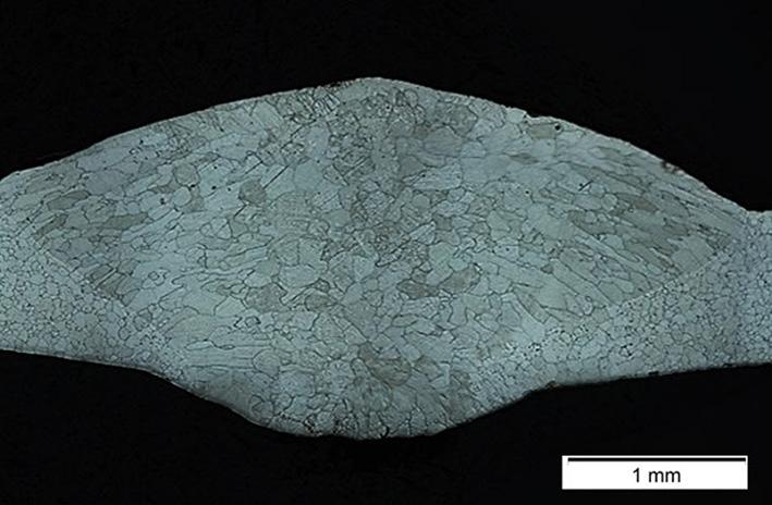
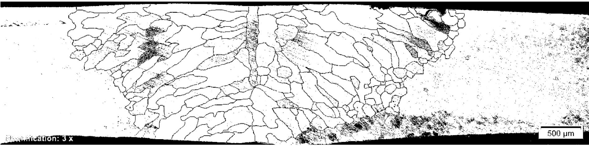
A typical cross-section of a welded joint is shown in Figure 3, with a mixture of long columnar grains and, towards the centre of the weld bead, smaller, more equiaxed grains. The fraction of Table II
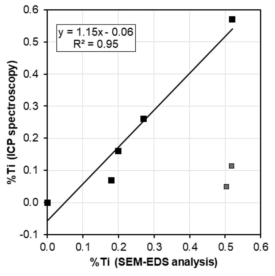
➤ The cumulative area fraction of grains with a Dmax/Dmin below a specific value was determined. Results and discussion SEM-EDS analysis is considered a semi-quantitative technique, so selected samples covering a range of Ti contents were submitted for ICP–OES analysis. The results are presented in Table III and Figure 2. Two analyses were obviously incorrect and were discarded. From the remaining five analyses, a correction to the SEM–EDS analysis could be defined (as shown in Figure 2). The average of the absolute value of the correction was 0.02% Ti, with a maximum of 0.05% Ti. The corrected values for the Ti content are reported in this document. The C content varied significantly, from about 0.01% to 0.1%; the N content was more stable, with an average of about 150 ppm.
GMAW 441 A 98% Ar–O₂ 23.3 122 21 0.12 GMAW 441 B 98% Ar–O₂ 16.7 93 20 0.13 GMAW 441 C 98% Ar–O₂ 16.7 50 17 0.13 GMAW 441 D 98% Ar–O₂ 8.3 50 19 0.08 GTAW 441 E 100% Ar 4.8 60 11 0.13 GTAW 441 1_1 100% Ar 4.8 65 10 0.16 GTAW 441 F 100% Ar 4.8 65 10 0.13 GTAW 441 G 100% Ar 4.8 65 9 0.11 GMAW 436 H 98% Ar–O₂ 10.0 56 18 0.11 GMAW 436 I 98% Ar–O₂ 10.0 57 18 0.12 GMAW 436 J 98% Ar–O₂ 8.3 60 18 0.17 GMAW 436 K 98% Ar–O₂ 16.7 117 20 0.16 GTAW 436 L 100% Ar 5.3 75 10 0.19 GTAW 436 M 100% Ar 4.8 75 10 0.14 GTAW 436 N 100% Ar 5.0 75 10 0.15 Table III Comparison of Ti content, as determined using SEM–EDS and ICP–OES. The carbon and nitrogen contents are also shown Sample Ti (%) (SEM) Ti (%) (ICP) C (%)(ICP) N (%) (ICP) GMAW 441 A ¹ 0.51 0.047 0.010 0.0166 GTAW 441 1_1₂ 0.27 0.260 0.015 0.0163 GMAW 436 H₃ 0.52 0.113 0.110 0.0156 GTAW 436 N 0.18 0.069 0.010 0.0160 441 base metal 0.20 0.161 0.024 0.0143 436 base metal 0.00 0.000 0.110 0.0143 T439Ti welding consumable 0.52 0.570 0.027 0.0145 ¹CPNotes:analysis disregarded – see Figure 2. ²Duplicate weld, generated for ICP analysis. ³Disregarded – incomplete weld penetration meant that specimen contained base metal and weld metal. Figure 2—Comparison of Ti content, as determined by SEM–EDS and ICP–OES
➤ The grain dimension (average of D max and Dmin) was calculated for each grain and the average dimension for all grains on a cross-section (weighted by the area of each grain on the polished surface) was calculated.
Effect of titanium content on solidification structure of ferritic stainless steel gas African
Sample ID Shielding gas Welding speed (mm/s) Average current (A) Average welding voltage (V) Heat input (kJ/mm)
welded joint was generated for image analysis. The maximum dimension of each grain (Dmax) was determined manually. The maximum dimension perpendicular to D max (Dmin) and cross-sectional area were then calculated by automated image processing (using ImageJ open-source software). Depending on the fraction of equiaxed grains and grain size on a specific crosssection, between about 130 and 380 grains were measured to fully characterize the cross-section of each welded joint. The results were processed as follows.
➤ The distribution of the ratio D max /Dmin, expressed in terms of the number of grains falling within a specific range of Dmax/Dmin, was determined.
Welding parameters
333The Journal of the Southern
Institute of Mining and Metallurgy VOLUME 122 JULY 2022
Institute of
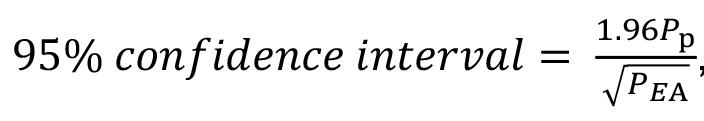
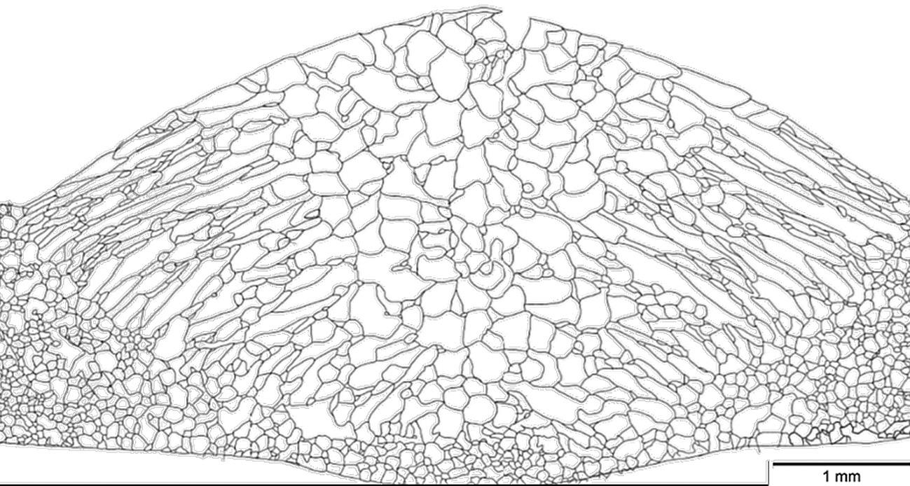
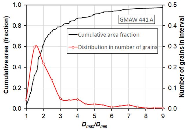
equiaxed grains was determined using manual point counting: a grid of points was superimposed on an image of the specific weld bead and the number of points falling on equiaxed grains and total number of grains in the weld metal were counted. The fraction of equiaxed grains was estimated from the ratio of the number of points falling on equiaxed grains divided by the total number of points in the weld metal area. The confidence interval was estimated using the equation proposed by Underwood (1970): [1] where P p and PEA are the fraction and number of points on equiaxed grains, respectively. Figures 4 to 6 show typical monotone images. Figure 7 shows an example of the results of image processing for the welded joint represented by Figures 3 and 4. The distribution of Dmax/Dmin, while relatively easy to interpret, could be skewed by the presence of a small number of very large grains that were sometimes observed in weld metal with low Ti content (see, for example, Figure 5). Calculation of the cumulative area fraction of the welded joint with an increase in Dmax/Dmin ratio eliminated this problem; however, quantifying the weld metal microstructure in terms of the Dmax/Dmin ratio for each grain did not distinguish between large grains and small grains. Furthermore, using a parameter based on Dmax/Dmin did not permit comparison of the results of this study with previous work. The fraction of equiaxed grains therefore proved to be the most suitable parameter to describe the weld metal
Figure 5—Grain boundaries of an autogenous weld in Type 436 ferritic stainless steel, containing very little Ti and a low fraction of equiaxed grains (GTAW 436 L)
and Metallurgy
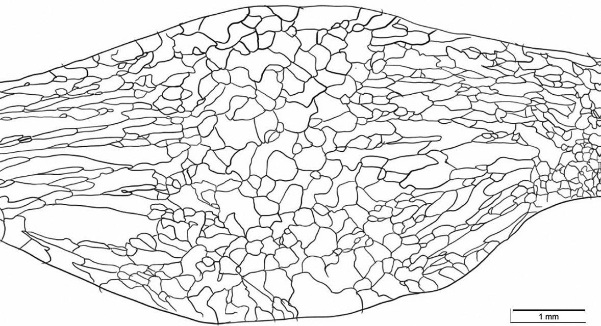
Figure 3—Typical cross-section of ferritic stainless steel weld deposited using GMAW (weld GMAW 441 A). The fraction of equiaxed grains is esti mated at 0.83 ± 0.10
Figure 6—Grain boundaries of a GTAW bead in Type 441 ferritic stainless steel, containing about 0.5% Ti (weld GTAW 441 D). The fraction of equiaxed grains is estimated at 0.47 ± 0.06
Figure 7—Distribution in ratio of major to minor grain dimensions (Dmax/ Dmin) and cumulative distribution (expressed in terms of surface area) in ratio (Dmax/Dmin) for the weld shown in Figure 3 and 4 (Weld 441 A)
334 JULY 2022 VOLUME 122 The Journal of the Southern
Effect of titanium content on solidification structure of ferritic stainless steel gas African Mining
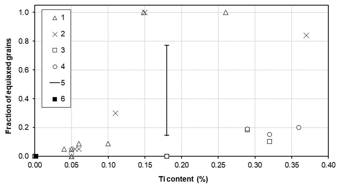
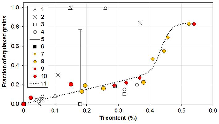
Resultsmicrostructure.forthefraction of equiaxed grains (as determined using point counting) and Ti content (measured using SEMEDS and corrected according to the ICP analyses) are presented in Table IV and Figure 8. Published data (Figure 1) is included in Figure 8 for ease of comparison. A wide range of weld metal Ti contents was achieved. There was no apparent difference in the fraction of equiaxed grains in the weld metal for GTAW and GMAW beads for similar Ti contents. The fraction of equiaxed grains gradually increased with a higher Ti content, up to approximately 0.4% Ti; above this value, the fraction of equiaxed grains in the weld metal increased rapidly and nonlinearly, reaching a plateau of approximately 0.80. Given the wide range of welding speeds used, the consistency of the fraction of equiaxed grains in the weld metal was unexpected: the Ti content apparently dominated the CET in these steels. Villaret
Figure 4—Grain boundaries of ferritic stainless steel weld shown in Figure 3 (weld GMAW 441 A)
Measured
analysis
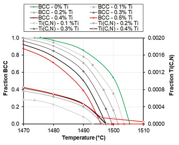
(%) Corrected Ti equiaxed grains of points equiaxed grains (SEM–EDS) content (%) GMAW 441 A 288 346 0.83 ± 0.10 0.51 0.52 GMAW 441 B 332 480 0.69 ± 0.07 0.45 0.46 GMAW 441 C 259 472 0.55 ± 0.07 0.44 0.45 GMAW 441 D 247 528 0.47 ± 0.06 0.41 0.41 GTAW 441 E 60 459 0.13 ± 0.03 0.21 0.18 GTAW 441 1_1 67 412 0.16 ± 0.04 0.27 0.25 GTAW 441 F 102 450 0.23 ± 0.04 0.38 0.38 GTAW 441 G 62 320 0.19 ± 0.05 0.22 0.20 GMAW 436 H 473 570 0.83 ± 0.07 0.52 0.54 GMAW 436 I 129 477 0.27 ± 0.05 0.37 0.37 GMAW 436 J 83 434 0.19 ± 0.04 0.30 0.29 GMAW 436 K 141 636 0.22 ± 0.04 0.33 0.33 GTAW 436 L 0 495 0 0.00 0.00 GTAW 436 M 31 480 0.06 ± 0.02 0.07 0.02 GTAW 436 N 45 220 0.20 ± 0.06 0.18 0.15 Figure 9—Changes in ferrite (body-centred cubic, BCC) and Ti(C,N) phases as a function of temperature under equilibrium conditions, esti mated using Thermo-Calc, for hypothetical chemical compositions based on Type 441 stainless steel with 0%, 0.3%, 0.4%, and 0.5% Ti
below.Possible
and
data Sample ID Number of points in Total number Estimated
et al. (2013a) reported a high fraction of equiaxed grains in Type 444 weld metal with more that 0.15% Ti, well below the 0.4% Ti observed during the current study. The Type 444 weld metal also contained 19% Cr, 2% Mo, and between 0.21 and 0.71% Nb. The low Ti content that is necessary to achieve a high fraction of equiaxed grains in 444 weld metal may be related to the high Nb content and the associated wider solifidifcation range (Konadu and Pistorius, 2021); this argument is explored in more detail reasons for the effect of Ti on the solidification structure were explored using Thermo-Calc software to estimate the amounts of specific phases present at a given temperature under equilibrium conditions. A weld pool, especially the very small weld pools encountered in the current study, cools down very rapidly, so solidification and solid-state phase transformations occur under conditions far from equilibrium. However, the equilibrium conditions represent a first-order approximation of the likely sequence of phase transformations. The chemical composition of Type 441 ferritic stainless steel (Table I) was used for the Thermo-Calc estimates. The Ti content was varied from zero to 0.5% Ti, which covered the full range of Ti contents encountered in this study. The results, summarized in Figure 9, show the ferrite and Ti(C,N) contents as a function of temperature from 0% to 0.5% Ti. Higher Ti content resulted in a gradual decrease in the liquidus temperature (the temperature at which the first ferrite forms during solidification) and solidus temperature (the temperature at which the last liquid disappears on cooling, not shown). As the Ti content increased, the Ti(C,N) content at a specific temperature did not increase significantly until approximately 0.5% Ti. At approximately 0.4% Ti, the liquidus temperature (the temperature at which the formation of ferrite from the liquid metal becomes thermodynamically possible) is similar to the temperature at which the first Ti(C,N) becomes thermodynamically stable on cooling. If Ti-rich precipitates were present at or above the liquidus temperature, heterogenous nucleation of ferrite on Ti(C,N) precipitates and the associated formation of equiaxed grains would be thermodynamically possible. The Thermo-Calc estimates for the changes in fractions of ferrite and Ti(C,N) with temperature were therefore consistent with the abrupt change in the fraction of equiaxed grains as the Ti content of the weld metal increased. The validity of using equilibrium data to estimate the minimum Ti content in a weld metal required to achieve equiaxed
Table IV Fraction
Effect of titanium content on solidification structure of ferritic stainless steel gas
335The Journal of the Southern African Institute of Mining and Metallurgy VOLUME 122 JULY 2022
Figure 8—Change in fraction of equiaxed grains as a function of Ti content (key to data: 1: pulsed GMAW, Villaret, et al., 2013a; 2: short circuit GMAW, Villaret et al., 2013a; 3: GTAW 3 mm/s Villafuerte, Pardo, and Kerr, 1990; 4: GTAW 14 mm/s Villafuerte et al., 1990; 5: Grade 441 Prins, 2020, 6: Grade 436: Prins, 2020; 7: current study GMAW 441; 8: current study GTAW 441; 9: current study GMAW 436; 10: GTAW 436; 11: interpolation of current results) of equiaxed grains (determined using manual point counting) Ti content of weld metal. SEM–EDS of Ti content corrected by reference to ICP fraction Ti
was
The Journal of the Southern African Institute of Mining and Metallurgy grains was verified by reviewing the data for the five Type 409 steels reported by Villafuerte, Pardo, and Kerr (1990), shown in Figure 10. With one exception (a welding speed of 14 mm/s), equiaxed grains were only present if the weld metal contained more than 0.2% Ti, and usually more than 0.28% Ti. The average chemical composition of these steels was calculated as (%) 11.2 Cr, 0.24 Ni, 0.009 C, 0.03 Al, 0.40 Mn, 0.45 Si. A Thermo-Calc estimate of the fractions of ferrite and Ti(C,N) as a function of temperature for this steel was calculated for variation in Ti content from 0.1% to 0.4% in 0.1% Ti increments. The results of these calculations are shown in Figure 11. Similar to the behaviour of Type 441 weld metal, the fraction of equiaxed grains started to increase only once the Ti content was high enough that, under equilibrium conditions, Ti(C,N) precipitates were present at the liquidus temperature. The difference in the minimum amount of Ti necessary for the formation of a significant fraction of equiaxed grains in the weld metal between Type 441 (approximately 0.4% Ti) and Type 409 (0.2%–0.3% Ti) is therefore related to the liquidus temperature and stability of the Ti(C,N) precipitate. The implication of the results of the current study is that a minimum Ti content is necessary for a ferritic stainless steel weld to contain a substantial proportion of equiaxed grains. The minimum amount of Ti necessary to achieve a substantially equiaxed structure is sensitive to the chemical composition of the specific grade of stainless steel: for Types 436 and 441, at least 0.4% Ti must be present in the weld metal to achieve a substantially equiaxed structure. The weld metal Ti content can be present in the base metal and an autogenous weld may be used. If a Ti-containing welding consumable is used, the Ti content of the weld metal can be considerably higher than that of the base metal. The high dilution (fraction of weld metal contributed by melting of the base metal) inherent in GTAW limits the maximum Ti content and therefore the fraction of equiaxed grains; if GMAW is used, weld metal with a high Ti content and a high fraction of equiaxed grains can be achieved.
➤ The response of the fraction of equiaxed grains to an increase in the Ti content of the weld metal was characterized by a gradual increase in the fraction of equiaxed grains up to a specific Ti content; above that value, the fraction of equiaxed grains increased rapidly with increasing Ti content. Thermodynamic modelling indicated that the transition in behaviour correlated with a Ti content at which some Ti(C,N) was stable at the predicted liquidus of the weld metal.
The Southern African Institute of Welding and Columbus Stainless provided financial support. Studies by several undergraduate students on the welding of ferritic stainless steels in recent years are recognized. S.S. Mahlalela contributed the Thermo-Calc data. References Konadu, D.S. and PisTorius, P.G.H. 2021. Investigation of formation of precipitates and solidification temperatures of ferritic stainless steels using differential scanning calorimetry and Thermo-Calc simulation. Sādhanā, vol. 46, no. 3. pp. Lippold,1–8.J.C. 2014. Welding Metallurgy and Weldability. Wiley. Prins, H.J. 2020. The effects of autogenous gas tungsten arc welding parameters on the solidification structure of two ferritic stainless steels. MEng thesis, University of Pretoria, South Africa. Underwood, E.E. 1970. Quantitative Stereology. Addison Wesley, Reading. p. 23. VillafuerTe, J.C., Pardo, E., and Kerr, H.W. 1990. The effect of alloy composition and welding conditions on columnar-equiaxed transitions in ferritic stainless steel gas-tungsten arc welds. Metallurgical Transactions A, vol. 21, no. 7. pp. Villafuer2009–2019.Te,J.C.,Kerr, H.W., and David, S.A . 1995. Mechanisms of equiaxed grain formation in ferritic stainless steel gas tungsten arc welds. Materials Science and Engineering A, vol. 194, no. 2. pp. 187–191. VillareT, V., Deschaux-Beaume, F., Bordreuil, C., RouqueTTe, S., and ChoveT, C 2013a. Influence of filler wire composition on weld microstructures of a 444 ferritic stainless steel grade. Journal of Materials Processing Technology, vol. 213, no. 9. pp. 1538–1547. https://doi.org/10.1016/j.jmatprotec.2013.03.026 VillareT, V., Deschaux-Beaume, F., Bordreuil, C., Fras, G., ChoveT, C., PeTiT, B., and Faivre, L. 2013b. Characterization of gas metal arc welding welds obtained with new high Cr–Mo ferritic stainless steel filler wires. Materials & Design, vol. 51. pp. 474–483. https://doi.org/10.1016/j.matdes.2013.04.054
Acknowledgements
Effect of titanium content on solidification structure of ferritic stainless steel gas
➤ The Ti content of the weld metal was determined by the Ti content of the base metal, the degree of dilution (dependent on the welding process used), and whether a Ti-containing welding consumable was used.
VillareT, V., Deschaux-Beaume, F., and Bordreuil, C. 2016. A solidification model for the columnar to equiaxed transition in welding of a Cr-Mo ferritic stainless steel with Ti as inoculant. Journal of Materials Processing Technology, vol. 233. pp. 115–124. https://doi.org/10.1016/j.jmatprotec.2016.02.017 u Figure 10—Data reported by Villafuerte, Pardo, and Kerr (1990) for the fraction of equiaxed grains observed on the surface of Type 409 stainless steel welds as a function of Ti content. The dotted lines are as proposed by Villafuerte, Pardo, and Kerr (1990) Figure 11—Changes in ferrite (body-centred cubic, BCC) and Ti(C,N) phases as a function of temperature under equilibrium conditions, esti mated using Thermo-Calc, for hypothetical chemical compositions based on the average composition of Type 409 steels reported by Villafuerte Pardo, and Kerr (1990), with the Ti content as indicated
Conclusions ➤ For the weld metal characterized in this study, the fraction of equiaxed grains in a ferritic stainless weld is dependent on the Ti content, but is not sensitive to the welding process. ➤ The use of SEM-EDS resulted in a reasonably accurate determination of the Ti content of the weld metal, with a correction (based on ICP-OES analyses) that did not exceed 0.05% Ti.
336 JULY 2022 VOLUME 122
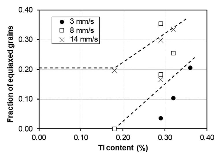
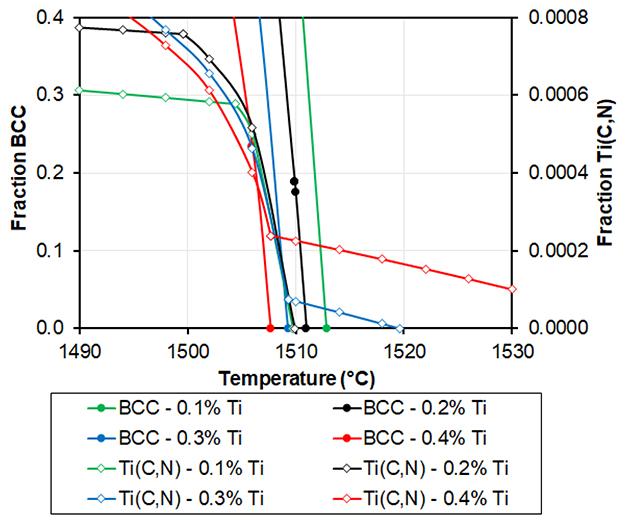
Published:
337The Journal of the Southern African Institute of Mining and Metallurgy VOLUME 122 JULY 2022
Correspondence to: C.C. Birch Email: clinton.birch@wits.ac.za Received: Oct. 2020 16 May 2022 16 May 2022 July 2022 Birch, C.C. estimation uncertainty A case study of Witwatersrand goldproducing areas. the Southern African Institute of Mining and Metallurgy, 122, no. 7, pp. 337–346
Optimizing cut-off grade considering grade estimation uncertainty – A case study of Witwatersrand goldproducing areas by C.C. Birch DueSynopsistograde estimation uncertainty, two statistical errors can occur. The Type I error is where material is classified as ore and mined, despite the true value being below the break-even grade. This material is dilution. The Type II error is where the material is estimated to be below the cut-off grade and is classified as waste, although the true grade is actually above the break-even grade. This material is not mined and is lost. The uncertainty was assumed to follow a normal distribution in a previous study. For this study, estimated block values are compared to those determined after mining (the best estimate of the true grade). This actual data from four mines shows that the uncertainty follows a Laplace distribution. There is no single solution regarding adjusting the cut-off grade away from the break-even grade, considering estimation uncertainty, that could be applied to all gold mines. However, adjusting the cut-off grade downwards (up to 22% for one mine) is noted when optimizing the profit considering grade uncertainties. This type of adjustment could open up significant mining areas and extend the life of the uncertainty,Keywordsmine.
13
vol.
DOI 9717/1403/2022http://dx.doi.org/10.17159/2411-ID:
–
Journal of
Revised:
Affiliation: 1School of Mining Engineering, University of the Witwatersrand, South Africa
Accepted:
Type I error, Type II error, cut-off grade, optimization, NPV; simulation, mixed-integer linear programming, @Risk, Excel Solver.
Dates:
How to cite:
Background Some mining companies apply the concept of break-even grade to individual ore blocks and assess if each block could be exploited profitably. This break-even grade is then applied as the mining cut-off grade (Minnitt, 2004) with some adjustments. With these approaches, the overall grade of the material being mined becomes the average grade of the blocks above the break-even-derived cut-off grade. An alternative approach is to apply the pay limit principle where the overall mining grade required to break even financially is determined. Then the profit margin required is determined and added to the breakeven grade. The mining planners then check the mix of the various mining areas to ensure the required mining grade is achieved. However, these approaches fail to consider the interaction between the royalties for mineral resources and the South African gold tax formula, which varies considering the mine’s overall profitability. A revised approach to optimizing the value of gold mines was required as part of a research project to understand the impact of the 2008 Mineral and Petroleum Resources Royalty Act on gold
Optimizing2022cut-off grade considering grade
Introduction This study is a follow-up to a previous investigation (Birch, 2017) in which cut-off grade optimization was undertaken for four South African narrow, tabular (Witwatersrand-type) gold mines while considering various hypothetical degrees of uncertainty. It was found that where there are higher degrees of uncertainty in the grade, reducing the cut-off grade compared to the break-even grade can improve the financial returns. For the present study, the break-even grade is considered the grade where the income from a mining block will cover all its mining and processing costs (as defined by the all-in sustainable cost (AISC)). The management team uses the cut-off grade to determine the areas to be mined or left and effectively split ore from waste. This study considers the actual grade uncertainty for four South African gold mines. Each case study determines how the cut-off grades should be adjusted compared to the break-even grade when taking grade uncertainties into account.
The Journal of the Southern African Institute of Mining and Metallurgy mines (Birch, 2016a). Considering the mine’s current planned economic and production profile, this approach considers the entire cash flow and optimizes overall profit or net present value (NPV) for the Measured and Indicated Resource. The financial optimizer uses mixed-integer linear programming (Excel Solver) to maximize profit or net present value NPV by varying the cut-off grade. This, in turn, alters the overall tonnage and average mining grade (AMG) above the cut-off grade. The approach is simple, robust, and provides a valuable tool to quickly assess the impact of grade uncertainty without the need for extensive information from the mines themselves (Birch, 2016b). The grade for each mining block is estimated by sampling the mineral deposit and projecting the values into the area to be evaluated. Various techniques are used, including nearest neighbour, inverse distance squared, and kriging. The estimated value is used to determine if a mining block is classified as ore or waste. There is, however, a degree of uncertainty regarding the estimated value due to sampling spacing, deposit heterogeneity, and the method of estimation used. Accepting a hypothesis that should have been rejected is a Type I error in statistics. The alternative error is rejecting a hypothesis that should have been accepted, and is called a Type II error (Underhill and Bradfield, 1994). Due to uncertainty in the estimation, the same two errors can occur. The Type I error is where the material is classified as ore and mined, although the true value is below the cut-off grade and thus this is waste material and constitutes dilution. The Type II error is where the material is estimated to be below the cut-off grade and is classified as waste, whereas the true grade is above the break-even grade and it could have contributed profits if it had been mined. This material is not mined and is lost (Minnitt, 2017).
Methodology
➤ When optimizing the NPV at 12%, the one mine would benefit from an 8% decrease in the cut-off grade. The NPV benefit is, however, only 1.3%. The other three mines would not benefit from adjusting the cut-off grades and using the model results in NPVs lower than not adjusting them, as indicated in two cases.
The following points were noted.
338 JULY 2022 VOLUME 122
Optimizing cut-off grade considering grade estimation uncertainty
➤ This reduction ranged from 2–10%. The fourth mine would not benefit from any change in the cut-off grade.
➤ It was found that when optimizing for profit, three of the four mines would benefit from a reduction in the cut-off grade compared to the break-even grade.
Previous work
A previous investigation (Birch, 2017) aimed to determine what adjustment should be made to the cut-off grade to reduce the financial impact of dilution or lost ore in typical narrow, tabular Witwatersrand gold mines. Three possible options were identified: ➤ Raise the cut-off grade to reduce the dilution – ‘the old adage that a low-grade ton should never keep a high-grade ton out of the mill’ (Minnitt, 2017) ➤ Keep cut-off grades the same, considering that the Type I and Type II errors would balance each other if there is no bias ➤ Lower cut-off grades to ensure all value from the orebody is obtained (thus recovering a higher percentage of the lost ore). The mines reviewed all have mining block listings. These listings include the area (m2), channel width (cm), and the estimated in-situ grade in grams per ton (g/t). The tonnage and stoping width can be determined from these values, along with the mining grade and expected metal content. South African gold mine block listings were run through a simple financial optimizer for the previous study. Various degrees of uncertainty for the block grades were considered. This uncertainty was introduced using @Risk software (a Monte Carlo simulation program developed by Palisade). The uncertainty distribution was assumed to be symmetrical, and no bias was considered (100% block factor). The databases used for this research exercise had been corrected for conditional bias and smoothing (Tolmay, 2014). The uncertainty dispersion was controlled using the standard deviation to give 5%, 6.7%, 10%, and 20% uncertainty.
The mining block listing is the starting point for the financial model used for this study. This mining block listing contains all potential mining areas, estimated grades, and volumes created from the geological block model. For South African gold mines, the mining blocks are the same size as the geological blocks (typically 30 m by 30 m for the Measured Resource blocks and 60 m by 60 m for the Indicated Resource blocks). The determination of the break-even grade is, in essence, quite simple. It determines what grade a unit of ore requires to return a profit. This is basically a break-even volume measurement where the quantity is known (usually limited due to shaft capacity, milling capacity, or other physical constraints). The unknown is the commodity’s in-situ value. The other factors needed for the calculation of the break-even grade are the mine recovery factor (MRF), which is the mine call factor (MCF) multiplied by the plant recovery factor (PRF). The metal price is quoted in US dollars (for gold and silver, in troy ounces). These are all projections and open to variation over the time over which the break-even grade is applied. Therefore, they contribute to the investors’ financial risk if they change significantly. This can be expressed as follows (School of Mining Engineering, 2021): At break-even grade: TR = TFC +TVC but TR = UR* X and TVC = UVC * X
High uncertainties characterize mining projects. Such uncertainties vary in magnitude and are very prevalent in the geological data and subsequent grade estimation on which the project is based. The method of handling uncertainty in mining projects may significantly affect the decisions made by the management team (Kühn and Visser, 2014). There is no straightforward process for adjusting the cut-off grade away from the break-even grade for narrow tabular orebodies, considering the uncertainties related to the grade estimation.
Problem statement
The previous study assumed that the uncertainty follows a normal distribution, and there is no bias present in the estimations. This research uses ‘actual’ uncertainty distributions to determine if the same conclusions can be drawn.
➤ When optimizing for 9% NPV, three of the four mines would benefit from reducing the cut-off grade by between 7 and 27%. The fourth mine would benefit by increasing the cut-off grade by 7%.
Figure 1—The Witwatersrand gold-producing areas in South Africa (Minerals Council South Africa, 2020)
Historical mining block listings were obtained from four gold mines for this study. The mines are located in the West Rand and the Free State gold mining regions of South Africa (Figure 1). They all mine the narrow, tabular gold-bearing conglomerates of the Witwatersrand Supergroup. For anonymity purposes, these mines will be called A, B, C, and D. It is important to note that these are not the mines that were used in the previous study. The data for the previous research was for four individual shafts belonging to two different mines. The data used for that study was the block listing and financial information used for the mines’ Mineral ResourceAccompanyingStatements.the historical block grades for the minedout areas is the post-mining grade for the block. This grade is considered the ‘true’ grade. Although it is still an estimate it is the figure used by the mine surveyor to allocate the called-for grade for the block. Discrepancies between the called-for gold estimates and the final recovered gold are dealt with in the breakeven formula where the MRF is considered. The distribution of the uncertainties was based on these listings. They display a significantly different pattern from the normal distribution assumed for the previous study (Birch, 2017), and significant grade overestimation bias in three cases. The relationship between the volume (tons) available for mining and the cut-off grade, and the resulting average grade above the cut-off grade, can be determined from the gradetonnage curve.
Sources of data
Optimizing cut-off grade considering grade estimation uncertainty 339The Journal of the Southern African Institute of Mining and Metallurgy VOLUME 122 JULY 2022 Therefore: UR * X = TFC + UVC * X Dividing both sides by X: UR =(TFC÷X) + UVC But UR = g/t * r * p Therefore at break-even grade (g/t): g/t = ((TFC÷X) + UVC)÷(r*p) where g/t is the break-even grade in grams per ton; r is the mine recovery factor in %; p is the metal price in US$ per gram; TFC is the total fixed costs in US$; X is the milled tons; and UVC is the unit variable costs in US$ per t. The cut-off grade is an extension of the concept of a breakeven grade. If only blocks above break-even grade are mined, this becomes the cut-off grade. However, the cut-off grade undergoes variations over the mine’s life. Hall (2014) describes the basics of cut-off grade theory. This book is an exhaustive study of the different techniques currently used in the mining industry. It includes various value measures, including discounted cash flow (DCF) and optimization of NPV. The South African Code for the Reporting of Mineral Asset Valuation (The SAMVAL Code) income approach to valuation requires a mine design with reasonable estimates of expected tonnages, grades, costs (fixed and variable), and recoveries (Border, 1991). The cost of capital is usually calculated by the weighted average capital cost (WACC) and is expressed as a percentage. The WACC represents a company’s average cost of capital from all sources. These include equities (common stock, preferred stock, and bonds) and other forms of debt. The cost of equity can be determined using various methods, including the capital asset pricing model (CAPM) and the Gordon growth model (GGM) (School of Mining Engineering, 2021). The cost of capital of the mine is used as the discount rate for cash inflows and outflows. The NPV is the difference between the present value of cash inflows and the present value of cash outflows over a period of time (Investopedia, 2021). Real monetary mining discount rates of between 9% and 12% are suitable for South African mining projects (Smith et al., 2007). That is equivalent in nominal terms to 14.5% to 17.6% at an annual inflation rate of 5% (typical for SouthTheAfrica).financial optimizer used for this study utilizes linear mixed-integer (Excel Solver) programming. Due to its availability to all Excel users, the Solver function built into Microsoft Excel was selected for this study (Meissner and Nguyen, 2014). The variable for the Solver function is the cut-off grade, and the Solver function is set to optimize the cut-off grade to maximize the resulting profit or NPV. These cut-off grades are then compared to the base break-even grade to indicate how the cut-off grades should be adjusted considering the uncertainty in the estimated in-situ grades.
The Journal of the Southern African Institute of Mining and Metallurgy
Optimizing cut-off grade considering grade estimation uncertainty
Analysis Estimated versus true block grades
The approximate value for one mining block and the true value will be the same in a perfect world. There will be no blocks above the cut-off grade with a true value below the cut-off grade (Type I error or dilution). There will also be no blocks calculated as below cut-off grade that are actually above cut-off grade (Type II error or missing ore). This ideal relationship can be seen in Figure 2.
The difference between the estimated and true grades for each block was determined. The distribution of these variations is analysed using the Palisade @Risk Distribution Fit tool. For the previous study, normal distributions with no bias were assumed. When the variation distributions for the four mines in this study were analysed, Laplace distributions were found to fit better than normal distributions. In probability theory and statistics, the Laplace distribution is a continuous distribution of probabilities, called the double exponential distribution. It can be viewed as two exponential distributions spliced together back to back (Hilali, 2016).
Figure 2—Ideal world situation where estimated and true values are the same (zero uncertainty). All the data-points plot along a single line. No dilution or lost ore occurs. The break-even cut-off grade of 7.5 g/t is shown, as are the Type I and II error areas. It is noted that no points plot into these two areas
The distribution which best fits the data was selected using the Akaike information criterion (AIC) value. AIC compares the relative ‘quality’ of a model (distribution) with the other models. @Risk ranks the various distribution model outputs according to this value. The distribution with the smallest AIC value is usually the preferred model (BPI Consulting, 2016). Figure 4 shows the Laplace and normal distribution curves for the four mines. It is clear from the figures that the Laplace distribution curve for the variation has a far higher kurtosis (the sharpness of the peak) than the normal distribution curve in all four examples. However, the normal curve reflects the mean variation of the input data better. It shows that the grades for mines A, B, and C are over-estimated by 0.8, 0.4, and 1.0 g/t, respectively. Only mine D has an overall variation of less than 0.1 g/t. Over- or underestimation is often reflected in the block factor value, with 100% indicating no bias. These block factors were found to be 94.3%, 93.2%, 92.4%, and 99.0%, respectively for the four mines. This overestimation of the block grades is very significant. Many blocks are being identified as ore while they are subeconomic and should not be mined. Suppose the overestimation is carried through to the post-mining true grade estimation for the blocks. In that case, the MCF will also be lower than expected. The MCF is used in the break-even grade calculation. This will raise the break-even grade. Financial modelling The tons above the cut-off grade and the AMG are determined from the block listing as inputs into the financial optimizer. The block lists obtained for these mines only contained the gold grades in centimetre-grams/ton (cmg/t). Since the block listing did not include block area, channel width, or stoping width, various assumptions have been made. These assumptions are assumed not to impact the validity of this study because they do not alter the comparative nature of the results. The same assumptions have been made for all four financial models used in the current study.
A generic financial model has been utilized to compare a typical deep-level gold mine producing 1.2 Mt of ore per annum. A generic financial model has been used to highlight the effect of the uncertainty and allow direct comparisons as to the effect of this between the different mines. A gold price of US$ 1500 per ounce is assumed for this case study. For all the examples, annual fixed costs are assumed to be US$260 million, and the variable cost is US$55 per ton. The split between fixed and variable costs is 75:25. A feature of South African gold mines is that labour costs are typically 50% (Savant, 2012) of the total costs, resulting in a higher fixed cost to variable cost ratio than more typical mining projects where a 50/50 split would be appropriate (Poxleitner, 2016). The annual production rate and 75% MRF have been selected to give a break-even grade of 7.5 g/t. Break-even face grades of 7.5 g/t are typical for deep-level South African gold mines and fit into the break-even grades determined from the detailed financial figures used in the previous study (6.9–10 g/t). The NPVs were determined using discount rates of 9 and 12%.
The pre-mining estimated and post-mining true block grades were obtained from four mines for this study. The number of blocks included in the analysis ranged from 1757 to 2547 for the respective mines. The estimated grades vs the true grades for the four mines are shown in Figure 3. It can be observed that there is significant overvaluation in the estimated block grades for three of the mines. This is reflected in the slope of the trend lines. For mine A, the slope is 0.85. For mine B it is 0.87, and for mine C it is 0.86. This is significant because it shows a clear bias in the estimation, which was not considered in the previous study (Birch, 2017). For mine D, the bias is far less, and the slope is 0.95. This overestimation of the block grades has a marked impact on the suggested cut-off grade optimization adjustments shown later in the analysis. The R2 values for the four mines range from 0.54 to 0.69. This shows a significant spread of the data-points and a poor correlation between the estimated and true values. A perfect correlation would result in an R2 value of 1.0 (see Figure 2). This poor correlation results in numerous points plotting in the graphs’ Type I (dilution) and Type II (lost ore) areas.
340 JULY 2022 VOLUME 122
Variation distribution
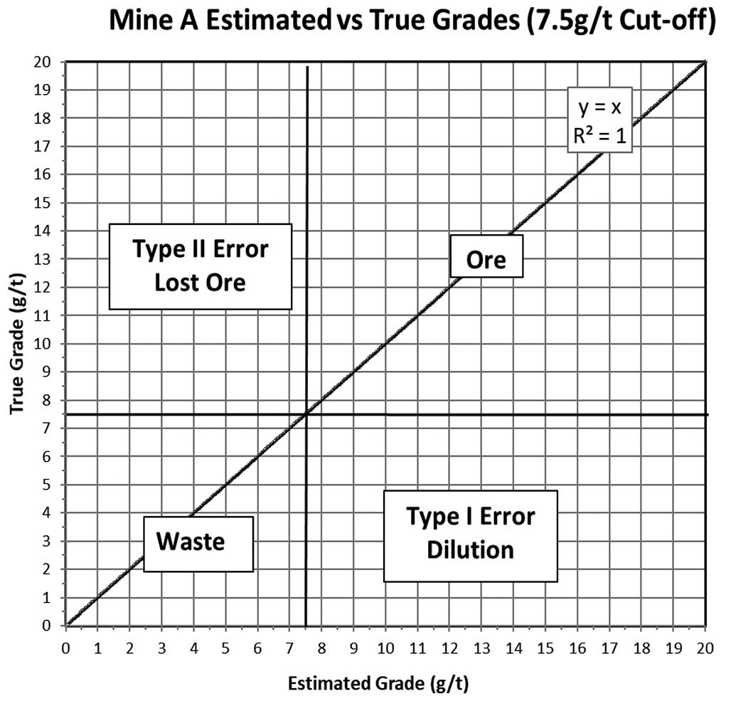
Some companies model accumulation value (cmg/t) rather than grade (g/t). Accumulation value is helpful for very narrow orebodies because it gives the metal content, rather than just the grade, over the mineralized width. The accumulation value is calculated by multiplying the grade of the sample by the width the sample represents. Multiple samples are taken and composited when sampling narrow tabular orebodies to get the average grade over the mineralized width. Each sample grade is multiplied by the width (in centimetres), and then all the individual values are summed. This combined value is then the value in cmg/t. This value can then be divided by the expected mining width, and the average mining face grade of the block determined. A 1000 cmg/t over 1 m will result in a face grade of 10 g/t. It is possible then to compare the metal content with a very narrow 1 cm mineralized zone with 1000 g/t (for example, the carbon-rich facies of the Basal Reef) to one with a 100 cm mineralized width with a grade of 10 g/t. Both faces will have the same mining face grade of 10 g/t if the minimum mining width is 100 cm. However, since this parameter is not widely used except on South African gold mines, it has been converted to grams per ton for easy explanation. The expected face grade for this study was determined for each block by dividing the cmg/t by a standard stoping width of 150 cm to get the face grade in grams per ton. This block area needs to exceed the smallest mining unit size determined by the mine design approach. Typical mining panels in deep-level South African gold mines are 30 m long.
341The Journal of the Southern African Institute of Mining and Metallurgy VOLUME 122 JULY 2022
Figure 3—Pre-mining estimated vs post-mining true block grades for mines A, B, C, and D
Optimizing cut-off grade considering grade estimation uncertainty
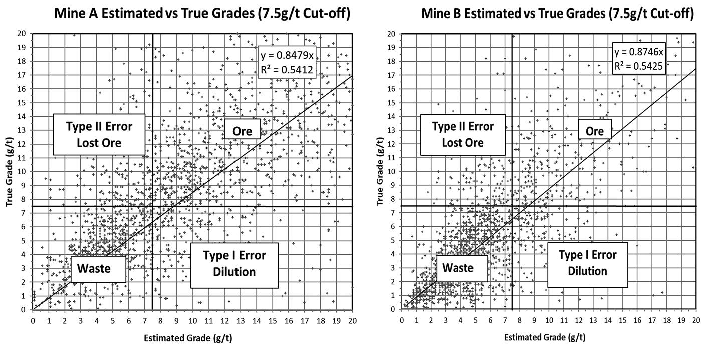
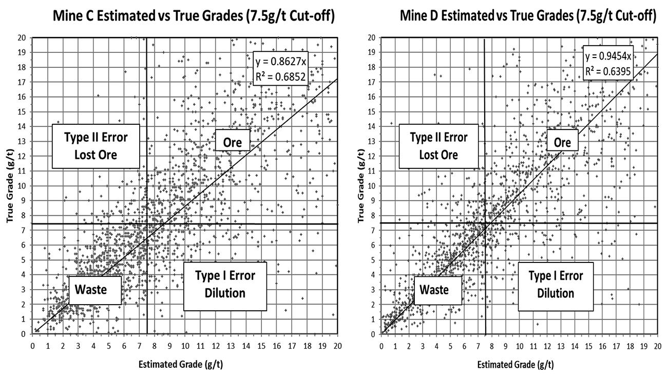
Figure 4—Variation distributions for mines A, B, C, and D. The sharp- Laplace distribution curves in the four plots (in red) can be and compared to the flatter normal distribution curves (in green)
Optimizing cut-off grade considering grade estimation uncertainty 342 JULY 2022 VOLUME 122 The Journal of the Southern African Institute of Mining and Metallurgy
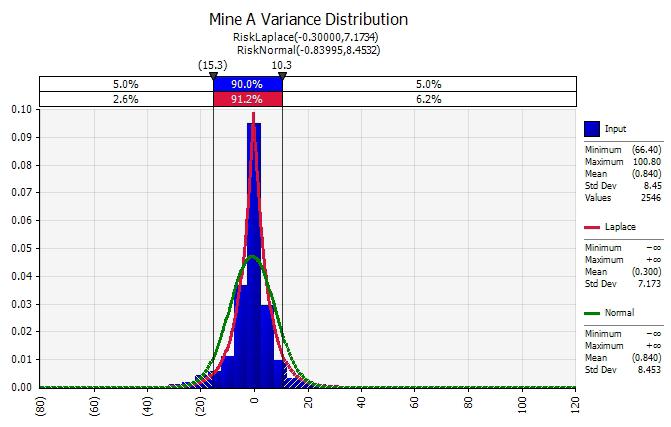
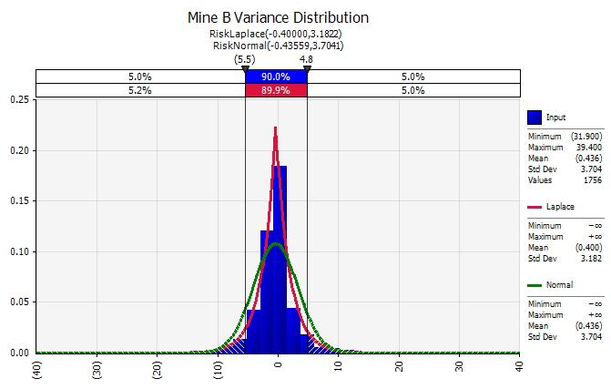
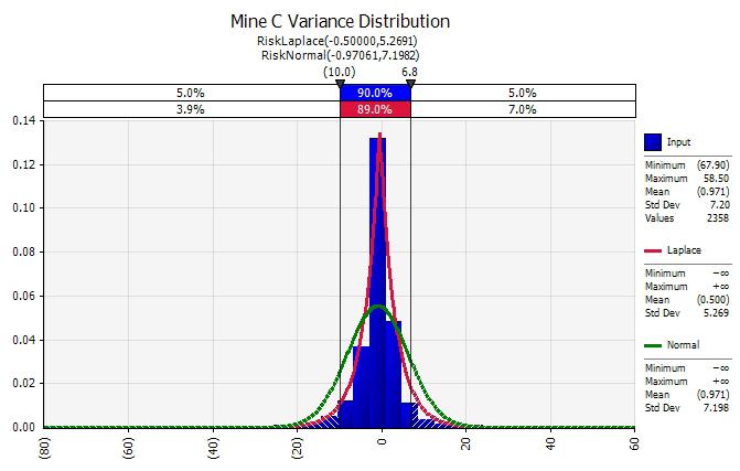
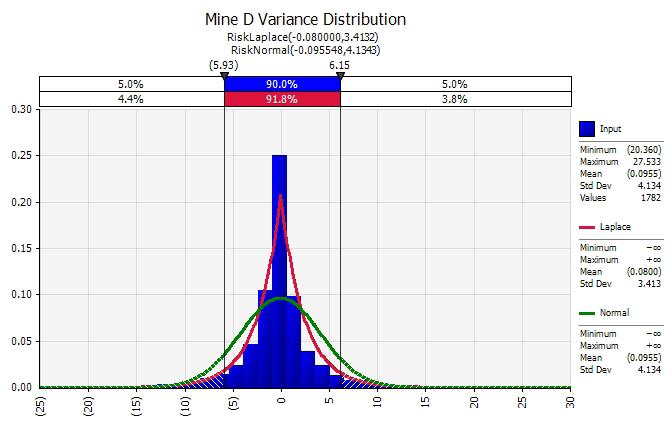
The block sizes have been standardized at 30 × 30 m (also the Measured Mineral Resource block size). The specific gravity of the quartzitic conglomerate ores on these mines is typically 2.72, which has been used to determine the tonnage for each block. The other parameters used for financial modelling were described previously.Thisstudy developed a model that can be optimized for either profit or NPV. Optimizing NPV can drive decision-making to focus on short-term gains at the expense of the longer term. Therefore, companies frequently use the total undiscounted cash flow (Hall, 2014). All four mines' financial models were run using zero (undiscounted profit), 9%, and 12% discount rates. This is consistent with the previous study, which used the same discount rates. The NPV cut-off grade is higher than when optimized for profit. The NPV optimization model favours high-grading mining because of the discounting. This leads to a shorter mine life and lower mineral resource extraction (Birch, 2016b). The optimized cut-off grade obtained from the financial optimizer excludes the estimated cost of the mineral resource royalty ( South Africa, 2008) and income tax calculated using the South African gold tax formula ( South Africa, 2019). The purpose of excluding these financial liabilities from the model is to consider profitability when determining the rate. Including these in the model creates interesting interplays between the optimal cut-off grade and these variable costs. This is the subject of further research by the author. This interplay adds a layer that is distracting from the purpose of this particular research project, which is studying the role of uncertainty in optimizing the cut-off grade.The financial optimizer uses mixed-integer linear programming (Excel Solver). The Solver feature is built into Microsoft Excel. It was selected for this study due to its availability to all users of Excel (Meissner and Nguyen, 2014). Solver can be used to determine an optimal value (maximum or minimum) for a formula in a target cell that is constrained or limited by the values of other formula cells in a worksheet. Solver adjusts the values in the decision variable cell (the cut-off grade) to fulfil the constraint bounds of the cell and provide the desired result for the target cell (the profit or NPV) (Microsoft, 2022). Solver uses three algorithms (Microsoft, 2022): ➤ Generalized reduced gradient (GRG) nonlinear (for problems that are smooth nonlinear)
The model was set to replace the pre-mining estimated block value with the post-mining true value for each block. The Solver function was then run to optimize the cut-off grade. This exercise was run considering both optimization for profit (zero NPV) and NPV at 9% and 12%. Figure 6 displays how the cut-off grade for
Results and discussion
Optimizing cut-off grade considering grade estimation uncertainty
➤ LP Simplex (for problems that are linear) ➤ Evolutionary (for problems that are non-smooth).
It has been found for the financial optimizer model that although the evolutionary approach is the slowest, it is the most reliable. The GRG approach gives inconstant results, often not changing the initial value input for the cut-off grade. The LP Simplex approach has not been tested because the nature of the model is not considered linear.
Overall bias not considered
Figure 5—An example of a grade-tonnage curve (mine D) with a cut-off of 7.5 g/t. The resultant tons above 7.5 g/t are 3.3 Mt, and the average mining grade is 13.8 g/t
The financial optimizer determines the tonnage above the cut-off grade and the AMG from the block listing sheet. The MRF and ratio between stope tonnage and total milled tonnage are obtained from the mines' ore flow sheets. These values form the primary inputs into the cash flow sheet, along with the production rate, metal price, and mining costs. As Solver's cut-off grade varies, the tonnage above the cut-off grade and AMG inputs change to maximize the target selected (profit or NPV). This relationship is shown in Figure 5. Mine D has been selected to demonstrate the grade-tonnage curve (Figure 5). This is due to mine D demonstrating block factors closest to 100% among the four mines included in this study.Agrade-tonnage curve can be used to visually display the tons above the cut-off grade and the average mining grade of the blocks above the cut-off grade. A vertical line drawn at the cut-off grade will intersect both the tonnage and grade curves. A horizontal line drawn from the tonnage curve to the tonnage axis (the left side in this case) will indicate the tons above the cut-off grade (3.3 Mt in this case). These tons can be used as the tons available for the financial model. A horizontal line drawn from the intersection point with the grade curve to the grade axis (right side) will indicate the average grade of all the blocks above the cut-off grade (13.8 g/t in this case). This can then be used as the AMG for the financial optimization model.
343The Journal of the Southern African Institute of Mining and Metallurgy VOLUME 122 JULY 2022
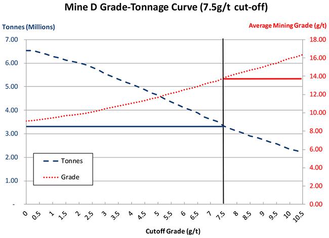
344 JULY 2022 VOLUME 122 The Journal of the Southern African Institute of Mining and Metallurgy
each of the four mines varies when considering the uncertainty of the block values when optimized for profit (zero NPV). It can be observed that only mine A shows a decrease in the cut-off grade when the grade uncertainty is considered. In the previous study, the overall tendency was that the cut-off grade when optimizing for profit is lower than the unoptimized breakeven grade when uncertainty is considered. Figure 7 shows the cut-off grade graphs optimized for 9% and 12% NPV. The following can be noted. ➤ Both the basic and grade estimate uncertainty-optimized cut-off grades are higher than the break-even cut-off grade of 7.5 g/t, which is expected when optimizing for either 9% or 12% NPV. ➤ The same trend as seen in the profit optimization is observed in the 9% NPV cut-off grade optimization. ➤ Only mine A shows that a significantly reduced cut-off grade is beneficial. ➤ For the 12% NPV optimization considering grade uncertainty, mine C shows a reduction in the cut-off grade, while the other three mines show an increase in the cut-off grade is preferable. These trends indicate that the bias in the pre-mining block estimation grades is significant and alters the previous study's findings. Overall bias considered Mines A, B, and C had block factors significantly below 100% at 94.3, 93.2, and 92.4%. Only mine D has a block factor close to 100%, at 99.0%. The distribution model used in the previous study to determine each model's true grades assumed a block factor of 100%. Considering this study's initial optimization exercise results, the impact of the overall bias in the estimated block grades needed to be considered. Whether to mine a block or not is based on the estimated grade. Suppose the overall tendency is to overestimate the block grades. In that case, more blocks will be considered ore than is Figure 6—Profit optimization. The basic cut-off grade does not consider the grade estimation uncertainty, whilw the optimized cut-off grade considers the true block
optimization. The basic cut-off grade does not consider the grade estimation uncertainty, while the optimized cut-off grade considers the true block values
Optimizing cut-off grade considering grade estimation uncertainty
Figurevalues7—NPV
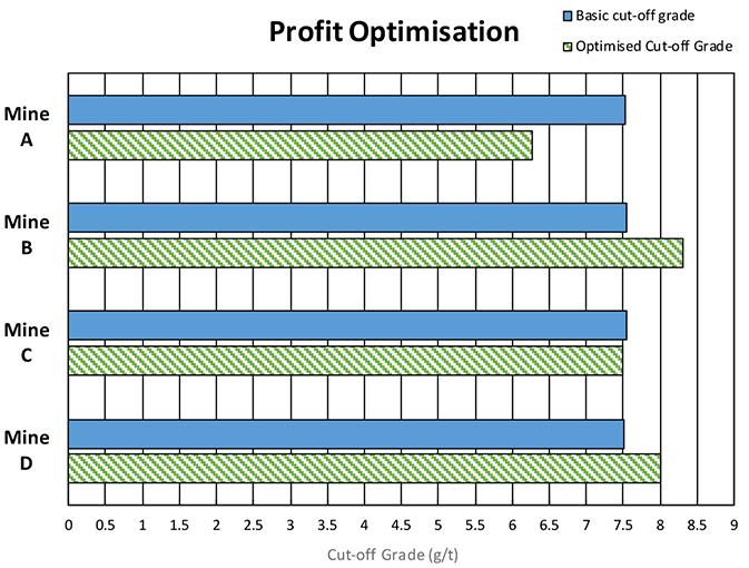
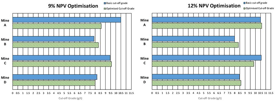
actually the case (Type I error), which will add to the dilution. Mines should constantly consider their block factor and adjust their evaluation parameters to reduce this bias. If the same technique is used to evaluate the blocks post-mining, this will reflect an apparent loss when determining the mine call factor (de Jager, 1997). The planned block grade is adjusted to bring the block factor to 100% to correct this bias. This correction was applied to all four mines. The model then selects the blocks based on this adjusted planned grade rather than the originally planned grades. For the profit optimization, the results indicate that two of the four mines (mines A and C) would benefit from a significant downward adjustment in the cut-off grade from the break-even grade of 7.5 g/t (Figure 8). The following is noted. ➤ The reduction in cut-off grade is 22% and 9%, respectively, for mines A and C. ➤ The other two mines (B and D) would require a 4–5% increase in cut-off grade.
For the exercise where the optimization maximizes the NPV, the overall tendency is to reduce the cut-off grade from the cut-off grade obtained without considering the uncertainty. This is shown in Figure 9. The following is noted.
➤ The indicated cut-off grade reduction for 9% NPV is 23% for mine A and 7% for mine C.
➤ No adjustment is suggested for mine D.
Conclusion and recommendations
Figure 9—NPV optimization following correction to the bias to bring the block factor to 100%. The basic cut-off grade does not consider the grade estimation uncertainty, while the optimized cut-off grade considers the true block values
Optimizing cut-off grade considering grade estimation uncertainty
The previous study (Birch, 2017) assumed a normal distribution with no bias for establishing the grade uncertainty. This study uses real data from four South African gold mines to establish whether the assumptions and results from the previous research are valid.
Figure 8—Profit optimization following correction to the bias to bring the block factor to 100%. The basic cut-off grade does not consider the grade estimation uncertainty, while the optimized cut-off grade considers the true block values
345The Journal of the Southern African Institute of Mining and Metallurgy VOLUME 122 JULY 2022
➤ The reductions for mines B and D are minor at 1% and 3%, respectively. ➤ For the 12% NPV, the indicated cut-off grade reduction for mines A and C is 4% and 14%, while for mine B there should be a 2% reduction.
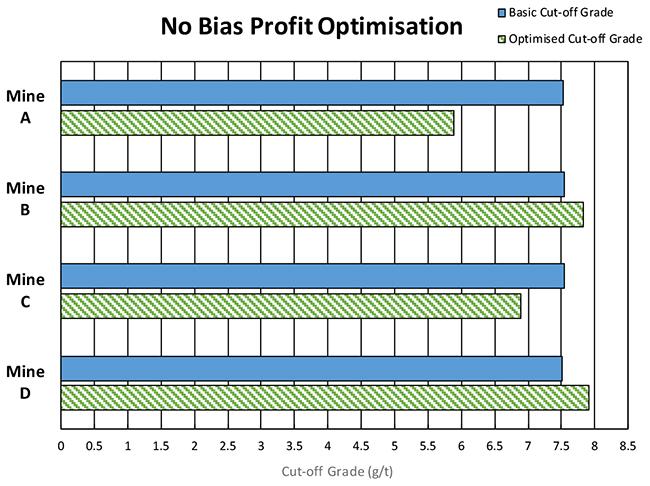
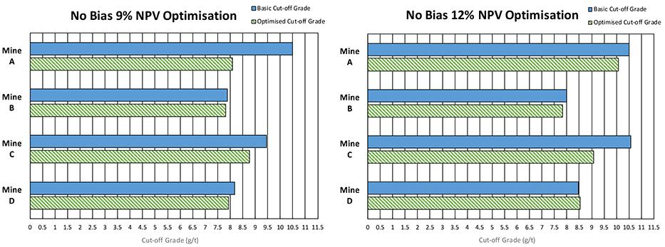
Tolmay, L. 2014. On the reduction of algorithmic smoothing of kriged estimates.
Kühn, C. and
Journal of the Southern African Institute of Mining and Metallurgy, vol. 107, no. 1. pp. 67–74. https:// journals.co.za/content/saimm/107/1/AJA0038223X_3255 [accessed 4 November 2019].
SouTh Africa. 2008. Mineral and Petroleum Resources Royalty Act 28 of 2008. Government Gazette. 521:13. SouTh Africa. 2019. Guide for Tax Rates/Duties/Levies (Issue 14). South African Revenue Service, Pretoria. https://www.sars.gov.za [accessed 15 October 2019].
January 2022].
Grades and Optimising the
The true data indicates in all four cases that the distribution curve of the uncertainty of the grade estimation follows a Laplace rather than a normal curve. This ‘double exponential’ curve displays far greater kurtosis than a normal curve with tails extending further.
Hall, B. 2014. Cut-off Strategic Spectrum, S. (ed.). of Mining Carlton. Victoria, Hilali,Australia.H.2016. [accessed 22
Journal of the Southern African Institute of Mining and Metallurgy, vol. 114, no. 8. pp. 667–672. https://www.saimm.co.za/Journal/v114n08p667.pdf [accessed 17 March 2020]. Underhill, L. and Bradfield, D. 1994. IntroSTAT 5.0. Juta & Co., Kenwyn, Cape Town. u
References Birch, C. 2016a. Impact of the South African mineral resource royalty on cut-off grades for narrow, tabular Witwatersrand gold deposits. Journal of the Southern African Institute of Mining and Metallurgy, vol. 116, no. 3. doi: 10.17159/2411Birch,9717/2016/v116n3a4C.2016b.Impact of discount rates on cut-off grades for narrow tabular gold deposits. Journal of the Southern African Institute of Mining and Metallurgy, vol. 116, no. 2. doi: 10.17159/2411-9717/2016/v116n2a2 Birch, C. 2017. Optimization of cut-off grades considering grade uncertainty in narrow, tabular gold deposits. Journal of the Southern African Institute of Mining and Metallurgy, vol. 117, no. 2. pp. 149–156. doi: 10.17159/2411-9717/2017M17n2a6. Border, S. 1991. Optimisation of cut-off grades during design of underground mines. Proceedings of the Mining Industry Optimisation Conference, Sydney. Australasian Institute of Mining and Metallurgy, Melbourne. BPI ConsulTing. 2016. Deciding which distribution fits your data best. fits-your-data-bestwww.spcforexcel.com/knowledge/basic-statistics/deciding-which-distribution-https://[accessed8April2020].
Laplace-distribution. https://www.coursehero.com/file/18659563/ Laplace-distribution/ [accessed 8 April 2020]. InvesTopedia. 2021. Net present value (NPV) definition. https://www.investopedia. com/terms/n/npv.asp
In three of the four case studies, there is a significant bias. This is displayed by block factors below 95%, indicating an overestimation in the estimated grades. The initial financial optimization exercise indicated that reducing the cut-off grade was preferable in a single case for the profit optimization and mixed results for the NPV optimization cases. This is contrary to the previous study (where the optimization model indicated a cutoff grade reduction was always preferable for profit optimization and generally preferable for NPV optimization). In the previous research the variances had no bias, and it was felt that the bias was altering the trends. The bias was corrected to bring the block factors for all four to 100%, and the exercise was repeated.
and Metallurgy,
When optimizing for profit, two of the four cut-off grade optimization models suggest a reduced cut-off grade by up to 22% from the break-even grade when considering grade uncertainty. However, no reduction was indicated for the other two mines, and a slight increase (4–5%) is suggested. With the 9% NPV model, the data from all the mines suggests that reducing the cut-off grade is preferable. This reduction varied significantly from 1–23%. This trend was also observed following the 12% NPV exercise, with reductions between 2–14% in three mines. For the fourth mine, no reduction in the cut-off grade is suggested. It is recommended that all mines focus on their block factors and other evaluation parameters to ensure no overall bias in the block estimations. This bias could also be carried through to estimate the mined grades (the true grade) and will result in gold being called for that does not exist. This apparent loss will mean an increase in cut-off grades. Once the bias is corrected, running a financial optimization exercise similar to this one, considering the grade uncertainty, could unlock value by reducing the number of lost blocks. The value of the lost blocks appears to be higher than the mining losses incurred by mining more un-pay blocks by reducing the cutoff grades. However, every orebody has a unique grade-tonnage characteristic and financial circumstances. No single solution could be applied to all gold mines, and the optimization strategy (profit or NPV) also affects the outcome.
Australasian Institute
Optimizing cut-off grade considering grade estimation uncertainty the Southern African Institute of Mining and Metallurgy
Mine Plan.
Visser, J.K. 2014. Managing uncertainty in typical mining project studies. South African Journal of Industrial Engineering, vol. 25, no. 2. pp. 105–120. doi: 10.7166/25-2-800 Meissner, J. and Nguyen, T. 2014. An introduction to spreadsheet optimization using Excel Solver. MinniMineralsMicrosofOptimization-Solver.pdfhttp://www.meiss.com/download/Spreadsheet-[accessed19March2020].T2022.DefineandsolveaproblembyusingSolver.https://support.microsoft.com/en-us/office/define-and-solve-a-problem-by-using-solver-5d1a388f-079d-43ac-a7eb-f63e45925040[accessed22January2022].CouncilSouThAfrica.2020.Gold.https://www.mineralscouncil.org.za/sa-mining/gold[accessed19March2020].TT,R.C.A.2004.Cut-offgradedeterminationforthemaximumvalueofasmallwits-typegoldminingoperation. Journal of the South African Institute of Mining and Metallurgy, vol. 104, no. 5. pp. 277–283. MinniTT, R.C.A . 2017. Poor sampling, grade distribution, and financial outcomes. Journal of the Southern African Institute of Mining and Metallurgy, vol. 117, no. 2. pp. 109–117. doi: 10.17159/2411-9717/2017/v117n2a2 PoxleiTner, G. 2016. Operating costs for mines. SRK Consulting (Canada). SmiSchoolSavanOperatingCostEstimationForMiners_2016.pdf.https://www.srk.com/sites/default/files/file/GPoxleitner_T,R.2012.Overviewofminingcosts.CPMGroup.Brooklyn,NY.http://www.goldconvention.in/iigc2012/presentation/CPMGroupOverviewofMiningCostsRS.pdf.ofMiningEngineering.2021.MINN7092ACourseNotes.UniversityoftheWitwatersrand.Th,G.L.,Pearson-Taylor,J.,Anderson,D.C.,andMarsh,A.M.2007.Projectvaluations,capitalinvestmentandstrategicalignment.
346 JULY 2022 VOLUME 122 The Journal of
De Jager, E. 1997. The analysis of the mine call factor in gold mining, with specific reference to Western Holding Mine. PhD thesis, University of the Witwatersrand. http://sierra-eds.wits.ac.za/iii/encore/record/C__Rb1382121__
SDe Jager, Ernst Jakobus.__Orightresult__X4?lang=eng&suite=def [accessed 10 April 2020].
Quality control in tailings resource exploration at Havelock Mine, Eswatini by S. Gan1, L. Birrell2, D. Robbertze2, B. Zhao1,3, E. van Niekerk1, and L. Ncubi1
347The Journal of the Southern African Institute of Mining and Metallurgy VOLUME 122 JULY 2022
The Barberton greenstone belt, located in the southeastern part of South Africa and including part of northern Eswatini, occupies an area of 120 × 50 km with an estimated depth of less than 8 km. It consists of the Paleoarchean Barberton Supergroup (ages ranging from 3 600 Ma to 3 200Ma) volcanosedimentary rocks, which are entirely engulfed in massive intrusive granitoid rocks (Figure 1).
Dates: Received: 29 Apr. 2021 Revised: 22 Dec. 2021 Accepted: 23 May 2022 Published: July 2022 How to cite: Gan, S., Birrell, L., Robbertze, D., Zhao, B. , van Niekerk, E., and Ncubi, L. 2022 Quality control in tailings resource exploration at Havelock Mine, JournalEswatini.of the Southern African Institute of Mining and Metallurgy, vol. 122, no. 7, pp. 347–362 DOI
QualitySynopsisassurance and quality control (or QAQC) plays a key role in safeguarding the level of confidence of the data generated during mineral exploration and mine development, and is also part of the reporting code requirements for resource estimation and reporting, as well as mining investment. Implementation of good policies and working protocols in quality management will result in the generation of reliable information, which is critical for decision-making on the future of the mining project. The use of certified reference materials, i.e., standard, blank, and duplicate samples, proves effective and efficient for ensuring the level of data confidence in terms of precision, accuracy, and sample contamination. This is well demonstrated by the practice of QC in the exploration programme for the chrysotile tailings storage facilities of Havelock Mine, using 1254 samples from 53 drill-holes. Different statistical tools were applied to analyse the assay results from these samples. The outcome substantiates that the QC practice established during the Havelock exploration project is aligned to best practice guidelines in the industry. The resource delineated indicates that the tailings material at Havelock could potentially become a significant source of supply to the global magnesium market.
qualityKeywordscontrol, QAQC, Resource estimation, exploration, magnesium, Havelock, Eswatini.
Geological setting Havelock Mine sits in the southern part of the Barberton greenstone belt, a geological heritage area renowned as one of a few sites where some of the oldest rocks on Earth are preserved.
Kobolondo Mining, a company registered in Eswatini, started an initiative to extract the magnesium resource from the chrysotile asbestos tailings at Havelock Mine. As part of this initiative, some of the authors participated in an exploration programme to evaluate the mineral resources of the TSFs. The aim of this programme was to produce a Mineral Resource statement that would meet the requirements of the Joint Ore Reserves Committee (JORC) Code of Australia. This paper covers the following major aspects: geological setting, mining history, geology of Havelock Mine, conception of quality assurance and quality control, QAQC policy and practice, composition of the tailings materials, and assay results.
Affiliation: 1Department of Environmental Sciences, College of Agriculture and Environmental Sciences, University of South Africa 2Salamander Mining International Limited. 3School of Geoscience and Technology, Southwest Petroleum University, China.
Introduction Havelock Mine, situated adjacent to the small town of Bulembu in the northwestern corner of Eswatini (previously Swaziland), used to be the biggest producer of asbestos in Africa. Mining operations were started in 1939 by Turner & Newwall of Manchester (Barton, 1982; Anhaeusser, 2012; Jourdan, 1990). The mine was closed in 2001. All the residues and waste materials which resulted from the mining operation have been contained in the two tailings storage facilities (TSFs) at Bulembu.
Correspondence to: S. Gan Email: shengfeig@outlook.com
3471https://orcid.org/0000-0003-0208-L.0810https://orcid.org/0000-0002-2269-H.J.1246https://orcid.org/0000-0003-4991-B.6502https://orcid.org/0000-0001-6227-S.ORCID9717/1612/2022http://dx.doi.org/10.17159/2411-ID::GanZhaovanNiekerkNcubi
Quality control in tailings resource exploration at Havelock Mine, Eswatini 348 JULY 2022 VOLUME 122 The Journal of the Southern African Institute of Mining and Metallurgy
Mining history
Rocks of the Barberton greenstone belt have experienced strong structural deformation, resulting in the development of folds and faults trending NE-SW and E-W.
Figure 1—Geological
Table I Annual output of
Havelock Mine commenced production of chrysotile asbestos in 1939 by open-pit operation, and in 1948 changed to underground extraction.Because of the rich and extensive nature of the deposit, Havelock Mine soon became one of the five largest asbestos mines in the world, producing an average of 30 000 t/a between 1939 and 1998, with the highest annual production of 42 000 t recorded in 1976 (Table I). In 1940, the mine contributed 70% of the income tax of Eswatini. It maintained its position as an economic mainstay of the country until the 1950s when agricultural products began to play an equally important role. It was the largest earner of foreign currency until 1962, when it was surpassed by sugar. During its 62 years of life, Havelock Mine produced nearly 1.8 Mt of asbestos fibre and was an important source of commodity exports for Eswatini. It is said that the asbestos product from Havelock Mine was used by the British Army during the Second World War. map of the Barberton greenstone belt, showing location of Havelock Mine (adapted from Köhler and Heubeck, 2019) asbestos
from Havelock Mine Year Output (ton) Year Output (ton) Year (Output (tons) 1939 4. 165 1960 29.054 1981 835.264 1940 18.873 1961 27.935 1982 30.145 1941 19.166 1962 29.783 1983 26.287 1942 23.219 1963 30.256 1984 25.832 1943 15.338 1964 36.162 1985 25.130 1944 29.628 1965 37.089 1986 24.475 1945 21.242 1966 32.788 1987 25.925 1946 29.155 1967 36.427 1988 22.804 1947 25.360 1968 38.960 1989 27.291 1948 29.421 1969 39.079 1990 35.938 1949 30.814 1970 33.057 1991 13.888 1950 29.635 1971 35.484 1992 32.301 1951 31.719 1972* 37.558 1993 33.862 1952 31.542 1973 39.632 1994 28.591 1953 27.310 1974 32.421 1995 28.591 1954 27.344 1975 37.600 1996 26.014 1955 29.586 1976 42.000 1997 25.888 1956 27.102 1977 38.000 1998 27.693 1957 27.875 1978* 36.000 1999 22.912 1958 22.916 1979 34.000 2000 12.690 1959 22.504 1980 32.833 Total 1 791.553 Note: The outputs of 1972 and 1978 are estimated based on the average of the production of the previous and following year
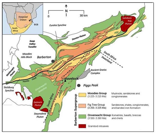
349The Journal of the Southern African Institute of Mining and Metallurgy VOLUME 122 JULY 2022
Figure 2—Aerial view of Bulembu and location of the TSFs
For mineral exploration, data reliability is one of the essential elements to ensure that correct decisions are made regarding the future of the project, namely whether to continue with further work or terminate the effort, whether further investment is warranted, or whether no added value will be generated with additional investigation. The key to the whole process is the reliability of information. Therefore, the quality assurance (QA) and quality control (QC) approach is fundamental to secure such reliability and correctness.
Precision, as defined by the Joint Committee for Guides in Metrology (JCGM, 2008), is the ‘closeness of agreement between indications or measured quantity values obtained by replicate measurements on the same or similar objects under specified conditions’. It is usually established by repeated measurements of the same sample or replicate samples under the same conditions.
The differences between these results indicate the attribute of precision, such as low precision or high precision. There are statistical tools to quantify precision, such as standard deviation, variance, and coefficient of variation.
Quality control in tailings resource exploration at Havelock Mine, Eswatini
For public companies that are traded on stock exchanges, there are legal requirements related to sampling and QC procedures, such as the well-known JORC Code, and the South African Code for the Reporting of Exploration Results, Mineral Resources and Mineral Reserves (SAMREC Code). Many financial institutions include reviewing and auditing of the QC practice of the target projects or companies as part of their due diligence studies for funding of mining opportunities. Therefore, the development and implementation of an appropriate sampling protocol and QC policy have been incorporated into the basic requirements for mineral exploration and mine development.
Precision and accuracy
QA aims to assure that the right production process is performed in the right manner, whereas QC assures that the product will match the requisite standard (Surbhi, 2019). On one hand, QA relates to how a process is performed or how a product is made and is about the process, plans, and designs to provide the confidence level satisfactory to the quality requirement. QC, on the other hand, is more associated with the inspection aspect of quality management and is a set of activities and procedures to guarantee the quality of the products against standards and requirements.Inpractice, the two terms are often used interchangeably (referred to as QAQC). Both have the same purpose – to safeguard the quality of products or services but with different emphases and approaches. Essentially, the purpose of QA is to prevent problems/errors from happening, being proactive, whereas QC is to detect and assess the problems when they occur, being reactive.
The goal of QAQC is to ensure precise, accurate, representative and reliable results of the information and to enhance the level of confidence of the data presented.
Concept of quality assurance and quality control
At its peak operation, Havelock Mine employed more than 10 000 mineworkers, being one of the largest employers in Eswatini. The town of Bulembu was established in 1936 solely for serving the mining activities. By the 1990s, with restrictions on asbestos usage in the developed countries and the resulting shrinking market, production at Havelock Mine began to decline. By 2000, output had fallen to just 12 690 t/a. The mine was no longer viable and was permanently closed. It is estimated that, during the operational period of the mine, about 50 Mt of ore were mined and milled. Most of the milled material has been stockpiled in the TSFs. Some of the tailings were reprocessed between 2001 and 2004 for recovery of chrysotile fibre. There are currently two tailings dumps in Bulembu (Figure 2). The old or West dump is the original site for the disposal of the processed material. The new or East tailings dump contains the reworked waste material produced during the reprocessing of the original tailings.
Quality assurance and quality control Quality assurance and quality control (QAQC) are two major components of any quality data-management system. The two have different definitions and functions in general, but at the same time they are closely integrated into the overall practice of quality management.Asdefined by the International Organization for Standardization (ISO, 1994), QA is ‘the assembly of all planned and systematic actions necessary to provide adequate confidence that a product, process, or service will satisfy given quality requirements’. Alternatively, it can be defined as ‘all the planned and systematic activities implemented within the quality system that can be demonstrated to provide confidence that a product or service will fulfil requirements for quality’, QC is rather ’the operational techniques and activities that are used to satisfy quality requirements’.
The reliability of and level of confidence in data are often measured against precision and accuracy, which are two important measurements in the information system.
Geology Havelock asbestos mine is hosted in the Havelock Ultramafic Complex, which is the uppermost division of the Paleoarchean Onverwacht Group of the Barberton greenstone belt (Barton, 1982; Anhaeusser, 1974). Serpentinite is the main rock type in the mine area. Other lithologies include banded iron formation, banded cherts, talc, and diabase dykes. Deformation of the Havelock Ultramafic Complex has resulted in the development of E-W striking thrust faults and folds. Chrysotile asbestos orebodies occur as a stockwork of cross-fibre seams and veins, striking E-W and NE-SW and dipping to the south at an angle of 45–70°.
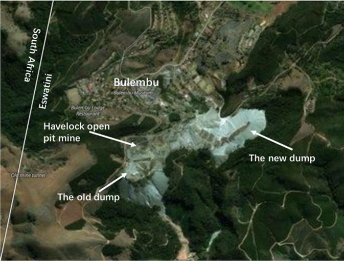
Quality control in tailings resource exploration at Havelock Mine, Eswatini 350 JULY 2022 VOLUME 122
Assay error and bias In data science, bias is the deviation from expectation in the data. It basically refers to an error in the data. The true value of the data, either a quantitative or qualitative attribute, is negatively influenced by errors and biases.
During exploration for the rehabilitation of the chrysotile tailings facilities of Havelock Mine, a comprehensive sampling protocol was established and strictly implemented. It covered the whole process of the operation, from topographic survey and drilling to sampling, sample storage and transportation, as well as core logging. This QAQC policy and practice laid a good foundation for the consequent resource estimation, as confirmed by external consultants. Drilling Drilling was carried out on the two TSFs of Havelock Mine. Selection of drill spacing is usually an important decision in any mineral exploration programme. A balance needs to be maintained between the appropriate drill-hole spacing and project costs. At Havelock Mine, the tailings materials contained in the residue dumps went through various production processes historically and were therefore well mixed, resulting in a relatively homogeneous composition. The materials in the new dump have been reprocessed again and thus are more homogeneous. Based on such considerations, as well as inputs from specialist consultants in resource modelling, a 50 m drill-hole grid was selected for the old dump, and a 75 m grid for the new dump (Figure 3). The main purpose of drilling was to collect samples of the tailings materials for assay and resource estimation, and other parameters such as the depth of the TSFs. One air-core rig, a type of reverse circulation drilling machine (RC rig), was mounted on a truck and deployed at the site (Figure 4). The rig used three tungsten steel blades to cut through the tailings materials, which were blown into the drilling rod by highpressure air and dropped into a cyclone on the surface. Samples were collected manually from the cyclone (Figure 4).
In assaying of geological and mining samples, there are three types of error (Abzalov, 2008, 2011). The first type relates to the process of sample collection, including how the samples are collected and stored, and the characteristics of the samples, such as weight, heterogeneity, and impurity content. It also includes the so-called fundamental sampling error, which is brought about by the structure of the sample materials, such as the shape and size of the mineral particles.
The extent of error and bias of data is measured by precision and accuracy. Reference materials In order to assess the precision and accuracy of assay results of samples, reference materials with known values of element contents are usually used as a benchmark to validate the quality of the data generated by the analytical process. If the reference material fulfils a number of requirements, such as proven homogeneity and stability, and characterization of the property values using suitable, well-described and validated methods, and is certified by a reputable agency, it is then referred to as a certified reference material (CRM). The commonly used CRMs include standard samples, in which the contents of a certain number of elements are well determined, and blank samples, which contain no detectable trace of the elements concerned and usually consist of barren quartz. Standard and blank samples can be purchased from qualified commercial institutions. They are inserted into the normal sample batches and go through the same analytical route. They are not affected by the preparation practice for the normal samples and are intended only to test the error and bias arising from the analytical procedures and instruments used in the laboratory.
In practice, accuracy is normally assessed through standard reference material in which the value of a specific element or elements is known. The deviation of the test result from the known value is an indication of the accuracy. Both precision and accuracy are used to describe the level of confidence in, and reliability of, data obtained from the measurement tests.
The second type of error occurs during laboratory preparation of the samples, involving delineation, crushing, pulverizing, weighing, and contamination. The third type of error, the instrumental error, occurs during the analytical operations. It is caused by the analytical instruments utilized in the process and is often referred as instrumental bias.
The Journal of the Southern African Institute of Mining and Metallurgy Accuracy, on the other hand, is defined as the ‘closeness of agreement between a measured quantity value and a true quantity value of a measurand’ (JCGM, 2008). It refers to how close the result of the measurement is to the ’true’ or predetermined value.
Error and bias occur for various reasons when sample assaying is carried out by technicians in laboratories under various conditions. They have an unfavourable impact on the quality of data but are unavoidable. What we can do is to minimize error and bias and find a way to assess their spread and make judgements about their influence.
Figure 3—Locations of drill-holes on the TSFs
QAQC policy and practice
In addition, it is also common practice to include duplicate samples of the same material with different identification numbers, which are treated as two separate entities for assay purposes.Standard samples are used to examine the accuracy of the assay results of the laboratory. Blank samples are used to test the possible contamination that might arise in the analytical process. Duplicate samples are inserted to scrutinize the repeatability and reproducibility (Runje, Novak, and Razumić, 2017; JCGM, 2008) or precision of the outcome of the analytical work.
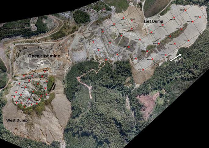
Prior to commencement of the drilling programme, drill-holes were first plotted on the airborne map (Figure 3) of the dumps produced by Swazi Survey, which also generated the coordinates of the drill-holes. In the field, a handheld GPS device (GARMIN GPSMAP64S) and a soft measuring tape were used to locate the preliminary position of the drill-holes. A peg with the identification number of the drill-hole was placed to mark each position. An accurate collar survey was carried out by Swazi Survey using the Trimble R10 dual-frequency Rtk GNSS system, which has an accuracy of 30 mm horizontally and 40 mm vertically. An iron rod (12 mm × 450 mm) was driven into the ground with a hammer to mark the surveyed position of the drill-hole. After the completion of drilling, 19 out of the 53 holes were resurveyed because their collar positions shifted from the planned locations during the drilling process. The downhole survey was carried out immediately after completion of each hole using an EZ-GYRO survey instrument from Reflex South Africa with an accuracy of ±1° for azimuth and ±0.3° for dip angle. For shallow holes (<60 m), readings of depth, dip, and azimuth were taken every 5-8 m. For deep holes (>60 m), readings were taken at 10 m intervals.
Quality control in tailings resource exploration at Havelock Mine, Eswatini 351The Journal of the Southern African Institute of Mining and Metallurgy VOLUME 122 JULY 2022
Sampling method
In order to minimize sample cross-contamination, the cyclone was cleaned every 7–8 m run with high-pressure air. Occasionally the rig was stopped and the cyclone was cleaned manually by knocking with a hammer, or opened for cleaning, depending on the flow of material through the system.
All the sampling activities, including splitting, bagging, logging, and sealing, took place at the drilling site. All the bagged samples were loaded onto a light delivery vehicle and transported to the sample storage facility in Bulembu. The distance between the sampling site and the storage was 2–3 km. The storage facilities were locked at all times and access was controlled by the geologist.
Figurerig6—Sampling
Figure 4—Air-core drill rig
The assay samples were contained in new, clean plastic bags after splitting. Sample storage
The assay samples were separated from the remaining bulk samples and kept in separate areas in the sample storage facility prior to being dispatched to the laboratory.
Prevention of contamination
Figure 5—Sampling site in the Havelock exploration programme: four samplers collected the tailings material from the cyclone of the air core drill
A large woven bag was attached to the cyclone to collect samples. At the end of each metre run, the sample bag was removed manually and a new bag was placed to catch the material. In other words, one sample was collected for each metre run (Figure 5). Each sample was weighed with a scale on site and the mass recorded in the sample logging sheet. Sample splitting After the sample was weighed, the material was placed onto a three-tier riffle splitter to separate the chrysotile tailings for assay and storage. The splitter had 16 slots with a width of 32.2 mm. Almost all the tailings materials could pass through the splitter. There were two trays at the bottom of the splitter. The material caught in the first tray, equal to 12.5% of the 1 m run sample, was collected for assay purposes. The remaining 87.5%, caught in the second tray, was bagged for every 1 m run and stored for future use (Figure 6). The split material in the first tray was composited over every 3 m interval to produce one assay sample, which was bagged and sealed for dispatch to the test laboratory.
team preparing samples with riffle splitter
The riffle splitter was cleaned by the sampling assistants with dry paintbrushes before and after each sample splitting. Bags used to catch samples from the cyclone were re-used a few times. After each use, the empty bag was shaken to get rid of the residue material from the previous catch.
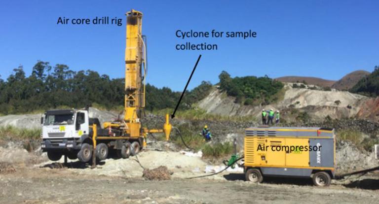
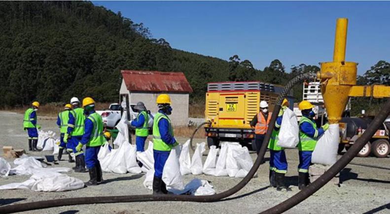
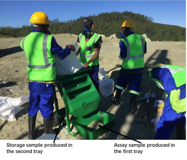
Figure 7—Preparation for sample delivery at sample storage facility in Bulembu
The blank samples were CRM AMIS0484. This is blank silica power made from silica sand. The duplicate samples were prepared from the field assay samples by dividing one sample into two portions with two different identification numbers. There is no uniform standard in the mining industry regarding the frequency of use of control samples. It varies from 15% to 25%, depending on the nature of the samples and the specific situation of the project. An overall insertion rate of 20% is in principle recommended and an acceptable average is 18% (Méndez, 2011).
The results of the chemical analysis of the 27 bulk samples collected from the tailings facility are shown in Table III. The dominant element is silicon (around 75%), followed by magnesium, accounting for over 20%, then iron, ranging from 3.46% to Other4.21%.major elements are present at very low levels of contents, such as nickel (average 0.21%), chromium (0.14%), manganese (0.06%), aluminum (0.94%), titanium (0.02%), potassium (0.04%), calcium (0.53%), sodium (0.05%), sulphur (0.05%), and phosphorus (0%). Chemical analysis was also carried out for other trace elements, precious metals, and toxic elements. All of these elements had very low contents (at the ppm level), with little impact in respect of economic and environmental considerations. Assay results of exploration programme
The tailings materials at Havelock were processed and mixed more than once during the mining operations and were fairly homogeneous. This means that there was a low probability of high variation in the composition of the material, and thus a low probability of extreme abnormal values occurring in the assay results.Inpractice, one blank sample was added to the first ten field samples. One standard sample was added to the next ten samples. A duplicate sample was added to the third batch of ten samples. In the 1 254 assay samples prepared in the field, a total of 125 control samples, including 42 standard samples (AMIS0389), 42 blank samples (AMIS0484), and 41 duplicate samples, were inserted. This represented 10% control samples, which was held to be sufficient considering the homogeneity of the tailings facility of HavelockDuringMine.theassay processes, Set Point inserted 200 control samples into the field samples. In total, for the analysis of the 1 254 field samples, 325 control samples were used for QAQC purposes. This represents a 26% insertion rate, which is in line with best practice guidelines for the industry (Méndez, 2011).
The purpose of the exploration programme at Havelock Mine was to assess the economic potential of the mineral resources contained in the TSFs and to produce a Resource estimation
The Journal of the Southern African Institute of Mining and Metallurgy Sample transportation When the assay samples were ready for delivery to Set Point Laboratories in Johannesburg, the following documents were prepared: ➤ Sample delivery record ➤ Sample checklist ➤ Set Point sample submission record. Before the transport truck arrived at the sample storage facility in Bulembu, the assay samples were taken out of the storage room and laid in sequence on the ground outside (Figure 7). The geologist and sampling assistants checked and counted the samples according to the sample checklist to ensure that everything was in good order. The sample delivery record was signed by the geologist and the truck driver to confirm the record after all the samples were loaded onto the truck. It took about 6 to 7 hours for the samples to be transported by road from Bulembu in Eswatini to Set Point Laboratories in Isando in South Africa. After the samples were checked in at Set Point, the representative of the laboratory signed the sample delivery record and issued a sample receipt to confirm the safe and complete arrival of the samples. Control samples Control samples, including standard, blank, and duplicate samples, were inserted into the sample batches of tailings material and went through the normal assay procedures in the laboratory. Both the standard and blank samples were purchased from African Minerals Standards (AMiS) in Johannesburg, which is an internationally certified laboratory providing CRMs to the mining industry.TheCRM used in the project was AMIS0389. It is very fine powder produced from the lumpy waste material of the Kroondal chrome mine in the western limb of the Bushveld Complex near Rustenburg in the North West Province of South Africa.
Composition of tailings material
Prior to the exploration programme, a preliminary sampling project was carried out at the TSFs of Havelock Mine. Twentyseven bulk samples were collected from shallow pits on the two tailings dumps. These samples were sent to Set Point for wholerock chemical analysis and mineralogical characterization. The results are summarized in Tables II and III. These samples were not part of the exploration programme and are not included in the assessment of QAQC practice. Chrysotile is the dominant mineral in the tailings, ranging from 36.18% to 53.86% with an average value of 46.66%. Lizardite, another member of the serpentine mineral group, is present between 7.72% and 18.71%, averaging 12.68%. Lizardite and chrysotile together constitute 59.34% of the mineral assemblage of the tailings material. This is in line with the ultramafic lithology of the host rocks of Havelock Mine. Magnesite is also a major mineral in the tailings with a content of 6.95% to 28.48%, averaging 16.27%. Minor minerals include talc (5.17% on average), dolomite (4.99%), chlorite (4.15%), diopside (3.86%), forsterite (1.8%), hornblende (0.18%), biotite (0.17%), quartz (1.08%), pyrite (0.20%), and magnetite (0.51%) (Table II).
Quality control in tailings resource exploration at Havelock Mine, Eswatini 352 JULY 2022 VOLUME 122
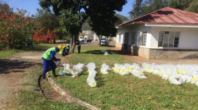
Quality control in tailings resource exploration at Havelock Mine, Eswatini 353The Journal of the Southern African Institute of Mining and Metallurgy VOLUME 122 JULY 2022 IITable
(%)SwazilandinProjectKobolondoofmaterialtailingsthefromsamplesonreportanalysisXRD
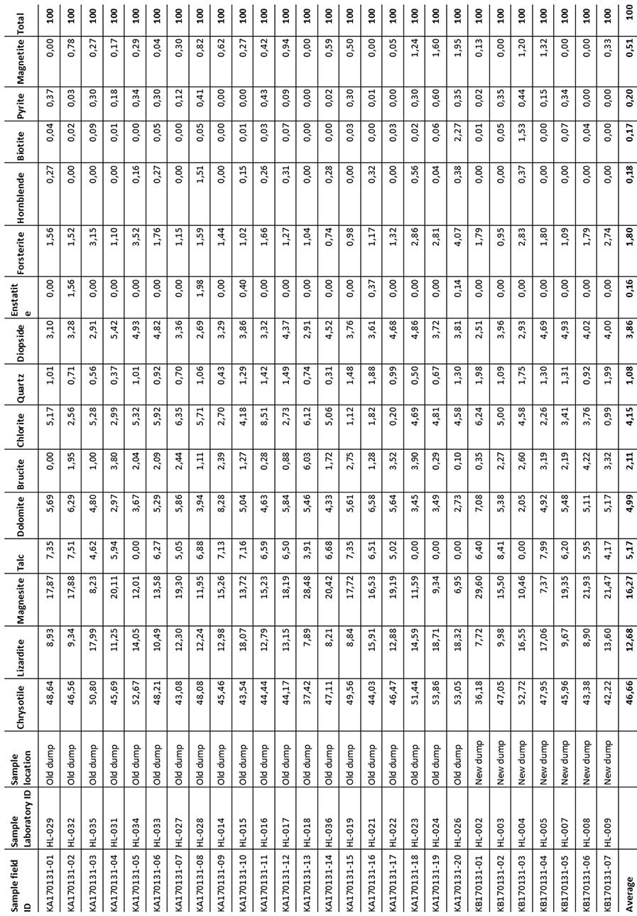
20.55 3.60 0.20 0.16 0.06 0.95 0.01 0 0 0.42 0 0 75.34 KA170131-06 20.11 3.68 0.20 0.13 0.06 0.92 0.02 0 0 0.60 0 0 75.72 KA170131-07 20.59 3.68 0.20 0.13 0.07 0.96 0.02 0 0 0.60 0 0 75.22 KA170131-08 20.10 3.72 0.19 0.14 0.06 1.07 0.02 0 0 0.95 0 0 75.67 KA170131-09 20.51 3.88 0.20 0.15 0.06 1.08 0.02 0.04 0 0.64 0 0 75.07 KA170131-10 20.37 3.81 0.20 0.14 0.06 1.02 0.02 0.05 0 0.58 0 0 75.29 KA170131-11 20.49 3.68 0.19 0.14 0.06 1.03 0.02 0.07 0 0.68 0 0 75.28 KA170131-12 20.32 3.67 0.20 0.14 0.06 1.03 0.02 0.07 0 0.69 0 0 75.46 KA170131-13 20.50 3.69 0.20 0.13 0.07 0.99 0.02 0.05 0 0.78 0 0 75.28 KA170131-14 19.89 3.51 0.20 0.12 0.06 0.81 0.01 0 0 0.51 0 0.00 76.13 KA170131-15 19.63 3.46 0.19 0.13 0.06 0.82 0.01 0 0 0.44 0 0.00 76.44 KA170131-16 19.83 3.66 0.19 0.12 0.06 1.04 0.02 0.05 0.05 0.58 0 0.00 76.01 KA170131-17 20.84 3.65 0.21 0.12 0.06 0.79 0.01 0 0 0.47 0 0 75.03 KA170131-18 21.03 4.02 0.21 0.14 0.06 0.84 0.01 0 0 0.31 0 0 74.46 KA170131-19 20.71 3.99 0.20 0.16 0.06 0.88 0.01 0 0 0.29 0 0 74.79 KA170131-20 20.68 4.21 0.24 0.15 0.07 0.78 0.01 0 0 0.27 0 0 74.56 KB170131-01 20.04 3.75 0.19 0.13 0.07 1.06 0.01 0.04 0.07 0.70 0.05 0.00 75.69 KB170131-02 20.69 3.59 0.20 0.16 0.06 0.91 0.02 0.035 0.05 0.49 0.05 0.00 75.21 KB170131-03 20.63 3.84 0.20 0.15 0.07 1.03 0.02 0.035 0.05 0.41 0.05 0.00 75.00 KB170131-04 20.91 3.87 0.20 0.14 0.07 1.03 0.02 0.035 0.05 0.41 0.05 0.00 74.69 KB170131-05 21.09 3.563 0.20 0.13 0.06 0.79 0.01 0.035 0.05 0.45 0.05 0 74.79 KB170131-06 20.61 3.62 0.20 0.12 0.06 0.80 0.01 0.035 0.05 0.46 0.05 0.00 75.29 KB170131-07 20.63 3.73 0.39 0.14 0.06 0.88 0.01 0.035 0.05 0.21 0.05 0 74.98 Average 20.44 3.74 0.21 0.14 0.06 0.94 0.02 0.04 0.05 0.53 0.05 0.00 75.31 ϑ
KA170131-04
Quality control in tailings resource exploration at Havelock Mine, Eswatini 354 JULY 2022 VOLUME 122 The Journal of the Southern African Institute of Mining and Metallurgy
KA170131-01 20.37 3.86 0.20 0.13 0.06 1.02 0.02 0 0 0.70 0 0.00 75.27
where Μ – Certified mean of a given standard sample L – Certified between laboratory standard deviation of a given standard sample. m – Arithmetic mean of the replicate analyses of the standard sample Sw – Estimated within-laboratory standard deviation of the replicate analyses of the standard sample included in assay batch n – Number of replicate assays of a given certified standard in analytical batch
Then, for magnesium, the result is: For iron, the result is: The above statistical tests indicate that the assay results for magnesium and iron in the standard samples (AMIS0389) satisfy the condition of Equation [1] and are acceptable in terms of accuracy. Precision Precision refers to the random measurement error. It is a reflection of the repeatability and consistency of the test work in the laboratory. It is assessed through the repeated assay of the same sample.
19.80 3.77 0.19 0.13 0.06 1.00 0.01 0 0 0.54 0 0.00 75.95
Table III Major element analysis (%) Element Mg Fe Ni Cr Mn Al Ti K Na Ca S P Si
KA170131-03
KA170131-02 20.44 3.70 0.20 0.14 0.06 0.88 0.01
20.40 3.75 0.20 0.13 0.06 0.85 0.01 0 0 0.44 0 0 75.37
0 0 0.62 0 0 75.36
There was no reference value for nickel in the AMIS0389 standard, and thus no comparison could be made. Accuracy can be measured with quantitative parameters using statistical tools. According to Abzalov (2011), the following equation is a statistical test of assay accuracy: [1]
report. On the basis of the preliminary sampling project, it is concluded that, under current economic and technical conditions, the commodities that could be utilized economically from the tailings material are magnesium, iron, and nickel. Laboratory assays were carried out on the 1254 field samples for only these three elements. Accuracy Accuracy of the assay results was assessed through the use of standard samples which went through the same analysis procedures as the normal samples in the laboratory. For this project, 42 standard samples (AMIS0389) were inserted into the field samples and submitted to Set Point for assay purposes. The results are shown in Table IV and Figure 8. As can be seen, of the 42 assay results for magnesium of the standard samples (AMIS0389), the deviation of 41 results (97.62% of total samples) from the certified reference value (14.1834%) is within the range of ±4%. The highest deviation is 4.1%. The deviation of 31 samples (73.81%) is within the range of ±2%. This is an indication of the high accuracy of the magnesium assay results. For iron, the deviation of all the results from the reference value (10.3655%) is within ±4%. Of these, 36 assays (85.71% of the total results) are within ±2%. Again, this indicates that the assay results produced by the laboratory are highly accurate.
If the condition of Equation [1] is satisfied, the analytical results are considered acceptable with regard to accuracy (Abzalov, 2011). The statistical parameters of the assay results for magnesium and iron in the standard sample (AMIS0389) (Table IV) are summarized in Table V.
KA170131-05
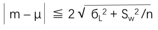
Quality control in tailings resource exploration at Havelock Mine, Eswatini 355The Journal of the Southern African Institute of Mining and Metallurgy VOLUME 122 JULY 2022 Figure 8—Deviation of assay results for standard sample AMIS0389 Table IV Assay results of standard sample AMIS0389 Sequence No Sample ID Mg (%) Mg content deviation from reference Fe (%) Fe content deviation from from reference value (14.1834%) value (10.3655%) 1 BM102 14.21 0.19% 10.18 -1.82% 2 BM105 14.61 2.92% 10.42 0.52% 3 BM108 14.36 1.23% 10.54 1.66% 4 BM111 14.56 2.59% 10.23 -1.32% 5 BM114 14.22 0.26% 1.34 -0.25% 6 BM117 14.34 1.09% 10.53 1.56% 7 BM120 14.26 0.54% 10.16 -2.02% 8 BM123 14.13 -0.38% 10.39 0.24% 9 BM126 14.17 -0.09% 10.44 0.71% 10 BM129 13.98 -1.45% 10.27 -0.93% 11 BM132 13.95 -1.67% 10.45 0.81% 12 BM135 14.54 2.45% 10.16 -2.02% 13 BM138 14.42 1.64 10.36 -0.05% 14 BM141 14.79 4.10% 10.67 2.85% 15 BM144 14.12 -0.45% 10.14 -2.22% 16 BM147 14.53 2.39% 10.26 -1.03% 17 BM150 14.55 2.52% 10.52 1.47% 18 BM153 14.29 0.75% 10.55 1.75% 19 BM156 14.68 3.38% 10.46 0.90% 20 BM159 14.04 -1.02% 10.26 -1.03% 21 BM162 14.17 -0.09% 10.39 0.24% 22 BM165 14.19 0.05% 10.26 -1.03% 23 BM168 14.70 3.51% 10.56 1.84% 24 BM171 14.30 0.82% 10.46 0.90% 25 BM174 13.99 -1.38% 10.29 -0.73% 26 BM177 14.47 1.98% 10.31 -0.54% 27 BM180 14.16 -0.17% 10.17 -1.92% 28 BM183 14.27 0.61% 10.31 -0.54% 29 BM186 14.47 1.98% 10.53 1.56% 30 BM189 14.21 0.19% 10.46 0.90% 31 BM192 14.49 2.12% 10.50 1.28% 32 BM194 14.64 3.12% 10.73 3.40% 33 BM197 14.30 0.82% 10.28 -0.83% 34 BM200 13.91 -1.97% 10.43 0.62% 35 BM203 14.30 0.82% 10.33 -0.34% 36 BM206 14.29 0.75% 10.40 0.33% 37 BM209 14.17 -0.09% 10.42 0.52% 38 BM212 14.03 -10.09% 10.55 1.75% 39 BM215 14.72 3.65% 10.36 -0.05% 40 BM218 14.44 1.78% 10.32 -0.44% 41 BM221 14.10 -0.59% 10.76 3.67% 42 BM224 14.06 -0.88% 10.28 -0.83%
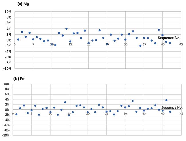
standard sample ElementAMIS0389n m m L Sw Mg 42 14.3126% 14.1834% 0.231 0.2306 Fe 42 10.3912% 10.3566% 0.186 0.1512 Table VI Assay results of field duplicate samples Squent No Element Mg (%) Fe (%) Ni (%) Sample ID Original Duplicate Difference Original Duplicate Difference Original Duplicate Difference 1 KBV05-05 23.20 23.38 0.78% 3.98 3.89 -2.26% 0.21 0.22 5.13% 2 KBV06-08 23.61 24.02 1.74% 3.84 3.87 0.78% 0.20 0.22 9.61% 3 KBV02-12 23.64 23.90 1.10% 4.17 3.80 -8.87% 0.22 0.22 -80.83% 4 KBV09-05 22.38 24.24 8.31% 3.61 3.76 4.16% 0.22 0.22 -0.50% 5 KBV09-20 24.60 24.03 -2.32% 4.09 3.94 -3.67% 0.22 0.22 1.65% 6 KBV11-14 22.50 23.50 4.44% 3.88 3.86 -0.52% 0.21 0.22 1.42% 7 KBV12-08 23.30 24.25 4.08% 3.97 3.99 0.50% 0.22 0.22 0.64% 8 KBV15-15 23.25 23.86 2.62% 3.62 3.89 7.46% 0.19 0.21 10.09% 9 KBV16-11 25.23 23.14 -8.28% 4.24 3.68 -13.21% 0.22 0.21 -2.62% 10 KBV17-05 24.06 23.50 -2.33% 3.71 3.78 1.89% 0.23 0.22 -5.10% 11 KBV19-10 23.99 23.80 -0.79% 3.76 3.72 -1.06% 0.22 0.22 -11.92% 12 KBV22-12 23.15 23.46 1.34% 3.65 3.82 4.66% 0.22 0.22 -1.34% 13 KBV25-10 22.40 23.65 5.58$ 3.85 3.97 3.12% 0.20 0.22 6.58% 14 KBV28-06 23.24 23.57 1.42% 3.95 3.88 -1.77% 0.21 0.21 0.11% 15 KAV12-17 0.72 0.61 -15.28% 2.37 1.94 -18.14% 0.03 0.02 -23.38% 16 KAV17-12 23.82 23.69 -0.55% 4.14 3.96 -4.35% 0.23 0.21 -6.62% 17 KAV13-11 19.24 23.62 22.77% 4.11 3.88 -5.60% 0.18 0.22 18.19% 18 KAV11-05 22.42 24.11 7.54% 3.73 3.86 3.49% 0.21 0.21 0.44% 19 KAV11-31 23.38 24.27 3.81% 3.78 3.74 -1.06% 0.22 0.21 -0.82% 20 KAV15-30 24.43 23.70 5.665 3.62 3.82 5.52% 0.22 0.21 -2.11% 21 KAV10-05 20.88 24.48 17.24% 3.82 3.82 0.00% 0.19 0.21 12.76% 22 KAV05-14 21.05 23.79 13.02% 3.99 4.03 1.00% 0.20 0.21 6.64% 23 KAV03-19 23.75 24.08 1.39% 3.58 4.01 12.01% 0.22 0.22 1.50% 24 KAV02-04 24.52 24.31 -0.86% 4.03 3.95 -1.99% 0.22 0.22 -1.90% 25 KAV02-30 24.35 23.66 -2.83% 4.07 3.96 -2.70% 0.22 0.22 -0.30% 26 KAV07-05 24.34 23.88 -1.89% 3.88 3.97 2.32% 0.25 0.21 -13.98% 27 KAV07-27 23.07 24.44 5.94% 4.16 3.75 -9.86% 0.23 0.21 -10.40% 28 KAA01-13 22.69 23.53 3.70% 3.95 3.80 -3.80% 0.22 0.22 -0.30% 29 KAA02-07 21.25 23.68 11.44% 3.78 3.99 5.56% 0.20 0.21 5.78% 30 KAA03-11 25.08 24.04 -4.15% 4.45 3.92 -11.91% 0.21 0.22 3.42% 31 KAA04-17 24.21 24.26 0.21% 3.81 3.86 1.31% 0.22 0.22 -2.46% 32 KAA05-06 22.69 23.74 4.63% 3.82 3.98 4.19% 0.20 0.21 9.47% 33 KAA06-28 23.31 24.18 3.73% 3.83 3.92 2.35% 0.21 0.21 2.81% 34 KBA02-19 25.23 24.36 -3.45% 3.81 3.83 0.52% 0.22 0.22 -1.44% 35 KBA01-17 24.47 24.16 -1.27% 3.83 3.89 1.57% 0.21 0.21 -0.02% 36 KBA04-19 24.64 24.46 -0.73% 4.01 3.91 -2.49% 0.22 0.22 -1.44% 37 KBA03-12 25.68 24.20 -5.76% 3.91 3.95 1.02% 0.23 0.21 -5.90% 38 KBA05-03 25.65 23.88 -6.90% 4.10 3.90 -4.88% 0.22 0.22 -3.13% 39 KBA08-03 23.64 24.63 4.19% 3.81 3.74 -1.84% 0.20 0.21 5.37% 40 KBA07-14 24.72 24.31 -1.66% 4.13 3.88 -6.05% 0.23 0.22 -3.34% 41 KAV08-04 14.28 23.47 64.36% 2.27 3.93 73.13% 0.14 0.22 57.91%
Quality control in tailings resource exploration at Havelock Mine, Eswatini 356 JULY 2022 VOLUME 122 The Journal of the Southern African Institute of Mining and Metallurgy
In the Havelock exploration programme, 41 duplicate samples were provided to the laboratory for analysis. The results are shown in Table VI and Figure 9. For the assay results of magnesium, 35 of the 41 field samples, (85.37% of the duplicate samples) show a difference between the original and duplicate assay within the range of ±10%. Four samples (9.76%) show a difference between ±10% and ±20%. One sample (2.44%) has a difference of 22.77%, and another a difference of 64.36% (Figure 9a). The assay results for iron demonstrate a similar pattern. Among the 41 field samples, 36 (87.80% of the total duplicate samples) indicate a difference between the original and duplicate assay within the range of ±10%. Four samples (9.76%) demonstrate a difference between ±10% and ±20%. One sample (2.44%) has a difference of 73.13% (Figure 9b). The assay results for nickel also have a similar pattern. Of the 41 field duplicate samples, 34 samples (82.93%) show a difference between the original and duplicate assay in the range of ±10%. Five samples (12.20%) indicate a difference between ±10% and ±20%. One sample (2.44%) has a difference of –23.38%, and another a difference of 57.91% (Figure 9c). The results for the three major elements (magnesium, iron, and nickel) indicate that the original and duplicate assay results have a reasonably good match. Over 80% of the difference between the original and duplicate assays is within the range of ±10%. One sample (KAV08-04) demonstrates an erratic mismatch between the original and duplicate values for magnesium, iron, and nickel and these results are clearly outliers (Abzalov, 2011), indicating a possible error in the test work. This sample was rejected for the QAQC assessment. Various statistical methods can be used to assess the precision of the assay results of paired samples, such as a scatter plot and a the
Table V Statistical reference of the assay results of

Calculation of the average coefficient of variantion (CV) of duplicate samples Element Number of samples CV Mg 40 0.044 247 4.70% Fe 40 0.036 630 4.28% Ni 40 0.052 129 5.11%
The CV is a statistical measure of the dispersion or variation of data-points in a data series around the mean. The lower the CV value, the less the variation.
HARD plot, Q-Q plot, and reduced-major-axis (RMA) plot (Stanley and Lawie, 2007; Abzalov, 2011, 2016; Scogings and Coombes, 2014).Several authors have suggested the use of the average coefficient of variation (CV) as the universal measure of relative precision error in geological applications (Stanley and Lawie, 2007; Abzalov, 2008, 2011). The average CV is considered to be an unbiased estimate of the random measurement error. The CV is the ratio of the standard deviation to the mean, usually expressed as a percentage:
Quality control in tailings resource exploration at Havelock Mine, Eswatini African Mining Metallurgy
VOLUME 122 JULY 2022
The CV for the pairs of assay results of duplicate samples can be calculated using the following equation (Abzalov, 2008, 2011)[2] awherei–Value of the original sample bi – Value of the duplicate sample N – Number of the duplicate sample
The average CVs for magnesium, iron, and nickel, based on the assay results of 40 duplicate samples, are shown in Table VII. The average CV is 4.70% for magnesium, 4.28% for iron, and 5.11% for nickel. The acceptable level of precision error (CV%) for sample assays in the mining industry is mostly between 10% and 30%. The best practice is in the range of 5% to 10% (Table VIII; Abzalov, 2011).
and
Table VII
Institute of
357The Journal of the Southern
Figure 9—Comparison of assay results for original and duplicate field samples
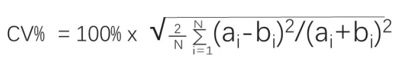
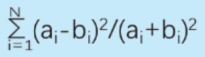
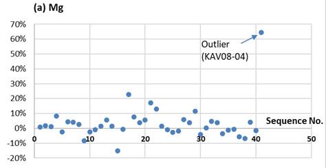
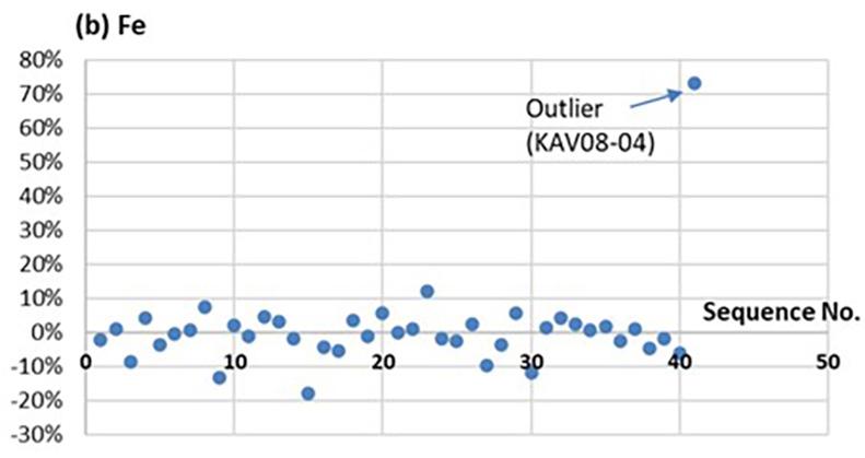
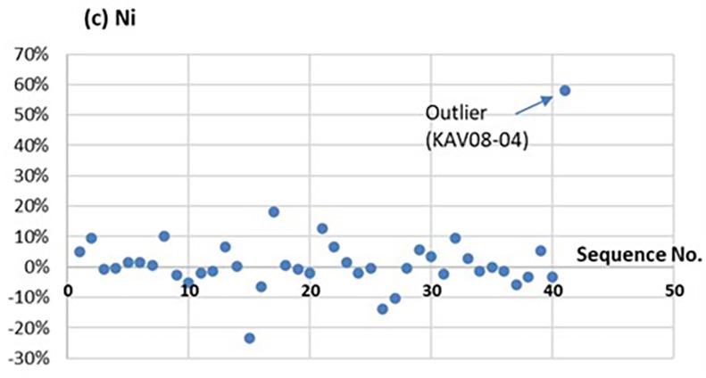
15
In the case of Havelock, all of the ARD values for magnesium and iron are less than the 25% acceptance criterion. For nickel, only one sample’s ARD (26.47%) is more than 25%. The other 39 samples (97.5% of the total) have an ARD of less than the 25% criterion. This indicates again that the quality of sample assay results, in terms of precision, is in line with best practice in the mining industry (Table IX, Figure 10). Contamination Contamination could occur at any stage of the testing processes in the laboratory, from sample preparation to analysis. Contamination is assessed through blank samples, which are basically barren samples with little or no content of the elements of interest.Where there is a low content of the relevant element, a slight change in the assay results will exaggerate the deviation of the reported value from the original reference value because of the sensitivity of the low value to any changes. As a general practice in the mining industry, if the assay results for blank samples yield values of the relevant elements less than three times the detection limits or the reference values of the analysed elements, the level of possible contamination is within the acceptable range (Méndez, 2011; Rossi and Deutch, 2014) For the Havelock exploration project, 42 blank samples (AMIS0484) were inserted into the sample batches for the assay process. The blank sample consisted of silica power with a composition of 99.15% SiO2, 0.02% MgO (0.01% Mg), 0.03% Fe2O3 (0.02% Fe), and 8.5 ppm nickel. The results are summarized in Table X. As can be seen, all the assay results for iron in the blank samples are at the same level as the certified reference value. For nickel, all of the 42 blank samples demonstrate an assay result less than three times the reference value. For magnesium, the results of 27 samples (64.3% of the total) are less than three times the certified reference value, 9 samples (14.5%) yield values of between three and four times the reference value, and 6 samples (14.3%) show values larger than four times the reference value. Overall, the assay results for the blank samples indicate that the level of possible contamination during the laboratory analytical process for the Havelock exploration project is well within the acceptance criteria.
10
10
Homogeneity The TSFs at Havelock Mine contain the waste materials from past mining operations. These materials underwent various production processes and were disposed of at the final stage. The waste materials are therefore well mixed and relatively homogeneous.
Ni (%) 5 10
(%) 5 10 PGE 10 20 Detrital
During the exploration programme, 1 254 samples of the tailings material were collected from the drill-holes and submitted for assay. VIII Best and acceptable levels of the precision errors (CV%) for mining projects (Abzalov, 2011)
(%) 10 16 PGE 15
(%) 10
Mineralization type/deposit Metal Best practice Acceptable practice Sample type
5 10
Gold, coarse to medium grained Au (g/t) 20 30 Coarse reject Au (g/t) 20 Pulp duplicate Cu (%) Cu-Mo-Au porphyry Mo (%) 15 Coarse reject Au (g/t) 15 Fe ore, channel iron deposit type Al₂O3 (%) 15 Field duplicate SiO2 Cu (%) 7.5 Au (g/t) 25 Coarse rejectCu-Au-Fe scam and iron oxide associated Cu-Au Au (g/t) 7.5 Ni 15 Cu 30 Coarse rejectNi-Cu-PGE-sulphide Cu ilmenite sands Total heavy minerals (%) Field duplicate
(%) 1 3 Iron
Cu (%) 5 10
10
15
15
Quality control in tailings resource exploration at Havelock Mine, Eswatini 358 JULY 2022 VOLUME 122 The Journal of the Southern African Institute of Mining and Metallurgy
Table
10
(%) 5 10
In comparison, the precision error of the assay results from the exploration programme at Havelock Mine is among the lowest in theAnotherindustry.simple statistical tool to assess the precision of duplicate assays is the absolute relative difference (ARD) between the original and duplicate values (Rossi and Deutch, 2014) [3] wherea–Original value b – Duplicate value For proper resource estimation, if 90% of the ARD of the field duplicate samples is equal to or less than 25%, the precision error of the assay results is acceptable (Rossi and Deutch, 2014).
5 10

The TSF Mineral Resource of 5.83 Mt of magnesium metal is predominantly (93%) in the Indicated category, based on the Table IX
No
Original
1
3
Quality control in tailings resource exploration at Havelock Mine, Eswatini
359The Journal of the Southern African Institute of Mining and Metallurgy VOLUME 122 JULY 2022
The statistical features of the sample assay results are summarized in Table XI and Figure 11. These results indicate that contents of magnesium, nickel, and iron in the samples are all concentrated around the mean values of the respective elements, with relatively low variance and standard deviation. For magnesium and nickel, 92% of the assay values are within the scope of the mean ±1 standard deviation, And 85% of the iron value are also within this range. To demonstrate the changes in values of the elements in a vertical direction, the sample assay results for magnesium were plotted along the drill-holes (Figure 12). The results indicate that there is no major variation with depth in terms of magnesium content. From the top to the bottom of the drill-holes, with a depth of 50 to 130 m, the content of magnesium is relatively constant.Thedistributions of iron and nickel contents with depth in the drill-holes show a similar trend. This again indicates the homogeneity of the tailings material at Havelock Mine.
2
1.09% 4.17 3.8 9.28% 0.22 0.22 0.83% 4 KBV09-05 22.38 24.24 7.98% 3.61 3.76 4.07% 0.22 0.22 0.51% 5 KBV09-20 24.60 24.03 2.34% 4.09 3.94 3.74% 0.22 0.22 1.63% 6 KBV11-14 22.50 23.50 4.35% 3.88 3.86 0.52% 0.21 0.22 1.41% 7 KBV12-08 23.30 24.25 4.00% 3.97 3.99 0.50% 0.22 0.22 0.64% 8 KBV15-15 23.25 23.86 2.59% 3.62 3.89 7.19% 0.19 0.21 9.61% 9 KBV16-11 25.23 23.14 8.64% 4.24 3.68 14.14% 0.22 0.21 2.66% 10 KBV17-05 24.06 23.50 2.35% 3.71 3.78 1.87% 0.23 0.22 5.23% 11 KBV19-10 23.99 23.80 0.80% 3.76 3.72 1.07% 0.22 0.22 1.93% 12 KBV22-12 23.15 23.46 1.33% 3.65 3.82 4.55% 0.22 0.22 1.35% 13 KBV25-10 22.40 23.65 5.43% 3.85 3.97 3.07% 0.20 0.22 6.37% 14 KBV28-06 23.24 23.57 1.41% 3.95 3.88 1.79% 0.21 0.21 0.11% 15 KAV12-17 0.72 0.61 16.54% 2.37 1.94 19.95% 0.03 0.02 26.47% 16 KAV17-12 23.82 23.69 0.55% 4.14 3.96 4.44% 0.23 0.21 6.84% 17 KAV13-11 19.24 23.62 20.44% 4.11 3.88 5.76% 0.18 0.22 16.67% 18 KAV11-05 22.42 24.11 7.26% 3.73 3.86 3.43% 0.21 0.21 0.44% 19 KAV11-31 23.38 24.27 3.74% 3.78 3.74 1.06% 0.22 0.21 0.82% 20 KAV15-30 24.43 23.70 5.51% 3.62 3.82 5.38% 0.22 0.21 2.14% 21 KAV10-05 20.88 24.48 15.87% 3.82 3.82 0.00% 0.19 0.21 11.99% 22 KAV05-14 21.05 23.79 12.22% 3.99 4.03 1.00% 0.20 0.21 6.43% 23 KAV03-19 23.75 24.08 1.38% 3.58 4.01 11.33% 0.22 0.22 1.49% 24 KAV02-04 24.52 24.31 0.86% 4.03 3.95 2.01% 0.22 0.22 1.92% 25 KAV02-30 24.35 23.66 2.87% 4.07 3.96 2.74% 0.22 0.22 0.30% 26 KAV07-05 24.34 23.88 1.91% 3.88 3.97 2.29% 0.25 0.21 15.03% 27 KAV07-27 23.07 24.44 5.77% 4.16 3.75 10.37% 0.23 0.21 10.97% 28 KAA01-13 22.69 23.53 3.63 3.95 3.8 3.87% 0.22 0.22 0.30% 29 KAA02-07 21.25 23.68 10.82% 3.78 3.99 5.41% 0.20 0.21 5.62% 30 KAA03-11 25.08 24.04 4.23% 4.45 3.92 12.66% 0.21 0.22 3.36% 31 KAA04-17 24.21 24.26 0.21% 3.81 3.86 1.30% 0.22 0.22 2.49% 32 KAA05-06 22.69 23.74 4.52% 3.82 3.98 4.10% 0.20 0.21 9.04% 33 KAA06-28 23.31 24.18 3.66% 3.83 3.92 2.32% 0.21 0.21 2.77% 34 KBA02-19 25.23 24.36 3.51% 3.81 3.83 0.52% 0.22 0.22 1.45% 35 KBA01-17 24.47 24.16 1.27% 3.83 3.89 1.55% 0.21 0.21 0.02% 36 KBA04-19 24.64 24.46 0.73% 4.01 3.91 2.53% 0.22 0.22 1.45% 37 KBA03-12 25.68 24.20 5.93% 3.91 3.95 1.02% 0.23 0.21 6.08% 38 KBA05-03 25.65 23.88 7.15% 4.1 3.9 5.00% 0.22 0.22 3.18% 39 KBA08-03 23.64 24.63 4.10% 3.81 3.74 1.85% 0.20 0.21 5.23% 40 KBA07-14 24.72 24.31 1.67% 4.13 3.88 6.24% 0.23 0.22 3.39% 41 KAV08-04 14.28 23.47 64.36% 2.27 3.93 73.13% 0.14 0.22 57.91%
Calculation of the absolute relative differences(ARD) of the duplicate samples Squence Sample Mg (%) Fe (%) Ni (%) ID Duplicate ARD Original Duplicate ARD Original Duplicate ARD KBV05-05 23.20 23.38 0.77% 3.98 3.89 2.29% 0.21 0.22 5.00% KBV06-08 23.61 24.02 1.72% 3.84 3.87 0.78% 0.20 0.22 9.17% KBV02-12 23.64 23.90
The aim of the exploration programme, together with the QAQC policy and practice, was to make a proper assessment of the economic potential of the TSFs at Havelock Mine. The assay data provided a good foundation for generating a suitable statement for the project. A reputable consultancy in the mining industry of South Africa, Minxcon (Pty) Ltd, was contracted to compile an independent Competent Person’s report for Kobolondo Mining. Taking into account the relevant factors affecting the reasonable prospects for eventual economic extraction (RPEEE) of the Mineral Resources in the TSFs of Havelock Mine, such as mining costs, market conditions, infrastructure, and technology, it was concluded that the entire tailings materials contained in the two dumps should be included in the Resource estimation with no cutoff grade applied. The result is demonstrated in Table XII.
Resource statement
Acknowledgement
The exploration programme on the TSFs at Havelock Mine was initiated and managed by Kobolondo Mining. The relevant governmental authorities of Eswatini provided support in various ways for the project. Bulembu Ministries Eswatini was helpful in offering convenience and logistical support to the exploration work. The authors wish to express gratitude to all the parties involved in the project for their cooperation and assistance extended in the fieldwork. Our thanks are also due to the language editor of the University of South Africa for improving the quality of the manuscript.Thecomments and suggestions from the two anonymous referees have helped to improve the manuscript of the paper.
References Abzalov, M.Z. 2008. Quality control of assay data: A review of procedures for measuring and monitoring precision and accuracy. Exploration and Mining Geology, vol. 7, no. 3 4. pp. 131 144.
Quality control in tailings resource exploration at Havelock Mine, Eswatini 360 JULY 2022 VOLUME 122 The Journal of the Southern African Institute of Mining and Metallurgy
Figure 10—ARD plots of assay results for duplicate samples quality and quantity of data. This represents a significant source of magnesium in the western world and could become a meaningful supply to the global magnesium industry when the project is eventually brought into production. Iron (Fe) and nickel (Ni) were estimated but have not been included in the Mineral Resource at this stage as it is not clear whether both Fe and Ni could be extracted economically. From the estimation, the grades of Fe and Ni are 3.9% and 0.21%, respectively. Potentially, the 1 Mt of iron metal and 53 000 t of nickel metal contained in the TSFs of Havelock Mine could be upgraded to Mineral Resources if the processes to extract the two metals become viable. Discussion and conclusion QAQC plays a vital role in mineral exploration and resource estimation, and requires dedicated policies and working protocols to safeguard the whole process of exploration, sampling, and assaying.Theuse of standard reference materials, i.e., standard, duplicate, and blank samples, is essential to monitor and assess the performance of QC practice in terms of accuracy, precision, and potential contamination affecting the reported analytical data. The sampling protocol applied during the exploration of the TSFs of Havelock Mine has proved to be effective and appropriate as far as QC is concerned. The assay results of the tailings samples yielded good-quality values as regards precision and accuracy of the analytical data, which provides a solid basis for resource estimation.
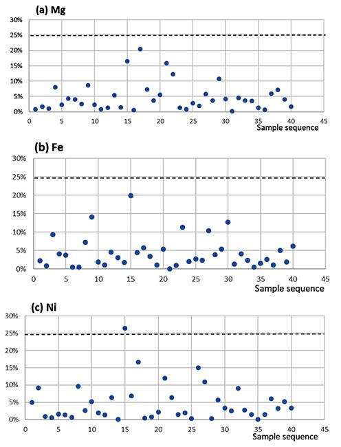
Quality control in tailings resource exploration at Havelock Mine, Eswatini 361The Journal of the Southern African Institute of Mining and Metallurgy VOLUME 122 JULY 2022 Abzalov, M.Z. 2011. Sampling errors and control of assay data quality in exploration and mining geology. Applications and Experiences of Quality Control. Ivanov, O. (ed.): InTech. and-experiences-of-quality-control/sampling-errors-and-control-of-assay-https://www.intechopen.com/books/applicationsdata-quality-in-exploration-and-mining-geology pp. 611 644. Abzalov, M. 2016, Quality control and assurance (QAQC). Applied Mining Geology. Modern Approaches in Solid Earth Sciences, vol. 12. pp. 135–159.: https://doi. org/10.1007/978-3-319-39264-6_10 Table X Assay results of 42 blankFesamples Mg Ni Sample Assay Reference Ratio of assay Assay Reference Ratio of assay Assay Reference Ratio of assay ID result value result to result value result to result value result to (%) (%) reference value (%) (%) reference value (ppm) (ppm) reference value BM101 0.05 0.05 1.00 0.04 0.01 3.31 12 8.5 1.45 BM104 0.05 0.05 1.00 0.05 0.01 4.13 12 8.5 1.39 BM107 0.05 0.05 1.00 0.04 0.01 3.31 5 8.5 0.59 BM110 0.06 0.05 1.20 0.05 0.01 4.13 5 8.5 0.59 BM113 0.05 0.05 1.00 0.04 0.01 3.31 5 8.5 0.59 BM116 0.05 0.05 1.00 0.05 0.01 4.13 5 8.5 0.59 BM119 0.05 0.05 1.00 0.06 0.01 4.96 5 8.5 0.59 BM122 0.03 0.05 0.60 0.05 0.01 4.13 5 8.5 0.59 BM125 0.03 0.05 0.60 0.03 0.01 2.48 5 8.5 0.59 BM128 0.04 0.05 0.80 0.03 0.01 2.48 5 8.5 0.59 BM131 0.04 0.05 0.80 0.03 0.01 2.48 5 8.5 0.59 BM134 0.04 0.05 0.80 0.03 0.01 2.48 5 8.5 0.59 BM137 0.05 0.05 1.00 0.05 0.01 4.13 11 8.5 1.26 BM140 0.0 40.05 0.80 0.03 0.01 2.48 5 8.5 0.59 BM143 0.03 0.05 0.60 0.01 0.01 0.83 5 8.5 0.59 BM146 0.03 0.05 0.60 0.02 0.01 1.65 12 8.5 1.38 BM149 0.04 0.05 0.80 0.03 0.01 2.48 12 8.5 1.47 BM152 0.04 0.05 0.80 0.03 0.01 2.48 11 8.5 1.25 BM155 0.04 0.05 0.80 0.04 0.01 3.31 5 8.5 0.59 BM158 0.03 0.05 0.60 0.04 0.01 3.31 5 8.5 0.59 BM161 0.04 0.05 0.80 0.03 0.01 2.48 5 8.5 0.59 BM164 0.03 0.05 0.60 0.03 0.01 2.48 11 8.5 1.32 BM167 0.03 0.05 0.60 0.03 0.01 2.48 5 8.5 0.59 BM170 0.04 0.05 0.80 0.03 0.01 2.48 5 8.5 0.59 BM173 0.03 0.05 0.60 0.03 0.01 2.48 5 8.5 0.59 BM176 0.04 0.05 0.80 0.03 0.01 2.4 85 8.5 0.59 BM179 0.04 0.05 0.80 0.04 0.01 3.3 15 8.5 0.59 BM182 0.04 0.05 0.80 0.03 0.01 2.48 19 8.5 2.25 BM185 0.03 0.05 0.60 0.04 0.01 3.31 17 8.5 2.02 BM188 0.03 0.05 0.60 0.04 0.01 3.31 5 8.5 0.59 BM191 0.04 0.05 0.80 0.04 0.01 3.31 5 8.5 0.59 BM193 0.04 0.05 0.80 0.02 0.01 1.65 16 8.5 1.91 BM196 0.04 0.05 0.80 0.02 0.01 1.65 17 8.5 1.96 BM199 0.04 0.05 0.80 0.03 0.01 2.48 17 8.5 1.99 BM202 0.04 0.05 0.80 0.01 0.01 0.83 11 8.5 1.25 BM205 0.04 0.05 0.80 0.03 0.01 2.48 13 8.5 1.56 BM208 0.04 0.05 0.80 0.03 0.01 2.48 11 8.5 1.26 BM211 0.04 0.05 0.80 0.03 0.01 2.48 20 8.5 2.35 BM214 0.03 0.05 0.60 0.03 0.01 2.48 19 8.5 2.27 BM217 0.04 0.05 0.80 0.03 0.01 2.48 5 8.5 0.59 BM220 0.03 0.05 0.60 0.03 0.01 2.48 19 8.5 2.25 BM223 0.04 0.05 0.80 0.03 0.01 2.48 14 8.5 1.68 Average 0.04 0.05 0.79 0.03 0.01 2.77 9.27 8.50 1.09 Table XI Summary of statistics of sample assay Mg Fe Ni Number of samples 1.254 1.254 1.254 Minimum 0.01% 0.90% 0.0005% Maximum 40.90% 7.04% 0.4150% Mean 23.02% 3.88% 0.2110% Median 23.28% 3.87% 0.2136% Sample variance 7.78% 0.16% 0.0006% Standard deviation (std dev) 2.79% 0.40% 0.0241% Coefficient of variation 12.12% 10.30% 11.43% Percentage of sample within mean +/- 1 std dev 92.42% 85.25% 92.58% Percentage of sample within mean +/- 2 std dev 97.93% 95.93% 97.85%
2007. Average relative error in geochemical determinations: Clarification, calculation, and a plea for consistency. Exploration and Mining Geology, vol. 16,
2019. Difference between quality assurance and quality control.: control.htmlkeydifferences.com/difference-between-quality-assurance-and-quality-https:// uFigure 11—Distribution of assay results for the tailings samples Figure 12—Vertical distribution of magnesium values Table XII Mineral resource estimation of the TSFs at the Havelock Mine Mineral resource classification Dry tons Million ton (Mt) Mg grade % Mg metal contenct Million ton (Mt) Indicated resource 23.44 23.28 5.41 Inferred resource 1.85 22.88 0.42 Total 25.10 23.25 5.83
IMR Open Report no. 104. Institute of Mining Research, University of Zimbabwe. 9 pp. Köhler, I. and Heubeck, C. 2019. Microbial-mat-associated tephra of the Archean Moodies Group, Barberton greenstone belt (BGB), South Africa: Resemblance to potential biostructures and ecological implications. South African Journal of Geology, vol. 122, no. 2. pp. 221–236. Méndez, A.S. 2011. A discussion on current quality-control practices in mineral exploration. Applications and Experiences of Quality Control. Ivanov, O. (ed.). pp. 595–610. InTech. Runje,Rossi,practices-in-mineral-explorationexperiences-of-quality-control/a-discussion-on-current-quality-control-https://www.intechopen.com/books/applications-and-M.E.andDeuTch,C.V.2014.MineralResourceEstimation.Springer.B.,Novak,A.H.,andRazumić,A.2017.Measurementsystemanalysisinproductionprocess. Proceedings of the XVII International Scientific Conference on Industrial Systems (IS'17). pp. 274–277. https://iim.ftn.uns.ac.rs/is17/papers/49. A. and Coombes, J. 50–54 STanley, C.R. and Lawie, D. no. 265–274. Surbhi, S.
Scogings,pdf.
3–4. pp.
The Journal of the Southern African Institute of Mining and Metallurgy Anhaeusser, C.R. 1974. The nature of chrysotile asbestos occurrences in Southern Africa - A review. Information Circular no .90, Economic Geology Research Unit, University of the Witwatersrand, Johannesburg. Anhaeusser, C.R . 2012. The history of mining in the Barberton greenstone belt, South Africa, with an emphasis on gold (1868–2012). Proceedings of the 9th International Mining History Congress, Johannesburg, pp. 1–29. BarTon, C.M. 1982. Geology and mineral resources of northwest Swaziland (Barberton greenstone belt). Swaziland Geological Survey and Mine Department. 97 pp. ISO. 1994. ISO8402. Quality management and quality assurance – Vocabulary. International Organization for Standardization, Geneva, Switzerland. JCGM. 2008. GCGM200, International vocabulary of metrology – Basic and general concepts and associated terms (VIM).: Jourdan,common/documents/jcgm/JCGM_200_2008.pdfhttps://www.bipm.org/utils/P.1990.ThemineralsindustryofSwaziland.
2014. Quality control and public reporting in industrial minerals. Industrial Mineral, September 2014. pp.
Quality control in tailings resource exploration at Havelock Mine, Eswatini 362 JULY 2022 VOLUME 122
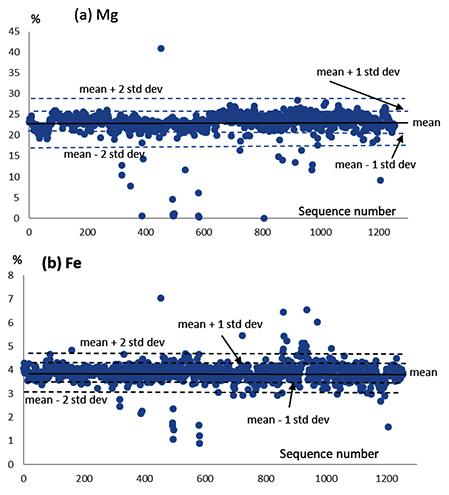
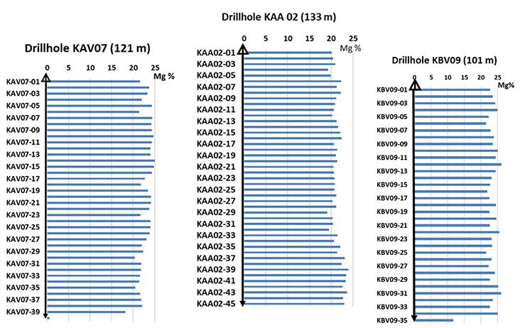
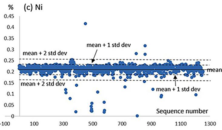
The literature shows that probabilistic analyses increases the reliability of the results by taking into account the spatial variability and uncertainty of the soil parameters (Mellah, Auvinet, and Masrouri, 2000; Le, 2014; Li et al., 2014, 2016), being widely used in 2D slope stability analyses (Malkawi, Hassan, and Abdulla., 2000; El-Ramly, Morgenstern, and Cruden, 2002; Griffiths and Fenton, 2004, Huang et al., 2013; Kasama and Whittle, 2016; Johari and Gholampour, 2018) but with limited cases of 3D analysis owing to the large computational demandsdue to soil heterogeneity and the uncertainties included therein (Hicks, Nuttall, and Chen, 2014; Xiao et al., 2016; Liu et al., 2018). The response surface method (RSM) is a statistical and mathematical technique applied to optimize a response influenced by several factors, where typically the relationship between the response and the factors is unknown. The RSM is recommended for analysing the reliability of non-linear structures with implicit failure surface (Soares et al.,2002). The RSM is a sequential process (Chiwaye and Stacey, 2010) in which we seek to find an appropriate approximation for the factor-response relationship until the closest possible optimum is reached. Due to the enormous number of factors that can influence the response, with the development of computational methods the RSM has become an increasingly important evaluation tool in different areas of knowledge. The RSM is used in geotechnical engineering to predict slope stability (Wong, 1985; Xu and Low, 2006; Zhang, Zhang, and Tang, 2011; Ji and Low, Affiliation: 1Vale Institute of Technology, Brazil. 2Itasca Chile, Chile. 3Vale, Brazil.
failure, factor of safety, response surface method, iron ore, open pit, three-dimensional model, interramp angle.
ThisSynopsispaper shows the importance of performing probabilistic analyses in open pits, especially for mine planning, which can lead to more efficient ore extraction and meeting the acceptability criteria for safety in mine slopes. Three-dimensional stability analyses were performed to evaluate the future geometry of a large open pit for iron ore extraction in Brazil. The strength parameters of the lithologies were calibrated using ruptures in the pit walls. After determining the factors of safety (FoSs) from the calibrated parameters, probabilistic analyses were performed using the total range of values of each parameter under different field conditions to verify the reliability of the initial analysis. In this sense, it was possible to plot the probability of failure (PoF) and the FoS on the graph of slope height versus slope interramp angle (IRA) for the future pit in each lithology. IRA recommendations are made for two scenarios: (1) the best scenario: dry without ubiquitous joints and (2) the worst scenario: the water table at 10 m depth with ubiquitous joints in the most unfavourable direction. The results show that probabilistic evaluation is an important tool for establishing alert mechanisms in slopes that can be termed probabilityKeywordsstable.of
DOI 0103https://orcid.org/0000-0003-1369-A.F.1138https://orcid.org/0000-0003-1523-J.M.0916https://orcid.org/0000-0002-4262-V.F.ORCID9717/2025/2022http://dx.doi.org/10.17159/2411-ID::NavarroTorresGiraoSotomayorSilva
Introduction The analysis of stability in mining slopes employs mean strength parameters obtained from laboratory tests on small samples to represent the behaviour of large volumes of soil or rock, limiting the reliability of the numerical models in terms of the uncertainties in the mechanical parameters introduced (Mellah, Auvinet, and Masrouri, 2000; Li et al., 2012, 2014; Le, 2014). To reduce uncertainties, probabilistic analyses consider the entire database available through statistical distributions, allowing a better view of the probability of slope ruptures by the interaction of a series of parameters linked to a given condition (Chowdhury and Xu, 1995; Phoon and Kulhawy, 1999; El-Ramly, Morgenstern, and Cruden, 2002; Terbrugge et al., 2006; Read and Stacey, 2009; Zhang, Zhang, and Tang, 2011; Contreras, 2015).
Correspondence to: J.M. Girao Sotomayor Email: juan.sotomayor@itv.org
Probability of failure and factor of safety in the design of interramp angles in a large open iron ore mine by V.F. Navarro Torres1, R. Dockendorff2, J.M. Girao Sotomayor1, C. Castro2, and A.F. Silva3
Dates: Received: 14 Oct. 2021 Revised: 8 Mar. 2022 Accepted: 16 Mar. 2022 Published: July 2022 How to cite: Navarro Torres, V.F., Dockendorff, R., Girao Sotomayor, J.M., Castro, C., and Silva, A.F. 2022 Probability of failure and factor of safety in the design of interramp angles in a large open iron ore mine. Journal of the Southern African Institute of Mining and Metallurgy, vol. 122, no. 7, pp. 363–376
363The Journal of the Southern African Institute of Mining and Metallurgy VOLUME 122 JULY 2022
The rupture affected three benches, reaching a maximum height of approximately 45 m. Before and after the occurrence, the slope showed the presence of a large amount of water. The rupture mechanism acting on the slope was interpreted as controlled by the contact between the mafic and iron-beaing rocks, called the shear zone (SZ). The iron formation consists of friable haematite (FH) and jaspilite (JP) lithotypes (Table I). The mafic formation consists of solid mafic (SM), semidecomposed mafic (SDM), and decomposed mafic (DM) lithotypes. The SZ occurs every where the iron formation overlies the mafic formation. Due to the different densities of these formations, shearing occurs along with relative displacement of the iron formation at the HS/SM, FH, SDM, FH/ DM, JP/SM, JP/SDM, and JP/DM contacts. Figure 3 shows the location of the SZ. In the model, the contact was implemented as a 2 m wide Consideringlayer. a low resistance and an SZ contact plane, the stability of the slope depends on the resistance of the FH lithotype; this lithotype was therefore, the calibrated rock unit.
The 2018 pit topography was used to construct the geometric model (Figure 1). The block model of the mine was used to spatially locate the lithologies within the geometric model. Information on the classification of rocks, tests on intact rock, hydrogeological information, geology, and strength properties of the rocks (Table I) were loaded for each lithology present in the model. The finite difference software used for geotechnical modelling was FLAC3D. In both the calibration model and the predictive model, the rock mass behaviour was represented using the elasto-plastic relationship with a failure envelope and ubiquitous joints for all the rock units. The most conservative fabric orientations were selected for each rock type.
The calibrated results are presented in terms of numerical velocity contours, which can be compared with the documented instability. The numerical velocity is used as an indicator to Table I
Mechanical strength parameters and elastic parameters
The Journal of the Southern African Institute of Mining and Metallurgy 2012; Jiang et al., 2014; Li and Chu, 2015; Li et al., 2016), including stability under earthquake action (Kasama, Furukawa, and Hu, 2021).The present study aims to contribute to the improvement in the determination of interramp angles (IRAs) in open pits by applying a probabilistic approach. The 3D stability of an iron ore pit located in Brazil was evaluated using the finite difference method in the software FLAC3D. The RSM was used to create a surface of factor of safety (FoS) values for different combinations of parameters in the areas where the 3D model showed critical stability. Finally, to determine the probability of failure (PoF), Monte Carlo simulations were performed on the RSM in each critical sector. With these results and the evaluation of a best and worst scenario in each sector, this study presents recommendations of IRAs for each lithology comparing the FoS versus the PoF obtained. Case description
A slope rupture that occurred in 2018 was used to calibrate the strength parameters of the rocks. Figure 1 shows the location of the rupture, and Figure 2 shows the location before and after the rupture.
The study comprises 3D modelling of the pit, calibration of the model, the location of the zones with critical stability, the PoF of these zones under the worst and best conditions, and finally the elaboration of a graph of slope height versus IRA where the PoF and the FoS can be compared.
Calibration of the model
Sterile/landfill LF 20 32 0.32 0.35 Chemical canga CC 65 43 2.00 0.35 Compact haematite CH 250 45 27.6 0.22 Friable haematite FH 99 40 0.38 0.28 Jaspilite JP 3750 48 45.9 0.21
Lithology ID c' φ' E rm ν (kPa) (°) (GPa)
Decomposed mafic DM 60 29 0.91 0.30 Solid mafic SM 3200 50 29.7 0.22 Semi-decomposed mafic SDM 240 32 27.6 0.22 Shear zone SZ 9 18 0.32 0.35 c’: Effective cohesion φ': Effective friction angle Erm: Rock mass deformation modulus ν: Poisson ratio
Figure 1—The open pit iron mine, showing the location of the 2018 slope ruptureFigure2—Slope failure 2018
3D modelling
364 JULY 2022 VOLUME 122
Probability of failure and factor of safety in the design of interramp angles
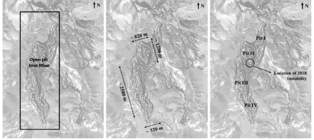
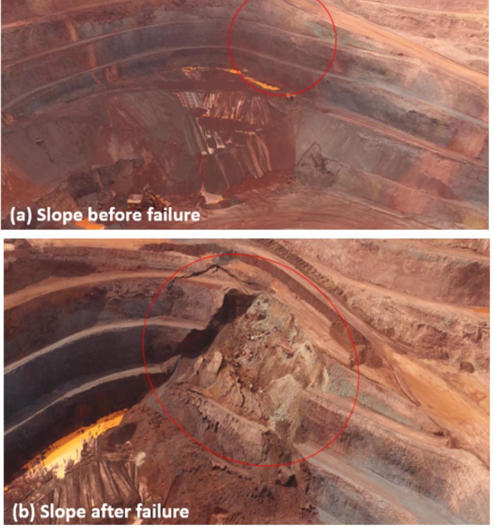
365The Journal of the Southern African Institute of Mining and Metallurgy VOLUME 122 JULY 2022
➤ Predicted scenario: This scenario uses the inferred phreatic surface for the final pit. This is the most likely predicted case, considering the available information.
Probability of failure and factor of safety in the design of interramp angles
Figure 3—Location of the hear zone Figure 4—2018 instability, (a) Real versus numerical response, (b) numerical response size
Location of critical stability zones (FoS)
A relevant finding during the calibration process was the importance of the phreatic levels in influencing the behaviour of the slopes. With this in mind, the geometry of the final pit (year 2030) was evaluated considering three alternative hydrogeology scenarios
The calibration process modified only the strength properties of the FH lithotype, which mainly participated in the 2018 instability condition. The calibration also defined the strength parameters of the ubiquitous joints used in the model, obeying the more conservative orientations with respect to the orientation of the pit. Table II shows the calibrated properties for the FH lithotype.
interpret the stability conditions in the numerical model. These velocities are given without units because they are mathematical devices used only to represent the convergence of the numerical solution. Wyllie and Mah (2004) and Lorig and Varona (2000) found that velocities below 1e-6 indicate stability in FLAC and FLAC3D; conversely, velocities above 1e-5 indicate instability. To reproduce the documented instability, it was assumed that the FH lithotype was under saturated conditions (water level near the surface). Under dry conditions, the slopes were stable. The saturation hypothesis was related to the observations documented before and after the rupture. The results in terms of the contour velocities are shown in Figure 4. Good reproduction of this condition was observed, where only the broken slope corresponded to the 2018 instability. Figure 5 shows that the rupture mechanism is captured well: a planar failure controlled by the SZ contact that occurs when the FH rock bridge breaks. In section E-E', the rock bridge between the SZ contact and the foot of the slope is close to 16 m for a slope 45 m in height. However, in section D-D', where the slope exhibits stable behaviour, the rock bridge between the SZ contact and the foot of the slope is close to 35 m for a 45 m high slope, which presents the slope geometric conditions to avoid instability.
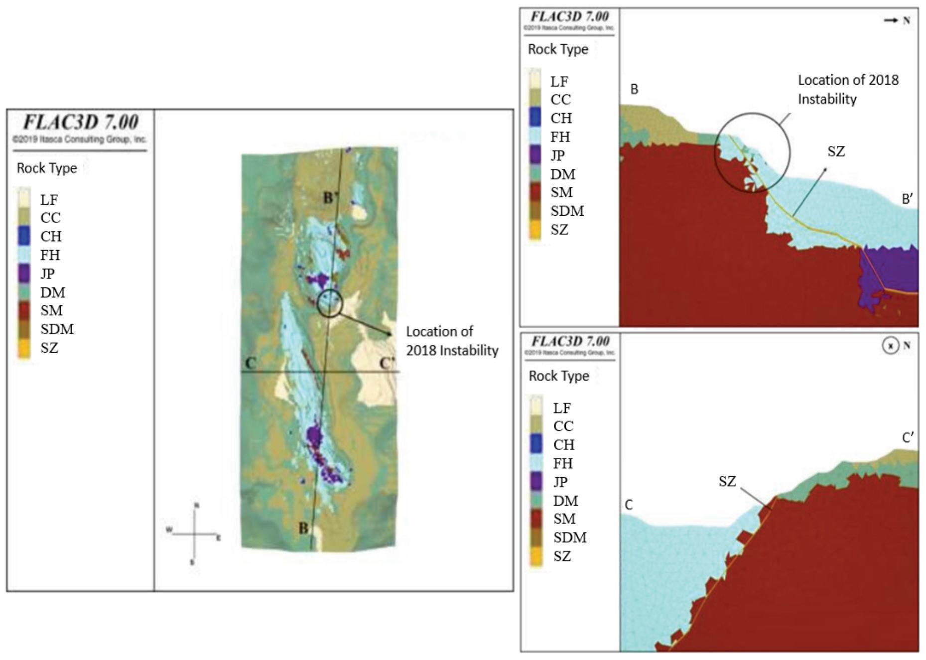
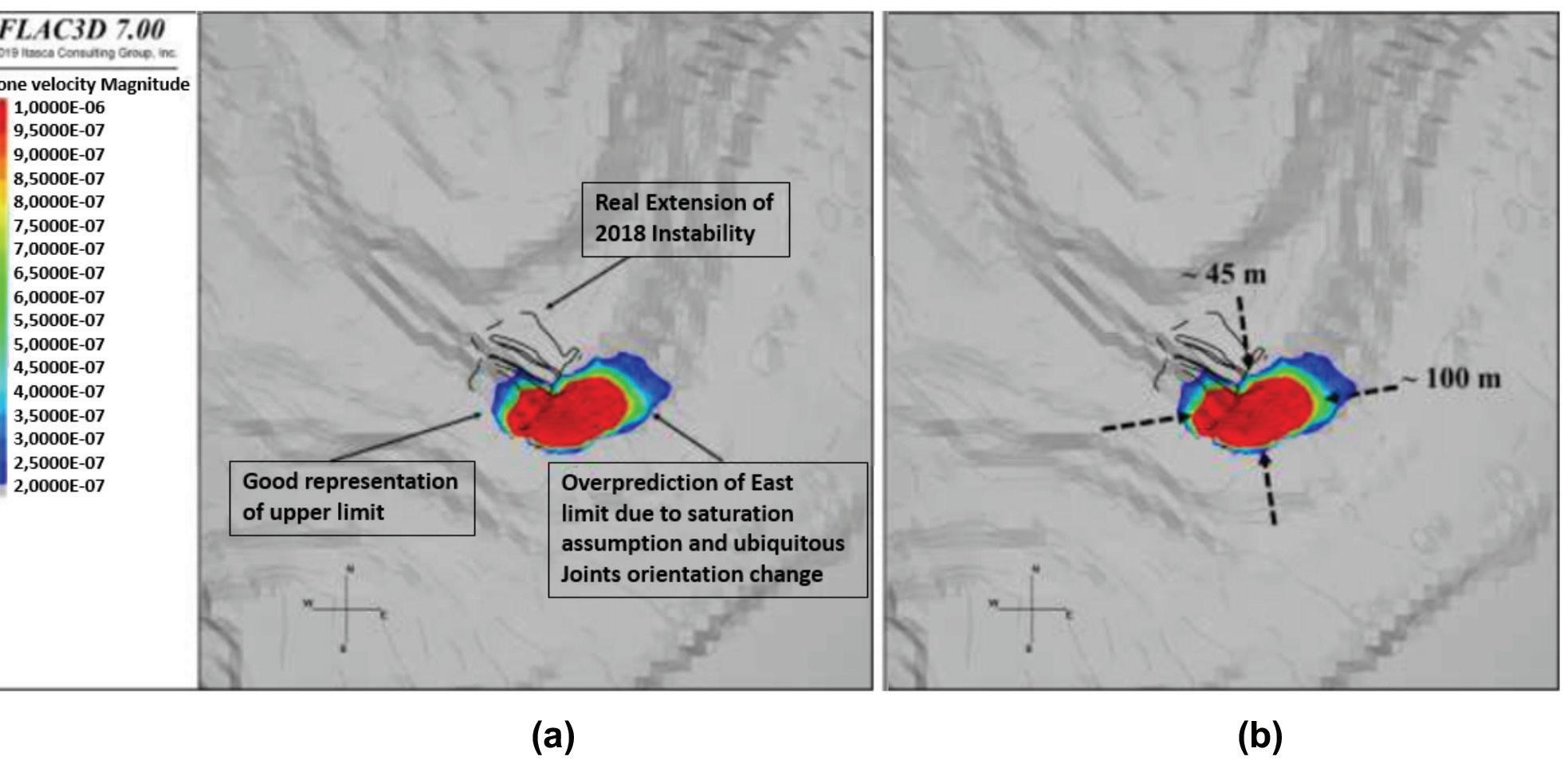
The objective of performing three analyses for the final pit was to compare the behaviour of the pit slopes under different groundwater regimes and, therefore, to illustrate the role of groundwater levels in the overall pit stability.
Areas not conforming to the acceptability criteria (1 < FoS < 1.3) Figure 9 shows the acceptability of the stability of the final pit in terms of FoS contours. Considering that all previously identified instabilities exhibit an FoS < 1.0 (due to their kinematically admissible geometries), the largest extension of the pit exhibits acceptable stability (FoS > 1.3). However, four sectors of the mine raise alarms within the analysis (FoS < 1.3). East wall of pit I (section J-J')
Institute of Mining and Metallurgy
The slope is excavated with an orientation of approximately 300° (D-D') and an IRA of 37° almost exclusively in an FH rock unit. The slope has a convex geometry, promoting lower lateral confinement. The predicted phreatic level is close to the surface Figure instability - real versus numerical response hematite
Table II Calibrated parameters for friable
➤ Saturated scenario: This scenario assumes total saturation of the slopes of the final pit. This is the worst possible scenario in terms of groundwater levels.
366 JULY 2022 VOLUME 122 The Journal of the Southern
- Stable areas that do not meet the acceptability criterion (1.1 < FoS < 1.3): These areas are distributed along the pit. Unstable areas (FoS <1.0) To improve visualization of unstable areas (FoS < 1.0), velocity contours are used as an intermediary between the numerical data and the user to understand the location and extent of the unstable area (Figure 7). The model predicts instabilities on a bench scale (FoS < 1.0; height < 15 m) distributed mainly on the southern slope of pit II and on the eastern slope of pits III and IV. In addition, four large instabilities (FoS < 1.0; height > 50 m) (Figure 8) are predicted. These vary between approximately 50 m and 125 m in height and between 10 m and 20 m in width. They are located on the NE slope of pit I, on the southern slope of pit II, and on the eastern slope of pit III. The bench-scale instabilities and the four main instabilities exhibit the same rupture mechanism. In all of them, the SZ shear contact defines a planar rupture geometry. This configuration makes all geometries kinematically admissible for sliding through the SZ shear contact. This geometric configuration makes the prevention of the occurrence of these instabilities ‘ inevitable’, considering the current definition of SZ shear contact.
Factor of safety (FoS) stability criteria Figure 6 shows the general behaviour of the pit in terms of the FoS contours. From this graphic, four results can be observed. ➤ Unstable areas (FoS < 1.0): These areas are mainly distributed in pit I, pit II, and pit III. ➤ Areas not in compliance with the acceptability criterion (FoS < 1.3): Although these areas are stable, they do not meet the acceptability criterion. Two cases can be distinguished in this section: - Areas of marginal stability (1.0 < FoS < 1.1): This area covers a large extension of the east wall of pit I.
5—2018
(FH) Lithology ID c' φ' E rm ν (kPa) (°) (GPa) Friable haematite FH 75 30 0.38 0.28
➤ Dry scenario: This scenario assumes dry conditions for all slopes of the final pit. This is the best-case scenario in terms of groundwater levels.
Probability of failure and factor of safety in the design of interramp angles African
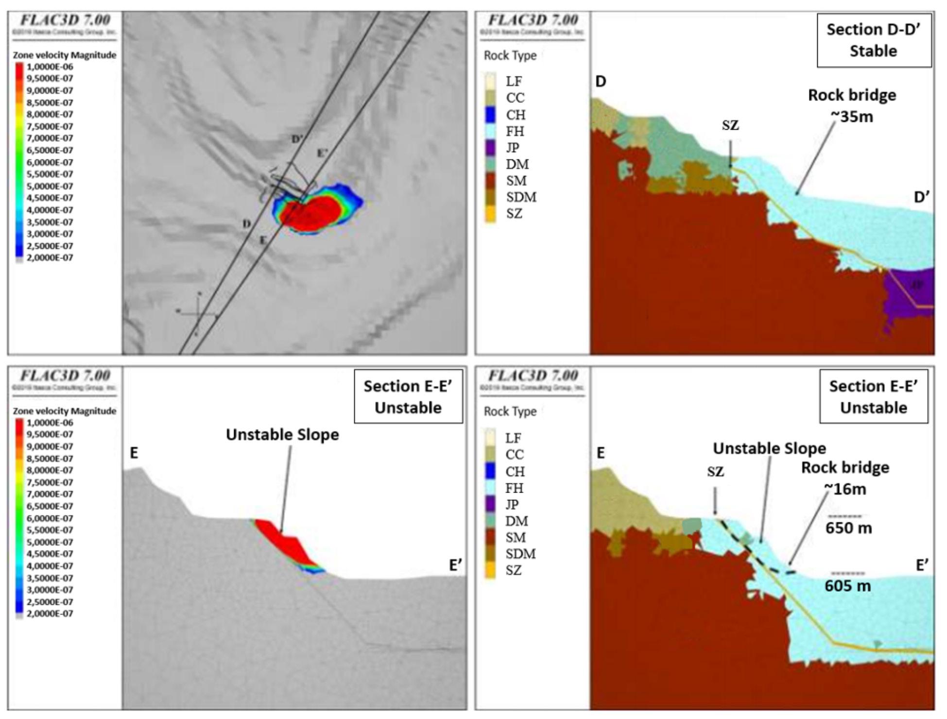
Figure 11 shows the effect of the water table (groundwater position) on the response of the east wall pit I in terms of FoS contours. Compared with that of the predicted scenario, the slope of the dry scenario shows an improvement in FoS contours, with a 0.1 increase in magnitude, going from a critical stability condition to 1.1 < FoS < 1.3. Although the slope continues to exhibit values that do not meet the acceptability criterion, this case shows the sensitivity of the slope to adequate drainage. Based on the results Figure 6—Safety factors for the final pit Figure 7—Unstable areas (FoS < 1)
at the foot of the slope. Considering the conservative criteria for assigning the different sets of joints, the FH rock unit in this area has ubiquitous joints with an orientation of 72°/282° (dip/ direction of dip). This implies that although the ubiquitous joints have a dip of 72°, they run subparallel to the slope (orientation difference less than 20°). These aspects, applied to an FH rock unit calibrated with 75 kPa of cohesion and friction angle of 30°, result in a slope with an FoS ranging from 1.0 to 1.1. In other words, considering the parameters calibrated for the FH rock unit and the geometric characteristics, this slope shows critical stability. The potential failure mechanism is rupture through the FH rock mass (Figure 10), limited to the east by the SZ and reaching approximiately 335 m. The SZ occurs behind the slope, forming an FH rock bridge of about 290 m. Because the slope is close to the water table, it is important to evaluate the sensitivity of this wall to the position of the water table.
Probability of failure and factor of safety in the design of interramp angles
367The Journal of the Southern African Institute of Mining and Metallurgy VOLUME 122 JULY 2022
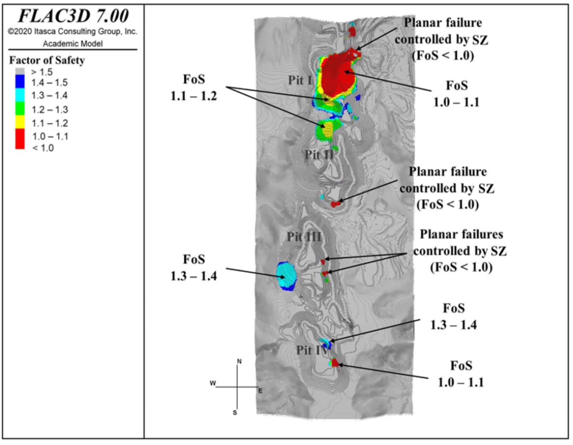
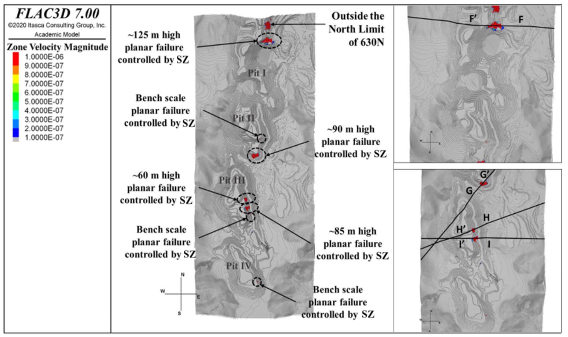
Probability of failure and factor of safety in the design of interramp angles the Southern African Institute of Mining Metallurgy of the FLAC3D model, a change in the IRA angles for the FH rock unit and a change in the east wall design from pit I to the 2030 final pit are recommended.
368 JULY 2022 VOLUME 122 The Journal of
and
South wall of pit I and north wall of pit II (section K-K')
The wall shows FoS contours ranging from 1.1 < FoS < 1.2 (Figure 12), which indicates that the slope is stable but does not meet the acceptability criterion (FoS > 1.3). This wall has two slopes thatdivide pit I and pit II. This wall is built almost entirely in the FH rock unit, with an IRA of approximately 39° for a maximum height of 195 m. The ubiquitous joints in these domains for the FH in this specific sector have orientations of 59/268 and 57/243, respectively, without affecting the slope performance because the slope orientation is almost E-W. In addition, neither the ubiquitous joints nor the water table affect the magnitude of the FoS contours (Figure 13). This is only a consequence of the resistance envelope of the calibrated FH rock unit. Based on the results of the FLAC3D Figure 8—Four main instabilities predicted for the final pit. (a) Section FF', (b) section GG', (c) section HH', and (d) section I-I'
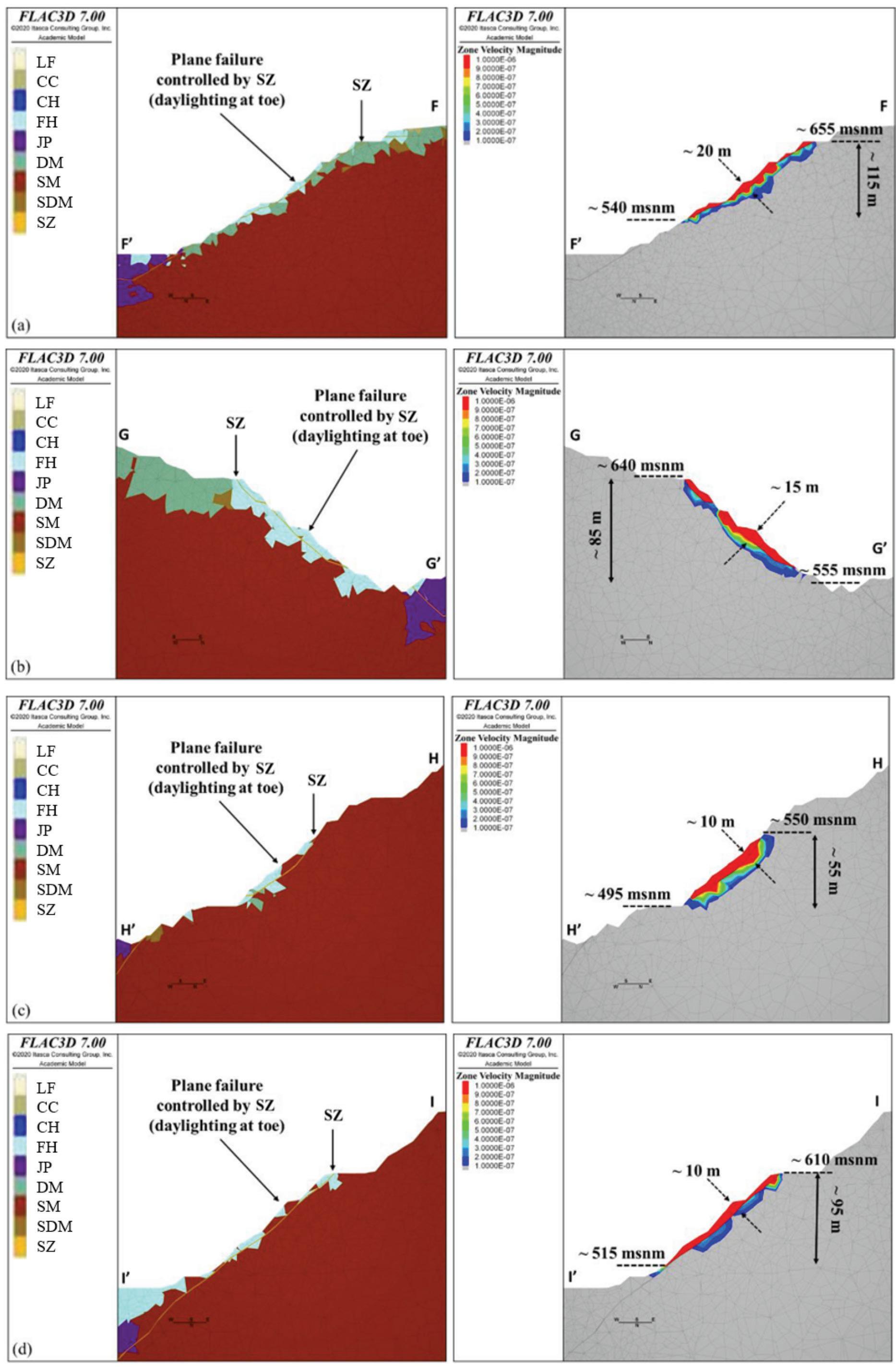
Probability of failure and factor of safety in the design of interramp angles 369The Journal of the Southern African Institute of Mining and Metallurgy VOLUME 122 JULY 2022 Figure 10—FoS of the final pit - east wall of pit I - section J -J' Figure 11—Sensitivity to the water table - comparison of the predicted scenario and the dry scenario for section J -J' - east wall of pit I Figure 9—Final pit (FoS > 1)
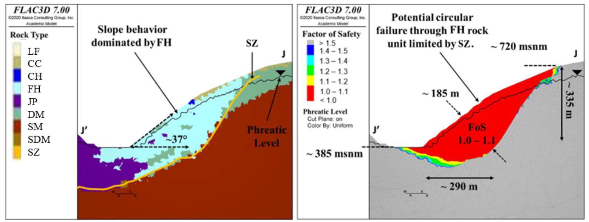
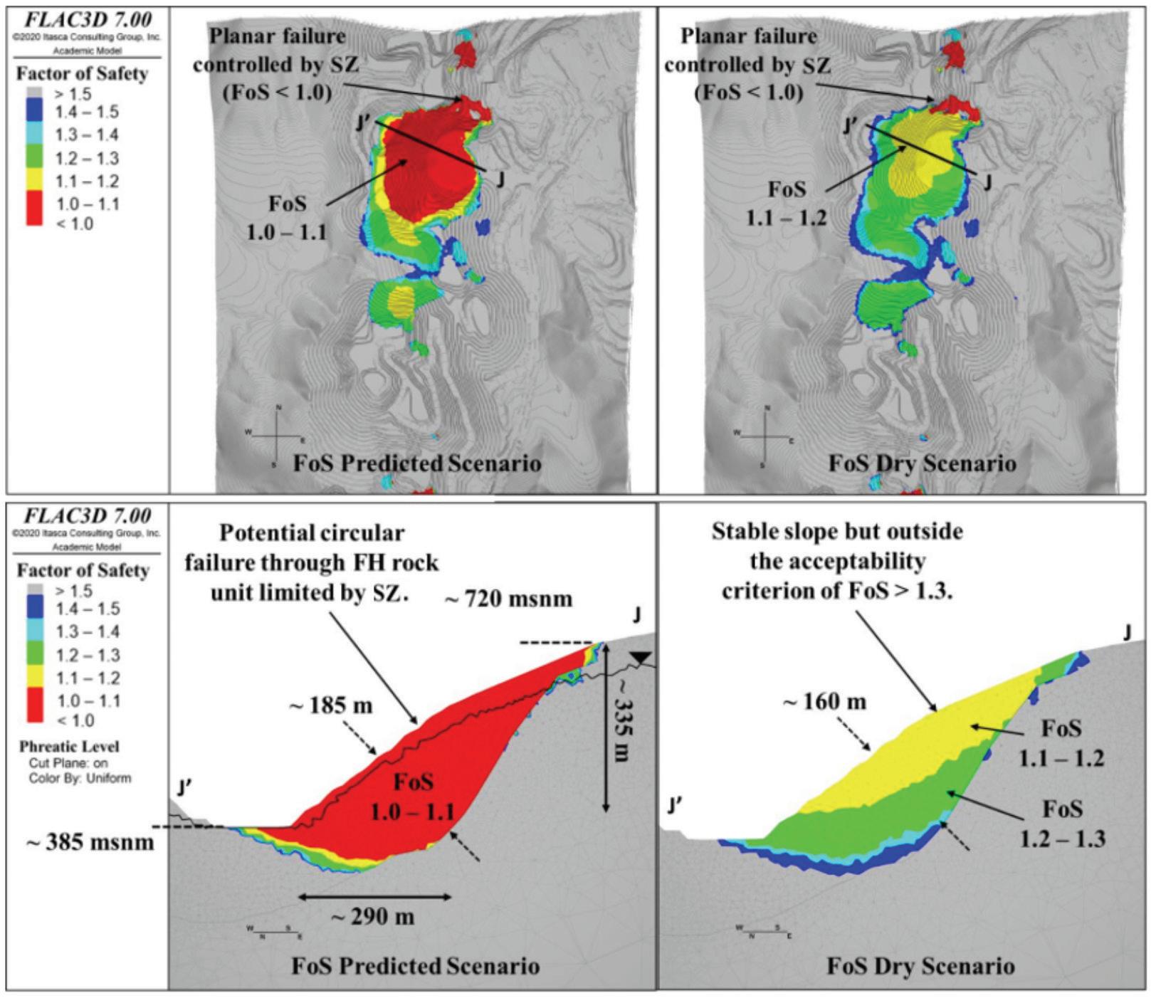
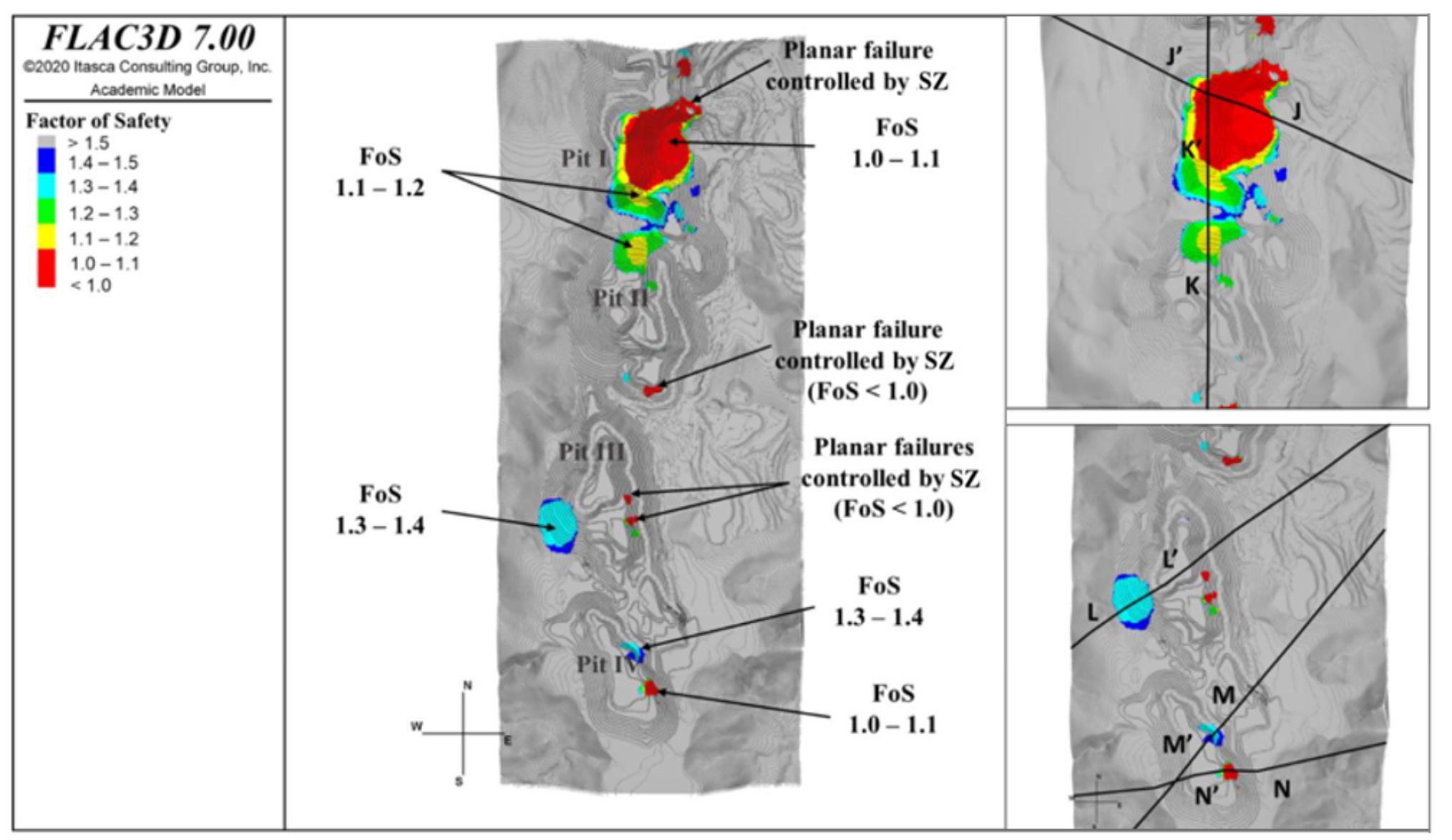
For this area, a key factor is the position of the SZ. Section NN' shows an FoS of 1.3-1.4. Although the FoS contours meet the acceptability criterion, the integrity of the rock bridge is the key to the stability of the slope.
Discussion of results - 3D stability analysis
Figure 13—Sensitivity to the water table - comparison of the predicted scenario and the dry scenario for section KK' - south wall pit I and north wall pit II
Institute of Mining and Metallurgy
370 JULY 2022 VOLUME 122 The Journal of the Southern
Figure 12—FoS of the final pit - south wall of pit I and north wall of pit II - section K-K'
Western wall of pit III (section L-L')
The 3D model of the final pit indicates that, to a great extent, the walls meet the acceptability criterion of FoS > 1.3. Considering that
model, it is also recommended to change the IRAs for the FH rock unit and to change the design of the south wall of pit I and the north wall of pit II to that of the final pit.
Probability of failure and factor of safety in the design of interramp angles African
East wall of the IV pit (sections M-M' and N-N')
The main rock unit in the upper three quarters of the western wall of pit III is DM (Figure 14). This unit (cohesion of 60 kPa, friction angle of 29°) supports a slope of approximately 32° IRA and exhibits FoS contours of 1.3-1.4, where water does not play a significant role in the predicted scenario. Although this slope is in accordance with the acceptability criterion (FoS > 1.3), a sensitivity analysis was performed to evaluate the slope response under the saturated scenario (Figure 15). Figure 15 shows the strong sensitivity of the DM, SDM, and FH rock units to the water level, especially in the slope of section L-L', where the wall transitions from an FoS of 1.3-1.4 to an unstable condition (FoS < 1.0) due only to changes in the water table. These results support the recommendation of adequate drainage of the slopes as stability control measures.
The western slope of pit IV has two areas where the SZ forms two planar fault geometries, with rock bridges ranging from approxamately 10 m in the M-M' section to 7 m in the NN' section (Figure 16). The MM' section exhibits critical stability (FoS 1.01.1), with a failure mechanism geometry of up to 90 m in height.
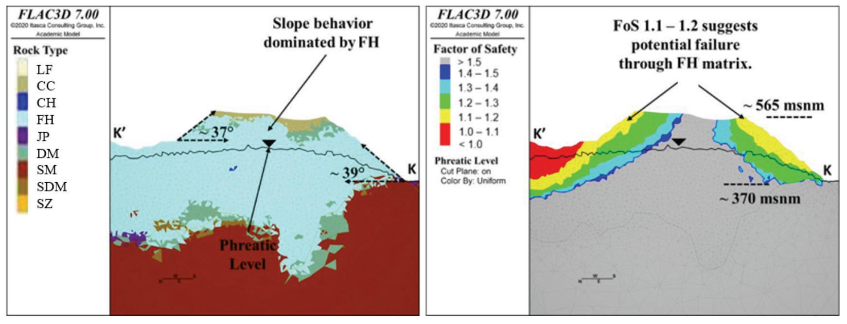
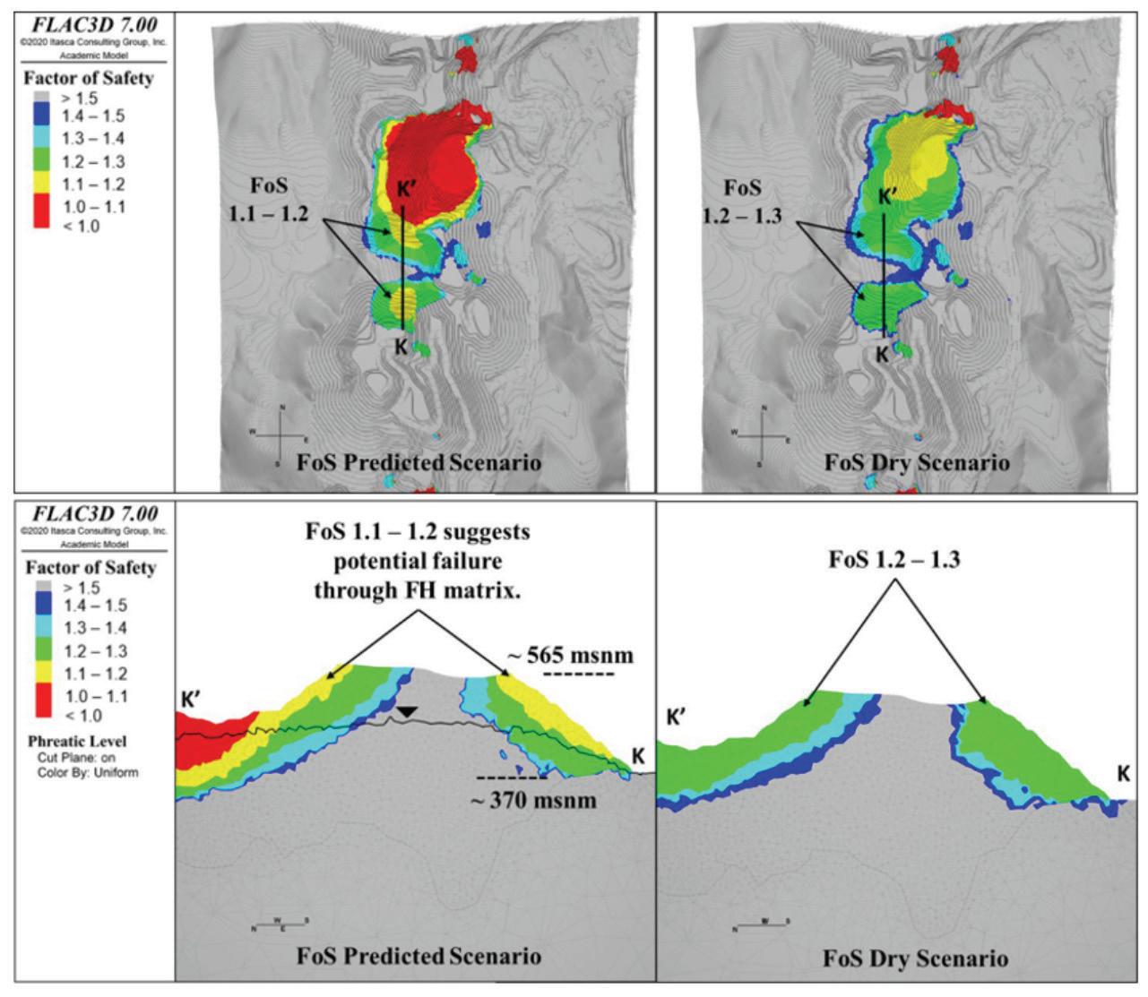
371The Journal of the Southern African Institute of Mining and Metallurgy VOLUME 122 JULY 2022
Figure 15—Water table sensitivity comparison between the predicted scenario and the dry scenario in section L-L' - east wall pit I
Figure 14—FoS for the final pit - west wall of pit III - section L-L'
several instabilities (FoS < 1.0) up to the bench scale are found (height ≤ 15 m), four main unstable geometries are described (height > 30 m). All of these have the same potential failure mechanism: planar failure geometry controlled by the SZ. When the FoS contours for the final pit were evaluated, additional information on pit stability was obtained. In the east wall of pit I, the model suggests a stable critical slope (1.0 < FoS < 1.1). This is mainly due to the calibrated parameters for the FH rock unit and the subparallel orientation of the ubiquitous joints. Based on the results of the FLAC3D model, it is necessary to change the IRAs for the FH rock unit and change the design of the east wall from pit I to that of the final pit. In the south wall of pit I and in the north wall of pit II, the model suggests a stable but not acceptable slope (1.1 < FoS < 1.2). For both slopes, a drop in the water table increases the FoS in increments of 0.1. However, the main factor for the stability behaviour is related to the calibrated strength parameters of the FH rock unit. Based on the results of the FLAC3D model, it is necessary to change the IRA for the FH rock unit and change the design of the south wall of pit I and the north wall of pit II to that of the final pit. In pit III, the DM rock slope shows 1.3 < FoS < 1.4, which meets the acceptability criterion but shows a strong sensitivity to changes in the water table. In addition to the above slopes, adequate drainage strategies for DM, FH, and SDM slopes are essential.Inpit IV, stability is controlled by the SZ contact shear. The stability depends exclusively on the position of the SZ contact and strength of the rock bridge. After the areas with critical stability were determined by the 3D stability analysis, the next step was to perform an analysis to determine the PoF of each sector.
Probability of failure and factor of safety in the design of interramp angles
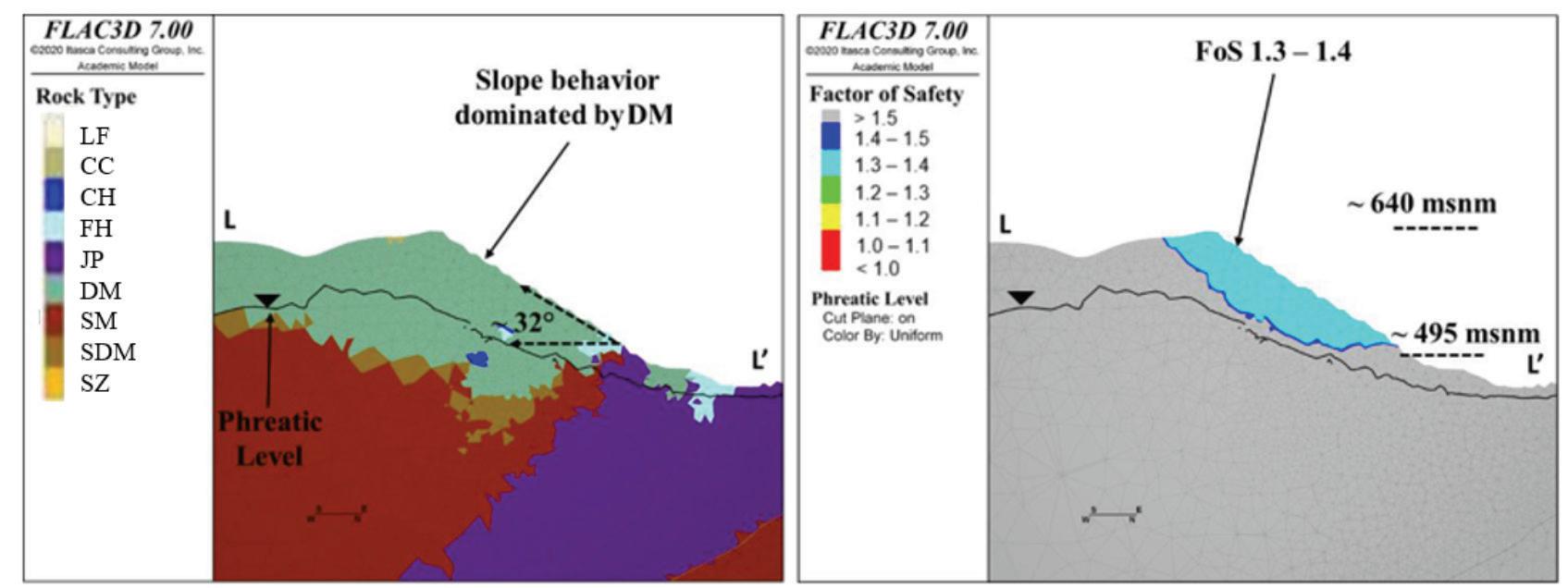
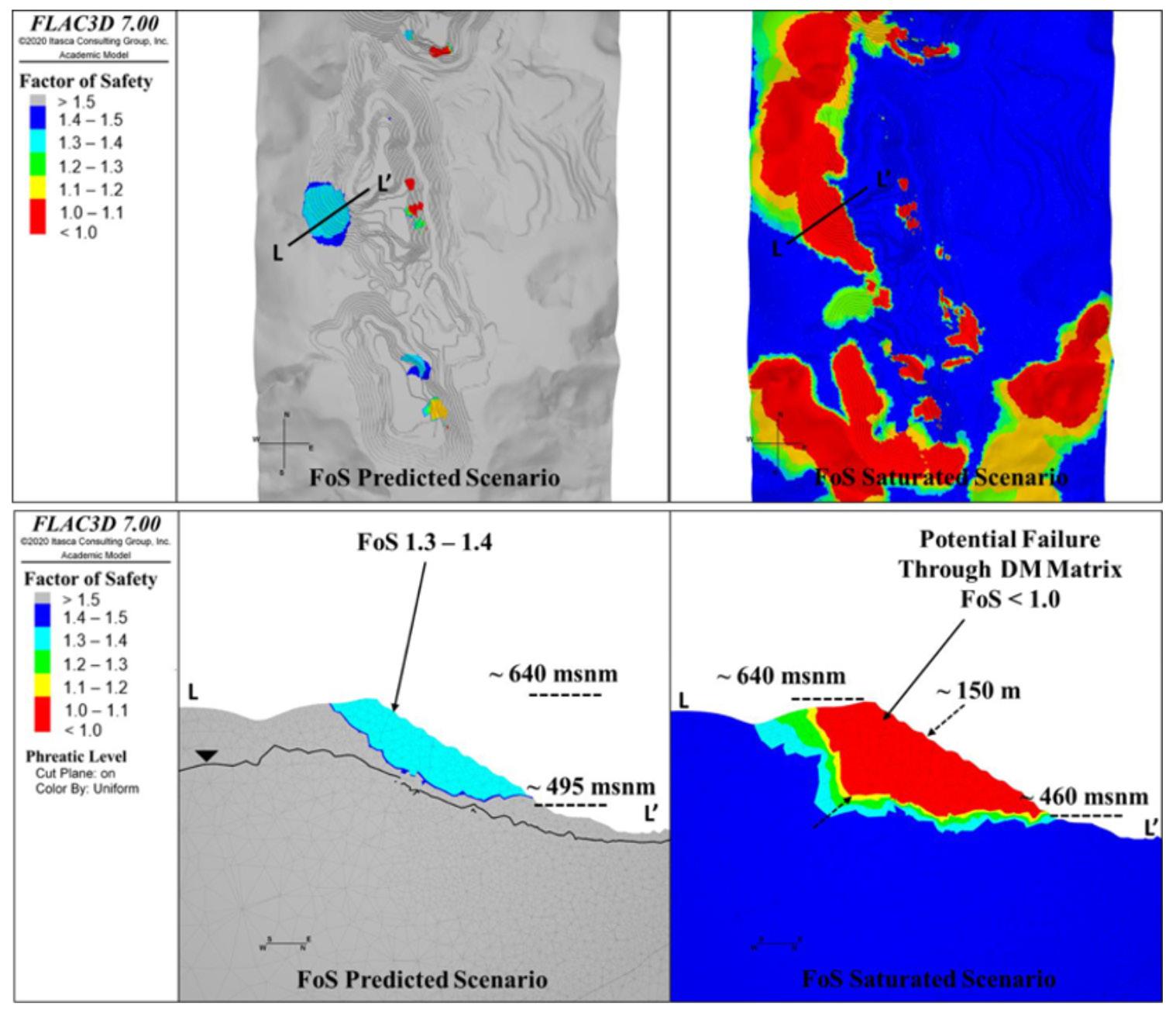
Figure 18—Example showing the best fit to the FoS sensitivity curve (Chiwaye and Stacey, 2010)
Figure 17—Example showing the FoS distribution resulting from the Mon te Carlo simulation and the PoF definition (Chiwaye and Stacey, 2010)
The sensitivity of the FoS in relation to the mean values (xi') is defined by the parameter b as: [3] This can be defined in two points on each side of the best estimated value, as shown in Figure 18. The best-fit curve is obtained for this case, and then any random combination of the input variables can be evaluated by: FOSi = FOSbc × b1i × b2i × … × bNi [4]
Random sampling, such as Monte Carlo simulation, ultimately facilitates the acquisition of the PoF (Figure 17): POF = P (FOS<1) [5] In this study, variable input parameters are assumed for the angle of friction and cohesion of the FH and DM units, which are the factors concerning the critical stability of the slopes.
Figure 16—FoS contours of the final pit - east wall of pit IV - sections M-M' and N-N'
Probability of failure and factor of safety in the design of interramp angles African
Institute of Mining and Metallurgy
Probability of failure (PoF)
The method assumes that the effect of each xi is independent of the others, where the base case (bc) represents the best estimate value (mean):
The analysis of the PoF was based on the application of the RSM to the critical sectors of the 2030 final pit. Two steps were performed to obtain the PoF. The first involved the use of a stability model (3DEC) to calculate the FoS for the various combinations of input parameters in the critical sectors, whose responses were fitted to a curve to obtain the total response surface. In the second stage, several realizations were performed with Monte Carlo simulation using the various probability distributions of the parameters. The result of the Monte Carlo simulation was a FoS distribution from which the PoF was calculated (Figure 17).
FOSbc = RSM (x'1, x'2, x'3, …, x'N) [2]
372 JULY 2022 VOLUME 122 The Journal of the Southern
Response surface method (RSM) The RSM represents the function that defines the distribution of FoS, dependent, for example, on N uncertain variables, such as: FOS = RSM (x1, x2, x3, …, xN) [1]
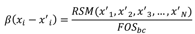
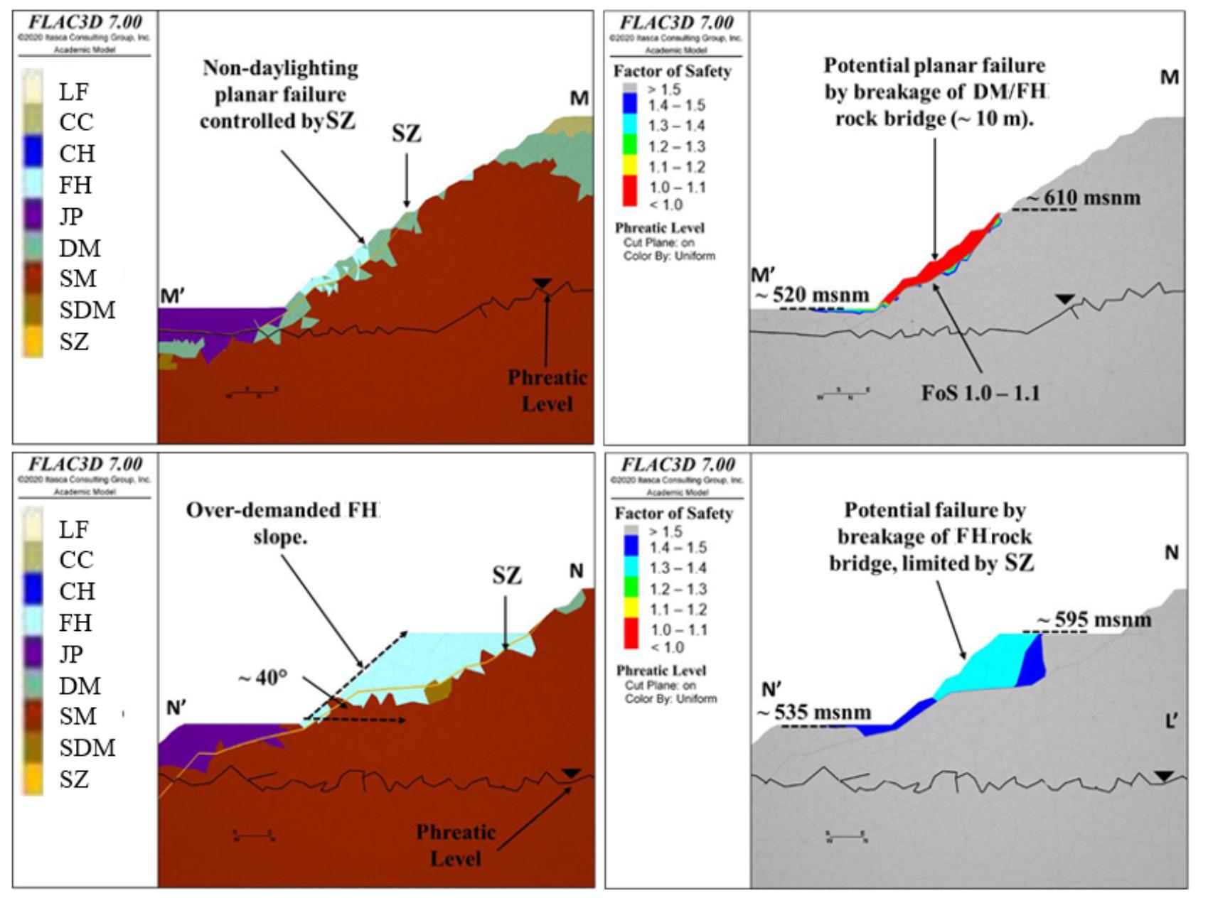
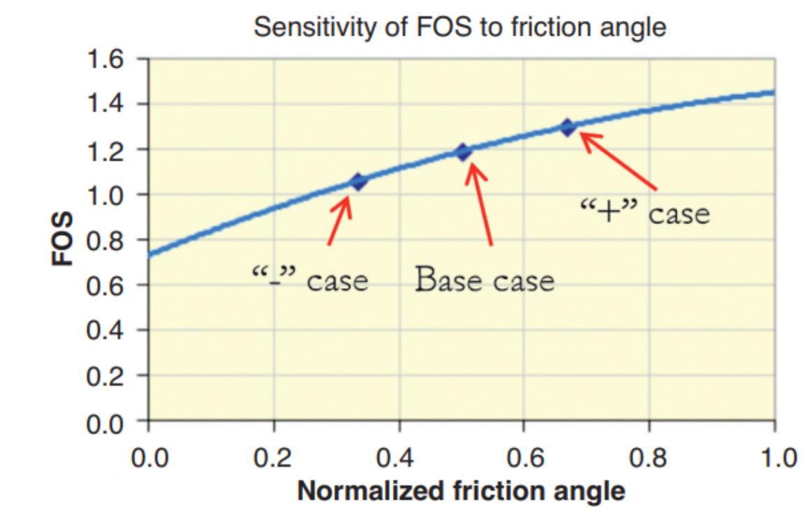
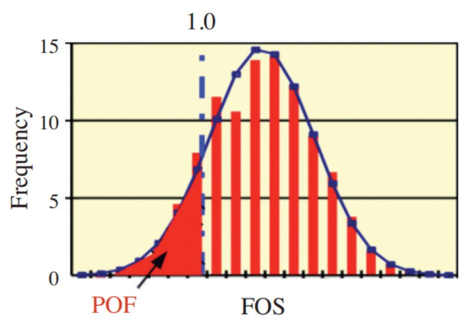
Institute of Mining and Metallurgy VOLUME 122 JULY 2022
Assessment scenarios and PoF Two scenarios were defined for the PoF calculation. The first scenario (PoF 5-95) assumes that the laboratory data is representative of the population; therefore, the data is used directly as received. The second scenario (PoF 10-90) assumes that the laboratory data is not completely representative of the population; therefore, it is assumed that P05 of the sample actually corresponds to the 10th percentile of the population, while P95 of the sample is assumed to correspond to the 90th percentile. This scenario is more conservative and helps explain how sensitive the analysis is to variations in some of the assumptions. The RSM was applied to all six sectors of interest. A quadratic fit was used as the best fit for the FoS results, and 10 000 Monte Carlo realizations were generated. The PoF of each sector is shown in Table V. It is observed that the PoF is typically low, except for two sectors, 4 and 6. The PoF varies from 8% to 10% in sector 4 and from 16% to 19% in sector 6. It is important to note that the analysis is based on the properties of the materials but the location of the water table is not part of the analysis. As shown in the sensitivity analyses, the location of the water table is a critical stability factor for the pit. Interramp angle (IRA) recommendations
➤ Worst case scenario: The analyses were performed for a water table 10 m below the surface for all types of rock, and joints with orientation parallel to the slope plunging in the worst direction. shear strength FH and DM Standard 5% 95% deviation Percentile Percentile Cohesion (kPa) 68 60.0 53.0 4.4 172.4 Friction (°) 68 29.2 5.4 21.2
Lithology Parameter Quantity Mean
A total of five cases were considered in the PoF analyses: (1) the average properties, (2) cohesion in the 5th percentile (P05) and average friction angle, (3) cohesion in the 95th percentile (P95) and average friction angle, (4) average cohesion and friction angle in P05, and (5) average cohesion and friction angle in P95. Based on the available laboratory data, the statistics of the resistance properties of FH and DM are shown in Table III.
Critical sectors defined for the probability of failure (PoF) analyses
➤ Best scenario: The analyses were performed for a dry environment, without ubiquitous joints, and the rock mass was represented only by the c, φ of each rock unit.
373The Journal of the Southern
Statistical cases of resistance evaluated
The 3D slope stability model was applied using the average properties to define the zones of interest to calculate the PoF. Figure 19 shows the results of the analysis and indicates the six zones of interest defined for the PoF analyses. The FoS of each zone of interest per PoF scenario is summarized in Table IV.
The recommendations for the IRA were developed using a simplified two-dimensional FLAC/Slope v8.0 analysis, considering that the acceptability criterion is FoS ≥ 1.3. The rock units were evaluated for the best and worst cases.
37.9 FH Cohesion (kPa) 24 99.5 71.0 3 220.6 Friction (°) 24 40.1 3.9 34.9 45.0 Table IV FoSw results in each zone of interest per PoF scenario Scenario Cohesion Friction Sector 1 Sector 2 Sector 3 Sector 4 Sector 5 Sector 6 1 Mean Mean 1.35 1.65 1.65 1.35 1.55 1.15 2 P95 Mean 1.55 1.85 1.85 1.95 1.75 1.45 3 Mean P95 1.55 1.85 1.85 1.75 1.55 1.25 4 P05 Mean 1.15 1.45 1.35 1.05 1.25 0.95 5 Mean P05 1.15 1.45 1.45 1.05 1.55 1.15 Figure 19—Areas of interest for the PoF analyses
Probability of failure and factor of safety in the design of interramp angles African
DM
properties of
Table III Statistics of the
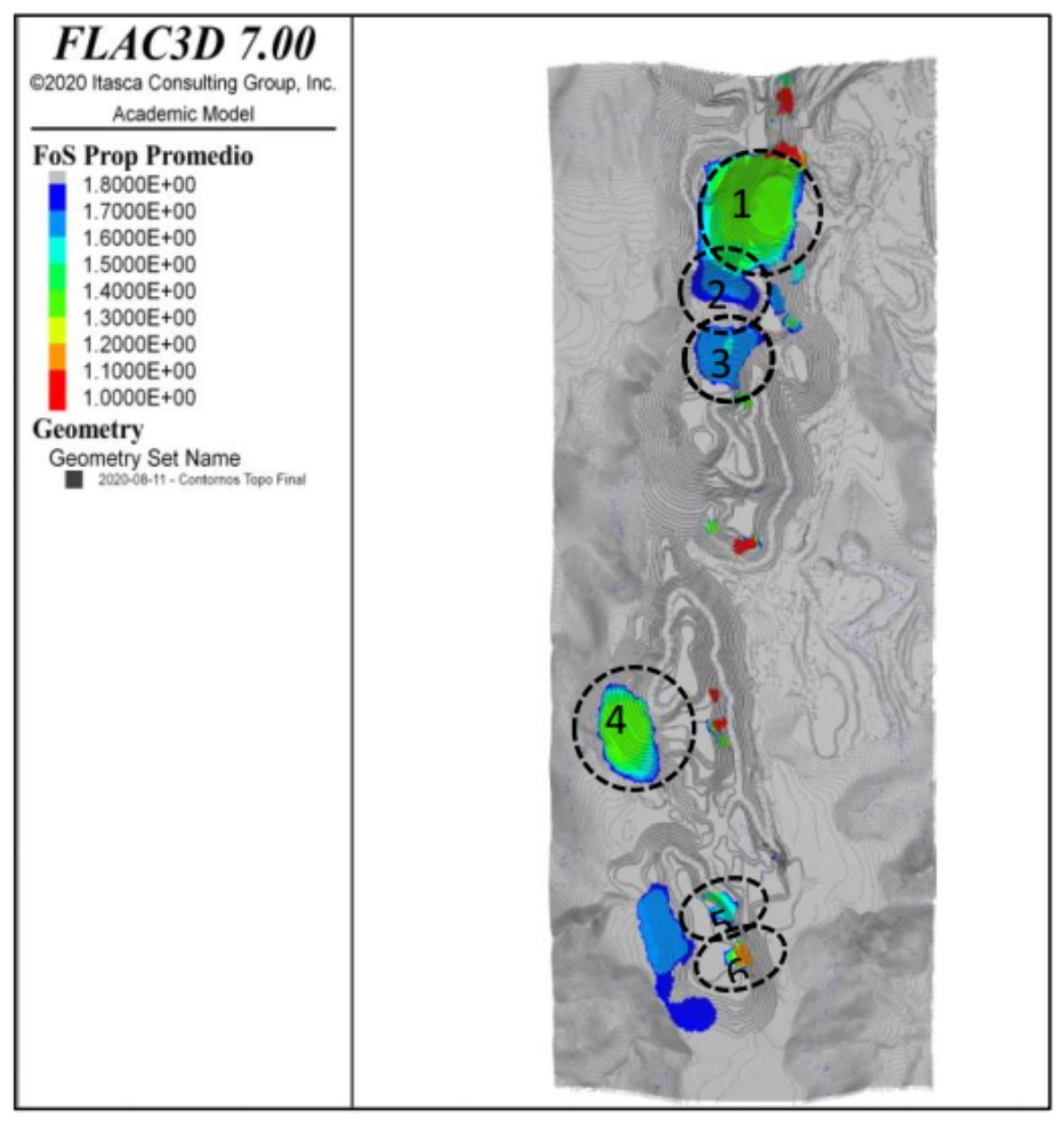
Factor of safety (FoS) - Probability of failure (PoF)
For all rock types (except SM and JP), the friction angle and the cohesion of the ubiquitous joints were considered 50% that of the host rock, while in the SM and JP rock units, they were considered 5% that of the host rock. Figures 20 and 21 show the correlation between the heights of the slopes and IRA for each type of rock. Almost all IRA-height curves exhibit an inverse relationship: the greater the height, the lower the IRA.
Figure 21—IRA vs. slope height - worst condition Table VI PoF for FoS = 1.3 Lithology Best Worst Friable haematite (FH) PoF < 1% PoF < 1% Decomposed mafic (DM) 5 < PoF < 10% 5 < PoF < 10% Semi-decomposed mafic (SDM) 5 < PoF < 10% PoF ~ 10% Solid mafic (SM) 5 < PoF < 10% Jaspilite (JP) 1 < PoF < 5%
The 3D stability analyses allowed us to divide the final pit into sectors according to the FoS values found. Sectors 1 and 4 presented 1.5 > FoS > 1.3, meeting the acceptability criterion (FoS ≥ 1.3); sectors 2, 3, and 5 were very stable, with FoS > 1.6, while sector 6 presented 1.1 > FoS > 1.3 stable areas that did not meet the acceptability criterion. The probabilistic analyses for all evaluated sectors considered two statistical scenarios. In the first scenario (5 < PoF < 95), it was assumed that the laboratory data is representative of the population. In the second scenario (10 < PoF < 90), it was assumed that the laboratory data is not completely representative of the population, and the scenario was more conservative. The probabilistic analysis used 10 000 Monte Carlo realizations. The results showed that for sectors 1, 2, 3, and 5, the PoF is < 1%, while for sectors 4 and 6, the PoF is between 8% < PoF < 10% and 16% < PoF < 19%, respectively. The high PoF of sector 6 verifies the results of the stability analyses previously performed, which is not the case with sector 4, where the criterion of acceptability of the stability of the sector is met (FoS ≥ 1.3) but the PoF can be considered high (8% < PoF < 10%) compared to those of the other sectors considered stable. In conclusion, the results show that probabilistic evaluation is an important tool for establishing alert mechanisms in slopes that can be termed stable. In addition, it broadens the view of those responsible for mine planning when deciding the slope of the IRA,
Institute of Mining and Metallurgy
Probability of failure and factor of safety in the design of interramp angles African
374 JULY 2022 VOLUME 122 The Journal of the Southern
Figure 20—IRA vs. slope height - best condition
A total of 240 cases were analysed for each geotechnical unit, and 48 combinations of IRA-slope height (H) for five times the statistical resistance cases evaluated. For each IRA-H combination, the corresponding PoF was calculated by the RSM methodology, obtaining 48 PoF values. Different PoF isocurves were calculated using the Python matplotlib library (shown in blue in the figures). As a reference, the FoS curves of the average properties are also plotted in the same figure (shown as discontinuous red lines). Similar to the recommendations of the FoS IRA project, two cases are analysed: dry conditions without ubiquitous joints and conditions with a water table 10 m below the surface and ubiquitous joints. The curves obtained are shown in Figures 22 to 26. Table VI shows the PoF of the slopes according to the lithology for each scenario with a FoS of 1.3. Conclusions The study showed the importance of performing probabilistic analyses to broaden the judgement of the FoS considered acceptable. Two extreme scenarios were evaluated, (1) the best scenario: a dry slope without ubiquitous joints and (2) the worst scenario: a water table at 10 m depth with ubiquitous joints in the most unfavourable direction. The IRA-slope height (H) graphs show the FoS placed between isolines that represent the PoF.
Table V Statistics of the shear strength properties of FH and DM Scenario Sector 1 Sector 2 Sector 3 Sector 4 Sector 5 Sector 6 PoF 5-95 <1% <1% <1% 8% <1% 16% PoF 10-90 1% <1% <1% 10% <1% 19%
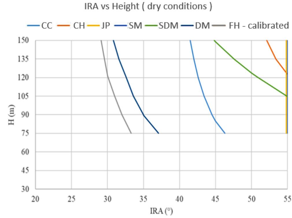
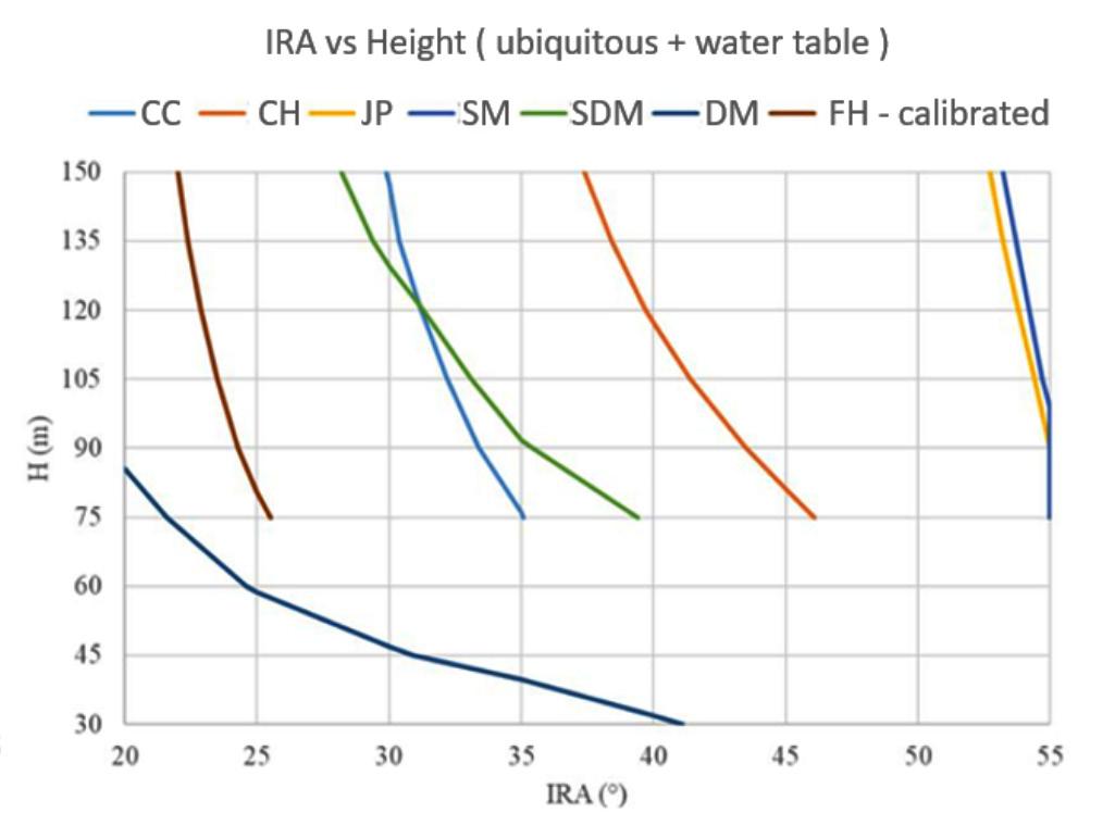
Acknowledgements
References Chiwaye, H.T. and STacey T.R. 2010. A comparison of limit equilibrium and numerical modelling approaches to risk analysis for open pit mining. Journal of the Southern African Institute of Mining and Metallurgy, vol. 110. pp. 571–580. Chowdhury, R.N. and Xu, D.W. 1995. Geotechnical system reliability of slopes. Reliability Engineering & System Safety, vol. 47, no. 3. pp. 141–151. ConTreras, L.F. 2015. An economic risk evaluation approach for pit slope optimization. Journal of the Southern African Institute of Mining and Metallurgy, vol. 115, no. 7. pp. 607-622. El-Ramly, H., MorgensTern, N.R., and Cruden, D.M. 2002. Probabilistic slope stability analysis for practice. Canadian Geotechnical Journal, vol. 39, no. 3. pp. 665–683. GriffiThs, D.V. and FenTon, G.A. 2004. Probabilistic slope stability analysis by finite elements. Journal of geotechnical and geoenvironmental engineering, vol. 130, no. 5. pp. 507–518. Hicks, M.A., NuTTall, J.D. and Chen, J. 2014. Influence of heterogeneity on 3D slope reliability and failure consequence. Computers and Geotechnics, vol. 61. pp. 198–208. Huang, J., Lyamin, A.V., GriffiThs, D.V., KrabbenhofT, K., and Sloan, S.W. 2013. Quantitative risk assessment of landslide by limit analysis and random fields. Computers and Geotechnics, vol. 53. pp. 60–67. Ji, J. and Low, B.K. 2012. Stratified response surfaces for system probabilistic evaluation of slopes. Journal of Geotechnical and Geoenvironmental Engineering, vol. 138, no. 11. pp. 1398–1406. Jiang, S.H., Li, D.Q., Zhang, L.M., and Zhou, C.B. 2014. Slope reliability analysis considering spatially variable shear strength parameters using a non-intrusive stochastic finite element method. Engineering Geology, vol. 168. pp. 120–128.
and
Figure 22—IRA vs. slope height - FH without ubiquitous and dry joints (left) and with ubiquitous joints and a water table 10 m below the surface (right). FoS curves for calibrated properties are shown as discontinuous red lines
Figure 24—IRA vs. slope height - DM with ubiquitous joints and a water table 10 m below the surface (height 30 to 75 m). FoS curves for calibrated properties are shown as discontinuous red lines
375The Journal of the
We thank Vale SA for providing the data and the Vale Institute of Technology for guidance and support in this work.
VOLUME 122 JULY 2022
All data, models, and code generated or used during the study appear in the submitted article.
Data availability statement
Probability of failure and factor of safety in the design of interramp angles Southern African Institute of Mining Metallurgy especially when the purpose of the mine is to remove as much material as possible under stability criteria that ensure the safety of the slopes, consequently increasing the reliability of operations and improving the mine safety system.
Johari, A. and Gholampour, A. 2018. A practical approach for reliability analysis of unsaturated slope by conditional random finite element method. Computers and Geotechnics, vol. 102. pp. 79–91.
Figure 23—IRA vs. slope height - DM without ubiquitous joints and dry (left) and with ubiquitous joints and a water table 10 m below the surface (right). FoS curves for calibrated properties are shown as discontinuous red lines
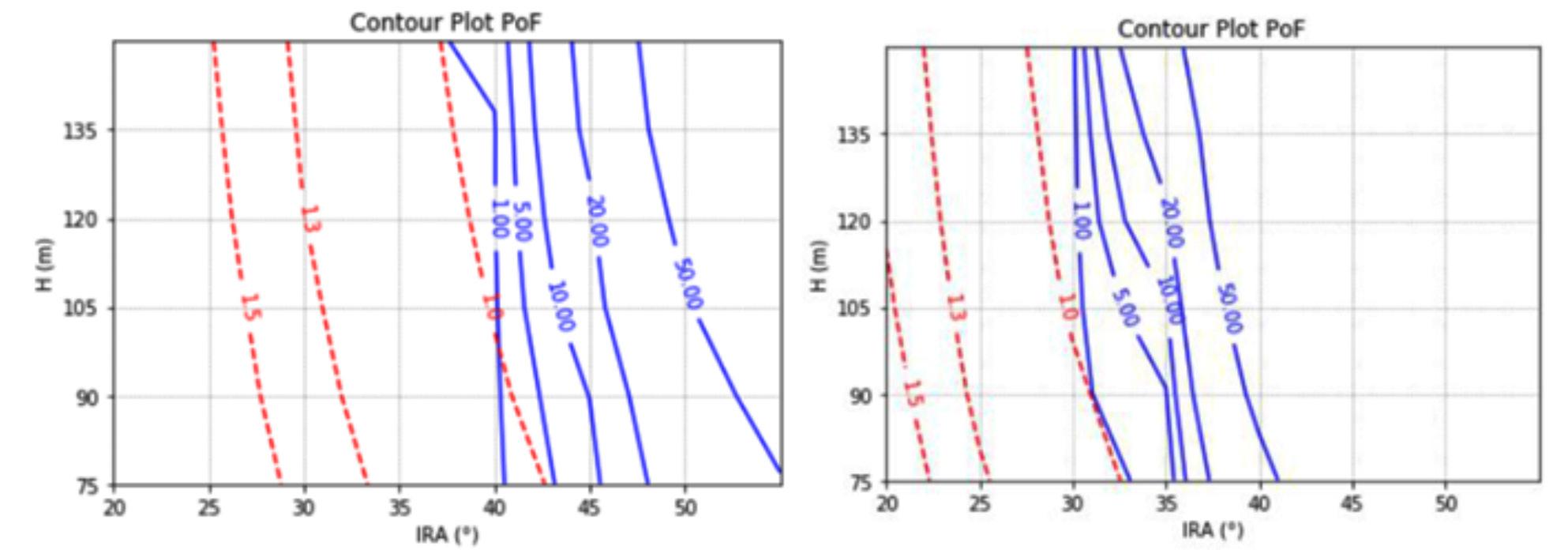
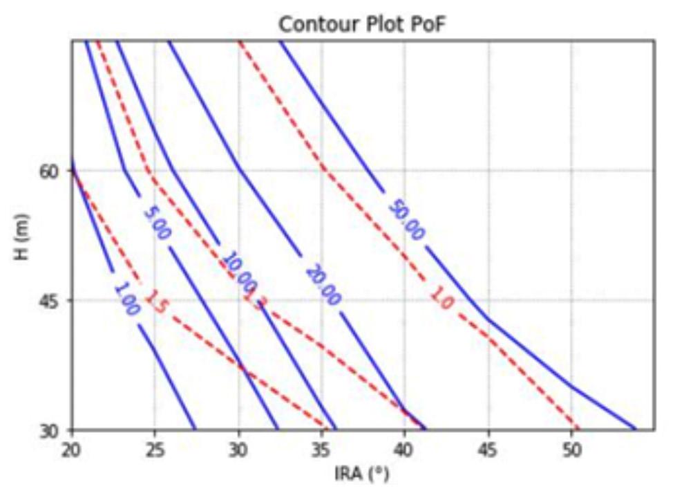
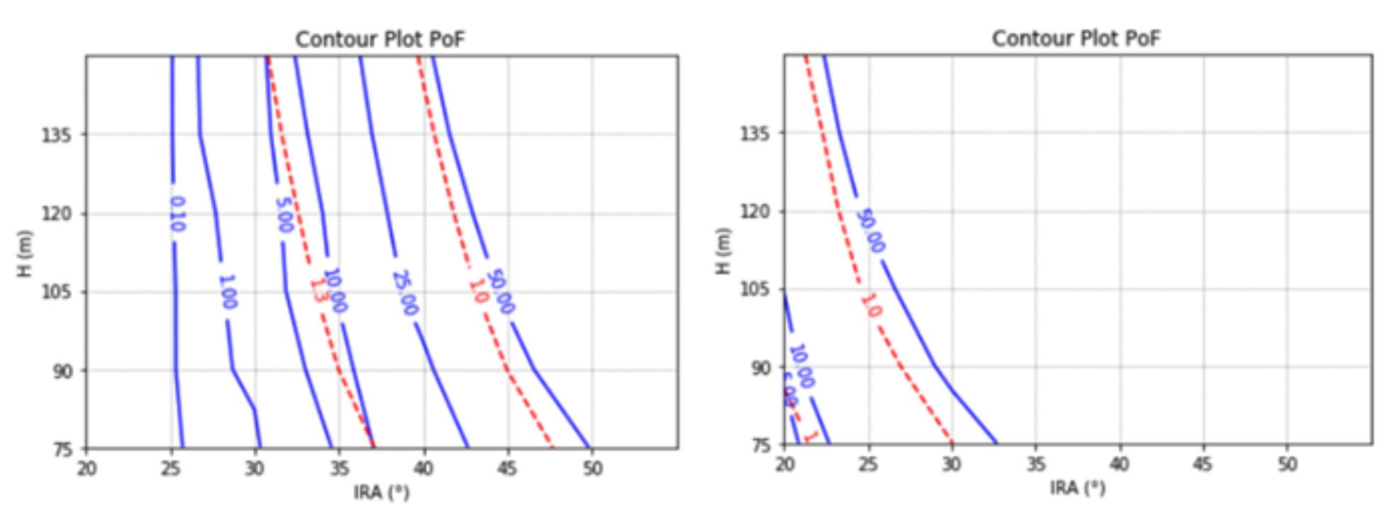
Probability of failure and factor of safety in the design of interramp angles African Mining
Institute of
Xiao, T., Li, D.Q., Cao, Z.J., Au, S.K., and Phoon, K.K. 2016. Three-dimensional slope reliability and risk assessment using auxiliary random finite element method. Computers and Geotechnics, vol. 79. pp. 146–158. Xu, B. and Low, B.K. 2006. Probabilistic stability analyses of embankments based on finite-element method. Journal of Geotechnical and Geoenvironmental Engineering, vol. 132, no. 11. pp. 1444–1454. Zhang, J., Zhang, L.M., and Tang, W.H. 2011. New methods for system reliability analysis of soil slopes. Canadian Geotechnical Journal, vol. 48, no. 7. pp. 1138–1148 u
Figure 25—IRA vs. slope height - SDM without ubiquitous joints and dry (left) and with ubiquitous joints and a water table 10 m below the surface (right). FoS curves for calibrated properties are shown as discontinuous red lines
Figure 26—IRA vs. slope height - JP (left) and DM (right) with ubiquitous joints and water level at 10 m depth. FoS curves for average properties are shown as discontinuous red lines
376 JULY 2022 VOLUME 122 The Journal of the Southern
Kasama, K. and WhiTTle, A.J. 2016. Effect of spatial variability on the slope stability using random field numerical limit analyses. Georisk: Assessment and Management of Risk for Engineered Systems and Geohazards, vol. 10, no. 1. pp. 42–54. Kasama, K., Furukawa, Z., and Hu, L. 2021. Practical reliability analysis for earthquake-induced 3D landslide using stochastic response surface method. Computers and Geotechnics, vol. 137. p. 104303. Le, T. 2014. Reliability of heterogeneous slopes with cross-correlated shear strength parameters. Georisk: Assessment and Management of Risk for Engineered Systems and Geohazards, vol. 8, no. 4. pp. 250–257. Li, D.Q., Qi, X.H., Phoon, K.K., Zhang, L.M., and Zhou, C.B. 2014. Effect of spatially variable shear strength parameters with linearly increasing mean trend on reliability of infinite slopes. Structural safety, vol. 49. pp. 45–55. Li, D.Q., Wu, S.B., Zhou, C.B., and Phoon, K.K. 2012. Performance of translation approach for modeling correlated non-normal variables. Structural safety, vol. 39. pp. 52–61. Li, D.Q., Xiao, T., Cao, Z., Zhou, C., and Zhang, L. 2016. Enhancement of random finite element method in reliability analysis and risk assessment of soil slopes using Subset Simulation. Landslides, vol. 13, no. 2. pp. 293–303. Li, D.Q., Zheng, D., Cao, Z.J., Tang, X.S., and Phoon, K.K. 2016. Response surface methods for slope reliability analysis: review and comparison. Engineering Geology, vol. 203. pp. 3–14, Li, L. and Chu, X. 2015. Multiple response surfaces for slope reliability analysis. International Journal for Numerical and Analytical Methods in Geomechanics, vol. 39, no. 2. pp. 175–192. Liu, Y., Zhang, W., Zhang, L., Zhu, Z., Hu, J., and Wei, H. 2018. Probabilistic stability analyses of undrained slopes by 3D random fields and finite element methods. Geoscience Frontiers, vol. 9, no. 6. pp. 1657–1664. Lorig, L. and Varona, P. 2000. Practical slope-stability analysis using finitedifference codes. Slope stability in surface mining. pp. 115–124.
Soares, R.C., Mohamed, A., VenTurini, W.S., and Lemaire, M. 2002. Reliability analysis of non-linear reinforced concrete frames using the response surface method. Reliability Engineering & System Safety, vol. 75, no. 1. pp. 1–16. Terbrugge, P.J., Wesseloo, J., VenTer, J., and STeffen, O.K.H. 2006. A risk consequence approach to open pit slope design, Journal of the Southern African Institute of Mining and Metallurgy, vol. 106, no. 7. pp. 503-511. Wyllie, DC. and Mah, C. 2004. Rock slope engineering: Civil and mining (4th ed.). London, CRC Press, London,. pp. 231-232. Wong, F.S. 1985. Slope reliability and response surface method. Journal of geotechnical Engineering, vol. 111, no. 1. pp. 32–53.
Malkawi, A., Hassan, W., and Abdulla, F. 2000. Uncertainty and reliability analysis applied to slope stability. Structural safety, vol. 22, no. 2. pp. 161–187. Mellah, R., AuvineT, G., and Masrouri, F. 2000. Stochastic finite element method applied to non-linear analysis of embankments. Probabilistic Engineering Mechanics, vol. 15, no. 3. pp. 251–259. Phoon, K. and Kulhawy, F.H. 1999. Characterization of geotechnical variability. Canadian geotechnical journal, vol. 36, no. 4. pp. 612–624. Read, J. and STacey, P. 2009. Guidelines for Open Pit Slope Design, CSIRO Publishing, Collingwood, Victoria, 496 pp.
and Metallurgy
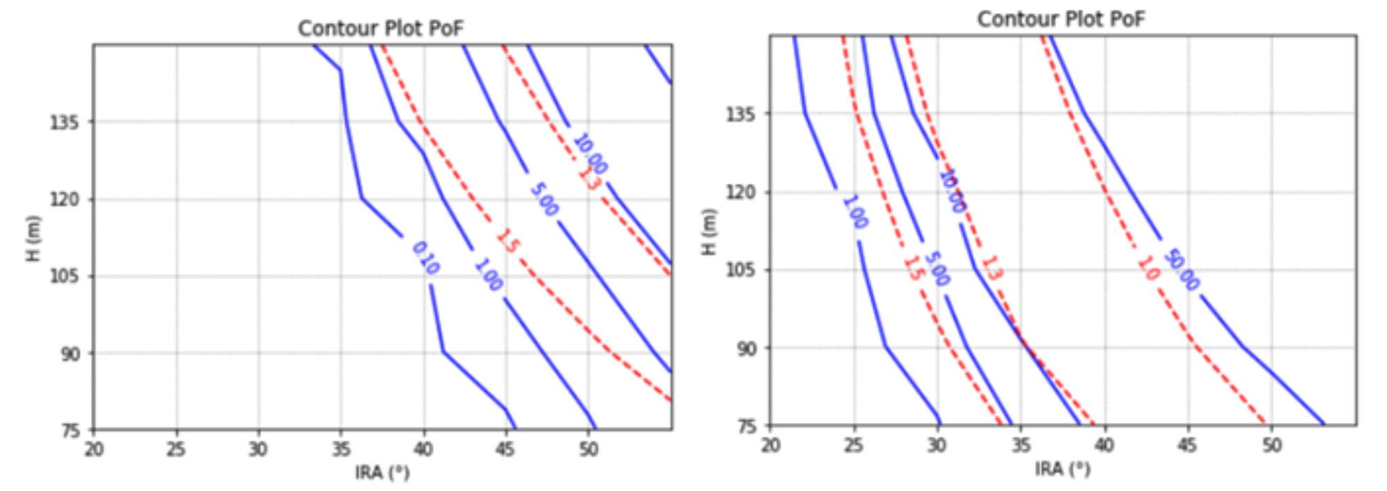
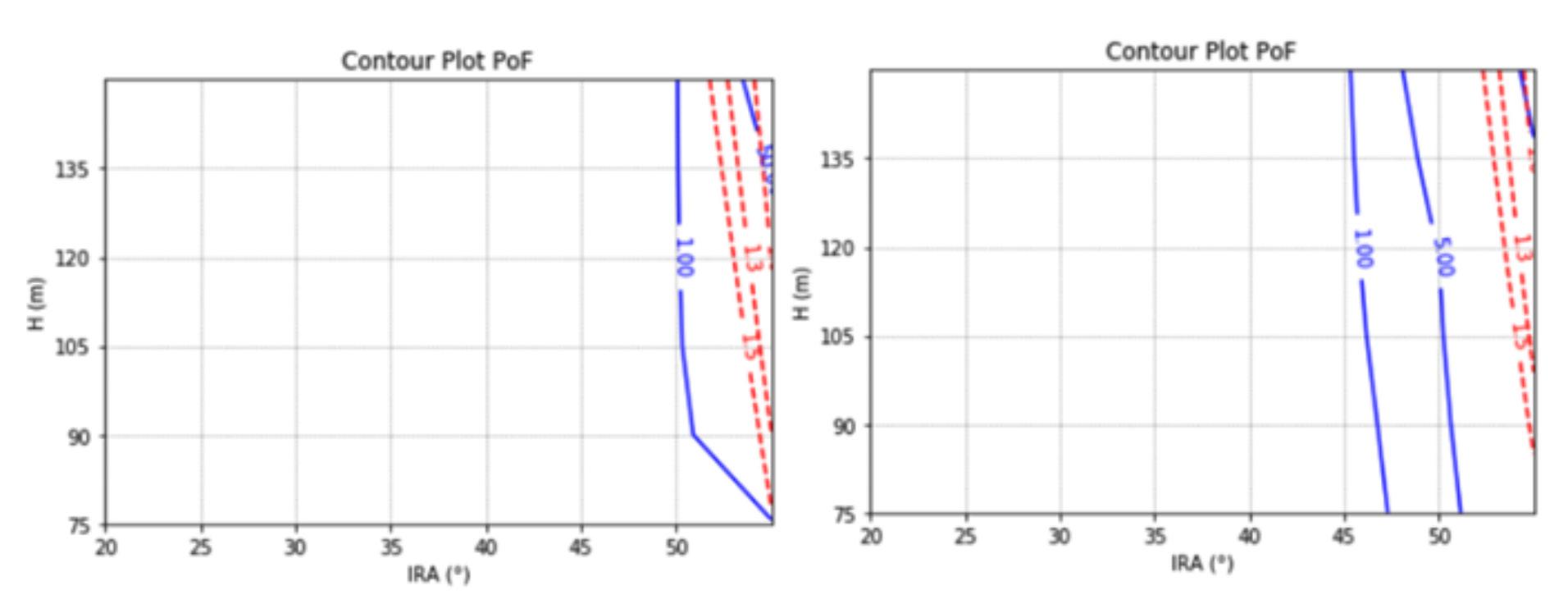
Dates: Received: 21 Aug. 2021 Revised: 8 Jun. 2022
377The Journal of the Southern African Institute of Mining and Metallurgy VOLUME 122 JULY 2022
Correspondence to: M.C. Bekker Email: giel.bekker@up.ac.za
Table I
Contribution of mining in low- to middle-income countries (ICMM, 2016)
Figure 1 shows the growth in mining production since 1995, together with the growth of revenue contributed to governments in the form of mineral rents over the same period, along with minerals exports.Ericsson and Lof (2018, p. 226), while examining the contribution of mining in various nations, found that in the Democratic Republic of the Congo (DRC), mining made up as much as 86% of total exports and constituted 12% of GDP. Carvalho (2018, p. 62) noted that production of mined ore increased by a factor of 27 during the 20th century.
Affiliation: 1Graduate School of Technology Management, University of Pretoria, South Africa
Accepted: 30 May 2022 Published: July 2022 How to cite: Mulder, H. and Bekker, M.C. 2022 A review of readiness assessments for mining projects. Journal of the Southern African Institute of Mining and Metallurgy, vol. 122, no. 7, pp. 377–386 DOI 2677https://orcid.org/0000-0002-4837-M.C.ORCID9717/1245/2022http://dx.doi.org/10.17159/2411-ID::Bekker
Foreign direct investment 60–90% Exports 30–60% Government revenue 3–25% National income 3–10% Employment 1–2%
projectKeywordsreadiness, mining projects, front-end planning, project evaluation, project assessment.
A review of readiness assessments for mining projects by H. Mulder1 and M.C. Bekker1
TheSynopsisobjective of this paper is to describe the research followed in creating a generalized, readiness assessment tool for mining projects. We start by highlighting the need for the assessment tool and then progress towards explaining the methodology followed during the study. The selection and finalization of the list of elements, sections, and categories that make up the unweighted values are described, followed by a summary of the weighting process applied. The outcome of this process is a weighted readiness assessment tool for mining project studies. The main benefits of the tool are that it will guide decision-makers and project managers through the definition phases of the project and improve the likelihood of project success.
The top 40 mining companies had revenues of US$642 billion in 2018 and paid US$31 billion in direct taxes (PWC, 2018). This grew to US $ 683 billion and US $ 33 billion in 2019 respectively (PWC, 2019, p. 9). Mining companies distributed around 22% of their revenue to employees, 23% to capital, and 21% to governments. It is noted that mining firms pay a bigger portion of their income to governments than most other industries, as they pay direct and indirect taxes, as well as substantial royalties. The
Introduction The mining industry contributes approximately 11.5% to the global gross domestic product (GDP). When the mining service industry (which include construction, fuel, and fertilizer production) is included, the total contribution to the global GDP is 45% (Creamer, 2012). The contribution of mining in lowand middle-income countries towards foreign direct investment, exports, government revenue, gross domestic production and employment is depicted in Table I.
378 JULY 2022 VOLUME 122 The Journal of the
This article focuses on the process used to create a project readiness assessment tool that can be utilized to evaluate the maturity and readiness of a mining project study or frontend planning phase. Using such a tool, a mining company can determine if the required rigour has been exercised in the frontend loading and the status of individual elements or the overall study.
Figure 1—Mining development trends since 1995: prices, exports, explora tion, value of mine production, exports (Ericsson and Lof, 2019)
Institute of
Some of the most common reasons for project failure include: ➤ Underestimating the ramp-up duration ➤ Overestimating production schedules ➤ Incorrect resource and reserve estimates ➤ Inadequate understanding of the orebody ➤ Failure to identify contaminants in the deposit ➤ Not understanding the composition of process water Thesechemistry.misunderstandings are attributed to insufficient time, budget, and skilled personnel allocated during the frontend loading phases of the project, as well as human factors, which include ‘prescient CEO syndrome’ – the CEO has already announced the project, therefore it must be feasible. Other human factors include pressure on engineering, procurement, construction, and management (EPCM) firms to ‘make’ the project viable in order to secure work during the construction phase and the nature of project employment contracts and bonusses, which means that executives and project managers receive payments and have moved on from the organization by the time a project fails. Dussud, et al., (2019) found that a lack of rigour during the feasibility stage of a mining project was a major contributor to failure. Of the more than 40 mining projects investigated, only 20% delivered the predicted returns. Dussud et al. state that if, by progressing a feasibility study from ‘good’ to ‘best’, 10% additional value can be created, it would translate into additional value of US$100 billion to the industry over the period between 2020 and 2025. One of the findings of Dussud et al. (2020) is that the industry does not use standard criteria for determining project maturity, and the studies therefore fail to ensure a narrow estimate band and predictable outcome. Some standards exist for Resource estimating and reporting, but many other elements are open to interpretation and companies apply their own standards inconsistently. These elements include engineering definition, operational readiness, commodity price predictions, and execution readiness, all of which could change the business case outcome of a project significantly. Some of the remedies for this situation which Dussud et al. propose include: ➤ Mining companies should set comprehensive standards for a Feasibility Study. They also add 11 criteria which they believe should always form part of a mining Feasibility Study. ➤ Assumptions during the Feasibility Study must be stress-tested by comparing them with detailed capex and opex benchmarks and then deciding on the correct combination of the two cost components.
introduction of carbon taxes and emission trading schemes have further contributed to the higher contribution of mining firms to the national fiscus. Addison and Roe (2018, p. 15) found that investment in the mining industry was expected to increase relative to historical averages, which would lead to an even higher dependency on the extractive in industries middle- and lowincome countries. McKinsey (2020) predicts capital expenditure in the mining will grow from a low of less than US$1 trillion per year in 2018, to in excess of US$1.5 trillion in 2026. Despite the significant role which mining plays in the global economy and the large amounts of capital spent in the industry, the success rate of mining projects remains low. Only 2.5% of large capital mining projects are considered successful when evaluated on scope, schedule, cost, and business benefits (Motta, et al., 2014, p. 402). More than 80% of mining projects are over budget and behind schedule by an average of 43%. (McKinley, 2017). Since 1965, cost overruns on mining projects averaged between 20% and 60% (Mining Markets Magazine, 2014). There are numerous examples of mining projects that have underperformed, with many failing to reach the intended outcome.
The mining industry poses some unique challenges as far as projects are concerned. Accenture (2012) found that the scale and complexity of mining projects, which are often multi-billion-dollar investments, often lead to budget and schedule overruns. They also found that insufficient detail during the planning stage was the third most significant contributor to project delays, behind the availability of skills and unconsidered regulatory requirements. Jamasmie (2012, p. 1) observed that according to 31 executives responsible for global mining projects, only a third of the projects were completed within 25% of the approved budget, and less than 20% within 10% of the approved budget. In total 42% of respondents regarded insufficient definition during the study of the project as the main reason for the overruns.
and Metallurgy
Ernst and Young (2020) list various risks faced by mining project, including failure to gain a social licence to operate, increasing complexities in mining, and additional needs for innovative approaches due to remote locations, declining ore grades, and access to and cost of energy and infrastructure. McKinsey (2017) adds that commodity prices are low and volatile, and that there is less room for error than in the past, as margins are slim. Schneider (2017) lists various factors that contribute to mining project failures, such as protests by the local population over pollution, concerns regarding sustainable water supplies, and other environmental problems. McCarthy (2020) notes some contributors to project failure in mining. These include: ➤ Higher capital cost than anticipated ➤ Operating cost that exceeds expectations ➤ Lower recovery grade than predicted ➤ Less revenue from sales than anticipated during the front-end loading phase ➤ Longer construction and ramp-up periods than Accordinganticipated.toMcCarty (2020) 25% of mining projects fail.
A review of readiness assessments for mining projects Southern African Mining
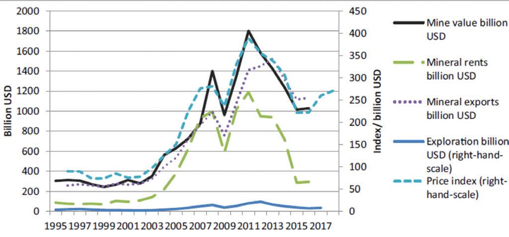
A review of readiness assessments for mining projects African
379The Journal of the Southern
Assigning weights to the individual elements
The identified elements were listed and arranged to form a draft, unweighted RAT. This was then used to facilitate discussions, gather inputs, and validate the elements listed, with participation by 66 professionals from three mining companies and five companies involved in design and implementation of projects (EPCMs). A pro-forma, semi-structured questionnaire was drafted, and inputs were obtained via telephonic interviews as well as emails. From these inputs a final list of well-defined, unweighted elements was compiled. During this process the elements were also arranged in sections and categories. Typically, elements that addressed a specific discipline or associated component of a project would be clustered into a category. Several categories would be combined into a section.
Methodology
Figure 2 illustrates the process followed. The first step was to examine the existing literature, both on the CII’s PDRIs and on mining projects. The aim was to define specific variables and elements that apply to projects in the mining industry.
The methodology study was based on the approach taken by the Construction Industry Institute (CII) in developing the Project Definition Rating Indexes (PDRIs) for other industries. A PDRI is a readiness assessment tool that measures the level of maturity of several elements, to determine the overall readiness of a project study to proceed into detail design and execution. Since the middle 1990s CII had developed four PDRIs, for building, industrial, infrastructure, and small industrial projects. The development of these PDRI tools included a combination of literature reviews, focus group discussions, workshops, scrutiny of project documentation, and one-on-one discussions with experts (Gibson and Dumont, 1996, p. 21; Cho, Furman, and Gibson, 1999, p. 35; Bingham, 2010, p. 28; Collins, 201, p. 78). Compiling a RAT for mining projects followed the same approach as for the PDRIs.
Institute of Mining and Metallurgy VOLUME 122 JULY 2022
Research problem No generally accepted readiness assessment tool is available for mining projects. To address this shortcoming, a study was undertaken to develop a Readiness Assessment Tool (RAT) for mining projects by researching what constitutes a RAT and how it should incorporate mining elements.
The third step in creating the RAT, was to allocate weights to the elements. The unweighted RAT for mining projects was distributed via email to 66 selected mining project professionals, both in mining operations and EPCM companies. The participants were asked to weight and asses the various elements that pertain to the front-end planning phase of mining projects. These role-players were situated mainly in North America, Africa, and Australia. The outcome of this exercise was a weighted RAT for mining projects.
The final unweighted RAT check-sheet consisted of 180 elements, which were divided into four sections and 18 categories. This check-sheet was used as the basis of the survey to assign weights to the various elements. A literature review was conducted to assign definitions to the various elements. The definitions would be useful in assisting participants in the survey, but also when the tools were completed, as project professionals could use the definitions to avoid any misunderstanding regarding terminology when using the tool.
The four sections which the RAT is divided into are: I Basis of project Decision II Project Details III Design for Construction IV Execution Approach.
The four sections are further divided into numerous categories. The Basis for Project Decision section is made up of seven categories, The Projects Details section is divided into three categories, the Design for Construction section into three categories, and the Execution Approach section into five categories.Assigning weights to the elements makes provision for the variance and unequal impact that different elements can have on project definition. For example, elements addressing the quality and quantity of the orebody will be more important than those addressing stormwater drainage. Both elements are important, and should be considered during the study, but if the orebody is not confirmed, the negative effect on the project viability could be more significant than the channelling of stormwater.
To determine the individual element weights, the opinions of experts in mining project management were sought. Due to the geographical spread of individuals with adequate experience in mining projects, it was decided to obtain the inputs via emailed questionnaires. In total, the survey was sent to 66 individuals who had significant experience in mining projects. These individuals represented project managers, engineers, and quantity surveyors working for large mining companies as well as EPCM companies. The email contained instructions on how to complete the questionnaire, as well as the contact details of the researcher, should any instructions be unclear. The unweighted RAT for the mining check-sheet was attached to the email. Instructions on how to complete the questionnaire, along with an example of a completed section, were included. There was also a section to beFigure 2—RAT Development process flow
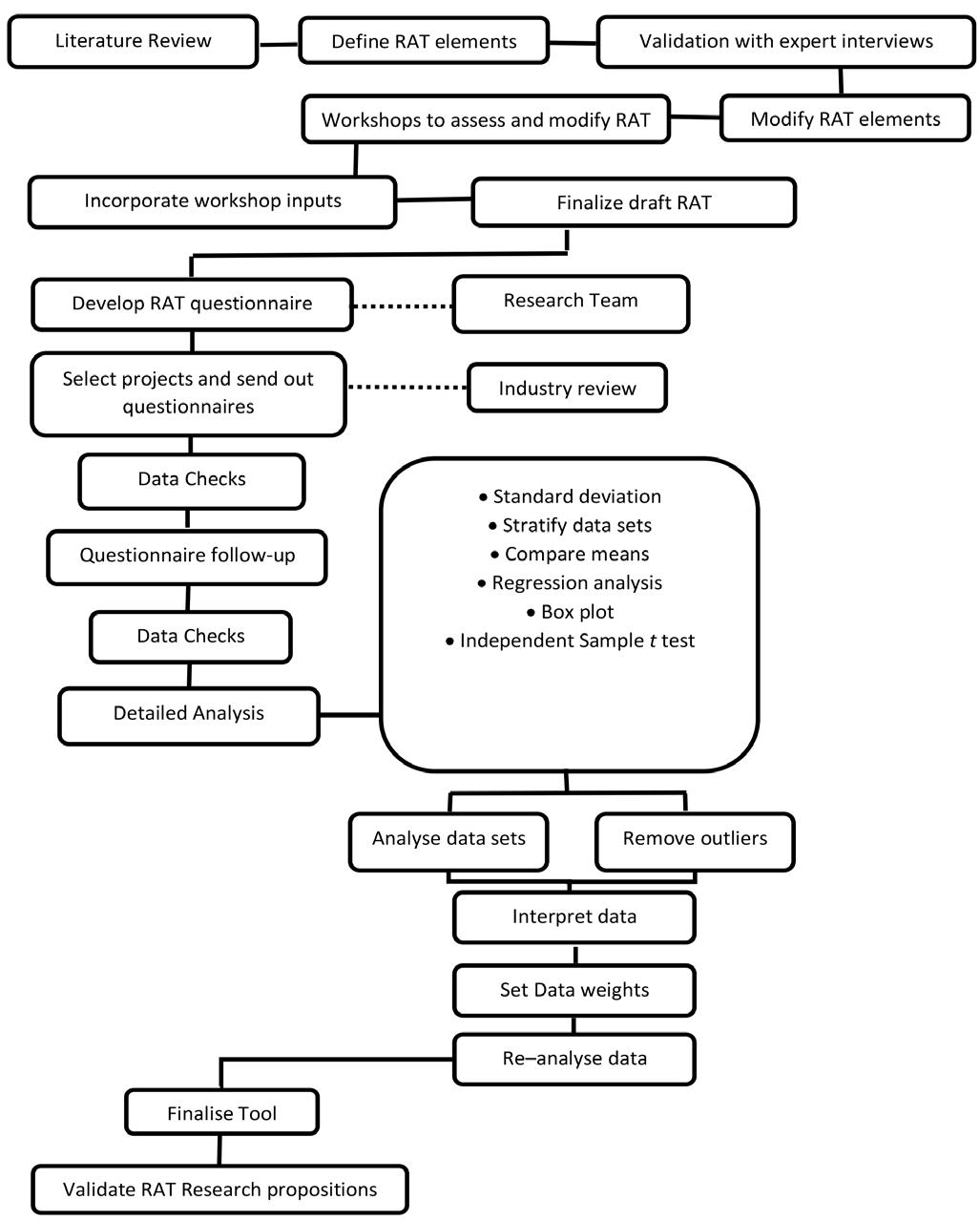
(b) Removing the entire contribution (data-set) of those individuals with a very high contribution score.
(d) Do not assign contingencies for definition levels 2, 3, and 4, as these will be interpolated.
Figure 3—Instructions for completion of the weighting sheet
(e) The contingency should represent the amount of money (as a percentage of total project cost) that would be necessary to offset uncertainties related to project
In previous studies (Bingham, 2010, p. 66), box-plots were used to determine the outliers and extremes. A box-plot is a graphical representation of the data and some of the descriptive statistics. A typical box-plot will indicate the data on a vertical or horizontal line. The median of the data, as well as the 25th and 75th percentile values, will be indicated. The difference between the 75th percentile and 25th percentile values is the box length. Outliers and extremes fall outside of the box. These values typically skew data, and the number of such values could be used to determine if only certain data-points, or entire data-sets should be eliminated to ensure that data was not skewed.
(c) If little to no definition exists, assign a contingency amount to each element under level 5.
(a) Not removing the data supplied by any participants, by deciding that those contributions were still valid.
380 JULY 2022 VOLUME 122
The Journal of the Southern African Institute of Mining and Metallurgy completed by the participants indicating their number of years of experience, as well as the value of projects in which they had been involved.Participants were asked to assign two weights to each of the 180 elements. The first weight reflected the amount of contingency (in percentage) if an element has been completely defined during the front-end loading phase. This weight was captured on a blank weighting sheet, under definition level 1. Similarly, participants were asked to assign an amount of contingency (in percentage) if an element had little to no definition. This contingency was entered on the blank weighting sheet under definition level 5. The request that was sent out, along with an example of how to complete the weighting sheet, is depicted in Figure 3.
(a) Consider a typical project in the mining industry. Assume that you have been asked to estimate the project cost just prior to the detail design phase of the project.
Participantsexecution.completed the weighting sheet by assigning weights to definition levels 1 and 5. The inputs from the various parties were normalised, which meant that the data points were all brought within the same range. All the participants used zero as the absolute minimum. Thus, the lower end of the scale was fixed. However, the upper end of the scale varied significantly between the individual participants. To enable the responses to be compared, the individual data-sets had to be normalized to within the same range, between zero and 100. The first step in this process entailed the calculation of individual modifiers for each of the participants. This was done by dividing the largest value used by the participant, into 100. This individual modifier was then multiplied with all the weights assigned to the individual elements, thereby bringing all the responses to within the same range of between zero and 100. Before the normalized values could be used to calculate the weights of the various elements, it was important to analyse the individual contributions to determine if any of these were skewing the data. This was done by calculating the descriptive statistics of each element, namely the mean, median, standard deviation, variance, and skewness. Further analysis of the data showed that the inputs from some of the participants were skewing the data.
For all the elements, the medians, interquartile range, and outlier, and extreme boundaries were calculated. These values were then used to determine the number of outliers and extremes for all data-sets. In total, 66 outliers and six extremes were identified in this manner. To identify individual contributions which could be skewing the results, individual contribution scores were calculated for each participant, using the formula: Contribution score = 3 x (Number of extremes) + 1 x (Number of outliers)Thoseparticipants with a low contribution score had few or no outliers or extremes in their data-sets and were thus not contributing significantly to skewing the data. Participants with a high contribution score were contributing significantly to skewing the data.Bingham (2010, p. 67) mentions several options to deal with participants who are identified as skewing the data. These include:
(b) Assign a contingency amount to each element. If the element had been completely defined, note the contingency amount under definition level 1.
A review of readiness assessments for mining projects
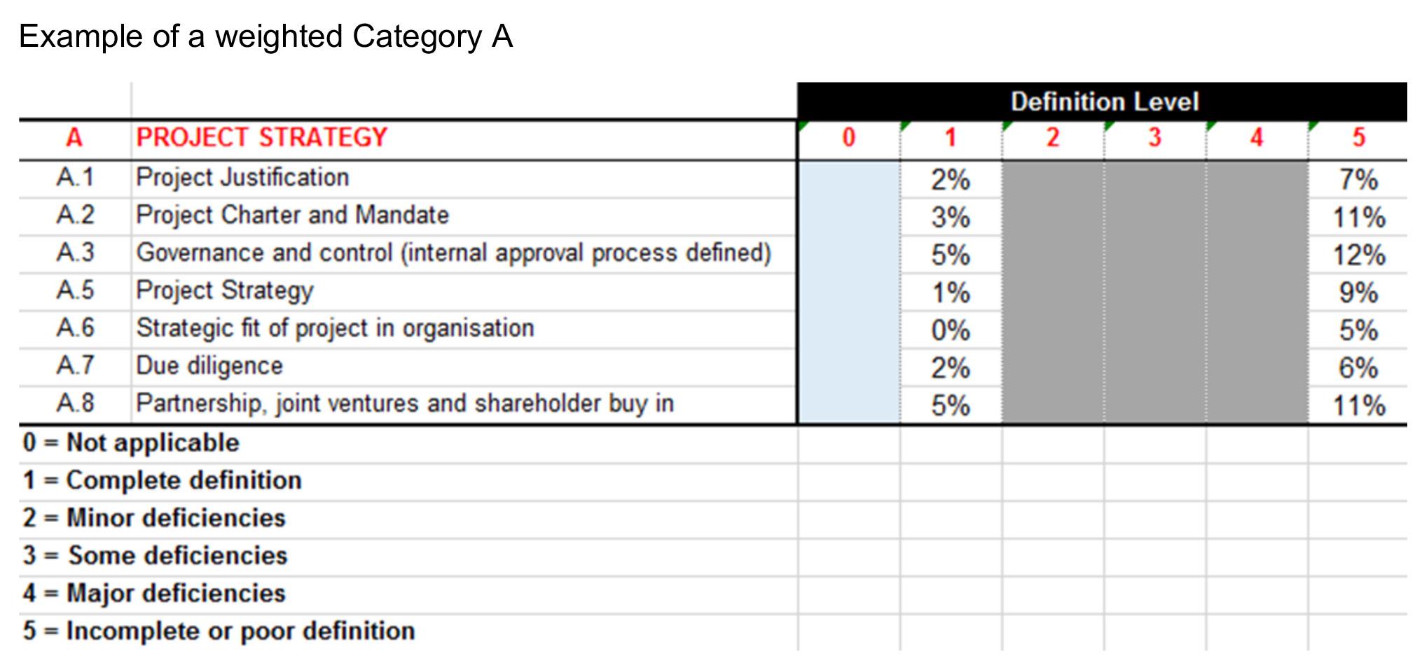
A review of readiness assessments for mining projects
(e) Leave the data-points calculated as outliers and remove only those data-points identified as extremes.
(c) Keeping all the individual contributions but removing those individual data-points that were skewing the data-sets. This would entail removing outliers and extremesfrom the data-set.
It was decided to go with option (d). This meant removing the entire contribution of some individuals who had a high individual contribution score, as well as the extreme and outlier data-points of all other contributors. The input of one individual with an individual contribution score of 39 was removed, as well as a total of 66 outliers and six extremes. Once the extremes and outliers were dealt with, the final RAT scores for the various elements could be calculated. This was done in two stages. The first stage entailed calculating the final values for all level 5 scores, and in the second stage the values for levels 1 to 4were interpolated. To calculate the final level 5 scores, the average of all the remaining data-sets had to be calculated. As some data-points had been removed as outliers or extremes, this had to be accounted for when calculating the average weights of the individual elements. To overcome this, the sums of the individual elements were divided by the number of remaining individual data-points, considering that some of the data-points had been removed. On average the upper (definition level 5) value for each element was reduced by 0.6% through this exercise. At this stage the potential RAT score of any project ranged between 180 (full definition) and 1000 (no definition). The RAT for mining projects could be used to determine the maturity of any single element, category, or section as well as to calculate an overall RAT score, which was an indication of the overall readiness of the project to proceed into detail design and construction. Because the tool would potentially be used by project participants who are familiar with the PDRI tools of the CII, it was decided to bring the potential RAT score to within the limits of 70 and 1000, which is the norm in the PDRIs. This meant that when there is no definition yet to any of the elements, a project study will have a PDRI score of 1000. When all the elements have been completely studied, the PDRI score would be 70. The weighted RAT was adjusted to fit within the range of 1000 and 70 in the following manner: The sum of all level 1 weights was divided by 70. This constant was then multiplied by the level 1 weight of each element. The sum of all the level 5 weights was divided by 1000. This constant was then multiplied by the level 5 weight of each element. Thus the weights were modified to fit between 70 and 1000.Once the final values for all the level 5 and level 1 scores had been calculated, the values for levels 2, 3, and 4 could be interpolated. This was done by basic interpolation of the data. The result of this process was a weighted RAT for mining projects.
References Addison, T. and Roe, A . 2018. Extractive industries: The management of resources as a driver of sustainable development. Oxford Scholarship Online, November 2018.
381The Journal of the Southern African Institute of Mining and Metallurgy VOLUME 122 JULY 2022
The four sections of the RAT for mining projects progress from a high-level more strategic perspective to a project definition to execution level. In section I the project feasibility as well as Resource and Reserve statements carry the highest weighting estimates which is important for the project decision. Section II addresses the detail of the project, with scope definition being allocated the highest weight. It is interesting to note that value improving practices are important in section III which emphasizes the focus on cost-effectiveness during the high capital expenditure stage of construction. The last section, section IV, considers the execution approach,with focus on control being weighted the highest. The detail weightings within each section are provided in Annexure 1. Conclusions Determining the readiness of mining projects is critical to project success. Not only should there be good criteria for selecting the right project, but also items and actions that should be given special attention to implement the selected project successfully. Thus far, a generally available project readiness assessment tool has not been available in the literature or, practice, hence the need to develop such a tool for mining projects. The factors that influence success during the front-end phase of a mining project, were determined through a mixed-method research approach whichd included a literature review, as well as workshops and email inputs from industry experts. The final weighted list of 180 elements was collated in four sections covering strategic decisionmaking to final project execution. The completed RAT for mining projects can assist professionals in the mining project field in several ways. By presenting a comprehensive, weighted list of elements to be addressed during the front-end phase of a project, it can assist project team members to come to a common understanding of the areas that need to be studied, as well as the relative importance of the various elements. Project teams can use the RAT as a selfassessment tool during any stage of the project study, to identify the areas which require more definition. Teams can also use the RAT to calculate an overall RAT rating at any stage, which will indicate the overall level of readiness of the project to proceed into the next phase. The RAT can also be used as a predictor of project success, based on the RAT score. By making use of the maturity of each of the 180 elements to determine a single RAT score, the RAT can assist project members, as well as decision-makers such as Boards of Directors, to make informed decisions regarding the approval of projects. The RAT for mining projects can also assist in reducing risk during project execution and improve project team alignment and communication, as it sets at a common framework for the study. By addressing all the above points, the RAT should improve the probability of a successful project.
(d) A combination of (b) and (c) above, where the entire contribution of individuals with high contribution scoreswas removed, as well as those individual data-points from other contributors that were outliers or extremes.
Results In total, 20 responses were received, of which 18 were used. This equated to a response rate of 27%. The two responses that were not included were not completed in the prescribed manner and therefore the data could not be incorporated in the study. The 18 participants represented a combined experience of 410 years, with projects to the value of R898 billion (US$62.5 billion). The average participant had 20.5 years of experience and averaged a lifetime project value of R44.9 billion (US $3.13billion). The final RAT consists of 180 elements, which are divided into four sections and 18 categories. The total of the weights of each section and category, as well as the average weight of each section and category, are depicted in Table II.
MoMiningMcKinseyMcKinseyprojects-report-20976/http://www.mining.com/mining-industry-could-save-billions-on-capital-[accessed:21September2018]..2017.Gettingbigminingprojectsright:Lessonsfrom(andfor)theindustry.Online.Available:https://www.mckinsey.com/industries/metals-and-mining/our-insights/getting-big-mining-projects-right-lessons-from-and-for-the-industry.Accessed20July2020..2020.Through-cycleinvestmentinmining.https://www.mckinsey.com/industries/metals-and-mining/our-insights/through-cycle-investment-in-mining.[accessed20July2020].MarkeTs.2014.Whybuildingamineonbudgetissorare.http://www.miningmarkets.ca/news/why-building-a-mine-on-budget-is-so-rare/[accessed:16September2018].TTa,O.,Quelhas,O.,Filho,J.,Franca,S.,andMeirino,M.2014.Megaprojectsfront-endplanning:ThecaseofBrazilianorganizationsofengineeringandconstruction. ICMM.2020].mega-projects-fail-infrastructure-energy-dams-nuclearhttps://www.nationalgeographic.com/news/2017/11/[accessed15July2012.Theroleofmininginnationaleconomies.3rdedn.InternationalCouncilonMiningandMetals,London.https://www.icmm.com/romine/index[accessed:15September2018].
A review of readiness assessments for mining projects 382 JULY 2022 VOLUME 122 The Journal of the Southern African Institute of Mining and Metallurgy
Mineral Economics, vol. 32. pp. 223–250. EY. 2020. Top 10 business risks and opportunities – 2020. en_gl/mining-metals/10-business-risks-facing-mining-and-metalshttps://www.ey.com/[accessed 25 July 2020]. Gibson, G. and DumonT, P. 1996. Project definition rating index (PDRI). Research Report 113-11. Construction Industry Institute, University of Texas at Austin. ICMM. 2016. The role of mining in national economies.3rd edn. International Council on Mining and Metals, p. 3. London. https://www.icmm.com/romine/ index [accessed: 15 September 2018]. Jamasmie, C. 2012. Mining industry could save billions on capital projects – report.
American Journal of Industrial and Business Management, vol. 4. pp. 401–412. PWC. 2018. Mine 2018. Tempting times. http:// www.pwc.com/mining. [accessed: 25 July 2020. PWC. 2019. Mine 2019. Resourcing the future. http:// www.pwc.com/mining. [accessed: 25 July 2020]. Schneider, K. 2017. Massive infrastructure projects are failing at unprecedented rates. National Geographic.
u Table II Average and total weights per section and category
Creamer, M. 2012. Global mining drives 45%-plus of world GDP – Cutifani. Ericsson,Dussud,gdp-cutifani-2012-07-04www.engineeringnews.co.za/article/global-mining-drives-45-plus-of-world-http://[accessed5May2016].M.,Kudar,G.,Lounsbury,P.,Pikul,P.,andRossi,F.2019.Optimizingminingfeasibilitystudies:The$100billionopportunity.McKinsey&Company.https://www.mckinsey.com/industries/capital-projects-and-infrastructure/our-insights/optimizing-mining-feasibility-studies-the-100-billion-opportunity[accessed25July2020].M.andLof,O.2018.Mining’scontributiontonationaleconomiesbetween1996and2016.
Bingham, E. 2010. Development of the Project Definition Rating Index (PDRI) for Infrastructure projects. Masters Dissertation, Arizona State University. Carvalho, F. 2017: Mining industry and sustainable development: time for change. Food and Energy security, vol. 6, no. 2. pp. 61–77. Cho, C., Furman, J., and Gibson, G. 1999. Development of the Project Definition Rating Index (PDRI) for building projects. University of Texas at Austin. Collins, W. 2015. Development of the Project Definition Rating Index (PDRI) for small Industrial projects. Arizona State University, Phoenix.
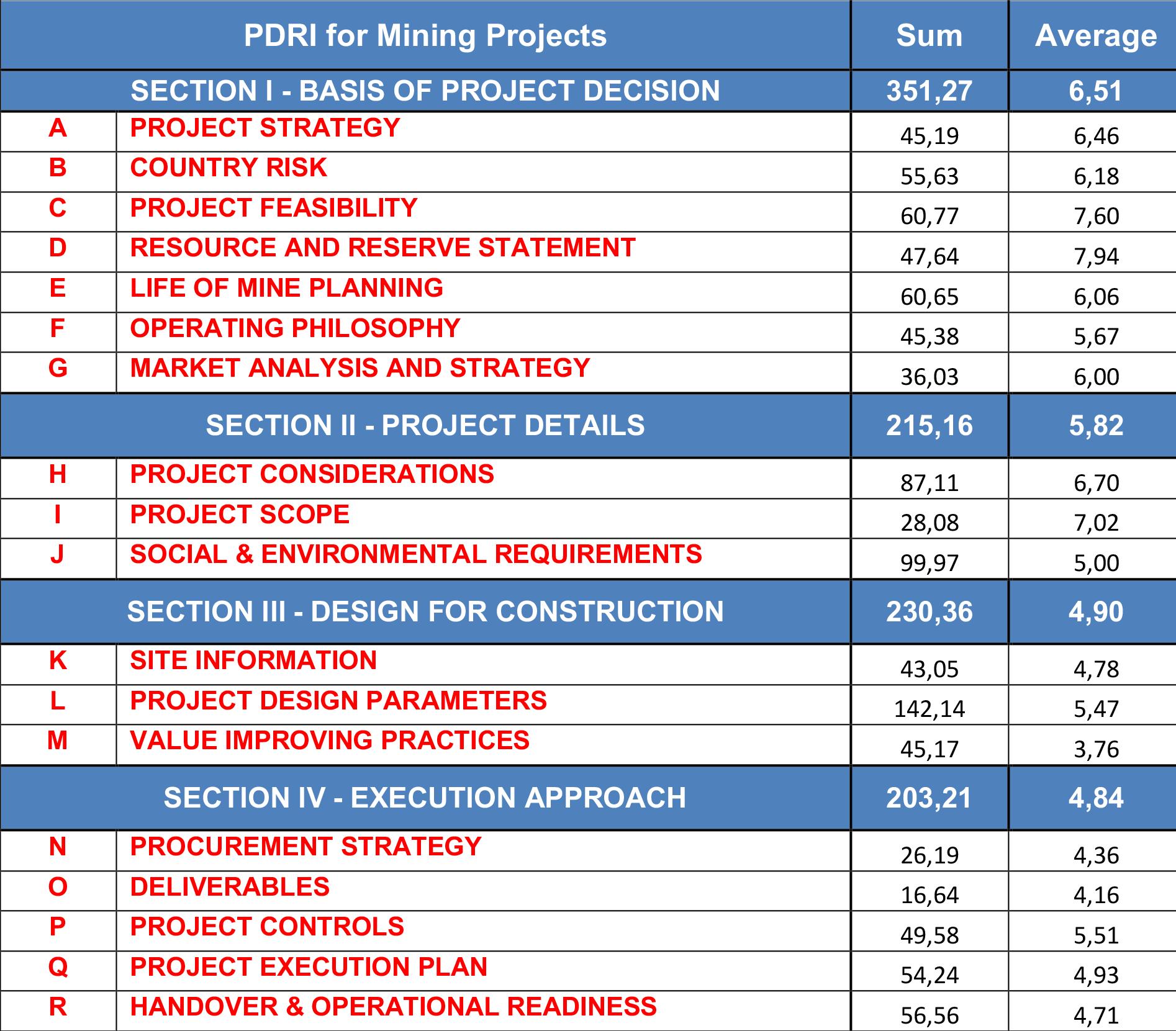
A review of readiness assessments for mining projects 383The Journal of the Southern African Institute of Mining and Metallurgy VOLUME 122 JULY 2022 Annexure 1 – Final weighted RAT for mining projects
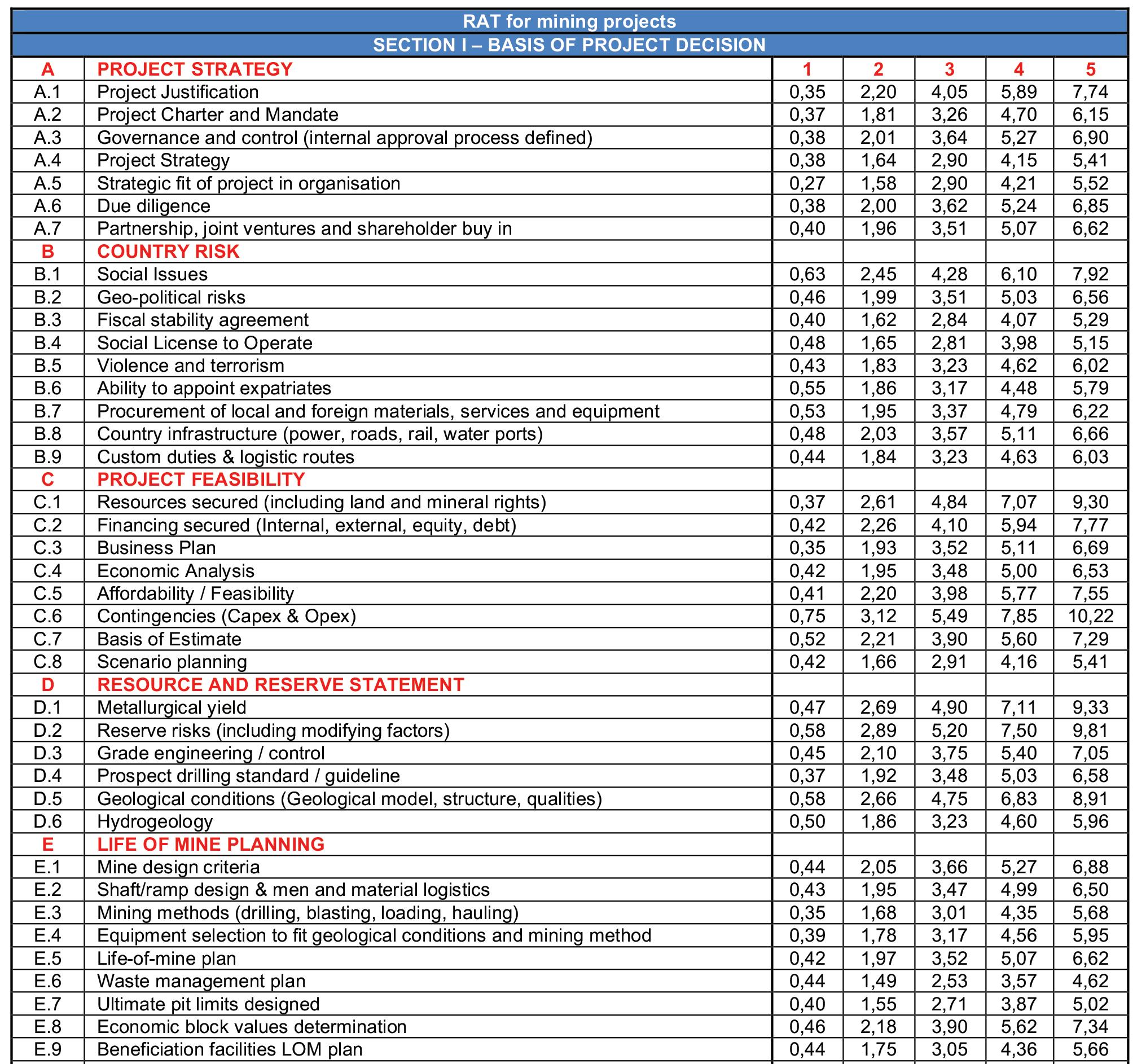
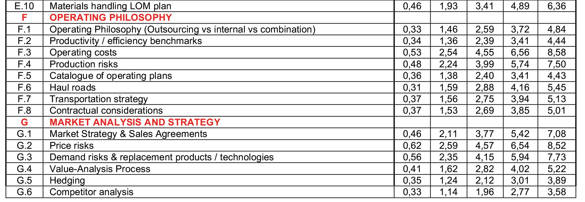
A review of readiness assessments for mining projects 384 JULY 2022 VOLUME 122 The Journal of the Southern African Institute of Mining and Metallurgy
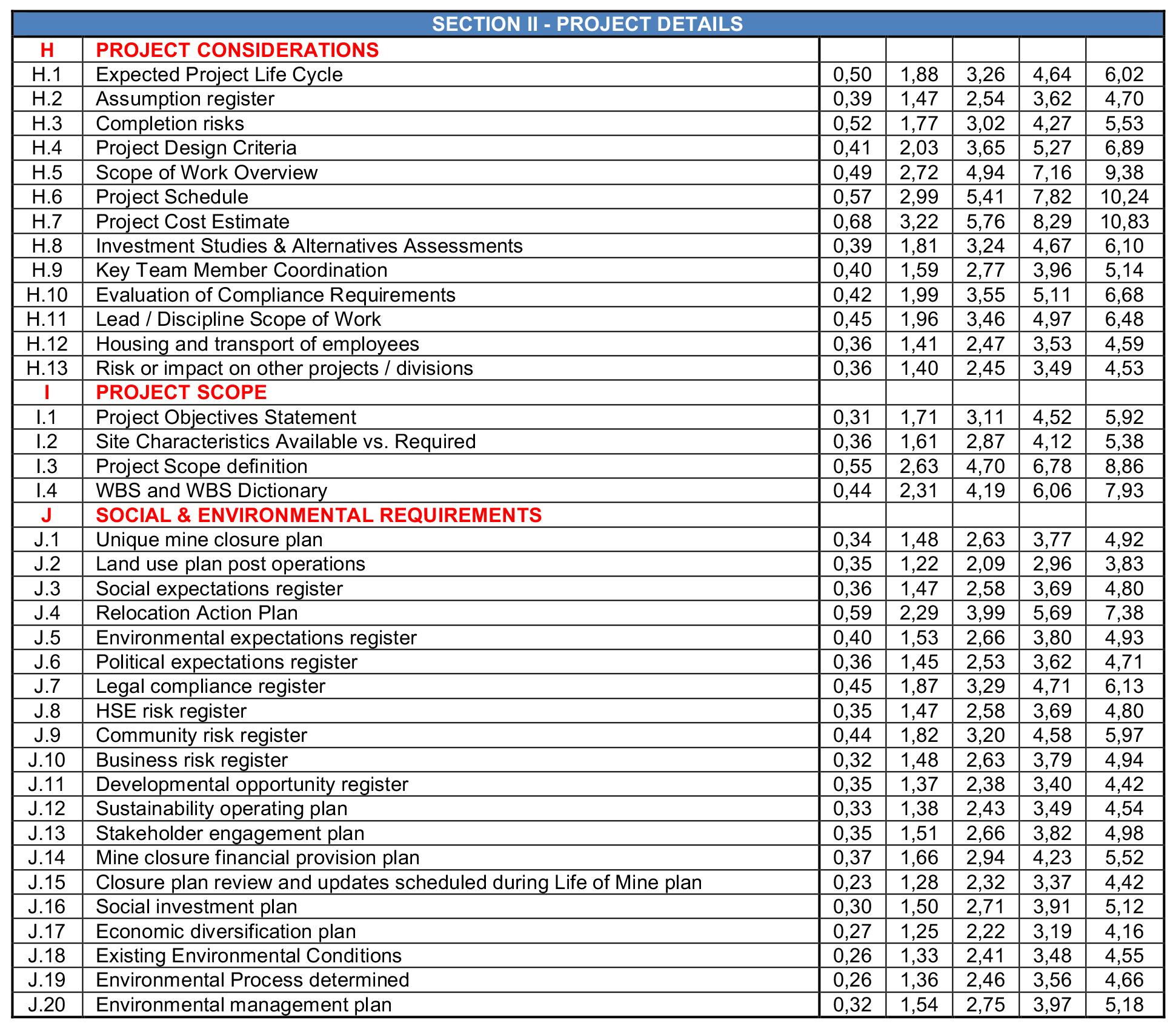
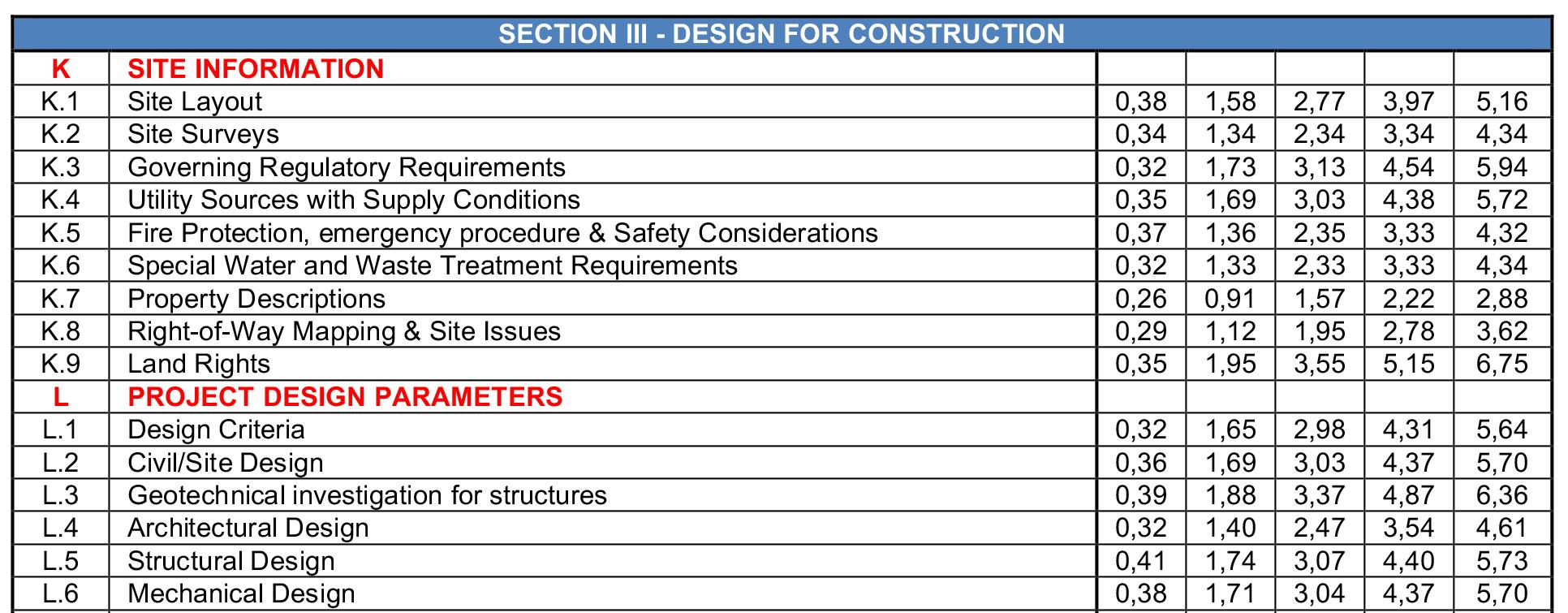
A review of readiness assessments for mining projects 385The Journal of the Southern African Institute of Mining and Metallurgy VOLUME 122 JULY 2022
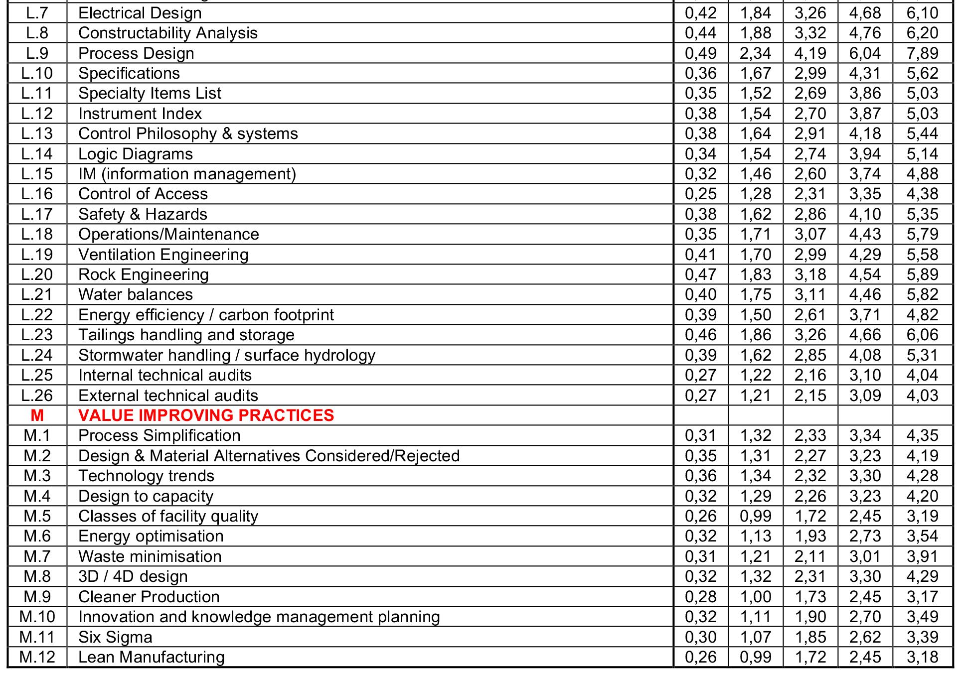
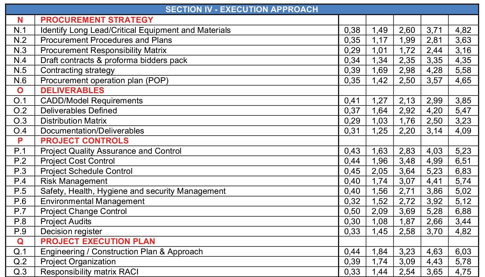
The aim of this conference is to provide the opportunity for thought leaders in the global
386 JJANUARY 2022 VOLUME 122
The of the Southern African Institute of Mining and Metallurgy
A review of readiness assessments for mining projects
Journal
research towards producing battery-grade Andproducts.challenges such as the means for recycling these batteries once they reach the end of their (first) life.
The intensified search over the past decade for alternatives to fossil-fuels as stores of energy has led to an exponential growth in the demand for batteries and research into battery technologies. The largest application by far has been in transportation, followed by electrical distribution grids.
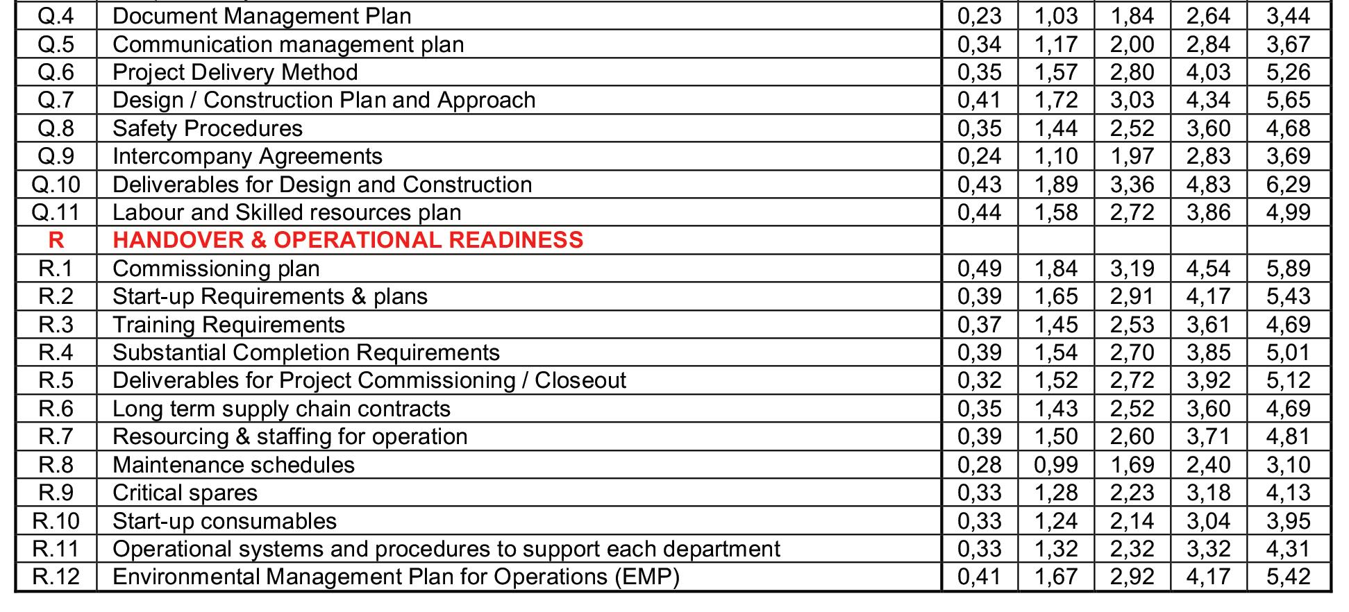

387The Journal of the Southern African Institute of Mining and Metallurgy VOLUME 122 JULY 2022
TheSynopsisincreased adoption of unmanned aerial vehicles (UAVs) may improve the productivity and costeffectiveness of remote sensing in the mining industry. This review’s objective is to enable stakeholders to identify possible application adoption, improvement, and innovation opportunities. The review merges a building block strategy and practical screening criteria to identify possible avenues of research to answer the review questions. After the screening process, 72 documents were included in the review.
The results may enable researchers to identify gaps in the published research or potential collaborators. In addition, other stakeholders may use re findings to identify possible opportunities for application adoption, improvement, and innovation.
A building-blocks search strategy was used to perform a systematic literature review. The three search terms used were ‘remote sensing’, ‘UAV’, and ‘mining’. The Boolean operator ‘AND’ was used to include Affiliation: 1Department of Engineering and Technology Management, University of Pretoria, South Africa Correspondence to: S. Grobbelaar Email: schalk.grobbelaar@up.ac.za
Although sensor-equipped UAVs are relatively new to the mining industry, their application has snowballed in terms of scale, speed, and service scope (Ren et al., 2019). For example, Szentpeteri (2016) investigated the use of UAVs for geological modelling and surface pit mapping. Jones et al. (2019) identified advances in applying autonomous UAVs in underground mines. Park and Choi (2020) focused on the applications of UAVs in mineral exploration, exploitation, and reclamation.
The review was limited to published papers in academic journals. Future studies could aim to include empirical data on the latest UAV applications used in the mining industry.
UAV,Keywordsremote sensing, mining industry, photogrammetry, monitoring, detection. Introduction and background Remote sensing is the science of capturing data with a device that is not in physical contact with the data source. The output is used to create a digital representation of the object. Unmanned aerial vehicles (UAVs) have become favoured instruments for remote sensing applications (Muchiri and Kimathi, 2016).
From the two UAV types identified, multi-rotor vehicles were the most favoured for all applications. From the eight remote sensing techniques identified, photogrammetry was the one most often used. Other techniques were limited because of complexity, cost, or the incompatibility of sensors and UAVs.
2. Which types of UAV and remote sensing methods are typically used in these applications?
A review of remote-sensing unmanned aerial vehicles in the mining industry by M. Loots1, S. Grobbelaar1, and E. van der Lingen1
This article reviews the status of published academic research in the field and aims to answer the following two questions:
Dates: Received: 19 Apr. 2021 Revised: 18 Mar. 2022 Accepted: 1 Jun. 2022 Published: July 2022 How to cite: Loots, M., Grobbelaar, S., and van der Lingen, E. 2022 A review of remote-sensing unmanned aerial vehicles in the mining Journalindustry.oftheSouthern African Institute of Mining and Metallurgy, vol. 122, no. 7, pp. 387–396 DOI 3564https://orcid.org/0000-0003-1648-E.2440https://orcid.org/0000-0001-8148-S.ORCID9717/1602/2022http://dx.doi.org/10.17159/2411-ID::GrobbelaarvanderLingen
Review method Search strategy and screening process
UAVs are capable of sustaining flight without onboard human involvement (Bento, 2008), and are remotely controlled either manually or by a computerized piloting program. The recent enhancement in UAVs, along with remote sensing technologies, have ensured an ever-expanding field of application in industries such as agriculture, forestry, surveying, construction, entertainment, and mining.
1. Which applications of remote-sensing UAV technology are used in the four phases (exploration, development, exploitation, and reclamation) of mining?
Fifteen applications were identified, the majority of which were in the exploration phase. The most often researched applications were topographic surveys, reclamation monitoring, and slope management.
Papers were classified into four categories: exploration, development, exploitation, and reclamation.
2.
Publication sources, research type, and country of origin
A review of remote-sensing unmanned aerial vehicles in the mining industry
Methods of synthesis and analysis
After the screening process, only articles published from 2015 to 2020 remained in the sample, even though the original search parameters were from 2010 to 2020. The earlier publications focused on how UAV technology can supplement manual methods, but the more recent publications emphasized standalone utilizations of UAVs.
Papers per mining phase and application type
3.
The research considered only publications related to mining applications in DHET-approved journals indexed in the Scopus or Web of Science databases. It didn’t consider unpublished developments in the industry, research that is kept confidential, or developments for which there are approved or pending patent applications. It also didn’t consider developments in related fields that might potentially be implemented in the mining industry. However, the results are relevant to researchers and stakeholders in the mining field since they can use them to identify potential applications, gaps in academic publications, and collaborators.
The journals with the most publications were Remote Sensing with nine publications, Sensors with eight, Environmental Earth Sciences with five, and Acta Montanistica Slovaca with three. China (21%) was the top contributor, with Australia (8%) and Italy (8%) following. South Africa published only one article on the review topic.
This review was a qualitative study, leaning towards an integrative approach. According to Boland, Cherry, and Dickson (2017), an integrative approach aggregates the primary research data. Therefore it summarizes already defined themes that are used in the industries in such a way that the review questions posed by the specific systematic literature review are answered. The developed codes included were ‘mining applications’, ‘UAV type’, ‘sensor type’, ‘remote sensing technique’, and ‘remote sensing outputs’. The coded documents were grouped according to their applicability to the four phases in mining. Limitations
388 JULY 2022 VOLUME 122
Year of publication
Figure 1 illustrates the number of papers per mining phase and application type. Of the 72 documents reviewed, the majority Figure 1—Applications per mining phase
4.
5.
The Journal of the Southern African Institute of Mining and Metallurgy only papers that were relevant for all the terms. The search results excluded ‘data mining’, and included the following journal paper provisos:1.South African (SA) Department of Higher Education and Training (DHET) approved journal list Published between 2010 and 2020 Indexed in the Scopus or Web of Science databases Written in English Available electronically 6. Relevant to the research questions. The Scopus database was selected because it is one of the most extensive and most popular databases in the engineering disciplines, and provides the largest number of abstracts and peerreviewed publications(Roux, van der Lingen, and Botha, 2019); while Web of Science is known as a database in leading scholarly research in the sciences worldwide. Following this screening process, only 72 papers remained from the initial sample. Data extraction In the data extraction process, the relevant information is taken from the individual research and stored in a single format (Boland, Cherry, and Dickson, 2017). A total of 72 articles and reviews were eligible for inclusion in the review. Microsoft Excel and ATLAS.ti software were used to extract meaningful data from the screened papers. Full-text academic material was imported into ATLAS.ti and subsequently coded.
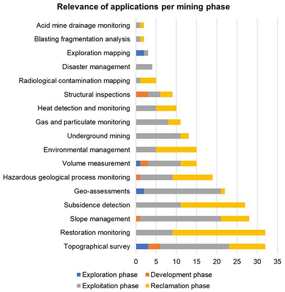
389The Journal of the
Institute of
The development phase typically includes construction activities such as buildings, infrastructure, and plant used for ore processing, and mineshafts. Within this phase, four applications were identified: slope management, structural inspections, topographic inspections, and volume measurement (see Figure 1). Surface deformation analysis (SDA) is a method used for structural inspections, employing dense geo-referenced point clouds. The latest point cloud is compared with earlier ones to identify any possible displacement. SDA inspections are traditionally completed by using 3D laser scanners, but remotesensing UAVs comply with the technical requirements for SDA inspections (Pinto et al., 2020). Photogrammetry is typically used for SDA on UAVs. Structure from motion (SfM) analysis is used with ground-control points to ensure that images are correctly orientated and geo-referenced (Pinto et al., 2020). Pinto et al. (2020) considered the inspection of both a rocky slope and a dam wall to test UAV photogrammetry’s applicability to SDA. The inspections were carried out with a multi-rotor UAV equipped with a digital camera and using an aerial robotics cognitive architecture (ARCog) enabling semi-autonomous flight. Decisions were based on the visual data gathered, as well as pre-programmed rules developed and provided by experts under well-known conditions. The project proved that semi-autonomous flights are possible for visual and 3D inspections. Several advantages were highlighted, such as the ability to access difficult areas and to carry out safe and fast inspections. Future work will look into implementing ARCog on multiple UAVs, and developing several machine-learning opportunities such as new behaviour training during missions and improving decision-making processes (Pinto et al., 2020). Exploitation phase
and
This phase focuses on environmental management and restoration monitoring. Applications include acid mine drainage, radiological contamination mapping, restoration monitoring, and subsidence detection. Acid mine drainage monitoring Acid mine drainage (AMD) originates from mining operations that produce acidic water and mine waste characterized by low pH values. Its environmental impact has led to a demand that AMD be monitored to enable mitigating strategies. Jackisch et al. (2018) investigated hyperspectral imaging integrated with photogrammetry for AMD mapping. Hyperspectral UAV sensing was used to gather the AMD mineral composition data. Common AMD minerals are jarosite, schwertmannite, goethite, and haematite (Jackisch et al., 2018). These minerals form the basis for mapping AMD areas. A Rikola hyperspectral camera was used on a multi-rotor UAV, which can capture images while hovering. A fixed-wing UAV was used to produce orthophotos and DEM with photogrammetry. The fixed-wing was chosen because it
Development phase
A review of remote-sensing unmanned aerial vehicles in the mining industry Southern African Mining Metallurgy concerned the exploitation (51) and reclamation phases (41). Several papers included more than one phase. Topographic surveying and restoration monitoring were the applications most frequently observed. The various applications and research findings per phase are discussed in the sections that follow.
The exploitation phase is the core of the mining process. This is where the minerals are extracted from the earth and processed into saleable products. The majority of remote-sensing UAV applications are prominent in this phase. Figure 2 is a Sankey diagram for the exploitation phase, showing the applications involved in it. The thickness of the connection line (between phase and application) illustrates the ratio of papers related to bothTheaspects.findings per application type in the exploitation phases are summarized in Table I. Reclamation phase
Results
Exploration phase Four applications – exploration mapping, topographic survey, geo-assessment, and volume measurement – are relevant to this phase, as indicated in Figure 1. Exploration mapping examines the relationship between mineral deposit characteristics and surface geology. Remote sensing technologies used for this include magnetic, hyperspectral, and photogrammetric. Magnetic imaging uses fluxgate magnetometers to detect variations in the Earth’ s magnetic field due to ferromagnetic minerals’ magnetism (Heincke et al., 2019). Hyperspectral imaging is used for a broader range of minerals, since every compound displays a unique spectral signature based on the wavelengths of electromagnetic radiation absorbed, emitted, or reflected (Kirsch et al., 2018). An example of a hyperspectral sensor is the visible to near-infrared (VNIR) camera, Senop Rikola, which was used by both Heincke et al. (2019) and Kirsch et al. (2018) in their studies of exploration mapping. Photogrammetry uses multiple 2D images of objects and reconstructs them into a 3D point cloud using triangulation. The models thus created can be grouped as digital elevation models (DEM), digital surface (DSM) models, digital terrain (DTM) models, and orthophotographs or 3D models. Photogrammetry can also be used for RGB (red-green-blue) analysis, which mimics human vision by differentiating objects based on their colour. Kirsch et al. (2018) integrated terrestrial and UAV exploration surveys by using hyperspectral imaging and photogrammetry. They demonstrated multiple benefits from this integration, such as spectral range, spatial coverage, flexibility, and appropriate validation. The study concluded that remote-sensing-enabled UAVs improve time-efficiency and geological interpretation, and reduce costs. Heincke et al. (2019) used magnetic, hyperspectral, and photogrammetry data-enabled UAVs to produce an integrated mineralogical property map under the EU-funded MULSEDRO project.Fixed-wing or multi-rotor UAVs can be used to transport the sensors. For exploration mapping, both multi-rotor and fixed-wing UAVs are used. For surveys that require low-elevation and highresolution data, the multi-rotor UAV is preferred. For coverage of large areas that require longer endurance, the fixed-wing UAV is preferred. Heincke et al. (2019) indicated that fixed-wing UAVs are preferable for magnetic mapping, as the multi-rotor UAV motors cause electromagnetic noise that distorts the magnetic sensor readings. Advances in exploration mapping will be dependent on the development of smaller and more lightweight sensors with an extended wavelength range for hyperspectral imaging, and higher resolution for digital cameras (Kirsch et al., 2018). The development and implementation of hydrogen fuel-cell (de Wagter et al., 2020) and hybrid energy systems may also increase flight endurance (Özbek et al. 2020).
VOLUME 122 JULY 2022
Haas et al. (2016) used photogrammetry to evaluate the impact of geomorphic processes (weathering and erosion) on recultivated mining slopes. Yucel and Turan (2016) used it to determine the anthropogenic and meteorological effects on mine lakes in Turkey. Both studies confirmed that photogrammetry is a useful visualization tool, that can rapidly and accurately detect chang. Xiang et al. (2018) used photogrammetry, DoD, and SLLAC to determine the geomorphic changes during and after mining. DoD was used to calculate the volumetric changes, while SLLAC was used to determine the extent of the mining and to visualize changes to the mine slopes. Gong et al. (2019) used a similar method to assess the effect of erosion on a mine dump site during a freeze–thaw cycle. Satellite images were compared with UAV photogrammetry to quantify the impact of mining on a forest area. Incekara et al. (2017) concluded that UAVs are a more appropriate option than satellite images for monitoring the effects of mining in forested areas. UAV data has higher spatial, spectral, radiometric, and temporal resolutions, with fewer cost and time implications.Kun(2019) used UAV photogrammetry to develop vegetation index maps of a rehabilitated mine dump site. The maps were used to determine the plant species’ adaptation, condition, and survival percentage. The RGB values of the surveyed area were used and characterized according to the triangular greenness index (TGI) and the visible atmospheric resistant index (VARI). Padró et al (2019) used a multi-rotor UAV equipped with a multispectral sensor to develop DSM, DEM, DTM, vegetation indices, and orthophoto maps showing land cover classifications. This provided to be a fast, high-resolution, and low-cost alternative to traditional restoration monitoring methods. Carabassa et al. (2020) also looked into the use of multispectral sensor UAVs and RGB-enabled digital cameras to determine the land cover classifications of mining areas. Isokangas et al. (2019) evaluated the use of thermal infrared (TIR)- and colour infrared (CIR)enabled UAVs as a monitoring system for peatland used to purify mine process water. The output consisted of TIR images and blue- normalized difference vegetation index (BNDVI) images. The TIR images indicated cold anomalies, which outlined areas of groundwater seepage, and the BNDVI indicated whether or not vegetation was stressed because of excess water. The method was found to be successful in monitoring treatment peatlands.
Figure 2—Exploitation stage applications
The Journal of the Southern African Institute of Mining and Metallurgy is able to cover a large area owing to its long flight endurance. Both UAVs flew autonomous flights after flight pre-planning. The study used data from surface sampling, such as chemical analysis by spectrometry and pH measurement, for verification and confirmed the feasibility of monitoring AMD with hyperspectralenabled UAVs.
390 JULY 2022 VOLUME 122
A review of remote-sensing unmanned aerial vehicles in the mining industry
Radiological contamination mapping Uranium mining produces waste and tailing storage facilities with high concentrations of radionuclides (Borbinha et al., 2020). These areas pose a high risk to humans, fauna, and flora. Radiological mapping aims to locate, identify, and quantify radiation sources (Borbinha et al., 2020). Martin et al. (2015) used a UAV at low altitude to perform radiological mapping of a disused mining site. The multi-rotor UAV was equipped with a GPS module, a gamma-ray spectrometer sensor, and a laser rangefinder. The gamma-ray spectrometer was a cadmium zinc telluride (CZT) detector. This recorded a spectrum of radiation energy with a time, location, and elevation stamp. The radiation map depicted the radiological intensity of the area by means of a scaled colour overlay. The survey produced metre-scale-accurate radiation measurements within a much shorter time-frame than traditional methods. The data also allowed isotopic fingerprinting of the region to determine the nature of the contamination. Borbinha et al. (2020) employed multi-rotor UAVs with GMCs (Geiger-Muller counters) and CZT gamma-ray spectrometers. A LiDAR UAV was used to develop a 3D model of the studied area. The GMC UAV drone was deployed over the entire area to detect hotspots, after which it hovered close to the ground to gather accurate readings. This allowed the CZT UAV to be deployed in specific hotspot areas to acquire the source spectra (Borbinha et al., 2020). This flight strategy provided radiological contamination maps that could be used for monitoring and control. Restoration monitoring Mining operations can cause geomorphic changes owing to their anthropogenic nature (Xiang et al., 2018). Mining rehabilitation and restoration monitoring track progress to determine whether restoration activities are effective. UAVs can capture data on the surface conditions and ecology, and track the process of restoration (Said et al., 2020).
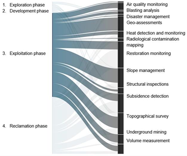
Photogrammetry with traditional surveying techniques can be used for geodata-based analysis to Leo Stalin and identify unstable slope areas. Gnanaprakasam, 2020
A review of remote-sensing unmanned aerial vehicles in the mining industry of exploitation phase findings Application Findings
Spectral imaging and photogrammetry can be used to develop land cover classification Carabassa et al., 2020 maps for rehabilitation planning
Slope monitoring allows slope failure to be predicted, ensuring that it can be successfully managed. Said et al., 2020 A framework for integrating UAV-based photogrammetry and total laser scanning (TLS) Tong et al., 2015 can provide 3D models of mining slopes to map and monitor their condition.
A multi-rotor UAV was employed to carry a high-definition video camera and Drager Irimia et al., 2019 XAM 5000 multi-gas detector. The sensor was able to monitor simultaneously five gases that can lead to explosion-prone conditions. Future developments may include flight-enhancement surveillance and measurement by integrating thermal infrared sensors to detect objects in vision-impaired situations, and using LiDAR to avoid collisions and produce 3D images. Air quality Mining operations can produce noxious or toxic gases and particulates that can Said et al., 2020 monitoring negatively affect the environment, surrounding communities, and mine employees.
Disaster UAVs can create 3D models of post-seismic building Yao, Qin and Chen, 2019 management collapses, which improves rescue planning and response time.
Photogrammetry with terrestrial laser scanning and distributed optical fibre Lanciano & Salvini, 2020 sensors (DOFS) can monitor strain and temperature to confirm the stability of quarry slopes and subsequently update geological models.
3D, DSM, orthophotographs, DTM, and DEM can be used to develop models for Blistan et al., 2016 geological measurements, such as angle of inclination and other structural parameters. Salvini et al., 2018 Katuruza and Birch, 2019
Infrared thermal-enabled UAVs can be used to detect coal fires and Lee and Choi, 2016 overheating of equipment and facilities. Ren et al., 2019 He et al., 2020 Said et al., 2020 Slope Slope stability is vital for safe and continuous production in opencast mines. Ren et al., 2019 management
Reference
Fragmentation analysis using photogrammetry Said et al., 2020 with multi-rotor UAVs is preferred.
UAV-photogrammetry can be used to appraise slope failures in iron ore mines. Bar et al., 2020 ShapeMetrix can generate 3D models from images obtained, and provide a direct analysis of geometric entities such as geological structures, bedding planes, and joints.
391The Journal of the Southern African Institute of Mining and Metallurgy VOLUME 122 JULY 2022 Table I Summary
Geo-assessments
UAVs have the advantage of being able to reach areas that traditional Said et al., 2020 remote-sensing methods cannot reach. Assessments of these areas are important for stability analysis and planning. UAV photogrammetry is the dominant remote-sensing technique used for geo-assessment in surface mining.
The evolution of geo-assessments can be automated by employing machine- Beretta et al., 2018 learning techniques to classify lithologies for geological mapping. Beretta et al., 2019a Beretta et al., 2019b Heat detection and Underground coal fires can lead to surface subsidence and surface fissures, causing Wang et al., 2015 monitoring geological disasters. Detecting and monitoring fires is crucial to helping with suppressing fires and predicting changes. A terrestrial infrared thermal imager can provide a surface temperature field model.
A global navigation satellite system (GNSS) can be used to identify displacement locations. Gül, Hastaoğlu UAV-photogrammetry can then determine the possible causes and the size of displacements. and Poyraz, 2020 Methods such as slope local length and autocorrelation (SLLAC) and surface peak curvature (SPC) Xiang et al., 2018 are used on DSMs and retrieved using photogrammetry, allowing a detailed view of mining extent and its terraces. This ability to detect terraces enables SLLAC to monitor their stability.
UAVs can be used to characterize blasting plumes (gas and particulate emissions) Alvarado et al., 2015 in near real-time. Fixed-wing and multi-rotor UAVs with autonomous flight path planning were used. Underground coal fires waste a valuable energy source, and emit various gases Dunnington and such as carbon dioxide, carbon monoxide, sulphur, and methane. Various sensors, Nakagawa, 2017 including infrared, catalytic, metal oxide, and electrochemical sensors, can be used in combination to detect gases.
TLS can be used for kinematic analysis to identify the most probable failure mechanism of slopes. Francioni et al., 2015
Topographical Compared with traditional surveying techniques such as laser scanning, UAV Kršák et al., 2016 survey photogrammetry provides faster, more cost-effective, and higher spatial data outputs. Blistan et al., 2019 Beretta et al., 2018
Blasting analysis
Subsidence detection
the mining industry 392 JULY 2022 VOLUME 122 The Journal of the Southern African Institute of Mining and Metallurgy
Underground UAVs can be used to explore the shape, condition, and surface mineralization Ren et al., 2019 mining of mining voids. Underground UAV applications are limited, since UAVs rely on GPS signals for autonomous navigation, and GPS signals cannot penetrate the depths required for most underground mines. Multi-rotor UAVs are the only type used in underground mining applications. Scannapieco, Renga The environment is usually narrow and cluttered and visibility is poor. Furthermore, and Moccia, 2015 the need to avoid obstacles, owing to the presence of stationary and moving objects, creates a significant challenge.
A visual-inertial sensor was tested to improve the localization of UAVs in dynamic underground Li et al., 2020 environments. Results indicated that the system was effective, and could be integrated into future work on real UAV platforms.
Synthetic aperture radar (SAR), radar interferometry, and millimetre-wave radar could Scannapieco, Renga and overcome the challenges imposed on UAVs by underground environments. Moccia, 2015 Simultaneous localization and mapping (SLAM) is a promising technique for Rochala et al., 2019 independent navigation. SLAM simultaneously builds 3D models and enables navigation in the surrounding area. Acoustic, passive, active electro-optical, or radar sensors are typically used.
A review of remote-sensing unmanned aerial vehicles in
I
Static images can be used to determine mineralogy by visual imaging, using Rahman et al., 2016 machine-learning algorithms and XRF signatures.
Thermal, multispectral, and RGB sensors can create LiDAR geo-referenced 3D point clouds Turner, MacLaughlin and to map and investigate adverse discontinuities in underground mining excavations. Iverson 2020
Volume measurement requires a ‘before’ and an ‘after’ model of the mining area to determine Esposito et al., 2017 the amount of excavated material by calculating the difference between the two models. Fixed-wing and multi-rotor UAVs are prevalent in this application. Since two different models are Liu et al., 2020 compared for volume measurement, geo-referencing of the images is critical. Indirect geo-referencing is employed by using ground control points. Software such as Agisoft Photoscan is able to create highly accurate geo-referenced 3D point clouds, DSMs, and orthophotos. CloudCompare with an M3C2 plugin can accurately detect volume differences and apply change Esposito et al., 2017 detection accurately. Other methods of change detection are also possible, such as DEM of Xiang et al., 2018 difference (DoD).DoD calculates the difference between two DEMs, allowing the volumetric changes to be estimated.
Table (continued) Application Findings Reference Volume Volume measurements are used in mine planning to determine the Esposito et al., 2017 measurement extraction rate and estimate stripping ratios. Photogrammetry is the preferred Shahbazi et al., 2015 technique for this.)
Although mining has its economic benefits, it has repercussions on the natural environment. Damage to land is evident where open-pit mines leave large voids behind after operations cease (Ren et al., 2019). The impacts of underground mining are less visible, but tend to manifest as surface subsidence (Zhao et al., 2020). Predicting mining-induced subsidence is seen as the basis for implementing proactive measures to reduce its effect (Dawei et al., 2020). Traditional subsidence mapping is prone to data gaps and errors owing to the inaccessibility of surveyed areas, safety issues, and human error. Thus the use of remote-sensing-enabled UAVs to gather information on dangerous and inaccessible areas is highlySeveralattractive.studies have considered the use of UAVs for subsidence detection, and highlighted their ability to provide centimetre-scale accuracy from autonomous flight missions. Both fixed-wing and multi-rotor drones have been employed for this purpose. Fixed-wing UAVs are mostly used where large areas have to be mapped, while multi-rotor UAVs are used for smaller areas where high resolution is required (Suh and Choi, 2017). Photogrammetry is the most often-used method, but multispectral imaging and LiDAR scanning are also employed. Suh and Choi (2017) utilized an autonomous multi-rotor UAV to obtain digitally geo-referenced orthophotographs and DTMs to calculate the position, area, and volume of an identified surface subsidence. They emphasized that UAV photogrammetry cannot fully replace traditional methods, which provide subsidence data such as horizontal ground relaxation and crack detection.
Rauhala et al. (2017) used fixed-wing UAV photogrammetry SfM to detect surface displacement on mine tailing facilities. Annual topographical models were used to detect the displacement over the years, and ground checkpoints were used to confirm the accuracy of that information. DoD was used to quantify the ground displacement between individual models. The study found that the models produced by UAV photogrammetry were sufficiently accurate to track surface subsidence of the tailing facilities to a decimetre scale. To obtain information on mining-induced subsidence on cultivated land, Hu and Li (2019) used a multi-rotor UAV equipped with a digital camera to develop vegetation index maps, using characteristic spectral values within the RGB bands. Multispectral and hyperspectral cameras can be employed for higher accuracy vegetation index maps, but the sensors are more costly than standard digital cameras. Zhao et al (2020) and Ren et al. (2020) used multispectral-enabled UAVs to measure damage to land caused by surface subsidence. Ren et al. (2020) focused on an above-ground biomass (AGB) measurement of the health of maize crops, while Zhao et al. (2020) used soil and plant analyser development (SPAD) to measure and determine
Summary of results
Underground mining is the most challenging application for remote-sensing UAVs: it poses implementation challenges, and requires a different navigation and communication architecture to that in the UAVs used for surface mining applications. AMD monitoring, exploration, and radiological contamination mapping are specialized applications, since they need unique sensors. The need for compatibility of the sensors with the limits of a UAV’s payload contributes to the slow adoption of these applications. A gap was identified in the case of structural inspections in the mining industry. This application is well-known in the building and construction industries, but the potential for use in mining operations has not been fully realized. Overall, remote sensing has several uses in mining, as discussed in the literature review. A summary is provided in Table II.
Table II Remote-sensing UAV applications and uses per mining phase Mining phase Aapplication category Application 1. Exploration Exploration mapping Ferromagnetic mineral identification Mapping variations in mineral composition Area geological interpretation 2. Development Structural inspections Infrastructure inspections Construction process monitoring 3. Exploitation Blasting analysis Fragmentation analysis Disaster management 3D models of disaster areas Change detection in disaster zones Disaster response missions Air quality monitoring Operational air quality monitoring Coal fire detection and monitoring Geo-assessments Assessment of inaccessible areas Geo-hazard identification Updating of geological model Heat detection and monitoring Coal fire detection and monitoring Overheating of equipment/facilities Slope management Slope failure prediction Slope failure appraisal Topographic survey Resource and reserve estimation Mine Reconciliationplanning Volume measurement Mine planning Legal reporting requirements Change detection Underground mining Geo-assessments and mineralogical classification Disaster response missions Gas detection 4. Reclamation AMD monitoring AMD detection and monitoring Radiological contamination Isotopic fingerprinting and radiological contamination mapping Restoration monitoring Change detection of surface condition and ecology Land cover recultivation monitoring Subsidence detection Subsidence detection and monitoring
Photogrammetry is the most widely used remote sensing technique, accounting for 67% of all applications discussed
A review of remote-sensing unmanned aerial vehicles in the mining industry the effect of subsidence on corn crops. Both studies indicated that multispectral-enabled UAVs are useful tools for assessing the impact of surface subsidence on reclaimed land. Ćwiakała et al. (2020) studied mining-induced subsidence using traditional field measurements as reference models, to assess UAV photogrammetry’s accuracy. Their study also focused on determining horizontal terrain displacements. Both fixed-wing and multi-rotor UAVs were employed in the survey, which showed that UAV photogrammetry could be used to assess the state of surface subsidence. However, the study founded that vegetation coverage was a limitation because it distorted the accuracy of the images. Similar studies by Dawei et al. (2020) and Stupar, Rošer, and Vulić (2020) concluded that UAV photogrammetry offers valuable information about subsidence detection and monitoring in a short time-frame without exposing personnel to dangerous environments. Technology, therefore, is highly suited to this application.
393The Journal of the Southern African Institute of Mining and Metallurgy VOLUME 122 JULY 2022
A review of remote-sensing unmanned aerial vehicles in the mining industry
Advances in tilt imaging systems on UAVs, known as gimbals, enable images to be acquired from any angle without distortions from the drone’s movements. Image post-processing is advanced with the SfM algorithm, allowing for the rapid development of any model that is required. Two software applications were prominent in the literature: Agisoft Photoscan and Pix4D, both of which use SfM algorithms to produce highly accurate photogrammetric models.Other software applications, such as CloudCompare and ShapeMetrix, use the developed models for further analysis. The models can be used in CAD software to update existing geological models with geo-assessments. Algorithms such as DoD, SLLAC, and SDA also use photogrammetric data to determine aspects such as slope movement, displacement, and volume change. Adoption of remote sensing techniques such as radiological and magnetic remote sensing is limited owing to the specialized nature of the sensors required for specific applications. The size and weight restrictions of UAVs and the high cost of sensors contribute to the slow adoption of hyperspectral, multispectral, LiDAR, and TIR remote sensing techniques. Table III provides a summary of the studies that have evaluated a specific sensor for a specific application and mining phase. Some studies evaluated more than one sensor. The review identified the following potential benefits of remote sensing aerial vehicles within the mining industry. ➤ Improved time-efficiency (Kirsch et al., 2018) ➤ Improved geological interpretation (Kirsch et al., 2018) ➤ Reduced costs (Kirsch et al., 2018) ➤ Spatial coverage (Kirsch et al., 2018; Heincke et al., 2019) ➤ flexibility (Kirsch et al. 2018) ➤ Semi-autonomous flights for visual and 3D inspections (Pinto et al., 2020) ➤ Assess ment of difficult areas and safe and fast inspections (Pinto et al., 2020; Said et al., 2020; Ren et al., 2019; Francioni et al., 2015; Leo Stalin and Gnanaprakasam, 2020; Borbinha et al., 2020) ➤ Monitoring progress to determine whether activities are effective (Said et al., 2020) ➤ Assessing the impact of surface subsidence (Ren et al., 2020; Zhao et al., 2020; Dawei et al. 2020; and Stupar, Rošer, and Vulić, 2020).
The Journal of the Southern African Institute of Mining and Metallurgy in the literature review. There is a significant gap between photogrammetry and other applications. Hyperspectral and multispectral remote sensing each account for 9%, followed by remote gas sensing at 6%. The adoption of photogrammetry is mainly a result of advances in the sensors utilized and in post-processing of data obtained from the UAV flight. The cost-effectiveness of digital cameras has increased leading to a significant improvement in quality image. Furthermore, the decreased size and weight of digital cameras has allowed photogrammetry using UAVs to be rapidly and broadly adopted.
2. Which types of UAV and remote sensing methods are typically used in these applications?
The SLR employed a methodology that identified 72 quality documents on the subjects of remote sensing, UAVs, and mining. A total of 15 applications were identified and synthesized in the four mining phases. The different remote sensing techniques and UAV types were considered for each application type. Most of the research reviewed the exploitation and reclamation phases of mining, with only limited applications identified in the exploration and development phases. Opportunities exist, therefore, to expand remote-sensing UAV applications in these phases. Photogrammetry was the most popular technique by Table III
394 JULY 2022 VOLUME 122
Application Sensors Multispectral Gas Radiological Magnetic LiDAR TIR Hyperspectral Photogrammetry 1. Exploration Exploration mapping 1 2 2 2. Development Structural inspections 1 3. Exploitation Blasting analysis 1 Disaster management 2 1 Air quality monitoring 4 Geo-assessments 1 10 Heat detection and monitoring 1 1 Slope management 1 11 Topographical survey 1 1 14 Volume measurement 6 Underground mining 1 1 1 2 4. Reclamation Acid mine drainage monitoring 1 1 1 Radiological contamination 1 Restoration monitoring 4 1 2 2 13 Subsidence detection 2 1 1 7
Conclusions This SLR aimed to review the status of academic publications in the field and to answer the following two research questions:
1. Which applications of remote-sensing UAV technology are used in the four phases (exploration, development, exploitation, and reclamation) of mining?
Mining phase
Remote sensing sensor studies per application type and mining phase
VOLUME
Incekara, A.H., Yildirim, O., Susam, T., and Seker, D.Z. 2017. Using unmanned aerial vehicles for open mining areas: Current applications and future potentials. 38th Asian Conference on Remote Sensing – Space Applications: Touching Human Lives. ACRS, New Delhi, India, 2017. Irimia, A., Găman, G.A., Pupăzan, D., Ilie, C., and Nicolescu, C. 2019. Using drones in support of rescue interventions teams in toxic/flammable/explosive environments. Environmental Engineering and Management Journal, vol. 18, no. 4. pp. 831–837. Isokangas, E., Davids, C., Kujala, K., Rauhala, A., Ronkanen, A.K., and Rossi, P.M. 2019. Combining unmanned aerial vehicle-based remote sensing and stable water isotope analysis to monitor treatment peatlands of mining areas. Ecological Engineering, vol. 133. pp. 137–147. Jackisch, R., Lorenz, S., Zimmermann, R., Möckel, R., and Gloaguen, R . 2018. Drone-borne hyperspectral monitoring of acid mine drainage: An example from the Sokolov lignite district. Remote Sensing, vol. 10, no. 3. 385 p.
BereTTa, F., ShibaTa, H., Cordova, R., Peroni, R.L., Azambuja, J., and CosTa, J.F.C.L. 2018. Topographic modelling using UAVs compared with traditional survey methods in mining. Revista Escola de Minas, vol. 71, no. 3. pp. 463–470. BlisTan, P., Kovanič, Ľ., PaTera, M., and Hurčík, T. 2019. Evaluation quality parameters of DEM generated with low-cost UAV photogrammetry and structure-from-motion (SfM) approach for topographic surveying of small areas. Acta Montanistica Slovaca, vol. 24, no. 3. pp. 198–212. BlisTan, P., Kovanič, Ľ., Zelizňaková, V., and Palková, J. 2016. Using UAV photogrammetry to document rock outcrops. Acta Montanistica Slovaca, vol. 21, no. 2. pp. 154–161. Boland, A., Cherry, M.G., and Dickson, R. 2017. Doing a Systematic Review. SAGE Los Borbinha,Angeles.J.,RomaneTs, Y., Teles, P., Corisco, J., Vaz, P., Carvalho, D., Brouwer, Y., Luís, R., PinTo, L., Vale, A., VenTura, R., Areias, B., Reis, A.B., and Gonçalves, B. 2020. Performance analysis of geiger–müller and cadmium zinc telluride sensors envisaging airborne radiological monitoring in NORM sites. Sensors (Switzerland), vol. 20, no. 5. 1538. Carabassa, V., MonTero, P., Crespo, M., Padró, J.C., Pons, X., Balagué, J., BroTons, L., and Alcañiz, J.M. 2020. Unmanned aerial system protocol for quarry restoration and mineral extraction monitoring. Journal of Environmental Management, vol. 270. 110717. Ćwiakała, P., Gruszczyński, W., SToch, T., Puniach, E., Mrocheń, D., MaTwij, W., MaTwij, K., Nedzka, M., SopaTa, P., and Wójcik, A . 2020. UAV applications for determination of land deformations caused by underground mining. Remote Sensing, vol. 12, no. 11. 1733. Dawei, Z., Lizhuang, Q., Demin, Z., Baohui, Z., and Lianglin, G. 2020. Unmanned aerial vehicle (UaV) photogrammetry technology for dynamic mining subsidence monitoring and parameter inversion: A case study in China. IEEE Access, vol. 8. pp. 16372–16386. De WagTer, C, Remes, B, Ruisink, R, Van Tienen, F., and Van Der HorsT, E 2020, Design and testing of a vertical take-off and landing UAV optimized for carrying a hydrogen fuel cell with a pressure tank. Unmanned Systems, vol. 8, no. 4. pp. 279–285. DunningTon, L. and Nakagawa, M. 2017. Fast and safe gas detection from underground coal fire by drone fly over. Environmental Pollution, vol. 229, pp. 139–145. EsposiTo, G., MasTrorocco, G., Salvini, R., OliveTi, M., and STariTa, P. 2017. Application of UAV photogrammetry for the multi-temporal estimation of surface extent and volumetric excavation in the Sa Pigada Bianca open-pit mine, Sardinia, Italy. Environmental Earth Sciences, vol. 76, no. 3. 103 p.
Jones, E., Sofonia, J., Canales Cardenas, C., Hrabar, S., and Kendoul, F. 2019. Advances and applications for automated drones in underground mining operations. Proceedings of the Ninth International Conference on Deep and High
Francioni, M., Salvini, R., STead, D., Giovannini, R., Riccucci, S., Vanneschi, C., and Gullì, D. 2015. An integrated remote sensing-GIS approach for the analysis of an open pit in the Carrara marble district, Italy: Slope stability assessment through kinematic and numerical methods. Computers and Geotechnics, vol. 67. pp. 46–63. Gong, C., Lei, S., Bian, Z., Liu, Y., Zhang, Z., and Cheng, W. 2019. Analysis of the development of an erosion gully in an open-pit coal mine dump during a winter freeze-thaw cycle by using low-cost UAVs. Remote Sensing, vol. 11, no. 11. 1356 p. Gül, Y., HasTaoğlu, K.Ö., and Poyraz, F. 2020. Using the GNSS method assisted with UAV photogrammetry to monitor and determine deformations of a dump site of three open-pit marble mines in Eliktekke region, Amasya province, Turkey. Environmental Earth Sciences, vol. 79, no. 11. 248 p. Haas, F., Hilger, L., Neugirg, F., UmsTädTer, K., BreiTung, C., Fischer, P., Hilger, P., Heckmann, T., Dusik, J., Kaiser, A., SchmidT, J., Della SeTa, M., Rosenkranz, R., and BechT, M. 2016. Quantification and analysis of geomorphic processes on a recultivated iron ore mine on the Italian island of Elba using long-term ground-based lidar and photogrammetric SfM data by a UAV. Natural Hazards and Earth System Sciences, vol. 16, no. 5. pp.1269–1288. He, X., Yang, X., Luo, Z., and Guan, T. 2020. Application of unmanned aerial vehicle (UAV) thermal infrared remote sensing to identify coal fires in the Huojitu coal mine in Shenmu city, China. Scientific Reports, vol. 10, no. 1. 13895.
References Alvarado, M., Gonzalez, F., Fletcher, A., and Doshi, A. 2015. Towards the development of a low cost airborne sensing system to monitor dust particles after blasting at open-pit mine sites. Sensors (Switzerland), vol. 15, no. 8, pp. 19667–19687. Bar, N., KosTadinovski, M., Tucker, M., Byng, G., RachmaTullah, R., Maldonado, A., PöTsch, M., Gaich, A., McQuillan, A., and Yacoub, T. 2020. Rapid and robust slope failure appraisal using aerial photogrammetry and 3D slope stability models. International Journal of Mining Science and Technology, vol. 30, no. 5, pp.651–658. BenTo, M.D.F. 2008. Unmanned aerial vehicles: An overview. insideGNSS, vol. 3, no. 1. pp.54–61. BereTTa, F., Rodrigues, Á.L., Peroni, R.L., and CosTa, J.F.C.L. 2019a. Using UAV for automatic lithological classification of open pit mining front. Revista Escola de Minas, vol. 72, no. 1. pp. 17–23. BereTTa, F., Rodrigues, A.L., Peroni, R.L., and CosTa, J.F.C.L. 2019b. Automated lithological classification using UAV and machine learning on an open cast mine. Applied Earth Science: Transactions of the Institute of Mining and Metallurgy, vol. 128, no. 3. pp. 79–88.
Heincke, B., Jackisch, R., SaarTenoja, A., Salmirinne, H., Rapp, S., Zimmermann, R., PirTTijärvi, M., Sörensen, E.V., Gloaguen, R., Ek, L., BergsTröm, J., Karinen, A., Salehi, S., Madriz, Y., and MiddleTon, M. 2019. Developing multi-sensor drones for geological mapping and mineral exploration: Setup and first results from the MULSEDRO project. GEUS Bulletin, vol. 43. e2019430302. Hu, X. and Li, X. 2019. Information extraction of subsided cultivated land in highgroundwater-level coal mines based on unmanned aerial vehicle visible bands. Environmental Earth Sciences, vol. 78, no. 14. pp. 1–11.
JULY
395The Journal of the Southern African Institute of Mining and Metallurgy 122 2022 far. Other remote sensing techniques are limited because costeffective, lightweight, and compact sensors are not yet available. There has been some progress in hyperspectral, multispectral, and LiDAR sensors, but they remain costly and are not entirely suited to UAV implementation. Researchers in the field could use this review to identify gaps in published research and potential collaborators. Stakeholders from the mining industry could use this review to identify relevant applications for opportunities for implementation, improvement, and innovation. Future research may aim to compare the status of academic publications with that of industry developments or patent applications.
A review of remote-sensing unmanned aerial vehicles in the mining industry
Salvini, R., MasTrorocco, G., EsposiTo, G., Di BarTolo, S., Coggan, J., and Vanneschi, C. 2018. Use of a remotely piloted aircraft system for hazard assessment in a rocky mining area (Lucca, Italy). Natural Hazards and Earth System Sciences, vol. 18, no. 1. pp. 287–302. Scannapieco, A.F., Renga, A., and Moccia, A . 2015. Preliminary study of a millimeterwave FMCW InSAR for UAS indoor navigation. Sensors (Switzerland), vol. 15, no. 2,. pp. 2309–2335. Shahbazi, M., Sohn, G., Théau, J., and Menard, P. 2015. Development and evaluation of a UAV-photogrammetry system for precise 3D environmental modeling. Sensors (Switzerland), vol. 15, no. 11. pp. 27493–27524. STupar, D.I., Rošer, J., and Vulić, M. 2020. Investigation of unmanned aerial vehicles-based photogrammetry for large mine subsidence monitoring. Minerals, vol. 10, no. 2. pp.196–210 Suh, J. and Choi, Y. 2017. Mapping hazardous mining-induced sinkhole subsidence using unmanned aerial vehicle (drone) photogrammetry. Environmental Earth Sciences, vol. 76, no. 4. 144. SzenTpeTeri, K. 2016. Drones (UAV’s) in mining and exploration. An application example: Pit mapping and geological modelling. Unconventional Exploration Target & Latest Technique and New Tools in Mineral and Coal Exploration, October. pp. 34–59. Tong, X., Liu, X., Chen, P., Liu, S., Luan, K., Li, L., Liu, S., Liu, X., Xie, H., Jin, Y., and Hong, Z. 2015. Integration of UAV-based photogrammetry and terrestrial laser scanning for the three-dimensional mapping and monitoring of open-pit mine areas. Remote Sensing, vol. 7, no. 6. pp. 6635–6662. Turner, R.M., MacLaughlin, M.M., and Iverson, S.R . 2020. Identifying and mapping potentially adverse discontinuities in underground excavations using thermal and multispectral UAV imagery. Engineering Geology, vol. 266. 105470. Wang, Y.J., Tian, F., Huang, Y., Wang, J., and Wei, C.J. 2015. Monitoring coal fires in Datong coalfield using multi-source remote sensing data. Transactions of Nonferrous Metals Society of China (English edition), vol. 25, no. 10. pp. 3421–3428. Xiang, J., Chen, J., Sofia, G., Tian, Y., and Tarolli, P. 2018. Open-pit mine geomorphic changes analysis using multi-temporal UAV survey. Environmental Earth Sciences, vol. 77, no. 6. p. 220. Yao, H., Qin, R. and Chen, X. 2019. Unmanned aerial vehicle for remote sensing applications – A review. Remote Sensing, vol. 11, no. 12. p. 1443. Yucel, M.A. and Turan, R.Y. 2016. Areal change detection and 3D modeling of mine lakes using high-resolution unmanned aerial vehicle images. Arabian Journal for Science and Engineering, vol. 41, no. 12. pp. 4867–4878.
Zhao, Y., Zheng, W., Xiao, W., Zhang, S., Lv, X., and Zhang, J. 2020. Rapid monitoring of reclaimed farmland effects in coal mining subsidence area using a multi-spectral UAV platform. Environmental Monitoring and Assessment, vol. 192, no. 7. p. 474. u
A review of remote-sensing unmanned aerial vehicles in the mining industry
The Journal of the Southern African Institute of Mining and Metallurgy Stress Mining, The Southern African Institute of Mining and Metallurgy, Johannesburg, South Africa, pp. 323–334. KaTuruza, M. and Birch, C. 2019. The use of unmanned aircraft system technology for highwall mapping at Isibonelo Colliery, South Africa. Journal of the Southern African Institute of Mining and Metallurgy, vol. 119, no. 3. pp. 291–295. Kirsch, M., Lorenz, S., Zimmermann, R., Tusa, L., Möckel, R., Hödl, P., Booysen, R., Khodadadzadeh, M., and Gloaguen, R . 2018. Integration of terrestrial and drone-borne hyperspectral and photogrammetric sensing methods for exploration mapping and mining monitoring. Remote Sensing, vol. 10, no. 9. 1366 p. Kršák, B., Blišťan, P., Pauliková, A., Puškárová, P., Kovanič, L., Palková, J., and Zelizňaková, V. 2016. Use of low-cost UAV photogrammetry to analyze the accuracy of a digital elevation model in a case study. Measurement: Journal of the International Measurement Confederation, vol. 91. pp. 276–287. Kun, M. 2019. Assessment and monitoring of rehabilitation studies on coal mine dump site with UAV’s. Applied Ecology and Environmental Research, vol. 17, no. 4. pp. 7381–7393. Lanciano, C. and Salvini, R . 2020. Monitoring of strain and temperature in an open pit using brillouin distributed optical fiber sensors. Sensors (Switzerland), vol. 20, no. 7. 1924. Lee, S. and Choi, Y. 2016. Reviews of unmanned aerial vehicle (drone) technology trends and its applications in the mining industry. Geosystem Engineering, vol. 19, no. 4. pp. 197–204. Leo STalin, J. and Gnanaprakasam, R.C.P. 2020. Application of unmanned aerial vehicle for mapping and modeling of Indian mines. Journal of the Indian Society of Remote Sensing, vol. 48, no. 6. pp. 841–852. Li, D., Yang, W., Shi, X., Guo, D., Long, Q., Qiao, F., and Wei, Q. 2020. A visualinertial localization method for unmanned aerial vehicle in underground tunnel dynamic environments. IEEE Access, vol. 8. pp. 76809–76822. Liu, S., Yu, J., Ke, Z., Dai, F., and Chen, Y. 2020. Aerial–ground collaborative 3D reconstruction for fast pile volume estimation with unexplored surroundings. International Journal of Advanced Robotic Systems, March-April 2020. pp. 1-11. MarTin, P.G., PayTon, O.D., Fardoulis, J.S., Richards, D.A., and ScoTT, T.B. 2015. The use of unmanned aerial systems for the mapping of legacy uranium mines. Journal of Environmental Radioactivity, vol. 143. pp. 135–140. Muchiri, N. and KimaThi, S. 2016. A review of applications and potential applications of UAV. Proceedings of the 2016 Annual Conference on Sustainable Research and Innovation, IEEE, vol. 7. pp. 280–283. Özbek, E., Yalin, G., Ekici, S., and Karakoc, T.H. 2020, Evaluation of design methodology, limitations, and iterations of a hydrogen fuelled hybrid fuel cell mini UAV, Energy, vol. 213. pp. 1–11 Padró, J.C., Carabassa, V., Balagué, J., BroTons, L., Alcañiz, J.M., and Pons, X 2019. Monitoring opencast mine restorations using unmanned aerial system (UAS) imagery. Science of the Total Environment, vol. 657. pp. 1602–1614. Park, S. and Choi, Y. 2020. Applications of unmanned aerial vehicles in mining from exploration to reclamation: A review. Minerals, vol. 10, no. 8. pp. 1–32. PinTo, M.F., Honorio, L.M., Melo, A., and MarcaTo, A.L.M. 2020. A robotic cognitive architecture for slope and dam inspections. Sensors (Switzerland), vol. 20, no. 16. pp. 1–19. Rahman, A., Timms, G., Shahriar, M.S., SennersTen, C., Davie, A., Lindley, C.A., Hellicar, A.D., SmiTh, G., Biggins, D., and Coombe, M. 2016. Association between imaging and XRF sensing: A machine learning approach to discover mineralogy in abandoned mine voids. IEEE Sensors Journal, vol. 16, no. 11. pp. Rauhala,4555–4565.A.,Tuomela, A., Davids, C., and Rossi, P.M. 2017. UAV remote sensing surveillance of a mine tailings impoundment in sub-arctic conditions. Remote Sensing, vol. 9, no. 12. pp. 1–14. Ren, H., Xiao, W., Zhao, Y., and Hu, Z. 2020. Land damage assessment using maize aboveground biomass estimated from unmanned aerial vehicle in high groundwater level regions affected by underground coal mining. Environmental Science and Pollution Research, vol. 27, no. 17. pp. 21666–21679.
Ren, H., Zhao, Y., Xiao, W., and Hu, Z. 2019. A review of UAV monitoring in mining areas: Current status and future perspectives. International Journal of Coal Science and Technology, vol. 6. pp. 320–333.
Rochala, Z., WojTowicz, K., Kordowski, P., and Brzozowski, B. 2019. Experimental tests of the obstacles detection technique in the hemispherical area for an underground explorer UAV. IEEE Aerospace and Electronic Systems Magazine, vol. 34, no. 10. pp. 18–26. Roux, R.N., Van der Lingen, E., and BoTha, A.P. 2019. A systematic literature review on the titanium metal product value chain. South African Journal of Industrial Engineering, vol. 30, no. 3. pp. 115–133. Said, K.O., Onifade, M., GiThiria, J.M., Abdulsalam, J., Bodunrin, M.O., Genc, B., Johnson, O., and Akande, J.M. 2020. On the application of drones: A progress report in mining operations. International Journal of Mining, Reclamation and Environment, pp. 1–33.
396 JULY 2022 VOLUME 122
Affiliation: 1State Key Laboratory of Coal Resources and Safe Mining, China University of Mining and Technology (Beijing), Beijing, China 2School of Mechanical, Electronic and Information Engineering, China University of Mining and Technology (Beijing), Beijing, China.
hydraulicKeywordssupport, impact load, transient dynamic simulation, AMESim.
Dates: Received: 15 Mar. 2021 Revised: 17 May 2022 Accepted: 2 Jun. 2022 Published: July 2022 How to cite: Zhai, G.D. and Yang, X. 2022 Modelling and analysis of a hydraulic support prop under impact load. Journal of the Southern African Institute of Mining and Metallurgy, vol. 122, no. 7, pp. 397–406 DOI 3337https://orcid.org/0000-0002-5379-G.D.8552https://orcid.org/0000-0001-7948-X.ORCID9717/1574/2022http://dx.doi.org/10.17159/2411-ID::YangZhai
International scholars have presented some significant research results related to hydraulic support props. Klishin and Tarasik (2001) established a mathematical model of hydraulic support under dynamic load, deduced the rigidity coefficient of the support, and carried out the dynamic load tests on hydraulic support. Zeng et al. (2018) used ADAMS software to establish a numerical simulation model for a double telescopic prop, and deduced the equivalent stiffness of hydraulic support through theoretical calculation. Through theoretical calculation and analysis, Klishin and Tarasik (2001) and Zeng et al. (2018) respectively derived the dynamic load coefficient and the equivalent stiffness of hydraulic support. Singh (2009) proposed a numerical modelling method to evaluate the performance of hydraulic support. By using the concept of ground reaction curves (GRC), Prusek, Płonka, and Walentek (2016) observed the pressure changes in the hydraulic cylinder and obtained a relationship between the height of the hydraulic support and the pressure changes in the prop with time. According to Chinese standard
Correspondence to: X. Yang Email: cumtb_yx@126.com
The dynamic impact load acting on the support is much greater than the static load. Generally, under dynamic load, the cylinder of the prop will expand, bend, or deform, and in serious cases this will cause the collapse of a large area of the coal mine roof (Verma and Deb, 2013; Boutrid et al., 2016; Wang et al., 2018; Trueman, Lyman, and Cocker, 2009). As the main part of the whole hydraulic support system , the prop plays an essential role in supporting, and its function directly affects the working performance of the hydraulic support (Singh and Singh, 2010; Pytlik, 2015; Meng et al., 2020). Therefore, it is of great importance to analyse the mechanical properties of the prop under impact load.
TheSynopsispropis the most important part to ensure the proper functioning of hydraulic support. When the hydraulic support is impacted by the roof, the prop is prone to extrusion deformation, expansion, and even bursting. In order to study the stress on a doubly-telescopic hydraulic support prop under impact load, an impact simulation was carried out based on the drop weight method. First, the impact model of the hydraulic system of the prop was established in AMESim software and the dynamic response curves of the bottom and middle cylinder of the prop obtained. Then, according to the conservation of energy, the pressure formulaes in the hydraulic cylinder of the prop under impact load were derived and verified by the AMESim simulation results, and the maximum pressure on the inner surface of the hydraulic cylinder of the prop obtained. Lastly, the transient dynamic simulation of a hydraulic support prop was carried out in ANSYS Workbench software, and cloud diagrams of stress and deformation of the prop obtained using Workbench simulation. The AMESim simulation process describes the change in fluid pressure in the prop, and the pressure formulae can be used to estimate the internal pressure of the prop under impact load. The finite element analysis results show that the stress of the middle hydraulic cylinder is much greater than that on the bottom hydraulic cylinder under impact load, which can provide a reference for prop design.
Introduction Hydraulic support is the main support method in underground coal mining. In coal mining, the working environment of hydraulic support is very complex. The load on hydraulic support mainly arises from two sources: the static load imposed by the roof and the dynamic load caused by rock block rotation or sliding (Witek and Prusek, 2016; Jasiulek et al., 2019; Cao et al., 2018; Ardehjani, Ataei, and Rafiee, 2020).
397The Journal of the Southern African Institute of Mining and Metallurgy VOLUME 122 JULY 2022
Modelling and analysis of a hydraulic support prop under impact load by G.D. Zhai1,2 and X. Yang1,2
The Journal of the Southern African Institute of Mining and Metallurgy MT313-1992 and European standard EN 1804-2-2001, Wang et al. (2013) applied 1.5 times and twice the rated axial load to the prop using the finite element analysis method, and carried out stress analysis and stability analysis of the prop. Based on fluid mechanics and fluid-solid coupling theory, Yang et al. (2020) simulated the force state of the hinge joint when the upper surface load acts on the top beam of the hydraulic support. Through finite element analysis, Zhao et al. (2015) determined some positions on the hydraulic support that are prone to fatigue failure, and then conducted fatigue tests on the welding. The above investigations analyse only the static load on hydraulic support without considering the dynamic load, and give some theoretical references or experimental conclusions. Finite element analysis method is widely used in the stress analysis of the prop. Szurgacz and Brodny (2018, 2019) used a falling weight to impact the prop in a working state, and recorded the movement change of the prop with high-speed camera. Liang et al. (2015) used ADAMS simulation software to establish the dynamic model of hydraulic support, and used step loading to simulate the impact load of the roof fracture on the support. The above three studies are based on dynamic analysis, but ignore the influence of high-pressure emulsion in the prop. However, they do not study the internal pressure change and structural deformation in a single prop under impact load, and few investigators draw a conclusion by applying impact load to the prop according to international standards. Most of them study the static load according to international standards, and often ignore the stiffness of the prop when studying the dynamic load. Deformation of or damage to the prop is easily caused due to insufficient stiffness of the prop in the process of testing. In this paper we combine the equivalent stiffness of the prop to analyse the force on the prop under impact load, so as to solve the problem of strength testing of doubly-telescopic prop. Based on previous research, this paper uses the prop of ZY8640/2550/5500 shield hydraulic support as an example for analysis. The paper is arranged as follows. First, based on the theory of spring series connection, the equivalent stiffness model of the whole prop is established. Then, the maximum pressure formulae for the bottom cylinder and the middle cylinder of the prop under impact loading is deduced from the conservation of energy. Next, the impact model of the hydraulic system of a doubly-telescopic prop is established in AMESim software. The simulation result shows the pressure variation curve in the hydraulic cylinder of the prop, and the formula is verified by comparing with the results of AMESim. Then, stress analysis is carried out in Workbench software. Finally, conclusions are drawn.
➤ The pipeline and seals are well sealed. Therefore, when the hammer strikes the mobile column of the prop, both hammer and column are regarded as a single impactor bonded together and continue to move downward. The whole prop can be regarded as a spring body with equivalent stiffness K, comprising the series connection of the middle cylinder (equivalent stiffness is K2) and the bottom cylinder (equivalent stiffness K1), as shown in Figure 3. When the prop is fully extended, the hydraulic cylinder is filled with high-pressure emulsion, and the cylinder and emulsion are in the solid-liquid coupling state. The emulsion in the cylinder
Figure 2—Schematic diagram of the prop impacted
The doubly-telescopic prop is the main component in hydraulic support, as shown in Figure 1, and its strength performance test has certain requirements. The prop is filled with high-pressure emulsion in the working state, so it is necessary to understand the change of the fluid pressure inside the prop when the impact is applied.According to Chinese standard GB 25974.2-2010, the pressure chamber of the prop is closed, during the test, and the prop shall be impacted with a weight of not less than 10 000 kg. Under the impact, the prop reaches 1.5 times the rated working pressure and the test results require that the hydraulic cylinder of the prop suffers no function failure. This standard is also in accordance with European standard EN 1804-2-2001.
➤ In the process of impact, the energy loss due to sound and heat is very small and is neglected.
The drop weight method is a method to test the impact performance of a doubly-telescopic prop, which uses a heavy hammer falling freely from a certain height to impact the prop, and the bottom cylinder of the prop is restrained, as shown in Figure 2.
Modelling and analysis of a hydraulic support prop under impact load
Methodology
Equivalent stiffness analysis of the doubly-telescopic prop model When the dropping hammer impacts the top of the prop, the pressure chamber of the hydraulic cylinder is locked, and the prop is regarded as an integral elastic element. In addition, the following hypotheses are proposed for the impactor and the impacted object.
398 JULY 2022 VOLUME 122
Figure 1—The main components of the hydrolic support
➤ At the moment of impact, there is no rebound between the impactor and the impacted object. After contact, they are regarded as a whole and continue to move in the original direction of movement.
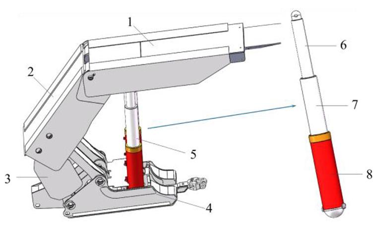
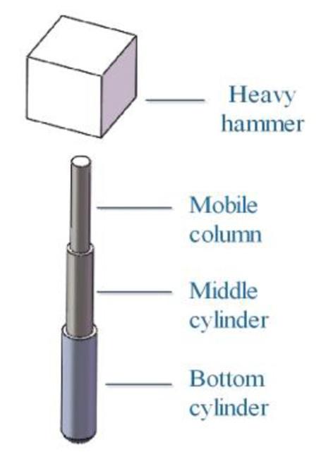
From Equations [5] to [7], A can be obtained as [8] Taking the ZY8640/2550/5500 shield hydraulic support prop as an example, the simplified model is shown in Figure 5. Some parameters of the prop are shown in Table I. The mass (M) of the hammer is 28 000 kg and the drop height (h) is 400 mm.
Figure 3—The model spring body rigidity of the hydraulic cylinder Figure 4—Relationship between the equivalent stiffness of cylinders Figure 5—Simplified model of the double telescopic prop
Modelling and analysis of a hydraulic support prop under impact load and the cylinder are regarded as a liquid-equivalent spring and solid-equivalent spring respectively. The equivalent stiffness of the hydraulic cylinder is equivalent to their series connection (Liu, Zhao, Zhao, 2012). The equivalent stiffness relationship of the whole prop is shown in Figure 4. According to the definition of bulk elastic modulus, the liquid equivalent stiffness of the ith stage cylinder (i =1, 2); i =1 is the bottom cylinder and i =2 is the middle cylinder) stage cylinder is obtained as [1] where Ai is the area of the inner circle of the ith stage cylinder (m²), di is the inner diameter of ith stage cylinder (m), hi is the height of liquid column in ith stage cylinder (m), Kl is the bulk modulus of 5% emulsion, and Kl = 1.8182 x 10⁹ Pa. From the relationship between bulk modulus and elastic modulus, the equivalent stiffness of the solid of the ith stage cylinder is expressed as [2] where, Kg is the bulk modulus (Pa), E is the elastic modulus of 27SiMn Steel (E = 2.06 x 10⁵ MPa), is Poisson's ratio of 27SiMn Steel (m = According0.3).to Equations [1] and [2], the equivalent stiffness of the ith stage cylinder is expressed as [3] From Equation [3], the equivalent stiffness of the hydraulic cylinder is negatively correlated with the height of the liquid column in the cylinder. Finally, according to the series connection between the bottom cylinder and the middle cylinder, the equivalent stiffness of the whole prop is expressed as [4] Liquid pressure in the hydraulic cylinder of a double telescop ic prop
399The Journal of the Southern African Institute of Mining and Metallurgy VOLUME 122 JULY 2022
According to the energy method, the dynamic load coefficient is expressed as [5] where h is the drop height of the hammer (m), g is the acceleration due to gravity (m/s2), and M is the weight of the hammer (kg). Since the prop is regarded as an integral elastic element, the relevant formula of linear elastic body can be obtained (Equations [6] and [7]). [6][7]
where F is the impact force (N), A is the displacement caused by the impact of the hammer (m), and Ast is the displacement caused by the gravitational mass of the hammer acting on the prop.
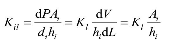
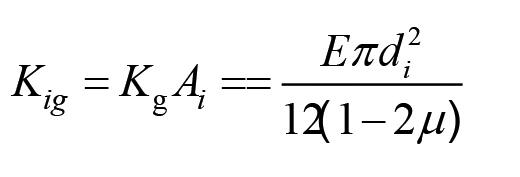
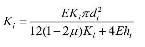
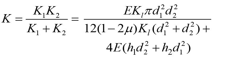
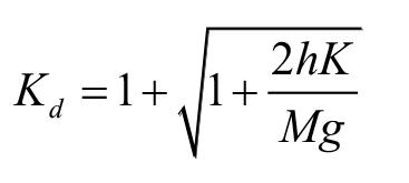
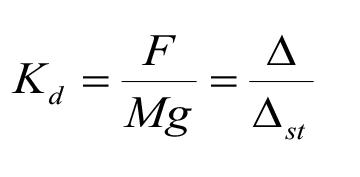
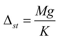
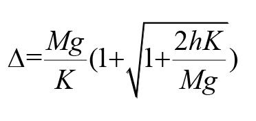
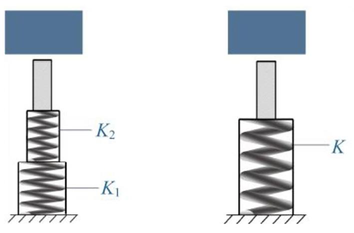
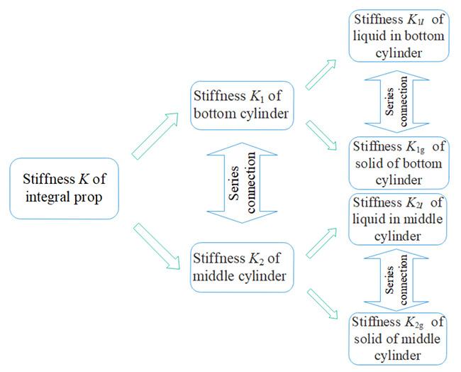
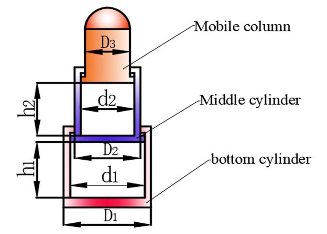
The AMESim model of the drop hammer is shown in Figure 8. In this model, the clearance in the damper LSTP00A is used to limit the drop distance of the mass block, and the appropriate contact damping parameters of the damper are set to reduce the rebound between the mass block and the prop. The relevant parameters of the drop hammer model are shown in Table IV. In addition, hydraulic pumps and motors are used from the hydraulic reservoir. The parameter of the hydraulic pump is 4000 cm3 per revolution, and that of the motor is 1000 r/min.
From the conservation of energy, the related equations can be obtained as [10] where ymax is the maximum displacement of the fluid’s main vibration in the cylinder (m), and P max is the maximum pressure in the cylinder (Pa). From Equation [10], ymax can be expressed as [11]
Figure 6—The AMESim model of the doubly-telescopic prop
Other simulation elements and their related parameters are shown in Table III.
Finally, the above three models are connected, and the whole AMESim model is shown in Figure 9.
Institute of
400 JULY 2022 VOLUME 122 The Journal of the Southern
AMESim simulation results
The AMESim simulation results are shown in Figures 10 and 11. The prop is in the extended phase before 0.13 seconds, and the hammer begins to contact the prop at 0.28 seconds. After the impact, the fluid pressure in the hydraulic cylinder of the prop continues to rise. The maximum fluid pressure in the bottom cylinder reaches 84.32 MPa at 0.32 seconds (see Figure 11), and that in the middle cylinder reaches 166.94 MPa at 0.37 seconds (see Figure 10). Compared with the calculation results in Equation [12] (the maximum hydraulic pressure in the middle cylinder is 172.97 MPa and that in the bottom cylinder is 92.13 MPa), the error estimation of the results for the middle cylinder is 3.61% and that for the bottom cylinder is about 8.48%. Therefore, the formula for the fluid pressure in the middle cylinder and bottom cylinder of the prop is basically correct. The hydraulic pressure peaks 5 ms later in the middle cylinder than in the bottom cylinder. In addition, the pressure in the middle cylinder
The relevant parameters in Table I are substituted into the above formula. After calculation, the maximum liquid pressure of the middle cylinder is 172.97 MPa, and that of the bottom cylinder is 92.13 MPa.
Some parameters of the ZY8640/2550/5500 hydraulic support prop Double telescop-ic prop Internal diameter di (mm) External diameter Di (mm) Length of liquid column hi (mm) Quality Mi (kg) Bottom cylinder (i=1) 400 470 1440 / Middle cylinder (i=2) 290 380 1485 876 Mobile column (i=3) / 260 / 1123
According to the boundary condition (y = ymax sin ωt), the fluid pressure in different hydraulic cylinders can be obtained as [12] where Pi is the fluid pressure in ith stage cylinder (Pa), ω is the main vibration angular frequency of the fluid (ω = √K/[M+M2+M3+(1/3)m2] Hz), and m2 is the quality of emulsion in the middle cylinder (kg). when sinωt is taken as unity in Equation [12], and the pressure in the hydraulic cylinder is at maximum.
The working pressure of the ZY8640/2550/5500 shield hydraulic support’s prop is 42.4 MPa. When the hydraulic pressure in the prop is P1 (working pressure), the axial downward displacement of the mobile column is y1 and the calculation is expressed as [9]
Simulation and results Establishment of AMESim model
The simulation parameters for the ZY8640/2550/5500 hydraulic support prop are set according to the actual structure of the prop. The AMESim model of the prop is shown in Figure 6. In this model, BAP12 and BAP11 form a fixed bottom cylinder, BRP18 and BRP17 form a middle cylinder, and mass block MAS30 simulates the static load generated by the roof and the weight of the canopy. Other simulation elements and their parameters are shown in TableTheII.model of the safety valve as built in the AMESiM design library of hydraulic components is shown in Figure 7. In this model, the left chamber of the spool was simulated with BAP12 piston with definite volume and BAP0RT with variable volume.
and Metallurgy
Table I
Modelling and analysis of a hydraulic support prop under impact load African Mining
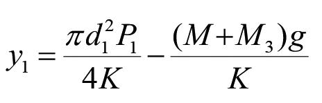
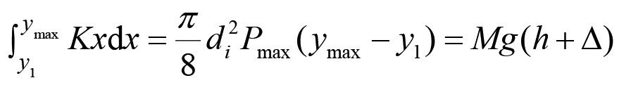
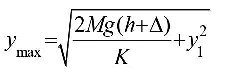
401
Establishment of doubly-telescopic prop model in Workbench In order to obtain the maximum stress change of the hydraulic cylinder in the prop, it is necessary to perform a finite element analysis.Before the finite element simulation analysis, it is necessary to simplify the geometric structure of the doubly-telescopic prop. Generally, the strength of the weld is higher than that of the cylinder, so the weld is ignored and the prop is built as a whole model. In order to make mesh division and computer calculation effective, the sealing ring and other devices are omitted. The simplified prop model includes the bottom cylinder, the middle
BAP12 Rod diameter (mm) 0 Left chamber of spoolChamber length at zero dis-placement (mm) 2 BAP0RT Rod diameter (mm) 0 BAP016 Rod diameter (mm) 2 Right chamber of spool with springChamber length at zero dis-placement (mm) 3 Spring stiffness (N/mm) 350 Spring force at zero dis-placement (N) 2 010
BHC11-1 Dead volume(cm3) 108 000 Volume of middle cylinder BHC11-2 Dead volume(cm3) 200 000 Volume of bottom cylinder
Figure 7—The AMESim model of the safety valve Table III Main parameters of the model of the safety valve Symbol Parameter Numerical value Physical elements
BAP11 Piston diameter (mm) 400 Bottom cylinder and pistonRod diameter (mm) 380 BAP12 Piston diameter (mm) 400 Rod diameter (mm) 0 BRP17 Piston diameter (mm) 290 Middle cylinder and pistonRod diameter (mm) 260 BRP18 Piston diameter (mm) 290 Rod diameter (mm) 0 MAS30 Mass M1(Kg) 5 250 Mass of canopy Mass M2(Kg) 62 450 Equivalent mass of roof
Modelling and analysis of a hydraulic support prop under impact load The Journal of the Southern African Institute of Mining and Metallurgy 122 JULY 2022 is significantly higher than that in the bottom cylinder. The main reason for this is that the diameter of the middle cylinder is smaller than that of the bottom cylinder. At drop heights of 400 mm and 500 mm, the fluid pressure in the bottom cylinder is shown in Figure 12. The maximum pressure increases slightly at a drop height of 500 mm.
VOLUME
Table II Main parameters of the model of the doubly-telescopic prop Symbol Parameter Numerical value Physical elements
MAS010RT Lower displacement limit (mm) 0 PoleHigher displacement limit (mm) 7
BAO001 Number of slots 10 Spool with orifice BHC11-3 Dead volume(cm3) 10 Chamber of spoolBHC11-4 Dead volume(cm3) 80
Figure 10—Fluid pressure in the middle cylinder 0.0 0.1 0.2 0.3 0.4 0.5 Time (s)
402 JULY 2022 VOLUME 122 The
Modelling and analysis of a hydraulic support prop under impact load Journal of the Southern African Institute of Mining and Metallurgy cylinder, and the mobile column (Yang et al., 2020). This simplification affects only the analysis of local stress, and has little effect on the load distribution analysis of the whole structure. The simplified geometric model of the prop after meshing is shown in Figure 13. Results of finite element simulation The cylinder block of the prop is made of 27SiMn high-strength steel, and its main properties are shown in Table V. Then, the material is added to the Workbench’s material library. Transient dynamics simulation of the prop model is carried out in Workbench. The bottom surface of the bottom cylinder is fixed and constrained. The surface load of Equation [12] is applied to the inner surface of the middle cylinder and bottom cylinder, which realizes the pressure setting in the hydraulic cylinder of the prop. The solution time is set to 30 ms.
Figure 12—Fluid pressure in the bottom cylinder at different heights 0.20 0.25 0.30 0.35 0.40 0.45 0.50 Time (s)
Through the simulation solution, the stress and strain cloud diagrams of the prop under the impact load of the hammer are obtained, as shown in Figures 14 and 15. After the impact on the mobile column of the prop, the pressure in the middle cylinder increases rapidly and acts on the bottom cylinder. It can be seen from Figures 14 and 15 that the overall stress on the middle cylinder is relatively large, and the maximum stress and maximum strain are located in the middle cylinder near the bottom cylinder. The maximum stress is 621.17 MPa, and both hydraulic cylinders are in a safe state. Figure 16 shows the maximum stress change on the prop during impact. The stress of the prop increases sharply and fluctuates rapidly, and is in a steady state with slight fluctuations after 13 ms.
Figure 8—AMESim model of the drop hammer
Table IV Main parameters of the drop hammer model Symbol Parameter Numerical Physical value elements LSTP00A Contact 100 000 Contact stiffness(N/mm) damping Gap or clearance with both 450 Height displacement zero (mm) of drop MAS002 Mass(kg) 28 000 Hammer Inclination 90
Figure 11—Fluid pressure in the bottom cylinder 0.0 0.1 0.2 0.3 0.4 0.5 Time (s)
Figure 9—AMESim simulatiuon model of the hydraulic system of the impacting drop
0.00.51.01.52.0Pa)(10Pressure8
-0.20.00.20.40.60.81.0Pa)(10Pressure8
-0.20.00.20.40.60.81.01.2Pa)(10Pressure8
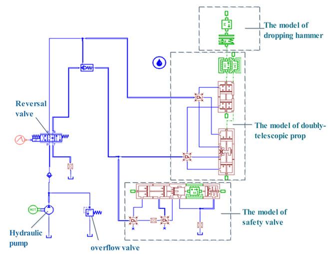
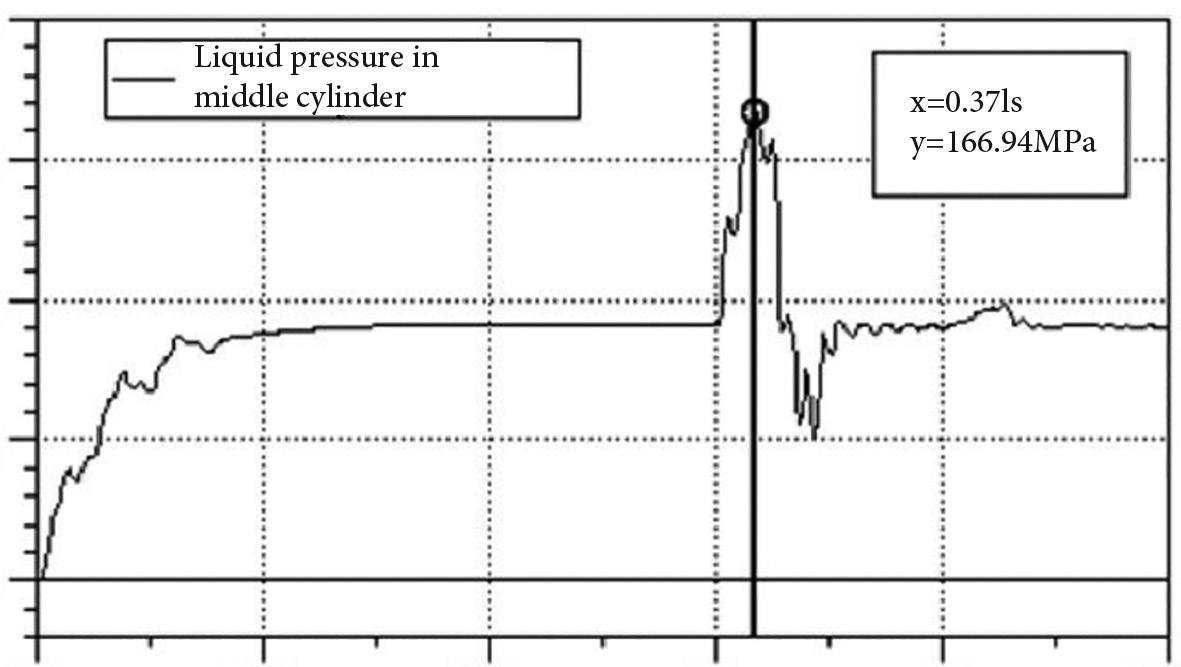
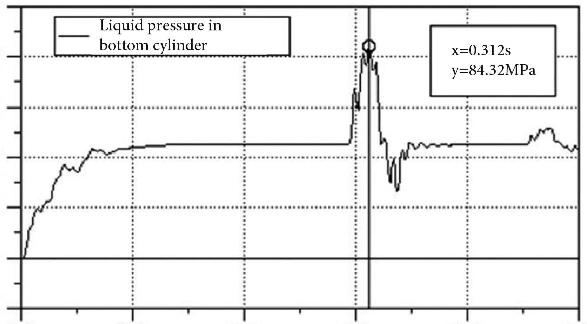
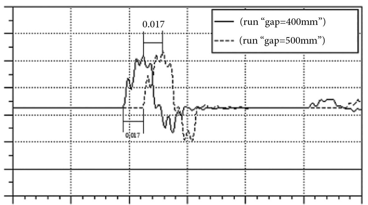
Figure 14—Stress cloud diagram of the prop Table V Main properties of 27SiMn steel Modulus of elasticity E (MPa) 2.06 × 10⁵ Density r (kg ·m–3) 7850 Poisson’s ratio m 0.3 Yield strength ss (MPa) 835 Tensile strength sb (MPa) 980
Conclusion and discussion In this paper, the hydraulic support prop under impact load is theoretically calculated and simulated. By modelling the hydraulic Figure 13—Simplified geometric model of the prop after meshing
Modelling and analysis of a hydraulic support prop under impact load 403The Journal of the Southern African Institute of Mining and Metallurgy VOLUME 122 JULY 2022
In actual working conditions, the impact load usually acts directly on the canopy of the hydraulic support, and the position of the applied load point has different effects on the prop. Taking the width of the canopy as the x-axis direction and the length direction as the y-axis direction, F(x,y) represents the position of impact load. The position of the load on the canopy is shown in Figure 17. As the impact load moves towards the front of the canopy (y-axis), the maximum stress of the middle cylinder first decreases and then increases, and when the impact load acts on both sides of the top beam (x-axis), the stress on the middle cylinder increases slightly (see Figure 18). The change in maximum stress on the bottom cylinder in the y-axis direction is the same as that of the middle cylinder. There is no change in the x-axis direction with the movement of the impact load point (Figure 19).
Figure 15—Strain cloud diagram of the prop Figure 16—Maximum stress change of the prop during impact
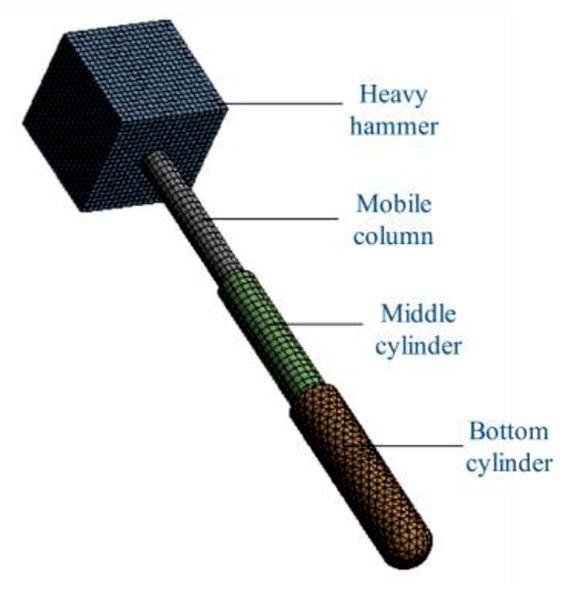
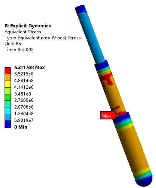
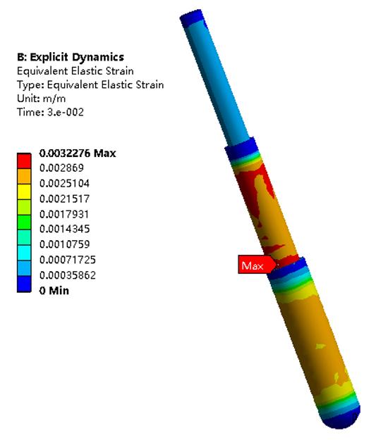
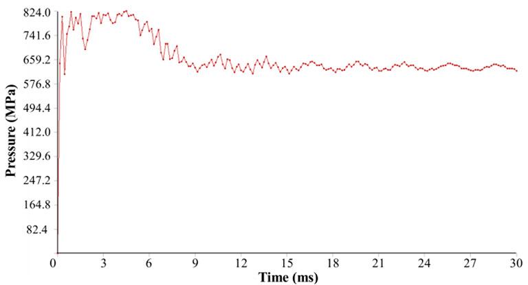
Acknowledgments
404 JULY 2022 VOLUME 122 The Journal of the Southern
Reference Ardehjani, E.A., ATaei, M., and Rafiee, R . 2020. Estimation of first and periodic roof weighting effect interval in mechanized longwall mining using numerical modeling. International Journal of Geomechanics, vol. 20, no. 2. http://dx.doi. org/10.1061/(ASCE)GM. 1943-5622.0001532 BouTrid, A., Djouamaa, M.C., CheTTibi, M., Bouhedja, A., and Talhi, K. 2016. Design of a model powered support system in Kenadsa mine (Algeria). Journal of Mining Science, vol. 52, no. 1. pp. 78–86. http://dx.doi.org/10.1134/ S1062739116010150 Cao, L.M., Sun, S.J., Zhang, Y.Z., Guo, H., and Zhang, Z. 2018. The research on characteristics of hydraulic support advancing control system in coal mining face. Wireless Personal Communications, vol. 102, no. 4. pp. 2667–2680. http:// Chinesedx.doi.org/10.1007/s11277-018-5294-4CoalIndusTrySTandardGB25974.
Modelling and analysis of a hydraulic support prop under impact load African Mining
This work is supported by Open Fund of State Key Laboratory of Coal Resources and Safe Mining (Grant No. SKLCRSM21KFA12).
➤ Under impact loading, the fluid pressure in the hydraulic cylinder of the prop increases and decreases rapidly, and the results show that the emulsion pressure in the middle cylinder is significantly higher than that in the bottom cylinder. The AMESim prop model provides reference and guidance for the construction of a testbed for dynamic load testing of double-telescopic props.
Figure 18—Maximum stress change on the middle cylinder under different force loading points
This paper adopts a simplified simulation method. The impact problem involves the solid-liquid coupling problem, but it is not simply involve mixing the solid and liquid together for impact analysis, but is also mainly related to the characteristics of a large-flow safety valve. The next step is the integrated analysis of solid-liquid coupling and large-flow safety valve in a joint simulation, so that the results are more accurate. In addition, there is still a certain gap between the impact results by computer simulation and those from a prop test-bed. In the future, it will be necessary to design the prop test-bed to accommodate the impact on double-telescopic props in different ways.
➤ Through the Workbench simulation analysis, it was found that the force on the middle cylinder of the prop under impact load is far greater than that on the bottom cylinder. The maximum stress point of the middle cylinder is located near the bottom cylinder. Therefore, in the structural design of doubly-telescopic props, more consideration should be given to the material properties of the middle cylinder, and the wall thickness of the middle cylinder should be increased if necessary. When the impact load is applied to different positions on the canopy, the maximum stress on the middle and bottom cylinders first decreases and then increases in the y-axis direction, and shows no obvious change in the x-axis direction. Installation of hydraulic supports so as to avoid impact on the front end of the canopy is therefore of great significance to prevent the prop from being damaged due to insufficient strength.
Figure 19—Maximum stress change on the bottom cylinder under different force loading point Figure 17—Application position of impact laod in the canopy
➤ According to the theory of solid-liquid coupling and spring series connection, the relationship between the stiffness of each component of the prop is discussed. The equivalent stiffness of the hydraulic cylinder is found to be negatively related to the height of the fluid column in the cylinder, and the equivalent stiffness theory of the doubly-telescopic prop is established. The maximum pressure of emulsion in hydraulic cylinder under impact is obtained by energy conservation. It provides an effective calculation method to estimate the pressure in the hydraulic cylinder of the prop under impact load.
2-2010. Hydraulic support for coal mines – Part 2: Technical conditions of prop and jack. 2010. gov.cn/gb/search/gbDetailed?id=71F772D7DC66D3A7E05397BE0A0AB82Ahttps://std.samr.
circuit of the impacted prop in AMESim, the curve of the fluid pressure in the hydraulic cylinder of the prop is obtained. Finite element simulation analysis of the hydraulic support prop in ANSYS Workbench software is used to obtain the stress and strain cloud diagrams of the prop.
Institute of
and Metallurgy
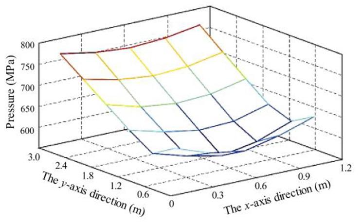
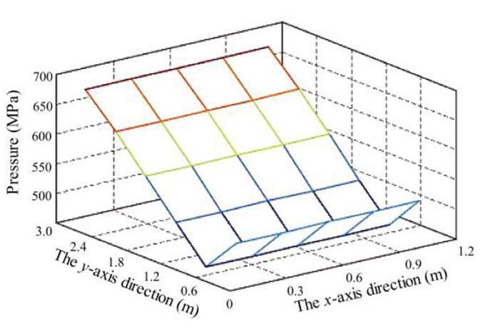
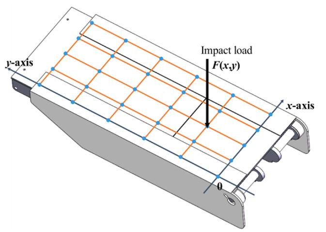
Singh, G.S.P. and Singh, U.K. 2010. Prediction of caving behavior of strata and optimum rating of hydraulic powered support for longwall workings.
Szurgacz, D. and Brodny, J. 2018. Analysis of load of a powered roof support’s hydraulic leg. Proceedings of the 18th Conference of PhD Students and Young Scientists - Interdisciplinary Topics in Mining and Geology, Szklarska Poreba. Szurgacz,http://dx.doi.org/10.1051/e3sconf/20187100002D.andBrodny,J.2019.Analysisoftheinfluence of dynamic load on the work parameters of a powered roof support’s hydraulic leg. Sustainability, vol. 11, no. 9. http://dx.doi.org/10.3390/su11092570
Plonka, M. 2019. Shield support monitoring system-operation during the support setting. Acta Montanistica Slovaca, vol. 24, no. 4. pp. 391–401. Klishin, V.I. and Tarasik, T.M. 2001. Stand tests of hydraulic props in dynamic loads. Journal of Mining Science, vol. 37, no. 1. pp. 77–84. http://dx.doi. Liang,org/10.1023/A:1016788903660L.C.,Tian,J.J.,Zheng,H.,and Jiao, S.J. 2015. A study on force transmission in a hydraulic support under impact loading on its canopy beam. Journal of the China Coal Society, vol. 40, no. 11. pp. 2522–2527. http://dx.doi.org/10.13225/j. cnki.jccs.2015.7021 Liu, X.K., Zhao, Z.H., and Zhao, R . 2012. Study on dynamic features of leg applied to hydraulic powered support under bumping load. Coal Science and Technology, vol. 40, no. 12. pp. 66–70. http://dx.doi.org/10 Meng, Z.S., Zhang, S., Xie, Y.Y., and Zeng, Q.L. 2020. Attitude adjustment of backfilling support based on mechanical-hydraulic co-simulation. International Journal of Simulation Modelling, vol. 19, no. 3. pp. 399–409. http://dx.doi. Prusek,org/10.2507/IJSIMM19-3-520S.,Płonka,M.,andWalenTek, A . 2016. Applying the ground reaction curve concept to the assessment of shield support performance in longwall faces. Arabian Journal of Geosciences, vol. 9, no. 3. http://dx.doi.org/10.1007/ s12517-015-2171-2 PyTlik, A . 2015. Process characteristics of hydraulic legs equipped with safety valves at dynamic load caused by mining tremor. Archives of Mining Sciences, vol. 60, no. 2. pp. 595–612. http://dx.doi.org/10.1515/amsc-2015-0039 Singh, G.S.P. and Singh, U.K. 2009. A numerical modeling approach for assessment of progressive caving of strata and performance of hydraulic powered support in longwall workings. Computers and Geotechnics, vol. 36, no. 7. pp. 1142–1156. http://dx.doi.org/10.1016/j.compgeo.2009.05.001
Zhao, X.H., Li, F.Y., Liu, Y., and Fan, Y.J. 2015. Fatigue behavior of a box-type welded structure of hydraulic support used in coal mine. Materials, vol. 8, no. 10. pp. 6609–6622. http://dx.doi.org/10.3390/ma8105325 u
International Journal of Rock Mechanics and Mining Sciences, vol. 47, no. 1. pp. 1–16. http://dx.doi.org/10.1016/j.ijrmms.2009.09.001
Modelling and analysis of a hydraulic support prop under impact load 405The Journal of the Southern African Institute of Mining and Metallurgy VOLUME 122 JULY 2022 Chinese Coal IndusTry STandard MT 313-1992, The technical condition of hydraulic support prop, 1992. Jasiulek,EuropeanstdHBDetailed?id=8B1827F16592BB19E05397BE0A0AB44Ahttps://std.samr.gov.cn/hb/search/sTandardEN1804-2-2001.Machinesforundergroundmines–Safetyrequirementsforhydraulicpoweredroofsupports–Part2:Powersetlegsandrams,2001.https://standards.cencenelec.eu/dyn/www/f?p=CEN:110:0::::FSP_PROJECT,FSP_ORG_ID:66119,6177&cs=1326821640B81E203D87F944FE8BD46E6D.,BarToszek,S.,PeruTka,K.,Korshunov,A.,Jagoda,J.,and
Trueman, R., Lyman, G., and Cocker, A . 2009. Longwall roof control through a fundamental understanding of shield-strata interaction. International Journal of Rock Mechanics and Mining Sciences, vol. 46, no. 2. pp. 371–380. http://dx.doi. Verma,org/10.1016/j.ijrmms.2008.07.003A.K.andDeb,D.2013.Numerical analysis of an interaction between hydraulic-powered support and surrounding rock strata. International Journal of Geomechanics, vol. 13, no. 2. pp. 181–192. http://dx.doi.org/10.1061/(ASCE) Wang,GM.1943-5622.0000190J.,Ning,J.,Jiang,L., Jiang, J.Q., and Bu, T. 2018. Structural characteristics of strata overlying of a fully mechanized longwall face: a case study. Journal of the Southern African Institute of Mining and Metallurgy, vol. 118, no. 11. pp. 1195–1204. http://dx.doi.org/10.17159/2411-9717/2018/v118n11a10 Wang, X.W., Yang, Z.J., Feng, J.L., and Liu, H.J. 2013. Stress analysis and stability analysis on doubly-telescopic prop of hydraulic support. Engineering Failure Analysis, vol. 32. pp. 274–282. http://dx.doi.org/10.1016/j.engfailanal.2013.04.006
WiTek, M. and Prusek, S. 2016. Numerical calculations of shield support stress based on laboratory test results. Computers and Geotechnics, vol. 72. pp. 74–88. http://dx.doi.org/ 10.1016/j.compgeo.2015.11.007 Yang, Z.K., Sun, Z.Y., Jiang, S.B., Mao, Q.H., Liu, P., and Xu, C.Z. 2020. Structural analysis on impact-mechanical properties of ultra-high hydraulic support. International Journal of Simulation Modelling, vol. 19, no. 1. pp. 17–28. http:// Zeng,dx.doi.org/10.2507/IJSIMM19-1-498Q.L.,Meng,Z.S.,Wan,L.R.,andWang, C.L. 2018. Analysis on force transmission characteristics of two-legged shield support under impact loading. Shock and Vibration, vol. 2018. http://dx.doi.org/10.1155/2018/3854684
• Circular economy concepts, closing the water loop ECSA AFRICAN OF MINING METALLURGY
• Waste to resource: remediation, resource
AND
• closure
Mine
practices
• Novel and emerging strategies sustainable management of mine-impacted water
IMPACTING THE CIRCULAR ECONOMY 12-13 OCTOBER 2022 CONFERENCE CLOSING THE WATER LOOP Mintek,
to the following
for
INSTITUTE
& Online via Zoom
and
studies
• Prediction mitigation Case
KEYNOTE SPEAKERS: Associate Professor: Gavin Mudd, RMIT University Professor: Mansour Edraki, The University of Queensland Professor: Craig Sheridan, University of the Witwatersarnd Panagiotix Xanthopoulos, KU Leuven
Presentations related, but not limited mine-impacted water related
Modelling and analysis of a hydraulic support prop under impact load 406 JULY 2022 VOLUME 122 The Journal of the Southern African Institute of Mining and Metallurgy FOR FURTHER INFORMATION, CONTACT: Camielah Jardine E-mail: camielah@saimm.co.za Head of Conferencing Tel: +27 11 538-0238 SAIMM Web: www.saimm.co.za KEY BENEFITS OF ATTENDING THE CONFERENCE • High quality presentations • Networking and knowledge transfer • Local and international participation • Comprehensive insight from stakeholders such as academia, industry and the government • Hybrid conference; attend from the comfort of your location ABOUT THE CONFERENCE
recovery
The Southern African Institute of Mining and Metallurgy (SAIMM), in collaboration with the University of the Witwatersrand through the DSI/NRF SARChI chair in Hydrometallurgy and Sustainable Development, and Mintek, will be hosting a hybrid conference on mineimpacted water including acid mine drainage (AMD) in October 2022. With a theme of “impacting the circular economy, closing the water loop”, the conference will run over a period of two days. This second SAIMM AMD themed conference will provide an excellent opportunity for industry, researchers and other global stakeholders to share their knowledge, new processes and technologies that can be used to advance the implementation of sustainable solutions to the challenges associated with mine-impacted water. The conference, with its extensive program, will also offer notable keynote speakers and, the popular student session, all with the purpose of giving a unique view into novel solutions and industry progression on the issue of mine-impacted water.
FOUNDED 1894
BESACNASPANDCPDPOINTSWILLALLOCATEDPERHOURATTENDED HYBRID CONFERENCE THE SOUTHERN
MINE-IMPACTED WATER Randburg, South Africa
topics are invited:
treatment technologies
• Legislation and policy drivers for sustainability
reuse and
• Sustainable and innovative mine-impacted water
CONFERENCE TOPICS


Economic analysis of rare earth element processing methods for Mountain Pass ore by T. Uysal1
The estimated global total REO production is 210,000 metric tons (USGS, 2020). China imposed export restrictions on REE between 2010 and 2014, resulting in dramatic increases in REE prices in those years. These high prices accelerated exploration for new deposit on a global scale and increased the number of active REE facilities (Laurent, 2014). Bayan Obo (China) and Mountain Pass (USA) are the world’s largest REE deposits. The Mountain Pass (California, USA) deposit, the second largest REE deposit in the world, is operated by MP Materials. In this deposit, the main REE minerals are bastnasite and monazite, and gangue minerals are barite, calcite, silicate, apatite, and dolomite (Abaka-Wood, Addai-Mensah, and Skinner, 2016; Yang et al., 2015).
407The Journal of the Southern African Institute of Mining and Metallurgy VOLUME 122 JULY 2022
economicKeywordsanalysis, rare earth elements, flotation, attrition scrubbing.
REE ores are beneficiated by physical and/or chemical (leaching) methods. Physical REE beneficiation methods are gravity, magnetic, electrostatic, and flotation, or combinations of these methods (Jordens, Cheng, and Waters, 2013; Zhang and Edwards, 2012). Gravity beneficiation is widely used for the Affiliation: 1Rare Earth Elements Application and Research Center, Munzur University, Tunceli, Türkiye Correspondence to: T. Uysal Email: turan.uysal@inonu.edu.tr
DOI 6725https://orcid.org/0000-0003-1643-T.ORCID9717/1989/2022http://dx.doi.org/10.17159/2411-ID::Uysal
Dates: Received: 18 Jan. 2020 Revised: 1 Apr. 2022 Accepted: 3 Jun. 2022 Published: July 2022 How to cite: Uysal, T. Economic2022analysis of rare earth element processing methods for Mountain Pass ore. Journal of the Southern African Institute of Mining and Metallurgy, vol. 122, no. 7, pp. 407–412
Introduction
The rare earth elements lanthanide group includes 17 elements consisting of scandium and yttrium. Rare earth elements, with their light emission, magnetism, and electronic properties resulting from their unsaturated 4f electronic structure, are used in the production of permanent magnets, the production of rare earth phosphors, in hydrogen storage materials and in the production of catalysts. In addition, owing to their different chemical, metallurgical, optical, electrical, and catalytic properties, the REE have different uses in high-technology industries such as, hybrid electric vehicles, rechargeable batteries, mobile phones, wind turbines, medical imaging devices, radar systems, catalytic converters, metal alloys, aircraft engines, ceramics, and defense (Adibi et al., 2014; Dushyanthaa et al., 2020; Suli et al., 2017). Although the REEs are included in more than 250 discrete minerals, 95% of commercial production from bastnasite [Ce, La, Nd](CO3)F, monazite [Ce, La, Nd](PO4 ), and xenotime (YPO4) ores. The most important REE producers are China and the USA. It is estimated that China produced 132 000 t rare earths oxides (REO) in 2019, while the USA produced 26 000 t (REO equivalent) of ores and compounds.
TheSynopsisincreasing demand for rare earth elements (REE) in highly strategic sectors such as hybrid electric vehicles, renewable energy, communication technologies, and the defense industry has made REE production methods important. In recent years, studies on REE have increased rapidly; however there are many studies on REE, there are not enough studies in the literature on the economics of the beneficiation process. RE ores are generally leached after beneficiation by gravity, magnetic and flotation methods. In this study, direct leaching, attrition scrubbing and leaching, and flotation and leaching methods are evaluated economically based on the data for the Mountain Pass (MP) facility. According to the sensitivity analysis performed as a function of capital cost (CAPEX), operating cost (OPEX), and rare earths oxides (REO) recovery, REO recovery has the biggest effect on the process economies. Although the flotation method entails additional investment and operating costs, transportation and operating costs are significantly reduced result of the higher grade and recovery. The flotation method is more profitable, with larger NPV and IRR values and a shorter payback period.
Economic analysis of rare earth element processing methods for Mountain Pass ore
408 JULY 2022 VOLUME 122
The Journal of the Southern African Institute of Mining and Metallurgy separation of REE minerals with relatively high densities (4-7 g/cm3) and gangue minerals with low specific gravity such as quartz, calcite and fluorite (Ferron, Bulatovic and Salter, 1991). In the attrition scrubbing method, the different resistance of the minerals to abrasion leads to a significant upgrading in the coarse or fine sizes. Pre-concentrate or concentrate is obtained by size classification of the attrition scrubbing product. Flotation vital in the beneficiation of low-grade and complex ores, which were previously uneconomic to mine and process (Wills, 2006). As the particle size decreases, beneficiation by gravity methods becomes more difficult and mineral losses increase. For this reason, flotation is used to beneficiated the minerals that are liberated between 100 μm and 15 μm. For selective flotation, the surfaces of REE minerals are rendered hydrophobic, while the gangue minerals are coated with depressants to increase surface hydrophilicity (Jordens, Cheng, and Waters, 2013). Beneficiation methods and feed and concentrate grades of active facilities producing REE are given in Table I. MP ore is beneficiated by flotation and leaching method, and the flow sheet of the facility is depicted in Figure 1. In the chemical beneficiation methods, raw ore and/or concentrate is leached with acidic or alkaline solutions. The pregnant leach solution is generally purified by solvent extraction (SX) and precipitation methods, and REO are obtained by calcining the purified product (Demol et al., 2019; Qi, 2018; Wang et al., Direct2017).leaching of the ore avoids beneficiation methods such as gravity and flotation will be eliminated, thus reducing the cost. However, direct leaching of raw ore will increase reagent, and transportation costs, and valuable mineral losses, while reducing the efficiency of chemical beneficiation. In this case, preconcentration by physical beneficiation becomes necessary both technically and economically. The main purpose of this study is to assess the economic importance of beneficiation and the selection of the economic beneficiation method. Direct leaching, attrition scrubbing, leaching, and flotation and leaching were investigated economically. Attrition scrubbing method is given as an example because it is generally used in the pre-beneficiation of minerals with different abrasion resistances. The profitability of these beneficiation methods was evaluated together with the economic analysis. Materials and methods
According to Table I Beneficiation methods and grade data of active facilities producing REE (Abaka-Wood, Addai-Mensah and
Crushing, grinding, classification, and attrition scrubbing methods are used to obtain pre-concentrate from the raw ore. Crushing, grinding, classification and flotation are used to obtain concentrate from raw ore. The data is based on data from the MP facility and published (preliminary) feasibility studies. In the absence of data on individual items, reasonable assumptions have been made using information from similar studies in the literature.According to the report published by MP Materials, (2020a), MP raw ore with 8.7% REO content is upgraded to an average REO grade of 60% by flotation. Since attrition scrubbing is not applied to the MP ore, an assumption was made based on attrition scrubbing of carbonatite ore similar to this deposit. Skinner,
2016; Huleat, 2019; Krishnamurthy and Gupta, 2015; Verban 2015) Mine Beneficiation method Feed, %REO Concentrate, %REO Lynas (Australia) Flotation 15 40 Mountain Pass (USA) Flotation 6-12 60 Bayan Obo (China) Magnetic-flotation 6 >60 Sichuan Mianning (China) Gravity- magnetic-flotation 3 6 60 Shandong Weishan (China) Magnetic-flotation 3 60 Lovozersky (Russia) Flotation 1 38 Steenkampskaal (South Africa) Magnetic -dense media separation 14.4 30 Toyotsu Rare Earths (India) Magnetic 0.35 Browns Range (Australia) Magnetic-flotation 0.66 20 Port Hope Simpson (Canada) Non-whole ore leach 1.07 NA Serra Verde (Brazil) Non-whole ore leach (desorption of ionic clays) 0.16 NA Zandskopdrift (South Africa) Non-whole ore leach (desorption of ionic clays) 1.9 NA Figure 1 REO production flow sheet for Mountain Pass ore (MP Materials, 2020a)
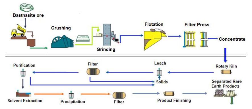
The data from Norgren ( 2018) wase used for income analysis. Current sales prices, percentage distribution ratios and sales percentages of REOs produced from MP ore are shown in Table V. Income was calculated based on these figures and prices. Economic analysis Different static and dynamic capital budgeting methods and a combination of these methods are applied to compare the profitability of projects. The first method is the payback period, a static method. This is a simple method often used for initial estimation, but does not provide an adequate basis for deciding between different investment projects. The second method is net present value (NPV) and internal rate of return (IRR), the most common dynamic capital budgeting method, for more detailed analysis. The NPV method is used to decide which project will be most profitable from an investor's point of view, as the IRR method alone is not always suitable for making the right investment decisions (Jaroni, Friedrich, and Letmathe, 2019). In this study, NPV, IRR, and payback period values were calculated and evaluated Sensitivitytogether.analysis is a risk analysis technique that measures the extent to which NPV changes as a result of changes in the key variables that can affect the NPV of the project. In this context, Figure 2—Attrition scrubbing
409The Journal of the
In the cost analysis, CAPEX and OPEX were determined separately. CAPEX inputs mainly include machinery and equipment, installation, piping, instrumentation, engineering, construction, and contingency costs. For CAPEX, data from Williams (2018) was used. The investment cost for the chemical plant is taken as 60% of that of the physical beneficiation plant. OPEX inputs are mainly reagents, energy, transportation and labour costs. These costs are given on the basis of the current reports and are included in the facility costs. The operating costs per ton TREO for the Mountain Pass operation are given in Table III, and the key performance indicators in Table IV. As seen in Table IV, the operating cost per ton REO in 2020 was $1 430. Operating cost per ton in the REO metric excludes costs attributable to selling obsolete stocks, shipping, freight, and depreciation. It has been added to OPEX costs as a separate item since shipping cost is not included. In this study, the transportation cost of raw ore and concentrate was taken as $8 per ton, based on the average cost in the mining industry (Sterba et al., 2019).
Economic analysis of rare earth element processing methods for Mountain Pass ore Southern African Institute of Mining Metallurgy Noble et al. (2014) Bear Lodge REE ore was upgraded to 19.0620.51% TREO (total REO) with 60 90% recovery in the -500 mesh size. Similarly, Özbayoğlu and Atalay (1995) state that Eskişehir (Turkey) REE ore reached a grade of 23.5% REO as a result of beneficiation by attrition scrubbing. Based on these results, it is assumed that MP ore can be upgrade to 20% REO by attrition scrubbing. The flow sheets for attrition scrubbing and leaching and flotation and leaching for REO production are given in Figure 2. The production and beneficiation data for the years 2018-2020 are given in Table II. According to MP Materials (2020b), the overall flotation recovery was 72%, calculated by the formula given in Equation [1]. The attrition scrubbing recovery is assumed to be lower than flotation recovery and it was taken as being 62% after evaluating the literature data (Noble et al, 2014). The ore beneficiation and chemical beneficiation losses, which are not included in the literature or published reports, are also assumed to be approximate. Accordingly, the ore beneficiation losses are taken as 10%, the chemical beneficiation loss of the raw ore is 10%, and the chemical beneficiation loss of the concentrate is 5%. [1]
and
VOLUME 122 JULY 2022
Cost and revenue analysis
& leaching and flotation & leaching flow sheets Table II Summary of operating results 2018 2020 (MP Materials, 2020b) 2020 2019 2018 (6 months) Ore mined (t) 682 775 598 683 564 228 Mill feed (dry t) 331 556 542 668 342 891 Concentrate production (dry t) 34 535 56 892 29 453 Concentrate grade (REO%) 60 53 5 52 1 TREO production (t) 18 969 27 620 13 914 TREO recovery to concentrate (%) 65 8 58 9 51 1 Table III Operating costs per ton TREO of the Mountain Pass operation (SRK, 2010)Cost Cost Distribution ($000) ($/ton TREO) (%) Mining 144 452 44 906 8.455 Milling 427 079 133 000 25.040 Flotation 106 769 33 000 6.213 Chemical plant* 1 033 150 320 242 60.292 Operation costs 1 711 450 531 148 100.00 *Chemical plant includes the costs of leaching, solvent extraction, precipitation, combined heat and power (CHP) plant, chlor-alkali plant, and brine treatment Table IV Key performance indicators (MP Materials, 2020c, 2021) 2020 2019 2018 REO production (t) 38 503 27 620 13 914 REO sales (t) 38 367 26 821 13 378 Realized price per ton REO t ($) $3 311 $2 793 $3 382 Cost of production per ton REO t $1 430 $1 980 $2 822
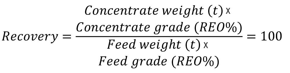
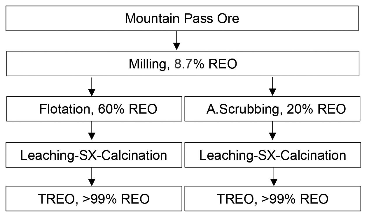
Product
Cerium
1 436
50 Lanthanum oxide (>99.5%) 1 374 33.0 100 Praseodymium oxide (>99%) 138 141 4.0 100 Neodymium oxide (>99.5%) 142 851 12.0 100 SEG* + others 1 436 1.0 100 *SEG: Samarium, europium, and gadolinium oxides Table VI Comparison of capital costs of different circuits (Williams, 2018) Machinery/equipment Attrition scrubbing and leaching Flotation and leaching Mining 958 648 958 648 Milling 7 016 966 7 016 966 Attrition scrubbing unit 86 720 Flotation 2 156 001 Chemical plant 13 759 450 13 759 450 Total cost 21 821 784 24 079 038 Table VII Total capital cost estimate using Mular’s Factored Capital Cost Estimate Guide (Mular, 2002) Cost Scrubbing and leaching Flotation and leaching Factor Explanation Equipment cost 21 821 784 24 079 038 Installed equipment cost 31 205 152 34 433 025 1 43 Multiplied by equipment cost Piping 6 241 030 68 86 605 0 2 Multiplied by total installed equipment cost Instrumentation 39 00 644 4 304 128 0 125 Multiplied by total installed equipment cost Total plant cost 63 168 610 69 702 796 Engineering and construction 22 109 014 24 395 979 0 35 Multiplied by total plant cost Contingency 6 316 861 6 970 280 0 1 Multiplied by total plant cost Total CAPEX 91 594 485 101 069 054
Results and discussion Cost and revenue analysis
Table V Current REO sales prices, percentage distribution, and sales rates (Metal,
sensitivity analysis is used to identify and estimate potential risk in project efficiency. It is used to estimate the effects of variables on NPV rather than finding the risk value. The greater the change in NPV, the greater the risk. Sensitivity analysis provides important information about which inputs have the greatest impact on the project. In this study, the changes in NPV as a function of CAPEX, OPEX, and REO recovery were investigated.
The 10-year pre-tax cash flow models the two circuits are shown in Table IX and Table X. No acceleration period is included in this analysis, although it is likely to exist in practice. NPV, IRR, and payback periods were calculated using the information in Tables IX and X. These values are shown in Table XI, assuming a discount rate of Table8%.XI shows that the NPV and IRR values of the flotation & leaching circuit are greater and the payback period is lower. The difference between the NPVs was found to be $1 565 498 542 and it is clearly seen that the flotation & leaching circuit is more profitable from these values. Economic analysis of the direct leaching circuit revealed that the NPV value is $365 019 511. This is not an economical method and physical beneficiation is 2021; Norgren, 2018) $/t % of REO product % of product sold oxide (>99.5%) 50.0
Institute of
410 JULY 2022 VOLUME 122 The Journal of the Southern
CAPEX and OPEX values for Attrition Scrubbing & Leaching and flotation & leaching circuits were determined. The investment costs for both circuits are compared in Table VI, and the estimated total investment cost using the Mular factor is given in Table VII. According to Table VII, capital costs are calculated as $91 594 485 for Attrition scrubbing & leaching and $101 069 054 for flotation & leaching. The operating cost is calculated by adapting the percentage cost rates of each input in the SRK (2010) report to the REO operating cost (1 430 $/per ton) in the MP (2020) report and is given in Table VIII. Since the operating cost of attrition scrubbing is unknown, it is assumed that it will be half of the flotation cost. The operating cost of the flotation and leaching circuit is $44 423 higher per ton raw ore than that of the attrition scrubbing and leaching circuit. The 10-year operating cost calculation, is based on the data in Table VIII.
and Metallurgy
Economic analysis of rare earth element processing methods for Mountain Pass ore African Mining
Economic analysis
Economic analysis of rare earth element processing methods for Mountain Pass ore 411The Journal of the Southern African Institute of Mining and Metallurgy VOLUME 122 JULY 2022 required for this ore. Sensitivity analyses as a function of CAPEX, OPEX, and REO recovery for both circuits are given in Figures 3 and 4. Figurs 3 and 4 show that for both circuits NPV is most sensitive to the total REO recovery. The most important parameters affecting the total REO recovery are the REO grade and recovery. In both beneficiation circuits, OPEX was severely affected, while CAPEX showed no significant effect. In addition, it was determined that NPV increased linearly as the REO recovered increased for both circuits, and decreased linearly as OPEX amount increased. In the attrition scrubbing and leaching circuit, the REO recovery amount is below -32%, while the NPV is negative. The NPV for the flotation and leaching circuit is positive at all rates of change. From this, it was determined that the attrition scrubbing and leaching circuit is more affected by the REO recovery and OPEX value. Table VIII Circuit operating costs of the MP plant per ton of REO Operational Items Attrition scrubbing and leaching, $/ton Flotation and leaching, $/ton Mining 120 900 120 900 Milling 358 073 358 073 Attrition scrubbing 44 423 Flotation 88 845 Chemical plant 862 180 862 181 Total 1 385 576 1 430 000 Table IX Cash flow for attrition scrubbing and leaching circuit Year 0 1 2 3 4 5 6 7 8 9 10 Mill feed, t/a 0 663 112 663 112 663 112 663 112 663 112 663 112 663 112 663 112 663 112 663 112 Preconcentrate production, t/a 0 178 841 178 841 178 841 178 841 178 841 178 841 178 841 178 841 178 841 178 841 REO recovered, t/a 0 32 131 32 131 32 131 32 1 31 32 131 32 131 32 131 32 131 32 131 32 131 CeO₂, t/a 0 16 096 16 096 16 096 16 096 16 096 16 096 16 096 16 096 16 096 16 096 La₂O₃, t/a 0 10 623 10 623 10 623 10 623 10 623 10 623 10 623 10 623 10 623 10 623 Pr₂O₃, t/a 0 1288 1 288 1 288 1 288 1 288 1 288 1 288 1 288 1 288 1 288 Nd₂O₃, t/a 0 3 863 3 863 3 863 3 863 3 863 3 863 3 863 3 863 3 863 3 863 Other, t/a 0 322 322 322 322 322 322 322 322 322 322 Gross revenue, t$ 0 756 323 756 323 756 323 756 323 756 323 756 323 756 323 756 323 756 323 756 323 Transport cost, t$ 0 1 431 1 431 1 431 1 431 1 431 1 431 1 431 1 431 1 431 1 431 Operat. costs, t$ 0 501 264 501 264 501 264 501 264 501 264 501 264 501 264 501 264 501 264 501 264 Capital costs, t$ 91 595 Net cash flow, t$ -91 595 253 629 253 629 253 629 253 629 253 629 253 629 253 629 253 629 253 629 253 629 Cumulative cash flow, t$ -91 595 162 034 415 663 669 292 922 920 117 6549 1430 178 168 3806 193 7435 219 1064 2444 692 Table X Cash flow for the flotation and leaching circuit Year 0 1 2 3 4 5 6 7 8 9 10 Mill feed, t/a 0 663 112 663 112 663 112 663 112 663 112 663 112 663 112 663 112 663 112 663 112 Preconcentrate production, t/a 0 69 070 69 0 70 69 070 69 070 69 070 69 070 69 070 69 070 69 070 69 070 REO recovered, t/a 0 39 370 39 370 39 370 39 370 39 370 39 370 39 370 39 370 39 370 39 370 CeO2, t/a 0 19 685 19 685 19 685 19 685 19 685 19 685 19 685 19 685 19 685 19 685 La2O3, t/a 0 12 992 12 992 12 992 12 992 12 992 12 992 12 992 12 992 12 992 12 992 Pr2O3, t/a 0 1 575 1 575 1575 1 575 1 575 1 575 1 575 1 575 1 575 1 575 Nd2O3, t/a 0 4 724 4 724 4 724 4 724 4 724 4 724 4 724 4 724 4 724 4 724 Other, t/a 0 394 394 394 394 394 394 394 394 394 394 Gross revenue,t$ 0 924 980 924 980 924 980 924 980 924 980 924 980 924 980 924 980 924 980 924 980 Transport cost, t$ 0 553 553 553 553 553 553 553 553 553 553 Operat. costs, t$ 0 436 079 436 079 436 079 436 079 436 079 436 079 436 079 436 079 436 079 436 079 Capital costs, t$ 101 069 Net cash flow, t$ 101 069 488 346 488 346 488 346 488 346 488 346 488 346 488 346 488 346 488 346 488 346 Cumulative cash flow, t$ 101 069 387 279 875 628 1 36 3976 1 85 2325 2 340 673 2 829 021 3 317 370 3 805 719 4 294 067 4 782 416 Table XI NPV, IRR, and payback period for each circuit Material Attrition scrubbing Flotation and and leaching leaching NPV (i: 8%) $1 610 274 499 $3 175 788 806 IRR 277% 483% Payback period (years) 0 36 0 21 Note: t$: thousand dollars / t/a represents annual tons
Figure 3 Sensitivity analysis
412 JULY 2022 VOLUME 122 The
Minerals, vol. 9. p. 576. doi:10.3390/min9100576 Jordens, A., Cheng, Y.P., and WaTers, K.E. 2013. A review of the beneficiation of rare earth element bearing minerals. Minerals Engineering, vol. 41. pp. 97–114. Krishnamurhttps://doi.org/10.1016/j.mineng.2012.10.017.Thy,N.andGupTa,C.K.2015.Extractive Metallurgy of Rare Earths Taylor&Francis, Boca Raton, FL. 848 pp. LaurenT, A . 2014. Commodities at a glance: Special issue on rare earths http:// unctad.org/en/PublicationsLibrary/suc2014d1_en.pdf [accessed 29 December 2021]. MeTal. 2021. Rare earth oxides https://www.metal.com/Rare-Earth-Oxides [accessed 29 December 2021]. MP MaTerials. 2020a. Powering process. Investing in America’s next generation supply chain, July, 15. Materials%20Transaction%20Deck.PDFhttps://mpmaterials.com/uploads/2020.07%20MP%20[accessed27December2021]. MP MaTerials. 2020b. Prospectus, Filed Pursuant to Rule 424(b)(3), Registration No. 333-251239. MP MaTerials. 2021a. Annual Reports, 10-K, March 22. [accessedcloudfront.net/CIK-0001801368/7c83b453-4580-4c19-935a-5d198af27e58.pdfhttps://d18rn0p25nwr6d.27December2021]. MP MaTerials. 2020c. Annual Reports, 8-K, November 23, Mular,[accessedArchives/edgar/data/1801368/000114036121015592/nt10023881x1_424b3.htmhttps://www.sec.gov/29December2021].U.A.2002.Majormineralprocessingequipmentcostsandpreliminarycapitalcostestimations. Mineral Processing Plant Design, Practice, and Control Society for Mining, Metallurgy and Exploration, Englewood.co. pp. 310–326. Noble, A.C., Jaye, T.P.E., PickarTs, P.E., and Richard, K.L. 2014. Technical report on the mineral reserves and resources and development of the Bull Hill mine, Wyoming. Canadian National Instrument. pp. 43–101. October 9th. http://www. rareelementresources.com/App_Themes/NI43 Qi,Özbayoglu,Norgren,2022].HTML/files/assets/common/downloads/publication.pdf101PreFeasibilityStudyReport/[accessed18JullyA.2018.Ultra-finegravityseparationofrareearthminerals.MScthesis,ColoradoSchoolofMines,Golden,co.G.andATalay,U.M.2000.Beneficiationofbastnasitebyamulti-gravityseparator.JournalofAlloysandCompounds,vol.303-304.pp.520–523.https://doi.org/10.1016/S0925-8388(00)00639-3D.2018.ExtractionofrareearthsfromREconcentrates.
Acknowledgement
Economic analysis of rare earth element processing methods for Mountain Pass ore Journal of the Southern African Institute of Mining and Metallurgy
Conclusions An economic analysis was carried out on attrition scrubbing and leaching and flotation and leaching circuits used in the beneficiation of REE ores. It was found that the NPV and IRR values for the flotation and leaching circuit were higher and the payback period was lower. Accordingly, the flotation and leaching circuit is the more profitable investment. Sensitivity analyses as a function of CAPEX, OPEX, and REO recovery were also performed. Iit was determined that while REO recovery amount and OPEX were seriously affected in both circuits, CAPEX did not show a significant effect. The sensitivity analysis indicated that the biggest effect was due to the amount of REO recovery, and this value was significantly affected by the REO grade and recovery values.
References Abaka-Wood, G.B., Addai-Mensah, J., and Skinner, W. 2016. Review of flotation and physical separation of rare earth element minerals. Proceedings of the 4th UMaT Biennial International Mining and Mineral Conference, Tarkwa Adibi,separation_of_rare_earths_element_minetalshttps://www.academia.edu/29740349/revier_of_flotation_and_physical_Ghana.N.,Lafhaj,Z.,Gemechu,E.D.,Sonnemann,G.,andPayeT,J.2014.Introducingamulticriteriaindicatortobetterevaluateimpactsofrareearthmaterialsproductionandconsumptioninlifecycleassessment. Journal of Rare Earths, vol. 32, no. 3. pp. 288–292. Demol, J., Ho, E., Soldenhoff, K., and Senanayake, G. 2019. The sulfuric acid bake and leach route for processing of rare earth ores and concentrates: A review. Hydrometallurgy, vol. 188. pp. 123-139. https://doi.org/10.1016/j. Dushyanhydromet.2019.05.015Tha,N.,BaTapola, N., Ilankoon, I., RohiTha, S., Premasiri, R., Abeysinghe, B., and Dissanayake, K. 2020. The story of rare earth elements (REEs): Occurrences, global distribution, genesis, geology, mineralogy and global production. Ore Geology Reviews, vol. 122. pp. 1–17. Ferron, C.J., BulaTovic, S.M., and SalTer, R.S. 1991. Beneficiation of rare earth oxide minerals. Prince Songkla University pp. 251–269. https:// www.scientific.net/MSF.70-72.251 Jaroni,Huleadata/1489137/000095012310065239/d74323fwfwp.htmhttps://www.sec.gov/Archives/edgar/[accessedJuly2021].TT,M.B.2019.Australianresourcereviews:Rareearthelements.GeoscienceAustralia,Canberra.http://dx.doi.org/10.11636/9781925848441M.S.,Friedrich,B.,andLeTmaThe,P.2019.EconomicalfeasibilityofrareearthminingoutsideChina. Hydrometallurgy of Rare Earths. 1stedn. pp. 1–185. Elsevier, Cambridge. SRK Suli, L.M, Ibrahim, W.H.W., Aziz, B.A, Deraman, M.R., and Ismail, N.A . 2017. A review of rare earth mineral processing technology. Chemical Engineering Research Bulletin, vol. 19. pp. 20–35. https://doi.org/10.3329/cerb.v19i0.33773 USGS. 2020. Rare earths. US Geological Survey, Mineral Commodity Summaries. pp. 132–133. https://pubs.usgs.gov/periodicals/mcs2020/mcs2020-rare-earths. pdf [accessed 14 June 2021]. Verbaan, N., Bradley, K., Brown, J., and Mackie, S. 2015. A review of hydrometallurgical flow sheets considered in current REE projects. Proceedings of the Symposium on Critical and Strategic Materials Wang, L., Huang, X., Yu, Y., Zhao, L., Wang, C., Feng, Z., Cui, D., and Long, Z. 2017. Towards cleaner production of rare earth elements from bastnaesite in China. Journal of Cleaner Production, vol. 165. pp. 231–242. https://doi. Williams,org/10.1016/j.jclepro.2017.07.107N.2018.Bastnasitebeneficiation by froth flotation and gravity separation. MSc Thesis Colorado School of Mines, co. Wills, B.A. 2006. Wills’ mineral processing technology. Elsevier Science & Technology, Oxford. Yang, X., SaTur, J.V., SanemaTsu, K., Laukkanen, J., and SaasTamoinen, T. 2015. Beneficiation studies of a complex REE ore. Minerals Engineering, vol. 71. pp. 55–64. https://doi.org/10.1016/j.mineng.2014.10.005 Zhang, J. and Edwards, C. 2012. A review of rare earth mineral processing technology. Proceedings of the 44th Annual Meeting of the Canadian Mineral Processors, Ottawa, CIM, Montreal. pp. 79–102. https://www.gbv.de/dms/tibub-hannover/715544179.pdf [accessed 18 Jully 2022].. u of the attrition scrubbing and leaching the flotation and leaching circuit
ConsulTing. 2010. Engineering study for the re-start of the Mountain Pass rare earth element mine and processing facility, Mountain Pass, California (U.S.A). STerba, J., Krzemień, A., Riesgo, F.P., Escanciano García-Miranda, C., Fidalgo, and Valverde, G. 2019. Lithium mining: Accelerating the transition to sustainable energy. Resources Policy, vol. 62. pp. 416–426. https://doi. org/10.1016/j.resourpol.2019.05.002
Figurecircuit 4 Sensitivity analysis of
The authors are thankful to the authorities of Munzur University Rare Earth Elements Application and Research Center (MUNTEAM) for the encouragement to prepare this research article.
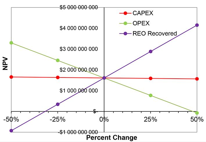
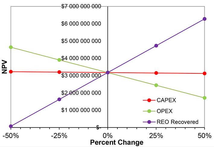
Affiliation: 1FLSmidth, Boksburg East, South 2AfricaVisiting Emeritus Professor, School of Mining Engineering, University of the Witwatersrand, Johannesburg, South Africa
All humans rationalize differently based on their cognitive processes or reasoning (culture, experience, educational background, level of management, etc.). As a result, decision-makers in mining financial departments may rationalize very differently about spending funds on corrective sampling compared to technical sampling experts, thus that well-conceived corrective sampling projects could be rejected.
sampling,Keywordsrepresentative, costs, value-add, fit-for-purpose. Introduction
The objective benefits of proposed fit-for-purpose sampling solutions should be presented to relevant decision-makers in such a way that adverse subjective decisions are countered so that appropriate solutions are implemented. Practical examples of the benefits from motivating the implementation of fit for purpose sampling solutions at sampling facilities around the world are provided.
Irrespective of the appropriateness of the technical design, or imperatives of the Theory of Sampling (TOS), approval for implementing a corrective sampling solution is usually declined unless value-add can be quantified and corroborated with basic proof. The fact that the costs of poor sampling never show up as a line item in the annual financial statements means that managers do not see a figure that represents a loss to their earnings. Attitudes towards a meaningful spend on correctly designed and installed sampling equipment therefore remain refractory. The rationale for the implementation of improved sampling solutions must be presented as simply as possible leaving little room for subjective interpretation.Estimating the value-add from implementing sound TOS-based sampling practices does not require a long or complicated report. A simple ‘back to basics’ approach, pointing out the critical points and findings with a summary of the financial benefits, provides a much better chance of getting your point across. The ‘sampling fraternity’ should also acknowledge that implementation of the ‘close-to-perfect sampling solutions’ are not always feasible. If the benefits of a fit-for-purpose solution compared to the capital cost of implementing a best-practice sampling solution are not immediately obvious, the project should not be rejected. The need to make compromises, knowing that not all solutions are perfect, may still provide some value-add by reducing the sampling error compared to current operations. This paper presents a back-to-basics approach for demonstrating the benefits of installing corrective sampling protocols, equipment, and fit-for-purpose sampling solutions to reluctant shareholders and those approving budgets. Technical studies of mines and plants around the world, with specific attention to the benefits and value created from improved sampling, are presented.
MiningSynopsisoperations
Costs and benefits of fit-for-purpose sampling solutions by T. Bruce1 and R.C.A. Minnitt2
413The Journal of the Southern African Institute of Mining and Metallurgy VOLUME 122 JULY 2022
Correspondence to: T. Bruce Email: trevor.bruce@flsmidth.com
Dates: Received: 25 Oct. 2019 Revised: 1 Mar. 2022 Accepted: 3 Jun. 2022 Published: July 2022 How to cite: Bruce, T. and Minnitt, R.C.A. 2022 Costs and benefits of fit-for-purpose sampling solution. of the Southern African Institute of Mining and Metallurgy, vol. 122, no. 7, pp. 413–420 DOI 9717/982/2022http://dx.doi.org/10.17159/2411-ID:
are generally reluctant to install high-cost sampling systems at operations that have been functioning for many years. The principal objection to installing appropriate equipment to extract correct and representative samples in process flows is the time and costs involved. The Theory of Sampling (TOS) provides a structured framework for identifying and quantifying the errors and bias associated with any sampling event, but this may be insufficient to initiate substantial investment in correctly designed sampling equipment. Financial losses arising from substandard sampling installations are usually disregarded because the value-add from a good quality sampling solution is invisible, but the cost is quite obvious. Depending on the needs, a less-than-perfect or fit-for-purpose sampling solution may be acceptable, provided the magnitude of sampling errors is understood and the assay results are interpreted accordingly. Categorical levels of acceptable accuracy and precision can be established depending on the sampling position in the mining value chain and the nature of the decisions to be made.
Journal
Costs and benefits of fit-for-purpose sampling solution 414 JULY 2022 VOLUME 122 The Journal of the Southern African Institute of Mining and Metallurgy
➤ For larger, more critical sampling points, has the supplier allowed a budget for computational modelling of material flow, using well established software and methods such as discrete element method (DEM) simulation (Hidding and Shaw, 2017)?
• The size of the sampler to fit existing infrastructure
• Minimizing cutter aperture to reduce the sample mass for easier downstream processing
A statement such as ‘…improved sampling equipment and procedures at a port facility, can improve your sampling preparation and measurement (SPM) precision from 0.22% to 0.15%...’ could be lost on non-technical managers and executives. What they would prefer to hear is ‘…let me show you what improving your SPM can do for your profits.’
Executive committees have neither the time for nor the interest in detailed or complex calculations of precision, so that technical jargon alone will seldom motivate budget approval. The insight, interest, and understanding of sampling technicalities is not common amongst such audiences, but simple statements such as ‘…every 0.01% improvement on the SPM precision could potentially increase the on-grade production by 0.01%...’ are more likely to pique their interest long enough for budget approval. Unfortunately, the best motivations for improved sampling facilities are benefits that appear after the fact. As an example, consider an iron ore mine with an annual production of 300 Mt and a price of US$75 per ton, as is the case with Vale and Rio Tinto. Rio Tinto’s Cape Lambert B port facility improved precision from 0.22% to 0.15% after implementing a well-designed automated sampling-to-analysis system (Brunning et al., 2014). This resulted in a 0.07% increase in on-grade ore, equivalent to 210 000 t, with an estimated value of US$15 750 000.
Names mean more than numbers
➤ Does the supplier understand the TOS sufficiently to challenge aspects in the scope of work that could impede good sampling?
• The ‘correctness’ of the sample and implications for sampling error and bias
• System reliability, ease of maintenance with minimal downtime, and access to inspection ports.
➤ Has the project owner ensured that the technical claims made by the supplier have been reviewed and validated?
Internal resources or sampling specialists should define the exact scope of work with as little ambiguity as possible before tenders are posted. Specifications should include descriptions of material flow characteristics in the stream to be sampled and details of the required sampler. Items to be defined include the sampler type, aperture size, cutter speed, replaceable cutter blades, easily accessible inspection hatches, no pneumatic or hydraulic drives on cutters, collection bins large enough to hold all sample material at maximum flow rates with no spillage, all contact surfaces to have a minimum angle of 70o from horizontal, and the cutter rest position is completely out of the material flow, etc.
Project owner responsibilitiesS Not all suppliers of sampling equipment apply similar standards, but they should aim to achieve complete solutions based on the TOS and good sampling practice. Solutions should include compromises required to accommodate restrictions on available space etc., but at the same time clearly stating the effects of such compromises on the end results. Sampling projects should not be awarded by project owners based purely on lowest cost procurement. The following questions are a guide to points to consider before selecting a sampling solution provider.
The role and responsibility of financial managers may not allow them time to digest the theoretical aspects of TOS. Collaboration and certification of designs by well-known experts add more confidence to improved sampling solutions than complex formulaes. Specialists who are able to validate or verify decisions about proposed sampling installations are an effective method of convincing shareholders or project owners that money is well spent on improved sampling. Few are impressed by jargon and equations Correct sampling nomenclature and application of equations to estimate financial benefits is critical, but shareholders and financial managers are unimpressed by complex procedures and formulaes. Shareholders are much more likely to approve projects provided one can demonstrate that the estimated value-add through improved sampling has been validated by reputable persons or sources.
Penalties for out-of-spec products
General concepts
➤ Have current and future maximum and minimum design criteria been effectively communicated to the supplier, i.e., what worst-case scenarios could be faced by the system being requested?
➤ To reduce capital costs suppliers should not compromise on:
• Alternative drive technologies, including pneumatic, electric, or hydraulic
• Materials or manufacturing techniques and designs
The adage that ‘If something sounds too good to be true, then it probably is’ is still applicable. Statements such as ‘…better sampling can produce an additional US$25 000 000 worth of on-grade ore per annum…’ sound too good to be true and arouse a certain level of scepticism. Numbers this large appear unrealistic and are probably not trustworthy unless they can be validated by providing realistic examples. It is better to begin by offering small numbers, for example ‘…correct sampling can deliver an additional US$7500 for a 100 000 t shipment of iron ore…’ and allow the decision-makers do the mental arithmetic themselves. Producers who deliver over 340 Mt/a can easily see the potential value of better sampling. Disinterest in statistics without practical application
The cost of underestimating the target analyte content is not reported in financial statements as it is not quantifiable, and in many cases is misunderstood. What should be seen on a company’s financials are the costs incurred due to penalties for delivering off-spec grade ore and deleterious elements that exceed allowable limits. Quantifying the amount paid in penalties highlights a ‘real’ cost that could be reduced by implementing better sampling practices and systems.
A number of observations have come to light as a result of presenting appeals to the boards of companies for funding to improve sampling facilities. Distrust of large unsubstantiated numbers
Rapid turn-around versus high precision
Costs and benefits of fit-for-purpose sampling solution African Mining
and Metallurgy VOLUME 122 JULY 2022
Motivating a sampling project
1Overall precision for sampling preparation and measurement βSPM1 = 2σSPM
Institute of
Although some principles may be the same, it is unwise to apply guidelines from a single ISO standard to two different materials. For example, ISO 3082 for iron ores should not be used to estimate sampling compliance for phosphate fertilizers because the material characteristics are so different; in this case the material-specific standard must be applied. Where no specifications are available for a material, TOS practices such as heterogeneity tests and calibration for establishing nomograms should be applied.
The objective of a sampling study should be to demonstrate how improved sampling practices can improve profitability. Motivating a project to improve sampling equipment and protocols requires an understanding of the complete value chain so that expectations about the outcome of the sampling project are met. This may include defining the levels of reliability and precision to be achieved as a result of improvements to sample extraction, handling/transport, preparation, and measurement. Motivating for added value and increased profit from improved sampling precision must be supported by realistic estimates of the capital cost and required investment. The capital investment needed for taking better samples using better sampling equipment, ensuring the correct sample size and sample frequency, must be calculated accurately. In addition, the costs of ensuring that samples are correctly transported, prepared, analysed, and reported, within an acceptable turn-around time that allows real-time changes to be made, must be established. The total investment required in terms of time, money, and effort must be understood by managers and financial officers if proposals to improve sampling processes are to have credibility and integrity.
Fit-for-purpose sampling
For example, taking more primary increments and analysing more subsamples than required by ISO during the loading of an iron ore vessel can give a better indication of the grade during loading. This can then be used to blend into the vessel more efficiently.
ISO standards versus Theory of Sampling ‘ISO compliant’ is a term often used when discussing upgrades to sampling facilities. ISO standards, although critical in establishing standard methods of sampling, preparation, and analysis for various materials, are too often applied out of context. There appears to be a widespread misunderstanding that compliance with the relevant ISO standard will automatically result in the best possible sampling results without due consideration of the carefully constructed requirements for correct and representative sampling established in the TOS. ISO standards provide recommendations for ascertaining a minimum precision and level of confidence in accordance with international standards, but without the constraints implied in the TOS framework, adherence to ISO does not necessarily guarantee a correct sampling solution. However, improving sampling equipment and methods above the minimum requirement recommended by ISO standards can add further value to a producer. As an example, if iron ore producers reduce the precision on a 270 000 t lot below the bSPM1 of 0.34% Fe stipulated by ISO 3082, substantial improvements in on-grade ore production can be achieved. Compliance is one thing, but before setting a limit on the resources assigned to sampling and analysis, it is critical to establish the monetary value of each sample using a minimum requirement, compared to what it could be worth if additional resources were spent on improving it. Rather than strict compliance with minimum requirements from relevant ISO standards, other aspects, especially efficiency for operational purposes, should be considered when specifying a sampling point.
Providing correct sampling solutions is a costly exercise and the more stringent the correct solutions, the higher will be the capital costs. This paper supports the concept that samples are suspect if the principles of the TOS are not followed. The rational man strives for perfection, but knowing that things in life are rarely perfect, attempts to demonstrate that fit-for-purpose sampling solutions may still offer value. Of course, the value depends on how the resulting analyses and associated confidence intervals will be used. This also assumes that benefits are not outweighed by the cost of taking, transporting, preparing, and assaying the sample - a simple concept, but one that may be overlooked by the sampling fraternity.Forexample, dip sampling from slurry or liquid launders is known to be ‘incorrect’, but frequent dip samples from a material stream having high concentrations of a target element with a relatively even distribution can be used to indicate sudden changes in concentration levels. Although the absolute concentration of the lot cannot be measured with any level of certainty using dip sampling, it can alert the plant superintendent to reduced or elevated levels of target analyte, on which to base further investigation. As a general rule of thumb, sampling can be used for either process control or product control. Process control, being used for internal operations to optimize a facility, can typically allow for a small level of flexibility, provided that the actions taken are aligned with the confidence in the sample. Product control, material accounting, and quality control for saleable goods typically allow little to no room for error and, in these applications, it is critical to precisely estimate the quality of the product with measurable confidence. In this case all TOS practices should be strictly adhered to.
A smelter aimed for less than 5 ppm precious metal in slag which it sells as silica waste for US$3 per ton. Slag analyses over a six-month period indicated the precious metal content to be as high as 18 ppm. The operating cost to recycle slag through the furnace, after it has cooled is approximately US$5 700 per ton, so although sampling error could be reduced by improved sampling methods, the cost benefit would be minimal unless the samples can be collected and analysed before the slag is cast. On average
Case studies and examples
The supplier should have discretion to stipulate what is deemed necessary to get the job done if these factors are not defined, but not necessarily what is best for ongoing long-term operations. Suppliers should suggest the additional features they offer, but project owners must know what is needed as a minimum to achieve the required sampling precision and to meet all the operational requirements. Using internal resources or specialists to define what is needed for sampling installations is more costeffective than investigating what went wrong after the system has been implemented.
415The Journal of the Southern
Costs and benefits of fit-for-purpose sampling solution
Figure 1 Stop-belt sampling on the waste conveyor
However, design constraints faced by the supplier meant that the compromises made to the sampling installation almost completely invalidated the system. As shown in Figure 2, to fit the sample collector into the available head chute area it was made very shallow, allowing material to bounce out of the cutter opening. The cutter was not perpendicular to the material flow and neither was it wide enough to be able to cross the complete stream and belt scraper. In addition, the cutter was driven by an underpowered hydraulic cylinder, unable to move the cutter through the stream at a constant speed.
Inspection of a large iron ore producer’s port facility revealed that the primary sample cutter could not extract a correct sample as defined by the TOS. The cross-belt sampler on the loading conveyor belt cut a stream of iron ore fines, lump, and pellets, flowing at 23 000 t/h (maximum design capacity). The secondary and tertiary sample cutters had been decommissioned because their design did not comply with requirements for large flow rates and physical characteristics of the material. The primary cut was diverted directly to a waste conveyor which was randomly stopped, once per primary increment, and a stop-belt sample of approximately 20 kg was taken as shown in Figure 1.
416 JULY 2022 VOLUME 122
Reducing the loss of precious metals in the slag to less than 5 ppm would result in an additional precious metal production of over US$400 000 per annum. This figure, based on historical data gathered from the smelter, compares the actual gold content of processed slag with what it should have been if the Au grade was maintained below 5 ppm. Assuming a 3-year return on investment, a sampling solution costing less than US$1 200 000 would add value. This example illustrates the necessity of understanding the limitations and effect of improved sampling before proposing a sampling-to-analysis solution. A less-than-perfect sampling solution still adds value A less than perfect sampling solution was observed at a phosphate fertilizer production plant where phosphate slurry is mixed with H2SO4 in a reactor vessel to produce phosphoric acid. Dip samples are taken between 50 cm – 500 cm below the slurry surface. Concentrations of free sulphate, measured by titration, and phosphoric acid cannot be quantified in the complete vessel with any certainty using this imperfect sample, but some knowledge of the concentrations is critical for controlling processes in the reactors.Inthis case time is of the essence. It is critical that the sample be filtered and analysed as soon after extraction as possible because the reaction in the sample container continues as the sample cools, affecting the accuracy of the analytical results significantly. To improve the integrity of the sample, an insulated sample container should be used to collect the sample (Ritchie, 2018, Personal communication). In addition, rapid transport to the laboratory using a pneumatic air tube conveyance was suggested.
Too many compromises invalidate the sampling point
The Journal of the Southern African Institute of Mining and Metallurgy around 10 ts of slag is produced per cycle, meaning that the value of precious metals in a single slag cycle would have to be greater than US$57 000 to make recycling through the furnace viable. If samples can be collected and analysed before the slag is poured, then remedial actions such as increasing the residence time in the furnace can be taken. In this case precision of the result is not as crucial as the sampling-to-analysis turnaround time, so this is where the focus for the project was placed. If the furnace charge is analysed before smelting it is possible to modify the charge and reduce the risk of precious metals reporting to the slag. In this case the precision is more critical to the process as small variations in the charge can affect the smelt efficiency.
Figure 2 Poorly designed cross-stream sampler at the end of a conveyor belt
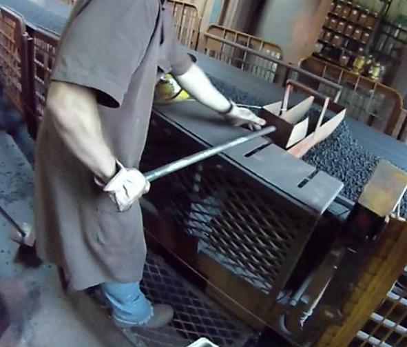
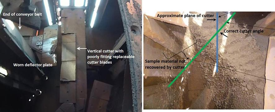
The system manufactured by the supplier fitted the available space but failed to consider the effect and possible consequences of implementing these compromises. It is also possible that this system was designed for lower flow rates even though the belt capacity could be increased to the maximum loading of 23 000Thet/h.estimated investment required to replace the sampling equipment for primary, secondary, and tertiary sampling with a properly designed reverse scoop sample cutter, as shown in Figure 3, was US$4 200 000, excluding the removal of the existing system and any other infrastructure modifications. Even though this would be a costly exercise for the end-user, the upgrade would allow a substantial improvement in the precision of the results and could allow production of over 1% more on-grade ore by blending various grades to a tighter tolerance with more confidence. This facility exports over 200 Mt/a of iron ore and with an iron ore price of US$75 per ton (at the time of writting), a 1% increase could be worth US$150 000 000 per annum. Modifications to the plant will allow the company to exploit the improved bSPM precision of Fe so they can rapidly blend the ore to achieve a tighter tolerance on the required export grade.
Institute of
Samples are stored at the sampling point and transported 500 m to the analytical lab once a shift, but this results in a degree of degradation of the sample (contamination from airborne particulates, moisture loss etc.) which means that the data from these samples is historical rather than real-time. Rapid, safe transport of tertiary sample increments from the sampling tower to the robotic automated preparation and analytical laboratory by an automated transport system can further improve precision and turnaround time. Good sampling to analytical practices A port iron ore laboratory provides an example of how good sampling and rapid automated sample preparation and measurement can add value. Trains and trucks deliver iron ore from various mines to the port facility where it is stockpiled according to grade. The two feed conveyors, one high-grade and the other low-grade, transport ore from different stockpiles to ships in dock. The sampling and laboratory stations are situated over these belts at the transfer chute to the primary ship-loading conveyors as shown in Figure 4. An innovative design by a sampling manufacturer, known as the swing-arm cutter, overcame the constraint that the primary sample cut needed to be lifted in order to allow for secondary sampling in the available space in the sampling building. The cross-stream swing-arm sample cutter is connected to a swivel point on a long-radius swing arm. The arm rotates, moving the sample cutter through the material stream at a constant speed with the sample being collected in the sample collection device behind and below the cutter openings. The arm continues to swing until completely vertical, at which point the sample bin is opened and the sample is dropped onto a feed conveyor which moves it to a weigh hopper and then to the secondary vezin-type cross-stream sampler, as shown in Figure 5. The sample is then transported on a secondary conveyor to a hopper on load-cells where it is weighed and transferred to another conveyor carrying the sample to the analytical laboratory (Figure 6).
Costs and benefits of fit-for-purpose sampling solution African Mining
and Metallurgy VOLUME 122 JULY 2022
Figure 3 Reverse scoop cross-stream sampler
Figure 4 Port automated sampling, preparation, and analysis conveyor
417The Journal of the Southern
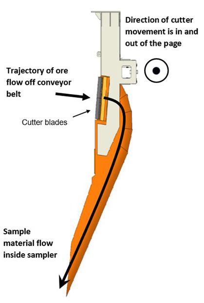
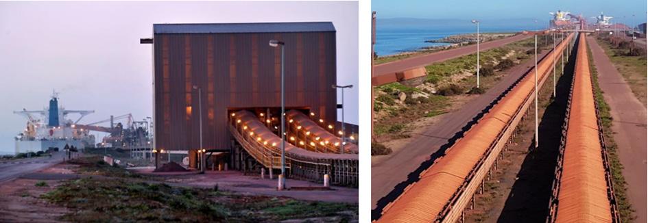
418 JULY 2022 VOLUME 122 The Journal of the
and
➤ Systematic sampling is carried out on a mass basis. The loaded conveyor belt passes over the load-cells and this information controls the sampling interval on the belt.
➤ The speed of the sample cutter is maintained at less than 0.6 m/s.
Costs and benefits of fit-for-purpose sampling solution Southern African Institute of Mining Metallurgy
This sampling station adheres to the various sampling TOS practices as noted below (Hofmeyr and Pretorius, 2013).
➤ Free-fall drops in the automated transport of samples are kept to a minimum to reduce size degradation of the ore and minimize bias in size distribution. No maximum heights are specified in the ISO manuals, but 1 m is understood to be the maximum height. However, this height is exceeded by a small margin in two places to accommodate automation.
➤ The minimum increment mass required by ISO for the primary sampling system at the laboratory in terms of tons per hour on the conveyor belt, cutter aperture, and cutter speed is 330 kg. In practice, this sampling facility achieves a primary sample of 350±70 kg.
➤ A complete cross-section of the falling stream is taken by the swing-arm sample cutter. ➤ The aperture of the sample cutter is more than three times the nominal top size of the ore.
Figure 5 Swing-arm cross-stream sampler and discharge of 370 kg iron ore sample into hopper
Figure 6 Secondary conveyor discharges iron ore sample into hopper mounted on a weigh frame from where it is carried to analytical laboratory on a tertiary conveyor
➤ The sample cutter travels at a uniform speed and both the leading and trailing edges clear the ore stream at the end of the traverse. ➤ The lips of the sample cutter are parallel.
The secondary sample cut is conveyed to the robotically automated sample preparation and analysis facility where each increment is accumulated in a steel bin ready for further preparation and analysis. As shown in Figure 7, the material is divided into subsamples. One portion is sent for automated ISO moisture and particle size distribution (PSD) analysis and a second is sent for automated chemical preparation and analysis. Using rapid infra-red drying technologies, the laboratory is able to produce verified results within 6 hours of the ship being loaded. Over a six-month period the average precision measured was better than 0.14%. This facility is also ISO 17025- and ISO 3082- compliant and certified.
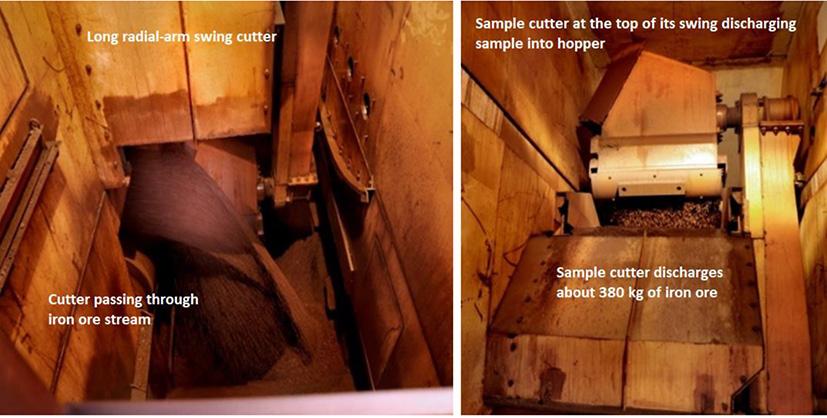
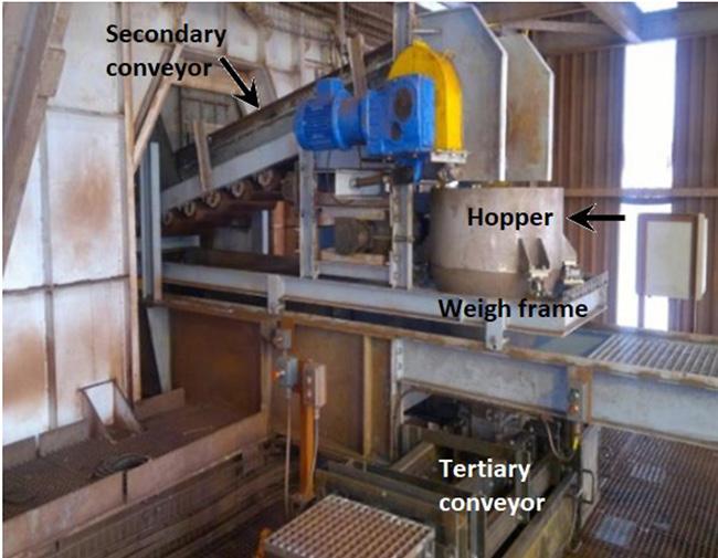
Method for the pricing of iron ore
Costs and benefits of fit-for-purpose sampling solution
The iron ore producer has not released the actual value of the investment to make this facility perform as it does, but the following information is available:
Every reasonable effort has been made to minimize SPM error in this facility and with the addition of automated preparation and analysis not only makes the system precise, but also offers the value of rapid preparation and analysis. As noted above, even though the sampling building did not have enough headroom to fit a standard traditional cross-stream sampler an innovative alternative was developed. This key contribution required that both the client and supplier have a strong understanding of the sampling requirements and work together to find a feasible solution.
Value of investment
➤ The iron ore producer can use the high precision as proof of the quality of their product, thereby giving them a commercial advantage over their competition (bragging rights).
In discussions with iron ore producers, there appear to be a number of methods of calculating the actual price of iron ore. Pricing guides are readily available online for the various grades of iron ore and commodities. Specific grades with upper specification limits on deleterious elements are defined for each commodity, but after ship loading the actual chemical and physical characteristics of the lot can be used to modify the price accordingly. How this is done for a shipment of iron ore, after the ship is loaded with a specific ore grade/type and results obtained while loading the ship have all been processed, is not clearly defined, but it could be by contract negotiation between suppliers and customers. The following is a proposal for determining the price.The Metal Bulletin publication of August 2018, entitled ‘Iron Ore Indices, Pricing Guide: Methodology specification and use’, employs an index called ‘Value-In-Use’ (VIU) to correct the price of specific ore grade/type using the final analyses of samples collected during the loading of the lot. The VIU index is released on the first working day of each month and could be applied as Iffollows:
➤ The final analysis is available 6 hours after ship loading is complete. This was previously a minimum of 48 hours. The benefit is that the lot can be invoiced nearly two days earlier than before, resulting in an estimated gain of US$5500 per 270 000 t shipment on interest alone.
α = The required value of Fe in the commodity, say 62% Fe fines index MBIOI(α) = The index price for iron ore with α% Fe, using the Metal Bulletin Iron Ore Indices (MBIOI) Pac = The selling price of iron ore (per dry ton) with an Fe concentration calculated during loading, and Fe-VIU index = Value in use index for the α grade of ore, then Pac = MBIOIα + (%Fe difference from α * Fe-VIU index).
➤ For large lots, the laboratory can release data during ship loading with a precision of less than 0.15%. This data is used to adjust the blend between low- and high-grade ore to control the final grade being loaded.
Thus, if the reported Fe content after loading is understated, it will directly impact the price of the ore (all other factors being equal). That is ignoring all other penalties or price adjustments for higher content of deleterious elements or less than the set range of Fe. The further away from the actual value that the reported value is, the more the producer will lose if the Fe content is understated.Thisinformation could be used to motivate a sampling, sample preparation, and analysis project as follows. Consider an iron ore producer loading ore of grade/type 62%Fe fines, having a daily index price of US$86.68 per dry ton with a monthly VIU index of US$1.28 on (21 February 2019, Metal Bulletin Iron Ore Index).
Figure 7 Robotic automated facility for sample preparation and analysis for chemical, PSD, and moisture
419The Journal of the Southern African Institute of Mining and Metallurgy VOLUME 122 JULY 2022
➤ Reduced risk of penalties due to deleterious elements exceeding upper specification limits of the lot, or lower than specified Fe content ➤ Disputes over the quality of the ore loaded through this terminal are quickly settled due to the overall compliance of the complete facility with the relevant laboratory and material specifications. This plant has proven that rapid analysis with consistently high precision is possible, so the producer is currently investigating upgrades and expansions of this facility to increase sampling and analytical capacity with the aim of optimizing inship grade blending.
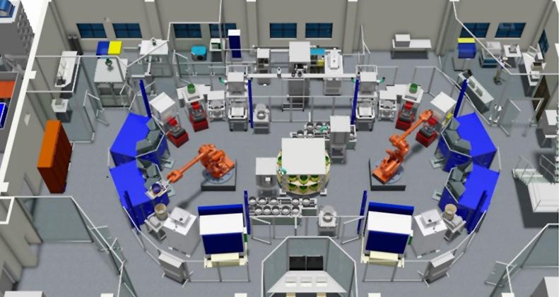
If the final combined SPM precision for Fe achieved by a supplier at a port loading is 0.3%, and if the supplier reported a value of 62% Fe, the actual value of Fe could be as much as 62.19%. If the supplier was able to reduce the SPM precision to 0.1% they would potentially be under- or over-reporting by only 0.062% Fe.
Hidding, M. and Shaw, R. 2017. Modelling ore flow in the design of high-capacity sample cutters. Proceedings of WCSB 8, the Eighth World Conference on Sampling and Blending, Perth, Western Australia. Australasian Institute of Mining and Metallurgy. pp 145 – 149.
Conclusions
Using the VIU correction calculation above, the price difference per dry ton between the first instance and the second is US$0.16. This value multiplied over a shipment mass of 270 000 t will be US$43 200, so the supplier would under-invoice their end client by this amount. This potential loss in profits, multiplied over a year’s production for a large company such as Rio Tinto, VALE, BHP etc., producing +300 Mt/a, could amount to well over US$50 000 000.00 per year.
A full understanding of the complete mineral production and sale process before and after the sampling point is essential. Such insights allow one to appreciate the current usage of the sample result, as well as identify other potential uses and value-add, especially if the quality of the sample can be improved. Ascribing a monetary value to a sample in a process or procedure is a new and important concept. An understanding of the levels of precision or sampling correctness of a sample, as well as the turnaround time to analysis, will influence this value. An appreciation of the constraints such as applicable standards or specifications, physical space available, accessibility for inspections, maintenance and sample collection, plant downtime for the installation, distance between sampling point and the laboratory must all be taken into consideration in order to create a fit-for-purpose sampling solution.Inthe process control domain, fit-for-purpose sampling has a wider scope as compromises can be made in various aspects of sampling to suit the application, provided the consequences of these compromises are understood. In the product control domain, where the same compromises cannot be made, fit-forpurpose sampling can still be applied when considering how the sampling will affect other aspects of the facility such as material throughput and the value of faster sampling-to-analysis. Using a cross-stream sampler will not affect loading rates, whereas a stopbelt sampler will, therefore the cross-stream sampler is fit-forpurpose in this case. The feasibility of motivating and actioning an upgrade process required by a facility in order to exploit the expected value-add from the specified sampling solution also requires insight and understanding. Some of the actions can include automated sample collection and transport systems to increase turnaround time from sampling to laboratory. Other actions could include upgrades to the laboratory to accommodate the sampling solution and an upgrade to standard operating procedures. The result of such actions would enable the facility to respond to sample information to achieve the value-add.
Costs and benefits of fit-for-purpose sampling solution of the Southern African Institute of Mining and Metallurgy
It is important that project owners communicate their needs to sampling equipment suppliers in a way that ensures the supplier provides the best solution for their application. Lowest cost procurement should not govern the selection of equipment, as this is likely to turn out to be a costly error of judgement. A policy of lowest cost procurement is short-sighted as it may mean not only inferior equipment selection, but also incorrect sample extraction that introduces costly bias associated with poor sampling.Thegreatest deterrent to decisions to install appropriate or improved sampling solutions is that the benefits are invisible, while the costs are obvious. No financial statements tell CEOs what the benefits from sampling are. The only indications might be increases in the costs of reagents and consumables. Sampling materials off the waste dumps and in the tailings launder may also provide the evidence needed to convince the financial managers that improved sampling equipment is essential. When presenting a sampling solution to an executive committee with the hope of getting their approval, the primary motivational factor should be a clear demonstration of the monetary benefits the solution can offer. The basis of the motivation should be a comparison of cost-to-implement against the long-term expected returns on investment. All mathematical and other technical aspects of the proposed solution should be kept as straightforward as possible with only key results presented, which are ideally verified by a well-respected specialist in the field.
Hofmeyr, P. and PreTorius, D. 2013. Automated sampling of iron ore for analysis at the Saldanha iron ore terminal in South Africa. Proceedings of Sampling and Analysis 2013. Southern African Institute of Mining and Metallurgy, Johannesburg. RiTchie, C. 2018. Personal communication sample. u
References Brunning, R., Andringa-BaTe, C., Graham, M., and WesTerngren, S. 2014. Cape Lambert Port B shiploading, sampling and analysis. Proceedings of the Sampling Conference, Perth, W.A. Australasian Institute of Mining and Metallurgy, Melbourne. pp 79 – 90.
420 JULY 2022 VOLUME 122 The Journal
NATIONAL & INTERNATIONAL ACTIVITIES
13–17 November 2022 — Copper 2022 Santiago, Chile Website: https://copper2022.cl/ 28 November –1 December 2022 — South African Geophysical Association’s 17TH Biennial Conference & Exhibition 2022 Sun City, South Africa Website: https://sagaconference.co.za/ 13-16 December 2022 — 4TH International Conference on Science and Technology of Ironmaking and Steelmaking Indian Institute of Technology Bombay (IIT Bombay) Website: http://stis2022.org/ Southern African of Mining Metallurgy 2022
7–8 November 2022 — SANCOT Symposium 2022 ´Tunnel boring in civil engineering and mining´ Wallenberg Conference Centre @ STIAS, Stellenbosch, Western Cape, South Africa Contact: Gugu Charlie Tel: 011 538-0238 E-mail: Website:gugu@saimm.co.zahttp://www.saimm.co.za
31 August–1 September 2022 — Caving 2022 Fifth International Conference on Block and Sublevel Caving Hilton Adelaide, South Australia Website: https://www.acgcaving.com/ 5–6 September 2022 — Implications of S-K1300 regulations and disclosures for dual-listed companies on the for dual listed companies on the JSE and NYSE Online Webinar Contact: Camielah Jardine Tel: 011 538-0238 E-mail: Website:camielah@saimm.co.zahttp://www.saimm.co.za
15–20 September 2022 — Sustainable Development in the Minerals Industry 2022 10TH Internationl Hybrid Conference (SDIMI) ´Making economies great through sustainable mineral development´ Windhoek Country Club & Resort, Windhoek, Namibia Contact: Gugu Charlie Tel: 011 538-0238 E-mail: Website:gugu@saimm.co.zahttp://www.saimm.co.za
2–4 November 2022 — PGM The 8TH International Conference 2022 Sun City, Rustenburg, South Africa Contact: Camielah Jardine Tel: 011 538-0238 E-mail: Website:camielah@saimm.co.zahttp://www.saimm.co.za
15–17 August 2022 — Static and Cyclic Liquefaction of Mine Tailings Course Misty Hills, Muldersdrift Website: https://saice.org.za/
20–21 September 2022 — 4TH Manganese School ´Environment/Energy - CO2 Emissions´ Fédération Nationale Des Travaux Publics (FNTP), Paris Contact: Camielah Jardine Tel: 011 538-0238 E-mail: Website:camielah@saimm.co.zahttp://www.saimm.co.za 2022 — 18TH Annual Student Colloquium 2022 Mintek Randburg, South Africa Contact: Gugu Charlie Tel: 011 538-0238 E-mail: Website:gugu@saimm.co.zahttp://www.saimm.co.za
8-14 September 2022 — 32ND Society of Mining Professors Annual Meeting and Conference 2022 (SOMP) Windhoek Country Club & Resort, Windhoek, Namibia Contact: Camielah Jardine Tel: 011 538-0238 E-mail: Website:camielah@saimm.co.zahttp://www.saimm.co.za
27-28 September 2022 — Wits Mining Institute Seminar Contact: Lileen.Lee@wits.ac.za Website: https://www.wits.ac.za/wmi/ 28–29 September 2022 — Thermodynamic from Nanoscale to Operational Scale (THANOS) International Hybrid Conference 2022 on Enhanced use of Thermodynamic Data in Pyrometallurgy Teaching and Research Mintek, Randburg, South Africa Contact: Camielah Jardine Tel: 011 538-0238 E-mail: Website:camielah@saimm.co.zahttp://www.saimm.co.za 4–6 October 2022 — 18TH MINEX Russia Mining and Exploration Forum Website:Moscow organisers/https://2021.minexrussia.com/en/contact-forum12–13 October 2022 — Mine-Impacted Water Hybrid Conference 2022 ´Impacting the Circular Economy´ Mintek Randburg, South Africa Contact: Camielah Jardine Tel: 011 538-0238 E-mail: Website:camielah@saimm.co.zahttp://www.saimm.co.za 26 October
2022 The Journal of the
VOLUME 122 JULY
24–25 August 2022 — Battery Materials Conference 2022 Misty Hills Conference Centre, Muldersdrift, Johannesburg, South Africa Contact: Gugu Charlie Tel: 011 538-0238 E-mail: Website:gugu@saimm.co.zahttp://www.saimm.co.za
vii ◀
and
Institute
21–23 August 2022 — International Mineral Processing Congress Asia-Pacific 2022 (IMPC) Melbourne, Brisbane + online Website: https://impc2022.com/ 21–25 August 2022 — XXXI International Mineral Processing Congress 2022 Melbourne, Australia + Online Website: www.impc2022.com
Minerals
MSA
Bafokeng Rasimone Platinum Mine Barloworld Equipment -Mining BASF Holdings SA (Pty) Ltd BCL BeckerLimitedMining (Pty) Ltd BedRock Mining Support (Pty) Ltd BHP Billiton Energy Coal SA Ltd Blue Cube Systems (Pty) Ltd Bluhm Burton Engineering (Pty) Ltd Bond Equipment (Pty) Ltd Bouygues Travaux Publics
Caledonia Mining South Africa Plc Castle Lead Works
Minerals Council
DRA Mineral Projects (Pty) Ltd DTP Mining - Bouygues Construction EHLDurasetConsulting Engineers (Pty) Ltd Elbroc Mining Products (Pty) Ltd eThekwini Municipality Ex Mente Technologies (Pty) Ltd Expectra 2004 (Pty) Ltd Exxaro Coal (Pty) Ltd Exxaro Resources Limited Filtaquip (Pty) Ltd FLSmidth Minerals (Pty) Ltd Fluor Daniel SA (Pty) Ltd Franki Africa (Pty) Ltd-JHB Fraser Alexander (Pty) Ltd G H H Mining Machines (Pty) Ltd Geobrugg Southern Africa (Pty) Ltd GravitasGlencoreMinerals (Pty) Ltd Hall Core Drilling (Pty) Ltd Hatch (Pty) HPEHerrenknechtLtdAGHydroPower
Ltd Northam Platinum Ltd - Zondereinde Opermin Operational Excellence OPTRON (Pty) Ltd Paterson & Cooke Consulting Engineers (Pty) Ltd PolysiusPerkinelmerADivision of Thyssenkrupp Industrial Sol Precious Metals Refiners Rams Mining Technologies Rand Refinery Limited Redpath Mining (South Africa) (Pty) Ltd Rocbolt Technologies Rosond (Pty) Ltd Royal Bafokeng Platinum Roytec Global (Pty) WorleyWeldingWeirWebberUmgeniUkwaziTrakaTomraTimriteTimeSRKSoundSmecSISASenminSENETSebiloSchauenburgSANIRERSASandvikDelmasSandvikSaleneRustenburgRungePincockMinarcoLtdLimitedPlatinumMinesLimitedMining(Pty)LtdMiningandConstruction(Pty)LtdMiningandConstruction(Pty)Ltd(Pty)LtdResources(Pty)Ltd(Pty)LtdInternational(Pty)LtdInspection(Pty)LtdSouthAfricaMiningSolution(Pty)LtdConsultingSA(Pty)LtdMiningandProcessing(Pty)Ltd(Pty)Ltd(Pty)LtdAfrica(Pty)LtdMiningSolutions(Pty)LtdWaterWentzelMineralsAfricaAlloysSouthAfrica ▶ viii JULY 2022 VOLUME 122 The Journal of the Southern African Institute of Mining and Metallurgy
Company affiliates
The following organizations have been admitted to the Institute as Company Affiliates
Equipment (Pty) Ltd Huawei Technologies Africa (Pty) Ltd Immersive Technologies IMS Engineering (Pty) Ltd Ingwenya Mineral Processing (Pty) Ltd
MineRP
Mining Projections Concepts MIPMintekProcess Technologies
Ivanhoe Mines SA Joy Global Inc.(Africa) Kudumane Manganese Resources Leica Geosystems (Pty) Ltd Loesche South Africa (Pty) Ltd Longyear South Africa (Pty) Ltd Lull Storm Trading (Pty) Ltd Maccaferri SA (Pty) Ltd Magnetech (Pty) Ltd Magotteaux (Pty) Ltd Malvern Panalytical (Pty) Ltd Maptek (Pty) Ltd Maxam Dantex (Pty) Ltd MBE Minerals SA Pty Ltd MCC Contracts (Pty) Ltd MD Mineral Technologies SA (Pty) Ltd MDM Technical Africa (Pty) Ltd Metalock Engineering RSA (Pty)Ltd Metorex Limited Metso Minerals (South Africa) (Pty) Ltd Micromine Africa (Pty) Ltd MineARC South Africa (Pty) Ltd of South Africa Operations Executive (Pty) Ltd Holding (Pty) Ltd (Pty) Limited Mining Systems Africa (Pty) Ltd Group (Pty) Ltd (Pty) Ltd Africa (Pty) Ltd Sands(Pty) Ltd Trading (Pty)
AMEC Foster Wheeler
Murray and Roberts Cementation Nalco
CDM Group CGG Services SA Coalmin Process Technologies CC Concor Opencast Mining Concor Technicrete Council for Geoscience Library
CRONIMET Mining Processing SA (Pty) Ltd CSIR Natural Resources and the Environment (NRE) Data Mine SA Digby Wells and Associates
AMIRA International Africa (Pty) Ltd ANDRITZ Delkor(Pty) Ltd Anglo Operations Proprietary Limited Anglogold Ashanti Ltd Arcus Gibb (Pty) Ltd AureconASPASA South Africa (Pty) Ltd Aveng Engineering Aveng Mining Shafts and Underground Axiom Chemlab Supplies (Pty) Ltd Axis House (Pty) Ltd
3M South Africa (Pty) Limited AECOM SA (Pty) Ltd AEL Mining Services Limited African Pegmatite (Pty) Ltd Air Liquide (Pty) Ltd Alexander Proudfoot Africa (Pty) Ltd Allied Furnace Consultants
Ncamiso
Namakwa
Multotec
MLB Investment CC Modular
Fundamental knowledge of thermodynamic principles and data is important in understanding and improving processes used in the production of metals as well as in the design and development of new processes. This is particularly so given the fact that the production of metals from ores and/or secondary resources using pyrometallurgical processes involve complex thermochemical phenomena as a result of high temperatures and application of energy to materials. In most cases, however, pyrometallurgists do not fully appreciate the immense potential of thermodynamics to the design and operation industrial processes. This trend is worrying so as the engineering society is moving towards competencies focusing on a wide area of knowledge. The shift towards “Wikipedia knowledge” is a natural consequence of availability of huge amounts of information, but invariably, tends to occur at the expense of fundamental knowledge which forms the backbone of high quality thermodynamics teaching and research. In some instances, students and researchers tend to regurgitate derivations of thermodynamic equations with no indication of how such thermodynamic principles and data are to be put to practical use. To keep the interest and the dedication to the teaching, learning and application of thermodynamics principles and data, new teaching methods must continuously be developed with emphasis on how the fundamental knowledge is used in the research, design and operation of pyrometallurgical processes.
Tel:
FOR FURTHER INFORMATION, CONTACT:
CONFERENCE OBJECTIVES
0.1 CPD points for every 1 hour event attended online or contact
Camielah Jardine, Head of Conferencing E mail: camielah@saimm.co.za +27 11 538 ENHANCED USE OF THERMODYNAMIC DATA IN PYROMETALLURGY TEACHING AND RESEARCH
The broad objective of the International Conference on enhanced use of Thermodynamic Data in Pyrometallurgy Teaching and Research is to enhance the use of thermodynamic data in pyrometallurgy teaching and research. The ultimate goal is to increase competitiveness of the South African pyrometallurgical industry by demystifying thermodynamics and equipping the industry to use thermodynamic principles and data in metal production. Hosted by the Metallurgy Technical Programme Committee of the Southern African Institute of Mining and Metallurgy, this conference will focus on two main pillars: (a) the enhanced use of thermodynamic tools and data and the understanding the fundamental reaction mechanisms in metal production, and (b) developing methods for teaching thermodynamics and enhancing the teaching and learning and availability of thermodynamic methods and data. The project is funded by the Research Council of Norway through the Programme for International Partnerships (INTPART) under the project “Thermodynamic from Nanoscale to Operational Scale” (THANOS).
0238 Web: www.saimm.co.za 2 DAY HYBRID CONFERENCE 28-29 SEPTEMBER 2022 - CONFERENCE VENUE - JOHANNESBURG INTERNATIONAL(MINTEK)CONFERENCE ON
BACKGROUND
THANOSPROJECTTHERMODYNAMICSFROMNANOSCALETOOPERATIONALSCALE
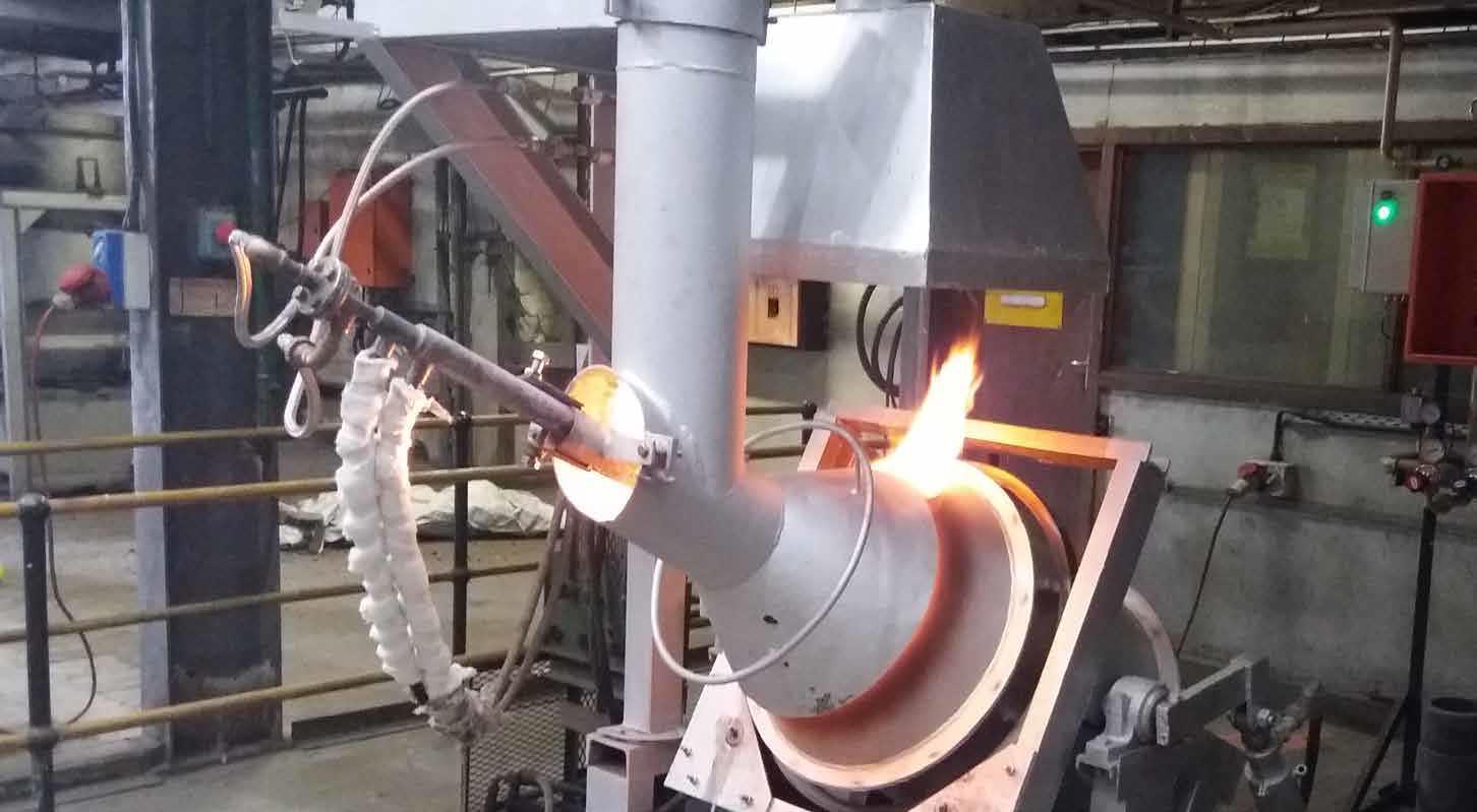
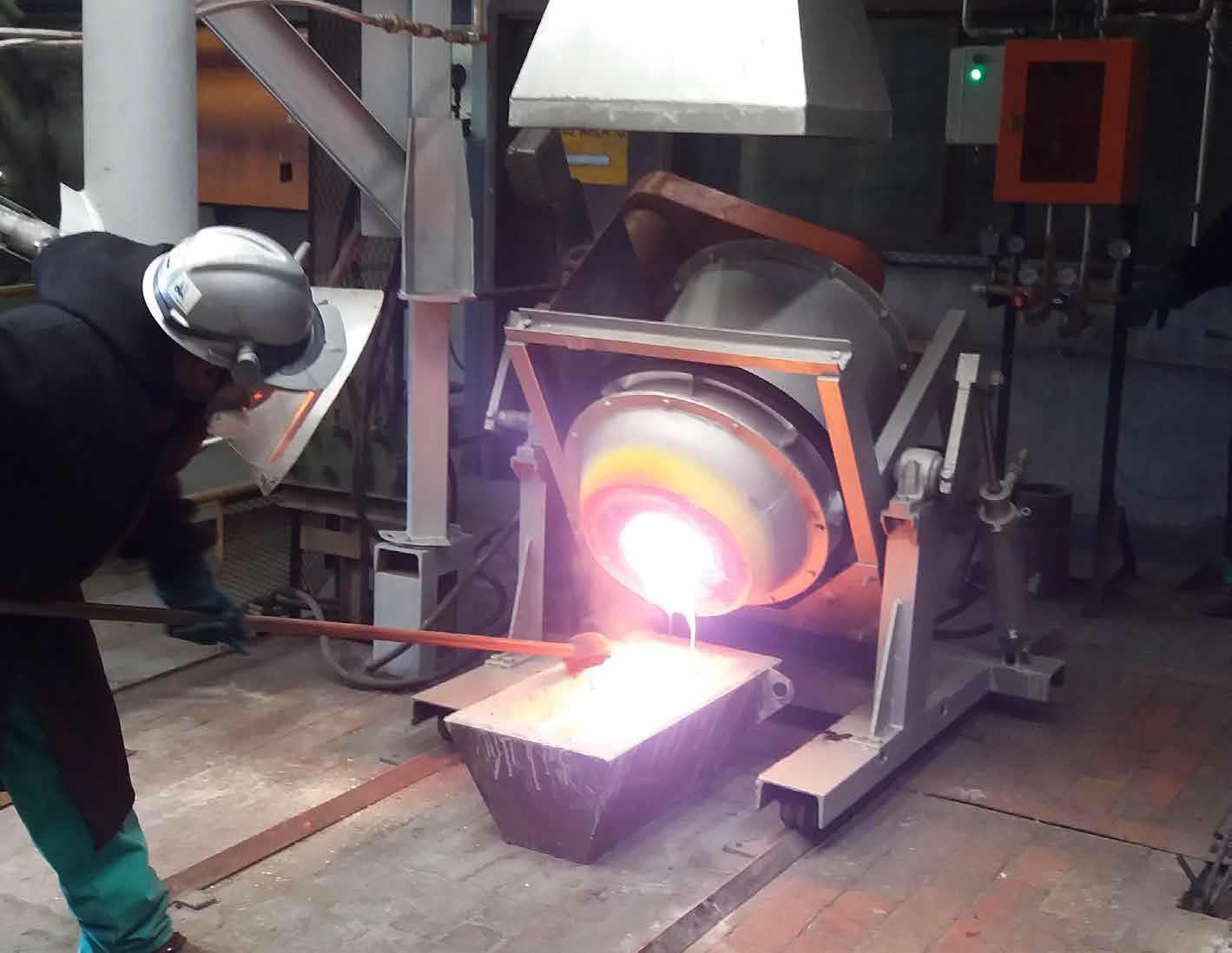
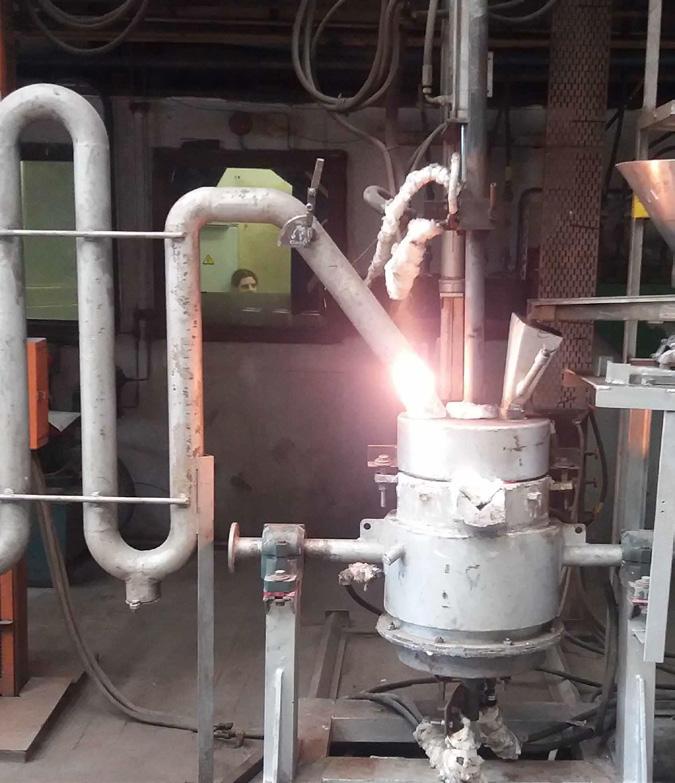
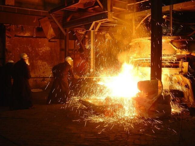


Make today matter www.up.ac.za Faculty of Engineering, Built Environment and Information Technology Fakulteit Ingenieurswese, Bou-omgewing en Inligtingtegnologie / Lefapha la Boetšenere, Tikologo ya Kago le Theknolotši ya Tshedimošo malika.khodja@up.ac.zawww.up.ac.za/materials-science-and-metallurgical-engineering|estie.powell@up.ac.zaCONTACTUPGRADEYOURMETALLURGICAL Can a metallurgical qualification enhance your knowledge and open new doors in your career? The Department of Materials Science and Metallurgical Engineering at the University of Pretoria is currently the #1 academic department of its kind in South Africa – offering postgraduate degree programmes in the full scope of the minerals and metals discipline: • Minerals processing • Pyro- and hydro-metallurgy • Physical and mechanical metallurgy • Welding engineering • Corrosion metallurgy KNOWLEDGE AND SKILLS APPLY NOW! ACADEMIC OFFERING BEngHons OR BScHons Applied Sciences with metallurgical or welding engineering specialisation, with associated master’s and doctoral programmes. ADMISSION Students are accepted from BTech and BSc streams, as well as from other engineering disciplines. PROFESSIONAL REGISTRATION The completion of your honours degree with welding engineering specialisation enables your professional registration as an International Welding Engineer (IWE) #33#1in South Africa for metallurgical engineering, rated by the Minerals Education Trust Fund in the world for minerals and mining engineering, rated by the QS World University Rankings