An unbiased spiral array for MASW data acquisition

Koya Suto1* proposes an omnidirectional, variable offshore offset array with a spiral pattern

that aims to eliminate biases.

Abstract

MASW surveys generally use linear arrays, and the result is posted at the centre of the geophone array. A question is asked whether there is any bias related to the source offset and direction relative to the linear array. This paper first examines the existence of the biases by a receiver array with variable source and a source array to different receiver locations.

A new pattern of geophone array is proposed to attempt to eliminate these biases. It is an omnidirectional, variable offset array with a spiral pattern. Geometrically, there is no uncertainty in the centre of the array. An experimental survey was carried out to compare this spiral array with a linear array centred at the same point. A record by the spiral array can be analysed using conventional MASW software which assumes constant geophone interval. The records are compared in both the time-distance and the frequency-phase velocity domains. The result demonstrates the spiral array delivers comparable dispersion image to the linear array and it assures a more confident array centre location.

The spiral array also indicates viability of a MASW array arranged two-dimensionally. This is also a step forward to a 3D MASW.

Introduction

A MASW survey (Park, et al, 1999) analyses data in the frequency-phase velocity domain and estimates the dispersion curve in this domain. The estimated dispersion curve is inverted to a 1D S-wave velocity profile along the depth. The input data are usually collected by a linear array with several geophones and the seismic source is placed away from the geophone array usually to one direction.

A 1D S-wave velocity profile from MASW processing is ‘traditionally’ plotted at the location of the centre of the geophone array regardless of the source direction and offset. The fundamental assumption of the MASW method is the S-wave velocity structure, a uniform layer cake with an infinitesimal extent larger than the array size and offset distance. This assumption is often violated and the variation of S-wave velocity structure is indeed the subject of the survey. The motivation of this paper is to examine the validity of this ‘tradition’.

Hayashi and Suzuki (2004) proposed to analyse the data in the common mid-point (CMP) gather rather than the shot gather. This eliminates the bias related to the source distance from one array,

1 Terra Australis Geophysica Pty Ltd

* Corresponding author, E-mail: koya @terra-au.com

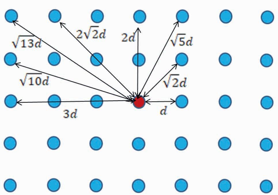
DOI: 10.3997/1365-2397.fb2023067 but data acquisition requires an intense field effort compared with a conventional landstreamer survey. It also does not address the issue of source direction unless the data are acquired from both ends of the geophone array, which doubles the field effort again. While the issue of plotting location of the result is solved by CMP analysis, a linear array does not account for variation in the lateral direction to the linear array. A cross line may be necessary to investigate the lateral variation. Ultimately MASW analysis of 3D seismic data is desired. The 3D equivalent of CMP sorting is binning commonly used in the 3D reflection processing. One problem in analysing binned data is that the offset distance is not a multiple of geophone interval or bin size (Figure 1), while current MASW software is based on equidistance geophones in an array.

Examining validity of collecting data for MASW processing in the multiple orientations is a necessary step towards the future development of 3D application of the MASW survey. A spiral array centred by a source point is designed to cover multiple azimuths and offset distances. A specialised but simple hardware is designed to locate geophones for this array. This paper shows the result of an experimental survey compared with a corresponding linear array survey.

An experimental survey took place in the courtyard of DMT GmbH & Co. KG in Essen, Germany. All the processing was carried out using the SurfSeis software by Kansas Geological Survey. For ease of comparison of dispersion images, the same processing parameters are used throughout this paper: transforming the entire data record of 12 channels to 1000 ms, with no top mute and its ‘advanced’ algorithm.

Current practice

Examination of bias by shot direction

A MASW survey is usually performed along a linear line moving the geophone source and array in one direction. The source is offset by a certain distance (‘initial offset’) from the array to one direction. It could be in ‘front’ of the array or ‘behind’ the array with respect to the direction of the survey. A question is cast whether there is any bias relating to the seismic source in relation to the receiver array. Figure 2 shows two seismic records shot in opposite directions with the same initial offset 2 m and their frequency-velocity transform. The dispersion images show similarity in the region over 9 Hz but show difference in the lower frequency band. Analysing dispersion curves from these records would lead to different curves, then inversion would result in different S-wave velocity structure.

Examination of bias by shot distance (initial offset)

The result of MASW analysis is plotted at the centre of the geophone array. This is regardless of the distance of the source location from the geophone array. However, this convention has not been proven to be correct and there is room for a challenge. Using a 12-channel fixed array, 13 shots were recorded (Figure 3). The number of shots was constrained by the available space.

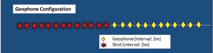
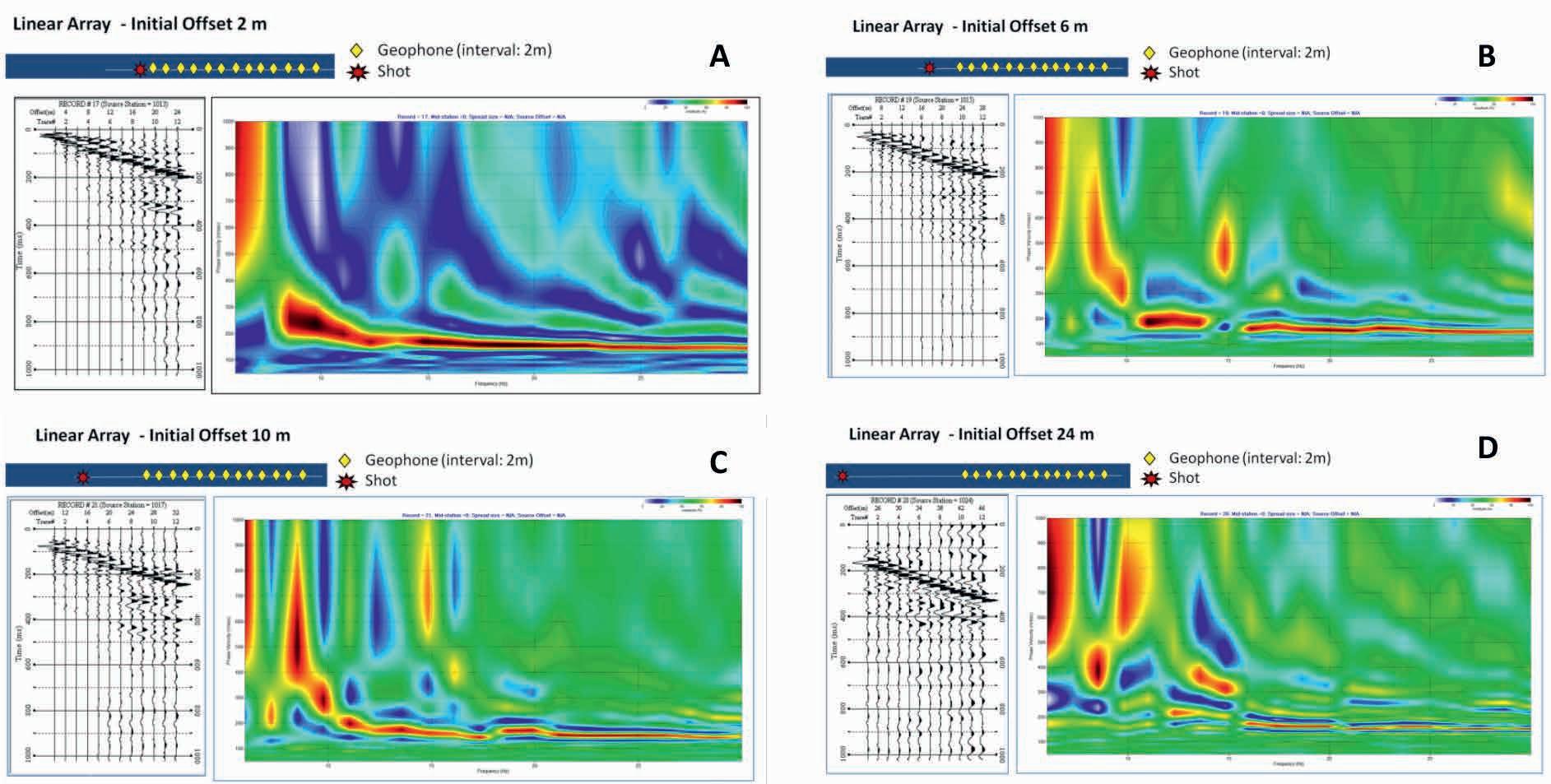
Figure 4 shows some of the shot records with various initial offsets and corresponding dispersion images. These dispersion images are clearly different from each other; particularly in the frequency range under 10 Hz. This suggests the surface waves observed by an array are not indicative of the condition directly under the array alone, but the source distance from array has some contribution. This is conceivable as the segment between the source and the geophone array may have some impact on the propagation of the seismic waves.

Attenuation by the distance (spherical divergence) is definitely one of the factors: the further the source is, the weaker the signal becomes, hence signal-to-noise ratio decreases. Any geological variation along the survey line may cause complication, too. The data of Figure 4D has a large offset range of 24-48 m. It shows significant noise in the data.

Apart from the issue of signal-to-noise ratio, variation of dispersion curve depending on the offset has a more serious effect on the analysis. Analysing these data for different dispersion curves will result in different S-wave velocity structure at the same point. As different shot points for the same geophone array change the geometry of the total travel path of seismic wave, the result may represent a point different from the centre of the geophone array. The dispersion image of short offset (Figure 4A) lacks clear definition of velocity of the low frequency components. The dispersion trend at low frequency range is clearer with larger offsets (Figure 5B and 5C). This is perhaps due to the near-field effect. If the source is too far away, the dispersion image is much disturbed (Figure 4 D). This is not only by the far-field effect but lowering the signal-to-noise ratio due to the absorption through the passage of the seismic waves. Quantitative analysis of this phenomenon is still open to a further examination.

While the issue of plotting location of the result is solved by CMP analysis, a linear array does not account for variation in the lateral direction of the linear array. A cross line may be necessary to investigate the lateral variation. Ultimately MASW analysis of 3D seismic data is desired. The 3D equivalent of CMP sorting is binning commonly used in the 3D reflection processing. One problem in analysing binned data is that the offset distance is not a multiple of the geophone interval or bin size (Figure 1), while current MASW software is based on equidistance geophones in an array.

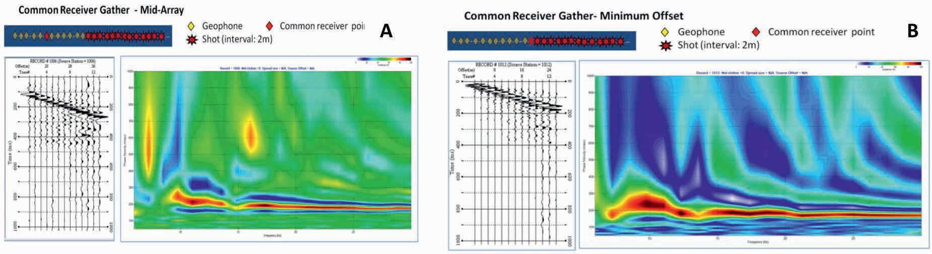
Common receiver point gather

If the location of the MASW solution depends only on the receiver array, what is the survey if the receiver array is only made by one geophone? Provided more than one shot location and signals from several offsets can be recorded by one geophone, the dataset can be acquired in the manner shown in Figure 3. Common receiver point (CRP) gathers are obtained for each receiver point. Figure 5 shows two of those gathers with corresponding dispersion images: Figure 5A for the centre of the geophone array and 5B for the geophone point closest to the series of source points. The offset range is 12 to 34 m and 2 to 26 m, respectively. The CRP of Figure 5A is the same location as the mid-array point. Among the four dispersion images in Figure 4, 4B seems to have the best resemblance to 5A. This may be coincidence as the actual array is not of the geophones but of the shot points away from the CRP. It may be representing the structure under the centre point of the shot array. Comparison between Figures 5A and 5B, different CRP with the same shot array, shows some difference, particularly at the lower end of the spectrum. This shows common receiver array records are still subject to the near- and far- field effects.

Spiral Array Design concept of spiral array

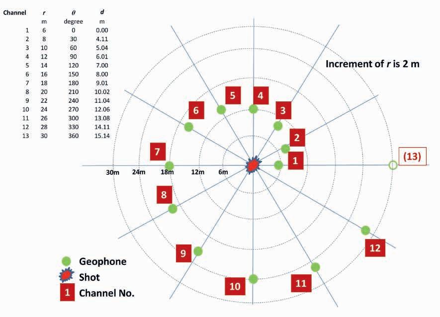
In order to eliminate the bias related to the orientation of the source from the receiver (or vice versa), we arrange geophones in a number of directions from the source location. Obviously, a circle array of geophones would satisfy this requirement. However, if a source is located at the centre point of the circle array, there is no variation in source-receiver offset, and it is impossible to estimate seismic velocity without this variation.

To get around this problem, geophones are arranged at different distances from the centre where the source is placed. In this study, the smallest distance from the source is placed at 6 m and incremented by 2 m as the direction is incremented by 30º resulting in a spiral pattern (Figure 6). When a shot is recorded with this array, no directional bias is expected. Because the increment of the distance is constant, the data can be processed and analysed using conventional software which assumes a constant geophone interval. In this arrangement of geophones, there is no room for argument of location at the centre of the array. It is in the middle coinciding with the shot location.

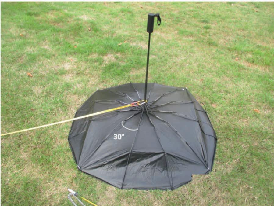
Hardware

Accurate placement of geophones in the spiral pattern may require intensive surveying if the Cartesian coordinates are to be used: position of each geophone has to be calculated for each point. For arrangement of geophones by the polar coordinates, the angles and radial distance need to be measured accurately. A simple azimuth pointer is improvised to point each 30º increment from the centre of an array to measure the radial distance with a tape (Figure 7). Once the geophones are laid, it is removed and a strike plate for the source is placed at the centre. This device is also useful to keep a PC dry when it rains.

A spiral array does not have a constant interval between geophones. Therefore, a conventional seismic cable with a fixed take-out interval is not suitable. In this experimental survey, a SUMMIT X One system by DMT (Figure 8) was used. With this system, geophones can be connected to any point of the cable. A wireless seismic data acquisition system may also be used for this array.

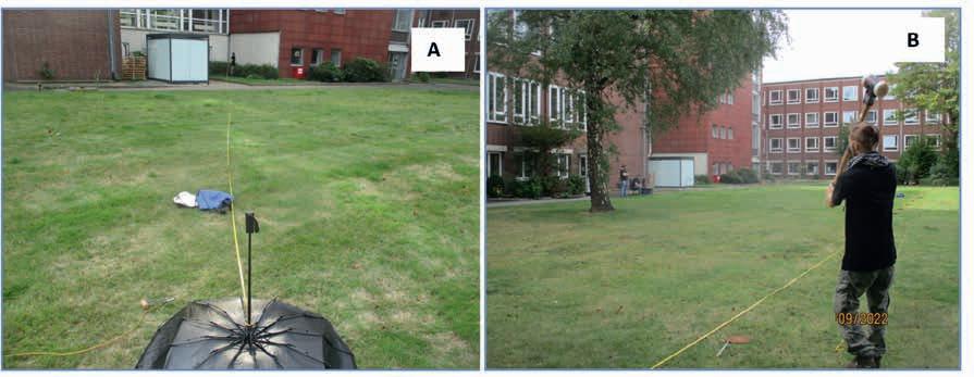
Data acquisition

The experimental data were acquired together with the linear array data in the courtyard of DMT in Essen, Germany on 13 September 2022 (Figure 9). The weather was fine with very little or no wind. The nearest main road was about 100 m away. A 6 kg sledgehammer was used as a seismic source. The natural frequency of the geophones used was 10 Hz. The 12-channel data were recorded for 1 s at a 0.5 ms sampling rate.

Records and transform

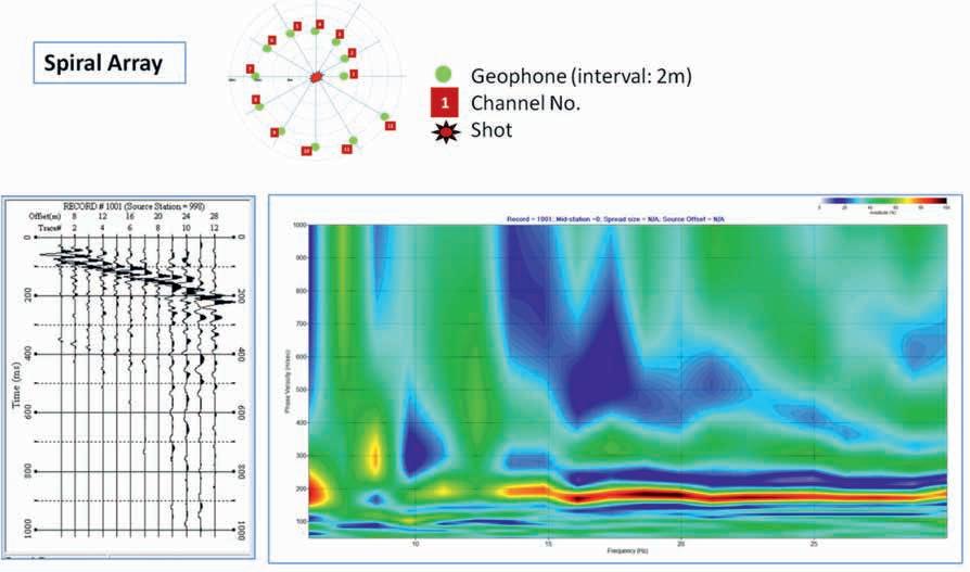
Figure 10 shows the seismic record acquired with the circle array and its transform into the frequency-velocity domain.

In the time-distance domain, the data trend does not look much different from the linear array data (Figure 4B). However, it is noted that the background noise is less coherent than in the linear array. This is because no background noise travels in the spiral path.

In the frequency domain the dispersion image from the spiral array data resembles the linear array with the same offset (Figure 4B) and the CRG with large 10 m offset (Figure 5A). In all these cases, the near-field effect is minimal and the fundamental mode trend is clear. This shows the validity of analysing the variable offset data of the spiral array. An apparent difference is that the intensity of the noise around 600 m/s at 10-12 Hz, perhaps of higher mode, is suppressed in the spiral array.

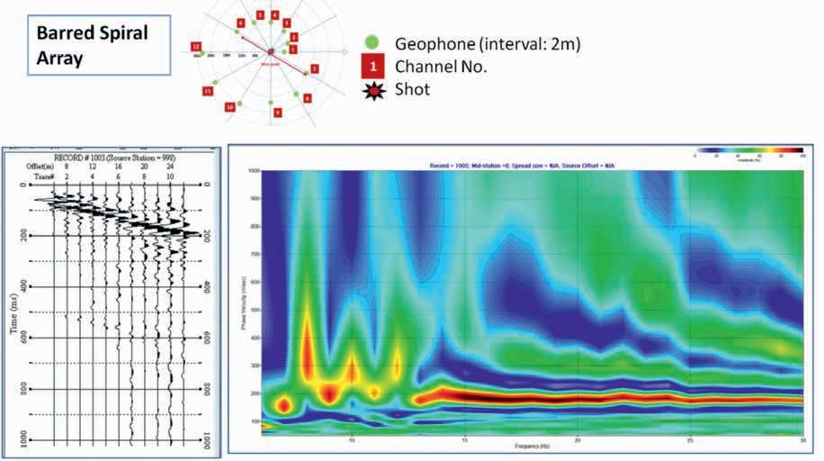
Barred spiral array

The spiral array shown in Figure 6 presents even distribution of shot-receiver azimuths. However, the distances between geophones in different directions vary. For example, the distance between geophones 1 and 7 is 24 m while the distance between geophones 4 and 10 is 36 m. This may become another source of directional bias.

A bar is introduced in the spiral array between geophones numbers 6 and 7 and the rest of the geophones are laid in the opposite direction (Figure 11). Distances between geophones across the array are constant: 34 m in this example.

Figure 12 shows the seismic record of this barred spiral array and its transform.

The dispersion image by the barred spiral array is somewhat confusing, but a dispersion curve similar to the spiral array can be picked in this domain. However, the spiral array delivers a better definition at the low-frequency – high velocity end of the dispersion image. The cause of this difference is yet to be clarified. It may not only be due to the different array, but it could be due to irregularity of the underground conditions over this short distance.

Discussion and conclusions

A new spiral array for seismic data acquisition is proposed to eliminate geometrical ambiguity of the location to post the MASW result, which is ‘traditionally’ placed at the centre of the geophone array. The ambiguity in the linear array is inevitably associated with the source distance and shot direction. Geometrically, there is no ambiguity at the centre of the spiral array, the origin of the spiral, where the shot takes place. In this experiment, the shot-receiver offset was incremented at a constant interval so that conventional MASW software, which assumes a constant geophone interval, can be used.

Seismic data of linear and spiral arrays collected at the same location are compared. The comparison shows similar results, but not exactly the same. This may be due to the difference in the ‘centre’ position of data arrays or lateral variation of geology for which a linear array does not account. The spiral array is considered to represent the central location while the linear array may indicate somewhere nearby.

The acquisition of spiral array data is admittedly not as easy and quick as a linear array. However, if a solution of S-wave velocity at an exact location is required, the spiral array is considered better than a linear array, as there is less geometrical ambiguity. The barred spiral array eliminates further ambiguity of bias due to variation of diagonal distance, but the experiment did not find a significant improvement of dispersion image.

This experiment also demonstrates the geophone array for MASW may not necessarily be linear as long as a range of offsets can be assured. In fact, adding the lateral direction is considered to improve the accuracy of the resultant model at that location, because it accounts for variation of geology in all the orientations. This is a step forward towards a possibility of applying the MASW to 3D data collected for reflection surveys. To achieve a 3D MASW analysis, a method to handle data with variable geophone interval as shown in Figure 1 is needed. This remains to be developed in the future.

Acknowledgments

The author would like to thank Mr Wolfram Gödde and his team at DMT for their help in experimental data acquisition and use of their site and equipment. Thanks are also due to Dr Nigel Fisher of Kenmore Geophysical for sorting the seismic data.

Parts of this work have been presented at the Australasian Exploration Geosciences Conference in Brisbane in March 2023 (Suto, 2023).

References

Hayashi, K. and Suzuki, H. [2004], CMP cross-correlation analysis of multi-channel surface-wave data: Exploration Geophysics, 35, 7-13. Park, C.B., Miller R.D. and Xia, J. [1999]. Multichannel analysis of surface waves: Geophysics, 64, 80-808. Doi:10.1190/1.1444590.

Suto, K. [2023]. Development of an unbiased spiral array for MASW data acquisition, SEG Extended Abstracts 2023 (4th Australasian Exploration Geoscience Conference).

POWERED BY

Lifelong Learning

FREE LEARNING

E-Lectures, Distinguished Lecturer Webinars, Student E-Lectures